Monotone difference schemes stabilized by discrete mollification for strongly degenerate parabolic equations

MONOTONE DIFFERENCE SCHEMES STABILIZED BY DISCRETEMOLLIFICATION FOR STRONGLY DEGENERATE PARABOLIC EQUATIONS

CARLOS D. ACOSTAA, RAIMUND BURGERB, AND CARLOS E. MEJIAC

Abstract. The discrete mollification method is a convolution-based filtering procedure suitable for the

regularization of ill-posed problems and for the stabilization of explicit schemes for the solution of PDEs.

This method is applied to the discretization of the diffusive terms of a known first-order monotone finitedifference scheme [S. Evje and K.H. Karlsen, SIAM J Numer Anal 37 (2000) 1838–1860] for initial value

problems of strongly degenerate parabolic equations in one space dimension. It is proved that the mollified

scheme is monotone, and converges to the unique entropy solution of the initial value problem, under a CFLstability condition which permits to use time steps that are larger than with the un-mollified (basic) scheme.

Several numerical experiments illustrate the performance, and gains in CPU time, for the mollified scheme.

Applications to initial-boundary value problems are included.

1. Introduction

1.1. Scope. This paper is concerned with finite difference methods for the following initial value problemfor a degenerate parabolic equation:

ut + f(u)x = A(u)xx, (x, t) ∈ ΠT := R× (0, T ), T > 0, (1.1)

u(x, 0) = u0(x), x ∈ R, (1.2)

where the integrated diffusion coefficient A is defined by

A(u) =∫ u

0

a(s) ds, a(u) ≥ 0, a ∈ L∞(R) ∩ L1(R). (1.3)

The function a is allowed to vanish on u-intervals of positive length, on which (1.1) degenerates to a first-order scalar conservation law. Therefore, (1.1) is called strongly degenerate. It is well known that solutionsof (1.1), (1.2) are, in general, discontinuous even if u0 is smooth, and need to be defined as weak solutionsalong with an entropy condition to select the physically relevant solution, the entropy solution. Applicationsof degenerate parabolic equations include two-phase flow in porous media, traffic flow, and sedimentation-consolidation processes.

Evje and Karlsen [1] introduced an explicit monotone difference scheme for the approximation of entropysolutions of (1.1), (1.2) based on the first-order accurate, monotone Engquist-Osher numerical flux [2] forthe convective part combined with a conservative discretization of the degenerate diffusion term. If ∆x and∆t denote the spatial meshwidth and the time step, respectively, they proved convergence of the scheme toan entropy solution as ∆x,∆t ↓ 0 provided that the following CFL stability condition is satisfied:

λ ‖f ′‖∞ + 2µ ‖a‖∞ ≤ 1, λ := ∆t/∆x, µ := ∆t/∆x2. (1.4)

Similar conditions appear for explicit finite difference schemes approximating smooth solutions of strictlyparabolic convection-diffusion equations. For these equations, the so-called method of discrete mollification[3, 4] consists in using certain convex combinations of finite difference stencils rather than a single one. This

Date: December 3, 2009.AUniversidad Nacional de Colombia, Department of Mathematics and Statistics, Manizales, Colombia.

E-Mail: [email protected] and Departamento de Ingenierıa Matematica, Facultad de Ciencias Fısicas y Matematicas, Universidad de Con-

cepcion, Casilla 160-C, Concepcion, Chile. E-Mail: [email protected] Nacional de Colombia, Department of Mathematics, Medellın, Colombia. E-Mail: [email protected].

1

2 ACOSTA, BURGER, AND MEJIA

device leads to a consistent numerical method with a new CFL condition that allows to use larger time steps,i.e. it stabilizes the given method.

In our case, the application of discrete mollification to the scheme introduced in [1] leads to a mollifiedscheme whose CFL stability condition is given by

λ ‖f ′‖∞ + 2µεη ‖a‖∞ ≤ 1, where εη := Cη (1− w0) ∈ (0, 1), (1.5)

where Cη and w0 are a parameter and the central weight, respectively, of the discrete mollification operatorthat depend on the width η of the mollification stencil. Since εη ∈ (0, 1), for given ∆x the condition (1.5)admits to employ values of ∆t that are up to several times larger than for the standard, un-mollified versionof the scheme with the restriction (1.4). This accelerates the given scheme but, as our numerical experimentsshow, introduces an at most moderate additional error.

It is the purpose of this paper to demonstrate that discrete mollification can also be applied to differencemethods for the initial value problem for a strongly degenerate parabolic equation (1.1), (1.2). We provethat the new method is monotone and converges to the unique entropy solution of (1.1), (1.2) under the lessrestrictive CFL condition (1.5). The performance of the method is illustrated in several numerical examples.

1.2. Related work. Discrete mollification [5, 6] is a versatile convolution-based filtering procedure for theregularization of ill-posed problems [6, 7, 8, 9] and the stabilization of explicit schemes for the solutionof PDEs. In [3] and [4] the mollification method was introduced as a stabilizer for numerical schemes forstrictly parabolic convection-diffusion equations and non-linear scalar conservation laws, respectively. In [10]it is shown that a particular discrete approximation of the second derivative of a smooth function, basedon discrete mollification, stabilizes operator splitting methods [11] for the numerical solution of convection-diffusion problems. The method of [10] is applied herein to strongly degenerate parabolic equations.

On the other hand, monotone schemes for first-order conservation laws (corresponding to A ≡ 0) werefirst analyzed in [12, 13]. Their attractive feature is the convergence to an entropy solution, which remainsvalid for the application to strongly degenerate parabolic equations. This was first exploited by Evje andKarlsen in [1]. Related analyses include implicit monotone schemes for degenerate parabolic equations [14],problems with boundary conditions [15], multidimensional degenerate parabolic equations [16], equationswith discontinuous coefficients [17, 18, 19], and problems of parameter identification [20] (this list is farfrom being complete). Of course, the robustness of monotone schemes, in particular the convergence to theentropy solution, comes at the well-known price of the generic limitation to first-order accuracy.

1.3. Outline of the paper. The remainder of the paper is organized as follows. In Section 2 we presentpreliminary material, including a definition of an entropy solution of (1.1), (1.2) in Section 2.1, a descriptionof the unmollified (basic) scheme from [1] in Section 2.2, a precise statement of the assumptions underlyingthe convergence analysis (Section 2.3), and an outline of the discrete mollification operator and its proper-ties (Section 2.4). Section 3 deals with the mollified scheme, which is motivated in Section 3.1, and whoseconvergence to an entopy solution of (1.1), (1.2) is shown in Section 3.2. Based on standard compactnessarguments, we prove that under the CFL condition (1.5) the mollified scheme is conservative and monotone,and produces uniformly bounded approximate solutions that satisfy the L1 Lipschitz continuity in timeproperty. Moreover, under an additional limitation of the choice of the mollification stencil the approxima-tions of the integrated diffusion coefficient have the appropriate regularity properties. Since the scheme ismonotone, it satisfies a discrete entropy inequality, and by a Lax-Wendroff-type argument we prove that itconverges to an entropy solution of (1.1), (1.2) as ∆t,∆x ↓ 0. The mollified scheme is further supportedby numerical experiments presented in Section 4, which are motivated by three different applicative modelsthat also include boundary conditions. Some conclusions are collected in Section 5.

2. Preliminaries

2.1. Definition of an entropy solution. We recall here the definition of entropy solutions of (1.1), (1.2)from [1].

Definition 2.1. A bounded measurable function u is said to be an entropy solution of (1.1), (1.2) if itsatisfies

MOLLIFIED SCHEMES FOR STRONGLY DEGENERATE PARABOLIC EQUATIONS 3

(1) u ∈ BV (ΠT ) and A(u) ∈ C1,1/2(ΠT ).(2) For all non-negative test functions φ ∈ C∞0 (ΠT ) with φ|t=T = 0 and any c ∈ R, the following entropy

Kruzkov-type inequality is satisfied:∫∫ΠT

{|u− c|φt + sgn(u− c)

(f(u)− f(c)

)φx +

∣∣A(u)−A(c)∣∣φxx}dtdx

+∫

R|u0 − c|φ(x, 0) dx ≥ 0.

(2.1)

It is well known that entropy solutions of (1.1), (1.2) in the sense of Definition 2.1 are L1-contractive,i.e., if u1 and u2 are two entropy solutions corresponding to the respective initial data u1

0 and u20, then

‖u1(·, t)− u2(·, t)‖1 ≤ ‖u10 − u2

0‖1 for 0 ≤ t ≤ T . In particular, entropy solutions of (1.1), (1.2) are unique.This is, in fact, valid for initial value problems of more general strongly degenerate parabolic equations, alsoin several space dimensions. See [21] for details.

2.2. The unmollified scheme (basic scheme). We select a mesh size ∆x > 0 and a time step ∆t > 0such that there exists an integer N with N∆t = T . Let unj denote the value of the difference approximationat (j∆x, n∆t) for j ∈ Z and n = 1, . . . , N . We then discretize the initial datum by

u0j :=

1∆x

∫ (j+1/2)∆x

(j−1/2)∆x

u0(x) dx, j ∈ Z, (2.2)

and calculate the solution values at time level tn+1 from those at time tn by the explicit marching formula

un+1j = unj − λ∆+F

EO(unj−1, u

nj

)+ µ∆2A

(unj), j ∈ Z, n = 0, 1, 2, . . . , N − 1, (2.3)

where we define the standard difference operators

∆+Vj−1 = ∆−Vj = ∆Vj−1/2 := Vj − Vj−1, ∆0Vj := (Vj+1 − Vj−1)/2, ∆2Vj := Vj+1 − 2Vj + Vj−1,

and use the Engquist-Osher [2] numerical flux given by FEO(unj , unj+1) = f+(unj ) + f−(unj+1), where

f+(u) := f(0) +∫ u

0

max{f ′(s), 0

}ds, f−(u) :=

∫ u

0

min{f ′(s), 0

}ds.

Under the CFL condition (1.4) the scheme (2.3) is monotone, therefore first-order accurate, and convergesto the unique entropy solution [1]. The new scheme will be based on replacing the term µ∆2A(unj ) in (2.3)by a different expression involving discrete mollification. We will therefore refer to (2.3) as the basic scheme.

2.3. Assumptions. With the notation related to the discretization at hand, we state, similarly to [15], asa further assumption that

u0 ∈ B :={u ∈ BV (R)

∣∣ ∃M1,M2 > 0 : u0(x) = const. for x 6∈ [−M1,M1], TV(A(u0)x) ≤M2

}. (2.4)

This means, in particular, that there exists a constant M3 such that∑m∈Z

∣∣∆2A(u0m

)∣∣ ≤M3∆x uniformly in ∆x.

2.4. The discrete mollification operator. The mollification method [5, 6] is based on replacing thediscrete function y = {yj}j∈Z, which can, for example, consist of evaluations or cell averages of a real functiony = y(x) given at equidistant grid points xj = x0 + j∆x, ∆x > 0, j ∈ Z, by its mollified version Jηy, whereJη is the so-called mollification operator defined by

[Jηy]j :=η∑

i=−ηwiyj−i, j ∈ Z, (2.5)

4 ACOSTA, BURGER, AND MEJIA

η i = 0 i = 1 i = 2 i = 3 i = 4 i = 5 i = 6 i = 7 i = 8 ζ0 1 −1 0.84272 0.07864 0.0786

2 0.60387 0.19262 5.4438e-3 0.1926

3 0.45556 0.23772 3.3291e-2 1.2099e-3 0.2341

4 0.36266 0.24003 6.9440e-2 8.7275e-3 4.7268e-4 0.2101

5 0.30028 0.22625 9.6723e-2 2.3430e-2 3.2095e-3 2.4798e-4 0.1266

6 0.25585 0.20831 0.11241 4.0192e-2 9.5154e-3 1.4905e-3 1.5434e-4 -0.0145

7 0.22270 0.19058 0.11942 5.4793e-2 1.8403e-2 4.5234e-3 8.1342e-4 1.0697e-4 -0.2121

8 0.19708 0.17444 0.12097 6.5725e-2 2.7973e-2 9.3255e-3 2.4348e-3 4.9782e-4 7.9691e-5 -0.4660

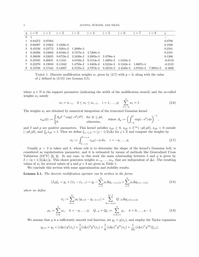
Table 1. Discrete mollification weights wi given by (2.7) with p = 3, along with the valueof ζ defined in (3.15) (see Lemma 3.5).

where η ∈ N is the support parameter (indicating the width of the mollification stencil) and the so-calledweights wi satisfy

wi = w−i, 0 ≤ wi ≤ wi−1, i = 1, . . . , η;η∑

i=−ηwi = 1. (2.6)

The weights wi are obtained by numerical integration of the truncated Gaussian kernel

κpδ(t) :=

{Apδ

−1 exp(−t2/δ2) for |t| ≤ pδ,0 otherwise,

where Ap :=(∫ p

−pexp(−s2) ds

)−1

,

and δ and p are positive parameters. This kernel satisfies κpδ ≥ 0, κpδ ∈ C∞(−pδ, pδ), κpδ = 0 outside[−pδ, pδ], and

∫R κpδ = 1. Then we define ξj−1/2 := (j − 1/2)∆x for j ∈ Z and compute the weights by

wi :=∫ ξi+1/2

ξi−1/2

κpδ(−s) ds, i = −η, . . . , η. (2.7)

Usually p = 3 is taken and δ, whose role is to determine the shape of the kernel’s Gaussian bell, isconsidered as regularization parameter, and it is estimated by means of methods like Generalized CrossValidation (GCV) [6, 8]. In any case, in this work the main relationship between δ and η is given byδ = (η + 1/2)∆x/p. This choice generates weights w−η, . . . , wη, that are independent of ∆x. The resultingvalues of wi for several values of η and p = 3 are given in Table 1.

We conclude this section with some approximation and stability results.

Lemma 2.1. The discrete mollification operator can be written in the forms

[Jηy]j = yj + (ψj − ψj−1) = yj −η∑i=1

ρi∆yj−i+1/2 +η∑i=1

ρi∆yj+i−1/2, (2.8)

where we define

ψj :=η∑k=1

ρk (yj+k − yj−k+1) =η−1∑

k=−η+1

Q−k∆yj+k+1/2,

ρk :=η∑i=k

wi, k = −η, . . . , η; Q−k = Qk :=η∑

i=k+1

ρi, k = 0, . . . , η − 1. (2.9)

We assume that g is a sufficiently smooth real function, set yj = g(xj), and employ the Taylor expansion

yj+i = yj + (i∆x) g′(xj) +12

(i∆x)2g′′(xj) +16

(i∆x)3g′′′(xj) +

124

(i∆x)4g(4)(ξj,i),

MOLLIFIED SCHEMES FOR STRONGLY DEGENERATE PARABOLIC EQUATIONS 5

where ξj,i is a real number between xj and xj+i. Then, defining

Cη :=

η∑i=−η

i2w−i

−1

,

we can write

[Jηy]j =η∑

i=−ηw−iyj+i = yj +

∆x2

2Cηg′′(xj) +

∆x4

24

η∑i=−η

i4w−ig(4)(ξj,i). (2.10)

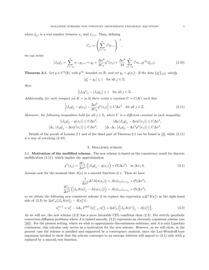
Theorem 2.1. Let g ∈ C4(R) with g(4) bounded on R, and set yj = g(xj). If the data {yεj}j∈Z satisfy∣∣yεj − yj∣∣ ≤ ε for all j ∈ Z,

then ∣∣[Jηyε]j − [Jηy]j∣∣ ≤ ε for all j ∈ Z.

Additionally, for each compact set K = [a, b] there exists a constant C = C(K) such that∣∣∣∣[Jηy]j − g(xj)−∆x2

2Cηg′′(xj)

∣∣∣∣ ≤ C∆x4 for all j ∈ Z. (2.11)

Moreover, the following inequalities hold for all j ∈ Z, where C is a different constant in each inequality:∣∣[Jηy]j − g(xj)∣∣ ≤ C∆x2,∣∣∆+ [Jηy]j −∆xg′(xj)∣∣ ≤ C∆x2,

∣∣∆0 [Jηy]j −∆xg′(xj)∣∣ ≤ C∆x3,∣∣∆−∆+ [Jηy]j −∆x2g′′(xj)∣∣ ≤ C∆x4.

Details of the proofs of Lemma 2.1 and of the third part of Theorem 2.1 can be found in [3], while (2.11)is a way of rewriting (2.10).

3. Mollified scheme

3.1. Motivation of the mollified scheme. The new scheme is based on the consistency result for discretemollification (2.11), which implies the approximation

g′′(xj) =2Cη∆x2

([Jηg]j − g(xj)

)+O(∆x2) as ∆x↓ 0. (3.1)

Assume now for the moment that A(u) is a smooth function of x. Then we have

1∆x2

∆2A(u(xj)

)= A(u)xx|x=xj +O(∆x2),

2Cη∆x2

([JηA(u)]j −A

(u(xj)

))= A(u)xx|x=xj +O(∆x2),

so we obtain the following new consistent scheme if we replace the expression µ∆2A(unj ) in the right-handside of (2.3) by 2µCη([JηA(u)]j −A(unj )):

un+1j = unj − λ∆+F

EO(unj−1, u

nj

)+ 2µCη

([JηA(un)]j −A

(unj)). (3.2)

As we will see, the new scheme (3.2) has a more favorable CFL condition than (2.3). For strictly parabolicconvection-diffusion problems where A is indeed smooth, (3.2) represents an obviously consistent scheme (see[10]). For the present setting, where we wish to approximate discontinuous solutions, and A is only Lipschitzcontinuous, this calculus only serves as a motivation for the new scheme. However, as we will show, in thepresent case the scheme is justified and supported by a convergence analysis, since the Lax-Wendroff-typeargument invoked to show that the scheme converges to an entropy solution will appeal to (3.1) only with greplaced by a smooth test function.

6 ACOSTA, BURGER, AND MEJIA

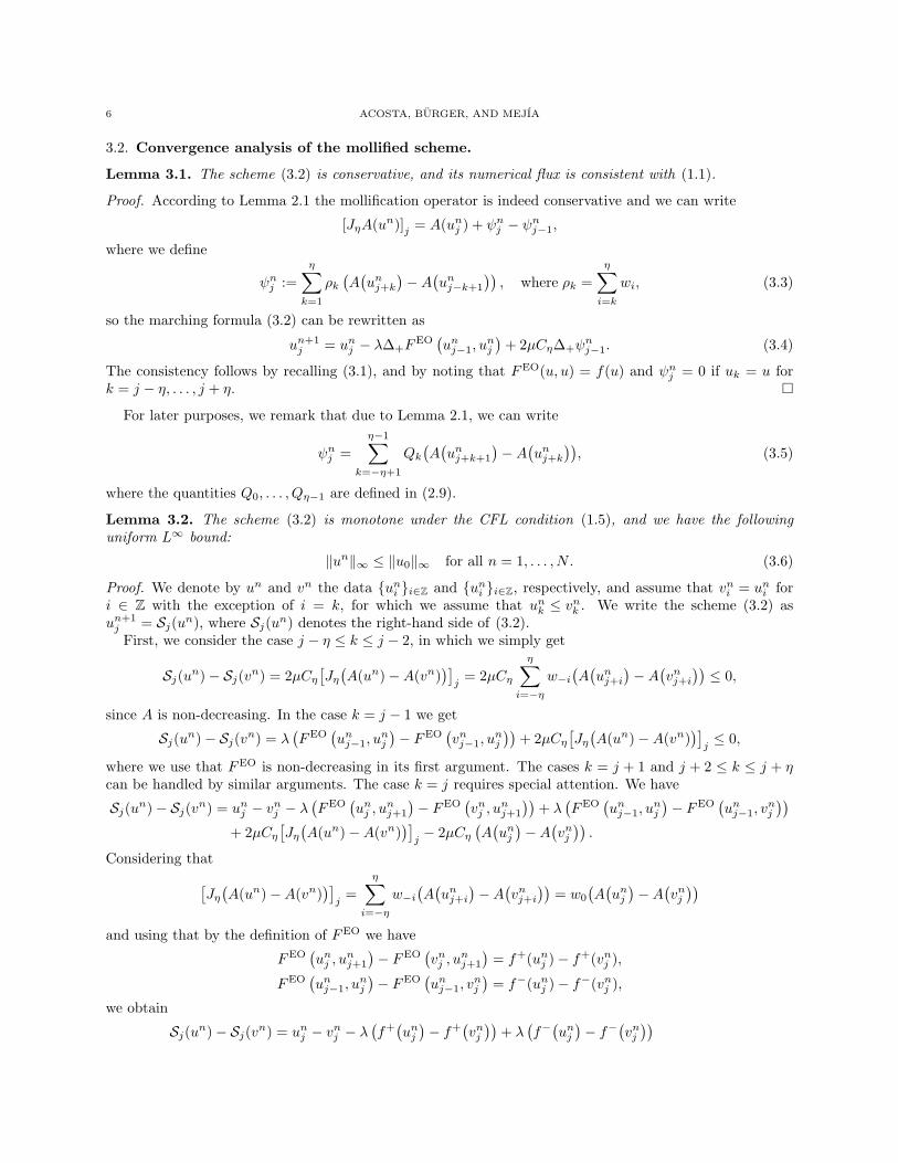
3.2. Convergence analysis of the mollified scheme.

Lemma 3.1. The scheme (3.2) is conservative, and its numerical flux is consistent with (1.1).

Proof. According to Lemma 2.1 the mollification operator is indeed conservative and we can write

[JηA(un)]j = A(unj ) + ψnj − ψnj−1,

where we define

ψnj :=η∑k=1

ρk(A(unj+k

)−A

(unj−k+1

)), where ρk =

η∑i=k

wi, (3.3)

so the marching formula (3.2) can be rewritten as

un+1j = unj − λ∆+F

EO(unj−1, u

nj

)+ 2µCη∆+ψ

nj−1. (3.4)

The consistency follows by recalling (3.1), and by noting that FEO(u, u) = f(u) and ψnj = 0 if uk = u fork = j − η, . . . , j + η. �

For later purposes, we remark that due to Lemma 2.1, we can write

ψnj =η−1∑

k=−η+1

Qk(A(unj+k+1

)−A

(unj+k

)), (3.5)

where the quantities Q0, . . . , Qη−1 are defined in (2.9).

Lemma 3.2. The scheme (3.2) is monotone under the CFL condition (1.5), and we have the followinguniform L∞ bound:

‖un‖∞ ≤ ‖u0‖∞ for all n = 1, . . . , N . (3.6)

Proof. We denote by un and vn the data {uni }i∈Z and {uni }i∈Z, respectively, and assume that vni = uni fori ∈ Z with the exception of i = k, for which we assume that unk ≤ vnk . We write the scheme (3.2) asun+1j = Sj(un), where Sj(un) denotes the right-hand side of (3.2).

First, we consider the case j − η ≤ k ≤ j − 2, in which we simply get

Sj(un)− Sj(vn) = 2µCη[Jη(A(un)−A(vn)

)]j

= 2µCηη∑

i=−ηw−i

(A(unj+i

)−A

(vnj+i

))≤ 0,

since A is non-decreasing. In the case k = j − 1 we get

Sj(un)− Sj(vn) = λ(FEO

(unj−1, u

nj

)− FEO

(vnj−1, u

nj

))+ 2µCη

[Jη(A(un)−A(vn)

)]j≤ 0,

where we use that FEO is non-decreasing in its first argument. The cases k = j + 1 and j + 2 ≤ k ≤ j + ηcan be handled by similar arguments. The case k = j requires special attention. We have

Sj(un)− Sj(vn) = unj − vnj − λ(FEO

(unj , u

nj+1

)− FEO

(vnj , u

nj+1

))+ λ

(FEO

(unj−1, u

nj

)− FEO

(unj−1, v

nj

))+ 2µCη

[Jη(A(un)−A(vn)

)]j− 2µCη

(A(unj)−A

(vnj)).

Considering that[Jη(A(un)−A(vn)

)]j

=η∑

i=−ηw−i

(A(unj+i

)−A

(vnj+i

))= w0

(A(unj)−A

(vnj))

and using that by the definition of FEO we have

FEO(unj , u

nj+1

)− FEO

(vnj , u

nj+1

)= f+(unj )− f+(vnj ),

FEO(unj−1, u

nj

)− FEO

(unj−1, v

nj

)= f−(unj )− f−(vnj ),

we obtain

Sj(un)− Sj(vn) = unj − vnj − λ(f+(unj)− f+

(vnj))

+ λ(f−(unj)− f−

(vnj))

MOLLIFIED SCHEMES FOR STRONGLY DEGENERATE PARABOLIC EQUATIONS 7

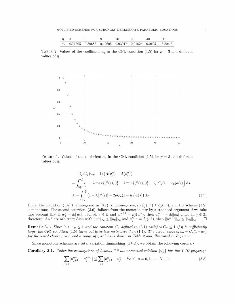
η 3 5 8 20 30 40 50

εη 0.71305 0.39686 0.19605 0.03917 0.01825 0.01051 6.82e-3

Table 2. Values of the coefficient εη in the CFL condition (1.5) for p = 3 and differentvalues of η.

0 10 20 30 40 50

0

0.2

0.4

0.6

0.8

1

η

ε η

Figure 1. Values of the coefficient εη in the CFL condition (1.5) for p = 3 and differentvalues of η.

+ 2µCη (w0 − 1)(A(unj)−A

(vnj))

=∫ vnk

unk

{1− λmax

{f ′(s), 0

}+ λmin

{f ′(s), 0

}− 2µCη(1− w0)a(s)

}ds

≤ −∫ vnk

unk

(1− λ

∣∣f ′(s)∣∣− 2µCη(1− w0)a(s))

ds. (3.7)

Under the condition (1.5) the integrand in (3.7) is non-negative, so Sj(un) ≤ Sj(vn), and the scheme (3.2)is monotone. The second assertion, (3.6), follows from the monotonicity by a standard argument if we takeinto account that if wnj = ±‖u0‖∞ for all j ∈ Z and wn+1

j = Sj(wn), then wn+1j = ±‖u0‖∞ for all j ∈ Z;

therefore, if un are arbitrary data with ‖un‖∞ ≤ ‖u0‖∞ and un+1j = Sj(un), then ‖un+1‖∞ ≤ ‖u0‖∞. �

Remark 3.1. Since 0 < w0 ≤ 1 and the constant Cη defined in (3.1) satisfies Cη ≤ 1 if η is sufficientlylarge, the CFL condition (1.5) turns out to be less restrictive than (1.4). The actual value of εη = Cη(1−w0)for the usual choice p = 3 and a range of η-values is shown in Table 2 and illustrated in Figure 1.

Since monotone schemes are total variation diminishing (TVD), we obtain the following corollary.

Corollary 3.1. Under the assumptions of Lemma 3.5 the numerical solution {unj } has the TVD property:∑j∈Z

∣∣un+1j+1 − u

n+1j

∣∣ ≤∑j∈Z

∣∣unj+1 − unj∣∣ for all n = 0, 1, . . . , N − 1. (3.8)

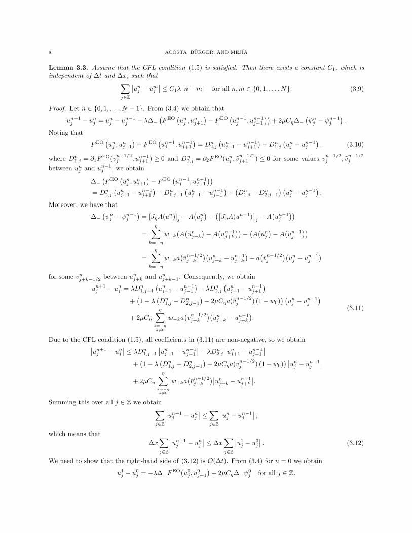
8 ACOSTA, BURGER, AND MEJIA

Lemma 3.3. Assume that the CFL condition (1.5) is satisfied. Then there exists a constant C1, which isindependent of ∆t and ∆x, such that∑

j∈Z

∣∣unj − umj ∣∣ ≤ C1λ |n−m| for all n,m ∈ {0, 1, . . . , N}. (3.9)

Proof. Let n ∈ {0, 1, . . . , N − 1}. From (3.4) we obtain that

un+1j − unj = unj − un−1

j − λ∆−(FEO

(unj , u

nj+1

)− FEO

(un−1j , un−1

j+1

))+ 2µCη∆−

(ψnj − ψn−1

j

).

Noting that

FEO(unj , u

nj+1

)− FEO

(un−1j , un−1

j+1

)= Dn

2,j

(unj+1 − un−1

j+1

)+Dn

1,j

(unj − un−1

j

), (3.10)

where Dn1,j = ∂1F

EO(vn−1/2j , un−1

j+1 ) ≥ 0 and Dn2,j = ∂2F

EO(unj , vn−1/2j+1 ) ≤ 0 for some values vn−1/2

j , vn−1/2j

between unj and un−1j , we obtain

∆−(FEO

(unj , u

nj+1

)− FEO

(un−1j , un−1

j+1

))= Dn

2,j

(unj+1 − un−1

j+1

)−Dn

1,j−1

(unj−1 − un−1

j−1

)+(Dn

1,j −Dn2,j−1

) (unj − un−1

j

).

Moreover, we have that

∆−(ψnj − ψn−1

j

)= [JηA(un)]j −A

(unj)−([JηA(un−1)

]j−A

(un−1j

))=

η∑k=−η

w−k(A(unj+k

)−A

(un−1j+k

))−(A(unj)−A

(un−1j

))=

η∑k=−η

w−ka(vn−1/2j+k

)(unj+k − un−1

j+k

)− a(vn−1/2j

)(unj − un−1

j

)for some vnj+k−1/2 between unj+k and unj+k−1. Consequently, we obtain

un+1j − unj = λDn

1,j−1

(unj−1 − un−1

j−1

)− λDn

2,j

(unj+1 − un−1

j+1

)+(1− λ

(Dn

1,j −Dn2,j−1

)− 2µCηa(vn−1/2

j ) (1− w0)) (unj − un−1

j

)+ 2µCη

η∑k=−ηk 6=0

w−ka(vn−1/2j+k

)(unj+k − un−1

j+k

).

(3.11)

Due to the CFL condition (1.5), all coefficients in (3.11) are non-negative, so we obtain∣∣un+1j − unj

∣∣ ≤ λDn1,j−1

∣∣unj−1 − un−1j−1

∣∣− λDn2,j

∣∣unj+1 − un−1j+1

∣∣+(1− λ

(Dn

1,j −Dn2,j−1

)− 2µCηa(vn−1/2

j ) (1− w0)) ∣∣unj − un−1

j

∣∣+ 2µCη

η∑k=−ηk 6=0

w−ka(vn−1/2j+k

)∣∣unj+k − un−1j+k

∣∣.Summing this over all j ∈ Z we obtain∑

j∈Z

∣∣un+1j − unj

∣∣ ≤∑j∈Z

∣∣unj − un−1j

∣∣ ,which means that

∆x∑j∈Z

∣∣un+1j − unj

∣∣ ≤ ∆x∑j∈Z

∣∣u1j − u0

j

∣∣ . (3.12)

We need to show that the right-hand side of (3.12) is O(∆t). From (3.4) for n = 0 we obtain

u1j − u0

j = −λ∆−FEO(u0j , u

0j+1

)+ 2µCη∆−ψ0

j for all j ∈ Z.

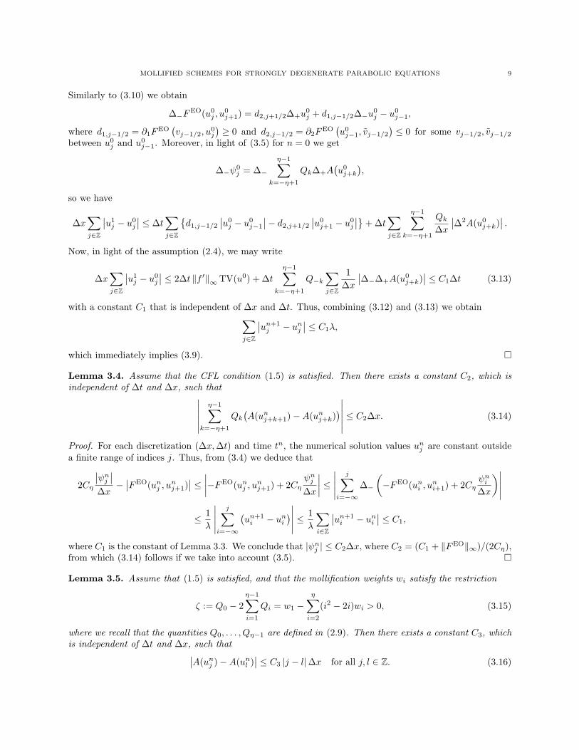
MOLLIFIED SCHEMES FOR STRONGLY DEGENERATE PARABOLIC EQUATIONS 9

Similarly to (3.10) we obtain

∆−FEO(u0j , u

0j+1) = d2,j+1/2∆+u

0j + d1,j−1/2∆−u0

j − u0j−1,

where d1,j−1/2 = ∂1FEO(vj−1/2, u

0j

)≥ 0 and d2,j−1/2 = ∂2F

EO(u0j−1, vj−1/2

)≤ 0 for some vj−1/2, vj−1/2

between u0j and u0

j−1. Moreover, in light of (3.5) for n = 0 we get

∆−ψ0j = ∆−

η−1∑k=−η+1

Qk∆+A(u0j+k

),

so we have

∆x∑j∈Z

∣∣u1j − u0

j

∣∣ ≤ ∆t∑j∈Z

{d1,j−1/2

∣∣u0j − u0

j−1

∣∣− d2,j+1/2

∣∣u0j+1 − u0

j

∣∣}+ ∆t∑j∈Z

η−1∑k=−η+1

Qk∆x

∣∣∆2A(u0j+k)

∣∣ .Now, in light of the assumption (2.4), we may write

∆x∑j∈Z

∣∣u1j − u0

j

∣∣ ≤ 2∆t ‖f ′‖∞ TV(u0) + ∆tη−1∑

k=−η+1

Q−k∑j∈Z

1∆x

∣∣∆−∆+A(u0j+k)

∣∣ ≤ C1∆t (3.13)

with a constant C1 that is independent of ∆x and ∆t. Thus, combining (3.12) and (3.13) we obtain∑j∈Z

∣∣un+1j − unj

∣∣ ≤ C1λ,

which immediately implies (3.9). �

Lemma 3.4. Assume that the CFL condition (1.5) is satisfied. Then there exists a constant C2, which isindependent of ∆t and ∆x, such that∣∣∣∣∣∣

η−1∑k=−η+1

Qk(A(unj+k+1)−A(unj+k)

)∣∣∣∣∣∣ ≤ C2∆x. (3.14)

Proof. For each discretization (∆x,∆t) and time tn, the numerical solution values unj are constant outsidea finite range of indices j. Thus, from (3.4) we deduce that

2Cη

∣∣ψnj ∣∣∆x−∣∣FEO(unj , u

nj+1)

∣∣ ≤ ∣∣∣∣−FEO(unj , unj+1) + 2Cη

ψnj∆x

∣∣∣∣ ≤∣∣∣∣∣

j∑i=−∞

∆−

(−FEO(uni , u

ni+1) + 2Cη

ψni∆x

)∣∣∣∣∣≤ 1λ

∣∣∣∣∣j∑

i=−∞

(un+1i − uni

)∣∣∣∣∣ ≤ 1λ

∑i∈Z

∣∣un+1i − uni

∣∣ ≤ C1,

where C1 is the constant of Lemma 3.3. We conclude that |ψnj | ≤ C2∆x, where C2 = (C1 + ‖FEO‖∞)/(2Cη),from which (3.14) follows if we take into account (3.5). �

Lemma 3.5. Assume that (1.5) is satisfied, and that the mollification weights wi satisfy the restriction

ζ := Q0 − 2η−1∑i=1

Qi = w1 −η∑i=2

(i2 − 2i)wi > 0, (3.15)

where we recall that the quantities Q0, . . . , Qη−1 are defined in (2.9). Then there exists a constant C3, whichis independent of ∆t and ∆x, such that∣∣A(unj )−A(unl )

∣∣ ≤ C3 |j − l|∆x for all j, l ∈ Z. (3.16)

10 ACOSTA, BURGER, AND MEJIA

Proof. We begin by setting znj := A(unj+1)−A(unj ). Since the initial datum is assumed to be constant outsidea bounded interval (see (2.4)), for a given pair of discretization parameters (∆x,∆t) there exists an integerK > 0, which in general depends on n, such that znj = zn−j = 0 for j > K. Additionally, from the triangularinequality and Lemma 3.4 we obtain

Q0

∣∣znj ∣∣− η−1∑i=1

Qi∣∣znj−i∣∣− η−1∑

i=1

Qi∣∣znj+i∣∣ ≤

∣∣∣∣∣∣η−1∑

k=−η+1

Q−kznj+k

∣∣∣∣∣∣ ≤ C2∆x, j = −K, . . . ,K. (3.17)

Actually, (3.17) is valid for j ∈ Z, but is trivially satisfied for |j| > K since znj = 0 for these j. Consequently,defining the vectors

dn :=(∣∣zn−K∣∣ , . . . , |znK |)T ∈ R2K+1, e := (1, . . . , 1)T ∈ R2K+1

and the (2η − 1)-diagonal (2K + 1)× (2K + 1)-matrix

M =

Q0 −Q1 · · · −Qη−1 0 · · · 0

−Q1 Q0. . . . . . . . .

......

. . . . . . . . . . . . 0

−Qη−1. . . . . . . . . −Qη−1

0. . . . . . . . . . . .

......

. . . . . . . . . . . . −Q1

0 · · · 0 −Qη−1 · · · −Q1 Q0

,

we can rewrite (3.17) as the system of inequalities Mdn ≤ C2∆xe, where “≤” holds in a component-wisesense. Clearly, due to its sign structure, M is an L-matrix. Moreover, if (3.15) is satisfied, then M becomesan M-matrix, which means that M−1 exists, M−1 ≥ 0 in a component-wise sense, and ‖M−1‖∞ ≤ ζ−1.This implies that dn ≤ C2∆xM−1e (in a component-wise sense), in particular ‖dn‖∞ ≤ (C2ζ

−1)∆x. Thus,(3.16) follows by taking C3 := C2/ζ, and noting that ζ does not depend on ∆x, ∆t, or K. �

Remark 3.2. We have just proved that by imposing that the mollification weights satisfy the additionalcondition (3.15), one can establish the spatial regularity property (3.16). For p = 3, (3.15) is satisfied forη = 1, . . . , 5, see Table 1, which also shows the corresponding values of ζ.

In light of Lemma 3.5 there exists a constant C4, which is independent of ∆t and ∆x, such that

λ∑j∈Z

N−1∑n=0

(A(unj+1

)−A

(unj))2 ≤ C4. (3.18)

Lemma 3.6. Under the assumptions of Lemma 3.5 there exists a constant C5, which is independent of ∆tand ∆x, such that ∣∣A(unj )−A(umj )

∣∣ ≤ C5 |(m− n) ∆t|1/2 for all n,m ∈ {0, . . . , N}.

The proof of Lemma 3.6 is given by the proof of [17, Lemma 4.2], which in turn is based on a techniqueintroduced in [1]. The proof is based on an interpolation technique that exploits (3.16) and does not dependon the particular scheme being considered.

As in [1], we denote by u∆ (where ∆ = (∆x,∆t)) the interpolant of degree one associated with the datapoints {unj }. The function u∆ is continuous everywhere and differentiable almost everywhere. From (3.6) inLemma 3.2, Corollary 3.1 and Lemma 3.3 we deduce that there is a constant C6 such that

‖u∆‖L∞(ΠT ) + TVΠT (u∆) ≤ C6, (3.19)

while Lemmas 3.5 and 3.6 imply that there is a constant C7 such that∣∣A(u∆(y, τ))−A

(u∆(x, t)

)∣∣ ≤ C7

(|x− y|+ |t− τ |1/2 + ∆x+ ∆t1/2

)for all (x, t), (y, τ) ∈ ΠT . (3.20)

MOLLIFIED SCHEMES FOR STRONGLY DEGENERATE PARABOLIC EQUATIONS 11

Lemma 3.7. Let us recall the standard notation a ∧ b := min{a, b} and a ∨ b := max{a, b}, and define

ψnj :=n∑k=1

ρk

(∣∣A(unj+k)−A(c)∣∣− ∣∣A(unj−k+1

)−A(c)

∣∣),where ρk is defined as in (3.3). Then the mollified scheme (3.2) satisfies the following cell entropy inequality:

∀c ∈ R :∣∣un+1j − c

∣∣ ≤ ∣∣unj − c∣∣− λ∆−

(FEO

(unj ∨ c, unj+1 ∨ c

)− FEO

(unj ∧ c, unj+1 ∧ c

)− 2Cη

∆xψkj

).

(3.21)

Proof. Recalling the definition of ψnj in (3.3), we obtain by replacing every ocurrence of unj in the definitionof Sj(un) by unj ∨ c, where un ∨ c := {unj ∨ c}j∈Z, the identity

Sj(un ∨ c) = unj ∨ c− λ∆−

(FEO

(unj ∨ c, unj+1 ∨ c

)− 2Cη

∆x

n∑k=1

ρk(A(unj+k ∨ c

)−A

(unj−k+1 ∨ c

))).

The same identity holds if every “∨” is replaced by “∧” and we define un ∧ c := {unj ∧ c}j∈Z. Subtractingthe second version from the first, we obtain

Sj(un ∨ c)− Sj(un ∧ c)=∣∣unj − c∣∣− λ∆−

(FEO

(unj ∨ c, unj+1 ∨ c

)− FEO

(unj ∧ c, unj+1 ∧ c

))− λ∆−

(−2Cη

∆x

n∑k=1

ρk

(A(unj+k ∨ c

)−A

(unj+k ∧ c

)−(A(unj−k+1 ∨ c

)−A

(unj−k+1 ∧ c

)))).

Since A is non-decreasing, we can rewrite this as

Sj(un ∨ c)− Sj(un ∧ c) =∣∣unj − c∣∣− λ∆−

(FEO

(unj ∨ c, unj+1 ∨ c

)− FEO

(unj ∧ c, unj+1 ∧ c

))+ λ

2Cη∆x

∆−ψnj .(3.22)

On the other hand, the monotonicity of the scheme implies that

Sj(un ∨ c)− Sj(un ∧ c) ≥ Sj(un) ∨ c− Sj(un) ∧ c =∣∣un+1j − c

∣∣ . (3.23)

Combining (3.22) and (3.23) we obtain the desired entropy inequality (3.21). �

Theorem 3.2. Assume that ∆t and ∆x satisfy the CFL condition (1.5), that the weights w−η, . . . , wη ofthe discrete mollification operator satisfy the restriction (3.15), and that the initial datum u0 satisfies (2.4).Then the interpolated approximate solution u∆ obtained from the mollified scheme (3.2) converges in thestrong topology of L1(ΠT ) to an entropy solution of (1.1), (1.2).

Proof. Due to the embedding of L∞(ΠT ) ∩ BV (ΠT ) in L1(QT ) ([22]; see [1]), we deduce from (3.19) thatthere exists a sequence {∆i}i∈N with ∆i → 0 for i → ∞ and a function u ∈ L∞(ΠT ) ∩ BV (ΠT ) such thatu∆ → u a.e. on ΠT . Moreover, in light of (3.20) the Arzela-Ascoli theorem implies that A(u∆) → A(u)uniformly on ΠT , and we have that A(u) ∈ C1,1/2(ΠT ).

It remains to prove that u satisfies the entropy inequality (2.1). This can be done by a standard Lax-Wendroff-type argument; namely, we choose a non-negative test function φ ∈ C∞(ΠT ) with compact supporton R× [0, T ), multiply the discrete entropy inequality (3.21) by ∆xφnj , where φnj = φ(xj , tn), sum the resultover all j and n, apply “summation by parts”, and let ∆ ↓ 0. Details (cf. e.g. [1, 15]) will be omitted here,but we mention that the “summation by parts” for the discretization of the diffusive terms in (3.21) can bedone as follows:

∆x∑j∈Z

N−1∑n=0

λφnj ∆−

(2Cη∆x

ψnj

)= ∆x∆t

N−1∑n=0

2Cη∆x2

∑j∈Z

φnj

η∑i=−η

w−i∣∣A(unj+i)−A(c)

∣∣− ∣∣A(unj )−A(c)∣∣

12 ACOSTA, BURGER, AND MEJIA

0 0.2 0.4 0.6 0.8 10

0.2

0.4

0.6

0.8

1

x

u

MollifiedBasicReference

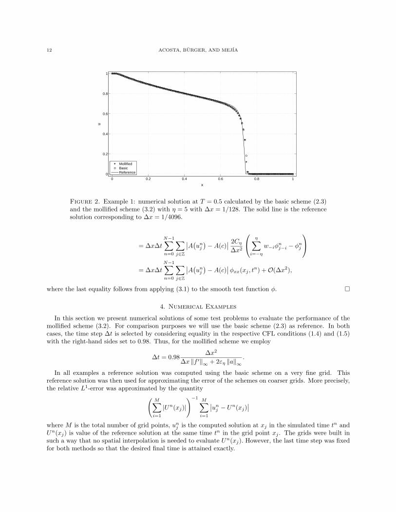
Figure 2. Example 1: numerical solution at T = 0.5 calculated by the basic scheme (2.3)and the mollified scheme (3.2) with η = 5 with ∆x = 1/128. The solid line is the referencesolution corresponding to ∆x = 1/4096.

= ∆x∆tN−1∑n=0

∑j∈Z

∣∣A(unj )−A(c)∣∣ 2Cη

∆x2

η∑i=−η

w−iφnj−i − φnj

= ∆x∆t

N−1∑n=0

∑j∈Z

∣∣A(unj )−A(c)∣∣φxx(xj , tn) +O(∆x2),

where the last equality follows from applying (3.1) to the smooth test function φ. �

4. Numerical Examples

In this section we present numerical solutions of some test problems to evaluate the performance of themollified scheme (3.2). For comparison purposes we will use the basic scheme (2.3) as reference. In bothcases, the time step ∆t is selected by considering equality in the respective CFL conditions (1.4) and (1.5)with the right-hand sides set to 0.98. Thus, for the mollified scheme we employ

∆t = 0.98∆x2

∆x ‖f ′‖∞ + 2εη ‖a‖∞.

In all examples a reference solution was computed using the basic scheme on a very fine grid. Thisreference solution was then used for approximating the error of the schemes on coarser grids. More precisely,the relative L1-error was approximated by the quantity(

M∑i=1

|Un(xj)|

)−1 M∑i=1

∣∣unj − Un(xj)∣∣

where M is the total number of grid points, unj is the computed solution at xj in the simulated time tn andUn(xj) is value of the reference solution at the same time tn in the grid point xj . The grids were built insuch a way that no spatial interpolation is needed to evaluate Un(xj). However, the last time step was fixedfor both methods so that the desired final time is attained exactly.

MOLLIFIED SCHEMES FOR STRONGLY DEGENERATE PARABOLIC EQUATIONS 13

Basic scheme (2.3) Mollified Scheme (3.2) with η = 31/∆x L1-error conv. rate CPU time [s] L1-error conv. rate CPU time [s]

64 2.6762e-2 – 0.0083 2.6105e-2 – 0.0107

128 1.5390e-2 0.7982 0.0286 1.4932e-2 0.8059 0.0384

256 8.5957e-3 0.8403 0.1074 8.3709e-3 0.8349 0.1330

512 4.5905e-3 0.9050 0.5497 4.5075e-3 0.8931 0.6497

1024 2.0265e-3 1.1797 3.4742 1.9997e-3 1.1725 3.8324

Mollified Scheme (3.2) with η = 5 Mollified Scheme (3.2) with η = 81/∆x L1-error conv. rate CPU time [s] L1-error conv. rate CPU time [s]

64 2.5327e-2 – 0.0101 2.5055e-2 – 0.0089

128 1.4287e-2 0.8259 0.0308 1.4133e-2 0.8260 0.0319

256 7.9698e-3 0.8420 0.1007 7.6883e-3 0.8783 0.0893

512 4.3271e-3 0.8811 0.4380 4.1141e-3 0.9020 0.3075

1024 1.9335e-3 1.1622 2.3848 1.8279e-3 1.1704 1.4976

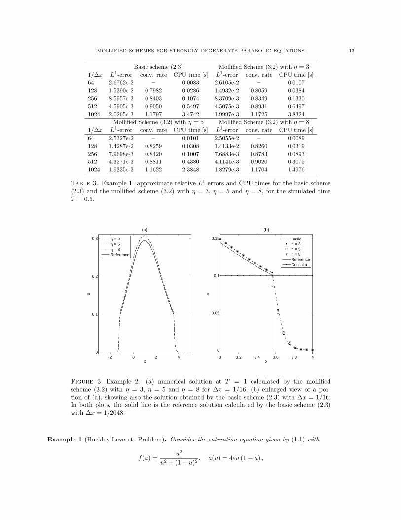
Table 3. Example 1: approximate relative L1 errors and CPU times for the basic scheme(2.3) and the mollified scheme (3.2) with η = 3, η = 5 and η = 8, for the simulated timeT = 0.5.

−2 0 2 40

0.1

0.2

0.3

x

u

(a)

η = 3η = 5η = 8Reference

3 3.2 3.4 3.6 3.8 4

0

0.05

0.1

0.15

x

u

(b)

Basicη = 3η = 5η = 8ReferenceCritical u

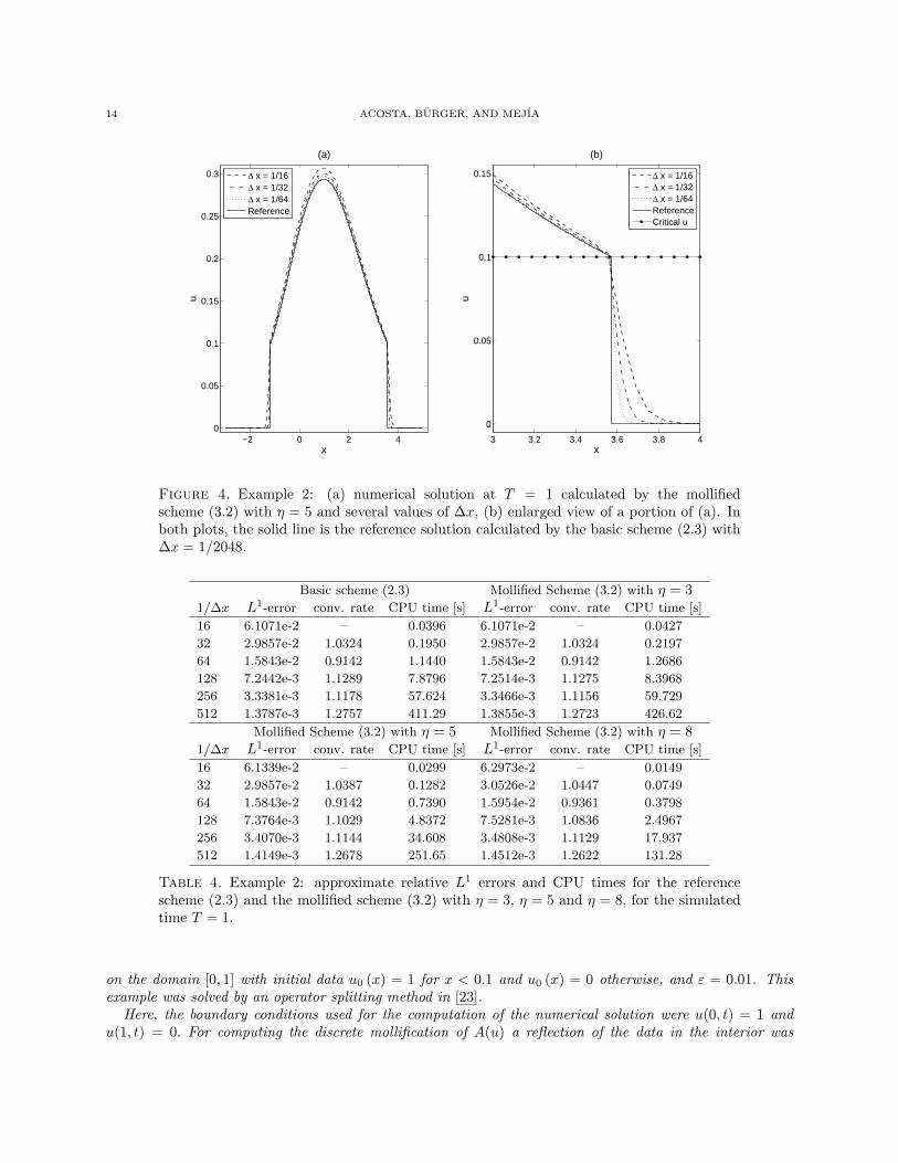
Figure 3. Example 2: (a) numerical solution at T = 1 calculated by the mollifiedscheme (3.2) with η = 3, η = 5 and η = 8 for ∆x = 1/16, (b) enlarged view of a por-tion of (a), showing also the solution obtained by the basic scheme (2.3) with ∆x = 1/16.In both plots, the solid line is the reference solution calculated by the basic scheme (2.3)with ∆x = 1/2048.

Example 1 (Buckley-Leverett Problem). Consider the saturation equation given by (1.1) with

f(u) =u2

u2 + (1− u)2, a(u) = 4εu (1− u) ,

14 ACOSTA, BURGER, AND MEJIA

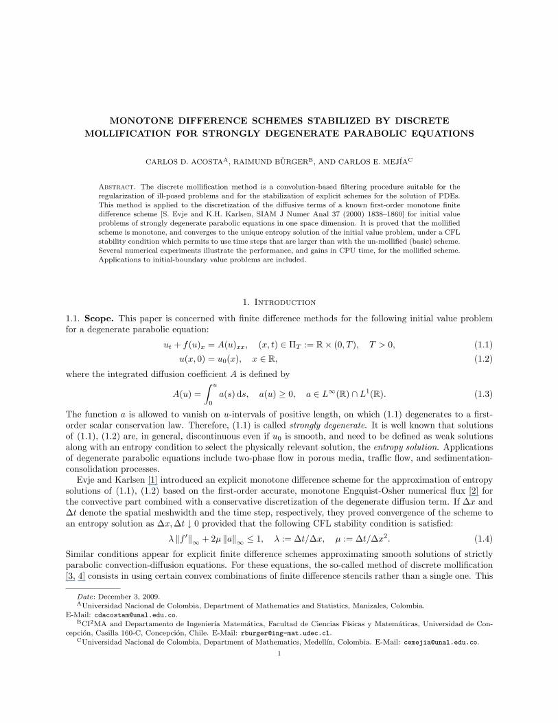
−2 0 2 40

0.05

0.1

0.15

0.2

0.25

0.3

x

u

(a)

Δ x = 1/16Δ x = 1/32Δ x = 1/64Reference

3 3.2 3.4 3.6 3.8 4

0

0.05

0.1

0.15

xu

(b)

Δ x = 1/16Δ x = 1/32Δ x = 1/64ReferenceCritical u

Figure 4. Example 2: (a) numerical solution at T = 1 calculated by the mollifiedscheme (3.2) with η = 5 and several values of ∆x, (b) enlarged view of a portion of (a). Inboth plots, the solid line is the reference solution calculated by the basic scheme (2.3) with∆x = 1/2048.

Basic scheme (2.3) Mollified Scheme (3.2) with η = 31/∆x L1-error conv. rate CPU time [s] L1-error conv. rate CPU time [s]

16 6.1071e-2 – 0.0396 6.1071e-2 – 0.0427

32 2.9857e-2 1.0324 0.1950 2.9857e-2 1.0324 0.2197

64 1.5843e-2 0.9142 1.1440 1.5843e-2 0.9142 1.2686

128 7.2442e-3 1.1289 7.8796 7.2514e-3 1.1275 8.3968

256 3.3381e-3 1.1178 57.624 3.3466e-3 1.1156 59.729

512 1.3787e-3 1.2757 411.29 1.3855e-3 1.2723 426.62

Mollified Scheme (3.2) with η = 5 Mollified Scheme (3.2) with η = 81/∆x L1-error conv. rate CPU time [s] L1-error conv. rate CPU time [s]

16 6.1339e-2 – 0.0299 6.2973e-2 – 0.0149

32 2.9857e-2 1.0387 0.1282 3.0526e-2 1.0447 0.0749

64 1.5843e-2 0.9142 0.7390 1.5954e-2 0.9361 0.3798

128 7.3764e-3 1.1029 4.8372 7.5281e-3 1.0836 2.4967

256 3.4070e-3 1.1144 34.608 3.4808e-3 1.1129 17.937

512 1.4149e-3 1.2678 251.65 1.4512e-3 1.2622 131.28

Table 4. Example 2: approximate relative L1 errors and CPU times for the referencescheme (2.3) and the mollified scheme (3.2) with η = 3, η = 5 and η = 8, for the simulatedtime T = 1.

on the domain [0, 1] with initial data u0 (x) = 1 for x < 0.1 and u0 (x) = 0 otherwise, and ε = 0.01. Thisexample was solved by an operator splitting method in [23].

Here, the boundary conditions used for the computation of the numerical solution were u(0, t) = 1 andu(1, t) = 0. For computing the discrete mollification of A(u) a reflection of the data in the interior was

MOLLIFIED SCHEMES FOR STRONGLY DEGENERATE PARABOLIC EQUATIONS 15

10-2 100 10210-4

10-3

10-2

10-1

CPU-time [s]

L1 Err

or

Example 1

Basicη = 3η = 5η = 8

10-2 100 102 10410-4

10-3

10-2

10-1

CPU-time [s]

L1 Err

or

Example 2

Basicη = 3η = 5η = 8

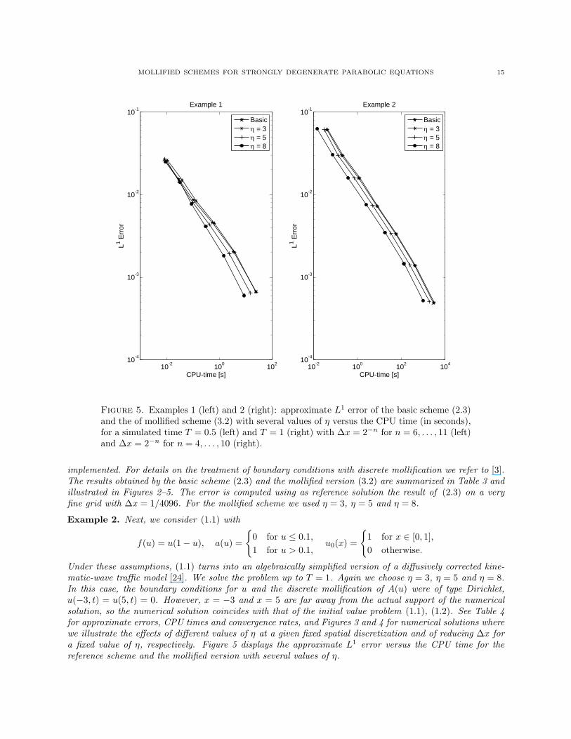
Figure 5. Examples 1 (left) and 2 (right): approximate L1 error of the basic scheme (2.3)and the of mollified scheme (3.2) with several values of η versus the CPU time (in seconds),for a simulated time T = 0.5 (left) and T = 1 (right) with ∆x = 2−n for n = 6, . . . , 11 (left)and ∆x = 2−n for n = 4, . . . , 10 (right).

implemented. For details on the treatment of boundary conditions with discrete mollification we refer to [3].The results obtained by the basic scheme (2.3) and the mollified version (3.2) are summarized in Table 3 andillustrated in Figures 2–5. The error is computed using as reference solution the result of (2.3) on a veryfine grid with ∆x = 1/4096. For the mollified scheme we used η = 3, η = 5 and η = 8.

Example 2. Next, we consider (1.1) with

f(u) = u(1− u), a(u) =

{0 for u ≤ 0.1,1 for u > 0.1,

u0(x) =

{1 for x ∈ [0, 1],0 otherwise.

Under these assumptions, (1.1) turns into an algebraically simplified version of a diffusively corrected kine-matic-wave traffic model [24]. We solve the problem up to T = 1. Again we choose η = 3, η = 5 and η = 8.In this case, the boundary conditions for u and the discrete mollification of A(u) were of type Dirichlet,u(−3, t) = u(5, t) = 0. However, x = −3 and x = 5 are far away from the actual support of the numericalsolution, so the numerical solution coincides with that of the initial value problem (1.1), (1.2). See Table 4for approximate errors, CPU times and convergence rates, and Figures 3 and 4 for numerical solutions wherewe illustrate the effects of different values of η at a given fixed spatial discretization and of reducing ∆x fora fixed value of η, respectively. Figure 5 displays the approximate L1 error versus the CPU time for thereference scheme and the mollified version with several values of η.

16 ACOSTA, BURGER, AND MEJIA

0 0.035 0.07 0.105 0.140

0.04

0.08

0.12

0.16

(a) T = 800 s

u

x [m

]

0 0.035 0.07 0.105 0.140

0.04

0.08

0.12

0.16

(b) T = 1600 s

ux

[m]

0 0.035 0.07 0.105 0.140

0.04

0.08

0.12

0.16

(c) T = 2400 s

u

x [m

]

0 0.035 0.07 0.105 0.140

0.04

0.08

0.12

0.16

(d) T = 4000 s

u

x [m

]

ReferenceMollifiedBasicCritical u

ReferenceMollifiedBasicCritical u

ReferenceMollifiedBasicCritical u

ReferenceMollifiedBasicCritical u

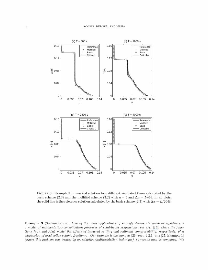
Figure 6. Example 3: numerical solution four different simulated times calculated by thebasic scheme (2.3) and the mollified scheme (3.2) with η = 5 and ∆x = L/64. In all plots,the solid line is the reference solution calculated by the basic scheme (2.3) with ∆x = L/2048.

Example 3 (Sedimentation). One of the main applications of strongly degenerate parabolic equations isa model of sedimentation-consolidation processes of solid-liquid suspensions, see e.g. [25], where the func-tions f(u) and A(u) model the effects of hindered settling and sediment compressibility, respectively, of asuspension of local solids volume fraction u. Our example is the same as [26, Sect. 4.2.1] and [27, Example 1](where this problem was treated by an adaptive multiresolution technique), so results may be compared. We

MOLLIFIED SCHEMES FOR STRONGLY DEGENERATE PARABOLIC EQUATIONS 17

10-2 100 10210-3

10-2

10-1

CPU-time [s]

L1 Err

or

T = 400

Basicη = 3η = 5η = 8

10-2 100 10210-3

10-2

10-1T = 2400

CPU-time [s]

L1 Err

or

Basicη = 3η = 5η = 8

10-2 100 10210-4

10-3

10-2

10-1T = 4000

CPU-time [s]

L1 Err

or

Basicη = 3η = 5η = 8

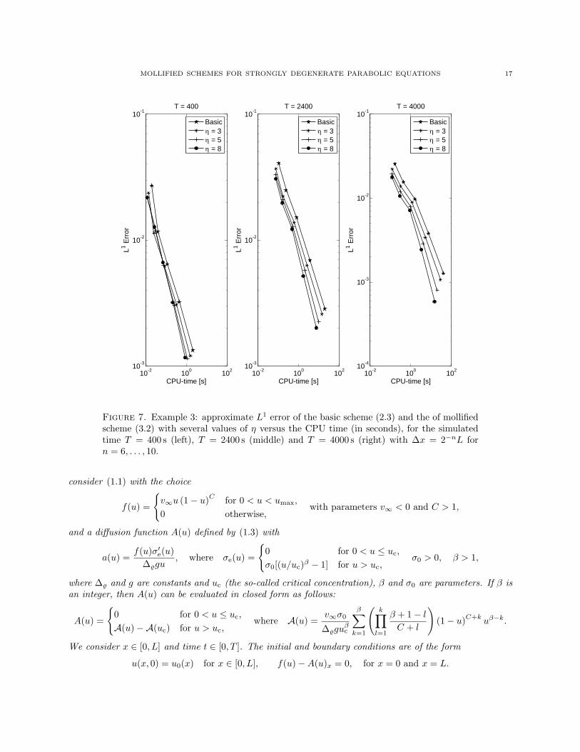
Figure 7. Example 3: approximate L1 error of the basic scheme (2.3) and the of mollifiedscheme (3.2) with several values of η versus the CPU time (in seconds), for the simulatedtime T = 400 s (left), T = 2400 s (middle) and T = 4000 s (right) with ∆x = 2−nL forn = 6, . . . , 10.

consider (1.1) with the choice

f(u) =

{v∞u (1− u)C for 0 < u < umax,0 otherwise,

with parameters v∞ < 0 and C > 1,

and a diffusion function A(u) defined by (1.3) with

a(u) =f(u)σ′e(u)

∆%gu, where σe(u) =

{0 for 0 < u ≤ uc,σ0[(u/uc)β − 1] for u > uc,

σ0 > 0, β > 1,

where ∆% and g are constants and uc (the so-called critical concentration), β and σ0 are parameters. If β isan integer, then A(u) can be evaluated in closed form as follows:

A(u) =

{0 for 0 < u ≤ uc,A(u)−A(uc) for u > uc,

where A(u) =v∞σ0

∆%guβc

β∑k=1

(k∏l=1

β + 1− lC + l

)(1− u)C+k

uβ−k.

We consider x ∈ [0, L] and time t ∈ [0, T ]. The initial and boundary conditions are of the form

u(x, 0) = u0(x) for x ∈ [0, L], f(u)−A(u)x = 0, for x = 0 and x = L.

18 ACOSTA, BURGER, AND MEJIA

(a) T = 400 s

Basic scheme (2.3) Mollified Scheme (3.2) with η = 31/∆x L1-error conv. rate CPU time [s] L1-error conv. rate CPU time [s]

64 2.7063e-2 – 0.0199 2.3574e-2 – 0.0135

128 1.1672e-2 1.2133 0.0388 1.1381e-2 1.0506 0.0257

256 6.4428e-3 0.8572 0.1134 6.2139e-3 0.8730 0.0845

512 3.2280e-3 0.9970 0.4365 3.0598e-3 1.0221 0.3255

Mollified Scheme (3.2) with η = 5 Mollified Scheme (3.2) with η = 81/∆x L1-error conv. rate CPU time [s] L1-error conv. rate CPU time [s]

64 2.1772e-2 – 0.0116 2.1746e-2 0.0116

128 1.1781e-2 0.8860 0.0305 1.2684e-2 0.7777 0.0264

256 6.3253e-3 0.8972 0.0779 6.6323e-3 0.9354 0.0695

512 3.0530e-3 1.0509 0.2604 3.1926e-3 1.0548 0.2117

(b) T = 2400 s

Basic scheme (2.3) Mollified Scheme (3.2) with η = 31/∆x L1-error conv. rate CPU time [s] L1-error conv. rate CPU time [s]

64 4.0720e-2 – 0.1070 3.6909e-2 0.0763

128 2.4783e-2 0.7164 0.2419 2.2321e-2 0.7256 0.1711

256 1.5127e-2 0.7122 0.8116 1.3774e-2 0.6965 0.5954

512 6.8969e-3 1.1331 3.5935 6.3001e-3 1.1285 2.5624

Mollified Scheme (3.2) with η = 5 Mollified Scheme (3.2) with η = 81/∆x L1-error conv. rate CPU time [s] L1-error conv. rate CPU time [s]

64 3.3140e-2 – 0.0751 3.0733e-2 – 0.0757

128 2.0822e-2 0.6705 0.1676 1.9756e-2 0.6375 0.1598

256 1.2763e-2 0.7061 0.5181 1.2194e-2 0.6961 0.4673

512 5.7278e-3 1.1559 2.0387 5.1709e-3 1.2377 1.6909

(c) T = 4000 s

Basic scheme (2.3) Mollified Scheme (3.2) with η = 31/∆x L1-error conv. rate CPU time [s] L1-error conv. rate CPU time [s]

64 2.5560e-2 – 0.1670 2.2249e-2 – 0.1209

128 1.5463e-2 0.7251 0.4342 1.3797e-2 0.6894 0.3133

256 9.7331e-3 0.6679 1.6177 8.8938e-3 0.6335 1.1459

512 3.7879e-3 1.3615 7.4223 3.3775e-3 1.3968 5.1181

Mollified Scheme (3.2) with η = 5 Mollified Scheme (3.2) with η = 81/∆x L1-error conv. rate CPU time [s] L1-error conv. rate CPU time [s]

64 1.9460e-2 – 0.1208 1.7743e-2 – 0.1211

128 1.1946e-2 0.7039 0.3008 1.0622e-2 0.7402 0.2863

256 7.8624e-3 0.6034 0.9887 7.1371e-3 0.5737 0.8896

512 2.8738e-3 1.4520 4.0391 2.4282e-3 1.5555 3.3389

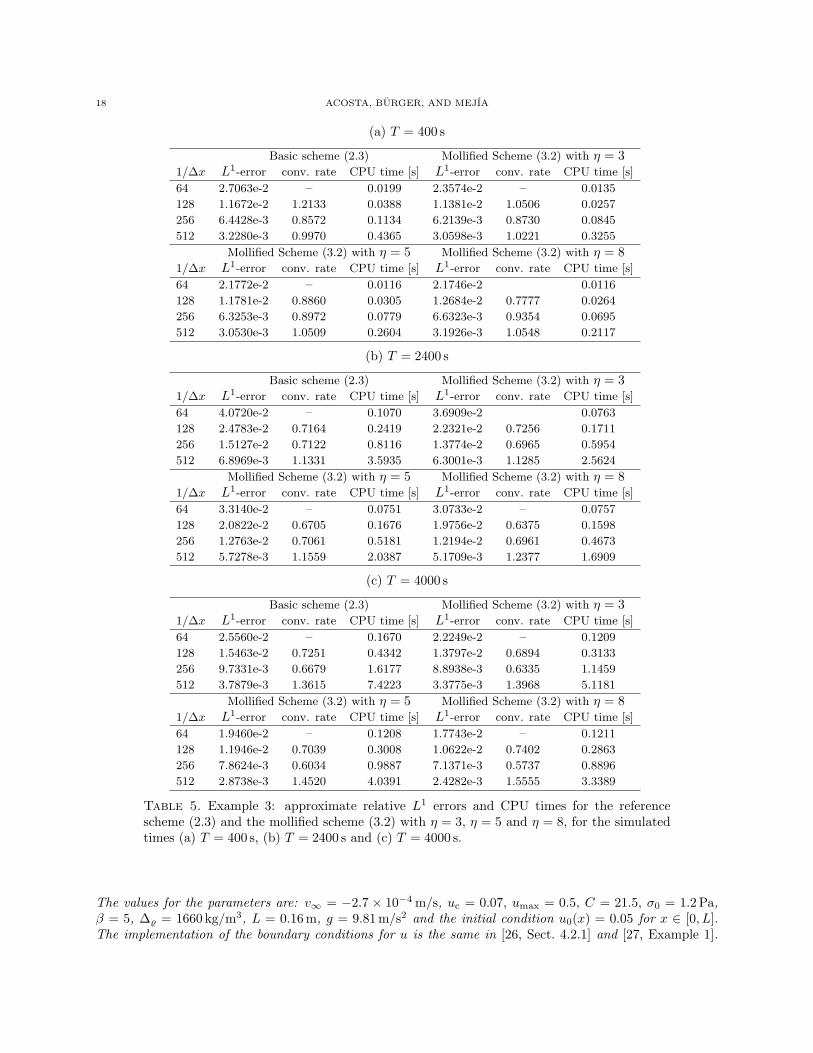
Table 5. Example 3: approximate relative L1 errors and CPU times for the referencescheme (2.3) and the mollified scheme (3.2) with η = 3, η = 5 and η = 8, for the simulatedtimes (a) T = 400 s, (b) T = 2400 s and (c) T = 4000 s.

The values for the parameters are: v∞ = −2.7 × 10−4 m/s, uc = 0.07, umax = 0.5, C = 21.5, σ0 = 1.2 Pa,β = 5, ∆% = 1660 kg/m3, L = 0.16 m, g = 9.81 m/s2 and the initial condition u0(x) = 0.05 for x ∈ [0, L].The implementation of the boundary conditions for u is the same in [26, Sect. 4.2.1] and [27, Example 1].

MOLLIFIED SCHEMES FOR STRONGLY DEGENERATE PARABOLIC EQUATIONS 19

For the discrete mollification of A(un), we obtained a linear extrapolation at the borders. For instance atx = 0, we use the knowledge of A(un0 ) and A(un0 )x = f(un0 ) for getting an interpolating straight line withslope f(un0 ). See Table 5 and Figures 6 and 7 for results.

5. Conclusions

The convergence analysis shows that standard compactness and entropicity arguments for finite differenceschemes for non-linear first-order conservation laws and strongly degenerate parabolic equations can beapplied to establish convergence of (3.2) to the entropy solution of (1.1), (1.2) under a CFL condition thatallows a larger time step than the basic (unmollified) scheme. Although the convergence statement holds onlyfor η ≤ 5 (when p = 3), encouraging numerical results were also obtained in the case η > 5, as illustratedabove with η = 8. A possibly sharper bound in Lemma 3.5 could lead to a less restrictive convergencecondition than (3.15). We have kept here the arguments fairly simple, and limited ourselves to one setof mollification weights, namely those obtained in Table 1 for p = 3; this value of p is also employed in[3, 10]. Variations of p and of the corresponding weights could equally turn out more favorable conditionsof satisfaction of (3.15).

Overall, the results of the numerical solutions look encouraging and in the cases of Examples 1 and 3illustrate that the mollified scheme works well also for problems with boundary conditions, which we have notincluded in our convergence analysis (see [15]). The computations have been performed with the maximaltime step allowed by the corresponding CFL conditions for the basic scheme and its mollified versions.One should keep in mind that the mollified schemes permit a larger time step, but the evaluation of thediscretization of A(u)xx for the mollified scheme is algebraically slightly more involved that that for thebasic scheme. In fact, in Examples 1 and 2 a significant gain in CPU time is achieved only for η = 5 andη = 8. In all examples, the approximate errors for the basic and mollified schemes at a given discretizationare similar. Probably the resulting speed-up is not as good as for implicit versions of the basic scheme, butthe mollification-based option presented herein is easy to implement and avoids, for example, the necessityto solve systems of nonlinear equations that appear with implicit schemes. Furthermore, we mention thatin any case a numerical solution calculated by the mollified scheme on a portion of ΠT requires less storagespace than the solution obtained from the basic scheme. This makes it potentially interesting to use themollified scheme (3.2) as the basic forward solver for parameter identification problems (see [20]), in whichthe coefficients of the so-called adjoint (backward-in-time) scheme depend on the properly stored solution ofthe direct (forward-in-time) problem.

Acknowledgements

CDA and RB acknowledge support by Fondap in Applied Mathematics, project 15000001, BASAL projectCMM, Universidad de Chile and Centro de Investigacion en Ingenierıa Matematica (CI2MA), Universidad deConcepcion, and project AMIRA P996/INNOVA 08CM01-17 “Instrumentacion y Control de Espesadores”.In addition, RB is supported by Fondecyt project 1090456 and CDA by Universidad Nacional de Colombia,DIMA Project 20201005215.

References

[1] S. Evje and K.H. Karlsen, Monotone difference approximations of BV solutions to degenerate convection-diffusion equa-tions, SIAM J Numer Anal 37 (2000), 1838–1860.

[2] B. Engquist and S. Osher, One-sided difference approximations for nonlinear conservation laws, Math Comp 36 (1981),

321–351.[3] C.D. Acosta and C.E. Mejıa, Stabilization of explicit methods for convection-diffusion problems by discrete mollification,

Comput Math Applic 55 (2008), 363–380.[4] C.D. Acosta and C.E. Mejıa, Approximate solution of hyperbolic conservation laws by discrete mollification, Appl Numer

Math 59 (2009), 2256–2265.

[5] D.A. Murio, The Mollification Method and the Numerical Solution of Ill-Posed Problems, John Wiley, New York, 1993.[6] D.A. Murio, Mollification and space marching, in: K. Woodbury (Ed.), Inverse Engineering Handbook, CRC Press, Boca

Raton, 2002.

20 ACOSTA, BURGER, AND MEJIA

[7] C.E. Mejıa and D.A. Murio, Numerical identification of diffusivity coefficient and initial condition by discrete mollification,

Comput Math Applic 30 (1995), 35–50.

[8] C.E. Mejıa and D.A. Murio, Numerical solution of generalized IHCP by discrete mollification, Comput Math Applic 32(1996), 33–50.

[9] D.A. Murio, C.E. Mejıa and S. Zhan, Some applications of the mollification method, in: M. Lassonde (Ed.), Approximation,

Optimization and Mathematical Economics, Physica-Verlag, 2001, pp. 213–222.[10] C.D. Acosta and C.E. Mejıa, A mollification-based operator splitting method for convection-diffusion equations, Comput

Math Applic, to appear.

[11] K.H. Karlsen and N.H. Risebro, An operator splitting method for nonlinear convection-diffusion equations, Numer Math77 (1997), 365–382.

[12] M.G. Crandall and A. Majda, Monotone difference approximations for scalar conservation laws, Math Comp 34 (1980),

1-21.[13] A. Harten, J.M. Hyman and P.D. Lax, On finite difference approximations and entropy conditions for shocks, Comm Pure

Appl Math 29 (1976), 297–322.[14] S. Evje and K.H. Karlsen, Degenerate convection-diffusion equations and implicit monotone difference schemes. In: H.

Freistuhler and G. Warnecke (eds.), Hyperbolic Problems: Theory, Numerics, Applications, Birkhauser-Verlag, Basel,

Switzerland, 1999, pp. 285–294.[15] R. Burger, A. Coronel and M. Sepulveda, A semi-implicit monotone difference scheme for an initial-boundary value problem

of a strongly degenerate parabolic equation modelling sedimentation-consolidation processes, Math Comp 75 (2006), 91–

112.[16] K.H. Karlsen and N.H. Risebro, Convergence of finite difference schemes for viscous and inviscid conservation laws with

rough coefficients, M2AN Math Model Numer Anal 35 (2001), 239–269.

[17] K.H. Karlsen, N.H. Risebro and J.D. Towers, Upwind difference approximations for degenerate parabolic convection-diffusion equations with a discontinuous coefficient, IMA J Numer Anal 22 (2002), 623–664.

[18] K.H. Karlsen, N.H. Risebro and J.D. Towers, L1 stability for entropy solutions of nonlinear degenerate parabolic convection-

diffusion equations with discontinuous coefficients, Skr K Nor Vid Selsk 3 (2003), 49 pp.[19] R. Burger, K.H. Karlsen and J.D. Towers, A mathematical model of continuous sedimentation of flocculated suspensions

in clarifier-thickener units, SIAM J Appl Math 65 (2005), 882–940.[20] A. Coronel, F. James and M. Sepulveda, Numerical identification of parameters for a model of sedimentation processes,

Inverse Problems 19 (2003), 951–972.

[21] K.H. Karlsen and N.H. Risebro, On the uniqueness and stability of entropy solutions of nonlinear degenerate parabolicequations with rough coefficients, Discr Cont Dyn Syst 9 (2003), 1081-1104.

[22] L.C. Evans and R.C. Gariepy, Measure Theory and Fine Properties of Functions. CRC Press, Boca Raton, FL, 1992.

[23] H. Holden, K.H. Karlsen and K.-A. Lie, Operator splitting methods for degenerate convection-diffusion equations II:numerical examples with emphasis on reservoir simulation and sedimentation, Comput Geosci 4 (2000), 287–322.

[24] R. Burger and K.H. Karlsen, On a diffusively corrected kinematic-wave traffic model with changing road surface conditions,

Math Models Methods Appl Sci 13 (2003), 1767–1799.[25] S. Berres, R. Burger, K.H. Karlsen and E.M. Tory, Strongly degenerate parabolic-hyperbolic systems modeling polydisperse

sedimentation with compression, SIAM J Appl Math 64 (2003), 41–80.

[26] R. Burger and K.H. Karlsen, On some upwind schemes for the phenomenological sedimentation-consolidation model, JEng Math 41 (2001), 145–166.

[27] R. Burger, A. Kozakevicius and M. Sepulveda, Multiresolution schemes for strongly degenerate parabolic equations in onespace dimension, Numer Meth Partial Diff Eqns 23 (2007), 706–730.