Numerical identification of a nonlinear diffusion coefficient by discrete mollification

Computers and Mathematics with Applications 62 (2011) 2187–2199

Contents lists available at SciVerse ScienceDirect

Computers and Mathematics with Applications

journal homepage: www.elsevier.com/locate/camwa

Numerical identification of a nonlinear diffusion coefficient by discretemollificationCarlos E. Mejía a,∗, Carlos D. Acosta b, Katerine I. Saleme c

a Escuela de Matemáticas, Universidad Nacional de Colombia, Medellín, Colombiab Departamento de Matemáticas y Estadística, Universidad Nacional de Colombia, Manizales, Colombiac High Performance Computing Collaboratory, Center for Advanced Vehicular Systems, Mississippi State University, Starkville, USA

a r t i c l e i n f o

Article history:Received 22 December 2010Received in revised form 5 June 2011Accepted 5 July 2011

Keywords:MollificationParameter identificationSpace-marching

a b s t r a c t

The discrete mollification method is a convolution-based filtering procedure suitable forthe regularization of ill-posed problems. Combined with explicit space-marching finitedifference schemes, it provides stability and convergence for a variety of coefficientidentification problems in linear parabolic equations. In this paper, we extend such atechnique to identify some nonlinear diffusion coefficients depending on an unknownspace dependent function in onedimensional parabolicmodels. For the coefficient recoveryprocess, we present detailed error estimates and to illustrate the performance of thealgorithms, several numerical examples are included.

© 2011 Elsevier Ltd. All rights reserved.

1. Introduction

A variety of analytical and numerical methods for inverse problems in evolution partial differential equations have beenproposed in the literature. They are useful to model situations in geophysics, oil recovery and heat conduction to list only afew. Among the general references on the subject, it is worth notice the book edited by Colton et al. [1] or the more recentbook by Vogel [2].

Research on the identification of unknown ingredients in forcing terms is very active. For instance, in [3], the authorsfind a close formula for an unknown space dependent ingredient in a linear heat equation. They refer to other works for theissues concerning identifiability and do not perform numerical computations. In [4], the problem is a nonlinear parabolicequation with a forcing term of the form p(x)f (u) for an unknown coefficient p(x) and a known smooth function f (u). Theauthors solve an optimization problem that takes care of the identifiability of the coefficient but do not include numericalexperiments.

Identification of diffusion coefficients is also quite frequent in the literature. For instance, identification of the spacedependent diffusion coefficient q(x) in

ut − ∇(q(x)∇u) = f (x, t),

is presented in [5]. The authors obtain the existence and introduce an approximation process for the identification problembut do not consider numerical issues. An inverse steady heat conduction problem appears in [6]. The problem is based onthe 2D elliptic equation

∇(q(u)∇u) = 0.

∗ Corresponding author.E-mail addresses: [email protected], [email protected] (C.E. Mejía).

0898-1221/$ – see front matter© 2011 Elsevier Ltd. All rights reserved.doi:10.1016/j.camwa.2011.07.004

2188 C.E. Mejía et al. / Computers and Mathematics with Applications 62 (2011) 2187–2199

The thermal conductivity is given by q(u) = b0 + b1u + b2u2 where b0, b1 and b2 are constants to be found. The paperintroduces a numerical identification of the three constant coefficients that do not take into consideration noise in the data.The theory on identifiability is not included.

In this paper, the framework is a one dimensional nonlinear heat conductionmodel and our problem is to identify a spacedependent ingredient in the thermal conductivity coefficient. Our strategy is to obtain a close formula for the approximationof the unknown ingredient by implementing a combination of discrete mollification and a space-marching finite differencenumerical scheme. Furthermore, we introduce several types of coefficients, allow noise in the data and deduce convergenceestimates for their respective numerical identifications.

The regularization tool is the mollification method, which is a reliable regularization procedure that has been widelyapplied for the stable numerical solution of ill-posed problems based on parabolic equations. In particular, for identificationproblems, we mention [7–10] for 1D linear diffusion and [11–13] for 2D linear diffusion.

Notice that the scope is a numerical identification problem in a distributed parameter system but we do not addresstheoretical issues related to identifiability of the coefficient. This endeavor is well accomplished in references like [14] for anonlinear diffusion coefficient and [4] for a space dependent ingredient in a nonlinear forcing term of a parabolic equation.

The remainder of the paper is organized as follows: In Section 2 we review basic facts about the discrete mollificationoperator. Section 3 is devoted to the identification problems and in Section 4 we include illustrative numerical examples.Finally, some concluding remarks are collected in Section 5.

2. Discrete mollification

When dealing with inverse problems, regularization techniques are a must. In this case, we perform regularization bydiscrete mollification, which is a filtering procedure based on convolution. In this section, we present definitions and factsrelated to mollification that give a good insight into the method. For a more complete introduction and proofs of the results,we recommend [15,16].

Let y = {yj}j∈Z be a discrete function, which can, for example, be evaluations or cell averages of a real function y = y(x)at equidistant grid points in

X = {xj : xj = x0 + jh, j ∈ Z}.

Its mollified version Jy, where J is the so-calledmollification operator,is defined by

(Jy)j :=

η−i=−η

ωiyj−i, (1)

where η is the integer support parameter and the weights ωi satisfy

ωi = ω−i, 0 ≤ ωi ≤ ωi−1, i = 1, . . . , η;

η−i=−η

ωi = 1,η−

i=−η

iωi = 0.

Let δ > 0 and p > 0. The mollification weights ωi and the discrete support parameter η, depend on δ > 0 and p > 0through the following setup. We choose η as the non-negative integer such that

(η − 1/2)h < pδ ≤ (η + 1/2)h; (2)

then we define a normalization constant

Ap =

∫ p

−pexp(−s2)ds

−1

and a truncated Gaussian kernel

κpδ(t) =

Apδ

−1 exp(−t2/δ2), |t| ≤ pδ0, |t| > pδ. (3)

This kernel satisfies the following properties: κpδ ≥ 0, κpδ ∈ C∞(−pδ, pδ), κpδ is zero outside [−pδ, pδ] and

R κpδ = 1.Based on the kernel, the mollification weights are computed by

ωi =

∫ ti+1

tiκpδ(−s)ds, (4)

where

tj = (j − 1/2)h, j ∈ Z. (5)

C.E. Mejía et al. / Computers and Mathematics with Applications 62 (2011) 2187–2199 2189

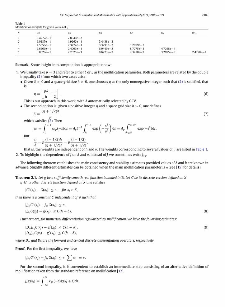
Table 1Mollification weights for given values of η.

η ω0 ω1 ω2 ω3 ω4 ω5

1 8.4272e−1 7.8640e−22 6.0387e−1 1.9262e−1 5.4438e−33 4.5556e−1 2.3772e−1 3.3291e−2 1.2099e−34 3.6266e−1 2.4003e−1 6.9440e−2 8.7275e−3 4.7268e−45 3.0028e−1 2.2625e−1 9.6723e−2 2.3430e−2 3.2095e−3 2.4798e−4

Remark. Some insight into computation is appropriate now:

1. We usually take p = 3 and refer to either δ or η as themollification parameter. Both parameters are related by the doubleinequality (2) from which two cases arise:• Given δ > 0 and a space grid size h > 0, one chooses η as the only nonnegative integer such that (2) is satisfied, that

is,

η =

pδh

+12

. (6)

This is our approach in this work, with δ automatically selected by GCV.• The second option is: given a positive integer η and a space grid size h > 0, one defines

δ =(η + 1/2)h

p. (7)

which satisfies (2). Then

ωi =

∫ ti+1

tiκδp(−s)ds = Apδ

−1∫ ti+1

tiexp

−

s2

δ2

ds = Ap

∫ ti+1/δ

ti/δexp(−s2)ds.

Buttiδ

= p(i − 1/2)h(η + 1/2)h

= p(i − 1/2)(η + 1/2)

,

that is, the weights are independent of h and δ. The weights corresponding to several values of η are listed in Table 1.2. To highlight the dependence of J on δ and η, instead of J we sometimes write Jδη .

The following theorem establishes the main consistency and stability estimates provided values of δ and h are known inadvance. Slightly different estimates can be obtained when the main mollification parameter is η (see [15] for details).

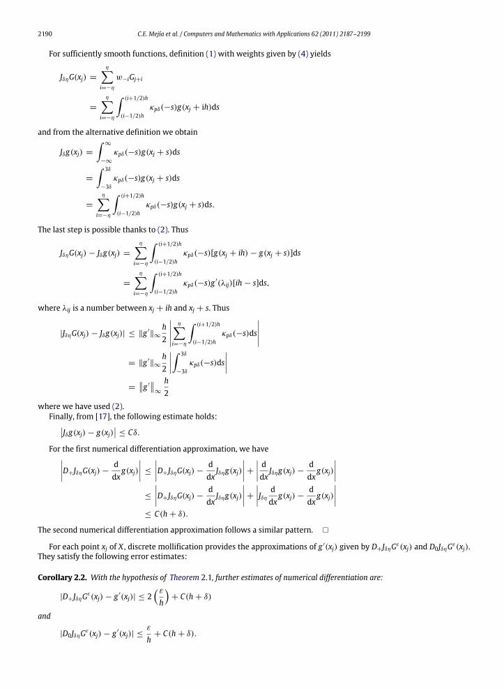
Theorem 2.1. Let g be a sufficiently smooth real function bounded in R. Let G be its discrete version defined on X.If Gε is other discrete function defined on X and satisfies

|Gε(xj) − G(xj)| ≤ ε, for xj ∈ X,

then there is a constant C independent of δ such that

|JδηGε(xj) − JδηG(xj)| ≤ ε,

|JδηG(xj) − g(xj)| ≤ C(h + δ). (8)

Furthermore, for numerical differentiation regularized by mollification, we have the following estimates:

|D+JδηG(xj) − g ′(xj)| ≤ C(h + δ), (9)|D0JδηG(xj) − g ′(xj)| ≤ C(h + δ),

where D+ and D0 are the forward and central discrete differentiation operators, respectively.

Proof. For the first inequality, we have

|JδηGε(xj) − JδηG(xj)| ≤ ε

− ωi

= ε.

For the second inequality, it is convenient to establish an intermediate step consisting of an alternative definition ofmollification taken from the standard reference on mollification [17].

Jδg(xj) =

∫∞

−∞

κpδ(−s)g(xj + s)ds.

2190 C.E. Mejía et al. / Computers and Mathematics with Applications 62 (2011) 2187–2199

For sufficiently smooth functions, definition (1) with weights given by (4) yields

JδηG(xj) =

η−i=−η

w−iGj+i

=

η−i=−η

∫ (i+1/2)h

(i−1/2)hκpδ(−s)g(xj + ih)ds

and from the alternative definition we obtain

Jδg(xj) =

∫∞

−∞

κpδ(−s)g(xj + s)ds

=

∫ 3δ

−3δκpδ(−s)g(xj + s)ds

=

η−i=−η

∫ (i+1/2)h

(i−1/2)hκpδ(−s)g(xj + s)ds.

The last step is possible thanks to (2). Thus

JδηG(xj) − Jδg(xj) =

η−i=−η

∫ (i+1/2)h

(i−1/2)hκpδ(−s)[g(xj + ih) − g(xj + s)]ds

=

η−i=−η

∫ (i+1/2)h

(i−1/2)hκpδ(−s)g ′(λij)[ih − s]ds,

where λij is a number between xj + ih and xj + s. Thus

|JδηG(xj) − Jδg(xj)| ≤ ‖g ′‖∞

h2

η−i=−η

∫ (i+1/2)h

(i−1/2)hκpδ(−s)ds

= ‖g ′

‖∞

h2

∫ 3δ

−3δκpδ(−s)ds

=

g ′

∞

h2

where we have used (2).Finally, from [17], the following estimate holds:Jδg(xj) − g(xj)

≤ Cδ.

For the first numerical differentiation approximation, we haveD+JδηG(xj) −ddx

g(xj) ≤

D+JδηG(xj) −ddx

Jδηg(xj) +

ddx

Jδηg(xj) −ddx

g(xj)

≤

D+JδηG(xj) −ddx

Jδηg(xj) +

Jδη ddx

g(xj) −ddx

g(xj)

≤ C(h + δ).

The second numerical differentiation approximation follows a similar pattern. �

For each point xj of X , discrete mollification provides the approximations of g ′(xj) given by D+JδηGε(xj) and D0JδηGε(xj).They satisfy the following error estimates:

Corollary 2.2. With the hypothesis of Theorem 2.1, further estimates of numerical differentiation are:

|D+JδηGε(xj) − g ′(xj)| ≤ 2ε

h

+ C(h + δ)

and

|D0JδηGε(xj) − g ′(xj)| ≤ε

h+ C(h + δ).

C.E. Mejía et al. / Computers and Mathematics with Applications 62 (2011) 2187–2199 2191

Proof.

|D+JδηGε(xj) − g ′(xj)| ≤ |D+JδηGε(xj) − D+JδηG(xj)| + |D+JδηG(xj) − g ′(xj)|

≤1h|JδηGε(xj+1) − JδηG(xj+1)| +

1h|JδηGε(xj) − JδηG(xj)|

+ |D+JδηG(xj) − g ′(xj)|

≤ 2ε

h

+ C(h + δ). (10)

The second result is analogous. �

3. Identification problem

Inverse problems come paired with direct problems. In the case of a model identification problem, there are two mainapproaches to put this relationship to work: the first one is through over posed data in the form of measurements on theevolving process (direct problem). The second one is by an iterative procedure in charge of updating the direct problemparameters, in each iteration the direct problem is numerically solved at least once. Our approach is the first one and asoverdetermined data, we require temperature distribution measurements for two consecutive time steps, not both of themcorresponding to the steady state.

3.1. Direct problem

Find a temperature u that satisfies the nonlinear initial boundary value heat conduction problem

∂u∂t

=∂

∂x

K(x, u)

∂u∂x

+ f (x, t), 0 < x < 1, 0 < t (11)

u(x, 0) = g(x), 0 ≤ x ≤ 1 (12)

K(x, u)∂u∂x

x=0

= q0(t) > 0, 0 < t (13)

u(1, t) = g1(t), 0 < t. (14)

The diffusion coefficient K is positive and bounded and as a function of u, is monotone. The temperature u is positive inthe interior of the domain and bounded everywhere. The forcing term f (x, t) is known throughout the domain. Furthermore,ux(x, t) is bounded andnonzero for 0 < x ≤ 1. From this assumption and the flux condition in (13), it is clear thatux(x, t) > 0for all x.

3.2. Inverse problem

Corresponding to the direct problem (11)–(14) we are interested in the following inverse problem: to identify thedistributed parameter a(x), an unknown ingredient of the diffusion coefficient K(x, u). The identification makes use ofEqs. (11), (13) and (14) along with the following over posed condition: two measurements uε(x, t1) and uε(x, t1 + k) thatsatisfy

|u(x, t1) − uε(x, t1)| ≤ ε (15)

|u(x, t1 + k) − uε(x, t1 + k)| ≤ ε (16)

for 0 ≤ x ≤ 1, 0 < t1 < t1 + k. At most one of the measurements corresponds to the steady state. Here parameter k is thediscretization time step, thus times t1 and t1 + k are consecutive.

The value of a(0) is obtained from the flux condition at x = 0. Examples of diffusion coefficients of interest are:K(x, u) = 1 + a(x)u2 and K(x, u) = a(x) + u2. For both of them we obtain complete error estimates in the next section.

We are in search of a formula for the identification of the distributed parameter a(x) and two kinds of procedures arereadily available. The first one is the variational approach, we could expand the coefficient a(x) in terms of a certain family ofbasic functions and estimate the finite number of expansion coefficients by an optimization procedure. In this case,measuredtemperatures at t = 0 and some T > 0 are required as over posed data and a lot of prior information on a(x) is assumed.

The second procedure is the space marching approach which allows the recovery of the distributed parameter a(x)without any prior information on its form. In this case, the over posed data is given by two consecutive temperatures inthe transient phase. An important feature of this approach is the resulting implicit-like scheme that allows the selection oftime steps of the same order of magnitude of the space discretization parameter.

This paper deals with a numerical identification process based on the second approach and, as far as we know, it is thefirst time that a nonlinear diffusion coefficient is identified by a mollified space marching algorithm.

2192 C.E. Mejía et al. / Computers and Mathematics with Applications 62 (2011) 2187–2199

4. Numerical method and error estimates

We implement a space marching finite difference method and the necessary regularization is provided by discretemollification with automatic selection of parameters. In order to simulate measurements, we add random noise to thetemperature distributions involved in the inverse problem solution process.

The numerical schemes depend on the following parameters:

ε: Maximum level of noise in the data. 0 < ε ≪ 1.M:Number of space divisions of the grid.h: Space step. 0 < h ≪ 1. The space nodes are xj = jh, with j = 0, 1, . . . ,M .k: Time step. 0 < k ≪ 1.δ: Maximum of the selected mollification parameters. 0 < δ ≪ 1.

The unknown for the numerical method is the vector A. Its component Aj for j = 1 : 1 : M , is the approximation to axj.

The value A0 is obtained from the flux at x = 0. The other variables of the numerical method are the vectors U, V ,W and Fwhose components are:

Uj = Jδηuε(xj, t1) j = 0 : 1 : M

Uj± 12

= Jδηuε

xj ±

h2, t1

j = 1 : 1 : M − 1

Vj =1h

Uj+ 1

2− Uj− 1

2

j = 1 : 1 : M − 1

Wj =1k(Jδηuε(xj, t1 + k) − Jδηuε(xj, t1)) j = 0 : 1 : M

Fj = f (xj, t1) j = 0 : 1 : M.

Likewise, we define the vectors a, u, v andw whose components aj, uj, vjywj correspond to a(xj), u(xj, t1), ux(xj, t1) andut(xj, t1), respectively for j = 0 : 1 : M .

The following estimates are important in the sequel.

Lemma 4.1. Assume hypothesis of Theorem 2.1 holds. Then

|Uj − uj| ≤ C(ε + δ + h)

|Vj − vj| ≤ Cε

h+ h + δ

|Wj − wj| ≤ C

k +

ε

k+ δ + h

.

Proof. Inequalities (8) of Theorem 2.1 yield the first statement. The second inequality follows from the second estimate ofCorollary 2.2 and for the last inequality, we have

|Wj − wj| =

D+,t Jδηuε(xj, t) − D+,t Jδηu(xj, t) + D+,t Jδηu(xj, t) −ddt

Jδηu(xj, t)

+ddt

Jδηu(xj, t) −ddt

u(xj, t)

≤ Cε

k+ k + δ + h

.

Notice that t-differentiation under the integral has been used for the last term. �

4.1. Space marching scheme for K(x, u) = 1 + a(x)u2

Forward finite difference discretization of (11) along with the substitution K(x, u) = 1 + a(x)u2 yield

aj+1 =1

u2j+1vj+1

[−vj+1 + (1 + aju2j )vj + h(wj − Fj)] + O(h). (17)

Thus, the space-marching finite difference scheme is:

1. Let A0 =(q0(t1)−V0)

U20 V0

.

C.E. Mejía et al. / Computers and Mathematics with Applications 62 (2011) 2187–2199 2193

2. For j = 0 : 1 : M − 1, compute

Aj+1 =1

U2j+1Vj+1

[−Vj+1 + (1 + AjU2j )Vj + h(Wj − Fj)]. (18)

The convergence result is the following:

Theorem 4.2. If hypotheses on K , u and ux presented in Section 3 are satisfied, then vector A defined above is so that |aj−Aj| → 0whenever h, k, ε, δ → 0 and are linked in a certain way.

Proof. In order to obtain an error estimate, we begin with the approximation of a(x) at x = 0. Since

|a0 − A0| =

q0(t1) − v0

u20v0

−q0(t1) − V0

U20V0

=

1U20V0u2

0v0

|q0(t1)U20V0 − v0U2

0V0 − q0(t1)u20v0 + V0u2

0v0|

=

1U20V0u2

0v0

|q0(t1)U20 (V0 − v0) + q0(t1)v0(U2

0 − u20) + v0V0(u2

0 − U20 )|

then, by Lemma 4.1, there exists a constant C , independent of h, k and ε so that

|a0 − A0| ≤ Cε

h+ h + ε + δ

. (19)

Next we apply Lemma 4.1 to obtain an estimate for |aj+1 − Aj+1|. Whenever a generic constant C appears, it is independenton h, k and ε. From (17) and (18) we obtain

|aj+1 − Aj+1| =

1U2j+1Vj+1u2

j+1vj+1[−vj+1U2

j+1Vj+1 + Vj+1u2j+1vj+1 + (1 + aju2

j )vjU2j+1Vj+1

− (1 + AjU2j )Vju2

j+1vj+1 + h(wj − Fj)U2j+1Vj+1 − h(Wj − Fj)u2

j+1vj+1] + O(h).

The first two terms are estimated as follows: 1U2j+1Vj+1u2

j+1vj+1[−vj+1U2

j+1Vj+1 + Vj+1u2j+1vj+1]

=1

U2j+1u

2j+1

|Uj+1 + uj+1||Uj+1 − uj+1|

≤ C(h + δ + ε).

The following terms allow a similar treatment: 1U2j+1Vj+1u2

j+1vj+1[(1 + aju2

j )vjU2j+1Vj+1 − (1 + AjU2

j )Vju2j+1vj+1

+h(wj − Fj)U2j+1Vj+1 − h(Wj − Fj)u2

j+1vj+1]

≤

1U2j+1Vj+1u2

j+1vj+1

[|vjU2j+1Vj+1 − Vju2

j+1vj+1| + |aju2j vjU2

j+1Vj+1 − AjU2j Vju2

j+1vj+1|

+ h|(Wj − Fj)u2j+1vj+1 − (wj − Fj)U2

j+1Vj+1|].

The first term of the right hand side second factor satisfies

|vjU2j+1Vj+1 − Vju2

j+1vj+1| ≤ |vjU2j+1Vj+1 − vju2

j+1Vj+1| + |vju2j+1Vj+1 − Vju2

j+1Vj+1|

+ |Vju2j+1Vj+1 − Vju2

j+1vj+1|

≤ Ch +

ε

h+ δ + ε

.

Likewise, we deal with the second term

|aju2j vjU2

j+1Vj+1 − AjU2j Vju2

j+1vj+1| ≤ |aju2j vjU2

j+1Vj+1 − ajU2j vjU2

j+1Vj+1| + |ajU2j vjU2

j+1Vj+1 − ajU2j VjU2

j+1Vj+1|

+ |ajU2j VjU2

j+1Vj+1 − ajU2j Vju2

j+1Vj+1| + |ajU2j Vju2

j+1Vj+1 − ajU2j Vju2

j+1vj+1|

+ |ajU2j Vju2

j+1vj+1 − AjU2j Vju2

j+1vj+1|

≤ Ch + ε +

ε

h+ δ

+ C1|aj − Aj|,

2194 C.E. Mejía et al. / Computers and Mathematics with Applications 62 (2011) 2187–2199

where C1 is a uniform bound for |U2j Vju2

j+1vj+1|. Finally

h|(Wj − Fj)u2j+1vj+1 − (wj − Fj)U2

j+1Vj+1| ≤ h[|(Wj − wj)u2j+1vj+1|

+ |(wj − Fj)vj+1(u2j+1 − U2

j+1)| + |(wj − Fj)U2j+1(vj+1 − Vj+1)|]

≤ C

ε +εhk

+ h2+ hk + hδ + hε

.

In summary,

|aj+1 − Aj+1| ≤ Ch + ε +

εhk

+ δ + hk + hδ + hε +ε

h

+ C1|aj − Aj|.

Wedenote C(h, k, ε, δ) = Ch + ε +

εhk + δ + hk + hδ + hε +

εh

and ej = |aj−Aj|. Choose a constant bj so that 1 ≤ bjej

and C1 ≤ bj. By the same procedure of [8], we conclude that

ej+1 ≤ C(h, k, ε, δ) + C1ej≤ bjej[1 + C(h, k, ε, δ)]

and by iteration, this yieldsej+1 ≤

∏jk=0 bk

[1 + C(h, k, ε, δ)]j+1e0 ≤ [maxk bk]M exp[MC(h, k, ε, δ)]e0.

That is, there exists a constant C(h, k, ε, δ), so that

ej ≤ C(h, k, ε, δ)e0.

If a theoretical convergence result is desired, a link between h, k and ε is in order, for instance, h = Oε

12

and k = O(h).

No condition on δ is required. �

4.2. Space marching scheme for K(x, u) = a(x) + u2

The same strategy can be implemented for this inverse problem. From the first equation of (11)–(14) we obtain

aj+1 =1

vj+1[−u2

j+1vj+1 + (aj + u2j )vj + h(wj − Fj)] + O(h). (20)

The marching in space finite difference scheme for the solution of the identification problem is:

1. Let A0 =(q0(t1)−U2

0 V0)V0

.2. For j = 1 : 1 : M − 1, compute

Aj+1 =1

Vj+1[−U2

j+1Vj+1 + (Aj + U2j )Vj + h(Wj − Fj)]. (21)

The convergence of the numerical scheme is summarized in the following theorem.

Theorem 4.3. If hypotheses on K , u and ux of Section 3 hold, then the vector A defined above is so that |aj − Aj| → 0 wheneverh, k, ε, δ → 0 and are linked in a certain way.

Proof. The proof follows the same strategy of the previous theorem. First we notice that at x = 0

|a0 − A0| =

q0(t1) − u20v0

v0−

q0(t1) − U20V0

V0

=

1V0v0

q0(t1)V0 − v0u20V0 − q0(t1)v0 + V0U2

0v0

=

1V0v0

|q0(t1)(V0 − v0) + v0V0(U20 − u2

0)|

≤ Cδ +

ε

h+ h + ε

.

Next, we notice that (20) and (21) yield

|aj+1 − Aj+1| =

1Vj+1vj+1

[−vj+1u2j+1Vj+1 + Vj+1U2

j+1vj+1 + (aj + u2j )vjVj+1 − (Aj + U2

j )Vjvj+1

+ h(wj − Fj)Vj+1 − h(Wj − Fj)vj+1] + O(h)

C.E. Mejía et al. / Computers and Mathematics with Applications 62 (2011) 2187–2199 2195

and following the same technique as before we get

|aj+1 − Aj+1| ≤

1Vj+1vj+1

{h[|Wj(vj+1 − Vj+1)| + |(Wj − wj)Vj+1| + |Fj(Vj+1 − vj+1)|]

+ |ajvj(Vj+1 − vj+1)| + |ajvj+1(vj − Vj)| + |vj+1Vj(aj − Aj)|

+ |Vj+1vj(u2j − U2

j )| + |U2j vj(Vj+1 − vj+1)| + |vj+1U2

j (vj − Vj)|

+ |Vj+1vj+1(U2j+1 − u2

j+1)|} + O(h).

Each difference in absolute value is easily estimated. Thus

|aj+1 − Aj+1| ≤ C(h, k, ε, δ) + C2|aj − Aj|,

where C2 is a uniform bound for |Vjvj+1| and C(h, k, ε, δ) = Ch + ε +

εhk + δ + hk + hδ +

εh

. By repeating the procedure

of the previous proof, we obtain

ej ≤ C(h, k, ε, δ)e0

and the same link between h, k and ε applies here. �

Remark. Some comments are in order now.

1. Right-hand side expressions with h or k in denominators are clear indications of the ill-posedness of the identificationproblem, which is due in part to the numerical approximation of derivatives.

2. The strategy described in this section is appropriate for the numerical identification of a variety of nonlinear coefficientsdepending on a distributed parameter a(x). In [18] slightly more general coefficients are considered. They are

K(x, t, u) = a(x)p(t) + b(x)u2(x, t)

and

K(x, t, u) = b(x) + a(x)p(t)u2(x, t)

where b and p are known positive functions of x and t , respectively but only noisy versions of both are available.3. The exponent 2 of u can be replaced by any other positive integer.

5. Numerical experiments

For computations we use MATLAB R2009b on a Fedora 14 Linux computer. In order to obtain error distributions andnorms, exact distributions for a(x), u(x) and f (x, t) are known for each example. The l2 discrete norm is the default norm inthe experiments. In all cases measurements are simulated by adding normally distributed random noise to the temperaturedistributions. The maximum level of noise in the data is not taken into consideration for the selection of regularizationparameters. It is useful only as away to simulatemeasured temperatures. Themollification parameter selection is automaticand is based on Generalized Cross Validation (GCV). Details of the implementation of the mollification method can be foundin [15]. A thorough sensitivity analysis of the data and the numerical variables is included in this section. The main findingsare:

1. Although the GCV procedure may fail to select an appropriate regularization parameter, it is fair to say that GCV is areliable parameter selection procedure.

2. Time step selections are not a concern. A rule of thumb is: k = O(h).

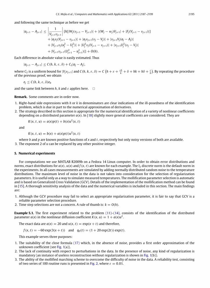
Example 5.1. The first experiment related to the problem (11)–(14), consists of the identification of the distributedparameter a(x) in the nonlinear diffusion coefficient K(x, u) = 1 + a(x)u2.

The exact data are a(x) = 20 and u(x, t) = exp(x + t) and therefore,

f (x, t) = −60 exp(3(x + t)) and q0(t) = (1 + 20 exp(2t)) exp(t).

This example serves three purposes:

1. The suitability of the close formula (17) which, in the absence of noise, provides a first order approximation of theunknown coefficient (see Fig. 1(a)).

2. The lack of continuity with respect to perturbations in the data. In the presence of noise, any kind of regularization ismandatory (an instance of useless reconstruction without regularization is shown in Fig. 1(b)).

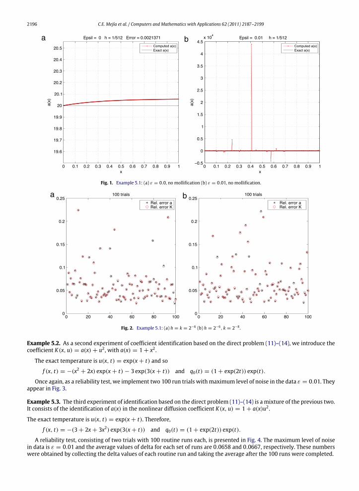
3. The ability of the mollified marching scheme to overcome the difficulty of noise in the data. A reliability test, consistingof two series of 100 routine runs is presented in Fig. 2, where ε = 0.01.

2196 C.E. Mejía et al. / Computers and Mathematics with Applications 62 (2011) 2187–2199

Fig. 1. Example 5.1: (a) ε = 0.0, no mollification (b) ε = 0.01, no mollification.

Fig. 2. Example 5.1: (a) h = k = 2−6 (b) h = 2−6, k = 2−8 .

Example 5.2. As a second experiment of coefficient identification based on the direct problem (11)–(14), we introduce thecoefficient K(x, u) = a(x) + u2, with a(x) = 1 + x2.

The exact temperature is u(x, t) = exp(x + t) and so

f (x, t) = −(x2 + 2x) exp(x + t) − 3 exp(3(x + t)) and q0(t) = (1 + exp(2t)) exp(t).

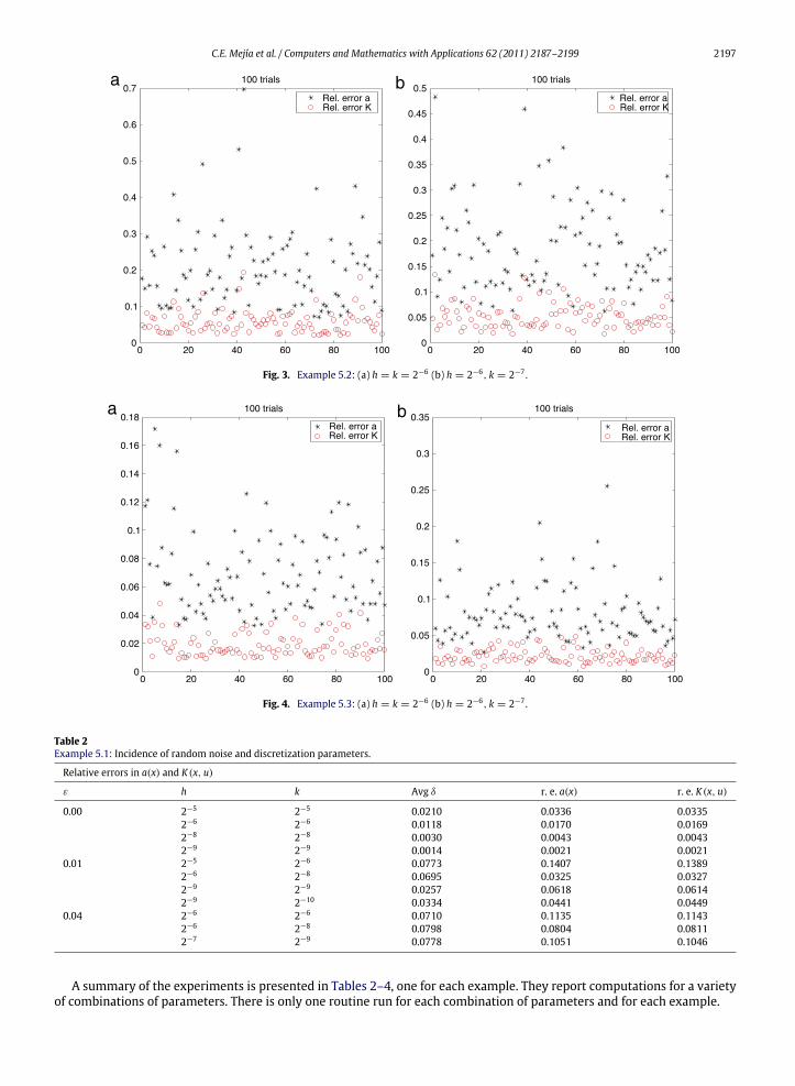
Once again, as a reliability test, we implement two 100 run trials withmaximum level of noise in the data ε = 0.01. Theyappear in Fig. 3.

Example 5.3. The third experiment of identification based on the direct problem (11)–(14) is a mixture of the previous two.It consists of the identification of a(x) in the nonlinear diffusion coefficient K(x, u) = 1 + a(x)u2.

The exact temperature is u(x, t) = exp(x + t). Therefore,

f (x, t) = −(3 + 2x + 3x2) exp(3(x + t)) and q0(t) = (1 + exp(2t)) exp(t).

A reliability test, consisting of two trials with 100 routine runs each, is presented in Fig. 4. The maximum level of noisein data is ε = 0.01 and the average values of delta for each set of runs are 0.0658 and 0.0667, respectively. These numberswere obtained by collecting the delta values of each routine run and taking the average after the 100 runs were completed.

C.E. Mejía et al. / Computers and Mathematics with Applications 62 (2011) 2187–2199 2197

Fig. 3. Example 5.2: (a) h = k = 2−6 (b) h = 2−6, k = 2−7 .

Fig. 4. Example 5.3: (a) h = k = 2−6 (b) h = 2−6, k = 2−7 .

Table 2Example 5.1: Incidence of random noise and discretization parameters.

Relative errors in a(x) and K(x, u)

ε h k Avg δ r. e. a(x) r. e. K(x, u)

0.00 2−5 2−5 0.0210 0.0336 0.03352−6 2−6 0.0118 0.0170 0.01692−8 2−8 0.0030 0.0043 0.00432−9 2−9 0.0014 0.0021 0.0021

0.01 2−5 2−6 0.0773 0.1407 0.13892−6 2−8 0.0695 0.0325 0.03272−9 2−9 0.0257 0.0618 0.06142−9 2−10 0.0334 0.0441 0.0449

0.04 2−6 2−6 0.0710 0.1135 0.11432−6 2−8 0.0798 0.0804 0.08112−7 2−9 0.0778 0.1051 0.1046

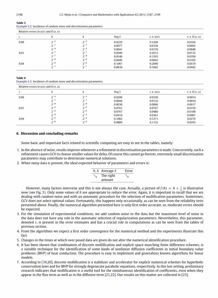
A summary of the experiments is presented in Tables 2–4, one for each example. They report computations for a varietyof combinations of parameters. There is only one routine run for each combination of parameters and for each example.

2198 C.E. Mejía et al. / Computers and Mathematics with Applications 62 (2011) 2187–2199

Table 3Example 5.2: Incidence of random noise and discretization parameters.

Relative errors in a(x) and K(x, u)

ε h k Avg δ r. e. a(x) r. e. K(x, u)

0.00 2−5 2−5 0.0259 0.1260 0.03562−7 2−7 0.0077 0.0336 0.00922−8 2−8 0.0041 0.0176 0.0048

0.01 2−7 2−7 0.0500 0.2672 0.07322−7 2−8 0.0546 0.1293 0.03502−8 2−8 0.0445 0.0602 0.0165

0.04 2−6 2−8 0.1067 0.2090 0.05702−7 2−7 0.0834 0.1602 0.0442

Table 4Example 5.3: Incidence of random noise and discretization parameters.

Relative errors in a(x) and K(x, u)

ε h k Avg δ r. e. a(x) r. e. K(x, u)

0.00 2−6 2−6 0.0200 0.0330 0.00742−7 2−7 0.0044 0.0132 0.00342−8 2−8 0.0030 0.0066 0.0017

0.01 2−6 2−6 0.0761 0.0767 0.01592−6 2−8 0.0767 0.0480 0.01082−8 2−8 0.0414 0.0361 0.0087

0.04 2−6 2−8 0.1002 0.1271 0.02762−6 2−6 0.0889 0.1132 0.0293

6. Discussion and concluding remarks

Some basic and important facts related to scientific computing are easy to see in the tables, namely:

1. In the absence of noise, results improvewhenever a refinement in discretization parameters ismade. Concurrently, such arefinement causes GCV to choose smaller values for delta. Of course this cannot go forever, extremely small discretizationparameters may contribute to deteriorate numerical solutions.

2. When noisy data is present, the ideal expected behavior of parameters and errors is:

h, k Average δ Error↘ The right

amount↘

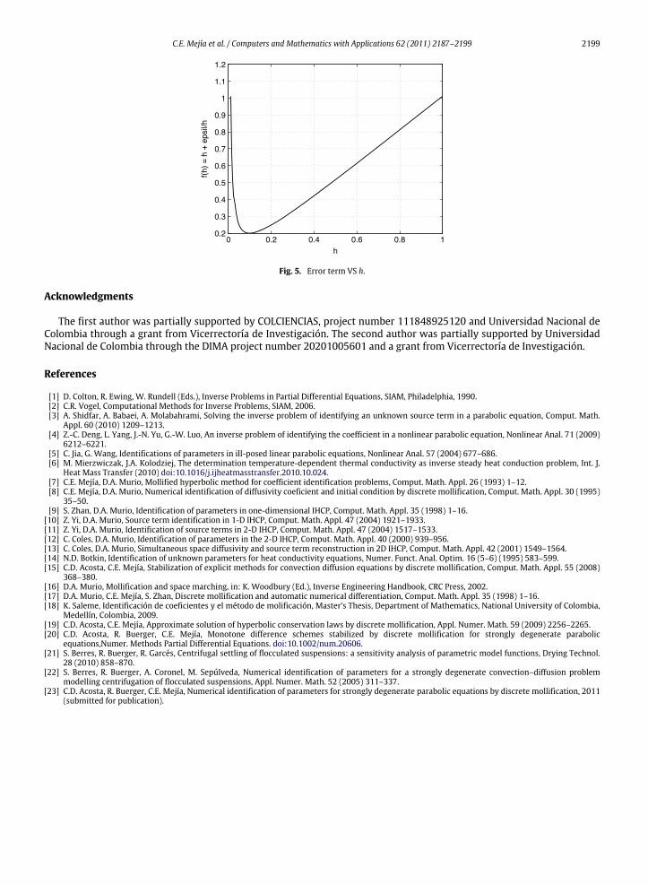
However, many factors intervene and this is not always the case. Actually, a picture of f (h) = h +εh is illustrative

now (see Fig. 5). Only some values of h are appropriate to reduce the error. Again, it is important to recall that we aredealing with random noise and with an automatic procedure for the selection of mollification parameters. Sometimes,GCV does not select optimal values. Fortunately, this happens only occasionally, as can be seen from the reliability testspresented above. Finally, the numerical algorithm presented here is only first order accurate, so, moderate errors shouldbe expected.

3. For the simulation of experimental conditions, we add random noise to the data but the maximum level of noise inthe data does not have any role in the automatic selection of regularization parameters. Nevertheless, this parameter,denoted ε, is present in the error estimates and has a crucial role in computations as can be seen from the tables ofprevious section.

4. From the algorithms we expect a first order convergence for the numerical method and the experiments illustrate thisfact.

5. Changes in the times at which over posed data are given do not alter the numerical identification procedure.6. It has been shown that combination of discrete mollification and explicit space-marching finite difference schemes, is

a suitable technique for the identification of some kinds of nonlinear diffusion coefficients in initial boundary valueproblems (IBVP) of heat conduction. The procedure is easy to implement and generalizes known algorithms for linearmodels.

7. According to [19,20], discrete mollification is a stabilizer and accelerator for explicit numerical schemes for hyperbolicconservation laws and for IBVP for strongly degenerate parabolic equations, respectively. In this last setting, preliminaryresearch indicates that mollification is a useful tool for the simultaneous identification of coefficients, even when theyappear in the flux term as well as in the diffusive term [21,22]. Our results on this matter are collected in [23].

C.E. Mejía et al. / Computers and Mathematics with Applications 62 (2011) 2187–2199 2199

Fig. 5. Error term VS h.

Acknowledgments

The first author was partially supported by COLCIENCIAS, project number 111848925120 and Universidad Nacional deColombia through a grant from Vicerrectoría de Investigación. The second author was partially supported by UniversidadNacional de Colombia through the DIMA project number 20201005601 and a grant from Vicerrectoría de Investigación.

References

[1] D. Colton, R. Ewing, W. Rundell (Eds.), Inverse Problems in Partial Differential Equations, SIAM, Philadelphia, 1990.[2] C.R. Vogel, Computational Methods for Inverse Problems, SIAM, 2006.[3] A. Shidfar, A. Babaei, A. Molabahrami, Solving the inverse problem of identifying an unknown source term in a parabolic equation, Comput. Math.

Appl. 60 (2010) 1209–1213.[4] Z.-C. Deng, L. Yang, J.-N. Yu, G.-W. Luo, An inverse problem of identifying the coefficient in a nonlinear parabolic equation, Nonlinear Anal. 71 (2009)

6212–6221.[5] C. Jia, G. Wang, Identifications of parameters in ill-posed linear parabolic equations, Nonlinear Anal. 57 (2004) 677–686.[6] M. Mierzwiczak, J.A. Kolodziej, The determination temperature-dependent thermal conductivity as inverse steady heat conduction problem, Int. J.

Heat Mass Transfer (2010) doi:10.1016/j.ijheatmasstransfer.2010.10.024.[7] C.E. Mejía, D.A. Murio, Mollified hyperbolic method for coefficient identification problems, Comput. Math. Appl. 26 (1993) 1–12.[8] C.E. Mejía, D.A. Murio, Numerical identification of diffusivity coeficient and initial condition by discrete mollification, Comput. Math. Appl. 30 (1995)

35–50.[9] S. Zhan, D.A. Murio, Identification of parameters in one-dimensional IHCP, Comput. Math. Appl. 35 (1998) 1–16.

[10] Z. Yi, D.A. Murio, Source term identification in 1-D IHCP, Comput. Math. Appl. 47 (2004) 1921–1933.[11] Z. Yi, D.A. Murio, Identification of source terms in 2-D IHCP, Comput. Math. Appl. 47 (2004) 1517–1533.[12] C. Coles, D.A. Murio, Identification of parameters in the 2-D IHCP, Comput. Math. Appl. 40 (2000) 939–956.[13] C. Coles, D.A. Murio, Simultaneous space diffusivity and source term reconstruction in 2D IHCP, Comput. Math. Appl. 42 (2001) 1549–1564.[14] N.D. Botkin, Identification of unknown parameters for heat conductivity equations, Numer. Funct. Anal. Optim. 16 (5–6) (1995) 583–599.[15] C.D. Acosta, C.E. Mejía, Stabilization of explicit methods for convection diffusion equations by discrete mollification, Comput. Math. Appl. 55 (2008)

368–380.[16] D.A. Murio, Mollification and space marching, in: K. Woodbury (Ed.), Inverse Engineering Handbook, CRC Press, 2002.[17] D.A. Murio, C.E. Mejía, S. Zhan, Discrete mollification and automatic numerical differentiation, Comput. Math. Appl. 35 (1998) 1–16.[18] K. Saleme, Identificación de coeficientes y el método de molificación, Master’s Thesis, Department of Mathematics, National University of Colombia,

Medellín, Colombia, 2009.[19] C.D. Acosta, C.E. Mejía, Approximate solution of hyperbolic conservation laws by discrete mollification, Appl. Numer. Math. 59 (2009) 2256–2265.[20] C.D. Acosta, R. Buerger, C.E. Mejía, Monotone difference schemes stabilized by discrete mollification for strongly degenerate parabolic

equations,Numer. Methods Partial Differential Equations. doi:10.1002/num.20606.[21] S. Berres, R. Buerger, R. Garcés, Centrifugal settling of flocculated suspensions: a sensitivity analysis of parametric model functions, Drying Technol.

28 (2010) 858–870.[22] S. Berres, R. Buerger, A. Coronel, M. Sepúlveda, Numerical identification of parameters for a strongly degenerate convection–diffusion problem

modelling centrifugation of flocculated suspensions, Appl. Numer. Math. 52 (2005) 311–337.[23] C.D. Acosta, R. Buerger, C.E. Mejía, Numerical identification of parameters for strongly degenerate parabolic equations by discrete mollification, 2011

(submitted for publication).