Welcome message from author
This document is posted to help you gain knowledge. Please leave a comment to let me know what you think about it! Share it to your friends and learn new things together.
Transcript

MONOPOLE PAIR PRODUCTION
VIA PHOTON FUSION
Approved by:
____________________________________Dr. Jingbo Ye, Professor
____________________________________Dr. Ryszard Stroynowski, Professor
____________________________________
Dr. Randall Scalise, Senior Lecturer

MONOPOLE PAIR PRODUCTION
VIA PHOTON FUSION
A Thesis Presented to the Graduate Faculty of
Dedman College
Southern Methodist University
for the degree of
Master of Science
with a
Major in Physics
by
Triston Dougall
( B.S. Michigan State University )( M.S. University of Texas at Arlington )
December 9, 2006

ACKNOWLEDGMENTS
I would like to thank Professor Stuart Wick for his genuine enthusiasms and
guidance from start to finish; and to Professor Jingbo Ye, for his continuing support that
kept me motivated throughout my work.
My gratitude goes out to Professor Ryszard Stroynowski for his role as graduate
advisor and additionally for sharing his wealth of knowledge in experimental physics.
Furthermore, my appreciation to all the faculty at SMU's physics department for
their generous assistance whenever I approached them, especially Dr. Randall Scalise for
his patience and insight.
Finally, I would like to express my gratitude to SMU's physics department and the
Dedman Graduate school for funding and providing me an opportunity to pursue my
interests in physics.
iii
Dougall, Triston B.S., Michigan State University, 1990 M.S., University of Texas at Arlington, 2004
Monopole Pair ProductionVia Photon Fusion
Advisor: Professor Jingbo Ye
Master of Science conferred December 9, 2006
Thesis completed December 6, 2006
The search for a magnetic monopole continues, spurred by the motivation to
explain charge quantization, impart symmetry to Maxwell's equation, introduce new
physics and to confirm or refute predictions founded in many gauge theories. To
promote the search for a Dirac monopole, specifically searches at colliders such as the
LHC or Tevatron, we present here the process of photon fusion as an additional process
to the DrellYan mechanism for monopole pair production.
When predicting monopole production at the Tevatron with a center of mass
energy of , we find the cross section of the photon fusion process induced
through the inelastic scattering of quarks, comparable to that reported for the DrellYan
mechanism for a monopole mass in the range of . Next, by
adding the cross section for photon fusion to the DrellYan cross section, we conclude
that the lower mass limit of the magnetic monopole can be extended up to
iv
beyond the reported by the CDF experiment.
With a center of mass energy seven times greater than that of the Tevatron, the
LHC at CERN offers an excellent opportunity to renew the search for a Dirac monopole.
However, unlike the Tevatron which is a collider, the LHC is a collider, rendering
the LHC less suitable to the DrellYan process as compared to the photon fusion process
for monopole pair production. We reported here the cross section for monopole pair
production via the photon fusion process for inelastic scattering at the LHC. With an
integrated luminosity of and assuming a magnetic monopole mass of ,
we anticipate the LHC could produce over 10 million monopole pairs of by the process of
photon fusion. By comparison, we estimate the DrellYan process may yield less than 1
million events.
v

TABLE OF CONTENT
LIST OF FIGURES
LIST OF ABBREVIATIONS
GLOSSARY
DEDICATION
Chapter
1. INTRODUCTION
2. BACKGROUND
3. PHOTON FUSION
4. MATERIAL AND METHODS
5. RESULTS AND ANALYSIS
6. DISCUSSION AND CONCLUSION
APPENDIX : ( FORTRAN SOURCE CODE )
REFERENCES
vii
viii
x
xi
1
14
21
30
32
35
37
48
vi
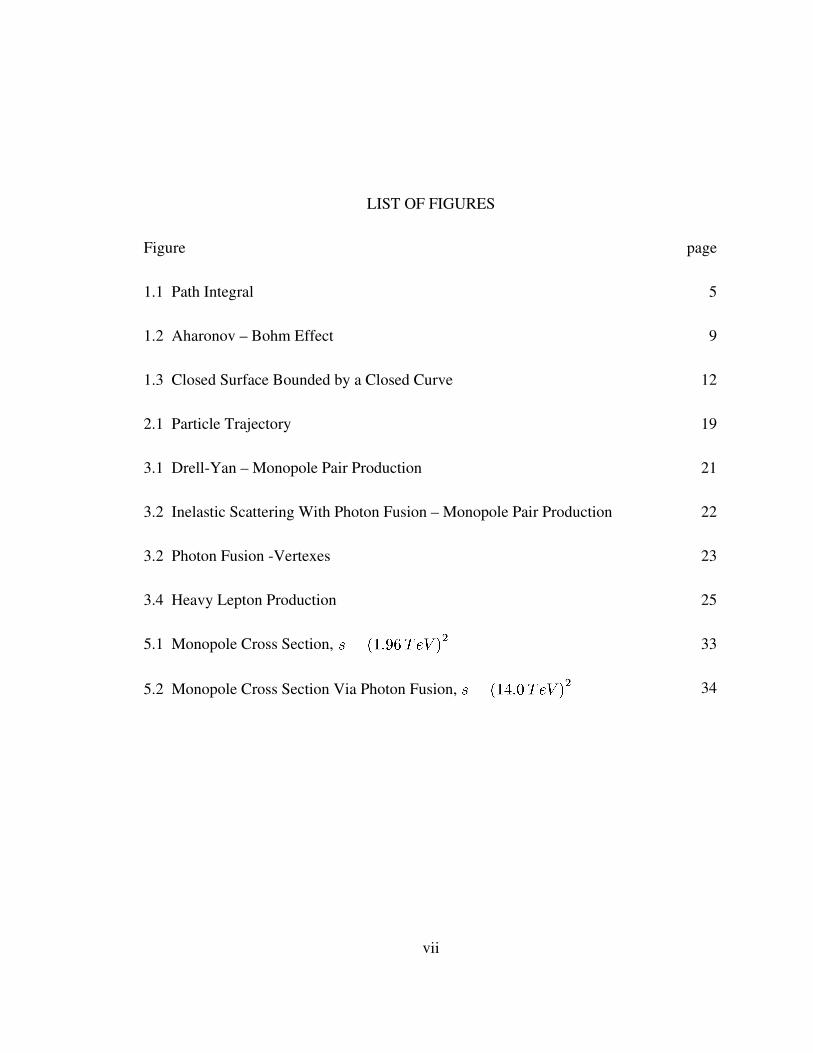
LIST OF FIGURES
Figure
1.1 Path Integral
1.2 Aharonov – Bohm Effect
1.3 Closed Surface Bounded by a Closed Curve
2.1 Particle Trajectory
3.1 DrellYan – Monopole Pair Production
3.2 Inelastic Scattering With Photon Fusion – Monopole Pair Production
3.2 Photon Fusion Vertexes
3.4 Heavy Lepton Production
5.1 Monopole Cross Section,
5.2 Monopole Cross Section Via Photon Fusion,
page
5
9
12
19
21
22
23
25
33
34
vii
LIST OF ABBREVIATIONS
CDF Collider Detector at Fermilab
CL Confidence Limit
CME Center of Mass Energy
COT Central Outer Detector
GeV Gigaelectron Volts
GHz Gigahertz
GUT Grand Unification Theory
LHC Large Hadron Collider
MIP MinimumIonizing Particle
MM Monopole Mass
PDF Parton Distribution Function
PMT Photomultiplier Tubes
SO(x) Standard Orthogonal – group, with x members
SS Super Symmetry
SSB Spontaneous Symmetry Breaking
viii
SU(x) Standard Unitary – group, with x members
TeV Teraelectron Volts
TOF Time of Flight
U(x) Unitary – group, with x members
WW WeizsäckerWilliams
ix

GLOSSARY
Coupling Constant for charge
barn Cross Section unit or
e Electric Charge
g Magnetic Charge
Lepton
AntiLepton
Monopole
AntiMonopole
Proton
AntiProton
Quark
AntiQuark
Cross Section
Wave function
Wave function with exact phase
x

DEDICATION
To William Saber and Dorin Leigh Dougall.
Chapter 1
INTRODUCTION
The concept of electric charge as a fundamental property of matter is well
established. But what about the idea of a fundamental magnetic charge? All empirical
evidence to date indicates that a magnetic field is created by the movement of electric
charges, and not the direct result of independent fundamental magnetic charges. Even the
modern theory of electroweak interactions is nicely packaged without the requirement of
a magnetic charge. So why consider the possible existence of a magnetic monopole?
First of all, in classical electrodynamics, there is no need to exclude magnetic
charges; of course this provides no constructive framework, but it does leave the
existence of monopoles open to debate. There is however a more elegant argument for
the possible existence of monopoles that is based on symmetry.
There is a comfort and an agreement in a symmetry, like the pattern of a
snowflake. Should the symmetry be disrupted, say a missing spike on a snowflake, the
broken symmetry is all too obvious and there is natural inclination to want to investigate
the nature of this broken symmetry. Equations (1.1a) – (1.1d) are the current Maxwell’s
1

equations of electromagnetism in cgs units.
(1.1a) (1.1c)
(1.1b) (1.1d)
The full symmetry inherent to Maxwell's equations is apparent by comparing these
equations to (1.2a) – (1.2d), where a magnetic charge has been included to Maxwell's
equations as indicated by large bold text.
(1.2a) (1.2c)
(1.2b) (1.2d)
It is important to observe that these alterations do not contradict the results of Maxwell's
equations or any other known phenomenon.
In (1.2), Maxwell's equations are now fully symmetric with respect to electric and
magnetic currents and fields, as (1.2a) resembles (1.2b) and (1.2c) is similar to (1.2d).
The modified Maxwell’s equations now state that electric and magnetic charges, fields
and currents share an electric/magnetic duality, and act like mirror images of each other.
Just as a moving electric charge creates a magnetic field, a moving magnetic charge
creates an electric field. Mathematically this symmetry is related by the rotational group
U(1) with , and isomorphic to the rotational group SO(2).
(1.3)
2

Here and represent any of the three electric or magnetic quantities , or . For
example using the charge currents,
(1.4)
(1.5)
Maxwell’s equations entice us with the existence of magnetic charge to restore the
electric/magnetic symmetry. Unfortunately this observation does not ensure the
existence of a magnetic charge or point us in a meaningful direction.
In 1931 P.A.M Dirac [1] provided a plausible motivation, within the framework
of quantum electrodynamics, for the existence of magnetic charge. This motivation is
based on the principle of electric charge quantization. It is an empirical fact that one
electron is identical to all other electrons, and possess precisely an equal but opposite
charge to a proton. In general, there is no reason that the charge should be quantized.
However Dirac explains the quantization of electric charge exclusively by the existence a
magnetic charge.
Dirac’s paper is a milestone in the search for a magnetic monopole. To reinforce
the incentive for this thesis and illustrate the significance of his work, the following will
outline Dirac's original publication titled, “Quantized Singularities in the Electromagnetic
Field”, with an effort to preserve the rationale of his argument. As stated by Dirac, "The
theory of this paper, while it looks at first as though it will give a theoretical value for ,
3

is found when worked out to give a connection between the smallest electric charge and
the smallest magnetic pole."
To emphasize Dirac's line of reasoning the main principles will be listed. This
will prevent the details inherent in each step from diluting the argument.
1) The wave function carries an undetermined phase factor :
The argument begins with the general wave function (1.7) and the undetermined
phase factor , or rewritten in (1.8), where the global phase constant is pulled out of .
In (1.8), is now determined precisely to a known value at each coordinate.
(1.7)
(1.8)
2) Nonvanishing phase difference around a closed curve:
Because a constant can be added to the phase without affecting the physics, what
must be important is the phase difference between two points and not the value of . To
determine the phase difference, the general method is is to take the path integral between
two points as shown in (1.9).
(1.9)
In a conserved system involving the function , the value of the path integral is
independent of the chosen path. If two paths and form a closed loop between
points and , as shown in Figure (1.1), the value of the path integral should be zero. 4

Figure 1.1 Path Integral
For now we are looking at the general case where the integral may be path dependent
(1.10). Therefore the phase change around a closed curve may not vanish.
(1.10)
4) Phase around a closed curve must be the same for all wave functions:
When computing the integral (1.11) with wave functions and , we known
the resultant should be a unique real number in quantum theory.
(1.11)
This implies that the integrand must have a definite phase difference between any
two points to prohibit obtaining multiple values when performing the integration. With
the phase difference independent of the path, the phase difference must vanish around a
closed curve. For this to occur, the phase change of must be equal and opposite to
the phase change of . Then by taking the conjugate of , the phase change for
will now be equal to .
5

5) Write path integral for phase change in terms of Stokes Theorem:
Even though the phase is a function of [ ], the phase does not carry a
definite value at each point. Classically a similar ambiguity holds for potential energy,
where potential energy is a function of coordinates but does not have a precise value at
each point. So instead of a exact value for the phase, it was shown the phase difference
between two points can be computed. For this to be true the derivatives of the phase
must be definite and continuous at all points. This is equivalent to being unaware of an
object's exact position relative to a coordinate system. If however, the object's velocity is
well defined at each coordinate, one can compute the change in its position. To
demonstrate this for the wave function, equation (1.7) can be explicitly written as,
(1.12)
where is now a wave function with a definite phase and all the phase ambiguity is
represented by . The derivatives of will be defined at each point as,
, , , . (1.13)
In general the derivatives do not have to satisfy the condition for an exact differential, for
example , making the change in phase dependent on the path. The path
integral determining the phase change around a closed curve can now be expressed
through Stokes' theorem and , as shown in (1.14)
6

(1.14)
6) The wave function's phase uncertainty is due to the electromagnetic field:
Taking the partial derivative of relationship (1.12) we obtained
(1.15)
where, with some manipulation, it can be shown that if satisfies any wave equation for
the momentum and energy operator, P and E, then will satisfy the wave equation for
the operators shown,
+ , (1.16)
Next, with the Lagrangian for a charged particle in an electromagnetic field
having a scalar potential and vector potential ,
(1.17)
then applying the EulerLagrangian equation, the energy and canonically conjugate
momentum will appear as (1.18). Note, this is shown without quantization of
the fields.
, (1.18)
Comparing (1.16) to (1.18), where is the kinetic term and , [ ]
are then related to the magnetic and electric potentials through,
, . (1.19)
7
Equation (1.19) indicates the uncertainty of the wave function, which is stored in
[ ], is directly related to the electromagnetic potential. This indicates that the
phase change of a particle's wave function will now be dependent on the electromagnetic
potential through which it travels.
7) Electromagnetic flux through the closed curve produces the nonzero phase change:
Since [ ] corresponds to the electromagnetic potentials, then the curl
of must be associated with the components of the magnetic field and .
Relating to Stokes' theorem applied in (1.14), it is apparent the phase shift depends of the
amount of electromagnetic flux though the closed curve, which determines the
uncertainly in the wave function.
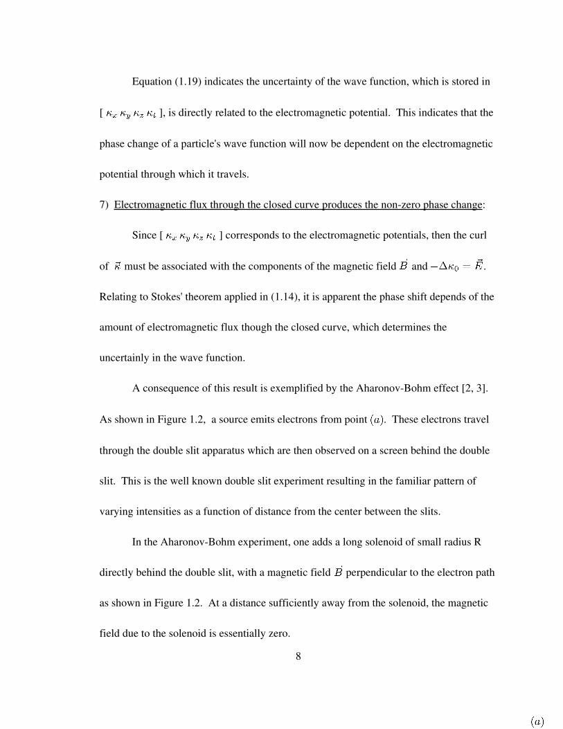
A consequence of this result is exemplified by the AharonovBohm effect [2, 3].
As shown in Figure 1.2, a source emits electrons from point . These electrons travel
through the double slit apparatus which are then observed on a screen behind the double
slit. This is the well known double slit experiment resulting in the familiar pattern of
varying intensities as a function of distance from the center between the slits.
In the AharonovBohm experiment, one adds a long solenoid of small radius R
directly behind the double slit, with a magnetic field perpendicular to the electron path
as shown in Figure 1.2. At a distance sufficiently away from the solenoid, the magnetic
field due to the solenoid is essentially zero.
8

Figure 1.2 Aharonov – Bohm Effect
Classically, only the fields E and B contribute to any observable change. With
the absence of any magnetic field the pattern on the screen should not be altered.
However, what is observed is a shift in the pattern that can be attributed only to the
electromagnetic vector potential of the solenoid. Outside the solenoid, the magnetic field
can be written as,
(1.20)
which by a choice of gauge can be written trivially as or more importantly
. (1.21)
For a path integral between two points the change in can be calculated.
(1.22)
(1.23)
9
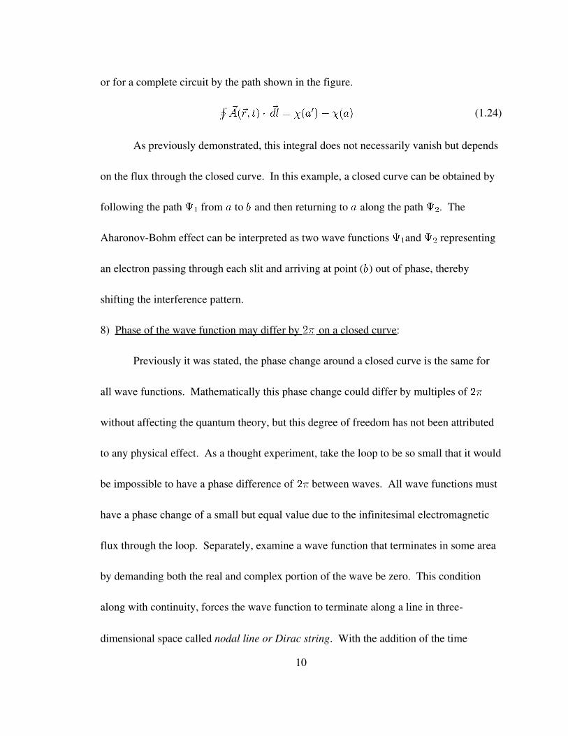
or for a complete circuit by the path shown in the figure.
(1.24)
As previously demonstrated, this integral does not necessarily vanish but depends
on the flux through the closed curve. In this example, a closed curve can be obtained by
following the path from to and then returning to along the path . The
AharonovBohm effect can be interpreted as two wave functions and representing
an electron passing through each slit and arriving at point ( ) out of phase, thereby
shifting the interference pattern.
8) Phase of the wave function may differ by on a closed curve:
Previously it was stated, the phase change around a closed curve is the same for
all wave functions. Mathematically this phase change could differ by multiples of
without affecting the quantum theory, but this degree of freedom has not been attributed
to any physical effect. As a thought experiment, take the loop to be so small that it would
be impossible to have a phase difference of between waves. All wave functions must
have a phase change of a small but equal value due to the infinitesimal electromagnetic
flux through the loop. Separately, examine a wave function that terminates in some area
by demanding both the real and complex portion of the wave be zero. This condition
along with continuity, forces the wave function to terminate along a line in three
dimensional space called nodal line or Dirac string. With the addition of the time
10
component, the line would scribe a sheet in spacetime.
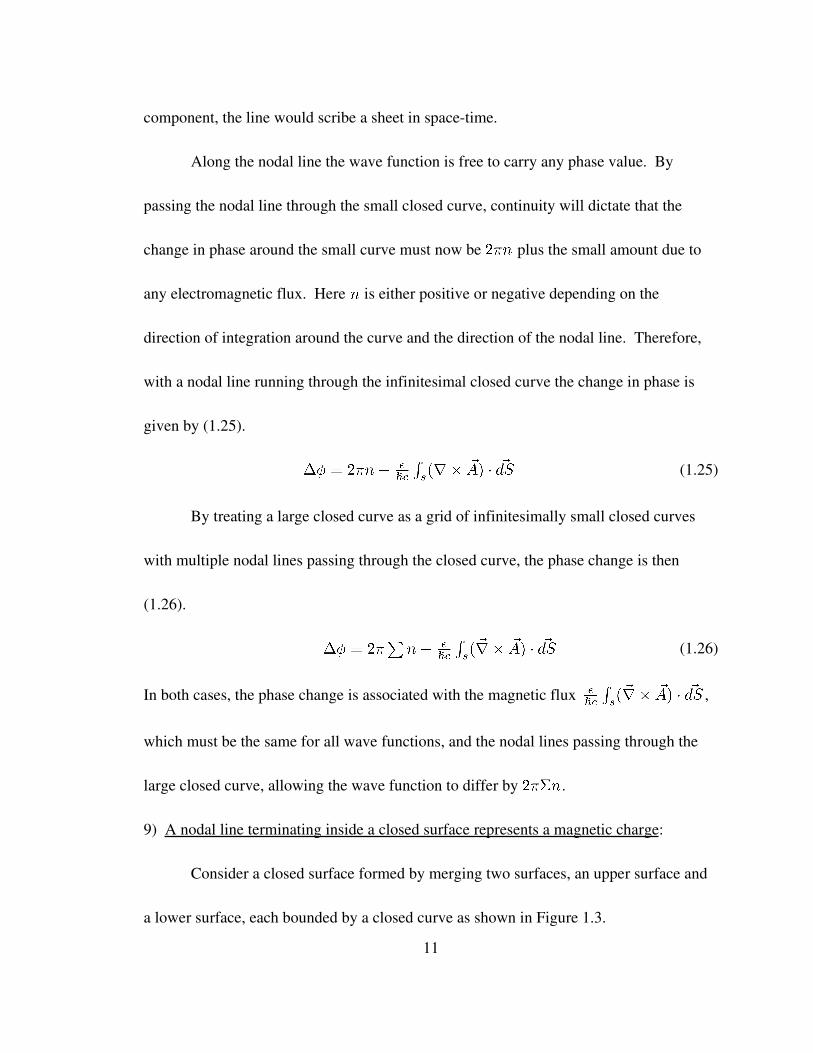
Along the nodal line the wave function is free to carry any phase value. By
passing the nodal line through the small closed curve, continuity will dictate that the
change in phase around the small curve must now be plus the small amount due to
any electromagnetic flux. Here is either positive or negative depending on the
direction of integration around the curve and the direction of the nodal line. Therefore,
with a nodal line running through the infinitesimal closed curve the change in phase is
given by (1.25).
(1.25)
By treating a large closed curve as a grid of infinitesimally small closed curves
with multiple nodal lines passing through the closed curve, the phase change is then
(1.26).
(1.26)
In both cases, the phase change is associated with the magnetic flux ,
which must be the same for all wave functions, and the nodal lines passing through the
large closed curve, allowing the wave function to differ by .
9) A nodal line terminating inside a closed surface represents a magnetic charge:
Consider a closed surface formed by merging two surfaces, an upper surface and
a lower surface, each bounded by a closed curve as shown in Figure 1.3.
11

Figure 1.3 Closed Surface Bounded by a Closed Curve
In Figure 1.3, and are separate paths traversing the entire closed curve from
opposite directions. If separate path integrals are performed along each of these paths it
is obvious they will cancel each other. Now holding Stokes' theorem to be absolute, this
is essentially stating the sum of the integrated flux along surface and must be zero.
By setting , equation (1.26) can thus be written as,
(1.27)
where is the number of nodal lines cross surface and is the number of nodal
lines crossing . Therefore, the left side of the equation mat not be zero if one or more
nodal lines terminate inside the bounded surface.
The left side of (1.27) must be in multiples of and the right side is integrated
over , so equation (1.27) becomes,
(1.28)
12
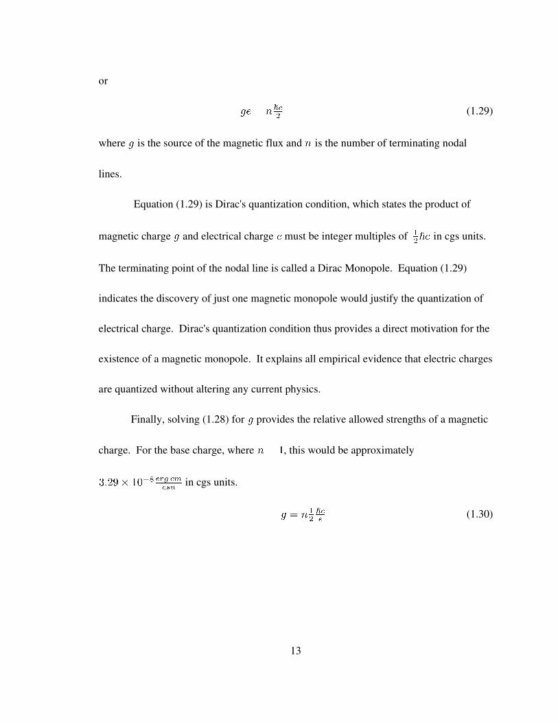
or
(1.29)
where is the source of the magnetic flux and is the number of terminating nodal
lines.
Equation (1.29) is Dirac's quantization condition, which states the product of
magnetic charge and electrical charge must be integer multiples of in cgs units.
The terminating point of the nodal line is called a Dirac Monopole. Equation (1.29)
indicates the discovery of just one magnetic monopole would justify the quantization of
electrical charge. Dirac's quantization condition thus provides a direct motivation for the
existence of a magnetic monopole. It explains all empirical evidence that electric charges
are quantized without altering any current physics.
Finally, solving (1.28) for provides the relative allowed strengths of a magnetic
charge. For the base charge, where , this would be approximately
in cgs units.
(1.30)
13

Chapter 2
BACKGROUND
The are many other suitable models to explain electric charge quantization or the
basis for magnetic monopoles. To not digress into an extensive argument for the
existence of magnetic monopoles, the following will summarize other significant theories
in the field of magnetic monopoles.
Prior to Dirac's publication in 1904, JJ Thomson [4] presented a simple example
of charge quantization which occurs in a static system composed of an electrically
charged particle ( ) and magnetically charged particle ( ) separated by a distance .
The angular momentum of the fields can be calculated by [5],
(2.1)
and due to the symmetry between the fields, the integration will yield a vector along ,
representing the axis. This is similar to the resultant electric field vector for a
uniform sheet of charges, where only the perpendicular component of the field vector
survives. Next, by applying the standard quantization to the angular moment, the charge
quantization is reached, (2.2 – 2.4). This again indicates that e or g are limited to definite
14

quantities of .
(2.2)
(2.3)
(2.4)
Calculating the scattering of an electron off a magnetic monopole will also reveal the
same charge quantization condition using the conservation of angular moment [6].
A new approach for the existence of monopoles was developed by 't Hooft and
Polyakov in 1974 [7, 8] by incorporating the Higgs field into the YangMills equation,
where monopoles occur as stable solutions. Their theories predict monopoles arising as
topological defects from spontaneous symmetry braking (SSB). In the case of 't Hooft
this is the SO(3) GeogiGlashow electroweak unification model, and for Polyakov it is
SU(2). In the theories derived by 't Hooft and Polyakov a monopole is a finite energy
solution to the field equation with a boundary condition on the Higgs field at infinity.
This is opposed to the Dirac monopole which has infinite energy and additionally
requires a Dirac string. Although 't Hoot's theory did not apply to the standard model of
SU(2) X U(1) for electroweak, it more importantly predicted stable monopoles as the
result of a group not containing U(1), breaking into a U(1).
The next logical step to predict monopoles is in Grand Unification Theories
(GUT), by using a SU(5) gauge theory for example [9], or notably the SU(5) breaking to
15

SU(3) SU(2) U(1) [10,11]. In GUT theories, the mass of the monopole , is
related to the symmetry breaking scale and coupling constant of the unified
interaction by [12,13]
(2.5)
For GUT theories and , producing Superheavy MM
. The enormous mass of a GUT monopole is several orders of
magnitude beyond the center of mass energy of the LHC as well as any
conceivable collider. However, during the early universe monopoles would have been
produced during phase transitions. The present flux of these relic monopoles is unclear
due to production uncertainties in the early universe and the diluting effect of an
inflationary universe. There is also the possibility of higher dimensional topological
defects such as strings and walls destroying the monopoles [14].
The mass of the Dirac monopole can be derived by assuming the monopole radius
is comparable to the classical electron's radius cm. The monopole's mass is then
proportional to the electron's mass according to the square of the charge ratios [12].
(2.6)
This puts the mass of the monopole at , which is well below the GUT
monopole and more importantly into the realm accelerators production.
The crosssection calculation performed in this thesis is intended to predict the
16

production of Dirac monopoles at the LHC, and additionally compare the results of
previous accelerator searches to set mass limits on the monopole. Therefore, the
following summary of previous monopole searches will focus on attempts to find a Dirac
monopole with masses accessible in current accelerators, such as the LHC.
In 2003 an extensive search was conducted at Fermilab's CDF II detector using
beams with center of mass energy at and integrated luminosity
[15]. The CDF detector is comprised of a magnetic spectrometer with silicon strips and
driftchamber tracking detectors and a scintillator timeofflight system, surrounded by
electromagnetic and hadronic calorimeters and muon chambers. The monopole search
relied heavily on two components of the CDF detector; the central outer tracker (COT)
and the and time of flight (TOF) scintillators to trigger a monopole hit.
The COT extends from 40 cm to 137 cm, and spans a pseudorapidity range of
. The COT is constructed from 8 superlayers, each containing 12 layers of
sense wires. In addition to determining the energy loss due to ionization, the COT made
timing measurements for track reconstruction.
Surrounding the COT are the time of flight scintillator bars with photomultiplier
tubes (PMT) connected to each end. There are 216 scintillator bars running parallel to
the beam and extending the outer tracker to a radius of 140 cm. For analysis, both the
time and PMT pulse height are measured. To detect a monopole, both the COT and
17
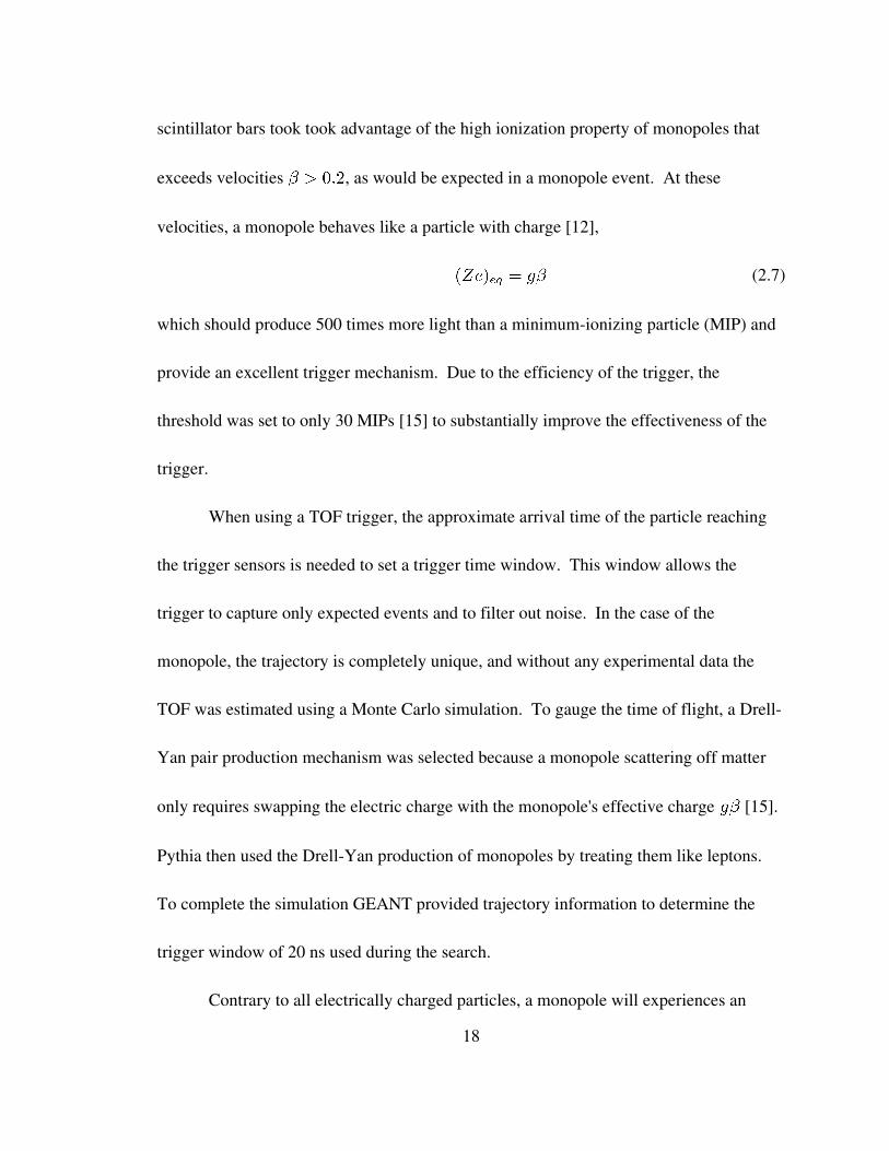
scintillator bars took took advantage of the high ionization property of monopoles that
exceeds velocities , as would be expected in a monopole event. At these
velocities, a monopole behaves like a particle with charge [12],
(2.7)
which should produce 500 times more light than a minimumionizing particle (MIP) and
provide an excellent trigger mechanism. Due to the efficiency of the trigger, the
threshold was set to only 30 MIPs [15] to substantially improve the effectiveness of the
trigger.
When using a TOF trigger, the approximate arrival time of the particle reaching
the trigger sensors is needed to set a trigger time window. This window allows the
trigger to capture only expected events and to filter out noise. In the case of the
monopole, the trajectory is completely unique, and without any experimental data the
TOF was estimated using a Monte Carlo simulation. To gauge the time of flight, a Drell
Yan pair production mechanism was selected because a monopole scattering off matter
only requires swapping the electric charge with the monopole's effective charge [15].
Pythia then used the DrellYan production of monopoles by treating them like leptons.
To complete the simulation GEANT provided trajectory information to determine the
trigger window of 20 ns used during the search.
Contrary to all electrically charged particles, a monopole will experiences an
18
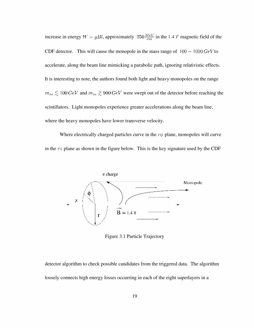
increase in energy , approximately in the magnetic field of the
CDF detector. This will cause the monopole in the mass range of to
accelerate, along the beam line mimicking a parabolic path, ignoring relativistic effects.
It is interesting to note, the authors found both light and heavy monopoles on the range
and were swept out of the detector before reaching the
scintillators. Light monopoles experience greater accelerations along the beam line,
where the heavy monopoles have lower transverse velocity.
Where electrically charged particles curve in the plane, monopoles will curve
in the plane as shown in the figure below. This is the key signature used by the CDF
Figure 3.1 Particle Trajectory
detector algorithm to check possible candidates from the triggered data. The algorithm
loosely connects high energy losses occurring in each of the eight superlayers in a
19
straight line, then attempts to piece the superlayers together to fit a trajectory which has a
low variance in , +/ 0.2 radians.
Out of collisions at CDF, the trigger only selected 130,000 events.
From these selected events none passed the reconstruction requirements. Based on their
findings the authors reported a 95% confidence limit on cross section versus mass
derived from,
(2.8)
where is integrated luminosity, = detector efficiency with acceptance and is the
number of expected events. To obtain as upper cross section limit, N would be set to 1.
Assuming a DrellYan production mechanism, a lower mass limit of was set on
the monopole mass.
20
Chapter 3
PHOTON FUSION
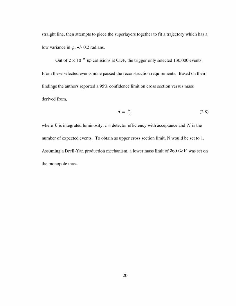
The favored model for Dirac monopole pair production has been the DrellYan
production mechanism. This model was used at the Tevatron in 2003 to set the timeof
flight trigger window, and it was also used as their benchmark to set a lower mass limit
on the magnetic monopole [15]. There are several reasons the DrellYan process is so
heavily relied on to model monopole production. First there is high expected cross
section for the first order term of the DrellYan process, shown in Figure 3.1.
Figure 3.1 DrellYan Monopole Pair Production
More importantly, with the coupling constant of the monopole at nearly 4700 times that
21

of the electron, perturbation theory breaks down for other processes including higher
order terms. The DrellYan process additionally avoids issues with perturbation theory,
since modeling a monopole interacting with matter only requires the replacement of the
electric charge with its effective charge [ 12, 15 ].
We use a similar assumption to calculate the photon fusion process as a second
source of monopole pair production, keeping only the first order terms. Photon fusion
induced through the inelastic scattering of two quarks is represented by the Feynman
diagrams shown in Figure 3.2a and 3.2b.
(a) (b)
Figure 3.2 Inelastic Scattering With Photon Fusion Monopole Pair Production
Due to the startup of the LHC at CERN in 2008 this process is worth pursuing.
The Tevatron which is a collider is well suited for the DrellYan mechanism.
22
However the LHC is a collider, the effectiveness of the DrellYan process will be
severely reduced as it will now rely on sea quark to furnish the antiquark for the
annihilation. We also believe photon fusion will be comparable to DrellYan in a
collider; significant enough to combine with the calculated DrellYan crosssection and
extend the lower mass limit of the monopole.
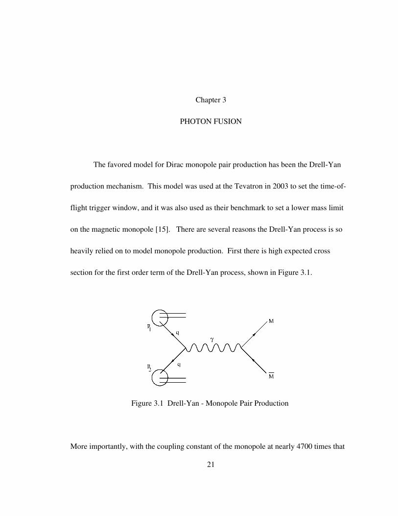
Photon fusion benefits from the large magnetic coupling constant , providing
process amplification at each vertex, inverse of an electric interaction, see Figure 3.3.
Figure 3.3 Photon Fusion Vertexes
In the squared matrix elements expression (3.1), where and refer to the exchanged
momenta squared for the two photon process, the full benefit inherent in the interaction is
evident, as each vertex now allows the matrix to be multiplied by times a factor.
23

(3.1)
This means the matrix elements for the photon fusion process is amplified by an
additional over the DrellYan process, which has only one vertex connected to the
monopoles.
The task now becomes to derive and compute the cross section for the inelastic
scattering. The goal will be to compare the photon fusion process to the DrellYan
process for energies of and , which are the center of mass energies
for the Tevatron and LHC respectively. Since a Dirac monopole shares identical
properties to a heavy lepton, except for the charge, we followed the work of Bhattacharya
and Drees [16, 17], who calculated the cross section for heavy lepton production through
the identical process of photon fusion induced through the inelastic scattering of quarks.
See Feynman diagram Figure 3.4. For an additional reference on lepton production
through the DrellYan process see [18].
As will be shown, the magnitudes of couplings of the monopole/photon or
lepton/photon vertices can be brought out of the cross section integral. This allows for a
quick estimation for the monopole crosssection at . One can then multiply the
heavy lepton crosssection obtained by Bhattacharya or Drees, by a ratio of . Due to
of improved patron distribution functions (PDF) since the date of their publications, we
will preform the integration for the monopole pair production cross section and use the 24
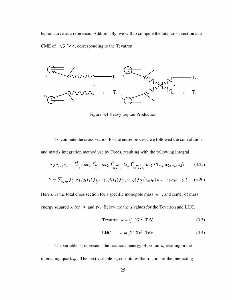
lepton curve as a reference. Additionally, we will to compute the total cross section at a
CME of , corresponding to the Tevatron.
Figure 3.4 Heavy Lepton Production
To compute the cross section for the entire process, we followed the convolution
and matrix integration method use by Drees, resulting with the following integral.
(3.2a)
(3.2b)
Here is the total cross section for a specific monopole mass , and center of mass
energy squared , for and . Below are the values for the Tevatron and LHC.
Tevatron TeV (3.3)
LHC TeV (3.4)
The variable represents the fractional energy of proton residing in the
interacting quark . The next variable , constitutes the fraction of the interacting
25

quark's energy carried off by . Therefore, the total energy of , in the photons
center of mass frame, is shown in equation (3.5).
(3.5)
The four integrals in equation (3.2a) essentially account for all the allowed combinations
of energies for the two quarks and two photons.
The lower limit on the outer integral starts the integration at the minimum amount
of energy fraction of in to create the monopoles onshell. This is,
. (3.6)
Moving to the integral over , the lower limit is determined from the value of by
solving (3.7) for resulting in equation (3.8).
(3.7)
(3.8)
Hence for the first infinitesimal portion where is minimum, must be at 1 or
100% of the energy of must be in . This combination then adds nothing to the cross
section with the limits of the inner integral ranging from 1 to 1. The integration proceeds
with the value of increasing after each completion of the inner integral, driving the
lower limit of down.
The integrals over the variables and follow the same pattern. The lower
26
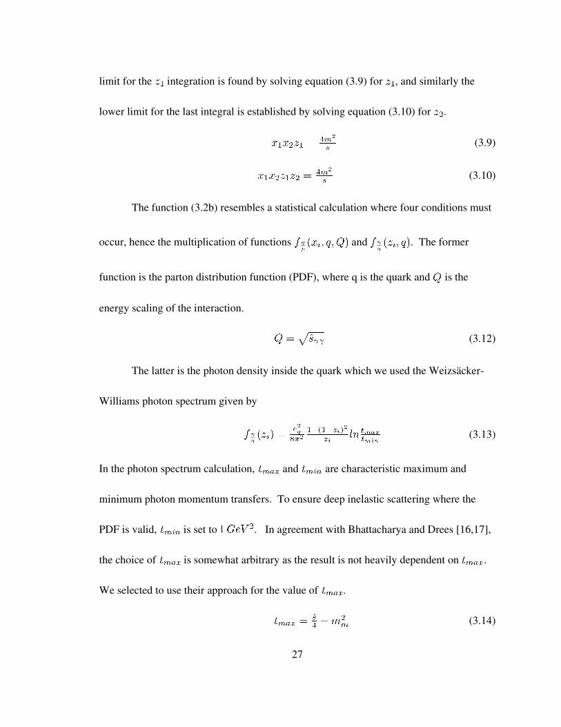
limit for the integration is found by solving equation (3.9) for , and similarly the
lower limit for the last integral is established by solving equation (3.10) for .
(3.9)
(3.10)
The function (3.2b) resembles a statistical calculation where four conditions must
occur, hence the multiplication of functions and . The former
function is the parton distribution function (PDF), where q is the quark and is the
energy scaling of the interaction.
(3.12)
The latter is the photon density inside the quark which we used the Weizsäcker
Williams photon spectrum given by
(3.13)
In the photon spectrum calculation, and are characteristic maximum and
minimum photon momentum transfers. To ensure deep inelastic scattering where the
PDF is valid, is set to . In agreement with Bhattacharya and Drees [16,17],
the choice of is somewhat arbitrary as the result is not heavily dependent on .
We selected to use their approach for the value of .
(3.14)
27
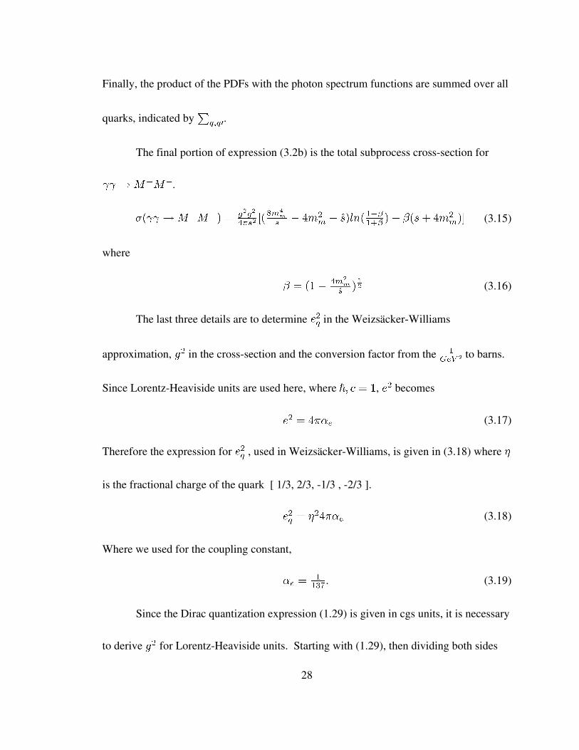
Finally, the product of the PDFs with the photon spectrum functions are summed over all
quarks, indicated by .
The final portion of expression (3.2b) is the total subprocess crosssection for
.
(3.15)
where
(3.16)
The last three details are to determine in the WeizsäckerWilliams
approximation, in the crosssection and the conversion factor from the to barns.
Since LorentzHeaviside units are used here, where , becomes
(3.17)
Therefore the expression for , used in WeizsäckerWilliams, is given in (3.18) where
is the fractional charge of the quark [ 1/3, 2/3, 1/3 , 2/3 ].
(3.18)
Where we used for the coupling constant,
. (3.19)
Since the Dirac quantization expression (1.29) is given in cgs units, it is necessary
to derive for LorentzHeaviside units. Starting with (1.29), then dividing both sides
28

by one obtains (3.19)
(1.29)
(3.20)
In cgs units, = , so the right side is unitless. Setting and squaring both sides,
. (3.21)
Now letting for LoretzHeaviside units, and solving for ,
. (3.22)
Due to the high energy scale of the photon interaction in the cross section calculation
(3.15), we used (3.23) for determining the value for .
(3.23)
By doing so, we assume the Dirac condition hold at all energy scales and the magnetic
coupling constant runs inversely to the electric coupling constant.
To convert the cross section calculation to barns the following conversion factor
was used.
(3.24)
29

Chapter 4
METERIAL AND METHODS
To compute the cross section for the process ,
equation (3.2) was numerically integrated using a right point integration method. Right
point integration was chosen as it is simple, and the integrands are well behaved to allow
for quick convergence.
Numerical integration was performed using a FORTRAN based program written
by the author, see appendix A for the source code. The source code was compiled and
executed on a Compaq computer running a Pentium 4, 3.8 GHz processor with a Fedora
Core 4 operating system.
Incorporated in the program are variables allowing the users to alter the following
quantities; monopole mass, center of mass energy, number of division for the integrals,
and choice of PDF. Unless specified all calculation were performed using Cteq6 1L
PDF.
For efficiency, 10 Compaq computers were employed to simultaneously test
different parameter settings, such as mass, energy and number of integration steps. Each
30

computer was verified using an adopted set of parameters to confirm all computers
compiled and executed the program identically. The benchmark was a double precision
output with all digits matching.
31

Chapter 5
RESULTS AND ANALYSIS
Equation (3.2) contains two independent parameters , and , to determine the
cross section from the process . Since the motivation for this
calculation is to help predict the cross section for Dirac monopole production at the LHC
and to set mass limits on the monopole by comparing results of the CDF search, the
monopole mass range covered by the calculation was
with CME of either or , referring to the Tevatron and LHC
respectively.
Figure 5.1 displays cross section vs monopole mass for a CME of . In
this figure, the solid line represents the photon fusion process and describes the
interpolated data points calculated for mass increments of . The other curve,
shown by the dashed line, is the predicted crosssection for the DellYan process, and
finally the dotdash line indicates the monopole crosssection upper limit with a 95% CL.
These last two curves were derived from the CDF publication [15].
32

Figure 5.1 Monopole Cross Section, ; Photon Fusion; DrellYan; 95% Confidence Limit
For the CME energy of , the plot of cross section vs monopole mass is
shown in Figure 5.2. As expected the shape of this curve closely resembles the heavy
lepton production curve for the photon fusion process as reported by Drees [17]. In this
figure the solid line again describes the interpolated data for the photon fusion process
and the dashed lines indicates an estimated cross section for the DrellYan process.
33
100 200 300 400 500 600 700 8001.0E16
1.0E15
1.0E14
1.0E13
1.0E12
1.0E11
1.0E10
1.0E09
1.0E08
Mass ( Gev )
Cros
s Sec
tion
( bar
n )

Figure 5.2 Monopole Cross Section Via Photon Fusion; Photon Fusion; DrellYan (estimated)
34
100 200 300 400 500 600 700 800 900 10001.0E12
1.0E11
1.0E10
1.0E09
1.0E08
1.0E07
1.0E06
Mass ( GeV )
Cros
s Sec
tion
( bar
n )
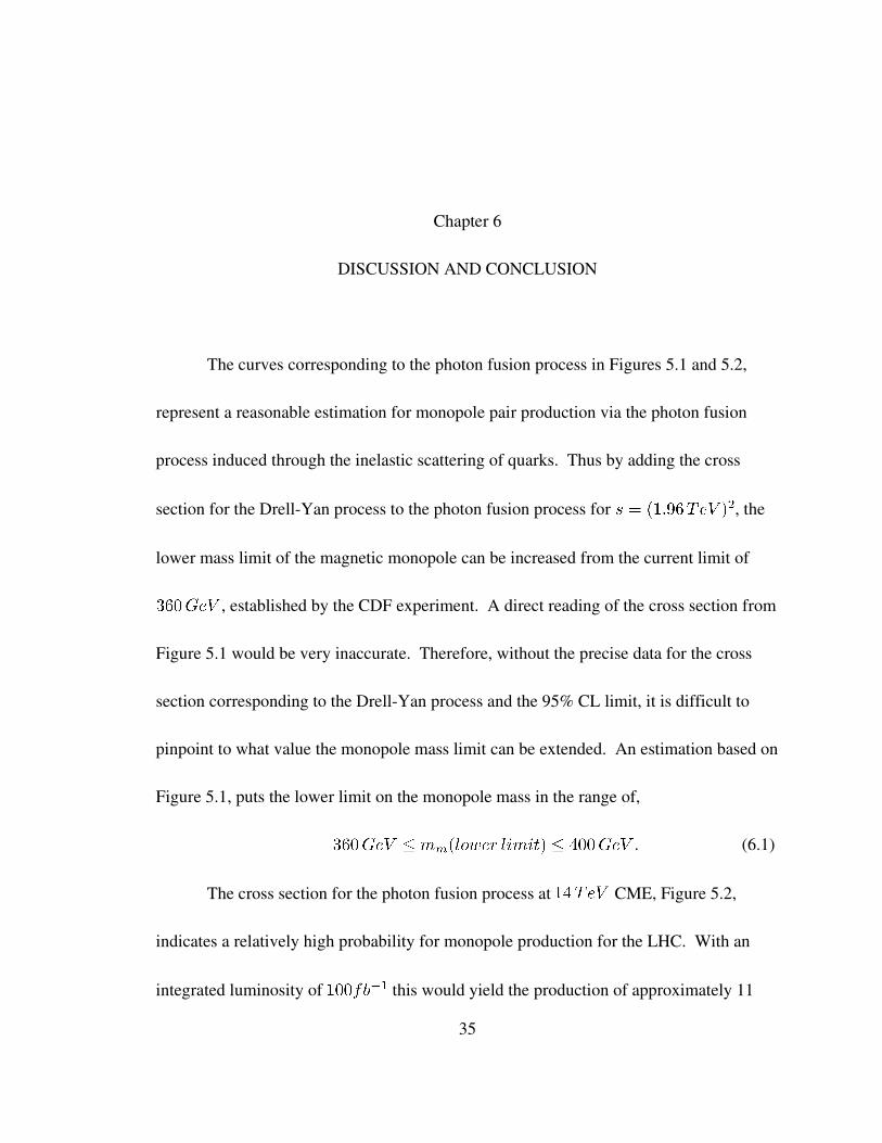
Chapter 6
DISCUSSION AND CONCLUSION
The curves corresponding to the photon fusion process in Figures 5.1 and 5.2,
represent a reasonable estimation for monopole pair production via the photon fusion
process induced through the inelastic scattering of quarks. Thus by adding the cross
section for the DrellYan process to the photon fusion process for , the
lower mass limit of the magnetic monopole can be increased from the current limit of
, established by the CDF experiment. A direct reading of the cross section from
Figure 5.1 would be very inaccurate. Therefore, without the precise data for the cross
section corresponding to the DrellYan process and the 95% CL limit, it is difficult to
pinpoint to what value the monopole mass limit can be extended. An estimation based on
Figure 5.1, puts the lower limit on the monopole mass in the range of,
. (6.1)
The cross section for the photon fusion process at CME, Figure 5.2,
indicates a relatively high probability for monopole production for the LHC. With an
integrated luminosity of this would yield the production of approximately 11
35
million monopole pairs for a monopole mass of . By comparison, the DrellYan
process will produce less than 1 million events. Therefore it is imperative that the
process of photon fusion be considered when a search for Dirac monopoles is conducted
at the LHC.
These favorable results reinforce the necessity to conduct future searches for
Dirac monopoles at the LHC. If the Dirac monopole exists, the addition of the photon
fusion process brings the Dirac monopole closer to being discovered than anticipated by
the DrellYan process alone.
36
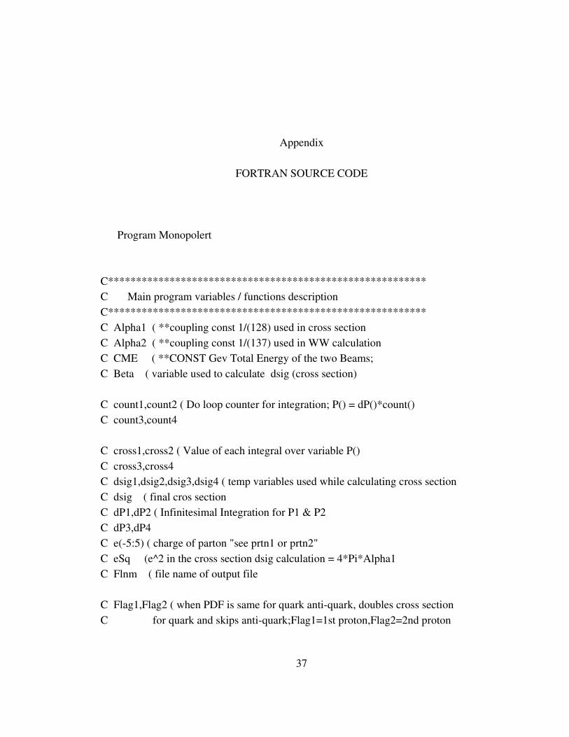
Appendix
FORTRAN SOURCE CODE
Program Monopolert
C*********************************************************C Main program variables / functions description C*********************************************************C Alpha1 ( **coupling const 1/(128) used in cross sectionC Alpha2 ( **coupling const 1/(137) used in WW calculationC CME ( **CONST Gev Total Energy of the two Beams; C Beta ( variable used to calculate dsig (cross section)
C count1,count2 ( Do loop counter for integration; P() = dP()*count() C count3,count4
C cross1,cross2 ( Value of each integral over variable P() C cross3,cross4 C dsig1,dsig2,dsig3,dsig4 ( temp variables used while calculating cross sectionC dsig ( final cros section C dP1,dP2 ( Infinitesimal Integration for P1 & P2 C dP3,dP4C e(5:5) ( charge of parton "see prtn1 or prtn2"C eSq (e^2 in the cross section dsig calculation = 4*Pi*Alpha1 C Flnm ( file name of output file
C Flag1,Flag2 ( when PDF is same for quark antiquark, doubles cross sectionC for quark and skips antiquark;Flag1=1st proton,Flag2=2nd proton
37
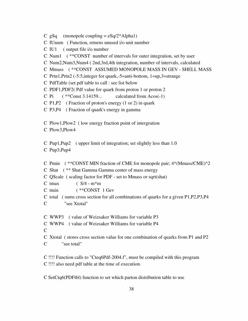
C gSq (monopole coupling = eSq/2*Alpha1)C IUnum ( Function, returns unused i/o unit numberC IU1 ( output file i/o numberC Num1 ( **CONST number of intervals for outer integration, set by userC Num2,Num3,Num4 ( 2nd,3rd,4th integration, number of intervals, calculatedC Mmass ( **CONST ASSUMED MONOPOLE MASS IN GEV SHELL MASSC Prtn1,Prtn2 (5:5,integer for quark,5=antibottom, 1=up,3=strangeC PdfTable (set pdf table to call : see list below C PDF1,PDF2( Pdf value for quark from proton 1 or proton 2C Pi ( **Const 3.14159... calculated from Acos(1)C P1,P2 ( Fraction of proton's energy (1 or 2) in quark C P3,P4 ( Fraction of quark's energy in gamma
C Plow1,Plow2 ( low energy fraction point of intergrationC Plow3,Plow4
C Pup1,Pup2 ( upper limit of integration; set slightly less than 1.0C Pup3,Pup4
C Pmin ( **CONST MIN fraction of CME for monopole pair; 4*(Mmass/CME)^2 C Shat ( ** Shat Gamma Gamma center of mass energyC QScale ( scaling factor for PDF set to Mmass or sqrt(shat)C tmax ( S/4 m*mC tmin ( **CONST 1 GevC total ( sums cross section for all combinations of quarks for a given P1,P2,P3,P4C "see Xtotal"
C WWP3 ( value of Weizsaker Williams for variable P3C WWP4 ( value of Weizsaker Williams for variable P4CC Xtotal ( stores cross section value for one combination of quarks from P1 and P2C "see total"
C !!!! Function calls to "Cteq6Pdf2004.f", must be compiled with this programC !!!! also need pdf table at the time of execution.
C SetCtq6(PDFtbl) function to set which parton distribution table to use
38

C Ctq6pdf(Prtn2, P2, Qscale) main function call to output the PDF value
C******************************************************** C********************************************************
Implicit None C Integer Num1,Num2,num3,num4,count3,count4 Integer Prtn1,prtn2,Pdftbl,count1,count2 Integer Flag1,Flag2,IU1,IUNumC Double Precision Alpha1,CME,Beta,cross1,cross2 + ,Cross3,Cross4,dP1,dP2,dP3,dP4,P1,P2,P3,P4 + ,eSq,gSQ,Mmass,Pi,Pmin,Shat,QScale,tmax,tmin + ,Plow1,Plow2,Plow3,Plow4,Pup1,Pup2,Pup3,Pup4 Double precision dsig,dsig1,dsig2,dsig3,dsig4 Double Precision Alpha2,Ctq6pdf Double Precision XTotal,PDF1,PDF2 + ,e(5:5),total,WW,WWP3,WWP4C Character flnm*9
C C set electromagnetic charge of partonC Data e/ (1.0/3.0),(2.0/3.0),(1.0/3.0) + ,(1.0/3.0),(2.0/3.0),(0.0),(2.0/3.0) + ,(1.0/3.0),(1.0/3.0),(2.0/3.0) + ,(1.0/3.0) /
CC******** VARIABLES TO MANUALLY SET ********** C *******units are Gev ****C Pi = dAcos(1.0d0) Alpha1 = 1.0d0/128.0d0
39

Alpha2 = 1.0d0/137.0d0 WW = alpha2 / (2.0d0*(PI)) eSq = 4.0d0*Pi*Alpha1 gSq = Pi/Alpha1 tmin = 1.0d0 PDFtbl = 4
CME = 14.0d3 Mmass = 100.0d0 Num1 = 50 flnm = '1M100.tbl'
C C Iset PDFset Description Alpha_s(Mz)**Lam4 Lam5 Table_FileC (PDFtbl)C ===========================================================================C 1 CTEQ6M Standard MSbar scheme 0.118 326 226 cteq6m.tblC 2 CTEQ6D Standard DIS scheme 0.118 326 226 cteq6d.tblC 3 CTEQ6L Leading Order 0.118** 326** 226 cteq6l.tblC 4 CTEQ6L1 Leading Order 0.130** 215** 165 cteq6l1.tblC C ********************************************************************C ************************ MAIN PROGRAM *******************C ********************************************************************
C C subroutine in CteqPdf2004.f to open pdf table C Call SetCtq6(PDFtbl)
C C find unallocated i/o unit and open file to write dataC IU1 = IUnum()
40
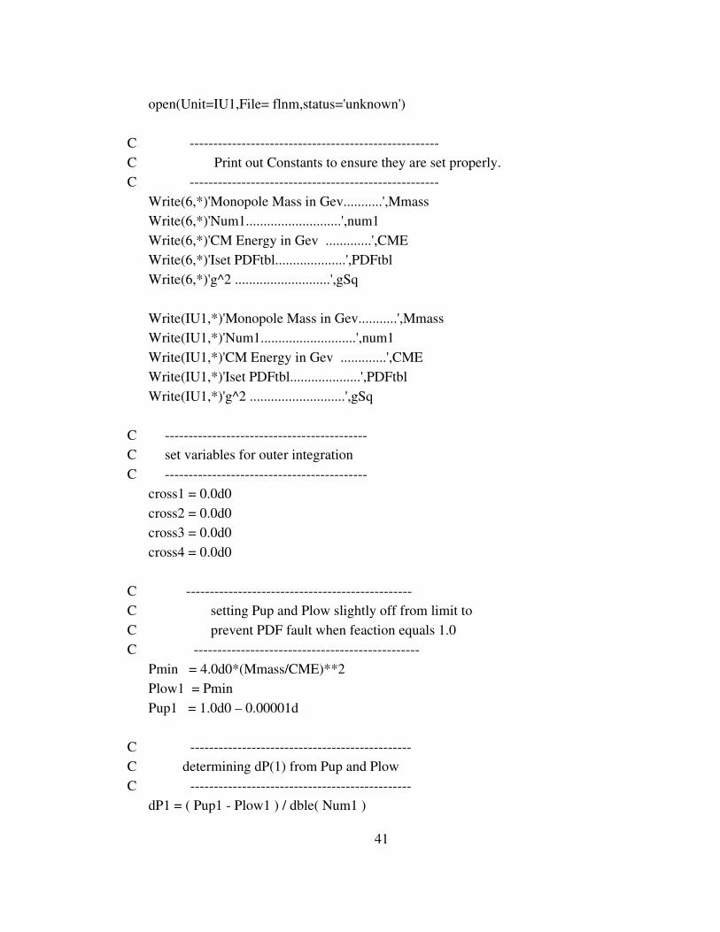
open(Unit=IU1,File= flnm,status='unknown')
C C Print out Constants to ensure they are set properly. C Write(6,*)'Monopole Mass in Gev...........',Mmass Write(6,*)'Num1...........................',num1 Write(6,*)'CM Energy in Gev .............',CME Write(6,*)'Iset PDFtbl....................',PDFtbl Write(6,*)'g^2 ...........................',gSq Write(IU1,*)'Monopole Mass in Gev...........',Mmass Write(IU1,*)'Num1...........................',num1 Write(IU1,*)'CM Energy in Gev .............',CME Write(IU1,*)'Iset PDFtbl....................',PDFtbl Write(IU1,*)'g^2 ...........................',gSq
C C set variables for outer integrationC cross1 = 0.0d0 cross2 = 0.0d0 cross3 = 0.0d0 cross4 = 0.0d0 C C setting Pup and Plow slightly off from limit to C prevent PDF fault when feaction equals 1.0C Pmin = 4.0d0*(Mmass/CME)**2 Plow1 = Pmin Pup1 = 1.0d0 – 0.00001d C C determining dP(1) from Pup and PlowC dP1 = ( Pup1 Plow1 ) / dble( Num1 )
41
CC***** Outer Integration Plow(1) to Pup(1) ************C Do 100, count1 = 1, ( Num1 ) P1 = Plow1 + dP1 * dble( count1 C C set variables for 2nd integrationC cross2 = 0.0d0 Plow2 = Plow1/P1 Pup2 = Pup1 dP2 = dP1C C determine Num2 from position of P2C Num2 = int( ( Pup2 Plow2 ) / dP2 )
C C ***** 2ND Integration Plow2 to Pup ***********C Do 200, count2 = 1, ( Num2 )
P2 = Plow2 + ( dP2 * dble( count2 ) )C C set variables for 3nd integrationC cross3 = 0.0d0 Plow3 = Plow2/P2 Pup3 = Pup2 dP3 = dP2 Num3 = int( ( Pup3 Plow3 ) / dP3 )
C C ***** 3RD Integration Plow2 to Pup ***********C
Do 300, count3 = 1, ( Num3 )
42
P3 = Plow3 + dP3 * dble( count3 ) C C set variables for 4th integrationC cross4 = 0.0d0 Pup4 = Pup3 Plow4 = Plow3/p3 dP4 = dP3 Num4 = int( ( Pup4 Plow4 ) / dP4 )C C ***** 4th Integration Plow2 to Pup ***********C Do 400, count4 = 1, ( Num4 )
P4 = Plow4 + dP4 * dble( count4 )C C *** calculting cross section ***C Shat = (CME**2)*P1*P2*P3*P4 tmax = (Shat / 4.0d0) Mmass**2 IF (tmax .lt. 1.0) then tmax = 1.0 write(6,*)'tmax limit' endif
qscale = dsqrt(Shat/4.0d0) Beta = ( 1.0d0 (4.0d0 * Mmass**2/Shat) )**0.5
dsig1 =( (8.0d0*Mmass**4.0d0)/Shat )(4.0d0*Mmass**2)Shat dsig2 = dsig1*dlog( (1Beta) / (1+Beta) ) dsig3 = dsig2 ( Beta * (Shat + 4.0d0*Mmass**2) ) dsig = ( (gSq*gSq ) / (4.0d0*Pi*Shat**2) ) * dsig3C C *** 3.894d4 barns*Gev^2 conversion factorC C dsig = dsig*3.894d4
43

C C *** other method to calculate cross sectionC C dsig1 = 4*PI*Alpha1**2*Beta/shatC dsig2 = ( 3.0 Beta**4)/(2.0*Beta)C dsig3 = dlog( (1.0d0 + Beta)/(1.0d0 Beta))C dsig4 = ( 2.0d0 Beta**2 )C dsig = dsig1*( dsig2*dsig3 dsig4)C C *** 3.894d4 barns*Gev^2 conversion factorC C dsig = dsig*3.894d4
C C **** compute WW ***C WWP3 = dlog(tmax/tmin)*WW*( 1.0d0+(1.0d0P3)**2.0 )/P3 WWP4 = dlog(tmax/tmin)*WW*( 1.0d0+(1.0d0P4)**2.0 )/P4
flag1 = 0.0 flag2 = 0.0 Total = 0.0
C C check parton from proton 1 C to skip similar PDF values for C quark antiquark. Also skip over gluonC Do 50, prtn1 = 2, 5 If (prtn1 .eq. 0) then goto 50 endif
If ( prtn1 .gt. 2) then flag1 = 1 endif
44
C C check parton from proton 2 C to skip similar PDF values for C quark antiquark. Also skip over gluonC
Do 60, prtn2 = 2, 5 If(prtn2 .eq. 0) then goto 60 endif
If ( prtn2 .gt. 2 )then flag2 =1 endif
C C **** find PDF value ***C PDF1 = Ctq6pdf(Prtn1, P1, Qscale) PDF2 = Ctq6pdf(Prtn2, P2, Qscale)
Xtotal=(e(prtn1)**2)*(e(prtn2)**2)*WWP3*WWP4*PDF1*PDF2*dsig
C C **** double Xtotal if similar PDFC for quark antiquark from Proton 2C If ( Flag2 .eq. 1 ) then
Xtotal = Xtotal*2.0 endifC C **** double Xtotal if similar PDFC for quark antiquak from Proton 1C even if already doubled from Proton 2C If ( Flag1 .eq. 1) then Xtotal = Xtotal*2.0 endif
45
total = total + Xtotal
Flag2 = 0
60 continue Flag1 = 0
50 continue Cross4 = Cross4 + total*dP4
400 continueCross3 = Cross3 + Cross4*dP3
300 continue Cross2 = Cross2 + Cross3*dP2 200 continue Cross1 = Cross1 + Cross2*dP1 Write(6,*)P1,cross1
100 continue Write(IU1,*)P1,cross1 close(unit=IU1)
endCC ********* END ************* C *******OF MAIN PROGRAM ***********C
46

C*************** F U N C T I O N ****************************C ************Returns an unallocated FORTRAN i/o unit. ******C ********************************************************** Function IUnum() Integer n Data n/10/ Save n Logical EXC C Checks for available i/o unit that is less then 100C otherwise terminate programC 10 INQUIRE (UNIT=N, OPENED=EX) If (EX) then n=n+1 If (n.gt.100) then Print *, 'There is no available I/O unit.' Stop Else goto 10
Endif Endif IUnum = n Return End
47

REFERENCES
1. Dirac, P.A.M., Quantised Singularities in the Electromagnetic Field. Proceedings of the Royal Society of London Series A133, 6072 (1931)
2. Bransden, B.H., Joachain, C.J., Quantum Mechanics, 567571, (Pearson Education Ltd, Second edition 2000)
3. Sakurai, J.J, Modern Quantum Mechanics, 136139, (The Benjamin/Cummings Publishing Company, Inc. 1985)
4. Thomson, J.J., Electricity and Matter, p. 26, (Scribners, New York 1904)
5. Jackson, J.D., Classical Electrodynamics, 275280, (John Wiley & Sons, Inc. Third edition 1999)
6. Milton, K.A., Kalbfleisch, G.R., Luo, W., Gamberg, L. Theoretical and experimental status of magnetic monopoles. International Journal of Modern Physics A17, 732750 (2002)
7. Hooft, G.'t, Magnetic monopoles in unified gauge theories, Nuclear Physics B79, 276284 (1974)
8. Polyakov A., JETP Lett. 20 (1974) 194
9. Dokos, C, Tomaras, T.N, Monopoles and dyons in the SU(5) model, Physical Review D21, 29402952 (1980)
10. Langacker, P., Pi, S.Y.,Magnetic Monopoles in Grand Unified Theories, Physical Review Letters 45, 14 (1980)
48

11. Liu, H., Vachaspati, T., SU(5) Monopoles and the Dual Standard Model, Physical Review D56, 13001312 (1997)
12. Giacomelli, G., Patrizzi, L., Magnetic Monopoles, Invited paper at the NATO ARW "Cosmic Radiations: from Astronomy to Particle Physics", Ojuda, Morocco 2123 March 2001
13. Wick, S.D., Kephart, T.W., Weiler, T.J., Biermann, P.L., Signatures for a cosmic flux of magnetic monopoles, Astroparticle Physics 18, 663687 (2003)
14. Wick, S.D.,Relativistic GUT Monpoles: Stopping Power and Signatures, Thesis (PhD). Vanderbilt University, Source DIAB 60/09, 46804773 (March 2000)
15. By CDF Collaboration, Direc Search for Dirac Magnetic Monopoles in Collisions at = 1.96 TeV, Physical Review Letter 96, 201801201809 (2006)
16. Bhattacharya, G., Kalyniak, P., Peterson, K.A., Photon and Z Induced Heavy Charged Lepton Pair Production at a Hadron Supercollider, Physical Review D53, 23712379 (1996)
17. Drees, M., Godbole, R.M., Nowakowski, M., Rindani, S.D., processes at high energy pp colliders, Physical Review D50, 23352338 (1994)
18. Stroynowski, R., Lepton pair production in Hardon collisions, Physics Report 711, 150 (May 1981)
49

Related Documents