Monitoring land degradation risk using ASTER data: The non-evaporative fraction as an indicator of ecosystem function

$Page 1: Monitoring land degradation risk using ASTER data: The non-evaporative fraction as an indicator of ecosystem function$
Remote Sensing of Environment 112 (2008) 3720–3736

Contents lists available at ScienceDirect

Remote Sensing of Environment

j ourna l homepage: www.e lsev ie r.com/ locate / rse

Monitoring land degradation risk using ASTER data: The non-evaporative fraction asan indicator of ecosystem function

Mónica García a,⁎, Cecilio Oyonarte b, Luis Villagarcía c, Sergio Contreras d,Francisco Domingo a,e, Juan Puigdefábregas a

a Departamento de Desertificación y Geoecología, Estación Experimental de Zonas Áridas (CSIC), Almería E-04001, Spainb Departamento de Edafología y Química Agrícola, Universidad de Almería, Almería E-04120, Spainc Departamento de Sistemas Físicos, Químicos y Naturales, Universidad Pablo de Olavide, Sevilla E-41013, Spaind Grupo de Estudios Ambientales, Universidad Nacional de San Luis, San Luis E-5700, Argentinae Departamento de Biología Vegetal y Ecología, Escuela Politécnica Superior, Universidad de Almería, Almería E-04120, Spain

⁎ Corresponding author. Tel.: +34 950281045.E-mail address: [email protected] (M. García).

0034-4257/$ – see front matter © 2008 Elsevier Inc. Aldoi:10.1016/j.rse.2008.05.011

A B S T R A C T
A R T I C L E I N F O
Article history:
There is a need to develop Received 16 August 2007Received in revised form 13 May 2008Accepted 24 May 2008
Keyword:Surface energy balanceEvapotranspirationEddy covarianceDesertificationSemiaridRemote sensingDisturbance

operational land degradation indicators for large regions to prevent losses ofbiological and economic productivity. Disturbance events press ecosystems beyond resilience and modify theassociated hydrological and surface energy balance. Therefore, new indicators for water-limited ecosystemscan be based on the partition of the surface energy into latent (λE) and sensible heat flux (H).In this study, a new methodology for monitoring land degradation risk for regional scale application isevaluated in a semiarid area of SE Spain. Input data include ASTER surface temperature and reflectanceproducts, and other ancillary data. The methodology employs two land degradation indicators, one related toecosystem water use derived from the non-evaporative fraction (NEF=H / (λE+H)), and another related tovegetation greenness derived from the NDVI. The surface energy modeling approach used to estimate theNEF showed errors within the range of similar studies (R2=0.88; RMSE=0.18 (22%)).To create quantitative indicators suitable for regional analysis, the NEF and NDVI were standardized betweentwo possible extremes of ecosystem status: extremely disturbed and undisturbed in each climatic region todefine the NEFS (NEF Standardized) and NDVIS (NDVI Standardized). The procedure was successful, as itstatistically identified ecosystem status extremes for both indicators without supervision. Evaluation of theindicators at disturbed and undisturbed (control) sites, and intermediate surface variables such as albedo orsurface temperature, provided insights on the main surface energy status controls following disturbanceevents. These results suggest that ecosystem functional indicators, such as the NEFS, can provide informationrelated to the surface water deficit, including the role of soil properties.

© 2008 Elsevier Inc. All rights reserved.

1. Introduction

Natural and human disturbances are known to modify the surfaceenergy balance and hydrological cycle to different extents (Wang &Takahashi, 1998; Nicholson, 2000;Wilson et al., 2002; Liu et al., 2005),which may produce feedbacks to regional or even global climatepatterns (Schlesinger et al., 1990; Xue & Shukla, 1993). Disturbanceevents pressing ecosystems beyond resilience cause land degradation(Puigdefábregas, 1995), defined as, “A reduction or loss in thebiological and economic productivity and complexity of terrestrialecosystems, as well as in the ecological, biochemical and hydrologicalprocesses that operate in them” (UNCCD, 1996).

l rights reserved.

Desertification is a process causing land degradation in arid,semiarid and dry-subhumid areas (hereinafter drylands) (UNCCD,1996). At present, drylands cover more than 45% of the global landsurface (Asner et al., 2003) and General Circulation Models (GCMs)predict increased aridity related to global warming (Okin, 2002).These areas sustain around 37% of the world's population (Reynoldset al., 2007) and are subject to climatic stress and strong pressures,which make them the regions most vulnerable to land degradation(Safriel et al., 2003). For these reasons, a better understanding of therelationships between disturbances, land degradation and water, themost limiting resource, is especially relevant in these regions.

There is currently a pressing need for operational, objectivedesertification indicators for large regions (Puigdefábregas&Mendizabal,1998;Wessels et al., 2004; Reynolds et al., 2007). This lack of informationis due in part to a change in the perception of desertification. It is nowwidely recognized that most of what was previously considereddesertification was in fact response to climatic fluctuations (Prince

mailto:[email protected]

http://dx.doi.org/10.1016/j.rse.2008.05.011

http://www.sciencedirect.com/science/journal/00344257

3721M. García et al. / Remote Sensing of Environment 112 (2008) 3720–3736

et al., 1998; Tucker & Nicholson, 1999; Nicholson, 2000). The old“advancing desert” paradigm prevalent during the 1970's and 1980's isnow obsolete and desertification is associated with a higher spatio-temporal heterogeneity of water and other resources with respect toundegraded areas (Schlesinger et al., 1990).

As several biophysical and biochemical processes are affected bydesertification or land degradation in drylands, indicators of ecosystemstatus identify alterations in awide range of properties, such asNPP (NetPrimary Productivity), RUE (Rainfall Use Efficiency), soil properties(salinity, organic matter), vegetation patterns, landscape fragmentation,andwater balance, amongothers (Schlesinger et al.,1990; Sharma,1998;Asner et al., 2003), reflecting the complexity of the problem.Evapotranspiration is a key ecosystem function that has not beenmuch used for desertification monitoring. In this regard, dysfunctionalor degraded ecosystemsare less capable of retaining, using and recyclinglocal resources, such as water, energy and nutrients than ecosystemsthat are not (LeHouerou, 1996; Ludwig & Tongway, 2000; Paruelo et al.,2000; Holm et al., 2003; Boer & Puigdefábregas, 2003, 2005). As thepartition of available energy reaching a surface into latent heat (λE) andsensible heat (H) depends mostly on water availability, undegradedecosystems should dissipate more energy through λE (or evapotran-spiration) compared to degraded or disturbed landscapes.

Therefore, development of regional-scale land degradation riskindicators evaluating alterations in the surface energy balance as aresult of disturbances could be based on the energy partition betweenλE and H. Remote sensing is the only data source currently providingfrequent, spatially disaggregated information related to the surfaceenergy status in the solar and thermal spectral ranges. Variables such assurface temperature, albedo or vegetation indices can be input intosurface energy balance and evapotranspiration models (Kustas &Norman, 1996).

Results from research projects using remote sensing data and fieldmethods, such as the SALSA (Semi-Arid Land-Surface-Atmosphere)project in Arizona (Chehbouni et al., 2000), the HAPEX-Sahel(Hydrologic Atmospheric Pilot Experiment in the Sahel) (Goutorbeet al., 1997) or the EFEDA (European field experiment in a desertifica-tion threatened area) project in Spain (Bolle et al., 1993), havecontributed to a better understanding the surface energy balance andevapotranspiration of drylands affected by land degradation. In amoreapplied context, land degradation has been assessed using thermaland reflectance data, either directly (Lambin & Ehrlich, 1997; Sobrino& Raissouni, 2000; Dall'Olmo & Karnieli, 2002; Mildrexler et al., 2007),or using remote sensing data as input to physical models (Wang &Takahashi, 1998). In general there is a trade-off between modelparameterization requirements and applicability that has to becarefully considered.

The purpose of this study is to develop and test a newmethodologyto monitor land degradation risk by detecting disturbed sites forregional-scale application. The methodology consists of a water-useindicator related to ecosystem functioning (NEFS, Non-EvaporativeFraction Standardized), and another indicator related to vegetationgreenness (NDVIS, Normalized Difference Vegetation Index Standar-dized). We hypothesize that disturbed sites, where land degradationmight occur if the effect of disturbance is sustained over time, shouldshow higher NEFS and lower NDVIS in response to increases in baresoil, and loss of vegetation and soil organicmatter. Therefore, disturbedsites can be considered at risk of land degradation due to their loss offunctionality. The changes in vegetation greenness and soil propertiesmentioned above should alter the surface energy balance by increasingthe sensible heat flux (H), and decreasing net radiation (Rn) similar toother land degradation situations in North Africa (Dolman et al., 1997)and Southeast Spain (Arribas et al., 2003). However, feedback effectsmight modify some of these responses (Phillips, 1993) and dependingon the magnitude of the changes in surface temperature and albedo,the partition of energy between sensible and latent heat flux may bequite different. Analysis of the NEFS, NDVIS and related variables at

disturbed and undisturbed sites will help to clarify some of theseresponses.

2. Study site and data

2.1. Study region

The study region (Fig. 1), located in the southeastern IberianPeninsula (Almería, Spain), comprises 3600 km2 (36.95°N, 2.58°W). Itis characterized by its heterogeneity, with altitudinal gradientsranging from sea level up to 2800 m (a.s.l.) in the Sierra NevadaMountains. Precipitation and temperature regimes vary widely due tothe orography (López-Bermúdez et al., 2005). Annual precipitation isthe lowest in the Tabernas lowlands, where it is less than 200 mm,while in the mountains it ranges from 400 mm to 700 mm, which isenough to sustain forest growth.

In the center of the study area, the karstic landscape of the Sierrade Gádor mountain range, covering 552 km2, consists of a series ofthick carbonate rocks (limestones and dolomites), highly permeableand fractured with intercalated marl and less permeable calcschistsunderlain by impermeable metapelites (Aldaya et al., 1977). Thesouthern edge of this mountain range is the main source of rechargefor the Triassic aquifers in the region known as the “Campo de Dalías”(Pulido-Bosch et al., 2000). In general, the soils are very thin, rocky andvulnerable to flash flooding and erosion. Themost common types varydepending on lithology and conservation status. On limestone anddolomitic materials, the most representative soils according to the SoilTaxonomy (Soil Survey Staff, 1990), are very thin Lythic Haploxeroll/Lythic Argixeroll (undisturbed sites) or Lythic Xerorthent (disturbedsites). The dominant types of less compact materials such as marls andcalcschists are Typic Xerorthent and to a lesser degree TypicHaploxeroll (preserved sites) (Oyonarte et al., 1994).

The Sierra de Gádor Mountains underwent intense, widespreaddeforestationduring the 18th and19th centuries,when the original oaks(Quercus ilex L. and Quercus faginea Lam.), olive trees (Olea europaea L.),poplars (Populus L. spp.) and strawberry trees (Arbutus unedo Lam.)werecut down for ship construction and fuel for mining activities (Perez dePerceval, 1984). Current disturbances include construction, fire, agri-culture and sheep grazing. At the present time, 73% of the Sierra deGádor has a mixture with less than 50% vegetation cover comprised ofsparse shrublands with rock outcrops, bare soil or grasses. The secondlargest natural land-cover type (12% of the area) is shrublands with asparse cover of pine woodland (Pinus L. sp.), around 9% of the Sierra deGádor is devoted to agriculture (mainly almondandolive trees) and only1.5% of the land is covered by dense pine, reforested 30 years ago (Valle,2003). The remaining 4.5% is composed of several different lessrepresentative land-use types (Contreras, 2006).

The rest of the study region, outside of the Sierra de Gádor,includes part of the Sierra Nevada Natural Park, which is comprised ofpine forest with oak relicts and shrublands. There is an area ofbadlands, the Tabernas lowlands in the northeast, and along theephemeral Andarax River there is a mosaic of citrus orchards andvineyards. One of the most salient features of the region is the morethan 330 km2 of plastic greenhouses in the “Campo de Dalías”. Thisunique combination of land covers and uses makes it a mostinteresting site for model testing. Within the study region threefield sites were selected for validation purposes.

2.1.1. Llano de los Juanes research siteLlano de los Juanes is a ∼2 km2

flat area with sparse shrubland, thesame vegetation type present in 73% of Sierra de Gádor. It is located at analtitudeof 1600m in thehigh,well-developedkarstic plainof the SierradeGádor. Vegetation cover is 50–60%andconsistsmainlyof patchyperennialdwarf shrubs (30–35%) dominated byGenista pumilla, Thymus serpylloidesBory. and Hormathopylla spinosa L., and grasses (20–25%) dominated byFestuca scariosa Lag. and Brachypodium retusum Pers. (Li et al., 2007).

Fig. 1. Study site in Southeast Spain (Almería). The large image shows NDVI (15 m) from ASTER July,18-2004. Three mountain ranges, are visible, the Sierra Nevada, Sierra Alhamillaand Sierra de Gádor (outlined inwhite). The locations of the three NEF (Non-evaporative fraction) validation sites, Llano de los Juanes in Sierra de Gádor, Rambla Honda in the Tabernaslowlands, and the lake Cañada de las Norias by the greenhouse area are shown bywhite arrows. Validation sites of the land degradation indicator NEFS (NEF Standardized) included aset of severely disturbed sites and another set of disturbed-soil sites. Severely disturbed sites in Sierra de Gádor are identifed as 1 (burnt scar), 2 (limestone quarry), 3 (almondorchards), 4 (abandoned mine). Undisturbed sites identified as 6 (dense oaks), 7 (oaks), 8 (sparse oaks), and 9 (old reforested pines). Disturbed -soil sampling sites on marl (redtriangles), and limestone (yellow triangles) lithologies are shown, as well as control sampling sites on marls (green triangles), and limestones (blue triangles).

3722 M. García et al. / Remote Sensing of Environment 112 (2008) 3720–3736

2.1.2. Rambla Honda research siteThe Rambla Honda research site is located in a dry valley near

Tabernas, Almería, Spain (37°8′N, 2°22′W, 630 m altitude). For adetailed description of the site, see Puigdefábregas et al. (1996). Thevalley has been abandoned for several decades and the activity is nowrestricted to small-scale sheepherding. Experiments related tohydrology and erosion (Puigdefábregas et al., 1999, 2005), surfaceenergy balance and evapotranspiration (Villagarcia et al., 2007) andvegetation ecology (Hasse et al., 2000; Pugnaire et al., 1996) amongothers have been performed at the site during the last decade.

Three perennial species dominate the landscape, Retama sphaer-ocarpa (L.) Boiss shrubs on the valley floor, Stipa tenacissimaL. tussocks on the steep sides of the valley and Anthyllis cytisoidesL. shrubs on alluvial fans between the two. The valley floor has deeploamy soils overlying mica schist bedrock. The average annual rainfallis 220 mm with a dry season from June to September.

2.1.3. Cañada de las Norias wetlandThewetland, located in thegreenhouse area, comprises 135hawith a

maximum depth of 2 m. The riparian vegetation is composed of Phrag-mites australis, Tamarix canariensis, and Tamarix africana, the latter alsoappears within thewater table. Shallower parts are dominated by Typhadomingensis and Scirpus litoralis. Within the wetland, macroalgae from

Entermorpha and Cladophora genus, indicative of high eutrofication,tend to replace aquatic macrophytes (Paracuellos, 2006). Solids andalgae increase water turbidity and reduce the effective penetration ofsolar radiation in the water column, which reduces the water storageterm at a daily scale (Gd) (Oswald and Rouse, 2004) that becomes almostnegligible in the case of vegetated wetlands (Burba et al., 1999).

2.2. Micrometeorological data

Micrometeorological data have been acquired continuously at theLlano de los Juanes research site (Fig. 1) since September 2003. Latentand sensible heat fluxes weremeasured by an eddy covariance systemusing a three-dimensional sonic anemometer CSAT3 and a kryptonhygrometer KH20 (both from Campbell Scientific Inc., Logan, USA).Fetch is sufficient for the vegetation height and sensors. Annualprecipitation recorded during the last three hydrological years by arain gauge installed in 2003 varied considerably: 506.7 mm in 2003/04, 212.4 mm in 2004/05, and 328.1 mm in 2005/06.

In Rambla Honda, there were no surface energy flux field measure-ments for 18-July-2004, the date of the ASTER scene covering this site.Therefore, daily sensible and latent heat fluxes for this site weresimulated using a detailed SVAT (Soil–Vegetation–Atmosphere Transfer)multilayer evapotranspiration model for sparse vegetation (Domingo

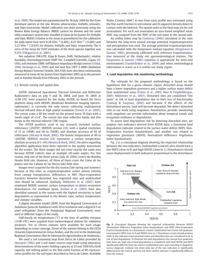
Fig. 2. Conceptual diagram showing the expected relationship between NDVIS(Normalized Difference Vegetation Index Standardized) and NEFS (Non-EvaporativeFraction Standardized) in a disturbance context. Undisturbed sites (lower left quadrant)correspond to NEFS close to 0 and NDVIS close to 1. Disturbance events should produceshifts in the indicators from potential status and disturbed sites are considered to be atrisk of land degradation. To illustrate the land degradation risk concept four quadrantshave been set: high risk of land degradation is considered with both NDVIS and NEFSsignificantly different from the control (undisturbed sites) and coinciding in diagnostic(across diagonal), medium risk when only one of the two indicators is significantlydifferent from the control, and low risk when neither indicator is significantly differentfrom the control.


et al.,1999). Themodelwas parameterized for 18-July-2004 for the threedominant species at the site, Retama sphaerocarpa, Anthyllis cytisoides,and Stipa tenacissima. Model calibration was done previously using theBowen Ratio Energy Balance (BREB) system for Retama and the sameeddy covariance system later installed at Llano de los Juanes for Anthyllisand Stipa. RMSEs (relative to themean in parenthesis) for the calibrationfor daily latent heat were 8.28 Wm−2 (6.48%), 4.22 Wm−2 (15.68%) and2.23 Wm−2 (12.03%) for Retama, Anthyllis and Stipa, respectively. The %error of the mean for SVAT estimates of the three species together was9.21% (Villagarcía et al., 2001).

Net radiation (NR-LITE; Kipp & Zonen, Delft, Netherlands), relativehumidity (thermohygrometer HMP 35C, Campbell Scientific, Logan, UT,USA), soilmoisture (SBIB; Self Balance ImpedanceBridge sensors) (Vidal,1994; Domingo et al., 1999) and soil heat flux (HFT-3, REBS (RadiationEnergy Balance Systems) Seattle,WA, USA) have also been continuouslymeasured at Llano de los Juanes from September 2003 up to the presentand in Rambla Honda from February 2002 to the present.

2.3. Remote sensing and spatial data

ASTER (Advanced Spaceborne Thermal Emission and ReflectionRadiometer) data on July 9 and 18, 2004, and June 19, 2005 at11.00 UTC were acquired for the study. ASTER, on board the Terraplatform along with MODIS (Moderate Resolution Imaging Spectro-radiometer), is currently the only sensor collecting multispectralthermal infrared data at high spatial resolution (French et al., 2005).The sensor scans a 60 km swath on the ground every 16 days with aswath angle of ±2.4°. The sensor has nine reflective bands and fivebands in the thermal infrared (TIR) region.

The ASTER products used in our research included surfacereflectance (2AST07; HDFEOS version 2.8), with a spatial resolutionof 15 m (VNIR) and 30 m (SWIR), and absolute accuracy of 4% ofreflectance (Abrams & Hook, 2002). The kinetic temperature at 90 m(2AST08; HDFEOS version 2.8) represents a surface temperatureabsolute accuracy of 1–4 K (Abrams &Hook, 2002). No alerts regardingalgorithm application have been reported in the quality assessmentfor the scenes. The three images did not cover exactly the same areabecause ASTER collects data at multiple off-nadir angles. For thisreason, only one of the three scenes (July 18, 2004) covers the RamblaHonda field site. However, all three of them cover the Llano de losJuanes and the Cañada de las Norias lake field sites.

Images were acquired for the dry season (late spring and summer)because at this time, as evapotranspiration comes almost entirelyfrom canopy transpiration, differences in NEF (Non-evaporativeFraction) between disturbed, less vegetated sites and undisturbedsites should be enhanced. Similarly, Mildrexler et al. (2007) haveemployed MODIS summer surface temperature to detect ecosystemdisturbances. For southeast Spain, Arribas et al. (2003) have alsoidentified summer as the season with the highest sensitivity to landdegradation as represented in the Bowen ratio, surface temperatureand climatic variables.

A digital elevation model (DEM) from the Regional Government ofAndalusia (Junta de Andalucia) with 30m resolution and a digital 0.5-mpixel orthophoto (from the Andalusian Regional Government) wereused at different stages of the study.

Half-hourly air temperatures (°C) at the time of satellite overpass(11.00 UTC) were acquired from meteorological stations for validationpurposes. Ten or eleven stations were available for each imagedepending on scene coverage. Seven of the stations belong to the EEZA(Estación Experimental de Zonas Áridas), and the rest to the AndalusianRegional Government (Red de Información Agroclimática de Andalucía).

We used a soil taxonomy map from Sierra de Gádor provided byOyonarte (1992) and a soil water reserve map made using laboratorydeterminations of thewater-holding capacity at 33 and 1500 kPa (fieldcapacity and wilting point) in the fine-earth fraction of 80 represen-tative profiles for the soil types described at Sierra de Gádor. Available

Water Content (AWC) in mm from each profile was estimated usingthe fine-earth fraction in soil volume and its apparent density down tocontact with the bedrock. The spatial units in the final map are for soilassociations. For each soil association an area-based weighted meanAWC was assigned from the AWC of the soil types in the spatial unit.

An aridity index map by Contreras (2006) calculated as the ratiobetween the long-term annual average potential evapotranspirationand precipitation was used. The average potential evapotranspirationwas calculated with the Hargreaves–Samani equation (Hargreaves &Samani, 1982), previously calibrated with reference evapotranspira-tion measured at the study site agrometeorological stations. TheHargreaves & Samani (1982) equation is appropriate for semi-aridenvironments (Vanderlinden et al., 2004) and when meteorologicalinformation is scarce as it is within our study region.

3. Land degradation risk monitoring methodology

The rationale for the proposed methodology is based on thehypothesis that for a given climatic region, disturbed areas shouldhave a lower vegetation greenness and a higher surface water deficitthan undisturbed areas (Potter et al., 2003; Boer & Puigdefábregas,2005; Mildrexler et al., 2007). Disturbed sites are considered “hotspots” at risk of land degradation due to their loss of functionality(Ludwig & Tongway, 2000) and because if the effects of thedisturbance persist, land will become degraded. We detect disturbedsites in our work using snapshots. Nonetheless, periodic monitoringwith snapshots can provide information about temporal trends andecosystem resilience or degradation.

To assess land degradation risk by detecting disturbed sites, wepropose two indicators derived from ASTER data, a functional landdegradation indicator related to the surface water deficit (NEFS, Non-Evaporative Fraction Standardized), and another one related tovegetation greenness (NDVIS, Normalized Difference VegetationIndex Standardized).

Fig. 2 is a conceptual diagram showing the expected relationshipbetween the two indicators. Undisturbed (control) sites should have alow NEFS (close to 0) and high NDVIS (close to 1). Disturbances shouldcause displacement in both indicators proportional to the disturbance


strenght (i.e., along the diagonal, similarly to Nemani & Running(1997)) increasing NEFS and decreasing NDVIS accordingly. However,in some cases, only one indicator can be significantly different fromthe control while the other is not.

We consider the risk of land degradation to be higher the greaterthe magnitude of the differences in the indicators from undisturbedsites, and when both indicators coincide in the diagnostic (close todiagram diagonal). The chart has been divided into four quadrants,despite a continuum of values, to make it more understandable. Highrisk of land degradation is associated with NDVIS and NEFSsignificantly different from the control (undisturbed sites), mediumrisk when only one of the two indicators is significantly different fromthe control, and low risk when neither indicator is significantlydifferent from the control.

In certain cases, the two indicators might provide oppositeassesments. This can be attributed to a lack of convergence betweenstructure and function at that particular time for a functionalvegetation type (e.g. evergreen forest in summer) (Gamon et al.,1995) different from the functional type dominating in the undis-turbed extreme of ecosystem status. NDVIS and NEFS might presentopposite responses due to the many overlapping processes operatingat different time and space scales within landscapes (Lambin, 1996)and the time scales that the proposed indicators are responding to arenot always the same. Thus, evapotranspiration is conditioned by leafarea and canopy cover but is also closely coupled to atmosphericconditions and soil water content, and therefore is more dynamic thanleaf area index (LAI) and canopy cover. For this reason, indicatorsrelated to vegetation greenness, such as the NDVIS, should be morestable, integrating past ecosystem processes to a greater extent andlagging behind indicators related to water deficit, such as the NEFS,which can be an early-warning indicator, but has to be more carefullyevaluated in a temporal context.

Fig. 3 shows a flow chart with the main steps in the methodologyused tomonitor land degradation risk. First, the NEF (non-evaporative

Fig. 3. Flowchart of the land degradation riskmonitoringmethodology proposed using two inNDVIS (Normalized Difference Vegetation Index Standardized) related to vegetation cover. TNDVI after rescaling between extremes for ecosystem status in each climatic region, enablingNEFd reliability as a water deficit indicator, and finally NEFS and NDVIS were evaluated at d

fraction) was modeled from remote sensing and ancillary data andevaluated as a surrogate of the surface water deficit by comparing itwith available field data. At this step, validation of NEF and surfaceenergy fluxes was performed (i) quantitatively at three field sites(Llano de los Juanes, Rambla Honda and Cañada de las Norias) and(ii) qualitatively by evaluating NEF coherency using a set of differentland cover types.

Because land degradation risk is a relative concept, in order tocreate meaningful quantitative indicators, boundary conditions forecosystem status and climate type need to be established (Lambin &Ehrlich, 1997). This was done in a second step for both NDVI and NEF,yielding NDVIS (NDVI standardized) and NEFS (NEF standardized).

At this step, we evaluated the performance of the NEFS and NDVISland degradation risk indicators at (i) severely disturbed sites whereland use or land cover changes have occurred and (ii) at sites that haveundergone soil surface horizon losses. Appropriate undisturbed sitesin each case were used as controls (see locations in Fig. 1).

3.1. Estimating awater deficit indicator: the non-evaporative fraction (NEF)

In a previous study (Garcia et al., 2007), three models requiring asimple parameterization for estimating the daily non-evaporativefraction (NEFd) were evaluated in Sierra de Gádor.

The MAE (Mean Absolute Error) of the regressions between NEFdmodeled and field data was 0.11 for the modified S-SEBI (SimplifiedSurface Energy Balance Index) model (Roerink et al., 2000), 0.14 for theso-called “simplified relationship” for unstable conditions (Seguin &Itier, 1983) and 0.18 for the approach of Carlson et al. (1995). However,due to the low size of the sample available for validation (n=9), the 1:1line was considered a better predictor of the goodness of fit for NEFdvalues out of the range of the sample size, present in the images. For thisreason, the simplified relationshipwas selected (slope=0.94; intercept=−0.08) instead of the modified S-SEBI (slope=0.75; intercept=0.18) orCarlson et al., 1995 (slope=0.70; intercept=0.01) estimates to calculate

dicators, the NEFS (Non-Evaporative Fraction Standardized) related towater use and thehese indicators were developed from the NEFd (daily non-evaporative fraction) and theregional analysis. Themethodology was first evaluated at an intermediate level to assessisturbed and undisturbed sites as land degradation risk indicators.


daily NEF (NEFd) in this work. NEFd was estimated from ASTER andancillary data using the ratio between daily sensible heat (Hd) derivedfrom the “simplified relationship”, and daily net radiation (Rnd):Hd/Rnd.

Daily soil heat flux (Gd) can be considered negligible compared tothe other components of the surface energy balance (Kustas &Norman, 1996; Seguin & Itier, 1983), as shown in Eq. (1)

NEFd ¼ 1−EFd ¼ 1−λEd

λEd þ Hd¼ 1−

λEdRnd−Gd

¼ Hd

Rnd−Gd≈Hd

Rndð1Þ

where EFd is the daily evaporative fraction, λEd is daily latent heat flux(Wm−2), Hd is the daily sensible heat flux (Wm−2), and Rnd is daily netradiation (Wm−2).

3.1.1. Daily net radiation (Rnd)Daily net radiation (Rnd) was calculated as the balance between

incoming (↓) and outgoing fluxes (↑) of shortwave (Rs) and longwave(Rl) radiation. By agreement, incoming fluxes are positive andoutgoing negative. Net radiation is the sum of net shortwave (Rns)and net longwave radiation (Rnl) (Kustas & Norman, 1996).

First, Rni, instantaneous net radiation at the time of imageacquisition, was calculated by estimating its four components,where the subscript i indicates instantaneous fluxes:

Rni ¼ Rsizþ RsiAþ Rlizþ RliA ¼ Rnsi þ Rnli ðWm−2Þ ð2Þ

The instantaneous shortwave net radiation (Rnsi) was calculatedusing remote sensing data as in Eq. (3):

Rnsi ¼ RsiA 1−αð Þ ðWm−2Þ ð3Þ

Rsi↓ is the incoming solar radiation or incoming shortwaveradiation, calculated at the time of the satellite overpass (11.00 UTC)using a solar radiation model (Fu & Rich, 2002) accounting forelevation, aspect, latitude and longitude, solar geometry, atmospherictransmissivity, and the influence of the surrounding topography. α isthe broadband surface albedo estimated according to Liang (2001)using six-band reflectance from ASTER Product 2AST07.

Longwave energy components are related to surface and atmo-spheric temperatures by the Stefan–Boltzmann Law. The instanta-neous outgoing longwave radiation (Rli↑) was calculated at the time ofimage acquisition as in Eq. (4):

Rliz ¼ −εsσT4si ðWm−2Þ ð4Þ

where σ is the Stefan–Boltzmann constant (5.67×10−8 W m−2), Tsi issurface temperature (K) at the time of satellite overpass, and ɛs isbroadband emissivity for the surface, estimated based on the logarith-mic relationship to NDVI as proposed by Vandegriend & Owe (1993).Radiometric surface temperature, Tsi, was acquired directly from theASTER kinetic temperature product (AST08) retrieved by the TES(Temperature Emissivity Separation) algorithm (Gillespie et al., 1998).An empirical function was used for the instantaneous incominglongwave radiation Rli↓ (Idso & Jackson, 1969). Daily net radiation(Rnd) (Wm−2) was calculated from Rni by assuming Rnd/Rni≈0.3±0.03at summer midday as proposed by Seguin & Itier (1983).

3.1.2. Daily sensible heat flux (hd)The simplified relationship (Jackson et al., 1977, 1987; Seguin &

Itier, 1983) states that λEd can be estimated from the differencebetween daily net radiation (Rnd) and daily sensible heat flux (Hd), byestimating Hd from the difference between instantaneous surface (Tsi)and air temperatures (Tai) near midday, as in Eq. (5):

Hd ¼ B � Tsi−Tai� � ðmm day−1Þ ð5Þ

The simplified relationship has been verified empirically andtheoretically (Seguin & Itier, 1983; Sugita & Brutsaert, 1991; Hall et al.,

1992; Kustas et al., 1994; Caselles et al., 1998). B can be understood as amean exchange coefficient of sensible heat transfer. According to thisrelationship, the surface-atmosphere temperature gradient at midday,related to instantaneous sensible heat flux at midday by B, can beconsidered representative of the influenceofHd in the energy balancebyassuming that the evaporative fraction is constant throughout the day(Seguin& Itier,1983; Bastiaanssenet al.,1998a; Sugita&Brutsaert,1991).

Seguin & Itier (1983) proposed two values for B as a firstapproximation, 0.25 mm K−1day−1 for stable atmospheric conditions(Tsi−Taib0) and 0.18 mm K−1day−1 for unstable conditions (Tsi−TaiN0).At the time of image acquisition, unstable conditions tend to beprevalent in our study region (Domingo et al., 1999).

3.1.3. Air temperature (Tai)Air temperature (Tai) is used to estimate Hd and Rnd. In order to

develop an indicator that could be applicable to scarce-data sites, amethodology not requiring meteorological information was applied toestimate Tai. Tai was estimated from the images using the NDVI-Tsitriangle as proposed by Carlson et al. (1995) in an approach similar toPrihodko & Goward (1997) and Czajkowski et al. (2000). The apex of theNDVI-Tsi space (high NDVI and low temperature) should correspond topixels with high NDVI located at thewet edge of the triangle that can beassumed to be at Tai. Tsi at the apex was found by locating minimumsurface temperature areas in the scene. Those with the highest NDVI,corresponding to forest patches, are identified, and the average Tsi forthat selected region is calculated. Tai was later corrected in order toinclude the impact of the strong altitudinal gradients present in thestudy area. A reference altitude, corresponding to the mean altitude forthose pixels selected for the apex region, was computed as a baseline.Then positive corrections can bemade for pixels below the baseline andvice-versa for pixels above it, at a lapse rate of 6.5 °C per 1000 m. Thisyields better results than considering a single Tai for the whole area byassuming constant meteorological conditions at the blending height asperformed by Carlson et al. (1995).

3.2. Evaluation of the non-evaporative fraction (NEFd) as a water deficitindicator

Validation of surface energy fluxes estimated from remote sensingdata is extremely complicated due to the limited availability of large-scale surfacefluxmeasurements for several surface types (Timmermanset al., 2007). In addition, field measurements and remote sensingfootprints are not always comparable. In this paper we propose twovalidation procedures: (a) qualitative evaluation of the spatial consis-tency of NEFd estimates from ASTER compared to NEFd spatial averagesfrom different land covers. (b) quantitative field validation: comparisonbetween surface fluxes estimated using ASTER and measured at thefield.

Table 1 explains procedure (b) showing the name of the site, thetype of surface used for validation, the date when a field site waspresent in the ASTER image, the validation source used for comparisonwith model estimates for that field site, and finally, the variablesvalidated in each case.

To compare the SVAT simulations for NEFd, Hd and Rnd at RamblaHonda made with ASTER data, patches of the three plant speciesmodeled were selected and ASTER estimates were spatially averagedwithin each patch. The patches ranged in size from 0.8 ha to 9.7 ha andwere selected based on field visits and the aerial photo (0.5 m).

A lake, Cañada de las Norias, was also used for field validation type(b) for NEFd andHd. In this lake, a daily field value ofHd=0was assumed,and so therefore, NEFd=0 also, as in Bastiaanssen et al. (1998a) andRoerink et al. (2000). The NEFdmodel usedwith ASTER data assumesGd

to benegligible comparedwith the rest of the components of the surfaceenergy balance. This is acceptable for land (Seguin & Itier, 1983) but notforwater surfaces. For this reason, ASTERmodel results for the lakewerecorrected for validation considering NEFd=Hd/(Rnd−Gd) instead of

Table 1Sampling scheme for quantiative field validation of Hd, NEFd and Rnd showing the nameof the field site, the type of surface used for validation, the date in which the field sitewas present in each ASTER image (DATE), and the field validation source used in eachcase to be compared with model estimates

Field sitename

Surfacetype

Date Validationsource

Fluxesvalidated

LlanoJuanes

Shrubs 09-07-04 Eddy covariance Hd, NEFdNet radiometer Rnd

LlanoJuanes


LlanoJuanes


RamblaHonda

Retamasphaerocarpa

18-07-04 SVAT (Domingo et al., 1999) Hd, NEFdRnd

RamblaHonda

Anthylliscytisoides


RamblaHonda

Stipatenacissima


RamblaHonda

Bare soil 18-07-04 Net radiometer Rnd

CañadaNorias

Lake 09-07-04 Assume Hd=0; NEFd=0 Hd, NEFd

CañadaNorias


CañadaNorias


A SVAT (Soil–Vegetation–Atmosphere Transfer) multilayer model for sparse vegetation(Domingo et al., 1999) was used in Rambla Honda. At the lake Hd (daily sensible heatflux) and also NEFd (non evaporative fraction) were assumed to be negligible. The lastcolumn shows the variables validated in each case.


NEFd=Hd/Rnd by assuming a range of dailymaximum andminimumGd

in the wetland of ±50 Wm−2 (±23% of Rnd) (Garcia et al., 2007).Estimated spatial means of Hd, Rnd and NEFd from each patch in

the image and daily means from the field validation sources werecompared using the variance of measurements and estimates, thecorrelation coefficient (R), the RMSE (Root Mean Square Error), theMAE (Mean Absolute Error), and the probability (p) of the regression.

3.3. Boundary conditions for ecosystem status and climate type

To create spatially comparable indicators suitable for regionalanalysis, the NEFd and NDVI were standardized between two possibleextremes of ecosystem status: extremely disturbed and undisturbedin each climatic region obtaining NEFS (NEF Standardized) and NDVIS(NDVI Standardized). Wemade the assumption that there was enoughvariability in the study region for there to be disturbed andundegraded or undisturbed areas. With this assumption, extremesfor ecosystem status in each image can be found statistically withboundary-line analysis as the maximum and minimum of theparticular variable for a given climate type (Boer & Puigdefábregas,2005). The aridity index was used here as a climatic index.

The NEFd for undisturbed areas should be at its lower boundary, asit is associated with the highest possible evapotranspiration level forlocal climate conditions. The NDVI for undisturbed areas should be atits upper boundary, associated with the highest possible vegetationgreenness for those climatic conditions.

For each aridity index level, NEFd and NDVI were standardizedbetween 0 and 1 according to the maximum and minimum NEFd orNDVI resulting in the NEFS and NDVIS. Boundary functionswere foundas the 5% and 95% quantile regression (Koenker & Hallock, 2001)between the NEFd vs. the aridity index and the NDVI vs. the aridityindex. Quantile regression, originally developed for econometricstudies, is a statistical technique intended to estimate conditionalquantile functions. Instead of estimating models for conditional meanfunctions as in classical regression, it allows to estimate models forany conditional quantile for a given population (Koenker & Hallock,2001). In ecological studies, this type of analysis has proven veryuseful to detect relationships between two variables when other

factors not included in the model are known to affect the response ofthe dependent variable (Poyatos et al., 2005).

For each pixel, the standardized NEF (NEFS) was found as in Eq. (6):

NEFS ¼ NEFdobs−NEFd5%

NEFd95%−NEFd5%

ð6Þ

where:

NEFd obs NEFd observed in the pixelNEFd 5% lower NEFd boundaryNEFd 95% upper NEFd boundary

The same procedure was followed to find the NDVIS (standardizedNDVI).

3.4. Evaluation of land degradation risk indicators at disturbed sites

Mean differences in NDVIS and NEFS related to land degradationrisk were evaluated using two sets of ground truth sites. The first setwas from severely disturbed sites. The second dataset was from soilsites affected by soil degradation. Undisturbed sites were selected ascontrols in both cases.

3.4.1. Severely disturbed sites: land use-land cover changesIn Sierra de Gádor, severely disturbed sites included areas where

human activities havemodified land use or recently burnt areas whereland cover has changed very quickly. The impact of disturbances isobserved as a loss of vegetation greenness and soil organic matter.

Selected disturbed sites included a burn scar from a severe fire in2002, an active limestone quarry, an abandoned mining area, andalmond orchards ploughed for weeds. Selection was based on fieldvisits and aerial photointerpretation (0.5 m pixel). Undisturbed orcontrol sites consisted of three different densities of oak woodlands(potential vegetation type), and an old reforested pine forest with adensity cover close to the maximum expected for local climaticconditions (Valle, 2003) (Fig. 1). Evaluation of significant differencesbetween sample means at disturbed and control sites was performedusing two-tailed t-tests for independent samples implemented in theStatistica 7.1. software package (StatSoft, 2005).

3.4.2. Disturbed soil sitesThe second set of ground truth sites was related to more subtle,

gradual changes. These processes, which might have occurred overlong periods, are independent of current land use and not necessarilythe result of recent changes. The entisolization index has been used todetermine where historical soil degradation has occurred (Dazzi &Monteleone, 1998; Grossman, 1983). The entisolization concept isintended as an indicator of the impact of erosion on soils and is basedon the fact that, as a result of erosion, deeper, more developed soiltypologies tend to be replaced by poorly developed ones (Entisols).Areas dominated by Entisols are therefore characterized by a varyingdegree of soil losses due to current or past erosion processes (Ibañezet al., 2005; Grossman, 1983).

This qualitative index, created fromsoil taxonomymaps,was appliedin the Sierra de Gádor mountains by Oyonarte et al., (2008), with soildegradation being associated with the disapearance of the mollicdiagnostic soil horizon. The presence of a mollic horizon requires stableconditions at the surface favouring accumulation of soil organic matter,of at least 18-cm of horizon depth, and the organic fraction should bebinded to themineral fraction generating stable aggregates (Soil SurveyStaff, 1990).

Table 2 shows the sampling design used to evaluate disturbed andundisturbed soil sites in Sierra de Gádor, stratified by the twodominant lithologic types (marls/calcschists and dolomitic/limestone;hereinafter referred to as marls and limestone, respectively) and by

Table 2Sampling scheme for degraded soil sites

Lithology Soil type association Disturbed

Dolomitic/limestone Lithic Haploxeroll-Typic Calcixeroll NoMollic Lithic Ruptic Xerorthentic YesXerochrept-Calcixerollic Xerochrept No

Marls/calcsquists Typic Haploxeroll-Mollic Xerochrept NoTypic Xerorthent-Typic Xerochrept Yes

Soils were classified as disturbed or undisturbed depending on the soil type association.

Table 4Quantitative field validation for daily net radiation Rnd (Wm−2) using Retama, Anthyllis,Stipa, shrubs, and bare soil sites

Date Surfacetype

Location Field ASTER AE (Wm− 2) %

Rnd (Wm−2) Rnd (Wm−2) Error

09-07-04 Shrubs LlanoJuanes

188.70 184.21 4.49 1.30


179.71 189.70 9.99 5.30


183.40 192.40 9.00 4.90

18-07-04 Retama Rambla 166.53 152.53 14.00 −8.41


disturbance status. Selection of soil disturbed sites was blind tovegetation cover and just based on the soil type association having amollic horizon present or not, according to the entisolization index.

To evaluate the land degradation risk indicators, five samples weretaken for each of the four categories, limestone-disturbed, limestone-control, marl-disturbed, and marl-control. Each sample consisted of a4×4 90-m pixel window (∼13 ha/sample) and therefore, the numberof selected pixels in each category was n=16×5=80. Each sample wastaken in the centroid of a different soil polygon to account for spatialrepresentativity and to avoid edge effects.

Variables analyzed were NEFS, NDVIS, NEFd, NDVI, as well asintermediate variables relevant for interpreting the results: albedo,surface temperature (Tsi), air temperature (Tai), Tsi−Tai, sensible heat(Hd), net radiation (Rnd) and instantaneous incoming shortwaveradiation (Rsi↓). As for severely disturbed sites, evaluation ofsignificant differences between sample means at soil disturbed andcontrol sites was performed using two-tailed t-tests for independentsamples stratified by geological type and implemented in theStatistica 7.1. software package (StatSoft, 2005).

4. Results and discussion

4.1. Evaluation of the water deficit indicator: non-evaporative fraction(NEF)

The NEFd (daily non-evaporative fraction) and the main variablesinvolved in its estimation, air temperature, daily sensible heat flux(Hd), and daily net radiation (Rnd) were evaluated.

4.1.1. Air temperatureThe overall fit of meteorological station and estimated data was

MAEb2.1 °C (Table 3), but Tai estimates are subject to local errors.Altitude is not the only factor affecting Tai, but using this approach hasthe advantage of not having to use meteorological station data andyields better results than considering a single Tai for the whole area byassuming constant meteorological conditions at the blending heightas performed by Carlson et al. (1995). Also, any systematic error in Tsiretrieval will propagate in Tai. These errors should therefore partiallycancel when calculating Tsi−Tai differences in estimating Hd.

Table 3Air temperature validation at the study site

18-07-2004 09-07-2004 19-06-2005

N=11 N=10 N=12

R2 (observed-predicted) 0.61 0.74 0.67MAE before adjustment (°C) 4.31 3.40 2.68MAE after adjustment (°C) 1.96 2.07 1.93

MAE (Mean Absolute Error) before adjustment is the average absolute difference inresiduals between estimated andmeasured air temperature at themeteorological stations.MAE after adjustment is the average absolute difference in residuals between estimatedvalues that have been corrected for altitudinal effects andmeasured air temperature at themeteorological stations. n is the number of stations within each ASTER scene.

4.1.2. Daily net radiation (Rnd)Rnd estimates using ASTER data show a correspondence with field

data (Table 4), with an RMSE of 9 Wm−2 (b5% of Rnd) similar to thereported Rnd accuracy of the net radiometer, around ±10% (NR-lite byKipp & Zonen).

In the sameconditions, Rnerrors atdaily scales shouldbe lower thanatinstantaneous scales due to averaging (Bisht et al., 2005). However,depending on input data, model and surface type used, a wide range oferrors can be foundwhich togetherwith differentways of error reporting,makes comparisons complicated among different studies. For instance,approaches combining sun-synchronous remotely sensed data withmeteorological data obtained RMSEs between 20–45 Wm−2 for hourlyandhalf-hourly estimates (Su, 2002; Jacob et al., 2002; Gómez et al., 2005;Timmermans et al., 2007). At daily scales, Hurtado & Sobrino (2001)obtained an RMSE of 42.5 Wm−2 combining meteorological informationand NOAA-AVHRR data and Samani et al. (2007) using ASTER data,obtained standard errors of daily estimates between 13.2–61.8 Wm−2.Usingexclusively remotely sensed informationduringoneyear (15MODISimages), Bisht et al. (2005) obtained RMSEs of 74 Wm−2 (15-minuteestimates) and 61.8 Wm−2 for daily estimates.

4.1.3. Daily sensible heat flux (Hd) and the non-evaporative fraction(NEFd)

Qualitative evaluation showed coherent NEFd spatial patterns withthose expected for these dates and land cover types (Fig. 4). Throughoutthe study region, the lowest NEFd was for water and high-altitudemountain forests. The highest NEFd values were found in the Tabernaslowlands (including the R. Honda research site) and abandonedmines inSierra de Gádor, which is plausible at this time of the year.

Quantitative validation results were similar for NEFd andHd (Wm−2)due to the low Rnd error (Tables 5 and 6). In addition to theoversimplification of the modeling approaches, error is propagatedfrom input data. Thus, although reported errors in Tsi are withinacceptable quality levels (b4 K), they contribute to final error combinedwith the error in Tai estimates (b2 K) and in the aerodynamic resistance.For instance at Llano de los Juanes Hd and NEFd underestimates arerelated to an overestimation in the aerodynamic resistance.

Honda18-07-04 Anthyllis Rambla

Honda165.07 156.59 8.48 −5.14

18-07-04 Stipa RamblaHonda

159.28 155.97 3.31 −2.08

18-07-04 Bare soil RamblaHonda

112.68 110.19 2.49 −2.21

Std 25.46 28.91MAE 7.39RMSE 8.94R 0.95p 0.0008

The column“Field” indicates Rnd field estimates, and “ASTER” the Rnd estimated usingASTER and ancillary data. AE is the absolute difference between (Rnd field−Rnd ASTER).The % Error is calculated as (Rnd field−Rnd ASTER)100/Rnd field. Std is the standarddeviation of Field and ASTER estimates. For overall error evaluation, the MAE (meanabsolute error), average AE, R (Pearson correlation coefficient), and p (probability),between field and ASTER results were calculated.

Fig. 4. Qualitative evaluation of NEFd (daily non-evaporative fraction) on selected surface types estimated with ASTER on three days. The first set of surfaces corresponds toundisturbed sites. Sierra N and Sierra S are pine forests on the northern and southern slopes of the Sierra Nevada mountain range, while oaks (dense), oaks (sparse) and oaks are relictoak woodlands of varying densities in Sierra de Gádor. Pines correspond to old reforested sites, also in Sierra de Gádor. The second set is for disturbed sites: greenhouses (Greenh), astrong burn scar (burnt), a limestone quarry (quarry), almond orchards (almond), and an abandoned mining area (mine). The third set is comprised of miscellaneous sites: theTabernas lowlands, Cañada de las Norias wetlands (lake), a golf course (golf), irrigated citrus orchards along the Andarax River (orchards); Ll. Juanes is the Llano de los Juanes, eph.river is the ephemeral Andarax River and R.Honda is the Rambla Honda research site. The location of these sites can be seen in Fig. 1.

Table 6Quantitative field validation of the NEFd (daily non-evaporative fraction), estimated


We should also be aware that the eddy covariance and Bowen RatioEnergy Balance techniques are subject to error. Uncertainty is around20% in the eddy covariance system (Baldocchi et al., 2001) and 10% inthe Bowen Ratio Energy Balance method (Nie et al., 1992; Gurney &Sewell, 1997). Moreover, in semiarid areas with sparse vegetationcover, the error in energy fluxes tends to be even higher, around 25%(Were et al., 2007). In addition, although the SVAT model error isestimated as less than 10%, within the uncertainty of the instrumentalmeasurements, it was calibrated during a prior period that wasconsidered representative enough of the variability found in surfaceand climate variables at longer time scales.

In general, the reported range of errors in Hd varies widelydepending on surface type, image data, average time period, andmodel used, and it is generally also more complicated to get accurateestimates for heterogeneous semiarid areas than for agricultural orhumid sites (Wassenaar et al., 2002). Hd estimates from remotesensing models usually contribute the highest uncertainty to the

Table 5Quantitative field validation of daily sensible heat flux (Hd) in Wm−2 estimated withASTER data using Retama, Anthyllis, Stipa, shrubs, and lake surfaces

Date Surface Location Field ASTER

Hd Hd AE

(Wm−2) (Wm−2) (Wm−2)

09-07-04 Shrubs Llano Juanes 158.77 110.29 48.4818-07-04 Shrubs Llano Juanes 154.94 106.70 48.2419-06-05 Shrubs Llano Juanes 157.43 115.99 41.4418-07-04 Retama Rambla Honda 157.34 152.39 4.9518-07-04 Anthyllis Rambla Honda 133.15 139.38 6.2418-07-04 Stipa Rambla Honda 122.54 126.16 3.6209-07-04 Lake Greenhouses 0.00 −27.33 27.3318-07-04 Lake Greenhouses 0.00 −19.07 19.0719-06-05 Lake Greenhouses 0.00 7.06 7.06

Std 74.70 71.12MAE 22.94RMSE 29.12R 0.95p 0.00009

The column“Field” indicates Hd field estimates, and “ASTER” the Hd estimated usingASTER and ancillary data. AE is the absolute error (absolute difference between modeland field observations). Std is the standard deviation of Field and ASTER estimates. The %Error is calculated as (Hdfield−HdASTER)100/Hd field. For overall error evaluation, theMAE (mean absolute error), which is the average AE, the R (Pearson correlationcoefficient), p (probability), of the regression between field and ASTER were calculated.

surface energy balance. Typical errors are around 20–30% or 1 mmday−1, equivalent to ∼29Wm−2 in Hd (Kustas & Norman,1996). In ourcase, the RMSE for Hd is below that threshold with individual errorsbetween 3% and 30% (Llano de los Juanes).

Seguin et al. (1999) consider an error of around 50Wm−2 acceptablefor Hi and 23Wm−2 for Hd. Best case errors for instantaneous and dailyfluxes in the literature are around10–22Wm−2 (Kustas&Norman,1996;Su, 2002) and can be up to 50%, even using sophisticated models, if theinformation required for parameterization is not available and severalassumptions about surface characteristics have to be made.

Our results for NEFd (non-evaporative fraction) are within the0.10–0.20 RMSEs reported for the daily evaporative fraction EFd(EFd=1−NEFd) for the more complex parameterization of the SEBAL

with ASTER data using Retama, Anthyllis, Stipa, shrubs, and lake surfaces

Date Surface Location Field ASTER

NEFd NEFd AE

09-07-04 Shrubs Llano Juanes 0.88 0.61 0.2718-07-04 Shrubs Llano Juanes 0.92 0.59 0.3319-06-05 Shrubs Llano Juanes 0.88 0.62 0.2618-07-04 Retama Rambla Honda 0.97 1.00 0.0318-07-04 Anthyllis Rambla Honda 0.83 0.89 0.0618-07-04 Stipa Rambla Honda 0.79 0.81 0.0209-07-04 Lake (Gd=50) Greenhouses 0.00 −0.17 0.1709-07-04 Lake (Gd=−50) Greenhouses −0.11 0.1118-07-04 Lake (Gd=50) Greenhouses 0.00 −0.12 0.1218-07-04 Lake (Gd=−50) Greenhouses −0.07 0.0719-06-05 Lake (Gd=50) Greenhouses 0.00 0.04 0.0419-06-05 Lake (Gd=−50) Greenhouses 0.02 0.02

Std 0.44 0.45 (0.44)MAE Gd lake =50 (−50) 0.14 (0.13)RMSE Gd lake =50 (−50) 0.18 (0.17)RGd lake =50 (−50) 0.94 (0.94)pGd lake =50 (−50) 0.0002 (0.0002)

The column “Field” indicatesNEFd field estimates, and “ASTER”NEFd estimated using ASTERand ancillary data. AE is the absolute error (absolute difference between model and fieldobservations). Two values for lake Gd (daily soil heat flux) were used for validation, Gd lake=50Wm−2 andGd lake=−50Wm−2. Std is the standard deviation of Field andASTERestimates.For overall error evaluation, the MAE (mean absolute error), which is the average AE, theR (Pearson correlation coefficient), p (probability) between field and ASTER data (n=9observations) were calculated. The overall error was calculated twice, oncewith the datasetincluding the lakewhenGd lake=50Wm−2 and the other with the dataset including the lakewhen Gd lake=−50 Wm−2 (in parentheses in the table).

Fig. 5. Scatterplot for (A) NEFd vs AI (Aridity index) and (B) NDVI vs AI for July 18, 2004 in Sierra de Gádor. Quantile regression is shown for ecosystem boundary conditions usingupper (95%) (solid squares) and lower (5%) quantiles (triangles).


model (Bastiaanssen et al., 1998b). Jiang and Islam (2001) found anRMSE for daily EF of 0.13, and Verstraeten et al., (2005) between 0.09–0.05 using S-SEBI in European forests compared to Euroflux data. Fieldvalidation shows that despite of the simplicity of the model, ourresults are within error ranges reported by other authors.

4.2. Boundary conditions for ecosystem status and climatic type

The two land degradation indicators, NEFS and NDVIS, werecalculated based on the two extremes (extremely disturbed andundisturbed) for ecosystem status and climate type. Fig. 5 shows theresults for the July 18–2004 scene as an example.

Spatial patterns do not change much on different dates for thesame indicator (Fig. 6). However, the spatial patterns from NDVIS andNEFS are correlated only to some extent. Higher NEFS and lower NDVISshould correspond to disturbed sites.

4.3. Evaluation of land degradation risk indicators at severely disturbed sites

Evaluation of NEFS and NDVIS at sites that have undergone fire orhuman disturbances (see Fig. 1 for location), showed that NEFS atdisturbed and control sites were close to 1 and 0, respectively, andvice-versa for NDVIS (Fig. 7). These results indicate that themethodology is successful, as, without supervision, it statisticallyidentifies the extremes for ecosystem status for both indicators.

The hypothesis that disturbed sites should have a higher NEFd thanundisturbed sites was confirmed with very significant differences(pb0.001) in NEFd from undisturbed sites ((Fig. 7). At this time of theyear the only source of evapotranspiration would be canopy

transpiration, and therefore, the almost complete absence of vegeta-tion cover produced a strong increase in the NEFd.

Disturbed and undisturbed sites may be located in differentclimatic regions, and therefore, it is preferable to perform directspatial comparisons with the NEFS or NDVIS rather thanwith NDVI orNEF before rescaling. Comparisons showed significant mean differ-ences in NDVIS and NEFS between disturbed and control sites,especially in the July 18–2004 image.

The key factor controlling NEFS reponses in this case wasvegetation greenness, as most of the variability in NEFS in this datasetis explained by NDVIS (R2=0.7 between NDVIS and NEFS; n=780;pb0.001) with 50–60% difference in NDVI between disturbed andundisturbed sites.

Results shown in Table 7 help understand the physical mechan-isms producing changes in NEFd at disturbed sites. Lower vegetationgreenness causes two main effects. First, there is a marked increasein Tsi (Friedl & Davis, 1994; Bastiaanssen et al., 1998a), whichenhances Hd transfer, as Tai does not increase in the same proportion.Second, albedo increases due to a larger area of bare soil, which is dryat this time of the year. These two effects were the main controls fordecreases in Rnd and compensated for the slightly higher levelsobserved in Rsi↓ (incoming shortwave radiation) at disturbed sites insummer.

Considering the surface energy balance equation λE=Rnd−H (withG≈0) (Kustas & Norman, 1996), and given the magnitude of theincreases in Hd and decreases in Rnd, daily evapotranspiration (λEd)should be significantly reduced at disturbed sites.

These findings are similar to responses attributed to land degrada-tion in the Sahel (Dolman et al., 1997) and results from Arribas et al.

Fig. 7. Comparison of means at severely disturbed sites (gray bars), and control sites (white bars) on three dates. Significant mean differences have been tested (t-test for independentsamples) between disturbed and control sites for NDVIS (NDVI standardized), NEFS (non-evaporative fraction standardized) NDVI and NEFd (daily non-evaporative fraction) withindates. Error bars represent within-site S.E (n=80). Differences significant at pb0.05, 0.01, 0.0001 are marked ⁎, ⁎⁎, ⁎⁎⁎, respectively and non-significant differences by ns.

Fig. 6. NEFS (left panel) for 09-July-2004 (A), 18-July-2004 and (B), 19-June-2005 (C), and NDVIS (right panel) 09-July-2004 (D) 18-July-2004 and (E) 19-June-2005 (F) in Sierra de Gádor.


Table 7Mean values for albedo, surface temperature (Tsi), air temperature (Tai), Tsi−Tai, dailysensible heat (Hd), daily net radiation (Rnd) and instantaneous incoming shortwaveradiation (Rsi↓) at undisturbed sites and sites disturbed by severe fire or humanactivities

Undisturbed Disturbed % change

Mean±SE Mean±SE

9-7-2004Albedo 0.14±0.01⁎⁎⁎ 0.26±0.02 77.46Tsi (°C) 30.09±2.28⁎⁎⁎ 39.73±2.4 32.02Tai (°C) 23.73±1.8⁎⁎⁎ 26.35±1.59 11.04Tsi−Tai (°C) 6.37±0.48⁎⁎⁎ 13.38±0.81 110.26Hd (Wm−2) 42.08±3.19⁎⁎⁎ 88.49±5.35 110.26Rnd (Wm−2) 172.63±13.09⁎⁎⁎ 154.17±9.31 −10.69Rsi↓ (Wm−2) 852.83±64.65⁎⁎⁎ 933.9±56.42 9.51

18-07-2004Albedo 0.17±0.01⁎⁎⁎ 0.26±0.01 55.2Tsi (°C) 31.96±2.44⁎⁎⁎ 41.21±2.19 28.94Tai (°C) 25.69±1.96⁎⁎⁎ 26.37±1.4 2.66Tsi−Tai (°C) 6.28±0.48⁎⁎⁎ 14.84±0.79 136.5Hd (Wm−2) 45.39±3.47⁎⁎⁎ 103.76±5.51 128.57Rnd (Wm−2) 168.82±12.91⁎⁎⁎ 153.21±8.14 −9.24Rsi↓ (Wm−2) 722.74±55.27⁎⁎⁎ 809.08±43 11.95

19-06-2005Albedo 0.18±0.01⁎⁎⁎ 0.23±0.02 28.2Tsi (°C) 36.07±2.88⁎⁎⁎ 42.85±3.61 18.8Tai (°C) 26.25±2.09⁎⁎⁎ 26.55±2.24 1.14Tsi−Tai (°C) 9.82±0.78ns 16.3±1.37 65.99Hd (Wm−2) 69.57±5.55⁎⁎⁎ 115.48±9.73 65.99Rnd (Wm−2) 196.55±15.69ns 182.72±15.39 −7.03Rsi↓ (Wm−2) 859.64±68.61⁎⁎⁎ 838.21±70.59 −2.49

Mean differences significant at pb0.05, 0.01, 0.0001 are marked by ⁎, ⁎⁎, ⁎⁎⁎ respectively,based on t-test for independent samples comparing means between disturbed andcontrol sites. Non-significant differences are shown by ns. % change represents thepercentage of change between disturbed and undisturbed sites.


(2003) on the sensitivity of climate and surface variables in a landdegradation scenario in southeast Spain. Arribas et al. (2003) used aregional climate model coupled with a land surface model to evaluatethe impact of land degradation simulated by changes in vegetation

Fig. 8. Comparisonofmeans at disturbed soil sites andundisturbed (Ctrl) soil sites stratifiedbygbeen tested (t-test for independent samples) for NDVIS (NDVI standardized), NEFS (non-evaporError bars represent within-site S.E (n=80). Differences significant at pb0.05, 0.01, 0.0001 are m

cover, soil water holding capacity and albedo. Their model predictschanges in surface variables in the same direction and order ofmagnitude as ours, which is remarkable given the different approachesand coarser spatial resolution (25 km). They found decreases in theavailable energy for evapotranspiration (Rnd−Gd), increases in Tsi and Taiproportional to the loss of vegetation cover, and increases in the Bowenratio (β). For instance, as the Bowen ratio (β=H /λE) is equivalent toβ=NEFd/(1−NEFd), differences in βdisturbed−βundisturbed at our study sitewere of 1.8, 1.0 and 1.2 (July 18, July 9 and June 19, respectively), whileArribas et al. (2003) found a mean difference of 2.0 for all southeastSpain in summer. Decreases in available energy (Rnd−Gd) of 15 Wm−2

found by Arribas et al., (2003) were similar to our results of 15.6, 18.4,and 13.8 Wm−2 for July 18, July 9 and June 19, respectively.

4.4. Evaluation of land degradation risk indicators at disturbed soil sites

The effects of soil disturbance on surface energy partition andvegetation greenness were more subtle than those of fire or humandisturbances. NDVI decreased from undisturbed to disturbed soil sitesthe same way regardless of lithological stratification. These decreaseswere greater in the NDVIS (significant at pb0.001), especially onmarlsin late summer (Fig. 8).

The behavior of NEFd and NEFS is more complex (Fig. 8). Limestonesamples presented the expected pattern of a higher NEFd at disturbedsites, enhancedwhen using NEFS, especially in July 18-2004. However,on marl lithology, there were no significant differences (pb0.01) inNEFd between disturbed and undisturbed sites. Furthermore, the landdegradation indicator, NEFS, decreased at disturbed sites in late spring(pb0.001) and late summer (pb0.05).

Within each lithology, the pattern of AWC (AvailableWater Content)observed in Fig. 9 was better explained by NEF than by NDVI, suggestingthat NEF not only responds to vegetation, but to differences in AWC, andis also influenced by other soil properties, as shown by its variationwithlithology. Thus, while AWC at disturbed limestone sites is significantlylower than at control sites (and NEF is higher), differences in AWC andNEFbetween control anddisturbedmarl sites are not significant, despitethe significant decrease observed in NDVI.

However, AWC alone cannot fully explain NEF interactions withlithology. Thus, AWC levels suggest that NEF at marl sites should be

eology, limestone (limest) ormarls (Marl), on threedates. Significantmeandifferences haveative fraction standardized) NDVI and NEFd (daily non-evaporative fraction) within dates.arked ⁎, ⁎⁎, ⁎⁎⁎, respectively and non-significant differences by ns.

Fig. 9. Available Water Content (AWC) in mm of disturbed soil sites affected by losses oftopsoil organic matter (mollic horizon) and at control sites on limestone and marllithology. Error bars represent the confidence interval at pb0.05 for the t-distribution(1.96·SE). Differences significant (t-test for independent samples) at pb0.0001 aremarked by ⁎⁎⁎, and non-significant differences by ns.


higher. For instance, despite similar AWC at disturbed marl andlimestone sites, NEF and NEFS at marl sites are significantly higher(Fig. 9). This could be because calcschist/marl is more plastic thanlimestone bedrock, allowing deeper root growth and a higher soilwater-holding capacity in the saprolite zone than limestone withlythic contact between soil and rock (Stolt & Baker, 1994).

Furthermore, AWC was estimated following standard proce-dures based only on soil volume of the fine-earth fraction to avoidoverestimating available water. In such analyses, the gravel frac-tion is usually assumed to have no water retention capacity, andits contribution to total water storage capacity is ignored. In theSierra de Gador the contribution to water retention by gravel canrepresent a considerable proportion (10–20%) of the AWC forplant growth, especially in the case of marl soils (Oyonarte et al.,1998).

A higher soil water reserve in marls could also explain the lower Tsiobserved on marls, despite the fact that disturbed soil sites on both

Table 8Mean values for albedo, surface temperature (Tsi), air temperature (Tai), Tsi−Tai, daily sensibl(Rsi↓) at disturbed and undisturbed soil sites affected by surface horizon loss stratified by t

Limestone sites

Undisturbed Disturbed % chan

Mean±SE Mean±SE

09-07-04Albedo 0.16±0.001⁎⁎⁎ 0.17±0.002 8.28Tsi (°C) 33.32±0.23⁎⁎⁎ 37.95±0.36 13.89Tai (°C) 23.99±0.19⁎⁎⁎ 25.99±0.14 8.35Tsi−Tai (°C) 9.33±0.21⁎⁎⁎ 11.96±0.39 28.13Hd (Wm−2) 61.72±1.39⁎⁎⁎ 79.08±2.6 28.13Rnd (Wm−2) 164.40±2.52 ns 165.1±1.55 0.42Rsi↓ (Wm−2) 847.35±12.07⁎ 881.55±7.41 4.04

18-07-04Albedo 0.17±0.002⁎⁎⁎ 0.19±0.002 10.47Tsi (°C) 33.41±0.27⁎⁎⁎ 37.88±0.37 13.38Tai (°C) 25.97±0.1⁎⁎⁎ 27.05±0.07 4.13Tsi−Tai (°C) 7.44±0.29⁎⁎⁎ 10.91±0.39 46.61Hd (Wm−2) 50.56±2.07⁎⁎⁎ 79.33±2.59 56.91Rnd (Wm−2) 168.73±2.05⁎⁎⁎ 157.87±2.21 −6.44Rsi↓ (Wm−2) 715.5±11.23ns 739.8±6.37 3.40

19-06-05Albedo 0.18±0.002⁎⁎⁎ 0.205±0.002 11.41Tsi (°C) 37.68±0.28⁎⁎⁎ 41.95±0.4 11.33Tai (°C) 27.12±0.15⁎⁎⁎ 28.74±0.02 5.99Tsi−Tai (°C) 10.56±0.28⁎⁎⁎ 13.21±0.4 25.04Hd (Wm−2) 74.82±2.00⁎⁎⁎ 93.55±2.85 25.04Rnd (Wm−2) 183.70±3.09 ns 182.13±1.59 −0.85Rsi↓ (Wm−2) 939.6±14.19ns 964.8±9.76 2.68

Mean differences significant at pb0.05, 0.01, 0.0001 are marked ⁎, ⁎⁎, ⁎⁎⁎, respectively, based oNon-significant differences are marked ns. % change is the percentage of change between d

types of lithology, especially marls, are subject to higher levels ofincoming shortwave radiation (Rsi↓) (Table 8). Consequently, Rnd

increases at disturbed marl sites, while it does not change or evendecreases on limestone. In marls, increases in albedo and Tsi are notenough to compensate for higher insolation, resulting in a non-significant change in Hd (pb0.01).

According to our results,marl and limestone disturbed sites presentdifferent energy partitioning into λE and Hd. Because λEd≈Rnd−Hd, onlimestone-soil disturbed sites, the increase in Hd and the absence ofchange or decrease in Rnd results in a reduction in λEd similar toseverely disturbed sites. In contrast, onmarl disturbed soil sites there isa slight increase in Rnd that has to be dissipated, mainly through aslight increase in λEd, as Hd does not change significantly (pb0.01)(Table 8). It seems plausible that transpiration from the remainingvegetated fraction on marls can be enhanced due to increases in Hd asreported by Kabat et al. (1997) in the Sahel; and depending on themagnitude of this increase and the surface properties (soil, vegetationtype) aggregated λE at the pixel level could be similar or even greaterthan at sites with intact horizons. It is known that advection of heatbetweenwarm soil and cool vegetation results in an increase in canopytranspiration, being stronger advection when surface heterogeneityincreases and when the difference between vegetation and soiltemperature is wider (Shuttleworth & Wallace, 1985). This issue willbe studied further in the future using more refined models.

Our results also suggest that marl sites receiving higher insolationrates are more vulnerable to lose surface soil horizons because theyare subjected to more extreme drought conditions in an already aridenvironment, as indicated by higher Rsi↓ at those sites (Table 8).Austin & Vivanco (2006) showed that inwater-limited ecosystems, theonly factor with a significant effect on carbon turnover was solarradiation via photodegradation which could explain a greatervulnerability to soil degradation.

For this dataset, the two indicators provide different information,in contrast to severely disturbed sites, with decoupling of NDVIS and

e heat (Hd), daily net radiation (Rnd) and instantaneous incoming shortwave radiationhe two dominant geological types: limestone and marl

Marl sites

ge Undisturbed Disturbed % change

Mean±SE Mean±SE

0.15±0.002⁎⁎⁎ 0.17±0.003 14.1934.13±0.31⁎⁎⁎ 36.40±0.19 6.6525.55±0.14⁎⁎⁎ 26.88±0.15 5.198.58±0.33⁎ 9.53±0.23 10.99

56.76±2.20⁎ 62.99±1.51 10.99167.99±1.99⁎⁎⁎ 178.33±1.86 6.16846.00±9.59⁎⁎⁎ 912.15±7.01 7.82

0.16±0.002⁎⁎⁎ 0.19±0.002 16.6734.24±0.38 ns 34.87±0.18 1.8526.68±0.07⁎⁎⁎ 27.48±0.07 3.027.476±0.41ns 7.47±0.19 −0.1257.23±2.96 ns 53.6±1.44 −7.23

163.36±1.73⁎⁎⁎ 179.43±1.24 9.84707.4±8.38⁎⁎⁎ 786.15±4.64 11.13

0.19±0.002⁎⁎⁎ 0.206±0.002 11.9640.54±0.34ns 41.14±0.24 1.4728.30±0.07⁎⁎⁎ 28.80±0 1.7712.24±0.35ns 12.33±0.24 0.7786.7±2.50 ns 87.37±1.68 0.77

188.75±1.32 ns 191.96±1.07 1.70974.25±8.28⁎⁎ 1002.15±5.26 2.86

n t-test for independent samples comparing means between disturbed and control sites.egraded and non-degraded sites.

Fig. 10. Scatter plot of NDVIS (standardized NDVI) versus NEFS (Standardized non-evaporative fraction) for all the pixels in the study site (gray points) on A) 9 July 2004, B)18 July 2004 and C) 19 June 2005. Overlaid red squares are the sample means atdisturbed sites for land use changes (lu), soil disturbed on marls sites (m), and soildisturbed on limestone sites (l). Overlaid black dots are control sites means for land use(lu), marl sites (m), and limestone sites (l). Error bars represent within-site S.E.


NEFS as shown by low R2 between NDVIS and NEFS (R2limestone=0.30;pb0.0001 and R2marls=0.12; pb0.0001). Soil properties and not justvegetation greenness play a significant role in the surface energybalance.

4.5. Monitoring land degradation risk using NEFS and NDVIS

Fig. 10 shows the scatter plot of NDVIS and NEFS on the three dateswith field samples for evaluating land degradation overlaid. As washypothesized in Fig. 2, pixels near the top of the y axis and left of the xaxis are significantly different from control values for both indicatorsshould present a high risk of land degradation (e.g., land use-landcover changes are located at this end) as both indicators detect signs ofdegradation (Fig. 10).

The two indicators, NEFS and NDVIS, provide different informationon land condition. In general, the stronger the disturbance is, thegreater the decrease in NDVIS and increase in NEFS. There is a gradientof states from undisturbed sites (low risk of degradation) to sites withsignificant differences with respect to undisturbed sites (high risk ofdegradation), at which either NDVIS or NEFS can have a dominanteffect, with non-abrupt transitions in some cases (e.g., undisturbedlimestone and disturbed marls). In general, NDVIS greater than 1 orNEFS much below 0 are associated with irrigated orchards. NDVISbelow 0 and NEFS over 1 are associated with sites altered by humanswithout vegetation, such as urban areas, roads, or barren land. AnNDVIS below 1 with relatively high NEFS is mainly associated withhigh-albedo greenhouses where ventilation releases high concentra-tions of water vapor.

Although there is a general trend toward increasing NEFS withdecreasing NDVIS, there is also considerable scatter (Fig. 10). Theirrelationship depends onmany factors affecting the NEFd and NDVI notevaluated in this work, such as vegetation water-use strategy,aerodynamic roughness, and spatial distribution of vegetation withinthe pixel among others.

This study provides a methodology for detecting disturbed sitesthat could be at risk of land degradation. It does not pretend to identifythe drivers of such disturbances or whether loss of functionalitydetected at hot-spots or sites at risk of degradation is irreversible(desertification), which would require long-term analyses (Parueloet al., 2000). Nonetheless, the methodology proposed, if included aspart of a long-termmonitoring systemmight contribute to a proactiveland degradation management. Land degradation assessments usingretrospective remote sensing time series have not been very successfulfrom a management perspective due to the high costs involved inecosystem restoration programs once degradation has already takenplace (Puigdefábregas, 1998).

5. Conclusions

This study presents a simple methodology to monitor landdegradation risk by detecting disturbed sites for regional-scaleapplication. It is based on the use of snapshots of two complementaryindicators: the standarized non-evaporative fraction (NEFS), and thestandardized NDVI (NDVIS). The non-evaporative fraction is related toecosystem water use through the partition of the surface energy intolatent and sensible heat flux, and NDVI to vegetation greenness.

Both indices were computed from ASTER data. The NEFd wasestimated using a simple surface energy balance model with validationresults comparable to other studies (R2=0.88; RMSE=0.18, pb0.0001).To allow spatial comparisons across different climatic contexts NEFd andNDVI were rescaled for each level of aridity between two possibleextremes for ecosystem status: extremely disturbed and undisturbed.These extremes were found statistically using quantile regression (5%and95%)with the aridity index. Results show thatNEFS values at groundtruth sites associated with the extremes (preserved and extremelydisturbed)were close to1 and0, andvice-versa forNDVIS indicating that

the methodology is successful in identification of ecosystem statusextremes (boundaries) without supervision.

The hypothesis that disturbed sites, at risk of land degradation,should have significantly higher NEFS than undisturbed ones wassupported at severely disturbed ground truth sites affected by fire andland use changes. At sites affected by loss of topsoil organicmatter, NEFSwas significantly higher than in undisturbed soils located at limestonesites but not at disturbed marl/calcschist soils. Available water capacity(AWC)was found to be similar betweendisturbed and controlmarl sites,but was significantly lower than control at disturbed limestone sites.These results suggest that NEFS is influenced more by other soilproperties such as the soil water reserve.


These results suggest that an NDVIS significantly lower than thecontrol is clearly symptomatic of land degradation risk. However theNEFS can provide additional information on the surface water deficit,including the role of soil properties in regulating surface water andenergy exchanges.

Results from this work also highlight some of the changes in surfaceproperties affectingenergyexchanges takingplace atdisturbedsites,withfindings similar to other studies. In general, disturbed sites presentedlower vegetation greenness, and higher albedo and surface temperature,leading to increased sensible heat flux and lower or no changes in netradiation. In this study, the magnitude of changes was dependent ondisturbance type anddate, being greater for the late summer scene and atsites affected by severe anthropogenic land use changes.

These results have implications, not only for identification ofdisturbed areas, at risk of land degradation, but also for evaluating theimpact of disturbances on the hydrological cycle, and possiblefeedback effects on climate if disturbances occur over large spatialscales. This methodology, if applied for continuous monitoring canprovide information about temporal trends and ecosystem resilienceor land degradation. Future research should focus in refinement of theNEFd model, and establishing degradation thresholds with theindicators for land degradation risk mapping.

Acknowledgements

This study received financial support from several different researchprojects: the integrated EUproject, DeSurvey (A Surveillance System forAssessing and Monitoring of Desertification) (ref.: FP6-00.950, contractno. 003950), the PROBASE (ref.: CGL2006-11619/HID) and CANOA (ref.:CGL2004-04919-C02-01/HID) projects funded by the Spanish Ministryof Education and Science; and the BACAEMA (‘Balance de carbono y deagua en ecosistemas de matorral mediterráneo en Andalucía: Efecto delcambio climático’, RNM-332) and CAMBIO (‘Efectos del cambio globalsobre la biodiversidad y el funcionamiento ecosistémico mediante laidentificación de áreas sensibles y de referencia en el SE ibérico’, RNM1280) projects funded by the Junta de Andalucía (Andalusian RegionalGovernment). The authors wish to thank Dr. Were, Dr. Litago andAngeles Ruiz for helpful discussions, S.Vidal and R.Ordiales for ITassistance, Alfredo Durán for field assistance, and Deborah Fuldauer forimproving the English text. The helpful comments and advise from twoanonymous reviewers are greatefully acknowldeged.

References

Abrams, M., & Hook, S. (2002). ASTER user handbook version 2. NASA JPL (pp. 100−109).2002.

Aldaya, F., Baena, J., & Ewert, K. (1977). Mapa Geológico de España. Serie MAGNA(E 1:50.000). Hoja 1.043-Berja. IGME Madrid, Spain: Servicio PublicacionesMinisterio Industria y Energía.

Arribas, A., Gallardo, C., Gaertner, M. A., & Castro, M. (2003). Sensitivity of the IberianPeninsula climate to a land degradation. Climate Dynamics, 20, 477−489.

Asner, G. P., Borghi, C. E., &Ojeda, R. A. (2003). Desertification inCentral Argentina: changesin ecosystem carbon and nitrogen from imaging spectroscopy. Ecological Applications,13, 629−648.

Austin, A. T., & Vivanco, L. (2006). Plant litter decomposition in a semi-arid ecosystemcontrolled by photodegradation. Nature, 442, 555−558.

Baldocchi, D., Falge, E., Gu, L.H., Olson,R., Hollinger, D., Running, S., et al. (2001). FLUXNET: anew tool to study the temporal and spatial variability of ecosystem-scale carbondioxide, water vapor, and energy flux densities. Bulletin of the AmericanMeteorologicalSociety, 82, 2415−2434.

Bastiaanssen, W. G. M., Menenti, M., Feddes, R. A., & Holtslag, A. A. M. (1998). A remotesensing surface energy balance algorithm for land (SEBAL)— 1. Formulation. Journalof Hydrology, 213, 198−212.

Bastiaanssen, W. G. M., Pelgrum, H., Wang, J., Ma, Y., Moreno, J. F., Roerink, G. J., et al.(1998). A remote sensing surface energy balance algorithm for land (SEBAL) — 2.Validation. Journal of Hydrology, 213, 213−229.

Bisht, G., Venturini, V., Islam, S., & Jiang, L. (2005). Estimation of the net radiation usingMODIS (Moderate Resolution Imaging Spectroradiometer) data for clear sky days.Remote Sensing of Environment, 97, 52−67.

Boer, M. M., & Puigdefábregas, J. (2003). Predicting potential vegetation index values asa reference for the assessment and monitoring of dryland condition. InternationalJournal of Remote Sensing, 24, 1135−1141.

Boer, M. M., & Puigdefábregas, J. (2005). Assessment of dryland condition using spatialanomalies of vegetation index values. International Journal of Remote Sensing, 26,4045−4065.

Bolle, H. J., Andre, J. C., Arrue, J. L., Barth, H. K., Bessemoulin, P., Brasa, A., et al. (1993).EFEDA — European Field Experiment in A Desertification-Threatened Area. AnnalesGeophysicae-Atmospheres Hydrospheres and Space Sciences, 11, 173−189.

Burba, G. G., Verma, S. B., & Kim, J. (1999). Energy fluxes of an open water area in a mid-latitude prairie wetland. Boundary-Layer Meteorology, 91, 495−504.

Carlson, T. N., Capehart,W. J., & Gillies, R. R. (1995). A new look at the simplifiedmethod forremote sensing of daily evapotranspiration. Remote Sensing of Environment, 54,161−167.

Caselles, V., Artigao, M. M., Hurtado, E., Coll, C., & Brasa, A. (1998). Mapping actualevapotranspiration by combining Landsat TM and NOAA-AVHRR images:application to the Barrax area, Albacete, Spain. Remote Sensing of Environment,63, 1−10.

Chehbouni, A., Goodrich, D. C., Moran, M. S., Watts, C. J., Kerr, Y. H., Dedieu, G., et al.(2000). A preliminary synthesis of major scientific results during the SALSAprogram. Agricultural and Forest Meteorology, 105, 311−323.

Contreras, S. (2006). Spatial distributionof the annualwater balance in semiaridmountainousregions. Application to Sierra de Gádor (Almería, SE Spain) (in Spanish). PhDdissertation,CD-Rom. Servicio de Publicaciones de la Universidad de Almería (Spain).

Czajkowski, K. P., Goward, S. N., Mulhern, T., Goetz, S. J., Walz, A., Shirey, D., et al. (2000).Estimating environmental variables using thermal remote sensing. In D. A.Quattrochi, & J. C. Luvall (Eds.), Thermal remote sensing in land surface processes(pp. 11−32). Boca Raton, Florida: CRC Press.

Dall'Olmo, G., & Karnieli, A. (2002). Monitoring phenological cycles of desert ecosystemsusing NDVI and LST data derived from NOAA-AVHRR imagery. International Journal ofRemote Sensing, 23, 4055−4071.

Dazzi, C., & Monteleone, S. (1998). Consequences of human activities on pedodiversityof soils: a case study in a vineyard area in south-east Sicily (Italy). Proceedings of the16th World Congress of Soil Sciences Montpellier, France: ISSS CD-ROM.

Dolman, A. J., Gash, J. H. C., Goutorbe, J. P., Kerr, Y., Lebel, T., Prince, S. D., et al. (1997). Therole of the land surface in Sahelian climate: HAPEX-Sahel results and futureresearch needs. Journal of Hydrology, 189, 1067−1079.

Domingo, F., Villagarcia, L., Brenner, A. J., & Puigdefábregas, J. (1999). Evapotranspirationmodel for semi-arid shrub-lands tested against data from SE Spain. Agricultural andForest Meteorology, 95, 67−84.

French, A. N., Jacob, F., Anderson, M. C., Kustas, W. P., Timmermans, W., Gieske, A., et al.(2005). Surface energy fluxes with the Advanced Spaceborne Thermal Emission andReflection radiometer (ASTER) at the Iowa 2002 SMACEX site (USA). Remote Sensingof Environment, 99, 55−65.

Friedl, M. A., & Davis, F. W. (1994). Sources of variation in radiometric surface-temperature over a tallgrass prairie. Remote Sensing of Environment, 48, 1−17.

Fu, P. D., & Rich, P. M. (2002). A geometric solar radiation model with applications inagriculture and forestry. Computers and Electronics in Agriculture, 37, 25−35.

Gamon, J. A., Field, C. B., Goulden, M. L., Griffin, K. L., Hartley, A. E., Joel, G., et al. (1995).Relationships between NDVI, canopy structure, and photosynthesis in 3 Californianvegetation types. Ecological Applications, 5, 28−41.

Garcia, M., Villagarcia, L., Contreras, S., Domingo, F., & Puigdefábregas, J. (2007).Comparison of three operativemodels for estimating the surface water deficit usingASTER reflective and thermal data. Sensors, 7, 860−883.

Gillespie, A., Rokugawa, S., Matsunaga, T., Cothern, J. S., Hook, S., & Kahle, A. B. (1998). Atemperature and emissivity separation algorithm for advanced spaceborne thermalemission and reflection radiometer (ASTER) images. (1998). IEEE Transactions ofGeoscience and Remote Sensing, 36, 1113−1126.

Gómez, M., Olioso, A., Sobrino, J. A., & Jacob, F. (2005). Retrieval of evapotranspirationover the Alpilles/ReSeDA experimental site using airborne POLDER sensor and athermal camera. Remote Sensing of Environment, 96, 399−408.

Goutorbe, J. P., Lebel, T., Dolman, A. J., Gash, J. H. C., Kabat, P., Kerr, Y. H., et al. (1997). Anoverview of HAPEX-Sahel: a study in climate and desertification. Journal ofHydrology, 189, 4−17.

Grossman,R. B. (1983). Entisols. Pedogenesis andsoil taxonomy. Part II. The Soil orders. In L. P.Wilding, N. E. Smeck, & G. F. Hall (Eds.), Developments in Soil Science (pp. 55−90).Amstersdam: Elsevier.

Gurney, R. J., & Sewell, I. J. (1997). Observation and simulation of energy budgets atthe surface of a prairie grassland. In P. R. Van Gardingen, G. M. Foody, & P. J. Curran(Eds.), Scaling-up: from cell to landscape (pp. 319−346). Cambridge, UK: CambridgeUniversity Press.

Hall, F. G., Huemmrich, K. F., Goetz, S. J., Sellers, P. J., & Nickeson, J. E. (1992). Satelliteremote sensing of surface energy balance— success, failures, and unresolved issuesin FIFE. Journal of Geophysical Research-Atmospheres, 97, 19061−19089.

Hargreaves, G. H., & Samani, Z. A. (1982). Estimating potential evapotranspiration. ASCEJournal of Irrigation and Drainage Engineering, 108, 225−230.

Hasse, P., Pugnaire, F. I., Clark, S. C., & Incoll, L. D. (2000). Photosynthetic rate and canopydevelopment in the drought-deciduous shrub Anthyllis cytisoides L. Journal of AridEnvironments, 46, 79−91.

Holm, A. M., Cridland, S. W., & Roderick, M. L. (2003). The use of time-integrated NOAANDVI data and rainfall to assess landscape degradation in the arid shrubland ofWestern Australia. Remote Sensing of Environment, 85, 145−158.

Hurtado, E., & Sobrino, J. A. (2001). Daily net radiation estimated from air temperatureand NOAA AVHRR data: a case study for the Iberian Peninsula. International Journalof Remote Sensing, 22(8), 1521−1533.

Ibáñez, J. J., Bello, A., & García-Álvarez, A. (2005). La conservación de los suelosEuropeos. Un análisis crítico de la actual estrategia de la Unión Europea. Proteccióndel Suelo y el Desarrollo SostenibleSerie Medio Ambiente, Vol 6. (pp. 133−161) Madrid:Publicaciones del IGME, MEC.


Idso, S. B., & Jackson, R. D. (1969). Thermal radiation from the Atmosphere. Journal ofGeophysical Research, 74, 5397−5403.

Jackson, R. D., Moran, M. S., Gay, L. W., & Raymond, L. H. (1987). Evaluating evaporationfrom field crops using airborne radiometry and ground-based meteorological data.Irrigation Science, 8, 81−90.

Jackson, R. D., Reginato, R. J., & Idso, S. B. (1977). Wheat canopy temperature— practicaltool for evaluating water requirements. Water Resources Research, 13, 651−656.

Jacob, F., Olioso, A., Gu, X. F., Su, Z. B., & Seguin, B. (2002). Mapping surface fluxes usingairborne visible, near infrared, thermal infrared remote sensing data and aspatialized surface energy balance model. Agronomie, 22, 669−680.

Jiang, L., & Islam, S. (2001). Estimation of surface evaporation map over southern GreatPlains using remote sensing data. Water Resources Research, 37, 329−340.

Kabat, P., Dolman, A. J., & Elbers, J. A. (1997). Evaporation, sensible heat and canopyconductance of fallow savannah and patterned woodland in the Sahel. Journal ofHydrology, 189, 494−515.

Koenker, R., & Hallock, K. F. (2001). Quantile regression. Journal of Economic Perspectives,15,143−156.

Kustas, W. P., & Norman, J. M. (1996). Use of remote sensing for evapotranspirationmonitoring over land surfaces. Hydrological Sciences Journal-Journal des SciencesHydrologiques, 41, 495−516.

Kustas, W. P., Perry, E. M., Doraiswamy, P. C., & Moran, M. S. (1994). Using satelliteremote sensing to extrapolate evapotranspiration estimates in time and space overa semiarid rangeland basin. Remote Sensing of Environment, 49, 275−286.

Lambin, E. F. (1996). Change detection at multiple temporal scales: seasonal and annualvariations in landscape variables. Photogrammetric Engineering and Remote Sensing,62, 931−938.

Lambin, E. F., & Ehrlich, D. (1997). Land-cover changes in sub-Saharan Africa (1982–1991): application of a change index based on remotely sensed surfacetemperature and vegetation indices at a continental scale. Remote Sensing ofEnvironment, 61, 181−200.

LeHouerou, H. N. (1996). Climate change, drought and desertification. Journal of AridEnvironments, 34, 133−185.

Li, X-Y., Contreras, S., & Solé-Benet, A. (2007). A spatial distribution of rock fragments indolines: a case study in a semiaridMediterraneanmountain-range (Sierra Gádor, SESpain). Catena, 70(3), 336−374.

Liang, S. L. (2001). Narrowband to broadband conversions of land surface albedo IAlgorithms. Remote Sensing of Environment, 76, 213−238.

Liu, H. P., Randerson, J. T., Lindfors, J., & Chapin, F. S. (2005). Changes in the surface energybudget afterfire in boreal ecosystems of interior Alaska: an annual perspective. Journalof Geophysical Research-Atmospheres, 110, D13101.

López-Bermúdez, F., Boix-Fayos, C., Solé-Benet, A., Albaladejo, J., Barberá, G. C., delBarrio, G., et al. (2005). Landscapes and desertification in South-East Spain:overview and field sites. Field Trip Guide. A-5.6th International conference onGeomorphology (pp. 18−23). Sociedad Española de Geomorfología.

Ludwig, J. A., & Tongway, D. J. (2000). Viewing rangelands as landscape systems. In O.Arnalds, & S. Archer (Eds.), Rangeland Desertification (pp. 39−52). Dordrecht, theNetherlands: Kluwer Academic Publishers.

Mildrexler, D. J., Zhao, M. S., Heinsch, F. A., & Running, S. W. (2007). A new satellite-basedmethodology for continental-scale disturbance detection. Ecological Applications, 17,235−250.

Nemani, R., & Running, S.W. (1997). Land cover characterization usingmultitemporal Red,Near-Ir, and Thermal-Ir data from NOAA/AVHRR. Ecological Applications, 7, 79−90.

Nicholson, S. (2000). Land surface processes and Sahel climate. Reviews of Geophysics,38, 117−139.

Nie, D., Flitcroft, I. D., & Kanemasu, E. T. (1992). Performance of Bowen-ratio systems ona slope. Agricultural and Forest Meteorology, 59, 165−181.

Okin, G. S. (2002). Toward a unified view of biophysical land degradation processes in aridandsemi-arid lands. In J. F. Reynolds,&D.M. StaffordSmith (Eds.),GlobalDesertification:Do Humans Cause Deserts? (pp. 95−109). Berlin: Dahlem University Press.

Oswald, C. J., & Rouse, W. R. (2004). Thermal characteristics and energy balance ofvarious-size Canadian Shield lakes in the Mackenzie River basin. Journal ofHydrometeorology, 5, 129−144.

Oyonarte, C.,Muñoz,M., &Delgado, R. (2008). El paisaje edáfico. InOyonarte, C., Gimenez, E. &Villalobos,M. (Eds). SierradeGádor.PatrimonioNaturalyCultural. (pp.69−90). FundaciónGypaetus Ed. Sevilla.

Oyonarte, C. (1992). Estudio Edáfico de la Sierra de Gádor (Almería). Evaluación parausos forestales. PhD thesis. 712 pp. Universidad de Granada.

Oyonarte, C., Perez-Pujalte, A., Delgado, G., Delgado, R., & Almendros, G. (1994). Factorsaffecting soil organic-matter turnover in a mediterranean ecosystems from Sierrade Gador (Spain)— an analytical approach. Communications in Soil Science and PlantAnalysis, 25, 1929−1945.

Oyonarte, C., Escoriza, I., Delgado, R., Pinto, V., & Delgado, G. (1998). Water-retentioncapacity in fine earth and gravel fractions of semiarid Mediterraneanmontane soils.Arid Soil Research and Rehabilitation, 12(1), 29−45.

Paracuellos, M. (2006). How can habitat selection affect the use of awetland complex bywaterbirds? Biodiversity and Conservation, 15, 4569−4582.

Paruelo, J. M., Sala, O. E., & Beltran, A. B. (2000). Long-term dynamics of water andcarbon in semi-arid ecosystems: a gradient analysis in the Patagonian steppe. PlantEcology, 150, 133−143.

Perez de Perceval, M. A. (1984). Fundidores, mineros y comerciantes: la metalurgia deSierra de Gádor 1820–1850. Almeria: Cajamar.

Phillips, J. D. (1993). Biophysical feedbacks and the risks of desertification. Annals of theAssociation of American Geographers, 83, 630−640.

Potter, C., Tan, P. N., Steinbach, M., Klooster, S., Kumar, V., Myneni, R., et al. (2003). Majordisturbance events in terrestrial ecosystems detected using global satellite datasets. Global Change Biology, 9, 1005−1021.

Poyatos, R., Llorens, P., & Gallart, F. (2005). Transpiration of montane Pinus sylvestris L.and Quercus pubescens Willd. forest stands measured with sap flow sensors in NESpain. Hydrology and Earth System Sciences, 9, 493−595.

Prihodko, L., & Goward, S. N. (1997). Estimation of air temperature from remotelysensed surface observations. Remote Sensing of Environment, 60, 335−346.

Prince, S. D., De Colstoun, E. B., & Kravitz, L. L. (1998). Evidence from rain-use efficienciesdoes not indicate extensive Sahelian desertification.Global Change Biology, 4, 359−374.

Pugnaire, F. I., Haase, P., Puigdefábregas, J., Cueto, M., Clark, S. C., & Incoll, L. D. (1996).Facilitation and succession under the canopy of a leguminous shrub, Retamasphaerocarpa, in a semi-arid environment in south-east Spain. Oikos, 76, 455−464.

Puigdefábregas, J., Delgado, L., Domingo, F., Cueto, M., Gutiérrez, L., Lázaro, R., et al.(1996). The Rambla Honda field site: interactions of soil and vegetation along acatena in semi-arid southeast Spain. In J. Brandt, & J. Thornes (Eds.), MediterraneanDesertification and Land Use (pp. 137−168). John Wiley & Sons, Ltd.

Puigdefábregas, J. (1995). Desertification — stress beyond resilience, exploring aunifying process structure. Ambio, 24, 311−313.

Puigdefábregas, J. (1998). Ecological impacts of global change on drylands and theirimplications for desertification. Land Degradation & Development, 9, 393−406.

Puigdefábregas, J. (2005). The role of vegetation patterns in structuring runoff andsediment fluxes in drylands. Earth Surface Processes and Landforms, 30, 133−147.

Puigdefábregas, J., & Mendizabal, T. (1998). Perspectives on desertification: westernMediterranean. Journal of Arid Environments, 39, 209−224.

Puigdefábregas, J., Sole, A., Gutierrez, L., del Barrio, G., & Boer, M. (1999). Scales andprocesses of water and sediment redistribution in drylands: results from theRambla Honda field site in Southeast Spain. Earth-Science Reviews, 48, 39−70.

Pulido-Bosch, A., Pulido-Leboeuf, P., Molina-Sanchez, L., Vallejos, A., & Martin-Rosales,W. (2000). Intensive agriculture, wetlands, quarries and water management. A casestudy (Campo de Dalias, SE Spain). Environmental Geology, 40, 163−168.

Reynolds, J. F., Smith,D.M. S., Lambin, E. F., Turner, B. L.,Mortimore,M.,Batterbury, S. P. J., et al.(2007). Global desertification: building a science for dryland development. Science, 316,847−851.

Roerink, G. J., Su, Z., & Menenti, M. (2000). S-SEBI: a simple remote sensingalgorithm to estimate the surface energy balance. Physics and Chemistry of theEarth Part B-Hydrology Oceans and Atmosphere, 25, 147−157.

Safriel, U., Adeel, Z., Niemeijer, D., Puigdefábregas, J., White, R., Lal, R., et al. (2003). Drylandsystems. Ecosystems & human well-being. Current state and trendsMillenium EcosystemAssessment Series. (pp. 623−662) Washington, DC: World Resources Institute.

Samani, Z., Bawazir, A. S., Bleiweiss, M., Skaggs, M., & Vien, D. (2007). Estimating dailynet radiation over vegetation canopy through remote sensing and climatic data.Journal of Irrigation and Drainage Engineering, 133(4), 291−297.

Schlesinger, W. H., Reynolds, J. F., Cunningham, G. L., Huenneke, L. F., Jarrell, W. M.,Virginia, R. A., et al. (1990). Biological feedbacks in global desertification. Science,247, 1043−1048.

Seguin, B., Becker, F., Phulpin, T., Gu, X. F., Guyot, G., Kerr, Y., et al. (1999). IRSUTE: aminisatellite project for land surface heat flux estimation from field to regionalscale. Remote Sensing of Environment, 68, 357−369.

Seguin, B., & Itier, B. (1983). Using midday surface-temperature to estimate dailyevaporation from satellite thermal IR data. International Journal of Remote Sensing, 4,371−383.

Sharma, K. D. (1998). The hydrological indicators of desertification. Journal of AridEnvironments, 39, 121−132.

Shuttleworth, W. J., & Wallace, J. S. (1985). Evaporation from sparse crops — an energycombination theory. Quarterly Journal of the Royal Meteorological Society, 111,839−855.

Sobrino, J. A., & Raissouni, N. (2000). Toward remote sensing methods for land coverdynamic monitoring: application to Morocco. International Journal of RemoteSensing, 21, 353−366.

Soil Survey Staff (1990). Keys to soil taxonomy. SMSS Technical Monograph, N° 19, 422.(pp. )Blacksburg, VA: Virginia Polytechnic and State University.

StatSoft, Inc. (2005). STATISTICA (data analysis software system), version 7.1.www.statsoft.comStolt,M.H., & Baker, J. C. (1994). Strategies for studying saprolite andsaprolite genesis. InD. L.

Cremeens, R. B. Brown, & J. H. Huddleston (Eds.), Whole regolith pedology (pp. 1−19).SSSA Special Publication.

Su, Z. (2002). The Surface Energy Balance System (SEBS) for estimation of turbulent heatfluxes. Hydrology and Earth System Sciences, 6, 85−99.

Sugita, M., & Brutsaert, W. (1991). Daily evaporation over a region from lower boundary-layer profiles measured with radiosondes. Water Resources Research, 27, 747−752.

Villagarcía, L., Were, A., Domingo, F., García, M., & Alados-Arboledas, L. (2007).Estimation of soil boundary-layer resistance in sparse semiarid stands forevapotranspiration modelling. Journal of Hydrology, 342, 173−183.

Timmermans, W. J., Kustas, W. P., Anderson, M. C., & French, A. N. (2007). Anintercomparison of the surface energy balance algorithm for land (SEBAL) and thetwo-source energy balance (TSEB) modeling schemes. Remote Sensing of Environment,108, 369−384.

Tucker, C. J., & Nicholson, S. E. (1999). Variations in the size of the Sahara Desert from1980 to 1997. Ambio, 28, 587−591.

UNCCD (1996). United Nations Convention to Combat Desertification in Those CountriesExperiencing Serious Drought and/or Desertification, Particularly in Africa. U.N.Doc., A/AC.241/27; 71.

Valle, F. (2003).Mapade Series deVegetacióndeAndalucía. Editorial Rueda. Sevilla 131 pp.Vandegriend, A. A., & Owe, M. (1993). On the relationship between thermal emissivity

and the normalized difference vegetation index for natural surfaces. InternationalJournal of Remote Sensing, 14, 1119−1131.

Vanderlinden, K., Giraldez, J. V., & Van Meirvenne, M. (2004). Assessing referenceevapotranspiration by the Hargreaves method in southern Spain. Journal ofIrrigation and Drainage Engineering, 130, 184−191.

http://www.statsoft.com


Verstraeten, W. W., Veroustraete, F., & Feyen, J. (2005). Estimating evapotranspiration ofEuropean forests from NOAA-imagery at satellite overpass time: towards anoperational processing chain for integrated optical and thermal sensor data products.Remote Sensing of Environment, 96, 256−276.

Vidal, S., 1994. Sensor para la determinación simultánea en suelos de humedad yconductividad eléctrica. Patent no. 9401681.

Villagarcía, L., Domingo, F., Alados-Arboledas, L., & Puigdefábregas, J. (2001). Modelizaciónde la evapotranspiración real en rodales de tres especies vegetales del SE español. VSimposio sobre el agua en Andalucía. Editorial de la Universidad de Almería, Almería, 1.(pp. 107−118).

Wang, Q. X., & Takahashi, H. (1998). Regional hydrological effects of grasslanddegradation in the Loess Plateau of China. Hydrological Processes, 12, 2279−2288.

Wassenaar, T., Olioso, A., Hasager, C., Jacob, F., & Chehbouni, A. (2002). J.A. Estimation ofevapotranspiration on heterogeneous pixels. In J. A. Sobrino (Ed.), Recent Advances inQuantitative Remote Sensing (pp. 458−465). Universidad de Valencia84-370-5515-6.

Were, A., Villagarcía, L., Domingo, F., Alados-Arboledas, L., & Puigdefábregas, J. (2007).Analysis of effective resistance calculation methods and their effect on modellingevapotranspiration in two different patches of vegetation in semi-arid SE Spain.HESSD (Hydrology and Earth System Sciences Discussions), 4, 1−44.

Wessels, K. J., Prince, S. D., Frost, P. E., & van Zyl, D. (2004). Assessing the effects of human-induced land degradation in the former homelands of northern South Africa with a1 km AVHRR NDVI time-series. Remote Sensing of Environment, 91, 47−67.

Wilson, K. B., Baldocchi, D. D., Aubinet, M., Berbigier, P., Bernhofer, C., Dolman, H., et al.(2002). Energy partitioning between latent and sensible heat flux during the warmseason at FLUXNET sites.Water Resources Research, 38 30–1/30–11.

Xue, Y. K., & Shukla, J. (1993). The influence of land-surface properties on Sahel climate1. Desertification. Journal of Climate, 6, 2232−2245.

Monitoring land degradation risk using ASTER data: The non-evaporative fraction as an indicator of ecosystem function

Documents