Molecular dynamics simulations of ion solvation by flexible-boundary QM/MM: on-the-fly partial charge transfer between QM and MM subsystems

Molecular Dynamics Simulations of Ion Solvation byFlexible-Boundary QM/MM: On-the-fly Partial ChargeTransfer between QM and MM Subsystems

Soroosh Pezeshki and Hai Lin*

The flexible-boundary (FB) quantum mechanical/molecular

mechanical (QM/MM) scheme accounts for partial charge

transfer between the QM and MM subsystems. Previous calcu-

lations have demonstrated excellent performance of FB-QM/

MM in geometry optimizations. This article reports an imple-

mentation to extend FB-QM/MM to molecular dynamics simu-

lations. To prevent atoms from getting unreasonably close,

which can lead to polarization catastrophe, empirical correct-

ing functions are introduced to provide additive penalty ener-

gies for the involved atom pairs and to improve the

descriptions of the repulsive exchange forces in FB-QM/MM

calculations. Test calculations are carried out for chloride, lith-

ium, sodium, and ammonium ions solvated in water. Compari-

sons with conventional QM/MM calculations suggest that the

FB treatment provides reasonably good results for the charge

distributions of the atoms in the QM subsystems and for the

solvation shell structural properties, albeit smaller QM subsys-

tems have been used in the FB-QM/MM dynamics simulations.

VC 2014 Wiley Periodicals, Inc.

DOI: 10.1002/jcc.23685

Introduction

Combined quantum mechanical and molecular mechanical

(QM/MM)[1–16] calculations have gained popularity in the

past decade. A QM/MM model divides an entire system into

a primary system (PS) described at the QM level and a usu-

ally much larger secondary system (SS) at the MM level. The

PS is of our primary interest, and it is under the influence

of the environmental SS. The combination of the high-

accurate QM treatment for the PS and computationally effi-

cient MM for the SS makes QM/MM a powerful tool in the

studies of many chemical, physical, and biological

processes.

One of the limitations in conventional QM/MM calculations

is that partial charge transfer between the PS and SS is prohib-

ited. Such partial charge “leakage” from one subsystem to the

other is, however, certainly possible in many situations, for

example, through hydrogen-bonds that connect the PS and

SS.[17] To gain a more realistic picture, it is highly desirable to

go beyond the limit by allowing partial charge transfer

between the two subsystems.

Recently, Zhang and Lin[17,18] developed the Flexible-

Boundary (FB) QM/MM method for this purpose. In this

method, the PS can exchange partial charges, according to the

principle of electronic chemical potential equalization and

charge conservation, with the SS atoms that are near the QM/

MM boundary. Those SS atoms are often referred to as MM

boundary atoms. Due to the screening effect, the SS atoms

that are further away from the boundary are deemed insignifi-

cantly affected by the partial charge transfer between the PS

and SS, and they are thus not included in the FB treatments.

The principle of electronic chemical potential equalization

(also known as the principle of electronegativity equalization)

has been applied to model the polarization and charge trans-

fer in classical force fields.[19–34] The works by Zhang and

Lin[17,18] have extended it to treat charge transfer between the

quantum and classical subsystems. Test calculations[17,18] of

the FB-QM/MM method on a series of model systems showed

that the FB treatments can provide reasonably good agree-

ments in the atomic charges for the PS when compared with

the full-QM calculations of the entire system. The FB treat-

ments also led to substantially improved bond distances in

geometry optimizations for the covalent bonds that connect

the PS and SS in comparisons with the calculations without

the FB treatments.

In this work, we report our implementation to extend the

FB-QM/MM scheme to molecular dynamics (MD) simulations.

In MD simulations, a molecule may be substantially distorted

from the equilibrium geometry, and atoms may occasionally

come in close contacts. How robust are the FB-QM/MM

schemes in handling those situations far from ideal? This is the

topic that we want to explore in this contribution, and we will

test the FB-QM/MM MD simulations on several models for ions

solvated in water.

S. Pezeshki H. Lin

Chemistry Department, CB 194, University of Colorado Denver, PO Box

173364, Denver, Colorado, 80217

E-mail: [email protected]

Author Contributions: H.L. formularized the algorithm. S.P. did the pro-

gramming and calculations. S.P. and H.L. wrote the article together.

Disclosure: The authors declare no competing financial interest.

Contract grant sponsor: National Science Foundation; Contract grant

number: CHE-0952337; Contract grant sponsor: Extreme Science and

Engineering Discovery Environment; Contract grant number: CHE-140070

VC 2014 Wiley Periodicals, Inc.

1778 Journal of Computational Chemistry 2014, 35, 1778–1788 WWW.CHEMISTRYVIEWS.COM

FULL PAPER WWW.C-CHEM.ORG

Methods

FB treatments

The FB-QM/MM method has been described previously.[17,18]

Here, we only give a brief outline. Basically, two questions

need to be answered. The first question is how to treat a QM

subsystem with fractional electrons, because partial charges

are transferred between the PS and SS. Several schemes have

been proposed, including Dewar’s half-electron method[35,36]

and its extension by Gogonea and Merz,[37,38] the treatment of

fractional particle number in density functional theory by Per-

dew et al.[39] and the further development by Yang and

coworkers,[40–47] the molecule-in-molecule method by Mayhall

and Raghavachari,[48] and the density functional partition

theory with fractional occupations by Wasserman and

coworkers.[49,50] Our approach[17,18] is similar to the one used

by Tavernelli et al.,[51] where the fractional electrons are real-

ized from the thermodynamics instead of the electronic-

structure point of view. We consider the PS as a statistical mix-

ture of reduced and oxidized states of different charges and

spins but the same geometry. Embedded-QM calculations will

be carried out for both oxidization states with integer charges.

Certain properties such as the energy E(PS) and atomic

charges qi(PS) of the PS are then computed as ensemble

averages:

EðPSÞ5x1EðX1Þ1xEðXÞ (1)

qiðPSÞ5x1qiðX1Þ1xqiðXÞ (2)

Here, x1 is the molar fraction of the oxidized state X1, and

x 5 (1 2 x1) is the molar fraction for the reduced state X.

This treatment is conceptually simple and straightforward to

implement, making it easy to use any QM level of theory and

most existing QM program packages.

The second question is how much charge (q) should be

transferred between the PS and SS. Our answer is based on

the principle of electron chemical potential equalization. (Note

that electronegativity is the negative of the electronic chemi-

cal potential, l.) For the SS at the MM level, the electron

chemical potential l(SS) is obtained by a classical electronega-

tivity equalization model. We have used the QEq model by

Rapp�e and Goddard[22] (with our extension to include the elec-

trostatic potential due to the PS), which also takes care of the

redistributions of the transferred charges in the SS (as done in

the polarized-boundary QM/MM scheme).[52] For the PS at the

QM level, the electron chemical potential depends on the

energies of the reduced state E(X) and of the oxidized state

E(X1) as well as an entropic contribution

lðe–Þ5EðXÞ–EðX1Þ1kBTelnðx=x1Þ (3)

Here, kB is the Boltzmann constant and Te is the electronic

temperature. Te is a parameter that signifies the tendency of

the PS exchanging electrons with the SS (not to be confused

with the temperature for nuclear motions). When charge trans-

fer occurs between the two subsystems, the molar fractions of

the reduced and oxidized states of the PS vary, and so do the

electronic chemical potentials of both the PS and SS. The

charge transfer ceases when equilibrium is reached for chemi-

cal potentials between the PS and SS. We have used an itera-

tive protocol to determine q variationally.[17]

An issue is how to calibrate the electronic chemical potentials

of the PS and SS, which are computed at two different levels of

theory. This can be achieved by requiring that the electronic

chemical potentials of the PS and of the SS have the same

value[17] and the same slope (@l/@q)[18] at x1 5 x 5 0.5, where

the entropic term in eq. (3) vanishes. The details have been

already provided in the literature[17,18] and will not be repeated

here. We just want to point out that the requirement of the

same slope provides an automate way[18] to determine the

parameter Te. It should also be noted that the FB treatments

optimize only the parameters for the one-electron terms that

enter the effective-QM Hamiltonian for the embedded-QM sub-

system and do not alter the point charges in the involved MM

calculations. Therefore, the FB treatments do not lead to incon-

sistency in the MM calculations.

Extension to MD simulations

A system treated by the FB scheme in the MD simulations can

be regarded as moving smoothly on a potential energy sur-

face of mixed reduced and oxidized state, and the energy

would be conserved. Therefore, one may think that the appli-

cation of the FB treatments to MD simulations is trivial and

straightforward. However, in MD simulations, a molecule may

be substantially distorted from the equilibrium geometry, and

atoms may occasionally come in close contacts. Can our FB

scheme handle those challenging situations?

Those situations are challenging because the QEq model

(and other classical models based on the principle of electro-

negativity equalization) are usually parameterized against ref-

erence data for molecules at or near equilibrium geometries.

Those models might not behave as well for systems with geo-

metries far from equilibrium. Without any measures to modify

the interactions between the atoms in close distances, polar-

ization catastrophe can occur, which leads to numerical insta-

bility and even the crash of the simulations. That has been

observed in our test calculations.

The prescription that we take in this work to overcome the

above difficulty is to introduce an empirical correcting function

that provides an additive “penalty” energy term when the

involved pair of atoms are in close distances. The penalty

energy discourages the atoms from getting unreasonably close

to the point where the polarization catastrophe may occur.

The correcting procedure is equivalent to amend the repulsive

exchange forces due to the Pauli Exclusion Principle, which are

typically computed as the repulsive component of the van der

Waals (vdW) interactions in an MM force field.

The vdW interactions in a “standard” MM force field are

designed to work with the other MM force field parameters.

They are not parameterized for FB-QM/MM calculations. In

principle, one should reoptimize the vdW parameters in the

FB-QM/MM calculations so that the interatomic interactions

FULL PAPERWWW.C-CHEM.ORG

Journal of Computational Chemistry 2014, 35, 1778–1788 1779

http://onlinelibrary.wiley.com/

including the repulsive exchange forces can be better

described. However, this is difficult to achieve, because the FB-

QM/MM energy depends in a complex way on the MM atomic

charges in the SS, the electric field generated by the PS, and

the distances and relative orientations between the involved

molecules. The correcting function introduced in this work

provides an alternative way to empirically improve the descrip-

tions of the repulsive exchange forces while leaving the exist-

ing vdW parameters unmodified. Although the solution is

probably not optimal, it is conceptually straightforward and

relatively easy to implement.

We note that such a correcting procedure was not used in

our previous FB-QM/MM calculations.[17,18] That is because the

repulsive exchange forces are significant only in short distan-

ces. Consequently, the amendment was not needed in our

previous test calculations based on geometry optimizations,

where the atoms were not in very close distances. For MD sim-

ulations in this study, however, the update of the repulsive

exchange forces would be important.

Correcting-function parameterization

The correcting function takes the following form:

f ðrÞ5A01A1r–11A2r–21A3r–31A4r–4 (4)

where 0 < r < rmax is the distance between the involved pair

of atoms and the coefficients An (n 5 0, 1, . . . 4) depend on

their atom types. For r > rmax, the correction is set to 0.

Because we will study the solvation of ions in water in this

article, we consider the pairs among the water oxygen (OW)

and water hydrogen (HW) atoms, in particular, the following

five atom-type pairs: OW(QM)-HW(FB), OW(FB)-HW(QM),

HW(QM)-HW(FB), HW(FB)-HW(FB), and HW(FB)-HW(MM), where

QM denotes a QM atom, FB an MM boundary atom whose

atomic charge will vary in FB calculations, and MM an

“ordinary” MM atom whose atomic charge will be fixed all the

time. To reduce the number of fitted parameters, we have

required that OW(QM)-HW(FB) and OW(FB)-HW(QM) have the

same correcting functions and that HW(FB)-HW(FB) and

HW(FB)-HW(MM) have the same correcting functions. Further-

more, as demonstrated in Figure S1 in the Supporting Informa-

tion, the OW(QM)-OW(FB) interactions are very repulsive, and

consequently, no correcting function was needed.

The requirements of the correcting function are that it

should reshape the FB-QM/MM energy curve such that the

corrected curve bears resemblance to the full-QM energy

curve as much as possible when the pair of atoms are in

medium to short distances of r (ca. 0.7 to 1.5 A) and that it

should be strongly repulsive for even shorter distances. The

coefficients An are determined in a fitting procedure. The pro-

cedure is exemplified here by the OW(QM)-HW(FB) interac-

tions. Two water molecules, each at its QM-optimized

geometry, are placed together, as shown in Figure 1a. Energy

surface scans are performed, where the distance between the

oxygen O1 and hydrogen H22 atoms are increased from 0.55

to 2.95 A with a step size of 0.1 A. For each geometry in the

surface scan, two sets of single-point calculations are carried

out: full-QM and FB-QM/MM, respectively. The full-QM calcula-

tions, where both water molecules are treated at the QM level

of theory, provides the reference interaction potentials for the

parameterizations. In the FB-QM/MM calculations, the first

water molecule is treated by QM, and the second by the FB

method. The coefficients An are adjusted by minimizing the

error function

Err 5 Ri½f ðriÞ2DEðriÞ�2 (5)

where ri is the distance between the involved pair of atoms,

DE the difference between the full-QM and FB-QM/MM

energies

DEðriÞ5Efull-QMðriÞ2EFB-QM=MMðriÞ (6)

and the sum is over all data points in the surface scan. A simi-

lar fitting process is applied for the HW(QM)-HW(FB) interac-

tions, where the initial geometry is illustrated in Figure 1b. The

distance between the two hydrogen atoms H12 and H22 are

scanned from 0.5 to 3.0 A.

For the HW(FB)-HW(FB) interactions, we have used a three-

water model complex for technical convenience. The first and

second water molecules take the same initial geometry as in

Figure 1b, while the third water molecule is placed about 20 A

away from the first and second molecules (along a line in the

H11-O1-H12 plane and perpendicular to line H12-H22). The

third water molecule is so far away from the other two mole-

cules that it has minimal effects on them. In the FB-QM/MM

calculations, the third water molecule is treated by QM,

whereas the first and second are treated by the FB methods.

Energy scans are performed with the distance between H12

and H22 from 0.5 to 3.0 A.

The finalized An are tabulated in Table 1, along with the val-

ues for rmax, which has been introduced to keep the correc-

tions in short ranges only. The values of rmax are selected

empirically, based on exploratory short-time simulations. The

hydrogen–hydrogen pairs have larger rmax values while the

oxygen–hydrogen pairs have a smaller one, because of the dif-

ferent (repulsive versus attractive) electrostatic forces between

the atoms pairs. The discontinuity at r 5 rmax is eliminated by

modifying the optimized A0, that is, by vertically shifting the

corrected curve, such that the corrected curve superimposes

with the curve without correction at r 5 rmax. Figure 2 demon-

strates in the short to medium distances of r, the reference

Figure 1. Initial geometries for energy surface scans. a) For OW(QM)-

HW(FB) and OW(FB)-HW(QM) interactions. r 5 0.55 A, plane H21-O2-H21

bisects angle H11-O1-H12, and dihedral H21-O2-H22-O1 5 4.5� . b) For

HW(QM)-HW(FB) interactions. r 5 0.5 A, dihedral H21-O2-H22-H12 5 25� .

In all energy scans, the step sizes are dr 5 0.1 A. [Color figure can be

viewed in the online issue, which is available at wileyonlinelibrary.com.]



http://wileyonlinelibrary.com

full-QM curve, the FB-QM/MM curves without and with correc-

tions, as well as the amount of charge transfer between the PS

and SS.

The transferability of the coefficients An are then tested in

additional energy surface scans with additional orientations of

the two water molecules (see Fig. S2 in the Supporting Infor-

mation), where correcting functions are applied to all involved

pairs. Overall, the applications of the correcting functions have

led to reasonably good agreements in the medium to short

range of r and strongly repulsive at short r distances. (Because

the correction does not apply in the long r distances, the sys-

tem is not affected there.)

Simulations of ion solvation

The FB-QM/MM method is applied to MD simulations of four

different types of ions in water using droplet models. The selec-

tion include one monatomic anion (Cl2), two monatomic cati-

ons (Li1 and Na1), and one polyatomic cation (NH14 ). The

solvation structures and dynamics of those ions in water have

been extensively investigated by computations. For example,

the Car–Parrinello dynamics[53] has been applied to examine the

hydration of Cl2,[54–56] Li1,[57,58] and Na1[59] ions. Other exam-

ples are the QM/MM dynamics simulations of the Cl2,[60–65]

Li1,[62,66,67] Na1,[60,62,65,68–70] and NH14 .[71,72] Those theoretical

investigations have contributed significantly to our understand-

ing of those hydrated ions. However, a detailed review of those

results is beyond the scope of this study, and we refer the read-

ers to recent review articles[73–75] for further discussion. Because

we are concentrated on the test of the applicability of the

FB-QM/MM in MD simulations, we are not pursuing the agree-

ments between the FB-QM/MM calculations and other compu-

tational or experimental data.

As illustrated in Figure 3, each model consists of an ion

(denoted as C) located at the center of the droplet and sur-

rounded by 1482 SPC water molecules (density 5 1.00 g/mL).

The water droplet, which is pre-equilibrated at the MM level,

has a radius of rME 5 22 A. In the FB-QM/MM simulations, the

water molecules are divided into four layers according to their

distances rc to the ion: the innermost QM layer (rc � rPS1)

described at the QM level, the second FB layer (rPS1 < rc �rPS2) for the MM boundary atoms whose atomic charges will

vary in the FB treatment, the third electrostatic-embedding

layer (rPS2 < rc � rEE) where the fixed atomic charges enter

the effective QM Hamiltonian, and the outermost mechanical-

embedding (ME) layer (rEE < rc) whose atoms interacts with

the atoms in the other layers via Coulomb’s Law using the MM

point charges at all water molecules and the formal charges at

the ions (for polyatomic ion NH14 , q(N) 5 20.40 e, and q(H) 5

0.35 e). The water oxygen atoms in the ME layer are restrained

to its original positions by harmonic potentials with force con-

stants of 20 kcal/mol/A2. The ME layer acts as an effective bar-

rier that prevents the water molecules in the other three

layers from escaping into the vacuum. The value of 4 A for

rPS1 is approximately the radius of the first solvation shell of

the central ion, that is, the ion and its first solvation shell are

Figure 2. The reference full-QM energy (dotted), the FB-QM/MM energies

without corrections (dashed), and with corrections (solid) for the correcting

function parameterization. The charges at the PS are also shown. Upper

panel: OW(QM)-HW(FB), middle panel: HW(QM)-HW(FB), and lower panel:

HW(FB)-HW(FB). [Color figure can be viewed in the online issue, which is

available at wileyonlinelibrary.com.]

Table 1. Coefficients An (n 5 0, 1, . . ., 4) for the correcting function.[a]

OW(QM)-HW(FB) and

OW(FB)-HW(QM) HW(QM)-HW(FB)

HW(FB)-HW(FB) and

HW(FB)-HW(MM)

A0 (Eh) 22.49735 3 102 1.3826 3 1021 1.17837 3 1022

A1 (Eh/A) 4.11942 3 102 26.82798 3 1021 26.42912 3 1022

A2 (Eh/A2) 22.38165 3 102 1.22407 9.01361 3 1022

A3 (Eh/A3) 5.75062 3 101 29.81811 3 1021 26.70845 3 1023

A4 (Eh/A4) 23.93202 0.33205 2.32565 3 1023

rmax (A) 0.75 1.80 2.70

[a] Defined by eq. (4) for 0<r<rmax. OW denotes water oxygen, and HW

water hydrogen. QM denotes QM atoms, FB boundary MM atoms, and

MM ordinary MM atoms.





treated at the QM level. The values are 6 A for rPS2 and 8 A for

rEE, respectively.

The QM level of theory is set to the Hartee–Fock[76] level with

the 6-31G[77–80] basis set for computational efficiency. One can

certainly choose a higher level of QM theory, but for the pur-

pose of testing the FB-QM/MM for MD simulations, the current

selection suffices. Higher QM level of theory and larger basis set

will be used in the future for achieving agreements with experi-

mental results, which will be our next step of development. The

OPLS force fields[81–84] are used together with the SPC water

model[85] for the MM calculations. Simulations are performed

using the QMMM 2.0.0.CO software package.[86] QMMM calls Tin-

ker[87] for MM calculations and Gaussian03[88] for QM calcula-

tions. The electron temperature was determined by the

automated method in the QMMM program as described ear-

lier.[17] Each model system was minimized and then equilibrated

for 1 ps in an NVT ensemble before productive MD runs are car-

ried out for 4 ps. The time step length was set to 1 fs/step. The

temperature was set to 300 K with a Berendsen thermostat.[89]

The cutoffs for the vdW and electrostatic are 14 A, with switch-

ing functions applied to taper both interactions beginning at

13 A. To check the equilibration of the model system, we have

plotted the velocity autocorrelation functions for the atoms in

the QM and FB layers in the Figure S3 in the Supporting Infor-

mation. The plots suggest that the equilibration time of 1 ps

was sufficient for the used model systems. The trajectories are

saved every step. For each ion, a number of independent trajec-

tories are propagated in parallel from different starting configu-

rations, providing trajectories combined of at least 30 ps in

total for data analysis. A brief summary of the number of inde-

pendent trajectories and total lengths of productive runs are

given in Table S1 in the Supporting Information.

For comparisons, we have also performed conventional QM/

MM simulations with a larger PS (denoted QM/MM-LPS) and

pure-MM (denoted MM) simulations, both using the same

model systems as in the FB-QM/MM simulations. The QM/MM-

LPS results serve as the reference for the FB-QM/MM results to

match, just like full-QM calculations as the reference for QM/

MM calculations to compare. In the QM/MM-LPS simulations,

the molecules in the FB layer are also treated at the QM level.

(The conventional QM/MM calculations where the PS contains

only the QM layer can be called QM/MM with smaller PS or

QM/MM-SPS for short.) The other setups are the same as those

in the FB-QM/MM simulations except that in the pure-MM sim-

ulations, owing to the lower computational costs, longer equil-

ibration (10 ps each) and productive run (90 ps each) are

performed, and the trajectories are saved every 100 steps.

Results and Discussion

Charge transfer between PS and SS

First, we look at the charges transfers between the PS and SS

during the MD simulations, which will not be possible in QM/

MM-SPS simulations. The total amounts of transferred charge

are reflected by the total charge for all atoms in the QM layer

as shown in Figure 4. Reasonable agreements can be seen

Figure 3. Schematics of the four layers of the droplet model in the FB-QM/

MM simulations of ion solvation. The central ion is denoted C. According

to its distance (rC) from C, a water molecule (W) will be treated by QM, by

the FB schemes, by the electrostatic-embedding scheme, or by the

mechanical-embedding (ME) scheme. rC is measured between the centers

of mass of the ion and of the water. The water oxygen atoms in the out-

most (ME) layer are restrained to its original positions by harmonic poten-

tials with force constants of 20 kcal/mol/A2. [Color figure can be viewed in

the online issue, which is available at wileyonlinelibrary.com.]

Figure 4. Distributions of the total charge in the MD simulations for the

atoms in the QM layer. The QM/MM-LPS results are shown in the upper

panel, while the FB-QM/MM data in the lower panel. [Color figure can be

viewed in the online issue, which is available at wileyonlinelibrary.com.]





between the QM/MM-LPS and the FB-QM/MM results. The best

agreement is observed for the Li1 model system, where both

results match each other very well. The agreement for Cl2 is

also quite good, although the FB-QM/MM results display a nar-

rower distribution. For Na1, FB-QM/MM underestimates the

amount of charge transfer by about 0.1 e, shifting the distribu-

tion to the right in the plot. The largest discrepancy is found

for NH14 , where FB-QM/MM overestimates the extent of charge

transfer by about 0.3 e and also shows a wider distribution.

The amount of charge transfer between the PS and SS is

determined by the electronic chemical potentials computed at

the QM for the PS and by the classical QEq model for the SS.

The accuracy depends on, to a large extent, the parameteriza-

tions of the QEq model. We expect that the agreements will

improve if the QEq model is reparameterized specifically for

the FB-QM/MM schemes. Such reparameterizations are beyond

the scope of this work, which is to test the feasibly of the FB

scheme in MD simulations. Therefore, we have not carried out

the reparameterizations and will leave them to the next study.

Atomic charges of PS atoms/groups

Here, the L€owdin charges of the PS atoms and groups are

compared. (It is well known that each charge model has its

pros and cons, and one can choose other charge models for

the present analysis, but the result will be qualitatively similar.)

Figure 5 shows the charge distributions for the ions from the

simulations. For each of the ions except NH14 , the FB-QM/MM

simulations give a single peak in the charge distribution,

whose location is within 0.1 e from the peak location by the

QM/MM-LPS simulations. The FB-QM/MM results for NH14 dis-

play one peak at the same location as in the QM/MM-LPS

curve and one shoulder at about 0.7 e. Overall, the FB-QM/MM

charge distributions are slightly broader than those by QM/

MM-LPS calculations, with again the only exception NH14 , for

which the shoulder at about 0.7 e has lead to quite substantial

broadening.

In Figures 6 and 7, we plot the charge distributions for the

oxygen and hydrogen of water, respectively, for the model sys-

tems. For the atoms in the QM layer, the FB-QM/MM calcula-

tions agree with QM/MM-LPS very well, with the difference

usually being 0.02 e or less. The only exception is the OW

atoms in the Cl2 model system, and their charge distributions

are centered around 21.02 e in the FB-QM/MM calculations,

which are larger by 0.05 e in magnitude than the charges in

the QM/MM-LPS calculations. For the atoms in the FB layer,

the charges obtained by FB-QM/MM are not the L€owdin

charges; instead they are based on the classical QEq model:

20.71 to 20.74 e for OW and 0.35 to 0.37 e for HW. Not sur-

prisingly, those charges differ significantly from the L€owdin

charges shown for the QM/MM-LPS results.

Structural properties

Next, we examined the structural properties, in particular, the

radial distribution functions (RDF) for the solvated ions. To

check the capability of the droplet model in giving reasonably

good RDF for the inner (QM and FB) layers, we have computed

the RDF obtained at the MM level using the periodic boundary

conditions (PBC). The PBC simulations were carried out in the

NVT ensemble at the same temperature, using a cubic box of

36 3 36 3 36 A3, with the same setups for vdW and electro-

static tapering, and yielded 540 ps productive trajectory. The

PBC-based RDF are compared with the RDF obtained at the

MM level using the droplet model, which is exemplified by the

Figure 5. Distributions of charge of the ions by simulations using QM/MM-

LPS (solid curves) and using FB-QM/MM (dotted curves). [Color figure can

be viewed in the online issue, which is available at wileyonlinelibrary.com.]





RDF for the Cl2-OW pair in Figure S4 in the Supporting Infor-

mation. It can be seen that the agreement are excellent up to

r(Cl-OW) 5 8 A, covering both the QM and FB layers,

Figure 7. Distributions of atomic charges of the water hydrogen (HW). For

atoms in the QM layer, the QM/MM-LPS results are shown by the solid

curves, and the FB-QM/MM results by the dotted curves. For atoms in the

FB layer, the QM/MM-LPS data are given by dashed curves, and the FB-QM/

MM results by dotted-dashed curves. The dotted-dashed straight lines indi-

cate the fixed atomic charge in the SPC-water force field. [Color figure can


Figure 6. Distributions of atomic charges of the water oxygen (OW). For

atoms in the QM layer, the QM/MM-LPS results are shown by the solid

curves, and the FB-QM/MM results by the dotted curves. For atoms in the

FB layer, the QM/MM-LPS data are given by dashed curves, and the FB-QM/

MM results by dotted-dashed curves. The dotted-dashed straight lines indi-

cate the fixed atomic charge in the SPC-water force field. [Color figure can






indicating negligible effects due to the restraints imposed on

the outmost ME-layer atoms.

The RDF for the X-OW pairs (X 5 Cl, Li, Na, and N) in the

ion model systems are plotted in Figure 8. Overall, the FB-QM/

MM results are rather similar to the QM/MM-LPS results, espe-

cially for r<rPS1 5 4A. Between 4 and 6 A, which correspond-

ing to the FB layer, the FB-QM/MM and QM/MM-LPS results

are in good agreements for the Cl2 and NH14 model systems,

but deviate from each other when r > 5 A for Li1 and Na1.

Both the QM/MM-LPS and FB-QM/MM results differ from the

MM simulations considerably.

Those structural differences are also echoed in the inte-

grated coordination numbers shown in Figure 9. The FB-QM/

MM and QM/MM-LPS curves superimpose with each other

Figure 8. RDF for the X-OW pairs, where X 5 Cl, Li, Na, and N, respectively.

The QM/MM-LPS results are shown by the solid curves, the FB-QM/MM

results by the dotted curves, and the MM results by dashed curves.

Figure 9. Integrated coordination numbers for the ions. The QM/MM-LPS

results are shown by the solid curves, the FB-QM/MM results by the dotted

curves, and the MM results by dashed curves.




very well, while the MM simulations clearly overestimate the

number of water molecules that are coordinating the ions by

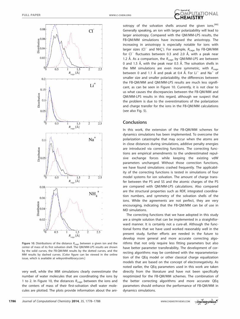
1 to 2. In Figure 10, the distances Rcage between the ions and

the centers of mass of their first-solvation shell water mole-

cules are plotted. The plots provide information about the ani-

sotropy of the solvation shells around the given ions.[90]

Generally speaking, an ion with larger polarizability will lead to

larger anisotropy. Compared with the QM/MM-LPS results, the

FB-QM/MM simulations have increased the anisotropy. The

increasing in anisotropy is especially notable for ions with

larger sizes (Cl2 and NH14 ). For example, Rcage by FB-QM/MM

for Cl2 fluctuates between 0.3 and 2.0 A, with a peak near

1.2 A. As a comparison, the Rcage by QM/MM-LPS are between

0 and 1.5 A, with the peak near 0.5 A. The solvation shells in

the MM simulations are even more symmetric, with Rcage

between 0 and 1.1 A and peak at 0.4 A. For Li1 and Na1 of

smaller size and smaller polarizability, the differences between

the FB-QM/MM and QM/MM-LPS results are much less signifi-

cant, as can be seen in Figure 10. Currently, it is not clear to

us what causes the discrepancies between the FB-QM/MM and

QM/MM-LPS results in this regard, although we suspect that

the problem is due to the overestimations of the polarization

and charge transfer for the ions in the FB-QM/MM calculations

(see also Fig. 5).

Conclusions

In this work, the extension of the FB-QM/MM schemes for

dynamics simulations has been implemented. To overcome the

polarization catastrophe that may occur when the atoms are

in close distances during simulations, additive penalty energies

are introduced via correcting functions. The correcting func-

tions are empirical amendments to the underestimated repul-

sive exchange forces while keeping the existing vdW

parameters unchanged. Without those correction functions,

we have found simulations crashed frequently. The applicabil-

ity of the correcting functions is tested in simulations of four

model systems for ion solvation. The amount of charge trans-

fer between the PS and SS and the atomic charges of the PS

are compared with QM/MM-LPS calculations. Also compared

are the structural properties such as RDF, integrated coordina-

tion numbers, and symmetry of the solvation shells of the

ions. While the agreements are not perfect, they are very

encouraging, indicating that the FB-QM/MM can be of use in

MD simulations.

The correcting functions that we have adopted in this study

are a simple solution that can be implemented in a straightfor-

ward manner. It is certainly not a cure-all. Although the func-

tional forms that we have used worked reasonably well in the

present study, further efforts are needed in the future to

develop more general and more accurate correcting algo-

rithms that not only require less fitting parameters but also

have better parameter transferability. The development of cor-

recting algorithms may be combined with the reparameteriza-

tion of the QEq model or other classical charge equalization

models that are based on the concept of electronegativity. As

noted earlier, the QEq parameters used in this work are taken

directly from the literature and have not been specifically

reoptimized for the FB-QM/MM schemes. The combination of

the better correcting algorithms and more accurate QEq

parameters should enhance the performance of FB-QM/MM in

dynamics simulations.

Figure 10. Distributions of the distance Rcage between a given ion and the

center of mass of its first solvation shell. The QM/MM-LPS results are shown

by the solid curves, the FB-QM/MM results by the dotted curves, and the

MM results by dashed curves. [Color figure can be viewed in the online

issue, which is available at wileyonlinelibrary.com.]




Computational cost is an important factor in choosing a

QM/MM scheme. In the current implementations of the FB

schemes, the molar fraction of the oxidized and reduced states

are determined variationally at each step of trajectory propa-

gation. While doing so offers accuracy, it is not very efficient.

It is strongly desirable to reduce the computational cost with-

out scarifying much accuracy. For example, it should be possi-

ble to propagate the molar fractions as dynamical variables

with extended Lagarangian formalism, which has been used

quite often in many dynamics simulation algorithms, for exam-

ple, in the Car–Parrinello dynamics[53] and in the dynamics sim-

ulations by the fluctuating charge force fields.[32] The use of

extended Lagarangian formalism should improve the efficiency

of the FB-QM/MM scheme, making it a competitive alternative

in dynamics simulations where the QM/MM-LPS simulations

are too expensive to apply.

Another highly desirable extension is to combine the FB

scheme with the adaptive-QM/MM algorithms,[16,64,91–102]

which treat the on-the-fly exchanges of atoms between the

QM and MM subsystems. The combination of the FB and

adaptive methods will lead to the open-boundary QM/

MM,[16,18] which permits dynamical transfers of both partial

charges and atoms at the same time between the QM and

MM subsystem in MD simulations. The open-boundary QM/

MM offers a seamless integration of QM and MM in dynamical

and complex environments and will be very useful in the MD

simulations of ion solvation and many other processes.

Keywords: chemical potential � electronegativity equaliza-

tion � polarization � ion salvation � combined quantum

mechanical /molecular mechanical

How to cite this article: S. Pezeshki, H. Lin, J. Comput. Chem.

2014, 35, 1778–1788. DOI: 10.1002/jcc.23685

] Additional Supporting Information may be found in the

online version of this article.

[1] A. Warshel, M. Levitt, J. Mol. Biol. 1976, 103, 227.

[2] U. C. Singh, P. A. Kollmann, J. Comput. Chem. 1986, 7, 718.

[3] M. J. Field, P. A. Bash, M. Karplus, J. Comput. Chem. 1990, 11, 700.

[4] J. Gao, Rev. Comput. Chem. 1996, 7, 119.

[5] R. A. Friesner, M. D. Beachy, Curr. Opin. Struct. Biol. 1998, 8, 257.

[6] J. Gao, M. A. Thompson, Eds. Combined Quantum Mechanical and

Molecular Mechanical Methods: ACS Symp. Ser. 712; American Chemi-

cal Society: Washington, DC, 1998.

[7] M. F. Ruiz-L�opez, J. L. Rivail, In Encyclopedia of Computational Chemis-

try; P. von Ragu�e Schleyer, Ed.; Wiley: Chichester, 1998; pp 437–448.

[8] G. Monard, K. M. Merz, Jr., Acc. Chem. Res. 1999, 32, 904.

[9] I. H. Hillier. THEOCHEM 1999, 463, 45.

[10] S. Hammes-Schiffer, Acc. Chem. Res. 2000, 34, 273.

[11] P. Sherwood, In Modern Methods and Algorithms of Quantum Chemis-

try; J. Grotendorst, Ed.; John von Neumann-Instituts: J€ulich, 2000;

pp 285–305.

[12] J. Gao, D. G. Truhlar, Annu. Rev. Phys. Chem. 2002, 53, 467.

[13] K. Morokuma, Philos. Trans. R. Soc. London, A 2002, 360, 1149.

[14] H. Lin, D. G. Truhlar, Theor. Chem. Acc. 2007, 117, 185.

[15] H. M. Senn, W. Thiel, Top. Curr. Chem. 2007, 268, 173.

[16] S. Pezeshki, H. Lin, Mol. Simul. 2014, DOI 10.1080/08927022.2014.911870,

1–22.

[17] Y. Zhang, H. Lin, J. Chem. Theory Comput. 2008, 4, 414.

[18] Y. Zhang, H. Lin, Theor. Chem. Acc. 2010, 126, 315

[19] W. J. Mortier, K. Van Genechten, J. Gasteiger, J. Am. Chem. Soc. 1985,

107, 829.

[20] W. J. Mortier, S. K. Ghosh, S. Shankar, J. Am. Chem. Soc. 1986, 108, 4315.

[21] K. T. No, J. A. Grant, H. A. Scheraga, J. Phys. Chem. 1990, 94, 4732.

[22] A. K. Rapp�e, W. A. Goddard, J. Phys. Chem. 1991, 95, 3358.

[23] J. Cioslowski, B. B. Stefanov, J. Chem. Phys. 1993, 99, 5151.

[24] S. W. Rick, S. J. Stuart, B. J. Berne, J. Chem. Phys. 1994, 101, 6141.

[25] F. De Proft, W. Langenaeker, P. Geerlings, J. Mol. Struct.: THEOCHEM

1995, 339, 45

[26] D. Bakowies, W. Thiel, J. Comput. Chem. 1996, 17 87.

[27] S. W. Rick, B. J. Berne, J. Am. Chem. Soc. 1996, 118, 672.

[28] D. M. York, W. Yang, J. Chem. Phys. 1996, 104, 159.

[29] Z.-Z. Yang, C.-S. Wang, J. Phys. Chem. A 1997, 101, 6315.

[30] P. Itskowitz, M. L. Berkowitz, J. Phys. Chem. A 1997, 101, 5687.

[31] P. Bultinck, W. Langenaeker, P. Lahorte, F. De Proft, P. Geerlings, M.

Waroquier, J. P. Tollenaere, J. Phys. Chem. A 2002, 106, 7887.

[32] S. Patel, C. L. Brooks, III, J. Comput. Chem. 2004, 25, 1.

[33] S. Patel, A. D. Mackerell, Jr., C. L. Brooks, III, J. Comput. Chem. 2004, 25,

1504.

[34] P. M. Lopes, B. Roux, A. MacKerell, Jr., Theor. Chem. Acc. 2009, 124, 11.

[35] M. J. S. Dewar, J. A. Hashmall, C. G. Venier, J. Am. Chem. Soc. 1968, 90,

1953.

[36] M. J. S. Dewar, N. Trinajstic, J. Chem. Soc. Chem. Commun. 1970, 646.

[37] V. Gogonea, K. M. Merz, Jr., J. Chem. Phys. 2000, 112, 3227.

[38] V. Gogonea, K. M. Merz, Jr., J. Phys. Chem. B 2000, 104, 2117.

[39] J. P. Perdew, R. G. Parr, M. Levy, J. L. Balduz, Phys. Rev. Lett. 1982, 49,

1691.

[40] Y. Zhang, W. Yang, J. Chem. Phys. 1998, 109, 2604.

[41] W. Yang, Y. Zhang, P. W. Ayers, Phys. Rev. Lett. 2000, 84, 5172.

[42] Y. Zhang, W. Yang, Theor. Chem. Acc. 2000, 103, 346.

[43] A. J. Cohen, P. Mori-Sanchez, W. Yang, J. Chem. Phys. 2008, 129,

121104/1-4.

[44] X. Zeng, H. Hu, X. Hu, A. J. Cohen, W. Yang, J. Chem. Phys. 2008, 128,

124510/1-10.

[45] A. J. Cohen, P. Mori-Sanchez, W. Yang, J. Chem. Theory Comput. 2009,

5, 786.

[46] D. H. Ess, E. R. Johnson, X. Hu, W. Yang, J. Phys. Chem. A 2011, 115, 76.

[47] S. N. Steinmann, W. Yang, J. Chem. Phys. 2013, 139, 074107/1-14.

[48] N. J. Mayhall, K. Raghavachari, J. Chem. Theory Comput. 2011, 7, 1336.

[49] P. Elliott, M. H. Cohen, A. Wasserman, K. Burke, J. Chem. Theory Com-

put. 2009, 5, 827.

[50] P. Elliott, K. Burke, M. H. Cohen, A. Wasserman, Phys. Rev. A 2010, 82,

024501/1-4.

[51] I. Tavernelli, R. Vuilleumier, M. Sprik, Phys. Rev. Lett. 2002, 88, 213002/1-4.

[52] Y. Zhang, H. Lin, D. G. Truhlar, J. Chem. Theory Comput. 2007, 3, 1378.

[53] R. Car, M. Parrinello, Phys. Rev. Lett. 1985, 55, 2471.

[54] P. Jungwirth, D. J. Tobias, J. Phys. Chem. A 2002, 106, 379.

[55] J. Sala, E. Gu�ardia, M. Masia, J. Chem. Phys. 2010, 133(23),234101.

[56] E. Gu�ardia, A. Calvo, M. Masia, Theor. Chem. Acc. 2012, 131, 1.

[57] A. P. Lyubartsev, K. Laasonen, A. Laaksonen, J. Chem. Phys. 2001, 114,

3120.

[58] Y. Zeng, C. Wang, X. Zhang, S. Ju, Chem. Phys. 2014, 433, 89.

[59] Y. Zeng, J. Hu, Y. Yuan, X. Zhang, S. Ju, Chem. Phys. Lett. 2012, 538, 60.

[60] W. Liu, R. H. Wood, D. J. Doren, J. Chem. Phys. 2003, 118, 2837.

[61] A. Tongraar, B. M. Rode, Phys. Chem. Chem. Phys. 2003, 5, 357.

[62] A. Ohrn, G. Karlstrom, J. Phys. Chem. B 2004, 108, 8452.

[63] A. Tongraar, B. M. Rode, Chem. Phys. Lett. 2005, 403, 314.

[64] K. Park, A. W. Gotz, R. C. Walker, F. Paesani, J. Chem. Theory Comput.

2012, 8, 2868.

[65] B. Lev, B. Roux, S. Y. Noskov, J. Chem. Theory Comput. 2013, 9, 4165.

[66] H. H. Loeffler, B. M. Rode, J. Chem. Phys. 2002, 117, 110.

[67] H. H. Loeffler, A. M. Mohammed, Y. Inada, S. Funahashi, Chem. Phys.

Lett. 2003, 379, 452.

[68] A. Tongraar, K. R. Liedl, B. M. Rode, J. Phys. Chem. A 1998, 102, 10340.

[69] B. B. Lev, D. R. Salahub, S. Y. Noskov, Interdiscip. Sci. 2010, 2, 12.

[70] C. N. Rowley, B. Roux, J. Chem. Theory Comput. 2012, 8, 3526.

[71] P. Intharathep, A. Tongraar, K. Sagarik, J. Comput. Chem. 2005, 26, 1329.

[72] Y. Koyano, N. Takenaka, Y. Nakagawa, M. Nagaoka, Bull. Chem. Soc. Jpn.

2010, 83, 486.



info:doi/10.1002/jcc.23685

info:doi/10.1080/08927022.2014.911870


[73] B. M. Rode, C. F. Schwenk, T. S. Hofer, B. R. Randolf, Coord. Chem. Rev.

2005, 249, 2993.

[74] A. A. Hassanali, J. Cuny, V. Verdolino, M. Parrinello, Philos. Trans. R. Soc.

A 2014, 372.

[75] P. Ren, J. Chun, D. G. Thomas, M. J. Schnieders, M. Marucho, J. Zhang,

N. A. Baker, Q. Rev. Biophys. 2012, 45, 427.

[76] C. C. J. Roothaan, Rev. Mod. Phys. 1951, 23, 69.

[77] R. Ditchfield, W. J. Hehre, J. A. Pople, J. Chem. Phys. 1971, 54, 724.

[78] W. J. Hehre, R. Ditchfield, J. A. Pople, J. Chem. Phys. 1972, 56, 2257.

[79] M. M. Francl, W. J. Pietro, W. J. Hehre, J. S. Binkley, D. J. DeFrees, J. A.

Pople, M. S. Gordon, J. Chem. Phys. 1982, 77, 3654.

[80] M. J. Frisch, J. A. Pople, J. S. Binkley, J. Chem. Phys. 1984, 80, 3265.

[81] W. L. Jorgensen, D. S. Maxwell, J. Tirado-Rives, J. Am. Chem. Soc. 1996,

118, 11225.

[82] R. C. Rizzo, W. L. Jorgensen, J. Am. Chem. Soc. 1999, 121, 4827.

[83] G. A. Kaminski, R. A. Friesner, J. Tirado-Rives, W. L. Jorgensen, J. Phys.

Chem. B 2001, 105, 6474.

[84] K. Kahn, T. C. Bruice, J. Comput. Chem. 2002, 23, 977.

[85] H. J. C. Berendsen, J. P. M. Postma, W. F. v. Gunsteren, J. Hermans, In

Intermolecular Forces; B. Pullman, Ed.; D. Reidel Publishing Company:

Dordrecht, 1981; pp 331–342.

[86] H. Lin, Y. Zhang, S. Pezeshki, D. G. Truhlar, QMMM 2.0.0.CO, University

of Minnesota: Minneapolis, 2012.

[87] J. W. Ponder, TINKER 5.1, Washington University: St. Louis, MO, 2010.

[88] M. J. Frisch, G. W. Trucks, H. B. Schlegel, G. E. Scuseria, M. A. Robb, J.

R. Cheeseman, J. Montgomery, J. A., T. Vreven, K. N. Kudin, J. C.

Burant, J. M. Millam, S. S. Iyengar, J. Tomasi, V. Barone, B. Mennucci, M.

Cossi, G. Scalmani, N. Rega, G. A. Petersson, H. Nakatsuji, M. Hada, M.

Ehara, K. Toyota, R. Fukuda, J. Hasegawa, M. Ishida, T. Nakajima, Y.

Honda, O. Kitao, H. Nakai, M. Klene, X. Li, J. E. Knox, H. P. Hratchian, J.

B. Cross, C. Adamo, J. Jaramillo, R. Gomperts, R. E. Stratmann, O.

Yazyev, A. J. Austin, R. Cammi, C. Pomelli, J. W. Ochterski, P. Y. Ayala, K.

Morokuma, G. A. Voth, P. Salvador, J. J. Dannenberg, V. G. Zakrzewski,

S. Dapprich, A. D. Daniels, M. C. Strain, O. Farkas, D. K. Malick, A. D.

Rabuck, K. Raghavachari, J. B. Foresman, J. V. Ortiz, Q. Cui, A. G.

Baboul, S. Clifford, J. Cioslowski, B. B. Stefanov, G. Liu, A. Liashenko, P.

Piskorz, I. Komaromi, R. L. Martin, D. J. Fox, T. Keith, M. A. Al-Laham, C.

Y. Peng, A. Nanayakkara, M. Challacombe, P. M. W. Gill, B. Johnson, W.

Chen, M. W. Wong, C. Gonzalez, J. A. Pople, GAUSSIAN03, Gaussian,

Inc.: Pittsburgh, PA, 2003.

[89] H. J. C. Berendsen, J. P. M. Postma, W. F. v. Gunsteren, A. DiNola, J. R.

Haak, J. Chem. Phys. 1984, 81, 3684.

[90] Z. Zhao, D. M. Rogers, T. L. Beck, J. Chem. Phys. 2010, 132, 014502/1-

10.

[91] T. Kerdcharoen, K. R. Liedl, B. M. Rode, Chem. Phys. 1996, 211, 313.

[92] T. Kerdcharoen, K. Morokuma, Chem. Phys. Lett. 2002, 355, 257.

[93] T. Kerdcharoen, K. Morokuma, J. Chem. Phys. 2003, 118, 8856.

[94] A. Heyden, H. Lin, D. G. Truhlar, J. Phys. Chem. B 2007, 111, 2231.

[95] R. E. Bulo, B. Ensing, J. Sikkema, L. Visscher, J. Chem. Theory Comput.

2009, 5, 2212.

[96] M. G. Guthrie, A. D. Daigle, M. R. Salazar, J. Chem. Theory Comput.

2009, 6, 18.

[97] S. O. Nielsen, R. E. Bulo, P. B. Moore, B. Ensing, Phys. Chem. Chem. Phys.

2010, 12, 12401.

[98] A. B. Poma, L. Delle Site, Phys. Rev. Lett. 2010, 104, 250201/1-4.

[99] S. Pezeshki, H. Lin, J. Chem. Theory Comput. 2011, 7, 3625.

[100] N. Bernstein, C. Varnai, I. Solt, S. A. Winfield, M. C. Payne, I. Simon, M.

Fuxreiter, G. Csanyi, Phys. Chem. Chem. Phys. 2012, 14, 646.

[101] N. Takenaka, Y. Kitamura, Y. Koyano, M. Nagaoka, Chem. Phys. Lett.

2012, 524, 56.

[102] C. V�arnai, N. Bernstein, L. Mones, G. Cs�anyi, J. Phys. Chem. B 2013,

117, 12202.

Received: 16 April 2014Revised: 19 June 2014Accepted: 30 June 2014Published online on 23 July 2014



Molecular dynamics simulations of ion solvation by flexible-boundary QM/MM: on-the-fly partial charge transfer between QM and MM subsystems

Documents