Module #: Title of Module 2 - Moses Lab · Module #: Title of Module 2. Overview • Review • Linear separability • Non-linear classification • Linear Support Vector Machines

Class #6: Non-linear classification

ML4Bio 2012February 17th 2012February 17th, 2012

Quaid Morris

1

2Module #: Title of Module

Overview• Review• Linear separability• Non-linear classificationNon linear classification• Linear Support Vector Machines (SVMs)

– Picking the best linear decision boundaryPicking the best linear decision boundary

• Non-linear SVMs• Decision TreesDecision Trees• Ensemble methods: Bagging and Boosting

3

Objective functions

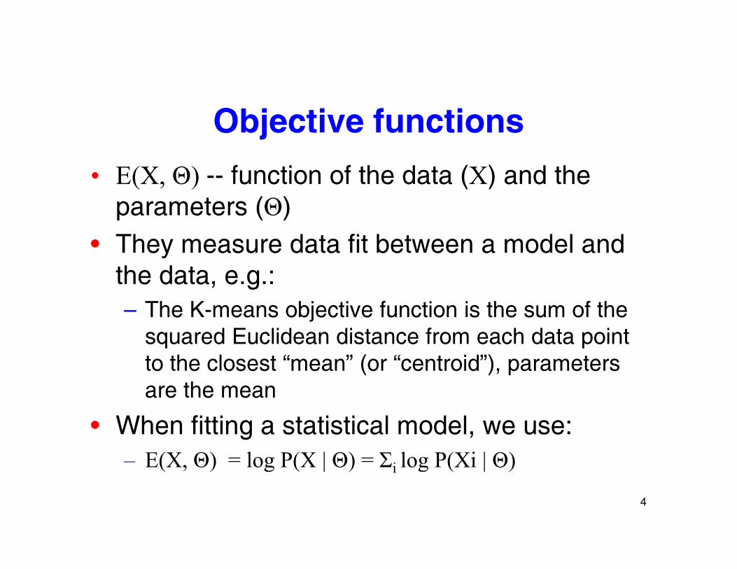
• E(X Θ) -- function of the data (X) and the • E(X, Θ) -- function of the data (X) and the parameters (Θ)

• They measure data fit between a model and They measure data fit between a model and the data, e.g.:– The K-means objective function is the sum of the j

squared Euclidean distance from each data point to the closest “mean” (or “centroid”), parameters are the meanare the mean

• When fitting a statistical model, we use:– E(X Θ) = log P(X | Θ) = Σi log P(Xi | Θ)E(X, Θ) log P(X | Θ) Σi log P(Xi | Θ)

4

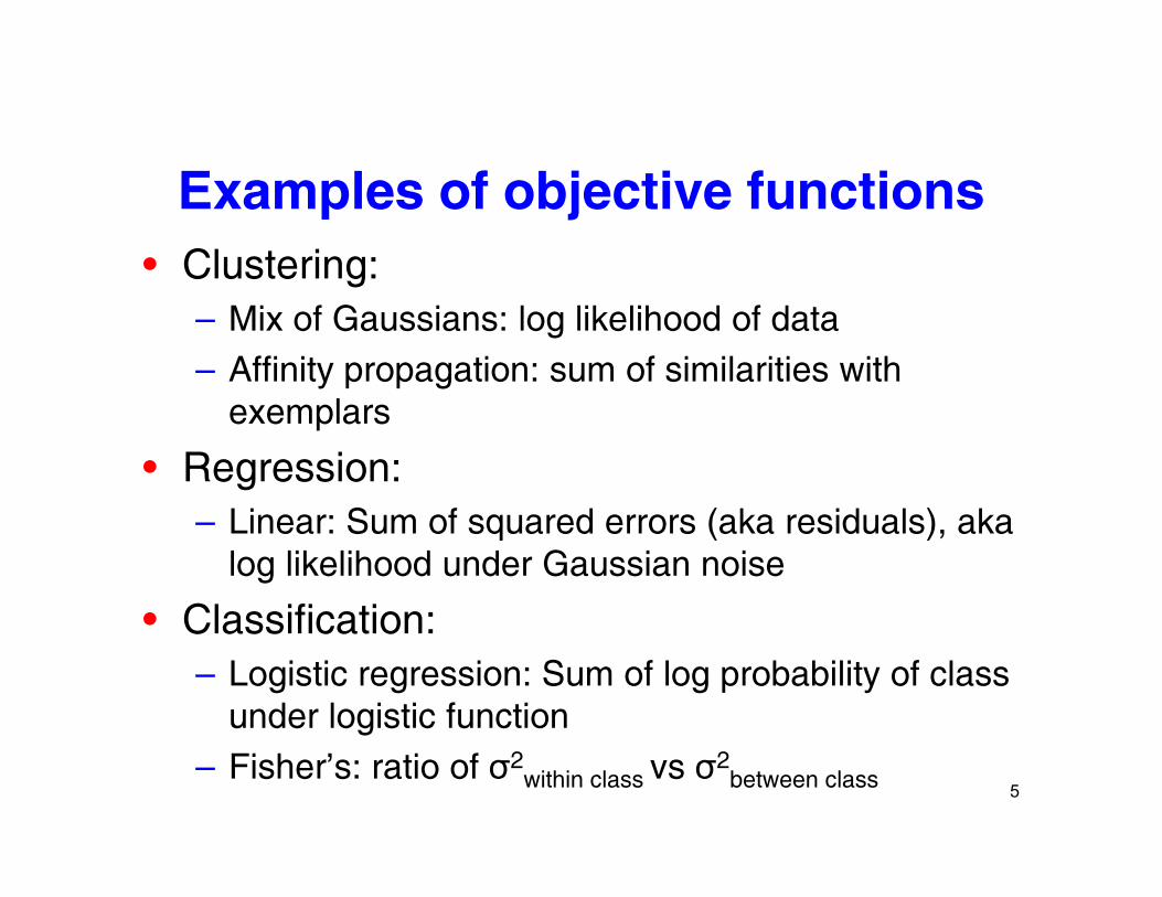
Examples of objective functions• Clustering:C us e g

– Mix of Gaussians: log likelihood of data– Affinity propagation: sum of similarities with

exemplars

• Regression:– Linear: Sum of squared errors (aka residuals), aka

log likelihood under Gaussian noise

• Classification:• Classification:– Logistic regression: Sum of log probability of class

under logistic functiong– Fisher’s: ratio of σ2

within class vs σ2between class 5

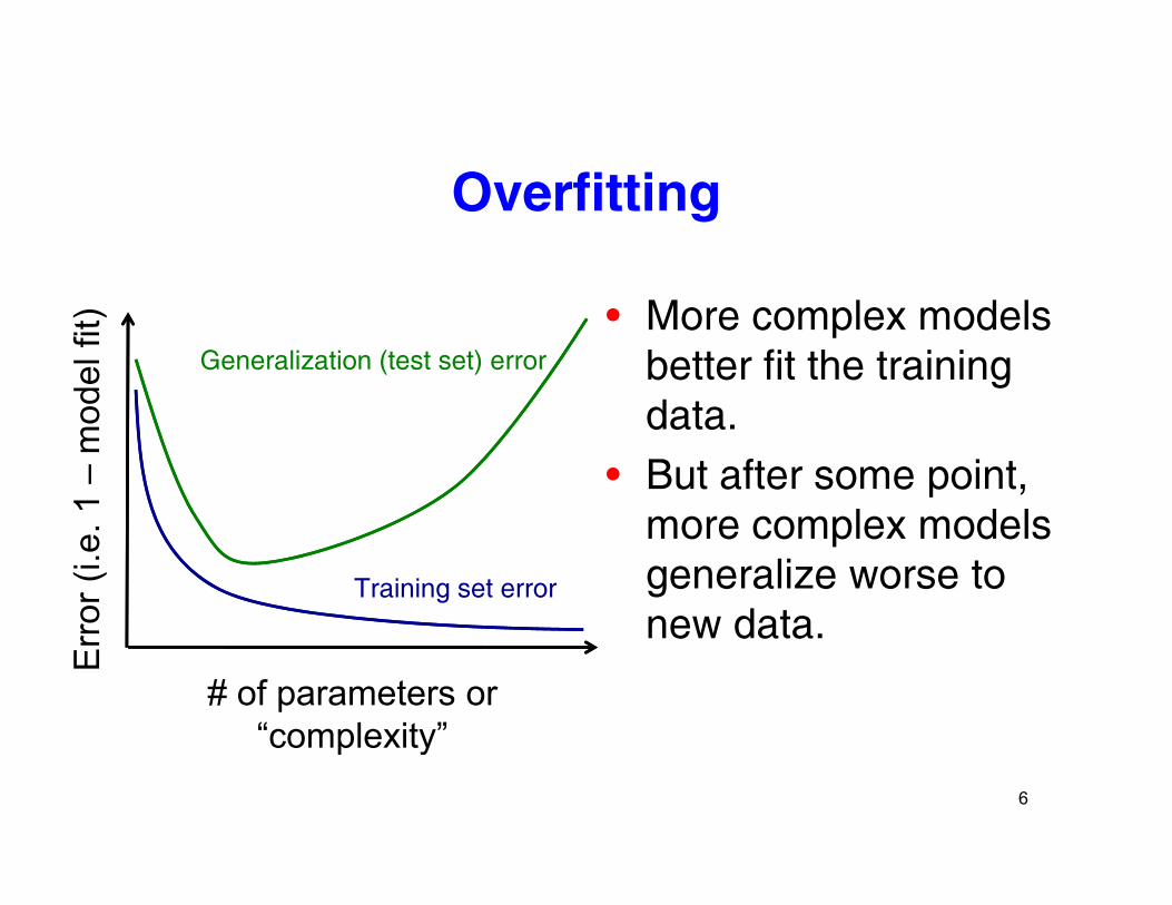
Overfitting

• More complex models better fit the training

del f

it)

Generalization (test set) error

data.• But after some point,

l d l

1 –

mod

more complex models generalize worse to new dataro

r (i.e

.

Training set error

new data.

# of parameters or“complexity”

Err

6

complexity

Dealing with overfitting by Dealing with overfitting by regularization

• Basic idea: add a term to the objective • Basic idea: add a term to the objective function that penalizes # of parameters or model complexity,p y,

• Now: E(X, Θ) = datafit(X, Θ) – λ complexity(Θ)• “Hyper-parameter” λ controls the strength of Hyper parameter λ controls the strength of

regularization – could have a natural value, or need to set this by cross-validation,

• Increases in model complexity need to be balanced by improved model fit. (each unit of

ladded complexity costs λ units of data fit) 7

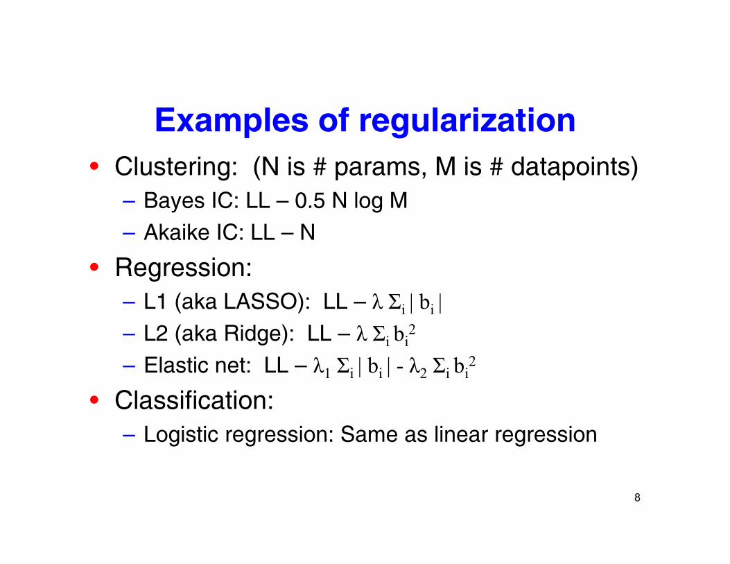
Examples of regularization• Clustering: (N is # params, M is # datapoints)C us e g ( s pa a s, s da apo s)

– Bayes IC: LL – 0.5 N log M– Akaike IC: LL – N

• Regression:– L1 (aka LASSO): LL – λ Σi | bi |– L2 (aka Ridge): LL – λ Σi bi

2

– Elastic net: LL – λ1 Σi | bi | - λ2 Σi bi2

C• Classification:– Logistic regression: Same as linear regression

8

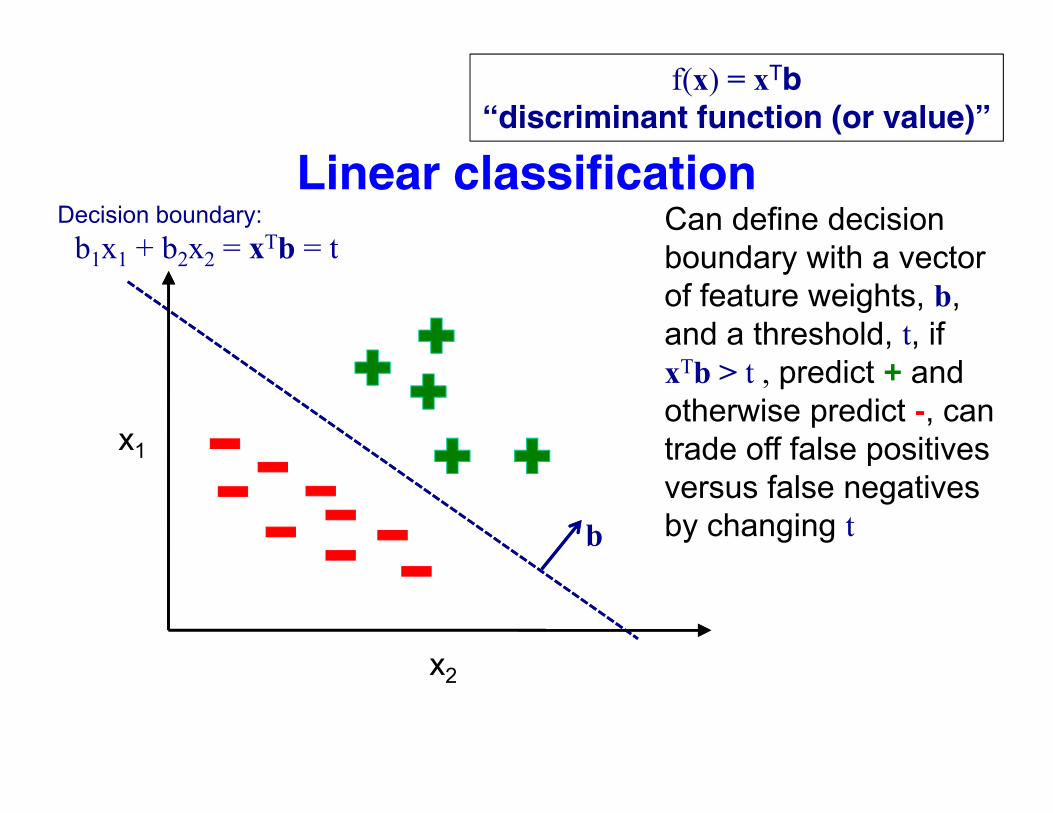
f(x) = xTb“discriminant function (or value)”

Linear classificationCan define decision boundary with a vectorb1x1 + b2x2 = xTb = t

Decision boundary:

boundary with a vector of feature weights, b, and a threshold, t, if

b1x1 + b2x2 x b t

x1

xTb > t , predict + and otherwise predict -, can trade off false positivestrade off false positives versus false negatives by changing tb

xx2

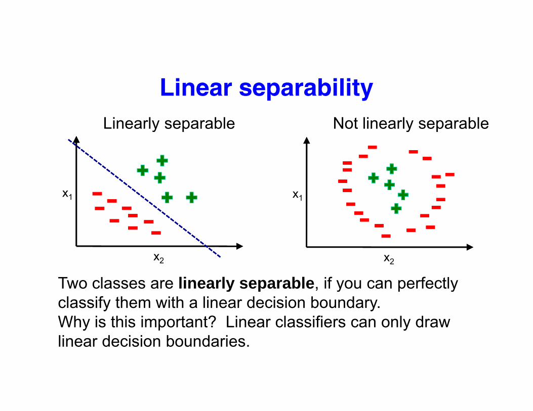
Linear separabilityLinearly separable Not linearly separableLinearly separable Not linearly separable

x1 x1

x2 x2

Two classes are linearly separable if you can perfectlyTwo classes are linearly separable, if you can perfectly classify them with a linear decision boundary.Why is this important? Linear classifiers can only draw li d i i b d ilinear decision boundaries.

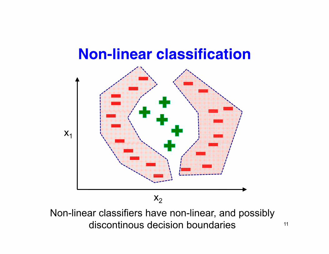
Non-linear classification

x1

x2

11

Non-linear classifiers have non-linear, and possibly discontinous decision boundaries

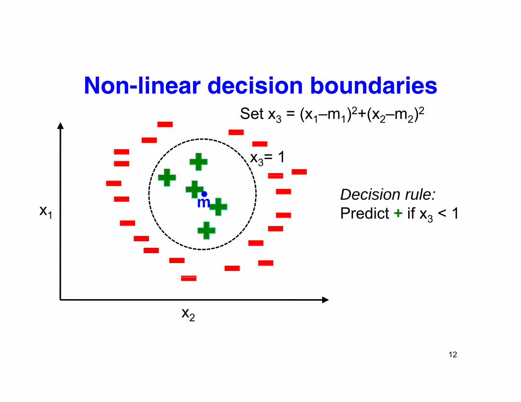
Non-linear decision boundariesSet x3 = (x1–m1)2+(x2–m2)2

x3= 1

x1m Decision rule:

Predict if x3 < 1

x2

12

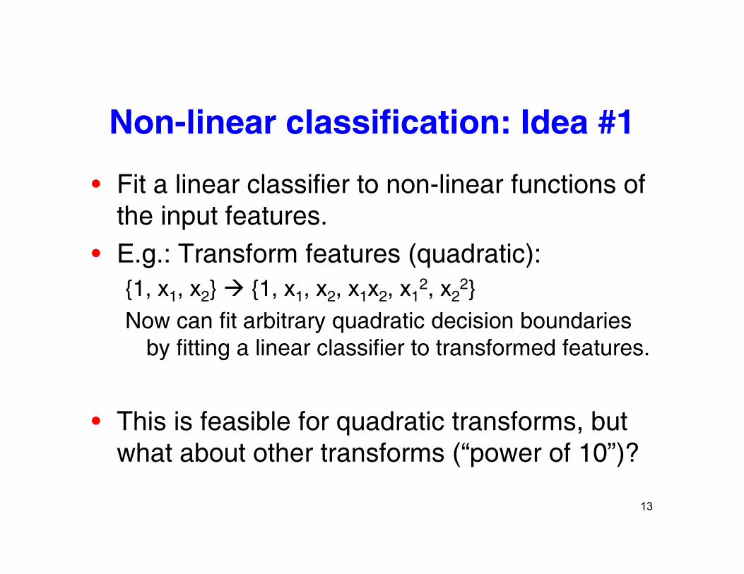
Non-linear classification: Idea #1

Fit a linear classifier to non linear functions of • Fit a linear classifier to non-linear functions of the input features.

• E g : Transform features (quadratic): • E.g.: Transform features (quadratic): {1, x1, x2} {1, x1, x2, x1x2, x1

2, x22}

Now can fit arbitrary quadratic decision boundaries Now can fit arbitrary quadratic decision boundaries by fitting a linear classifier to transformed features.

• This is feasible for quadratic transforms, but what about other transforms (“power of 10”)?

13

Support Vector Machinespp

VladimirVapnik

14

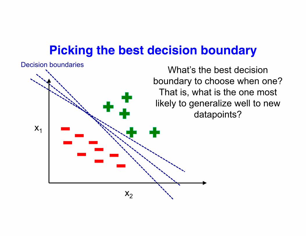
Picking the best decision boundary

What’s the best decision Decision boundaries

boundary to choose when one? That is, what is the one most

likely to generalize well to new

x1

likely to generalize well to new datapoints?

xx2

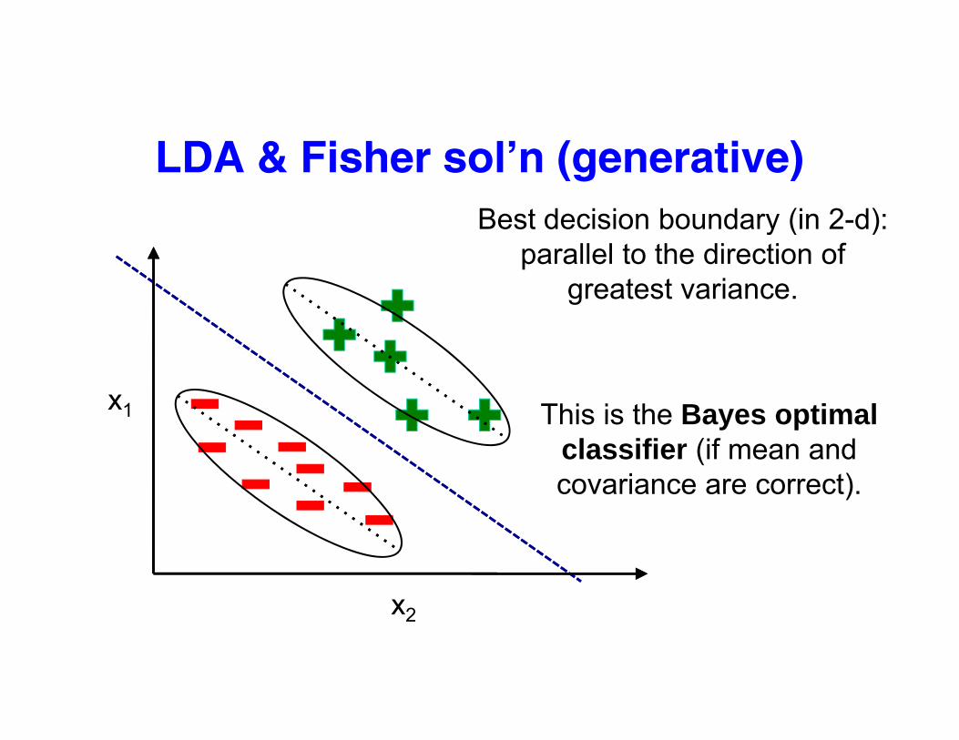
LDA & Fisher sol’n (generative)Best decision boundary (in 2-d): y ( )

parallel to the direction of greatest variance.

x1 This is the Bayes optimalThis is the Bayes optimal classifier (if mean and covariance are correct).

xx2

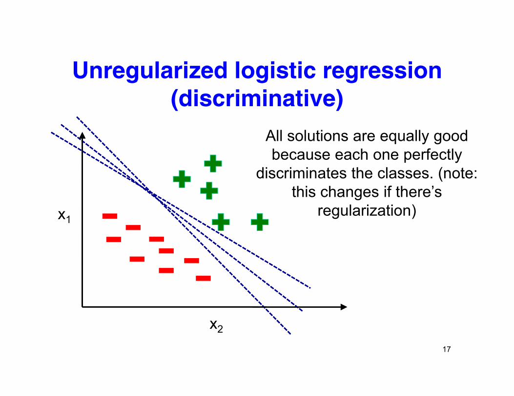
Unregularized logistic regression Unregularized logistic regression (discriminative)

All solutions are equally good because each one perfectly

discriminates the classes (note:

x1

discriminates the classes. (note: this changes if there’s

regularization)

x17

x2

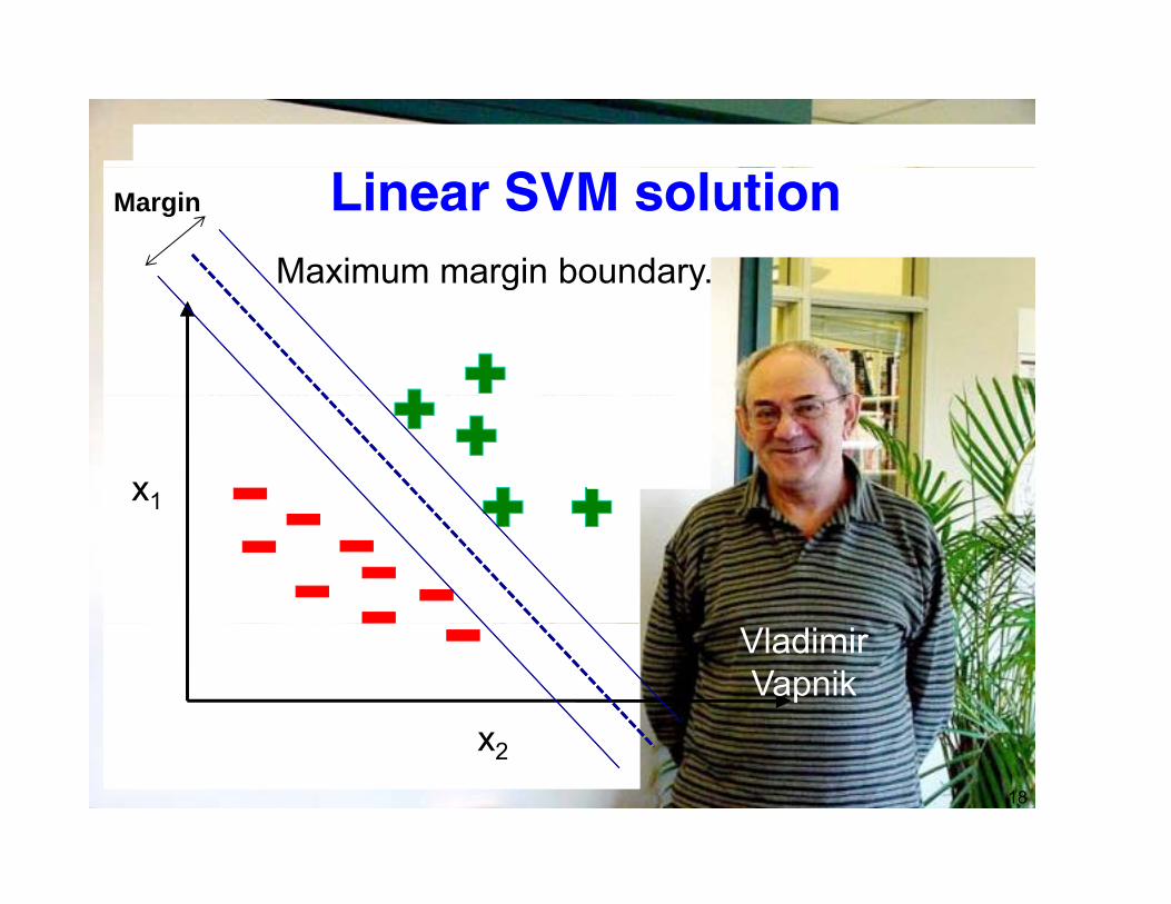
Linear SVM solutionMaximum margin boundary.

Margin

Maximum margin boundary.

x1

x

VladimirVapnik

18

x2

SVM decision boundariesHere the maximum margin

Margin

Here, the maximum margin boundary is specified by three points, called the

t t

x1

support vectors.

Support vectors

x

VladimirVapnik

19

x2

SVM objective function

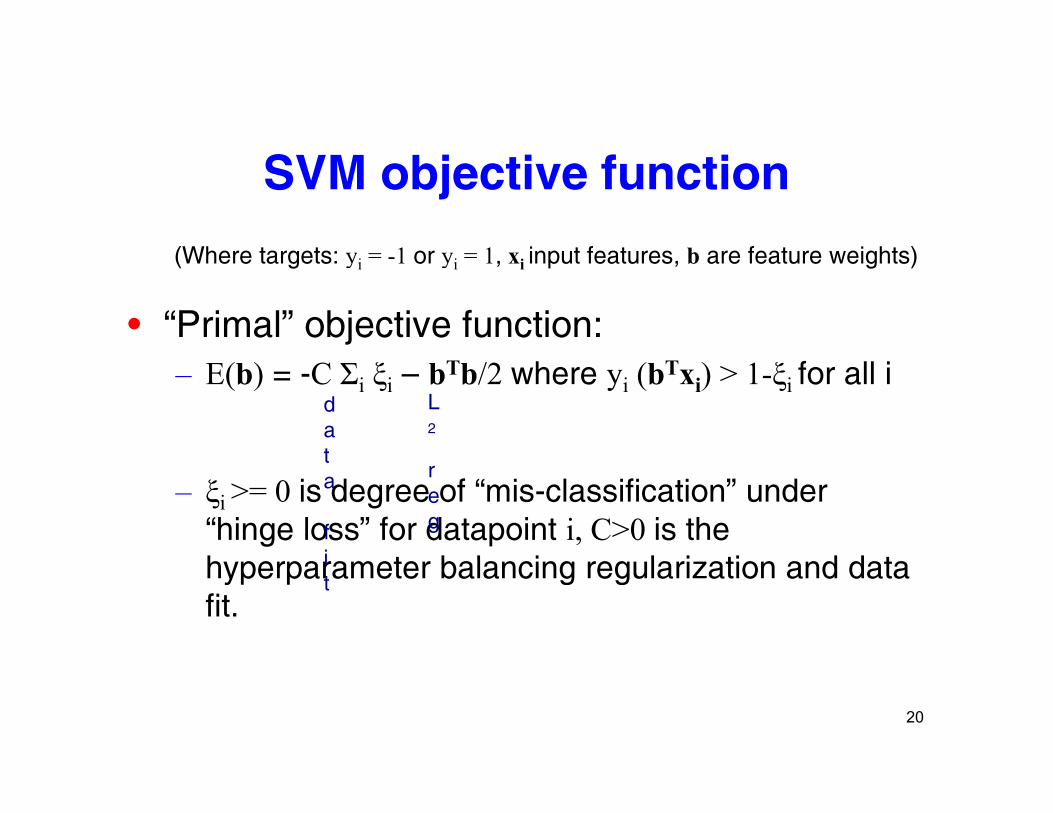
(Where targets: y 1 or y 1 x input features b are feature weights)(Where targets: yi = -1 or yi = 1, xi input features, b are feature weights)

• “Primal” objective function:– E(b) = -C Σi ξi – bTb/2 where yi (bTxi) > 1-ξi for all i

L2

dat

– ξi >= 0 is degree of “mis-classification” under “hinge loss” for datapoint i, C>0 is the hy er ara eter balancing regularization and data

reg

ta

fihyperparameter balancing regularization and data

fit.

it

20

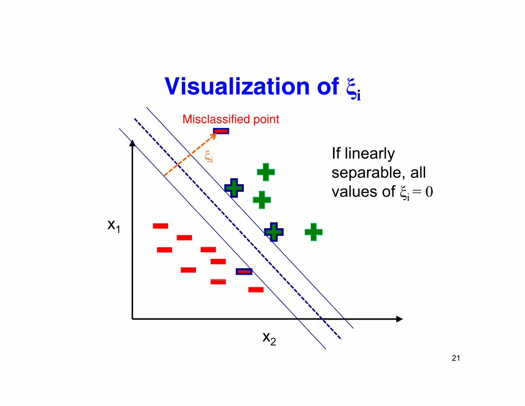
Visualization of ξiMisclassified point

ξi If linearly separable, all

x1

separable, all values of ξi = 0

x1

VladimirVapnik

21

x2

Another SVM objective function

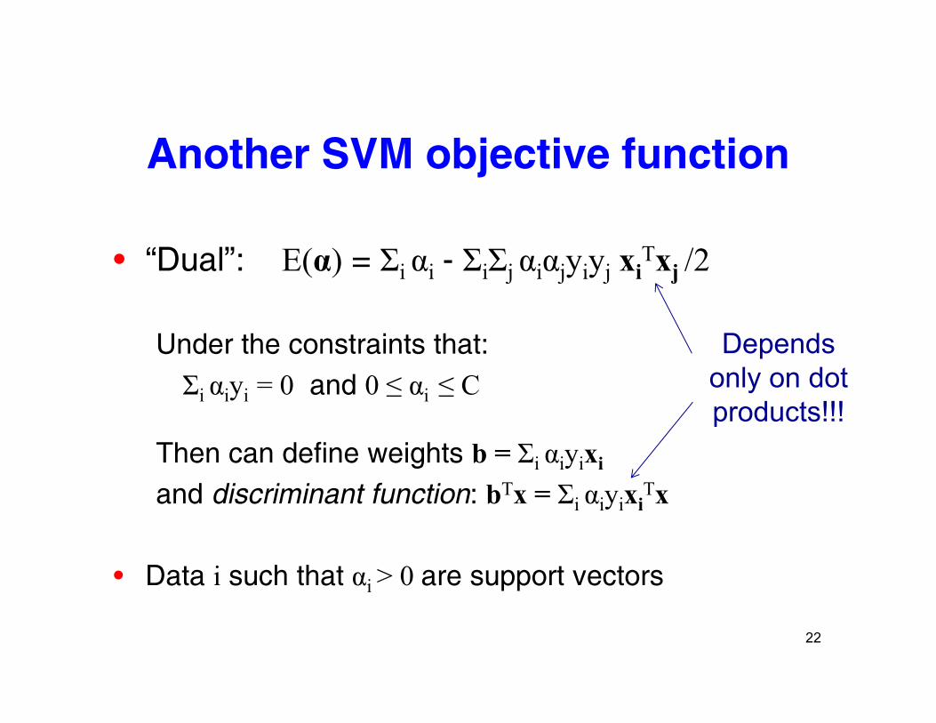
• “Dual”: E(α) = Σi αi - ΣiΣj αiαjyiyj xiTxj /2

Under the constraints that:Σi αiyi = 0 and 0 ≤ αi ≤ C

Depends only on dot products!!!

Then can define weights b = Σi αiyixi

and discriminant function: bTx = Σi αiyixiTx

products!!!

and discriminant function: b x Σi αiyixi x

• Data i such that αi > 0 are support vectorsi pp

22

Dot products of transformed Dot products of transformed vector as “kernel functions”

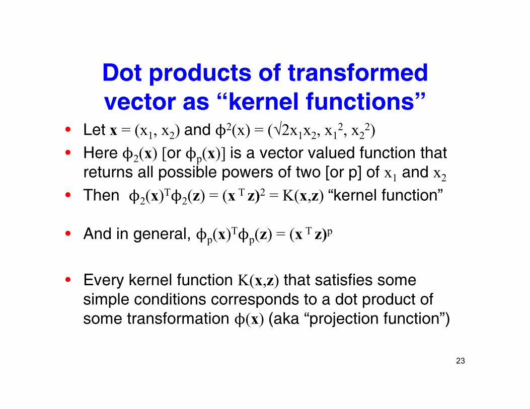
• Let ( ) and 2( ) (√2 2 2)• Let x = (x1, x2) and 2(x) = (√2x1x2, x12, x2

2)• Here 2(x) [or p(x)] is a vector valued function that

returns all possible powers of two [or p] of x1 and x2p p [ p] 1 2

• Then 2(x)T2(z) = (x T z)2 = K(x,z) “kernel function”

And in general ( )T ( ) ( T )p• And in general, p(x)Tp(z) = (x T z)p

• Every kernel function K(x z) that satisfies some Every kernel function K(x,z) that satisfies some simple conditions corresponds to a dot product of some transformation (x) (aka “projection function”)

23

Non-linear SVM objective function

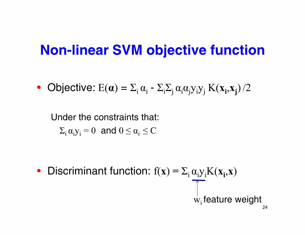
• Objective: E(α) = Σi αi - ΣiΣj αiαjyiyj K(xi,xj) /2

Under the constraints that:Σi αiyi = 0 and 0 ≤ αi ≤ CΣi αiyi 0 and 0 ≤ αi ≤ C

• Discriminant function: f(x) = Σi αiyiK(xi,x)

24wi feature weight

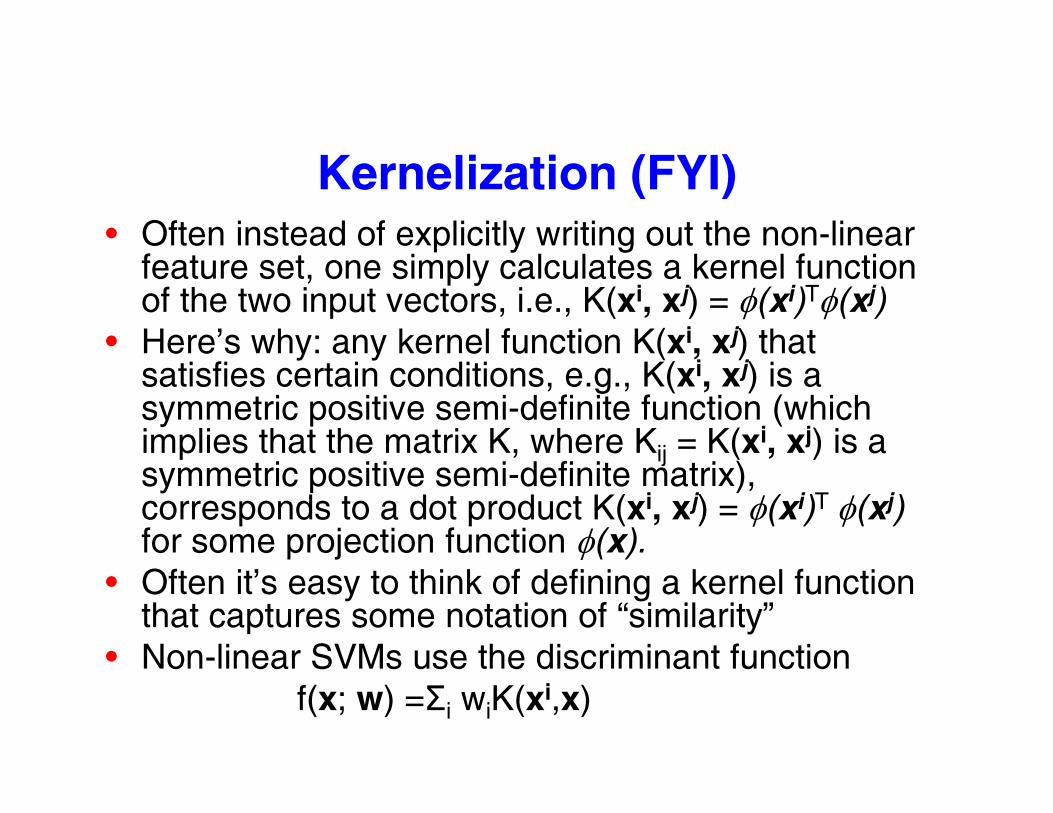
Kernelization (FYI)• Often instead of explicitly writing out the non-linear

l l l lfeature set, one simply calculates a kernel function of the two input vectors, i.e., K(xi, xj) = φ(xi)Tφ(xj)

• Here’s why: any kernel function K(xi, xj) that y y ( , )satisfies certain conditions, e.g., K(xi, xj) is a symmetric positive semi-definite function (which implies that the matrix K, where Kij = K(xi, xj) is a p ij ( , )symmetric positive semi-definite matrix), corresponds to a dot product K(xi, xj) = φ(xi)T φ(xj) for some projection function φ(x).

• Often it’s easy to think of defining a kernel function that captures some notation of “similarity”

• Non-linear SVMs use the discriminant functionNon linear SVMs use the discriminant functionf(x; w) =Σi wiK(xi,x)

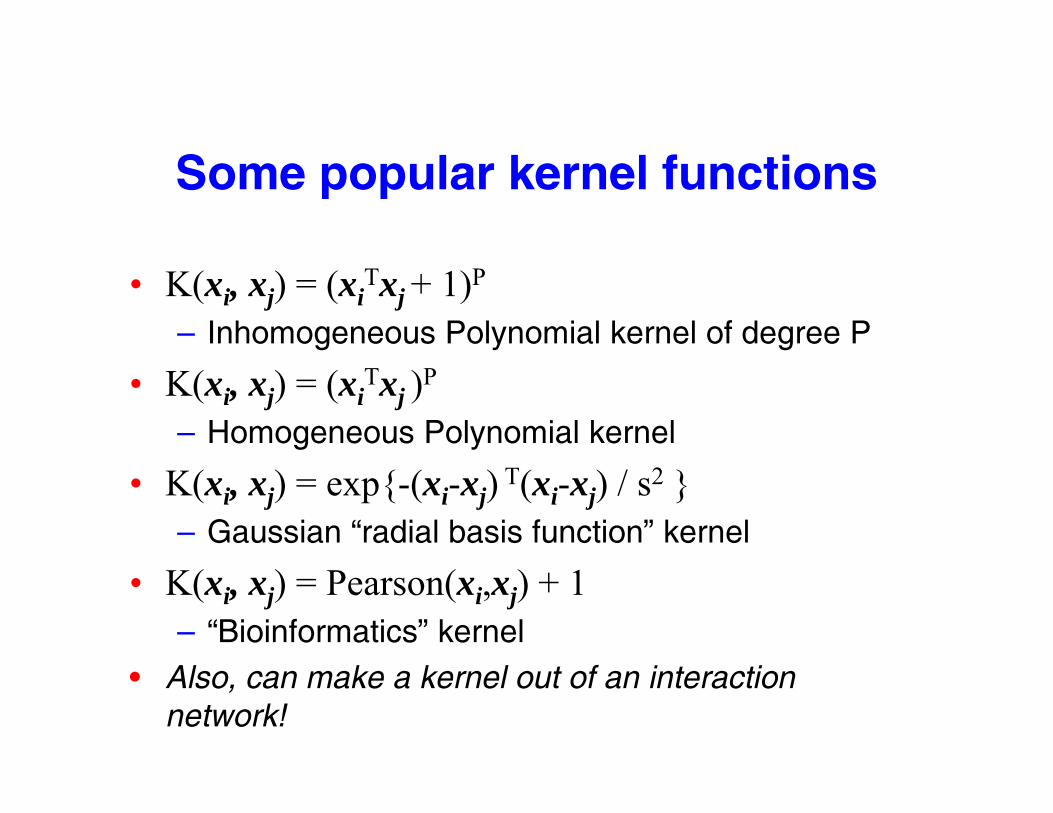
Some popular kernel functions

• K(xi, xj) = (xiTxj + 1)P

– Inhomogeneous Polynomial kernel of degree P

• K(xi, xj) = (xiTxj )P

– Homogeneous Polynomial kernel

• K(xi, xj) = exp{-(xi-xj) T(xi-xj) / s2 }– Gaussian “radial basis function” kernel

• K(xi, xj) = Pearson(xi,xj) + 1– “Bioinformatics” kernel

A• Also, can make a kernel out of an interaction network!

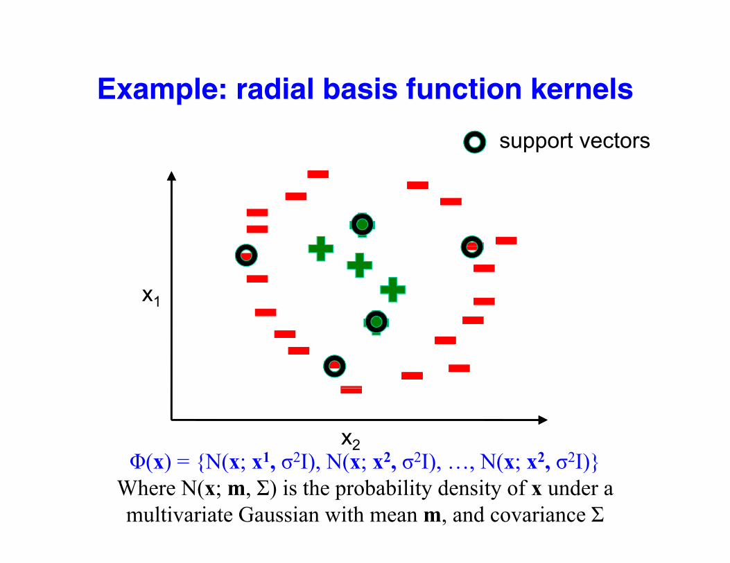
Example: radial basis function kernelsp

support vectors

x1

x2Φ(x) = {N(x; x1 σ2I) N(x; x2 σ2I) N(x; x2 σ2I)}Φ(x) = {N(x; x1, σ2I), N(x; x2, σ2I), …, N(x; x2, σ2I)}

Where N(x; m, Σ) is the probability density of x under a multivariate Gaussian with mean m, and covariance Σ

SVM summary

A “sparse” linear classifier that uses as features p“kernel functions” that measure similarity to each data point in the training.

28

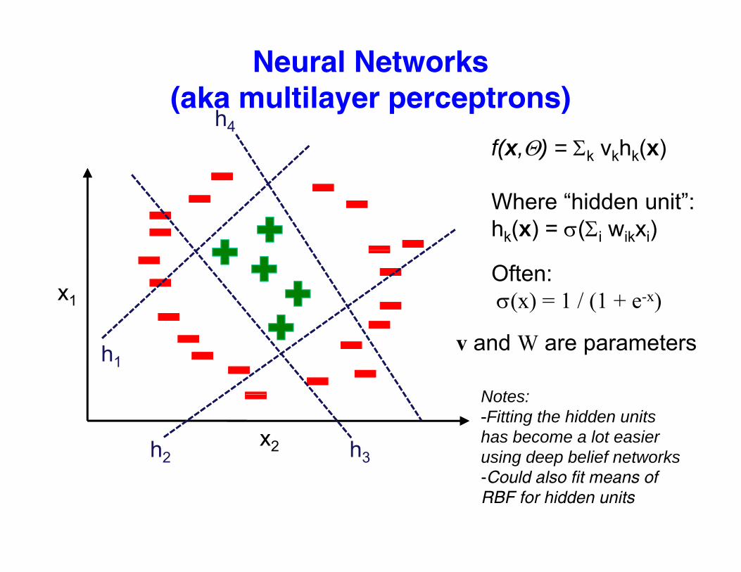
Neural Networks(aka multilayer perceptrons)(aka multilayer perceptrons)

f(x,Θ) = Σk vkhk(x)h4

Where “hidden unit”:hk(x) = σ(Σi wikxi)

Often:σ(x) = 1 / (1 + e-x)x1

h1

Notes:

v and W are parameters

x2h2 h3

Notes:-Fitting the hidden units has become a lot easier using deep belief networks-Could also fit means of RBF for hidden units

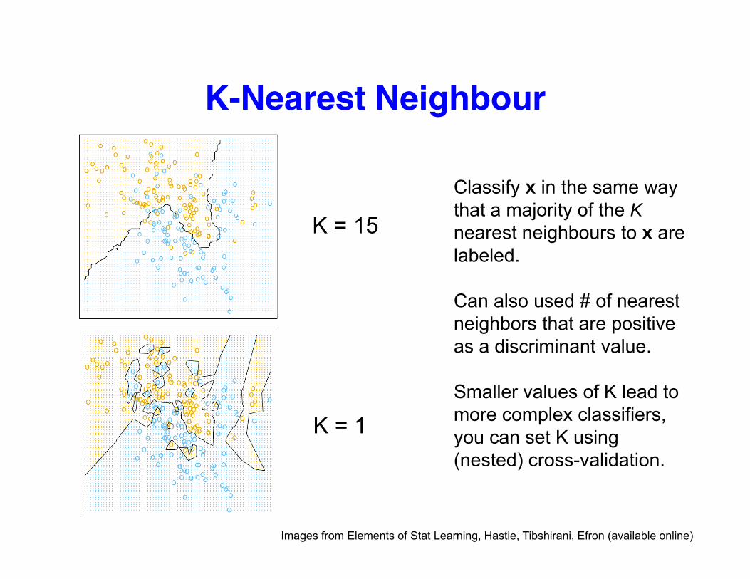
K-Nearest NeighbourK Nearest Neighbour

Cl if i hClassify x in the same way that a majority of the Knearest neighbours to x are labeled

K = 15labeled.

Can also used # of nearest neighbors that are positiveneighbors that are positive as a discriminant value.

Smaller values of K lead to more complex classifiers, you can set K using (nested) cross-validation.

K = 1

Images from Elements of Stat Learning, Hastie, Tibshirani, Efron (available online)

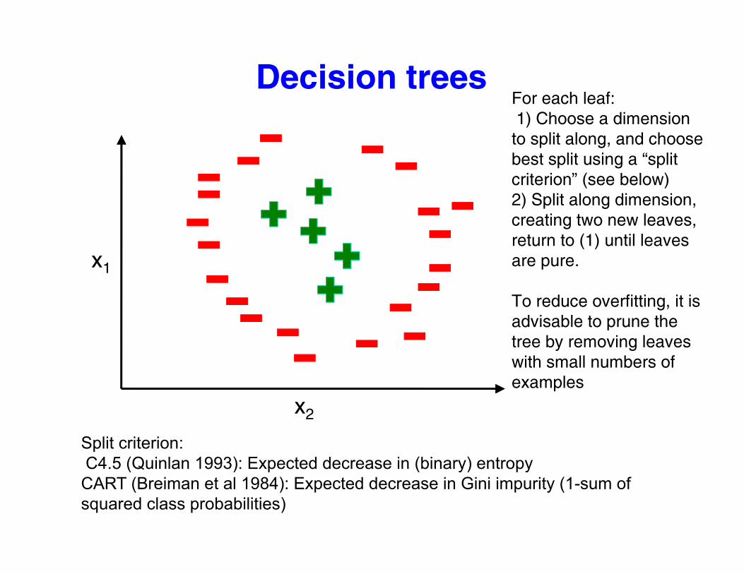
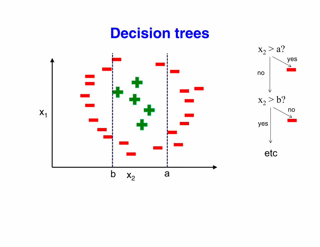
Decision treesFor each leaf:1) Choose a dimension to split along, and choose best split using a “split criterion” (see below)criterion (see below)2) Split along dimension, creating two new leaves,return to (1) until leaves

x1 are pure.

To reduce overfitting, it is advisable to prune the advisable to prune the tree by removing leaves with small numbers of examples

x2

Split criterion:C4.5 (Quinlan 1993): Expected decrease in (binary) entropyC4.5 (Quinlan 1993): Expected decrease in (binary) entropyCART (Breiman et al 1984): Expected decrease in Gini impurity (1-sum of squared class probabilities)

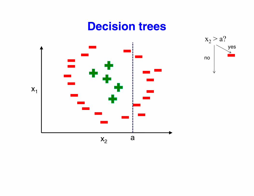
Decision trees?x2 > a?

yes

no

x1

x2a

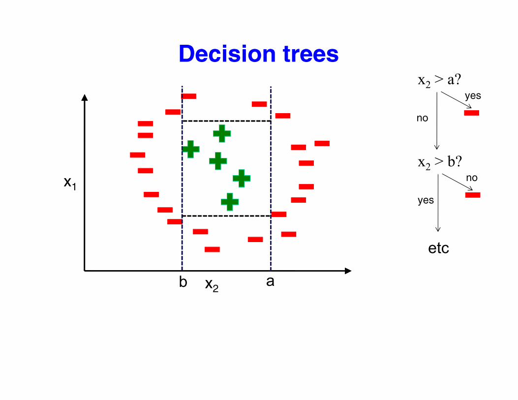
Decision trees?x2 > a?

yes

no

x2 > b?nox1no

yes

b

etc

x2ab

Decision trees?x2 > a?

yes

no

x2 > b?nox1no

yes

b

etc

x2ab

Decision tree summary

Decision trees learn a recursive splits of the pdata along individual features that partition the input space into “homogeneous” groups

f d i i h h l b l of data points with the same labels.

35

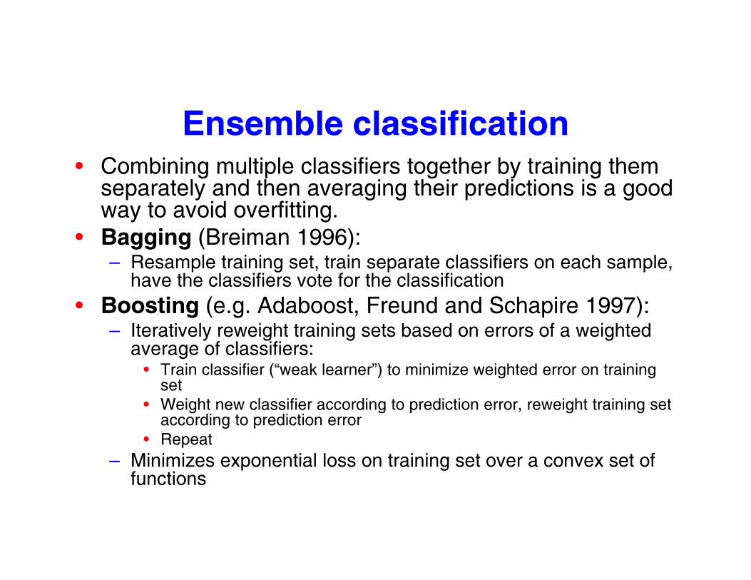
Ensemble classification• Combining multiple classifiers together by training them

t l d th i th i di ti i d separately and then averaging their predictions is a good way to avoid overfitting.

• Bagging (Breiman 1996):R– Resample training set, train separate classifiers on each sample, have the classifiers vote for the classification

• Boosting (e.g. Adaboost, Freund and Schapire 1997):Iteratively reweight training sets based on errors of a weighted – Iteratively reweight training sets based on errors of a weighted average of classifiers:

• Train classifier (“weak learner”) to minimize weighted error on training setW i ht l ifi di t di ti i ht t i i t • Weight new classifier according to prediction error, reweight training set according to prediction error

• Repeat– Minimizes exponential loss on training set over a convex set of

f tifunctions

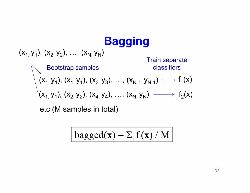
Bagging(x1, y1), (x2, y2), …, (xN, yN)

Train separate

(x1, y1), (x1, y1), (x3, y3), …, (xN-1, yN-1)Bootstrap samples

f1(x)

Train separate classifiers

(x1, y1), (x2, y2), (x4, y4), …, (xN, yN)

etc (M samples in total)

f2(x)

etc (M samples in total)

b d( ) Σ f ( ) / Mbagged(x) = Σj fj(x) / M

37

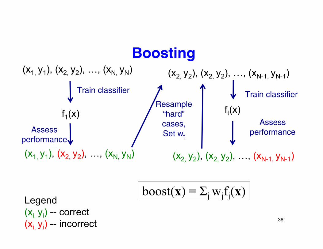
Boosting(x1, y1), (x2, y2), …, (xN, yN) (x2 y2), (x2 y2), …, (xN-1 yN-1)

f (x)

Train classifier

Resample

( 2, y2), ( 2, y2), , ( N 1, yN 1)

Train classifier

f1(x) ft(x)

Assess performance

“hard” cases,Set wt

Assess performance

performance

(x1, y1), (x2, y2), …, (xN, yN) (x2, y2), (x2, y2), …, (xN-1, yN-1)

boost(x) = Σj wjfj(x)Legend

38

Legend(xi, yi) -- correct(xi, yi) -- incorrect

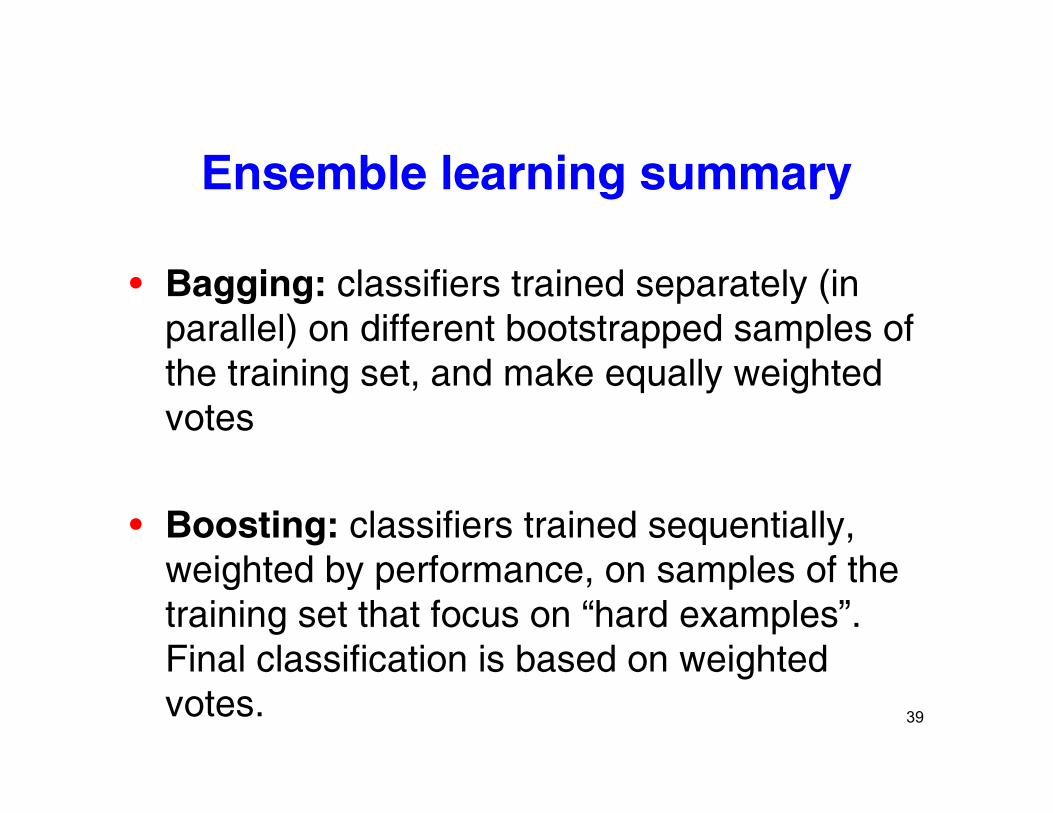
Ensemble learning summary

• Bagging: classifiers trained separately (in parallel) on different bootstrapped samples of the training set, and make equally weighted votes

• Boosting: classifiers trained sequentially, eighted by erfor ance on sa les of the weighted by performance, on samples of the

training set that focus on “hard examples”. Final classification is based on weighted Final classification is based on weighted votes. 39

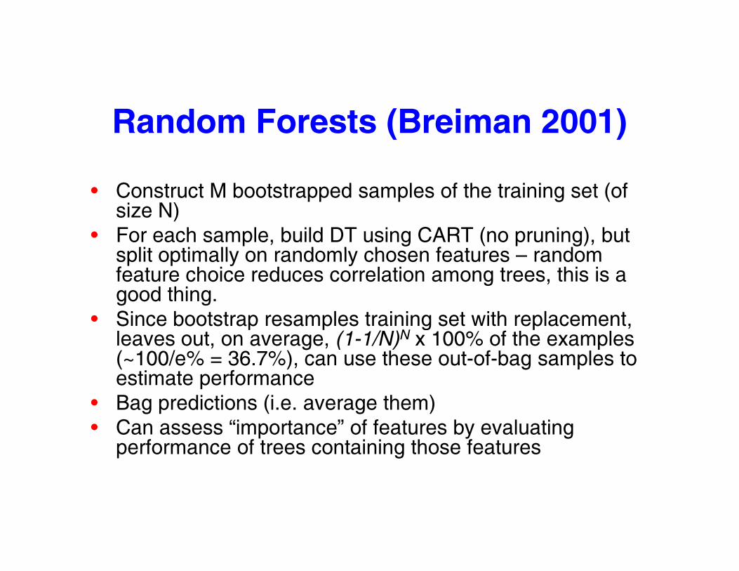
Random Forests (Breiman 2001)

• Construct M bootstrapped samples of the training set (of size N)

• For each sample, build DT using CART (no pruning), but s lit o ti ally on rando ly chosen features rando split optimally on randomly chosen features – random feature choice reduces correlation among trees, this is a good thing.

• Since bootstrap resamples training set with replacement Since bootstrap resamples training set with replacement, leaves out, on average, (1-1/N)N x 100% of the examples (~100/e% = 36.7%), can use these out-of-bag samples to estimate performance

• Bag predictions (i.e. average them)• Can assess “importance” of features by evaluating

performance of trees containing those features

Advantages of Decision Trees

• Relatively easy to combine continuous and discrete (ordinal or categorical) features within the same classifier this is harder to do within the same classifier, this is harder to do for other methods

• Random Forests can be trained in parallel Random Forests can be trained in parallel (unlike boosted decision trees), and relatively quickly.

• Random Forests tend to do quite well in empirical tests (but see “No Free Lunch” theorem)theorem)

Networks as kernels

• Can use matrix representations of graphs to generate kernels.O l h b d k l i h • One popular graph-based kernel is the diffusion kernel:– K =(λI – L)-1K (λI L)– Where L = D – W, D is a diagonal matrix with the

row sums, and W is the matrix representation of the graphthe graph.

• GeneMANIA label propagation:– f = (λI – L)-1yf (λI L) y