Introduction to Water Engineering 1 Slide 1 Introduction to Water Engineering 2. Turbines and Pumps Module 3 Pumps and Dimensional Analysis Dr James Ward Lecturer School of Natural and Built Environments Welcome to Module 3, today we’re looking at turbines and pumps Slide 2 Do not remove this notice. COMMMONWEALTH OF AUSTRALIA Copyright Regulations 1969 WARNING This material has been produced and communicated to you by or on behalf of the University of South Australia pursuant to Part VB of the Copyright Act 1968 (the Act). The material in this communication may be subject to copyright under the Act. Any further reproduction or communication of this material by you may be the subject of copyright protection under the Act. Do not remove this notice. Copyright Notice Please note Slide 3 Intended Learning Outcomes At the end of this section, students will be able to understand:- - Pumps - Energy and efficiency - Pump performance - Pump selection - Pumps in series and parallel So the learning outcomes are here – we’ll look mostly at pumps rather than turbines, but the concepts are relevant to both anyway - energy and efficiency, pump performance, pump selection and we’ll also look at how pumps can be added together in series and parallel.

Welcome message from author
This document is posted to help you gain knowledge. Please leave a comment to let me know what you think about it! Share it to your friends and learn new things together.
Transcript

Introduction to Water Engineering
1
Slide 1
Introduction to Water Engineering
2. Turbines and Pumps
Module 3 Pumps and Dimensional Analysis
Dr James Ward
Lecturer
School of Natural and Built Environments
Welcome to Module 3, today we’re looking at turbines and pumps
Slide 2 Do not remove this notice.
COMMMONWEALTH OF AUSTRALIACopyright Regulations 1969
WARNING
This material has been produced and communicated to you by or on
behalf of the University of South Australia pursuant to Part VB of the
Copyright Act 1968 (the Act).
The material in this communication may be subject to copyright under the
Act. Any further reproduction or communication of this material by you
may be the subject of copyright protection under the Act.
Do not remove this notice.
Copyright Notice
Please note
Slide 3 Intended Learning Outcomes
At the end of this section, students will be able to
understand:-
- Pumps
- Energy and efficiency
- Pump performance
- Pump selection
- Pumps in series and parallel
So the learning outcomes are here – we’ll look mostly at pumps rather than turbines, but the concepts are relevant to both anyway - energy and efficiency, pump performance, pump selection and we’ll also look at how pumps can be added together in series and parallel.

Introduction to Water Engineering
2
Slide 4
• Pumps are used to add energy to a system
– Boost pressure and/or increase velocity.
• Turbines are used to harvest energy from moving water
(typically with a significant driving head), to generate
mechanical or electrical power.
Turbines & pumps
Turbines and pumps are basically the same device, just working in opposite directions. Pumps are used to add energy to a system. We didn’t consider pumps in any of the energy equations in our previous lectures because we were always looking at gravity-driven flow. But a pump essentially adds energy to the energy equation at some point in the pipe system. Turbines do the exact reverse – they take energy out of the system. Typically turbines are placed where water can come from a high elevation, like a big dam, down to a low elevation and the turbine harvests some of the energy on the way. We’re going to focus primarily on pumps but the theory can be related to turbines too.
Slide 5
• Linear relationship between pump speed and discharge
• Used for low-flow applications where a predictable and
reliable flow is required
• Can be capable of extremely high lift
• Not common in large civil engineering applications
Positive displacement machines
Pumps are broadly categorised into two types. Positive displacement machines are where there’s a known displacement of water for every stroke of the pump. A good example is piston in a cylinder, which always displaces a known volume of water. In these pumps, there’s a linear relationship between the pump speed, or the number of strokes per unit time, and the discharge, which might be a useful relationship in planning the design discharge of the pump. Positive displacement pumps generally don’t generate high flows and they’re used for smaller applications – especially where a very reliable and predictable flow’s required, like delivering a measured chemical dose slowly to a system. Despite their low discharge rate, these sorts of pumps can be capable of lifting water to large heights, or in other words they can force extremely high pressure into the system. As an example, traditional mechanical windmill pumps tend to operate a piston-type positive displacement pump, which can pump up water from hundreds of metres below the ground. It’s good to be aware of these sorts of pumps but realistically you’re not that likely to encounter them much in civil engineering applications.

Introduction to Water Engineering
3
Slide 6
• Basically all turbines, and most pumps you’ll come
across
• All have a continuously rotating element, called a
“runner” (turbines) or an “impeller” (pump)
Rotodynamic machines
Pumps in the other category are called rotodynamic machines, where there’s a continuous rotating element; this is pretty much the only way to run a turbine and most pumps you’ll deal with are in the rotodynamic category. The rotating element’s called a “runner” in a turbine and an “impeller” in a pump.
Slide 7
• http://www.youtube.com/watch?v=3DNKP
cCPmUg&feature=related
Making a centrifugal pump
This YouTube video shows someone fabricating a tiny centrifugal pump, like the sort that might be used in an aquarium. You can see the inlet and outlet pipes, and the little impeller. You can also see how the impeller needs to be driven by some mechanical power input, which is a little electric motor in this case.
Slide 8 Basic principle
http://www.youtube.com/watch?v=UrChdDwHyb
Y&NR=1
So we’re going to look at the basics of how these centrifugal pumps actually work. Fluid comes in behind the central spinning impeller, which creates extra velocity in the fluid as it spins round and outwards, meaning that by the time it exits the system it’s got more overall energy that can be turned into pressure or elevation head. There’s also a link there to a little YouTube video showing the basic operation of a centrifugal pump.

Introduction to Water Engineering
4
Slide 9 A pump adds energy to fluid
Water in
Impeller adds
velocity to fluid
g
V
2
2
increases
g
P
g
VZE
1
2
111
2
g
P
g
VZE
2
2
222
2E2 > E1
So let’s walk through how it works. Water comes in somewhere near the centre and the impeller’s spinning round and round, forcing water to migrate to the outside by centrifugal motion. This adds velocity to the fluid, because as it moves outwards it has to move faster and faster to keep up with the spinning impeller. So we’ve got higher velocity which translates to higher velocity head. The outlet’s typically tangential to the motion so the fluid can shoot off into the pipe. The crucial thing to understand here is that the pump’s added energy to the system. It’s possible that the inflow and outflow pipes are the same diameter, so the velocity head on both sides of the pump’s the same, But because inside the pump we temporarily added more energy in the form of velocity head, the energy in the outflow’s going to be more than in the inflow. The extra velocity head mostly turns into pressure head as it enters the outflow pipe, so the overall result is that the pump adds pressure head to the system. Obviously then depending on the rest of the pipe system, this extra pressure’s available to push the water up to a higher elevation or to overcome friction losses in the system, or both.
Slide 10
• A turbine extracts energy from the moving fluid
Turbine ~ pump in reverse
A turbine acts just like a pump in reverse. So they extract energy from the moving fluid. If a turbine’s arranged with an inflow and outflow pipe of the same diameter, then the net result’s going to be a loss of pressure, corresponding to the energy removed from the system.
Introduction to Water Engineering
5
Slide 11
http://www.youtube.com/watch?v=K4_dXiAzN2Y
Changing a large turbine
Here’s a little video showing some workers changing a large turbine. It’s worth looking at, even though we’re focusing on pumps in this lecture, just because it’s a pretty impressive feat of engineering. Big hydroelectric turbines are way bigger than the biggest pumps.
Slide 12
Energy and Efficiency
DO NOT REMOVE THIS NOTICE. Reproduced and communicated on behalf of the University of South Australia pursuant to Part VB of the copyright Act 1968 (the Act) or with permission of the
copyright owner on (29/3/08) Any further reproduction or communication of this material by you may be the subject of copyright protection under the Act. DO NOT REMOVE THIS NOTICE.
The next topic is energy and efficiency
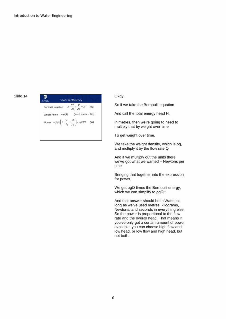
Slide 13
• Recall that the energy (Bernoulli) equation is defined as
the energy (in Joules) per unit weight (N) of the flowing
water
• We’re interested in actual energy (Joules)
• For dimensional homogeneity:
– Energy (J) = Bernoulli energy (J/N) x weight (N)
– and Power (J/s) = Energy (J) / Time (s)
– So Power = Bernoulli energy x weight / time
Power & efficiency
Now, you may or may not remember that the energy equation is actually defined as the energy per unit weight of water moving along. Obviously if we want to know how much energy a pump’s going to consume, or conversely how much energy a turbine’s going to generate, then we need to get this as energy in joules, not per unit weight. So to make sure the dimensions balance, If our target’s energy in joules and we’ve got the Bernoulli energy in joules per Newton, it stands to reason that we’re going to need to multiply by the weight in Newtons to get what we want. Now actually, what we really want is power, which is energy over time – one Watt is one Joule per second so we’re going to have to multiply by weight and divide by time.
Introduction to Water Engineering
6
Slide 14 Power & efficiency
Hg
P
g
Vz
2
2
(m)
gQHg
P
g
VzgQ
2
2
Bernoulli equation
Weight / time gQ (N/m3 x m3/s = N/s)
Power (W)
Okay, So if we take the Bernoulli equation And call the total energy head H, in metres, then we’re going to need to multiply that by weight over time To get weight over time, We take the weight density, which is ρg, and multiply it by the flow rate Q And if we multiply out the units there we’ve got what we wanted – Newtons per time Bringing that together into the expression for power, We get ρgQ times the Bernoulli energy, which we can simplify to ρgQH And that answer should be in Watts, so long as we’ve used metres, kilograms, Newtons, and seconds in everything else. So the power is proportional to the flow rate and the overall head. That means if you’ve only got a certain amount of power available, you can choose high flow and low head, or low flow and high head, but not both.

Introduction to Water Engineering
7
Slide 15
• So the power of a moving fluid is:
• A perfectly efficient turbine would be capable of
capturing 100% of this fluid power and turning it into
useful power (e.g. electricity)
• A perfectly efficient pump could be provided with exactly
this amount of power (e.g. as electricity input) and would
convert it all to fluid motion
Power & efficiency
gQHPow
So now we’ve got a neat equation for the power of a moving fluid, which is ρgQH. Now hypothetically, a perfectly efficient turbine would be able to harvest all of that power, ρgQH, and turn it into useful power, like, electric energy. Likewise, a perfectly efficient pump could be provided with exactly this amount of power and would convert it all to fluid motion.
Slide 16
• For a turbine, efficiency is the proportion of the fluid
energy that is actually harvested:
• For a pump, efficiency is the proportion of input energy
that is converted to fluid energy:
Efficiency (%) = output / input
gQH
PowT
Pow
gQHP
Power output (e.g. Electricity)
Power input (e.g. Electricity)
Fluid power input
Fluid power output
Of course efficiency’s always less than 100%. In the case of a turbine, we can work out the real-world efficiency by looking at the power generated as a proportion of the known power in the moving fluid. Likewise for a pump, you look at The power output, which is the power of the moving fluid Versus the power input to the system, which might be the electrical power.
Slide 17
• The force on a
turbine can be
calculated
using the
momentum
equation
Calculating forces on a vane
RFVVQ
12
The textbook has some interesting material on the internal dynamics of pumps and turbines, where you can actually verify the power relationship using the momentum equation, and look at the forces on the vanes of the impeller or runner. At first glance this stuff looks pretty complicated but it’s actually fairly basic mechanics. Image source- Les Hamill 2011, Understanding hydraulics.
Introduction to Water Engineering
8
Slide 18
• Not going through it, just making you aware of it
• Fairly basic mechanics
• Read Box 11.1 carefully (p. 382)
• Go through worked examples 11.1-11.5
Read Section 11.2 (pp. 381-392)
The good news for you is that this internal dynamics stuff isn’t being assessed – but I’d encourage you to read the section and go through the worked examples anyway, just to strengthen your fundamental understanding of forces, momentum and power as they apply to pumps. You won’t find it overwhelmingly hard to understand and it might come in handy.
Slide 19
Pump Performance
DO NOT REMOVE THIS NOTICE. Reproduced and communicated on behalf of the University of South Australia pursuant to Part VB of the copyright Act 1968 (the Act) or with permission of the
copyright owner on (29/3/08) Any further reproduction or communication of this material by you may be the subject of copyright protection under the Act. DO NOT REMOVE THIS NOTICE.
So now let’s move on to look at pump performance
Slide 20
• A pump is a bit like a car
• You can drive from Sydney to Perth in 2nd gear if you
want to, but it’s not the most efficient way to get there!
• There is typically a certain RPM point where an engine is
most efficient – different engines are designed for
different optimum RPM
• Likewise, pumps are designed for optimum efficiency
at a particular head and discharge combination
Pump performance
Pump performance is actually the key thing we’re interested in today, especially efficiency. In some respects a pump is a bit like a car. Driving a car a really long way in a low gear is physically possible but the vehicle’s drive system’s been optimised to give the best efficiency at higher speeds. More specifically, the fuel efficiency of a car engine’s typically best at a particular range of revs, and different engines have different optimal rev ranges. So in this respect pumps are similar – a given pump’ll have a particular combination of head and discharge that achieves the highest efficiency. Like a car, a pump can be operated outside the optimal range – for instance at a higher flow rate and lower head – but the energy efficiency wouldn’t be as good.

Introduction to Water Engineering
9
Slide 21 Pump performance
• Rated head and
discharge refer to the
most efficient operating
point
– Pumps can usually
discharge at higher
head (lower flow) or at
higher flow (lower
head) but will be less
efficient
Here’s a graph of pump performance We’ve got rated head here, which is a percentage scale, so 100% is the head that the pump’s been designed to operate at. Likewise we’ve got rated discharge on the bottom axis so 100% here means the discharge that the pump’s designed for. So the combination of design head and design discharge is the design operating point of the pump And that should correspond to the peak efficiency as shown by this curve So if you’ve got a pump with rated head and rated discharge info, you can expect that to correspond to the peak efficiency. But of course that doesn’t mean the pump can only deliver that particular head or that particular flow rate; if you look at the head-discharge line, you can see there’s a whole continuum of different heads and flow rates that the pump can operate at – either higher head and lower flow, or higher flow and lower head – but if you move away from the design point you can seriously sacrifice efficiency and that might mean you should choose a different pump more suited to the particular combination of head and flow that you need. Image source- Les Hamill 2011, Understanding hydraulics.

Introduction to Water Engineering
10
Slide 22
• Recall from dimensional analysis last week:
• Discharge head relationship
• Pump/turbine power relationship
Pump performance equations
223 DN
gHf
ND
Q
2253 DN
gHf
DN
Pow
If you don’t trust the
dimensional analysis,
see pp. 402-403 for a
hydraulic explanation of
why these relationships
occur.
Now If you can remember any of last week’s presentation on dimensional analysis, You might recall that we arrived at this relationship between head and discharge, where N’s the rotational speed and D’s the impeller diameter, and form of the function “f” is a power relationship. We also – well, you would have, as long as you actually worked it out – determined the power relationship for a pump or a turbine, which is a similar power-type function of the same parameters, but with a different dimensionless group on the left-hand side. Now if you found all that stuff too unbelievable, you can check out the explanation based on the physical hydraulics in the textbook. The good news is the dimensional analysis checks out.
Slide 23
• Assuming g and ρ are constant, then for a group of
geometrically similar pumps:
From pp. 402-403...
HD
Q2
3ND
Q
22DN
H
53DN
Pow
is a constant
is a constant
is a constant
is a constant
From that physical explanation in the textbook, a few useful extra relationships jump out. Assuming we’re talking about geometrically similar pumps, which means we’re talking about a collection of pumps where the physical shape’s the same, just some are big and some are small, then there are a few clusters of parameters that are constant. The first one’s Q on ND3. So that’s constant for all pumps that are geometrically similar – that means if you build it twice as big, so D’s doubled, then for the same rotational speed your flow rate’d multiply by a factor of 8. Next up’s this relationship which is a kind of strange-looking one. But that should hold for similar shaped pumps. H on N2D2 isn’t a huge surprise since it was one of the main dimensionless groups and we’ve already seen the first one, Q on ND3, comes out as a constant. And so likewise, the other one’s related to the power on N3D5. You can use any of these constant relationships to work out how a particular change in one variable’s going to change another one. Let’s do an example to see that in action.

Introduction to Water Engineering
11
Slide 24
• Suppose we have a pump with a variable speed motor.
• At 1200 RPM it delivers QA = 0.12m3/s
• What RPM would be required to deliver 0.15m3/s ?
• Use:
Example 11.6
3ND
Qconstant
So let’s say we’ve got a pump that’s got a nifty variable speed motor driving it. These sorts of variable-speed drives are actually getting increasingly more common ‘cos they’re a way to deliver a range of different design points, rather than just one. Anyway, we’re told that it delivers 120 litres a second when it runs at 1200 RPM and we want to know what speed we have to crank it up to, to push the discharge up to 150 litres a second. Hopefully you can see that the formula you want to use is Q on ND3, since it’s the only one with Q and N both in it. This is pretty simple since you’re not changing the diameter of the impeller, and you know the proportional change in Q. See how you go.
Slide 25
• A pump has an impeller diameter of 0.8m and runs at
1200 RPM
• If the speed is increased to 1500 RPM, what impeller
diameter would we need to keep the power requirement
the same?
• Use:
Example 11.9
53DN
Powconstant
Here’s another example. This time we’ve got a pump – a pretty big one actually, with an 80-centimetre impeller, and it normally operates at 1200 RPM. Now for some reason, we need to reconfigure the pump with a different impeller so it can run at 1500 RPM – don’t ask me why we’d need to do that – but we don’t want to increase the power requirement. Obviously if we’re running the pump faster but with the same power, we’re going to need a smaller impeller. And you’ve only got one relationship that brings power into the picture, and luckily it relates to both the rotational speed and the diameter. Same basic principle as the last example, just with some slightly trickier arithmetic.

Introduction to Water Engineering
12
Slide 26
• How would the change in diameter affect the discharge
and head produced by the pump?
• Use:
Example 11.9 (continued)
22DN
Hconstant
3ND
Qconstant
Now continuing on with that example, assuming you coped okay with the diameter calculation, now we want to know how that’s going to affect the head and discharge of the pump. I guess from a practical point of view, you’re in a hypothetical situation where you’ve got a strict, narrow band of power available and there’s more tolerance in your head and discharge. It’s probably more common that the design process’d be the reverse but let’s keep on going anyway. So you know the rotational speed’s increased from 1200 to 1500, and hopefully you’ve calculated the decrease in diameter, so now you’ve got to use this equation to relate these changed values to a change in flow rate – it’ll either increase it or decrease it And then use this relationship to do the same thing with head – again, it’ll either increase or decrease it. It’s not super difficult but it can take some practice to know what to do with these sorts of problems. So feel free to check the worked example in the textbook.
Slide 27
• Speed (i.e. RPM) required to discharge 1m3/s at 1m
head
• (Derivation pp. 404-405)
• Can aid in selecting the best type of pump
– Centrifugal NS = 10-70 high H, low Q
– Mixed flow NS = 70-170 mid H, mid Q
– Axial flow NS >110 low H, high Q
Specific speed
43
21
H
NQNS
We’re working our way towards a concept called “pump selection”, and as well as looking at individual pump performance data we might also need to take a step back and figure out what broad type of pump we actually need. We’ll assume we’ve already moved away from positive displacement and we know we need a rotodynamic pump. Then the two big categories are centrifugal and axial flow. The parameter we use to choose whether we need a centrifugal or an axial flow pump is “specific speed” which is a sort of artificial construct being the rotational speed required to hypothetically deliver a cubic metre per second at a head of 1 metre. The formula for specific speed, NS, is derived in the textbook and you can see it here. So assuming you know what sort of motor or drive you’ve got, you know N, and assuming you know what flow rate and head you need, you can work out NS like this. Then you can use your value of NS to figure out what sort of pump’s going to be best by comparing it to quoted specific speed values for different pumps.

Introduction to Water Engineering
13
So centrifugal pumps are suitable for NS values in the lower end, meaning they’re good for relatively high head and relatively low flow – bearing in mind that like we said right at the start, if you need extremely high head and very low flow you might be looking at a positive displacement machine. But in the more normal circumstances for relatively high head, low flow you might find a centrifugal pump’s the way to go. The images shown earlier to illustrate impellers and so on were from centrifugal pumps. On the other hand if you’ve got a fairly high NS value you might need to look at a thing called an axial flow pump, which is good for high flow rates so long as it’s a low head. An axial flow pump’s like a big propeller in a pipe, so you’re not forcing the fluid to change direction as much as in a centrifugal pump. Axial pumps can shift a lot of water along, which is why they’re good for high flow, but they aren’t designed to add significant pressure to the system. In between, there are things called mixed flow pumps, which are a sort of compromise between centrifugal and axial and suitable for NS values in the middle to upper range, for medium flow and medium head.
Slide 28
• We need a pump!
• We’ve been given the following requirements:
– Speed 3000 RPM
– H = 7m
– Q = 0.15m3/s
• What type of pump should we use?
Example 11.10
43
21
H
NQNS
So here’s an easy example of that. We’ve got a particular speed, presumably set by the efficiency of the motor we want to use, and we need to deliver 7 metres of head with a flow of 150 litres a second. So we’ve got to use the specific speed equation and relate it back to the pump types on the previous page.

Introduction to Water Engineering
14
Slide 29
Pump Selection
DO NOT REMOVE THIS NOTICE. Reproduced and communicated on behalf of the University of South Australia pursuant to Part VB of the copyright Act 1968 (the Act) or with permission of the
copyright owner on (29/3/08) Any further reproduction or communication of this material by you may be the subject of copyright protection under the Act. DO NOT REMOVE THIS NOTICE.
Now, the main thing we’re interested in is “pump selection”
Slide 30
• Careful pump selection is important!
• Really bad pump selection can result in a pump which
does not work properly (or at all)
• Even if the pump works, incorrect pump selection can
result in:
– Excessive capital costs (wasted money)
– Inefficient operation (wasted money & energy)
Pump selection
Like we said before, pumps can run at different heads and flow rates but the difference in efficiency can be really significant. With more and more emphasis on energy conservations, we need to select pumps carefully. Actually, quite apart from efficiency, we need to be careful that we select a pump that’s going to work properly at the flow rate we need. It’s easy to get it wrong and deliver way more flow than your system needs, meaning you need to throttle it back, or even worse – you accidentally choose a pump that can’t deliver the flow rate you need at the head required. And assuming you get a pump that works, you’ve got to consider whether your pump Was the best choice in terms of minimising capital expenditure And of course there’s the original question of efficiency again. So let’s look at what’s involved in pump selection.

Introduction to Water Engineering
15
Slide 31
• In-text example (p. 407)
• Required lift:
13m
• Required discharge:
0.4 – 0.6 m3/s
• Pump A, B, C, D, or E?
• Target max. efficiency AND absolute power
consumption
Pump selection
Let’s walk through the example from the textbook, which you can find on page 407. We need to lift water 13 m, and the required discharge is between 0.4 to 0.6 m3/s. So we’re given a range of flow rates, but it sounds like we’re really looking for a pump that can deliver up 0.6 m3/s against a head of 13 metres, so that’s our target performance. If we find a pump that can do that, then we can assume it’s capable of delivering the lower flow rate at the same head. So they’ve given us a series of 5 pump performance curves, A, B, C, D and E, which we’ll look at in a minute, and we have to choose one or more pumps from that.
Slide 32 Pump selection
Okay, so starting with pump A. First things first, we need to see if it can actually deliver the performance we need. So here’s our flow rate at 0.6 m3/s And here’s the head at about 13 metres And we compare this against the actual head-discharge line for this pump, which goes like this. So we’ve definitely got enough performance from this pump without it being excessive. But if we look at the efficiency of this pump, we can see we’re a bit off optimum. Not too much, mind you, so pump A’s probably a reasonable contender for the system. Let’s look at the others. Image source- Les Hamill 2011, Understanding hydraulics.

Introduction to Water Engineering
16
Slide 33 Pump selection
So moving to pump B now, And drawing on those lines we see a pretty perfect match for performance And efficiency’s right up close to the optimum, In fact if you consider we’re after a pump that works in this range of flows, you couldn’t really ask for a better match with peak efficiency. So it’s looking like this’ll be hard to top. Image source- Les Hamill 2011, Understanding hydraulics.
Slide 34 Pump selection
Pump C’s easy to evaluate It simply doesn’t cut it – not enough flow at the head we need. It’s a shame since the peak efficiency’s at just the right flow range. Oh well. Image source- Les Hamill 2011, Understanding hydraulics.
Slide 35 Pump selection
Now for pump D So again we look at the performance data. At first glance this looks really good – efficiency’s in the right place and the head-discharge curve has this weird little flat spot right in the range we’re interested in. But that fact is actually the downfall of this pump. To understand this, you need to think about the way you might control the discharge in a typical system – namely using a throttle valve which induces a head loss to consume some of the available pressure and reduces the flow as a result. So hopefully you can see that having this flat spot right here, where we want to be able to control the flow by adjusting the head, would give an unstable result – in other words if we changed the head just a little bit by adjusting a valve, the flow rate could change by a much larger amount. So we’d probably have to say goodbye to Pump D.

Introduction to Water Engineering
17
Image source- Les Hamill 2011, Understanding hydraulics.
Slide 36 Pump selection
Last but not least is Pump E Which looks like a really good option, right up there with Pump B. So you could leave it there, and further evaluate those two pumps based on reliability and cost. But we haven’t quite considered these pumps fully. In each case we’ve looked at the efficiency curve, aiming for an operating point coinciding with the peak of that curve, but if you look carefully at the graph, you’ll see efficiency doesn’t actually have a scale – the axis on the right is absolute power consumption so we don’t actually know how efficient these pumps are – and maybe Pump B’s peak efficiency is better than Pump E’s. Well, we can figure this out ‘cos we’ve been given another line on the curve, which is the power line. And we can see in the case of pump E it’s about 190 kilowatts. If we bring in the corresponding power curve from Pump B, it comes in at under 150 kilowatts. So even though both pumps are in their element in terms of operating at peak efficiency, Pump B’s an inherently more efficient pump than Pump E. Image source- Les Hamill 2011, Understanding hydraulics.
Introduction to Water Engineering
18
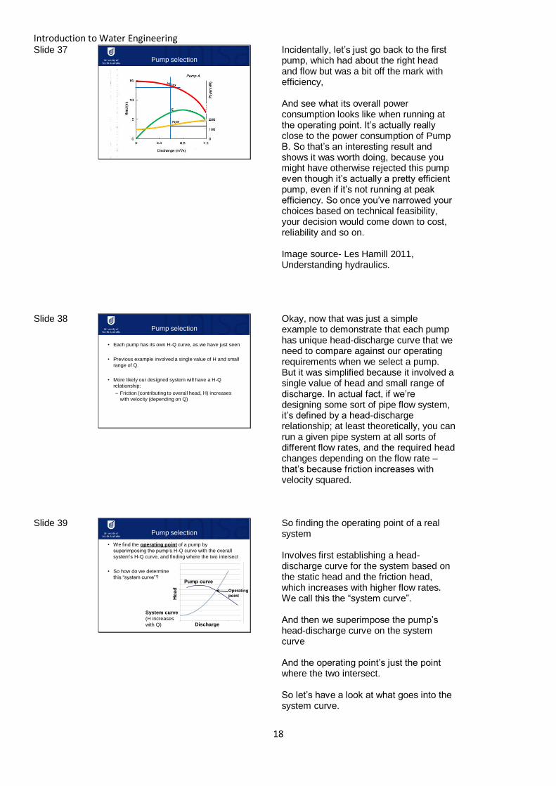
Slide 37 Pump selection
Incidentally, let’s just go back to the first pump, which had about the right head and flow but was a bit off the mark with efficiency, And see what its overall power consumption looks like when running at the operating point. It’s actually really close to the power consumption of Pump B. So that’s an interesting result and shows it was worth doing, because you might have otherwise rejected this pump even though it’s actually a pretty efficient pump, even if it’s not running at peak efficiency. So once you’ve narrowed your choices based on technical feasibility, your decision would come down to cost, reliability and so on. Image source- Les Hamill 2011, Understanding hydraulics.
Slide 38
• Each pump has its own H-Q curve, as we have just seen
• Previous example involved a single value of H and small
range of Q.
• More likely our designed system will have a H-Q
relationship:
– Friction (contributing to overall head, H) increases
with velocity (depending on Q)
Pump selection
Okay, now that was just a simple example to demonstrate that each pump has unique head-discharge curve that we need to compare against our operating requirements when we select a pump. But it was simplified because it involved a single value of head and small range of discharge. In actual fact, if we’re designing some sort of pipe flow system, it’s defined by a head-discharge relationship; at least theoretically, you can run a given pipe system at all sorts of different flow rates, and the required head changes depending on the flow rate – that’s because friction increases with velocity squared.
Slide 39
• We find the operating point of a pump by
superimposing the pump’s H-Q curve with the overall
system’s H-Q curve, and finding where the two intersect
• So how do we determine
this “system curve”?
Pump selection
System curve
(H increases
with Q)
Pump curve
Hea
d
Discharge
Operating
point
So finding the operating point of a real system Involves first establishing a head-discharge curve for the system based on the static head and the friction head, which increases with higher flow rates. We call this the “system curve”. And then we superimpose the pump’s head-discharge curve on the system curve And the operating point’s just the point where the two intersect. So let’s have a look at what goes into the system curve.
Introduction to Water Engineering
19
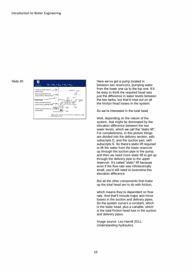
Slide 40 HT = HS + hFS + HD + hFD
Static (elevation) lift from
suction level to pump inlet
Total head
Friction & minor losses in
delivery pipe
Friction & minor losses in
suction pipe
Static (elevation) lift from
pump outlet to delivery level
Here we’ve got a pump located in between two reservoirs, pumping water from the lower one up to the top one. It’d be easy to think the required head was just the difference in water levels between the two tanks, but that’d miss out on all the friction head losses in the system. So we’re interested in the total head Well, depending on the nature of the system, that might be dominated by the elevation difference between the two water levels, which we call the “static lift”. For completeness, in this picture things are divided into the delivery section, with subscripts D, and the suction part, with subscripts S. So there’s static lift required to lift the water from the lower reservoir up through the suction pipe to the pump, and then we need more static lift to get up through the delivery pipe to the upper reservoir. It’s called “static” lift because even if the flow rate was infinitesimally small, you’d still need to overcome this elevation difference. But all the other components that make up the total head are to do with friction, which means they’re dependent on flow rate. And that’ll include major and minor losses in the suction and delivery pipes. So the system curve’s a constant, which is the static head, plus a variable, which is the total friction head loss in the suction and delivery pipes. Image source- Les Hamill 2011, Understanding hydraulics.
Introduction to Water Engineering
20
Slide 41
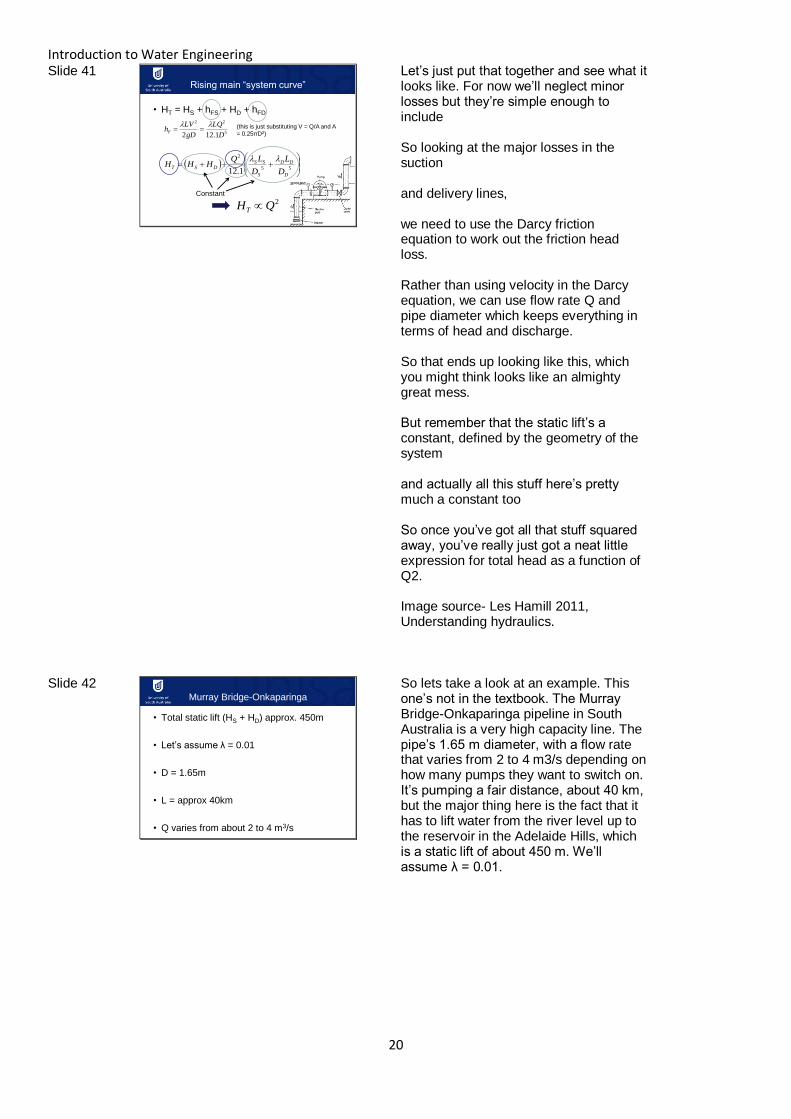
• HT = HS + hFS + HD + hFD
Rising main “system curve”
5
22
1.122 D
LQ
gD
LVhF
(this is just substituting V = Q/A and A
= 0.25πD2)
55
2
1.12D
DD
S
SSDST
D
L
D
LQHHH
Constant2QHT
Let’s just put that together and see what it looks like. For now we’ll neglect minor losses but they’re simple enough to include So looking at the major losses in the suction and delivery lines, we need to use the Darcy friction equation to work out the friction head loss. Rather than using velocity in the Darcy equation, we can use flow rate Q and pipe diameter which keeps everything in terms of head and discharge. So that ends up looking like this, which you might think looks like an almighty great mess. But remember that the static lift’s a constant, defined by the geometry of the system and actually all this stuff here’s pretty much a constant too So once you’ve got all that stuff squared away, you’ve really just got a neat little expression for total head as a function of Q2. Image source- Les Hamill 2011, Understanding hydraulics.
Slide 42
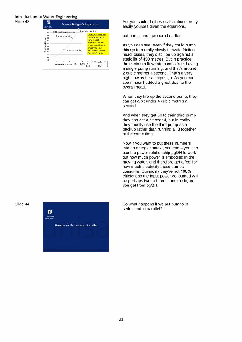
• Total static lift (HS + HD) approx. 450m
• Let’s assume λ = 0.01
• D = 1.65m
• L = approx 40km
• Q varies from about 2 to 4 m3/s
Murray Bridge-Onkaparinga
So lets take a look at an example. This one’s not in the textbook. The Murray Bridge-Onkaparinga pipeline in South Australia is a very high capacity line. The pipe’s 1.65 m diameter, with a flow rate that varies from 2 to 4 m3/s depending on how many pumps they want to switch on. It’s pumping a fair distance, about 40 km, but the major thing here is the fact that it has to lift water from the river level up to the reservoir in the Adelaide Hills, which is a static lift of about 450 m. We’ll assume λ = 0.01.
Introduction to Water Engineering
21
Slide 43
5
32
65.1
104001.0
1.12450
QHT
445
450
455
460
465
470
475
480
485
490
495
500
0 1 2 3 4 5
To
tal h
ead
HT
(m
)
Discharge Q (m3/s)
MBO pipeline system curve
BONUS exercise:
Use the equation
Pow = ρgQH
to determine the
power (and hence
energy per kL)
required to deliver
Adelaide’s water
1 pump running
2 pumps running
3 pumps running
Murray Bridge-Onkaparinga
So, you could do these calculations pretty easily yourself given the equations, but here’s one I prepared earlier. As you can see, even if they could pump this system really slowly to avoid friction head losses, they’d still be up against a static lift of 450 metres. But in practice, the minimum flow rate comes from having a single pump running, and that’s around 2 cubic metres a second. That’s a very high flow as far as pipes go. As you can see it hasn’t added a great deal to the overall head. When they fire up the second pump, they can get a bit under 4 cubic metres a second And when they get up to their third pump they can get a bit over 4, but in reality they mostly use the third pump as a backup rather than running all 3 together at the same time. Now if you want to put these numbers into an energy context, you can – you can use the power relationship ρgQH to work out how much power is embodied in the moving water, and therefore get a feel for how much electricity these pumps consume. Obviously they’re not 100% efficient so the input power consumed will be perhaps two to three times the figure you get from ρgQH.
Slide 44
Pumps in Series and Parallel
DO NOT REMOVE THIS NOTICE. Reproduced and communicated on behalf of the University of South Australia pursuant to Part VB of the copyright Act 1968 (the Act) or with permission of the
copyright owner on (29/3/08) Any further reproduction or communication of this material by you may be the subject of copyright protection under the Act. DO NOT REMOVE THIS NOTICE.
So what happens if we put pumps in series and in parallel?

Introduction to Water Engineering
22
Slide 45
• Add head but don’t
increase discharge
• Good in constant Q,
variable H situations
• One pump fails, whole
system fails
Pumps in series
Putting pumps in series means the outflow from one pump goes straight into the next pump. Two pumps in series increase the head delivered by the combined pumps, but don’t increase the discharge compared with a single pump. An appropriate situation might be where you need to deliver a narrow flow range over a wider range of heads. Another situation would be where you’ve got a really high head required, like the 450 metres lift in the previous example, and you can’t get a single pump to deliver it at the right flow. Assuming you can find pumps that are efficient at the right flow rate, doubling them up makes a lot of sense as a way to boost the head. And in fact that’s precisely what they do in the pump stations on the Murray Bridge-Onkaparinga pipeline. One drawback of pumps in series is that if one pump fails, the combined system fails since a single pump can’t deliver enough head on its own. Image source- Les Hamill 2011, Understanding hydraulics.
Slide 46
• Operating point for
single pump
• Second pump added in
series
– New pump curve, so
new intersection
(operating point)
Pumps in series
Finding the operating point for single pump is the intersection of the rising main system curve with the pump's head-discharge curve, as we said before. If we want to add a second pump in series, the result is that the pump’s head-discharge curve is doubled in the vertical direction, in other words there’s twice as much head for every flow rate. That means the intersection point will move and even though the pumps in series technically don’t add anything to the flow rate capacity, it’s likely that the new operating point’s going to be marginally higher. In fact this figure isn’t describing a particularly realistic situation where you’d bother to double up the pumps, because the single pump offers a pretty good operating point and you don’t get much improvement by putting in the second pump. A more realistic situation might be where the system curve’s actually up here and one pump just won’t cut it. Image source- Les Hamill 2011,

Introduction to Water Engineering
23
Understanding hydraulics.
Slide 47
• Add discharge but don’t
increase head
• Good in situations (like
MBO) where range of Q
is needed at approx.
constant H – simply
switch on as many
pumps as needed
Pumps in parallel
You might be able to guess the result of adding pumps in parallel They increase the discharge, but don’t increase the head. This might be useful in a situation where you need a range of discharges at a relatively constant head – then you simply switch on as many pumps as you need. In the case of the Murray Bridge-Onkaparinga pipeline, in fact each pump station has 6 pumps in it –three pairs of pumps. Each pair’s got two pumps in series, which gives them the static lift they need, and then they can switch on 1, 2 or even all 3 of the pairs, in parallel, to boost the flow without adding much extra head. Image source- Les Hamill 2011, Understanding hydraulics.
Slide 48
• Operating point for
single pump
• Second pump added in
parallel
– New operating point
Pumps in parallel
Again if we look at what happens to the operating point, starting with the single pump system, Adding the second pump in parallel essentially doubles the flow rate for every value of head – so it’s doing the exact inverse of what happened when we added them in series. So again we’ve got a new operating point but this time it’s way further to the right, meaning a significantly larger flow rate. What you’ll notice is that the new flow rate isn’t exactly double the old one, even though we’ve exactly doubled the flow rates in the pump curve – and that’s because at the higher flow rate, we’ve increased friction head loss too. Image source- Les Hamill 2011,
Introduction to Water Engineering
24
Understanding hydraulics.
Slide 49
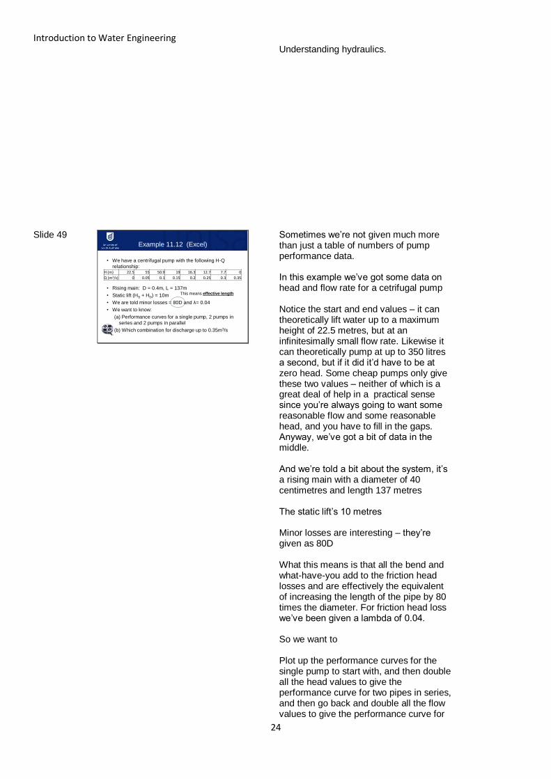
• We have a centrifugal pump with the following H-Q
relationship:
• Rising main: D = 0.4m, L = 137m
• Static lift (HS + HD) = 10m
• We are told minor losses = 80D and λ= 0.04
• We want to know:
(a) Performance curves for a single pump, 2 pumps in
series and 2 pumps in parallel
(b) Which combination for discharge up to 0.35m3/s
Example 11.12 (Excel)
H (m) 22.5 55 50.9 19 16.3 12.7 7.7 0
Q (m3/s) 0 0.05 0.1 0.15 0.2 0.25 0.3 0.35
This means effective length
Sometimes we’re not given much more than just a table of numbers of pump performance data. In this example we’ve got some data on head and flow rate for a cetrifugal pump Notice the start and end values – it can theoretically lift water up to a maximum height of 22.5 metres, but at an infinitesimally small flow rate. Likewise it can theoretically pump at up to 350 litres a second, but if it did it’d have to be at zero head. Some cheap pumps only give these two values – neither of which is a great deal of help in a practical sense since you’re always going to want some reasonable flow and some reasonable head, and you have to fill in the gaps. Anyway, we’ve got a bit of data in the middle. And we’re told a bit about the system, it’s a rising main with a diameter of 40 centimetres and length 137 metres The static lift’s 10 metres Minor losses are interesting – they’re given as 80D What this means is that all the bend and what-have-you add to the friction head losses and are effectively the equivalent of increasing the length of the pipe by 80 times the diameter. For friction head loss we’ve been given a lambda of 0.04. So we want to Plot up the performance curves for the single pump to start with, and then double all the head values to give the performance curve for two pipes in series, and then go back and double all the flow values to give the performance curve for
Introduction to Water Engineering
25
two pipes in parallel. Then, based on a target discharge of 350 litres a second, we want to figure out whether to use the series or parallel combo. Obviously we can tell we won’t get there using a single pump on its own since it can only discharge that flow rate at zero head.
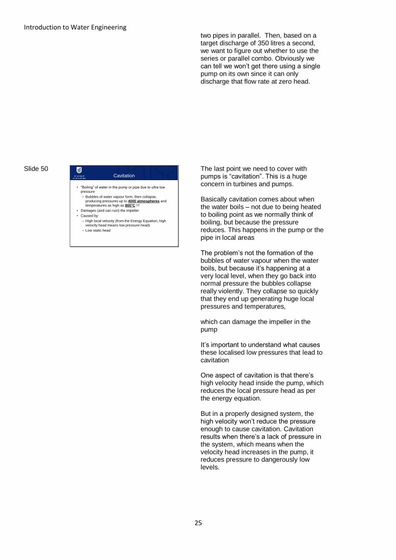
Slide 50
• “Boiling” of water in the pump or pipe due to ultra low
pressure
– Bubbles of water vapour form, then collapse,
producing pressures up to 4000 atmospheres and
temperatures as high as 800 C !!!
• Damages (and can ruin) the impeller
• Caused by:
– High local velocity (from the Energy Equation, high
velocity head means low pressure head)
– Low static head
Cavitation
The last point we need to cover with pumps is “cavitation”. This is a huge concern in turbines and pumps. Basically cavitation comes about when the water boils – not due to being heated to boiling point as we normally think of boiling, but because the pressure reduces. This happens in the pump or the pipe in local areas The problem’s not the formation of the bubbles of water vapour when the water boils, but because it’s happening at a very local level, when they go back into normal pressure the bubbles collapse really violently. They collapse so quickly that they end up generating huge local pressures and temperatures, which can damage the impeller in the pump It’s important to understand what causes these localised low pressures that lead to cavitation One aspect of cavitation is that there’s high velocity head inside the pump, which reduces the local pressure head as per the energy equation. But in a properly designed system, the high velocity won’t reduce the pressure enough to cause cavitation. Cavitation results when there’s a lack of pressure in the system, which means when the velocity head increases in the pump, it reduces pressure to dangerously low levels.

Introduction to Water Engineering
26
Slide 51
• The fluid pressure required to prevent cavitation in a
given pump is called Net Positive Suction Head (NPSH):
• NPSH (m) = HATM – HVAP – HS – hFS
Preventing cavitation
Atmospheric pressure
Vapour pressure of liquid
Maximum allowable static suction lift
Friction & minor losses
in suction pipe
(all pressures expressed in metres
of water)
The fluid pressure required to prevent cavitation is called the Net Positive Suction Head (NPSH). It’s equal to atmospheric pressure minus the vapour pressure of the liquid, which varies with temperature, minus maximum allowable static suction lift minus friction and minor losses in suction pipe. Obviously all of these need to be expressed in metres of water to be consistent with the units of NPSH. It’s all about the suction side of the pump because that’s what determines the pressure in the water entering the pump.
Slide 52
• Determined during pump design & testing
• Usually quoted by the pump manufacturer
• So for a given system, we can determine maximum
allowable static suction lift (HS) + friction in the suction
pipe (hSF):
HS + hFS = HATM - HVAP – NPSH
NPSH – a pump specification
The Net Positive Suction Head required for safe operation, or in other words to prevent cavitation, is generally based on the outcomes of the design and testing of a pump So it’s a property of the pump that gets quoted by the pump manufacturer, along with the operating characteristics of head and discharge, power consumption and so on. So what we need to know is how we use that piece of information in our overall system design to make sure the pump gets enough pressure to prevent cavitation. What we do is rearrange the equation on the previous slide to give us the design parameters – that is, the static lift and friction head loss in the suction side, equal to the atmospheric pressure minus the vapour pressure minus the NPSH term from the pump manufacturer. So the larger the vapour pressure and the larger the value of NPSH, the lower the allowable suction lift plus friction loss. If the right-hand side of this equation drops below zero, you need to physically lower the pump to make HS negative, in other words installing the pump below the water surface.

Introduction to Water Engineering
27
Slide 53
• HATM is about 10m
• HVAP for water varies with temperature
– 0m at 0 C
– 0.2m at 20 C
– 0.8m at 40 C
– 2m at 60 C
– 10m at 100 C
Few Assumptions
We can assume few things. For a start, atmospheric pressure’s fairly constant at about 10 m of water Vapour pressure varies with temperature; at 0 degrees Celsius, it’s 0 m; at 100 degrees it’s 10 m. What this means is the warmer the water, the closer you are to boiling anyway, and if you hypothetically had a pump that could cope with water as hot as 100 degrees, it’d be basically boiling on its own, and to prevent cavitation you’d need to put the pump a long way under the water surface to drive the HS term way down below zero. The good news is it’s a non-linear relationship so you’ve got a fairly wide range of temperatures you can handle without increasing the vapour pressure too much. Obviously if you’re pumping something other than water, like hydrocarbons for instance, it could have a different NPSH requirement and the vapour pressures are all going to be different. But then you’d have different viscosities and densities and everything anyway so your whole hydraulic system’d be totally different.
Slide 54
• Allow, say, HVAP = 1m
• HS + hFS = HATM - HVAP – NPSH
• HS + hFS = 10 – 1 – 2.5 = 6.5m
• So if the pump is located 5m above the water level (i.e.
HS = 5), that leaves 1.5m for friction and minor losses in
the suction pipe
– We would have to design the suction pipe accordingly
(pipe diameter, valves, bends etc so that
total losses < 1.5m)
• Sometimes, design guidelines may specify a safety
margin (say, 600mm)
Suppose a pump has NPSH=2.5m
Okay, a little example. Suppose a pump has a required NPSH equal to 2.5 m Say we’ve got vapour pressure at 1 m. So we put this into our equation And total suction lift becomes 6.5 m based on the assumption of HATM = 10 metres. So in practical terms, if the pump’s positioned 5 metres above the water level, it leaves 1.5 m available for friction and minor losses in the suction pipe. That means we’d have to design the suction pipe accordingly, so pipe diameter, valves, bends etc. such that the total energy head loss is less than 1.5 metres. If we couldn’t possibly design the pipe to give less than 1.5 metres of head loss, we’d have to turn round and lower the pump. We also need to use a safety margin. If that was, say, 600 millimetres, it’d reduce the total from 6.5 down to 5.9 metres, and so on.

Introduction to Water Engineering
28
Slide 55
• Very roughly...
– Occurs due to momentum of moving water when a
pump is suddenly switched off, or when a valve is
suddenly closed or opened.
• Surge can be said to be likely to occur when:
where L is the length of the pipe, and c is the acoustic
velocity of water (i.e. the speed of sound in water),
typically 900-1250 m/s
Surge
22
c
L
The final thing we’re looking at today is a phenomenon called “surge”, but really this is left to more advanced hydraulics, and we’re just mentioning it here so you’re aware of it. Put very simply, surge occurs due to the momentum of moving water when a pump is suddenly switched off, or when a valve is suddenly closed or opened. The sudden change in momentum translates to a pressure wave that moves through the pipe much faster than the physical movement of the water itself. Think about how fast sound waves can propagate through the air, compared to how fast the air actually moves for instance due to wind. Actually the sound wave concept is more than just an analogy, because surge is essentially a sound wave moving up and down the pipe. It tends to occur in pipes that are relatively long with respect to the acoustic velocity of water. The typical value of the acoustic velocity, c, is around 1000 m/s but it varies in different water types. As I said we won’t do any more on this – you can find out a bit more by reading the section in the textbook but apart from that I expect you’ll visit it in later studies.
Slide 56 Summary
- Pumps
- Energy and efficiency
- Pump performance
- Pump selection
- Pumps in series and parallel
So in summary, we looked briefly at turbines but mostly pumps, we worked out how to determine the power of moving water and therefore understand the efficiency of pumps, as well as pump performance and selection and how to design systems with pumps in series or parallel.

Introduction to Water Engineering
29
Slide 57
Thank you
If you’ve got any questions or need further clarification please post a question or comment on the Forum.
Related Documents