MODULE 2 ONE-WAY ANOVA - Derek Oglederekogle.com/NCMTH207/book/One-Way ANOVA.pdf · 2019-03-31 · 2.1. ANALYTICAL FOUNDATION MODULE 2. ONE-WAY ANOVA Atwo-sample t-test is used speci

MODULE 2

ONE-WAY ANOVAModule Objectives:

1. Understand the hypotheses tested with a one-way ANOVA.

2. Understand the models tested with a one-way ANOVA.

3. Identify the four assumptions of a one-way ANOVA.

4. Identify how to test the assumptions of a one-way ANOVA.

5. Understand why 2-sample t-tests cannot be used to make all pairwise comparisons.

6. Understand why multiple comparisons follow a significant one-way ANOVA.

7. Understand the distinction between individual-wise and experiment-wise error rates.

8. Understand the strengths and weaknesses of Tukey-Kramer HSD and Dunnett’s multiple compar-ison procedures.

9. Understand what transformations are used for in a one-way ANOVA.

10. Understand how to use the trial-and-error method to choose a power transformation.

11. Present the results of a one-way ANOVA in an efficient, comprehensive, readable format.

17

2.1. ANALYTICAL FOUNDATION MODULE 2. ONE-WAY ANOVA

A two-sample t-test is used specifically when the means of two independent populations are com-pared. Many realistic experiments and samples result in the comparison of means from more than two

independent populations. For example, consider the following situations:

• Determining if the mean volume of white blood cells of Virginia opossums (Didelphis virginiana)differed by season in the same year (Woods and Hellgren 2003).

• Determining if the mean frequency of occurrence of badgers (Meles meles) in plots differs betweenplots at different locations (Virgos and Casanovas 1999).

• Testing for differences in the mean total richness of macroinvertebrates between the three zones of ariver (Grubbs and Taylor 2004).

• Testing if the mean mass of porcupines (Erithizon dorsatum) differs among months of summer (Sweitzerand Berger 1993).

• Testing if the mean clutch size of spiders differs among three types of parental care categories (Simpson1995).

• Determining if the mean age of harvested deer (Odocoelius virginianus) differs among deer harvestedfrom Ashland, Bayfield, Douglas, and Iron counties.

In each of these situations, the mean of a quantitative variable (e.g., age, frequency of occurrence, totalrichness, or body mass) is compared among two or more populations of a single factor variable (e.g., county,locations, zones, or season). A two-sample t-test cannot be used in these situations because more thantwo groups are compared. A one-way analysis of variance (or one-way ANOVA) may be used in thesesituations. The theory and application of one-way ANOVAs are discussed in this module.1

� The two-sample t-test is used to determine if a significant difference exists between themeans of two populations.

� A one-way analysis of variance (ANOVA) is used to determine if a significant differenceexists among the means of more than two populations.

2.1 Analytical Foundation

The generic null hypothesis for a one-way ANOVA is

H0 : µ1 = µ2 = . . . = µI

where I is the total number of groups identified by the factor variable. From this, it is evident that theone-way ANOVA is a direct extension of the two-sample t-test (see Section 1.1). The alternative hypothesisis complicated because not all pairs of means need differ for the null hypothesis to be rejected. Thus, thealternative hypothesis for a one-way ANOVA is “wordy” and is often written as

HA : “At least one pair of means is different”

Thus, a rejection of the null hypothesis in favor of this alternative hypothesis is a statement that somedifference in group means exists. It does not clearly indicate which group means differ. Methods to identifywhich group means differ are in Section 2.4.

1This module depends heavily on the foundational material in Module 1.

18

MODULE 2. ONE-WAY ANOVA 2.1. ANALYTICAL FOUNDATION

The simple and full models for the one-way ANOVA are the same as those for the two-sample t-test, exceptthat there are I > 2 means in the full model (Figure 2.1). Thus, SStotal, SSwithin, and SSamong arecomputed using the same formulas – i.e., Equations (1.3.2), (1.3.3), and (1.3.5) – except to note that I > 2.The degrees-of-freedom are computed similarly – i.e., dfWithin = n − I and dfAmong = I − 1. The MS, F ,and p-value are also computed the same.2

0.4

0.5

0.6

0.7

0.8

0.9

Season

Imm

unog

lobu

lin C

once

ntra

tion

Feb May Nov

Figure 2.1. Immunoglobulin concentrations in Virginia opossums sampled from different seasons. The redhorizontal line represents the simple model of a grand mean for both groups. The three blue horizontal linesrepresent the full model of separate means for each group.

� The numerator df in a one-way ANOVA are I − 1.

� The denominator df in a one-way ANOVA are n− I.

2.1.1 One-way ANOVA in R

Data Format

As with a two-sample t-test, the data for a one-way ANOVA must be stacked (Section 1.1.1). For example,the Opposums.csv (view, download, meta) file contains the immunoglobulin concentration levels measuredon Virginia opossums sampled from three different seasons. The structure of the data file indicates twovariables – imm, the immunoglobulin concentration levels, and season, the season the opossum was sampled– for 27 opossums. In addition, the structure indicates that the season variable is a factor with three levels.The display of several lines of the file shows the stacked nature of the data.

> opp <- read.csv("Opposums.csv")

> str(opp)

'data.frame': 27 obs. of 2 variables:

$ imm : num 0.64 0.68 0.731 0.587 0.668 0.613 0.713 0.701 0.729 0.726 ...

$ season: Factor w/ 3 levels "feb","may","nov": 1 1 1 1 1 1 1 1 1 1 ...

2The MS, F , and p-value are computed the same in nearly every ANOVA table encountered in this class.

19

https://github.com/droglenc/NCData/blob/master/Opposums.csv

https://raw.githubusercontent.com/droglenc/NCData/master/Opposums.csv

https://github.com/droglenc/NCData/blob/master/Opposums_meta.txt

2.2. ASSUMPTIONS MODULE 2. ONE-WAY ANOVA

> headtail(opp)

imm season

1 0.640 feb

2 0.680 feb

3 0.731 feb

25 0.490 nov

26 0.333 nov

27 0.492 nov

Recall that the levels of a factor variable are ordered alphabetically by default. In this example, the alpha-betical ordering is acceptable; i.e., “feb”, “may”, and “nov” is both the alphabetic and natural order forthese levels. Changing the order of the levels was described in Section 1.1.3.

Fitting Model & Results

A one-way ANOVA model is fit with lm() exactly as described for a two-sample t-test in Section 1.1.3.3

For example, the very small p-value (p < 0.0005) below indicates that the full model of a separate mean foreach group fits the data “better” than the simple model of one common mean. Thus, there is a significantdifference in mean immunoglobulin level between at least one pair of the three seasons.

> opp.lm <- lm(imm~season,data=opp)

> anova(opp.lm)

Analysis of Variance Table

Response: imm

Df Sum Sq Mean Sq F value Pr(>F)

season 2 0.23401 0.117005 14.449 7.609e-05

Residuals 24 0.19435 0.008098

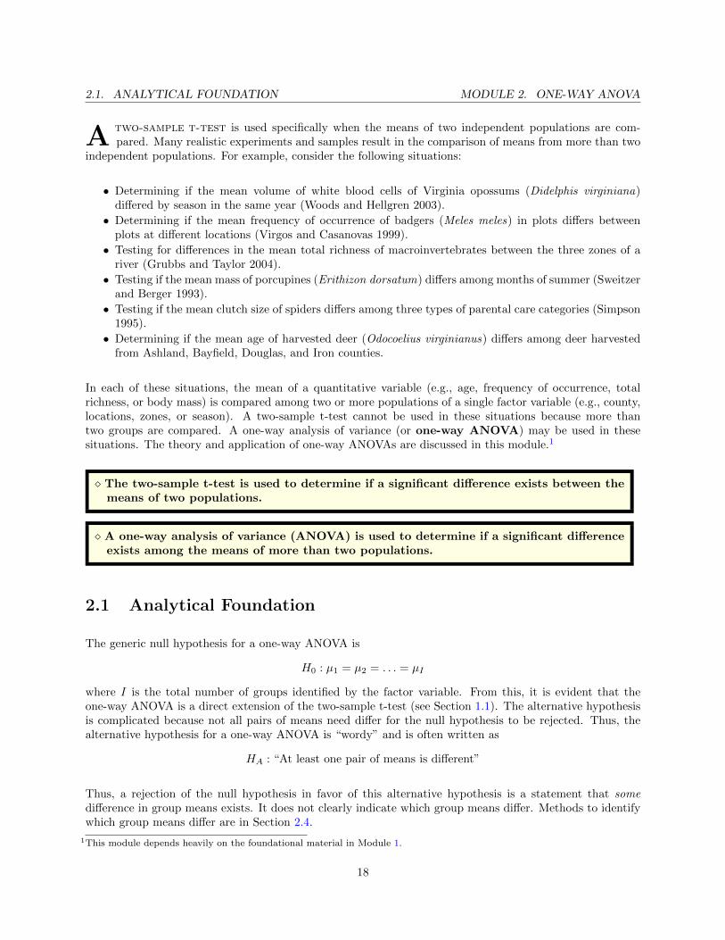
The natural reaction at this point is to ask “Which means are different?”. This question will be answeredmore completely in Section 2.4. However, giving the saved linear model object to fitPlot() will produce agraphic to visually compare group means (Figure 2.2).

> fitPlot(opp.lm,xlab="Season",ylab="Immunoglobulin Concentration")

2.2 Assumptions

A one-way ANOVA has the same assumptions as a two-sample t-test. The four assumptions are

1. independence of individuals within and among groups,

2. equal variances among groups,

3. normality of residuals within each group, and

4. no outliers

3The aov() function can also be used. However, aov() calls lm() to make the calculations. For this reason, and the fact thatlm() is more general and can be used for a wider variety of situations, only lm() is discussed here.

20

MODULE 2. ONE-WAY ANOVA 2.2. ASSUMPTIONS

0.5

0.6

0.7

0.8

Season

Imm

unog

lobu

lin C

once

ntra

tion

feb may nov

Figure 2.2. Mean (with 95% CI) immunoglobulin concentrations in Virginia opossums from different seasons.

� The one-way ANOVA has four assumptions: independence among individuals, equalvariances among groups, normality within groups, and no outliers.

It is critical to the proper analysis and interpretation of one-way ANOVAs that the individuals are indepen-dent both within and among groups. In other words, there must be no connections between the individualswithin a group or between individuals among groups. Examples of a lack of independence include applyingmultiple treatments to the same individual (e.g., treatment A in week 1, treatment B in week 2, etc.), havingall related individuals within the same group (e.g., all siblings are in the same group), or having individualsthat are not separated in space and time (e.g., the first four individuals receive treatment A, the secondfour individuals receive treatment B, etc., or four clustered individuals are in group A, four other clusteredindividuals are in group B, etc.). Violations of this assumption are usually detected by careful considerationof the design of the data collection. Violations that are discovered after the data are collected cannot becorrected and the data have to be analyzed with techniques specific to dependent data. In other words, de-signing data collections with independence among individuals is critical and needs to be ascertained beforethe data are collected.

� Independence of individuals is a critical assumption of one-way ANOVAs. Violations ofthis assumption cannot be corrected.

The variances among groups must be equal because the estimate of MSWithin is based on a pooling ofestimates from the individual groups. In other words, if the variances among each group are equal, then theMS within each group is an estimate of the overall MSWithin. In this instance, combining the values fromeach group provides a robust estimate of the overall variance within groups.

The assumption of equal variances can be tested with Levene’s homogeneity of variances test.4 The hypothe-ses tested by Levene’s test are

H0 : σ21 = σ2

2 = · · · = σ2I

HA : “At least one pair of variances is different”

4There are a wide variety of statistical tests for examining equality of variances. We will use the Levene’s test in this classbecause it is common in the literature and simple to implement in most statistical software packages.

21

2.2. ASSUMPTIONS MODULE 2. ONE-WAY ANOVA

Thus, a p-value less than α means that the variances are not equal and the assumption of the one-wayANOVA has not been met.5

In certain instances,6 Levene’s test is not practical for examining the equality of variances. In these instances,the equality of variances may be visually examined with a boxplot of full model residuals by group. If the“boxes” on this boxplot are not roughly the same, then the equal variances assumption may be violated.This boxplot should only be used if Levene’s test cannot be used to test for equal variances.

� Equal variances among groups is a critical assumption of a one-way ANOVA. Violationsof this assumption should be corrected.

� The equal variance assumption is tested with Levene’s test. P-values less than α indicatethat the variances are not equal and the assumption was violated.

The normality of residuals WITHIN each group is difficult to test because there may be (1) many groupsbeing considered or (2) relatively few individuals in each group. Because most linear models are robustto slight departures from normality, it is often assumed that if the full model residuals are approximatelynormally distributed, then the residuals within each group are also normally distributed. Thus, the normalityassumption for one-way ANOVA reduces to examining the normality of full model residuals together (i.e.,not separated by groups).

The normality of residuals may be tested with the Anderson-Darling Normality Test.7 In this instance, thehypotheses tested by an Anderson-Darling test are

H0 : “Residuals are normally distributed”

HA : “Residuals are not normally distributed”

An Anderson-Darling p-value greater than α indicates that the residuals appear to be normally distributedand the normality assumption is met. An Anderson-Darling p-value less than α suggests that the normalityassumption has been violated.

� The normality assumption is tested with the Anderson-Darling test of the full modelresiduals. P-values less than α indicate that the residuals are not normally distributedand the normality assumption was violated.

As mentioned before, the one-way ANOVA is robust to slight departures from normality within groups.Some authors argue that a one-way ANOVA can still be used if the residuals from the one-way ANOVA fitare, at least, not strongly skewed and the sample size is moderately large. Thus, if the Anderson-Darlingnormality test suggests non-normality in the residuals, one should construct a histogram of the residuals todetermine if they are not strongly skewed. If the residuals are strongly skewed, then the methods of Section2.6 should be considered. If the residuals are only slightly skewed and the other assumptions have been met,then one can proceed relatively confidently with a one-way ANOVA.

5Methods for “working around” this assumption are discussed in Section 2.6.6For example, if there is a large number of groups with a small number of individuals each or if only one individual perblock-treatment combination is used.

7There are also a wide variety of normality tests. Some authors even argue against the use of hypothesis tests for testingnormality and suggest the use of graphical methods instead. For simplicity, the Anderson-Darling normality test will be usedthroughout this book.

22

MODULE 2. ONE-WAY ANOVA 2.2. ASSUMPTIONS

� A one-way ANOVA is robust to slight violations of the normality assumption. Severeviolations of this assumption should be corrected.

The one-way ANOVA is very sensitive to outliers. Outliers should be corrected if possible (usually if thereis a data transcription or entry problem). The outlier should be deleted if it is determined that the outlieris clearly in error or is not part of the population of interest. If the outlier is not corrected or deleted, thenthe relative effect of the outlier on the analysis should be determined by completing the analysis with andwithout the outlier present. Any differences in results or interpretations due to the presence of the outliershould be clearly explained to the reader.

� A one-way ANOVA is very sensitive to outliers.

� Outliers that are obvious errors should be fixed or deleted. The effect of outliers thatare not errors should be assessed by completing the one-way ANOVA with and withoutthe outlier in the data set.

Outliers may be detected by visual examination of a residual plot. In addition, potential outliers can be moreobjectively detected with Studentized residuals, which is a residual divided by the standard deviation of theresidual. Because residuals have a mean of zero, this calculation essentially computes how many standarddeviations an individual residual is from the group mean. Because this is the standard definition of a t teststatistic, Studentized residuals have the property of following a t distribution with n− I df.

One problem with Studentized residuals is that the standard deviation of the residual is inflated if the indi-vidual is indeed an outlier. One method of correcting this problem is to compute the standard deviation ofthe residual with that residual removed from the data. This standard deviation is called the “leave-one-out”standard deviation and is common practice for many calculations aimed at finding potential outliers. A Stu-dentized residual computed with the “leave-one-out” standard deviation is called an externally Studentizedresidual.8 Externally Studentized residuals will be used exclusively in this course and will simply be calledStudentized residuals.

The main advantage of Studentized residuals is that their distribution is well known – i.e., they follow at distribution with degrees-of-freedom equal to dfWithin − 1 or n − I − 1.9 This allows construction of ahypothesis test to determine whether an individual can be considered to be a significant outlier or not. Thep-value for this hypothesis test is calculated by converting the Studentized residual to a two-tailed p-valueusing a t distribution.

This method of testing for outliers is “dangerous” because the researcher will “sort through” all of theresiduals to focus on the most extreme residual. So, in essence, the researcher constructs n hypothesistests, but only focuses on one. This type of “testing” leads to a difficulty called the “problem of multiplecomparisons”, which is discussed in much more detail in Section 2.4. The multiple comparisons problem canbe conservatively corrected with a Bonferroni correction, which constructs an adjusted p-value by multiplyingthe original p-value by the number of comparisons made (in this case n). If the Bonferroni adjusted p-valuefor the most extreme residual is less than α, then that individual is considered to be a significant outlier andshould be flagged for further inspection as described above.

8Some authors call these jackknife residuals.9The extra one is subtracted because of the “leave-one-out” practice.

23

2.3. EXAMPLE ANALYSES I MODULE 2. ONE-WAY ANOVA

2.2.1 Assumption Checking in R

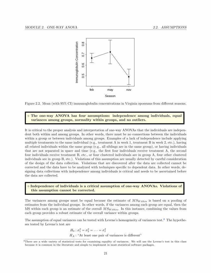
All plots and tests of assumptions can be completed by submitting the saved lm object to transChooser().A residual plot and histogram of residuals will be produced. In RStudio, a ”gear icon” will appear in theupper-left corner of this plot. Open this gear icon and select ”Use Boxplot for Residuals” and, to show theassumptions tests results, ”Show Test Results.” With this the p-values from the Levene’s, Anderson-Darling,and outlier tests10 will be shown on the plot (Figure 2.3).11

> transChooser(opp.lm)

Thus, in this example, it appears that the variances among the three seasons are equal (p = 0.371),12 theresiduals are not non-normal (p = 0.061) or strongly skewed, and there were no significant outliers (p > 1).13

Therefore, the assumptions of a one-way ANOVA have been met for these data.

Figure 2.3. Residual plot (Left) and histogram of residuals (Right) for the one-way ANOVA of immunoglob-ulin concentrations in Virginia opossums sampled from different seasons.

2.3 Example Analyses I

2.3.1 Tomatoes-Nematodes I

Nematodes are microscopic worms found in soil that may negatively affect the growth of plants through theirtrophic dynamics. Tomatoes are a commercially important plant species that may be negatively affected byhigh densities of nematodes in culture situations.

10Note that significant outliers, as identified with outlierTest(), will be marked with the observation number on the defaultresidual plot from residPlot().

11Note that the individual tests can be constructed with levenesTest(), adTest(), and outlierTest() and the residual plot canbe constructed with residPlot().

12Note also that the “box” heights in Figure 2.3-Left are “roughly” equal, but that the Levene’s test result is the definitive answerabout equal variances in this instance.

13ndividual 19 had an absolute value of the Studentized residual of 2.175 and a Bonferroni-adjusted p > 1. Note that R will notshow p-values greater than 1 and returns an NA instead. There is also a note at the beginning of this output that shows that noBonferroni p-value is < 1. This adjusted p-value is much greater than α and, thus, there is no indication of an outlier in thesedata.

24

MODULE 2. ONE-WAY ANOVA 2.3. EXAMPLE ANALYSES I

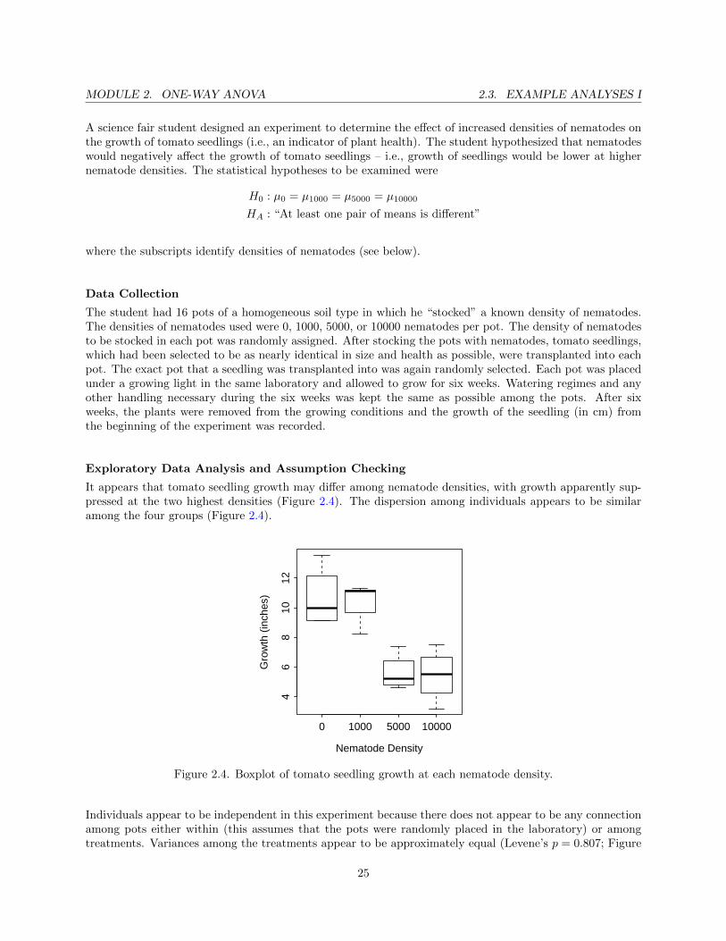
A science fair student designed an experiment to determine the effect of increased densities of nematodes onthe growth of tomato seedlings (i.e., an indicator of plant health). The student hypothesized that nematodeswould negatively affect the growth of tomato seedlings – i.e., growth of seedlings would be lower at highernematode densities. The statistical hypotheses to be examined were

H0 : µ0 = µ1000 = µ5000 = µ10000


where the subscripts identify densities of nematodes (see below).

Data Collection

The student had 16 pots of a homogeneous soil type in which he “stocked” a known density of nematodes.The densities of nematodes used were 0, 1000, 5000, or 10000 nematodes per pot. The density of nematodesto be stocked in each pot was randomly assigned. After stocking the pots with nematodes, tomato seedlings,which had been selected to be as nearly identical in size and health as possible, were transplanted into eachpot. The exact pot that a seedling was transplanted into was again randomly selected. Each pot was placedunder a growing light in the same laboratory and allowed to grow for six weeks. Watering regimes and anyother handling necessary during the six weeks was kept the same as possible among the pots. After sixweeks, the plants were removed from the growing conditions and the growth of the seedling (in cm) fromthe beginning of the experiment was recorded.

Exploratory Data Analysis and Assumption Checking

It appears that tomato seedling growth may differ among nematode densities, with growth apparently sup-pressed at the two highest densities (Figure 2.4). The dispersion among individuals appears to be similaramong the four groups (Figure 2.4).

0 1000 5000 10000

46

810

12

Nematode Density

Gro

wth

(in

ches

)

Figure 2.4. Boxplot of tomato seedling growth at each nematode density.

Individuals appear to be independent in this experiment because there does not appear to be any connectionamong pots either within (this assumes that the pots were randomly placed in the laboratory) or amongtreatments. Variances among the treatments appear to be approximately equal (Levene’s p = 0.807; Figure

25


2.5-Left), the residuals appear to be approximately normally distributed (Anderson-Darling p = 0.927) andthe histogram does not indicate any major skewness (Figure 2.5-Right), and there does not appear to be anymajor outliers in the data (outlier test p = 0.671; Figure 2.5). The analysis will proceed because the majorassumptions of the one-way ANOVA have been met.

Figure 2.5. Boxplot (Left) and histogram (Right) of residuals from the initial fit of the one-way ANOVAmodel to the tomato seedling growth at each nematode density.

Results

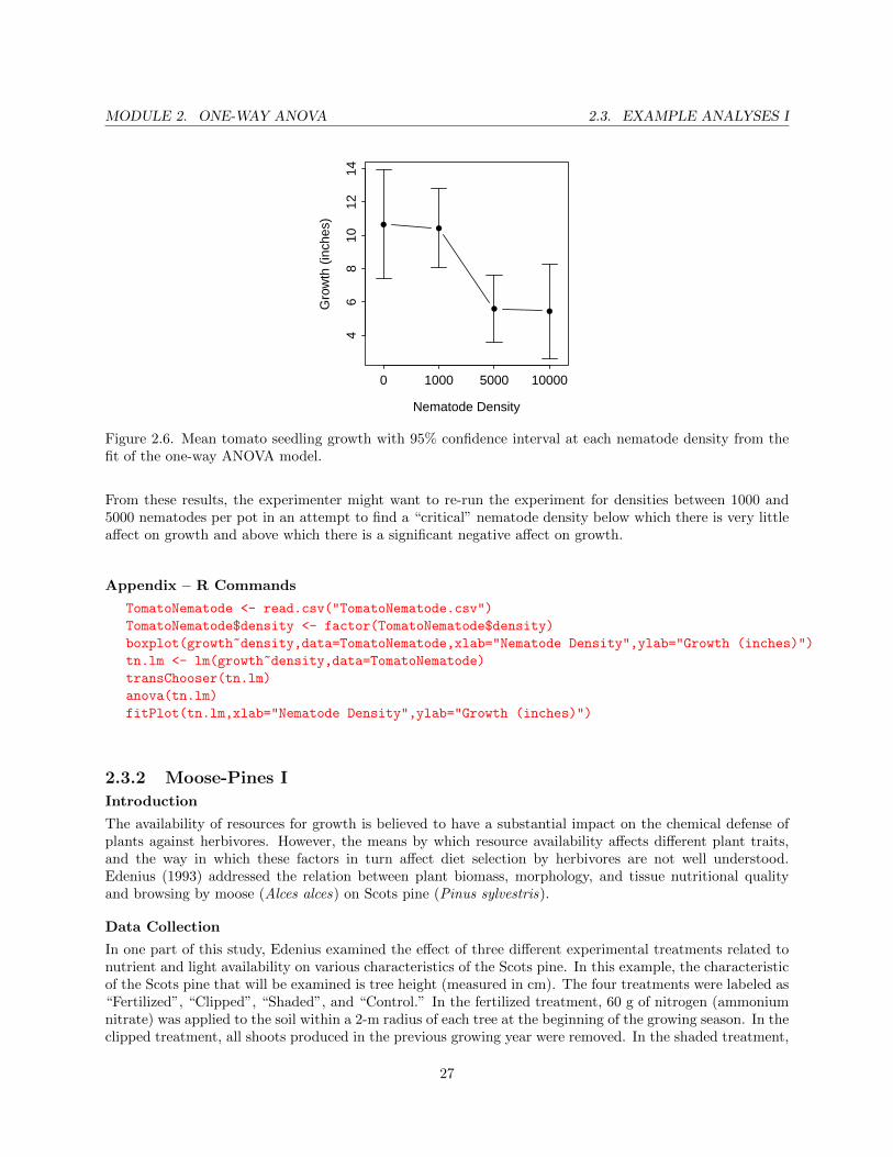
There appears to be a significant difference in mean tomato seedling growth among the four treatments(p = 0.001; Table 2.1). The plot of each treatment mean with 95% confidence intervals indicates that themean growth at the two lowest nematode densities probably are not different and the mean growth at thetwo highest nematode densities probably are not different, but the mean growth at the two lowest nematodedensities are different from the two highest nematode densities (Figure 2.6).14

Table 2.1. ANOVA results for tomato seedling growth at four nematode densities.


density 3 100.647 33.549 12.08 0.0006163

Residuals 12 33.327 2.777

Conclusion

The student’s hypothesis was generally supported; however, it does not appear that tomato seedling growthis negatively affected for all increases in nematode density. For example, seedling growth declined for anincrease in nematode density from 1000 to 5000 per pot but not for increases from 0 to 1000 nematodes perpot or from 5000 to 10000 nematodes per pot.

It can be concluded that the different nematode densities caused the differences in tomato seedling growthbecause the individual seedlings were randomly allocated to treatment groups and all other variables werecontrolled. However, the inferences cannot be extended to a general population of tomatoes because the 16seedlings used in the experiment were not randomly chosen from the population of seedlings.

14Objective methods for determining which treatment means are significantly different are discussed in Section 2.4.

26


46

810

1214

Nematode Density

Gro

wth

(in

ches

)

0 1000 5000 10000

Figure 2.6. Mean tomato seedling growth with 95% confidence interval at each nematode density from thefit of the one-way ANOVA model.

From these results, the experimenter might want to re-run the experiment for densities between 1000 and5000 nematodes per pot in an attempt to find a “critical” nematode density below which there is very littleaffect on growth and above which there is a significant negative affect on growth.

Appendix – R Commands

TomatoNematode <- read.csv("TomatoNematode.csv")

TomatoNematode$density <- factor(TomatoNematode$density)

boxplot(growth~density,data=TomatoNematode,xlab="Nematode Density",ylab="Growth (inches)")

tn.lm <- lm(growth~density,data=TomatoNematode)

transChooser(tn.lm)

anova(tn.lm)

fitPlot(tn.lm,xlab="Nematode Density",ylab="Growth (inches)")

2.3.2 Moose-Pines I

Introduction

The availability of resources for growth is believed to have a substantial impact on the chemical defense ofplants against herbivores. However, the means by which resource availability affects different plant traits,and the way in which these factors in turn affect diet selection by herbivores are not well understood.Edenius (1993) addressed the relation between plant biomass, morphology, and tissue nutritional qualityand browsing by moose (Alces alces) on Scots pine (Pinus sylvestris).

Data Collection

In one part of this study, Edenius examined the effect of three different experimental treatments related tonutrient and light availability on various characteristics of the Scots pine. In this example, the characteristicof the Scots pine that will be examined is tree height (measured in cm). The four treatments were labeled as“Fertilized”, “Clipped”, “Shaded”, and “Control.” In the fertilized treatment, 60 g of nitrogen (ammoniumnitrate) was applied to the soil within a 2-m radius of each tree at the beginning of the growing season. In theclipped treatment, all shoots produced in the previous growing year were removed. In the shaded treatment,

27


the top- and lateral-most branches were covered with a shade cloth that reduced the light intensity by 50%in the 400-700 nm wavelengths. Finally, a fourth group of trees were maintained without any manipulationas a control.

A total of 140 unbrowsed trees that were approximately 1.4 m in height were specifically selected for use inthe experiment. The trees were randomly allocated to the four treatments such that each group had 35 treesin it. Selected trees were separated by at least 5 m to avoid interference among individual trees and, thus,treatment groups. Trees were allowed to grow for one full growing season and then were measured for height.Edenius, wanted to determine if there was a significantly different mean height among the treatments. Thus,

H0 : µFert = µClip = µShade = µControl


One-way ANOVA will be used to identify if any significant differences exist among the treatment means.

Exploratory Data Analysis and Assumption Checking

It appears that tree height differs among treatments, with the clipped group being substantially smallerthan the other three groups (Table 2.2, Figure 2.7). There is also some indication that the variances mightbe different as the standard deviation for the “control” group appears to be substantially larger than thestandard deviation for the “shaded” group (Table 2.2).

Control

Height (cm)

Fre

quen

cy

120 160 200

05

1015

Fertilized

Height (cm)

Fre

quen

cy

120 160 200

05

1015

Clipped

Height (cm)

Fre

quen

cy

120 160 200

05

1015

Shaded

Height (cm)

Fre

quen

cy

120 160 200

05

1015

Figure 2.7. Histograms of Scots pine height for four treatment groups.

The random allocation of trees to the treatments and the realization that applying the treatment to anyone tree has no affect on any other tree implies that there is independence both within a treatment andamong treatments. Variances among the treatments may be non-constant (Levene’s p = 0.049), though theresidual plot (Figure 2.8-Left) does not indicate any extreme differences in variances and no transformation(see Section 2.6) corrected this problem. The residuals from the initial model fit appear to be approximatelynormal (Anderson-Darling p = 0.543). None of the individuals appeared to be a significant outlier (outliertest p = 0.685). The one-way ANOVA analysis will continue as the assumptions either appear to be met,are not grossly unmet, or no reasonable solution to the problems exists.

Table 2.2. Descriptive statistics for height of Scots pines in four treatment groups.

treat n mean sd min Q1 median Q3 max

Control 35 165.3514 11.392138 144.9 157.55 164.7 173.15 185.6

Fertilized 35 170.8857 9.915352 145.9 165.35 171.6 175.15 192.8

Clipped 35 131.9314 7.838846 117.1 126.10 131.0 138.55 150.0

Shaded 35 163.9514 6.409156 150.7 159.25 162.8 169.25 175.3

28


Figure 2.8. Boxplot (Left) and histogram (Right) of residuals from the initial fit of the one-way ANOVAmodel to the Scots pines heights at each treatment level.

Results

There appears to be a significant difference in mean tree growth among the four treatments (p < 0.0005;Table 2.3). Plots for each treatment group indicate that mean height for the clipped treatment is lowerthan mean height in all other treatments, mean height in the fertilized treatment may be greater than meanheight in all other treatments, and mean heights in the shaded and control groups do not differ (Figure 2.9).

Table 2.3. ANOVA results for tree growth for four treatments.


treat 3 32728 10909.2 131.98 < 2.2e-16

Residuals 136 11241 82.7

Conclusion

The clipped treatment resulted in significantly lower growth of Scots pine. The fertilized treatment mayhave produced slightly taller trees than the control group.

It can be concluded that the different treatments caused the differences in tree growth because the individualtrees were randomly allocated to treatment groups and all other variables were controlled. However, theinferences cannot be extended to a general population of trees because the 140 trees used in the experimentwere not randomly chosen from the population of trees.

Appendix – R Commands

MooseBrowse <- read.csv("MooseBrowse.csv")

MooseBrowse$treat <- factor(MooseBrowse$treat,

levels=c("Control","Fertilized","Clipped","Shaded"))

Summarize(height~treat,data=MooseBrowse)

hist(height~treat,data=MooseBrowse,xlab="Treatment",ylab="Tree Height (cm)")

mb.lm <- lm(height~treat,data=MooseBrowse)

transChooser(mb.lm)

anova(mb.lm)

fitPlot(mb.lm,xlab="Treatment",ylab="Tree Height (cm)")

29

2.4. MULTIPLE COMPARISONS MODULE 2. ONE-WAY ANOVA

130

140

150

160

170

Treatment

Tree

Hei

ght (

cm)

Control Fertilized Clipped Shaded

Figure 2.9. Mean Scots pine height with 95% confidence interval for each treatment group from the initialfit of the one-way ANOVA model.

2.4 Multiple Comparisons

A significant result (i.e., reject H0) in a one-way ANOVA indicates that the means of at least one pair ofgroups differ. At this time, it is not known whether all means are different, two means are equivalent butdifferent from all other means, all means are equivalent except for one pair, or any other possible combinationof equivalencies and differences. Thus, once a significant overall result is obtained in a one-way ANOVA,specific follow-up analyses are needed to identify which pairs of means are significantly different.

� A one-way ANOVA only indicates that at least one pair of means differ. Follow-upanalyses are required to specifically determine which pairs of means are different.

2.4.1 The Problem

The most obvious solution for identifying which pairs of means are different is to perform multiple two-samplet-tests on all pairs of groups. Unfortunately, this seemingly simple answer has at least two major difficulties.First, the number of two-sample t-tests needed increases dramatically with increasing numbers of groups(Table 2.4). Second, the probability of incorrectly concluding that at least one pair of means differs whenno pairs actually differ increases dramatically with increasing numbers of groups (Table 2.4). Of these twodifficulties, the second is much more problematic and needs to be better understood.

In any one comparison of two means the probability of incorrectly concluding that the means are differentwhen they are actually not different is α. This incorrect conclusion is called a Type I error and α is calledthe individual-wise Type I error rate because it relates to only one comparison of a pair of means.

∆ Individual-wise error rate: The probability of a Type I error in a single comparison of two means.The individual-wise error rate is set at α.

� A Type I error is rejecting H0 when H0 is actually true. In a two-sample t-test, a Type Ierror is concluding that two means are significantly different when in fact they are not.

30

MODULE 2. ONE-WAY ANOVA 2.4. MULTIPLE COMPARISONS

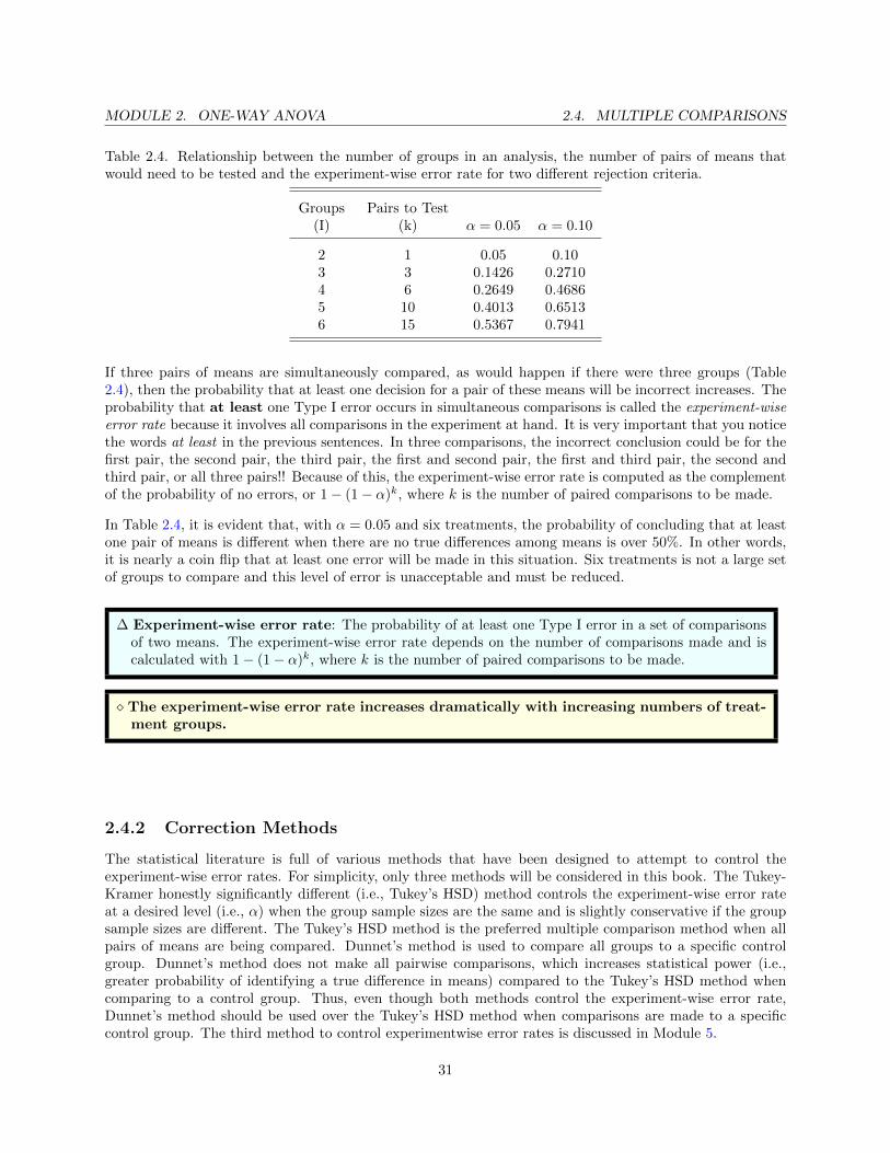
Table 2.4. Relationship between the number of groups in an analysis, the number of pairs of means thatwould need to be tested and the experiment-wise error rate for two different rejection criteria.

Groups Pairs to Test(I) (k) α = 0.05 α = 0.10

2 1 0.05 0.103 3 0.1426 0.27104 6 0.2649 0.46865 10 0.4013 0.65136 15 0.5367 0.7941

If three pairs of means are simultaneously compared, as would happen if there were three groups (Table2.4), then the probability that at least one decision for a pair of these means will be incorrect increases. Theprobability that at least one Type I error occurs in simultaneous comparisons is called the experiment-wiseerror rate because it involves all comparisons in the experiment at hand. It is very important that you noticethe words at least in the previous sentences. In three comparisons, the incorrect conclusion could be for thefirst pair, the second pair, the third pair, the first and second pair, the first and third pair, the second andthird pair, or all three pairs!! Because of this, the experiment-wise error rate is computed as the complementof the probability of no errors, or 1− (1− α)k, where k is the number of paired comparisons to be made.

In Table 2.4, it is evident that, with α = 0.05 and six treatments, the probability of concluding that at leastone pair of means is different when there are no true differences among means is over 50%. In other words,it is nearly a coin flip that at least one error will be made in this situation. Six treatments is not a large setof groups to compare and this level of error is unacceptable and must be reduced.

∆ Experiment-wise error rate: The probability of at least one Type I error in a set of comparisonsof two means. The experiment-wise error rate depends on the number of comparisons made and iscalculated with 1− (1− α)k, where k is the number of paired comparisons to be made.

� The experiment-wise error rate increases dramatically with increasing numbers of treat-ment groups.

2.4.2 Correction Methods

The statistical literature is full of various methods that have been designed to attempt to control theexperiment-wise error rates. For simplicity, only three methods will be considered in this book. The Tukey-Kramer honestly significantly different (i.e., Tukey’s HSD) method controls the experiment-wise error rateat a desired level (i.e., α) when the group sample sizes are the same and is slightly conservative if the groupsample sizes are different. The Tukey’s HSD method is the preferred multiple comparison method when allpairs of means are being compared. Dunnet’s method is used to compare all groups to a specific controlgroup. Dunnet’s method does not make all pairwise comparisons, which increases statistical power (i.e.,greater probability of identifying a true difference in means) compared to the Tukey’s HSD method whencomparing to a control group. Thus, even though both methods control the experiment-wise error rate,Dunnet’s method should be used over the Tukey’s HSD method when comparisons are made to a specificcontrol group. The third method to control experimentwise error rates is discussed in Module 5.

31

2.4. MULTIPLE COMPARISONS MODULE 2. ONE-WAY ANOVA

� Use Tukey’s HSD method when comparing all pairwise means.

� Use Dunnett’s method when comparing all means to a single control group.

2.4.3 Multiple Comparisons in R

Tukey’s HSD

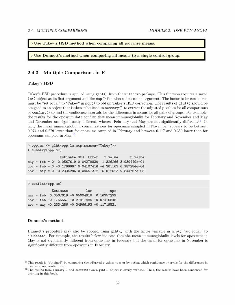
Tukey’s HSD procedure is applied using glht() from the multcomp package. This function requires a savedlm() object as its first argument and the mcp() function as its second argument. The factor to be consideredmust be “set equal” to "Tukey" in mcp() to obtain Tukey’s HSD correction. The results of glht() should beassigned to an object that is then submitted to summary() to extract the adjusted p-values for all comparisonsor confint() to find the confidence intervals for the differences in means for all pairs of groups. For example,the results for the opossum data confirm that mean immunoglobulin for February and November and Mayand November are significantly different, whereas February and May are not significantly different.15 Infact, the mean immunoglobulin concentrations for opossums sampled in November appears to be between0.074 and 0.279 lower than for opossums sampled in February and between 0.117 and 0.350 lower than foropossums sampled in May.16

> opp.mc <- glht(opp.lm,mcp(season="Tukey"))

> summary(opp.mc)

Estimate Std. Error t value p value

may - feb = 0 0.0567619 0.04279830 1.326266 3.939449e-01

nov - feb = 0 -0.1766667 0.04107416 -4.301163 6.987284e-04

nov - may = 0 -0.2334286 0.04657372 -5.012023 9.844767e-05

> confint(opp.mc)

Estimate lwr upr

may - feb 0.0567619 -0.05004918 0.16357299

nov - feb -0.1766667 -0.27917485 -0.07415848

nov - may -0.2334286 -0.34966193 -0.11719521

Dunnett’s method

Dunnett’s procedure may also be applied using glht() with the factor variable in mcp() “set equal” to"Dunnett". For example, the results below indicate that the mean immunoglobulin levels for opossums inMay is not significantly different from opossums in February but the mean for opossums in November issignificantly different from opossums in February.

15This result is “obtained” by comparing the adjusted p-values to α or by noting which confidence intervals for the differences inmeans do not contain zero.

16The results from summary() and confint() on a glht() object is overly verbose. Thus, the results have been condensed forprinting in this book.

32

MODULE 2. ONE-WAY ANOVA 2.4. MULTIPLE COMPARISONS

> opp.mc2 <- glht(opp.lm,mcp(season="Dunnett"))

> summary(opp.mc2)


may - feb = 0 0.0567619 0.04279830 1.326266 0.3370801781

nov - feb = 0 -0.1766667 0.04107416 -4.301163 0.0004836763

> confint(opp.mc2)

Estimate lwr upr

may - feb 0.0567619 -0.04437157 0.15789538

nov - feb -0.1766667 -0.27372596 -0.07960737

It is vitally important to note that all other groups will be compared to the group that is the first level inthe factor variable. If the “base” group is not the first level of the factor variable, then the levels will needto be changed with factor() as shown in Section 1.1.3. Suppose, for example, that you wanted “may” tobe the group that “feb” and “nov” would be compared to. The factor would then need to be re-leveled, anew linear model fit and saved, and this new model sent to glht().

> opp$season1 <- factor(opp$season,levels=c("may","feb","nov"))

> opp.lm2 <- lm(imm~season1,data=opp)

> opp.mc3 <- glht(opp.lm2,mcp(season1="Dunnett"))

> summary(opp.mc3)


feb - may = 0 -0.0567619 0.04279830 -1.326266 3.175589e-01

nov - may = 0 -0.2334286 0.04657372 -5.012023 7.787847e-05

Note that using the Dunnett’s procedure is unwarranted in this example – it is used here for the sole purposeof illustrating the method.

Graphing Significance Results

Multiple comparison results are often reported as ”significance letters” on a plot of group means (usuallywith corresponding confidence intervals). Significance letters are assigned such that group means with thesame letter are considered statistically the same (i.e., insignificant) and group means with different lettersare considered statistically different (i.e., significant). The Tukey HSD results for the opossum data fromabove indicated that February and May should have the same letter (e.g., “a”) and November should havea different letter (e.g., “b”).

The plot of the group means is constructed with fitPlot() as illustrated previously. Significance letters areadded to this plot with addSigLetters(). The first argument to addSigLetters() is the saved lm() object.The lets= argument is a character vector containing the letters to be placed next to each group mean, inthe order that the group means are plotted. The pos= argument contains a numeric vector of positionsthat describe the position the letter should be placed relative to the point, with 1=“below”, 2=“left-of”,3=“above”, and 4=“right-of”.17 Finding “good” pos values may take some trial-and-error. Figure 2.10 wasconstructed with the code below.

> fitPlot(opp.lm,xlab="Season",ylab="Immunoglobulin level")

> addSigLetters(opp.lm,lets=c("a","a","b"),pos=c(2,4,4))

17Note that the numbers are clockwise around the point beginning below the point.

33

2.5. EXAMPLE ANALYSES II MODULE 2. ONE-WAY ANOVA

0.5

0.6

0.7

0.8

Season

Imm

unog

lobu

lin le

vel

feb may nov

a

a

b

Figure 2.10. Mean tomato seedling growth with 95% confidence interval at each nematode density from theinitial fit of the one-way ANOVA model. Means with the same letter are not significantly different.

2.5 Example Analyses II

2.5.1 Tomatoes-Nematodes II

In Section 2.3.1 the growth of tomato plants relative to the density of nematodes was examined. The one-way ANOVA results indicated that there was a significant difference in mean plant growth among the fourdensities of nematodes examined. Tukey’s HSD procedure is used here to determine which pairs of groupsmeans differ.

It appears that mean growth at densities 0 and 1000 are not significantly different, 0 and 5000 are different,0 and 10000 are different, 1000 and 5000 are different, 1000 and 10000 are different, and 5000 and 10000 arenot different (Table 2.5, Figure 2.11).18

Table 2.5. Tukey’s multiple comparisons for the Tomato - Nematode data.


1000 - 0 = 0 -0.225 1.178408 -0.1909355 0.997389751

5000 - 0 = 0 -5.050 1.178408 -4.2854421 0.005138071

10000 - 0 = 0 -5.200 1.178408 -4.4127324 0.003798960

5000 - 1000 = 0 -4.825 1.178408 -4.0945065 0.006908589

10000 - 1000 = 0 -4.975 1.178408 -4.2217969 0.005957967

10000 - 5000 = 0 -0.150 1.178408 -0.1272904 0.999219902

Appendix – R commands

tn.mc <- glht(tn.lm, mcp(density="Tukey"))

summary(tn.mc)

confint(tn.mc)

fitPlot(tn.lm,xlab="Treatment",ylab="Tree Height (cm)")

addSigLetters(tn.lm,lets=c("a","a","b","b"),pos=c(2,4,2,4))

18Recall that two means are considered different if the adjusted p-value is less than α.

34

MODULE 2. ONE-WAY ANOVA 2.5. EXAMPLE ANALYSES II

46

810

1214

Treatment

Tree

Hei

ght (

cm)

0 1000 5000 10000

a a

b b

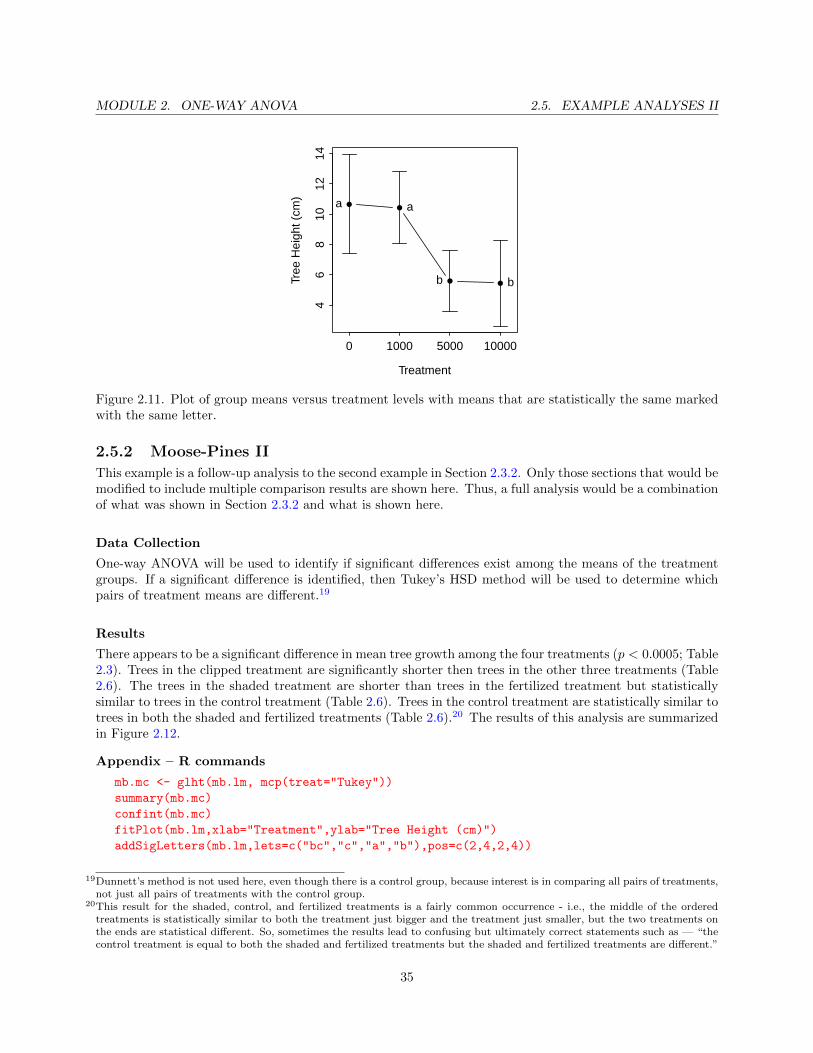
Figure 2.11. Plot of group means versus treatment levels with means that are statistically the same markedwith the same letter.

2.5.2 Moose-Pines II

This example is a follow-up analysis to the second example in Section 2.3.2. Only those sections that would bemodified to include multiple comparison results are shown here. Thus, a full analysis would be a combinationof what was shown in Section 2.3.2 and what is shown here.

Data Collection

One-way ANOVA will be used to identify if significant differences exist among the means of the treatmentgroups. If a significant difference is identified, then Tukey’s HSD method will be used to determine whichpairs of treatment means are different.19

Results

There appears to be a significant difference in mean tree growth among the four treatments (p < 0.0005; Table2.3). Trees in the clipped treatment are significantly shorter then trees in the other three treatments (Table2.6). The trees in the shaded treatment are shorter than trees in the fertilized treatment but statisticallysimilar to trees in the control treatment (Table 2.6). Trees in the control treatment are statistically similar totrees in both the shaded and fertilized treatments (Table 2.6).20 The results of this analysis are summarizedin Figure 2.12.


mb.mc <- glht(mb.lm, mcp(treat="Tukey"))

summary(mb.mc)

confint(mb.mc)

fitPlot(mb.lm,xlab="Treatment",ylab="Tree Height (cm)")

addSigLetters(mb.lm,lets=c("bc","c","a","b"),pos=c(2,4,2,4))

19Dunnett’s method is not used here, even though there is a control group, because interest is in comparing all pairs of treatments,not just all pairs of treatments with the control group.

20This result for the shaded, control, and fertilized treatments is a fairly common occurrence - i.e., the middle of the orderedtreatments is statistically similar to both the treatment just bigger and the treatment just smaller, but the two treatments onthe ends are statistical different. So, sometimes the results lead to confusing but ultimately correct statements such as — “thecontrol treatment is equal to both the shaded and fertilized treatments but the shaded and fertilized treatments are different.”

35

2.6. TRANSFORMATIONS MODULE 2. ONE-WAY ANOVA

Table 2.6. Tukey’s adjusted confidence intervals for mean tree growth for four treatments. Note that theoutput was modified to save space.


Fertilized - Control = 0 5.534286 2.173279 2.546515 0.057159442

Clipped - Control = 0 -33.420000 2.173279 -15.377688 0.000000000

Shaded - Control = 0 -1.400000 2.173279 -0.644188 0.917411421

Clipped - Fertilized = 0 -38.954286 2.173279 -17.924202 0.000000000

Shaded - Fertilized = 0 -6.934286 2.173279 -3.190703 0.009303548

Shaded - Clipped = 0 32.020000 2.173279 14.733500 0.000000000

130

140

150

160

170

Treatment

Tree

Hei

ght (

cm)

Control Fertilized Clipped Shaded

bc

c

a

b

Figure 2.12. Plot of group means versus treatment levels with means that are statistically the same markedwith the same letter.

2.6 Transformations

If the assumptions of a one-way ANOVA are violated, then the results of the one-way ANOVA are inap-propriate. Fortunately, if the equality of variances or normality assumptions are violated, then correctivemeasures can usually be taken so that appropriate results can be obtained. The most common correctivemeasure is to transform the response variable to a scale where the variances among treatment groups areequal and the individuals within treatment groups are normally distributed.

Besides the obvious reason related to assumption violations, Fox (1997) gave four arguments for why datathat is skewed or shows a non-constant variance should be transformed:

• Highly skewed distributions are difficult to examine because most of the observations are confined toa small part of the range of the data.

• Apparently outlying individuals in the direction of the skew are brought in towards the main body ofthe data when the distribution is made more symmetric. In contrast, unusual values in the directionopposite to the skew can be hidden prior to transforming the data.

• Linear models summarize distributions based on means. The mean of a skewed distribution is not,however, a good summary of its center.

• When a variable has very different degrees of variation in different groups, it becomes difficult toexamine the data and to compare differences in levels across the groups.

36

MODULE 2. ONE-WAY ANOVA 2.6. TRANSFORMATIONS

The identification of an appropriate transformation and the understanding of the resultant output is thefocus of this section.

� If the assumptions of a one-way ANOVA are not met, then the data may be transformedto a scale where the assumptions are met.

2.6.1 Families of Transformations

There are two major families of transformations – power and special transformations. Special transformationsare generally identified based on the type of data to be transformed. Certain special transformations arecommon in particular fields of study and are generally well-known to scientists in those fields. An examplethat crosses many fields is the transformation of proportions or percentages data by using the arcsine square-root function (sin−1(

√Y )). The effect of this transformation on right-skewed proportions data is illustrated

in Figure 2.13. The histogram for the values on the original scale is shown upside-down in the lower portionof this figure, the transforming function is shown in the middle, and the resultant transformed data is shownsideways on the left. The “spreading out” and “compressing” can be visualized by drawing a line up fromthe original scale until the transforming function is met and then moving to the left until the transformedscale is met. This should be tried for a variety of values on the original scale to “feel” how the sin−1(

√Y )

transformation spreads out small values and compresses large values.

asin( Y)

Y

Figure 2.13. Demonstration of the result (left) from applying the arcsine square-root transformation function(blue line) to right-skewed original values (lower).

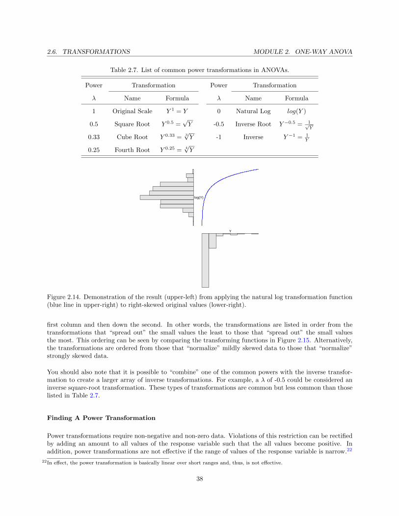
With power transformations, the response variable is transformed by raising it to a particular power, λ, i.e.,Y λ (Table 2.7). Each of the power transformations shown in Table 2.7 tends to “spread out” relatively smallvalues and “draw in” or “compress” relatively large values in a distribution. This process is illustrated inFigure 2.14 for a natural log transformation.21

The common transformations listed in Table 2.7 are ordered from least to most powerful moving down the

21Try a few values as was done with the sin−1(√Y ) transformation function in Figure 2.13.

37


Table 2.7. List of common power transformations in ANOVAs.

Power Transformation Power Transformation

λ Name Formula λ Name Formula

1 Original Scale Y 1 = Y 0 Natural Log log(Y )

0.5 Square Root Y 0.5 =√Y -0.5 Inverse Root Y −0.5 = 1√

Y

0.33 Cube Root Y 0.33 = 3√Y -1 Inverse Y −1 = 1

Y

0.25 Fourth Root Y 0.25 = 4√Y

log(Y)

Y

Figure 2.14. Demonstration of the result (upper-left) from applying the natural log transformation function(blue line in upper-right) to right-skewed original values (lower-right).

first column and then down the second. In other words, the transformations are listed in order from thetransformations that “spread out” the small values the least to those that “spread out” the small valuesthe most. This ordering can be seen by comparing the transforming functions in Figure 2.15. Alternatively,the transformations are ordered from those that “normalize” mildly skewed data to those that “normalize”strongly skewed data.

You should also note that it is possible to “combine” one of the common powers with the inverse transfor-mation to create a larger array of inverse transformations. For example, a λ of -0.5 could be considered aninverse square-root transformation. These types of transformations are common but less common than thoselisted in Table 2.7.

Finding A Power Transformation

Power transformations require non-negative and non-zero data. Violations of this restriction can be rectifiedby adding an amount to all values of the response variable such that the all values become positive. Inaddition, power transformations are not effective if the range of values of the response variable is narrow.22

22In effect, the power transformation is basically linear over short ranges and, thus, is not effective.

38

MODULE 2. ONE-WAY ANOVA 2.6. TRANSFORMATIONS

y

y*

square rootcube rootfourth rootnatural loginverse

Figure 2.15. Most common power transformation functions.

� A positive value should be added to each value of the response variable if a powertransformation is to be used and the response variable contains zeroes or negative values.

There are several methods for identifying the power transformation that is most likely to correct problemswith assumptions for a one-way ANOVA.23 One simple method is trial-and-error – i.e., trying various powersuntil one is found where the assumptions of the model are most closely met. This trial-and-error method istedious but is made more efficient with the use of transChooser(), the same function used previous whenassessing the model assumptions. In addition to the saved lm() object, a start value can be included withthe starty= argument. As before, a histogram of model residuals, a boxplot of the residuals separated foreach group, and p-values for the assumption tests are constructed. A slider is in the “gear box” that can beused to “try” various values of λ with the plots and p-values being updated as λ is changed. One can tryvarious values of λ until a value is found that provides approximately normal residuals and equal variances.When actually transforming the variable it is best to choose one of the common values of λ from Table 2.7that is closest to the value found by trial-and-error.

Another option for choosing a possible power transformation is to rely on theory related to the responsevariable. As with the special transformations discussed above, power transformations based on theory willgenerally be well-known by the scientists within a particular field. However, for example, it is common totransform response variables that are areas by taking the square root and those that are volumes with thecube root. In addition, discrete counts are often transformed with the square root.

� Transformations may be chosen based on known theory regarding the response variable.

23Box and Cox (1964) provided a statistical and graphical method for identifying the appropriate power transformation for theresponse variable. The details of this method are beyond the scope of this class but, in general, the method searches for a λthat minimizes the RSS (or SSwithin). A slightly modified Box and Cox approach is implemented in R by sending a lm objectto boxcox() from the MASS package.

39


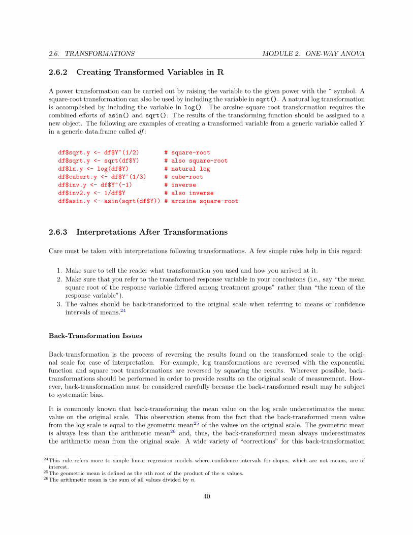
2.6.2 Creating Transformed Variables in R

A power transformation can be carried out by raising the variable to the given power with the ^ symbol. Asquare-root transformation can also be used by including the variable in sqrt(). A natural log transformationis accomplished by including the variable in log(). The arcsine square root transformation requires thecombined efforts of asin() and sqrt(). The results of the transforming function should be assigned to anew object. The following are examples of creating a transformed variable from a generic variable called Yin a generic data.frame called df :

df$sqrt.y <- df$Y^(1/2) # square-root

df$sqrt.y <- sqrt(df$Y) # also square-root

df$ln.y <- log(df$Y) # natural log

df$cubert.y <- df$Y^(1/3) # cube-root

df$inv.y <- df$Y^(-1) # inverse

df$inv2.y <- 1/df$Y # also inverse

df$asin.y <- asin(sqrt(df$Y)) # arcsine square-root

2.6.3 Interpretations After Transformations

Care must be taken with interpretations following transformations. A few simple rules help in this regard:

1. Make sure to tell the reader what transformation you used and how you arrived at it.

2. Make sure that you refer to the transformed response variable in your conclusions (i.e., say “the meansquare root of the response variable differed among treatment groups” rather than “the mean of theresponse variable”).

3. The values should be back-transformed to the original scale when referring to means or confidenceintervals of means.24

Back-Transformation Issues

Back-transformation is the process of reversing the results found on the transformed scale to the origi-nal scale for ease of interpretation. For example, log transformations are reversed with the exponentialfunction and square root transformations are reversed by squaring the results. Wherever possible, back-transformations should be performed in order to provide results on the original scale of measurement. How-ever, back-transformation must be considered carefully because the back-transformed result may be subjectto systematic bias.

It is commonly known that back-transforming the mean value on the log scale underestimates the meanvalue on the original scale. This observation stems from the fact that the back-transformed mean valuefrom the log scale is equal to the geometric mean25 of the values on the original scale. The geometric meanis always less than the arithmetic mean26 and, thus, the back-transformed mean always underestimatesthe arithmetic mean from the original scale. A wide variety of “corrections” for this back-transformation

24This rule refers more to simple linear regression models where confidence intervals for slopes, which are not means, are ofinterest.

25The geometric mean is defined as the nth root of the product of the n values.26The arithmetic mean is the sum of all values divided by n.

40

MODULE 2. ONE-WAY ANOVA 2.7. EXAMPLE ANALYSES III

bias with logarithms have been suggested in the literature. The most common correction, derived from theanalysis of normal and log-normal distributional theory, is to multiply the back-transformed value by

eMSWithin

2

Another issue arises when back-transforming differences in means. For example, because the difference inthe log of two values is equal to the log of the ratio of the two values, the back-transformed difference in twovalues becomes the ratio of the two values; i.e.,

elog(x1)−log(x2) = elog(x1x2

) =x1x2

Thus, a confidence interval for the difference in two means of a log-transformed variable becomes a confidenceinterval for the RATIO of two means on the original scale.

2.7 Example Analyses III

2.7.1 Peak Discharge

Mathematical models are used to predict flood flow frequency and estimates of peak discharge for the Mis-sissippi River watershed. These models are important for forecasting potential dangers to the public. A civilengineer is interested in determining whether four different methods for estimating flood flow frequency pro-duce equivalent estimates of peak discharge when applied to the same watershed. The statistical hypothesesto be examined are

H0 : µ1 = µ2 = µ3 = µ4

HA : At least one pair of means is different

where the subscripts identify the four different methods.

Data Collection

Each estimation method was used six times on the watershed and the resulting discharge estimates (in cubicfeet per second) were recorded.

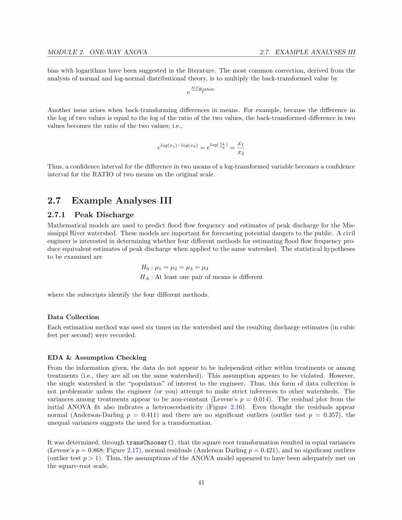
EDA & Assumption Checking

From the information given, the data do not appear to be independent either within treatments or amongtreatments (i.e., they are all on the same watershed). This assumption appears to be violated. However,the single watershed is the “population” of interest to the engineer. Thus, this form of data collection isnot problematic unless the engineer (or you) attempt to make strict inferences to other watersheds. Thevariances among treatments appear to be non-constant (Levene’s p = 0.014). The residual plot from theinitial ANOVA fit also indicates a heteroscedasticity (Figure 2.16). Even thought the residuals appearnormal (Anderson-Darling p = 0.411) and there are no significant outliers (outlier test p = 0.357), theunequal variances suggests the need for a transformation.

It was determined, through transChooser(), that the square root transformation resulted in equal variances(Levene’s p = 0.868; Figure 2.17), normal residuals (Anderson Darling p = 0.421), and no significant outliers(outlier test p > 1). Thus, the assumptions of the ANOVA model appeared to have been adequately met onthe square-root scale.

41

2.7. EXAMPLE ANALYSES III MODULE 2. ONE-WAY ANOVA

Figure 2.16. Residual plot (Left) and histogram of residuals (Right) from the one-way ANOVA on raw peakdischarge data.

Figure 2.17. Residual plot (Left) and histogram of residuals (Right) from one-way ANOVA on square roottransformed peak discharge data.

Results

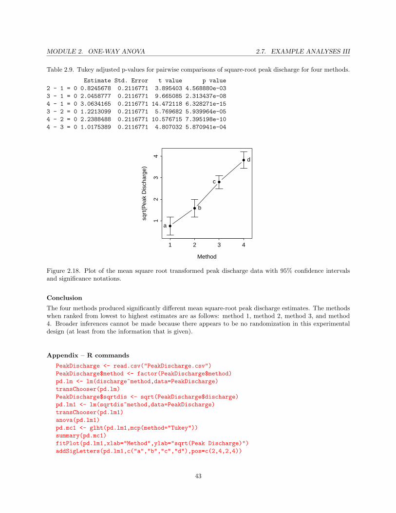
There appeared to be a significant difference in mean square root peak discharge among the four methods(p < 0.0005; Table 2.8). Tukey’s HSD multiple comparison method indicated that no two means were equal(Table 2.9) and, thus, the mean square-root of peak discharge increased significantly at each step frommethod 1 to method 4 (Figure 2.18).

Table 2.8. ANOVA results of square-root peak discharge for four methods.


method 3 32.684 10.8947 81.049 2.296e-11

Residuals 20 2.688 0.1344

42

MODULE 2. ONE-WAY ANOVA 2.7. EXAMPLE ANALYSES III

Table 2.9. Tukey adjusted p-values for pairwise comparisons of square-root peak discharge for four methods.


2 - 1 = 0 0.8245678 0.2116771 3.895403 4.568880e-03

3 - 1 = 0 2.0458777 0.2116771 9.665085 2.313437e-08

4 - 1 = 0 3.0634165 0.2116771 14.472118 6.328271e-15

3 - 2 = 0 1.2213099 0.2116771 5.769682 5.939964e-05

4 - 2 = 0 2.2388488 0.2116771 10.576715 7.395198e-10

4 - 3 = 0 1.0175389 0.2116771 4.807032 5.870941e-04

12

34

Method

sqrt

(Pea

k D

isch

arge

)

1 2 3 4

a

b

c

d

Figure 2.18. Plot of the mean square root transformed peak discharge data with 95% confidence intervalsand significance notations.

Conclusion

The four methods produced significantly different mean square-root peak discharge estimates. The methodswhen ranked from lowest to highest estimates are as follows: method 1, method 2, method 3, and method4. Broader inferences cannot be made because there appears to be no randomization in this experimentaldesign (at least from the information that is given).


PeakDischarge <- read.csv("PeakDischarge.csv")

PeakDischarge$method <- factor(PeakDischarge$method)

pd.lm <- lm(discharge~method,data=PeakDischarge)

transChooser(pd.lm)

PeakDischarge$sqrtdis <- sqrt(PeakDischarge$discharge)

pd.lm1 <- lm(sqrtdis~method,data=PeakDischarge)

transChooser(pd.lm1)

anova(pd.lm1)

pd.mc1 <- glht(pd.lm1,mcp(method="Tukey"))

summary(pd.mc1)

fitPlot(pd.lm1,xlab="Method",ylab="sqrt(Peak Discharge)")

addSigLetters(pd.lm1,c("a","b","c","d"),pos=c(2,4,2,4))

43

2.8. SUMMARY PROCESS MODULE 2. ONE-WAY ANOVA

2.8 Summary Process

The process of fitting and interpreting linear models is as much an art as it is a science. The “feel” for fittingthese models comes with experience. The following is a process to consider for fitting a one-way ANOVAmodel. Consider this process as you learn to fit one-way ANOVA models, but don’t consider this to be aconcrete process for all models.

1. Perform a thorough EDA of the quantitative response variable.

• Pay close attention to the distributional shape, center, dispersion, and outliers within each levelof the factor variable.

2. Fit the untransformed ultimate full model [lm()].

3. Check the assumptions of the fit of the untransformed model with transChooser().

• Check equality of variances with a Levene’s test and residual plot.

• Check normality of residuals with an Anderson-Darling test and histogram of residuals.

• Check for outliers with an outlier test, residual plot, and histogram of residuals.

4. If an assumption or assumptions are violated, then attempt to find a transformation where the as-sumptions are met.

• Use the trial-and-error method [transChooser()], theory, or experience to identify a possibletransformation.

• If only an outlier exists (i.e., equal variances and normal residuals) and no transformation correctsthe “problem” then consider removing the outlier from the data set.

• Fit the ultimate full model with the transformed response or reduced data set.

5. Construct an ANOVA table for the full model [anova()] and interpret the overall F-test.

6. If differences among level means exist, then use a multiple comparison technique [glht()] to identifyspecific differences.

• Use Tukey’s HSD method if comparing all possible pairs of means.

• Use Dunnett’s method if comparing all group means to one specific group mean (e.g., a control).

7. Summarize findings with significance letters [addSigLetters()] on a means plot [fitPlot()] or table[Summarize()].

44

MODULE 2 ONE-WAY ANOVA - Derek Oglederekogle.com/NCMTH207/book/One-Way ANOVA.pdf · 2019-03-31 · 2.1. ANALYTICAL FOUNDATION MODULE 2. ONE-WAY ANOVA Atwo-sample t-test is used speci

Documents