Modifications and enhancements to the NCAR community ...

NCAR/TN-336+STRNCAR TECHNICAL NOTE

June 1989

Modifications and Enhancements to theNCAR Community Climate Model (CCM1)

JAMES J. HACKLINDA M. BATHGLORIA S. WILLIAMSONBYRON A. BOVILLE

CLIMATE AND GLOBAL DYNAMICS DIVISION

NATIONAL CENTER FOR ATMOSPHERIC RESEARCHBOULDER, COLORADO

II

CONTENTS

Page

1. Introduction . ..................... ... .. 1

2. Changes and Additions to the Formulation of CCM1 . . . . . . . . . . . 6

2.1 Surface Temperature Calculation .... . . . . . . . . . . . . . . 6

2.2 Mass Adjustment . . ... ............... .. 13

2.3 Gravity Wave Drag . . . . . . .. . .. . .. . . . . .. . . . . 14

2.3.1 Gravity Wave Drag: Description ............... 15

2.3.2 Gravity Wave Drag: Numerical Approximations ......... 16

3. Changes and Additions to the CCM1 Users' Guide ...... . . . . 19

4. Changes and Additions to the CCM1 Program Modules Guide . . . . . . . 20

5. Changes and Additions to the CCM1 Circulation Statistics Atlas ..... 49

5.1 MSS History Tape Names for R15 Seasonal Controls . . . . . . . . . 57

5.2 MSS History Tape Names for T42 Seasonal Controls . . . . . . . . . 65

6. Summary Remarks . ......................... 72

Acknowledgments ........ ...................... 72

References . . . ... . . . ... . .......... . . . .. . ...... 73

Appendix A . . . . . . . .. . . . . . . . . .. . . . . . . . . . 75

iii

1. Introduction

Two new unresequenced program libraries were created for CCM1 in the early

fall of 1988 which incorporate fixes to several bugs that were discovered earlier in the

spring, improvements in computational performance, and a number of other enhance-

ments to components of the model. These libraries are derivatives of the original CCM1

program library called CCM1PL (MSS pathname /CSM/CCM1/%CODEn/CCM1PL), and are

called CCM1PL1 (MSS pathname /CSM/CCM1/%CODE%/CCM1PLI), which should be used

for standard R15 work, and CCM1PL2 (MSS pathname /CSM/CCMI/%CODE%/CCM1PL2)

which can be used for experimentation at T42. The new libraries are documented in

this technical report by simply noting changes and additions to the previous documen-

tation for CCM1; the CCM1 description (Williamson et al. 1987), the CCM1 users'

guide (Bath et al. 1987a), the CCM1 program modules documentation (Bath et al.

1987b), and the CCM1 circulation statistics atlas (Williamson and Williamson 1984).

In this section, we provide an overview of the changes that have been introduced

in the new libraries along with other improvements that have been released more re-

cently as modifications to the frozen libraries. The two program libraries CCM1PL1

and CCM1PL2 are identical except for the incorporation of different resolution param-

eters in CCM1PL2 (parameters appropriate for a T42 spectral truncation), and the

incorporation of a gravity wave drag parameterization, which will be described in detail

later in this document. Thus, the remaining discussion applies equally to both program

libraries, except where noted.

Three known bugs were fixed with the introduction of these new libraries. The first

and most serious change involved a correction to the formulation and implementation of

the surface temperature calculation. The incorporation of a stability dependent formu-

lation for the surface energy exchanges in CCM1 was not correctly accounted for in the

1

formulation of instantaneous energy balance at the earth's surface. This inconsistancy

resulted in a situation where the iteration procedure for determining the surface tem-

perature appeared to have converged on an energy balance when it actually had not.

The equations for the instantaneous energy balance have been reformulated and imple-

mented in the new CCM1 program libraries, resulting in the complete replacement of

subroutine TSCALC. The new formulation, which resulted in some minor changes to the

simulated climate, is described in detail in section 2.1.

The second error which has been fixed in these libraries involves a correction to an

internal inconsistency in the radiation code. The path length for the water vapor contin-

uum, defined in subroutine RADABS, was corrected so that it is now consistent with the

path length defined in RADEMS and the published expression (eq. 27) in (Ramanathan

and Downey 1986). This correction was shown to change the longwave fluxes by less

than 0.04 Wmn- 2, and as such had no significant impact on the simulated climate.

The final change corrects WRTHDR so header records are written using the explicit

record length documented in the header itself; i.e., LENHDI, word 1 of the integer header

record, LENHDC, word 31, and LENHDR, word 32. Header record number 3 had previously

been written using the incorrectly calculated length PLENHR (also corrected), causing

the actual record length to be one word longer than LENHDR indicated.

Other major functional changes incorporated in the new program libraries affect

the way in which the mass field is adjusted, and change the type of information con-

tained in the Mass Storage System comment field. The mass field is now modified

so that horizontal derivatives of ln p for the adjusted mass field are consistent with

derivatives for the unadjusted mass field. The standard information provided in the

Mass Storage System comment field has been changed to include the beginning and

ending dates and times for the history volume, information that should be more helpful

to the user. The details of these modifications are discussed in section 2.2.

2

As mentioned earlier, the correction to the instantaneous surface energy balance

introduced some marginally significant differences in the new model climate, previously

described by Williamson and Williamson (1984). Thus, a new set of control experi-

ments have been completed and analyzed over the last eight months for the R15 version

of the model. They currently include a ten-year seasonal cycle simulation with speci-

fied surface conditions, and a 12-year seasonal cycle simulation with a variable surface

hydrology. New perpetual control runs for January and July will be conducted if re-

quested by the user community. These new seasonal control simulations are discussed

in section 5.

Since the new program libraries were created, two additional errors associated with

the virtual temperature have been discovered in the CCM1 code by B. Boville and D.

Williamson. The first is extremely minor and occurs in the explicit term T2 of the

thermodynamic equation (4.f.6) of Williamson et al. (1987). In the last term of T2

the To component was erroneously not divided by the factor 1 + ( - ) qk] aris-

ing from Ck and in the next to last term To was erroneously divided by this term.

The equation is correct as it stands in Williamson et al. (1987). The correction of

these terms in the code has insignificant effect on the simulations. The second error

occurred in the hydrostatic integral in the divergence equation (4.f.2) of Williamson et

al. (1987). The diagonal component of the matrix B was inadvertently multiplied by

0.5 in the product B (T - Tn + T T 1 ). Apparently, since it is the gradient of the

term that affects the momentum forecast, this error has little effect on the simulation in

the standard 12-layer version with the top at 10 mb. However, in experimental strato-

spheric versions which have a much higher top, vertically propagating waves are set up

which produce an increase in kinetic energy in the small scales in the stratosphere. A

MOD deck correcting both of the above errors is available on the CSMLIB machine as

BUGFIX2 CCM1MODS, and is applicable to both the R15 and T42 program libraries.

3

A number of code changes to the original frozen CCM1 code, CCM1PL, were in-

corporated in the new program libraries to provide significant improvements in compu-

tational performance. These changes included modifications to RADCSW, TSCALC, PHYS,

and CLDCMP, resulting in a 27% improvement in performance at R15, and a 33% im-

provement in performance at T42, even after the incorporation of the gravity wave drag

parameterization. Since the program libraries were frozen, the CCM Core Group has

released other modifications to the model code which provide an additional 9% improve-

ment in performance without imposing algorithmic changes (i.e., without changing the

numerical results). These MODS replace the CCMlPLx Cray Update decks RADCLW,

RADTPL, and RADALB, and modify decks MADADJ, MADCLC, and TSCALC. They are avail-

able from IBM user ID CSMLIB under the filename FASTCCM1 MODS.

Also available on CSMLIB are a number of Cray Update MOD files that improve I/O

aspects of the model. The file UNBLOCK MODS synchronizes and unblocks the I/O to

the 5 CCM1 scratch data sets, and assign the data sets to the SSD. Since the SSD pro-

vides I/O access and transfer times that are much faster than disk-based I/O, the model

can make use of synchronous I/O without incurring a significant performance penalty,

even in a dedicated environment. These changes eliminate nearly half of the memory

required for main model buffer storage and virtually eliminate the disk activity charges

which typically accounted for one half of the total Cray charges. The use of this Cray

Update file also eliminates approximately 65% of the required system overhead at R15

and nearly 70% of the required system overhead at T42 when compared to the standard

frozen program libraries. Consequently, we are encouraging all users to make use of the

UNBLOCK MODS as soon as possible, particularly those individuals using the older

combination of Cray Update files which modified CCM1 I/O called CCM1 SSDMODS

and CCM1 SYNCMODS (see section 2 in Williamson 1988). The use of UNBLOCK

MODS in place of this previous combination of Cray Update files reduces the system

overhead by approximately 80% at both R15 and T42 resolutions. Users who wish

4

to continue using the older I/O modifications should replace CCM1 SSDMODS with

NEWCCM1 SSDMODS to minimize the generation of system overhead (e.g., reduces

system overhead by 50% at T42). The use of the file UNBLOCK MODS will introduce

changes to CCM1PLx Cray Update decks PARAMS, COMLEG, CONCAT, DATINI, GRCALC,

INIDAT, LEG, LNGTHS, MODIFY, RESUME, SCAN1, SCAN2, SPLITF, STEPON, and STRTN, and

adds or replaces decks REQUST, LJUST, NBLANK, and COMRST.

The combined use of the new program libraries with the Cray Update mod files

FASTCCM1 MODS and UNBLOCK MODS discussed above allows the user to execute

the CCM at approximately one third the GAU cost when compared to the original

CCM1PL program library. The total number of computational cycles required to exe-

cute the model has also been cut by more than 40%.

Generic job decks for running these program libraries are available on CSMLIB

under the names CCM1PL1 R15 and CCM1PL2 T42. These generic decks include

modifications to the frozen libraries that allow for the model to be restarted correctly

in the event that the user chooses to modify the ORO field on the initial data set at the

Gaussian latitude nearest the pole, a known limitation in all CCM1 program libraries.

In addition to the new control runs at R15, a five-year seasonal cycle control ex-

periment with specified surface conditions, and a three-year seasonal cycle simulation

with a variable surface hydrology, have been completed at T42. Although a T42 version

of CCM1 has been introduced with the CCM1PL2 program library, the R15 version of

CCM1 should still be considered to be the basic working version of CCM1 for purposes

of climate simulation. This is the resolution at which the model was developed and at

which the majority of the diagnostic effort has thus far been expended. The T42 control

runs were completed to provide a starting point for the development of a higher resolu-

tion version of the CCM. We emphasize that this version and its control runs have been

made available to the community primarily for diagnostic purposes and may not be

suitable for certain classes of numerical experimentation without further development.

5

2. Changes and Additions to the Formulation of CCM1

Two major changes to the formulation of the equations and algorithms in CCM1

are the formulation of the surface temperature calculation, and the formulation of the

mass adjustment procedure. The program library CCM1PL2 also incorporates an ad-

ditional physical parameterization which represents the momentum drag attributable

to orographically excited, vertically propogating, gravity waves. These three topics are

described in the remainder of this section.

2.1 Surface Temperature Calculation

As stated earlier, the formulation of the surface energy balance was found to be

in error in the original CCM1. This error was introduced with the incorporation of

a stability dependent formulation for the surface energy exchanges. The new proce-

dure did not properly account for the variation of the drag coefficient, CH, and the

pseudo-velocity, Vcl , with surface temperature in the formulation of instantaneous

surface energy balance (see equations 4.c.12, 4.c.29, 4.c.30 and 4.c.36 in Williamson

et al. 1987). This oversight resulted in a situation where the iteration procedure for

determining the surface temperature over land incorrectly appeared to have converged

on a surface energy balance. The surface energy balance, in particular the procedure

for the surface temperature calculation, has been reformulated and replaced in the new

program libraries. The following material describes the reformulated procedure, and as

such replaces section 4.c in (Williamson et al. 1987). For consistency and the conve-

nience of the reader, we have adopted the identical numbering convention utilized in

the Williamson et al. (1987) document.

The surface temperature is specified as an external boundary condition over the

oceans. Over land and sea ice, the surface temperature T. is computed from the

6

surface-energy-balance equation

B (T) 4 - F s" - Fl(p,) n + Hn+7/2 + LRK+l/2 + QnCE = 0, (4.c.1)

where

CB = Stefan-Boltzmann constant

Fs = Net downward solar flux at surface

F (ps) = Downward longwave flux at surface

H:+41/2 = Vertical flux of sensible heat at surface

R-+ 1 /2 = Evaporation

L = Latent heat of condensation

QICE = Heat conduction from sea ice (where present) to water below.

The terms Fsn and Fl(p,)n are provided by the radiation parameterization described

in section 4b.

The terms in (4.c.1) are given below. The latent heat flux (or evaporation) is

R+ 1/2 = K CHDWVK I (q,(T;) - qK 1) (4.c.2)

where, as described in the vertical differencing, AK is the index of the first atmosphere

level above the surface and qs is the saturation specific humidity for temperature T,,

pq - (1E-n1 )e (4.c.3)

where e = .622 and en is the saturation vapor pressure at temperature Tn computed

by linear interpolation within a table of values specified for 1-temperature intervals.

The drag coefficient CH, evaporation factor Dw, and surface velocity IVKJ are given

following (4.c.9). The density PK-I is computed from

-n-1Hl

.VK

7

using p = ap,, and the virtual temperature is

TVK = TK [1 + ( - i.k.) <-* (4.c.5)

The sensible heat flux is given by

HKh+12= PK CPKCHIVK 'I S(Tn ) ) (4.C.6)

CP CP [1 + ( - 1) * (4.C.7)

The heat conduction out of the sea ice to the ocean below isT+n _ T

QnE = KIT S- , (4.c.8)

where

KI = Thermal conductivity of ice = 2.092 W m - 1 K - 1

I = Ice thickness = 2 m (4.c.9)

TSUW = Temperature of sea water below the pack ice = 271.2°K

We now present the details of the drag coefficient computation. First, define a

pseudo-velocity to provide a minimum exchange for the unstable case

2(T? - Tf l/k-) 1/2 T > Tn- 1/ ,|Vc= I (4.c.10)

t0 Tn < T /1c.

Then

VVK-- = max (1.0, (UK-l)2 + (Vr 1 )2 + IVVK2) (4.c.11)

Note that, in any case, IVK I has a minimum value of 1 m s - 1 . The bulk Richardson

number is given by

gh T /.- T )RIB -= g -n-1 2 (4.c.12)

TK /aK VK

where the height of the boundary layer h is taken to be the thickness of the first layer,

8

with a minimum value of 500.0 m.

h = max (500.0, RT K (4..13)g9 rK

The virtual temperature T, is given by (4.c.5).

In order to provide a minimum exchange between the atmosphere and the surface

in the stable case, the Richardson number is not allowed to exceed .5 times a critical

value,

RIB =min (RIB, 0.5RIC), (4.c.14)

where the critical value is

RIC = 3.05. (4.c.15)

Neutral drag coefficients are defined by

CUN k - In + 8.4 , (4.c.16)

CON = k ln (° ) + 7.3 (4.c.17)

where the roughness length is

(0.25 m over land, sea ice, and snow cover,Zo = (4.c.18)

0.001 m over ocean,

and

k = 0.4 . (4.c.19)

For the stable case, RIB > 0,

Cu = CUN (1 - RIB/RIC), (4.c.20)

CO = CON (1 - RIB/RIC), (4.C.21)

9

and for the unstable case, RIB < 0,

CU = [CUN - 25.0exp (0.26C - 0.030( 2)] , (4.c.22)

Co = [Co- + C ' - C] ]- , (4.c.23)

= 1log 10(-RIB)- 3.5. (4.c.24)

Finally, the drag coefficients are

CD = CU, (4.c.25)

CH = CUCO. (4.c.26)

The drag coefficient CH is used for sensible and latent heat fluxes [(4.c.2) and (4.c.6)].

The other drag coefficient CD will be used for momentum shortly.

The wetness factor Dw in the latent heat flux (4.c.2), which sets the evaporation

from the earth's surface to be a specified fraction of the evaporation from a saturated

surface, is 1.0 over ocean, sea ice, and snow cover, 0.1 over grassland and scrub, 0.01

over deserts, and 0.25 over all other land types. These various land types are specified

as external input parameters to the model.

The energy-balance equation (4.c.1) is implicit in Tj, since TJ1 appears not only in

the surface emission CB(Tn)4 but also in the latent and sensible heat fluxes [(4.C.2) and

(4.C.6)], the conduction from sea ice (4.C.9), and the bulk Richardson number [(4.c.10)

and (4.C.12)]. The implicit equation is solved by the Newton-Raphson iterative proce-

dure. The general form of the equation is

f(T) = O0. (4.C.27)

The iterative solution is given by

TS(M +l ) = T ( M ) - f(T(M)) (4.c.28)

where (M) indicates the iteration count.

10

The functional form involving T, is

f(TS) = o'BT + b V K1 CH(Tr)TS + d V K ) CH(Tr)q,(T,) + eT.

(4.c.29)

+c Cvk CHH(T)+F 1F= O.

The derivative of f with respect to T, used in the denominator of (4.C.28) is

f'(T) = 4BT + b VK CH(T) + TJ fVK 9CT + CH(T) TOlS OSTI

+d VK CHH(T)) _T

, ^ _ aCH (T K 4,+ f n- (TSH) { VK) [+ CH(T) T+ e

+ n-1 aCH(TS) ) H(T)

(4.c.30)

The variation of all terms in (4.c.1) with respect to Ts is included in f' except Fsn

and Fl (ps )n which have been grouped into the term F1 in (4.c.29). If the variation in

CH were not included but, rather, an earlier value such as Tn were used to calculate

CH, which is then held fixed during the iteration, a 2At oscillation could result as the

state switched between stable and unstable on alternate time steps. To avoid such

an oscillation, the current iterate of T(A is used to determine the stability for that

iteration of (4.c.28).

For the stable case, RIB > 0,

A9Cu CUN ORIB0T8 R=0 ~ (4.c.31)9TS ~~ Ric 9Tf '

OCe CON ORIB9T8 RIc 9T8 (4.c.32)aTS Ric 8Ts

11

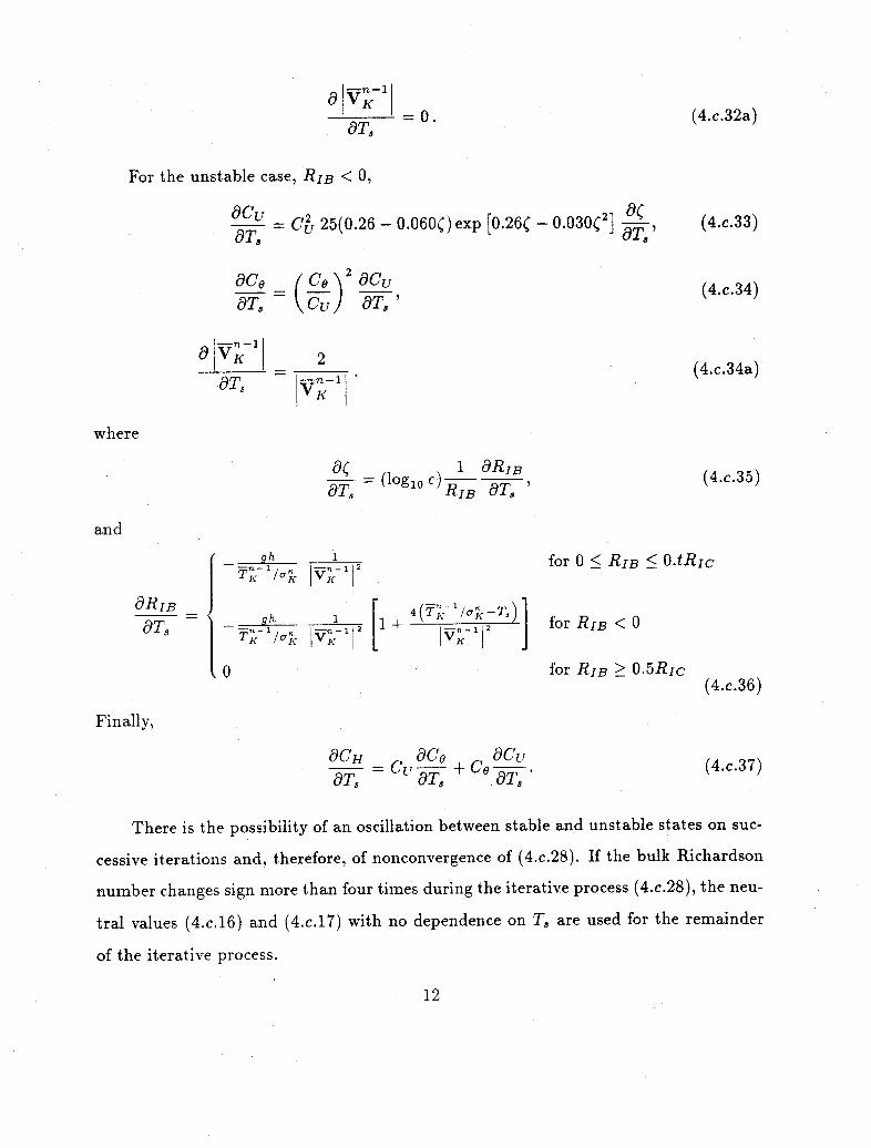
na V-I

OT8

For the unstable case, RIB < 0,

AU = -C 25(0.26 - 0.060C)exp [0.26 - 0.030C2] -0(0T' Ta

OCeT,8

co 2acu

OCu T,'

a V -1 1

VK 2n-l-

04? 1 aRIB9T (l°glog e)B T, '

_ gh 1

T n-1 /CT I L vn-+ 1 2

T /. 7 2 1 + 1 20T K /oK v K 1 V K

0 I

for 0 < RIB < O.tRic

for RIB < 0

for RIB > 0.5RIC(4.c.36)

9CH C 9Ce 9 CrT,= Cu AT + Co -T0T8q 0T8 a

(4.c.37)

There is the possibility of an oscillation between stable and unstable states on suc-

cessive iterations and, therefore, of nonconvergence of (4.c.28). If the bulk Richardson

number changes sign more than four times during the iterative process (4.c.28), the neu-

tral values (4.c.16) and (4.c.17) with no dependence on T, are used for the remainder

of the iterative process.

12

(4.c.32a)

(4.c.33)

(4.c.34)

(4.c.34a)

where

and

oRIB9Ts

(4.c.35)

Finally,

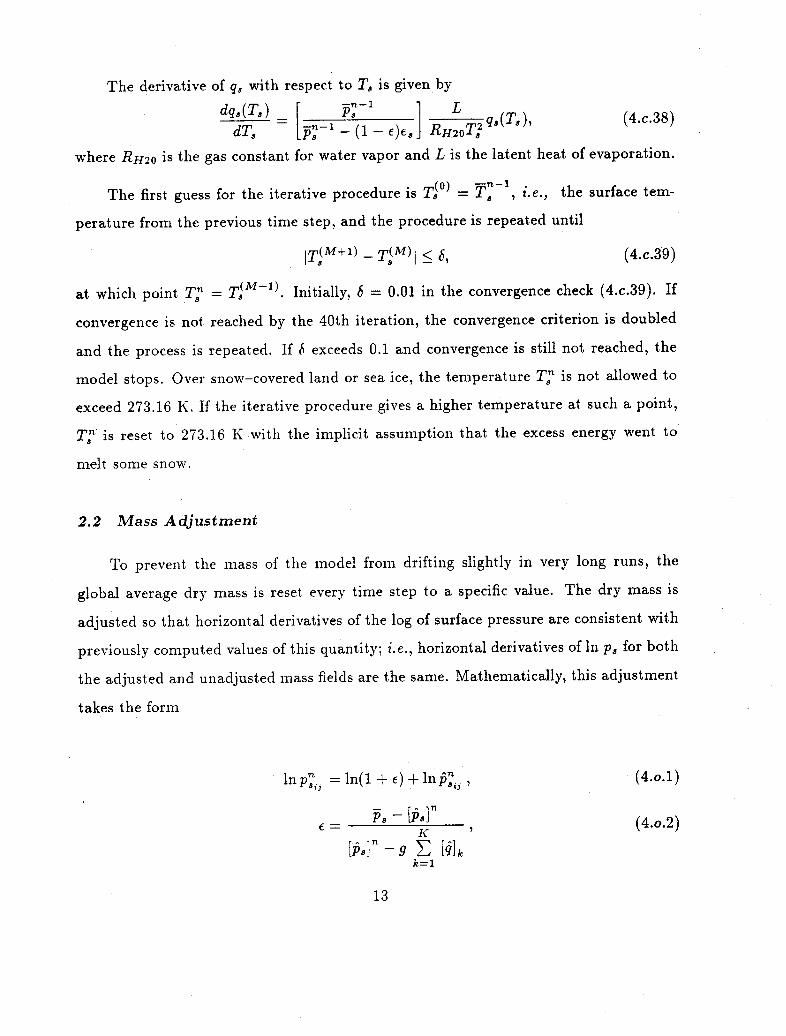
The derivative of q, with respect to T., is given by

7dT8 [La -'-(1 - e)e8e 2]0RTo qJ (T s (4.c.38)

where RH20 is the gas constant for water vapor and L is the latent heat of evaporation.

The first guess for the iterative procedure is T T( , i.e., the surface tem-

perature from the previous time step, and the procedure is repeated until

]T(M+I) -T(M)I < 6, (4.c.39)

at which point Tn = T(M+l). Initially, 6 = 0.01 in the convergence check (4.c.39). If

convergence is not reached by the 40th iteration, the convergence criterion is doubled

and the process is repeated. If 6 exceeds 0.1 and convergence is still not reached, the

model stops. Over snow-covered land or sea ice, the temperature Tn is not allowed to

exceed 273.16 K. If the iterative procedure gives a higher temperature at such a point,

TJn is reset to 273.16 K with the implicit assumption that the excess energy went to

melt some snow.

2.2 Mass Adjustment

To prevent the mass of the model from drifting slightly in very long runs, the

global average dry mass is reset every time step to a specific value. The dry mass is

adjusted so that horizontal derivatives of the log of surface pressure are consistent with

previously computed values of this quantity; i.e., horizontal derivatives of In p8 for both

the adjusted and unadjusted mass fields are the same. Mathematically, this adjustment

takes the form

in P = ln(1 + e) + In P,,i, (4.o.1)

E = KP- [P] , (4.o.2)

] 9k E [= kk=l

13

1J

j=1[Pr] = j -__ p8 ,, w, (4.o.3)

and p is the specified value of the dry mass taken as 98222 Pa for average mountains,

following (Trenberth and Christy 1985). Thus, if

pt = (1 + e)p 8, (4.o.4)

we can easily show that

alnp' Olnp (Ox Ox

The correction term is generally less than .02 Pa per time step and not of consistent

sign, so that any accumulated drift in long runs without the correction would imply a

much smaller average.

2.3 Gravity Wave Drag

Vertically propagating gravity waves can be excited in the atmosphere where sta-

bly stratified air flows over an irregular lower boundary. These waves are capable of

transporting significant quantities of horizontal momentum between their source re-

gions and regions where they are absorbed or dissipated. Previous GCM results have

shown that the large-scale momentum sinks resulting from breaking gravity waves play

an important role in determining the structure of the large-scale flow, particularly for

higher resolution truncations. Thus, the experimental T42 implementation of CCM1,

program library CCM1PL2, incorporates the stationary orographic gravity wave drag

parameterization described by McFarlane (1987). We will discuss the implementation

details here, and refer the reader to McFarlane's paper for a discussion of fundamental

theoretical aspects of gravity wave drag effects.

14

2.3.1 Gravity Wave Drag: Description

As with all CCM1 physical parameterizations, non-resolvable-scale effects of verti-

cally propagating gravity waves are determined in physical space on the transform grid.

The wave drag force in pressure coordinates is written as

=V a _n (T )- (2.3.1)

where

r = -aA 2 pNU - aA2 NU = -MU, (2.3.2)

n is a unit vector parallel to the reference level flow VO, U is the component of the local

flow which is parallel to the reference level flow

U-=V. V/ I V , (2.3.3)

N is the local Brunt-Vaisala frequency defined as

N_ (-g 2p 09) (2.3.4)

A(Z) is the local wave amplitude, H is the local scale height, and the "tunable" pa-

rameter a is defined as

a = ELe/2 (2.3.5)

where i/e is a representative horizontal wavenumber and E is an efficiency factor as-

sumed to be less than unity. The wave amplitude at the reference level is defined in

terms of the subgrid-scale orographic variance, but constrained so that the local Froude

number does not exceed some critical value denoted by Ft. Thus

Ao = min {2Sd, Fc Uo/No} (2.3.6)

where Sd is the standard deviation of the subgrid-scale orography associated with hor-

izontal space scales assumed to be most responsible for the generation of vertically

15

propagating gravity waves. The wave momentum flux at the surface is written as

-gr- aAopoNoUo/HO. (2.3.7)

The wave momentum flux above the reference level is assumed to be constant with

height except in regions of wave saturation. Thus at all model levels above the reference

level, the local wave amplitude is computed in terms of the wave amplitude of the layer

below so that the wave momentum flux is constant except in saturation regions where

A=F U/N. (2.3.8)

The wave momentum flux at some level k is then given by

[-gr]k = min [-gr]k+, [H (N ) (2.3.9)

2.3.2 Gravity Wave Drag: Numerical Approximations

The gravity wave drag parameterization is applied immediately after the nonlinear

vertical diffusion (see section 4.e.1, Williamson et al. 1987). The interface temperatures

are first determined fromn-1 _n-1

Tk+1/2 = T- + l In (pk+1/2/pk) , (2.3.10)+ in (Pk+/)

where the layer and interface pressures are given by

Pk -=O kP- (2.3.11)

Pk+1/2 = Cok+1/2 Ps (2.3.12)

The projection of the interface winds on the reference level wind is evaluated as

Vk+1 - Vk Pk+/\Uk+1/2 = Vk + (Pk ln ( / ) , (2.3.13)

Pk

where

V2k ( +: ) () (2.3.14)

16

while the interface Brunt-Vaisala frequencies are given by

Nk+12 { 2 Pk+1(- - ' P k+1/2 (2.3.15)k+1/ 2 k 1 - Pk -Pk Pk+1/2 3

The top interface Brunt-Vaisala frequency is evaluated assuming an isothermal atmo-

sphere above the top model layer so that

( g2 )1/2

Nil 2 =( (2 ) (2.3.16)

Assuming that the magnitude of the reference level wind exceeds a critical value, cur-

rently 2 m s - 1, and that the subgrid-scale standard deviation exceeds a critical value,

currently 5m, the surface momentum flux is given by

9gK+1/2 = E-ieh e PAKNK-12 I VK (2.3.17)

where

he = min (2Sd, Fc -1/2/NK-1/2) , (2.3.18)

Sd is the subgrid-scale orographic standard deviation, Fc is the critical Froude number

taken as 2 and H is the local scale height. The remaining momentum fluxes are

computed from the lowest level upwards using

T 7 ,,, =min -g (2.3-19)9k + 1/2 h 1 k+3/'2 2HkNk+1/2 (.3.19

with the exception of the top interface level where the momentum flux is calculated

assuming the top interface is located an equal increment in lnp above the two interfaces

immediately below, and that all variables are constant above the uppermost integer

level

i {n 3EF2HN/ Pl/2 } (2.3.20)

The momentum tendencies (stress divergence) are then evaluated as

_ n- 1 __ _ -_ }/^ (2.3.21)\Et V n~ 1 Pk+1/2 -Pk-1/2

k KI

17

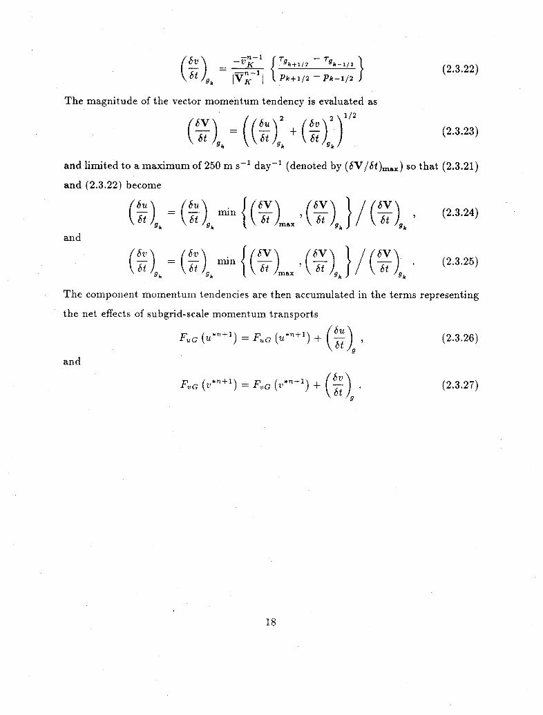
Kv _ A -v K Jg ._+ / 2-./ 2l

(6v h IVK" I l Pk+1/2 Pk-1/2

The magnitude of the vector momentum tendency is evaluated as

(6V\ _ ( ( Iu\2(22 1/2gbV bu bV

(2.3.22)

(2.3.23)

and limited to a maximum of 250 m s - day - ' (denoted by (SV/6t)max) so that (2.3.21)

and (2.3.22) become

(bu\ 6u m 6 ( }/V I (V\

) =- (Et), m/in{(tmx ( Et ), y ( 2*3.24)and

(btXl< -(f i) ( )max'( I j / k(V)

-(^""'*l^L *(<!/(<~~~~~~ (2.3.25)

The component momentum tendencies are then accumulated in the terms

the net effects of subgrid-scale momentum transports

FUG (U +) = FUG (U +) + I)

and

FvG (V'+1) = FG ( ' n+ l ) + ( )

representing

(2.3.26)

(2.3.27)

18

3. Changes and Additions to the CCM1 Users' Guide

A number of minor corrections and additions have been made to the CCM1 Users'

Guide (Bath et al. 1987a) with the introduction of the CCM1PL1 and CCM1PL2 pro-

gram libraries. We summarize these changes below and provide a "page change packet"

(making use of change bar notation) for the user in Appendix A of this document.

The MSS comment field associated with output history tapes is now composed of

the beginning and ending dates and times for the particular volume (see revised page 8

in Appendix A). Thus, information on the history tape contents can easily be obtained

by executing the standard Mass Store System utilities (e.g., "MSINFO") and examining

the contents of the comment field.

The incorporation of the gravity wave drag parameterization in CCM1PL2 requires

an additional input dataset. This dataset contains the standard deviation of the 1/6°

resolution orography (see description of Navy Fleet Numerical Oceanography Center

surface data in Joseph 1984) on a T63 transform grid, which has been spectrally trun-

cated for representation on the T42 transform grid. This dataset is described on page

28.1 in Appendix A.

All other significant changes, particularly the addition of the gravity wave drag

procedures, are reflected in modifications to Table 1.9 and Figs. I.l.c, II.18a, II.19b,

II.20a, and II.20b, all of which are contained in Appendix A.

19

4. Changes and Additions to the CCM1 Program Modules Guide

A number of minor corrections and additions have been made to the Documenta-

tion of NCAR CCM1 Program Modules (Bath et al. 1987b) with the introduction of

the CCM1PL1 and CCM1PL2 program libraries. The new libraries require additions to

the CCM1 calling tree (see Fig. l.c for changes associated with CCM1PL2), changes to

six CCM1 Cray Update deck descriptions (BLDCOM, SAVDIS, TSCALC, WECOEF, WOCOEF,

and WRTHDR), changes to six CCM1 Cray Update COMDECK descriptions (/COMMAP/,

/COMQFL/, /COMTIM/, /COMZER/, /CRDCTL/, and /PARAMS/), and the addition of three

new Cray Update decks (GWD, GWDDRV, and PLV). Each of these modified program mod-

ules is described below in its entirety.

20

GWD

SUBROUTINE GWD

Update deck location: GWD. 3 - GWD. 262

Concordance identifier: GWD

PURPOSE

Calculate momentum tendencies attributable to stationary orographic gravitywave drag.

U : [input ] u momentumV : [input ] v momentumT : [input ] temperataureSGH : [input ] 2*Sd where Sd is orographic standard deviationPINT : [input ] pressure on interfacesPMID : [input ] pressure on midpoint surfacesORO : [input ] orography flagNLOND : [input] NLON+2NLON : [input ] number of longitude pointsNLEV : [input n] umber of levelsG : [input ] gravitational constantR : [input ] gas constant for dry airCP : [input ] specific heat for dry airUT : output u momentum tendency due to gravity wave dragVT [output ] v momentum tendency due to gravity wave dragUB [output ] normalized lowest level u momentumVB [output ] normalized lowest level v momentumVMB : [output ] magnitude of lowest level wind vector |V|VP : [output ] projection of wind on reference level windUBG : [output ] values of UB gathered from points where gravity wave gen-

eration is activeVBG : [output ] values of VB gathered from points where gravity wave gen-

eration is activeVMBG [output ] values of VMBG gathered from points where gravity wave

generation is activeVPG : [output ] values of VP gathered from points where gravity wave gen-

eration is activeTG : [output ] values of T gathered from points where gravity wave gen-

eration is activeBVG : [output ] values of Brunt-Vaisalai gathered from points where gravity

wave generation is activeUIG : [output ] interface values of U gathered from points where gravity

wave generation is activeTIB : [output] interface values of T gathered from points where gravity

wave generation is active

21

GWD-2

PIG [output ] values of PINT gathered from points where gravity wavegeneration is active

PMG : [output ] values of PMID gathered from points where gravity wavegeneration is active

GTAU [output ] values of gravity wave stress gathered from points wheregravity wave generation is active

UTG [output ] values of gravity wave u momentum tendency gatheredfrom points where gravity wave generation is active

VTG : [output ] values of gravity wave v momentum tendency gatheredfrom points where gravity wave generation is active

SGHG [output ] values of SGH gathered from points where gravity wave gen-eration is active

TAUSX [output ] gravity wave drag surface stress in u momentumTAUSY : [output ] gravity wave drag surface stress in v momentumTAUSXG [output ] values of TAUSX gathered where gravity wave generation is

activeTAUSYG [output ] values of TAUSY gathered where gravity wave generation is

activeINDX : [output ] indirect address vector for gathered points

ALGORITHM

1.0 Calculate magnitude of lowest level wind and associated unit vectors1.1 Determine points at which gravity wave drag scheme will be applied,

points must satisfy following 3 criteria:1) point must be over land2) lowest level wind must exceed a critical value (currently 2 ms - 1 )3) orographic standard deviation must exceed a critical value

(currently 5 m)1.4 Gather points at which gravity wave drag scheme will be applied2.1 Calculate interior interface temperatures and wind projections2.15 Assume an equal increment in lnp between interfaces to reset the top

interface pressure2.3 Calculate interior interface Brunt-V/aisala frequencies2.4 Calculate top interface Brunt-Vaisalai frequency assuming isothermal

condition from top midpoint temperature2.7 Calculate lowest level stress2.9 Calculate remaining interior stresses from bottom to top3.0 Calculate stress at top interface assuming previously computed interface

pressure and constant state variables above top level midpoint3.1 Compute and bound momentum tendency due to gravity wave drag

scheme3.4 Calculate surface stress components4.0 Clean up and scatter momentum tendency and stress information

22

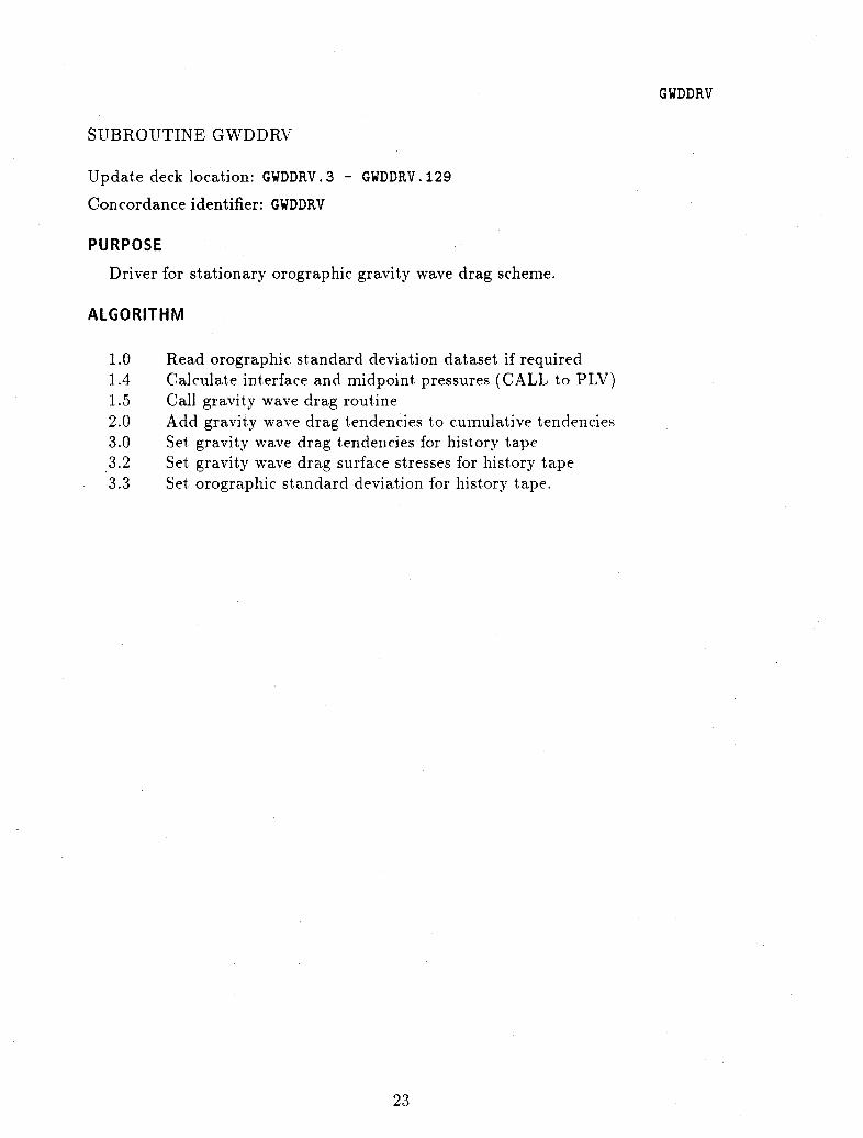
GWDDRV

SUBROUTINE GWDDRV

Update deck location: GWDDRV.3 - GWDDRV. 129

Concordance identifier: GWDDRV

PURPOSE

Driver for stationary orographic gravity wave drag scheme.

ALGORITHM

1.0 Read orographic standard deviation dataset if required1.4 Calculate interface and midpoint pressures (CALL to PLV)1.5 Call gravity wave drag routine2.0 Add gravity wave drag tendencies to cumulative tendencies3.0 Set gravity wave drag tendencies for history tape3.2 Set gravity wave drag surface stresses for history tape3.3 Set orographic standard deviation for history tape.

23

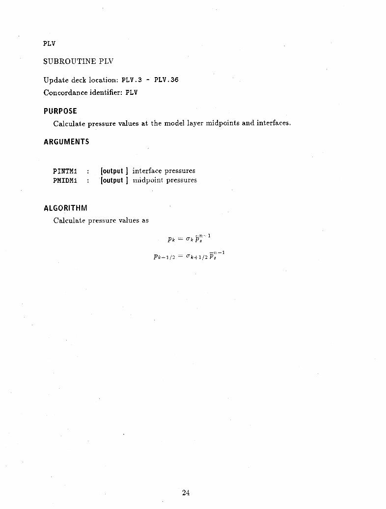
PLV

SUBROUTINE PLV

Update deck location: PLV. 3 - PLV. 36

Concordance identifier: PLV

PURPOSE

Calculate pressure values at the model layer midpoints and interfaces.

ARGUMENTS

PINTM1 : [output ] interface pressuresPMIDM1 : [output ] miidpoint pressures

ALGORITHM

Calculate pressure values as

-n-1Pk -= rk P s

Pk+1/2 = 0'k+ /2P Rs

24

TSCALC

SUBROUTINE TSCALC (KROW)

Update deck location: TSCALC. 3 - TSCALC. 636

Concordance identifier: TSCAL

PURPOSE

Solves implicit equation f(Ts) = 0 for surface T8 over non-ocean points usingNewton-Raphson iterative procedures.

TM+' - TM_ f(T )s - 8 f'SI(TS)

Iterations repeated until IT i'+' - Ts < e.

Initially e = 0.01. A maximum of 40 (100 for first time step of a run) iterationsare performed for each value of e. If no convergence after 40 interations, e isdoubled and the process repeated. If e > 0.1 and convergence is not reached,the model stops.

Computes surface fluxes using new T., 1 of T, q, and surface stresses of u andv for use as boundary conditions in vertical diffusion. Updates water equivalentsnow depth, soil moisture and runoff according to surface fluxes if required (HYDRO= .TRUE.).

ARGUMENT

KROW : [input ] latitude line index.

ALGORITHM

2. SPECIFY AND STORE SOME COMMONLY USED EXPRESSIONS

WET min(WS * QWSSAT, 1) if not over ocean and no snowWET = { n S

1 otherwise

TKTNLEV =

KoK

* CALCULATE SURFACE WIND

VMAG = 4. max(0, Ts - TNLEV)

UMAG = max (1, UMAG + (u1)2 + ( + (-1)2 )

25

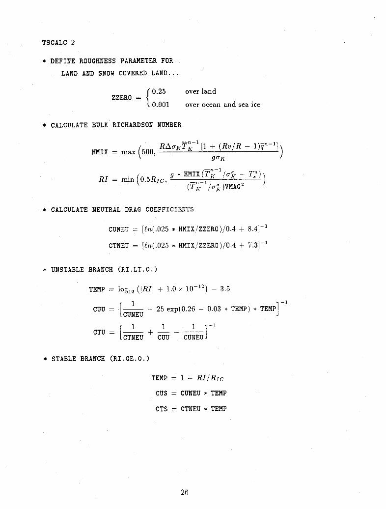
TSCALC-2

* DEFINE ROUGHNESS PARAMETER FOR

LAND AND SNOW COVERED LAND...

f0.25ZZERO = 0.001

I 0.001

over land

over ocean and sea ice

* CALCULATE BULK RICHARDSON NUMBER

HMIX max (500 RKTK [1 + (Rv/R - 1)qn- l]HMIX = max 500, R [

· gc9K

RI = min (0.5RI,'--n -- ]

g * HMIX(TK /cT^ - Tr;)

(TI-'- / )VMAG 2

*. CALCULATE NEUTRAL DRAG COEFFICIENTS

CUNEU = [fn(.025 * HMIX/ZZERO)/0.4 + 8.4] -

CTNEU = [Cn.(.025 * HMIX/ZZERO)/0.4 + 7.3] - l

* UNSTABLE BRANCH (RI.LT.O.)

TEMP = log1 o ([RI + 1.0 x 10-12) - 3.5

CUU = CUNEU - 25 exp(0.26 - 0.03 * TEMP) * TEMPCUNEU

CTU = + -CTNEU CUU CUNEUJ

* STABLE BRANCH (RI.GE.O.)

TEMP = 1 - RI/RIc

CUS = CUNEU * TEMP

CTS = CTNEU * TEMP

26

TSCALC-3

* MERGE STABLE AND UNSTABLE VALUES

CUS if RI > 0CUS =

ICUU if RI < 0

(CTS if RI > 0CTS =

ICTU ifRI < 0

CD = CUS 2

CH = CUS * CTS

bu= CD * VMAG * · CTK

b = C(H * VMAG * PS CKC' [1 + (C'PZ/CW P - 1) * g7 1]-n-1

TI KC [1 + (R,/ - 1)* qK]

d = CHDW * VMAG * -P s- K 1

TR R [1 + (R,/R - 1) * qK ]

UP2= <0 otherwise

c = -[(1 - A)So + Fo] - [b * TK /o'- + d * q]-- UP2 * 271.2

3. CALCULATION OF FLUXES, SNOWMELT, ETC.

If (HYDRO), the following calculation is done.

Estimate snowmelt (estimate calculated only if over land or sea ice covered bysnow) using energy relation.

WFLUX = max(-a* (TMELT) 4 - * TMELT - d * QPS * ESMELT, -c - UP2 * TMELT, 0)

If estimated snowmelt is greater than available snow cover keep track of actualsnow melt in UP2 for later use in surface energy balance computation.

Decrease snow amount SNM1 and increase soil moisture WSM1 by estimatedsnowmelt stored in WFLUX.

If (.NOT.HYDRO), set actual snow melt (UP2) and estimated snowmelt (WFLUX)vectors to zero.

3.2 LAND, NORMAL CONDITIONS, NEWTON-RAPHSON PROCEDURE

27

TSCALC-4

If over ocean or area where snow has melted, the following calculations are notperformed.

* INITIALIZE VARIABLES CARRIED FROM ONE ITER TO NEXT

SNWNRG = Energy sink where all snow has melted (exposed land)

The following calculation is done iteratively.

* CALCULATE DERIVATIVE OF DRAG COEFFICIENT W.R.T. TS

{0 if RI > RIMAX

DRIDTS = gHMIX

T^ /K * VMAG 2

If an oscillation between stable and unstable branches has occurred in RIduring earlier iterations,

DCUSDT = 0

DCTSDT = 0

Otherwise, if RI < 0 (unstable branch),

DRITS = DRITSn-4(T-4 T4( /-T/- T

1 + 'VMAG2

oCTEMPi = A

TEMP2 = (

DCUSDT =

DCTSDT =

aCr,

aTs

aCeaT8

Or if RI > 0 (stable branch),

DC

DC

-TEMP 1 ORIBTEMP -

Ric OTs

TUSDT = v r O-RI

ATSDT = -C-Ric OT,

28

TSCALC-5

In all cases,1 &CH

DCHDTS =--CH oTs

* TERM FOR CONDUCTION THRU SEA ICE...

a =- t B

ESK = eM computed fromT^' via call to ESTABL

MZQS = q - - -(1 e )

____ L n- qDQSDT - s - PS >

DT RH20 p - (1 -e)

NEW GUESS AT SURFACE TEMP ... CHECK FOR CONVERGENCE

RNUMER = a(T."') 4 + b(T') + e(TA1) + dqm + c- SNWNRG

DSHF = 9H n + aTs

DLHF = R /

RDENOM = 4a(TNI )3 + DSHF + DLHF + e

If DSHF or DLHF are negative, or RDENOM is zero, force RI = 0.5RIC andrecalculate quantities for another pass through iteration procedure. Otherwise:

~,+ l =M Tf_ RNUMERTAI+1 - TAl RNUMERRDENOM

If (ITA 1+ 1 - Tll < ZEPS), the solution has converged and the iteration loopis exited.

If the solution has not converged, the drag coefficients and their derivativesare recalculated. This calculation duplicates that at the beginning of thissubroutine, before the iteration loop.

If RI switches between stable and unstable values four times, a logical variableis set so that neutral values are used for the remaining iterations.

The convergence criterion ZEPS is initially set to 0.01.

The iteration is performed 40 times (100 if NSTEP = 0). If convergence is notachieved, the convergence limit is doubled and the iteration started again.

If ZEPS > 0.1, the model prints a message and stops.

After convergence, if the point is over snow cover or sea ice,

T += mrin (T+', TMELT)

29

TSCALC-6

3.3 CALCULATE SURFACE FLUXES OF SENSIBLE HEAT AND MOISTURE

UP2 = e8 calculated via call to ESTABL using T.

UP2 = q -n-

WFLUX = Pa' CHDw\V L( 9 - L (q ; -()//p1

2Atg-n-- 1 RO, K+1/2

QFLX = WFLX

P - P( (K K 9 -/P-

-1 '

· , 2Atg KCPi * _P ACTK

TFLX = HFLM1

If (HYDRO), then update snow cover, soil moisture, and runoff based on calcu-lated evaporative flux WFLUX.

If snow covered land,

SNM1 m= max(SNM1 - AtRK+1 / 2 /pH20,O)

Else,

WSM1 = max(WSM1 - AtR /2 /pH2, O)

RNFM1 = RNFM1 + min(WSM1 - WSSAT, 0.0)

30

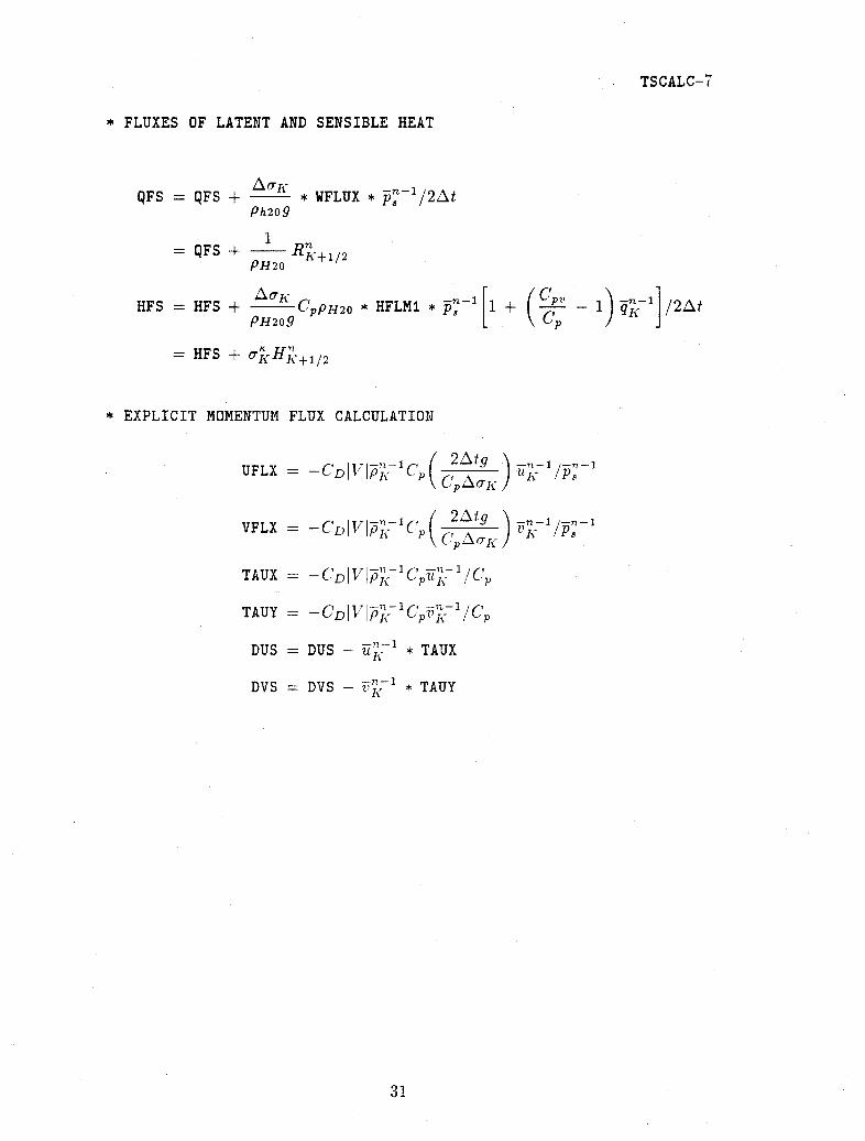
TSCALC-7

* FLUXES OF LATENT AND SENSIBLE HEAT

QFS = QFS + - * WFLUX * p8 /2ztPh209

1= QFS + RK+1/2

PH20

HFS = HFS + K CppH2o * HFLM1 * p- [1PH209 L

= HFS + CKHK+ / 2

* EXPLICIT MOMENTUM FLUX CALCULATION

UFLX = -C'D IP Cp(

VFLX = -CDIIIP-CP (

TAUX = -CDIVI-K CP.-K/C

TAUY = -CD I PK 1Cp I / pC

DUS = DUS - uK 1 * TAUX

DVS = DVS - -I"1 * TAUY-- -'K *TU

31

2Atg n -

C AZ OK /, /-Cpah

1 2 At

+ c p -1 4nI /2,A

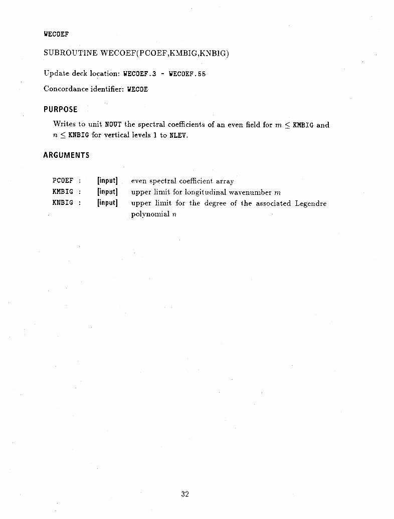
WECOEF

SUBROUTINE WECOEF(PCOEF,KMBIG,KNBIG)

Update deck location: WECOEF. 3 - WECOEF. 55

Concordance identifier: WECOE

PURPOSE

Writes to unit NOUT the spectral coefficients of an even field for m < KMBIG andn < KNBIG for vertical levels 1 to NLEV.

ARGUMENTS

PCOEF : [input] even spectral coefficient array

KMBIG : [input] upper limit for longitudinal wavenumber mnKNBIG : [input] upper limit for the degree of the associated Legendre

polynomial n

32

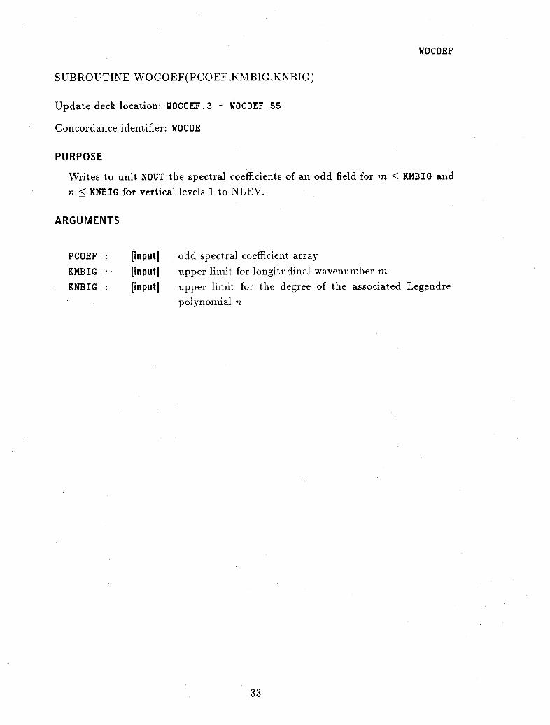
WOCOEF

SUBROUTINE WOCOEF(PCOEF,KMBIG,KNBIG)

Update deck location: WOCOEF.3 - WOCOEF.55

Concordance identifier: WOCOE

PURPOSE

Writes to unit NOUT the spectral coefficients of an odd field for m < KMBIG and

n < KNBIG for vertical levels 1 to NLEV.

ARGUMENTS

PCOEF : [input] odd spectral coefficient array

KMBIG : [input] upper limit for longitudinal wavenumber m

KNBIG : [input] upper limit for the degree of the associated Legendre

polynomial n

33

WRTHDR

SUBROUTINE WRTHDR

Update deck location: WRTHDR. 3 - WRTHDR. 173

Concordance identifier: WRTHD

PURPOSE

Updates and writes to unit NDATA the three header records contained in/COMHDI/, /COMHDC/ and /COMHDR/. There are 4 time levels for the updatingof header information: first, when the case begins, second, when a job (initialor restart) is submitted, third, at the start of a new history tape volume, andfourth, upon any entry to WRTHDR.

ALGORITHM

1.0 VARIABLES UPDATED AT THE START OF A NEW CASE

This block executed when IFLGR = 1 and not a restart (beginning of newcase). The following variables are updated:

MLONNLONWMORECMLEVMSPHERMTRKMTRMMTRNNSTEPHLNHSTALDHSTALTHSTALSHSTALENHDILENHDCLENHDRMFTYPNDBASENSBASENBDATE

NBSECMDTMHISF

MCASEMCSTIT

34

WRTHDR-2

LNHSTFLDHSTFLTHSTFLSHSTF

2.0 VARIABLES UPDATED AT THE START OF A NEW RUN

This block executed when IFLGR = 1 (the first pass through WRTHDR).

NOTE: IFLGR is set = 1 in a DATA statement and reset = -1 upon exit

of WRTHDR.

Set variables NSTPRH, NDCUR, NSCUR, NCDATE, NCSEC and MFSTRT.

3.0 VARIABLES FOR THE FIRST HEADER ON A NEW VOLUME

This block executed when a new volume is started. Update the following

variables:

LNHSTP

LDHSTPLTHSTPLSHSTPLNHSTC

4.0 THESE VARIABLES CHANGED FOR EACH HEADER

Set MFILH. NSTEPL is set to the last value of NSTEPH. This value is saved for

normalization of fields accumulated since last. write. Set. NSTEPH and NIT-

SLF. Call subroutine NUTIME to calculate NDCUR, NSCUR, NCDATE and NCSEC. If

the first header on this volume, save these time variables for the Mass Store

comment field. Set the following header variables:

LDHSTC

LTHSTC

LSHSTC

5.0 WRITE OUT HEADER

Call PRNTHD with an argument of .TRUE. for the first time, and .FALSE.

thereafter to print header. Write header records to unit NDATA, set IFLGR =

-1 and return.

35

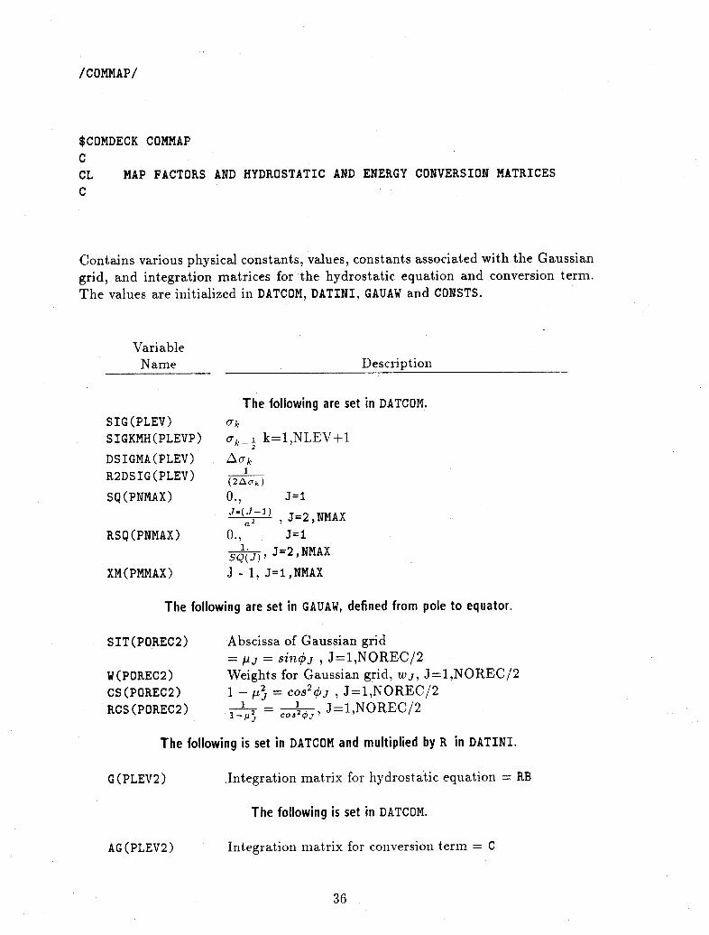
/COMMAP/

$COMDECK COMMAP

C

CL MAP FACTORS AND HYDROSTATIC AND ENERGY CONVERSION MATRICES

C

Contains various physical constants, values, constants associated with the Gaussiangrid, and integration matrices for the hydrostatic equation and conversion term.The values are initialized in DATCOM, DATINI, GAUAW and CONSTS.

VariableName Description

SIG (PLEV)

SIGKMH (PLEVP)

DSIGMA (PLEV)

R2DSIG (PLEV)

SQ (PNMAX)

RSQ(PNMAX)

XM(PMMAX)

The following are set in DATCOM.

O'k

crk i k=1,NLEV+l2

(2 k)0., J

0., J=l

J*( J- ) J=2, NMAX

0., J=1J)-,J=2,NMAX

J - 1, J=1,NMAX

The following are set in GAUAW, defined from pole to equator.

SIT(POREC2)

W(POREC2)CS(POREC2)

RCS (POREC2)

Abscissa of Gaussian grid== .j = sinej , J=1,NOREC/2Weights for Gaussian grid, wj, J=1,NOREC/21 - - = cos2qpj , J=1,NOREC/2

I -- = Cos-2 q, J=1,NOREC/2

The following is set in DATCOM and multiplied by R in DATINI.

.Integration matrix for hydrostatic equation = RB

The following is set in DATCOM.

AG(PLEV2) Integration matrix for conversion term = C

36

G(PLEV2)

/COMQFL/

$COMDECK COMQFLC

CL GLOBAL INTEGRALS FOR MOISTURE AND MASS CONSERVATION

C

Contains integrals for moisture and mass conservation. Calculated in INIDAT or

SCAN2.

Variable Description

TQ (PLEV)DQ (PLEV)

TMASSTMASSO

QMASS 1

Global average mass of moisture in layer.Global average correction needed to make mois-ture non-negative.Total mass of atmosphere before correctionPrescribed total dry mass of Model atmosphere.Set in DATA statement in QNEG2.

Globally integrated water mass.

Value

[5]

98222.

K

g E []k=l

1 This variable exists only in Program Libraries CCM1PL1 and CCM1PL2.

37

/COMTIM/

$COMDECK COMTIMCCL MCC

3DEL TIME VARIABLES

Contains variables which carry time information through the Model.

Description

DTIME

NRSTRT

NSTEPNNUMWT

NWTIME(50)

NESTEP

MDBASE

MSBASE

Real Model time step in seconds. Initialized in PRESETto 1080. (18 minutes), and read in from NAMELIST$NEWRUN.

Integer Time step which started this run. Initialized to 0 inPRESET and set to restart time step NSTEPR in RESUME,if run is a continuation of a previous run.

Integer Current Model time stepInteger Read in from NAMELIST $NEWRUN, defines the frequency

of history tape writes if using automatic mode. If posi-tive, value is assumed to be in iterations, If negative, illhours. Preset in PRESET to -12.

Integer. Array of up to fifty iteration numbers at which thehistory tape will be written, defining "manual mode"write-up. Read in from NAMELIST $NEWRUN.

Integer Read in from NAMELIST $NEWRUN, defines the end of theModel run. If positive, NESTEP is the final iteration ofthe run. If negative, NESTEP is the number of days torun. Defaults to -10 (10 days) in PRESET.

Integer BASE Day number for this case, i.e., the day numberfrom which the Model time variables will begin. De-faults to the current day number on the initial dataset.Read in as NNDBAS in NAMELIST $NEWRUN.

Integer The number of Seconds into the BASE day

38

VariableName

VariableType

/COMTIM/-2

Variable VariableName Type Description

MDCUR Integer The Day number corresponding to the CURrent historytape file. Set initially from NDBASE and incremented asthe Model runs.

MSCUR Integer The number of Seconds into the CURrent day NDCURMBDATE Integer The Base DATE for this case, in the form yymmdd, de-

faults to the current date on the initial dataset. Read inas parameter NNBDAT in NAMELIST $NEWRUN. The rela-tionship between this date and the base day (NDBASE)is entirely user-defined.

MBSEC Integer The number of SEConds into the day of the Base dateNBDATE

MCDATE Integer The Current DATE as yymmdd, initialized to the valueof NBDATE and incremented as the model runs

MCSEC Integer The number of SEConds into the day of the Currentdate NCDATE

NNDBAS Integer Read in from NAMELIST $NEWRUN, used to set MDBASE,base day for the run. Defaults to the value of NDCUR(MDCUR) from the initial dataset.

NNSBAS Integer Read in from NAMELIST $NEWRUN, used to set MSBASE,base seconds of the day. Defaults to the value of NSCUR(MSCUR) from the initial dataset.

NNBDAT Integer Read in from NAMELIST $NEWRUN, used to set MBDATE,base date for the run. Defaults to the value of NBDATE(MBDATE) from the initial dataset.

NNBSEC Integer Read in from NAMELIST $NEWRUN, used to set MCSEC,base seconds of the date. Defaults to the value of NCSEC(MCSEC) from the initial dataset.

NSTEPL Integer Last time step at which history tape was written. Usedin WSHIST to normalize accumulated fields to valuesaveraged over the number of iterations since the lastwrite.

NDCURF 1 Integer Current day number from first file on this volume.NCDATF 1 Integer Current date, as yymmdd, from first file on this volume.

NSCURF1 Integer Seconds of current day from first file on this volume.NCSECF' Integer Seconds into the day of current date, from first file on

this volume.

These variables exist only in Program Libraries CCM1PL1 and CCM1PL2.

39

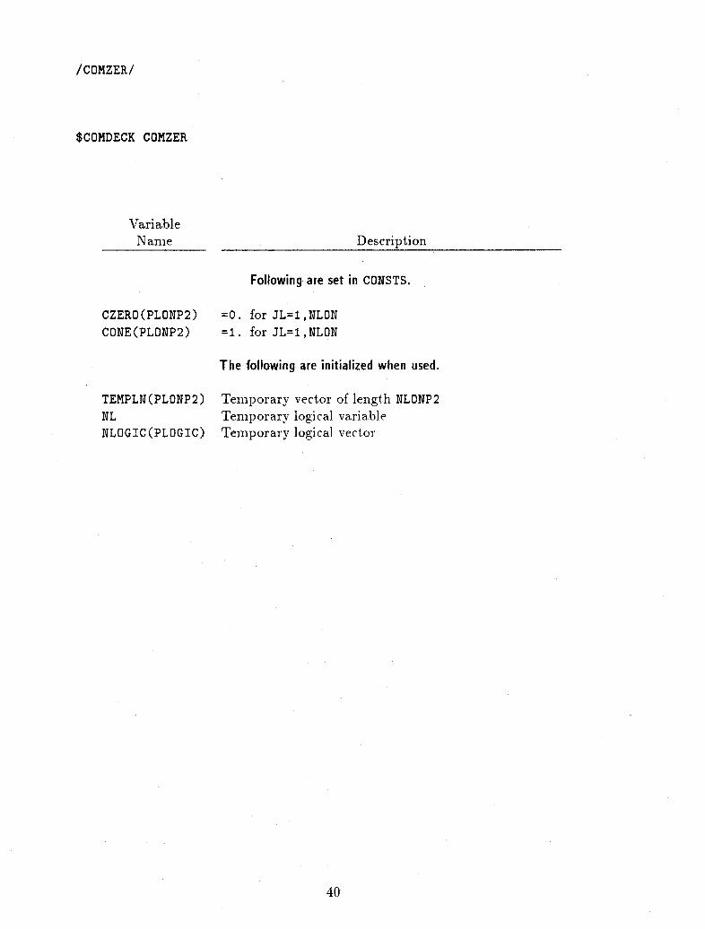
/COMZER/

$COMDECK COMZER

VariableName Description

Following are set in CONSTS.

CZERO(PLONP2)

CONE(PLONP2)

=0. for JL=1,NLON

=1. for JL=1,NLON

The following are initialized when used.

TEMPLN(PLONP2)NL

NLOGIC(PLOGIC)

Temporary vector of length NLONP2Temporary logical variable

Temporary logical vector

40

/CRDCTL/

$COMDECK CRDCTLCCL RADIATION CONTROL VARIABLESC

VariableName Description

FRADSW Logical flag; true iff full SW computations are being donefor the current iteration

FRADLW Logical flag; true iff full LW computations are being donefor the current iteration

IRADSW Frequency of full SW computations, in iterationsIRADLW Frequency of full LWT computations, in iterationsNACLW Accumulation counter for averaged LW history tape fields

NACSW Accumulation counter for averaged SW history tape fields

FNLW Normalization factor for averaged LW history tape fieldsFNSW Normalization factor for averaged SW history tape fields

FRADSW and FRADLW are set in RADCTL; IRADSW and IRADLW are set to their defaultvalues in subroutine PRESET, then potentially modified by NAMELIST $NEWRUN insubroutine DATA. Due to implicit assumptions imbedded in various parts of theradiation computation code, IRADSW and IRADLW must be set to the same value.This is assured by a test in subroutine DATA at the time these parameters are readin to the Model. The accumulation counters NACLW and NACSW are initialized insubroutine LINEMS, incremented in RADOUT, and used in LINEMS to compute thenormalization factors FNLW and FNSW. Averaged fields are normalized in WSHISTjust before they are written.

41

/PARAMS/

$COMDECK PARAMSC

CL CCM1 PARAMETER DEFINITIONSC

This Update Common Deck contains the INTEGER statements and PARAMETER state-

ments defining the FORTRAN PARAMETER values used throughout the Model. All

PARAMETERs are typed INTEGER.

Parameter Value Description

Truncation Parameters

PTRM 15 M spectral truncation parameter, used to defineModel variable NTRM in COMMON /COMTRU/

PTRN 15 N spectral truncation parameter, used to defineModel variable NTRN in COMMON /COMTRU/

PTRK 30 K spectral truncation parameter, used to defineModel variable NTRK in COMMON /COMTRU/

Model Domain

PLEV 12 Number of vertical levels, must match NLEV in/COMDMN/ as read from the Model initial data.

PLON 48 Number of longitudes in the horizontal domain,must match NLON in /COMDMN/ as read from theModel initial data.

POREC 40 Number of latitudes (records) in the horizontaldomain. Must match NOREC in /COMDMN/ as readfrom the Model initial data.

PSPHER 1 Global/hemispheric run flag. Code is currentlyvalid for PSPHER=1 only.

PLONP2 PLON+2 Number of grid points in the longitudinal di-rection, including 2 wraparound points. Mustmatch NLONP2 in /COMDMN/ as read from theModel initial data. The wraparound points arerequired for the FFT calculation.

42

/PARAMS/-2

Parameter Value

PCRAY

PEMAX

POMAX

PEMAXPPOMAXP-PNMAX

PMMAX

PLEVPPLEVP2PLEV2PLEV2NPOREC2

64

Description

Machine Word Size

Length of Cray word in bits, used to setNCRAY in /COMFFT/

Dimensions for Spectral Arrays

(PTRN/PSPHER) +1

(PTRN+1) /PSPHER

PEMAX+ 1POMAX+1PTRK+1

PTRM+1

PLEV+1PLEV+2PLEV*PLEVPLEV2*PNMAXPOREC/2

Number of even diagonals in spectral ar-rays. Used in dimensioning arrays in/COMTRU/.Number of odd diagonals. Used in dimen-sioning spectral arrays in /COMTRU/.

Number of values of n, used in dimension-ing arrays in /COMMAP/

Number of values of m, used in dimen-sioning arrays in /COMMAP/

Number of latitude lines in a hemisphere,used to dimension arrays in /COMMAP/

Intermediate Parameter Values

The following values are calculated geometrically to describe the storage of spectralcoefficients in COMMON /COMSPE/. The spectral coefficients conceptually form a 2-dimensional space, but because the rhomboidal truncation scheme leaves "gaps"in a rectangular array, instead the coefficients are stored consecutively in singly-dimensioned arrays, in diagonal order. The figures below show this 2-dimensionalconcept, with the actual area of stored values outlined in solid lines, the truncatedportions ill dashed lines. Figure 2 should make it easier to visualize PARAMETERvalues PARO, PAR1, PAR2 and PARS. Figure 3 illustrates values PAR6 through PAR10.See section II.B.2.a. of "Users' Guide to NCAR CCM1", (Bath et al., 1987) for adetailed description and further graphical representation of this storage scheme.

43

/PARAMS/-3

K+1)+1

(M,O)

(O.M+NN

K+K

(0,1*2[(N/2+1)-l]

Figure 2.(M.M+N)

//'I

////

figure 3.

2[(N/2 + 1) - 1] =number of last even diagonal.

t2[(N/2 + 1) - 1] + M - (K + 1) + 1 =number of diagonals in the triangle up to

and including the last even diagonal.

44

IrI I X \ - --1 - -1U, M + i j

vLK 1

K

(O,N)

(0,0)

1]4+M

-1]+M-(K+ 1)+ I1t

_,

FI

I

. I

I

I

I

I

I

I

I

I I

I

I

I

/PARAMS/-4

Parameter Value Description

PTRM+PTRN-PTRK

(PTRN+I)*PMMAX

PARO*(PARO+1)/2

PEMAX*PMMAX

POMAX*PMMAX

PARO/2PAR5*(PAR5+1)

PAR2-PAR6

2*(PEMAX-1)+PTRM-PTRK

PAR8-2*(PAR8/2)

PAR3

-(1-PAR9)*PAR6

-PAR9*PAR7

M+N-K, the number of diagonals in the"deleted" triangular tip of the rhonm-boid(N+1) * (M+ 1), the number of points inthe full rhomboid(M+N-K)*(M+N-K+1)/2, the numberof points in the deleted triangular tip,= 1+2+3+.. ..+ (M+N-K), the sum of in-tegers up to and including (M+N-K)Number of points in the full rhomboidof even diagonalsNumber of points in the full rhomboidof odd diagonals(M+N-K)/2((M+N-K)/2)*((M+N-K)/2+1)= 2+4+6+...+2*((M+N-K)/2),

sum of even numbers up to the num-ber of diagonals in triangular tip1+3+5+...+2*(((M+N-K+1)/2)-1),sum of odd numbers up to the numberof diagonals in triangular tip2*((N/2+1)-i)+M-K, number of diag-onals in triangular tip up to and in-cluding the last even one0 for even PAR81 for odd PAR8Number of points in full even rhom-boid

- sum of every other diagonal whenlast even diagonal has even number ofpoints- sum of every other diagonal whenlast even diagonal has odd number ofpoints= number of coefficients for even fieldat one level in hemispheric case

45

PARO

PAR1

PAR2

PAR3

PAR4

PARS

PAR6

PAR7

PAR8

PAR9

PAR1O

/PARAMS/-5

Parameter Value Description

Dimensions For Legendre Arrays

PAR1-PAR2

PSPT*2

PSPT-PAR10

Number of spherical harmonic func-tions in representationNumber of words required for complexcoefficients at one levelTotal number of coefficients at onelevel minus number for even field =number of coefficients for odd field atone level in hemispheric case

Blank COMMON Buffer Lengths

Refer to Figure 11.18 in "Users' Guide to NCAR CCM1", (Bath et al., 1987)for a graphical representation of these lengths.

4

(6*PLEV+2)*PLONP2+ PSCAL*PLEV*PLONP2

(6*PLEV+26)*PLONP2

(10*PLEV+7)*PLONP2

PTFLEN+PDFLEN

PLREC+PBPHYSPLREC+2*PLONP2(11*PLEV+1)*PLONP2

Number of diffusion terms stored inNLINE1Length of prognostic variablesin NLINE1,NLINE2Length of time history fields inNLINE1,NLINE2Length of diagnostic fields inNLINE1,NLINE2Total length of physical fields inNLINE1,NLINE2Total length of NLINE1 or NLINE2Total length of NLINE3Length of NLINE4 based on spaceneeded for spectral transformation.This length is checked in subroutineLNGTHS against N4END-NLINE4(= 8*PLEV*PLONP2+4*PSPT), spaceneeded for transformation to spectralspace.

1 These parameters are used in actual allocation of space for the blank COMMON bufferand differ in value for Program Libraries CCM1PL1 and CCM1PL2. Refer to"Users' Guide to NCAR CCMI", (Bath et al., 1987)" for detailed instructions forcalculating these values when running the Model at changed resolutions.

46

PSPT

PSPT2

PAR11

PSCAL

PLREC

PTFLEN'

PDFLEN1

PBPHYS

PBFLNB'PBFLNA1

PSYM1

_ _

/PARAMS/-6

Parameter Value Description

(10*PLEV+1)*PLONP2

+13*PLON

23

29

(PMULTI*PLEV

+PSINGL)*PLON+6

PLONP2+PLENHT+

(3*PLEV+1)*PLONP2

PMULTI+PSINGL

4*PBFLNB+2*PBFLNA

+PSYM+PLEN5

Length of NLINE5, based on grid point

storage required in LINEMS

The maximum of the number of multi-

level fields on the history tape and the

number on the initial dataset

The maximum of the number of single-

level fields on the history tape and the

number on the initial dataset

Length of history tape buffer

Length of NLINE5 based on historytape buffer requirements. This is the

the length actually used in allocating

space for NLINE5.

Total number of fields on history tape

Total length of blank COMMON buffer

FFT Parameters

3*PLON/2+1

(PLON+1)*PCRAY

2* (PSPT* (2-PSPHER)

+(PSPHER-1)*PAR10)

2*(PSPT*(2-PSPHER)

+(PSPHER-1)*PAR11)

Used to dimension trig table in/COMFFT/

Used to dimension FFT work space in/COMFFT/

The number of words needed for thethe spectral coefficients of the evenfield at one level. Used to dimensionarray ALPS in /COMSPE/.

The number of words needed for the

spectral coefficients of the odd field at

one level.

These parameters are used in actual allocation of space for the blank COMMON buffer,and differ in value for Program Libraries CCM1PL1 and CCM1PL2. Refer to"Users' Guide to NCAR CCM1" (Bath, et al., 1987) for detailed instructions forcalculating this value when changing the Model resolution or history tape.

47

PBAUXL

PMULTI'

PSINGL 1

PLENHT

PLEN5'

PTPLEN

PLNBUF

PFFT1

PFFT2

PSPE

PSPO

/PARAMS/-7

Parameter Value Description

PSPE*PLEV

PSPO*PLEV

Number of words needed for spectral co-efficients of even fields with PLEV levels,used to dimension arrays in /COMSPE/Number of words needed for spectral co-efficients of odd fields with PLEV levels,used to dimension arrays in /COMSPE/

Miscellaneous Parameters

(100+PLEV)/PLONP2PLONP2*(PLOG1+1)10

3

23*PTPLEN37+PLENBI2*PTPLEN76+PLENBC2*PLEV+1+2*POREC

PLENBR

Used to calculate PLOGIC belowDimension of NLOGIC in /COMZER/Number of fields needed by the Model

from the initial dataset

Number of records preceding data rec-ords on an output history tape file

History tape format typeLength of /COMHDI/ bufferLength of entire integer header recordLength of /COMHDC/ bufferLength of entire character header recordLength of /COMHDR/ bufferLength of entire real header record

48

PSPEL

PSPOL

PLOG1PLOGICPFLDS

PRBD

PFTYPPLENBIPLENHIPLENBCPLENHCPLENBR

PLENHR

5. Changes and Additions to the CCM1 Circulation Statistics Atlas

In December of 1987 an atlas was produced which contained horizontal maps

and meridional cross sections of selected circulation statistics from CCM1 R15 con-

trol simulations (Williamson and Williamson 1984). Preliminary examination of a short

CCM1PL1 control suggested that the correction to the formulation of the surface energy

balance had resulted in some changes to the statistical properties of the earlier CCM1

control simulations. Therefore, a new set of ten-year seasonal control simulations were

conducted and analyzed in detail for comparison with the earlier CCM1 controls. These

seasonal simulations were started on October 1, rather than mid-January as in the ear-

lier control simulations. Thus, the first winter (Dec-Jan-Feb) sample occurs two months

into the integration. As before, the history data for these two control experiments (Case

256, fixed hydrology; Case 263, variable hydrology) was written every 12 hours and is

available for analysis on a series of MSS data sets which are tabulated later in section

5.1. Two experimental T42 controls have also been completed with the CCM1PL2 pro-

gram library where the history data was written every 24 hours. The MSS history files

for these controls are tabulated later in section 5.2.

A more detailed analysis of the new seasonal controls generally indicated only small

quantitative changes in the statistical properties of the simulated climate as published

in (Williamson and Williamson 1984). The exception is the surface and near surface

climate in the polar regions which is up to 2° colder (in the zonal average at the sur-

face) in the winter hemisphere. Although this cooling is observed in both hemispheres

during their respective winter seasons, the largest differences, both in magnitude and

horizontal extent, occur in the Northern Hemlisphere. An example of the near sur-

face temperature change can be seen in Fig. 5.1 which shows the December-February

and June-August ensemble averaged difference in the lowest model layer temperatures

between the new CCM1 seasonal control (Case 256) and the CCM1 seasonal control

published in Williamson and Williamson (Case 239). The colder regions, which are

49

DECEMBER-FEBRUARY

90N

60N

30N

0

30S

60S

90S

180W 150W 120W 90W 60W 30W 30E 60E 90E 120E 10E 1 E80E

JUNE-AUGUST

180s 150w 120W 90W 60W 30W 0 30E 60E 9OE 120E 150E 180E

Fig. 5.1 Difference of ensemble average of time-averaged temperature for CASE 256-CASE239 at first atmospheric level above the surface for DECEMBER-FEBRUARY (top) and

JUNE-AUGUST (bottom), global cylindrical projection, contour interval 1 K.

50

'

0.

---------- -- -- - .......................... . . . . - . …

.......... ~ ~ ~ ---..

I

geographically located in the vicinity of Hudson Bay and eastern Siberia, reach maxi-

mum departures of just under 5 K. Although these appear to be large differences, they

are, for the most part, within one standard deviation of the seasonal means of the earlier

Case 239 CCM1 control experiment.

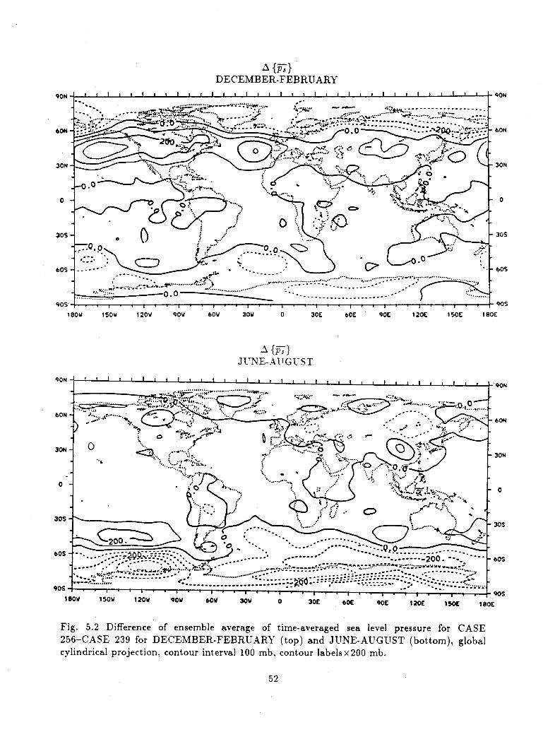
Another example of one of the more extreme differences between the CCM1PL1

and CCM1PL controls is shown in Fig. 5.2 which shows the change in the December-

February and June-August time-averaged sea level pressure. This figure exhibits a zonal

band of increased surface pressure in mid-latitudes and a comparable pattern of reduced

surface pressure in the polar regions in the winter hemisphere. The spacial coherence

of this difference is particularly pronounced during the Northern Hemisphere winter.

Maximum departures are between 4 and 5 mb, and as in the case of the near surface

temperature, are within about one standard deviation of the seasonal means of the Case

239 control experiment.

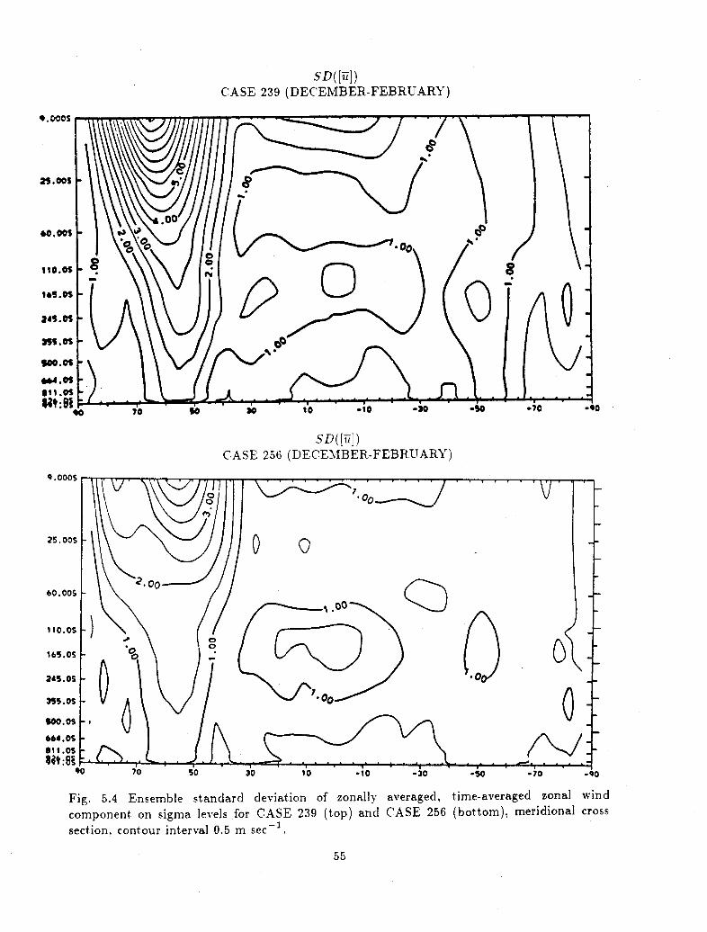
The zonally and time averaged state variables (temperature, zonal wind, meridional

wind, etc.) exhibit only very minor changes from the Case 239 control. For example,

the December-February ensemble average shows a maximum departure in the tempera-

ture field of 0.55 K (in the lower troposphere near the north pole), while the zonal wind

exhibits a maximum departure of 1.5 ms - 1, and local changes in the meridional wind

remain less than 0.15 ms- '. Although the mean states exhibit only small changes, the

variability of the temperature and zonal wind fields is significantly reduced, particularly

in the polar stratosphere where the ensemble standard deviation is about a factor of two

smaller. As an example, we show the zonally and time averaged zonal wind for both

Cases 239 and 256, along with their ensemble standard deviations in Figs. 5.3 and 5.4.

The mean states are virtually identical, as can be seen in Fig. 5.3, but the local variabil-

ity is considerably reduced in certain regions. During Northern Hemisphere summer,

differences in the zonally and time averaged fields are of comparable magnitude to the

winter season differences, while the variability (in terms of the ensemble average stan-

dard deviations) is almost identical. Thus, the major differences in seasonal variability

51

DECEMBER-FEBRUARY90N

60N

30N

0

30S

OS

9OS

180W 150V 120W 90W 60W 30W 0 30E 60E 90E 120E 150E 180E

A{ G}SJUNE-AUTGUST

- b60

180u 150W 120W 90W 60 3W 0 30E 60E OE 120 150 80E

Fig. 5.2 Difference of ensemble average of time-averaged sea level pressure for CASE256-CASE 239 for DECEMBER-FEBRUARY (top) and JUNE-AUGUST (bottom), globalcylindrical projection, contour interval 100 mb, contour labelsx200 mb.

52

... ,-r -s~~~~~~~~~~~ -..........- ----- ;.--:-: - -- -

.- . . . . . . . . .- - -.-.i--- I I I I I T I I -. I . --1 I i v , r . . -i v I . --- 90S

I1gUo ?

z

.!-Wlw

appear to be largely confined to the Northern Hemisphere circulation during Northern

Hemisphere winter.

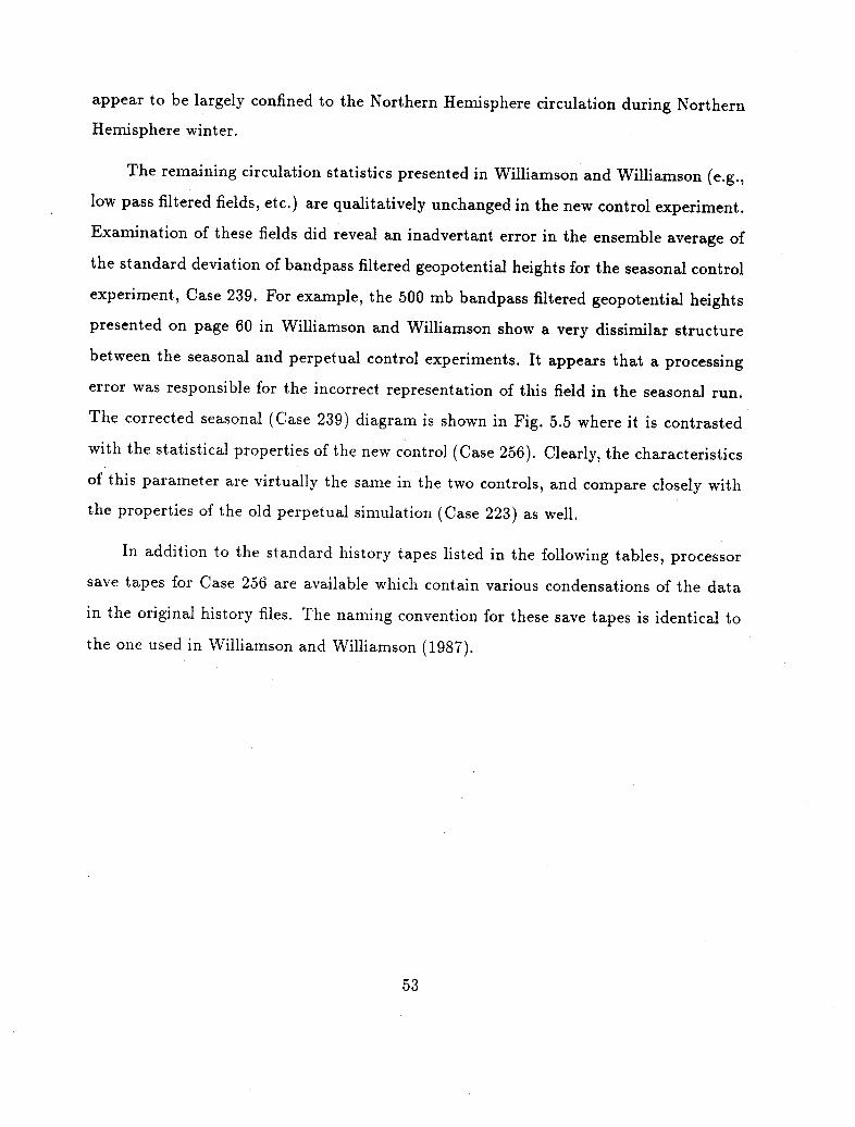
The remaining circulation statistics presented in Williamson and Williamson (e.g.,

low pass filtered fields, etc.) are qualitatively unchanged in the new control experiment.

Examination of these fields did reveal an inadvertant error in the ensemble average of

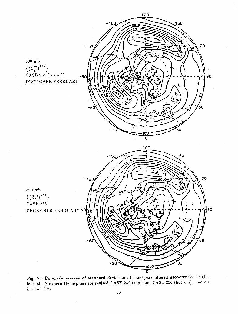
the standard deviation of bandpass filtered geopotential heights for the seasonal control

experiment, Case 239. For example, the 500 mb bandpass filtered geopotential heights

presented on page 60 in Williamson and Williamson show a very dissimilar structure

between the seasonal and perpetual control experiments. It appears that a processing

error was responsible for the incorrect representation of this field in the seasonal run.

The corrected seasonal (Case 239) diagram is shown in Fig. 5.5 where it is contrasted

with the statistical properties of the new control (Case 256). Clearly, the characteristics

of this parameter are virtually the same in the two controls, and compare closely with

the properties of the old perpetual simulation (Case 223) as well.

In addition to the standard history tapes listed in the following tables, processor

save tapes for Case 256 are available which contain various condensations of the data

in the original history files. The naming convention for these save tapes is identical to

the one used in Williamson and Williamson (1987).

53

CE 29 (CASE 239 (DECEMBER-FEBRUARY)

{[u( ]CASE 256 (DECEMBER FEBRUARY)

Fig. 5.3 Ensemble average of zonally averaged, time-averaged zonal wind component on sigma

levels for CASE 239 (top) and CASE 256 (bottom), meridional cross section, contour interval

5 m sec .

54

9.ooos

25.005

25. OOS60.005

110.0S

16S.05

245.0S

355.OS

S4.01M.OS

- ----

SD([u])CASE 239 (DECEMBER-FEBRUARY)

SD([Ti])CASE 256 (DECEMNIBER-FEBRUARY)

Fig. 5.4 Ensemble standard deviation of zonally averaged, time-averaged zonal windcomponent on sigma levels for CASE 239 (top) and CASE 256 (bottom), meridional cross

section. contour interval 0.5 m sec 1.

55

*. coos

25. 001

*0..00'

110.01

1*9.01

245.0

900.0

MM.O611.0

$t :1.

180

500 mb

{ (z2)1/2}

CASE 239 (revised)

DECEMBER-FEBRUARY

12C

90

-12(

90

Fig. 5.5 Ensemble average of standard deviation of band-pass filtered geopotential height,

500 mb. Northern Hemisphere for revised CASE 239 (top) and CASE 256 (bottom), contour

interval 5 m.56

Iq

I

5.1 MSS History Tape Names for R15 Seasonal Controls

The following tables contain MSS history tape names for R15 seasonal controls

Case 256 (fixed hydrology) and Case 263 (variable hydrology). History data was written

every 12 hours and each MSS volume contains 30 files. The data format is described in

(Bath et al. 1987a).

57

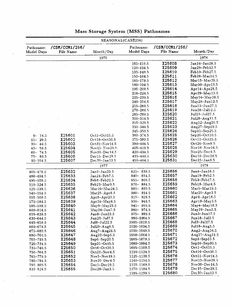
Mass Storage System (MSS) Pathnames

SEASONAL(CASE256)

Pathname: /CSM/CCM1/256/ Pathname: /CSM/CCM1/256/Model Days File Name Month/Day Model Days File Name Month/Day

1975 1976

105-119.5 X25608 Janl4-Jan28.5120-134.5 X25609 Jan29-Febl2.5135-149.5 X25610 Febl3-Feb27.5150-164.5 X25611 Feb28-Marl4.5165-179.5 X25612 Marl5-Mar29.5180-194.5 X25613 Mar30-Aprl3.5195-209.5 X25614 Aprl4-Apr28.5210-224.5 X25615 Apr29-Mayl3.5225-239.5 X25616 Mayl4-May28.5240-254.5 X25617 May29-Junl2.5255-269.5 X25618 Junl3-Jun27.5270-284.5 X25619 Jun28-Jull2.5285-299.5 X25620 Jull13-Jul27.5300-314.5 X25621 Jul28-Augll.5315-329.5 X25622 Augl2-Aug26.5330-344.5 X25623 Aug27-SeplO.5345-359.5 X25624 Sepll-Sep25.5

0- 14.5 X25601 Octl-Octl5.5 360-374.5 X25625 Sep26-Oct10.515- 29.5 X25602 Octl6-Oct30.5 375-389.5 X25626 Oct1-Oct25.530- 44.5 X25603 Oct31-Novl4.5 390-404.5 X25627 Oct26-Nov9.545- 59.5 X25604 Nov15-Nov29.5 405-419.5 X25628 NovlO-Nov24.560- 74.5 X25605 Nov30-Decl4.5 420-434.5 X25629 Nov25-Dec9.575- 89.5 X25606 Decl5-Dec29.5 435-449.5 X25630 DeclO-Dec24.590-104.5 X25607 Dec30-Janl3.5 450-464.5 X25631 Dec25-Jan8.5

1977 1978

465-479.5 X25632 Jan9-Jan23.5 825- 839.5 X25656 Jan4-Janl8.5480-494.5 X25633 Jan24-Feb7.5 840- 854.5 X25657 Janl19-Feb2.5495-509.5 X25634 Feb8-Feb22.5 855- 869.5 X25658 Feb3-Febl7.5510-524.5 X25635 Feb23-Mar9.5 870- 884.5 X25659 Febl8-Mar4.5525-539.5 X25636 MarlO-Mar24.5 885- 899.5 X25660 Mar5-Marl9.5540-554.5 X25637 Mar25-Apr8.5 900- 914.5 X25661 Mar20-Apr3.5555-569.5 X25638 Apr9-Apr23.5 915- 929.5 X25662 Apr4-Aprl8.5570-584.5 X25639 Apr24-May8.5 930- 944.5 X25663 Aprl9-May3.5585-599.5 X25640 May9-May23.5 945- 959.5 X25664 May4-Mayl8.5600-614.5 X25641 May24-Jun7.5 960- 974.5 X25665 Mayl9-Jun2.5615-629.5 X25642 Jun8-Jun22.5 975- 989.5 X25666 Jun3-Junl7.5630-644.5 X25643 Jun23-Jul7.5 990-1004.5 X25667 Junl8-Jul2.5645-659.5 X25644 Jul8-Jul22.5 1005-1019.5 X25668 Jul3-Jull7.5660-674.5 X25645 Ju123-Aug6.5 1020-1034.5 X25669 Jull8-Augl.5675-689.5 X25646 Aug7-Aug21.5 1035-1049.5 X25670 Aug2-Augl6.5690-704.5 X25647 Aug22-Sep5.5 1050-1064.5 X25671 Augl7-Aug31.5705-719.5 X25648 Sep6-Sep20.5 1065-1079.5 X25672 Sepl-Sepl5.5720-734.5 X25649 Sep21-Oct5.5 1080-1094.5 X25673 Sepl6-Sep30.5735-749.5 X25650 Oct6-Oct20.5 1095-1109.5 X25674 Octl-Octl5.5750-764.5 X25651 Oct21-Nov4.5 1110-1124.5 X25675 Octl6-Oct30.5765-779.5 X25652 Nov5-Novl9.5 1125-1139.5 X25676 Oct31-Novl4.5780-794.5 X25653 Nov20-Dec4.5 1140-1154.5 X25677 Novl5-Nov29.5795-809.5 X25654 Dec5-Decl9.5 1155-1169.5 X25678 Nov30-Decl4.5810-824.5 X25655 Dec20O-Jan3.5 1170-1184.5 X25679 Decl5-Dec29.5

1185-1199.5 X25680 Dec30-Janl3.5

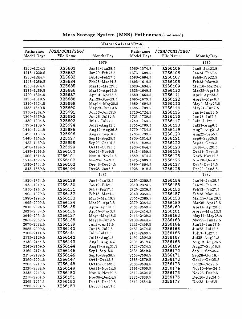
Mass Storage System (MSS) Pathnames (continued)

SEASONAL(CASE256)

Pathname: /CSM/CCM1/256/ Pathname: /CSM/CCM1/256/Model Days File Name Month/Day Model Days File Name Month/Day

1979 1980

1200-1214.5 X25681 Janl4-Jan28.5 1560-1574.5 X256105 Jan9-Jan23.51215-1229.5 X25682 Jan29-Febl2.5 1575-1589.5 X256106 Jan24-Feb7.51230-1244.5 X25683 Febl3-Feb27.5 1590-1604.5 X256107 Feb8-Feb22.51245-1259.5 X25684 Feb28-Marl4.5 1605-1619.5 X256108 Feb23-Mar9.51260-1274.5 X25685 Marl5-Mar29.5 1620-1634.5 X256109 MarlO-Mar24.51275-1289.5 X25686 Mar30-Aprl3.5 1635-1649.5 X256110 Mar25-Apr8.51290-1304.5 X25687 Apr14-Apr28.5 1650-1664.5 X256111 Apr9-Apr23.51305-1319.5 X25688 Apr29-Mayl3.5 1665-1679.5 X256112 Apr24-May8.51320-1334.5 X25689 Mayl4-May28.5 1680-1694.5 X256113 May9-May23.51335-1349.5 X25690 May29-Junl2.5 1695-1709.5 X256114 May24-Jun7.51350-1364.5 X25691 Junl3-Jun27.5 1710-1724.5 X256115 Jun8-Jun22.51365-1379.5 X25692 Jun28-Jull2.5 1725-1739.5 X256116 Jun23-Jul7.51380-1394.5 X25693 Jull3-Ju127.5 1740-1754.5 X256117 Jul8-Jul22.51395-1409.5 X25694 Ju128-Augll.5 1755-1769.5 X256118 Jul23-Aug6.51410-1424.5 X25695 Augl2-Aug26.5 1770-1784.5 X256119 Aug7-Aug21.51425-1439.5 X25696 Aug27-Sepl O.5 1785-1799.5 X256120 Aug22-Sep5.51440-1454.5 X25697 Sepll-Sep25.5 1800-1814.5 X256121 Sep6-Sep20.51455-1469.5 X25698 Sep26-Oct10.5 1815-1829.5 X256122 Sep21-Oct5.51470-1484.5 X25699 Octll-Oct25.5 1830-1844.5 X256123 Oct6-Oct20.51485-1499.5 X256100 Oct26-Nov9.5 1845-1859.5 X256124 Oct21-Nov4.51500-1514.5 X256101 NovlO-Nov24.5 1860-1874.5 X256125 Nov5-Novl9.51515-1529.5 X256102 Nov25-Dec9.5 1875-1889.5 X256126 Nov20-Dec4.51530-1544.5 X256103 DeclO-Dec24.5 1890-1804.5 X256127 Dec5-Decl9.51545-1559.5 X256104 Dec25-Jan8.5 1905-1919.5 X256128 Dec20-Jan3.5

1981 1982

1920-1934.5 X256129 Jan4-Janl8.5 2295-2309.5 X256154 Janl4-Jan28.51935-1949.5 X256130 Janl9-Feb2.5 2310-2324.5 X256155 Jan29-Febl2.51950-1964.5 X256131 Feb3-Febl7.5 2325-2339.5 X256156 Febl3-Feb27.51965-1979.5 X256132 Febl8-Mar4.5 2340-2354.5 X256157 Feb28-Marl4.51980-1994.5 X256133 Mar5-Marl9.5 2355-2369.5 X256158 Marl5-Mar29.51995-2009.5 X256134 Mar20-Apr3.5 2370-2384.5 X256159 Mar30-Aprl3.52010-2024.5 X256135 Apr4-Aprl8.5 2385-2569.5 X256160 Aprl4-Apr28.52025-2039.5 X256136 Aprl9-May3.5 2400-2414.5 X256161 Apr29-Mayl3.52040-2054.5 X256137 May4-Mayl8.5 2415-2429.5 X256162 Mayl4-May28.52055-2069.5 X256138 Mayl9-Jun2.5 2430-2444.5 X256163 May29-Junl2.52070-2084.5 X256139 Jun3-Junl7.5 2445-2459.5 X256164 Junl3-Jun27.52085-2099.5 X256140 Junl8-Jul2.5 2460-2474.5 X256165 Jun28-Jull2.52100-2114.5 X256141 Jul3-Jull17.5 2475-2489.5 X256166 Jull13-Jul27.52115-2129.5 X256142 Jull8-Augl.5 2490-2504.5 X256167 Jul28-Augll.52130-2144.5 X256143 Aug2-Augl6.5 2505-2519.5 X256168 Augl2-Aug26.52145-2159.5 X256144 Augl7-Aug31.5 2520-2534.5 X256169 Aug27-SeplO.52160-2174.5 X256145 Sepl-Sepl5.5 2535-2549.5 X256170 Sepll-Sep25.52175-2189.5 X256146 Sepl6-Sep30.5 2550-2564.5 X256171 Sep26-OctlO0.52190-2204.5 X256147 Octl-Octl5.5 2565-2579.5 X256172 Octll-Oct25.52205-2219.5 X256148 Octl6-Oct30.5 2580-2594.5 X256173 Oct26-Nov9.52220-2234.5 X256149 Oct31-Novl4.5 2595-2609.5 X256174 NovlO-Nov24.52235-2249.5 X256150 Novl5-Nov29.5 2610-2624.5 X256175 Nov25-Dec9.52250-2264.5 X256151 Nov30-Decl4.5 2625-2639.5 X256176 DeclO-Dec24.52265-2279.5 X256152 Decl5-Dec29.5 2640-2654.5 X256177 Dec25-Jan8.52280-2294.5 X256153 Dec30-Janl3.5

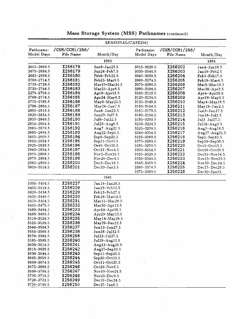
Mass Storage System (MSS) Pathnames (continued)

SEASONAL(CASE256)

Pathname: /CSM/CCM1/256/ Pathname: /CSM/CCM1/256/Model Days File Name Month/Day Model Days File Name Month/Day

1983 1984

2655-2669.5 X256178 Jan9-Jan23.5 3015-3029.5 X256202 Jan4-Janl8.52670-2684.5 X256179 Jan24-Feb7.5 3030-3044.5 X256203 Jan19-Feb2.52685-2699.5 X256180 Feb8-Feb22.5 3045-3059.5 X256204 Feb3-Febl7.52700-2714.5 X256181 Feb23-Mar9.5 3060-3074.5 X256205 Febl8-Mar4.52715-2729.5 X256182 MarlO-Mar24.5 3075-3089.5 X256206 Mar5-Marl9.52730-2744.5 X256183 Mar25-Apr8.5 3090-3104.5 X256207 Mar20-Apr3.52275-2759.5 X256184 Apr9-Apr23.5 3105-3119.5 X256208 Apr4-Aprl8.52760-2774.5 X256185 Apr24-May8.5 3120-3134.5 X256209 Apr19-May3.52775-2789.5 X256186 May9-May23.5 3135-3149.5 X256210 May4-MayI8.52790-2804.5 X256187 May24-Jun7.5 3150-3164.5 X256211 Mayl9-Jun2.52805-2819.5 X256188 Jun8-Jun22.5 3165-3179.5 X256212 Jun3-Junl7.52820-2834.5 X256189 Jun23-Jul7.5 3180-3194.5 X256213 Junl8-Jul2.52835-2849.5 X256190 Jul8-Ju122.5 3195-3209.5 X256214 Ju13-Jull7.52850-2864.5 X256191 Jul23-Aug6.5 3210-3224.5 X256215 Jull8-Augl.52865-2879.5 X256192 Aug7-Aug21.5 3225-3239.5 X256216 Aug2-Augl6.52880-2894.5 X256193 Aug22-Sep5.5 3240-3254.5 X256217 Aug17-Aug31.52895-2909.5 X256194 Sep6-Sep20.5 3255-3269.5 X256218 Sepl-Sepl5.52910-2924.5 X256195 Sep21-Oct5.5 3270-3284.5 X256219 Sepl6-Sep30.52925-2839.5 X256196 Oct6-Oct20.5 3285-3299.5 X256220 Octl-Octl5.52940-2854.5 X256197 Oct21-Nov4.5 3300-3314.5 X256221 Octl6-Oct30.52955-2869.5 X256198 Nov5-Novl9.5 3315-3329.5 X256222 Oct31-Novl4.52970-2884.5 X256199 Nov20-Dec4.5 3330-3344.5 X256223 Nov15-Nov29.52985-2899.5 X256200 Dec5-Decl9.5 3345-3359.5 X256224 Nov30-Decl4.53000-3014.5 X256201 Dec20-Jan3.5 3360-3374.5 X256225 Decl5-Dec29.5

3375-3389.5 X256226 Dec30-Janl3.

1985

3390-3404.5 X256227 Janl4-Jan28.53405-3419.5 X256228 Jan29-Febl2.53420-3434.5 X256229 Febl3-Feb27.53435-3449.5 X256230 Feb28-Marl4.53450-3464.5 X256231 Marl5-Mar29.53465-3479.5 X256232 Mar30-Aprl3.53480-3494.5 X256233 Aprl4-Apr28.53495-3409.5 X256234 Apr29-Mayl3.53510-3524.5 X256235 Mayl4-May28.53525-3539.5 X256236 May29-Junl2.53540-3554.5 X256237 Junl3-Jun27.53555-3569.5 X256238 Jun28-Jull2.53570-3584.5 X256256 Jull3-Ju127.53585-3599.5 X256240 Jul28-Augll.53600-3614.5 X256241 Augl2-Aug26.53615-3629.5 X256242 Aug27-SeplO.53630-3644.5 X256243 Sepll-Sep25.53645-3659.5 X256244 Sep26-OctlO.53660-3674.5 X256245 Octll-Oct25.53675-3689.5 X256246 Oct26-Nov9.53690-3704.5 X256247 NovlO-Nov24.53705-3719.5 X256248 Nov25-Dec9.53720-3734.5 X256249 DeclO-Dec24.53735-3749.5 X256250 Dec25-Jan8.5

Mass Storage System (MSS) Pathnames

SEASONAL-HYDRO(CASE263)

Pathname: /CSM/CCM1/263/ Pathname: /CSM/CCM1/263/Model Days File Name Month/Day Model Days File Name Month/Day

1975 1976

105-119.5 X26308 Janl4-Jan28.5120-134.5 X26309 Jan29-Febl2.5135-149.5 X26310 Febl3-Feb27.5150-164.5 X26311 Feb28-Marl4.5165-179.5 X26312 Marl5-Mar29.5180-194.5 X26313 Mar30-Aprl3.5195-209.5 X26314 Aprl4-Apr28.5210-224.5 X26315 Apr29-Mayl3.5225-239.5 X26316 Mayl4-May28.5240-254.5 X26317 May29-Junl2.5255-269.5 X26318 Jun13-Jun27.5270-284.5 X26319 Jun28-Jull2.5285-299.5 X26320 Jull13-Ju127.5300-314.5 X26321 Jul28-Aug1ll.5315-329.5 X26322 Aug12-Aug26.5330-344.5 X26323 Aug27-SeplO.5345-359.5 X26324 Sepl l-Sep25.5

0- 14.5 X26301 Octl-Oct15.5 360-374.5 X26325 Sep26-OctlO.515- 29.5 X26302 Octl6-Oct30. 375-389.5 X26326 Octll-Oct25.530- 44.5 X26303 Oct31-Novl4. 390-404.5 X26327 Oct26-Nov9.545- 59.5 X26304 Novl5-Nov29. 405-419.5 X26328 NovlO-Nov24.560- 74.5 X26305 Nov30-Decl4. 420-434.5 X26329 Nov25-Dec9.575- 89.5 X26306 Decl5-Dec29. 435-449.5 X26330 DeclO-Dec24.590-104.5 X26307 Dec30-Janl3.5 450-464.5 X26331 Dec25-Jan8.5

1977 1978

465-479.5 X26332 Jan9-Jan23.5 825- 839.5 X26356 Jan4-Jan18.5480-494.5 X26333 Jan24-Feb7.5 840- 854.5 X26357 Janl9-Feb2.5495-509.5 X26334 Feb8-Feb22.5 855- 869.5 X26358 Feb3-Febl7.5510-524.5 X26335 Feb23-Mar9.5 870- 884.5 X26359 Febl8-Mar4.5525-539.5 X26336 MarlO-Mar24.5 885- 899.5 X26360 Mar5-Marl9.5540-554.5 X26337 Mar25-Apr8.5 900- 914.5 X26361 Mar20-Apr3.5555-569.5 X26338 Apr9-Apr23.5 915- 929.5 X26362 Apr4-Aprl8.5570-584.5 X26339 Apr24-May8.5 930- 944.5 X26363 Aprl9-May3.5585-599.5 X26340 May9-May23.5 945- 959.5 X26364 May4-Mayl8.5600-614.5 X26341 May24-Jun7.5 960- 974.5 X26365 Mayl9-Jun2.5615-629.5 X26342 Jun8-Jun22.5 975- 989.5 X26366 Jun3-Junl7.5630-644.5 X26343 Jun23-Ju17.5 990-1004.5 X26367 Jun18-Jul2.5645-659.5 X26344 Jul8-Jul22.5 1005-1019.5 X26368 Jul3-Jull17.5660-674.5 X26345 Jul23-Aug6.5 1020-1034.5 X26369 Jull8-Augl.5675-689.5 X26346 Aug7-Aug21.5 1035-1049.5 X26370 Aug2-Augl6.5690-704.5 X26347 Aug22-Sep5.5 1050-1064.5 X26371 Augl7-Aug31.5705-719.5 X26348 Sep6-Sep20.5 1065-1079.5 X26372 Sepl-Sep15.5720-734.5 X26349 Sep21-Oct5.5 1080-1094.5 X26373 Sepl6-Sep30.5735-749.5 X26350 Oct6-Oct20.5 1095-1109.5 X26374 Octl-Octl5.5750-764.5 X26351 Oct21-Nov4.5 1110-1124.5 X26375 Octl6-Oct30.5765-779.5 X26352 Nov5-Novl9.5 1125-1139.5 X26376 Oct31-Nov14.5780-794.5 X26353 Nov20-Dec4.5 1140-1154.5 X26377 Novl5-Nov29.5795-809.5 X26354 Dec5-Decl9.5 1155-1169.5 X26378 Nov30-Decl4.5810-824.5 X26355 Dec20-Jan3.5 1170-1184.5 X26379 Decl5-Dec29.5

1185-1199.5 X26380 Dec30-Jan13.5

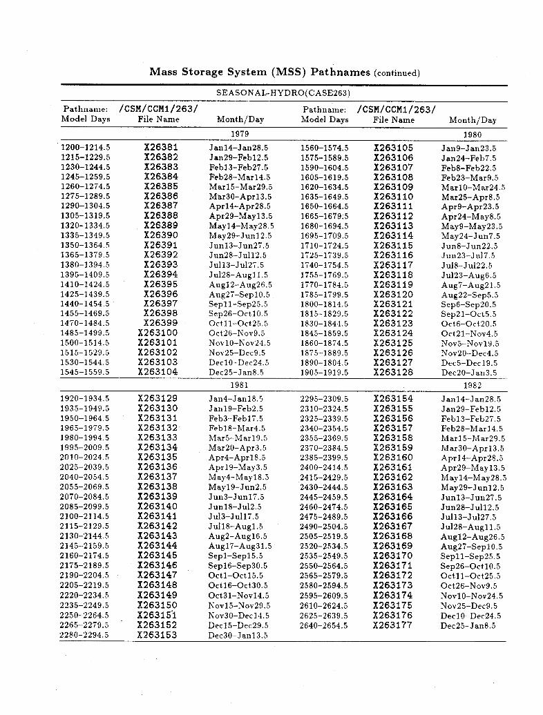
Mass Storage System (MSS) Pathnames (continued)

SEASONAL-HYDRO(CASE263)

Pathnamne: /CSM/CCM1/263/ Pathname: /CSM/CCM1/263/Model Days File Name Month/Day Model Days File Name Month/Day

1979 1980

1200-1214.5 X26381 Jan14-Jan28.5 1560-1574.5 X263105 Jan9-Jan23.51215-1229.5 X26382 Jan29-Febl2.5 1575-1589.5 X263106 Jan24-Feb7.51230-1244.5 X26383 Febl3-Feb27.5 1590-1604.5 X263107 Feb8-Feb22.51245-1259.5 X26384 Feb28-Marl4.5 1605-1619.5 X263108 Feb23-Mar9.51260-1274.5 X26385 Marl5-Mar29.5 1620-1634.5 X263109 MarlO-Mar24.51275-1289.5 X26386 Mar30-Aprl3.5 1635-1649.5 X263110 Mar25-Apr8.51290-1304.5 X26387 Apr14-Apr28.5 1650-1664.5 X263111 Apr9-Apr23.51305-1319.5 X26388 Apr29-Mayl3.5 1665-1679.5 X263112 Apr24-May8.51320-1334.5 X26389 Mayl4-May28.5 1680-1694.5 X263113 May9-May23.51335-1349.5 X26390 May29-Junl2.5 1695-1709.5 X263114 May24-Jun7.51350-1364.5 X26391 Junl3-Jun27.5 1710-1724.5 X263115 Jun8-Jun22.51365-1379.5 X26392 Jun28-Jull2.5 1725-1739.5 X263116 Jun23-Jul7.51380-1394.5 X26393 Jull3-Jul27.5 1740-1754.5 X263117 Ju18-Jul22.51395-1409.5 X26394 Jul28-Augll.5 1755-1769.5 X263118 Jul23-Aug6.51410-1424.5 X26395 Augl2-Aug26.5 1770-1784.5 X263119 Aug7-Aug21.51425-1439.5 X26396 Aug27-Sepl0.5 1785-1799.5 X263120 Aug22-Sep5.51440-1454.5 X26397 Sepll-Sep25.5 1800-1814.5 X263121 Sep6-Sep20.51455-1469.5 X26398 Sep26-OctlO0.5 1815-1829.5 X263122 Sep21-Oct5.51470-1484.5 X26399 Oct 1l-Oct25.5 1830-1844.5 X263123 Oct6-Oct20.51485-1499.5 X263100 Oct26-Nov9.5 1845-1859.5 X263124 Oct21-Nov4.51500-1514.5 X263101 NovlO-Nov24.5 1860-1874.5 X263125 Nov5-Novl9.51515-1529.5 X263102 Nov25-Dec9.5 1875-1889.5 X263126 Nov20-Dec4.51530-1544.5 X263103 DeclO-Dec24.5 1890-1804.5 X263127 Dec5-Decl9.51545-1559.5 X263104 Dec25-Jan8.5 1905-1919.5 X263128 Dec20-Jan3.5

1981 1982

1920-1934.5 X263129 Jan4-Janl8.5 2295-2309.5 X263154 Janl4-Jan28.51935-1949.5 X263130 Janl9-Feb2.5 2310-2324.5 X263155 Jan29-Febl2.51950-1964.5 X263131 Feb3-Febl7.5 2325-2339.5 X263156 Febl3-Feb27.51965-1979.5 X263132 Febl8-Mar4.5 2340-2354.5 X263157 Feb28-Marl4.51980-1994.5 X263133 Mar5-Marl9.5 2355-2369.5 X263158 MarlS5-Mar29.51995-2009.5 X263134 Mar20-Apr3.5 2370-2384.5 X263159 Mar30-Aprl3.52010-2024.5 X263135 Apr4-Aprl8.5 2385-2399.5 X263160 Aprl4-Apr28.52025-2039.5 X263136 Aprl9-May3.5 2400-2414.5 X263161 Apr29-Mayl3.52040-2054.5 X263137 May4-May18.5 2415-2429.5 X263162 Mayl4-May28.52055-2069.5 X263138 Mayl9-Jun2.5 2430-2444.5 X263163 May29-Junl2.52070-2084.5 X263139 Jun3-Junl7.5 2445-2459.5 X263164 Junl3-Jun27.52085-2099.5 X263140 Jun18-Ju12.5 2460-2474.5 X263165 Jun28-Jull2.52100-2114.5 X263141 Ju13-Jull7.5 2475-2489.5 X263166 Jull13-Jul27.52115-2129.5 X263142 Jull8-Augl.5 2490-2504.5 X263167 Jul28-Augll.52130-2144.5 X263143 Aug2-Augl6.5 2505-2519.5 X263168 Augl2-Aug26.52145-2159.5 X263144 Augl7-Aug31.5 2520-2534.5 X263169 Aug27-SeplO.52160-2174.5 X263145 Sepl-Sepl5.5 2535-2549.5 X263170 Sepll-Sep25.52175-2189.5 X263146 Sepl6-Sep30.5 2550-2564.5 X263171 Sep26-Oct10.52190-2204.5 X263147 Octl-Oct15.5 2565-2579.5 X263172 Octll-Oct25.52205-2219.5 X263148 Octl6-Oct30.5 2580-2594.5 X263173 Oct26-Nov9.52220-2234.5 X263149 Oct31-Novl4.5 2595-2609.5 X263174 NovlO-Nov24.52235-2249.5 X263150 Novl5-Nov29.5 2610-2624.5 X263175 Nov25-Dec9.52250-2264.5 X263151 Nov30-Decl4.5 2625-2639.5 X263176 DeclO-Dec24.52265-2279.5 X263152 Decl5-Dec29.5 2640-2654.5 X263177 Dec25-Jan8.52280-2294.5 X263153 Dec30-Jan13.5

Mass Storage System (MSS) Pathnames (continued)

SEASONAL-HYDRO(CASE263)

Pathname: /CSM/CCM1/263/ Pathname: /CSM/CCM1/263/Model Days File Name Month/Day Model Days File Name Month/Day

1983 1984

2655-2669.5 X263178 Jan9-Jan23.5 3015-3029.5 X263202 Jan4-Jan18.52670-2684.5 X263179 Jan24-Feb7.5 3030-3044.5 X263203 Janl9-Feb2.52685-2699.5 X263180 Feb8-Feb22.5 3045-3059.5 X263204 Feb3-Febl7.52700-2714.5 X263181 Feb23-Mar9.5 3060-3074.5 X263205 Febl8-Mar4.52715-2729.5 X263182 MarlO-Mar24.5 3075-3089.5 X263206 Mar5-Marl9.52730-2744.5 X263183 Mar25-Apr8.5 3090-3104.5 X263207 Mar20-Apr3.52275-2759.5 X263184 Apr9-Apr23.5 3105-3119.5 X263208 Apr4-Aprl8.52760-2774.5 X263185 Apr24-May8.5 3120-3134.5 X263209 Aprl9-May3.52775-2789.5 X263186 May9-May23.5 3135-3149.5 X263210 May4-Mayl8.52790-2804.5 X263187 May24-Jun7.5 3150-3164.5 X263211 Mayl9-Jun2.52805-2819.5 X263188 Jun8-Jun22.5 3165-3179.5 X263212 Jun3-Junl7.52820-2834.5 X263189 Jun23-Jul7.5 3180-3194.5 X263213 Junl8-Jul2.52835-2849.5 X263190 Jul8-Ju122.5 3195-3209.5 X263214 Jul3-Jull7.52850-2864.5 X263191 Jul23-Aug6.5 3210-3224.5 X263215 Jull8-Augl.52865-2879.5 X263192 Aug7-Aug21.5 3225-3239.5 X263216 Aug2-Augl6.52880-2894.5 X263193 Aug22-Sep5.5 3240-3254.5 X263217 Augl7-Aug31.52895-2909.5 X263194 Sep6-Sep20.5 3255-3269.5 X263218 Sepl-Sepl5.52910-2924.5 X263195 Sep21-Oct5.5 3270-3284.5 X263219 SepI6-Sep30.52925-2839.5 X263196 Oct6-Oct20.5 3285-3299.5 X263220 Octl-Octl5.52940-2854.5 X263197 Oct21-Nov4.5 3300-3314.5 X263221 Octl6-Oct30.52955-2869.5 X263198 Nov5-Novl9.5 3315-3329.5 X263222 Oct31-Novl4.52970-2884.5 X263199 Nov20-Dec4.5 3330-3344.5 X263223 Novl5-Nov29.52985-2899.5 X263200 Dec5-Decl9.5 3345-3359.5 X263224 Nov30-Decl4.53000-3014.5 X263201 Dec20-Jan3.5 3360-3374.5 X263225 Decl5-Dec29.5

3375-3389.5 X263226 Dec30-Janl3.

1985 1986

3390-3404.5 X263227 Jan14-Jan28.5 3750-3764.5 X263251 Jan9-Jan23.53405-3419.5 X263228 Jan29-Febl2.5 3765-3779.5 X263252 Jan24-Feb7.53420-3434.5 X263229 Febl3-Feb27.5 3780-3794.5 X263253 Feb8-Feb22.53435-3449.5 X263230 Feb28-Marl4.5 3795-3809.5 X263254 Feb23-Mar9.53450-3464.5 X263231 Marl5-Mar29.5 3810-3824.5 X263255 MarlO-Mar24.53465-3479.5 X263232 Mar30-Aprl3.5 3825-3839.5 X263263 Mar25-Apr8.53480-3494.5 X263233 Aprl4-Apr28.5 3840-3854.5 X263257 Apr9-Apr23.53495-3409.5 X263234 Apr29-Mayl3.5 3855-3869.5 X263258 Apr24-May8.53510-3524.5 X263235 Mayl4-May28.5 3870-3884.5 X263259 May9-May23.53525-3539.5 X263236 May29-Junl2.5 3885-3899.5 X263260 May24-Jun7.53540-3554.5 X263237 Junl3-Jun27.5 3900-3914.5 X263261 Jun8-Jun22.53555-3569.5 X263238 Jun28-Jull2.5 3915-3929.5 X263262 Jun23-Jul7.53570-3584.5 X263263 Jull13-Jul27.5 3930-3944.5 X263263 Jul8-Jul22.53585-3599.5 X263240 Jul28-Augll.5 3945-3959.5 X263264 Jul23-Aug6.53600-3614.5 X263241 Augl2-Aug26.5 3960-3974.5 X263265 Aug7-Aug21.53615-3629.5 X263242 Aug27-SeplO.5 3975-3989.5 X263266 Aug22-Sep5.53630-3644.5 X263243 Sepll-Sep25.5 3990-4004.5 X263267 Sep6-Sep20.53645-3659.5 X263244 Sep26-Oct10.5 4005-4019.5 X263268 Sep21-Oct5.53660-3674.5 X263245 Octll-Oct25.5 4020-4034.5 X263269 Oct6-Oct20.53675-3689.5 X263246 Oct26-Nov9.5 4035-4049.5 X263270 Oct21-Nov4.53690-3704.5 X263247 NovlO-Nov24.5 4050-4064.5 X263271 Nov5-Novl9.53705-3719.5 X263248 Nov25-Dec9.5 4065-4079.5 X263272 Nov20-Dec4.53720-3734.5 X263249 DeclO-Dec24.5 4080-4094.5 X263273 Dec5-Decl9.53735-3749.5 X263250 Dec25-Jan8.5 4095-4109.5 X263274 Dec20-Jan3.5

Mass Storage System (MSS) Pathnames (continued)

SEASONAL-HYDRO(CASE263)

Pathname: /CSM/CCM1/263/ Pathname: /CSM/CCM1/263/Model Days File Name Month/Day Model Days File Name Month/Day

1987

X263275X263276X263277X263278X263279X263280X263281X263282X263283X263284X263285X263286X263287X263288X263289X263290X263291X263292X263293X263294X263295X263296X263297X263298X263299

Jan4-Janl8.5Janl9-Feb2.5Feb3-Febl7.5Febl8-Mar4.5Mar5-Marl9.5Mar20-Apr3.5Apr4-Aprl8.5Aprl9-May3.5May4-Mayl8.5Mayl9-Jun2.5Jun3-Junl7.5Junl8-Jul2.5Jul3-Jull7.5Jull18-Augl.5Aug2-Augl6.5Augl7-Aug31.5Sepl-Sepl5.5Sepl6-Sep30.5Octl-Oct 15.5Octl6-Oct 30.5Oct31-Novl4.5Novl5-Nov29.5Nov30-Decl4.5Decl5-Dec29.5Dec30-Janl3.5

4110-4124.54125-4139.54140-4154.54155-4169.54170-4184.54185-4199.54200-4214.54215-4229.54230-4244.54245-4259.54260-4274.54275-4289.54290-4304.54305-4319.54320-4334.54335-4349.54350-4364.54365-4379.54380-4394.54395-4409.54410-4424.54425-4439.54440-4454.54455-4469.54470-4484.5

5.2 MSS History Tape Names for T42 Seasonal Controls

The following tables contain MSS history tape names for T42 seasonal controls

Case 261 (fixed hydrology) and Case 275 (variable hydrology). History data was written

every 24 hours and each MSS volume contains 10 files. The data format is described in

(Bath et al. 1987a).

65

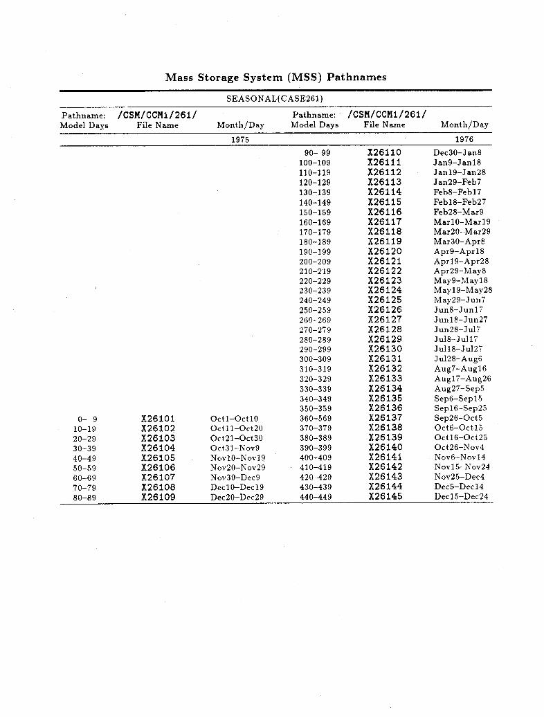
Mass Storage System (MSS) Pathnames

SEASONAL(CASE261)

Pathname: /CSM/CCM1/261/ Pathname: /CSM/CCM1/261/Model Days File Name Month/Day Model Days File Name Month/Day

1975 1976

Octl-OctlOOctll-Oct20Oct21-Oct30Oct31-Nov9NovlO-Novl9Nov20-Nov29Nov30-Dec9DeclO-Decl9Dec20-Dec29

90- 99100-109110-119120-129130-139140-149150-159160-169170-179180-189190-199200-209210-219220-229230-239240-249250-259260-269270-279280-289290-299300-309310-319320-329330-339340-349350-359360-569370-379380-389390-399400-409410-419420-429430-439440-449

X26110X26111X26112X26113X26114X26115X26116X26117X26118X26119X26120X26121X26122X26123X26124X26125X26126X26127X26128X26129X26130X26131X26132X26133X26134X26135X26136X26137X26138X26139X26140X26141X26142X26143X26144X26145

Dec30-Jan8Jan9-Janl8Janl9-Jan28Jan29-Feb7Feb8-Febl7Febl8-Feb27Feb28-Mar9MarlO-Marl9Mar20-Mar29Mar30-Apr8Apr9-Aprl 8Aprl9-Apr28Apr29-May8May9-Mayl8Mayl9-May28May29-Jun7Jun8-Junl 7Junl8-Jun27Jun28-Jul7Jul8-Jull7Jull8-Jul27Ju128-Aug6Aug7-Augl6Augl7-Aug26Aug27-Sep5Sep6-Sep 15Sepl6-Sep25Sep26-Oct5Oct6-Octl 5Octl6-Oct25Oct26-Nov4Nov6-Novl4Novl 5-Nov24Nov25-Dec4Dec5-Dec14Decl5-Dec24

0- 910-1920-2930-3940-4950-5960-6970-7980-89

X26101X26102X26103X26104X26105X26106X26107X26108X26109

Mass Storage System (MSS) Pathnames

SEASONAL( CASE261)

Pathname: /CSM/CCM1/261/ Pathname: /CSM/CCM1/261/Model Days File Name Month/Day Model Days File Name Month/Day

1977 1978

450-459 X26146 Dec25-Jan3 820- 829 X26183 Dec30-Jan8Jan4-Janl3Janl4-Jan23Jan24-Feb2Feb3-Febl 2Febl3-Feb22Feb23-Mar4Mar5-Marl4Marl5-Mar24Mar25-Apr3Apr4-Aprl 3Aprl4-Apr23Apr24-May3May4-Mayl3Mayl4-May23May24-Jun2Jun3-Junl2Junl3-Jun22Jun23-Jul2Jul3-Jull2Jull13-Jul22Jul23-AuglAug2-AugllAugl2-Aug21Aug22-Aug31Sepl-SeplOSepll-Sep20Sep21-Sep30Octl-Oct10Octll-Oct20Oct21-Oct30Oct31-Nov9NovlO-Novl9Nov20-Nov29Nov30-Dec9Dec10-Dec19Dec20-Dec29

830- 839840- 849850- 859860- 869870- 879880- 889890- 899900- 809910- 819920- 829930- 839940- 849950- 859960- 869970- 879980- 889990- 899

1000-10091010-10191020-10291030-10391040-10491050-10591060-10691070-10791080-10891090-10991100-11091110-11191120-11291130-11391140-11491150-11591160-11691170-1179

X26184X26185X26186X26187X26188X26189X26190X26191X26192X26193X26194X26195X26196X26197X26198X26199X261100X261101X261102X261103X261104X261105X261106X261107X261108X261109X261110X261111X261112X261113X261114X261115X261116X261117X261118

Jan9-Janl 8Janl9-Jan28Jan29-Feb7Feb8-Febl 7Febl8-Feb27Feb28-Mar9MarlO-Marl9Mar20-Mar29Mar30-Apr8Apr9-Aprl 8Aprl9-Apr28Apr29-May8May9-May18Mayl9-May28May29-Jun7Jun8-Junl7Junl8-Jun27Jun28-Jul7Jul8-Jull7Jull8-Jul27Jul28-Aug6Aug7-Augl6Augl 7-Aug26Aug27-Sep5Sep6-Sepl 5Sepl6-Sep25Sep26-Oct5Oct6-Oct 15Octl6-Oct25Oct26-Nov4Nov5-Novl4Novl 5-Nov24Nov25-Dec4Dec5-Decl4Dec15-Dec24

460-469470-479480-489490-499500-509510-519520-529530-539540-549550-559560-569570-579580-589590-599600-609610-619620-629630-639640-649650-659660-669670-679680-689690-699700-709710-719720-729730-739740-749750-759760-769770-779780-789790-799800-809810-819

X26147X26148X26149X26150X26151X26152X26153X26154X26155X26156X26157X26158X26159X26160X26161X26162X26163X26164X26165X26166X26167X26168X26169X26170X26171X26172X26173X26174X26175X26176X26177X26178X26179X26180X26181X26182

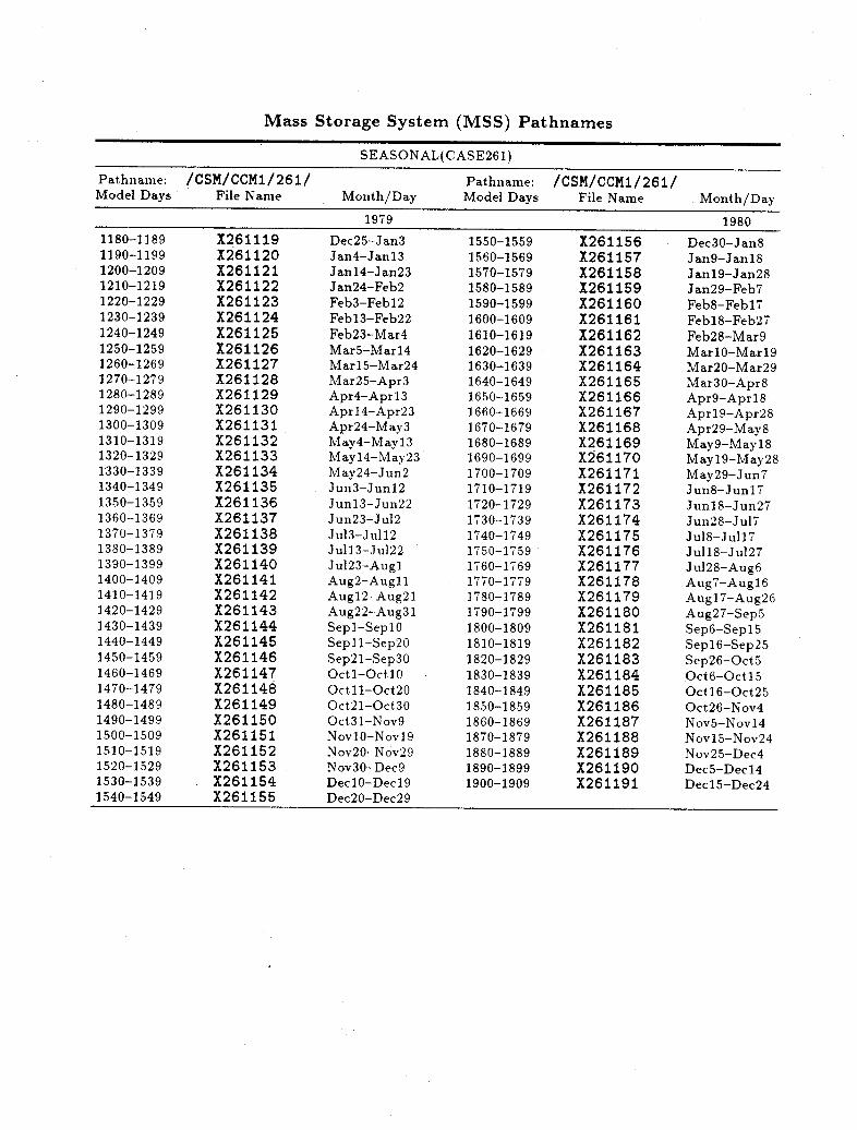
Mass Storage System (MSS) Pathnames

SEASONAL(CASE261)

Pathname: /CSM/CCM1/261/ Pathname: /CSM/CCM1/261/Model Days File Name Month/Day Model Days File Name Month/Day

1979 1980

Dec25-Jan3Jan4-Janl3Janl4-Jan23Jan24-Feb2Feb3-Febl 2Febl3-Feb22Feb23-Mar4Mar5-Marl4Marl5-Mar24Mar25-Apr3Apr4-Aprl 3Apr14-Apr23Apr24-May3May4-Mayl 3Mayl4-May23May24-Jun2Jun3-Junl2Junl3-Jun22Jun23-Jul2Jul3-Jull2Ju113-Jul22Jul23-AuglAug2-AugllAugl2-Aug21Aug22-Aug31Sepl-SeplOSepll-Sep20Sep21-Sep30Octl-Oct 10Octll-Oct20Oct21-Oct30Oct31-Nov9NovlO-Novl9Nov20-Nov29Nov30-Dec9DeclO-Decl9Dec20-Dec29

1550-15591560-15691570-15791580-15891590-15991600-16091610-16191620-16291630-16391640-16491650-16591660-16691670-16791680-16891690-16991700-17091710-17191720-17291730-17391740-17491750-17591760-17691770-17791780-17891790-17991800-18091810-18191820-18291830-18391840-18491850-18591860-18691870-18791880-18891890-18991900-1909

X261156X261157X261158X261159X261160X261161X261162X261163X261164X261165X261166X261167X261168X261169X261170X261171X261172X261173X261174X261175X261176X261177X261178X261179X261180X261181X261182X261183X261184X261185X261186X261187X261188X261189X261190X261191

Dec30-Jan8Jan9-Janl8Janl9-Jan28Jan29-Feb7Feb8-Febl7Febl8-Feb27Feb28-Mar9MarlO-Marl9Mar20-Mar29Mar30-Apr8Apr9-Aprl 8Aprl9-Apr28Apr29-May8May9-Mayl8Mayl9-May28May29-Jun7Jun8-Junl7Junl8-Jun27Jun28-Jul7Jul8-Jull 7Jull18-Jul27Jul28-Aug6Aug7-Augl6Augl7-Aug26Aug27-Sep5Sep6-Sepl5Sepl6-Sep25Sep26-Oct5Oct6-Octl5Oct16-Oct25Oct26-Nov4Nov5-Nov14Novl 5-Nov24Nov25-Dec4Dec5-Decl4Dec15-Dec24

1180-11891190-11991200-12091210-12191220-12291230-12391240-12491250-12591260-12691270-12791280-12891290-12991300-13091310-13191320-13291330-13391340-13491350-13591360-13691370-13791380-13891390-13991400-14091410-14191420-14291430-14391440-14491450-14591460-14691470-14791480-14891490-14991500-15091510-15191520-15291530-15391540-1549

X261119X261120X261121X261122X261123X261124X261125X261126X261127X261128X261129X261130X261131X261132X261133X261134X261135X261136X261137X261138X261139X261140X261141X261142X261143X261144X261145X261146X261147X261148X261149X261150X261151X261152X261153X261154X261155

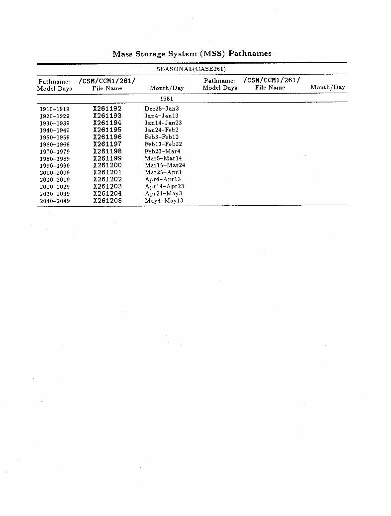
Mass Storage System (MSS) Pathnames

SEASONAL( CASE261)

Pathnalne: /CSM/CCM1/26'1/ Pathname: /CSM/CCM1/261/Model Days File Name Month/Day Model Days File Name Month/Day

1981

1910-1919 X261192 Dec25-Jan31920-1929 X261193 Jan4-Janl31930-1939 X261194 Janl4-Jan231940-1949 X261195 Jan24-Feb21950-1959 X261196 Feb3-Febl21960-1969 X261197 Febl3-Feb221970-1979 X261198 Feb23-Mar41980-1989 X261199 Mar5-Marl41990-1999 X261200 Marl5-Mar242000-2009 X261201 Mar25-Apr32010-2019 X261202 Apr4-Aprl32020-2029 X261203 Aprl4-Apr232030-2039 X261204 Apr24-May32040-2049 X261205 May4-Mayl3

Mass Storage System (MSS) Pathnames

SEASONAL-HYDRO(CASE275)

Pathname: /CSM/CCM1/275/ Pathname: /CSM/CCM1/275/Model Days File Name Month/Day Model Days File Name Month/Day

1975 1976

Octl-OctlOOctll-Oct20Oct21-Oct30Oct31-Nov9NovlO-Novl9Nov20-Nov29Nov30-Dec9Dec 1 O-Dec19Dec20-Dec29

90- 99100-109110-119120-129130-139140-149150-159160-169170-179180-189190-199200-209210-219220-229230-239240-249250-259260-269270-279280-289290-299300-309310-319320-329330-339340-349350-359360-569370-379380-389390-399400-409410-419420-429430-439440-449

X27510X27511X27512X27513X27514X27515X27516X27517X27518X27519X27520X27521X27522X27523X27524X27525X27526X27527X27528X27529X27530X27531X27532X27533X27534X27535X27536X27537X27538X27539X27540X27541X27542X27543X27544X27545

Dec30-Jan8Jan9-Janl8Janl9-Jan28Jan29-Feb7Feb8-Febl 7Febl8-Feb27Feb28-Mar9MarlO-Marl9Mar20-Mar29Mar30-Apr8Apr9-Aprl8Aprl9-Apr28Apr29-May8May9-Mayl8Mayl9-May28May29-Jun7Jun8-Junl7Junl8-Jun27Jun28-Jul7Jul8-Jull7Jull8-Jul27Ju128-Aug6Aug7-Augl 6Augl7-Aug26Aug27-Sep5Sep6-Sepl5Sepl6-Sep25Sep26-Oct5Oct6-Octl5Oct16-Oct25Oct26-Nov4Nov6-Novl4Novl5-Nov24Nov25-Dec4Dec5-Decl4Decl 5-Dec24

0- 9

10-1920-2930-3940-49

1 50-5960-6970-7980-89

X27501X27502X27503X27504X27505X27506X27507X27508X27509

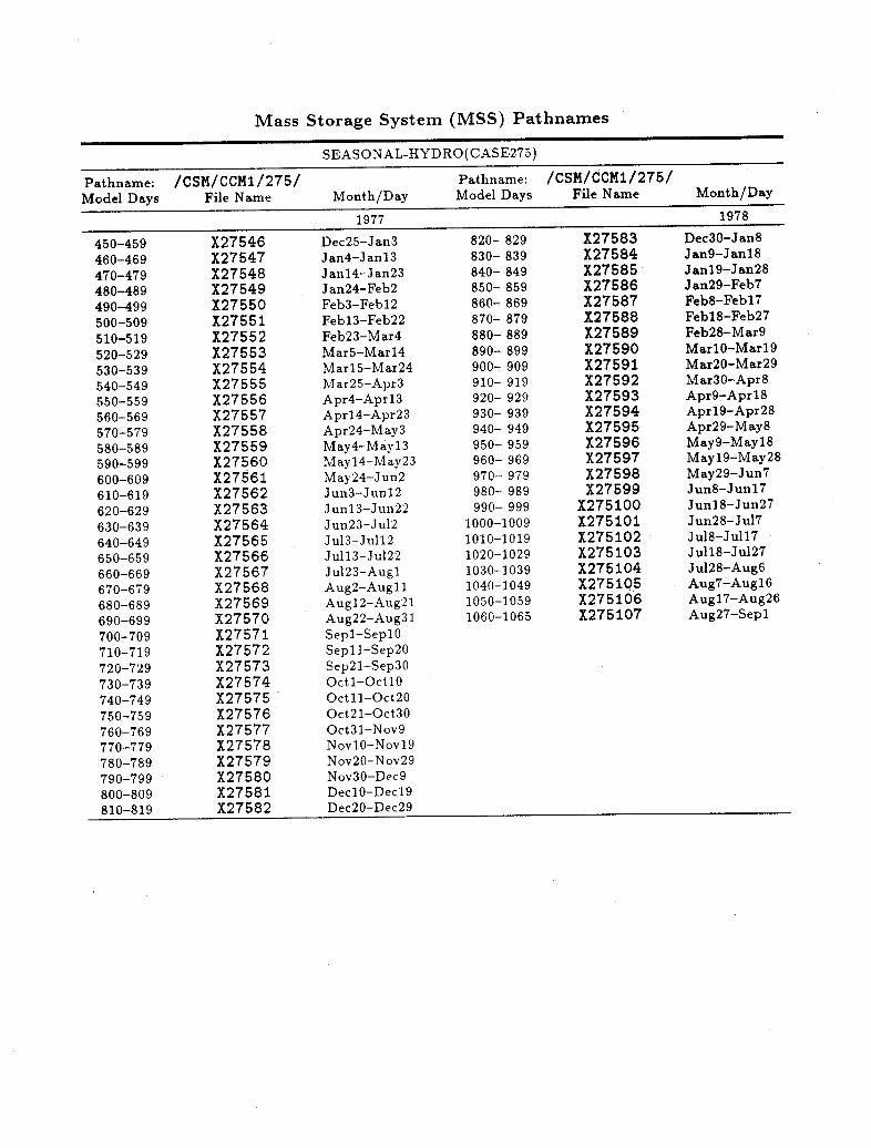
Mass Storage System (MSS) Pathnames

SEASONAL-HYDRO(CASE275)

Pathname: /CSM/CCM1/275/ Pathname: /CSM/CCM1/275/

Model Days File Name Month/Day Model Days File Name Month/Day

1977 1978.......... .a

Dec25-Jan3Jan4-Jan13Janl4-Jan23Jan24-Feb2Feb3-Febl2Febl3-Feb22Feb23-Mar4Mar5-Marl4Marl5-Mar24Mar25-Apr3Apr4-Apr 1 3Aprl4-Apr23Apr24-May3May4-Mayl3Mayl4-May23May24-Jun2Jun3-Junl2Junl3-Jun22Jun23-Jul2Jul3-Jull2Jull3-Ju122Jul23-AuglAug2-AugllAugl2-Aug21Aug22-Aug31Sepl-SepiOSepll-Sep20Sep21-Sep30Octl-OctlOOctll-Oct20Oct21-Oct30Oct31-Nov9NovlO-Novl9Nov20-Nov29Nov30-Dec9DeclO-Decl9Dec20-Dec29

820- 829830- 839840- 849850- 859860- 869870- 879880- 889890- 899900- 909910- 919920- 929930- 939940- 949950- 959960- 969970- 979980- 989990- 999

1000-10091010-10191020-10291030-10391040-10491050-10591060-1065

X27583X27584X27585X27586X27587X27588X27589X27590X27591X27592X27593X27594X27595X27596X27597X27598X27599X275100X275101X275102X275103X275104X275105X275106X275107

Dec30-Jan8Jan9-Janl8Janl9-Jan28Jan29-Feb7Feb8-Febl7Febl8-Feb27Feb28-Mar9MarlO-Marl9Mar20-Mar29Mar30-Apr8Apr9-Aprl8Aprl9-Apr28Apr29-May8May9-May18Mayl9-May28May29-Jun7Jun8-Junl 7

Junl8-Jun27Jun28-Jul7Jul8-Jull7Jull18-Jul27Jul28-Aug6Aug7-Augl6Augl7-Aug26Aug27-Sepl

450-459460-469470-479480-489490-499500-509510-519520-529530-539540-549550-559560-569570-579580-589590-599600-609610-619620-629630-639640-649650-659660-669670-679680-689690-699700-709710-719720-729730-739740-749750-759760-769770-779780-789790-799800-809810-819

X27546X27547X27548X27549X27550X27551X27552X27553X27554X27555X27556X27557X27558X27559X27560X27561X27562X27563X27564X27565X27566X27567X27568X27569X27570X27571X27572X27573X27574X27575X27576X27577X27578X27579X27580X27581X27582--- --

6. Summary Remarks

New unresequenced program libraries have been generated for the NCAR CCM1

which include several bug fixes, improvements in computational performance, and other

enhancements, including an experimental T42 version of the CCM. The use of the new

program libraries, along with the Cray Update mod files FASTCCM1 MODS and UN-

BLOCK MODS (available from IBM 4381 userid CSMLIB) allows the user to execute

the CCM1 at approximately one third the GAU cost when compared to the original

CCM1PL program library. The total number of computational cycles required to exe-

cute the model has also been significantly reduced.

A new set of seasonal control experiments have been completed at R15 and at T42

resolutions. The statistical properties of these controls are generally unchanged with

the exception of the average properties of the near surface climate in the winter polar

regions (which are within one standard deviation of the previous control experiment),

and reduced seasonal variability in several selected fields. Users should be aware of these

changes when examining the statistical significance of circulation changes introduced by

modifications to the new CCM1 program library's model physics.

Acknowledgments

We wish to thank N. A. MacFarlane at the Canadian Climate Center for providing

us with a version of his gravity wave drag scheme. We also wish to acknowledge R. J.

Wolski for his contributions to the Cray Update file FASTCCM1 MODS, which further

enhance the performance of several key radiation routines in the new CCM1 program

libraries, and J. T. Kiehl and B. P. Briegleb for identifying the inconsistency in the

water vapor continuum path length calculation. Finally, we thank E. R. Boettner for

her assistance in the preparation of this technical report and D. L. Williamson for his

careful review.

72

References

Bath, L. M., M. A. Dias, D. L. Williamson, G. S. Williamson and R. J. Wolski, 1987a:

Users' Guide to NCAR CCM1. NCAR Tech. Note, NCAR/TN-286+IA, National

Center for Atmospheric Research, Boulder, Colo., NTIS PB87-224374/AS, 173 pp.

Bath, L. M., M. A. Dias, D. L. Williamson, G. S. Williamson and R. J. Wolski, 1987b:

Documentation of NCAR CCM1 Program Modules. NCAR Tech. Note, NCAR/

TN-287+IA, National Center for Atmospheric Research, Boulder, Colo., NTIS

PB87-213567/AS, 307 pp.

Joseph, D. H., 1984: Data format for global 10-minute elevation data from the U.S.

Navy. Internal Memo of the NCAR Data Support Section, National Center for

Atmospheric Research, Boulder, Colo., 5 pp.

McFarlane, N. A., 1987: The effect of orographically excited gravity wave drag on the

general circulation of the lower stratosphere and troposphere. J. Atmos. Sci., 44,

1775-1800.

Ramanathan, V., and P. Downey, 1986: A nonisothermal emissivity and absorptivity

formulation for water vapor. J. Geophys. Res., 91, 8649-8666.

Trenberth, K. E., and J. R. Christy, 1985: Global fluctuations in the distribution of

atmospheric mass. J. Geophys. Res., 90, 8042-8052.

Williamson, D. L., 1988: The effect of vertical finite difference approximations on sim-

ulations with the NCAR Community Climate Model. J. Climate, 1, 40-58.

Williamson, D. L, J. T. Kiehl, V. Ramanathan, R. E. Dickinson and J. J. Hack, 1987:

Description of NCAR Community Climate Model (CCM1). NCAR Tech. Note,

NCAR/TN-285+STR, National Center for Atmospheric Research, Boulder, Colo.,

NTIS PB87-203782/AS, 112 pp.

73

Williamson, D. L., and G. S. Williamson, 1984: Circulation Statistics from January and

July Simulations with the NCAR Community Climate Model (CCMOB). NCAR

Tech. Note, NCAR/TN-244+STR, National Center for Atmospheric Research,

Boulder, Colo., NTIS PB85-165637/AS, 112 pp.

Williamson, G. S, and D. L. WilliamsonS., 1987: Circulation Statistics from Seasonal

and Perpetual January Simulations with the NCAR Community Climate Model

(CCM1):R15. NCAR Tech. Note, NCAR/TN-302+STR, National Center for At-

mospheric Research, Boulder, Colo., NTIS PB88-192620/AS, 199 pp.

74

APPENDIX A

75

CONTENTS

A cknowledgm ents ................................................................... vIntroduction . .. . ... ... . . .. ............................................... viiReferences ...........................................................................List of Figures ...................................................................... xiList of Tables ................................................................. ..... xiiSection I. How to Use CCM 1 ........................................................ 1

A . Running the M odel .................................................... .... . 11. M odel Run Deck ........................................................... .12. M odel O utput .............................................................. 13. Sample Run Decks ......................... ................................. 1

Example 1. One-day simulation, perpetual January .......................... 2Example 2. Generate CFT listings for selected decks ................... . 4Example 3. Send source file of selected decks to front-end .. 5........... 5

4. Use of the Mass Store Subsystem ................................. ..e.ee 65. Model Input Parameters ....................................................

Example 1. Initial run, perpetual January .................................. 16Example 2. Initial run, perpetual July .................... ................. 17Example 3. Restart run, seasonal, hydrological cycle ....................... 18Example 4. Regeneration run, seasonal cycle ....................... ........ 19Example 5. Initial run, perpetual January, irregular

history tape write frequency . .................................. 20B. M odel Input Dataset Form ats ........... .................. .... ............... 21

1. Initial Atm ospheric Data .......................................... 212. Ozone Dataset ...................................... . ..................... 243. Sea Surface Temperature Dataset ...................................... 264. Albedo D ataset ......... ..................................... 275. Standard Deviation Dataset (CCM1PL2 only) . ........................... 28.1

C. Output from the Model ... ............................... ........ 291. Model History Tape ......................................... 29

Header records ....................... ....................... 30Data records ............ ............................. 36Information concerning packing of history tapes ............................ 42CCM M odular Processor .............................................. 42

2. M odel "Save D ata" . .................................... ................... 423. M odel Printed O utput .............. ... ...... ......... ....................... 424. Model Error Messages ........................ ...... .......... 60

D. Simple Changes to the Model..... 701. Adding New Variables to Model Grid Point Buffers ........................ 70

Pointers for the new field ................................................. 70Changes to PARAMETER definitions .......................................... G 72Changes to history tape header ......................... 7............73

iii

2. Creating Your Own Initial Dataset ......................................... 753. Changing M odel Resolution ................................................ 76

Spherical harmonic truncation parameters .................................. 76G rid point resolution ...................................................... 76

Section II. How the CCM1 Code Works ............................................. 81A. Model Code Design .. 81

1. Model Control Logic: Initial, Restart andRegeneration Runs .......................................................... 85

R estart run ............................... ................... ..... ... .. . 85Regeneration run .......................................................... 86

2. M odel Code Flow .......................................................... 893. Model Physical Parameterizations Implemented as

Separate C ode Packages .. .. . ..................................99G eneric D escription ........................................................ 99Radiation Parameterization ............................................... 101Cloud Param eterization .................................................. 116

4. Budget Calculation . .................................................... 120B. M odel D ata Buffers ......................................................... 123

1. Spectral Coeffi cient Arrays ............................................... 123Use of indexing arrays in spectral storage scheme ......................... 126Looping in spectral space ................................................. 127

2. Code Flow Associated with Spectral Aspects .............................. 1293. G rid Point Buffers ....................................................... 131

Duplicate buffers to allow overlapped I/O ................... .............. 133A uxiliary disk units ...................................................... 133Lengths associated with grid point buffers ................................ 135M odel fields within buffers ................................................ 136Values within buffers .............................................. ....... 137

C. Time Flow Through the Model ................. ............................. 154D. Data Flow Through the Model .............................................. 156E. Adding Parameterizations to the Model ..................................... 161

A parameterization using the Model buffers ............................... 161F. W orking with the CCM 1 Code .............................................. 162

1. Trouble-Shooting Your Model Run ........................................ 162Tracing through the pointer structure: the Concordance ................... 162The Cray Symbolic Debugger ............................................. 163

2. Debugging Your Model Changes .......................................... 164Comparing history tape output ........................................... 164

3. Coding Standards for CCM1 .. 165Appendix A. Table A.1. CCMOB History Tape File Header . ........................168In dex .......................... ................................................ .... 173

iv

The Model input parameters provided for naming output volumes are flexibleenough to allow the user access to most of the advanced features of the MSS hier-archical file management system.

Refer to the previous Model run deck example 1. Here the single input volumeICDATA, the initial dataset, input in NAMELIST $EXPDEF, appears as a simple filename 'JANIRIS'. In this case the default Mass Store directory pathname for inputdatasets, /CSM/CCM1/%DATA%/, will be concatenated to the file name 'JANIRIS'before acquiring from the Mass Store. The user may override this pathname bysetting ICDATA to a full file pathname, including the initial '/' character, suchas '/user/CCMI/INITIAL/JANDAT', and the dataset will be acquired using thatcomplete pathname.

Where lists of output files are required, as in the case of LTAPES for Model historytape output, an additional input paranmeter is provided to allow the user to definea Mass Store pathname to associate with each element in the list. In example 1,the $NEWRUN parameter LHPATH could be set to '/user/CCMI/OUTPUT/ ' and the his-tory tape would then be disposed to /user/CCM1/OUTPUT/tttttt. The pathnames inLHPATH and LRPATH (for regeneration datasets NRVSNS) may contain up to 72 charac-ters, providing access to the convenient cataloging capabilities of the MSS software.If no such pathname is input, a default directory pathname /user/CCM1/case nunm-ber/ is provided for the history tapes and regeneration datasets if requested, whereuser may be specified by the $NEWRUN parameter IUSER, or if not input, defaultsto the username associated with the JOB card. Case number is extracted from thesecond parameter card to the Model, the run identifier for the history tape header.Additional input parameters related to the Mass Store include a MSS retention timefor output volumes, shown in example 1 as $EXPDEF parameter IRT, and a writepassword, $EXPDEF parameter NSWRPS. For more detailed information on Model in-put parameters, see Table 1.2, "Description of Input Through $IN". The sampleinput decks in Section I.A.5. also show the use of the volume naming parametersin several forms.

Model input volumes accessed by the program via subroutine ATTACH may includethe initial dataset, the restart or regeneration dataset, or a previously written his-tory tape. In all cases the volume is staged from the MSS if it is not already residenton the Cray disk. The last 14 characters of the full file pathname, less slashes, areused to form the permanent dataset name (PDN) for the Cray disk copy. The last,7 alphabetic characters form the local dataset name (DN). For the input datasetslisted above, the ID parameter is used to provide added permanent dataset security.The accessed dataset is then copied to a local dataset and released from the job.

Model output volumes are saved on the Cray disk and disposed to the MSS usingsubroutine SAVDIS. Prior to the SAVE, any previous edition of the dataset is deletedfrom the disk. The PDN is formed in the same way as for a dataset ACQUIRE, andan ID parameter and write password are associated with the permanent dataset.

Volumes are disposed to the Mass Store with a write password, $EXPDEF parameterNSWRPS and a retention time, $EXPDEF parameter IRT. A MSS comment is associated

7

with output history tapes, composed of beginning and ending dates and times forthe volume. The user may specify MSS "virtual volumes" for the history tapes andregeneration datasets separately, allowing for a longer maximum retention time onthe Mass Store.

5. Model Input Parameters

The following table describes i the imodel. All records areread as NAMELIST input except the first two records, the case title and identifier(number) f or y tape header, also used in determining the names for outputvolumes. The format of each record is shown in the "value" column, along with adefault value as initialized in the Model code, the COMMON block wheree variableappears, and a short description. If other defaults apply to a particular parameter,they will be explained in the "description" column. Although variables MTITL,the case title, and MCSTEM, the case identifier, are initialized to blanks, becausethey are not included in a Fortran NAMELIST, they will always be reset by the firsttwo records in the $IN parameter file. Therefore, the user should consider theseparameters mandatory. Records within NAMELIST groups may appear in any orderand, if the default value is the desired one, the record need not be included. Seethe Cray "Fortran (CFT) Reference Manual" for detailed information on the use ofNAMELIST.

Several input parameter descriptions refer to "restart" or "regeneration" runs ofthe Model. For more detail on these types of continuation runs and their usage, seeSection II.A.2.

The set of input parameters which specify the timing and frequency of history tapewrites can be somewhat difficult to understand. The following explanation shouldclarify the use of these parameters, including NWPTR, NNUMWT, and NWTIME.

The Model provides twoc methods to specifiy when data will be written to thehistory tape. The first of these methods, the "automatic mode", specifies a constantfrequency in time of history tape writes, and is invoked by including the parameterNNUMWT in NAMELIST $NEWRUN.

NNUMWT may be specified in units of time steps, as a positive value, or in hours,as a negative value. NNUMWT is converted to units of time steps if necessary insubroutine DATA. In the automatic mode, a logical file will be written to the historytape when subroutine LINEMS calls WSHIST at NSTEP (Model iteration counter) =1,and thereafter when NSTEP=NNUMWT+1, 2*NNUMWT+1,3*NNUMWT+1,..., n*NNUMWT+1where n is the largest integer for which n*NNUMWT+1 < NESTEP, NESTEP being thefinal timestep as specified by the user. Because variables written to the history tapeare valid at time n - 1, the variables on the tape represent values at times t=0,NNUMWT, 2*NNUMWT, ... , n*NNUMWT.

The second method of specifying history tape write times, the "manual mode,"involves the use of NAMELIST $NEWRUN parameter NWTIME, an array of up to fiftytime steps for which the user wishes to put data on the history tape. The Model willwrite to the history tape data which are valid at the time steps specified in NWTIME,

8

although the write actually takes place at the iterations following the specified ones.The use of the manual mode is the only way to accomplish a write of the data valid attime t = -At. This may be done by specifying NWTIME(1) = -1, with NESTEP > 0.See input parameter Example 5 following Table 1.2 in this section for a discussionof time t = -At data.

9

5. Standard Deviation Dataset (CCM1PL2 only)

The Standard Deviation dataset contains the standard deviation of topography at eachpoint in the Model grid. It is used by the gravity wave drag parameterization in programlibrary CCM1PL2.

This is a binary dataset consisting of a single floating point array of standard deviations,

SGH(PLONP2 ,POREC),

where

PLONP2 = the number of longitude points plus wraparound,

POREC = the number of latitudes

28.1

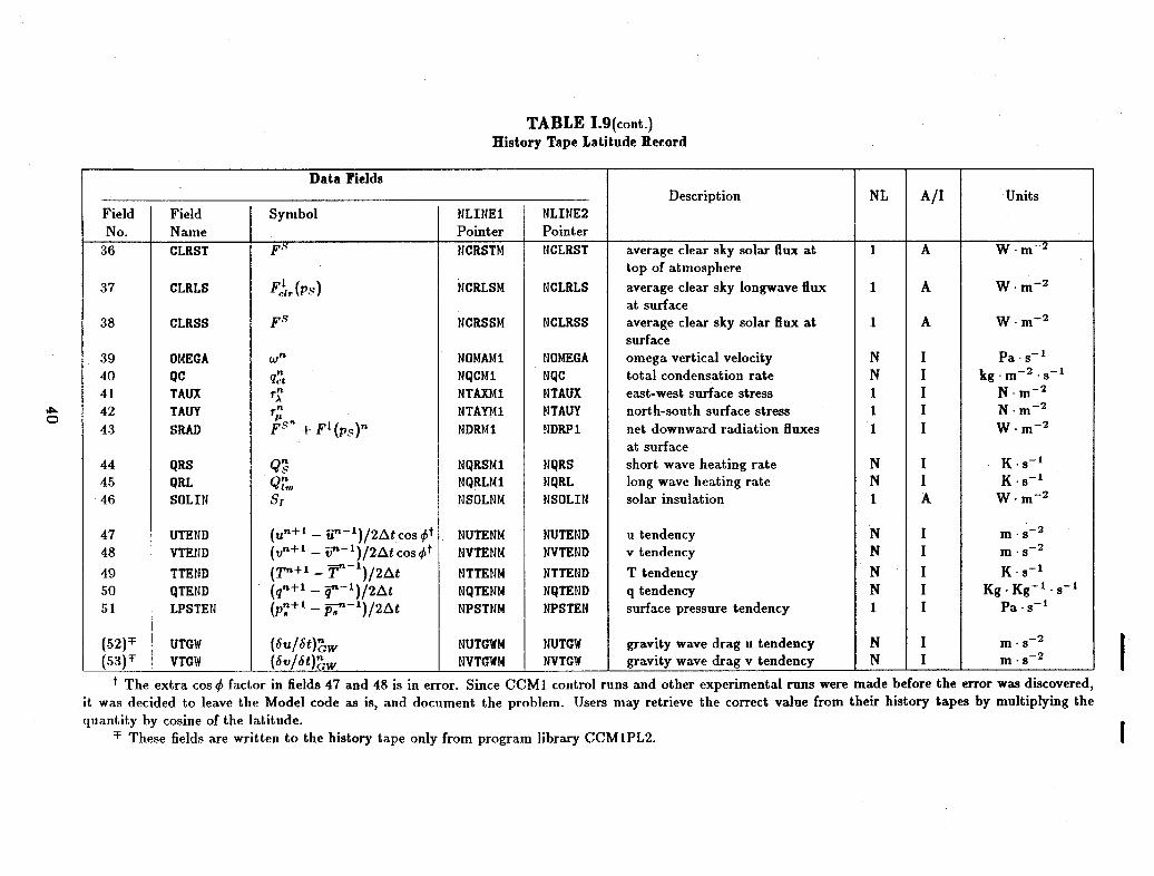
TABLE I.9(cont.)History Tape Latitude Record

Data FieldsDescription NL A/I Units

Field Field Symbol NLINE1 NLINE2No. Name Pointer Pointer

36 CLRST Fs NCRSTM NCLRST average clear sky solar flux at 1 A W m- 2

top of atmosphere37 CLRLS Fr (ps) NCRLSM NCLRLS average clear sky longwave flux 1 A W m - 2

at surface38 CLRSS Fs NCRSSM NCLRSS average clear sky solar flux at 1 A W m - 2

surface39 OMEGA | n NOMAM1 NOMEGA omega vertical velocity N I Pa s - 1

40 QC qnt NQCM1 NQC total condensation rate N I kg -m-2 s-41 TAUX NTAXM1 NTAUX east-west surface stress 1 I N m - 2

42 TAUY | NTAYM1 | NTAUY north-south surface stress 1 I N m- 2

43 SRAD FS' + F 1 (ps)"n NDRM1 NDRP1 net downward radiation fluxes 1 I W m - 2

at surface44 QRS Qn NQRSM1 NQRS short wave heating rate N I K s-45 QRL Qn NQRLM1 NQRL long wave heating rate N I K-s- 1

46 SOLIN SI NSOLNM NSOLIN solar insulation 1 A W m- 2

47 UTEND ((un +I - in-I)/2At cos bt NUTENM NUTEND u tendency N I m s- 2

48 VTEND (vtn+ - i"n-)/2Atcosqt NVTENM NVTEND v tendency N I m-s- 2

49 TTEND (T+' - Tn- )/2At NTTENM NTTEND T tendency N I K s -~

50 QTEND (qn+l -_ l-)/2At | NQTENM NQTEND q tendency N I Kg Kg- s-51 LPSTEN (pn + l - p7--l)/2At NPSTNM NPSTEN surface pressure tendency 1 I Pa s-I

(52)=T UTGW (6 u/ 6 t)nw NUTGWM NUTGV gravity wave drag u tendency N I m - 2

(53) :F VTGW (6v/6t)nw | NVTGWM NVTGW gravity wave drag v tendency N I | m .s - 2

t The extra cos factor in fields 47 and 48 is in error. Since CCM1 control runs and other experimental runs were made before the error was discoverit was decided to leave the Model code as is, and document the problem. Users may retrieve the correct value from their history tapes by multiplyingquantity by cosine of the latitude.

T These fields are written to the history tape only from program library CCM1PL2.

ed,the

0

II

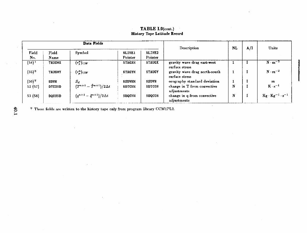
TABLE 1.9(cont.)History Tape Latitude Record

Data Fields

Symbol

(Tr')GW

(r )GW

S,(T"+ - T+ 1)/2At

(qn+l _ -+x)/2At

NLINE1Pointer

. - - -

NTAGXM

NTAGYM

NSDVHM

NDTCNM

NDQCNM

NLINE2Pointer

_ .NTAUGX

NTAUGY

NSDVH

NDTCON

NDQCON

Description

gravity wave drag east-westsurface stressgravity wave drag north-southsurface stressorography standard deviationchange in T from convectiveadjustmentschange in q from convectiveadjustments

NL

1

1

1N

N

A/I

, ,

I

I

II

I

F These fields are written to the history tape only from program library CCM1PL2.

FieldNo.

(54)+

FieldNameTAUGWX

TAUGWY

SDVH

DTCOND

DQCOND

(55)F

(56)T52 (57)

53 (58)

i

Units_ _ _ _ _ _I

I .- _e-

N -m- 2

mK s- 1

Kg Kg- x s-

-- ~~~~~~~~~~~~~~~~~~ --

-

Information concerning packing of history tapes

The Model will optionally pack the data records of the history tape in ratios of 2, 3 or 4to one. The user may request packing by specifying a value greater than one for $NEWRUNinput parameter NDENS. This packing density is then stored in the MFLDS array of thehistory tape header for the use of post-processors. Subroutine PACKA, an entry point in theCRAYLIB routine FPACKER, is called by Model subroutine COPYHT if packing is requested,and data are packed one field at a time, level by level, as they are copied from the Modelbuffer to the history tape buffer.

Although the Modular Processor, referenced below, can read packed tapes directly, occa-sionally the user may have need to unpack a packed history tape, particularly if it is tobe used as an initial data tape. The Model cannot start from a packed tape. An optionis available in the Modular Processor to produce an unpacked initial tape from a packedhistory tape. See Section I.D.2 for more information on this option.

CCM Modular Processor

The Modular Processor is a general-purpose analysis program for use with Model outputhistory tapes. Using the Processor, it is possible to plot history tape fields and derivedfields in a variety of formats, and to generate secondary datasets from the history tape,such as time averaged save tapes, etc. The Processor is documented in the two NCARtechnical notes, "Introduction to the CCM Modular Processor (Version PROC02)" (M.A.Dias, 1987) and "CCM Modular Processor Users' Guide (Version PROC02)" (R.J. Wolski,1987).

2. Model "Save Data"

The Model writes to unit NSRE, at the same frequency with which it writes the historytape, the subset of Model variables and the data buffer necessary to restart the run atthat point. The following variables are written on unit NSDS: the initial dataset nameICDATA, the current history tape pathname LHTAPE, the packing density NDENS, and historytape file control variable IFIL. For program libraries CCM1PL1 and CCM1PL2 only,COMMON /COMTIM/ variables containing date and time information for the first header on thecurrent history volume are written to NSDS. Also written to NSDS are commons /COMBUD/,/COMBUD1/, /COMDYR/, /CRDSNL/, /CRDSLZ/ and /COMQFL/. The contents of the disk unitsNRA1 and NRB1, described in Section II.B.3 under "Auxiliary Disk Units," are then copiedto unit NSRE, followed by the contents of unit NSDS.

Unit NSRE is overwritten each time a file is written to the history tape. It is saved onthe Cray disk and disposed to the Mass Store as volume NSVSN, the restart dataset, andto regeneration dataset NRVSNS(n) if requested. If no values of NRVSNS are input and thevalue of NLSAVE is true, unit NSRE is concatenated to the end of the history tape, where itmay be used in a regeneration run to rebuild the next sequential history volume.

3. Model Printed Output

The following pages contain an example of printed output from a one-day Model simulation.This output results from an initial run of a one-day January simulation, using programlibrary CCM1PL. Printed output may vary slightly for program libraries CCM1PL1 and

42

CCM1PL2. Comments in boldface type describe each section of the output and indicate |the program module from which it is printed. They do not appear on the actual Modeloutput.

42.1

II. HOW THE CCM1 CODE WORKS

A. MODEL CODE DESIGN

The CCM1 program is approximately 32,500 lines in length, and contains 10,500 Fortranstatements. The source code is maintained in Cray Update Program Library form on theNCAR Mass Store Subsystem. The original program library, CCM1PL, is known as the"frozen" CCM1. Two additional program libraries have been generated with CCM1PL asa base. In CCM1PL1, the surface energy balance physics has been completely reformulatedand reimplemented, an improved scheme for adjusting total mass has been implemented,several additional physics components have been modified to improve vectorization, andthe Mass Store comment field for output history tapes has been changed. CCM1PL2 is aT42 version of CCM1PL1, and contains a gravity wave drag parameterization.

The use of Cray Update allows "batch editing" of the source code via Update directives,or alternatively the user may generate an Update source file of selected routines, disposethis file to a front-end machine such as the IBM 4381, and modify it using the full-screenediting facilities of the IBM. These routines may then replace the existing routines by theuse of the $PURGEDK directive. See Section I.A.3.,"Sample Run Decks", Examples 4 and 5,

for job decks to accomplish these tasks.

Section II is divided into two main subsections. The first describes the Model code as acombination of control logic, the computational looping structure, and a series of physi-cal parameterizations which are modular in nature. Figure 11.1 provides a detailed staticcalling tree of all control and computational subroutines in the Model. A narrative ex-planation of the control logic from the Model follows, with information on Model flow inan initial run, a restart continuing an initial run, and a regeneration run, which recoverslost history volumes. Next is a description of the main computational loop, describing thetime-marching procedure. Detailed explanations are included for the radiation and cloudparameterizations and the budget calculations.

The second subsection, starting with II.B, covers the somewhat complex subject of datastructures, data flow and manipulation within the Model. Although the spectral and gridpoint buffers were briefly described in Section I, this more detailed presentation is intendedto help the user modify these buffers or add parameterizations which interface with theexisting Model data storage. Included as well is a description of the time variables withinthe Model and more information on making changes to the Model, along with a write-upof the CCM1 coding standards.

81

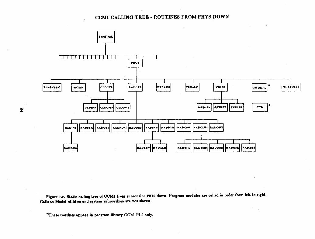
CCM1 CALLING TREE - ROUTINES FROM PHYS DOWN

Figure I.c. Static calling tree of CCM from subroutine PHY8 down. Program modules are called in order from left to right.

Calls to Model utilities and system subroutines are not shown.

*These routines appear in program library CCM1PL2 only.

1. Model Control Logic: Initial, Restart and Regeneration Runs

Control logic within the Model allows it to restart when a case ternminates, whether nor-mally or abnormally, and continue running with little or no loss of resources. The restartis exact - that is, the model results for a restart run will be identical to the results of thecase if it had not been interrupted. Also available is the capability to regenerate one ormore history volumes which may have been corrupted since the case was run, as long asa previous good volume (or appropriate regeneration dataset) from the same case exists.These two features are called respectively "restart" and "regeneration".

The Model periodically saves information required to restart the case and writes it to aseparate file known as the restart dataset. This information consists of the data on unitsNRA1 and NRB1, and variables from COMMON blocks /COMSDS/, /COMTAP/, COMTIM, /COMBUD/,/COMDYR/, /CRDSNL/, /CRDSLZ/ and /COMQFL/. This dataset is saved to disk and disposedto the Mass Store Subsystem at the same frequency as is the history tape. This frequencyis specified by the NAMELIST $NEWRUN input variables MFILS and MFILT. (See Section I.A.5for a description of Model input parameters.) At time steps for which the information isto be saved, the three local units NRA1, NRB1, and NSDS are concatenated to unit NSRE,forming the restart dataset. This dataset is then appended to unit NDATA, the history tape,if input parameter NLSAVE is . TRUE., to make possible the regeneration of the next volumeif it should become corrupted. Then units NDATA and NSRE are copied, saved as permanentdatasets on the Cray disk, and disposed to the Mass Store. If NLSAVE is .FALSE. anda list of dataset names NRVSNS parallel to the history tape name list exists, unit NSRE isnot appended to the history tape unit, but is saved and disposed as a separate file to theappropriate regeneration dataset NRVSNS(i). See Section I.A.4, Use of the Mass StoreSubsystem, for more detail on dataset naming parameters.

Restart run

A restart is accomplished by resubmitting the same Model job deck which produced theinitial run with the NAMELIST $EXPDEF parameter NSREST set to 1 and the $NEWRUN param-eter NESTEP changed if the ending time of the run is to be changed. If this is a seasonal run,care must be taken to assure that the setting of IRADSW and IRADLW in NAMELIST $NEWRUNspecifies a full radiation calculation at the first time step after restart; this will be true ifthe history tape write frequency NNUMWT is a multiple of IRADSW. This is necessary becausethe frequency of sea-surface temperature updates is based on IRADSW. * The Model restartprocedure then initializes the Model from the saved data sets, positions the history tapeproperly, and continues the run.

Often users ask if it is possible to change certain aspects of the Model run on a restart,such as history tape packing density, or the fields that are written to the tape. It is helpfulto follow the code flow in determining which parameters may be changed: first subroutinePRESET initializes the $NEWRUN parameters, then subroutine DATA reads them in. However,on a restart run subroutine RESUME then calls RESTRT, which reads the restart dataset,

* See Section II.A.3, Radiation Parameterization, for more discussion on how this pointaffects the radiation variables on the history tape.

85

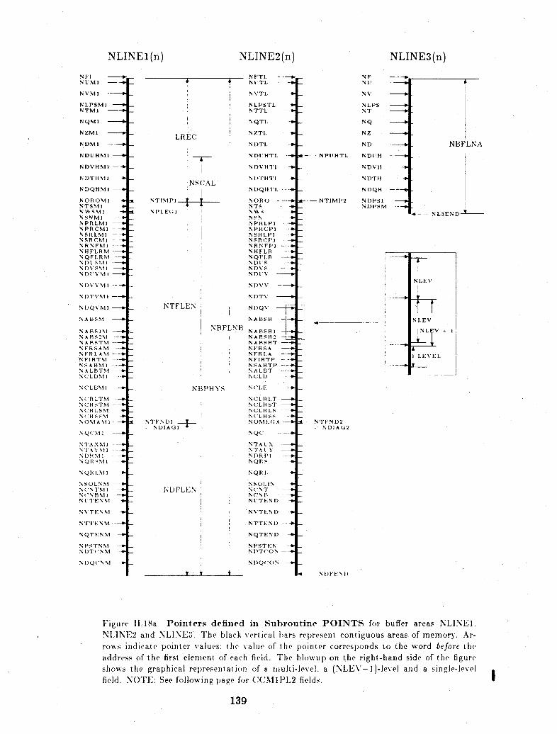
NLINE1(n) NLINE2(n) NLINE3(n)

I i

LREC

NSCAL

-NTIMP1 i IP

NPLE;1 i

NTFLEN i

NBF

NBPHYSI

INTFNDl- NDIAGI

NDFLEN

Nl TL - -

NVTI, -

NLPSTLNTTL

NQTL

NZTL

N DTL

NDUHTL

N DVI TL

N D)'T'1 '1.

N I)QHTL

NORO -NTS

NSNNPRLPINPRC!IIN SR LP]N SR C P ]NRN FP]NHF LRNQF LRNDl 'SNDVSND V -

NDVV -

----_.

-- _-

-4

-_.

--.

--

-4.

N DTV ------

N I)QV -

NABSB -,--

'LNB NABS] 4N A BSB2 --;,-.NABSBT -fNFRSA -4.tN F R S A -fNFRLA -- _NFIRTP - --NSABTP ---_NALBT .-- --N CL) -- 4

N CIF -- _.

NCLRI.TN CLR ST -NCLRLS --.N (CLH SS - _NOM EG A -4--

NQC ---

N TAtX ----N 'J' .t' -- fNDRP1 --4.

NQr S -- _

NQR!. -4.

NSO. IN -4-

N:('N. --N NTEND -_

NNTEND -4.

NTTENI) --_

NQTEND --)

N PSTEN -

NDTC'ON --f

NDQ(CON --

d -

,,--

.

-

-4

N V -

NLPS --NT -

NQ --

NZ---

ND --- O

NPI'HTI, NDIH -----

NDVH ----

N I)Tr --

NI)QH -- t

NTIMP2 NDPSL-_NDPSM ----

.4

--

i

I

N T F N D 2 ~ ~--

NTFND2- NDIAG2

NI)lFE NI)

A

- NBFLN,'

L

iN L3ENDND I

I

N LENV

NLEV

NL1V -+ 1

1 LEVEL

Figure 11.18a Pointers defined in Sul)routine POINTS for buffer areas NLINEI.NL1NE2 and NLINE3. The black vertical bars represent contiguous areas of memory. Ar-rows indicate pointer values; the value of the pointer corresponds to the word before theaddress of the first element of each field. The blowup on the right-hand side of the figureshows thle graphical represelltation of a multi-level, a (NLEV- 1)-level and a single-levelfield. NOTE: See follouing page for (CCMIPL2 fields.

139

A-

A

N V M 1 ----

NLPSM] -NTMI ---

NQMI ---

NZMI -

N DM -I

NDUHNI1 -

NDVHM 1 --

NDTIHMI -

NDQHMI -H -

NOROM1 --NTSMI] -NWSNM -4NSNMI -9--NPRLM1 --_NPRCMI - -NSRLMI --NSRCMN - -NRNFMI --NHFLRMNQFLRM --N D I S.M -1 -NDVSM1 ---ND.VM I--

NDVVMI --_

N DTVM --

NDQVN1 ---

NABSM --

NA B.SM ----N A BS2M --NABSTM ---

N F R L A N ---N FI RTM ----NSABMl -----N A L BTNI -NCLDM I

NCLEN1 ---

NCRLTM --.NCRSTM --NC RLSM --N ('H 1 ---NO\1 AM I --

NQC(M] --_

N TAX M ---NTA N11 ---

N QR SM I ----NQRLMI -...

NSOINN1 -- -N'NCT\l --NCNBM1 --9N t' T'ENM -

NVTENM -.

NTTF N M --

N Q T E N M -

NPST'NM ---N 1)T('NM --

-N Q)Q('' N - -\-.

NF'I1 NP T I- - -__F-

NF 4b

I

i

.

-,.M-

A

With the addition of the gravity wave drag parameterization to program library CCM1PL2,five new fields were added to the Model buffer in sections NLINE1 and NLINE2. These fieldsfollow LPSTEN, pointed to by NPSTNM near the bottom of NLINE1 and NPSTEN in NLINE2.They are:

UTGW, pointed to by NUTGWM and NUTGW, multilevel,

VTGW, pointed to by NVTGWM and NVTGW, multilevel,

TAUGWX, pointed to by NTAGXM and NTAUGX, single level,

TAUGWY, pointed to by NTAGYM and NTAUGY, single level,

SDVH, pointed to by NSDVHM and NSDVH, single level.

139.1

NLINE1(1)

STRTN 2.3STRTN 2.1,2.2 SCAN1 1.4

SCAN1 1.4 LINEMS 1.2 LINEMS 1.5BUFFERED IN CONVAD 1. CONVAD 3. Time Filter(2) LINEMS 1.58

LINEMS 2. LINEMS 4.WSHIST PHYS 1.1 to 1.3 VDIFF PHYS 5.1 to 5.3

()t()

EF(p^i)n-1

ZE ,jq)r'

wn-I

n-I

n-I

QRS"n-'QRL

n -

KCHI n - 1

KCLOWn- 1

Un-2

vn-2T 'n-2

qn-2

lnpn- 2

qn(Tn - )/2t(Tqn - T)/2At(qn _ )/2At

F(p)n-l/NEI()/N()/N()/N

,F" "q)n- 1/N

E sn- 1 /N

(un - un- 2 )/2At cos q F(vn - vn 2)/2At cos q

(Tn - T"- )/2At( qn-2 )/2At

(pn - pn - 2 )/2At

t () represents a field for which there is no symbol.T Note error in Model code. These fields are divided by an extra factor of cos g.

Figure II.19b Variables in NLINE1 during LINEMS (first Gaussian scan). This is the lower half of NLINE1. Note:For Program Libraries CCM1PL1 and CCM1PL2 only, gravity wave drag fields have been added following pointer NPSTNM.(See Fig. II.18a)

-t.ND

NABSMNABS1MNABS2MNABSTMNFRSAMNFRLAMNFIRTMNSABM1NALBTMNCLDM1NCLEM1NCRLTMNCRSTMNCRLSMNCRSSMNOMAM1NQCM1NTAXM1NTAYM1NDRM1NQRSM1NQRLM1NSOLNMNCNTM1NCNBM1NUTENMNVTENMNTTENMNQTENMNPSTNMNDTCNMNDQCNM

I

LINEMS 1.1, 1.15copied fromNLINE1(1)

NLINE2(1)

LINEMS 1.155copy fromNLINEI(1)

LINEMS 1.165 LINEMS 1.175save(or OMCALC

accumulate)diffusion

LINEMS 1.57 LINEMS 3.TIMESM(1)

CONVAD

PHYS 2.5radiation

calculation

CLDT RACTL RADCTLTSCALC

, (u***n-l)

T (Tv***"-I)F (q***"-n)

surface type

enp n-!ZPRECL

ZPREcs n-IEPRECS.-EPRECS."

-- 1

~H;LUX"-ZEVAP"-

-DUS n -

EDVS'n- I

n-1 FU((u*n)/C:

-v- Fv.(v*n)/Ci,FT(c.(T *)

F I )

(0)t(0)(0)(0)

np,

TnqninSn

,***n)

fu.q(* )F lr- (q* * * )

T nwn

(0)(0)(0)(0)(0)(0)(0)(0)(0)(0)(0)(0)(0)

EPRECnEPRECnEPRECS.EPRECS,.

ERnIHFLUX"

YEvAPnEDUSnZDVSn

-unF u*n+l)/c*-toG(v*n+l)+/Cp

FTG(T*n+l)Fq(q*n+l)

t Accumulated values for time n are zeroed in LINEMS only if history tape (for time n - 1) will be written on this time step.

Figure II.20a Variables in NLINE2 during LINEMS. This is the upper half of NLINE2.

VDIFF

NFTLNUTLNVTLNLPSTLNTTLNQTLNZTLNDTLNDUHTLNDVHTLNDTHTLNDQHTLNORONTS

' NWS' NSNNPRLP1NPRCP1NSRLP1NSRCP1NRNFP1NHFLRNQFLRNDUSNDVSNDUVNDWNDTVNDQV

___

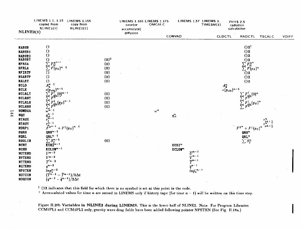
LINEMS 1.1. 1.15copied fromNLINE1(1)

NLINE2(1)

LINEMS 1.155copy fromNLINE1(1)

LINEMS 1.165 LINEMS 1.175save(or OMCALC

accumulate)diffusion

LINEMS 1.57 LINEMS 3.TIMESM(1)

ONVAD CL

PHYS 2.5radiation

calculation

DCTL RAD TSCALC

(0)T

(0)(0)(0)(0)(0)

(0)(0)(0)(0)

Wn

()xt()OX()x()x

E rE F(ps)"()Ox()x()x

1

E Ar^(o)"ZF

F; r~S'

qnrnA kk+ 1

Fs ' + F1 (ps) k+QRS"QRL *n

E S(0)KCHInKCLOWn

lnpn- 2

Tn1- Tn~-l)/2At(qV' 1 _-n- /A

Un - ;vn-1

n-1

r-1lnW-

t ()X indicates that this field for which there is no symbol is set at this point in the code.T Accumulated values for time n are zeroed in LINEMS only if history tape (for time n - 1) will be written on this time step.

Figure II.20b Variables in NLINE2 during LINEMS. This is the lower half of NLINE2. Note: For Program LibrariesCCM1PL1 and CCM1PL2 only, gravity wave drag fields have been added following pointer NPSTEN (See Fig. II.18a.)

VDIFF

E F(ps)"- 1

nFc)"-1n-1rn

rn-1

n-I

,An - I

s^-+ Fl(ps)n-I

QRS n - 1

QRL- 1E Sn- 1

KCHI n - 1

KICLOW"- 1

Un-2

NABSBNABSB1NABSB2NABSBTNFRSANFRLANFIRTP

NSABTPNALBT

NCLDNCLENCLRLTNCLRSTNCLRLSNCLRSSNONEGA

NQCNTAUX

NTAUY

NDRP1NQRSNQRLNSOLINNCNTNCNBNUTENDNVTEND

NTTENDNQTEND

NPSTENNDTCONNDQCON

I

___ __