Moderators. Definition Moderator - A third variable that conditions the relations of two other variables Example: SAT-Quant and math grades in school.

Moderators

Definition

Moderator - A third variable that conditions the relations of two other variables

Example: SAT-Quant and math grades in school

Correlation for females greater than for males

Sex is a moderator of the relations between SAT and grades

Types of ModeratorsCategorical or nominal

Analogous to factors in ANOVASex (F v M), race, study type (published vs. dissertation vs. not)Analyzed by analog to ANOVA

ContinuousTime between test & retest, age of participants, number of visits or duration of therapyAnalyzed by weighted regression (meta-regression)

Handled as weighted GLM (no correlated errors)

Types of Analysis

Fixed (common effects) model

The moderator(s) are expected to account for all systematic variance in effect sizes.

One analysis only.

Mixed modelThe moderators(s) account for some, but not all, variance in effect sizes. Some REVC left over.

Recalculate weights for residual REVC and re-estimate conditional means.

Multiple ways to consider error and weights

Number of Independent Variables

In theory, a meta-analysis model can contain both continuous and categorical moderator variables.

In theory, a model can contain an unlimited number of independent variables – statistical control for IVs

In practice, independent variables are usually modeled one at a time, and there are often only a few IVs

There are problems with missing data and capitalization on chance.

Often problems with both Type I and Type II errors

Categorical Example

Correlation of SAT and Grades for Males (studies 1-3) and Females (studies 4-6)

Hypothetical SAT dataStudy r z N w Sex

1 .40 .42 200 197 M

2 .42 .45 175 172 M

3 .45 .48 250 247 M

4 .60 .69 250 247 F

5 .55 .62 200 197 F

6 .65 .78 225 223 F

What is the correlation overall? Is it different for males and females?

Study z w w**2 w*z w*(z-zbar)**2

1 .42 197 38809 83.46 4.90

2 .45 172 29584 77.00 3.07

3 .48 247 61009 119.72 2.31

4 .69 247 61009 171.21 3.09

5 .62 197 38809 121.82 0.27

6 .78 223 49284 172.12 8.35

Sum 1282 278504 745.33 21.99

05.,99.21)( 2 pzzwQT58.1282

33.745

w

wzz

016.)1282/278504(1282

599.21

/

)1(ˆ

22

iii

z www

kQREVC

Male SubsetStudy z w w**2 w*z w*(z-zbar)**2

1 .42 197 38809 83.46 .192

2 .45 172 29584 77.00 .009

3 .48 247 61009 119.72 .220

Sum 616 129402 280.18 .421

45.616

18.280

w

wzz ..,421.)( 2 snzzwQM

0)616/129402(616

2421.

/

)1(ˆ

22

iii

z www

kQREVC

Female Subset Study z w w**2 w*z w*(z-zbar)**2

4 .69 247 61009 171.21 .007

5 .62 197 38809 121.82 1.26

6 .78 223 49284 172.12 1.31

Sum 666 149102 465.14 2.58

698.666

14.465

w

wzz ..,58.2)( 2 snzzwQF

001.)666/149102(666

258.2

/

)1(ˆ

22

iii

z www

kQREVC

Test of ModeratorTotal Male Female

Zbar .58 .45 .70

Q 21.99 .42 2.58

WBT QQQ

WTB QQQ

group

iW QQ1

05.,5,99.21 pdfQT

..,4,00.358.242. sndfQW

05.,1,99.18399.21 pdfQB

The test of the moderator is the test of QB. The test has df = (Number groups –1). Here df=1, QB=18.99, p<.05.

Group MeansGroup Sum

(w)

SE zbar CI

95L

CI

95U

rbar CI

95L

CI

95U

Male 616 .040 .45 .38 .53 .43 .36 .49

Female 666 .039 .70 .62 .77 .60 .55 .65

Total 1282 .028 .58 .53 .64 .52 .48 .56

wES

1..

Note that the difference in means is .25, which is quite large (and hypothetical; fictional data).

Mixed ModelIn the previous example, the moderators accounted for all the variance in the effect sizes (excepting sampling error). Suppose there was remaining variance, e.g., QW = 6.

001878.)1282/278504(1282

46

/

)1(ˆ

22

iii

z www

kQREVC

Mixed Model (2)Study z w w2 w2*z

1 .42 197 143.79 60.92

2 .45 172 130.00 58.20

3 .48 247 168.72 81.78

4 .69 247 168.72 116.95

5 .62 197 143.79 88.92

6 .78 223 156.67 121.47

Sum 1282 911.69 528.23001878.REVC

]/1/[1 12 REVCww 58.69.911/23.582 z

In this example, it makes little difference whether fixed or mixed. Sometimes it matters.

Analog to ANOVAReview the Excel and R analog to ANOVA programs.

Software note: Avoid interpreting Q tests from the random-effects models if the REVC weights were applied. The values of Q only conform to the chi-square statistic when the fixed weights are used.

Test the moderator with fixed effects. If you want random effects (usually you do) estimate the means with pooled or separate estimates of REVC, but do not interpret the resulting values of Q. Interpret the confidence and prediction intervals.

Input File

z w V Sex0.42 197 0.005076142 10.45 172 0.005813953 10.48 247 0.004048583 10.69 247 0.004048583 20.62 197 0.005076142 20.78 223 0.004484305 2

Results from R (1)

The overall mean is estimated to be .58

Lots of variability in these data.

Test for heterogeneity is significant.

Overall mean with no moderators (sex is not part of the analysis).My results are slightly different because of rounding z for input.

Results from R (2)

Sex is fixed, study is random.

Little residual heterogeneity

This is the test of the moderator. In this case, M vs. F difference.

The estimate in the intercept is the mean for males.

The second estimate is the DIFFERENCE between males and females.

Results from R (3)

Intercept is suppressed. The Male and Female means are estimated.

This is a test of the simultaneous effects – the joint test of both male and female means being zero.

rma doesn’t allow separate REVC estimates

Subsets

R command ‘subset’ allows you to partition data for separate analysis

Suppose we want to run a meta-analysis solely on females.

Analog to FIn ANOVA (primary data analysis), we would compute an overall F regardless of the number of factors.

With meta-analysis, we substitute a chi-square test.

As you saw in the example, metafor tests different things when you include or suppress the intercept {mods = ~factor(Sex) vs. mods = ~factor(Sex)-1}

Be sure to test what you want and to interpret your results correctly

In the particular case, we probably are more interested in whether there is a difference between men and women than whether the joint test of slopes is zero.

Class ExerciseFind the Excel file DevineR. It contains 54 studies comparing length of stay in the hospital for a control group and an educational treatment group given information about the benefits of going home. Positive d means the treatment appears helpful. The moderator is published article (J for journal) versus dissertation (D for dissertation).

Analyze

Import the data to R.

Compute the overall mean effect size.

Test for the moderator (difference in means).

Also look at variability within each group.

Prepare to share your findings with the group.

Weighted Regression

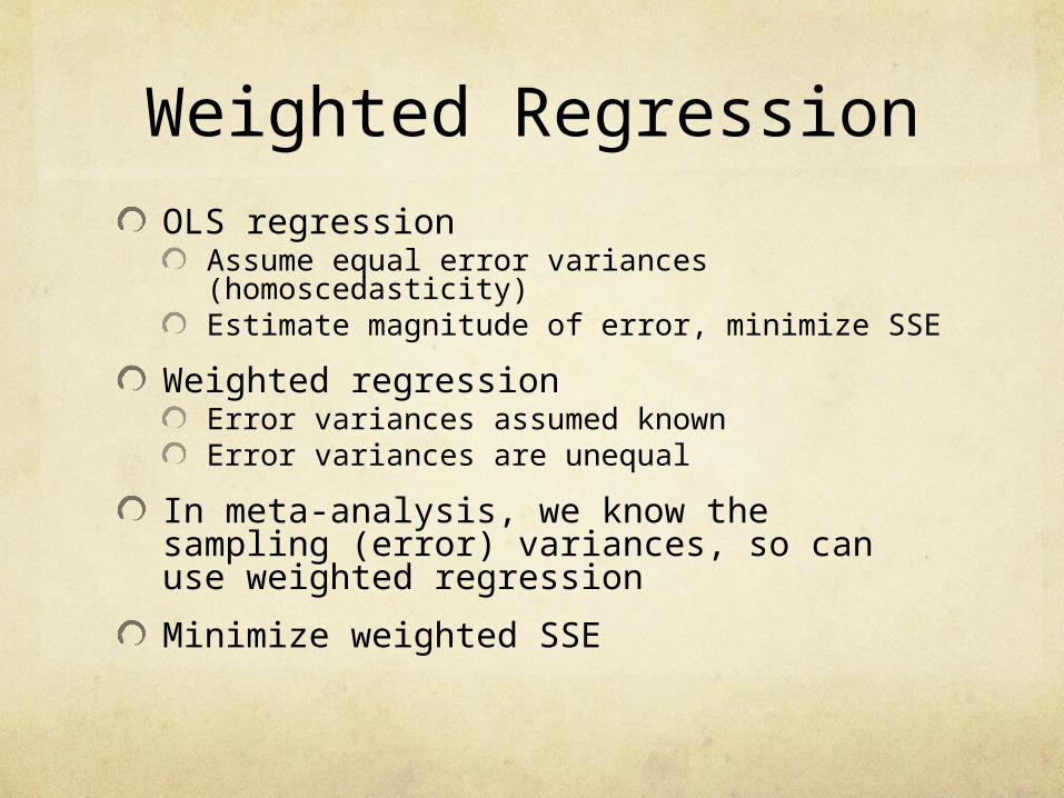
OLS regressionAssume equal error variances (homoscedasticity)Estimate magnitude of error, minimize SSE

Weighted regressionError variances assumed knownError variances are unequal

In meta-analysis, we know the sampling (error) variances, so can use weighted regression

Minimize weighted SSE

Weighted Regression Defined

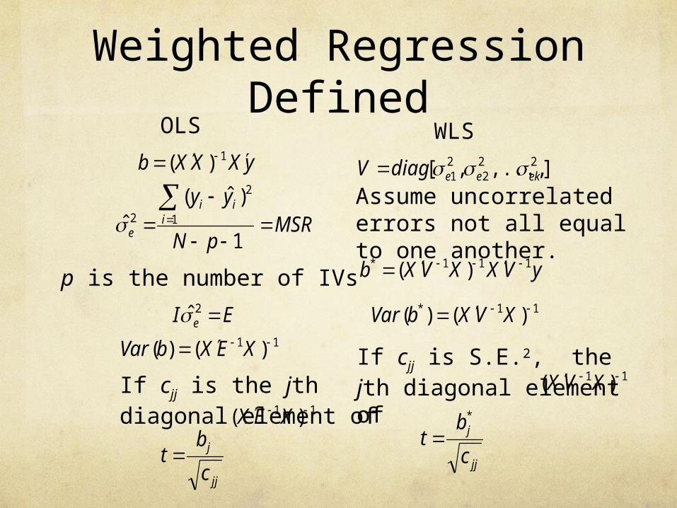
OLS

yXXXb 1)(

MSRpN

yyi

ii

e

1

)ˆ(ˆ 1

2

2

WLS

],...,,[ 222

21 ekeediagV

Assume uncorrelated errors not all equal to one another.

yVXXVXb 111* )(

11* )()( XVXbVar

If cjj is S.E.2, the jth diagonal element of

11 )( XVX

jj

j

c

bt

*

EI e 2̂11 )()( XEXbVar

jj

j

c

bt

If cjj is the jth diagonal element of 11 )( XEX

p is the number of IVs

Hypothetical SAT-Q and pct quant courses in

GPAStudy r z N w Pct Q

1 .40 .42 200 197 .10

2 .42 .45 175 172 .15

3 .45 .48 250 247 .12

4 .60 .69 250 247 .20

5 .55 .62 200 197 .25

6 .65 .78 225 223 .30

Does the percentage of quantitative courses influence the size of the correlation between SAT-Q and GPA?

SAT-Q Matrices (1)X y

1 .10 .42

1 .15 .45

1 .12 .48

1 .20 .69

1 .25 .62

1 .30 .78

1 1 1 1 1 1

.10 .15 .12 .20 .25 .30X’

yVXXVXb 111* )(

.005 0 0 0 0 0

0 .006 0 0 0 0

0 0 .004 0 0 0

0 0 0 .004 0 0

0 0 0 0 .005 0

0 0 0 0 0 .005

V

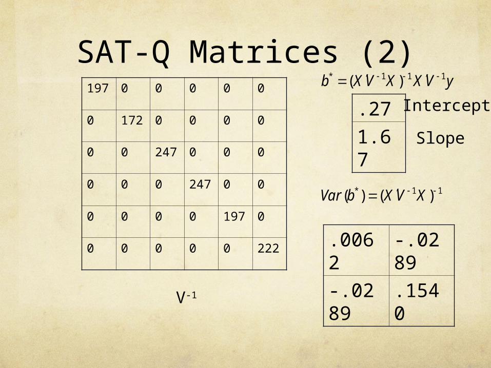
SAT-Q Matrices (2)197 0 0 0 0 0

0 172 0 0 0 0

0 0 247 0 0 0

0 0 0 247 0 0

0 0 0 0 197 0

0 0 0 0 0 222

V-1

11* )()( XVXbVar

yVXXVXb 111* )(

.27

1.67

.0062 -.0289

-.0289 .1540

Intercept

Slope

SAT-Q (3)

S.E. = sqrt(cjj).0787

.3924

S. E.

t (or z) = b/S.E. 3.41

4.25

t

Intercept

Slope

Intercept

Slope

yVXXVXb 111* )(

.27

1.67Intercept

Slope

.0062 -.0289

-.0289 .1540

11* )()( XVXbVar

Mixed ModelIn the event that homogeneity analysis reveals a large Q value for the residual, you can use the Q value to estimate the residual REVC. The REVC can be used to recalculate the weights for estimating specific values. Generally, however, researchers use weighted regression to compute significance tests for continuous moderators.

Weighted Regression in R

Review the weighted regression program in R. Run the PowerPoint example. Run an example with 2 independent variables and discuss output.

R will produce a mixed model by default (method = “REML” or “DL”). If you want a fixed-effects model (that assumes all REVC is accounted for by the moderator(s), then request a common effects model (method = “FE”).

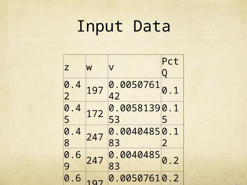
Input Data

z w v PctQ

0.42 197 0.005076142 0.10.45 172 0.005813953 0.150.48 247 0.004048583 0.120.69 247 0.004048583 0.20.62 197 0.005076142 0.250.78 223 0.004484305 0.3

Results from RMy results are slightly different because of rounding z for input.

Test of percent of quant classes. This would be test of all coefficients if we had more.

Regression estimates and test of each coefficient.

Moderator appears to account for all REVC.

Example 2

Study of relations between LMX (quality of Leader-Member eXchange and other variables. In this sheet, only affective organizational commitment (AC) is included.

Correlation between LMX and AC

Country classification as individualistic (Western) or collectivistic (Eastern) culture by country by Hofstede

Reliability of measurement of AC in the sample

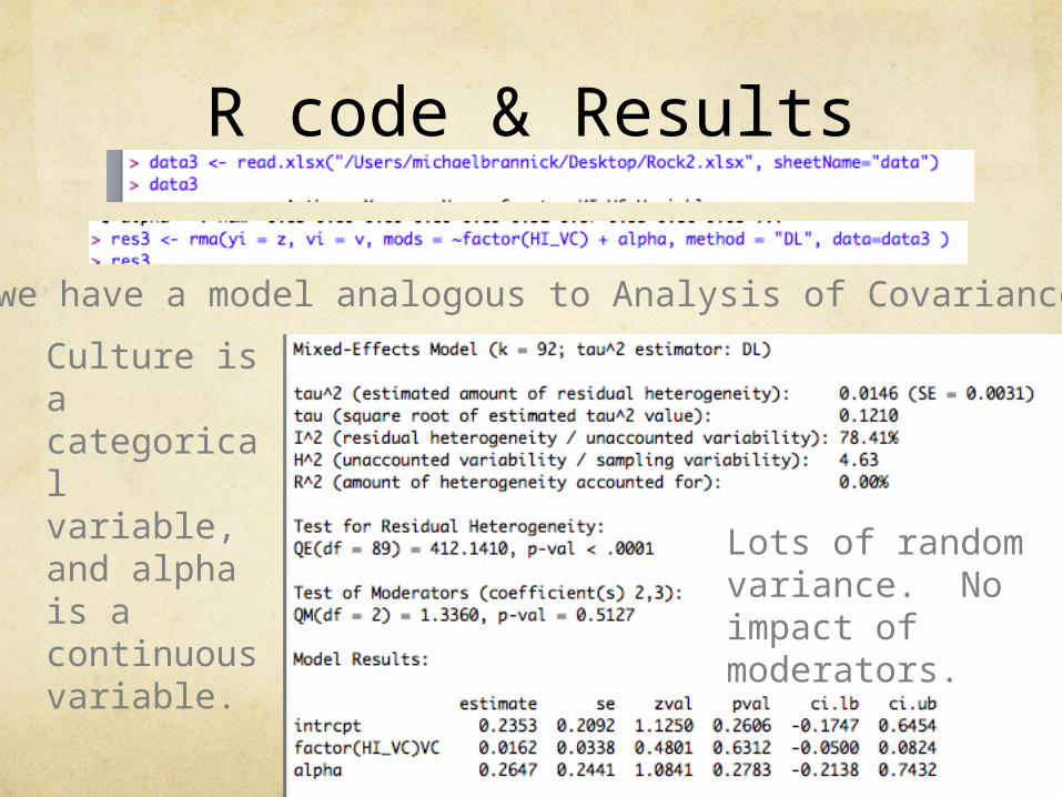
R code & Results

Here we have a model analogous to Analysis of Covariance.

Culture is a categorical variable, and alpha is a continuous variable.

Lots of random variance. No impact of moderators.

What if…

No effect for alpha by itself.

What else?

Culture is not significant by itself

Exercise

Download the file Rockstuhl2012LMX.xlsx

Select those studies that are for job satisfaction (variable = JS); delete the rest (Excel: data sort, select, delete; or subset in R)

Compute z and v (or use n, r, and ZCOR in R)

Test for moderators Culture and Alpha (reliability)

Prepare to share your results