Modelling the Hydrological Sensitivity to Land Use Change in a Tropical Mountainous Environment by Mauricio Edilberto Rincón Romero April 2001 A thesis submitted to the University of London for the degree of Doctor of Philosophy Department of Geography King’s College London

Welcome message from author
This document is posted to help you gain knowledge. Please leave a comment to let me know what you think about it! Share it to your friends and learn new things together.
Transcript
Modelling the Hydrological Sensitivity to Land UseChange in a Tropical Mountainous Environment
by
Mauricio Edilberto Rincón Romero
April 2001
A thesis submitted to the University of London for the degreeof Doctor of Philosophy
Department of GeographyKing’s College London

To my lovely wife
And sons
Manuel Felipe and
Miguel Angel
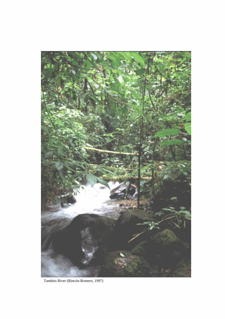
Tambito River (Rincón-Romero, 1997)
i
Abstract
The main subject of this thesis is the production of a sensitivity
analysis to land use and land cover change (LUCC) for a tropical
montane cloud forest (TMCF) environment on the basis of flux
responses in a hydrological model. Human pressure is one of the
main causes of LUCC in the TMCF which often results in important
consequences on natural resources like reduction of water quality,
loss of biodiversity, micro-climatic change or ecosystem
degradation (Koning et al., 1998). Deforestation of the tropical
cloud forest is an activity of recent decades that is modifying the
landscape significantly. The impact of this deforestation, rather
than the deforestation itself, is studied here by comparing variation
in fluxes of erosion and overland flow derived from different land
uses within a mountainous tropical forest catchment. A physically
based hydrological model of the Tambito watershed, Cauca-
Colombia and 5 LUCC pattern scenarios are implemented for the
study. A 2.5D dynamic surface hydrological model integrated with
a Geographic Information System (GIS) working on an hourly time
step is designed for the catchment, to assess flux variability in time
and space. The hydrological model includes the following sub-
modules: solar radiation and energy balance, evaporation,
interception and effective precipitation, infiltration, soil
hydrological balance, overland flow, recharge and erosion. Three
hydro-meteorological stations installed on experimental plots
collect basic model information for parameterisation and
validation. Experimental description, methodology, field data,
model implementation and analysed results are presented. Each
LUCC scenario uses 15 to 22 consecutive GIS iterations, which
transform forest to pasture within the catchment. Summaries of
annual average hydrological flux variations are used in the
sensitivity analysis. Multiple linear correlation was carried out for

ii
flux variations and hydrological sensitivity with landscape physical
properties of the deforested area by iteration for each scenario, in
order to determine the correlation between landscape catchment
physical properties and hydrological flux sensitivities. This process
also facilitated the identification of the topographic characteristics
of the most sensitive areas within the catchment to LUCC. The
model and statistical analysis provides a means of assessing the
contribution of different landscape units to hydrological change in
the face of LUCC. The impact of LUCC is assessed in terms of
catchment hydrological changes and the areas within the
catchment with more hydrological sensitivity to LUCC are
identified.

iii
ACKNOWLEDGEMENT
This thesis was funded by the Higher Education Programme of the
Office of Presidency of Republic of Colombia, through
COLCIENCIAS, and the “Instituto de Investigaciones Biológicas
Alexander Von Humboldt” for the development and application of
GIS-modelling technologies in Colombia. Additionally some field-
work expedition were possible due to the help of the University of
London Central Research Fund.
I want to express my special thanks to my supervisor Dr. Mark
Mulligan for his unconditional support in all fields including
academic, logistic, personal and moral. Without his direct
assistance this thesis would not have been possible. Also, I would
like to express my gratitude to the late Alvaro Jose Negret, of
Fundacion Proselva and the University of Cauca, Popayan, for his
enthusiastic support and permission to use the Tambito field site
and its facilities. I am also grateful to other Colombian
organisations that provided logistic support, in particular the
International Centre of Tropical Agriculture (CIAT), the Regional
Corporation for Cauca (CRC) and the ‘Instituto de Hidrología
Meteorología y estudios Ambientales’ (IDEAM), this last one who
brought meteorological information of the region.
I would like to make a special mention to the other KCL students
who came to the Tambito Reserve, to provide their assistance in the
field, and additionally, who gave a pleasant touch to the difficult

iv
experience, making the situation bearable and enjoyable. They
were Koulla Pallaris, Andrew Jarvis, Jorge Rubiano, Robert Stein
Rostaing, Matthew Letts, Juliana Gonzalez, Sim Reaney and Lydia
Bruce-Burgess. Also there were some special people who gave local
support in the campaign activities particularly Quintin and Olga.
This work would not have been possible without constant and
valuable support from my family, particularly my lovely wife who
day by day was behind my shoulders encouraging me and feeding
my hopes to get successful results. Also, to my beautiful and
innocent son Manuel Felipe for his constant stimulation and for
showing me the sense of our life. Also, my father and my brothers
who have been constantly interested in my progress / development
with this thesis. Thanks to all of them.
It is impossible to pass without mentioning the ‘DUNGEON’
friends, Andy, Sotto, Benny, Elias, Matt, Jim, and Christos,
because through the circumstances, we became a family, giving
our support to each other in both personal and academic aspects.
They were the ones who made London a pleasant place to live, and
the dungeon an agreeable palace in the middle of an eighteenth
century building. I would also like to thank the Pallaris family, who
welcomed me in their home during the last stages of the writing up
this thesis.
v
Table of contents
Chapter I Introduction
1.1 Land use and cover change (LUCC): a global issue 11.2 LUCC: global impacts 31.3 A review of models for LUCC 5
1.3.1 Methods for identifying the impact of LUCC 71.3.2 Strategies for evaluating hydrological fluxes in the
assessment of LUCC impact 81.4 LUCC: issues and impacts in tropical montane
environments outside Colombia 91.5 LUCC in Colombia: History and impacts in hillside
areas 111.5.1 Historical review of LUCC in Colombia 111.5.2 The hydrological impacts of LUCC in Colombia 16
1.6 Structure of the thesis 20
Chapter II Literature review of hydrological models applied to LUCC impacts research
2.1 Structure of this chapter 232.2 General concepts of hydrological models 232.3 A general classification of hydrological models 242.4 Handling spatial variability in hydrological models 262.5 A review of hydrological models related to LUCC impact 272.6 Hydrological modelling in tropical montane
environments 372.6.1 A review of modelling studies of the hydrologicalimpact of LUCC in Colombia 38
2.7 Research approaches to LUCC impacts 392.8 Main objective 402.9 Specific aims 402.10 Rationale 41

vi
Chapter III Methodology
3.1 Structure of this chapter 423.2 Description of the study area 433.3 Experimental strategy 493.4 Land use change scenario generation for this thesis 50
3.4.1 Estimating initial vegetation cover for LUCCScenarios 51
3.4.2 Scenario descriptions 543.5 Field methodology 64
3.5.1 Plot scale 643.5.1.1 The hydrological weather stations 673.5.1.2 Data collected from the weather stations 70
3.5.2 Catchment scale 713.5.2.1 Soil data 713.5.2.2 vegetation data 74
3.5.2.2.1 Leaf area index 753.5.2.2.2 Vegetation cover 763.5.2.2.3 Canopy water storage capacity 76
3.5.3 Other spatial data 783.6 Hydrological Modelling methodology 83
3.6.1 Introduction 833.6.2 Strategy 833.6.3 Consideration for modelling process 87Climate3.6.4 Solar Radiation sub-model 90
3.6.4.1 Hourly extraterrestrial solar radiationModel 91
3.6.4.2 Hourly cloud-cover attenuation model 923.6.4.3 Net solar radiation function 98
Hydrology3.6.5 Evaporation sub-model 1003.6.6 Canopy storage, interception and throughfall 1083.6.6.1 The Rutter model 1113.6.7 Sub-surface water sub-model 115
3.6.7.1 Modelling flow of water in porous media 1163.6.7.2 Soil water retention and matric potential 1173.6.7.3 Pedotransfer functions 119
3.6.8 Infiltration sub-model 1243.6.9 Overland flow sub-model 131
3.6.9.1 Sub-model description 1313.6.9.2 Surface component of overland flow at the
catchment scale 1343.6.10 Erosion sub-model 134
vii
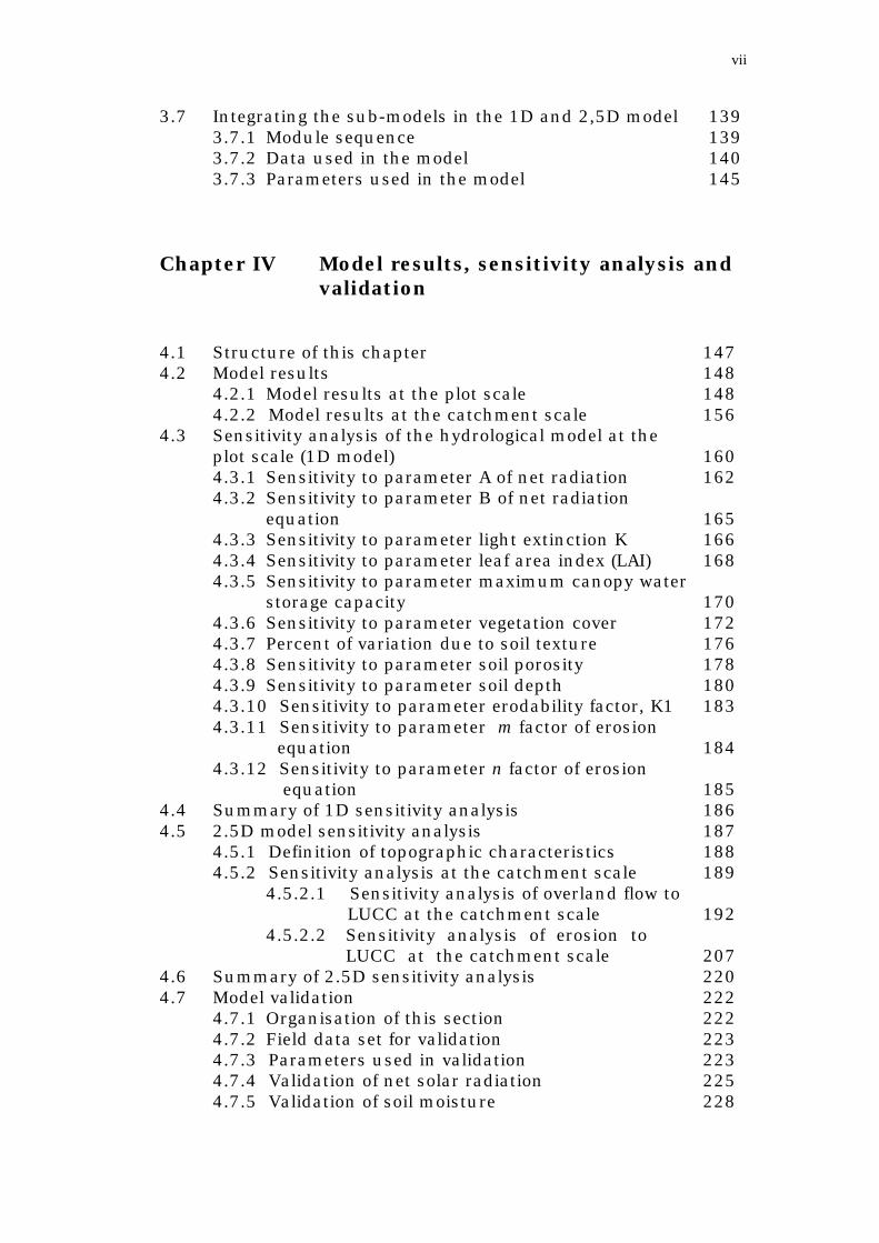
3.7 Integrating the sub-models in the 1D and 2,5D model 1393.7.1 Module sequence 1393.7.2 Data used in the model 1403.7.3 Parameters used in the model 145
Chapter IV Model results, sensitivity analysis andvalidation
4.1 Structure of this chapter 1474.2 Model results 148
4.2.1 Model results at the plot scale 1484.2.2 Model results at the catchment scale 156
4.3 Sensitivity analysis of the hydrological model at theplot scale (1D model) 1604.3.1 Sensitivity to parameter A of net radiation 1624.3.2 Sensitivity to parameter B of net radiation
equation 1654.3.3 Sensitivity to parameter light extinction K 1664.3.4 Sensitivity to parameter leaf area index (LAI) 1684.3.5 Sensitivity to parameter maximum canopy water
storage capacity 1704.3.6 Sensitivity to parameter vegetation cover 1724.3.7 Percent of variation due to soil texture 1764.3.8 Sensitivity to parameter soil porosity 1784.3.9 Sensitivity to parameter soil depth 1804.3.10 Sensitivity to parameter erodability factor, K1 1834.3.11 Sensitivity to parameter m factor of erosion
equation 1844.3.12 Sensitivity to parameter n factor of erosion
equation 1854.4 Summary of 1D sensitivity analysis 1864.5 2.5D model sensitivity analysis 187
4.5.1 Definition of topographic characteristics 1884.5.2 Sensitivity analysis at the catchment scale 189
4.5.2.1 Sensitivity analysis of overland flow to LUCC at the catchment scale 192
4.5.2.2 Sensitivity analysis of erosion toLUCC at the catchment scale 207
4.6 Summary of 2.5D sensitivity analysis 2204.7 Model validation 222
4.7.1 Organisation of this section 2224.7.2 Field data set for validation 2234.7.3 Parameters used in validation 2234.7.4 Validation of net solar radiation 2254.7.5 Validation of soil moisture 228
viii
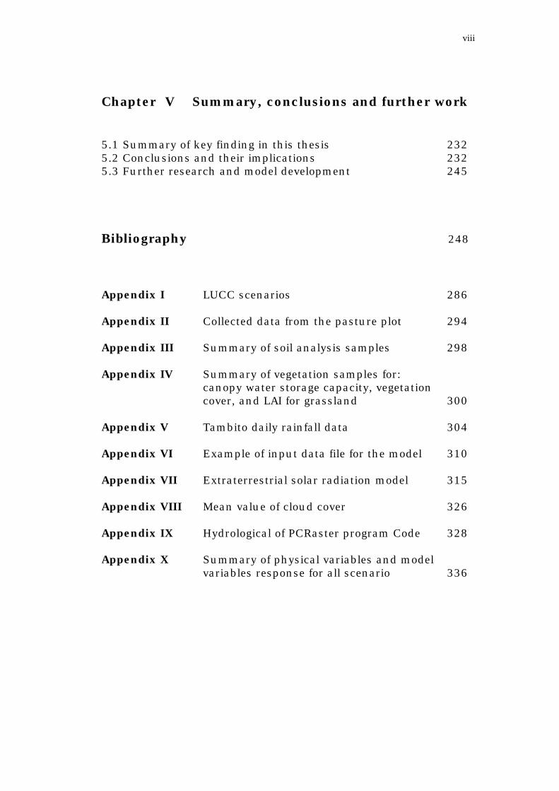
Chapter V Summary, conclusions and further work
5.1 Summary of key finding in this thesis 2325.2 Conclusions and their implications 2325.3 Further research and model development 245
Bibliography 248
Appendix I LUCC scenarios 286
Appendix II Collected data from the pasture plot 294
Appendix III Summary of soil analysis samples 298
Appendix IV Summary of vegetation samples for:canopy water storage capacity, vegetationcover, and LAI for grassland 300
Appendix V Tambito daily rainfall data 304
Appendix VI Example of input data file for the model 310
Appendix VII Extraterrestrial solar radiation model 315
Appendix VIII Mean value of cloud cover 326
Appendix IX Hydrological of PCRaster program Code 328
Appendix X Summary of physical variables and modelvariables response for all scenario 336
ix
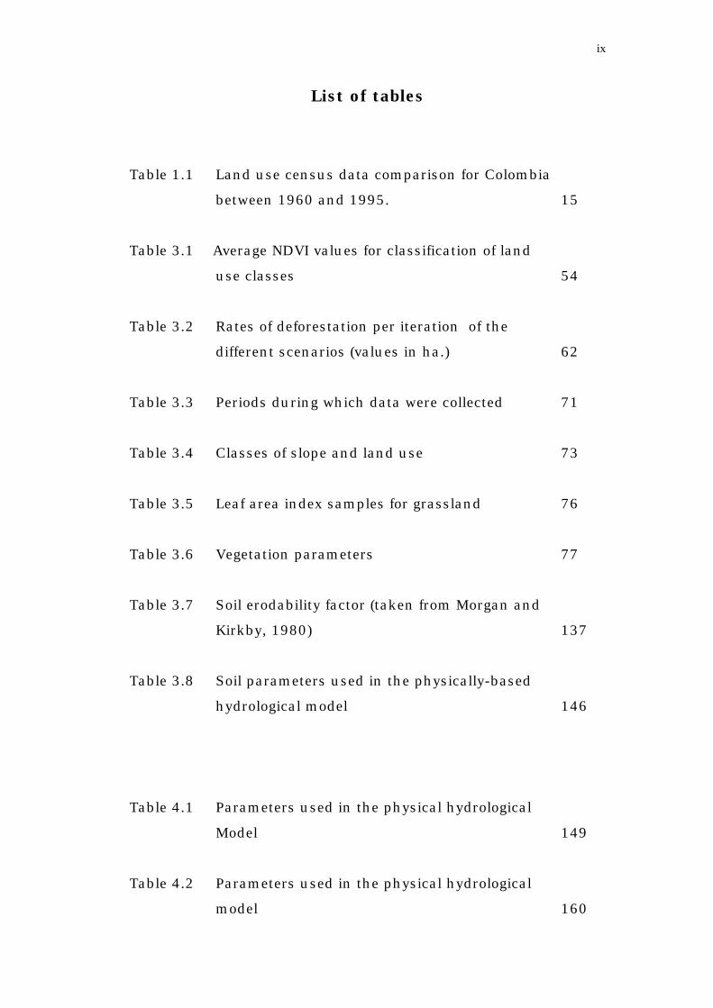
List of tables
Table 1.1 Land use census data comparison for Colombia
between 1960 and 1995. 15
Table 3.1 Average NDVI values for classification of land
use classes 54
Table 3.2 Rates of deforestation per iteration of the
different scenarios (values in ha.) 62
Table 3.3 Periods during which data were collected 71
Table 3.4 Classes of slope and land use 73
Table 3.5 Leaf area index samples for grassland 76
Table 3.6 Vegetation parameters 77
Table 3.7 Soil erodability factor (taken from Morgan and
Kirkby, 1980) 137
Table 3.8 Soil parameters used in the physically-based
hydrological model 146
Table 4.1 Parameters used in the physical hydrological
Model 149
Table 4.2 Parameters used in the physical hydrological
model 160
x
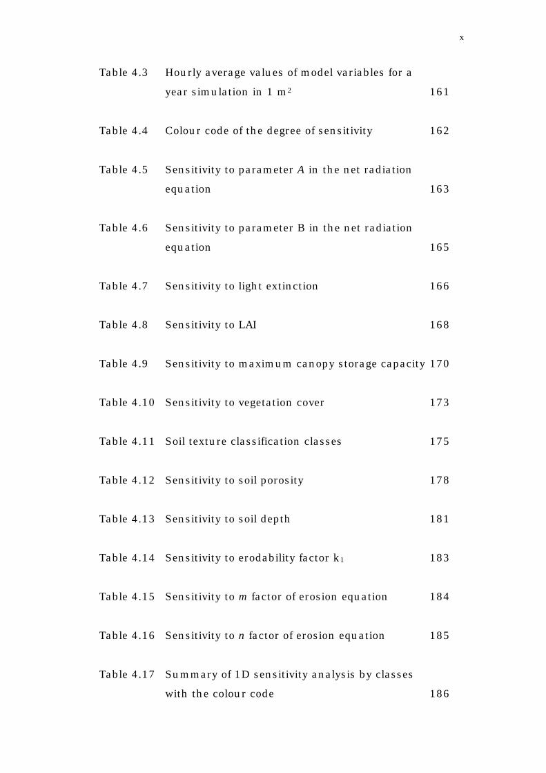
Table 4.3 Hourly average values of model variables for a
year simulation in 1 m2 161
Table 4.4 Colour code of the degree of sensitivity 162
Table 4.5 Sensitivity to parameter A in the net radiation
equation 163
Table 4.6 Sensitivity to parameter B in the net radiation
equation 165
Table 4.7 Sensitivity to light extinction 166
Table 4.8 Sensitivity to LAI 168
Table 4.9 Sensitivity to maximum canopy storage capacity 170
Table 4.10 Sensitivity to vegetation cover 173
Table 4.11 Soil texture classification classes 175
Table 4.12 Sensitivity to soil porosity 178
Table 4.13 Sensitivity to soil depth 181
Table 4.14 Sensitivity to erodability factor k1 183
Table 4.15 Sensitivity to m factor of erosion equation 184
Table 4.16 Sensitivity to n factor of erosion equation 185
Table 4.17 Summary of 1D sensitivity analysis by classes
with the colour code 186

xi
Table 4.18 Summary of data used in OF sensitivity
Analysis 205
Table 4.19 Multiple regression analysis of overland flow
for all scenarios. Significant relationships
are highlighted 206
Table 4.20 Summary of data used in Erosion sensitivity
analysis 217
Table 4.21 Multiple regression analysis of erosion for all
scenarios 219
Table 4.22 Parameters used in model validation 224
Table 5.1 Overland flow and erosion model results for the
original vegetation (from Landsat TM, 1989)
comparison with other research 236
xii
List of figures
Figure 3.1 Location of the Tambito watershed and prevailing land uses 45
Figure 3.2 Monthly average rainfall of the nearest weatherstation to Tambito (3km distance) 47
Figure 3.3 NDVI radiance from Landsat TM for Tambito Catchment 52
Figure 3.4 Transition of LUC by scenarios(a) Scenario 1. Forest conversion to pastures from cellular automata.(b) Scenario 2 Forest conversion with a fixed distance from river channels.(c) Scenario 3. Forest conversion with a fixed distance
toward river channels.(d) Scenario 4. Forest conversion with a fixed altitudinal distance from lower point in up hill
direction.(e) Scenario 5. Forest conversion with a fixed
altitudinal distance from higher point in downhill direction. 55
Figure 3.5 An example of an iteration for SC1 56
Figure 3.6 An example of an iteration for SC2 57
Figure 3.7 An example of an iteration for SC3 59
Figure 3.8 An example of an iteration for SC4 60
Figure 3.9 An example of an iteration for SC5 63
Figure 3.10 Distribution of plots and weather stations 66
Figure 3.11 Location of gutters in plots 66
Figure 3.12 Throughfall collector 68
Figure 3.13 Weather station in deforested areas. 68
Figure 3.14 Classification map for collecting soil samples 72
Figure 3.15 Basic cartography of the area (source from IGAC, 1985) 80
xiii
Figure 3.16 Digital elevation model for the study area derived from digitised contours using Arc/Info 7.3 80
Figure 3.17 Slope map derived the digital elevation model 81
Figure 3.18 Aspect map derived from the digital elevation model 81
Figure 3.19 LUCC map for Tambito watershed from Fundación Proselva (Museo de História Natural 1996) 82
Figure 3.20 Landsat image TM for the study area, false colour (5,4,3) 82
Figure 3.21 Schematic diagram of the hydrological model 86
Figure 3.22 Hourly cloud cover 96
Figure 3.23 Range of modelled cloud cover 97
Figure 3.24 Linear relation between measured and modelled cloud cover 97
Figure 3.25 Regression for computing net radiation in the model. 98
Figure 3.26 Diagram of net solar radiation model 99
Figure 3.27 Evapotranspiration variation with respect to Net Solar Radiation using the Penman-Monteith equation 106
Figure 3.28 Evaporation variation with respect to atmospheric and stomatal conductance 106
Figure 3.29 Flow diagram for potential evaporation 109
Figure 3.30 Diagram of the Rutter model (Jetten, 1994) 112
Figure 3.31 Diagram of interception sub-model 115
Figure 3.32 Soil texture triangle classification (Dingman, 1994) 117
Figure 3.33 Diagram of soil hydrologic characteristics 123
Figure 3.34 Diagram of infiltration sub-model 130
xiv
Figure 3.35 Diagram of runoff sub-model. 133
Figure 3.36 Diagram of erosion sub- model 138
Figure 3.37 A map of simulated rainfall distribution for Tambito watershed 142
Figure 3.38 One year of hourly rainfall from Tambito weather station (1995) 143
Figure 3.39 Histogram distribution for Tambito rainfall using simulated data of 1995 144
Figure 4.1 Modelled evaporation with 1D model for forestand grassland LUCC compared with the rainfallevents 151
Figure 4.2 Modelled canopy interception with 1D model forforest and grassland LUCC, compared withrainfall events 151
Figure 4.3 Modelled matric potential with 1D model forforest and grassland LUCC, compared withrainfall events 152
Figure 4.4 Modelled hydraulic conductivity with 1D modelfor forest and grassland LUCC, compared withrainfall events 152
Figure 4.5 Modelled infiltration with 1D model for forestand grassland LUCC 153
Figure 4.6 Modelled soil moisture with 1D model for forestand grassland LUCC compared with rainfallevents 153
Figure 4.7 Modelled overland flow with 1D model for forestand grassland compared with rainfall events 154
Figure 4.8 Difference between modelled overland flow forboth forest and grassland LUCC, compared withthe rainfall events 154
xv
Figure 4.9 Modelled erosion with 1D model for forest andgrassland, compared with rainfall events 155
Figure 4.10 Difference between modelled erosion for forestand grassland, compared with rainfall events 155
Figure 4.11 Changes in overland flow due to LUCC (units inmm) for a modelled year. 157
Figure 4.12 Changes in erosion due to LUCC (units inmm m-2) in a modelled year 159
Figure 4.13 Sensitivity to parameter A in the net radiationequation 164
Figure 4.14 Sensitivity to parameter B of the net radiationequation 165
Figure 4.15 Sensitivity to light extinction 167
Figure 4.16 Sensitivity to LAI 169
Figure 4.17 Sensitivity to maximum canopy storagecapacity 171
Figure 4.18 Sensitivity to vegetation cover 174
Figure 4.19 Sensitivity to soil textures 177
Figure 4.20 Sensitivity to soil porosity 179
Figure 4.21 Sensitivity to soil depth 182
Figure 4.22 Sensitivity to erodability factor k1 183
Figure 4.23 Sensitivity to m factor of erosion equation 184
Figure 4.24 Sensitivity to n factor of erosion equation 185
Figure 4.25 Modelled soil moisture with different initialconditions for the same rainfall pattern 191
Figure 4.26 Overland flow sensitivity in scenario 1(deforested pattern with cellular automata) 194
Figure 4.27 Mean topographic variables for deforested areasin SC1 194
xvi
Figure 4.28 Overland flow sensitivity in scenario 2 (forestconversion with a fixed horizontal distance fromriver channel in uphill direction) 195
Figure 4.29 Mean topographic variables of deforested areasin SC2 195
Figure 4.30 Overland flow sensitivity in scenario 3 (forestconversion with a fixed horizontal distancetowards channel rivers in downhill direction) 197
Figure 4.31 Mean topographic variables of deforested areasin SC3 197
Figure 4.32 Overland flow sensitivity in scenario 4 (forestconversion with fixed distance of altitude, inuphill direction from the lowest to the highestpoint) 199
Figure 4.33 Mean topographic variables of deforested areasin SC4 199
Figure 4.34 Overland flow sensitivity Scenario 5 (forestconversion with fixed distance of altitude, indownhill direction from the highest to thelower point) 201
Figure 4.35 Mean topographic variables of deforested areasin SC5 201
Figure 4.36 Erosion sensitivity in scenario 1 (deforestedpattern with cellular automata) 209
Figure 4.37 Mean topographic variables for deforested areasin SC1 209
Figure 4.38 Erosion sensitivity in scenario 2 (forestconversion with horizontal a fixed distancefrom river channel uphill direction) 210
Figure 4.39 Mean topographic variables of deforested areasin SC2 210
Figure 4.40 Erosion sensitivity in scenario 3 (forestconversion with horizontal a fixed distancetowards channel rivers downhill direction) 212
Figure 4.41 Mean topographic variables of deforested areasin SC3 212
xvii
Figure 4.42 Erosion sensitivity in scenario 4 (forestconversion with a fixed distance of altitude,in uphill direction from the lower to the highestpoint) 214
Figure 4.43 Mean topographic variables of deforested areasin SC4 214
Figure 4.44 Erosion sensitivity in scenario 5 (forestconversion with a fixed distance of altitude, indownhill direction from the highest to the lowerpoint) 215
Figure 4.45 Mean topographic variables of deforested areasin SC5 215
Figure 4.46 Modelled and measured solar net radiation forvalidation 226
Figure 4.47 Linear regression between modelled andmeasured net radiation in validation 226
Figure 4.48 Hourly average solar net radiation during theday for validation 227
Figure 4.49 Linear regression between hourly average ofsolar net radiation modelled and measured forvalidation 227
Figure 4.50 Modelled and measured soil moisture forvalidation 230
Figure 4.51 Linear regression of modelled and measured soilmoisture for validation 230
Figure 6.52 Daily soil moisture comparison betweenmodelled and measured, for validation, inJuly of 1999 231
Figure 4.53 Linear regression between measured andmodelled daily soil moisture, for validation 231
1
Chapter I Introduction
Land use and cover change (LUCC) has been recognised as a
modifying agent of landscapes. Some of the effects of LUCC on the
ecosystem are studied in this thesis, particularly those related to
the hydrological cycle.
In this chapter, first LUCC is investigated as one of many globally
important environmental changes. Later, in Colombia is analysed,
as a historical process (including socio-economic and political
factors) concentrating on its effects the hillside areas.
Subsequently, the thesis structure is discussed, indicating briefly
the content of the thesis chapters.
1.1 Land use and cover change (LUCC): a global issue
Of the world’s 12000 million ha. of tropical forest in 1988, 3600
million ha were tropical rain forests, 40% being located in Latin
America (Koning et al., 1998).
The tropical rain forest (TRF) is one of the world’s richest
ecosystems in plant and animal diversity (Jetten, 1994) but is also
one that is threatened by human pressure (Park, 1992; Dale, 1997)
where LUCC is mainly driven by population increase (Sinha, 1997).
Land use and land cover (LUCC) change plays an important role in
this ecosystem when compared with natural events, and can
impact upon water quality, biodiversity, regional climate, and
ecosystem degradation (Koning et al., 1998).
The conversion of TRF to pasture and the subsequent succession of
pasture to secondary forest has a significant effect on canopy
2
cover, canopy height, species composition, and biodiversity
(Reiners et al., 1994). Increasing food demand and changes in land
management and land tenure have pushed forward the agricultural
frontier in many tropical countries. Subsistence farmers are
continuously being displaced and forced to clear new areas for
cultivation on steeper slopes.
Throughout history, the land surface has undergone changes in
use. However, over the last decades, these changes have not only
been rapid but also drastic. The forces behind land cover changes
include population growth, which leads to an increased demand for
food and, as result, agricultural expansion, but economic and
technological development are also important (Dale, 1997; FAO,
1997; Sinha, 1997). Most of these processes start at the micro-
level, but because of indiscriminate replication over large areas,
they soon become a global problem (Lambin, 1997). One of the
major expressions of LUCC is deforestation for agriculture and
grazing and to provide wood for housing and fuel (Sinha, 1997). In
most cases, deforestation is the result of complex chains of
causality, originating outside the forestry sector (Lambin, 1997).
Park (1992) reported that 23 million km2 of the earth’s surface was
covered by tropical forest and woodland. In the mid-80s, Latin
America accounted for about 11 million km2 of the world total area.
A historical review of deforestation conducted by Houghton (1994)
revealed that approximately 28% of the forests in Latin America
vanished between 1859 and 1985. During the same period,
croplands and pastures had increased from 3.5 million to 9.2
million km2. FAO reported that 0.15 million km2 of forest are lost
each year (FAO, 1997). Therefore, the area dedicated to agriculture
today is twice that 90 years ago, half of which is accounted for in
the tropics in the last 50 years (Houghton, 1994). Tropical
deforestation can be viewed as a growth process whereby the forest
conversion rate is regulated by the density of deforested areas; the

3
larger the deforested area, the more likely that deforestation will
continue to expand and spread outwards (Lambin, 1997).
This problem has been addressed by FAO’s Global Terrestrial
Observing System (GTOS). The following limitations to the
accurate prediction of LUCC have been found: the lack of data on
terrestrial ecosystems and on the changes occurring within them,
and the lack of technical capacity to identify operative solutions
(FAO, 1997). The knowledge and understanding of the processes
involved in LUCC are fragmented and, in many cases, restricted to
a given area (Watson, 1997). All approaches to the analysis of
LUCC yield only information on specific aspects of the process.
According to Lambin (1997), several essential questions must be
addressed when studying LUCC such as: Why does LUCC occur?
What variables contribute to these changes? Where does LUCC
occur? (In other words, which locations are affected by LUCC?)
When does LUCC occur? , and At what rate does LUCC take place?
1.2 LUCC: global impacts
Land conversion and intensification through human intervention
brings about changes in the ecosystem’s balance, generating a
response in the system (Dale, 1997). System alterations include
increased air temperatures, increased atmospheric CO2, release of
nitrogen to the atmosphere, soil salinity, soil compaction,
pronounced changes in erosion rates, and even soil degradation
and water contamination. In some cases recovery can take from
100 to 500 years, or these effects on the ecosystem may be
irreversible (Dale, 1997).
Variations in vegetation cover in hillside areas generate changes in
hydrological cycles, soil properties and atmospheric fluxes, and

4
meso-climatic conditions, as well as the loss of biodiversity.
Researches have shown that tropical forests play a major role in
regulating the earth’s climate, whereby the elimination of forests
can have enormous implications on local, regional and global
climate (O’Brien, 1996).
Several factors determine the impact of deforestation on the
climate. O’Brien (1996) argues that different controls affect the
climatic system in different ways, and that it is not easy to predict,
analytically, just how deforestation will change the climate.
Furthermore, the impact appears to vary depending on local
conditions, such as topography and proximity to oceans. As a
result, neither the magnitude nor the direction of climatic change
associated with deforestation can be considered definite. One
important factor that affects the climate is the change in
concentrations of atmospheric gases. Deforestation increases
atmospheric CO2 because of reduced sequestration of CO2 through
photosynthesis and emissions of CO2 through burning and
decomposition (Melillo et al., 1996; Tinker et al., 1996; Sinha,
1997). Methane (CH4) production, including the variation of
nitrous oxide (N2O), is another significant atmospheric flux that
occurs when forest or grass covers are converted to croplands
(Mosier et al., 1997; Sinha, 1997).
Pitman et al. (1993) evaluated different ways of assessing climate
response to deforestation in South America and Asia. By
comparing the output of six general circulation models (GCM), each
based on different scenarios, whereby forest areas were replaced by
different land uses. The short-term global effect, the global area
affected, and the climate response were all very significant.
Changes in climate variables involved increased air temperature
and reduced annual precipitation and annual evaporation.

5
In contrast to the effects occurring in lowland forests, deforestation
in hillside areas has drastic effects on soil stability and
hydrological cycles, in particular the increasing water runoff and
erosion as well as impacting nutrient cycles (Dale, 1997).
Dale (1997) argues that LUCC has a greater effect on ecological
variables compared with climatic change and LUCC has little to do
with climatic change or even with climate. Man will change the
land use, and especially land management practices, to adjust to
climatic change. The ecological impact of these adaptations is
therefore more significant. However, it can be argued that climatic
and hydrological factors affect, to a certain degree, ecological
factors. Therefore, even small changes in these factors will have a
significant impact on ecosystem ecology.
Both considerations are applicable to long-term LUCC change.
Changes will occur and one way to understand these changes is
through the application of simulation models.
1.3 A review of models for LUCC
Modelling activities on LUCC impacts have taken on more and
more importance in recent decades. Modelling has become an
important tool for understanding physical and hydrological
processes and impacts (Bronstert, 1999). The most common
reasons for applying simulation models are:
1. To monitor and assess potential impact. Impact of LUCC is
assessed by comparing model responses to the incorporation of
different scenarios of land cover (Mosier et al., 1997).

6
2. To conduct sensitivity analysis. To understand which
processes or landscape properties are the key determinants of
hydrological response to land use change (Johnes and Burt,
1990). Sensitivity analysis also illustrates the effects of LUCC
on single model variables or on groups of these variables, giving
the degree of change in the modelled response (LeBlanc et al.,
1997).
3. To predict and forecast. The modelling of hydrological fluxes
and the variation in ecosystem response to LUCC can be used
as a forecasting tool in the short term (Kirkby, 1990; Crohn,
1995; LeBlanc et al., 1997). Forecasting tools are used in the
assessment of water resources for flood risk and hazard.
4. Better understanding of the system. The need for a much
better understanding of the underlying driving forces behind
LUCC and its impact (Turner et al., 1994). Modelling is a mean
of rapid and inexpensive experimentation with model systems to
understand the relationships between variables, especially over
spatially heterogeneous landscapes.
5. Integrate processes. The interaction between climatological
and hydrological mechanisms in hillslope physically-based
models produces an integration of a number of diverse
processes in the disciplines of forest and land management
(Bonell, 1993). Models are a tool for the formal integration of
research applications across disciplines.

7
1.3.1 Methods for identifying the impact of LUCC
A benchmark land cover (LC) must be considered before LUCC can
be modelled. The LC is obtained by direct field observation or
remote sensing, which is clearly defined as a reference point. A
baseline inventory then identifies LC distributions in the recent
past. This initial scenario can be based either on physical or on
biological conditions. The initial hydro-climatological or biological
conditions produced by the reference scenario of LUCC are the
state budget or flux initial conditions, which will be used in the
comparison process.
LUCC can be studied at different scales; global, regional,
watershed, and plot scale (Kirkby, 1990; Dunn and Mackay, 1995;
Johnes, 1996; Leemans et al., 1996). Each scale has related
constraints, such as data availability, and the most appropriate
model type (Kirkby, 1990). Large-scale models and data are
usually integrated with small-scale models for parameterisation
and validation, for example, plot to watershed scale, watershed to
regional scale, regional to global scale (Johnes and Heathwaite,
1997; Bronstert, 1999).
The method most used to determine hydrological LUCC impact
involves the comparison of sequential land-cover maps, which
allows subtle changes to be detected.
Results of spatial statistical models of tropical deforestation show
that single-variable models based on landscape data from a
previous time period provide forecasts information of spatial
deforestation patterns and trends. Predicting the spatial pattern of
deforestation is therefore a much easier task than predicting future
rates of forest clearance (Lambin, 1997). Spatial statistical models
primarily identify location predictors of areas with the greatest

8
propensity for LUCC change. They do not predict when the change
will occur, they only identify proximate causes of LUCC change.
1.3.2 Strategies for evaluating hydrological fluxes in theassessment of LUCC impact
Numerous hydrological models have been adopted to estimate the
hydrological impact of LUCC. Studies on how LUCC affects the
hydrological environment must involve the response of these fluxes
to LUCC. Different approaches can be used to assess the
variations in hydrological fluxes, with respect to initial flux
conditions. Some approaches are summarised below:
1. Real-time LUCC scenarios. The model is used to integrate
scenarios with different land uses; the scenarios can be
generated from measured or remotely-sensed data or from land
use change models. Parameters for each land use must be
previously identified, to be included in the model. The model
includes land cover conversion, with real-time variations in the
scenario during the simulation period (Gustard and Wesselink,
1993).
2. Off-line LUCC scenarios. Remotely-sensed data or models are
used to generate a series of LUCC conditions which are applied
to the hydrological model off-line as alterations of the
equilibrium rather than transient change experiments (Frohn et
al., 1996).

9
1.4 LUCC: Issues and impacts in tropical forestenvironments outside Colombia
About half of all the world’s forests are in the Tropics. Though
there are many different types of tropical forest (moist forest, dry
forest lowland forest, upland forest) some of the characteristics of
this environment are precipitation greater than 1500 mm a year,
dense vegetation, an abundance of epiphytes, and dense under
stories of smaller trees, and shrubs, with harbouring high
biodiversity (Whitmore, 1998). This type of forest can be found in
America, Asia, Africa and Australia.
The main areas of remaining tropical rain forest, particularly
lowland forest are in Brazil and a number of other Latin American
countries, Congo and its neighbours, Indonesia, and Malaysia.
Tropical rain forest are known, as the world’s most productive
plant communities, with giant trees up to 60m in height supporting
thousands of other species of plants and animals.
Montane RainforestMontane rain forest differs in some characteristics growing at
higher elevations, where the climatic and topographic
characteristics are diverse and include extreme wetness
environment and steep slopes. Changes in environmental
characteristics change the forest appearance and structure.
Canopy height decreases with the elevation, reaching up to 35m in
the lower part of the montane zone, but only 9m above 3000m of
elevation (Whitmore, 1998). The structure is simpler than lowland
forest, with large buttresses, branches and epiphytes, which
become more numerous with increasing the elevation (Whitmore,
1998). Temperature can range from 10°C to 25°C according to
elevation (from 1000 to 3000 masl) and latitude. Climatic
conditions are also characterised by low ground level clouds,

10
particularly at different times during the day. The combination of
these creates a particular environment that is known as tropical
montane cloud forest (TMCF).
FAO estimated that for the period 1981-1990 the annual forest loss
in tropical highlands and mountains was 1.1%, much more than
other tropical forest, including lowland forest (Singh, 1994). The
main reason for the disappearance and degradation of this
environment was conversion to grazing land and temperate
vegetable cropping, trimber harvesting and wood production at
unsustainable rates (Bruijnzeel, 2000). Researchers have
expressed that the conversion of TMCF to other land uses could
result in significant declines in overall river flows (Brown et al.,
1996).
LUCC in tropical montane environments and its is becoming
important due to the deleterious nature of its consequences.
Tropical forests are considered a global climate regulator due to the
interaction between land surface processes and atmospheric and
climatic activities (Lambin, 1997).
Some consequences of tropical deforestation have been identified in
the literature including changes in surface and subsurface fluxes,
reduction in infiltration and water retention capacities, ecological
changes and loss of biodiversity, diminished cloud water
interception, increased runoff and thus soil erosion (Scatena and
Larsen, 1991; Brown et al., 1996; Scatena, 1998; Pounds et al.,
1999; Bruijnzeel, 2000; Sperling, 2000),
There are very few well monitored TMCFs in the world. Some of
these important studies areas are: Monte Verde Cloud Forest
reserve in Costa Rica (Pounds et al., 1999) where the forest
conversion to pasture and its effects have been studied by Pounds
11
et al. (1999), and Cusuco National Park in Honduras (Brown et al.
1996). Other notable examples are Sierra de Minas in Guatemala
(Brown et al., 1996) and Mt Kinabalu Sabah in Malaysia for forest
clearance for vegetable cropping. Luquillo Mountains in Puerto
Rico (Scatena, 1998), the Blue Montains in Jamaica (Tanner,
1977), and Talamanca in Costa Rica (Calvo, 1986) among others.
1.5 LUCC in Colombia: History and impacts in hillside areas
Several human activities have affected the vegetation cover in
Colombia, particularly LUCC for subsistence of the majority of the
population. Those activities are driven by socio-political factors
which control land tenancy and land use, and as a consequence
the environment is threatened. A brief historical review of
Colombian agrarian conflicts and land tenancy is presented to
understand the evolution of land use processes in the country.
Then some of the land use activities in the hillside of Colombia are
discussed to provide the context of the national problem and the
importance of a better understanding of hydrological process
affected by LUCC.
1.5.1 Historical review of land use change in Colombia
In Colombia as in most of the Latin American countries the
agrarian problems go back by the time of the great Spanish
conquests in the New world. The conquistadores were amply
rewarded by the Spanish Crown for their efforts on its behalf
through grants of land. The land was granted to the
conquistadores through the system of capitulaciones. Which were a
type of contract in which privileges over lands were granted by the
sovereign to the discoverers (Duff, 1968). By the end of eighteenth
12
century a Spanish system of large landholdings had replaced the
former small areas of communal Indian land tenure system. From
the Independence from the Spanish until the end of the nineteenth
century the land tenure changed ownership with owners,
increasing in number (because the land passed from the Spanish
Crown to the Colombian State, and then to the bourgeoisie
landholders currently in ownership (Duff, 1968).
In the XX Century after the First World War and up to 1920’s the
Colombian bourgeoisie efforts went to build the basis of an
industrial framework for an international open market of
agricultural products. The commercial activities were based in the
latifundio (large extension of land) created through two centuries of
the New Great Colombia, and to take the advantage of increasing
international prices in agricultural products (Bejarano, 1977). The
tendency was for property concentration and land monopoly,
including land holding of good land without production. Those
activities changed the way that the land has been used. In that
time the working population is divided into the workers of the
incipient industrial process in Colombia in the cities and the
farmers that have been attached to small lands and isolated from
the market for the prevailing commercial conditions imposed by the
monopoly (Buitrago, 1977). As consequence, on the one hand the
increasing populations in the cities where the factories improve the
production, and for the other hand, the remaining part of the
landholdings who were expropriated from their own land, were
pushed to colonise new lands meanwhile some of them remain in
the land but becomes land workers (without land) in the big
properties of terratenientes. In this time the government gave the
chance to landowners to make official the land tenancy by owning
property titles through new laws. Using the guise of ‘giving the
owning title to the small farmer’, but in reality they wanted to make
official their big properties which they had appropriated before (Ley

13
de tierras 200 of 1936), where the new structure of land property
were the couple ‘big property – small property’ (latifundio and
minifundio) (Cartier, 1990).
After the Second World War several social and political problems
kept the peoples attention, hiding the agricultural problem. In that
time, the Currie Mission, was assigned to build a program for
Colombia’s development. They highlighted the problem that large
flat extensions allocated on fertile valleys were used for cattle while
people in the hillsides fight for a piece of land to crop their own
food, which meant that the best land was used in the wrong way
(cattle instead of intensive agriculture). In the fifties and sixties the
fast rhythm of agricultural industrialisation and mechanisation,
displaced the field workers from the big farms to the hills, adding
to these hill areas more necessities, been the low yield production a
characteristic these land. This changes the land tenancy stage
from small production to commercial agriculture (as an industry)
and traditional agriculture (survive crops) (Banco de la República,
1951).
As a consequence of those processes the workers displaced from
farming became unemployed in the cities and hillside areas
increasing the social and agricultural problems. The bourgeoisie
hiding behind the government realised the problem and in the
sixties and seventies a project of law (The Agrarian Reform, Law
135 of 1961) was proposed. This law with the face of ‘justness for
the people’ allocated the land redistribution with equal
opportunities, offering the unoccupied lands and the worse types of
land to the population that did not have land (because the better
lands were already occupied by the terratenientes). That law of
land had the purpose to, stop the people that started to invade the
bourgeoisie productive lands. In this way, the agricultural labour
force that were not absorbed by the small industries (because of

14
the mechanisation of agriculture) were neutralised temporally
(Bejarano, 1977). The land problem remained in the country,
displacing the population to colonising new lands, logging the
forest, or on occasion practising slash and burn to increase the soil
fertility for a few years, and then moving to a new forest area and
repeating the procedure.
In the last decades, people that occupied unproductive land were
forced to move to the forest and agricultural frontiers, colonising
and deforesting new land, to supply the necessary food to survive.
However between 1978 and 1992, the proportion of the rural
population in extreme poverty (the countryside farmers) declined
fairly slowly (from 38% to 31%) (The World Bank, 1996), due to the
socio-political conflicts between gerrilla and paramilitares, which
both razing several towns in the countryside and killing people with
the excuse that they were collaborators with the enemy. As
consequence those farmers escape from the countryside to main
cities.
In addition, the most recent problem (illicit cropping of coca leaf
and amapola (opium poppy), as a fast solution to economic
problems), in combination with narco-economy, paramilitaries and
increasing violence, become others factors adding to the problems
of land use change. Also the growth of populations and their
migration to marginal areas, increased the pressure on the forest,
changing the forest to land with low agricultural potential,
producing environmental impacts such as degrading the soil,
natural resources and, vegetation followed by abandonment.
(Fajardo, 1996).
Nowadays these problems are still hitting most of the poor
population and the effects of bad agrarian practices are appearing
markedly on the hillsides areas, characterised by the high density
15
of minifundios (small parcel less than 3 ha), increasing land
degradation and ecosystem instability.
No much information in the country has been published about
deforestation rates. The first agricultural census carried out by the
“Departamento Administrativo Nacional de Estadística” DANE,
which is the national institution with the responsibility of produce
this type of information, was in 1960, covering small parts of the
country, only for the productive area, without including large areas
such as savannas, forest and deserts. The most recent agricultural
census was in 1995, covering less of a half of the country. A
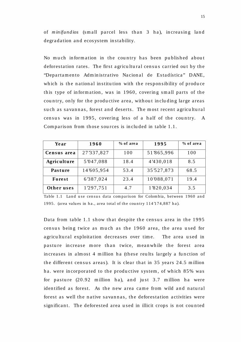
Comparison from those sources is included in table 1.1.
Year 1960 % of area 1995 % of area
Census area 27’337,827 100 51’865,996 100
Agriculture 5’047,088 18.4 4’430,018 8.5
Pasture 14’605,954 53.4 35’527,873 68.5
Forest 6’387,024 23.4 10’088,071 19.4
Other uses 1’297,751 4.7 1’820,034 3.5
Table 1.1 Land use census data comparison for Colombia, between 1960 and
1995. (area values in ha., area total of the country 114’174,887 ha).
Data from table 1.1 show that despite the census area in the 1995
census being twice as much as the 1960 area, the area used for
agricultural exploitation decreases over time. The area used in
pasture increase more than twice, meanwhile the forest area
increases in almost 4 million ha (these reults largely a function of
the different census areas). It is clear that in 35 years 24.5 million
ha. were incorporated to the productive system, of which 85% was
for pasture (20.92 million ha), and just 3.7 million ha were
identified as forest. As the new area came from wild and natural
forest as well the native savannas, the deforestation activities were
significant. The deforested area used in illicit crops is not counted

16
in these assessments, but the rate of deforestation for this activity
is estimated reach up to 60,000 ha per year. Winograd (1995)
reports that the deforestation rate between 1980 to 1990 reached
up to 60% more than previous decade, meanwhile the agriculture
area decrease in a rate of –0.5 % a year and the areas used in
pastures increase in +3.4 % a year.
1.5.2 The hydrological impacts of LUCC in Colombia
Colombia is one of the richest countries in hydrological resources
with abundant rivers and natural resources, which are well
distributed geographically. Colombia occupies the fourth place
after Soviet Union, Canada and Brazil in hydrological richness,
with more than 88% of the total area (1’141,748 km2) with
precipitation over 2000 mm a year, and an average of 3000 mm a
year. The mean evaporation in Colombia is 1150 mm a year, and
the total runoff could average 2,112 km3, which is 67 m3 s-1
approximately (annual values for the whole country area) (Marin-
Ramirez, 1992).
During the last decades water resources have become a problem,
with watershed management in the Andean hillside areas,
producing ecological, social and economical damages due mainly to
population growth, changes in vegetation cover, industrial
development and land use change (Marin-Ramirez, 1992). The
obvious consequences that can be mentioned are, among others:
loss of biodiversity in relation to the rapid loss of natural forest
cover; loss of wild relatives of useful crop species; soil instability
and landslides. Soil erosion, principally loss of topsoil due to water
erosion. Nutrient loss through leaching, with monocultuves and
badly-managed sown pastures. Water quality issues, associated

17
with high sediment load in head waters are also a growing problem
(CIAT-Hillsides Program, 1994).
The World Bank estimated that 45% of the rural Colombian
population were predominantly in hillside areas in the beginning of
the 1990’s, with 23% being the indigenous population. Rural
impoverishment has increased for those areas relative to the
country as a whole (Cepal, 1990).
Poor agricultural practices on the hillsides are used extensively
such as fallow rotation systems in which forest or bush are cleared
for cropping, and then are returned to pasture or bush fallow once
yields decline to a level that is not economically useful.
Deforestation, overgrazing and agricultural activities are also
causes of degradation in the hillside agro-ecosystem.
Environmental degradation in the hillsides has serious implications
not only for the viability of agricultural production in the ecosystem
itself, but for “downstream” lowland agriculture and coastal
ecosystems affected by soil erosion and agrochemical pollution in
the uplands. Soil erosion, sedimentation and major land
degradation caused by deforestation and cropping without use of
soil conservation practices affects watercourses originating in the
hillsides. The most irreversible and potentially damaging with
major social cost caused by hillside environmental degradation, is
the loss of biodiversity due to the disappearance of montane forest
which amounts to 32% of the forest area in the Colombian Andean
Region. The rate of deforestation in hillsides is higher than in the
lowlands. Causing a loss of 90% of the original montane forest
cover by 1990 (CIAT-Hillsides Program, 1994). Montane forest has
very high biodiversity, which is considered important to conserving
wild crop genetic resources in-situ. In ecosystems where the land
use is intensive the most important environmental degradation is

18
the excessive use of agrochemicals which is a characteristic of
agricultural intensification, causing soil and groundwater pollution
(CIAT-Hillsides Program, 1994).
A CIAT study carried out on the hillsides in the Andean Region in
Colombia, was centred in the Rio Ovejas watershed in the Cauca
Department. This watershed covers 100,000 ha. and encompasses
a diverse range of Andean hillside systems ranging from indigenous
slash and burn cultivation to peri-urban, high-input horticulture,
and includes CIAT commodities (Knapp and Buitrago, 1994).
Consequently, the assessment of the location and extent of the
erosion problem in the hillsides was an additional activity
undertaken by CIAT in the study area, as well as the ex-ante
impact assessment of land use change and development of a
diagnostic simulation model of alternative technological
interventions. The model considered impact on soil erosion,
nutrient loss, crop productivity and water quality (Knapp and
Buitrago, 1994).
The relationship between soil erosion and productivity remains
poorly researched and little understood in tropical soils. It is
identified as a need for research focused on improving
methodologies for characterising the extent and cost of soil
degradation. In addition systematising the available data requires
regional collaboration, due to the diversity of the hillside land use
classes found in the country.
To improve crop productivity and forage availability, to enhance
erosion control and soil physical rooting conditions, and to
increase water infiltration, water-holding capacity, and nutrient
retention of the soil, the incorporation into hillside production
systems of practices for soil conservation and regeneration are
being energetically promoted (Knapp and Buitrago, 1994).

19
Knapp and Buitrago (1994) also points out that while farmers
consider the monetary benefits of erosion control, such as yield
increases, they are unlikely to consider non-monetary benefits
such as soil resilience, or downstream benefits which accrue to
others.
Hillside agro-ecosystems are a mosaic of diverse micro-edapho-
climatic regimes, user circumstances and cultures. In any one-
area the results of technological innovation will be location-specific.
An essential task is to develop a replicable approach to innovation,
based on strategic understanding of how to intervene in the hillside
agro-ecosystem and how to make transitions to ecologically-sound
and economically-viable alternatives, acceptable to users.
Determining why some technological options are more acceptable
to farmers than others, and the trade-off between production and
conservation objectives this involves, requires technology testing
which is embedded in a community based participatory framework
(Knapp and Beltran, 1994).
The hillside approach is focused on the effects of soil degradation
that involve diagnostic research to better identify problems and set
priorities amongst them with respect to biophysical and economic
aspects of soil degradation due to agricultural practices and
catchment management. In addition, the design of decision-
support systems incorporating different types of models, including
knowledge-based models drawing on indigenous technical
knowledge and research results that can be introduced into models
to facilitate the understand of LUCC effects in the watershed (CIAT-
Hillsides Program, 1994).

20
1.6 Structure of the thesis
Physical hydrological fluxes are dynamically modelled from the
atmospheric interface to the soil bedrock interface. A 1D dynamic
hydrological model was initially developed at the plot scale for each
type of land cover. The 1D model is parameterised and validated
on the basis of data from hydrological stations in pasture, primary
and secondary forest. Lessons learned from the production and
sensitivity analysis of this model were applied in the development
of a 2.5D distributed hydrological model, integrated within a
Geographic Information Systems (GIS). This was then applied to
understanding the impact of LUCC at the catchment scale. A
sensitivity analysis of the 2.5D model was performed to identify
hydrological flux variation with land use change to determine key
variables of the ecosystem that are affected by different spatial
patterns of LUCC. Five different scenarios of LUCC were used
within the analysis, to assess the hydrological flux sensitivity and
to determine the most sensitive areas in the studied catchment.
Chapter 1 introduces the topic of LUCC in this thesis. First a
discussion about the impact of LUCC in general terms and
additional information about LUCC modelling is provided,
including methods and tools. Then the LUCC impact on tropical
montane forest is discussed in a global context. Subsequently, the
development of LUCC modelling in Colombia are also presented,
and provides brief background of the LUCC in Colombia,
historically and the actual situation of the hillsides research, and
finally the thesis structure is presented. Chapter 2 presents the
literature review of hydrological models applied to LUCC. The
strategy for estimating LUCC is discussed. Then the literature
review of the hydrological models is discussed: characteristics,
classification, types and results, and also a brief review of some of
the best known contemporary hydrological models with their main

21
features. Also hydrological models in tropical montane
environments are reviewed and finally, understanding the problem
and the research approach are presented in the thesis and the
thesis objectives, main goals, and the obtained achievements
discussed.
Chapter 3 describes the methodology used in this thesis. This
chapter has two marked sections: the first is related to the
collection of the information for modelling, the second is related
with the construction of the hydrologically-based model. Initially
the structure of the chapter and the study area are presented. The
research and experimental strategies are provided and detailed
description of the scenarios of LUCC used in combination with the
hydrologically-based model are given. Then the fieldwork
methodology is discussed for plot and catchment scale studies; the
installation of hydrological stations, and the field methods used for
the collection of data are illustrated. The data collected in the field
are presented and additional data used for model parameterisation,
experimentation and for model verification and also for validation
are discussed. Secondly the modelling aspects are discussed. This
section describes the development of the 1D and 2.5D models,
together with a description of the following sub-model components:
solar radiation, energy balance, evaporation, canopy storage and
interception, infiltration, soil water hydrology, overland flow, and
erosion. Each component is explained in detail and source
equations, flow diagrams, and data requirements are indicated.
The inter-relationship between components and information flow is
also indicated. After describing the sub-model, model performance
and initial conditions are explained. Then model integration with
Geographic Information Systems (GIS) is also described.
In Chapter 4 the model results are presented. 1D and 2.5D model
results are shown to discuss the model characteristics and some

22
implication of landscape properties on the hydrological response.
Then 1D model parameterisation and sensitivity analysis is
discussed, and subsequently 2.5D model sensitivity analysis for
overland flow and erosion is shown; the relationship between those
variables and the topographic variables is evaluated. A summary
of TMCF sensitivity to LUCC is presented in terms of overland flow
and erosion sensitivity. Finally, validation of some output variables
is carried out to evaluate the model goodness of fit.
Chapter 5 gives the summary and the conclusions, the objectives
evaluation and the achievements, including the recommendations
for estimating hydrologically sensitive areas to LUCC for the TMCF
environments, and then the conclusions are drawn with further
model applications and future research possibilities elaborated.

23
Chapter II Literature review of hydrological models appliedto LUCC impacts research
2.1 Structure of this chapter
This chapter presents the literature review of hydrological models,
which begins with the general concepts used in the modelling
activities, particularly with the issues related to hydrologically-
based simulations. Then a classification of these models is
presented, including the importance of spatial variability as a
characteristic of modelling the surface water fluxes. A complete
review of the existing commonly used hydrological models related
to LUCC impact is presented, and finally the main objective and
the specific aims of this thesis are numerated.
2.2 General concepts of hydrological models
Hydrological models aim for simplicity by selecting a system’s
fundamental aspects at the expense of incidental detail (Anderson
and Burt, 1985). A number of alternative techniques and
modelling approaches have been developed.
The first integrated hydrological model, called the Stanford
Watershed Model (Singh, 1995), was reported in the literature in
1966 by Crawford and Linsley. During the following decades,
hydrological modelling improved significantly because of advances
in technology and computer hardware.
Better hydrological models are becoming available with these
technological advances and the continuous improvement in
24
modelling strategies, such as inclusion of GIS, remote sensing or
cellular automata (MacMillan et al., 1993; Beven and Moore, 1994;
Robin et al., 1995). Many of these methods are used in
contemporary watershed models, such as TOPMODEL (Beven et
al., 1995); KINEROS, a kinematic runoff and erosion model
developed by Rovey et al. (1977) and described by Smith et al.
(1995), and TOPOG_IRM (CSIRO, 1993).
Many of the latest generation hydrological models use GIS, but, in
many cases, GIS and environmental models are not well integrated,
just used together. GISs are frequently used as post-processors to
display and further analyse model results. In turn, modelling
approaches directly built into a GIS appear rather simple and
restrictive (Fedra, 1993). Dangermond (1993) indicates that the
tendency for integration is to use specialised software systems.
“Such powerful tools without well distributed data are, at best
expensive interpolation tools and, at worst subject to GIGO
(garbage in-garbage out)” (Fedra, 1993). One of the main
restrictions on good spatial (GIS) modelling is a lack of good,
spatially detailed hydrological parameters for model
parameterisation and validation.
2.3 A general classification of hydrological models
Models can be characterised by the type of relations used within
the routines. The relationship between real and model processes
can be represented either empirically or physically.
1. Empirical models. Model relationships are based on empirical
data, not necessarily on physical processes. These models tend
to have a high predictive ability but their physical explanatory
power is often low. They are sometimes called “black box” or

25
“input/output” models. These terms are usually applied to
those models whose internal operation does not aim to directly
represent “real” operative processes, even at an abstract
mathematical level (Kirkby et al., 1993). Successful
applications of this strategy include the unit hydrograph,
extreme frequency analysis, regression analysis, and real time
forecasting models (Anderson and Burt, 1985). Statistical
analysis faces several methodological and interpretative
difficulties, such as measuring complex dependent variables,
and spatial aggregation of data in large units. The existence of a
statistically significant association does not establish a causal
relationship. Moreover, a regression model that fits well in the
region for which it was designed might not function well in other
regions, because it should not be transferred beyond the
physical limits for which it was developed, parameterised and
calibrated.
2. Physically-based models. These models, based on physical
processes, are modelled on the understanding of physical
mechanisms and often make large demands in terms of
computational time and data requirements. Nevertheless, such
models offer increased explanatory and experimental power.
However, because of the higher number of assumptions that are
necessary, their predictive capacity is often equal or worse than
that of empirical models. Beven (1989) argued that highly
complex, physically-based models are possible at smaller scales.
However, larger-scale models must be simple to allow
parameterisation. Woolhiser (1996) pointed out that simpler
models are often more accurate than physically-complex
models, but are difficult to scale up to larger watersheds.
Parameter generalisation within the watershed involves simple
representations of main model elements. Several variables such
as soil characteristics which are important at reduced scales for

26
detailed studies are also important at the watershed level,
increasing model complexity while not necessarily adding
precision to the results.
2.4 Handing spatial variability in hydrological models
Several approaches to represent spatial variability within a
watershed exist. These approaches can be classified as:
1. Lumped modelling, expressed by ordinary differential
equations that describe simple hydraulic laws. These models
do not take into account the spatial variability of processes,
inputs, boundary conditions, or the system’s geometric
characteristics. Instead, a single value for properties and
parameters is applied to the entire watershed. Some examples
are HEC-1 (Hydrologic Engineering Center, 1981) described by
Feldman (1995), RORB (Laurenson and Mein, 1995), and
SSARR (USA Army Engineer, 1972) described by Speers (1995).
2. Distributed modelling, which explicitly accounts for the spatial
variability of processes, inputs, boundary conditions and system
characteristics. The spatial distribution of features and their
spatial inter-relationships are especially important to explaining
physical processes within the watershed. Examples are SHE
(Abbott et al., 1989) described by Bathurst et al. (1995), SWMM
(Metcalf et al., 1971) as described by Huber (1995).
Models can also be classified according to the type of equation used
and the resulting output. Model results can be a singular, or a
population of answers. Processes can be described either by
deterministic or stochastic equations. Deterministic models
have just one possible outcome, whilst stochastic models have a

27
population of answers. In most cases both types of equations
occur within the same model. However, in the cases when the
relevant information for parameterisation is not available, some
processes are better modelled by stochastic equations that could
give an approximation for modelling purposes.
2.5 A Review of hydrological models related to LUCC impact
There are several hydrological models that have been created for
particular purposes or environments. The models have different
abilities, characteristics and type of results, including resolutions
in time and space. Some of the most widely used models are
discussed here, identifying some of their important features related
to the subject of this thesis, and the reasons that the models are
not used in this thesis.
SHE/SHESED
The SHE/SHESED combination is a physically based, spatially
distributed modelling system for water flow and sediment transport
to be applied at a catchment scale. The SHESED model was
developed in the University of Newcastle upon Tyne, UK, and is
based on the SHE (Systeme Hydrologique Europeen) model which
was developed by international collaboration between groups in the
UK, Denmark, and France. SHESED is used to investigate land
management especially the prediction of LUCC and climate change
impacts. SHE was designed as a flexible modelling system,
encompassing several levels of complexity, consisting of sub-
components for evapo-transpiration and interception, overland and
channel flow, unsaturated zone flow, saturated zone flow,
snowmelt and channel/surface aquifer exchange. The SHE model
28
is driven by meteorological inputs and provides inputs to the
sediment transport component (Bathurst et al., 1995).
The interception sub-component is an adaptation of the Rutter
model (1971), and the evapo-transpiration is based on the Penman-
Monteith equation. Some sub-components require more
parameters and input information than are not available for
Tambito such as the atmospheric component, sediment yield and
transport of material within the channels component, as well as
soil matric suction, raindrop impact amongst others (see section
3.6). Also the model has a number of simulation routines that are
not useful for this study. Nevertheless, this model is one of the
investigated models that could be appropriate for this thesis, but
its complexity is too high for the application intended here.
In addition to the lack of information available for parameterisation
and validation of the SHE model, most of the literature consulted
reported the use of the model for short time simulations (days)
providing good simulation results (Wicks and Bathutst, 1996), or
for bigger spatial resolution up to 4000 m of pixel size (Refsgaard,
1997). However, Wicks and Bathust, (1996) used the model for two
small agricultural catchments (5.1 and 6.4 ha) in Iowa, with good
reproduction of the observed temporal variations in sediment yield.
In contrast Refsgaard (1997) applied this model to a catchment of
440 km2 in Denmark, for which calibration and validation
processes were carried out splitting the catchment in seven
sections, and to producing better results at a pixel size resolution
of 500m.

29
SHETRAN
The SHETRAN system was developed by the Water Resource
Systems Research Laboratory (UK), based also on the SHE
(Systeme Hydrologique Europeen). SHETRAN is a 3D, coupled
surface sub-surface physically-based spatially-distributed finite-
difference model for coupled water flow, multi-fraction sediment
transport and multiple, reactive solute transport in river basins
(Parkin, 1996). The model is a powerful tool for studying the
environmental impact of land erosion, pollution, and land use as
well as climate change effects, and also surface and sub-surface
water resources and management. It is integrated in a decision
support system to maximise its usefulness in environmental
impact management. Some of the features of the model are:
- Basin-wide modelling for water resource planning
- 3D solute transport in the surface and sub-surface
- Sediment erosion and transport
- Water balance in large basins (50,000 km2 +)
- Long-term basin evaluation (1,000 years +)
- Coupled hydrological and meteorological modelling
- Impact assessment for land use and climate change
- Risk and pollution assessment for proposed industrial
developments
- Monte Carlo simulation for uncertainty prediction.
SHETRAN is a robust model that simulates more than is needed in
Tambito for the purpose of this thesis for example sediment
transport in the channels, and effects of climate change amongst
others, and also it could have problems due to the lack of input
information for parameterisation for the sub-routines because data
are required which are not available from Tambito (for example
river sediment transport) (see sections 3.6).
30
Lukey (2000) applied the SHETRAN model to assess hydrological
impact of reforestation particularly on runoff and sediment yield,
for a badlands catchment at Draix, France. The semi-arid
environment, shallow slopes and low rainfall rate make it quite
different to the Tambito study area. Lukey (2000) found strong
effects of forestation on decreasing runoff and sediment yield. Also
the SHETRAN model has been integrated into the NELUP Decision-
Support System (Dunn, 1996), to estimate the predictive impact on
water resources and ecological diversity, which has been applied on
Cam river basin.
TOPMODEL
TOPMODEL is a set of conceptual tools that reproduces the
hydrological behaviour of a catchment in a distributed or semi-
distributed way, in particular the dynamic surface or subsurface
contributing areas (Beven et al., 1995).
Despite the fact that TOPMODEL models land-surface-atmosphere
interaction, the main components are centred on the simulation of
subsurface water flow. It could be used as a prediction tool for
catchment hydrology for long time series, based on soil response
using the Topographic Index.
The hydrological processes on the surface that TOPMODEL
simulates are very simple. The level of generalisation of the
atmosphere-soil interface is very high with the model only treating
the evaporation of the surface water, without more attention to
other surface events. Runoff and erosion process are not presented
as an important feature in the model (Beven et al., 1995). These
two features are important for research in Tambito, where the
31
evaporation process is very specific to TMCF environments and
where runoff and erosion processes are the key flux processes in
the model assessment of LUCC impact in hydrological processes for
this thesis.
The main features of TOPMODEL are to produce indices and
parameters of the saturated zone (or storage deficit), the saturated
transmissivity, the root zone parameter, and in large catchments a
channel routing velocity (not available or necessary in Tambito, see
section 3.6).
Most of the evaluation of the TOPMODEL concept has been based
on comparisons of stream flow hydrographs and do not necessarily
provide a test of predictions of subsurface flow, saturated source
areas, runoff-erosion and their effects on the environment (Moore,
1996). Also, most of the applications of the TOPMODEL have been
concentrated on comparison of the predicted water table depth
against the validation data in instrumented catchments from wells
with good results (Beven et al., 1984; Moore, 1996; Saulnier et al.,
1997), but in some cases with poor results (Seibert et al., 1999). In
the same way TOPMODEL has been evaluated to predict the
saturated areas on the basis of topographic information, where the
sensitivity to the spatial resolution takes an important role (Kim et
al, 1999) and different sizes (Blazkova and Beven, 1997).
TOPOG
TOPOG is a terrain analysis-based on a hydrological modelling
package, which describes the topographic attributes of complex
three dimensional landscapes in complex terrain characteristics
and heterogeneous soils and vegetation, predicts the spatial
distribution of steady state water-logging, erosion hazard and
32
landslide indices; it simulates the transient hydrological behaviour
of catchments, and how this is affected by changes in vegetation
cover. Also it models the growth of vegetation and how it impacts
on the water balance; it models solute movement through the soil
and sediment transport over the soil surface (Vertessy et al., 1994).
TOPOG is a robust deterministic distributed-parameter hydrologic
modelling package; this model requires a good set of information as
input data and also works with vector data derived from TAPES-C,
Topographic Analysis Programs for the Environmental Sciences –
Contour data. TAPES-C is a terrain analysis software that
subdivides a catchment into elements using the stream-tube
approach and calculates a variety of topography attributes for each
element (Grayson et al., 1995).
The TOPOG model complexity means that it requires good input
information such as 3D soil characteristics for the Richard’s
equation and vegetation data, information on crop physiology, soil
salinity, fertility, the spatial distribution of rainfall, among others
(Short et al., 1995; Hatton and Dawes, 1993). Despite this many of
the parameters could be extracted from the literature within their
normal range of variation or from a short period of observation
from the field, the long term simulation evaluated monthly or
yearly yields up to +/-10% of variation compared with observed
data. It was the results for 12 year simulation in a 32 ha
catchment size in the central Victorian highlands, Australia
(Vertessy et al., 1993). An important feature of TOPOG is that the
good results are obtained for instrumented catchments, at high
spatial resolution (up to 25m) and small catchment (up to 50ha)
(Hatton T., personal communication in 1993).
Parameterisation of this model in Tambito could be difficult due to
the lack of information on vegetation cover (growth and physiology),
33
surface fluxes and soil characteristics. Also the Tambito
catchment-size could be an impediment to apply this hydrological
model.
THALES
THALES is a dynamic hydrological model based on the element
network created by TAPES-C. THALES is a combination of surface
and sub-surface models that simulate kinematic overland flow
from saturation excess and infiltration excess mechanisms, as well
as sub-surface stormflow. The structural difference of the model is
the partition of the catchment into stream-tubes, beginning at the
contour line of lowest elevation and ending at the highest contour
line (Grayson et al., 1995). Related to hydrological features,
interception and evaporation are considered not relevant, and they
are incorporated only for simulation of long periods and research
applications. Despite the fact that THALES was built as a simple
hydrological model, the surface and sub-surface modules request
parameters not available in Tambito such as cross-sectional area of
tube-element, channel shapes amongst others. Also the model
pays much more attention to within channel processes than is
necessary for this project.
KINEROS
The kinematic runoff and erosion model (KINEROS) is a routing
model for surface runoff over cascades of overland flow planes
contributing lateral inflow to channels with an interactive
infiltration component. Also, it comes with erosion and sediment
transport components, a pond element and spatial variability of the
rainfall. It can be used at several scales (1 to 700 ha.). The
34
interception routine is very simple and works for each runoff
element separated, based on the vegetation or other surface
conditions. Roughness relationships, sediment transport and
channel routines are parts of the model that could be difficult to
adapt to this study, due to the lack of source information for
parameterisation (see sections 3.5 and 3.6) (Smith et al., 1995).
The KINEROS model has been used in semi-arid environments and
different catchment size (3 to 700 ha.) with good results (Goodrich,
1991; Michaud, 1992), however Duru and Hjelmfelt (1994) did not
get the same successful results in a catchment of 30 ha. in Iowa.
A particular reason that this model is not implemented in this
thesis is that the Kineros model transforms the catchment into an
equivalent network composed of runoff surface planes, intercepting
channels, ponds or detention storage; then the flow is analysed in a
1D of network channels, where the runoff surfaces are
encompassed by a cascade of rectangular surfaces of non-uniform
slope, hydraulic resistance or soils (Smith et al., 1995). This
generalises the distributed landscape and topographic
characteristics, which are important in this study. Also the
surface-atmosphere interface does not have the relevant
importance in the process as is requested in Tambito for this
modelling exercise (see section 3.6).
CREAMS
CREAMS are a collection of hydrology components for water quality
models. CREAMS model was developed to assess edge-of-field non-
point source pollutant loading for alternative management systems.
Land use can be changed within a rotation cycle, fertilisation and
pest control practices could be incorporated during the simulation.
The time step used in the routines is daily, but the model was
35
designed to simulate long-term storm by storm differences up to 20
years, as opposed to other models such as ANSWERS that simulate
a single storm (Knisel and Williams, 1995). Also CREAMS model is
not a distributed parameter model, and so can not be applied to
understand the outcomes of spatial variability of distributed LUCC
in Tambito (see section 3.5).
SWAT
The Soil and Water Assessment Tool (SWAT) was developed in the
Grassland, Soil and Water Research Laboratory USDA-ARS Texas,
and is based on the water balance equation. The SWAT model is a
modification of the SWRRB and ROTO models, for application to
large and complex rural basins. It is therefore a distributed version
of the CREAMS model, running simultaneously in several hundred
sub-basins (SWAT website).
The SWAT is to be used only in USA environments. This model use
the USDA geo-database (soil and weather database) and several
other types of information which are the basis of empirical
concepts developed for USA environments such as SCS curve
number for computing overland flow and runoff volume or the
Modified Universal Soil Loss Equation MUSLE, amongst others.
Due to the fact that the SWAT model was designed only for US
environments, it is not readily transferable for use in the Tambito
catchment.

36
HYRROM
HYRROM The Hydrological Rainfall Runoff Model is a computer
model developed by the Software Development Office of the
Institute of Hydrology, UK; it is based on a simple representation of
the physical processes that govern the water flow in a catchment
area. The model incorporates interception, soil, ground water and
runoff stores, and includes some representation of the losses due
to evapo-transpiration. The main use of this rainfall runoff model
is to predict the river flows from rainfall and evaporation data for a
catchment. HYRROM can be used to generate flow records for
periods in which flow data are missing or of doubtful accuracy, but
where rainfall records are complete. It can also be used for quality
control of data, extending historical flow records and generating
synthetic flow sequences for water resources assessments
(Scientific Software Group website, http://www.scisoftware.com).
The reason why HYRROM is not suitable for the analysis is that the
documentation does not mention that the model is spatially-
distributed, this being an important feature in the thesis subject
(see section 3.6).
WATFLOOD
The WATFLOOD hydrologic model is a distributed hydrological
model developed by Dr. Nick Koumen at the University of Waterloo,
Canada. It is an integrated set of computer programs to forecast
flood flows for watersheds having response times ranging from one
hour to several weeks. The emphasis of this model is on making
optimal use of remote sensed data, Radar rainfall data, Landsat
data or Spot data, with incorporation of land cover data directly to
the hydrological system.

37
The reason why this model is not used in the Tambito study is that
the time and the spatial resolution are very different to that which
are needed here, also the remote sensing information are not
available for Tambito (see sections 3.5 and 3.6).
2.6 Hydrological modelling in tropical montaneenvironments
Researchers have paid special attention to the physical hydrology
of forests because previous studies have demonstrated that forests
and, in particular tropical rain forests, have a significant effect on
climate and energy balance (Turner et al., 1994; Dale, 1997) and
catchment hydrology (Copeland et al., 1996). Specialists have
pointed out the importance of canopy storage on all hydrological
processes and its importance for the hydrological balance (Hancock
and Crowther, 1979). Studies have also been conducted on rainfall
interception (Rutter et al., 1971, 1975, 1977; Aston, 1979; Gash,
1979; Gash et al. 1980; Calder, 1986; Calder et al., 1986; Calder,
1996), canopy evaporation (Ford and Deans, 1978; Pearce and
Rowe, 1980), infiltration (Whitehead and Hinkley, 1991), and runoff
(Loukas and Quick, 1996). Their results have been integrated in
studies at the watershed level (Mein and Brown, 1978; Loague and
Freeze, 1985; Jetten, 1994; Sudjono, 1995).
Fewer studies have been conducted on TMCF as compared with
their lowland counterparts. Several studies, for example Golley
(1983), Bonell et al. (1993), Veneklaas (1990; 1991) and Veneklaas
et al. (1990a, 1990b), concentrate on understanding specific
processes such as cloud interception and nutrient budgets rather
than the integrated hydrological system.

38
2.6.1 A review of modelling studies of the hydrological impactof LUCC in Colombia
Little empirical, theoretical or modelling research on land use
change has been carried out in Colombia. This is particularly the
case for the tropical mountains of Colombia.
One of the few examples of modelling LUCC impact in Colombia is
the Andean Amazon River Analysis and Monitoring (AARAM)
project. The project investigates the effects of regional LUCC and
global climatic change on biochemical and hydrological cycles
within riverine ecosystems of the Andean Amazon basin. It also
conducts field research in Colombia, specifically in the Caqueta
watershed (AARAM, 1998). AARAM is a regional research initiative
to develop the scientific understanding necessary for effective
management of aquatic resources in the face of ongoing
development and potential climate change. The research activities
in AARAM examine the fundamental physical and biological
processes controlling the health and the dynamics of Andean
riverine ecosystems, with emphasis on terrestrial-aquatic and
upstream-downstream linkages, with spatial scales ranging from
meso- to micro-scales watersheds (AARAM, 1998).
Another example is the Tropenbos-Colombia programme, which is
oriented toward a land use planning policy centered on the
conservation of biodiversity and the control of deforestation. This
project is located in the Araracuara and Alto Caqueta regions. The
main aims of this project are to: (a) determine the demand for
timber and non-timber products for subsistence use and regional
markets; (b) characterise existing extraction activities in the region
and their impact on biodiversity; (c) establish permanent plots and
monitoring systems to study forest dynamics (Tropenbos
Foundation, 1997). Tropenbos Colombian programme is centred
39
on conservation on biodiversity and control of deforestation as part
of land use planning policy for Colombian Amazonia. In the area
are numerous indigenous people, and the rain forest abounds with
an unmatched diversity of plant and animals. The agricultural
frontier is advancing and a large number of environmental and
social conflicts, such as active agriculture colonisation, coca
plantation, poverty and armed conflicts.
Despite the fact that at governmental level, LUCC impact modelling
is not publicised, The “Departamento Nacional de Planeación”
(DNP) of Colombia is carrying out a programme “Plan Nacional de
Desarrollo Alternativo PLANTE”, in cooperation with the Agriculture
Ministery for rural development alternatives. This is mainly to
encourage farmers to replace illicit crops with productive
plantations (DNP, 1999). In the same way, the DNP has
environmental polices to protect endangered ecosystems, and
improve environmental sustainable mechanisms in order to
increase the quality life and better agricultural production
plantations (DPN, 1999).
2.7 Research approaches to LUCC impacts
Many studies have compared and assessed runoff under different
land uses in coupled catchments but do not take into account the
changes occurring over time due to deforestation (Coles et al.,
1997; Finch, 1998; Rai et al., 1998). Others concentrate on
computer modelling to simulate soil water behaviour, without
modelling surface water (Binley et al., 1992; Faunt et al., 1993) or
the overall runoff, which is assumed to go directly into the river
channel (Taha et al., 1997). In contrast, other studies include very
complex models of water fluxes, providing detailed descriptions of
each process and of fluxes and stores, but do not include the

40
dynamics of LUCC change within the simulation framework
(Speers, 1995; Zhao and Liu, 1995; Singh, 1997; Bronstert, 1999;
Flugel and Smith, 1999). This thesis tries to integrate some of the
hydrological processes with land use and land cover change (LUCC)
to give an approach to understanding the environmental
consequences of LUCC in tropical montane cloud forest (TMCF).
2.8 Main Objective
To determine the importance of LUCC change on the hydrological
cycle in tropical mountainous environments (TMEs) by analysing
the spatial variability of hydrological sensitivity to land use change.
The test watersheds of the Palo Verde and Tambito catchments are
located in a tropical mountainous cloud forests (TMCF) of the
western cordillera of the Colombian Andes.
2.9 Specific aims
1. To compile, for both watersheds, data corresponding to two
years of monitoring of hydrological fluxes at the plot scale
under forest and pasture.
2. To produce a GIS-based hydrological model to monitor and
simulate the impact of LUCC on hydrological processes at
the plot and then at the catchment scale.
3. To parameterise and validate components of the hydrological
model in 1D at the plot scale for different land covers.
4. To develop methods for model parameterisation at the
watershed scale.
5. Through simulation experiments, to determine the spatial
variability of hydrological sensitivity to LUCC using different
scenarios and different patterns of LUCC across the two
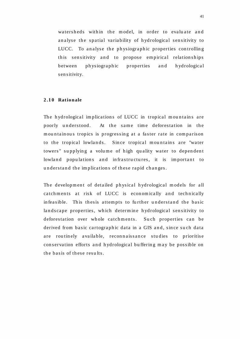
41
watersheds within the model, in order to evaluate and
analyse the spatial variability of hydrological sensitivity to
LUCC. To analyse the physiographic properties controlling
this sensitivity and to propose empirical relationships
between physiographic properties and hydrological
sensitivity.
2.10 Rationale
The hydrological implications of LUCC in tropical mountains are
poorly understood. At the same time deforestation in the
mountainous tropics is progressing at a faster rate in comparison
to the tropical lowlands. Since tropical mountains are "water
towers" supplying a volume of high quality water to dependent
lowland populations and infrastructures, it is important to
understand the implications of these rapid changes.
The development of detailed physical hydrological models for all
catchments at risk of LUCC is economically and technically
infeasible. This thesis attempts to further understand the basic
landscape properties, which determine hydrological sensitivity to
deforestation over whole catchments. Such properties can be
derived from basic cartographic data in a GIS and, since such data
are routinely available, reconnaissance studies to prioritise
conservation efforts and hydrological buffering may be possible on
the basis of these results.
42
Chapter III. Methodology
3.1 Structure of this chapter
This chapter has three sections: the first part is a description of the
study area, the research strategy, and the methodology for this
thesis; the second part illustrates the methodology of field activities
and the empirical data collected, and the last part describes the
characteristics of the proposed hydrological model with the
justification for the individual components of that model within the
context of the aims of this thesis.
The study area is described in terms of its location, types of
vegetation, and physical, topographic and climatological
characteristics. Several general characteristics of TMCFs are also
discussed. Then the experimental design is presented highlighting
the importance of LUCC. The vegetation cover in the study area is
described. On the basis of the knowledge of the study area, a
hydrological model is proposed, to evaluate the flux variation
within the catchment, in combination with the land use scenarios
presented in section 3.4. The modelling strategy is described and
includes a combination of 1D and 2.5D models which are used to
generalise the plot hydrology to the catchment level. Finally an
introduction to the sensitivity analysis is presented.
After the research strategy is presented, the field methods for the
collection of basic information for modelling and parameterisation
are described at both plot and watershed scale, and the data
collected for model parameterisation are indicated. Instrumented
plots and the characteristics of the installed weather stations are
also described, and the collection of soil and vegetation samples is

43
discussed. In addition, data from other sources (national and
international) used within this study described.
Subsequently, the identification of the model characteristics for the
study area and for the purpose of this research are mentioned.
Details of the hydrological model (i.e. scale, resolution) are
enumerated, on the basis of the knowledge of the environment of
Tambito and the information collected. These suggest the type of
the models that are most suitable for this study, to represent the
physical hydrological behaviour of the catchment. Also the means
of including LUCC scenarios within the analyses; the types of
scenarios generated, and the type of sensitivity analyses conducted
with both 1D and 2.5D model results are discussed. All the model
subroutines are described in detail along with the way that all of
them are integrated within the model.
3.2 Description of the study area
The study area is located in a natural reserve called ‘Centro de
Estudios Ambientales del Pacífico Tambito’, which is managed by
the Fundación Proselva and the Universidad del Cauca, Colombia.
The area, located in the cloud forests of the Eastern Cordillera of
the Andes, in the Department of Cauca in southwestern Colombia
(Figure 3.1) is about 75 km from the Pacific coast (between 77° 01’
and 76° 58’ W and 2° 28’ and 2° 32’ N). Cartographically, the
study area is included in a window delimited by:
X low left corner 1’008,210.00
Y low left corner 766,088.00
X up right corner 1’012,285.00
Y up right corner 771,538.00
44
These coordinate values are in metres using the Colombian west
origin on Transverse Mercator projection defined by IGAC (IGAC,
1975) (see Figure 3.1).
Elevations in the study area range from 1377 m to 2860 m.a.s.l.
The watershed covers approximately 1500 ha., and contains the
Tambito and the Palo Verde sub-watersheds. Vegetation is largely
tropical montane cloud forest (TMCF), and comprises both primary
and secondary forest, with a high density of epiphytes being
characteristic of the area. About 96% of the watershed is covered
by primary and secondary forest. Approximately 4% is deforested
mainly in areas close to dwellings (Figure 3.1) and in some isolated
patches throughout the watershed, which could be created by tree
fall for strong winds or illegal cultivation by colonists. The
existence of different land uses makes it an ideal watershed for
assessing hydrological impact. The Tambito and Palo Verde sub-
watersheds are paired catchments, with very similar landscape and
terrain properties but differing levels of deforestation.
The climate in TMCF has two main distinguishing features:
relatively constant seasonal temperatures and heavy rainfall with
the presence of persistent ground level clouds for some or all the
day being particularly characteristic. In Tambito the diurnal
temperature ranges from 15 °C to 25 °C, and variations are often
greater from day to night than from month to month. Therefore
dynamic changes vary more over short-term diurnal cycles than for
longer seasonal or annual time-scales, due to latitude.
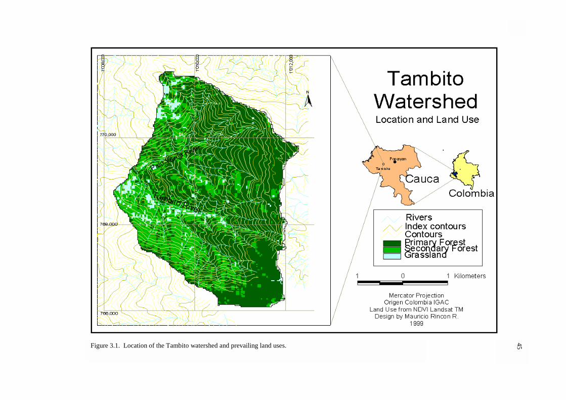
45
Figure 3.1. Location of the Tambito watershed and prevailing land uses.
45
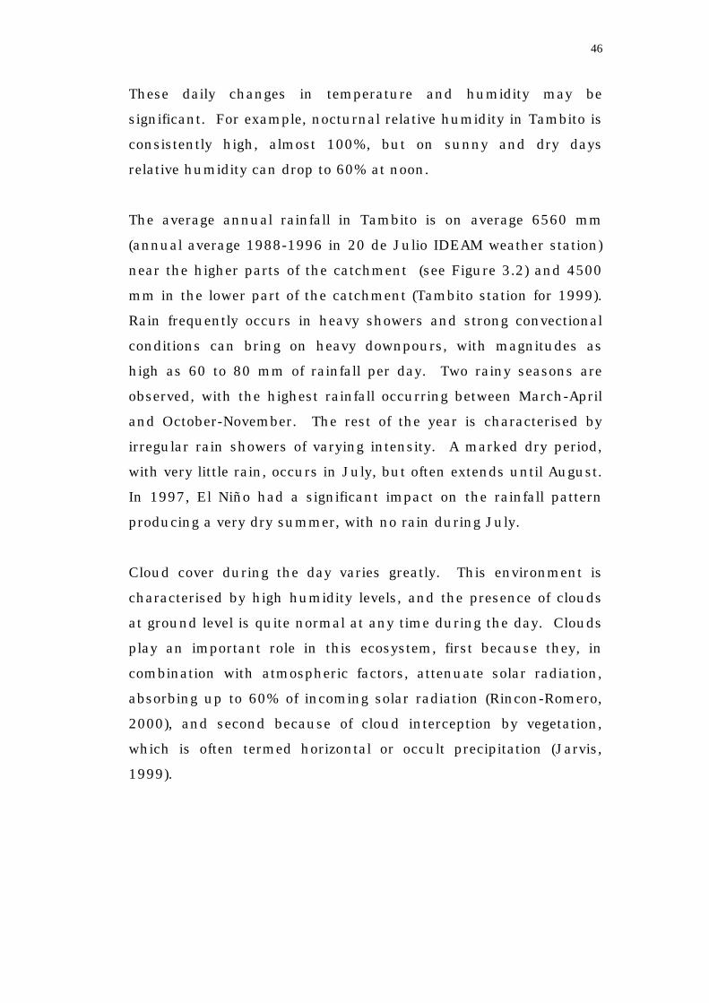
46
These daily changes in temperature and humidity may be
significant. For example, nocturnal relative humidity in Tambito is
consistently high, almost 100%, but on sunny and dry days
relative humidity can drop to 60% at noon.
The average annual rainfall in Tambito is on average 6560 mm
(annual average 1988-1996 in 20 de Julio IDEAM weather station)
near the higher parts of the catchment (see Figure 3.2) and 4500
mm in the lower part of the catchment (Tambito station for 1999).
Rain frequently occurs in heavy showers and strong convectional
conditions can bring on heavy downpours, with magnitudes as
high as 60 to 80 mm of rainfall per day. Two rainy seasons are
observed, with the highest rainfall occurring between March-April
and October-November. The rest of the year is characterised by
irregular rain showers of varying intensity. A marked dry period,
with very little rain, occurs in July, but often extends until August.
In 1997, El Niño had a significant impact on the rainfall pattern
producing a very dry summer, with no rain during July.
Cloud cover during the day varies greatly. This environment is
characterised by high humidity levels, and the presence of clouds
at ground level is quite normal at any time during the day. Clouds
play an important role in this ecosystem, first because they, in
combination with atmospheric factors, attenuate solar radiation,
absorbing up to 60% of incoming solar radiation (Rincon-Romero,
2000), and second because of cloud interception by vegetation,
which is often termed horizontal or occult precipitation (Jarvis,
1999).
47
47
0100
200
300400
500
600700
800
900
Ranf
all (
mm
)
Jan Feb Mar Apr May June July Aug Sep Oct Nov Dec
Months
Monthly average rainfall in 20 de Julio weather station (1988 - 1996)R
ain
fall
(m
m)
Figure 3.2 Monthly average rainfall of the nearest weather station to Tambito (3km distance)
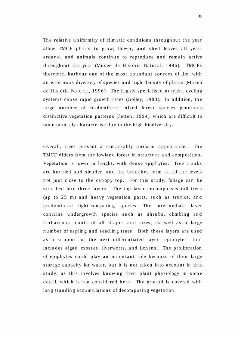
48
The relative uniformity of climatic conditions throughout the year
allow TMCF plants to grow, flower, and shed leaves all year-
around, and animals continue to reproduce and remain active
throughout the year (Museo de História Natural, 1996). TMCFs
therefore, harbour one of the most abundant sources of life, with
an enormous diversity of species and high density of plants (Museo
de História Natural, 1996). The highly specialised nutrient cycling
systems cause rapid growth rates (Golley, 1983). In addition, the
large number of co-dominant mixed forest species generates
distinctive vegetation patterns (Jetten, 1994), which are difficult to
taxonomically characterise due to the high biodiversity.
Overall, trees present a remarkably uniform appearance. The
TMCF differs from the lowland forest in structure and composition.
Vegetation is lower in height, with dense epiphytes. Tree trunks
are knurled and slender, and the branches form at all the levels
not just close to the canopy top. For this study, foliage can be
stratified into three layers. The top layer encompasses tall trees
(up to 25 m) and heavy vegetation parts, such as trunks, and
predominant light-competing species. The intermediate layer
contains undergrowth species such as shrubs, climbing and
herbaceous plants of all shapes and sizes, as well as a large
number of sapling and seedling trees. Both these layers are used
as a support for the next differentiated layer –epiphytes– that
includes algae, mosses, liverworts, and lichens. The proliferation
of epiphytes could play an important role because of their large
storage capacity for water, but it is not taken into account in this
study, as this involves knowing their plant physiology in some
detail, which is not considered here. The ground is covered with
long standing accumulations of decomposing vegetation.

49
3.3 Experimental strategy
Land use and land cover differentiation plays an important role in
the type of modelling studied in this thesis. Three kinds of land
uses were distinguished within the study area, on the assumption
that these have different hydrological impacts (Bonell and Balek,
1993; Calder et al., 1995): (a) primary forest, (b) secondary forest,
and (c) deforested areas. Different land cover combinations were
found within both the Tambito and Palo Verde sub-watersheds. As
will be shown in section 3.5, the hydrological parameters for both
primary and secondary forest were found on the basis of field
measurement, to be very similar. The analysis will therefore only
differentiate between two classes, since these were quite different
in properties: (a) forests and (b) grasslands.
A physical hydrological model (see section 3.6) is designed and
used in combination with the five scenarios of LUCC designed for
this study (see section 3.4). Hydrological flux variations as a result
of the land use change between individual iterations and different
scenarios are analysed.
The hydrological model proposed in this thesis is a hydrological
budget model. The model is initially implemented as a 1D lumped
model at the plot scale for each type of land use that exists within
the study area. Field hydrological stations are the main source of
data, providing information on collected fluxes and energy. In
order to investigate a) spatial variability of landscape sensitivity
according to the landscape properties, and b) the impact of the
spatial connectivity along the hydrological pathways, the same
routines and equations of 1D model are implemented on 2.5D
physically- based distributed model, which runs within a GIS. A
2.5D model means in this thesis that the fluxes are modelled in a

50
vertical direction and then complemented with lateral surface
fluxes for every time step.
Sensitivity analysis involves comparing hydrological outputs of
model variables, such as overland flow and erosion generated
between different iterations of different land use scenarios
patterns. Sensitivity is assessed as the change in model outputs
(runoff and erosion) per unit change in deforested area. The
hydrological model used was designed to operate on an hourly time
step, and runs with the same parameters and input data (with the
exception of land cover) for all scenarios. Each scenario of LUCC
includes between 15 and 22 iterations before the watershed is
completely deforested.
3.4 Land use change scenario generation for this thesis
Modelling of LUCC is not the topic of this thesis, but LUCC
scenarios are necessary for the hydrological modelling carried out
here. Five different scenarios are used in the hydrological
sensitivity analysis for the study area (see Chapter IV).
LUCC scenarios are used in the analysis to investigate how LUCC
combined with the geographical position of LUCC can affect the
hydrological behaviour of the watershed. The scenarios were
designed using criteria of advancing deforestation fronts rather
than a spatially complex pattern of deforestation. All scenarios
start with the same initial LC, and the LUCC transformation in
each iteration is carried out relative to various physical properties
of the landscape such as change in the vegetation type, then
changes in vegetation parameters. The physical determinant of
advancing deforestation is different for each scenario, leading to
transformations occurring over different parts of the catchment for

51
each scenario. The schemes are designed to produce scenarios,
which will have hydrologically different responses rather than to
simulate spatially realistic deforestation patterns. Each scenario
occurs over a number of iterations, which are not related to
temporal changes, but are used as step changes throughout which
LUCC occurs.
This strategy specifically deals with the significance of:
1. The location where the LUCC occurs within the catchment.
2. Recognition of the sensitive areas where the catchment
hydrological response is significantly affected by different LUCC
trends.
3. The identification of the relationship between areas with
different responses to LUCC with their physical properties.
4. Analysis of how the different LUCC patterns used in the
scenarios affects the model hydrological response.
5. Whether the preceding and current arrangement of LUCC could
affect the catchment hydrological response (Fisher et. al, 1997),
i.e. the importance of the temporal pattern of change.
3.4.1 Estimating initial vegetation cover for LUCC Scenarios
All the scenarios simulate the conversion of forest to pasture,
starting from the Normalised Difference Vegetation Index (NDVI)
image derived initial vegetation cover, obtained from a 1989
Landsat TM image (Figure 3.3).
52
Figure 3.3 NDVI radiance from Landsat TM for Tambito catchment

53
NDVI ratio was selected as land vegetation cover instead of the
most traditional approach normally used (maximum likelihood
classification) because for this type of landscape (high
mountainous and steep slopes), the NDVI minimises the shadow
effects from the topographic variations stress (Cohen, 1991).
The Normalised Difference Vegetation Index (NDVI) is a ratio-based
index applied to a Landsat Thematic Mapper (TM) image using the
near infrared (band 4; 0.76 to 0.9 µm) and the red reflectance ratio
(band 3; 0.63 to 0.69 µm). This index identifies changes in amount
of green biomass, chlorophyll content, and leaf stress (Cohen,
1991), which is defined by,
NDVI = (band4 – band3) / (band4 + band3) (Eq. 3.1)
The NDVI ratio is a relationship which holds both for shadowed
and for directly illuminated pixels (Cohen, 1991). Therefore, a ratio
image shows the radiance information without effects of
topography. This permits the examination of spectral properties of
the surface, without confusing the mixed brightness of the
topography effects and material reflectance (Campbell, 1987).
This NDVI image was reclassified using signature classes extracted
from texture patterns, which were identified with the help of aerial
panchromatic photographs, 1:32,000 scale (approximate resolution
of 0.6X0.6m pixel size). The vegetation texture patterns appears on
the panchromatic photographs as several granules or flat areas,
which produce different textures due to the size of the shadows
and forest trees, showing where the vegetation is forest or
grassland. According to these patterns on the panchromatic
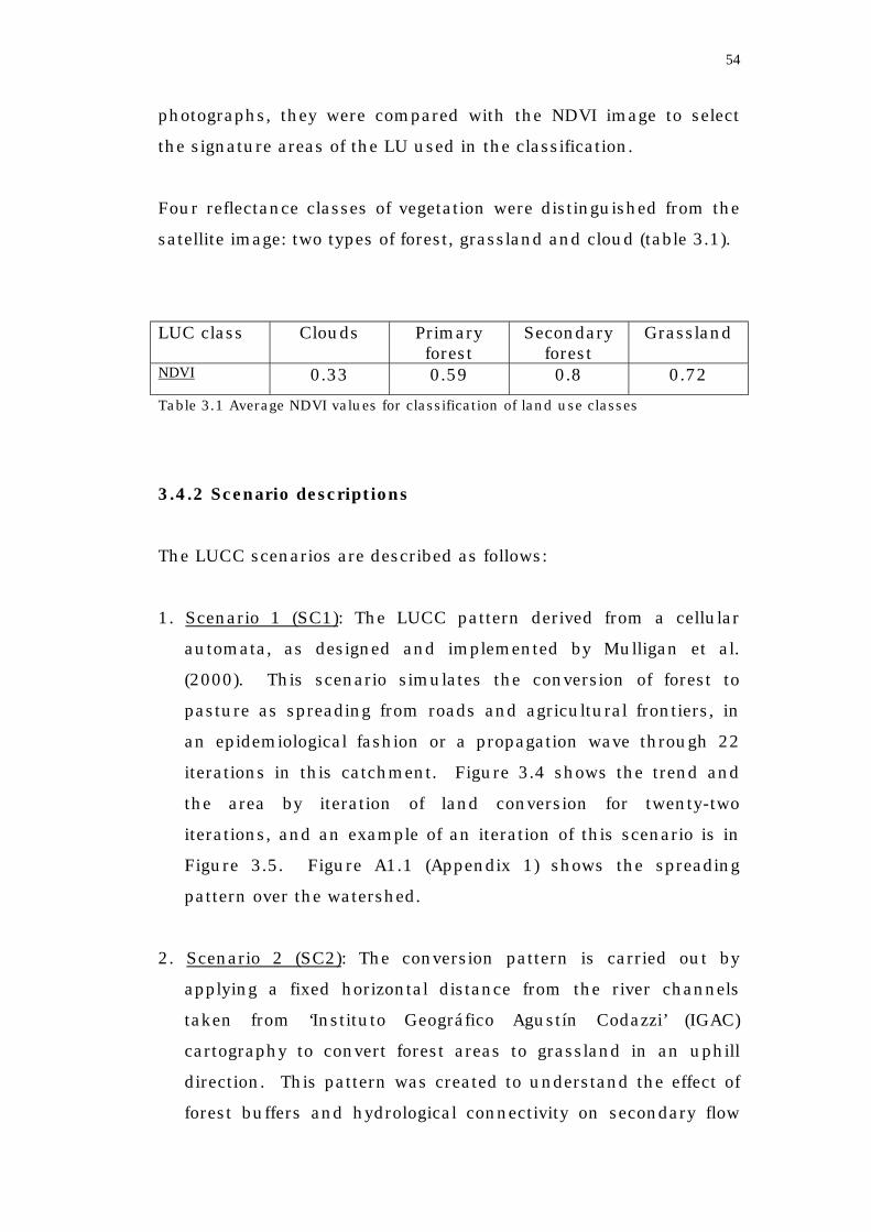
54
photographs, they were compared with the NDVI image to select
the signature areas of the LU used in the classification.
Four reflectance classes of vegetation were distinguished from the
satellite image: two types of forest, grassland and cloud (table 3.1).
LUC class Clouds Primaryforest
Secondaryforest
Grassland
NDVI 0.33 0.59 0.8 0.72
Table 3.1 Average NDVI values for classification of land use classes
3.4.2 Scenario descriptions
The LUCC scenarios are described as follows:
1. Scenario 1 (SC1): The LUCC pattern derived from a cellular
automata, as designed and implemented by Mulligan et al.
(2000). This scenario simulates the conversion of forest to
pasture as spreading from roads and agricultural frontiers, in
an epidemiological fashion or a propagation wave through 22
iterations in this catchment. Figure 3.4 shows the trend and
the area by iteration of land conversion for twenty-two
iterations, and an example of an iteration of this scenario is in
Figure 3.5. Figure A1.1 (Appendix 1) shows the spreading
pattern over the watershed.
2. Scenario 2 (SC2): The conversion pattern is carried out by
applying a fixed horizontal distance from the river channels
taken from ‘Instituto Geográfico Agustín Codazzi’ (IGAC)
cartography to convert forest areas to grassland in an uphill
direction. This pattern was created to understand the effect of
forest buffers and hydrological connectivity on secondary flow
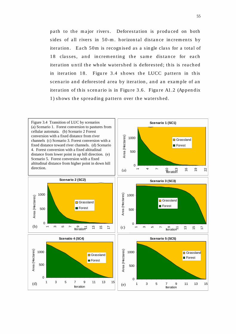
55
path to the major rivers. Deforestation is produced on both
sides of all rivers in 50-m. horizontal distance increments by
iteration. Each 50m is recognised as a single class for a total of
18 classes, and incrementing the same distance for each
iteration until the whole watershed is deforested; this is reached
in iteration 18. Figure 3.4 shows the LUCC pattern in this
scenario and deforested area by iteration, and an example of an
iteration of this scenario is in Figure 3.6. Figure A1.2 (Appendix
1) shows the spreading pattern over the watershed.
Scenario 1 (SC1)
0
500
10001 4 7 10 13 16 19 22Iteration
Are
a (H
ecta
res)
Grassland
Forest
Scenario 2 (SC2)
0
500
1000
1 3 5 7 9 11 13 15 17Iteration
Are
a (H
ecta
res)
Grassland
Forest
Scenario 3 (SC3)
0
500
1000
1 3 5 7 9 11
13
15
17
Iteration
Are
a (
Hec
tare
s)
Grassland
Forest
Scenatio 4 (SC4)
0
500
1000
1 3 5 7 9 11 13 15
Iteration
Are
a (H
ecta
res)
Grassland
Forest
Scenario 5 (SC5)
0
500
1000
1 3 5 7 9 11 13 15Iteration
Are
a (H
ecta
res)
Grassland
Forest
Figure 3.4 Transition of LUC by scenarios(a) Scenario 1. Forest conversion to pastures fromcellular automata. (b) Scenario 2 Forestconversion with a fixed distance from riverchannels (c) Scenario 3. Forest conversion with afixed distance toward river channels. (d) Scenario4. Forest conversion with a fixed altitudinaldistance from lower point in up hill direction. (e)Scenario 5. Forest conversion with a fixedaltitudinal distance from higher point in down hilldirection.
(a)
(b) (c)
(d) (e)
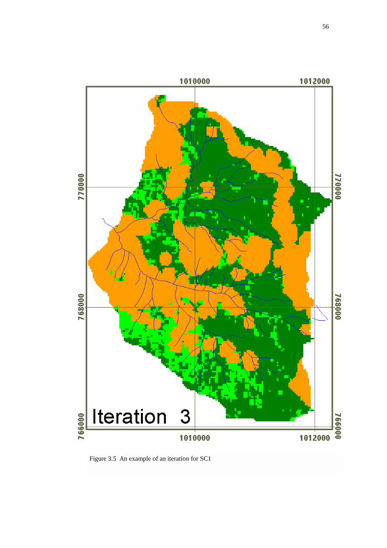
56
Figure 3.5 An example of an iteration for SC1
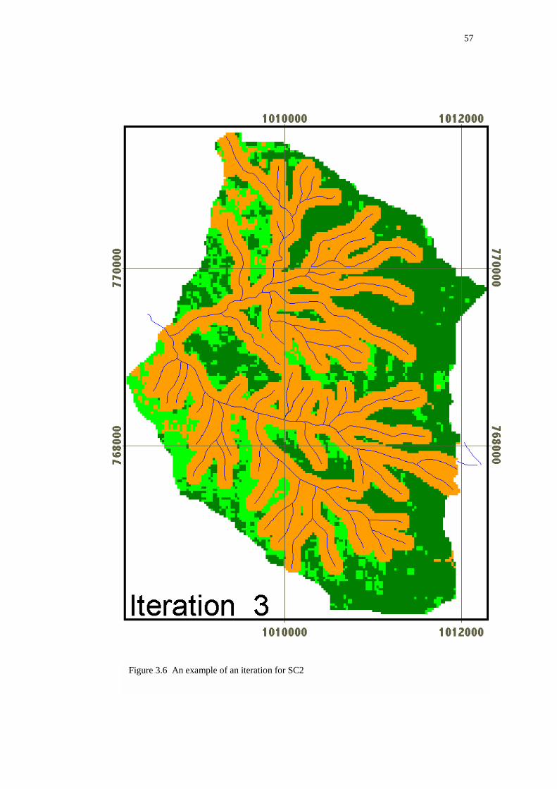
57
Figure 3.6 An example of an iteration for SC2
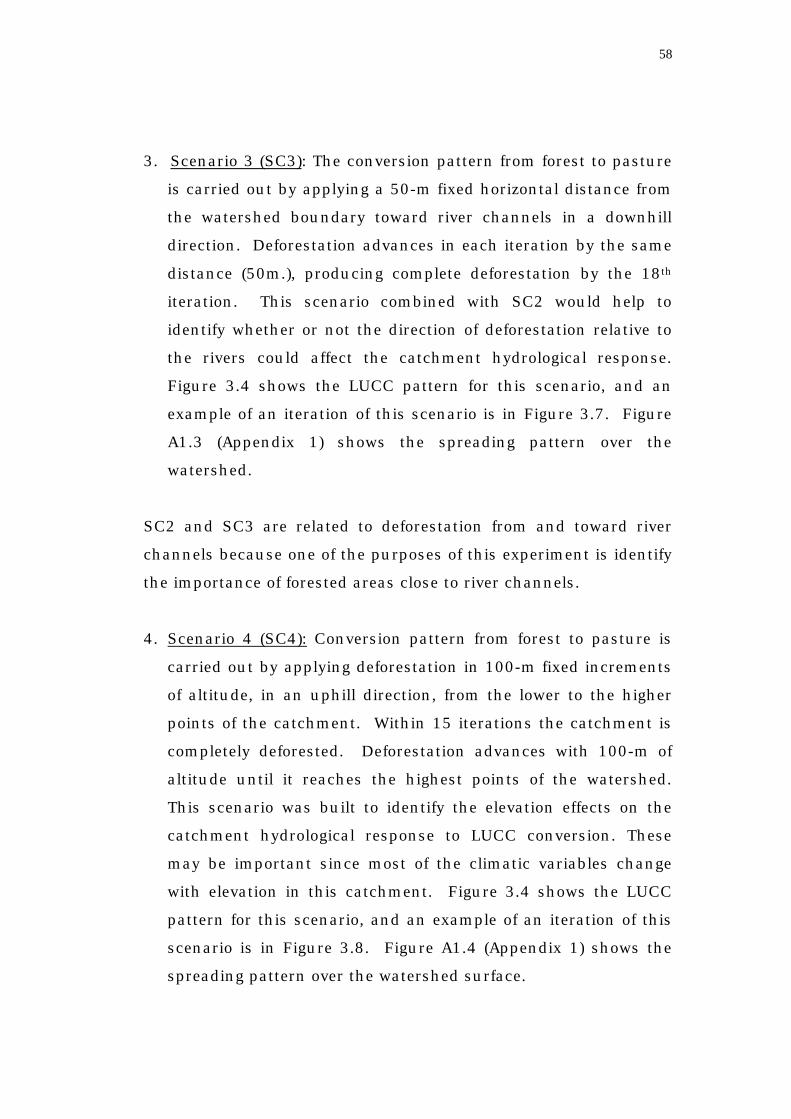
58
3. Scenario 3 (SC3): The conversion pattern from forest to pasture
is carried out by applying a 50-m fixed horizontal distance from
the watershed boundary toward river channels in a downhill
direction. Deforestation advances in each iteration by the same
distance (50m.), producing complete deforestation by the 18th
iteration. This scenario combined with SC2 would help to
identify whether or not the direction of deforestation relative to
the rivers could affect the catchment hydrological response.
Figure 3.4 shows the LUCC pattern for this scenario, and an
example of an iteration of this scenario is in Figure 3.7. Figure
A1.3 (Appendix 1) shows the spreading pattern over the
watershed.
SC2 and SC3 are related to deforestation from and toward river
channels because one of the purposes of this experiment is identify
the importance of forested areas close to river channels.
4. Scenario 4 (SC4): Conversion pattern from forest to pasture is
carried out by applying deforestation in 100-m fixed increments
of altitude, in an uphill direction, from the lower to the higher
points of the catchment. Within 15 iterations the catchment is
completely deforested. Deforestation advances with 100-m of
altitude until it reaches the highest points of the watershed.
This scenario was built to identify the elevation effects on the
catchment hydrological response to LUCC conversion. These
may be important since most of the climatic variables change
with elevation in this catchment. Figure 3.4 shows the LUCC
pattern for this scenario, and an example of an iteration of this
scenario is in Figure 3.8. Figure A1.4 (Appendix 1) shows the
spreading pattern over the watershed surface.
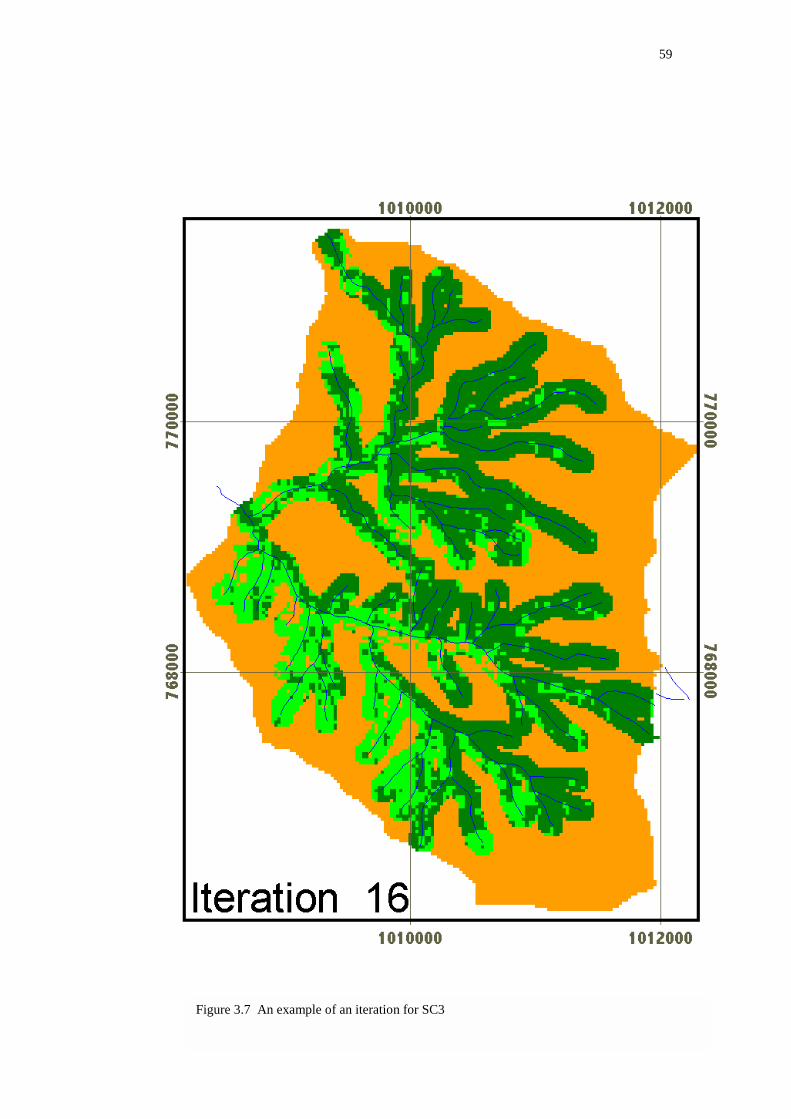
59
Figure 3.7 An example of an iteration for SC3
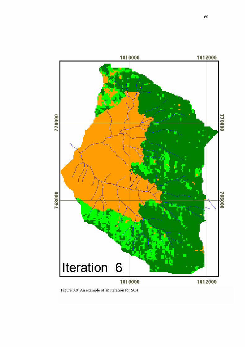
60
Figure 3.8 An example of an iteration for SC4

61
5. Scenario 5 (SC5): Conversion pattern from forest to pasture is
carried out by applying deforestation in 100-m. fixed elevation
distance, from higher to lower points of altitude, in a downhill
direction, through 15 iterations. Higher points in the watershed
are deforested in the first iterations. Figure 3.4 shows the
LUCC pattern for this scenario, and an example of an iteration
of this scenario is in Figure 3.9. Figure A1.5 (Appendix 1)
shows the spreading pattern on the watershed surface.
SC4 and SC5 show the pattern of deforestation related to elevation
change. Deforestation from and towards the highest points are
included in the analysis with the purpose of identifying altitudinal
whether the order of deforestation (top to bottom or bottom to top)
is significant.
Iterations within scenarios are not related to any concept of time
taken for LUCC. Iterations are steps in a pattern of change in
which forest is converted to pasture within the terms that the
scenarios define.
Table 3.2 summarises the extent of deforested areas by scenario
and by iteration. Values in table 3.2 were extracted using GIS
utilities developed for the study area, which is widely explained in
following chapter.
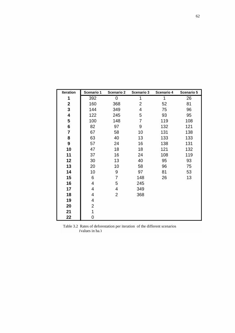
62
Table 3.2 Rates of deforestation per iteration of the different scenarios (values in ha.)
Iteration Scenario 1 Scenario 2 Scenario 3 Scenario 4 Scenario 5
1 392 0 1 1 262 160 368 2 52 813 144 349 4 75 964 122 245 5 93 955 100 148 7 119 1086 82 97 9 132 1217 67 58 10 131 1388 63 40 13 133 1339 57 24 16 138 131
10 47 18 18 121 13211 37 16 24 108 11912 30 13 40 95 9313 20 10 58 96 7514 10 9 97 81 5315 6 7 148 26 1316 4 5 24517 4 4 34918 4 2 36819 420 221 122 0
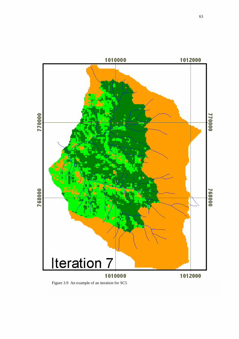
63
Figure 3.9 An example of an iteration for SC5
64
3.5 Field methodology
The hydrological characteristics of each land use type were
sampled using 20-m2 plots (2m x 10m), each with a hydrological
station to collect data of the main elements of the hydrological
cycle to be used for model input and validation. Samples were
collected throughout the watersheds to determine vegetation
biomass, leaf area index, and soil properties for each land use.
Field work was applied at the plots and distributed through the
watershed. Data on vegetation and soils were collected following
the Field Manual Version 3.1 of Medalus (Cammeraat, 1991). In
cases where the topography and tall vegetation made it difficult to
delimit, 1-ha. plots for sample collection (as the manual suggests),
a different strategy was adopted: samples were systematically
collected in the areas surrounding the hydrological plots. Data
gathered on the plots were used to determine and monitor the
physical and hydrological properties, and parameterisation of each
land use type. The field data necessary to parameterise and
validate a 1D lumped model were also collected. The vegetation
and soil samples collected throughout the watershed
complemented the land use parameters used in both the 1D and
2.5D models.
3.5.1 Plot scale
Instruments for parameterisation of meteorological conditions were
installed. Instruments for verification and validation data for
overland flow, throughflow, erosion, soil moisture and recharge
were also installed from 20-m2 (10m x 2m) plots. To ensure that
the areas were representative of each land use, all plots were
located in the middle of a large area that adequately characterised
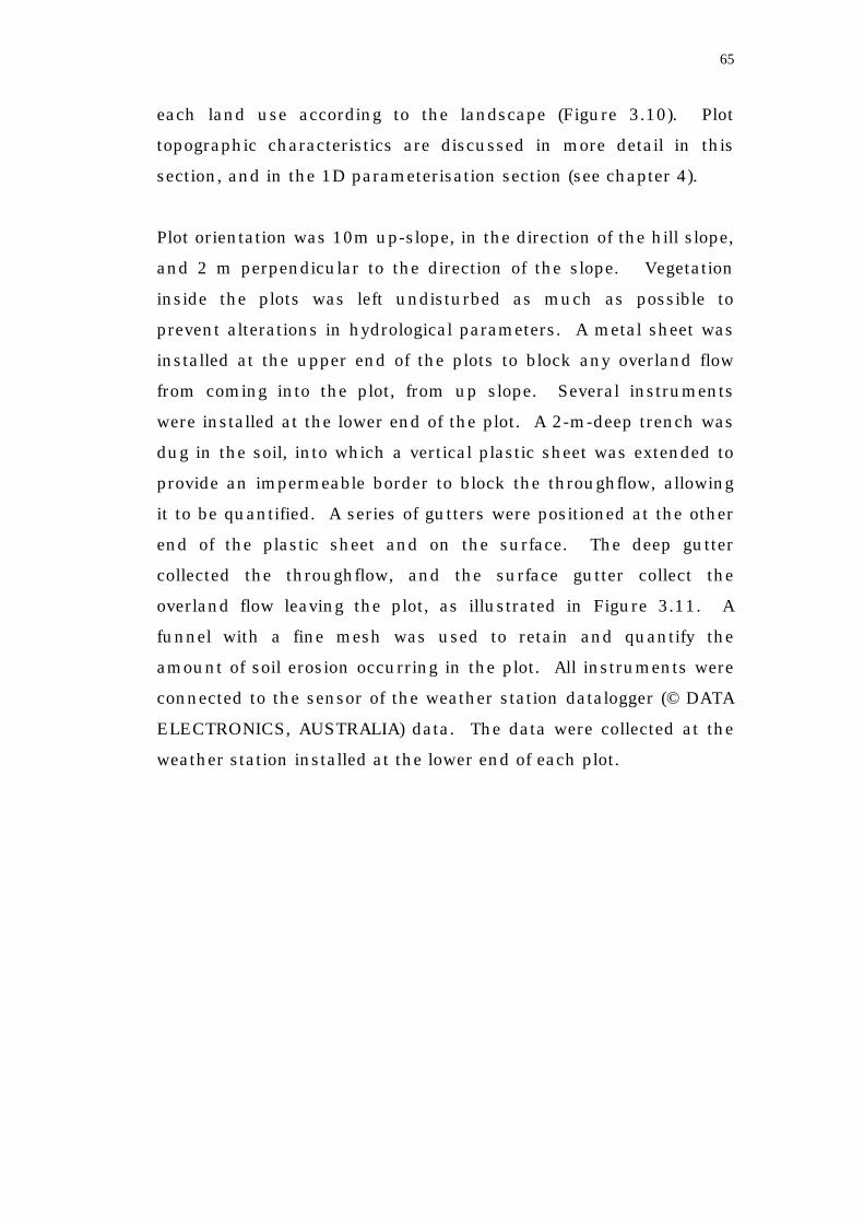
65
each land use according to the landscape (Figure 3.10). Plot
topographic characteristics are discussed in more detail in this
section, and in the 1D parameterisation section (see chapter 4).
Plot orientation was 10m up-slope, in the direction of the hill slope,
and 2 m perpendicular to the direction of the slope. Vegetation
inside the plots was left undisturbed as much as possible to
prevent alterations in hydrological parameters. A metal sheet was
installed at the upper end of the plots to block any overland flow
from coming into the plot, from up slope. Several instruments
were installed at the lower end of the plot. A 2-m-deep trench was
dug in the soil, into which a vertical plastic sheet was extended to
provide an impermeable border to block the throughflow, allowing
it to be quantified. A series of gutters were positioned at the other
end of the plastic sheet and on the surface. The deep gutter
collected the throughflow, and the surface gutter collect the
overland flow leaving the plot, as illustrated in Figure 3.11. A
funnel with a fine mesh was used to retain and quantify the
amount of soil erosion occurring in the plot. All instruments were
connected to the sensor of the weather station datalogger (© DATA
ELECTRONICS, AUSTRALIA) data. The data were collected at the
weather station installed at the lower end of each plot.
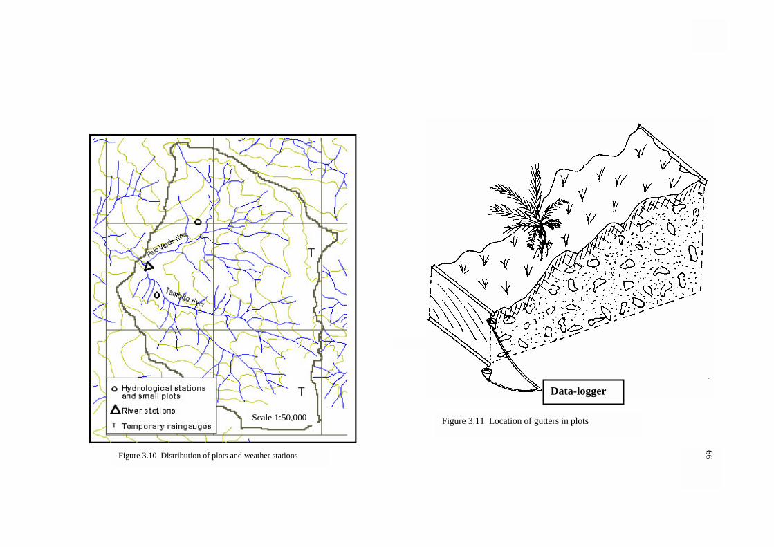
66
Data-logger
Figure 3.11 Location of gutters in plots
Figure 3.10 Distribution of plots and weather stations
66
Scale 1:50,000
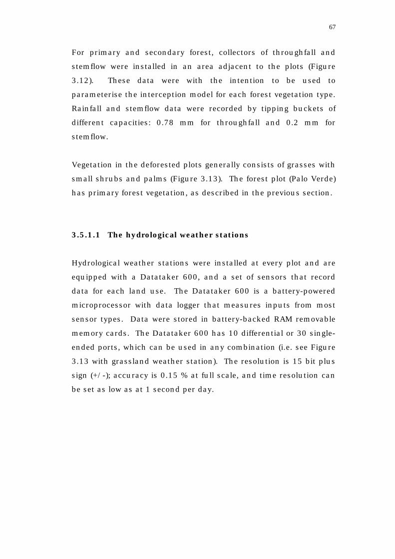
67
For primary and secondary forest, collectors of throughfall and
stemflow were installed in an area adjacent to the plots (Figure
3.12). These data were with the intention to be used to
parameterise the interception model for each forest vegetation type.
Rainfall and stemflow data were recorded by tipping buckets of
different capacities: 0.78 mm for throughfall and 0.2 mm for
stemflow.
Vegetation in the deforested plots generally consists of grasses with
small shrubs and palms (Figure 3.13). The forest plot (Palo Verde)
has primary forest vegetation, as described in the previous section.
3.5.1.1 The hydrological weather stations
Hydrological weather stations were installed at every plot and are
equipped with a Datataker 600, and a set of sensors that record
data for each land use. The Datataker 600 is a battery-powered
microprocessor with data logger that measures inputs from most
sensor types. Data were stored in battery-backed RAM removable
memory cards. The Datataker 600 has 10 differential or 30 single-
ended ports, which can be used in any combination (i.e. see Figure
3.13 with grassland weather station). The resolution is 15 bit plus
sign (+/-); accuracy is 0.15 % at full scale, and time resolution can
be set as low as at 1 second per day.
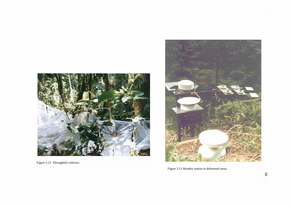
68
Figure 3.12 Throughfall collector.
Figure 3.13 Weather station in deforested areas.
68

69
The data logger was set to record at 15-minute intervals, and
average data for each variable on an hourly basis (writing the mean
and standard deviation). In the case of event variables such as
precipitation, data was recorded on a per event basis. Data used in
the analysis of this thesis is identified in the list with asterisks ***.
The weather station located in the Tambito sub-watershed, which
is considered as being more disturbed, collected the following data
(Figure 3.13):
- Solar radiation received and reflected (Skye Instruments silicon
cell pyranometer) ***- Red/far red radiation received and reflected (Skye Instruments
silicon cell sensor)
- Blue radiation reflected (Skye Instruments silicon cell sensor)
- PAR radiation reflected (Skye instruments PAR sensor)
- Humidity (Skye instruments capacitance based humidity sensor)
- Air temperature (Skye instruments thermistor) ***- Rainfall, using tipping bucket rain gauge (0.02 mm bucket size)-
Environmental Measurements. (UK Ltd) ***- Overland flow, tipping bucket (1 tip 105 ml)
- Throughflow (0.12 mm bucket size)
- Soil erosion (strain gauge-based sediment weighing system)
- Soil matric potential at 40, 80, and 120 cm depth (Soil
Moisture Corporation - gypsum blocks) ***- Soil temperature (thermocouple)
For the primary forest plot, in addition to the instruments
mentioned above, the weather station includes the following:
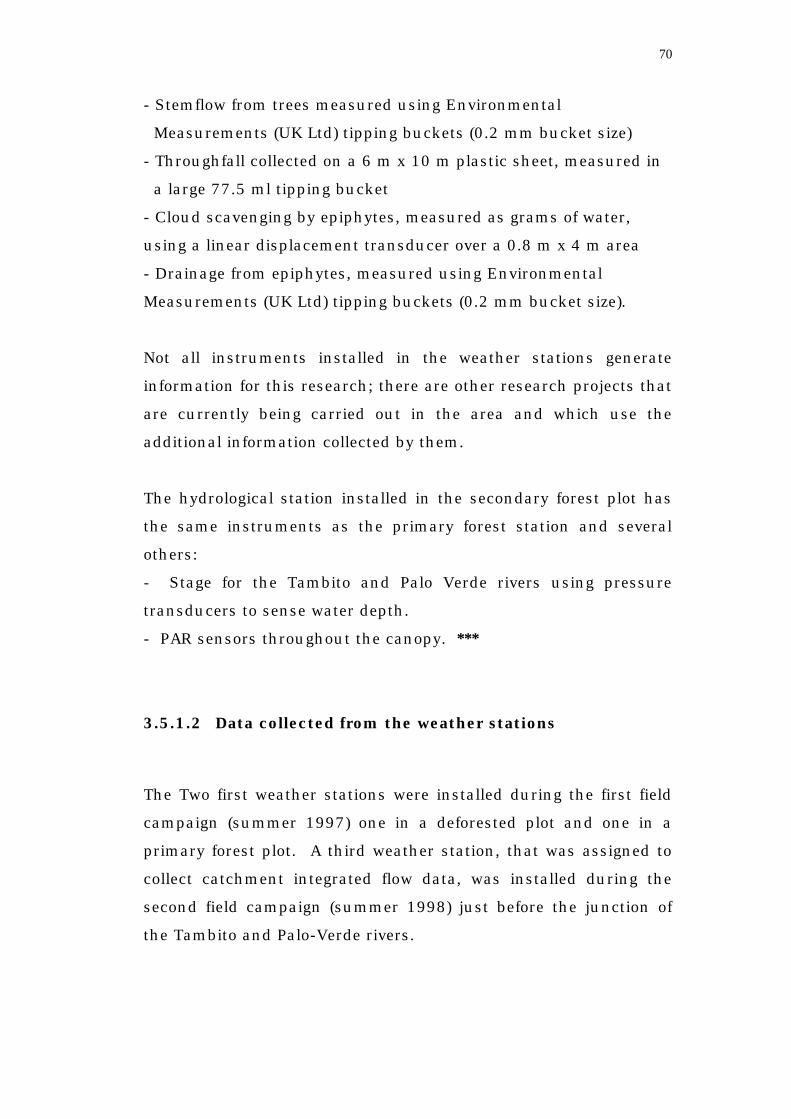
70
- Stemflow from trees measured using Environmental
Measurements (UK Ltd) tipping buckets (0.2 mm bucket size)
- Throughfall collected on a 6 m x 10 m plastic sheet, measured in
a large 77.5 ml tipping bucket
- Cloud scavenging by epiphytes, measured as grams of water,
using a linear displacement transducer over a 0.8 m x 4 m area
- Drainage from epiphytes, measured using Environmental
Measurements (UK Ltd) tipping buckets (0.2 mm bucket size).
Not all instruments installed in the weather stations generate
information for this research; there are other research projects that
are currently being carried out in the area and which use the
additional information collected by them.
The hydrological station installed in the secondary forest plot has
the same instruments as the primary forest station and several
others:
- Stage for the Tambito and Palo Verde rivers using pressure
transducers to sense water depth.
- PAR sensors throughout the canopy. ***
3.5.1.2 Data collected from the weather stations
The Two first weather stations were installed during the first field
campaign (summer 1997) one in a deforested plot and one in a
primary forest plot. A third weather station, that was assigned to
collect catchment integrated flow data, was installed during the
second field campaign (summer 1998) just before the junction of
the Tambito and Palo-Verde rivers.

71
Unfortunately, all weather stations suffered technical problems due
to the excessive humidity (100%), and lack of maintenance of the
instruments because of their remote location. However, some data
were recovered from the loggers and were subsequently used in the
research. Table 3.3 indicates the periods in which data were
collected at the weather stations.
Plot 1997 1998 1999 2000
Grassland 31st October/97-31st January/98
28th July – 30th
NovemberJuly 11th toNovember 4th
February 14th
To March 11th
Primaryforest
None 8th August –12th August
22nd June to18th September
None
River andsecondary
None 9th August –21st August
None None
Table 3.3. Periods during which data were collected.
An example of data collected at the weather stations is presented in
Appendix 2.
3.5.2 Catchment scale
3.5.2.1 Soil data
In physical distributed modelling (2.5D), soil parameters are
derived from samples collected across the watershed. A
classification map was made to choose the most suitable places for
sampling the soil (Figure 3.14). Soils were classified using
topographic data and a preliminary land use maps from Fundación
Proselva (Museo de História Natural, 1996), assuming that these
would be major controls on soil properties.
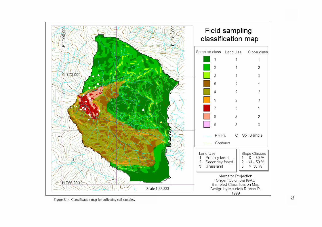
72
Figure 3.14 Classification map for collecting soil samples.
Scale 1:33,333
72
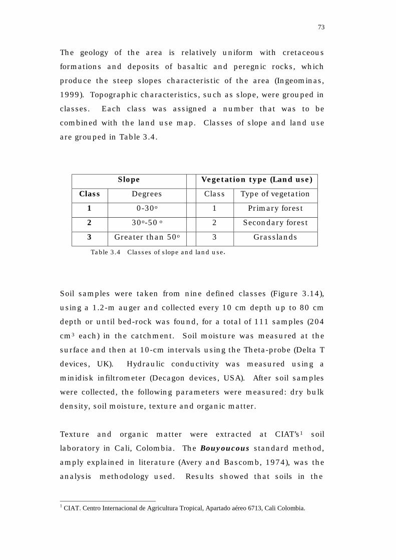
73
The geology of the area is relatively uniform with cretaceous
formations and deposits of basaltic and peregnic rocks, which
produce the steep slopes characteristic of the area (Ingeominas,
1999). Topographic characteristics, such as slope, were grouped in
classes. Each class was assigned a number that was to be
combined with the land use map. Classes of slope and land use
are grouped in Table 3.4.
Slope Vegetation type (Land use)
Class Degrees Class Type of vegetation
1 0-30o 1 Primary forest
2 30o-50 o 2 Secondary forest
3 Greater than 50o 3 Grasslands
Table 3.4 Classes of slope and land use.
Soil samples were taken from nine defined classes (Figure 3.14),
using a 1.2-m auger and collected every 10 cm depth up to 80 cm
depth or until bed-rock was found, for a total of 111 samples (204
cm3 each) in the catchment. Soil moisture was measured at the
surface and then at 10-cm intervals using the Theta-probe (Delta T
devices, UK). Hydraulic conductivity was measured using a
minidisk infiltrometer (Decagon devices, USA). After soil samples
were collected, the following parameters were measured: dry bulk
density, soil moisture, texture and organic matter.
Texture and organic matter were extracted at CIAT’s1 soil
laboratory in Cali, Colombia. The Bouyoucous standard method,
amply explained in literature (Avery and Bascomb, 1974), was the
analysis methodology used. Results showed that soils in the
1 CIAT. Centro Internacional de Agricultura Tropical, Apartado aéreo 6713, Cali Colombia.
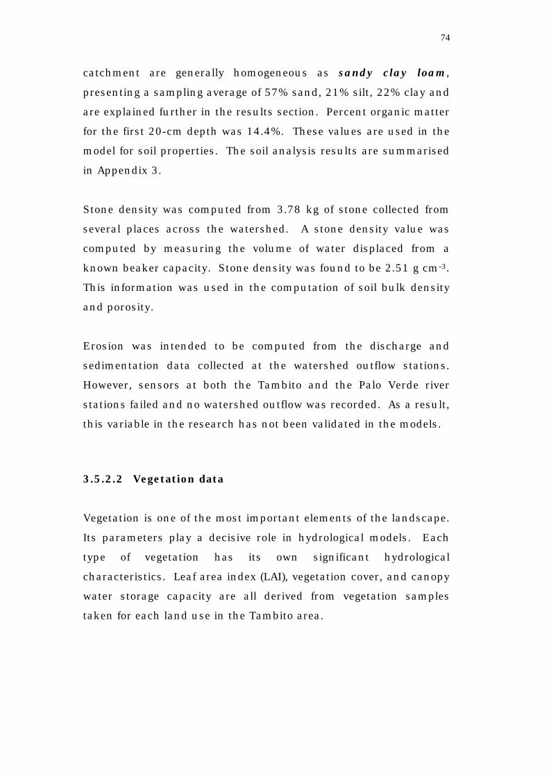
74
catchment are generally homogeneous as sandy clay loam,
presenting a sampling average of 57% sand, 21% silt, 22% clay and
are explained further in the results section. Percent organic matter
for the first 20-cm depth was 14.4%. These values are used in the
model for soil properties. The soil analysis results are summarised
in Appendix 3.
Stone density was computed from 3.78 kg of stone collected from
several places across the watershed. A stone density value was
computed by measuring the volume of water displaced from a
known beaker capacity. Stone density was found to be 2.51 g cm-3.
This information was used in the computation of soil bulk density
and porosity.
Erosion was intended to be computed from the discharge and
sedimentation data collected at the watershed outflow stations.
However, sensors at both the Tambito and the Palo Verde river
stations failed and no watershed outflow was recorded. As a result,
this variable in the research has not been validated in the models.
3.5.2.2 Vegetation data
Vegetation is one of the most important elements of the landscape.
Its parameters play a decisive role in hydrological models. Each
type of vegetation has its own significant hydrological
characteristics. Leaf area index (LAI), vegetation cover, and canopy
water storage capacity are all derived from vegetation samples
taken for each land use in the Tambito area.

75
3.5.2.2.1 Leaf area index
Leaf area index (LAI) for the forest vegetation class was calculated
by Rubiano (1998) using a network of PAR sensors at different
heights in the canopy at the secondary forest site (to calculate the
light extinction coefficient) and by integrating Beers Law for light
levels measured by the lowest of these sensors (at 1m from the
ground) compared with an open sensor.
The resulting value for LAI are 3.26 which agrees with values
measured in primary and secondary forest at the same site using a
ceptometer (Letts, personal communication); this value is assumed
for both primary and secondary forest. The literature reports LAI
for lower montane cloud forest between 3.4 to 5.5 (Kato et al. 1978;
Yakamura et al 1986; Huttel, 1975).
The same method could not be used to grassland, because grass is
so short and the PAR instruments can not fit under grass leaves.
In the case of grasslands, LAI was calculated from 5 sets of 10-cm2
samples, from which the leaves were separated and superimposed
on a known flat, white area. Monochrome pictures were taken and
then processed. Those pictures were analysed for surface area
using image-processing software (Photoshop 4.0). The relationship
between known area (10 cm2) compared with the dark area from
grass leaves indicate the LAI for grassland. A summary of samples
used for LAI calculation for grassland is in table 3.5.
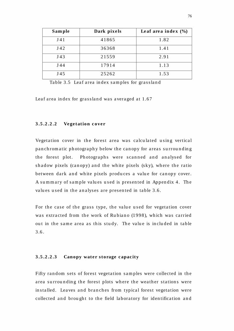
76
Sample Dark pixels Leaf area index (%)
J41 41865 1.82
J42 36368 1.41
J43 21559 2.91
J44 17914 1.13
J45 25262 1.53
Table 3.5 Leaf area index samples for grassland
Leaf area index for grassland was averaged at 1.67
3.5.2.2.2 Vegetation cover
Vegetation cover in the forest area was calculated using vertical
panchromatic photography below the canopy for areas surrounding
the forest plot. Photographs were scanned and analysed for
shadow pixels (canopy) and the white pixels (sky), where the ratio
between dark and white pixels produces a value for canopy cover.
A summary of sample values used is presented in Appendix 4. The
values used in the analyses are presented in table 3.6.
For the case of the grass type, the value used for vegetation cover
was extracted from the work of Rubiano (1998), which was carried
out in the same area as this study. The value is included in table
3.6.
3.5.2.2.3 Canopy water storage capacity
Fifty random sets of forest vegetation samples were collected in the
area surrounding the forest plots where the weather stations were
installed. Leaves and branches from typical forest vegetation were
collected and brought to the field laboratory for identification and
77
subsequent estimation of canopy storage capacity parameters.
Samples values are summarised in Appendix 4.
Vegetation samples were weighed firstly dry and then were wetted
by submerging in water and shaking, to estimate the weight of the
water they hold per unit leaf area. The area of collected leaves was
measured using the same procedure in the estimation of LAI for
grassland. The density of retained water was assumed 1.0 g.cm-3
to calculate the volume.
Canopy water retention calculation for grassland used the same
procedure as forest samples, using 3 blocks of grassland samples
with an area of 10 cm2. These parameters are summarised in
Table 3.6 and source data are compiled in Appendix 4.
Land use LAIm2 m-2
Maximum canopystorage capacity
Vegetationcover
Primaryforest
3.3 0.18 mm (n=53) 91 %
Secondaryforest
3.3 0.2 mm (n=12) 91 %
Grassland 1. 7 0.03 mm (n=5) 86 %
Table 3.6 Vegetation parameters
The literature reports 1.15mm for maximum canopy water storage
capacity (Schellekens et al., 1999) from Luquillo experimental
forest in Puerto Rico, which was determined using the methods of
Jackson (1975), Gash and Morton (1978) and Rowe (1983). Those
methods were applied for the determination of vegetation
parameters for the evaluation of interception models. Schellekens
et al. (1999) through the literature search compiled values for
canopy water storage capacity ranging from 0.08 mm (from palm-
filled ravine sites) up to 1.3 mm (for well-stocked ridges). Values

78
for canopy storage capacity in table 3.6 were adopted because they
come from Tambito field measurements, despite the fact they are
very different from the mean values reported in the literature.
3.5.3 Other spatial data
Complementary data were also collected from different sources.
1. Basic cartography
From the Instituto Geografico Agustin Codazzi IGAC: the
1:25000 scale, sheets 343 I a, b, and c. All the cartographic
elements were created in a cartographic projection (see section
3.2), according to IGAC’s map normalisation. Contour lines and
rivers were digitised by GIS and Modelling Services Ltda1, and
used to create the Digital Elevation Model (DEM), 25-m. pixel
size. The aspect, slope and topographic index (see section 4.5.1)
were derived from the DEM (see Figures 3.15 to 3.18), using
Geographic Information System software Arc-Info 7.3 (ESRI,
1998) and PCRaster, version 2 (Utrecht University, 1996).
2. Aerial photography of part of the area, scale 1:40000, taken in
1985 by IGAC, for texture characterisation of vegetation and
identification texture for remote sensing image.
3. Distribution map of vegetation cover. A draft made by
Fundación Proselva (Museo de Historia Natural, 1996) based on
field work for characterisation of vegetation, was used for initial
characterisation of study area and for designing soil sampling
(see Figure 3.19).
1 GIS and Modelling Services Ltda. Cartographic and environmental management services, Cali,
Colombia. E-mail [email protected]

79
4. Remotely sensed data of the area, obtained from a Landsat
Image (1989), pixel size of approximately 30m side size, without
geometric correction, supplied by Fundación Proselva (Museo
de História Natural, 1996) (see Figure 3.20).
5. Daily rainfall data from 1987, obtained from the database of the
Hacienda Carpinterias and 20 de Julio weather stations, both
located close to the Tambito watershed (7 and 10 km,
respectively) and belonging to the Instituto de Hidrología,
Meteorología y Estudios Ambientales (IDEAM).
6. Four years of rainfall data that were collected manually at the
Tambito cabin were used to compare data consistency and
analyse rainfall spatial distribution.
7. Additional rain gauges were spread both across and outside the
watershed to compare rainfall distribution (Figure 3.10).

80
Figure 3.15 Basic cartography of the area (source from IGAC, 1985)
Scale 1:50,000
Figure 3.16 Digital elevation model for the study area derived from digitised contours using Arc/Info 7.3
80
Scale 1:50,000
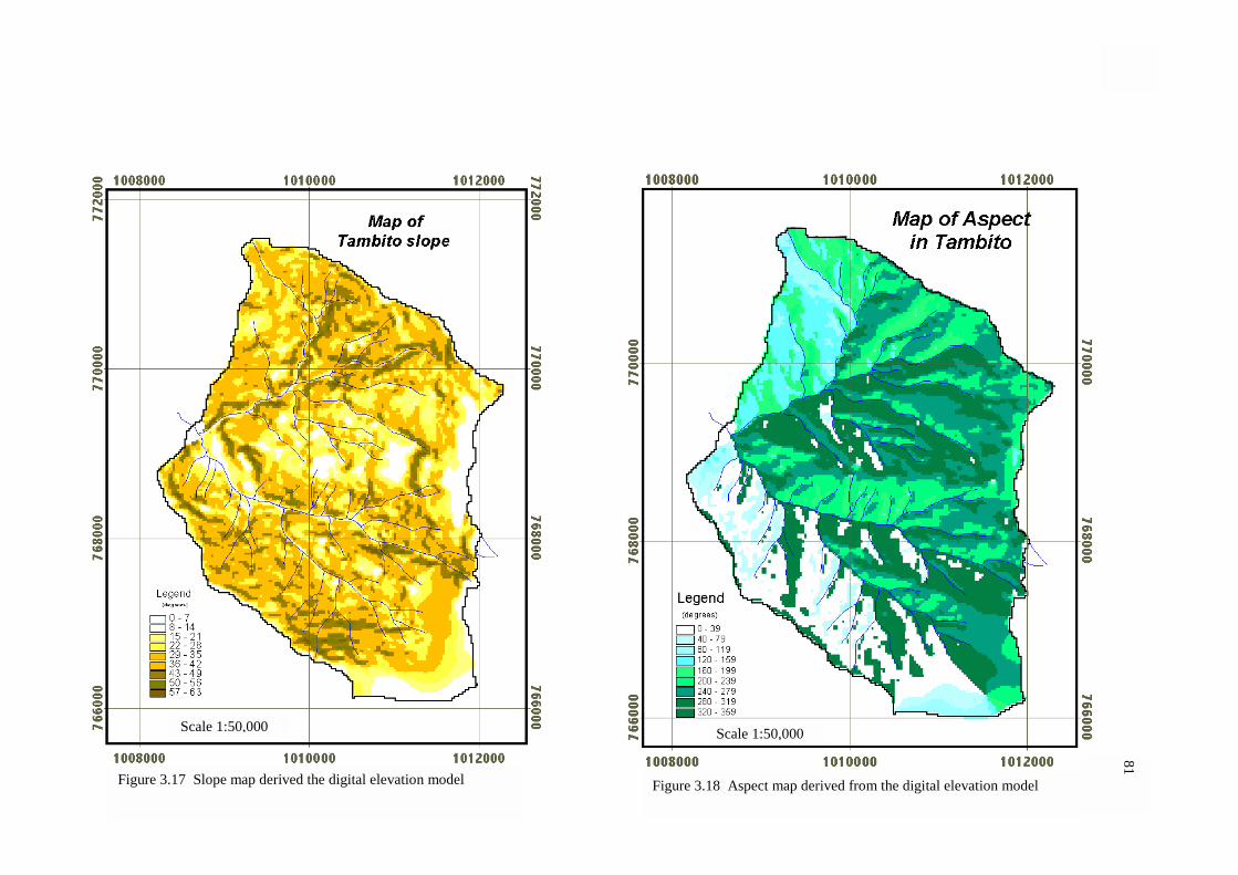
81
Figure 3.17 Slope map derived the digital elevation model Figure 3.18 Aspect map derived from the digital elevation model
81
Scale 1:50,000 Scale 1:50,000
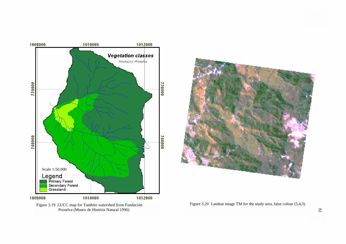
82
Tambito Landsat TM image (bands 5,2,3)
Figure 3.19 LUCC map for Tambito watershed from Fundación Proselva (Museo de História Natural 1996)
Figure 3.20 Landsat image TM for the study area, false colour (5,4,3)
82
Scale 1:50,000

83
3.6 Hydrological Model methodology
3.6.1 Introduction
Although many hydrological models already exist, most have been
designed for (and implemented in) environments that differ
significantly to TMEs and often require input data that are not
always relevant or available for this environment. This was clearly
identified in the section 2.3.3, where several models were described
and their characteristics were evaluated with respect to the
environment of Tambito.
Instead of using an existing model, hydrological processes are
modelled using simple, physical routines that have been
implemented and combined especially for this purpose, with two
important features: a) models should work with minimal data, and
b) models should emphasise the properties of spatial variation and
hydro-connectivity, which are important in this thesis. The
following sections cover the methodology used and model
development.
3.6.2 Strategy
The 1D model was designed to work in a single cell in the vertical
dimension. The main hydrological processes were included to
reproduce the hydrological response for each of the land uses
identified in Tambito catchment. Then the same hydrological
model was implemented in a spatially distributed 2.5D form
produce results over the whole study area and simulate the
hydrological behaviour in the whole catchment simultaneously. A
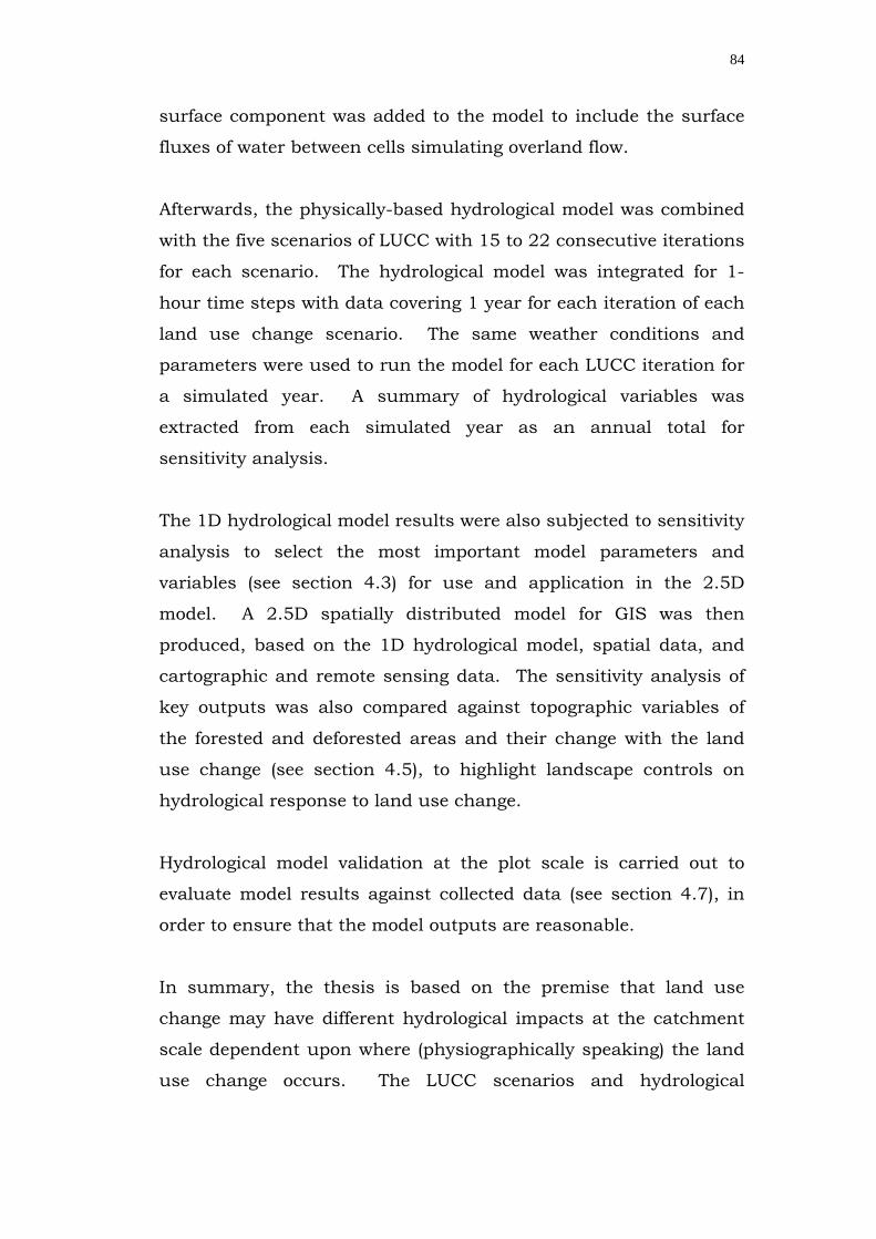
84
surface component was added to the model to include the surface
fluxes of water between cells simulating overland flow.
Afterwards, the physically-based hydrological model was combined
with the five scenarios of LUCC with 15 to 22 consecutive iterations
for each scenario. The hydrological model was integrated for 1-
hour time steps with data covering 1 year for each iteration of each
land use change scenario. The same weather conditions and
parameters were used to run the model for each LUCC iteration for
a simulated year. A summary of hydrological variables was
extracted from each simulated year as an annual total for
sensitivity analysis.
The 1D hydrological model results were also subjected to sensitivity
analysis to select the most important model parameters and
variables (see section 4.3) for use and application in the 2.5D
model. A 2.5D spatially distributed model for GIS was then
produced, based on the 1D hydrological model, spatial data, and
cartographic and remote sensing data. The sensitivity analysis of
key outputs was also compared against topographic variables of
the forested and deforested areas and their change with the land
use change (see section 4.5), to highlight landscape controls on
hydrological response to land use change.
Hydrological model validation at the plot scale is carried out to
evaluate model results against collected data (see section 4.7), in
order to ensure that the model outputs are reasonable.
In summary, the thesis is based on the premise that land use
change may have different hydrological impacts at the catchment
scale dependent upon where (physiographically speaking) the land
use change occurs. The LUCC scenarios and hydrological
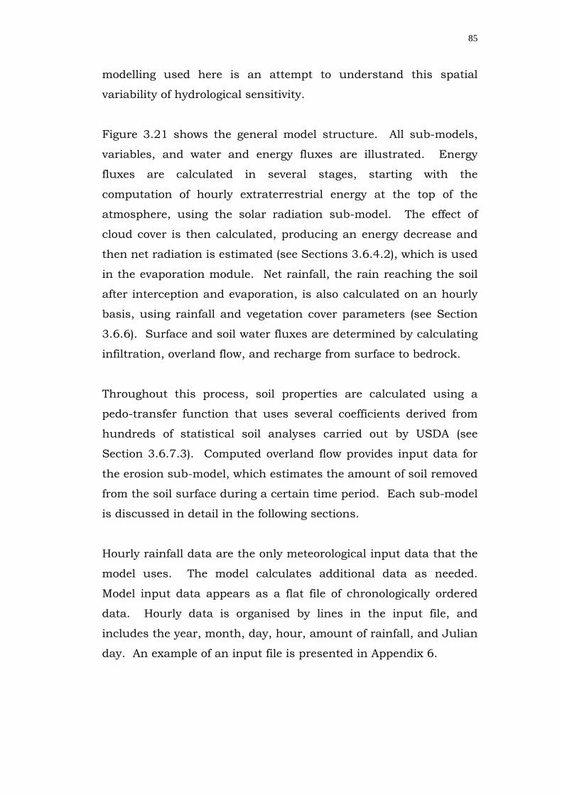
85
modelling used here is an attempt to understand this spatial
variability of hydrological sensitivity.
Figure 3.21 shows the general model structure. All sub-models,
variables, and water and energy fluxes are illustrated. Energy
fluxes are calculated in several stages, starting with the
computation of hourly extraterrestrial energy at the top of the
atmosphere, using the solar radiation sub-model. The effect of
cloud cover is then calculated, producing an energy decrease and
then net radiation is estimated (see Sections 3.6.4.2), which is used
in the evaporation module. Net rainfall, the rain reaching the soil
after interception and evaporation, is also calculated on an hourly
basis, using rainfall and vegetation cover parameters (see Section
3.6.6). Surface and soil water fluxes are determined by calculating
infiltration, overland flow, and recharge from surface to bedrock.
Throughout this process, soil properties are calculated using a
pedo-transfer function that uses several coefficients derived from
hundreds of statistical soil analyses carried out by USDA (see
Section 3.6.7.3). Computed overland flow provides input data for
the erosion sub-model, which estimates the amount of soil removed
from the soil surface during a certain time period. Each sub-model
is discussed in detail in the following sections.
Hourly rainfall data are the only meteorological input data that the
model uses. The model calculates additional data as needed.
Model input data appears as a flat file of chronologically ordered
data. Hourly data is organised by lines in the input file, and
includes the year, month, day, hour, amount of rainfall, and Julian
day. An example of an input file is presented in Appendix 6.
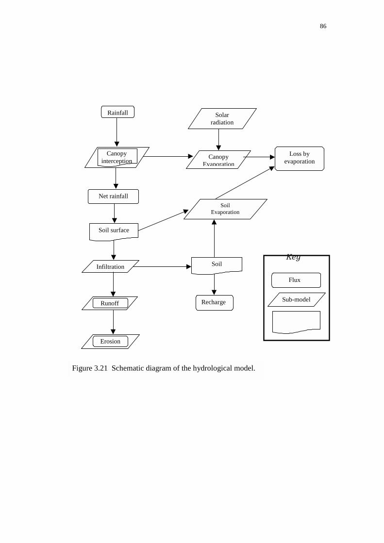
86
Rainfall Solarradiation
CanopyEvaporation
Loss byevaporation
Canopyinterception
Net rainfall
Soil surface
Infiltration
SoilEvaporation
Recharge
Soil
Runoff
Erosion
Figure 3.21 Schematic diagram of the hydrological model.
Flux
Sub-model
Key
87
3.6.3 Considerations for the modelling process
Technical aspectsModel development occurred in many stages. The initial model 1D
model was highly detailed and, accordingly, difficult to implementin
both plot and catchment scale. Sensitivity analysis of this model
suggested that it should be simplified in order to make it
computationally manageable and parameterisable.
In technical terms, the model was developed in two stages: the first
consists of a 1D hydrological model, implemented in a spreadsheet.
This model was very cumbersome and slow to react for long
simulations because its complexity. This suggested that for this
research activity a complex model with several modules, which
modelled a year in hourly time steps (8760 hours-) was
inappropriate and unworkable within the context of a spreadsheet
approach. The same model was then implemented in PCRaster for
a single cell, which operationally speaking gave good results.
A lumped model is however inappropriate to the spatial modelling
aspects of this thesis so that a second model saw the development
of a spatially distributed 2.5D hydrological model using the same
equations as the 1D hydrological model routines with additional
surface components for lateral flow, which are then applied to the
entire watershed. As in the 1D hydrological model, an
unsuccessful experience in the implementation of this model was
encountered was when the model attempting to implement it in
Arc/Info Macro Language (AML) of Arc/Info 7.3 (ESRI). The
operational problems arose because the temporal information
created by the system throughout the process generates several
files which are stored in the hard drive of the computer. This
produces a very slow simulation process and after several hours
the simulation process stops, due to the fact that the number of
88
subdirectories that are possible to be created is limited (no more
than the maximum available integer number in a computer –
32767-). These is no workaround for this problem in AML. The
2.5D hydrological distributed model was eventually implemented in
PCRaster with good results.
Data availabilityWith regard to the modelling data, unfortunately complete hourly
rainfall data for a single year could not be obtained from the
weather stations because of technical problems, although a broken
record exists. A Monte Carlo simulation technique (Mulligan,
1996) was used to generate hourly data on the basis of daily totals
for both Tambito and 20 de Julio weather stations and probability
distribution function of hourly rainfall measured at the Tambito
station.
Transpiration modellingDespite the fact that plant transpiration is important to take into
account when vegetation is involved in any study, researchers have
pointed out that this process contributes relatively low amount of
water, compared to water evaporation process from the water
canopy and does not contribute significantly to the water balance
in TMCF (Rutter, 1975; Grubb, 1977; Korner, 1983; Cavalier,
1986).
One of the main processes that regulates gas and water exchange
in the plant, is the stomatal conductance, which varies in response
to many meteorological variables. Stomata are sensitive to the
quality and quantity of light, to temperature, to humidity, to plant
water stress and vapour pressure deficit among others.
Temperatures in TMCF are low and relative humidity is high, solar
radiation low and water stress less frequent compared to lowlands
(Jarvis, 1976). Reductions in stomatal conductance have been
89
observed in response to increases in vapour pressure deficit in
tropical and warm temperature of TMCF (Korner et al., 1983; Jane
et al., 1985; Cavalier, 1986). Additionally Bruijnzeel et al. (1993)
argued that transpiration rates in TMCF are low even during
episodes of bright sunshine. Kapos et al. (1985) found that
stomatal responses to changing atmospheric conditions were less
pronounced in Blue Mountains (Jamaica) than other tropical
forests.
The leaf anatomy in TMCF have been shown to have a small
number of stomata per unit surface area (Korner et al., 1983), the
density of which varies between 37 to 299 mm2 in the cloud forest
of Colombia and Venezuela (Cavalier, 1986).
Mulligan and Jarvis (2000b) noted that humidity and atmospheric
saturation for Tambito occurs up to 92 % of the time on an annual
basis, and in the same place, Letts (2000) found the maximum
transpiration rate was 1-4 mmol∙m-2∙s-1.
In addition to these arguments, due to the lack of spatially
distributed instrumentation in Tambito for the collection of data for
transpiration parameterisation, this sub-model is not included in
the proposed hydrological model. Since it is complex to model and
requires spatially distributed meteorological and plant canopy data
that are simply not available for this (and many others
catchments), the process was not modelled though the author
recognises that this is a serious simplification and also limits the
applicability of the model outside of TMCF environments.
Cloud interceptionThe important contribution that fog and cloud deposition on
vegetation surfaces provides an extra source of moisture for the
hydrological cycle in TMCF is broadly acknowledged (Bruijnzeel,
90
2000). However, the difficulty in quantifying this extra input of
moisture has been recognised since 1968 (Kerfoot, 1968).
Bruijnzeel and Proctor (1995) recognised how little is actually
known about hydrological functioning of the vegetation in TMCF
such as epiphytes exposed to cloud impaction, with respect to
cloud water interception and retention. In a literature survey
carried out by Jarvis (1999), the range of cloud deposition on the
vegetation of TMCF, as a contribution to the net rainfall varies
between 2.4 to 60%. The same author reported through modelling
that 73% of annual precipitation resulted from cloud deposition.
Cloud interception is not modelled in this thesis because in the
early stage of understanding the hydrology of Tambito, the purpose
was to produce a model that can be used later on as a framework
for further research, incorporating as yet unquantified additions
such as cloud interception.
3.6.4 Solar Radiation sub-model
Solar energy is the driving force for the Earth’s climate (Brock,
1981; Forseth and Norman, 1993). Therefore, the solar radiation
(SR) sub-model plays a key role in determining the system’s
hydrological balance because it defines the energy available for
evaporation at the Earth surface. SR receipt is highly spatially
variable across steep slopes and over time. Although geographic
location exerts control on SR, the study area under consideration
was too small to yield significant differences in SR because of
latitude and longitude. Accordingly, average geographic co-
ordinates were applied to the whole area to compute an energy
balance.

91
Solar radiation models can be adapted to data produced at any
given time step, whether yearly, monthly, daily or hourly. Model
accuracy depends mainly on the existence of long-term weather
data (20 years or more) (Gansler et al., 1994). It also depends on
the time-step, the resolution and the quality of source data.
However, even if these prerequisites are met, model results do not
always replicate real situations and values accurately.
The SR model includes three stages:
1. Modelling the hourly extraterrestrial SR with physical and
astronomical principles. This involves calculating the amount of
energy available from SR at the top of the atmosphere for any given
point (cell) and time during the day and for any slope, and aspect
(Iqbal, 1983).
2. Application of an hourly cloud-cover attenuation model, with
specific weather conditions for each hour during the day.
3. Development of an empirical net radiation model for specific
surface conditions (Mulligan, 1996).
Each of these components is explained briefly below.
3.6.4.1 Hourly extraterrestrial solar radiation model
According to the literature, extraterrestrial SR is determined by
simplified physical principles, for example solar constant, solar
declination, position on Earth surface and time (Robinson, 1966;
Brock, 1981; Iqbal, 1983; Dobson and Smith, 1988; Dingman,
1994; Forseth and Norman, 1993; Gueymard, 1993). Gueymard,
(1993) analysed several SR models and recommended the Iqbal
(1983) procedure that is physically based with RMS error below 6%
92
for global radiation. This process is outlined in Appendix 7. This
process was used to obtain the extraterrestrial SR for a point (Iobs)
(KJ h-1) with a given aspect and slope, using an hourly time-step.
3.6.4.2 Hourly cloud-cover attenuation model
Clear sky irradiance models have been developed to predict beam,
diffuse, and global radiation on a horizontal surface. A diversity of
models can be found in the literature, ranging from simple
empirical formulae to highly sophisticated spectral codes. Both
empirical and physical model approaches seek to interpret the
physical extinction of energy through the atmosphere (Gueymard,
1993).
The purpose of this sub-model is not to study the atmospheric
components effects on the solar irradiance such as water vapour,
cloud, aerosols, or ozone, but to introduce in the computation a
cloudiness factor, which diminishes the solar radiation reaching
the land surface, in a simple way that takes into account the
temporal and spatial variation in cloud cover in the catchment.
Gueymard (1993) compared 11 physical and empirical models for
atmospheric attenuation that varied in complexity. Gueymard
(1993) compared and analysed all input model parameters in order
to identify model limitations and areas, where their adequate
performance under real conditions, in order to evaluate the models
adaptability. He found that models designed to compute clear sky
irradiance had not been validated against real data, because in
many cases, long term data for parameterisation and validation do
not exist. Hourly irradiation models are more appropriate because
they compute continuously changing cloudiness in short time
steps. Because most of the short-term variability in radiation
93
values can be attributed to clouds, this atmospheric and
meteorological effect must be taken into account. However, model
results have not been statistically verified and the time resolution
for which they predict changes can lead to large errors.
Cloud models require large data sets because they need to account
for optical air mass, aerosol transmittance, Rayleigh scattering,
ozone absorption, water vapour absorptance, extraterrestrial
irradiance (see previous section), and clear sky albedo. Most of
these parameters are not available for the study area, and even if
they were available, the complexity of the relationships between
them makes model implementation difficult. Furthermore,
Gueymard (1993) argued that the use of a large amount of
information does not necessarily give more accurate predictions for
cloudy sky conditions variability, such as those found in the
Tambito area.
Dobson et al. (1988) analysed bulk SR models at sea level and
compared their results. Models that estimate SR from solar
elevation and from hourly cloud amount and type, using empirical
or simple physical formulae, yield poor results in some cases
compared with existing formulae at noon solar elevation and daily
mean cloud amount. He studied models such as that of Budyko
(1974) which calculates monthly clear sky insolation Qc (W m-2)
using a tabulated function of latitude and time with quadratic
formulae to obtain monthly solar insolation:
Where n is the monthly cloud fraction, a is an empirical function of
latitude and b is an empirical constant. Although the monthly
cloud amount varies, cloud factors do not allow the discrimination
of differences in cloud types or seasonal variations with solar
{ }Q Q a bn nc= − +1 ( ) Eq. 3.2
94
elevation. As a result, the path length through clouds does not
take into account regional scale or cloud dynamics which are the
major control on cloud cover in Tambito.
Regarding hourly models, Dobson et al. (1988) expressed the
radiation in terms of the atmospheric factor T, which is defined as
the ratio of downward short-wave radiation Q at the surface with
the radiation incident on the horizontal surface above the
atmosphere:
Where Qo is mean solar flux assumed as 1368 (W m-2) and θ is
solar elevation as a function of time and position.
Dobson et al. (1988) also used a Lumb approach model (1964) that
estimates SR for each hourly cloud observation and can be fitted
into nine categories, based on a combination of cloud amount and
type, expressed as:
Where for each category i, the atmospheric transmission factor T is
a regression function of the sine of solar elevation S. Most models
discussed by Dobson et al. (1988) are expressed as regression
equations, whether linear or exponential, but can be divided into
categories according to cloud height and type. Dobson et al. (1988)
concluded that complex models do not necessarily fit better than
simple models and that complex models require sets of cloud
observation data that are often not available for the study area. A
simple relationship derived from regression values and the sine of
T Q Q Sino= / ( )θ Eq. 3.3
T A B Si i= + Eq. 3.4
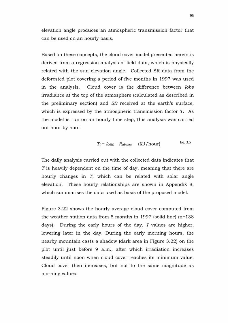
95
elevation angle produces an atmospheric transmission factor that
can be used on an hourly basis.
Based on these concepts, the cloud cover model presented herein is
derived from a regression analysis of field data, which is physically
related with the sun elevation angle. Collected SR data from the
deforested plot covering a period of five months in 1997 was used
in the analysis. Cloud cover is the difference between Iobs
irradiance at the top of the atmosphere (calculated as described in
the preliminary section) and SR received at the earth’s surface,
which is expressed by the atmospheric transmission factor T. As
the model is run on an hourly time step, this analysis was carried
out hour by hour.
Ti = IOBS – Robserv (KJ/hour)
The daily analysis carried out with the collected data indicates that
T is heavily dependent on the time of day, meaning that there are
hourly changes in T, which can be related with solar angle
elevation. These hourly relationships are shown in Appendix 8,
which summarises the data used as basis of the proposed model.
Figure 3.22 shows the hourly average cloud cover computed from
the weather station data from 5 months in 1997 (solid line) (n=138
days). During the early hours of the day, T values are higher,
lowering later in the day. During the early morning hours, the
nearby mountain casts a shadow (dark area in Figure 3.22) on the
plot until just before 9 a.m., after which irradiation increases
steadily until noon when cloud cover reaches its minimum value.
Cloud cover then increases, but not to the same magnitude as
morning values.
Eq. 3.5
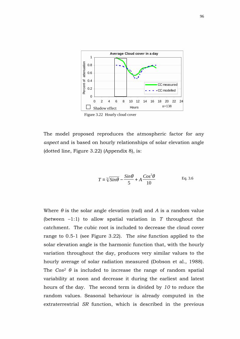
96
The model proposed reproduces the atmospheric factor for any
aspect and is based on hourly relationships of solar elevation angle
(dotted line, Figure 3.22) (Appendix 8), is:
Where θ is the solar angle elevation (rad) and A is a random value
(between –1:1) to allow spatial variation in T throughout the
catchment. The cubic root is included to decrease the cloud cover
range to 0.5-1 (see Figure 3.22). The sine function applied to the
solar elevation angle is the harmonic function that, with the hourly
variation throughout the day, produces very similar values to the
hourly average of solar radiation measured (Dobson et al., 1988).
The Cos2 θ is included to increase the range of random spatial
variability at noon and decrease it during the earliest and latest
hours of the day. The second term is divided by 10 to reduce the
random values. Seasonal behaviour is already computed in the
extraterrestrial SR function, which is described in the previous
T SinSin
ACos
= − +θθ θ
32
5 10Eq. 3.6
Average Cloud cover in a day
0
0.2
0.4
0.6
0.8
1
0 2 4 6 8 10 12 14 16 18 20 22 24
Hours
Perc
ent o
f a
ttenu
atio
nCC measured
CC modelled
n=138Shadow effect
Figure 3.22 Hourly cloud cover
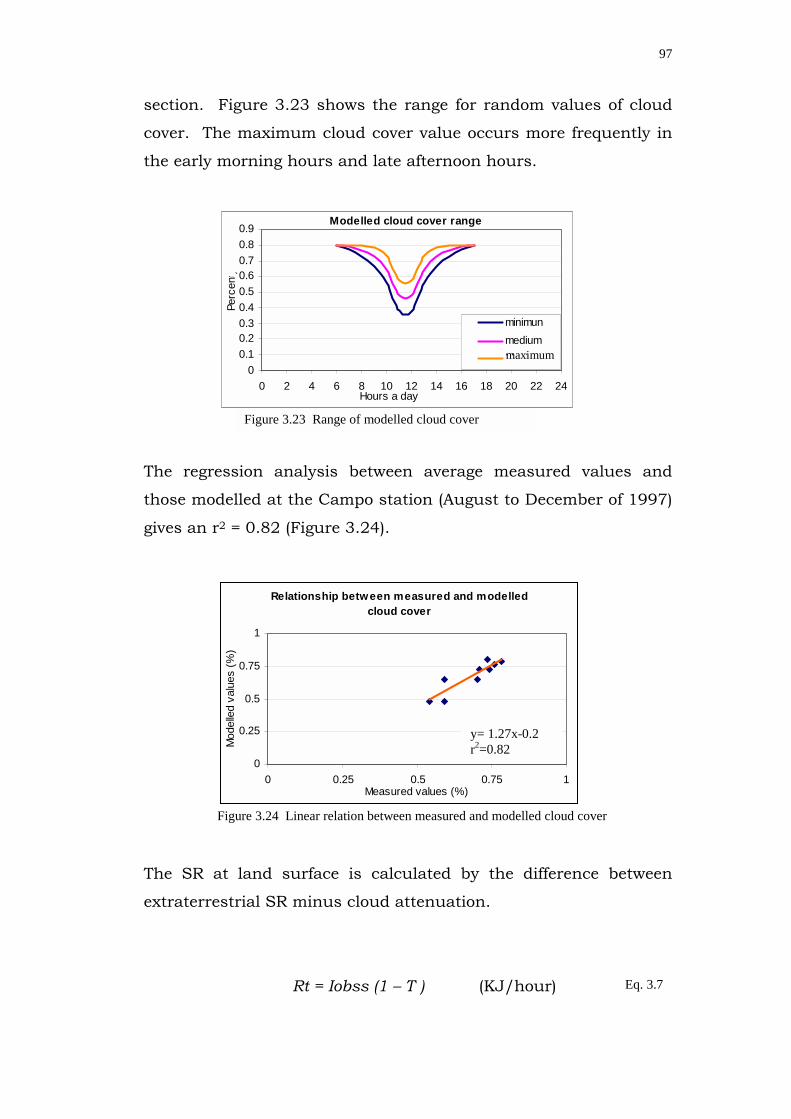
97
section. Figure 3.23 shows the range for random values of cloud
cover. The maximum cloud cover value occurs more frequently in
the early morning hours and late afternoon hours.
The regression analysis between average measured values and
those modelled at the Campo station (August to December of 1997)
gives an r2 = 0.82 (Figure 3.24).
The SR at land surface is calculated by the difference between
extraterrestrial SR minus cloud attenuation.
Rt = Iobss (1 – T ) (KJ/hour) Eq. 3.7
Figure 3.23 Range of modelled cloud cover
Modelled cloud cover range
0
0.1
0.20.3
0.4
0.5
0.60.7
0.8
0.9
0 2 4 6 8 10 12 14 16 18 20 22 24Hours a day
Perc
ent)
minimun
medium
Maximunmaximum
Relationship between measured and modelled cloud cover
y = 1.2679x - 0.1934R2 = 0.8203
0
0.25
0.5
0.75
1
0 0.25 0.5 0.75 1Measured values (%)
Mod
elle
d va
lues
(%
)
Figure 3.24 Linear relation between measured and modelled cloud cover
y= 1.27x-0.2r2=0.82
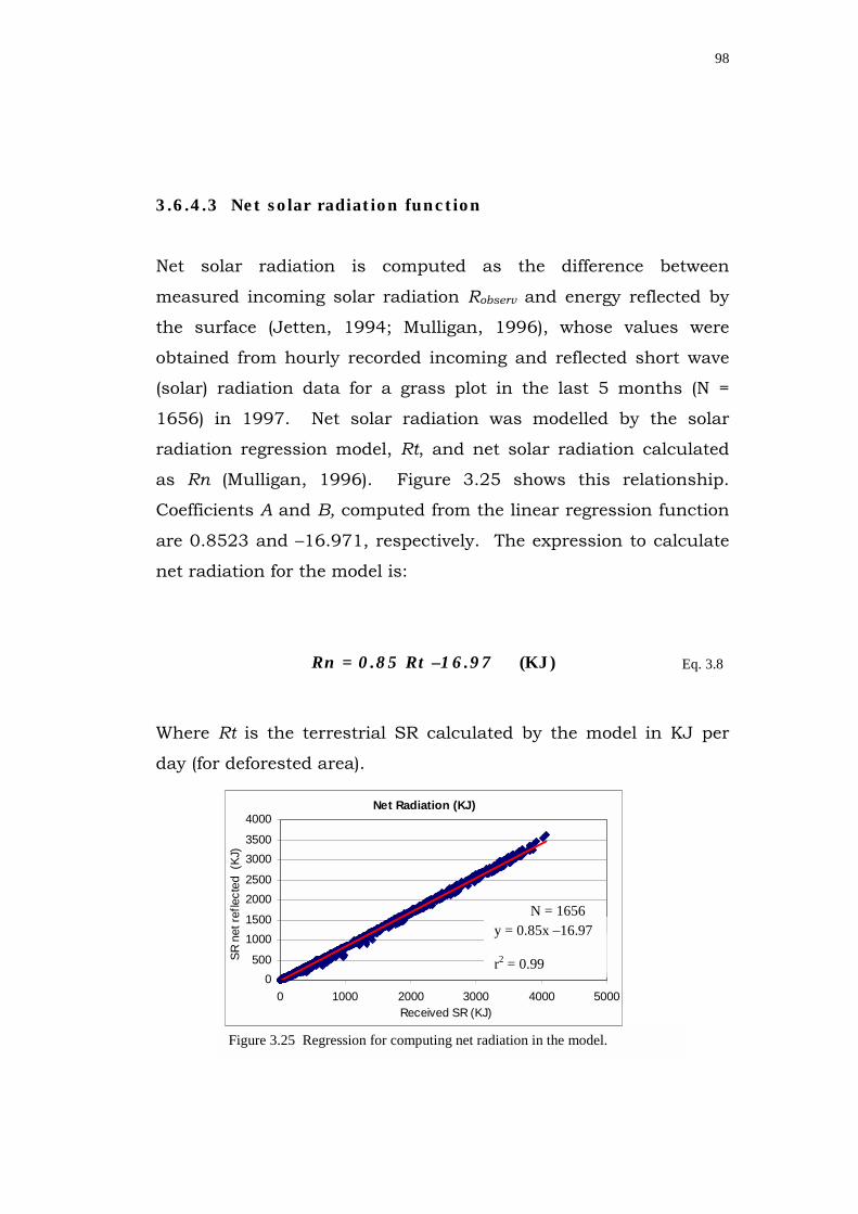
98
3.6.4.3 Net solar radiation function
Net solar radiation is computed as the difference between
measured incoming solar radiation Robserv and energy reflected by
the surface (Jetten, 1994; Mulligan, 1996), whose values were
obtained from hourly recorded incoming and reflected short wave
(solar) radiation data for a grass plot in the last 5 months (N =
1656) in 1997. Net solar radiation was modelled by the solar
radiation regression model, Rt, and net solar radiation calculated
as Rn (Mulligan, 1996). Figure 3.25 shows this relationship.
Coefficients A and B, computed from the linear regression function
are 0.8523 and –16.971, respectively. The expression to calculate
net radiation for the model is:
Rn = 0.85 Rt –16.97 (KJ)
Where Rt is the terrestrial SR calculated by the model in KJ per
day (for deforested area).
Eq. 3.8
Figure 3.25 Regression for computing net radiation in the model.
Net Radiation (KJ)
y = - 16.971+ 0.8523x R2 = 0.9979
0
500
1000
1500
2000
2500
3000
3500
4000
0 1000 2000 3000 4000 5000Received SR (KJ)
SR
net
ref
lect
ed (
KJ)
N = 1656y = 0.85x –16.97
r2 = 0.99
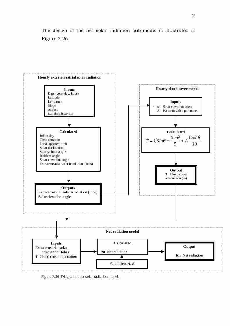
99
The design of the net solar radiation sub-model is illustrated in
Figure 3.26.
Figure 3.26 Diagram of net solar radiation model.
Hourly extraterrestrial solar radiation
InputsDate (year, day, hour)LatitudeLongitudeSlopeAspectt1,t2 time intervals
CalculatedJulian dayTime equationLocal apparent timeSolar declinationSunrise hour angleIncident angleSolar elevation angleExtraterrestrial solar irradiation (Iobs)
OutputsExtraterrestrial solar irradiation (Iobs)Solar elevation angle
Hourly cloud cover model
Calculated
T SinSin
ACos
= − +θθ θ
32
5 10
Inputs- θ Solar elevation angle- A Random value parameter
OutputT Cloud coverattenuation (%)
Net radiation model
InputsExtraterrestrial solar
irradiation (Iobs)T Cloud cover attenuation
Calculated
Rn Net radiation
Output
Rn Net radiation
Parameters A, B
100
3.6.5 The evaporation sub-model
In understanding the hydrological impacts of the land use change,
one of the major factors that may vary between forested and
deforested areas is evaporation. This is thus a key component of
the model and worthy of attention here.
Evaporation E occurs when water in liquid or solid phase, at or just
below the earth’s surface, is converted into water vapour and
transferred in this form to the atmosphere. The process can only
occur if there is an energy input from either the sun or the
atmosphere itself, and is controlled by the rate at which the energy,
in the form of vapour, can diffuse away from the earth’s surface
(Shaw, 1984; Dolman et al., 1991; Maidment, 1993).
The combined process of evaporation Ei, (from various water
surfaces such as water bodies, water intercepted on the vegetation
and moist, bare soil) and transpiration Et, (water vapour escaping
from within plants, mostly via leaves) from a dry canopy will
constitute the total evaporation E (Bonell and Balek, 1993).
The latent heat (λ) of vapourisation is the energy required to
evaporate 1 kg of water under normal conditions (at 10 °C), and is
estimated at 2.47X10⁶ J kg-1 (Shaw, 1984). It changes slightly with
temperature (about 0.1 % per °C), because the initial separation of
the molecules that make up liquid varies with temperature (Ward
et al., 1990). Maidment (1993) expressed this relationship as
λ = 2.501 – 0.002361 Ts MJ kg-1
where Ts is the surface temperature of water in degrees Celsius.
Eq. 3.9
101
The flow of water vapour molecules away from an evaporating
water surface implies a transfer of energy away from the surface, in
the form of latent heat. The energy transferred is numerically
equal to the product of the mass flow, i.e., evaporation E, in mm
h-1, and the latent heat of evaporation (Kramer et al., 1995).
Evaporation is controlled by net radiation, Sn, which is the portion
of incident short-wave radiation captured at ground level, taking
into account losses because of reflection and emission:
Sn = St(1-α)+ Lw(1-Εo) MJ M-2 h-1
where α is the albedo, Lw the long-wave radiation incident, and -Εo
the long- wave radiation emitted (both in MJ m-2 h-1). In equation
3.10, the first term represents the short wave radiation, which is
dependent of the albedo, which, in turn, is a function of the surface
reflectance properties. Atmospheric gases are not very good
absorber of short-wave (0.15 – 3.0 µm) and are much better for
transitivity compared to long-wave radiation, in the band (3 – 100
µm). As a result, the portion of net radiation due to short-wave
radiation is greater than long-wave. The incoming long-wave
radiation emitted by the atmosphere, in absence of cloud, depends
upon the bulk atmospheric temperature and emissivity so incident
long-wave radiation is almost constant through the day. The
outgoing long-wave radiation from the surface depends also on
temperature and emissivity of the land surface. This is usually
greater than the atmospheric counterpart, and because
temperature varies considerably through the day, net long-wave
radiation is usually negatively and relative small (75 – 125 W m-2)
(Oke, 1987) if the surface and air temperature are not significantly
different.
Eq. 3.10

102
Potential evaporation (Ep) is a standard evaporation defined as the
amount of water evaporated per unit area and per unit time from
an idealised, extensive free water surface, under prevailing
atmospheric conditions without any surface resistance (Oke,
1987). Evaporation introduces water into the air and can remove
energy from it, changing atmospheric humidity deficit and possibly
altering evaporation at downwind locations (Maidment, 1993). This
concept measures the meteorological control on evaporation from
an open water surface (Ward et al., 1990).
The Priestley-Taylor (1972) equation provides the basis of an
approximation which keeps strong relation to the first term of
Penman equation (will be discussed later), with the exception of the
inclusion of an empirical coefficient (α) to allow some advection,
which is
Where λ is the latent heat of vaporisation of water (J.Kg-1), EPT is
the rate of evaporation (kg m-2 s-1), Sn is the net energy available for
evaporation (W m-2), γ is the psychrometric constant (J kg-1 °C-1 /
J kg-1) and D is the slope of the saturation vapour pressure curve
(kg kg-1 °C-1), and α theoretically becomes to 1 under advection free
conditions (McNaughton and Jarvis, 1983).
The Penman wet-surface equation (λEp), is the most frequently
used potential evaporation concept, and represents ‘the
evaporation rate from a moist surface exposed to the existing
available energy and atmospheric conditions’ (Granger. 1989). The
Penman equation is totally independent of the surface conditions
and controlled only by energy supply and atmospheric conditions
(Bonell and Balek, 1993).
nPT SEγ
αλ+∆∆⋅= Eq. 3.11
103
The estimation of actual evaporation in vegetation conditions which
are not moist, suggests that the involvement of factors such as
physiology and stomatal resistance of the plants, which also
involves the soil moisture availability in the process.
The energy-balance (Penman-Monteith) approach to determine the
average evaporation rate over a given time period involves
measuring the input and output of energy, as well as the change in
energy storage. The following equation is used to determine
evaporation by this method:
where S is short-wave radiation; L, long-wave radiation, G, ground
conduction and Aw, advected energy which are given in W m-2; ∆, is
the slope of the saturation vapour pressure curve (kg kg-1 °C-1); ρ is
water density (kg m-3); Cp specific heat of air (J kg-1 °C-1); δq is the
vapour pressure deficit (Kpa); ga is the atmospheric conductance
(m s-1); gs is the stomatal conductance (m s-1) and γ is the
psynchrometric constant (0.655) (Dingman, 1994).
The equation assumes the canopy is acting as a “big leaf”
physically. The atmospheric conductance describes the physical
roughness effects of the vegetation on the transfer of energy and
mass from the surface to a reference level in the atmosphere. The
surface resistance describes the biological control over the rate of
transpiration and is particularly linked to the physiological
behaviour of plants expressed through the bulk stomatal resistance
(Stewart, 1989). Normally, this equation in combination with an
interception model yields good results, where the vegetation in the
W m-2 Eq. 3.12[ ]
++∆
++−+∆=
s
a
aqpW
g
g
gCAGLSE
1γ
δρλ
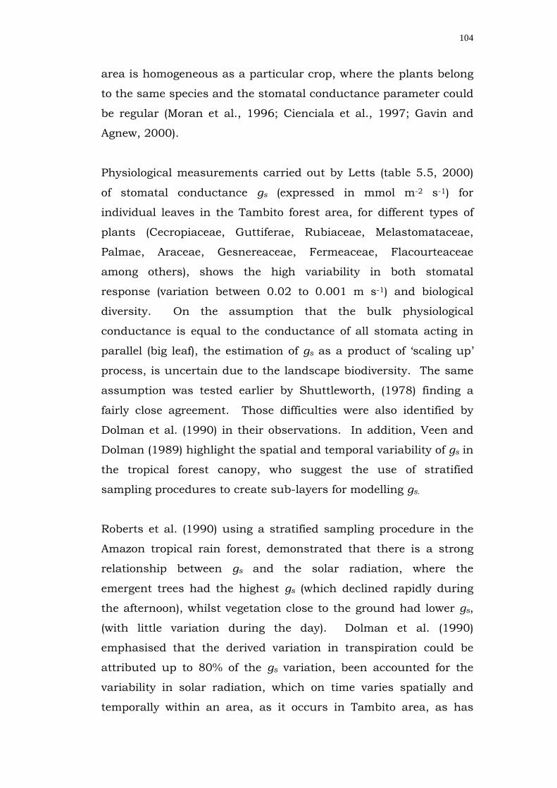
104
area is homogeneous as a particular crop, where the plants belong
to the same species and the stomatal conductance parameter could
be regular (Moran et al., 1996; Cienciala et al., 1997; Gavin and
Agnew, 2000).
Physiological measurements carried out by Letts (table 5.5, 2000)
of stomatal conductance gs (expressed in mmol m-2 s-1) for
individual leaves in the Tambito forest area, for different types of
plants (Cecropiaceae, Guttiferae, Rubiaceae, Melastomataceae,
Palmae, Araceae, Gesnereaceae, Fermeaceae, Flacourteaceae
among others), shows the high variability in both stomatal
response (variation between 0.02 to 0.001 m s-1) and biological
diversity. On the assumption that the bulk physiological
conductance is equal to the conductance of all stomata acting in
parallel (big leaf), the estimation of gs as a product of ‘scaling up’
process, is uncertain due to the landscape biodiversity. The same
assumption was tested earlier by Shuttleworth, (1978) finding a
fairly close agreement. Those difficulties were also identified by
Dolman et al. (1990) in their observations. In addition, Veen and
Dolman (1989) highlight the spatial and temporal variability of gs in
the tropical forest canopy, who suggest the use of stratified
sampling procedures to create sub-layers for modelling gs.
Roberts et al. (1990) using a stratified sampling procedure in the
Amazon tropical rain forest, demonstrated that there is a strong
relationship between gs and the solar radiation, where the
emergent trees had the highest gs (which declined rapidly during
the afternoon), whilst vegetation close to the ground had lower gs,
(with little variation during the day). Dolman et al. (1990)
emphasised that the derived variation in transpiration could be
attributed up to 80% of the gs variation, been accounted for the
variability in solar radiation, which on time varies spatially and
temporally within an area, as it occurs in Tambito area, as has
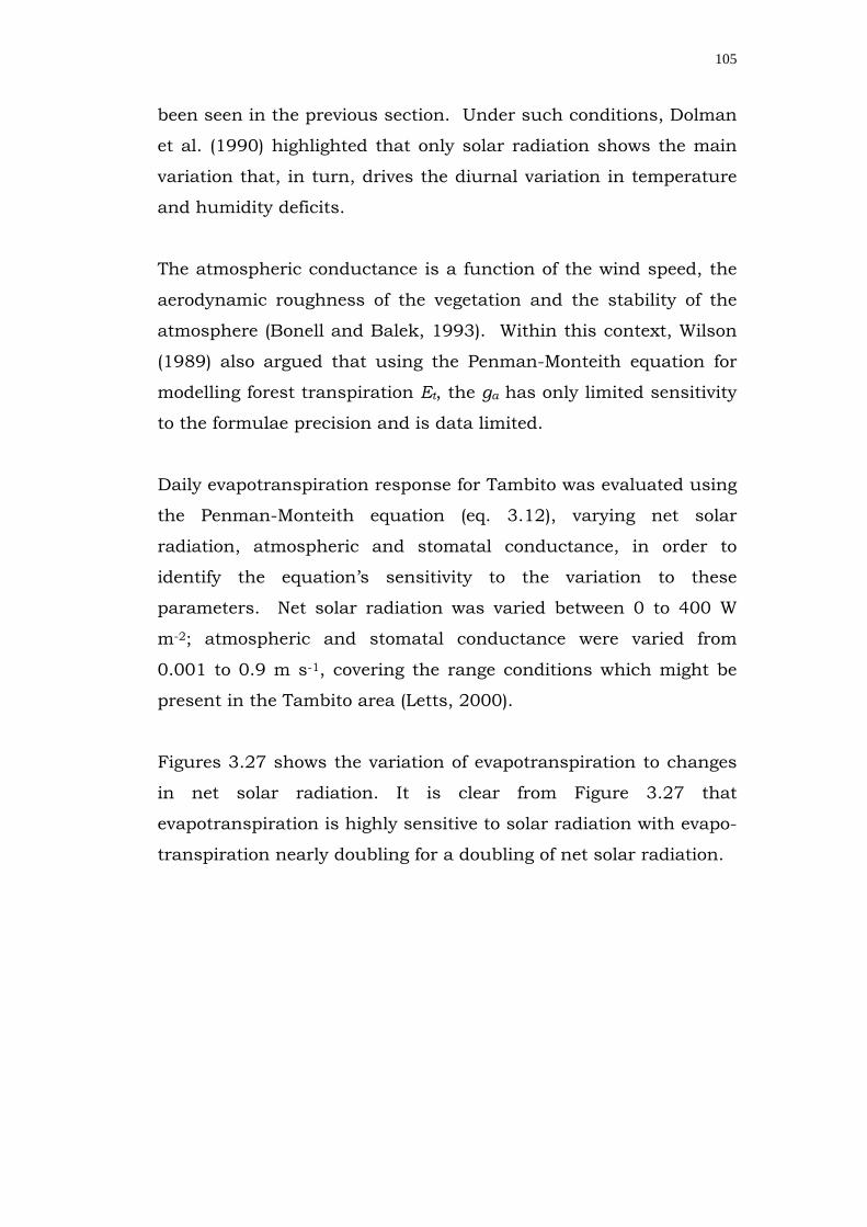
105
been seen in the previous section. Under such conditions, Dolman
et al. (1990) highlighted that only solar radiation shows the main
variation that, in turn, drives the diurnal variation in temperature
and humidity deficits.
The atmospheric conductance is a function of the wind speed, the
aerodynamic roughness of the vegetation and the stability of the
atmosphere (Bonell and Balek, 1993). Within this context, Wilson
(1989) also argued that using the Penman-Monteith equation for
modelling forest transpiration Et, the ga has only limited sensitivity
to the formulae precision and is data limited.
Daily evapotranspiration response for Tambito was evaluated using
the Penman-Monteith equation (eq. 3.12), varying net solar
radiation, atmospheric and stomatal conductance, in order to
identify the equation’s sensitivity to the variation to these
parameters. Net solar radiation was varied between 0 to 400 W
m-2; atmospheric and stomatal conductance were varied from
0.001 to 0.9 m s-1, covering the range conditions which might be
present in the Tambito area (Letts, 2000).
Figures 3.27 shows the variation of evapotranspiration to changes
in net solar radiation. It is clear from Figure 3.27 that
evapotranspiration is highly sensitive to solar radiation with evapo-
transpiration nearly doubling for a doubling of net solar radiation.
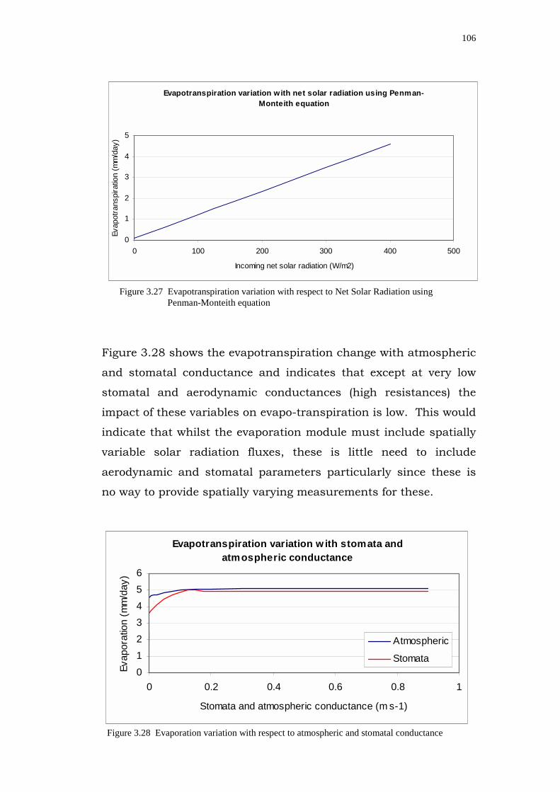
106
Figure 3.28 shows the evapotranspiration change with atmospheric
and stomatal conductance and indicates that except at very low
stomatal and aerodynamic conductances (high resistances) the
impact of these variables on evapo-transpiration is low. This would
indicate that whilst the evaporation module must include spatially
variable solar radiation fluxes, these is little need to include
aerodynamic and stomatal parameters particularly since these is
no way to provide spatially varying measurements for these.
Figure 3.27 Evapotranspiration variation with respect to Net Solar Radiation using Penman-Monteith equation
Evapotranspiration variation with net solar radiation using Penman-Monteith equation
0
1
2
3
4
5
0 100 200 300 400 500
Incoming net solar radiation (W/m2)
Evap
otra
nspi
ratio
n (m
m/d
ay)
Figure 3.28 Evaporation variation with respect to atmospheric and stomatal conductance
Evapotranspiration variation w ith stomata and atmospheric conductance
0
1
2
3
4
5
6
0 0.2 0.4 0.6 0.8 1
Stomata and atmospheric conductance (m s-1)
Evap
orat
ion
(mm
/day
)
Atmospheric
Stomata
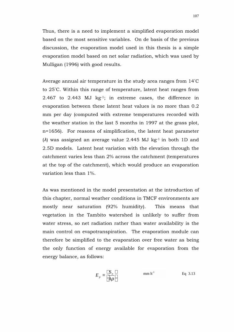
107
Thus, there is a need to implement a simplified evaporation model
based on the most sensitive variables. On de basis of the previous
discussion, the evaporation model used in this thesis is a simple
evaporation model based on net solar radiation, which was used by
Mulligan (1996) with good results.
Average annual air temperature in the study area ranges from 14°C
to 25°C. Within this range of temperature, latent heat ranges from
2.467 to 2.443 MJ kg-1; in extreme cases, the difference in
evaporation between these latent heat values is no more than 0.2
mm per day (computed with extreme temperatures recorded with
the weather station in the last 5 months in 1997 at the grass plot,
n=1656). For reasons of simplification, the latent heat parameter
(λ) was assigned an average value 2.445 MJ kg-1 in both 1D and
2.5D models. Latent heat variation with the elevation through the
catchment varies less than 2% across the catchment (temperatures
at the top of the catchment), which would produce an evaporation
variation less than 1%.
As was mentioned in the model presentation at the introduction of
this chapter, normal weather conditions in TMCF environments are
mostly near saturation (92% humidity). This means that
vegetation in the Tambito watershed is unlikely to suffer from
water stress, so net radiation rather than water availability is the
main control on evapotranspiration. The evaporation module can
therefore be simplified to the evaporation over free water as being
the only function of energy available for evaporation from the
energy balance, as follows:
mm h-1 Eq 3.13
=
λρn
p
SE
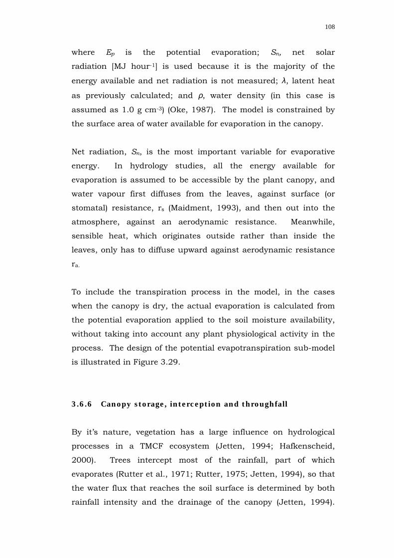
108
where Ep is the potential evaporation; Sn, net solar
radiation [MJ hour-1] is used because it is the majority of the
energy available and net radiation is not measured; λ, latent heat
as previously calculated; and ρ, water density (in this case is
assumed as 1.0 g cm-3) (Oke, 1987). The model is constrained by
the surface area of water available for evaporation in the canopy.
Net radiation, Sn, is the most important variable for evaporative
energy. In hydrology studies, all the energy available for
evaporation is assumed to be accessible by the plant canopy, and
water vapour first diffuses from the leaves, against surface (or
stomatal) resistance, rs (Maidment, 1993), and then out into the
atmosphere, against an aerodynamic resistance. Meanwhile,
sensible heat, which originates outside rather than inside the
leaves, only has to diffuse upward against aerodynamic resistance
ra.
To include the transpiration process in the model, in the cases
when the canopy is dry, the actual evaporation is calculated from
the potential evaporation applied to the soil moisture availability,
without taking into account any plant physiological activity in the
process. The design of the potential evapotranspiration sub-model
is illustrated in Figure 3.29.
3.6.6 Canopy storage, interception and throughfall
By it’s nature, vegetation has a large influence on hydrological
processes in a TMCF ecosystem (Jetten, 1994; Hafkenscheid,
2000). Trees intercept most of the rainfall, part of which
evaporates (Rutter et al., 1971; Rutter, 1975; Jetten, 1994), so that
the water flux that reaches the soil surface is determined by both
rainfall intensity and the drainage of the canopy (Jetten, 1994).
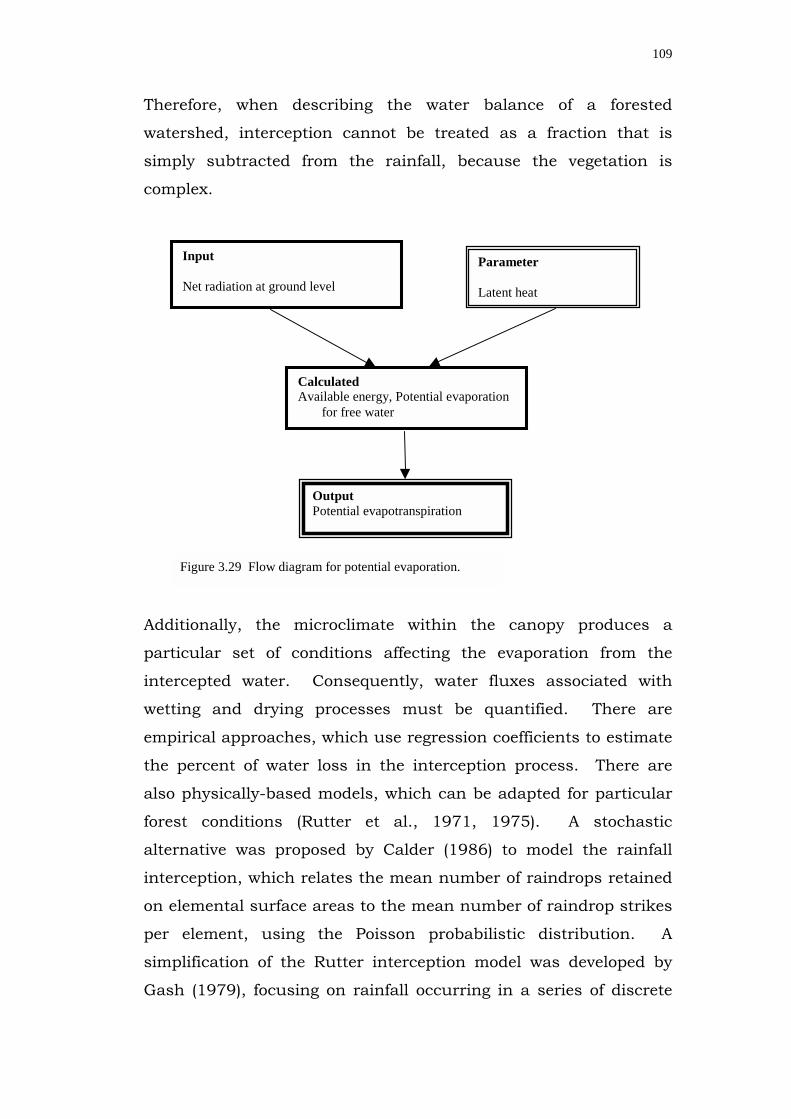
109
Therefore, when describing the water balance of a forested
watershed, interception cannot be treated as a fraction that is
simply subtracted from the rainfall, because the vegetation is
complex.
Additionally, the microclimate within the canopy produces a
particular set of conditions affecting the evaporation from the
intercepted water. Consequently, water fluxes associated with
wetting and drying processes must be quantified. There are
empirical approaches, which use regression coefficients to estimate
the percent of water loss in the interception process. There are
also physically-based models, which can be adapted for particular
forest conditions (Rutter et al., 1971, 1975). A stochastic
alternative was proposed by Calder (1986) to model the rainfall
interception, which relates the mean number of raindrops retained
on elemental surface areas to the mean number of raindrop strikes
per element, using the Poisson probabilistic distribution. A
simplification of the Rutter interception model was developed by
Gash (1979), focusing on rainfall occurring in a series of discrete
Input
Net radiation at ground level
CalculatedAvailable energy, Potential evaporation
for free water
Parameter
Latent heat
OutputPotential evapotranspiration
Figure 3.29 Flow diagram for potential evaporation.
110
storms, each of which comprises a period of wetting up, a period of
saturation an a period of drying out to empty the canopy storage.
The models of rainfall interception discussed have been applied on
tropical forest environments in combination with the Penman-
Monteith equation to estimate the rainfall interception loss, with
acceptable results. For example, Bruijnzeel and Wiersum (1987)
used the Gash rainfall interception model in West Java, Indonesia.
In contrast, Calder et al. (1986) used the Rutter interception model
in West Java without good results; the model predicted only 50% of
measured interception. Lloyd et al. (1988) compared the Rutter
and Gash models in the rain forest of Amazonas, obtaining similar
and reasonable results.
In relation with tropical montane rain forest, Herwitz (1987) worked
in north-east Queensland, and identified that the assumption of
constant canopy/trunk storage capacities was an
oversimplification, and highlighted the need to take into account
dynamic changes in storage capacities; also it was pointed out that
there is a need for additional studies concerning the effects of
forest structure parameters, interception measurement and
modelling.
In this thesis the Rutter rainfall interception model is adapted to
assess the rainfall intercepted, which combined with the
evaporation module is used to estimate the water lost by
evaporation of intercepted rainfall.
111
3.6.6.1 The Rutter model
The Rutter model (Rutter et al., 1971; 1975; 1977), was designed
as an interception model for a Corsican pine stand in Great Britain
but has been applied successfully to tropical rain forests (Calder et
al., 1986; Lloyd et al., 1988; Veen and Dolman, 1989; Jetten,
1996). Canopy water balance is calculated using empirical forest
stand parameters and potential evaporation.
The Rutter model offers several advantages: the input parameters
are relatively easy to obtain from throughfall measurements and
basic meteorological data. It uses stand characteristics rather
than properties of individual plants and calculates water fluxes on
a small time step basis, making it easy to link to a vertical water
balance model. The Rutter model was expanded by Jetten (1994)
to include canopy structure. In this extended model, called
CASCADE, the canopy is layered but uses virtually the same
parameters as the original model. The “cascade” concept is not
applied in this thesis because parameterisation of the model for
TMCF would be very difficult due to the heterogeneous vegetation
types present in TMCF (including epiphytes, for which hydrological
properties are poorly known). Therefore, vegetation has to be
assumed as a single layer for the purposes of modelling
interception. The processes involved in the Rutter model are
shown in Figure 3.30.
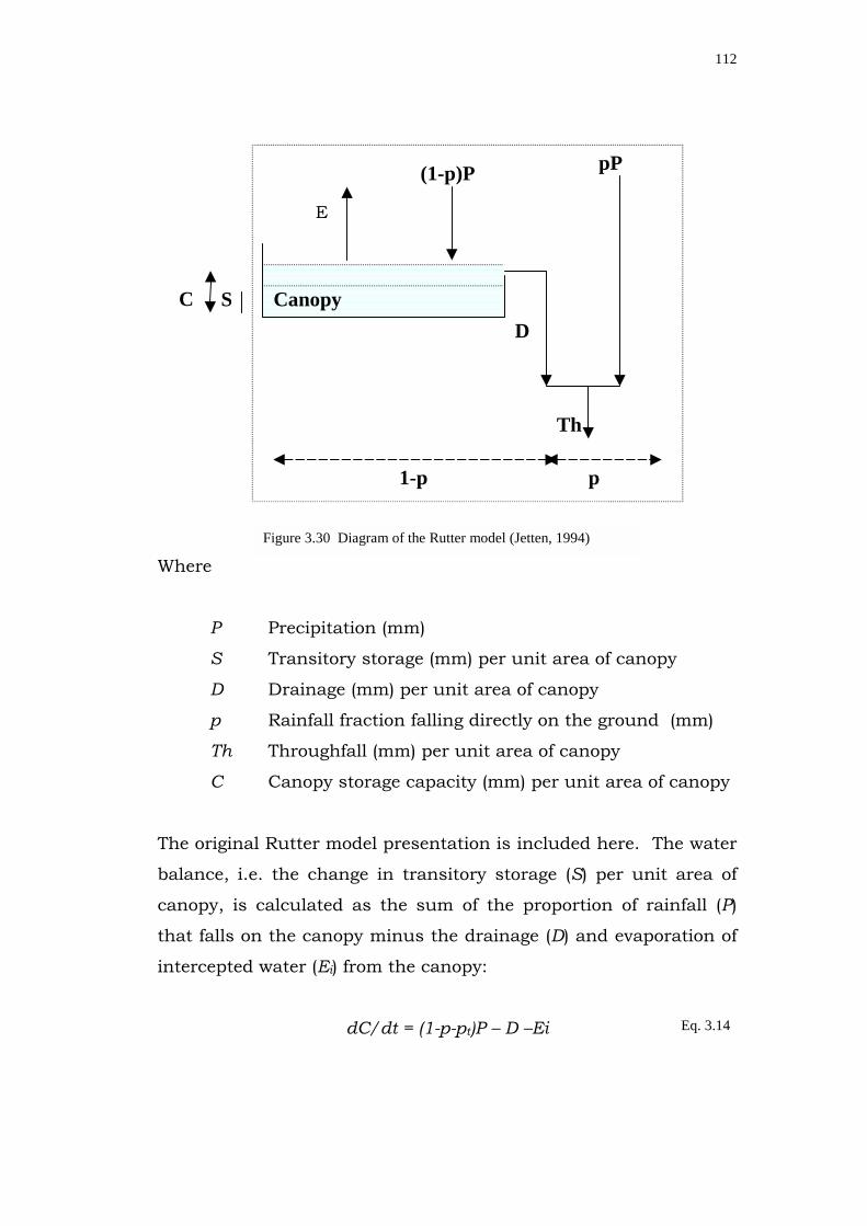
112
Where
P Precipitation (mm)
S Transitory storage (mm) per unit area of canopy
D Drainage (mm) per unit area of canopy
p Rainfall fraction falling directly on the ground (mm)
Th Throughfall (mm) per unit area of canopy
C Canopy storage capacity (mm) per unit area of canopy
The original Rutter model presentation is included here. The water
balance, i.e. the change in transitory storage (S) per unit area of
canopy, is calculated as the sum of the proportion of rainfall (P)
that falls on the canopy minus the drainage (D) and evaporation of
intercepted water (Ei) from the canopy:
dC/dt = (1-p-pt)P – D –Ei
p1-p
Th
D
pP(1-p)P
E
SC Canopy
Figure 3.30 Diagram of the Rutter model (Jetten, 1994)
Eq. 3.14

113
where C is in mm and the other variables in mm hour-1. The
fraction of rainfall intercepted by the canopy is calculated as the
difference between rainfall (P), the fraction of rainfall falling directly
on the ground (p), and the fraction of the rainfall diverted to stem
flow (pt) (Jetten, 1994). The canopy drainage is given by
D = 0 where C < S
D = Do eb(C-S) where C >= S
where S is the storage capacity (in mm), the amount of water
retained by the canopy when rainfall and throughfall have ceased
and the canopy is saturated. The minimum drainage rate, Do, is
the drainage rate when C is equal to S (in mm) and b is a
dimensionless parameter. Because the Rutter model was designed
for small time steps (min), the b parameter could not be adjusted
with an exponential function for this thesis in an hourly time step
because it produces model instability. Increasing the dripping
value produces more net rainfall than the real values; additionally
there are no field data to parameterise this parameter in either an
hourly or minute time step. As Rutter et al. (1971, 1975)
recognised, the canopy storage changes significantly during a 5-
min period (the time step used by Rutter et al. 1971) and this is a
further reason why the b parameter can not be adopted from their
work.
Drainage from the canopy is computed as a water balance with
canopy parameters. Then the drainage function is modified to:
D = 0 where C < S
D = C-S where C >= S
The evaporation from a wet canopy surface is considered equal to
the evaporation from an open water body. The potential
Eq. 3.15
Eq. 3.16

114
evaporation (PE), calculated for the atmospheric conditions
prevailing at the top of the canopy, can therefore be used.
Furthermore, the evaporation of intercepted water (Ei) is
proportional to the area of the wetted surface (Rutter et al., 1971):
Ei = PE * C/S where C < S
Ei = PE where C >= S
Total throughfall (Th) is the sum of direct throughfall and canopy
drainage, and is expressed as:
Th = D + (o –pt) * P
The Rutter model includes routines to compute stemflow, but this
part of the model is not included in this thesis due to the lack of
data for parameterisation. The characteristics of the stemflow
model are included here just for information. Stemflow (Sf) is the
depletion of trunk storage capacity (Ct) as compared with trunk
storage capacity (St). The excess water is completely diverted to
stemflow at the end of each time step, and evaporation is measured
as 0.02*PE (Jetten, 1994). Based on Gash et al. (1978), the model
includes a numerical solution with a finite difference
approximation of the change in canopy water storage (dC/dt).
The evaporation of intercepted water from the canopy depends on
the micro-climate inside the canopy (Jetten, 1994). The energy
available is calculated with an exponential extinction parameter
describing the cumulative leaf area, which was used by Rubiano
(1998) in the Beers Law equation.
The extinction factor (k) was determined using photosynthetically
active radiation (PAR) measured at three different heights (1, 3, and
Eq. 3.17
Eq. 3.18
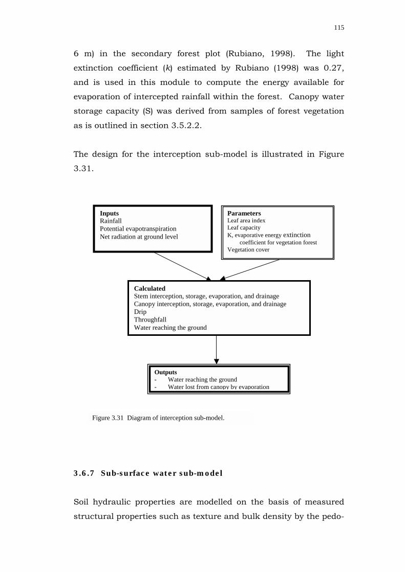
115
6 m) in the secondary forest plot (Rubiano, 1998). The light
extinction coefficient (k) estimated by Rubiano (1998) was 0.27,
and is used in this module to compute the energy available for
evaporation of intercepted rainfall within the forest. Canopy water
storage capacity (S) was derived from samples of forest vegetation
as is outlined in section 3.5.2.2.
The design for the interception sub-model is illustrated in Figure
3.31.
3.6.7 Sub-surface water sub-model
Soil hydraulic properties are modelled on the basis of measured
structural properties such as texture and bulk density by the pedo-
InputsRainfallPotential evapotranspirationNet radiation at ground level
ParametersLeaf area indexLeaf capacityK, evaporative energy extinction
coefficient for vegetation forestVegetation cover
CalculatedStem interception, storage, evaporation, and drainageCanopy interception, storage, evaporation, and drainageDripThroughfallWater reaching the ground
Outputs- Water reaching the ground- Water lost from canopy by evaporation
Figure 3.31 Diagram of interception sub-model.
116
transfer function of Saxton et al. (1986) that uses the Brooks and
Corey (1964) water retention function. The Saxton et al. (1986)
method is also used to determine soil hydraulic conductivity for
recharge calculation. These model sections are described next.
3.6.7.1 Modelling flow of water in porous media
The size of soil pores through which water flows and pore-size
distribution are mainly determined by grain-size distribution
(Dingman, 1994). For many purposes, particle-size and pore-size
distribution are characterised by soil texture, which is determined
by the proportion per weight of clay, silt, and sand. Figure 3.32
illustrates the scheme for defining soil textures developed by
USDA. Soil texture is determined from soil samples after particles
larger than sand (> 2 mm) have been removed.
The definitions of soil composition, soil classification, and soil
properties, as given by Kutilet and Nielsen (1994), were used in this
study. The routine aims to determine soil hydraulic properties, for
example hydraulic conductivity, matric potential, and soil
moisture. Several attempts have been made to predict moisture
release functions from soil texture data (Van Genuchten, 1980;
Arya and Paris, 1981; Grismer, 1986). Knowledge of particle-size
distribution helps determine pore-size distribution and moisture
retention characteristics. Although this approach presents several
difficulties, it is cheaper and easier than field determination
(Campbell, 1985) but this approach must be used with care
because the soils are extremely complex and variable. The
determination of pore-size, particle-size and pore-size distribution
facilitates the calculation of the space available in the soil for water
storage and movement. Arya and Paris (1981) established a non-
linear relationship between particle-size and pore-size

117
distributions, because water is held within the soil by capillary
binding of water in the pores; then the shape of water-retention
curve depends to a great extent on the pore-size distribution of the
soil (Anderson, 1990).
3.6.7.2 Soil water retention and matric potential
Matric potential is the amount of potential energy per unit of mass
or volume of water in a system, compared to that in pure free water
at a reference elevation point. Because water movement is very
slow through soil micro-pores, kinetic energy is extremely low and
may be neglected. Potential energy therefore dominates and
Figure 3.32. Soil texture triangle classification (Dingman, 1994).

118
results from gravity, capillary, and adsorptive forces. Hence, soil
water potential is the work (energy) needed to overcome forces
acting on soil water, referred from a given datum to the point of
interest.
Darcy’s law describes water infiltration and redistribution of flow in
unsaturated porous media. Campbell (1985) expressed the law as
where fw is the water flux density (kg m-2 s-1), dψ/dx the water
potential gradient, and k the hydraulic conductivity (m s-1). Water
potential is the energy potential per unit mass (or volume) (J kg-1,
J m-3) and is defined as the amount of work per unit mass of water
required to transport a certain quantity of liquid from the soil
matrix, taking into account a reference point.
Brooks and Corey (1964) fitted the following equation to describe
water potential:
where ψ is the soil water potential (J m-2), ψe the soil water
potential at air entry (J m-2), θ the soil water content (mm3 mm-3), θs
the saturated soil water content (mm3 mm-3), and θr the residual
soil water content (mm3 mm-3). This value is empirical to
straighten a curved log-log scale, and B is the fitted value. The
volumetric relationship between soil water content and soil water
potential for ψ < -5 kPa at any spatial location, i, is
Ln[-ψi(θ)] = ai + bi ln(θ)
f kd
dxw = −ψ
( )( )ψ ψθ θθ θ
=−
−
e
r
s r
B
Eq. 3.19
Eq. 3.20
Eq. 3.21

119
Campbell (1985) and others (Ahuja and Williams, 1991) assumed
θr= 0 and parameter b equal to the inverse of the Brooks and Corey
(1964) pore size index, λ (b=1/λ), then
where ψe is the air entry potential and b the slope of lnψ vs lnθ.
According to the Campbell (1985) notation for porosity, ψe
decreases with decreasing mean pore diameter size, and b
increases with increasing standard deviation of pore size.
Campbell (1985) correlated the geometric standard deviation (σg)
with b, approximating the relationship for soils at a bulk density of
1.3 Mg m-3.
3.6.7.3 Pedotransfer functions
An alternative way to determine the soil’s hydraulic characteristics,
for example hydraulic conductivity, soil water content, or soil water
retention other than direct methods with field or laboratory
measurements, is to use a pedotransfer function (PTF). The PTF
includes basic data describing the soil (e.g., particle-size
distribution, bulk density, and organic C content) and yields the
water retention function or the unsaturated hydraulic conductivity
function (Tietje and Tapkenhinrichs, 1993) on the basis of
empirical relationships based on analysis of a wide variety of soils.
Many researchers have performed this approximation using
different tools – algorithmic, empirical or semi-empirical – with the
general idea of producing a tool that can be applied to a broad
range of different soil conditions (Arya and Paris, 1981; Ahula, et
al., 1984; Mulla, 1989; Vereecken et al., 1989, 1990; Vereecken,
( )ψ ψ θ θm e s
b=
−/ Eq. 3.22
120
1992; Tietje and Tapkenhinrichs, 1993; Rawls et al., 1993). In
addition, many reports have been written comparing the results of
several modelled pedotransfer functions (Ahuja et al., 1984;
Vereecken et al., 1990; Tietje and Tapkenhinrichs, 1993).
Three different methods can produce a pedotransfer function: (a)
the point regression method, (b) the physical model method, and (c)
the functional parameter regression method. Tietje and
Tapkenhinrichs (1993) used a point regression method to estimate
retention functions from basic data and predict water content, θi at
certain matric potential, ψI, by regression analysis (generally
multiple linear). Their study included references from methods
developed by Gupta and Larson (1979) and Rawls et al. (1982).
The physical model method consists of three steps: (i) description of
pore-size distribution, (ii) prediction of soil water content from
pore-size distribution via mass conservation, and (iii) prediction of
matric potentials from pore-size distribution by the capillary
equation. This method was followed by Arya and Paris (1981), who
used an empirical relationship that incorporated different particle
forms into the pedo-transfer function and established a non-linear
relationship between particle-size and pore-size distributions.
Parameters were fitted to the data.
In the functional parameter regression method, a certain closed
form function is assumed for the relationship between ψ and θ, and
the parameters are found by regression or other estimators. Most
researchers in the field used the retention function parameter of
Brooks and Corey (1964); one of the most recent approaches by
Van Genuchten (1980) uses the parameters θr, θs (equivalent to the
inverse of ψb), n (equivalent to plus 1), and, in the most cases, m=1-
1/n:
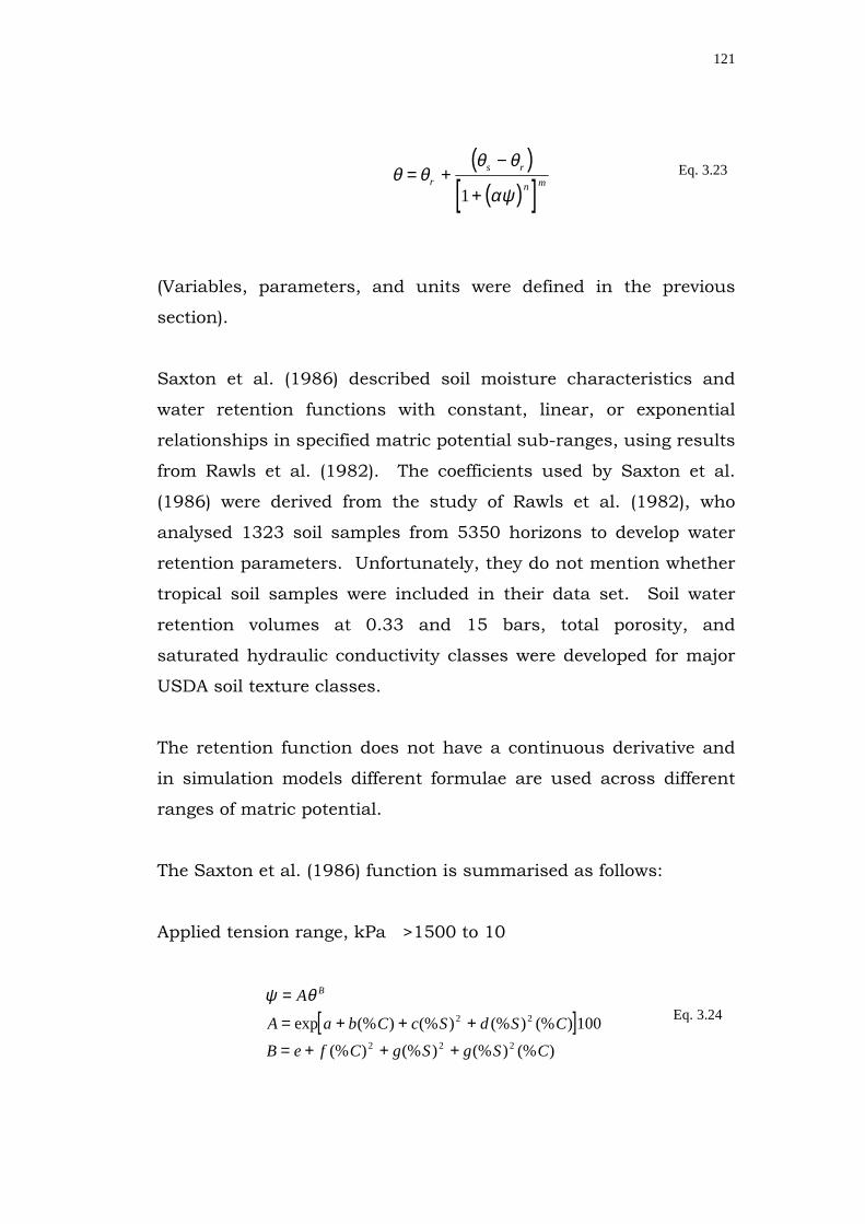
121
(Variables, parameters, and units were defined in the previous
section).
Saxton et al. (1986) described soil moisture characteristics and
water retention functions with constant, linear, or exponential
relationships in specified matric potential sub-ranges, using results
from Rawls et al. (1982). The coefficients used by Saxton et al.
(1986) were derived from the study of Rawls et al. (1982), who
analysed 1323 soil samples from 5350 horizons to develop water
retention parameters. Unfortunately, they do not mention whether
tropical soil samples were included in their data set. Soil water
retention volumes at 0.33 and 15 bars, total porosity, and
saturated hydraulic conductivity classes were developed for major
USDA soil texture classes.
The retention function does not have a continuous derivative and
in simulation models different formulae are used across different
ranges of matric potential.
The Saxton et al. (1986) function is summarised as follows:
Applied tension range, kPa >1500 to 10
( )( )[ ]
θ θθ θ
αψ= +
−
+r
s r
n m
1
[ ]ψ θ=
= + + +
= + + +
A
A a b C c S d S C
B e f C g S g S C
B
exp (% ) (% ) (% ) (% )
(% ) (% ) (% ) (% )
2 2
2 2 2
100
Eq. 3.23
Eq. 3.24

122
Applied tension range, kPa 10 to ψe
Applied tension range, kPa ψe to 0.0
Applied tension range, kPa >1500 to 0.0
Coefficients
a = -4.396 g = -3.484 x 10⁻⁶ p = 12.012
b = -0.0715 h = 0.332 q = -7.55 x 10⁻²
c = -4.88 x 10⁻⁴ j = -7.251 x 10⁻⁴ r = -3.8950
d = -4.285 x 10⁻⁵ k = 0.1276 t = 3.871 x 10⁻²
e =- 3.140 m = -0.108 u = -0.1103
f = - 2.22 x 10⁻³ n = 0.341 v = 8.7546 x 10⁻⁴
Definitions
ψ = water potential, kPa
ψe = water potential at air entry, kPa
θ = water content, m3 m-3
θs = water content at saturation, m3 m-3
θ10 = water content at 10 kPa, m3 m-3
K = water conductivity, m s-1
(%S) = percent sand
(%C) = percent clay
( )[ ][ ]
ψ θ θ ψ θ θθ
ψ θθ
= − − − −
= −
= += + +
10 0 10 0
2 302
100 0
10 10
10
10
. ( . ) / ( )
exp . ln /
. ( )
(% ) log (% )
e s
e s
s
A B
m n
h j S k C
θ θ= s
[ ]( )[ ]{ }K p q S r t S u C v C= × − + + + + +2 778 10 6 12. exp (% ) (% ) (% ) (% / θ
Eq. 3.25
Eq. 3.26
Eq. 3.27
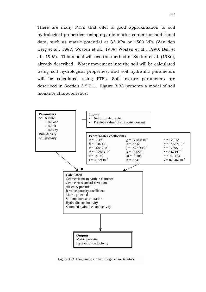
123
There are many PTFs that offer a good approximation to soil
hydrological properties, using organic matter content or additional
data, such as matric potential at 33 kPa or 1500 kPa (Van den
Berg et al., 1997; Wosten et al., 1989; Wosten et al., 1990; Bell et
al., 1995). This model will use the method of Saxton et al. (1986),
already described. Water movement into the soil will be calculated
using soil hydrological properties, and soil hydraulic parameters
will be calculated using PTFs. Soil texture parameters are
described in Section 3.5.2.1. Figure 3.33 presents a model of soil
moisture characteristics:
ParametersSoil texture
. % Sand
. % Silt
. % ClayBulk densitySoil porosity
Pedotransfer coefficientsa = -4.396 g = -3.484x10⁻⁵ p = 12.012b = -0.0715 h = 0.332 q = -7.55X10⁻²
c = -4.88x10⁻⁴ j = -7.251x10⁻⁴ r = -3.895d = -4.285x10⁻⁵ k = -0.1276 t = 3.671x10⁻²
e = -3.140 m = -0.108 u = -0.1103f = -2.22x10⁻³ n = 0.341 v = 87546x10-4
CalculatedGeometric mean particle diameterGeometric standard deviationAir entry potentialB-value porosity coefficientMatric potentialSoil moisture at saturationHydraulic conductivitySaturated hydraulic conductivity
OutputsMatric potentialHydraulic conductivity
Figure 3.33 Diagram of soil hydrologic characteristics.
Inputs- Net infiltrated water- Previous values of soil water content

124
3.6.8 Infiltration sub-model
Infiltration is the process by which rainfall or ponded water enters
the soil surface (Anderson, 1985; Campbell, 1985; Dingman, 1994)
and is one of the most difficult aspects of hydrology to estimate.
Infiltration is controlled by factors governing water movement
through the soil, for example pore size, pore-size distribution, soil
water content, hydrologic conductivity, and soil matric potential.
Both soil properties and vegetation characteristics play an
important role in determining infiltration.
Several attempts have been made to understand infiltration (Smith
et al., 1993; Morin and Kosovsky, 1995; Chu, 1997) and others
have tried to adapt or modify known models (Madramootoo and
Enright, 1990; James et al., 1993; Chu, 1994; Chu, 1995). A wide
range of modelling approaches: physically based, empirical,
stochastic, or mixed, have been used. Most of the previously
mentioned models have been based on Darcy’s Law, mass
conservation, and energy conservation.
Maidment (1993) discusses the following infiltration models:
Horton (1940), Brooks and Corey (1964), Richards (1965), Philip
(1957), and Van Genuchten (1980). A general agreement is that
Richard’s equation represents the closest physical approximation,
but is difficult to implement in numerical terms. Therefore, this
study applies Green and Ampt (1911) formulae, with soil
parameters as calculated by the Saxton et al. (1986) pedotransfer
function.
The main assumptions of the Green-Ampt approach are that a
distinct and precisely definable wetting front exists, and that the
matric suctions at this wetting front remain effectively constant,

125
regardless of time and position (Hillel, 1971). It is also assumed
that the soil behind the wetting front is uniformly wet and of
constant conductivity. The wetting front is thus viewed as a plane
separating a uniformly wetted infiltrated zone from a totally
uninfiltrated zone. This assumes that the relationship between
hydraulic conductivity (k) and soil water content (θ) is
discontinuous (Hillel, 1971).
For Green and Ampt (1911), ideal conditions would be as follows:
The vertical axis (elevation) z indicates the downward direction, f(t)
is the infiltration rate at time t [L T-1], and F(t) is the total amount
of water infiltrated up to time t [L]. The water content just before t
= 0, at the initial value θo <φ. The notation is taken from Dingman
(1994).
Just before water input begins at t = 0, the downward flux of water
given as Vz(z,0) is Kh(θo). Beginning at time t = 0, liquid water
begins arriving at the soil surface at a specified rainfall rate, w, and
continues at this rate until the time tw. Two cases are under
consideration at this point:
Where the water input rate is less than saturated hydraulic
conductivity, w < Khsat. If we assume that w > Kh(θo), then water
will enter the soil, increasing soil water content and, as a result,
both hydraulic conductivity and outward flux will also increase.
However, as long as the water entering the soil is less than the
water content at which conductivity equals water input rate Kh(θo),
soil water content will continue to increase. When soil water
content reaches θw, the hydraulic conductivity is Kh(θw) = w, so the
rate of the outflow from the soil equals the rate of the inflow, and
there is no further change in water content until water input
ceases. So, if

126
If w < Khsat f(t) = w ; 0 < t < tw ,
F(t) = 0 ; t > tw .
The water input rate is greater than saturated hydraulic
conductivity,
w > Khsat.
The process described above will occur in the early stages of
infiltration. Water arrives to the soil faster than it can be
transmitted downward, and will initially go into storage, increasing
the soil water content and hydraulic conductivity. However, soil
water content cannot exceed its value at saturation, φ, and
hydraulic conductivity cannot increase beyond w < Khsat. After the
soil surface is saturated, some rain will continue to infiltrate, but
excess water will accumulate on the surface as ponding or
detention storage. On sloping ground, this excess becomes
potential overland flow. The soil surface to become saturated is
referred to as time to ponding tp.
Until tp, all rain falling infiltrates. Therefore,
F(tp) = w tp
where zf is the depth to the wetting front, all this water occupying
the soil between the surface and zf (tp), so
F(tp) = zf (tp) (φ − θο )
Eq. 3.28
Eq. 3.29
Eq. 3.30
Eq. 3.31
127
To determine zf (tp), Darcy’s law was applied in a finite difference
form, between surface and depth zf (tp)
where ψf is the effective tension at the wetting front. At the time of
ponding, the soil surface is saturated and the tension is 0, the
hydraulic conductivity is equal to its saturation value, and the
infiltration rate is equal to the rainfall rate. When ψf < 0, then
because water input continues after ponding time as does
infiltration, but at a decreasing rate. If zf (t) is the wetting front
depth at the same time t, where tp < t < tw., then the infiltration
equation for this period is a function of infiltration capacity and a
function of the total infiltration that has occurred.
F(t) = zf (t) (φ − θο )
Regarding the relation of t as a function of F, then
V t f t w K kz tz p p hsat hsat
f
f p
( , ) ( )( )
00
= = = −−ψ Eq. 3.32
( )( )
( )f t KF thsat
o f= +−
1φ θ ψ
( ) ( )( )t
F t F t
K
f
K
F t f
F t f
p
hsat
o
hsat
p o
o
=−
+− + −
+ −
( ) ( )ln
( )
( )
ψ φ θ ψ φ θ
ψ φ θ
( )t
K
w w Kp
hsat f
hsat
=−
−
ψ φ θ
( )
Eq. 3.33
Eq. 3.34
Eq. 3.35
Eq. 3.36

128
where:
Khsat effective hydraulic conductivity (L T-1)
φ soil porosity (L3 L-3)
θo initial water content (L3 L-3)
F accumulated infiltration (L)
f infiltration rate (L T)
tp ponding time (T)
t evaluation time (T)
The infiltration sub-model includes the Green and Ampt model
(1911), using bulk density, and soil properties for the watershed,
with a pedo-transfer function, defined in the preliminary sub-
model, integrated into this sub-model. In the Green and Ampt
infiltration model, several variations were made to the final
equation after ponding time. These were:
where:
f(t) infiltration rate (mm h-1)
F(t) cumulative infiltration (mm)
w rainfall rate (mm h-1)
( )( )
( )( )
( )( )
f t ww K
Kt
F t K ww K
w K
Kt
hsat
hsat f o
hsat
f o
hsat
hsat
hsat f o
( )
( )
= +−
−
=−
−× +
−
−
−
−
1 2
1 2 1
21
2
2
21
2
ψ φ θ
ψ φ θ
ψ φ θ
Eq. 3.37
Eq. 3.38

129
ψf pressure head (mm)
φ porosity (mm3 mm-3)
θo initial moisture (mm)
Khsat saturated hydraulic conductivity (mm h-1)
t infiltration evaluation time
Both equations are valid for X < 1, where
for tp < t < tw , where tp is ponding time and tw the rainfall time.
In the model, the sub-routines for calculating ponding time (tp),
rate of infiltration after ponding time (f(tp)) and amount of
infiltration (F(tp)) are created considered to be processes to be used
when needed.
Both initial soil moisture, θo, and soil depth are important
parameters for this sub-model. The initial soil moisture θo was
assumed to be half the porosity. Sampling to determine soil depth
was not carried out because soil depth is very heterogeneous and
difficult to measure.
Though soil thickness is clearly an important hydrological
parameter which controls the soil storage capacity, amongst other
properties, it is extremely difficult to access. The only method
accessible is excavation and, since soil thickness was shown to
vary in a complex way spatially and at a range of scales, providing
a realistic spatially distributed soil thickness is not feasible. In
order to counteract this problem a representative depth of 1m was
chosen and applied uniformly across the catchment.
( )XF t
wt
w
f o p
≡− +
( )
ψ φ θ Eq. 3.39
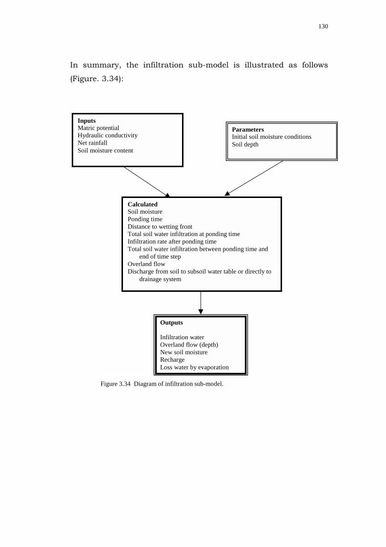
130
In summary, the infiltration sub-model is illustrated as follows
(Figure. 3.34):
InputsMatric potentialHydraulic conductivityNet rainfallSoil moisture content
ParametersInitial soil moisture conditionsSoil depth
CalculatedSoil moisturePonding timeDistance to wetting frontTotal soil water infiltration at ponding timeInfiltration rate after ponding timeTotal soil water infiltration between ponding time and
end of time stepOverland flowDischarge from soil to subsoil water table or directly to
drainage system
Outputs
Infiltration waterOverland flow (depth)New soil moistureRechargeLoss water by evaporation
Figure 3.34 Diagram of infiltration sub-model.

131
3.6.9 Overland flow sub-model
3.6.9.1 Sub-model description
Overland flow occurs whenever the rate of water application to the
ground surface exceeds the rate of infiltration into the soil (ward
and Elliot, 1995), or on the hillsides during rainstorm events when
surface depression storage is exceeded (Kirkby et al., 1980).
Runoff may result from short, highly intense rainfall, long low-
intensity rainfall, or a combination of both (Maidment, 1993).
Several approaches are used to estimate overland flow. Black-box
models have an input-output structure rather than physically
based transfer function. A statistical correspondence needs to be
established between input and output data. The unit hydrograph,
extreme frequency analysis, and regression analyses are examples
of this type of model. Deterministic models are based on complex
physical theory. They include several flow equations, which
produce high computational cost and significant data
requirements. They improve our understanding of the hydrological
system, regardless of their predictive success which is often not as
good as simpler models. In all cases models need to be adapted to
the problem rather than vice-versa. Conceptual models are a
combination of deterministic and black box models. Such models
are formulated on the basis of a simple arrangement of a relative
small number of components with a simplified representation of
elementary system.
To understand the processes that control overland flow, the factors
involved were systematically analysed. Four different processes
were taken in account at different times: Hortonian overland flow,
subsurface flow, saturation overland flow, and ground water
movement. Hortonian overland flow, as discussed in the
132
infiltration model (see Section 3.6.8), refers to the amount of
effective rainfall that reaches the soil at rates higher than soil
infiltration capacity. Subsurface flow or throughflow refers to the
water that infiltrates into the soil and percolates rapidly, mainly
through macropores. Saturation overland flow occurs when the
water table reaches the surface (100% soil saturation) and forms
excess water, thus generating overland flow. Ground water
movement can generally be described in two ways: vertical
movement, which includes raising the ground water table or
pumping water through wells with natural hydraulic
characteristics, and lateral movement, such as throughflow.
Rainfall characteristics exert a strong influence on overland flow
events. Rainfall intensity combined with soil water saturation and
storm characteristics have important implications for flow
generation.
Temporal and spatial variations in runoff, caused by rainfall
properties, may be greatly enhanced by spatial variations in
infiltration capacity of the soil surface. Research conducted in
humid areas indicates that the frequency and magnitude of storm
channel runoff is controlled mainly by the extent and distribution
of saturated areas (Anderson and Burt, 1985). Such areas respond
quickly even to low-intensity rainstorms. Therefore, the spatial
distribution of soil moisture cannot be regarded as a major factor
in the control of storm runoff generation, and spatial non-
uniformity of runoff generation relates significantly to spatial
variations in infiltration capacities.
Overland flow frequency and magnitude therefore depends on
several factors, including geomorphological characteristics (such as
slope, slope distance, aspect, catchment area, among others),
rainfall characteristics (frequency, intensity, duration) and soil
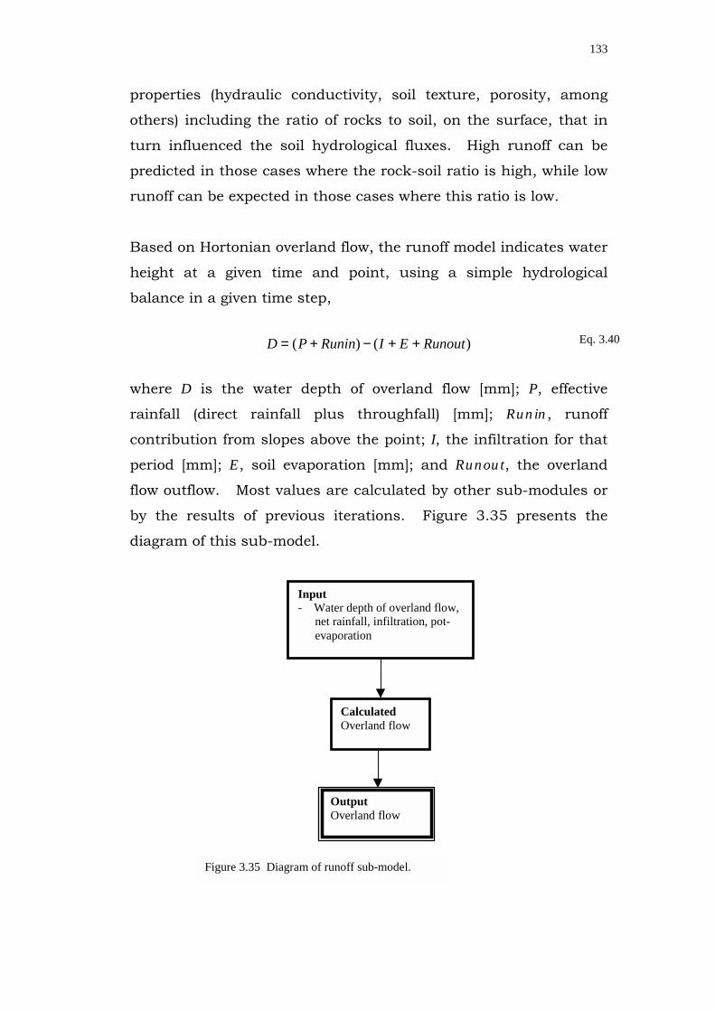
133
properties (hydraulic conductivity, soil texture, porosity, among
others) including the ratio of rocks to soil, on the surface, that in
turn influenced the soil hydrological fluxes. High runoff can be
predicted in those cases where the rock-soil ratio is high, while low
runoff can be expected in those cases where this ratio is low.
Based on Hortonian overland flow, the runoff model indicates water
height at a given time and point, using a simple hydrological
balance in a given time step,
where D is the water depth of overland flow [mm]; P, effective
rainfall (direct rainfall plus throughfall) [mm]; Runin, runoff
contribution from slopes above the point; I, the infiltration for that
period [mm]; E, soil evaporation [mm]; and Runout, the overland
flow outflow. Most values are calculated by other sub-modules or
by the results of previous iterations. Figure 3.35 presents the
diagram of this sub-model.
D P Runin I E Runout= + − + +( ) ( )
Input- Water depth of overland flow,
net rainfall, infiltration, pot-evaporation
OutputOverland flow
CalculatedOverland flow
Figure 3.35 Diagram of runoff sub-model.
Eq. 3.40
134
3.6.9.2 Surface component of overland flow at the catchmentscale
The integration of a surface component in the model produces an
extension of the 1D model at the plot scale to a 2.5 D model at the
catchment scale.
The overland flow sub-model is the only component within the
hydrological model that is changed in this way. Water which ponds
is allowed to flow downslope according to the local drainage
direction (LDD). The overland flow sub-model computes the
amount of outflow surface water in a down slope direction for a
particular area. The inflow water volume is computed by the
UPSTREAM routine used in the GIS component (PCRaster
software), which is the sum of all overland flow values of the
upslope direction areas. This command (upstream) uses as a
parameter the local drainage direction (ldd) network, which is a
direction network connection between areas, which indicates the
flow direction; ldd is derived from the digital elevation model
(DEM). All surface water that is not infiltrated or evaporated
moves down slope direction. The model does not incorporate a
detention storage capacity. LDD is calculated using the 8 point
pour algorithm with flow directions from each cell to its steepest
downslope neighbour. The manner in which PCRaster calculates
the LDD is explained in the user manual (Utrecht University,
1996).
3.6.10 Erosion sub-model
Soil erosion is modelled to identify areas where soil detachment
and loss by natural or anthropogenic causes occurs. The
importance of assessing and quantifying soil loss in TMEs due to
135
LUCC lies in its effects on landscape transformation and
environmental consequences.
Most of the knowledge of soil erosion mechanisms is the result of
studies carried out by the US Soil Conservation Service, which has
emphasised the prediction of erosion rates. Therefore, most of
these approaches are based on empirical equations or on
generalisations for specific scenarios. Kirkby and Morgan (1980)
compiled a number of these developments in detail. The most
common reference point in this field is the Universal Soil Loss
Equation (USLE), which estimates erosion as the product of a
series of terms such as rainfall, slope gradient, slope length, soil
and cropping factors. The equation allows individual factors,
developed from extensive observation of experimental plots in the
US, to be tabulated.
Recent developments in this field are discussed by Boardman and
Favis-Mortlock (1993), who compiled the most commonly used
erosion models and described the different approaches used and
the specific characteristics of each. Although these models often
require significant data for parameterisation and input information,
they describe erosion in detail and the accuracy of the approaches.
Despite technological advances, the development of erosion models
is still largely empirical. Further, research is required because of
the extreme complexity of the physical processes involved in
erosion.
Climatic variables, such as rainfall intensity, have a major effect on
the ecosystem and also exert an effective control on the variables
that determine soil stability. Vegetation cover also has an
important effect because it provides protection against rain splash
and sediment detachment and transportation (Kirkby and Morgan,
1980; Boardman and Favis-Mortlock 1993).

136
Musgrave (1947) developed a relationship between rainfall
characteristics and the amount of soil loss using data from several
stations. He developed a relation which involves slope parameter,
surface runoff and rainfall properties (Thornes and Gilman, 1983;
Thornes, personal communication), and is expressed as follows:
where k1, m and n are parameters (discussed below), and q the
surface overland flow per unit width (mm.h-1) (Thornes, 1990) as
defined in previous section.
Musgrave’s (1947) equation was the basis for Thornes’s model
(1985) which was developed on the basis of results of small
experimental plots (20m2) in Spain and with rainfall records
shorter than an hour, which guarantee that the rainfall properties
are important.
The erosion model proposed by Thornes (1985) was used in this
study, and focuses on the competitive interaction between erosion
and vegetation cover. This routine can be incorporated into the
hydrological model because it is based on physical characteristics
of the soil profile (Thornes, 1990). The spatial variation of erosion
on hillsides can also be examined for the entire watershed. This
method was also chosen because (a) it is a physically-based
approach that uses local data; (b) the spatial resolution of the
proposed model (25m pixel side size) which is related to the
experimental plot size used by Thornes; (c) the input data needed
are available, which uses local information at a good temporal
resolution; and (d) the parameters are easy to estimate or adapt
from the literature.
E k q sm n= 1 Equ. 3.41
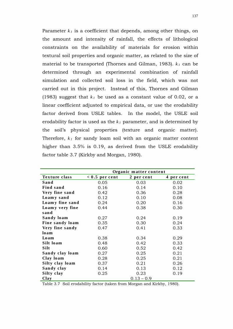
137
Parameter k1 is a coefficient that depends, among other things, on
the amount and intensity of rainfall, the effects of lithological
constraints on the availability of materials for erosion within
textural soil properties and organic matter, as related to the size of
material to be transported (Thornes and Gilman, 1983). k1 can be
determined through an experimental combination of rainfall
simulation and collected soil loss in the field, which was not
carried out in this project. Instead of this, Thornes and Gilman
(1983) suggest that k1 be used as a constant value of 0.02, or a
linear coefficient adjusted to empirical data, or use the erodability
factor derived from USLE tables. In the model, the USLE soil
erodability factor is used as the k1 parameter, and is determined by
the soil’s physical properties (texture and organic matter).
Therefore, k1 for sandy loam soil with an organic matter content
higher than 3.5% is 0.19, as derived from the USLE erodability
factor table 3.7 (Kirkby and Morgan, 1980).
Organic matter contentTexture class < 0.5 per cent 2 per cent 4 per centSand 0.05 0.03 0.02Find sand 0.16 0.14 0.10Very fine sand 0.42 0.36 0.28Loamy sand 0.12 0.10 0.08Loamy fine sand 0.24 0.20 0.16Loamy very finesand
0.44 0.38 0.30
Sandy loam 0.27 0.24 0.19Fine sandy loam 0.35 0.30 0.24Very fine sandyloam
0.47 0.41 0.33
Loam 0.38 0.34 0.29Silt loam 0.48 0.42 0.33Silt 0.60 0.52 0.42Sandy clay loam 0.27 0.25 0.21Clay loam 0.28 0.25 0.21Silty clay loam 0.37 0.21 0.26Sandy clay 0.14 0.13 0.12Silty clay 0.25 0.23 0.19Clay 0.13 – 0.9Table 3.7 Soil erodability factor (taken from Morgan and Kirkby, 1980).
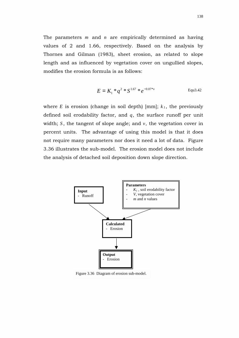
138
The parameters m and n are empirically determined as having
values of 2 and 1.66, respectively. Based on the analysis by
Thornes and Gilman (1983), sheet erosion, as related to slope
length and as influenced by vegetation cover on ungullied slopes,
modifies the erosion formula is as follows:
where E is erosion (change in soil depth) [mm]; k1, the previously
defined soil erodability factor, and q, the surface runoff per unit
width; S, the tangent of slope angle; and v, the vegetation cover in
percent units. The advantage of using this model is that it does
not require many parameters nor does it need a lot of data. Figure
3.36 illustrates the sub-model. The erosion model does not include
the analysis of detached soil deposition down slope direction.
E K q S e v= −1
2 1 67 0 07* * *. . *
Figure 3.36 Diagram of erosion sub-model.
Input- Runoff
Parameters- K1 , soil erodability factor- V, vegetation cover- m and n values
Calculated- Erosion
Output- Erosion
Equ3.42
139
3.7 Integrating the sub-models in the 1D and 2.5D models
The 1D model was applied at the plot scale, using the collected
data from the weather stations. The 2.5D model was developed at
catchment scale on the basis of 1D model data and modules, in
order to produce comparable results. However, the 2.5D model
was integrated over the whole Tambito watershed (see Figure
3.21). In GIS concepts, the study area is delimited by the defined
window in section 3.2, which contains 35,534 square regular areas
of 25m pixel side size, organised in 163 columns by 218 rows, and
from which 22577 internal pixels conform the Tambito watershed
that is around 1,411 ha.
3.7.1 Module sequence
Model execution starts with the reading of data from the input file
(see Appendix 6). This file organised by lines, contains two main
data sets: the first, which has year, month, day, and hour, which
all together define the time step, and the second set is the rainfall
occurring within that time step.
With the date and time the solar module computes the incident
solar radiation for each pixel. Then cloud cover is computed
followed by net radiation, which is used in the computation of
potential evaporation.
Intercepted rainfall is computed using an image of vegetation type,
which the first image of the scenarios, derived from TM Landsat
image (Museo de Historia Natural, 1989) (see section 3.4.1), and
the following iterations use the vegetation cover images created for
the processes described in section 3.4.2 as dynamic LUCC
scenarios, which are complemented with vegetation parameters

140
(see section 3.5.2.2). The potential evaporation module is then
used to compute canopy evaporation using the energy extinction
according to LAI (see section 3.5.2.2). Evaporated water from the
canopy and effective rainfall (direct rainfall plus throughfall) (see
section 3.6.5 and 3..6.6) are outputs from the interception module.
This effective rainfall is used in the infiltration module to estimate
the soil water infiltrated (see section 3.6.8), recharge and surface
water as overland flow. The overland flow module computes the
accumulated surface water, which is moved between cells; then
erosion is finally computed.
The units used within the models are KJ∙m-2 for energy and mm∙h-1
for water fluxes. All fluxes for the analysis use this unit in order to
be able to compare and evaluate the results. Erosion is computed
as depth of removed soil (mm∙h-1).
Cumulative images and average values are used to summarise flux
values within the sub-models. The main model outputs variables
are: solar radiation, cloud cover, net radiation, rainfall
interception, effective rainfall, infiltration, matric potential,
hydraulic conductivity, soil moisture, recharge, overland flow and
erosion. Most of these variables are used in the analysis. The
program code of the model can be seen in Appendix 9.
3.7.2 Data used in the model
The only input data variable in the model is rainfall. In the 1D
model the rainfall value is used directly from the input file. In the
2.5D model rainfall it is distributed through the catchment surface
using a rainfall elevation function derived from IDEAM weather
station (20 de Julio – 2200 masl-) and Tambito weather station
(1450 masl), (Mulligan et al., 2000) using the annual rainfall. The
141
derived rainfall distribution function combined with the elevation
and rainfall of Tambito station was
Rainfall = Rainfall(i) * (1 + diff-elevation * 0.001) (mm)
Where,
Rainfall(i) is the input rainfall (mm per hour) (Tambito station
rainfall) and diff-elevation is the difference in elevation between
any point within the catchment from digital elevation model (DEM)
and the Tambito station elevation.
The annual rainfall for the simulated period was 7325 mm in
Tambito station (elev. 1410 masl); the example used here is one of
the wettest years in Tambito, because the normal annual rainfall is
around 4500 mm a year. A map of the estimated rainfall
distribution is shown in Figure 3.37. Hourly rainfall data are
plotted in Figure 3.38 and the frequency distribution in Figure
3.39. 73% of all recorded hours studied (6427) were without
rainfall. 25% of hours (2239) has rainfall less than 20mm. Less
than 1.5% (80) hours have rainfall between 20-50mm. Just 13
hours had rainfall greater than 50mm, with just 4 hours with more
than 80mm, with a maximum of 110.2 mm in one hour.
Equ. 3.43
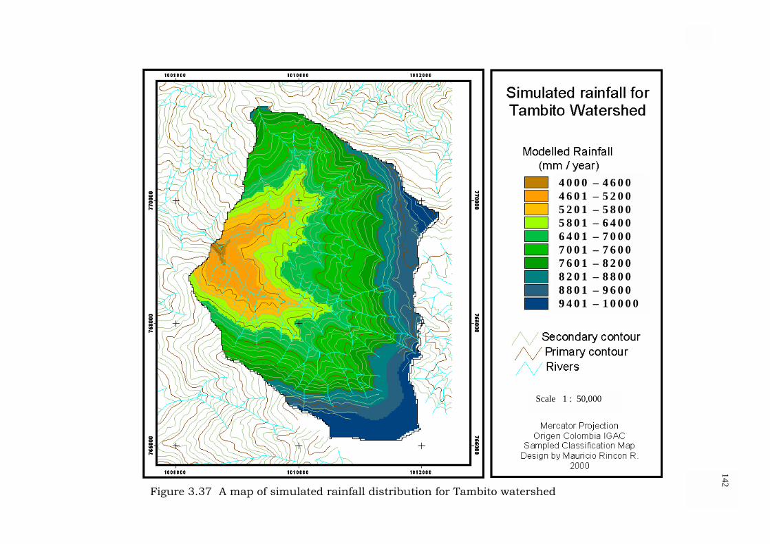
142
Figure
4000 – 46004601 – 52005201 – 5800
3.37 A map of simulated rainfall distribution for Tambito watershed
5801 – 64006401 – 70007001 – 76007601 – 82008201 – 88008801 – 96009401 – 10000
142
Scale 1 : 50,000
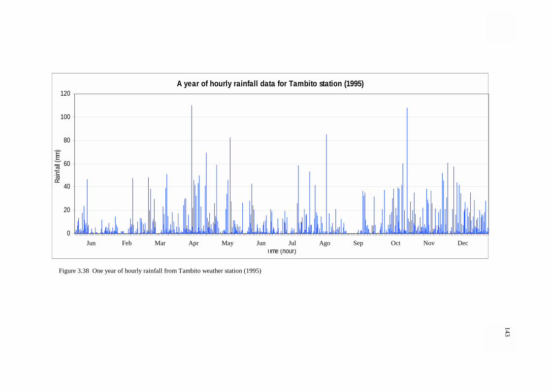
143
A year of hourly rainfall data for Tambito station (1995)
0
20
40
60
80
100
120
1 1001 2001 3001 4001 5001 6001 7001 8001Time (hour)
Rain
fall (
mm
)
Figure 3.38 One year of hourly rainfall from Tambito weather station (1995)
Jun Feb Mar Apr May Jun Jul Ago Sep Oct Nov Dec
143
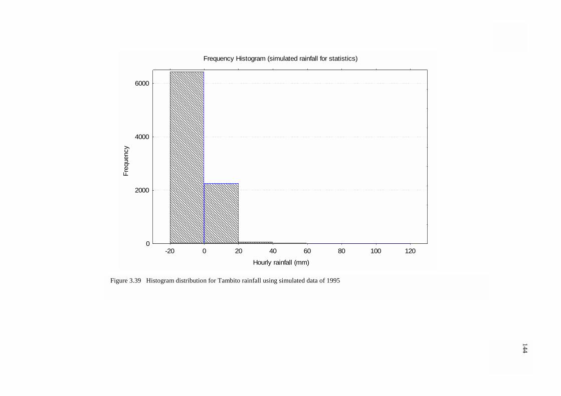
144144
Frequency Histogram (simulated rainfall for statistics)
Hourly rainfall (mm)
Fre
quen
cy
���������������������������������������������������������������������������������������������������������������������������������������������������������������������������������������������������������������������������������������������������������������������������������������������������������������������������������������������������������������������������������������������������������������������������������������������������������������������������������������������������������������������������������������������������������������������������������������������������������������������������������������������������������������������������������������������������
������������������������������������������������������������������������������������������������������������������������������������������������������������������������������������������������������������������������������������������������������������������������������������������������������������������ ��������������� ���������������0
2000
4000
6000
-20 0 20 40 60 80 100 120
Figure 3.39 Histogram distribution for Tambito rainfall using simulated data of 1995

145
The mean hourly rainfall was 0.83mm, with a variance of 19.38
and standard deviation of 4.4.
As seen, the rainfall pattern is typical of rain forests, with a high
precipitation level overall and few, but powerful strong showers,
which can produce very high overland flow and erosion.
3.7.3 Parameters used in the model
Three classes of parameters are used in the model:
Class 1: Parameters used in net radiation equation A and B (see
linear regression equation, section 3.6.4.3) the parameter values
are 0.85 and 16.97 respectively, and those values are used for the
whole catchment. They are assumed to be non-varying with the
surface and are the same for any point within the catchment.
Class 2: Parameters that vary with vegetation type:
- Light extinction for evaporative energy inside of forest canopy,
which is 0.26 for forest. In grassland it is not taken into
account.
- Leaf area index
- Maximum water storage canopy
- Vegetation cover.
Values of the last three parameters are in table 3.6, and a
description of their measurement is given in section 3.5. The
distribution of these parameters over the catchment is in
accordance with LUCC images generated for the LUCC scenarios
(see section 3.4 and Appendix 1).

146
Class 3: Parameters which depend upon soil physical properties.
One soil type was defined on the basis of field data as
representative for the whole catchment: sandy clay loam. There is
no soil type variation throughout the catchment. Parameter values
for sandy clay loam are in table 3.8. In this way, the soil module is
conceptually lumped and the only response to deforestation is
through its effect on the vegetation properties.
Parameter valueSoil texture (sand, clay and silt) 57.03% , 21.8% , 21.23%
Soil porosity 0.61
Soil depth 1000 mm
Erodibility factor K 0.2
M value of erosion equation 2
N value of erosion equation 1.667
Table 3.8 Soil parameters used in the physically-based hydrological
model
Soil parameter definitions are described in section 3.5.2.1.

147
Chapter IV Model results, sensitivity analysis and validation
4.1 Structure of this chapter
Throughout this chapter the results for model experiments are
reported in order to show the model response to hydrological
events. In addition the hydrological model sensitivity are also
presented to illustrate the effects of LUCC on the hydrological cycle
for TMCF environments. First of all, both 1D and 2.5D models
were integrated twice, one with a completely forested catchment
and the other with the catchment completely covered by grassland.
The 1D model was run for a short period (fifteen days) and the
results are shown graphically to identify the model behaviour at
this time resolution (an hourly time step). Also this gives the
manner of model response to rainfall events for the different land
uses. Subsequently results of 2.5D hydrological modelling for one
modelled year are presented, particularly for overland flow and
erosion. Model results are presented in maps to show the
behaviour of the hydrological events for each point within the
catchment, which summarises the yield (difference by m2) between
the runs and the variables for forested and deforested catchment
response.
Sensitivity analyses at both the plot and the catchment scales are
presented. First of all, sensitivity analysis at the plot scale (1D
model) is carried out for all parameters within the model, and
secondly at the catchment scale (2.5D model), analysing the
implications of surface connectivity and the relationships between
hydrological flux changes and the controlling landscape
topographic variables of forested and deforested areas. The
collection of initial parameter values are described in this section,
as well as the data used for model parameterisation.

148
Sensitivity analysis for the 1D model is used to indicate which are
the most important parameters within the model and the most
sensitive variables to parameter change. Sensitivity analysis for
the 2.5D model shows the relationship between overland flow and
erosion sensitivities with respect to landscape topographic
characteristics, and in relation to the location of deforested areas
within the catchment. Sensitivity analysis at the catchment scale
identifies the most sensitive areas to land use change and the
relationship of these with the surface physical properties.
Model validation at the plot scale is discussed in the final section of
the chapter, where the agreement between modelled and measured
data for both an hourly time step and for daily average time step is
shown.
4.2 Model results
Examples of 1D and 2.5D model runs are presented as model
results to illustrate the behaviour of the flux variables during the
hydrological modelling process. The 1D model is presented at
hourly time steps for a short period to show the model skills
required to represent the flux variations at this time resolution.
The 2.5D model results are shown for one modelled year for the
main variables presented here (overland flow and erosion) for the
whole catchment as a surface image.
4.2.1 Model results at the plot scale
As a means of verifying the function of the 1D model, it was run
with collected data for the first fifteen days of the month of April
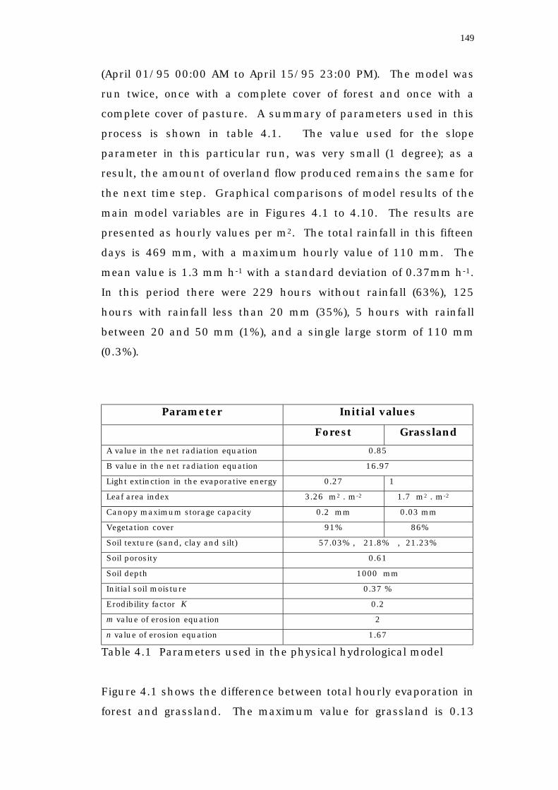
149
(April 01/95 00:00 AM to April 15/95 23:00 PM). The model was
run twice, once with a complete cover of forest and once with a
complete cover of pasture. A summary of parameters used in this
process is shown in table 4.1. The value used for the slope
parameter in this particular run, was very small (1 degree); as a
result, the amount of overland flow produced remains the same for
the next time step. Graphical comparisons of model results of the
main model variables are in Figures 4.1 to 4.10. The results are
presented as hourly values per m2. The total rainfall in this fifteen
days is 469 mm, with a maximum hourly value of 110 mm. The
mean value is 1.3 mm h-1 with a standard deviation of 0.37mm h-1.
In this period there were 229 hours without rainfall (63%), 125
hours with rainfall less than 20 mm (35%), 5 hours with rainfall
between 20 and 50 mm (1%), and a single large storm of 110 mm
(0.3%).
Parameter Initial values
Forest GrasslandA value in the net radiation equation 0.85
B value in the net radiation equation 16.97
Light extinction in the evaporative energy 0.27 1
Leaf area index 3.26 m2 . m-2 1.7 m2 . m-2
Canopy maximum storage capacity 0.2 mm 0.03 mm
Vegetation cover 91% 86%
Soil texture (sand, clay and silt) 57.03% , 21.8% , 21.23%
Soil porosity 0.61
Soil depth 1000 mm
Initial soil moisture 0.37 %
Erodibility factor K 0.2
m value of erosion equation 2
n value of erosion equation 1.67
Table 4.1 Parameters used in the physical hydrological model
Figure 4.1 shows the difference between total hourly evaporation in
forest and grassland. The maximum value for grassland is 0.13
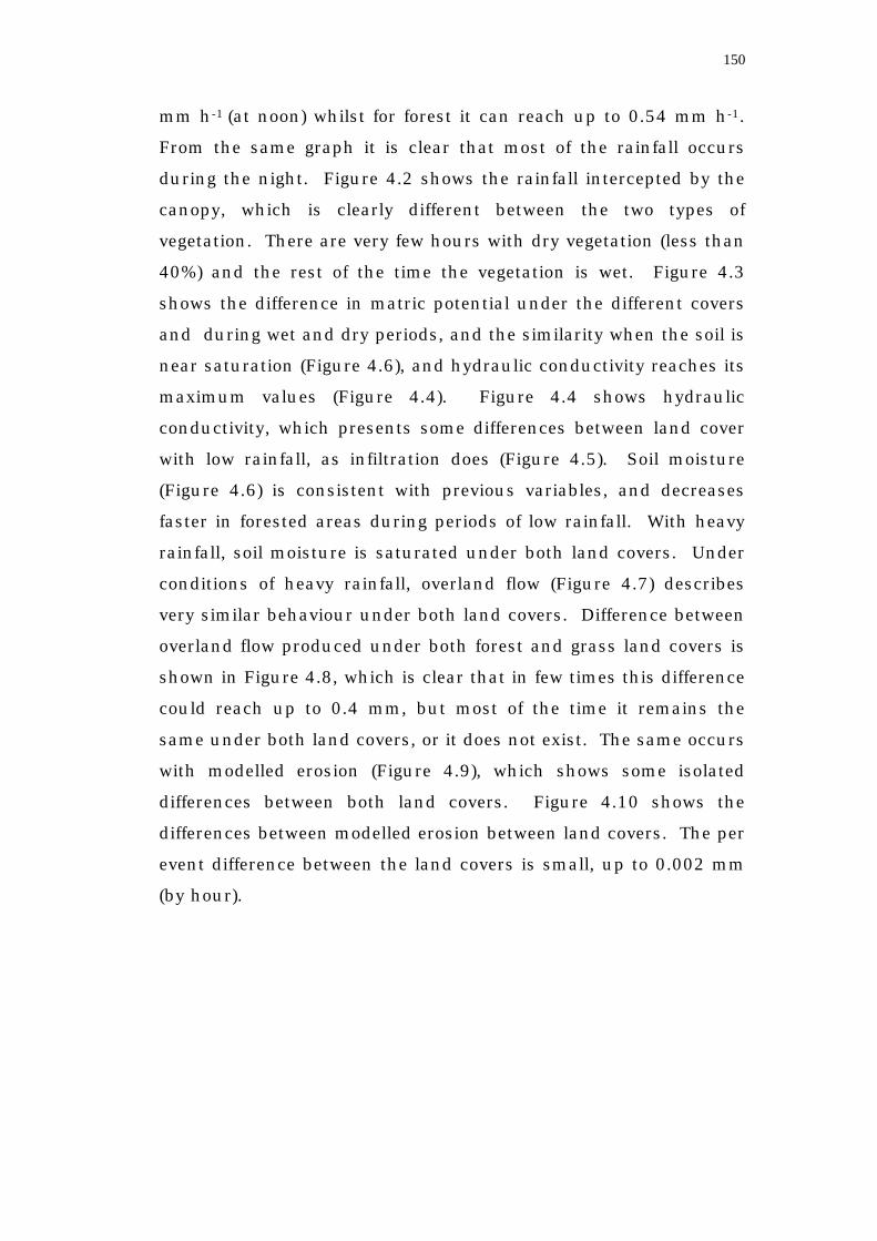
150
mm h-1 (at noon) whilst for forest it can reach up to 0.54 mm h-1.
From the same graph it is clear that most of the rainfall occurs
during the night. Figure 4.2 shows the rainfall intercepted by the
canopy, which is clearly different between the two types of
vegetation. There are very few hours with dry vegetation (less than
40%) and the rest of the time the vegetation is wet. Figure 4.3
shows the difference in matric potential under the different covers
and during wet and dry periods, and the similarity when the soil is
near saturation (Figure 4.6), and hydraulic conductivity reaches its
maximum values (Figure 4.4). Figure 4.4 shows hydraulic
conductivity, which presents some differences between land cover
with low rainfall, as infiltration does (Figure 4.5). Soil moisture
(Figure 4.6) is consistent with previous variables, and decreases
faster in forested areas during periods of low rainfall. With heavy
rainfall, soil moisture is saturated under both land covers. Under
conditions of heavy rainfall, overland flow (Figure 4.7) describes
very similar behaviour under both land covers. Difference between
overland flow produced under both forest and grass land covers is
shown in Figure 4.8, which is clear that in few times this difference
could reach up to 0.4 mm, but most of the time it remains the
same under both land covers, or it does not exist. The same occurs
with modelled erosion (Figure 4.9), which shows some isolated
differences between both land covers. Figure 4.10 shows the
differences between modelled erosion between land covers. The per
event difference between the land covers is small, up to 0.002 mm
(by hour).
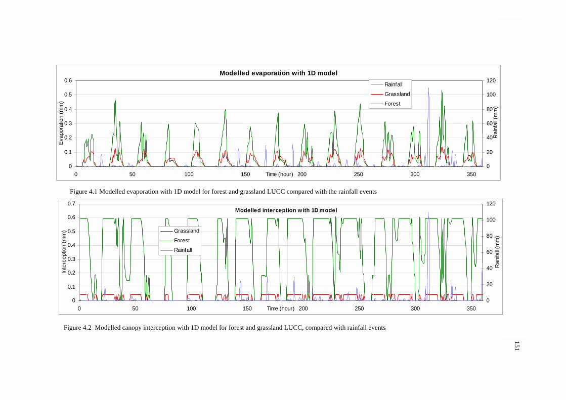
151
Figure 4.1 Modelled evaporation with 1D model for forest and grassland LUCC compared with the rainfall events
Modelled evaporation with 1D model
0
0.1
0.2
0.3
0.4
0.5
0.6
0 50 100 150 200 250 300 350Time (hour)
Eva
pora
tion
(mm
)
0
20
40
60
80
100
120
Rai
nfal
l (m
m)
Rainfall
Grassland
Forest
Figure 4.2 Modelled canopy interception with 1D model for forest and grassland LUCC, compared with rainfall events
Modelled interception w ith 1D model
0
0.1
0.2
0.3
0.4
0.5
0.6
0.7
0 50 100 150 200 250 300 350Time (hour)
Inte
rcep
tion
(mm
)
0
20
40
60
80
100
120
Ran
ifall
(mm
)
Grassland
Forest
Rainfall
151
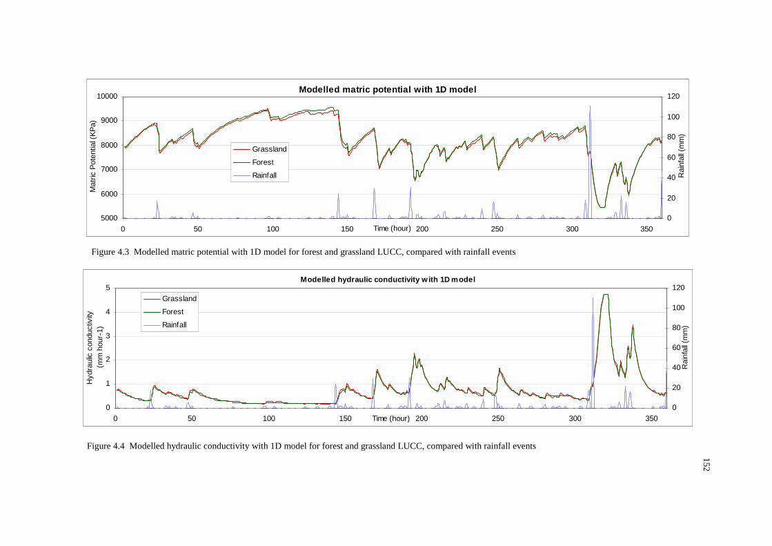
152
Figure 4.3 Modelled matric potential with 1D model for forest and grassland LUCC, compared with rainfall events
Modelled matric potential with 1D model
5000
6000
7000
8000
9000
10000
0 50 100 150 200 250 300 350Time (hour)
Mat
ric P
oten
tial (
KP
a)
0
20
40
60
80
100
120
Rai
nfal
l (m
m)
Grassland
Forest
Rainfall
Figure 4.4 Modelled hydraulic conductivity with 1D model for forest and grassland LUCC, compared with rainfall events
Modelled hydraulic conductivity w ith 1D model
0
1
2
3
4
5
0 50 100 150 200 250 300 350Time (hour)
Hyd
raul
ic c
ondu
ctiv
ity
(mm
hou
r-1)
0
20
40
60
80
100
120
Rai
nfal
l (m
m)
Grassland
Forest
Rainfall
152
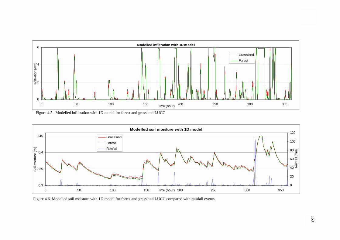
153
Modelled infiltration w ith 1D model
0
2
4
6
0 50 100 150 200 250 300 350Time (hour)
Infil
trat
ion
(mm
)
Grassland
Forest
Figure 4.5 Modelled infiltration with 1D model for forest and grassland LUCC
Modelled soil moisture with 1D model
0.3
0.35
0.4
0.45
0 50 100 150 200 250 300 350Time (hour)
Soi
l moi
stur
e (%
)
0
20
40
60
80
100
120
Rai
nfal
l (m
m)
Grassland
Forest
Rainfall
Figure 4.6 Modelled soil moisture with 1D model for forest and grassland LUCC compared with rainfall events
153
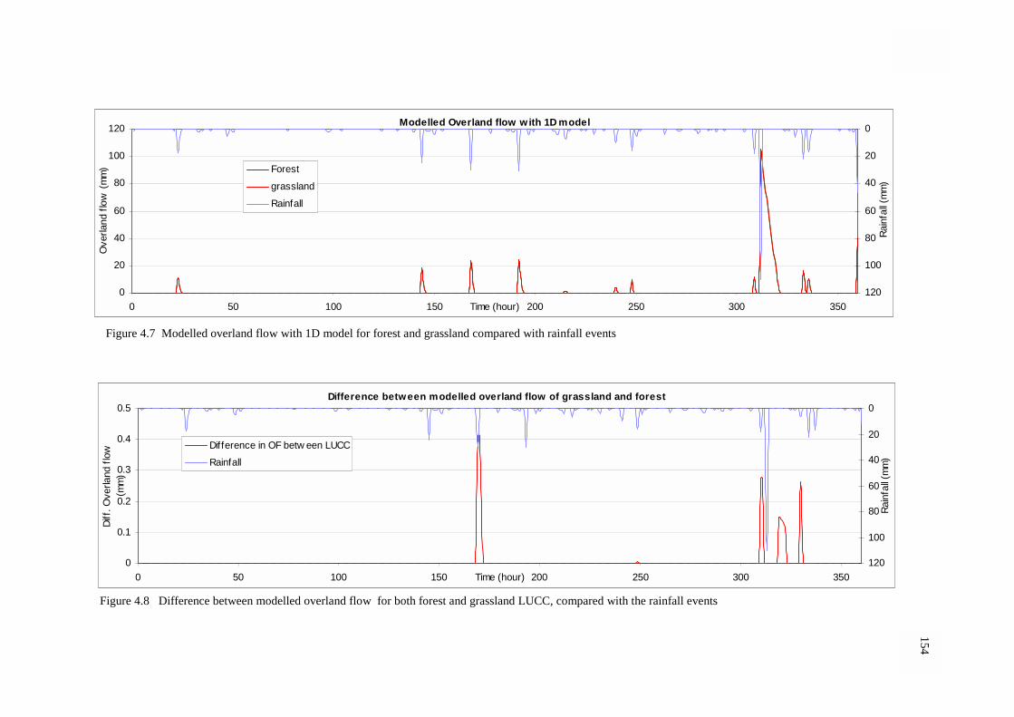
154
Difference between modelled overland flow of grassland and forest
0
0.1
0.2
0.3
0.4
0.5
0 50 100 150 200 250 300 350Time (hour)
Diff
. Ove
rland
flo
w
(mm
)
0
20
40
60
80
100
120
Rai
nfal
l (m
m)
Dif ference in OF betw een LUCC
Rainfall
Modelled Overland flow w ith 1D model
0
20
40
60
80
100
120
0 50 100 150 200 250 300 350Time (hour)
Ove
rland
flo
w (
mm
)
0
20
40
60
80
100
120
Rai
nfal
l (m
m)
Forest
grassland
Rainfall
Figure 4.7 Modelled overland flow with 1D model for forest and grassland compared with rainfall events
Figure 4.8 Difference between modelled overland flow for both forest and grassland LUCC, compared with the rainfall events
154
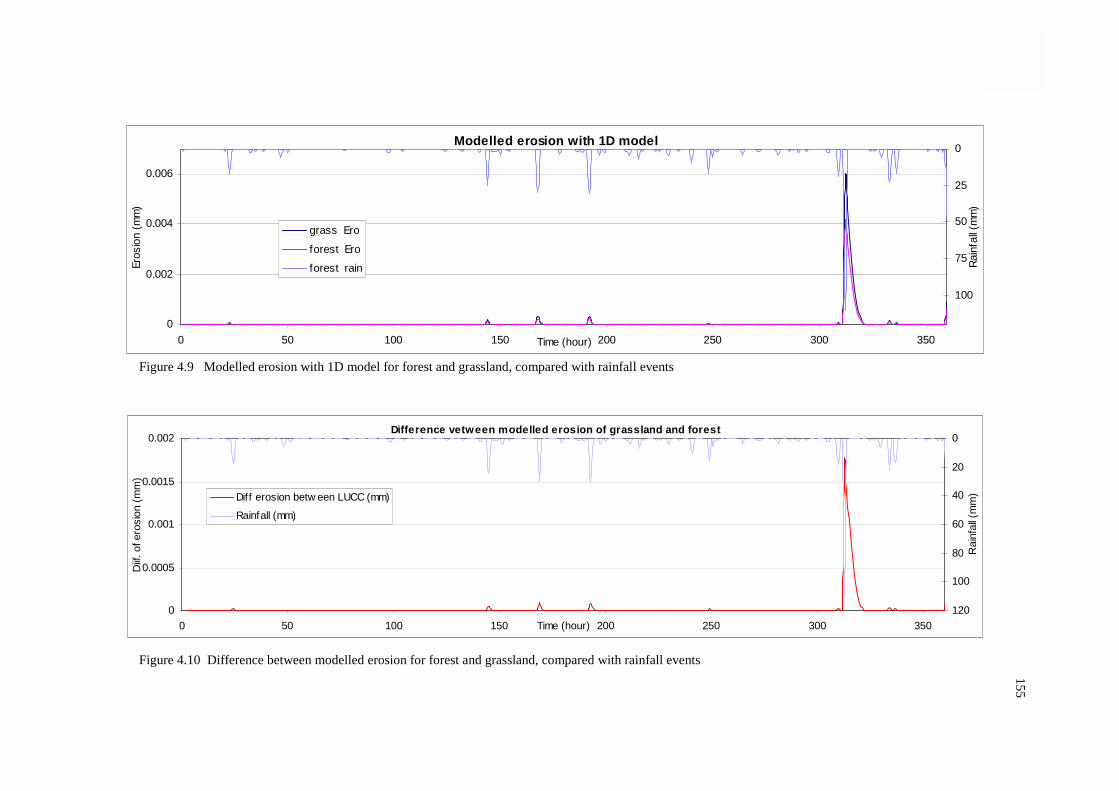
155
Modelled erosion with 1D model
0
0.002
0.004
0.006
0 50 100 150 200 250 300 350Time (hour)
Eros
ion
(mm
)0
25
50
75
100
Rai
nfal
l (m
m)
grass Ero
forest Ero
forest rain
Figure 4.9 Modelled erosion with 1D model for forest and grassland, compared with rainfall events
Figure 4.10 Difference between modelled erosion for forest and grassland, compared with rainfall events
Difference vetween modelled erosion of grassland and forest
0
0.0005
0.001
0.0015
0.002
0 50 100 150 200 250 300 350Time (hour)
Diif
. of e
rosi
on (
mm
)
0
20
40
60
80
100
120
Rai
nfal
l (m
m)Diff erosion betw een LUCC (mm)
Rainfall (mm)
155

156
4.2.2 Model results at the catchment scale
In order to illustrate the model flux variation at the catchment
scale, the 2.5D model was run twice; first with the initial image of
vegetation cover used in the scenarios (NDVI from the Landsat
image TM 1989), and secondly, with the whole catchment
deforested and replaced with the grass cover. Overland flow and
erosion were summarised in the catchment images, which in both
cases show the difference in yield per m2 between the two model
runs, for forested and then deforested catchment. These maps
show the increase in overland flow and erosion due to complete
LUCC in the catchment.
Overland flow (Figure 4.11) increased up to 300mm in a year for
the areas with steepest slopes as a product of deforestation. Areas
within the river channels were not taken into account, because
thesis will not deal with modelling flow in river channels, only
hillslopes. About 15% of the catchment area has less than 46mm
of increment in overland flow with deforestation. Most of these
areas are in the lower part of the catchment (related with altitude
which controls rainfall) with the exception of some high altitude
areas at the northern side of the Palo Verde sub-catchment that
have low slope angles. About 68% of the catchment area has an
increment in overland flow between 46 and 85mm, which occurs
throughout the catchment, with shallow slopes (lower than 11°)
and distance from the river channels. About 14% of the area has
an increase in overland flow of between 85 and 137mm, in the
areas with moderate slope (around 14° of slope) or near to the
areas with steep slopes in an up-slope direction. Just 3% of the
area shows an increase in the overland flow up 300 mm due to
LUCC. These areas have steep slopes, generally with high
elevation. The effects of overland flow connectivity are clearly
identified with the surface water accumulation on downslope areas.
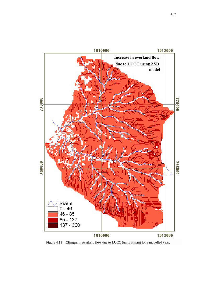
157
Figure 4.11 Changes in overland flow due to LUCC (units in mm) for a modelled year.
Increase in overland flow
due to LUCC using 2.5Dmodel

158
The increment in erosion due to LUCC is strongly related to the
slope of the area. Figure 4.12 shows those erosion increments over
the catchment with a clear relation with the steepest areas (see the
slope map Figure 3.17, pag. 81). Less than 14% of the catchment
has an increment in erosion between 0 and 3mm a year. These
areas are in both the highest and the lowest parts of the mountain
of the catchment (related to altitude) and areas of moderate slope.
About 45% of the area shows erosion increases of between 3 and
37 mm a year; those areas are where the slope is steep. 17% of the
area shows increases in erosion of between 37 to 73 mm a year;
they are in steeper slope areas in the down-slope direction furthest
away from the river channels. Finally, the largest increases in
erosion, due to LUCC, occur in areas nearest to river channels, in
the highest parts of the catchment (related to elevation) with
steepest slopes; those areas represent about 22% of the catchment.
Despite the fact that all processes in the model are affected by the
spatial rainfall function distribution the sensitive areas with
respect to erosion are clearly identified in Figure 4.12 as described
above. Higher areas in the catchment receive a high volume of
rainfall, which produces a large amount of wash erosion in both
land uses, but markedly higher after deforestation. Also as is
commonly assumed based on the topographic index, the areas
close to the river channels have more probability of soil saturation.
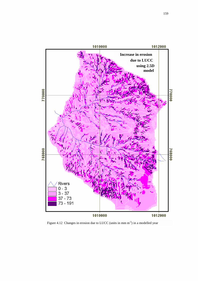
159
Figure 4.12 Changes in erosion due to LUCC (units in mm m-2) in a modelled year
Increase in erosion
due to LUCCusing 2.5D model
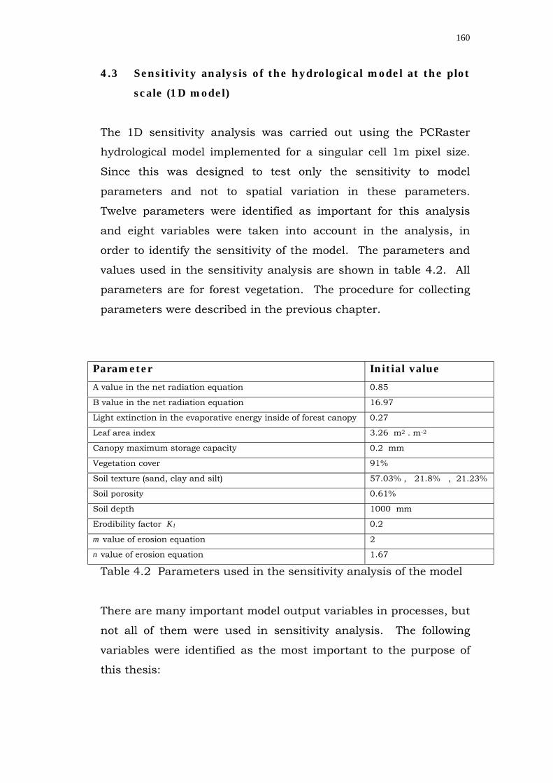
160
4.3 Sensitivity analysis of the hydrological model at the plotscale (1D model)
The 1D sensitivity analysis was carried out using the PCRaster
hydrological model implemented for a singular cell 1m pixel size.
Since this was designed to test only the sensitivity to model
parameters and not to spatial variation in these parameters.
Twelve parameters were identified as important for this analysis
and eight variables were taken into account in the analysis, in
order to identify the sensitivity of the model. The parameters and
values used in the sensitivity analysis are shown in table 4.2. All
parameters are for forest vegetation. The procedure for collecting
parameters were described in the previous chapter.
Parameter Initial valueA value in the net radiation equation 0.85
B value in the net radiation equation 16.97
Light extinction in the evaporative energy inside of forest canopy 0.27
Leaf area index 3.26 m2 . m-2
Canopy maximum storage capacity 0.2 mm
Vegetation cover 91%
Soil texture (sand, clay and silt) 57.03% , 21.8% , 21.23%
Soil porosity 0.61%
Soil depth 1000 mm
Erodibility factor K1 0.2
m value of erosion equation 2
n value of erosion equation 1.67
Table 4.2 Parameters used in the sensitivity analysis of the model
There are many important model output variables in processes, but
not all of them were used in sensitivity analysis. The following
variables were identified as the most important to the purpose of
this thesis:

161
Soil moisture
Matric potential
Hydrological conductivity
Infiltration
Evaporation
Detention storage
Overland flow (OF)
Erosion (E)
Parameters were varied by plus and minus 10% from the original
value (table 4.2) to +/-100% for the parameter sensitivity analysis
(Fisher et.al, 1997; Saltelli, 1999), where the results compared
between iterations give the ratio of change which is interpreted as
the sensitivity of the evaluated parameter. Model initial conditions
were derived from the model outputs of the previous year-long run
of the model. The model was re-run for each parameter variation
for a year of simulation time.
Results of the first model run using the parameters from table 4.2
are shown in table 4.3. Each variable used in the sensitivity
analysis was summed yearly, and was then divided by 8760 (the
number of hours in a year) to represent the hourly average for that
year by m2.
Table 4.3 Hourly average values of model variables for a year simulation in 1 m2
ErosionEffectiverainfallmm.h-1
SoilMoisture
%
MatricPotential
kPa
Hydraulicconductivity
mm.h-1Infiltration
mm.h-1
Totalevaporation
mm.h-1
Overlandflow
mm.h-1 mm.h-11.34 0.35 8536 0.49 0.51 0.02 0.8 0.1
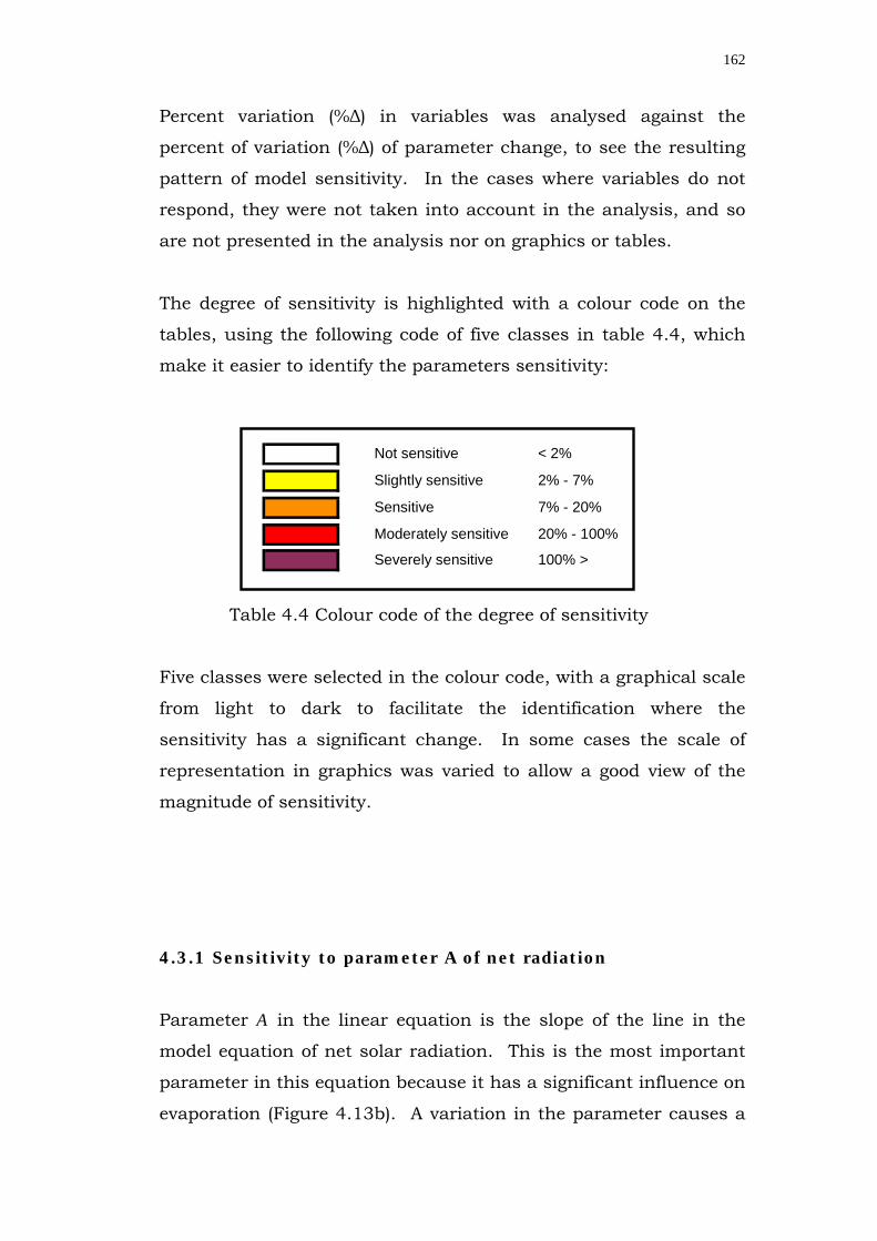
162
Percent variation (%Δ) in variables was analysed against the
percent of variation (%Δ) of parameter change, to see the resulting
pattern of model sensitivity. In the cases where variables do not
respond, they were not taken into account in the analysis, and so
are not presented in the analysis nor on graphics or tables.
The degree of sensitivity is highlighted with a colour code on the
tables, using the following code of five classes in table 4.4, which
make it easier to identify the parameters sensitivity:
Table 4.4 Colour code of the degree of sensitivity
Five classes were selected in the colour code, with a graphical scale
from light to dark to facilitate the identification where the
sensitivity has a significant change. In some cases the scale of
representation in graphics was varied to allow a good view of the
magnitude of sensitivity.
4.3.1 Sensitivity to parameter A of net radiation
Parameter A in the linear equation is the slope of the line in the
model equation of net solar radiation. This is the most important
parameter in this equation because it has a significant influence on
evaporation (Figure 4.13b). A variation in the parameter causes a
Not sensitive < 2%
Slightly sensitive 2% - 7%
Sensitive 7% - 20%
Moderately sensitive 20% - 100%
Severely sensitive 100% >
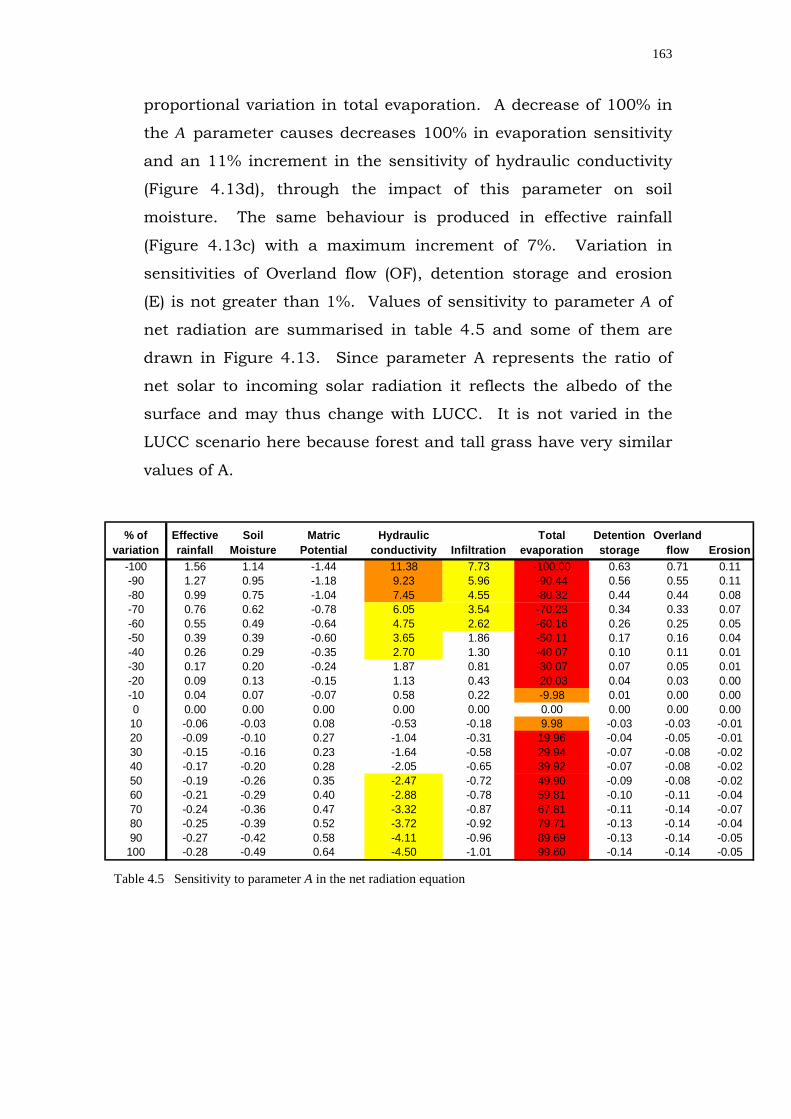
163
proportional variation in total evaporation. A decrease of 100% in
the A parameter causes decreases 100% in evaporation sensitivity
and an 11% increment in the sensitivity of hydraulic conductivity
(Figure 4.13d), through the impact of this parameter on soil
moisture. The same behaviour is produced in effective rainfall
(Figure 4.13c) with a maximum increment of 7%. Variation in
sensitivities of Overland flow (OF), detention storage and erosion
(E) is not greater than 1%. Values of sensitivity to parameter A of
net radiation are summarised in table 4.5 and some of them are
drawn in Figure 4.13. Since parameter A represents the ratio of
net solar to incoming solar radiation it reflects the albedo of the
surface and may thus change with LUCC. It is not varied in the
LUCC scenario here because forest and tall grass have very similar
values of A.
% of variation
Effective rainfall
Soil Moisture
Matric Potential
Hydraulic conductivity Infiltration
Total evaporation
Detention storage
Overland flow Erosion
-100 1.56 1.14 -1.44 11.38 7.73 -100.00 0.63 0.71 0.11-90 1.27 0.95 -1.18 9.23 5.96 -90.44 0.56 0.55 0.11-80 0.99 0.75 -1.04 7.45 4.55 -80.32 0.44 0.44 0.08-70 0.76 0.62 -0.78 6.05 3.54 -70.23 0.34 0.33 0.07-60 0.55 0.49 -0.64 4.75 2.62 -60.16 0.26 0.25 0.05-50 0.39 0.39 -0.60 3.65 1.86 -50.11 0.17 0.16 0.04-40 0.26 0.29 -0.35 2.70 1.30 -40.07 0.10 0.11 0.01-30 0.17 0.20 -0.24 1.87 0.81 -30.07 0.07 0.05 0.01-20 0.09 0.13 -0.15 1.13 0.43 -20.03 0.04 0.03 0.00-10 0.04 0.07 -0.07 0.58 0.22 -9.98 0.01 0.00 0.000 0.00 0.00 0.00 0.00 0.00 0.00 0.00 0.00 0.0010 -0.06 -0.03 0.08 -0.53 -0.18 9.98 -0.03 -0.03 -0.0120 -0.09 -0.10 0.27 -1.04 -0.31 19.96 -0.04 -0.05 -0.0130 -0.15 -0.16 0.23 -1.64 -0.58 29.94 -0.07 -0.08 -0.0240 -0.17 -0.20 0.28 -2.05 -0.65 39.92 -0.07 -0.08 -0.0250 -0.19 -0.26 0.35 -2.47 -0.72 49.90 -0.09 -0.08 -0.0260 -0.21 -0.29 0.40 -2.88 -0.78 59.81 -0.10 -0.11 -0.0470 -0.24 -0.36 0.47 -3.32 -0.87 67.81 -0.11 -0.14 -0.0780 -0.25 -0.39 0.52 -3.72 -0.92 79.71 -0.13 -0.14 -0.0490 -0.27 -0.42 0.58 -4.11 -0.96 89.69 -0.13 -0.14 -0.05
100 -0.28 -0.49 0.64 -4.50 -1.01 99.60 -0.14 -0.14 -0.05
Table 4.5 Sensitivity to parameter A in the net radiation equation

164
Sensitivity to parameter A of net radiation
-100
-50
0
50
100
-100 -50 0 50 100
Percent variation of param eter A of net radiation
Infiltration
Total evaporation
Sensitivity to parameter A of net radiation
-0.2
0.0
0.2
0.4
0.6
0.8
-100 -50 0 50 100
Percent variation of param eter A of net radiation
Detention storage
Overland flow
Erosion
Sensitivity to parameter A of net radiation
-0.5
0.0
0.5
1.0
1.5
2.0
-100 -50 0 50 100
Percent variation of param eter A of net radiation
Efective rainfall
Sensitivity to parameter A of net radiation
-8
-4
0
4
8
12
16
-100 -50 0 50 100
Percent variation of param eter A of net radiation
Soil m oisture
M atric potential
Hydrological conductivity
%∆
%∆
%∆
%∆
%∆
%∆
%∆
%∆
a b
c d
Figure 4.13. Sensitivity to parameter A in the net radiation equation
164
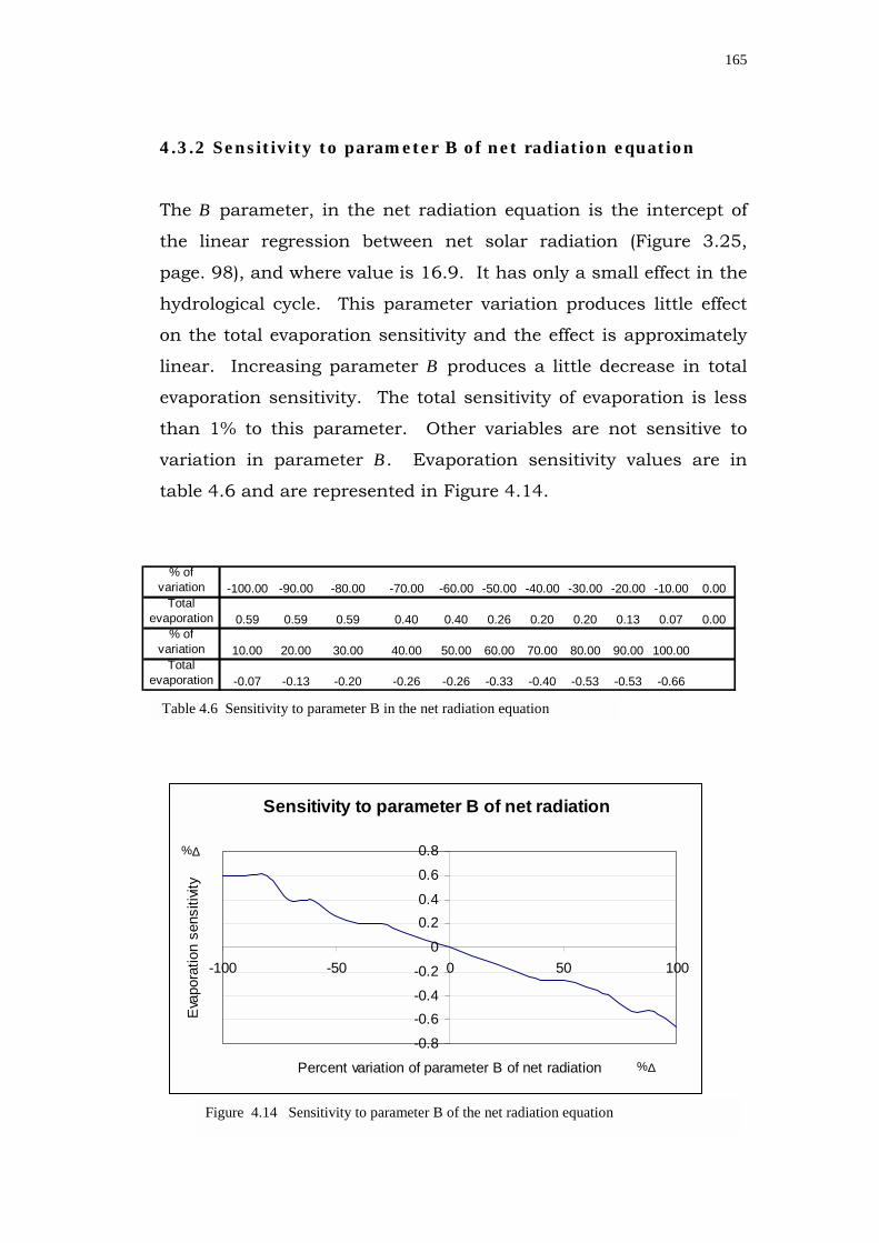
165
4.3.2 Sensitivity to parameter B of net radiation equation
The B parameter, in the net radiation equation is the intercept of
the linear regression between net solar radiation (Figure 3.25,
page. 98), and where value is 16.9. It has only a small effect in the
hydrological cycle. This parameter variation produces little effect
on the total evaporation sensitivity and the effect is approximately
linear. Increasing parameter B produces a little decrease in total
evaporation sensitivity. The total sensitivity of evaporation is less
than 1% to this parameter. Other variables are not sensitive to
variation in parameter B. Evaporation sensitivity values are in
table 4.6 and are represented in Figure 4.14.
Table 4.6 Sensitivity to parameter B in the net radiation equation
% of variation -100.00 -90.00 -80.00 -70.00 -60.00 -50.00 -40.00 -30.00 -20.00 -10.00 0.00
Total evaporation 0.59 0.59 0.59 0.40 0.40 0.26 0.20 0.20 0.13 0.07 0.00
% of variation 10.00 20.00 30.00 40.00 50.00 60.00 70.00 80.00 90.00 100.00
Total evaporation -0.07 -0.13 -0.20 -0.26 -0.26 -0.33 -0.40 -0.53 -0.53 -0.66
Figure 4.14 Sensitivity to parameter B of the net radiation equation
Sensitivity to parameter B of net radiation
-0.8
-0.6
-0.4
-0.2
0
0.2
0.4
0.6
0.8
-100 -50 0 50 100
Percent variation of parameter B of net radiation
Eva
pora
tion
sens
itivi
ty
%∆
%∆

166
4.3.3 Sensitivity to parameter light extinction K
Sensitivity to parameter K, the light extinction parameter, is small
in the variables. The most sensitive variables are hydraulic
conductivity and infiltration, with an extreme value of 8%. This
parameter does not produce important changes in hydrological flux
sensitivities, which means they are not sensitive to this parameter.
Sensitivity values to these parameters are in table 4.7 and are
shown in Figure 4.15. K is function of three canopy forms.
% of variation
Effective rainfall
Soil Moisture
Matric Potential
Hydraulic conductivity Infiltration
Total evaporation
Detention storage
Overland flow Erosion
-100 1.56 0.78 0.00 7.89 7.73 0.73 0.63 0.63 0.11-90 1.25 0.59 0.00 6.00 5.87 0.59 0.54 0.55 0.11-80 0.98 0.46 0.00 4.59 4.50 0.46 0.44 0.44 0.08-70 0.75 0.36 0.00 3.58 3.49 0.33 0.34 0.33 0.07-60 0.54 0.26 0.00 2.63 2.60 0.26 0.24 0.25 0.05-50 0.38 0.20 0.00 1.85 1.81 0.20 0.17 0.16 0.02-40 0.26 0.13 0.00 1.29 1.28 0.13 0.10 0.11 0.01-30 0.17 0.10 0.00 0.81 0.81 0.07 0.07 0.05 0.01-20 0.09 0.07 0.00 0.44 0.43 0.07 0.04 0.03 0.00-10 0.04 0.03 0.00 0.23 0.22 0.00 0.01 0.00 0.000 0.00 0.00 0.00 0.00 0.00 0.00 0.00 0.00 0.0010 -0.06 0.00 0.03 -0.18 -0.18 0.00 -0.03 -0.03 -0.0120 -0.09 -0.03 0.04 -0.32 -0.31 -0.07 -0.04 -0.05 -0.0130 -0.15 -0.03 0.04 -0.60 -0.58 -0.07 -0.07 -0.08 -0.0240 -0.17 -0.07 0.04 -0.67 -0.65 -0.07 -0.07 -0.08 -0.0250 -0.19 -0.07 0.04 -0.74 -0.72 -0.07 -0.09 -0.08 -0.0260 -0.21 -0.07 0.04 -0.78 -0.76 -0.07 -0.10 -0.11 -0.0470 -0.24 -0.07 0.04 -0.90 -0.87 -0.07 -0.11 -0.14 -0.0480 -0.25 -0.07 0.04 -0.95 -0.92 -0.07 -0.13 -0.14 -0.0490 -0.26 -0.07 0.04 -0.99 -0.96 -0.13 -0.13 -0.14 -0.05
100 -0.28 -0.10 0.04 -1.04 -1.01 0.13 -0.14 -0.14 -0.05
Table 4.7 Sensitivity to light extinction
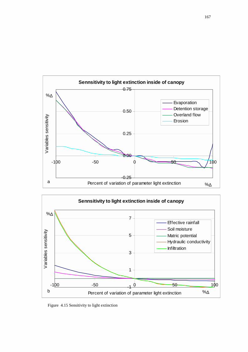
167
Sennsitivity to light extinction inside of canopy
-0.25
0.00
0.25
0.50
0.75
-100 -50 0 50 100
Percent of variation of parameter light extinction
Var
iabl
es s
ensi
tivity
EvaporationDetention storageOverland f lowErosion
Sennsitivity to light extinction inside of canopy
-1
1
3
5
7
-100 -50 0 50 100
Percent of variation of parameter light extinction
Var
iabl
es s
ensi
tivity
Effective rainfall
Soil moisture
Matric potentialHydraulic conductivity
Infiltration
b
a
%∆
%∆
%∆
%∆
Figure 4.15 Sensitivity to light extinction
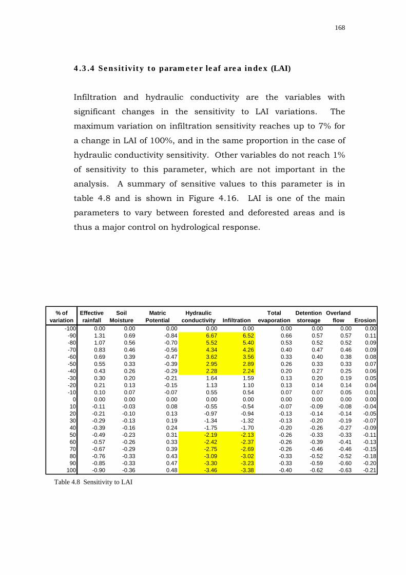
168
4.3.4 Sensitivity to parameter leaf area index (LAI)
Infiltration and hydraulic conductivity are the variables with
significant changes in the sensitivity to LAI variations. The
maximum variation on infiltration sensitivity reaches up to 7% for
a change in LAI of 100%, and in the same proportion in the case of
hydraulic conductivity sensitivity. Other variables do not reach 1%
of sensitivity to this parameter, which are not important in the
analysis. A summary of sensitive values to this parameter is in
table 4.8 and is shown in Figure 4.16. LAI is one of the main
parameters to vary between forested and deforested areas and is
thus a major control on hydrological response.
% of variation
Effective rainfall
Soil Moisture
Matric Potential
Hydraulic conductivity Infiltration
Total evaporation
Detention storeage
Overland flow Erosion
-100 0.00 0.00 0.00 0.00 0.00 0.00 0.00 0.00 0.00-90 1.31 0.69 -0.84 6.67 6.52 0.66 0.57 0.57 0.11-80 1.07 0.56 -0.70 5.52 5.40 0.53 0.52 0.52 0.09-70 0.83 0.46 -0.56 4.34 4.26 0.40 0.47 0.46 0.09-60 0.69 0.39 -0.47 3.62 3.56 0.33 0.40 0.38 0.08-50 0.55 0.33 -0.39 2.95 2.89 0.26 0.33 0.33 0.07-40 0.43 0.26 -0.29 2.28 2.24 0.20 0.27 0.25 0.06-30 0.30 0.20 -0.21 1.64 1.59 0.13 0.20 0.19 0.05-20 0.21 0.13 -0.15 1.13 1.10 0.13 0.14 0.14 0.04-10 0.10 0.07 -0.07 0.55 0.54 0.07 0.07 0.05 0.01
0 0.00 0.00 0.00 0.00 0.00 0.00 0.00 0.00 0.0010 -0.11 -0.03 0.08 -0.55 -0.54 -0.07 -0.09 -0.08 -0.0420 -0.21 -0.10 0.13 -0.97 -0.94 -0.13 -0.14 -0.14 -0.0530 -0.29 -0.13 0.19 -1.34 -1.32 -0.13 -0.20 -0.19 -0.0740 -0.39 -0.16 0.24 -1.75 -1.70 -0.20 -0.26 -0.27 -0.0950 -0.49 -0.23 0.31 -2.19 -2.13 -0.26 -0.33 -0.33 -0.1160 -0.57 -0.26 0.33 -2.42 -2.37 -0.26 -0.39 -0.41 -0.1370 -0.67 -0.29 0.39 -2.75 -2.69 -0.26 -0.46 -0.46 -0.1580 -0.76 -0.33 0.43 -3.09 -3.02 -0.33 -0.52 -0.52 -0.1890 -0.85 -0.33 0.47 -3.30 -3.23 -0.33 -0.59 -0.60 -0.20
100 -0.90 -0.36 0.48 -3.46 -3.38 -0.40 -0.62 -0.63 -0.21
Table 4.8 Sensitivity to LAI
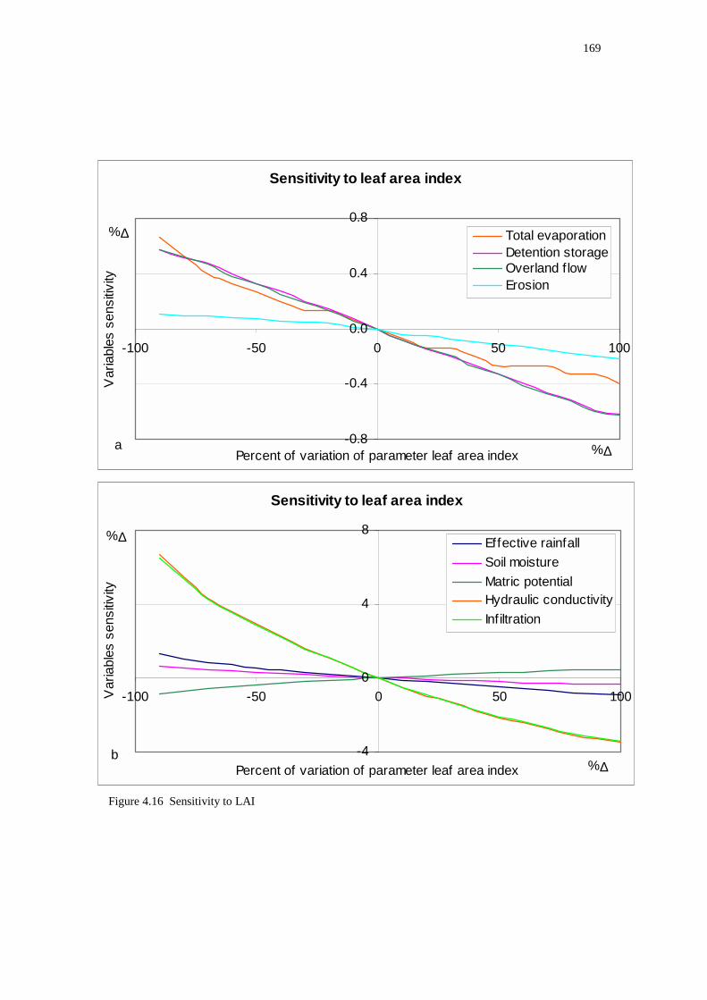
169
Sensitivity to leaf area index
-0.8
-0.4
0.0
0.4
0.8
-100 -50 0 50 100
Percent of variation of parameter leaf area index
Var
iabl
es s
ensi
tivity
Total evaporationDetention storageOverland f lowErosion
Sensitivity to leaf area index
-4
0
4
8
-100 -50 0 50 100
Percent of variation of parameter leaf area index
Var
iabl
es s
ensi
tivity
Ef fective rainfall
Soil moisture
Matric potentialHydraulic conductivity
Inf iltration
b
a
%∆
%∆
%∆
%∆
Figure 4.16 Sensitivity to LAI
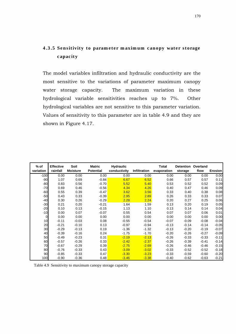
170
4.3.5 Sensitivity to parameter maximum canopy water storagecapacity
The model variables infiltration and hydraulic conductivity are the
most sensitive to the variations of parameter maximum canopy
water storage capacity. The maximum variation in these
hydrological variable sensitivities reaches up to 7%. Other
hydrological variables are not sensitive to this parameter variation.
Values of sensitivity to this parameter are in table 4.9 and they are
shown in Figure 4.17.
% of variation
Effective rainfall
Soil Moisture
Matric Potential
Hydraulic conductivity Infiltration
Total evaporation
Detention storage
Overland flow Erosion
-100 0.00 0.00 0.00 0.00 0.00 0.00 0.00 0.00 0.00-90 1.07 0.69 -0.84 6.67 6.52 0.66 0.57 0.57 0.11-80 0.83 0.56 -0.70 5.52 5.40 0.53 0.52 0.52 0.09-70 0.69 0.46 -0.56 4.34 4.26 0.40 0.47 0.46 0.09-60 0.55 0.39 -0.47 3.62 3.56 0.33 0.40 0.38 0.08-50 0.43 0.33 -0.39 2.95 2.89 0.26 0.33 0.33 0.07-40 0.30 0.26 -0.29 2.28 2.24 0.20 0.27 0.25 0.06-30 0.21 0.20 -0.21 1.64 1.59 0.13 0.20 0.19 0.05-20 0.10 0.13 -0.15 1.13 1.10 0.13 0.14 0.14 0.04-10 0.00 0.07 -0.07 0.55 0.54 0.07 0.07 0.06 0.01
0 0.00 0.00 0.00 0.00 0.00 0.00 0.00 0.00 0.0010 -0.11 -0.03 0.08 -0.55 -0.54 -0.07 -0.09 -0.08 -0.0420 -0.21 -0.10 0.13 -0.97 -0.94 -0.13 -0.14 -0.14 -0.0530 -0.29 -0.13 0.19 -1.36 -1.32 -0.13 -0.20 -0.19 -0.0740 -0.39 -0.16 0.24 -1.75 -1.70 -0.20 -0.26 -0.27 -0.0950 -0.49 -0.23 0.31 -2.19 -2.13 -0.26 -0.33 -0.33 -0.1160 -0.57 -0.26 0.33 -2.42 -2.37 -0.26 -0.39 -0.41 -0.1470 -0.67 -0.29 0.39 -2.75 -2.69 -0.26 -0.46 -0.46 -0.1580 -0.76 -0.33 0.43 -3.09 -3.02 -0.33 -0.52 -0.52 -0.1890 -0.85 -0.33 0.47 -3.30 -3.23 -0.33 -0.59 -0.60 -0.20
100 -0.90 -0.36 0.48 -3.46 -3.38 -0.40 -0.62 -0.63 -0.21
Table 4.9 Sensitivity to maximum canopy storage capacity
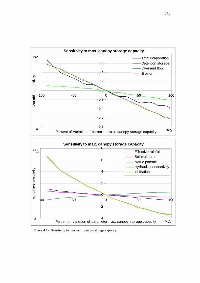
171
Sensitivity to max. canopy storage capacity
-0.8
-0.6
-0.4
-0.2
0.0
0.2
0.4
0.6
0.8
-100 -50 0 50 100
Percent of variation of parameter max. canopy storage capacity
Var
iabl
es s
ensi
tivity
Total evaporation
Detention storageOverland f low
Erosion
Sensitivity to max. canopy storage capacity
-4
-2
0
2
4
6
8
-100 -50 0 50 100
Percent of variation of parameter max. canopy storage capacity
Var
iabl
es s
ensi
tivity
Effective rainfallSoil moisture
Matric potentialHydraulic conductivityInfiltration
b
a
%∆
%∆
%∆
%∆
Figure 4.17 Sensitivity to maximum canopy storage capacity
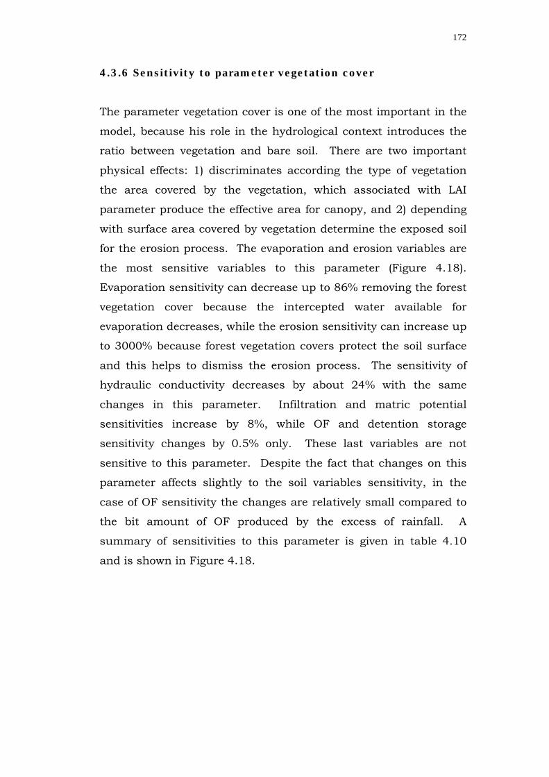
172
4.3.6 Sensitivity to parameter vegetation cover
The parameter vegetation cover is one of the most important in the
model, because his role in the hydrological context introduces the
ratio between vegetation and bare soil. There are two important
physical effects: 1) discriminates according the type of vegetation
the area covered by the vegetation, which associated with LAI
parameter produce the effective area for canopy, and 2) depending
with surface area covered by vegetation determine the exposed soil
for the erosion process. The evaporation and erosion variables are
the most sensitive variables to this parameter (Figure 4.18).
Evaporation sensitivity can decrease up to 86% removing the forest
vegetation cover because the intercepted water available for
evaporation decreases, while the erosion sensitivity can increase up
to 3000% because forest vegetation covers protect the soil surface
and this helps to dismiss the erosion process. The sensitivity of
hydraulic conductivity decreases by about 24% with the same
changes in this parameter. Infiltration and matric potential
sensitivities increase by 8%, while OF and detention storage
sensitivity changes by 0.5% only. These last variables are not
sensitive to this parameter. Despite the fact that changes on this
parameter affects slightly to the soil variables sensitivity, in the
case of OF sensitivity the changes are relatively small compared to
the bit amount of OF produced by the excess of rainfall. A
summary of sensitivities to this parameter is given in table 4.10
and is shown in Figure 4.18.
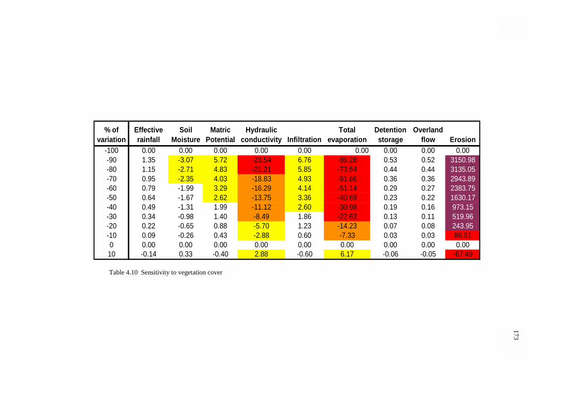
173
Table 4.10 Sensitivity to vegetation cover
% of variation
Effective rainfall
Soil Moisture
Matric Potential
Hydraulic conductivity Infiltration
Total evaporation
Detention storage
Overland flow Erosion
-100 0.00 0.00 0.00 0.00 0.00 0.00 0.00 0.00 0.00-90 1.35 -3.07 5.72 -23.54 6.76 -86.28 0.53 0.52 3150.98-80 1.15 -2.71 4.83 -21.21 5.85 -73.54 0.44 0.44 3135.05-70 0.95 -2.35 4.03 -18.83 4.93 -61.86 0.36 0.36 2943.89-60 0.79 -1.99 3.29 -16.29 4.14 -51.14 0.29 0.27 2383.75-50 0.64 -1.67 2.62 -13.75 3.36 -40.69 0.23 0.22 1630.17-40 0.49 -1.31 1.99 -11.12 2.60 -30.98 0.19 0.16 973.15-30 0.34 -0.98 1.40 -8.49 1.86 -22.63 0.13 0.11 519.96-20 0.22 -0.65 0.88 -5.70 1.23 -14.23 0.07 0.08 243.95-10 0.09 -0.26 0.43 -2.88 0.60 -7.33 0.03 0.03 86.510 0.00 0.00 0.00 0.00 0.00 0.00 0.00 0.00 0.0010 -0.14 0.33 -0.40 2.88 -0.60 6.17 -0.06 -0.05 -67.49
173
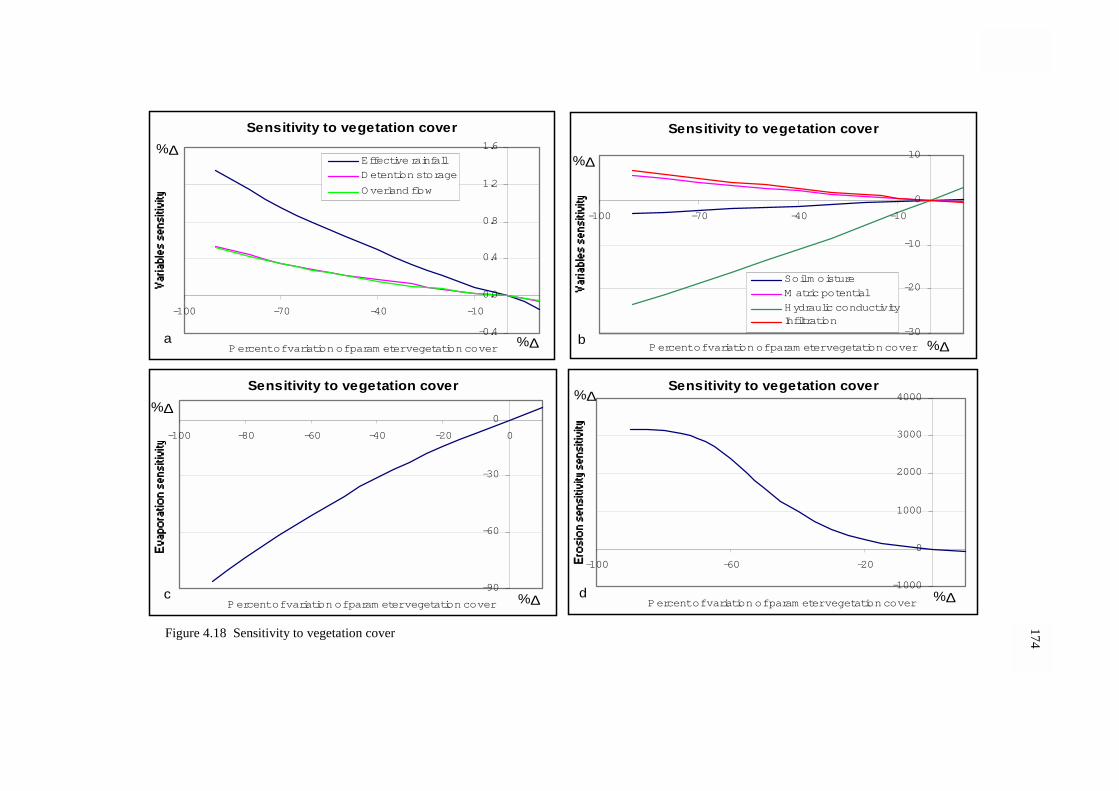
174
Sensitivity to vegetation cover
-0.4
0.0
0.4
0.8
1.2
1.6
-100 -70 -40 -10
Percent of variation of param eter vegetation cover
Effective rainfall
Detention storage
Overland flow
Sensitivity to vegetation cover
-30
-20
-10
0
10
-100 -70 -40 -10
Percent of variation of param eter vegetation cover
Soil m oisture
M atric potential
Hydraulic conductivityInfiltration
Sensitivity to vegetation cover
-90
-60
-30
0
-100 -80 -60 -40 -20 0
Percent of variation of param eter vegetation cover
Sensitivity to vegetation cover
-1000
0
1000
2000
3000
4000
-100 -60 -20
Percent of variation of param eter vegetation cover
a b
dc
%∆
%∆
%∆%∆
%∆
%∆
%∆
%∆
Figure 4.18 Sensitivity to vegetation cover
174
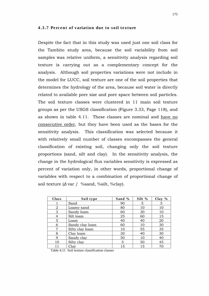
175
4.3.7 Percent of variation due to soil texture
Despite the fact that in this study was used just one soil class for
the Tambito study area, because the soil variability from soil
samples was relative uniform, a sensitivity analysis regarding soil
texture is carrying out as a complementary concept for the
analysis. Although soil properties variations were not include in
the model for LUCC, soil texture are one of the soil properties that
determines the hydrology of the area, because soil water is directly
related to available pore size and pore space between soil particles.
The soil texture classes were clustered in 11 main soil texture
groups as per the USGS classification (Figure 3.33, Page 118), and
as shown in table 4.11. These classes are nominal and have no
consecutive order, but they have been used as the bases for the
sensitivity analysis. This classification was selected because it
with relatively small number of classes encompasses the general
classification of existing soil, changing only the soil texture
proportions (sand, silt and clay). In the sensitivity analysis, the
change in the hydrological flux variables sensitivity is expressed as
percent of variation only, in other words, proportional change of
variables with respect to a combination of proportional change of
soil texture (∆ var / %sand, %silt, %clay).
Class Soil type Sand % Silt % Clay %1 Sand 90 5 52 Loamy sand 80 10 103 Sandy loam 60 30 104 Silt loam 25 60 155 Loam 40 40 206 Sandy clay loam 60 10 307 Silty clay loam 10 55 358 Clay loam 30 40 309 Sandy clay 50 10 4010 Silty clay 5 50 4511 Clay 15 15 70
Table 4.11 Soil texture classification classes

176
The percent of variation of soil moisture, hydraulic conductivity
and infiltration reaches up to 50% between soil classes. The
percent variation of OF and detention storage varies with the soil
texture, which the highest value of variation is (160%) between
class 5 and class 6 (Sandy clay loam). This class also is the
dominant soil class of the Tambito watershed, while erosion
percent variation reaches up to 100% in half of the soil classes.
The percent variation in matric potential changes in different scale
of magnitude, with the highest value up to 1000% in soil class 5
(loam). Sensitivity to soil texture is shown in fig. 4.19.
From this analysis is clear the importance of the soil textures in
the hydrological context. Unfortunately soil samples were not
collected with LUCC discrimination, because this parameter could
introduce a relevant information within the land use classes as in
this exercise with forested and deforested areas. Also the
correlation between soil properties and land use classes could be
important and significant in the hydrological response, and needs
to be taken into account within the field expeditions.
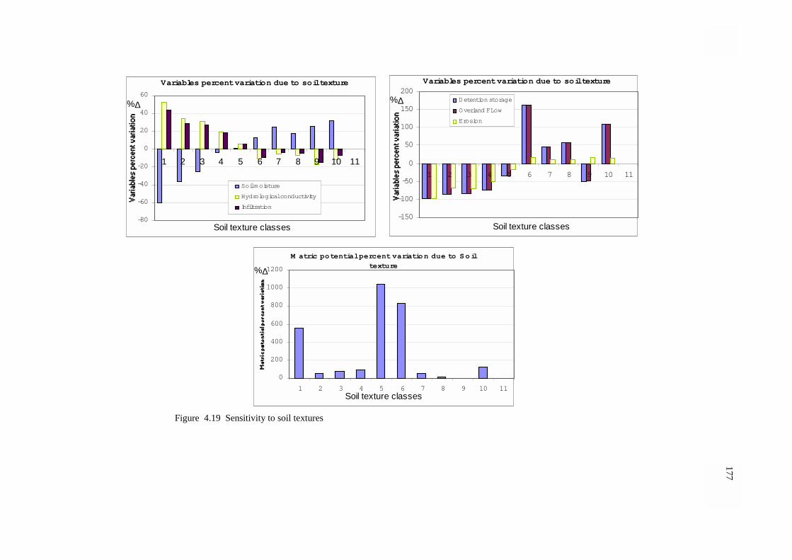
177
Variables percent variation due to soil texture
-150
-100
-50
0
50
100
150
200
1 2 3 4 5 6 7 8 9 10 11
Soil texture classes
Detention storage
Overland FLow
Erosion
M atric potential percent variation due to So il
texture
0
200
400
600
800
1000
1200
1 2 3 4 5 6 7 8 9 10 11Soil texture classes
Variables percent variation due to soil texture
-80
-60
-40
-20
0
20
40
60
1 2 3 4 5 6 7 8 9 10 11
Soil texture classes
Soil moisture
Hydrological conductivity
Infiltration
%∆ %∆
%∆
Figure 4.19 Sensitivity to soil textures
177
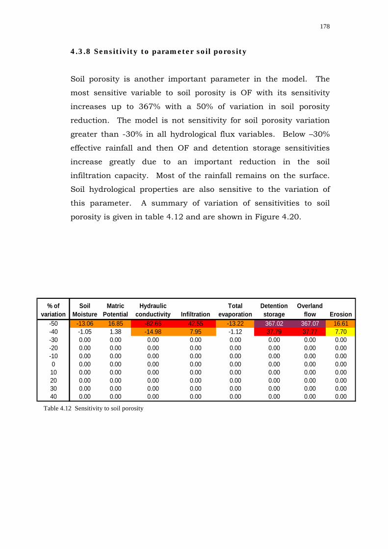
178
4.3.8 Sensitivity to parameter soil porosity
Soil porosity is another important parameter in the model. The
most sensitive variable to soil porosity is OF with its sensitivity
increases up to 367% with a 50% of variation in soil porosity
reduction. The model is not sensitivity for soil porosity variation
greater than -30% in all hydrological flux variables. Below –30%
effective rainfall and then OF and detention storage sensitivities
increase greatly due to an important reduction in the soil
infiltration capacity. Most of the rainfall remains on the surface.
Soil hydrological properties are also sensitive to the variation of
this parameter. A summary of variation of sensitivities to soil
porosity is given in table 4.12 and are shown in Figure 4.20.
% of variation
Soil Moisture
Matric Potential
Hydraulic conductivity Infiltration
Total evaporation
Detention storage
Overland flow Erosion
-50 -13.06 16.85 -82.66 42.55 -13.22 367.02 367.07 16.61-40 -1.05 1.38 -14.98 7.95 -1.12 37.79 37.77 7.70-30 0.00 0.00 0.00 0.00 0.00 0.00 0.00 0.00-20 0.00 0.00 0.00 0.00 0.00 0.00 0.00 0.00-10 0.00 0.00 0.00 0.00 0.00 0.00 0.00 0.000 0.00 0.00 0.00 0.00 0.00 0.00 0.00 0.0010 0.00 0.00 0.00 0.00 0.00 0.00 0.00 0.0020 0.00 0.00 0.00 0.00 0.00 0.00 0.00 0.0030 0.00 0.00 0.00 0.00 0.00 0.00 0.00 0.0040 0.00 0.00 0.00 0.00 0.00 0.00 0.00 0.00
Table 4.12 Sensitivity to soil porosity
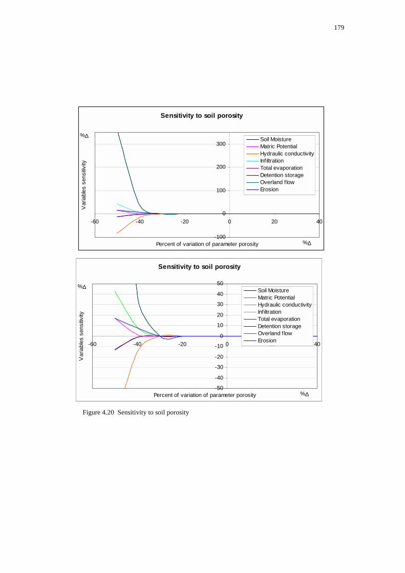
179
Sensitivity to soil porosity
-100
0
100
200
300
-60 -40 -20 0 20 40
Percent of variation of parameter porosity
Var
iabl
es s
ensi
tivity
Soil MoistureMatric PotentialHydraulic conductivityInfiltrationTotal evaporationDetention storageOverland f lowErosion
%∆
%∆
Sensitivity to soil porosity
-50
-40
-30
-20
-10
0
10
20
30
40
50
-60 -40 -20 0 20 40
Percent of variation of parameter porosity
Var
iabl
es s
ensi
tivity
Soil MoistureMatric PotentialHydraulic conductivityInfiltrationTotal evaporationDetention storageOverland f lowErosion
%∆
%∆
Figure 4.20 Sensitivity to soil porosity
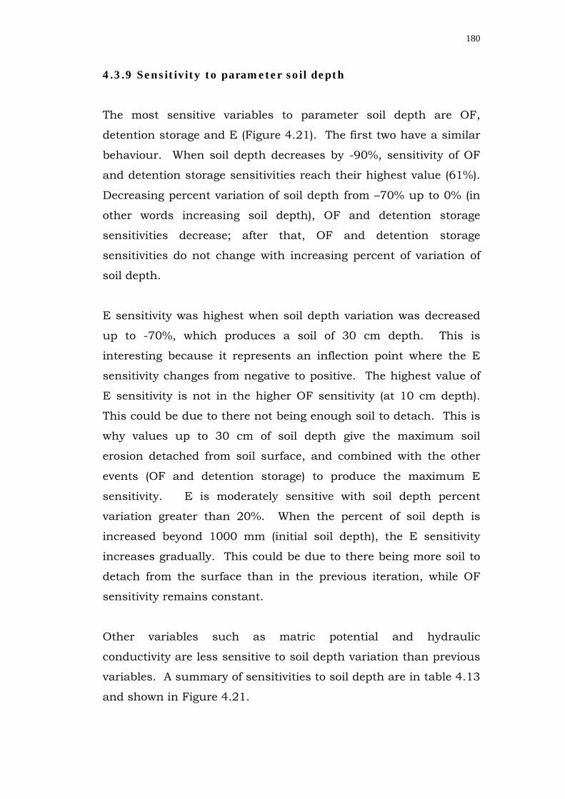
180
4.3.9 Sensitivity to parameter soil depth
The most sensitive variables to parameter soil depth are OF,
detention storage and E (Figure 4.21). The first two have a similar
behaviour. When soil depth decreases by -90%, sensitivity of OF
and detention storage sensitivities reach their highest value (61%).
Decreasing percent variation of soil depth from –70% up to 0% (in
other words increasing soil depth), OF and detention storage
sensitivities decrease; after that, OF and detention storage
sensitivities do not change with increasing percent of variation of
soil depth.
E sensitivity was highest when soil depth variation was decreased
up to -70%, which produces a soil of 30 cm depth. This is
interesting because it represents an inflection point where the E
sensitivity changes from negative to positive. The highest value of
E sensitivity is not in the higher OF sensitivity (at 10 cm depth).
This could be due to there not being enough soil to detach. This is
why values up to 30 cm of soil depth give the maximum soil
erosion detached from soil surface, and combined with the other
events (OF and detention storage) to produce the maximum E
sensitivity. E is moderately sensitive with soil depth percent
variation greater than 20%. When the percent of soil depth is
increased beyond 1000 mm (initial soil depth), the E sensitivity
increases gradually. This could be due to there being more soil to
detach from the surface than in the previous iteration, while OF
sensitivity remains constant.
Other variables such as matric potential and hydraulic
conductivity are less sensitive to soil depth variation than previous
variables. A summary of sensitivities to soil depth are in table 4.13
and shown in Figure 4.21.

181
% of variation
Soil Moisture
Matric Potential
Hydraulic conductivity Infiltration
Total evaporation
Detention storage
Overland flow Erosion
-100 0.00 0.00 0.00 0.00 0.00 -89.70 -89.70 22.60-90 -4.08 11.17 3.92 3.40 -4.69 61.40 61.38 -11.70-80 -2.12 4.93 3.83 2.80 -2.05 40.12 40.12 -43.20-70 -1.31 2.78 3.72 2.13 -1.12 23.42 23.42 -64.94-60 -0.88 1.68 3.60 1.46 -0.66 11.16 11.15 -53.32-50 -0.59 1.06 3.48 0.76 -0.46 3.38 3.36 -42.52-40 -0.36 0.62 3.35 0.07 -0.26 0.09 0.08 -32.57-30 -0.20 0.29 2.49 0.00 -0.13 0.00 0.00 -23.33-20 -0.07 0.12 1.66 0.00 -0.07 0.00 0.00 -14.75-10 0.00 0.04 0.83 0.00 0.00 0.00 0.00 -7.02
0 0.00 0.00 0.00 0.00 0.00 0.00 0.00 0.0010 0.00 0.04 -0.83 0.00 -0.07 0.00 0.00 6.3720 -0.10 0.13 -1.68 0.00 -0.13 0.00 0.00 12.1830 -0.20 0.43 -2.52 0.00 -0.26 0.00 0.00 17.4640 -0.36 1.51 -3.35 0.00 -0.46 0.00 0.00 22.3750 -0.56 3.65 -4.15 0.00 -0.66 0.00 0.00 26.8160 -0.82 7.05 -4.98 0.00 -0.93 0.00 0.00 30.7970 -1.08 12.16 -5.82 0.00 -1.19 0.00 0.00 34.6480 -1.40 19.48 -6.65 0.00 -1.52 0.00 0.00 38.0390 -1.76 30.65 -7.48 0.00 -1.92 0.00 0.00 41.30
100 -2.16 46.43 -8.29 0.00 -2.31 0.00 0.00 44.34
Table 4.13 Sensitivity to soil depth
181
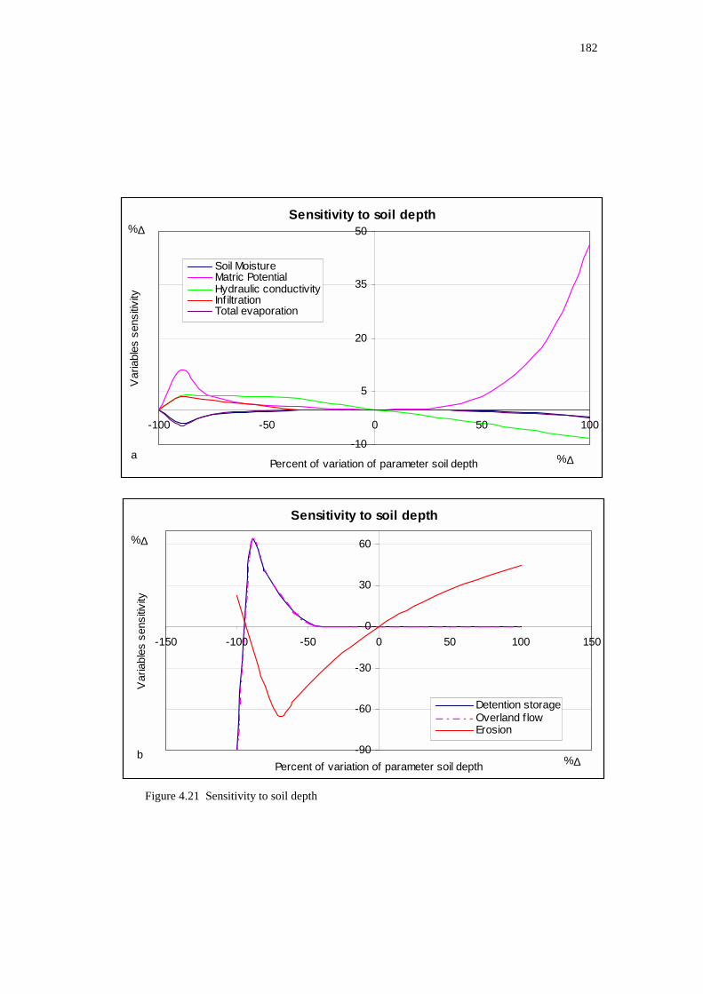
182
Sensitivity to soil depth
-10
5
20
35
50
-100 -50 0 50 100
Percent of variation of parameter soil depth
Var
iabl
es s
ensi
tivity
Soil MoistureMatric PotentialHydraulic conductivityInf iltrationTotal evaporation
Sensitivity to soil depth
-90
-60
-30
0
30
60
-150 -100 -50 0 50 100 150
Percent of variation of parameter soil depth
Var
iabl
es s
ensi
tivity
Detention storageOverland f lowErosion
b %∆
%∆
a
%∆
%∆
Figure 4.21 Sensitivity to soil depth
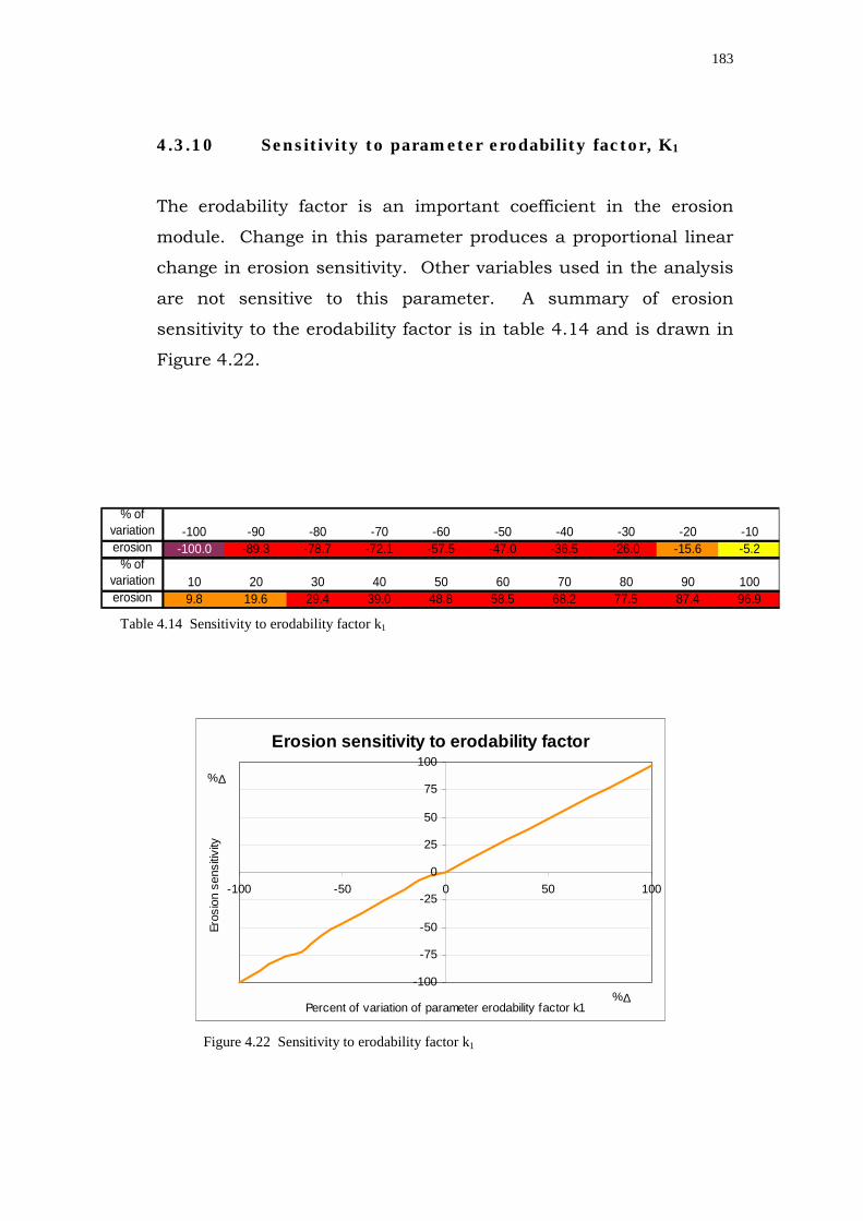
183
4.3.10 Sensitivity to parameter erodability factor, K1
The erodability factor is an important coefficient in the erosion
module. Change in this parameter produces a proportional linear
change in erosion sensitivity. Other variables used in the analysis
are not sensitive to this parameter. A summary of erosion
sensitivity to the erodability factor is in table 4.14 and is drawn in
Figure 4.22.
% of variation -100 -90 -80 -70 -60 -50 -40 -30 -20 -10erosion -100.0 -89.3 -78.7 -72.1 -57.5 -47.0 -36.5 -26.0 -15.6 -5.2
% of variation 10 20 30 40 50 60 70 80 90 100erosion 9.8 19.6 29.4 39.0 48.8 58.5 68.2 77.5 87.4 96.9
Table 4.14 Sensitivity to erodability factor k1
Erosion sensitivity to erodability factor
-100
-75
-50
-25
0
25
50
75
100
-100 -50 0 50 100
Percent of variation of parameter erodability factor k1
Eros
ion
sens
itivi
ty
%∆
%∆
Figure 4.22 Sensitivity to erodability factor k1

184
4.3.11 Sensitivity to parameter m factor of erosionequation
The sensitivity to the parameter m factor in erosion equation is
strong only on the variable E. E sensitivity increases by more than
367% of the proportion in sensitivity of m factor in an exponential
curve. Decreasing the percent of m factor does not reproduce the
same sensitivity displayed when increasing; sensitivity of erosion
decreases in the almost in same proportion to the m factor of
erosion. Other variables within the model are not sensitive to this
parameter.
This parameter has an exponential effect on E sensitivity, because
it drastically increases or reduces the OF within the E equation. A
summary of the erosion sensitivity to the m factor is given in table
4.15 and is drawn in Figure 4.23.
% of variation Erosion
-100 -92.1-50 -93.750 17.1100 366.6
Table 4.15 Sensitivity to m factor of erosion equation
Erosion sensitivity to m factor of erosion equation
-200
-100
0
100
200
300
400
-100 -50 0 50 100
Percent variation of parameter m factor of erosion
Eros
ion
sens
itivi
ty
%∆
%∆
Figure 4.23 Sensitivity to m factor of erosion equation
185
4.3.12 Sensitivity to parameter n factor of erosionequation
Erosion sensitivity to the n factor of the erosion equation increases
in a lesser proportion when the n factor proportion decreases, and
decreases in greater proportion when the n factor proportion
increases. When the n factor increase, E sensitivity decrease
linearly by –30%. Other variables are not affected by this
parameter. Erosion sensitivity values are summarised in table
4.16 and are shown in Figure 4.24.
% of variation -100 -90 -80 -70 -60 -50 -40 -30 -20 -10Erosion 16.0 15.5 14.9 14.0 12.9 11.5 9.8 7.8 5.5 2.9
% of variation 10 20 30 40 50 60 70 80 90 100Erosion -3.2 -6.6 -10.1 -13.9 -17.7 -21.6 -25.6 -29.6 -33.5 -37.4
Table 4.16 Sensitivity to n factor of erosion equation
Erosion sensitivity to n factor of erosion
-44
-24
-4
16
-100 -50 0 50 100
Percent variation of parameter n of erosion equation
Eros
ion
sens
itivi
ty
%∆
%∆
Figure 4.24 Sensitivity to n factor of erosion equation
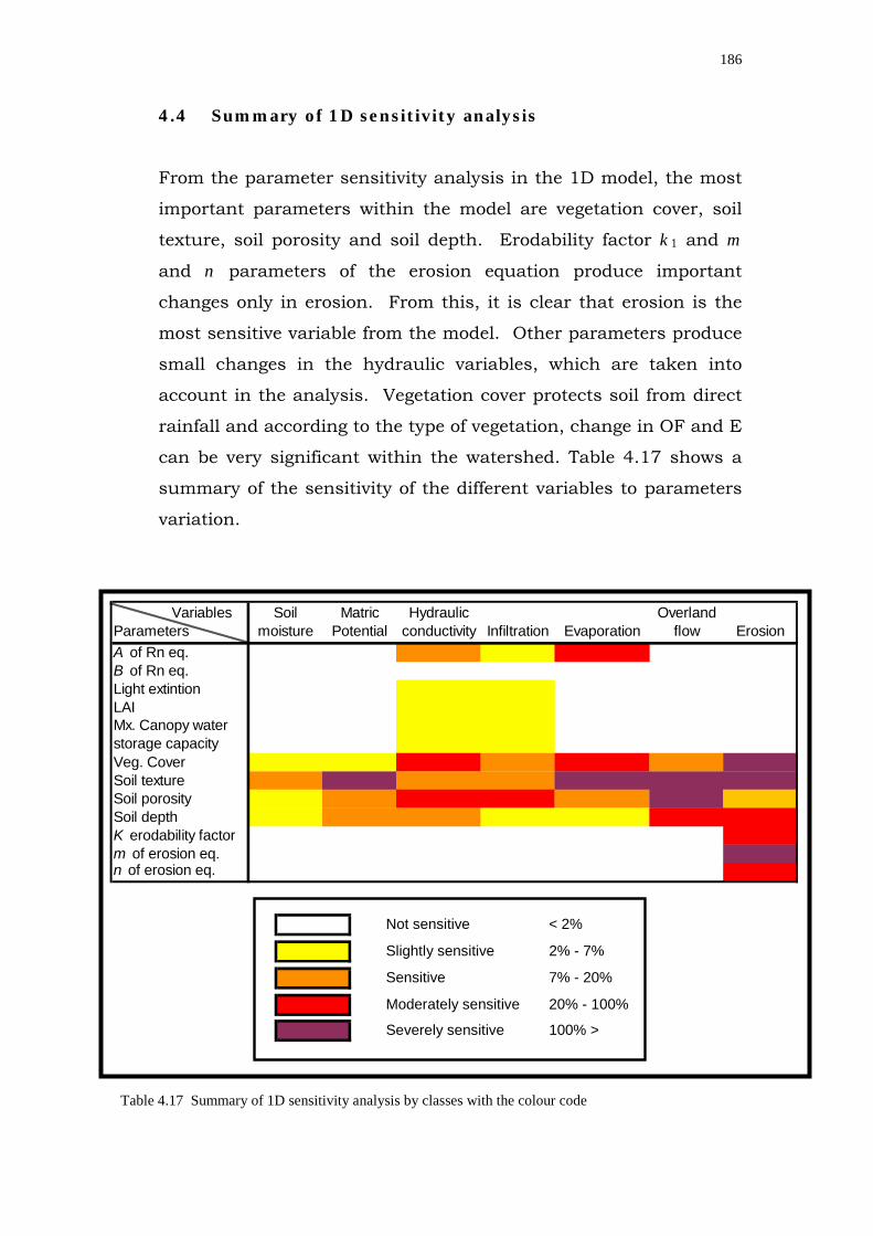
186
4.4 Summary of 1D sensitivity analysis
From the parameter sensitivity analysis in the 1D model, the most
important parameters within the model are vegetation cover, soil
texture, soil porosity and soil depth. Erodability factor k1 and m
and n parameters of the erosion equation produce important
changes only in erosion. From this, it is clear that erosion is the
most sensitive variable from the model. Other parameters produce
small changes in the hydraulic variables, which are taken into
account in the analysis. Vegetation cover protects soil from direct
rainfall and according to the type of vegetation, change in OF and E
can be very significant within the watershed. Table 4.17 shows a
summary of the sensitivity of the different variables to parameters
variation.
Variables Parameters
Soil moisture
Matric Potential
Hydraulic conductivity Infiltration Evaporation
Overland flow Erosion
A of Rn eq.B of Rn eq.Light extintionLAIMx. Canopy water storage capacityVeg. CoverSoil textureSoil porositySoil depthK erodability factorm of erosion eq.n of erosion eq.
Not sensitive < 2%
Slightly sensitive 2% - 7%
Sensitive 7% - 20%
Moderately sensitive 20% - 100%
Severely sensitive 100% >
Table 4.17 Summary of 1D sensitivity analysis by classes with the colour code

187
4.5 2.5D model sensitivity analysis
Sensitivity analysis at the catchment scale is carried out to identify
the area characteristics within a given LUCC scenario, which
produce the highest impact on the model hydrological variables.
Based on the sensitivity analysis at the plot scale (1D model), the
most sensitive hydrological variables to LUCC were overland flow
and soil erosion. These two variables are then used in this part of
the analysis process as an indicator of LUCC impact. The
parameter (vegetation cover) was identified from the 1D sensitivity
analysis as one of the drivers of LUCC impact, and in essence,
changes in vegetation cover are the same as changes in LUCC. So
vegetation cover at the catchment scale is going to be included in
the model with the LUCC scenarios designed for this thesis.
Physical soil property parameters (soil texture, soil porosity and
soil depth, as well as the soil parameters in the erosion equation)
are assumed uniform across the whole catchment irrespective of
land cover since the objective of this modelling is to understand
landscape sensitivity resulting from topographical variability and
hydrological connectivity in combination with LUCC. These
topographic variables are used in the sensitivity analysis at the
catchment scale, to identify how they control catchment sensitivity
to LUCC and thus which areas within the catchment are more
sensitive to LUCC.
Further up, the topographic characteristics used, are defined and
described. In addition, overland flow and erosion sensitivity
analyses are presented.

188
4.5.1 Definition of topographic characteristics
In order to analyse the flux variation with changes in scenarios,
physical properties of deforested areas within the watershed
between iterations in the scenarios were summarised and
averaged.
Topographic variables have been used to explain and assess some
physical events that occur in the environment. Quine and Walling
(1993) used topographic variables to assess the landscape
sensitivity to erosion and deposition. Gerrard (1993) used specific
relief values like maximum slope angle, stream density, stream
frequency and stream order to assess the landscape sensitivity.
McKenzie and Ryan (1999) combined environmental variables from
the landscape to predict spatial soil properties with good results.
The variables taken into account in this part of the analysis were:
slope, aspect, topographic index, altitude and proximity of the
deforested area to river channels.
Slope: the degree of rate of change of elevation per unit of
horizontal distance. Slope can be derived from a Digital Elevation
Model1 (DEM, which is a raster2 image whereby each grid cell has
an elevation value).
Aspect is the direction of the maximum slope in a given point with
relation to a geographical north direction (given in degrees). It is
also derived from the DEM.
Altitude or elevation is the vertical distance (m) of a given point in
relation to a reference point, usually mean sea level.
Distance to rivers (m) was computed using the raster image of the
river channels, which was classified into 18 classes using a 50m
buffer of horizontal distance either side of the rivers channels.
1 Interpolated surface derived from elevation points.2 An image surface conformed by pixels or cells of uniform size

189
Topographic index was first proposed by Kirkby (1975) and then
developed as a part of a complete hydrological model by Beven and
Kirkby (1976, 1979). This index represents the propensity of any
point in the catchment to develop saturated conditions. High
values will be caused by either long slopes or upslope contour
convergence, and low slope angles. It can be used as a guide for
water and sediment movement. It has proven a useful index for
predicting soil properties within the landscape (Mckenzie et al.,
1999). It is defined as:
TopIndex = ln (Ac / tan Β)
Where Ac is the specific contributing area expressed in m2 per unit
width orthogonal to the flow direction, and B is the slope angle.
Normally both Ac and B are derived from the analysis of digital
terrain model, in which the evaluation of pixel connectivity is
produced, and integrated by the accumulative area of upslope
direction (Beven et al., 1995).
All variables were calculated with the GIS at a 25-m pixel size and
averaged for each of the deforested areas of each iteration in each
scenario. A summary of average values of topographic variables
from deforested areas, by iteration per scenario, is given in
Appendix 10.
4.5.2 Sensitivity analysis at the catchment scale
Sensitivity analysis was carried out for five LUCC scenarios. Each
iteration of each scenario was run for a year at an hourly time step,
using the 2.5D model developed in PCRaster (Utrecht University,
1996) for the whole catchment. Model initial conditions were
taken from modelled results produced at the end of a one-year pre-
Eq. 4.1

190
run. Overland flow (OF) and erosion (E) were the variables taken
into account in the analysis. The last nine months of the
simulated year were summarised using the one year average by m2
for each of the flux variables. This was done to avoid the inclusion
of data from the period when the model was adjusting to initial
conditions. Three months were shown to be enough time for model
recovery. Three different initial soil moisture conditions were used
to run the model with the same rainfall events; as is shown in
Figure 4.25 the soil moisture takes similar pattern after the first
600 hours. The model was parameterised with the parameters
outlined in the previous section 4.3 and with the initial image of
LUCC for scenarios. The simulated period includes two rainy
seasons and one dry season, and accounts for more than 6000
time steps in the model process.
Graphical analysis of each variable (OF and E) within each scenario
(SC1 to SC5) was undertaken and presented in a set of 6 graphics.
The graphics contain:
1- Pixel average for the catchment of one year total yielded by the
variables (OF in mm and E in mm).
2- Percent variation for each variable between each LUCC iteration,
given as a percentage.
3- Sensitivity of the variable to LUCC, which is the percent of
variation between two consecutive iterations divided by the change
in deforested area between the same iterations. This gives the net
response per unit of deforestation. They are shown on the same
scale for all scenarios to allow comparison of the sensitivities.
4- Total deforested area by iterations (ha.) compared with mean
altitude of deforested area by iteration (masl).
5- Mean slope and aspect of deforested area by iteration. Both are
presented in degrees.
6- Mean topographic index and mean distance to river of the
deforested area.
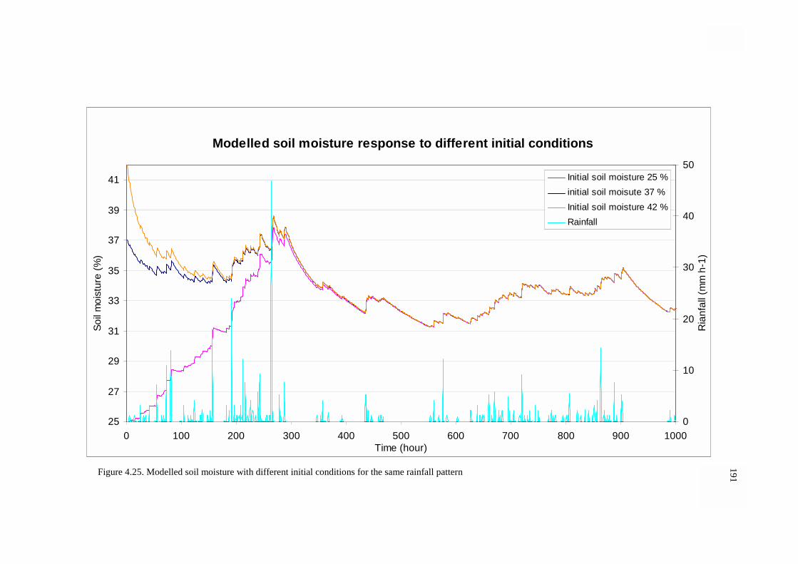
191
191Figure 4.25. Modelled soil moisture with different initial conditions for the same rainfall pattern
Modelled soil moisture response to different initial conditions
25
27
29
31
33
35
37
39
41
0 100 200 300 400 500 600 700 800 900 1000Time (hour)
So
il m
ois
ture
(%
)
0
10
20
30
40
50
Ria
nfa
ll (m
m h
-1)
Initial soil moisture 25 %
initial soil moisute 37 %
Initial soil moisture 42 %
Rainfall

192
4.5.2.1 Sensitivity analysis of overland flow to LUCC at the catchment scale
Variation in OF between iterations was calculated and then divided
by the deforested area between iterations to get the OF sensitivity
to LUCC by scenario (table 4.18, page 205). Table 4.18
summarises the total OF by iteration for each scenario, the percent
of variation and the sensitivity to LUCC. The sensitivity is
highlighted with colours to identify the highest sensitivities.
Figures 4.26 to 4.35 show total of OF by iteration, the percent
variation of OF between iteration and the OF sensitivity for the
scenarios.
The pattern of deforestation between iterations by scenario is
different. Consequently the OF yield is also different for each
scenario throughout the iterations. Although SC1 (cellular
automata scenario, page 54) has one of the largest deforested areas
in the initial iterations (see table 4.18), it is ranked third due to the
average yield of OF. Also SC1 was the most uniform in
deforestation pattern because the percent variation was the lowest
(83%).
The scenarios with the lowest yield in OF during the simulation
period were SC3 and SC4 (averaging per iteration at 7919 and
7927 mm respectively). The percent variation of these two
scenarios were relatively uniform (132 and 135 %).
Scenarios SC2 and SC5 produce the highest average OF by
iteration (7965 and 7964 mm respectively). Scenarios SC3 and
SC4 both have the same deforestation pattern in opposing
directions, SC2 starts form the lower part of the catchment, and

193
SC5 starts from the top of the catchment. The percent of variation
were similar for both (132 and 125 %).
The LUCC pattern in SC1 is very varied (see Figures 4.26 and
4.27). Deforestation occurs at the beginning in the lowest part of
the catchment (lower mean altitude) and where the slope is small.
More than half of the area (816.4 ha) in SC1 is deforested in the
first four iterations, which produces an additional 35 mm in OF
and 10 mm in E. For this reason, the percentage of variation of
OF and E decreases rapidly. Mean altitude and mean slope of the
deforested area increases gradually through the iterations, but the
area deforested per iteration decreases. A few oscillations of slope
in the deforested area at the end of the scenario, have some
relation with the variations in OF sensitivity. The decreasing trend
of mean topographic values and mean distance to the river also
have some similarities with the OF sensitivity in the last iterations.
Despite those variations, the OF sensitivity in SC1 is very low,
without large changes (range 0.2 to 1.7).
In SC2, 1109 ha (78% of the area) were deforested in the first five
iterations producing 4 mm OF (4% of additional OF generated by
deforestation) and 18 mm in E ( 81% of additional E generated by
deforestation). In these iterations, while OF sensitivity remains
constant, E sensitivity decreases until iteration 2 and then remains
constant. This means that E is affected by other additional
variables compared to OF. The percent variation in OF is related to
the amount of OF. However, it is important to highlight that the
biggest changes in mean altitude, deforested area, and topographic
index occur in the first iterations (see Figures 4.28 and 4.29).
Between iterations 8 and 12, OF sensitivity changes significantly.
These changes are related to a decreasing mean slope in deforested
area, and increasing mean altitude, topographic index, and
distance to rivers of the deforested area.

194
Figure 4.27 Mean topographic variables for deforested areas in SC1
D eforested area and m ean altitude in S C 1
0
100
200
300
400
500
0 5 10 15 20 25Iteration
1400
1900
2400
2900
D eforested areaA ltitude
M ean slope and aspect of defo rested area in
SC 1
0
100
200
300
0 5 10 15 20 25Iteration
0
10
20
30
40
50
60
Aspect
Slope
M ean to p.index and distance to rivers in S C 1
6
7.5
9
10.5
12
0 5 10 15 20 25Iteration
0
3
6
9
12
15
18
Topographic Index
Distance to river
194
Figure 4.26 Overland flow sensitivity in scenario 1 (deforested pattern with cellular automata)
T otal o verland flow by iteratio n
7850
7880
7910
7940
7970
8000
0 5 10 15 20 25Iteration
% variation of o verland flow
betw een iterations
0
0.05
0.1
0.15
0.2
0.25
0.3
0 5 10 15 20 25Iteration
O verland flo w sensitivity
0
5
10
15
0 5 10 15 20 25Iteration

195
D efo rested area and m ean altitude in S C 2
0
100
200
300
400
0 5 10 15 20Iteration1400
1900
2400
2900
D eforested area
A ltitude
M ean slo pe and aspect o f defo rested area in
S C 2
0
100
200
300
0 5 10 15 20Iteration
0
10
20
30
40
50
60
A spect
Slope
M ean to p.index and distant to rivers in S C 2
6
7.5
9
10.5
12
0 5 10 15 20Iteration
0
3
6
9
12
15
18
Top. index
Distance to rivers
Figure 4.29 Mean topographic variables of deforested areas in SC2
195
Figure 4.28 Overland flow sensitivity in scenario 2 (forest conversion with a fixed horizontal distance from river channel in uphill direction)
T otal O verland flo w by iteratio n
7850
7880
7910
7940
7970
8000
0 5 10 15 20Iteration
% variatio n o f overland flo w
betw een iteratio ns
0
0.05
0.1
0.15
0.2
0.25
0.3
0 5 10 15 20Iteration
S ensitivity o f O verland flo w
0
5
10
15
0 5 10 15 20Iteration

196
After iteration 12, OF sensitivity has a big oscillation, decreasing
and then increasing to its maximum value, as a result of the
change in distance to rivers, mean altitude, and topographic index.
This wave on the graphic of OF sensitivity could be explained by
the combination of those factors, in particular the high values of
mean slope and mean altitude, which in the last iterations produce
the highest variation in OF sensitivity. Overall, the highest OF
sensitivity is produced in SC2, and ranged from 0 to 16 (see Figure
4.28).
In the SC3 (see Figure 4.30), the deforested area within the first 12
iterations is 148 ha (10% of the total area), which produces 30 mm
of OF (29% of additional OF generated by deforestation) and 2.8
mm of E (12% of additional E generated by deforestation). The OF
sensitivity in SC3 is a mirror view of the OF sensitivity of SC2 with
small variations. That is expected because the deforested areas are
very similar but in reverse directions. Although the areas are
similar, the OF sensitivity is larger in SC3 than SC2. This could be
due to the biggest change in mean slope and mean topographic
index occurring in the first three iterations, and the longer distance
to rivers. In SC3, the OF sensitivity in the first iterations is high
and extensive, with some variability during the last few iterations.
The big oscillation in the OF sensitivity occurs in iterations 5, 6
and 7, and could be due to changes in percent variation of OF,
because none of the other aspects have the same trends (see Figure
4.31).
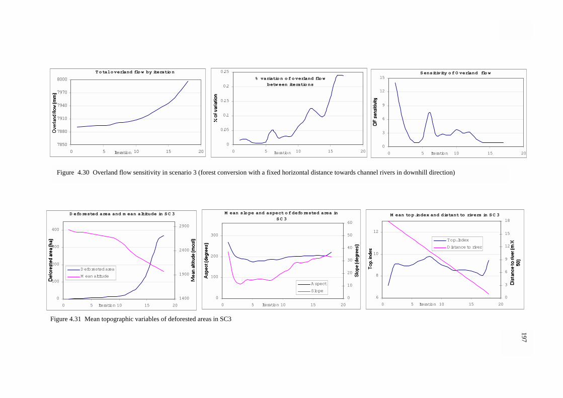
197
D eforested area and m ean altitude in S C 3
0
100
200
300
400
0 5 10 15 20Iteration
1400
1900
2400
2900
D eforested area
M ean altitude
M ean slo pe and aspect o f defo rested area in
S C 3
0
100
200
300
0 5 10 15 20Iteration
0
10
20
30
40
50
60
A spect
Slope
M ean top.index and distant to rivers in S C 3
6
8
10
12
0 5 10 15 20Iteration
0
3
6
9
12
15
18
Top. Index
D istance to river
Figure 4.31 Mean topographic variables of deforested areas in SC3
197
Figure 4.30 Overland flow sensitivity in scenario 3 (forest conversion with a fixed horizontal distance towards channel rivers in downhill direction)
T o tal overland flo w by iteratio n
7850
7880
7910
7940
7970
8000
0 5 10 15 20Iteration
% variatio n o f overland flo w
betw een iteratio ns
0
0.05
0.1
0.15
0.2
0.25
0 5 10 15 20Iteration
S ensitivity o f O verland flo w
0
3
6
9
12
15
0 5 10 15 20Iteration

198
The OF sensitivity for SC4 ranges from 0.6 up to 7, which is half
compared to SC2 and SC3. This means that the areas close to
river channels are more hydrologically sensitive to LUCC than the
deforested areas created with the elevation pattern (SC4 and SC5).
The deforested area in SC4 between iterations 1 to 8 was 735 ha
(52% of the catchment), which produces 29.4 mm of OF (27% of OF
generated by deforestation) and 9.7 mm of E (42% of E generated
by deforestation) (see Figures 4.32 and 4.33). The variation of OF
sensitivity in the first eight iterations (see Figure 4.32) is relatively
constant and small. The areas deforested during these iterations
are the lowest (in terms of altitude) in the watershed; the elevation
of these areas ranges between 1400m to 2000m (see Appendix 10).
After the eighth iteration, the OF sensitivity changes in proportion
with a number of oscillations and increases until the fifteenth
iteration. Between iterations 10 and 15 the percentage variation of
OF increases and decreases, but the OF sensitivity in the same
range always increases. Those variations in the OF sensitivity
could be due to a combination of a decrease in mean slope and
mean aspect and an increase in mean distance to rivers (see Figure
4.33) of the deforested area. Also, the mean elevation, which
increases constantly through the simulation, might have some
effects on the OF sensitivity since rainfall is distributed as a
function of elevation. The large variations in OF sensitivity are in
the last 5 iterations, even though the slope values of the deforested
areas in the last iterations are small, and those areas are further
away from rivers channels, but do have high rainfall receipts.
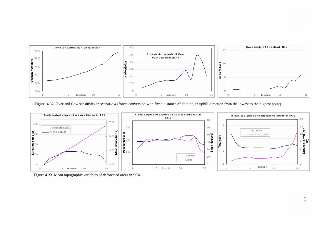
199
D eforested area and m ean altitude in S C 4
0
100
200
300
400
0 5 10 15Iteration
1400
1900
2400
2900
D eforested area
M ean altitude
M ean slope and aspect of defo rested area in
SC 4
0
100
200
300
0 5 10 15Iteration
0
10
20
30
40
50
60
Aspect
Slope
M ean to p.index and distant to rivers in SC 4
6
8
10
12
0 5 10 15Iteration0
3
6
9
12
15
18
Top. Index
D istance to river
Figure 4.33 Mean topographic variables of deforested areas in SC4
199
Figure 4.32 Overland flow sensitivity in scenario 4 (forest conversion with fixed distance of altitude, in uphill direction from the lowest to the highest point)
T otal o verland flo w by iteratio n
7850
7880
7910
7940
7970
8000
0 5 10 15Iteration
% variation overland flo w
betw een iteratio ns
0
0.05
0.1
0.15
0.2
0.25
0.3
0 5 10 15Iteration
S ensitivity o f O verland flo w
0
5
10
15
0 5 10 15Iteration
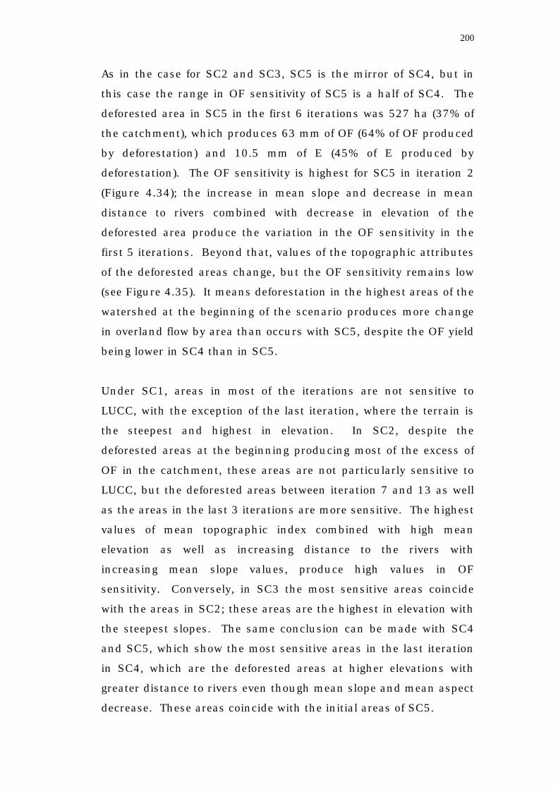
200
As in the case for SC2 and SC3, SC5 is the mirror of SC4, but in
this case the range in OF sensitivity of SC5 is a half of SC4. The
deforested area in SC5 in the first 6 iterations was 527 ha (37% of
the catchment), which produces 63 mm of OF (64% of OF produced
by deforestation) and 10.5 mm of E (45% of E produced by
deforestation). The OF sensitivity is highest for SC5 in iteration 2
(Figure 4.34); the increase in mean slope and decrease in mean
distance to rivers combined with decrease in elevation of the
deforested area produce the variation in the OF sensitivity in the
first 5 iterations. Beyond that, values of the topographic attributes
of the deforested areas change, but the OF sensitivity remains low
(see Figure 4.35). It means deforestation in the highest areas of the
watershed at the beginning of the scenario produces more change
in overland flow by area than occurs with SC5, despite the OF yield
being lower in SC4 than in SC5.
Under SC1, areas in most of the iterations are not sensitive to
LUCC, with the exception of the last iteration, where the terrain is
the steepest and highest in elevation. In SC2, despite the
deforested areas at the beginning producing most of the excess of
OF in the catchment, these areas are not particularly sensitive to
LUCC, but the deforested areas between iteration 7 and 13 as well
as the areas in the last 3 iterations are more sensitive. The highest
values of mean topographic index combined with high mean
elevation as well as increasing distance to the rivers with
increasing mean slope values, produce high values in OF
sensitivity. Conversely, in SC3 the most sensitive areas coincide
with the areas in SC2; these areas are the highest in elevation with
the steepest slopes. The same conclusion can be made with SC4
and SC5, which show the most sensitive areas in the last iteration
in SC4, which are the deforested areas at higher elevations with
greater distance to rivers even though mean slope and mean aspect
decrease. These areas coincide with the initial areas of SC5.
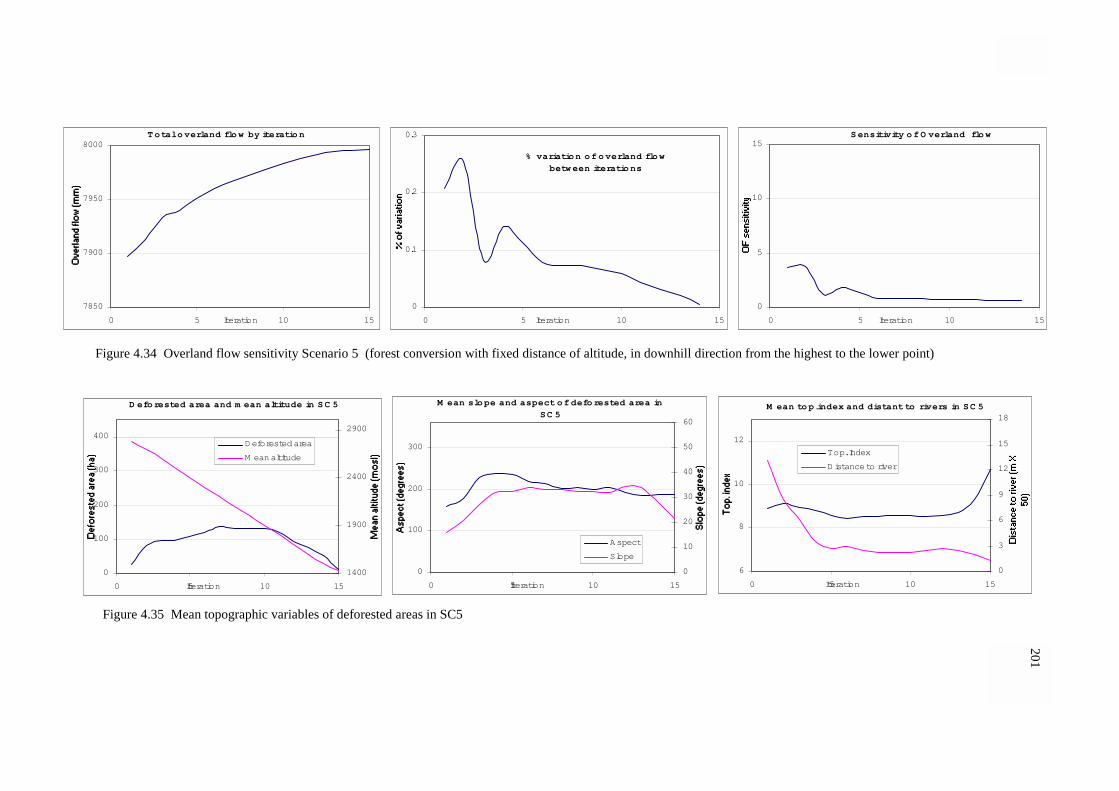
201
Figure 4.35 Mean topographic variables of deforested areas in SC5
D eforested area and m ean altitude in S C 5
0
100
200
300
400
0 5 10 15Iteration
1400
1900
2400
2900
D eforested area
M ean altitude
M ean slope and aspect of defo rested area in
SC 5
0
100
200
300
0 5 10 15Iteration
0
10
20
30
40
50
60
Aspect
Slope
M ean to p.index and distant to rivers in SC 5
6
8
10
12
0 5 10 15Iteration
0
3
6
9
12
15
18
Top. Index
D istance to river
201
Figure 4.34 Overland flow sensitivity Scenario 5 (forest conversion with fixed distance of altitude, in downhill direction from the highest to the lower point)
T otal o verland flo w by iteratio n
7850
7900
7950
8000
0 5 10 15Iteration
% variation of o verland flow
betw een iteratio ns
0
0.1
0.2
0.3
0 5 10 15Iteration
S ensitivity o f O verland flo w
0
5
10
15
0 5 10 15Iteration
202
This highlights that the areas with highest OF sensitivity to LUCC
within the catchment are at elevations higher than 2200 m.
Despite the fact that high overland flow is produced in the highest
elevations, the stronger OF sensitivity is shown in SC2 and SC3,
which are related with distance to rivers. Clearly, as elevation
increases so does distance from rivers.
To identify whether or not physical variables are involved in the OF
sensitivity explanation, first of all a Kolmogorov-Smirnov test to
determent the topographic variables normal distribution which
they are, and then a multiple regression analysis was performed for
all scenarios, using the statistical package STATISTICA 6.0
(produced by Statsoft Inc., USA). Table 4.19 summarises and
compares the results of the multiple regression analysis for the
scenarios on the basis of data from Appendix 10. The dependent
variable was OF sensitivity and topographic variables were used as
independent variables. The analysis included calculation of the
explanatory coefficient of determination (R2) of the OF sensitivity, in
relation to independent variables, and the t-coefficient for
statistical significance for each variable (Rincon-Romero, 2000).
The multiple linear correlation coefficient (R) shows how dependent
variables (OF sensitivity) can be explained as a function of the
linear combination of independent variables (topographic
variables). Comparing the R values from the five scenarios (see
table 4.19), the R of SC4 (0.98) shows that 98% of the OF
sensitivity can be explained by linear combination of the
topographic variables for the deforested area, while for SC1 the R is
just 51%, only 51% of the OF sensitivity can be explained by linear
combination of topographic variables. The highest coefficients of
determination are in SC4 and SC5, which are the scenarios based
on elevation, followed by SC3 and SC2 (0.84 and 0.83, respectively)

203
and the lowest is SC1. In the same way, R2 is the proportion of the
variation in the dependent variable that can be attributed to the
variation of the combined independent variables. The maximum
value of R2 is in SC4 (R2 = 0.97) and the minimum in SC1 (R2 =
0.26).
The critical value of a statistically significant F value, with 95%
probability with (5,15 in SC1), (5,11 in SC2 and SC3), (5,8 in SC4
and SC5) degrees of freedom is 1.89. From table 4.19, it is clear
that none of the computed F values from all scenarios surpassed
the critical value, and as a result, the null hypothesis was not
rejected in any scenario. This confirms that there is no reason to
believe that the independent variables are correlated with each
other. The probability that R would have fortuitously occurred if
the null hypothesis held true was less than 0.05 in all scenarios
with the exception of SC1. The criteria to argue that each variable
helps in the explanation of dependent variable when its used in
combination with the other variables is the t-critical value.
Assuming α=0.5 the t-critical value for the explanation of OF
sensitivity by the landscape properties discussed is 2.131 for SC1
(N=15), is 2.201 for SC2 and SC3 (N=11) and is 2.306 for SC4 and
SC5 (N=8). If the computed t-value exceeds the t-critical value, it
means that the variable is a significant contributor to explanation
of the dependent variable when it is used in combination with the
other variables. The significant contributor for SC1 is slope, for
SC3 is aspect and for SC4 and SC5 is the distance to rivers. For
SC2 none of the topographic variables appear as a significant
contributor in the explanation of the OF sensitivity. This does not
mean that the other variables are not involved in the explanation of
OF sensitivity; it simply says that the associated probability that
the relationships of those variables could occur by chance, if the
null hypothesis were true, is less than 0.05.

204
From this analysis, it can be concluded that the topographic
variables, which are involved in greater proportion in the
explanation of the OF sensitivity, are slope and distance to rivers.
Aspect is not an important variable, a part of that paradoxically, in
SC3 and also SC2, where is the greatest contributor to the
explanation of the OF sensitivity. Topographic index seems not to
be an important variable in the explanation of the OF sensitivity for
all scenarios with the exception in SC1. Despite the fact that SC2
and SC3 appear as the most sensitive scenarios, the variable
distance to rivers was not the most important in the regression
analysis for those scenarios. Although the degree of correlation
between dependent and independent variables in some models are
not high, further combinations of variables could be tested in order
to produce a better correlation of topographic variables and the OF
sensitivity.
205205
Table 4.18 Summary of data used in OF sensitivity analysis
OverlandOverlandOverlandOverland Flow Flow Flow Flow (mm)(mm)(mm)(mm) Percent Percent Percent Percent of of of of VariationVariationVariationVariation OverlandOverlandOverlandOverland Flow Flow Flow Flow SensitivitySensitivitySensitivitySensitivityScenario 1 Scenario 2 Scenario 3 Scenario 4 Scenario 5 Scenario 1Scenario 2 Scenario 3Scenario 4Scenario 5 Scenario 1 Scenario 2Scenario 3Scenario 4 Scenario 5
1111 7889 7889 7892 7889 78972222 7910 7908 7893 7891 7913 0.27 0.02 0.24 0.02 0.21 0.97 0.95 14.01 0.65 3.663333 7917 7926 7894 7893 7934 0.09 0.02 0.23 0.03 0.25 0.82 0.96 6.49 0.67 3.764444 7924 7939 7895 7897 7940 0.08 0.01 0.17 0.04 0.08 0.81 1.02 2.43 0.71 1.215555 7929 7947 7895 7901 7951 0.07 0.00 0.10 0.06 0.14 0.75 1.04 0.89 0.75 1.856666 7934 7956 7896 7907 7960 0.06 0.01 0.11 0.07 0.11 0.89 1.67 1.72 0.75 1.397777 7938 7966 7900 7913 7966 0.05 0.05 0.12 0.07 0.08 0.81 3.31 7.55 0.82 0.828888 7941 7973 7902 7918 7972 0.04 0.02 0.08 0.07 0.07 0.82 3.05 2.66 0.83 0.829999 7944 7978 7905 7925 7978 0.04 0.03 0.06 0.08 0.07 0.82 3.88 2.81 0.83 0.82
10101010 7946 7980 7907 7934 7983 0.03 0.03 0.03 0.11 0.07 0.84 2.48 2.48 1.39 0.7511111111 7948 7983 7912 7945 7988 0.03 0.06 0.03 0.14 0.06 1.04 2.82 3.85 1.85 0.7412121212 7950 7985 7919 7951 7992 0.02 0.08 0.02 0.08 0.04 0.69 2.68 3.05 1.21 0.7113131313 7952 7989 7929 7971 7994 0.02 0.13 0.05 0.24 0.03 0.84 7.76 3.28 3.64 0.6614141414 7953 7989 7938 7988 7996 0.01 0.11 0.01 0.21 0.02 0.90 1.72 1.67 3.87 0.6515151515 7953 7990 7946 7996 7996 0.01 0.10 0.00 0.10 0.00 0.95 0.88 1.00 5.73 0.6116161616 7954 7991 7958 0.00 0.16 0.01 0.98 2.46 0.9817171717 7954 7992 7977 0.00 0.24 0.02 1.16 6.72 1.0018181818 7954 7993 7996 0.00 0.24 0.02 0.94 15.45 0.9519191919 7954 0.00 1.2120202020 7954 0.00 0.8021212121 7955 0.00 1.0122222222 7955 0.00 0.30
Sum 142889 143371 142556 118919 119461 82.55 131.87 131.91 134.91 124.90 15.02 58.85 56.82 23.70 18.45average 7941 7965 7920 7928 7964 0.04 0.08 0.08 0.10 0.09 0.87 3.46 3.34 1.69 1.32
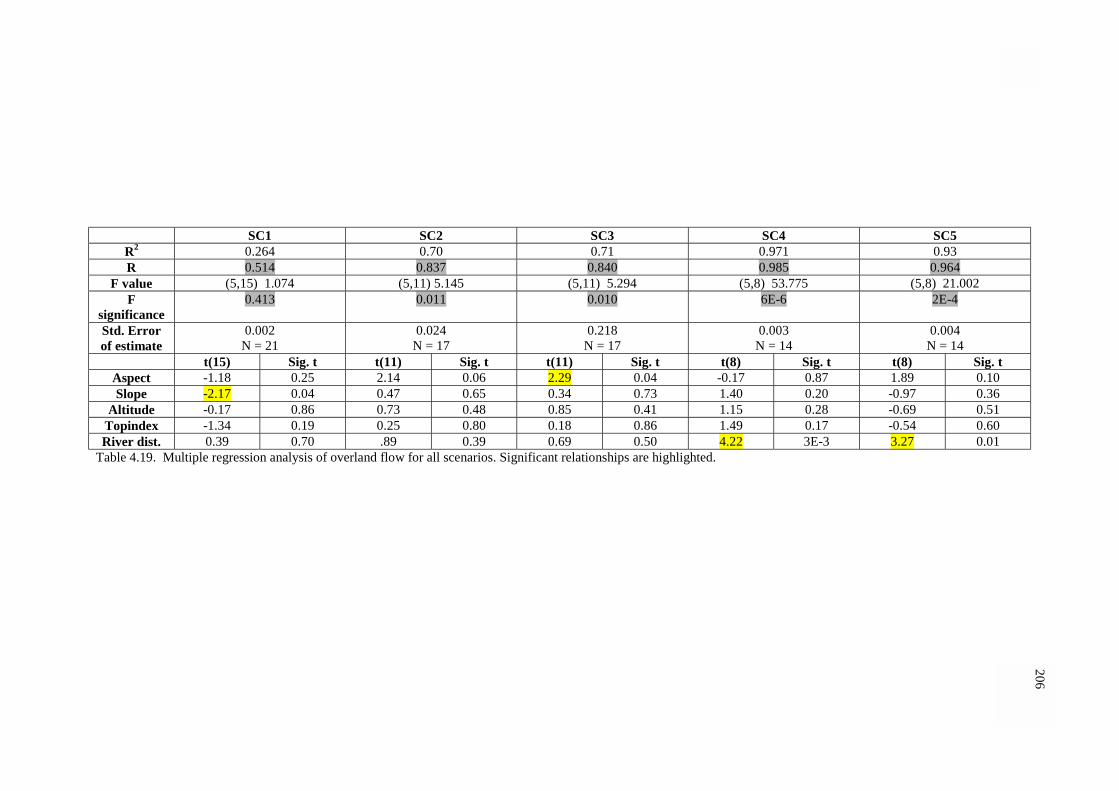
206
SC1 SC2 SC3 SC4 SC5R2 0.264 0.70 0.71 0.971 0.93R 0.514 0.837 0.840 0.985 0.964
F value (5,15) 1.074 (5,11) 5.145 (5,11) 5.294 (5,8) 53.775 (5,8) 21.002F
significance0.413 0.011 0.010 6E-6 2E-4
Std. Errorof estimate
0.002N = 21
0.024N = 17
0.218N = 17
0.003N = 14
0.004N = 14
t(15) Sig. t t(11) Sig. t t(11) Sig. t t(8) Sig. t t(8) Sig. tAspect -1.18 0.25 2.14 0.06 2.29 0.04 -0.17 0.87 1.89 0.10Slope -2.17 0.04 0.47 0.65 0.34 0.73 1.40 0.20 -0.97 0.36
Altitude -0.17 0.86 0.73 0.48 0.85 0.41 1.15 0.28 -0.69 0.51Topindex -1.34 0.19 0.25 0.80 0.18 0.86 1.49 0.17 -0.54 0.60River dist. 0.39 0.70 .89 0.39 0.69 0.50 4.22 3E-3 3.27 0.01
Table 4.19. Multiple regression analysis of overland flow for all scenarios. Significant relationships are highlighted.
206
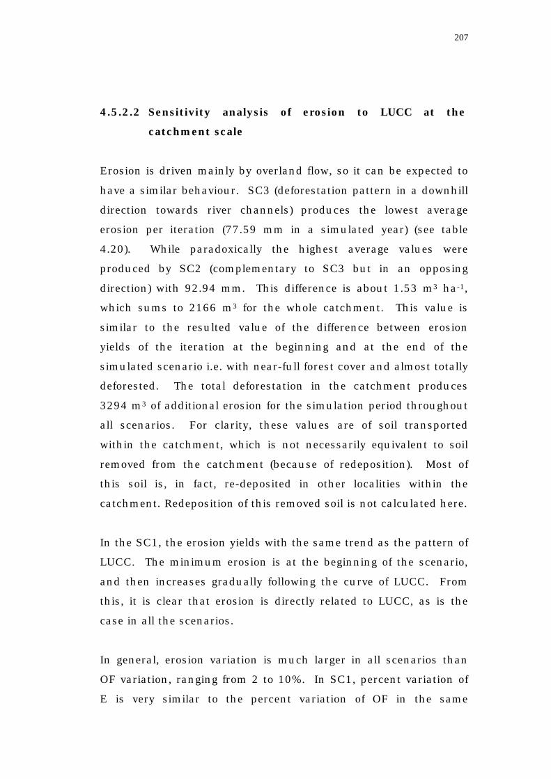
207
4.5.2.2 Sensitivity analysis of erosion to LUCC at the catchment scale
Erosion is driven mainly by overland flow, so it can be expected to
have a similar behaviour. SC3 (deforestation pattern in a downhill
direction towards river channels) produces the lowest average
erosion per iteration (77.59 mm in a simulated year) (see table
4.20). While paradoxically the highest average values were
produced by SC2 (complementary to SC3 but in an opposing
direction) with 92.94 mm. This difference is about 1.53 m3 ha-1,
which sums to 2166 m3 for the whole catchment. This value is
similar to the resulted value of the difference between erosion
yields of the iteration at the beginning and at the end of the
simulated scenario i.e. with near-full forest cover and almost totally
deforested. The total deforestation in the catchment produces
3294 m3 of additional erosion for the simulation period throughout
all scenarios. For clarity, these values are of soil transported
within the catchment, which is not necessarily equivalent to soil
removed from the catchment (because of redeposition). Most of
this soil is, in fact, re-deposited in other localities within the
catchment. Redeposition of this removed soil is not calculated here.
In the SC1, the erosion yields with the same trend as the pattern of
LUCC. The minimum erosion is at the beginning of the scenario,
and then increases gradually following the curve of LUCC. From
this, it is clear that erosion is directly related to LUCC, as is the
case in all the scenarios.
In general, erosion variation is much larger in all scenarios than
OF variation, ranging from 2 to 10%. In SC1, percent variation of
E is very similar to the percent variation of OF in the same

208
scenario. The relation between E and OF in SC1 is high, but the
erosion sensitivity changes strongly in the final few iterations of
this scenario. The erosion sensitivity in SC1 ranges from 25 to 60
(Figure 4.36). In this scenario while OF sensitivity decreases in the
last iteration, erosion sensitivity increases markedly. The erosion
sensitivity oscillations indicate that there are some differences
between the physical properties of the deforested areas in each
iteration. The topographic variables most related (see Figures 4.36
and 4.37) with erosion sensitivity in this case (SC1) are slope and
altitude. The magnitude of variation in topographic variables is not
as strong as the apparent variation in erosion sensitivity.
For SC2, the erosion yield is very similar to the LUCC pattern,
which is not the case for OF yield. The percentage variation of E
between iterations is similar to the LUCC pattern, but with a higher
rate of decrease in the first half of the iterations, followed by a
lower rate which then reduces to zero. The erosion sensitivity in
SC2 ranges from 12 to 38; the highest values are at the beginning
of the scenario, and then decrease gradually without significant
changes until iteration 16. For the last two iterations there is an
increase in erosion sensitivity (see Figure 4.38). The differences
between OF and E sensitivities are that OF sensitivity is small at
the beginning of the scenario and increases at the end whilst the
opposite is true for E sensitivity. The sensitivities of OF and E in
SC2 show that the initial deforestation near to the river channels
produces small changes in the percentage variation of OF, though
the sensitivity does not change too much. By comparing E
sensitivity with the mean topographic variables of the deforested
area (Figures 4.38 and 4.39) it can be seen that the most similar
behaviour is produced in slope, which has the same trend
throughout the iterations. The mean aspect of deforested area
does not change very much through the simulation.
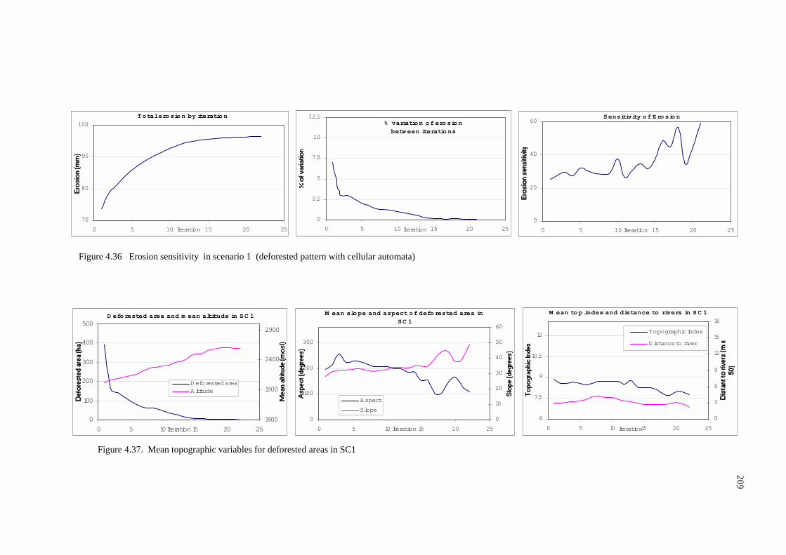
209
Figure 4.37. Mean topographic variables for deforested areas in SC1
D eforested area and m ean altitude in S C 1
0
100
200
300
400
500
0 5 10 15 20 25Iteration
1400
1900
2400
2900
D eforested areaA ltitude
M ean slope and aspect of defo rested area in
SC 1
0
100
200
300
0 5 10 15 20 25Iteration
0
10
20
30
40
50
60
Aspect
Slope
M ean to p.index and distance to rivers in S C 1
6
7.5
9
10.5
12
0 5 10 15 20 25Iteration
0
3
6
9
12
15
18
Topographic Index
Distance to river
209
Figure 4.36 Erosion sensitivity in scenario 1 (deforested pattern with cellular automata)
T otal ero sio n by iteratio n
70
80
90
100
0 5 10 15 20 25Iteration
% variation of erosion
betw een iteratio ns
0
2.5
5
7.5
10
12.5
0 5 10 15 20 25Iteration
S ensitivity o f Ero sio n
0
20
40
60
0 5 10 15 20 25Iteration
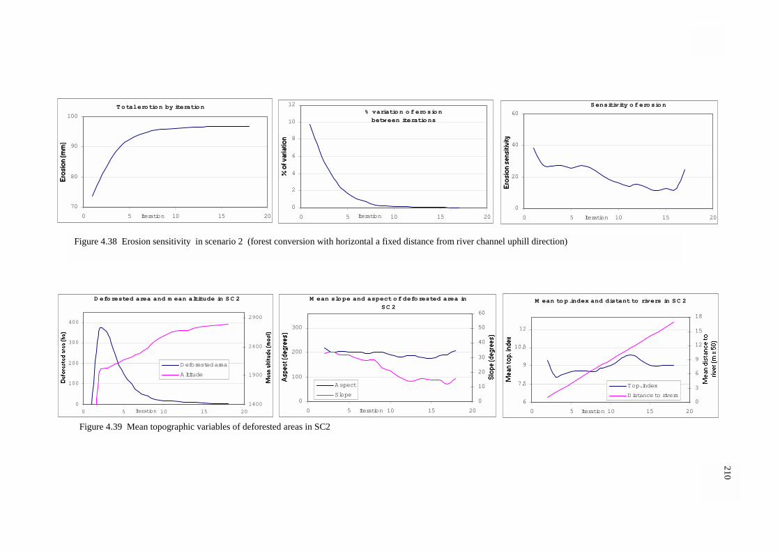
210
D eforested area and m ean altitude in S C 2
0
100
200
300
400
0 5 10 15 20Iteration1400
1900
2400
2900
D eforested area
A ltitude
M ean slope and aspect of defo rested area in
SC 2
0
100
200
300
0 5 10 15 20Iteration
0
10
20
30
40
50
60
Aspect
Slope
M ean to p.index and distant to rivers in SC 2
6
7.5
9
10.5
12
0 5 10 15 20Iteration
0
3
6
9
12
15
18
Top. index
D istance to rivers
Figure 4.39 Mean topographic variables of deforested areas in SC2
210
Figure 4.38 Erosion sensitivity in scenario 2 (forest conversion with horizontal a fixed distance from river channel uphill direction)
T o tal ero tion by iteration
70
80
90
100
0 5 10 15 20Iteration
% variatio n o f ero sio n
between iteratio ns
0
2
4
6
8
10
12
0 5 10 15 20Iteration
S ensitivity o f ero sio n
0
20
40
60
0 5 10 15 20Iteration

211
However, there is a large increment with significant changes to
percentage variation early in the LUCC iterations. This is also the
case for erosion sensitivity. The highest erosion sensitivity to
LUCC in this scenario is in deforested areas close to the river
channels (in the first iterations) and this is where most of the
erosion is produced in the catchment. This is the opposite of OF
sensitivity, which is high at the top of the catchment, that can be
due high mean slope values in these deforested areas.
In SC3 the erosion yield by iteration does not increase a lot in the
first 12 iterations (2 mm) and the E percent variation remains
equal (Figure 4.40). Through within these iterations the erosion
sensitivity varies highly (15 to 33). Then it remains low until
iteration 7, then, between iterations 7 to 11, where the E sensitivity
increases again to its highest value (33) after which it oscillates
once more, at a higher level of sensitivity. As in the SC2, the
topographic variable most related with S-E in SC3 is slope,
showing the same trend and pattern but with more exaggerated
changes. Topographic index in the first iteration shows the
opposite trend, but in the last iteration it is the same as erosion
sensitivity (see Figure 4.41). Distance to the rivers is opposite in
trend to erosion sensitivity and this suggests that, erosion
sensitivity is highest when the areas closest to the rivers are
deforested. Mean altitude of deforested area in this case does not
have any bearing on erosion sensitivity. Overall this scenario has
the lowest erosion sensitivity values. By taking into account both
SC2 and SC3 it can be concluded that the areas within 150m of
the rivers are very important for E, in magnitude, variation and
sensitivity. The areas farthest from the river channels do not
increase the E much, but they have a big influence in decreasing
the erosion sensitivity. In the middle areas the erosion sensitivity
increases once more. Slope and topographic index seem to be the
most significant control on erosion sensitivity.
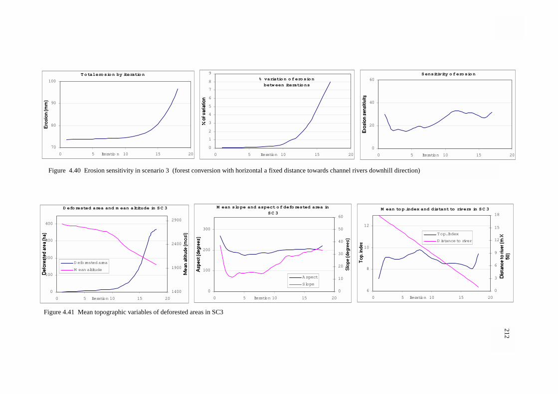
212
D eforested area and m ean altitude in S C 3
0
100
200
300
400
0 5 10 15 20Iteration
1400
1900
2400
2900
D eforested area
M ean altitude
M ean slope and aspect of defo rested area in
SC 3
0
100
200
300
0 5 10 15 20Iteration
0
10
20
30
40
50
60
Aspect
Slope
M ean to p.index and distant to rivers in SC 3
6
8
10
12
0 5 10 15 20Iteration
0
3
6
9
12
15
18
Top. Index
D istance to river
Figure 4.41 Mean topographic variables of deforested areas in SC3
212
Figure 4.40 Erosion sensitivity in scenario 3 (forest conversion with horizontal a fixed distance towards channel rivers downhill direction)
T otal ero sio n by iteratio n
70
80
90
100
0 5 10 15 20Iteratio n
% variatio n o f ero sio n
betw een iterations
0
1
2
3
4
5
6
7
8
9
0 5 10 15 20Iteration
S ensitivity o f ero sio n
0
20
40
60
0 5 10 15 20Iteration
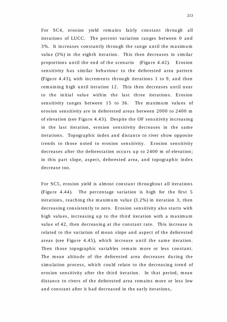
213
For SC4, erosion yield remains fairly constant through all
iterations of LUCC. The percent variation ranges between 0 and
3%. It increases constantly through the range until the maximum
value (3%) in the eighth iteration. This then decreases in similar
proportions until the end of the scenario (Figure 4.42). Erosion
sensitivity has similar behaviour to the deforested area pattern
(Figure 4.43), with increments through iterations 1 to 9, and then
remaining high until iteration 12. This then decreases until near
to the initial value within the last three iterations. Erosion
sensitivity ranges between 15 to 36. The maximum values of
erosion sensitivity are in deforested areas between 2000 to 2400 m
of elevation (see Figure 4.43). Despite the OF sensitivity increasing
in the last iteration, erosion sensitivity decreases in the same
iterations. Topographic index and distance to river show opposite
trends to those noted to erosion sensitivity. Erosion sensitivity
decreases after the deforestation occurs up to 2400 m of elevation;
in this part slope, aspect, deforested area, and topographic index
decrease too.
For SC5, erosion yield is almost constant throughout all iterations
(Figure 4.44). The percentage variation is high for the first 5
iterations, reaching the maximum value (3.2%) in iteration 3, then
decreasing consistently to zero. Erosion sensitivity also starts with
high values, increasing up to the third iteration with a maximum
value of 42, then decreasing at the constant rate. This increase is
related to the variation of mean slope and aspect of the deforested
areas (see Figure 4.45), which increase until the same iteration.
Then those topographic variables remain more or less constant.
The mean altitude of the deforested area decreases during the
simulation process, which could relate to the decreasing trend of
erosion sensitivity after the third iteration. In that period, mean
distance to rivers of the deforested area remains more or less low
and constant after it had decreased in the early iterations,
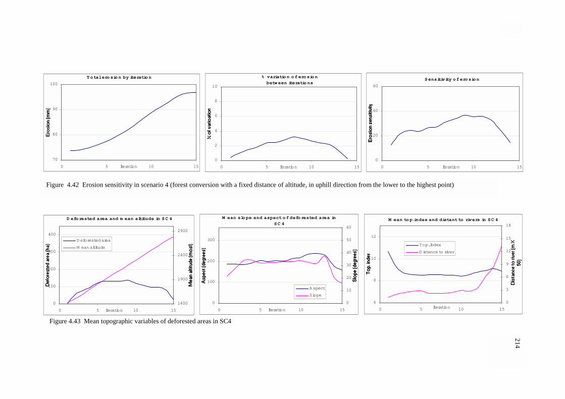
214
D eforested area and m ean altitude in S C 4
0
100
200
300
400
0 5 10 15Iteration
1400
1900
2400
2900
D eforested area
M ean altitude
M ean slope and aspect of defo rested area in
SC 4
0
100
200
300
0 5 10 15Iteration
0
10
20
30
40
50
60
Aspect
Slope
M ean to p.index and distant to rivers in SC 4
6
8
10
12
0 5 10 15Iteration0
3
6
9
12
15
18
Top. Index
D istance to river
Figure 4.43 Mean topographic variables of deforested areas in SC4
214
Figure 4.42 Erosion sensitivity in scenario 4 (forest conversion with a fixed distance of altitude, in uphill direction from the lower to the highest point)
T o tal ero sio n by iteratio n
70
80
90
100
0 5 10 15Iteration
% variatio n o f ero sio n
betw een iteratio ns
0
2
4
6
8
10
0 5 10 15Iteration
Sensitivity of erosion
0
20
40
60
0 5 10 15Iteration
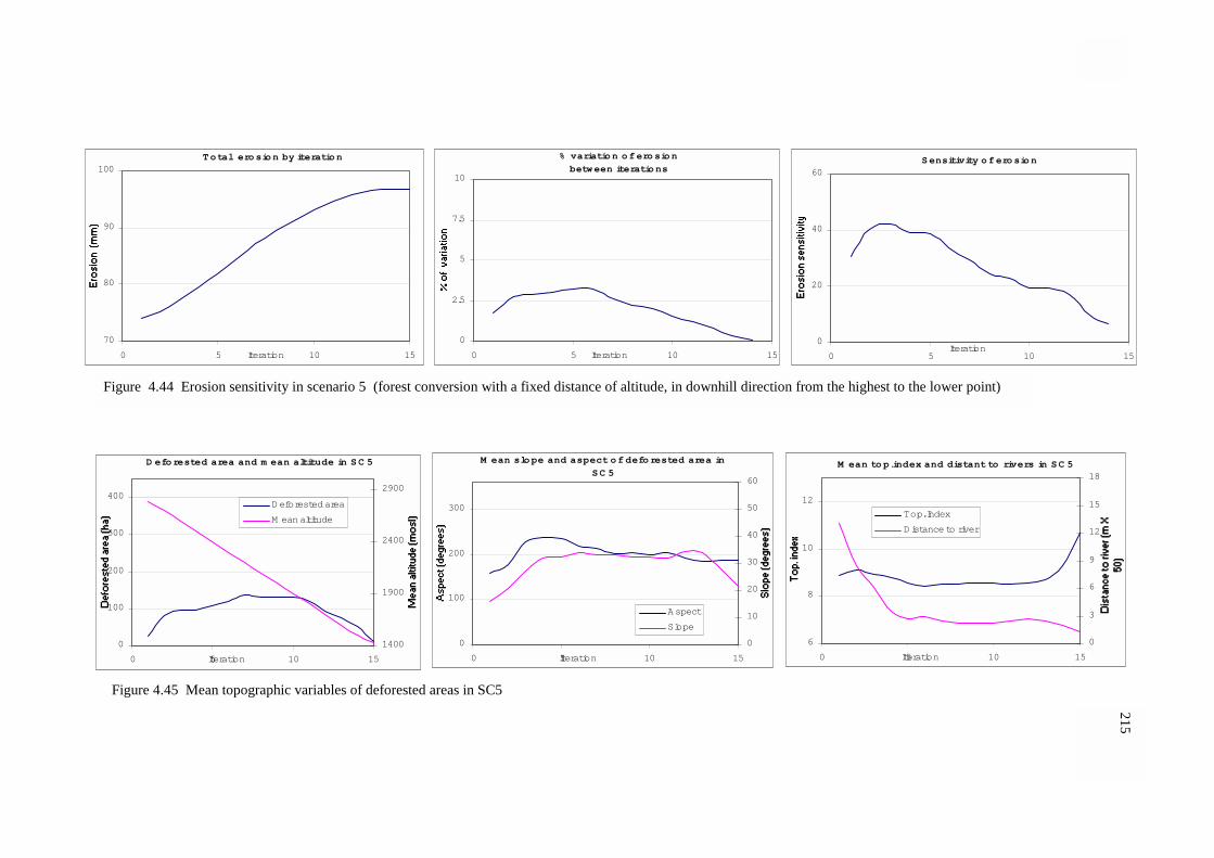
215
Figure 4.45 Mean topographic variables of deforested areas in SC5
D eforested area and m ean altitude in S C 5
0
100
200
300
400
0 5 10 15Iteration
1400
1900
2400
2900
D eforested area
M ean altitude
M ean slope and aspect of defo rested area in
SC 5
0
100
200
300
0 5 10 15Iteration
0
10
20
30
40
50
60
Aspect
Slope
M ean to p.index and distant to rivers in SC 5
6
8
10
12
0 5 10 15Iteration
0
3
6
9
12
15
18
Top. Index
D istance to river
215
Figure 4.44 Erosion sensitivity in scenario 5 (forest conversion with a fixed distance of altitude, in downhill direction from the highest to the lower point)
T o tal ero sio n by iteratio n
70
80
90
100
0 5 10 15Iteration
% variatio n o f ero sio n
betw een iteratio ns
0
2.5
5
7.5
10
0 5 10 15Iteration
S ensitivity o f ero sio n
0
20
40
60
0 5 10 15Iteration
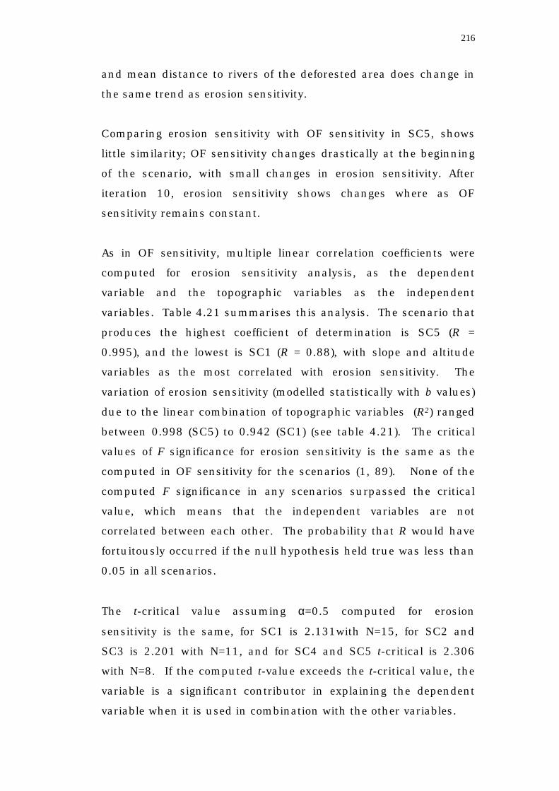
216
and mean distance to rivers of the deforested area does change in
the same trend as erosion sensitivity.
Comparing erosion sensitivity with OF sensitivity in SC5, shows
little similarity; OF sensitivity changes drastically at the beginning
of the scenario, with small changes in erosion sensitivity. After
iteration 10, erosion sensitivity shows changes where as OF
sensitivity remains constant.
As in OF sensitivity, multiple linear correlation coefficients were
computed for erosion sensitivity analysis, as the dependent
variable and the topographic variables as the independent
variables. Table 4.21 summarises this analysis. The scenario that
produces the highest coefficient of determination is SC5 (R =
0.995), and the lowest is SC1 (R = 0.88), with slope and altitude
variables as the most correlated with erosion sensitivity. The
variation of erosion sensitivity (modelled statistically with b values)
due to the linear combination of topographic variables (R2) ranged
between 0.998 (SC5) to 0.942 (SC1) (see table 4.21). The critical
values of F significance for erosion sensitivity is the same as the
computed in OF sensitivity for the scenarios (1, 89). None of the
computed F significance in any scenarios surpassed the critical
value, which means that the independent variables are not
correlated between each other. The probability that R would have
fortuitously occurred if the null hypothesis held true was less than
0.05 in all scenarios.
The t-critical value assuming α=0.5 computed for erosion
sensitivity is the same, for SC1 is 2.131with N=15, for SC2 and
SC3 is 2.201 with N=11, and for SC4 and SC5 t-critical is 2.306
with N=8. If the computed t-value exceeds the t-critical value, the
variable is a significant contributor in explaining the dependent
variable when it is used in combination with the other variables.
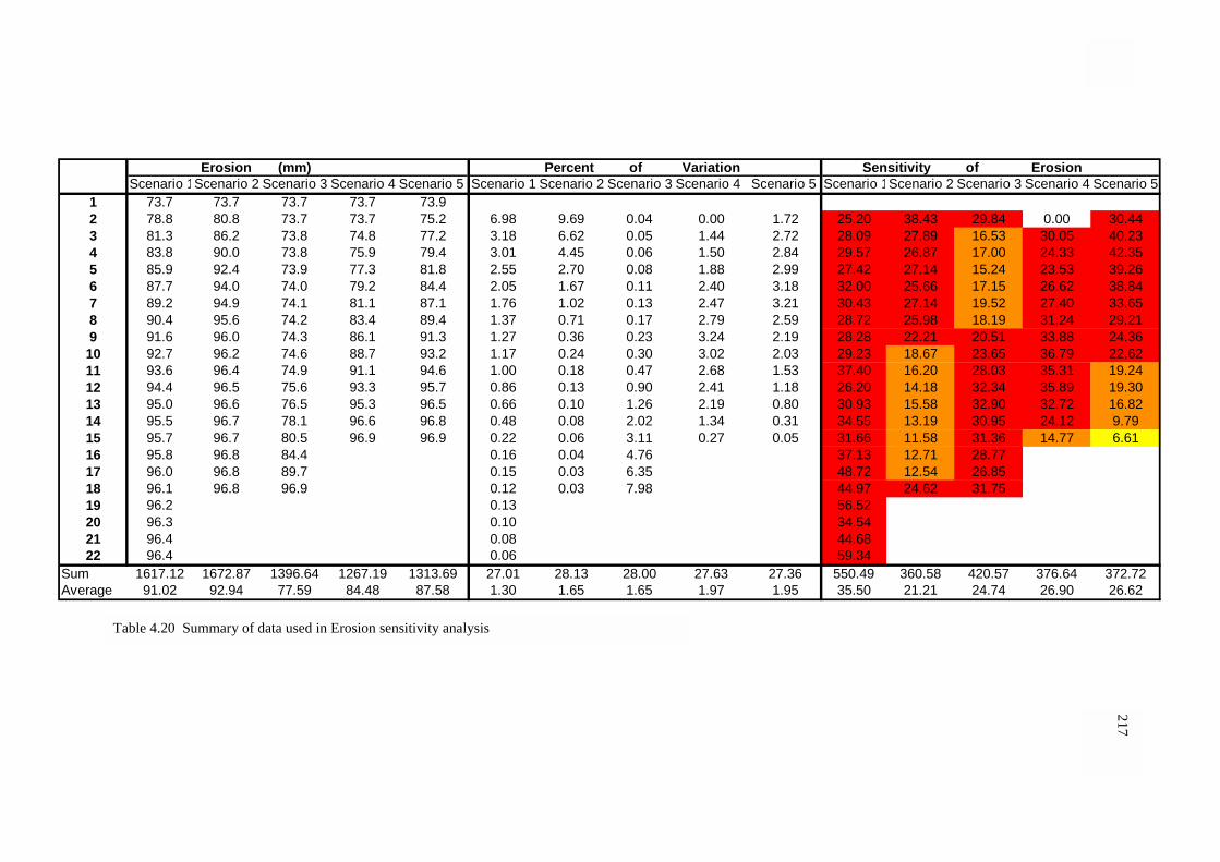
217
217
Table 4.20 Summary of data used in Erosion sensitivity analysis
Erosion (mm) Percent of Variation Sensitivity of ErosionScenario 1Scenario 2 Scenario 3 Scenario 4 Scenario 5 Scenario 1 Scenario 2 Scenario 3 Scenario 4 Scenario 5 Scenario 1Scenario 2 Scenario 3 Scenario 4 Scenario 5
1 73.7 73.7 73.7 73.7 73.92 78.8 80.8 73.7 73.7 75.2 6.98 9.69 0.04 0.00 1.72 25.20 38.43 29.84 0.00 30.443 81.3 86.2 73.8 74.8 77.2 3.18 6.62 0.05 1.44 2.72 28.09 27.89 16.53 30.05 40.234 83.8 90.0 73.8 75.9 79.4 3.01 4.45 0.06 1.50 2.84 29.57 26.87 17.00 24.33 42.355 85.9 92.4 73.9 77.3 81.8 2.55 2.70 0.08 1.88 2.99 27.42 27.14 15.24 23.53 39.266 87.7 94.0 74.0 79.2 84.4 2.05 1.67 0.11 2.40 3.18 32.00 25.66 17.15 26.62 38.847 89.2 94.9 74.1 81.1 87.1 1.76 1.02 0.13 2.47 3.21 30.43 27.14 19.52 27.40 33.658 90.4 95.6 74.2 83.4 89.4 1.37 0.71 0.17 2.79 2.59 28.72 25.98 18.19 31.24 29.219 91.6 96.0 74.3 86.1 91.3 1.27 0.36 0.23 3.24 2.19 28.28 22.21 20.51 33.88 24.3610 92.7 96.2 74.6 88.7 93.2 1.17 0.24 0.30 3.02 2.03 29.23 18.67 23.65 36.79 22.6211 93.6 96.4 74.9 91.1 94.6 1.00 0.18 0.47 2.68 1.53 37.40 16.20 28.03 35.31 19.2412 94.4 96.5 75.6 93.3 95.7 0.86 0.13 0.90 2.41 1.18 26.20 14.18 32.34 35.89 19.3013 95.0 96.6 76.5 95.3 96.5 0.66 0.10 1.26 2.19 0.80 30.93 15.58 32.90 32.72 16.8214 95.5 96.7 78.1 96.6 96.8 0.48 0.08 2.02 1.34 0.31 34.55 13.19 30.95 24.12 9.7915 95.7 96.7 80.5 96.9 96.9 0.22 0.06 3.11 0.27 0.05 31.66 11.58 31.36 14.77 6.6116 95.8 96.8 84.4 0.16 0.04 4.76 37.13 12.71 28.7717 96.0 96.8 89.7 0.15 0.03 6.35 48.72 12.54 26.8518 96.1 96.8 96.9 0.12 0.03 7.98 44.97 24.62 31.7519 96.2 0.13 56.5220 96.3 0.10 34.5421 96.4 0.08 44.6822 96.4 0.06 59.34
Sum 1617.12 1672.87 1396.64 1267.19 1313.69 27.01 28.13 28.00 27.63 27.36 550.49 360.58 420.57 376.64 372.72Average 91.02 92.94 77.59 84.48 87.58 1.30 1.65 1.65 1.97 1.95 35.50 21.21 24.74 26.90 26.62

218
For SC1, the significant independent variable is slope. In the rest
of the scenarios all four variables are good contributors in
explanation of erosion sensitivity, with the exception of altitude in
SC2, distance to rivers in SC3 and SC5, and aspect in SC4 and
SC5 (the significants are highlighted with yellow in table 4.21).
Those variables contribute to the explanation of erosion sensitivity
for the respective scenarios.
From this analysis erosion sensitivity is strongly related to
topographic variables, and the mean slope of deforested area is
particularly strongly related to erosion sensitivity.
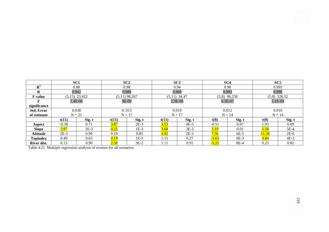
219
SC1 SC2 SC3 SC4 SC5R2 0.88 0.98 0.94 0.98 0.995R 0.942 0.989 0.969 0.992 0.998
F value (5,15) 23.422 (5,11) 98.267 (5,11) 34.47 (5,8) 96.258 (5,8) 326.52F
significance1.4E-06 9E-09 2.3E-06 6.3E-07 5.1E-09
Std. Errorof estimate
0.038N = 21
0..013N = 17
0.019N = 17
0.012N = 14
0.010N = 14
t(15) Sig. t t(11) Sig. t t(11) Sig. t t(8) Sig. t t(8) Sig. tAspect -0.38 0.71 3.87 2E-3 3.53 4E-3 -0.51 0.07 1.93 0.09Slope 3.97 1E-3 4.25 1E-3 3.68 3E-3 3.19 0.01 5.58 5E-4
Altitude 2E-3 0.99 0.19 0.85 3.92 2E-3 7.56 6E-5 11.56 2E-6Topindex 0.49 0.63 4.19 1E-3 1.15 0.27 -3.63 6E-3 3.84 4E-3River dist. 0.13 0.90 2.56 3E-2 1.11 0.91 -5.22 8E-4 0.23 0.82
Table 4.21 Multiple regression analysis of erosion for all scenarios
219
220
4.6 Summary of 2.5D sensitivity analysis
From the result of the multiple linear regression analysis (tables
4.19 and 4.21), it is clear that OF sensitivity and E sensitivity are
very different within the modelled period. For all scenarios, OF
sensitivity is lower than E sensitivity. The highest OF sensitivity
reaches up to 15 in the last iteration of SC2, when deforestation
occurs in the upper areas of the catchment furthest from the river
channels.
Generally E sensitivity is moderately sensitive (between 20 to 60),
which needs to be considered. The highest E sensitivity occurs in
the last iteration of SC1, where the deforestation occurs in the
highest and steepest part of the catchment. This is also clear for
SC4 and SC5, where the highest E sensitivity occurs when the
deforestation pattern starts from the top of the catchment and
progresses in the downhill direction. Consequently, as was shown
in the regression analysis, the mean slope of the deforested area
has a great effect on OF sensitivity and E sensitivity, as does mean
elevation and mean distance to rivers of the deforested area. Areas
close to river channels also had high E sensitivity values. The
aspect variable was not a significant control, though it appears to
have some effects due to its impact on soil hydrology through
evaporation.
The regression values for erosion sensitivity indicate a strong
relationship with topographic variables, but not in the same form
as for OF sensitivity, though they are related.
Combining this analysis with the parameter sensitivity analysis of
the 1D model, it can be concluded that vegetation cover plays an
important role in perturbations of the hydrological cycle due to
221
LUCC, particularly to overland flow and erosion. Moreover, the
location where the LUCC occurs in relation to the topographic
attributes of those locations within the catchment, produce these
changes on E sensitivity and OF sensitivity. The most sensitive
parts of the catchment are at the highest altitudes with steep
slopes and also areas close to the river channels with steep slopes.
The importance of the change in vegetation cover for flux variation
was made clear with the vegetation parameter analysis in 1D.
Changes in vegetation affect the surface and underground fluxes.
Soil moisture was shown to be particularly sensitive to vegetation
parameter changes.
This catchment analysis, by scenarios, was very useful in
identifying those areas most sensitive to LUCC. From some
scenarios it can be concluded that those areas at the top of the
catchment produce the highest OF sensitivity and E sensitivity.
Those areas nearest to the rivers (within 150 m), which have the
steepest slopes, also produce high OF sensitivity and E sensitivity.
Slope is an important factor because it determines overland flow
and in particular, erosion directly. Altitude is an important factor
because rainfall is highest at high elevations within the catchment
and proximity to rivers is also significant factor because of the
cumulative effect of runoff from large contributing areas.

222
4.7 Model validation
4.7.1 Organisation of this section
Validation is an important part of the modelling process because it
allows determination of the accuracy of process simulation and the
confidence to be engendered in the model results.
Both the 1D and 2.5D hydrological models have been developed on
the basis of plot scale parameters, and the model processes can
only be validated at the plot scale because of data availability.
Validation at the catchment scale was intended by comparison of
model generated runoff and sediment yield with field measured
values near the junction of the Tambito and Palo Verde rivers but,
as a result of instrumental failure, this was not possible.
Validation at the plot scale allows one to judge the accuracy of
process modelling under the two types of land cover (forest and
pasture) but does not allow testing of the accuracy of the runoff
and erosion routing.
A comparison between modelled and measured data of some of the
hydrological fluxes is carried out in order to test the model
accuracy. The agreement between measured and modelled data is
assessed for the variables net solar radiation and soil moisture
produced by the 1D model. The behaviour of those variables plays
a significant role within the model. The importance of those
variables in the hydrological process is: (i) net solar radiation
determines the energy availability for canopy and surface water
evaporation, and (ii) soil moisture is significant as the product of
the balance between evaporation, infiltration, overland flow and
recharge processes.
223
Validation is carried out at the same time step that the model was
designed for (1 hour), but was also evaluated as daily summed
values, in order to compare the results at other time scale. Daily
validation could dismiss some noise variation from small time
resolutions, and as well it could show clearly the model
adjustment. Despite the fact that the model is used to simulate a
year, the validation is carried out for a set of data of 20 days, for
which quality data are available and to facilitate detailed
understanding of the results, not possible for much larger series of
data.
4.7.2 Field data set for validation
Validation is carried out using field data from the pasture plot,
because the weather station of this plot was the most stable in
collecting data. The set of data used in the validation process is for
1999 (from 11th of July at 2 p.m. to 3rd of August at 11 a.m.) in
total 550 hours. This period was selected for validation because it
has no interruption in the records in these variables. This set of
data was used to take advantage of times when the key sensors
had optimum reliability and performance.
The model run was allowed to stabilise for 1000 hours before
entering the validation period to allow adjustment from initial
conditions.
4.7.3 Parameters used in validation
Parameters for validation at the pasture plot were very similar to
the parameters used in the model runs for sensitivity analysis
discussed earlier. The only slight difference is in the soil
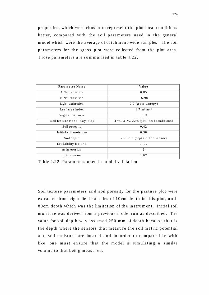
224
properties, which were chosen to represent the plot local conditions
better, compared with the soil parameters used in the general
model which were the average of catchment-wide samples. The soil
parameters for the grass plot were collected from the plot area.
Those parameters are summarised in table 4.22.
Parameter Name Value
A Net radiation 0.85
B Net radiation 16.98
Light extinction 0.0 (grass canopy)
Leaf area index 1.7 m2 m-2
Vegetation cover 86 %
Soil texture (sand, clay, silt) 47%, 31%, 22% (plot local conditions)
Soil porosity 0.42
Initial soil moisture 0.38
Soil depth 250 mm (depth of the sensor)
Erodability factor k 0. 02
m in erosion 2
n in erosion 1.67
Table 4.22 Parameters used in model validation
Soil texture parameters and soil porosity for the pasture plot were
extracted from eight field samples of 10cm depth in this plot, until
80cm depth which was the limitation of the instrument. Initial soil
moisture was derived from a previous model run as described. The
value for soil depth was assumed 250 mm of depth because that is
the depth where the sensors that measure the soil matric potential
and soil moisture are located and in order to compare like with
like, one must ensure that the model is simulating a similar
volume to that being measured.

225
4.7.4 Validation of net solar radiation
Modelled net solar radiation shows similarities with measured net
radiation. Figure 4.46 shows both modelled and measured hourly
net radiation for the simulation period. As it was expected, there
are some differences between modelled and measured values,
which occur throughout the simulation because of the effects of
clouds, which are stochastic in the model, however both take the
same pattern. Figure 4.47 shows the agreement between modelled
and measured hourly net radiation. The coefficient of
determination (R2) is 0.71, which means that 71% of measured net
solar radiation is explained with modelled net solar radiation, with
the assumption that the variables have a normal distribution, this
is statistically significant at the 99%. The correlation coefficient is
0.84 (n=550), which shows the level of association between
measured and modelled net solar radiation. Figures 4.48 and 4.49
show the diurnal pattern of hourly average net radiation for the
pasture site (modelled and measured). The relationship between
them, which has a coefficient of determination (R2) is 0.86, which
means that 86% of measured net solar radiation is explained by
the modelled net solar radiation, with the assumption that the
variables are normally distributed, and it is statistically significant
at 99%. The coefficient of correlation is 0.92. The agreement
between measured and modelled net solar radiation is better in the
diurnal hourly average than the simple observations, because on
using the average the stochastic variation in cloud cover is no
longer important.
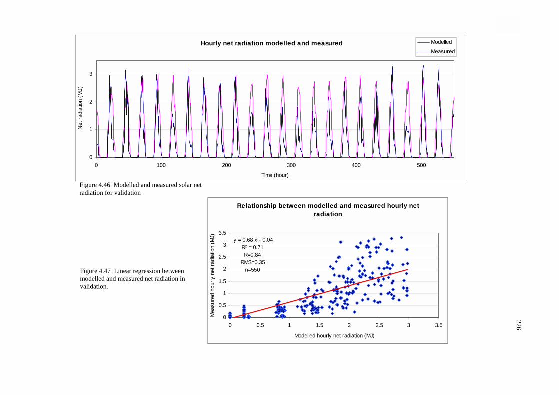
170
Figure 4.46 Modelled and measured solar netradiation for validation
Hourly net radiation modelled and measured
0
1
2
3
0 100 200 300 400 500
Time (hour)
Net
rad
iatio
n (M
J)
Modelled
Measured
Figure 4.47 Linear regression betweenmodelled and measured net radiation invalidation.
Relationship between modelled and measured hourly net radiation
y = 0.68 x - 0.04R2 = 0.71R=0.84
RMS=0.35n=550
0
0.5
1
1.5
2
2.5
3
3.5
0 0.5 1 1.5 2 2.5 3 3.5
Modelled hourly net radiation (MJ)
Mea
sure
d ho
urly
net
rad
iatio
n (M
J)
226
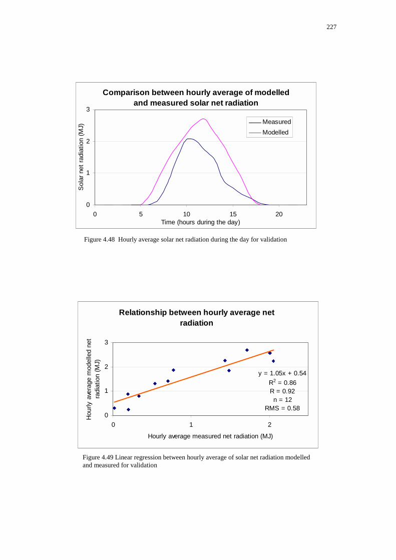
227
Figure 4.48 Hourly average solar net radiation during the day for validation
Comparison between hourly average of modelled and measured solar net radiation
0
1
2
3
0 5 10 15 20Time (hours during the day)
Sol
ar n
et r
adia
tion
(MJ)
Measured
Modelled
Figure 4.49 Linear regression between hourly average of solar net radiation modelledand measured for validation
Relationship between hourly average net radiation
y = 1.05x + 0.54
R2 = 0.86R = 0.92n = 12
RMS = 0.580
1
2
3
0 1 2
Hourly average measured net radiation (MJ)
Hou
rly a
vera
ge m
odel
led
net
radi
atio
n (M
J)

228
4.7.5 Validation of soil moisture
Soil moisture is one of the most important variables in the
hydrological model, because it is the means of hydrological control
of the atmosphere-vegetation-soil interface and the result of the
processes of the soil water balance. Validating soil moisture
indirectly allows validation of other components of the hydrological
cycle such as net rainfall, evaporation, infiltration, recharge and
overland flow, which exercise control on soil moisture; so the soil
moisture validation could be interpreted as the validation of the
outcome of all of these processes.
Soil moisture was evaluated with the same input data set as net
solar radiation. Parameters for this validation are shown in section
4.7.3. Figure 4.50 shows modelled and measured soil moisture for
the validation period. Shape and trends of both graphs are quite
similar. Rainfall is shown in the same graph and assuming linear
correlation between rainfall events and soil moisture the response
is clear.
Figure 4.51 shows the linear regression between modelled and
measured soil moisture. The coefficient of determination (R2) is
0.84, and is statistically significant at 99%, which means that 84%
of measured soil moisture can be explained by the modelled soil
moisture, assuming that the variables are normally distributed.
The correlation coefficient is 0.91 (n=550), which indicates the
association level between measured and modelled soil moisture are
correlated in 91%. Figure 4.51 shows two important things: (i)
There is an associated dependency between consecutive
observations (consecutive time steps), and (ii) a longer validation
period is required in order to produce a more robust test of model
accuracy. Statistically significant at 99% the soil moisture

229
validation gives enough confidence to conclude that the basic soil
hydrological fluxes are reasonable represented in the model
balance.
Soil moisture validation as well was carried out using daily average
for the same period. Figure 4.52 shows the agreement between
modelled and measured soil moisture in trend and shape. Figure
4.53 shows the agreement between daily average modelled and
measured soil moisture through the simulation period for
validation. The coefficient of determination (R2) is 0.84, which
indicates that the modelled daily average soil moisture can explain
84% of the measured daily average soil moisture, assuming that
the variables are normally distributed. The correlation coefficient
is 0.92 (n=21), indicating the association level between variables.
Comparing hourly and daily analysis, the daily linear regression is
not much better than the regression for hourly time step.
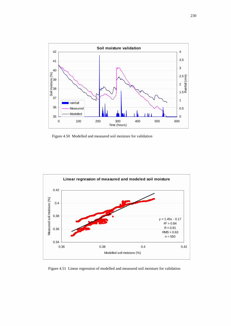
230
Figure 4.50 Modelled and measured soil moisture for validation
Soil moisture validation
35
36
37
38
39
40
41
42
0 100 200 300 400 500 600Time (hours)
Soi
l moi
stur
e (%
)
0
0.5
1
1.5
2
2.5
3
3.5
4
Rai
nfal
l (m
m)
rainfall
Measured
Modelled
Figure 4.51 Linear regression of modelled and measured soil moisture for validation
Linear regression of measured and modeled soil moisture
y = 1.45x - 0.17R2 = 0.84R = 0.91
RMS = 0.63n = 550
0.34
0.36
0.38
0.4
0.42
0.36 0.38 0.4 0.42
Modelled soil moisture (%)
Mea
sure
d so
il m
oist
ure
(%)
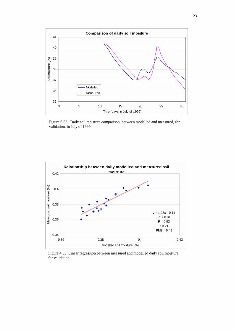
231
Figure 6.52. Daily soil moisture comparison between modelled and measured, forvalidation, in July of 1999
Comparison of daily soil moisture
35
36
37
38
39
40
41
0 5 10 15 20 25 30
Time (days in July of 1999)
Soi
l moi
stur
e (%
)
Modelled
Measured
Figure 4.53 Linear regression between measured and modelled daily soil moisture,for validation
Relationship between daily modelled and measured soil moisture
y = 1.28x - 0.11R2 = 0.84R = 0.92n = 21
RMS = 0.490.34
0.36
0.38
0.4
0.42
0.36 0.38 0.4 0.42
Modelled soil moisture (%)
Mea
sure
d so
il m
oist
ure
(%)

232
Chapter V Summary, conclusions and further work
5.1 Summary of the key findings in the thesis
A few important advances have been made throughout this thesis,
these they are:
- The application of advanced dynamic modelling techniques to
TMCF.
- The development of a new GIS-based 2.5D hydrological
distributed model for tropical montane environments (TMEs).
- The compilation of hydrological flux data from a series of
experimental plots in a TME in Colombia.
- The combination of LUCC scenarios with a distributed
hydrological model to access the impact of LUCC.
- The identification of the importance of topographic properties on
the flux variations with LUCC.
- The strong relationship discovered between the pattern of LUCC
and erosion sensitivity to it.
- The identification of the most sensitive areas to LUCC within the
catchment, and their relationship with the landscape physical
properties.
5.2 Conclusions and their implications
LUCC is recognised as being an important control on hydrological
processes. Therefore this study sets out to determine how LUCC
impacts on hydrological fluxes at the catchment scale in TMCF
environments. This assessment was reached through the
application of a 2.5D GIS-based hydrological model coupled with
233
LUCC scenarios. The overall achievement of this study, is not only
obtaining a better understanding of the spatial distribution of
hydrological sensitivity given the spatial pattern of LUCC, but also
going someway to provide an advanced and robust tool to help
decision makers to develop and protect the environment, and
produce a basis for further research on TMCF hydrology and the
impacts of LUCC.
The importance of LUCC on hydrological fluxes has been
highlighted in this thesis. The sensitivity analysis of the spatial
variability of hydrological sensitivity within the watershed has
identified the importance of the spatial distribution of landscape
physical properties with respect to where the LUCC occurs and the
differing levels of impact if the same LUCC is applied to different
parts of a catchment.
With respect to the aims proposed at the beginning of the thesis
(see chapter 2), all the objectives were realised but to varying
extents. Specifically:
1- Collecting hydrological data in TMCF at both watershed and plot
scale for forest and grassland land uses.
The climatic conditions and the permanent difficulties in collecting
field data impeded the collection from the weather stations of the
two years data that were proposed. Instrumental problems in
humid tropical forest have been addressed also by Manley and
Askew (1993) in a review of hydrological problems for research, and
also those problems have been addressed for TMCF environments
in particular in the reassessment carried out by Bruijnzeel (2000).
Nevertheless, several months of data were collected at the plot
scale with some interruptions for both types of land uses, to be
able to carry out this research and this highly detailed dataset is
234
unusual for TMCF studies (see table 3.3, page 71). The same
kinds of problems affect the weather station that collected the river
flow data for catchment scale analysis. As a consequence no data
were collected in this scale.
2- The development of a physically based hydrological model, which
includes the most important processes of the hydrological cycle at
the plot scale, and the implementation of this model at the catchment
scale for analysis of impacts of various spatial LUCC scenarios.
Chapter 3 discusses the hydro-meteorological and landscape
characteristics of the study area and gives a clear idea of the rather
hydrologically extreme nature (very steep slopes, very high rainfall)
of the environment where the research was carried out. In general
terms, the hydrology in Tambito is very dynamic. The permanently
high rainfall and atmospheric humidity create a climatic condition,
which is unique to TMCF. An almost permanently wet canopy
means that intercepted water is available for evaporation
throughout the day, and the atmosphere is charged with this
water. The catchment has frequent low-level cloud cover but cloud
interception was not studied in this thesis due to lack of data,
though should certainly be a subject for further research in the
area. In the same way, the high rainfall in the area enhances
catchment wetness. At the catchment scale rainfall was
distributed with a function based on data from field stations at
different altitudes. The extrapolation of these data to the extremes
of the catchment meant that these areas received an exaggerated
value of rainfall at more than 10,000 mm a year (see Figure 3.38.
page 144). Whilst the rainfall parameterisation requires
improvement, this is not possible without many more stations.
Overland flow produced by heavy and persistent rainfall is of high
frequency and magnitude in Tambito and this is replicated in the

235
model, as is the resulting potentially high soil loss in non-vegetated
areas on steep slopes.
The model prediction accuracy is very dependent upon the
parameters used for the land use type (see 1D sensitivity analysis,
section 4.3), and the rainfall distribution function used at the
catchment scale. The hydrological model responds to different land
use type through the parameters, which vary between the land
uses. Since soil hydrological properties for forest and pasture were
shown to be very similar, the only parameters varying with land
use were those of the vegetation, in particular vegetation cover, leaf
area index and canopy interception capacity (which may not be as
important if cloud interception were incorporated into the model).
All of these were shown to be important parameters. At the
catchment scale the relationship between the change in land use
parameters and the soil conditions (varying with geology and
geomorphology on the basis of field measurements) was also shown
to be important (see section 4.5).
The hydrological model was validated by comparing soil moisture
at the plot scale with the 1D model results. This indicates that the
model has the ability to reproduce the hydrological balance with
sufficient accuracy. This is discussed in the validation section.
Not much research has been carried out on the impact of LUCC in
TMCF that could have reported data for comparison. Bruijnzeel
(2000) reviews the existing studies in this environment. From a
catchment close to the study area, Restrepo and Kjerfve (2000)
collected water and sediment yield data in the San Juan River
catchment, approximately 200 kilometres to the north of the
Tambito area, in the same side of western cordillera in Colombia).
From this dataset, a small sub-catchment (the Tadó river) has
similar annual rainfall (7410 mm) to Tambito and was selected in
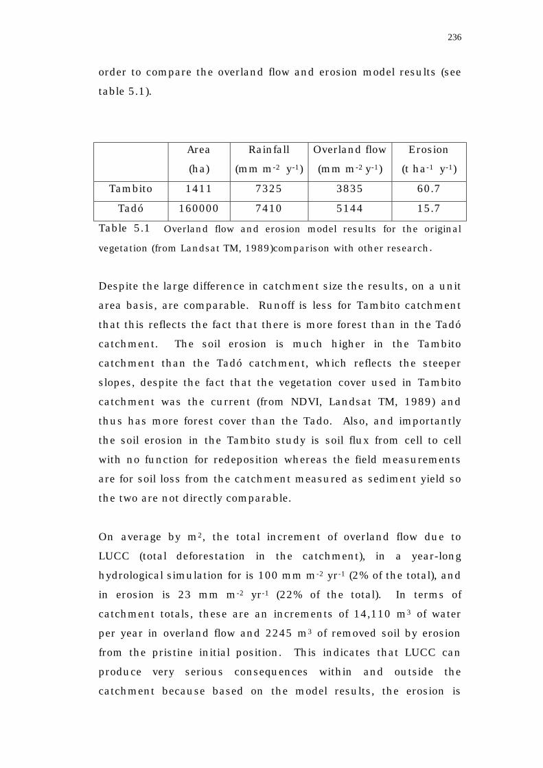
236
order to compare the overland flow and erosion model results (see
table 5.1).
Area
(ha)
Rainfall
(mm m-2 y-1)
Overland flow
(mm m-2 y-1)
Erosion
(t ha-1 y-1)
Tambito 1411 7325 3835 60.7
Tadó 160000 7410 5144 15.7
Table 5.1 Overland flow and erosion model results for the original
vegetation (from Landsat TM, 1989)comparison with other research.
Despite the large difference in catchment size the results, on a unit
area basis, are comparable. Runoff is less for Tambito catchment
that this reflects the fact that there is more forest than in the Tadó
catchment. The soil erosion is much higher in the Tambito
catchment than the Tadó catchment, which reflects the steeper
slopes, despite the fact that the vegetation cover used in Tambito
catchment was the current (from NDVI, Landsat TM, 1989) and
thus has more forest cover than the Tado. Also, and importantly
the soil erosion in the Tambito study is soil flux from cell to cell
with no function for redeposition whereas the field measurements
are for soil loss from the catchment measured as sediment yield so
the two are not directly comparable.
On average by m2, the total increment of overland flow due to
LUCC (total deforestation in the catchment), in a year-long
hydrological simulation for is 100 mm m-2 yr-1 (2% of the total), and
in erosion is 23 mm m-2 yr-1 (22% of the total). In terms of
catchment totals, these are an increments of 14,110 m3 of water
per year in overland flow and 2245 m3 of removed soil by erosion
from the pristine initial position. This indicates that LUCC can
produce very serious consequences within and outside the
catchment because based on the model results, the erosion is
237
much more sensitive to LUCC than overland flow, but that impacts
can be minimised if land use change occurs in areas with low
sensitivity to LUCC.
Although, model results must be used with care, modelling at the
catchment scale allows us to define areas where runoff and erosion
is increased significantly by LUCC. The model limitations mainly
result from the parameters used, because those parameters are
derived from the land use types present in the Tambito watershed.
The model was designed for a TMCF environment, but with several
adjustments it could be used for other landscapes and
environments, although De Roo (1993) and Lorup et al. (1998) in
discussed this idea order to prevent large errors. The 1D model
can more readily be applied to other landscapes. An evident
limitation of 2.5D model is its spatial resolution, because the cell
size of this study was fixed to 25m pixels which according to the
available data and the type of geomorphology was the most suitable
to make the model operational. To improve this spatial resolution
requires more and better data.
In order to apply the model to different areas, several
considerations must be taken into account:
- The scale of integration needs to be related to the landscape
where the model is applied. Spatial resolution has to reflect the
required level of detail in the model in order to produce
reasonable results (see sections 3.3 and 3.6). In the same way,
cell size needs to be considered and adapted to fit the
landscape, and the computationally efficient operation of the
model.
- Vegetation type and land cover need to be parameterised
carefully within the model, in order to be representative and to
reproduce reasonable results (see section 4.3).

238
- The geomorphology of the landscape has to be taken into
account, in order to define the spatial resolution, which must
represent landforms at the level at which the study is carried
out.
- For larger areas, changes in resolution (large pixels) and scale
must be considered carefully, because model adjustments are
required in order to use the model with larger cells (i.e. erosion
sub-model).
There are two important features derived from the catchment scale
model: the effects of cell connectivity and the effects of landscape
variability on the catchment scale response to spatially distributed
LUCC. Connectivity in the model produces an increment in
overland flow in downslope areas due to the accumulation of water
along flow lines. Additionally, this increase depends upon the
distribution of land cover along flow lines and the spatial variability
of landscape properties along the same lines.
3- The parameterisation of the hydrological model at the plot scale
and identification of the most important parameters influencing
hydrological sensitivity to LUCC (see chapter 4).
From modelling at the plot scale (section 3.5.1), parameters, which
change with LUCC and create the greatest sensitivity in runoff and
erosion for this particular catchment and environment were
highlighted. The most sensitive parameters are vegetationcover, soil depth, porosity and the parameters of the erosionequation. Changing land use produces significant changes in
water fluxes (see sensitivity analysis, chapter 4). Soil depth is the
main control on the amount of soil water storage, which plays an
important role in the catchment water balance.

239
Hydraulic soil properties (such as hydraulic conductivity and
matric potential) are linked directly to the most sensitive soil
parameters used in this model, that were also identified by Kirkby
(1978), as having a critical role dominating surface water
processes. Also Ternan et al. (1987) and Elsenbeer and Cassel
(1990) in Grenada and Western Amazonia respectively emphasise
that soil hydraulic properties are an integral part of hillslope
hydrology in the tropical forest. Particularly, the permeability of
the soil in combination with the topography (steep slopes) and the
soil depth are the control of hillslope responses, with a high rate of
infiltration, with the exception of during extreme rainfalls
(Bruijnzeel, 1990), where the generated saturation overland flow is
considered the principal delivery mechanism to the rivers, in
response to steep and concave slopes combined with heavy storms
(Nortcliff and Thornes, 1981), that are a characteristic of TMCF.
The top soil layer (0.2m) is where the soil hydrology controls the
infiltration and consequently the saturated overland flow as was
described in the sensitivity analysis to the parameter soil depth
(see section 4.3.9), as is highlighted by Bonell et al (1983),
Elsenbeer and Cassel (1990) and Bruijzeel (1990). In addition, this
zone is often the most porous of any in the soil profile, with high
available soil water storage capacities. The saturated infiltration
rates ranged from 5 to 12 mm h-1 for undisturbed rain forest, as
was argued by Wierda et al. (1989) in a tropical rain forest in Coté
d’Ivoire, West African, and compares with that calculated for
Tambito (6 mm h-1) with the pedo-transfer function using the soil
texture parameters.
The most sensitive parameter related to the land use type is
vegetation cover (see section 4.3.6). Vegetation cover affects
evaporation increasing it with almost linear trend as forest
vegetation cover increases, and erosion increases in an exponential
240
way as forest vegetation cover decreases (see Figure 4.18). Under
30% forest vegetation cover, erosion sensitivity does not increase at
all, because the remaining forest areas are not significant for
erosion sensitivity as much as the complementary areas of
vegetation cover (between 80% to 30%). Other parameters change
with vegetation type change in the model, but do not produce large
effects on hydrological fluxes as does vegetation cover does.
Burt et al. (1993) came to similar conclusions after analysing
several studies where LUCC can affect the variations in runoff and
erosion, despite the fact that they were carried out on different
environments to this one (North California USA and Plynlimon mid-
Wales), where the experimental catchments were forested rather
than deforested. Those experiments showed that afforestation
reduced the runoff by 25%, this loss being attributed to increasing
water loss by evaporation due to changes in vegetation properties
that are involved in the rainfall interception process. Similarly,
decreases in evapo-transpiration and thus of increasing runoff with
the reduction of forest cover were identified by Bosch and Hewlett
(1982) and Calder (1992).
The increase of erosion with changes in vegetation cover,
particularly deforestation were also identified by Bruijnzeel (1990),
Falkenmark and Chapman, (1989), who argued that forest
conservation can prevent the occurrence of landslides in similar
slopes to those in the study area.
The soil erosion model seems to be very sensitive to the vegetation
cover parameter, and also to the erosion parameters involved in the
erosion equation of the model, such as erodibility factor. This also
has been recognised by Govindaraju (1998) in his study of effective
field scale values for shear stress and soil erodibility and their
spatial variability for physically-based models.
241
Others, mainly soil parameters, were classified as sensitive
parameters, but do not change with change in land use type within
the model (such as the assumption of one type of soil for the whole
catchment, see section 3.5) based on field measurements. Soils are
much more related to the geology and geomorphology of the area.
Within the modelling process those parameters remain constant
between land cover types, so basically the effect of LUCC is applied
in the model at the catchment scale as a change of the vegetation
cover on the catchment surface.
4- To develop methods for model parameterisation at the catchment
scale
One of the difficulties in the generalisation of model parameters at
the catchment scale, is how they vary throughout the surface. In
this respect, the parameters changing on the catchment surface
are the parameters related to the land use type. Land use type in
the catchment was identified and grouped into two classes in this
study (forest and grassland), and for each land use type
parameters were determined by field sampling (see sections 3.2,
3.3 and 3.5). To assign those parameters throughout the
catchment surface the NDVI was extracted from Landsat TM and
was used to distinguish between the main land covers as the most
suitable and economic way to collect land cover information over
the catchment, and with iterations of the scenarios through the
simulation process.
Vegetation parameters such as cover, LAI and canopy storage
capacity also vary within a cover class in response to species
variability and altitudinal change but this level of complexity could
not be taken into account in this study.

242
Model validation at the plot scale
Soil moisture was used in the model validation process, because all
hydrological fluxes contribute to the soil moisture balance. The
agreement between modelled and measured was significant (r2 =
0.83, RMS = 0.63 at one hour time resolution, and r2 = 0.83, RMS
= 0.49 as a daily average), which provides a degree of confidence in
the behaviour of the hydrological model. Unfortunately validation
was carried out over a small period due to a lack of availability of
uninterrupted good quality data.
Validation at the catchment scale was not carried out because data
at this scale were not available; but the modelling suggests that
there are significant effects of LUCC at the catchment level,
necessitating the improvement of the field methodology for data
collection at this level.
5- The application of the model to identify the location of areas
within the Tambito catchment where hydrological processes are most
sensitive to LUCC in relation to physiographic properties, combined
with different scenarios of LUCC.
Burt et al. (1993) recognised the difficulties of identifying the areas
within a catchment that are sensitive to LUCC, and they suggest
the use of hydrological simulation models for this purpose. Such a
simulation model has been developed and used for the stated
purpose here.
The combined process of sensitivity analysis in the 1D and 2.5D
models, helps us to understand first of all, which parameters
within the model are important for surface hydrological fluxes and
secondly, the properties of spatial variability of the sensitive areas.
243
Using a combination of different scenarios indicates how landscape
sensitivity responds to the pattern of deforestation. From the
analysis of the impact of LUCC, the areas within the catchment
that should be protected from LUCC can be identified, because
those areas with greatest sensitivity can, if deforested, lead to more
serious environmental consequences, such as soil degradation,
erosion and sedimentation (see Figures 4.11 and 4.12). In the
same way, hydrological models offer the possibilities to evaluate the
outcome of particular LUCC strategies. The combination of LUCC
scenarios with a distributed hydrological model also was used by
Mulligan et al. (2000) finding serious effects of progressive
deforestation on runoff and erosion yields. A similar process using
the combination of hydrological models and statistical tests was
carried out by Lorup et al. (1998), who highlight the ability to
improve the analysis of the impact of LUCC on the catchment
runoff, compared to using them separately. On the other hand,
Fahey and Jackson (1997) used a comparison approach for
catchments with different vegetation (forest, grasslands, and pine
plantations) to estimate the differences in hydrological properties.
The LUCC scenarios developed in this thesis are not intended to
represent real patterns of land use change, rather they serve as a
means of testing the sensitivity to landscape physical properties
(table 4.18 to 4.21), which the LUCC patterns produce hydrological
variation in the catchment. The relationship between landscape
properties and hydrological flux variation were also studied by
Quine and Walling (1993), where the erosion rate predictions were
derived from a statistical function of a combination of topographic
attributes. Those types of landscape attributes have also been
used to predict the soil properties with good results (McKenzie and
Ryan, 1999).

244
A reduction in the catchment forest cover in the humid tropics
produces an increment in overland flow and a decrease in water
evaporation (see sections 4.3 and 4.5), that also was identified by
Bosch and Hewlett (1982), Bruijnzeel (1990) and Fahey and
Jackson (1997), among others researches. They highlight that
forest acts as a sponge, so that forest conversion increases
flooding. Unfortunately cloud interception was not taken into
account, though this is one of the processes that can affect the
hydrological balance in montane cloud forest, where may
compensate for the extra water evaporation identified in conversion
to forest (Zadroga, 1981). Also with this respect, Calder (1998)
associates the changes in evaporation rates with the variations on
large leaf surface area and the deeper root system of forest.
The pattern of variation in erosion within the modelled scenarios is
very similar to the LUCC pattern, which indicates a strong relation
between LUCC and hydrological change that is driven by vegetation
cover change.
The importance of the landscape physical properties is identified
from modelling at the catchment scale. Slope, aspect, elevation,
and distance to rivers of the deforested area, among others,
produce an important effect on the hydrological fluxes from those
same areas. Those properties, combined with the location of the
deforested areas relative to the hydrological flow-routing network
are critical to the hydrological response to land use change.
Modelling at the catchment scale combined with the sensitivity
analysis helped to identify the topographic characteristics of the
areas most sensitive to LUCC within the catchment (see section
4.5). Those characteristics are:
245
- steep slopes, within 150m distance to rivers and with highelevation (see Slope Map, Figure 3.17, page 81).
- steep slopes furthest away from river channels, which areclose to the boundary of the catchment, where rainfall ishighest (see Elevation Map, Figure 3.16, page 80).
The same land use change can have quite different effects on the
hydrological cycle if it occurs in the high parts of the catchment as
opposed to the lower parts, or at the top of a slope as opposed to its
base.
5.3 Further research
The validation process carried out in this thesis used short periods
of data. It is necessary to collect more field information and re-
validate the model, in order to check the model predictions more
fully.
The initial aim was to produce a simple framework model for this
landscape (TMCF) where the main hydrological events were
represented, and also that the model could operate with little
information. Therefore, there is now a need to incorporate other
modules or improve some of the existing one. The improvements
required include:
- Adjusting the model rainfall equation in order to produce more
realistic results through the acquisition of more spatially
detailed field rainfall data.
- The incorporation of cloud interception by trees to integrate
additional water in the hydrological cycle. Also the interception
module needs to be calculated at shorter time resolutions, in

246
order to assess with more accuracy the loss of intercepted
water.
- Modelling soil deposition and sedimentation. Erosion in the
current module is modelled only as soil detachment; this soil
will be re-deposited or incorporated to the river flux as
suspended sediment.
- Plant transpiration routine. Evapotranspiration could have a
more significant role in the hydrological cycle in TMCFs than
assumed here. As the variation in altitude within the
catchment is significant (more than 1000m) and in the same
way the environmental conditions and vegetation change.
Plants could have a complex and differing response through the
altitudinal range.
- Throughflow may also be more important at the catchment scale
for hydrology in this particular environment (TMCFs), than
assumed here by its non-inclusion.
- Changes in soil properties produced by LUCC could be usefully
included for catchments or LUCC's where LUCC impacts on soil
as well as vegetation properties.
In terms of land use change
- To incorporate dynamic scenarios where the LUCC forces to
change in soil properties (such as porosity and bulk density) as
well as plant properties.
- Allow the capacity for forest growth and regeneration,
incorporating plant physiology processes within the model.
247
In terms of modelling
- There is still a gap between modelling activities and GIS
interfaces. The spatial representations of some processes are
not simple and require better GIS tools.
- The relationships between hydrological fluxes and physical
landscape properties have been shown through this thesis. On
the basis of the analysis, a statistical model could be
developed to identify the sensitive areas (in terms of overland
flow and erosion) within catchments with similar characteristics
and land use to the ones in which the model is developed. On
the basis of catchment physical properties such as those
studied here (slope, aspect, topographic index, altitude, and
distance to rivers) and derived from DEMs should be used in the
statistical model. This statistical model could be a fast
alternative to evaluate the hydrological impact of LUCC in
catchments with similar characteristics without carrying out the
whole process of hydrological modelling, land use
parameterisation and sensitivity analysis developed here, using
only secondary information derived from DEMs. This is the
subject of further papers based on the information and
processes developed in this thesis.
It is recognised that this model is useful to support further
research on TMCF environments. Understanding landscape
sensitivity to land use change could also assist conservation
planning and rural agricultural sustainability. These types of
research can be used by the government and also in more local
areas, by the Corporations who have the responsibility to manage
natural resources within the catchments in Colombia, as a fast
alternative to assess the LUCC impact of proposed plans of
catchment management.

248
Bibliography
AARAM Andean Amazon Rivers Analysis and Monitoring project.
1998. http:boto.ocean.washington.edu/aaram/
Abbott, M. B., Bathurst, J, C., Cunge, J. A., O’Connell, P. E., and
Rasmussen, J. 1989. An Introduction to the European System –
Systeme Hydrologique Europeen, “SHE”, 2. Structure of a
physically-based, distributed modelling system. Journal of
Hydrology, 87: 61 – 77.
Ahuja, L. R., Naney, J. W., and Williams, R. D. 1984. Estimating
soil water characteristics from simpler properties or limited data.
Soil Science Society American Journal, 49: 1100 - 1105.
Ahuja, L. R., and Williams, R. D. 1991. Scaling water
characteristic and hydraulic conductivity based on Gregson-
Hector-McGowan approach. Soil Science Society American Journal,
55: 308 - 319.
Anderson, M. G., and Burt, T. P. 1985. Hydrological Forecasting.
John Wiley & Sons Ltd. Chichester, UK.
Anderson, M. G., and Burt, T. P. 1990. Process studies in hillslope
hydrology. John Wiley & Sons. Chishester, U. K.
249
Arya, L. M., and Paris, J. F. 1981. A physicoempirical model to
predict the soil moisture characteristic from particle-size
distribution and bulk density data. Soil Science Society American
Journal, 45: 1023 - 1030.
Aston A.R. 1979. Rainfall Interception by eight small trees.
Journal of Hydrology, 42: 383 - 396.
Avery B.W., and Bascomb C.L. 1974. Soil survey and laboratory
methods. Harpenden Soil Survey of Great Britain. UK.
Banco de la República, 1951. Bases de un programa de fomento
para Colombia – Informe de una Misión dirigida por Lauchlin Currie.
Banco de la República (eds). Bogotá, Colombia.
Bathurst J. C., Wicks J.M., and O’Connell P. E. 1995. The
SHE/SHESED Basin Scale Water Flow and Sediment Transport
Modelling System. In: Computer models of Watershed Hydrology.
Edited by Vijay P. Singh. Department of Civil and Environment
Engineering Louisiana State University, Baton Rouge, LA 70803-
64405, USA.
Bejarano, J. A. 1977. Contribución al debate sobre el problema
agrario. In: El agro en el desarrollo histórico colombiano. Edutorial
Punta de Lanza, Bogotá, Colombia.
Bell, M. A. and Van Keulen, H. 1995) Division S-5 -Pedology. Soil
Pedotransfer Functions for Four Mexican Soils. Soil Science
Society. American Journal, 59: 865 - 871.
Beven, K. J., and Kirkby, M. J. 1976. Towards a simple
physically-based variable contributing area of catchment
250
hydrology. Working paper 154, School of Geography, University of
Leeds.
Beven, K. J., and Kirkby, M. J. 1979. A physically based variable
contributing area model of basin hydrology. Hydrological Science
Bulletin, 24, 1: 43 – 69.
Beven, K. J., Kirkby, M. J., Schofiled, N., and Tagg, A. F. 1984.
Testing a physically-based flood forecasting model (TOPMODEL) for
three U.K. catchments. Journal of Hydrology, 69: 119 – 143.
Beven, K. J. 1989. Changing ideas in hydrology – the case of
physically-based models. Journal of Hydrology, 105: 157 – 172.
Beven K.J., and Moore I.D. 1994. Advances in Hydrological
Processes. Terrain Analysis and Distributed Modelling in Hydrology.
John Wiley & Sons. New York. USA.
Beven K., Lamb R., Quinn P., Romanowicz R., and Freer J. 1995.
TOPMODEL. In: Computer Models of Watershed Hydrology. Water
Resources Publications. Edited by Vijay P. Singh. Department of
Civil and Environment Engineering Louisiana State University,
Baton Rouge, LA 70803-64405, USA.
Binley, A., and Beven, K. 1992. Three-dimensional modelling of
hillslope hydrology. Hydrological Processes, 6: 347 – 359.
Blazkova, S., and Beven K. 1997. Flood frequency prediction for
data limited catchments in the Czech Republic using a stochastic
rainfall model and TOPMODEL. Journal of Hydrology, 195, 1-4:
256 – 278.
251
Bonell, M. 1993. Progress in the understanding of runoff
generation dynamics in forest. Journal of Hydrology, 150: 217 –
275.
Bonell, M, and Balek, J. 1993. Recent Scientific Developments
and Research Needs in Hydrological Processes of the Humid
Tropics. In: Hydrology and Water Management in the Humid
Tropics. Hydrological research issues and strategies for water
management. Edited by Michael Bonell, Maynard M, Hyfschmidt
and John S. Gladwell. International hydrology series, Cambridge
University press, UK.
Bosch, J.M., and Hewlett, J. D. 1982. A review of catchment
experiments to determine the effect of vegetation changes on water
yield and evapotranspiration. Journal of Hydrology, 55: 3 – 23.
Broadman, J., and Favis-Mortlock, D. T. 1993. Simple methods of
characterizing erosive rainfall with reference to the South Downs,
southern England. In: Farmland Erosion in Temperate Plains,
Wicherek, S. (ed.). Environments and hills. Elsevier, Amsterdam,
The Netherlands: 17 – 29.
Brock, T. D. 1981. Calculating solar radiation for ecological
studies. Ecological Modelling, 14: 1 - 19.
Bronstert, A. 1999. Capabilities and limitations of detailed
hillslope hydrological modelling. Hydrological Processes, 13: 21 –
48.
Brooks, R. H., and Corey, A. T. 1964. Hydraulic properties of
porous media. Hydrology, Paper3. Colorado State University, Fort
Collins, Colorado.
252
Brown, M. B., de la Roca, I., Vallejo, A., Ford, G., Casey, J.,
Aguilar, B., and Haaker, R. 1996. A valuation analysis of the role
of cloud forest in watershed protection, Sierra de Minas Biosphere
Reserve, Guatemala ans Cusuco N. P. Honduras. RARE Center for
Tropical Conservation, Philadelphia, USA.
Bruijnzeel, L. A., and Wiersum, K. F. 1987. Rainfall interception
by a young Acacia auriculiformis A. Cunn. Plantation forest in
West Java, Indonesia: Application of Gash’s analytical model.
Hydrological Processes, 1: 309 – 319.
Bruijnzeel, L. A. 1989. (De)forestation and dry season flow in the
tropics: A closer look. Journal of Tropical Forest Science, 1, 3: 229 –
243.
Bruijnzeel, L. A. 1990. Hydrology of moist tropical forest and
effects of conversion: a state of knowledge review. UNESCO
International Hydrological Programme, A publication of Humid
Tropics Programme, UNESCO, Paris.
Bruijnzeel, L. A., Waterloo, M. J., Proctor, J., Kuiters, A. T., and
Kotterick, B. 1993. Hydrological observations in montane rain
forest on Gunung Silam, Sabah, Malaysia, with special reference to
the “Massenerhebung’ effect. Journal of Ecology, 81: 145 – 167.
Bruijnzeel, L. A., and Proctor, J. 1995. Hydrology and
biogeochemistry of tropical montane cloud forest: what do we really
know? In: L. S. Hamilton, Juvik, J. O., and Scatena, F. N., eds.
Tropical Montane Cloud Forests. Ecological Studies 110, Springer
Verlag, New York: 38 – 78.
Bruijnzeel, L. A. 2000. Hydrology of Tropical Montane Cloud
Forests: A Reassessment. Submitted to Hydrological Processes.
253
Buitrago, F. L. 1977. Desarrollo, Subdesarrollo y Ciencias
Sociales. In: El Agro en el Desarrollo Histórico Colombiano.
Edutorial Punta de Lanza, Bogotá, Colombia.
Budyco, M. I., 1974. Climate and Life. Academic press, London –
UK.
Burt, T. P., Heathwaite, A. L., and Trudgill, S. T. 1993. Catchment
sensitivity to land use controls. In: Landscape Sensitivity. Eds. by
D. S. G. Thomas and R. J. Allison. John Wiley & Sons.
Chichester, UK.
Calder, I. R. 1986. A stochastic model of rainfall interception.
Journal of Hydrology, 89: 65 – 71.
Calder, I. R., Wright, I. R., and Murdiyarso, D. 1986. A study of
evaporation from tropical rainforest – West Java. Journal of
Hydrology, 89, 1 - 2: 13 – 31.
Calder, I. R. 1992. The hydrological impact of land use change
(with special reference to afforestation and deforestation). In:
Proceedings of the Conference on Priorities of Water Resources
Allocation and Management. Southhampton, July 1992. Overseas
Development Administration, London. ISBN: 090 2500 49X.
Calder, I.R., Hall, R.L., Bastable, H.G., Gunston, H.M., Shela, O.,
and Chirwa A. 1995. The impact of land-use change on water
resources in Sub-Saharan Africa. A modelling study of lake
Malawi. Journal of Hydrology. 170, 1-4: 123-135.
254
Calder, I. R. 1996. Dependence of rainfall interception on drop
size: 1. Development of two-layer stochastic model. Journal of
Hydrology, 185: 363 – 378.
Calder, I. R. 1998. Water use by forests: Limits and controls.
Trees Physiology, 18: 625 – 631.
Calvo, J. C. 1986. An evaluation of Thronthwaite’s water balance
technique in predicting stream runoff in Costa Rica. Hydrological
Science Journal, 31: 51 – 60.
Cammeraat, L. H. 1991. MEDALUS, Mediterranean Desertification
and Land Use. Field Manual. Version 3.1.
Campbell, G. S. 1985. Soil physics with basic. Transport models
for soil-plant systems. Elsevier Science Publishers B.V.
Netherlands.
Campbell, J. B. 1987. Introduction to remote sensing. A division of
Guilford publications Inc. 200 Park Avenue south, New York. N.Y.
10003. USA.
Cartier W., and Forero-Alvarez, J. 1990. Planeación Agropecuaria
en Colombia. Cuadernos de Agroindustria y Economía Rural en
Colombia, 24: 9 – 127.
Cavalier, J. 1986. Relaciones Hídricas de Nutrientes en Bosques
Enanos Nublados Tropicales. Magister Scientiae en Ecología
Vegetal, Universidad de los Andes de Merida, Venezuela.
255
CEPAL. 1990. Magnitud de la Pobreza en América Latina en los
Años Ochenta. Comisión económica para América Latina y el
Caribe. Santiago de Chile, Chile.
CIAT - Hillside Program. 1994. Hillsides Program Annual Report
1992 – 1994. Internal document, Ciat, Cali – Colombia.
Cienciala, E., Kucera, J., Lindroth, A., Cermak, J., Grelle, A., and
Halldin, S. 1997. Canopy transpiration from a boreal forest in
Sweden during a dry year. Agricultural and Forest Meteorology, 86:
157 – 167.
Chu, S. T. 1994. Capillary-tube infiltration model with Brooks-
Corey parameters. American Society of Agricultural Engineers, 37,
4: 1205 - 1208.
Chu, S. T. 1995. Effect of initial water content on Green-Ampt
parameters. American Society of Agricultural Engineers, 3, 3: 839 -
841.
Chu, S. T. 1997. Infiltration model for soil profiles with a water
table. American Society of Agricultural Engineers, 4, 4: 1041-1046.
Cohen, W. B. 1991. Response of vegetation indices to changes in
three measures of leaf water stress. Photogrammetric Engineering
& Remote Sensing, 57, 2: 195 – 202.
Coles, N.A., Sivapalan, M., Larsen, J.E., Linnet, P.E. and Fahrner,
C.K. 1997. Modelling runoff generation on small agricultural
catchments: Can real world runoff responses be captured?
Hydrological Processes, 11: 111 – 136.

256
Copeland, J. H., Pielke R. A. and Kittel T. G. F. 1996. Potential
climate impacts of vegetation change: A regional modelling study.
Journal of Geophysical Research, 101, D3: 7409 – 7418.
Crohn, D. M. 1995. Sustainability of sewage sledge land
application to northern hardwood forest. Ecological Applications, 5,
1: 53 - 62.
CSIRO Institute of Natural Resources and Environment. 1993.
TOPOG_IRM, Model description. Division of Water Resources,
Camberra Laboratory, By W. Dawes and T. Hatton. Camberra,
Australia.
Dale, V.H. 1997. The relationship between land use change and
climate change. Ecological Applications, 7, 3: 753 - 769.
Dangermond, J. 1993. The Role of Software Vendors in
Integrating GIS and Environmental Modelling, . Environmental
Modelling with GIS. Oxford University press. New York – Oxford,
USA.
De Roo, A. P. J. 1993. Validation of the ANSWERS catchment
model for runoff and soil erosion simulation in catchments in The
Netherlands and the United Kingdom. In: HydroGIS 93:
Application of Geographic Information Systems in hydrology and
Water Resources. Proceedings of the Vienna Conference, April
1993. IAHS Publ. No. 221.
Digman, S. Lawrence. 1994. Physical Hydrology. Prentice-hall,
Inc. New York, USA.
Dobson, F. and Smith, S. 1988. Bulk models of solar radiation at
sea. Q. J. R. Meteorol. Soc., 114: 165 – 182.
257
Dolman, A. J., Gash, J. H. C., Roberts, J., and Shuttleworth, W. J.
1991. Stomatal and surface conductance of tropical rain-forest.
Agricultural and Forest Meteorology, 54, 2-4: 303 – 318.
DPN, 1999. Planning National Department, Colombia Government.
http://www.dnp.gov.co/plan_nal/LEY_508_1999.pdf
Duff, E. A. 1968. Agrarian Reform in Colombia. Frederick A.
Praeger, Publishers. New York, USA.
Dunn, S. M., and Mackay, R. 1995. Spatial variation on evapo-
transpiration and the influence of land-use on catchment
hydrology. Journal of Hydrology, 171, 1-2: 49-73.
Dunn, S. M. 1996. The hydrological component of the NELUP
decision-support system: an appraisal. Journal of Hydrology, 177,
3-4: 213 – 235.
Duru, J. O., and Hjelmfelt, A. T. 1994. Investigation prediction
capability of HEC-1 and KINEROS kinematic wave runoff models.
Journal of Hydrology, 157, 1-4: 87 – 103.
Elsenbeer, H, and Cassel, D. K. 1990. Surficial processes in the
rainforest of western Amazonia. In : Research Needs and
Applications to Reduce Erosion and Sedimentation in Tropical
Steeplands. R. R. Zimmer, C. L. O’Loughlin, and L. S. Hamilton.
Proc. Fiji Symp. International Association of Hydrological Science
Publications, 192: 289 – 297.
ESRI. 1998. Environmental Systems Research Institute, Inc.
Arc/Info V 7.3. Redlands, California. USA.
258
Falkenmark, M., and Chapman, T. 1989. Comparative hydrology.
An Ecological approach to land and water resources, UNESCO.
Paris.
FAO, Food and Agriculture Organization, 1997.
Http://www.fao.org/gtos/about/gtodbdir/GTOSa001.html.
Faunt, C., D’agnese, F., and Turner, K. 1993. Development of a
three-dimensional hydrological framework model for the Death
Valley region, southern Nevada and California, USA. HydroGIS 93:
Application of Geographic Information Systems. In: Hydrology and
Water Resources. IAHS Publ. No. 211.
Favis-Mortlock, D. 1993. Validation of field scale soil erosion
models using common data sets. Modelling soil erosion by water.
Edited by John Boardman and David Favis-Mortlock. University of
Oxford. UK.
Fedra, Kurt. 1993. GIS and Environmental Modelling.
Environmental Modelling with GIS. Oxford University press. New
York – Oxford, USA.
Fajardo, D. 1996. La Reforma Agraria en la Política Social. In:
Una mirada social al campo. Ministerio de Agricultura y Desarrollo
Rural. Santafé de Bogotá, Colombia.
Fahey, B., and Jackson, R. 1997. Hydrological impacts of
converting native forest and grasslands to pine plantations, South
Island, New Zealand. Agricultural and Forest Meteorology, 84: 69 –
82.
Feldman, A. D. 1995. HEC-1 Flood Hydrograph Package.
Computer models of Watershed Hydrology. Edited by Vijay P.
259
Singh. Department of Civil and Environment Engineering
Louisiana State University, Baton Rouge, LA 70803-64405, USA.
Finch, J. W. 1998. Estimating direct groundwater recharge using
a simple water balance model – Sensitivity to land surface
parameters. Journal of Hydrology, 211: 112 – 125.
Fisher, P., Abrahart R. J, and Herbinger W. 1997. The sensitivity
of two distributed non-point source pollution models to the spatial
arrangement of the landscape. Hydrological Processes, 11: 241 –
252.
Flugel, W. A. and Smith, R. E. 1999. Integrated process studies
and modelling simulations of hillslope hydrology and interflow
dynamics using the HILLS model. Environmental Modelling and
Software, 14: 153 – 160.
Ford, E. D., and Deans, J. D. 1978. The effects of canopy
structure on stemflow, throughfall and interception loss in a young
Sitka Spruce plantation. Journal of Applied Ecology, 15: 905 - 917.
Forseth, I. N., and Norman, J. M. 1993. Modelling of solar
irradiance, leaf energy budget and canopy photosynthesis.
Photosynthesis and Production in a Changing Environment: field and
laboratory manual. Edited by D.O. Hall, J.M.O. Scurlock, H.R.
Bolhar-Nordenkampt, R.C. Leegood and S.P. Long. Chapman &
Hall, London.
Frohn, R. C., McGwire, K. C., Dale, V. H., and Estes, J. E. 1996.
Using remote sensing analysis to evaluate a socio-economic and
ecological model of deforestation in Rondonia, Brazil. International
Journal of Remote Sensing, 17, 16: 3233 - 3255.
260
Gansler, R. A., Klein, S. A., and Beckman, W. A. 1994. Assessment
of the accuracy of generated meteorological data for use in solar
energy simulations studies. Solar Energy, 53, 3: 279 - 287.
Gash, J. H. C., and Morton, A. J. 1978. An application of Rutter
model to the estimation of interception loss from Thetford forest.
Journal of Hydrology, 38: 49 - 58.
Gash, J. H. C. 1979. An analytical model of rainfall interception
in forests. Quart. J. Met. Soc., 105: 43 – 55.
Gash, J. H. C., Wright, I. R., and Lloyd, C. R. 1980. Comparative
estimates of interception loss from three coniferous forest in Great
Britain. Journal of Hydrology, 48: 89 – 105.
Gavin, H., and Agnew, C. T. 2000. Estimating Evaporation and
Surface Resistance from Wet Grassland. Phys. Chem. Earth (B), 25,
7-8: 599 – 603.
Gerrard, A. J. W. 1993. Landscape sensitivity and changes on
Dartmoor. Landscape sensitivity. Edited by D. S. G. Thomas and
R. J. Allison. John Wiley & Sons. Baffins Lane, Chichester,
England.
Golley, F. B. 1983. Ecosystems of the world 14A. ‘Tropical rain
forest ecosystems’. Elsevier Scientific Publishing Company. New
York, U.S.A.
Goodrich, D. C. 1991. Basin scale and runoff model complexity.
Univ. of Arizona, Dept. of Hydrology and Water Resources Tech.
Rep. No. HWR 91010, 361 p.
261
Govindaraju, R. S. 1998. Effective erosion Parameters for slopes
with spatially varying properties. Journal of Irrigation and Drainage
Engineering, 124, 2: 81 – 88.
Granger, R. J. 1989. An examination of the concept of potential
evaporation. Journal of Hydrology, 111: 9 – 19.
Grayson, R. B., Bloschl, G., and Moore, I. D. 1995. Distributed
parameter hydrologic modelling using vector elevation data:
THALES and TAPES-C. In: Computer models of watershed
hydrology. Vijay P. Singh (ed.). Water Resources Publications.
USA.
Green, W., and Ampt, A. 1911. Studies on Soil Physics – Part I.
The flow of air and water through soils. Journal of Agricultural
Science, 4: 1 - 24.
Grismer, M. E. 1986. Pore-size distribution and Infiltration. Soil
Science, 141, 4: 249 - 259.
Grubb, P. J. 1977. Control of forest growth and distribution on
wet tropical mountains: with special reference to the mineral
nutrition. Annual Review of Ecology and Systematics, 8: 83 – 107.
Gueymard, C. 1993. Critical analysis and performance
assessment of clear sky solar irradiance models using theoretical
and measured data. Solar Energy, 51, 2: 121 – 138.
Gupta, S. C., and Larson, W. E. 1979. Estimating soil water
retention characteristics from particle size distribution, organic
matter content, and bulk density. Water Resources Research, 15:
1633 – 1635.
262
Gustard, A. and Wesselink, A. J. 1993. Impact of land-use change
on water resources-Balquhidder catchments. Journal of Hydrology,
145, 3-4: 389 - 401.
Hafkenscheid, R. L. L. J. 2000. Hydrology and biogeochemistry of
tropical montane rainforest of contrasting stature in the Blue
Mountains, Jamaica. Universiteit De Boelelaam, 1105.
Hancock, N. H., and Crowther, J. M. 1979. A Technique for the
direct measurement of water storage on a forest canopy. Journal of
Hydrology, 41: 105 - 122.
Hatton, T. J., and Dawes W. 1993. TOPOG_IRM. 2. Examples
simulation. CSIRO Division of Water Resources, Tech. Memo. 93/6.
Herwitz’s, S. R. 1987. Raindrop impact and water flow on the
vegetative surfaces of trees and the effects of stemflow and
throughfall generation. Earth Surf. Processes Landf., 12: 425 –
432.
Hillel, D. 1971. Soil and Water, Physical principles and processes.
Academic Press, Inc. New York, USA.
Horton, R. E. 1940. An approach toward a physical interpretation
of infiltration-capacity. Soil Science Society American Journal, 5:
399 – 417.
Houghton, R. A. 1994. The worldwide extent of land use change.
Bioscience, 44, 5: 305 - 313.
Huber, W. C. 1995. EPA Storm Water Management Model –
SWMM. Computer Models of Watershed Hydrology. Edited by Vijay
263
P. Singh. Department of Civil and Environment Engineering
Louisiana State University, Baton Rouge, LA 70803-64405, USA.
Huttel, C. 1975. Recherches sur l’écosystème de la fôret
subéquatoriale de basse Côte d’Ivoire. III. Inventaire et structure
de la végétation ligneuse. In: La Terre et la Vie., 29: 178 – 191.
IDEAM, Instituto de Hidrología Meteorología y Estudios
Ambientales. Weather Database. Ministerio del Ambiente,
Colombia.
IGAC- Instituto Geográfico Agustín Codazzi, 1975. Geodésia.
Resultados Definitivos de Parte de las Redes Geodésicas
Establesidas en el País. Publicación epsecial #1. Cuarta Edición.
Santafé de Bogotá, Colombia. Pp 3 - 6.
IGAC Instituto Geografico Agustin Codazzi. 1983. Mapa de Suelos
de Colombia. Ministerio de Agricultura. Bogota, Colombia.
IGAC Instituto Geografico Agustin Codazzi. 1985. Panchromatic
air-photograph scale 1:40,000.
Ingeominas, Insitituto Nacional de Investigaciones Geológico
Mineras, Colombia. 1999. Tambito geomorphology. Verbal
comunication from Patricia Negret.
Iqbal, M. 1983. An Introduction to Solar Radiation. Academic press.
Toronto, Canada.
Jackson, I. J. 1975. Relationships between rainfall parameters
and interception by tropical rainforest. Journal of Hydrology, 24:
215 – 238.
264
James, W., Warinner, J., and Reedy M. 1993. Application of the
Green-Ampt infiltration equation to watershed modelling. Water
Resources Bulletin, 28, 3: 623 - 635.
Jane, G. T., and Green, T. G. A. 1985. Patterns of stomatal
conductance in six evergreen tree species from a New Zealand
cloud forest. Botanical Gazette, 46: 413 – 420.
Jarvis, P. G. 1976. The interpretation of the variations in leaf
water potential and stomatal conductance found in canopies in the
field. Philosophical Transactions of the Royal Society of London B,
273: 543 – 610.
Jarvis, A. 1999. Quantifying the Hydrological Role of Cloud
Deposition onto Epiphytes in a Tropical Montane Cloud Forest,
Colombia. BSc dissertation in Geography at King’s College London,
University of London.
Jetten, V. G. 1994. Modelling the Effects of Logging on the Water
Balance of a Tropical Rainforest. A Study in Guyana. Tropenbos
Series 6. The Tropenbos foundation. Wageningen. Department of
Physical Geography, Faculty of Geographical Sciences. Universiteit
Utrecht, P.O.Box 80.115,3508 TC Utrecht, The Netherlands.
Jetten, 1996. Interception of tropical rain forest: performance of a
canopy water balance model. Hydrological Processes, 10, 5: 671 -
685.
Johnes, P. J., and Burt, T. P. 1990. Modelling the impact of
agriculture upon water quality in the Windrush catchment – an
export coefficient approach in a representative basin. Proceedings
and Information – Committee for Hydrological Research TNO, 44:
245 - 252.
265
Johnes, P. J. 1996. Evaluation and management of the impact of
land use change on nitrogen and phosphorus load derived to
surface waters: the export coefficient modelling approach. Journal
of Hydrology, 183, 3-4: 323 - 349.
Johnes, P. J., and Heathwaite, A. L. 1997. Modelling the impact of
land use change on water quality in agricultural catchments.
Hydrological Processes, 11: 269 - 286.
Kapos, V., and Tanner, E. V. J. 1985. Water relations of Jamaican
upper montane forest trees. Ecology, 66: 241 – 250.
Kato, R., Y. Tadaki, and H. Ogawa. 1978. Plant biomass and
growth increment studies in Pasoh Forest. Malayan Nature
Journal, 30: 211 – 224.
Kerfoot, O. 1968. Mist precipitation on vegetation. Forestry
Abstracts, 29: 8 - 20.
Kim, S., Delleur, J. W., Mitchell, J. K., Engell, B. E., and Walker S.
E. Simulation of runoff in agricultural watersheds with tile drains
using an extended TOPMODEL. Transactions of the ASAE, 42, 3:
639 – 650.
Kinsel, W. G., and Williams, J. R. 1995. Hydrology components of
CREAMS and GLEAMS models. In: Computer Models of Watershed
Hydrology. Vijay P. Singh (ed.). Water Resources Publications.
USA.
266
Kirkby, M.J. 1975. Hydrograph modelling strategies. In R. Peel.
M. Chisholm and P. Haggett (Eds). Process in Physical and Human
Geography. Heinemann, 69 – 90.
Kirkby, M. J. (ed.). 1978. Hillslope Hydrology, Wiley, Chichester,
UK.
Kirkby, M. J., and Morgan, R. P. C. 1980. Soil Erosion. John
Wiley & Sons Ltd. Chichester, UK.
Kirkby, M. J. 1990. Modelling vegetation, water balance and
sediment yield to forecast landscape change due to expected
climate change. Proc. Conference. In: Landscape-Ecological Impact
of Climatic Change.
Kirkby, M. J., Naden, P. S., Burt, T. P., and Butcher, D. P. 1993.
Computer Simulation in Physical Geography. John Wiley & Sons.
Chichester, U.K.
Knapp, E. B., and Buitrago, C. 1994. Improving soil quality
inventory mapping by assessing nutrient retention. In: Hillsides
Program Annual Report 1992 – 1994. Internal document, Ciat, Cali
– Colombia.
Knapp, E. B., and Beltran, J. A. 1994. Soil quality appraisal using
estimates of the irreversible loss of theoretical soil productivity. In:
Hillsides Program Annual Report 1992 – 1994. Internal document,
Ciat, Cali – Colombia.
Koning, H. H. J. de, Vekdkamo, A., Verbulrg, P. H., and Beergsma,
A. R. 1998. CLUE: A Tool for Spatially Explicit and Scale Sensitive
Exploration of Land Use Changes. Wageningen Agricultural
University.
267
Korner, C., Allison A., and Hilscher, H. 1983. Altitudinal variation
of leaf conductance and leaf anatomy in heliophytes of montane
New Guinea and their interrelation with microclimate. Flora, 174:
91 – 135.
Kramer, P. J., and Boyer, J. S. 1995. Water Relations of Plants
and Soils. Academic Press Limited, San Diego, California, USA.
Kutilet, M., and Nielsen, D. R. 1994. Soil Hydrology. Geoecology
Textbook. Catena Verlag, 38162 Cremlingen-Destedt, Germany.
Lambin, E. F. 1997. Modelling and monitoring land-cover change
processes in tropical regions. Progress in Physical Geography, 21,
3: 375 - 393.
Lange, O. L., Losch, R., and Schulze, E. D. 1976. Water and plant
life. Vol 19. Springer-Verlag, Berling.
Laurenson, E. M., and Mein, R. G. 1995. RORB: Hydrograph
Synthesis by Runoff Routing. In: Computer models of Watershed
Hydrology. Edited by Vijay P. Singh. Department of Civil and
Environment Engineering Louisiana State University, Baton Rouge,
LA 70803-64405, USA.
LeBlanc, R. T., Brown, R. D. and FitzGibbon, J. E. 1997.
Modelling the effects of land use change on the water temperature
in unregulated urban streams. Journal of Environmental
Management, 49, 4: 445 - 469.
Leemans, R., Van Amsel, A., Battjes, C., Kreileman, E., and Toel, S.
1996. The land cover and carbon cycle consequences of large-scale
268
utilizations of biomass as an energy source. Global Environmental
Change, 6, 4: 335 - 357.
Letts, M. 2001. Processes of Carbon Assimilation within Tropical
Montane Cloud Forests of the Pacific Occidental Cordillera of Cauca,
Colombia. Unpublished Ph.D. thesis at King’s College London,
University of London, Ph.D. thesis Unpublished.
Lloyd, C. R., Gash, J. H. C., Shuttleworth, W. L. and Marques, F.
1988. The measurement and modelling of rainfall interception by
Amazonian rain forest. Agricultural & Forest Meteorology, 43, 3-4:
277 - 294.
Lloyd, C. R., and Marques Filho, A. de O. 1988. Spatial variability
of throughfall and stemflow measurements in Amazonian
rainforest. Agricultural & Forest Meteorology, 42: 63 – 73.
Loague, K. M., and Freeze, R. A. 1985. A comparison of rainfall-
runoff modelling techniques on small upland catchments. Water
Resources Research, 21, 2: 229 - 248.
Lorup, J. K., Refsgaard, J. C., and Mazvimavi, D. 1998. Assessing
the effects of land use change on catchment runoff by combined
use of statistical tests and hydrological modelling: Case studies
from Zimbabwe. Journal of Hydrology, 205: 147 – 163.
Loukas, A. and, Quick, M. 1996. Physically-based estimation of
lag time for forested mountainous watershed. Hydrological Sciences
Journal, 41, 1: 1 - 19.
Lukey, B. T., Sheffield, J., Bathurst, J. C., Hiley, R. A., and
Mathys, N. 2000. Test of the SHETRAN technology for modelling

269
the impact of reforestation on badlands runoff and sediment yield
at Draix, France. Journal of Hydrology, 235: 44 – 62.
MacMillan, R. A., Furley, P. A., and Healey, R. G. 1993. Using
hydrological models and geographic information systems to assist
with the management of surface water in agricultural landscapes.
Landscape. Taylor & Francis Ltd. London, UK.
Madramootoo, Ch., and Enright, P. 1990. Prediction of surface
runoff using the Green-Ampt. infiltration model and estimation
soils parameters. Canadian Agricultural Engineering, 32, 1: 39 -
45.
Maidment, D. R. 1993. Handbook of Hydrology. McGraw-Hill, Inc.
New York, USA.
Manley, R. E., and Askew, J. A. 1993. Operational hydrology
problems in humid tropics. In: Hydrology and Water Management
in the Humid Tropics. Hydrological research issues and strategies
for water management. Edited by Michael Bonell, Maynard M,
Hyfschmidt and John S. Gladwell. International hydrology series,
Cambridge University press, UK.
Marin-Ramirez, R. 1992. Estadísticas Sobre el Recurso Agua en
Colombia. Ministerio de Agricultura, Instituto Colombiano de
Hidrología, Meteorología y adecuación de Tierras. Santafé de
Bogotá, Colombia.
McKenzie, N. J., and Ryan, P. 1999. Spatial prediction of soil
properties using environmental correlation. Geoderma, 89: 67 –
94.
270
McNaughton, K. G., and Jarvis, P. G. 1983. Predicting effects of
vegetation changes on transpiration and evaporation. In: Water
Deficits and Plant Growth. T. Kozlowski (ed.) Academic Press, New
Yor: 1 – 47.
Mein, R. G., and Brown, B. M. 1978. Sensitivity of optimized
parameters in Watershed Models. Water Resources Research. 4, 2:
299 - 303.
Melillo, J. M., Houghton, R. A., Kicklighter, D. W., and McGuire, A.
D. 1996. Tropical deforestation and the global carbon budget.
Annual Review of Energy and the Environment, 21: 293 - 310.
Michaud, J. D. 1992. Distributed rainfall-runoff modeling of
thunderstorm generated floods: A case study in mid-sized semiarid
watershed in Arizona. PhD. Dissertation, Univ. of Arizona, Tucson.
Moore, R. D. 1996. Are water table variations in a shallow forest
soil consistent with the TOPMODEL concept? Water Resources
Research, 32, 3: 663 – 669.
Moran, M, S,m Rhman, A. F., Wasburne, F. C., Goodrich, D. C.,
Weltz, M. A., and Kustas, W. P. 1996. Combining the Penman-
Monteith equation with measurements of surface temperature and
reflectance to estimate evaporation rates of semiarid grass.
Agricultural and Forest Meteorology, 80: 87 – 109.
Morin, J., and Kosovsky, A. 1995. The surface infiltration model.
Journal of Soil and Water Conservation, 50, 5: 470 - 476.
Mosier, A. R., Parton, W. J., Valentine, D. W., Ojima, D. S.,
Schimel, D. S., and Heinemeyer, O. 1997. CH4 and NO2 fluxes in
271
the Colorado short grass steppe 2. Long-term impact of land use
change. Global Biochemical Cycles, 11, 1: 29 - 42.
Mulla, D. J. 1989. Estimating spatial patterns in water content,
matric suction, and hydraulic conductivity. Soil Science Society
American Journal, 52: 1547 - 1553.
Mulligan, M. 1996. Modelling hydrology and vegetation in a
degraded semi-arid environment. Ph.D. thesis, King’s College
London. University of London.
Mulligan, M., Rubiano, J., and, Rincon-Romero, M. 2000.
Hydrological sensitivity to progressive deforestation in a tropical
montane environment. Submitted to Hydrological Processes.
Mulligan, M., and Jarvis, A. 2000a. Monitoring processes of cloud
interception to epiphytes in a tropical montane cloud forest,
Colombia. Submitted to Water Resources Research.
Mulligan, M., and Jarvis, A. 2000b. Laboratory simulation of cloud
interception by mossy epiphytes and implications for the hydrology
of the Tambito experimental cloud forest, Colombia.
Submitted to Water Resources Research.
Museo de Historia Natural, 1989. TM Landsat image for the study
area.
Museo de Historia Natural. 1996. Centro de Estudios Ambientales
Tambito. Universidad del Cauca, Corporacion Autonoma Regional
del Cauca, C.R.C. Biopacifico. Popayan, Cauca –Colombia.
272
Musgrave, G. W. 1947. The quantitative evaluation of factors in
erosion – a first approach. Journal of Soil and Water Conservation,
2: 133 – 138.
Nortcliff, S., and Thornes, J. B. 1981. Seasonal variations in the
hydrology of a small forested catchment near Manaus, Amazonas,
an the implications for its management. In: Tropical Agricultural
Hydrology – Watershed Management and Land Use. R. Lal, and E.
W. Russell (eds). Wiley, Chichester, UK: 37 – 57.
O’Brien, K. L. 1996. Tropical deforestation and climate change.
Progress in Physical Geography. 20, 3: 311 - 335.
Oke, T. R. 1987. Boundary Layer Climate. Cambridge University.
2nd edition. London, Mathuen, UK.
O’Loughlin, E. M. 1981. Saturating regions in catchments and
their relation to soil and topographic properties. Journal of
Hydrology, 53: 229 – 246.
Pack, C. C. 1992. Tropical Rain Forest. Biddles Ltd. Guildford
and King’s Lynn. UK.
Parkin, G. 1996. Validation of catchment models for predicting
land-use and climate change impacts. 2. Case study for a
Mediterranean catchment. Journal of Hydrology, 174, 1-4: 595 –
613.
Pearce, A. J., and Rowe, L. K. 1980. Nighttime wet canopy
evaporation rates and water balance of an evergreen mixed forest.
Water Resources Research, 16, 5: 955 - 959.
273
Philip, J. R. 1957. The theory of infiltration: 4. Sorptivity and
algebraic infiltration equations. Soil Science, 84: 257 – 264.
Pitman, A. J., Durbidge, B., and Henderson-Sellers, A. 1993.
Assessing climate model sensitivity to prescribed deforestation
landscapes. International Journal of Climatology, 13: 879 - 898.
Pounds, J. A., Fogden, M. P. A., and Campbell, J. H. 1999.
Biological response to climate change on a tropical mountain.
Nature, 398: 611 – 615.
Priestley, C. H., and Taylor, R. J. 1972. On the assessment of
surface heat flux and evaporation using large-scale parameters.
Mon. Weather Review, 100: 81 – 92.
Quine, T. A., and Walling, D. E. 1993. Use of Caaesium-137
measurements to investigate relationships between erosion rates
and topography. Landscape Sensitivity. Edited by D. S. G.
Thomas and R. J. Allison. John Wiley & Sons. Baffins Lane,
Chichester, England.
Rai, S. C., and Sharma, E. 1998. Comparative assessment of
runoff characteristics under different land use patterns within a
Himalayan watershed. Hydrological Processes, 12: 2235 – 2248.
Rawls, W. J., Brakensiek, D. L. and K. E. Saxton. 1982.
Estimation of soil water properties. American Society of Agricultural
Engineers, 25: 1316 – 1320.
Rawls, W. J., Brakensiek, D. L., and Logsdon, S. D. 1993.
Predicting saturated hydraulic conductivity utilizing fractal
principles. American Society of Agricultural Engineers, 57: 1193 -
1197.
274
Refsgaard, J. C. 1997. Parameterisation, calibration and
validation of distributed hydrological models. Journal of Hydrology,
198, 1-4: 69 – 97.
Reiners, W. A., Bouwman, A. F., Parsons, W. F. J., and Keller, M.
1994. Tropical rain forest conversion to pasture – Change in
vegetation and soil properties. Ecological Applications, 4, 2: 363-
377.
Resptrepo, J. D., and Kjerfve, D. 2000. Water discharge and
sediment load from the Western slopes of the Colombian Andes
with focus on Rio San Juan. The Journal of Geology, 108: 17 – 33.
Richards, L. A. 1965. Physical condition of water in soil. In:
methods of Soil Analysis, pt 1 C. A. Black (ed.) Agronomy 9,
American Society of Agronomy. Madison, Wis.: 128 - 137.
Richards, P. W. 1996. The Tropical Rain Forest and Ecological
Study. Second edition. Cambridge University press. UK.
Rincon-Romero, M. 2000. Effects of surface hydrological
connectivity on hydrological response to land use change.
Advances in Environmental Monitoring and Modelling.
http://www.kcl.ac.uk/kis/schools/hums/geog/advemm.html
Roberts, J., Cabral, O. M. R., and De Aguilar, L. F. 1990.
Stomatal and boundary-layer conductances in an Amazonian terra
firme rain forest. Journal of Applied Ecology, 27: 336 – 353.
Robin, P. Merot, Ph., Beven, K. 1995. Sensitivity to space and
time resolution of a hydrological model using digital elevation data.
Hydrological Processes, 9: 69 - 85.
275
Robinson, N. 1966. Solar Radiation. Elsevier, London – UK.
Rovey, E. W., Woolhider, D. A., and Smith, R. E. 1977. A
Distributed Kinematic Model of Upland Watersheds. Hydrology
Paper No. 93. Colorado State University.
Rowe, L. K. 1983. Rainfall interception by an evergreen beech
forest Nelson, New Zealand, Journal of Hydrology, 66: 143 – 158.
Rubiano, J. E. 1988. Hydrological impact of land use change in
tropical hillsides: the impact of patterns. M.Sc. dissertation in
Department of Geography, King’s College London, University of
London.
Rutter, A. J., Kershaw, K. A., Robins, P. C., and Morton, A. J.
1971. A predictive model of rainfall interception in forest, 1.
Derivation of the model from observations in a plantation of
Corsican pine. Agricultural Meteorology, 9: 367 - 384.
Rutter, A. J. 1975. The hydrological cycle in vegetation. In:
Vegetation and the Atmosphere. Monteith, J. L. 1975Academic
Press, New York: 111 – 154.
Rutter, A. J., Morton, A. J., and Robins, P. C. 1975. A predictive
model of interception in forest II. Generalization of the model and
comparison with observations in some coniferous and hardwood
stands. Journal of Applied Ecology, 12: 367 - 380.
Rutter, A. J., and Morton, A. J. 1977. A predictive model of
rainfall interception in forest. III. Sensitivity of the model to stand
parameters and meteorological variables. Journal of Applied
Ecology, 14: 567 - 588.
276
Saltelli, A. 1999. Sensitivity analysis: could better methods be
used? Journal of Geophysical Research, 104, D3: 3789 – 3973.
Saulnier, G M., Beven, K, and Obled, C. 1997. Including spatially
variable effective soil depths in TOPMODEL. Journal of Hydrology,
202, 1-4: 158 – 172.
Saxton, K. E., Rawls, W. J., Romberger, J. S. and Papendick, R. I.
1986. Estimating generalized soil-water characteristics from
texture. Soil Science Society American Journal, 50: 1031 - 1036.
Scatena, F. N., and Larsen, M. 1991. Physical aspect of hurricane
Hugo in Puerto Rico. Biotropica, 23: 317 – 323.
Scatena, F. N. 1998. An assessment of climatic change in the
Luquillo Mountains of Puerto Rico. In: Third International
Symposium on Water Resources. American Water Resources
Association. USA.
Seibert, J., Diekkruger, B., Kirkby, M. J., and Schrder, U. 1999.
On TOPMODEL’s ability to simulate groundwater dynamics. In:
Regionalization in hydrology. Proceeding of an International
Conference held at the Technical University of Braunschweig,
Germany, 10 – 14 March 1997, 211 – 220. IAHS Press; Wallingford,
UK.
Shaw, E. M. 1984. Hydrology in Practice. Wokingham, Vam
Nostrand. Reinhold, U. K.
Shellekens, J., Scatena, F. N., Bruijnzeel, L. A., and Wickel, A. J.
1999. Modelling rainfall interception by a lowland rain forest in
northeastern Puerto Rico. Journal of Hydrology, 225: 168 – 184.
277
Short, D., Dawes, W. R., and White, I. 1995. The practicability of
using Richard’s equation for general purpose soil-water dynamics
models. Environmental International, 22, 5: 723 – 730.
Shuttleworth, W. J. 1978. A simplified one-dimensional
theoretical description of the vegetation-atmosphere interaction.
Boundary-Layer Meteorology, 14: 3-27.
Singh, K. D. 1994. Tropical forest resources: an analysis of the
1990. Journal of Forestry, 92: 27 – 31.
Singh, V. P. 1995. Computer Models of Watershed Hydrology.
Vijay P. Singh (ed.). Water Resources Publications. USA.
Singh V. P. 1997. Effect of spatial and temporal variability in
rainfall and watershed characteristics on stream flow hydrograph.
Hydrological Processes, 11: 1649 – 1669.
Sinha, S. K. 1997. Global change scenario: Current and future
with reference to land cover change and sustainable agriculture –
South and South-East Asia context. Current Science, 72, 11: 846 -
854.
Smith, R. E., Goodrich, D. C., Wollhiser, D. A., and Unkrich, C. L.
1995. KINEROS – A kinematic runoff and erosion model. In:
Computer models of watershed hydrology. Vijay P. Singh (ed.).
Water Resources Publications. USA.
278
Smith R., Corrandini C., and Melone F. 1993. Modelling
infiltration for Mltistorm Runoff events. Water Resources Research,
29, 1: 133 - 144.
Speers, D.D. 1995. SSARR model. Computer Models of Watershed
Hydrology. Water Resources Publications. Edited by Vijay P.
Singh. USA.
Sperling, F. 2000. Tropical montane cloud forest – Ecosystems
under the threat of climate change. Unpublished report, World
Conservation Monitoring Centre, Cambridge, UK.
Steward, J. B. 1989. One of the use of the Penman-Monteith
equation for determining areal evapotranspiration. In: Estimation
of Areal evapotranspiration. T. A. Black, D. L. Splittlehouse, M. D.
Novak, and D. T. Price (eds.). Proc. Vancouver Symp., Aug. 1987,
Int’l. Assoc. of Hydrol. Sci. Publ., 177: 3 – 12.
Sudjono, P. 1995. A mathematical concept of runoff prediction
model for small tropical catchment areas. Water Science
Techniques, 31, 9: 27-36.
Taha, A., Gresillon, J. M., and Clothier, B. E. 1997. Modelling the
link between hillslope water movement and stream flow:
Application to a small Mediterranean forest watershed. Journal of
Hydrology, 203: 11 – 20.
Takeuchi, K., Ao, T., and Ishidaira, H. 1999. Introduction of
block-wise use of TOPMODEL and Muxkingum-Cunge method for
the hydro-environmental simulation of a large ungauged basin.
Hydrological Science Journal, 44, 4: 633 - 647.

279
Tanner, E. V. J. 1977. Four montane rain forest of Jamaica: a
quantitative characterization of the floristics, the soils and the
foliar mineral levels, and a discussion of the interrelations. Journal
of Ecology, 65: 883 – 918.
The World Bank. 1996. Review of Colombia’s Agriculture and
Rural Development Strategy. A World Bank Country Study. The
International Bank for Reconstruction and Development / The
World Bank. Washington, USA.
Ternan, J. L., Williams, A. G., and Solman, K. 1987. A preliminary
assessment of soil hydraulic properties, and their implications for
agroforestry management in Granada, West Indies. In : Forest
Hydrology and Watershed Management. R. H. Swanson, P. Y.
Bernier and P. D. Woodard (eds). Proc Vancouver Symp.
International Association of Hydrological Science Publication, 167:
409 – 421.
Thornes, J. B., and Gilman, A. 1983. Potential and actual erosion
around archaeological sites in south east Spain. Rainfall
simulation, runoff and soil erosion. Catena, suplement 4,
Braunschweig. 91 - 113.
Thornes, J. B. 1985. The Ecology of Erosion. Geography 70: 222
– 235.
Thornes, J. B. 1990. The interaction of erosional and vegetation
dynamics in land degradation: spatial outcomes. Vegetation and
Erosion, Processes and Environments. Edited by J. Thornes. John
Wiley & Sons Ltd. London. UK.
280
Tietje, O., and Tapkenhinrichs, M. 1993. Evaluation of Pedo-
Transfer functions. Soil Science Society American Journal, 57:
1088-1095.
Tinker, P. B., Ingram, J. S. I., and Struwe, S. 1996. Effects of
slash and burn agriculture and deforestation on climate change.
Agriculture Ecosystems and Environment, 58, 1: 13 - 22.
Tropenbos Foundation. 1997. Tropenbos - Colombia.
http:www.tropenbos.nl/tropenbos/sites-colombia.html
Turner II, B.L., and Meyer, W. B. 1991. Land use and land cover
in global environmental change: consideration for study.
International Social Science Journal, 43, 130: 669 - 679.
Turner II, B. L., Meyer, W. B. and Skole, D. L. 1994. Global Land-
Use/Land-Cover change: Towards an Integrated Study. Ambio,
23, 1: 91 – 95.
Utrecht University, 1996. PCRaster Environmental Software V.O.F.
Derk-Jan Karssenberg, and the Department of Physical Geography.
The Netherlands.
Van den Berg, M., Klamt, E., van Reeuwijk, L. P. and Sombroek, W.
G. 1997. Pedotransfer functions for the estimation of moisture
retention characteristics of ferralsols and related soils. Geoderma,
78: 161-180.
Van Genuchten, M. Th. 1980. A closed-form equation for
predicting the hydrological conductivity of unsaturated soil. Soil
Science Society American Journal. 44: 892 - 898.
281
Veen, A. W. L., and Dolman, A. J. 1989. Water dynamics of forest:
one-dimensional modelling. Progress in Physical Geography, 13,
4: 474 - 506.
Veneklaas E.J. 1990. Nutrient fluxes in bulk precipitation and
throughfall in two montane tropical rain forest, Colombia. Journal
of Ecology, 78: 974 - 992.
Veneklaas, E. J. 1991. Litterfall and nutrient fluxes in two
montane tropical rain forest, Colombia. Journal of Tropical Ecology,
7: 319 - 336.
Veneklaas, E. J., and Van Ek. R. 19901. Rainfall interception in
two tropical montane rain forest, Colombia. Hydrological
Processes, 4: 311 - 326.
Veneklaas, E. J., Zagt, R. J., Van Leerdam, A., Van Ek, R.,
Broekhoven. A. J., and Van Genderen, M. 19902. Hydrological
properties of the epiphyte mass of a montane tropical rain forest,
Colombia. Vegetation, 89: 183 - 192.
Vereeken, H., Maes J., Feyen J. and Darius P. 1989. Estimation
the soil moisture retention characteristics from texture, bulk
density and carbon content. Soil Science, 148, 6: 389 - 403.
Vereecken, H., Maes, J., and Feyen, J. 1990. Estimating
unsaturated hydraulic conductivity from easily measured soil
properties. The Journal on Soil and Soil-Plant Problems. 149, 1: 1-
12.
Vereeken, H., Diels, J., Van Orshoven, J. F., and Bouma, J. 1992.
Functional evaluation of pedotransfer functions for the estimation
of soil hydraulic properties. Journal of Hydrology, 56: 1371 - 1378.
282
Vertessy, R., Hatton, T. J., O’Shaughnessy, P. J., and Jayasuriya,
M. D. A. 1993. Predicting water yield from a mountain ash forest
catchment using a terrain analysis based catchment model.
Journal of Hydrology, 150: 665 – 700.
Vertessy, R., O’Loughlin, e>, Beverly, e., and Butt, T. 1994.
Australian experiences with the CSIRO TOPOG model in land and
water resources management. In: Proceedings of UNESCO
International Symposium on Water Resources Planning in a
Changing World, Karlsruhe, Germany, June 20-30: III 135 – 144.
Ward, R. C., and Robinson, M. 1990. Principles of Hydrology.
McGraw Hill book company. London, UK.
Ward, A. D., and Elliot, W. J. 1995. Environmental Hydrology.
Lewis Publishers, CRC Press, Inc. USA.
Watson, R. W. 1997. Land Use and Land Cover. Introduction to the
proceedings of the Open Science Meeting. Amsterdam, The
Netherlands, January 29th –31st, 1996. Institut Cartografic de
Catalunya. Barcelona – Catalonia Spain.
Whitehead, D., and Hinckley, T. M. 1991. Models of water flux
through forest stands: critical leaf and stand parameters. Tree
Physiology, 9: 35 - 57.
Whitmore. T. C. 1998. An Introduction to tropical rain forest (2nd
edn), Clarendon Press, Oxford Science Publications ISBN 0 19
850148 X.
Wicks, J. M., and Bathutst, J. C. 1996. SHESED: a physically
based, distributed erosion and sedimentation yield component for
283
the SHE hydrological model system. Journal of Hydrology, 175, 1-
4: 213 – 238.
Wierda, A., Veen, A. W. L., and Hutjes, R. W. A. 1989. Infiltration
at the Tai rain forest (Ivory Coast): Measurements and modelling.
Hydrological Processes, 3: 371 – 382.
Wilson, J. D. 1990. Turbulent transport within the canopy. In:
Estimation of Areal Evapotranspiration. T. A. Black, D. L.
Splittlehouse, M. D. Novak, and D. T. Price (eds). Proc. Vancouver
Symp. Aug. 1987. International Association of Hydrology Science.
Publ. 177: 43 – 80.
Woolhiser, D. A. 1996. Search for Physically-Based Runoff Models
– A hydrologic El Dorado?. Journal or Hydrology, 122, 3: 122 - 129.
Wosten, J. H. M., and Van Genuchten, M. TH. 1988. Division S-6-
Soil and water management and conservation. Using Texture and
other soil properties to predict the unsaturated soil hydraulic
functions. Soil Science Society American Journal, 52: 1762 -
1770.
Wosten, J. H. M., Schuren, C. H. J. E., and Stein, A. 1990.
Functional sensitivity of four methods to generate soil hydraulic
functions. Soil Science Society American Journal, 54: 832 - 836.
Yakamura, T., Hagihara, S., Sukardjo, and H. Ogawa. 1986. Tree
size in a mature dipterocarp forest stand in Sebulu, east
Kalimantan, Indonesia. Southeast Asian Sutdies, 1, 23: 441 – 475.
Zadroga, F. 1981. The hydrological importance of montane cloud
forest area in Costa Rica. In: Tropical Agricultural Hydrology –

284
Watershed Management and Land Use. R Lal, and W. Russelll
(eds.) Wiley, Chichester, UK: 59 –73.
Zhao, R.J., and Liu X. R., 1995. The Xinanjiang model. Computer
Models of Watershed Hydrology. Water Resources Publications.
USA.

285
Appendices

286
Appendix I
LUC ScenariosAnd
Iterations trends
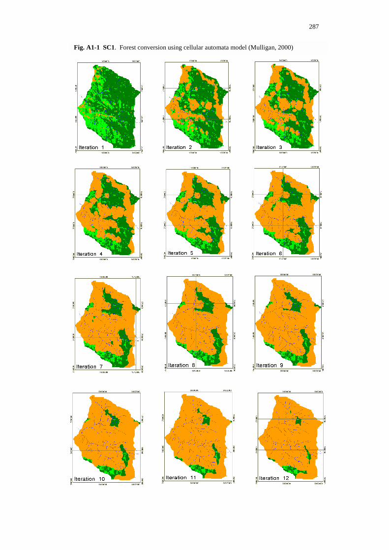
287
Fig. A1-1 SC1. Forest conversion using cellular automata model (Mulligan, 2000)
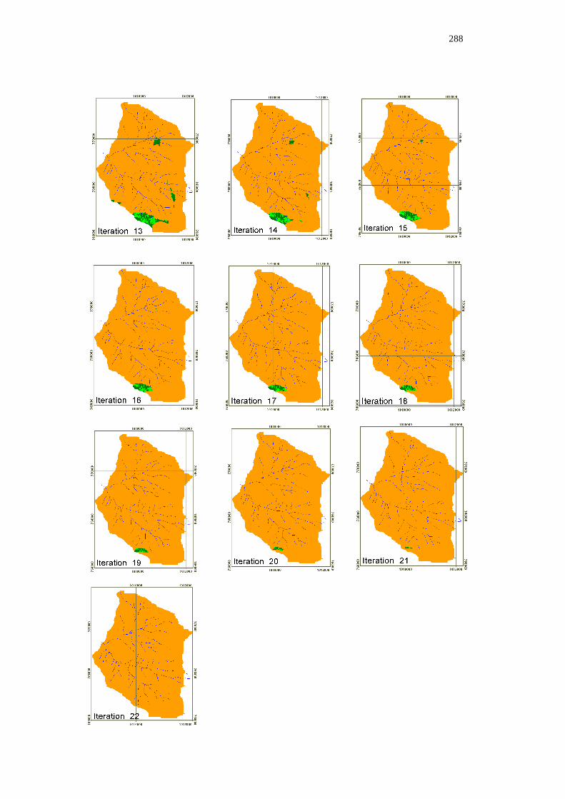
288
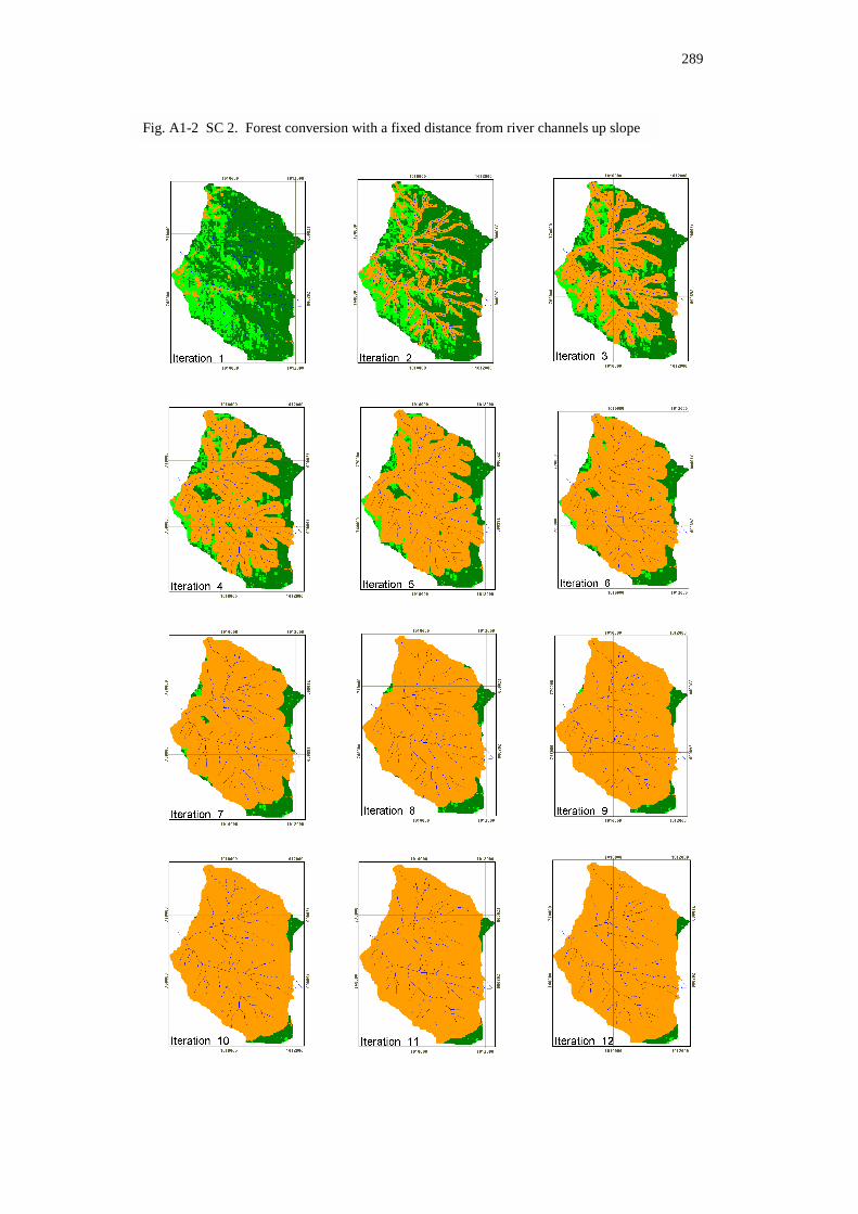
289
Fig. A1-2 SC 2. Forest conversion with a fixed distance from river channels up slope

290
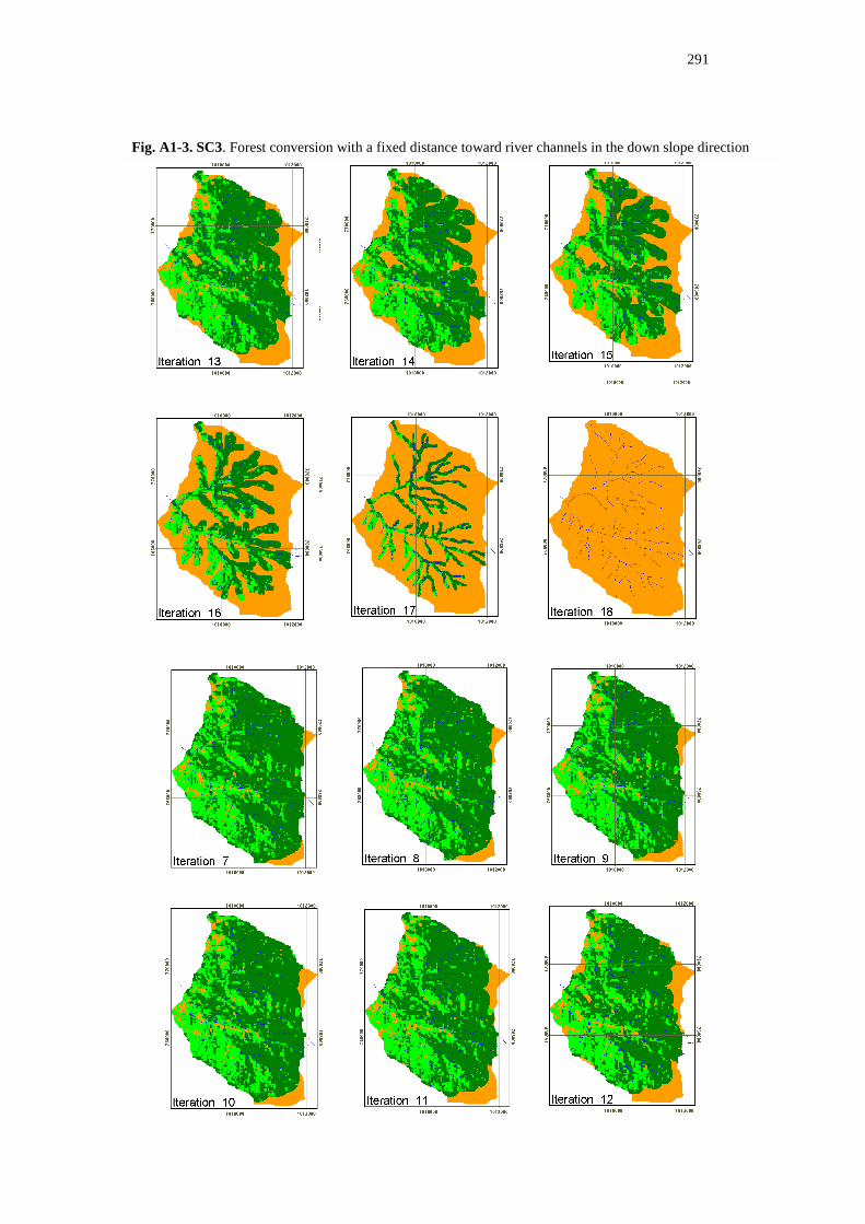
291
Fig. A1-3. SC3. Forest conversion with a fixed distance toward river channels in the down slope direction
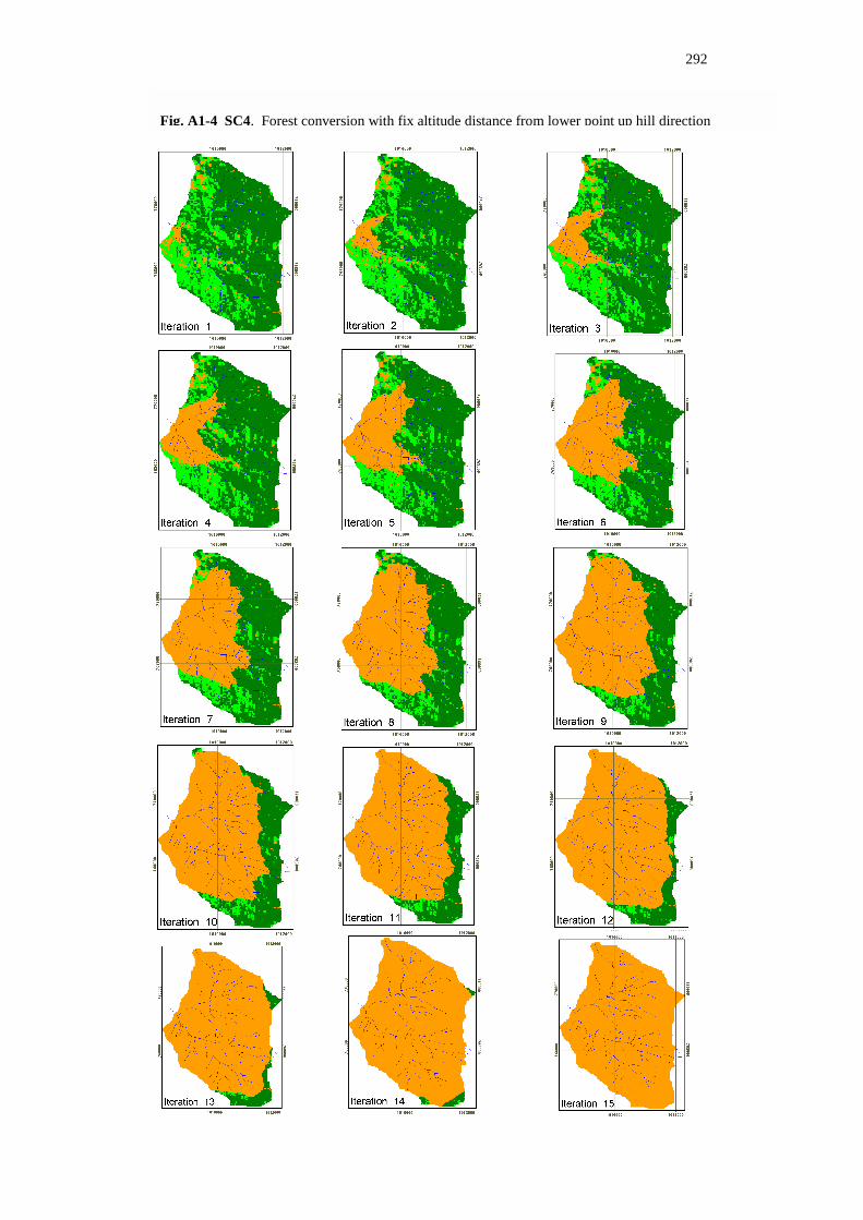
292
Fig. A1-4 SC4. Forest conversion with fix altitude distance from lower point up hill direction
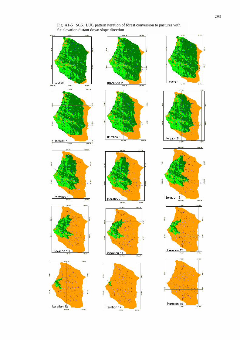
293
Fig. A1-5 SC5. LUC pattern iteration of forest conversion to pastures withfix elevation distant down slope direction
294
Appendix No. II
Data collected from grassland weather stationNov 22/97 to Nov 24/97
(Example)
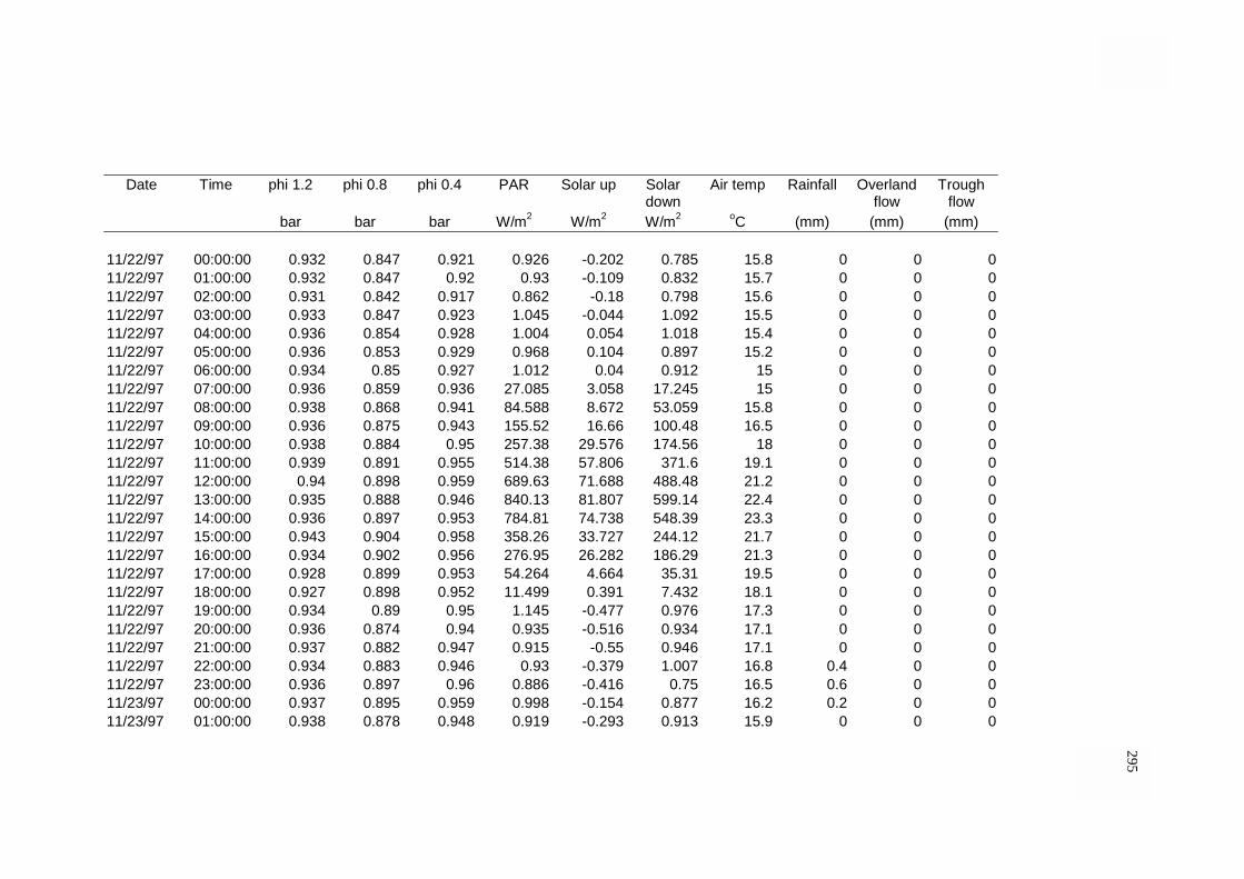
295
Date Time phi 1.2 phi 0.8 phi 0.4 PAR Solar up Solardown
Air temp Rainfall Overlandflow
Troughflow
bar bar bar W/m2 W/m2 W/m2 oC (mm) (mm) (mm)
11/22/97 00:00:00 0.932 0.847 0.921 0.926 -0.202 0.785 15.8 0 0 011/22/97 01:00:00 0.932 0.847 0.92 0.93 -0.109 0.832 15.7 0 0 011/22/97 02:00:00 0.931 0.842 0.917 0.862 -0.18 0.798 15.6 0 0 011/22/97 03:00:00 0.933 0.847 0.923 1.045 -0.044 1.092 15.5 0 0 011/22/97 04:00:00 0.936 0.854 0.928 1.004 0.054 1.018 15.4 0 0 011/22/97 05:00:00 0.936 0.853 0.929 0.968 0.104 0.897 15.2 0 0 011/22/97 06:00:00 0.934 0.85 0.927 1.012 0.04 0.912 15 0 0 011/22/97 07:00:00 0.936 0.859 0.936 27.085 3.058 17.245 15 0 0 011/22/97 08:00:00 0.938 0.868 0.941 84.588 8.672 53.059 15.8 0 0 011/22/97 09:00:00 0.936 0.875 0.943 155.52 16.66 100.48 16.5 0 0 011/22/97 10:00:00 0.938 0.884 0.95 257.38 29.576 174.56 18 0 0 011/22/97 11:00:00 0.939 0.891 0.955 514.38 57.806 371.6 19.1 0 0 011/22/97 12:00:00 0.94 0.898 0.959 689.63 71.688 488.48 21.2 0 0 011/22/97 13:00:00 0.935 0.888 0.946 840.13 81.807 599.14 22.4 0 0 011/22/97 14:00:00 0.936 0.897 0.953 784.81 74.738 548.39 23.3 0 0 011/22/97 15:00:00 0.943 0.904 0.958 358.26 33.727 244.12 21.7 0 0 011/22/97 16:00:00 0.934 0.902 0.956 276.95 26.282 186.29 21.3 0 0 011/22/97 17:00:00 0.928 0.899 0.953 54.264 4.664 35.31 19.5 0 0 011/22/97 18:00:00 0.927 0.898 0.952 11.499 0.391 7.432 18.1 0 0 011/22/97 19:00:00 0.934 0.89 0.95 1.145 -0.477 0.976 17.3 0 0 011/22/97 20:00:00 0.936 0.874 0.94 0.935 -0.516 0.934 17.1 0 0 011/22/97 21:00:00 0.937 0.882 0.947 0.915 -0.55 0.946 17.1 0 0 011/22/97 22:00:00 0.934 0.883 0.946 0.93 -0.379 1.007 16.8 0.4 0 011/22/97 23:00:00 0.936 0.897 0.96 0.886 -0.416 0.75 16.5 0.6 0 011/23/97 00:00:00 0.937 0.895 0.959 0.998 -0.154 0.877 16.2 0.2 0 011/23/97 01:00:00 0.938 0.878 0.948 0.919 -0.293 0.913 15.9 0 0 0
295
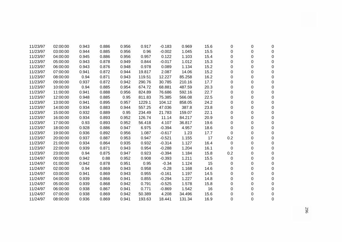
296
11/23/97 02:00:00 0.943 0.886 0.956 0.917 -0.183 0.969 15.6 0 0 011/23/97 03:00:00 0.944 0.885 0.956 0.96 -0.002 1.045 15.5 0 0 011/23/97 04:00:00 0.945 0.886 0.956 0.957 0.122 1.103 15.4 0 0 011/23/97 05:00:00 0.943 0.878 0.949 0.844 -0.017 1.012 15.3 0 0 011/23/97 06:00:00 0.943 0.876 0.948 0.978 0.089 1.134 15.2 0 0 011/23/97 07:00:00 0.941 0.872 0.944 19.817 2.087 14.06 15.2 0 0 011/23/97 08:00:00 0.94 0.871 0.943 119.51 12.227 85.258 16.2 0 0 011/23/97 09:00:00 0.937 0.872 0.942 290.76 30.785 210.16 17.7 0 0 011/23/97 10:00:00 0.94 0.885 0.954 674.72 68.881 487.59 20.3 0 0 011/23/97 11:00:00 0.941 0.888 0.956 824.89 76.686 592.16 22.7 0 0 011/23/97 12:00:00 0.948 0.885 0.95 811.83 75.385 566.08 22.5 0 0 011/23/97 13:00:00 0.941 0.895 0.957 1229.1 104.12 858.05 24.2 0 0 011/23/97 14:00:00 0.934 0.883 0.944 557.25 47.036 387.8 23.8 0 0 011/23/97 15:00:00 0.932 0.889 0.95 234.49 21.783 159.07 22.1 0 0 011/23/97 16:00:00 0.934 0.893 0.952 126.74 11.14 84.217 20.9 0 0 011/23/97 17:00:00 0.93 0.893 0.952 56.418 4.107 36.817 19.6 0 0 011/23/97 18:00:00 0.928 0.886 0.947 6.975 -0.394 4.957 18.6 0 0 011/23/97 19:00:00 0.936 0.892 0.956 1.087 -0.617 1.23 17.7 0 0 011/23/97 20:00:00 0.937 0.887 0.953 0.947 -0.521 1.155 17 0.2 0 011/23/97 21:00:00 0.934 0.864 0.935 0.932 -0.314 1.127 16.4 0 0 011/23/97 22:00:00 0.939 0.871 0.943 0.954 -0.288 1.204 16.1 0 0 011/23/97 23:00:00 0.94 0.875 0.947 0.923 -0.394 1.184 15.8 0.2 0 011/24/97 00:00:00 0.942 0.88 0.952 0.908 -0.393 1.211 15.5 0 0 011/24/97 01:00:00 0.942 0.878 0.951 0.95 -0.34 1.124 15 0 0 011/24/97 02:00:00 0.94 0.869 0.943 0.958 -0.28 1.168 14.6 0 0 011/24/97 03:00:00 0.941 0.869 0.943 0.955 -0.161 1.197 14.5 0 0 011/24/97 04:00:00 0.939 0.866 0.941 0.855 -0.294 1.227 14.8 0 0 011/24/97 05:00:00 0.939 0.868 0.942 0.791 -0.525 1.578 15.8 0 0 011/24/97 06:00:00 0.938 0.867 0.941 0.771 -0.869 1.542 16 0 0 011/24/97 07:00:00 0.938 0.869 0.942 50.389 4.208 34.496 15.6 0 0 011/24/97 08:00:00 0.936 0.869 0.941 193.63 18.441 131.34 16.9 0 0 0
296
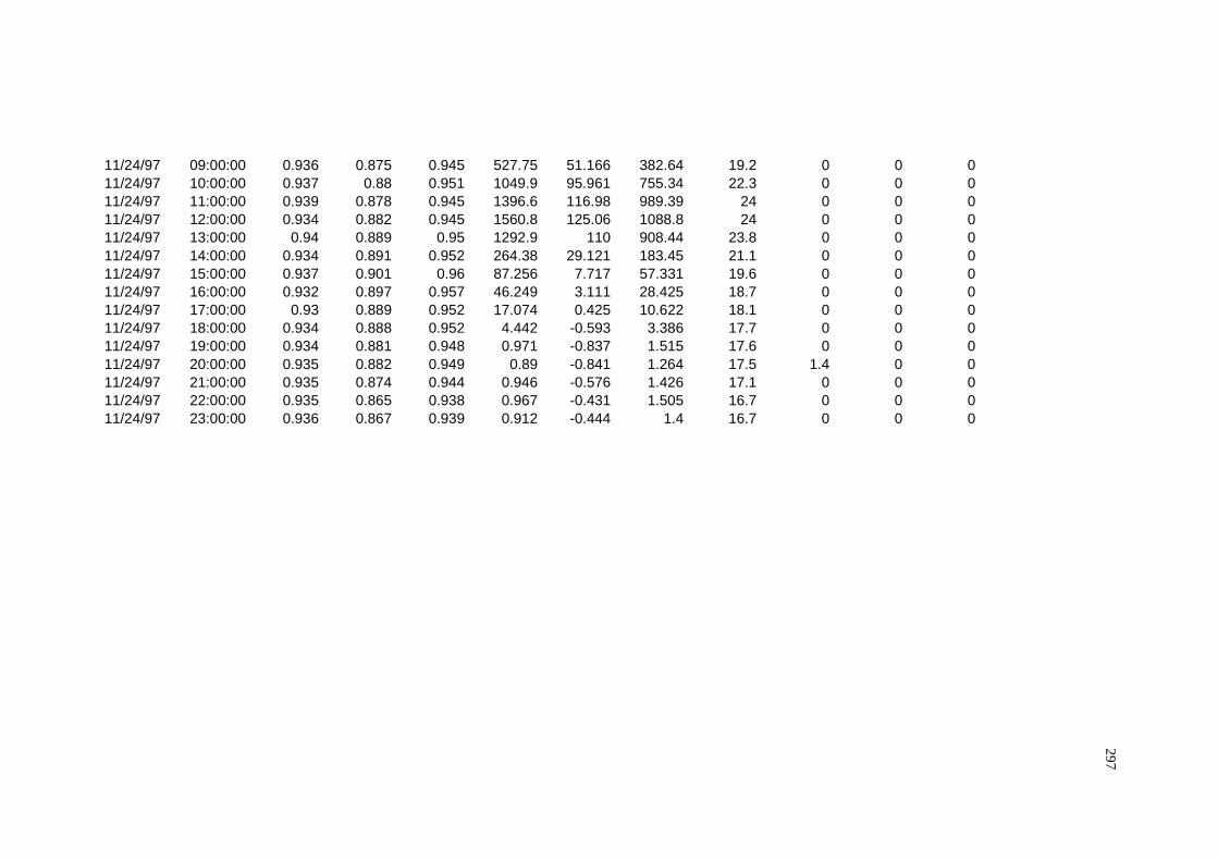
297
11/24/97 09:00:00 0.936 0.875 0.945 527.75 51.166 382.64 19.2 0 0 011/24/97 10:00:00 0.937 0.88 0.951 1049.9 95.961 755.34 22.3 0 0 011/24/97 11:00:00 0.939 0.878 0.945 1396.6 116.98 989.39 24 0 0 011/24/97 12:00:00 0.934 0.882 0.945 1560.8 125.06 1088.8 24 0 0 011/24/97 13:00:00 0.94 0.889 0.95 1292.9 110 908.44 23.8 0 0 011/24/97 14:00:00 0.934 0.891 0.952 264.38 29.121 183.45 21.1 0 0 011/24/97 15:00:00 0.937 0.901 0.96 87.256 7.717 57.331 19.6 0 0 011/24/97 16:00:00 0.932 0.897 0.957 46.249 3.111 28.425 18.7 0 0 011/24/97 17:00:00 0.93 0.889 0.952 17.074 0.425 10.622 18.1 0 0 011/24/97 18:00:00 0.934 0.888 0.952 4.442 -0.593 3.386 17.7 0 0 011/24/97 19:00:00 0.934 0.881 0.948 0.971 -0.837 1.515 17.6 0 0 011/24/97 20:00:00 0.935 0.882 0.949 0.89 -0.841 1.264 17.5 1.4 0 011/24/97 21:00:00 0.935 0.874 0.944 0.946 -0.576 1.426 17.1 0 0 011/24/97 22:00:00 0.935 0.865 0.938 0.967 -0.431 1.505 16.7 0 0 011/24/97 23:00:00 0.936 0.867 0.939 0.912 -0.444 1.4 16.7 0 0 0
297

298
Appendix No. III
Summary of soil analysis samples

299
Soilmapzone
slopeclass
vegetationclass
Sand Silt Clay BulkDensity
Porosity Numberof
samples1 1 1 0.58 0.19 0.23 0.87 0.65 132 2 1 0.56 0.23 0.21 0.85 0.66 193 3 1 0.58 0.20 0.22 0.74 0.71 74 2 2 0.57 0.24 0.19 0.80 0.68 145 3 2 0.56 0.24 0.20 0.85 0.66 76 1 2 0.63 0.20 0.17 0.69 0.72 157 1 3 0.60 0.19 0.21 0.96 0.62 148 2 3 0.58 0.22 0.20 1.00 0.58 149 3 3 0.56 0.24 0.20 0.83 0.67 8
Table A3.1 Summary of soil properties corresponding of 9 sampledclasses of fig. 4.7.
Soil samples were taken until the bed rock could allow to penetratethe auger, and in some cases more than one set was collected.
Stone density = 2.51 g cm-3
Volume of samples = 204 cm3
This field work collecting samples were carried out with JorgeRubiano1 co-operation.
1 - M.Sc. KCL Geography Student, 1997

300
Appendix IV
Summary of vegetation samples for:
canopy water storage capacity,
vegetation cover
and LAI for grassland
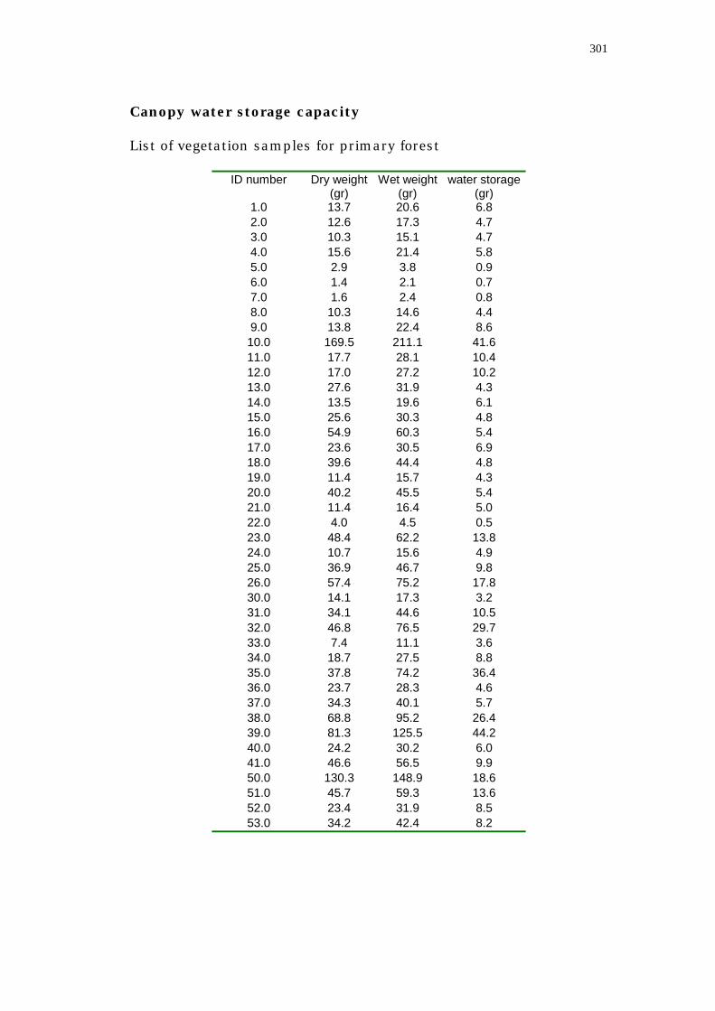
301
Canopy water storage capacity
List of vegetation samples for primary forest
ID number Dry weight(gr)
Wet weight(gr)
water storage(gr)
1.0 13.7 20.6 6.82.0 12.6 17.3 4.73.0 10.3 15.1 4.74.0 15.6 21.4 5.85.0 2.9 3.8 0.96.0 1.4 2.1 0.77.0 1.6 2.4 0.88.0 10.3 14.6 4.49.0 13.8 22.4 8.610.0 169.5 211.1 41.611.0 17.7 28.1 10.412.0 17.0 27.2 10.213.0 27.6 31.9 4.314.0 13.5 19.6 6.115.0 25.6 30.3 4.816.0 54.9 60.3 5.417.0 23.6 30.5 6.918.0 39.6 44.4 4.819.0 11.4 15.7 4.320.0 40.2 45.5 5.421.0 11.4 16.4 5.022.0 4.0 4.5 0.523.0 48.4 62.2 13.824.0 10.7 15.6 4.925.0 36.9 46.7 9.826.0 57.4 75.2 17.830.0 14.1 17.3 3.231.0 34.1 44.6 10.532.0 46.8 76.5 29.733.0 7.4 11.1 3.634.0 18.7 27.5 8.835.0 37.8 74.2 36.436.0 23.7 28.3 4.637.0 34.3 40.1 5.738.0 68.8 95.2 26.439.0 81.3 125.5 44.240.0 24.2 30.2 6.041.0 46.6 56.5 9.950.0 130.3 148.9 18.651.0 45.7 59.3 13.652.0 23.4 31.9 8.553.0 34.2 42.4 8.2
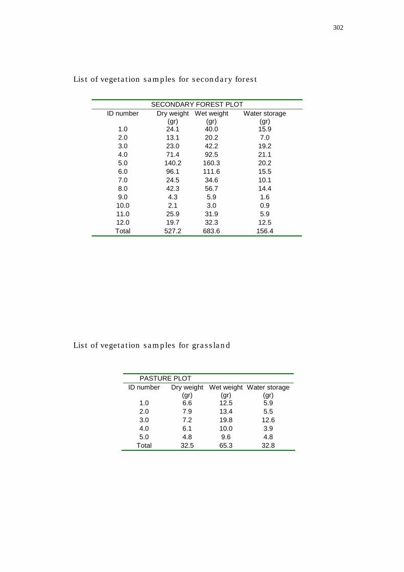
302
List of vegetation samples for secondary forest
SECONDARY FOREST PLOTID number Dry weight
(gr)Wet weight
(gr)Water storage
(gr)1.0 24.1 40.0 15.92.0 13.1 20.2 7.03.0 23.0 42.2 19.24.0 71.4 92.5 21.15.0 140.2 160.3 20.26.0 96.1 111.6 15.57.0 24.5 34.6 10.18.0 42.3 56.7 14.49.0 4.3 5.9 1.610.0 2.1 3.0 0.911.0 25.9 31.9 5.912.0 19.7 32.3 12.5Total 527.2 683.6 156.4
List of vegetation samples for grassland
PASTURE PLOTID number Dry weight
(gr)Wet weight
(gr)Water storage
(gr)1.0 6.6 12.5 5.92.0 7.9 13.4 5.53.0 7.2 19.8 12.64.0 6.1 10.0 3.95.0 4.8 9.6 4.8
Total 32.5 65.3 32.8
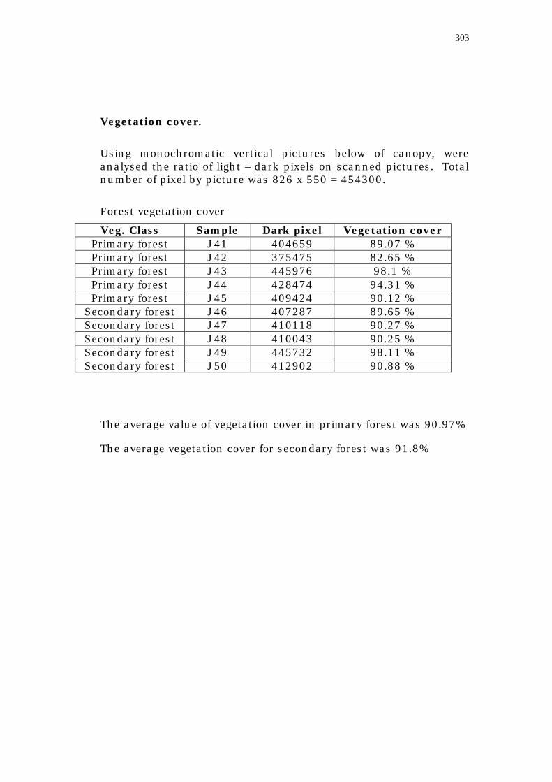
303
Vegetation cover.
Using monochromatic vertical pictures below of canopy, wereanalysed the ratio of light – dark pixels on scanned pictures. Totalnumber of pixel by picture was 826 x 550 = 454300.
Forest vegetation cover
Veg. Class Sample Dark pixel Vegetation coverPrimary forest J41 404659 89.07 %Primary forest J42 375475 82.65 %Primary forest J43 445976 98.1 %Primary forest J44 428474 94.31 %Primary forest J45 409424 90.12 %
Secondary forest J46 407287 89.65 %Secondary forest J47 410118 90.27 %Secondary forest J48 410043 90.25 %Secondary forest J49 445732 98.11 %Secondary forest J50 412902 90.88 %
The average value of vegetation cover in primary forest was 90.97%
The average vegetation cover for secondary forest was 91.8%

304
Appendix V
Tambito daily rainfall data
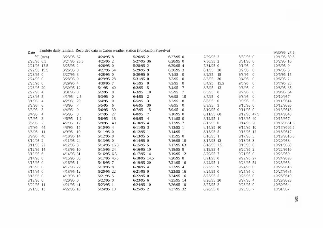
305
Date Rain fall (mm)2/20/95 6.52/21/95 17.52/22/95 19.52/23/95 02/24/95 02/25/95 02/26/95 202/27/95 42/28/95 53/1/95 43/2/95 63/3/95 33/4/95 43/5/95 33/6/95 23/7/95 443/8/95 113/9/95 403/10/95 23/11/95 223/12/95 143/13/95 63/14/95 03/15/95 03/16/95 03/17/95 03/18/95 03/19/95 03/20/95 113/21/95 13
3/22/95 53/23/95 673/24/95 25.53/25/95 23/26/95 03/27/95 83/28/95 03/29/95 43/30/95 123/31/95 04/1/95 2.54/2/95 204/3/95 74/4/95 04/5/95 04/6/95 1.24/7/95 124/8/95 154/9/95 104/10/95 144/11/95 244/12/95 84/13/95 104/14/95 814/15/95 854/16/95 14/17/95 224/18/95 124/19/95 104/20/95 04/21/95 414/22/95 10
4/23/95 24/24/95 84/25/95 24/26/95 04/27/95 544/28/95 04/29/95 284/30/95 75/1/95 405/2/95 05/3/95 05/4/95 05/5/95 65/6/95 305/7/95 275/8/95 185/9/95 405/10/95 45/11/95 05/12/95 05/13/95 05/14/95 16.55/15/95 245/16/95 6.55/17/95 45.55/18/95 75/19/95 85/20/95 225/21/95 55/22/95 05/23/95 15/24/95 10
5/25/95 205/26/95 25/27/95 365/28/95 25/29/95 95/30/95 05/31/95 06/1/95 06/2/95 56/3/95 106/4/95 26/5/95 36/6/95 306/7/95 156/8/95 76/9/95 46/10/95 46/11/95 36/12/95 16/13/95 56/14/95 06/15/95 56/16/95 106/17/95 146/18/95 14.56/19/95 206/20/95 46/21/95 06/22/95 06/23/95 66/24/95 106/25/95 2
6/26/95 36/27/95 06/28/95 06/29/95 46/30/95 37/1/95 07/2/95 07/3/95 07/4/95 77/5/95 77/6/95 107/7/95 87/8/95 07/9/95 07/10/95 07/11/95 07/12/95 27/13/95 17/14/95 17/15/95 07/16/95 107/17/95 637/18/95 87/19/95 127/20/95 87/21/95 167/22/95 47/23/95 167/24/95 167/25/95 147/26/95 107/27/95 32
7/28/95 87/29/95 77/30/95 27/31/95 08/1/95 208/2/95 198/3/95 308/4/95 15.58/5/95 128/6/95 08/7/95 08/8/95 08/9/95 38/10/95 08/11/95 688/12/95 18/13/95 08/14/95 108/15/95 58/16/95 18/17/95 138/18/95 7.58/19/95 48/20/95 78/21/95 08/22/95 18/23/95 98/24/95 08/25/95 58/26/95 208/27/95 28/28/95 0
8/29/95 08/30/95 08/31/95 09/1/95 09/2/95 09/3/95 09/4/95 09/5/95 09/6/95 09/7/95 09/8/95 09/9/95 59/10/95 09/11/95 09/12/95 47.59/13/95 409/14/95 209/15/95 109/16/95 129/17/95 59/18/95 39/19/95 09/20/95 29/21/95 09/22/95 279/23/95 549/24/95 09/25/95 09/26/95 09/27/95 49/28/95 09/29/95 7
9/30/95 27.510/1/95 30.510/2/95 1610/3/95 010/4/95 310/5/95 1510/6/95 210/7/95 2310/8/95 3510/9/95 6410/10/95710/11/951410/12/952010/13/951810/14/954310/15/95710/16/9551.510/17/9565.510/18/951710/19/9516.510/20/95310/21/955010/22/951010/23/95910/24/952010/25/95510/26/951610/27/953510/28/951010/29/952310/30/95410/31/957
Tambito daily rainfall. Recorded data in Cabin weather station (Fundación Proselva)
305
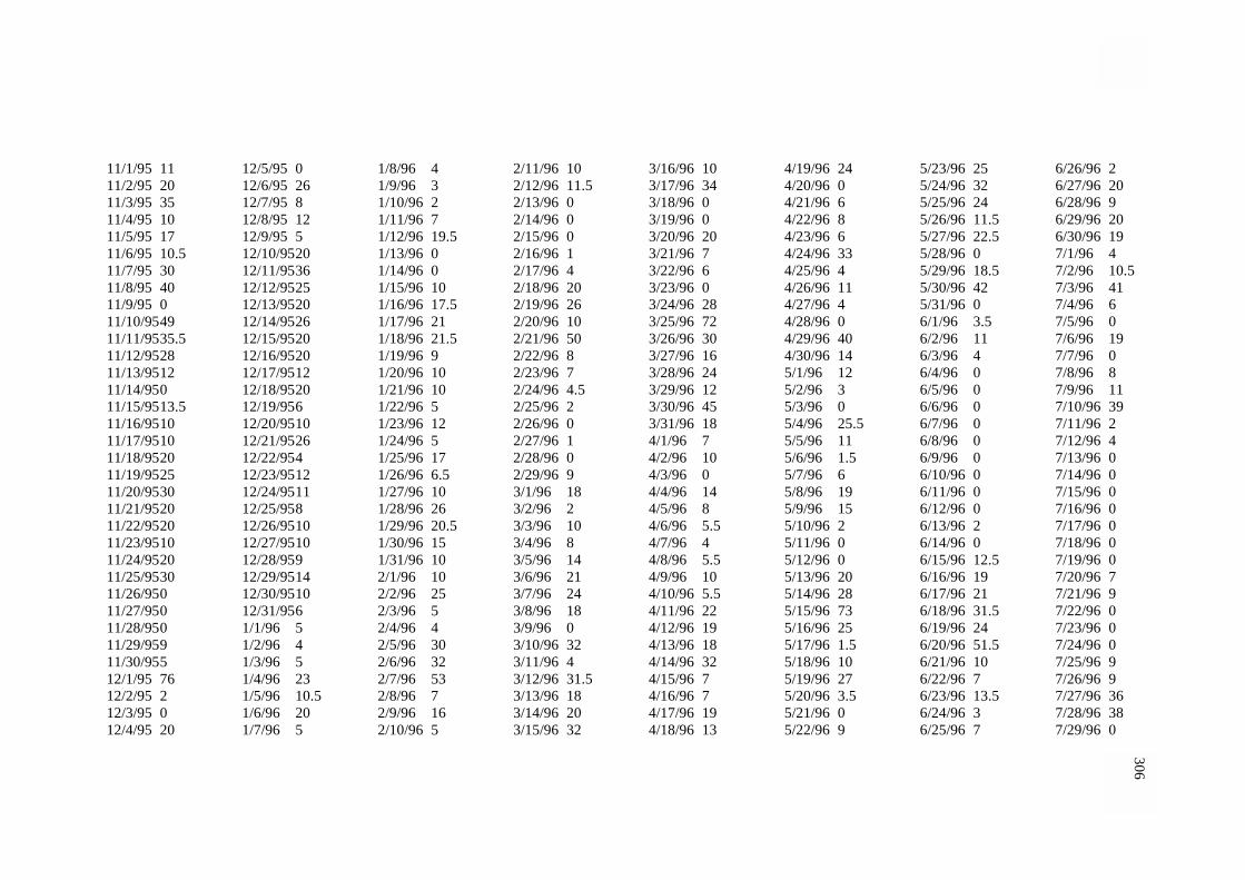
306
11/1/95 1111/2/95 2011/3/95 3511/4/95 1011/5/95 1711/6/95 10.511/7/95 3011/8/95 4011/9/95 011/10/954911/11/9535.511/12/952811/13/951211/14/95011/15/9513.511/16/951011/17/951011/18/952011/19/952511/20/953011/21/952011/22/952011/23/951011/24/952011/25/953011/26/95011/27/95011/28/95011/29/95911/30/95512/1/95 7612/2/95 212/3/95 012/4/95 20
12/5/95 012/6/95 2612/7/95 812/8/95 1212/9/95 512/10/952012/11/953612/12/952512/13/952012/14/952612/15/952012/16/952012/17/951212/18/952012/19/95612/20/951012/21/952612/22/95412/23/951212/24/951112/25/95812/26/951012/27/951012/28/95912/29/951412/30/951012/31/9561/1/96 51/2/96 41/3/96 51/4/96 231/5/96 10.51/6/96 201/7/96 5
1/8/96 41/9/96 31/10/96 21/11/96 71/12/96 19.51/13/96 01/14/96 01/15/96 101/16/96 17.51/17/96 211/18/96 21.51/19/96 91/20/96 101/21/96 101/22/96 51/23/96 121/24/96 51/25/96 171/26/96 6.51/27/96 101/28/96 261/29/96 20.51/30/96 151/31/96 102/1/96 102/2/96 252/3/96 52/4/96 42/5/96 302/6/96 322/7/96 532/8/96 72/9/96 162/10/96 5
2/11/96 102/12/96 11.52/13/96 02/14/96 02/15/96 02/16/96 12/17/96 42/18/96 202/19/96 262/20/96 102/21/96 502/22/96 82/23/96 72/24/96 4.52/25/96 22/26/96 02/27/96 12/28/96 02/29/96 93/1/96 183/2/96 23/3/96 103/4/96 83/5/96 143/6/96 213/7/96 243/8/96 183/9/96 03/10/96 323/11/96 43/12/96 31.53/13/96 183/14/96 203/15/96 32
3/16/96 103/17/96 343/18/96 03/19/96 03/20/96 203/21/96 73/22/96 63/23/96 03/24/96 283/25/96 723/26/96 303/27/96 163/28/96 243/29/96 123/30/96 453/31/96 184/1/96 74/2/96 104/3/96 04/4/96 144/5/96 84/6/96 5.54/7/96 44/8/96 5.54/9/96 104/10/96 5.54/11/96 224/12/96 194/13/96 184/14/96 324/15/96 74/16/96 74/17/96 194/18/96 13
4/19/96 244/20/96 04/21/96 64/22/96 84/23/96 64/24/96 334/25/96 44/26/96 114/27/96 44/28/96 04/29/96 404/30/96 145/1/96 125/2/96 35/3/96 05/4/96 25.55/5/96 115/6/96 1.55/7/96 65/8/96 195/9/96 155/10/96 25/11/96 05/12/96 05/13/96 205/14/96 285/15/96 735/16/96 255/17/96 1.55/18/96 105/19/96 275/20/96 3.55/21/96 05/22/96 9
5/23/96 255/24/96 325/25/96 245/26/96 11.55/27/96 22.55/28/96 05/29/96 18.55/30/96 425/31/96 06/1/96 3.56/2/96 116/3/96 46/4/96 06/5/96 06/6/96 06/7/96 06/8/96 06/9/96 06/10/96 06/11/96 06/12/96 06/13/96 26/14/96 06/15/96 12.56/16/96 196/17/96 216/18/96 31.56/19/96 246/20/96 51.56/21/96 106/22/96 76/23/96 13.56/24/96 36/25/96 7
6/26/96 26/27/96 206/28/96 96/29/96 206/30/96 197/1/96 47/2/96 10.57/3/96 417/4/96 67/5/96 07/6/96 197/7/96 07/8/96 87/9/96 117/10/96 397/11/96 27/12/96 47/13/96 07/14/96 07/15/96 07/16/96 07/17/96 07/18/96 07/19/96 07/20/96 77/21/96 97/22/96 07/23/96 07/24/96 07/25/96 97/26/96 97/27/96 367/28/96 387/29/96 0
306
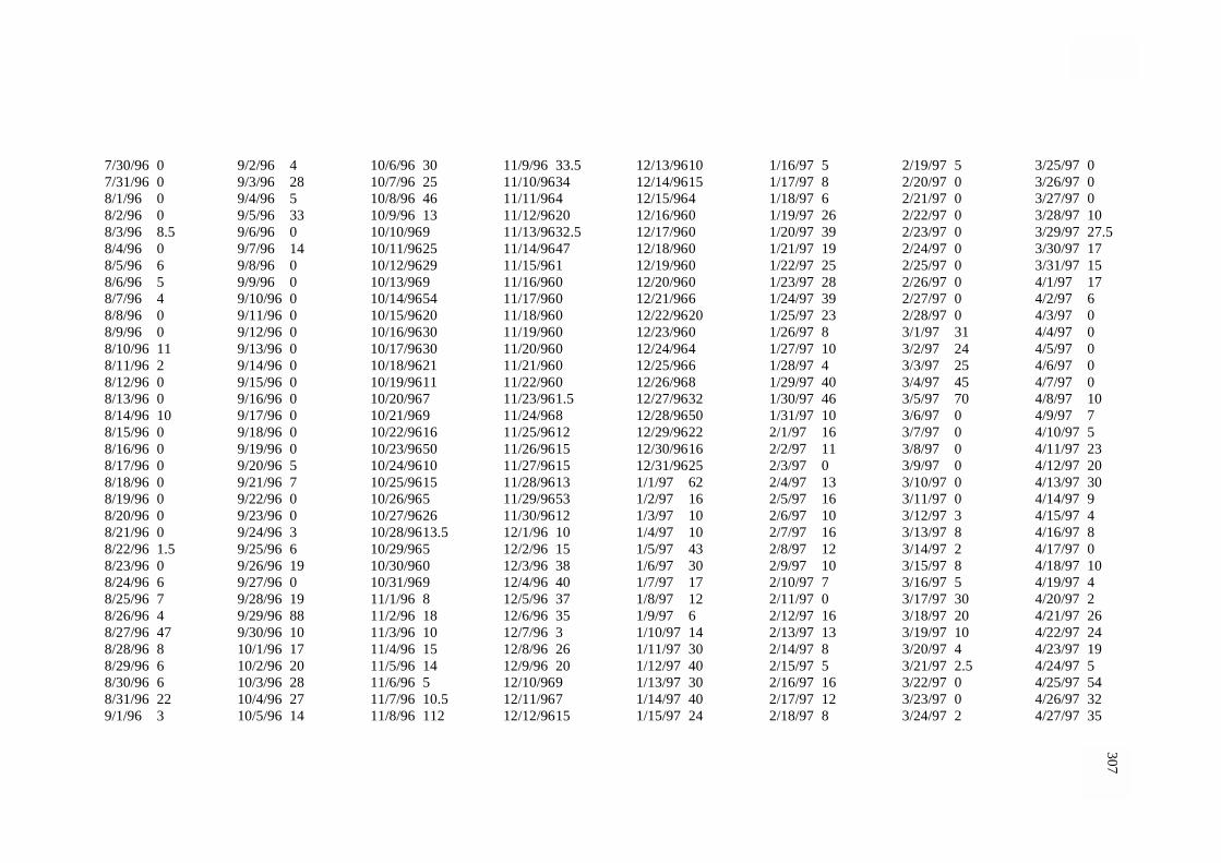
307
7/30/96 07/31/96 08/1/96 08/2/96 08/3/96 8.58/4/96 08/5/96 68/6/96 58/7/96 48/8/96 08/9/96 08/10/96 118/11/96 28/12/96 08/13/96 08/14/96 108/15/96 08/16/96 08/17/96 08/18/96 08/19/96 08/20/96 08/21/96 08/22/96 1.58/23/96 08/24/96 68/25/96 78/26/96 48/27/96 478/28/96 88/29/96 68/30/96 68/31/96 229/1/96 3
9/2/96 49/3/96 289/4/96 59/5/96 339/6/96 09/7/96 149/8/96 09/9/96 09/10/96 09/11/96 09/12/96 09/13/96 09/14/96 09/15/96 09/16/96 09/17/96 09/18/96 09/19/96 09/20/96 59/21/96 79/22/96 09/23/96 09/24/96 39/25/96 69/26/96 199/27/96 09/28/96 199/29/96 889/30/96 1010/1/96 1710/2/96 2010/3/96 2810/4/96 2710/5/96 14
10/6/96 3010/7/96 2510/8/96 4610/9/96 1310/10/96910/11/962510/12/962910/13/96910/14/965410/15/962010/16/963010/17/963010/18/962110/19/961110/20/96710/21/96910/22/961610/23/965010/24/961010/25/961510/26/96510/27/962610/28/9613.510/29/96510/30/96010/31/96911/1/96 811/2/96 1811/3/96 1011/4/96 1511/5/96 1411/6/96 511/7/96 10.511/8/96 112
11/9/96 33.511/10/963411/11/96411/12/962011/13/9632.511/14/964711/15/96111/16/96011/17/96011/18/96011/19/96011/20/96011/21/96011/22/96011/23/961.511/24/96811/25/961211/26/961511/27/961511/28/961311/29/965311/30/961212/1/96 1012/2/96 1512/3/96 3812/4/96 4012/5/96 3712/6/96 3512/7/96 312/8/96 2612/9/96 2012/10/96912/11/96712/12/9615
12/13/961012/14/961512/15/96412/16/96012/17/96012/18/96012/19/96012/20/96012/21/96612/22/962012/23/96012/24/96412/25/96612/26/96812/27/963212/28/965012/29/962212/30/961612/31/96251/1/97 621/2/97 161/3/97 101/4/97 101/5/97 431/6/97 301/7/97 171/8/97 121/9/97 61/10/97 141/11/97 301/12/97 401/13/97 301/14/97 401/15/97 24
1/16/97 51/17/97 81/18/97 61/19/97 261/20/97 391/21/97 191/22/97 251/23/97 281/24/97 391/25/97 231/26/97 81/27/97 101/28/97 41/29/97 401/30/97 461/31/97 102/1/97 162/2/97 112/3/97 02/4/97 132/5/97 162/6/97 102/7/97 162/8/97 122/9/97 102/10/97 72/11/97 02/12/97 162/13/97 132/14/97 82/15/97 52/16/97 162/17/97 122/18/97 8
2/19/97 52/20/97 02/21/97 02/22/97 02/23/97 02/24/97 02/25/97 02/26/97 02/27/97 02/28/97 03/1/97 313/2/97 243/3/97 253/4/97 453/5/97 703/6/97 03/7/97 03/8/97 03/9/97 03/10/97 03/11/97 03/12/97 33/13/97 83/14/97 23/15/97 83/16/97 53/17/97 303/18/97 203/19/97 103/20/97 43/21/97 2.53/22/97 03/23/97 03/24/97 2
3/25/97 03/26/97 03/27/97 03/28/97 103/29/97 27.53/30/97 173/31/97 154/1/97 174/2/97 64/3/97 04/4/97 04/5/97 04/6/97 04/7/97 04/8/97 104/9/97 74/10/97 54/11/97 234/12/97 204/13/97 304/14/97 94/15/97 44/16/97 84/17/97 04/18/97 104/19/97 44/20/97 24/21/97 264/22/97 244/23/97 194/24/97 54/25/97 544/26/97 324/27/97 35
307
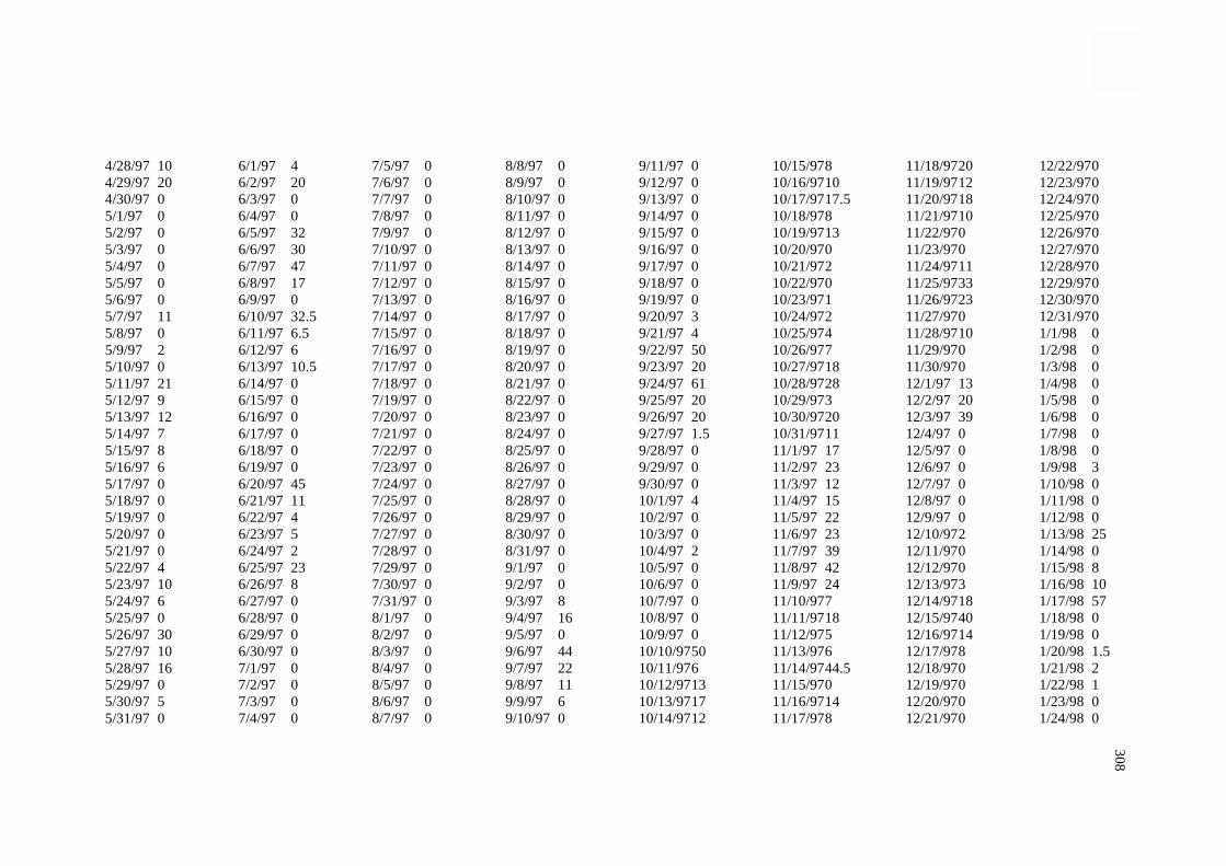
308
4/28/97 104/29/97 204/30/97 05/1/97 05/2/97 05/3/97 05/4/97 05/5/97 05/6/97 05/7/97 115/8/97 05/9/97 25/10/97 05/11/97 215/12/97 95/13/97 125/14/97 75/15/97 85/16/97 65/17/97 05/18/97 05/19/97 05/20/97 05/21/97 05/22/97 45/23/97 105/24/97 65/25/97 05/26/97 305/27/97 105/28/97 165/29/97 05/30/97 55/31/97 0
6/1/97 46/2/97 206/3/97 06/4/97 06/5/97 326/6/97 306/7/97 476/8/97 176/9/97 06/10/97 32.56/11/97 6.56/12/97 66/13/97 10.56/14/97 06/15/97 06/16/97 06/17/97 06/18/97 06/19/97 06/20/97 456/21/97 116/22/97 46/23/97 56/24/97 26/25/97 236/26/97 86/27/97 06/28/97 06/29/97 06/30/97 07/1/97 07/2/97 07/3/97 07/4/97 0
7/5/97 07/6/97 07/7/97 07/8/97 07/9/97 07/10/97 07/11/97 07/12/97 07/13/97 07/14/97 07/15/97 07/16/97 07/17/97 07/18/97 07/19/97 07/20/97 07/21/97 07/22/97 07/23/97 07/24/97 07/25/97 07/26/97 07/27/97 07/28/97 07/29/97 07/30/97 07/31/97 08/1/97 08/2/97 08/3/97 08/4/97 08/5/97 08/6/97 08/7/97 0
8/8/97 08/9/97 08/10/97 08/11/97 08/12/97 08/13/97 08/14/97 08/15/97 08/16/97 08/17/97 08/18/97 08/19/97 08/20/97 08/21/97 08/22/97 08/23/97 08/24/97 08/25/97 08/26/97 08/27/97 08/28/97 08/29/97 08/30/97 08/31/97 09/1/97 09/2/97 09/3/97 89/4/97 169/5/97 09/6/97 449/7/97 229/8/97 119/9/97 69/10/97 0
9/11/97 09/12/97 09/13/97 09/14/97 09/15/97 09/16/97 09/17/97 09/18/97 09/19/97 09/20/97 39/21/97 49/22/97 509/23/97 209/24/97 619/25/97 209/26/97 209/27/97 1.59/28/97 09/29/97 09/30/97 010/1/97 410/2/97 010/3/97 010/4/97 210/5/97 010/6/97 010/7/97 010/8/97 010/9/97 010/10/975010/11/97610/12/971310/13/971710/14/9712
10/15/97810/16/971010/17/9717.510/18/97810/19/971310/20/97010/21/97210/22/97010/23/97110/24/97210/25/97410/26/97710/27/971810/28/972810/29/97310/30/972010/31/971111/1/97 1711/2/97 2311/3/97 1211/4/97 1511/5/97 2211/6/97 2311/7/97 3911/8/97 4211/9/97 2411/10/97711/11/971811/12/97511/13/97611/14/9744.511/15/97011/16/971411/17/978
11/18/972011/19/971211/20/971811/21/971011/22/97011/23/97011/24/971111/25/973311/26/972311/27/97011/28/971011/29/97011/30/97012/1/97 1312/2/97 2012/3/97 3912/4/97 012/5/97 012/6/97 012/7/97 012/8/97 012/9/97 012/10/97212/11/97012/12/97012/13/97312/14/971812/15/974012/16/971412/17/97812/18/97012/19/97012/20/97012/21/970
12/22/97012/23/97012/24/97012/25/97012/26/97012/27/97012/28/97012/29/97012/30/97012/31/9701/1/98 01/2/98 01/3/98 01/4/98 01/5/98 01/6/98 01/7/98 01/8/98 01/9/98 31/10/98 01/11/98 01/12/98 01/13/98 251/14/98 01/15/98 81/16/98 101/17/98 571/18/98 01/19/98 01/20/98 1.51/21/98 21/22/98 11/23/98 01/24/98 0
308

309
1/25/98 01/26/98 01/27/98 01/28/98 01/29/98 21/30/98 11/31/98 02/1/98 02/2/98 02/3/98 02/4/98 02/5/98 82/6/98 52/7/98 82/8/98 322/9/98 552/10/98 19.52/11/98 372/12/98 72/13/98 0
2/14/98 02/15/98 292/16/98 02/17/98 02/18/98 02/19/98 22/20/98 702/21/98 202/22/98 02/23/98 252/24/98 02/25/98 02/26/98 02/27/98 02/28/98 123/1/98 23/2/98 03/3/98 03/4/98 03/5/98 0
3/6/98 03/7/98 63/8/98 33/9/98 03/10/98 73/11/98 15.53/12/98 2.53/13/98 03/14/98 03/15/98 03/16/98 03/17/98 33/18/98 03/19/98 03/20/98 03/21/98 03/22/98 03/23/98 203/24/98 123/25/98 0
3/26/98 143/27/98 503/28/98 20.53/29/98 423/30/98 213/31/98 854/1/98 284/2/98 504/3/98 214/4/98 404/5/98 84/6/98 54/7/98 04/8/98 154/9/98 34/10/98 54/11/98 654/12/98 164/13/98 304/14/98 18
4/15/98 04/16/98 244/17/98 204/18/98 104/19/98 384/20/98 304/21/98 204/22/98 104/23/98 44/24/98 04/25/98 74/26/98 354/27/98 304/28/98 264/29/98 64/30/98 85/1/98 105/2/98 155/3/98 285/4/98 40
5/5/98 35/6/98 75/7/98 05/8/98 205/9/98 155/10/98 105/11/98 165/12/98 75/13/98 165/14/98 05/15/98 05/16/98 05/17/98 05/18/98 05/19/98 05/20/98 05/21/98 05/22/98 05/23/98 05/24/98 0
5/25/98 05/26/98 125/27/98 515/28/98 365/29/98 17.55/30/98 45/31/98 46/1/98 216/2/98 36/3/98 146/4/98 06/5/98 06/6/98 06/7/98 06/8/98 06/9/98 256/10/98 46/11/98 26/12/98 06/13/98 0
6/14/98 06/15/98 06/16/98 06/17/98 06/18/98 56/19/98 26/20/98 06/21/98 06/22/98 06/23/98 26/24/98 16/25/98 06/26/98 26/27/98 36/28/98 06/29/98 0
309

310
Appendix VI
Example of input data file
for use in the
hydrological model

311
7yearmonthdayhourrainfall (mm)
1 1995 9 10 3 2.2 2532 1995 9 10 4 10 2533 1995 9 10 5 0 2534 1995 9 10 6 20 2535 1995 9 10 7 0 2536 1995 9 10 8 3.2 2537 1995 9 10 9 0 2538 1995 9 10 10 1.2 2539 1995 9 10 11 0 25310 1995 9 10 12 30 25311 1995 9 10 13 0 25312 1995 9 10 14 0.2 25313 1995 9 10 15 0 25314 1995 9 10 16 0 25315 1995 9 10 17 1.2 25316 1995 9 10 18 0 25317 1995 9 10 19 0 25318 1995 9 10 20 0.2 25319 1995 9 10 21 0 25320 1995 9 10 22 1.8 25321 1995 9 10 23 0 25322 1995 9 11 0 2.2 25423 1995 9 11 1 0 25424 1995 9 11 2 0.2 25425 1995 9 11 3 0 25426 1995 9 11 4 0 25427 1995 9 11 5 0 25428 1995 9 11 6 0 25429 1995 9 11 7 0 25430 1995 9 11 8 0 25431 1995 9 11 9 0 25432 1995 9 11 10 0 25433 1995 9 11 11 0 25434 1995 9 11 12 0 25435 1995 9 11 13 0 25436 1995 9 11 14 0 25437 1995 9 11 15 0 25438 1995 9 11 16 0 25439 1995 9 11 17 0.2 25440 1995 9 11 18 0.2 25441 1995 9 11 19 0.2 25442 1995 9 11 20 0 25443 1995 9 11 21 1.2 25444 1995 9 11 22 0 25445 1995 9 11 23 36.8 25446 1995 9 12 0 0 25547 1995 9 12 1 17.2 25548 1995 9 12 2 0 25549 1995 9 12 3 0 25550 1995 9 12 4 0 25551 1995 9 12 5 0 25552 1995 9 12 6 0 25553 1995 9 12 7 0 25554 1995 9 12 8 0 25555 1995 9 12 9 0 25556 1995 9 12 10 0.2 25557 1995 9 12 11 0.2 25558 1995 9 12 12 0.2 25559 1995 9 12 13 0 25560 1995 9 12 14 5.2 25561 1995 9 12 15 0.2 25562 1995 9 12 16 0 25563 1995 9 12 17 0 25564 1995 9 12 18 0 25565 1995 9 12 19 0.2 25566 1995 9 12 20 0 25567 1995 9 12 21 0 25568 1995 9 12 22 0 25569 1995 9 12 23 32.6 25570 1995 9 13 0 0 25671 1995 9 13 1 1.2 25672 1995 9 13 2 0 25673 1995 9 13 3 0 25674 1995 9 13 4 0.2 25675 1995 9 13 5 0 25676 1995 9 13 6 0 256
77 1995 9 13 7 1.2 25678 1995 9 13 8 0 25679 1995 9 13 9 0 25680 1995 9 13 10 0.2 25681 1995 9 13 11 0 25682 1995 9 13 12 0 25683 1995 9 13 13 2.2 25684 1995 9 13 14 0 25685 1995 9 13 15 0.2 25686 1995 9 13 16 2.2 25687 1995 9 13 17 0 25688 1995 9 13 18 0 25689 1995 9 13 19 0 25690 1995 9 13 20 0.2 25691 1995 9 13 21 0 25692 1995 9 13 22 0 25693 1995 9 13 23 35.4 25694 1995 9 14 0 0 25795 1995 9 14 1 0 25796 1995 9 14 2 12.2 25797 1995 9 14 3 1.2 25798 1995 9 14 4 0 25799 1995 9 14 5 0 257100 1995 9 14 6 0.2 257101 1995 9 14 7 0 257102 1995 9 14 8 0 257103 1995 9 14 9 0 257104 1995 9 14 10 0.2 257105 1995 9 14 11 0 257106 1995 9 14 12 0 257107 1995 9 14 13 1.2 257108 1995 9 14 14 0 257109 1995 9 14 15 0 257110 1995 9 14 16 0 257111 1995 9 14 17 0 257112 1995 9 14 18 0.2 257113 1995 9 14 19 1.2 257114 1995 9 14 20 0 257115 1995 9 14 21 1.2 257116 1995 9 14 22 0 257117 1995 9 14 23 6.4 257118 1995 9 15 0 1.2 258119 1995 9 15 1 0.2 258120 1995 9 15 2 0 258121 1995 9 15 3 0 258122 1995 9 15 4 0 258123 1995 9 15 5 0 258124 1995 9 15 6 0.2 258125 1995 9 15 7 0 258126 1995 9 15 8 0 258127 1995 9 15 9 1.2 258128 1995 9 15 10 0.2 258129 1995 9 15 11 0 258130 1995 9 15 12 0 258131 1995 9 15 13 0 258132 1995 9 15 14 0 258133 1995 9 15 15 0 258134 1995 9 15 16 0 258135 1995 9 15 17 0 258136 1995 9 15 18 0 258137 1995 9 15 19 0.2 258138 1995 9 15 20 0 258139 1995 9 15 21 0 258140 1995 9 15 22 0 258141 1995 9 15 23 7.8 258142 1995 9 16 0 0 259143 1995 9 16 1 7.2 259144 1995 9 16 2 1.2 259145 1995 9 16 3 0 259146 1995 9 16 4 0.2 259147 1995 9 16 5 0 259148 1995 9 16 6 0.2 259149 1995 9 16 7 1.2 259150 1995 9 16 8 2.2 259151 1995 9 16 9 0 259152 1995 9 16 10 4.2 259153 1995 9 16 11 0.2 259154 1995 9 16 12 0 259155 1995 9 16 13 0 259156 1995 9 16 14 0 259157 1995 9 16 15 0 259158 1995 9 16 16 0 259159 1995 9 16 17 0 259160 1995 9 16 18 0.2 259
Example of Input data filefor modelling in PCraster
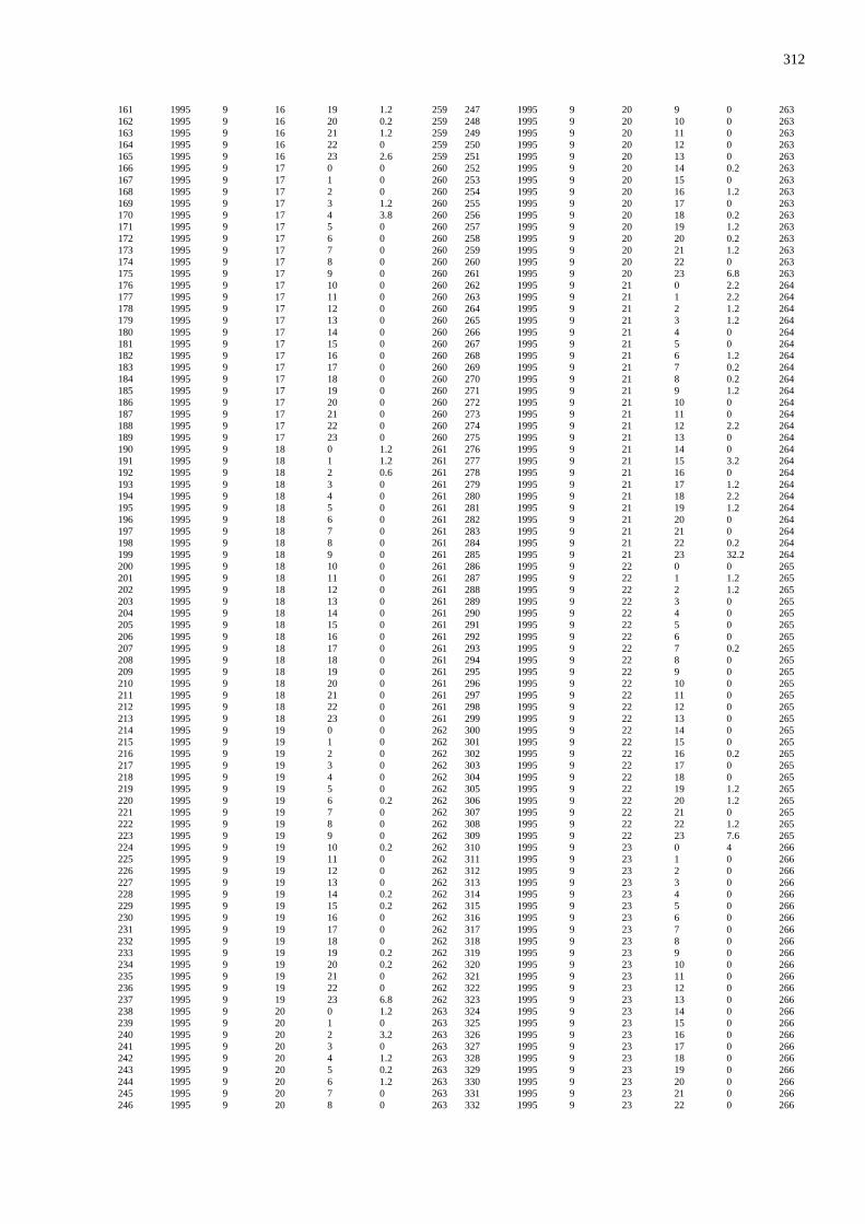
312
161 1995 9 16 19 1.2 259162 1995 9 16 20 0.2 259163 1995 9 16 21 1.2 259164 1995 9 16 22 0 259165 1995 9 16 23 2.6 259166 1995 9 17 0 0 260167 1995 9 17 1 0 260168 1995 9 17 2 0 260169 1995 9 17 3 1.2 260170 1995 9 17 4 3.8 260171 1995 9 17 5 0 260172 1995 9 17 6 0 260173 1995 9 17 7 0 260174 1995 9 17 8 0 260175 1995 9 17 9 0 260176 1995 9 17 10 0 260177 1995 9 17 11 0 260178 1995 9 17 12 0 260179 1995 9 17 13 0 260180 1995 9 17 14 0 260181 1995 9 17 15 0 260182 1995 9 17 16 0 260183 1995 9 17 17 0 260184 1995 9 17 18 0 260185 1995 9 17 19 0 260186 1995 9 17 20 0 260187 1995 9 17 21 0 260188 1995 9 17 22 0 260189 1995 9 17 23 0 260190 1995 9 18 0 1.2 261191 1995 9 18 1 1.2 261192 1995 9 18 2 0.6 261193 1995 9 18 3 0 261194 1995 9 18 4 0 261195 1995 9 18 5 0 261196 1995 9 18 6 0 261197 1995 9 18 7 0 261198 1995 9 18 8 0 261199 1995 9 18 9 0 261200 1995 9 18 10 0 261201 1995 9 18 11 0 261202 1995 9 18 12 0 261203 1995 9 18 13 0 261204 1995 9 18 14 0 261205 1995 9 18 15 0 261206 1995 9 18 16 0 261207 1995 9 18 17 0 261208 1995 9 18 18 0 261209 1995 9 18 19 0 261210 1995 9 18 20 0 261211 1995 9 18 21 0 261212 1995 9 18 22 0 261213 1995 9 18 23 0 261214 1995 9 19 0 0 262215 1995 9 19 1 0 262216 1995 9 19 2 0 262217 1995 9 19 3 0 262218 1995 9 19 4 0 262219 1995 9 19 5 0 262220 1995 9 19 6 0.2 262221 1995 9 19 7 0 262222 1995 9 19 8 0 262223 1995 9 19 9 0 262224 1995 9 19 10 0.2 262225 1995 9 19 11 0 262226 1995 9 19 12 0 262227 1995 9 19 13 0 262228 1995 9 19 14 0.2 262229 1995 9 19 15 0.2 262230 1995 9 19 16 0 262231 1995 9 19 17 0 262232 1995 9 19 18 0 262233 1995 9 19 19 0.2 262234 1995 9 19 20 0.2 262235 1995 9 19 21 0 262236 1995 9 19 22 0 262237 1995 9 19 23 6.8 262238 1995 9 20 0 1.2 263239 1995 9 20 1 0 263240 1995 9 20 2 3.2 263241 1995 9 20 3 0 263242 1995 9 20 4 1.2 263243 1995 9 20 5 0.2 263244 1995 9 20 6 1.2 263245 1995 9 20 7 0 263246 1995 9 20 8 0 263
247 1995 9 20 9 0 263248 1995 9 20 10 0 263249 1995 9 20 11 0 263250 1995 9 20 12 0 263251 1995 9 20 13 0 263252 1995 9 20 14 0.2 263253 1995 9 20 15 0 263254 1995 9 20 16 1.2 263255 1995 9 20 17 0 263256 1995 9 20 18 0.2 263257 1995 9 20 19 1.2 263258 1995 9 20 20 0.2 263259 1995 9 20 21 1.2 263260 1995 9 20 22 0 263261 1995 9 20 23 6.8 263262 1995 9 21 0 2.2 264263 1995 9 21 1 2.2 264264 1995 9 21 2 1.2 264265 1995 9 21 3 1.2 264266 1995 9 21 4 0 264267 1995 9 21 5 0 264268 1995 9 21 6 1.2 264269 1995 9 21 7 0.2 264270 1995 9 21 8 0.2 264271 1995 9 21 9 1.2 264272 1995 9 21 10 0 264273 1995 9 21 11 0 264274 1995 9 21 12 2.2 264275 1995 9 21 13 0 264276 1995 9 21 14 0 264277 1995 9 21 15 3.2 264278 1995 9 21 16 0 264279 1995 9 21 17 1.2 264280 1995 9 21 18 2.2 264281 1995 9 21 19 1.2 264282 1995 9 21 20 0 264283 1995 9 21 21 0 264284 1995 9 21 22 0.2 264285 1995 9 21 23 32.2 264286 1995 9 22 0 0 265287 1995 9 22 1 1.2 265288 1995 9 22 2 1.2 265289 1995 9 22 3 0 265290 1995 9 22 4 0 265291 1995 9 22 5 0 265292 1995 9 22 6 0 265293 1995 9 22 7 0.2 265294 1995 9 22 8 0 265295 1995 9 22 9 0 265296 1995 9 22 10 0 265297 1995 9 22 11 0 265298 1995 9 22 12 0 265299 1995 9 22 13 0 265300 1995 9 22 14 0 265301 1995 9 22 15 0 265302 1995 9 22 16 0.2 265303 1995 9 22 17 0 265304 1995 9 22 18 0 265305 1995 9 22 19 1.2 265306 1995 9 22 20 1.2 265307 1995 9 22 21 0 265308 1995 9 22 22 1.2 265309 1995 9 22 23 7.6 265310 1995 9 23 0 4 266311 1995 9 23 1 0 266312 1995 9 23 2 0 266313 1995 9 23 3 0 266314 1995 9 23 4 0 266315 1995 9 23 5 0 266316 1995 9 23 6 0 266317 1995 9 23 7 0 266318 1995 9 23 8 0 266319 1995 9 23 9 0 266320 1995 9 23 10 0 266321 1995 9 23 11 0 266322 1995 9 23 12 0 266323 1995 9 23 13 0 266324 1995 9 23 14 0 266325 1995 9 23 15 0 266326 1995 9 23 16 0 266327 1995 9 23 17 0 266328 1995 9 23 18 0 266329 1995 9 23 19 0 266330 1995 9 23 20 0 266331 1995 9 23 21 0 266332 1995 9 23 22 0 266

313
333 1995 9 23 23 0 266334 1995 9 24 0 0 267335 1995 9 24 1 0 267336 1995 9 24 2 0 267337 1995 9 24 3 0 267338 1995 9 24 4 0 267339 1995 9 24 5 0 267340 1995 9 24 6 0 267341 1995 9 24 7 0 267342 1995 9 24 8 0 267343 1995 9 24 9 0 267344 1995 9 24 10 0 267345 1995 9 24 11 0 267346 1995 9 24 12 0 267347 1995 9 24 13 0 267348 1995 9 24 14 0 267349 1995 9 24 15 0 267350 1995 9 24 16 0 267351 1995 9 24 17 0 267352 1995 9 24 18 0 267353 1995 9 24 19 0 267354 1995 9 24 20 0 267355 1995 9 24 21 0 267356 1995 9 24 22 0 267357 1995 9 24 23 0 267358 1995 9 25 0 1 268359 1995 9 25 1 0 268360 1995 9 25 2 0 268361 1995 9 25 3 0 268362 1995 9 25 4 0 268363 1995 9 25 5 0 268364 1995 9 25 6 0 268365 1995 9 25 7 0 268366 1995 9 25 8 0 268367 1995 9 25 9 0 268368 1995 9 25 10 0 268369 1995 9 25 11 0 268370 1995 9 25 12 0 268371 1995 9 25 13 0 268372 1995 9 25 14 0 268373 1995 9 25 15 0 268374 1995 9 25 16 0 268375 1995 9 25 17 0 268376 1995 9 25 18 0 268377 1995 9 25 19 0 268378 1995 9 25 20 0 268379 1995 9 25 21 0 268380 1995 9 25 22 0 268381 1995 9 25 23 0 268382 1995 9 26 0 0 269383 1995 9 26 1 0 269384 1995 9 26 2 0 269385 1995 9 26 3 0 269386 1995 9 26 4 0 269387 1995 9 26 5 0 269388 1995 9 26 6 0 269389 1995 9 26 7 0 269390 1995 9 26 8 0 269391 1995 9 26 9 0 269392 1995 9 26 10 0 269393 1995 9 26 11 0 269394 1995 9 26 12 0 269395 1995 9 26 13 0 269396 1995 9 26 14 0 269397 1995 9 26 15 0 269398 1995 9 26 16 0 269399 1995 9 26 17 0 269400 1995 9 26 18 0 269401 1995 9 26 19 0 269402 1995 9 26 20 0 269403 1995 9 26 21 0 269404 1995 9 26 22 0 269405 1995 9 26 23 0 269406 1995 9 27 0 0.2 270407 1995 9 27 1 3.2 270408 1995 9 27 2 0 270409 1995 9 27 3 0 270410 1995 9 27 4 0 270411 1995 9 27 5 0 270412 1995 9 27 6 0.2 270413 1995 9 27 7 0 270414 1995 9 27 8 0 270415 1995 9 27 9 3.2 270416 1995 9 27 10 0 270417 1995 9 27 11 6.2 270418 1995 9 27 12 0 270
419 1995 9 27 13 0 270420 1995 9 27 14 0 270421 1995 9 27 15 0 270422 1995 9 27 16 0 270423 1995 9 27 17 0 270424 1995 9 27 18 0 270425 1995 9 27 19 0 270426 1995 9 27 20 0 270427 1995 9 27 21 0 270428 1995 9 27 22 0 270429 1995 9 27 23 0 270430 1995 9 28 0 0 271431 1995 9 28 1 1.2 271432 1995 9 28 2 9.2 271433 1995 9 28 3 0.2 271434 1995 9 28 4 3.2 271435 1995 9 28 5 3.2 271436 1995 9 28 6 0 271437 1995 9 28 7 0 271438 1995 9 28 8 0 271439 1995 9 28 9 0 271440 1995 9 28 10 0 271441 1995 9 28 11 0 271442 1995 9 28 12 0 271443 1995 9 28 13 0 271444 1995 9 28 14 0 271445 1995 9 28 15 0 271446 1995 9 28 16 0 271447 1995 9 28 17 0 271448 1995 9 28 18 0 271449 1995 9 28 19 0 271450 1995 9 28 20 0 271451 1995 9 28 21 0 271452 1995 9 28 22 0 271453 1995 9 28 23 0 271454 1995 9 29 0 0 272455 1995 9 29 1 0 272456 1995 9 29 2 21.2 272457 1995 9 29 3 0 272458 1995 9 29 4 0 272459 1995 9 29 5 0.2 272460 1995 9 29 6 0.2 272461 1995 9 29 7 0.4 272462 1995 9 29 8 0 272463 1995 9 29 9 0 272464 1995 9 29 10 0 272465 1995 9 29 11 0 272466 1995 9 29 12 0 272467 1995 9 29 13 0 272468 1995 9 29 14 0 272469 1995 9 29 15 0 272470 1995 9 29 16 0 272471 1995 9 29 17 0 272472 1995 9 29 18 0 272473 1995 9 29 19 0 272474 1995 9 29 20 0 272475 1995 9 29 21 0 272476 1995 9 29 22 0 272477 1995 9 29 23 0 272478 1995 9 30 0 0.2 273479 1995 9 30 1 0 273480 1995 9 30 2 0 273481 1995 9 30 3 0 273482 1995 9 30 4 0 273483 1995 9 30 5 1.2 273484 1995 9 30 6 0 273485 1995 9 30 7 0 273486 1995 9 30 8 1.2 273487 1995 9 30 9 0 273488 1995 9 30 10 0 273489 1995 9 30 11 0 273490 1995 9 30 12 0.2 273491 1995 9 30 13 0 273492 1995 9 30 14 0 273493 1995 9 30 15 0.2 273494 1995 9 30 16 0 273495 1995 9 30 17 0 273496 1995 9 30 18 0.2 273497 1995 9 30 19 0.2 273498 1995 9 30 20 0 273499 1995 9 30 21 0 273500 1995 9 30 22 0 273501 1995 9 30 23 37.6 273502 1995 10 1 0 2.2 274503 1995 10 1 1 0 274504 1995 10 1 2 0 274
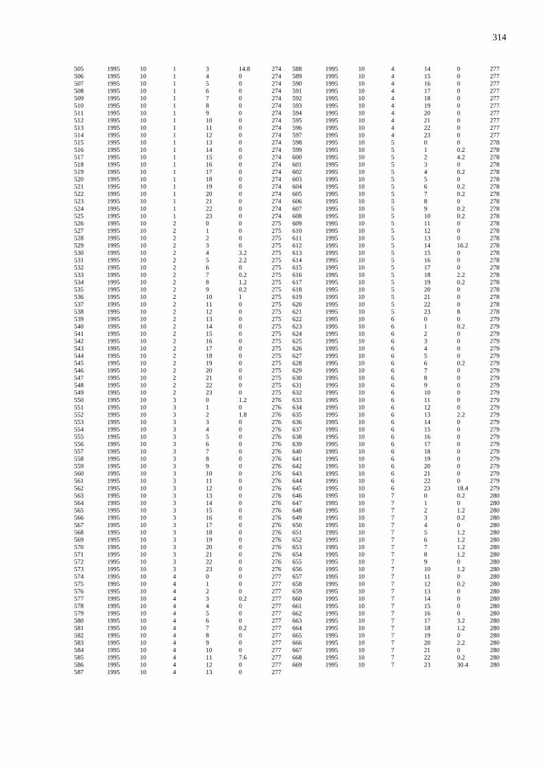
314
505 1995 10 1 3 14.8 274506 1995 10 1 4 0 274507 1995 10 1 5 0 274508 1995 10 1 6 0 274509 1995 10 1 7 0 274510 1995 10 1 8 0 274511 1995 10 1 9 0 274512 1995 10 1 10 0 274513 1995 10 1 11 0 274514 1995 10 1 12 0 274515 1995 10 1 13 0 274516 1995 10 1 14 0 274517 1995 10 1 15 0 274518 1995 10 1 16 0 274519 1995 10 1 17 0 274520 1995 10 1 18 0 274521 1995 10 1 19 0 274522 1995 10 1 20 0 274523 1995 10 1 21 0 274524 1995 10 1 22 0 274525 1995 10 1 23 0 274526 1995 10 2 0 0 275527 1995 10 2 1 0 275528 1995 10 2 2 0 275529 1995 10 2 3 0 275530 1995 10 2 4 3.2 275531 1995 10 2 5 2.2 275532 1995 10 2 6 0 275533 1995 10 2 7 0.2 275534 1995 10 2 8 1.2 275535 1995 10 2 9 0.2 275536 1995 10 2 10 1 275537 1995 10 2 11 0 275538 1995 10 2 12 0 275539 1995 10 2 13 0 275540 1995 10 2 14 0 275541 1995 10 2 15 0 275542 1995 10 2 16 0 275543 1995 10 2 17 0 275544 1995 10 2 18 0 275545 1995 10 2 19 0 275546 1995 10 2 20 0 275547 1995 10 2 21 0 275548 1995 10 2 22 0 275549 1995 10 2 23 0 275550 1995 10 3 0 1.2 276551 1995 10 3 1 0 276552 1995 10 3 2 1.8 276553 1995 10 3 3 0 276554 1995 10 3 4 0 276555 1995 10 3 5 0 276556 1995 10 3 6 0 276557 1995 10 3 7 0 276558 1995 10 3 8 0 276559 1995 10 3 9 0 276560 1995 10 3 10 0 276561 1995 10 3 11 0 276562 1995 10 3 12 0 276563 1995 10 3 13 0 276564 1995 10 3 14 0 276565 1995 10 3 15 0 276566 1995 10 3 16 0 276567 1995 10 3 17 0 276568 1995 10 3 18 0 276569 1995 10 3 19 0 276570 1995 10 3 20 0 276571 1995 10 3 21 0 276572 1995 10 3 22 0 276573 1995 10 3 23 0 276574 1995 10 4 0 0 277575 1995 10 4 1 0 277576 1995 10 4 2 0 277577 1995 10 4 3 0.2 277578 1995 10 4 4 0 277579 1995 10 4 5 0 277580 1995 10 4 6 0 277581 1995 10 4 7 0.2 277582 1995 10 4 8 0 277583 1995 10 4 9 0 277584 1995 10 4 10 0 277585 1995 10 4 11 7.6 277586 1995 10 4 12 0 277587 1995 10 4 13 0 277
588 1995 10 4 14 0 277589 1995 10 4 15 0 277590 1995 10 4 16 0 277591 1995 10 4 17 0 277592 1995 10 4 18 0 277593 1995 10 4 19 0 277594 1995 10 4 20 0 277595 1995 10 4 21 0 277596 1995 10 4 22 0 277597 1995 10 4 23 0 277598 1995 10 5 0 0 278599 1995 10 5 1 0.2 278600 1995 10 5 2 4.2 278601 1995 10 5 3 0 278602 1995 10 5 4 0.2 278603 1995 10 5 5 0 278604 1995 10 5 6 0.2 278605 1995 10 5 7 0.2 278606 1995 10 5 8 0 278607 1995 10 5 9 0.2 278608 1995 10 5 10 0.2 278609 1995 10 5 11 0 278610 1995 10 5 12 0 278611 1995 10 5 13 0 278612 1995 10 5 14 16.2 278613 1995 10 5 15 0 278614 1995 10 5 16 0 278615 1995 10 5 17 0 278616 1995 10 5 18 2.2 278617 1995 10 5 19 0.2 278618 1995 10 5 20 0 278619 1995 10 5 21 0 278620 1995 10 5 22 0 278621 1995 10 5 23 8 278622 1995 10 6 0 0 279623 1995 10 6 1 0.2 279624 1995 10 6 2 0 279625 1995 10 6 3 0 279626 1995 10 6 4 0 279627 1995 10 6 5 0 279628 1995 10 6 6 0.2 279629 1995 10 6 7 0 279630 1995 10 6 8 0 279631 1995 10 6 9 0 279632 1995 10 6 10 0 279633 1995 10 6 11 0 279634 1995 10 6 12 0 279635 1995 10 6 13 2.2 279636 1995 10 6 14 0 279637 1995 10 6 15 0 279638 1995 10 6 16 0 279639 1995 10 6 17 0 279640 1995 10 6 18 0 279641 1995 10 6 19 0 279642 1995 10 6 20 0 279643 1995 10 6 21 0 279644 1995 10 6 22 0 279645 1995 10 6 23 18.4 279646 1995 10 7 0 0.2 280647 1995 10 7 1 0 280648 1995 10 7 2 1.2 280649 1995 10 7 3 0.2 280650 1995 10 7 4 0 280651 1995 10 7 5 1.2 280652 1995 10 7 6 1.2 280653 1995 10 7 7 1.2 280654 1995 10 7 8 1.2 280655 1995 10 7 9 0 280656 1995 10 7 10 1.2 280657 1995 10 7 11 0 280658 1995 10 7 12 0.2 280659 1995 10 7 13 0 280660 1995 10 7 14 0 280661 1995 10 7 15 0 280662 1995 10 7 16 0 280663 1995 10 7 17 3.2 280664 1995 10 7 18 1.2 280665 1995 10 7 19 0 280666 1995 10 7 20 2.2 280667 1995 10 7 21 0 280668 1995 10 7 22 0.2 280669 1995 10 7 23 30.4 280

315
Appendix VII
Extraterrestrial solar radiation

316
Solar Radiation
The “solar constant” is the energy received per unit time, at
Earth’s mean distance from the sun, outside the atmosphere.
The standard value, accepted by the U.S. National Aeronautical
and Space Administration (NASA) and the American Society for
Testing Material, was given by Duffie and Beckman (1980) as
1353 W m-2 or 1940 cal m-2 min-1 or 428 BTU ft-2 h-1 or 4871
MJ m-2 h-1 (Duffie and Benckman, 1980).
The amount of solar radiation reaching the earth is inversely
proportional to the square of its distance from the sun.
Therefore it is important that the value of the sun-earth
distance be accurate.
The mean of sun-earth distance, ro, is called one astronomical
unit:
1 AU = 1.496 x 10⁸ km
The minimum sun-earth distance is about 0.983 AU and the
maximum, 1.017 AU. The distance r is traditionally expressed
in terms of a Fourier series type, with a maximum error of
0.0001. Thus, the eccentricity correction factor of the earth’s
orbit, Eo, is:
E r r Cos Sin
Cos Sino o= = + +
+ +( / ) . . .
. .
2 1000110 0 034221 0 001280
0 000719 2 0 000077 2
Γ ΓΓ Γ
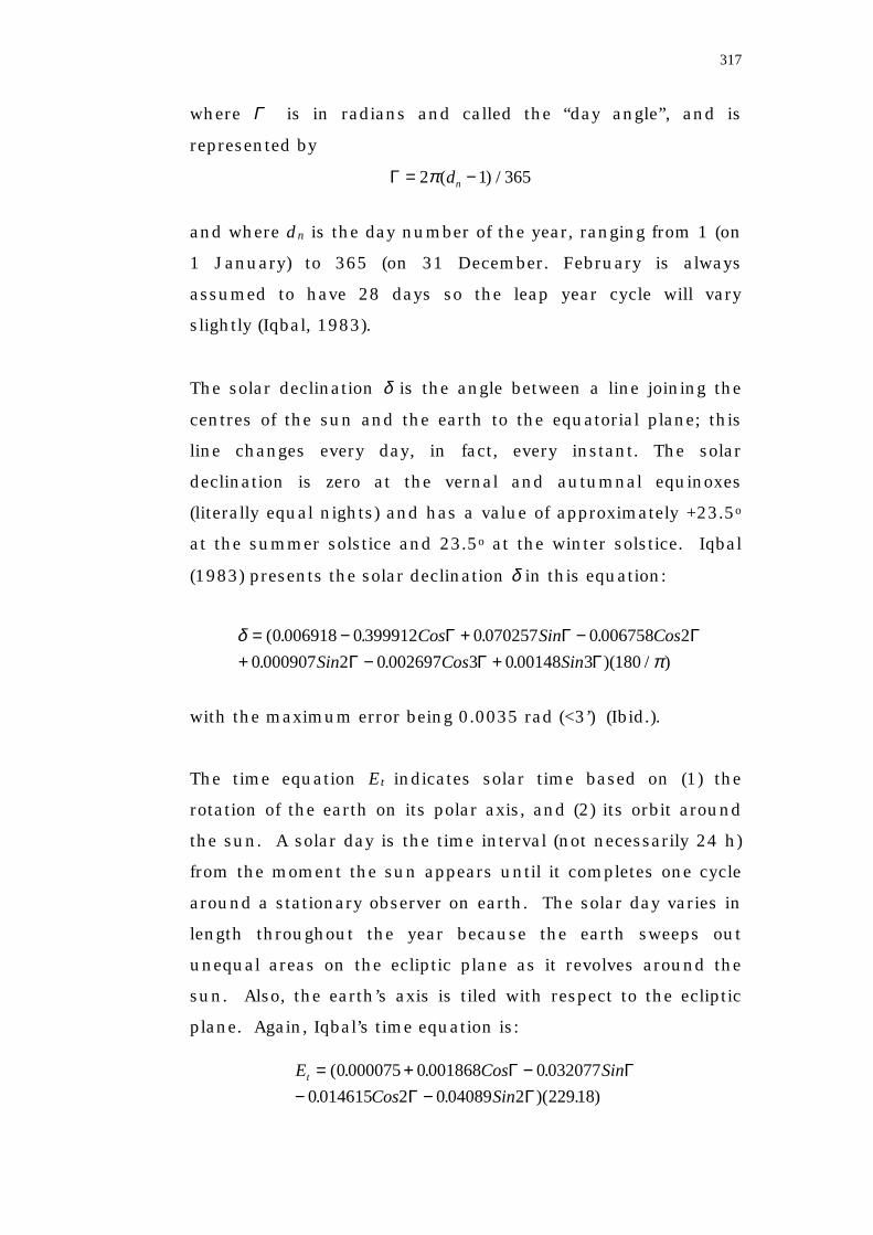
317
where Γ is in radians and called the “day angle”, and is
represented by
and where dn is the day number of the year, ranging from 1 (on
1 January) to 365 (on 31 December. February is always
assumed to have 28 days so the leap year cycle will vary
slightly (Iqbal, 1983).
The solar declination δ is the angle between a line joining the
centres of the sun and the earth to the equatorial plane; this
line changes every day, in fact, every instant. The solar
declination is zero at the vernal and autumnal equinoxes
(literally equal nights) and has a value of approximately +23.5o
at the summer solstice and 23.5o at the winter solstice. Iqbal
(1983) presents the solar declination δ in this equation:
with the maximum error being 0.0035 rad (<3’) (Ibid.).
The time equation Et indicates solar time based on (1) the
rotation of the earth on its polar axis, and (2) its orbit around
the sun. A solar day is the time interval (not necessarily 24 h)
from the moment the sun appears until it completes one cycle
around a stationary observer on earth. The solar day varies in
length throughout the year because the earth sweeps out
unequal areas on the ecliptic plane as it revolves around the
sun. Also, the earth’s axis is tiled with respect to the ecliptic
plane. Again, Iqbal’s time equation is:
Γ = −2 1 365π( ) /dn
δπ
= − + −+ − +
( . . . .
. . . )( / )
0 006918 0 399912 0 070257 0 006758 2
0 000907 2 0 002697 3 0 00148 3 180
Cos Sin Cos
Sin Cos Sin
Γ Γ ΓΓ Γ Γ
E Cos Sin
Cos Sint = + −
− −( . . .
. . )( . )
0 000075 0 001868 0 032077
0 014615 2 0 04089 2 22918
Γ ΓΓ Γ
318
The first right-hand site term in parentheses represents Et in
radians and the multiplier 229.18 converts it to minutes. The
maximum error with this series is 0.0025 rad like 35 sec (Ibid.).
Solar radiation data are often given in terms of local apparent
time (LAT), also called true solar time (TST). The LAT is
expressed as:
LAT = local standard time + longitude correction + time equation
LAT = local standard time + 4(Ls – Le) + Et
where Ls is the standard longitude and Le,, the local longitude.
The longitude correction, 4 min for every degree, accounts for
the difference between the local and the standard meridians
(Ibid.).
The relative position of the sun in reference to a horizontal
surface is shown in Figure A5.1 and Figure A5.2. At any given
time, an observer on the earth’s surface has a corresponding
position on the celestial sphere that is called the “observer’s
zenith”. This is a point of intersection, with the celestial
sphere, of a normal to the earth’s surface at the observer’s
position. The observer’s horizon is the large circle in the
celestial sphere, the plane of which passes through the centre
of the earth normal to the line joining the centre of the earth
and the zenith. The zenith angle θz (or zenith distance) is the
angle (between 0o to 90o) between the local zenith and the line
joining the observer and the sun. The solar altitude α (also
called solar elevation) is the sun’s angular height above the
observer’s celestial horizon and ranges between 0o to 90o. The
solar altitude is the complement of the zenith angle. The solar
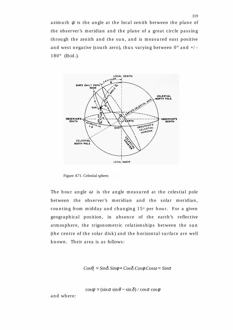
319
azimuth ψ is the angle at the local zenith between the plane of
the observer’s meridian and the plane of a great circle passing
through the zenith and the sun, and is measured east positive
and west negative (south zero), thus varying between 0° and +/-
180° (Ibid.).
The hour angle ω is the angle measured at the celestial pole
between the observer’s meridian and the solar meridian,
counting from midday and changing 15o per hour. For a given
geographical position, in absence of the earth’s reflective
atmosphere, the trigonometric relationships between the sun
(the centre of the solar disk) and the horizontal surface are well
known. Their area is as follows:
and where:cos (sin sin sin ) / cos cosψ α θ δ α φ= −
Figure A71. Celestial sphere.
Cos Sin Sin Cos Cos Cos Sinzθ δ φ δ φ ω α= + =. . .

320
then:
θz is the zenith angle, also called zenith distance, in
degrees
α is the solar altitude, also called solar height or solar
elevation, in degrees;
A = 90 – θz
ω is the hour angle, noon zero and morning positive
φ is the geographic latitude, in degrees, north positive
is the solar azimuth, in degrees, south zero, east positive
(Figure A5.2)
δ is the declination, the angular position of the sun at
the solar noon with respect to the plane of the equator,
north positive, in degrees
0 90 0
90 180 0
o o
o o
Cos
Cos
≤ ≤ ≥
≤ ≤ ≤
ψ ψψ ψ
,
,
Figure A7.2 Definition of the sun’s zenith, altitude and azimuth angles.

321
The sunrise angle, Ws, at θz = 90o is
The daylength, Nd, is 2 ω and is expressed in hours as
Nd = (2/15)Cos-1(-Tan φ.Tan δ)
To determine the sun’s position relative to an inclined plane,
the following information is needed:
β is the slope of the surface, measured from horizontal
position, in degrees
γ is the surface azimuth angle; in other words, the
deviation of the normal to the surface regarding the
local meridian, in degrees, east positive
θ is the angle of incidence for an arbitrarily oriented
surface, the angle between normal to the surface and
the sun-earth vector, in degrees
Then, for arbitrarily oriented surface, θ is:
The time of sunrise and sunset are also included:
ωsr is the sunrise hour angle for an arbitrarily oriented
surface, in degrees
ωss is the sunset hour angle for an arbitrarily oriented
ω φ δs Cos Tan Tan= −−1( . )
Cos Sin Cos Cos Cos Sin
Cos Cos Sin Cos Cos Cos Cos
θ φ β φ γ δφ β φ β γ δ ω
= −+ +
( . . )
( . . . ) .
+ Cos Sin Sin Sinδ β γ ω. . .

322
surface, in degrees
The period during which the sun is seen on the surface is ωsr -
ωss, in degrees (Ibid.).
It is clear that the magnitudes of ωsr , ωss are not identical.
Furthermore, each one of these angles should be evaluated
separately for surfaces oriented toward the east and surfaces
oriented toward the west. It is also necessary to watch for two
possible situations: (1) those in which the sunrise hour angle
might be greater than the sunrise angle for the horizontal
surface, or (2) those in which the sunset hour angle is greater
than corresponding angle for the horizontal surface. ωsr can be
obtained numerically, through interaction, by setting θ = 90o.
The following expressions have been developed explicitly for
each one of the two surfaces oriented +/- γ:
0 = A Sin ω + Β Sin ω + C
where
A = Cos δ Sin β Sin φ ,
B = Cos δ Cos φ Cos β + Cos δ Sin φ Sin β Cos γ ,
C = Sin δ Sin φ Cos β - Sin δ Cos φ Sin β Cos γ .
in which ω should be written as:
It should also be expressed as:
x2 = B2/A2 , y2 = C2/A2
CosBC A A B A C
B Aω =
− ± + −+
4 2 2 2 2
2 2

323
so
where
and
When γ > 0, surface oriented toward the east, then:
And when γ < 0, surface oriented toward the west, then (Ibid.):
xCos
Sin Tan
Sin
Tan= +
φγ β
φγ.
y TanSin
Sin Tan
Cos
Tan= −
δ
φγ β
φγ.
ω ωsr s Cosxy x y
x=
− − − ++
−min , 12 2
2
1
1
ω ωss s Cosxy x y
x= −
− + − ++
−min , 12 2
2
1
1
ω ωsr s Cosxy x y
x=
− + − ++
−min , 12 2
2
1
1
ω ωss s Cosxy x y
x= −
− − − ++
−min , 12 2
2
1
1
Cosxy x y
xω =
− − − ++
2 2
2
1
1

324
The extraterrestrial irradiation on a horizontal surface can be
estimated for a different period, for example an hour, a day, a
month, etc. On a given day, IOn is the extraterrestrial irradiance
(energy rate) on a surface normal to sun rays,
where
ISC is the solar constant (1367 Wm-2;ISC without overdot,
in SI energy units (7921 kJm-2h-1)
ro is the mean sun-earth distance (149 597 89Q km)
Eo is the eccentricity correction factor of earth (ro /r)2
The irradiation (amount of energy), dIo, during a short period of
time, dt, will be
dIo = ISC Eo Cos θz.dt
and the irradiation during a 1-hour period is:
If ωi is at noon, then Cos ωi equals zero. In some cases, the
radiation for a period other than an exact hour may be
expressed between hours t1 and t2. Counting the hours from
midnight, and as long as t1 and t2 are during the day, the
radiation on a horizontal surface is given by:
I I r r I EOn SC o SC o= =( / )2
I I E Sin Sin Cos Cos Coso SC o i= +. ( . . . )δ φ δ φ ω
( ) ( ) ( ) ( )[ ]{ }I I E Sin Sin t t Cos Cos Sin t Sin to tt
SC o12
2 1 1 212 15 15= − + −δ φ π δ φ. .
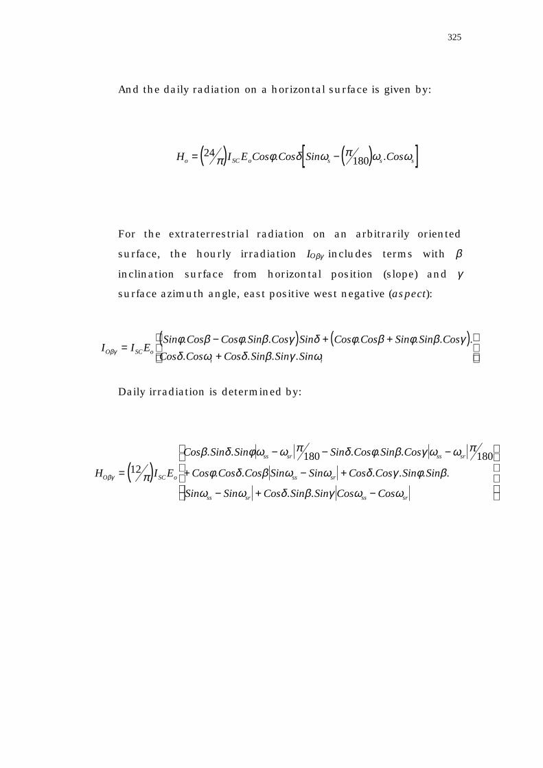
325
And the daily radiation on a horizontal surface is given by:
For the extraterrestrial radiation on an arbitrarily oriented
surface, the hourly irradiation IOβγ includes terms with β
inclination surface from horizontal position (slope) and γ
surface azimuth angle, east positive west negative (aspect):
Daily irradiation is determined by:
( ) ( )I I E
Sin Cos Cos Sin Cos Sin Cos Cos Sin Sin Cos
Cos Cos Cos Sin Sin SinO SC o
i i
βγ
φ β φ β γ δ φ β φ β γδ ω δ β γ ω
=− + ++
. . . . . . .
. . . .
( )H I E
Cos Sin Sin Sin Cos Sin Cos
Cos Cos Cos Sin Sin Cos Cos Sin Sin
Sin Sin Cos Sin Sin Cos Cos
O SC o
ss sr ss sr
ss sr
ss sr ss sr
βγ π
β δ φ ω ω π δ φ β γ ω ω π
φ δ β ω ω δ γ φ β
ω ω δ β γ ω ω
=
− − −
+ − +
− + −
12180 180. . . . .
. . . . . .
. .
( ) ( )[ ]H I E Cos Cos Sin Coso SC o s s s= −24180π φ δ ω π ω ω. .

326
Appendix VIII
Mean value of cloud cover
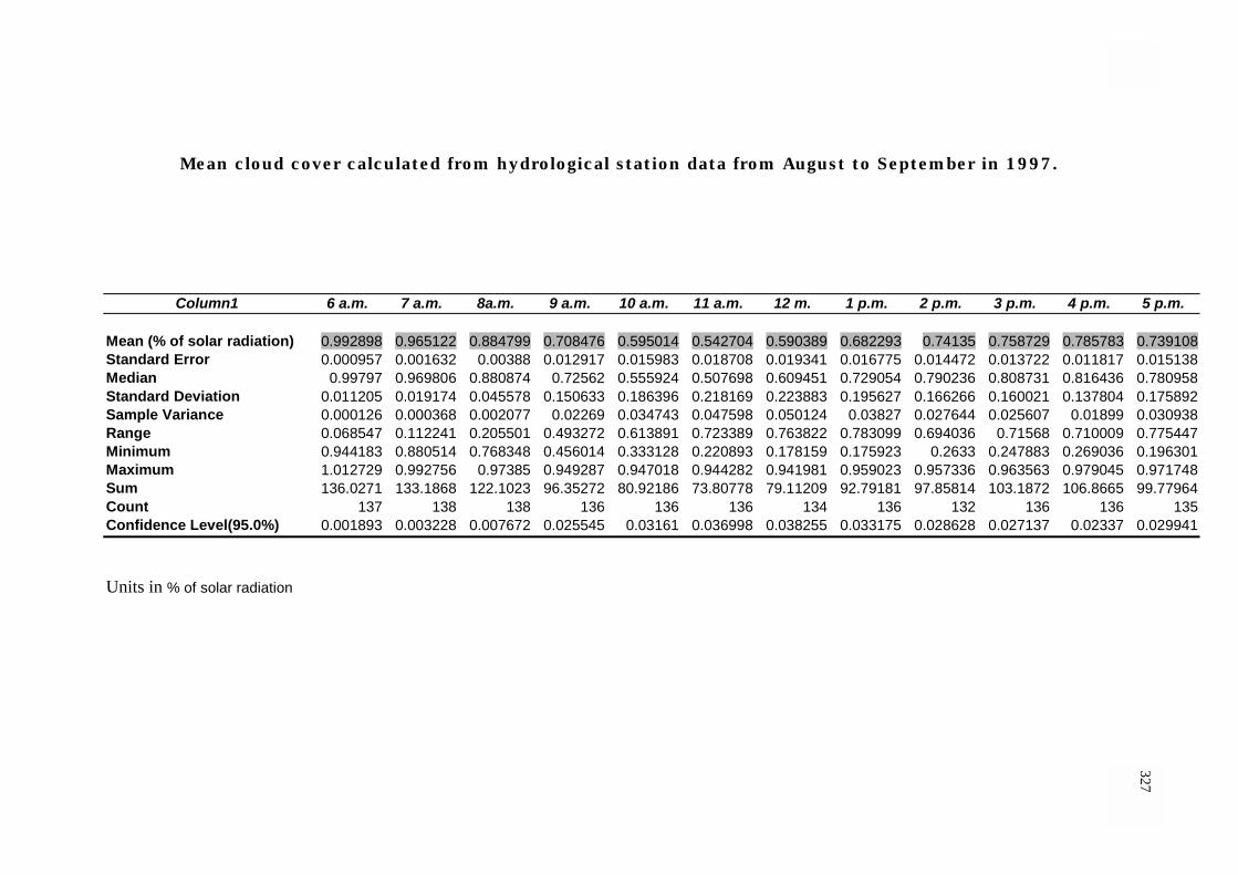
327
Mean cloud cover calculated from hydrological station data from August to September in 1997.
Column1 6 a.m. 7 a.m. 8a.m. 9 a.m. 10 a.m. 11 a.m. 12 m. 1 p.m. 2 p.m. 3 p.m. 4 p.m. 5 p.m.
Mean (% of solar radiation) 0.992898 0.965122 0.884799 0.708476 0.595014 0.542704 0.590389 0.682293 0.74135 0.758729 0.785783 0.739108Standard Error 0.000957 0.001632 0.00388 0.012917 0.015983 0.018708 0.019341 0.016775 0.014472 0.013722 0.011817 0.015138Median 0.99797 0.969806 0.880874 0.72562 0.555924 0.507698 0.609451 0.729054 0.790236 0.808731 0.816436 0.780958Standard Deviation 0.011205 0.019174 0.045578 0.150633 0.186396 0.218169 0.223883 0.195627 0.166266 0.160021 0.137804 0.175892Sample Variance 0.000126 0.000368 0.002077 0.02269 0.034743 0.047598 0.050124 0.03827 0.027644 0.025607 0.01899 0.030938Range 0.068547 0.112241 0.205501 0.493272 0.613891 0.723389 0.763822 0.783099 0.694036 0.71568 0.710009 0.775447Minimum 0.944183 0.880514 0.768348 0.456014 0.333128 0.220893 0.178159 0.175923 0.2633 0.247883 0.269036 0.196301Maximum 1.012729 0.992756 0.97385 0.949287 0.947018 0.944282 0.941981 0.959023 0.957336 0.963563 0.979045 0.971748Sum 136.0271 133.1868 122.1023 96.35272 80.92186 73.80778 79.11209 92.79181 97.85814 103.1872 106.8665 99.77964Count 137 138 138 136 136 136 134 136 132 136 136 135Confidence Level(95.0%) 0.001893 0.003228 0.007672 0.025545 0.03161 0.036998 0.038255 0.033175 0.028628 0.027137 0.02337 0.029941
Units in % of solar radiation
327

328
Appendix IX
Hydrological PCRaster Program code

329
# MAO PCRaster hydrological model# Release V 1.0# October 03 2000# Dynamic model for surface hydrological fluxes# Basic analysis for Geography Ph.D. degree# King’s College London, London - UK
binding
PI = 3.141592654; # Conversion value data = dry9523.txt ; # file input data AU = 1.49597890E8 ; # {DISTANCIA AL SOL EN KM} SolarKteW = 1373 ; # { W m-2} SolarkteJ = 4921 ; # { kJ m-2 h-1} GR = 0.017453292 ; # Conversion value to rad olat = 2.5 ; # Latitude of the area olong = -76.85 ; # Longitude of the area oslope = slope.map ; # Slope map name oaspect = aspect.map ; # Aspect map name cellnum = 22780; # Number of cell in the catchment
# Parameters of interception
landuse = lucriof0.012; # Land use for this run b_canopy_drip = 0.5; # Parameter empirical value
# for drip from canopy min_drainage = 0.002; # Minimum drainage from
# canopy num_layers = 5; # Layer in the canopy canopy_retention = 0.6; # Canopy retention
# empirical value
# pedotransfer function parameters
av = -4.396; bv = -0.0715; cv = -0.000488; dv = -0.00004285; ev = -3.140; fv = -0.00222; gv = -0.00003484; hv = 0.332; jv = -0.0007251; kv = 0.1276; mv = -0.108; nv = 0.341; pv = 12.012; qv = -0.0755; rv = -3.8950; tv = 0.03671; uv = -0.1103 ; vv = 0.00087546;
# Other parameters
soildepth = mil.map; # soildept.map; soileroda = 0.02;
#---------Salidas---------- IobssSalida = Iobss.new; CloudSalida = Cloud.new; NetRadSalida = NetRad.new; PotEvapoSalida = PotEva.new; InterCanopySal = Intercep.new; EvapocanSal = Evapocan.new; rainsal = rain.new; ThroSal = Thro.new; ThroWSal = ThroW.new; RioSal = RioS.new; TetaSal = Teta.new; TetamSal = Tetamm.new; MatrixPotSal = MatrixPo.new;
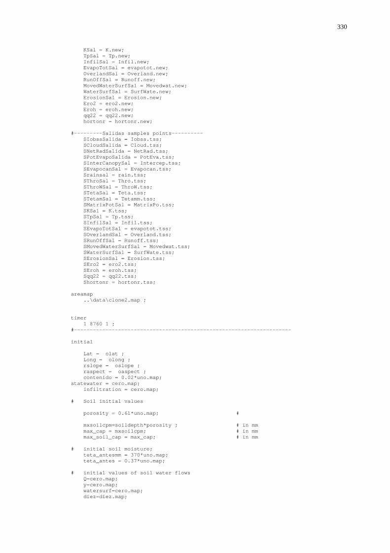
330
KSal = K.new; TpSal = Tp.new; InfilSal = Infil.new; EvapoTotSal = evapotot.new; OverlandSal = Overland.new; RunOffSal = Runoff.new; MovedWaterSurfSal = Movedwat.new; WaterSurfSal = SurfWate.new; ErosionSal = Erosion.new; Ero2 = ero2.new; Eroh = eroh.new; qq22 = qq22.new; hortonr = hortonr.new;
#---------Salidas samples points---------- SIobssSalida = Iobss.tss; SCloudSalida = Cloud.tss; SNetRadSalida = NetRad.tss; SPotEvapoSalida = PotEva.tss; SInterCanopySal = Intercep.tss; SEvapocanSal = Evapocan.tss; Srainsal = rain.tss; SThroSal = Thro.tss; SThroWSal = ThroW.tss; STetaSal = Teta.tss; STetamSal = Tetamm.tss; SMatrixPotSal = MatrixPo.tss; SKSal = K.tss; STpSal = Tp.tss; SInfilSal = Infil.tss; SEvapoTotSal = evapotot.tss; SOverlandSal = Overland.tss; SRunOffSal = Runoff.tss; SMovedWaterSurfSal = Movedwat.tss; SWaterSurfSal = SurfWate.tss; SErosionSal = Erosion.tss; SEro2 = ero2.tss; SEroh = eroh.tss; Sqq22 = qq22.tss; Shortonr = hortonr.tss;
areamap ..\data\clone2.map ;
timer 1 8760 1 ;#---------------------------------------------------------------------
initial
Lat = olat ; Long = olong ; rslope = oslope ; raspect = oaspect ; contenido = 0.02*uno.map;statewater = cero.map; infiltration = cero.map;
# Soil initial values
porosity = 0.61*uno.map; #
mxsoilcpm=soildepth*porosity ; # in mm max_cap = mxsoilcpm; # in mm max_soil_cap = max_cap; # in mm
# initial soil moisture; teta_antesmm = 370*uno.map; teta_antes = 0.37*uno.map;
# initial values of soil water flows Q=cero.map; y=cero.map; watersurf=cero.map; diez=diez.map;
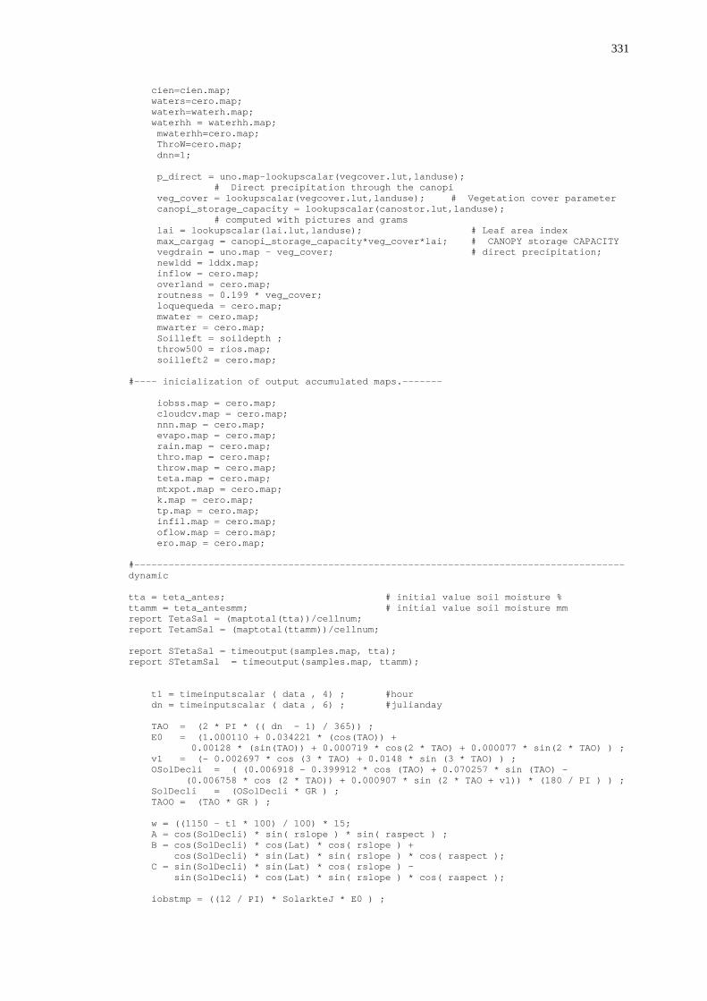
331
cien=cien.map; waters=cero.map; waterh=waterh.map; waterhh = waterhh.map; mwaterhh=cero.map; ThroW=cero.map; dnn=1;
p_direct = uno.map-lookupscalar(vegcover.lut,landuse);# Direct precipitation through the canopi
veg_cover = lookupscalar(vegcover.lut,landuse); # Vegetation cover parameter canopi_storage_capacity = lookupscalar(canostor.lut,landuse);
# computed with pictures and grams lai = lookupscalar(lai.lut,landuse); # Leaf area index max_cargag = canopi_storage_capacity*veg_cover*lai; # CANOPY storage CAPACITY vegdrain = uno.map - veg_cover; # direct precipitation; newldd = lddx.map; inflow = cero.map; overland = cero.map; routness = 0.199 * veg_cover; loquequeda = cero.map; mwater = cero.map; mwarter = cero.map; Soilleft = soildepth ; throw500 = rios.map; soilleft2 = cero.map;
#---- inicialization of output accumulated maps.-------
iobss.map = cero.map; cloudcv.map = cero.map; nnn.map = cero.map; evapo.map = cero.map; rain.map = cero.map; thro.map = cero.map; throw.map = cero.map; teta.map = cero.map; mtxpot.map = cero.map; k.map = cero.map; tp.map = cero.map; infil.map = cero.map; oflow.map = cero.map; ero.map = cero.map;
#--------------------------------------------------------------------------------------dynamic
tta = teta_antes; # initial value soil moisture %ttamm = teta_antesmm; # initial value soil moisture mmreport TetaSal = (maptotal(tta))/cellnum;report TetamSal = (maptotal(ttamm))/cellnum;
report STetaSal = timeoutput(samples.map, tta);report STetamSal = timeoutput(samples.map, ttamm);
t1 = timeinputscalar ( data , 4) ; #hour dn = timeinputscalar ( data , 6) ; #julianday
TAO = (2 * PI * (( dn - 1) / 365)) ; E0 = (1.000110 + 0.034221 * (cos(TAO)) + 0.00128 * (sin(TAO)) + 0.000719 * cos(2 * TAO) + 0.000077 * sin(2 * TAO) ) ; v1 = (- 0.002697 * cos (3 * TAO) + 0.0148 * sin (3 * TAO) ) ; OSolDecli = ( (0.006918 - 0.399912 * cos (TAO) + 0.070257 * sin (TAO) - (0.006758 * cos (2 * TAO)) + 0.000907 * sin (2 * TAO + v1)) * (180 / PI ) ) ; SolDecli = (OSolDecli * GR ) ; TAOO = (TAO * GR ) ;
w = ((1150 - t1 * 100) / 100) * 15; A = cos(SolDecli) * sin( rslope ) * sin( raspect ) ; B = cos(SolDecli) * cos(Lat) * cos( rslope ) + cos(SolDecli) * sin(Lat) * sin( rslope ) * cos( raspect ); C = sin(SolDecli) * sin(Lat) * cos( rslope ) - sin(SolDecli) * cos(Lat) * sin( rslope ) * cos( raspect );
iobstmp = ((12 / PI) * SolarkteJ * E0 ) ;
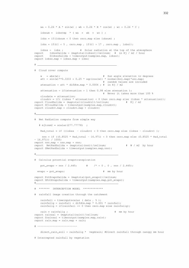
332
wa = 0.26 * A * sin(w) ; wb = 0.26 * B * cos(w) ; wc = 0.26 * C ;
iobsum = iobstmp * ( wa + wb + wc ) ;
iobs = if(iobsum < 0 then cero.map else iobsum) ;
iobs = if(t1 < 5 , cero.map , if(t1 > 17 , cero.map , iobs));
iobss = iobs ; # Solar radiation at the top of the atmospherereport IobssSalida = (maptotal(iobss))/cellnum; # in Kj / m2 / hourreport SIobssSalida = timeoutput(samples.map, iobss);report iobss.map = iobss.map + iobs;
# ____________________________________________________
# Cloud cover compute
w = abs(w); # Sun angle elevation in degrees att = sin(w)**0.3333 + 0.25 * sqr(cos(w)) * normal(bol.map)*uno.map; # random values are included atenuation = att * difdtm.map * 0.0004 ; # in Kj / m2
attenuation = if(atenuation > 1 then 0.98 else atenuation );# Never it takes more than 100 %
cloudate = attenuation; cloudcv = if( (iobss * attenuation) < 0 then cero.map else (iobss * attenuation));report CloudSalida = (maptotal(cloudcv))/cellnum; # Kj / m2report SCloudSalida = timeoutput(samples.map,cloudcv);report cloudcv.map = cloudcv.map + cloudcv;
#______________________________________________________
# Net Radiation compute from simple way
# mjtonm2 = scalar(277.77778) ;
Rad_total = if ((iobss - cloudcv) < 0 then cero.map else (iobss - cloudcv) );
nnn = if ((0.8525 * Rad_total - 16.971) < 0 then cero.map else (0.8525 * Rad_total- 16.971)) / 1000;report nnn.map = nnn.map + nnn;report NetRadSalida = (maptotal(nnn))/cellnum; # W / m2 by hourreport SNetRadSalida = timeoutput(samples.map,nnn);
#______________________________________________________
# Calculus potential evapotranspiration
pot_evapo = nnn / 2.445; # /* < 0 , 0 , nnn / 2.445);
evapo = pot_evapo; # mm by hour
report PotEvapoSalida = (maptotal(pot_evapo))/cellnum;report SPotEvapoSalida = timeoutput(samples.map,pot_evapo);#______________________________________________________
# ******* INTERCEPTION MODEL *************
# rainfall image creation through the catchment
rainfall = timeinputscalar ( data , 5 ); rainfallg = rainfall + difdtm.map * 0.001 * rainfall; rainfallg = if(rainfall <= 0 then cero.map else rainfallg);
rain = rainfallg ; # mm by hourreport rainsal = (maptotal(rain))/cellnum;report Srainsal = timeoutput(samples.map,rain);report rain.map = rain.map + rain;
# --------------------------
direct_rain_soil = rainfallg * vegdrain; #Direct rainfall through canopy mm hour
# Intercepted rainfall by vegetation
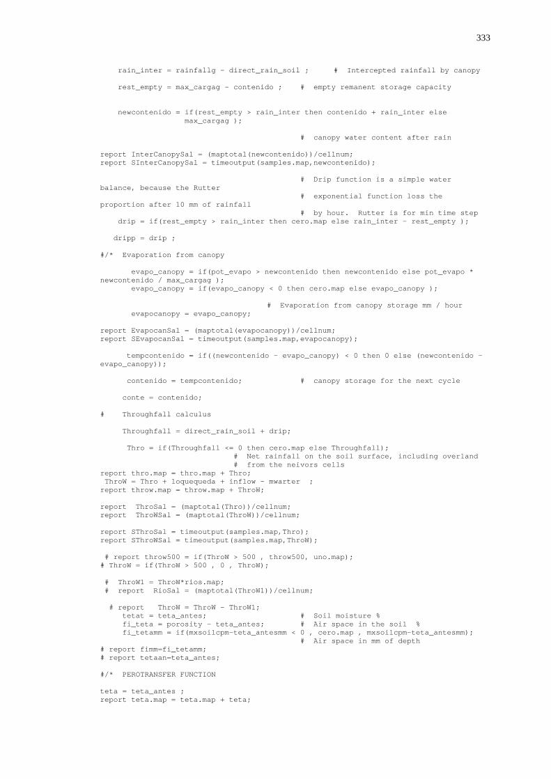
333
rain_inter = rainfallg - direct_rain_soil ; # Intercepted rainfall by canopy
rest_empty = max_cargag - contenido ; # empty remanent storage capacity
newcontenido = if(rest_empty > rain_inter then contenido + rain_inter else max_cargag );
# canopy water content after rain
report InterCanopySal = (maptotal(newcontenido))/cellnum;report SInterCanopySal = timeoutput(samples.map,newcontenido);
# Drip function is a simple waterbalance, because the Rutter
# exponential function loss theproportion after 10 mm of rainfall
# by hour. Rutter is for min time step drip = if(rest_empty > rain_inter then cero.map else rain_inter - rest_empty );
dripp = drip ;
#/* Evaporation from canopy
evapo_canopy = if(pot_evapo > newcontenido then newcontenido else pot_evapo *newcontenido / max_cargag ); evapo_canopy = if(evapo_canopy < 0 then cero.map else evapo_canopy );
# Evaporation from canopy storage mm / hour evapocanopy = evapo_canopy;
report EvapocanSal = (maptotal(evapocanopy))/cellnum;report SEvapocanSal = timeoutput(samples.map,evapocanopy);
tempcontenido = if((newcontenido - evapo_canopy) < 0 then 0 else (newcontenido -evapo_canopy));
contenido = tempcontenido; # canopy storage for the next cycle
conte = contenido;
# Throughfall calculus
Throughfall = direct_rain_soil + drip;
Thro = if(Throughfall <= 0 then cero.map else Throughfall);# Net rainfall on the soil surface, including overland# from the neivors cells
report thro.map = thro.map + Thro; ThroW = Thro + loquequeda + inflow - mwarter ;report throw.map = throw.map + ThroW;
report ThroSal = (maptotal(Thro))/cellnum;report ThroWSal = (maptotal(ThroW))/cellnum;
report SThroSal = timeoutput(samples.map,Thro);report SThroWSal = timeoutput(samples.map,ThroW);
# report throw500 = if(ThroW > 500 , throw500, uno.map);# ThroW = if(ThroW > 500 , 0 , ThroW);
# ThroW1 = ThroW*rios.map; # report RioSal = (maptotal(ThroW1))/cellnum;
# report ThroW = ThroW - ThroW1; tetat = teta_antes; # Soil moisture % fi_teta = porosity - teta_antes; # Air space in the soil % fi_tetamm = if(mxsoilcpm-teta_antesmm < 0 , cero.map , mxsoilcpm-teta_antesmm);
# Air space in mm of depth# report fimm=fi_tetamm;# report tetaan=teta_antes;
#/* PEROTRANSFER FUNCTION
teta = teta_antes ;report teta.map = teta.map + teta;
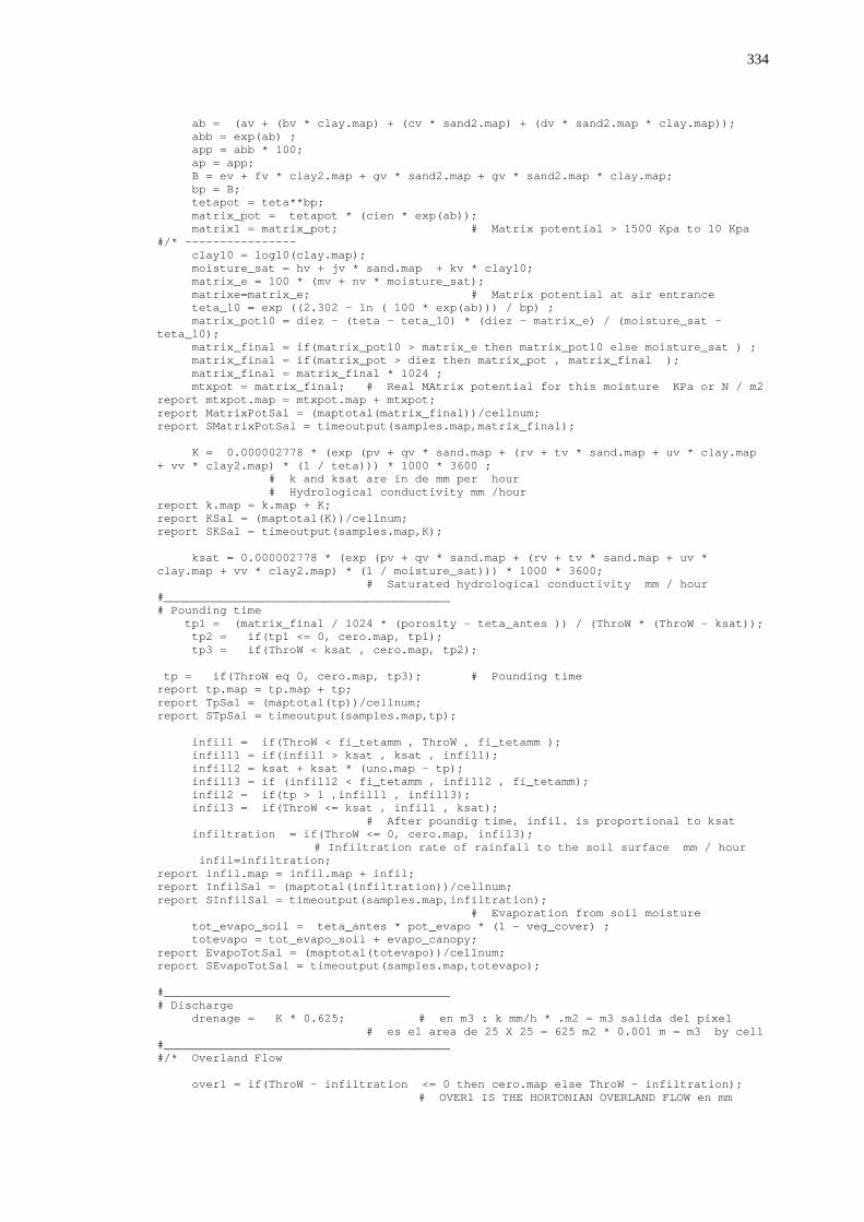
334
ab = (av + (bv * clay.map) + (cv * sand2.map) + (dv * sand2.map * clay.map)); abb = exp(ab) ; app = abb * 100; ap = app; B = ev + fv * clay2.map + gv * sand2.map + gv * sand2.map * clay.map; bp = B; tetapot = teta**bp; matrix_pot = tetapot * (cien * exp(ab)); matrix1 = matrix_pot; # Matrix potential > 1500 Kpa to 10 Kpa#/* ---------------- clay10 = log10(clay.map); moisture_sat = hv + jv * sand.map + kv * clay10; matrix_e = 100 * (mv + nv * moisture_sat); matrixe=matrix_e; # Matrix potential at air entrance teta_10 = exp ((2.302 - ln ( 100 * exp(ab))) / bp) ; matrix_pot10 = diez - (teta - teta_10) * (diez - matrix_e) / (moisture_sat -teta_10); matrix_final = if(matrix_pot10 > matrix_e then matrix_pot10 else moisture_sat ) ; matrix_final = if(matrix_pot > diez then matrix_pot , matrix_final ); matrix_final = matrix_final * 1024 ; mtxpot = matrix_final; # Real MAtrix potential for this moisture KPa or N / m2report mtxpot.map = mtxpot.map + mtxpot;report MatrixPotSal = (maptotal(matrix_final))/cellnum;report SMatrixPotSal = timeoutput(samples.map,matrix_final);
K = 0.000002778 * (exp (pv + qv * sand.map + (rv + tv * sand.map + uv * clay.map+ vv * clay2.map) * (1 / teta))) * 1000 * 3600 ; # k and ksat are in de mm per hour
# Hydrological conductivity mm /hourreport k.map = k.map + K;report KSal = (maptotal(K))/cellnum;report SKSal = timeoutput(samples.map,K);
ksat = 0.000002778 * (exp (pv + qv * sand.map + (rv + tv * sand.map + uv *clay.map + vv * clay2.map) * (1 / moisture_sat))) * 1000 * 3600;
# Saturated hydrological conductivity mm / hour#_________________________________________# Pounding time tp1 = (matrix_final / 1024 * (porosity - teta_antes )) / (ThroW * (ThroW - ksat)); tp2 = if(tp1 <= 0, cero.map, tp1); tp3 = if(ThroW < ksat , cero.map, tp2);
tp = if(ThroW eq 0, cero.map, tp3); # Pounding timereport tp.map = tp.map + tp;report TpSal = (maptotal(tp))/cellnum;report STpSal = timeoutput(samples.map,tp);
infil1 = if(ThroW < fi_tetamm , ThroW , fi_tetamm ); infil11 = if(infil1 > ksat , ksat , infil1); infil12 = ksat + ksat * (uno.map - tp); infil13 = if (infil12 < fi_tetamm , infil12 , fi_tetamm); infil2 = if(tp > 1 ,infil11 , infil13); infil3 = if(ThroW <= ksat , infil1 , ksat);
# After poundig time, infil. is proportional to ksat infiltration = if(ThroW <= 0, cero.map, infil3);
# Infiltration rate of rainfall to the soil surface mm / hour infil=infiltration;report infil.map = infil.map + infil;report InfilSal = (maptotal(infiltration))/cellnum;report SInfilSal = timeoutput(samples.map,infiltration); # Evaporation from soil moisture tot_evapo_soil = teta_antes * pot_evapo * (1 - veg_cover) ; totevapo = tot_evapo_soil + evapo_canopy;report EvapoTotSal = (maptotal(totevapo))/cellnum;report SEvapoTotSal = timeoutput(samples.map,totevapo);
#_________________________________________# Discharge drenage = K * 0.625; # en m3 : k mm/h * .m2 = m3 salida del pixel # es el area de 25 X 25 = 625 m2 * 0.001 m = m3 by cell#_________________________________________#/* Overland Flow
over1 = if(ThroW - infiltration <= 0 then cero.map else ThroW - infiltration);# OVER1 IS THE HORTONIAN OVERLAND FLOW en mm
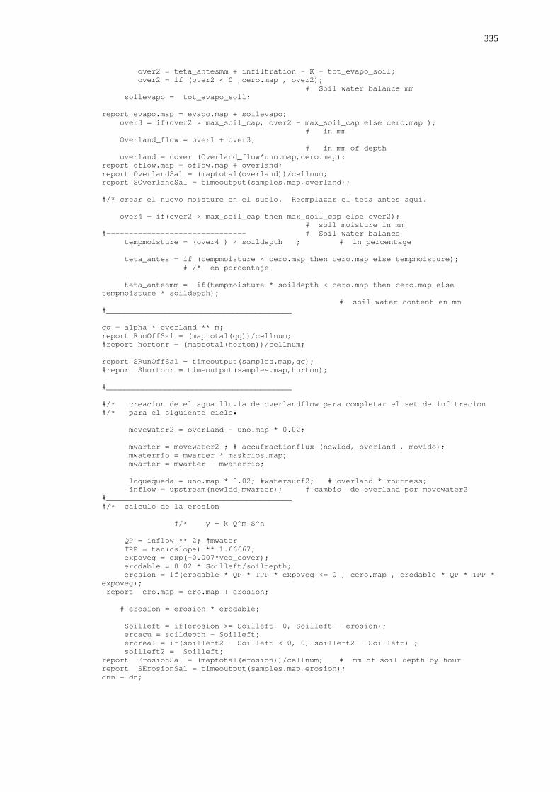
335
over2 = teta_antesmm + infiltration - K - tot_evapo_soil; over2 = if (over2 < 0 ,cero.map , over2); # Soil water balance mm soilevapo = tot_evapo_soil;
report evapo.map = evapo.map + soilevapo; over3 = if(over2 > max_soil_cap, over2 - max_soil_cap else cero.map );
# in mm Overland_flow = over1 + over3; # in mm of depth overland = cover (Overland_flow*uno.map,cero.map);report oflow.map = oflow.map + overland;report OverlandSal = (maptotal(overland))/cellnum;report SOverlandSal = timeoutput(samples.map,overland);
#/* crear el nuevo moisture en el suelo. Reemplazar el teta_antes aqui.
over4 = if(over2 > max_soil_cap then max_soil_cap else over2); # soil moisture in mm#------------------------------- # Soil water balance tempmoisture = (over4 ) / soildepth ; # in percentage
teta_antes = if (tempmoisture < cero.map then cero.map else tempmoisture); # /* en porcentaje
teta_antesmm = if(tempmoisture * soildepth < cero.map then cero.map elsetempmoisture * soildepth);
# soil water content en mm#_________________________________________
qq = alpha * overland ** m;report RunOffSal = (maptotal(qq))/cellnum;#report hortonr = (maptotal(horton))/cellnum;
report SRunOffSal = timeoutput(samples.map,qq);#report Shortonr = timeoutput(samples.map,horton);
#_________________________________________
#/* creacion de el agua lluvia de overlandflow para completar el set de infitracion#/* para el siguiente ciclo•
movewater2 = overland - uno.map * 0.02;
mwarter = movewater2 ; # accufractionflux (newldd, overland , movido); mwaterrio = mwarter * maskrios.map; mwarter = mwarter - mwaterrio;
loquequeda = uno.map * 0.02; #watersurf2; # overland * routness; inflow = upstream(newldd,mwarter); # cambio de overland por movewater2#_________________________________________#/* calculo de la erosion
#/* y = k Q^m S^n
QP = inflow ** 2; #mwater TPP = tan(oslope) ** 1.66667; expoveg = exp(-0.007*veg_cover); erodable = 0.02 * Soilleft/soildepth; erosion = if(erodable * QP * TPP * expoveg <= 0 , cero.map , erodable * QP * TPP *expoveg); report ero.map = ero.map + erosion;
# erosion = erosion * erodable;
Soilleft = if(erosion >= Soilleft, 0, Soilleft - erosion); eroacu = soildepth - Soilleft; eroreal = if(soilleft2 - Soilleft < 0, 0, soilleft2 - Soilleft) ; soilleft2 = Soilleft;report ErosionSal = (maptotal(erosion))/cellnum; # mm of soil depth by hourreport SErosionSal = timeoutput(samples.map,erosion);dnn = dn;

336
Appendix X
Summary of physical variables
and
model variable response
for all scenarios
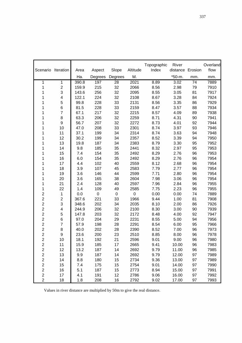
337
Values in river distance are multiplied by 50m to give the real distance.
Scenario Iteration Area Aspect Slope AltitudeTopographic
IndexRiver
distance ErosionOverland
flow
Ha. Degrees Degrees M. *50-m. mm. mm.1 1 390.8 197 28 2021 8.89 3.02 74 78891 2 159.9 215 32 2066 8.56 2.98 79 79101 3 143.6 256 32 2095 8.55 3.05 81 79171 4 122.1 224 32 2108 8.67 3.28 84 79241 5 99.8 228 33 2131 8.56 3.35 86 79291 6 81.5 228 33 2159 8.47 3.57 88 79341 7 67.1 217 32 2215 8.57 4.09 89 79381 8 63.3 206 32 2259 8.71 4.31 90 79411 9 56.7 207 32 2272 8.73 4.01 92 79441 10 47.0 208 33 2301 8.74 3.97 93 79461 11 37.1 199 34 2314 8.74 3.63 94 79481 12 30.2 199 34 2357 8.52 3.39 94 79501 13 19.8 187 34 2383 8.79 3.30 95 79521 14 9.8 185 35 2441 8.32 2.97 95 79531 15 7.4 154 35 2492 8.29 2.76 96 79531 16 6.0 154 35 2492 8.29 2.76 96 79541 17 4.4 102 40 2559 8.12 2.68 96 79541 18 3.9 107 45 2583 7.79 2.77 96 79541 19 3.6 146 44 2599 7.71 2.80 96 79541 20 3.6 165 38 2604 7.98 3.06 96 79541 21 2.4 128 40 2597 7.96 2.84 96 79551 22 1.4 109 49 2585 7.75 2.23 96 79552 1 0.0 0 0 0 0.00 0.00 74 78892 2 367.6 221 33 1966 9.44 1.00 81 79082 3 348.6 202 34 2035 8.10 2.00 86 79262 4 244.9 206 32 2100 8.30 3.00 90 79392 5 147.8 203 32 2172 8.48 4.00 92 79472 6 97.0 204 29 2231 8.55 5.00 94 79562 7 57.9 198 28 2291 8.54 6.00 95 79662 8 40.0 202 28 2390 8.52 7.00 96 79732 9 23.6 200 23 2510 8.85 8.00 96 79782 10 18.1 192 21 2596 9.01 9.00 96 79802 11 15.9 185 17 2665 9.41 10.00 96 79832 12 13.2 187 14 2692 9.79 11.00 96 79852 13 9.9 187 14 2692 9.79 12.00 97 79892 14 8.8 180 15 2734 9.36 13.00 97 79892 15 7.4 175 15 2754 9.01 14.00 97 79902 16 5.1 187 15 2773 8.94 15.00 97 79912 17 4.1 191 12 2786 9.06 16.00 97 79922 18 1.8 208 16 2792 9.02 17.00 97 7993
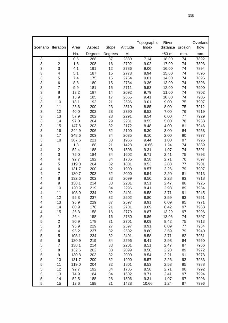
338
Scenario Iteration Area Aspect Slope AltitudeTopographic
IndexRiver
distance ErosionOverland
flow
Ha. Degrees Degrees M. *50-m. mm. mm.3 1 0.6 268 37 2830 7.14 18.00 74 78923 2 1.8 208 16 2792 9.02 17.00 74 78933 3 4.1 191 12 2786 9.06 16.00 74 78943 4 5.1 187 15 2773 8.94 15.00 74 78953 5 7.4 175 15 2754 9.01 14.00 74 78953 6 8.8 180 15 2734 9.36 13.00 74 78963 7 9.9 181 15 2711 9.53 12.00 74 79003 8 13.2 187 14 2692 9.79 11.00 74 79023 9 15.9 185 17 2665 9.41 10.00 74 79053 10 18.1 192 21 2596 9.01 9.00 75 79073 11 23.6 200 23 2510 8.85 8.00 75 79123 12 40.0 202 28 2390 8.52 7.00 76 79193 13 57.9 202 28 2291 8.54 6.00 77 79293 14 97.0 204 29 2231 8.55 5.00 78 79383 15 147.8 203 32 2172 8.48 4.00 81 79463 16 244.9 206 32 2100 8.30 3.00 84 79583 17 348.6 203 34 2035 8.10 2.00 90 79773 18 367.6 221 33 1966 9.44 1.00 97 79964 1 1.3 188 21 1428 10.66 1.24 74 78894 2 52.4 188 28 1506 9.31 1.97 74 78914 3 75.0 184 34 1602 8.71 2.41 75 78934 4 92.7 192 34 1705 8.58 2.71 76 78974 5 119.0 204 32 1801 8.53 2.83 77 79014 6 131.7 200 32 1900 8.57 2.26 79 79074 7 130.7 203 32 2000 8.54 2.20 81 79134 8 132.6 202 33 2099 8.50 2.28 83 79184 9 138.1 214 33 2201 8.51 2.47 86 79254 10 120.9 219 34 2296 8.41 2.93 89 79344 11 108.0 234 32 2401 8.58 2.71 91 79454 12 95.3 237 32 2502 8.80 3.59 93 79514 13 95.9 229 37 2597 8.91 6.09 95 79714 14 80.9 178 21 2701 9.09 8.42 97 79884 15 26.3 158 16 2779 8.87 13.29 97 79965 1 26.4 158 16 2780 8.86 13.05 74 78975 2 80.9 178 21 2701 9.09 8.42 75 79135 3 95.9 229 27 2597 8.91 6.09 77 79345 4 95.2 237 32 2502 8.80 3.59 79 79405 5 108.1 234 32 2401 8.58 2.71 82 79515 6 120.9 219 34 2296 8.41 2.93 84 79605 7 138.1 214 33 2201 8.51 2.47 87 79665 8 132.6 202 33 2099 8.50 2.28 89 79725 9 130.8 203 32 2000 8.54 2.21 91 79785 10 131.7 200 32 1900 8.57 2.26 93 79835 11 119.0 204 32 1801 8.53 2.53 95 79885 12 92.7 192 34 1705 8.58 2.71 96 79925 13 74.9 184 34 1602 8.71 2.41 97 79945 14 52.5 188 28 1506 9.31 1.97 97 79965 15 12.6 188 21 1428 10.66 1.24 97 7996
Related Documents