Welcome message from author
This document is posted to help you gain knowledge. Please leave a comment to let me know what you think about it! Share it to your friends and learn new things together.
Transcript


��������� ��� �� ����� ��� ��� ������ �� ���� ���� � �� ��� �� �� ����� �������� ����� ��� ��� ������ �� ���� ��� ������ ��� � � ���!���"�� ����"����� #������������� ���������� ��������� ������ ��� �� $�������% �#����� �������� ������ ��& �� ���!� �#���'��&%�������#� ������!���"�� ����"����� � ���������������! ������������(�� ���) �)�# �%*+����� ���",�"���"(����� * ��������! � �� ��� �� (�� ��� ��-�������*+"���������./��"��(���)����*�0�! �-��� ��1��(���)����* ��� ����� ����2 ���("���� ����� ����*+"��������� "������ (����� *� ����� �� �������� (���� �� ) ����*� � ��%����� ��"���� (1�' �*� -��� ����3�" (�� ��*� 0�!� 2 � �",,/..� (��1�" ) ����*� -��� �� -"�� (���� �� ) ����*� ������� -��"��(����� �*�1����-�..�(1���'�*�-�� ���1"����(����� *���� ��,�45�(���)� ����*������1",,"(- ����*
,�SOCIETÀ GEOLOGICA ITALIANA%�%������ �67������!��8998�������������-����������� �����������8:����!�� 899; ,� �������� � � ��� ���� ��� � ���� ����� � �� ��2� ����� ���� ����� ��� ��2�� /� '��� �� � �����1 �22���"���-����;)<<89;���������&
#�SOCIETÀ GEOLOGICA ITALIANA=��%������ �>��������������!��67�#�8998 ��=�������� 2�������)���% ��������� ��= �#�#���&���������%����!��8:�#�899; #���������&�%% �� �#�����!&�#�� ���� ������ �� ��2�����������%�#���� ��2�/� '��� �&�1 �22���"���-����;)<<89;���������&
������� (��������*+�� ?@7)<A)B7;7)@7<C0�D?@7)<A)B778)B8;BC�)�� �+ �%�E������� �� ��=�!(��� ��&F�!� ��*+#���+GG=== ������� ���� ��0 �����(�������D���!��*+9<6;9:7<;9;C��������������������(1������ ���������*+@;<<<7
������,�������3�6<86(-��!����%����� �%��6<86*+
����� ���,���� ) 1��� ����� "��������� ./��"�� ) ������� ��������&� -���� 1��" ) ��������� �� ��!������>"� ����� �� �",�"���"� ���%��� �",,"� ��' � ��3���� ������� -��"��� 0�! � -��� �� 1��� ������������,,�(� ��%�#��4�)>���*
��3������������6<88(0 ���� ��"�� ����6<86*+
��! ��>����-����>�"��"�����!� �����"�"���"-/���.." ��.������,,"�����H���,����"�",�"�"(���� �������� ������ ��&���� ���*+
��' ���������������&+,��"�"-�,�–�#� �I ����&��������&+�����%��"����)�#� �-�� ��������&+0���������I�����)�#� �1�������&������&+� ����!� ������)�#� �I&���������&+� �'��� >"����/)�#� ����!�����������&+���� ���"�"1��"�"���� �1�"/�,��)�#� �����) �%����� ��+�# ���D’A->����)�#� �����������������&+�����1",,")�#� �L���������� ���+�������"��)�#� �
La Società Geologica Italiana è affiliate alla European Geosciences Union (EGU). The Società Geologica Italiana is affiliated to the European Geosciences Union (EGU). M/�""�����"�3"6<86("���� �� ��0���6<86*+��� ������� ����(���������%����=*€ 8<<���� ���� ��� �(��� ���&%����=* € 7@C ��� � ��� �� (��� �� %����=* € A9� ��� � $�� �� ($�� �� %����=* € A9C ������� (��������* € @AC ��� ��2 �� (���� ��� ���*€ @<< ���� 2 ���������� ��(��!��� �� ����*+#���+GG=== ������� �G69BG�����O��� ��� #�������
#���+GG=== ������� �G69;G���������O���� ��O�����O� O���� �� #���,�Società Geologica Italiana��� ��� ����&� �#����� ��� ��� ��� ��� ������% ������ ����� ������ �����!!� ���� 1�����������% ���������������&��#������� ����!� �#�������'����!&�#����&� �#��=�!&�#�Società Geologica Italiana. DISCLAIMER: The Società Geologica Italiana, the Editors (Chief, Associate and Advisory), and the Publisher are not responsible for the ideas, opinions, and contents of the papers published; the authors of each paper are responsible for the ideas opinions and contents published. La Società Geologica Italiana, i curatori scientifici (Chief, Associate and Advisory), e la Casa Editrice non sono responsabili delle opinioni espresse e delle affermazioni pubblicate negli articoli: l’autore/i è/sono il/i solo/i responsabile/i.
ROMASOCIETÀ GEOLOGICA ITALIANA
2012www.socgeol.it
Volume 21 (parte prima)
ISSN 2035-8008
NOTE BREVI E RIASSUNTI
A cura di: Salvatore Critelli, Francesco Muto, Francesco Perri, Fabio Massimo Petti, Maurizio Sonnino, Alessandro Zuccari
RENDICONTI Online della
Società Geologica Italiana
86° Congresso Nazionale della Società Geologica Italiana
Arcavacata di Rende 18-20 Settembre 2012
Editori: Salvatore Critelli, Francesco Muto, Francesco Perri, Fabio Massimo Petti, Maurizio Sonnino, Alessandro Zuccari.
Realizzazione del volume dei riassunti a cura di:Francesco Perri, Fabio Massimo Petti, Alessandro Zuccari.
In copertina: “Morpho-Bathymetry of the Mediterranean Sea”, CIESM, Ifremer SpecialPublication, France. 1/3.000000 scale map.
© Società Geologica Italiana, Roma 2012
86° Congresso Nazionale della Società Geologica Italiana
Arcavacata di Rende 18-20 Settembre 2012
Rend. Online Soc. Geol. It., Vol. 21 (2012), pp. 407-409, 2 figs. © Società Geologica Italiana, Roma 2012
407
Key words: landslide, hydrological model, genetic algorithm, calibration, validation, sensitivity analysis.
INTRODUCTION
In Italy, a recent nationwide investigation has identified more than 1.6 landslides per km2 (GUZZETTI et al., 2008). Most of the landslides that affect the Country are usually triggered by rainfalls. Forecasting the timing of rainfall-induced landslides is then a fundamental step for Civil Protection purposes. This goal can be obtained by means of either empirical “hydrological” or physically-based, “complete” models.
The hydrological approach (adopted in the present study) tries to identify the mathematical relationship that links the rainfall series to the dates of landslide activation. With respect to shallow landslides, the dynamics of deep seated slope movements generally shows a more complex relationship with rainfall: activations commonly require greater rainfall amounts, spanned over longer periods (from ca. 30 days to more than a single rainy season).
MODELING APPROACH
SAKe (Self Adaptive Kernel) is a hydrological model that can be employed to predict the occurrence of one of the most pernicious effects of rainfall on slope stability: slope movements. The model can be useful for real-time warning purposes. It is self-adaptive and based on the assumption of a linear and steady response, in terms of stability, of the slope to rainfall.
SAKe is based on an empirical approach – “black-box” type (Fig. 1) – inspired from FLaIR (SIRANGELO & VERSACE, 1996). By properly tuning the model parameters, a mobility function and a threshold value can be identified that allow to reconstruct the series of known landslide activations of the past by minimizing the occurrence of false alarms. The ranges of
parameters depend on: (i) the specific hydrological conditions that characterize the triggering events, (ii) the characteristics of the slope and, (iii) the landslide type.
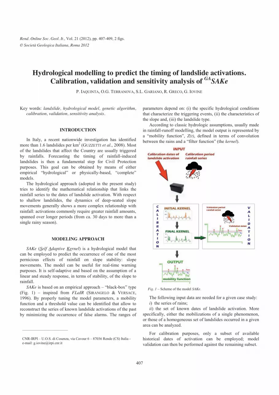
According to classic hydrologic assumptions, usually made in rainfall-runoff modelling, the model output is represented by a “mobility function”, Z(t), defined in terms of convolution between the rains and a “filter function” (the kernel).
The following input data are needed for a given case study: i) the series of rains; ii) the set of known dates of landslide activation. More
specifically, either the mobilizations of a single phenomenon, or those of a homogeneous set of landslides occurred in a given area can be analyzed.
For calibration purposes, only a subset of available historical dates of activation can be employed; model validation can then be performed against the remaining subset.
Hydrological modelling to predict the timing of landslide activations. Calibration, validation and sensitivity analysis of GASAKe
P. IAQUINTA, O.G. TERRANOVA, S.L. GARIANO, R. GRECO, G. IOVINE
Fig. 1 – Scheme of the model SAKe.
_________________________ CNR-IRPI – U.O.S. di Cosenza, via Cavour 6 – 87036 Rende (CS) Italia - e-mail: [email protected]

86° CONGRESSO SOCIETÀ GEOLOGICA ITALIANA 18-20 SETTEMBRE 2012, ARCAVACATA DI RENDE (CS)
408
As regards model calibration, different automated tools can be utilized, based on either iterative cluster modification – CMSAKe – or Genetic Algorithms (HOLLAND, 1975) – GASAKe – as recently done for debris flows modelling by IOVINE et al. (2005). As a result, a family of optimal, discretised kernels can be obtained from initial standard analytical functions, whose values represent the probability of landslide activation given that a critical threshold is overcome.
The family of optimal kernels – that maximize the adopted fitness function – is selected by means of a calibration technique based on elitist Genetic Algorithms. In this way, the values of model parameters are iteratively changed, aiming at improving the fitness of the tested solutions. A suitable fitness function must first be defined, able to minimise the number of false alarms. In the present study, fitness is defined as follows: a) the N available dates of landslide activation are sorted, in
chronological order, in the vector S = {S1,…, Si,…, SN}; b) the vector of the relative maxima of the mobility function Z
= {z1,…, zk, …, zM}, where M is the number and k is the rank of the relative maxima, is sorted in decreasing order;
c) the vector of the partial fitness values is defined as φ ={φ1,…, φi, ... φN}.
The following cases can occur: i) φi = 1 if the date of the i th activation, Si, matches, within a
pre fixed tolerance (Δ), the date of a k th relative maximum of the mobility function, zk, with k≤N;
ii) φi = (k N+1) 1 i.e. it is inversely proportional to the rank of zk in Z – if the date of the i th activation, Si, matches, within a pre fixed tolerance, the date of a k th relative maximum of the mobility function, zk, with k>N;
iii) φi = 0 if the date of the i th activation, Si, does not match any date of the relative maxima in Z.
Accordingly, the fitness of a generic kernel is:
���
N
i iN 1
1 �� .
GASAKe is based on two levels of optimization. The first
optimization process allows to search for the mobility function that gives the maximum fitness function fn. The second optimization process looks for the maximum difference between the critical threshold, Zcr, and the smallest value of the relative maxima of the mobility function, Zs. Note that the operational levels can modify the filter function, producing an integral that differs from the unity. Thus, a normalization process is also necessary.
The genetic algorithm is an iterative process based on the following operators (Fig. 2): � Selection of the elements to be copied in the “mating pool”
for reproduction purposes (in this study, it is of elitist type); � Crossover of pairs of elements (based on probability, pc); � Mutation of elements (based on probability, pm).
The mating pool contains N elements of the population;
these elements eventually originate N new mobility functions. Minimum, average and maximum values of the fitness functions for each iteration are evaluated and plotted. New generations are obtained by repeating the steps above.
An example of model optimization is presented, with reference to the Uncino rock slide (maximum width = 200 m, length > 650 m) (Fig. 3), developed in clay and conglomerate (Late Miocene) overlaying gneiss and biotitic schist (Palaeozoic). The landslide repeatedly threatened the northern rim of the San Fili village, in Northern Calabria. For this case study, N=7 historical dates of mobilization are available. On such occasions, the railroad connecting Cosenza to the Tyrrhenian coast was damaged or even interrupted. Preliminary results of model calibration, carried out using all the dates of activation, are shown in Fig. 4. Aiming at temporal validation purposes, only a subset of the dates of landslide activation has been used; sensitivity analysis results are discussed.
REFERENCES
GUZZETTI F., PERUCCACCI S., ROSSI M. & STARK C.P. (2008) –The rainfall intensity duration control of shallow landslides and debris flow: an update. Landslides, 5, 3 17.
HOLLAND J.H. (1975) – Adaptation in Natural and Artificial Systems, University of Michigan Press, Ann Arbor.
Fig. 2 – Steps of the Genetic Algorithm for model calibration.

86° CONGRESSO SOCIETÀ GEOLOGICA ITALIANA 18-20 SETTEMBRE 2012, ARCAVACATA DI RENDE (CS)
409
IOVINE G., D’AMBROSIO D. & DI GREGORIO S. (2005) – Applying genetic algorithms for calibrating a hexagonal cellular automata model for the simulation of debris flows characterised by strong inertial effects. Geomorphology, 66(1-4), 287-303.
SIRANGELO B. & VERSACE P. (1996) – A real time forecasting for landslides triggered by rainfall. Meccanica, 31, 1–13.
Fig. 3 – Localization and photo of the Uncino rock slide at San Fili (CS), Calabria, Southern Italy (photo courtesy of L. Antronico).
Fig. 4 – Example of output of GASAKe (elitist approach) for the Uncino case study at San Fili. On top, the red stars mark the known dates of landslide activations (S1...S5). The series of daily rainfalls (from 01.01.1955 to 31.12.1993), the best mobility function (fitness=100%) and the final value of Δzcr are also shown. In the middle the solution space of the kernel with the best solution (in red, tb = 77), the not-normalized envelope including all the solutions (in dashed, light blue) built considering the maximum value for each element of the kernel function, and the normalized-envelope of the kernel function (in dashed, blue) are shown. At bottom, the evolution of the fitness function, in terms of maximum (red) and average (pink) values per iteration are shown. The evolution of the maximum values of Δzcr, (black line) per iteration, is also shown.
Related Documents