Modelling Demand For Tourism In Italy - ePrints Soton

University of Southampton

Modelling Demand For Tourism In Italy

Manuela Pulina

Doctor of Philosophy

Faculty of Social Sciences

Department of Economics

February 2002

ABSTRACT

F\4JCTJTUnr(]i;;S()C:L4JL, S(:iEhfC]ES

Doctor of Philosophy

MODELLING DEMAND FOR TOURISM IN ITALY

by

Manuela Pulina

The aim of this thesis is to construct and estimate the demand for tourism for the Italian Province of Sassari, in the Sardinian island, and Italy as a whole. Several propositions are investigated. A systematic understanding is carried out for separating the domestic from the international demand of tourism to Sassari Province. The historic evolution of tourists' flows, the seasonality, trading-day effects and the empirical findings from the econometric investigation validate the separation of the two components. The sample period under estimation is from 1972 up to 1995. Three dynamic models are estimated at monthly, quarterly and annual frequencies for Sassari Province; similarities and differences are explored amongst the three models. On balance, the evidence indicates that the monthly and quarterly data models are superior to annual data models. However, one does not want to omit the annual estimation. Ideally, one should integrate and learn from each of the separate analysis.

Some of the recently developed econometric techniques are used. A pre-modelling data analysis is undertaken for the economic series of interest. Seasonal and long run unit roots tests have given insight on the properties of the variables under study. The Johansen cointegration analysis is used in order to examine possible long run relationships amongst variables integrated of order one. Dynamic estimations are run in terms of the number of tourists for Sassari Province and monthly data expenditure for Italy. The LSE general-to-specific methodology is followed and a full range of diagnostic tests is provided. Short and long run income elasticities, negativity and substitutability are tested in the light of economic theory and other empirical studies existing in the tourism literature.

Ill

LIST OF CONTENTS

DECLARATION OF STATEMENTS I

ABSTRACT Il l

LIST OF CONTENTS IV

LIST OF TABLES IX

LIST OF FIGURES XII

ACKNOWLEDGEMENTS XIV

ABBREVIATIONS XV

CHAPTER 1 INTRODUCTION

1.1 TOURISM AND ECONOMETRIC ANALYSIS 1

1.2 AIM AND PROPOSITIONS OF THE THESIS 2

1.3 OUTLINE OF THE CHAPTERS IN THE THESIS 4

CHAPTER 2 METHODOLOGY

2.1 INTRODUCTION 7

2.2 METHODOLOGY 7

2.3 ECONOMIC THEORY 8

2.4 DATA COLLECTION 11

2.4.1 SPECIFICATION FORM 12

2.5 LONG RUN UNIT ROOTS 13

2.6 QUARTERLY AND MONTHLY SEASONAL UNIT ROOTS 14

2.7 COINTEGRATION 16

2.7 .1 COINTEORATION ANALYSIS IN SINGLE EQUATIONS 17

2 . 7 . 2 JOHANSEN COINTEGRATION PROCEDURE 18

2.8 LSE GENERAL-TO-SPECIFIC METHODOLOGY 19

2.8 .1 DEVELOPMENTS OF THE GENERAL-TO-SPECIFIC PROCEDURE 2 2

2.9 OTHER METHODS 23

2.9.1 SIMULTANEITY 2 3 2 . 9 . 2 TESTING FOR STRUCTURAL BREAKS 2 4

2 .9 .3 NON-LINEAR MODEL 2 5

2.10 CONCLUSION 25

IV

CHAPTER 3 CHARACTERISTICS OF INTERNATIONAL AND DOMESTIC DEMAND FOR TOURISM IN THE ITALIAN PROVINCE OF SASSARI: A GENERAL INTRODUCTION

3.1 THE DEVELOPMENT OF TOURISM IN THE NORTH OF SARDINIA 27

3.2 FOREIGN VERSUS DOMESTIC DEMAND 28

3 .2 .1 TOURIST FLOWS A N D THEIR EVOLUTION 2 8

3 . 2 . 2 SEASONALITY 3 0

3.3 POSSIBLE DETERMINANTS OF TOURISM IN NORTH SARDINIA 33

3 .3 .1 THE DEPENDENT VARIABLE 3 3 3 . 3 . 2 ECONOMIC DETERMINANTS 3 5

3 . 3 . 3 EXTRA ECONOMIC DETERMINANTS 3 9

3.4 CONCLUSION 39

CHAPTER 4 INTERNATIONAL DEMAND FOR TOURISM IN THE NORTH OF SARDINIA

4.1 INTRODUCTION 40

4.2 INTERNATIONAL DEMAND FOR TOURISM USING MONTHLY DATA 42

4 . 2 . 1 A TIME SERIES ANALYSIS 4 2

4 . 2 . 2 . COINTEGRATION ANALYSIS 4 8

4 . 2 . 3 MODEL SPECIFICATION USING MONTHLY DATA 51

4 . 2 . 4 LINEAR VERSUS LOGARITHMIC SPECIFICATION 5 9

4.3 THE MODEL SPECIFICATION USING ANNUAL DATA ANALYSIS 60

4 . 3 . 1 THE MODEL SPECIFICATION USING ANNUAL DATA ANALYSIS AND SUPPLY COMPONENTS 6 7

4 . 3 . 2 TESTING FOR SIMULTANEITY WITH ANNUAL DATA 6 9

4 . 3 . 3 TESTING FOR SIMULTANEITY WITH MONTHLY DATA WHEN THE NUMBER OF BOAT ARRIVALS ARE

INCLUDED 7 6

4.4 THE MODEL SPECIFICATION USING QUARTERLY DATA ANALYSIS 84

4.5 SUMMARY 91

4.6 CONCLUSION 94

CHAPTER 5 THE DOMESTIC DEMAND FOR TOURISM IN THE NORTH OF SARDINIA

5.1 INTRODUCTION 96

5.2 DOMESTIC DEMAND FOR TOURISM USING MONTHLY DATA 97

5.2 .1 SEASONAL UNIT ROOTS TESTING 9 7

5 . 2 . 2 THE MODEL A N D POSSIBLE REGIME CHANGES 1 0 2

5 .2 .3 THE MODEL SPECIFICATION FOR THE UNADJUSTED SERIES OF ARRIVALS OF TOURISTS 1 1 6

5 .2 .4 LOGARITHMIC VERSUS LINEAR SPECIFICATION 121

5 . 2 . 5 THE MODEL SPECIFICATION USING MONTHLY DATA FOR THE ADJUSTED SERIES OF ARRIVALS OF

TOURISTS 122

5.3 THE MODEL SPECIFICATION USING ANNUAL DATA 123

5.3 .1 INDUSTRIAL PRODUCTION INDEX A S A PROXY FOR THE PERSONAL DISPOSABLE INCOME 1 2 4

5 . 3 . 2 ANNUAL DATA ANALYSIS FOR THE DOMESTIC ARRIVALS 126

5 .3 .3 SUPPLY COMPONENTS A N D SIMULTANEITY 1 3 0

5.4 THE MODEL SPECIFICATION USING QUARTERLY DATA 133

5.5 SUMMARY 145

5.6 CONCLUSION 146

CHAPTER 6 SASSARI PROVINCE COMPETITORS; REAL SUBSTITUTE PRICE

6.1 INTRODUCTION 149

6.2 REAL SUBSTITUTE PRICE FOR THE COMPETITORS AND DOMESTIC DEMAND 151

6.3 PRICES FOR COMPETITORS AND EXCHANGE RATES: A DISAGGREGATED STUDY 157

6.4 DOMESTIC DEMAND MODEL USING DISAGGREGATED REAL SUBSTITUTE PRICES ... 162

6.5 MODEL FOR THE INTERNATIONAL TOURISM DEMAND USING THE REAL SUBSTITUTE PRICE IN A DISAGGREGATED MANNER 167

6.6 SUMMARY 171

6.7 CONCLUSION 174

CHAPTER 7 ITALIAN TOURISM: SEASONALITY, NUMBERS AND EXPENDITURE


7.2 AN ANALYSIS OF ITALIAN TOURISM 177

7.2.1 INTERNATIONAL VERSUS DOMESTIC FLOWS 177

7 .2 .2 INTERNATIONAL FLOWS AND SEASONALITY 180

7.3 NUMBERS VERSUS EXPENDITURE 187

7.3.1 SOME DEFINITIONS 188 7 .3 .2 A COMPARISON BETWEEN NUMBERS AND EXPENDITURE 189

7.4 CONCLUSIONS 193

CHAPTER 8 ESTIMATING THE DEMAND FOR ITALIAN TOURISM


8.2 SINGLE EQUATION VERSUS SYSTEM OF EQUATIONS MODELS 196

8.3 ITALIAN TOURIST RECEIPTS AS THE DEPENDENT VARIABLE 197

8.3.1 DEFINITION OF THE VARIABLES 197

8 .3 .2 SEASONAL UNIT ROOTS AND LONG RUN UNIT ROOTS 201

8 .3 .3 POSSIBLE COINTEGRATION AMONGST 1(1) VARIABLES 2 0 5

8 .3 .4 ESTIMATION USING REAL TOURIST RECEIPTS 2 0 9

8 .3 .5 ESTIMATING A NON-LINEAR MODEL FOR THE REAL TOURIST RECEIPTS 2 1 3

8 .3 .6 ESTIMATING ITALL^ TOURIST EXPENDITURE A S 1(1) 2 1 9

8.4 BUDGET SHARE AS THE DEPENDENT VARIABLE 224

VI

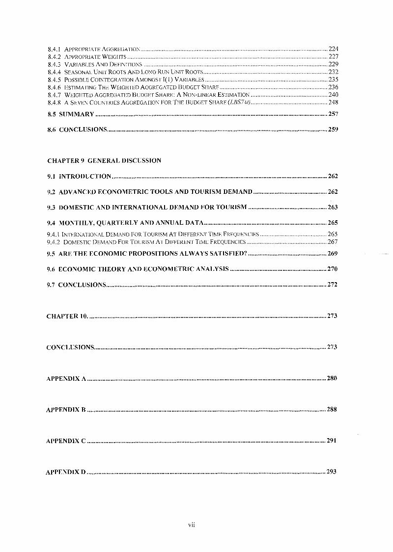
8.4.1 APPROPRIATE AGGREGATION 2 2 4

8 .4 .2 APPROPRIATE WEIGHTS 2 2 7

8 .4 .3 VARIABLES AND DEFINITIONS 2 2 9

8 .4 .4 SEASONAL UNIT ROOTS AND LONG RUN UNIT ROOTS 2 3 2

8 .4 .5 POSSIBLE COINTEGRATION AMONGST 1(1) VARIABLES 2 3 5

8 .4 .6 ESTIMATING THE WEIGHTED AGGREGATED BUDGET SHARE 2 3 6

8 .4 .7 WEIGHTED AGGREGATED BUDGET SHARE: A NON-LINEAR ESTIMATION 2 4 0

8 .4 .8 A SEVEN COUNTRIES AGGREGATION FOR THE BUDGET SHARE 2 4 8

8.5 SUMMARY 257

8.6 CONCLUSIONS 259

CHAPTER 9 GENERAL DISCUSSION


9.2 ADVANCED ECONOMETRIC TOOLS AND TOURISM DEMAND 262

9.3 DOMESTIC AND INTERNATIONAL DEMAND FOR TOURISM 263

9.4 MONTHLY, QUARTERLY AND ANNUAL DATA 265

9.4.1 INTERNATIONAL DEMAND FOR TOURISM AT DIFFERENT TIME FREQUENCIES 2 6 5

9 . 4 . 2 DOMESTIC DEMAND FOR TOURISM AT DIFFERENT TIME FREQUENCIES 2 6 7

9.5 ARE THE ECONOMIC PROPOSITIONS ALWAYS SATISFIED? 269

9.6 ECONOMIC THEORY AND ECONOMETRIC ANALYSIS 270

9.7 CONCLUSIONS 272

CHAPTER 10 273

CONCLUSIONS 273

APPENDIX A 280

APPENDIX B 288

APPENDIX C 291

APPENDIX D 293

VII

APPENDIX E 296

APPENDIX F 308

APPENDIX G 312

APPENDIX H 315

APPENDIX 1 318

REFERENCES 321

vin

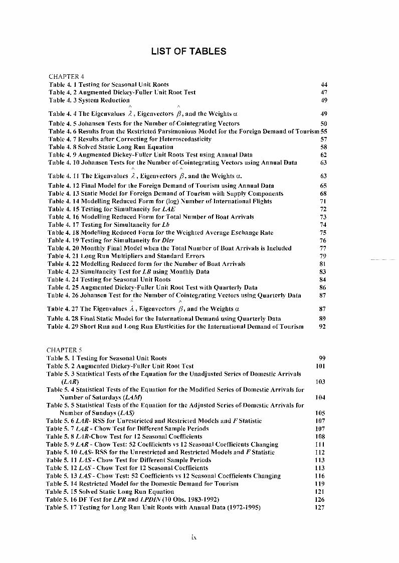
LIST OF TABLES

CHAPTER 4 Table 4. 1 Testing for Seasonal Unit Roots 44 Table 4. 2 Augmented Dickey-Fuller Unit Root Test 47 Table 4. 3 System Reduction 49

A A Table 4. 4 The Eigenvalues A, Eigenvectors yg, and the Weights a 49 Table 4. 5 Johansen Tests for the Number of Cointegrating Vectors 50 Table 4. 6 Results from the Restricted Parsimonious Model for the Foreign Demand of Tourism 55 Table 4. 7 Results after Correcting for Heteroscedasticity 57 Table 4. 8 Solved Static Long Run Equation 58 Table 4. 9 Augmented Dickey-Fuller Unit Roots Test using Annual Data 62 Table 4 .10 Johansen Tests for the Number of Cointegrating Vectors using Annual Data 63

Table 4. 11 The Eigenvalues A, Eigenvectors j i , and the Weights a. 63

Table 4. 12 Final Model for the Foreign Demand of Tourism using Annual Data 65 Table 4 .13 Static Model for Foreign Demand of Tourism with Supply Components 68 Table 4. 14 Modelling Reduced Form for (log) Number of International Flights 71 Table 4. 15 Testing for Simultaneity for LAE 72 Table 4. 16 Modelling Reduced Form for Total Number of Boat Arrivals 73 Table 4. 17 Testing for Simultaneity for Lb 74 Table 4 .18 Modelling Reduced Form for the Weighted Average Exchange Rate 75 Table 4. 19 Testing for Simultaneity for Dler 76 Table 4. 20 Monthly Final Model when the Total Number of Boat Arrivals is Included 77 Table 4. 21 Long Run Multipliers and Standard Errors 79 Table 4. 22 Modelling Reduced form for the Number of Boat Arrivals 81 Table 4. 23 Simultaneity Test for LB using Monthly Data 83 Table 4. 24 Testing for Seasonal Unit Roots 84 Table 4. 25 Augmented Dickey-Fuller Unit Root Test with Quarterly Data 86 Table 4. 26 Johansen Test for the Number of Cointegrating Vectors using Quarterly Data 87

/\ A Table 4. 27 The Eigenvalues X, Eigenvectors p , and the Weights a 87

Table 4. 28 Final Static Model for the International Demand using Quarterly Data 89

Table 4. 29 Short Run and Long Run Elasticities for the International Demand of Tourism 92

CHAPTER 5 Table 5 .1 Testing for Seasonal Unit Roots 99 Table 5. 2 Augmented Dickey-Fuller Unit Root Test 101 Table 5. 3 Statistical Tests of the Equation for the Unadjusted Series of Domestic Arrivals

{LAR) 103 Table 5. 4 Statistical Tests of the Equation for the Modified Series of Domestic Arrivals for

Number of Saturdays {LAM) 104 Table 5. 5 Statistical Tests of the Equation for the Adjusted Series of Domestic Arrivals for

Number of Sundays (LAS) 105 Table 5. 6 LAR- RSS for Unrestricted and Restricted Models and F Statistic 107 Table 5. 7 LAR - Chow Test for Different Sample Periods 107 Table 5. 8 LAR-Chov/ Test for 12 Seasonal Coefficients 108 Table 5. 9 LAR - Chow Test: 52 Coefficients vs 12 Seasonal Coefficients Changing 111 Table 5 .10 LAS- RSS for the Unrestricted and Restricted Models and F Statistic 112 Table 5 .11 LAS - Chow Test for Different Sample Periods 113 Table 5 .12 LAS - Chow Test for 12 Seasonal Coefficients 113 Table 5 .13 LAS - Chow Test: 52 Coefficients vs 12 Seasonal Coefficients Changing 116 Table 5. 14 Restricted Model for the Domestic Demand for Tourism 119 Table 5 .15 Solved Static Long Run Equation 121 Table 5. 16 DF Test for LPR and LPDIN {\Q Obs. 1983-1992) 126 Table 5. 17 Testing for Long Run Unit Roots with Annual Data (1972-1995) 127

IX

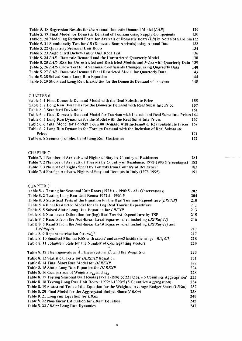
Table 5. 18 Regression Results for the Annual Domestic Demand Model {LAR) 129 Table 5 .19 Final Model for Domestic Demand of Tourism using Supply Components 130 Table 5. 20 Modelling Reduced Form for Arrivals of Domestic Boats (LB) in North of Sardinia 132 Table 5. 21 Simultaneity Test for LB (Domestic Boat Arrivals) using Annual Data 133 Table 5. 22 Quarterly Seasonal Unit Roots 134 Table 5. 23 Augmented Dickey-Fuller Unit Root Test 136 Table 5. 24 LAR - Domestic Demand and the Unrestricted Quarterly Model 138 Table 5. 25 LAR- RSS for Unrestricted and Restricted Models and F-test with Quarterly Data 139 Table 5. 26 LAR- Chow Test for 4 Seasonal Coefficients Changes, using Quarterly Data 140 Table 5. 27 LAR - Domestic Demand Final Restricted Model for Quarterly Data 143 Table 5. 28 Solved Static Long Run Equation 144 Table 5. 29 Short and Long Run Elasticities for the Domestic Demand of Tourism 145

CHAPTER 6 Table 6. 1 Final Domestic Demand Model with the Real Substitute Price 155 Table 6. 2 Long Run Dynamics for the Domestic Demand with Real Substitute Price 157 Table 6. 3 Standard Deviations 161 Table 6. 4 Final Domestic Demand Model for Tourism with Inclusion of Real Substitute Prices 164 Table 6. 5 Long Run Dynamics for the Model with the Real Substitute Prices 167 Table 6. 6 Final Model for Foreign Tourism Demand with Inclusion of Real Substitute Prices 169 Table 6. 7 Long Run Dynamics for Foreign Demand with the Inclusion of Real Substitute

Prices 171 Table 6. 8 Summary of Short and Long Run Elasticities 172

CHAPTER 7 Table 7. 1 Number of Arrivals and Nights of Stay by Country of Residence: 181 Table 7. 2 Number of Arrivals of Tourists by Country of Residence: 1972-1995 (Percentages) 182 Table 7. 3 Number of Nights Spent by Tourists from Country of Residence: 183 Table 7. 4 Foreign Arrivals, Nights of Stay and Receipts in Italy (1973-1995) 191

CHAPTER 8 Table 8. 1 Testing for Seasonal Unit Roots (1972:1 - 1990:5 - 221 Observations) 202 Table 8. 2 Testing Long Run Unit Roots: 1972:1- 1990:5 204 Table 8. 3 Statistical Tests of the Equation for the Real Tourism Expenditure (LREXP) 210 Table 8. 4 Final Restricted Model for the Log Real Tourist Expenditure 211 Table 8. 5 Solved Static Long Run Equation for LREXP 213 Table 8. 6 Non-linear Estimation for (log) Real Tourist Expenditure by TSP 215 Table 8. 7 Results from the Non-linear Least Squares when including LRPRa(-ll) 216 Table 8. 8 Results from the Non-linear Least Squares when including LRPRa(-ll) and

LRPRa(-3) 217 Table 8. 9 Reparametrisation for msig* 217 Table 8. 10 Smallest Minima RSS with mmul and mmu2 inside the range |-0.1, 0.7| 218 Table 8. 11 Johansen Tests for the Number of Cointegrating Vectors 220

A A

Table 8. 12 The Eigenvalues A , Eigenvectors /?, and the Weights a 220

Table 8 .13 Statistical Tests for DLREXP Equation 221 Table 8. 14 Final Short Run Model for DLREXP 222 Table 8 .15 Static Long Run Equation for DLREXP 224 Table 8. 16 Comparison of Weights wi f and x,- ^ 228 Table 8. 17 Testing Seasonal Unit Roots (1972:1-1990:5; 221 Obs. - 5 Countries Aggregation) 233 Table 8 .18 Testing Long Run Unit Roots: 1972:1-1990:5 (5 Countries Aggregation) 234 Table 8. 19 Statistical Tests of the Equation for the Weighted Average Budget Share (LBSm) 237 Table 8. 20 Final Model for the Aggregated Budget Share {LBSm) 238 Table 8. 21 Long run Equation for LBSm 240 Table 8. 22 Non-linear Estimation for LBSm Equation 242 Table 8. 23 LBSm: Long Run Dynamics 247

Table 8. 24 Seasonal Unit Roots for LBS7m 248 Table 8. 25 ADF Test for LBSJin Defined for Seven Countries Aggregation 249 Table 8. 26 Statistical Tests of the Equation for LBS7m 250 Table 8. 27 Final Model for LBS7m 251 Table 8. 28 Non-linear Estimation for LBSJm Equation 253 Table 8. 29 LBS7m\ Long Run Dynamics 256 Table 8. 30 DLREXP: Short and Long Run Elasticities for Italian Tourism Demand 257 Table 8. 31 LBSm - LBS7m: Short and Long Run Elasticities for Italian Tourism Demand 258 Table 8. 32 Song et al. (2000): Results for Italy 259

APPENDIX A Table A. 1 Testing for Seasonal Unit Roots 281 Table A. 2 Results from the Unrestricted Model for the Foreign Demand of Tourism 282 Table A. 3 Results from the Parsimonious Model for the Foreign Demand of Tourism 284 Table A. 4 Solved Static Long Run Equation 286

APPENDIX D Table D. 1 Results from the Unrestricted System for the Foreign Demand of Tourism 293 Table D. 2 Results from the Parsimonious Model for the Foreign Demand of Tourism 295

APPENDIX E Table E. 1 LAR - Program for Performing Chow Structural Break Test 296 Table E. 2 LAR - Program for Checking for Seasonal Parameters Changes 299 Table E. 3 Results from the Unrestricted System for the Domestic Demand of Tourism 301 Table E. 4 Restricted Model for the Domestic Demand for Tourism {LAR) 303 Table E. 5 Unrestricted Model for the Adjusted Series of Domestic Arrivals of Tourism {LAS) 304 Table E. 6 Parsimonious Model for the Adjusted Series {LAS) 306 Table E. 7 VAR(l) for Testing Industrial Production as Proxy for Personal Disposable Income 307

APPENDIX F Table F. 1 Cointegration Analysis for the Real Substitute Price for Greece and Portugal 308 Table F. 2 Cointegration Analysis for the Real Substitute Price for France and Spain 309 Table F. 3 Cointegration Analysis for the Relative Price and Exchange Rate 310 Table F. 4 Cointegration Analysis for Real Industrial Production (LRPRa), Relative Price

{LRPa) and Exchange Rate {LEXa) 310

APPENDIX G Table G. 1 Johansen Tests for the Number of Cointegrating Vectors 312 Table G. 2 Johansen Tests for the Number of Cointegrating Vectors 313 Table G. 3 Non-Linear Model for the (log) Real Tourism Expenditure 314

APPENDIX H Table H. 1 Common Trend Analysis 315 Table H. 2 Cointegration Analysis for the Relative Price and Exchange Rate 316 Table H. 3 Cointegration Analysis for Real Industrial Production {LRPRa), Relative Price

{LRPa) and Exchange Rate {LEXa) 317

APPENDIX I Table I. 1 Johansen Tests for the Number of Cointegrating Vectors 319 Table I. 2 Johansen Tests for the Number of Cointegrating Vectors 319

XI

LIST OF FIGURES

CHAPTER2 Figure 2. 1 Methodology of the Thesis

CHAPTER 3 Figure 3 .1 Domestic and Foreign Arrivals in Registered Accommodation for Sassari Province 29 Figure 3. 2 Foreign Seasonality (Averages Arrivals per Equivalent Month 1990:1-1995:12) 31 Figure 3. 3 Domestic Seasonality (Averages Arrivals per Equivalent Month 1990:1-1995:12) 32 Figure 3. 4 Actual Rate Utilisation 38

CHAPTER 4 Figure 4. 1 Natural Logarithm of the Series (1972:1 - 1995:12) 43

CHAPTER 5 Figure 5 .1 Natural Logarithms of the Series (1972:1 - 1995:12) 98 Figure 5. 2 Changes in Seasonal Pattern between 1990/91 109 Figure 5. 3 Changes in Seasonal Pattern between 1984/85 109 Figure 5. 4 LAS - Changes in Seasonal Pattern between 1990/91 114 Figure 5. 5 LAS - Changes in Seasonal Effects between 1980/81 114 Figure 5. 6 (Log) Industrial Production Index and (log) Personal Disposable Income 125 Figure 5. 7 Natural Logarithms of the Quarterly Series (1972:1 - 1995:4) 134 Figure 5. 8 Changes in Seasonal Pattern between 1985/86 using Quarterly Data 141 Figure 5. 9 Changes in Seasonal Pattern between 1990/91 using Quarterly Data 141

CHAPTER 6 Figure 6 .1 Log: Weighted Average Exchange Rate (LWTC), Substitute Price {LSP) and Real

Substitute Price (LRPS), 1972:1 - 1995:12 152 Figure 6. 2 (Log) Exchange Rates: Lira/Franc {LEXFR), Lira/Pesetas(Z,f%9f), Lira/Escudo

(LEXPOR) and Lira/Drachma (LEXGR) 158 Figure 6. 3 (Log) Substitute Prices: Sassari-France (LSPFR), Sassari-Spain (LSPSP), Sassari-

Portugal (LSPPOR) and Sassari-Greece (LSPGR) 159 Figure 6. 4 Substitute Prices Adjusted for Exchange Rates 161

CHAPTER 7 Figure 7. 1 Number of Domestic and Foreign Arrivals in Italy 179 Figure 7. 2 Number of Domestic and Foreign Nights Stay in Italy 179 Figure 7. 3 Number of Arrivals of Foreign and Domestic Tourists: Seasonality (Averages for

Each of the Correspondent Month 1990:1 - 1995:12) 180 Figure 7. 4 Nights Spent by Foreign and Italian Tourists: Seasonality (Averages for Each of the

Correspondent Month 1972:1 - 1995:12) 180 Figure 7. 5 Arrivals and Nights of Stay for Belgium: Seasonality (Averages for Each of the

Correspondent Month 1990:1 - 1995:12) 184 Figure 7. 6 Arrivals vs Nights of Stay for France: Seasonality (Averages for Each of the

Correspondent Month 1990:1 - 1995:12) 184 Figure 7. 7 Arrivals and Nights of Stay for Germany: Seasonality (Averages for Each of the

Correspondent Month 1990:1 - 1995:12) 185 Figure 7. 8 Arrivals and Nights of Stay for Japan: Seasonality (Averages for Each of the

Correspondent Month 1990:1 - 1995:12) 185 Figure 7. 9 Arrivals and Nights of Stay for Sweden: Seasonality (Averages for Each of the

Correspondent Month 1990:1 - 1995:12) 186 Figure 7. 10 Arrivals and Nights of Stay for Switzerland: Seasonality (Averages for Each of the

Correspondent Month 1990:1 - 1995:12) 186

xn

Figure 7. 11 Arrivals and Nights of Stay for the UK: Seasonality (Averages for Each of the Correspondent Month 1990:1 - 1995:12) 187

Figure 7. 12 Arrivals and Nights of Stay for USA: Seasonality (Averages for Each of the Correspondent Month 1990:1 - 1995:12) 187

Figure 7. 13 International Arrivals {LAR), Nights of Stay {LNS), Nominal Receipts (AWr-million lire) and Real Receipts (IjRF-thousands lire). Figures in logarithm (1972-1995) 190

CHAPTER 8 Figure 8. 1 Plots for (log) Real Tourist Receipts, Real Industrial Production Index {LRPRa),

Relative Price (LRPa) and Exchange Rate (LEXa) (1972:1 - 1990:5) 200 Figure 8. 2 (Log) Real Substitute Price: France, Greece, Portugal and Spain (1972:1 - 1990:5) 200 Figure 8. 3 Logistic Transformation of LRPRa: plot of z/ 216 Figure 8. 4 Multiple Minima for 33 cases; plot of RSS against the Starting Points [-0.1, 0.7] 218 Figure 8. 5 (Log) Budget Shares for: France, Germany, Japan and Sweden (1972:1 - 1990:5) 225 Figure 8. 6 (Log) Budget Shares for: Sweden, Switzerland, UK and USA (1972:1 - 1990:5) 226 Figure 8. 7 Annual versus Monthly Weights (1972:1 - 1990:5) 229 Figure 8. 8 Real Industrial Production Index {LRPRa), Relative Price {LRPa) and Exchange

Rate (Z.£Xfl) (1972:1 - 1990:5) 232 Figure 8. 9 LBSm: Plot of LRPRa i f on Z ( f 245 Figure 8 .10 LBSm: Plot of NLRPRai f on NZjj 246 Figure 8. 11 LBS7m: Plot of LRPRai f on Z4i f 254 Figure 8 .12 LBS7m: Plot oiNLRPRai f on NZ4i f 255

APPENDIX H Figure H. 1 Real Industrial Production Index {LRPRm), Relative Price {LRPm) and Exchange

Rate {LEXm) (1972:1 - 1990:5 - 5 countries aggregation) 315

xni

ACKNOWLEDGEMENTS

My first thought goes to my supervisor Mr Ray O'Brien. His insightful comments, his

patience in reading all my drafts with admirable care, his support and encouragement

have been a guide over these years.

I am also grateful to Mr Peter Smith for his supervision and helpful comments that

have led to exploring new knowledge.

I would also like to thank Isabel Andrade for her time and support during my research;

and to all those members of the Economic Department that, either directly or

indirectly, have helped in achieving the aim.

Thanks must go to Sardinian Region for providing financial support for this research.

Finally, a special mention to Stefano Usai, from the Economic Department of Sassari

University, for his valuable support.

X I V

ABBREVIATIONS

ADF - Augmented Dickey and Fuller unit root test

AIC - Akaike Information Criterion

ARDF - Augmented Rank Dickey-Fuller

CADF - Covariate Augmented Dickey Fuller

CI - Cointegrating Vector

D.E.I.S. - Dipartimento di Economia Istituzioni e Societa, Sassari University

DF - Dickey and Fuller unit root test

ECM - Error Correction Models

EEC - European Economic Community

EPT - Ente Provinciale per il Turismo

ESIT - Ente Sardo Industrie Turistiche, Sardinia (Italy)

EU - European Union

GDP - Gross Domestic Product

GNP - Gross National Product

HQ - Hannan and Quinn information criterion

IFS - International Financial Statistics

ISTAT - Istituto Centrale di Statistica, Italy

LR - Likelihood Ratio

LSE - London School of Economics general-to-speciGc methodology

XV

MDV - Mean of the Dependent Variable

M-TAR - Momentum Threshold AutoRegressive model

O E C D - Organisation for Economic Co-operation and Development

OLS - Ordinary Least Squares

PPP - Purchasing Power Parity

P V A R - Parsimonious Vector AutoRegressive model

RDF - Rank Dickey-Fuller

RSS - Residual Sum of Squares

SC - Schwarz information Criterion

SEM - Structual Econometric Model

SER - Standard Error of the Regression

SSE - Sum of the Squared Errors

S S E L - Sum of the Squared Errors for the Linear specification

S S E L L - Sum of the Squared Errors for the Log-Linear specification

TAR - Threshold AutoRegressive model

U V A R - Unrestricted Vector AutoRegressive model

VAR - Vector AutoRegressive models

WTO - World Tourism Organisation

X V I

Chapter 1

CHAPTER 1.

INTRODUCTION

1.1 TOURISM AND ECONOMETRIC ANALYSIS

Tourism is a heterogeneous activity. Its sui generis nature involves multiple

aspects which interact with geographical, environmental, political, sociological and

economic elements. Thus, different disciplines have analysed tourism as a

phenomenon because of its importance and impact which has been growing throughout

the world over the recent decades.

Since the Fifties studies on tourism demand have been undertaken; however, the

dawn of a systematic economic analysis of tourism has been seen with Gray (1966). In

the Seventies, an increased number of empirical studies appeared in the tourism

literature. The determinants of international demand for tourism started to be analysed

by applying economic concepts, econometric methodologies and forecasting tools (see

for example Artus, (1972); Archer, (1976)). Crouch (1994) and Lim (1997) provide a

comprehensive literature review for more than one hundred empirical studies over

three decades of international tourism demand. In these surveys, a detailed account is

provided on the type of data used, methodologies adopted, dependent and explanatory

variables employed. According to Lim (1997) and Sinclair (1998), extensive

econometric effort still needs to be done in the study of international tourism demand.

Small sample sizes, lack of discussion of the appropriate functional forms, failure in

including the full range of diagnostic tests are pointed out as some of the main

deficiencies in empirical tourism demand studies. One also might point out that more

advanced econometric approaches, which include amongst others Hendry's

methodology, seasonal and long run unit roots and cointegration analysis are still much

neglected in the tourism literature (examples in this direction are Lanza and Urga,

1995; Syriopoulos, 1995; Vogt and Wittayakom, 1998; Song gf a/., 2000; Kulendran

and Witt, 2001). Little attention is also paid to the analysis of the determinants of

Chapter

domestic demand for tourism, which represents a great quota of tourism demand in

developed countries (see Seddighi and Shearing, 1997).

This thesis analyses and models tourism demand in Italy by making use of recent

econometric methodologies. In particular, the focus on tourism in the Northern

Province of Sardinia will be taken.

1.2 AIM AND PROPOSITIONS OF THE THESIS

The aim of this thesis is to formulate and validate an economic model of

tourism for Italy and Sardinia. It anticipates that this study will concentrate on the

demand of tourism (both foreign and domestic) in the Northern Province of Sardinia.

This Province sees the major quota of tourist flows in the island for the sample period

under analysis. While, the demand for tourism to the north of Sardinia will be

modelled in terms of numbers, the Italian tourism will be modelled in terms of tourism

receipts given the existing availability of data.

Song et al. (2000) have shown that more sophisticated econometric approaches

have given significant results in analysing, modelling and testing economic theory.

Kulendran and Witt (2001) have also shown that the forecasts obtained by using more

recent econometric methodologies are more accurate than those obtained by least

squares regression. Hence, the proposition of this thesis is the following; can advanced

econometric approaches give more insight in modelling and understanding tourism

demand in Sardinia and Italy? The major questions arising from this proposition are

the following:

® Are there any differences between domestic and international tourism? The majority

of the studies focus on the analysis and modelling of international demand for

tourism. In general, there has been little attention in understanding the validity in

differentiating the domestic from international demand for tourism. One of the aims

of this study is to give foundations for modelling the two components separately.

For this purpose, graphical and econometric tools will be employed.

• Are there common findings by using different data frequencies {i.e. annual,

quarterly and monthly)? One of the suggestions given by Witt and Witt (1992) for

further research is to estimate tourism models at different data frequencies. They

write: "First, only annual data have been used to estimate the models and forecast

Chapter 1

tourism demand. Tliis is by no means uncommon, in that almost all the studies

concerned with international tourism demand forecasting employ annual data.

However, the use of monthly and quarterly data would allow for more precise

estimation and examination of lags. It would also be interesting to see whether the

results established for annual data hold for monthly and quarterly data" (p. 171).

The lack of research in this area is also pointed out by Uysal and Roubi (1999) "the

use of different data periods is one of the areas that would need further research in

tourism demand and forecasting studies" (p. 116). The scope of this thesis is to

investigate this proposition.

o Are the economic propositions always satisfied? This thesis makes use of economic

concepts that are commonly applied in the tourism literature. The aim is to test the

theory by using dynamic econometric modelling. Short and long run effects of

changes in income and relative prices on the demand for tourism in Italy and Sassari

Province will be investigated. Propositions such as negativity and substitutability

will be tested. Hence, one will consider: a) the sensitivity of the demand for tourism

to changes in the prices for goods and services in the destination country relative to

prices in the source countries; b) the sensitivity of tourism demand to changes in the

prices of tourist goods and services relative to prices in other competitor

destinations.

® Is there any conflict between economic theory and econometric results? The role of

econometrics in falsifying economic theory and/or adding new knowledge is still

the object of major debate amongst academics; see Hylleberg and Paldam (1991)

for a discussion of different schools of thoughts. The scope of this thesis is not that

of assessing new economic knowledge from the conflict between data and priors.

Instead, the aim is to use the guidance and help of the existing theoretical

framework in interpreting and co-ordinating the results from the econometric

analysis. Hence, econometrics is employed as a tool for testing a priori theoretical

propositions making use of several models and time series that are new with respect

to other empirical studies available in the tourism literature.

This thesis answers these questions by making use of distinct research steps, as

follows:

a) literature review that focuses on the aspects and characteristics of the tourism

Chapter 1

phenomenon having in mind a priori economic assumptions;

b) data collection and modelling the demand of tourism using particular case studies;

c) use of more advanced and recent econometric tools to test the theoiy;

d) feedback to economic theory.

1.3 OUTLINE OF THE CHAPTERS IN THE THESIS

An outline of each chapter of the thesis is given belovy.

• Chapter 2: Methodology

TThis cliapKer is cLechcabsd to tlie rnellrockyLogry acLopdkxi in thx: tliesis aiid linlis TArhii iWie

literature review on tourism economy covered in Chapter 1. This allows a focus on the

aspects and characteristics of the tourism phenomenon having in mind a priori

economic assumptions. The next step links together the theory with the empirical

practise that requires data collection to be undertaken. From the raw data, variables of

interest are calculated in monthly, quarterly and annual frequencies. Such variables are

tested for both possible seasonal and long run unit roots. Once the status of the

variables of interest is established, further testing for possible cointegration is carried

out whenever necessary. Hence, the LSE general-to-specific methodology is used in

modelling the demand for tourism. The empirical results obtained are compared with

economic theory.

• Chapter 3: Characteristics of International and Domestic Demand for

Tourism in the Italian Province of Sassari: A General Introduction

Chapter 3 is a general introduction to the main characteristics of tourism demand in

Sassari Province of Italy. An account is given of the differences between the

international and domestic demand based on the evolution of the tourist flows and on

the seasonal distribution. In accordance with economic theory, the possible

determinants that might have a role in explaining the demand for tourism are

described.

Chapter 1

• Chapter 4: International Demand for Tourism in the North of Sardinia

The aim of this chapter is to examine the economic factors affecting the demand for

international tourism in the Province of Sassari. An econometric model is developed

for a short run and long run analysis. Elements like the "trading-days" factor and the

Easter effect are examined and included into the equation. The relationship between

the short run, long run income and price elasticities is investigated by making use of

different time frequencies.

® Chapter 5: The Domestic Demand for Tourism in the North of Sardinia

Chapter 5 is dedicated to the analysis of the domestic demand. It is possible to find out

other distinctive characteristics that differentiate this component from the international

demand. Further investigation is carried out to assess the possible validity of the

correction of the dependent variable (i.e. the number of domestic arrivals) for the

number of weekends in a month. Relationships between short run, long run income

and price elasticities are also explored and a comparison with other empirical findings

is given. Different data frequency models are estimated. A section is dedicated to test

and establish that the Italian production index can be considered as a valid proxy of the

personal disposable income.

• Chapter 6: Sassari Province Competitors: Substitute Price and Exchange Rate

In Chapter 6, the inclusion of the exchange rate for the main competitors in the

Mediterranean area is considered. A careful investigation is carried out to include

either the aggregated substitute price variable adjusted for the exchange rate or a

disaggregated real substitute price for each of the competitor countries. The analysis is

undertaken for both the domestic and international demand for tourism in the north of

Sardinia.

• Chapter 7: Italian Tourism: Seasonality, Numbers and Expenditure

Chapter 7 gives an in-depth analysis on tourism in Italy as a whole. A graphical

analysis identifies possible differences between domestic and international demand for

tourism. An analysis on the seasonal pattern of the major origin countries, that is

Belgium, France, Germany, Japan, Sweden, Switzerland, United Kingdom and United

Chapter 1

States is undertaken.

Tourism demand can be expressed in terms of the number of tourists in

registered accommodation and in terms of tourist expenditure. Hence, a comparison is

made amongst the number of tourists' arrivals, nights of stay, nominal and real tourism

expenditure for the period from 1972 to 1995.

• Chapter 8: Estimating Italian Tourism

Chapter 8 gives an account of the findings in modelling the demand for tourism in

Italy as a whole. In this case, monthly expenditure data {i.e. tourist receipts from the

balance of payments) are used as the dependent variable. One of the aims is to model

the real tourism receipts, commonly used in time-series empirical studies on tourism.

The second variable is the real aggregated budget share for the main source countries,

commonly used in cross-section studies. Monthly data are used for the period 1972:1

uptol99&T2.

® Chapter 9: General Discussion

In Chapter 9, details are given on the main contributions of the present thesis to the

tourism literature. The initial propositions are investigated in the light of the findings

obtained from this empirical analysis. For the first proposition, an understanding is

given on whether more advanced econometric approaches are able to give insight to

modelling and estimating the demand for tourism. For the second proposition, it is

reported whether it is appropriate to separate domestic from international tourism in

terms of evolution of tourists' flows, seasonality, statistics and econometric findings.

Under the third proposition, similarities and/or differences that have been encountered

in estimating tourism demand at different time frequencies are underpinned. An

analysis of the empirical findings in terms of economic theory is carried out. Finally,

for the last proposition to be investigated, it is assessed whether any conflict emerges

between theory and econometric findings from this analysis.

• Chapter 10: Conclusions

Chapter 10 gives concluding remarks.

Chapter 2

CHAPTER 2.

METHODOLOGY

Aim of the Chapter:

To introduce the methodological steps followed in this thesis.

2.1 INTRODUCTION

This chapter will introduce the main methodological steps followed in this

thesis. The aim is to use some recent developments in econometric methodology to test

the theory and analyse the demand of tourism in Italy and in the Sardinian Province of

Sassari. The following sections are dedicated to the topics which this work is based on.

2.2 METHODOLOGY

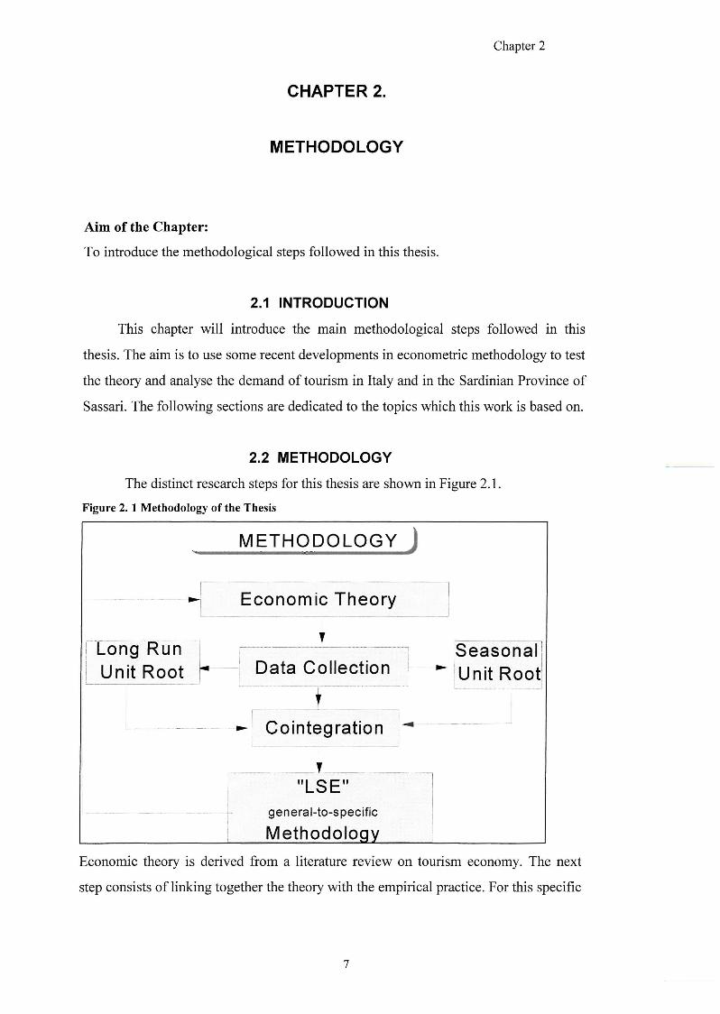
The distinct research steps for this thesis are shown in Figure 2.1.

Figure 2. 1 Methodology of the Thesis

Long Run Unit Root

METHODOLOGY J

Economic Theory

T

Data Collection

f

^ Cointegration ^

"LSE" general-to-specific

Methodology

Seasonal Unit Root

Economic theory is derived from a literature review on tourism economy. The next

step consists of linking together the theory with the empirical practice. For this specific

Chapter 2

study, data collection is obtained both in the local Ente Provinciale per il Turismo

(EPT of Sassari) and in the official statistical sources, e.g. Istituto Centrale di Statistica

(ISTAT), Datastream and Bank of Italy. From the raw data, approximations to the

variables of interest are calculated on a monthly, quarterly and annual frequency. Such

variables are tested for both possible seasonal and long run unit roots. Once the status

of the variables of interest has been established, further testing for possible

cointegration is carried out whenever necessary. Hence, the LSE general-to-specific

methodology is used in modelling the demand for tourism. Finally, the empirical

results obtained are compared with economic theory.

In the following sections, a more detailed analysis of each of the steps shown in

Figure 2.1 is given.

2.3 ECONOMIC THEORY

Economic analysis of tourism involves modelling the supply and/or the demand

side. This thesis focuses on the demand side; however, some consideration of the

supply side will be given in Chapters 4 and 5. Very few studies exist on the demand

for tourism in Sassari Province (Solinas, 1992; D.E.I.S., 1995; Contu, 1997) and none

of them makes use of the most recent econometric methodology.

The aim of the thesis is to analyse the most significant determinants of the

demand for tourism in the north of Sardinia and in Italy. According to neo-classical

consumer demand theory, a tourist is a consumer who derives utility from a vector of

goods and services that range from food through to travel and recreation. Consumer

theory also suggests that an individual consumer maximises his/her utility subject to a

budget constraint. Thus, by setting up the utility maximisation condition subject to a

budget constraint, one can derive the tourism demand equation by solving using the

Lagrange multiplier (see Var et ah, 1990). By means of this conceptual model one can

understand the main factors which influence the international and domestic demand of

tourism for the north of Sardinia and Italy. The most relevant determinants are the

following: the personal disposable income level of the potential tourists; the price of

the commodities and services of tourism; the price of substitutes; the exchange rate on

the grounds that some consumers may be more aware of exchange rates than

destination costs of living for tourists; the tastes and preferences of the potential

Chapter 2

tourists (Archer, 1976). The generic demand equation for tourism can be written in the

following manner;

D = EA;

D = Dependent variable. It can be defined as the demand for tourist goods and

services. In several empirical studies, different proxies are used as the dependent

variable. In some of the studies, the level of expenditure and receipts on goods and

services is used as a measure of consumption (Smeral, 1988; Di Matteo and Di Matteo,

1993; Gonzales and Moral, 1996; Uysal and Roubi, 1999). In many other studies, the

number of arrivals is taken as the dependent variable (Martin and Witt, 1989;

Makridakis a/., 1989; Witt and Witt, 1992; Carraro and Manente, 1996). Which is

the variable to best approximate the demand for tourism? The answer depends on the

aim of the analysis. As Sheldon (1993) points out, "measures of international tourism

volume and international tourism expenditures are both important for a destination"

(p. 13). Forecasts of the demand for tourism, using tourist expenditure as the dependent

variable, are needed to assess the economic impact of tourism. Forecasts of the

demand for tourism, using the number of arrivals as the dependent variable, are

important for private tourism businesses and for governments in planning their

activities in terms of investments and infrastructure needs. In analysing the demand for

tourism in the north of Sardinia, the number of arrivals of tourists is taken as the

dependent variable. Even if the number of arrivals is the variable one wishes to model,

using economic theory for expenditure involves an approximation. This choice is

constrained by the availability of the data. Figures on tourist expenditure are, in fact,

not available for the Province of Sassari. One of the limitations of the Bank of Italy

reports in terms of tourism receipts is that there is no availability of disaggregated data

by region and/or province (see Ballatori and Vaccaro, 1992). On the other hand, the

analysis of Italian tourism will involve the use of expenditure as the dependent

variable.

IN = Income is considered as one of the main relevant explanatory variables in the

analysis of tourism. Tourism, in fact, is defined as a consumption good. International

tourism activity might be regarded as a luxury good whereas domestic tourism may on

estimation appear as a necessity good. Income, according to economic theory as well

as empirical findings, constitutes one of the main indicators of an origin country, and

Chapter 2

individual wealth. One would expect that an increase in income level leads to an

expansion in tourism. Empirical studies have shown that international demand for Italy

presents values for income elasticities within a range of 1.00 (Germany) to 2.40 (for

UK) (Syriopoulos, 1995). Note that these elasticities are obtained by estimating the

foreign demand for tourism in Italy in terms of expenditure. Malacarni (1991), in

estimating the demand for tourism in terms of numbers, finds a value of income

elasticity of 1.49 for the foreign demand and a value of 0.92 for the domestic demand.

The latter results show foreigners seem to consider the Italian destination as a luxury

good more than the locals. An increase in income level leads to a tourism flow

expansion. The expected sign of this variable is positive (Summary, 1987).

RP = Relative Price. Another important determinant of the demand for tourism is the

"own price" of goods and services. Two types of costs can be considered: living cost in

the destination country and travel cost. As Sinclair (1998) and Lim (1999) report,

transport costs have appeared to be statistically not significant and in the majority of

single equation studies have been excluded. Price effects can be substantial. Many

studies confirm that the elasticity of tourism commodities with respect to a unitary

change in the holiday price is negative and sometimes more than unity (Grasselli,

1982; Gardini, 1984; Syriopoulos, 1995). In Syriopoulos (1995) for example, the range

of elasticities is within the range -0.38 for United States to -1.61 for Germany, when

Italy is considered as the destination country. One of the aims of this thesis is to test

these findings for the Province of Sassari.

EX= Exchange Rate. In the empirical tourism literature, the exchange rate is included

as an explanatory variable. It is used either as a proxy for the tourist price index or

together with the relative price. The main evidence for this combination is that the

international visitor will consider the exchange rate before going to a certain

destination country. Hence, the exchange rate is seen as a good approximation of the

holiday cost. "Prices are seldom completely known in advance by travellers so that the

price level foreseen by the potential traveller will depend predominantly upon the rate

of exchange of his domestic currency.... The rate of exchange can be expected to be a

prime indicator of expected prices" (Gray, 1966, p.86). Including the exchange rate

alone as a proxy of the tourist price index can lead to biased results by not taking into

account the inflation rate of the destination country. Hence "though the exchange rate

10

Chapter 2

in a destination may become more favourable this could be counter balanced by a

relatively high inflation rate" (Witt and Witt, 1992, p. 19). In this study the relative

price and exchange rate will be included separately.

SF - Substitute Price. Economic theory suggests that the price of substitutes are

another relevant determinant of demand. In the tourism literature, a common

specification is to consider the substitution price between tourist visits to the foreign

destination under consideration and domestic tourism (Gray, 1966; Martin and Witt,

1988). On the other hand, Sinclair and Stabler (1997) point out "occasionally, the

prices and exchange rates of other competing destinations have been also

incorporated" (p. 42). For this argument, amongst the other studies, see Gonzales and

Moral (1995), Syriopoulos (1995) and Lee et al. (1996). Chapter 6 will evaluate which

variable best explains tourism demand.

DM = Extra Economic Variables. In this thesis, the models will include other

determinants which are assumed to have an impact on tourism demand. Amongst these

are a weather variable, an "Easter" dummy and seasonal dummies. The construction of

these variables will be discussed later in the thesis.

2.4 DATA COLLECTION

Bearing in mind the main determinants for tourism demand, the next step

consists in the collection of relevant data. In this way, it is possible to analyse and

build a model for the demand of tourism.

One of the aims of this thesis is to consider whether one can reach common

findings using data at different frequencies {i.e. annual, quarterly and monthly). The

number of tourist arrivals in Sassari Province are available in a monthly frequency and

are supplied by the government agency EPT of Sassari. These data are defined in terms

of the number of tourists' arrivals in all registered accommodation in the north of

Sardinia. Such data omit tourist movement in private and non-registered

accommodation. According to Solinas' study (1992), registered accommodation

supply represents almost 1/3 of the total accommodation supply. However, such an

omission is common to many tourist statistical sources, as pointed out by Lickorish

(1997X

11

Chapter 2

The data used to create the other explanatory variables are obtained from several

statistical sources. The Bank of Italy is the source for exchange rates and tourist

receipts data. The International Financial Statistics (IPS) Datastream is the source for

the industrial production index, consumer price index and private consumption. The

Organisation for Economic Co-operation and Development (OECD) is the source for

the number of tourists' arrivals for the competitors. The Central Institute of Statistics

in Italy (ISTAT) is the source for the consumer price index in Sassari and the annual

Italian personal disposable income. Of the non-economic variables, the weather

variable is supplied by the Agricultural University of Sassari. This variable is

expressed in terms of the monthly average temperature in Sassari.

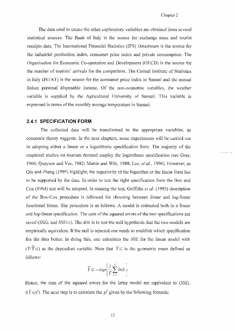
2.4.1 SPECIFICATION FORM

The collected data will be transformed to the appropriate variables, as

economic theory suggests. In the next chapters, some experiments will be carried out

in adopting either a linear or a logarithmic specification form. The majority of the

empirical studies on tourism demand employ the logarithmic specification (see Gray,

1966; Quayson and Var, 1982; Martin and Witt, 1988; Lee, et al., 1996). However, as

Qiu and Zhang (1995) highlight, the superiority of the logarithm or the linear form has

to be supported by the data. In order to test the right specification form the Box and

Cox (1964) test will be adopted. In running the test, Griffiths et al. (1993) description

of the Box-Cox procedure is followed for choosing between linear and log-linear

functional forms. The procedure is as follows. A model is estimated both in a linear

and log-linear specification. The sum of the squared errors of the two specifications are

saved {SSEL and SSELL). The aim is to test the null hypothesis that the two models are

empirically equivalent. If the null is rejected one needs to establish which specification

fits the data better. In doing this, one calculates the SSE for the linear model with

(177 G) as the dependent variable. Note that FG is the geometric mean defined as

follows:

P G

Hence, the sum of the squared errors for the latter model are equivalent to (SSEL

/( FG)^. The next step is to calculate the given by the following formula:

12

Chapter 2

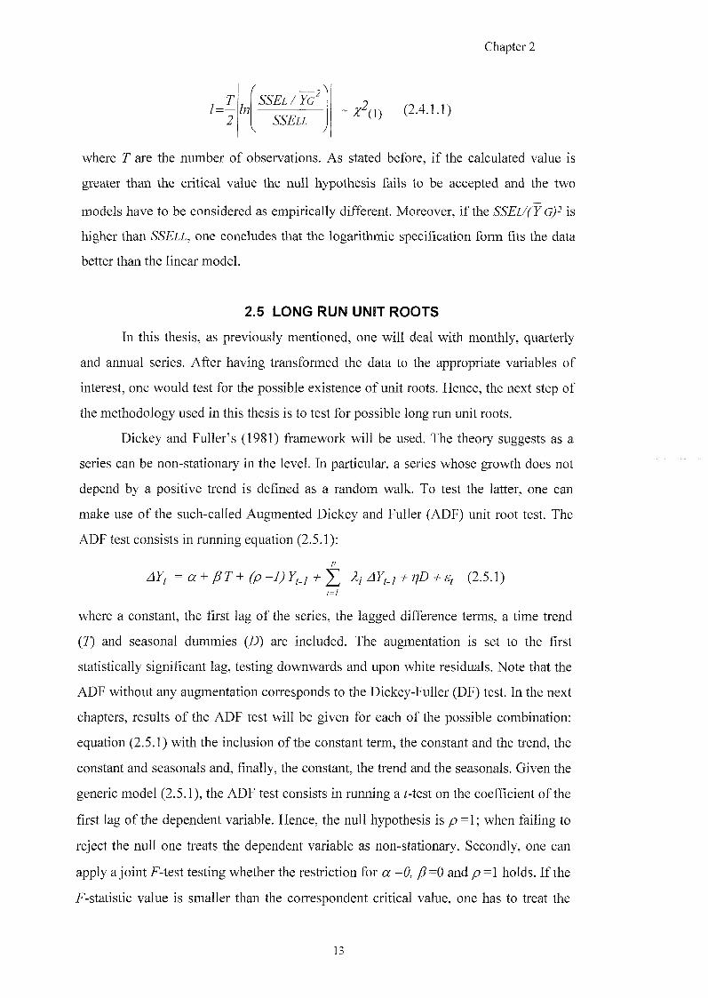
i J -2

In

/ —

Z^( l ) (2 .4 .1 .1 )

where T are the number of observations. As stated before, if the calculated value is

greater than the critical value the null hypothesis fails to be accepted and the two

models have to be considered as empirically different. Moreover, if the SSEL/(Y Gp is

higher than SSELL, one concludes that the logarithmic specification form fits the data

better than the linear model.

2.5 LONG RUN UNIT ROOTS

In this thesis, as previously mentioned, one will deal with monthly, quarterly

and annual series. After having transformed the data to the appropriate variables of

interest, one would test for the possible existence of unit roots. Hence, the next step of

the methodology used in this thesis is to test for possible long run unit roots.

Dickey and Fuller's (1981) framework will be used. The theory suggests as a

series can be non-stationary in the level. In particular, a series whose growth does not

depend by a positive trend is defined as a random walk. To test the latter, one can

make use of the such-called Augmented Dickey and Fuller (ADF) unit root test. The

ADF test consists in running equation (2.5.1):

p

= a + y g r + ^ - y ; f ^ f /yD f (2 .5 .1 )

/ = /

where a constant, the first lag of the series, the lagged difference terms, a time trend

(T) and seasonal dummies (D) are included. The augmentation is set to the first

statistically significant lag, testing downwards and upon white residuals. Note that the

ADF without any augmentation corresponds to the Dickey-Fuller (DF) test. In the next

chapters, results of the ADF test will be given for each of the possible combination:

equation (2.5.1) with the inclusion of the constant term, the constant and the trend, the

constant and seasonals and, finally, the constant, the trend and the seasonals. Given the

generic model (2.5.1), the ADF test consists in running a f-test on the coefficient of the

first lag of the dependent variable. Hence, the null hypothesis is p =1; when failing to

reject the null one treats the dependent variable as non-stationary. Secondly, one can

apply a joint F-test testing whether the restriction for a =0, j3=0 and p =1 holds. If the

F-statistic value is smaller than the correspondent critical value, one has to treat the

Chapter 2

variable of interest as a random walk. Some of the critical values can be found in

Dickey and Fuller (1991, p.1063). The critical values when including the seasonal

dummies are provided by the package used to run the test, that is PcGive 9.0 package

(see Doornik and Hendry, 1996, pp.93-95).

The use of the unit roots test enables one to assess the status of the economic

series of interest. If a series is found to be non-stationary in the level, whenever the

null hypothesis fails to be rejected, it has to be differenced. For example, if Yf in

(2.5.1) has been found to be a random walk it needs to be differenced. In particular, 7

is said to be integrated of order one if the first difference AY is stationary but Yj is not

(i.e. 1(1)). More in general, a series can be integrated of higher order if the series

differenced d times is stationary but the series differenced d-1 times is not {i.e. 1(d)).

Note also that a 1(0) series is stationary in the level.

2.6 QUARTERLY AND MONTHLY SEASONAL UNIT ROOTS

Recently, many studies have involved the investigation of seasonal variation.

This development is due to the realisation that the seasonal components can be the

main cause for the variations in many economic time series, and that the seasonal

variation in many time series is often irregular. Thus, the seasonal pattern of many

economic time series cannot be described by deterministic seasonal dummies, i.e. it

cannot be represented by a model which assumes that the seasonal components are

regular and non-changing. As Hyllerberg points out (see Hargreaves, 1994, pp. 153-

177), there are many different causes for seasonal variation. As far as tourism is

concerned, the change in tourists' preferences (e.g. winter holidays being preferred to

summer holidays) or the change in the timing of vacations by institutions and/or

employers can cause a shift in the seasonal pattern. The possibility of an irregular

seasonal pattern can be tested by means of investigating the possible existence of

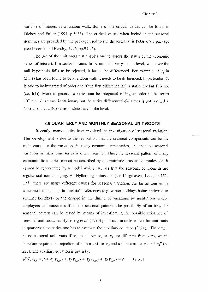
seasonal unit roots. As Hylleberg aZ. (1990) point out, in order to test for unit roots

in quarterly time series one has to estimate the auxiliary equation (2.6.1). "There will

be no seasonal unit roots if 712 either tij or 714 are different from zero, which

therefore requires the rejection of both a test for and a joint test for and (p.

223). The auxiliary equation is given by:

(2 .6 .1 )

14

Chapter 2

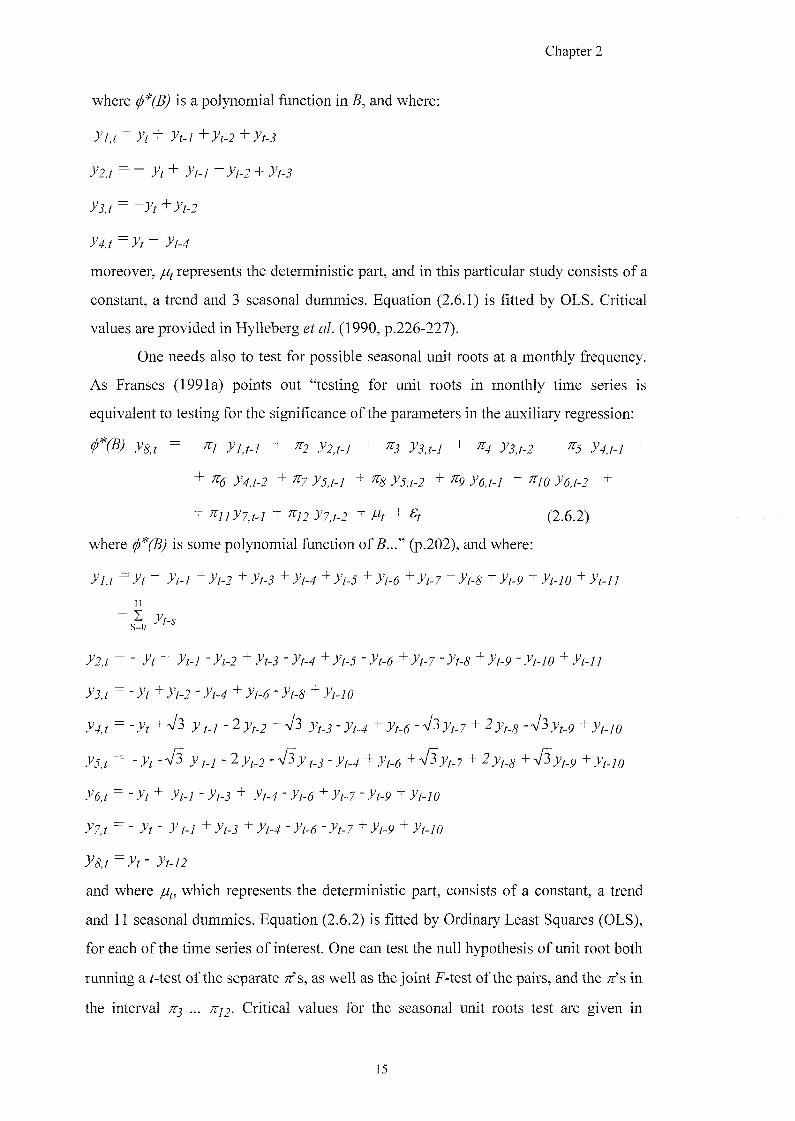
where (l)*(B) is a polynomial function in B, and where:

^ yr + + ^(-2 +

moreover, represents the deterministic part, and in this particular study consists of a

constant, a trend and 3 seasonal dummies. Equation (2.6.1) is fitted by OLS. Critical

values are provided in Hylleberg er aZ. (1990, p.226-227).

One needs also to test for possible seasonal unit roots at a monthly frequency.

As Franses (1991a) points out "testing for unit roots in monthly time series is

equivalent to testing for the significance of the parameters in the auxiliary regression;

+ % . y j / - / + % % / - 2 +

+ + ^72 }'7,f-2 + m + 'Sy (2 .6 .2 )

where ^*(B) is some polynomial function of i?..." (p.202), and where:

.yy.f ^ + .y/-/ + )^/-2 +

-.yf-2 + >"^3 -

= - .yr + }'r-2 -

+ V s ; / / . / - 2 + V s - V s + 2 - V s }; _p + _y _yg

^ - .yr - ^ f-y - 2 }'f.2 - V s _y (_j - + V s + 2 + V s _y _p +

^ + y^-7 - - 7r-p +

^ - .yf - /-/ + j +

- }'f-72

and where fj. , which represents the deterministic part, consists of a constant, a trend

and 11 seasonal dummies. Equation (2.6.2) is Gtted by Ordinary Least Squares (OLS),

for each of the time series of interest. One can test the null hypothesis of unit root both

running a Mest of the separate yz's, as well as the joint f-test of the pairs, and the yr's in

the interval ... 7ij2. Critical values for the seasonal unit roots test are given in

15

Chapter 2

Franses (1991b, pp. 161-165). If the null hypothesis is rejected one can treat the

variable of interest as stationary.

Note that both the tests for quarterly and monthly seasonal unit roots are run in

Microfit 4.0 package (Pesaran and Pesaran, 1997).

2.7 COINTEGRATION

As shown in Figure 2.1, the findings from the seasonal and long run unit roots

test lead to a possible cointegration of the variables of interest.

As Johansen (1995) points out "it is important that one allows the components

of a vector process to be integrated of different orders. The reason for this is that when

analysing economic data the variables are chosen for their economic importance and

not for their statistical properties. Hence, one should be able to analyse for instance

1(0) as well as 1(1) variables in the same model, in order to be able to describe the

long-run relation as well as the short-run adjustments" (p. 34). If one has a vector of

time series X , that achieves stationarity after differencing and a linear combination

is stationary, the time series ^ are said to be co-integrated with co-integrating

vector /?. Given two generic series and and the components of the vector = (y^

Xf) ' are both 1(1), then the equilibrium error, if it exists, would be 1(0) (Engle and

Granger, 1987).

Many estimators of long run coefficients exist in the literature (see Hargreaves,

1994, pp. 87-131 for a more detailed review). In investigating cointegrating relations

Engle and Granger (1987), for example, suggest using the Cointegrating Regression

Durbin Watson approach. Amongst the others is the Johansen Vector AutoRegressive

(VAR) maximum likelihood estimator. Hargreaves' (1994) Monte Carlo simulations

suggest that the Johansen estimator is best, amongst other five estimators of

cointegrating relations (z.g. OLS, Augmented OLS, Fully-Modified, Three-Step, and

Box-Tiao), as long as the sample is reasonably large (about 100 observations) and the

model is accurately specified.

In this thesis, cointegration testing in single equations as well as the Johansen

cointegration procedure will be used.

16

Chapter 2

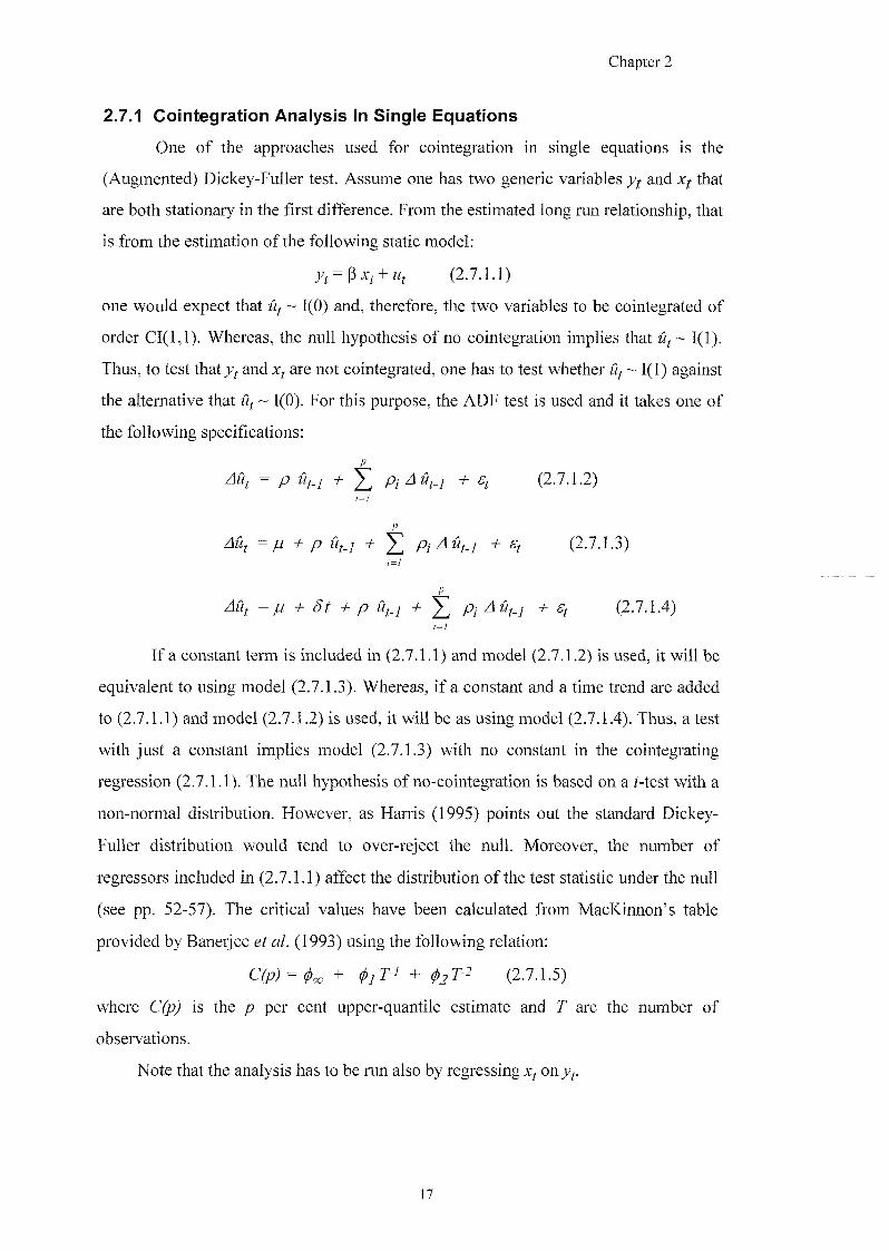
2.7.1 Cointegration Analysis In Single Equations

One of the approaches used for cointegration in single equations is the

(Augmented) Dickey-Fuller test. Assume one has two generic variables yf and Xf that

are both stationary in the first difference. From the estimated long run relationship, that

is from the estimation of the following static model;

+ (2.7.1.1)

one would expect that Uf ~ 1(0) and, therefore, the two variables to be cointegrated of

order CI(1,1). Whereas, the null hypothesis of no cointegration implies that w, ~ 1(1).

Thus, to test that and Xf are not cointegrated, one has to test whether - 1(1) against

the alternative that Uf ~ 1(0). For this purpose, the ADF test is used and it takes one of

the following specifications:

p

^ Z ^ 4 (2.7.1.2) 1=1

P

Auj = jj, + p U(.j Pi A Uf.] + Ef (2.7.1.3) / = /

Au^ — ju + St + p iif.i + ^ Pi AUf_i + Sj (2.7.1.4)

i=i

If a constant term is included in (2.7.1.1) and model (2.7.1.2) is used, it will be

equivalent to using model (2.7.1.3). Whereas, if a constant and a time trend are added

to (2.7.1.1) and model (2.7.1.2) is used, it will be as using model (2.7.1.4). Thus, a test

with just a constant implies model (2.7.1.3) with no constant in the cointegrating

regression (2.7.1.1). The null hypothesis of no-cointegration is based on a f-test with a

non-normal distribution. However, as Harris (1995) points out the standard Dickey-

Fuller distribution would tend to over-reject the null. Moreover, the number of

regressors included in (2.7.1.1) affect the distribution of the test statistic under the null

(see pp. 52-57). The critical values have been calculated from MacKinnon's table

provided by Banerjee et al. (1993) using the following relation:

= (2.7.1.5)

where C(p) is the p per cent upper-quantile estimate and T are the number of

observations.

Note that the analysis has to be run also by regressing on)/^.

17

Chapter 2

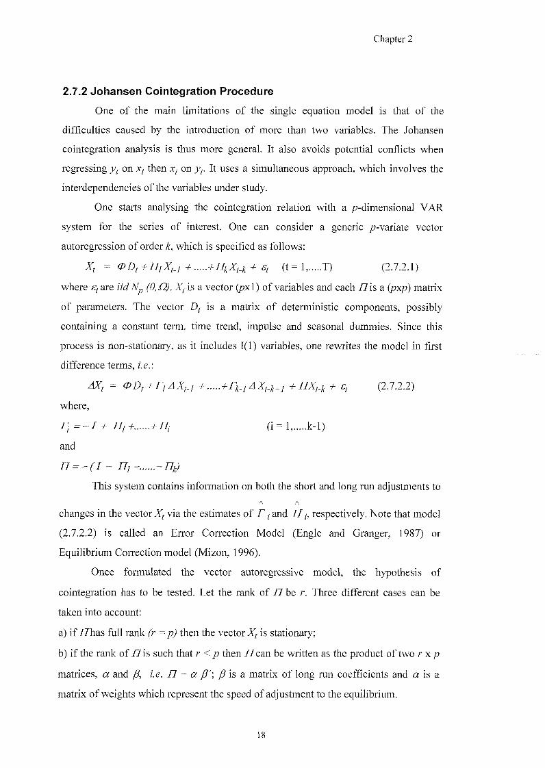
2.7.2 Johansen Cointegration Procedure

One of the main limitations of the single equation model is that of the

difficulties caused by the introduction of more than two variables. The Johansen

cointegration analysis is thus more general. It also avoids potential conflicts when

regressing on Xf then on y . It uses a simultaneous approach, which involves the

interdependencies of the variables under study.

One starts analysing the cointegration relation with a ^-dimensional VAR

system for the series of interest. One can consider a generic ^-variate vector

autoregression of order k, which is specified as follows:

^ T) (2.7.2.1)

where are W (D, is a vector (pxl) of variables and each 77is a (p?^) matrix

of parameters. The vector Df is a matrix of deterministic components, possibly

containing a constant term, time trend, impulse and seasonal dummies. Since this

process is non-stationary, as it includes 1(1) variables, one rewrites the model in first

difference terms, i.e.:

AYj, = f f gjf (2.7.2.2)

where,

^ 77/f . fZ?; ( i - 1, k-1)

and

77 = - r 7 - 77/- . - 7 ^

This system contains information on both the short and long run adjustments to

A A

changes in the vector^ via the estimates of 7", and 77,, respectively. Note that model

(2.7.2.2) is called an Error Correction Model (Engle and Granger, 1987) or

Equilibrium Correction model (Mizon, 1996).

Once formulated the vector autoregressive model, the hypothesis of

cointegration has to be tested. Let the rank of 77 be r. Three different cases can be

taken into account:

a) if 77has fiill rank (r then the vector^ is stationaiy;

b) if the rank of 77 is such that r < ^ then 77 can be written as the product of two r x

matrices, and f.e. 7 7 = ar yg is a matrix of long run coefficients and a is a

matrix of weights which represent the speed of adjustment to the equilibrium.

18

Chapter 2

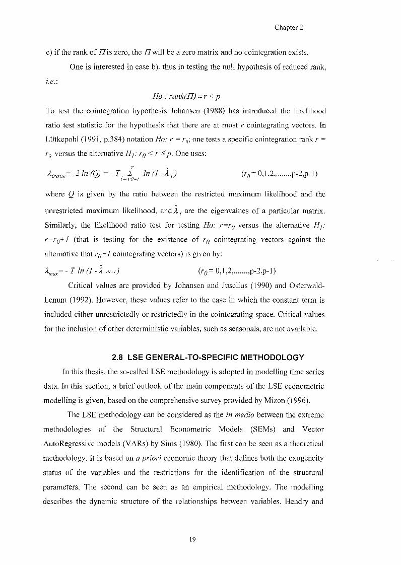
c) if the rank of /7 is zero, the 77will be a zero matrix and no cointegration exists.

One is interested in case b), thus in testing the null hypothesis of reduced rank,

; . g . :

/To . = r < /?

To test the cointegration hypothesis Johansen (1988) has introduced the likelihood

ratio test statistic for the hypothesis that there are at most r cointegrating vectors. In

Lutkepohl (1991, p.384) notation Ho: r = Tq, one tests a specific cointegration rank r =

/"g versus the alternative /"g < r One uses:

-2 ("7 - 1 y; (ro= 0,1,2, ,p-2,p-l)

where Q is given by the ratio between the restricted maximum likelihood and the

unrestricted maximum likelihood, and 1 j are the eigenvalues of a particular matrix.

Similarly, the likelihood ratio test for testing Ho: r=rQ versus the alternative Hf

^=7-0+7 (that is testing for the existence of rg cointegrating vectors against the

alternative that tq+I cointegrating vectors) is given by:

- r (7 - i (ro= 0,1,2, ,p-2,p-l)

Critical values are provided by Johansen and Juselius (1990) and Osterwald-

Lenum (1992). However, these values refer to the case in which the constant term is

included either unrestrictedly or restrictedly in the cointegrating space. Critical values

for the inclusion of other deterministic variables, such as seasonals, are not available.

2.8 LSE GENERAL-TO-SPECIFIC METHODOLOGY

In this thesis, the so-called LSE methodology is adopted in modelling time series

data. In this section, a brief outlook of the main components of the LSE econometric

modelling is given, based on the comprehensive survey provided by Mizon (1996).

The LSE methodology can be considered as the in medio between the extreme

methodologies of the Structural Econometric Models (SEMs) and Vector

AutoRegressive models (VARs) by Sims (1980). The first can be seen as a theoretical

methodology. It is based on a priori economic theory that defines both the exogeneity

status of the variables and the restrictions for the identification of the structural

parameters. The second can be seen as an empirical methodology. The modelling

describes the dynamic structure of the relationships between variables. Hendry and

19

Chapter 2

Mizon (1990) propose: SEMs can be derived from an underlying congruent VAR

representation of the data via a sequence of reductions. Hence, in Hendry and Mizon

methodology both VARs and SEMs play an important role. Starting with a general

Unrestricted Vector AutoRegressive model (UVAR), one obtains a Parsimonious VAR

(PVAR) via a series of valid statistical reductions; hence, a congruent SEM is

achieved. This final congruent SEM can be viewed as an important source for

achieving meaningful and interpretable hypotheses in terms of economic theory;

moreover, the capability of these hypotheses to encompass the PVAR can be

statistically tested.

The main central concepts, on which the LSE methodology is based, follow.

An econometric model needs to be congruent and encompassing.

1. Which are the information for which a model can be recognised as congruent?

# Economic Theory.

One of the requirements for an econometric model is to be founded upon

economic theory. The theory is useful in choosing the variables to include in the model

as well as the functional form to characterise the relationship between them. It is

desirable for the econometric model to be coherent with economic theory. However, as

Hendry (1993) points out, the findings can be in contrast with economic theory. The

divergence between theory and empirical evidence is the first step for the development

of new theories. The main argument is the theory cannot be considered as endowed

with veracity a priory and the theory has to be proven by evidence. This proposition is

still the object of major debates amongst academics.

« Relative Past, Present and Future Sample Information.

a) A model is not congruent with the past sample information if the errors are

correlated with their lagged values. This type of congruence can be tested by the serial

correlation test. It represents a way for checking the adequacy of the dynamic

specification of the model.

b) Several tests can be used to test for model congruence with the present sample

information. These are tests of homoscedasticity, omitted variables and normality in

the error distribution.

c) A model is considered as congruent to the future sample information whenever the

parameter estimates are approximately constant across varying estimation periods.

20

Chapter 2

Tests are available to find out such a property: e.g. Chow (1960) prediction test

statistics.

® Measurement System.

This is another property required for a congruent model. This means that the

variables included in the model have to be transformed in an admissible way. One can

extend the concept to other characteristics of the data such as stationarity, deterministic

non-stationarity, integratedness and seasonality.

9 Rival Models.

Encompassing is an essential property for a model to be congruent. For this,

one requires a model to dominate other rival models. Moreover, a model that

encompasses the general model and is data admissible will be the dominant model.

Hence, the parsimonious encompassing refers to a model that is an acceptable

reduction of the congruent embedding model.

2. What is the information for which a model can be recognised as encompassing?

« Encompassing is the other property of the LSE methodology. Previously, a

definition of parsimonious encompassing has been given. However, there is the

possibility that further information is available after having completed the

modelling and having reached a parsimonious encompassing model with respect to

the "old" information set. In this case, it is necessary to incorporate the new

information and find out if the original model is still robust for this new set of

information. As Mizon (1996) writes, "each model is evaluated with respect to an

information set more general than the minimum one required for its own

implementation, thus achieving robustness to extensions of its information set in

directions relevant for competing models" (p. 122).

The strategy of "general-to-specific" is recognised to be the best strategy within

the LSE methodology. Starting with a very general model, it is possible via a testing

down procedure to reach a congruent and encompassing model, which might also

validate a priori economic theory.

In estimating an autoregressive distributed lag model the choice of the lag

length is of extreme importance. In choosing the lag length one might use the

statistical tests: Wald test and likelihood ratio test (LR). These tests allow one to test

2]

Chapter 2

whether it is statistically significant to reduce the lag length by one. The lag length of a

model can be also chosen by making use of information criteria; Hannan-Quinn,

denoted as the HQ criterion; Schwarz, denoted as the SC criterion; finally, Akaike,

denoted as the AIC criterion. The information criteria are defined as follows:

/ / g = - 2 Zog Z / T + 2/7

where L is the maximised likelihood, T is the sample size and n is the number of

parameters. The estimated information criteria are chosen so that they are minimised.

The final step of the methodology used in this thesis is the feedback to

economic theory (Figure 2.1). The results obtained from the congruent and

encompassing model are compared with the theory. The initial propositions with

respect to income and price elasticities and, in general, the capability of the

independent variables to explain the dependent variable v\ill be examined.

2.8.1 Developments Of The General-To-Specific Procedure

Recent developments have been made in adopting the general-to-specific

approach. Hoover and Perez (1999) find that Hendry and Doornik's computer-

automated PcGets performs well in evaluating econometric model selection strategies

by simulation. A further improvement has been reached by Hendry and Krolzig (1999a

and 1999b). They implement PcGets by introducing concepts from the LSE

methodology such as: tests for pre-selection and encompassing tests for choosing

between multiple models which are found to be congruent with the information set. A

unique model is reached either from the combination of congruent contenders when

the algorithm terminates or by using an information criterion. This new "data mining

reconsidered" needs still further improvements as Hendiy and Krolzig (1999b) point

out. Problems appear in the appropriate parameterisation, functional forms, variable

choice, and inclusion of seasonals and dummies which requires a careful prior

analysis. Moreover, issues as the role of structural breaks and, for example, first

difference constraints on the lags of stationary variables, have still to be investigated

further. It is worth noting that PcGets in Hendry and Krolzig (1999a and 1999b) is

employed to reconsider existing empirical estimations {i.e. UK money demand and the

22

Chapter 2

US narrow-money demand). In their re-analysis, Hendry and Krolzig (1999a) write "it

remains to stress that these cases benefit from "fore-knowledge (e.g. of dummies, lag

length etc.), some of which took the initial investigators time to find" (p.21).

Moreover, Monte Carlo investigation of model selection, which is only possible

because PcGets is automatic, suggests that the pre-test bias is quite manageable. That

is, using 5% level tests gives a reasonable probability of finding the right model, rather

than always finding something, simply because one has done so much testing.

2.9 OTHER METHODS

The following subsections are dedicated to give an account of other methods

that are used in this thesis.

2.9.1 Simultaneity

In Chapters 4 and 5, the problem of simultaneity will be examined by including

some supply variables, that is the number of boats and the number of flight arrivals in

the north of Sardinia. One will employ the Durbin-Wu-Hausman's simultaneity test

when using annual and monthly data (see Pindyck and Rubinfeld, pp. 303-305 for

more details). Such a test will assess the lack of correlation between a right-hand side

variable and the error term. The null hypothesis of no simultaneity implies that the

variable of interest will be treated as predetermined; the alternative hypothesis is that

such a variable can be treated as endogenous.

A brief note, in terms of terminology tised, is due. According to the

the classification of variables into "exogenous" and

"endogenous" (in the case they are determined outside or within the model) and the

causal structure of the model are given a priori and are untestable. This approach has

been criticised on several grounds (see Maddala, 1992, p.389). In particular, Learner

(1985) suggests re-defining the concept of exogeneity. Two concepts of exogeneity are

distinguished:

1) Predeterminedness. A variable is predetermined in a particular equation if it is

independent of the contemporaneous and future errors in that equation.

2) Strict exogeneity. A variable is strictly exogenous if it is independent of the

contemporaneous, future and past errors in the relevant equation.

23

Chapter 2

Engle, Hendry and Richard (1983) extend such concepts in order to "seek

conditions which validate treating one subset of variables as given when analysing

others" (Hendry, 1995, p. 156) and the new notions of weak exogeneity, strong

exogeneity and super-exogeneity are given. One can argue that the notion of weak

exogeneity involves more than a lack of correlation between a right-hand side variable

and the error term.

In this study, the Durbin-Wu-Hausman's test is employed. This test assesses

whether the variable under study is predetermined. One can assume that the generic

demand and supply models can be expressed as follows:

+ (2.9.1.1)

+ + (2.9.1.2)

where:

yf = ^ generic explanatory variable;

Xj= variable which is thought to be determined by the level ofy,;

Zi = variable treated as the instrument.

To test for the existence of simultaneity one follows two steps. Firstly, the

reduced form is obtained by regressing on the variables included into equation

(2.9.1.2) and the instrument variable z . Hence, in the second phase, the residuals

obtained from this regression (say res =w) are added into equation (2.9.1.1). The null

hypothesis of no simultaneity would be rejected at the 10% level when using the two-

tailed f-test. Hence, if the null is rejected the variable (x ) can be treated as endogenous.

2.9.2 Testing For Structural Breaks

In Chapter 5, one will investigate the possible existence of structural breaks in

the seasonal pattern. The presence of seasonal unit roots at some frequencies on one

hand, and problems of specification form appeared in the residuals on the other, can be

considered as a symptom of possible non-stationarity which needs to be examined.

Adopting the Chow test (1967) the null hypothesis of no change is tested, that is the

seasonal coefficients have remained the same within the period under investigation.

An F statistic is calculated and this value will be compared with the correspondent

critical value from the conventional tables. The rejection of the null implies that a

structural break is present. However, such a test assumes the knowledge of the change

24

Chapter 2

point. In the case in which the change point is unknown, one needs to make use of

non-standard distribution. Andrews (1993) has investigated and provided critical

values which one will use in testing for structural changes.

2.9.3 Non-linear Model

In Chapter 8, a non-linear model in modelling real tourism expenditure for Italy

is used. The weighted real industrial production for the main origin countries has been

found to be 1(1) from the ADF test. This implies that the income proxy is non-

stationary in the level, whereas the tourist expenditure is stationary in the level. Hence,

one might want to investigate a non-linear specification for the real income proxy, in

order to reconcile an 1(1) variable as the explanatory variable with an 1(0) variable as

the dependent. The non-linear model is run with TSP 4.3A. The approach involves n

iterations whose objective is to minimise the residuals sum of the squares and Gauss's

method is used. Firstly, derivatives of the equation residual with respect to each

parameter are computed. Then, TSP regresses the current residual on the derivatives,

and the resulting regression coefficients are used as the changes in the parameters. If a

local minimum of the residual sum of squares is achieved the final coefficients in the

artificial regression will be zero. After convergence is achieved, non-linear estimation

statistics have a standard OLS interpretation, although the underlying theory is only

asymptotic.

2.10 CONCLUSION

This chapter has given a description of the main methodological steps adopted

in the thesis. Firstly, a tourism literature review is undertaken which gives the

economic theoretic assumptions. One of the aims of the thesis is to test the theory

using advanced econometric modelling. An extensive data collection exercise is

undertaken for achieving the purpose. Data are collected on different time frequencies

and appropriate variables are constructed. In Section 2.6, an account of Franses

(1991a, and 1991b) and Hylleberg e/ a/. (1990) methodologies is given; these methods

will be used to test for the existence of possible monthly and quarterly seasonal unit

roots, respectively. Hence, the ADF test for testing the existence of long run unit roots

is described. Once established the integration status of the economic series of interest.

25

Chapter 2

a cointegration analysis is undertaken both using single equations and Johansen

cointegration analyses. These cointegration tests have been described in Sections 2.7.1

and 2.7.2. Hence, an account of the LSE general-to-specific methodology is given as

provided in Mizon (1996).

Other topics used in the thesis have been discussed in Section 2.9. In Section

2.9.1, an account is given of the Durbin-Wu-Hausman's simultaneity test when

including supply variables into the model. In Section 2.9.2, it has been discussed the

use of Andrews' (1993) critical values in the case of unknown structural break point.

Finally, Section 2.9.3 has given an account on non-linear modelling which will be one

of the objectives of Chapter 8. Further details for such methods will be given when

they are used.

26

Chapter 3

CHAPTER 3.

CHARACTERISTICS OF INTERNATIONAL AND DOMESTIC

DEMAND FOR TOURISM IN THE ITALIAN PROVINCE OF

SASSARI: A GENERAL INTRODUCTION

Aim of the Chapter:

To examine and identify possible differences between domestic and international

tourism in the north of Sardinia.

3.1 THE DEVELOPMENT OF TOURISM IN THE NORTH OF SARDINIA

According to Crenos (2000), the Sardinian economic system has seen structural

changes since the '50s. Its traditional specialisation sectors, that is agriculture and

mining, have declined due to public policies of industrialisation. High capital

industries, that is chemicals, energy and construction, have driven the economy to a

brief period of expansion until the first half of the '70s. However, along the decades,

this transformation has led to a progressive worsening of Sardinian performance in

terms of internal productivity capacity (GDP from labour and GDP relative

to other Italian regions. Crenos points out the failure of the actual productivity system

in creating jobs opportunities. There are several causes: the small size of the industries,

low levels of highly specialised human capital and institutional inefficiencies.

This study is concerned with tourism that can be considered as a key sector in the

economic development strategy of this Mediterranean island. Sardinia represents one

of the important tourist areas in the Mediterranean Sea. Its main attraction for tourists

consists in the quantity and quality of its natural resources. Its "isolation", its physical

distance from the main Italian tourist destinations (e.g. Costa Adriatica) and

investment projects such as the well known Coworz/o (North-East

Coast) in the early Sixties are all elements that increase the image of this island as an

"exclusive and elite holiday" destination.

2 7

Chapter 3

In this study, particular attention is given to the flows of foreign and domestic

tourists into the north of Sardinia, known as Sassari Province. This Province sees 54%

of the overall flows of tourism to this Italian island (see Confcommercio, 1994). Since

the Fifties the north of Sardinia has been the first Sardinian Province to invest in

tourism. The first investment projects were seen in Alghero (North West Coast),

followed by the Consorzio of Costa Smeralda by Prince Aga Khan. In the Seventies,

other coastal centres were developed such as; Stintino, La Maddalena, Palau and Santa

Teresa di Gallura. Another element that encouraged tourist flows to Sassari Province is

the presence of two of the most important airports and harbours in Sardinia that serve

both national and international traffic to the Western and Eastern Coast.

3.2 FOREIGN VERSUS DOMESTIC DEMAND

In the tourism literature, domestic and foreign flows of tourists are investigated

separately, due to their different characteristics. The majority of empirical studies are

dedicated to the analysis of international demand for tourism. Only a few consider the

domestic component (see for example Raeside ef 1997; Seddighi and Shearing,

1997) or both the components (see Malacarni, 1991).

The following sections are dedicated to capturing the characteristics and

possible differences of the two components in Sassari Province.

3.2.1 Tourist Flows And Their Evolution

The first main difference between domestic and international flows can be

noticed in terms of percentages; the domestic flows of tourists count for the 81%

against a 19% of foreigners. These percentages are calculated in terms of the number

of arrivals of tourists in registered accommodation, averaged for the period between

1972-1995. Figure 3.1 shows the time series from 1972 to 1995 6)r the arrivals of

foreign and domestic tourists, and gives us a better understanding of the historical

evolution of the two components.

28

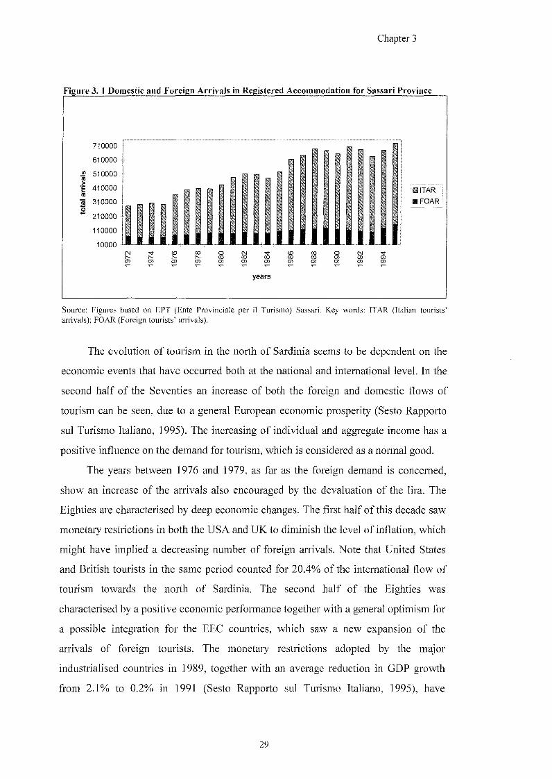
Chapter 3

Figure 3. 1 Domestic and Foreign Arrivals in Registered Accommodation for Sassari Province

710000

610000

« 510000 > •= 410000 ro ra 310000 o

210000

110000

10000

ilTAR IFOAR

o oj M-CO CO CO o> O) cn

years

Source: Figures based on EPT (Ente Provinciale per il Turismo) Sassari. Key words: ITAR (Italian tourists'

arrivals); FOAR (Foreign tourists' arrivals).

The evolution of tourism in the north of Sardinia seems to be dependent on the

economic events that have occurred both at the national and international level. In the

second half of the Seventies an increase of both the foreign and domestic flows of

tourism can be seen, due to a general European economic prosperity (Sesto Rapporto

sul Turismo Italiano, 1995). The increasing of individual and aggregate income has a

positive influence on the demand for tourism, which is considered as a normal good.

The years between 1976 and 1979, as far as the foreign demand is concerned,

show an increase of the arrivals also encouraged by the devaluation of the lira. The

Eighties are characterised by deep economic changes. The first half of this decade saw

monetary restrictions in both the USA and UK to diminish the level of inflation, which

might have implied a decreasing number of foreign arrivals. Note that United States

and British tourists in the same period counted for 20.4% of the international flow of

tourism towards the north of Sardinia. The second half of the Eighties was

characterised by a positive economic performance together with a general optimism for

a possible integration for the EEC countries, which saw a new expansion of the

arrivals of foreign tourists. The monetary restrictions adopted by the major

industrialised countries in 1989, together with an average reduction in GDP growth

from 2.1% to 0.2% in 1991 (Sesto Rapporto sul Turismo Italiano, 1995), have

29

Chapter 3

produced a negative effect on tourism (see Figure 3.1, 1990-1992). The subsequent

expansion of tourism flows in 1994 and 1995 may be due to different causes; the

depreciation of the lira at the end of 1992, political crises in some of the main

competitor countries in the Mediterranean area (e.g. ex-Yugoslavia), the stabilisation

of prices for tourist goods and the intensification of promotional policies by private

firms and public agencies in Sardinia.

As far as domestic arrivals are concerned, an upward trend of arrivals can be

seen within the period under study, with the exception of 1984, 1989, 1990 and 1993;

the latter shows the lowest performance since the second half of the 80's.

3.2.2 Seasonality

Other aspects distinguishing the domestic to the foreign demand for tourism

have to be highlighted. One of the main characteristics of tourism is its seasonality.

The distribution of public holidays and school vacations, as well as the climatic

conditions, have a strong impact on tourism. For example, in the western industrialised

countries (e.g. Italy and France) the môr periods of public holidays are either in the

summer months or at Christmas or Easter. Thus, many resorts and tourist regions

experience "overcrowded" and the "holiday-rush" seasons (Hartmann, 1986). This

strong seasonality appears to be problematic for the tourist service system in the north

of Sardinia. There are a variety of problems, including: an uneven utilisation of

tourism facilities such as hotels, holiday villages, beaches and entertainment, whereas

a more uniform utilisation might lead to a reduction in average prices and an improved

profitability. In the low season, the work force is under-utilised with the consequence

of increased uncertainty for labour conditions. The public sector, on the other hand,

faces problems related to the optimal scale of the public services and infrastructure. In

recent years, both private and public agencies (such as the

Turistiche (ESIT)) have undertaken several projects aimed at the promotion and

marketing of specific products for the period of low season (between October and

May). These could cause changes in the seasonal pattern. It should be noted that

Sardinia's mild climate, with average temperature between 9° C degrees in the colder

30

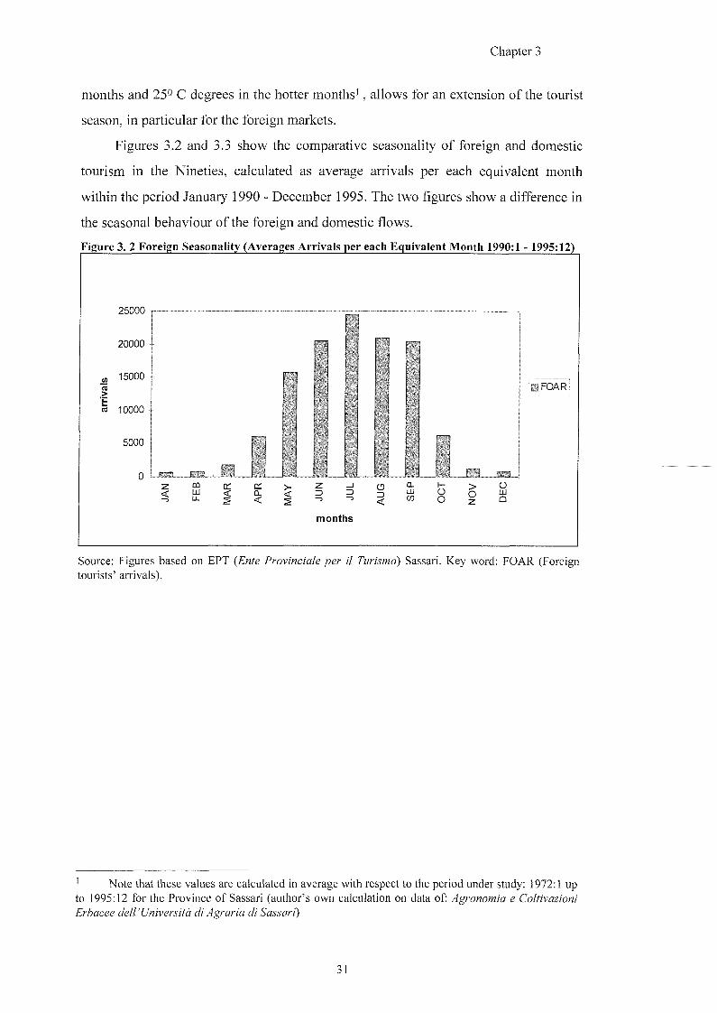
Chapter 3

months and 25^ C degrees in the hotter months', allows for an extension of the tourist

season, in particular for the foreign markets.

Figures 3.2 and 3.3 show the comparative seasonality of foreign and domestic

tourism in the Nineties, calculated as average arrivals per each equivalent month

within the period January 1990 - December 1995. The two figures show a difference in

the seasonal behaviour of the foreign and domestic flows.

Figure 3. 2 Foreign Seasonality (Averages Arrivals per each Equivalent Month 1990:1 - 1995:12)

25000

20000

„ 15000

re 10000

5000

0

iFOAR

CO cc < tr CL <

o <

CL LU (0 u

o z

o UJ Q

months

Source: Figures based on EPT (Ente Provinciale per il Turismo) Sassari. Key word: FOAR (Foreign tourists' arrivals).

' Note that these values are calculated in average with respect to the period under study: 1972:1 up to 1995:12 for the Province of Sassari (author's own calculation on data of: XgroMom/a g Co/Zn'ozzoMf

31

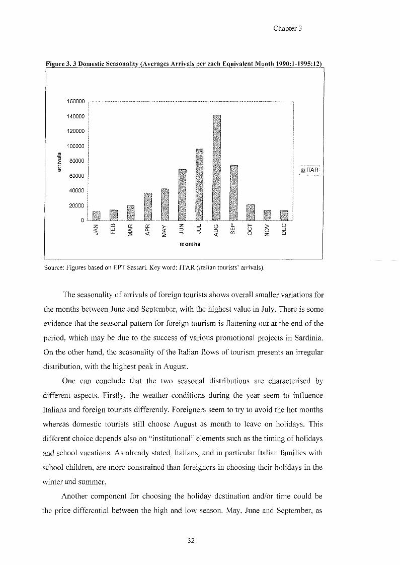
Chapter 3

Figure 3. 3 Domestic Seasonality (Averages Arrivals per each Equivalent Month 1990:1-1995:12)

160000

140000

120000

100000

80000

60000

40000

20000

0 n m LU

rn

iFTAR

ce < cc CL < <

o Z) <

CL 111 w

o o o

o HI Q

months

Source: Figures based on EPT Sassari. Key word: ITAR (Italian tourists' arrivals).

The seasonality of arrivals of foreign tourists shows overall smaller variations for

the months between June and September, with the highest value in July. There is some

evidence that the seasonal pattern for foreign tourism is flattening out at the end of the

period, which may be due to the success of various promotional projects in Sardinia.

On the other hand, the seasonality of the Italian flows of tourism presents an irregular

distribution, with the highest peak in August.

One can conclude that the two seasonal distributions are characterised by

different aspects. Firstly, the weather conditions during the year seem to influence

Italians and foreign tourists differently. Foreigners seem to try to avoid the hot months

whereas domestic tourists still choose August as month to leave on holidays. This

different choice depends also on "institutional" elements such as the timing of holidays

and school vacations. As already stated, Italians, and in particular Italian families with

school children, are more constrained than foreigners in choosing their holidays in the

winter and summer.

Another component for choosing the holiday destination and/or time could be

the price differential between the high and low season. May, June and September, as

32

Chapter 3

low season months, are characterised by lower prices for tourist accommodation. From

the previous graphical comparison, it seems that foreign tourists are more sensitive

than Italians to price changes. Such a hypothesis has been investigated by Malacarni

(1991) in a study on Italian tourism. Malacami has derived a price elasticity of -0.83

for the international tourism demand in Italy and a price elasticity of -0.16 for the

domestic demand. One of the aims is to consider whether these results can be extended

to Sassari Province case.

So far, the main differences in the evolution of tourist flows as well as in the

seasonal characteristics suggest modelling foreign and domestic demand for tourism

separately. However, such a priori assumption needs to be investigated further. In the

next chapters the aim will consist in validating such a distinction within an

econometric and statistical frame.

3.3 POSSIBLE DETERMINANTS OF TOURISM IN NORTH SARDINIA

In the following subsections, an account will be given of the main determinants

that are expected to have an impact on the demand for tourism in the north of Sardinia

in accordance with economic theory.

3.3.1 The Dependent Variable

In analysing the demand for tourism in the north of Sardinia the number of

arrivals of tourists is taken as the dependent variable. As already noted in Section 2.3

(Chapter 2), this choice is constrained by the availability of the data.

Given the complexity of the tourism phenomenon, difficulties appear in finding

a comprehensive and agreeable deRnition. In the tourism literature, as Masberg (1998)

writes, dissimilar definitions appear. In this thesis, one accepts the notion provided by

the United Nations Conference on International Travel and Tourism of 1963 (see

Sinclair, 1998) for which: a tourist is a "temporary visitor who spends more than 24

hours in destinations other than their normal place of residence, whose journey is for

the purpose of holiday-making, recreation, health, study, religion, sport, visiting family

or Mends, business or meetings. Those who spend less than 24 hours in their

destinations are defined as excursionists" (p.4). Hence, when one talks about tourists'

flows one does not separate the flows for recreation purposes from those for business.

Chapter 3

However, the latter component can be considered as a small quota in the overall tourist

flows to the north of Sardinia. Note, in fact, that the most industrialised province is

that of Cagliari in the south of the region, with its own airport and harbour. More

generally, it is worth noting that very few surveys exist that make a differentiation

between the two components, see for example the Swedish Tourism and Travel Data

Base (Nordstrom, 1996 gives a detailed discussion). In Italy, such a differentiation has

only been carried out since 1995 by means of surveys, and, therefore, the sample size

available is quite small.

As Baron (1989) points out the "trading-day factors" might be important in the

analysis of monthly data, that take into account the effects of four of five Saturdays (or

Sundays) in a particular month. As far as the demand for international tourism is

concerned, Saturday has been chosen as the starting day of the holiday. The majority of

the charter flights and boat trips to the north of Sardinia occur, in fact, on a Saturday.

Therefore, the dependent variable has been adjusted in order to take into account the

number of Saturdays in each month for the period under consideration. It is worth

noting that the latter normalisation cannot be considered arbitrary. A previous

investigation has been carried out using the raw series of the foreign arrivals (see

Appendix A for a complete discussion). Such analysis encountered problems of non-

normality and heteroscedasticity (at the 1% level), which have been corrected with the

adjustment of the dependent variable for the number of Saturdays in a month.

In the analysis for the domestic demand of tourism, Sunday has been chosen as

the starting day of the holiday. Such a choice will be supported by the results obtained

from two separate models. The first model includes the series of arrivals normalised

for the number of Sundays in a month as the dependent variable. The second model

has the dependent variable normalised for the number of Saturdays in a month. A

complete discussion is provided in Chapter 5. "It is evident that the distribution of

public holidays, especially school vacations, has a strong impact on the individual

timing of the vacation and travel days within the annual cycle", (Hartmann, 1986, p.

26). It is plausible to believe that a great part of arrivals of domestic clients tend to

occur on Sunday, as, in Italy, for the majority of private and public activity Saturdays

are trading-days. However, any day of the week is likely to be the starting day of the

34

Chapter 3

holidays for Italians and this point will emerge from the econometric analysis later in

this thesis.

In the present study, one will also consider whether the current tourist

consumption is influenced by the past demand. For this purpose, one will include the

lagged dependent variable in order to determine whether domestic and foreign tourists

can be defined as "psychocentric" or "allocentric"^ (Sinclair and Stabler, 1997).

3.3.2 Economic Determinants

As already stated in the methodology chapter (Section 2.3), income, relative

price, exchange rate and substitute price are considered as the main relevant

explanatory variables in the analysis of tourism.

a) Income. The best variable to construct the income index is the personal disposable

income (see Witt and Witt, 1992). However, such a variable is not available with a

monthly frequency. Thus, as suggested by some authors (see Gonzalez and Moral,

1995; Garcia-Ferrer and Queralt, 1997) one will use the weighted average of the

industrial production (see Appendix B for the construction of this variable), for the

main clients of the north of Sardinia, as a proxy of income. The index of industrial

production in Italy is taken as a proxy of income for the analysis of the domestic

demand for tourism. From a VAR analysis, as given in Chapter 5, there is statistical

evidence that the Italian industrial production index is a valid proxy of the Italian

disposable income per capita.

b) gxcAange mfg. According to economic theory another important

determinant of the demand for tourism is the price of goods and services. However,

there are many problems in determining a tourist consumer price index. The tourist

good, in fact, is heterogeneous including costs of transportation, accommodation

resorts, entertainment, souvenirs, etc. Because of the lack of such an index, many

researchers use as its proxy the consumer price index. As Sinclair and Stabler (1997)

point out, Martin and Witt (1987) study is virtually the only study to investigate its

2 "Phychocentric" is a tourist who prefers a familiar destination other than a new destination. In this case, a positive coefficient sign is expected between current and past demand, and the coefficient for the long lags is expected to be statistically significant. "Allocentric" is a tourist who prefers new destination for his/her own holidays. A negative coefficient sign is hence expected together with a rapid adjustment. Note that the negative sign for the lagged dependent variable could be also due to undesiderable characteristic of a particular destination.

35

Chapter;

suitability as a proxy. As many other authors, the present study will base on their

empirical findings employing the consumer price index as a valid proxy.

Furthermore, in analysing the international demand for tourism in the north of

Sardinia, the exchange rate is included on its own, in addition to the relative price. In

particular, the exchange rate has been constructed using a weighting system based on

market shares of the major clients {i.e. Belgium, France, Germany, Sweden,

Switzerland, UK and USA) for the north of Sardinia (see Appendix B for a more

detailed analysis).

c) Substitute price. One of the debates in the tourism literature is related to which is

the most appropriate specification for the substitute price. Sometimes substitute prices

and exchange rates have been included as separate explanatory variables, whereas in

other studies a real substitute price was included.

The analysis will be articulated in the following manner. In Chapters 4 and 5,

one will assume that the nominal substitute price could be thought to be the main

determinant in explaining the demand for tourism in the north of Sardinia. In Chapter

6, one will examine the possibility to include either the exchange rate for the

competitors as a separate variable or the real substitute price.

d) Supply variables. So far one has taken into consideration the variables linked with

the demand side. "Tourism is traditionally conceived in terms of the demand-side or

consumer characteristics (e.g. the duration and geographic extent of a trip taken by a

traveller), which places the industry in a difficult political and statistical position"

(Smith, 1995, p.34). The tourism activity, in fact, can be considered sui generis, since

it is not defined in terms of its products but in terms of its consumers.

It is important to classify the components of the supply of tourism, which is a

composite of activities, services, and industries that facilitate travel and activity away

from one's usual environment. The main components of tourism supply are: natural

resources which include climate, natural beauty, flora, Anna, beaches and many others;

infrastructures, such as harbours, airports, roads, bus and train station facilities, hotels,

restaurants, entertainments and similar structures; transportation that includes

aeroplanes, boats, trains, taxis, and other facilities; hospitality and cultural resources,

such as the attitude of the residents toward tourists, arts, history, traditions, sports and

many others (Mcintosh, Goeldner and Ritchie, 1995).

Chapter 3

It might be relevant, therefore, to consider variables that express both the

quantity and the quality of the supply services. The amount of accommodation and for

example: beds, flights, trains or/and boats can define the extent of the quantity of

supply; while the proportion of 3-5 star hotels and/or the ratio (beds/toilets) could be

considered as a good proxy for the quality of the supply.

In order to take into consideration a component of the quantity of the supply

services, in estimating the annual foreign and domestic demand for tourism in the

north of Sardinia, one will include two variables that is: the number of arrivals of boats

in the two main ports (Porto Torres and Olbia) and the number of arrivals of flights in

the two main airports (Fertilia and Olbia)^. The results from estimating the

international and domestic demand for tourism using annual data will suggest a further

investigation by adopting the simultaneity Durbin-Wu-Hausman's test.

Providing an ample tourism supply to match anticipated demand in the long run

is a challenge for the planners. The evolution of the supply of tourism is strictly linked

with the evolution of the demand. In developed countries, in recent years, there has

been an increase both in the standard required in, and the total demand for, tourism.

Not only wealthier individuals look for leisure time but also larger and larger

proportions of the total population. Demand can change quite rapidly. Supply

components (e.g. infrastructures and services) are more rigid.

In a short run context it is important to detect the seasonal fluctuations of the

demand and supply levels. Tourism, unlike many other products, is a composite

product and has a perishable nature, since unfilled airline seats and unused hotel rooms

cannot be stockpiled. "If firms selling tangible goods can deal with demand fluctuation

through the inventory process, this option is not available to firms providing travel

services. In the travel industry, an effort must be made to reduce seasonal fluctuations

as much as possible" (Mcintosh et al., 1995, p.291).

The intent is to illustrate the supply situation associated with fluctuating

demand levels for the Province of Sassari. In order to understand the extent of

utilisation of accommodation by the total number of tourists in Province of Sassari,

one introduces the following definition:

The source is the ''Annuario Statistico Italiand" ( 1 9 7 2 - 1 9 9 6 ) .

3 7

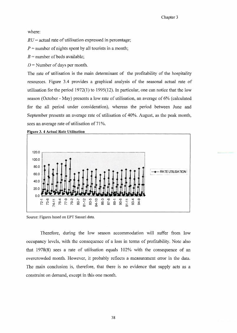
Chapter 3

where;

RU= actual rate of utilisation expressed in percentage;

P = number of nights spent by all tourists in a month;

B = number of beds available;

D = Number of days per month.

The rate of utilisation is the main determinant of the profitability of the hospitality

resources. Figure 3.4 provides a graphical analysis of the seasonal actual rate of

utilisation for the period 1972(1) to 1995(12). In particular, one can notice that the low

season (October - May) presents a low rate of utilisation, an average of 6% (calculated

for the all period under consideration), whereas the period between June and

September presents an average rate of utilisation of 40%. August, as the peak month,

sees an average rate of utilisation of 71%.

Figure 3. 4 Actual Rate Utilisation

-RATELmUSATDNl

co i c o r ^ c n o i c o ^ i -C 0 < ' C 0 C 0 C O O ) T - O ) O )

CO O )

Source: Figures based on EPT Sassari data.

Therefore, during the low season accommodation will suffer from low

occupancy levels, with the consequence of a loss in terms of profitability. Note also

that 1978(8) sees a rate of utilisation equals 102% with the consequence of an

overcrowded month. However, it probably reflects a measurement error in the data.

The main conclusion is, therefore, that there is no evidence that supply acts as a

constraint on demand, except in this one month.

38

Chapter 3

3.3.3 Extra Economic Determinants

Tastes and preferences of tourists, and environment are considered as the main

factors affecting the demand for tourism. Dummy variables can be introduced in the

econometric model to take some of these qualitative determinants into account.

In this study some extra-economic determinants have been taken into

consideration: a) the Easter effect which has major importance for the performance of

the tourism in the north of Sardinia. Some mis-specifications have arisen in the model

by not taking into account the former variable, b) The weather conditions that can also

be considered as a natural resource and, therefore, regarded as a component of the

tourism supply, as mentioned in the previous subsection (Mcintosh et al, 1995). c)

Two main streams of thought are in the literature. First, a time trend is included in the

model in order to pick up possible changes in consumers' tastes for a specific

destination over time. Second, the time trend variable is recognised as hiding problems

of multicollinearity, i.e. as possibly highly correlated to other economic variables such

as income. In this study, a time trend will be included in the final restricted model

upon a statistically significant coefficient.

3.4 CONCLUSION

So far, one has given a general introduction on the main characteristics of the

tourism demand in Sassari Province of Italy. An account has been given of the

differences between the international and domestic demand based on the evolution of

the tourist flows and on the seasonal distributions. In accordance with economic

theory, the possible determinants that might have a role in explaining the demand for

tourism in the north of Sardinia have been described.

The plan of the next three chapters is the following. Chapter 4 will be dedicated

to the analysis of the international demand. In Chapter 5, a model for the domestic

tourism demand will be estimated. In Chapter 6, a deeper investigation for the

inclusion of the nominal substitute price and exchange rate for the main competitors

will be carried out.

Chapter 4

CHAPTER 4.

INTERNATIONAL DEMAND FOR TOURISM IN THE NORTH OF

SARDINIA

Aim of the Chapter:

To model and estimate the international demand for tourism in Sassari Province of

Sardinia (north of Sardinia), Italy.

4.1 INTRODUCTION

The aim of this chapter is to examine the economic factors affecting the demand

for international tourism in the Province of Sassari in the island of Sardinia with the

view of developing an econometric model for the short run and long run analysis. As

already pointed out, given the noticeable differences in the seasonal pattern of the

domestic and foreign demand, particular attention will be given in studying the

determinants of foreign demand and of the domestic demand separately.

In many empirical studies the demand for tourism has been investigated using

annual or quarterly data (Summary, 1987; Martin and Witt, 1988; Smeral, 1988;

Kulendran, 1995; Seddighi and Shearing, 1997; Song et al., 2000; Kulendran and Witt,

2001), whereas very few studies deal with monthly data (Rugg, 1973; Bond, 1979;

Gonzales and Moral, 1996; Lim and McAleer, 2001). In the present study particular

emphasis is given to the use of monthly time series (from January 1972 until

December 1995). Such a time interval allows for the investigation of seasonal variation

in the time series under consideration. It is possible, for example, that changes in the

tastes and preferences of tourists can affect the seasonal pattern. Other influences on

demand will also be examined. In particular, the importance of variations in the date of

Easter will be highlighted, where Easter Sunday varies between March 26 and April 22

as far as the period under modelling is concerned. In addition, the so called "trading-

days" effect will be carefully studied (Baron, 1989). This involves allowing for the

4 0

Chapter 4

effect of four or five weekends in a particular month. The study includes also a

comparison between the use of monthly, quarterly and annual data.

Use is made of the Johansen multivariate cointegration procedure in order to

identify stable long run relationships amongst the variables under consideration. In the

literature, there are just a few studies which apply the notion of cointegration to

modelling demand for tourism. See Sinclair (1998) for a review. Lanza and Urga

(1995), for example, apply the Johansen procedure to annual tourism expenditure for

13 European countries from 1975 to 1992. Vogt and Wittayakorn (1998), apply a test

for stationarity and cointegration to variables with an annual frequency in estimating

the determinants of the demand for Thailand's exports of tourism. Notably, Song et al.

(2000) apply the LSE methodology in estimating the outbound tourism demand in the

UK; annual expenditure data from 1965 to 1994 have been employed.

In the present study, the total arrivals of foreign tourists in all registered tourist

accommodation in the north of Sardinia will be analysed and modelled. "Tourist

arrivals" have been used in many empirical studies and are considered a good proxy

for the demand for tourist goods and services (Crouch, 1994, gives a detailed review).

This study assumes that the supply of tourism services and in particular the

supply of accommodation in the north of Sardinia is perfectly elastic in the short run,

/. e. not acting as a constraint on demand. The support for this assumption has already

been given in the general introduction (Chapter 3). As a reminder, the only exception

was for August 1978.

In terms of economic analysis, emphasis will be given in exploring the

relationship between short and long run income and prices elasticities.

Section 4.2 will be dedicated to the analysis and estimation of the international

demand for tourism in the north of Sardinia employing monthly data. In the

subsections the analysis will be concentrated on the following; a time series analysis

for the international demand; the notion of cointegration will be introduced for the

variables which present long run unit roots (i.e. relative price and exchange rate); a

monthly frequency model will be estimated, where short run and long run relationships

will be taken into consideration. In Section 4.3, an annual model will be estimated.

The subsections will be dedicated to simultaneity problems when supply variables,

such as the number of international number of flights and the total number of boat

4 1

Chapter 4

arrivals in Sassari Province will be considered. Section 4.4 will be dedicated to the

estimation of a model when employing quarterly data. A summary and conclusions

will be given as final sections.

4.2 INTERNATIONAL DEMAND FOR TOURISM USING MONTHLY DATA

4.2.1 A Time Series Analysis

One needs to take into account seasonality and non-stationarity, and test for

cointegration that will lead to the framework of the Error Correction Models (ECM). A

"pre-modelling" analysis is of particular value in order to assess the properties of the

variables under study without which the quality of the empirical results may be

questionable (see Song ef aZ. 2000; Lim and McAleer, 2000).

In this study the method described in Franses (1991a, 1991b) to test for

seasonal unit roots with monthly data is used. This is applied to five series: i.e. the

adjusted foreign arrivals of tourists'^, LA, for the period January 1972 up to December

1995; the exchange rate, (1972:1 to 1995:12); a relative price index, is

taken into consideration for the period from January 1972 to December 1995 and a

substitution price index, LSP-, and finally, the index of industrial production

(1990=100) from 1972:1 to 1995:12, LPR. See Appendix B for a detailed discussion of

the determination of these variables. In each case the natural logarithm of the variables

is used. Graphs of each series are provided in Figure 4.1.

The tourist arrivals data are collected by the (/e/ e t/eZ/o and through the Enti Provinciali per il Turismo (EPT) e le Stazioni di cur a, di soggiorno e di turismo. Data are collected all over the national territory for all the accommodation infrastructures (hotels, pensioni, locande, youth hotels, camp sites, tourist residences, houses for holidays, rifugi, pensionati, colonie, religious institutions, private residences, villas, flats or rooms rented for holidays).

The data collection is done on the basis of the daily declarations from the providers of accommodation, of the clients' arrivals and of total nights spent in the particular accommodation.

Note that this variable has been created dividing the monthly number of tourists' arrivals by the number of Saturdays in a month (as stated in Chapter 3).

4 2

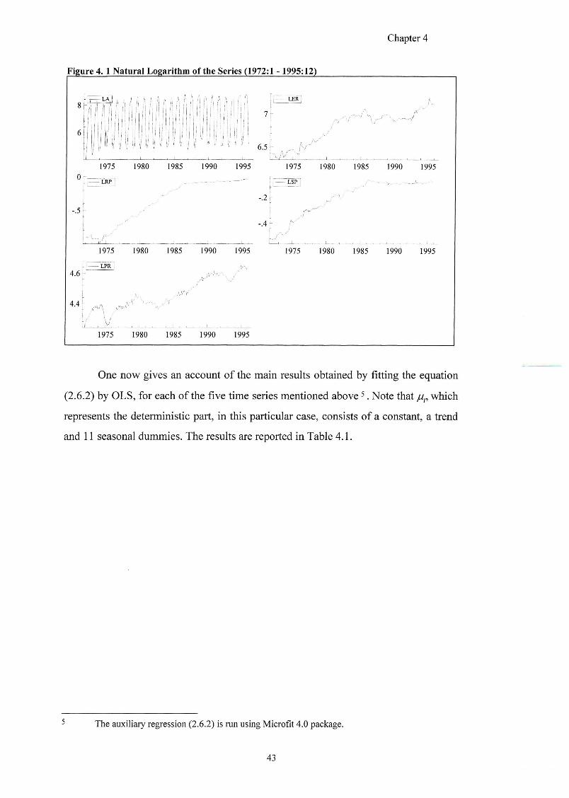
Chapter 4

Figure 4 .1 Natural Logarithm of the Series (1972:1 -1995:12)

I 'ill

-.5-

4jl

4.4

S A i r r i A f i I!

I III 11 ; !; ! '! i!

J

6.5;

1975 1980 1985 1990 1995 1975 1980 1985 1990 1995

, — LSP

- .2 r

-.4

1975 1980 1985 1990 1995

_ _ v 1975 1980 1985 1990 1995

1975 1980 1985 1990 1995

One now gives an account of the main results obtained by fitting the equation

(2.6.2) by OLS, for each of the five time series mentioned above ^. Note that //,, which

represents the deterministic part, in this particular case, consists of a constant, a trend

and 11 seasonal dummies. The results are reported in Table 4.1.

The auxiliary regression (2.6.2) is run using Microfit 4.0 package.

43

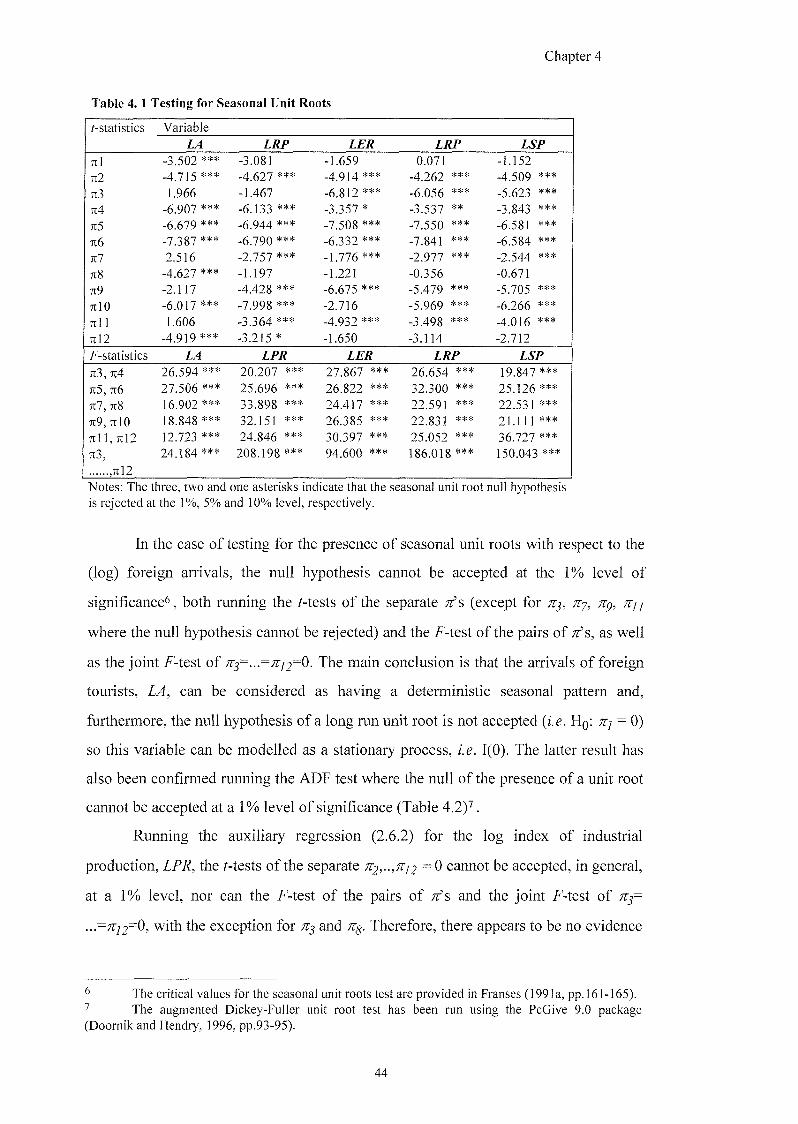
Chapter 4

Table 4. 1 Testing for Seasonal Unit Roots

^-statistics Variable

LA LRP LER LRP LSP

7t l - 3 . 5 0 2 *** -3 .081 - 1 . 6 5 9 0 .071 - 1 . 1 5 2

7I2 -4 .715 *** - 4 . 6 2 7 *** - 4 . 9 1 4 *** - 4 . 2 6 2 *** - 4 . 5 0 9 ***

tc3 1.966 -1 .467 - 6 . 8 1 2 *** - 6 . 0 5 6 *** -5 .623 ***

-6 .907 *** -6 .133 *** - 3 . 3 5 7 * -3 .537 ** -3 .843 ***

Ji5 - 6 . 6 7 9 *** . 6 . 9 4 4 *** -7 .508 *** - 7 . 5 5 0 *** -6 .581 ***

7X6 -7 .387 *** - 6 . 7 9 0 *** - 6 . 3 3 2 *** -7 .841 *** -6.584 ***

Til 2 . 5 1 6 - 2 . 7 5 7 *** -1 .776 *** - 2 . 9 7 7 *** - 2 . 5 4 4 ***

- 4 . 6 2 7 *** - 1 . 1 9 7 -1 .221 - 0 . 3 5 6 -0 .671

-2.117 - 4 . 4 2 8 *** -6 .675 *** - 5 . 4 7 9 *** -5 .705 ***

TllO -6 .017 *** - 7 . 9 9 8 *** - 2 . 7 1 6 - 5 . 9 6 9 *** - 6 . 2 6 6 ***

Til 1 1.606 - 3 . 3 6 4 *** - 4 . 9 3 2 *** -3 .498 *** -4 .016 ***

7112 - 4 . 9 1 9 *** - 3 . 2 1 5 * - 1 . 6 5 0 -3.114 - 2 . 7 1 2

F-statistics LPR LER LRP LSP

;r3,714 2 6 . 5 9 4 *** 2 0 . 2 0 7 *** 2 7 . 8 6 7 *** 2 6 . 6 5 4 *** 19 .847 ***

7l5, 7l6 2 7 . 5 0 6 *** 2 5 . 6 9 6 *** 2 6 . 8 2 2 *** 3 2 . 3 0 0 *** 2 5 . 1 2 6 ***

7l7, 7[8 16 .902 *** 3 3 . 8 9 8 *** 2 4 . 4 1 7 *** 22 .591 *** 22 .531 ***

7t9, nlO 18.848 *** 32 .151 *** 2 6 . 3 8 5 *** 22 .831 *** 21 .111 ***

T i l l , Till 12.723 *** 2 4 . 8 4 6 *** 3 0 . 3 9 7 *** 2 5 . 0 5 2 *** 3 6 . 7 2 7 ***

7I3, 2 4 . 1 8 4 *** 2 0 8 . 1 9 8 *** 9 4 . 6 0 0 *** 186 .018 *** 150 .043 ***

,7112 Notes; The three, two and one asterisks indicate that the seasonal unit root null hypothesis is rejected at the 1%, 5% and 10% level, respectively.

In the case of testing for the presence of seasonal unit roots with respect to the

(log) foreign arrivals, the null hypothesis cannot be accepted at the 1% level of

significance^, both running the Mests of the separate (except for

where the null hypothesis cannot be rejected) and the F-test of the pairs of Tfs, as well

as the joint F-test of The main conclusion is that the arrivals of foreign

tourists, LA, can be considered as having a deterministic seasonal pattern and,

furthermore, the null hypothesis of a long run unit root is not accepted {i.e. Hq: tij = 0)

so this variable can be modelled as a stationary process, z.e. 1(0). The latter result has

also been confirmed running the ADF test where the null of the presence of a unit root

cannot be accepted at a 1% level of significance (Table 4.2)^.

Running the auxiliary regression (2.6.2) for the log index of industrial

production, the f-tests of the separate cannot be accepted, in general,

at a 1% level, nor can the F-test of the pairs of ; f s and the joint F-test of ;zj=

...=;r;2=0, with the exception for and Therefore, there appears to be no evidence

° The critical values for the seasonal unit roots test are provided in Franses (1991a, pp. 161-165). ^ The augmented Dickey-Fuller unit root test has been run using the PcGive 9.0 package (Doomik and Hendry, 1996, pp.93-95).

44

Chapter 4

for the presence of seasonal unit roots. On the other hand, the null hypothesis nj =0

cannot be accepted at a 20% level of significance, but can at the 10% level. The latter

result is investigated further by an ADF test. As shown in Table 4.2, one can see that

the level of this series is stationary as the null hypothesis of the presence of a unit root

cannot be accepted at a 5% level where a constant and a trend have been included.

Thus, it can be concluded that LPR is stationary in the level about a trend. However,

the income proxy {LPR) can be considered non-stationary in the level, but stationary in

the first difference when including just the constant (and seasonal dummies). This

result suggests that deviations from linear trend might have a role in explaining the

international demand for tourism.

The main result of running equation (2.6.2) for the relative price, (LRP), is that

the null of the presence of seasonal unit roots cannot be accepted, taking into account

the outcomes for the r-tests (with the exception for and ; t j2) the F-tests for pairs of

n's, and for the joint F-test, at a 1% level of significance. Note also that the null

hypothesis 7rj=0 cannot be rejected at a 5% level. From the ADF unit root test (Table

4.2) one concludes that is integrated of order one, when a constant, constant and

trend, and constant, trend and seasonal dummies are included.

The seasonal unit roots test has been run for the exchange rate (lEjf) for the

same period. Running the auxiliary regression (2.6.2), one can conclude that there

appears to be no evidence for the presence of seasonal unit roots, denoting a regular

seasonal pattern. The null hypothesis has to be accepted for TTJQ and ;r/2, as well for

the long run frequency. As in the previous case, the null hypothesis of non-stationarity

cannot be rejected at a 5% level of significance, testing 7rj=0 using the f-test. This

result is confirmed also by the ADF test (see Table 4.2). Thus, LER has to be

considered an 1(1) process.

The last variable under consideration is the substitute price (LSP). The main

result from the OLS regression is that the presence of seasonal unit roots cannot be

accepted at a general 1% level, both performing the /-tests of the separate (except

fbr and /zy ) and the F-test of the pairs of ;r's, as well as the joint F-test of ;Zj=...=

Whereas, the Hg: cannot be rejected at a 5% level; this result seems to

indicate that this series is non-stationary. To test further the latter finding, an ADF test

is run. From this test the null of the presence of a unit root cannot be accepted at a 5%

45

Chapter 4

level (Table 4.2), but can, marginally, at the 1% level of significance, when including

either a constant or a constant and seasonals. Thus, one might treat 2 5 ? as a stationary

process, i.e. 1(0). At this point a brief observation is due with respect to the substitute

price. Experiments have shown as the substitute price can be considered stationary in

the level when a constant is included, whereas such a variable seems to be integrated

of order one when a constant and a time trend are included (Table 4.2). The choice of

including just a constant in performing the ADF test is supported by the following

assumptions. Firstly, the inclusion of a trend implies the presence of unit root plus a

quadratic trend. Secondly, as can be seen in Figure 4.1, the data show an adjustment to

a stable situation, given the zones for exchange rate stability in the European Union

(EU). As the competitors included are EU (France, Greece, Spain and Portugal), it is

difficult to accept long run non-stationarity in this variable.

4 6

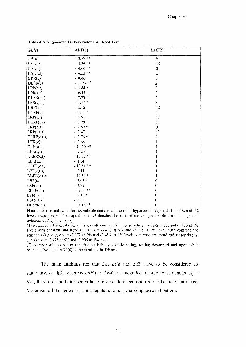
Chapter 4

Table 4. 2 Augmented Dickey-Fuller Unit Root Test

Series

LAÔ - 3 . 8 7 * * 9

LA(c,t) - 4 J 6 * * 10 LA(c,s) - 4 . 0 6 * * 2 LA(c,s,t) - 6 J 3 * * 2 LPR(c) - 0 . 4 6 3 DLPR(c) - I L 7 7 * * 2 LPR(c,t) - 3 . 8 4 * 8 LPR(c,s) - O j j 3 DLPR(c,s) - 7 J 3 * * 2 LPR(c,t,s) - 3 J 7 * 8 LRP(c) - 2 U 6 12 DLRP(c) - 3 U 1 * 11 LRP(c,t) - 0.64 12 DLRP(c,t) - 3 J 8 * 11 LRP(c,s) - 2 . 8 9 * LRP(c,t,s) - O j J 12 DLRP(c,t,s) - 3 J % * 11

LERÔ - 1 . 6 8 1 DLER(c) - l O J O * * 1 LER(c,t) - 2 . 2 0 1 DLER(c,t) - 1&72** 1 LER(c,s) - 1.61 1 DLER(c,s) - 10.51 ** 1 LER(c,t,s) - 2 J 1 1 DLER(c,t,s) - 1&54** 1 LSP(c) - 3 . 0 3 * 0 LSP(c,t) - 1 . 2 4 0 DLSP(c,t) - 1 5 3 6 * * 0 LSP(c,s) - 3 U 6 * 0 LSP(c,t,s) - I J 8 0 DLSP(c,t,s) - 1 5 ^ 3 * * 0

Notes: The one and two asterisks indicate that the unit root null hypothesis is rejected at the 5% and 1% level, respectively. The capital letter D denotes the first-difference operator defined, in a general notation, by Dx( = Xf (1) Augmented Dickey-Fuller statistics with constant (c) critical values = -2.872 at 5% and -3.455 at 1% level; with constant and trend (c, f ) c.v.= -3.428 at 5% and -3.995 at 1% level; with constant and seasonals {i.e. c, s) c.v. = -2.872 at 5% and -3.456 at 1% level; with constant, trend and seasonals {i.e. c, t, s) c.v. = -3.428 at 5% and -3.995 at 1% level; (2) Number of lags set to the first statistically significant lag, testing downward and upon white residuals. Note that ADF(O) corresponds to the DP test.

The main findings are that LA, LPR and LSP have to be considered as

stationary, i.e. 1(0), whereas LRP and LER are integrated of order d=\, denoted ~

1(1)-, therefore, the latter series have to be differenced one time to become stationary.

Moreover, all the series present a regular and non-changing seasonal pattern.

47

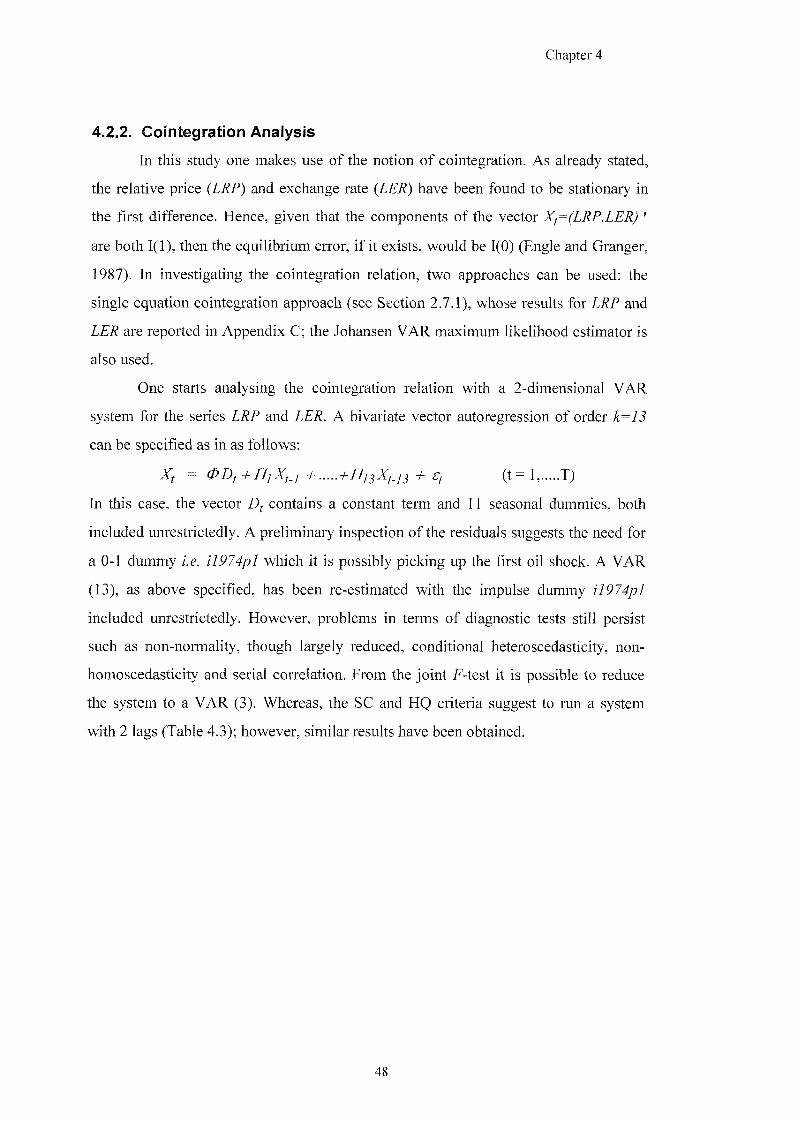
Chapter 4

4.2.2. Cointegration Analysis

In this study one makes use of the notion of cointegration. As already stated,

the relative price {LRP) and exchange rate {LER) have been found to be stationary in

the first difference. Hence, given that the components of the vector XF=(LRP,LER) '

are both 1(1), then the equilibrium error, if it exists, would be 1(0) (Engle and Granger,

1987). In investigating the cointegration relation, two approaches can be used: the

single equation cointegration approach (see Section 2.7.1), whose results for LRP and

LER are reported in Appendix C; the Johansen VAR maximum likelihood estimator is

also used.

One starts analysing the cointegration relation with a 2-dimensional VAR

system for the series LRP and LER. A bivariate vector autoregression of order k=13

can be specified as in as follows;

^ ( t = l , T)

In this case, the vector contains a constant term and 11 seasonal dummies, both

included unrestrictedly. A preliminary inspection of the residuals suggests the need for

a 0-1 dummy i.e. il974pl which it is possibly picking up the first oil shock. A VAR

(13), as above specified, has been re-estimated with the impulse dummy

included unrestrictedly. However, problems in terms of diagnostic tests still persist

such as non-normality, though largely reduced, conditional heteroscedasticity, non-

homoscedasticity and serial correlation. From the joint F-test it is possible to reduce

the system to a VAR (3). Whereas, the SC and HQ criteria suggest to run a system

with 2 lags (Table 4.3); however, similar results have been obtained.

4 8

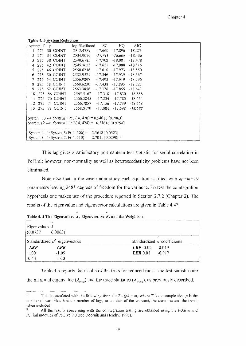
Chapter 4

Table 4. 3 System Reduction

system T P log-likelihood SC HQ AIC 1 275 30 COINT 2512.4789 -17.660 -17.896 -18.273 2 275 34 COINT 2534.9070 -18.009 -18.436 3 275 38 COrNT 2540.6785 -17.702 -18.001 -18.478 4 275 42 COINT 2545.7655 -17.657 -17.988 -18.515 5 275 46 COINT 2550.6216 -17.610 -17.973 -18.550 6 275 50 COINT 2552.9521 -17.546 -17.939 -18.567 7 275 54 COINT 2556.9897 -17.493 -17.919 -18.596 8 275 58 COINT 2560.6230 -17.438 -17.895 -18.623 9 275 62 COINT 2563.3856 -17.376 -17.865 -18.643 10 275 66 COINT 2565.5167 -17.310 -17.830 -18.658 n 275 70 COINT 2566.2845 -17.234 -17.785 -18.664 12 275 74 COINT 2566.7857 -17.156 -17.739 -18.668 13 275 78 COINT 2568.0470 -17.084 -17.698 -7&677

System 13 —> System 12: F( 4, 470) = -0.54016 [0.7063] System 12 - > System 11: F( 4, 474) = = 0.21616 (0.9294]

System 4 -> System 3: F( 4, 506) = 2.3618 [0.0523] System 3 -> System 2: F(4, 510) = 2.7041 [0.0298] *

This lag gives a satisfactory portmanteau test statistic for serial correlation in

PcFiml; however, non-normality as well as heteroscedasticity problems have not been

eliminated.

Note also that in the case under study each equation is fitted with

parameters leaving 248* degrees of freedom for the variance. To test the cointegration

hypothesis one makes use of the procedure reported in Section 2.7.2 (Chapter 2). The

results of the eigenvalue and eigenvector calculations are given in Table 4.4^

Table 4. 4 The Eigenvalues X, Eigenvectors p , and the Weights a

Eigenvalues A (0.0737 0.0063)

Standardized eigenvectors Standardized a coefficients

LRP LER ljU*-0.02 0.019 1.00 -1.09 ZEÔ.Ol -0.017

-0.43 1.00

Table 4.5 reports the results of the tests for reduced rank. The test statistics are

the maximal eigenvalue trace statistics ( ,race)' ^ previously described.

^ This is calculated with the following formula: T - (pk + m) where T is the sample size, p is the number of variables, k is the number of lags, m consists of the constant, the dummies and the trend, when included. 9 All the results concerning with the cointegration testing are obtained using the PcGive and PcFiml modules of PcGive 9.0 (see Doomik and Hendry, 1996).

49

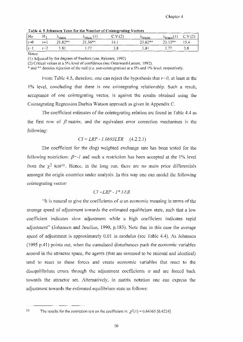
Chapter 4

Table 4. 5 Johansen Tests for the Number of Cointegrating Vectors

Ho Hi ^max ^max (1) C.V.(2) ^trace ^trace(^) C.V.(2)

r=0 r=l 21.82** 2L36** 14.1 23.62** 23.13** 154

r=l r=2 1.81 L77 3.8 1.81 1.77 3.8

Notes: (1) Adjusted by the degrees of freedom (see, Reimers, 1992) (2) Critical values at a 5% level of confidence (see Osterward-Lenum, 1992). * and ** denotes rejection of the null {i.e. non-cointegration) at a 5% and 1% level, respectively.

From Table 4.5, therefore, one can reject the hypothesis that r=0, at least at the

1% level, concluding that there is one cointegrating relationship. Such a result,

acceptance of one cointegrating vector, is against the results obtained using the

Cointegrating Regression Durbin Watson approach as given in Appendix C.

The coefficient estimates of the cointegrating relation are found in Table 4.4 as

the first row of matrix, and the equivalent error correction mechanism is the

following:

c ; = z ; ; ? - ( 4 . 2 . 2 . 1 )

The coefRcient for the (log) weighted exchange rate has been tested for the

following restriction: and such a restriction has been accepted at the 1% level

from the test'O. Hence, in the long run, there are no main price differentials

amongst the origin countries under analysis. In this way one can model the following

cointegrating vector:

"It is natural to give the coefficients of a an economic meaning in terms of the

average speed of adjustment towards the estimated equilibrium state, such that a low

coefficient indicates slow adjustment while a high coefficient indicates rapid

adjustment" (Johansen and Juselius, 1990, p. 183). Note that in this case the average

speed of adjustment is approximately 0.01 in modulus (see Table 4.4). As Johansen

(1995 p.41) points out, when the cumulated disturbances push the economic variables

around in the attractor space, the agents (that are assumed to be rational and identical)

tend to react to these forces and create economic variables that react to the

disequilibrium errors through the adjustment coefficients a and are forced back

towards the attractor set. Alternatively, in matrix notation one can express the

adjustment towards the estimated equilibrium state as follows;

The results for the restriction test on the coefficient is: %^(1) = 0.64365 [0.4224]

50

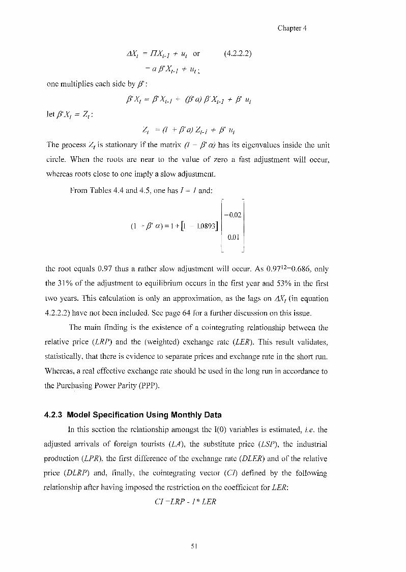
Chapter 4

zLiQ — + Uj or (4.2.2.2)

= a ;

one multiplies each side by /?':

P ~ P ^t-1 (P '^) P ^t-1 P

let P'X^ = Zf:

Z, f yg' W,

The process Zf is stationary if the matrix (1 ^ p d) has its eigenvalues inside the unit

circle. When the roots are near to the value of zero a fast adjustment will occur,

whereas roots close to one imply a slow adjustment.

From Tables 4.4 and 4.5, one has 1=1 and:

( l + / r a ) = 1+D -10%%]

-0 .02

o a i

the root equals 0.97 thus a rather slow adjustment will occur. As 0.97^^=0.686, only

the 31% of the adjustment to equilibrium occurs in the first year and 53% in the first

two years. This calculation is only an approximation, as the lags on (in equation

4.2.2.2) have not been included. See page 64 for a further discussion on this issue.

The main finding is the existence of a cointegrating relationship between the

relative price {LRP) and the (weighted) exchange rate (LER). This result validates,

statistically, that there is evidence to separate prices and exchange rate in the short run.

Whereas, a real effective exchange rate should be used in the long run in accordance to

the Purchasing Power Parity (PPP).

4.2.3 Model Specification Using Monthly Data

In this section the relationship amongst the 1(0) variables is estimated, i.e. the

adjusted arrivals of foreign tourists (LA), the substitute price {LSP), the industrial

production {LPR), the first difference of the exchange rate (DLER) and of the relative

price (DLRF) and, finally, the cointegrating vector (CI) defined by the following

relationship after having imposed the restriction on the coefficient for lER:

51

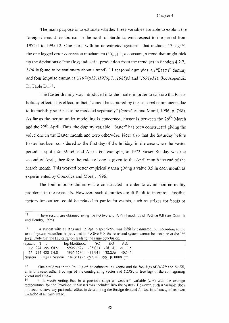
Chapter 4

The main purpose is to estimate whether these variables are able to explain the

foreign demand for tourism in the north of Sardinia, with respect to the period from

1972:1 to 1995:12. One starts with an unrestricted system'' that includes 13 lags'^,

the one lagged error correction mechanism , a constant, a trend that might pick

up the deviations of the (log) industrial production from the trend (as in Section 4.2.2.,

LPR is found to be stationary about a trend), 11 seasonal dummies, an "Easter" dummy

and four impulse dummies and See Appendix

D, Table

The Easter dummy was introduced into the model in order to capture the Easter

holiday effect. This effect, in fact, "cannot be captured by the seasonal components due

to its mobility so it has to be modeled separately" (Gonzales and Moral, 1996, p. 748).

As far as the period under modelling is concerned, Easter is between the 26^^ March

and the 22^^ April. Thus, the dummy variable "Easter" has been constructed giving the

value one in the Easter month and zero otherwise. Note also that the Saturday before

Easter has been considered as the first day of the holiday, in the case when the Easter

period is split into March and April. For example, in 1972 Easter Sunday was the

second of April, therefore the value of one is given to the April month instead of the

March month. This worked better empirically than giving a value 0.5 in each month as

experimented by Gonzales and Moral, 1996.

The four impulse dummies are constructed in order to avoid non-normality

problems in the residuals. However, such dummies are difficult to interpret. Possible

factors for outliers could be related to particular events, such as strikes for boats or

' ' These results are obtained using the PcGive and PcFiml modulus of PcGive 9.0 (see Doornik and Hendry, 1996).

A system with 13 lags and 12 lags, respectively, was initially estimated, but according to the test of system reduction, as provided in PcGive 9.0, the restricted system cannot be accepted at the 1% level. Note that the HQ criterion leads to the same conclusion.

system T p log-likelihood SC HQ AlC 12 274 395 OLS 5906.7627 -35.023 -38.141 -41.115 13 274 420 OLS 5965.6730 -34.941 -38.256 -40.545

System 13 lags > System 12 lags: F(25, 692) = 3.3991 [0.0000] **

One could put in the first lag of the cointegrating vector and the free lags of DLRP and DLER, as in this case; either free lags of the cointegrating vector and DLRP, or free lags of the cointegrating vector and DLER.

It is worth noting that in a previous stage a "weather" variable {LW) with the average temperatures for the Province of Sassari was included into the system. However, such a variable does not seem to have any particular effect in determining the foreign demand for tourism; hence, it has been excluded at an early stage.

52

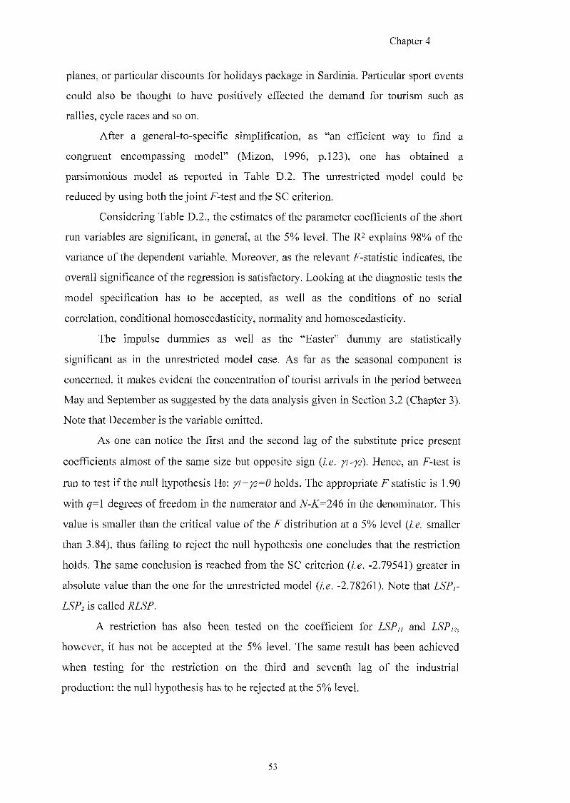
Chapter 4

planes, or particular discounts for holidays package in Sardinia. Particular sport events

could also be thought to have positively effected the demand for tourism such as

rallies, cycle races and so on.

After a general-to-specific simplification, as "an efficient way to find a

congruent encompassing model" (Mizon, 1996, p. 123), one has obtained a

parsimonious model as reported in Table D.2. The unrestricted model could be

reduced by using both the joint F-test and the SC criterion.

Considering Table D.2., the estimates of the parameter coefficients of the short

run variables are significant, in general, at the 5% level. The R2 explains 98% of the

variance of the dependent variable. Moreover, as the relevant F-statistic indicates, the

overall significance of the regression is satisfactory. Looking at the diagnostic tests the

model specification has to be accepted, as well as the conditions of no serial

correlation, conditional homoscedasticity, normality and homoscedasticity.

The impulse dummies as well as the "Easter" dummy are statistically

significant as in the unrestricted model case. As far as the seasonal component is

concerned, it makes evident the concentration of tourist arrivals in the period between

May and September as suggested by the data analysis given in Section 3.2 (Chapter 3).

Note that December is the variable omitted.

As one can notice the first and the second lag of the substitute price present

coefficients almost of the same size but opposite sign (z.g. Hence, an F-test is

run to test if the null hypothesis Ho: p+]^=0 holds. The appropriate F statistic is 1.90

with q=l degrees of freedom in the numerator and VV-A7=246 in the denominator. This

value is smaller than the critical value of the F distribution at a 5% level (i.e. smaller

than 3.84), thus failing to reject the null hypothesis one concludes that the restriction

holds. The same conclusion is reached from the SC criterion {i.e. -2.79541) greater in

absolute value than the one for the unrestricted model {i.e. -2.78261). Note that LSP,-

26"?; is called .

A restriction has also been tested on the coeBicient for IS'?,, and

however, it has not be accepted at the 5% level. The same result has been achieved

when testing for the restriction on the third and seventh lag of the industrial

production: the null hypothesis has to be rejected at the 5% level.

53

Chapter 4

As a further experiment a restriction on the seasonal dummies has been

imposed. In particular, the seasonal May, Jun and present coefficients almost of

the same size and same sign (i.e. Model 1) confirming the seasonal pattern

shown in Figure 3.2. A new dummy (say MJJ, Model 2) was created giving the value 1

to May, June and July months and 0 otherwise. An F-test is run in order to test Model

1 versus Model 2 (where the RSS equals 9.6393). The appropriate F statistic is 0.155

with q=2 degrees of freedom in the numerator and N-K=2A1 in the denominator. This

value is smaller than the critical value of the F distribution at a 5% level {i.e. 3.00),

thus failing to reject the null hypothesis the restriction holds. Note that the SC criterion

suggests accepting the restriction as in Model 1 it is equal to -2.79541 and in Model 2

it equals -2.83513.

Given the previous analysis, the final parsimonious encompassing model is

reported in Table 4.6.

Note that May is created giving the value 1 in May and 0 otherwise; Jun takes the value 1 in June and 0 otherwise; finally, Jul takes the value 1 in July and 0 otherwise.

5 4

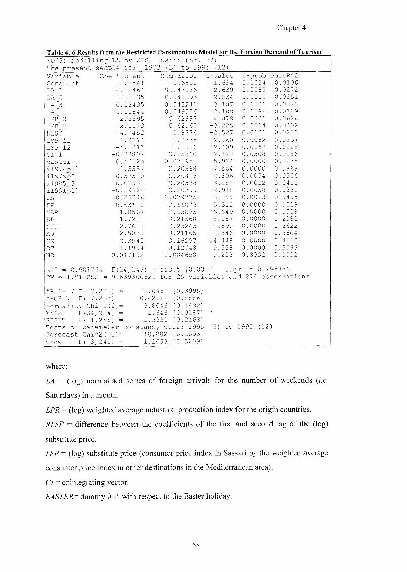
Chapter 4

Table 4. 6 Results from the Restricted Parsimonious Model for the Foreign Demand of Tourism EQ(3) Modelling LA by OLS (using For.in?) The present sample is: 1973 (3) to 1995 (12)

Variable Coefficient Std .Error t-value t -prob PartR'^2

Constant -2.7541 1.6850 -1 634 0 1034 0. 0106

LA 1 0.12464 0 . 047236 2 639 0 0089 0 0272

LA 2 0.10335 0 . 040793 2 534 0 0119 0. 0251 LA 3 0.13435 0. 043241 3 107 0 0021 0. 0373

LA 11 0.10844 0 . 049556 2 188 0 0296 0. 0189 LPR 3 2.5695 0 .62997 4 079 0 0001 0. 0626

LPR 7 -2.0073 0 .62160 -3 229 0 0014 0. 0402 RLSP -4.7452 1.8776 -2 527 0 0121 0. 0250 LSP 11 5.2114 1.8885 2 760 0 0062 0 0297 LSP 12 -4.5311 1.8806 -2 409 0 0167 0. 0228 CI_1 -0.33807 0 .15560 -2 173 0 0308 0 . 0186 easter 0.42625 0 . 071951 5 924 0 0000 0. 1235 il974pl2 1.5557 0 .20568 7 564 0 0000 0. 1868 il979p3 -0.57510 0 .20496 -2 806 0 0054 0. 0306

il985p3 0.67531 0 .20578 3 282 0 0012 0. 0415 il991pll -0.59522 0 .20399 -2 918 0 0038 0 . 0331

JA 0.25746 0. 079375 3 244 0 0013 0. 0405

FE 0.63111 0 .11875 5 315 0 0000 0. 1019

MAR 1.0567 0 .15893 6 649 0 0000 0 . 1508

AP 1.7281 0 .21368 8 087 0 0000 0. 2080 MJJ 2.7638 0 .23245 11 890 0 0000 0 . 3622 AU 2.5070 0 .21165 11 846 0 0000 0. 3604

SE 2.3545 0 .16297 14 448 0 0000 0. 4560 OT 1.1904 0 .12748 9 338 0 0000 0. 2593

NO 0.017192 0. 084658 0 203 0 8392 0. 0002

R''2 = 0.981794 F(24, 249) = 559 .5 [0.0000] sigma = 0.1967 54 DM = 1.91 RSS = 9.639300629 for 25 variables and 274 observations

AR 1- 7 F( 7 ,242) = 1. 0461 [0.3995] ARCH 7 F( 7,235) = 0.42111 [0.8886] Normality Chi'"2(2)= 3. 8046 [0.1492] Xi'^2 F( 34 ,214) = 1 . 64 6 [0.0187] *

RESET F( 1 ,248) = 1. 5331 [0.2168] Tests of parameter constancy over: 1995 (5) to 1 995 (12) Forecast Chi '"2( 8)= 10 .082 [0.2593] Chow F( 8 ,241) = 1. 1653 [0.3209]

where;

= (log) normalised series of foreign arrivals for the number of vyeekends (;.e.

Saturdays) in a month.

Zf = (log) weighted average industrial production index for the origin countries.

= difference between the coefficients of the first and second lag of the (log)

substitute price.

= (log) substitute price (consumer price index in Sassari by the weighted average

consumer price index in other destinations in the Mediterranean area).

CI = cointegrating vector.

dummy 0 -1 with respect to the Easter holiday.

55

Chapter 4

MJJ = seasonal dummy giving the value of 1 to May, June and July months and 0

otherwise.

In terms of statistical tests, one can say the same results achieved for the model

reported in Table D.2., hold for the final parsimonious model which, therefore, can be

considered as data congruent. Further tests for parameter constancy over the last eight

observations of the sample are reported. The null hypothesis of constancy fails to be

rejected. Moreover, it has to be noted that the null hypothesis of White

homoscedasticity for the residuals is marginally rejected at the 5% level. In this case

the "ordinary least-squares parameter estimators are unbiased and consistent, but they

are not efficient; i.e. the variances of the estimated parameters are not the minimum

variances" (Pindyck and Rubinfeld, 1991, p. 128). A White correction for

heteroscedasticity has been used for the standard errors^^ as reported in Table 4.7.

Such a correction has been run using Microfit 4.0.

56

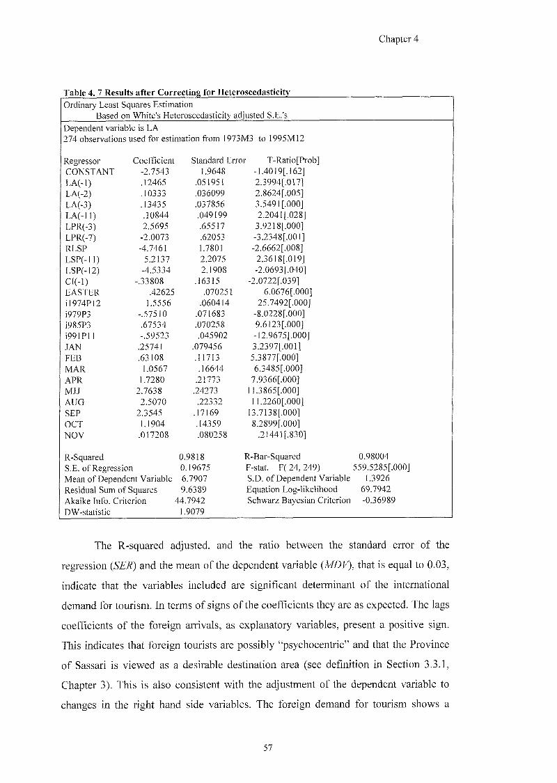
Chapter 4

Table 4. 7 Results after Correcting for Heteroscedasticity

Ordinary Least Squares Estimation Based on White's Heteroscedasticity adjusted S.E.'s

Dependent variable is LA 274 observations used for estimation from 1973M3 to 1995M12

Regressor Coefficient Standard Error T-Ratio[Prob]

CONSTANT -2.7543 1.9648 -1.4019[.162] LA(.l) .12465 .051951 2.3994[.0]7] LA(-2) .10333 .036099 2.8624[.005] LA(-3) .13435 .037856 3.5491 [.000] LA(-l l ) .10844 .049199 2.2041 [.028] LPR(-3) 2.5695 .65517 3.9218 [.000] LPR(-7) -2.0073 .62053 -3.2348[.00l] RLSP -4.7461 1.7801 -2.6662[.008] LSP(-ll) 5.2137 2.2075 2.3618[.019] LSP(-12) -4.5334 2.1908 -2.0693[.040] CI(-l) -.33808 .16315 -2.0722[.039] EASTER .42625 .070251 6.0676[.000] il974P12 1.5556 .060414 25.7492[.000] i979P3 -.57510 .071683 -8.0228[.000] i985P3 .67534 .070258 9.6123[.000] i99]P11 -.59523 .045902 -12.9675[.000] JAN .25741 .079456 3.2397[.001] FEB .63108 .11713 5.3877[.000] MAR 1.0567 .16644 6.3485[.000] APR 1.7280 .21773 7.9366[.000] MJJ 2.7638 .24273 11.3865[.000] AUG 2.5070 .22332 11.2260[.000] SEP 2.3545 .17169 13.7138[.000] OCT 1.1904 .14359 8.2899[.000] NOV .017208 .080258 .21441 [.830]

R-Squared 0.9818 R-Bar-Squared 0.98004 S.E. of Regression 0.19675 F-stat. F( 24, 249) 559.5285[.000] Mean of Dependent Variable 6.7907 S.D. of Dependent Variable 1.3926 Residual Sum of Squares 9.6389 Equation Log-likelihood 69.7942 Akaike Info. Criterion 44.7942 Schwarz Bayesian Criterion -0.36989 DW-statistic 1.9079

The R-squared acûsted, and the ratio between the standard error of the

regression (SER) and the mean of the dependent variable {MDV), that is equal to 0.03,

indicate that the variables included are significant determinant of the international

demand for tourism. In terms of signs of the coefficients they are as expected. The lags

coefGcients of the foreign arrivals, as explanatory variables, present a positive sign.

This indicates that foreign tourists are possibly "psychocentric" and that the Province

of Sassari is viewed as a desirable destination area (see definition in Section 3.3.1,

Chapter 3). This is also consistent with the adjustment of the dependent variable to

changes in the right hand side variables. The foreign demand for tourism shows a

57

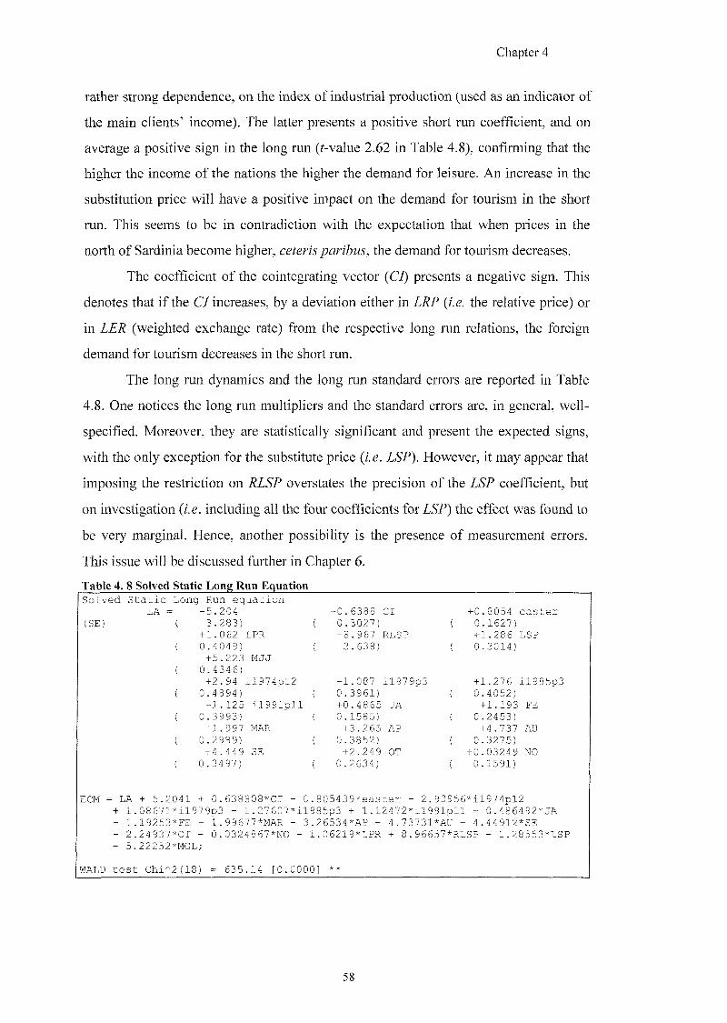
Chapter 4

rather strong dependence, on the index of industrial production (used as an indicator of

the main clients' income). The latter presents a positive short run coefficient, and on

average a positive sign in the long run (r-value 2.62 in Table 4.8), confirming that the

higher the income of the nations the higher the demand for leisure. An increase in the

substitution price will have a positive impact on the demand for tourism in the short

run. This seems to be in contradiction with the expectation that when prices in the

north of Sardinia become higher, ceteris paribus, the demand for tourism decreases.

The coefficient of the cointegrating vector (CI) presents a negative sign. This

denotes that if the CI increases, by a deviation either in LRP (/. e. the relative price) or

in LER (weighted exchange rate) from the respective long run relations, the foreign

demand for tourism decreases in the short run.

The long run dynamics and the long run standard errors are reported in Table

4.8. One notices the long run multipliers and the standard errors are, in general, well-

specified. Moreover, they are statistically significant and present the expected signs,

with the only exception for the substitute price {i.e. LSP). However, it may appear that

imposing the restriction on RLSP overstates the precision of the LSP coefficient, but

on investigation {i.e. including all the four coefficients for LSP) the effect was found to

be very marginal. Hence, another possibility is the presence of measurement errors.

This issue will be discussed further in Chapter 6.

S o l v e d S t a t i c L o n g e q u a t i o n LA = - 5 . 2 0 4 - 0 . 6 3 8 8 CI + 0 . 8 0 5 4 e a s t e r

(SE) ( 3 . 2 8 3 ) 0 . 3 0 2 7 ) ( 0 . 1 6 2 7 ) + 1 . 0 6 2 LPR - 8 . 9 6 7 RLSP + 1 . 2 8 6 LSP

( 0 . 4 0 4 9 ) 3 . 6 3 8 ) ( 0 . 3 0 1 4 ) + 5 ^ ^ 3 M ^ J

( 0 . 4 3 4 6 ) + 2 . 9 4 i l 9 7 4 p l 2 - 1 . 0 8 7 i l 9 7 9 p 3 + 1 . 2 7 6 i l 9 8 5 p 3

( 0 . 4 8 9 4 ) ( 0 . 3 9 6 1 ) ( 0 . 4 0 5 2 ) - 1 . 1 2 5 i l 9 9 1 p l l + 0 . 4 8 6 5 J A + 1 . 1 9 3 FE

{ 0 . 3 9 9 3 ) ( 0 . 1 5 8 5 ) { 0 . 2 4 5 3 ) + 1 . 9 9 7 M&R + 3 . 2 6 5 AP + 4 . 7 3 7 AU

( 0 . 2 9 8 9 ) ( 0 . 3 8 5 2 ) ( 0 . 3 2 7 5 ) + 4 . 4 4 9 SE + 2 . 2 4 9 OT + 0 . 0 3 2 4 9

( 0 . 3 4 9 7 ) ( 0 . 2 6 3 4 ) ( 0 . 1 5 9 1 )

ECM = LA + 5 . 2 0 4 1 + 0 . 6 3 8 8 0 8 * C I - 0 . 8 0 5 4 3 9 * e a s t e r - 2 . 9 3 9 5 6 * i l 9 7 4 p l 2 + 1 . 0 8 6 7 1 * i l 9 7 9 p 3 - 1 . 2 7 6 0 7 * i l 9 8 5 p 3 + 1 . 1 2 4 7 2 * i l 9 9 1 p l l - 0 . 4 8 6 4 9 2 * J A - 1 . 1 9 2 5 3 * F E - 1 . 9 9 6 7 7 * M A R - 3 . 2 6 5 3 4 + A P - 4 . 7 3 7 3 1 * A U - 4 . 4 4 9 1 2 + S E - 2 . 2 4 9 3 7 * 0 T - 0 . 0 3 2 4 8 6 7 * N O - 1 . 0 6 2 1 9 + L F R + 8 . 9 6 6 5 7 * R L S P - 1 . 2 8 5 5 3 + L S P - 5 . 2 2 2 5 2 * M G L ;

VMULD t e s t C h i * 2 ( 1 8 ) = 6 3 5 . 1 4 [ 0 . 0 0 0 0 ] **

5 8

Chapter 4

Thus, with few exceptions, one can conclude that the model gives satisfactory

results in the short run as well in the long run, in terms both of statistical tests and

economic theory.

4.2.4 Linear Versus Logarithmic Specification

In this paragraph, an account is given of the experiments carried out in

assessing whether the logarithmic specification form is more appropriate than the

linear form, in estimating the demand for international tourism.

The integration status of the variables expressed in a linear specification will be

tested using; A (number of arrivals modified for number of weekends), PR (income

proxy, as a weighted average for the source countries), RP (relative price,

Sassari/origin countries), SP (substitute price, Sassari/other destinations) and ER

(weighted average exchange rate for the origin countries). At this point, it is worth

noting that one cannot directly compare the results from the ADF for the logarithmic

form with those obtained using the linear specification for the variables of interest. As

Granger and Hallman (1991) point out, a unit root test invariant to the transformation

has to be used. Such tests are the Rank Dickey-Fuller (RDF) and Augmented RDF

(ARDF). It is not in the scope of this thesis to investigate the possibility that the

logarithmic transformation used in the present study could lead to an over-rejection of

the null hypothesis. However, this can be thought as further work. From the ADF test

with 13 lags the following results have been obtained: A, PR and SP can be considered

as 1(0). The income proxy is stationary in the level when the time trend is included in

the ADF test, whereas the substitute price is stationary in the level when the constant,

and a constant and seasonals are included. On the other hand, RP and ER are 1(1). As

for the logarithmic case, the cointegration status for the coefficients of the latter

variables has been investigated. The Johansen analysis, has shown the existence of a

cointegration relationship between the coefficients of the relative price and exchange

rate. In particular, an initial 13 lag system, used to run the Johansen analysis, which

also includes a constant and seasonal dummies could be reduced to a VAR(3). The

cointegration relationship for the linear specification is defined as follows:

59

Chapter 4

In order to run the Box and Cox test, one estimates an unrestricted 13 lag

tourism demand equation expressed both in a logarithmic and linear form, where the

independent variables are defined as before.

= +<3yC/^_y+

+ ag + ap DwTM/wzej' +

and

^ / m e a r /br/M

AF= UJ + A2 PRP + <^4 SPJ.. + AJ DERJ.. + DRPT ^ CIY ECLJ_J +

+ a g + op 5'eaj + a / g Dw/M/Mzgj' +

The sum of the squared errors from the logarithmic form (SSELL) is equal to

1.90, whereas the sum of the squared errors for the linear form (SSEL) equals

34301958.14. To test whether the two models are empirically equivalent and find out

which of the two models fits better the data. In doing this, the sum of the squared

errors needs to be calculated for the linear model with (A/ A G) as the dependent

variable. Note that A G is the geometric mean defined as follows:

For the latter model, the sum of the squared errors (that is equals

46.4971. The Box-Cox test (see formula 2.4.1.1, Chapter 2) indicates that the two

models are empirically different as the calculated is 438.06 and the correspondent

tabulated value is 3.84 at the 5% significance level. Moreover, the is

higher than SSEU, hence one can conclude that the logarithmic specification form fits

the data better than the linear model.

Note that it would be possible to compare different specification in linear and

logarithmic forms, but the rejection of the linear model is so clear that this has not

been pursued.

4.3 THE MODEL SPECIFICATION USING ANNUAL DATA ANALYSIS

From the analysis so far, several advantages have emerged in the use of

monthly data. They give the possibility to identify the short run characteristics of the

demand for tourism. One can study carefully the seasonal pattern that seems to be of

extreme importance for operators in the tourism activity. Moreover, the relatively large

60

Chapter 4

number of observations available in the previous analysis (288 observations) has

allowed one to test for the possible presence of seasonal unit roots as well as for long

run unit roots.

At this stage it could be interesting to assess the characteristics of the

international demand for tourism also in the long run by making use of annual and

quarterly data. The annual and quarterly analysis should be broadly consistent with the

monthly results. Further, the availability of extra variables, only obtainable on a

quarterly and annual basis, may enrich the analysis or remove the need to use proxy

variables. On the other hand, one of the main limitations when dealing with annual

tourism data could be the relative small number of observations available.

One starts estimating an annual model for the period 1972-1995. In order to

obtain homogeneous results and comparisons between models, the same time series as

for the monthly case will be used. A "pre-modelling" analysis is carried out. Table 4.9

reports the results from running an ADF test for each of the economic series. However,

as one can notice, such a table can be interpreted as illustrative of the problems of

using ADF tests in small samples {i.e. T=24) rather than being informative as to the

integration status of the variables under study.

61

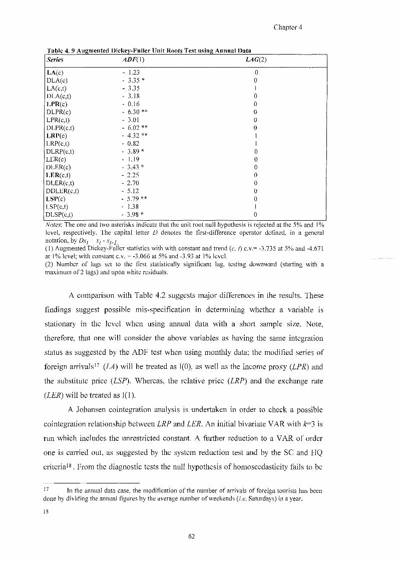
Chapter •

Table 4. 9 Augmented Dickey-Fuller Unit Roots Test using Annual Data

Series ADFi\) IXG(2)

LA(c) - 1.23 0 DLA(c) - 3.35 * 0 LA(c,t) - 3.35 1 DLA(c,t) - 3.18 0 LPR(c) - 0.16 0 DLPR(c) - 6.30 ** 0 LPR(c,t) - 3.01 0 DLPR(c,t) - 6.02 ** 0 LRP(c) - 4.32 ** 1 LRP(c,t) - 0.82 1 DLRP(c,t) - 3 .89* 0 LER(c) - 1.19 0 DLER(c) - 3.43 * 0 LER(c,t) - 2.25 0 DLER(c,t) - 2.70 0 DDLER(c,t) - 5.12 0 LSP(c) - 5.79 ** 0 LSP(c,t) - 1.38 1 DLSP(c,t) - 3.98 * 0

Notes: The one and two asterisks indicate that the unit root null hypothesis is rejected at the 5% and 1% level, respectively. The capital letter D denotes the first-difference operator defined, in a general notation, by (1) Augmented Dickey-Fuller statistics with with constant and trend (c, t) c.v.= -3.735 at 5% and -4.671 at 1% level; with constant c.v. = -3.066 at 5% and -3.93 at 1% level. (2) Number of lags set to the first statistically significant lag, testing downward (starting with a maximum of 2 lags) and upon white residuals.

A comparison with Table 4.2 suggests major differences in the results. These

findings suggest possible mis-specification in determining whether a variable is

stationary in the level when using annual data with a short sample size. Note,

therefore, that one will consider the above variables as having the same integration

status as suggested by the ADF test when using monthly data; the modified series of

foreign arrivals''^ {LA) will be treated as 1(0), as well as the income proxy {LPR) and

the substitute price {LSF). Whereas, the relative price {LRP) and the exchange rate

{LER) will be treated as 1(1).

A Johansen cointegration analysis is undertaken in order to check a possible

cointegration relationship between LRP and LER. An initial bivariate VAR with A=3 is

run which includes the unrestricted constant. A further reduction to a VAR of order

one is carried out, as suggested by the system reduction test and by the SC and HQ

criteria'^. From the diagnostic tests the null hypothesis of homoscedasticity fails to be

In the annual data case, the modification of the number of arrivals of foreign tourists has been done by dividing the annual figures by the average number of weekends (/. e. Saturdays) in a year.

18

62

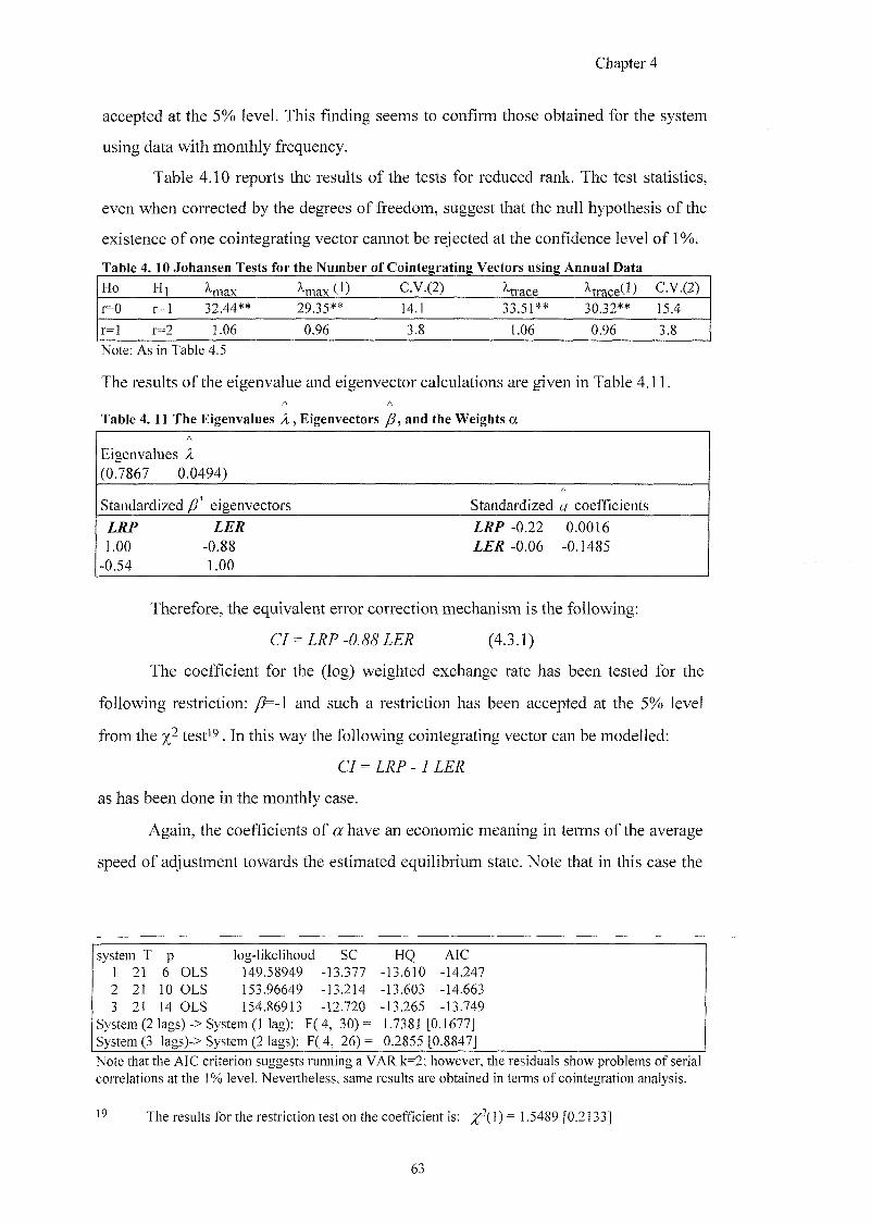
Chapter 4

accepted at the 5% level. This finding seems to confirm those obtained for the system

using data with monthly frequency.

Table 4.10 reports the results of the tests for reduced rank. The test statistics,

even when corrected by the degrees of freedom, suggest that the null hypothesis of the

existence of one cointegrating vector cannot be rejected at the confidence level of 1%.

Ho Hi ^ a x ^max (^) C.V.(2) ^trace ^trace(l) C.V.(2)

r=0 r=l 32.44** 29.35** 14.1 33.51** 30.32** 15.4

r=l r=2 1.06 0.96 3.8 1.06 0.96 3.8

Note; As in Table 4.5

The results of the eigenvalue and eigenvector calculations are given in Table 4.11.

Table 4.11 The Eigenvalues A, Eigenvectors (5, and the Weights a

Eigenvalues X (0.7867 0.0494)

Standardized yg' eigenvectors Standardized a coefficients

LRP LER Z&P -0.22 0.0016 1.00 -0.88 -0.06 -0.1485

-0.54 1.00

Therefore, the equivalent error correction mechanism is the following;

= (4.3.1)

The coefficient for the (log) weighted exchange rate has been tested for the

following restriction: /?=-l and such a restriction has been accepted at the 5% level

from the test'^. In this way the following cointegrating vector can be modelled;

C7 = i ; ; ? - 7 l E j ;

as has been done in the monthly case.

Again, the coefGcients of or have an economic meaning in terms of the average

speed of adjustment towards the estimated equilibrium state. Note that in this case the

system T p log-likelihood SC HQ AIC 1 21 6 OLS 149.58949 -13.377 -13.610 -14.247 2 21 10 OLS 153.96649 -13.214 -13.603 -14.663 3 21 14 OLS 154.86913 -12.720 -13.265 -13.749

System (2 lags) -> System (1 lag): F( 4, 30) = 1.7381 [0.1677] System (3 lags)-> System (2 lags): F( 4, 26) = 0.2855 [0.8847]

Note that the AIC criterion suggests running a VAR k=2; however, the residuals show problems of serial correlations at the 1% level. Nevertheless, same results are obtained in terms of cointegration analysis.

The results for the restriction test on the coefficient is: %- ( ] )= 1.5489 [0.2133]

63

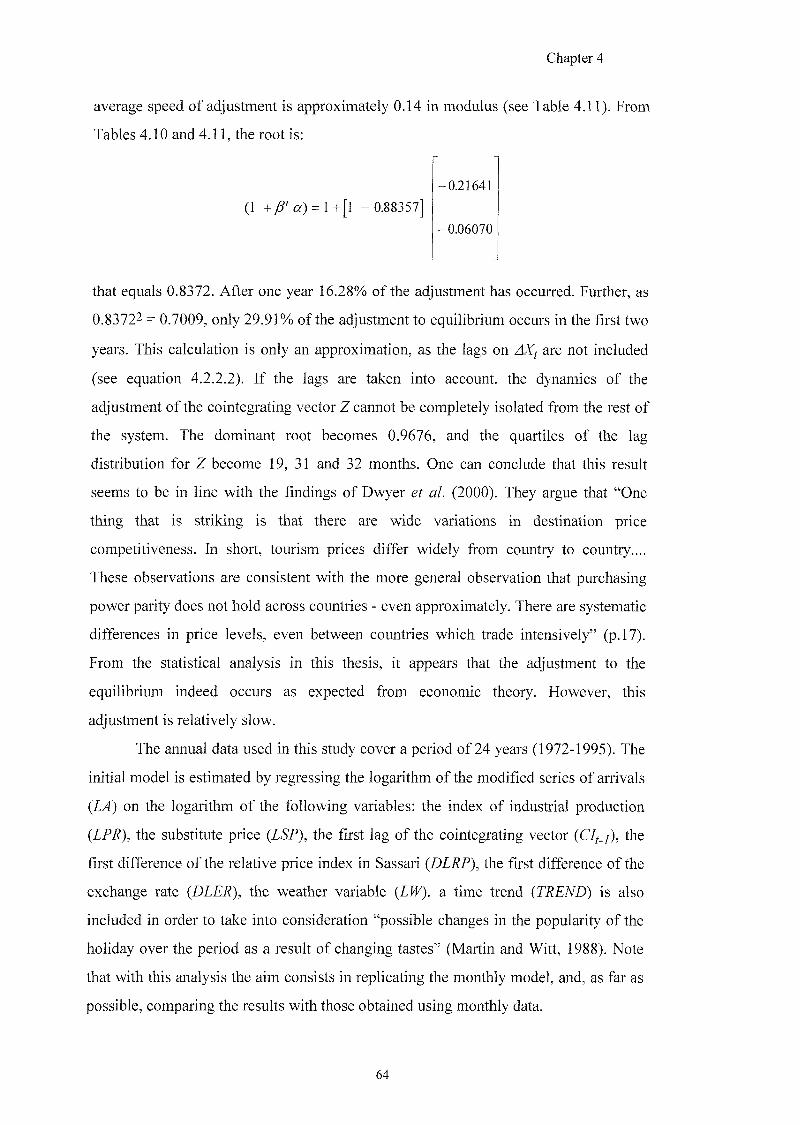
Chapter 4

average speed of ad|justment is approximately 0.14 in modulus (see Table 4.11). From

Tables 4.10 and 4.11, the root is;

(I + , g ' « ) = ] + [ ! - 0.88357]

-0.21641

-0.06070

that equals 0.8372. After one year 16.28% of the adjustment has occurred. Further, as

0.8372^ = 0.7009, only 29.91% of the adjustment to equilibrium occurs in the first two

years. This calculation is only an approximation, as the lags on AX are not included

(see equation 4.2.2.2). If the lags are taken into account, the dynamics of the

adjustment of the cointegrating vector Z cannot be completely isolated from the rest of

the system. The dominant root becomes 0.9676, and the quartiles of the lag

distribution for Z become 19, 31 and 32 months. One can conclude that this result

seems to be in line with the findings of Dwyer et al. (2000). They argue that "One

thing that is striking is that there are wide variations in destination price

competitiveness. In short, tourism prices differ widely from country to country....

These observations are consistent with the more general observation that purchasing

power parity does not hold across countries - even approximately. There are systematic

differences in price levels, even between countries which trade intensively" (p. 17).

From the statistical analysis in this thesis, it appears that the adjustment to the

equilibrium indeed occurs as expected from economic theory. However, this

adjustment is relatively slow.

The annual data used in this study cover a period of 24 years (1972-1995). The

initial model is estimated by regressing the logarithm of the modified series of arrivals

{LA) on the logarithm of the following variables; the index of industrial production

(Zf ), the substitute price (25?), the first lag of the cointegrating vector (C/^_/), the

first difference of the relative price index in Sassari (DLRP), the first difference of the

exchange rate (DLER), the weather variable (LW), a time trend (TREND) is also

included in order to take into consideration "possible changes in the popularity of the

holiday over the period as a result of changing tastes" (Martin and Witt, 1988). Note

that with this analysis the aim consists in replicating the monthly model, and, as far as

possible, comparing the results with those obtained using monthly data.

64

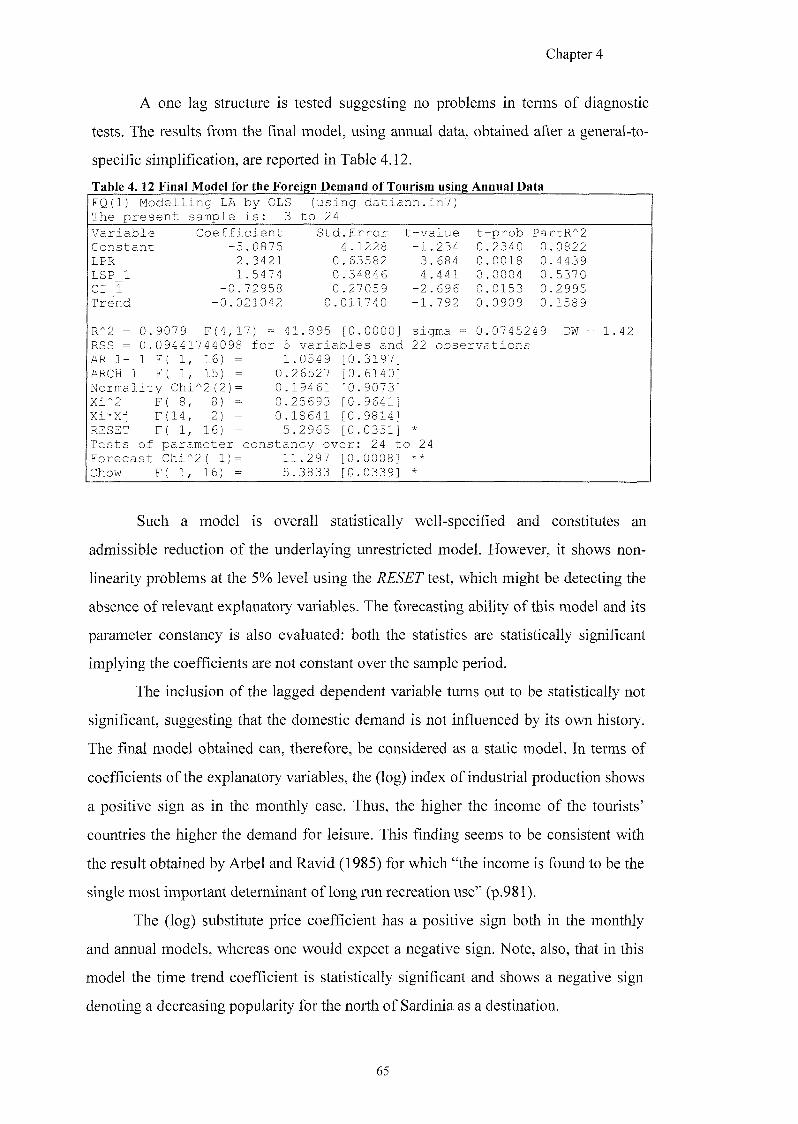
Chapter 4

A one lag structure is tested suggesting no problems in terms of diagnostic

tests. The results from the final model, using annual data, obtained after a general-to-

specific simplification, are reported in Table 4.12.

Table 4 .12 Final Model for the Foreign Demand of Tourism using Annual Data EQ(1) Modelling LA by OLS (using The present sample is: 3 to 24

datiann.in7)

Variable Coefficient Std.Error t -value t -prob PartR"^2 Constant -5.0875 4. 1228 -1.234 0 .2340 0 0822 LPR 2.3421 0.63582 3. 684 0 .0018 0 4439 LSP 1 1.5474 0.34846 4.441 0 .0004 0 5370 CI_1 -0.72958 0.27059 -2.696 0 .0153 0 2995 Trend -0.021042 0.011740 -1.792 0 .0909 0 1589

R"2 = 0. 9079 F(4,17) = 41.895 [0 .0000] sigma = 0 .0745249 DW = 1.42 RSS = 0. 09441744098 for 5 variables and 22 observations AR 1- 1 F( 1, 16) = 1.0549 [0 .3197] ARCH 1 1, 15) = 0.26527 [0 .6140] Normality Chi "2(2)= 0.19461 [0 .9073] Xi"2 F( 8, 8) = 0.25693 [0 .9641] Xi*Xi F(14, 2) = 0.18641 [0 .9814] RESET F( 1, 16) = 5.2965 [0 .0351] *

Tests of parameter constancy over : 24 to 24 Forecast Chi"" 2( 1)= 11.297 [0 0008] * *

Chow F( 1, 16) = 5.3833 [0 .0339] *

Such a model is overall statistically well-specified and constitutes an

admissible reduction of the underlaying unrestricted model. However, it shows non-

linearity problems at the 5% level using the RESET test, which might be detecting the

absence of relevant explanatory variables. The forecasting ability of this model and its

parameter constancy is also evaluated: both the statistics are statistically significant

implying the coefficients are not constant over the sample period.

The inclusion of the lagged dependent variable turns out to be statistically not

significant, suggesting that the domestic demand is not influenced by its own history.

The final model obtained can, therefore, be considered as a static model. In terms of

coefficients of the explanatory variables, the (log) index of industrial production shows

a positive sign as in the monthly case. Thus, the higher the income of the tourists'

countries the higher the demand for leisure. This finding seems to be consistent with

the result obtained by Arbel and Ravid (1985) for which "the income is found to be the

single most important determinant of long run recreation use" (p.981).

The (log) substitute price coefficient has a positive sign both in the monthly

and annual models, whereas one would expect a negative sign. Note, also, that in this

model the time trend coefficient is statistically significant and shows a negative sign

denoting a decreasing popularity for the north of Sardinia as a destination.

65

Chapter 4

The cointegrating vector enters the equation with a negative sign, as is the case

when using monthly data. The (log) weather variable once again does not play a role in

explaining the domestic demand for tourism.

A couple of further comments are due. Experimenting with the unadjusted

series of foreign arrivals of tourists gives almost equivalent results both in terms of

coefficients, significance and diagnostic statistics.

Furthermore, a brief account on the appropriate functional form to use is given.

The investigation of the integration status of the economic series of interest, by using

the ADF test suggests: A, PR and ER to be non-stationary in the level, and statistical

evidence is found for the substitute price and the relative price to be stationary in the

level. However, these results, as already mentioned for the logarithmic specification,

have to be considered with some caution given that the number of observations is quite

small (24 in total). Hence, one proceeds as for the linear monthly case, treating only

RP and ER as stationary in the first difference, which leads to a cointegration analysis

for these variables. By adopting the Johansen analysis, evidence is found for the

existence of one cointegrating vector. An initial unrestricted k=3 VAR, which includes

a constant and a trend unrestrictedly, can be reduced to a one lag system. The resulting

cointegrating vector for the linear specification is the following;

E c z = - 0.000,^

In order to run the Box and Cox test, an unrestricted 1 lag annual tourism

demand equation is estimated, and expressed both in a logarithmic and linear form,

where the explanatory variables are defined as before.

LAF = AJ + CI2 LAI_J... + LPR^... + LSPF.. + AJ DLER^..+ DLRPP. + AY CIJ_J +

and

Zmear /brm

AF= AJ + A2AF_J... + A^PRP. + A/FSPF..+ DERP.+ AGDRPJ.. + AY ECLI_] +

+ a g ^ + ap


0.06381525754, whereas the sum of the squared errors for the linear form (SSEL)

equals 52722686.58. The aim is to test whether the null hypothesis that the two models

66

Chapter 4

are empirically equivalent and find out which of the two models fits better the data.

Using formula 2.4.1.1 (Chapter 2)2", the calculated y} equals 5.95 that is greater than

the tabulated critical value, 3.84, at the 5% level; hence, the null fails to be accepted

and the two models are empirically different. Moreover, one infers that the logarithmic

specification is better than the linear specification as the SSEL/( A G)^ is higher than

4.3.1 The Model Specification Using Annual Data Analysis And Supply

Components

As already stated, an advantage when dealing with annual data is the possibility

of including variables which are just available with an annual frequency. Such

variables might be able, in fact, to explain much better the variation of the dependent

variable under study.

In estimating the annual foreign demand for tourism in the north of Sardinia, a

component of the quantity of the supply services can be taken into consideration. For

this purpose one includes two more variables, that is; the (log) number of total boats

arrived {LB) in the two main ports (Porto Torres and Olbia) and the (log) number of

international flights {LAE) in the two main airports (Fertilia and Olbia)^!,

An initial unrestricted one lag model including the explanatory variables as

mentioned above (z.g. jW, 25?, DZE/g, the two new variables

{i.e. LAE and LB as above defined), a constant and a time trend is run. The final results

are shown in Table 4.13.

20 Note that (5'5'EZ, / ( A G)^) equals 0.109696. The source is the ''Annuario Statistico Italiand" (1972-1996). These figures are available with

an annual frequency. In particular, the total international flights and total boat arrivals are considered. Though, in the statistical sources, international arrivals of boats are reported separately from domestic arrivals, nevertheless, one has considered the total: i.e. international plus domestic arrivals of boats. One can argue, in fact, that foreign tourists (in particular Germans that represent the highest percentage) are more likely to use Genova, Livorno or Civitavecchia harbours to reach the north of Sardinia.

67

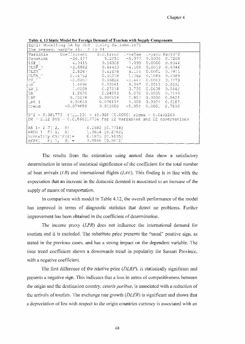
Chapter 4

Table 4. 13 Static Model for Foreign Demand of Tourism with Supply Components EQ(1) Modelling LA by OLS The present sample is: 3

(using datiann. to 24

in7)

Variable Coefficient Std.Error t-value t-prob PartR^2 Constant -26.477 5.2151 5 .077 0. 0005 0 7205 LSP 1 4.0415 0.56928 7 .099 0. 0000 0 8344 DLRP 1 -2.6862 0.64453 4 .168 0 . 0019 0 6346 DLER 2.6267 0.42678 6 .155 0. 0001 0 7911 DLER 1 0.54752 0.31078 1 .762 0. 1086 0 2369 CI 1 -2.0057 0.36824 5 .447 0 . 0003 0 7479 LW 1.4098 0.32061 4 .397 0. 0013 0 6591 LW 1 1.0208 0.27218 3 .750 0. 0038 0 5845 LB 1.2670 0.24993 5 .070 0. 0005 0 7199 LAE 0.70078 0.088519 7 .917 0 . 0000 0 8624 LAE_1 0.30659 0.076114 4 .028 0. 0024 0 6187 Trend -0.079658 0.013380 5 .954 0. 0001 0 7800

R^2 = 0.98 1773 F(ll,10) = = 48.968 [0.0000 ] sigma = 0.0 432263 DW = 2.12 RSS = 0.01868512734 for 12 variables and 22 observations

AR 1- 2 F( 2, E ) = 0. 2682 [0.7714] ARCH 1 F( 1, E ) = 1 3654 [0.2762] Normality Chi^2 2)= 0. 1875 [0.9105] RESET F( 1, 9) = 3. 8546 [0.0812]

The results from the estimation using annual data show a satisfactory

determination in terms of statistical significance of the coefficient for the total number

of boat arrivals (LB) and international flights (LAE). This finding is in line with the

expectation that an increase in the domestic demand is associated to an increase of the

supply of means of transportation.

In comparison with model in Table 4.12, the overall performance of the model

has improved in terms of diagnostic statistics that detect no problems. Further

improvement has been obtained in the coefficient of determination.

The income proxy (LPR) does not influence the international demand for

tourism and it is excluded. The substitute price presents the "usual" positive sign, as

stated in the previous cases, and has a strong impact on the dependent variable. The

time trend coefficient shows a downwards trend in popularity for Sassari Province,

with a negative coefficient.

The first difference of the relative price (DLRP), is statistically significant and

presents a negative sign. This indicates that a loss in terms of competitiveness between

the origin and the destination country, ceteris paribus, is associated with a reduction of

the arrivals of tourists. The exchange rate growth (DLER) is significant and shows that

a depreciation of lira with respect to the origin countries currency is associated with an

Chapter 4

increase in demand for tourism. The coefficient for the cointegrating vector presents a

negative sign confirming the results obtained so far.

The (log) weather variable, in this model, plays a role in explaining the

international demand for tourism, differently from the previous models. The

coefficient is statistically significant at the 5% level and it has a positive sign. It may

well be that relative average high temperatures have a positive impact in the choice of

clients that come from quite cold climates, such as Germans and Swiss tourists.

4.3.2 Testing For Simultaneity With Annual Data

The statistical significance of the coefficients for LAE, LB and DLER suggests

a further issue in testing the presence of simultaneity for these explanatory variables.

This test is carried out by adopting the Durbin-Wu-Hausman's procedure as discussed

in Section 2.9.1 (Chapter 2).

It is assumed that the demand and supply models can be expressed as

follows:

1) LAf = gcq + (Xj LSPf_] + CC2 DLRPf_] + oij DLER^ + cc^ DLERf_] + oc^ + (x^

+ CCY LWF_J + CCG LBF + CXG LAEJ + OCJQ LAEJ _J + CCJJ TREND £J ^

^ A) + A ^

in accordance with the previous results obtained using OLS (Table 4.12), where:

a) LA = normalised series of foreign arrivals for the average number of weekends {i.e.

Saturdays) in a year.

b) LSP= substitute price (consumer price index in Sassari by the weighted average


c) DLRP= relative price growth (Sassari - origin countries).

d) DLER = exchange rate growth.

e) CI= cointegrating vector.

f)LW= annual average temperatures in Sassari.

g) ZB = total number of international and domestic arrivals of boats in the north of

Sardinia.

h) LAE = total number of international flights in the north of Sardinia.

i) LPR = weighted average industrial production index for the main clients of foreign

tourists. This variable is treated as instrument.

6 9

Chapter 4

Firstly, one obtains the reduced form by regressing LAE on the variables

included into equation 1) plus the instrument variable LPR (one assumes, in fact, that

the industrial production index, used as the income proxy is able to explain the number

of foreign arrivals as well as the number of international flights in the north of

Sardinia). Hence, the residuals obtained 6om this regression (say = w) are

saved. The complete results are shown in Table 4.14.

70

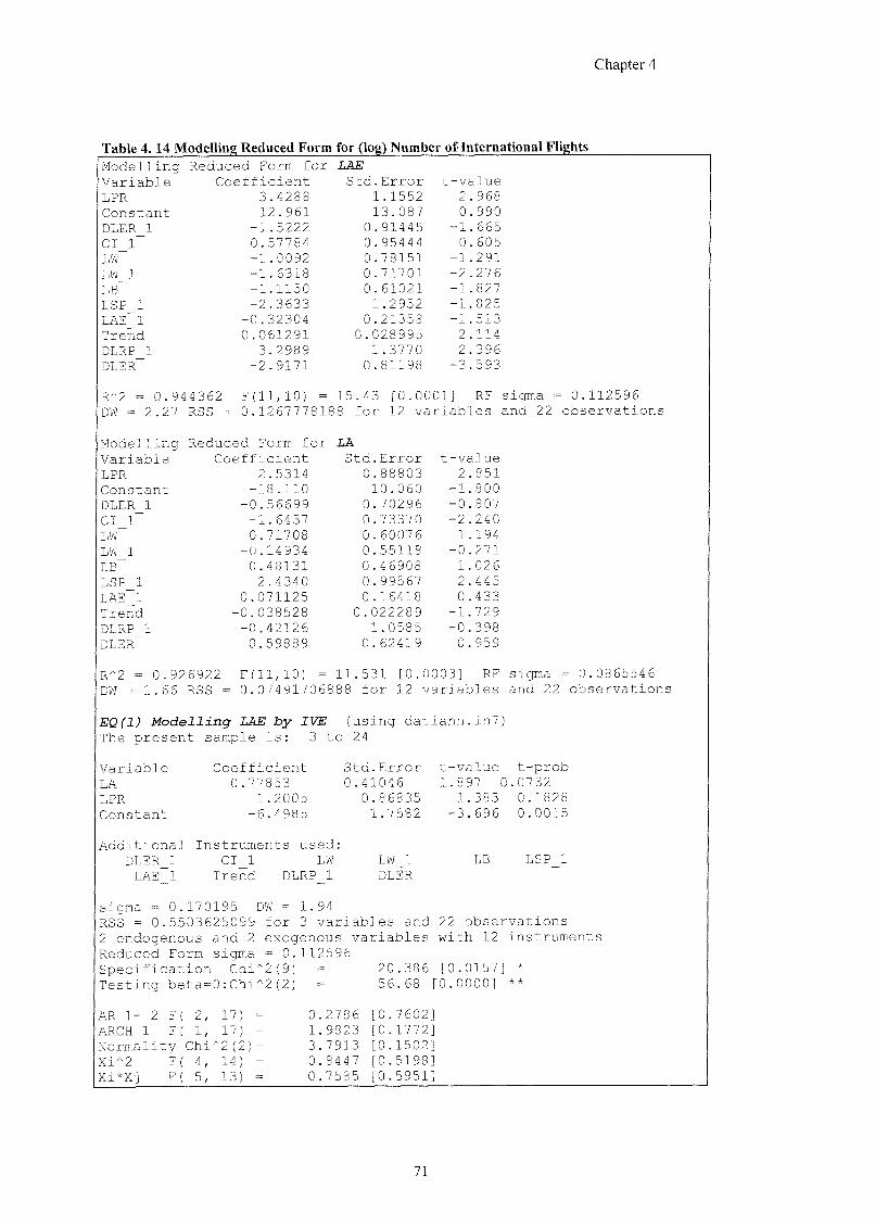
Chapter 4

Table 4 . 1 4 Modelling Reduced Form for (log) Number of International Flights Modelling Reduced Form for LAE Variable Coefficient Std.Error t-value LPR 3.4288 1.1552 2 968 Constant 12.961 13.087 0 990 DLER 1 -1.5222 0.91445 -1 665 CI 1 0.57784 0.95444 0. 605 LW -1.0092 0.78151 -1 291 LW 1 -1.6318 0.71701 —2 276 LB -1.1150 0.61021 -1 827 LSP 1 -2.3633 1.2952 -1. 825 LAE_1 -0.32304 0.21358 — 1 513 Trend 0.061291 0.028995 2 114 DLRP 1 3.2989 1.3770 2 396 DIER -2.9171 0.81198 -3. 593

R*2 = 0.9443g 2 F(ll,10) = 15.43 [0.0001] RF sigma = 0.112596 DW = 2.27 RSE = 0.1267778 188 for 12 variables and 22 observations

Modelling Reduced Form for LA Variable Coefficient Std.Error t-value LPR 2.5314 0.88803 2 . 851 Constant -18.110 10.060 -1. 800 DLER 1 -0.56699 0.70296 -0 . 807

CI 1 -1.6437 0.73370 -2. 240 LW 0.71708 0.60076 1. 194 LW 1 -0.14934 0.55118 -0. 271 LB 0.48131 0.46908 1. 026

LSP 1 2.4340 0.99567 2 . 445 LAE_1 0.071125 0.16418 0 . 433 Trend -0.038528 0.022289 -1. 729 DLRP 1 -0.42126 1.0585 -0. 398

DLER 0.59889 0.62419 0 . 959

B"2 = 0.926922 F(ll,10) 11.531 [0.0003] RF sigma = 0.0865546 DW = 1.66 RSS = 0.074917068 88 for 12 variables and 22 observations

EQ(1) Modelling LAE by IVE (using datiann. in7) The present s ample is: 3 to 24

Variable Coefficient Std.Error t-value t-prob

LA 0.77853 0.41046 1.897 0 .0732

LPR 1.2005 0.86835 1. 383 0.1828 Constant -6.4985 1.7582 -3. 696 0.0015

Additional Instruments used DLER 1 CI_1 LW LW 1 LB LSP_1 LAE_1 Trend DLRP 1 DLER

sigma = 0.170195 DW = 1. 94 RSS = 0.5503625099 for 3 variables and 22 observations 2 endogenous and 2 exogenous variables with 12 instruments

Reduced Form sigma = 0.112596 Specification Chi"2(9) = 20.386 [0.0157] *

Testing beta= 0:Chi*2(2) 56.68 : o . o o o o ] * *

AR 1- 2 F( 2, 17) = 0 .2786 [0.7602] ARCH 1 F( 1, = 1 .9823 [0.1772] Normality Chi ^(2)= 3 .7913 [0.1502] Xi*2 F( 4, 1 ^ = 0 . 8 447 [0.5198] Xi*Xi F( 5, 13) = 0 .7585 [0.5951]

71

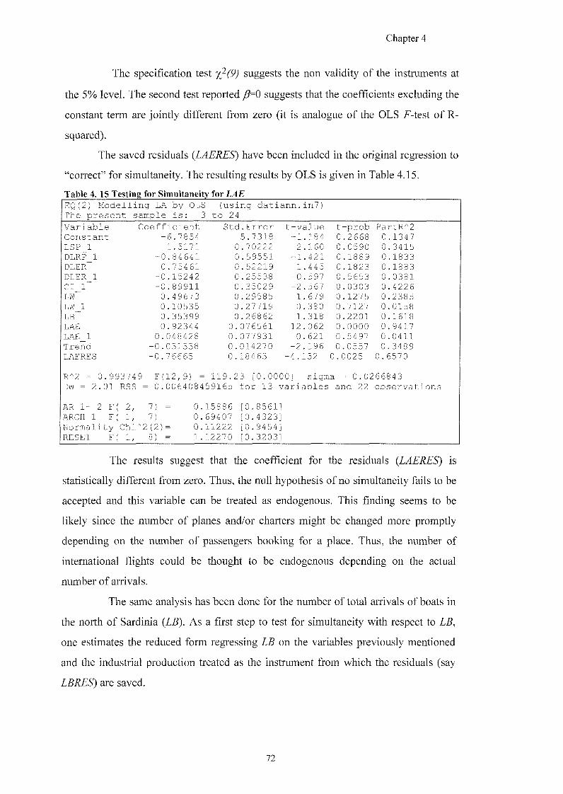
Chapter 4

The specification test y^(9) suggests the non validity of the instruments at

the 5% level. The second test reported suggests that the coefficients excluding the

constant term are jointly different from zero (it is analogue of the OLS F-test of R-

squared).

The saved residuals (LAERES) have been included in the original regression to

"correct" for simultaneity. The resulting results by OLS is given in Table 4.15.

Table 4 .15 Testing for Simultaneity for LAE EQ(2) Modelling LA by OLS (using datiann. The present sample is: 3 to 24

in7)

Variable Coefficient Std.Error t-value t -prob PartR''2 Constant -6.7854 5.7318 -1 . 184 0 2668 0 . 1347 LSP 1 1.5171 0.70222 2 .160 0 0590 0 .3415 DLRP 1 -0.84641 0.59551 -1 .421 0 1889 0 . 1833 DLER 0.75461 0.52219 1 . 445 0 1823 0 . 1883 DLER 1 -0.15242 0.25538 -0 .597 0 5653 0 . 0381 CI 1 -0.89911 0.35029 -2 .567 0 0303 0 .4226 LW 0.49673 0.29585 1 . 679 0 1275 0 .2385 LW 1 0.10535 0.27719 0 .380 0 7127 0 .0158 LB 0.35399 0.26862 1 .318 0 2201 0 . 1618 LAE 0.92344 0.076561 12 .062 0 0000 0 . 9417 LAE_1 0.048428 0.077931 0 . 621 0 5497 0 .0411 Trend -0.031338 0.014270 -2 . 196 0 0557 0 .3489 LAERES -0.76665 0.18463 -4 . 152 0 .0025 0.6570

R"2 = 0.993749 F(12,9) = 119.23 [0.0000] sigma = 0.0266843 DW = 2.01 RSS = 0.006408459165 for 13 variables and 22 observations

AR 1- 2 F( 2, 7) = 0 .15886 [0.8561 ] ARCH 1 F( 1, 7) - 0 69407 [0.4323 ] Normality Chi 2(2)= 0 .11222 [0.9454 ] RESET F( 1, 8) = 1 .12270 [0.3203 ]

The results suggest that the coefficient for the residuals {LAERES) is

statistically different from zero. Thus, the null hypothesis of no simultaneity fails to be

accepted and this variable can be treated as endogenous. This finding seems to be

likely since the number of planes and/or charters might be changed more promptly

depending on the number of passengers booking for a place. Thus, the number of

international flights could be thought to be endogenous depending on the actual

number of arrivals.

The same analysis has been done for the number of total arrivals of boats in

the north of Sardinia {LB). As a first step to test for simultaneity with respect to LB,

one estimates the reduced form regressing LB on the variables previously mentioned

and the industrial production treated as the instrument from which the residuals (say

are saved.

72

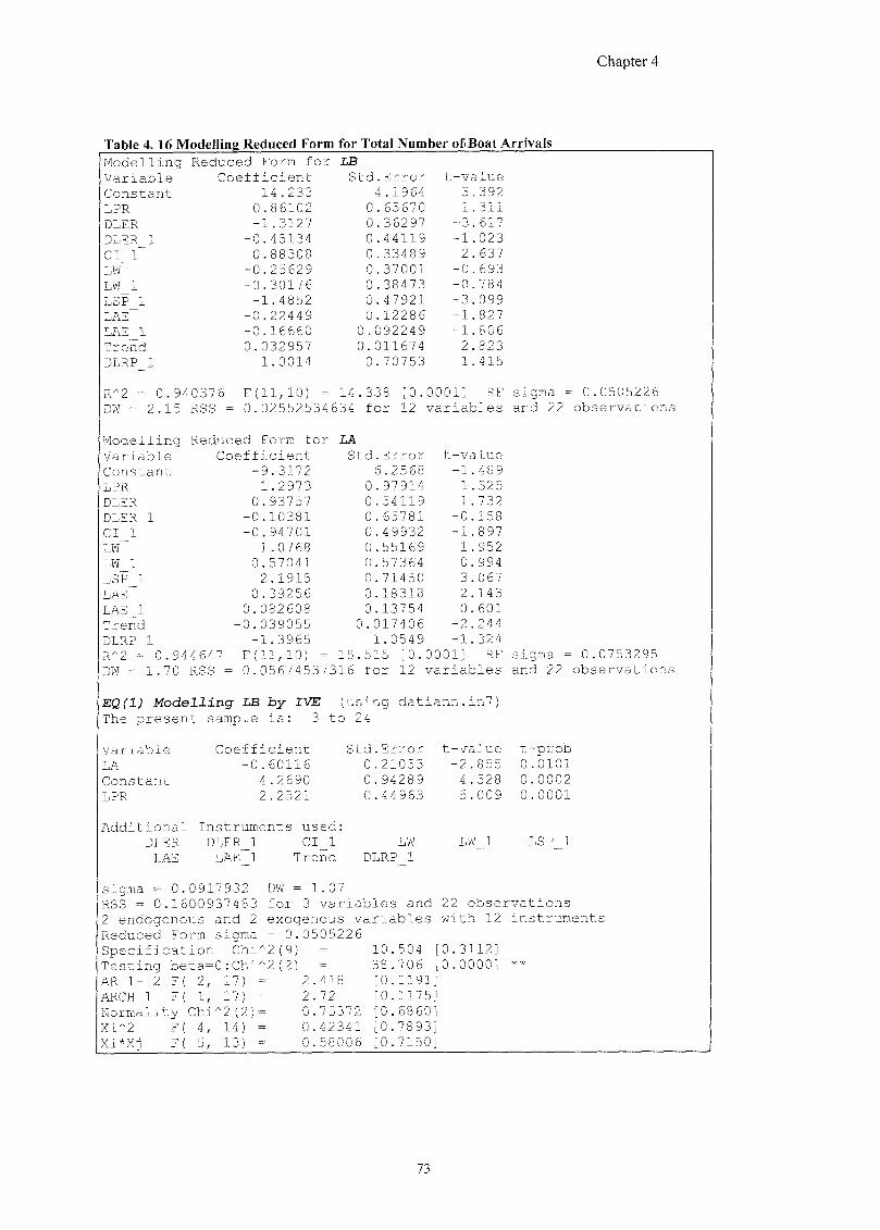
Chapter 4

Table 4. 16 Modelling Reduced Form for Total Number of Boat Arrivals Modelling Reduced Form for LB Variable Coefficient Std.Error t-value Constant 14.233 4.1964 3. 392 LPR 0.86102 0.65670 1 311

DLER -1.3127 0.36297 -3. 617

DLER 1 -0.45134 0.44119 -1 023 CI 1 0.88308 0.33489 2 . 637 LW -0.25629 0.37001 -0. 693

LW 1 -0.30176 0.38473 -0. 784 LSP 1 -1.4852 0.47921 -3. 099 LAE -0.22449 0.12286 -1. 827 LAE_1 -0.16660 0.092249 — 1 . 806 Trend 0.032957 0.011674 2 . 823 DLRP_1 1.0014 0.70753 1. 415

R^2 = 0.940376 F(ll,10) = 14.338 [0.0001] RF sigma = 0 0505226 DW = 2.15 RSE = 0.02552534634 for 12 variables and 22 observations

Modelling Reduced Form for LA Variable Coefficient Std.Error t-value Constant -9.3172 6.2568 -1. 489 LPR 1.2973 0.97914 1. 325 DLER 0.93757 0.54119 1. 732 DLER 1 -0.10381 0.65781 -0. 158 CI 1 -0.94701 0.49932 ~ 1 . 897 LW 1.0768 0.55169 1. 952 LW 1 0.57041 0.57364 0 . 994 LSP 1 2.1915 0.71450 3. 067 LAE 0.39256 0.18318 2 . 143 LAE_1 0.082608 0.13754 0. 601 Trend -0.039055 0.017406 — 2 . 244 DLRP 1 -1.3965 1.0549 -1. 324 R"2 = 0.944647 F(ll,10) = 15.515 [0.0001] RF sigma = 0 0753295 DW = 1.70 RSS = 0.05674537316 for 12 variables and 22 observations

EQ(1) Modelling LB by IVE (using datiann.in7) The present sample is: 3 to 24


LA -0.60116 0.21053 — 2. 855 0.0101 Constant 4.2690 0.94289 4 . 528 0.0002

LPR 2.2521 0.44963 5. 009 0.0001

Additional Instruments used DLER DLER 1 CI 1 LW LW _1 LSP_1 LAE LAE 1 Trend DLRP_1

sigma = 0. 0917932 DW = 1.07 R5S = 0.1600937483 for 3 variables and 22 observations 2 endogenous and 2 exogenous variables with 12 instruments Reduced Form sigma = 0.0505226 Specification Chi^2(9) = 10.504 [ 0.3112] Testing beta= 0:Chi*2(2) = 38.706 [ 0.0000] * *

AR 1- 2 F( 2, 17) = 2.41 8 [0.1191] AKCH 1 F( 1, 17) = 2.72 [0.1175] Normality Chi 2(2)= 0.75372 [0.6860] Xi^2 F( 4, 14) = 0.42341 [0.7893] Xi*Xj F( 5, 13) = 0.58006 [0.7150]

7 3

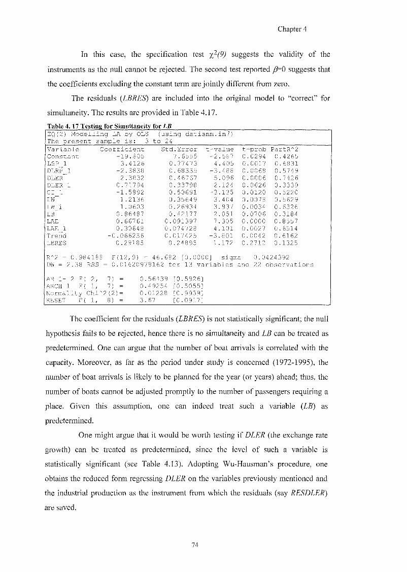
Chapter 4

In this case, the specification test y}(9) suggests the validity of the

instruments as the null cannot be rejected. The second test reported /?=0 suggests that

the coefficients excluding the constant term are jointly different from zero.

The residuals {LBRES) are included into the original model to "correct" for

simultaneity. The results are provided in Table 4.17.

Table 4 .17 Testing for Simultaneity for LB EQ(2) Modelling LA by OLE The present sample is: 2

(using datiann. to 24

in7)

Variable Coefficient Std.Error t -value t-prob PartR^2 Constant -19.805 7.6555 -2 .587 0 0294 0 4265 LSP 1 3.4126 0.77473 4 .405 0 0017 0 6831 DLRP 1 -2.3838 0.68335 -3 .488 0 0068 0 5749 DLER 2.3832 0.46767 5 .096 0 0006 0 7426 DLER 1 0.71794 0.33798 2 .124 0 0626 0 3339 CI 1 -1.5892 0.50691 -3 .135 0 0120 0 5220 LW 1.2136 0.35649 3 .404 0 0078 0 5629 LW 1 1.0603 0.26934 3 .937 0 0034 0 6326 LB 0.86487 0.42177 2 .051 0 0706 0 3184 LAE 0.66761 0.091397 7 .305 0 0000 0 8557 LAE_1 0.30648 0.074728 4 .101 0 0027 0 6514 Trend -0.066236 0.017425 -3 .801 0 0042 0 6162 LBRES 0.29185 0.24895 1 .172 0 2712 0 1325

R"2 = 0.98 418 8 F(12,9) = 46.682 [0.0000 sigma = 0.0424392 DM = 2.38 RSS = 0.0162097 8162 for 13 variables anc 22 observations

AR 1- 2 F( 2, 7) = 0. 56439 [0.5926] ARCH 1 F( 1, 7) = 0. 49254 [0.5055] Normality Chi "2(2)= 0. 01228 [0.9939] RESET F( 1, 8) = 3. 67 [0.0917]

The coefficient for the residuals (LBRES) is not statistically significant; the null

hypothesis fails to be rejected, hence there is no simultaneity and LB can be treated as

predetermined. One can argue that the number of boat arrivals is correlated with the

capacity. Moreover, as far as the period under study is concerned (1972-1995), the

number of boat arrivals is likely to be planned for the year (or years) ahead; thus, the

number of boats cannot be adjusted promptly to the number of passengers requiring a

place. Given this assumption, one can indeed treat such a variable {LB) as

predetermined.

One might argue that it would be worth testing if (the exchange rate

growth) can be treated as predetermined, since the level of such a variable is

statistically significant (see Table 4.13). Adopting Wu-Hausman's procedure, one

obtains the reduced form regressing DLER on the variables previously mentioned and

the industrial production as the instrument from which the residuals (say RESDLER)

are saved.

74

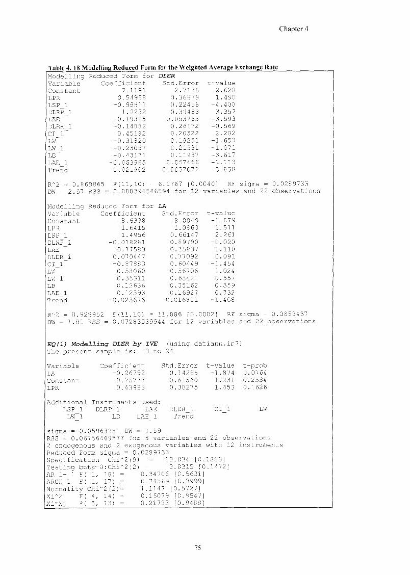
Chapter 4

Table 4 .18 Modelling Reduced Form for the Weighted Average Exchange Rate Modelling Reduced Form for DLER Variable Coefficient Std.Error t-value Constant 7.1191 2.7176 2 . 620 LPR 0.54958 0.36879 1 490 LSP 1 -0.98811 0.22456 -4 . 400 DLRP 1 1.0232 0.30483 3. 357 LAE -0.19315 C .053765 -3. 593 DLER 1 -0.14882 0.26172 -0. 569 CI 1 0.45182 0.20522 2. 202 LW -0.31820 0.19251 — 1 . 653 LW 1 -0.23057 0.21531 -1. 071 LB -0.43171 0.11937 -3. 617 LAE_1 -0.063965 0 .057466 — 1 . 113 Trend 0.021902 0 . 0057072 3. 838

R^2 = 0.8( 9865 F(ll,10) = 6.0767 [0.0040] RF sigma = 0.0289733 DM = 2.57 RSS = 0.008394546594 for 12 variables and 22 observations

Modelling Reduced Form for 2A Variable Coefficient Std.Error t-value Constant -8.6338 8.0049 -1. 079 LPR 1.6415 1.0863 1. 511 LSP 1 1.4956 0.66147 2 . 261 DLRP 1 -0.018281 0.89790 -0. 020 LAE 0.17583 0.15837 1. 110 DLER 1 0.070447 0.77092 0 . 091 CI 1 -0.87883 0.60449 -1. 454 LW 0.58060 0.56706 1. 024 LW 1 0.35311 0.63421 0. 557

LB 0.12636 0.35162 0. 359 LAE_1 0.12393 0.16927 0. 732 Trend -0.023676 0 .016811 -1. 408

R*2 = 0.928952 F(ll,10) = 11. 886 [0.0002] RF sigma = 0.0853437 DW = 1.81 RSS = 0.07283539944 for 12 variables and 22 observations

EQ(1) Modelling DLER by IVE ( using datiann .in7 ) The present sample is: 3 to 24


LA -0.26792 0.14295 -1. 874 0.0764

Constant 0.75777 0.61560 1. 231 0.2334 LPR 0.43985 0.30275 1. 453 0.1626

Additional Instruments used: LSP 1 DLRP 1 LAE DLER_1 CI _1 LW LW_1 LB LAE 1 Trend

sigma = 0. 0596325 DW = 1 .59 RSS = 0.06756469577 for 3 variables and 22 observations 2 endogenous and 2 exogenous variables with 12 instruments Reduced Form sigma = 0.0289733 Specification Chi^2(9) 13.834 [0. 1283 ] Testing beta=0:Chi^2(2) = 3.8315 [0 .1472] AR 1- 1 F( 1, 18) = 0. 34706 [0.5631] ARCH 1 F( 1, 17) = 0. 74569 [0.3999] Normality Chi*2(2)= 1. 1147 [0.5727] Xi^2 F( 4 , 1 4 ) = 0. 16079 [0.9547]

Xi*Xi F( 5, 13) = 0. 21733 [0.9488]

75

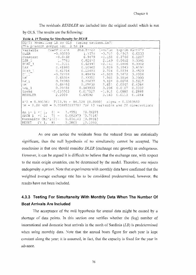
Chapter 4

The residuals RESDLER are included into the original model which is run

by OLS. The results are the following:

Table 4 .19 Testing for Simultaneity for DLER EQ(2) Modelling LA by OLS The present sample is: 3

(using datiann.in?) to 24

Variable Coefficient Std.Error t-value t -prob PartR*2 DLER -0.80289 1.1278 -0 712 0 .4945 0 0533 Constant -8.0468 6.9479 -1 158 0 .2766 0 1297 LSP 1 1.7765 0.82675 2 149 0 .0602 0 3391 DLRP 1 -1.3511 0.62997 -2 145 0 .0606 0 3382 LAE 0.41980 0.10962 3 829 0 .0040 0 6197 DLER 1 0.61716 0.22653 2 724 0 .0234 0 4520 CI 1 -0.72784 0.48439 -1 503 0 1672 0 2006 LW 0.65384 0.33351 1 960 0 0816 0 2993 LW 1 0.74090 0.21637 3 424 0 0076 0 5657 LB 0.68486 0.25838 2 651 0 0265 0 4384 LAE_1 0.20488 0.063900 3 206 0 0107 0 5332 Trend -0.033503 0.017527 -1 912 0 0882 0 2888 RESDLER 2.2009 0.69592 3 163 0 0115 0 5264

R^2 = 0.991367 DW = 2.60 RSS =

F(12,9) = 86.128 [0.0000] sigma = 0.0313582 0.008850037787 for 13 variables and 22 observations

AR 1- 1 F( 1, 8) = ARCH 1 F( 1, 7) = Normality Chi^2(2)= RESET F( 1, 8) =

1.4551 [0.2622] 0.082979 [0.7816] 0.034143 [0.9831] 3.3803 [0.1033]

As one can notice the residuals from the reduced form are statistically

significant, thus the null hypothesis of no simultaneity cannot be accepted. The

conclusion is that one should consider DLER (exchange rate growth) as endogenous.

However, it can be argued it is difficult to believe that the exchange rate, with respect

to the main origin countries, can be determined by the model. Therefore, one rejects

endogeneity a priori. Note that experiments with monthly data have confirmed that the

weighted average exchange rate has to be considered predetermined, however, the

results have not been included.

4.3.3 Testing For Simultaneity With IVlonthly Data When The Number Of

Boat Arrivals Are Included

The acceptance of the null hypothesis for annual data might be caused by a

shortage of data points. In this section one verifies whether the (log) number of

international and domestic boat arrivals in the north of Sardinia {LB) is predetermined

when using monthly data. Note that the annual boats figure for each year is kept

constant along the year; it is assumed, in fact, that the capacity is fixed for the year in

advance.

76

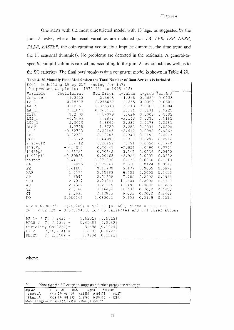
Chapter 4

One starts with the most unrestricted model with 13 lags, as suggested by the

joint F-test22, where the usual variables are included {i.e. LA, LPR, LSP, DLRP,

DLER, EASTER, the cointegrating vector, four impulse dummies, the time trend and

the 11 seasonal dummies). No problems are detected in the residuals. A general-to-

specific simplification is carried out according to the joint F-test statistic as well as to

the SC criterion. The final parsimonious data congruent model is shown in Table 4.20.

Table 4. 20 Monthly Final Model when the Total Number of Boat Arrivals is Included

EQ(1) Modelling LA by OLS (using for.inV) The present sample is: 1973 (3) to 1995 ( 12)

Variable Coefficient Std.Error t-value t -prob PartR'^2 Constant -4.3618 2.3605 -1 . 848 0 0658 0 0135 LA 1 0.18618 0.043652 4 .265 0 0000 0 .0681 LA 3 0.18961 0.036370 5 .213 0 0000 0 0984 LA 11 0.11843 0.049458 2 .394 0 0174 0 0225 RLPR 2.2509 0.62079 3 . 626 0 0003 0 0502 LSP 1 -4.0493 1.8892 -2 . 143 0 0330 0 0181 LSP 2 5.0600 1.8865 2 . 682 0 0078 0 0281 RLSPl 4.2708 1.8729 2 .280 0 0234 0 0205 CI 1 -0.52733 0.20185 -2 . 612 0 0095 0 0267 LB 0.32381 0.13785 2 . 349 0 0196 0 0217 RLE 1.5142 0.64903 2 .333 0 0204 0 0214 il974pl2 1.4712 0.20459 7 . 191 0 0000 0 1720 il979p3 -0.54071 0.20548 -2 . 631 0 0090 0 0271 il985p3 0.68751 0.20543 3 347 0 0009 0 0430 il991pll -0.59885 0.20465 -2 . 926 0 0037 0 0332 easter 0.44111 0.071892 6 . 136 0 0000 0 1313 JA 0.19026 0.075547 2 .518 0 0124 0 0248 FE 0.61605 0.11900 5 177 0 0000 0 0972 MAR 1.0174 0.15893 6 401 0 0000 0. 1413 AP 1.6592 0.21328 7 780 0 0000 0 1955 MJJ 2.7017 0.23283 11 .604 0 0000 0. 3510 AU 2.4382 0.21215 11 493 0 0000 0. 3466 SE 2.3180 0.16404 14 131 0 0000 0. 4450 OT 1.1633 0.12875 9 035 0 0000 0. 2469 NO 0.050349 0.083041 0 606 0 5449 0. 0015

R"2 = 0 . 9 8 1731 F(24,249) = 557.51 [0.0000_ sigma = 0.197C 98 DM = 2.02 RSS = 9.673094916 for 25 variables and 274 observations

AR 1- 7 F( 7, 242) = 0. 82018 [0.5713] ARCH 7 F( 7, 235) = 0. 40581 [0.8982] Normality Chi "2(2)= 3.898 [0.1424] Xi"2 F( 34, 214) = 1 .4196 [0.0723] RESET F( 1, 248) = 1 .7184 [0.1911]

where;

22 Note that the SC criterion suggests a further parameter reduction. dep.var T k df RSS sigma Schwarz 12 lags: LA 0 L S 274 95 179 6.81893 0.195178 -1.74727 13 lags: LA OLS 274 10] 173 6.18796 0.189126 -1.72145

Model 13 lags - > 12 lags: F( 6, 173) = 2.9401 [0.0093] **

77

Chapter 4

LA = (log) normalised series of foreign arrivals for the number of weekends {i.e.

Saturdays) in a month.

RLPR = difference between the coefficients of the third and seventh lag of the (log)

weighted average industrial production index for the origin countries. Such a

restriction is suggested both from the joint F-test and the SC criterion^^.

RLSPl = difference between the coefficients of the eleventh and twelfth lag of the

(log) substitute price. One accepts such a restriction from the joint F-test and as

suggested by the SC criterion^^.

LSP = (log) substitute price (consumer price index in Sassari by the weighted average


C / = cointegrating vector between LRP (relative price) and LER (exchange rate).

RLB = Difference between the coefficient of the fourth and fifth lag of the (log) total

number of boat arrivals in north of Sardinia. Such a restriction has been suggested by

the SC criterion and accepted by the joint F-test^^.

EASTER= dummy 0-1 with respect to the Easter holiday.

MJJ = seasonal dummy giving the value of 1 to May, June and July months and 0

otherwise. Such a restriction was possible given the results from the joint F-test and

the SC criterion^^.

Considering the coefficients of LB the fourth lag has presented a positive sign

that reflects as the number of foreign tourists is increasing given the number of boats

determined at the beginning of the year (say in January); however, the fifth lag, that

could occur in June, has shown a negative sign that reflects a decrease in the number

The restriction on the coefficients of the third and seventh lag is accepted at the 5% level from the F-test (1,246) as the calculated value (2.0527) is smaller than the critical value (3.84). Moreover, the SC criterion is minimised when the restriction is imposed; from -2.79465 to -2.80683, after imposing the restriction. 24 The restriction on the coefficients of the eleven and twelfth lag is accepted at the 5% level from the f-test (1,245) as the calculated value (0.23764) is smaller than the critical value (3.84). Moreover, the SC criterion is minimised when the restriction is imposed; from -2.77514 to -2.79465, after imposing the restriction. 25 The restriction on the coefficients of the fourth and fifth lag is accepted at the 5% level from the F-test (1,248) as the calculated value (3.515) is smaller than the critical value (3.84). Moreover, the SC criterion is minimised when the restriction is imposed; from -2.82522 to -2.83163, after imposing the restriction. 26 The restriction on the coefficients of May, June and July is accepted at the 5% level fi-om the F-test (2,247) as the calculated value (0.56814) is smaller than the critical value (3.84). Moreover, the SC criterion is minimised when the restriction is imposed; from -2.80683 to -2.84321, after imposing the restriction.

78

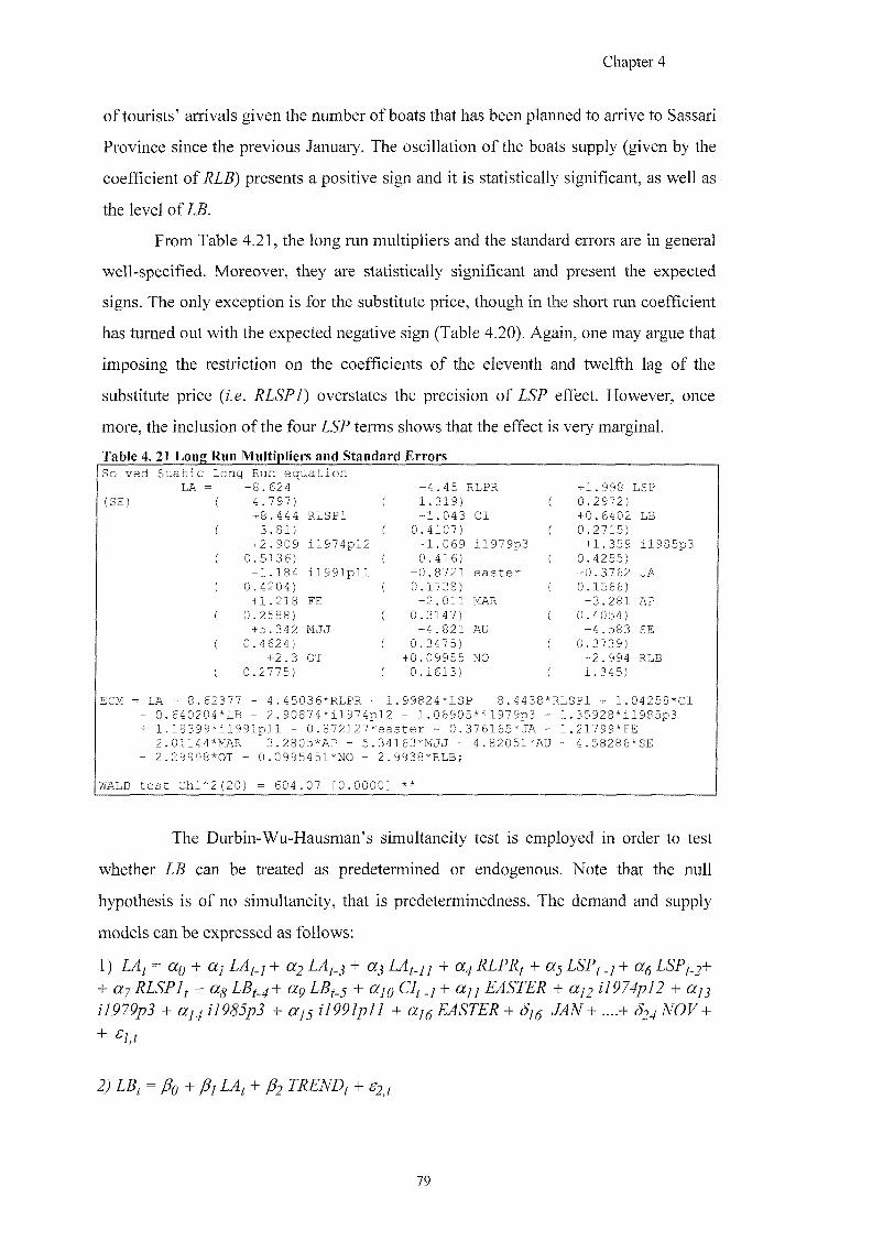
Chapter 4

of tourists' arrivals given the number of boats that has been planned to arrive to Sassari

Province since the previous January. The oscillation of the boats supply (given by the

coefficient of RLE) presents a positive sign and it is statistically significant, as well as

the level of

From Table 4.21, the long run multipliers and the standard errors are in general

well-specified. Moreover, they are statistically significant and present the expected

signs. The only exception is for the substitute price, though in the short run coefficient

has turned out with the expected negative sign (Table 4.20). Again, one may argue that

imposing the restriction on the coefficients of the eleventh and twelfth lag of the

substitute price {i.e. RLSPl) overstates the precision of LSP effect. However, once

more, the inclusion of the four LSP terms shows that the effect is very marginal.

Table 4. 21 Long Run Multipliers and Standard Errors S o l v e d S t a t i c L o n g R u n e q u a t i o n

LA (SE)

- 8 . 6 2 4 +4 . 4 5 RLPR + 1 . 9 9 8 LSP 4 . 7 9 7 ) 1 . 3 1 9 ) 0 . 2 9 7 2 ) + 8 . 4 4 4 R L S P l - 1 . 0 4 3 CI + 0 . 6 4 0 2 LB

3 . 8 1 ) 0 . 4 1 0 7 ) 0 . 2 7 1 5 ) + 2 . 9 0 9 i l 9 7 4 p l 2 - 1 . 0 6 9 i l 9 7 9 p 3 + 1 . 3 5 9 i l 9 8 5 p 3

0 . 5 1 3 6 ) 0 . 4 1 6 ) 0 . 4 2 5 5 ) - 1 . 1 8 4 i l 9 9 1 p l l + 0 . 8 7 2 1 e a s t e r + 0 . 3 7 6 2 JA

0 . 4 2 0 4 ) 0 . 1 7 3 8 ) 0 . 1 5 6 6 ) + 1 . 2 1 8 FE + 2 . 0 1 1 MAR + 3 . 2 8 1 AP

0 . 2 5 8 8 ) 0 . 3 1 4 7 ) 0 . 4 0 5 4 ) + 5 . 3 4 2 M J J + 4 . 8 2 1 AU + 4 . 5 8 3 SE

0 . 4 6 2 4 ) 0 . 3 4 7 5 ) 0 . 3 7 3 9 ) + 2 . 3 OT + 0 . 0 9 9 5 5 NO + 2 . 9 9 4 RLE

0 . 2 7 7 5 ) 0 . 1 6 1 3 ) 1 . 3 4 5 )

ECM = LA + 8 . 6 2 3 7 7 - 4 . 4 5 0 3 6 * R L P R - 1 . 9 9 8 2 4 * L S P - 8 . 4 4 3 8 * R L S P 1 + 1 . 0 4 2 5 8 * C I - 0 . 6 4 0 2 0 4 * L B - 2 . 9 0 8 7 4 * i l 9 7 4 p l 2 + 1 . 0 6 9 0 5 * i l 9 7 9 p 3 - 1 . 3 5 9 2 8 * i l 9 8 5 p 3 + 1 . 1 8 3 9 9 * i l 9 9 1 p l l - 0 . 8 7 2 1 2 7 * e a s t e r - 0 . 3 7 6 1 6 5 * J A - 1 . 2 1 7 9 9 * F E - 2 . 0 1 1 4 4 * M A R - 3 . 2 8 0 5 * A P - 5 . 3 4 1 6 3 * M J J - 4 . 8 2 0 5 1 * A U - 4 . 5 8 2 8 6 * S E - 2 . 2 9 9 9 8 * 0 T - 0 . 0 9 9 5 4 5 1 * N O - 2 . 9 9 3 8 * R L B ;

WALD t e s t C h i ^ 2 ( 2 0 ) 6 0 4 . 0 7 [ 0 . 0 0 0 0 ] * *

The Durbin-Wu-Hausman's simultaneity test is employed in order to test

whether LB can be treated as predetermined or endogenous. Note that the null

hypothesis is of no simultaneity, that is predeterniinedness. The demand and supply

models can be expressed as follows:

1) LAj^ = GCQ + (Xj LA^_j + L^t-3 ^ ^3 1 ^4 RLPR[ + LSPj _j + + ccy RLSPl J + ccg LBf_^ + ccg LBf_^ + (XjQ CI^ _j + ccj j EASTER + ccj2 il974pl2 + ocjj

il979p3 + cxj^ il985p3 + ocj^ il99Ipl 1 + EASTER + JAN —+ 824 NOV + +

79

Chapter 4

Note that the trend and the constant are used as instruments in the second equation.

Firstly, one obtains the reduced form by regressing LB on the variables

included into equation 1) plus the instrument variable TREND; one can assume, in

fact, that the time trend, used as a proxy in a possible change in the consumers' tastes,

is able to explain the number of foreign arrivals as well as the number of boat arrivals

in the north of Sardinia. Hence, the residuals obtained from this regression

{RESIDUAL = w ) are saved. The results are reported in Table 4.22.

80

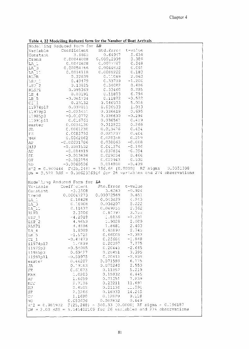
Chapter 4

Table 4. 22 Modelling Reduced form for the Number of Boat Arrivals Modelling Reduced Form for LB Variable Coefficient Std.Error t-value Constant 3.6605 0.64947 5 .636 Trend 0.00044008 0.00012998 3 .386

LA 1 0.0042628 0.0077787 0 .548 LA 3 0.00058766 0.0064852 0 .091 LA 11 0.0016118 0.0088222 0 .183 RLPR 0.22839 0.11069 2 .063 LSP 1 -0.40479 0.33739 -1 .200 LSP 2 0.13825 0.34082 0 .406 RLSPl 0.095369 0.33460 0 .285 LB 4 0.80191 0.11803 6 .794 LB 5 -0.061734 0.11822 -0 .522 CI 1 0.23132 0.046003 5 .028 il974pl2 0.037011 0.036533 1 .013 il979p3 -0.025451 0.036619 -0 .695 il985p3 -0.010772 0.036630 -0 294 il991pll 0.016765 0.036561 0 .459 easter 0.0034130 0.012822 0 266 JA 0.0061230 0.013476 0 454 FE 0.0085795 0.021237 0 404

MAR 0.0062162 0.028358 0 219 AP -0.00031706 0.038063 -0 008 MJJ -0.0081502 0.041574 -0 196 AU -0.014919 0.037854 -0 394 SE -0.013636 0.029254 -0 466 OT -0.012154 0.022943 -0 530 NO -0.0060506 0.014800 -0 409 R^2 = 0.94 0444 F(25,248) = 156.64 [0 0000. RF sigma = 0.0351398 DW = 0.522 = 0.3062316914 for 26 variables and 274 observations

Modelling Reduced Form for LA Variable Coefficient Std.Error t-value Constant -3.3508 3.6260 -0 924 Trend 0.00047273 0.00072569 0 651 LA 1 0.18428 0.043429 4 243 LA 3 0.18908 0.036207 5 222 LA 11 0.11632 0.049255 2 362 RLPR 2.3206 0.61797 3 755 LSP 1 -4.2018 1.8836 -2 231 LSP 2 4.9653 1.9028 2 609 RLSPl 4.4886 1.8681 2 403 LB 4 1.8089 0.65897 2 745 LB 5 -1.5728 0.66005 -2 383 CI 1 -0.47473 0.25684 -1 848 il974pl2 1.4839 0.20397 7 275 il979p3 -0.54085 0.20445 -2. 645 il985p3 0.69427 0.20451 3. 395 il991pll -0.59975 0.20412 -2 938 easter 0.44207 0.071588 6 175 JA 0.19183 0.075240 2 550 FE 0.61873 0.11857 5. 219

MAR 1.0203 0.15832 6. 445 AP 1.6659 0.21251 7 839 MJJ 2.7136 0.23211 11. 691 AU 2.4502 0.21134 11 594 SE 2.3266 0.16333 14 245 OT 1.1680 0.12809 9. 118 NO 0.053636 0.082632 0. 649 R^2 = 0.98 1972 F(25,248) = 540.33 [0. 0000] RF sigma = 0.196187 DW = 2.03 RSS = 9.545402109 for 26 variables and 274 observations

81

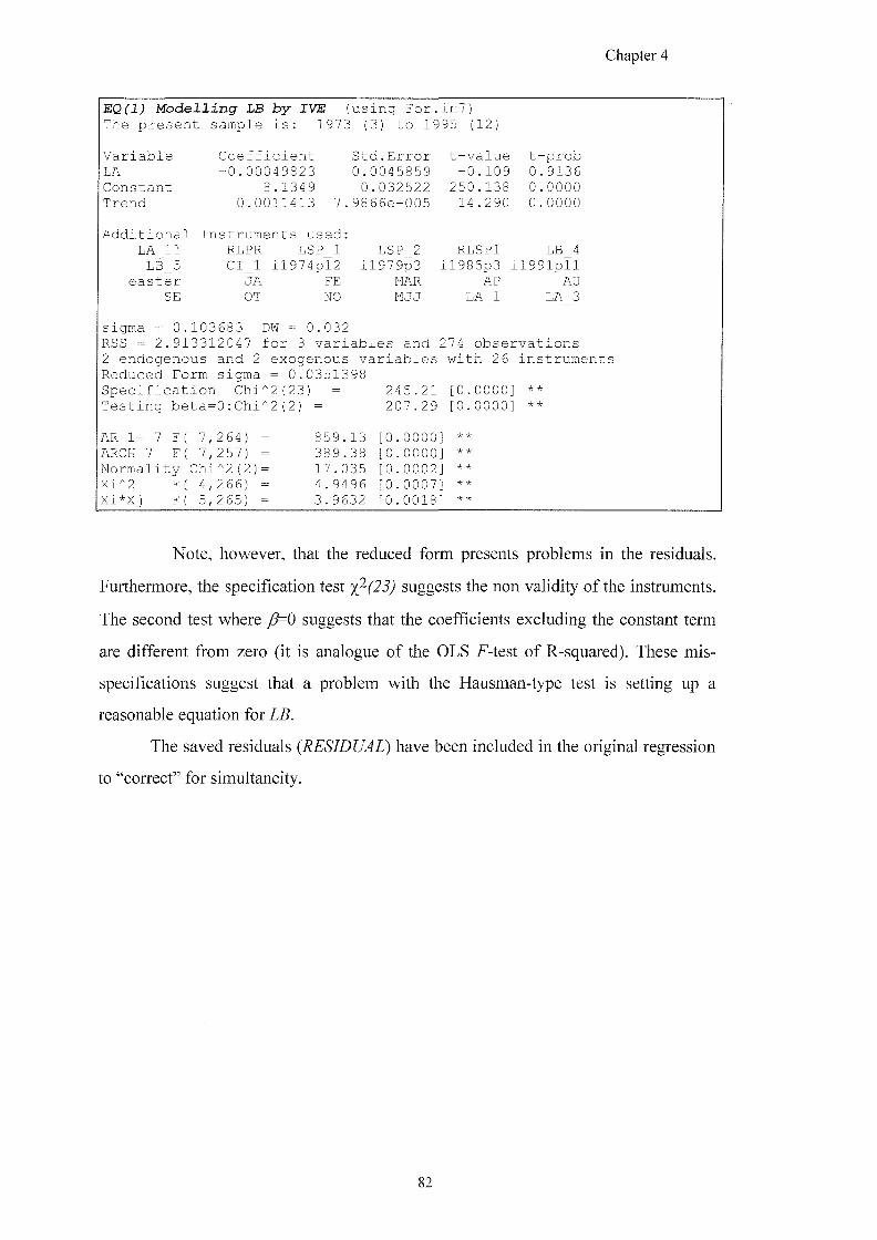
Chapter 4

EQ(1) Modelling LB by IVE (using For.in?) The present sample is: 1973 (3) to 1995 (12)

Variable Coefficient Std.Error t-value t-prob LA -0.00049823 0.0045859 -0.109 0.9136 Constant 8.1349 0.032522 250.138 0.0000 Trend 0.0011413 7.9866e-005 14.290 0.0000

Additional Instruments used: LA_11 RLPR LSP_1 LSP_2 RLSPl LB_4 LB_5 CI_1 il974pl2 il979p3 il985p3 il991pll

easter JA FE MAR AP AU SE OT NO MJJ LA_1 LA_3

sigma = 0.103683 DW = 0.032 RSS = 2.913312047 for 3 variables and 274 observations 2 endogenous and 2 exogenous variables with 26 instruments Reduced Form sigma = 0.0351398 Specification Chi*2(23) = 245.21 [0.0000] ** Testing beta=0:Chi"2(2) = 207.29 [0.0000] **

AR 1- 7 F( 7,264) = 859.13 [0.0000] ** ARCH 7 F( 7,257) = 389.38 [0.0000] ** Normality Chi^2(2)= 17.035 [0.0002] ** Xi^2 F( 4,266) = 4.9496 [0.0007] ** Xi*Xi F( 5,265) = 3.9632 [0.0018] **

Note, however, that the reduced form presents problems in the residuals.

Furthermore, the specification test y}(23) suggests the non validity of the instruments.

The second test where 13=0 suggests that the coefficients excluding the constant term

are different from zero (it is analogue of the OLS F-test of R-squared). These mis-

specifications suggest that a problem with the Hausman-type test is setting up a

reasonable equation for LB.

The saved residuals {RESIDUAL) have been included in the original regression

to "correct" for simultaneity.

82

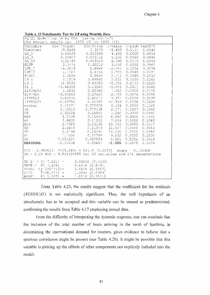
Chapter 4

Table 4. 23 Simultaneity Test for LB using Monthly Data EQ(2) Modelling LA by OLS (using For.in?) The present sample is: 1973 (3) to 1995 (12)

Variable Coefficient Std.Error t-value t -prob PartR*2 Constant -5.8184 2.3279 -2 .499 0 0131 0 .0246 LA 1 0.18615 0.043369 4 .292 0 0000 0 .0691 LA 3 0.18917 0.036154 5 .232 0 0000 0 .0994 LA 11 0.11748 0.049150 2 .390 0 0176 0 .0225 RLPR 2.3874 0.62210 3 838 0 0002 0 .0561 LSP 1 -4.3059 1.8848 -2 285 0 0232 0 .0206 LSP 2 5.1107 1.8754 2 725 0 0069 0 0291 RLSPl 4.5028 1.8650 2 414 0 0165 0 0230 LB 4 2.1219 0.69542 3 051 0 0025 0 0362 LB 5 -1.5539 0.64853 -2 396 0 0173 0 0226 Cl"l -0.44319 0.23560 -1 881 0 0611 0 0141 il974pl2 1.4932 0.20393 7 322 0 0000 0 1778 il979p3 -0.55160 0.20421 -2 701 0 0074 0 0286 il985p3 0.68875 0.20414 3 374 0 0009 0 0439 il991pll -0.59784 0.20365 -2 936 0 0036 0 0336 easter 0.44271 0.071479 6 194 0 0000 0 1340 JA 0.19316 0.075138 2 571 0 0107 0 0260 FE 0.62024 0.11837 5 240 0 0000 0 0997 MAR 1.0208 0.15803 6 460 0 0000 0 1440 AP 1.6631 0.21201 7 844 0 0000 0 1988 MJJ 2.7069 0.23136 11. 700 0 0000 0 3557 AU 2.4418 0.21073 11 . 587 0 0000 0 3512 SE 2.3199 0.16294 14 238 0 0000 0. 4498 OT 1.1630 0.12792 9. 092 0 0000 0. 2500 NO 0.051254 0.082529 0. 621 0 5351 0. 0016 RESIDUAL -0.35678 0.33497 — 1 . 065 0 2879 0. 0046

R"2 = 0.98 2023 F(25,248) = 541.9 [0.0000] sigma = 0.195908 DW = 2.04 RSS = 9.518194855 for 26 variables and 274 observations

AR 1- 7 F( 7, 241) = 0. 84238 [0.5531 ] ARCH 7 F( 7, 234) = 0. 4358 [0.8791] Normality Chi "2(2)= 3. 6614 [0.1603] Xi*2 F( 36, 211) = 1. 3694 [0.0909] RESET F( 1, 247) = 1. 0216 [0.3131]

From Table 4.23, the results suggest that the coefScient for the residuals

(RESIDUAL) is not statistically significant. Thus, the null hypothesis of no

simultaneity has to be accepted and this variable can be treated as predetermined,

confirming the results from Table 4.17 employing annual data.

From the difficulty of interpreting the dynamic response, one can conclude that

the inclusion of the total number of boats arriving in the north of Sardinia, in

determining the international demand for tourism, gives evidence to believe that a

spurious correlation might be present (see Table 4.20). It might be possible that this

variable is picking up the effects of other components not explicitly included into the

inodeL

83

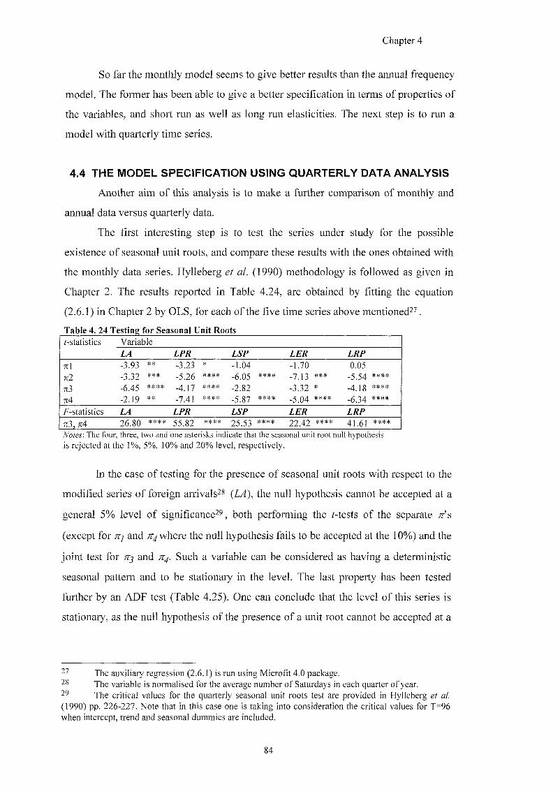
Chapter 4

So far the monthly model seems to give better results than the annual frequency

model. The former has been able to give a better specification in terms of properties of

the variables, and short run as well as long run elasticities. The next step is to run a

model with quarterly time series.

4.4 THE MODEL SPECIFICATION USING QUARTERLY DATA ANALYSIS

Another aim of this analysis is to make a further comparison of monthly and

annual data versus quarterly data.

The first interesting step is to test the series under study for the possible

existence of seasonal unit roots, and compare these results with the ones obtained with

the monthly data series. Hylleberg et al. (1990) methodology is followed as given in

Chapter 2. The results reported in Table 4.24, are obtained by fitting the equation

(2.6.1) in Chapter 2 by OLS, for each of the five time series above mentioned^^.

Table 4. 24 Testing for Seasonal Unit Roots /-statistics Variable

LA LPR LSP LER LRP

Ttl -3.93 ** -3.23 * -1.04 -L70 &05

7[2 - 3 J 2 *** -5.26 * * * * -&05 **** -7.13 *** - 5 J 4 * * * *

TC3 -&45 **** -4.17 * * * * -2.82 - 3 J 2 * * * * *

7I4 - 2 J 9 ** -7.41 * * * * * * * * -5.04 **** -&34 * * * *

F-statistics LA LPR LSP LER LRP

713, 7t4 2&80 **** 5 5 ^ 2 * * * * 25.53 **** 22.42 **** 4T61 * * * *

Notes: The four, three, two and one asterisks indicate that the seasonal unit root null hypothesis is rejected at the 1%, 5%, 10% and 20% level, respectively.

In the case of testing for the presence of seasonal unit roots with respect to the

modified series of foreign arrivals^^ {LA), the null hypothesis cannot be accepted at a

general 5% level of significance^^, both performing the Mests of the separate Tfs

(except for and where the null hypothesis fails to be accepted at the 10%) and the

joint test for and Such a variable can be considered as having a deterministic

seasonal pattern and to be stationary in the level. The last property has been tested

further by an ADF test (Table 4.25). One can conclude that the level of this series is

stationary, as the null hypothesis of the presence of a unit root cannot be accepted at a

The auxiliary regression (2.6.1) is run using Microfit 4.0 package. The variable is normalised for the average number of Saturdays in each quarter of year. The critical values for the quarterly seasonal unit roots test are provided in Hylleberg et al.

(1990) pp. 226-227. Note that in this case one is taking into consideration the critical values for T=96 when intercept, trend and seasonal dummies are included.

84

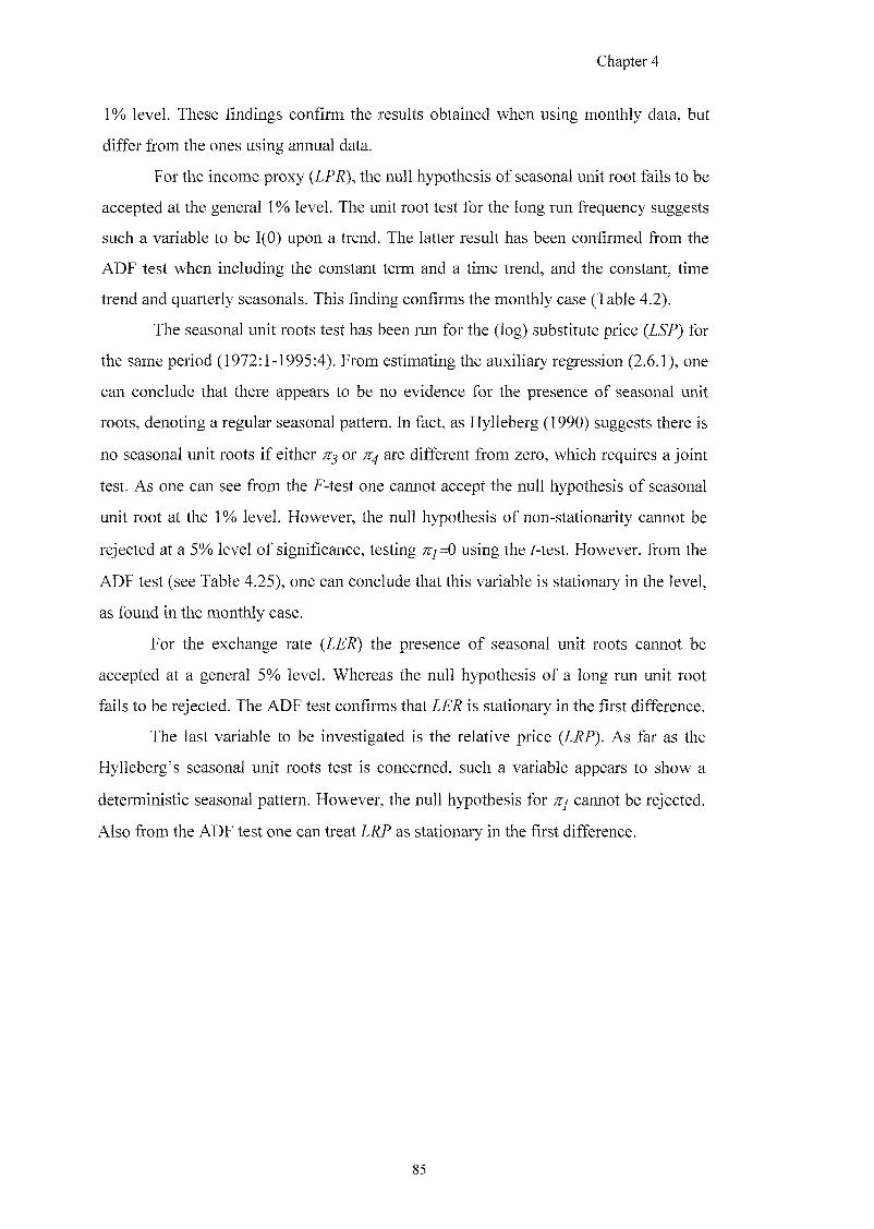
Chapter 4

1% level. These findings confirm the results obtained when using monthly data, but

differ from the ones using annual data.

For the income proxy ( I f .R), the null hypothesis of seasonal unit root fmls to be

accepted at the general 1% level. The unit root test for the long run frequency suggests

such a variable to be 1(0) upon a trend. The latter result has been confirmed from the

ADF test when including the constant term and a time trend, and the constant, time

trend and quarterly seasonals. This finding confirms the monthly case (Table 4.2).

The seasonal unit roots test has been run for the (log) substitute price (LSP) for

the same period (1972:1-1995:4). From estimating the auxiliary regression (2.6.1), one

can conclude that there appears to be no evidence for the presence of seasonal unit

roots, denoting a regular seasonal pattern. In fact, as Hylleberg (1990) suggests there is

no seasonal unit roots if either TTJ or are different from zero, which requires a joint

test. As one can see from the F-test one cannot accept the null hypothesis of seasonal

unit root at the 1% level. However, the null hypothesis of non-stationarity cannot be

rejected at a 5% level of significance, testing ;r/=0 using the r-test. However, from the

ADF test (see Table 4.25), one can conclude that this variable is stationary in the level,

as found in the monthly case.

For the exchange rate (ZE/Z) the presence of seasonal unit roots cannot be

accepted at a general 5% level. Whereas the null hypothesis of a long run unit root

fails to be rejected. The ADF test confirms that LER is stationary in the first difference.

The last variable to be investigated is the relative price (LRP). As far as the

Hylleberg's seasonal unit roots test is concerned, such a variable appears to show a

deterministic seasonal pattern. However, the null hypothesis for cannot be rejected.

Also from the ADF test one can treat LRP as stationary in the first difference.

85

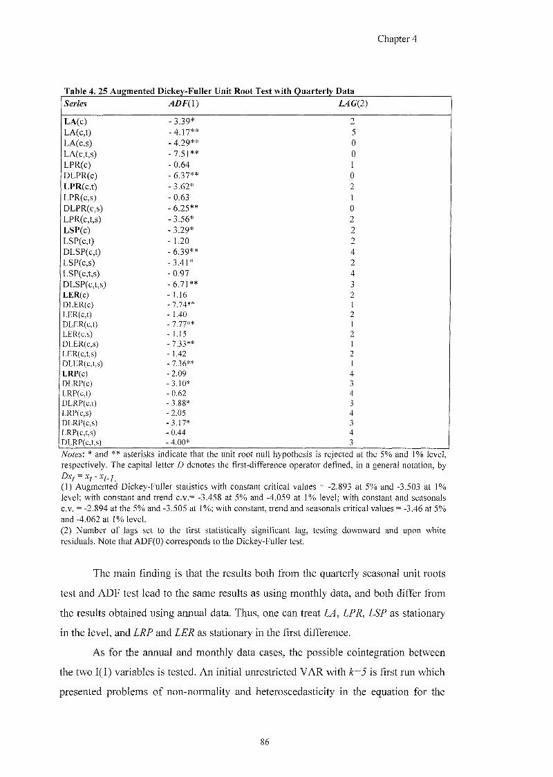
Chapter 4

Table 4. 25 Augmented Dickey-Fuller Unit Root Test with Quarterly Data

Series AXC(2)

LA&O - 3 J 9 * 2 LA(c,t) - 4 J 7 * * 5 LA^:X) -4.29** 0 LA(c,t,s) -7.51** 0 LPR^) - 0.64 1 DLPR(c) -6.37** 0 LPR(c,t) -3.62* 2 LPR(c,s) - 0 ^ 3 1 DLPR(c,s) -6.25** 0 LPR(c,t,s) - 3 J 6 * 2 LSP(c) - 3 J y * 2 LSP(c,t) -1 .20 2 DLSP(c,t) -&39** 4 LSP(c,s) - 1 4 1 * 2 LSP(c,t,s) - 0 4 7 4 DLSP(c,t,s) -6.71** 3 LER(c) - 1 1 6 2 DLER(c) -7.74** 1 LER(c,t) -1.40 2 DLER(c,t) -"^77** 1

- 1,15 2 DLER(c,s) -"^33** 1 LER(c,t,s) -1.42 2 DLER(c,t,s) -"^36** 1 LRP(c) -2.09 4 DLRP(c) -3.10* 3 LRP(c,t) -0.62 4 DLRP(c,t) -3.88* 3 LRP(c,s) -2.05 4 DLRP(c.s) -3.17* 3 LRP(c,t,s) -0/W 4 DLRP(c,t,s) -4L00* 3

Notes: * and ** asterisks indicate that the unit root null hypothesis is rejected at the 5% and 1% level, respectively. The capital letter D denotes the first-difference operator defined, in a general notation, by

(1) Augmented Dickey-Fuller statistics with constant critical values = -2.893 at 5% and -3.503 at 1% level; with constant and trend c.v.= -3.458 at 5% and -4.059 at 1% level; with constant and seasonals c.v. = -2.894 at the 5% and -3.505 at 1%; with constant, trend and seasonals critical values = -3.46 at 5% and -4.062 at 1% level. (2) Number of lags set to the first statistically significant lag, testing downward and upon white residuals. Note that ADF(O) corresponds to the Dickey-Fuller test.

The main finding is that the results both from the quarterly seasonal unit roots

test and ADF test lead to the same results as using monthly data, and both differ from

the results obtained using annual data. Thus, one can treat LA, LPR, LSP as stationary

in the level, and LRP and LER as stationary in the first difference.

As for the annual and monthly data cases, the possible cointegration between

the two 1(1) variables is tested. An initial unrestricted VAR with k=5 is first run which

presented problems of non-normality and heteroscedasticity in the equation for the

86

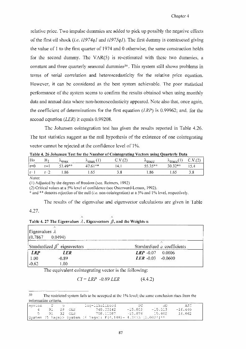
Chapter 4

relative price. Two impulse dummies are added to pick up possibly the negative effects

of the first oil shock {i.e. il974ql and il975ql). The first dummy is constructed giving

the value of 1 to the first quarter of 1974 and 0 otherwise; the same construction holds

for the second dummy. The VAR(5) is re-estimated with these two dummies, a

constant and three quarterly seasonal dummies^". This system still shows problems in

terms of serial correlation and heteroscedasticity for the relative price equation.

However, it can be considered as the best system achievable. The poor statistical

performance of the system seems to confirm the results obtained when using monthly

data and annual data where non-homoscedasticity appeared. Note also that, once again,

the coefficient of determinations for the first equation {LRP) is 0.99962; and, for the

second equation {LER) it equals 0.99208.

The Johansen cointegration test has given the results reported in Table 4.26.

The test statistics suggest as the null hypothesis of the existence of one cointegrating

vector cannot be rejected at the confidence level of 1%.

Table 4. 26 Johansen Test for the Number of Cointegrating Vectors using Quarterly Data

Ho Hi ^max ^ a x (1) C.V.(2) ^trace îrace(l) C.V.(2)

r=0 r=l 53 49** 47.61** 14.1 55J5** 30.32** 15 j

r=l r=2 1.86 3.8 1.86 1.65 3.8

(1) Adjusted by the degrees of freedom (see, Reimers, 1992) (2) Critical values at a 5% level of confidence (see Ostei-ward-Lenum, 1992). * and ** denotes rejection of the null {i.e. non-cointegration) at a 5% and 1% level, respectively.

The results of the eigenvalue and eigenvector calculations are given in Table

4.27.

Table 4. 27 The Eigenvalues X, Eigenvectors p , and the Weights a

Eigenvalues (0.7867 0.0494)

Standardized p' eigenvectors Standardized a coefficients

LRP LER 2 ^ -0.07 0.0006 LOO -&89 2^^ -0.03 -0.0600

-&62 LOO The equivalent cointegrating vector is the following:

= (4.4.2)

30 The restricted system fails to be accepted at the 1% level; the same conclusion rises from the information criteria. s y s t e m T p l o g - l i k e l i h o o d SC HQ A I C

4 9 1 2 8 OLS 7 4 8 . 0 0 1 4 2 - 1 5 . 0 5 2 -15 5 1 3 - 1 6 4 4 0 5 9 1 3 2 OLS 7 5 8 . 1 1 0 8 7 - 1 5 . 0 7 6 - 1 5 6 0 2 -16 6 6 2

S y s t e m (5 l a g s ) > S y s t e m H l a g s ) : F ( 4 , 1 4 8 ) = 4 . 3 4 7 5 [0 0 0 2 4 * *

87

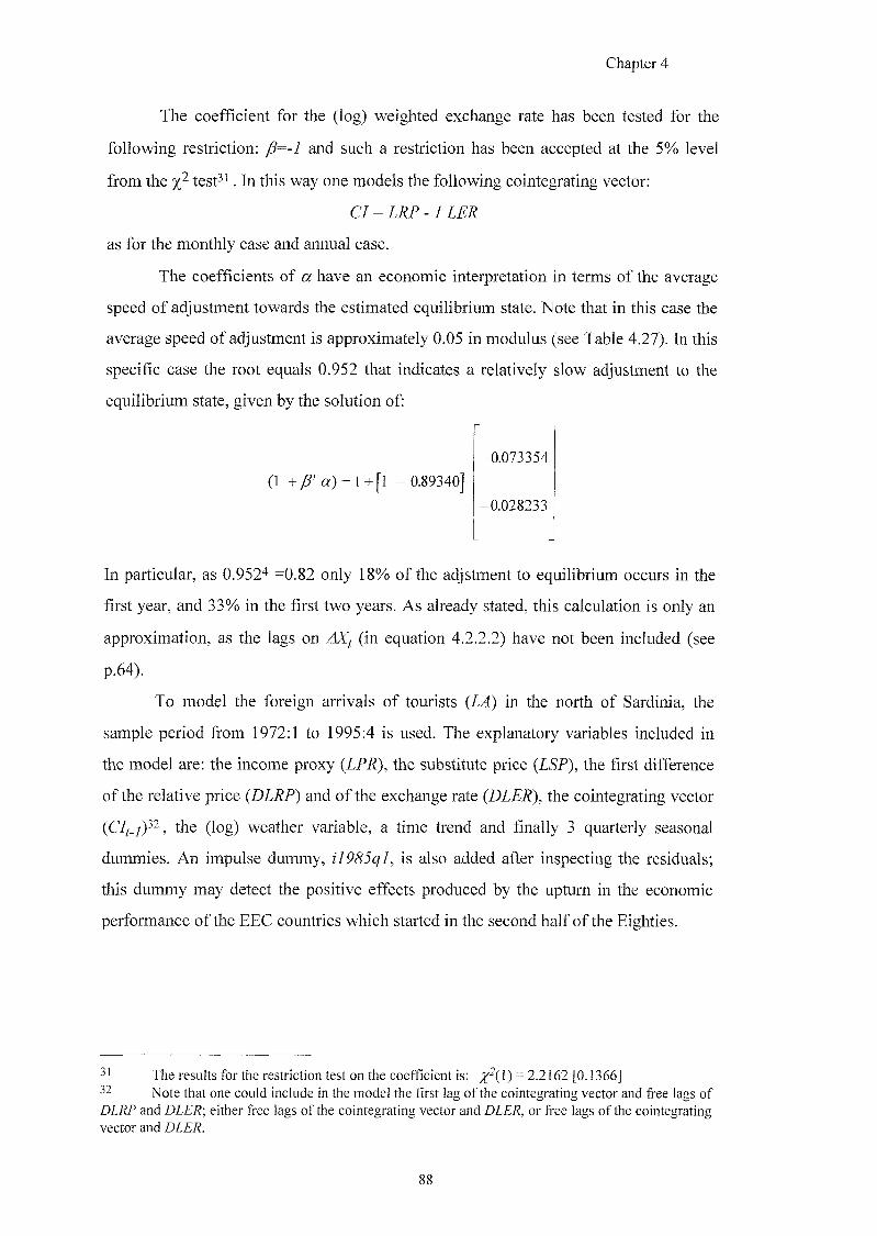
Chapter 4

The coefficient for the (log) weighted exchange rate has been tested for the

following restriction: y5=-7 and such a restriction has been accepted at the 5% level

from the testî. In this way one models the following cointegrating vector:

C / = - 7

as for the monthly case and annual case.

The coefficients of a have an economic interpretation in terms of the average

speed of adjustment towards the estimated equilibrium state. Note that in this case the

average speed of adjustment is approximately 0.05 in modulus (see Table 4.27). In this

specific case the root equals 0.952 that indicates a relatively slow adjustment to the

equilibrium state, given by the solution of;

(1 +yg'a) = l+[ l - 0.89340]

-0.073354

-0.028233

In particular, as 0.952^ =0.82 only 18% of the adjstment to equilibrium occurs in the

first year, and 33% in the first two years. As already stated, this calculation is only an

approximation, as the lags on AiQ (in equation 4.2.2.2) have not been included (see

p.64).

To model the foreign arrivals of tourists {LA) in the north of Sardinia, the

sample period from 1972:1 to 1995:4 is used. The explanatory variables included in

the model are: the income proxy (lf.R), the substitute price (l&P), the first difference

of the relative price {DLRP) and of the exchange rate {DLER), the cointegrating vector

{CIj_jy^, the (log) weather variable, a time trend and finally 3 quarterly seasonal

dummies. An impulse dummy, il985ql, is also added after inspecting the residuals;

this dummy may detect the positive effects produced by the upturn in the economic

performance of the EEC countries which started in the second half of the Eighties.

The results for the restriction test on the coefficient is: %-(!) = 2.2162 [0.1366] 32 Note that one could include in the model the first lag of the cointegrating vector and free lags of DLRP and DLER; either free lags of the cointegrating vector and DLER, or free lags of the cointegrating vector and DLER.

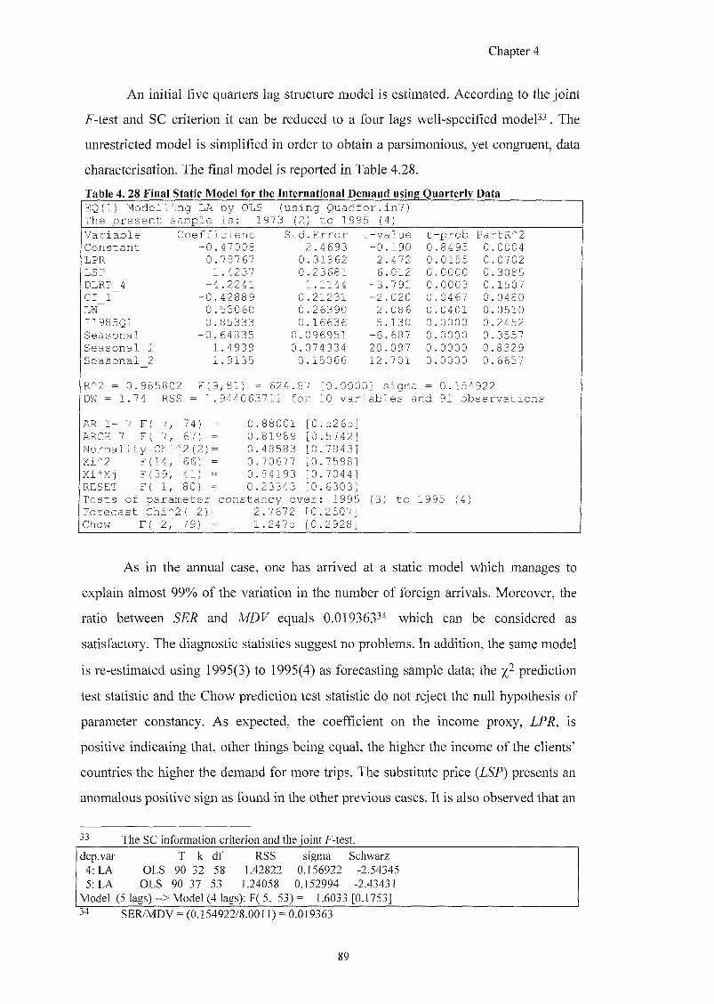
Chapter 4

An initial five quarters lag structure model is estimated. According to the joint

F-test and SC criterion it can be reduced to a four lags well-specified modeP^. The

unrestricted model is simplified in order to obtain a parsimonious, yet congruent, data

characterisation. The final model is reported in Table 4.28.

Table 4. 28 Final Static Model for the International Demand using Quarterly Data EQ(1) Modelling LA by OLS (using Quadfor.inl] The present sample is: 1973 (2) to 1995 (4)

Variable Coefficient Std.Error t-value t -prob PartR*2 Constant -0.47008 2.4693 -0 190 0 8495 0 0004 LPR 0.78767 0.31862 2 472 0 0155 0 0702 LSP 1.4237 0.23681 6 012 0 0000 0 3085 DLRP 4 -4.2241 1.1144 -3 791 0 0003 0 1507 CI 1 -0.42889 0.21231 -2 020 0 0467 0 0480 LW 0.55060 0.26390 2 086 0 0401 0 0510 I1985Q1 0.85333 0.16636 5 130 0 0000 0 2452 Seasonal -0.64835 0.096951 -6 687 0 0000 0 3557 Seasonal 1 1.4939 0.074334 20 097 0 0000 0 8329 Seasonal '2 1.9135 0.15066 12 701 0 0000 0 6657


AR 1- 7 F( 7, 74) = 0 ARCH 7 F( 7, 67) = 0 Normality Chi*2(2)= 0 Xi^2 F(14, 66) = 0 Xi*Xi F(39, 41) = 0 RESET F( 1, 80) = 0

88001 [0.5265] 81989 [0.5742] 48583 [0.7843] 70677 [0.7598] 84193 [0.7044] 23343 [0.6303]

Tests of parameter constancy over: 1995 Forecast Chi^2( 2)= 2.7672 [0.2507] Chow F( 2, 79) = 1.2475 [0.2928]

:3) to 1995

As in the annual case, one has arrived at a static model which manages to

explain almost 99% of the variation in the number of foreign arrivals. Moreover, the

ratio between SER and MDV equals 0.01936334 which can be considered as

satisfactory. The diagnostic statistics suggest no problems. In addition, the same model

is re-estimated using 1995(3) to 1995(4) as forecasting sample data; the prediction

test statistic and the Chow prediction test statistic do not reject the null hypothesis of

parameter constancy. As expected, the coefficient on the income proxy, LPR, is

positive indicating that, other things being equal, the higher the income of the clients'

countries the higher the demand for more trips. The substitute price (LSP) presents an

anomalous positive sign as found in the other previous cases. It is also observed that an

33 The SC information criterion and the joint F-test.

dep.var T k df RSS sigma Schwarz 4: LA OLS 90 32 58 1.42822 0.156922 -2.54345 5: LA OLS 90 37 53 1.24058 0.152994 -2.43431

Model (5 lags) - > Model (4 lags): F( 5, 53) = 1.6033 [0.1753] 34 SER/MDV = (0.154922/8.0011) = 0.019363

89

Chapter 4

increase in the prices in Sassari Province, holding constant the prices in the origin

countries, decreases the demand of tourism with a quite strong impact, with a negative

elasticity of 4.22. However, the coefficient for DLRP shows a rather high standard

error suggesting an imprecise estimation. The coefficient of the cointegrating vector

{CI) shows a negative sign. This denotes that if the CI increases, by deviations either

of the relative price or the exchange rate from the respective long run relations, the

foreign demand for tourism decreases in the long run. The same result was obtained in

the annual and monthly models. Turning to the climate variable, describing quarterly

averaged temperatures, it turns out to be statistically significant. It appears that in the

long run this variable has a positive impact on the international demand for tourism;

whereas, in the monthly model case such a variable does not have any particular

influence (see Table 4.7). Finally, the three seasonal dummy variables demonstrate that

the foreign demand for tourism is rather highly influenced by seasonal factors,

including statutory or religious holidays such as Christmas.

As for the monthly and annual models, a brief note on the use of the log-linear

form is due. As a first step, one proceeds by testing the integration status of the

variables expressed in a linear specification, that is: A (number of arrivals modified for

the average number of Saturdays in a year), f (income proxy, as a weighted average

for source countries), .Rf (relative price, Sassari/origin countries), S? (substitute price,

SassaiA^her de&dnafions) and ^weig^dcd zn^r^ge exchmy^: n#e for ong^n

countries). Running the ADF test with an initial 5 lags, one infers the following

results: A, PR and SP are 1(0), and RP and ER are 1(1). These results confirm those

obtained in the linear monthly case.

Hence, a Johansen cointegration analysis is run for the relative price and

exchange rate. An initial unrestricted k=5 VAR, which includes a constant, quarterly

seasonals and a trend unrestrictedly, can be reduced to a two lag system. Statistical

evidence is found for the existence of the following cointegrating vector:

In order to run the Box and Cox test, one runs an unrestricted 5 lag quarterly

tourism demand equation expressed both in a logarithmic and linear form. The

independent variables are defined as before.

9 0

Chapter 4

/ogarzYA/Mfc

LAI = Qj + a2 LA^_J... + LPRF... + LSPF..+ DLER^.. + a^DLRP^.. + a-JCI f_j+

+ ag ZPF + ap

and

^ Zmgar ybrTM

v4^=a/ +a2v4^_y... +ayECZ,^_;+

+ ag ^ + gp T r e W + a ; g 5'eaj' +

The SSELL from the logarithmic form equal 1.613690187, whereas the SSEL for

the linear form equals 46091983.21. The aim is to test whether the null hypothesis that

the two models are empirically equivalent and find out which of the two models fits

the data better. Following the Box and Cox test procedure (see Section 2.4.1), the

calculated equals 53.03 that is greater than the tabulated critical value, 3.84, at the

5% level; hence, the two models are empirically different. Moreover, one infers that

the logarithmic specification is "much better" than the linear specification as the SSELL

(f.g. 1.613690187) is less than5'6'^l/(ZG)2 (z.e. 5.243292).

4.5 SUMMARY

In this section the main economic findings in terms of income and price

elasticities are reported, considering both the short and long run behaviour. Particular

emphasis will be given to the main difkrences in using the three different data

&equencies. Table 4.29 summarises the findings.

91

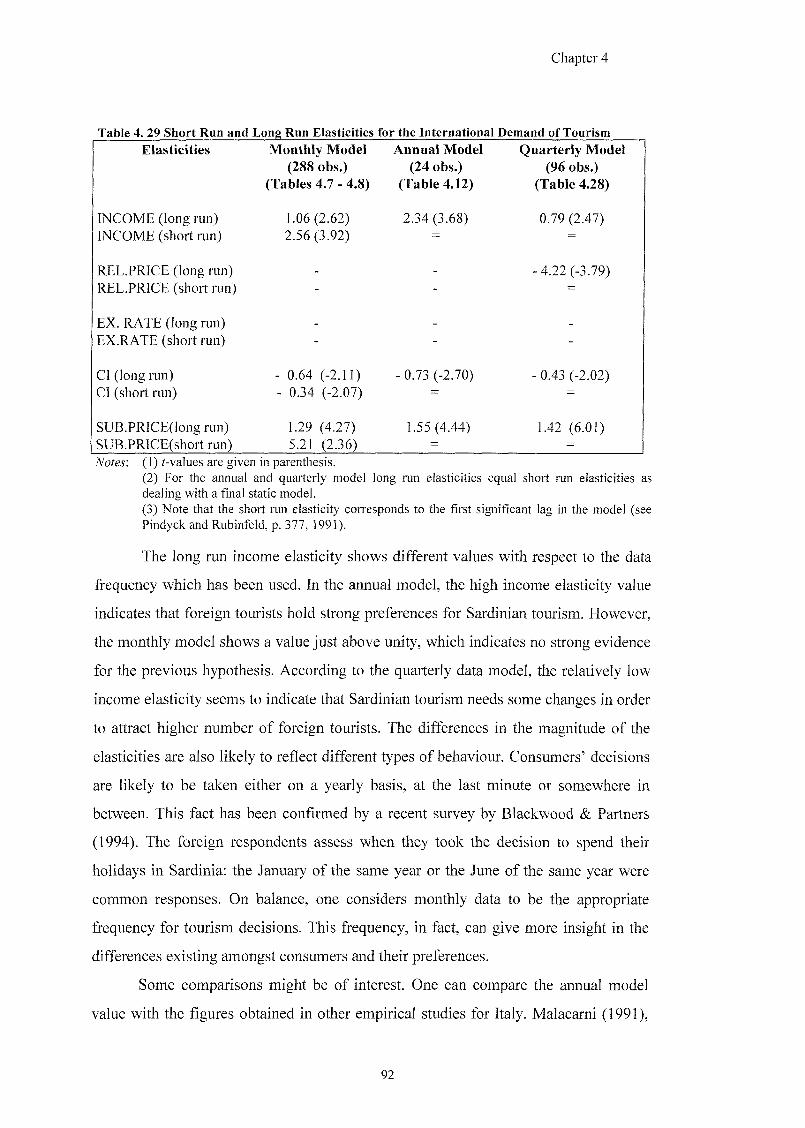
Chapter 4

Table 4. 29 Short Run and Long Run Elasticities for the International Demand of Tourism Elasticities Month ly Mode l

(288 obs.) (Tables 4.7 - 4.8)

Annua l Model (24 obs.)

(Table 4.12)

Quarter ly Model (96 obs.)

(Table 4.28)

I N C O M E (long run)

I N C O M E (short run)

1.06 (2.62) 2.56 (3.92)

2.34 (3.68) 0.79 (2.47)

R E L . P R I C E (long run)

R E L . P R I C E (short run)

-

"

- 4.22 (-3.79)

EX. RATE (long run) EX.RATE (short run)

-

-

-

C I (long run)

C I (short run)

- 0.64 (-2.11) - 0 J 4 ( ^ ^ I 7 )

- 0.73 (-2.70) - 0.43 (-2.02)

SUB.PRICE(iong run) SUB.PRlCE(short run)

L29 (427) 5.21 (2.36)

1.55 (4.44) 1.42 (6XH)

Notes'. (1) ^-values are given in parenthesis. (2) For the annual and quarterly model long run elasticities equal short run elasticities as dealing with a final static model. (3) Note that the short run elasticity corresponds to the first significant lag in the model (see Pindyck and Rubinfeld, p. 377, 1991).

The long run income elasticity shows different values with respect to the data

frequency which has been used. In the annual model, the high income elasticity value

indicates that foreign tourists hold strong preferences for Sardinian tourism. However,

the monthly model shows a value just above unity, which indicates no strong evidence

for the previous hypothesis. According to the quarterly data model, the relatively low

income elasticity seems to indicate that Sardinian tourism needs some changes in order

to attract higher number of foreign tourists. The differences in the magnitude of the

elasticities are also likely to reflect different types of behaviour. Consumers' decisions

are likely to be taken either on a yearly basis, at the last minute or somewhere in

between. This fact has been confirmed by a recent survey by Blackwood & Partners

(1994). The foreign respondents assess when they took the decision to spend their

holidays in Sardinia: the January of the same year or the June of the same year were

common responses. On balance, one considers monthly data to be the appropriate

frequency for tourism decisions. This frequency, in fact, can give more insight in the

differences existing amongst consumers and their preferences.

Some comparisons might be of interest. One can compare the annual model

value with the figures obtained in other empirical studies for Italy. Malacarni (1991),

92

Chapter 4

for example, finds an income elasticity of 1.49 in estimating the aggregated

international demand for Italy, where 17 observations have been employed. Clauser

(1991), in a disaggregated study for international demand in Italy by main origin

countries (20 observations), finds a value in the range within 0.55 for Holland and 2.42

for Japan. Witt and Witt (1992), using 16 observations in total, found values of 1.23

for Germany and 2.57 for France. Note that in all these studies the number of tourist

arrivals have been used as the dependent variable. However, a comparison with other

empirical studies is difficult. The income elasticities and, in general, the explanatory

power of the other independent variables are highly dependent on other elements such

as the level of aggregation, the time periods and the measure of demand used in each

empirical study. As Sinclair and Stabler (1997) also note, one of the main problems is

related with elasticity inferences obtained from models which have not included a full

range of statistical tests. For example, problems of heteroscedasticity, as incurred in

this study, are ignored in the môrity of the cases.

From the quarterly data model one infers that international tourism demand is

highly negative dependent on the growth in the relative price. This fact may suggest a

high degree of substitutability of Sardinian tourism for the source countries. As a

reminder, Malacarni (1991) finds a price elasticity of -0.83 for the international

demand of tourism in Italy. Again, one notes that a comparison is difficult. Firstly, an

annual model is estimated rather than a quarterly model as in this case. Secondly, this

study concerns Sassari Province rather than Italy as a whole.

Note also that, in general, the short run price changes were found not to play

any important role in explaining the foreign demand for tourism. The same conclusion

has been reached when considering the exchange rate. However, the cointegrating

vector appears to be statistically significant in each of three models.

Contrasting results appear for the substitute price elasticities, which present a

positive sign. As already pointed out, this result might be indicating bias in not having

taken into consideration other explanatory variables such as the exchange rate for the

main north of Sardinia competitors. The latter hypothesis will be investigated in

Chapter 6.

93

Chapter 4

4.6 CONCLUSION

In this study an empirical investigation of the international tourism demand to

the north of Sardinia for the period between 1972 and 1995 has been presented.

Different concepts have been utilised such as: seasonality, non-stationary,

cointegration and Equilibrium Correction Models. Particular determinants of the

demand for tourism, i.e. the relative prices and the exchange rate, are 1(1) and

cointegrated.

In this study one makes use of different data frequencies. Monthly, annual and

quarterly data have been used in order to assess the characteristics of the demand for

tourism in the short run as well as in the long run. The relatively large number of

observations available in this study when using monthly data, has allowed to

test the possible presence of seasonal unit roots as well as long run unit roots. One can

notice that monthly and quarterly series have given homogenous results in terms of

seasonal and long run unit roots testing. Whereas, annual data have shown different

and perhaps misleading results. One of the main problems when dealing with tourism

annual data is the relative short number of observations available (24 observations in

this case). Nevertheless, testing for cointegration has revealed similar findings using

any of the three frequencies.

There are numerous advantages in using monthly data. Firstly, they reveal the

short term characteristics of the demand for tourism as well as the long run dynamics.

This separation is of particular importance in tourism since consumers' decisions are

likely to be taken several months in advance or sometimes at the last minute in

response of "special oHers".

Secondly, one can study carefully the seasonal pattern that seems to be of

extreme importance for the operators in the tourism sector. In particular, foreign

tourists seem to appreciate less crowded and cheaper holidays, and months in which

the weather temperatures are milder. In this respect the island of Sardinia represents an

appealing destination in the off-season months (May, June, July and September).

Furthermore, the empirical analysis reveals the particular importance of the Easter

holiday in explaining the pattern of tourism. However, the weather conditions, given

9 4

Chapter 4

by the average temperatures in Sassari Province, seem not to have any particular

effects in determining international demand.

One can conclude that the monthly data model is rather satisfactory in terms of

coefficient of determination (98% of the variance of the dependent variable is

explained), diagnostic statistics (with the exception for heteroscedasticity detected at

the 5% level), coefficients significance and signs. Moreover, the long run responses

show an overall good specification in terms of low standard errors and statistical

significance.

The best results have been obtained by taking into account the effects of four or

five weekends {i.e. the number of Saturdays) in each month with respect to the foreign

arrivals. In this way, it has been possible to correct the presence of non-normality and

heteroscedasticity (at the 1% level) that have arisen when using the unadjusted series

(see Appendix A).

In the annual model, some problems of mis-specification in the functional form

have appeared. Overall, the final static model shows a worse performance than the

monthly model, denoted also by the 91% of explanatory power shown by the

coefficient of determination. An advantage from using annual data is the possibility of

using data only available with annual frequency, in this case supply components. In

this way one can test problems of simultaneity for determinants such as the number of

international flight arrivals.

The use of quarterly data determines a final well-specified model. There have

been no problems in terms of diagnostic tests. The coefficients are statistically

significant and in general present the correct signs. In this case, the final choice of a

static model might suggest that adjustment to equilibrium is quite rapid.

Finally, the Box and Cox (1964) test has been applied to determine whether the

logarithmic form is appropriate. The three models have given statistical proof that the

log-linear specification fits the data better. Note also that the ADF test for the

economic series in a linear specification has shown to be more robust in the monthly

and quarterly models. Moreover, by using the Johansen analysis, a cointegrating

relationship has been suggested for (relative price) and (weighted exchange

rate) using each of the three time frequencies. Hence, in the long run, the use of

effective exchange rates has been validated statistically.

95

Chapter 5

CHAPTER 5.

THE DOMESTIC DEMAND FOR TOURISM IN THE NORTH OF

SARDINIA

Aim of the Chapter:

To model and estimate the domestic demand for tourism in the Sardinian Sassari

Province, Italy.

5.1 INTRODUCTION

In this chapter an account is given of the main findings from the analysis of the

demand for tourism by domestic clients in Sassari Province. As pointed out in Chapter

3, various characteristics distinguish domestic from foreign flows of tourism for the

north of Sardinia. Amongst others the seasonal pattern (see Figures 3.2 and 3.3) shows

noticeably different behaviour for the two types of clients.

By making use of Franses' seasonal unit roots test, one will find out possible

non-stationarity in the domestic seasonal pattern. From a deeper investigation,

structural breaks will be identified in the seasonal pattern.

In the following analysis, further investigation is carried out to assess the

possible validity of the correction of the dependent variable {i.e. the number of

domestic arrivals) for the number of weekends in a month. As already highlighted in

Chapter 3, several experiments are carried out for the raw series of domestic arrivals,

as well as for the series adjusted for either the number of Saturdays or Sundays in a

month.

Relationships between short and long run income and price elasticities will also

be explored, and a comparison with other empirical findings will be given. Different

data frequencies models will be estimated. A full range of test statistics, such as serial

correlation, heteroscedasticity and specification form will be included. In the majority

of tourism empirical studies these tests have been ignored (see Sinclair, 1998). The

dynamics of the models will be investigated by including lagged

9 6

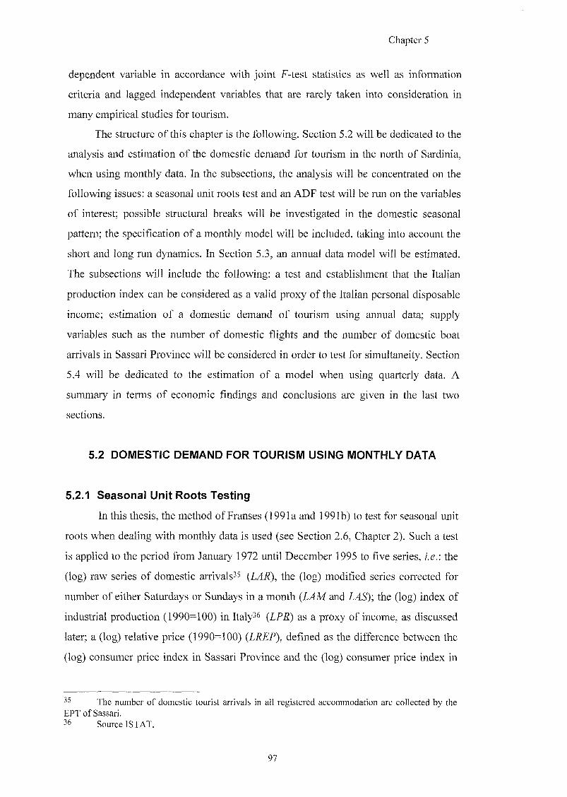
Chapter 5

dependent variable in accordance with joint F-test statistics as well as information

criteria and lagged independent variables that are rarely taken into consideration in

many empirical studies for tourism.

The structure of this chapter is the following. Section 5.2 will be dedicated to the

analysis and estimation of the domestic demand for tourism in the north of Sardinia,

when using monthly data. In the subsections, the analysis will be concentrated on the

following issues: a seasonal unit roots test and an ADF test will be run on the variables

of interest; possible structural breaks will be investigated in the domestic seasonal

pattern; the specification of a monthly model will be included, taking into account the

short and long run dynamics. In Section 5.3, an annual data model will be estimated.

The subsections will include the following: a test and establishment that the Italian

production index can be considered as a valid proxy of the Italian personal disposable

income; estimation of a domestic demand of tourism using annual data; supply

variables such as the number of domestic flights and the number of domestic boat

arrivals in Sassari Province will be considered in order to test for simultaneity. Section

5.4 will be dedicated to the estimation of a model when using quarterly data. A

summary in terms of economic findings and conclusions are given in the last two

sections.

5.2 DOMESTIC DEMAND FOR TOURISM USING MONTHLY DATA

5.2.1 Seasonal Unit Roots Testing

In this thesis, the method of Franses (1991a and 1991b) to test for seasonal unit

roots when dealing with monthly data is used (see Section 2.6, Chapter 2). Such a test

is applied to the period from January 1972 until December 1995 to five series, i.e.: the

(log) raw series of domestic arrivals^^ (LAR), the (log) modified series corrected for

number of either Saturdays or Sundays in a month (L4M and 1/45); the (log) index of

industrial production (1990=100) in Italy^^ (^f^) as a proxy of income, as discussed

later; a (log) relative price (1990=100) {LREP), defined as the difference between the

(log) consumer price index in Sassari Province and the (log) consumer price index in

The number of domestic tourist arrivals in all registered accommodation are collected by the EPT of Sassari. 36 Source ISTAT.

97

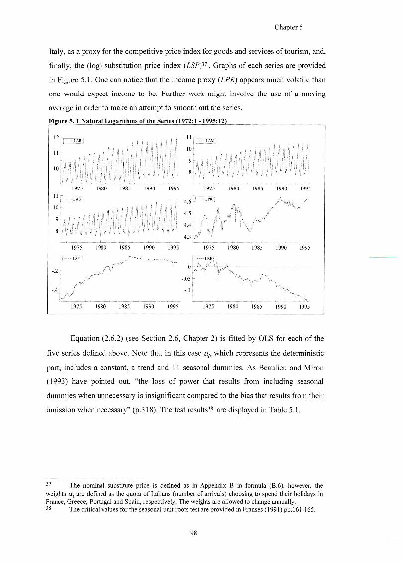
Chapter 5

Italy, as a proxy for the competitive price index for goods and services of tourism, and,

finally, the (log) substitution price index (LSPy^. Graphs of each series are provided

in Figure 5.1. One can notice that the income proxy (LPR) appears much volatile than

one would expect income to be. Further work might involve the use of a moving

average in order to make an attempt to smooth out the series.

Figure 5 .1 Natural Logarithms of the Series (1972:1 - 1995:12)

12 f

l l h n i l

! S I ::: i\ I : I : i : I !

iJ

1975 1980 1985 1990 1995 1975 1980 1985 1990 1995

11

10

-LAS '

1 I I t

/!

1975 1980 1985 1990 1995

-.2

• A ' I

4.6 K

4 , -

4.4 r

4.3

Olv'

-.05 ' [

- . 1 i -

A/' ^ 1975 1980 1985 1990 1995

- LREP:

1975 1980 1985 1990 1995 1975 1980 1985 1990 1995

Equation (2.6.2) (see Section 2.6, Chapter 2) is fitted by OLS for each of the

five series defined above. Note that in this case which represents the deterministic

part, includes a constant, a trend and 11 seasonal dummies. As Beaulieu and Miron

(1993) have pointed out, "the loss of power that results from including seasonal

dummies when unnecessary is insignificant compared to the bias that results from their

omission when necessary" (p.318). The test results^* are displayed in Table 5.1.

The nominal substitute price is defined as in Appendix B in formula (B.6), however, the weights a j are defined as the quota of Italians (number of arrivals) choosing to spend their holidays in France, Greece, Portugal and Spain, respectively. The weights are allowed to change annually.

The critical values for the seasonal unit roots test are provided in Franses (1991) pp. 161-165.

98

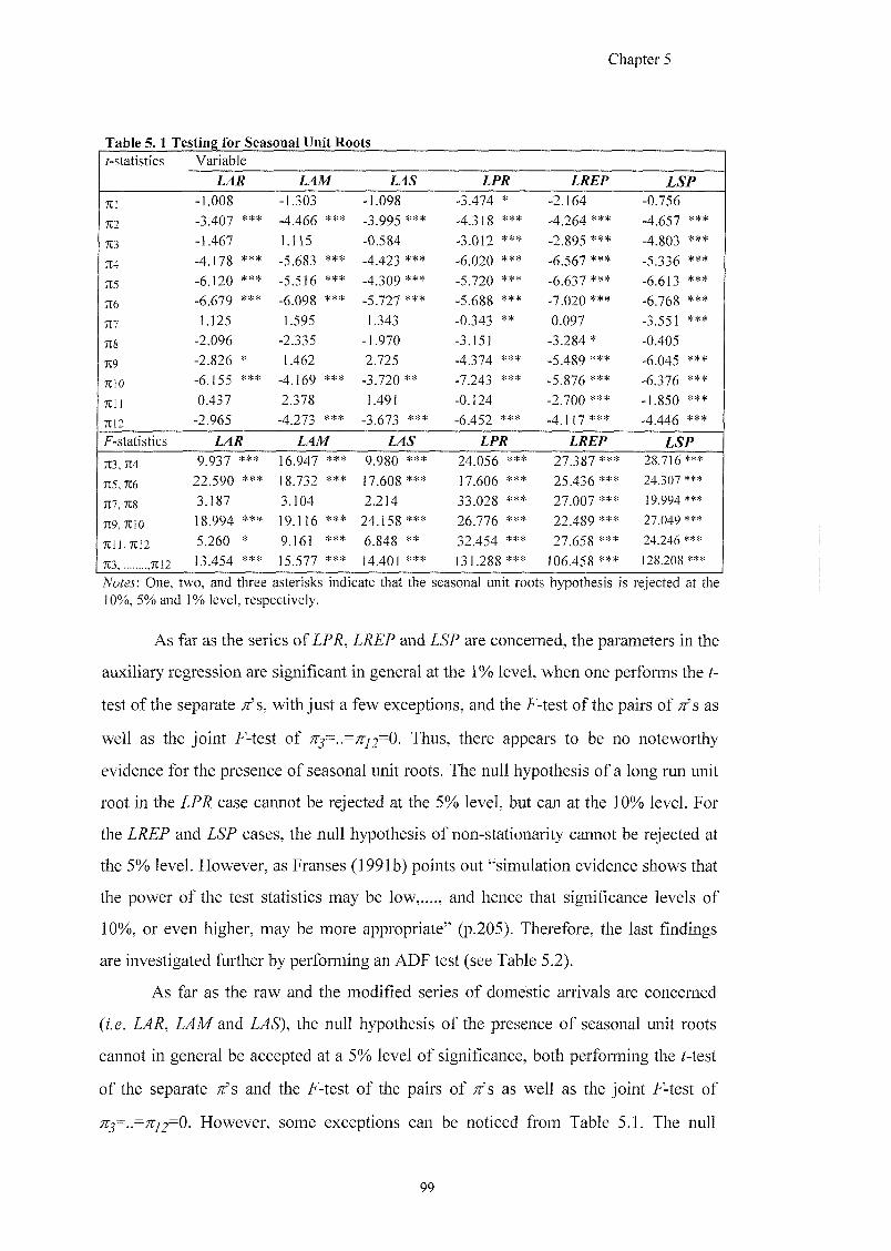
Chapter 5

Table 5. 1 Testing for Seasonal Unit Roots /-statistics Variable

LAR LPR LREP LSP

711 -1.008 -1.303 -1.098 -3.474 * -2.164 -0.756

712 -3.407 *** -4.466 * * * -3.995 *** -4.318 *** -4.264 *** -4.657 ***

713 -1.467 1.115 -0.584 -3.012 *** -2.895 *** -4.803 ***

714 -4.178 *** -5.683 * * * -4.423 *** -6.020 *** -6.567 *** -5.336 ***

715 -6.120 *** -5.516 * * * -4.309 *** -5.720 *** -6.637 *** -6.613 ***

716 -6.679 *** -6.098 * * * -5.727 *** -5.688 *** -7.020 *** -6.768 ***

717 1.125 1.595 1.343 -0.343 ** 0.097 -3.551 ***

718 -2.096 -2.335 -1.970 -3.151 -3.284 * -0.405

719 -2.826 * 1.462 2.725 -4.374 *** -5.489 *** -6.045 ***

7110 -6.155 *** -4.169 * * * -3.720 ** -7.243 *** -5.876 *** -6.376 ***

7111 0.437 2.378 1.491 -0.124 -2.700 *** -1.850 ***

7112 -2.965 -4.273 * * * -3.673 *** -6.452 *** -4.117 *** -4.446 ***

F-statistics LAR LAS LPR LREP LSP

713, 7M 9.937 *** 16.947 * * * 9.980 *** 24.056 *** 27.387 *** 28.716 ***

715,716 22.590 *** 18.732 * * * 17.608 *** 17.606 *** 25.436 *** 24.307 ***

717, 718 3.187 3.104 2.214 33.028 *** 27.007 *** 19.994 ***

719,7110 18.994 *** 19.116 * * * 24.158 *** 26.776 *** 22.489 *** 27.049 ***

7tll,7tl2 5.260 * 9.161 * * * 6.848 ** 32.454 *** 27.658 *** 24.246 ***

7r3, ,7112 13.454 *** 15.577 * * * 14.401 *** 131.288 *** 106.458 *** 128.208 ***

Notes: One, two, and three asterisks indicate that the seasonal unit roots hypothesis is rejected at the 10%, 5% and 1% level, respectively.

As far as the series of LPR, LREP and LSP are concerned, the parameters in the

auxiliary regression are significant in general at the 1% level, when one performs the

test of the separate 'z's, with just a few exceptions, and the F-test of the pairs of z's as

well as the joint F-test of Thus, there appears to be no noteworthy

evidence for the presence of seasonal unit roots. The null hypothesis of a long run unit

root in the LPR case cannot be rejected at the 5% level, but can at the 10% level. For

the LREP and LSP cases, the null hypothesis of non-stationarity cannot be rejected at

the 5% level. However, as Franses (1991b) points out "simulation evidence shows that

the power of the test statistics may be low,...., and hence that significance levels of

10%, or even higher, may be more appropriate" (p.205). Therefore, the last findings

are investigated further by performing an ADF test (see Table 5.2).

As far as the raw and the modified series of domestic arrivals are concerned

(f.g. Zy4Mand the null hypothesis of the presence of seasonal unit roots

cannot in general be accepted at a 5% level of significance, both performing the Nest

of the separate s and the F-test of the pairs of n's as well as the joint F-test of

7if=.=nj2=0. However, some exceptions can be noticed from Table 5.1. The null

99

Chapter 5

hypothesis, in fact, cannot be rejected for some of the separate z's (;.e.:

;r/; and for Zar; , ;ry, ;zg, and y for Z/^Mand Z/46) as well for one pair

of /zfs, /.g. ;ry, (z.e. at frequency w3). In conclusion, for the unadjusted and acûsted

series of domestic arrivals one rejects unit roots at most frequencies; thus, in

accordance with the findings in Franses (1991b), and Beaulieu and Miron (1993), it

appears that there is no strong evidence for the presence of seasonal unit roots.

However, as Webb (1995) notices "other types of nonstationarity are also possible. An

alternative...involves large, infrequent shocks" (p.277). The possibility of regime

changes in the seasonal pattern is investigated in more detail in the next section. A

further investigation is done in testing for the presence of a unit root at the zero

frequency by running an ADF test. The results are reported in Table 5.2.

100

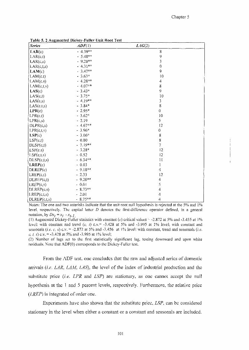
Chapter 5


Series ADF(]) ZXC(2)

LAR(c) - 4.39** 8 LAR(c,t) - 5.48** 9 LAR(c,s) - 9.28** 3 LAR(c,t,s) - 4.31** 0 LAM(c) - 3.47** 9 LAM(c,t) - 3.63* 10 LAM(c,s) - 4.28** 4 LAM(c,t,s) - 4.07** 8 LAS(c) - 3.43* 9 LAS(c,t) - 3.75* 10 LAS(c,s) - 4.19** 3 LAS(c,t,s) - 3.84* 8 LPR(c) - 2.95* 0 LPR(c,t) - 3.62* 10 LPR(c,s) - 2.19 5 DLPR(c,s) - 4.67** 12 LPR(c,t,s) - 3.96* 0 LSP(c) - 3.06* 8 LSP(c,t) - 0.80 8 DLSP(c,t) - 7.19** 7 LSP(c,s) - 3.28* 12 LSP(c,t,s) - 0.52 12 DLSP(c,t,s) - 6.34** 11 LREP(c) - 0.03 1 DLREP(c) - 9.18** 4 LREP(c,t) - 2.33 12 DLREP(c,t) - 9.20** 4 LREP(c,s) - 0.01 5 DLREP(c,s) - 8.73** 4 LREP(c,t,s) - 2.01 4 DLREP(c,t,s) - 8.75** 4

Notes: The one and two asterisks indicate that the unit root null hypothesis is rejected at the 5% and 1% level, respectively. The capital letter D denotes the first-difference operator defined, in a general notation, by (1) Augmented Dickey-Fuller statistics with constant (c) critical values = -2.872 at 5% and -3.455 at 1% level; with constant and trend {c, t) c.v.= -3.428 at 5% and -3.995 at 1% level; with constant and seasonals {i.e. c, s) c.v. = -2.872 at 5% and -3.456 at 1% level; with constant, trend and seasonals {i.e. c, t, s) c.v. = -3.428 at 5% and -3.995 at 1% level; (2) Number of lags set to the first statistically significant lag, testing downward and upon white residuals. Note that ADF(O) corresponds to the Dickey-Fuller test.

From the ADF test, one concludes that the raw and adjusted series of domestic

arrivals (z.g. 1/45), the level of the index of industrial production and the

substitute price (i.e. LPR and LSP) are stationary, as one cannot accept the null

hypothesis at the 1 and 5 percent levels, respectively. Furthermore, the relative price

(LREP) is integrated of order one.

Experiments have also shown that the substitute price, LSP, can be considered

stationary in the level when either a constant or a constant and seasonals are included.

101

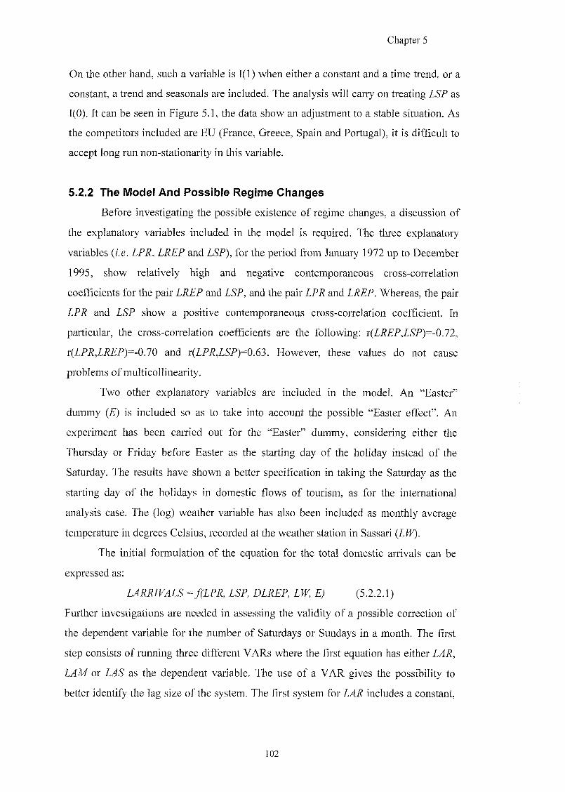
Chapter 5

On the other hand, such a variable is 1(1) when either a constant and a time trend, or a

constant, a trend and seasonals are included. The analysis will carry on treating LSP as

1(0). It can be seen in Figure 5.1, the data show an adjustment to a stable situation. As

the competitors included are EU (France, Greece, Spain and Portugal), it is difficult to

accept long run non-stationarity in this variable.

5.2.2 The Model And Possible Regime Changes

Before investigating the possible existence of regime changes, a discussion of

the explanatory variables included in the model is required. The three explanatory

variables {i.e. LPR, LREP and LSP), for the period from January 1972 up to December

1995, show relatively high and negative contemporaneous cross-correlation

coefficients for the pair LREP and LSP, and the pair LPR and LREP. Whereas, the pair

LPR and LSP show a positive contemporaneous cross-correlation coefficient. In

particular, the cross-correlation coefficients are the following: x{LREP,LSP)=-0.12,

V{LPR,LREP)=^-Q.LQ and T(LPR,LSP)=0.63. However, these values do not cause

problems of multicollinearity.

Two other explanatoiy variables are included in the model. An "Easter"

dummy (E) is included so as to take into account the possible "Easter effect". An

experiment has been carried out for the "Easter" dummy, considering either the

Thursday or Friday before Easter as the starting day of the holiday instead of the

Saturday. The results have shown a better speciGcation in taking the Saturday as the

starting day of the holidays in domestic flows of tourism, as for the international

analysis case. The (log) weather variable has also been included as monthly average

temperature in degrees Celsius, recorded at the weather station in Sassari (ZPF).

The initial formulation of the equation for the total domestic arrivals can be

expressed as:

^ (5 .2 .2 .1 )

Further investigations are needed in assessing the validity of a possible correction of

the dependent variable for the number of Saturdays or Sundays in a month. The first

step consists of running three different VARs where the first equation has either

LAM or LAS as the dependent variable. The use of a VAR gives the possibility to

better identify the lag size of the system. The first system for includes a constant,

102

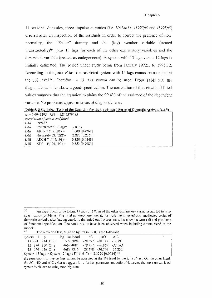
Chapter 5

11 seasonal dummies, three impulse dummies {i.e. il974pll, il992p3 and il993p3)

created after an inspection of the residuals in order to correct the presence of non-

normality, the "Easter" dummy and the (log) weather variable (treated

unrestrictedly)^^, plus 13 lags for each of the other explanatory variables and the

dependent variable (treated as endogeneous). A system with 13 lags versus 12 lags is

initially estimated. The period under study being from January 1972:1 to 1995:12.

According to the joint F-test the restricted system with 12 lags cannot be accepted at

the 1% levelô. Therefore, a 13 lags system can be used. From Table 5.3, the

diagnostic statistics show a good specification. The correlation of the actual and fitted

values suggests that the equation explains the 99.4% of the variance of the dependent

variable. No problems appear in terms of diagnostic tests.

Table 5. 3 Statistical Tests of the Equation for the Unadjusted Series of Domestic Arrivals {LAK)

cr = 0.0949295 RSS = 1.847379485 co/reW/oM ocfwaZ awt/

0.99437 LAR :Portmanteau 12 lags= 9.8167 1/4/; : A R 1 - 7 F ( 7 , 1 9 8 ) = 1.009 [0.4261] L4/; :Normality Chi^2(2)= 2.880 [0.2369] AW/; :ARCH 7 F( 7,191) = 0.320 [0.9443] AW/; :Xi^2 F(]04,100)= 0.553 [0.9985]

An experiment of including 13 lags of LW, as of the other explanatory variables has led to mis-specification problems. The final parsimonious model, for both the adjusted and unadjusted series of domestic arrivals, after having carefully dummied out the seasonals, has shown a worse fit and problems of functional specification. The same results have been observed when including a time trend in the models. 40 The reduction test, as given by PcFiml 9.0, is the following:

system T p log-likelihood SC HQ AIC 11 274 244 OLS 574.5094 -28.392 -30.318 -32.391 12 274 260 OLS 4669.4087 -2&7j7 -jO.gOP 13 274 276 OLS 4689.7316 -28.578 -30.756 -32.232

System 13 lags-> System 12 lags ; F(16, 617) = 2.3270 [0.0024] **

the restriction for twelve lags cannot be accepted at the 1% level by the joint F-test. On the other hand, the SC, HQ and AIC criteria suggest for a further parameter reduction. However, the most unrestricted system is chosen as using monthly data.

103

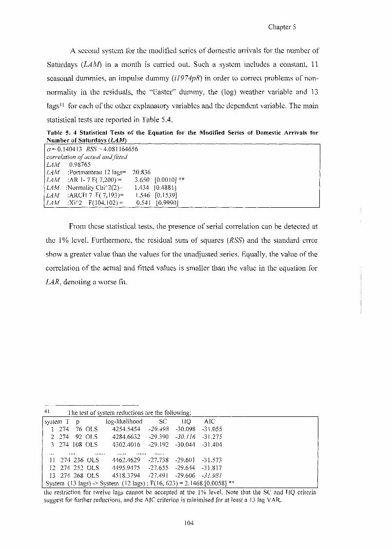
Chapter 5

A second system for the modified series of domestic arrivals for the number of

Saturdays {LAM) in a month is carried out. Such a system includes a constant, 11

seasonal dummies, an impulse dummy {il974p8) in order to correct problems of non-

normality in the residuals, the "Easter" dummy, the (log) weather variable and 13

lagsî for each of the other explanatory variables and the dependent variable. The main

statistical tests are reported in Table 5.4.

Table 5. 4 Statistical Tests of the Equation for the Modified Series of Domestic Arrivals for Number of Saturdays (LAM)

o-= 0.140413 a s s = 4.081164656

0.98765

LAM :Portmanteau 12 lags= 20.836 :/LR 1-7 | : (7 ,200) = 3.650 [0.0010] **

L4M iNormality 0^/^2(2)= 1.434 [0.4881] ZJM :ARCH7F(7 ,193)= 1.546 [0.1539]

:Xr2 F(104,102)= 0.541 [0.9990]

From these statistical tests, the presence of serial correlation can be detected at

the 1% level. Furthermore, the residual sum of squares and the standard error

show a greater value than the values for the unadjusted series. Equally, the value of the

correlation of the actual and fitted values is smaller than the value in the equation for

LAR, denoting a worse fit.

The test of system reductions are the following:

system T p log-likelihood SC HQ AIC 1 274 76 OLS 4254.5454 -30.098 -31.055 2 274 92 OLS 4284.6632 -29.390 -31.275 3 274 108 OLS 4302.4016 -29.192 -30.044 -31.404

11 274 236 OLS 4462.4629 -27.738 -29.601 -31.573 12 274 252 OLS 4495.9475 -27.655 -29.644 -31.817 13 274 268 OLS 4518.3794 -27.491 -29.606

System (13 lags)-> System (12 lags) : F(16, 623) = 2.1468 [0.0058] **

the restriction for twelve lags cannot be accepted at the 1% level. Note that the SC and HQ criteria suggest for further reductions, and the AIC criterion is minimised for at least a 13 lag VAR.

104

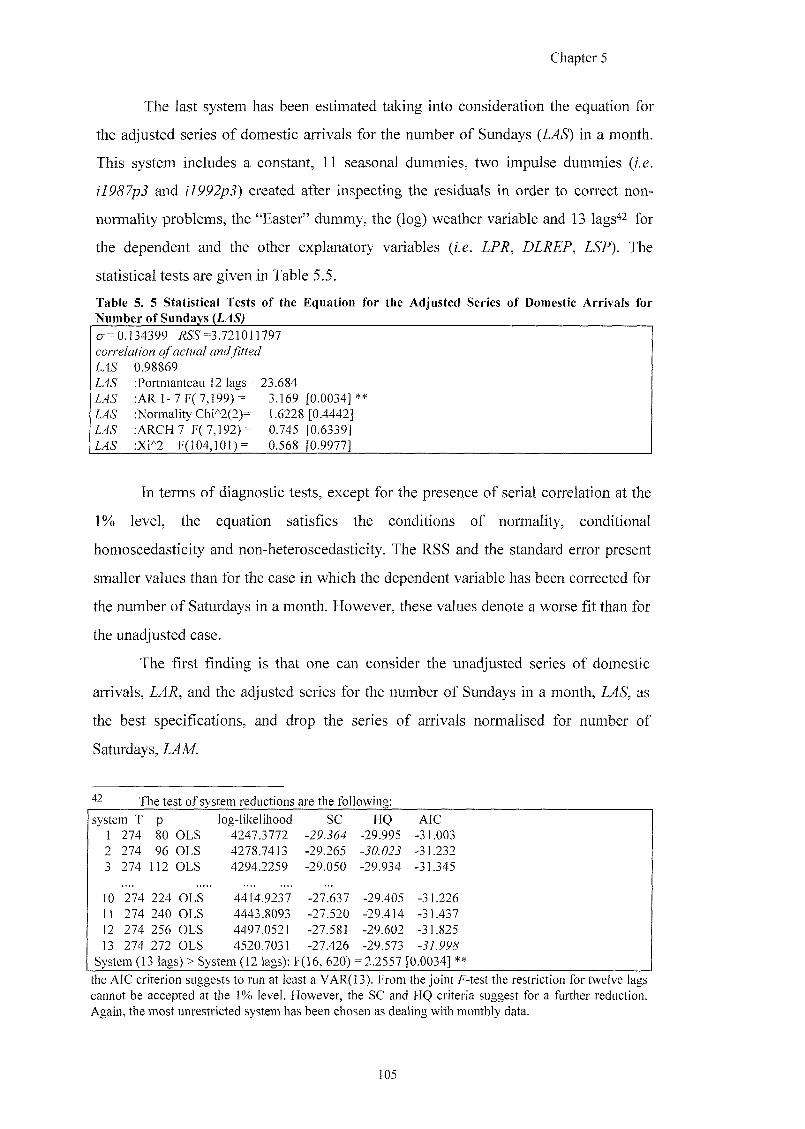
Chapter 5

The last system has been estimated taking into consideration the equation for

the adjusted series of domestic arrivals for the number of Sundays {LAS) in a month.

This system includes a constant, 11 seasonal dummies, two impulse dummies {i.e.

il987p2 and il992p3) created after inspecting the residuals in order to correct non-

normality problems, the "Easter" dummy, the (log) weather variable and 13 lags^^ for

the dependent and the other explanatory variables {i.e. LPR, DLREP, LSP). The

statistical tests are given in Table 5.5.

Table 5. 5 Statistical Tests of the Equation for the Adjusted Series of Domestic Arrivals for Number of Sundays {LAS)

o-= 0.134399 ASS =3.721011797

L4S' 0.98869

1^5'

Portmanteau 12 lags= 23.684 A R 1 - 7 F ( 7 , 1 9 9 ) = 3.169 [0.0034]** Normality 011/^2(2)= 1.6228 [0.4442] ARCH 7 F( 7,192)= 0.745 [0.6339] Xi/'2 F(104 ,10n= 0.568 [0.9977]

In terms of diagnostic tests, except for the presence of serial correlation at the

1% level, the equation satisfies the conditions of normality, conditional

homoscedasticity and non-heteroscedasticity. The RSS and the standard error present

smaller values than for the case in which the dependent variable has been corrected for

the number of Saturdays in a month. However, these values denote a worse fit than for

the unadjusted case.

The first finding is that one can consider the unadjusted series of domestic

arrivals, and the acûsted series for the number of Sundays in a month, Z/45', as

the best specifications, and drop the series of arrivals normalised for number of

Saturdays, Z/4M

The test of system reductions are the following:

system T p log-likelihood SC HQ AIC 1 274 80 OLS 4247.3772 -29.36^ -29.995 -31.003 2 274 96 OLS 4278.7413 -29.265 -31.232 3 274 112 OLS 4294.2259 -29.050 -29.934 -31.345

10 274 224 OLS 4414.9237 -27.637 -29.405 -31.226 11 274 240 OLS 4443.8093 -27.520 -29.414 -31.437 12 274 256 OLS 4497.0521 -27.581 -29.602 -31.825 13 274 272 OLS 4520.7031 -27.426 -29.573 -j/.PPg

System (13 lags) > System (12 lags): F(16, 620) = 2.2557 [0.0034] **

the AIC criterion suggests to run at least a VAR(]3). From the joint F-test the restriction for twelve lags cannot be accepted at the 1% level. However, the SC and HQ criteria suggest for a further reduction. Again, the most unrestricted system has been chosen as dealing with monthly data.

105

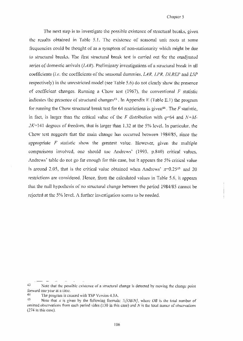
Chapter 5

The next step is to investigate the possible existence of structural breaks, given

the results obtained in Table 5.1. The existence of seasonal unit roots at some

frequencies could be thought of as a symptom of non-stationarity which might be due

to structural breaks. The first structural break test is carried out for the unadjusted

series of domestic arrivals {LAR). Preliminary investigations of a structural break in all

coefficients {i.e. the coefficients of the seasonal dummies, LAR, LPR, DLREP and LSP

respectively) in the unrestricted model (see Table 5.6) do not clearly show the presence

of coefficient changes. Running a Chow test (1967), the conventional F statistic

indicates the presence of structural changes'^^. In Appendix E (Table E. l) the program

for running the Chow structural break test for 64 restrictions is given'*^. The f statistic,

in fact, is larger than the critical value of the F distribution with g=64 and N+M-

2A>141 degrees of freedom, that is larger than 1.32 at the 5% level. In particular, the

Chow test suggests that the main change has occurred between 1984/85, since the

appropriate F statistic show the greatest value. However, given the multiple

comparisons involved, one should use Andrews' (1993, p.840) critical values.

Andrews' table do not go far enough for this case, but it appears the 5% critical value

is around 2.05, that is the critical value obtained when Andrews' ;z=0.25' ^ and 20

restrictions are considered. Hence, from the calculated values in Table 5.6, it appears

that the null hypothesis of no structural change between the period 1984/85 cannot be

rejected at the 5% level. A further investigation seems to be needed.

Note that the possible existence of a structural change is detected by moving the change point forward one year at a time. ^ The program is created with TSP Version 4.3A.

Note that n: is given by the following formula: 'AlOB/N], where OB is the total number of omitted observations from each period sides (130 in this case) and N is the total numer of observations (274 in this case).

106

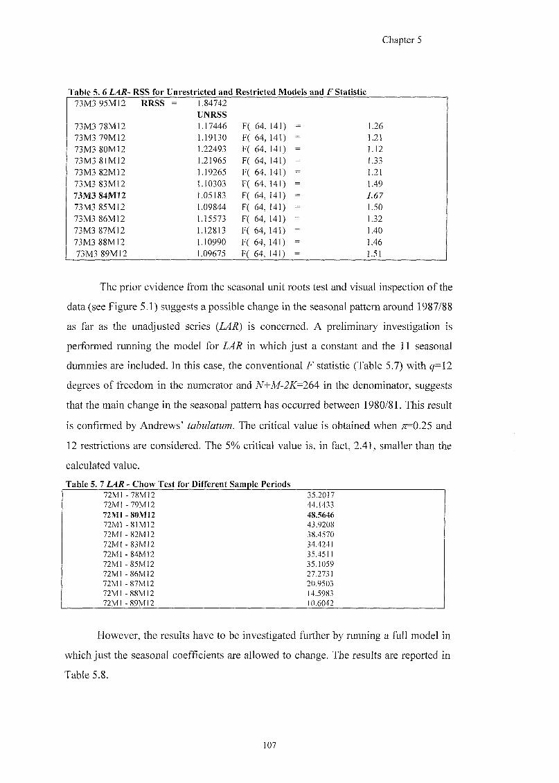
Chapter 5

Table 5. 6 LAR- RSS for Unrestricted and Restricted Models and F Statistic 73M3 95M12 RRSS = 1.84742

UNRSS

73M3 78M12 1.17446 F ( 6 4 1 4 0 = L26 73M3 79M12 1.19130 F ( 6 ^ 1 4 ^ = L21 73M3 80M12 1.22493 F ( 6 4 1 4 ^ = 1.12

73M3 81M12 1.21965 F ( 6 4 1 4 ^ = 1J3 73M3 82M12 1.19265 F( 64 , 141) = L21

73M3 83M12 1.10303 F( 64 ,141) = L49 73M3 84M12 1.05183 F( 64[, 141) == A67 73M3 85M12 1.09844 F ( 6 4 1 4 n = 1^0

73M3 86M12 1.15573 F ( 6 4 1 4 n = 132

73M3 87M12 1.12813 F ( 6 ^ 1 4 0 = 1.40 73M3 88M12 1.10990 F ( 6 4 1 4 ^ = 1 4 6 73M3 89M12 1.09675 F( 64, 141) = 1.51

The prior evidence from the seasonal unit roots test and visual inspection of the

data (see Figure 5.1) suggests a possible change in the seasonal pattern around 1987/88

as far as the unadjusted series {LAR) is concerned. A preliminary investigation is

performed running the model for LAR in which just a constant and the 11 seasonal

dummies are included. In this case, the conventional F statistic (Table 5.7) with q=\l

degrees of freedom in the numerator and N+M-2K=264 in the denominator, suggests

that the main change in the seasonal pattern has occurred between 1980/81. This result

is confirmed by Andrews' tabulatum. The critical value is obtained when ;^0.25 and

12 restrictions are considered. The 5% critical value is, in fact, 2.41, smaller than the

calculated value.

Table 5. 7 LAR - Chow Test for Different Sample Periods 72M1 - 78M12 35.2017 72M] - 79M12 44.1433 72M1 -80M12 48.5646 72M1 - 8 1 M 1 2 43.9208 72M1 - 82M12 38.4570 72M] - 83M12 34.4241 72M1 - 84M12 35.4511 72M1 - 85M12 35.1059 72M1 - 86M12 27.2731 72M1 - 8 7 M 1 2 20.9503 7 2 M 1 - 8 8 M 1 2 14.5983 72MI - 8 9 M 1 2 10.6042

However, the results have to be investigated further by running a full model in

which just the seasonal coefficients are allowed to change. The results are reported in

Table 5.8.

107

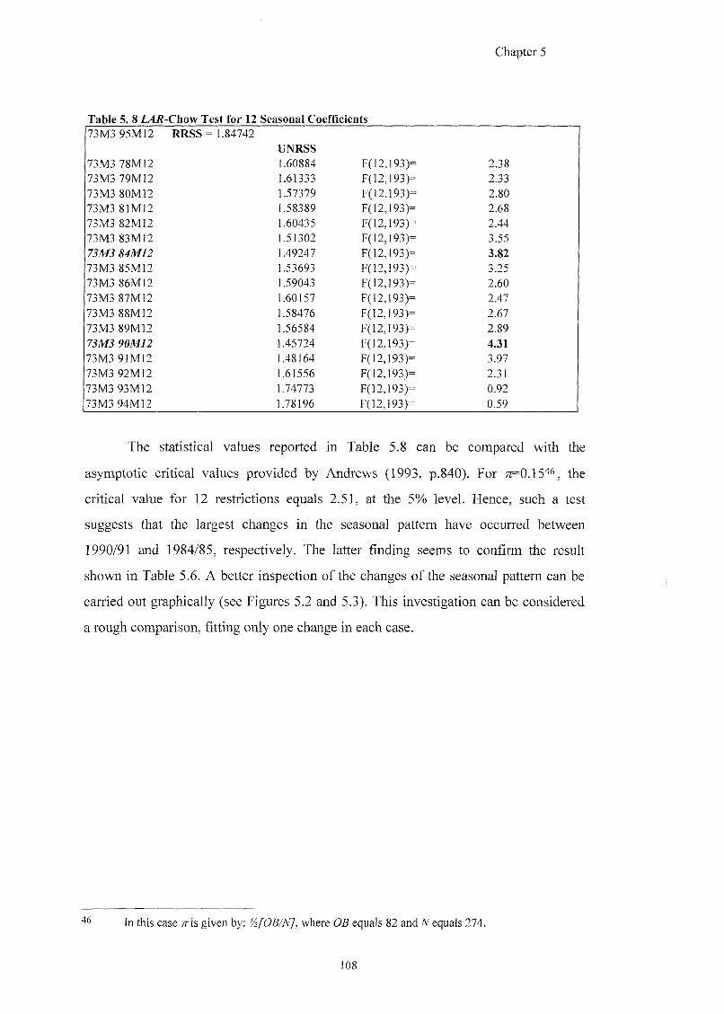
Chapter 5

Table 5. 8 Z^^-Chow Test for 12 Seasonal Coefficients 73M3 95M12 RRSS = 1.84742

UNRSS 73M3 78M12 1.60884 F(12,193)= 2.38 73M3 79M12 1.61333 F(12,193)= 2.33 73M3 80M12 1.57379 F(12,193)= 2.80 73M3 81M12 1.58389 F(12,193)= 2.68 73M3 82M12 1.60435 F(12,193)=: 2.44 73M3 83M12 1.51302 F(12,193)= 3.55

1.49247 F(12,193)= 3.82 73M3 85M12 1.53693 F(12,193)= 3.25 73M3 86M12 1.59043 F(]2,193)= 2.60 73M3 87M12 1.60157 F(12,193)= 2.47 73M3 88M12 1.58476 F(12,193)= 2.67 73M3 89M12 1.56584 F(12,193)= 2.89

1.45724 F(]2,193)= 4.31 73M3 91M12 1.48164 F(12,193)= 3.97 73M3 92M12 1.61556 F(12,193)= 2.31 73M3 93M12 1.74773 F(12,193)= 0.92 73M3 94M12 1.78196 F(12,193)= 0.59

The statistical values reported in Table 5.8 can be compared with the

asymptotic critical values provided by Andrews (1993, p.840). For ;7=0.15'* , the

critical value for 12 restrictions equals 2.51, at the 5% level. Hence, such a test

suggests that the largest changes in the seasonal pattern have occurred between

1990/91 and 1984/85, respectively. The latter finding seems to confirm the result

shown in Table 5.6. A better inspection of the changes of the seasonal pattern can be

carried out graphically (see Figures 5.2 and 5.3). This investigation can be considered

a rough comparison, fitting only one change in each case.

46 In this case ;ris given by: '/:[OB/N], where OB equals 82 and N equals 274.

108

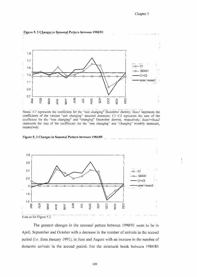
Chapter 5

Figure 5^2 Changes in Seasonal Pattern between 1990/91

-C1

- SEAS1

-C1+C2

•seasl+seas2

Notes: CI represents the coefficient for the "non changing" December dummy; Seasl represents the coefficients of the various "non changing" seasonal dummies; C1+C2 represents the sum of the coefficient for the "non changing" and "changing" December dummy, respectively; Seasl+Seas2 represents the sum of the coefficients for the "non changing" and "changing" monthly seasonals, respectively.

Figure 5. 3 Changes in Seasonal Pattern between 1984/85

- 0 1

- SB\S1

-C14C2

-seas1+seas2

Note as for Figure 5.2.

The greatest changes in the seasonal pattern between 1990/91 seem to be in

April, September and October with a decrease in the number of arrivals in the second

period {i.e. from January 1991), in June and August with an increase in the number of

domestic arrivals in the second period. For the structural break between 1984/85

109

Chapter 5

(Figure 5.3), the main changes in the seasonal pattern seem to occur in June, July and

August, with an overall increase of the number of domestic arrivals. Such assumptions

have been investigated further (see the complete and final program for running the

tests in Appendix E, Table E.2). Three separate dummies are fitted; for the whole

period /war, and so on), for 1985:1 onwards and so on),

and for 1991:1 onwards {jan3,feb3, and so on). Firstly, the structural break between

1984/85 has been considered. The F statistic (8,194) when the coefficients for the

seasonals apr2,jun2,jiil2 and aug2 are allowed to change between 1984 and 1985 has

to be accepted at the 5% level. In fact, the F statistic (8,194) calculated equals 1.54 and

it is smaller than the critical value {i.e. 1.94). Note that the null hypothesis when just

the coefficients of jun2,jul2 and aug2 are allowed to change is not accepted at the 5%

level.

Secondly, the structural seasonal change between 1990/1991 has been

investigated by testing for possible restrictions on the coefficients of the seasonals: cJ,

yaMj, j, /waA-j, yw/j and Movj; that is, allowing just the coefficients of the

seasonals awgj, and ocf j to change. The F statistic (7,194), in such a

case, equals 0.91 that is smaller than the conventional critical value at the 5% level

{i.e. 2.01). Thus, the null hypothesis cannot be rejected.

The restricted seasonal changes with the unrestricted dummy model need to be

compared. This is not a full specification search; in fact, when testing the 1984/1985

changes after restricting the 1990/91 changes the same results are not obtained. The

restrictions on all the seasonal coefficients except for and cannot

be accepted at a 5% level. That is the F statistic (8,188) equals 2.53 and this value is

greater than 1.94 from the conventional tables. However, 6om a further investigation

the coefficients for and seem to be changing in the second

period, that is from 1985:1 until 1990:12. The F statistic (7,188) is equal to 1.96

smaller than the conventional critical value (2.01) at a 5% level.

The same investigation has been done for the structural change occurring

between 1990 and 1991, after restricting the 1984/85 changes. The F statistic (7,188)^7

suggests that the restriction on all seasonal coefficients, with the exception for oprj,

jwMJ, awgJ, j'gp j and ocfJ, cannot be accepted at the 5% level. From a fiirther analysis,

47 T h e F statistic (7,188) is equal to 2.48 greater than the critical value (2.01) at the 5% level.

110

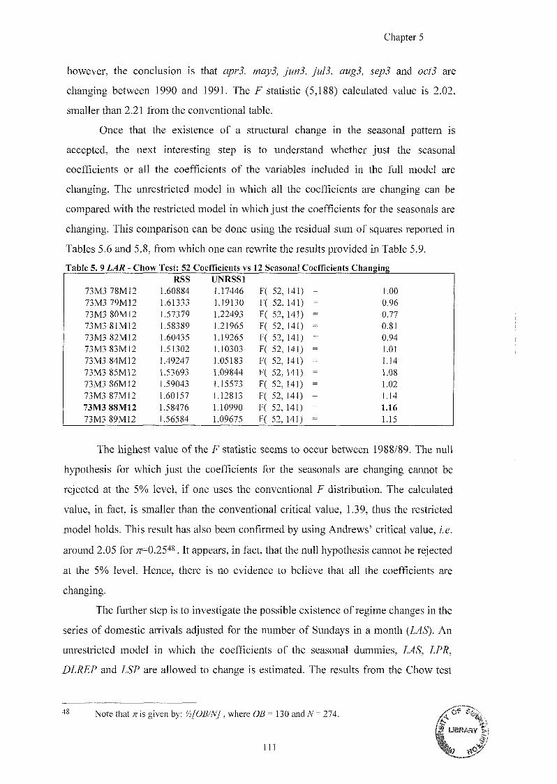
Chapter 5

however, the conclusion is that oprj, ywMj, yw/j, awgj, and oc^j are

changing between 1990 and 1991. The F statistic (5,188) calculated value is 2.02,

smaller than 2.21 from the conventional table.

Once that the existence of a structural change in the seasonal pattern is

accepted, the next interesting step is to understand whether just the seasonal

coefficients or all the coefficients of the variables included in the full model are

changing. The unrestricted model in which all the coefficients are changing can be

compared with the restricted model in which just the coefficients for the seasonals are

changing. This comparison can be done using the residual sum of squares reported in

Tables 5.6 and 5.8, from which one can rewrite the results provided in Table 5.9.

Table 5. 9 LAR - Chow Test: 52 Coefficients vs 12 Seasonal Coefficients Changing RSS UNRSSl

73M3 78M12 1.60884 117446 F ( 5 % 1 4 n = 1.00 73M3 79M12 1.61333 1.19130 F ( 5 % 1 4 n = 0.96 73M3 80M12 1.57379 1.22493 F ( 5 % 1 4 ^ = 0 J 7 73M3 81M12 1.58389 1.21965 F ( 5 % 1 4 n = 0.81 73M3 82M12 1.60435 1.19265 F ( 5 ^ 1 4 n = 0.94 73M3 83M12 1.51302 1.10303 F ( 5 % 1 4 U = 1.01 73M3 84M12 1.49247 1.05183 F ( 5 % 1 4 ^ = 1J4 73M3 85M12 1.53693 1.09844 F ( 5 % 1 4 n = 73M3 86M12 1.59043 1.15573 F ( 5 % 1 4 n = 1.02 73M3 87M12 1.60157 1.12813 F ( 5 % 1 4 U = 1J4 73M3 88M12 1.58476 1.10990 F ( 5 % 1 4 n = 1.16 73M3 89MI2 1.56584 1.09675 F ( 5 % 1 4 n = 1.15

The highest value of the F statistic seems to occur between 1988/89. The null

hypothesis for which just the coefficients for the seasonals are changing cannot be

rejected at the 5% level, if one uses the conventional F distribution. The calculated

value, in fact, is smaller than the conventional critical value, 1.39, thus the restricted

model holds. This result has also been confirmed by using Andrews' critical value, i.e.

around 2.05 for nÔ.25'^^. It appears, in fact, that the null hypothesis cannot be rejected

at the 5% level. Hence, there is no evidence to believe that all the coefficients are

changing.

The further step is to investigate the possible existence of regime changes in the

series of domestic arrivals adjusted for the number of Sundays in a month (LAS). An

unrestricted model in which the coefficients of the seasonal dummies, LAS, LPR,

DLREP and LSP are allowed to change is estimated. The results from the Chow test

48 Note that kis given by: '/2[OB/N] , where OB = 130 and yv= 274.

I l l

of

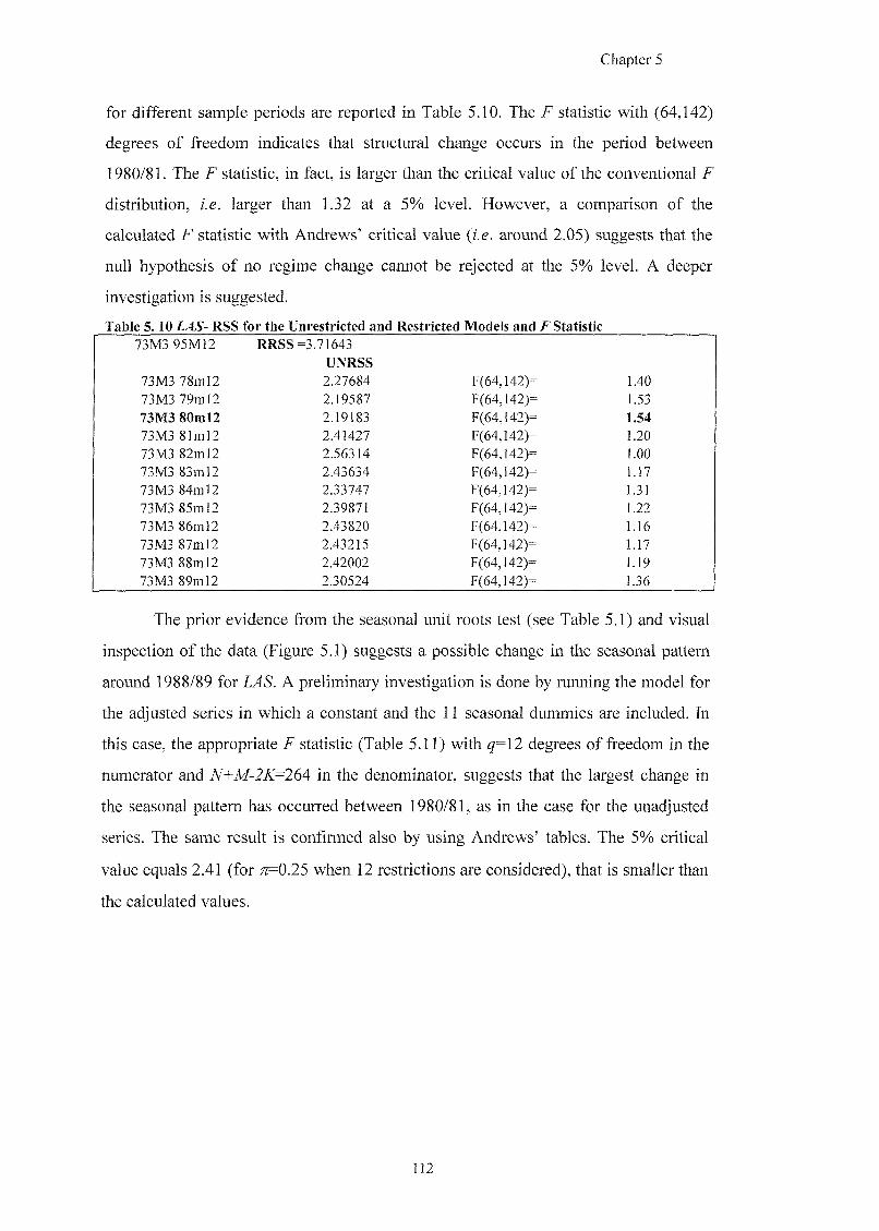
Chapter 5

for different sample periods are reported in Table 5.10. The F statistic with (64,142)

degrees of freedom indicates that structural change occurs in the period between

1980/81. The F statistic, in fact, is larger than the critical value of the conventional F

distribution, i.e. larger than 1.32 at a 5% level. However, a comparison of the

calculated F statistic with Andrews' critical value (i.e. around 2.05) suggests that the

null hypothesis of no regime change cannot be rejected at the 5% level. A deeper

investigation is suggested.

Table 5. 10 LAS- RSS for the Unrestricted and Restricted Models and F Statistic 73M3 95M12 RRSS =3.71643

UNRSS 73M3 78m 12 2.27684 F(64,142)= 1.40 73M3 79m 12 2.19587 F(64,142)= 1.53 73M3 80ml2 2.19183 F(64,142)= 1.54 73M3 8]m]2 2.41427 F(64,142)= 1.20 73M3 82m]2 2.56314 F(64,142)= 1.00 73M3 83ml2 2.43634 F(64,142)= 1.17

73M3 84m 12 2.33747 F(64,]42)= 1.31

73M3 85m 12 2.39871 F(64,142)= 1.22 73M3 86m 12 2.43820 F(64,142)= 1.16 73M3 87m]2 2.43215 F(64,]42)= 1.17 73M3 88m 12 2.42002 F(64,142)= 1.19 73M3 89ml2 2.30524 F(64,142)= 1.36

The prior evidence from the seasonal unit roots test (see Table 5.1) and visual

inspection of the data (Figure 5.1) suggests a possible change in the seasonal pattern

around 1988/89 for LAS. A preliminary investigation is done by running the model for

the adjusted series in which a constant and the 11 seasonal dummies are included. In

this case, the appropriate F statistic (Table 5.11) with g=12 degrees of freedom in the

numerator and N+M-2K=264 in the denominator, suggests that the largest change in

the seasonal pattern has occurred between 1980/81, as in the case for the unacûsted

series. The same result is confirmed also by using Andrews' tables. The 5% critical

value equals 2.41 (for ;z=0.25 when 12 restrictions are considered), that is smaller than

the calculated values.

1 1 2

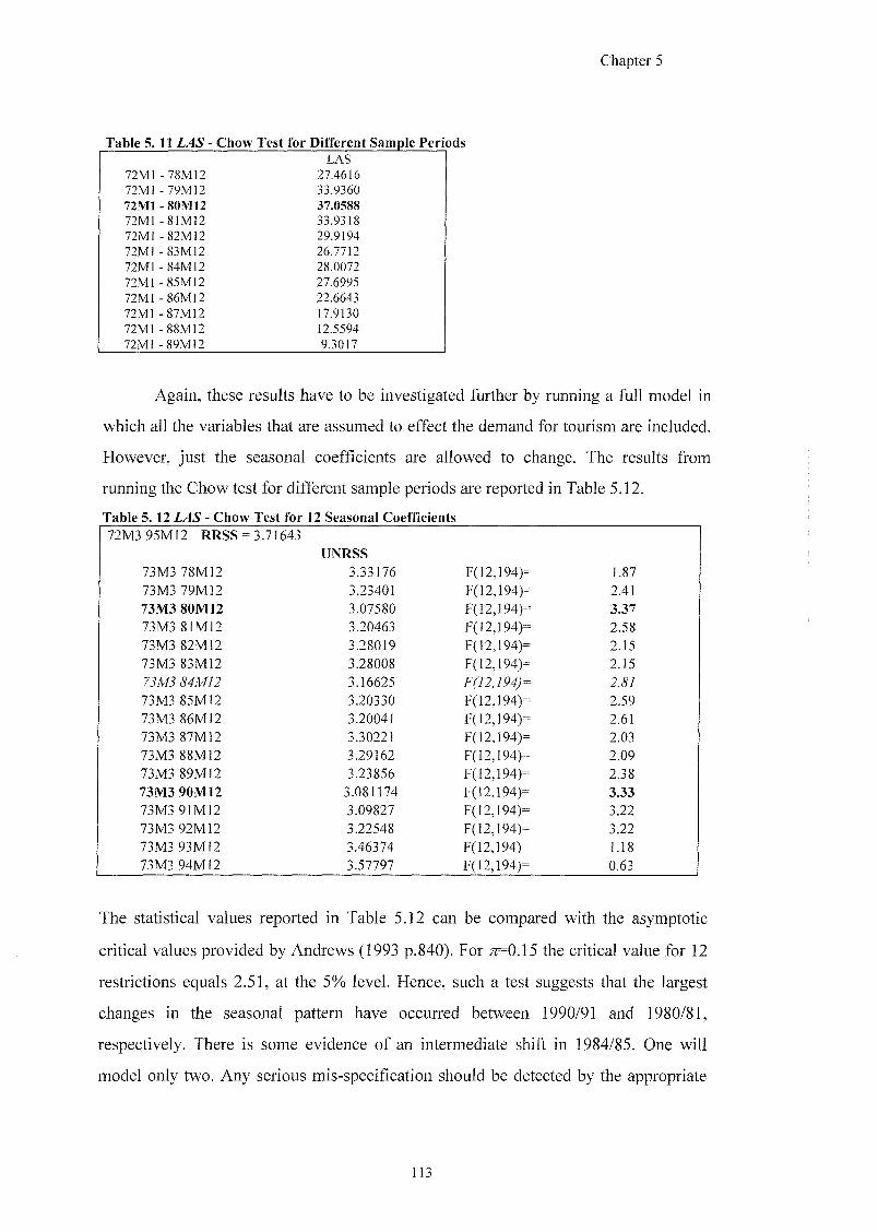
Chapter 5

Table 5 .11 LAS - Chow Test for Different Sample Periods LAS

72M] -78M12 27.4616 72M1 - 79M12 33.9360 72M1 -80M12 37.0588 72M1 -81M12 33.9318 72M1-82MI2 29.9194 72M1-83M12 26.7712 72M1 - 84M12 28.0072 72M1 .85MI2 27.6995 72M1 -86M12 22.6643 72M1 - 87M12 17.9130 72M] -88M12 12.5594 72M1 - 89M12 9^3017

Again, these results have to be investigated further by running a full model in

which all the variables that are assumed to effect the demand for tourism are included.

However, just the seasonal coefficients are allowed to change. The results from

running the Chow test for different sample periods are reported in Table 5.12.

Table 5. 12 LAS - Chow Test for 12 Seasonal Coefficients 72M3 95M12 RRSS = 3.71643

UNRSS

73M3 78M12 3.33176 F(12,]94)= 1.87 73M3 79M12 3.23401 F(12,194)= 2.41 73M3 80M12 3.07580 F(12,194)- 3.37 73M3 81M12 3.20463 F(12,194)= 2 ^ 8 73M3 82M12 3.28019 F( 12,194)- 2U5 73M3 83M12 3.28008 F(12,194)= 2 1 5

3.16625 z a v 73M3 85M12 3.20330 F(12,194)= 2 ^ 9 73M3 86M12 3.20041 F(12,194)= 2 j n

73M3 87M12 3.30221 F(12,194)= 2.03 73M3 88M12 3.29162 F(I2,]94)= 2IW 73M3 89M12 3.23856 F(12,194)= 2 J 8 73M3 90M12 3.081174 F(12,194)= 3.33 73M3 91M12 3.09827 F(]2,194)= 3 2 2 73M3 92M12 3.22548 F(12,]94)= 3 2 2 73M3 93M12 3.46374 F(12,194)= 1J8 73M3 94M12 3.57797 F(12,194)= oâ

The statistical values reported in Table 5.12 can be compared with the asymptotic

critical values provided by Andrews (1993 p.840). For ;z=0.15 the critical value for 12

restrictions equals 2.51, at the 5% level. Hence, such a test suggests that the largest

changes in the seasonal pattern have occurred between 1990/91 and 1980/81,

respectively. There is some evidence of an intermediate shift in 1984/85. One will

model only two. Any serious mis-specification should be detected by the appropriate

i i :

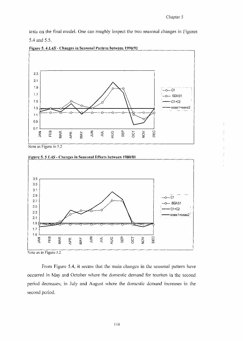
Chapter 5

tests on the final model. One can roughly inspect the two seasonal changes in Figures

5.4 and 5.5.

Figure 5. 4 LAS - Changes in Seasonal Pattern between 1990/91

C14C2

Note as Figure in 5.2

Figure 5. 5 LAS - Changes in Seasonal Effects between 1980/81

-CI

- SB\S1

-C1+C2

-seas1+seas2

Note as in Figure 5.2

From Figure 5.4, it seems that the main changes in the seasonal pattern have

occurred in May and October where the domestic demand for tourism in the second

period decreases; in July and August where the domestic demand increases in the

second period.

114

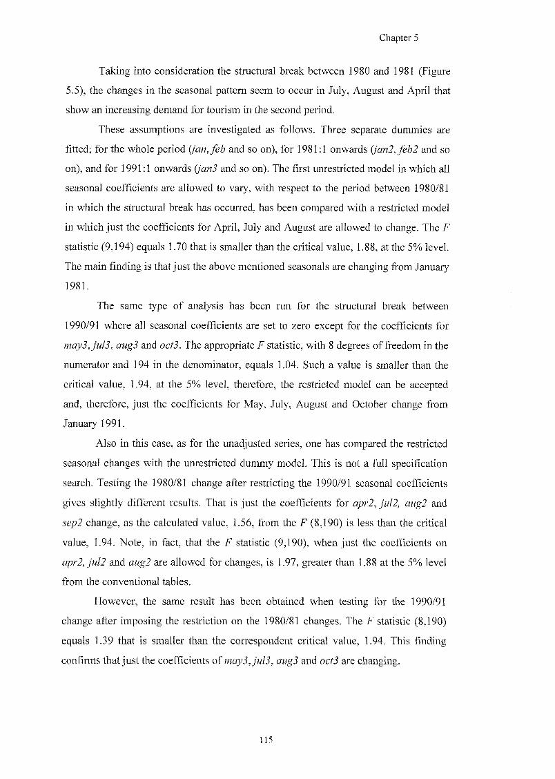
Chapter 5

Taking into consideration the structural break between 1980 and 1981 (Figure

5.5), the changes in the seasonal pattern seem to occur in July, August and April that

show an increasing demand for tourism in the second period.

These assumptions are investigated as follows. Three separate dummies are

fitted; for the whole period (jan,feb and so on), for 1981:1 onwards {jan2,feb2 and so

on), and for 1991:1 onwards (janS and so on). The first unrestricted model in which all

seasonal coefficients are allowed to vary, with respect to the period between 1980/81

in which the structural break has occurred, has been compared with a restricted model

in which just the coefficients for April, July and August are allowed to change. The F

statistic (9,194) equals 1.70 that is smaller than the critical value, 1.88, at the 5% level.

The main finding is that just the above mentioned seasonals are changing from January

1981.

The same type of analysis has been run for the structural break between

1990/91 where all seasonal coefficients are set to zero except for the coefficients for

may3Jul3, aug3 and oct3. The appropriate F statistic, with 8 degrees of freedom in the

numerator and 194 in the denominator, equals 1.04. Such a value is smaller than the

critical value, 1.94, at the 5% level, therefore, the restricted model can be accepted

and, therefore, just the coeîcients for May, July, August and October change from

January 1991.

Also in this case, as for the unadjusted series, one has compared the restricted

seasonal changes with the unrestricted dummy model. This is not a full specification

search. Testing the 1980/81 change after restricting the 1990/91 seasonal coefficients

gives slightly different results. That is just the coefficients for and

change, as the calculated value, 1.56, 6om the F (8,190) is less than the critical

value, 1.94. Note, in fact, that the F statistic (9,190), when just the coefficients on

and are allowed for changes, is 1.97, greater than 1.88 at the 5% level

from the conventional tables.

However, the same result has been obtained when testing for the 1990/91

change after imposing the restriction on the 1980/81 changes. The F statistic (8,190)

equals 1.39 that is smaller than the correspondent critical value, 1.94. This finding

confirms that just the coefficients of awgj and ocf j are changing.

115

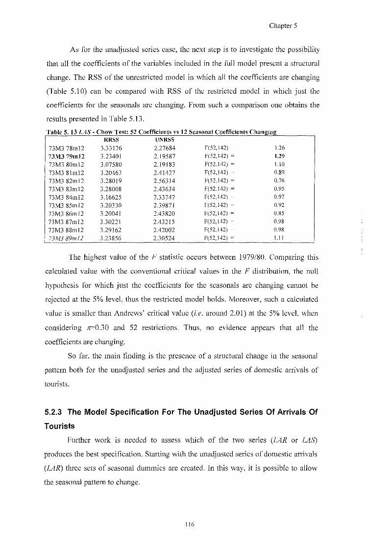
Chapter 5

As for the unadjusted series case, the next step is to investigate the possibility

that all the coefficients of the variables included in the full model present a structural

change. The RSS of the unrestricted model in which all the coefficients are changing

(Table 5.10) can be compared with RSS of the restricted model in which just the

coefficients for the seasonals are changing. From such a comparison one obtains the

results presented in Table 5.13.

Table 5. 13 LAS - Chow Test: 52 Coefficients vs 12 Seasonal Coefficients Changing RRSS UNRSS

73M3 78ml2 3.33176 2.27684 F(52,142) = 1.26

73M3 79ml2 3.23401 2.19587 F(52,142) = 1.29

73M3 80m 12 3.07580 2.19183 F(52,142) = 1.10

73M3 81ml2 3.20463 2.41427 F(52,M2) = 0.89

73M3 82ml2 3.28019 2.56314 F(52,]42) = 0.76

73M3 83m]2 3.28008 2.43634 F(52,142) = 0.95

73M3 84ml2 3.16625 2.33747 F(52,142) = 0.97

73M3 85m 12 3.20330 2.39871 F(52,]42) = 0.92

73M3 86m 12 3.20041 2.43820 F(52,I42) = 0.85

73M3 87ml2 3.30221 2.43215 F(52,I42) = 0.98

73M3 88ml2 3.29162 2.42002 F(52,]42) = 0.98

($9^72 3.23856 2.30524 F(52,I42) = 1.11

The highest value of the F statistic occurs between 1979/80. Comparing this

calculated value with the conventional critical values in the F distribution, the null

hypothesis for which just the coefficients for the seasonals are changing cannot be

rejected at the 5% level, thus the restricted model holds. Moreover, such a calculated

value is smaller than Andrews' critical value {i.e. around 2.01) at the 5% level, when

considering ;z=0.30 and 52 restrictions. Thus, no evidence appears that all the

coefScients are changing.

So far, the main finding is the presence of a structural change in the seasonal

pattern both for the unadjusted series and the adjusted series of domestic arrivals of

tourists.

5.2.3 The Model Specification For The Unadjusted Series Of Arrivals Of

Tourists

Further work is needed to assess which of the two series (LAR or LAS)

produces the best specification. Starting with the unacûsted series of domestic arrivals

{LAR) three sets of seasonal dummies are created. In this way, it is possible to allow

the seasonal pattern to change.

116

Chapter 5

The first set includes c,yaM,^6, and so on. Note thatye6, mar and Mov present

the same coefficients in all three periods. Note also that jan takes the value 1 in the

first period (1972:1-1984:12) and in the third period (1991:1-1995:12), and zero in the

second period (1985:1-1990:12). Whereas may, sep and oct take the value 1 in the first

and in the second period, and zero in the last period. Moreover, the apr, jun, Jul and

aug dummies take the value 1 in the first period and zero in the second and third

period.

The second set of seasonal dummies allows for a structural break in the second

period and contains and This set takes the value one in the

second period and zero otherwise.

The third set of dummies, allowing for a structural break in the third period,

contains moyj, ywMj, yw/J, awgJ, j and ocfJ. This set takes the value one in

the third period and zero otherwise.

An initial unrestricted model has been fitted for LAR including 13 lags for the

dependent variable as well as the (log) industrial production (LPR), the (log) first

difference of relative price (Sassari Province-Italy) (DLREP) and the (log) substitute

price (25?). The model also includes the "Easter" dummy ( ^ , the (log) weather

variable (ZfF), three impulse dummies (zVPZ'^yj, and f7PPjpj) created aAer

inspecting the residuals in order to correct non-normality problems, and, finally, the

above described seasonal dummies. The results for the equation for LAR are reported

in the Appendix E, Table E.3. No problems appear in terms of diagnostic tests.

A general-to-specific simplification has been carried out, and a parsimonious

model (see Table E.4, Appendix E) has been obtained with non-autocorrelated, normal

residuals. The coefficients of the second and third lag of the industrial production is

almost of the same size and opposite sign. The imposition of a restriction in such

coefBcients has been accepted at the 5% leveM. No further restriction has been

accepted. Note also that the relative price growth variable does not turn out to be

statistically significant. Nevertheless, the exclusion of such a variable does not worsen

the model noticeably, and its inclusion is suggested by the SC criterion as well as by a

joint F-test on all 13 lags.

The appropriate F statistic with q=\ and N-K=231, after imposing the restriction Y2 + 73 = 0, is 0.34. Therefore, the restriction cannot be rejected since 0.34 is smaller than the critical value (3.84). Note that LPR2-LPR^ is called RLPR.

.17

Chapter 5

The final model (Table 5.14) is parsimoniosly well-specified in terms of

reduction testing as well as in terms of the SC criterion. Moreover, the model does not

present any problems in terms of diagnostic tests. The R-squared adjusted shows the

good of fitness which is also supported by a satisfactory ratio between the SER and

DMV THAT equals 0.007997^" Further tests for parameter constancy over the last 33

observations of the sample are also reported. The null hypothesis of parameter

constancy cannot be rejected.

50 SER/MDV = (0.081626/10.146) = 0.007997.

118

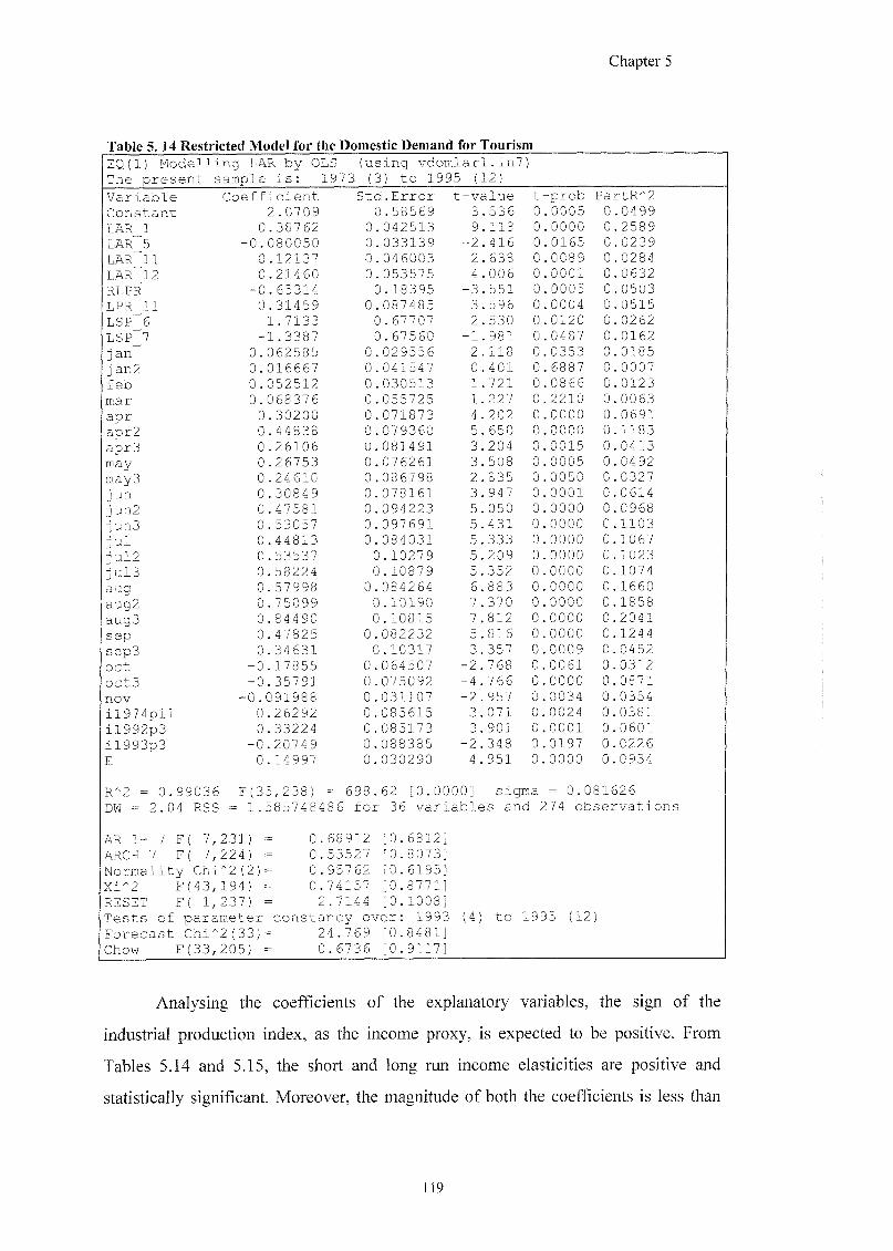
Chapter 5

Table 5. 14 Restricted Model for the Domestic Demand for Tourism EQ(1) Modelling LAR by OLS (using vdomlarl.inl) The present sample is: 1973 (3) to 1995 (12)

Variable Coefficient Std.Error t--value t -prob PartR'^2 Constant 2.0709 0.58569 3 536 0 0005 0 .0499 LAR 1 0 .38762 0.042513 9 118 0 0000 0 2589 LAR 5 -0. 080050 0.033139 -2 416 0 0165 0 .0239 LAR 11 0 .12137 0.046003 2 638 0 0089 0 .0284 LAR 12 0 .21460 0.053575 4 006 0 0001 0 0632 RLPR -0 .65314 0.18395 -3 551 0 0005 0 0503 LPR 11 0 .31459 0.087485 3. 596 0 0004 0 0515 LSP 6 1.7133 0.67707 2 530 0 0120 0 0262 LSP 7 _ 1.3387 0.67560 1. 981 0 0487 0 0162 jan 0 . 062585 0.029556 2. 118 0 0353 0 0185

ian2 0. 016667 0.041547 0 401 0 6887 0 0007

f eb 0. 052512 0.030513 1 721 0 0866 0 0123

mar 0. 068376 0.055725 1 227 0 2210 0 0063

apr 0 .30200 0.071873 4 202 0 0000 0 0691 apr2 0 .44838 0.079360 5. 650 0 0000 0 1183

apr3 0 .26106 0.081491 3. 204 0 0015 0 0413 may 0 .26753 0.076261 3. 508 0 0005 0 0492 may3 0 .24610 0.086798 2 835 0 0050 0 0327 jun 0 .30849 0.078161 3. 947 0 0001 0 0614

iun2 0 .47581 0.094223 5. 050 0 0000 0 0968

iun3 0 .53057 0.097691 5 . 431 0 0000 0 1103

jul 0 .44813 0.084031 5 . 333 0 0000 0 1067

iul2 0 .53537 0.10279 5 . 209 0 0000 0 1023

iul3 0 .58224 0.10879 5. 352 0 0000 0 1074

aug 0 .57998 0.084264 6. 883 0 0000 0 1660

aug2 0 .75099 0.10190 7 . 370 0 0000 0 1858

aug3 0 .84490 0.10815 7 . 812 0 0000 0 2041

sep 0 .47825 0.082232 5 . 816 0 0000 0 1244

sep3 0 .34631 0.10317 3. 357 0 0009 0 0452

oct -0 .17855 0.064507 2 . 768 0 0061 0 0312

oct3 -0 .35791 0.075092 4 . 766 0 0000 0 0871

nov -0 . 091988 0.031107 2 . 957 0 0034 0 0354 il974pll 0 .26292 0.085615 3. 071 0 0024 0 0381

il992p3 0 .33224 0.085173 3. 901 0 0001 0 0601 il993p3 -0 .20749 0.088385 2 . 348 0 0197 0 0226 E 0 .14997 0.030290 4 . 951 0 0000 0. 0934

R"2 = 0.99036 F(35,238) = 698.62 [0.0000 ] sigma = 0.081626

DW = 2.04 RSS = 1. 5857484 86 for 36 variables and 274 observations

AR 1- 7 F( 7,231) 0. 68912 [0.6812] ARCH 7 F( 7, 224) 0. 53527 [0.8073] Normality Chi '"2 (2) 0 . 95762 [0.6195] Xi'^2 F(43, 194) 0. 74157 [0.8771] RESET F( 1, 237) 2 .7144 [0.1008] Tests of parameter constancy over: 1993 ( 4) to 1995 (12 ) Forecast Chi"^ 2 (33) 24.769 [0.8481] Chow F(33, 205) 0 .6736 [0.9117]

Analysing the coefBcients of the explanatory variables, the sign of the

industrial production index, as the income proxy, is expected to be positive. From

Tables 5.14 and 5.15, the short and long run income elasticities are positive and

statistically significant. Moreover, the magnitude of both the coefGcients is less than

119

Chapter 5

unity. Hence, the hypothesis that domestic tourism is to be considered as a necessity

good has been confirmed. This finding is also consistent with the result obtained by

Malacarni (1991) when using annual data for the Italian case.

In general, in almost all economic transactions the principle that the demand

and the price are inversely correlated holds. However, as in the case for the

international demand for tourism, the coefficient for the substitute price, both in the

short and long run, turns out to be positive. Once again, there might be problems in not

taking explicitly into account the possible influence of the exchange rate for other

competitors of the north of Sardinia. Chapter 6 is dedicated to a deeper investigation of

modelling the domestic demand for tourism with the inclusion of the substitute price

and exchange rate for the competitor countries.

From Table 5.14, the weather variable does not appear to have any effects on

the determination of the domestic flows of tourists. The same results have been

achieved in the international tourism demand case.

Turning to the "Easter" dummy, it is highly statistically significant in

explaining domestic demand for tourism. This finding is in agreement with the

international demand case.

In Table 5.15, the long run dynamics and standard errors (in parenthesis) are

reported. In general, the standard errors are relatively low and and the long run

coefficients are jointly significant as inferred from the Wald test. It can be concluded

that the monthly model presents an overall good specification both in the short and

long run.

120

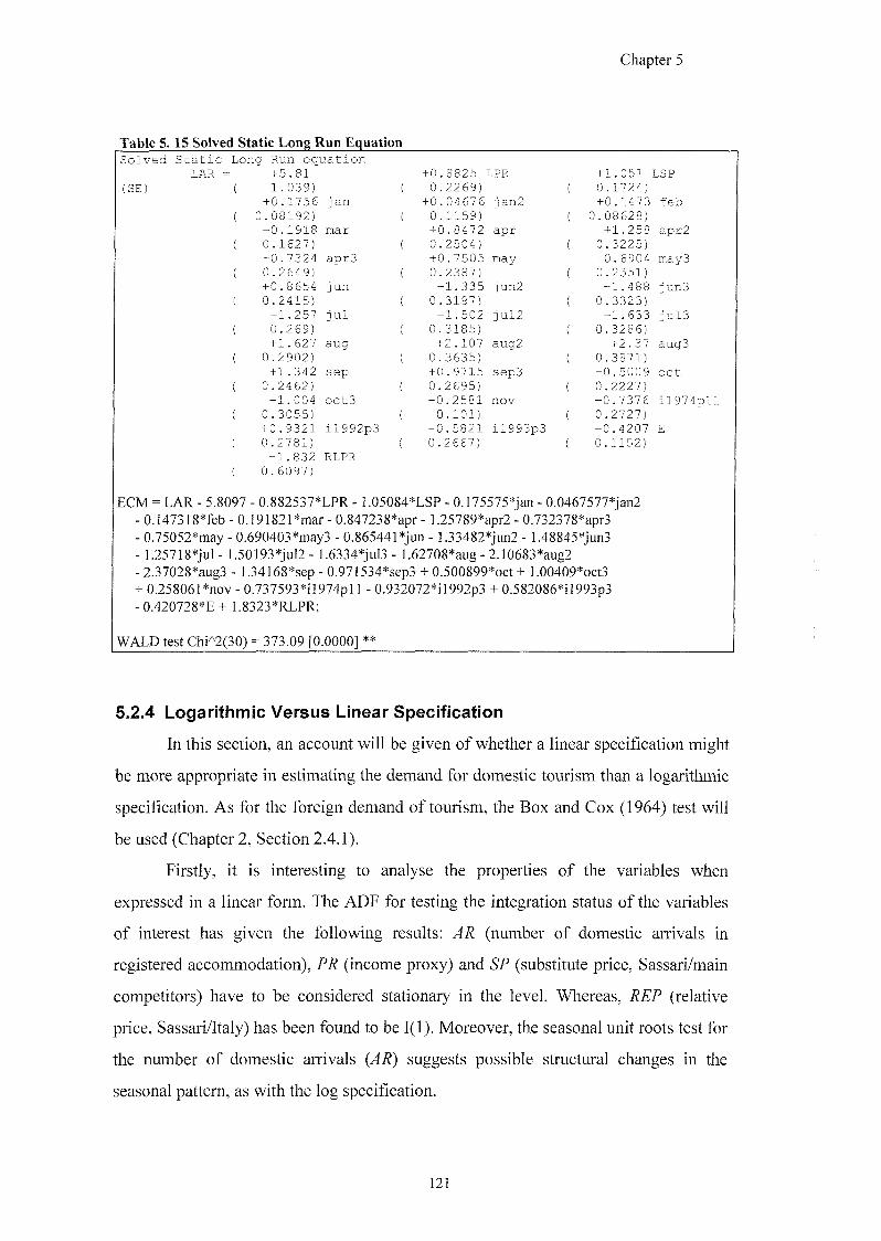
Chapter 5

Table 5 .15 Solved Static Long Run Equation Solved Static Long equation

LAR (SE)

+ 5.81 +0.8825 LPR +1.051 LSP 1.039) 0.2269) 0.1724)

+0.1756 jan +0.04676 jan2 +0.1473 feb .08192) 0.1159) 0.08628) +0.1918 mar +0.8472 apr +1.258 apr2 0.1627) 0.2504) 0.3225) +0.7324 apr3 +0.7505 may +0.6904 may3 0.2649) 0.2387) 0.2551) +0.8654 jun +1.335 junZ +1.488 iun3 0.2415) 0.3197) 0.3323) +1.257 jul +1.502 iul2 +1.633 iul3 0.269) 0.3185) 0.3286) +1.627 aug +2.107 aug2 +2.37 aug3

0.2902) 0.3635) 0.3871) +1.342 Sep +0.9715 sep3 -0.5009 oct

0.2462) 0.2695) 0.2227) -1.004 oct3 -0.2581 nov +0.7376 il974pll

0.3055) 0.101) 0.2727) +0.9321 il992p3 -0.5821 il993p3 +0.4207 E 0.2781) 0.2667) 0.1152) -1.832 RLPR

0.6097)

ECM = LAR - 5.8097 - 0.882537*LPR - 1.05084*LSP - 0.175575*jan - 0.0467577*jan2 - 0.147318*kb - 0.191821*mar - 0.847238*apr- 1.25789*apr2 - 0.732378*apr3 - 0.75052*may - 0.690403*may3 - 0.865441*jun - 1.33482*jun2 - 1.48845*jun3 - 1.25718*jul - 1.50193*jul2 - 1.6334*jul3 - 1.62708*aug -2.10683*aug2 -2.37028*aug3 - 1.34168*sep-0.97]534*sep3 + 0.500899*oct+ 1.00409*oct3 + 0.258061*nov - 0.737593*il974p] 1 - 0.932072*il992p3 + 0.582086*il993p3 - 0.420728*E + 1.8323*RLPR;

WALD test Chi''2(30) = 373.09 [0.0000] **

5.2.4 Logarithmic Versus Linear Specification

In this section, an account will be given of whether a linear specification might

be more appropriate in estimating the demand for domestic tourism than a logarithmic

specification. As for the foreign demand of tourism, the Box and Cox (1964) test will

be used (Chapter 2, Section 2.4.1).

Firstly, it is interesting to analyse the properties of the variables when

expressed in a linear form. The ADF for testing the integration status of the variables

of interest has given the following results: AR (number of domestic arrivals in

registered accommodation), PR (income proxy) and SP (substitute price, Sassari/main

competitors) have to be considered stationary in the level. Whereas, REP (relative

price, Sassari/Italy) has been found to be 1(1). Moreover, the seasonal unit roots test for

the number of domestic arrivals {AR) suggests possible structural changes in the

seasonal pattern, as with the log specification.

121

Chapter 5

In order to run the Box-Cox test, one estimates the unrestricted 13 lag model

for the demand equation as follows:

LAR( = CI] + a2 LARj_]... + LPRj.. + LSPp. + aj DLREPp. + Ufj LW^ + ay E +

+ og Seag + Op

and

ZzMgoryor/M

ARf ^ CI J + ^2 ^^t-1-- ^5 DREPp. + Wp + dy E + ag Seas + + opDw/Mm/gj' +

where the explanatory variables are defined as before, and the seasonals are

constructed so as to allow structural changes in the seasonal pattern. The impulse

dummies are the following; il974pll, il992p3 and il993p3.

In particular, the sum of the squared errors from the logarithmic form (SSELL)

equals 1.828891408, whereas the sum of the squared errors for the linear form (SSEL)

equals 3626196276. The aim is to test whether the two models are empirically

equivalent and find out which of the two models best fits the data. In doing this, one

needs to calculate the sum of the squared errors for the linear model with {AR/A R G)

as the dependent variable and where AR G is the geometric mean. The sum of the

squared errors fbr the latter model (z.e. equals 5.581458. The Box-Cox

test indicates that the two models are empirically different as the calculated is

152.86 and the correspondent tabulated value is 3.84 at the 5% level. Moreover, the

is higher that hence, it can be concluded the logarithmic

specification form fits the data better than the linear model. The same result is

obtained in the foreign model.

5.2.5 The Model Specification Using Monthly Data For The Adjusted

Series Of Arrivals Of Tourists

The next step is to carry out an investigation for the adjusted series of domestic

arrivals for the number of Sundays in a month (LAS). An unrestricted model is fitted

for 13 lags of the dependent variable, LPR, LSP, DLREP, E and L W (as previously

defined), and two impulse dummies {il987p3 and il992p3) are included after having

inspected the residuals in order to avoid non-normality problems. Three sets of

seasonal dummies are created to allow the seasonal pattern to change, in accordance

122

Chapter 5

with the structural change findings as assessed in the previous section. The first set

includes c, jan,feb, and so on. Note that apr and sep take the value 1 in the first period

(1972:1-1980:12) and in the third period (1991:1-1995:12); whereas, may takes the

value of one in the first and second period (1981:1-1990:12) and the value of zero in

the third period. Note also that Jul and aug dummies take the value 1 just in the first in

the first period. The second set of seasonal dummies allows for the structural break in

the second period and consists of and ^^2. This set of dummies takes

the value of one in the second period and zero otherwise. Finally, the third set of

dummies that allows for structural change in the third period consists of may3, jul3,

augS and oct3. In this case these dummies take the value of one in the third period and

zero otherwise.

The results for the unrestricted model are shown in Appendix E (Table E.5) and

no problems arise from the diagnostic tests. The residual sum of squares present, as

pointed out in the VAR analysis, a greater value than the RSS for the unadjusted

series. The results of the parsimonious model (see Appendix E, Table E.6) indicate

problems in terms of specification {RESET test).

The main conclusion from this analysis is that, for the domestic demand of

tourism, the adjustment of the dependent variable for the number of weekends (either

Saturdays or Sundays in a month) does not appear to be acceptable. However, one can

argue that such a finding seems plausible in that domestic tourists can easily arrive to

the north of Sardinia any day of the week either by boat or plane. Foreign tourists, on

the other hand, are much more constrained by the day of arrival as are more likely to

use charter flights which occur mainly in the weekends, as far as the period under

study is concerned.

5.3 THE MODEL SPECIFICATION USING ANNUAL DATA

The aim of this section is twofold. Firstly, one will assess whether the Italian

industrial production index {LPR) can indeed be thought to be a valid proxy for the

Italian personal disposable income (PDIN).

According to Lim (1997), 62% of the total tourism studies have used annual

data, whereas just a very limited number has made use of monthly data. One of the

problems is the low precision of estimates associated with the use of annual data, as in

123

Chapter 5

many circumstances the sample sizes are very small and do not allow for specification

of the dynamics of the demand for tourism (Witt and Witt, 1992; Lim, 1997). Hence,

the second aim of this section is assessing the characteristics of the domestic demand

for tourism in the long run by making use of annual data, and hence, comparing them

with the short run characteristics.

5.3.1 Industrial Production Index As A Proxy For The Personal

Disposable Income

It is of interest to find out whether the industrial production index can be

considered a valid proxy of the personal disposable income in the Italian case. The

analysis in this thesis refers to the period from 1983 until 1992. The total number of

observations available for the Italian personal disposable income, PDIN, are ten

(source ISTAT). In particular, the disposable income per capita consists of grants from

public authorities, wages of self-employed and employees, earnings 6om different

kind of investments minus income tax, health contributions, public and private

contributions to pension funds. The Italian index of industrial production published

annually (source IPS) is also used for the same period. The logarithm of the two series

are shown in Figure 5.6.

124

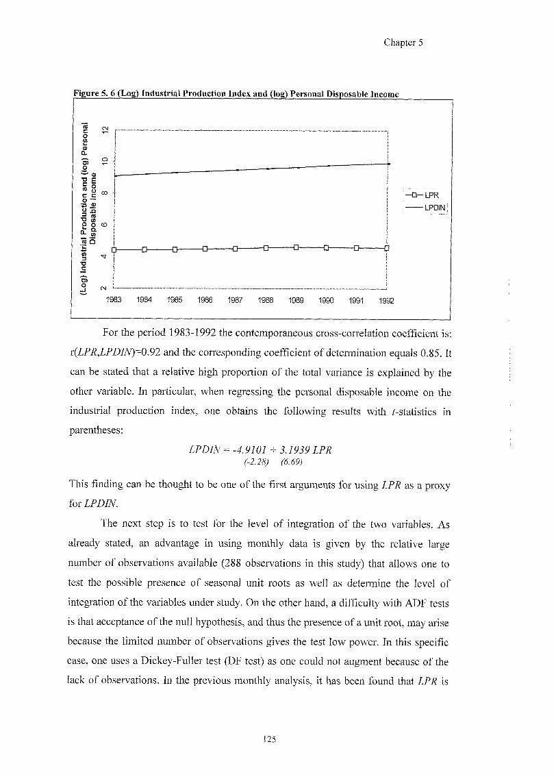
Chapter 5

Figure 5. 6 (Log) Industrial Production Index and (log) Personal Disposable Income

•p to

-LPR

-LPDIN

1983 1984 1985 1986 1987 1988 1989 1990 1991 1992

For the period 1983-1992 the contemporaneous cross-correlation coefficient is:

v{LPR,LPDIN)=0.91 and the corresponding coefficient of determination equals 0.85. It

can be stated that a relative high proportion of the total variance is explained by the

other variable. In particular, when regressing the personal disposable income on the

industrial production index, one obtains the following results with r-statistics in

parentheses:

z f D W = - 4 . 9 7 0 7 + j . y p j p I f

This finding can be thought to be one of the first arguments for using I f as a proxy

f o r Z f D W .

The next step is to test for the level of integration of the two variables. As

already stated, an advantage in using monthly data is given by the relative large

number of observations available (288 observations in this study) that allows one to

test the possible presence of seasonal unit roots as well as determine the level of

integration of the variables under study. On the other hand, a difficulty with ADF tests

is that acceptance of the null hypothesis, and thus the presence of a unit root, may arise

because the limited number of observations gives the test low power. In this specific

case, one uses a Dickey-Fuller test (DF test) as one could not augment because of the

lack of observations. In the previous monthly analysis, it has been found that Zf is

125

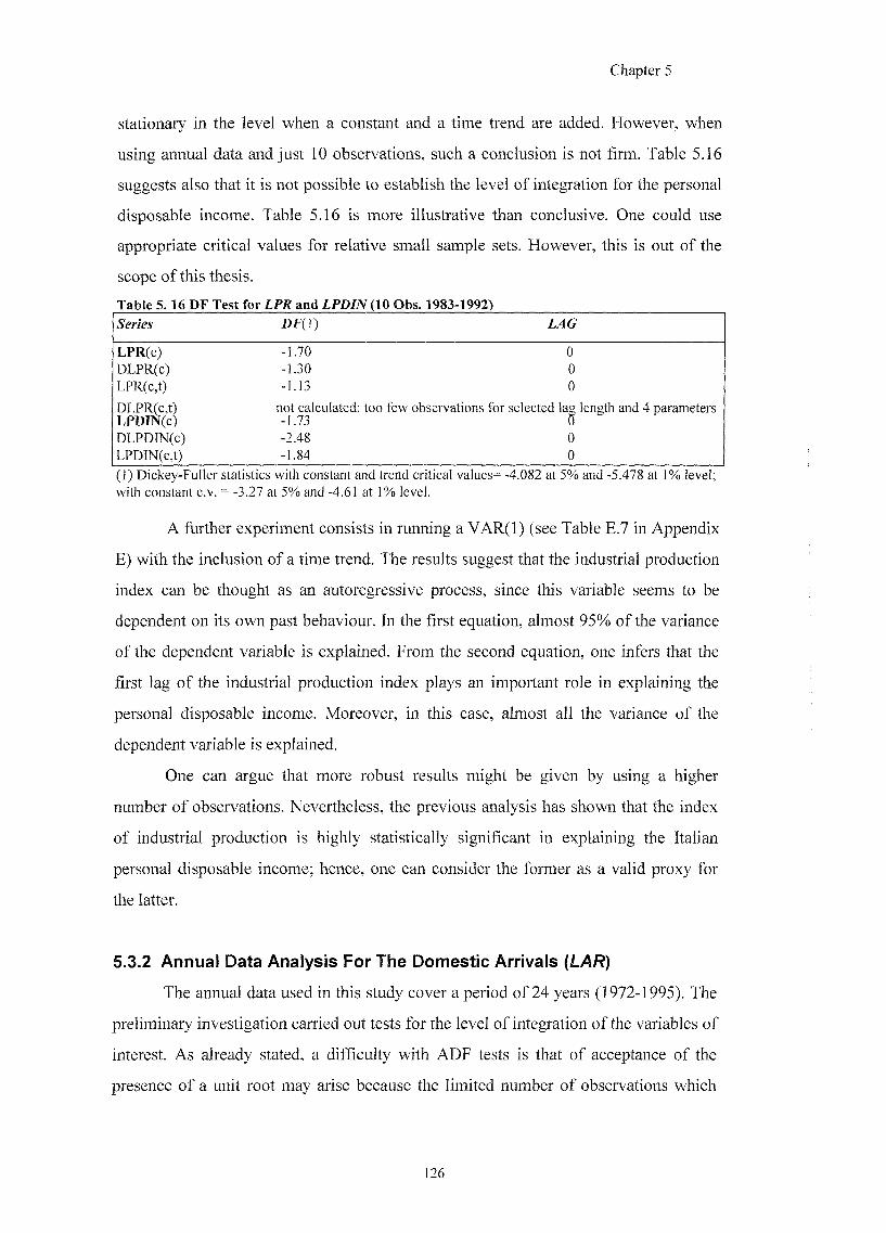
Chapter 5

stationary in the level when a constant and a time trend are added. However, when

using annual data and just 10 observations, such a conclusion is not firm. Table 5.16

suggests also that it is not possible to establish the level of integration for the personal

disposable income. Table 5.16 is more illustrative than conclusive. One could use

appropriate critical values for relative small sample sets. However, this is out of the

scope of this thesis.

Table 5. 16 DF Test for LPR and LPDIN (10 Obs. 1983-1992)

Series LAG

LPR(c) -1.70 0 DLPR(c) -1.30 0 LPR(c,t) -1.13 0

DLPR(c,t) not calculated; too few observations for selected las length and 4 parameters LPDIN(c) -1.73 DLPDn\((c) -2.48 0 LPDIN(c,t) -1.84 0

(1) Dickey-Fuller statistics with constant and trend critical values= -4.082 at 5% and -5.478 at 1% level; with constant c.v. = -3.27 at 5% and -4.61 at 1% level.

A further experiment consists in running a VAR(l) (see Table E.7 in Appendix

E) with the inclusion of a time trend. The results suggest that the industrial production

index can be thought as an autoregressive process, since this variable seems to be

dependent on its own past behaviour. In the first equation, almost 95% of the variance

of the dependent variable is explained. From the second equation, one infers that the

first lag of the industrial production index plays an important role in explaining the

personal disposable income. Moreover, in this case, almost all the variance of the

dependent variable is explained.

One can argue that more robust results might be given by using a higher

number of observations. Nevertheless, the previous analysis has shown that the index

of industrial production is highly statistically significant in explaining the Italian

personal disposable income; hence, one can consider the former as a valid proxy for

the latter.

5.3.2 Annual Data Analysis For The Domestic Arrivals (LAR)

The annual data used in this study cover a period of 24 years (1972-1995). The

preliminary investigation carried out tests for the level of integration of the variables of

interest. As already stated, a difficulty with ADF tests is that of acceptance of the

presence of a unit root may arise because the limited number of observations which

126

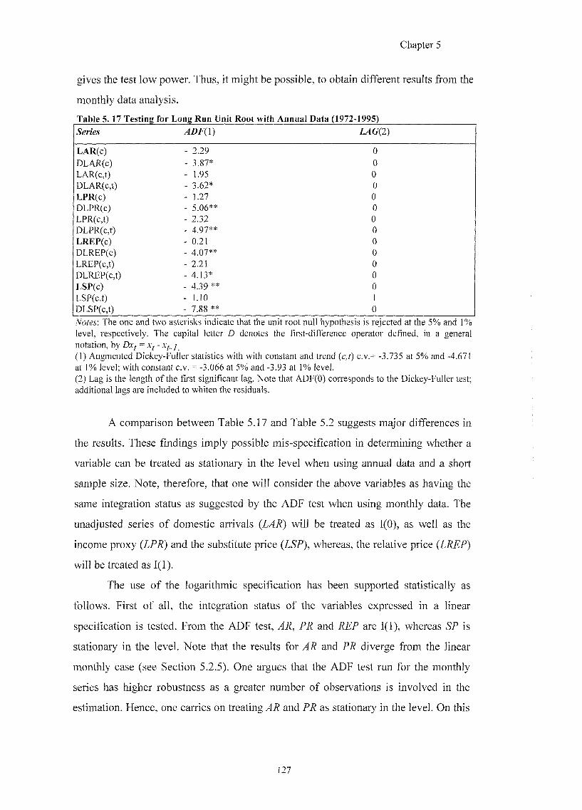
Chapter 5

gives the test low power. Thus, it might be possible, to obtain different results from the

monthly data analysis.

Series IX (7(2)

LAR(c) - 2.29 0

DLAR(c) - 3.87* 0 LAR(c,t) - 1.95 0 DLAR(c,t) - 3.62* 0 LPR(c) - 1.27 0 DLPR(c) - 5.06** 0 LPR(c,t) - 2.32 0 DLPR(c,t) - 4.97** 0 LREP(c) - 0.21 0 DLREP(c) - 4.07** 0 LREP(c,t) - 2.21 0 DLREP(c,t) - 4.13* 0 LSP(c) - 4.39 ** 0 LSP(c,t) - 1.10 1 DLSP(c,t) - 7.88 ** 0

Notes'. The one and two asterisks indicate that the unit root null hypothesis is rejected at the 5% and 1% level, respectively. The capital letter D denotes the first-difference operator defined, in a general notation, by Dxj = (1) Augmented Dickey-Fuller statistics with with constant and trend {c,t) c.v.= -3.735 at 5% and -4.671 at 1% level; with constant c.v. = -3.066 at 5% and -3.93 at 1% level. (2) Lag is the length of the first significant lag. Note that ADF(O) corresponds to the Dickey-Fuller test; additional lags are included to whiten the residuals.

A comparison between Table 5.17 and Table 5.2 suggests major differences in

the results. These findings imply possible mis-specification in determining whether a

variable can be treated as stationary in the level when using annual data and a short

sample size. Note, therefore, that one will consider the above variables as having the

same integration status as suggested by the ADF test when using monthly data. The

unadjusted series of domestic arrivals will be treated as 1(0), as well as the

income proxy {LPR) and the substitute price {LSP), whereas, the relative price (LREP)

will be treated as 1(1).

The use of the logarithmic specification has been supported statistically as

follows. First of all, the integration status of the variables expressed in a linear

specification is tested. From the ADF test, AR, PR and REP are 1(1), whereas SP is

stationary in the level. Note that the results for AR and PR diverge from the linear

monthly case (see Section 5.2.5). One argues that the ADF test run for the monthly

series has higher robustness as a greater number of observations is involved in the

estimation. Hence, one carries on treating and as stationary in the level. On this

127

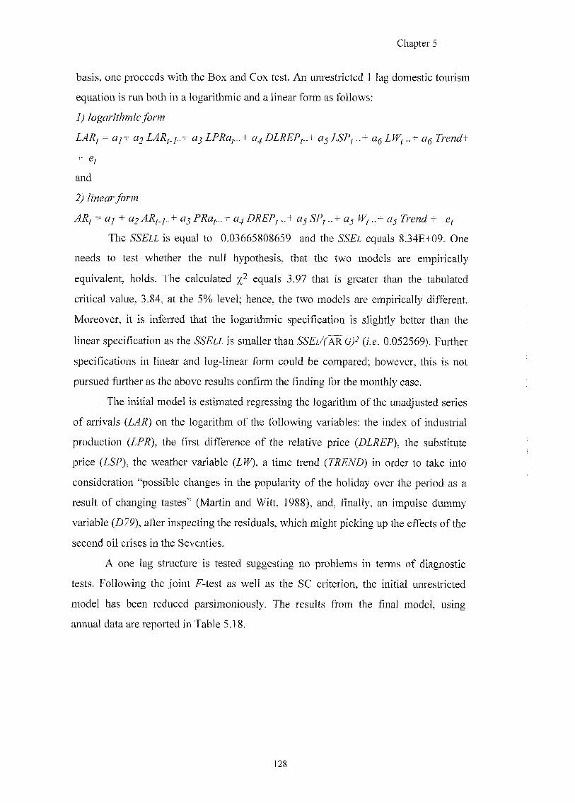
Chapter 5

basis, one proceeds with the Box and Cox test. An unrestricted 1 lag domestic tourism

equation is run both in a logarithmic and a linear form as follows:

LARj = a]+ a2 LARf_j..+ LPRap..+ DLREPi..+ L S P f L W ^ a g Trends

+

and

ARj = aj + a2 ARf_]..+ PRaf...+ a^DREPf..+ a^SPj..+ aj ^ ..+ gj Trend +

The is equal to 0.03665808659 and the equals 8.34E+09. One

needs to test whether the null hypothesis, that the two models are empirically

equivalent, holds. The calculated equals 3.97 that is greater than the tabulated

critical value, 3.84, at the 5% level; hence, the two models are empirically different.

Moreover, it is inferred that the logarithmic specification is slightly better than the

linear specification as the is smaller than (i.e. 0.052569). Further

specifications in linear and log-linear form could be compared; however, this is not

pursued further as the above results confirm the finding for the monthly case.

The initial model is estimated regressing the logarithm of the unacûsted series

of arrivals {LAR) on the logarithm of the following variables; the index of industrial

production (LPR), the first difference of the relative price (DLREP), the substitute

price (Z&P), the weather variable (IfF), a time trend (ZRETVD) in order to take into

consideration "possible changes in the popularity of the holiday over the period as a

result of changing tastes" (Martin and Witt, 1988), and, finally, an impulse dummy

variable (079), after inspecting the residuals, which might picking up the effects of the

second oil crises in the Seventies.

A one lag structure is tested suggesting no problems in terms of diagnostic

tests. Following the joint F-test as well as the SC criterion, the initial unrestricted

model has been reduced parsimoniously. The results from the final model, using

annual data are reported in Table 5.18.

128

Chapter 5

Table 5 .18 Regression Results for the Annual Domestic Demand Model {LAR) EQ(1) Modelling LAR by OLS (using datiann.inV) The present sample is: 3 to 24

Variable Coefficient Std.Error t -value t--prob PartR''2 Constant 8.9790 1.0444 8.597 0 .0000 0 8221 LPR 0.46779 0.18235 2.565 0 .0207 0 2914 LSP 1.4932 0.19786 7.547 0 0000 0 7807 LW 0.69008 0.24934 2.768 0 0137 0 3238 Trend 0.015705 0.0037756 4.160 0 0007 0 5196 D79 -0.13515 0.048525 -2.785 0 0132 0 3265 R''2 = 0.981208 F(5,16) = 167.09 [0.0000 sigma — 0.0447279 DW = 1.97 RSS = 0.03200929317 for 6 var. and 22 obs .

AR 1- 7 F( 7, 9) = 1.9714 [0.1692] ARCH 7 F( 7, 2) = 0.45772 [0.8169] Normality Chi"2(2)= 0.27006 [0.8737] Xi"2 F( 9, 6) = 0.30248 [0.9472] RESET F( 1, 15) = 0.31175 [0.5848] Tests of parameter constancy over: 23 to 24 Forecast Chi''2( 2)= 4.5929 [0.1006] Chow F( 2, 14) = 2.0679 [0.1634]

Such a model is statistically well-specified and constitutes an admissible

reduction of the underlying unrestricted model. The model is able to explain almost

98% of the variation of the dependent variable; moreover, the goodness of the fit is

also suggested by the ratio of and MDF equal to 0.0035^^. Note also that the null

hypothesis of parameter constancy for the last two observations fails to be rejected.

The inclusion of the lagged dependent variable does not turn out to be

statistically significant, suggesting that the model converges rapidly to the long run

equilibrium. Moreover, this finding suggests that domestic tourists are likely to be

"allocentric" in that they prefer new destinations for their own holiday trip. The (log)

index of industrial production is found to be statistically significant. This finding

seems to be consistent with the results obtained by Arbel and Ravid (1985) for which

"the income is found to be the single most important determinant of long run

recreation use" (p.981). Moreover, it confirms the results obtained in the monthly

model; the coefficient is positive and less than unity suggesting that domestic tourism

has to be regarded as a necessity good. Hence, the results obtained in Malacarni (1991)

are confirmed. The (log) substitute price coefficient has a positive sign and is in

contrast with economic theory. However, these Gndings restate the results from the

51 SER/MDV = (0.0447279/12.895) = 0.0035.

129

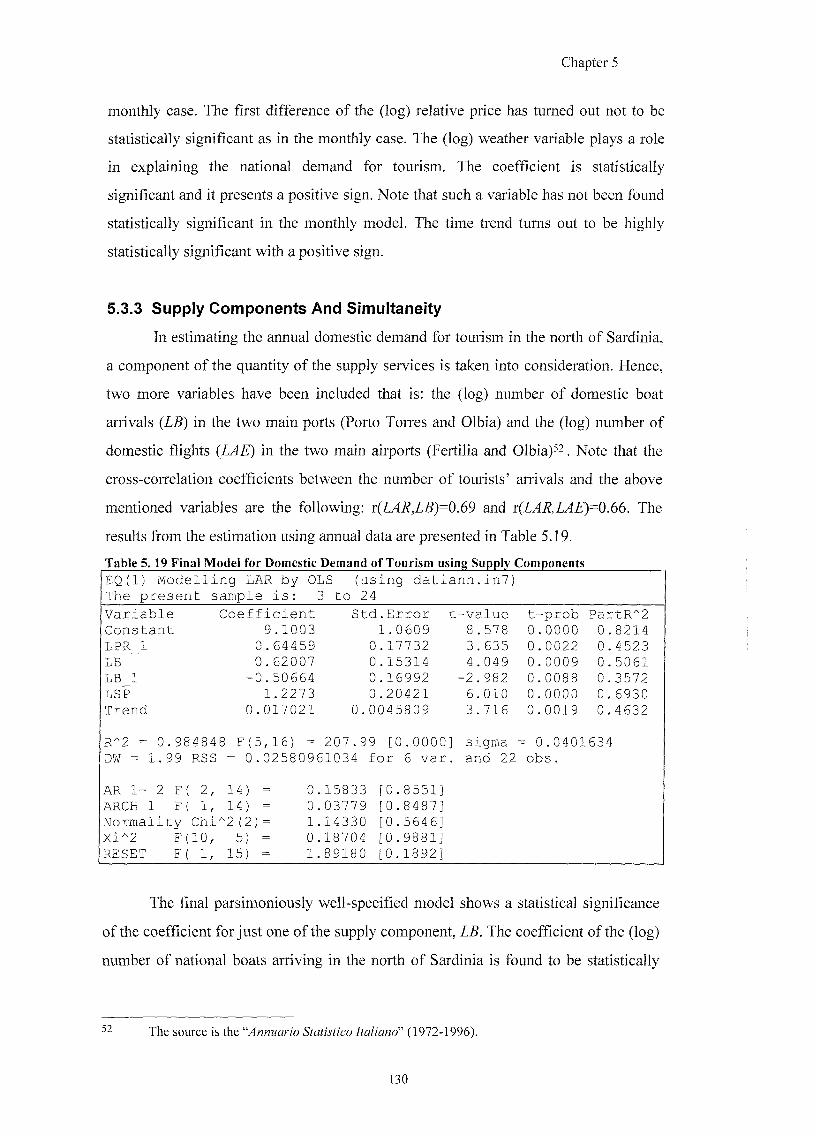
Chapter 5

monthly case. The first difference of the (log) relative price has turned out not to be

statistically significant as in the monthly case. The (log) weather variable plays a role

in explaining the national demand for tourism. The coefficient is statistically

significant and it presents a positive sign. Note that such a variable has not been found

statistically significant in the monthly model. The time trend turns out to be highly

statistically significant with a positive sign.

5.3.3 Supply Components And Simultaneity

In estimating the annual domestic demand for tourism in the north of Sardinia,

a component of the quantity of the supply services is taken into consideration. Hence,

two more variables have been included that is: the (log) number of domestic boat

arrivals {LB) in the two main ports (Porto Torres and Olbia) and the (log) number of

domestic flights {LAE) in the two main airports (Fertilia and Olbia)^^ Note that the

cross-correlation coefficients between the number of tourists' arrivals and the above

mentioned variables are the following: x{LAR,LB)=0.69 and r(LAR,LAE)=0.66. The

results from the estimation using annual data are presented in Table 5.19.

EQ(1) Modelling LAR by OLS (using datiann.in?)

The present sample is: 3 to 24

Variable Coefficient Std.Error t -value t-prob PartR"2 Constant 9.1003 1.0609 8.578 0.0000 0. 8214 LPR 1 0.64459 0.17732 3.635 0.0022 0. 4523 LB 0.62007 0.15314 4.049 0.0009 0. 5061 LB 1 -0.50664 0.16992 -2.982 0.0088 0. 3572 LSP 1.2273 0.20421 6.010 0.0000 0. 6930 Trend 0.017021 0.0045809 3.716 0.0019 0. 4632

Fr2 = 0.98484 8 F(5,16) = 207.99 [0.0000] sigma = 0.0401634 DW = 1.99 RSS = 0.02580961034 for 6 var. and 22 obs.

AR 1- 2 F( 2, 14) = 0.15833 [0.8551]

ARCH 1 F( 1, 14) = 0.03779 [0.8487]

Normality Chi "2(2)= 1.14330 [0.5646]

Xi"2 F(10, 5) = 0.18704 [0.9881]

RESET F( 1, 15) = 1.89180 [0.1892]

The final parsimoniously well-specified model shows a statistical significance

of the coefficient for just one of the supply component, LB. The coefficient of the (log)

number of national boats arriving in the north of Sardinia is found to be statistically

2 The source is theAnnuario Statistico Italiand" (1972-1996).

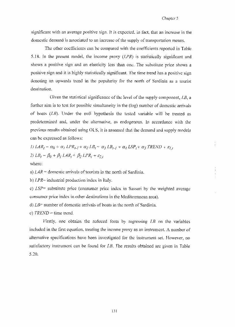
Chapter 5

significant with an average positive sign. It is expected, in fact, that an increase in the

domestic demand is associated to an increase of the supply of transportation means.

The other coefficients can be compared with the coefficients reported in Table

5.18. In the present model, the income proxy {LPR) is statistically significant and

shows a positive sign and an elasticity less than one. The substitute price shows a

positive sign and it is highly statistically significant. The time trend has a positive sign

denoting an upwards trend in the popularity for the north of Sardinia as a tourist

destination.

Given the statistical significance of the level of the supply component, LB, a

further aim is to test for possible simultaneity in the (log) number of domestic arrivals

of boats {LB). Under the null hypothesis the tested variable will be treated as

jpreckstemiinexi euid, iinder tlwe sJteinatrve, gus endojgerwous. ]bi acciirckuice v/iiAi the

previous results obtained using OLS, it is assumed that the demand and supply models

can be expressed as follows:

L) LARf = gcq + ccj LPR^_j + c(2 LB^ + cc^ LB^_j + oc^ LSPf+ ot^ TREND + gy

^ = A) + A + A

where:

a) LAR = domestic arrivals of tourists in the north of Sardinia.

b) LPR= industrial production index in Italy.

c) 2,5?= substitute price (consumer price index in Sassari by the weighted average


d) LB= number of domestic arrivals of boats in the north of Sardinia.

e) TREND = time trend.

Firstly, one obtains the reduced form by regressing Z.8 on the variables

included in the first equation, treating the income proxy as an instrument. A number of

alternative specifications have been investigated for the instrument set. However, no

satisfactory instrument can be found for The results obtained are given in Table

5.20.

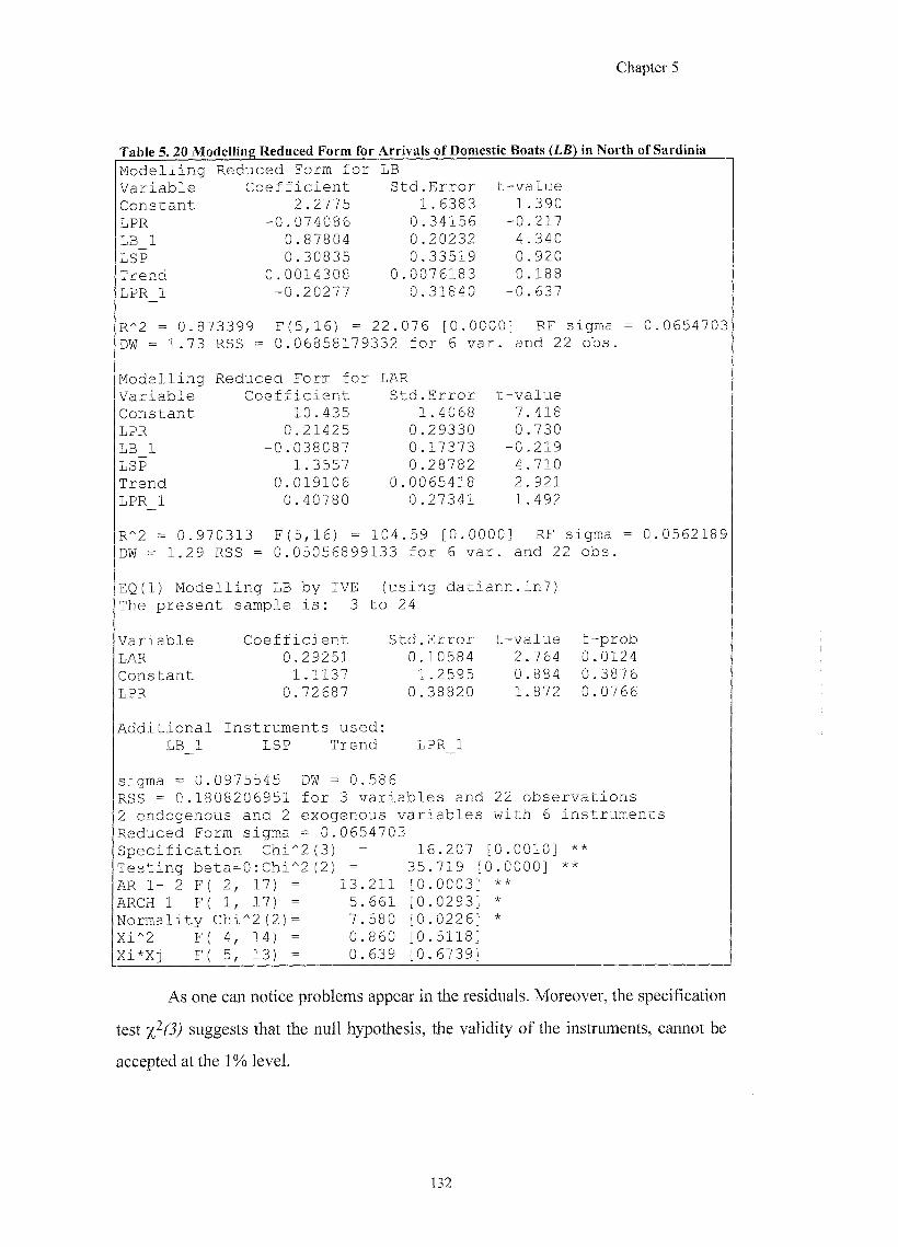
Chapter 5

Modelling Reduced Form for LB Variable Coefficient Std.Error t-value

Constant 2.2775 1.6383 1.390

LPR -0.074086 0.34156 -0.217

LB 1 0.87804 0.20232 4.340

ISP 0.30835 0.33519 0.920

Trend 0.0014308 0 .0076183 0.188

IjPR_l -0.20277 0.31840 -0.637

R"2 = 0.873399 F(5,16) = 22 . 076 [0.0000] RF sigma = 0.0654703 DW = 1.73 RSS = 0.06858179332 for 6 var. and 22 obs.

Modelling Reduced Form for LAR Variable Coefficient Std.Error t-value

Constant 10.435 1.4068 7.418

LPR 0.21425 0.29330 0.730

LB 1 -0.038087 0.17373 -0.219

LSP 1.3557 0.28782 4 .710

Trend 0.019106 0 .0065418 2.921

LPR_1 0.40780 0.27341 1.492

R"2 = 0.970313 F(5,16) = 104 .59 [0.0000] RF sigma = 0.0562189

DW = 1.29 RSS = 0.05056899133 for 6 var . and 22 obs.

EQ(1) Modelling LB by IVE (using datiann.in7)

The present sample is: 3 to 24


LAR 0.29251 0.10584 2.764 0.0124

Constant 1.1137 1.2595 0.884 0.3876

LPR 0.72687 0.38820 1.872 0.0766

Additional Instruments used: LB_1 LSP Trend LPR_1

sigma = 0. 0975545 DW = 0. 586 RSS = 0.1808206951 for 3 variables and 22 observations 2 endogenous and 2 exogenous variables with 6 instruments Reduced Form sigma = 0.0654703 Specification Chi""2(3) 16.207 [ 0.0010] ** Testing beta=0:Chi'^2(2) = 35.719 [0 .0000] **

AR 1- 2 F( 2, 17) = 13. 211 [0.0003] *

ARCH 1 F( 1, 17) = 5. 661 [0.0293] *

Normality Chi"2(2)= 7. 580 [0.0226] •k Xi"'2 F( 4, 14) = 0. 860 [0.5118]

Xi*Xi F( 5, 13) = 0. 639 [0.6739]

As one can notice problems appear in the residuals. Moreover, the specification

test suggests that the null hypothesis, the validity of the instruments, cannot be

accepted at the 1% level.

132

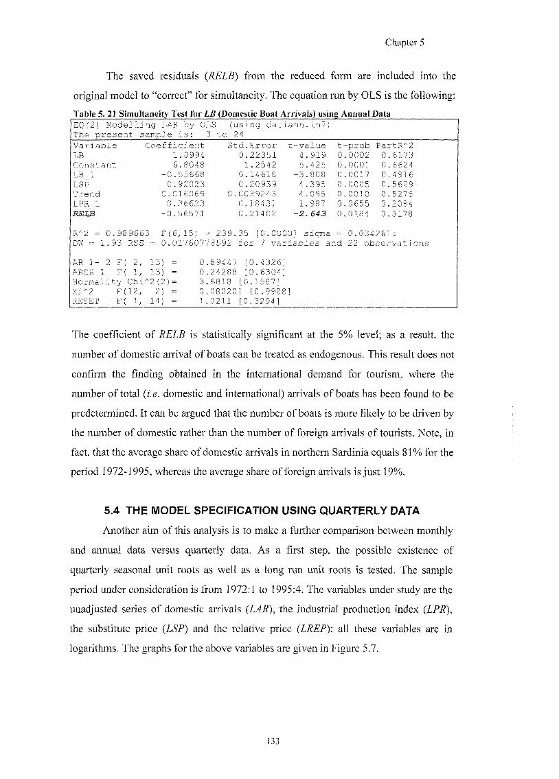
Chapter 5

The saved residuals (RELB) from the reduced form are included into the

original model to "correct" for simultaneity. The equation run by OLS is the following;

EQ(2) Modelling LAR by OLS (using datiann.in?) The present sample is: 3 to 24

Variable Coefficient Std.Error t-value t -prob PartR''2 LB 1.0994 0.22351 4.919 0 0002 0. 6173 Constant 6.8048 1.2542 5.425 0 .0001 0. 6624 LB 1 -0.55668 0.14618 -3.808 0 0017 0. 4916 LSP 0.92023 0.20939 4.395 0 .0005 0. 5629 Trend 0.016069 0 . 0039243 4.095 0 .0010 0. 5278 LPR 1 0.36623 0.18431 1.987 0 .0655 0. 2084 RELB -0.56571 0.21402 -2.643 0 0184 0. 3178

R''2 = 0.9E 39663 F(6,15) = 239. 35 [0.0000] sigma = 0.0342615 DM = 1.93 RSS = 0.0176077 8592 for 7 variables and 22 observations

AR 1- 2 F 2, 13) = 0. 89447 [0.4326] ARCH 1 F 1, 13) = 0. 24288 [0.6304] Normality Chi^2( 2)= 3. 6818 [0.1587] Xi'^2 F(12, 2 ) = 0. 080201 [0.9988] RESET F 1, 14 } = 1. 0211 [0.3294]

The coefBcient of is statistically significaiit at the 5% level; as a result, the

number of domestic arrival of boats can be treated as endogenous. This result does not

confirm the finding obtained in the international demand for tourism, where the

number of total (/. e. domestic and international) arrivals of boats has been found to be

predetermined. It can be argued that the number of boats is more likely to be driven by

the number of domestic rather than the number of foreign arrivals of tourists. Note, in

fact, that the average share of domestic arrivals in northern Sardinia equals 81% for the

period 1972-1995, whereas the average share of foreign arrivals is just 19%.

5.4 THE MODEL SPECIFICATION USING QUARTERLY DATA

Another aim of this analysis is to make a further comparison between monthly

and annual data versus quarterly data. As a first step, the possible existence of

quarterly seasonal unit roots as well as a long run unit roots is tested. The sample

period under consideration is from 1972:1 to 1995:4. The variables under study are the

unadjusted series of domestic arrivals (LAR), the industrial production index (LPR),

the substitute price (LSP) and the relative price (LREP); all these variables are in

logarithms. The graphs for the above variables are given in Figure 5.7.

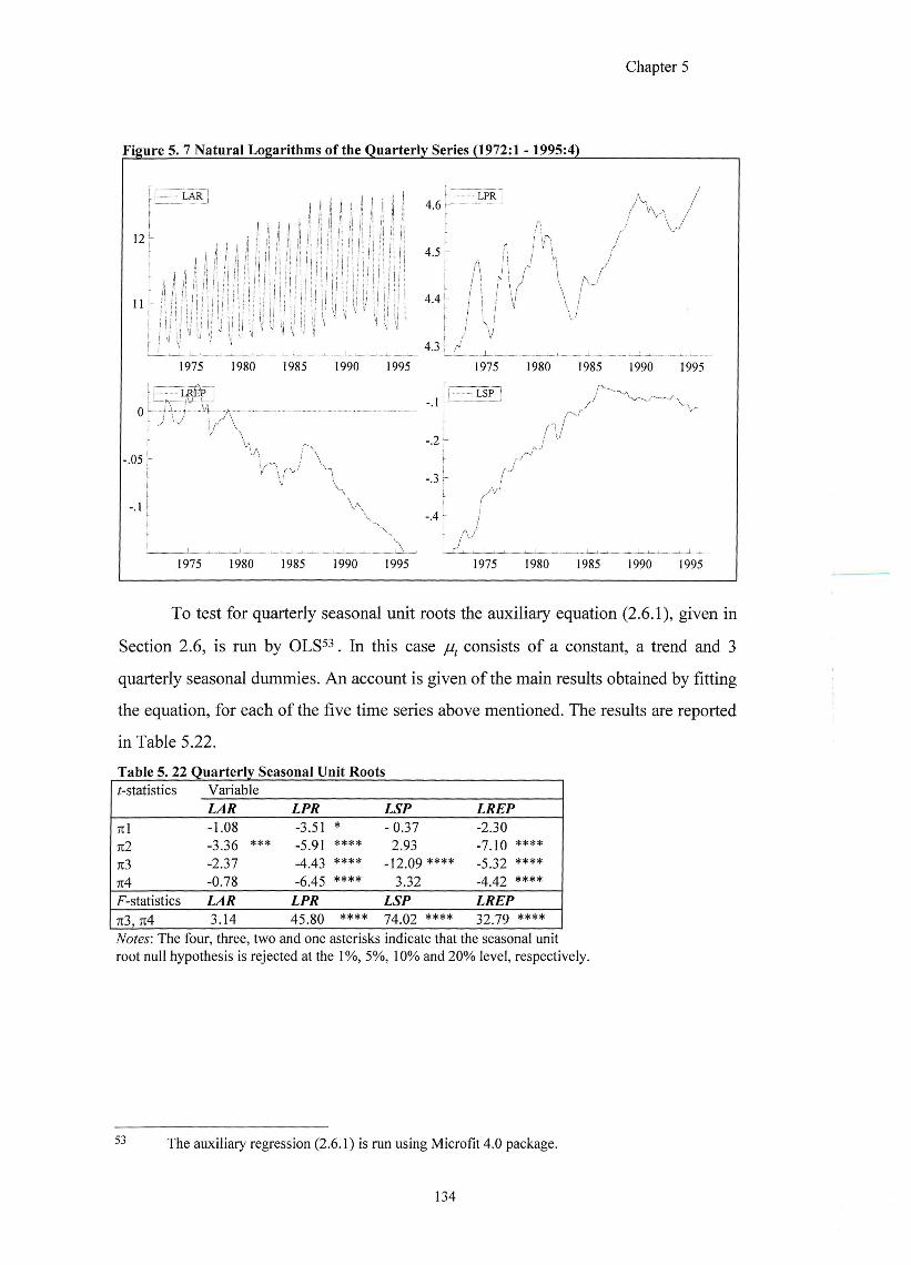
Chapter 5

Figure 5. 7 Natural Logarithms of the Quarterly Series (1972:1 -1995:4)

r 1 1 1 1 1 1 . 1 p n M !i l l l j

I" 4,6 rL-

h

LPR

12 h

J 11

, I I I fl H il II Hll II H'lIINlll!H

II i ; i 111 ^1I I ! h |i 11 Hi 1II1

I ll 1J

. 4 [ t

11 .f! n fl I'i (1 : !

r ft II !UI 11! ! U u iMi H

MlII!lIIIIll 11'.IIIIIII lU! i

n H i p H f U ' " '

4.4 i

1 : V ' . . 1 .

1975 1980 1985 1990 1995 1975 1980 1985 1990 1995

r ^—

Q 1— Y -.1''-LSI

\ , r. -.2-

-.05

-.3 r /

- 4 v \ -A:

r""

1975 1980 1985 1990 1995 1975 1980 1985 1990 1995

To test for quarterly seasonal unit roots the auxiliary equation (2.6.1), given in

Section 2.6, is run by O L S " . In this case fj. consists of a constant, a trend and 3

quarterly seasonal dummies. An account is given of the main results obtained by fitting

the equation, for each of the five time series above mentioned. The results are reported

in Table 5.22.

Table 5. 22 Quarterly Seasonal Unit Roots f-statistics Variable f-statistics

LAR LPR LSP LREP

Til -1.08 -3.51 * - 0 3 7 -230 7t2 -3J6 *** -5.91 * * * * Z93 -7.10 ****

7I3 -237 -4.43 * * * * -12.09 **** -5.32 **** 7I4 -0J8 -6.45 **** 3 J 2 -4.42 ****

F-statistics LAR LPR LSP LREP 713, 7I4 3.14 45.80 **** 74.02 **** 32.79 **** Notes'. The four, three, two and one asterisks indicate that the seasonal unit root null hypothesis is rejected at the 1%, 5%, 10% and 20% level, respectively.

53 The auxiliary regression (2.6.1) is run using Microfit 4.0 package.

134

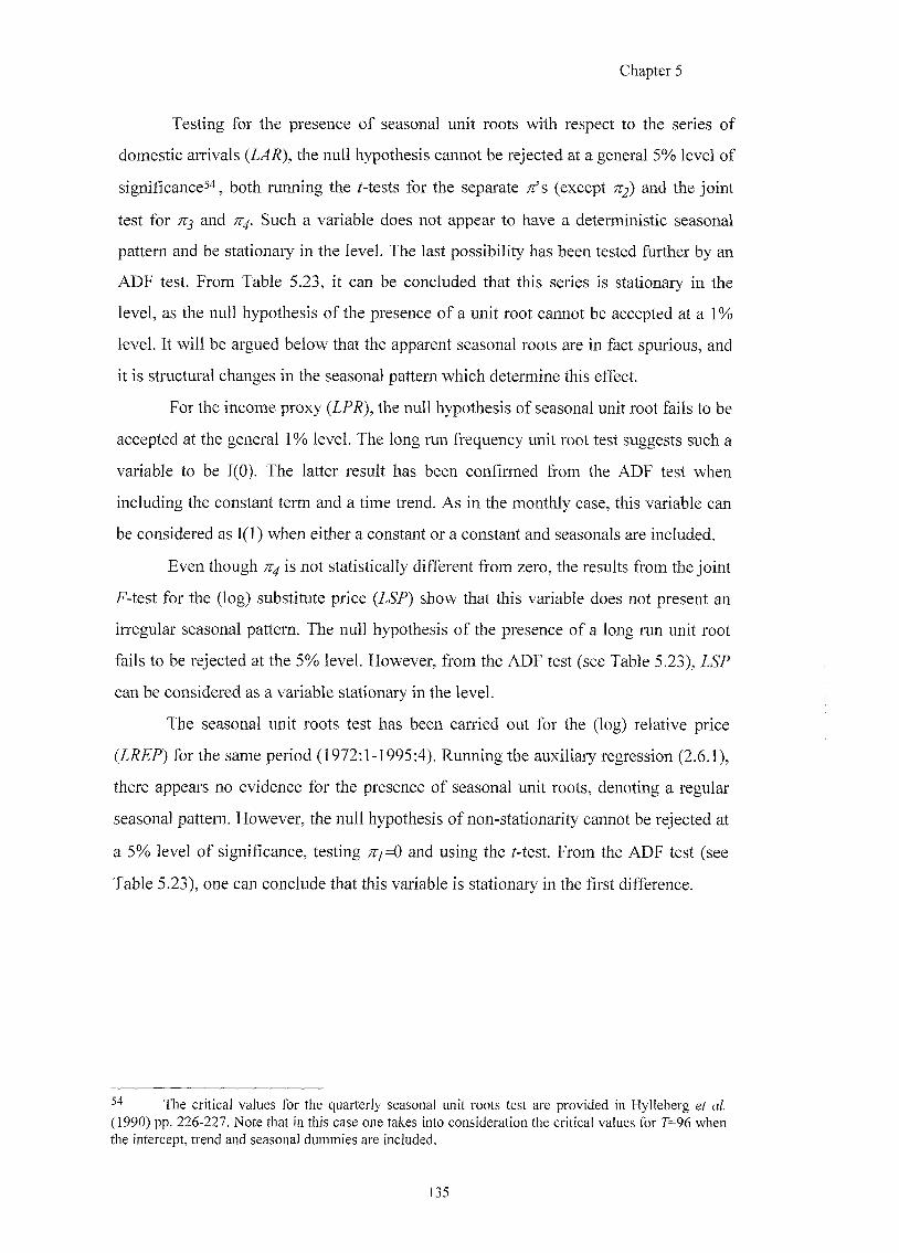
Chapter 5

Testing for the presence of seasonal unit roots with respect to the series of

domestic arrivals (LAR), the null hypothesis cannot be rejected at a general 5% level of

significance^'^, both running the ^-tests for the separate yr's (except and the joint

test for and 714. Such a variable does not appear to have a deterministic seasonal

pattern and be stationary in the level. The last possibility has been tested further by an

ADF test. From Table 5.23, it can be concluded that this series is stationary in the

level, as the null hypothesis of the presence of a unit root cannot be accepted at a 1%

level. It will be argued below that the apparent seasonal roots are in fact spurious, and

it is structural changes in the seasonal pattern which determine this effect.

For the income proxy (LPR), the null hypothesis of seasonal unit root fails to be

accepted at the general 1% level. The long run frequency unit root test suggests such a

variable to be 1(0). The latter result has been confirmed from the ADF test when

including the constant term and a time trend. As in the monthly case, this variable can

be considered as 1(1) when either a constant or a constant and seasonals are included.

Even though is not statistically different from zero, the results 60m the joint

F-test for the (log) substitute price (LSP) show that this variable does not present an

irregular seasonal pattern. The null hypothesis of the presence of a long run unit root

fmls to be rqected at the 5% level. However, from the ADF test (see Table 5.23), 2 6 ?

can be considered as a variable stationary in the level.

The seasonal unit roots test has been carried out for the (log) relative price

(LREP) for the same period (1972:1-1995:4). Running the auxiliary regression (2.6.1),

there appears no evidence for the presence of seasonal unit roots, denoting a regular

seasonal pattern. However, the null hypothesis of non-stationarity cannot be rejected at

a 5% level of significance, testing ;ry=0 and using the /-test. From the ADF test (see

Table 5.23), one can conclude that this variable is stationary in the first difference.

The critical values for the quarterly seasonal unit roots test are provided in Hylleberg et al. (1990) pp. 226-227. Note that in this case one takes into consideration the critical values for 7'=96 when the intercept, trend and seasonal dummies are included.

135

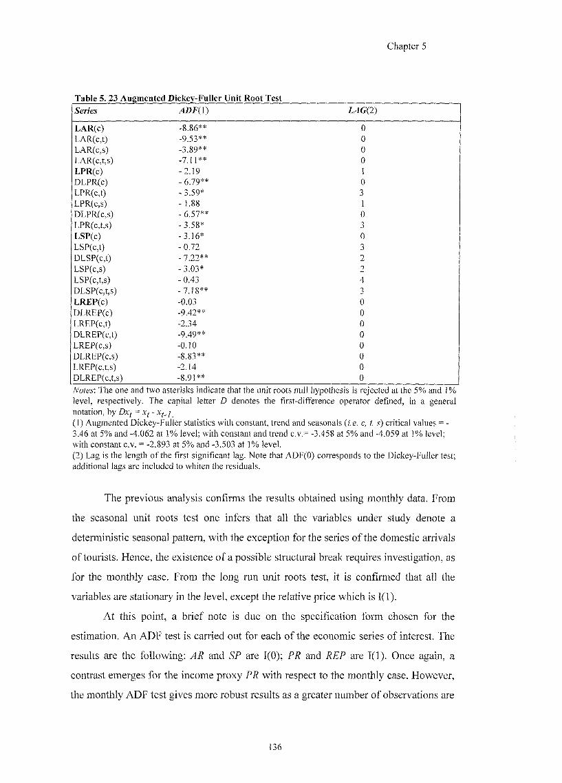
Chapter 5


Series / 4Df ( l ) 1^C(2)

LAR(c) -8.86** 0 LAR(c,t) -9.53** 0 LAR(c,s) -3.89** 0 LAR(c,t,s) -7.11** 0 LPR(c) -2.19 1 DLPR(c) - 6.79** 0 LPR(c,t) -3.59* 3 LPR(c,s) -1.88 1 DLPR(c,s) -6.57** 0 LPR(c,t,s) -3.58* 3 LSP(c) -3.16* 0 LSP(c,t) -0 .72 3 DLSP(c,t) - 7.22** 2 LSP(c,s) -3.03* 2 LSP(c,t,s) -0.43 4 DLSP(c,t,s) -7.18** 3 LREP(c) -0.03 0 DLREP(c) -9.42** 0 LREP(c,t) -2.34 0 DLREP(c,t) -9.49** 0 LREP(c,s) -0.10 0 DLREP(c,s) -8.83** 0 LREP(c,t,s) -2.14 0 DLREP(c,t,s) -8.91** 0

Notes: The one and two asterisks indicate that the unit roots null hypothesis is rejected at the 5% and 1 % level, respectively. The capital letter D denotes the first-difference operator defined, in a general notation, by Dx^ = (1) Augmented Dickey-Fuller statistics with constant, trend and seasonals {i.e. c, t, s) critical values = -3.46 at 5% and -4.062 at 1% level; with constant and trend c.v.= -3.458 at 5% and -4.059 at 1% level; with constant c.v. = -2.893 at 5% and -3.503 at 1% level. (2) Lag is the length of the first significant lag. Note that ADF(O) corresponds to the Dickey-Fuller test; additional lags are included to whiten the residuals.

The previous analysis confirms the results obtained using monthly data. From

the seasonal unit roots test one infers that all the variables under study denote a

deterministic seasonal pattern, with the exception for the series of the domestic arrivals

of tourists. Hence, the existence of a possible structural break requires investigation, as

for the monthly case. From the long run unit roots test, it is confirmed that all the

variables are stationary in the level, except the relative price which is 1(1).

At this point, a brief note is due on the specification form chosen for the

estimation. An ADF test is carried out for each of the economic series of interest. The

results are the following: and .SP are 1(0); f and are 1(1). Once again, a

contrast emerges for the income proxy PR with respect to the monthly case. However,

the monthly ADF test gives more robust results as a greater number of observations are

136

Chapter 5

employed. Hence, one carries on using the same property for PR as for the monthly

case (see Section 5.2.4). In order to run the Box and Cox test, an unrestricted five lag

tourism demand equation is estimated, for the period 1972:1-1995:4, expressed both in

a logarithmic and linear form. Given the previous definition for the explanatory

variables, one estimates:

7,) /Ogarzf/ZTMZCybr/M

LARf = cij + ^2 LARf_]..+ LPRf...+ LSPf..+ DLREPj..+ a^LW^ + a-j Trend +

+

and

Zmgarybrm

= a ; + ^2 5 ? ^ . . + Oj ^ 4- oy TreMcf +

+ ag

Running the two equations, equals 0.4890330516 and equals

6.7E+09. The statistic equals 36.29 and this value is greater than the correspondent

critical value, 3.84, at the 5% level; hence, the null hypothesis cannot be accepted.

Moreover, one infers that the logarithmic specification is better than the linear

specification as (z.e. 1.095428) is greater than One proceeds with

the estimation of the quarterly domestic demand in a log-linear specification.

A generic unrestricted model is estimated for the domestic demand for tourism.

This model includes the following variables: the (log) income proxy (ZfJ^), the

substitute price (l&P), the first difference of the relative price (DZJÊf), one impulse

dummy (zPjgJ) which takes the value of one in the first quarter and zero otherwise, a

trend in order to pick up possible changes in the consumers' tastes, the weather

variable (ZfF), and, finally, 3 quarterly seasonal dummies.

137

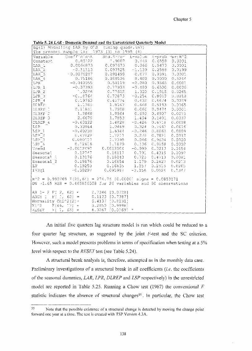
Chapter 5

Table 5. 24 LAR - Domestic Demand and the Unrestricted Quarterly Model EQ(1) Modelling LAR by OLS (using quadr The present sample is: 1973 (3) to 1995

in7) (4)

Variable Coefficient Std.Error t--value t--prob PartR''2 Constant 0.85122 1.9007 0 .448 0 6558 0 .0031 LAR 1 0.0064873 0.097673 0 .066 0 9473 0 0001 LAR 2 -0.11113 0.097525 -1 .139 0 2588 0 0199 LAR 3 -0.0070207 0.091499 -0 .077 0 9391 0 .0001 LAR 4 0.75186 0.089506 8 .400 0 0000 0 5244 LPR -0.040055 0.50119 -0 .080 0 9365 0 0001 LPR 1 -0.37393 0.77933 -0 .480 0 6330 0 0036 LPR 2 1.0246 0.77622 1 .320 0. 1915 0 0265 LPR 3 -0.18764 0.73873 0 .254 0 8003 0 0010 LPR 4 0.19763 0.45774 0 .432 0. 6674 0 0029 DLREP 1.1785 1.8187 0 . 648 0. 5193 0 0065 DLREP 1 0.11851 1.7908 0 . 066 0. 9474 0 0001 DLREP 2 1.2868 1.8564 0 . 693 0. 4907 0 0075 DLREP 3 2.6670 1.7853 1 .494 0. 1401 0 0337 DLREP 4 -0.63122 1.4828 0 .426 0 . 6718 0 0028 LSP 0.33964 1.0469 0 .324 0. 7467 0 0016 LSP 1 -0.40238 1.6344 0 .246 0. 8063 0 0009 LSP 2 0.47828 1.7217 0 .278 0. 7821 0 0012 LSP 3 0.080117 1.7395 0 046 0. 9634 0 0000 LSP_4 0.12616 1.1879 0 .106 0. 9158 0 0002 Trend -0.0012497 0.0012504 0 999 0. 3213 0. 0154 Seasonal 0.12747 0.16117 0 791 0. 4319 0. 0097 Seasonal 1 0.13076 0.18043 0 725 0. 4713 0. 0081 Seasonal 2 0.19876 0.16854 1 179 0. 2427 0 0213 LW 0.19250 0.16635 1 157 0. 2515 0. 0205 i93ql -0.30297 0.095987 3 156 0. 0024 0. 1347

R'"2 = 0. 990769 F(25, 64) = 274.76 [0.0000] sigma = 0.0853171 DW =1.65 RSS = 0.465856358 for 26 variables and 90 observations

AR 1- 2 F( 2, 62) = 2. 7346 [0.0728] ARCH 1 F( 1, 62) = 0. 1123 [0.7387] Normality Chi ''2(2)= 0. 4137 [0.8131] Xi'^2 F(46, 17) = 0. 2850 [0.9996] RESET F( 1, 63) = 6. 0267 [0.0169] *

An initial five quarters lag structure model is run which could be reduced to a

four quarter lag structure, as suggested by the joint F-test and the SC criterion.

However, such a model presents problems in terms of specification when testing at a 5%

level with respect to the RESET test (see Table 5.24).

A structural break analysis is, therefore, attempted as in the monthly data case.

Preliminary investigations of a structural break in all coefficients (i.e. the coefficients

of the seasonal dummies, LAR, LPR, DLREP and LSP respectively) in the unrestricted

model are reported in Table 5.25. Running a Chow test (1967) the conventional F

statistic indicates the absence of structural changes^^. In particular, the Chow test

Note that the possible existence of a structural change is detected by moving the change point forward one year at a time. The test is created with TSP Version 4.3 A.

138

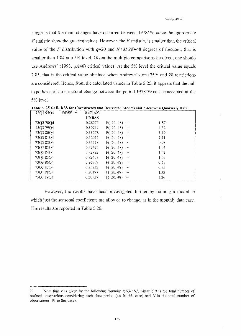
Chapter 5

suggests that the main changes have occurred between 1978/79, since the appropriate

F statistic show the greatest values. However, the F statistic, is smaller than the critical

value of the F distribution with q=20 and N+M-2K=4% degrees of freedom, that is

smaller than 1.84 at a 5% level. Given the multiple comparisons involved, one should

use Andrews' (1993, p.840) critical values. At the 5% level the critical value equals

2.05, that is the critical value obtained when Andrews's and 20 restrictions

are considered. Hence, from the calculated values in Table 5.25, it appears that the null

hypothesis of no structural change between the period 1978/79 can be accepted at the

5% level.

73Q3 95Q4 RRSS = 0.471603 UNRSS

73Q3 78Q4 0.28275 F( 20,48) = 1.57 73Q3 79Q4 0.30211 F( 20,48) = 1J2 73Q3 80Q4 0.31278 F( 20,48) = IJ^ 73Q3 81Q4 0.32012 F( 20,48) = 1.11 73Q3 82Q4 0.33318 F( 20, 48) = 0.98 73Q3 83Q4 0.32622 F( 20,48) = 1.05 73Q3 84Q4 0.32892 F( 20,48) = 1.02 73Q3 85Q4 0.32605 F(20,4%| = 1.05 73Q3 86Q4 0.36997 F( 20, 48) = oâ 73Q3 87Q4 0.35739 F( 20, 48) = 0J5 73Q3 88Q4 0.30197 F( 20,48) = 1J2 73Q3 89Q4 0.30737 F( 20,48) = 1J#

However, the results have been investigated further by running a model in

which just the seasonal coefficients are allowed to change, as in the monthly data case.

The results are reported in Table 5.26.

56 Note that tt is given by the following formula; '/2[0B/N], where OB is the total number of omitted observations considering each time period (46 in this case) and N is the total number of observations (91 in this case).

139

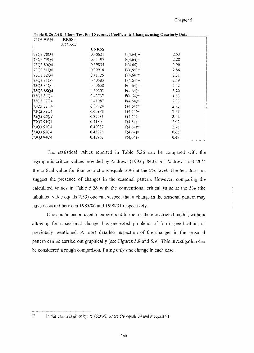
Chapter 5

Table 5. 26 LAR- Chow Test for 4 Seasonal Coefficients Changes, using Quarterly Data 73Q3 95Q4 RRSS=

0.471603 UNRSS

73Q3 78Q4 0.40621 F(4,64)= 2.53 73Q3 79Q4 0.41197 F(4,64)= 2.28 73Q3 80Q4 0.39835 F(4,64)= 2.90 73Q3 81Q4 0.39916 F(4,64)=: 2.86 73Q3 82Q4 0.41125 F(4,64)= 2.31 73Q3 83Q4 0.40503 F(4,64)= 2.59 73Q3 84Q4 0.40658 F(4,64)= 2.52 73Q3 85Q4 0.39203 F(4,64)= 3.20 73Q3 86Q4 0.42737 F(4,64)= 1.63 73Q3 87Q4 0.41087 F(4,64)- 2.33 73Q3 88Q4 0.39724 F(4,64)= 2.95 73Q3 89Q4 0.40988 F(4,64)= 2.37

0.39531 F(4,64)= 3.04 73Q3 91Q4 0.41804 F(4,64)- 2.02 73Q3 92Q4 0.40087 F(4,64)= 2.78 73Q3 93Q4 0.45298 F(4,64)= 0.65 73Q3 94Q4 0.45763 F(4,64)= 0.48

The statistical values reported in Table 5.26 can be compared with the

asymptotic critical values provided by Andrews (1993 p.840). For Andrews' ;'z=0.20 ^

the critical value for four restrictions equals 3.96 at the 5% level. The test does not

suggest the presence of changes in the seasonal pattern. However, comparing the

calculated values in Table 5.26 with the conventional critical value at the 5% (the

tabulated value equals 2.53) one can suspect that a change in the seasonal pattern may

have occurred between 1985/86 and 1990/91 respectively.

One can be encouraged to experiment further as the unrestricted model, without

allowing for a seasonal change, has presented problems of form specification, as

previously mentioned. A more detailed inspection of the changes in the seasonal

pattern can be carried out graphically (see Figures 5.8 and 5.9). This investigation can

be considered a rough comparison, fitting only one change in each case.

In this case TI is given by: % [OB/N], where OB equals 34 and N equals 91.

140

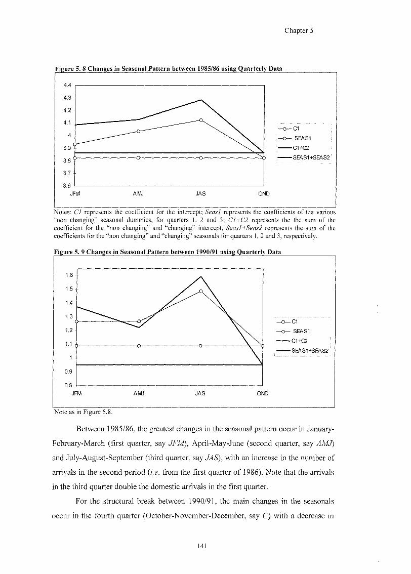
Chapter 5

Figure 5. 8 Changes in Seasonal Pattern between 1985/86 using Quarterly Data

C1+C2

Notes: CI represents the coefficient for the intercept; Seasl represents the coefficients of the various "non changing" seasonal dummies, for quarters 1, 2 and 3; C1+C2 represents the the sum of the coefficient for the "non changing" and "changing" intercept; Seasl+Seas2 represents the sum of the coefficients for the "non changing" and "changing" seasonals for quarters 1, 2 and 3, respectively.

Figure 5. 9 Changes in Seasonal Pattern between 1990/91 using Quarterly Data

Note as in Figure 5.

Between 1985/86, the greatest changes in the seasonal pattern occur in January-

February-March (first quarter, say April-May-June (second quarter, say

and July-August-September (third quarter, say JAS), with an increase in the number of

arrivals in the second period {i.e. from the first quarter of 1986). Note that the arrivals

in the third quarter double the domestic arrivals in the first quarter.

For the structural break between 1990/91, the main changes in the seasonals

occur in the fourth quarter (October-November-December, say C) with a decrease in

141

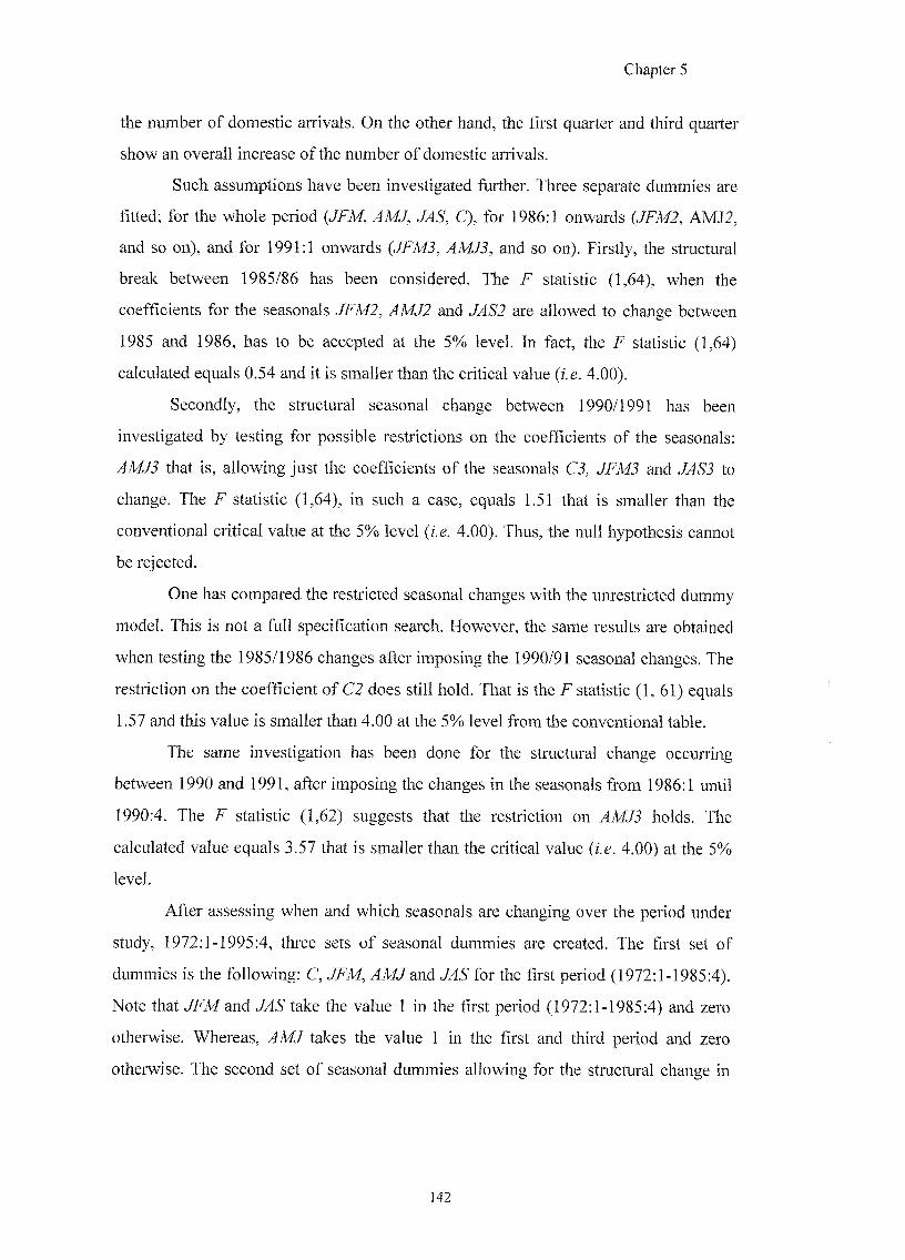
Chapter 5

the number of domestic arrivals. On the other hand, the first quarter and third quarter

show an overall increase of the number of domestic arrivals.

Such assumptions have been investigated further. Three separate dummies are

fitted; for the whole period ^5", C), for 1986:1 onwards AMJ2,

and so on), and for 1991:1 onwards and so on). Firstly, the structural

break between 1985/86 has been considered. The F statistic (1,64), when the

coefficients for the seasonals .TFM?, /4M/2 and are allowed to change between

1985 and 1986, has to be accepted at the 5% level, hi fact, the F statistic (1,64)

calculated equals 0.54 and it is smaller than the critical value {i.e. 4.00).

Secondly, the structural seasonal change between 1990/1991 has been

investigated by testing for possible restrictions on the coefficients of the seasonals:

that is, allowing just the coefficients of the seasonals CJ, and to

change. The F statistic (1,64), in such a case, equals 1.51 that is smaller than the

conventional critical value at the 5% level {i.e. 4.00). Thus, the null hypothesis cannot

be rejected.

One has compared the restricted seasonal changes with the unrestricted dummy

model. This is not a full specification search. However, the same results are obtained

when testing the 1985/1986 changes after imposing the 1990/91 seasonal changes. The

restriction on the coefficient of C2 does still hold. That is the f statistic (1, 61) equals

1.57 and this value is smaller than 4.00 at the 5% level 6om the conventional table.

The same investigation has been done for the structural change occurring

between 1990 and 1991, after imposing the changes in the seasonals from 1986:1 until

1990:4. The F statistic (1,62) suggests that the restriction on holds. The

calculated value equals 3.57 that is smaller than the critical value (;.g. 4.00) at the 5%

level.

After assessing when and which seasonals are changing over the period under

study, 1972:1-1995:4, three sets of seasonal dummies are created. The first set of

dummies is the following: C, .TFM, v4M/and for the first period (1972:1-1985:4).

Note that JFM and ^6" take the value 1 in the first period (1972:1-1985:4) and zero

otherwise. Whereas, takes the value 1 in the first and third period and zero

otherwise. The second set of seasonal dummies allowing for the structural change in

142

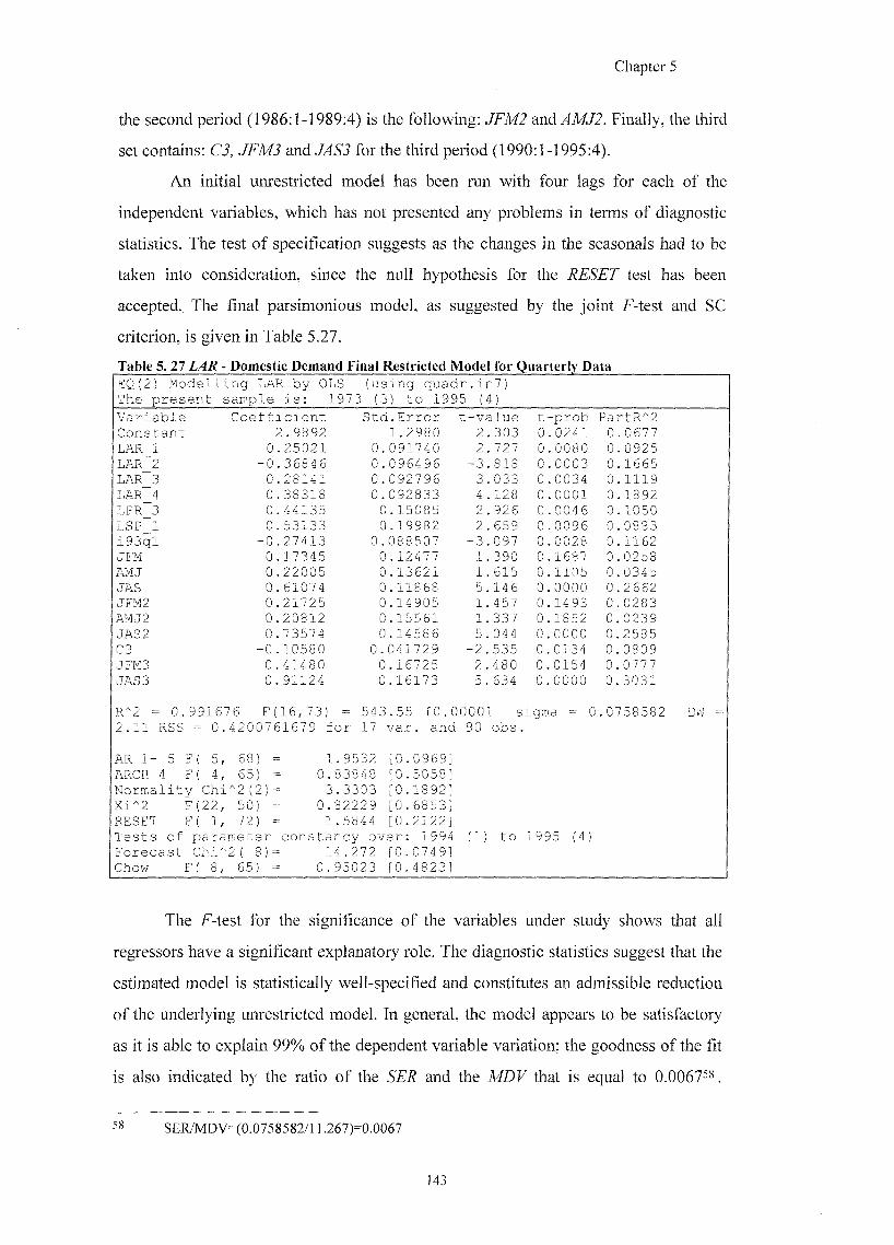
Chapter 5

the second period (1986:1-1989:4) is the following: JFM2 a.ndAMJ2. Finally, the third

set contains: CJ, ./FM3 6)r the third period (1990:1-1995:4).

An initial unrestricted model has been run with four lags for each of the

independent variables, which has not presented any problems in terms of diagnostic

statistics. The test of specification suggests as the changes in the seasonals had to be

taken into consideration, since the null hypothesis for the RESET test has been

accepted. The final parsimonious model, as suggested by the joint F-test and SC

criterion, is given in Table 5.27.

Table 5. 27 LAR - Domestic Demand Final Restricted Model for Quarterly Data EQ(2) Modelling LAR by OLS The present sample is: 1972

(using quadr (3) to 1995

.in7) (4)

Variable Coefficient Std.Error t -value t -prob PartR''2 Constant 2.9892 1.2980 2 .303 0 0241 0 0677 LAR 1 0 .25021 0.091740 2 727 0 0080 0 0925 LAR 2 -0 .36846 0.096496 -3 818 0 0003 0 1665 LAR 3 0 .28141 0.092796 3 033 0 0034 0 1119 LAR 4 0 .38318 0.092833 4 128 0 0001 0 1892 LPR 3 0 .44135 0.15085 2 926 0 0046 0 1050 LSP 1 0 .53133 0.19982 2 659 0 0096 0 0883 i93ql -0 .27413 0.088507 -3 097 0 0028 0 1162 JFM 0 .17345 0.12477 1 390 0 1687 0 0258 AMJ 0 .22005 0.13621 1 615 0 1105 0 0345 JAS 0 .61074 0.11868 5 146 0 0000 0 2662 JFM2 0 .21725 0.14905 1 457 0 1493 0 0283 AMJ2 0 .20812 0.15561 1 337 0 1852 0 0239 JAS 2 0 .73574 0.14586 5 044 0 0000 0 2585 C3 -0 .10580 0.041729 -2 535 0 0134 0 0809 JFM3 0 .41480 0.16725 2 480 0 0154 0 0777 JAS 3 0 91124 0.16173 5 634 0 0000 0 3031

R''2 = 0.991676 F 16,73) — 543.55 [0.0000 sigma = 0 .0758582 DW = 2.11 RSS = 0. 4200761679 for 17 var. and 90 obs

AR 1- 5 F( 5, 68) 1 .9532 [0.0969] ARCH 4 F( 4, 65) 0. 838 48 [0.5058] Normality Chi "2(2)= 3 .3303 [0.1892] Xi' Z F(22, 50) 0. 82229 [0.6853] RESET F( 1, 72) 1 .58 44 [0.2122] Tests of parameter constancy over: 1994 (1) to 1995 (4) Forecast Chi'' 2( 8) = 14.272 [0.0749] Chow F( 8, 65) 0. 95023 [0.4823]

The F-test for the significance of the variables under study shows that all

regressors have a significant explanatory role. The diagnostic statistics suggest that the

estimated model is statistically well-specified and constitutes an admissible reduction

of the underlying unrestricted model. In general, the model appears to be satisfactory

as it is able to explain 99% of the dependent variable variation; the goodness of the fit

is also indicated by the ratio of the and the MDF that is equal to 0.0067^*.

58 SER/MDV=(0.0758582/] 1.267)=0.0067

143

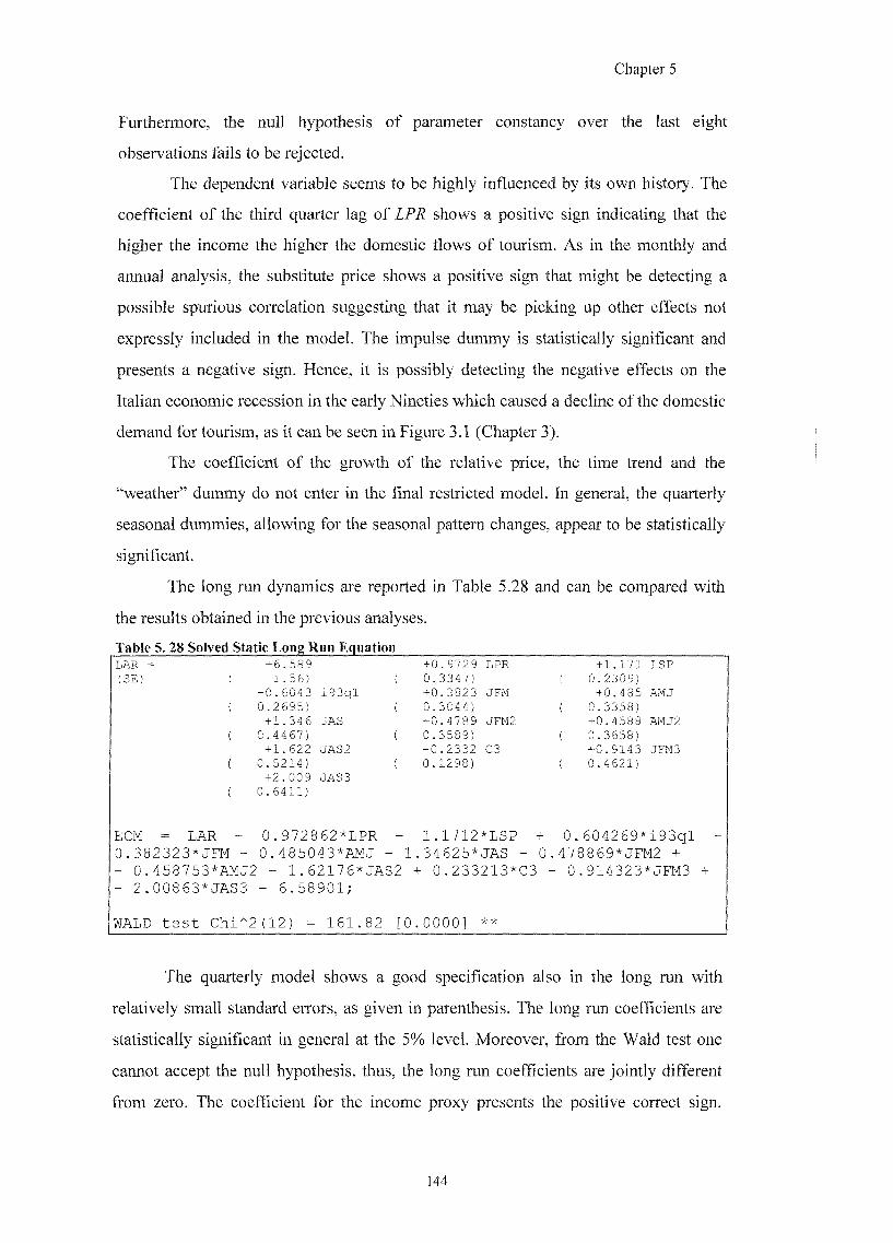
Chapter 5

Furthermore, the null hypothesis of parameter constancy over the last eight

observations fails to be rejected.

The dependent variable seems to be highly influenced by its own history. The

coefficient of the third quarter lag of LPR shows a positive sign indicating that the

higher the income the higher the domestic flows of tourism. As in the monthly and

annual analysis, the substitute price shows a positive sign that might be detecting a

possible spurious correlation suggesting that it may be picking up other effects not

expressly included in the model. The impulse dummy is statistically significant and

presents a negative sign. Hence, it is possibly detecting the negative effects on the

Italian economic recession in the early Nineties which caused a decline of the domestic

demand for tourism, as it can be seen in Figure 3.1 (Chapter 3).

The coefficient of the growth of the relative price, the time trend and the

"weather" dummy do not enter in the final restricted model. In general, the quarterly

seasonal dummies, allowing for the seasonal pattern changes, appear to be statistically

significant.

The long run dynamics are reported in Table 5.28 and can be compared with

the results obtained in the previous analyses.

LAR = +6.589 +0.9729 LPR +1.171 ISP (SE) ( 1.56) ( 0.3347) ( 0.2309)

-0.6043 i93ql +0.3823 JFM +0.485 AMJ ( 0.2695) { 0.3044) { 0.3358)

+1.346 JAS +0.4789 JFM2 +0.4588 AMJ2 ( 0.4467) ( 0.3589) ( 0.3658)

+1.622 JAS 2 -0.2332 C3 +0.9143 JFM3 { 0.5214) ( 0.1298) ( 0.4621)

+2.009 JAS 3 ( 0.6411)

ECM = LAR - 0.972862:^LPR - 1.1712 *LSP + 0. 604269* i93ql -0.382323* JFM - 0.485043*AMJ - 1 .34625* JAS - 0 .47 3869*JFM2 + - 0.458753*AMJ2 - 1.62176*JAS2 + 0.233213*C3 - 0 .914323*JFM3 + - 2.00863 *JAS3 - 6.58901;

WALD test Chi^2 (12) = 161.82 [0 .00001 *

The quarterly model shows a good specification also in the long run with

relatively small standard errors, as given in parenthesis. The long run coefficients are

statistically significant in general at the 5% level. Moreover, from the Wald test one

cannot accept the null hypothesis, thus, the long run coefScients are jointly different

from zero. The coefficient for the income proxy presents the positive correct sign.

144

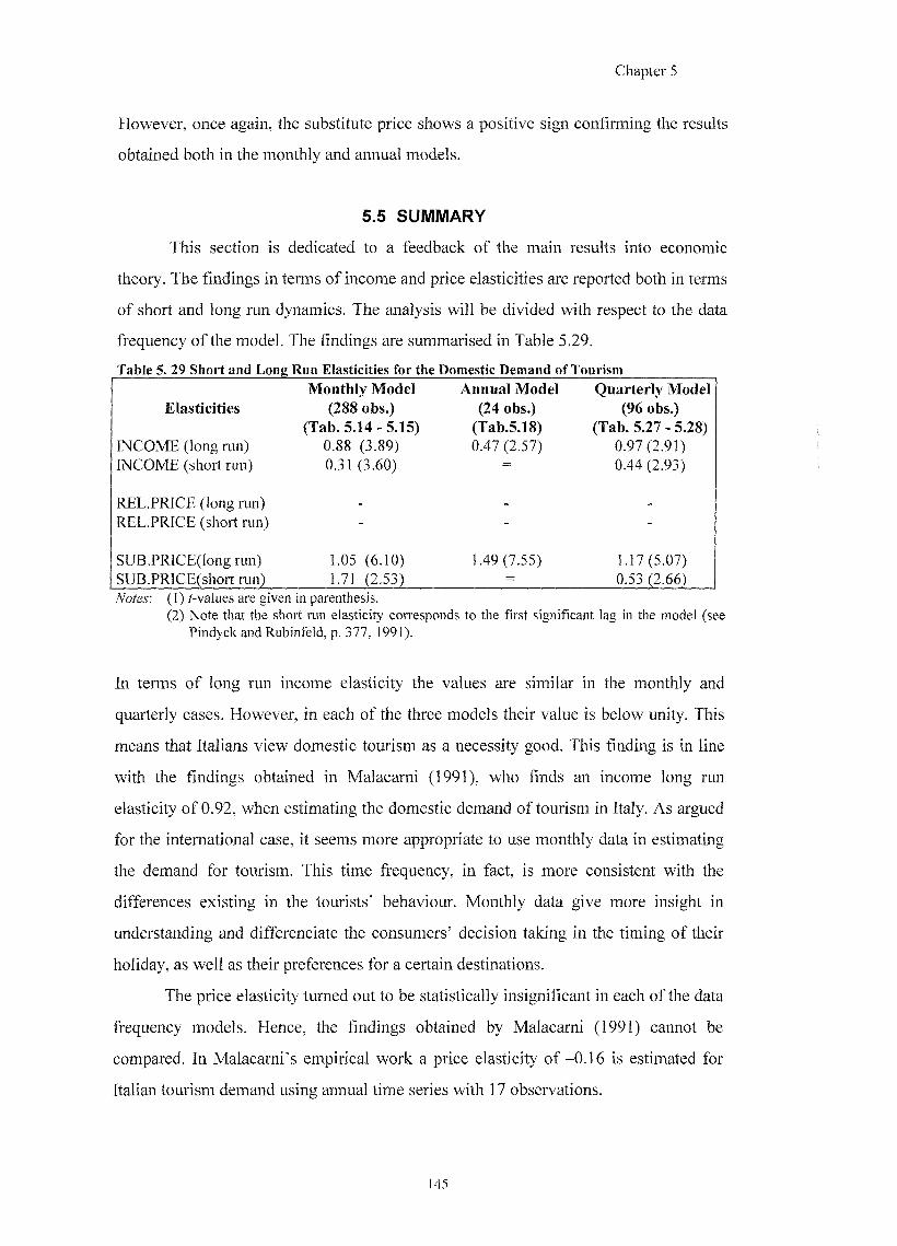
Chapter 5

However, once again, the substitute price shows a positive sign confirming the results

obtained both in the monthly and annual models.

5.5 SUMMARY

This section is dedicated to a feedback of the main results into economic

theory. The findings in terms of income and price elasticities are reported both in terms

of short and long run dynamics. The analysis will be divided with respect to the data

frequency of the model. The findings are summarised in Table 5.29.

Monthly Model Annual Model Quarterly Model Elasticities (288 obs.) (24 obs.) (96 obs.)

(Tab. 5.14 - 5.15) (Tab.5.18) (Tab. 5.27 - 5.28) INCOME (long run) 0.88 (3.89) 0.47 (2.57) 0.97 (2.91) INCOME (short run) 0.31 (3.60) 0.44 (2.93)

REL.PRICE (long run) _ _

REL.PRICE (short run) - - -

SUB.PRICE(long run) 1.05 (6.10) 1.49 (7.55) 1 .17(5.07) SUB.PRICE(short run) 1.71 (2.53) = 0.53 (2.66) Notes'. (1) values are given in parenthesis.

(2) Note that the short run elasticity corresponds to the first significant lag in the model (see Pindyck and Rubinfeld, p. 377, 1991).

In terms of long run income elasticity the values are similar in the monthly and

quarterly cases. However, in each of the three models their value is below unity. This

means that Italians view domestic tourism as a necessity good. This finding is in line

with the findings obtained in Malacarni (1991), who finds an income long run

elasticity of 0.92, when estimating the domestic demand of tourism in Italy. As argued

for the international case, it seems more appropriate to use monthly data in estimating

the demand for tourism. This time frequency, in fact, is more consistent with the

difkrences existing in the tourists' behaviour. Monthly data give more insight in

understanding and differenciate the consumers' decision taking in the timing of their

holiday, as well as their preferences for a certain destinations.

The price elasticity turned out to be statistically insignificant in each of the data

frequency models. Hence, the findings obtained by Malacami (1991) cannot be

compared. In Malacami's empirical work a price elasticity o f -0 .16 is estimated for

Italian tourism demand using annual time series with 17 observations.

145

Chapter 5

The substitute price elasticities are positive in both the long and short run in

each of the three models. Possible problems might be derived from not having taken

into consideration the exchange rate for the main north of Sardinia competitors as an

explanatory variable. As already stated, such a hypothesis will be investigated in

Chapter 6.

5.6 Conclusion

A phenomenon characterising almost all tourism is that of seasonality. Such a

phenomenon is particular evident in countries or regions (such as Sardinia) in which

tourists search for "sea and sun" holidays. From this research a different seasonal

pattern has been detected between foreign and domestic tourist flows to Sassari

Province. This finding has suggested modelling the two components separately.

Chapter 5 has been dedicated to the empirical study of the domestic demand

for tourism to the north of Sardinia for the period between 1972 and 1995. An

investigation of the possibility of an irregular seasonal pattern for the variables under

study (i.e. domestic arrivals of tourists, the Italian index of industrial production,

relative price - Sassari/Italy - and substitute price) has been carried out by means of

testing for the possible existence of seasonal unit roots. Such a possibility has been

rejected for all the series, with the only exception for the series of domestic arrivals.

However, 6om a deeper investigation, the dependent variable has shown a structural

break in the seasonal pattern. This finding has confirmed that the apparent seasonal

roots 6om Franses' test are spurious and it is changes in the seasonal pattern which

give rise to this effect. Calculated values have been compared both with the

conventional tables and with Andrews' critical values, as a multiple comparison was

involved. The integration status of the variables under study has been tested by using

an ADF unit roots test. All the variables of interest have been found to be stationary in

the level, with the only exception for the relative price, which is stationary in the first

difference.

An important step has been investigating the effect of a correction of the

domestic arrivals series for the number of weekends (Saturdays or Sundays) in a

month. Such a normalisation has not been found to be appropriate as the best results

are obtained with the unacûsted series. One can argue that domestic tourists are less

]46

Chapter 5

constrained in the choice of the day of arrival, as they are likely to be able to catch a

boat or a flight any day of the week. On the other hand, those foreign tourists who use

charter flights or international boats are more likely to travel on Saturdays as the

analysis in Chapter 4 has suggested.

Another aim of the chapter has been the use of different data frequencies:

monthly, quarterly and annual data. The aim was to assess the characteristics of the

domestic demand for tourism in the short and long run, as well as to assess the

advantages and disadvantages in using each data frequency.

The advantages in using monthly data are as follows. Firstly, such a frequency

has allowed to test for the possible presence of seasonal unit roots and to identify the

integration status of the variables of interest, thanks to the relative large sample

(7^288). However, it is interesting to note that monthly and quarterly data (7^96) have

provided homogenous results in terms of seasonal and long run unit roots testing,

confirming in this way the findings obtained from the international tourism demand.

Moreover, the two data frequencies have given similar results in terms of testing for

structural breaks. In both cases, a structural break in the seasonal pattern has been

detected in the second half of the Eighties and in the first half of the Nineties.

Another advantage from the monthly series is the possibility to study the

domestic demand dynamics. The final parsimonious model has given satisfactory

results as 99% of the variance of the dependent variable has been explained. The

inclusion of the "Easter" dummy has turned out to have an important role in explaining

the pattern of tourism in the north of Sardinia, confirming the results in the

international demand case. This model has allowed the study of short run as well as the

long run dynamics. As an example, in the short and long run the Italian index of

industrial production has presented a positive sign which is in line with economic

theory and other empirical studies for Italy as a whole.

The model obtained using quarterly data has given satisfactory results. The

coefficient of determination is 99% and the coefficients are overall well-specified in

terms of statistical significance and signs. In both models the weather variable has

turned out not to be statistically significant.

Another aim was to compare disaggregated and aggregate 6equencies. One will

refer to the advantages and disadvantages in using annual data. An important

147

Chapter 5

advantage that has revealed in using aggregated data has consisted in the possibility of

making use of data that are often available only at an annual frequency. In this case, it

has been possible to test and establish whether the Italian production index can indeed

be considered as a valid proxy of the personal disposable income. Statistical evidence

has been given from several statistics and tests such as the simple cross-correlation.

From the single equation model, estimating LPDIN on LPR, the f-value for the

coefficient of LPR is equal to 6.69. Finally, from the VAR analysis, the first lag of

LPR plays an important role in explaining LPDIN and almost all its variance is

explained. By using annual data, it has also been possible to take into consideration

supply components such as the number of domestic boat and flight arrivals in the north

of Sardinia. Evidence has been found for the arrivals of national boats to be an

endogenous variable.

The disadvantages incurred are related to the power of testing with a small

number of observations. No conclusive judgement could be made in terms of the

integration status of the variables of interest. The same problem has occurred when

using Wu-Hausman's test for testing the simultaneity of the supply component.

However, the final parsimonious model does show an explanatory power of almost

98% and the model is well-specified in terms of diagnostic tests. Note, that this model

converges rapidly to the long run equilibrium.

A further analysis has been carried out for giving statistical evidence in using

the log-linear specification form. By using the Box and Cox (1964) test, it has been

established that the logarithmic form is a better specification than the linear form. The

same results have been achieved in each of the models {i.e. monthly, annual and

quarterly). However, some divergence has been found in the properties of the

economic variables of interest. The ADF test seems to give better results employing

series at a monthly frequency.

On balance, one can conclude a better specification and findings seem to be

given by using monthly or quarterly data. Nevertheless, one would not want to omit

the findings obtained with aggregated annual data.

148

Chapter 6

CHAPTER 6.

SASSARI PROVINCE COMPETITORS: REAL SUBSTITUTE

PRICE

Aim of the Chapter:

To identify the impact of the real substitute price on domestic and international

tourism demand in Sassari Province of Sardinia, Italy.

6.1 INTRODUCTION

As already stated, according to economy theory, one would have expected a

negative sign for the substitute price which measures the price of tourism in Sassari

Province relative to that in other destinations in the Mediterranean area. When the

consumer price index in Sassari Province gets higher, ceteris paribus, one would

expect a decrease in the number of arrivals. However, in the analysis in this thesis so

far a positive sign has been found, which might be indicating problems of mis-

specification.

So far, in both the domestic and international demand model, one has included

the nominal substitute price as a possible determinant of the demand for tourism.

However, one can argue that tourists are more aware of exchange rates than the cost of

living in a foreign country. On this basis, Gray (1966), one of the pioneers in the

tourism literature, includes the exchange rate alone as a proxy for the cost of living in

the destination country. In many other empirical studies of tourism, prices and

exchange rates have been combined and used separately as explanatory variables. Witt

and Witt (1992), for example, argue that "consumer price index (either alone or

together with the exchange rate) is a reasonable proxy for the cost of tourism. The

exchange rate on its own, however, is not an acceptable proxy" (p.46). As Crouch

(1994) writes, it does not appear clear cut in the literature which the best selection is:

"How should changes in exchange rates be modelled? Would it be best to acûst prices

for changes in exchange rates, or do tourists respond differently to exchange rate

changes than they do to price changes?" (p.48). It seems clear that an answer cannot be

149

Chapter 6

unequivocal, as the statistical significance of these variables, used either separately or

jointly, is highly dependent on the origin country and/or destination country under

study (see Martin and Witt 1988; Witt and Witt, 1992). Some studies, amongst the

others Gonzales and Moral (1995), show that real relative prices and real substitute

prices have an important role in explaining the international demand for tourism in

Spain.

Another argument for including the exchange rate in the model is related to the

Purchasing Power Parity. The theory of PPP assumes that, ignoring trade barriers and

transportation costs, in the long run exchange rates should perfectly reflect the relative

costs of living between countries. However, substantial deviations between prices and

exchange rates are highly likely to occur in the short run (see among the others Lee, ef

ah, 1996; Garratt et ah, 1998). On this argument, statistical evidence has been given in

Chapter 4.

The aim of this chapter is to carry out a further investigation of the

characteristics of the real substitute price and its components. The plan of the chapter

is as follows. The first section is dedicated to the analysis of the domestic demand for

tourism in the north of Sardinia when taking into consideration the weighted average

exchange rate for the other main destination countries in the Mediterranean area {i.e.

France, Greece, Portugal and Spain). The aim is to determine whether the real

substitute price, given by the difference between the (log) substitute price and the (log)

weighted average exchange rate, plays a role in explaining the domestic demand for

tourism. The second section is dedicated to the analysis of the characteristics of the

individual components of the real substitute price. The main conclusion is that one can

define and use a real substitute price for each of the main competitor countries of

Sassari Province. In the third section, a model is estimated for the domestic demand

for tourism in the north of Sardinia with the inclusion of the real substitute prices for

each of the competitor countries under analysis. In the fourth section, an international

demand model is estimated including the real substitute price for each of the main

competitor countries. As will be assessed in the first section, the weighted average

exchange rate includes the exchange rate lira/S-anc and the exchange rates for the other

three countries. The latter are calculated as a ratio between lira/dollar and

drachma/dollar, escudo/dollar and pesetas/dollar, respectively, as the series are readily

150

Chapter 6

available in the statistical sources. Hence, the weighted average exchange rate for the

competitors is not employed in estimating the international demand for tourism in

order to avoid possible problems of multicollinearity. Note, in fact, that this model

includes the real substitute price for each of the individual source countries. The last

section concludes the chapter.

6.2 REAL SUBSTITUTE PRICE FOR THE COMPETITORS AND DOMESTIC

DEMAND

This section is dedicated to the investigation of the real substitute price as a

possible determinant of the domestic demand for tourism in the north of Sardinia. So

far, one has included only the nominal substitute price as an explanatory variable for

the number of tourists' arrivals. However, one can argue that consumers are more

aware of the exchange rates than the cost of living in a foreign country. The aim is to

estimate a model in which the substitute price and exchange rate are expressed as

weighted averages of the consumer price indices and exchange rates, respectively, for

the main competitor countries in the Mediterranean area. The analysis is carried out

with monthly data for the period between 1972:1 and 1995:12. The use of a monthly

frequency takes into consideration seasonal effects, such as the "Easter" effect and

structural changes in the seasonal pattern, which have been analysed in Chapter 5.

Moreover, it gives more robust results in identifying the properties of the variables of

interest, as one employs 288 observations.

Figure 6.1 shows the (log) weighted average exchange rate lira/currencies for

the main destination countries (ZfFTC), the (log) nominal substitute price (15?) and

the difference between the two variables which gives the real substitute price (ZJ^S?).

Hence, LRSP can be defined as:

where:

SPf = ratio between the consumer price index in Sassari Province and the weighted

average consumer price index in the main competitor countries (z.g. France, Greece,

Portugal and Spain).

= weighted average exchange rate, lira/currencies for the competitor countries,

calculated as follows:

151

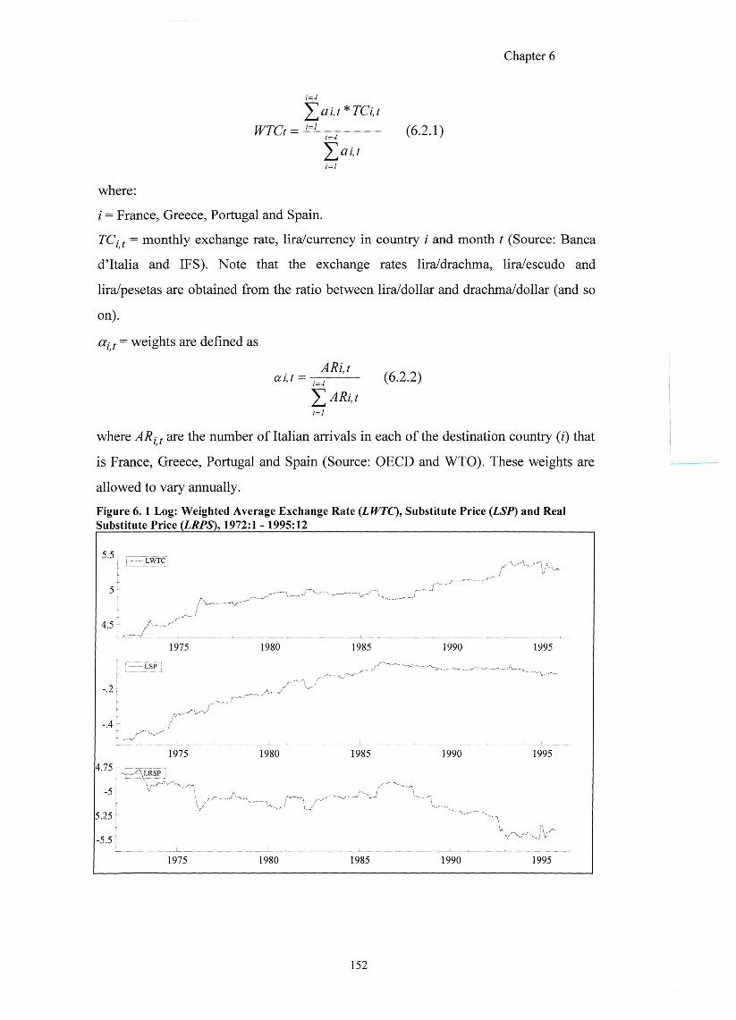
Chapter 6

i=4

'âi,t *TCi,t

WTCt = (6.2.1)

âi,t ( = /

where;

i = France, Greece, Portugal and Spain.

TCj f = monthly exchange rate, lira/currency in country i and month t (Source: Banca

d'ltalia and IFS). Note that the exchange rates lira/drachma, lira/escudo and

lira/pesetas are obtained from the ratio between lira/dollar and drachma/dollar (and so

on).

ai f = weights are defined as

« ' ' ^ = (6 .2 .2)

^ ARi, t

i=I

where ARj f are the number of Italian arrivals in each of the destination country (i) that

is France, Greece, Portugal and Spain (Source: OECD and WTO). These weights are

allowed to vary annually. Figure 6. 1 Log: Weighted Average Exchange Rate (LWTC), Substitute Price (LSP) and Real

; ! LWTC

5-l- / \ ^

4.5 / ' —

1975 1980 1985 1990 1995

-.2 r

-.4"" /

1975 1980 1985 1990 1995

-5^

1975 1980 1985 1990 1995

152

Chapter 6

As already stated, the nominal substitute price {LSP) is stationary in the level if

a constant, or a constant and seasonals are included in the unit root ADF test (see

Table 5.2). Thus, one is interested in the integration status of the weighted average

exchange rate and the real substitute price. An ADF unit root test with up to 13 lags is

applied, as one is dealing with monthly data. Both the (log) weighted exchange rate

and (log) real substitute price have been found to be 1(1). This finding holds for each

of the ADF cases, that is when including only the constant, the constant and seasonals

and so on.

The next step is to use a Johansen cointegration analysis in order to test for a

possible cointegration relationship between the (log) nominal substitute price and (log)

weighted average exchange rate for the main competitors. Using the joint F-test, an

initial unrestricted 13 lag system can be reduced to a 5 lag system when including only

a constant term, and to a 7 lag system when including a constant and seasonals. Note

that the information criteria SC, HQ and AIC are minimised when further coefKcient

restrictions are imposed in both the cases. From the cointegration analysis, using both

the 7 and 5 lag system, there is no evidence for the two variables to be cointegrated.

The same results have been obtained when including in the system the constant, and

the constant and trend unrestrictedly.

The joint F-test and the other information criteria lead to the use of the first

difference of the real substitute price, and thus consider only the short run adjustments.

However, it is difficult to see how this variable can really be 1(1); PPP must have some

force, even if only in the long run. One does need to assume that consumers have a

perfect knowledge of exchange rates as well as the cost of living in their own and

competitor countries. Further, using only the first difference excludes consideration of

the long run effect that is a strong assumption. Thus, one will include in the equation

the level of the real substitute price and the level of the relative price (Sassari/Italy),

LREP (see Chapter 5 for the definition).

The model for the domestic demand for tourism (LAR) contains the following

determinants: the income proxy (I f^) , the relative price (Z^Ff), the real substitute

price ( i / ^ f ) , the 'Sveather" variable ( Z ^ , the "Easter" dummy, the seasonal dummies

that allow for structural breaks in the seasonal pattern in accordance with the findings

in Chapter 5 and, finally, an impulse dummy (i7P9.^j) created in order to avoid non-

153

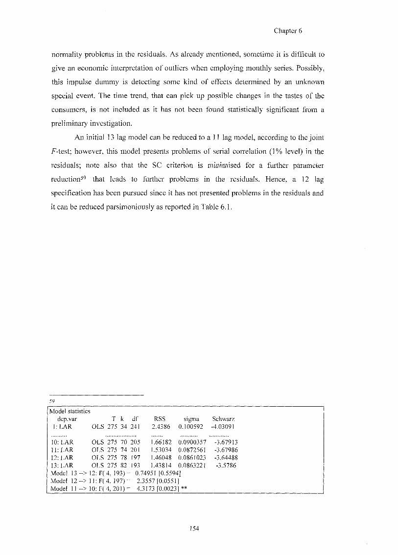
Chapter 6

normality problems in the residuals. As already mentioned, sometime it is difficult to

give an economic interpretation of outliers when employing monthly series. Possibly,

this impulse dummy is detecting some kind of effects determined by an unknown

special event. The time trend, that can pick up possible changes in the tastes of the

consumers, is not included as it has not been found statistically significant from a

preliminary investigation.

An initial 13 lag model can be reduced to a 11 lag model, according to the joint

F-test; however, this model presents problems of serial correlation (1% level) in the

residuals; note also that the SC criterion is minimised for a further parameter

reduction^^ that leads to further problems in the residuals. Hence, a 12 lag

specification has been pursued since it has not presented problems in the residuals and

it can be reduced parsimoniously as reported in Table 6.1.

59

Model statistics dep.var T k df RSS sigma Schwarz

LLAR 0LS 275 34 241 Z4386 0.100592 -4.03091

10: LAR OLS 275 70 205 1.66182 0.0900357 -3.67913 ]1:LAR 0LS 275 74 201 1.53034 0.0872561 -3.67986 12: LAR 0LS 275 78 197 1.46048 0.0861023 -3.64488 13; LAR OLS 275 82 193 1.43814 0.0863221 -3.5786 Model 13 - > 12: F(4, 193) = 0.74951 [0.5594] Model 12 - > 1 L F ( 4 1 9 ^ I = 2 3557 [0.0551] Model 11 - > 10: F(4, 201) = 4 3173 [0.0023] **

154

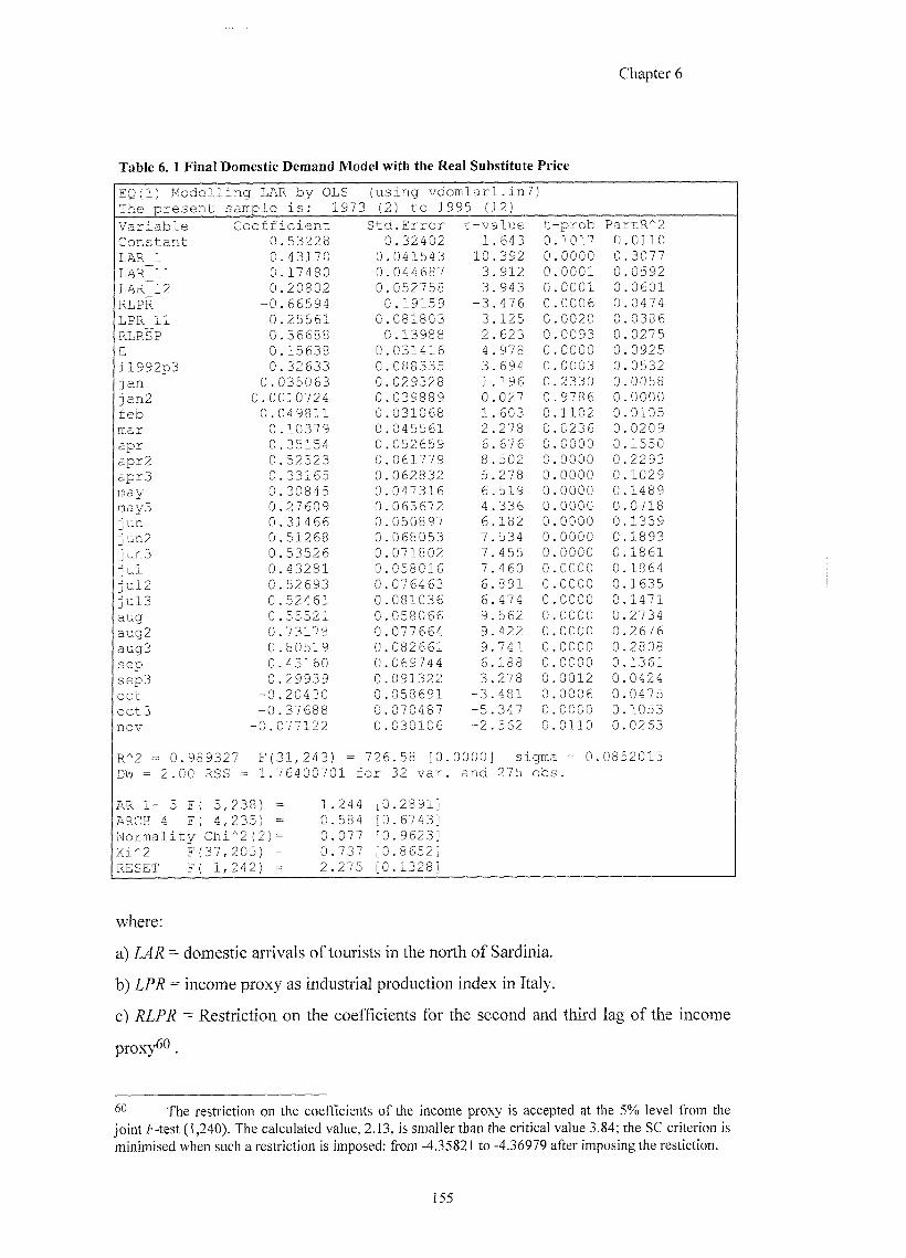
Chapter 6

Table 6. 1 Final Domestic Demand Model with the Real Substitute Price

EQ(1) Modelling LAR by OLS (using vdomlarl.in? The present sample is: 1973 (2) to 1995 (12)

Variable Constant LAR_1 LAR_11 LAR_12 RLPR LPR_11 RLRSP E il992p3 jan i a n 2 feb mar apr apr2 apr3 may may3 jun i u n 2 i u n 3 j u l jul2 iul3 aug aug2 aug3 sep sep3 Oct oct3 nov

R^2 = 0.98932 DW = 2.00 RSS

Coefficient Std.Error t-value t--prob PartR^2 0 .53228 0.32402 1 .643 0 1017 0 .0110 0 .43170 0 .041543 10 392 0 0000 0 3077 0 .17480 0 .044687 3 912 0 0001 0 0592 0 .20802 0 .052758 3 943 0 0001 0 .0601

-0 .66594 0.19159 -3 476 0 0006 0 0474 0 .25561 0 .081803 3 125 0 0020 0 0386 0 .36688 0.13988 2 623 0 0093 0 0275 0 .15638 0 .031416 4 978 0 0000 0 0925 0 .32633 0 .088335 3 694 0 0003 0 0532

0 . 035063 0 .029328 1 196 0 2330 0 0058 0.0010724 0 .039889 0 027 0 9786 0 0000 0 . 049811 0 .031068 1 603 0 1102 0 0105 0 .10379 0 .045561 2 278 0 0236 0 0209 0 .35154 0 .052659 6 676 0 0000 0 1550 0 .52523 0 .061779 8 502 0 0000 0 2293 0 .33165 0 .062832 5 278 0 0000 0 1029 0 .30845 0 .047316 6 519 0 0000 0 1489 0 .27609 0 .063672 4 336 0 0000 0 0718 0 .31466 0 .050897 6 182 0 0000 0 1359 0 .51268 0 .068053 7 534 0 0000 0 1893 0 .53526 0 .071802 7 455 0 0000 0 1861 0 .43281 0 .058016 7 460 0 0000 0 1864 0 .52693 0 .076463 6 891 0 0000 0 1635 0 .52461 0 .081036 6 474 0 0000 0 1471 0 .55521 0 .058066 9 562 0 0000 0 2734 0 .73178 0 .077664 9 422 0 0000 0 2676 0 .80519 0 .082661 9. 741 0 0000 0 2808 0 .43160 0 .069744 6. 188 0 0000 0 1361 0 .29939 0 .091322 3. 278 0 0012 0 0424

-0 .20430 0 .058691 -3. 481 0 0006 0 0475 -0 .37688 0 .070487 -5. 347 0 0000 0 1053

-0. D77122 0 .030106 -2 562 0 0110 0 0263

7 F(31,243) = 726.58 [0. 0000] Sigma = 0. 0852015 1.76400701 for 32 var. and 275 obs.

AR 1- 5 F( 5,238) = 1.244 [0.2891] ARCH 4 F( 4,235) = 0.584 [0.6743] Normality Chi*2(2)= 0.077 [0.9623] Xi"2 F(37,205) = 0.737 [0.8652] RESET F( 1,242) = 2.275 [0.1328]

where;


b) LPR = income proxy as industrial production index in Italy.

c) RLPR = Restriction on the coefficients for the second and third lag of the income

proxy^().

60 The restriction on the coefficients of the income proxy is accepted at the 5% level from the joint F-test (1,240). The calculated value, 2.13, is smaller than the critical value 3.84; the SC criterion is minimised when such a restriction is imposed: G-om -4.35821 to -4.36979 after imposing the restiction.

155

Chapter 6

d) RLRSP = Restriction on the coefficients for the fifth and seventh lag of the real

substitute price^l .

q) E = "Easter" dummy.

The model is data congruent and well-specified. Restrictions on the

coefficients can be imposed in accordance with the joint F-test and the SC criterion.

The dependent variable is highly dependent on its own past behaviour. The income

proxy shows a positive sign both in the short and long run. In the short run, the income

elasticity is below unity; whereas, in the long run, the income elasticity is above unity

with a /-value equal to 3.73 (see Table 6.2). The positive sign shows that the higher the

income for Italians the higher the number of tourists in Sassari Province. Note also that

the coefficient of the oscillation (RLPR) presents a negative sign, which can be picking

up possible "over-time" effects. The relative price and the "weather" variable do not

play any role in explaining the domestic demand for tourism. Both of them do not

appear statistically significant in the final restricted model. Interestingly, the real

substitute price enters the equation in its difference with a positive statistically

significant coefficient. The "Easter" dummy once again appears to be highly

significant. Moreover, the coefficients of the seasonal dummies, allowing for a

changing seasonal pattern, are in general statistically significant.

The dynamics are reported in Table 6.2. The long run coefficients are, in

general, well determined and the null hypothesis that they are all zero excluding the

constant term is rejected at the 1% level.

The restiction on the coefficients of the real substitute price is accepted at the 5% level. The calculated F-test (1,242) is equal to 0.60 that is smaller than the critical value 3.84. The SC criterion is also minimised when the coefficient restriction is imposed: from -4.3776 to -4.3956 after imposing the restriction.

156

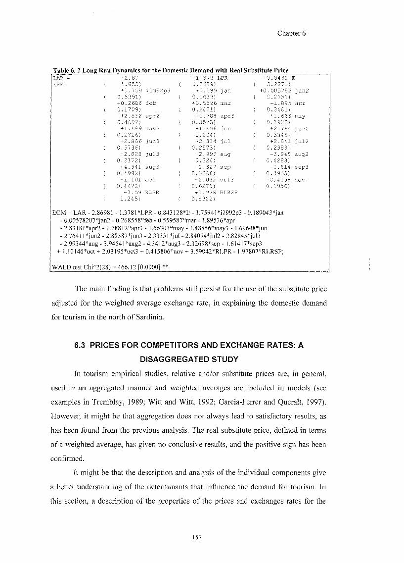
Chapter 6

Table 6. 2 Long Run Dynamics for the Domestic Demand with Real Substitute Price LAR (SE)

+2.87 +1.378 LPR +0.8431 E 1.655) 0.3689) ( 0.2271) 4-1.759 il992p3 +0.189 jan +0.005782 ian2

0.5391) 0.1639) ( 0.2151) +0.2686 feb +0.5596 mar +1.895 apr 0.1709) 0.2401) ( 0.3481) +2.832 ap]:2 +1.788 aprS +1.663 may

0.4697) 0.3573) ( 0.1935) +1.489 may3 +1.696 jun +2.764 jun2

0.2716) 0.204) ( 0.3345) +2.886 jun3 +2.334 jul +2.841 iul2

0.3736) 0.2573) ( 0.2989) +2.828 iul3 +2.993 aug +3.945 aug2

0.3172) 0.324) ( 0.4283) +4.341 aug3 +2.327 Sep +1.614 sep3

0.4992) 0.3266) ( 0.3955) -1.101 Oct -2.032 oct3 -0.4158 nov

0.4472) 0.6279) ( 0.1956) -3.59 RLPR +1.978 RIRSP

1.245) 0.8322)

ECM = LAR-2 .86981 - l .3781*LPR-0.843128*E- ].75941*i]992p3 -0.189043*jan - 0.00578207*jan2 - 0.268558*fbb - 0.559587*mar- 1.89536*apr -2 .83]81*apr2- 1.78812*apr3 - 1.66303*may- 1.48856*may3 - 1.69648*jun - 2.7641 l*jun2 - 2.88587*jun3 - 2.33351 *jul - 2.84094*jul2 - 2.82845*jul3 - 2.99344*aug - 3.94541*aug2 - 4.3412*aug3 - 2.32698*sep - 1.61417*sep3

+ 1.10146*oct + 2.03195*oct3 + 0.415806*nov + 3.59042*RLPR.- 1.97807*RLRSP;

WALD test Chi/'2(28) = 466.12 [0.0000] **

The main finding is that problems still persist for the use of the substitute price

ad[justed for the weighted average exchange rate, in explaining the domestic demand

for tourism in the north of Sardinia.

6.3 PRICES FOR COMPETITORS AND EXCHANGE RATES: A

DISAGGREGATED STUDY

In tourism empirical studies, relative and/or substitute prices are, in general,

used in an aggregated manner and weighted averages are included in models (see

examples in Tremblay, 1989; Witt and Witt, 1992; Garcia-Ferrer and Queralt, 1997).

However, it might be that aggregation does not always lead to satisfactory results, as

has been found from the previous analysis. The real substitute price, defined in terms

of a weighted average, has given no conclusive results, and the positive sign has been

confirmed.

It might be that the description and analysis of the individual components give

a better understanding of the determinants that influence the demand for tourism. In

this section, a description of the properties of the prices and exchanges rates for the

157

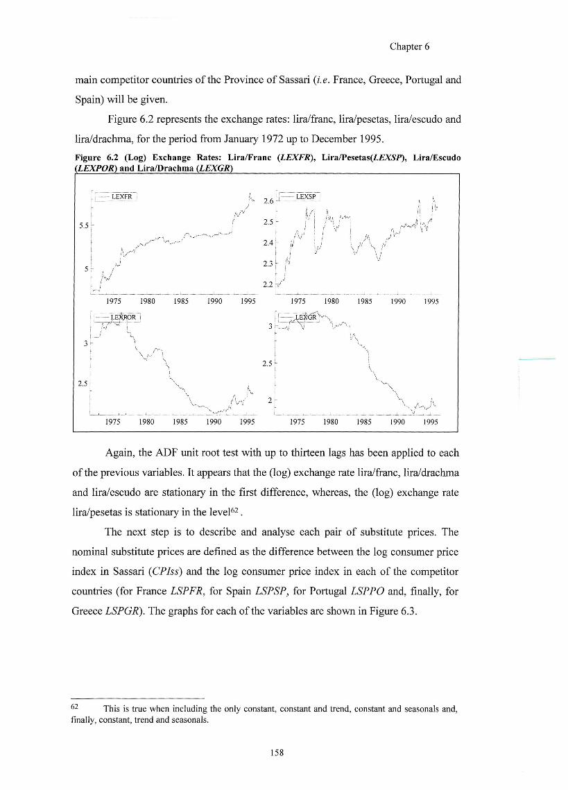
Chapter 6

main competitor countries of the Province of Sassari {i.e. France, Greece, Portugal and

Spain) will be given.

Figure 6.2 represents the exchange rates: lira/franc, lira/pesetas, lira/escudo and

lira/drachma, for the period from January 1972 up to December 1995.

Figure 6.2 (Log) Exchange Rates: Lira/Franc {LEXFR), Lira/Pesetas(6f%9f), Lira/Escudo {LEXPOR) and Lira/Drachma (LEXGR)

5.5- 2.5 ' il i

^ 2.4'

! J IJr

1975 1980 1985 1990 1995 1975 1980 1985 1990 1995

f r : 3

- LE#PR I I!

r 2.5 r

2.5 '

2'

1975 1980 1985 1 990 1995 1975 1980 1985 1990 1995

Again, the ADF unit root test with up to thirteen lags has been applied to each

of the previous variables. It appears that the (log) exchange rate lira/franc, lira/drachma

and lira/escudo are stationary in the first difference, whereas, the (log) exchange rate

lira/pesetas is stationary in the level^^ _

The next step is to describe and analyse each pair of substitute prices. The

nominal substitute prices are defined as the difference between the log consumer price

index in Sassari (CPIss) and the log consumer price index in each of the competitor

countries (for France LSPFR, for Spain LSPSP, for Portugal LSPPO and, finally, for

Greece LSPGR). The graphs for each of the variables are shown in Figure 6.3.

This is true when including the only constant, constant and trend, constant and seasonals and, finally, constant, trend and seasonals.

158

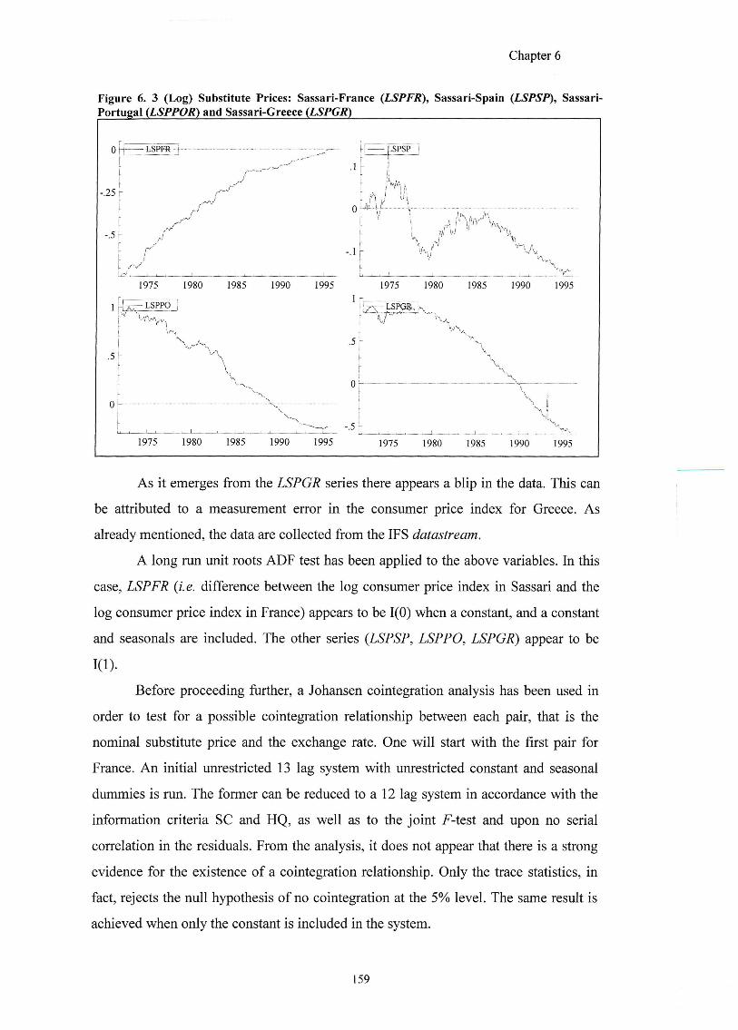
Chapter 6

Figure 6. 3 (Log) Substitute Prices: Sassari-France (LSPFR), Sassari-Spain (LSPSf), Sassari Portugal (LSPPOR) and Sassari-Greece (LSPGR)

0 [ L

I -.25 r

- .5. /

/V

1-P=LSPSP !

1975 1980 1985 1990 1995 1975 1980 1985 1990 1995

V .5r

L

OK h

0;

IMO 1W5 IMO 1995 1975 1980 1985 1990 1995

As it emerges from the LSPGR series there appears a bHp in the data. This can

be attributed to a measurement error in the consumer price index for Greece. As

already mentioned, the data are collected from the IFS datastream.

A long run unit roots ADF test has been applied to the above variables. In this

case, LSPFR (i.e. difference between the log consumer price index in Sassari and the

log consumer price index in France) appears to be 1(0) when a constant, and a constant

and seasonals are included. The other series (LSPSP, LSPPO, LSPGR) appear to be

1(1).

Before proceeding further, a Johansen cointegration analysis has been used in

order to test for a possible cointegration relationship between each pair, that is the

nominal substitute price and the exchange rate. One will start with the first pair for

France. An initial unrestricted 13 lag system with unrestricted constant and seasonal

dummies is run. The former can be reduced to a 12 lag system in accordance with the

information criteria SC and HQ, as well as to the joint F-test and upon no serial

correlation in the residuals. From the analysis, it does not appear that there is a strong

evidence for the existence of a cointegration relationship. Only the trace statistics, in

fact, rejects the null hypothesis of no cointegration at the 5% level. The same result is

achieved when only the constant is included in the system.

159

Chapter 6

The Johansen test is also applied to the second pair of variables for Spain. A 13

lag system, with the inclusion of constant, trend and seasonal dummies treated

unrestrictedly, can be reduced to a 2 lag system in accordance with the SC and HQ

criteria, and the joint F-test; this system exhibits no serial correlation in the residuals.

From the maximal eigenvalue and trace statistics there appears to be evidence for the

coefficients of the substitute price and exchange rate to be cointegrated.

The third pair tested is for Portugal. In this case, a final 9 lag system with

constant, trend and seasonals can be run. The results from the Johansen analysis seems

to give evidence for stationarity between the coefficients of the two variables under

study. Analogous results are obtained when including a constant and a trend in the

system. However, such results can be considered as misleading as both variables are

stationary in the first difference, as derived from the ADF test.

The last pair under consideration is for Greece. An initial unrestricted system of

13 lags, including a constant, trend and seasonals could be reduced to 7 lag system,

which does not present any problems of serial correlation in the residuals. From the

Johansen cointegration analysis, there appears to be evidence for stationarity between

the coefficients of the substitute price and exchange rate. Once again, the result

appears to be misleading.

As one can see the results are neither in agreement with the ADF test nor with

each other or economic theory. It is difGcult to see how an economy's exchange rate

and price level, would not be cointegrated, if they are 1(1), with a coefficient of unity.

Given the conflicting empirical evidence it seems reasonable to impose the

cointegration assumption. The analysis is, therefore, continued considering the

substitute price ad[justed for the exchange rate. That is, four different variables have

been created and expressed as follows;

= (6.3.1)

where:

j = France, Greece, Portugal and Spain.

Cf r = monthly consumer price index in Sassari (1990=100) (Source: ISTAT).

CPlj, t = monthly consumer price index in country j (1990=1 GO) (Source: IPS).

^ = monthly exchange rate, lira per unit of currency of countryy (elaborated on

160

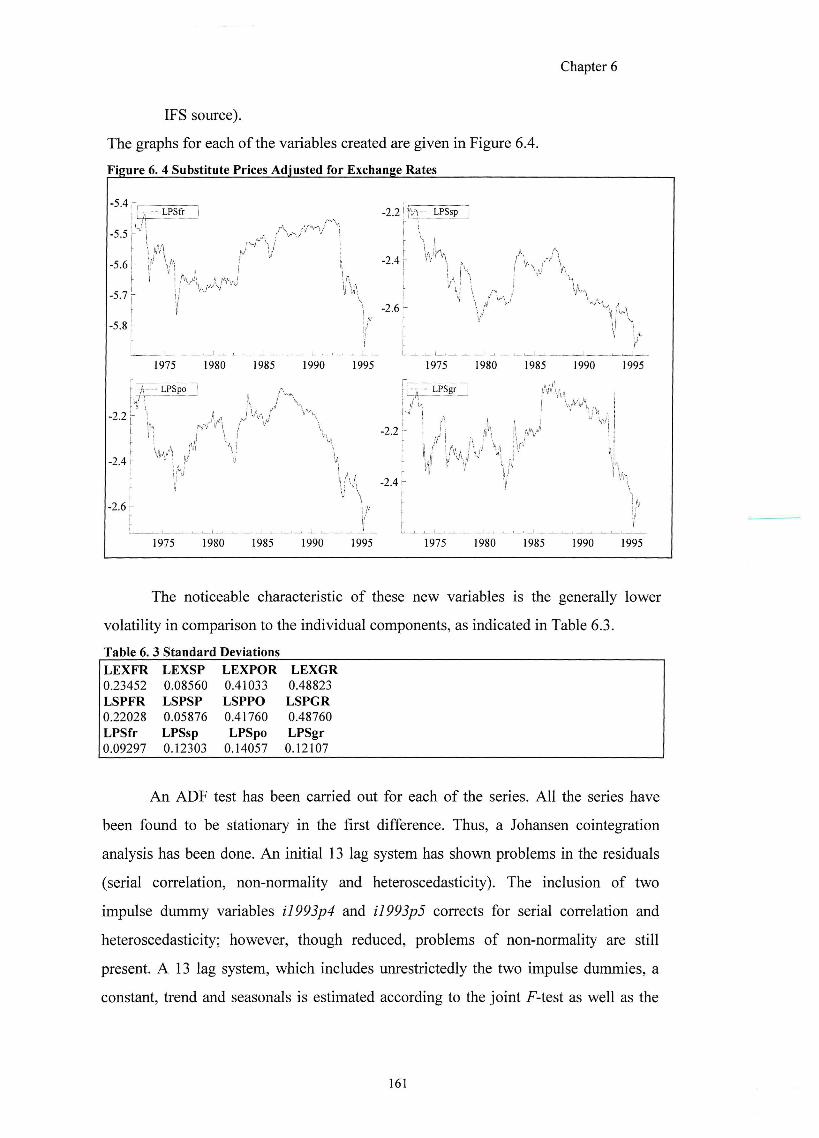
Chapter 6

IFS source).

The graphs for each of the variables created are given in Figure 6.4.

-5.4 -5.4 1 1 '1 — LPSfr - 2 . 2 LPSsp ^

-5.5

A i f

1 u

-2.4 • A ,

-5.7

/ -2.6

i >

i /U

1 1975 1980 1985 1990 1995 1975 1980 1985 1990 1995

1 LPSpo - LPSgr ;

H i A J A ( '

- 2 . 2 1 i I i 1- M , \

1 -2.2

lAu! . A .

'1 i

-2.4 J i - -2,4 r f

- 2 . 6

' r

1975 1980 1985 1990 1995 1975 1980 1985 1990 1995

The noticeable characteristic of these new variables is the generally lower

volatility in comparison to the individual components, as indicated in Table 6.3.

Table 6. 3 Standard Deviations

LEXFR LEXSP LEXPOR LEXGR 0.23452 0.08560 0.41033 0.48823 LSPFR LSPSP LSPPO LSPGR 0.22028 0.05876 0.41760 0.48760

LPSfr LPSsp LPSpo LPSgr 0.09297 0.12303 0.14057 0.12107

An ADF test has been carried out for each of the series. All the series have

been found to be stationary in the first difference. Thus, a Johansen cointegration

analysis has been done. An initial 13 lag system has shown problems in the residuals

(serial correlation, non-normality and heteroscedasticity). The inclusion of two

impulse dummy variables il993p4 and il993p5 corrects for serial correlation and

heteroscedasticity; however, though reduced, problems of non-normality are still

present. A 13 lag system, which includes unrestrictedly the two impulse dummies, a

constant, trend and seasonals is estimated according to the joint F-test as well as the

161

Chapter 6

AIC criterion. From the analysis, the null hypothesis of no cointegration cannot be

rejected. Analogous results have been obtained when including only a constant, or the

constant and the time trend.

Overall, one can conclude the substitute prices adjusted for the exchange rates

show a higher homogeneity in terms of properties and results than the individual

components. Thus, the four real substitute prices will be used in running the model for

the domestic and international demand for tourism in the north of Sardinia. However,

there are reservations as to the order of integration of the constructed variables.

6.4 DOMESTIC DEMAND MODEL USING DISAGGREGATED REAL

SUBSTITUTE PRICES

This section is dedicated to the specification of a model for the domestic

demand for tourism in the north of Sardinia, that includes the four variables of

substitute price acûsted for the exchange rate, as defined in the previous paragraph. It

is possible that the heterogeneity of the properties of the individual components, that is

the nominal substitute price and exchange rate for each of competitor countries, has

created problems on an aggregated level (i.e. when using the real substitute price as a

weighted average).

Firstly, one starts with the strong, but plausible assumption, that consumers

have a perfect knowledge of the living costs in their own country as well as in the

competitor countries. This assumption, can be thought to be true on the basis that

tourists are well informed thanks to their own past experience, as well as 6om

information received by other sources (newspapers, friends and family's experience).

The assumption of perfect information on the exchange rates is widely accepted. In

this way, one can use the level of those variables which appear to be stationary in the

first difference, z.e. relative price Sassari-Italy real substitute price for France

Greece Portugal and Spain

The model for the domestic arrivals in Sassari Province (LAR) contains the

following explanatory variables: the income proxy (Zf J?), the relative price (ZTÊP),

the real substitute prices for the competitor countries {LPSfr, LPSgr, LPSpo and

Zf&^), the "weather" variable (ZP^3, the "Easter" dummy variable (Z), an impulse

dummy created after inspecting the residuals, in order to avoid non-

162

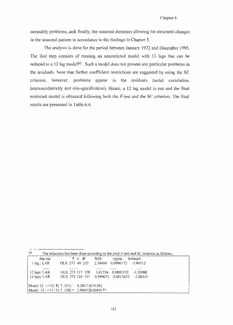
Chapter 6

normality problems, and, finally, the seasonal dummies allowing for structural changes

in the seasonal pattern in accordance to the findings in Chapter 5.

The analysis is done for the period between January 1972 and December 1995.

The first step consists of running an unrestricted model with 13 lags that can be

reduced to a 12 lag model^^ Such a model does not present any particular problems in

the residuals. Note that further coefficient restrictions are suggested by using the SC

criterion, however, problems appear in the residuals (serial correlation,

heteroscedasticity and mis-specification). Hence, a 12 lag model is run and the final

restricted model is obtained following both the F-test and the SC criterion. The final

results are presented in Table 6.4.

63 The reduction has been done according to the joint _F-test and SC criterion as follows:

dep.var T k (# RSS sigma Schwarz

1 lag; LAR OLS 275 40 235 2.30404 0.0990172 -3.96512

12 lags: LAR OLS 275 117 158 1.01736 0.0802432 -3.20988 13 lags: LAR OLS 275 124 151 0.999672 0.0813655 -3.08445

Model 13 ->12: F(7, 151)= 0.3817 [0.9120] Model 12->11 F( 7, 158) = 2.9069 [0.0069] **

163

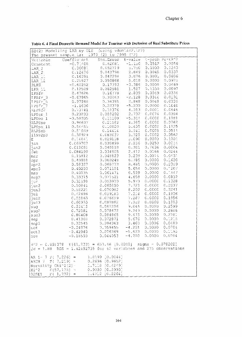
Chapter 6

Table 6. 4 Final Domestic Demand Model for Tourism with Inclusion of Real Substitute Prices

EQ(2) Modell The present

ing LAR by OLS sample is: 1973

[using vdoml (2) to 1995

ar2.in7) (12)

Coefficient Std.Error t-value t -prob PartR*2 -0 .71408 0.62081 -1 .150 0 2512 0 .0056 0 .30081 0.052319 5 .750 0 0000 0 .1243 0 .12476 0.043796 2 .849 0 0048 0 .0337 0 .16391 0.042294 3 .876 0 0001 0 .0606 0 .25527 0.050868 5 .018 0 0000 0 .0975

-0 .60252 0.17793 -3 .386 0 0008 0 .0469 0 .12509 0.082981 1 .507 0 1330 0 .0097 0 .47626 0.16778 2 .839 0 0049 0 0334

-0 .63965 0.30063 -2 128 0 0344 0 0191 0 .97948 0.34391 2 848 0 0048 0 0336 - 1.1636 0.22378 -5 200 0 0000 0 1040 0 .73741 0.18376 4 013 0 0001 0 0646 0 .23833 0.088202 2 702 0 0074 0 0304

-0 .59035 0.11109 -5 314 0 0000 0 1081 0 .94637 0.21582 4 385 0 0000 0 0762 0 .54455 0.10020 5 435 0 0000 0 1125 0 .51039 0.14414 3 541 0 0005 0 0511 0 .30929 0.083037 3 725 0 0002 0 0562 0 .14841 0.029158 5 090 0 0000 0 1001

0. 069707 0.030899 2 256 0 0250 0 0214 0. 012081 0.040118 0 301 0 7636 0 0004 0 . 084199 0.034905 2 412 0 0166 0 0244 0 .15812 0.048823 3 239 0 0014 0 0431 0 .40881 0.060249 6 785 0 0000 0 1650 0 .58327 0.068773 8 481 0 0000 0 2359 0 .40203 0.071101 5 654 0 0000 0 1207 0 .40135 0.061471 6 529 0 0000 0 1547 0 .33315 0.071521 4 658 0 0000 0 0852 0 .32198 0.053910 5 973 0 0000 0 1328 0 .50841 0.065850 7 721 0 0000 0 2037 0 .58221 0.070982 8 202 0 0000 0 2241 0 .42696 0.059183 7 214 0 0000 0 1826 0 .55863 0.076659 7 287 0 0000 0 1856 0 .60933 0.082882 7 352 0 0000 0. 1883 0 .55415 0.061256 9. 046 0 0000 0. 2599 0 .72581 0.078472 9. 249 0 0000 0. 2686 0 .80408 0.084865 9. 475 0 0000 0. 2781 0 .41360 0.072871 5. 676 0 0000 0. 1215 0 .32545 0.094063 3. 460 0 0006 0 0489

-0 .24976 0.059455 -4 201 0 0000 0. 0704 -0 .42940 0.076369 -5 623 0 0000 0. 1195 -0 .18503 0.044053 -4 . 200 0 0000 0. 0704

Variable Constant LAR_1 LAR_2 LAR_11 LAR_12 RLPR LPR_11 LPSfr LPSfr_3 LPSfr_5 LPSfr_7 RLPSfr LPSgr_l LPSpo_l RlfSpo LPSpo_ll RLPSsp il992p3 E jan ian2 feb mar apr apr2 apr3 may may3 jun i u n 2 i u n 3 j u l iul2 i u l 3 aug aug2 aug3 sep sep3 oct oct3 nov

Er2 = 0.991378 F(41,233) = 653.46 [0.0000] s i ^ ^ = 0.0782021 DM = 1.88 RSS = 1.42492738 for 42 variables and 275 observations

AR 1- 7 F( 7,226) AACH 7 F( 7,219) Normality Chi*2(2) Xi^2 F(57,r75) RESET F( 1,232)

1.8199 [0.0844] 0.2696 [0.9652] 1.7118 [0.4249] 0.9393 [0.5993] 1.4712 [0.2264]

164

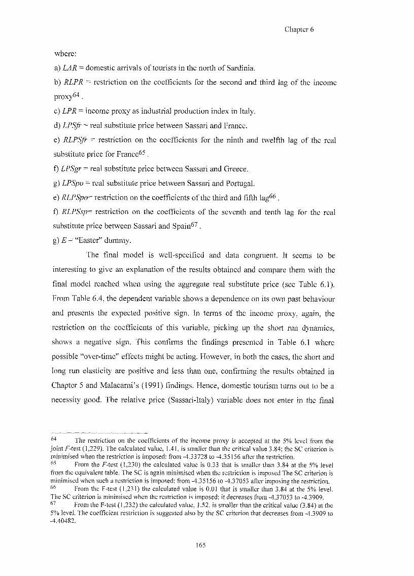
Chapter 6

where:


b) RLPR = restriction on the coefficients for the second and third lag of the income

p r o x y ^ .

c) LPR = income proxy as industrial production index in Italy.

d) I f = real substitute price between Sassari and France.

e) RLPSfr = restriction on the coefficients for the ninth and twelfth lag of the real

substitute price for France^^ .

f) LPSgr = real substitute price between Sassari and Greece.

g) Zf = real substitute price between Sassari and Portugal.

e) RLPSpo= restriction on the coefficients of the third and fifth lag^6

f) RLPSsp= restriction on the coefficients of the seventh and tenth lag for the real

substitute price between Sassari and Spain^^ .

g) E = "Easter" dummy.

The final model is well-specified and data congruent. It seems to be

interesting to give an explanation of the results obtained and compare them with the

final model reached when using the aggregate real substitute price (see Table 6.1).

From Table 6.4, the dependent variable shows a dependence on its own past behaviour

and presents the expected positive sign. In terms of the income proxy, again, the

restriction on the coefficients of this variable, picking up the short run dynamics,

shows a negative sign. This confirms the findings presented in Table 6.1 where

possible "over-time" eflects might be acting. However, in both the cases, the short and

long run elasticity are positive and less than one, confirming the results obtained in

Chapter 5 and Malacarni's (1991) findings. Hence, domestic tourism turns out to be a

necessity good. The relative price (Sassari-Italy) variable does not enter in the final

The restriction on the coefficients of the income proxy is accepted at the 5% level from the joint f - tes t (1,229). The calculated value, 1.4], is smaller than the critical value 3.84; the SC criterion is minimised when the restriction is imposed; from -4.33728 to -4.35156 after the restriction.

From the F-test (1,230) the calculated value is 0.33 that is smaller than 3.84 at the 5% level from the equivalent table. The SC is again minimised when the restriction is imposed The SC criterion is minimised when such a restriction is imposed; from -4.35156 to -4.37053 after imposing the restriction.

From the F-test (1,231) the calculated value is 0.01 that is smaller than 3.84 at the 5% level. The SC criterion is minimised when the restriction is imposed; it decreases from -4.37053 to -4.3909.

From the F-test (1,232) the calculated value, 1.52, is smaller than the critical value (3.84) at the 5% level. The coefficient restriction is suggested also by the SC criterion that decreases from -4.3909 to -4.40482.

165

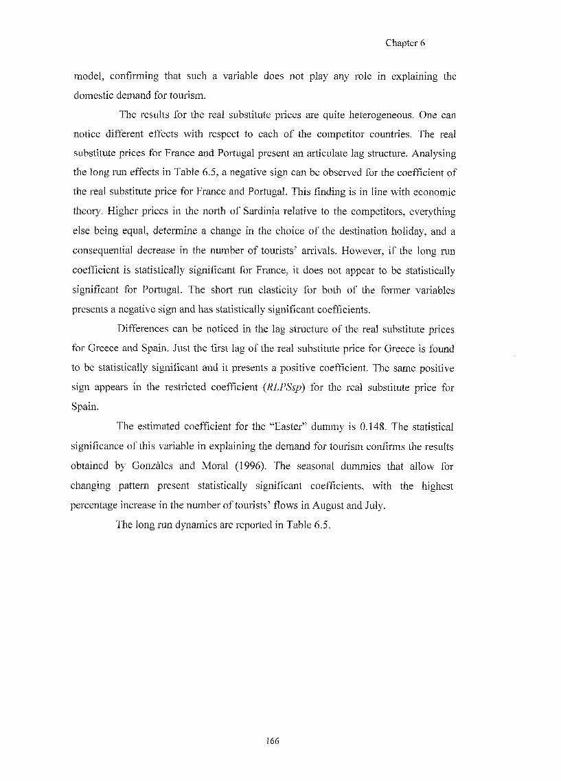
Chapter 6

model, confirming that such a variable does not play any role in explaining the

domestic demand for tourism.

The results for the real substitute prices are quite heterogeneous. One can

notice different effects with respect to each of the competitor countries. The real

substitute prices for France and Portugal present an articulate lag structure. Analysing

the long run effects in Table 6.5, a negative sign can be observed for the coefficient of

the real substitute price for France and Portugal. This finding is in line with economic

theory. Higher prices in the north of Sardinia relative to the competitors, everything

else being equal, determine a change in the choice of the destination holiday, and a

consequential decrease in the number of tourists' arrivals. However, if the long run

coefScient is statistically significant for France, it does not appear to be statistically

significant for Portugal. The short run elasticity for both of the former variables

presents a negative sign and has statistically significant coefficients.

Differences can be noticed in the lag structure of the real substitute prices

for Greece and Spain. Just the first lag of the real substitute price for Greece is found

to be statistically significant and it presents a positive coefficient. The same positive

sign appears in the restricted coefficient (Jdf&p) for the real substitute price for

Spain.

The estimated coefficient for the "Easter" dummy is 0.148. The statistical

significance of this variable in explaining the demand for tourism confirms the results

obtained by Gonzales and Moral (1996). The seasonal dummies that allow for

changing pattern present statistically significant coefficients, with the highest

percentage increase in the number of tourists' flows in August and July.

The long run dynamics are reported in Table 6.5.

166

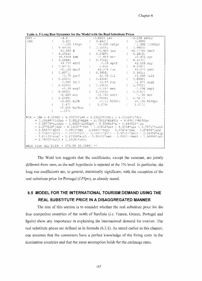
Chapter 6

Table 6. 5 Long Run Dynamics for the Mode with the Real Substitute Prices LAR : (SE)

-4 . 6 +0.8058 LPR -2.238 LPSfr 4.52) ( 0.4481) ( 0.988)

+1.535 LPSgr -0.295 LPSpo +1.992 il992p3 0.6959) ( 0.5266) ( 0.6683) +0.956 E +0.449 jan +0.07782 ian2

0.2821) ( 0.2387) ( 0.2618) +0.5424 feb +1.019 mar +2.633 apr 0.2669) ( 0.3722) ( 0.6474) +3.757 apr2 +2.59 apr3 +2.585 may

0.8714) ( 0.65) ( 0.5584) +2.146 may3 +2.074 jun +3.275 iun2

0.4971) ( 0.3655) ( 0.5631) +3.75 jun3 +2.75 jul +3.598 iul2

0.6605) ( 0.4386) ( 0.6006) +3.925 iul3 +3.57 aug +4.675 aug2

0.6585) ( 0.5915) ( 0.7701) +5.18 aug3 +2.664 Sep +2.096 sep3

0.8602) ( 0.4961) ( 0.5161) -1.609 oct -2.766 oct3 -1.192 nov

0.6569) ( 0.9801) ( 0.4614) -3.881 RLPR + 4.75 RLPSfr +6.096 RLPSpo 1.47) ( 1.679) ( 2.011)

+3.288 RLPSsp 1.157)

ECM = LAR + 4.59982 -+ 0.294997*LPSpo - 3.28773*RLPSsp - 0.077818*ian2 -- 2.58972*apr3 -- 3.75037*iun3 -- 4.67535*aug2 -+ 2.76605*oct3 +

WAID test Chi''2{33)

0.80579*LPR + 2.23829*LPSfr - 1.53526*LPSgr + 3.8812*RI,PR - 4.75012*RLPSfr - 6.09617*RlPSpo - 1.9923*il992p3 - 0.956016*E - 0.449024*ian 0.542377*feb - 1.01852*mar - 2.6334*apr - 3.75717*apr2

2.5853*may - 2.14602*may3 - 2.07404*jun - 3.27496*jun2 2.75032*jul - 3.59844*iul2 - 3.92507*jul3 - 3.56959*aug 5.17959*aug3 - 2.66422*sep - 2.09641*sep3 + 1.60886*oct 1.19191*nov;

276.98 [0.0000] **

The Wald test suggests that the coefficients, except the constant, are jointly

different from zero, as the null hypothesis is rejected at the 1% level. In particular, the

long run coefficients are, in general, statistically significant, with the exception of the

real substitute price for Portugal (LPSpo), as already stated.

6.5 MODEL FOR THE INTERNATIONAL TOURISM DEMAND USING THE

REAL SUBSTITUTE PRICE IN A DISAGGREGATED MANNER

The aim of this section is to consider whether the real substitute price for the

four competitor countries of the north of Sardinia {i.e. France, Greece, Portugal and

Spain) show any importance in explaining the international demand for tourism. The

real substitute prices are defined as in formula (6.3.1). As stated earlier in this chapter,

one assumes that the consumers have a perfect knowledge of the living costs in the

destination countries and that the same assumption holds for the exchange rates.

167

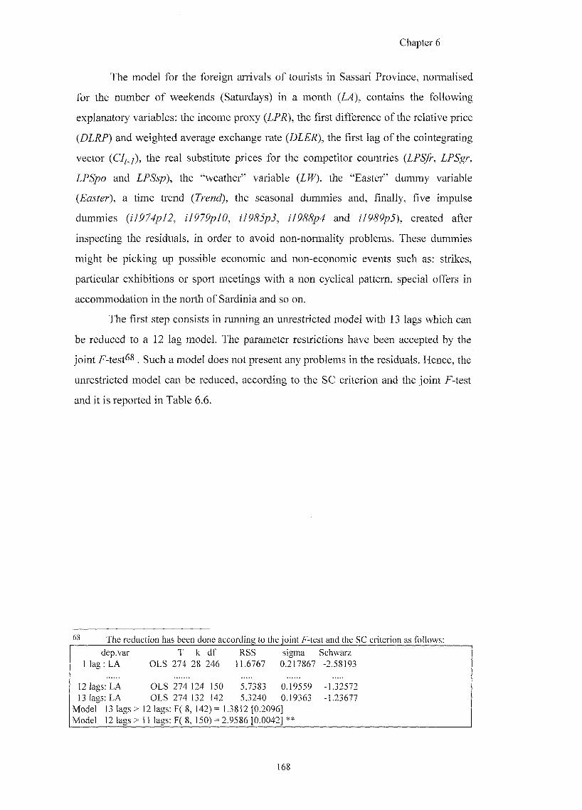
Chapter 6

The model for the foreign arrivals of tourists in Sassari Province, normalised

for the number of weekends (Saturdays) in a month {LA), contains the following

explanatory variables; the income proxy (LPR), the first difference of the relative price

(DZ^) and weighted average exchange rate (DIEJZ), the first lag of the cointegrating

vector (Clf.j), the real substitute prices for the competitor countries (LPSfr, LPSgr,

and If&p), the "weather" variable ( 2 ^ , the "Easter" dummy variable

{Easter), a time trend {Trend), the seasonal dummies and, finally, five impulse

dummies and created aAer

inspecting the residuals, in order to avoid non-normality problems. These dummies

might be picking up possible economic and non-economic events such as: strikes,

particular exhibitions or sport meetings with a non cyclical pattern, special offers in

accommodation in the north of Sardinia and so on.

The first step consists in running an unrestricted model with 13 lags which can

be reduced to a 12 lag model. The parameter restrictions have been accepted by the

joint i^-test^S . Such a model does not present any problems in the residuals. Hence, the

unrestricted model can be reduced, according to the SC criterion and the joint F-test

and it is reported in Table 6.6.

The reduction has been done according to the joint F-test and the SC criterion as follows:

dep.var T k df RSS sigma Schwarz 1 lag; LA OLS 274 28 246 11.6767 0.217867 -2.58193

12 lags; LA OLS 274 124 150 5.7383 0.19559 -1.32572 13 lags: LA OLS 274 132 142 5.3240 0.19363 -1.23677

Model 13 lags > 12 lags: F( 8, 142) = 1.3812 [0.2096] Model 12 lags > 1 lags: F( 8, 150) = 2.9586 [0.0042] **

168

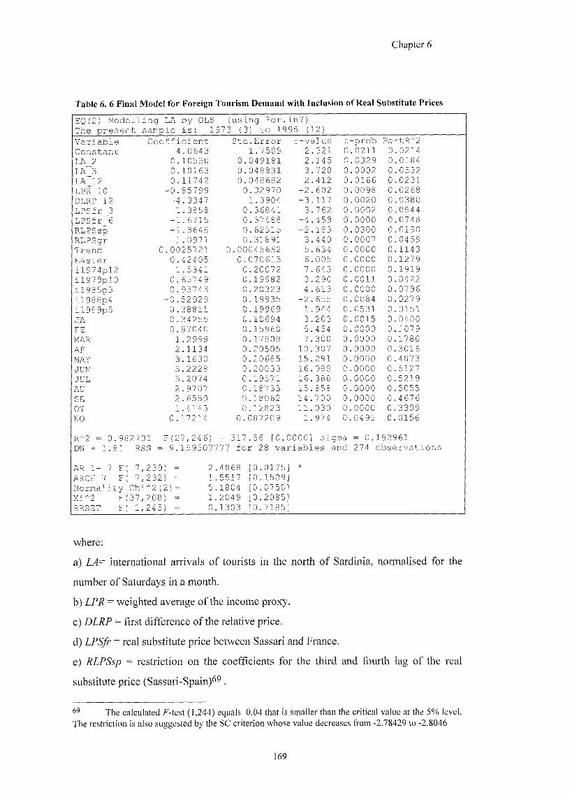
Chapter 6

Table 6. 6 Final Model for Foreign Tourism Demand with Inclusion of Real Substitute Prices

EQ(2) Modelling LA by OLS (using For.in7) The present sample is: 1973 (3) to 1995 ( 12)

Variable Coefficient Std .Error t-value t -prob PartR^2 Constant 4.0643 1.7509 2 .321 0 .0211 0 0214

LA 2 0.10550 0. 049181 2 .145 0 0329 0 0184

LA 3 0.18163 0. 048831 3 .720 0 0002 0 0532

LA 12 0.11742 0. 048682 2 .412 0 0166 0 0231

LPR 10 -0.85799 0 .32970 -2 .602 0 0098 0 0268

DLRP 12 -4.3347 1.3904 -3 .117 0 0020 0 0380

LPSfr 3 1.3858 0 .36841 3 .762 0 0002 0 0544 LPSfr 6 -1.6715 0 .37488 -4 .459 0 0000 0 0748

RLPSsp -1.3648 0 .62515 -2 .183 0 0300 0 0190 RLPSgr 1.0971 0 .31891 3 .440 0 0007 0 0459 Trend 0.0025721 0.00045652 5 .634 0 0000 0 1143 Easter 0.42405 0. 070613 6 .005 0 0000 0 1279 il974pl2 1.5341 0 .20072 7 .643 0 0000 0 1919 il979plO 0.65749 0 .19982 3 .290 0 0011 0 0422 il985p3 0.93743 0 .20323 4 .613 0 0000 0 0796

il988p4 -0.52929 0 .19935 -2 .655 0 0084 0 0279 il989p5 0.38811 0 .19969 1 .944 0 0531 0 0151 JA 0.34255 0 .10694 3 .203 0 0015 0 0400

FE 0.87040 0 .15960 5 .454 0 0000 0 1079

MAR 1.2999 0 .17808 7 .300 0 0000 0 1780 AP 2.1134 0 .20505 10 .307 0 0000 0 3016

MAY 3.1630 0 .20685 15 .291 0 0000 0 4873 JUN 3.2228 0 .20033 16 .088 0 0000 0 5127 JUL 3.2074 0 .19571 16 .388 0 0000 0 5219 AU 2.9707 0 .18733 15 .858 0 0000 0 5055 SE 2.6550 0 .18062 14 .700 0 0000 0 4676 OT 1.4143 0 .12823 11 .030 0 0000 0. 3309

NO 0.17214 0. 087209 1 .974 0 0495 0. 0156

R^2 = 0.982701 F(27,246) = 517 .56 [0. 0000 sigma = 0.192961 DW = 1.81 RSS = 9.159507777 for 28 variables and 274 observations

AR 1- 7 F( 7,239) = 2 4868 [0.0175 ] * ARCH 7 F( 7,232) = 1 5517 [0.1509] Normality Chi^2(2)= 5 1804 [0.0750 ] Xi*2 F( 37,208) = 1 2049 [0.2085 ] RESET F( 1,245) = 0 1303 [0.7185 ]

where:

a) LA= international arrivals of tourists in the north of Sardinia, normalised for the

number of Saturdays in a month.

b) LPR = weighted average of the income proxy.

c) DLRP = first difference of the relative price.

d) LPSfr = real substitute price between Sassari and France.

e) = restriction on the coefficients for the third and fourth lag of the real

substitute price (Sassari-Spain)^^.

69 The calculated f -test (1,244) equals 0.04 that is smaller than the critical value at the 5% level. The restriction is also suggested by the SC criterion whose value decreases from -2.78429 to -2.8046

169

Chapter 6

f) RLPSgr = restriction on the coefficients for the eleventh and twelfth lag of the real

substitute price (Sassari-Greece)^®.

The model is able to explain a 98% of the variance of the dependent

variable. However, the final model fails to accept the null hypothesis of non serial

correlation in the residuals, at the 5% level. The past behaviour of the dependent

variable plays a role in explaining the international demand for tourism in the north of

Sardinia and has a positive sign coefRcient. In terms of income proxy, only the tenth

lag is found to be statistically significant with a negative sign. The cointegrating vector

does not appear in the final restricted model, as well as the first difference of the

weighted exchange rate. However, the relative price growth is statistically significant

with the expected negative sign. Hence, the long run information does not have any

importance in explaining the international demand.

The real substitute price for France, statistically significant in the long run,

presents a negative sign coefficient, as reported in Table 6.7. However, the exchange

rate and the consumer price index for France are also present in the weighted average

exchange rate and consumer price index for the main origin countries. This might be

indicating a substitute effect between home and Sardinian vacations for French

tourists. The real substitute price for Portugal does not turn out to be statistically

significant. Moreover, the real substitute prices for Spain and Greece enter in the

equation as differences, since a coefficient restriction could be imposed. The first

coefficient presents a negative sign, whereas the coefficient for Greece shows a

positive sign.

The time trend, picking up changes in consumers' tastes, is highly

significant and it has a positive sign. The "Easter" dummy, once again, plays an

important role in explaining the international demand for tourism. The seasonal

dummies show statistically significant coefficients, with the highest percentage

increase in the number of foreign arrivals in June and July.

The long run dynamics are presented in Table 6.7. The Wald test suggests

the joint significance of the long run coefficients.

From the F-test (1,246) the calculated value is 0.49 smaller than 3.84 at the 5% level from the conventional table. Again, the SC is minimised when this restriction is imposed, i.e. from -2.8046 to -2.8247.

170

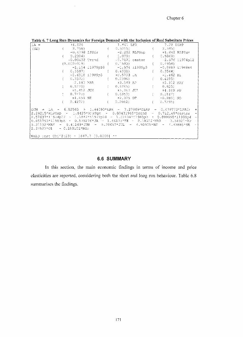
Chapter 6

Table 6. 7 Long Run Dynamics for Foreign Demand with the Inclusion of Real Substitute Prices LA = +6.826 -1.441 LPR -7.28 DLRP

( 2/^^) ( 0.5715) 2.585) -0.4798 LPSfr -2.292 RLPSsp +1.842 RLPSgr

( 0 ^ ^ 8 ^ ( 1.079) 0.5869) +0.00432 Trend +0.7121 easter +2.576 il974pl2

( 0 .0007019) ( 0.1503) 0.4954) +1.104 il979plO +1.574 11985p3 -0.8889 il988p4

( 0.3587) ( 0.4031) 0.3544) +0.6518 il989p5 +0.5753 JA +1.462 FE

( 0.3372) ( 0.2396) 0.4285) +2.183 IWW +3.549 AP +5.312 MAY

{ 0 ^ ^ 7 ^ ( 0.6785) 0.825) +5.412 JUN +5.387 JUL +4.989 AU

I o.74rn ( 0.6353) 0.5167) +4.459 SE +2.375 OT +0.2891 NO

{ 0.4272) ( 0.2062) 0.1295)

EOM = LA - 6 .82563 + 1.44093*LPR + 7.27969*DLRP + 0.479773*LPSfr + 2.29215*RLPSsp - 1.8425*RLPSgr - 0.00431965*Trend - 0.712148 *easter 2.57637*il974pl2 - 1.1042'îl979pl0 - 1.57434 *il985p3 + 0.888898' il988p4 -0.651793*il989p5 - 0.575276*JA - 1 .46175+FE - 2.18312 *MAR - 3.54921*AP -5.31192*MAY - 5.41249*JUN - 5.38 657*JUL - 4.98905* AU - 4.4 5889*SE -2.37527*0T - 0 .289101*NO;

WALD test Chi''2 (23) = 1847.7 [0.0000]

6.6 SUMMARY

In this section, the main economic findings in terms of income and price

elasticities are reported, considering both the short and long run behaviour. Table 6.8

summarises the findings.

171

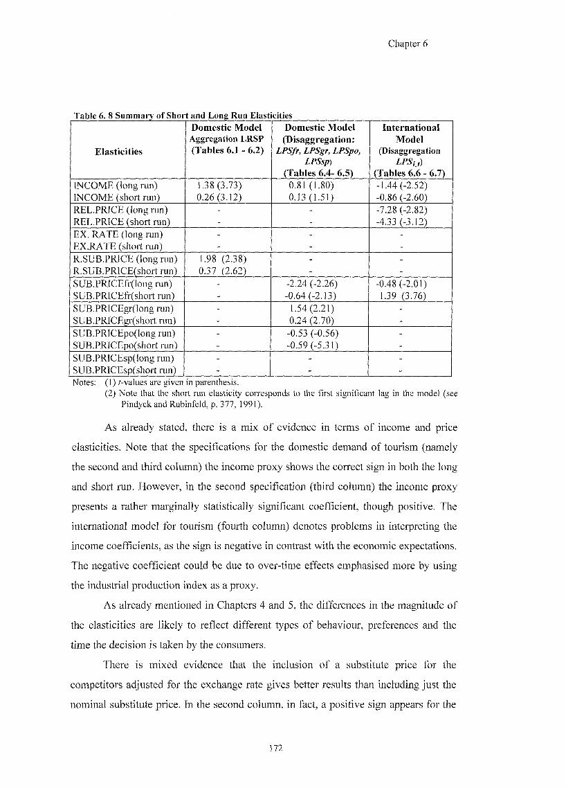
Chapter 6

Elasticities

Domestic Model Aggregation LRSP (Tables 6.1 - 6.2)

Domestic Model (Disaggregation:

LPSfr, LPSgr, LPSpo, LPSsp)

(Tables 6.4- 6.5)

Internat ional Model

(Disaggregation

(Tables 6.6 - 6.7)

I N C O M E ( long run)

I N C O M E (short run)

1.38(3.73) 0.26 (3.12)

0.81 (1.80) 0.13 (1.51)

-1.44 (-2.52) -0.86 (-2.60)

REL.PRICE (long run) R E L . P R I C E (short run)

- - -7.28 (-2.82) -4.33 (-3.12)

E X . R A T E (long run)

EX.RATE (short run) - - -

R . S U B . P R I C E (long run)

R .SUB.PRICE(shor t run)

1.98 (2.38) 0.37 (2.62)

- -

SUB.PRICEfr(long run) SUB.PRICEfr (short run)

- -2.24 (-2.26) -0.64 (-2.13)

-0.48 (-2.01) 1.39 (3.76)

SUB.PRICEgr ( long run)

SUB.PRICEgr(short run)

- 1.54 (2.21) 0.24 (2.70)

-

SUB.PRICEpo( long run)

SUB.PRICEpo(short run) - -0.53 (-0.56)

-0.59 (-5.31) -

SUB.PRICEsp( long run)

SUB.PRICEsp(short run) - - -

Notes: (1) ^-values are given in parenthesis. (2) Note that the short run elasticity corresponds to the first significant lag in the model (see

Pindyck and Rubinfeld, p. 377, 1991).

As already stated, there is a mix of evidence in terms of income and price

elasticities. Note that the specifications for the domestic demand of tourism (namely

the second and third column) the income proxy shows the correct sign in both the long

and short run. However, in the second specification (third column) the income proxy

presents a rather marginally statistically significant coefficient, though positive. The

international model for tourism (fourth column) denotes problems in interpreting the

income coefficients, as the sign is negative in contrast with the economic expectations.

The negative coefficient could be due to over-time effects emphasised more by using

the industrial production index as a proxy.

As already mentioned in Chapters 4 and 5, the differences in the magnitude of

the elasticities are likely to reflect different types of behaviour, preferences and the

time the decision is taken by the consumers.

There is mixed evidence that the inclusion of a substitute price for the

competitors acûsted for the exchange rate gives better results than including just the

nominal substitute price. In the second column, in fact, a positive sign appears for the

172

Chapter 6

the aggregated real substitute price in its difference (namely jZZJ&SP). The

disaggregation of the real substitute price for each of the competitors has given better

results for France and Portugal. These substitute prices, in fact, adjusted for the

exchange rates show a long run coefficient with a negative sign. This finding is in line

with economic theory. However, while the long run coefficient for France is

statistically significant, the long run coefficient for Portugal is not. Both these real

substitute prices present a distributed lag structure and reasonably short run dynamics,

with significant and expected negative signs.

Different behaviour has been noticed for Spain and Greece. Both of them

present a short run dynamic structure. Just the first lag of the real substitute price for

Greece is found to be statistically significant with a positive sign. The same positive

sign appears in the oscillation for the real substitute price for Spain (namely RLPSsp in

Table 6.5).

Heterogeneous results have also been achieved in modelling the foreign

demand for tourism. Only the long run coefficient of the real substitute price for

France is fbund to be statistically significant, with the expected negative sign. The real

substitute price for Portugal has turned out not to play any role in explaining the

international demand. Moreover, just the oscillations (first differences) for Spain and

Greece appear to be statistically significant in the final restricted model (see Table

6.7), the former with a negative sign and the latter with a positive sign.

On balance, the domestic model estimations give better results than the

international demand model. This fact might also be suggesting a different choice of

competitors for the source countries under analysis could be more appropriate.

Interestingly, the only real substitute price for France enters in the final equation with

the expected negative sign. One can think that France and the Corsican isle can be a

substitute for example for Germans, British and Swiss. However, as one is dealing

with an aggregated model for the origin countries, it may be possible that other

countries can be thought to be competitors. For example, the British could think of

Ireland or Holland as substitutes; Americans the Southern American countries;

Germans their boundary countries and so on. It could be interesting to investigate these

assumptions but is outside the scope of this thesis.

173

Chapter 6

6.7 CONCLUSION

In the empirical tourism literature, the substitute price, used either with or

without the exchange rate, has been identified as one of the main determinants of the

demand for tourism, with a general expected negative sign. In the previous chapters, a

positive sign for the nominal substitute price has been determined.

This chapter has been dedicated to investigating whether the exchange rate for

the main competitor countries plays a role in explaining the demand for tourism in the

north of Sardinia. The inclusion of the exchange rate is also supported by the

Purchasing Power Parity theory, for which, in the short run, substantial deviations

between prices and exchange rates are likely to occur.

In this chapter, the characteristics of the real substitute price in an aggregated

and disaggregated maimer have also been investigated for the main competitor

countries (z.e. France, Greece, Portugal and Spain). Data with a monthly frequency, for

the period between January 1972 and December 1995, have been used.

In the first section, evidence has been given that the use of a real substitute

price used in an aggregated manner can lead to non-conclusive results. However, a

deeper investigation of the characteristics and properties of the individual components

of such variables has given more insight and conclusive results. Hence, four separate

series have been considered, one for each of the competitor countries under study.

According to the findings, the real substitute price for each of the destination countries

has shown less variance and higher homogeneity in terms of properties, such as

integration and cointegration status, than the individual components (i.e. nominal

substitute price and weighted average exchange rate). These findings have suggested

the use of four real substitute prices in modelling the domestic and international

demand for tourism to Sassari Province.

From the results obtained, by fitting the models for the domestic and

international demand for tourism, evidence has been found that there is a lack of

homogeneity amongst the variables under analysis, both in terms of statistical

significance as well as dynamic structure. On balance, France and Portugal have

appeared to be the most likely substitute countries for the north of Sardinia tourism.

174

Chapter 6

These findings seem to encourage a more careful investigation of the individual

components of the determinants of tourism demand and problems of aggregation.

175

Chapter 7

CHAPTER 7.

ITALIAN TOURISM: SEASONALITY, NUMBERS AND

EXPENDITURE

Aim of the Chapter:

To introduce Italian tourism in terms of historic evolution of tourists' flows,

seasonality, numbers and expenditure with an econometric analysis following in

Chapter 8.

7.1 INTRODUCTION

So far, the demand for tourism in this thesis has been measured in terms of the

number of tourists &om particular origin countries, relative to their market share, to a

certain destination that is the Italian Province of Sassari. The most significant

determinants that influence the demand level of tourism in the north of Sardinia have

been analysed. Chapters 7 and 8 will be dedicated to the study of Italian tourism as a

whole.

Chapter 2 has covered the main debates in the tourism literature by assessing

which variable best approximates the demand for tourism. The answer does not seem

to be either unequivocal or conclusive. The first problem is the definition of tourism

itself A multitude of definitions can be found in the literature, and there is no common

agreement as to what the constituents of tourism are. According to the World Tourism

Organisation (WTO), tourism consumption should be defined as "the value of goods

and services used by or for tourism units" (NordstrOm, 1996, p. 15). Thus, the demand

for tourism can be considered as a variegated "bundle" of goods and services. Given

such a definition it does not seem to be clear cut which is the best variable to proxy the

demand for tourism. In the majority of the current tourism literature, the number of

arrivals is used as the dependent variable. However, there are some studies that analyse

and/or forecast tourist expenditure as well as tourism arrivals (see Sheldon, 1993; Qiu

and Zhang, 1995; Gonzales and Moral, 1996). The aim of this chapter is to give a

176

Chapter 7

general introduction to Italian tourism with a particular emphasis on comparing

expenditure and number of arrivals.

The chapter is divided in the following manner. Section 7.2 is dedicated to a

general introduction to the domestic and international demand for tourism in Italy.

Particular emphasis is given to the evolution of the flows of foreign tourists and to

seasonality by country of origin. In the next section, a distinction is made between

numbers (that is, number of arrivals of tourists and nights of stay in all registered

accommodation) and expenditure. Several definitions are reported as given by the

Bank of Italy. The last section concludes the chapter.

7.2 AN ANALYSIS OF ITALIAN TOURISM

Italy can be considered as one of the main tourist destinations amongst all

European countries. As Papatheodorou (1999) points out, Italy together with Spain can

be considered as the cof e of the six Mediterranean destinations that are examined in

his study; on the other hand, Greece, Portugal, Turkey and Yugoslavia are defined as

the He notes that the core has a share of almost 80% for the main source

countries of tourism (Germany, France and UK) for the period 1957 to 1990. Indeed,

Mediterranean tourism has experienced an Italian monopoly with a share of more than

75% in 1957. This share declined rapidly up to 1975 and then stabilised at lower

levels. Baloglu and McCleary (1999) provide insight on the weaknesses and strengths

of Italy with respect to two other Mediterranean competitors (Greece and Turkey) in

the minds of U.S. visitor and non-visitor tourists. Italy is viewed as having superior

quality accommodation provided, appealing local cuisine and high comfort for the

whole travel experience. However, Italy has the minimum score in providing an

unpolluted and unspoiled environment.

A description of the evolution of Italian tourism in terms of flows, expenditure

and seasonality follows.

7.2,1 International Versus Domestic Flows

The characteristics of international and domestic flows in Italy are different,

and a distinction between the two components is due. One notices, that domestic

arrivals in all registered accommodation represent 65.7% against 34.3% of foreign

177

Chapter 7

arrivals; whereas domestic nights spent in registered accommodation represent 70.3%

against 29.7% of foreigners. Note that such percentages are averages for the period

between 1972 and 1995.

As far as the number of foreign arrivals are considered (see Figures 7.1 and

7.2), one can notice a general upward trend during the Seventies which sees the peak

in 1979 and 1980. A similar pattern characterises the nights of stay in registered

accommodation (Figure 7.2). The Eighties sees a period of maturity (see also Formica

and Uysal, 1996). In these years Italian tourism has seen a loss of competitiveness with

respect to other Mediterranean countries, e.g. Greece, Spain, Turkey and Yugoslavia.

The causes are various: the high cost of living, the increasing congestion of most

historical cities and the algae in the Adriatic sea which helped to spoil the image of the

Italian beaches during 1988 and 1989. The Nineties (between 1990 and 1992) faced a

decline, more evident in terms of nights spent in registered accommodation than

arrivals. Some help for Italian tourism derived from the devaluation of Italian lira

(September 1992) allowing a come-back in competitiveness since 1993.

The domestic flows of tourists see a general upward trend in terms of arrivals

during the Seventies and Eighties. One can also notice an upward trend in terms of

number of nights of stay in the Seventies and a flattening of the trend in the Eighties

(Figure 7.2). As is the case for foreign tourists, a decline can be seen since 1989, that is

particularly evident in terms of nights of stay in registered accommodation. This

decline might be caused by the growth of the "outgoing" phenomenon amongst Italian

tourists, as well as by the increase of world-wide competition. As Formica and Uysal

(1996) point out, "a one-week stay in the Seychelles (air ticket included) for an Italian

resident is less expensive than the same amount of time spent in an Italian resort of

equal quality" (p.327).

178

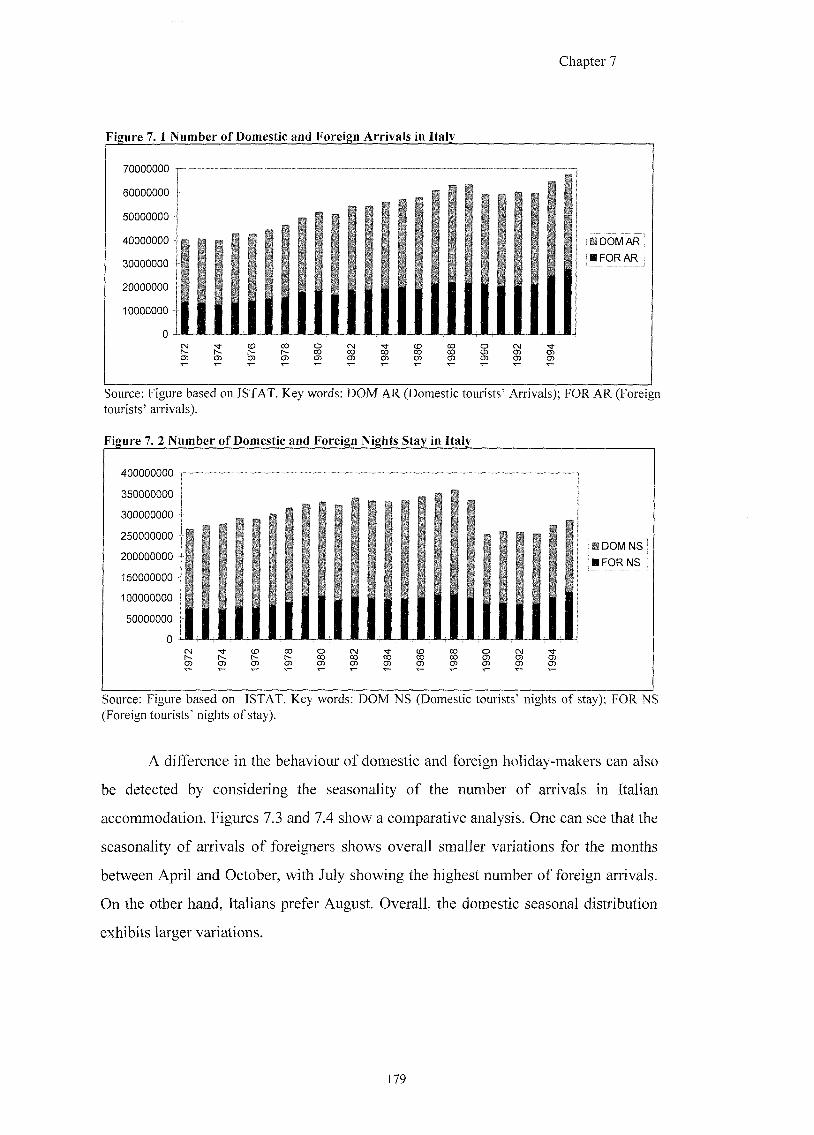
Chapter 7

Figure 7. 1 Number of Domestic and Foreign Arrivals in Italy

70000000

60000000

50000000

40000000

30000000

20000000

10000000

0

DDOMAR HFORAR

CO CO SS ™ cn CD O) O CM ^ a> cr> a> cn cn

Source: Figure based on ISTAT. Key words: DOM AR (Domestic tourists' Arrivals); FOR AR (Foreign tourists' arrivals).

Figure 7. 2 Number of Domestic and Foreign Nights Stay in Italy

400000000

350000000

300000000

250000000

200000000

150000000

100000000

50000000

0

ODOMNS • FOR NS

S G)

(O 00 CO CO O) 0) i CM -f O) O) O) CT)

Source: Figure based on ISTAT. Key words; DOM NS (Domestic tourists' nights of stay); FOR NS (Foreign tourists' nights of stay).

A difference in the behaviour of domestic and foreign holiday-makers can also

be detected by considering the seasonality of the number of arrivals in Italian

accommodation. Figures 7.3 and 7.4 show a comparative analysis. One can see that the

seasonality of arrivals of foreigners shows overall smaller variations for the months

between April and October, with July showing the highest number of foreign arrivals.

On the other hand, Italians prefer August. Overall, the domestic seasonal distribution

exhibits larger variations.

179

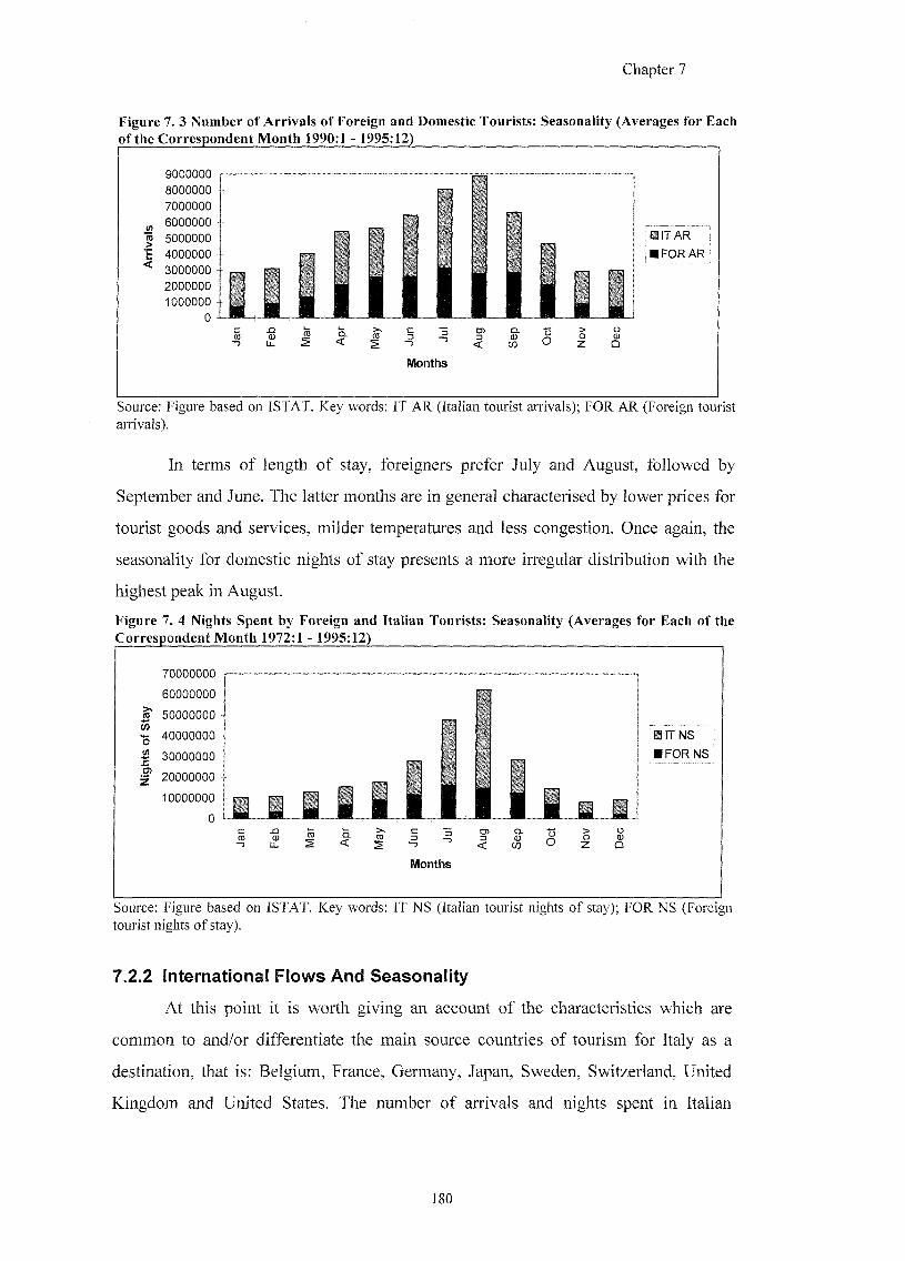
Chapter 7

Figure 7. 3 Number of Arrivals of Foreign and Domestic Tourists: Seasonality (Averages for Each of the Correspondent Month 1990:1 -1995:12)

9000000 8000000 7000000

* 6000000 ra 5000000 'E 4000000 ^ 3000000

2000000 1000000

0

• FORAR

Months

Source; Figure based on ISTAT. Key words: IT AR (Italian tourist arrivals); FOR AR (Foreign tourist arrivals).

In terms of length of stay, foreigners prefer July and August, followed by

September and June. The latter months are in general characterised by lower prices for

tourist goods and services, milder temperatures and less congestion. Once again, the

seasonality for domestic nights of stay presents a more irregular distribution with the

highest peak in August.

Figure 7. 4 Nights Spent by Foreign and Italian Tourists: Seasonality (Averages for Each of the Correspondent Month 1972:1 - 1995:12)

70000000

60000000

^ 50000000

^ 40000000

B 30000000

5 20000000

10000000

a IT NS

• FOR NS

Months

Source: Figure based on ISTAT. Key words: IT NS (Italian tourist nights of stay); FOR NS (Foreign tourist nights of stay).

7.2.2 International Flows And Seasonality

At this point it is worth giving an account of the characteristics which are

common to and/or differentiate the main source countries of tourism for Italy as a

destination, that is: Belgium, France, Germany, Japan, Sweden, Switzerland, United

Kingdom and United States. The number of arrivals and nights spent in Italian

180

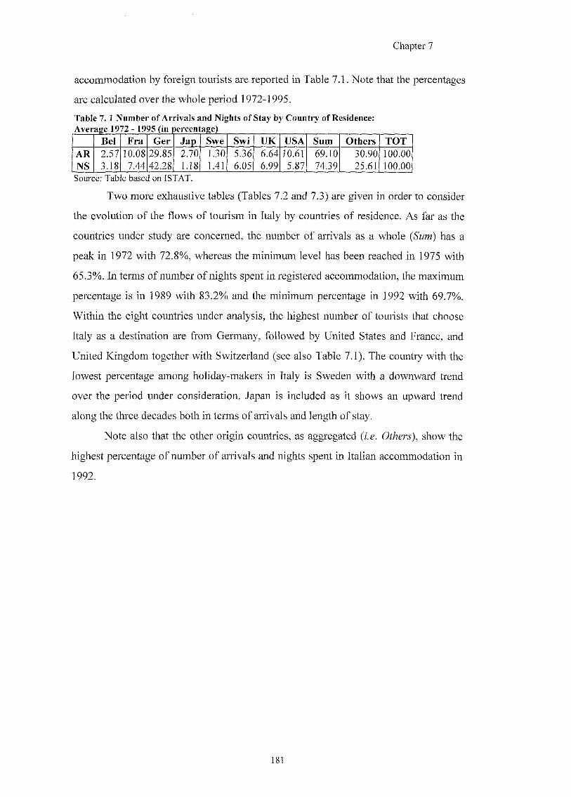
Chapter 7

accommodation by foreign tourists are reported in Table 7.1. Note that the percentages

are calculated over the whole period 1972-1995.

Table 7. 1 Number of Arrivals and Nights of Stay by Country of Residence:

Bel F ra Ger Jap Swe Swi U K USA Sum Others T O T

A R

NS

2.57 3.18

10.08 7.44

29.85 42.28

2.70 ].18

1.30 1.41

5.36 6.05

6.64 6.99

10.61 5.87

69.10 74.39

30.90 25.61

100.00 100.00

Source: Table based on ISTAT.

Two more exhaustive tables (Tables 7.2 and 7.3) are given in order to consider

the evolution of the flows of tourism in Italy by countries of residence. As far as the

countries under study are concerned, the number of arrivals as a whole (6'wyM) has a

peak in 1972 with 72.8%, whereas the minimum level has been reached in 1975 with

65.3%. In terms of number of nights spent in registered accommodation, the maximum

percentage is in 1989 with 83.2% and the minimum percentage in 1992 with 69.7%.

Within the eight countries under analysis, the highest number of tourists that choose

Italy as a destination are from Germany, followed by United States and France, and

United Kingdom together with Switzerland (see also Table 7.1). The country with the

lowest percentage among holiday-makers in Italy is Sweden with a downward trend

over the period under consideration. Japan is included as it shows an upward trend

along the three decades both in terms of arrivals and length of stay.

Note also that the other origin countries, as aggregated (z.e. show the

highest percentage of number of arrivals and nights spent in Italian accommodation in

1992.

181

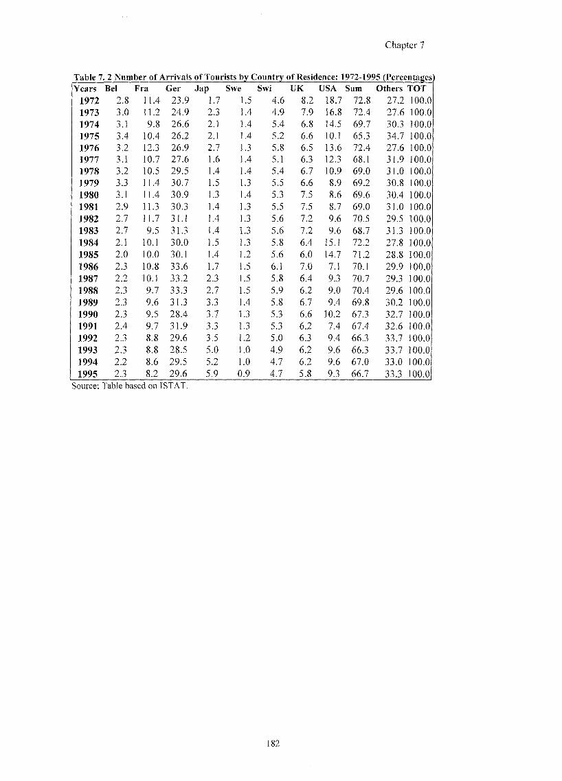
Chapter 7

Table 7. 2 Number of Arrivals of Tourists by Country of Residence: 1972-1995 (Percentages) Years Bel Fra Ger Jap Swe Swi UK USA Sum Others TOT

1972 2.8 1L4 2 1 4 1.7 1.5 4.6 8.2 1&7 7Z8 27.2 100.0

1973 3.0 11^ 2 4 4 2.3 1.4 4.9 7.9 16.8 724 27.6 lO&O

1974 3.1 9.8 2&6 2.1 1.4 5.4 6.8 14.5 6 9 J 3 0 J lO&O

1975 3.4 1&4 26.2 2.1 1.4 5.2 6.6 10.1 65J 34.7 lO&O 1976 3.2 12J 26.9 2.7 1.3 5.8 6.5 13.6 7Z4 2 7 ^ lO&O 1977 3.1 l O J 27.6 1.6 1.4 5.1 6.3 123 68J 3L9 lO&O 1978 3.2 10^ 29.5 1.4 1.4 5.4 6.7 10.9 690 3L0 100.0 1979 3.3 11.4 3&7 1.5 1.3 5.5 6.6 8.9 692 3&8 lO&O 1980 3.1 11^ 30.9 1.3 1.4 5.3 7.5 8.6 69.6 3&4 100.0 1981 2.9 11.3 30JI 1.4 1.3 5.5 7.5 8.7 6&0 3L0 100.0 1982 2.7 11.7 31.1 1.4 1.3 5.6 7.2 9.6 7 0 j 2 9 j 100.0 1983 2.7 9.5 3L3 1.4 1.3 5.6 7.2 9.6 6 8 J 3L3 100.0 1984 2.1 lOJ 30.0 1.5 1.3 5.8 6.4 15J 722 2%8 100.0 1985 2.0 l&O 3&1 1.4 1.2 5.6 6.0 14.7 7L2 2&8 100.0 1986 2.3 10^ 33.6 1.7 1.5 6.1 7.0 7.1 70^ 299 100.0 1987 2.2 lOJ 33.2 2.3 1.5 5.8 6.4 9.3 7 0 J 2 9 J 100.0 1988 2.3 9.7 33JI 2.7 1.5 5.9 6.2 9.0 7&4 2 9 j 100.0 1989 2.3 9.6 3L3 3.3 1.4 5.8 6.7 9.4 69.8 302 100.0 1990 2.3 9.5 2&4 3.7 1.3 5.3 6.6 10.2 673 327 100.0 1991 2.4 9.7 3 L 9 3.3 1.3 5.3 6.2 7.4 67.4 326 100.0 1992 2.3 8.8 29.6 3.5 1.2 5.0 6.3 9.4 6 6 J 3 3 J 100.0 1993 2.3 8.8 2&5 5.0 1.0 4.9 6.2 9.6 6&3 317 100.0 1994 2.2 8.6 2&5 5.2 1.0 4.7 6.2 9.6 67.0 310 100.0 1995 2.3 8.2 29.6 5.9 0.9 4.7 5.8 9.3 66.7 313 100.0

Source: Table based on ISTAT.

182

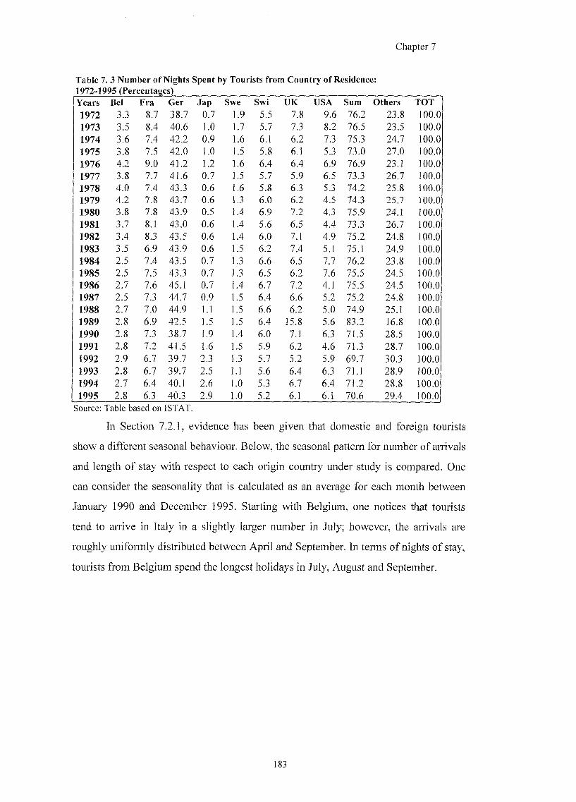
Chapter 7

Table 7. 3 Number of Nights Spent by Tourists from Country of Residence;

Years Bel Fra Ger Jap Swe Swi UK USA Sum Others TOT

1972 3.3 8.7 38.7 0.7 1.9 5.5 7.8 9.6 76.2 2 1 8 100.0

1973 3.5 8.4 40.6 1.0 1.7 5.7 7.3 8.2 76.5 2 1 5 100.0

1974 3.6 7,4 42.2 0.9 1.6 6.1 6.2 7.3 7 5 J 2 4 J lO&O

1975 3.8 7.5 42.0 1.0 1.5 5.8 6.1 5.3 73.0 2 7 0 100.0

1976 4.2 9.0 4 L 2 1.2 1.6 6.4 6.4 6.9 76.9 2 1 1 100.0

1977 3.8 7.7 4 L 6 0.7 1.5 5.7 5.9 6.5 7 1 3 2&7 lO&O

1978 4.0 7.4 4 3 J 0.6 1.6 5.8 6.3 5.3 74.2 2 5 ^ lO&O 1979 4.2 7.8 43.7 0.6 1.3 6.0 6.2 4.5 7 4 3 2 5 J 100.0 1980 3.8 7.8 43.9 0.5 1.4 6.9 7.2 4.3 75.9 2 4 J 100.0 1981 3.7 8.1 43.0 0.6 1.4 5.6 6.5 4.4 7 1 3 2&7 100.0 1982 3.4 8.3 4 3 ^ 0.6 1.4 6.0 7.1 4.9 75.2 2 4 ^ 100.0 1983 3.5 6.9 4 1 9 0.6 1.5 6.2 7.4 5.1 7 5 1 2 4 4 100.0 1984 2.5 7.4 4 1 5 0.7 1.3 6.6 6.5 7.7 76.2 2 1 8 100.0 1985 2.5 7.5 4 3 J 0.7 1.3 6.5 6.2 7.6 75.5 2 4 ^ 100.0 1986 2.7 7.6 4 5 J 0.7 1.4 6.7 7.2 4.1 7 5 j 24 j 100.0 1987 2.5 7.3 4 4 J 0.9 1.5 6.4 6.6 5.2 7 5 ^ 2 4 ^ 100.0 1988 2.7 7.0 4 4 4 1.1 1.5 6.6 6.2 5.0 7 4 4 2 5 J 100.0 1989 2.8 6.9 4 2 5 1.5 1.5 6.4 15.8 5.6 8 1 2 16.8 100.0 1990 2.8 7.3 3&7 1.9 1.4 6.0 7.1 6.3 7L5 2&5 100.0 1991 2.8 7.2 4 L 5 1.6 1.5 5.9 6.2 4.6 7 L 3 2 8 J 100.0 1992 2.9 6.7 3 9 J 2.3 1.3 5.7 5.2 5.9 6 9 J 3 0 J 100.0 1993 2.8 6.7 3 9 J 2.5 1.1 5.6 6.4 6.3 71.1 2 8 4 100.0 1994 2.7 6.4 4 0 J 2.6 1.0 5.3 6.7 6.4 7 L 2 2 8 ^ 100.0 1995 2.8 6.3 4 0 J 2.9 1.0 5.2 6.1 6.1 7&6 29^4 100.0

Source; Table based on ISTAT.

In Section 7.2.1, evidence has been given that domestic and foreign tourists

show a different seasonal behaviour. Below, the seasonal pattern for number of arrivals

and length of stay with respect to each origin country under study is compared. One

can consider the seasonality that is calculated as an average for each month between

January 1990 and December 1995. Starting with Belgium, one notices that tourists

tend to arrive in Italy in a slightly larger number in July; however, the arrivals are

roughly uniformly distributed between April and September. In terms of nights of stay,

tourists from Belgium spend the longest holidays in July, August and September.

183

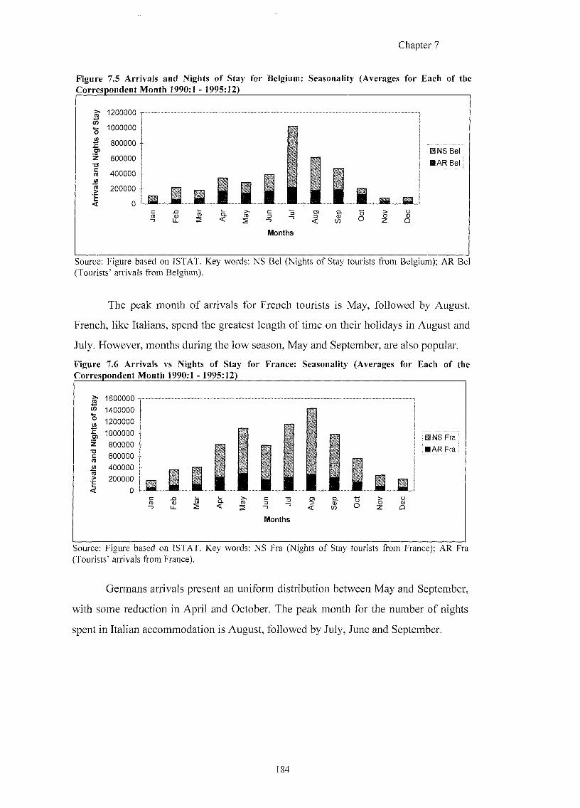
Chapte r 7

Figure 7.5 Arrivals and Nights of Stay for Belgium: Seasonality (Averages for Each of the Correspondent Month 1990:1 - 1995:12)

to %

I Oi -O c (0 * g

1200000

1000000

800000

600000

400000

200000

INS Bel

lAR Bel

Months

Source: Figure based on ISTAT. Key words: NS Bel (Nights of Stay tourists from Belgium); AR Bel (Tourists' arrivals from Belgium).

The peak month of arrivals for French tourists is May, followed by August.

French, like Italians, spend the greatest length of time on their holidays in August and

July. However, months during the low season. May and September, are also popular.

Figure 7.6 Arrivals vs Nights of Stay for France: Seasonality (Averages for Each of the Correspondent Month 1990:1 - 1995:12)

> 1600000

W 1400000

1200000

1000000 NS Fra 800000

A R F m 600000 400000

200000

Months

Source: Figure based on ISTAT. Key words: NS Fra (Nights of Stay tourists from France); AR Fra (Tourists' arrivals from France).

Germans arrivals present an uniform distribution between May and September,

with some reduction in April and October. The peak month for the number of nights

spent in Italian accommodation is August, followed by July, June and September.

184

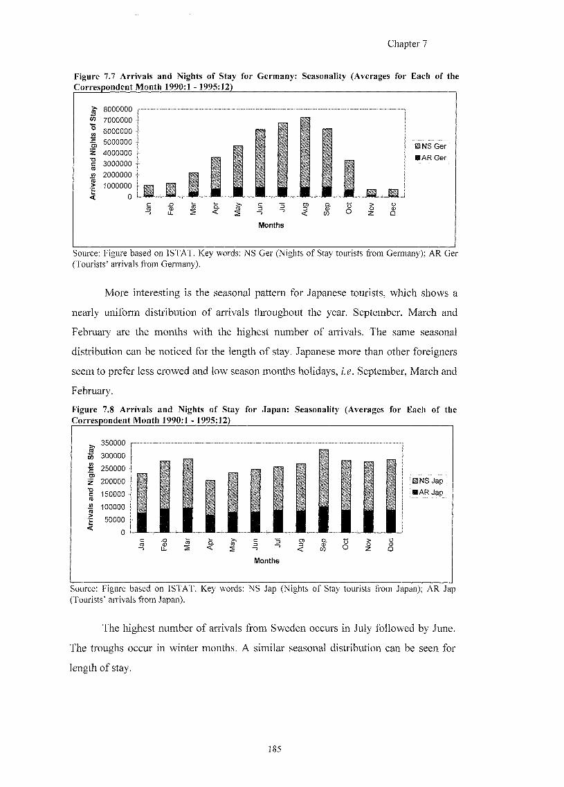
Chapte r 7

Figure 7.7 Arrivals and Nights of Stay for Germany: Seasonality (Averages for Each of the Correspondent Month 1990:1 -1995:12)

8000000 w 7000000 o B

6000000 s: 5000000 Z 4000000 •o c 3000000

iS 2000000 ,> 1000000

< 0

HNS Ger • AR Ger

Months

Source: Figure based on ISTAT. Key words: NS Ger (Nights of Stay tourists from Germany); AR Ger (Tourists' arrivals from Germany).

More interesting is the seasonal pattern for Japanese tourists, which shows a

nearly uniform distribution of arrivals throughout the year. September, March and

February are the months with the highest number of arrivals. The same seasonal

distribution can be noticed for the length of stay. Japanese more than other foreigners

seem to prefer less crowed and low season months holidays, i.e. September, March and

February.

Figure 7.8 Arrivals and Nights of Stay for Japan: Seasonality (Averages for Each of the Correspondent Month 1990:1 - 1995:12)

350000 ro w 300000

1 250000 O)

z 200000

? 150000 TO w (5

100000 > fc 50000 <

0 0

INS Jap lAR Jap

Months

Source: Figure based on ISTAT. Key words: NS Jap (Nights of Stay tourists from Japan); AR Jap (Tourists' arrivals from Japan).

The highest number of arrivals from Sweden occurs in July followed by June.

The troughs occur in winter months. A similar seasonal distribution can be seen for

length of stay.

185

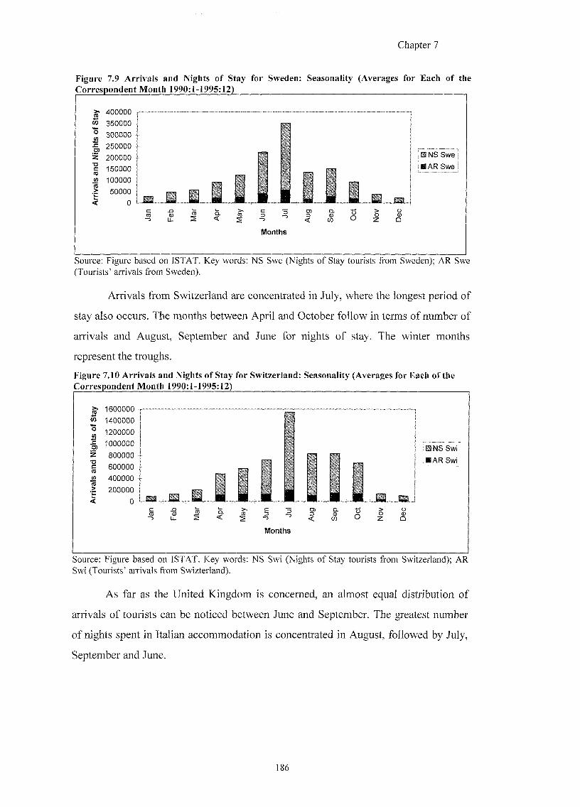
Chapte r 7

Figure 7.9 Arrivals and Nights of Stay for Sweden: Seasonality (Averages for Each of the Correspondent Month 1990:1-1995:12)

>• 400000

W 350000

200000

150000

!» 100000

50000

INS Swe

IAR Swe

Months

Source: Figure based on ISTAT. Key words: NS Swe (Nights of Stay tourists from Sweden); AR Swe (Tourists' arrivals from Sweden).

Arrivals from Switzerland are concentrated in July, where the longest period of

stay also occurs. The months between April and October follow in terms of number of

arrivals and August, September and June for nights of stay. The winter months

represent the troughs.

Figure 7.10 Arrivals and Nights of Stay for Switzerland: Seasonality (Averages for Each of the Correspondent Month 1990:1-1995:12)

1600000 3) 1400000

1200000

1000000

800000

600000

400000

200000 0

0

1 O) z •o c ro

m >

# N S Swi

BAR Swi:

Months

Source: Figure based on ISTAT. Key words; NS Swi (Nights of Stay tourists from Switzerland); AR Swi (Tourists' arrivals from Swizterland).

As far as the United Kingdom is concerned, an almost equal distribution of

arrivals of tourists can be noticed between June and September. The greatest number

of nights spent in Italian accommodation is concentrated in August, followed by July,

September and June.

186

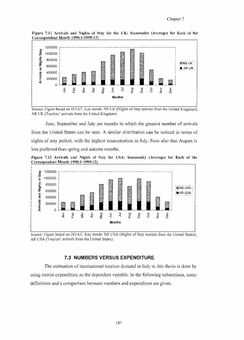
Chap te r 7

Figure 7.11 Arrivals and Nights of Stay for the UK: Seasonality (Averages for Each of the Correspondent Month 1990:1-1995:12)

CO

i I

1200000

1000000

800000

600000

400000

•£ 200000

INS UK I AR UK

> o O ffl Z Q

Months

Source; Figure based on ISTAT. Key words; NS UK (Nights of Stay tourists from the United Kingdom); AR UK (Tourists' arrivals from the United Kingdom).

June, September and July are months in which the greatest number of arrivals

from the United States can be seen. A similar distribution can be noticed in terms of

nights of stay period, with the highest concentration in July. Note also that August is

less preferred than spring and autumn months.

Figure 7.12 Arrivals and Nights of Stay for USA: Seasonality (Averages for Each of the Correspondent Month 1990:1-1995:12)

w 0

1 •D C to tn

1200000

1000000

800000

600000

400000

200000

ONS USA ;

BAR USA

Months

Source: Figure based on ISTAT. Key words; NS USA (Nights of Stay tourists from the United States); AR USA (Tourists' arrivals from the United States).

7.3 NUMBERS VERSUS EXPENDITURE

The estimation of international tourism demand in Italy in this thesis is done by

using tourist expenditure as the dependent variable. In the following subsections, some

definitions and a comparison between numbers and expenditure are given.

187

Chapter 7

7.3.1 Some Definitions

It is important to give a prior definition of tourism expenditure. According to

the World Tourism Organisation (WTO) tourism expenditure is defined as "the total

consumption expenditure made by a visitor or on behalf of a visitor for and during

his/her trip and stay at destination" (Nordstrom, 1996, p. 15). Total tourist expenditure

measures a global quantity. In particular, tourist expenditure in any country can be

expressed as the product of three factors: the number of tourists, average length of stay

and average expenditure per (yze/M. It may be very important to know which of the

factors is responsible for a given change in expenditure. For example, a fall in

expenditure may be accompanied by an increase in numbers, reflecting a decrease in

the average length of stay and/or average expenditure jpgr

Tourist expenditure data are collected using three different methods, that is:

bank records of foreign exchange transactions, surveys of tourists and surveys of

tourism establishments. It appears that a good indicator for the real demand of tourism

can be obtained by surveys that include information on private consumption behaviour

for different kinds of goods and services such as accommodation, transportation, food

and so on.

In Italy the main source of tourist expenditure data are bank records. In

particular, tourist expenditure data are collected as bank records of foreign exchange

transactions that can be considered as a proxy for tourism expenditure. The item

"Foreign travel" in the balance of payments contains the expenditure of the "traveller".

The "traveller", in this particular context, is defined as a person who spends a given

period of time in another economy with a purpose different from working within that

economy as an employee of the visited country and without becoming a citizen of that

country. Travellers can be divided into two categories: a) excursionists, those who visit

a foreign country for less than 24 hours; b) tourists, those who spend at least one night

in the foreign country.

The item "Foreign travel" includes a consumption basket of goods and services

such as: accommodation, re6eshments, amusements, souvenirs and means of

transportation within the visited country. However, it does not include expenditure for

international travel. In more detail, the item "Foreign travel" includes the following

components:

Chapter 7

a) bank transfers on residents' and non-residents' account, for tourism, business,

health, study and for other tourist services;

b) transactions with credit card issuers;

c) purchases/sales of petrol coupons;

d) forwarding/receiving of Italian coupons;

e) direct negotiation of bills, coins and other means of payments, denominated in

foreign currencies or in lire, with residents and non-residents (traveller cheques,

drawings from cash dispensers, bank cheques with value up to 20 million lire).

Ad hoc criteria have been used to avoid statistical problems. In the Seventies,

for example, there was a realisation that the remittances of Italian banknotes by Swiss

banks in Italy was due to capital investments rather than activities for tourism. Such

remittances, originally exported to Italy illegally, were included into the item

"movements of capital". However, from 1987 on, since this phenomenon was over the

statistical computation was back to the aw/e. Another under-estimation of

tourist receipts and expenditures, in the Seventies, was given by the monetary

restrictions in terms of the maximum amount of money that could be taken into

another country. All the banknotes which circulated outside the bank system were not

subject to any statistical computation. From the second half of the Eighties, given the

increase of the maximum amount of money portable into another country, the quality

of the data improved. In 1988, currency liberalisation extended the variety of means of

payments that are used extensively in financing tourist expenditure (Banca D'Italia,

1995, pp. 7-10).

Ballatori and Vaccaro (1992) point out further limitations of tourism

expenditure data. For example, they do not give any information about the motives for

tourism (holiday, business, sport, health, etc); moreover, these data refer to the time in

which the currency transaction occurred, whereas no information is given on the

moment in which the expenditure takes place (pp. 206-216).

7.3.2 A Comparison Between Numbers And Expenditure

As previously stated, it would be of interest to better understand the

relationship between numbers and expenditure. For this purpose international tourists'

arrivals, nights of stay, nominal tourism receipts and real tourism receipts are

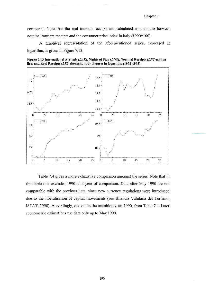
Chapter 7

compared. Note that the real tourism receipts are calculated as the ratio between

nominal tourism receipts and the consumer price index in Italy (1990=100).

A graphical representation of the aforementioned series, expressed in

logarithm, is given in Figure 7.13.

Figure 7.13 International Arrivals {LAR), Nights of Stay (JLNS), Nominal Receipts (ZA'T'-niillion lire) and Real Receipts (AAF-thousand lire). Figures in logarithm (1972-1995)

— LAR 1 18.5

17 ^

[

1

1 & 4 - / /

6.75 '•

16^1

[

/

\/

I S J r /

18.1 r

0 5 10 15 20 25 0 5 10 15 20 25

tL-z -LNTJ / Lj — l r t I 19.5:-

, /

-/

/

r-' 19:

15 1- 1&5: /

0 5 10 15 20 25 0 5 10 15 20 25

Table 7.4 gives a more exhaustive comparison amongst the series. Note that in

this table one excludes 1990 as a year of comparison. Data after May 1990 are not

comparable with the previous data, since new currency regulations were introduced

due to the liberalisation of capital movements (see Bilancia Valutaria del Turismo,

IS TAT, 1990). Accordingly, one omits the transition year, 1990, from Table 7.4. Later

econometric estimations use data only up to May 1990.

190

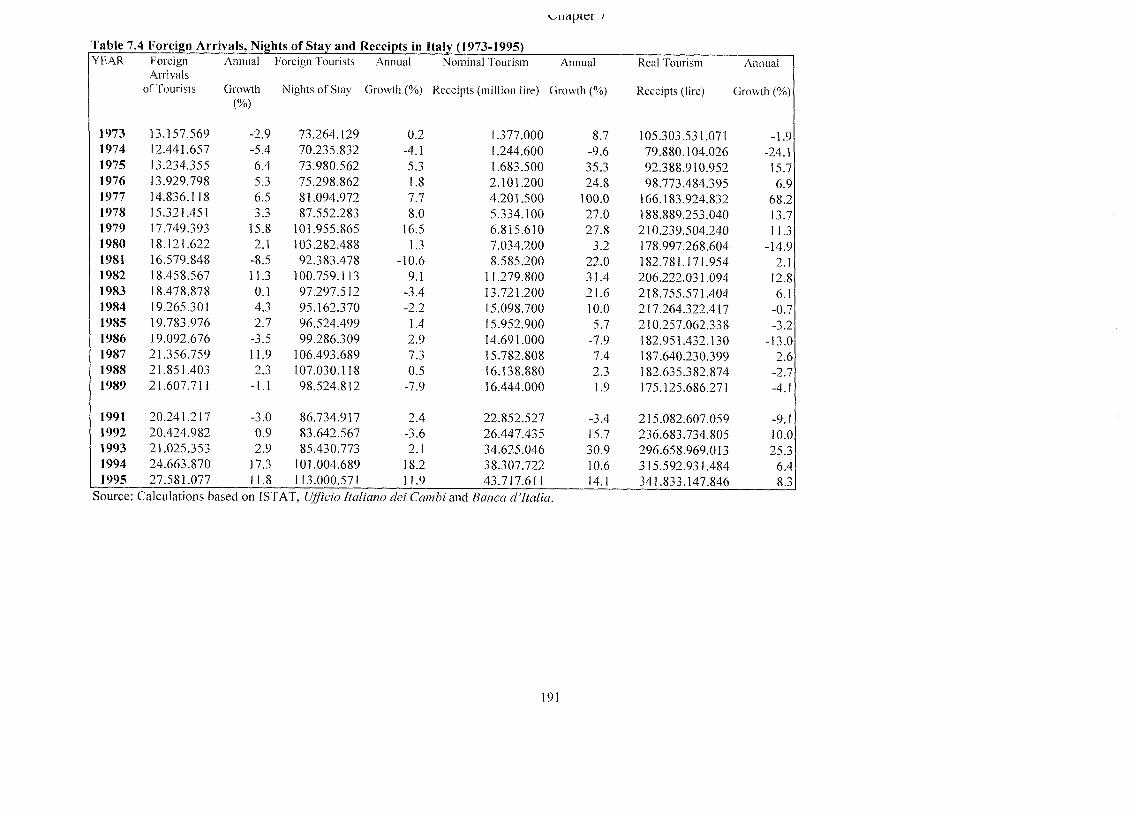
" iiapicr / Table 7.4 Foreign Arrivals, Nights of Stay and Receipts in Italy (1973-1995) YEAR Foreign Annual Foreign Tourists Annual Nominal Tourism Annual Real Tourism Annual

Arrivals

of Tourists Growth Nights of Stay Growth (%) Receipts (million lire) Growth (%) Receipts (lire) Growth (%) (%)

Growth (%)

1 9 7 3 1 3 . 1 5 7 . 5 6 9 - 2 . 9 7 3 . 2 6 4 . 1 2 9 0 .2 1 . 3 7 7 . 0 0 0 8 .7 1 0 5 . 3 0 3 . 5 3 1 . 0 7 1 - 1 . 9 1 9 7 4 1 2 . 4 4 1 . 6 5 7 - 5 . 4 7 0 . 2 3 5 . 8 3 2 -4 .1 1 . 2 4 4 . 6 0 0 - 9 . 6 7 9 . 8 8 0 . 1 0 4 . 0 2 6 -24 .1 1 9 7 5 1 3 . 2 3 4 . 3 5 5 6 . 4 7 3 . 9 8 0 . 5 6 2 5 .3 1 . 6 8 3 . 5 0 0 3 5 . 3 9 2 . 3 8 8 . 9 1 0 . 9 5 2 15.7 1 9 7 6 1 3 . 9 2 9 . 7 9 8 5 .3 7 5 . 2 9 8 . 8 6 2 1.8 2 . 1 0 1 . 2 0 0 2 4 . 8 9 8 . 7 7 3 . 4 8 4 . 3 9 5 6 . 9 1 9 7 7 1 4 . 8 3 6 . 1 1 8 6 .5 8 1 . 0 9 4 . 9 7 2 7 . 7 4 . 2 0 1 . 5 0 0 100 .0 1 6 6 . 1 8 3 . 9 2 4 . 8 3 2 6 8 . 2 1 9 7 8 1 5 . 3 2 1 . 4 5 1 3 .3 8 7 . 5 5 2 . 2 8 3 8 . 0 5 . 3 3 4 . 1 0 0 2 7 . 0 1 8 8 . 8 8 9 . 2 5 3 . 0 4 0 13.7 1 9 7 9 1 7 . 7 4 9 . 3 9 3 15 .8 1 0 1 . 9 5 5 . 8 6 5 16 .5 6 . 8 1 5 . 6 1 0 2 7 . 8 2 1 0 . 2 3 9 . 5 0 4 . 2 4 0 11.3 1 9 8 0 1 8 . 1 2 1 . 6 2 2 2 .1 1 0 3 . 2 8 2 . 4 8 8 1.3 7 . 0 3 4 . 2 0 0 3.2 1 7 8 . 9 9 7 . 2 6 8 . 6 0 4 - 1 4 . 9 1981 1 6 . 5 7 9 . 8 4 8 -8 .5 9 2 . 3 8 3 . 4 7 8 - 1 0 . 6 8 . 5 8 5 . 2 0 0 2 2 . 0 1 8 2 . 7 8 1 . 1 7 1 . 9 5 4 2.1 1 9 8 2 1 8 . 4 5 8 . 5 6 7 11.3 1 0 0 . 7 5 9 . 1 1 3 9.1 1 1 . 2 7 9 . 8 0 0 3 1 . 4 2 0 6 . 2 2 2 . 0 3 1 . 0 9 4 12.8 1 9 8 3 1 8 . 4 7 8 . 8 7 8 0.1 9 7 . 2 9 7 . 5 1 2 - 3 . 4 1 3 . 7 2 1 . 2 0 0 2 1 . 6 2 1 8 . 7 5 5 . 5 7 1 . 4 0 4 6 .1 1 9 8 4 1 9 . 2 6 5 . 3 0 1 4 . 3 9 5 . 1 6 2 . 3 7 0 - 2 . 2 1 5 . 0 9 8 . 7 0 0 10 .0 2 1 7 . 2 6 4 . 3 2 2 . 4 1 7 - 0 . 7 1 9 8 5 1 9 . 7 8 3 . 9 7 6 2 . 7 9 6 . 5 2 4 . 4 9 9 1.4 1 5 . 9 5 2 . 9 0 0 5 .7 2 1 0 . 2 5 7 . 0 6 2 . 3 3 8 - 3 . 2 1 9 8 6 1 9 . 0 9 2 . 6 7 6 -3 .5 9 9 . 2 8 6 . 3 0 9 2 . 9 1 4 . 6 9 1 . 0 0 0 - 7 . 9 1 8 2 . 9 5 1 . 4 3 2 . 1 3 0 - 1 3 . 0 1 9 8 7 2 1 . 3 5 6 . 7 5 9 11 .9 1 0 6 . 4 9 3 . 6 8 9 7.3 1 5 . 7 8 2 . 8 0 8 7 . 4 1 8 7 . 6 4 0 . 2 3 0 . 3 9 9 2 . 6 1 9 8 8 2 1 . 8 5 1 . 4 0 3 2 . 3 1 0 7 . 0 3 0 . 1 1 8 0 . 5 1 6 . 1 3 8 . 8 8 0 2 .3 1 8 2 . 6 3 5 . 3 8 2 . 8 7 4 -2 .7 1 9 8 9 2 1 . 6 0 7 . 7 1 1 -1 . 1 9 8 . 5 2 4 . 8 1 2 - 7 . 9 1 6 . 4 4 4 . 0 0 0 1.9 1 7 5 . 1 2 5 . 6 8 6 . 2 7 1 -4 .1

1 9 9 1 2 0 . 2 4 1 . 2 1 7 - 3 . 0 8 6 . 7 3 4 . 9 1 7 2 . 4 2 2 . 8 5 2 . 5 2 7 - 3 . 4 2 1 5 . 0 8 2 . 6 0 7 . 0 5 9 -9.1 1 9 9 2 2 0 . 4 2 4 . 9 8 2 0 . 9 8 3 . 6 4 2 . 5 6 7 - 3 . 6 2 6 . 4 4 7 . 4 3 5 15.7 2 3 6 . 6 8 3 . 7 3 4 . 8 0 5 10 .0 1 9 9 3 2 1 . 0 2 5 . 3 5 3 2 . 9 8 5 . 4 3 0 . 7 7 3 2 .1 3 4 . 6 2 5 . 0 4 6 3 0 . 9 2 9 6 . 6 5 8 . 9 6 9 . 0 1 3 2 5 . 3 1 9 9 4 2 4 . 6 6 3 . 8 7 0 17.3 1 0 1 . 0 0 4 . 6 8 9 18 .2 3 8 . 3 0 7 . 7 2 2 10.6 3 1 5 . 5 9 2 . 9 3 1 . 4 8 4 6 ,4 1 9 9 5 2 7 . 5 8 1 . 0 7 7 11.8 1 1 3 . 0 0 0 . 5 7 1 11 .9 4 3 . 7 1 7 . 6 1 1 14.1 3 4 1 . 8 3 3 . 1 4 7 . 8 4 6 8 .3

Source: Calculations based on ISTAT, /W/aMo and (/VW/a.

191

Chapter 7

In the first period (1973-1989), it is interesting to note that in 8 out of 17 cases,

arrivals, nights of stay, nominal and real receipts move in the same direction. In 1974,

for example, Italian tourism declines both in terms of numbers and expenditure. The

highest expansion in terms of receipts has been experienced in 1977 with a continuous

growth in the following two years. The first half of the Eighties sees a decline in the

growth of number of tourists. With the exception for the year 1982, where the number

of foreign arrivals reach almost 18.5 million, the nights of stay in Italian registered

accommodation were 100 million, the nominal receipts almost 11 thousand billion lire,

and, finally, the real receipts two hundred billion lire. Note also that the decline of

growth for Italian tourism in these years is picked up by the nominal receipts figures

only in 1986, with a fall of almost 8% over the previous year. The year 1987 sees an

increase in Italian tourism, followed by a fall in 1989.

In the second period (1991-1995), 3 out of the 5 times these series move in the

same direction. After a decline in the growth of tourism, more evident in terms of

numbers than receipts, there is a new upward trend which could be associated with the

devaluation of the lira in 1992. Other factors have positively influenced Italian tourism

such as the war in Yugoslavia which negatively affected the transit towards Turkey

and Greece.

Overall, there are many instances in which the differences amongst the four

series are of considerable magnitude and many others in which they move in a

different direction. In terms of simple correlation analysis for the first period (1973-

1989) the values are the following: r( .R,jV5)=0.92, r(7V7 j(7)=0.756, r(/4j(,jV7)=0.95,

r(v4j?,JZ7]=0.76, r(7V5 jV7)=0.83 and, finally, r(A%./Zr)=0.&4. The highest positive

correlation is given by the total number of foreign arrivals of tourists (y jZ) and the

nominal tourism receipts (NT). Note also that the total number of nights spent in

registered accommodation by foreigners shows a higher correlation with the real

tourism receipts (RT) than the total number of arrivals with the latter series.

For the second period (1991-1995) the values are the following;

r(.4^M$)=0.99, r(jV7:j;7)=0.996, r(v4jg,#r)=0.91, r(y4J2,;;73=0.87, r(A%M)-0.85 and,

finally, r(A%^7)=0.81. The highest positive correlation is given by the nominal

tourism receipts (NT) and the real tourism receipts (RT), and by the total number of

foreign arrivals of tourists (v4.R) and total number of nights of stay. The pair of total

192

Chapter 7

number of arrivals {AR) and nominal tourism receipts {NT) presents a correlation value

equal to 0.91.

7.4 CONCLUSIONS

This chapter has been dedicated to a general discussion of the demand for

tourism in Italy. A graphical basis has been provided for distinguishing domestic from

international tourism demand. Differences have been identified both in terms of

historic evolution and seasonality of demand. These findings encourage the author to

distinguish the two components.

The characteristics for each of the main origin countries have been investigated.

Germany, France, U.S.A., UK and Switzerland are the clients with the highest number

of arrivals and nights of stay in Italy. These countries, except Switzerland, have also

shown a more regular seasonal pattern, more visible in terms of nights of stay. The

other source countries, that is Belgium, Sweden and Switzerland are characterised by

an irregular seasonal distribution. Interestingly, Japan, that has shown an upward trend

during the years between 1972 and 1995, is characterised by an almost uniform

distribution in terms of arrivals and nights of stay.

Some definitions have been provided for tourism expenditure and a description

of the method used by the Bank of Italy in collecting the tourism receipts data. The

other aim of the chapter has been to make a comparison between numbers and

expenditure. The sample period has been divided into two, as a discontinuity of the

time series is due to different currency regulations introduced from June 1990. As far

as the first sample period is concerned (1973-1989), a strong positive correlation has

been found between number of foreign arrivals and nominal tourism receipts. The

lowest correlation is obtained for the pair nominal and real receipts. Note also that the

correlation between nights of stay and real tourism receipts has been found higher than

the correlation for the pair arrivals and real tourism receipts. The latter finding seems

to confirm the belief that the longer a tourist stays in a certain destination the more

he/she is likely to spend (Sheldon, 1993).

193

Chapter 8

CHAPTER 8.

ESTIMATING THE DEMAND FOR ITALIAN TOURISM

Aim of the Chapter:

To examine and model the international demand of tourism in Italy using monthly

tourist expenditure.

8.1 INTRODUCTION

This chapter is dedicated to estimating Italian international tourism demand. As

far as Italy is concerned, data on the actual amounts spent by tourists from the main

origin countries do not exist for the period under study. Hence, tourist demand will be

expressed in terms of tourist receipts defined in terms of foreign currency exchange

transactions of value less than 20 millions of hre (see Chapter 7, Section 7.3.1). In the

present study, monthly data will be employed for the period 1972:1-1990:5; as already

pointed out in Ch^ter 7, a new currency regulation has been introduced 6om June

1990 on.

In this chapter, two distinct variables will be used as dependent variables; real

tourist receipts and a weighted budget share for the main origin countries of tourism to

Italy. In the majority of time-series empirical studies on tourism, real tourist receipts

are employed as the dependent variable (e.g. Lee a/., 1993; Garcla-Ferrer and

Queralt, 1997). On the other hand, the budget share variable is commonly used in

panel data studies (Fujii a/., 1985; Syriopoulos and Sinclair, 1993). The purpose of

this chapter is to use the weighted average budget share of tourism in Italy in a time-

series context. The aim is to understand which of the two variables best can be used to

model the demand for tourism.

A "pre-modelling" analysis is carried out in order to identify the properties of the

variables that one expects to influence tourism demand in Italy according to economic

theory. Hence, once the integration and possibly cointegration status of such variables

is established, one makes use of the LSE methodology. In this way, it will be possible

to determine income and price elasticities that will be evaluated theoretically. It will

194

Chapter 8

also be possible to identify the explanatory power of other qualitative variables such as

seasonal dummies and an "Easter" dummy included in the model.

At this point, a brief note has to be given on the supply constraint. One of the

main assumptions in estimating the international demand for tourism in Italy is that

one can assume the existence of no supply constraint. As Syriopoulos (1995) notes, "it

is reasonable to accept that the supply of tourism does not impose any constraints on

tourism demand" (p.321). This assumption is based on two arguments. The first

argument is that hotels and tourist infrastructure are constructed to satisfy not only the

current consumption but also the consumption in the future. Secondly, tourists make

increasing use of accommodation other than registered accommodation, e.g. second

houses, apartments and villas (there are many examples in Tuscany).

The chapter is divided in the following manner. Section 8.2 is dedicated to the

use of a single equation rather than a system of equation modelling. In Section 8.3, and

its subsections, definitions of the economic variables of interest are given and the

integration and possible cointegration status of these variables is investigated. A linear

and a non-linear model are estimated for the real tourism receipts. Finally, a further

investigation is carried out treating the dependent variable as 1(1). Section 8.4 and its

subsections are articulated as follows. A trend analysis gives insight as to whether the

seven origin countries under study (z.g. France, Germany, Japan, Sweden, Switzerland,

UK and USA) constitute an appropriate aggregation in defining the weighted budget

share. The choice of the weights will be discussed. Franses' seasonal unit roots test

and the ADF test is carried out in order to establish the integration status of the

economic series under study. A cointegration analysis amongst the 1(1) variables is the

objective of Section 8.4.5. In Sections 8.4.6 and 8.4.7, a linear and a non-linear model

is run, respectively. Section 8.4.8 is dedicated to a discussion of the results obtained

from the seven countries' aggregation for the budget share variable. Sections 8.9 and

8.10 provide a summary of the main findings and conclusions.

195

Chapter 1

8.2 SINGLE EQUATION VERSUS SYSTEM OF EQUATIONS MODELS

In the majority of the studies of tourism demand, the single equation approach

has been used. This approach has the advantage to allow the incorporation of variables

in each equation that effect one particular country but not others. Moreover, this

approach can also be used to estimate the short run as well as the long run dynamics.

The main disadvantage of single equation models is that they do not link with

microeconomic consumer behaviour theory. On the other hand, some authors suggest

that a system of demand equations has the advantage of being able to provide a more

rigorous link with economic theory. These models are able to establish the

interdependencies, such as complementary or substitutability, amongst competitor

countries (O'Hagan and Harrison, 1984; Syriopoulos and Sinclair, 1993;

Papatheodorou, 1999). It is also possible to test different restrictions on a

representative consumer's behaviour which are related to microeconomic theory.

Negativity is the restriction which implies a negative relationship between demand and

prices. Homogeneity asserts that a proportional change of a consumer expenditure and

all prices does not affect the quantities purchased; symmetry asserts that the consumer

choice is consistent; finally, adding-up for which the total expenditure equals the sum

of individual expenditures. However, the main limit for these models is that they Ibrce

the researcher to use the same explanatory variables in all equations of the system,

though not important in explaining the demand for tourism in a particular country or

countries under study.

As far as this study is concerned, another aspect to take into consideration is the

availability of the data at a given frequency. The objective is to use monthly data that

are not available from the official statistics (e.g. WTO). Moreover, the majority of the

empirical studies on tourism expenditure, with very few exceptions (see Gonzales and

Moral, 1996; Seddighi and Shearing, 1997) employ annual data. On this basis, one will

make use of the single equation approach.

The aim is to consider two possible specifications, which can be expressed in

general terms as follows;

a) DP9 (8.2.1)

b) ^ (8.2.2)

where:

196

Chapter 8

EZP = tourist receipts 6om foreigners.

BS = real weighted average budget share for the main source countries of tourists for

Italy (i.e. France, Germany, Japan, Sweden, Switzerland, UK and USA). Note that

countries such as Belgium have been not included, as the frequency of the data is not

homogeneous. In particular, private consumption is available only with an annual

frequency (see definition below). Further details will be given for the validity of

countries' aggregation.

PR = income (as the weighted average industrial production index for the main origin

countries).

= relative price (consumer price index for destination/weighted average consumer

price index for origin countries).

exchange rate as a weighted average for the main origin cotmtries.

RSP = real substitute price (i.e. substitute price adjusted for the exchange rate).

dummy variables.

Definitions of the above variables are given in Section 8.3 in more detail.

8.3 ITALIAN TOURIST RECEIPTS AS THE DEPENDENT VARIABLE

This section is dedicated to the estimation of tourist expenditure in Italy using

the real tourist receipts (LREXP) as the dependent variable.

In Section 8.3.1, the definitions of the explanatory variables under study are

provided. Section 8.3.2 is dedicated to the investigation of the integration status of the

variables of interest. In Section 8.3.3 a cointegration analysis is carried out for the

integrated 1(1) variables. In Sections 8.3.4 and 8.3.6, the model is estimated.

8.3.1 Definition Of The Variables

In this section, a definition of the variables under study is provided on basis of

the generic function (8.2.1). The dependent variable is constructed as follows:

A) Real Tourist Receipts (REXP).

(8.3.1.1)

where:

197

Chapter 8

EXPf = Tourist receipts in current billions of lire, in month t (Source; Bank of

Italy). As already stated, this is expressed in terms of foreign currency exchange

transactions of value less than 20 million lire.

CPIifj = Consumer price index (1990=100) in Italy, it, in month t (Source; ISTAT).

B) Income Proxy (RPRd).

The nominal weighted average income proxy with respect to the main origin

countries, /, can be expressed by the following formula;

;=7

^ Wi, t * PRi, t

= ^ (8.3.1.2)

/ = /

However, as dealing with a real dependent variable, the real weighted average

income proxy is used and it is defined as follows:

i=7

t

= (8.3.1.3)

^wi,t* Pi,t

( = /

where;

PRi J = index of industrial production (1990=100), in country i in month t (Source;

IPS Dafaj frgaTM).

P j j = index of consumer price (1990=100), in country i in month t (Source; IPS

IPS

= This weight is formed taking into consideration the number of nights spent

(say by the tourists of each origin country z in all registered accommodation in

year (Source: ISTAT), and it is given by the following formula:

= (8.3.1.4)

Use of substantial lags for the real income proxy implies that vacations are planned

well in advance.

C) Relative Price (RPa).

The relative price represents the price of Italian tourism to the set of client countries i

as previously listed. Such a variable can be expressed by the following formula:

198

Chapter 8

(8.3.1.5)

where;

CPlif f = monthly consumer price index (1990=100) in Italy (Source: ISTAT).

CPIQJ = weighted average consumer price index, calculated as follows:

i=7

^ wi, t * CPU, t

Cf/o, r = (8.3.1.6)

i=]

where:

C P I j j = monthly consumer price index (1990=100) in country i and month t

(Source: IPS Dafaj rgaTw).

M/;' = the weights as defined in formula (8.3.1.4).

D) Exchange Rate (E/â).

The weighted average exchange rate with respect to the main origin countries, /, can be

expressed by the following formula: i=7

^ = (8.3.1.7)

i w u /=/

where:

= nominal exchange rate, in country z in month / (Source: ^7Wza).

Wjf = the weights as defined in formula (8.3.1.4).

E) Real Substitute Price (RSP).

In this case, the results achieved for the model of tourism in Sassari Province

are followed. Evidence has been found that one could obtain a better specification by

disaggregating the real substitute price for each of the pair destination/competitor

country. Moreover, one could argue that the inclusion of a weighted average exchange

rate for the competitors might create problems of multicollinearity, given the inclusion

of the weighted average exchange rate for the source countries. As a reminder, the

exchange rate for France is defined by the ratio (lira/dollar)/(franc/dollar), and so on

for all the other competitors.

Hence, four different variables have been created which can be expressed as

such:

199

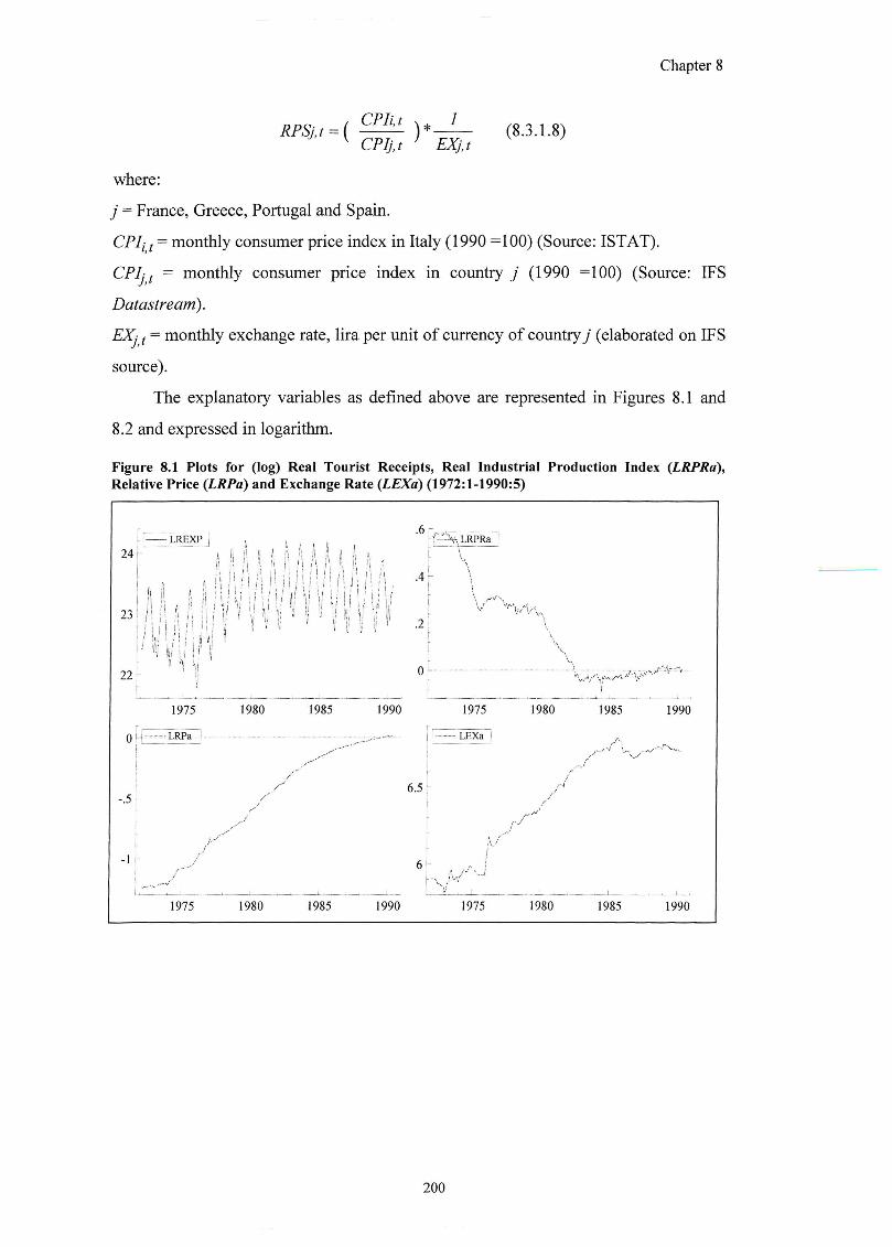
Chapter 8

= ( ^ (8.3.1.8) ^ Cf&f /

where:

j = France, Greece, Portugal and Spain.

CPIj I = monthly consumer price index in Italy (1990 =100) (Source: ISTAT).

CPIj f = monthly consumer price index in country j (1990 =100) (Source: IFS

Datastream).

EXj f = monthly exchange rate, lira per unit of currency of country j (elaborated on IFS

source).

The explanatory variables as defined above are represented in Figures 8.1 and

8.2 and expressed in logarithm.

Figure 8.1 Plots for (log) Real Tourist Receipts, Real Industrial Production Index (LRPRd), Relative Price (LRPa) and Exchange Rate (JLEXd) (1972:1-1990:5)

.6 -LREXP I . , , r'—^LRPRa

24 r s (1 ;! 1 J A i' !\ ii i S

:1 I : ! i 11 i ! M ! : M

I \

4 -

. 2 -

1975 1980 1985 1990 1975 1980 1985 1990

Q 1—iLRPft 1 ^ ^ [ | LEXS ^

- 1

1975 1980 1985 1990 1975 1980 1985 1990

200

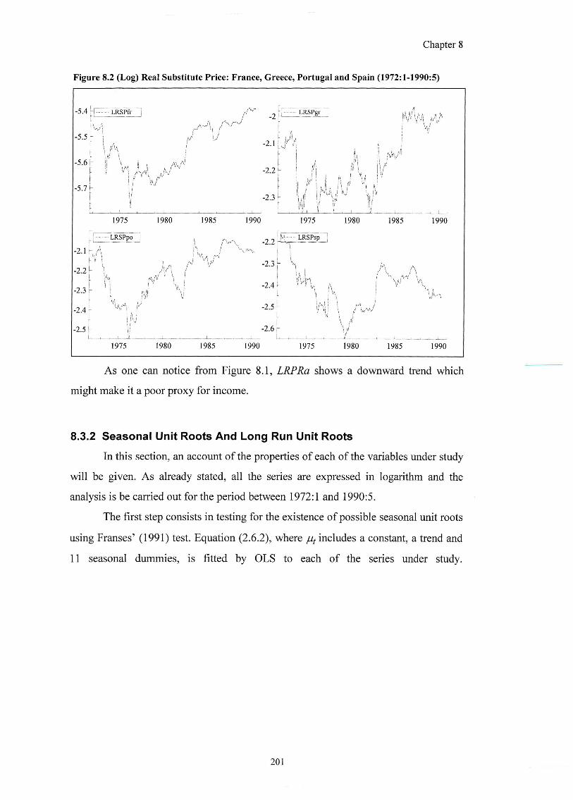
Chapter 8

Figure 8.2 (Log) Real Substitute Price: France, Greece, Portugal and Spain (1972:1-1990:5)

-5.4 - r = ^ L R S P f r - 2

LRSPgr

-5.5 r 1

-5.6 r

-2.1

-5.7 ^ -2.3

fl I "4 1

1975 1980 1985 1990 1975 1980 1985 1990

LRSPpo '

-2-1 an -2.2 L \

-Z3H M ^ 1/

-2.4'r I"

-2.2

-2.41

-2.5 r I

-2.6 r

LRSPsp

1975 1980 1985 1990 1975 1980 1985 1990

As one can notice from Figure 8.1, LRPRa shows a downward trend which

might make it a poor proxy for income.

8.3.2 Seasonal Unit Roots And Long Run Unit Roots

In this section, an account of the properties of each of the variables under study

will be given. As already stated, all the series are expressed in logarithm and the

analysis is be carried out for the period between 1972:1 and 1990:5.

The first step consists in testing for the existence of possible seasonal unit roots

using Franses' (1991) test. Equation (2.6.2), where includes a constant, a trend and

11 seasonal dummies, is fitted by OLS to each of the series under study.

201

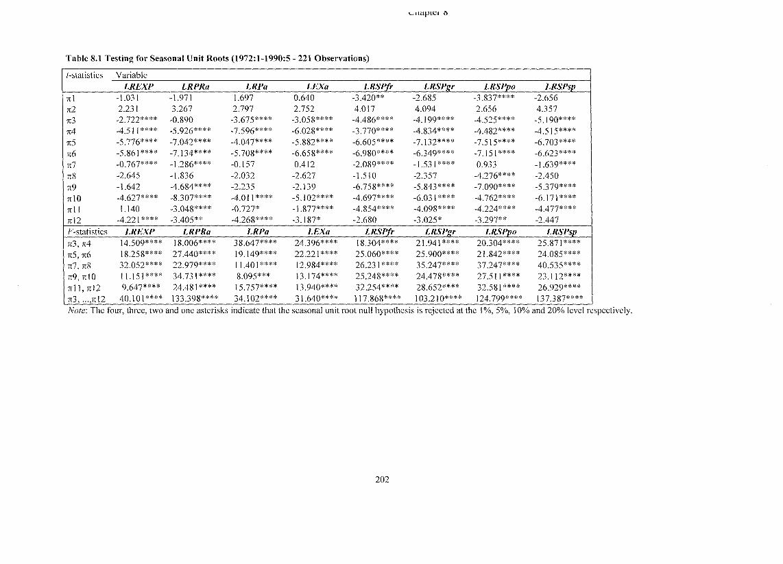
v impici o

Table 8.1 Testing for Seasonal Unit Roots (1972:1-1990:5 - 221 Observations)

(-statistics Variable

LREXP LRPRa LRPa LEXa LRSPfr LRSPgr LRSPpo LRSPsp

7ll - T 0 3 1 - 1 . 9 7 1 1 . 6 9 7 & 6 4 0 - 3 . 4 2 0 * * - 2 . 6 8 5 - 3 . 8 3 7 * * * * - 2 j 6 5 6

TI2 2L23] 3 . 2 6 7 Z 7 9 7 2 J 5 2 4 . 0 1 7 4 . 0 9 4 Z 6 5 6 4 3 5 7

7I3 - 2 . 7 2 2 * * * * - & 8 9 0 - 3 . 6 7 5 * * * * - 3 . 0 5 8 * * * * - 4 . 4 8 6 * * * * - 4 . 1 9 9 * * * * - 4 . 5 2 5 * * * * - 5 . 1 9 0 * * * *

7r4 - 4 . 5 1 1 * * * * - 5 . 9 2 6 * * * * - 7 . 5 9 6 * * * * - 6 . 0 2 8 * * * * - 3 . 7 7 0 * * * * - 4 . 8 3 4 * * * * - 4 . 4 8 2 * * * * - 4 . 5 1 5 * * * *

n 5 - 5 . 7 7 6 * * * * - 7 . 0 4 2 * * * * - 4 . 0 4 7 * * * * - 5 . 8 8 2 * * * * - 6 . 6 0 5 * * * * - 7 . 1 3 2 * * * * - 7 . 5 1 5 * * * * - 6 . 7 0 3 * * * *

7i6 - 5 . 8 6 1 * * * * - 7 . 1 3 4 * * * * - 5 . 7 0 8 * * * * - 6 . 6 5 8 * * * * - 6 . 9 8 0 * * * * - 6 . 3 4 9 * * * * - 7 . 1 5 1 * * * * - 6 . 6 2 3 * * * *

Til - 0 . 7 6 7 * * * * - 1 . 2 8 6 * * * * - 0 . 1 5 7 0 . 4 1 2 - 2 . 0 8 9 * * * * - 1 J # 1 * * * * 0 . 9 3 3 - 1 . 6 3 9 * * * *

- 2 . 6 4 5 - 1 . 8 3 6 - 2 . 0 3 2 - 2 . 6 2 7 - 1 . 5 1 0 - 2 . 3 5 7 - 4 . 2 7 6 * * * * - 2 . 4 5 0

- 4 . 6 8 4 * * * * - 2 . 2 3 5 - 2 . 1 3 9 - 6 . 7 5 8 * * * * - 5 . 8 4 3 * * * * - 7 . 0 9 0 * * * * - 5 . 3 7 9 * * * *

TUlO - 4 . 6 2 7 * * * * - 8 . 3 0 7 * * * * - 4 . 0 1 1 * * * * - 5 . 1 0 2 * * * * - 4 . 6 9 7 * * * * - 6 . 0 3 1 * * * * - 4 . 7 6 2 * * * * - 6 . 1 7 1 * * * *

7tl 1 1 J 4 0 - 3 . 0 4 8 * * * * - 0 . 7 2 7 * - 1 . 8 7 7 * * * * - 4 . 8 5 4 * * * * - 4 . 0 9 8 * * * * - 4 . 2 2 4 * * * * - 4 . 4 7 7 * * * *

7 1 1 2 - 4 . 2 2 1 * * * * - 3 . 4 0 5 * * - 4 . 2 6 8 * * * * - 3 . 1 8 7 * - 2 . 6 8 0 - 3 . 0 2 5 * - 3 . 2 9 7 * * - 2 . 4 4 7

F-statistics LREXP LRPRa LRPa LRSPfr LRSPgr LRSPpo LRSPsp

n3,7t4 1 4 . 5 0 9 * * * * 1 8 . 0 0 6 * * * * 3 8 . 6 4 7 * * * * 2 4 . 3 9 6 * * * * 1 8 . 3 0 4 * * * * 2 1 . 9 4 1 * * * * 2 0 . 3 0 4 * * * * 2 5 . 8 7 1 * * * *

K5, n6 1 8 . 2 5 8 * * * * 2 7 . 4 4 0 * * * * 1 9 . 1 4 9 * * * * 2 2 . 2 2 1 * * * * 2 5 . 0 6 0 * * * * 2 5 . 9 0 0 * * * * 2 1 . 8 4 2 * * * * 2 4 . 0 8 5 * * * *

7I7, TTS 3 2 . 0 5 2 * * * * 2 2 . 9 7 9 * * * * 1 1 . 4 0 1 * * * * 1 2 . 9 8 4 * * * * 2 6 . 2 3 1 * * * * 3 5 . 2 4 7 * * * * 3 7 . 2 4 7 * * * * 4 0 . 5 3 5 * * * *

•K9, TtlO 1 1 . 1 5 1 * * * * 3 4 . 7 3 1 * * * * 8 . 0 9 5 * * * 1 3 . 1 7 4 * * * * 2 5 . 2 4 8 * * * * 2 4 . 4 7 8 * * * * 2 7 . 5 1 1 * * * * 2 3 . 1 1 2 * * * *

Ttl 1 , 7 t 1 2 9 . 6 4 7 * * * * 2 4 . 4 8 1 * * * * 1 5 . 7 5 7 * * * * 1 3 . 9 4 0 * * * * 3 2 . 2 5 4 * * * * 2 8 . 6 5 2 * * * * 3 2 . 5 8 1 * * * * 2 6 . 9 2 9 * * * *

TI3, . . . ,7tl2 4 0 . 1 0 1 * * * * 1 3 3 . 3 9 8 * * * * 3 4 . 1 0 2 * * * * 3 1 . 6 4 0 * * * * 1 1 7 . 8 6 8 * * * * 1 0 3 . 2 1 0 * * * * 1 2 4 . 7 9 9 * * * * 1 3 7 . 3 8 7 * * * *

Note: The four, three, two and one asterisks indicate that the seasonal unit root null hypothesis is rejected at the 1%, 5%, 10% and 20% level respectively.

202

Chapter 8

As can be seen from Table 8.1, there is no evidence of seasonal unit roots.

However, the null hypothesis of the existence of a long run unit root cannot be

accepted for LRSPfr and LRSPpo. The latter result is in line with the ADF test.

in fact, appears to be 1(0) about a trend; whereas, the long run unit root is

accepted for LRSPfr by the ADF test (see Table 8.2). Note also that LRSPgr is found

to be 1(0) about a trend from the ADF test, whereas Franses' test suggests this variable

to be non-stationary in the level. A divergence appears also for LREXP which by the

ADF test is found to be stationary in the level (Table 8.2).

There follows the long run ADF unit roots test in order to establish the

integration status of each of the variables (Table 8.2).

203

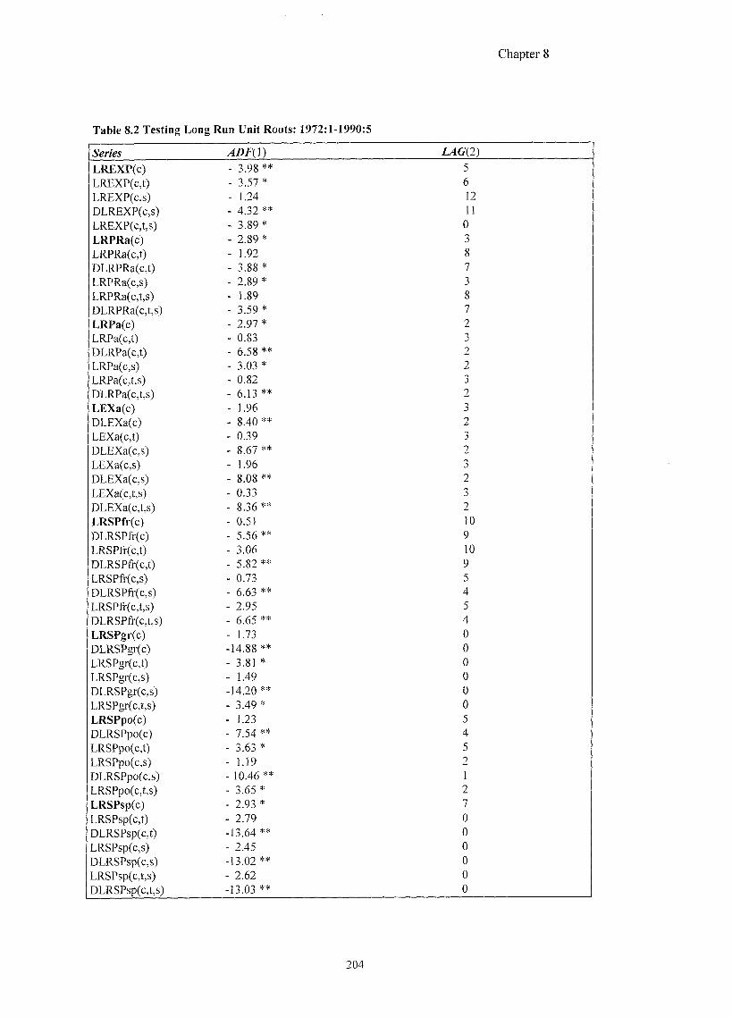
Chapter 8

Table 8.2 Testing Long Run Unit Roots: 1972:1-1990:5

Series ^ f ( l ) 1XC(2)

LREXP(c) - 3 4 8 * * 5

LREXP(c,t) - 3 . 5 7 * 6

LREXP(c,s) - l j U 12

DLREXP(c,s) - 4 3 2 * * 11

LREXP(c,t,s) - 3 j # * 0

LRPRa(c) - 2 ^ 9 * 3

LRPRa(c,t) - 1 . 9 2 8

DLRPRa(c,t) - 3 ^ W * 7

LRPRa(c,s) - 2 j # * 3

LRPRa(c,t,s) 8

DLRPRa(c,t,s) - 3 J # * 7

LRPa(c) - 2 . 9 7 * 2

LRPa(c,t) - 0 ^ 3 3

DLRPa(c,t) - &58** 2 LRPa(c,s) - 3 j G * 2 LRPa(c,t,s) - 0 ^ 2 3 DLRPa(c,t,s) - 6 1 3 * * 2

LEXa(c) - 1 . 9 6 3

DLEXa(c) - &40** 2

LEXa(c,t) - 0 J 9 3

DLEXa(c,s) - g j J * * 2

LEXa(c,s) - 1 . 9 6 3

DLEXa(c,s) - &08** 2

LEXa(c,t,s) - 0 J 3 3

DLEXa(c,t,s) - 8 3 6 * * 2

LRSPfr(c) - 0 . 5 1 10

DLRSPfr(c) - 5 . 5 6 * * 9

LRSPA-(c,t) - 3 . 0 6 10

DLRSPfr(c,t) - 5 ^ 2 * * 9

LRSPA(c,s) - 0 J 3 5

DLRSPfT(c,s) - 6.63** 4

LRSPAfc.t^s) - 2 4 5 5 DLRSPjT(c,t,s) - 6.65** 4

LRSPgr(c) - 1.73 0

DLRSPgr(c) -14.88 ** 0

LRSPgr(c,t) - 3 . 8 1 * 0 LRSPgr(c,s) - 1 4 9 0

DLRSPgr(c,s) -14.20 ** 0

LRSPgr(c,t,s) - 3 4 4 * 0

LRSPpo(c) - 1 J 3 5

DLRSPpo(c) - 7.54** 4

LRSPpo(c,t) - 3 . 6 3 * 5

LRSPpo(c,s) - 1 J 9 2

DLRSPpo(c,s) -1&46** 1

LRSPpo(c,t,s) - 3 ^ 3 * 2

LRSPsp(c) - 2 4 3 * 7

LRSPsp(c,t) - 2 J 9 0

DLRSPsp(c,t) -13.64 ** 0

LRSPsp(c,s) - 2 4 5 0

DLRSPsp(c,s) -13.02 ** 0

LRSPsp(c,t,s) - 2 j G 0

DLRSPsp(c,t,s) -13.03 ** 0

204

Chapter 8

Notes for Table 8.2: (1) Augmented Dickey-Fuller (ADF) statistics with constant (c) critical values: 5%=-2.876 l%=-3.463; when c and t included c.v.; 5%=-3.433 I%=-4.005; c and s included c.v.; 5% = -2.876 1% = -3.463; c,t and 5 are included c.v.: 5% = -3.433 and 1% = -4.005; (2) Number of lags set to the first statistically significant lag, testing downward and upon white residuals. Note that ADF(O) corresponds to the DP test. (3) ** significant at 1%; * significant at 5%.

From the ADF test, it emerges that the dependent variable LREXP can be

treated as stationary in the level. This finding seems to suggest that tourism in Italy is

not increasing over time and it has reached maturity. The relative price (LRPa) appears

to be 1(0) when a constant, or constant and seasonals are included, otherwise to be

stationary in the first difference. The real substitute price for Greece (LRSPgr) is found

to be 1(0) about a trend, as is the real substitute price for Portugal (UtS/ô). On the

other hand, the exchange rate (LEXa), the real substitute price for France (LRSPfr) and

for Spain (LRSPsp) are found to be 1(1). Interestingly, the income proxy (LRPRa)

appears to be non-stationary in the level. This finding is in line with the empirical

results obtained in Hansen (1995). In this article, it is shown that the (log) U.S. real

industrial production turns out to be a random walk.

8.3.3 Possible Cointegration Amongst 1(1) Variables

Once the integration status of the variables of interest is established, the next

step is to consider the possible existence of a cointegrating relationship amongst the

1(1) variables.

A Johansen cointegration analysis is run by including the real substitute price

for each of the main competitor countries for Italy (i.e. LRSPfr, LRSPgr, LRSPpo and

LRSPsp). An unrestricted 13 lag system is estimated that indicates problems of non-

normality in the residuals. Three impulse dummies have been created after inspecting

the residuals for the equations fbr and that is and

il983pL The inclusion of these dummies reduces the problems in the residuals but

does not eliminate them. Hence, a Johansen cointegration analysis is run on an

unrestricted 13 lag system including the aforementioned dummies and a time trend,

treated unrestrictedly. The system can be reduced, according to the joint F-test, the SC

and HQ criteria to 4 lags. One can conclude that the 4 variables do not appear to be

cointegrated or stationary.

205

Chapter 8

A second test is carried out on the pair LRSPgr and LRSPpo, that according to

the ADF test have been found to be stationary in the level (see Table 8.2). Starting

with an unrestricted 13 lag system, an impulse dummy (il983pl) is included after

inspecting the residuals for the LRSPgr equation. A time trend is also included. The

system can be reduced parsimoniously t o l l lags, in accordance with the joint F-test.

The results from the Johansen cointegration analysis suggest treating the two variables

as stationary in agreement with the ADF test findings. The results are in Appendix F,

Table F.l . Note also that the SC and HQ criteria suggest the estimation of a 1 lag

system. Nevertheless, from the Johansen analysis, the conclusion is that the two

variables are stationary.

The second investigation is carried out on the pair LRSPfr and LRSPsp. An

unrestricted 13 lag system is run with the inclusion of an impulse dummy il977p7,

created after having inspected the residuals for LRSPsp equation. A constant, a time

trend and seasonals are also included unrestrictedly which give the best results in terms

of diagnostics. The 13 lag system can be reduced to a 7 lag system, according to the

joint F-test. Also in this case, there is evidence for the two variables to be stationary.

The complete Johansen analysis results are reported in Appendix F, Table F.2. Note,

also, that the information criteria SC and HQ suggest running a one lag and two lag

system, respectively. Nevertheless, the results indicate that and jp are

stationaiy.

In conclusion, there is statistical evidence to believe that each of the real

substitute prices can be treated as stationary in the level.

In accordance with economic theory, prices and exchange rate are expected to

drift together in the long run. Thus, a cointegration analysis is done on the (log)

relative price {LRPa) and (log) weighted average exchange rate (LEXa). An initial 13

lag system has been run, which includes a constant, trend and seasonals treated

unrestrictedly. Impulse dummies created after inspecting the residuals, in order to

avoid problems of non-normality, worsen the results in terms of diagnostics, so they

are not included in the system. The system can be reduced further, up to 2 lags, as the

restriction has been accepted by the joint F-test. Moreover, the 2 lag system is

suggested also by the SC and HQ criteria (the complete results are reported in

Appendix F, Table F.3). From the Johansen cointegration analysis, one infers that there

206

Chapter 8

is evidence for the presence of one cointegrating relationship between the two

variables. From Table F.3, the equivalent cointegrating vector can be derived and it is

given by the first row of p matrix:

C/ = Zjgfa - 0 . Z & Y a (8.3.3.1)

The expectation is that the two cointegrated variables will present a long run

coefficient of one. Thus, the following restriction: /?=-l is tested for the coefficient for

the (log) weighted exchange rate; however, the null hypothesis has not been accepted

at the 5% level from the testî. This fact might be due to differences in the inflation

rates in each of the countries under consideration.

A further ADF cointegration analysis is carried out on the above two variables.

The static models, for the relative price and exchange rate, are estimated by OLS for

the period 1972:1 to 1990:5, where a constant is included. The results are as follows:

+ 7 . + wy 0. P76 0.0^

and

The second step consists of estimating the static models where a constant and a

time trend are included, which gives the following results:

a = - J. 7 + 0.00jJ + 0. + wy o. pp o.2j

and

= 7 - 0 . T r e W + 7. j ^ j 7 O . P P 0.23

The saved residuals w; and which can be interpreted as the deviations of the

generic 6om the long run path, are tested for a unit root under the null hypothesis of

no-cointegration. The number of lags for the ADF test is set to the first statistically

significant lag, testing downward and upon white residuals. The initial number of lags

in the ADF test is set up to 13. The first significant lag is the third and the /-value for

the corresponding coefficient is -1.82. MacKinnon's critical value is equal to -3.36^^

at the 5% that is greater, in absolute value, than -1.82. The null hypothesis cannot be

rejected and, thus, there is no evidence for cointegration between the two variables of

interest.

The results for the restriction test on the coefficient is: %-(!) = 4.9247 [0.0265] *. The estimatedp =5% critical value for 7=221 observations is the following: C(p) = -3.3377 +

(-5.967/221) + (-8.98/(221)^).

2 0 7

Chapter 8

The same finding has been obtained when, in the static model, a constant plus a

trend are included. The critical value is -3.82^3 at the 5% level which is greater, in

absolute value, than the r-value of the corresponding coefficient, -3.42, when the

model is run with nine lags. Again, no evidence appears of the existence of

cointegration between the relative price and weighted exchange rate.

The next step consists of regressing LEXa on LRPa with just the constant in the

static model. Using the cointegration ADF test, based on the statistically significant lag

approach, testing downwards, the lag length equals three and the correspondent f-value

is -2.01. In this case, MacKinnon's critical value equals -3.36 '* at the 5% level. Thus,

this critical value, in absolute term, is greater than the value for /7. Therefore, there is

statistical evidence for the existence of no-cointegration.

Including a constant and a trend in the static model, the results are the

following. The critical value determined from MacKinnon's parameters, is -3.82^5

The ^-value for the correspondent coefficient for an ADF model of 9 lags equals -4.10

that, in absolute value, is greater than the critical value. Hence, there appears evidence

for the existence of cointegration between the two variables. On balance, as argued

before, one can consider the Johansen analysis to be more robust. It uses a

simultaneous approach which involves the interdependencies of the variables under

study.

A cointegration analysis has also been run for the three 1(1) variables (i.g. real

industrial production, relative price and exchange rate). Statistical evidence has been

found for the existence of one cointegrating vector (see Appendix F, Table F.4);

however, some difficulties appear in interpreting the results on an economic basis. An

investigation follows in employing a non-linear transformation for the real industrial

production index.

The estimated p = 5% critical value for 7=221 observations is the following: C(p) = -3.7809 + (-9.421/221)+ (-15.06/(221)^).

The estimatedp =5% critical value for 7=221 observations is the following; C(p) = -3.3377 + (-5.967/221) + (-8.98/(221)^).

The estimatedp = 5% critical value for 7=221 observations is the following; C(p) = -3.7809 + (-9.421/221) (-15.06/(221)2).

208

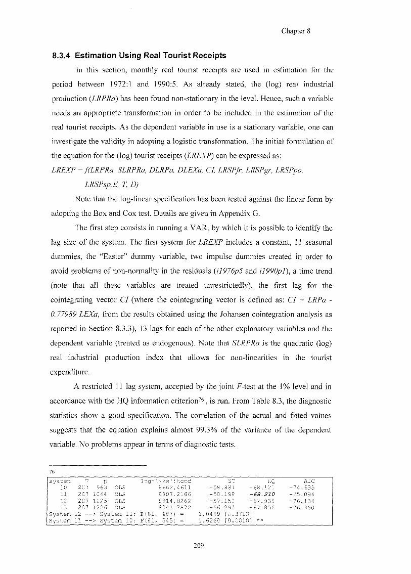
Chapter 8

8.3.4 Estimation Using Real Tourist Receipts

In this section, monthly real tourist receipts are used in estimation for the

period between 1972:1 and 1990:5. As already stated, the (log) real industrial

production (LRPRa) has been found non-stationary in the level. Hence, such a variable

needs an appropriate transformation in order to be included in the estimation of the

real tourist receipts. As the dependent variable in use is a stationary variable, one can

investigate the validity in adopting a logistic transformation. The initial formulation of

the equation for the (log) tourist receipts (LREXP) can be expressed as:

Note that the log-linear specification has been tested against the linear form by

adopting the Box and Cox test. Details are given in Appendix G.

The first step consists in running a VAR, by which it is possible to identify the

lag size of the system. The first system for LREXP includes a constant, 11 seasonal

dummies, the "Easter" dummy variable, two impulse dummies created in order to

avoid problems of non-normality in the residuals (z7P7^j and a time trend

(note that all these variables are treated unrestrictedly), the first lag for the

cointegrating vector C/ (where the cointegrating vector is defined as: C/ = -

0.77989 LEXa, from the results obtained using the Johansen cointegration analysis as

reported in Section 8.3.3), 13 lags for each of the other explanatory variables and the

dependent variable (treated as endogenous). Note that is the quadratic (log)

real industrial production index that allows for non-linearities in the tourist

expenditure.

A restricted 11 lag system, accepted by the joint F-test at the 1% level and in

accordance with the HQ information c r i t e r i o n ^ ^ ^ jg run. From Table 8.3, the diagnostic

statistics show a good specification. The correlation of the actual and fitted values

suggests that the equation explains almost 99.3% of the variance of the dependent

variable. No problems appear in terms of diagnostic tests.

7 6

system T P log-likelihood SC HQ AIC 10 207 963 OLS 8662.4611 -58 887 -68. 121 -74 695 11 207 1044 OLS 8807.2166 -58 198 -68. 210 - 7 5 094 12 207 1125 OLS 8914.8262 - 5 7 1 5 1 -67. 939 -76 134 13 207 1206 OLS 9041.7872 -56 291 -67 . 856 -76 360

System 12 - -> System 11: 48^ = 1.0499 [0.3713 System 11 - -> System 10: 54^ = 1.6268 [0.0010 * *

209

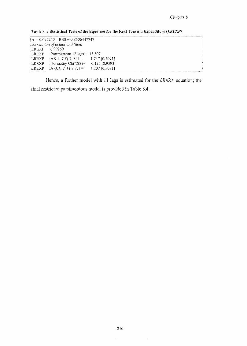
Chapter 8

Table 8. 3 Statistical Tests of the Equation for the Real Tourism Expenditure {LREXP)

cr = 0.097250 RSS = 0.8606447747 corre/an'oM o/"acfua/ OMgf LREXP 0.99269 LREXP ;Portmanteau 12 lags= 15.507 LREXP : A R 1 - 7 F ( 7 , 8 4 ) = 1.747 [0.1091] LREXP :NormalityCbi'"2(2)= 0.125 [0.9393] LREXP : A R C H 7 F ( 7 , 7 7 ) = 1.207 [0.3091]

Hence, a further model with 11 lags is estimated for the LREXP equation; the

final restricted parsimonious model is provided in Table 8.4.

210

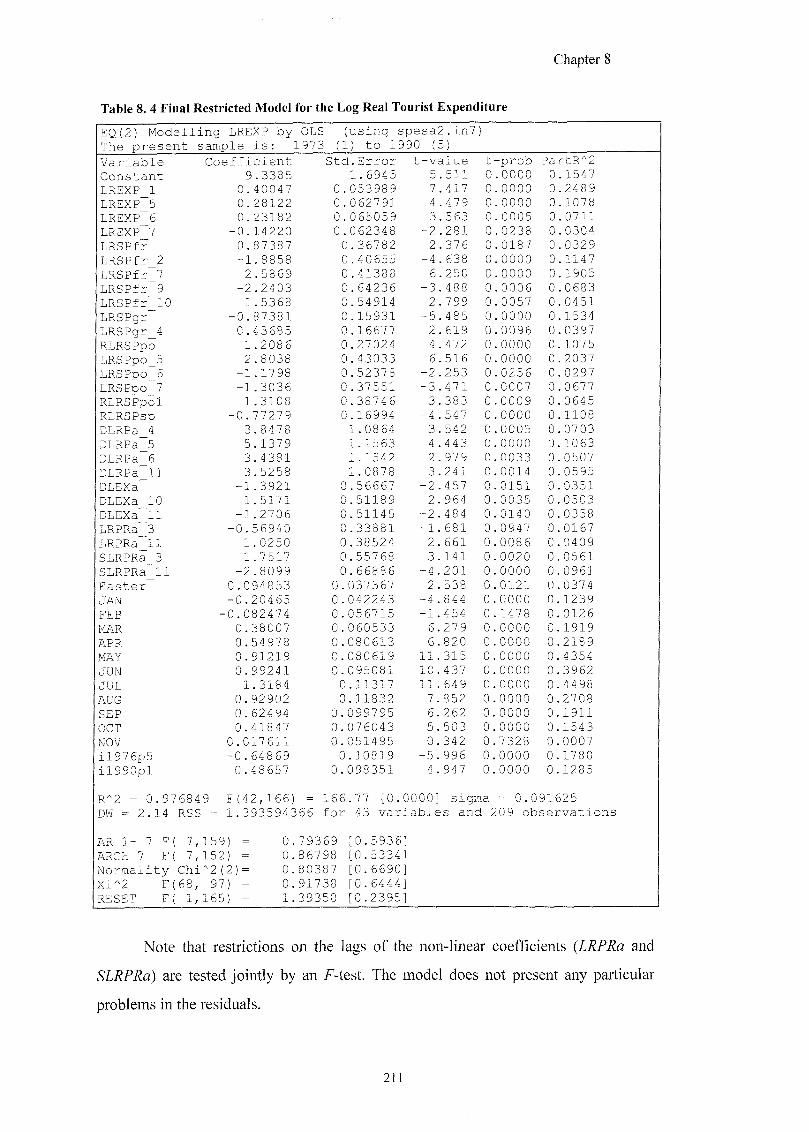
Chapter 8

Table 8. 4 Final Restricted Model for the Log Real Tourist Expenditure

EQ(2) Modelling LREXP by The present sample is:

OLS (using spesa2.in7) 1973 (1) to 1990 (5)

Variable Coefficient Std.Error t-value t -prob PartR^2

Constant 9.3385 1.6945 5 .511 0 0000 0 .1547

LREXP 1 0.40047 0.053989 7 .417 0 0000 0 .2489

LREXP 5 0.28122 0.062791 4 . 479 0 0000 0 .1078

LREXP 6 0.23182 0.065059 3 .563 0 0005 0 0711

LREXP 7 -0.14220 0.062348 -2 .281 0 0238 0 .0304 LRSPfr 0.87387 0.36782 2 .376 0 0187 0 .0329

LRSPfr 2 -1.8858 0.40655 -4 . 638 0 0000 0 1147 LRSPfr 7 2.5869 0.41388 6 .250 0 0000 0 .1905 LRSPfr 9 -2.2403 0.64236 -3 . 488 0 0006 0 .0683 LRSPfr 10 1.5368 0.54914 2 .799 0 0057 0 0451 LRSPgr -0.87381 0.15931 -5 .485 0 0000 0 1534 LRSPgr 4 0.43685 0.16677 2 . 619 0 0096 0 0397 RLRSPpo 1.2086 0.27024 4 . 472 0 0000 0 1075 LRSPpo 5 2.8038 0.43033 6 .516 0 0000 0 2037 LRSPpo 6 -1.1798 0.52378 -2 .253 0 0256 0 0297 LRSPpo 7 -1.3036 0.37551 -3 .471 0 0007 0 0677 RLRSPpo1 1.3108 0.38746 3 . 383 0 0009 0 0645 RLRSPsp -0.77279 0.16994 -4 . 547 0 0000 0 1108 DLRPa 4 3.8478 1.0864 3 .542 0 0005 0 0703 DLRPa 5 5.1379 1.1563 4 .443 0 0000 0 1063 DLRPa 6 3.4381 1.1542 2 . 979 0 0033 0 0507 DLRPa 11 3.5258 1.0878 3 .241 0 0014 0 0595 DLEXa -1.3921 0.56667 -2 . 457 0 0151 0 0351 DLEXa 10 1.5171 0.51189 2 964 0 0035 0 0503 DLEXa 11 -1.2706 0.51145 -2 .484 0 0140 0 0358 LRPRa 3 -0.56940 0.33881 -1 681 0 0947 0 0167 LRPRa 11 1.0250 0.38524 2 .661 0 0086 0 0409 SLRPRa 3 1.7517 0.55768 3 141 0 0020 0 0561 SLRPRa_ll -2.8099 0.66886 -4 .201 0 0000 0 0961 Easter 0.094853 0.037367 2 .538 0 0121 0 0374 JAN -0.20465 0.042243 -4 844 0 0000 0 1239 FEB -0.082474 0.056715 -1 454 0 1478 0 0126 MAR 0.38007 0.060533 6 279 0 0000 0 1919

APR 0.54978 0.080613 6 820 0 0000 0 2189 MAY 0.91219 0.080619 11 315 0 0000 0. 4354 JUN 0.99241 0.095081 10 437 0 0000 0 3962 JUL 1.3184 0.11317 11 649 0 0000 0 4498 AUG 0.92902 0.11832 7 852 0 0000 0 2708 SEP 0.62494 0.099795 6 262 0 0000 0. 1911 OCT 0.41847 0.076043 5 503 0 0000 0. 1543 NOV 0.017611 0.051495 0 342 0 7328 0. 0007 il976p5 -0.64869 0.10819 -5 996 0 0000 0. 1780 il990pl 0.48657 0.098351 4 947 0 0000 0. 1285

R 'Z = 0.97 68 49 F(42,166) = 166.77 [0.0000] sigma = 0.091625 DM = 2.14 RSS = 1.393594366 for 43 variables and 209 observations

AR 1- 7 F( 7 ,159) = 0. 79369 [0.5936] ARCH 7 F( 7 ,152) = 0. 867 98 [0.5334] Normality Chi"2(2)= 0. 80387 [0.6690] Xi^2 F( 68 , 97) = 0. 91738 [0.6444] RESET F( 1 ,165) = 1. 39350 [0.2395]

Note that restrictions on the lags of the non-linear coefficients (LRPRa and

are tested jointly by an F-test. The model does not present any particular

problems in the residuals.

2 1 ]

Chapter 8

Few restrictions could be imposed, as one can see in Table 8.4; RLRSPpo is

defined as the difference between the coefficients of the second and fourth lags of the

substitute price for PortugaF^, RLRSPpol is the difference between the coefficients of

the ninth and tenth lags^*, RLRSPsp is the difference between the fifth and tenth lag

coefficients'^^. No other restrictions have been accepted either by the joint F-test or by

suggestion of the SC criterion.

Again, the final restricted model does not show any problems in the residuals

and the model is overall well-specified.

The long run dynamics are reported in Table 8.5. The Wald test suggests that

the long run coefficients are jointly significantly different from zero. An analysis of the

short and long run dynamics is appropriate (see Tables 8.4 and 8.5). One might want to

compare the long run dynamics with the short run dynamics as given by the previous

table. The real substitute price for France (LRSPfr) shows a positive and statistically

significant (/-statistic +2.04) long run coefficient. In Table 8.4, the short run coefficient

presents a negative sign and a r-value equal to -4.64. The long run

coefficient for LRSPpo is positive and statistically significant (/-statistic equals +2.22).

The same positive sign appears in the short run, with a highly statistically significant

coefficient (/-statistic equals +6.52 for the first significant lag, that is the fifth). As far

as the real substitute price for Greece (LRSPgr) is concerned, in the long run, the

coefficient shows the expected negative sign with a /-value equal to -3.22; whereas, in

the short run the coefficient of the fourth lag is positive. The real substitute price for

Spain presents a short run dynamic structure with the coefficient for the oscillation

presenting a negative sign. In conclusion, one cannot observe a simple

pattern across the competing tourist destinations, which exhibit noticeable differences

in both the short and long run.

The restriction on the coefficient of the second and fourth lags, that present an opposite sign and similar magnitude, is accepted at the 5% level from the joint F-test (1,163) as the calculated value 0.000070 is smaller than the critical value 3.84; moreover, the SC criterion is minimised when the restriction is imposed; from -3.84058 to -3.86614.

The restriction on the coefficient of the ninth and tenth lags is accepted at the 5% level from the joint F-test (1,164) as the calculated value 0.97 is smaller than the critical value 3.84; moreover, the SC criterion is minimised when such a restriction is imposed: from -3.86614 to -3.88583.

The restriction on the coefficient of the fifth and tenth lags for the substitute price for Spain, is accepted at the 5% level. The joint F-test (1,165) value is 0.013 is smaller than the critical value 3.84; moreover, the SC criterion is minimised when such a restriction is imposed: from -3.88583 to -3.91131.

212

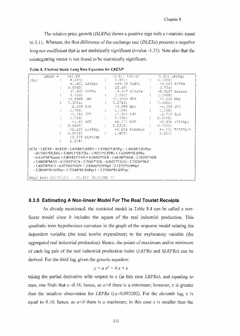
Chapter 8

The relative price growth (DLRPa) shows a positive sign with a ^statistic equal

to 3.11. Whereas, the first difference of the exchange rate {DLEXa) presents a negative

long run coefficient that is not statistically significant (r-value -1.33). Note also that the

cointegrating vector is not found to be statistically significant.

Table 8. 5 Solved Static Long Run Equation for LREXP

LREXP = + 4 0 . 8 3 + 3 . 8 1 1 L R S P f r - 1 . 9 1 1 L R S P g r ( 8 . 6 1 5 ) ( 1 . 8 7 1 ) ( 0 . 5 9 2 6 )

+ 1 . 4 0 1 L R S P p o + 6 9 . 7 4 DLRPa - 5 . 0 0 9 DLEXa ( 0 . 6 3 0 5 ) ( 2 2 . 4 5 ) { 3 . 7 64 )

+ 1 . S 9 2 LRPRa - 4 . 6 2 7 SLRPRa + 0 . 4 1 4 7 E a s t e r ( 1 . 3 5 6 ) ( 2 . 2 1 3 ) { 0 . 1 9 1 8 )

- 0 . 8 9 4 8 JAN - 0 . 3 6 0 6 FEB + 1 . 6 6 2 MAR ( 0 . 3 0 8 1 ) ( 0 . 2 7 1 6 ) { 0 . 5 1 8 2 )

+ 2 . 4 0 4 APR + 3 . 9 8 9 MAY + 4 . 3 3 9 JUN ( 0 . 7 8 6) ( 1 . 1 8 4 ) { 1 . 3 3 9 )

+ 5 . 7 6 5 J U L + 4 . 0 6 2 AUG + 2 . 7 3 3 SEP ( 1 . 7 2 6 ) ( 1 . 3 0 8 ) ( 0 . 9 3 9 9 )

+ 1 . 8 3 OCT + 0 . 0 7 7 NOV - 2 . 8 3 6 i l 9 7 6 p 5 ( 0 . 6 4 9 9 ) ( 0 . 2 3 0 5 ) ( 0 . 7 6 3 2 )

+ 2 . 1 2 8 i l 9 9 0 p l + 5 . 2 8 4 R L R S P p o + 5 . 7 3 1 R L R S P p o l ( 0 . 6 8 3 6 ) ( 1 . 4 8 3 ) ( 2 XL53)

- 3 ^ 7 9 R L R S P s p ( 1 . 2 0 4 )

ECM = LREXP-40.8329-3.81086*LRSP&+ I.91062*LRSPgr- 1.40108*LRSPpo - 69.7401 *DLRPa+ 5.0091 MDLEXa - 1.992] 1 *LRPRa + 4.62699*SLRPRa - 0.414748*Easter+ 0.894831*JAN + 0.36062*FEB - 1.66189*MAR - 2.40395*APR - 3.98858*MAY - 4.33935*JUN - 5.76467*JUL - 4.06217*AUG 2.73256*SEP - 1.82978*0CT - 0.077003*NOV + 2.83643*1 1976p5 -2L12755*) 1990p1 - 5.28449*RLRSPpo - 5.73148*RLRSPpol + 3.37904*RLRSPsp;

WALD t e s t C h i ' ' 2 ( 2 4 ) = 7 5 . 3 2 7 [ 0 . 0 0 0 0 ] * *

8.3.5 Estimating A Non-linear Model For The Real Tourist Receipts

As already mentioned, the restricted model in Table 8.4 can be called a non-

linear model since it includes the square of the real industrial production. This

quadratic term hypothesizes curvature in the graph of the response model relating the

de Derxieiit viiniable (the total Ikxuiist (sxixsncWtim:) to the esqplarwitory i/ariable (the

aggregated real industrial production). Hence, the points of maximum and/or minimum

of each lag pair of the real industrial production index (LRPRa and SLRPRa) can be

derived. For the third lag, given the generic equation:

y ==<2: 2 + ^ g

taluiig the jpaitial dk%i\ratr/e \vith resqpetit to jc (ui this case JLRLPJ&a), aiui ecpiating; 1k)

zero, one finds that x=^0.16; hence, as a>0 there is a minimum; however, x is greater

than the smallest observation for LRPRa (i.e.-0.093202). For the eleventh lag, x is

equal to 0.7^/ hence, as there is a maximum; in this case x is smaller than the

2i;

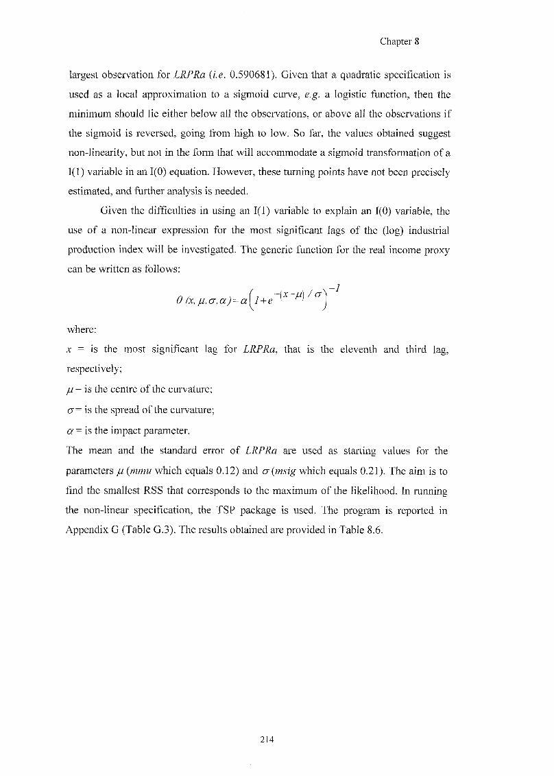
Chapter 8

largest observation for LRPRa {i.e. 0.590681). Given that a quadratic specification is

used as a local approximation to a sigmoid curve, e.g. a logistic function, then the

minimum should lie either below all the observations, or above all the observations if

the sigmoid is reversed, going from high to low. So far, the values obtained suggest

non-linearity, but not in the form that will accommodate a sigmoid transformation of a

1(1) variable in an 1(0) equation. However, these turning points have not been precisely

estimated, and further analysis is needed.

Given the difficulties in using an 1(1) variable to explain an 1(0) variable, the

use of a non-linear expression for the most significant lags of the (log) industrial

production index will be investigated. The generic function for the real income proxy

can be written as follows:

-1

where;

X = is the most significant lag for LRPRa, that is the eleventh and third lag,

respectively;

// = is the centre of the curvature;

(7= is the spread of the curvature;

(2 = is the impact parameter.

The mean and the standard error of LRPRa are used as starting values for the

parameters // {mmu which equals 0.12) and cj(msig which equals 0.21). The aim is to

find the smallest RSS that corresponds to the maximum of the likelihood. In running

the non-linear specification, the TSP package is used. The program is reported in

Appendix G (Table G.3). The results obtained are provided in Table 8.6.

214

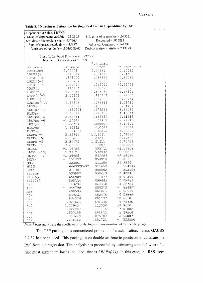
Chapter 8

Table 8. 6 Non-linear Estimation for (log) Real Tourist Expenditure by TSP

Dependent variable; LREXP Mean of dependent variable = 23.2305

Std. dev. of dependent var. = .537965 Sum of squared residuals = 1.45187

Std. error of regression = .093521 R-squared = .975883

Adjusted R-squared = .969781 Variance of residuals = .874620E-02 Durbin-Watson statistic = 2.13199

Log of Likelihood Function = 222. Number of Observations = 209

753

Standard Parameter Estimate Error t--statistic constant 8 . 70871 1 .70631 5 .10383 LREXP(-1) 440847 .054119 8 .14592 LREXP(-5) 275400 .063671 4 .32533 LREXP(-6) 200937 .067075 2 .99569 LREXP(-7) — . 184227 .063941 -2 .88121 LRSPfr 796134 .362670 2 .19520 LRSPfr(-2) -1 .96245 .423037 -4 .63894 LRSPfr(-7) 2 .55358 .425734 5 .99806 LRSPfr(-9) -2 .29417 .667382 -3 .43757 LRSPfr(-10) 1 .47403 .569316 2 .58913 LRSPgr - .819077 .163356 -5 .01407 LRSPgr(-4) .356904 .179291 1 .99064 RLSPpo 1 .15511 .276183 4 .18241 LRSPpo(-5) 2 .82234 .439880 6 .41615 LRSPpo(-6) -1 .20271 .539467 -2 .22945 LRSPpo(-7) -1 .22724 .388804 -3 .15644 RLSPpo1 1 .36442 .410582 3 .32314 RLSPsp - .694331 .172594 -4 .02291 DLRPa(-4) 3 .58945 1, .16461 3 .08210 DLRPa(-5) 4 .61411 1, ,23251 3 .74367 DLRPa(-6) 3 .34473 1, .21211 2 .75942 DLRPa(-11) 3 .43636 1, .11207 3 .09006 DLEXa -1 .49456 .583111 —2 .56308 DLEXa(-10) 1 .33121 ,532032 2 .50212 DLEXa(-11) -1 .35985 ,530082 -2, .56536

BETA* - .151937 ,054010 -2. .81311 MMU .323501 ,011059 29, .2536 MSIG .646002E-02 ,011653 .554344 ETA* - .011287 ,055862 - . .202054 easter .095587 ,038413 2 . ,48841 il976p5 - .656908 ,111077 -5 . ,91399 il990pl .508124 ,099663 5 . ,09843 jan - .183298 .043358 -4 . ,22759 f eb - .048799 .058312 - , ,836857

mar .408593 .062045 6. ,58539 apr .539261 .082470 6. ,53889

may .864576 081137 10, , 6558

jun .921625 094336 9, ,76960 jul 1 .22945 112330 10. , 9450 aug .822007 .117115 7 , ,01882 sep .533189 .098822 5 , ,39546 oct .353449 075703 4 . ,66887 nov - .018303 051721 - . .353886

Note: * beta and eta are the coefficients for the logistic transformation of the income proxy.

The TSP package has encountered problems of maximisation; hence, GAUSS

3.2.32 has been used. This package uses double arithmetic precision to calculate the

RSS from the regression. The analysis has proceeded by estimating a model where the

first most significant lag is included, that is LRPRa(-ll). In this case, the RSS from

215

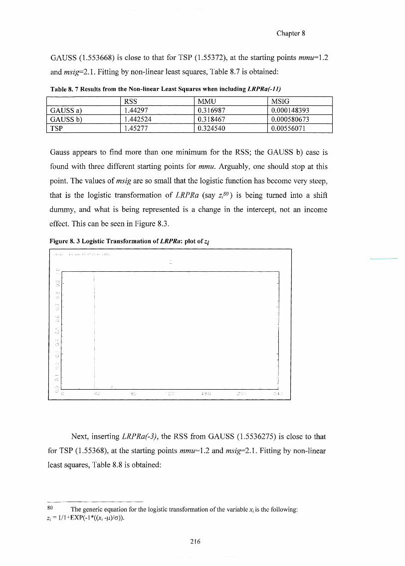
Chapter 8

GAUSS (1.553668) is close to that for TSP (1.55372), at the starting points mmu=\.2

and msig^^lA. Fitting by non-linear least squares. Table 8.7 is obtained:

Table 8. 7 Results from the Non-linear Least Squares when including LRPRa(-ll)

RSS MMU MSIG GAUSS a) 1.44297 0.316987 0.000148393 GAUSS b) 1.442524 0.318467 0.000580673 TSP 1.45277 0.324540 0.00556071

Gauss appears to find more than one minimum for the RSS; the GAUSS b) case is

found with three different starting points for mmu. Arguably, one should stop at this

point. The values of msig are so small that the logistic function has become very steep,

that is the logistic transformation of LRPRa (say zP'^) is being turned into a shift

dummy, and what is being represented is a change in the intercept, not an income

effect. This can be seen in Figure 8.3.

Figure 8. 3 Logistic Transformation of LRPRa: plot of z,-

Next, inserting LRPRa(-3), the RSS from GAUSS (1.5536275) is close to that

for TSP (1.55368), at the starting points mmu=\.2 and msig=2.\. Fitting by non-linear

least squares, Table 8.8 is obtained:

The generic equation for the logistic transformation of the variable x, is the following: z, = l/l+EXP(-l*((;c/-p)/5)).

216

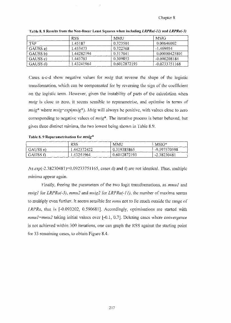
Chapter 8

Table 8. 8 Results from the Non-linear Least Squares when including LRPRa(-ll) and LRPRa(-3)

RSS M M U MSIG

TSP 1.45187 0.323501 0.00646002

GAUSS a) 1.453473 0.322368 -1.469054

GAUSS b) 1.44282194 0.317041 0.00000425801

GAUSS G) 1.445763 0.309853 -0.000208184

GAUSS d) 1.43241964 0.6012872193 -0.0233751168

Cases a-c-d show negative values for msig that reverse the shape of the logistic

transformation, which can be compensated for by reversing the sign of the coefficient

on the logistic term. However, given the instability of parts of the calculation when

msig is close to zero, it seems sensible to reparametrise, and optimise in terms of

where AAfg will always be positive, with values close to zero

corresponding to negative values of The iterative process is better behaved, but

gives three distinct minima, the two lowest being shown in Table 8.9.

Table 8. 9 Reparametrisation for msig*

RSS M M U MSIG*

GAUSS e) 1.442372422 0.319385865 -9.597570598

GAUSS f) 1.43241964 0.6012872193 -2.38230481

As ex^(-2.38230481)=0.09233751165, cases d) and f) are not identical. Thus, multiple

minima appear again.

Finally, freeing the parameters of the two logit transformations, as mmuJ and

msigl for LRPRa(-3), mmu2 and msig2 for LRPRa(-l 1), the number of maxima seems

to multiply even further. It seems sensible for mmu not to lie much outside the range of

LRPRa, that is [-0.093202, 0.590681], Accordingly, optimisations are started with

mmul=mmu2 taking initial values over [-0.1, 0.7]. Deleting cases where convergence

is not achieved within 300 iterations, one can graph the RSS against the starting point

for 33 remaining cases, to obtain Figure 8.4.

2 1 7

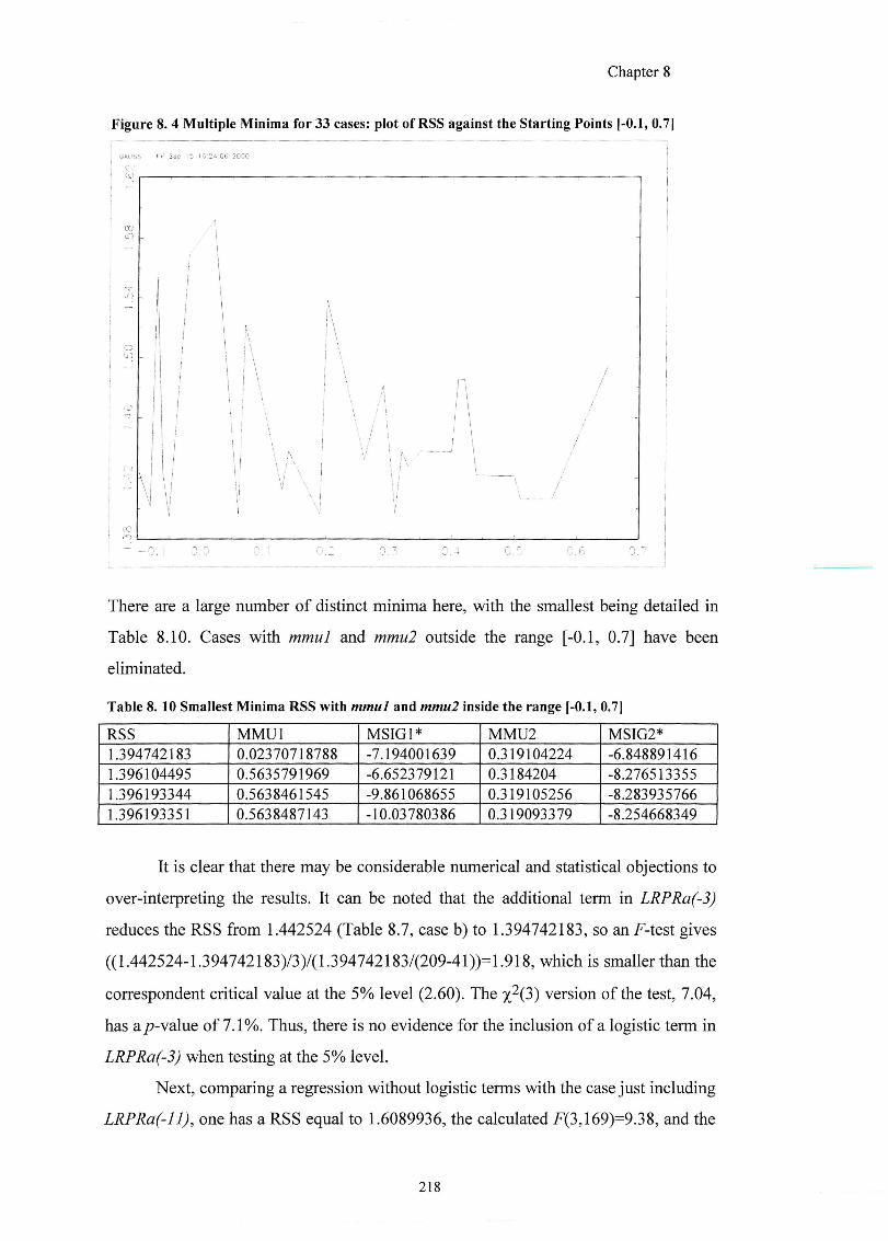
Chapter 8

Figure 8. 4 Multiple Minima for 33 cases: plot of RSS against the Starting Points [-0.1, 0.7]

bep

There are a large number of distinct minima here, with the smallest being detailed in

Table 8.10. Cases with mmul and mmu2 outside the range [-0.1, 0.7] have been

eliminated.

Table 8. 10 Smallest Minima RSS with mmul and mmu2 inside the range [-0.1, 0.7]

RSS MMUl MSIGl* MMU2 MSIG2* 1.394742183 0.02370718788 -7.194001639 (1319104224 -6.848891416 1.396104495 0.5635791969 -6.652379121 0.3184204 -8.276513355

L396193344 0.5638461545 J&.861068655 0.319105256 -8.283935766

1.396193351 0.5638487143 -10.03780386 0.319093379 -8.254668349

It is clear that there may be considerable numerical and statistical objections to

over-interpreting the results. It can be noted that the additional term in LRPRa(-3)

reduces the RSS from 1.442524 (Table 8.7, case b) to 1.394742183, so an F-test gives

((1.442524-1.394742183)/3)/(1.394742183/(209-41))=1.918, which is smaller than the

correspondent critical value at the 5% level (2.60). The % (3) version of the test, 7.04,

has ap-value of 7.1%. Thus, there is no evidence for the inclusion of a logistic term in

LRPRa(-3) when testing at the 5% level.

Next, comparing a regression without logistic terms with the case just including

LRPRa(-l 1), one has a RSS equal to 1.6089936, the calculated F(3,169)=9.38, and the

218

Chapter 8

calculated % (3)=22.8, which are both significant at the 1% level. Thus, it seems that

there is variation in the dependent variable that can be explained, even if the logistic

form used seems not to give satisfactory modelling results. These experiments at non-

linear modelling thus fail, in part, from numerical problems: there are multiple maxima

in the likelihood. However, the inclusion of the LRPRa(-l 1), results in a more

important difficulty emerging; a sigmoid transfomation of a trending variable may be

indistinguishable from a shift dummy, and the interpretation of its coefficient will

either change or lose its meaning.

8.3.6 Estimating Italian Tourist Expenditure As 1(1)

In this section, one will estimate a model considering the real tourist

expenditure (LREXP) as non-stationary in the level, but stationary in the first

difference. Some evidence for this variable to be a random walk has been found from

Franses' unit roots test (see Table 8.1). Moreover, in the majority of the empirical

studies, tourist expenditure is treated as integrated of order one (e.g. Lanza and Urga,

1995; Song ef a/., 2000).

The aim is to test for the existence of a possible cointegrating vector with the

other 1(1) variables: real industrial production (LRPRa), relative price (LRPa) and

exchange rate (Z&Ya). A Johansen analysis is run; a 13 lag system is estimated for the

sample period 1972(1)-1990(5). The system also includes a constant, a trend and

seasonals treated unrestrictedly, as it gives the best results in terms of diagnostic

statistics. Non-normality problems cannot be avoided in each of the equations by

including impulse dummies. The joint F-test indicates that the null hypothesis of a 12

lag system cannot be accepted at the 1% level. On the other hand, the information

criteria suggest for a further parameter reduction; however, the diagnostic statistics

have shown problems of heteroscedasticity and serial correlation. Hence, a 13 lag

system has been estimated. From Table 8.11, the existence of one cointegrating vector

is inferred.

219

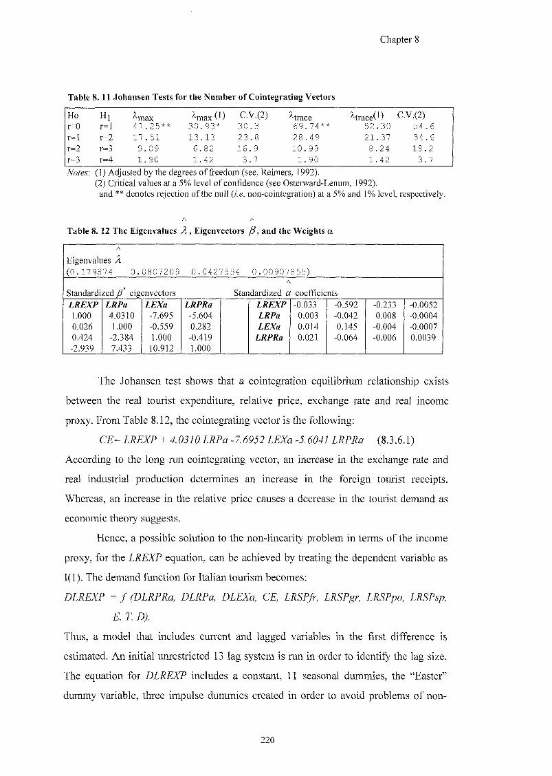
Chapter 8

Table 8 .11 Johansen Tests for the Number of Cointegrating Vectors

Ho Hi ^ a x ^max (^) C.V.(2) ^trace ^trace(^) C.V.(2) r=0 r=l 4 1 . 2 5 * * 3 0 . 9 3 * 3 0 . 3 6 9 . 7 4 * * 5 2 . 3 0 54 6

r=l r=2 17 . 51 1 3 . 1 3 2 3 . 8 2 8 . 4 9 2 1 . 3 7 34 6 r=2 r=3 9 . 0 9 6 . 82 1 6 . 9 1 0 . 99 8 . 2 4 1 8 . 2 r=3 r=4 1 . 9 0 1 . 4 2 3.7 1 . 90 1 . 4 2 3. 7

Notes'. (1) Adjusted by the degrees of freedom (see, Reimers, 1992). (2) Critical values at a 5% level of confidence (see Osterward-Lenum, 1992).

and ** denotes rejection of the null {i.e. non-cointegration) at a 5% and 1% level, respectively.

Table 8. 12 The Eigenvalues X , Eigenvectors /3 , and the Weights a

/ \

Eigenvalues X

( 0 . 1 7 9 8 74 0 . 0 8 0 7 2 0 9 0 . 0 4 2 7 5 5 4 0 . 0 0 9 0 7 855)

Standardized p' eigenvectors A

Standardized a coefficients

LREXP LRPa LEXa LRPRa LREXP -0.033 -0.592 -0.233 -0.0052 1.000 4.0310 -7.695 -5.604 LRPa 0.003 -0.042 0.008 -0.0004 0.026 1.000 -0.559 0.282 LEXa 0.014 0.145 -0.004 -0.0007 0.424 -2.384 1.000 -0.419 LRPRa 0.021 -0.064 -0.006 0.0039 -2.939 7.433 10.912 1.000

The Johansen test shows that a cointegration equilibrium relationship exists

between the real tourist expenditure, relative price, exchange rate and real income

proxy. From Table 8.12, the cointegrating vector is the following:

+ ^ . 0 3 7 0 - 7 . 6 P j 2 ( 8 . 3 . 6 . 1 )

According to the long run cointegrating vector, an increase in the exchange rate and

real industrial production determines an increase in the foreign tourist receipts.

Whereas, an increase in the relative price causes a decrease in the tourist demand as

economic theory suggests.

Hence, a possible solution to the non-linearity problem in terms of the income

proxy, for the LREXP equation, can be achieved by treating the dependent variable as

1(1). The demand function for Italian tourism becomes;

Thus, a model that includes current and lagged variables in the first difference is

estimated. An initial unrestricted 13 lag system is run in order to identify the lag size.

The equation for DLREXP includes a constant, 11 seasonal dummies, the "Easter"

dummy variable, three impulse dummies created in order to avoid problems of non-

220

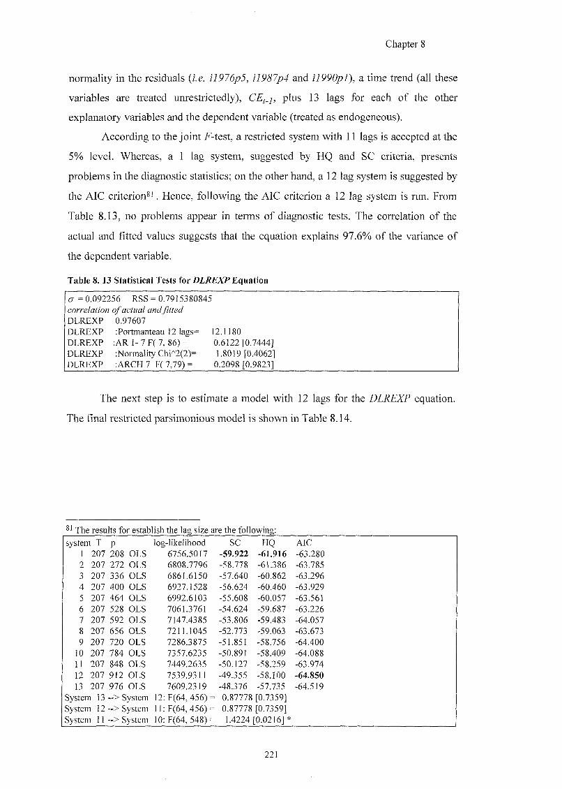
Chapter 8

normality in the residuals (;.e. and 996( 7), a time trend (all these

variables are treated unrestrictedly), CEj_i, plus 13 lags for each of the other

explanatory variables and the dependent variable (treated as endogeneous).

According to the joint F-test, a restricted system with 11 lags is accepted at the

5% level. Whereas, a 1 lag system, suggested by HQ and SC criteria, presents

problems in the diagnostic statistics; on the other hand, a 12 lag system is suggested by

the AlC criterion^'. Hence, following the AIC criterion a 12 lag system is run. From

Table 8.13, no problems appear in terms of diagnostic tests. The correlation of the

actual and Gtted values suggests that the equation explains 97.6% of the variance of

the dependent variable.

Table 8 .13 Statistical Tests for DLREXP Equation

O- = 0.092256 RSS = 0.7915380845

DLREXP 0.97607 DLREXP :Portmanteau 12 lags= 12.1180 DLREXP :AR 1 - 7 F( 7, 86) = 0.6122 [0.7444] DLREXP iNormality Chi'^2(2)= 1.8019 [0.4062] DLREXP :ARCH7 F(7,79) = 0.2098 [0.9823]

The next step is to estimate a model with 12 lags for the DLREXP equation.

The final restricted parsimonious model is shown in Table 8.14.

The results for establish the lae size are the following:

system T P log-likelihood SC HQ AIC 1 207 208 OLS 6756.5017 -59.922 -61.916 -63.280 2 207 272 OLS 6808.7796 -58.778 -61.386 -63.785 3 207 336 OLS 6861.6150 -57.640 -60.862 -63.296 4 207 400 OLS 6927.1528 -56.624 -60.460 -63.929 5 207 464 OLS 6992.6103 -55.608 -60.057 -63.561 6 207 528 OLS 7061.3761 -54.624 -59.687 -63.226 7 207 592 OLS 7147.4385 -53.806 -59.483 -64.057 8 207 656 OLS 721L1045 -52.773 -59.063 -63.673 9 207 720 OLS 7286.3875 -51.851 -58.756 -64.400

10 207 784 OLS 7357.6235 -50.891 -58.409 -64.088 11 207 848 OLS 7449.2635 -50.127 -58.259 -63.974 12 207 912 OLS 7539.9311 -49.355 -58.100 -64.850 13 207 976 OLS 7609.2319 -48.376 -57.735 -64.519

System 13 ~> System 12: F(64, 456) = 0.87778 [0.7359] System 12 - > System 11:F(64, 456) = 0.87778 [0.7359] System 11 - > System 10: F(64, 548) = 1.4224 [0.0216]*

2 2 1

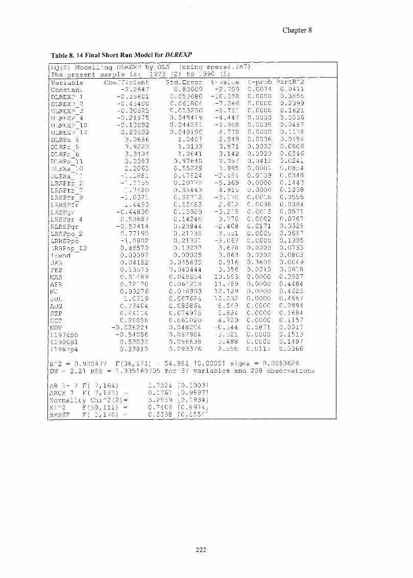
Chapter 8

Table 8. 14 Final Short Run Model for DLREXP

EQ(2) Modell The present

ing DLREXP by sample is: 1

OLS (using 973 (2) to 1

spesa4.in7) 990 (5)

Variable Coefficient Std.Error t-value t -prob PartR^2 Constant -2.2647 0.83609 -2 .709 0 0074 0 0411 DLREXP 1 -0.55601 0.053680 -10 .358 0 0000 0 3855

DLREXP 2 -0.45400 0.061804 -7 .346 0 0000 0 2399 DLREXP 3 -0.30625 0.053250 -5 .751 0 0000 0 1621 DLREXP 4 -0.21975 0.049419 -4 .447 0 0000 0 1036 DLREXP 10 -0.13092 0.044251 -2 .958 0 0035 0 0487 DLREXP 12 0.23502 0.049190 4 .778 0 0000 0 1178

DLRPa 4 3.0686 1.0407 2 .949 0 0036 0 0484 DLRPa 5 3.9223 1.0133 3 871 0 0002 0 0806 DLRPa 6 3.3434 1.0641 3 142 0 0020 0 0546 DLRPa 11 2.0083 0.97640 2 057 0 0412 0 0241 DLEXa 10 2.2065 0.55229 3 995 0 0001 0 0854 DLEXa 11 -1.1881 0.47824 -2 484 0 0139 0 0348 LRSPfr 2 -1.1155 0.20778 -5 369 0 0000 0 1443 LRSPfr 7 1.7420 0.35443 4 915 0 0000 0 1238 LRSPfr 9 -1.0371 0.32712 -3 170 0 0018 0 0555 LRRSPfr 1.4493 0.55485 2 612 0 0098 0 0384 LRSPgr -0.44830 0.13929 -3 218 0 0015 0 0571 LRSPgr 4 0.53687 0.14240 3 770 0 0002 0 0767 RLRSPgr -0.57414 0.23844 -2 408 0 0171 0 0328 LRSPpo_2 0.77190 0.21735 3 551 0 0005 0 0687 LRRSPpo -1.0802 0.21321 -5 067 0 0000 0 1305 LRSPsp_10 0.48570 0.13207 3 678 0 0003 0 0733 Trend 0.00097 0.00025 3 863 0 0002 0 0803 JAN 0.04182 0.045639 0 916 0 3608 0 0049

FEB 0.13573 0.040444 3 356 0 0010 0 0618

MAR 0.51489 0.048654 10 583 0 0000 0 3957 APR 0.72170 0.061218 11 789 0 0000 0 4484 MJ 0.93276 0.076903 12 129 0 0000 0 4625 JUL 1.0719 0.087624 12 232 0 0000 0 4667 AUG 0.73404 0.085864 8 549 0 0000 0 2994 SEP 0.44114 0.074975 5 884 0 0000 0 1684 OCT 0.28858 0.061020 4 729 0 0000 0 1157 NOV -0.026224 0.048204 -0 544 0 5871 0 0017 il976p5 -0.54056 0.097904 -5. 521 0 0000 0 1513 il990pl 0.53032 0.096638 5. 488 0 0000 0 1497 il987p4 0.23810 0.093376 2 550 0 0117 0 0366

R*2 = 0.920477 F(36,171) = 54.981 [0.0000] sigma = 0.0883626 DM = 2.21 RSS = 1.335160705 for 37 variables and 208 observations

AR 1- 7 F( 7,164) ARCH 7 F( 7,157) Normality Chi^2(2; Xi^2 F(59,lll) RESET F( 1,170)

1.7524 0.1767 3.2859 0.7409 0.5598

[0.1003] [0.9897] [0.1934] [0.8974] [0.4554]

222

Chapter 8

Few coefGcient restrictions can be imposed applying the joint F-test as follows.

MJ as the first restriction that involves the coefficients for the seasonal dummies May

and June as they have a similar m a g n i t u d e ^ ^ xhe second restriction RLRSPgr^^ is

given by the difference between the sixth and seventh lag coefficients of the real

substitute price for Greece. The further restriction is given by the difference between

the coefficients for the fourth and fifth lag of the (log) real substitute price for Portugal

{LRRSPpoy^. The final restriction involves the coefficients for the tenth and eleventh

lag of the (log) real substitute price for France {LRRSPfry^.

The final model passes all diagnostic statistics and it is data admissible to its

information set. From Tables 8.14 and 8.15, the growth in Italian tourist expenditure is

positively related to the growth of the relative price with an elasticity equal to +3.07.

The growth in the relative price shows a long run positive sign and it has a highly

statistical significance (/-value +5.49). This finding suggests that foreign consumers do

not respond quickly to short run changes in the Italian price with respect to home

prices. As a reminder, from the Johansen long run analysis, it emerges that the

negativity condition for the relative price does hold. The growth of the dependent

variable is positively influenced by the growth in the exchange rate, both in the short

run and in the long run. This finding confirms the Johansen long run elasticity (see

8.3.6.1). On the other hand, a permanent shift in the real substitute price for France

{LRSPfr), which is stationary in the level, causes a permanent decrease in the growth

of Italian expenditure in tourist goods and services. Moreover, a permanent shift in the

real substitute price for Greece, Portugal and Spain causes a permanent increase in the

growth of Italian expenditure. These findings seem to indicate that the competitor

countries included in this study might not be the appropriate ones, with the only

exception being France. The time trend plays a role in explaining the dependent

The restriction on the coefficient of the May and June dummy is accepted at the 5% level from the joint f - tes t (1,166) as the calculated value 0.15 is smaller than the critical value 3.84; moreover, the SC criterion is minimised when such a restriction is imposed; from -3.98751 to -4.01229. ^3 The calculated F-test (1,167) equals 0.60 that is smaller than the critical value 3.84. Hence, the restriction on the coefficient of the sixth and seventh lag of the substitute price for Greece is accepted at the 5% level. Moreover, the SC criterion is minimised when such a restriction is imposed: from -4.01229 to-4.03435. ^ The calculated F (1,168) equals 0.77 and it is smaller than the critical value (3.84) at the 5% level. The SC criterion also suggests for this parameter reduction, it decreases from -4.03435 to -4.05541.

The calculated F (1,169) equals 0.33 and it is smaller than the critical value (3.84) at the 5% level. The SC criterion suggests for this parameter reduction, decreasing from -4.05541 to -4.07859.

223

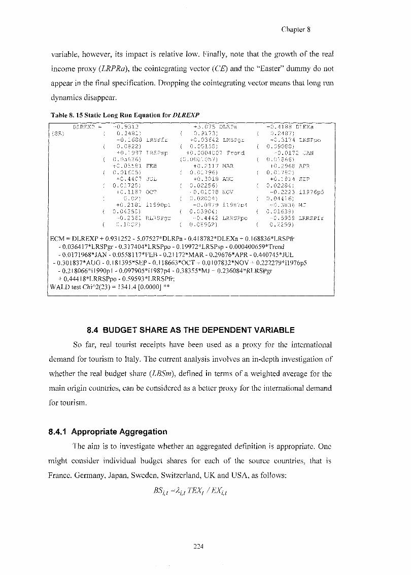
Chapter 8

variable, however, its impact is relative low. Finally, note that the growth of the real

income proxy 7(<3), the cointegrating vector (CE) and the "Easter" dummy do not

appear in the final specification. Dropping the cointegrating vector means that long run

dynamics disappear.

Table 8 .15 Static Long Run Equation for DLREXP

DLREXP (SE)

- 0 . 9 3 1 3 + 5 . 0 7 5 D l R P a + 0 . 4 1 8 8 DLEXa 0 . 3 4 8 1 ) ( 0 . 9 1 7 3 ) 0 . 2 4 8 7 ) - 0 . 1 6 8 8 L R S P f c + 0 . 0 3 6 4 2 L R S P g r + 0 . 3 1 7 4 L R S P p o 0 . 0 8 2 2 ) ( 0 . 0 5 1 5 5 ) 0 . 0 9 0 8 8 ) + 0 . 1 9 9 7 I R S P s p + 0 . 0 0 0 4 0 0 7 T r e n d + 0 . 0 1 7 2 JAN

0 . 0 5 6 3 6 ) ( 0 . 0 0 0 1 0 5 7 ) 0 . 0 1 8 6 6 ) + 0 . 0 5 5 8 1 FEB + 0 . 2 1 1 7 MAR + 0 . 2 9 6 8 APR 0 . 0 1 6 0 5 ) ( 0 . 0 1 7 9 6 ) 0 . 0 1 7 8 2 )

+ 0 . 4 4 0 7 JUL + 0 . 3 0 1 8 AUG + 0 . 1 8 1 4 SEP 0 . 0 1 7 2 5 ) ( 0 . 0 2 2 5 6 ) 0 . 0 2 2 8 4 )

+ 0 . 1 1 8 7 OCT - 0 . 0 1 0 7 8 NOV - 0 . 2 2 2 3 i l 9 7 6 p 5 0 . 0 2 ) ( 0 . 0 2 0 0 4 ) 0 . 0 4 4 1 6 )

+ 0 . 2 1 8 1 i l 9 9 0 p l + 0 . 0 9 7 9 i l 9 8 7 p 4 + 0 . 3 8 3 6 MJ 0 . 0 4 3 5 5 ) ( 0 . 0 3 9 0 4 ) 0 . 0 1 6 3 9 )

- 0 . 2 3 6 1 R l R S P g r - 0 . 4 4 4 2 LRRSPpo + 0 . 5 9 5 9 L R R S P f r 0 . 1 0 0 2 ) ( 0 . 0 8 9 5 2 ) 0 . 2 2 9 9 )

ECM = DLREXP + 0.931252 - 5.07527*DLRPa - 0.4]8782*DLEXa + 0.168836*LRSPfr - 0.036417*LRSPgr - 0.317404*LRSPpo - 0.19972*LRSPsp - 0.000400659*Trend - 0.0171968*JAN - 0.0558117*FEB - 0.21172*MAR - 0.29676*APR - 0.440745*JUL

- 0.301837*AUG - 0.181395*SEP - 0.118663*0CT + 0.0107832*NOV + 0.222279*il976p5 - 0.218066*il990pl - 0.097905*il987p4 - 0.38355*MJ + 0.236084*RLRSPgr + 0.44418*LRRSPpo - 0.59593*LRRSPfT;

WALO test Chi^2(23) = 1341.4 [0.0000] **

8.4 BUDGET SHARE AS THE DEPENDENT VARIABLE

So far, real tourist receipts have been used as a proxy for the international

demand for tourism to Italy. The current analysis involves an in-depth investigation of

whether the real budget share (LBSm), defined in terms of a weighted average for the

main origin countries, can be considered as a better proxy for the international demand

for tourism.

8.4.1 Appropriate Aggregation

The aim is to investigate whether an aggregated definition is appropriate. One

might consider individual budget shares for each of the source countries, that is

France, Germany, Japan, Sweden, Switzerland, UK and USA, as follows:

224

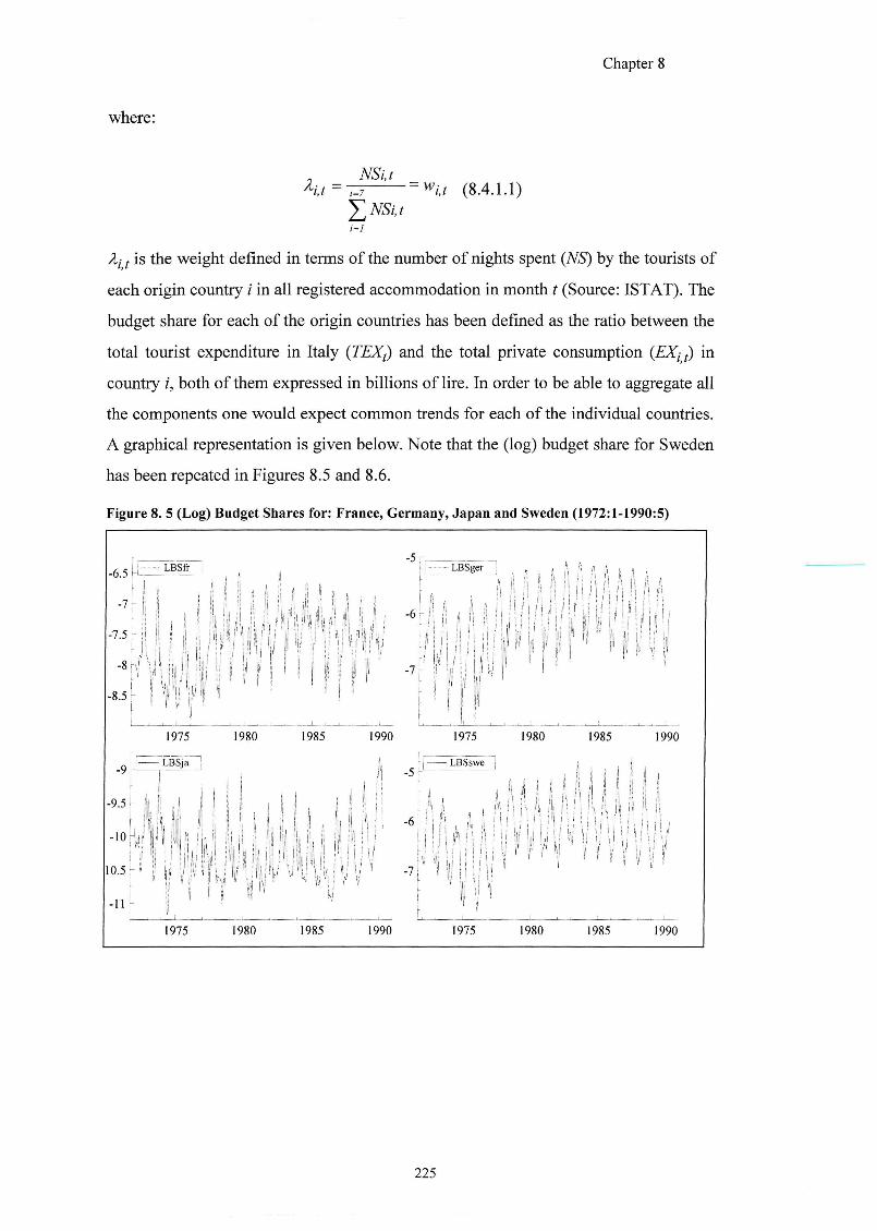
Chapter 8

where;

A ; t = NSi,t

•i,t - ,=7

i=]

= î,t (8.4.1.1)

Af (is the weight defined in terms of the number of nights spent (NS) by the tourists of

each origin country i in all registered accommodation in month t (Source; ISTAT). The

budget share for each of the origin countries has been defined as the ratio between the

total tourist expenditure in Italy (TEXf) and the total private consumption (EXij) in

countiy /, both of them expressed in billions of lire. In order to be able to aggregate all

the components one would expect common trends for each of the individual countries.

A graphical representation is given below. Note that the (log) budget share for Sweden

has been repeated in Figures 8.5 and 8.6.

Figure 8. 5 (Log) Budget Shares for: France, Germany, Japan and Sweden (1972:1-1990:5)

-6,5

1 -7.5: I

LBSfr -5

LBSger t

i

ii i'l li

1

1 1 1 j ! , I

I j j II ^ I

UUI i i l j iUMj iH !i Mi If U I ' i ! I

111 iJ ^ ij 11! f II

, V I' -lOriJlU) ku; II'

s 1

IS i; ri|i i| !ii 11! ill yl 11 Hi 11: 'i! ir

-11 ; I '•

1975 1980 1985

!> -7 ' '

M i f s

1975 1980 1985 1990

. 9 ^

' I , I I , , . I I I ! -9 .5 '

-5 t

i - !

- 6 ^ !

1975 1980 1985 1990

LBSswe I I j ^

^ I ,M I I I I ! I I ! ! E1 1 '

1 Ifl

' f i AI n i l A III l ! f II HiII y i i L

\n .-]•

I l! 1

1990

! i i 'i f f

1975 1980 1985 1990

2 2 5

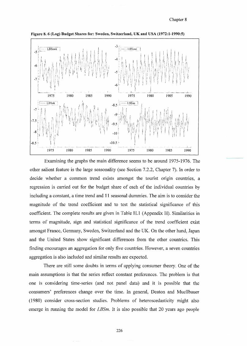
Chapter 8

Figure 8. 6 (Log) Budget Shares for; Sweden, Switzerland, UK and USA (1972:1-1990:5)

-5

- 6

LBSswe ( I t !

a I

11 k ,'l II11! w i IJIIN11II U 111 I

! I

-3 i

-4

LBSswi

i f -7r

u ; < i M l | / l (

: I n n I i i n n n i ii i

U !

i II n M

i !

!i ii ii !l U' U

'ii \!

ji 11 li i! 11 11 !i V u u II ,Mi i| ii ii i j ' y ii !j

- 6 ^ ' t ' I ' ' W '

I

1975 1980 1985 1990

^ a '

' H I M i il -7.5

-8.5 h

I! 'i

1 I

/ « i

-8 .5 '

1975 1980 1985 1990

LBSus J

i ' ' 1; '1 ill I

ly ^ ill

I -10! iMmrn ' t I I I I

!i!

'(I

,

-10.5 i

1975 1980 1985 1990 1975 1980 1985 1990

Examining the graphs the main difference seems to be around 1975-1976. The

other salient feature is the large seasonality (see Section 7.2.2, Chapter 7). In order to

decide whether a common trend exists amongst the tourist origin countries, a

regression is carried out for the budget share of each of the individual countries by

including a constant, a time trend and 11 seasonal dummies. The aim is to consider the

magnitude of the trend coefficient and to test the statistical significance of this

coefficient. The complete results are given in Table H.l (Appendix H). Similarities in

terms of magnitude, sign and statistical significance of the trend coefficient exist

amongst France, Germany, Sweden, Switzerland and the UK. On the other hand, Japan

and the United States show significant differences from the other countries. This

finding encourages an aggregation for only five countries. However, a seven countries

aggregation is also included and similar results are expected.

There are still some doubts in terms of applying consumer theory. One of the

main assumptions is that the series reflect constant preferences. The problem is that

one is considering time-series (and not panel data) and it is possible that the

consumers' preferences change over the time. In general, Deaton and Muellbauer

(1980) consider cross-section studies. Problems of heteroscedasticity might also

emerge in running the model for LBSm. It is also possible that 20 years ago people

226

Chapter 8

with average income did not want to spend their wages on foreign holidays; whereas,

today there is more willingness to spend money on leisure abroad.

As already mentioned, budget shares are usually used with panel data and

system of equations. There is explicit economic reasoning from micro foundations. A

consumer allocates his/her income over a whole range of goods and services. Several

stages can be identified within the budget allocation. The first stage consists of

allocating income over a set of groups and services such as food, housing, holidays and

so on. In the case of leisure, the second stage consists of allocating expenditure

between destination subgroups (domestic tourism, holidays in Europe, in South

America, in Australia, etc.). A further stage involves allocating expenditure within

destinations of the same subgroup. Hence, on would model the budget share of Italy

versus its close competitors.

A stronger assumption has been adopted in this chapter. The consumers, from

the origin countries under study, are allocating their income over holidays in Italy and

a whole range of goods and services. The main limitation of this assumption is that one

does not underpin the modelling of the budget share with the main assumptions based

on microeconomic theory of consumer demand. Moreover, the values of the dependent

variable are very low. However, the procedure adopted in this chapter has several

advantages. The first is that it allows a straightforward comparison between the results

from the budget share and tourist receipts, as given earlier in the chapter. Furthermore,

one of the main purposes of Chapter 8 is that of using time series at a monthly

frequency. As already mentioned, there are grounds for believing that monthly series

are the appropriate frequency for analysing and modelling the demand for tourism.

Hence, one of the main problems is the lack of data at monthly frequency in the

official statistics for the main competitors of Italy. Future work needs to be undertaken

to expand the monthly database for other competitors.

8.4.2 Appropriate Weights

In defining the variables of interest, an investigation has been carried out on the

appropriate weight to use. Some experiments have been done in understanding

whether the (annual) weights calculated in terms of foreign nights of stay in registered

accommodation (w - ) could approximate the values of the (annual) weights calculated

227

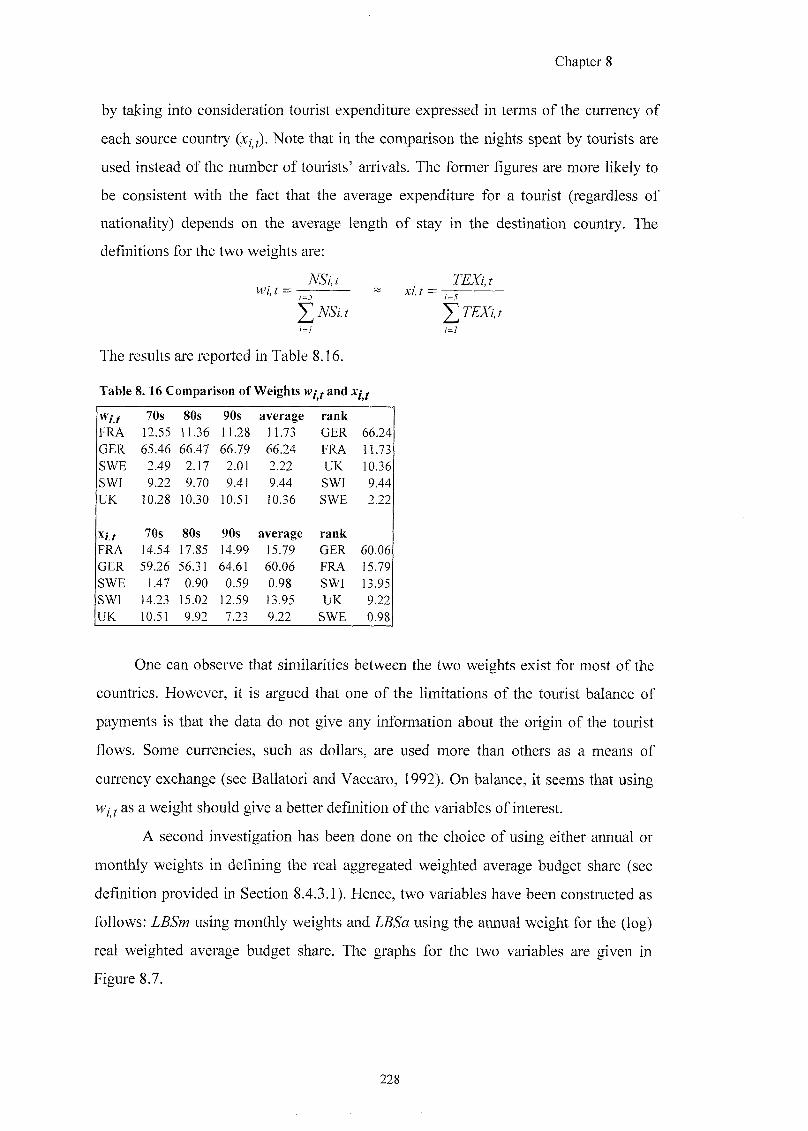
Chapter 8

by taking into consideration tourist expenditure expressed in terms of the currency of

each source country (x,;). Note that in the comparison the nights spent by tourists are

used instead of the number of tourists' arrivals. The former figures are more likely to

be consistent with the fact that the average expenditure for a tourist (regardless of

nationality) depends on the average length of stay in the destination country. The

definitions for the two weights are:

! = }

The results are reported in Table 8.16.

Table 8 .16 Comparison of Weights wi f and xi f

w,-./ 70s 80s 90s average rank FRA 12.55 11.36 11.28 11.73 GER 66.24 GER. 65.46 66.47 66.79 66.24 FRA 11.73 SWE 2.49 2.17 2.01 2.22 UK 10.36 SWI 9.22 9.70 9.41 9.44 SWl 9.44 UK 10.28 10.30 10.51 10.36 SWE 2.22

X,-./ 70s 80s 90s average rank FRA 14.54 17.85 14.99 15.79 GER 60.06 GER 59.26 56.31 64.61 60.06 FRA 15.79 SWE 1.47 0.90 0.59 0.98 SWI 13.95 SW] 14.23 15.02 12.59 13.95 UK 9.22 UK 10.51 9.92 7.23 9.22 SWE 0.98

/ = /

One can observe that similarities between the two weights exist for most of the

countries. However, it is argued that one of the limitations of the tourist balance of

payments is that the data do not give any information about the origin of the tourist

flows. Some currencies, such as dollars, are used more than others as a means of

currency exchange (see Ballatori and Vaccaro, 1992). On balance, it seems that using

as a weight should give a better definition of the variables of interest.

A second investigation has been done on the choice of using either annual or

monthly weights in defining the real aggregated weighted average budget share (see

definition provided in Section 8.4.3.1). Hence, two variables have been constructed as

follows: using monthly weights and using the annual weight for the (log)

real weighted average budget share. The graphs for the two variables are given in

Figure 8.7.

228

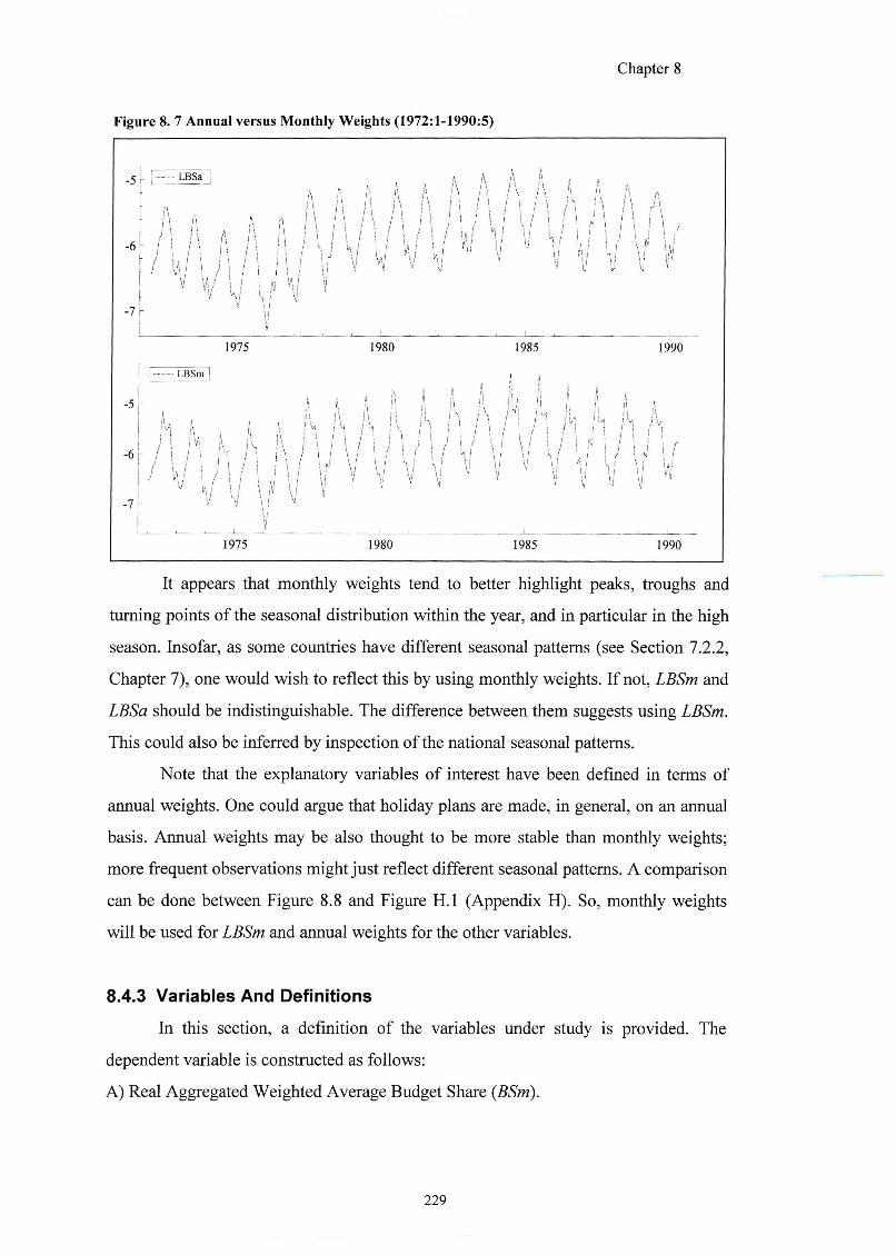
Chapter 8

Figure 8. 7 Annual versus Monthly Weights (1972:1-1990:5)

-5 1 LBSa J

\

S

-6

7

A n ^ !

1 \

-7 \j !

1975 1980 1985 1990

-5

LBSm

1 l\ i j i

-6 1

•'!

H/

1975 1980 1985 1990

It appears that monthly weights tend to better highlight peaks, troughs and

turning points of the seasonal distribution within the year, and in particular in the high

season. Insofar, as some countries have different seasonal patterns (see Section 7.2.2,

Chapter 7), one would wish to reflect this by using monthly weights. If not, LBSm and

LBSa should be indistinguishable. The difference between them suggests using LBSm.

This could also be inferred by inspection of the national seasonal patterns.

Note that the explanatory variables of interest have been defined in terms of

annual weights. One could argue that holiday plans are made, in general, on an annual

basis. Annual weights may be also thought to be more stable than monthly weights;

more frequent observations might just reflect different seasonal patterns. A comparison

can be done between Figure 8.8 and Figure H.I (Appendix H). So, monthly weights

will be used for LBSm and annual weights for the other variables.

8.4.3 Variables And Definitions

In this section, a definition of the variables under study is provided. The

dependent variable is constructed as follows:

A) Real Aggregated Weighted Average Budget Share (BSm).

229

Chapter 8

^ 1 (8.4.3.1)

where:

BSj = Real aggregated weighted average budget share. Note that this variable has

been deflated by dividing the total expenditure for tourism in Italy (TEXf) by the total

expenditure in the origin country i {EXPjj).

i = France, Germany, Sweden, Switzerland and United Kingdom, which

represent an average 65% of the total countries originating tourism to Italy, for the

period under study.

TEXf = Total tourist receipts in current billions of lire, in month t (Source: Bank of

Italy).

EXPj f = Total expenditure in country /, in month t (Source: IPS Datastream, private

consumption, average of quarterly data expressed in the currency of country /). Note

that these figures have been calculated in billions of lire.

Wij = This weight is formed by taking into consideration the number of nights

spent {NS) by the tourists of each origin country i in all registered accommodation in

month t (Source: ISTAT), and it is given by the following formula:

Wf.,= (8.4.3.2)

2 m S ( , / = /

At this point a note is due. Ideally, the budget share should be defined as follows:

^ (8.4.3.3)

where:

( 8 / L 1 4 )

i — I ,

i= 0

and where is defined as in (8.4.3.2). However, tourism receipts disaggregated by

country (TEXij) are available only at an annual frequency; hence, the monthly total

receipts have been used to calculate this variable, as mentioned before. One can define:

TEXi (= Ajj TEXf. Hence, definition (8.4.3.3) can be written as:

'=^ ( TF Yf \ - y a/. f * (8.4.3.5)

230

Chapter 8

One method to approximate is to use the monthly share of nights spent by tourists

in all registered accommodation, as follows:

TVSu (8.4.3.6)

E ® / , , / = /

By substituting by and re-deGning in terms of w, in definition (8.4.3.5),

the final formula of the budget share (8.4.3.1) is obtained.

B) Income Proxy (RPRa), Relative Price (RPa) and Exchange rate (EXa) are defined as

reported in Section 8.3.1 for five countries' aggregation only.

C) Real Substitute Price (RSPJ) is defined in a disaggregated manner for the main

competitors in the Mediterranean area, that is France, Greece, Portugal and Spain (see

Section 8.3.1).

The plot of LBSm is given in Figure 8.7 (Section 8.4.1). The graphs of LRPRa,

ZJgfa and are represented in Figure 8.8, and 2^(57^, and

LRSPsp in Figure 8.2 (Section 8.3.1). All the variables mentioned are expressed in

logarithm.

231

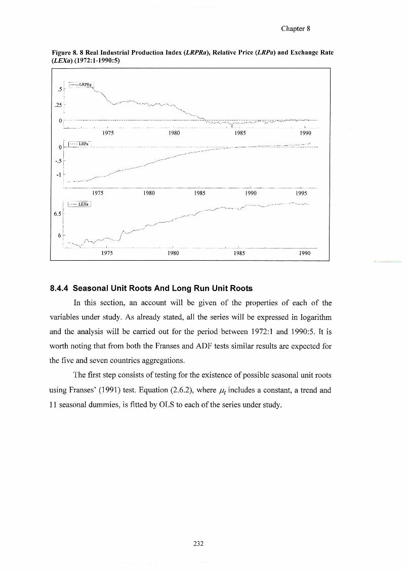
Chapter 8

Figure 8. 8 Real Industrial Production Index (LRPRa), Relative Price (LRPa) and Exchange Rate (LEXa) (1972:1-1990:5)

8.4.4 Seasonal Unit Roots And Long Run Unit Roots

In this section, an account will be given of the properties of each of the

variables under study. As already stated, all the series will be expressed in logarithm

and the analysis will be carried out for the period between 1972:1 and 1990:5. It is

worth noting that from both the Franses and ADF tests similar results are expected for

the five and seven countries aggregations.

The first step consists of testing for the existence of possible seasonal unit roots

using Franses' (1991) test. Equation (2.6.2), where includes a constant, a trend and

11 seasonal dummies, is fitted by OLS to each of the series under study.

232

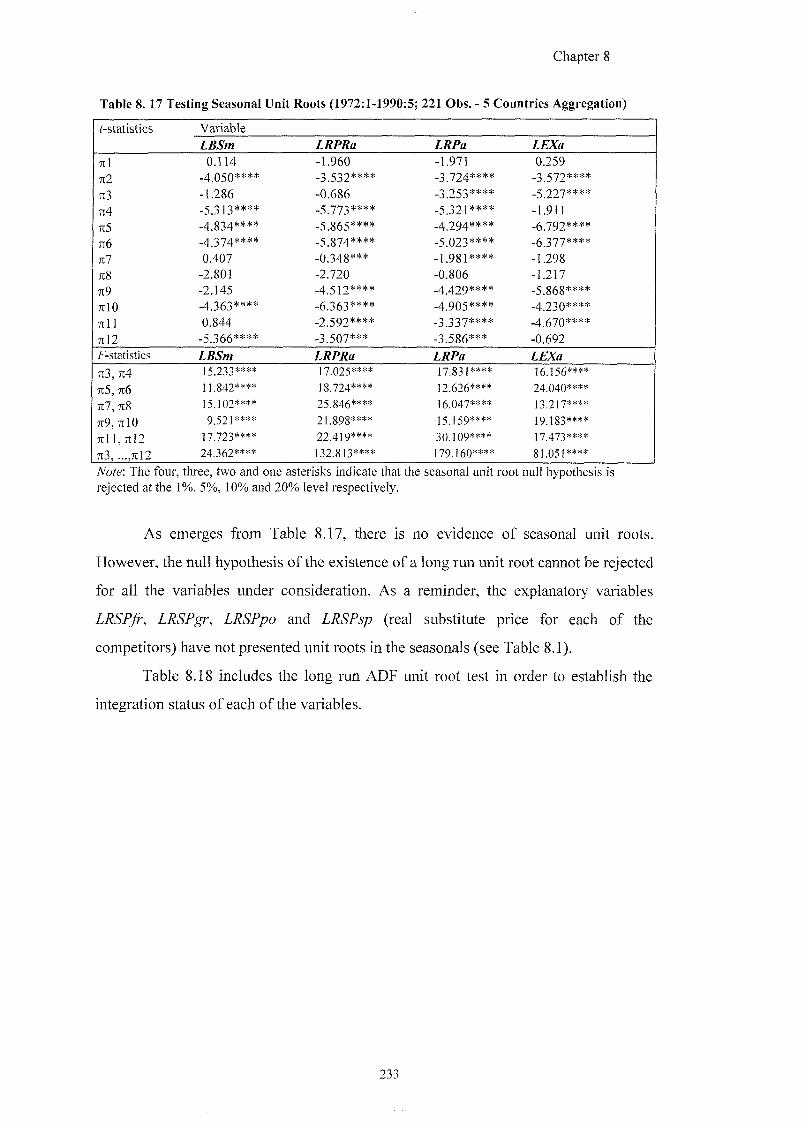
Chapter 8

Table 8. 17 Testing Seasonal Unit Roots (1972:1-1990:5; 221 Obs. - 5 Countries Aggregation)

f-statistics Variable LBSm LRPRa LRPa LEXa

7tl 0JU4 -1.960 -1.971 &259

n2 -4.050**** -3.532**** -3.724**** -3.572**** 7:3 -1286 -0.686 -3.253**** -5.227**** 7r4 -5.313**** -5.773**** -5.321**** -1.911 k5 -4.834**** -5.865**** -4.294**** -6.792**** ti6 -4.374**** -5.874**** -5.023**** -6.377**** 71? 0.407 -0.348*** -l.SHBl**** -L298 7I8 -2.801 ^^^20 -0.806 -L217 n9 -2J45 -4.512**** -4.429**** -5.868**** TllO -4.363**** -6.363**** -4.905**** -4.230**** n i l 0.844 -2.592**** -3.337**** -4.670**** 7tl2 -5.366**** -3.507*** -3.586*** -0.692 F-statistics LBSm LRPRa LRPa LEXa 7I3, 7I4 15.233**** 17\025**** 17\831**** 16.156****

n5, n6 11.842**** 1&724**** 12.626**** 24.040**** 15.102**** :%\846**** l(x047**** 13.217****

7r9, TilO SI.52]**** 21 898**** 15.159**** 19.183****

7tl 1, 7tl2 17.723**** 22.419**** 30.109**** 17\473****

7t3, ...,7rl2 2Mk362**** 132.813**** 179.160**** 81.051**** 1 Note-. The four, three, two and one asterisks indicate that the seasonal unit root null hypothesis is rejected at the 1%, 5%, 10% and 20% level respectively.

As emerges from Table 8.17, there is no evidence of seasonal unit roots.

However, the null hypothesis of the existence of a long run unit root cannot be rejected

for all the variables under consideration. As a reminder, the explanatory variables

LRSPfr, LRSPgr, LRSPpo and LRSPsp (real substitute price for each of the

competitors) have not presented unit roots in the seasonals (see Table 8.1).

Table 8.18 includes the long run ADF unit root test in order to establish the

integration status of each of the variables.

23:

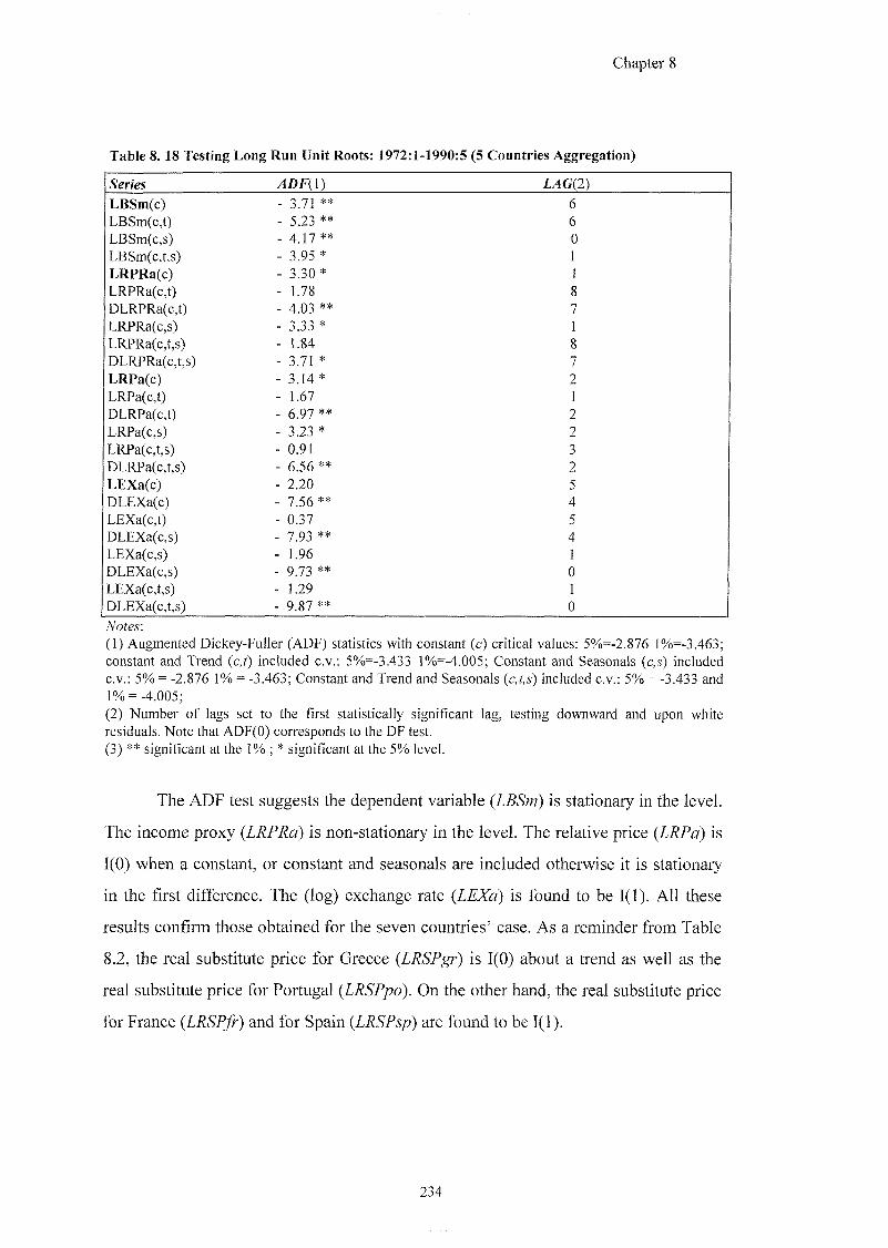
Chapter 8

Table 8. 18 Testing Long Run Unit Roots: 1972:1-1990:5 (5 Countries Aggregation)

Series /*DF(1) jL4G(2)

LBSm(c) - 3.71 ** 6 LBSm(c,t) - 5.23 ** 6 LBSm(c,s) - 4.17 ** 0 LBSm(c,t,s) - 3.95 * 1 LRPRa(c) - 3.30 * 1 LRPRa(c,t) - 1.78 8 DLRPRa(c,t) - 4.03 ** 7 LRPRa(c,s) - 3.33 * 1 LRPRa(c,t,s) - 1.84 8 DLRPRa(c,t,s) - 3.71 * 7 LRPa(c) - 3 .14* 2 LRPa(c,t) - 1.67 1 DLRPa(c,t) - 6.97** 2 LRPa(c,s) - 3.23 * 2 LRPa(c,t,s) - 0.91 3 DLRPa(c,t,s) - 6.56 ** 2 LEXa(c) - 2.20 5 DLEXa(c) - 7.56** 4 LEXa(c,t) - 0.37 5 DLEXa(c,s) - 7.93 ** 4 LEXa(c,s) - 1.96 1 DLEXa(c,s) - 9.73 ** 0 LEXa(c,t,s) - 1.29 1 DLEXa(c,t,s) - 9.87 ** 0

(1) Augmented Dickey-Fuller (ADF) statistics with constant (c) critical values: 5%=-2.876 l%=-3.463; constant and Trend {c,t) included c.v.: 5%=-3.433 l%=-4.005; Constant and Seasonals {c,s} included C . V . : 5% = -2.876 1% = -3.463; Constant and Trend and Seasonals (c,l,s) included c.v.: 5% = -3.433 and ]% =-4.005; (2) Number of lags set to the first statistically significant lag, testing downward and upon white residuals. Note that ADF(O) corresponds to the DF test. (3) ** significant at the 1% ; * significant at the 5% level.

The ADF test suggests the dependent variable (Z.SS'/M) is stationary in the level.

The income proxy (LRPRa) is non-stationary in the level. The relative price (LRPa) is

1(0) when a constant, or constant and seasonals are included otherwise it is stationary

in the first difference. The (log) exchange rate (LEXa) is found to be 1(1). All these

results confirm those obtained for the seven countries' case. As a reminder from Table

8.2, the real substitute price for Greece (LRSPgr) is 1(0) about a trend as well as the

real substitute price for Portugal (LRSPpo). On the other hand, the real substitute price

for France and for Spain are foimd to be 1(1).

234

Chapter 8

8.4.5 Possible Cointegration Amongst 1(1) Variables

The next step of the analysis consists in considering the possible existence of a

cointegrating relationship between the relative price (LRPa) and (LEXa). The

expectations are twofold; these two variables should drift together in the long run, in

accordance with economic theory, and similar results are expected to the seven

countries aggregation case.

An initial 13 lag system has been run, which includes a constant, a trend and 11

seasonals treated unrestrictedly. Impulse dummies, created after inspecting the

residuals in order to avoid problems of non-normality, worsen the results in terms of

diagnostics, so they are not included in the system. The system can be reduced further

to 2 lags, as suggested by the SC and HQ criteria (the complete results are reported in

Appendix H, Table H.2). From a Johansen cointegration analysis, there is evidence for

the presence of one cointegrating relationship between the two variables. From Table

H.2, the cointegrating vector can be derived and it is given by the first row of the / '

matrix:

c ; = I j g f a - 0.PP6P; (8.4.5.1)

The expectation is that the two cointegrated variables will present a long run

coefficient of one. Thus, the restriction; /9=-l is tested for the coefficient for the (log)

exchange rate and the null hypothesis fails to be rejected at the 5% level from the

test&s. This finding is consistent with economic theory for which, in the long run, there

appear no significant differences in the inflation rates for the countries under

consideration. As a reminder from Section 8.3.3, the long run coefficient restriction

could not be accepted when including Japan and USA as source countries of tourism to

Italy.

As for the seven countries aggregation case, a cointegration analysis has also

been run for the three 1(1) variables (i.e. real industrial production, relative price and

exchange rate). Statistical evidence has been found for the existence of one

cointegrating vector (see Appendix H, Table H.3); however, there are difficulties in

interpreting the results on an economic basis. Hence, an investigation follows in

employing a non-linear transformation for the real industrial production index.

86 The results for the restriction test on the coefficient is: ZÔ) ^ 3.7093 [0.0541]

235

Chapter 8

The cointegration analysis results for each of the real substitute prices have

been given in Section 8.3.3. Statistical evidence has been found for each of real

substitute prices to be treated as stationary in the level.

8.4.6 Estimating The Weighted Aggregated Budget Share

The first aim of this analysis is to estimate a model using the weighted budget

share for a five countries aggregation as the dependent variable.

As stated in the previous sections, the real income proxy (LRFRa) has been

found to be non-stationary in the level. Thus, this variable needs an appropriate

transformation in order to be included in the estimation of the real budget share. In this

section, an account of the use of a logistic transformation for LRPRa is given.

The Box and Cox procedure has been applied in order to give a statistical

foundation for the choice of the logarithmic functional form. The complete results for

this analysis are reported in Appendix I.

The initial formulation of the equation for the aggregated budget share

is the following;

C /

71 &&4S: D) (8.4.6.1)

By using a VAR, it is possible to identify the lag size of the system. The system for

LBSm includes; a constant, 11 seasonal dummies (SEAS), the "Easter" dummy variable

three impulse dummies created in order to correct for problems of non-

normality in the residuals (D that is and a time trend (7)

(all these variables are treated unrestrictedly), the first lag for the cointegrating vector

(C7), plus 13 lags for each of the other explanatory variables and the dependent

variable (treated as endogenous). Note that in (8.4.6.1) is the quadratic (log)

real production index which allows for non-linearities in the budget share. The period

under study is from 1972:1 to 1990:5.

236

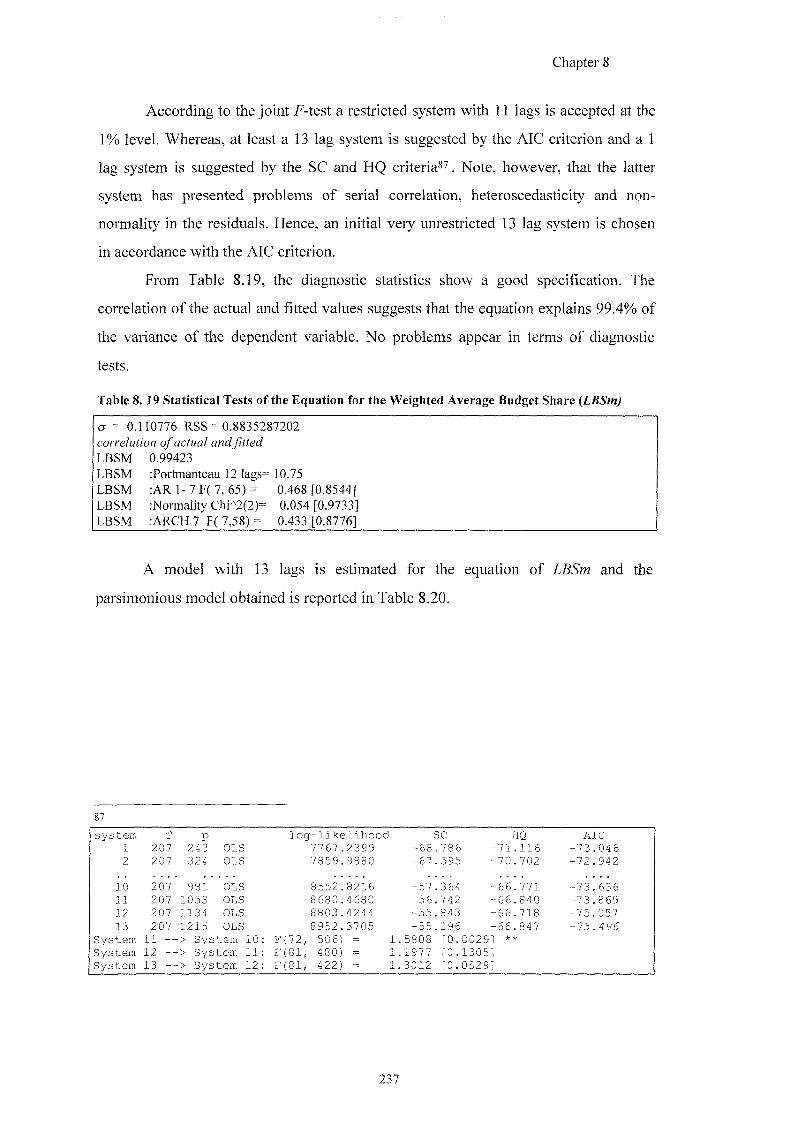
Chapter 8

According to the joint f-test a restricted system with 11 lags is accepted at the

1% level. Whereas, at least a 13 lag system is suggested by the AIC criterion and a 1

lag system is suggested by the SC and HQ criteria* . Note, however, that the latter

system has presented problems of serial correlation, heteroscedasticity and non-

normality in the residuals. Hence, an initial very unrestricted 13 lag system is chosen

in accordance with the AIC criterion.

From Table 8.19, the diagnostic statistics show a good specification. The

correlation of the actual and fitted values suggests that the equation explains 99.4% of

the variance of the dependent variable. No problems appear in terms of diagnostic

tests.

Table 8 .19 Statistical Tests of the Equation for the Weighted Average Budget Share (LBSm)

(7= 0.110776 RSS = 0.8835287202 corre/an'oM o/ acfwo/ ancfyzffecf LBSM 0.99423 LBSM :Portmanteau 12 lags= 10.75 LBSM :AR 1 - 7 F( 7, 65) = 0.468 [0.8544] LBSM :Normality Chi^2(2)= 0.054 [0.9733] LBSM :ARCH 7 F( 7,58) = 0.433 [0.8776]

A model with 13 lags is estimated for the equation of LBSm and the

parsimonious model obtained is reported in Table 8.20.

87

s y s t e m T P l o g - l i k e l i h o o d sc HQ A I C 1 2 0 7 2 4 3 OLS 7 7 6 7 . 2 3 9 9 - 6 8 . 7 6 6 7 1 . 1 1 6 - 7 3 . 0 4 6 2 2 0 7 3 2 4 OLS 7 8 5 9 . 9 8 8 0 - 6 7 . 5 9 5 7 0 . 7 0 2 - 7 2 . 9 4 2

1 0 2 0 7 9 8 1 OLS 8 5 5 2 . 8 2 1 6 - 5 7 . 3 6 4 6 6 . 7 7 1 - 7 3 . 6 3 6 1 1 2 0 7 1 0 5 3 OLS 8 6 8 0 . 4 6 8 0 - 5 6 . 7 4 2 6 6 . 8 4 0 - 7 3 . 8 6 9 12 2 0 7 1 1 3 4 OLS 8 8 0 3 . 4 2 4 4 - 5 5 . 8 4 3 6 6 . 7 1 8 - 7 5 . 0 5 7 1 3 2 0 7 1 2 1 5 OLS 8 9 5 2 . 3 7 0 5 - 5 5 . 1 9 6 6 6 . 8 4 7 - 7 5 .

S y s t e m 1 1 — > S y s t e m 1 0 : F ( 7 2 , 5 0 6 ) = 1 5 8 0 8 [ 0 . 0 0 2 9 ] S y s t e m 12 — > S y s t e m 1 1 : F ( 8 1 , 4 8 0 ) = 1 1 9 7 7 [ 0 . 1 3 0 5 ] S y s t e m 1 3 — > S y s t e m 1 2 : F ( 8 1 , 4 2 2 ) = 1 3 0 1 2 [ 0 . 0 5 2 9 ]

237

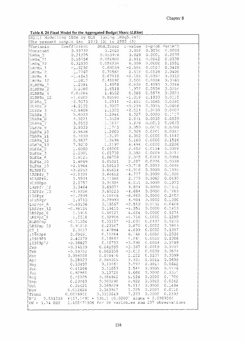
Chapter 8

Table 8. 20 Final Model for the Aggregated Budget Share {LBSm) EQ(1) Modelling LBSm by OLS (using LBSqS.in?) The present sample is: 1973 (3) to 1990 (5)

Variable Coefficient Std.Error t-value t -prob PartR*2

Constant 0. 18732 3.2028 0 .058 0 9534 0 .0000

LBSm 3 0. 21205 0.053976 3 .929 0 0001 0 .0939

LBSm 11 0. 15896 0.054602 2 .911 0 0042 0 .0538

LBSm 12 0. 32590 0.054234 6 .009 0 0000 0 .1951 LRPRa 1 -1 .6292 0.63039 -2 .584 0 0107 0 .0429

LRPRa 2 1 .7767 0.70564 2 .518 0 0129 0 .0408 LRPRa 4 -1 .4645 0.67118 -2 .182 0 0307 0 .0310 LRPRa 12 1 .5817 0.45190 3 .500 0 0006 0 .0760 SLRPRa 1 1 .2384 1.4958 0 .828 0 4090 0 .0046 SLRPRa 2 3 .2580 1.6518 1 .972 0 0504 0 .0254 SLRPRa 4 0. 85284 1.4502 0 .588 0 5574 0 .0023 SLRPRa 12 -1 .0602 0.80590 -1 .316 0 1903 0 .0115 DLRPa 1 -2 .9373 1.2111 -2 .425 0 0165 0 .0380 DLRPa 2 -4 .2135 1.3007 -3 .239 0 0015 0 .0658 DLRPa 3 -2 .8408 1.1300 -2 .514 0 0130 0 .0407 DLRPa 5 5 .6023 1.2946 4 .327 0 0000 0 1117 DLRPa 6 4 .0221 1.3539 2 .971 0 0035 0 0559

DLRPa 7 3 .8810 1.1837 3 .279 0 0013 0 0673 DLRPa 9 3 .9333 1.1743 3 .350 0 0010 0 0700

DLRPa 10 2 .9606 1.2603 2 .349 0 0201 0 0357 DLRPa 11 5 .7830 1.3197 4 .382 0 0000 0 1142 DLRPa 12 6 .9637 1.3496 5 .160 0 0000 0 1516 DLRPa 13 7 .9210 1.2197 6 .494 0 0000 0 2206

DLEXa 2 1 .6060 0.65508 2 .452 0 0154 0 0388

DLEXa 3 2 .2301 0.65738 3 .392 0 0009 0 0717 DLEXa 6 1 .6125 0.68758 2 .345 0 0203 0 0356

DLEXa 10 1 .4869 0.65011 2 .287 0 0236 0 0339

DLEXa 13 -2 .1964 0.59113 -3 .716 0 0003 0 0848 RLRSPfr -3 .2253 0.65614 -4 .916 0 0000 0 1395 LRSPfr 7 -2 .1331 0.44652 -4 777 0 0000 0 1328 RLRSPfrl 1 .9834 0.71368 2 779 0 0062 0 0493

RLRSPpo 2 .0757 0.34304 6 051 0 0000 0 1973

LRSPfr 12 3 .3464 0.69374 4 824 0 0000 0 1351 LRSPfr 13 -2 .8206 0.60223 -4 684 0 0000 0 1283

LRSPgr -1 .2939 0.18846 -6 865 0 0000 0 2403

RLRSPgr 1 .4710 0.29993 4 904 0 0000 0 1390

LRSPgr 6 -0. 49106 0.19567 -2 510 0 0132 0 0406

LRSPgr 12 -0. 96124 0.19415 -4 951 0 0000 0 1413 LRSPpo 6 1 .5918 0.34127 4 664 0 0000 0 1274 LRSPpo 8 -1 .5518 0.32906 -4 716 0 0000 0 1299

RLRSPsp -0. 71504 0.35157 -2 034 0 0437 0 0270 LRSPsp 10 0 . 91210 0.23567 3 870 0 0002 0. 0913

CI 1 2 .3457 0.47884 4 899 0 0000 0. 1387 il980p6 0 . 69481 0.11264 6 168 0 0000 0. 2034

I1989P5 0 . 45579 0.10697 4 261 0 0000 0. 1086 il989pl2 -0. 38827 0.10792 -3 598 0 0004 0. 0799

Jan -0. 14139 0.041999 -3 367 0 0010 0. 0707

Feb -0. 18752 0.062258 -3 012 0 0030 0. 0574 Mar 0.086108 0.070476 1 222 0 2237 0. 0099

Apr 0.28023 0.084015 3 335 0 0011 0. 0695 May 0. 33459 0.10467 3 197 0 0017 0. 0642

Jun 0. 41264 0.11653 3 541 0 0005 0. 0776 Jul 0. 92968 0.10728 8 666 0 0000 0. 3351

Aug 0.48025 0.086942 5 524 0 0000 0. 1700 Sep 0. 23460 0.080298 2 922 0 0040 0. 0542

Oct 0 . 35421 0.069229 5 117 0 0000 0. 1494

Nov 0.052624 0.040947 1 285 0 2007 0. 0110

Trend 0.0076918 0.0010649 7 223 0 0000 0. 2593 R^2 = 0.981018 F(57,149) = 135.1 [0.0000] sigma 0.0989364 DM = 1.74 RSS = 1.458471906 for 58 variables and 207 observations

23 g

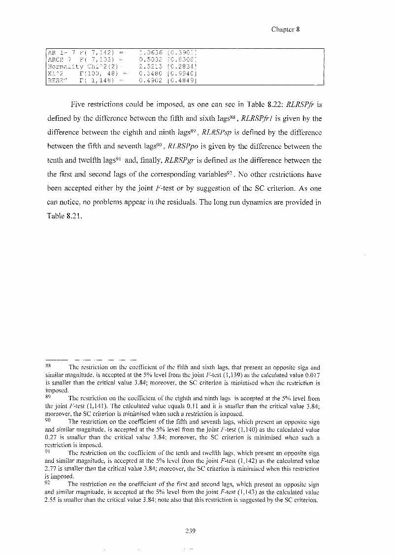
Chapter 8

AR 1- 7 F 7,142) = 1 0636 [0 3901] ARCH 7 F 7,135) = 0 5032 [0 8308] Normality Chi^2(2)= 2 5215 [0 2834] Xi*2 F 100, 48) = 0 5480 [0 9940] RESET F 1,148) = 0 4902 [0 4849]

Five restrictions could be imposed, as one can see in Table 8.22: RLRSPfr is

defined by the difference between the fifth and sixth lags^^, RLRSPfr 1 is given by the

difference between the eighth and ninth lags*^, RLRSPsp is defined by the difference

between the fifth and seventh lagsô, RLRSPpo is given by the difference between the

tenth and twelfth lags ^ and, finally, jdj&Sfgr is defined as the difference between the

the first and second lags of the corresponding v a r i a b l e s ^ ^ N q other restrictions have

been accepted either by the joint F-test or by suggestion of the SC criterion. As one

can notice, no problems appear in the residuals. The long run dynamics are provided in

Table 8.21.

The restriction on the coefficient of the fifth and sixth lags, that present an opposite sign and similar magnitude, is accepted at the 5% level from the joint F-test (1,139) as the calculated value 0.017 is smaller than the critical value 3.84; moreover, the SC criterion is minimised when the restriction is imposed.

The restriction on the coefficient of the eighth and ninth lags is accepted at the 5% level from the joint f- test (1,141). The calculated value equals 0.11 and it is smaller than the critical value 3.84; moreover, the SC criterion is minimised when such a restriction is imposed.

The restriction on the coefficient of the fifth and seventh lags, which present an opposite sign and similar magnitude, is accepted at the 5% level from the joint F-test (1,140) as the calculated value 0.27 is smaller than the critical value 3.84; moreover, the SC criterion is minimised when such a restriction is imposed.

The restriction on the coefficient of the tenth and twelfth lags, which present an opposite sign and similar magnitude, is accepted at the 5% level from the joint F-test (1,142) as the calculated value 2.77 is smaller than the critical value 3.84; moreover, the SC criterion is minimised when this restriction is imposed.

The restriction on the coefficient of the first and second lags, which present an opposite sign and similar magnitude, is accepted at the 5% level from the joint F-test (1,143) as the calculated value 2.55 is smaller than the critical value 3.84; note also that this restriction is suggested by the SC criterion.

239

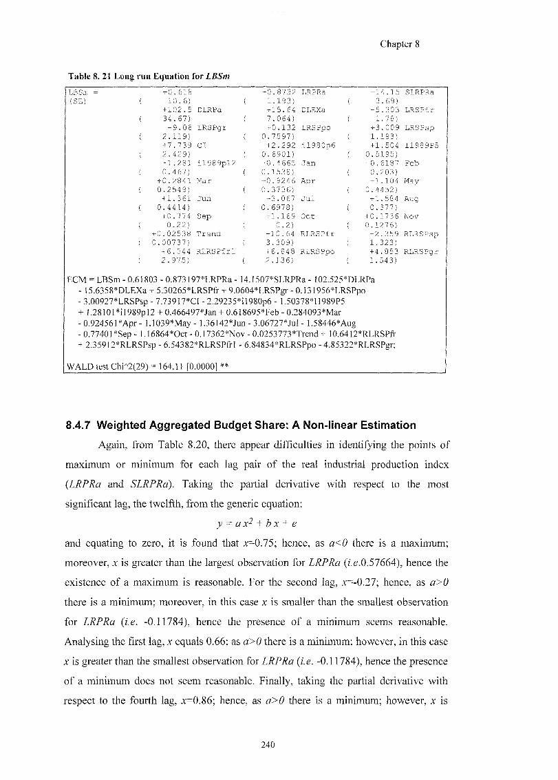
Chapter 8

Table 8. 21 Long run Equation for LBSm

LBSm (SE)

+ 0 . 6 1 8 + 0 . 8 7 3 2 LRPRa + 1 4 . 1 5 SLRPRa 1 0 . 6 ) ( 1 . 1 9 3 ) 3 . 69)

+ 1 0 2 . 5 DLRPa + 1 5 . 6 4 DLEXa - 5 . 3 0 3 L R S P f r 3 4 . 6 7 ) ( 7 . 0 6 4 ) 1 . 7 8 )

- 9 . 0 6 L R S P g r + 0 . 1 3 2 LRSPpo + 3 . 0 0 9 L R S P s p 2 . 1 1 9 ) ( 0 . 7 5 9 7 ) 1 . 1 9 3 ) + 7 . 7 3 9 CI + 2 . 2 9 2 i l 9 8 0 p 6 + 1 . 5 0 4 I 1 9 8 9 P 5 2 . 4 2 9 ) ( 0 . 6 9 0 1 ) 0 . 5 1 9 5 ) - 1 . 2 8 1 i l 9 8 9 p l 2 - 0 . 4 6 6 5 J a n - 0 . 6 1 8 7 F e b 0 . 4 6 7 ) ( 0 . 1 5 3 8 ) 0 . 2 0 3 )

+ 0 . 2 8 4 1 M a r + 0 . 9 2 4 6 A p r + 1 . 1 0 4 May 0 . 2 5 4 9 ) ( 0 . 3 7 3 6 ) 0 . 4 4 5 2 )

+ 1 . 3 6 1 J u n + 3 . 0 6 7 J u l + 1 . 5 8 4 Aug 0 . 4 4 1 4 ) ( 0 . 6 9 7 8 ) 0 . 3 7 7 )

+ 0 . 7 7 4 S e p + 1 . 1 6 9 O c t + 0 . 1 7 3 6 Nov 0 . 2 2 ) ( 0 . 2 ) 0 . 1 2 7 6 )

+ 0 . 0 2 5 3 8 T r e n d - 1 0 . 6 4 R L R S P f r - 2 . 3 5 9 R L R S P s p 0 . 0 0 7 3 7 ) ( 3 . 3 0 9 ) 1 . 3 2 3 )

+ 6 . 5 4 4 R L R S P f r l + 6 . 8 4 8 RLRSPpo + 4 . 8 5 3 R L R S P g r 2 . 9 7 5 ) ( 2 . 1 3 6 ) 1 . 5 4 3 )

ECM = LBSm - 0.61803 - 0.873197*LRPRa - 14.]507*SLRPRa - ]02.525*DLRPa - 15.6358*DLEXa + 5.30265*LRSPfT + 9.0604*LRSPgr - 0.131956*LRSPpo - 3.00927*LRSPsp - 7.73917*CI - 2.29235*il980p6 - L50378*n989P5 + 1.28101*il989pl2 + 0.466497*Jan + 0.618695*Feb - 0.284093*Mar -0.924561*Apr- 1.1039*May- 1.36142*Jun-3.06727*Jul- L58446*Aug - 0.7740]*Sep - 1 .]6864*0ct - 0.17362*Nov - 0.0253773*Trend + 10.6412*RLRSP& + 2.35912*RLRSPsp - 6.54382*RLRSPfrl - 6.84834*RLRSPpo - 4.85322*RLRSPgr;

WALD test Chi/'2(29) = 164.11 [0.0000] **

8.4.7 Weighted Aggregated Budget Share: A Non-linear Estimation

Again, from Table 8.20, there appear difficulties in identifying the points of

maximum or minimum for each lag pair of the real industrial production index

(LRPRa and SLRPRa). Taking the partial derivative with respect to the most

significant lag, the twelfth, from the generic equation:

and equating to zero, it is found that %=0.75; hence, as a<0 there is a maximum;

moreover, x is greater than the largest observation for LRPRa (z.e.0.57664), hence the

existence of a maximum is reasonable. For the second lag, x=-0.27; hence, as a>0

there is a minimum; moreover, in this case x is smaller than the smallest observation

for LRPRa {i.e. -0.11784), hence the presence of a minimum seems reasonable.

Analysing the first lag, x equals 0.66; as a>0 there is a minimum; however, in this case

X is greater than the smallest observation for LRPRa {i.e. -0.11784), hence the presence

of a minimum does not seem reasonable. Finally, taking the partial derivative with

respect to the fourth lag, x=0.86; hence, as a>0 there is a minimum; however, x is

240

Chapter 8

greater than the smallest observation for ZTgfTZa (f.g. -0.11784), hence the presence of

a minimum does not seem reasonable. As already mentioned, given that a quadratic

specification is used as a local approximation to a sigmoid curve, g.g. a logistic

function, then the minimum should lie below all the observations. Therefore, the

values obtained suggest non-linearity, but not in the form that will accommodate an

1(1) variable in an 1(0) equation. These turning points have not been precisely

estimated for each of the lags. Hence, as in the tourist receipts case, there are

difficulties in using an 1(1) variable to explain an 1(0) variable.

These Gndmgs lead to the use of a non-linear expression for the most

significant lags of the (log) real industrial production index. The generic logistic

function for the real income proxy is used, as follow:

-1

where:

X = is the most significant lag for LRPRa; in this case the twelfth, second, first and

fourth lag, respectively;

jU = is the centre of the curvature;

(7= is the spread of the curvature;

a= is the impact parameter.

The mean and the standard error of have used as starting values of the

parameters // (/Mw equals 0.16) and cr(^fg equals 0.20). The aim is to find the smallest

RSS that corresponds to the maximum of the likelihood. In running the non-linear

specification, the TSP package is used. The results obtained are provided in Table

8.22.

241

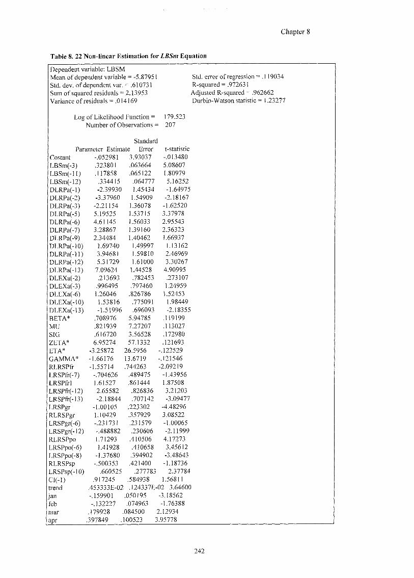
Chapter 8

Table 8. 22 Non-linear Estimation for LBSm Equation

Dependent variable; LBSM Mean of dependent variable = -5.87951 Std. error of regression = 119034 Std. dev. of dependent var. = XS10731 R-squared = .972631 Sum of squared residuals = 2J^953 Adjusted R-squared = .962662 Variance of residuals = .014169 Durbin-Watson statistic = 1.23277

Log of Likelihood Function = 179.523 Number of Observations = 207

Standard Parameter Estimate Error t-statistic

Costant -.052981 3.93037 -.013480 LBSm(-3) .323801 .063664 5.08607 LBSm(-ll) J17858 .065122 1.80979 LBSm(-12) .334415 .064777 5.16252 DLRPa(-l) -2.39930 1.45434 -1.64975 DLRPa(-2) -3.37960 1.54909 -2.18167 DLRPa(-3) -2.21154 1.36078 -1.62520 DLRPa(-5) 5.19525 1.53715 3.37978 DLRPa(-6) 4.61145 1.56033 2.95543 DLRPa(-7) 3.28867 1.39160 2.36323 DLRPa(-9) 2.34484 1.40462 1.66937 DLRPa(-lO) 1.69740 1.49997 1.13162 DLRPa(-]]) 3^^681 1.59810 2.46969 DLRPa(-12) 5.31729 1.61000 3.30267 DLRPa(-]3) 7.09624 1^4528 4.90995 DLEXa(-2) .213693 .782453 .273107 DLEXa(-3) .996495 .797460 1.24959 DLEXa(-6) 1.26046 .826786 1.52453 DLEXa(-10) 1.53816 .775091 1.98449 DLEXa(-13) -1.51996 .696093 -2.18355 BETA* .708976 5.94785 .119199 MU .821939 7.27207 .113027 SIG .616720 3.56528 .172980

ZETA* 6.95274 57.1332 .121693 ETA* -3.25872 2&5956 -.122529 GAMMA* -1.66176 13.6719 -.121546 RLRSP& -1.55714 .744263 -2.09219 LRSPfr(-7) -.704626 .489475 -1.43956 LRSP&l 1.61527 .861444 1.87508 LRSPfr(-12) 2.65582 .826836 3.21203 LRSPfi-(-I3) -2.18844 .707142 -3.09477 LRSPgr -L00105 .223302 -4.48296 RLRSPgr 1.10429 .357929 3.08522 LRSPgr(-6) -.231731 .231579 -1.00065 LRSPgr(-12) -.488882 .230606 -2.11999 RLRSPpo 1.71293 .410506 4.17273 LRSPpo(-6) 1.41928 .410658 3.45612 LRSPpo(-8) -1.37680 .394902 -3.48643 RLRSPsp -.500353 .421400 -1.18736 LRSPsp(-lO) .660525 .277783 2.37784 CI(-l) .917245 .584938 1.56811 trend .453333E-02 .124337E-02 3.64600 jan -.159901 .050195 -3.18562 feb -.132227 .074963 -1.76388 mar .179928 084500 2.12934 apr .397849 100523 3 95778

242

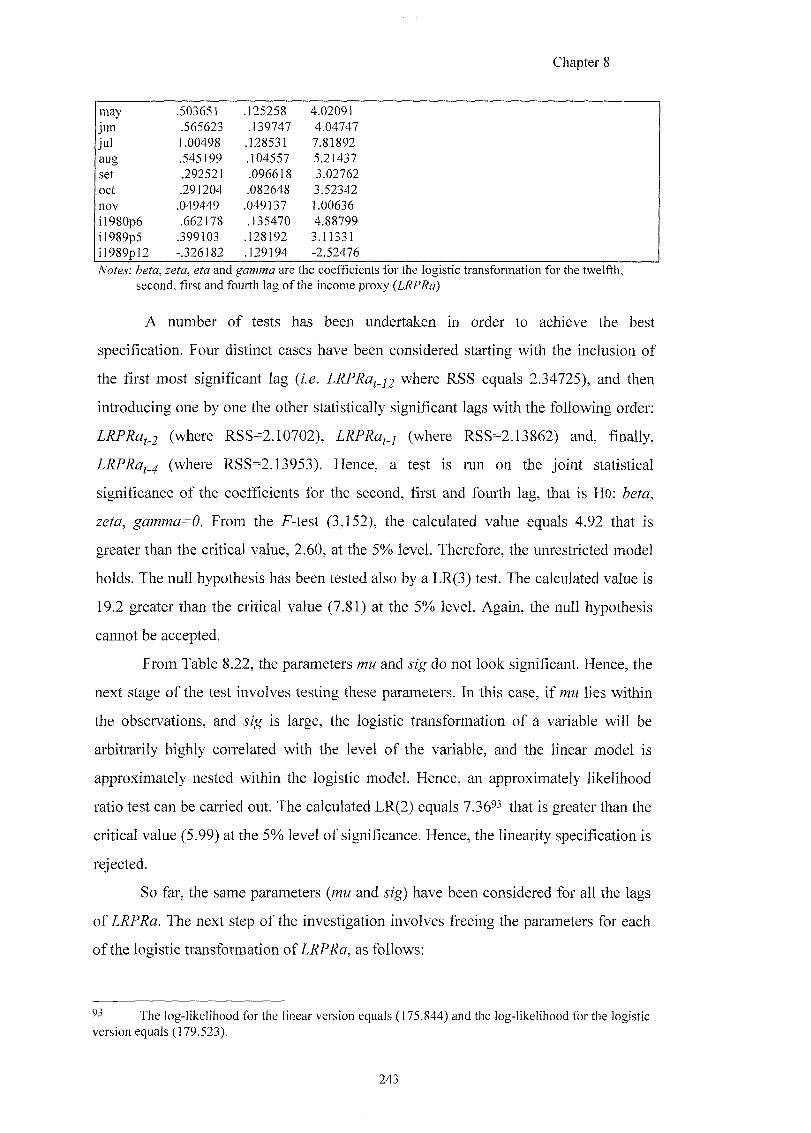
Chapter!

may .503651 .125258 4.02091 jun .565623 .139747 4.04747 jul 1.00498 .128531 7.81892 aug .545199 .104557 5.21437 set .292521 .096618 3.02762 oct .291204 .082648 3.52342 nov .049449 .049137 1.00636 il980p6 .662178 .135470 4.88799 il989p5 .399103 .128192 3.11331 i l989pl2 -.326182 .129194 -2.52476

Notes: beta, zeta, eta and gamma are the coefficients for the logistic transformation for the twelfth, second, first and fourth lag of the income proxy (LRPRa)

A number of tests has been undertaken in order to achieve the best

specification. Four distinct cases have been considered starting with the inclusion of

the first most significant lag (/.e. where R.SS equals 2.34725), and then

introducing one by one the other statistically significant lags with the following order;

^ (wha? R.SS=Z10702), (who? R^;S=2^3862) and,

LRPRaj,4 (where RSS=2.13953). Hence, a test is run on the joint statistical

significance of the coefficients for the second, first and fourth lag, that is HO: beta,

zeta, gamma=0. From the F-test (3,152), the calculated value equals 4.92 that is

greater than the critical value, 2.60, at the 5% level. Therefore, the unrestricted model

holds. The null hypothesis has been tested also by a LR(3) test. The calculated value is

19.2 greater than the critical value (7.81) at the 5% level. Again, the null hypothesis

cannot be accepted.

From Table 8.22, the parameters mu and sig do not look significant. Hence, the

next stage of the test involves testing these parameters. In this case, if wiw lies within

the observations, and sig is large, the logistic transformation of a variable will be

arbitrarily highly correlated with the level of the variable, and the linear model is

approximately nested within the logistic model. Hence, an approximately likelihood

ratio test can be carried out. The calculated LR(2) equals 7.36^3 that is greater than the

critical value (5.99) at the 5% level of significance. Hence, the linearity specification is

rejected.

So far, the same parameters {mu and sig) have been considered for all the lags

of LRPRa. The next step of the investigation involves freeing the parameters for each

of the logistic transformation of LRPRa, as follows:

^3 The log-likelihood for the linear version equals (175.844) and the log-likelihood for the logistic version equals (179.523).

243

Chapter 8

A) mw and for

B ) 2g/â, /Mw7 and for ZTZf

C) efa, yMw2 and ^yg2 for ZJZf

D) gamma, mw3 and j:zgj for Zj(f

Hence, the aim is to test the following hypotheses:

HO: mul = mu2 = mu3 = mu and sigl = sig2 = sig3 = sig

H I : TMwJ ; 7MW and

by running a LR(6) test. In this case, the log-likelihood for the restricted (Lres) model

equals 179.523 and the log-likelihood for the unrestricted {Lures) model equals

179.444. The TSP package fails to find the maximum as the log-likelihood in the

unrestricted model is worse. A further experiment has been done by freeing off fewer

parameters at a time, in mu and sig pairs. The following tests are more illustrative than

conclusive. The first parameters {i.e. mul and sigl) are for the second lag of the

income proxy. The F-test (2,150) equals 9.90 greater than the critical value (3.00) at

the 5% level '*. The LR(2) equals 26.14 greater than the critical value (5.99) at the 5%

leveP^. Hence, in both the cases the restriction cannot be accepted. The same tests are

run for the second set of parameters (/Mw2 and /g^). The F-test (2,148) presents a

negative sign (-26.53) as the RSS for the unrestricted model equals 5.89203, that is

greater than the RSS in the restricted model. On the other hand, the LR(2) is equal to

5.46 smaller than the critical value (5.99) at the 5% level. Freeing the third set of

parameters (mwj and j'zgj) leads to the following results. The calculated F-test (2,146)

equals 328.47 greater than 3.00, hence the unrestricted model has to be run. However,

the LR(2) presents a negative sign (-31.76). It is worth noting that similar findings

have been reached when using different starting values for mu and In

conclusion, TSP does not seem to be accurate enough in handling the maximisation

and it does not improve the likelihood of the restricted model but even makes it worse.

Hence, the analysis is continued considering the four lags for the logistic

transformation of the income proxy where only mu and sig are freely estimated (see

The RSS for the restricted model equals 2.13953 and the RSS for the unrestricted model is 1.88996.

The log-likelihood for the restricted model is 179.523 and for the unrestricted model equals 192.592.

One solution has been pursued starting the unrestricted model from the restricted maximum, that is setting mu = 0.821939 and sig = 0.616720 (see Table 8.22). Nevertheless, the TSP package has shown similar problems in achieving the maximisation.

244

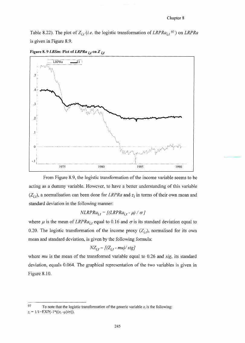
Chapter 8

Table 8.22). The plot of (i.e. the logistic transformation of LRPRajj on LRPRa

is given in Figure 8.9,

Figure 8. 9 LBSm: Plot of LRPRa i f on Z ^

LRPRa

From Figure 8.9, the logistic transformation of the income variable seems to be

acting as a dummy variable. However, to have a better understanding of this variable

(Zi f), a normalisation can been done for LRPRa and zy in terms of their own mean and

standard deviation in the following manner:

NLRPRaj f = [(LRPRaI f - ju) / <J]

where ju is the mean of LRPRa^ equal to 0.16 and cr is its standard deviation equal to

0.20. The logistic transformation of the income proxy (Z, f), normalised for its own

mean and standard deviation, is given by the following formula:

where mu is the mean of the transformed variable equal to 0.26 and sig, its standard

deviation, equals 0.064. The graphical representation of the two variables is given in

Figure 8.10.

To note that the logistic transformation of the generic variable x, is the following:

245

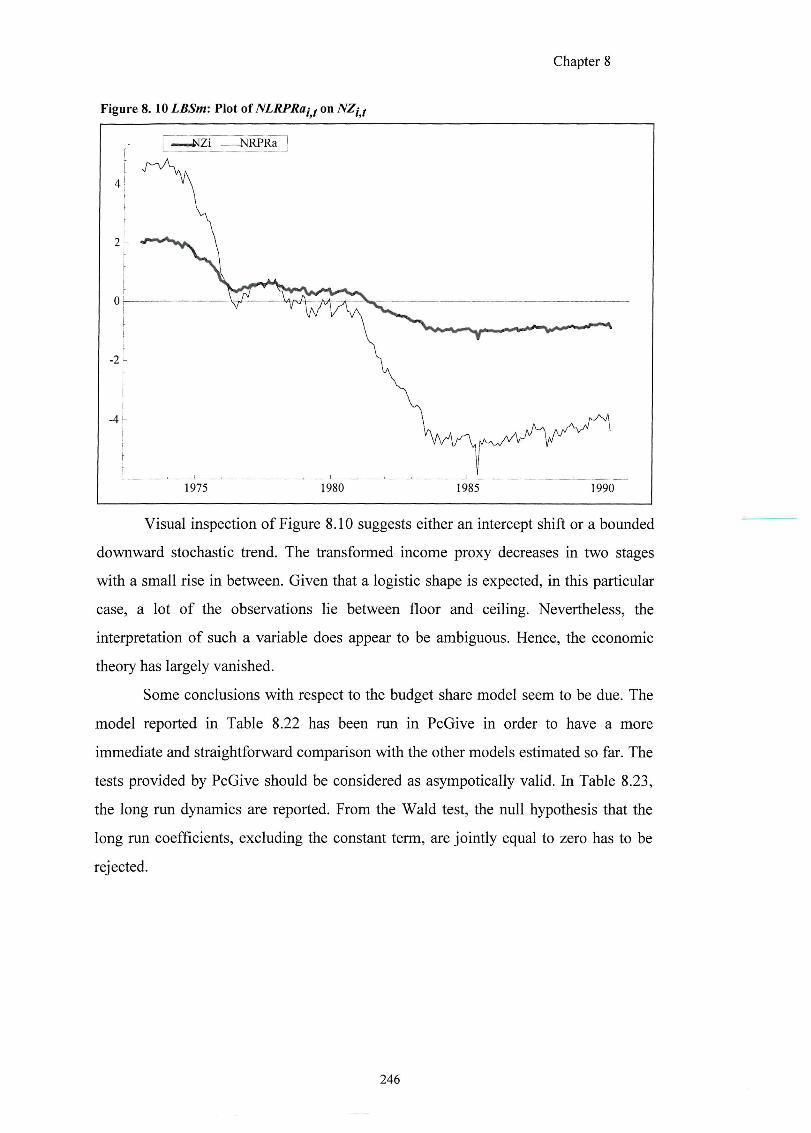
Chapter 8

Figure 8.10 LBSm: Plot of NLRPRai f on

(wwmNZi NRPR3.

Visual inspection of Figure 8.10 suggests either an intercept shift or a bounded

downward stochastic trend. The transformed income proxy decreases in two stages

with a small rise in between. Given that a logistic shape is expected, in this particular

case, a lot of the observations lie between floor and ceiling. Nevertheless, the

interpretation of such a variable does appear to be ambiguous. Hence, the economic

theory has largely vanished.

Some conclusions with respect to the budget share model seem to be due. The

model reported in Table 8.22 has been run in PcGive in order to have a more

immediate and straightforward comparison with the other models estimated so far. The

tests provided by PcGive should be considered as asympotically valid. In Table 8.23,

the long run dynamics are reported. From the Wald test, the null hypothesis that the

long run coefficients, excluding the constant term, are jointly equal to zero has to be

rejected.

246

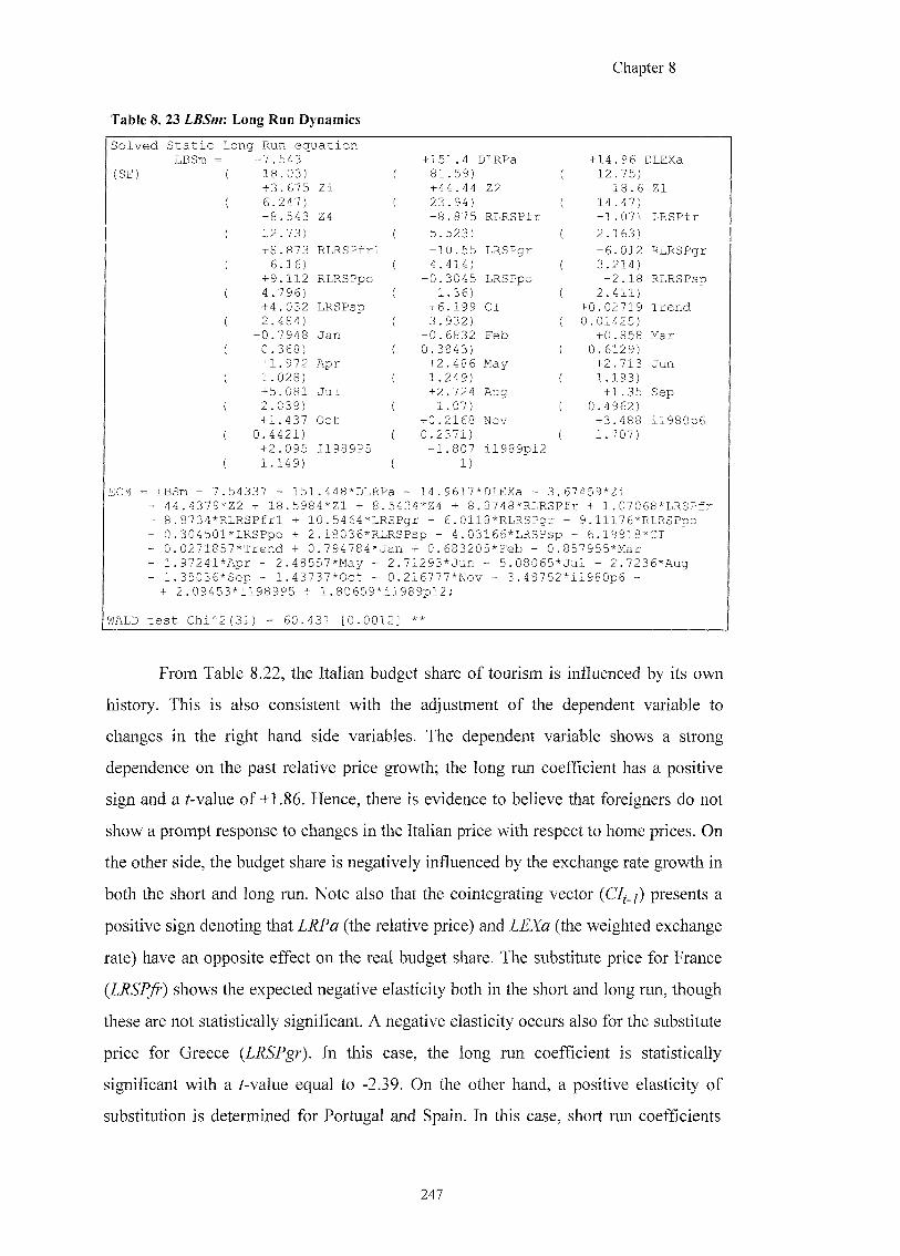
Chapter 8

Table 8. 23 LBSm: Long Run Dynamics

S o l v e d S t a t i c

(SE)

L o n g R u n e q u a t i o n + 7 . 5 4 3 + 1 5 1 . 4 DLRPa + 1 4 . 9 6 DLEXa

1 8 . 0 3 ) ( 8 1 . 5 9 ) 1 2 . 7 5 ) + 3 . 6 7 5 2 1 + 4 4 . 4 4 2 2 - 1 8 . 6 Z1 6 . 2 4 7 ) ( 2 3 . 9 4 ) 1 4 . 4 7 ) - 8 . 5 4 3 24 - 8 . 8 7 5 R L R S P f r - 1 . 0 7 1 L R S P f r

1 2 . 7 3 ) ( 5 . 5 2 3 ) 2 . 1 6 3 )

+ 8 . 8 7 3 R L R S P f r l - 1 0 . 5 5 L R S P g r + 6 . 0 1 2 R L R S P g r 6 . 1 6 ) ( 4 . 4 1 4 ) 3 . 2 1 4 )

+ 9 . 1 1 2 RLRSPpo + 0 . 3 0 4 5 L R S P p o - 2 . 1 8 R L R S P s p 4 . 7 9 6 ) ( 1 . 3 6 ) 2 . 4 1 1 ) + 4 . 0 3 2 L R S P s p + 6 . 1 9 9 C I + 0 . 0 2 7 1 9 T r e n d 2 . 4 8 4 ) ( 3 . 9 3 2 ) 0 . 0 1 4 2 5 )

- 0 . 7 9 4 8 J a n - 0 . 6 8 3 2 F e b + 0 . 8 5 8 M a r 0 . 3 6 8 ) ( 0 . 3 8 4 3 ) 0 . 6 1 2 9 ) + 1 . 9 7 2 A p r + 2 . 4 8 6 May + 2 . 7 1 3 J u n 1 . 0 2 8 ) ( 1 . 2 4 9 ) 1 . 1 9 3 ) + 5 . 0 8 1 J u l + 2 . 7 2 4 A u g + 1 . 3 5 S e p 2 . 0 3 9 ) ( 1 . 0 7 ) 0 . 4 9 6 2 ) + 1 . 4 3 7 O c t + 0 . 2 1 6 8 N o v + 3 . 4 8 8 i l 9 8 0 p 6

0 . 4 4 2 1 ) ( 0 . 2 3 7 1 ) 1 . 7 0 7 ) + 2 . 0 9 5 I 1 9 8 9 P 5 - 1 . 8 0 7 i l 9 8 9 p l 2 1 . 1 4 9 ) ( 1)

ECM = LBSm - 7 . 5 4 3 3 7 - 1 5 1 . 4 4 8 * D L R P a - 1 4 . 9 6 1 7 * D L E X a - 3 . 6 7 4 5 9 * Z i - 4 4 . 4 3 7 9 * 2 2 + 1 8 . 5 9 8 4 * 2 1 + 8 . 5 4 3 4 * 2 4 + 8 . 8 7 4 8 * R L R S P f r + 1 . 0 7 0 6 8 * L R S P f r - 8 . 8 7 3 4 * R L R S P f r l + 1 0 . 5 4 6 4 * L R S P g r - 6 . 0 1 1 8 * R L R S P g r - 9 . 1 1 1 7 6 * R L R S P p o - 0 . 3 0 4 5 0 1 * L R S P p o + 2 . 1 8 0 3 6 * R L R S P s p - 4 . 0 3 1 6 6 * L R S P s p - 6 . 1 9 9 1 8 * C I - 0 . 0 2 7 1 8 5 7 * T r e n d + 0 . 7 9 4 7 8 4 * J a n + 0 . 6 8 3 2 0 5 * F e b - 0 . 8 5 7 9 5 5 * M a r - 1 . 9 7 2 4 1 * A p r - 2 . 4 8 5 5 7 * M a y - 2 . 7 1 2 9 3 * J u n - 5 . 0 8 0 6 5 * J u l - 2 . 7 2 3 6 * A u g - 1 . 3 5 0 3 6 * S e p - 1 . 4 3 7 3 7 * 0 c t - 0 . 2 1 6 7 7 7 * N o v - 3 . 4 8 7 5 2 * i l 9 8 0 p 6 -

+ 2 . 0 9 4 5 3 * I 1 9 8 9 P 5 + 1 . 8 0 6 5 9 * i l 9 8 9 p l 2 ;

WALD t e s t C h i ' " 2 ( 3 1 ) 6 0 . 4 3 1 [ 0 . 0 0 1 2 ] * '

From Table 8.22, the Italian budget share of tourism is influenced by its own

history. This is also consistent with the adjustment of the dependent variable to

changes i n the r ight hand side variables. The dependent variable shows a strong

dependence on the past relative price growth; the long run coefficient has a positive

sign and a lvalue of +1.86. Hence, there is evidence to believe that foreigners do not

show a prompt response to changes in the Italian price with respect to home prices. On

the other side, the budget share is negatively influenced by the exchange rate growth in

both the short and long run. Note also that the cointegrating vector (C/^./) presents a

positive sign denoting that LRPa (the relative price) and LEXa (the weighted exchange

rate) have an opposite effect on the real budget share. The substitute price for France

{LRSPfr) shows the expected negative elasticity both in the short and long run, though

these are not statistically significant. A negative elasticity occurs also for the substitute

price for Greece I n this case, the long run coefRcient is statistically

significant with a /-value equal to -2.39. On the other hand, a positive elasticity of

substitution is determined for Portugal and Spain. In this case, short run coefficients

247

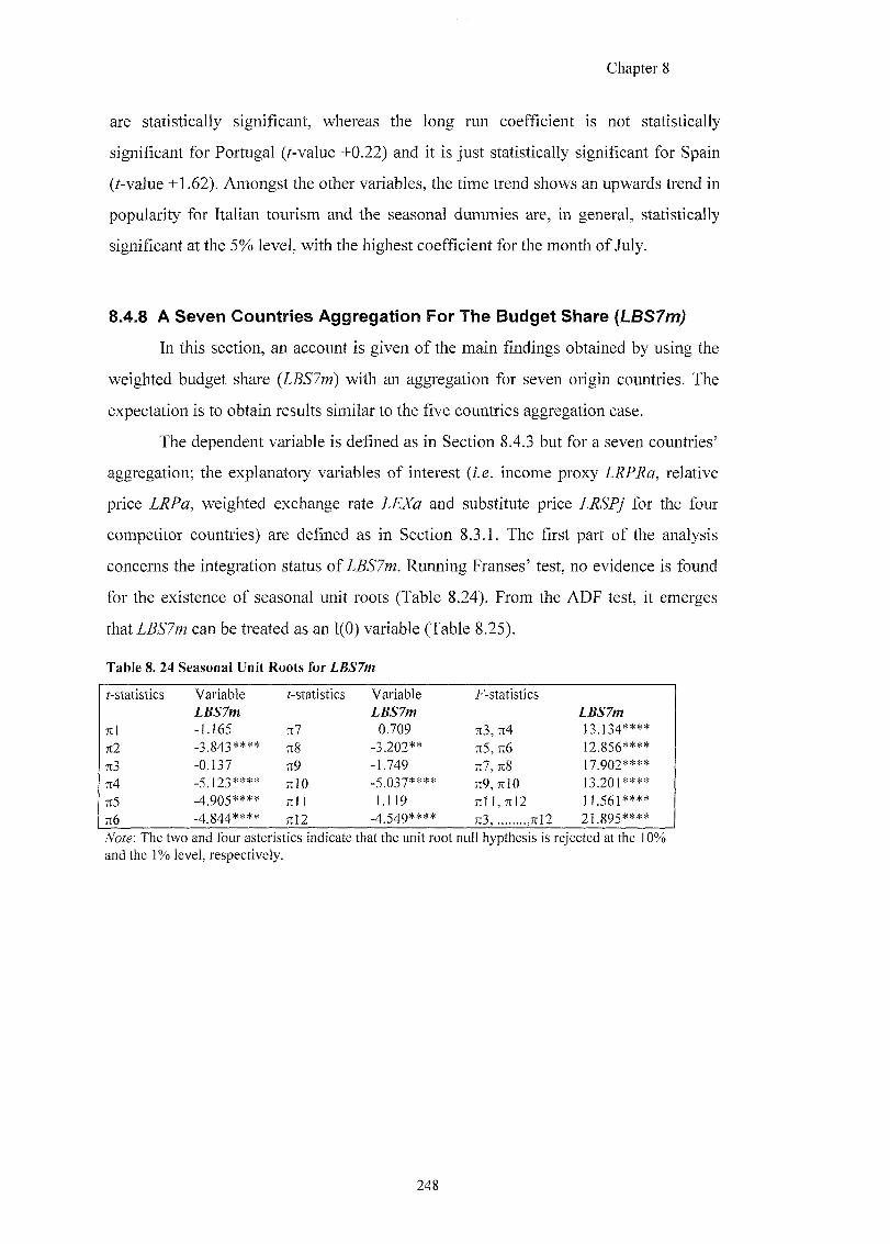
Chapter 8

are statistically significant, whereas the long run coefficient is not statistically

signif icant for Portugal (r-value +0.22) and i t is jus t statistically signif icant for Spain

(/-value +1.62). Amongst the other variables, the time trend shows an upwards trend in

popularity for Italian tourism and the seasonal dummies are, in general, statistically

significant at the 5% level, with the highest coefficient for the month of July.

8.4.8 A Seven Countries Aggregation For The Budget Share (LBS7m)

In this section, an account is given of the main findings obtained by using the

weighted budget share (LBS7m) with an aggregation for seven origin countries. The

expectation is to obtain results similar to the five countries aggregation case.

The dependent variable is defined as in Section 8.4.3 but for a seven countries'

aggregation; the explanatory variables o f interest (i.e. income proxy relat ive

price LRPa, weighted exchange rate LEXa and substitute price LRSPj for the four

competitor countries) are defined as in Section 8.3.1. The first part of the analysis

concerns the integrat ion status o f Runn ing Franses' test, no evidence is found

for the existence of seasonal unit roots (Table 8.24). From the ADF test, it emerges

that can be treated as an 1(0) variable (Table 8.25).

Table 8. 24 Seasonal Unit Roots for LBS7m

/-statistics Variable /-statistics Variable f-statistics LBSlm LBS7m

TCl -1.165 •Kl 0.709 Tt3, Tl4 13.134**** 7T2 -3.843**** n8 -3.202** nS, 7T6 12.856**** 7:3 -0.137 7t9 -1.749 7t7, 7I8 17.902**** 7t4 -5.123**** TtlO -5.037**** 7T9, TtlO 13.201**** 7t5 -4.905**** Til 1 1.119 Til 1, Jtl2 11.561**** %6 -4.844**** )il2 -4.549**** 7[3, ,;tl2 21.895****

Note: The two and four asteristics indicate that the unit root null hypthesis is rejected at the 10% and the 1 % level, respectively.

248

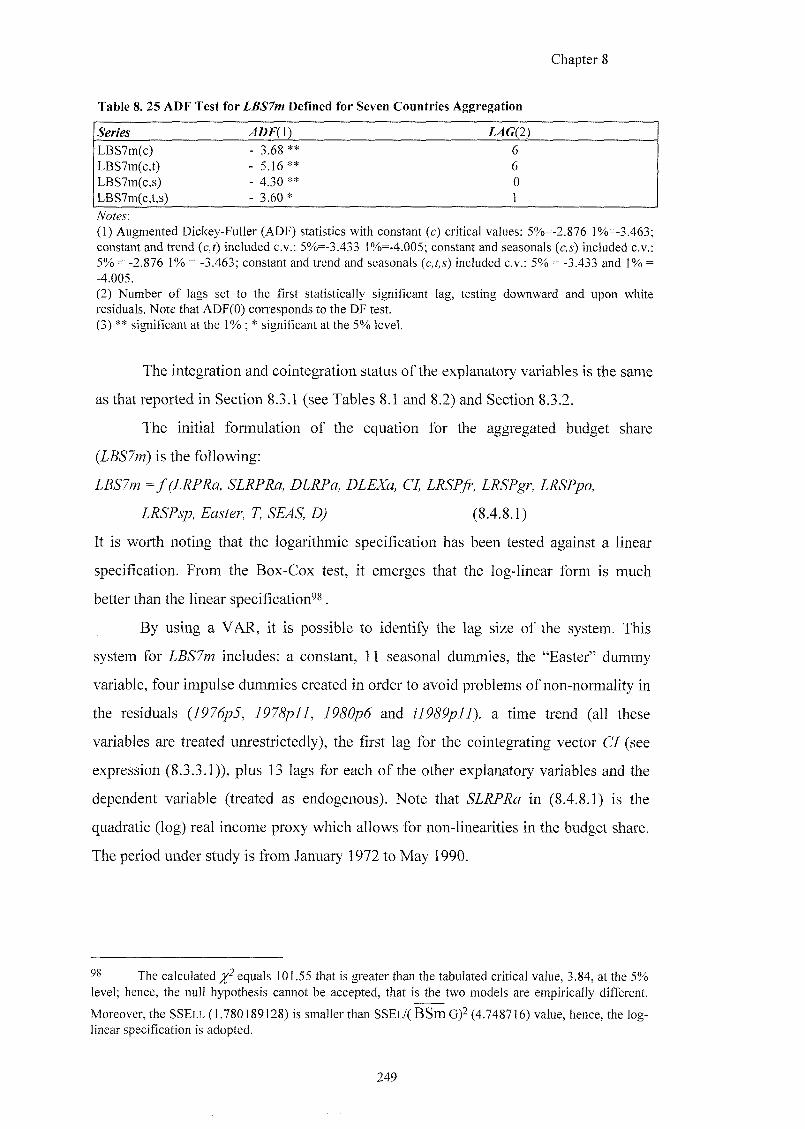
Chapter 8

Table 8. 25 ADF Test for LBS7m Defined for Seven Countries Aggregation

Series A O f ( l ) ZXG(2)

LBS7m(c) - 3.68 ** 6 LBS7m(c,t) - 5.16** 6 LBS7m(c,s) - 4.30 ** 0 LBS7m(c,t,s) - 3.60* 1

(1) Augmented Dickey-Fuller (ADF) statistics with constant (c) critical values; 5%=-2.876 ]%=-3.463; constant and trend (c,f) included c.v.; 5%=-3.433 l%=-4.005; constant and seasonals (c,^) included c.v.; 5% = -2.876 1% = -3.463; constant and trend and seasonals {c,t,s) included c.v.: 5% = -3.433 and 1% = -4.005. (2) Number of lags set to the first statistically significant lag, testing downward and upon white residuals. Note that ADF(O) corresponds to the DF test. (3) ** significant at the 1% ; * significant at the 5% level.

The integration and cointegration status of the explanatory variables is the same

as that reported i n Section 8.3.1 (see Tables 8.1 and 8.2) and Section 8.3.2.

The initial formulation of the equation for the aggregated budget share

(LBS7m) is the following:

Jga, SZTgfJga, DZJgfa,

7] D ) (8.4.8.1)

It is worth noting that the logarithmic specification has been tested against a linear

specification. From the Box-Cox test, it emerges that the log-linear form is much

better than the linear specification^^.

By using a VAR, it is possible to identify the lag size of the system. This

system for includes: a constant, 11 seasonal dummies, the "Easter" dummy

variable, four impulse dummies created in order to avoid problems of non-normality in

the residuals (7P7dpJ, 7 9 7 ^ 7 7 , and a t ime trend (al l these

variables are treated unrestrictedly), the first lag for the cointegrating vector CI (see

expression (8.3.3.1)), plus 13 lags for each o f the other explanatory variables and the

dependent variable (treated as endogenous). Note that SLRPRa in (8.4.8.1) is the

quadratic (log) real income proxy which allows for non-linearities in the budget share.

The period under study is from January 1972 to May 1990.

The calculated equals 101.55 that is greater than the tabulated critical value, 3.84, at the 5% level; hence, the null hypothesis cannot be accepted, that is the two models are empirically different.

Moreover, the SSELL (1.780189128) is smaller than SSEL /(BSmG)^ (4.748716) value, hence, the log-linear specification is adopted.

249

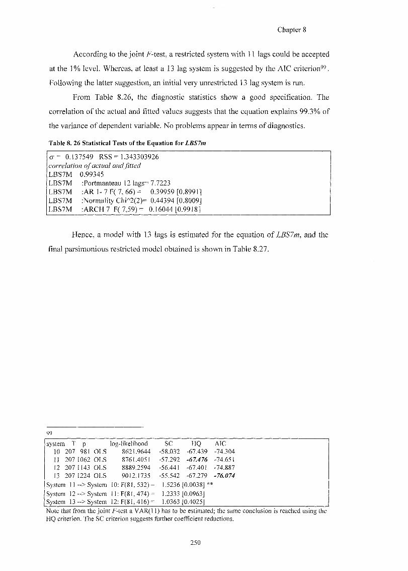
Chapter 8

According to the joint F-test, a restricted system with 11 lags could be accepted

at the 1% level. Whereas, at least a 13 lag system is suggested by the A I C criterion^^.

Fo l l ow ing the latter suggestion, an in i t ia l very unrestricted 13 lag system is run.

From Table 8.26, the diagnostic statistics show a good specification. The

correlation of the actual and fitted values suggests that the equation explains 99.3% of

the variance of dependent variable. No problems appear in terms of diagnostics.

Table 8. 26 Statistical Tests of the Equation for LBSlm

o - = 0.137549 RSS= 1.343303926 corre/af/oM q /

LBS7M 0.99345 L B S 7 M :Por tmanteau 12 lags= 7.7223

LBS7M : A R 1 - 7 F ( 7 , 6 6 ) = 0.39959 [0.8991] LBS7M iNormality Chi^2(2)= 0.44394 [0.8009] LBS7M A R C H 7 F( 7,59)= 0.16044 [0.9918]

Hence, a model with 13 lags is estimated for the equation of LBS7m, and the

final parsimonious restricted model obtained is shown in Table 8.27.

99

system T p log-likelihood SC HQ AIC m 207 981 OLS 8621.9644 -58.032 -67.439 -74.304 11 207 1062 OLS 8761.4051 -57.292 -67X76 -74.651 12 207 1143 OLS 8889.2594 -56.441 -67.401 -74.887 13 207 1224 OLS 9012.1735 -55.542 -67.279 -76.07^

System l l - > System 10:F(8] ,532)= 1.5236 [0.0038]**

System 12 - > System 11: F(81, 474) = 1.2333 [0.0963] System 13 - > System 12: F(81, 416) = 1.0363 [0.4025]

Note that from the joint F-test a VAR(11) has to be estimated; the same conclusion is reached using the HQ criterion. The SC criterion suggests further coefficient reductions.

250

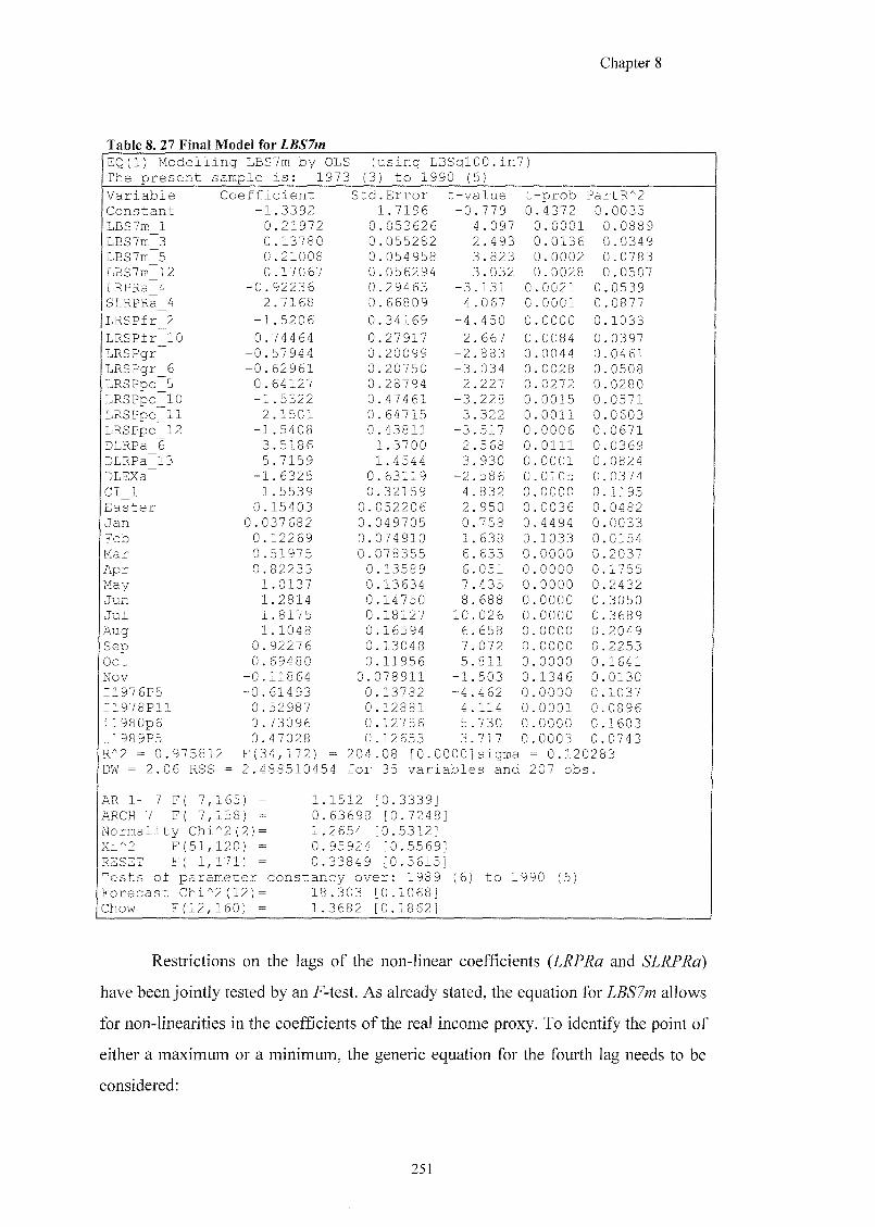
Chapter 8

Table 8. 27 Final Model for LBS7m EQ(1) Modelling LBSlm by OLS (using LBSqlOO.in?) The present sample is: 1973 (3) to 1990 (5)

Variable Coefficient Std.Error t-value t -prob ?artR*2 Constant -1.3392 1.7196 -0 .779 0 .4372 0 .0035 LBS7m 1 0.21972 0.053626 4.097 0.0001 0.0889 LBS7m 3 0.13780 0.055282 2.493 0.0136 0.0349 LBS7m 5 0.21008 0.054958 3.823 0.0002 0.0783 LBS7m 12 0.17067 0.056294 3.032 0.0028 0.0507 LRPRa 4 -0.92236 0.29463 -3 .131 0 0021 0 .0539 SLRPRa_4 2.7168 0.66809 4 .067 0 0001 0 .0877

LRSPfr 2 -1.5206 0.34169 -4 .450 0 0000 0 .1033

LRSPfr 10 0.74464 0.27917 2 .667 0 0084 0 .0397 LRSPgr -0.57944 0.20099 -2 .883 0 0044 0 .0461 LRSPgr 6 -0.62961 0.20750 -3 .034 0 0028 0 .0508 LRSPpo 5 0.64127 0.28794 2 .227 0 0272 0 .0280 LRSPpo 10 -1.5322 0.47461 -3 .228 0 0015 0 .0571 LRSPpo 11 2.1501 0.64715 3 .322 0 0011 0 .0603 LRSPpo 12 -1.5408 0.43811 -3 .517 0 0006 0 .0671 DLRPa 6 3.5186 1.3700 2 .568 0 0111 0 .0369 DLRPa 13 5.7159 1.4544 3 .930 0 0001 0 .0824 DLEXa -1.6325 0.63119 -2 .586 0 0105 0 .0374 CI_1 1.5539 0.32159 4 .832 0 0000 0 .1195 Easter 0.15403 0.052206 2 .950 0 0036 0 .0482 Jan 0.037682 0.049705 0 .758 0 4494 0 .0033 Feb 0.12269 0.074910 1 .638 0 1033 0 .0154 Mar 0.51975 0.078355 6 .633 0 0000 0 .2037 Apr 0.82233 0.13589 6 .051 0 0000 0 .1755 May 1.0137 0.13634 7 .435 0 0000 0 .2432 Jun 1.2814 0.14750 8 .688 0 0000 0 .3050 Jul 1.8175 0.18127 10 .026 0 0000 0 .3689 Aug 1.1048 0.16594 6 .658 0 0000 0 .2049 Sep 0.92276 0.13048 7 .072 0 0000 0 .2253 Oct 0.69480 0.11956 5 .811 0 0000 0 1641 Nov -0.11864 0.078911 -1 .503 0 1346 0 .0130 I1976P5 -0.61493 0.13782 -4 462 0 0000 0 .1037 I1978P11 0.52987 0.12881 4 114 0 0001 0 0896 il980p6 0.73096 0.12756 5 730 0 0000 0 1603 I1989P5 0.47028 0.12653 3 717 0 0003 0 0743 R^2 = 0.97581 2 F(34,172) = 204.08 [0.0000 Sigma = 0.120283 DW = 2.06 RSS = 2.488510454 for 35 variables and 207 obs

AR 1- 7 F 7, 165) = 1. 1512 [0.3339] ARCH 7 F 7,158) = 0. 63698 [0.7248 Normality Chi 2(2)= 1. 2654 [0.5312] Xi^2 F(51, 120) = 0. 95924 [0.5569 R2SET F( 1, 171) = 0. 33849 [0.5615 Tests of parameter constancy over: 1989 (6) to 1990 (5) Forecast Chi^ 2(12)= 18 .303 [0.1068] Chow F(12, 160) = 1. 3682 [0.1862]

Restrictions on the lags of the non-linear coefficients (LRPRa and SLRPRa)

have been jointly tested by an F-test. As already stated, the equation for LBS7m allows

for non-linearities in the coefficients of the real income proxy. To identify the point of

either a maximum or a minimum, the generic equation for the fourth lag needs to be

considered;

251

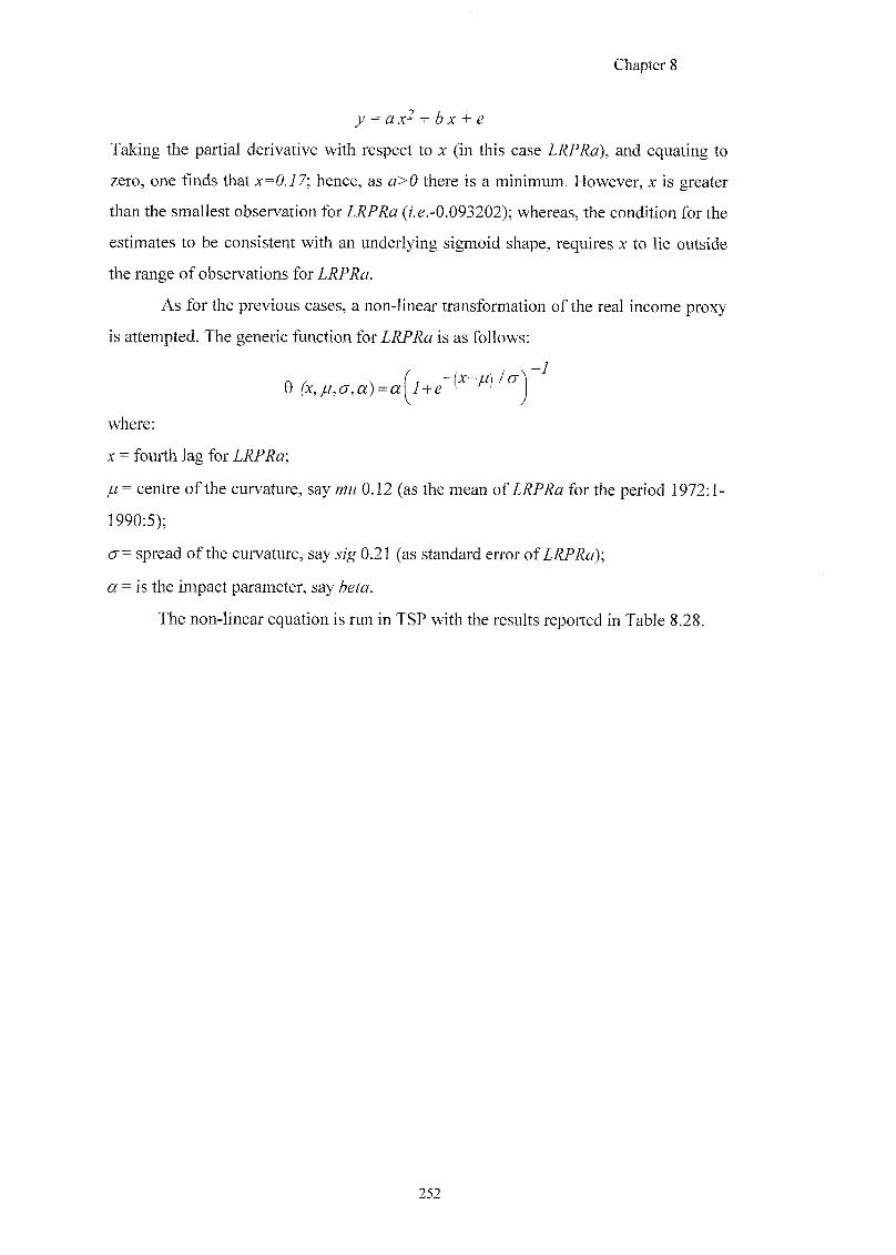
Chapter 8

Taking the partial derivative with respect to x (in this case LRPRa), and equating to

zero, one finds that x=0.17; hence, as a>0 there is a minimum. However, x is greater

than the smallest observation for LRPRa (z.e.-0.093202); whereas, the condition for the

estimates to be consistent with an underlying sigmoid shape, requires x to lie outside

the range of observations for LRPRa.

As for the previous cases, a non-linear transformation o f the real income proxy

is attempted. The generic function for LRPRa is as follows;

-1 e

where:

X = fourth lag for LRPRa;

ju = centre of the curvature, say mu 0.12 (as the mean of LRPRa for the period 1972:1-

1990:5);

cr= spread o f the curvature, say 0.21 (as standard error o f Z ^ . R a ) ;

a = is the impact parameter, say beta.

The non-linear equation is run in TSP with the results reported in Table 8.28.

252

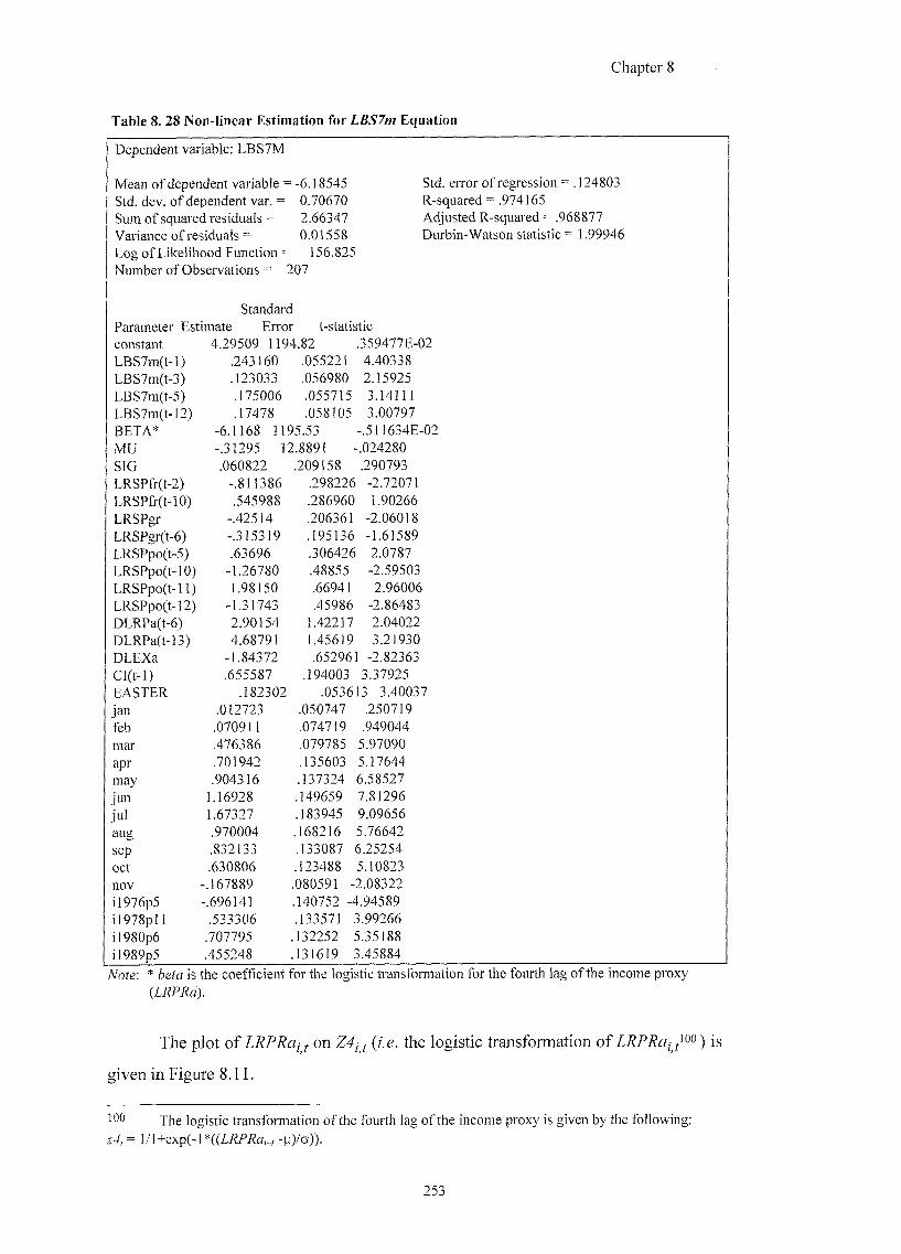
Chapter 8

Table 8. 28 Non-linear Estimation for LBS7m Equation

Dependent variable; LBS7M

Mean of dependent variable = -6.18545 Std. error of regression = 124803 Std. dev. of dependent var. = 0.70670 R-squared = .974165 Sum of squared residuals = 2.66347 Adjusted R-squared = .968877 Variance of residuals = 0.01558 Durbin-Watson statistic = 1.99946 Log of Likelihood Function = 156.825 Number of Observations = 207

Standard Parameter Estimate Error t-statistic constant 4.29509 1194.82 .359477E-02 LBS7m(t-l) .243160 .055221 4.40338 LBS7m(t-3) .123033 .056980 2.15925 LBS7m(t-5) .175006 .055715 3.14111 LBS7m(t-12) .17478 .058105 3.00797 BETA* -6.1168 1195.53 -.511634E-02 MU -.31295 12.8891 -.024280 SIG .060822 .209158 .290793 LRSP(r(t-2) -.811386 .298226 -2.72071 LRSP&(t-10) .545988 .286960 1.90266 LRSPgr -.42514 .206361 -2.06018 LRSPgr(t-6) -.315319 .195136 -1.61589 LRSPpo(t-5) .63696 .306426 2.0787 LRSPpo(t-]0) -1.26780 .48855 -2.59503 LRSPpo(t-l 1) 1.98150 .66941 2.96006 LRSPpo(t-12) -1.31743 .45986 -2.86483 DLRPa(t-6) 2.90154 1.42217 2.04022 DLRPa(t-13) 4.68791 1.45619 3.21930 DLEXa -1.84372 .652961 -2.82363 CI(t-l) .655587 .194003 3.37925 EASTER .182302 .053613 3.40037 jan .012723 .050747 .250719 feb .070911 .074719 .949044 mar .476386 .079785 5.97090 apr .701942 .135603 5.17644 may .904316 .137324 6.58527 jun 1.16928 .149659 7.81296 jul 1.67327 .183945 9.09656 aug .970004 .168216 5.76642 sep .832133 .133087 6.25254 oct .630806 .123488 5.10823 nov -.167889 080591 -2.08322 il976p5 -.696141 140752 -4.94589 i]978p]l .533306 .133571 3.99266 i]980p6 .707795 132252 5.35188 iI989p5 .455248 131619 3.45884

Nofe: * is the coefRcient for the logistic transformation for the fourth lag of the income proxy

The p lo t o f on (z.e. the logist ic transformation o f ) ig

given in Figure 8.11.

100 The logistic transformation of the fourth lag of the income proxy is given by the following;

z4, = \l\+ex\){-l*{{LRPRa,.4 -ti)/o)).

253

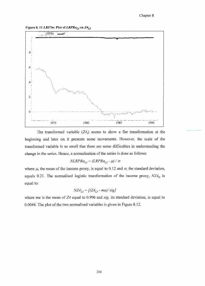
Chapter 8

Figure 8. 11 LBS7m: Plot of LRPRai f on Z4i f

The transformed variable seems to show a flat transformation at the

beginning and later on it presents some movements. However, the scale of the

transformed variable is so small that there are some difficulties in understanding the

change in the series. Hence, a normalisation of the series is done as follows;

NLRPRaij = (LRPRai f - / cr

where //, the mean of the income proxy, is equal to 0.12 and cr, the standard deviation,

equals 0.21. The normalised logistic transformation of the income proxy, NZ4f, is

equal to:

where mu is the mean of Z4 equal to 0.996 and sig, its standard deviation, is equal to

0.0044. The plot of the two normalised variables is given in Figure 8.12.

254

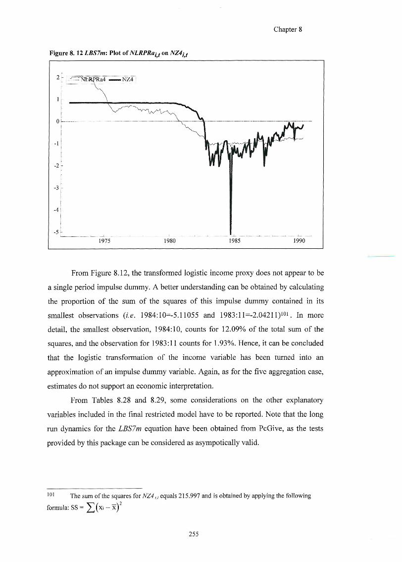
Chapter 8

Figure 8 .12 LBS7m: Plot of NLRPRai f on NZ4i (

2 h FT ^

- 1

-3 r

-4L

-5r

% R P R a 4 . — - N Z 4

1975 1980 1985 1990

From Figure 8.12, the transformed logistic income proxy does not appear to be

a single period impulse dummy. A better understanding can be obtained by calculating

the proportion of the sum of the squares of this impulse dummy contained in its

smallest observations (i.e. 1984:10=-5.11055 and 1983:1 l=-2.04211)ioi. In more

detail, the smallest observation, 1984:10, counts for 12.09% of the total sum of the

squares, and the observation for 1983:11 counts for 1.93%. Hence, it can be concluded

that the logistic transformation of the income variable has been turned into an

approximation of an impulse dummy variable. Again, as for the five aggregation case,

estimates do not support an economic interpretation.

From Tables 8.28 and 8.29, some considerations on the other explanatory

variables included in the final restricted model have to be reported. Note that the long

run dynamics for the LBS7m equation have been obtained from PcGive, as the tests

provided by this package can be considered as asympotically valid.

'01 The sum of the squares for NZ4 ^ equals 215.997 and is obtained by applying the following

formula: SS = ^ ( x i — x ) '

255

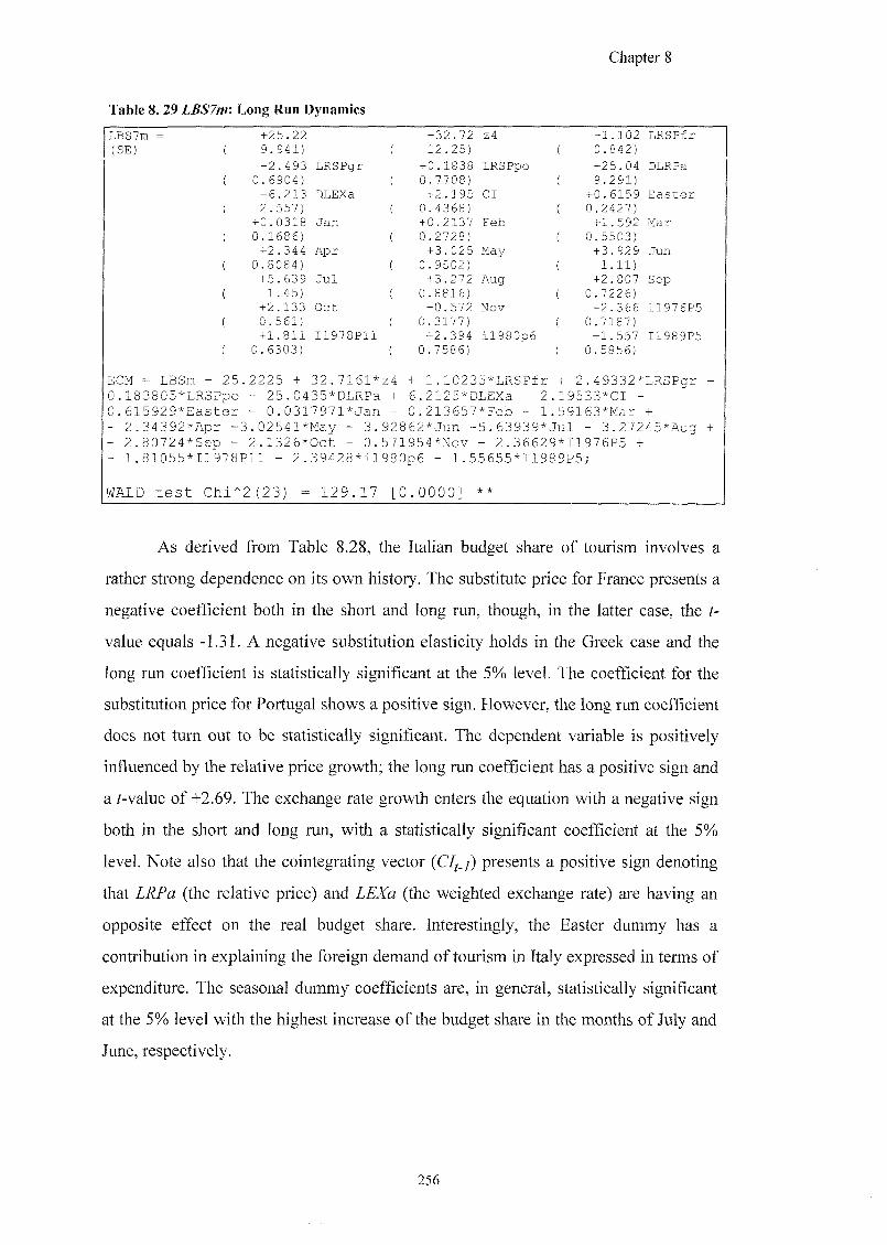
Chapter 8

Table 8. 29 LBS7m\ Long Run Dynamics

L B S l m = + 2 5 . 2 2 - 3 2 . 7 2 z 4 - 1 . 1 0 2 L R S P f r ( 9 . 9 4 1 ) ( 1 2 . 2 5 ) 0 . 8 4 2 )

- 2 ^ ^ 3 I R S P g r + 0 . 1 8 3 8 L R S P p o + 2 5 . 0 4 DLRPa ( 0 . 6 9 0 4 ) ( 0 . 7 7 0 8 ) 9 . 2 9 1 )

- 6 . 2 1 3 D l E X a + 2 . 1 9 5 C I + 0 . 6 1 5 9 E a s t e r ( 2 . 5 5 7 ) ( 0 . 4 3 6 8 ) 0 . 2 4 2 7 )

+ 0 . 0 3 1 8 J a n + 0 . 2 1 3 7 F e b + 1 . 5 9 2 M a r ( 0 . 1 6 8 6 ) ( 0 . 2 7 2 8 ) 0 . 5 5 0 3 )

+ 2 ^ M 4 A p r + 3 . 0 2 5 May + 3 . 9 2 9 J u n ( 0 . 8 0 8 4 ) ( 0 . 9 5 0 2 ) 1 . 1 1 )

+ 5 . 6 3 9 J u l + 3 . 2 7 2 A u g + 2 . 8 0 7 S e p ( 1 . 4 5 ) ( 0 . 8 8 1 6 ) 0 . 7 2 2 6 )

+ 2 . 1 3 3 O c t - 0 . 5 7 2 N o v - 2 . 3 6 6 I 1 9 7 6 P 5 ( 0 . 5 6 1 ) ( 0 . 3 1 7 7 ) 0 . 7 1 8 7 )

+ 1 ^ ^ 1 I 1 9 7 8 P 1 1 + 2 . 3 9 4 i l 9 8 0 p 6 + 1 . 5 5 7 I 1 9 8 9 P 5 ( 0 . 6 3 0 3 ) ( 0 . 7 5 8 ^ 0 . 5 8 5 6 )

ECM = L B S m - 2 5 . 2 2 2 5 + 3 2 . 7 1 6 1 * z 4 + 1 . 1 0 2 3 5 * L R S P f r + 2 . 4 9 3 3 2 * L R S P g r -0 . 1 8 3 8 0 5 * L R S P p o - 2 5 . 0 4 3 5 * D L R P a + 6 . 2 1 2 5 * D L E X a - 2 . 1 9 5 3 3 * C I -0 . 6 1 5 9 2 9 * E a s t e r - 0 . 0 3 1 7 9 7 1 * J a n - 0 . 2 1 3 6 5 7 * F e b - 1 . 5 9 1 6 3 * M a r + - 2 . 3 4 3 9 2 * A p r - 3 . 0 2 5 4 1 * M a y - 3 . 9 2 8 6 2 * J u n - 5 . 6 3 9 3 9 * J u l - 3 . 2 7 2 4 5 * A u g + - 2 . 8 0 7 2 4 * S e p - 2 . 1 3 2 6 * O c t + 0 . 5 7 1 9 5 4 * N o v + 2 . 3 6 6 2 9 * I 1 9 7 6 P 5 +

- 1 . 8 1 0 5 5 + I 1 9 7 8 P 1 1 - 2 . 3 9 4 2 8 * 1 1 9 8 0 p 6 - 1 . 5 5 6 5 5 * 1 1 9 8 9 P 5 ;

WAIiD t e s t C h i ' ^ 2 ( 2 3 ) = 1 2 9 . 1 7 [ 0 . 0 0 0 0 ] * *

As derived from Table 8.28, the Italian budget share of tourism involves a

rather strong dependence on its own history. The substitute price for France presents a

negative coefficient both in the short and long run, though, in the latter case, the t-

value equals -1.31. A negative substitution elasticity holds in the Greek case and the

long run coefficient is statistically significant at the 5% level. The coefficient for the

substitution price for Portugal shows a positive sign. However, the long run coefficient

does not turn out to be statistically significant. The dependent variable is positively

influenced by the relative price growth; the long run coefficient has a positive sign and

a value o f +2.69. The exchange rate g rowth enters the equation w i t h a negative sign

both in the short and long run, with a statistically significant coefficient at the 5%

level. Note also that the cointegrating vector (C/^./) presents a positive sign denoting

that LRPa (the relative price) and LEXa (the weighted exchange rate) are having an

opposite effect on the real budget share. Interestingly, the Easter dummy has a

contribution in explaining the foreign demand of tourism in Italy expressed in terms of

expenditure. The seasonal dummy coefficients are, in general, statistically significant

at the 5% level with the highest increase of the budget share in the months of July and

June, respectively.

256

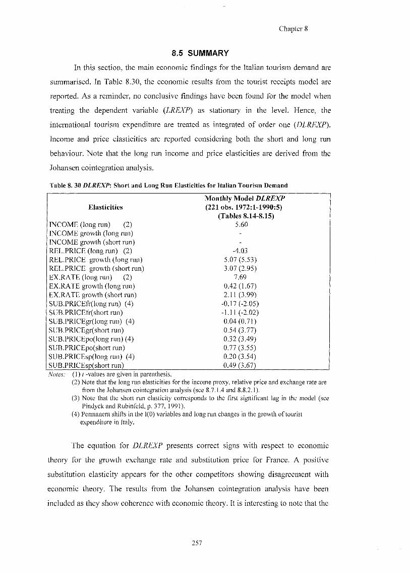
Chapter 8

8.5 SUMMARY

In this section, the main economic findings for the Italian tourism demand are

summarised. In Table 8.30, the economic results from the tourist receipts model are

reported. As a reminder, no conclusive findings have been found for the model when

treating the dependent variable (LREXP) as stationary in the level. Hence, the

international tourism expenditure are treated as integrated of order one (DLREXP).

Income and price elasticities are reported considering both the short and long run

behaviour. Note that the long run income and price elasticities are derived from the

Johansen cointegration analysis.

Table 8. 30 DLREXP-. Short and Long Run Elasticities for Italian Tourism Demand

Month ly Model DLREXP Elasticities (221 obs. 1972:1-1990:5)

(Tables 8.14-8.15) INCOME (long run) (2) 5.60 I N C O M E growth ( long run) -

I N C O M E growth (short run) -

REL.PRICE (long run) (2) -4.03 R E L . P R I C E growth ( long run) 5.07 (5.53) R E L . P R I C E growth (short run) 3.07 (2.95) Ii)LlRVnrE ( loryr i i in) (2) 7.69 E X . R A T E growth ( long run) 0.42(1.67) E X . R A T E growth (short run) 2.11 (3.99)

SUB.PRICEfr(longrun) (4) -0.17 (-2.05) SUB.PRICEfr (short run) -1.11 (-2.02) SUB.PRlCEgr ( long run) (4) 0.04 (0.71) SUB.PRICEgr(short run) 0.54 (3.77) SUB.PR]CEpo()ong run) (4) 0.32 (3.49) SUB.PRICEpo(short run) 0.77 (3.55) SUB.PRICEsp( long run) (4 ) 0.20 (3.54) SUB.PRICEsp(short run) 0.49 (3.67)

Notes: (1) / -values are given in parenthesis. (2) Note that the long run elasticities for the income proxy, relative price and exchange rate are

from the Johansen cointegration analysis (see 8.7.1.4 and 8.8.2.1). (3) Note that the short run elasticity corresponds to the first significant lag in the model (see

Pindyck and Rubinfeld, p. 377, 1991). (4) Permanent shifts in the 1(0) variables and long run changes in the growth of tourist

expenditure in Italy.

The equation for DLREXP presents correct signs with respect to economic

theory for the growth exchange rate and substitution price for France. A positive

substitution elasticity appears for the other competitors showing disagreement with

economic theory. The results from the Johansen cointegration analysis have been

included as they show coherence with economic theory. It is interesting to note that the

257

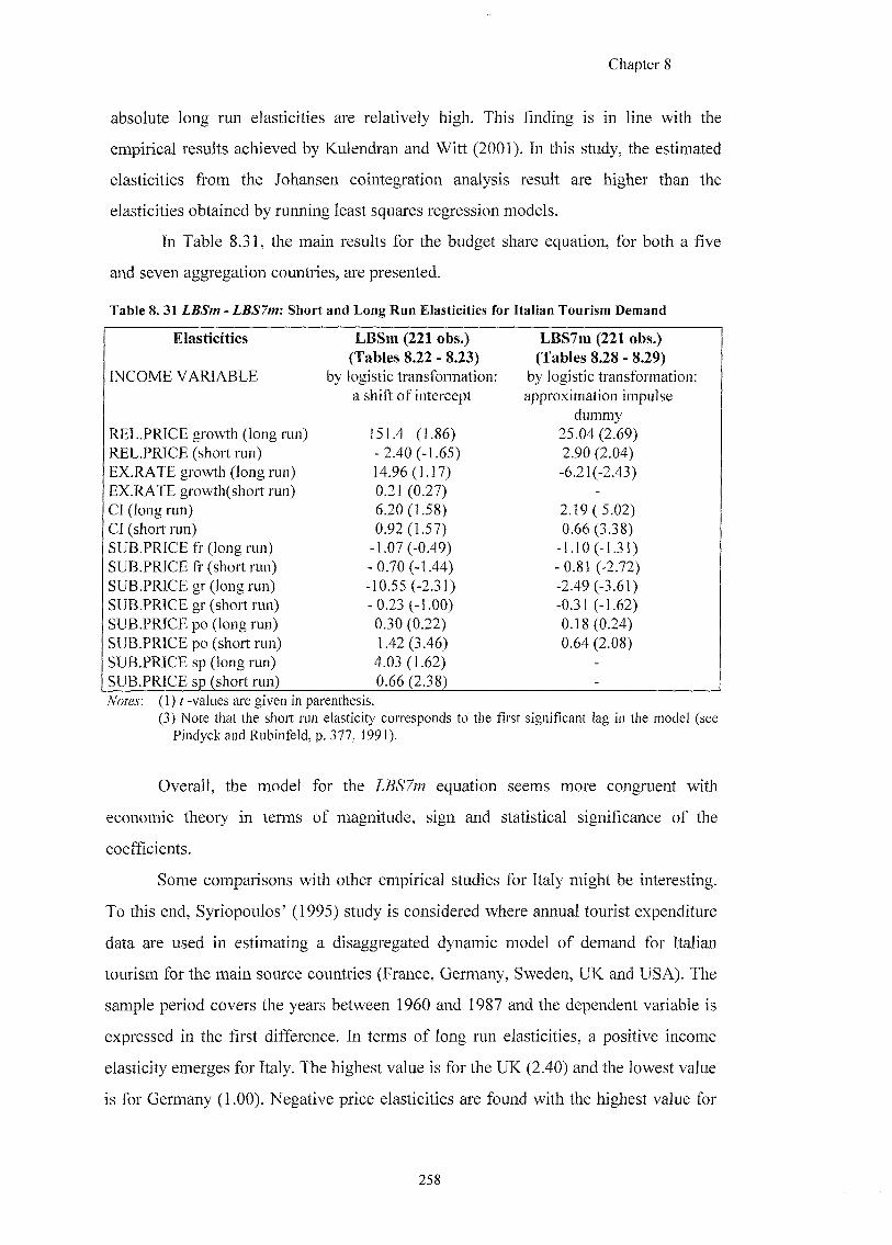
Chapter 8

absolute long run elasticities are relatively high. This finding is in line with the

empirical results achieved by Kulendran and Witt (2001). In this study, the estimated

elasticities from the Johansen cointegration analysis result are higher than the

elasticities obtained by running least squares regression models.

In Table 8.31, the main results for the budget share equation, for both a five

and seven aggregation countries, are presented.

Table 8. 31 LBSm - LBS7m: Short and Long Run Elasticities for Italian Tourism Demand

Elasticities LBSm (221 obs.) LBSTm (221 obs.) (Tables 8.22 - 8.23) (Tables 8.28 - 8.29)

INCOME V A R I A B L E by logistic transformation: by logistic transformation;

a shift o f intercept approximation impulse

dummy

R E L . P R I C E growth ( long run) 151.4 (1.86) 25.04 (2.69) R E L . P R I C E (short run) -2.40 (-1.65) 2.90 (2.04) E X . R A T E growth ( long run) 14.96(1.17) -6.21 (-2.43) E X . R A T E growth(short run) 0.21 (0.27) -

C I ( long run) 6.20(1.58) 2.19(5.02) C I (short run) 0.92(1.57) 0.66 (3.38) SUB.PRICEfr (long run) -1.07 (-0.49) -1.10(-1.31) S U B . P R I C E fr (short run) -0.70 (-1.44) -0.81 (-2.72) SUB.PRICE gr (long run) -10.55 (-2.31) -2.49 (-3.61) S U B . P R I C E gr (short run) -0.23 (-1.00) -0.31 (-1.62) SUB.PRICE po (long run) 0.30 (0.22) 0.18(0.24) S U B . P R I C E po (short run) 1.42 (3.46) 0.64 (2.08) SUB.PRICE sp (long run) 4.03(1.62) -

S U B . P R I C E sp (short run) 0.66 (2.38) -

Notes: (1) / -values are given in parenthesis. (3) Note that the short run elasticity corresponds to the first significant lag in the model (see

Pindyck and Rubinfeld, p. 377, 1991).

Overall, the model for the LBS7m equation seems more congruent with

economic theory in terms of magnitude, sign and statistical significance of the

coefRcients.

Some comparisons with other empirical studies for Italy might be interesting.

To this end, Syriopoulos' (1995) study is considered where annual tourist expenditure

data are used in estimating a disaggregated dynamic model of demand for Italian

tourism for the main source countries (France, Germany, Sweden, UK and USA). The

sample period covers the years between 1960 and 1987 and the dependent variable is

expressed in the first difference. In terms of long run elasticities, a positive income

elasticity emerges for Italy. The highest value is for the UK (2.40) and the lowest value

is for Germany (1.00). Negative price elasticities are found with the highest value for

258

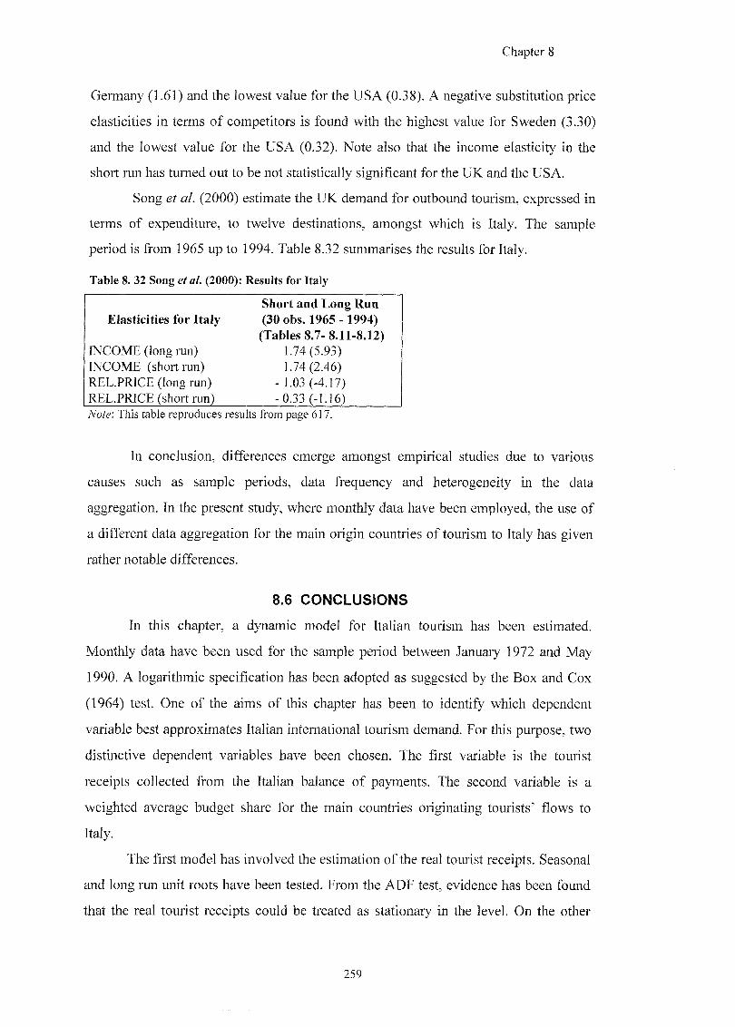
Chapter:

Germany (1.61) and the lowest value for the USA (0.38). A negative substitution price

elasticities in terms of competitors is found with the highest value for Sweden (3.30)

and the lowest value for the USA (0.32). Note also that the income elasticity in the

short run has turned out to be not statistically significant for the UK and the USA.

Song et al. (2000) estimate the UK demand for outbound tourism, expressed in

terms of expenditure, to twelve destinations, amongst which is Italy. The sample

period is from 1965 up to 1994. Table 8.32 summarises the results for Italy.

Table 8. 32 Song et al. (2000): Results for Italy

Short and Long Run Elasticities for I ta ly (30 obs. 1965 -1994)

(Tables 8.7- 8.11-8.12) INCOME (long run) 1.74 (5.93) INCOME (short run) 1.74(2.46) REL.PRICE (long run) - 1.03 (-4.17) REL.PRICE (short run) -0.33 (-1.16)

Note: This table reproduces results from page 617.

I n conclusion, differences emerge amongst empir ica l studies due to various

causes such as sample periods, data frequency and heterogeneity i n the data

aggregation. In the present study, where monthly data have been employed, the use of

a di f ferent data aggregation for the ma in or ig in countries o f tour ism to I ta ly has g iven

rather notable differences.

8.6 CONCLUSIONS

In this chapter, a dynamic model for Italian tourism has been estimated.

Mon th l y data have been used for the sample per iod between January 1972 and M a y

1990. A logar i thmic specif icat ion has been adopted as suggested by the B o x and Cox

(1964) test. One of the aims of this chapter has been to identify which dependent

variable best approximates Italian international tourism demand. For this purpose, two

distinctive dependent variables have been chosen. The first variable is the tourist

receipts collected from the Italian balance of payments. The second variable is a

weighted average budget share for the ma in countries or ig inat ing tourists' f lows to

Italy.

The first model has involved the estimation of the real tourist receipts. Seasonal

and long run unit roots have been tested. From the ADF test, evidence has been found

that the real tourist receipts could be treated as stationary in the level. On the other

259

Chapter 8

hand, the income proxy (LRPRd) has been found to be non-stationary in the level but

in the first difference. Hence, a non-linear specification in the income proxy variable

has been used in estimating Italian tourism. However, no clear conclusion has been

reached by using a logistic transformation. Several minima for the residual sum of the

squares have been found. Following Franses' test results and other empirical studies

(see Song er a/. 2000), an experiment has been done using expenditure i n f i rst

differences. By applying a Johansen cointegration analysis, statistical evidence has

been found that the real tourist receipts, the real income proxy, the relative price and

exchange rate drift together in the long run. Interestingly, the long run relationship

amongst these variables has given the expected sign in accordance with economic

theory. In this way, it has been possible to estimate a dynamic model that includes both

the short and long run information. Some unexpected results have been found in terms

of substitution elasticity.

A further aim of this chapter has been to estimate Italian tourism demand by

using a weighted budget share as the dependent variable. An initial investigation has

i nvo lved an understanding o f the appropriate level o f aggregation. Seven ma in or ig in

countries of tourism to Italy have been considered: France, Germany, Japan, Sweden,

Switzerland, the U K and the U S A . F rom graphical inspect ion and statistical analysis,

the weighted budget share should have included all of these countries, except Japan

and the USA that show differences in the magnitude, sign and statistical significance

of the trend coefficient. As a next step, a twofold analysis has been carried out for five

and seven coimtries aggregation, respectively. Interestingly, though using a di f ferent

level o f aggregation, s imi lar results have been achieved i n terms o f the integrat ion and

cointegration status of the main economic variables of interest. In particular, the real

industrial production index has been found stationary in the first difference. Hence, a

non-linear specification has been undertaken in both of these cases. The results have

shown that the logistic transformation of the real income proxy has given an

ambiguous interpretation in the five countries' model, whereas the income proxy has

been transformed into an approximation to an impulse dummy in the seven countries'

model. Hence, i n bo th cases the economic interpretat ion has vanished. Overal l , the

seven countries aggregation has shown a better specif ication. Considering the acûsted

R-squared, the f i rst model has been able to expla in 96% o f the variance o f the

260

Chapter 8

dependent variable, whereas the second model has been able to explain almost 97% of

the variance of the budget share. As already reported in Section 8.9, the seven

countries' aggregation model has shown better results in terms of economic theory for

the explanatory variables included in the final restricted model.

Finally, it is worth noting that the "Easter" dummy included in the three models

has turned out statistically significant only in the budget share equation for the seven

countries aggregation. This finding contrasts with the other two specifications and with

Gonzales and Moral (1995) study. In the latter, the coefficient of the Easter dummy

has been found statistically significant only when using tourists' arrivals as the

dependent variable.

26]

Chapter 9

CHAPTER 9.

GENERAL DISCUSSION

A i m o f the C h a p t e r :

To discuss the contributions of this thesis to the tourism literature, bearing in mind the

initial propositions on which this work is based.

9.1 INTRODUCTION

This chapter contains a general discussion of the main contributions of this thesis

to the existing tourism literature. The findings obtained from the empirical work are

structured to reflect the main propositions and aims of this thesis as given in Chapter 1.

The first proposition is concerned with the capability of more advanced econometric

approaches to give insight into modelling and estimating the demand for tourism. As a

second proposition, one gives grounds, both in terms of evolution of tourists' flows,

seasonality and econometric findings, for separating domestic from international

tourism. The third proposition investigates whether estimates of tourism demand at

different time frequencies can be reconciled. Finally, the fourth and last investigation

examines the capability of the estimated models to satisfy economic theory, and

whether any conflict between theory and econometric findings emerges from this

analysis.

9.2 ADVANCED ECONOMETRIC TOOLS AND TOURISM DEMAND

One of the questions which has been answered in this empirical work is: can

advanced econometric approaches give more insight into modelling and understanding

tourism demand? More advanced econometric tools, largely used in other applied

econometric studies, have transferred to the analysis of tourism demand the possibility

to investigate the characteristics and properties of the economic series under study.

First, the integrat ion status o f a variable as we l l as any possible cointegration

relationship between variables can be detected. Next, seasonal unit roots tests and mis-

262

Chapter 9

specification tests have led to the investigation of seasonal patterns; evidence has been

found for the existence of seasonal structural breaks which have been carefully

dummied out. From the Johansen cointegration analysis, evidence has been found for

the existence of long run relationships amongst 1(1) variables. For example, the

relative price (Sassari/main origin countries, LRP) and the weighted exchange rate

{LER) for the main source countries have been found to be cointegrated. The same

conclusion has been reached for the relative price Italy/main origin countries (LRPa)

and the exchange rate {LEXa), considering both seven and five countries' aggregations.

These findings have led to the inclusion in the models both short and long run

information. Moreover, the use of dynamic modelling has given more insight into the

differences between short and long run income and price elasticities as discussed

below.

Hence, by means of more advanced econometric approaches, it has been possible

to discover properties and relationships between economic series which are still much

neglected in the tourism literature. A more rigorous testing procedure, by making use

of the LSE methodology, has revealed mis-specification problems, and other problems

in the residuals (e.g. heteroscedasticity) that have hardly been considered in the

tourism literature. The finding of this thesis shows how more advanced econometric

approaches give the researcher help in modelling and estimating the demand for

tourism.

9.3 DOMESTIC AND INTERNATIONAL DEMAND FOR TOURISM

In testing the second proposition, evidence for distinguishing domestic from

international tourism has been given. The analysis holds for tourism in the north of

Sardinia. Several differences can be pointed out from a graphical inspection alone as

shown in Chapter 3. The first substantial difference is evident in the historic evolution

of the flows of tourists, over the period under study. Moreover, a graphical analysis has

shown different seasonal distributions for the two components. The seasonal

distribution for foreign tourists shows overall smaller variations for the months

between June and September, with the highest value in July. On the other hand, the

seasonality of the domestic flows of tourists presents a more irregular distribution,

with the highest peak in August. On this basis, the two components can be considered

263

Chapter 9

as different.

The next step is to find econometric evidence for modelling international and

domestic demand for tourism separately. A list of the main differences that have been

discovered follows.

1) Trading-day factors -

The first element that indicates the need to estimate two separate models relates

to the "trading-day" factors. The dependent variable, that is the total number of foreign

tourists in all registered accommodation, has to be adjusted in order to take into

account the number of Saturdays in each month for the period under consideration. A

comparison between the models both with and without the normalisation has been

made. The model with the raw series as the dependent variable has encountered

problems of non-normality and heteroscedasticity (at the 1% level), which have been

corrected after imposing the normalisation.

A different normalisation is required for the number of domestic arrivals. Three

different models have been estimated. The first model includes the raw data; the

second includes the adjustment for the number of Saturdays and the third the

normalisation for the number of Sundays in a month. From a first round estimation, the

first and third models can be considered as superior. The residual sum of the squares

have presented smaller values than in the case where the dependent variable has been

corrected for the number of Saturdays in a month. However, from a second round

estimation, the model that includes the raw data as the dependent variable has been

chosen; it presents, in fact, the best specification in terms of diagnostic tests. Problems

of mis-specification (RESET test at the 1% level) appear in the model with the

normalisation for the number of Sundays. This finding suggests that domestic tourists

are likely to arrive in Sassari Province any day of the week by either boat or plane.

Foreign tourists, o n the other hand, are much more constrained by the arr ival day, as

they are more likely to use charter flights that occur mainly at the weekends as far as

the period of study is concerned'"2.

2) Structural Breaks -

Relevant characteristics have been discovered in modelling the domestic

102 It is worth noting that in recent years there are more international flights available to the north of Sardinia during the week. It would be interesting in further work to find out if this circumstance affects the decisions of holiday-makers.

264

Chapter 9

demand for tourism in the north of Sardinia. The existence of seasonal unit roots at

some frequencies are detected by applying Franses' (1991) test. This could be thought

a symptom of non-stationarity that might be due to structural breaks. A preliminary

Chow test (1967) carried out on all the coefficients of the variables of interest,

seasonal dummies, and using Andrews' (1993) critical values indicate that a structural

break is evident in the seasonal pattern. Analogous results have been found both in the

monthly and quarterly data models. Two structural changes occur. The first, between

the first and second half of the Eighties, and the second occurs between the Eighties

and Nineties. Changes in the tastes of domestic consumers, who seem to prefer to

spend their hol idays i n the peak months (z.e. July, August and September), are

observed. On the other hand, a general decrease of tourism demand has been detected

in the off-peak months, i.e. April and October.

The previous results suggest once more the validity of modelling domestic and

international demand for tourism separately. Note that no structural breaks have been

detected in estimating the international demand for tourism in the north of Sardinia.

9.4 MONTHLY, QUARTERLY AND ANNUAL DATA

In this section, an account is given of the main similarities and differences in

employing data points at different time frequencies. The first part is dedicated to the

international demand for tourism in Sassari Province and the second subsection is

dedicated to the domestic demand.

9.4.1 International Demand For Tourism At Different Time Frequencies

Another purpose of this thesis has been to estimate models at different time

frequencies. This section gives an account of the main similarities and differences

from the estimation of the international demand for tourism in Sassari Province. In

order to have homogeneity in the results, the same economic series have been used in

running the three models.

1) S I M I L A R I T I E S

a) Long run and seasonal unit roots.

The first relevant analogy appears in the characteristics and properties of the economic

series under study when using monthly and quarterly data. The ADF test suggests that

265

Chapter 9

the adjusted series of foreign arrivals {LA), the nominal weighted average industrial

production index {LPR) and the substitute price (LSP) are stationary in the level. On

the other hand, the relative price {LRP) and weighted average exchange rate {LER) are

1(1). No seasonal unit roots have been detected by applying Franses' test.

b) Cointegration analysis.

The 1(1) variables, LRP and LER, have been used to test for possible cointegration

adopting the Johansen analysis. Homogenous results have been achieved from the

cointegration analysis for the three data frequencies. The restriction on the long run

coe@icient (say /?), i.e. has been accepted i n al l cases. Th is result suggests that

there are no major differences in the inflation rates in the countries under

consideration.

c) Long run elasticities.

The three models have given the same positive sign for the income proxy {LPR) which

is in line with economic theory. An increase in the income causes a rise in tourism

demand in the north of Sardinia. Homogeneous results have been obtained in terms of

sign of the coefficient for the substitute price {LSP). However, it presents a positive

sign that contrasts with economic theory. Note that the magnitude of the substitute

price coefficient is slightly smaller in the monthly model than in the other two models.

Common results have been achieved for the coefficient sign and magnitude of the

cointegrating vector (C7). In particular, an increase in CI, determined either by an

increase in the relative price {LRP) or a decrease in the exchange rate {LER), decreases

the international demand for tourism in the long run. Notably, the exchange rate

growth {DLER) has been found not statistically significant in any of the three models.

d) Short run elasticities.

No common results have been reached in terms of short run dynamics. It is worth

noting that a static final model has been achieved in both the annual and quarterly case.

The last finding suggests that the models converge rapidly to their long run equilibria.

. D I F F E R E N C E S

a) Long run unit roots.

The first relevant difference appears when applying the ADF test to annual data. The

integration status of the economic series under study differs considerably from that

observed for the other time frequencies. For example, the dependent variable {LA) and

266

Chapter 9

the income proxy {LPR) have been found to be non-stationary in the level and

difficulties have appeared in establishing the integration status of the exchange rate

(LER). As already pointed out in Chapter 4, the use of a small number of observations

(24 in total) causes a lack of power of the ADF test, leading to a relatively frequent

failure to reject the null hypothesis of an unit root.

b) Cointegrat ion analysis.

Given the differences encountered in the ADF test, the cointegration analysis for LRP

and LER, when using annual data, has been based on the ADF test results obtained in

the monthly and quarterly cases.

c) Long run elasticities.

Though the sign of the income proxy (LPR) has been found to be positive, its elasticity

varies across the three models. The annual model shows a quite high coefficient

(+2.34), which is in line with some empirical results for the Italian case (Clauser,

1991; Witt and Witt, 1992). The monthly data model presents an income elasticity

above unity (+1.06) which denotes a not very strong preference of foreign tourists for

Sardinian tourism as in the annual case. A coefficient less than one (+0.79) has been

obtained in the quarterly model case; this result seems to suggest that the marketing

policy in Sardinia needs improvement in order to attract a higher number of foreign

tourists. On the other hand, the quarterly model gives a statistically negative price

elasticity in terms of first difference of the relative price (DLRP). An increase in the

growth o f relat ive price is associated w i t h a decrease i n the foreign demand for

tourism.

d) Short run elasticities.

The monthly model is the only one that gives insight into the differences between short

and long run dynamics. It is interesting to note that this model shows a high income

elasticity (+2.56) in the short run. Moreover, the coefficient for the substitute price

presents a very high positive elasticity in the short run, in contrast again with current

economic theory.

9.4.2 Domestic Demand For Tourism At Different Time Frequencies

This section is dedicated to the similarities and differences encountered in the

estimation of the domestic demand for tourism in Sassari Province.

267

Chapter 9

. S I M I L A R I T I E S

a) Long run and seasonal unit roots.

As for the international case, homogeneous results have been obtained from the ADF

test when using monthly and quarterly economic series. The raw series of domestic

arrivals {LAR), the Italian industrial production index {LPR) and the substitute price

{LSP) are 1(0). The relative price (LREP) is 1(1). Moreover, no seasonal unit roots have

been detected by applying Franses' test as shown in Chapter 5.

b) Long run elasticities.

The three data models have given the same results in terms of long run income

elasticity. The income proxy (LPR) coefficient has presented the expected positive

sign, in line with economic theory, and an elasticity less than one, as Malacarni (1991)

found for the Italian case (that is +0.92). However, the magnitude of the income proxy

coefficient is slightly smaller in the annual model than in the other two models. In each

of the three models, homogeneous results have been obtained in terms of the sign of

the coefficient for the substitute price (LSP). Though highly statistically significant, it

presents an unusual positive sign. On the other hand, the relative price growth

elasticity does not turn out to be statistically significant in the long run.

c) Short run elasticities.

The short run income elasticity is found to be positive and less than one. These

findings are in line with economic theory. The short run elasticity is less than the long

run elasticity w h i c h conf i rms other empir ica l studies (Syriopoulos, 1995; Song er a/.

2000). This suggests that if income increases then Italian tourists adjust relatively

slowly in the short run and substantially in the long run. Again, the monthly, quarterly

and annual models show a positive sign for the substitute price coefficient. Moreover,

the relative price does not turn out to be statistically significant in the short run.

. D I F E B t B N C E S

a) Long run unit roots.

Using 24 data points, the annual series of number of domestic arrivals and the index of

industrial production are found to be 1(1) by applying the ADF test. These results

diverge from the ADF test findings using the other time frequencies. Again, the lack of

power of the ADF test is confirmed by the use of a small number of observations.

On balance, the models estimated with monthly and quarterly data have given

268

Chapter 9

the most homogenous results. Similar findings, in fact, have been achieved in terms of

characteristics and properties of the series under study, in terms of short and long run

income and price elasticities as well as in terms of magnitude of the coefficients.

9.5 ARE THE ECONOMIC PROPOSITIONS ALWAYS SATISFIED?

The next proposition explored in this thesis relates to the capability of the

estimated models to satisfy economic theory. Are income elasticity, negativity and

substitutability always satisfied in the estimated dynamic models?

Starting with the income elasticity, overall these results confirm those obtained

in other empirical studies. In the majority of the present estimations, the long run

income elasticity has been found to be positive which suggests tourism to be a normal

good. In estimating the annual international tourism for the Province of Sassari, the

income elasticity has been found to be greater than one. This result implies Sardinian

tourism is viewed as a luxury good; this elasticity value confirms the results achieved

by Malacarni (1991) for Italy. However, the income elasticity findings for the monthly

and quarterly cases cannot be compared with other empirical studies; there are no other

studies available either for Sardinia or for Italy. In the monthly data case, in fact, the

long run income elasticity has been found to be just above unity (+1.06) and less than

unity (+0.79) in the quarterly data case. This fact suggests that foreign tourists consider

Sardinian tourism as a necessity good. The results in estimating domestic tourism

confirm that Italians view Sassari tourism as a necessity good. This finding, that holds

for each of the time frequencies used in estimation, is in line with the results obtained

by Malacarni (1991) for the Italian case.

In general, the negativity hypothesis has been satisfied in the quarterly model

used for the international demand for tourism. The relative price growth has presented

a negative and statistically significant coefficient.

The major conflict between econometric results and a priori economic theory

has been found in the positive sign for the nominal substitute price coefficient. This

finding has encouraged a further investigation (see Chapter 6). An unequivocal answer

has not been achieved by including the real substitution price in an aggregated manner.

Further investigation of the individual components {i.e. the real substitute price for

each of the main Sardinian competitors) has led to heterogeneous results both in the

269

Chapter 9

short and long run dynamics. On balance, the empirical findings seem to suggest that

France and Portugal can be viewed as the main competitor countries for tourism in the

north of Sardinia.

In estimating the Italian tourism demand in terms of expenditure, four real

substitution prices have been included for the main Italian competitors in the

Mediterannean area (France, Greece, Portugal and Spain). Again, heterogeneous

results have been achieved in the three equations (that is tourist receipts equation and

budget share equations for five and seven-origin countries' aggregations). On balance,

from the empirical findings, France and Greece can be considered as the main

competitors for Italian tourism. These findings seem to confirm Syriopoulos' (1995)

study in which "the performance of the "substitute effective price" variable (effective

price in a destination relative to competitor destinations) was not statistically

satisfactory i n al l cases" (p.331).

9.6 ECONOMIC THEORY AND ECONOMETRIC ANALYSIS

The last proposition explored in this thesis relates to the existence of any

conflict between economic theory and econometric results.

In Chapter 8, evidence has been found that the (log) real weighted industrial

production (LRFRa) is stationary in the first difference. This finding suggests the real

industrial production is drifting increasingly as the time goes on and it confirms

Hansen's (1995) results when employing U.S. annual macroeconomic time series. In

Hansen's article, there is evidence for the (log) real per capita GNP to be 1(0) and the

(log) real industrial production to be 1(1) when the first difference of the unlogged

unemployment rate is used as a covariate.

Given the previous result, a non-linear specification in the income proxy has

been pursued in estimating the international demand of tourism to Italy, expressed both

in terms of tourist receipts and budget share. In both cases, the logistic transformation

of the income proxy has turned into a dummy variable. This is clear for the seven

countries aggregation, where the transformed proxy looks like an impulse dummy. For

the five countries aggregation visual inspection suggests either an intercept shift, or a

bounded downward (stochastic) trend. Transformation into a dummy makes the

economic interpretation vanish. The expectation is, in fact, that the logistic

270

Chapter 9

transformation of the income proxy is able to describe the economic relationship

existing between the international tourist expenditure for Italy and the real income

proxy for the main source countries. Economic theory suggests that below a certain

income level the tourist expenditure is expected to be zero. As income starts rising,

Italian tourist expenditure should increase until the point in which a maximum is

reached. Hence, at a certain level of income tourist expenditure reaches its maximum.

For further increases in the income, the level of tourist expenditure is expected to

become stable around a certain value.

However, any conflict with economic theory arising from the current empirical

work, far from invalidating the theory, can be thought of as the result of different

causes. For example, proxy variables may not completely express economic reality;

one is constrained by the availability of the data. One, for instance, is obliged to

employ the industrial production index as a measure of individuals' income instead of

using disposable income when dealing with models at a monthly frequency.

Arguably, in Chapters 4, 5 and 6 the use of the nominal industrial production

index as the income proxy has, in general, given the positive expected sign in the long

nm. However , exceptions can be detected i n the negative sign result ing i n the

coefficients of the income proxy whenever oscillations are involved. Furthermore,

some discrepancies have been obtained in estimating the international demand for

Sassari Province both in terms of long and short run dynamics (see Chapter 6). In this

case, a negative income elasticity has been obtained. The last findings denote that the

industrial production seems possibly to be detecting "over-time" effects overstated by

the use of such a proxy. That is, while the trend in industrial production differs from

that in disposable income, it may reflect short run movements in income: for example,

more overtime working in periods of prosperity. In the short run, this may reduce the

demand for leisure in general, and tourism in particular. It does seem that for the

period in question industrial production is a reasonable proxy, not ideal, but

satisfactory for disposable income.

Interestingly, some economic ground has been found in the equation for the

I ta l ian tourist receipts growth. A s a reminder, Franses' un i t roots test has suggested the

Italian real tourist receipts is non-stationary in the level. This finding is also in line

with other empirical studies existing in the tourism literature (e.g. Lanza and Urga,

271

Chapter 9

1995). By applying the Johansen cointegration analysis, the possible existence of a

long run relationship has been tested for the four 1(1) variables {i.e. real tourist receipts

(LREXP), real industrial production (LRPRa), relative price (LRPa) and weighted

average exchange rate (LEXa)). From this test, evidence has been found that the

previous variables drift together in the long run. This finding is consistent with the

international demand for Italian tourism being linked to variables identified by

economic theory in the long run. Note also that the long run coefficients show the

expected sign: a positive income elasticity for the real industrial production; negativity

holds for the relative price and a positive long run coefficient turns out correctly for

the weighted exchange rate.

9.7 CONCLUSIONS

This chapter has been dedicated to the contributions of this thesis to the tourism

literature. An account has been given in terms of the initial propositions of the

investigation.

In Section 9.2, the contribution from analysing tourism demand with more

advanced econometric techniques has been discussed. Franses (1991) and Hylleberg et

al. (1990) seasonal unit root tests, ADF test, Johansen cointegration analysis, and a

series of diagnostic tests following the LSE methodology have given new knowledge

and understanding in estimating tourism demand for the Province of Sassari and for

Italy. In Section 9.3, a discussion for separating international from domestic demand

for tourism has been given. Differences and similarities in modelling and estimating

tourism demand at different time frequencies are reported in Section 9.4. If economic

theory is relevant, one would expect income elasticity, negativity and substitutability to

be satisfied; Section 9.5 has been dedicated to the validation of these a priori

propositions as derived from this empirical work. Some incongruities between

economics and econometrics emerging from this thesis have been the objectives of the

last section.

272

Chapter 10

CHAPTER 10.

CONCLUSIONS

Sinclair and Stabler (1997), and Sinclair (1998), have emphasised that there is

still a requirement to develop research into the demand for tourism. They also suggest

that there are still many relevant aspects not explicitly taken into consideration by

empirical studies in the tourism literature. Amongst others, there is a lack of discussion

of functional forms. The inclusion of diagnostic tests in addition to the usual r-test, F-

test, R-squared adjusted and D-W statistics is also desirable. Problems of

heteroscedasticity are hardly considered. Short and long run elasticities are still much

neglected. At this point, Sinclair and Stabler (1997) write "with few exceptions,

notably Syriopoulos (1995), the majority of studies have assumed that demand

depends on current income but not on past or expected future income" (p. 39). This

thesis makes a new contribution in analysing and modelling the demand of tourism.

The aim has been estimating the demand of tourism in Italy as a whole and a particular

emphasis has been given to tourism in the Province of Sassari (Sardinia). Several

contributions to knowledge have been made by this empirical work.

® Economic theory has been tested by employing more advanced econometric

modelling, such as: seasonal and long run unit root testing, the Johansen

cointegration analysis and the LSE general-to-specific methodology.

® Greater sample sizes have been used with a minimum of 24 observations, when

using annual data, to a maximum of 288 observations when employing monthly

data. This has established similarities and differences both in the pre-modelling

and estimation phase.

# For each o f the estimated models, statistical evidence has been given for adopting

the logarithmic functional form. A full range of diagnostic tests has been included

in the estimation procedure.

® Elasticities have been estimated. The derivation of short and long run dynamics has

been possible by including actual and lagged dependent and explanatory variables.

In Chapter 2, a description of the main methodological steps adopted in the thesis has

been given.

273

Chapter 10

Chapters 3, 4, 5 and 6 have been dedicated to analysing, modelling and

estimating tourism demand in the Province of Sassari. New information has been

given on both international and domestic tourist flows. The analysis in Chapter 3 has

highlighted major differences between domestic and international demand for tourism

in the north of Sardinia. In terms of the historic evolution of tourist flows, domestic

arrivals in all registered accommodation have shown an upward trend in the years

between 1972 and 1995, with only a few exceptions. On the other hand, the trend for

international demand appears to be more influenced by economic events during the

three decades, such as higher standards of living, monetary restrictions and exchange

rate depreciation. From an initial graphical inspection, major differences have also

emerged in the seasonality of the two components. This finding has been confirmed by

the pre-modelling and estimation analysis in Chapters 4 and 5. While the international

seasonal pattern has turned out to be deterministic, a varying seasonal pattern has been

found for domestic tourism demand. Evidence for the latter result has emerged from

Franses' seasonal unit roots test as well as from problems of mis-specification in the

models, which does not include seasonal parameter changes. A further distinction

between the two components is in the so-called "trading-day" factor. From the

econometric analysis, the need to normalise the total international tourists' arrivals for

the number of Saturdays in a month has emerged. In Chapter 5, the domestic demand

model has given the best specification without any correction for the dependent

variable. Hence, this study has discovered characteristics and properties of the

economic series which can be used as a basis for further forecasting exercises

employing time-series and econometric models in this thesis. However, it is worth

noting that forecasting has not been the objective of this thesis.

In Chapter 3, an account has been given of the main explanatory variables that

could have an impact in explaining the demand of tourism in accordance with

economic theory. The scope of Chapters 4, 5, 6 and 8 has been to test economic theory

by adopting the Johansen cointegration analysis and the LSE methodology. Firstly, the

integration status of the economic series of interest has been established by the ADF

test. Evidence has been found for the relative price {LRP) and exchange rate {LER) to

be random walks and thus 1(1). Furthermore, a Johansen cointegration analysis has

suggested that LRP and LER converge to a common equilibrium path in the long run,

274

Chapter 10

which satisfies the a priori theory. The same conclusion has been reached for the

relative price and exchange rate within the Italian model. A log-linear form, suggested

by the Box and Cox test, has been chosen for all the models estimated in this thesis.

Short and long run income and price elasticities have been obtained via a dynamic

analysis and inclusion of 1(0) and 1(1) variables. The main discrepancy between

economic theory and econometric results is that of a positive sign for the coefficient of

the nominal substitution price, that is Sassari/main competitors in the Mediterranean

area (France, Greece, Portugal and Spain). Economic theory states that a decrease in

tourism demand is expected when the price in a certain destination increases with

respect to other competitors, ceteris paribus. The unexpected result has led to a further

investigation in Chapter 6, where the monthly tourism demand is modelled with the

inclusion of the exchange rate for the competitor countries. However, the results have

confirmed a positive sign for the coefficient of the real substitution price defined in an

aggregated manner. Therefore, an investigation has been undertaken in analysing the

properties of the individual components of the substitution price, which has led to the

inclusion of four distinctive real substitute prices for each of the competitors. The ADF

test and cointegration tests have given higher homogeneity for the real substitute price

of each of the individual competitors that has been included both in the foreign and

domestic demand models. However, the final models obtained have not given a

definitive answer in terms of short and long run substitute price elasticities. Statistical

evidence has shown France and Portugal appear to be the main competitors for tourism

in the north of Sardinia. Heterogeneous results have also been achieved in estimating

international tourism in Italy (Chapter 8). On balance, France and Greece have

appeared to be the main competitors for Italian tourism.

This empirical work has investigated whether homogenous results can be

obtained by employing series at different frequencies. On balance, from Chapters 4 and

5, monthly and quarterly models have given more homogenous and robust results both

in the pre-modelling and final estimated values when compared with annual data

alone. However, it has also under-pinned the validity of employing monthly as well as

annual time series. By using monthly variables, it has been possible to include in the

model an "Easter" dummy which has entered with a satisfactory r-value. This finding

has confirmed that the seasonal dummies are not able to capture the Easter holiday

275

Chapter 10

effect due to its mobility between March and May. On the other hand, the use of

annual data has given the possibility to test the validity of using the Italian industrial

production index {LPR) as a proxy for the personal disposable income (LPDIN).

However, some caution should be sounded as just 10 observations have been used

(that is 1983-1992) in doing such an analysis. The use of annual data has also given the

possibility to include in the model two supply variables, that is; arrivals of boats and

flights in the north of Sardinia. The estimation results, for the international demand of

tourism, have shown a satisfactory determination in terms of statistical significance

and signs. Both of the two components present a positive sign indicating that the

higher the mean of transportation supplied the higher the number of foreign arrivals.

These results have suggested a more careful analysis. The problem of simultaneity has

been investigated via the Durbin-Wu-Hausman's test. From the analysis, it has

appeared that the number of international flights to the north of Sardinia is to be

considered as endogenous. However, it has not been in the scope of the study to fit a

model for such a variable. Moreover, the total number of arrivals of boats has been

found to be predetermined. One inference is that the total number of boats is picking

up other determinants that affect tourism demand. In the domestic demand model

(Chapter 5), the coefficient for the national arrivals of boats to the north of Sardinia

has been found to be statistically significant. The issue of possible simultaneity has

also been investigated by the Durbin-Wu-Hausman's test. The null hypothesis of no

simultaneity has been rejected and the supply variable has to be treated as endogenous.

One can conclude that a combination of different time frequency models is able to give

more insight in understanding tourism demand as well as its components.

Chapter 8 has involved the study of Italian tourism as a whole. Two separate

dependent variables have been constructed: the real tourism expenditure (LREXP),

expressed in terms of real tourism receipts in Italy and an aggregated budget share for

the main origin countries (LBSm). The sample period under study is from 1972:1 up to

1990:5. From June 1990 on, in fact, the data are collected with new currency

regulations which are not comparable with the previous data. The new contribution is

the use of monthly data, pre-modelling analysis and the use of the LSE methodology.

The aim has been to establish which variable better represents tourism demand.

276

Chapter 10

As far as LREXP is concerned, a model has been estimated by using a quadratic

and a non-linear equation, respectively. Note, in fact, that the weighted average real

industrial production for the main source countries {LRPRa), has been found to be 1(1)

from both the ADF test and Franses' unit roots test. A quadratic transformation was

not found to be an adequate approximation to a logistic transformation. Hence, a non-

linear model has been estimated. From this analysis, multiple maxima in the likelihood

have been detected giving evidence that the logistic form used does not turn out to be

satisfactory.

A further experiment has been carried out in estimating the tourist receipts

growth (DLREXP) as the dependent variable, in accordance to Franses' test. From a

Johansen cointegration analysis, the 1(1) variables have been found to have a long run

relationship as suggested by economic theory.

Several investigations have been undertaken for analysing and estimating the

weighted budget share (LSBm). The first investigation has involved a deeper

understanding on the appropriate degree of aggregation. From a graphical inspection

and statistical testing, evidence has been found for a five countries aggregation {i.e.

France, Germany, Sweden, Switzerland and UK, with the exclusion of Japan and

USA). However, for either the five or seven countries aggregations, similar results

have been obtained in terms of integration and cointegration status of the variables

under study. In particular, the income proxy {LRPRa) has been found 1(1) and a

quadratic and non-linear model, respectively, have been run in both the cases. Notably,

the results for the income proxy coefficient have failed to satisfy economic theory. In

each of the three models, in fact, the logistic transformation of the income proxy has

turned out to be interpretable as an approximation to a dummy variable. Overall, the

models for the tourist receipts growth has given results more in line with economic

theory.

From the empirical findings of the thesis, some important implications emerge

for both private and public operators.

® The analysis of the "trading-day" factor has highlighted different choices in the

timing of holiday trips by foreign and domestic tourists. International tourists seem

to choose Saturdays as the departure day. Italians, on the other hand, seem to prefer

Sundays rather than Saturdays as the departure day and, in fact, any day of the

277

Chapter 10

week. This empirical finding can assist the private sector in terms of using price

discrimination for consumers choosing Sassari Province as the destination for their

holidays.

® A graphical inspection of the possible existence of a capacity constraint in

accommodation supplied in Sassari Province gives useful information for both

private and public operators. There is no evidence that supply is a constraint on

demand. Moreover, the peak month, August, shows an average rate of utilisation of

almost 71%. June, July and September present an average rate of utilisation of

around 40%. These findings suggest that the objective of the private and public

sector does not seem to be that of increasing the accommodation capacity but using

the existing capacity in off-peak months.

® Seasonality is one of the main features of tourism activity. Hence, the understanding

of the seasonality is a necessity for both private and public operators. In this thesis,

the use of monthly time series has given a deeper insight into the characteristics of

the seasonal pattern for both the international and domestic demand components.

There are reasons for believing that the public administration, at a regional level,

should adopt promotion policies to encourage a de-seasonalisation process, in

particular for the domestic demand. The objective of the local authorities should

also be that of promoting Sassari tourism in off-peak months for Northern European

clients. It is worth recalling that some econometric evidence has been found for the

existence of a positive correlation between international demand and temperatures

in Sassari Province.

e Econometric and graphical analysis has demonstrated the existence of structural

changes in the domestic seasonal pattern. In both the 1980s and 1990s, evidence has

been found of a further extension of the high season by Italians. This finding

represents useful information for the public sector. The supply of public

infrastructure and natural resources need to be examined in order to avoid possible

negative externalities. In Sardinia, for example, one of the main problems is the

lack of adequate water resources. Increasing consumption of water, in peak months

(the driest months of the year) by the increased number of users, can create a

negative impact for locals not only in the tourist season but also, more and more, in

off-season months.

278

Chapter 10

• The existence of an "Easter" effect has suggested the importance of "second

holidays" for both foreigners and Italians. Hence, the "Easter" factor constitutes

new information for the operators in tourism activity. The private sector can adopt

price discrimination for tourist consumers, together with higher standard of quality

of the goods and services supplied during "second holidays" periods. The local

authorities should be aware of these effects in order to improve the quality of public

goods and services supplied in off-peak months.

• Econometric evidence has also indicated that France and Portugal are substitute

destinations for Sassari Province, and France and Greece for Italy as a whole. This

finding is useful for both private and public operators, who shoud consider

promoting Sassari and Italian tourism on a competitive base with these substitute

countries.

279

Appendix A

APPENDIX A

In this appendix, the analysis for the series of the foreign arrivals of tourists

without adjustment for the number of weekends per month is given.

The degree of augmentation appropriate when testing for unit roots is a subject

for debate (see Hansen, 1995; Caporale and Pittis, 1997). Hansen (1995) suggests a

Covariate Augmented Dickey Fuller (CADF) testing procedure for unit roots which

produces more precise estimates than a conventional ADF test. Caporale and Pittis

(1997) find that a number of macroeconomic time series are non-stationary using the

ADF, but are indeed stationary when using a CADF test. They regard this as

supporting the case of CADF tests, on the grounds that one is controlling the size of

the test, and working for improvements in power as rejection of the null corresponds to

acceptance of stationarity.

On the basis of these assumptions a previous seasonal unit roots test is

performed on the unadjusted series LAR. The first notable change with respect to the

adjusted series {i.e. LA) is the need for at least three impulse dummies {i.e. il994p4,

il992p7, il995p9'o^). Evidence for using such dummies is detected from the existence

of serial correlation and from an inspection of the residuals. The equation (2.6.2)

(Chapter 2) is fitted by OLS for the (log) foreign arrivals. Note that in this case also

includes the three impulse dummies in order to correct for the presence of serial

correlation. For the presence of seasonal unit roots caimot be accepted at a

general 1% level of s i g n i f i c a n c e ( T a b l e A.l), both performing the Mests of the

separate ;r's (with exception of and and the F-test of the pairs of ;7r's, as

well as the joint F-test of 7r^=..='7ii2=0.

103 and //PPjpP take the value 1 in in and respectively, and 0 elsewhere. '"4 The critical values for the seasonal unit roots test are provided in Franses (1991) pp.161-165.

280

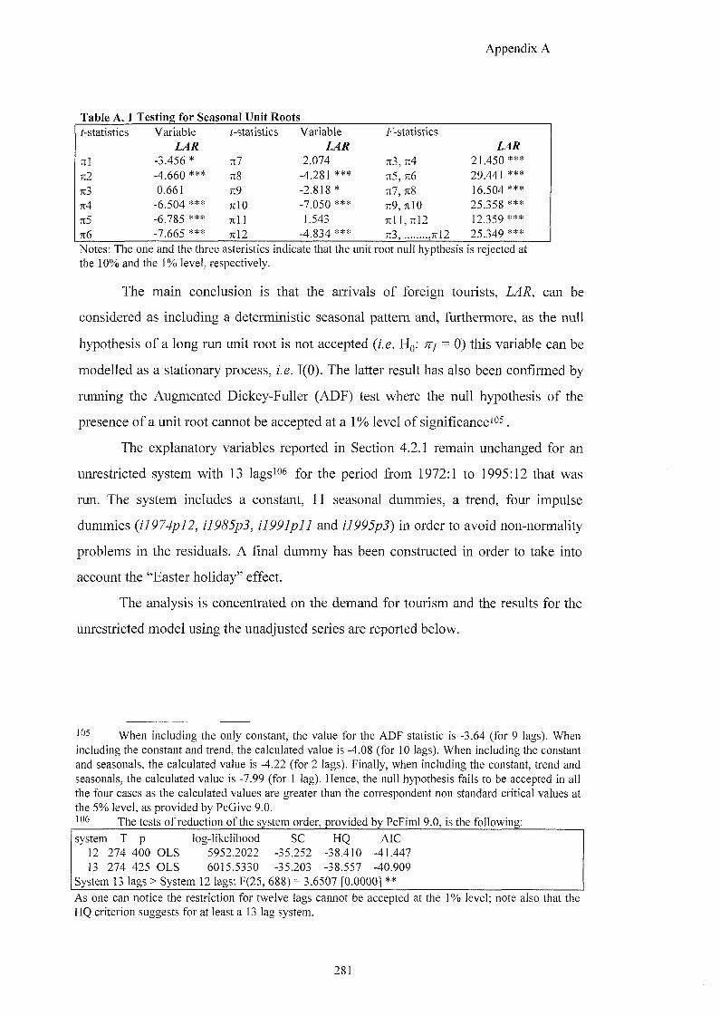
Appendix A

Table A. 1 Testing for Seasonal Unit Roots f-statistics Variable f-statistics Variable F-statistics

LAR LAR

111 -3.456 * %1 2.074 :t3, n4 21.450 ***

7^ -4.660 *** 7I8 -4.281 *** Tt5, 7I6 29.441 *** 7I3 0.661 719 -2.818 * :i7, n8 16.504 *** Tt4 -6.504 *** jilO -7.050 *** 7I9, 7I10 25.358 *** 7I5 -6.785 *** Til 1 1.543 7il 1,7:12 12.359 *** 7I6 -7.665 *** 7I12 -4.834 *** 7t3, ,7tl2 25.349 *** Notes; The one and the three asteristics indicate that the unit root null hypthesis is rejected at the 10% and the 1% level, respectively.

The main conclusion is that the arrivals of foreign tourists, LAR, can be

considered as including a deterministic seasonal pattern and, furthermore, as the null

hypothesis of a long run unit root is not accepted {i.e. nj = 0) this variable can be

modelled as a stationary process, i.e. 1(0). The latter result has also been confirmed by

running the Augmented Dickey-Fuller (ADF) test where the null hypothesis of the

presence of a unit root cannot be accepted at a 1% level of significance'05.

The explanatory variables reported in Section 4.2.1 remain unchanged for an

unrestricted system with 13 lags^^s for the period from 1972:1 to 1995:12 that was

run. The system includes a constant, 11 seasonal dummies, a trend, four impulse

dummies {il974pl2, il985p3, il991pll and il995p3) in order to avoid non-normality

problems in the residuals. A final dummy has been constructed in order to take into

account the "Easter holiday" effect.

The analysis is concentrated on the demand for tourism and the results for the

unrestricted model using the unadjusted series are reported below.

105 When including the only constant, the value for the ADF statistic is -3.64 (for 9 lags). When including the constant and trend, the calculated value is -4.08 (for 10 lags). When including the constant and seasonals, the calculated value is -4.22 (for 2 lags). Finally, when including the constant, trend and seasonals, the calculated value is -7.99 (for 1 lag). Hence, the null hypothesis fails to be accepted in all the four cases as the calculated values are greater than the correspondent non standard critical values at the 5% level, as provided by PcGive 9.0.

0 The tests of reduction of the system order, provided by PcFiml 9.0, is the following:

system T p log-likelihood SC HQ AIC 12 274 400 OLS 5952.2022 -35.252 -38.410 -41.447 13 274 425 OLS 6015.5330 -35.203 -38.557 -40.909

System 13 lags > System 12 lags; F(25, 688) = 3.6507 [0.0000] **

As one can notice the restriction for twelve lags cannot be accepted at the 1% level; note also that the HQ criterion suggests for at least a 13 lag system.

281

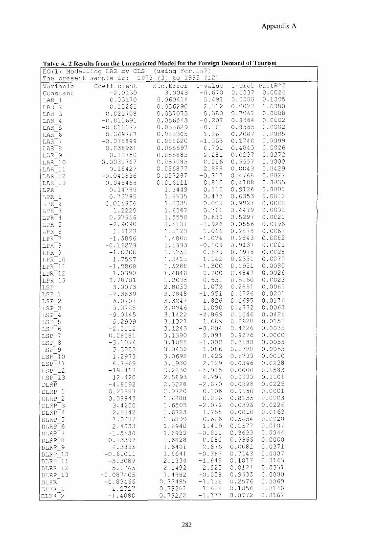
Appendix A

Table A. 2 Results from the Unrestricted Model for the Foreign Demand of Tourism EQ(1) Modelling L & R b y OLS The present sample is: 1973

(using For.in7) (3) to 1995 (12)

Variable Coefficient Std. Error t-value t -prob PartR^2 Constant -2.0130 3 .0043 -0 .670 0 .5037 0 .0024

LAR 1 0.33170 0 060414 5 .491 0 .0000 0 .1395

LAR 2 0.15265 0 056290 2 .712 0 .0073 0 .0380

LAR 3 0.021708 0 057073 0 .380 0 .7041 0 .0008

LAR 4 -0.011691 0 056543 -0 .207 0 .8364 0 .0002

LAR 5 -0.010077 0 055629 -0 .181 0 .8565 0 .0002

LAR 6 0.069763 0 055305 1 .261 0 .2087 0 .0085 LAR 7 -0.075899 0 055620 -1 .365 0 .1740 0 .0099 LAR 8 0.038961 0 055597 0 .701 0 .4843 0 .0026

LAR 9 -0.12750 0 055885 -2 .281 0 .0237 0 .0272 LAR 10 0.0031767 0 057085 0 .056 0 .9557 0 0000

LAR 11 0.16427 0 056877 2 .888 0 .0043 0 0429

LAR 12 -0.040836 0. 057287 -0 .713 0 .4768 0 0027

LAR 13 0.045468 0 056111 0 .810 0 .4188 0 0035

LPR 0.14790 1 .3449 0 .110 0 .9126 0 0001

LPR 1 0.73795 1 .5535 0 .475 0 .6353 0 0012

LPR 2 0.014950 1 .6305 0 .009 0 9927 0 0000

LPR 3 1.2220 1 .6067 0 .761 0 .4479 0 0031

LPR 4 0.97956 1 .5558 0 .630 0 .5297 0 0021 LPR 5 -2.9090 1 .5101 -1 .926 0 0556 0 0196

LPR 6 1.6123 1 .5123 1 .066 0 2878 0 0061

LPR 7 -1.5896 1 .4805 -1 .074 0 2843 0 0062

LPR 8 -0.16279 1 .4993 -0 .109 0 9137 0 0001

LPR 9 -1.0700 1 .5751 -0 .679 0 4978 0 0025

LPR 10 1.7597 1 .5415 1 .142 0 2551 0 0070

LPR 11 -1.9868 1 .5280 -1 .300 0 1951 0 0090

LPR 12 1.0390 1 .4840 0 .700 0 4847 0 0026

LPR 13 0.78701 1 .2095 0 .651 0 5160 0 0023 LSP 3.0073 2 .8053 1 .072 0 2851 0 0061 LSP 1 -7.3839 3 .7848 -1 .951 0 0526 0 0201 LSP 2 6.0701 3 .3247 1 .826 0 0695 0 0176 LSP 3 3.3728 3 .0946 1 .090 0 2772 0 0063

LSP 4 -9.0145 3 .1422 -2 .869 0 0046 0 0424

LSP 5 5.2909 3 .1321 1 .689 0 0928 0 0151 LSP 6 -2.5112 3 .1243 -0 .804 0 4226 0 0035

LSP 7 0.28581 3 .1390 0 091 0 9276 0 0000

LSP 8 -3.1074 3 .1088 -1 .000 0 3188 0 0053

LSP 9 3.3053 3 .0432 1 .086 0 2788 0 0063

LSP 10 1.2973 3 .0692 0 423 0 6730 0 0010

LSP 11 6.7969 3 .1930 2 129 0 0346 0 0238

LSP 12 -19.417 3 .2830 -5 915 0 0000 0 1583

LSP 13 12.420 2 .5893 4 797 0 0000 0 1101

DLRP -4.8092 2 .3228 -2 070 0 0398 0 0225

DLRP 1 0.21883 2 .0720 0 106 0 9160 0 0001

DLRP 2 0.38943 1 .6488 0 236 0 8135 0. 0003

DLRP 3 -3.4200 1 .6503 -2 072 0 0396 0 0226

DLRP 4 2.9342 1 .6723 1 755 0 0810 0 0163

DLRP 5 1.0237 1 .6899 0 606 0 5454 0. 0020

DLRP 6 2.4033 1 .6940 1 419 0 1577 0. 0107

DLRP 7 -1.5430 1 .6930 -0 911 0. 3633 0 0044

DLRP 8 0.13397 1 .6828 0 080 0 9366 0. 0000

DLRP 9 4.3895 1 .6401 2 676 0 0081 0. 0371

DLRP 10 -0.61011 1 .6641 -0 367 0. 7143 0. 0007

DLRP 11 -3.5089 2 .1334 -1 645 0. 1017 0. 0143

DLRP 12 5.1743 2 .0492 2 525 0 0124 0. 0331

DLRP 13 -0.087405 1 .4982 -0 058 0 9535 0 0000

DLER -0.83466 0 .73495 -1 136 0. 2576 0. 0069

DLER 1 1.2727 0 .78261 1 626 0 1056 0. 0140

DLER 2 -1.4080 0 .79222 -1 777 0. 0772 0 0167

282

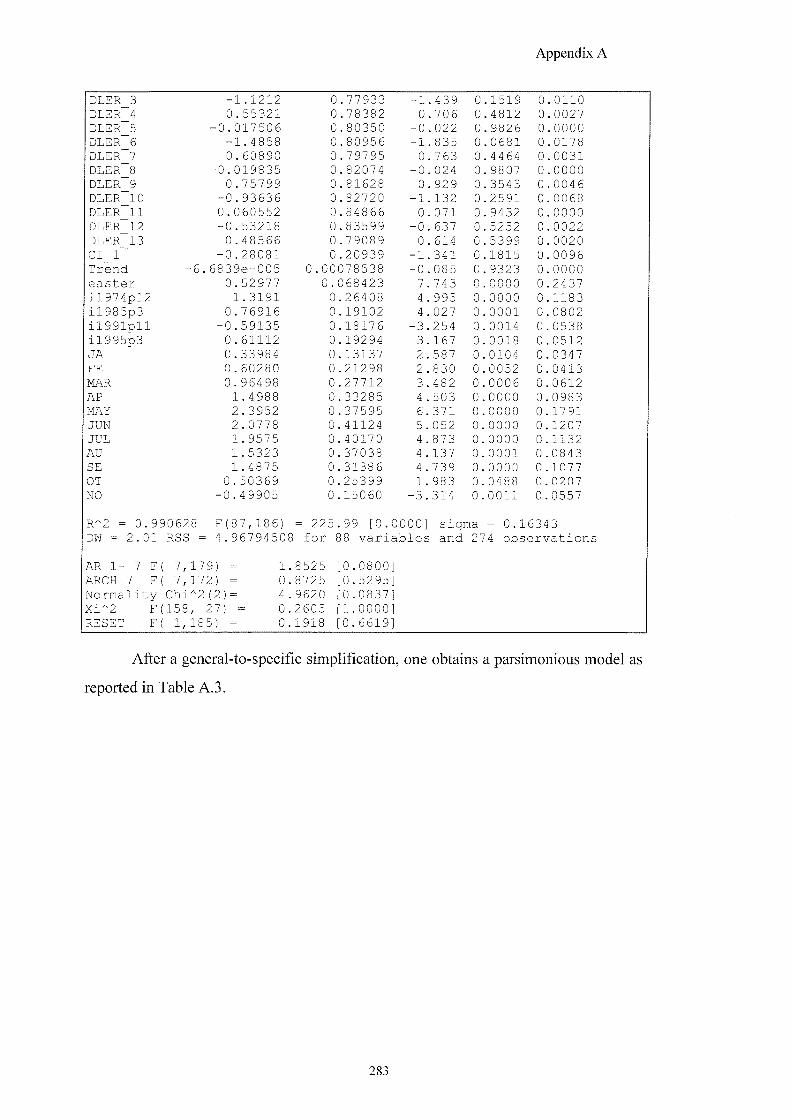
Appendix A

DLER 3 -1.1212 0 .77933 -1 439 0 .1519 0 .0110 DLER 4 0.55321 0 .78382 0 706 0 .4812 0 .0027 DLER 5 -0.017506 0 .80350 -0 022 0 .9826 0 .0000 DLER 6 -1.4858 0 .80956 -1 835 0 .0681 0 .0178 DLER 7 0.60890 0 .79795 0 763 0 .4464 0 .0031 DLER 8 -0.019835 0 .82074 -0 024 0 .9807 0 .0000 DLER 9 0.75799 0 .81628 0 929 0 .3543 0 .0046 DLER 10 -0.93636 0 .82720 -1. 132 0 .2591 0 0068 DLER 11 0.060552 0 .84866 0. 071 0 9432 0 0000 DLER 12 -0.53218 0 .83599 -0 637 0 5252 0 0022 DLER 13 0.48566 0 .79089 0. 614 0 5399 0 0020 CI 1 -0.28081 0 .20939 -1. 341 0 1815 0 0096 Trend 6.6839e-005 0.00078538 -0. 085 0 9323 0 0000 easter 0.52977 0. 068423 7 . 743 0 0000 0 2437 il974pl2 1.3191 0 .26408 4 . 995 0 0000 0 1183 il985p3 0.76916 0 .19102 4 . 027 0 0001 0 0802 il991pll -0.59135 0 .18176 -3. 254 0 0014 0 0538 il995p3 0.61112 0 .19294 3. 167 0 0018 0 0512 JA 0.33984 0 .13137 2 . 587 0 0104 0 0347 FE 0.60280 0 .21298 2 . 830 0 0052 0 0413 MAR 0.96498 0 .27712 3. 482 0 0006 0 0612 AP 1.4988 0 .33285 4 . 503 0 0000 0 0983 MAY 2.3952 0 .37595 6. 371 0 0000 0 1791 JUN 2.0778 0 .41124 5. 052 0. 0000 0. 1207 JUL 1.9575 0 .40170 4 . 873 0. 0000 0. 1132 AU 1.5323 0 .37038 4 . 137 0 0001 0. 0843 SE 1.4875 0 .31386 4 . 739 0. 0000 0. 1077 OT 0.50369 0 .25399 1 . 983 0. 0488 0. 0207 NO -0.49905 0 .15060 -3. 314 0 0011 0. 0557

R^2 = 0.990628 F(87,186) = 225 .99 [0.0000] Sigma = 0.16343 DW = 2.01 RSS = 4.9679450! 3 for 38 variables and 274 observations

AR 1- 7 F( 7, 179) = 1 8525 [0.0800] ARCH 7 F( 7, 172) = 0 8725 [0.5295] Normality Chi "2(2)= 4 9620 [0.0837] Xi"2 F( 158 , 27) = 0 2605 [1.0000] RESET F( 1, 185) = 0 1918 [0.6619]

After a general-to-specific simplification, one obtains a parsimonious model as

reported in Table A.3.

283

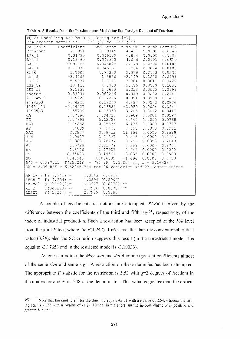
Appendix A

Table A. 3 Results from the Parsimonious Model for the Foreign Demand of Tourism

EQ(2) Modelling LAR by OLS (using For.in7) The present sample is: 1973 (3) to 1995 (12)

Variable Coefficient Std .Error t-value t -prob PartR'^2 Constant 2.6891 0 .60149 4 471 0 0000 0 0746 LAR 1 0.31795 0. 046389 6 .854 0 0000 0 1593 LAR 2 0.18469 0 . 045643 4 046 0 0001 0 .0619 LAR 9 -0.099788 0. 045825 -2 178 0 0304 0 0188 LAR 11 0.15070 0 . 046565 3 .236 0 0014 0 0405 RLPR 1.8605 0 .78308 2 376 0 0183 0 0223 LSP 8 -3.4268 1.5586 -2 199 0 0288 0 0191 LSP 9 5.9937 1.8141 3 304 0 0011 0 0422 LSP 12 -10.118 1.8409 -5 4 96 0 0000 0 1086 LSP_13 8.1853 1.5670 5 223 0 0000 0 0991 easter 0.53934 0. 060266 8 949 0 0000 0 2441 il974pl2 1.5228 0 .17205 8 851 0 0000 0 2401 il985p3 0.84225 0 .17260 4 880 0 0000 0 0876 il991pll -0.49827 0 .16838 -2 959 0 0034 0 0341 il995p3 0.55709 0 .16959 3 285 0 0012 0 0417 JA 0.37596 0. 094733 3 969 0 0001 0 0597 FE 0.57799 0 .12728 4 541 0 0000 0 0768 MAR 0.94282 0 .15373 6 133 0 0000 0 1317 AP 1.4639 0 .19123 7 655 0 0000 0. 1911 MAY 2.2977 0 .19712 11. 656 0 0000 0. 3539 JUN 2.0427 0 .21327 9. 578 0 0000 0. 2700 JUL 1.9601 0 .20737 9 452 0 0000 0. 2648 AU 1.5729 0 .21579 7 289 0 0000 0 1764 SE 1.5116 0 .17907 8. 441 0 0000 0. 2232 OT 0.55079 0 .14361 3. 835 0 0002 0 0560 NO -0.43545 0. 096889 -4 494 0 0000 0. 0753 R'"2 = 0.98 7511 F(25,248) = 784 .39 [0.0000] sigma = 0.163387 DW = 2.09 RSS = 6.6204678 44 for 26 variables and 274 observations

AR 1- 7 F( 7 ,241) = 1 .0143 [0.4217] ARCH 7 F( 7,234) = 1 . 0594 [0.3906] Normality Chi''2(2)= 9 . 9227 [0.0070] * *

Xi''2 F( 34 ,213) = 1 .7956 [0.0070] * *

RESET F( 1 ,247) = 2 .7585 [0.0980]

A couple of coefficients restrictions are attempted. RLPR is given by the

difference between the coefficients of the third and fifth lag'O?^ respectively, of the

index of industrial production. Such a restriction has been accepted at the 5% level

from the joint F-test, where the F( 1,247)= 1.66 is smaller than the conventional critical

value (3.84); also the SC criterion suggests this result (in the unrestricted model it is

equal to -3.17653 and in the restricted model is -3.19033).

As one can notice the May, Jun and Jul dummies present coefficients almost

of the same size and same sign. A restriction on these dummies has been attempted.

The appropriate F statistic for the restriction is 5.53 with ^ =2 degrees of freedom in

the numerator and N-K=2A^ in the denominator. This value is greater than the critical

'0^ Note that the coefficient for the third lag equals +2.01 with a f-value of 2.54, whereas the fifth lag equals -1.77 with a f-value of -1.87. Hence, in the short run the income elasticity is positive and greater than one.

284

Appendix A

value of the F distribution at a 5% level, thus failing to accept the null hypothesis the

restriction does not hold. Hence, the model reported in Table A.3 has been kept.

The results from Table A. 3 are quite different to the ones obtained using LA

{i.e. the adjusted series for the foreign arrivals) as the dependent variable (see Table

4.7). In terms of diagnostic statistics, the model where the unadjusted series of arrivals

of tourists are considered (Table A.3) presents problems of non-normality and

heteroscedasticity at the 1% level. However, the value of the R2 denotes a good fit.

Moreover, as the relevant F-statistic indicates, the overall significance of the

regression is satisfactory.

In terms of significance of parameter coefficients, the cointegrating vector does

not influence the foreign demand of tourism, as well as the first difference of the

relative price (DLRP) and of the weighted exchange rate (DLER). The lags of foreign

arrivals, as explanatoiy variables, present an average positive sign. The statistical

significance of the first, second, ninth and eleventh lag of the dependent variable

confirms that adjustment is not rapid. The income proxy enters the final equation with

its difference (RLPR) which has a positive sign. The substitute price shows a negative

elasticity in the short run and a positive elasticity in the long run (see Table A.4),

which is in conflict with economic theory.

As assumed from the analysis of the unrestricted model, the "Easter" dummy

{EASTER) has a particular importance in explaining the pattern of international

tourism. Such a variable has been constructed giving the value one in the Easter month

and zero o t h e r w i s e . The time trend does not have any particular power in explaining

the demand for tourism.

The long run dynamics are reported in Table A.4. The long run multipliers and

the standard errors are, in general, well-specified. The long run responses of the

foreign demand for tourism to changes in the expanatory variables are also statistically

significant.

One can conclude that this model presents mis-specification in the residuals

with heteroscedasticity and non-normality problems.

108 For a more detailed description of the construction of the Easter dummy see Chapter 3.

285

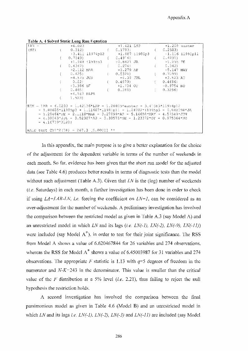
Append ix A

Table A. 4 Solved Static Long Run Equation LAR = + ^ 2 3 + 1 . 4 2 1 LSP + 1 . 2 0 8 e a s t e r (SE) ( 0 . 3 1 2 ) ( 0 . 1 7 9 3 ) ( 0 . 2 5 8 3 )

+ 3 . 4 1 1 i l 9 7 4 p l 2 + 1 . 8 8 7 i l 9 8 5 p 3 < U 1 1 6 i l 9 9 1 p l l ( 0 . 7 2 4 9 ) ( 0 . 4 9 1 6 ) ( 0 . 4 2 9 1 )

+ 1 . 2 4 8 i l 9 9 5 p 3 + 0 . 8 4 2 1 JA + 1 . 2 9 5 FE ( 0 . 4 3 4 7 ) ( 0 ^ 7 4 ) ( 0 . 3 4 2 )

+ 2 . 1 1 2 MAR + 3 ^ n 9 AP + 5 . 1 4 7 MAY { 0 . 4 2 5 ) ( 0 . 5 3 2 6 ) ( 0 . 7 0 9 9 )

+ ^ 7 5 JUN + ^ 9 JUL + 3 . 5 2 3 AU ( 0 . 5 2 ) ( 0 . 4 8 7 9 ) ( 0 . 4 6 9 6 )

+ ^ 8 6 SE + 1 ^ 3 4 OT - 0 . 9 7 5 4 NO ( 0 . 4 6 5 ) ( 0 ^ 8 ^ l ( 0 . 3 2 9 6 )

+ 4 . 1 6 7 RLPR ( 1 . 9 2 3 )

ECM = LAR - 6. 0 2 3 3 - 1 . 4 2 1 3 6 * L S P - 1 . 2 0 8 0 5 * e a s t e r - 3 . 4 1 0 8 3 * i l 9 7 4 p l 2 — 1 . 8 8 6 5 5 * i l 9 8 5 p 3 + 1 . 1 1 6 0 7 * i l 9 9 1 p l l - 1 . 2 4 7 8 2 * i l 9 9 5 p 3 - 0 . 8 4 2 0 9 8 + J A - 1. 2 9 4 6 4 *FE - 2 . 1 1 1 8 *MAR - 3 . 2 7 8 9 9 * A P - 5 .14658*MAY - 4 . 5 7 5 4 9 * JUN - 4. 3 9 0 4 3 *JUL - 3 . 5 2 3 0 7 * A U - 3 . 3 8 5 7 5 * S E - 1 . 2 3 3 7 2 * 0 T + 0 . 9 7 5 3 6 4 *N0 - 4. 1 6 7 3 9 *RLPR;

WALD t e s t C h i ^ 2 ( 1 8 = 2 6 7 . 3 [ 0 . 0 0 0 0 ] * *

In this appendix, the main purpose is to give a better explanation for the choice

of the adjustment for the dependent variable in terms of the number of weekends in

each month. So far, evidence has been given that the short run model for the adjusted

data (see Table 4.6) produces better results in terms of diagnostic tests than the model

without such adjustment (Table A.3). Given that LN is the (log) number of weekends

{i.e. Saturdays) in each month, a further investigation has been done in order to check

if using LA=LAR-LN, i.e. forcing the coefficient on LN=I, can be considered as an

over-adjustment for the number of weekends. A preliminary investigation has involved

the comparison between the restricted model as given in Table A. 3 (say Model A) and

an unrestricted model in which LN and its lags (i.e. LN(-l), LN(-2), LN(-9), LN(-ll))

were included (say Model A^), in order to test for their joint significance. The RSS

from Model A shows a value of 6.620467844 for 26 variables and 274 observations,

whereas the RSS for Model A* shows a value of 6.45003987 for 31 variables and 274

observations. The appropriate F statistic is 1.13 with q=5 degrees of freedom in the

numerator and N-K=2A3 in the denominator. This value is smaller than the critical

value of the F distribution at a 5% level {i.e. 2.21), thus failing to reject the null

hypothesis the restriction holds.

A second investigation has involved the comparison between the final

parsimonious model as given in Table 4.6 (Model B) and an unrestricted model in

which Z#aiid its lags ;.e. and are included (say Model

286

Appendix A

B*), in order to test for their joint significance. The RSS from Model B is

9.639300629 for 25 variables and 274 observations, whereas the RSS from the

unrestricted model (Model B*) is 7.300511685 for 30 variables and 274 observations.

The joint significance of the (log) number of weekends is tested by performing an F-

test. The value of the F statistic equals 15.62 with q=5 degrees of freedom in the

numerator and # - ^ = 2 4 4 in the denominator, thus the restricted model cannot be

accepted at the 5% level.

Hence, the main conclusion from this analysis is that there is no statistical

evidence for the adjustment for the number of weekends. In fact, from the previous

analysis one infers that Model A", where the (log) number of weekends are included,

does not reject Model A; the opposite conclusion is reached from the comparison

between Model B and Model B'^, where the (log) number of weekends are included.

However, one chooses Model B in which the adjustment for the number of weekends

has been involved. Firstly, Model B can be considered better than Model A in that it

does not present signs of non-normality as well as heteroscedasticity (at least at the 1%

level). On the other hand, Model B* is difficult to interpret. Therefore, Model B, as

reported in Tables 4.6 and 4.7 with the White correction for heteroscedasticity at the

5% level, has been chosen. It is important to assess that it might be possible to obtain a

better model specification by running a model in which the motivation for tourism is

taken into account. It might be the case that a distinction between the number of

"business holiday trips" and "holiday trips" could determine better results in terms of

both statistical and economic performance. However, as already pointed out in Chapter

3, such a distinction is not available from the official statistics as far as the period

under study is concerned.

287

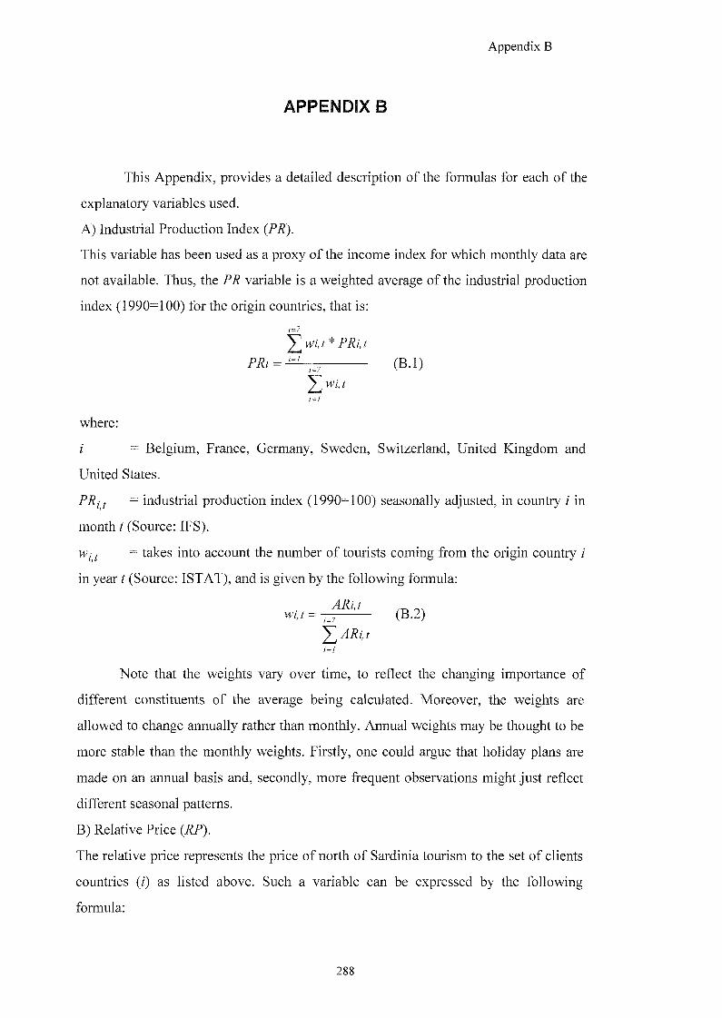
Appendix B

APPENDIX B

This Appendix, provides a detailed description of the formulas for each of the

explanatory variables used.

A) Industrial Production Index (PR).

This variable has been used as a proxy of the income index for which monthly data are

not available. Thus, the PR variable is a weighted average of the industrial production

index (1990=100) for the origin countries, that is:

i=7

^ Wi. t * PRi, I

PRt = ^ , (B.l)

/ = /

where:

i = Belgium, France, Germany, Sweden, Switzerland, United Kingdom and

United States.

PRi t = industrial production index (1990=100) seasonally adjusted, in country / in

month t (Source: IPS).

= takes into account the number of tourists coming from the origin country i

in year (Source: ISTAT), and is given by the following formula:

(B.2)

i=J

Note that the weights vary over time, to reflect the changing importance of

different constituents of the average being calculated. Moreover, the weights are

allowed to change annually rather than monthly. Annual weights may be thought to be

more stable than the monthly weights. Firstly, one could argue that holiday plans are

made on an annual basis and, secondly, more frequent observations might just reflect

different seasonal patterns.

B) Relative Price (RP).

The relative price represents the price of north of Sardinia tourism to the set of clients

countries (/) as listed above. Such a variable can be expressed by the following

formula:

288

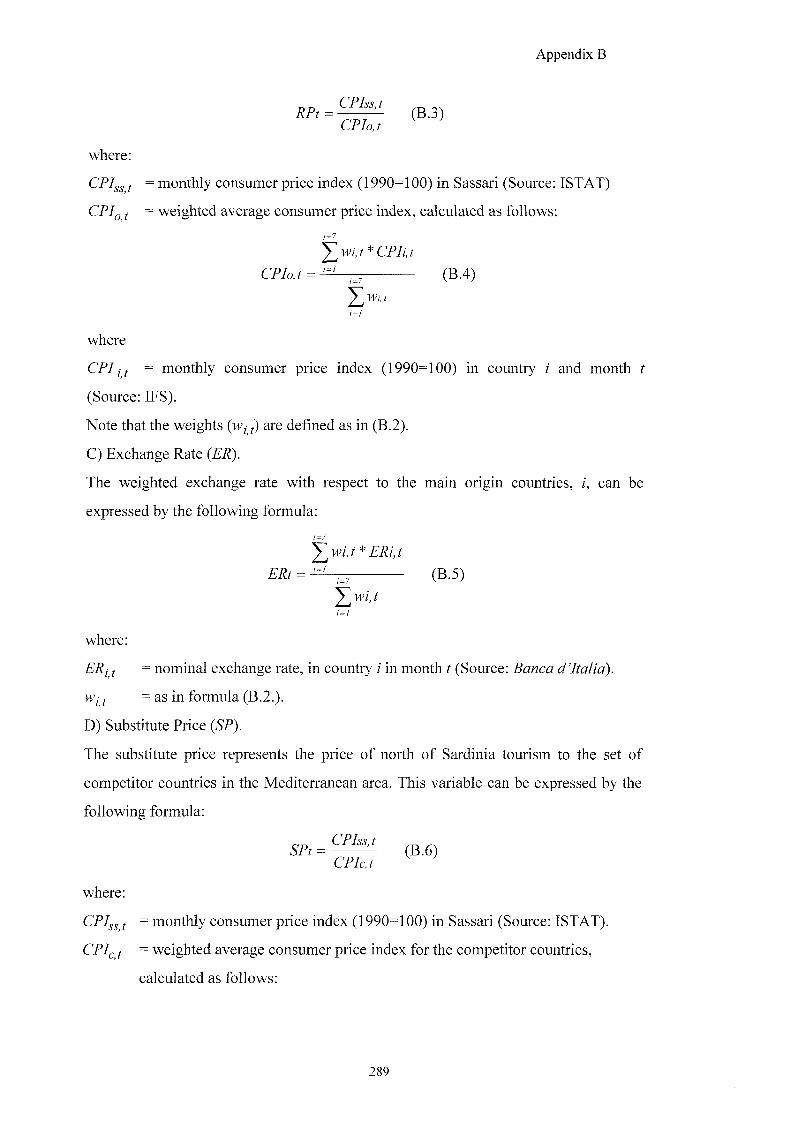
Appendix B

where:

CPI^^ I = monthly consumer price index (1990=100) in Sassari (Source: ISTAT)

CPIq ^ = weighted average consumer price index, calculated as follows:

/=7

Z '

CFh.i = -1=^3 (B.4) V '

1=1

where

CPII J = monthly consumer price index (1990=100) in country / and month t

(Source: IPS).

Note that the weights (wy ) are defined as in (B.2).

C) Exchange Rate {ER).

The weighted exchange rate with respect to the main origin countries, i, can be

expressed by the following formula: 1=7

^ wi, t * ERi, t

2 2 , = ^ ^ - - ; 03 .5 )

i=i

where:

ERj i = nominal exchange rate, in country i in month t (Source: Banca d'ltalia).

=asinfbmmla(B.2.).

D) Substitute Price (5?).

The substitute price represents the price of north of Sardinia tourism to the set of

competitor countries in the Mediterranean area. This variable can be expressed by the

following formula:

5"? / = (B.6)

C f / c x

where:

CPIss,t ^ monthly consumer price index (1990=100) in Sassari (Source: ISTAT).

CPI^J = weighted average consumer price index for the competitor countries,

calculated as follows:

289

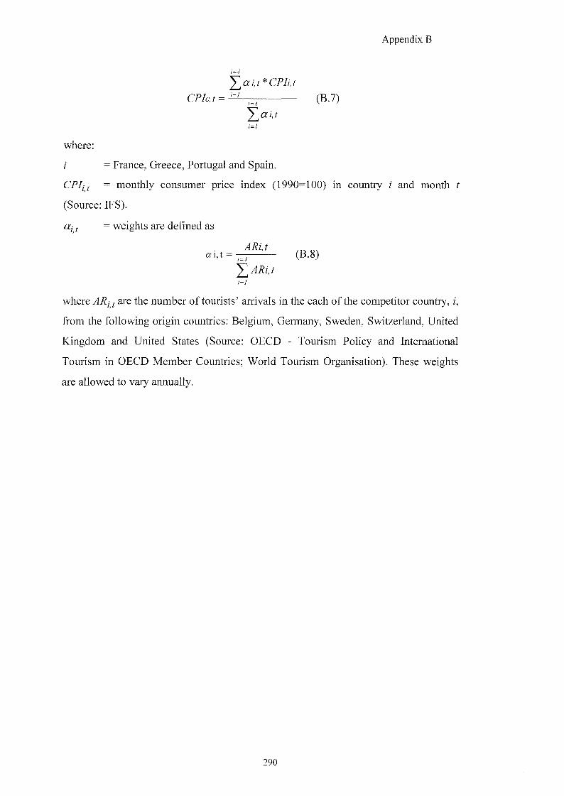
Appendix B

11=4

= OBJ)

2_âi,t

i=i

where:

i = France, Greece, Portugal and Spain.

CPIif = monthly consumer price index (1990=100) in country i and month t

(Source: IPS). ai f = weights are defined as

(B.8)

i=i

where ARi f are the number of tourists' arrivals in the each of the competitor country, z,

from the following origin countries: Belgium, Germany, Sweden, Switzerland, United

Kingdom and United States (Source: OECD - Tourism Policy and International

Tourism in OECD Member Countries; World Tourism Organisation). These weights

are allowed to vary annually.

290

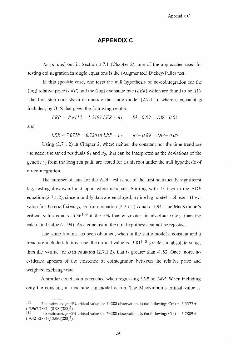
Appendix C

APPENDIX C

As pointed out in Section 2.7.1 (Chapter 2), one of the approaches used for

testing cointegration in single equations is the (Augmented) Dickey-Fuller test.

In this specific case, one tests the null hypothesis of no-cointegration for the

(log) relative price {LRP) and the (log) exchange rate {LER) which are found to be 1(1).

The first step consists in estimating the static model (2.7.1.1), where a constant is

included, by OLS that gives the following results:

and

I E ; ; = 7.077,^ + 0.720^g + 62 0. D;F= 0.0 j

Using (2.7.1.2) in Chapter 2, where neither the constant nor the time trend are

included, the saved residuals u j and that can be interpreted as the deviations of the

generic yf from the long run path, are tested for a unit root under the null hypothesis of

no-cointegration.

The number of lags for the ADF test is set to the first statistically significant

lag, testing downward and upon white residuals. Starting with 13 lags in the ADF

equation (2.7.1.2), since monthly data are employed, a nine lag model is chosen. The t-

value for the coefficient p, as from equation (2.7.1.2) equals -1.94. The MacKinnon's

critical value equals -3.36'09at the 5% that is greater, in absolute value, than the

calculated value (-1.94). As a conclusion the null hypothesis cannot be rejected.

The same finding has been obtained, when in the static model a constant and a

trend are included. In this case, the critical value is - 3 . 8 1 g r e a t e r , in absolute value,

than the r-value for p in equation (2.7.1.2), that is greater than -1.63. Once more, no

evidence appears of the existence of cointegration between the relative price and

weighted exchange rate.

A similar conclusion is reached when regressing LER on LRP. When including

only the constant, a final nine lag model is run. The MacKinnon's critical value is

The estimatedp =5% critical value for 7^=288 observations is the following: C(p) = -3.3377 (-5.967/288) - (8.98/(288)2). " 0 The estimatedp =5% critical value for 7=288 observations is the following; C(p) = -3.7809 -(-9.42 l/288)-(l 5.06/(288)2).

291

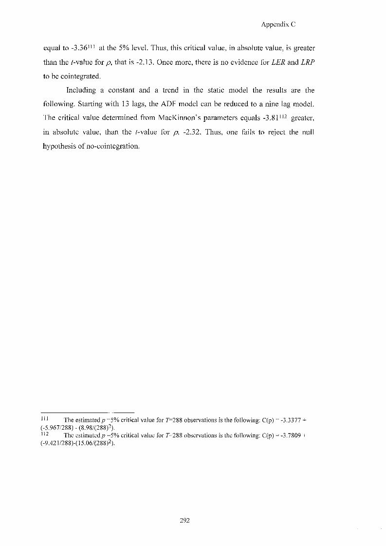
Appendix C

equal to -3.36"i at the 5% level. Thus, this critical value, in absolute value, is greater

than the /-value for p, that is -2.13. Once more, there is no evidence for LER and LRP

to be cointegrated.

Including a constant and a trend in the static model the results are the

following. Starting with 13 lags, the ADF model can be reduced to a nine lag model.

The critical value determined from MacKinnon's parameters equals -3.81 greater,

in absolute value, than the /-value for p, -2.32. Thus, one fails to reject the null

hypothesis of no-cointegration.

' ' ' The estimatedp =5% critical value for 7=288 observations is the following: C(p) = -3.3377 + (-5.967/288) - (8.98/(288)2).

The estimatedp =5% critical value for 7-288 observations is the following: C(p) = -3.7809 + (-9.421/288)-(15.06/(288)2).

292

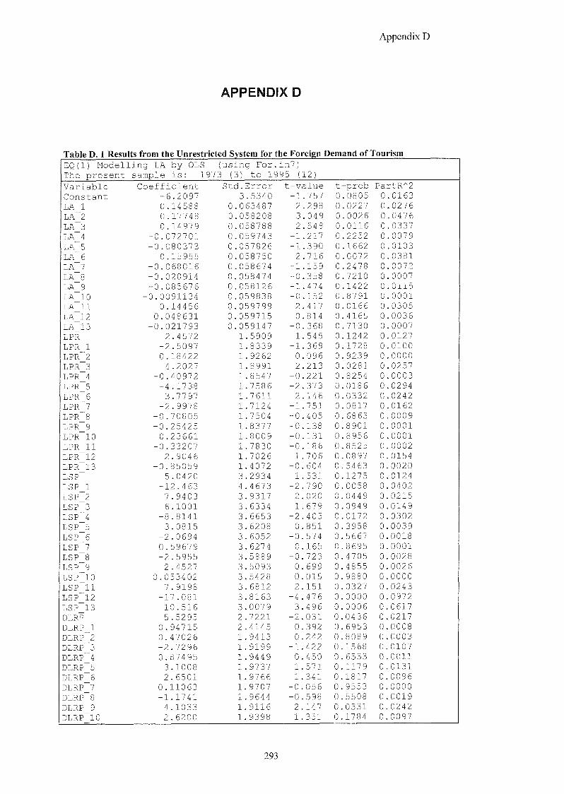
Appendix D

APPENDIX D

EQ(1) Modelling LA by OLS (using For.in?) The present sample is: 1913 (3) to 1995 (12)

Variable Coefficient Std. Error t-value t -prob PartR^2 Constant -6.209? 3 .5340 -1 .757 0 .0805 0 .0163

LA 1 0.14588 0 .063487 2 .298 0 .0227 0 .0276

LA 2 0.17?48 0 .058208 3 .049 0 .0026 0 .0476

LA 3 0.14979 0 .058788 2 .548 0 .0116 0 .033?

LA 4 -0.072701 0 .059743 -1 .21? 0 .2252 0 .0079

LA 5 -0.080373 0 .057826 -1 .390 0 .1662 0 .0103

LA 6 0.15955 0 .058750 2 .716 0 .0072 0 .0381

LA ? -0.068016 0 .058674 -1 .159 0 .2478 0 .0072

LA 8 -0.020914 0 058474 -0 .358 0 .7210 0 000?

LA 9 -0.085676 0 .058126 -1 .474 0 .1422 0 .0115

LA 10 -0.0091134 0 059838 -0 .152 0 .8791 0 0001

LA 11 0.14456 0 059799 2 417 0 0166 0 0305

LA 12 0.048631 0 059715 0 814 0 4165 0 0036

LA 13 -0.021793 0 059147 -0 368 0 .7130 0 000?

LPR 2.4572 1 .5909 1 545 0 1242 0 0127

LPR 1 -2.509? 1 .8339 -1 369 0 1728 0 0100

LPR 2 0.18422 1 .9262 0 096 0 9239 0 0000

LPR 3 4.2027 1 .8991 2 213 0 0281 0 025?

LPR 4 -0.40972 1 .8547 -0 221 0 8254 0 0003

LPR 5 -4.1738 1 .7586 -2 373 0 0186 0 0294

LPR 6 3.7797 1 .7611 2 146 0 0332 0 0242

LPR 7 -2.9978 1 .7124 -1 751 0 081? 0 0162

LPR 8 -0.70805 1 .7504 -0 405 0 6863 0 0009

LPR 9 -0.25425 1 .8377 -0 138 0 8901 0 0001

LPR 10 -0.23661 1 .8009 -0 131 0 8956 0 0001

LPR 11 -0.33207 1 .7830 -0 186 0 8525 0 0002

LPR 12 2.9046 1 .7026 1 706 0 089? 0 0154

LPR 13 -0.85059 1 .4072 -0 604 0 5463 0 0020

LSP 5.0420 3 .2934 1 531 0 1275 0 0124 LSP 1 -12.463 4 .4673 -2 790 0 0058 0 0402

LSP 2 7.9403 3 .9317 2 020 0 0449 0 0215

LSP 3 6.1001 3 .6334 1 679 0 0949 0 0149

LSP 4 -8.8141 3 .6653 -2 405 0 0172 0 0302

LSP 5 3.0815 3 .6208 0 851 0 3958 0 0039

LSP 6 -2.0694 3 .6052 -0 574 0 566? 0 0018

LSP ? 0.59679 3 .6274 0 165 0 8695 0 0001

LSP 8 -2.5955 3 .5889 -0 723 0 4705 0 0028

LSP 9 2.4527 3 .5093 0 699 0 4855 0 0026

LSP 10 0.053402 3 .5428 0 015 0 9880 0 0000

LSP 11 7.9198 3 .6812 2 151 0 0327 0 0243

LSP 12 -17.081 3 .8163 -4 476 0 0000 0 0972 LSP 13 10.516 3 .0079 3 496 0 0006 0 0617

DLRP -5.5295 2 .7221 -2. 031 0 0436 0. 021?

DLRP 1 0.94715 2 .4145 0 392 0 6953 0 0008

DLRP 2 0.47026 1 .9413 0. 242 0 8089 0 0003

DLRP 3 -2.7296 1 .9199 -1 422 0 1568 0. 010?

DLRP 4 0.87495 1 .9449 0 450 0 6533 0 0011 DLRP 5 3.1008 1 .973? 1 571 0 1179 0 0131

DLRP 6 2.6501 1 .9766 1 341 0 1817 0. 0096

DLRP ? -0.11063 1 9707 -0. 056 0. 9553 0. 0000

DLRP 8 -1.1741 1 .9644 -0. 598 0 5508 0 0019

DLRP 9 4.1033 1 9116 2 14? 0. 0331 0. 0242

DLRP 10 2.6200 1 9398 1. 351 0. 1784 0. 0097

293

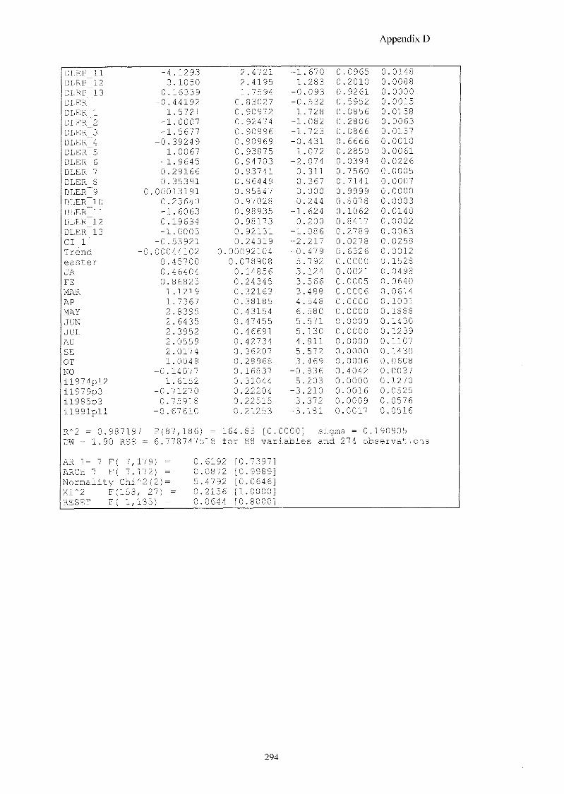
Appendix D

DLRP 11 -4.1293 2 .4721 -1 .670 0 0965 0 0148

DLRP 12 3.1050 2 .4195 1 .283 0 2010 0 .0088

DLRP 13 -0.16339 1 .7594 -0 .093 0 9261 0 .0000

DLER -0.44192 0. 83027 -0 532 0 5952 0 0015

DLER 1 1.5721 0. 90972 1 728 0 0856 0 .0158

DLER 2 -1.0007 0. 92474 -1 082 0 2806 0 0063

DLER 3 -1.5677 0. 90996 -1 723 0 0866 0 0157

DLER 4 -0.39249 0. 90969 -0 431 0 6666 0 0010

DLER 5 1.0067 0. 93875 1 072 0 2850 0 0061

DLER 6 -1.9645 0 . 94703 -2 074 0 0394 0 0226 DLER 7 0.29166 0. 93741 0 311 0 7560 0 0005 DLER 8 0.35391 0 . 96449 0 367 0 7141 0 0007

DLER 9 0 .00013191 0. 95847 0 000 0 9999 0 0000

DLER 10 0.23640 0. 97028 0 244 0 8078 0 0003

DLER 11 -1.6063 0. 98935 -1 624 0 1062 0 0140 DLER 12 0.19634 0. 98173 0 200 0 8417 0 0002 DLER 13 -1.0005 0. 92131 -1 086 0 2789 0 0063

CI_1 -0.53921 0. 24319 -2 217 0 0278 0 0258 Trend -0 .00044102 0. 00092104 -0 479 0 6326 0 0012 easter 0.45700 0.078908 5 792 0 0000 0 1528

JA 0.46404 0. 14856 3 124 0 0021 0 0498

FE 0.86825 0. 24345 3 566 0 0005 0 0640 MAR 1.1219 0 . 32163 3 488 0 0006 0 0614 AP 1.7367 0. 38185 4 548 0 0000 0 1001 MAY 2.8395 0. 43154 6 580 0 0000 0 1888 JUN 2.6435 0. 47455 5 571 0 0000 0 1430 JUL 2.3952 0. 46691 5 130 0 0000 0 1239

AU 2.0559 0. 42734 4 811 0 0000 0 1107 SE 2.0174 0 . 36207 5 572 0 0000 0 1430 OT 1.0048 0. 28968 3 469 0 0006 0 0608 NO -0.14077 0. 16837 -0. 836 0 4042 0 0037 il974pl2 1.6152 0. 31044 5 203 0 0000 0 1270 il979p3 -0.71270 0. 22204 -3. 210 0 0016 0 0525 il985p3 0.75918 0. 22515 3. 372 0 0009 0 0576 iiggipii -0.67610 0. 21253 -3. 181 0 0017 0 0516

R^2 = 0.98 7197 F(87,186) = 164. 85 [0. 0000] sigma = 0. 190905 DW = 1.90 RSS = 6.778747518 for 88 variables and 274 observations

AR 1- 7 F( 7, 179) = 0. 6192 [0 .7397] ARCH 7 F( 7, 172) = 0. 0872 [0 .9989] Normality Chi '"2 ) = 5. 4792 [0 .0646] Xi*2 F(158 , 27) = 0. 2156 [1 .0000] RESET F( 1, 185) = 0. 0644 [0 .8000]

294

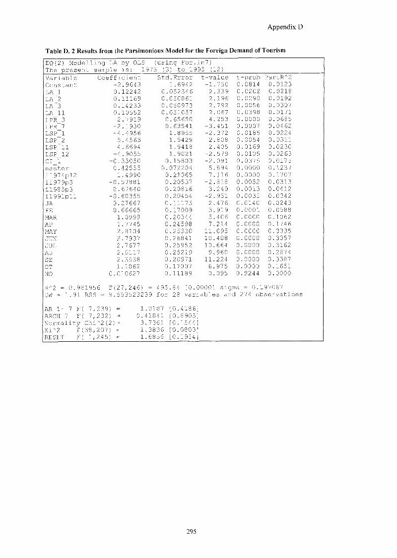
Appendix D

Table D. 2 Results from the Parsimonious Model for the Foreign Demand of Tourism

EQ(2) Modelling LA by OLS (using For.in?) The present sample is: 19?3 (3) to 1995 ( 12)

Variable Coefficient Stc .Error t-value t -prob PartR*2 Constant -2.9643 1.6942 -1 .750 0 0814 0 0123

LA 1 0.12242 0 . 052346 2 .339 0 0202 0 0218

LA 2 0.11169 0. 050861 2 .196 0 0290 0 0192

LA 3 0.14233 0 . 050973 2 .792 0 0056 0 0307

LA 11 0.10552 0. 051057 2 .067 0 0398 0 0171 LPR 3 2.7919 0 .65650 4 .253 0 0000 0 0685 LPR ? -2.1930 0 .63541 -3 .451 0 0007 0 0462 LSP 1 -4.4956 1.8955 -2 .372 0 0185 0 0224 LSP 2 5.4563 1.9429 2 .808 0 0054 0 0311 LSP 11 4.6694 1.9418 2 .405 0 0169 0 0230 LSP 12 -4.9055 1.9021 -2 .579 0 0105 0 0263 CI_1 - 0.33050 0 .15803 -2 .091 0 0375 0 0175 easter 0.42555 0. 072204 5 .894 0 0000 0 1237 il9?4pl2 1.4990 0 .21065 7 .116 0 0000 0 1707 il9?9p3 - 0.57881 0 .20537 -2 .818 0 0052 0 0313 il985p3 0.67640 0 .20816 3 .249 0 0013 0 0412 il991pll - 0.60355 0 .20454 -2 .951 0 0035 0 0342 JA 0.27667 0 .11173 2 .476 0 0140 0 0243 FE 0.66665 0 .17009 3 .919 0 0001 0 0588

MAR 1.0998 0 .20344 5 .406 0 0000 0 1062 AP 1.7745 0 .24598 7 .214 0 0000 0 1746

MAY 2.8104 0 .25330 11 .095 0 0000 0 3335 JUN 2.7937 0 .26841 10 .408 0 0000 0 3057

JUL 2.7677 0 .25952 10 .664 0 0000 0 3162 AU 2.5117 0 .25219 9 .960 0 0000 0 2874 SE 2.3538 0 .20971 11 .224 0 0000 0 3387 OT 1.1862 0 .17007 6 .975 0 0000 0. 1651 NO 0 .010627 0 .11189 0 .095 0 9244 0 0000

R*2 = 0.981956 F (27,246) 495 .84 [0.0000 Sigma = 0.197067 DM = 1.91 RSS = 9 .553523239 for 28 variables and 274 observations

AR 1- ? F( 7, 239) 1 .0187 [0.4186] ARCH 7 F( 7, 232) 0. 418 41 [0.8903] Normality Chi 2(2 ) = 3 . 73 61 [0.1544] Xi*2 F( 38, 207) 1 .3836 [0.0803] RESET F( 1, 245) 1 .6856 [0.1954]

295

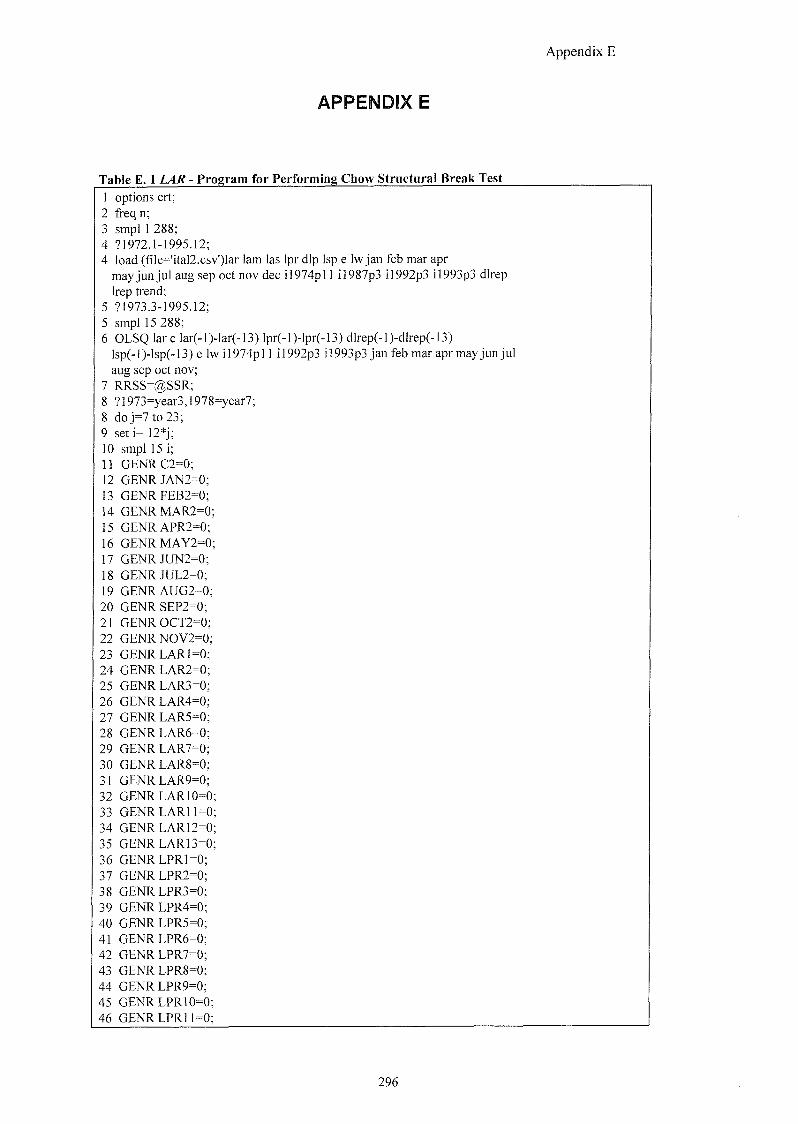
Appendix E

APPENDIX E

Table E. 1 LAR - Program for Performing Chow Structural Break Test

1 options crt; 2 freqn; 3 smpl 1 288; 4 71972.1-1995.12; 4 load (file='ital2.csv')lar lam las Ipr dip Isp e Iw jan feb mar apr

may jun jul aug sep oct nov dec il974pl 1 il987p3 il992p3 il993p3 direp Irep trend;

5 71973.3-1995.12; 5 smpl 15 288; 6 OLSQ lar c lar(-l)-lar(-13) lpr(-l)-lpr(-13) dlrep(-l)-dlrep(-13)

lsp(-l)-lsp(-13) e Iw i l974pl 1 il992p3 il993p3 jan feb mar apr may jun jul aug sep oct nov;

7 RRSS=@SSR; 8 ?1973=year3,1978=year7; 8 do j=7 to 23; 9 set i= 12*j; 10 smpl 15 i; 11 GENRC2=0; 12 GENRJAN2=0; 13 GENRFEB2=0; 14 GENRMAR2=0; 15 GENRAPR2=0; 16 GENRMAY2=0; 17 GENRJUN2=0; 18 GENRJUL2=0; 19 GENRAUG2=0; 20 GENRSEP2=0; 21 GENROCT2-0; 22 GENRNOV2=0; 23 GENRLARMO; 24 GENRLAR2=0 25 GENRLAR3=0 26 GENRLAR4=0 27 GENRLARS=0 28 GENRLAR6=0 29 GENRLAR7=0 30 GENRLAR8=0 31 GENRLAR9=0 32 GENR LAR 10=0 33 GENR LARl 1=0 34 GENRLAR12=0 35 GENRLAR13=0 36 GENRLPR1=0 37 GENRLPR2=0 38 GENRLPR3=0 39 GENRLPR4=0 40 GENRLPR5=0; 41 GENRLPR6=0; 42 GE}4RLPR7=0; 43 GENRLPR8=0; 44 GE}4RLPR9=0; 45 GENRLPR10=0; 46 GENR LPR 11=0;

296

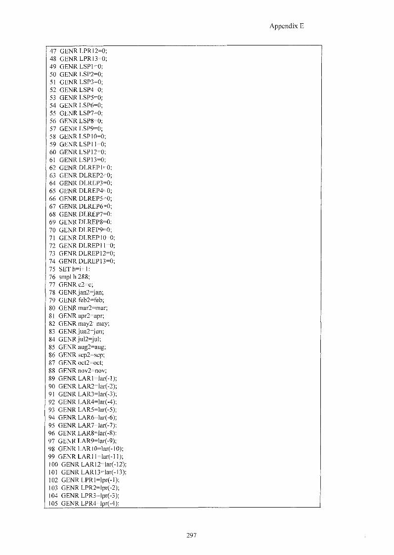
Appendix E

47 GENRLPR12=0; 48 GENR LPRl 3=0; 49 GENR LSP 1=0; 50 GENRLSP2=0; 51 GENRLSP3=0; 52 GENRLSP4=0; 53 GENRLSP5=0; 54 GENRLSP6=0; 55 GENRLSP7=0; 56 GENRLSP8=0; 57 GENRLSP9=0; 58 GENRLSP10=0; 59 GENR LSPl 1=0; 60 GENR LSP 12=0; 61 GENR LSP 13=0; 62 GENR DLREP 1=0 63 GENRDLREP2=0 64 GENRDLREP3=0 65 GENRDLREP4=0 66 GENRDLREP5=0 67 GENRDLREP6=0 68 GENRDLREP7=0 69 GENRDLREP8=0 70 GENRDLREP9=0 71 GENRDLREP10=0; 72 GENR DLREP 11=0; 73 GENRDLREP12=0; 74 GENRDLREP13=0; 75 SETh=i+l; 76 smpl h 288; 77 GENRc2=c; 78 GENRjan2=jan; 79 GENR&b2=feb; 80 GENR mar2=mar; 81 GENR apr2=apr; 82 GENR may2=may; 83 GENRjun2ûn; 84 GENRju]2=jul; 85 GENR aug2=aug; 86 GENR sep2=sep; 87 GENR oct2=oct; 88 GENR nov2=nov; 89 GENRLARl=lar(-l); 90 GENRLAR2=]ar(-2); 91 GENRLAR3=lar(-3); 92 GENRLAR4=]ar(-4); 93 GENRLAR5=lar(-5); 94 GENRLAR6=]ar(-6); 95 GENRLAR7=lar(-7); 96 GENRLAR8=lar(-8); 97 GENRLAR9=lar(-9); 98 GENRLAR10=lar(-10); 99 GENRLARll=]ar( -11); 100 GENRLAR12=lar(-12); 101 GENRLAR13=lar(-13); 102 GENR LPRl=]pr(-l); 103 GENRLPR2=lpr(-2); 104 GENRLPR3=lpr(. 3); 105 GENRLPR4=lpr(-4);

297

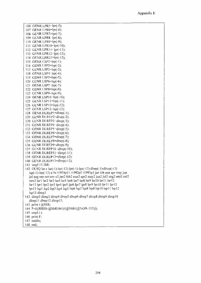
Appendix E

106 GENRLPR5=lpr(-5); 107 GENRLPR6Hpr(-6); 108 GENRLPR7=lpr(-7); 109 GENRLPR8=lpr(-8); 110 GENRLPR9=lpr(-9); 111 GENRLPR10=lpr(-10); 112 GENRLPRll=lpr(-ll); 113 GENRLPR12=lpr(-12); 114 GENRLPR13=lpr(-13); 115 GENRLSPl=lsp(-l); 116 GENRLSP2=lsp(-2); 117 GENRLSP3=lsp(-3); 118 GENRLSP4=]sp(-4); 119 GENRLSP5=]sp(-5); 120 GENRLSP6=lsp(-6); 121 GENRLSP7=lsp(-7); 122 GENRLSP8=lsp(-8); 123 GENRLSP9=lsp(-9); 124 GENRLSP10=lsp(-10); 125 GENRLSPl l - l sp( - l l ) ; 126 GENRLSP12=lsp(-12); 127 GENRLSP13=lsp(-13); 128 GENRDLREPl=dlrep(-l); 129 GENRDLREP2=dlrep(-2); 130 GENRDLREP3=dlrep(-3); 131 GENRDLREP4=dIrep(-4); 132 GENRDLREP5=d]rep(-5); 13 3 GENR DLREP6=dlrep(-6); 134 GENRDLREP7=dlrep(-7); 135 GENRDLREP8=dlrep(-8); 136 GENR DLREP9=dlrep(-9); 137 GE}) R DLREP10=dlrep(-10); 138 GENRDLREPll=dlrep(-ll); 139 GENRDLREP12=dlrep(-12); 140 GENRDLREP13=dlrep(-13); 141 s m p l l 5 288; 142 OLSQ lar c lar(-l)-lar(-13) lpr(-l)-lpr(-13) dlrep(-l)-dlrep(-13)

lsp(-l)-lsp(-13) e Iw il974pl 1 il992p3 il993p3 jan feb mar apr may jun jul aug sep oct nov c2 jan2 feb2 mar2 apr2 may2 jun2 jul2 aug2 sep2 oct2 nov2 larl lar2 lar3 lar4 larS lar6 lar? Iar8 lar9 larlO lar l l lar 12 lar 13 Iprl lpr2 Ipr3 lpr4 IprS lpr6 lpr7 lpr8 Ipr9 IprlO Iprll Iprl2 Iprl3 Isp] lsp2 lsp3 lsp4 lsp5 lsp6 lsp7 lsp8 lsp9 IsplO Ispl 1 Ispl2 Ispl3 dlrepl

142 dlrep2 dlrepS dlrep4 dlrepS dlrep6 dlrep? dlrepS dlrep9 dlreplO dlrepl 1 dlrep 12 dlrep 13;

143 print i @SSR; 144 F=(((RRSS-@SSR)/64)/(@SSR/(@N0B-133))); 145 smpl i i; 146 print F; 147 enddo; 148 end;

298

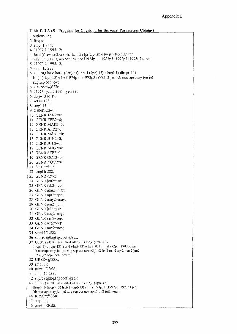
Appendix E

Table E. 2 LAR - Program for Checking for Seasonal Parameters Changes

1 options crt; 2 freq n; 3 smpl 1 288; 4 71972.1-1995.12; 4 load (file='ital2.csv')lar lam las Ipr dip Isp e Iwjan feb mar apr

may jun jul aug sep oct nov dec i l974p l l il987p3 il992p3 il993p3 dlrep; 5 71973.2-1995.12; 5 smpl 15 288; 6 70LSQ lar c lar(-l)-lar(-13) lpr(-l)-lpr(-13) dlrep(-l)-dlrep(-13)

lsp(-l)-lsp(-13) e Iw i l974pl l i]992p3 il993p3 jan feb mar apr may jun jul aug sep oct nov;

6 ?RRSS=@SSR; 6 ?1973=year2,1984=yearl3; 6 do j=13 to 19; 7 seti= 12*j; 8 smpl 15 i; 9 GE})RC2=0; 10 GENRJAN2=0; 11 GENRFEB2=0; 12 GENRMAR2=0; 13 GENRAPR2=0; 14 GENRMAY2=0; 15 GENRJUN2=0; 16 GENRJUL2=0; 17 GENRAUG2=0; 18 GENRSEP2=0; 19 GENROCT2=0; 20 GENRNOV2=0; 21 SETh=i+l; 22 smpl h 288; 23 GENRc2=c; 24 GENRjan2=jan; 25 GENRfeb2=feb; 26 GENR mar2=mar; 27 GENR apr2=apr; 28 GENR may2=may; 29 GENRjun2=jun; 30 GENRjul2=jul; 31 GENR aug2=aug; 32 GENRsep2=sep; 33 GENR oct2=oct; 34 GENR nov2=nov; 35 smpl 15 288; 36 supres@]ogl@coef@ses; 37 OLSQ (silent) lar c lar(-])-lar(-]3) lpr(-l)-lpr(-]3)

dlrep(-l)-dlrep(-13) lsp{-l)-lsp(-13) e Iw i l974pl I i l992p3 il993p3 jan feb mar apr may jun jul aug sep oct nov c2 jan2 feb2 mar2 apr2 may2 jun2 jul2 aug2 sep2 oct2 nov2;

38 URSS=@SSR; 39 smpl i i; 40 print i URSS; 41 smpl 15 288; 42 supres @log] @coef @ses; 43 OLSQ (silent) lar c lar(-l)-lar(-13) lpr(-l)-lpr(-13)

dlrep(-l)-dlrep(-13) lsp(-l)-lsp(-13) e Iw i l974pl I i l992p3 il993p3 jan feb mar apr may jun jul aug sep oct nov apr2 jun2 jul2 aug2;

44 RRSS=@SSR; 45 smpl i i; 46 print i RRSS;

299

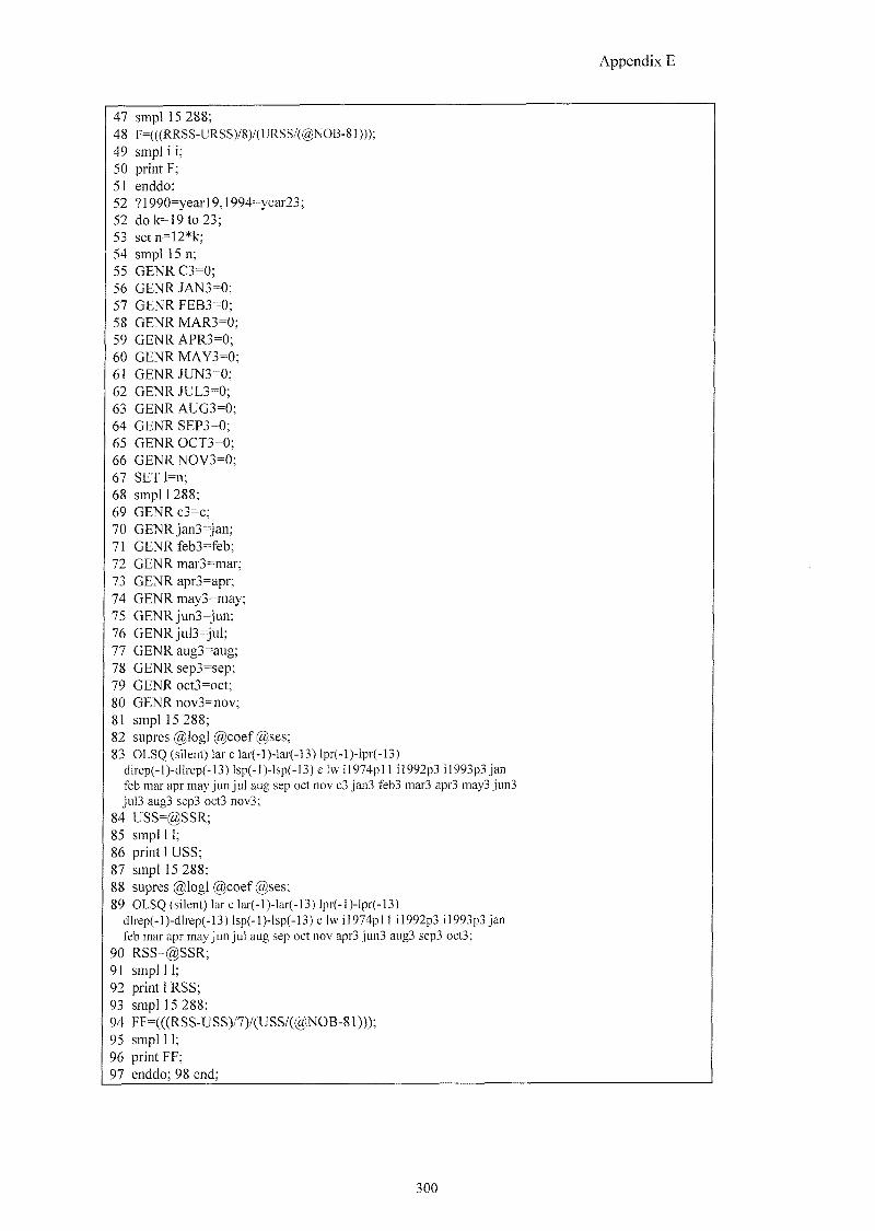
Appendix E

47 s m p n 5 288; 48 F=(((RRSS-URSS)/8)/(URSS/(@N0B-81))); 49 smpl i i; 50 print F; 51 enddo; 52 ?1990=yearl9,1994=year23; 52 do k=] 9 to 23; 53 setn=12*k; 54 smpl 15 n; 55 GENRC3=0; 56 GENRJAN3=0; 57 GENRFEB3=0; 58 GENRMAR3=0; 59 GENRAPR3=0; 60 GENRMAY3=0; 61 GENRJUN3=:0; 62 GE})RJUL3=0; 63 GENRAUG3=0; 64 GENRSEP3=0; 65 GENROCT3=0; 66 GENRl\fOV3=0; 67 SET t=n; 68 smpl 1 288; 69 GENRc3=c; 70 GENRjanSân; 71 GENRkb3=feb; 72 GENR mar3=mar; 73 GENR apr3=apr; 74 GENR may3=may; 75 GENRjun3=jun; 76 GENRju]3=jul; 77 GENR aug3=aug; 78 GENR sep3=sep; 79 GENR oct3=oct; 80 GENR nov3=nov; 81 smpl 15 288; 82 supres @logl @coef @ses; 83 OLSQ (silent) lar c lar(-l)-lar(-13) lpr(-l)-lpr(-13)

dlrep(-l)-dlrep(-13) lsp(-])-Isp(-13) e Iw i l974pl 1 il992p3 il993p3 jan feb mar apr may jun jul aug sep oct nov c3 jan3 feb3 mar3 apr3 may3 jun3 jul3 aug3 sep3 oct3 nov3;

84 USS=@SSR; 85 smpl 11; 86 print 1 USS; 87 smpl 15 288; 88 supres @logl @coef @ses; 89 OLSQ (silent) lar c lar(-l)-lar(-13) lpr(-l)-lpr(-13)

dlrep(-l)-dlrep(-13) lsp(-l)-lsp(-13) e Iw i]974pl 1 il992p3 il993p3 jan feb mar apr may jun jul aug sep oct nov apr3 jun3 aug3 sep3 oct3;

90 RSS=@SSR; 91 smpl 11; 92 print I RSS; 93 smpl 15 288; 94 FF=(((RSS-USSy7y(USS/(@N0B-81))); 95 smpl 11; 96 print FF; 97 enddo; 98 end;

300

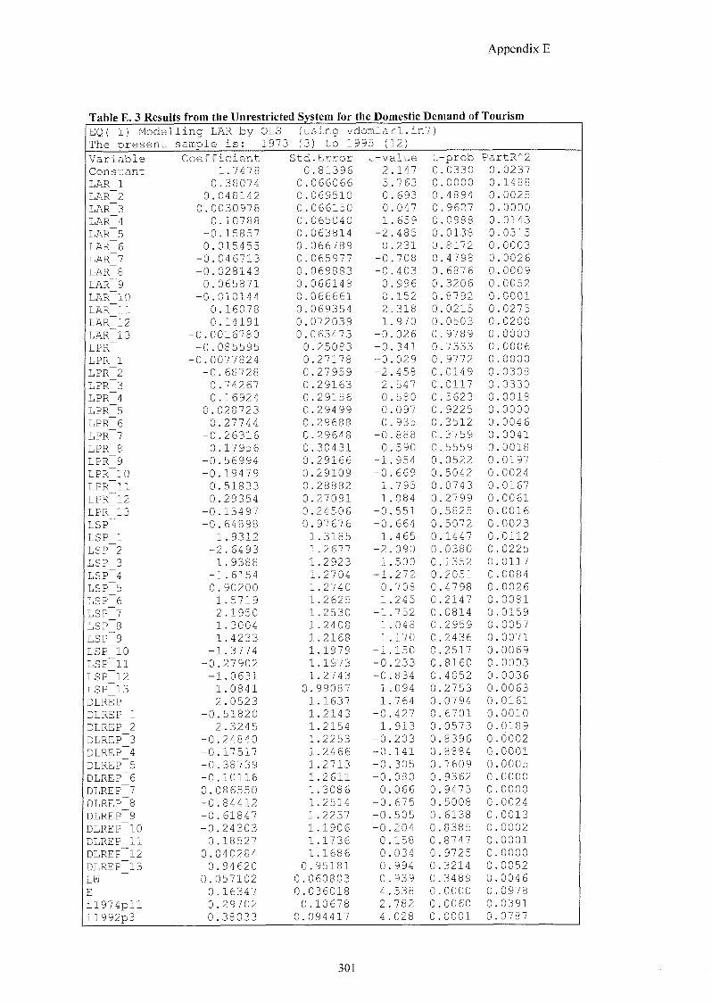
Appendix E

Table E. 3 Results from the Unrestricted System for the Domestic Demand of Tourism EQ( 1) Modell The present s

ing LAR by OLS (using vdomlarl.in?) ample is: 1973 (3) to 1995 (12)

Variable Coefficient Std.Error t-value t -prob PartR^2

Constant 1.7478 0.81396 2 .147 0 .0330 0 .0237

LAR 1 0.38074 0.066066 5 .763 0 .0000 0 .1488

LAR 2 0.048142 0.069510 0 .693 0 .4894 0 .0025

LAR 3 0.0030978 0.066150 0 .047 0 .9627 0 .0000

LAR 4 0.10788 0.065040 1 .659 0 .0988 0 .0143

LAR 5 -0.15857 0.063814 -2 .485 0 .0138 0 .0315

LAR 6 0.015455 0.066789 0 .231 0 .8172 0 .0003

LAR 7 -0.046713 0.065977 -0 .708 0 .4798 0 .0026

LAR 8 -0.028143 0.069883 -0 .403 0 .6876 0 .0009

LAR 9 0.065871 0.066148 0 .996 0 .3206 0 .0052

LAR 10 -0.010144 0.066661 -0 .152 0 .8792 0 .0001

LAR 11 0.16078 0.069354 2 .318 0 .0215 0 .0275

LAR 12 0.14191 0.072039 1 .970 0 .0503 0 .0200 LAR 13 -0.0016780 0.063473 -0 026 0 .9789 0 0000

LPR -0.085595 0.25083 -0 .341 0 .7333 0 .0006

LPR 1 -0.0077824 0.27178 -0 .029 0 .9772 0 0000

LPR 2 -0.68728 0.27959 -2 458 0 0149 0 0308 LPR 3 0.74267 0.29163 2 .547 0 .0117 0 .0330

LPR 4 0.16924 0.29156 0 580 0 .5623 0 0018

LPR 5 0.028723 0.29499 0 097 0 9225 0 0000

LPR 6 0.27744 0.29688 0 935 0 3512 0 0046

LPR 7 -0.26316 0.29648 -0 888 0 3759 0 0041

LPR 8 0.17956 0.30431 0 590 0 5559 0 0018

LPR 9 -0.56994 0.29166 -1 954 0 0522 0 0197

LPR 10 -0.19479 0.29109 -0 669 0 5042 0 0024

LPR 11 0.51833 0.28882 1 795 0 0743 0 0167

LPR 12 0.29354 0.27091 1 084 0 2799 0 0061

LPR 13 -0.13497 0.24506 -0 551 0 5825 0 0016

LSP -0.64898 0.97676 -0 664 0 5072 0 0023

LSP 1 1.9312 1.3185 1 465 0 1447 0 0112

LSP 2 -2.6493 1.2677 -2 090 0 0380 0 0225

LSP 3 1.9388 1.2923 1 500 0 1352 0 0117

LSP 4 -1.6154 1.2704 -1 272 0 2051 0 0084 LSP 5 0.90200 1.2740 0 708 0 4798 0 0026

LSP 6 1.5719 1.2625 1 245 0 2147 0 0081 LSP 7 -2.1950 1.2530 -1 752 0 0814 0 0159 LSP 8 1.3004 1.2408 1 048 0 2959 0 0057 LSP 9 1.4233 1.2168 1 170 0 2436 0 0071

LSP 10 -1.3774 1.1979 -1 150 0 2517 0 0069

LSP 11 -0.27902 1.1973 -0 233 0 8160 0 0003

LSP 12 -1.0631 1.2743 -0 834 0 4052 0 0036 LSP 13 1.0841 0.99087 1. 094 0 2753 0 0063

DLREP 2.0523 1.1637 1 764 0 0794 0. 0161 DLREP 1 -0.51820 1.2143 -0. 427 0 6701 0 0010

DLREP 2 2.3245 1.2154 1. 913 0 0573 0 0189

DLREP 3 -0.24840 1.2253 — 0 . 203 0 8396 0. 0002

DLREP 4 -0.17517 1.2466 -0. 141 0 8884 0 0001

DLREP 5 -0.38739 1.2713 -0 305 0 7609 0. 0005

DLREP 6 -0.10116 1.2611 -0. 080 0. 9362 0. 0000

DLREP 7 0.086550 1.3086 0. 066 0. 9473 0 0000

DLREP 8 -0.84412 1.2514 -0. 675 0. 5008 0. 0024 DLREP 9 -0.61847 1.2237 -0. 505 0. 6138 0 0013

DLREP 10 -0.24303 1.1906 -0 204 0 8385 0. 0002 DLREP 11 0.18527 1.1736 0 158 0 8747 0 0001

DLREP 12 0.040284 1.1686 0. 034 0 9725 0. 0000

DLREP 13 0.94620 0.95181 0. 994 0. 3214 0. 0052

LW 0.057102 0.060803 0 . 939 0. 3489 0 0046

E 0.16347 0.036018 4 . 538 0. 0000 0. 0978

il974pll 0.29702 0.10678 2. 782 0. 0060 0. 0391

il992p3 0.38033 0.094417 4 . 028 0 0001 0. 0787

301

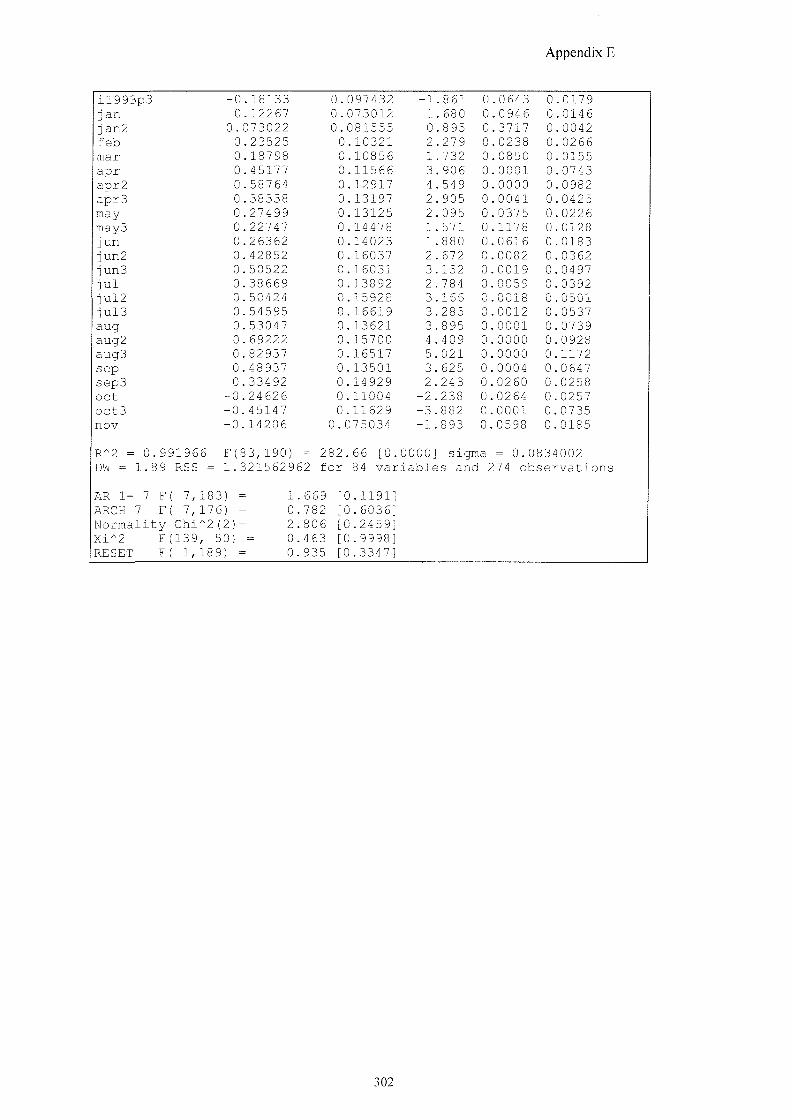
Appendix E

il993p3 -0 .18133 0.097432 -1 861 0 .0643 0 .0179 jan 0 .12267 0.073012 1 680 0 .0946 0 .0146 ian2 0 . 073022 0.081555 0 895 0 .3717 0 .0042 feb 0 .23525 0. 10321 2 279 0 .0238 0 .0266 mar 0 .18798 0 . 10856 1 732 0 .0850 0 0155 apr 0 .45177 0. 11566 3 906 0 0001 0 0743 apr2 0 .58764 0. 12917 4 549 0 0000 0 0982 apr3 0 .38338 0 . 13197 2 905 0 0041 0 0425 may 0 .27499 0. 13125 2 095 0 0375 0 0226 may3 0 .22747 0. 14478 1 571 0 1178 0 0128 jun 0 .26362 0. 14023 1. 880 0 0616 0 0183 iun2 0 .42852 0. 16037 2 672 0 0082 0 0362 iun3 0 .50522 0 . 16031 3. 152 0 0019 0 0497 jul 0 .38669 0 . 13892 2 784 0 0059 0 0392 iul2 0 .50424 0. 15928 3 166 0 0018 0 0501 iul3 0 .54595 0 . 16619 3. 285 0 0012 0 0537 aug 0 .53047 0. 13621 3 895 0 0001 0 0739 aug2 0 .69222 0. 15700 4 . 409 0 0000 0 0928 aug3 0 .82937 0 . 16517 5 . 021 0 0000 0 1172 sep 0 .48937 0. 13501 3. 625 0 0004 0 0647 sep3 0 .33492 0 . 14929 2 . 243 0 0260 0 0258 Oct -0 .24626 0 . 11004 -2. 238 0. 0264 0 0257 oct3 -0 .45147 0. 11629 -3. 882 0 0001 0. 0735 nov -0 .14206 0.075034 -1. 893 0. 0598 0. 0185

R"2 = 0 991966 F(83,190) = 282. 66 [0. 0000] sigma = 0.0834002 DW = 1.89 RSS = 1.321562962 for 84 variables and 274 observations

AR 1- 7 F( 7, 183) 1 669 [0 .1191] ARCH 7 F{ 7, 176) 0 782 [0 .6036] Normality Chi 2(2)= 2 806 [0 .2459] Xi^2 F(139 , 50) 0 463 [0 .9998] RESET F( 1, 189) = 0 935 [0 .3347]

302

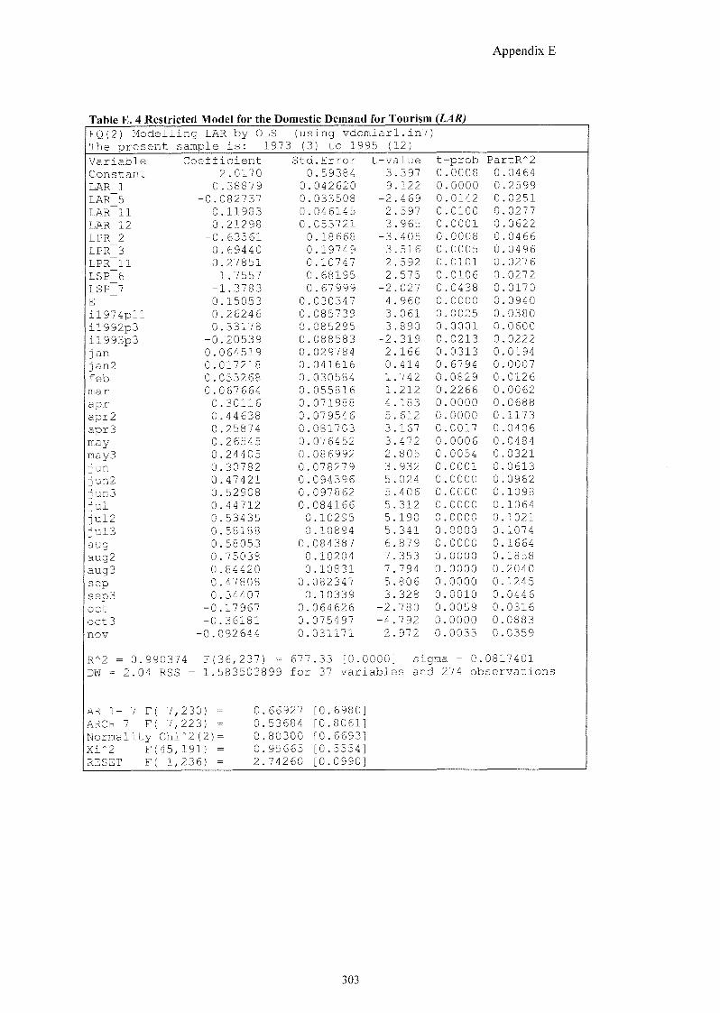
Appendix E

Table E. 4 Restricted Model for the Domestic Demand for Tourism {LAR) EQ(2) Modelling LAR by OLS (using vdomlarl.in?] The present sample is: 1973 (3) to 1995 (12)

Coefficient Std.Error t-value t -prob PartR^2 2.0170 0.59384 3 .397 0 .0008 0 .0464

0 .38879 0.042620 9 .122 0 0000 0 .2599 - 0. 082737 0.033508 -2 .469 0 0142 0 .0251

0 .11983 0.046145 2 597 0 0100 0 0277 0 .21298 0.053721 3 .965 0 0001 0 .0622

-0 .63561 0.18668 -3 405 0 0008 0 0466 0 .69440 0.19749 3 516 0 0005 0 0496 0 .27851 0.10747 2 592 0 0101 0 0276 1.7557 0.68195 2 575 0 0106 0 0272

- 1.3783 0.67999 -2 027 0 0438 0 0170 0 .15053 0.030347 4 960 0 0000 0 0940 0 .26246 0.085739 3 061 0 0025 0 0380 0 .33178 0.085295 3 890 0 0001 0 0600

-0 .20539 0.088583 -2 319 0 0213 0 0222 0. 064519 0.029784 2 166 0 0313 0 0194 0 . 017218 0.041616 0 414 0 6794 0 0007 0. 053268 0.030584 1 742 0 0829 0 0126 0 . 067664 0.055816 1 212 0 2266 0 0062 0 .30116 0.071988 4 183 0 0000 0 0688 0 .44638 0.079546 5 612 0 0000 0 1173 0 .25874 0.081703 3 167 0 0017 0 0406 0 .26545 0.076452 3 472 0 0006 0 0484 0 .24405 0.086992 2 805 0 0054 0 0321 0 .30782 0.078279 3 932 0 0001 0 0613 0 .47421 0.094396 5 024 0 0000 0 0962 0 .52908 0.097862 5 406 0 0000 0 1098 0 .44712 0.084166 5 312 0 0000 0 1064 0 .53435 0.10295 5 190 0 0000 0 1021 0 .58188 0.10894 5 341 0 0000 0 1074 0 .58053 0.084387 6 879 0 0000 0 1664 0 .75038 0.10204 7 353 0 0000 0 1858 0 .84420 0.10831 7 794 0 0000 0 2040 0 .47808 0.082347 5 806 0 0000 0 1245 0 .34407 0.10339 3. 328 0 0010 0 0446

-0 .17967 0.064626 — 2 . 780 0 0059 0 0316 -0 .36181 0.075497 -4 792 0 0000 0. 0883

-0. 092644 0.031171 — 2 . 972 0 0033 0 0359

Variable Constant LAR_1 LAR 5 LAR_11 LAR_12 LPR_2 LPR 3 LPR_11 LSP 6 LSP_7 E il974pll il992p3 il993p3 i an i a n 2 f eb mar apr apr2 apr3 may may3 jun iun2 i u n 3 j u l i u l 2 i u l 3 aug aug2 aug3 sep sep3 oct oct3 nov

R^2 = 0.990374 F(36,237) = 677.33 [0.0000] sigma = 0.0817401 DW = 2.04 RSS = 1.583503899 for 37 variables and 274 observations

AB 1- 7 F( 7,230) ARCH 7 F( 7,223) Normality Chi*2(2; Xi^2 F(45,191) RESET F( 1,236)

0.66927 [0.6980] 0.53684 [0.8061] 0.80300 [0.6693] 0.95665 [0.5554] 2.74260 [0.0990]

303

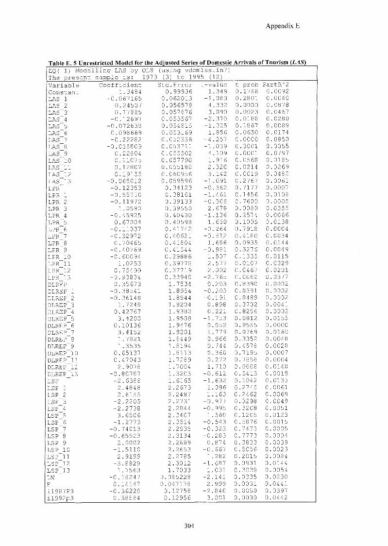
Appendix E

Table E. 5 Unrestricted Model for the Adjusted Series of Domestic Arrivals of Tourism {LAS) EQ( 1) Modelling LAS by OLS The present sample is: 1973

(using vdomlas.in7) (3) to 1995 (12)

Variable Coefficient Std.Error t-value t -prob PartR^2 Constant 1.3484 0.99936 1 .349 0 .1788 0 .0092

LAS 1 -0.067165 0.062013 -1 .083 0 .2801 0 .0060 LAS 2 0.24507 0.056578 4 .332 0 .0000 0 .0878 LAS 3 0.17885 0.057876 3 .090 0 .0023 0 .0467 LAS 4 -0.12697 0.053567 -2 .370 0 .0188 0 .0280 LAS 5 -0.072638 0.054815 -1 .325 0 .1867 0 .0089 LAS 6 0.098669 0.053169 1 .856 0 .0650 0 .0174 LAS 7 -0.22282 0.052336 -4 .257 0 .0000 0 .0850 LAS 8 -0.055809 0.053711 -1 .039 0 .3001 0 .0055 LAS 9 0.22804 0.055502 4 .109 0 .0001 0 .0797 LAS 10 0.11075 0.057790 1 .916 0 .0568 0 .0185 LAS 11 0.12802 0.055180 2 320 0 .0214 0 0269 LAS 12 0.19155 0.060956 3 .142 0 .0019 0 .0482 LAS 13 -0.065012 0.059596 -1 091 0 .2767 0 0061 LPR -0.12353 0.34123 -0 362 0 7177 0 0007 LPR 1 -0.55750 0.38161 -1 .461 0 .1456 0 .0108 LPR 2 -0.11972 0.39133 -0 306 0 .7600 0 0005 LPR 3 1.0590 0.39550 2 678 0 0080 0 0355 LPR 4 -0.45925 0.40430 -1 136 0 .2574 0 0066 LPR 5 0.67004 0.40598 1 650 0 1005 0 0138 LPR 6 -0.11037 0.41742 -0 264 0 7918 0 0004 LPR 7 -0.32972 0.40621 -0 812 0 4180 0 0034 LPR 8 0.70465 0.41804 1 686 0 0935 0 0144 LPR 9 -0.40769 0.41544 -0 981 0 3276 0 0049 LPR 10 -0.60094 0.39886 -1 507 0 1335 0 0115 LPR 11 1.0253 0.39778 2 577 0 0107 0 0329 LPR 12 0.75499 0.37719 2 002 0 0467 0 0201 LPR 13 -0.93834 0.33940 -2 765 0 0062 0 0377 DLREP 0.35673 1.7534 0 203 0 8390 0 0002 DLREP 1 -0.38541 1.8954 -0 203 0 8391 0 0002 DLREP 2 -0.36148 1.8944 -0 191 0 8489 0 0002 DLREP 3 1.7248 1.9204 0 898 0 3702 0 0041 DLREP 4 0.42767 1.9382 0 221 0 8256 0 0002 DLREP 5 -3.4200 1.9508 -1 753 0 0812 0 0155 DLREP 6 0.10136 1.9476 0 052 0 9585 0 0000 DLREP 7 3.4152 1.9201 1 779 0 0769 0 0160 DLREP 8 1.7821 1.8449 0 966 0 3352 0 0048 DLREP 9 1.3535 1.8194 0 744 0 4578 0 0028 DLREP 10 0.65137 1.8113 0 360 0 7195 0 0007 DLREP 11 0.47043 1.7289 0 272 0 7858 0 0004 DLREP 12 2.9078 1.7004 1 710 0 0888 0 0148 DLREP 13 -0.80787 1.3203 -0 612 0 5413 0 0019 LSP -2.6388 1.6165 -1 632 0 1042 0 0135 LSP 1 2.4848 2.2673 1 096 0 2745 0 0061 LSP 2 2.6155 2.2487 1 163 0. 2462 0. 0069 LSP 3 -2.2205 2.2731 -0. 977 0 3298 0 0049 LSP 4 -2.2738 2.2844 -0 995 0. 3208 0. 0051 LSP 5 3.6506 2.3407 1. 560 0. 1205 0. 0123 LSP 6 -1.2773 2.3514 -0 543 0 5876 0. 0015 LSP 7 -0.74013 2.2935 -0. 323 0. 7473 0. 0005 LSP 8 -0.65523 2.3134 -0. 283 0 7773 0. 0004 LSP 9 2.0002 2.2889 0. 874 0. 3833 0. 0039 LSP 10 -1.5110 2.2653 -0. 667 0. 5056 0. 0023 LSP 11 2.9199 2.2785 1 282 0. 2015 0. 0084 LSP 12 -3.8829 2.3012 -1. 687 0. 0931 0. 0144 LSP 13 1.7563 1.7033 1 031 0 3038 0. 0054 LW -0.18247 0.085228 -2 141 0. 0335 0. 0230 E 0.14147 0.047178 2 . 999 0. 0031 0. 0441 il987P3 -0.36229 0.12758 -2. 840 0. 0050 0. 0397 il992p3 0.38884 0.12956 3. 001 0. 0030 0. 0442

304

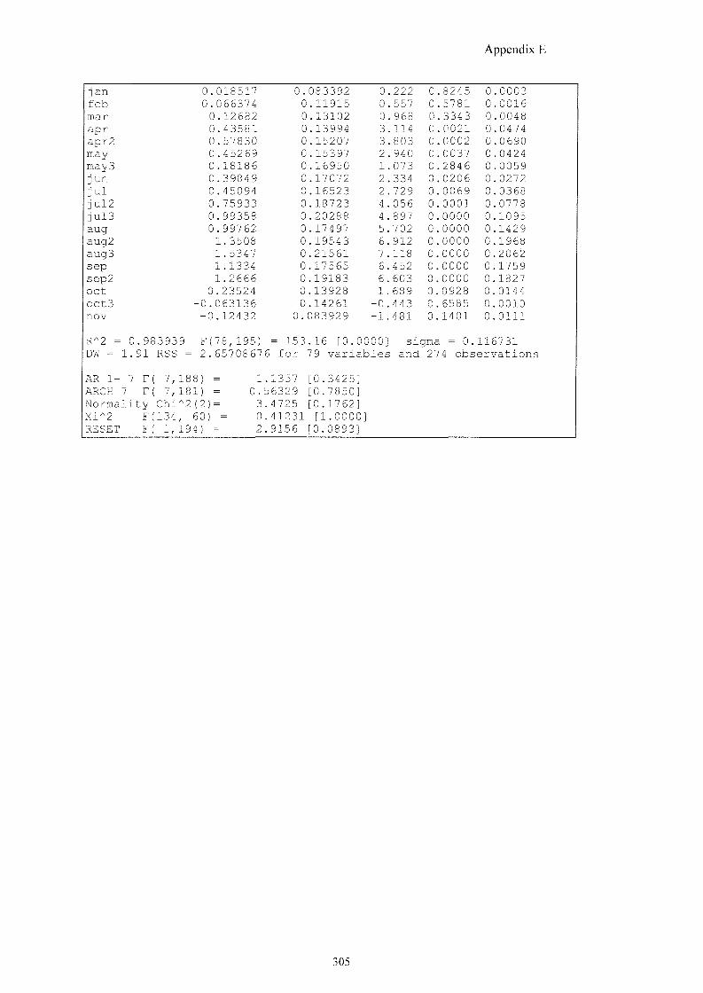
Appendix E

jan 0.018517 0.083392 0. 222 0 8245 0 0003 feb 0.066374 0.11915 0. 557 0 5781 0 0016 mar 0.12682 0.13102 0 968 0 3343 0 0048 apr 0.43581 0.13994 3. 114 0 0021 0 0474 apr2 0.57830 0.15207 3. 803 0 0002 0 0690 may 0.45269 0.15397 2 . 940 0 0037 0 0424 may3 0.18186 0.16950 1. 073 0 2846 0 0059 jun 0.39849 0.17072 2 . 334 0 0206 0 0272 jul 0.45094 0.16523 2 . 729 0 0069 0 0368 iul2 0.75933 0.18723 4 . 056 0 0001 0 0778 iul3 0.99358 0.20288 4 . 897 0 0000 0 1095 aug 0.99762 0.17497 5 . 702 0 0000 0 1429 aug2 1.3508 0.19543 6. 912 0 0000 0 1968 aug3 1.5347 0.21561 7 . 118 0 0000 0 2062 sep 1.1334 0.17565 6. 452 0 0000 0 1759 sep2 1.2666 0.19183 6. 603 0 0000 0 1827 Oct 0.23524 0.13928 1. 689 0 0928 0 0144 oct3 -0.063136 0.14261 -0. 443 0 6585 0 0010 nov -0.12432 0.083929 — 1. 481 0 1401 0 0111

R"2 = 0 .983939 F(78,195) = 153.16 [0.0000] sigma = 0. 116731 DW = 1. 91 RSS = 2.65708676 for 79 variables and 274 observations

AR 1- 7 F( 7, 188) = 1 .1357 [0.3425] ARCH 7 F( 7, 181) = 0. 56329 [0.7850] Normality Chi "2(2)= 3 .4725 [0.1762] Xi^2 F(134 , 60) = 0 .41231 [1.0000] RESET F( 1, 194) = 2 .9156 [0.0893]

305

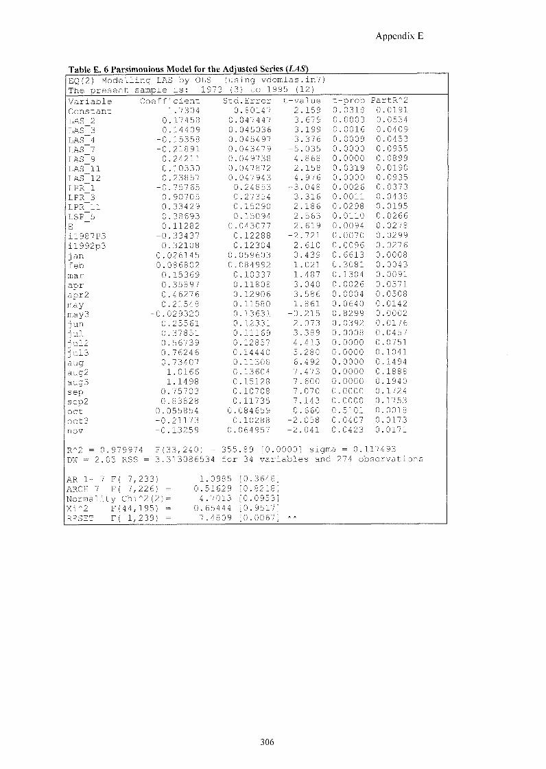
Appendix E

Table E. 6 Parsimonious Model for the Adjusted Series (LAS) EQ(2) Modelling LAS by OLS The present sample is: 1973

using vdomlas.in?) (3) to 1995 (12)

Variable Constant LAS_2 LAS_3 LAS_4 LAS_7 LAS_9 LAS_11 LAS 12 LPR_1 LPR_3 LPR_11 LSP_5 E il987P3 il992p3 i an f eb mar apr apr2 may may3 jun jul iul2 iul3 aug aug2 aug3 sep sep2 oct oct3 nov


Coefficient Std.Error t-value t -prob PartR^2 1.7304 0.80147 2 159 0 0318 0 0191

0 .17458 0.047447 3 679 0 0003 0 .0534 0 .14409 0.045036 3 199 0 0016 0 .0409

-0 .15358 0.045497 -3 376 0 0009 0 0453 -0 .21891 0.043479 -5 035 0 0000 0 0955 0 .24211 0.049738 4 868 0 0000 0 0899 0 .10330 0.047872 2 158 0 0319 0 0190 0 .23857 0.047943 4 976 0 0000 0 0935

-0 .75765 0.24853 -3 048 0 0026 0 0373 0 .90705 0.27354 3 316 0 0011 0 0438 0 .33429 0.15290 2 186 0 0298 0 0195 0 .38693 0.15094 2 563 0 0110 0 0266 0 .11282 0.043077 2 619 0 0094 0 0278

-0 .33437 0.12288 -2 721 0 0070 0 0299 0 .32108 0.12304 2 610 0 0096 0 0276

0 . 026145 0.059603 0 439 0 6613 0 0008 0. 086802 0.084992 1 021 0 3081 0 0043 0 .15369 0.10337 1 487 0 1384 0 0091 0 .35897 0.11808 3 040 0 0026 0 0371 0 .46276 0.12906 3 586 0 0004 0 0508 0 .21548 0.11580 1 861 0 0640 0 0142

-0. 029320 0.13631 -0 215 0 8299 0 0002 0 .25561 0.12331 2 073 0 0392 0 0176 0 .37851 0.11169 3 389 0 0008 0 0457 0 .56739 0.12857 4 413 0 0000 0 0751 0 .76246 0.14440 5. 280 0 0000 0 1041 0 .73407 0.11308 6 492 0 0000 0 1494 1.0166 0.13604 7 473 0 0000 0 1888 1.1498 0.15128 7 600 0 0000 0 1940

0 .75703 0.10708 7 070 0 0000 0 1724 0 .83828 0.11735 7 143 0 0000 0. 1753

0.055854 0.084659 0 660 0 5101 0 0018 -0 .21173 0.10288 -2 058 0 0407 0 0173 -0 .13259 0.064957 -2 041 0 0423 0. 0171

AR 1- 7 F( 7,233) ARCH 7 F( 7,226) Normality Chi*2(2; Xi^2 F(44,195) RESET F( 1,239)

1.0985 [0.3648] 0.51629 [0.8218] 4.7013 [0.0953]

0.65444 [0.9517] 7.4809 [0.0067] **

306

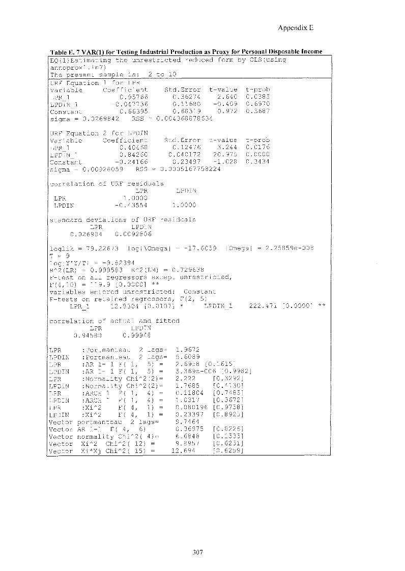
Appendix E

Table E. 7 VAR(l) for Testing Industrial Production as Proxy for Personal Disposable Income E Q ( 1 ) E s t i m a t i n g t h e u n r e s t r i c t e d r e d u c e d f o r m b y O L S ( u s i n g

a n n o p r o x l . i n ? ) The present sample is: 2 to 10

URF Equation 1 for LPR Variable Coefficient L P R l 0.95766 LPDIN_1 -0.047136 Constant 0.66395

Std.Error 0.36274 0.11680 0.68319

t-value 2.640

-0.409 0.972

Sigma 0.0269842 RSS 0.004368878634

URF Equation 2 for LPDIN Variable Coefficient L P R l 0.40468 LPDIN_1 0.84260 Constant -0.24166 sigma = 0.00928059 RSS

Std.Error 0.12476

0.040172 0.23497

t-value 3.244

20.975 -1.028

t-prob 0.0385 0.6970 0.3687

t-prob 0.0176 0.0000 0.3434

0.0005167758224

correlation of URF residuals LPR LPDIN

LPR 1.0000 LPDIN -0.43554 1.0000

standard deviations of URF residuals LPR LPDIN

0.026984 0.0092806

loglik = 79.22673 log|\Omega| = -17.6059 T = 9 log|Y'Y/T| = -9.82394 R*2(LR) = 0.999583 R"2(LM) = 0.729638 F-test on all regressors except unrestricted, F(4,10) = 119.9 [0.0000] ** variables entered unrestricted: Constant F-tests on retained regressors, F(2, 5)

LPR_1 12.8304 [0.0107] * LPDIN_1

correlation of actual and fitted LPR LPDIN

0.94580 0.99948

Omega I 2.25859e-

222.471 [0.0000]

LPR :Portmanteau 2 lags= LPDIN :Portmanteau 2 lags= LPR :AR 1- 1 F( 1, 5) = LPDIN :AR 1- 1 F( 1, 5) = LPR :Normality Chi*2(2)= LPDIN :Normality Chi^2(2)= LPR :ARCH 1 F( 1, 4) = LPDIN :ARCH 1 F( 1, 4) = LPR :Xi*2 F( 4, 1) = LPDIN :Xi"2 F( 4, 1) = Vector portmanteau 2 lags= Vector AR 1-1 F( 4, 6) = Vector normality Chi^2( 4)= Vector Xi^2 Chi^2( 12) = Vector Xi*Xj Chi^2( 15) =

1.9672 5.6089 2.6958 [0 5.369e-00 2 . 2 2 2 1.7685 0.11804 1.0317 0.080196 0.23397 9.7464 0.36975 6.6848 9.8957

12.694

.1615] 6 [0.9982] [0.3292] [0.4130] [0.7485] [0.3672] [0.9758] [0.8925]

[ 0 . 8 2 2 6 ] [0.1535] [0.6251] [0.6259]

307

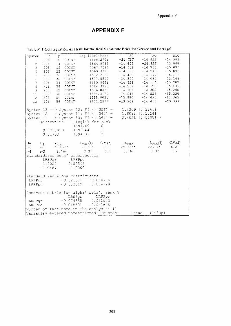
Appendix F

APPENDIX F

Table F. 1 Cointegration Analysis for the Real Substitute Price for Greece and Portugal

system T P log-likelihood SC HQ AIC 1 208 10 COINT 1558 .2764 -14 727 14 .822 14 .983 2 208 14 COINT 1564 .9739 14 689 14 .822 15 .048 3 208 18 COINT 1567 .7096 14 612 14 .784 15 .074 4 208 22 COINT 1569 .8325 14 530 14 .740 15 .095 5 208 26 COINT 1572 .2129 14 450 14 .699 15 .117 6 208 30 COINT 1577 .5609 14 399 14 .686 15 .169 7 208 34 C%n^T 1580 .9661 14 329 14 .654 15 .202 8 208 38 COINT 1584 .3920 14 259 14 .623 15 .235 9 208 42 COINT 1586 .8838 14 181 14 .582 15 .258

11 208 50 COINT 1594 3170 14 047 14 .525 15 .330 12 208 54 COINT 1598 0031 13 980 14 .496 15 365 13 208 58 COINT 1601 2977 13 909 14 .463 15 .397

System 13 --> System 12: F( 4, 356) = 1 . 4209 [0 .2265] System 12 --> System 11: F( 4, 360) = 1 . 6092 [ 0 .1714] System 11 --> System 10: F( 4, 364) = 2 . 4026 [ 0 .0495] *

eigenvalue loglik for rank 1581.49 0

0.0998829 1592.44 1

0.01793 1594.32 2

Ho H; ^ a x \nax(^) C.V.(2) A trace 'HraceO C.V.(2) r=0 r=l 2 1 . 89** 19.57* 16.9 25 65** 22.94* 18.2 r=l r=2 3 . 76* 3.37 3 . 7 3 .76* 3.37 3 . 7

standardized beta' eigenvectors LRSPgr LRSPpo 1.0000 0.87546

-1.0467 1.0000

standardized alpha coefficients LRSPgr -0.021506 0.050780 LRSPpo -0.053549 -0.004728

long-run matrix Po= alpha* beta rank 2 LRSPgr LRSPpo

LRSPgr -0.074658 0.031952 LRSPpo -0.048601 -0.051608

Number of lags used in the analysis: 11 Variables entered unrestricted: Constant Trend il983pl

308

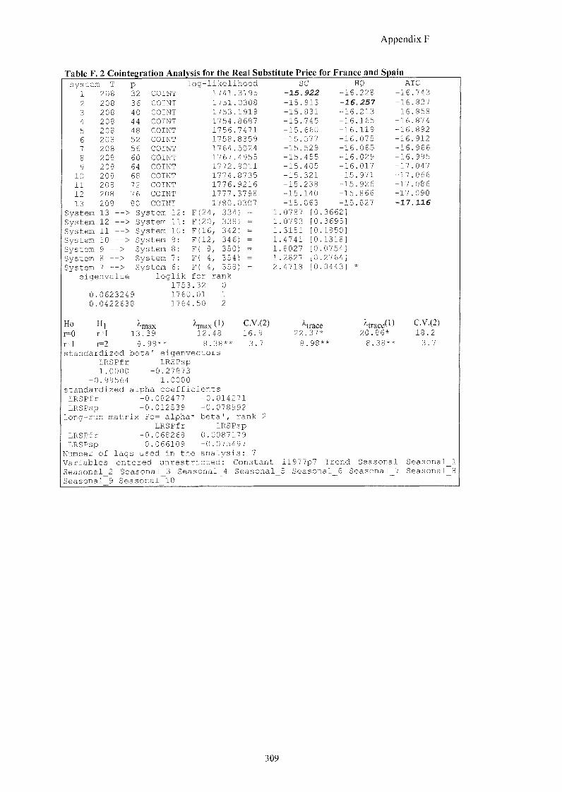
A p p e n d i x F

Table F. 2 Cointegration Analysis for the Real Substitute Price for France and Spain s y s t e m T

1 208 2 208

3 2 0 8 4 2 0 8 5 2 0 8 6 208

208 208 208 208

1

9 10 11 12 13

S y s t e m S y s t e m S y s t e m S y s t e m S y s t e m S y s t e m S y s t e m

P 32 3 6 4 0 44 48 52 5 6 60 64

l o g

>

208 208 13 12 — > 11 — >

10 — > 9 — > 8 — >

7 — >

COINT COINT COINT COINT COINT COINT COINT COINT COINT

8 COINT 2 COINT 6 COINT 0 COINT S y s t e m 12 S y s t e m S y s t e m S y s t e m S y s t e m S y s t e m S y s t e m

- l i k e l i h o o d 1 7 4 1 . 3 1 9 5 1 7 5 1 . 0 3 0 8 1 7 5 3 . 1 7 5 4 . 1 7 5 6 . 1 7 5 8 . 1 7 6 4 , 1 7 6 7 . 1 7 7 2 .

1 9 1 9 8 6 8 7 7 4 7 1 8 3 5 9 5 0 2 4 4 9 5 5 9 0 1 1

11 10

F ( F ( F{ F ( F ( F{ F (

2 4 , 20, 1 6 , 12,

e i g e n v a l u e

0 . 0 6 2 3 2 4 9 0 . 0 4 2 2 6 3 8

l o g l i k f o r 1 7 5 3 . 3 2 1 7 6 0 . 0 1 1 7 6 4 . 5 0

"max 1 3 . 3 9

A max 12.'

1 7 7 4 . 8 7 3 5 1 7 7 6 . 9 2 1 6 1 7 7 7 . 3 7 9 8 1 7 8 0 . 0 3 0 7 , 3 3 4 ) =

3 3 8 ) = 3 4 2 ) = 3 4 6 ) =

, 3 5 0 ) = , 3 5 4 ) = , 3 5 8 ) = r a n k

1 2

(1)

SC -15.922 - 1 5 . 9 1 3 - 1 5 . 8 3 1 - 1 5 . 7 4 5 - 1 5 . 6 6 0 - 1 5 . 5 7 7 - 1 5 . 5 2 9 - 1 5 . 4 5 5 - 1 5 . 4 0 5 - 1 5 . 3 2 1 - 1 5 . 2 3 8 - 1 5 . 1 4 0 - 1 5 . 0 6 3

. 0 7 8 7

. 0 7 9 3

. 3 1 5 1 , 4 7 4 1

1 . 8 0 2 7 1 . 2 8 2 7 2 . 4 7 1 8

C.V.(2) 1 6 . 9

3 . 7

Ho Hi r=0 r=] r=] r=2 8 . 9 8 * * 8 . 3 8 * * s t a n d a r d i z e d b e t a ' e i g e n v e c t o r s

L R S P f r L R S P s p 1 . 0 0 0 0 - 0 . 2 7 8 7 3

- 0 . 9 9 5 6 4 1 . 0 0 0 0 s t a n d a r d i z e d a l p h a c o e f f i c i e n t s

I R S P f r - 0 . 0 8 2 4 7 7 - 0 . 0 1 4 2 7 1 L R S P s p - 0 . 0 1 2 5 3 9 - 0 . 0 7 8 9 9 2

l o n g - r u n m a t r i x Po= a l p h a * b e t a ' , r a n k 2 L R S P f r L R S P s p

L R S P f r - 0 . 0 6 8 2 6 8 0 . 0 0 8 7 1 7 9 L R S P s p 0 . 0 6 6 1 0 9 - 0 . 0 7 5 4 9 7

N u m b e r o f l a g s u s e d i n t h e a n a l y s i s : 7 V a r i a b l e s e n t e r e d u n r e s t r i c t e d : C o n s t a n t S e a s o n a l _ 2 S e a s o n a l _ 3 S e a s o n a l _ 4 S e a s o n a l _ S e a s o n a l 9 S e a s o n a l 1 0

HQ 1 6 . 2 2 8 16.257 1 6 . 2 1 3 1 6 . 1 6 5

1 1 9 0 7 5 0 6 5 0 2 9

AIC - 1 6 . 7 4 3 - 1 6 . 8 3 7 - 1 6 . 8 5 8 - 1 6 . 8 7 4

- 1 6

- 1 6

- 1 6

-16 - 1 6 . 0 1 7 - 1 5 . 9 7 1 - 1 5 . 9 2 6

-16. -16. -16. -16. - 1 7 .

8 9 2 9 1 2 9 6 6 9 9 5 0 4 7

- 1 5 - 1 5

[ 0 . 3 6 6 2 ] [ 0 . 3 6 9 5 ] [ 0 . 1 8 5 0 ] [ 0 . 1 3 1 8 ] [ 0 . 0 7 5 4 ] [ 0 . 2 7 6 4 ] [ 0 . 0 4 4 3 ]

8 6 6 . 8 2 7

- 1 7 . 0 6 6 - 1 7 . 0 8 6 - 1 7 . 0 9 0 -17.116

^-trace 2 2 . 3 7 *

'trace( ) 20.86*

8 . 3 8 * *

C,V,(2) 18.2

3 . 7

i l 9 7 7 p 7 T r e n d S e a s o n a l 5 S e a s o n a l 6 S e a s o n a l 7

S e a s o n a l _ S e a s o n a l

309

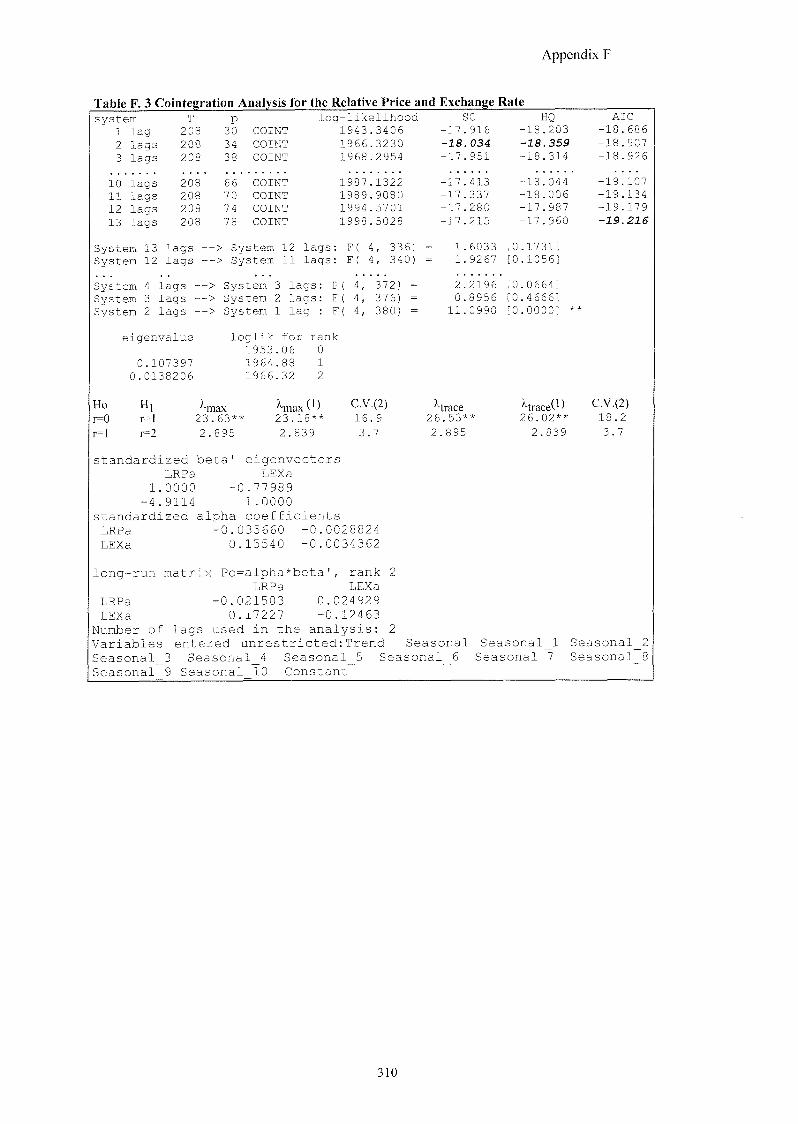
A p p e n d i x F

Table F. 3 Cointegration Analysis for the Relative Price and Exchange Rate y s t e m T P l o g - l i k e l i h o o d SC HQ AIC

1 l a g 2 0 8 3 0 COINT 1 9 4 3 . 3 4 0 6 - 1 7 . 9 1 6 - 1 8 . 2 0 3 - 1 8 . 6 8 6

2 l a g s 2 0 8 34 COINT 1 9 6 6 . 3 2 3 0 -18.034 -18.359 - 1 8 . 9 0 7

3 l a g s 2 0 8 38 COINT 1 9 6 8 . 2 9 5 4 - 1 7 . 9 5 1 - 1 8 . 3 1 4 - 1 8 . 9 2 6

10 l a g s 2 0 8 6 6 COINT 1 9 8 7 . 1 3 2 2 - 1 7 . 4 1 3 - 1 8 . 0 4 4 - 1 9 . 1 0 7

1 1 l a g s 2 0 8 70 COINT 1 9 8 9 . 9 0 8 0 - 1 7 . 3 3 7 - 1 8 . 0 0 6 - 1 9 . 1 3 4

12 l a g s 2 0 8 74 COINT 1 9 9 4 . 5 7 0 1 - 1 7 . 2 8 0 - 1 7 . 9 8 7 - 1 9 . 1 7 9

1 3 l a g s 2 0 8 78 COINT 1 9 9 8 . 5 0 2 8 - 1 7 . 2 1 5 - 1 7 . 9 6 0 -19.216

S y s t e m 1 3 l a g s — > S y s t e m 12 l a g s : F ( 4 , 3 3 6 ) S y s t e m 12 l a g s — > S y s t e m 1 1 l a g s : F ( 4 , 3 4 0 )

S y s t e m 4 l a g s — > S y s t e m 3 l a g s : F ( 4 , 3 7 2 ) = S y s t e m 3 l a g s — > S y s t e m 2 l a g s : F ( 4 , 37 6) = S y s t e m 2 l a g s — > S y s t e m 1 l a g : F ( 4 , 3 8 0 ) =

1 . 6 0 3 3 [ 0 . 1 7 3 1 ] 1 . 9 2 6 7 [ 0 . 1 0 5 6 ]

2 . 2 1 9 6 [ 0 . 0 6 6 4 ] 0 . 8 9 5 6 [ 0 . 4 6 6 6 ]

1 1 . 0 9 9 0 [ 0 . 0 0 0 0 ] **

e i g e n v a l u e

0 . 1 0 7 3 9 7 0 . 0 1 3 8 2 0 6

l o g l i k f o r r a n k 1 9 5 3 . 0 6 0 1 9 6 4 . 8 8 1 1 9 6 6 . 3 2 2

Ho H ]

r=0 r=l r=l r=2

\nax 2 3 . 6 3 * * 2 . 8 9 5

\nax 2 3 . 1 8 * *

2 . 8 3 9

C.V.(2) 1 6 . 9

3 . 7

^ trace 2 6 . 5 3 * *

2 . 8 9 5

2 6 . 0 2 * *

2 . 8 3 9

C.V.(2) 1 8 . 2 3 . 7

standardized beta' eigenvectors LRPa L E X a

1.0000 -0.77989 -4.9114 1.0000

standardized alpha coefficients LRPa -0.035660 -0.0028824 LEXa 0.15540 -0.0034362

long-run matrix Po=alpha*beta', rank 2 LRPa LEXa

LRPa -0.021503 0.024929 LEXa 0.17227 -0.12463

Number of lags used in the analysis: 2 Variables entered unrestricted:Trend Seasonal Seasonal 1 Seasonal_3 Seasonal_4 Seasonal_5 Seasonal 9 Seasonal 10 Constant

Seasonal 6 Seasonal 7 Seasonal_2 Seasonal 8

310

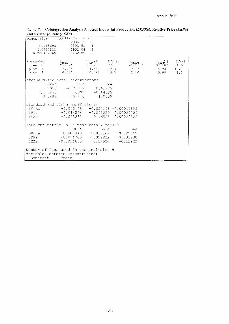
Appendix F

Table F. 4 Cointegration Analysis for Real Industrial Production {LRPRa), Relative Price {LRPa) and Exchange Rate {LEXa) eigenvalue loglik for rank

2880.72 0 0.115695 2893.51 1 0.0787522 2902.04 2

0.000459869 2902.09 3

Ho:rank=p ^max C.V.(2) ^"trace ^-trace(^) C.V.(2) p== 0 25.57* 22.25 23.8 42.73** 37 18* 34 6 p < = 1 17.06* 14.85 16.9 17.16 14 93 18 2 p < ^ 2 0.096 0.083 3.7 0.10 0 08 3 7

standardized beta' eigenvectors LRPRa LRPa LEXa 1.0000 -0.20819 0.61705

0.16833 1.0000 -0.64085 3.3898 10.116 1.0000

standardized alpha coefficients LRPRa -0.080158 -0.031148 -0. 00016882 LRPa -0.014504 -0.065039 0. 00020729 LEXa -0.038281 0.16525 0. 00029502

long-run matrix Po= alpha* beta', rank 3 LRPRa LRPa LEXa

LRPRa -0.085973 -0.016167 0.029669 LRPa -0.024749 -0.059922 0.032938 LEXa -0.0094650 0.17620 -0.12922

Number of lags used in the analysis: 9 Variables entered unrestricted:

Constant Trend

ni

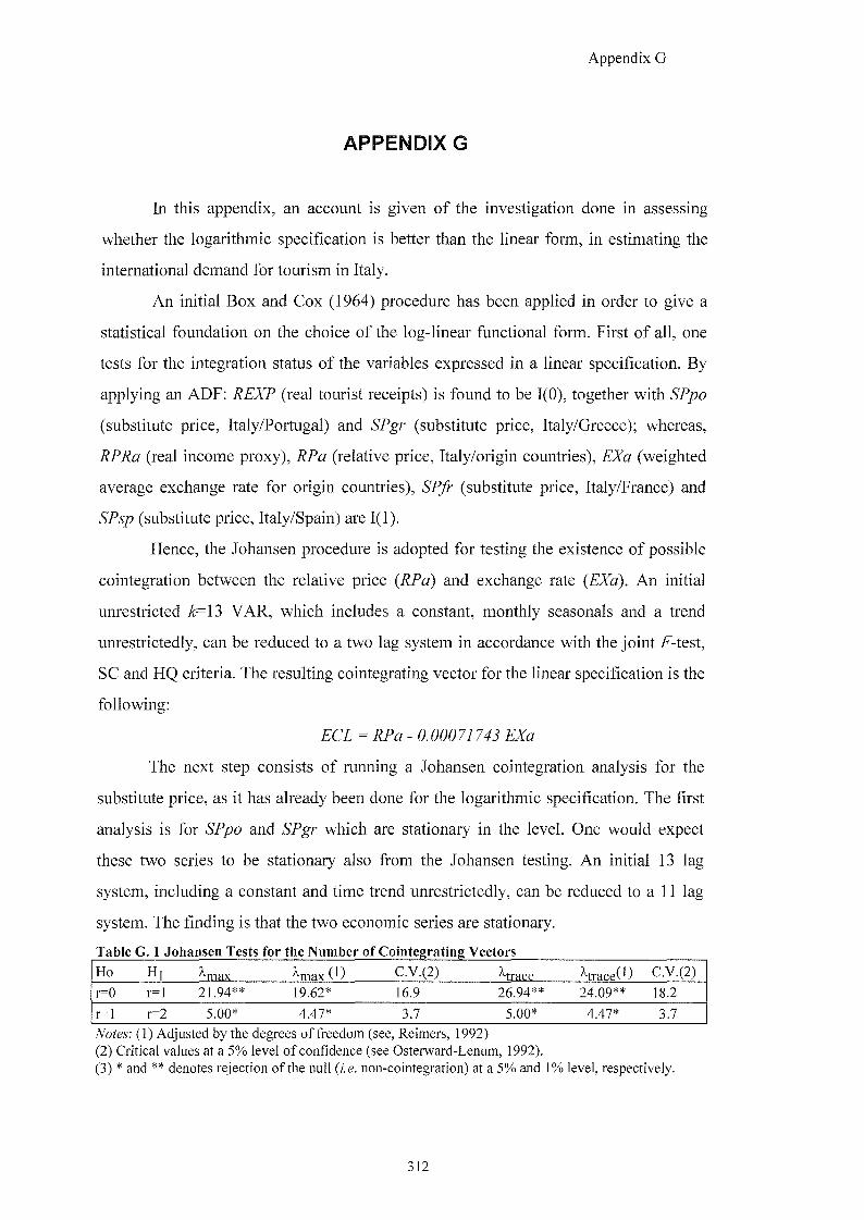
Appendix G

APPENDIX G

In this appendix, an account is given of the investigation done in assessing

whether the logarithmic specification is better than the linear form, in estimating the

international demand for tourism in Italy.

An initial Box and Cox (1964) procedure has been applied in order to give a

statistical foundation on the choice of the log-linear functional form. First of all, one

tests for the integration status of the variables expressed in a linear specification. By

applying an ADF: REXP (real tourist receipts) is found to be 1(0), together with SPpo

(substitute price, Italy/Portugal) and SPgr (substitute price, Italy/Greece); whereas,

RPRa (real income proxy), RPa (relative price, Italy/origin countries), EXa (weighted

average exchange rate for origin countries), SPfr (substitute price, Italy/France) and

SPsp (substitute price, Italy/Spain) are 1(1).

Hence, the Johansen procedure is adopted for testing the existence of possible

cointegration between the relative price {RPa) and exchange rate {EXa). An initial

unrestricted A=13 VAR, which includes a constant, monthly seasonals and a trend

unrestrictedly, can be reduced to a two lag system in accordance with the joint F-test,

SC and HQ criteria. The resulting cointegrating vector for the linear specification is the

following:

E C Z = j;?a - 0.00077 7^j

The next step consists of running a Johansen cointegration analysis for the

substitute price, as it has already been done for the logarithmic specification. The first

analysis is for SPpo and SPgr which are stationary in the level. One would expect

these two series to be stationary also from the Johansen testing. An initial 13 lag

system, including a constant and time trend unrestrictedly, can be reduced to a 11 lag

system. The finding is that the two economic series are stationary.

Ho Hi ^max ^max (1) C.V.(2) ^trace ^trace(l) C.V.(2)

r=0 r=l 21^%** 1&62* ]&9 26.94** 24.09** 1&2

r=l r=2 5^0* 3.7 5^0* 4 j J * 3.7

Notes'. (1) Adjusted by the degrees of freedom (see, Reimers, 1992) (2) Critical values at a 5% level of confidence (see Osterward-Lenum, 1992). (3) * and ** denotes rejection of the null {i.e. non-cointegration) at a 5% and 1% level, respectively.

512

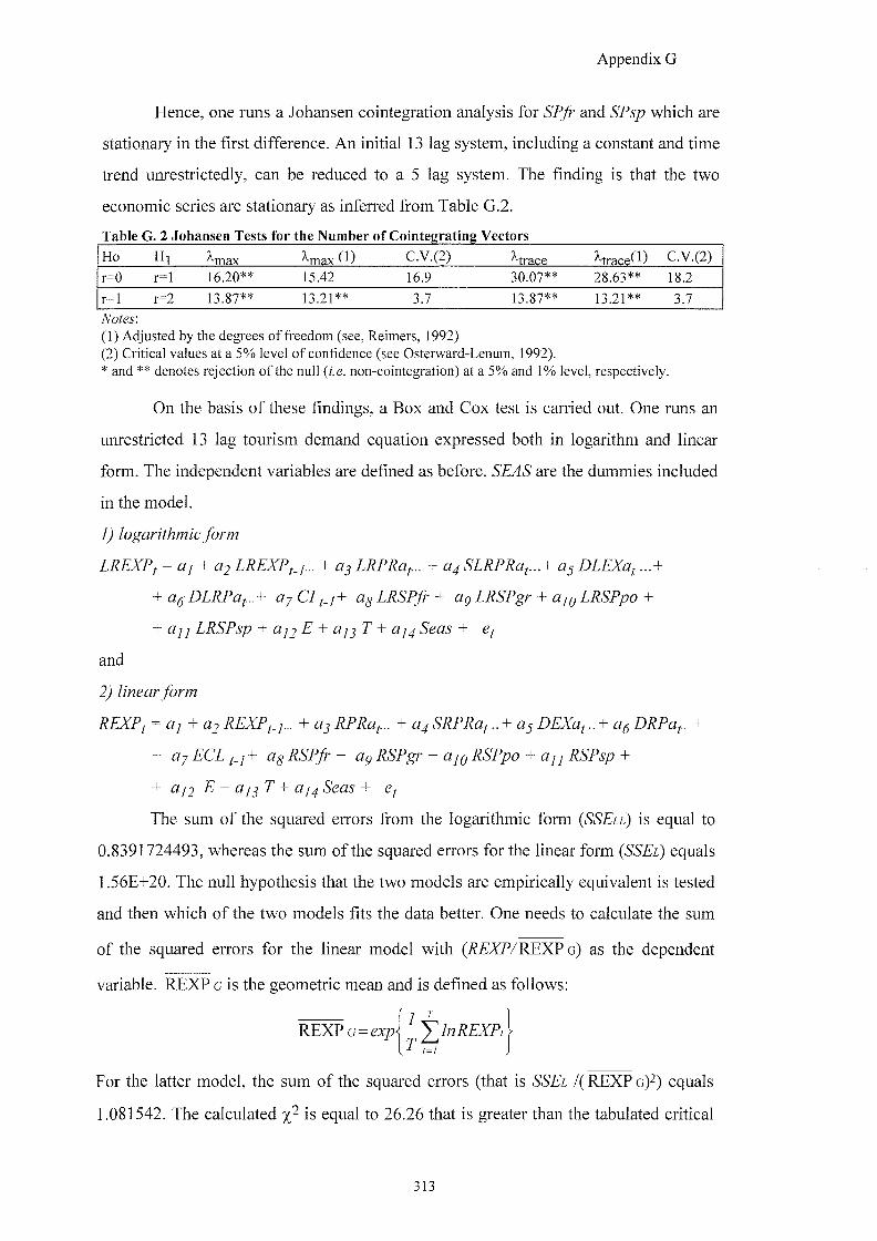
Appendix G

Hence, one runs a Johansen cointegration analysis for SPfr and SPsp which are

stationary in the first difference. An initial 13 lag system, including a constant and time

trend unrestrictedly, can be reduced to a 5 lag system. The finding is that the two

economic series are stationary as inferred from Table G.2.

Ho Hi înax ^max (1) C.V.(2) ^trace ^trace(^) C.V.(2) r=0 r=] 16.20** 15.42 16.9 30.07** 28.63** 18.2

r=l r=2 13.87** 13.21** 3.7 13.87** 13/21** 3.7

(1) Adjusted by the degrees of freedom (see, Reimers, 1992) (2) Critical values at a 5% level of confidence (see Osterward-Lenum, 1992). * and ** denotes rejection of the null {i.e. non-cointegration) at a 5% and 1% level, respectively.

On the basis of these findings, a Box and Cox test is carried out. One runs an

unrestricted 13 lag tourism demand equation expressed both in logarithm and linear

form. The independent variables are defined as before. SEAS are the dummies included

in the model.

= ay + ...+

+ DLRPaf... + ay CI;./+ ag LRSPfr + ag LRSPgr + ajg LRSPpo +

and

= a; +<32 .. + aj +

+ ay ECL f_j+ ag RSPfr + ag RSPgr + ajq RSPpo + cij] RSPsp +

+ aj2 E + a j j T + aj^ Seas +


0.8391724493, whereas the sum of the squared errors for the linear form equals

1.56E+20. The null hypothesis that the two models are empirically equivalent is tested

and then which of the two models fits the data better. One needs to calculate the sum

of the squared errors for the linear model with (^£ZP/REXPg) as the dependent

variable. REXP c is the geometric mean and is defined as follows:

'7 REXP G=gjgpj- ^ jgEZP,

For the latter model, the sum of the squared errors (that is SSEL / ( R E X P g ) ^ ) equals

1.081542. The calculated is equal to 26.26 that is greater than the tabulated critical

313

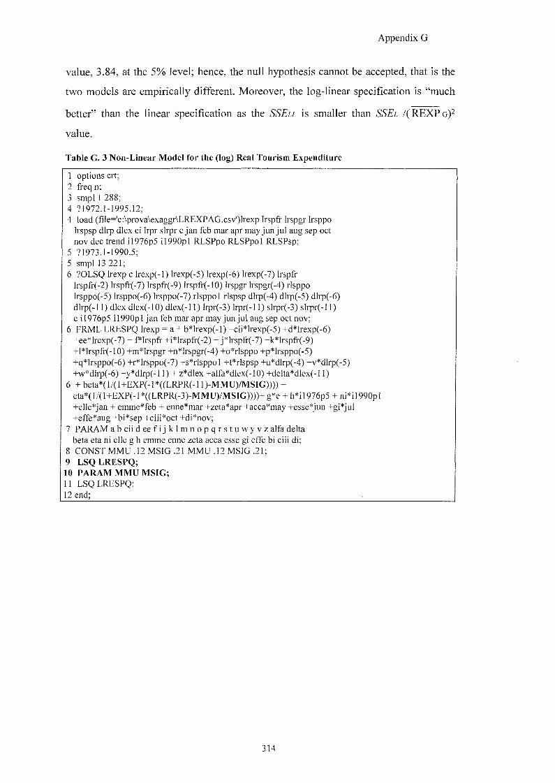
Appendix G

value, 3.84, at the 5% level; hence, the null hypothesis cannot be accepted, that is the

two models are empirically different. Moreover, the log-linear specification is "much

better" than the linear specification as the SSELL is smaller than SSEL / ( R E X P g ) ^

value.

Table G. 3 Non-Linear Model for the (log) Real Tourism Expenditure

1 options crt; 2 freq n; 3 smp] 1 288; 4 91972.1-1995.12; 4 load (file='c:\prova\exaggr\LREXPAG.csv')lrexp Irspfr Irspgr Irsppo

Irspsp dlrp dlex ci Irpr slrpr e jan feb mar apr may jun Jul aug sep oct nov dec trend il976p5 i]990pl RLSPpo RLSPpol RLSPsp;

5 71973.1-1990.5; 5 smpl 13 221; 6 70LSQ Irexp c Irexp(-l) lrexp(-5) lrexp(-6) lrexp(-7) Irspfr

]rspfr(-2) lrspfr(-7) lrspfr(-9) Irspfr(-lO) Irspgr lrspgr(-4) rlsppo lrsppo(-5) lrsppo(-6) lrsppo(-7) rlsppo 1 rlspsp dlrp(-4) dlrp(-5) dlrp(-6) dlrp(-l 1) dlex dlex(-lO) dlex(-l 1) lrpr(-3) lrpr(-l 1) slrpr(-3) slrpr(-l 1) e il976p5 il990pl jan feb mar apr may jun jul aug sep oct nov;

6 FRML LRESPQ Irexp = a + b*lrexp(-l) +cii*lrexp(-5) +d*lrexp(-6) +ee*lrexp(-7) + f Irspfr +i*lrspfr(-2) + j*lrspfr(-7) +k*lrspfr(-9) +l*lrspfi"(-10) +m* Irspgr +n*Irspgr(-4) +o*rlsppo +p*lrsppo(-5) +q*lrsppo(-6) +r*lrsppo(-7) +s*rlsppol +t*rlspsp +u*dlrp(-4) +v*dlrp(-5) +w*dlrp(-6) +y*dlrp(-l 1) + z*dlex +alfa*dlex(-10) +delta*dlex(-ll)

6 + beta*(l/(l+EXP(-l *((LRPR(-11)-MMU)/MSIG)))) + eta*(l/(l+EXP(-l*((LRPR(-3)-MMU)/MSIG))))+ g*e + h*i]976p5 + ni*i]990pl +elle*jan + emme*feb + enne*mar +zeta*apr +acca*may +esse*jun +gi*jul +effe*aug +bi*sep +ciii*oct +di*nov;

7 PARAM a b c i i d e e f i j k l m n o p q r s t u w y v z alfa delta beta eta ni elle g h emme enne zeta acca esse gi effe bi ciii di;

8 CONST MMU .12 MSIG .21 MMU .12 MSIG .21; 9 LSQ LRESPQ; 10 PARAM MMU MSIG; 11 LSQ LRESPQ; 12 end;

314

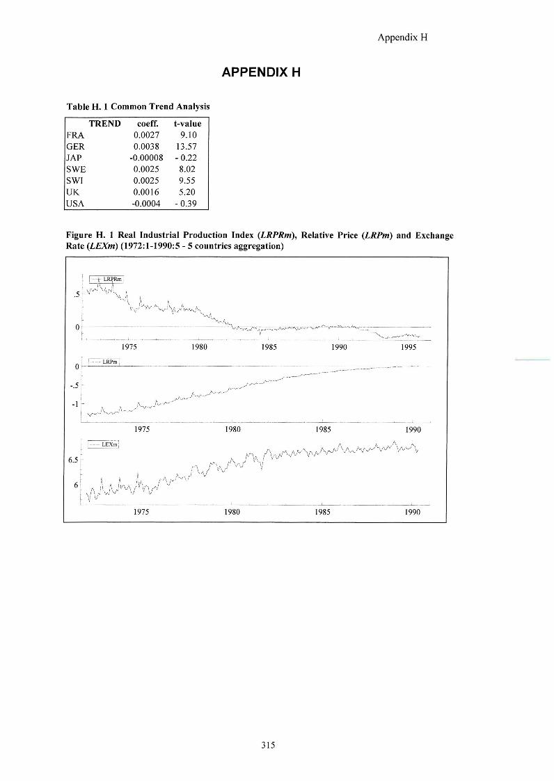
Appendix H

APPENDIX H

Table H. 1 Common Trend Analysis

TREND coeff. t-value FRA 0.0027 9.10 GER 0.0038 13.57 JAP -0.00008 -0.22 SWE 0.0025 8 ^ 0 SWI 0.0025 UK 0.0016 5.20 USA -0.0004 - 0 J 9

Figure H. 1 Real Industrial Production Index (LRPRm), Relative Price {LRPm) and Exchange Rate {LEXm) (1972:1-1990:5 - 5 countries aggregation)

.5 A ^

"vr:v;c:

1975 1980

-1/—

1985 1990 1995

Or

-.5 i-

- 1

,,—J

67

1975

- LEXm

A Av , / '

1975

1980 1985 1990

1980 1985 1990

315

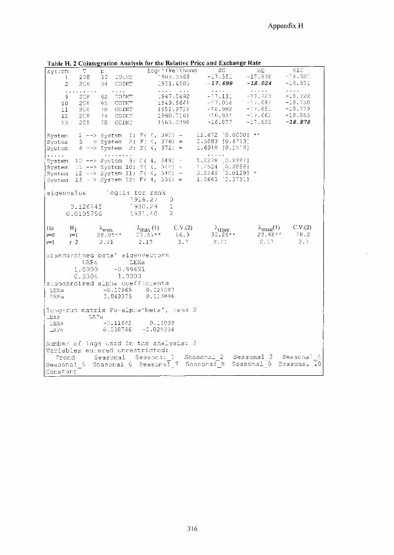
Appendix H

Table H. 2 Cointegration Analysis for the Relative Price and Exchange Rate system T p log-likelihood SC HQ AIC

1 208 30 COIN^ 1905.3568 - 1 7 .551 17.838 -18.321 2 208 34 COIK^ 1931.4005 -17 . 699 18. 024 -18.571

9 208 62 COIK^ 1947.0492 - 1 7 .131 17.723 -18.722 10 208 66 COn^ 1949.9641 - 1 7 .056 17.687 -18.750 11 208 70 COINT 1952.9712 —16 .982 17.651 -18.779 12 208 74 1960.7161 -16 .954 17.661 -18.853 13 208 78 COIN^ 1963.3398 - 1 6 .877 17.622 -18.878

System 2 — > System 1 F 4, 380) = 12.672 [0.0000] System 3 — > System 2 F 4, 376) = 0.5883 [0.6713] System 4 — > System 3 F 4, 372) = 1.6918 [0.1512]

System 10 — > System 9 F( 4, 348) = 1.2278 [0.2987] System 11 — > System 10 F 4, 344) = 1.2524 [0.2886] System 12 — > System 11 F 4, 340) = 3.2246 [0.0129] System 13 — > System 12 F( 4, 336) = 1.0663 [0.3731]

eigenvalue loglik for rank 1916 .27 0

0.126145 1930 .29 1 0.0105796 1931 .40 2

Ho H J ^ max C.V.(2) trace traceO C.V.(2) M ) r=] 28.05** 27. 51** 16.9 30 .26** 29.68** 18.2 r=] r=2 2.21 2 . 17 3.7 2 21 2.17 3 . 7

standardized beta' eigenvectors LRPa LEXa

1.0000 -0.99691 -0.3304 1.0000

standardized alpha coefficients LEXa -0.10969 0.021587 LRPa 0.043375 0.013886

long-run matrix Po=alpha* 3eta', rank 2 LEXa LRPa LEXa -0.11682 0.13093 LRPa 0.038786 - 0.029354

Number of lags used in the analysis: 2

Variables entered unrestricted: Trend Seasonal Seasonal 1 Seasonal 2 Seasonal 3 Seasonal 4

Seasonal 5 Seasonal_6 Seasonal 7 Seasonal 8 Seasonal 9 Seasonal 10 Constant

316

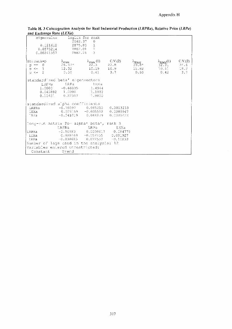
Appendix H

Table H. 3 Cointegration Analysis for Real Industrial Production {LRPRa), Relative Price (LRPa) and Exchange Rate {LEXa)

eigenvalue

0.121612 0.0575214

0.00241357

loglik for rank 2862.37 0 2875.85 1 2882.01 2 2882.26 3

Ho:rank=p p == 0 p < = 1 p < = 2

"max 26.97^ 12.32 0.50

^max (I) 22.3 10.19 0.41

S t a n d a r d i z e d b e t a ' e i g e n v e c t o r s LRPRa LRPa LEXa 1.0000 -0.66035 1.4944 0.045892 1.0000 -1.1082 0.10451 0.22367 1.0000

s t a n d a r d i z e d a l p h a c o e f f i c i e n t s LRPRa -0.10597 -0.065215 LEXa 0.029159 -0.035512 LRPa -0.041019 0.044879

C.V.(2) 23.8 16.9 3.7

'"trace 39.8* 12.82 0.50

32.91 10.61 0.42

C.V.(2) 34.6 18.2 3.7

0.0013233 0.0089947 0.0026422

long-run matrix Po= alpha* beta', rank 3 LRPRa LRPa LEXa

LRPRa -0.10883 0.0050617 -0.084778 LEXa 0.028469 -0.052755 0.091927 LRPa -0.038683 0.072557 -0.10839

Number of lags used in the analysis: 12 Variables entered unrestricted:

Constant Trend

317

Appendix I

APPENDIX I

In this appendix, a detailed account of the specification form adopted in

estimating the real aggregated budget share (LBSm) is given. A non-linear

transformation for the income proxy is considered.

The initial formulation of the equation for the aggregated budget share {LBSm)

is as follows:

JDyLEL*/;, (3% jCJ&SuP/r, jCJ&SjPgr

jT (I.l)

A Box and Cox (1964) procedure has been applied in order to give a statistical

foundation on the choice of the log-linear functional form. Firstly, one tests for the

integration status of the variables expressed in a linear specification, that is: BSm

(aggregated real budget share), (real income proxy), (relative price,

Italy/origin countries), EXa (weighted average exchange rate for origin countries), SPfr

(substitute price, Italy/France), (substitute price, Italy/Greece), (substitute

price, Italy/Portugal) and SPsp (substitute price, Italy/Spain). From applying the ADF,

BSm, SPpo and SPgr have been found to be stationary in the level; whereas, RPRa

57^ and 5 ? ^ are 1(1).

Hence, the Johansen procedure is adopted for testing the existence of possible

cointegration between the relative price (RPa) and exchange rate (EXa). An initial

unrestricted k=13 VAR, which includes a constant, monthly seasonals and a trend

unrestrictedly, can be reduced to a two lag system in accordance with the joint F-test,

SC and HQ criteria. The resulting cointegrating vector for the linear specification is the

following:

IC/ = - 0.0072 E &

The next step consists in running a Johansen cointegration analysis for the

substitute price, as has already been done for the logarithmic specification. The first

analysis is fbr and which are stationary in the level. One would expect

these two series to be stationary also from the Johansen testing. An initial 13 lag

system, including a constant and time trend unrestrictedly, can be reduced to an 11 lag

system. The finding shows that the two economic series are stationary.

118

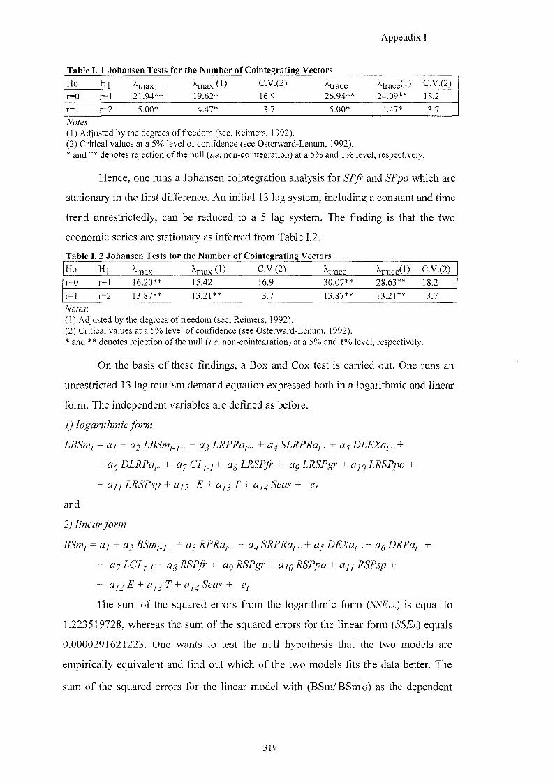
Appendix I

Table I. 1 Johansen Tests for the Number of Cointegrating Vectors

Ho Hi ^max ^max( l ) C.V.(2) ^trace ^trace(l) C.V.(2)

r=0 r=l 21.94** 19.62* 16.9 26.94** 24.09** 18.2

r=l r=2 5.00* 4.47* 3.7 5.00* 4.47* 3.7

(1) Adjusted by the degrees of freedom (see, Reimers, 1992). (2) Critical values at a 5% level of confidence (see Osterward-Lenum, 1992). * and ** denotes rejection of the null {i.e. non-cointegration) at a 5% and 1% level, respectively.

Hence, one runs a Johansen cointegration analysis for SPfr and SPpo which are

stationary in the first difference. An initial 13 lag system, including a constant and time

trend unrestrictedly, can be reduced to a 5 lag system. The finding is that the two

economic series are stationary as inferred from Table 1.2.

Table I. 2 Johansen Tests for the Number of Cointegrating Vectors

Ho Hi ^max ^max (1) C.V.(2) ^race ^trace(') C.V.(2)

r=0 r=l 16.20** 15.42 16.9 30.07** 28.63** 18.2

r=l r=2 13.87** 13.21** 3.7 13.87** 13.21** 3.7

(1) Adjusted by the degrees of freedom (see, Reimers, 1992). (2) Critical values at a 5% level of confidence (see Osterward-Lenum, 1992). * and ** denotes rejection of the null {i.e. non-cointegration) at a 5% and 1% level, respectively.

On the basis of these findings, a Box and Cox test is carried out. One runs an

unrestricted 13 lag tourism demand equation expressed both in a logarithmic and linear

form. The independent variables are defined as before.

7,) ZogarzYA/Mfcybr/M

= a/ +

+ + gy C7 _y+ ag + ap + ayg +

and

Zmear yorm

= A; + ^ 2 . . + +

+ ay ZC/^_y+ ag + ap + a;g + 77 +

+ ay2 ^ i9gaj' +

The sum of the squared errors from the logarithmic form {SSELL) is equal to

1.223519728, whereas the sum of the squared errors for the linear form (SSEL) equals

0.0000291621223. One wants to test the null hypothesis that the two models are

empirically equivalent and find out which of the two models fits the data better. The

sum of the squared errors for the linear model with (BSm/BSmo) as the dependent

119

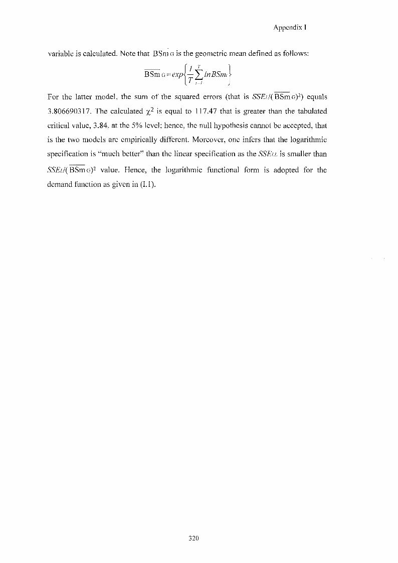
Appendix I

variable is calculated. Note that BSmo is the geometric mean defined as follows:

BSm G = ^

For the latter model, the sum of the squared errors (that is SSEL/{BSmcy) equals

3.806690317. The calculated is equal to 117.47 that is greater than the tabulated

critical value, 3.84, at the 5% level; hence, the null hypothesis cannot be accepted, that

is the two models are empirically different. Moreover, one infers that the logarithmic

specification is "much better" than the linear specification as the SSEu is smaller than

BSm o) value. Hence, the logarithmic functional form is adopted for the

demand function as given in (I.l).

320

References

REFERENCES

Andrews, D.W.K. (1993). "Tests for Parameter Instability and Strutural Change With Unknown Change Point". Econometrica, Vol.61: 821-856.

Arbel, A., and S.A. Ravid (1985). "On Recreation Demand: A Time-Series Approach". Applied Economics, no. 17: 979-990.

Archer, B.H. (1976). Demand Forecasting in Tourism. Occasional Papers in Economics, no.9, Bangor: University of Wales Press.

Artus, J.R. (1972). "An Econometric Analysis of International Travel". IMF Staff Papers, no.19: 579-614.

Ballatori, E., and G. Vaccaro (1992). fZ Zwrfj'/Mo". FrancoAngeli: Milano.

Baloglu, S., and K.W. McCleary (1999). "U.S. International Pleasure Travelers' Images of Four Mediterranean Destinations: A Comparison of Visitors and Nonvisitors". JowrMa/ q/Trove/ 144-152.

Banca D'ltalia (1995). MaMwa/e Bz/ancza &z fagameMrf in Italia. Fonti Statistiche e Metodi di Elaborazione; 7-10.

Banerjee, A., J.J. Dolado, J.W. Galbraith, and D.F. Hendry (1993). Co-Integration, .Error Correcfzon, aW f/ze coMoyMe zcv4»a .yzj' Da/a. Oxford Univerity Press: New York.

Baron, R. (1989). Travel and Tourism Data. Euromonitor Publication Limited: Wiltshire.

Beaulieu, J.J., and J.A. Miron (1993). "Seasonal Unit Roots in Aggregate U.S. Data". Jbwrna/ q/EcoMomefrzca:, no.55: 305-328.

Blackwood & Partners (1994). T fgrvM/e Twrzj'/z 5'/ra»zgrz. ESIT, Cagliari.

Bond, M.E. (1979). "The World Trade Model: Invisibles". International Monetary FwW Aq^T' êr.y, 26: 257-333.

Box, G.E.P., and D.R. Cox (1964). "An Analysis of Transformations". Journal of /Ae 5'fafzj'fzcaZ &rzgj' .8, 26(2): 211- 43.

Caporale, G.M., and N. Pittis (1997). "Unit Root Testing Using Covariates: Some Theory and Evidence." Centre for Economic Forecasting, london Business School, D.P. no. 20-97: 1-31.

321

References

Carraro, C., and M. Manente (1996). "The TRIP and STREP Forecasting Models of Tourism Flows: from World-Wide to Regional Analysis in the Italian Case". FoWozzoMg E/zf Ewfco November: 1-19.

Chow, G.C. (1960). "Tests of Equality Between Sets of Coefficients in Two Regressions". EcoMO/Mefrzca, 28: 591-605.

Chow, G.C. (1967). "Technological Change and the Demand for Computers". The American Economic Review, 57: 1117-1130.

Clauser, O. (1991). "Ruolo della Spesa Promozionale nelle Esportazioni Turistiche Italiane". Politica del Turismo, 2: 19-29.

Confcommercio (1994). II Sistema Turistico nel Nord Sardegna, Sassari.

Contu, G. (1997). Do/MaWa neZ TVbrcf .S'argfggMa e ckz frezzz e Qualitd. Tesi di Laurea in Scienze Politiche, Universita degli Studi di Sassari.

Cooley, T.F., and S.F. LeRoy (1985). "Atheoretical Macroeconometrics. A Critique". Jbwmg/ 16: 283-308.

CRENoS (2000). JZapporfo (/z frevzj'zoMg Centro Ricerche Economiche Nord Sud. Universita degli Studi di Cagliari.

Crouch, G.I. (1994). "The Study of International Tourism Demand: A Survey of Practice". Joz/maZ q/Trm/eZ 32(4): 41-55.

Deaton, A., and J. Muellbauer (1980). "An Almost Ideal Demand System". The American Economic Review, 70(3): 312-326.

D.E.I.S. (1995). m Corj'zca g Universita degli Studi di Sassari.

Delbono, F., and G. Fiorentini (1987). Economia del Turismo. LaNuova Italia Scientifica: Roma.

Di Matteo, L., and R. Di Matteo (1993). "The Determinants of Expenditures by Canadian Visitors to the United States". Joz/rMaZ CyTraweZ 31(4): 34-42.

Dickey, D.A., and W.A. Fuller (1981). "Likelihood Ratio Statistics for Autoregressive Time Series with a Unit Root". Econometrica, 49(4): 1061-1072.

Doomik, J.A., and D.F. Hendry (1996). f C F/MZ, P. 0 - .EcoMomg/rzc Modelling of Dynamic Systems. Institute of Economics and Statistics: University of Oxford.

Doornik, J.A., and D.F. Hendry (1996). PC GIVE 9.0 - Empirical Econometric Modelling Using. International Thomson Business Press: London.

322

References

Dwyer, L., P. Forsyth, and P. Rao (2000). "The Price Competitiveness of Travel and Tourism: a Comparison of 19 Destinations". Tourism Management, 21; 9-22.

Enders, W., and C.W.J. Granger (1998). "Unit-Root Tests and Asymmetric Adjustment With an Example Using the Term Structure of Interest Rates".

JowrnaZ a W EcoMO/Mzc

16(3): 304-311.

Engle, R.E., and C.W.J. Granger (1987). "Co-Integration and Error Correction: Representation, Estimation, and Testing". Econometrica, 55(2): 251-276.

Engle, R.E., D.F. Hendry, and J.F. Richard (1983). "Exogeneity". Econometrica, 51:277-304.

Formica, S., and M. Uysal (1996). "The Revitalization of Italy as a Tourist Destination". Tourism Management, 17(5): 323-331.

Franses, P.H. (1991a). "Model Selection and Seasonality in Time Series". Institute Research Series, Tinbergen, 10: 94-165.

Franses, P.H. (1991b). "Seasonality, Non-Stationarity and the Forecasting of Monthly Time Series". W g r n a / f o M a / 7 : 199-208.

Fujii, E.T, M. Khaled, and J. Mak, (1985). "An Almost Ideal Demand System For Visitor Expenditures". Journal of Transport and Policy, 19: 161-171.

Garcla-Ferrer, A., and R.A. Queralt (1997). "A Note on Forecasting International Tourism Demand in Spain". (/e Ma /rzt/.

Gardini, A. (1984). "La Domanda Turistica, Un'Analisi Econometrica". Politica del 2(1): 179-195.

Garratt, A., K. Lee, M.H. Peresan, and Y. Shin, (1998). "A Long Run Structural Macroeconometric Model of the UK." Unpublished paper : 1-28.

Gonzales, P., and P. Moral (1995). "An Analysis of the International Tourism Demand in Spain". International Journal of Forecasting, 11: 233-251.

Gonzales, P., and P. Moral (1996). "Analysis of Tourism Trends in Spain". Annals of Tbz rM/M 23(4): 739-754.

Granger, C.W.J., and J. Hallman (1991). "Nonlinear Transformations of Integrated Time Series". JbwrMaZ c rz/Me 12(3): 207-224.

Granger, C.W.J., and T.H. Lee (1989). "Investigation of Production, Sales, and Inventory Relationships Using Multicointegration and Non-Symmetric Error-Correction Models". .EcoMO/Mg/rzcj', 4: S145-S159.

Grasselli, P. (1982). Economia e Politica del Turismo. FrancoAngeli: Milano.

323

References

Gray, H.P. (1966). "The Demand for International Travel by the United States and Canada". 7(1): 83-92.

Griffiths, W., R.C. Hill, and G. Judge (1993). Learning and Practising Econometrics . John Wiley and Sons: WE A.

Hamilton, J.D. (1994). Time Series Analysis. Princeton: Princeton University Press.

Hansen, B.E. (1995). "Rethinking the Univariate Approach to Unit Root Testing -Using Covariates to Increase Power". Econometric Theory, 11: 1148-1171.

Hargreaves, C.P. (1994). Tzme New York: Oxford University Press.

Harris, R. (1995). Cointegration Analysis in Econometric Modelling. Prentice Hall and Harvester Wheatsheaf: London.

Hartmann, R. (1986). "Tourism, Seasonality and Social Change". Leisure Studies, 5: 25-33.

Hendry, D.F. (1993). "The Roles of Economic Theory and Econometrics in the Analysis of Economic Time Series". Unpublished paper, Institute of Economics and Statistic, Oxford. Presented to the European Meeting of the Econometric Society, Uppsala, September.

Hendry, D.F. (1995). Dynamic Econometric. New York: Oxford University Press.

Hendry, D.F., and G.E. Mizon (1990). "Procrustean Econometrics: or Stretching and Squeezing Data". Chapter 7 in Granger (ed.) (1990a), S'erzgj.

ZM Oxford: Oxford University Press.

Hendry, D.F., and H-M. Krolzig (1999a). "Computer Automation of General-to-Specific Model Selection Procedures". Discussion Paper, Institute of Economics and Statistics and Nuffield College, Oxford: 1-26.

Hendry, D.F., and H-M. Krolzig (1999b). "Improving on "Data Mining Reconsidered"" by K.D. Hoover and S.J. Perez". EcoMO/Mzc 2: 202-219.

Hoover, K.D., and S.J. Perez (1999). "Data Mining Reconsidered: Encompassing and the General-to-Specific Approach to Specification Search". Econometrics Journal, 2:1-25.

Hylleberg, S., R.F. Engle, C.W.J. Granger, and B.S. Yoo (1990). "Seasonal Integration and Cointegration". Journal of Econometrics, 44: 215-238.

Hylleberg, S., and M. Paldam (1991). TVgyy To Macroeconomics. Cambridge: Blackwell Publishers.

324

References

Johansen, S. (1988) "Statistical Analysis of Cointegration Vectors". JbwfMaZ .ECOMOTMZC aW 12: 231-254.

Johansen, S. (1995). m CofMfegraW Fec/or Autoregressive Models. Oxford: Oxford University Press.

Johansen, S., and K. Juselius (1990). "Maximum Likelihood Estimation and Inference on Cointegration - With Applications to the Demand for Money". Oxford Bulletin

52(2): 169-210.

Kulendran, N. (1995). "Forecasting International Quarterly Tourist Arrivals to Australia with Time-Series Models". Working Papers, Victoria University Melbourne, No.3/95: 1-44.

Kulendran, N., and S.F. Witt (2001). "Cointegration Versus Least Squares Regression". q/'Tbwnj'/M 28(2): 291-311.

Lutkepohl, H. (1991). Introduction to Multiple Time Series Analysis. Berlin: Springer-Verlag.

Lanza, A., and G. Urga (1995). "Tourism Specialisation and Economic Growth: A Cross Country Study Using Multivariate Cointegration". Discussion Paper, LBS, 10:1-17.

Learner, E.E. (1985). "Vector Autoregressions for Causal Inference", in K. Brunner and A. Meltzer (eds.), (supplement to

22: 255-303.

Lee, C., T.Var, and T.W. Blaine (1996). "Determinants of Inbound Tourist Expenditures". Annals of Tourism Research, 23 (3): 527-541.

Lickorish, L.J. (1997). "Travel Statistics - the Slow Move Forward". Tourist 18 (8): 491-497.

Lim, C. (1997). "Review of International Tourism Demand Models". Annals of TowrMTM 24 (4): 835-849.

Lim, C. (1999). "A Meta-Analytic Review of International Tourism Demand". Journal 37: 273-284.

Lim, C. and M. McAleer (2000). "A Seasonal Analysis of Asian Tourist Arrivals to Australia". v 4 ; ? p Z / g G ^ 3 2 : 499-509.

Lim, C. and M. McAleer (2001). "Monthly Seasonal Variations. Asian Tourism to Australia". q/Tbwnj'/M T gj garcA, 28(1): 68-82.

Maddala, G.S. (1992). Introduction to Econometrics. New York: MacMillan Publishing Company 2nd ed..

325

References

Makridakis, S., S.C. Wheelwright, and V.E. McGee (1989). Forecasting: Methods and Applications. New York: Wiley.

Malacami, L. (1991). "Analisi Econometrica della Domanda Turistica in Italia". foZzfzca (/eZ 2: 19-29.

Martin, C.A., and S.F. Witt (1987). "Tourism Demand Forecasting Models; Choice of Appropriate Variable to Represent Tourists Cost of Living". Tourism Management, 8:223-245.

Martin, C.A., and S.F. Witt (1988). "Substitute Prices in Models of Tourism Demand". o/Towrz.yTM 15(2): 255-268.

Martin, C.A., and S.F. Witt (1989). "Forecasting Tourism Demand: a Comparison of the Accuracy of Several Quantitative Methods". International Journal of

5: 7-19.

Masberg, B.A. (1998). "Defining the Tourism: Is it Possible? A View from the Convention and Visitors Bureau". Journal of Travel Research, 37: 67-70.

Mcintosh, R.W., C.R. Goeldner, and J.R.B. Ritchie (1995). Tourism. Principles, Practices, Philosophies. New York: Wiley.

Ministero del Turismo e dello Spettacolo (1995). Sesto Rapporto Sul Turismo Mercury, Firenze.

Mizon, G.E. (1996). "Progressive Modelling of Macroeconomic Time Series - The LSE Methodology", Ch. 4 in Hoover, K.D. (ed) Macroeconometrics. California: Kluwer Academic Publishers.

Nordstrom, J. (1996). "Tourism Satellite Account for Sweden 1992-93". Tourism Economics, 2(1): 13-42.

O'Hagan, J.W., and M.J. Harrison (1984). "Market Shares of US Tourism Expenditure in Europe: an Econometric Analysis". Applied Economics, 16:919-931.

Osterwald-Lenum, M. (1992). "A Note With Quantiles of the Asymptotic Distribution of the Maximum Likelihood Cointegration Rank Test Statistics". Cbc/oT-tf aW 54: 461-472.

Papatheodorou, A. (1999). "The Demand for International Tourism in the Mediterranean Region". iico;70OT/c5, 31: 619-630.

Pesaran, M.H., and B. Pesaran (1997). ivfYA Mzcrq/zf ^.0. O.U.P.

Pindyck, R.S., and D.L. Rubinfeld (1991). Econometric Models and Economic Forecasts. Singapore: International Editions.

326

References

Qiu, H., and J. Zhang (1995). "Determinants of Tourism and Expenditures in Canada". JowmaZ q/'Trave/ 34(2): 43-49.

Quayson, J., and T. Var (1982). "A Tourism Demand Function for the Okanagan, BC". 3: 108-115.

Raeside, R., J. Adams, R. Rush, and K. Haldane (1997). "Modelling and Forecasting Domestic Tourism in Scotland". Paper presented at the 17th International Symposium on Forecasting, Barbados'. 6-11.

Reimers, H.E. (1992). "Comparison of Tests for Multivariate Cointegration". 33: 335-359.

Rugg, D.D. (1973). "The Choice of Journey Destination: A Theoretical and Empirical Analysis". 55(1): 64-71.

Seddighi, H.R., and D.F. Shearing (1997). "The Demand for Tourism in North East England with Special Reference to Northumbria: An Empirical Analysis". Tbwnj'/MMzMagg/MgMf, 18(8): 499-511.

Sheldon, P.J. (1993). "Forecasting Tourism: Expenditure Versus Arrivals". Journal of Travg/ 32: 13-19.

Sims, C.A. (1980). "Macroeconomics and Reality". Econometrica, 48 (1): 1-48; reprinted as Chapter 8 in Granger (ed.) (1990a).

Sinclair, M.T. (1998). "Tourism and Economic Development. A Survey". Journal of 34(5): 1-51.

Sinclair, M.T., and M. Stabler (1997). The Economics of Tourism. Routledge: London and New York.

Smeral, E. (1988). "Tourism Demand, Economic theory, and Econometrics: An Integrated Approach". u/owmaZ q/TrarveZ 26(4): 38-42.

Smith, S.L.J. (1995). Tourism Analysis. Essex: Longman.

Solinas, C. (1992). 77 Mg/ jVbrcf S'ar /ggMa. Fa/w oz/oMg 6/g77'7/? a o Mg/Za ^g.ya no. 99: CERIEC.

Song, H., P. Romilly, and X. Liu (2000). "An Empirical Study of Outbound Tourism Demand in the UK". Applied Economics, 32: 611-624.

Summary, R. (1987). "Estimation of Tourism Demand by Multivariable Regression Analysis: Evidence from Kenya". Tourism Management, 8(4): 317-322.

Syriopoulos, T.C. (1995). "A Dynamic Model of Demand for Mediterranean Tourism". International Review of Applied Economics, 9(3): 318-336.

327

References

Syriopoulos, T.C., and M.T. Sinclair (1993). "An Econometric Study of Tourism Demand: the AIDS Model of US and European Tourism in Mediterranean Countries". 25: 1541-1552.

Tremblay, R. (1989). "Pooling International Tourism in Western Europe". Annals of Tourism Research, 16: 477-491.

Uysal, M., and M.S. El Roubi (1999). "Artificial Neural Networks Versus Multiple Regression in Tourism Demand Analysis". JbwrW 38.T 11-118.

Var, T., G. Mohammad, and O. Icoz (1990). "Factors Affecting International Tourism Demand for Turkey". Annals of Tourism Research, 17 (4): 606-611.

Vogt, G.M., and C. Wittayakorn (1998). "Determinants of the Demand for Thailand's Exports of Tourism". Applied Economics, 30: 711-715.

Webb, R.H. (1995). "Forecasts of Inflation from VAR Models". Journal of Vol. 14: 267-285.

Witt, S., and C.A. Witt (1992). Modelling and Forecasting Demand in Tourism. London: Academic Press.

328

Modelling Demand For Tourism In Italy - ePrints Soton

Documents