FACULTY OF ENGINEERING AND APPLIED SCIENCE DEPARTMENT OF ELECTRONICS AND COMPUTER SCIENCE T/iisiRu/t/TifCDihJ ]:x:)TA/TE:BL]3]L) POWERED MICROSYSTEMS by Peter Glynne-Jones A thesis submitted for the degree of Doctor of Philosophy University of Southampton June 2001

Welcome message from author
This document is posted to help you gain knowledge. Please leave a comment to let me know what you think about it! Share it to your friends and learn new things together.
Transcript
FACULTY OF ENGINEERING AND APPLIED SCIENCE
DEPARTMENT OF ELECTRONICS AND COMPUTER SCIENCE
T/iisiRu/t/TifCDihJ ]:x:)TA/TE:BL]3]L)
POWERED MICROSYSTEMS
by
Peter Glynne-Jones
A thesis submitted for the degree of
Doctor of Philosophy
University of Southampton
June 2001
i i N % T / E R s r T i r ( ) F s c y L n r H L 4 A 4 P T r o ] ^
jAJESisnriRL/icrTr
FACULTY OF ENGINEERING AND APPLIED SCIENCE
DEPARTMENT OF ELECTRONICS AND COMPUTER SCIENCE
Doctor of Philosophy
VIBRATION POWERED GENERATORS FOR SELF-
POWERED MICROSYSTEMS by Peter Glynne-Jones
Methods are examined for deriving energy from vibrations naturally present around sensor systems. Devices of this type are described in the literature as self-powered. This term is defined as describing systems that operate by harnessing ambient energy present within their environment. Traditionally, remote devices have used batteries to supply their energy, which offer only a limited life span to a system. The recent rapid advances in integrated circuit technology have not been matched by similar advances in battery technology, thus, power requirements place important limits on the capability of modem remote microsystems. Self-power offers a potential solution to power requirements, and when combined with some form of wireless communications, can produce truly wireless autonomous systems.
A generator based on the thick-film piezoelectric material, PZT, is produced. The resulting device is tested, and methods are devised to measure the material properties of its constituent layers. Power output is low at only Modelling shows that the low power output is due to the low electromagnetic coupling of thick-film PZT. The modelling includes the development of a new model of a resistively shunted piezoelectric element undergoing pure bending. Numerical optimisation is used to predict the power output from piezoelectric generators of arbitrary dimensions and excitation conditions.
Experiments have been devised to assess the long-term stability of thick film PZT materials. A technique for measuring the ageing rate of the d], and K33 coefficients of a PZT thick-film sample is presented. The d], coefficient is found to age at -4.4% per time decade, and K33, at -1.34% per time decade (PZT-5H).
An electrical equivalent circuit model of a generator based on electromagnetic induction has been described, and verified by producing a prototype generator. The prototype could produce 4.9mW in a volume of 4cm^ at a resonant frequency of 99Hz. A typical configuration is modelled, and numerical methods used to find optimum generator dimensions, and predict power output for various excitations. The model is used to compare this type of generator to piezoelectric generators, and hence evaluate the two technologies. Graphs are produced to permit estimates of how much power could be produced by either generator type under arbitrary excitation conditions. It is concluded that neither generator type is superior under all excitation conditions, but that severe manufacturing difficulties with piezoelectric generators mean that they are unlikely to be commonly used in future applications.
The following points have been identified as the key contributions to knowledge made by this thesis: A thick-film piezoelectric generator has been presented for the first time, and its performance assessed. A simple way of calculating the power that can be produced by a piezoelectric generator has been presented, including a new model of a resistively shunted piezoelectric element undergoing bending. An investigation to measure the previously unquantified long-term stability of thick-film PZT has been described. Idealised generator models have been used to make predictions of how much power can be generated from both piezoelectric and magnet-coil generators for a range of harmonic excitation frequencies and amplitudes. This data has been collected in a graph that permits future designers to simply calculate the most suitable technology for a given application, and to obtain an estimate of how much power can be produced.

To Mum and Dad.

Acknowledgements
I would like to thank Dr. Neil White, my supervisor, for his support and friendship throughout my
studies. The trust and freedom to explore in my own way was really appreciated.
Special thanks to Steve Beeby and Neil Grabham for the many times they have given their time
and support, and to Thomas Papakostas, and Seyed Almodarresi for making the lab a friendly
place to work.
Thanks also to Danny Patrick and Ken Frampton, for their great patience as my many designs
unfolded in their workshop.
This PhD would not have been possible without the many friends who I am lucky enough to have
shared the past three years. In particular, a deep bow to Henry and Jenny for lunch and much
more.

/Ac TMzWfAerg a r e maM}/ poj'j/6zVfYzgj', m /Ae gxperf '^ f/zgre a r e y e w "
Shunryu Suzuki
Contents
Contents
List of Figures 10
List of Tables 13
List of Symbols 14
Glossary of Terms 17
1 Introduction 18
1.1 Thesis Outline 19
2 Self-Powered Systems, A Review 21
2.1 Sources of Power 21
2.1.1 Vibration (Inertia! Generators) 21
2.1.2 Non-inertia! mechanical sources 24
2.1.3 Optical Energy sources 27
2.1.3.1 Solar and Incident Light 27
2.1.3.2 Fibre Optic supplies 28
2.1.4 Thermoelectric and Nuclear Power Sources 28
2.1.5 Radio Power and Magnetic Coupling 29
2.1.6 Battery Energy 30
2.2 Power Management 30
2.3 Systems design 32
2.4 Summary 34
3 Background Material 35
3.1 Transduction Technologies 35
3.1.1 Piezoelectric Materials 35
3.1.1.1 Piezoelectric Notation 36
3.1.1.2 Piezoelectric Materials 38
3.1.2 Electrostrictive Polymers 40
3.1.3 Electromagnetic Induction 42
3.2 Principles of Resonant Vibration Generators 42
3.2.1 First Order Modelling of Generator Structures 42
3.2.2 Placement of Resonant Frequency and Choice of Damping Factor 46
3.2.3 Coupling Energy Into Transduction mechanisms 47
3.3 Power requirements of Vibration-Powered Systems 48
4 Development of a Thick-Film PZT Generator 51
4.1 Introduction to Thick-Film Processes 51
4.1,1 Paste Composition 52
Contents 7
4.1.2 Deposition 52
4.1.3 Drying and firing 53
4.2 Development of Materials, and Processes for Printing Thick-Film PZT on Steel Beams . 54
4.2.1 Choice of Substrate 54
4.2.2 Thermal Mismatch and Substrate Warping 54
4.2.3 Substrate Preparation 55
4.2.4 Chemical Interaction Between PZT layers and Steel substrate 55
4.2.5 Dielectric Layer 55
4.2.6 Electrodes 56
4.2.7 Piezoelectric Layers 56
4.2.7.1 Thick-Film PZT Paste Composition 57
4.2.7.2 Processing the film 57
4.2.7.3 Polarisation 58
4.3 Fabrication of a Test Device 59
4.3.1 Design Criteria 59
4.3.2 Choice of Screens 60
4.3.3 Processing Information 61
4.4 Testing Material Properties 62
4.4.1 Measuring Device Dimensions 62
4.4.2 Dielectric Constants 62
4.4.3 Young's Modulus 63
4.4.4 Measuring the Coefficient of Thick-Film PZT 65
4.4.4.1 Prior Work 66
4.4.4.2 Design of a Direct Measurement System 68
4.4.5 Measuring the d3i Coefficient of Thick-Film PZT 70
4.5 Response of Prototype Tapered Beams 72
4.5.1 Experimental Apparatus 72
4.5.2 Device Performance 77
4.6 Summary 79
5 Modelling Piezoelectric Generators 81
5.1 Approaches to Modelling 82
5.2 Decoupling the Electrical and Mechanical Responses of a Shunted Piezoelectric Element
83
5.3 Model of a Generally Shunted Piezoelectric Beam 86
5.3.1 Introduction 86
5.3.2 Procedure 87
5.3.3 Electrode Voltage 87
Contents 8
5.3.4 Bending Moments 90
5.3.5 Introducing an Electrical Load and Drive Current 91
5.3.6 Resistive Shunting 92
5.3.7 Implications of the Beam Model 95
5.4 Harmonic Response of a Piezoelectric Generator 96
5.4.1 Finite Element Analysis (FEA) 97
5.4.2 The Electrical Energy Available to a Resistive Load 99
5.5 Analysis of a Piezoelectric Generator Beam 99
5.6 Design Considerations for Piezoelectric Generators 104
5.7 Theoretical Limits for inertial generators 105
5.8 Summary 116
6 Ageing Characteristics of Thick-Film PZT 118
6.1 Introduction 118
6.2 Background 118
6.3 Compensation of Charge Amplifier Response 120
6.4 Temporal ageing after polling 121
6.4.1 Experimental procedure 121
6.4.2 Results and Discussion 123
6.5 Ageing caused by cyclic stress 125
6.5.1 Method 126
6.5.2 Results and Discussion 127
6.6 Summary 128
7 Generators based on Electromagnetic Induction 130
7.1 Possible Design Configurations 13 1
7.2 Equivalent circuit model of a generator 134
7.3 Prototype generators 136
7.3.1 Prototype: A 137
7.3.1.1 Results and Discussion 139
7.3.2 Prototypes: B 141
7.3.2.1 Construction 144
7.3.2.2 Testing '45
7.4 Theoretical Limits for electromagnetic generators 151
7.4.1 Magnetic Core Analysis 152
7.4.2 Vertical-coil Configuration 157
7.4.2.1 Analysis 158
7.4.3 Horizontal-coil Configuration 162
7.4.3.1 Finding the optimum generator dimensions 168
Contents 9
7.4.4 Planar Springs ' 6 9
7.4.5 Example Calculations 173
7.5 Producing practical generators 176
7.5.1 Extracting power 176
7.5.2 Micro-devices 176
7.6 Comparison of piezoelectric and magnet-coil generators 178
7.7 Summary ' ^ 0
8 Conclusions and Suggestions for Further Work 181
8.1 Conclusions 181
8.2 Key Contributions made by thesis 184
8.3 Suggestions for Further Work 185
Appendix A: Publications List 187
Appendix B: Finite element programs for thick-film generator analysis 189
Appendix C: The Proportion of Energy Stored in the Piezoelectric Layers of a Composite Beam
198
Appendix D: Optimisation program for piezoelectric generators 200
Function: genpow() 204
Appendix E: Phase Locked Loop (PLL) test circuit 207
Appendix F: Magnetic circuit model 210
Batch File: corex.txt 211
Appendix G: Optimisation program for magnet-coil generators 217
Function: coilpow() 220
Program: beamsize.m 222
Results graphs 224
References 225
10
List of Figures
Figure 1: An electromangnetic vibration-powered generator 21
Figure 2: Generator to produce power from vibrations (after Shearwood [5] ) 22
Figure 3; A non-linear piezoelectric vibration powered generator (after Umeda et al [8]) 23
Figure 4: Principle of operation of the Seiko Kinetics™ watch (after Hayakawa [10]) 24
Figure 5: Communications using a 2-D CCR mirror (after Chu et al [39]) 33
Figure 6: The Polarity of Piezoelectric Voltages from Applied Forces (after Matroc []) 35
Figure 7: Notation of Axes 36
Figure 8: Cubic and Tetragonal forms of BaTiO:, (after Shackleford []) 39
Figure 9: Alignment of dipoles in (a) unpolarised ceramic and (b) polarised ceramic (after Matroc
[44]) 39
Figure 10: Principle of Operation of an Electrostrictive Polymer Actuator (after Kornbluh et al
[50]) 41
Figure 1 1: Model of a Single Degree of Freedom Damped Spring-Mass System 43
Figure 12: Power From a Generator of Unit Mass, Unit Amplitude Excitation, Unit Natural
Frequency 45
Figure 13: The Effect of Damping Factor and Natural Frequency on the Power Generated from
Broadband Excitation 47
Figure 14: The thick-film printing process 53
Figure 15: SEM image of PZT layer with 'river-bed cracking' 58
Figure 16: Design of test device 59
Figure 17: Beam stiffness apparatus 64
Figure 18: Device bending due to negative strain in thick film PZT layer 66
Figure 19: Initial direct dj} measurement rig (after Dargie [65]) 67
Figure 20: Alternating load djs measurement rig (after Dargie [65]) 67
Figure 21: Final testing rig 69
Figure 22: Graph of Charge Displaced Against Amplitude, to Find d], 71
Figure 23: Experimental Set-up 72
Figure 24: Photograph of prototype beam in clamp 75
Figure 25: Sample Clamp Block 75
Figure 26: Shaker, Clamp, and Vernier Gauge Arrangement 76
Figure 27: Mounting a Mass on Samples, Detail 76
Figure 28: Graph of a Typical Resonant Response of a Sample 77
Figure 29: Beam Power Versus Load Resistance for different Beam Amplitudes 78
Figure 30: Load Voltage Versus Beam Amplitude for an Optimally Shunted Beam 78
Figure 31: Energy Flow Diagram for a Resonant PZT Generator 82
Figure 32; A Piezoelectric Element Shunted in the Polarisation Axis, Stressed Along "'1" Axis. .84
Figure 33: Diagram of Beam Undergoing Pure Bending 86
Figure 34: A Symmetrical Sandwich Structure 87
Figure 35: Current Flow for a Shunted PZT Element 91
Figure 36: Graph of Normalised Damping Ratio versus Layer Thickness Ratio, and K-factor 95
Figure 37: Finite Element Mesh Model of Tapered Generator 98
Figure 38: Sequence of Calculations for Calculating the Power from a Piezo-Generator 100
Figure 39: Longitudinal Stress Across the Surface of the PZT Layer, Along Beam Axis
(Deflection = 0.8mm) 102
Figure 40: Longitudinal Stress Across the Surface of the PZT Layer, Along Beam Root
(Deflection - 0.8mm) 102
Figure 41: Experimental and Predicted Values for Generator Power Output (error bars show
potential error in model) 103
Figure 42: The Relationship Between Beam Amplitude, and Load Voltage 104
Figure 43: Simplified Inertial Generator 106
Figure 44: Strain energy of a generator beam versus internal dimensions 108
Figure 45: Energy Density for Generator of Optimal Dimensions Versus Enclosure Size 110
Figure 46: Splitting a Generator into Partitions to Increase Energy Density 110
Figure 47: Predicted generator power 115
Figure 48: Parameters that lead to optimum PZT generators 116
Figure 49: Compensation of charge amplifiers 120
Figure 50: Graph of normalised d31 versus time after polarisation 124
Figure 51: Graph of dg, response versus time without compensation 125
Figure 52: Graph of normalised k)] versus time after polarisation 125
Figure 53: Ageing of response of a sample with amplitude 0.51 mm 128
Figure 54: Typical generator configurations 131
Figure 55: Magnetic circuit configurations 132
Figure 56: Schematic diagram of a magnet-coil generator 134
Figure 57: Free body diagram of generator mass relative to enclosure 135
Figure 58: Generator equivalent circuits 135
Figure 59: Prototype generator A 138
Figure 60: Coil voltage versus vibration amplitude, prototype A 139
Figure 61: Power versus load voltage, Base amplitude=4.4p.m, prototype A 140
Figure 62: Power versus vibration amplitude with optimum load resistance, prototype A 140
Figure 63: Designs for prototypes Bl , B2 and B3 142
Figure 64: Photographs of generator 8 2 143
12
Figure 65: Photochemically etched steel beam designs 145
Figure 66: Q-factor test circuit !47
Figure 67: Coil voltage versus beam amplitude, prototype B 149
Figure 68: Power versus load resistance, beam B1 150
Figure 69: Demonstrator power during a driving trip 151
Figure 70: Magnetic core design 152
Figure 71: FEA model of magnetic core 153
Figure 72: The effects of varying core parameters 154
Figure 73: Optimum core design (dimensionless, to scale) 155
Figure 74: Field pattern for optimum core design 156
Figure 75: Vertical-coil generator configuration 157
Figure 76: Vertical-coil equivalent circuit 159
Figure 77: Horizontal-coil generator configuration 162
Figure 78: Coil positions relative to core 164
Figure 79: Graph of the function A(U„A) 166
Figure 80: Visualisation of part of the optimisation space 169
Figure 81: Tapered spring (model) 171
Figure 82: Tapered spring (example) 171
Figure 83: Comparison of magnet-coil and piezoelectric generators 178
Figure 84: Comparison of magnet-coil and piezoelectric generators (repeated) 184
Figure 85: A composite PZT beam 198
Figure 86: PLL block diagram 208
Figure 87: Phase detector circuit 208
Figure 88: Loop filter circuit 209
Figure 89: VCO circuit 209
Figure 90: Internal dimensions of optimum horizontal-coil generators 224
List of Tables
Table 1: Comparisons of common energy sources after Starner [13] 25
Table 2: Energy density of storage mediums (after Koeneman g/ a/ [1 I]) 31
Table 3: Comparing Piezoelectric Materials 40
Table 4: Test device dimensions 60
Table 5: Screen Parameters 61
Table 6: Young's Modulus of device materials 65
Table 7: Summary of PZT material properties 79
Table 8: Bending modes of Test Beam 101
Table 9: Example application excitations 112
Table 10: Piezoelectric model parameters 112
Table 11: Predicted power output for a range of practical applications 113
Table 12: Ageing processes (after Jaffe et al [43]) 1 19
Table \ 3: ageing rates of samples 124
Table 14: ageing rates of samples 124
Table 15: Beam amplitudes for ageing experiment 127
Table 16: Stress induced ageing of samples 128
Table 17: Electromagnetic inertia! generators to date 130
Table 18: Equivalent circuit model mapping 136
Table 19: Equivalent circuit parameters 136
Table 20: prototypes B dimensions 144
Table 21: Prototype parameters 146
Table 22: Prototype Q-factors 148
Table 23: Magnetic field values 149
Table 24: Prototype power results 150
Table 25: Optimum core dimensions 156
Table 26: Model parameters 173
Table 27: Applying magnet-coil models to sample applications 175
Table 28: Component values 209

14
List of Symbols
General Symbols
CO
A
A
8
n p
Abound
Ptree
Pvoiume
X
a
P
£
Go
Cl
C O , ,
V
Y
Cfi)b
( YI)complex
A
b
B
diagonal matrix of clamped susceptibility
permittivity in the 3 direction, of a material clamped in the 1 direction
damping factor / damping ratio
circular frequency
a non dimensional function
deflection
logarithmic decrement
loss factor
non-dimensional frequency, density, radius of curvature
area bound charge density
area free charge density
volume charge density inside dielectric
inverse of radius of curvature
ratio of the layer thickness to the distance from the neutral axis to the centre
of the layer, base excitation amplitude
ratio of gap to core width
permittivity
permittivity of free space
electrical damping factor
unwanted / lossy damping factor
natural circular frequency
matrix of un-clamped permittivity
relates to the amount of magnetic energy stored per core volume
the value of ijVmax
real bending stiffness
complex bending stiffness
area, amplitude, maximum beam deflection
width
constant based on layer thickness, magnetic flux density

15
c viscous damping coefficient, the distance of the outer surface of a beam
from its neutral axis
Cjj elements of stiffness matrix
C capacitance
clamped capacitance
D vector of electrical displacements, average core density
d piezoelectric constant matrix
d height of piezoelectric layer
effective d3]
dij element of piezoelectric constant matrix
E vector of electrical field
Eden.a energy density in actuation
Eden.g energy density in generation
E,„ peak value of elastic energy
F force
f frequency
F|, F2 frequencies
F force
f„ natural frequency
g gap width
h height
H height
I second moment of area, current
k spring constant
K frequency amplitude density, constant based on degree of electromechanical
coupling, ageing constant
kij electromechanical coupling coefficient, constants
Kij constants, dielectric constant
I length
L length, inductance
m mass
M moment
N number of cycles, number of coil windings
P electrical power, pressure
P vector of electric polarisation
Pp electrical power

16
Pe res electrical power at resonance
Q charge
R resistance
R' normalised load resistance
Rsu shunting resistance
S vector of material engineering strains
s stiffness matrix
s Laplace complex frequency variable
Sij element of stiffness matrix
T vector of material stresses, stress, depth
T' stress at beam surface
t thickness
Tc coefficient of thermal expansion
T|„aN maximum rated stress
U Maximum strain energy
V voltage
V velocity
W width
W„ amplitude of nth cycle
W j electrical energy produced per cycle
X displacement of coil
y position variable
V modulus of elasticity
y(t) base excitation
Yo amplitude of base excitation
Yb distance from neutral surface to bottom of PZT layer
y„ distance to the centre of the piezoelectric layer from the neutral surface.
Ysu shunting admittance
y, distance from neutral surface to top of PZT layer
z(t) beam displacement relative to enclosure
Zmax maximum possible beam amplitude
complex mechanical impedance
Mathematical Symbols
()'^ open circuit boundary conditions
17
( f
( ) '
O t
( f
bold
j
ln()
logO
short circuit boundary conditions
clamped boundary conditions
matrix transpose
un-clamped boundary conditions
Laplace transform of variable, Matrix / vector
natural logarithm
decadic logarithm
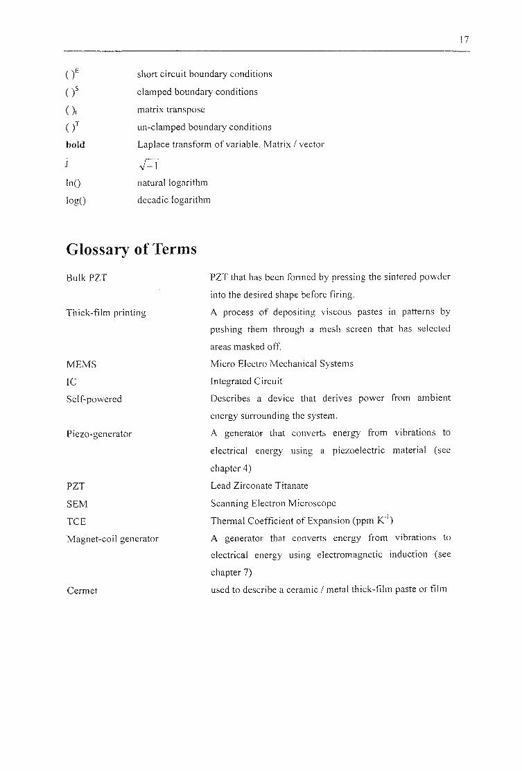
Glossary of Terms
B u ^ P Z T
Thick-film printing
MEMS
IC
Self-powered
Piezo-generator
PZT
SEM
TCE
Magnet-coil generator
Cermet
PZT that has been formed by pressing the sintered powder
into the desired shape before firing.
A process of depositing viscous pastes in patterns by
pushing them through a mesh screen that has selected
areas masked off.
Micro Electro Mechanical Systems
Integrated Circuit
Describes a device that derives power from ambient
energy surrounding the system.
A generator that converts energy from vibrations to
electrical energy using a piezoelectric material (see
chapter 4)
Lead Zircon ate Titanate
Scanning Electron Microscope
Thermal Coefficient of Expansion (ppm K"')
A generator that converts energy from vibrations to
electrical energy using electromagnetic induction (see
chapter 7)
used to describe a ceramic / metal thick-film paste or film
Introduction 18
(CHAPTER I
Introduction
This thesis examines power sources for devices that are often described in the literature as 'self-
powered'. In particular, there is a focus on methods for deriving energy from vibrations naturally
present around sensor systems.
The term self-powered is confusing, and brings to mind perpetual-motion type systems that
somehow defy the first law of thermodynamics. To avoid ambiguity, self-powered systems are
defined here as those that operate by harnessing ambient energy present within their environment.
Power sources of this type are also described as micro power supplies, and self-sufficient power
supplies in the literature. Possible sources of ambient energy include vibration, solar energy, and
temperature difference. They are comparable, if at a smaller scale, to sources of alternative
energy such as wind, wave, and geothermal power.
Self-powered systems have several potential advantages over more conventional alternatives. As
Micro Electro Mechanical Systems (MEMS) become cheaper and more widespread, the cost of
connecting sensors to both power supplies and communications links will become a more
dominant factor. For a high unit-cost system such as a hard drive head this is not an issue, but
there is a trend towards distributed sensor systems utilising several orders of magnitude more
sensors than currently used. Such systems have the advantage of higher reliability, and the ability
to compensate for the peculiarities of any single sensor through data fusion. The drawback is the
need to connect and power all the devices. Appropriate power supplies are also difficult to
engineer in systems that are physically some distance from normal power sources, or in
inaccessible places. Examples include systems on buildings, aircraft structures, and inside of
large machinery.
Traditionally, remote devices have used batteries to supply their energy, which offer only a
limited life span to a system. The recent rapid advances in integrated circuit technology have not
been matched by similar advances in battery technology. Thus, power requirements place
important limits on the capability of modern remote microsystems. Self-power offers a potential
!. Introduction 19
solution to power requirements, and when combined with some form of wireless communications,
can produce truly wireless autonomous systems.
As the literature review chapter will reveal, self-power is not a new area of study; the first self-
winding watch was built by Abraham-Louis Perrelet in 1770 [1], Interest in self-power is
currently growing rapidly with several sessions dedicated to the subject in recent international
conferences [2]. Technologies vary in the level of research undertaken to date. Solar power is a
particularly mature and well characterised technology, while vibration powered devices by
comparison have attracted little interest. No existing studies survey different techniques for
extracting power from vibrations, or permit a comparison of techniques. Neither have simple
models or graphs been produced to enable designers to predict how much power might be
produced from a given vibration source by a practical generator. This thesis fills these gaps, and
sets out to form a sound basis for future vibration-powered applications.
1.1 Thesis Outline
Chapter 2 reviews existing power sources for self-powered systems, and describes some of the
many applications that have been explored. It concludes with a description of some other current
research projects in this area.
Chapter 3 introduces possible transduction technologies that may be used in vibration powered
generators, including piezoelectric and electrostrictive materials, and electromagnetic induction.
A simple first order model of a generic resonant vibration generator is presented and some of its
implications explored. The question of how much power a generator needs to produce to be
considered 'useful' is addressed.
Chapter 4 describes the development of a thick-film PZT generator. It includes fabrication details
and discussion of technical problems. The resulting device is tested, and methods are devised to
measure the material properties of its constituent layers.
Chapter 5 develops a method for modelling the response of piezoelectric generators. It includes
the development of a new model of a resistively shunted piezoelectric element undergoing pure
bending. The model is supported by experimental results. The model is used in conjunction with
numerical methods to find optimum generator dimensions, and predict power output for a range of
excitations that might be found in practice.
Chapter 6 investigates the long-term stability of thick film PZT materials. In particular,
experimental techniques are developed to measure the ageing rate of the dn and coefficients.
Introduction 20
Chapter 7 explores generators based on electromagnetic induction. Typical design configurations
are examined. An electrical equivalent circuit model is described, and verified by producing a
prototype generator. A demonstrator mounted on a car engine block is shown to produce a useful
amount of power. A typical configuration is modelled, and numerical methods used to find
optimum generator dimensions, and predict power output for various excitations. The model is
used to compare this type of generator to piezoelectric generators, and hence evaluate the two
technologies.
Chapter 8 presents conclusions, drawing out the main points established by the thesis and
discusses possible directions for further work.
2. Self-Powered Systems, A Review 21
CHAPTER 2
Self-Powered Systems, A Review
The first small-scale self-powered device was the self-winding watch, built by Abraham-Louis
Perrelet in 1770 [1]. It is only recently, however, that other self-powered devices have become
feasible thanks to the revolution in integrated circuit design. Interest in self-power is currently
growing rapidly with several sessions dedicated to the subject in recent international conferences
[2], To date, no review of this subject has been published (although this chapter has now been
published, see appendix A). This chapter draws together a range of work that focuses on
alternative sources of energy suitable for small portable or embeddable systems, and examines
some integrated systems.
2.1 Sources of Power
2.1.1 Vibration (Inertial Generators)
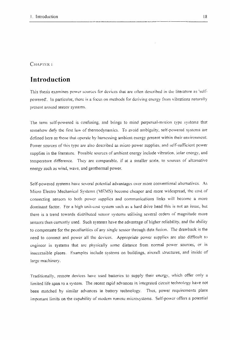
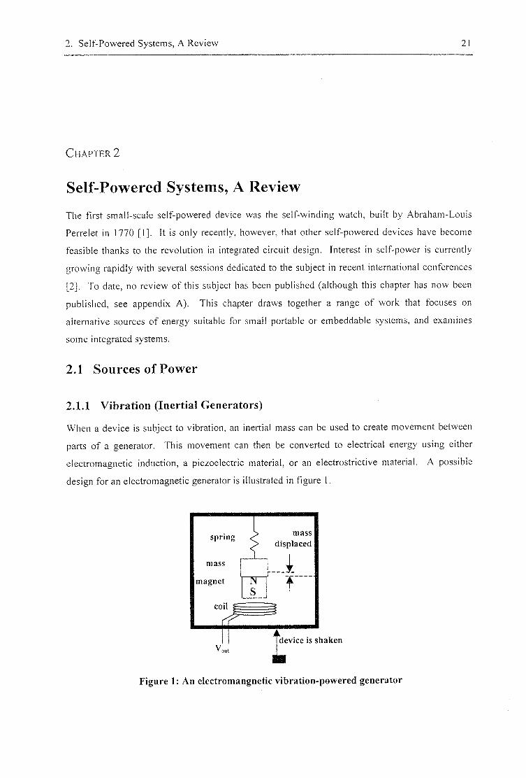
When a device is subject to vibration, an inertial mass can be used to create movement between
parts of a generator. This movement can then be converted to electrical energy using either
electromagnetic induction, a piezoelectric material, or an electrostrictive material. A possible
design for an electromagnetic generator is illustrated in figure 1.
spring
mass
magnet
coil
T T S
mass displaced
T "
Fdevice is shaken
Figure 1: An electromangnetic vibration-powered generator
2. Self-Powered Systems, A Review
Williams and Yates [3] make predictions for this type of generator by applying a standard damped
spring mass model (as described in section 3.2) to this type of device. Using this model they
predict how much power could be generated in a given volume for a number of different
excitation amplitudes, and excitation frequencies. The predictions are based on a fixed damping
factor, and are thus not optimum values; also, no account is taken of whether a practical generator
could be produced to meet the model parameters chosen.
In another paper [4], Williams et al consider how much power could be generated from the
vibrations induced in road bridges by passing traffic to enable the remote detection of bridge
condition. The results showed that relatively large devices of volume 1000cm'' and 1 kg mass
would be required to produce power in the range 50-500|.iW, Scaling the figures to the
dimensions typically found in microsystems, only nW would be produced for these types of
vibrations.
25mm
550nm
PkmarAucoM
400 im
Figure 2: Generator to produce power from vibrations (after Shearvvood [5] )
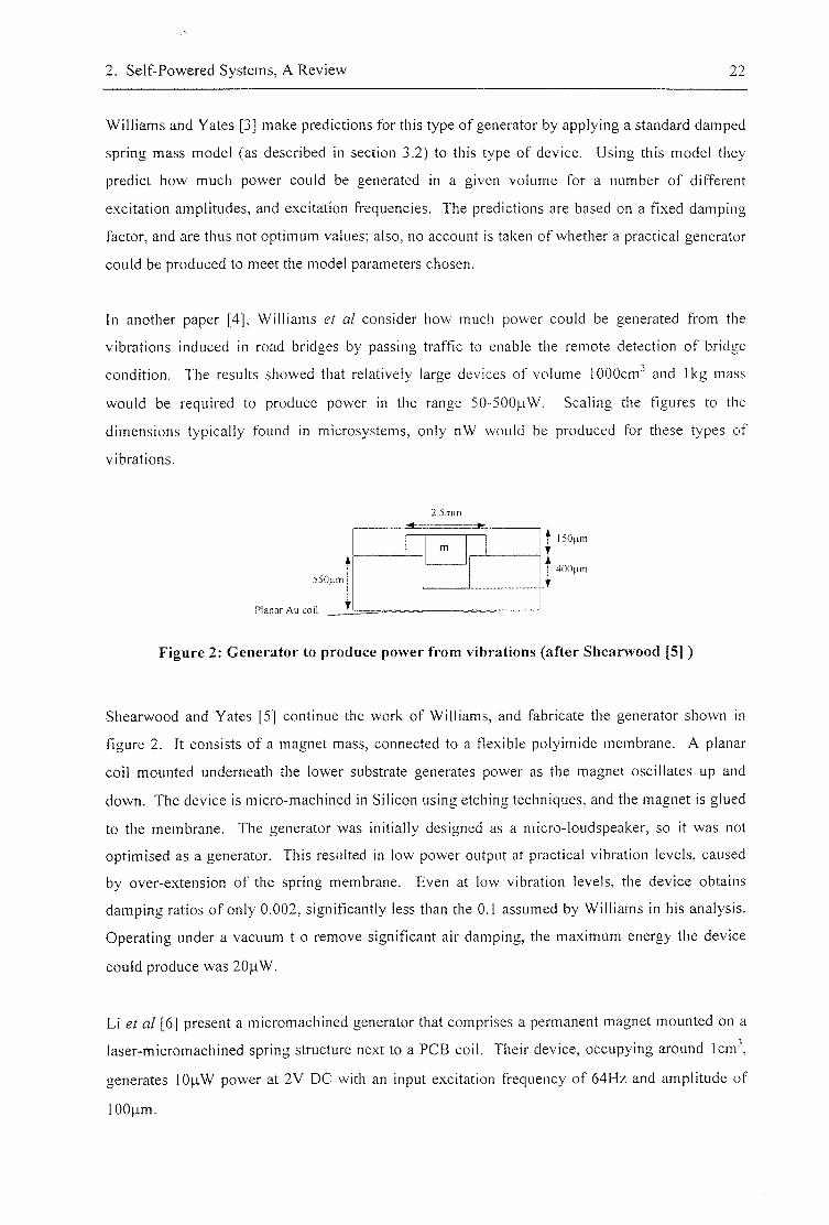
Shearwood and Yates [5] continue the work of Williams, and fabricate the generator shown in
figure 2. It consists of a magnet mass, connected to a flexible polyimide membrane. A planar
coil mounted underneath the lower substrate generates power as the magnet oscillates up and
down. The device is micro-machined in Silicon using etching techniques, and the magnet is glued
to the membrane. The generator was initially designed as a micro-loudspeaker, so it was not
optimised as a generator. This resulted in low power output at practical vibration levels, caused
by over-extension of the spring membrane. Even at low vibration levels, the device obtains
damping ratios of only 0.002, significantly less than the 0.1 assumed by Williams in his analysis.
Operating under a vacuum t o remove significant air damping, the maximum energy the device
could produce was 20)iW.
Li et al [6] present a micromachined generator that comprises a permanent magnet mounted on a
laser-micromachined spring structure next to a PCB coil. Their device, occupying around 1cm',
generates lOjiW power at 2V DC with an input excitation frequency of 64Hz and amplitude of
100p.m.
2. Self-Powered Systems, A Review 23
A macro-sized device (500mg mass) of a similar design is constructed by Amirtharajah and
Chandrakasan [7]. The device is designed to work from vibrations induced by human walking,
and is predicted to produce 400p,W of power. A sophisticated low-power signal-processing
system is connected to the generator, and shown to perform 11000 cycles of operation from a
single impulse excitation.
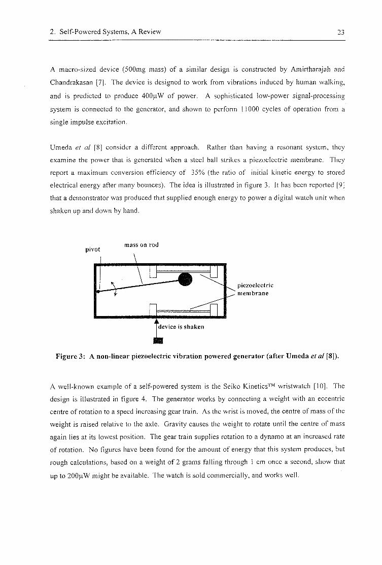
Umeda et al [8] consider a different approach. Rather than having a resonant system, they
examine the power that is generated when a steel ball strikes a piezoelectric membrane. They
report a maximum conversion efficiency of 35% (the ratio of initial kinetic energy to stored
electrical energy after many bounces). The idea is illustrated in figure 3. It has been reported [9]
that a demonstrator was produced that supplied enough energy to power a digital watch unit when
shaken up and down by hand.
pivot mass on rod
device is shaken
piezoelectric membrane
Figure 3: A non-linear piezoelectric vibration powered generator (after Umeda et al [8]).
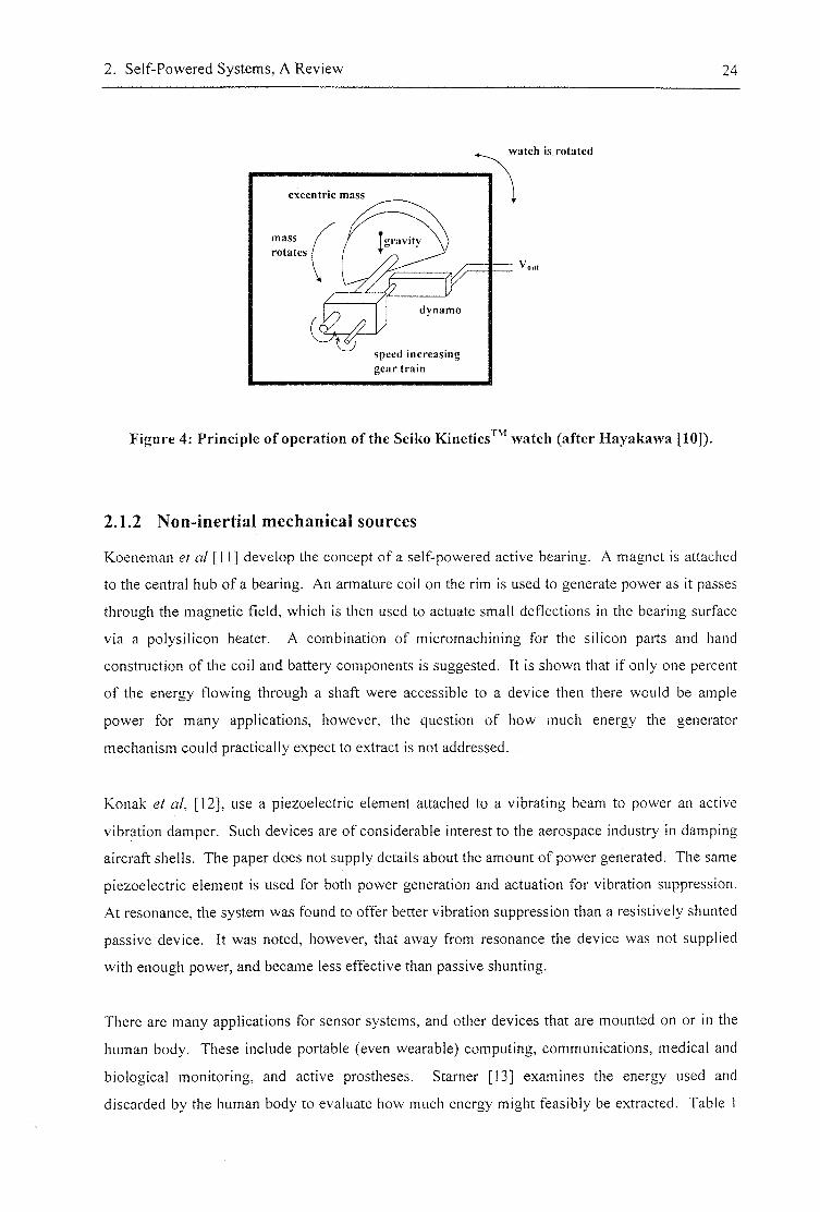
A well-known example of a self-powered system is the Seiko Kinetics''"'^ wristwatch [10]. The
design is illustrated in figure 4. The generator works by connecting a weight with an eccentric
centre of rotation to a speed increasing gear train. As the wrist is moved, the centre of mass of the
weight is raised relative to the axle. Gravity causes the weight to rotate until the centre of mass
again lies at its lowest position. The gear train supplies rotation to a dynamo at an increased rate
of rotation. No figures have been found for the amount of energy that this system produces, but
rough calculations, based on a weight of 2 grams falling through 1 cm once a second, show that
up to 200p.W might be available. The watch is sold commercially, and works well.
2. Self-Powered Systems, A Review 24
excentnc mass
mass gravity rotates
dynamo
watch is rotated
speed increasing gear tnun
Figure 4: Principle of operation of the Seiko Kinetics^^' watch (after Hayakawa [10])
2.1.2 Non-inertial mechanical sources
Koeneman et al [11] develop the concept of a self-powered active bearing. A magnet is attached
to the central hub of a bearing. An armature coil on the rim is used to generate power as it passes
through the magnetic field, which is then used to actuate small deflections in the bearing surface
via a polysilicon heater. A combination of micromachining for the silicon parts and hand
construction of the coil and battery components is suggested. It is shown that if only one percent
of the energy flowing through a shaft were accessible to a device then there would be ample
power for many applications, however, the question of how much energy the generator
mechanism could practically expect to extract is not addressed.
Konak et al, [12], use a piezoelectric element attached to a vibrating beam to power an active
vibration damper. Such devices are of considerable interest to the aerospace industry in damping
aircraft shells. The paper does not supply details about the amount of power generated. The same
piezoelectric element is used for both power generation and actuation for vibration suppression.
At resonance, the system was found to offer better vibration suppression than a resistively shunted
passive device. It was noted, however, that away from resonance the device was not supplied
with enough power, and became less effective than passive shunting.
There are many applications for sensor systems, and other devices that are mounted on or in the
human body. These include portable (even wearable) computing, communications, medical and
biological monitoring, and active prostheses. Stamer [13] examines the energy used and
discarded by the human body to evaluate how much energy might feasibly be extracted. Table 1
2. Self-Powered Systems, A Review 25
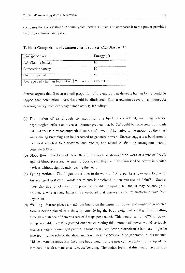
compares the energy stored in some typical power sources, and compares it to ttie power provided
by a typical human daily diet.
Table 1: Comparisons of common energy sources after Starner [13]
Energy Source Energy (J)
AA alkaline battery 10"
Camcorder battery 10'
One litre petrol 10'
Average daily human food intake (2500kcal) 1.05 X 10'
Stamer argues that if even a small proportion of the energy that drives a human being could be
tapped, then conventional batteries could be eliminated. Starner examines several techniques for
deriving energy from everyday human activity including;
(a) The motion of air through the mouth of a subject is considered, including adverse
physiological effects on the user. Starner predicts that 0.40W could be recovered, but points
out that this is a rather unpractical source of power. Alternatively, the motion of the chest
walls during breathing can be harnessed to generate power. Starner suggests a band around
the chest attached to a flywheel and ratchet, and calculates that this arrangement could
generate 0.42W.
(b) Blood flow. The flow of blood through the aorta is shown to do work at a rate of 0.93W
against blood pressure. A small proportion of this could be harnessed to power implanted
devices without significantly loading the heart.
(c) Typing motions. The fingers are shown to do work of 1.3mJ per keystroke on a keyboard.
An average typist of 40 words per minute is predicted to generate around 6.9mW. Starner
notes that this is not enough to power a portable computer, but that it may be enough to
produce a wireless and battery free keyboard that derives its communications power from
keystrokes.
(d) Walking. Starner places a maximum bound on the amount of power that might be generated
from a device placed in a shoe, by considering the body weight of a 68kg subject falling
through a distance of 5cm at a rate of 2 steps per second. This would result in 67W of power
being available, but it is pointed out that extracting this amount of power would seriously
interfere with a normal gait pattern. Starner considers how a piezoelectric laminate might be
inserted into the sole of the shoe, and concludes that 5W could be generated in this manner.
This estimate assumes that the entire body weight of the user can be applied to the tip of the
laminate in such a manner as to cause bending. The author feels that this would have serious
2. Self-Powered Systems, A Review 26
effect on the gait of the user, and is thus an overestimate of the power that might be produced.
Stamer also considers a rotary electromagnetic generator mounted in the heel of a shoe. A
typical running shoe is shown to only return 50 percent of the energy stored in the heel
material, so a generator that extracted a similar amount of power would not interfere with the
gait. Starrier thus concludes that taking into account the efficiency of a generator, 8.4Wcould
be generated. This estimate, however, is based on the assumption above that the body falls
5cm with each step; this may be true of the feet, but the centre of mass of the body rises less
than a centimetre with each step. Thus, the author feels that 8.4W is an overestimate,
(e) Body heat: Discussed below.
Other workers have considered shoe-based generators. Chen holds a patent [14] for a simple heel
mounted generator that uses a speed increasing gear train to transfer the motion of a pivot plate in
the heel to a dynamo. Another patent [15] describes an elaborate design for a rotary generator
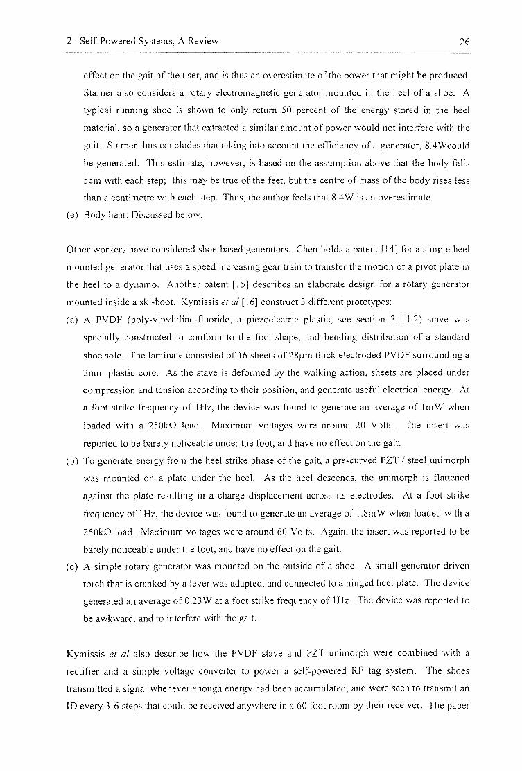
mounted inside a ski-boot. Kymissis et a/ [16] construct 3 different prototypes:
(a) A PVDF (poly-vinylidine-fluoride, a piezoelectric plastic, see section 3.1.1.2) stave was
specially constructed to conform to the foot-shape, and bending distribution of a standard
shoe sole. The laminate consisted of 16 sheets of 28p.m thick electroded PVDF surrounding a
2mm plastic core. As the stave is deformed by the walking action, sheets are placed under
compression and tension according to their position, and generate useful electrical energy. At
a foot strike frequency of IHz, the device was found to generate an average of I m W when
loaded with a 2 5 0 k 0 load. Maximum voltages were around 20 Volts. The insert was
reported to be barely noticeable under the foot, and have no effect on the gait.
(b) To generate energy from the heel strike phase of the gait, a pre-curved PZT / steel unimorph
was mounted on a plate under the heel. As the heel descends, the unimorph is flattened
against the plate resulting in a charge displacement across its electrodes. At a foot strike
frequency of I Hz, the device was found to generate an average of 1.8mW when loaded with a
250kQ load. Maximum voltages were around 60 Volts. Again, the insert was reported to be
barely noticeable under the foot, and have no effect on the gait.
(c) A simple rotary generator was mounted on the outside of a shoe. A small generator driven
torch that is cranked by a lever was adapted, and connected to a hinged heel plate. The device
generated an average of 0.23W at a foot strike frequency of 1 Hz. The device was reported to
be awkward, and to interfere with the gait.
Kymissis et al also describe how the PVDF stave and PZT unimorph were combined with a
rectifier and a simple voltage converter to power a self-powered RF tag system. The shoes
transmitted a signal whenever enough energy had been accumulated, and were seen to transmit an
ID every 3-6 steps that could be received anywhere in a 60 foot room by their receiver. The paper
2. Self-Powered Systems, A Review 27
is a proof of concept paper, and its authors predict that significant improvements in generated
power are possible.
Hausler and Stein [17] propose generating power from the motions that occur between the ribs
during breathing. They construct a device that consists of a roll of PVDF material that is attached
at each end to different ribs. As breathing occurs the tube is stretched and generates power. The
device was surgically implanted in a mongrel dog. Spontaneous breathing resulted in an average
power of only a few microwatts. The author questions whether it is ethical to perform such an
experiment, when the poor results could easily be predicted by theory, and no significant
improvements in surgical technique are derived. They predict that if the coupling factor of the
PVDF film were increased by materials research to 0.3 (a rather optimistic increase of around
300%) then the device could produce up to ImW.
The well publicised windup radio invented by Trevor Bay I is [18] is a familiar self powered
device. The design was motivated by a desire to provide battery free radio reception to
disseminate advice on the prevention of AIDS in Africa. Users wind a spring using a crank-
handle; the energy from the spring is fed via a speed increasing gear chain to a dynamo. The
radio is reported to run for 30 minutes from a full wind that takes 30 seconds to perform.
A novel power system for active bullets has been described by Segal and Bran sky [19]. The
generator consists of a piezoelectric disc connected to an inertial mass mounted inside a bullet.
As the bullet is fired the acceleration causes the mass to compress the disc and displace charge
between the PZT's electrodes; this charge is fed onto a capacitor by a rectifier. A bullet fired with
an acceleration of 4.9xl0'ms"^ and muzzle velocity of 1.4kms"' (typical of a powder charge)
caused 0.19J to be stored on the capacitor.
2.1.3 Optical Energy sources
2 J. y
Solar cells are a mature and well characterised technology. Solar self-powered devices such as
calculators and watches are commonplace. Lee et al [20] develop a thin film solar cell
specifically designed to produce the open circuit voltages required to supply MEMS electrostatic
actuators. The array consists of 100 single solar cells connected in series, occupying a total area
of only l c m \ By connecting the array to a micro-mirror, a microsystem is produced that responds
to modulation of the applied light.
2. Self-Powered Systems, A Review 28
Calculations by van der Woerd et a/ [21] show that under incandescent lighting situations, an area
of 1cm- will generate around 60|iW of power. A prototype solar power directional hearing aid
was integrated into a pair of spectacles. With solar cells, as the light intensity varies the solar cell
voltage also fluctuates. This problem was overcome by producing a power converter integrated
circuit.
2 .7 . .3.2 6'
Systems operate on electrical power generated from light will be examined here, rather than the
more familiar distributed, all optical sensors
Ross [22] delivers optical power to a remote system with an optical fibre. The light is converted
to electrical power by a photocell, and voltage converters are used to produce a useful voltage.
With a GaAs photocell an overall efOciency (both optical to electrical and voltage conversion) of
around 14% is predicted. Typically, 4mW is injected into the fibre by the laser, but, at a price, up
to IW can be applied. This results in typically O.SmW of power being available for sensing.
Information in this case is transmitted back via a separate fibre, although other studies [23] have
discussed using the same fibre for both power, and duplex information transmission. See also
Gross [24].
Connecting systems by optical fibre has several advantages over more conventional wired
systems:
(a) Owing to the wide bandwidth of optical fibres, a large number of devices can be connected to
the same fibre, reducing large amounts of wiring.
(b) Optical fibres neither send nor receive electromagnetic energy, so they are free from EMI.
(c) The low powers involved means that the system is ideal for applications where low power is a
safety requirement. See Kuntz and Mores [23], for a discussion of this topic. (Al-Mohandi et
a/ [25] found that energy stored in the inductors of certain power converters can compromise
this safety though, by causing a spark hazard)
(d) Electrical isolation enables operation in areas of high electromagnetic fields
The disadvantages of this technology over the other power sources discussed here, is that the
system is still not truly wireless, however, the power generated from the light is of an order of
magnitude higher than solar power, and thus forms an important source of power.
2.1.4 Thermoelectric and Nuclear Power Sources
Temperature differences can be exploited to generate power. Unless the temperature difference is
large, the low efficiency of this type of conversion means that very little power can be extracted.
2. Self-Powered Systems, A Review 29
Stamer [13], calculates the amount of energy that could be extracted from the skin temperature of
a human being. The temperature difference between the skin and the surrounding atmosphere
drives a flow of heat energy that could be captured. Using a simple model, Stamer predicts that
2.4-4.8W of electrical power could be obtained if the entire body surface were covered. Noting
the restrictive nature of a full body suit, it is predicted that a neck covering device should have
access to a maximum of 0.20-0.32W.
Thermoelectric power has found applications in cardiac pacemakers. Renner et al [26] describe a
pacemaker that uses a radioactive plutonium source to generate heat. A thermocouple array is
used to convert this into useful electrical energy. The device could supply up to 180p,W power.
"The nuclear pacemaker program was discontinued some 20 years ago, hindered by bureaucratic
obstacles, and superseded by the lithium battery" [27]
More recently, Stordeur and Stark [28] have developed a thermoelectric generator targeted
specifically at microsystems. Based on thermocouples, the device uses modern materials systems
to improve efficiency. The device combines 2250 thermocouples in an area of 67mm", and can
produce 20p.W at a temperature difference of 20K. The device offers relatively high output
voltages of lOOmVK"'.
2.1.5 Radio Power and Magnetic Coupling
Radio waves have been used to supply power, and communicate with smart cards and Radio
Frequency Identity Tags (RFID) for several years. The commercially available Texas Instruments
TIRIS system [29] has been available since 1991. The design is described by Kaiser and
Steinhagen [30]. A ferrite coil picks up energy from an interrogating reader module. The energy
is stored and managed, allowing the transponder to return a unique identity code. Data is returned
by modulating the impedance of the coil, and thus varying the back-scattered RF energy. Ranges
of around 2m are achieved, depending on the size of the antenna and allowable field strength.
Another commercial system produced by IBM is described by Friedman et al [31]. Typical
applications for RFID tags include vehicle identification, animal tagging, and smart inventory
systems. Warwick [32] became the first human to receive an RFID implant in 1998. His
intelligent building project connects the implant to a computer system that operates doors, lights,
and other computers.
To produce low-cost smart card solutions, integrated coils have been developed [33]. A reader
also contains a coil, which couples magnetically with the smart card, allowing the transmission of

2. Self-Powered Systems, A Review
power, and data. The small dimensions of these devices, however, limit the transmission distance
to an order of millimetres.
These technologies present a feasible means of powering a microsystem. They have the
advantage of combining both power, and communications. The limitation is the necessity to
periodically bring the reader / power unit within transmission range of the device. The amount of
power available is relatively large (very application specific, but in the region of ImW) compared
to other sources of energy discussed here, so with modern battery technology energy could be
stored within the device between readings, to allow autonomous functions to be carried out.
Matsuki et al [34] address the need for power for implanted devices by developing an implantable
transformer. The device, designed with artificial hearts in mind, couples power from an external
coil into a woven coil design that is implanted under the skin. A trial transformer (70 x 30 x
Imm^) was able to supply 6W of power without significant temperature rise.
2.1.6 Battery Energy
A Battery is not a renewable power source, and it is the purpose of this work to eliminate the need
for a primary battery, so that the operational lifetime of a system is not limited by the amount of
energy it can store. It is, however, worth considering how much energy a battery can contain,
since for some systems of fixed life, a battery will provide an ideal solution.
The lithium battery has a high energy density, and a long shelf life. A commercial example [35]
shows that a battery of 7.20 cm^ can hold 1,300 mAh of energy, a density of 0.65 x 10^ J/L. If
this battery were operated at lOOjiW (similar to the amount of power that a solar cell might
produce), it would last for around 18 months.
2.2 Power Management
Self-powered systems often rely on ambient power taken from the environment. Since this power
is not placed there with the system in mind, the power is not always going to be present in a
continuous and uniform way. This is especially true of vibrational, solar, and radio powered
devices. To smooth out this variation in supply some form of energy storage is required.
A particular type of system will arise when power is never present at a high enough level to
directly power the system. In this case the system must use a strategy of storing up energy until
enough has accumulated to perform the task required, then going back to 'sleep' again. The
feasibility of this approach will be determined by the application. There must be enough energy
present so that energy gathers faster than it leaks away. If the scheduling of tasks is not easily
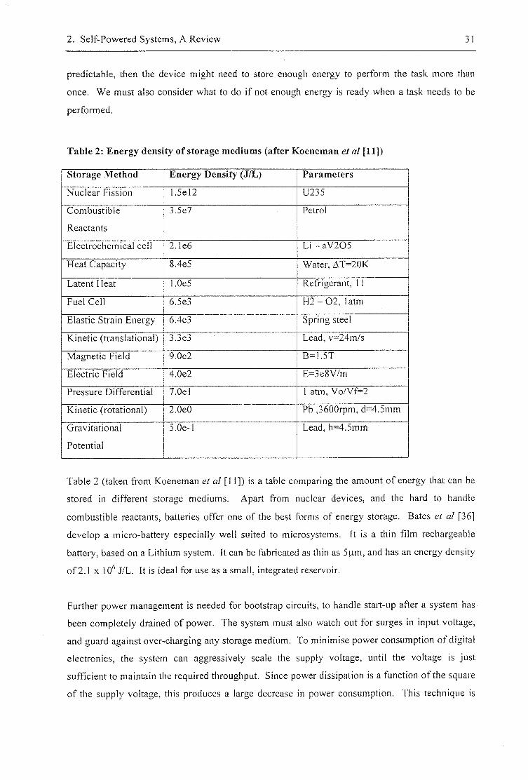
2. Self-Powered Systems, A Review 31
predictable, then the device might need to store enough energy to perform the task more than
once. We must also consider what to do if not enough energy is ready when a task needs to be
performed.
Table 2: Energy density of storage mediums (after Koeneman et al [11])
Storage Method Energy Density (J/L) Parameters
Nuclear Fission L5el2 1^35
Combustible
Reactants
3Jie7 Petrol
Electrochemical cell 2Te6 Li - aV205
Heat Capacity 8.4e5 Water, AT=20K
Latent Heat I.OeS Refrigerant, 1 1
Fuel Cell 6.5e3 H 2 - 0 2 , latm
Elastic Strain Energy 6.4e3 Spring steel
Kinetic (translational) 3 J e 3 Lead, v=24m/s
Magnetic Field 9.0e2 B = I 5 T
Electric Field 4.0e2 E=3e8V/m
Pressure Differential 7.0el 1 atm, Vo/Vf=2
Kinetic (rotational) 2.0e0 Pb ,3600rpm, d=4.5mm
Gravitational
Potential
5.0e-l Lead, h=4.5mm
Table 2 (taken from Koeneman et al [11]) is a table comparing the amount of energy that can be
stored in different storage mediums. Apart from nuclear devices, and the hard to handle
combustible reactants, batteries offer one of the best forms of energy storage. Bates et al [36]
develop a micro-battery especially well suited to microsystems. It is a thin film rechargeable
battery, based on a Lithium system. It can be fabricated as thin as 5fim, and has an energy density
of 2.1 X 10^ J/L. It is ideal for use as a small, integrated reservoir.
Further power management is needed for bootstrap circuits, to handle start-up after a system has
been completely drained of power. The system must also watch out for surges in input voltage,
and guard against over-charging any storage medium. To minimise power consumption of digital
electronics, the system can aggressively scale the supply voltage, until the voltage is just
sufficient to maintain the required throughput. Since power dissipation is a function of the square
of the supply voltage, this produces a large decrease in power consumption. This technique is
2, Self-Powered Systems, A Review 32
used by Amirtharajah and Chandrakasan [7], along with a number of other state-of-the-art low
power techniques.
2.3 Systems design
The concept of a self-powered sensor would not have seemed practical some 30 years ago. White
and Brignell [37] anecdotally report the derision expressed by industrialists when the concept of
combining computer systems with individual sensor elements was expressed in the 1980s. The
cause of this response is that "at that time a microprocessor cost considerably more than a basic
sensor and it did not make sense to dedicate the former to the latter". The well-documented
revolution in speed, size, cost and power consumption of microprocessor units means that this
practice is now common place.
In the literature, this new generation of devices is variously labelled as intelligent or smart
systems. The advantages of these devices are that they offer increased reliability and accuracy,
can pre-process data, and can perform measurements that simply would not have been possible
before. Recent devices have combined the intelligent sensor concept with small, efficient
communications, facilitating remote wireless sensor systems. For background on the field of
intelligent sensors the reader is directed towards Brignell and White [37].
Below are some recent projects whose aims include pushing back the frontiers of power
consumption for wireless sensor systems. These, currently battery powered, devices are the types
of system that are likely to benefit from self-power technologies.
(a) Smart Dust
This well-established project is the work of a group based at Berkeley. The group aims to
incorporate sensing, communications, and computing hardware, and a power supply in a volume
no more than a few cubic millimetres [38]. They label the resulting intelligent sensors "Smart
Dust", anticipating that perhaps these sensors may one day permeate our environment in much the
same manner as dust. The project focuses upon free-space optical communications, by both
active laser transmission, and a novel corner-cube retroreflector (CCR) design. The principle is
illustrated in figure 5. A CCR will reflect any incident ray of light back to its source (provided
the source lies within a certain solid angle). The device can be used to communicate information
by modulating the stream of reflected light. This is achieved by fractionally displacing one of the
mirrors, which removes the retroreflective property. The CCR's have been successfully
fabricated in gold coated polysilicon, and Chu et al [39] have demonstrated data transmission at 1
kilobit per second over a range of 150 meters, using a 5-milliwatt illuminating laser.

2. Self-Powered Systems, A Review 33
The group has recently produced a device that occupies lOOOmm^ (this was non-functional due to
faults in the C M O S design) and plans to construct one occupying only 20mm^ in the near future.
light emitter / detector
mirror
hinge
(a) (b)
Figure 5: Communications using a 2-D CCR mirror (after Chu et al [39])
(b) Wireless Integrated Network Sensors (WINS)
This project at UCLA is very similar in spirit to the Smart Dust project. Its main difference is that
WINS has chosen to concentrate on RF communications over short distances, and that some
techniques for low power sensing have been examined. The group has created new micro-power
C M O S RF circuits operating in the 400-900MHz region. Their papers focus on efficient VCO
and mixer designs, producing designs which are claimed to give the lowest power dissipation
reported at the time [40].
A complete sensor, and communications design is described by Bult et al [41]. A micromachined
accelerometer, and loop antenna is combined with the requisite CMOS circuitry using a compact
flip-chip bonding technique. Each section of the system is described, but it is not clear whether
the group produced a functional device. Two different communications systems are described:
the first is described as consuming an average of only 90p.W, operating at a low data rate
(lOkbsps), short range (10-30m), and low duty cycle (this is unspecified, and makes these figures
hard to interpret); the second reports a receiver consumption of 90)liW at a data rate of 100kbps
(this from a I m W transmitter power, 10m range and Icm^ single loop antenna area).
(c) Ultra Low Power Wireless Sensor Project
This program, based at MIT, proposes "developing a prototype wireless image sensor system
capable of transmitting a wide dynamic range of data rates (Ibit/s - IMbit/s) over a wide range of
average transmission output power levels ( lOpW - IOmW)"[42]. They also propose an initial

2. Self-Powered Systems, A Review 34
prototype that consumes approximately 50mW. To date, no results have been published from this
program.
2.4 Summary
There is no single technological answer to self-power; each potential application must be
evaluated to determine where power might be derived. Applying such solutions will require
careful tailoring to the specific application, as devices will often need to scavenge for power at the
edges of feasibility.
The future is bright for self-power. There is wide interest in this field that ranges from mature
solutions such as solar cells to vibration generators that have still to be fully evaluated. As the
power requirements for integrated circuits continue to fall, more and more applications will
become feasible candidates for self-power.
3. Background Material 35
CHAPTER 3
Background Material
3.1 Transduction Technologies
Existing work has examined both piezoelectric, and magnet-coil based techniques for extracting
power from vibrations. These are examined here, along with electrostrictive polymers, as
potential transduction mechanisms for an inertia! generator.
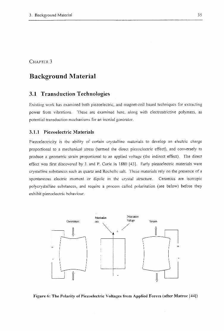
3.1.1 Piezoelectric Materials
Piezoelectricity is the ability of certain crystalline materials to develop an electric charge
proportional to a mechanical stress (termed the direct piezoelectric effect), and conversely to
produce a geometric strain proportional to an applied voltage (the indirect effect). The direct
effect was first discovered by J. and P. Curie in 1880 [43]. Early piezoelectric materials were
crystalline substances such as quartz and Rochelle salt. These materials rely on the presence of a
spontaneous electric moment or dipole in the crystal structure. Ceramics are isotropic
polycrystalline substances, and require a process called polarisation (see below) before they
exhibit piezoelectric behaviour.
Cbtpression
Warisaticn
axis
PDlar isa t icn
Taision
Figure 6; The Polarity of Piezoelectric Voltages from Applied Forces (after Matroc [44|)
3. Background Material 36
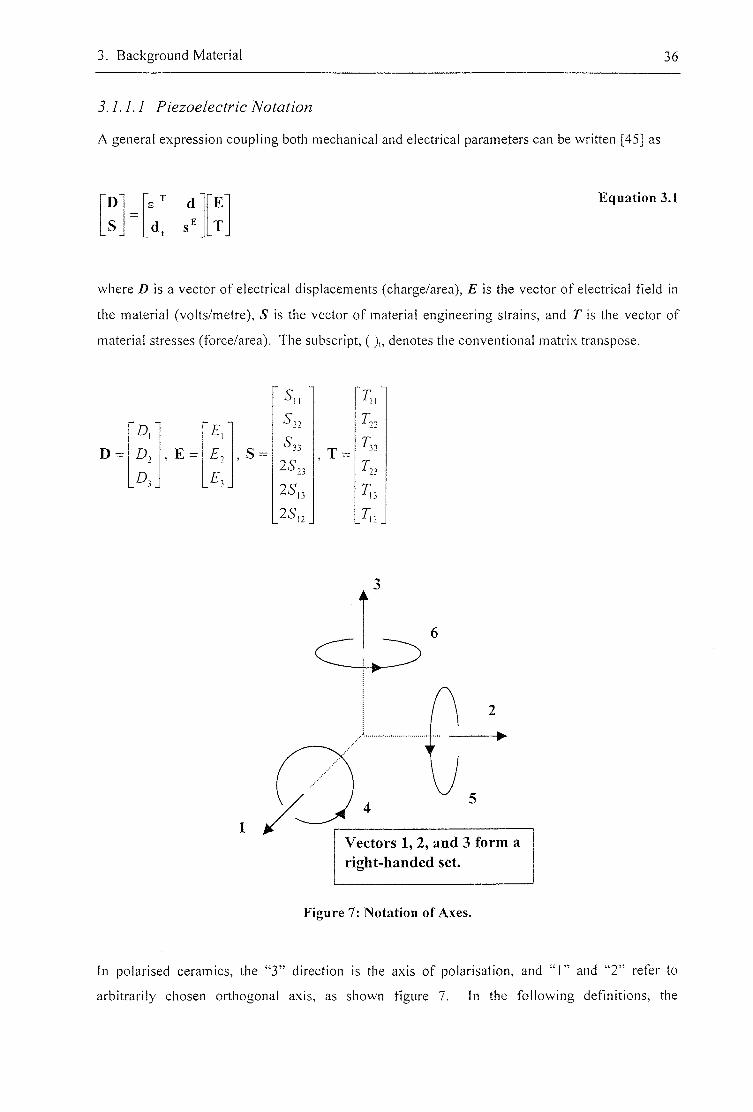
3.1.1.1 Piezoelectric Notation
A general expression coupling both mechanical and electrical parameters can be written [45] as
D e ? d E
. 4 , T
Equation 3.1
where Z) is a vector of electrical displacements (charge/area), E is the vector of electrical field in
the material (volts/metre), S is the vector of material engineering strains, and T is the vector of
material stresses (force/area). The subscript, (), , denotes the conventional matrix transpose.
D = D, , E =
A . A -
'Tu
Tn
, S = ^33 , T = Tr.
23% Tn
r,3
7 . 3 .
Vectors 1, 2, and 3 form a right-handed set.
Figure 7: Notation of Axes.
In polarised ceramics, the "3" direction is the axis of polarisation, and "1" and "2" refer to
arbitrarily chosen orthogonal axis, as shown figure 7. In the following definitions, the
3. Background Material 37
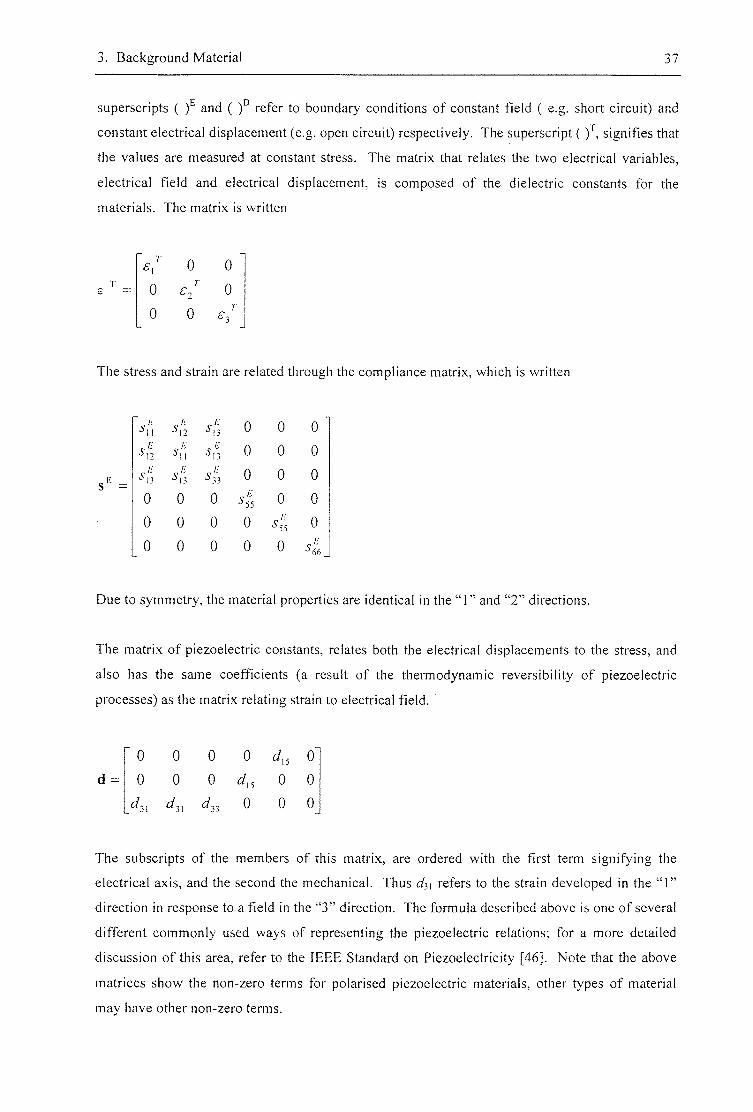
superscripts ( and ( refer to boundary conditions of constant field ( e.g. short circuit) and
constant electrical displacement (e.g. open circuit) respectively. The superscript ( ) \ signifies that
the values are measured at constant stress. The matrix that relates the two electrical variables,
electrical field and electrical displacement, is composed of the dielectric constants for the
materials. The matrix is written
0 0
0 0
0 0 '
s.
The stress and strain are related through the compliance matrix, which is written
4 4 0 0 0
•4 4 0 0 0
4 4 0 0 0 0 0 0 4 0 0 0 0 0 0 55 0 0 0 0 0 0 4
Due to symmetry, the material properties are identical in the "1" and "2" directions.
The matrix of piezoelectric constants, relates both the electrical displacements to the stress, and
also has the same coefficients (a result of the thermodynamic reversibility of piezoelectric
processes) as the matrix relating strain to electrical field.
0 0 0 0 i/,5 0
0 0 0 0 0
c/3, 4 , 0 0 0
The subscripts of the members of this matrix, are ordered with the first term signifying the
electrical axis, and the second the mechanical. Thus d^\ refers to the strain developed in the "1"
direction in response to a field in the "3" direction. The formula described above is one of several
different commonly used ways of representing the piezoelectric relations; for a more detailed
discussion of this area, refer to the IEEE Standard on Piezoelectricity [46]. Note that the above
matrices show the non-zero terms for polarised piezoelectric materials, other types of material
may have other non-zero terms.
3. Background Material 38
The electromechanical coupling factor, k, is a useful measure of the strength of the piezoelectric
effect for a material, and is an important parameter when power generation is required. It
measures the proportion of input electrical energy converted to mechanical energy when a field is
applied (or vice versa when a material is stressed). The relationship is expressed in terms o f / r :
^2 _ electrical energy converted to mechanical energy
input electrical energy
or
^2 _ mechanical energy converted to electrical energy
input mechanical energy
Since this conversion is always incomplete, k is always less than one.
The earliest piezoelectric materials were crystalline materials, that exhibited a natural polarisation.
To use such materials, single crystals must be cut into the required shape, and can only be cut
along certain crystallographic directions, thus limiting the possible shapes. In contrast,
piezoelectric ceramics can be fabricated into a wide range of sizes and shapes, so they are more
suitable for generator designs.
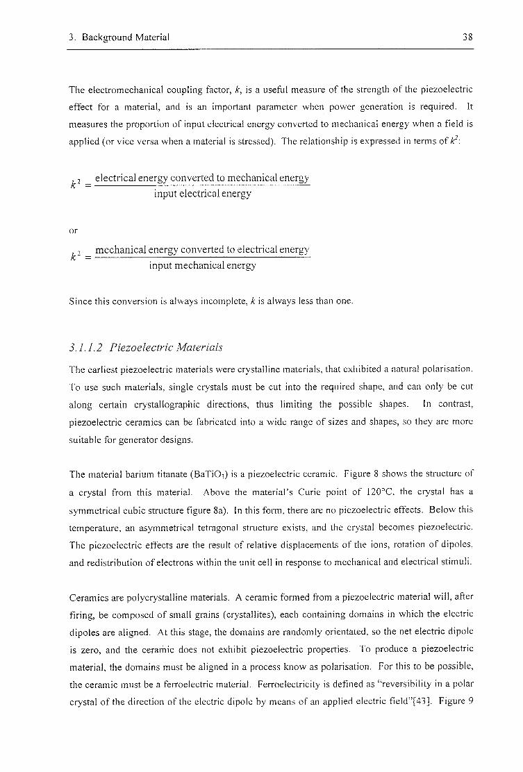
The material barium titanate (BaTiOs) is a piezoelectric ceramic. Figure 8 shows the structure of
a crystal from this material. Above the material's Curie point of 120°C, the crystal has a
symmetrical cubic structure figure 8a). In this form, there are no piezoelectric effects. Below this
temperature, an asymmetrical tetragonal structure exists, and the crystal becomes piezoelectric.
The piezoelectric effects are the result of relative displacements of the ions, rotation of dipoles,
and redistribution of electrons within the unit cell in response to mechanical and electrical stimuli.
Ceramics are polycrystalline materials. A ceramic formed from a piezoelectric material will, after
firing, be composed of small grains (crystallites), each containing domains in which the electric
dipoles are aligned. At this stage, the domains are randomly orientated, so the net electric dipole
is zero, and the ceramic does not exhibit piezoelectric properties. To produce a piezoelectric
material, the domains must be aligned in a process know as polarisation. For this to be possible,
the ceramic must be a ferroelectric material. Ferroelectricity is defined as "reversibility in a polar
crystal of the direction of the electric dipole by means of an applied electric field"[43]. Figure 9
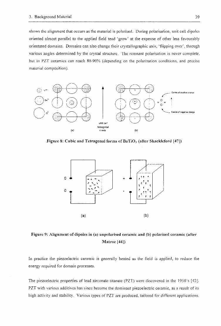
3. Background Material 39
shows the alignment that occurs as the material is polarised. During polarisation, unit cell dipoles
oriented almost parallel to the applied field tend 'grow' at the expense of other less favourably
orientated domains. Domains can also change their crystallographic axis, 'flipping over' , through
various angles determined by the crystal structure. The remnant polarisation is never complete,
but in PZT ceramics can reach 80-90% (depending on the polarisation conditions, and precise
material composition).
unit cell
tetragonal
Centreof po#Hlve chmrge
Centre of negative charge
(a) (b)
Figure 8; Cubic and Tetragonal forms of BaTiOs (after Shackleford [47])
1 1 f f f
f , t t f
t t
t f t
f t . f t t t
f t
(a) (b)
Figure 9: Alignment of dipoles in (a) unpolarised ceramic and (b) polarised ceramic (after
Matroc [44])
In practice the piezoelectric ceramic is generally heated as the field is applied, to reduce the
energy required for domain processes.
The piezoelectric properties of lead zirconate titanate (PZT) were discovered in the 1950's [43].
PZT with various additives has since become the dominant piezoelectric ceramic, as a result of its
high activity and stability. Various types of PZT are produced, tailored for different applications.

3. Background Material 40
The materials can be roughly divided into two groups: hard, and soA materials. Hard materials
such as PZT 4 or PZT 8 (UK notation) are suitable for power applications, possessing low
mechanical and dielectric losses. SoA materials such as PZT 5H offer better sensitivity, at the
cost of more losses, and a lower coercive field (the field required to depolarise the material).
Other specialist materials are also available for requirements such as high stability. Table 3
compares these materials. In this thesis PZT 5H was used for initial work as it was readily
available. The results of modelling, however, suggest that harder materials are better for power
generation.
Polyvinylidene fluoride (PVDF) is another important piezoelectric material. PVDF is a
fluorocarbon polymer, commonly used as an inert lining or pipe-work material. Since its
discovery as a piezoelectric material by Kawai in 1969 [48], it has been the subject of much
research, and is available commercially as a pre-polarised film. Like ceramic materials, PVDF
requires polarisation, which means that it can be manufactured in a wide variety of shapes. It is
less active than common ceramic materials, but its low cost, lower stiffness, and easy
manufacturability makes it ideal for many applications. Table 3 lists some key properties.
Table 3: Comparing Piezoelectric Materials
Material d 3 3 ( p C N " ) (ilO""m"N") k33
PZT 8 [44] -225 74 0.64
PZT 5H [44] -593 48 0.75
PVDF [48] -18 400 O.IO
3.1.2 Electrostrictive Polymers
The term electrostriction in its general sense covers 'any interaction between an electric field and
the deformation of a dielectric in the field'[49], and hence includes the piezoelectric effect.
However, it is common practice to reserve the term to refer to phenomena where the deformation
is independent of the direction of the field, and proportional to the square of the field [49]. This
phenomenon is generally caused by a combination of Maxwell stresses, and a dependence of the
dielectric constant upon the strain. In electrostrictive polymers described here, the former is the
dominant mechanism. The effect is generally small, and can be ignored unless field strengths
exceed 20kVcm' ' .
3. Background Material 41
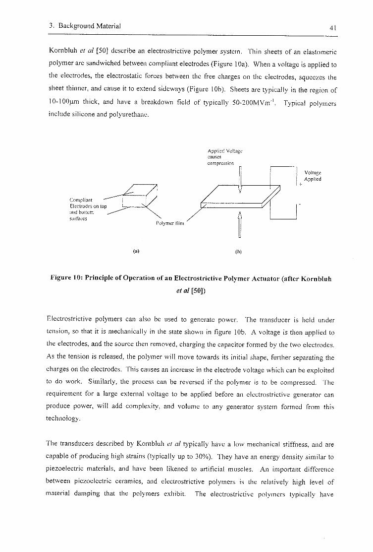
Kornbluh et al [50] describe an electrostrictive polymer system. Thin sheets of an elastomeric
polymer are sandwiched between compliant electrodes (Figure 10a). When a voltage is applied to
the electrodes, the electrostatic forces between the free charges on the electrodes, squeezes the
sheet thinner, and cause it to extend sideways (Figure 10b). Sheets are typically in the region of
I0-I00p.m thick, and have a breakdown field of typically 50-200MVm '. Typical polymers
include silicone and polyurethane.
Compl iant
Electrodes on top
and bottom
surfaces
Applied Voltage
causes compression
Polymer film
(a)
V
A
u
(b)
Voltage
Applied
Figure 10: Principle of Operation of an Electrostrictive Polymer Actuator (after Kornbluh
et al [50])
Electrostrictive polymers can also be used to generate power. The transducer is held under
tension, so that it is mechanically in the state shown in figure 10b. A voltage is then applied to
the electrodes, and the source then removed, charging the capacitor formed by the two electrodes.
As the tension is released, the polymer will move towards its initial shape, further separating the
charges on the electrodes. This causes an increase in the electrode voltage which can be exploited
to do work. Similarly, the process can be reversed if the polymer is to be compressed. The
requirement for a large external voltage to be applied before an electrostrictive generator can
produce power, will add complexity, and volume to any generator system formed from this
technology.
The transducers described by Kornbluh g/ a/ typically have a low mechanical stiffness, and are
capable of producing high strains (typically up to 30%). They have an energy density similar to
piezoelectric materials, and have been likened to artificial muscles. An important difference
between piezoelectric ceramics, and electrostrictive polymers is the relatively high level of
material damping that the polymers exhibit. The electrostrictive polymers typically have

3. Background Material ^2
hysteretic losses of 20% at 200Hz, which means that a high Q-factor resonator could not be built
from this material.
Although electrostrictive polymers may be useful for generator applications where the material is
actively deformed, they are not considered to be useful for inertial generators of the type
described in this thesis. They could be modelled in a similar manner to the piezoelectric
generators described in Chapter 5, however, they have an even lower electromagnetic coupling
factor than piezoceramics and will thus not generate significant power (see section 5.8 for
discussion of this relationship). For this reason, and also their high level material damping
described above, electrostrictive polymers will not be considered further in the remainder of this
thesis.
3.1.3 Electromagnetic Induction
Electromagnetic induction is another method of converting mechanical energy to electrical
energy. The principles are well known, and the pertinent equations will be described here as an
aid to memory. For a wire of length, I , carrying a current, /, that runs through a perpendicular
magnetic field of flux density, B, the perpendicular force on that wire, F, is given by
F / • B X L Equation 3.2
Similarly the voltage, V, induced across the wire is given by
V B X L • V Equation 3.3
where v is the velocity of the wire. Generators based on electromagnetic induction are explored
further in chapter 7.
3.2 Principles of Resonant Vibration Generators
In this section, generators will be modelled as first order resonant systems. This generalisation
will lay a framework that will enable generators of different technologies to be compared in
section 7.6.
3.2.1 First Order Modelling of Generator Structures
It is possible to represent the resonant generators described in this thesis using a simple first order
model as shown in figure II. The seismic mass, combines the effect of the actual mass in the
system with any effective mass added by reactive load circuits. The spring, stiffness Ar, combines
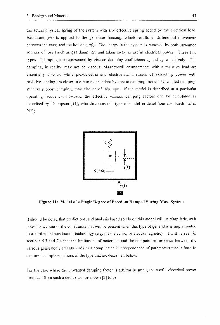
3. Background Material 43
the actual physical spring of the system with any effective spring added by the electrical load.
Excitation, y(t) is applied to the generator housing, which results in differential movement
between the mass and the housing, z(t). The energy in the system is removed by both unwanted
sources of loss (such as gas damping), and taken away as useful electrical power. These two
types of damping are represented by viscous damping coefficients C/, and C/,- respectively. The
damping, in reality, may not be viscous; Magnet-coil arrangements with a resistive load are
essentially viscous, while piezoelectric and electrostatic methods of extracting power with
resistive loading are closer to a rate independent hysteretic damping model. Unwanted damping,
such as support damping, may also be of this type. If the model is described at a particular
operating frequency, however, the effective viscous damping factors can be calculated as
described by Thompson [51], who discusses this type of model in detail (see also Nash if et al
[52]).
k <
1 ———•—--J—
C l+CE L z ( 0
t Figure 11: Model of a Single Degree of Freedom Damped Spring-Mass System
It should be noted that predictions, and analysis based solely on this model will be simplistic, as it
takes no account of the constraints that will be present when this type of generator is implemented
in a particular transduction technology (e.g. piezoelectric, or electromagnetic). It will be seen in
sections 5.7 and 7.4 that the limitations of materials, and the competition for space between the
various generator elements leads to a complicated interdependence of parameters that is hard to
capture in simple equations of the type that are described below.
For the case where the unwanted damping factor is arbitrarily small, the useful electrical power
produced from such a device can be shown [3] to be
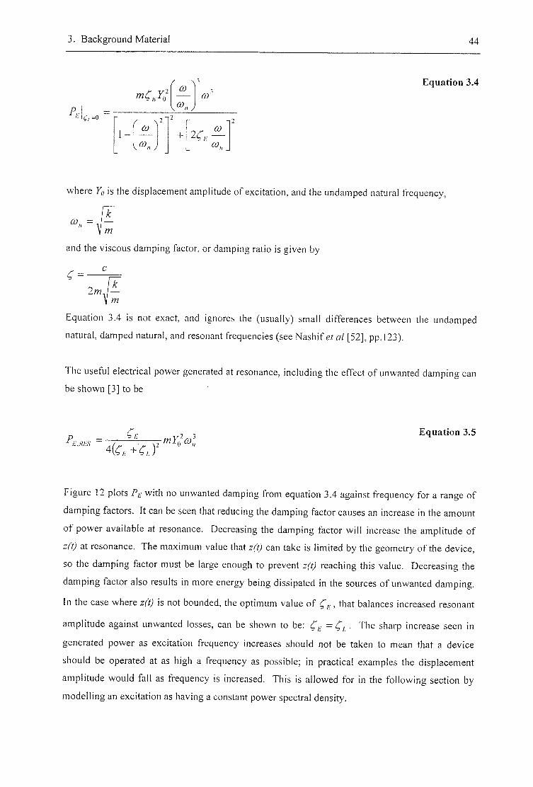
3. Background Material 44
P,
/ a,
3 0)
CO
2 r -
+
Equation 3.4
CO
CO..
where F« is the displacement amplitude of excitation, and the undamped natural frequency,
and the viscous damping factor, or damping ratio is given by
2/M.
Equation 3.4 is not exact, and ignores the (usually) small differences between the undamped
natural, damped natural, and resonant frequencies (see Nashif g/ a/ [52], pp. 123).
The useful electrical power generated at resonance, including the effect of unwanted damping can
be shown [3] to be
p
+ C . ) '
Equation 3.5
Figure 12 plots Pe with no unwanted damping from equation 3.4 against frequency for a range of
damping factors. It can be seen that reducing the damping factor causes an increase in the amount
of power available at resonance. Decreasing the damping factor will increase the amplitude of
at resonance. The maximum value that can take is limited by the geometry of the device,
so the damping factor must be large enough to prevent reaching this value. Decreasing the
damping factor also results in more energy being dissipated in the sources of unwanted damping.
In the case where is not bounded, the optimum value of , that balances increased resonant
amplitude against unwanted losses, can be shown to be: . The sharp increase seen in
generated power as excitation frequency increases should not be taken to mean that a device
should be operated at as high a frequency as possible; in practical examples the displacement
amplitude would fall as frequency is increased. This is allowed for in the following section by
modelling an excitation as having a constant power spectral density.
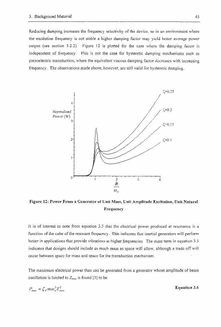
3. Background Material 45
Reducing damping increases the frequency selectivity of the device, so in an environment where
the excitation frequency is not stable a higher damping factor may yield better average power
output (see section 3.2.2). Figure 12 is plotted for the case where the damping factor is
independent of frequency. This is not the case for hysteretic damping mechanisms such as
piezoelectric transduction, where the equivalent viscous damping factor decreases with increasing
frequency. The observations made above, however, are still valid for hysteretic damping.
(;=0.25
Normalised Power (W)
Figure 12: Power From a Generator of Unit Mass, Unit Amplitude Excitation, Unit Natural
Frequency
It is of interest to note from equation 3.5 that the electrical power produced at resonance is a
function of the cube of the resonant frequency. This indicates that inertial generators will perform
better in applications that provide vibrations at higher frequencies. The mass term in equation 3.5
indicates that designs should include as much mass as space will allow, although a trade off will
occur between space for mass and space for the transduction mechanism.
The maximum electrical power than can be generated from a generator whose amplitude of beam
oscillation is limited to is found [3] to be
P.. Equation 3.6
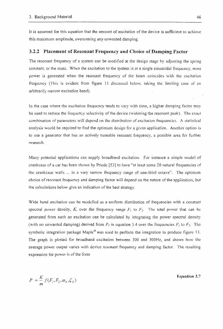
3. Background Material 46
It is assumed for this equation that the amount of excitation of the device is sufficient to achieve
this maximum amplitude, overcoming any unwanted damping.
3.2.2 Placement of Resonant Frequency and Choice of Damping Factor
The resonant frequency of a system can be modified at the design stage by adjusting the spring
constant, or the mass. When the excitation to the system is at a single sinusoidal frequency, most
power is generated when the resonant frequency of the beam coincides with the excitation
frequency (This is evident from figure 13 discussed below, taking the limiting case of an
arbitrarily narrow excitation band).
In the case where the excitation frequency tends to vary with time, a higher damping factor may
be used to reduce the frequency selectivity of the device (widening the resonant peak). The exact
combination of parameters will depend on the distribution of excitation frequencies. A statistical
analysis would be required to find the optimum design for a given application. Another option is
to use a generator that has an actively tuneable resonant frequency, a possible area for further
research.
Many potential applications can supply broadband excitation. For instance a simple model of
crankcase of a car has been shown by Priede [53] to have "at least some 20 natural frequencies of
the crankcase walls ... in a very narrow frequency range of one-third octave". The optimum
choice of resonant frequency and damping factor will depend on the nature of the application, but
the calculations below give an indication of the best strategy.
Wide band excitation can be modelled as a uniform distribution of frequencies with a constant
spectral power density, K, over the frequency range F, to Fj . The total power that can be
generated from such an excitation can be calculated by integrating the power spectral density
(with no unwanted damping) derived from P/.- in equation 3.4 over the frequencies F/ to F, . The
symbolic integration package Maple® was used to perform the integration to produce figure 13.
The graph is plotted for broadband excitation between 300 and 500Hz, and shows how the
average power output varies with device resonant frequency and damping factor. The resulting
expression for power is of the form
v Equation 3.7
m
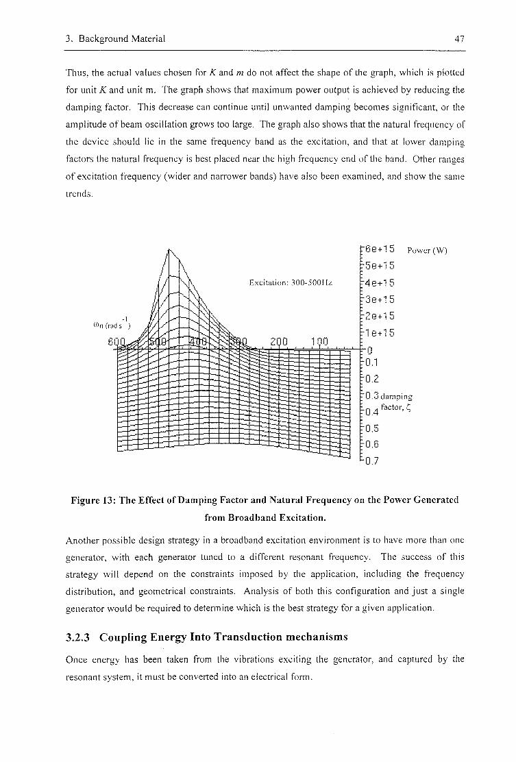
3. Background Material 47
Thus, the actual values chosen for AT and m do not affect the shape of the graph, which is plotted
for unit K and unit m. The graph shows that maximum power output is achieved by reducing the
damping factor. This decrease can continue until unwanted damping becomes significant, or the
amplitude of beam oscillation grows too large. The graph also shows that the natural frequency of
the device should lie in the same frequency band as the excitation, and that at lower damping
factors the natural frequency is best placed near the high frequency end of the band. Other ranges
of excitation frequency (wider and narrower bands) have also been examined, and show the same
trends.
Exci ta t ion: 3 0 0 - 5 0 0 H z
uJn (rad s
6 6 + 1 5 Power ( W )
5e+15
4e+15
3e+15
2e+15
rl e+15
U.u damping
Q factor,
Figure 13: The Effect of Damping Factor and Natural Frequency on the Power Generated
from Broadband Excitation.
Another possible design strategy In a broadband excitation environment is to have more than one
generator, with each generator tuned to a different resonant frequency. The success of this
strategy will depend on the constraints imposed by the application, including the frequency
distribution, and geometrical constraints. Analysis of both this configuration and just a single
generator would be required to determine which is the best strategy for a given application.
3.2.3 Coupling Energy Into Transduction mechanisms
Once energy has been taken from the vibrations exciting the generator, and captured by the
resonant system, it must be converted into an electrical form.
3. Background Material 48
To generate power from a piezoelectric (or electrostrictive) material, the material must be
deformed. This deformation causes charge to be displaced across the material, which gives rise to
a potential difference which can be exploited to do work. The piezoelectric material will
contribute to both the stiffness, and the loss factor of the system. Piezoelectric materials are
generally too stiff to be connected mechanically in series with the mass, which must be connected
to a lower mechanical impedance to resonate at typical vibration frequencies. Instead, the
piezoelectric material can form part of a beam. One method is to attach the piezoelectric material
to the root of a beam. This arrangement is not ideal, as the elastic energy is shared between the
stiffness of the beam and the piezoelectric material. In a situation where the proportion of elastic
energy that can be converted to electrical energy is limited (especially the case with thick-film and
polymer piezoelectrics) this is important as it reduces the power generating capacity.
Alternatively, the beam can be formed from only piezoelectric material (this is harder to
manufacture). It is important to note that a symmetrical piezoelectric beam formed from a single
piece of PZT, with no substrate, will have its neutral axis at its centre and thus develop no charge
between its top and bottom electrodes, since the charge produced by the tension at one surface
will cancel that caused by compression at the other.
Electromagnetic induction can also be used to extract the energy from the resonant system, either
in the form of a magnet mounted on the oscillating beam moving through a fixed coil, or vice
versa. In this case, the design of the magnet and coil does not directly influence the stiffness of
the resonator.
3.3 Power requirements of Vibration-Powered Systems
Portions of this thesis deal with the question of whether vibration-powered generators can produce
enough power to be useful. Before this can be answered we must first establish how much power
can be considered to be 'useful'.
A vibration-powered system will typically have three distinct power consuming functions:
sensing, data processing, and communications.
Sensing; Typical applications could use any of a wide range of different sensors, so the power
required will be highly application specific. For example a device periodically checking the
condition of a structure with a resistive strain gauge could achieve an average power consumption
of below a microwatt if only a low duty cycle were required. In contrast a device sending back
live video information will require up to lOmW [42]. Little work has been found on existing
ultra-low power sensors, however, given the large range of different sensor types and technologies
there is likely to be ample scope for future research.
3. Background Material 49
Data processing: Digital electronics is still undergoing the expansion predicted by Moore's law.
Along with the improvements in speed and density that this facilitates, the miniaturisation and
trend towards lower supply voltages reduces the amount of power required. Discussing medium
throughput DSP circuits that in 1998 consumed around I m W to O.OlmW, Amirtharajah and
Chandrakasan [7] predict that "projecting current power scaling trends into the future (based on
deep voltage scaling, and other power management techniques), we expect the power
consumption to be reduced to tens of p,W to hundreds of nW". Vittoz [54] states that current
watch circuits containing several tens of thousands of transistors are routinely produced with a
power consumption of below 0.5p.W,
Communications: The power required to actively transmit data using a radio signal depends on
factors such as the data rate, the operating frequency, the range, and the aerial sizes. Given
sufficiently large receiving aerials (for instance those used to receive power from deep space
probes) even very faint signals can be decoded. Bult et al [41] work on a state of the art low
power communications system, and report two devices: the first is described as consuming an
average of only 90)liW, operating at a low data rate (lOkbsps), short range (10-30m), and low duty
cycle (this is unspecified, and renders these figures almost meaningless); the second reports a
receiver consumption of 90p.W at a data rate of 100kbps (this from a I m W transmitter power,
10m range and Icm^ single loop antenna area). An MIT project proposal states that chips have
been produced that demonstrate a "transmitter capable of 1.25Mb/s at 1.8GHz using only
22mW"[42]. Radio is not the only way to communicate, the 'smart dust' system using passive
retro-reflective mirrors (described in section 2.3) offers a passive communications technique. The
near-field coupling used in RFID tags (described in section 2.1.5) is another possibility, although
this technology can also supply power, so a vibration powered system is unlikely to be required in
applications that are amenable to this approach.
Comparing the sub-systems, it can be seen that in many applications communications will
demand the most power. Given the low energy cost of processing, it will often be more efficient
to process data to reduce its bulk before transmission. An example of this technique is a condition
based monitoring system; a sensor could spend most of its time processing input data to evaluate
the health of a structure, then communicate at a higher power once a day at a low data rate to
signal the state of the structure.
The MIT 'Ultra Low Power Wireless Sensor Project' [42] is working on producing a ' prototype
image sensor system ... capable of wirelessly transmitting a wide range of data rates (1 bit/sec - 1
megabit/sec) over a wide range of average transmission output power levels (10 microwatts - 10

3. Background Material 50
milliwatts)'. The group holds expertise in ultra-low power circuits, so these figures should
represent an achievable goal. For the evaluation of devices discussed in the remainder of the
thesis, any power above SOfiW will be considered potentially useful.
4. Development of a Thick-Film PZT Generator
CHAPTER 4
Development of a Thick-Film PZT Generator
Thick-film techniques (see below) allow piezoelectric materials to be accurately, and repeatably
deposited on substrates. Thicknesses in excess of 100p.m can be routinely deposited. Alternative
deposition techniques (sol gel [55], sputtered [56] or metal-organic chemical vapour deposition
( M O C V D ) [57]) cannot, at present, deposit material in such film thicknesses.
In this section processes required to produce a thick-film generator are developed, and a prototype
generator is produced. The design is not optimised, but chosen to provide reliable experimental
data. Mechanical and electrical properties of the thick-film PZT layer (which have not previously
been measured) are examined. The prototype is tested and assessed for power generating
capacity.
4.1 Introduction to Thick-Film Processes
Thick-fi lm devices typically consist of successively printed layers of materials of varying
electrical and mechanical properties. An key factor distinguishing thick-film technologies from
others is the manner in which the films are deposited. This is screen-printing, similar to that used
in the traditional silk screen-printing of T-shirts, mugs, etc. Printing is only part of the process,
and the other stages are described below.
Thick-fi lm technology was introduced around thirty years ago as a means of producing hybrid
circuits [58] (thick-film tracks and resistors combined on a substrate with silicon die). More
recently thick-film techniques have been used to produce a wide range of sensors. Thick-film
processes can be automated with relative ease, and together with the additive nature of the
techniques, this means that low cost devices may be produced with little waste. Thick-film
devices are also generally compact and robust as a result of the solid state nature of the layers.
Despite the high precision that can be achieved with micro-machined silicon devices, thick-film
technologies still have wide applications. The cost of capital equipment is considerably lower
than that required for semiconductor manufacture, and short production runs can be undertaken
relatively cheaply.
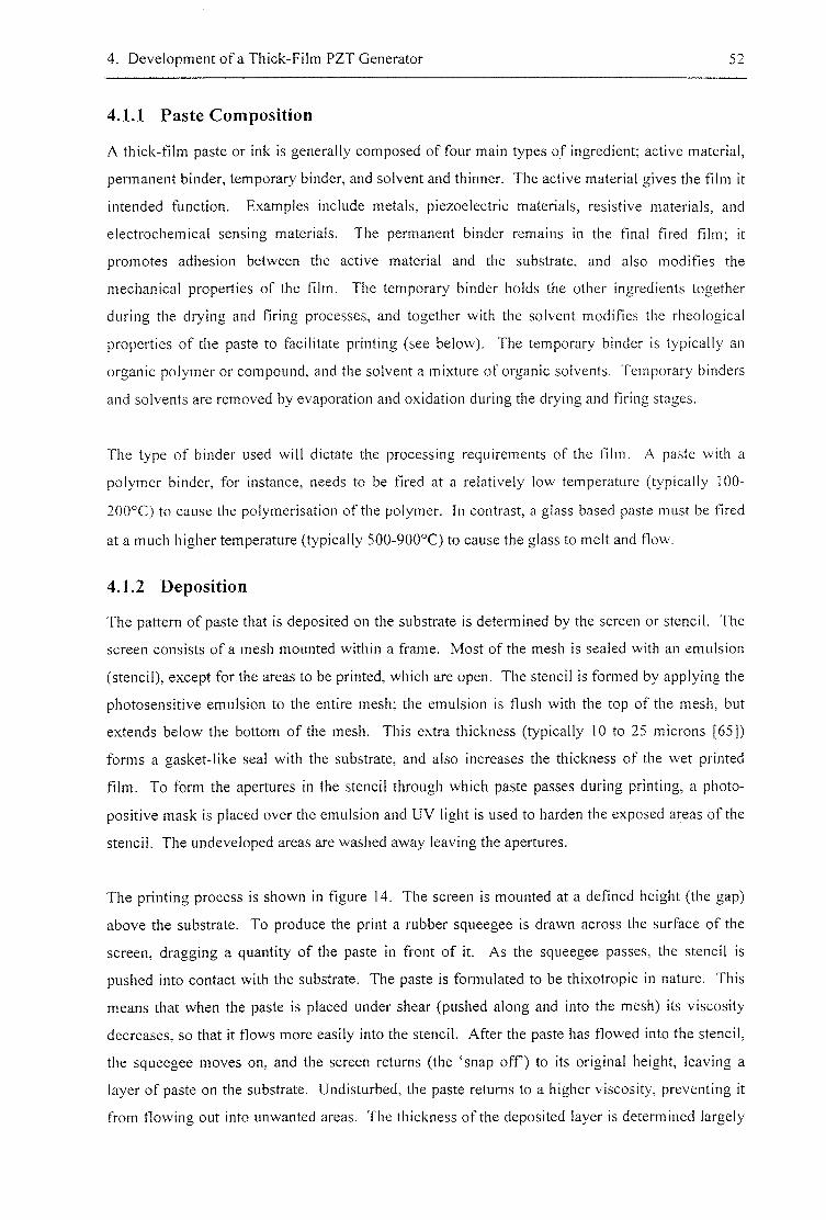
4. Development of a Thick-Film PZT Generator 52
4.1.1 Paste Composition
A thick-film paste or ink is generally composed of four main types of ingredient; active material,
permanent binder, temporary binder, and solvent and thinner. The active material gives the film it
intended function. Examples include metals, piezoelectric materials, resistive materials, and
electrochemical sensing materials. The permanent binder remains in the final fired film; it
promotes adhesion between the active material and the substrate, and also modifies the
mechanical properties of the film. The temporary binder holds the other ingredients together
during the drying and firing processes, and together with the solvent modifies the rheological
properties of the paste to facilitate printing (see below). The temporary binder is typically an
organic polymer or compound, and the solvent a mixture of organic solvents. Temporary binders
and solvents are removed by evaporation and oxidation during the drying and firing stages.
The type of binder used will dictate the processing requirements of the film. A paste with a
polymer binder, for instance, needs to be fired at a relatively low temperature (typically 100-
200°C) to cause the polymerisation of the polymer. In contrast, a glass based paste must be fired
at a much higher temperature (typically 500-900°C) to cause the glass to melt and flow.
4.1.2 Deposition
The pattern of paste that is deposited on the substrate is determined by the screen or stencil. The
screen consists of a mesh mounted within a frame. Most of the mesh is sealed with an emulsion
(stencil), except for the areas to be printed, which are open. The stencil is formed by applying the
photosensitive emulsion to the entire mesh; the emulsion is flush with the top of the mesh, but
extends below the bottom of the mesh. This extra thickness (typically 10 to 25 microns [65])
forms a gasket-like seal with the substrate, and also increases the thickness of the wet printed
film. To form the apertures in the stencil through which paste passes during printing, a photo-
positive mask is placed over the emulsion and UV light is used to harden the exposed areas of the
stencil. The undeveloped areas are washed away leaving the apertures.
The printing process is shown in figure 14. The screen is mounted at a defined height (the gap)
above the substrate. To produce the print a rubber squeegee is drawn across the surface of the
screen, dragging a quantity of the paste in front of it. As the squeegee passes, the stencil is
pushed into contact with the substrate. The paste is formulated to be thixotropic in nature. This
means that when the paste is placed under shear (pushed along and into the mesh) its viscosity
decreases, so that it flows more easily into the stencil. After the paste has flowed into the stencil,
the squeegee moves on, and the screen returns (the 'snap o f f ) to its original height, leaving a
layer of paste on the substrate. Undisturbed, the paste returns to a higher viscosity, preventing it
from flowing out into unwanted areas. The thickness of the deposited layer is determined largely
4. Development of a Thick-Film PZT Generator 53
by the emulsion thickness, but the squeegee traverse speed, squeegee down pressure, screen gap,
and paste properties also have an effect on this thickness.
Direction of print stroke
screen frame
squeegee
screen mesh
paste
screen gap substrate
Printer workholder
Figure 14: The thick-film printing process
4.1.3 Drying and firing
Following the printing, the wet print is left to settle for typically 10-15 minutes. This allows
irregularities in the surface of the print (caused by the impression of the mesh in the print surface)
to smooth out as the print flows a little. After the settling time, the print is dried. For cermet
(ceramic / me ta l ) type pastes, this typically consists of using infra-red heating to hold the paste at
150-175°C for 10-15 minutes [65]. This process causes most of the solvent to evaporate, which
typically reduces the thickness of the wet print by up to 50%.
The firing profile depends upon the type of permanent binder used. Low temperature polymer
based pastes are generally cured using either an oven or by exposing the paste to UV-light.
Higher temperature (typically glass based) pastes are often fired in a multi-zone belt furnace. A
typical furnace will consist of a metal belt which carries the substrate through a number of
different temperature zones, which are arranged to give the required temperature profile. In the
initial stages of the firing process, any remaining solvent is evaporated or oxidised, along with the
temporary binder. This leaves behind a porous structure composed of the active material, and the
permanent binder, separated by gas filled voids left by the temporary binder. As the permanent
binder melts, it wets the surface of the active material. Particles are then drawn together by
surface tension, leaving a denser, thinner film [65]. Trapped gas will not fully escape and some
porosity will remain. After firing, the resulting layer of sintered paste is referred to as a film.
Following firing, the printing process can be repeated to create multi-layered devices.
4. Development of a Thick-Film PZT Generator 54
4.2 Development of Materials, and Processes for Printing Thick-
Film PZT on Steel Beams
A set of experiments were performed, with the intention of finding a reliable method of producing
piezoelectric elements printed on steel beams.
4.2.1 Choice of Substrate
316 stainless steel was chosen for the substrate (Goodfellow FE240261: Hardened AISI 316
steel). Mechanically, steel offers a good stiffness, and a low material damping factor. 316 steel
has a low carbon content (less than 0,08%[59]). This is important since during the PZT firing
cycle, the substrate is heated to around 950°C. A steel with a higher carbon content would tend to
oxidise at this temperature.
316 steel is an austenitic steel, which means that the steel can only be hardened by cold working.
This is a drawback, since as the steel is heated during the PZT, and two electrode firing stages,
any hardening produced through initial cold-work will be lost. In the designs discussed in this
project, however, the tensile strength of the steel is not an issue, as the maximum beam deflection
is governed by the strength of the PZT layers.
4.2.2 Thermal Mismatch and Substrate Warping
The first problem encountered during thick-film printing was that the thermal expansion
mismatch between the thick-film materials, and the steel caused warping during the firing phase.
The steel has a coefficient of thermal expansion, 2c==16-18)j,-strain K"', large compared to typical
6jLi-strain K"' of PZT-5H (The temperature coefficients of both materials, especially the PZT, are
actually highly temperature dependent). During the cooling phase of the film firing (whether
electrode, insulator or PZT film) the film binds to the substrate, and as cooling continues, the
double layer bends in the manner of a bimorph.
Exact measurements were not performed, but the degree of mismatch is such that a single-sided
50(j.m thick layer of PZT on a 100|Lim thick 316 steel sheet results in a bent substrate with a
bending radius of around 3cm. This degree of bending prevents any further thick-film processing
of the substrate. To counteract this problem, all subsequent substrates were printed with a
symmetrical pattern on the front and back sides. The two patterns must be carefully aligned, as a
mismatch of 0.5mm was found to be large enough to cause sufficient bending of a lOOfim thick
substrate to prohibit further processing. A further difficulty is that the screen printing process
does not always result in an even film thickness across the substrate. This can be caused by an

4. Development of a Thick-Film PZT Generator 55
uneven squeegee, or a slight angle between the screen and the substrate, which will produce a
variation in snap-ofF speed. The variation in thickness will not be repeated symmetrically on the
opposite face of the substrate, which will again cause warping.
These problems place a lower bound on the thickness of substrates that can be used. Using
manual alignment marks (the only method possible with the screen printer used), It was not found
possible to work reliably with substrates less than lOOjim thick. Even with arbitrarily good
alignment, the thickness variation will limit the substrate thickness.
As a result of the thermal mismatch the thick-film layers in a double sided structure will be under
compression, even when there are no external loads. This has advantages for the device as a
whole, as it means that when the beam is flexed, the brittle PZT layer (a ceramic) will not be
placed under tension until a certain deflection is passed. Since the breaking strain of a ceramic is
greater under compression than it is under tension, it means that more strain can be stored in the
piezoelectric element, resulting in a higher capacity to generate power.
4.2.3 Substrate Preparation
To ensure good adhesion between the substrate and the subsequent layers, the following method
was adopted to roughen, and degrease the surface:
(1) The surface was sanded with a grade PI000 emery paper.
(2) The substrate was immersed, and washed in acetone.
Following this procedure, gloves must be worn when handling the substrate to avoid
contamination with finger grease.
4.2.4 Chemical Interaction Between PZT layers and Steel substrate
Initially, silver electrodes were printed directly onto the prepared steel, followed by the PZT
paste. After firing, the PZT became a discoloured yellow, and the steel in areas adjacent to the
PZT had reacted in some manner, causing it to darken. The effect is similar in appearance to that
observed by Beeby et al [60]. Beeby's experiments involved printing the same thick-film paste
onto Silicon. The effect is thought to be caused by the volatile Lead Oxide in the PZT reacting
with the substrate.
4.2.5 Dielectric Layer
To eliminate the problem of chemical interaction between the steel and the PZT, a dielectric
material was chosen to separate the layers. The paste used was the IP222L paste produced by
Heraeus Silica and Metals Ltd. The paste is an 850°C firing glaze for Cr-Steels.
4. Development of a Thick-Film PZT Generator 56
The Heraeus data sheet [61] recommends printing 3 separate layers to achieve a printed thickness
of 50nm for reliable electrical insulation. It was found that this many layers produced a substrate
that was too mechanically stiff to be useful, and experimentation showed that a single layer of
around lO^im was sufficient to prevent damaging interaction between the steel and the PZT.
The data sheet also recommends a peak firing temperature of 860°C for 8-12 minutes. At this
temperature, the film was found to not adhere properly to the steel. The Heraeus data sheet for
steel pre-treatment [62] advises etching the steel in a 60°C nitric acid bath to improve adhesion,
however, this did not solve the problem. A profile with a peak firing temperature of 890°C for 10
minutes was chosen instead, which resulted in good adhesion of the film, even without a nitric
acid etch.
4.2.6 Electrodes
To make electrical connection with the PZT, top and bottom electrodes must be printed. The
original intention was to use the steel as the bottom electrode to reduce complexity, however, the
dielectric layer blocks this connection.
The bottom electrode must be made using a cermet film, so that it can withstand subsequent firing
of the PZT layers. A wide range of conducting pastes exists. Gold and Platinum were rejected as
too expensive - at least for development work. Initially the 9635C Silver Palladium paste [63]
produced by Electro-Science Laboratories Inc. was tested. This is a standard conductor for
volume hybrid production. Printing proceeded well; however, after the PZT layer was fired areas
of PZT over the electrode became discoloured, indicating that silver was leaching from the film
into the PZT. This leaching reduces the piezoelectric activity of the PZT. To remove the
problem, a low migration silver paste, 9633B [64], was chosen.
Initially top electrodes were also fabricated with a cermet paste, however, the cermet films are
mechanically stiff, and a top electrode substantially reduces the proportion of elastic strain stored
in the PZT when the beam is flexed. A silver loaded polymer paste (ESL 1107) was chosen for
the top electrode. Since the polymer is cured at only 180°C, silver leaching is not an immediate
problem. In older samples produced by other researchers, however, I have observed significant
poisoning of the PZT through slow silver leaching. Thus, in devices produced for commercial use
it would be better to replace the silver with a more inert conductor such as gold.
4.2.7 Piezoelectric Layers
Commercial piezoelectric pastes are not currently available. The pastes used in this project are
based on a PZT5H powder of particle size 6p.m supplied by Morgan Matroc Ceramics. The
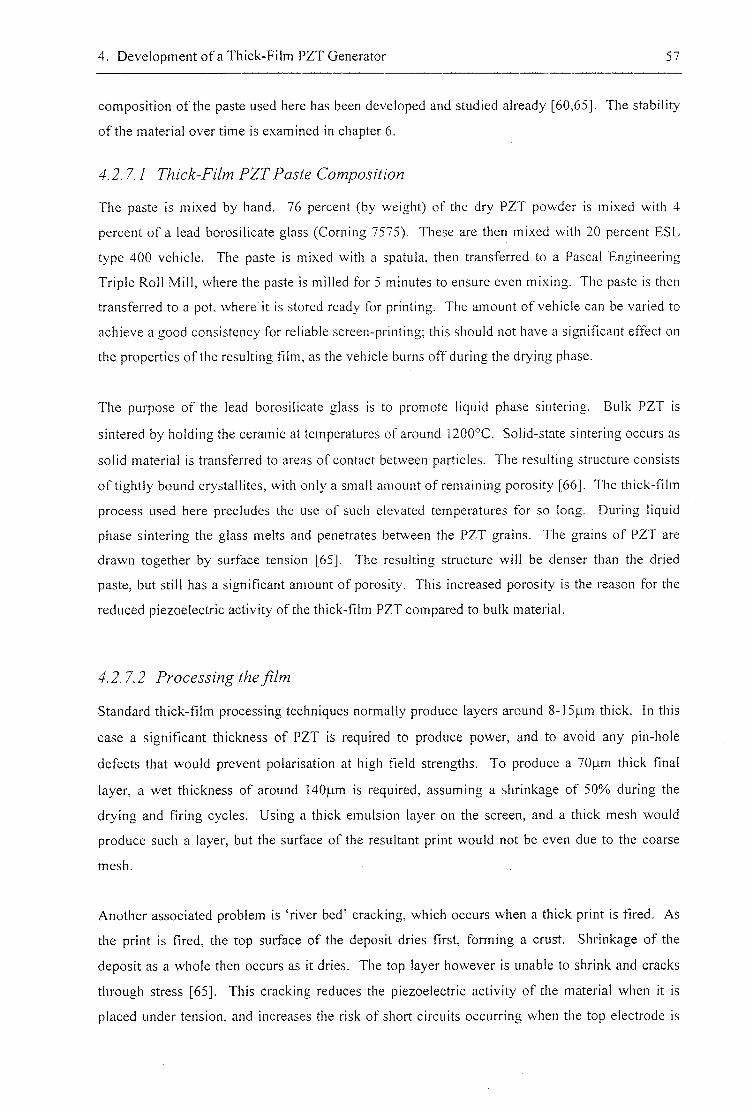
4. Development of a Thick-Film PZT Generator 57
composition of the paste used here has been developed and studied already [60,65]. The stability
of the material over time is examined in chapter 6.
2 . 7 . 7
The paste is mixed by hand. 76 percent (by weight) of the dry PZT powder is mixed with 4
percent of a lead borosilicate glass (Corning 7575). These are then mixed with 20 percent ESL
type 400 vehicle. The paste is mixed with a spatula, then transferred to a Pascal Engineering
Triple Roll Mill, where the paste is milled for 5 minutes to ensure even mixing. The paste is then
transferred to a pot, where it is stored ready for printing. The amount of vehicle can be varied to
achieve a good consistency for reliable screen-printing; this should not have a significant effect on
the properties of the resulting film, as the vehicle burns off during the drying phase.
The purpose of the lead borosilicate glass is to promote liquid phase sintering. Bulk. PZT is
sintered by holding the ceramic at temperatures of around 1200°C. Solid-state sintering occurs as
solid material is transferred to areas of contact between particles. The resulting structure consists
of tightly bound crystallites, with only a small amount of remaining porosity [66]. The thick-film
process used here precludes the use of such elevated temperatures for so long. During liquid
phase sintering the glass melts and penetrates between the PZT grains. The grains of PZT are
drawn together by surface tension [65]. The resulting structure will be denser than the dried
paste, but still has a significant amount of porosity. This increased porosity is the reason for the
reduced piezoelectric activity of the thick-film PZT compared to bulk material.
^ . 2 . 7 . 2
Standard thick-film processing techniques normally produce layers around 8-15|_im thick. In this
case a significant thickness of PZT is required to produce power, and to avoid any pin-hole
defects that would prevent polarisation at high field strengths. To produce a 70p,m thick final
layer, a wet thickness of around MOjum is required, assuming a shrinkage of 50% during the
drying and firing cycles. Using a thick emulsion layer on the screen, and a thick mesh would
produce such a layer, but the surface of the resultant print would not be even due to the coarse
mesh.
Another associated problem is 'river bed' cracking, which occurs when a thick print is fired. As
the print is fired, the top surface of the deposit dries first, forming a crust. Shrinkage of the
deposit as a whole then occurs as it dries. The top layer however is unable to shrink and cracks
through stress [65]. This cracking reduces the piezoelectric activity of the material when it is
placed under tension, and increases the risk of short circuits occurring when the top electrode is

4. Development of a Thick-Film PZT Generator 58
printed over the PZT. This problem was encountered during initial tests, figure 15 shows a
typical set of cracks.
20KV WD:21MM S'00800 P:00000
Figure 15: SEM image of PZT layer with 'river-bed cracking'
To produce a reliable thick layer it is necessary to print several layers on top of each other, firing
once every 50-70p,m to prevent 'river bed cracking'. The exact sequence of printing, drying and
firing used is described in section 4.3.3. By forming the PZT in several layers it is possible to use
a finer mesh, which results in a better resolution, and a more uniform top surface. However the
extra firing cycles required may increase the possibility of lead loss from the PZT, and hence
lower performance.
The paste is fired at a peak temperature of 890°C dwelling at the peak for around 8-lOminutes.
Total firing time is one hour. Current work is being undertaken to determine the effect of longer
firing cycles and lower firing temperatures.
4.2.7.3 Polarisation
To render the PZT piezoelectric, it must be polarised (see section 3.1.1.2). Polarisation of devices
was performed in a box oven. Samples are heated to 150°C then left for 10 minutes to become
thermally stable. A field of 3.5MVm'' is then applied via the electrodes. The field is maintained
for 60 minutes in total, 30 minutes at temperature, followed by another 30 as the sample is
allowed to cool down. The value obtained by polarisation is a logarithmic function of time.
The procedure outlined above should result in a value of some 60% of the final value that
would be obtained in 24 hours [65]. Higher fields can be applied to the devices, Dargie reports
maximum field strengths of around 4.5MVm''. Variations in sample thicknesses, especially
localised thin areas, mean that the actual field being applied can be hard to measure if the
polarising field is applied using the devices own electrodes. Thus the lower field described above
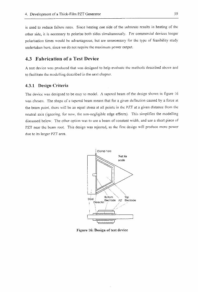
4. Development of a Thick-Film PZT Generator 59
is used to reduce failure rates. Since heating one side of the substrate results in heating of the
other side, it is necessary to polarise both sides simultaneously. For commercial devices longer
polarisation times would be advantageous, but are unnecessary for the type of feasibility study
undertaken here, since we do not require the maximum power output.
4.3 Fabrication of a Test Device
A test device was produced that was designed to help evaluate the methods described above and
to facilitate the modelling described in the next chapter.
4.3.1 Design Criteria
The device was designed to be easy to model. A tapered beam of the design shown in figure 16
was chosen. The shape of a tapered beam means that for a given deflection caused by a force at
the beam point, there will be an equal stress at all points in the PZT at a given distance from the
neutral axis (ignoring, for now, the non-negligible edge effects). This simplifies the modelling
discussed below. The other option was to use a beam of constant width, and use a short piece of
PZT near the beam root. This design was rejected, as the first design will produce more power
due to its larger PZT area.
Clamp here
Not to scale
Bottom , Electrode PZT Electrode
Top Steel /
CZ
Figure 16: Design of test device
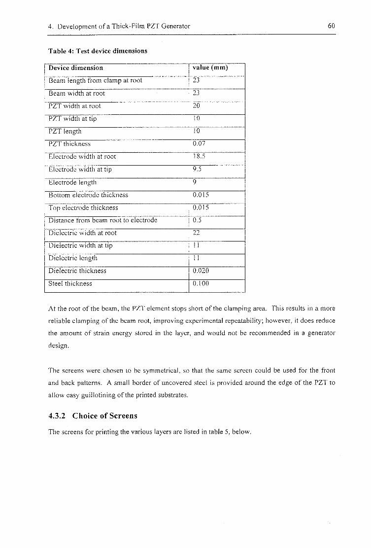
4. Development of a Thick-Film PZT Generator 60
Table 4: Test device dimensions
Device dimension value (mm)
Beam length from clamp at root 23
Beam width at root 23
PZT width at root 20
PZT width at tip 10
PZT length 10
PZT thickness 0.07
Electrode width at root 18.5
Electrode width at tip 9.5
Electrode length 9
Bottom electrode thickness 0.015
Top electrode thickness 0.015
Distance from beam root to electrode 0.5
Dielectric width at root 22
Dielectric width at tip 11
Dielectric length 11
Dielectric thickness 0.020
Steel thickness OUOO
At the root of the beam, the PZT element stops short of the clamping area. This results in a more
reliable clamping of the beam root, improving experimental repeatability; however, it does reduce
the amount of strain energy stored in the layer, and would not be recommended in a generator
design.
The screens were chosen to be symmetrical, so that the same screen could be used for the front
and back patterns. A small border of uncovered steel is provided around the edge of the PZT to
allow easy guillotining of the printed substrates.
4.3.2 Choice of Screens
The screens for printing the various layers are listed in table 5, below.
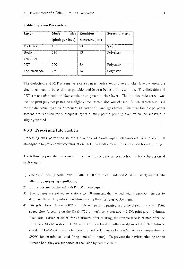
4. Development of a Thick-Film PZT Generator 61
Table 5: Screen Parameters
Layer Mesh size
(pitch per inch)
Emulsion
thickness ()im)
Screen material
Dielectric 180 23 Steel
Bottom
electrode
230 13 Polyester
PZT 200 23 Polyester
Top electrode 230 18 Polyester
The dielectric, and PZT screens were of a coarser mesh size, to give a thicker layer, whereas the
electrodes need to be as thin as possible, and have a better print resolution. The dielectric and
PZT screens also had a thicker emulsion to give a thicker layer. The top electrode screen was
used to print polymer pastes, so a slightly thicker emulsion was chosen. A steel screen was used
for the dielectric layer, as it produces a clearer print, and ages better. The more flexible polyester
screens are required for subsequent layers as they permit printing even when the substrate is
slightly warped.
4.3.3 Processing Information
Processing was performed in the University of Southampton clean-rooms in a class 1000
atmosphere to prevent dust contamination. A DEK-1750 screen printer was used for all printing.
The following procedure was used to manufacture the devices (see section 4.1 for a discussion of
each stage);
1) Sheets of steel (Goodfellows FE240261; lOOjim thick, hardened AISI 316 steel) are cut into
50mm squares using a guillotine.
2) Both sides are roughened with PI000 emery paper,
3) The squares are soaked in acetone for 10 minutes, then wiped with clean-room tissues to
degrease them. Dry nitrogen is blown across the substrates to dry them.
4) Dielectric layer: Heraeus IP222L dielectric paste is printed using the dielectric screen (Print
speed slow (a setting on the DEK-1750 printer), print pressure = 2.2N, print gap = 0.6mm).
Each side is dried at 200°C for 15 minutes after printing; the reverse face is printed after the
front face has been dried. Both sides are then fired simultaneously in a BTU Belt furnace
(model QA41-6-54) using a temperature profile known as Dupont60 (A peak temperature of
890°C for 10 minutes, total firing time 60 minutes). To prevent the devices sticking to the
furnace belt, they are supported at each side by ceramic strips.
4. Development of a Thick-Film PZT Generator 62
5) Bottom electrode: ESL 9633B Silver Palladium paste is printed using the bottom electrode
screen. (Print speed slow, print pressure = 2.2N, print gap = 1.2mm). Each side is dried and
fired in the same way as the dielectric layer,
6) PZT layer: The paste is made up as described in section 4.2.7. On each side, the following
sequence is followed: Double print, dry, double print, dry, fire, double print, dry, double print,
dry, fire. Print speed slow, print pressure = 2.2N, print gap - l . l m m (Double printing
involves printing, then printing again over the wet layer, to ensure full coverage. This is
necessary when the paste fails to print evenly on the first pass - a problem with the current
formulation of PZT paste).
7) Top electrode: ESL 1107 silver loaded polymer paste is printed using the top electrode
screen (Print speed slow, print pressure = 2.2N, print gap = 1.2mm). The paste is cured at
200°C for 60 minutes after printing. Double wet printing is required to ensure coverage (this
could be due to the age of the paste used).
8) A guillotine is used to separate each device from its neighbours on the substrate.
9) Wires are soldered to the electrodes.
10) The device is polarised as described in section 4.2.7,3.
4.4 Testing Material Properties
To produce meaningful models of the piezoelectric beam generators, it is necessary to have
information on the electrical and mechanical properties of the various materials. Thick-film
technology is typically used for hybrid electronics applications, so while thermal and electrical
properties are readily available, mechanical properties must be measured. The electrical
properties of the PZT film are dependent on the exact processing parameters, so these too must be
measured.
4.4.1 Measuring Device Dimensions
The thickness of the various layers was measured using a Tencor Alphastep Profiler (model 10-
0040). The uneven nature of the substrate (caused by thermal-mismatch warping and variations in
print thickness) reduces the measurement accuracy to around ±3|-im. Vernier callipers were used
to measure the dimensions of each device
4.4.2 Dielectric Constants
The mathematical models used below require only the permittivity in the polarisation direction.
To calculate the permittivity, a Wayne Kerr Automatic LCR meter 4250 was used to measure the
capacitance between the electrodes of a sample. The permittivity was derived from the equation
for a parallel plate capacitor.
4. Development of a Thick-Film PZT Generator 63
The thickness was measured as described above, however, even though a migration resistant film
was used for the bottom electrode some migration may have still occurred. This would lower the
effective thickness of the PZT and hence give an artificially high value for the permittivity. Since
the piezoelectric constants themselves are subject to wide variation (see section 4.4.4 ), this effect
has been ignored.
4.4.3 Young's Modulus
The Young's modulus of each layer was measured by determining the bending stiffness of thin
uniform composite beams (i.e. rectangular beams, rather than the tapered beams of other
sections). The bending stiffness is deduced by displacing the beam root vertically, while holding
the beam tip still. The force at the beam tip is measured and hence, the beam stiffness can be
determined
Figure 17 shows the apparatus used: The beam under test is held by an aluminium clamp, which is
attached in place of the microscope barrel on a Chesterman Engineer's microscope. The
microscope base is placed on its side, thus by adjusting the microscope slider the beam can be
moved vertically. The displacement is read off on a vernier scale, accurate to +0.01mm. A screw
is placed upside down on the centre of a Precisa 1600C weighing scales. The tip of the beam rests
on the point of the screw, allowing the force applied to the tip of the beam to be determined to
±0.01 grams.
The elastic deflection of the clamp assembly, and deflection of the weigh-pan of the scales for a
given force was measured by resting the aluminium clamp on the screw point. This was found to
be 0.6kg(mm)' ' , Subsequent measurements were normalised by removing the effect of this
stiffness from the stiffness obtained experimentally. Since typical beams measured here have a
stiffness of O.Olkg(mm)'' this is not a large effect.
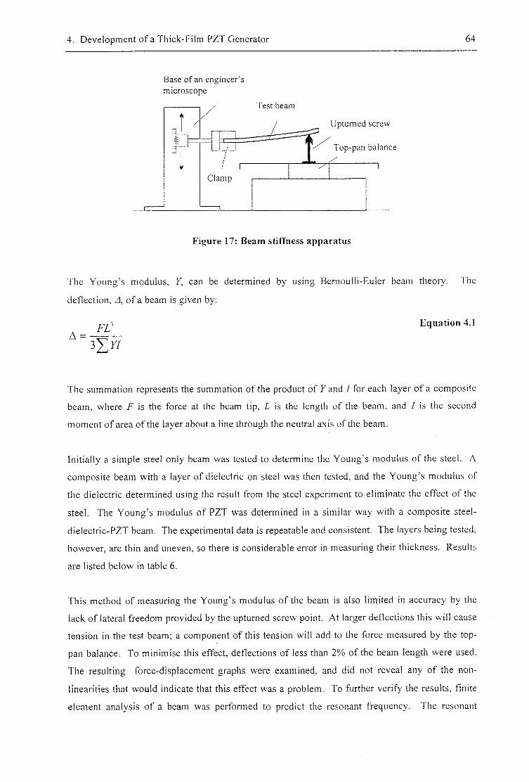
4. Development of a Thick-Film PZT Generator 64
Base of an engineer's microscope
Test beam
Upturned screw
Top-pan balance
Figure 17: Beam stiffness apparatus
The Young's modulus, Y, can be determined by using Bernoulli-Euler beam theory. The
deflection, zl, of a beam is given by:
Equation 4.1
A • ' i n
The summation represents the summation of the product of Fand / for each layer of a composite
beam, where F is the force at the beam tip, L is the length of the beam, and I is the second
moment of area of the layer about a line through the neutral axis of the beam.
Initially a simple steel only beam was tested to determine the Young's modulus of the steel. A
composite beam with a layer of dielectric on steel was then tested, and the Young's modulus of
the dielectric determined using the result from the steel experiment to eliminate the effect of the
steel. The Young 's modulus of PZT was determined in a similar way with a composite steel-
dielectric-PZT beam. The experimental data is repeatable and consistent. The layers being tested,
however, are thin and uneven, so there is considerable error in measuring their thickness. Results
are listed below in table 6.
This method of measuring the Young's modulus of the beam is also limited in accuracy by the
lack of lateral freedom provided by the upturned screw point. At larger deflections this will cause
tension in the test beam; a component of this tension will add to the force measured by the top-
pan balance. To minimise this effect, deflections of less than 2% of the beam length were used.
The resulting force-displacement graphs were examined, and did not reveal any of the non-
linearities that would indicate that this effect was a problem. To further verify the results, finite
element analysis of a beam was performed to predict the resonant frequency. The resonant
4. Development of a Thick-Film PZT Generator 65
frequency was measured experimentally (see section 4.5.2), and found to lie within the bounds of
experimental error.
Table 6: Young's Modulus of device materials
Material Young's Modulus (GPa) Error (±GPa)
3 16 Steel (fired) 162 10
IP222 dielectric 74 5
PZT 18 5
4.4.4 Measuring the rfy Coefficient of Thick-Film PZT
Background material about piezoelectric coefficients can be found in section 3.1.1.
There are 3 fundamental methods for measuring the dis coefficient:
1) The direct effect: A known force is applied to the PZT, and the resulting charge measured.
The force that is applied can either be determined in advance, or deduced by placing a
piezoelectric standard mechanically in series with the sample. To maintain the constant
displacement boundary condition, the electrodes are usually short circuited into a charge
amplifier.
2) The indirect effect: A known voltage is applied to the PZT, and the resulting displacement
measured. To maintain the constant stress boundary condition, the top surface are usually
undamped.
3) Resonant techniques: The resonant frequency of a suitably excited piece of PZT is measured.
A piezoelectric analysis that includes secondary piezoelectric effects is required to calculate
the relevant d coefficients.
For crystals and bulk samples, Mason and Jaffe [67] suggest that resonant techniques are by far
the most accurate. In thick-film samples, however, the presence of the substrate means that the
mechanical resonant frequency of the sample is largely determined by geometry and the
mechanical properties of the materials. Due to the generally low nature of this resonant
frequency, the electromechanical coupling coefficients have little influence on its frequency.
Thus this method is unsuitable for thick-film samples.
The direct and indirect methods are essentially quasi-static techniques, in that they are performed
well away from the resonant frequency of the material. The shape of the test specimen is
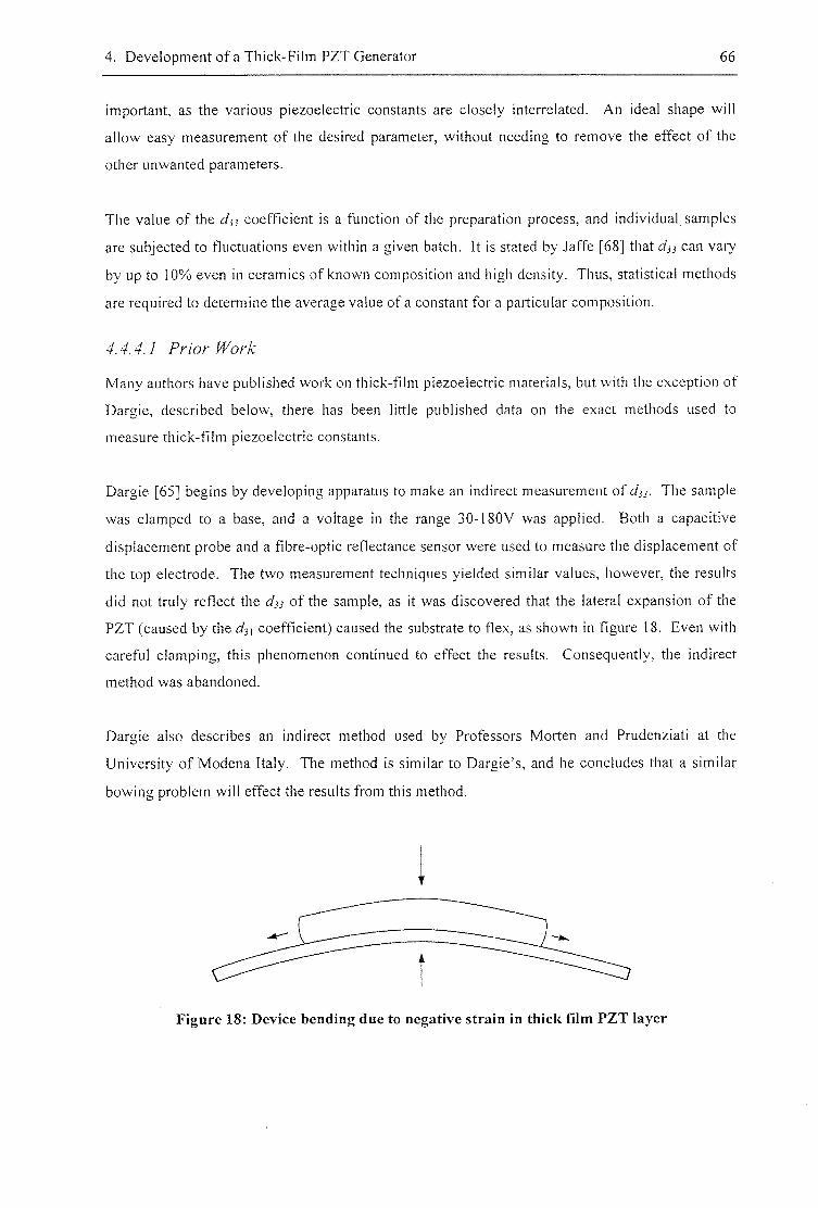
4. Development of a Thick-Film PZT Generator 66
important, as the various piezoelectric constants are closely interrelated. An ideal shape will
allow easy measurement of the desired parameter, without needing to remove the effect of the
other unwanted parameters.
The value of the coefficient is a function of the preparation process, and individual samples
are subjected to fluctuations even within a given batch. It is stated by Jaffe [68] that dss can vary
by up to 10% even in ceramics of known composition and high density. Thus, statistical methods
are required to determine the average value of a constant for a particular composition.
Many authors have published work on thick-film piezoelectric materials, but with the exception of
Dargie, described below, there has been little published data on the exact methods used to
measure thick-film piezoelectric constants.
Dargie [65] begins by developing apparatus to make an indirect measurement of djj. The sample
was clamped to a base, and a voltage in the range 30-180V was applied. Both a capacitive
displacement probe and a fibre-optic reflectance sensor were used to measure the displacement of
the top electrode. The two measurement techniques yielded similar values, however, the results
did not truly reflect the dj i of the sample, as it was discovered that the lateral expansion of the
PZT (caused by the d^\ coefficient) caused the substrate to flex, as shown in figure 18. Even with
careful clamping, this phenomenon continued to effect the results. Consequently, the indirect
method was abandoned.
Dargie also describes an indirect method used by Professors Morten and Prudenziati at the
University of Modena Italy. The method is similar to Dargie's, and he concludes that a similar
bowing problem will effect the results from this method.
Figure 18: Device bending due to negative strain in thick film PZT layer
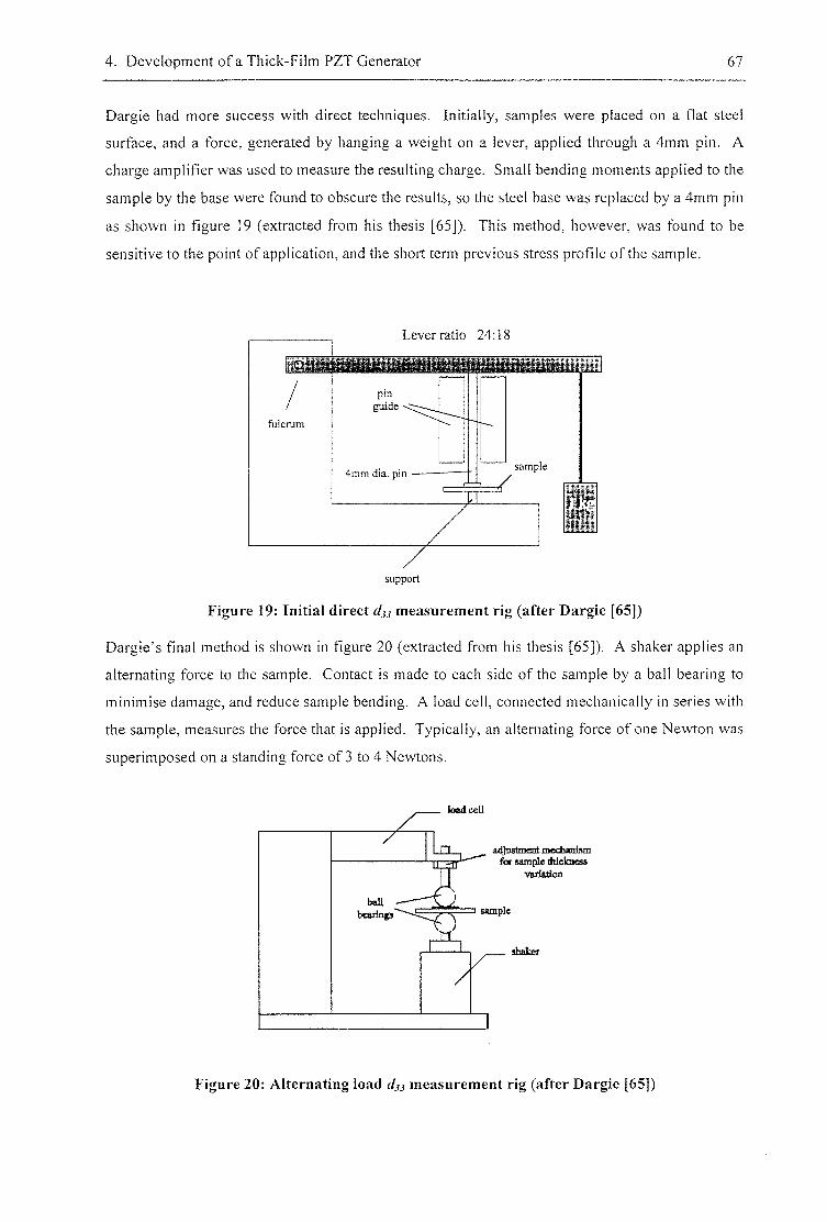
4. Development of a Thick-Film PZT Generator 67
Dargie had more success with direct techniques. Initially, samples were placed on a flat steel
surface, and a force, generated by hanging a weight on a lever, applied through a 4mm pin. A
charge amplifier was used to measure the resulting charge. Small bending moments applied to the
sample by the base were found to obscure the results, so the steel base was replaced by a 4mm pin
as shown in figure 19 (extracted from his thesis [65]). This method, however, was found to be
sensitive to the point of application, and the short term previous stress profile of the sample.
Lever ratio 24:18
p m g u i d e
sample 4mm dia. pin
support
Figure 19: Initial direct <r/jj measurement rig (after Dargie [65])
Dargie's final method is shown in figure 20 (extracted from his thesis [65]). A shaker applies an
alternating force to the sample. Contact is made to each side of the sample by a ball bearing to
minimise damage, and reduce sample bending. A load cell, connected mechanically in series with
the sample, measures the force that is applied. Typically, an alternating force of one Newton was
superimposed on a standing force of 3 to 4 Newtons.
kttdcell
adjmtment mmhanism fot sample thickness
variation
sample
ifaakor
Figure 20: Alternating load djj measurement rig (after Dargie [65])
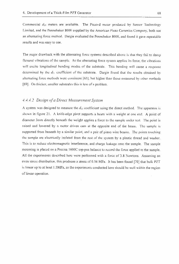
4. Development of a Thick-Film PZT Generator 68
Commercial meters are available. The Piezo-d meter produced by Sensor Technology
Limited, and the Pennebaker 8000 supplied by the American Piezo Ceramics Company, both use
an alternating force method. Dargie evaluated the Pennebaker 8000, and found it gave repeatable
results and was easy to use.
The major drawback with the alternating force systems described above is that they fail to damp
flexural vibrations of the sample. As the alternating force system applies its force, the vibrations
will excite longitudinal bending modes of the substrate. This bending will cause a response
determined by the di\ coefficient of the substrate. Dargie found that the results obtained by
alternating force methods were consistent [65], but higher than those measured by other methods
[69]. On thicker, smaller substrates this is less of a problem.
4 . 2 Dej'zgM q / a D/z-gc/
A system was designed to measure the d}] coefficient using the direct method. The apparatus is
shown in figure 21. A knife-edge pivot supports a beam with a weight at one end. A point of
diameter 3mm directly beneath the weight applies a force to the sample under test. The point is
raised and lowered by a motor driven cam at the opposite end of the beam. The sample is
supported from beneath by a similar point, and a pair of piano wire beams. The points touching
the sample are electrically isolated from the rest of the system by a plastic thread and washer.
This is to reduce electromagnetic interference, and charge leakage onto the sample. The sample
mounting is placed on a Precisa 1600C top-pan balance to record the force applied to the sample.
All the experiments described here were performed with a force of 3.8 Newtons. Assuming an
even stress distribution, this produces a stress of 0.54 MPa. It has been found [70] that bulk PZT
is linear up to at least l.SMPa, so the experiments conducted here should be well within the region
of linear operation.
4. Development of a Thick-Film PZT Generator 69
Weight
Cam to lift beam Support
Knife Edge Pivot
Beam 3mm points
Insulated spacer
Sample
Piano wire support beams
"Top-pan balance
Figure 21: Final ([33 testing rig
It was found that the friction in the mechanism supporting the weight was an important factor.
Friction causes any small vibration in the surrounding environment (e.g. people walking past the
test bench), to be coupled directly into the sample. This can have a significant effect on the
observed response. By using a longer beam, leverage factors down any small torques applied by
the knife edge pivot.
Like Dargie, the initial design of sample holder consisted of a flat surface, and a clamp. When
this was tested, it was found that bending moments within the sample (caused by an uneven base,
or warped substrate) could contribute to the charge produced. By applying forces to the substrate
next to the piezoelectric area, it was found that the bending could produce a signal at least as large
as the one caused by the d u coefficient. Experiments were performed with samples firmly glued
to a block of aluminium with super glue. This reduced the bending significantly, but it was still
large enough to interfere with samples having dsi coefficients of an order of 50pCN"'. Gluing the
samples is also a destructive test, which is not satisfactory.
The final design uses a set of springy piano wire beams (diameter 0.5mm, length 10cm) to
support the sample between the steel point below the sample, and the point on the force unit. This
arrangement allows the sample to rotate as necessary when the force is applied, so that all forces
are tangential to the sample. Experiments showed that this reduces the charge caused by bending
to around 2pC on ceramic substrates around 5cm long.
The output from the PZT's electrodes was fed directly into a Kistler 5001 Charge Amplifier, The
output from the charge amplifier was measured using an Hewlett Packard HP35660A Dynamic
Signal Analyser. To make a reading, the sample is placed between the points, and the piano wire
beams adjusted to support the sample at the right height. The top-pan balance is examined to
4. Development of a Thick-Film PZT Generator 70
record the force being applied to the sample, then the cam is used to raise the beam. The Signal
Analyser is paused to allow the amount of charge displaced to be recorded.
The surrounding material which constrains the PZT where the force is applied, must also be
considered. The measurement rig applies a force to only a small fraction of the total electrode
area of the sample. This means that the material surrounding the clamped area will constrain any
lateral expansion of the PZT layer, and cause a corresponding change in the observed response.
The effective d n is calculated by Nemirovsky et al [71] as
d „ , „ , = d , 3 - 2 d „ { c / / c / ) Equ. . , io„4.2
Where C / / and Cjl' are terms of the stiffness matrix for the PZT under boundary conditions of
constant field. Using typical material constants for bulk PZT [44], we obtain
d 3 3 . e f r = d 3 3 + 1 . 4 x d , , Equa t ion 4.3
The main source of error in this experiment arises from the mains hum picked up by the circuit,
which limits accuracy to around ±3pCN' ' . This was present even after screening connecting
wires, and earthing major conductors. Since these results were not required for the remainder of
this work, significant effort was not applied to reducing this error.
Bending moments are also still present, and limit the substrate thickness to being thicker than
around 200p.m. The limit on thickness means that it is not possible to directly measure the d}} of
the test devices described in section 4.3. To determine the dys produced by this process, the same
steps were performed on a 1mm thick substrate. This resulted in a effective d j j coefficient of
around -120pCN' ' . Taking the results for dy\ described below, and using equation 4.3, this yields
a value of -13 5 pCN"' for dn •
4.4.5 Measuring the dg. Coefficient of Thick-Film PZT
The t/ji coefficient can be measured using the same basic techniques described above for d ^
(direct, indirect, and resonant techniques). The thin nature of the thick-film materials being
measured, however, means that it is difficult to directly apply or measure forces and
displacements in directions perpendicular to the thickness. Like the d n coefficient, there is little
available information in the literature, on experimental methods of measuring d^].
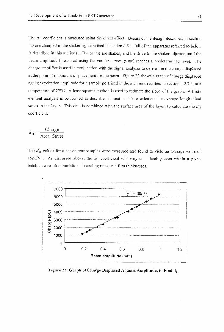
4. Development of a Thick-Film PZT Generator 71
The coefficient is measured using the direct effect. Beams of the design described in section
4.3 are clamped in the shaker rig described in section 4.5.1 (all of the apparatus referred to below
is described in this section) . The beams are shaken, and the drive to the shaker adjusted until the
beam amplitude (measured using the vernier screw gauge) reaches a predetermined level. The
charge amplifier is used in conjunction with the signal analyser to determine the charge displaced
at the point of maximum displacement for the beam. Figure 22 shows a graph of charge displaced
against excitation amplitude for a sample polarised in the manner described in section 4.2.7.3, at a
temperature of 22°C. A least squares method is used to estimate the slope of the graph. A finite
element analysis is performed as described in section 5.5 to calculate the average longitudinal
stress in the layer. This data is combined with the surface area of the layer, to calculate the J , ,
coefficient.
t/ji Charge
A j e a S&tiss
The t/ji values for a set of four samples were measured and found to yield an average value of
15pCN"'. As discussed above, the coefficient will vary considerably even within a given
batch, as a result of variations in cooling rates, and film thicknesses.
7000
6000
5000
o 4000 Q.
0) 3000 P <0 sz 2000 O
1000
y = 6285.7X
0 2 &4 &6
Beam amplitude (mm)
1.2
Figure 22: Graph of Charge Displaced Against Amplitude, to Find d 31

4. Development of a Thick-Film PZT Generator 72
4.5 Response of Prototype Tapered Beams
4.5.1 Experimental Apparatus
The results described in this section have been obtained using the apparatus shown in figure 23.
A c c e l e r o m e t e r
C l a m p e d
S a m p l e
P o t e n t i o m e t e r
A m p l i f i e r
V o l t a g e
F o l l o w e r
S i g n a l
G e n e r a t o r
C h a r g e
A m p l i f i e r
T e m p e r a t u r e
Probe
E l e c t r o m e c h a n i c a l
S h a k e r
S p e c t r u m
A n a l y s e r
Figure 23: Experimental Set-up
A Goodman V.50 Mk.l (Model 390) Vibration Generator (shaker) is used to supply mechanical
vibrations to the samples under test. Auxiliary suspension is fitted to the shaker, which improves
the lateral constraint of the central spindle, and reduces the load on the shaker suspension. The
loads mounted during the course of these experiments are below the 21b limit suggested by the
manufacturer [72]. The shaker can supply vibrations in the range 5Hz-4kHz (limited by the
current consumption of the coil, and its first resonant frequency respectively). The shaker is
driven by a Ling PA50VA valve amplifier. The amplifier is driven from the frequency source
incorporated into a Hewlett Packard HP35660A Dynamic Signal Analyser. The output from the
signal analyser is reduced by feeding it through a 20 turn, wire-wound I k O potentiometer. This
allows fine adjustments to be made to the output of the signal analyser.
The samples are clamped, and mounted on the shaker using the specially designed clamp shown
in figure 25. Figure 24 shows a photograph of a prototype beam in the clamp. The clamp is
mounted on the shaker spindle thread, and held by a lock-nut. An accelerometer is mounted
axially above the spindle on a short thread (Bruel & Kjaer Accelerometer Type 4369). The
accelerometer provides data on the amplitude of vibrations applied to the samples, which can not
be determined solely from the electrical drive to the shaker, since the shaker has a non-linear
response. The accelerometer has a first resonance at 36kHz, which is well above frequencies of
interest in the experiments described here. The clamp consists of an aluminium plate at each end
of the aluminium base, held in place by a pair of bolts through each plate. The end surfaces are
4. Development of a Thick-Film PZT Generator 73
machined with the plates in position to ensure that the end surfaces of the plates and the base lie in
the same plane. The twin plates allow two samples to be clamped at once, which is useful for
holding a reference sample. To clamp a sample, shims of the same thickness as the sample are
held under the rear edge of the plate to ensure that the plate is parallel to the base.
A vernier screw gauge is mounted on a plate that is attached by threaded steel rods to the shaker.
The screw gauge has a resolution of 0.01mm, and allows the tip amplitude of a vibrating beam to
be measured. Figure 26 shows the shaker, suspension, clamp block, accelerometer, screw gauge,
and a typical sample as they are mounted together. The accuracy of measurements obtained this
way is limited by the size of the point at the tip of the gauge, since as the amplitude of the beam
changes, the point of contact with the screw gauge will also change.
A mass can be attached to the tip of a sample using the method illustrated in figure 27. A short
thread holds a pair of nuts that are tightened on either side of the sample to hold the mass in place.
Washers separate the sample from the nuts, and have a flattened edge, which provides a more
even stress distribution in the area of the sample next to the mass.
Connecting wires can be attached to the sample using either solder, or a conductive epoxy.
Soldering was found to be reliable, and produced a conveniently small bond for attaching wires to
the cermet bottom electrodes of the samples described in section 4.3. The clamp described above
has channels cut in the top plates (as shown in figure 25) to allow the connecting wire from the
bottom electrode to pass under the plate. A hole drilled down to the channel from the top of the
plate makes room for the soldered joint. The contact resistance of these soldered joints is
negligible. For the polymer top electrode, soldering was found to be unreliable. The elevated
temperatures required for soldering also partially depolarise the sample, and there is a risk that the
solder or flux will penetrate into to piezoelectric layer and cause changes to the piezoelectric
response of the sample. A silver loaded epoxy (Circuit Works, CW2400) was found to be
suitable. A typical joint has a contact resistance of less than O.IQ. A lacquered 0.2mm diameter
copper wire was chosen for the electrical connections. It is important to chose a thin wire for
connecting to the top electrode, as the wire can interact mechanically with the sample. The wire
is attached to the base with double sided tape so that movement of wires distal to the sample will
not have a mechanical effect on the sample. This wire is soldered to thicker single core wire,
which is in turn held by crocodile clips attached to BNC cables. The BNC cables reduce
interference from mains hum in the experiments. The effect of mains hum is also reduced by
conducting experiments at frequencies that are not multiples of 50Hz, adjusting the resonant
frequency of beams by changing the clamping position where necessary.
4. Development of a Thick-Film PZT Generator 74
To measure the charge displaced by the piezoelectric materials, and the charge signal from the
accelerometer, a Kistler Charge Amplifier (model 5001) is used. The charge amplifier was
calibrated by applying a reference voltage to the built-in calibration capacitor. The charge
amplifier has three built-in discharge resistors. A larger discharge resistor gives better frequency
performance, at the expense of higher DC drift. The experiments performed here are at a
sufficiently high frequency that the smallest discharge resistor (lO^O , labelled 'short ' on the
amplifier) can be used, to minimise DC drift.
To measure the open circuit voltage produced by the piezoelectric samples, and to measure the
voltage developed across load resistors, a voltage follower was constructed. Measuring these
voltages directly is difficult with a conventional oscilloscope, as the impedance of the
oscilloscope will discharge the piezoelectric layer. The voltage follower was implemented using
a TLC251 JFET-input op-amp, which has very low input bias and offset currents (typically 0.1 pA,
and 0.6pA respectively). Since the voltage follower is used in experiments where frequency
analysis is used to isolate the required signal from other components, issues such as supply
voltage ripple rejection, and voltage offsets do not have significant impact on the accuracy of the
experiments.
The outputs from the voltage follower and the charge amplifier, are both monitored by a Hewlett
Packard HP35660A Dynamic Signal Analyser.
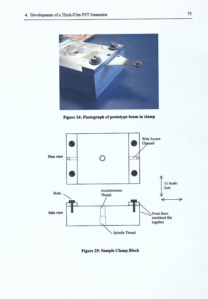
4. Development of a Thick-Film PZT Generator 75
Figure 24: Photograph of prototype beam in clamp
Plan view Q:
Bolts
Side view
:D
Wire Access Channel
Accelerometer Thread
X L
A
To Scale: 2cm
V • >
Front faces machined flat together
, Spindle Thread
Figure 25: Sample Clamp Block
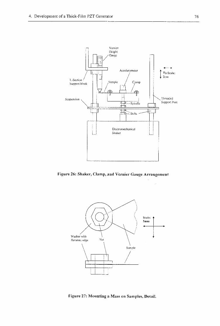
4. Development of a Thick-Film PZT Generator 76
Vernier
He igh t
G a u g e
T o Sca le :
2 c m L-Sec t ion '
S u p p o r t b lock ,Sample C l a m p
T h r e a d e d
S u p p o r t Post Suspens ion
— S p i n d l e
E lec t romechan ica l
Shake r
Figure 26: Shaker, Clamp, and Vernier Gauge Arrangement
W a s h e r with
f lat tened edge Nut
Scale:
5 m m
Sample
Figure 27: Mounting a Mass on Samples, Detail.
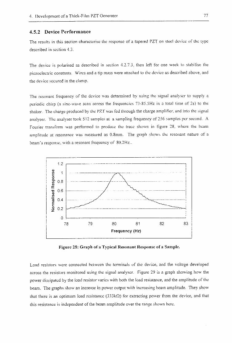
4. Development of a Thick-Film PZT Generator 77
4.5.2 Device Performance
The results in this section characterise the response of a tapered PZT on steel device of the type
described in section 4.3.
The device is polarised as described in section 4.2.7.3, then left for one week to stabilise the
piezoelectric constants. Wires and a tip mass were attached to the device as described above, and
the device secured in the clamp.
The resonant frequency of the device was determined by using the signal analyser to supply a
periodic chirp (a sine-wave scan across the frequencies 73-85.5Hz in a total time of 2s) to the
shaker. The charge produced by the PZT was fed through the charge amplifier, and into the signal
analyser. The analyser took 512 samples at a sampling frequency o f 2 5 6 samples per second. A
Fourier transform was performed to produce the trace shown in figure 28, where the beam
amplitude at resonance was measured as 0.8mm. The graph shows the resonant nature of a
beam's response, with a resonant frequency of 80.2Hz..
-D 0.6
re 0.4
Frequency (Hz)
Figure 28: Graph of a Typical Resonant Response of a Sample.
Load resistors were connected between the terminals of the device, and the voltage developed
across the resistors monitored using the signal analyser. Figure 29 is a graph showing how the
power dissipated by the load resistor varies with both the load resistance, and the amplitude of the
beam. The graphs show an increase in power output with increasing beam amplitude. They show
that there is an optimum load resistance (333kQ) for extracting power from the device, and that
this resistance is independent of the beam amplitude over the range shown here.
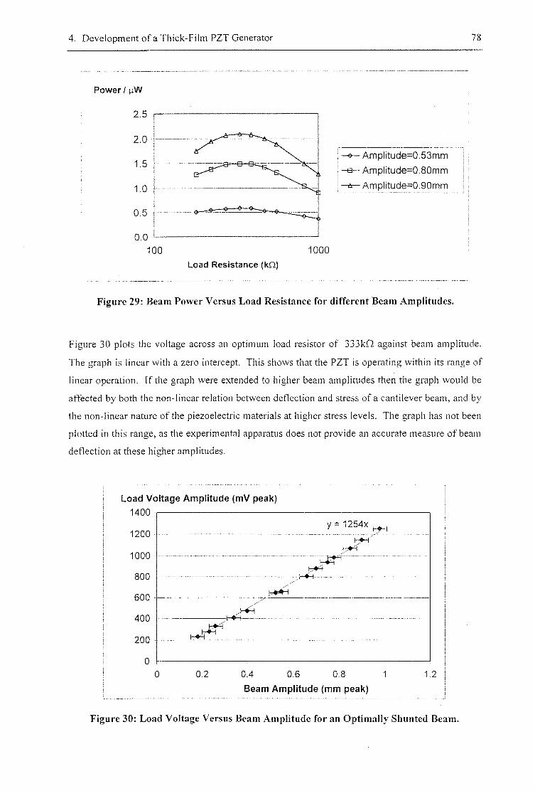
4. Development of a Thick-Film PZT Generator 78
Power I LiW
100 1000
Load Resistance (kO)
-0— Amplitude=0,53mm
-B— Amplitude=0.80mm
Amplitude=0.90mm
Figure 29; Beam Power Versus Load Resistance for different Beam Amplitudes.
Figure 30 plots the voltage across an optimum load resistor of 333kQ against beam amplitude.
The graph is linear with a zero intercept. This shows that the PZT is operating within its range of
linear operation. If the graph were extended to higher beam amplitudes then the graph would be
affected by both the non-linear relation between deflection and stress of a cantilever beam, and by
the non-linear nature of the piezoelectric materials at higher stress levels. The graph has not been
plotted in this range, as the experimental apparatus does not provide an accurate measure of beam
deflection at these higher amplitudes.
Load Voltage Amplitude (mV peak)
1400
1200
1000
800
600
400
200
0
y = 1254x
&2 0/1 &6 0 ^ 1
Beam Amplitude (mm peak)
1.2
Figure 30: Load Voltage Versus Beam Amplitude for an Optimally Shunted Beam.
4. Development of a Thick-Film PZT Generator 79
The quality factor, Q, was measured by examining the width of the resonant peak. The relation
Equation 4.4 CO,
26;„
is used where coi and coi are the frequencies where the response falls by 3dB from its peak value.
A series of four measurements at a beam amplitude of 0.55mm revealed a Q-factor of 111.5
±10%.
4.6 Summary
Techniques have been developed for depositing a functional thick-film layer of PZT on thin
stainless-steel substrates. Chemical interaction between the two materials is prevented with an
intermediate layer of a glassy dielectric, and thermal mismatch is compensated for using
symmetrical structures.
Mechanical and electrical properties of the thick-film PZT layer have been measured. The
practical measurement of piezoelectric thick-films on substrates is not straightforward. Although
previous work has quoted piezoelectric properties, there has been little published data on the
experimental methods used to measure piezoelectric constants of these materials. Thus methods
have been developed for measuring the and coefficients of thick-film piezoceramics. The
Young's modulus of thick-film PZT has also been measured. The following results are obtained:
Table 7: Summary of PZT material properties
Property Value Error (%)
15pC/N 30
d}} 135pC/N 20
Young's Modulus ISGPa 10
A prototype piezoelectric generator has been produced, and tested. A maximum of 3p.W was
produced at an amplitude of 1.9mm. Since the maximum stress permitted in the PZT before
depolarisation or mechanical damage occurs is unknown, the maximum power output for long-
term operation cannot be stated. At the amplitude of 1.9mm no immediate damage was observed,
but experiments were discontinued to preserve the generator. See chapter 6 for more discussion
on stress related changes in PZT layers. The results show that the amount of power that is
supplied to the load is influenced by the type of loading applied. The power produced by the

4. Development of a Thick-Film PZT Generator 80
prototype generators is not large enough to be practically useful (as discussed above in section
3.3). The cause of this low power output will be investigated in the following Chapter.
5. Modelling Piezoelectric Generators
c h a p t e r 5
Modelling Piezoelectric Generators
This chapter focuses on techniques for modelling the electrical and mechanical responses of a
piezoelectric beam generator of the type described in the previous chapter (referred to in this
section as a piezo-generator). Mathematical modelling of layered generators is performed,
including a new mode! for the mechanical impedance of a resistively shunted piezoelectric beam.
The modelling is used to provide predictions to compare with the experimental data from the
prototype. Confident that the modelling provides realistic estimates of generator performance, the
model is used to assess how much power could possibly be extracted from a generator of arbitrary
dimensions and excitation.
Figure 31 is an energy flow diagram, showing how energy is taken from the external environment
and converted into a useful electrical form, including energy losses. The energy undergoes a
series of conversions, from the initial kinetic energy of the beam through elastic energy of the
beam, electrical energy in the piezoelectric material and load circuit, and is f inally stored in a
chemical form in a battery. An important point to note is that the amount of energy generated by
the system is determined by both the amount of energy lost at each stage (related to the
efficiency), and by the proportion of energy that is converted from one stage to the next. The
eff iciency of such a generator system is generally not important, as the energy taken from the
excitation medium is generally only a tiny proportion of that available, so it doesn ' t matter if
some of it is wasted. We are interested in maximising the output power, even if that means a
lowered efficiency.
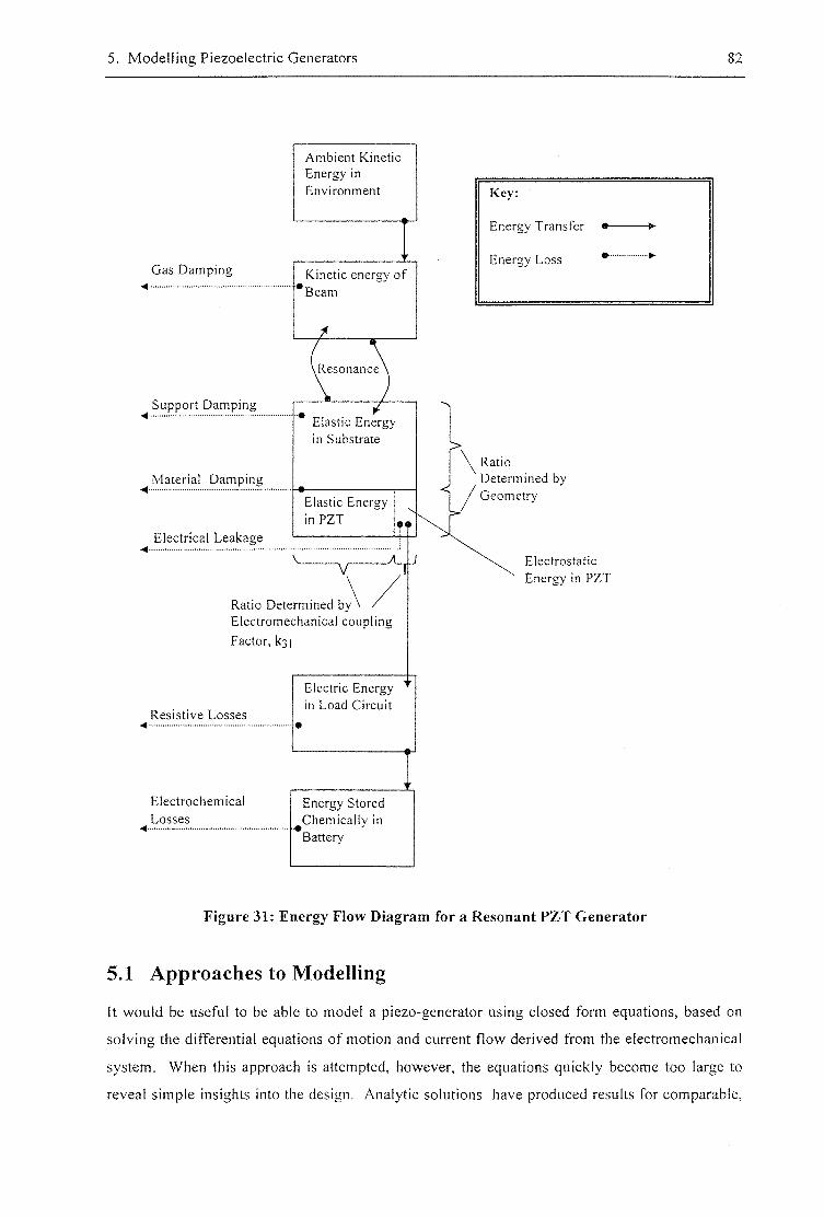
5. Modelling Piezoelectric Generators 82
G a s D a m p i n g
S u p p o r t D a m p i n g
M a t e r i a l D a m p i n g
E lec t r i ca l L e a k a g e
A m b i e n t Kine t i c
E n e r g y in
E n v i r o n m e n t
Kine t ic e n e r g y o f
' B e a m
\ R e s o n a n c e
Elas t ic E n e r g y
in Subs t r a t e
Elast ic E n e r g y
mPZT
Rat io D e t e r m i n e d by
E l e c t r o m e c h a n i c a l c o u p l i n g
Fac tor , k ] ]
R e s i s t i v e L o s s e s
Elec t r ic E n e r g y
in L o a d Ci rcu i t
Key:
E n e r g y T r a n s f e r • — — •
E n e r g y Loss * i«-
Rat io
D e t e r m i n e d by
G e o m e t r y
E lec t ros t a t i c
E n e r g y in P Z T
E l e c t r o c h e m i c a l
L o s s e s
E n e r g y S to red
^ C h e m i c a l l y in
Bat te ry
Figure 31: Energy Flow Diagram for a Resonant PZT Generator
5.1 Approaches to Modelling
It would be useful to be able to model a piezo-generator using closed form equations, based on
solving the differential equations of motion and current flow derived from the electromechanical
system. When this approach is attempted, however, the equations quickly become too large to
reveal simple insights into the design. Analytic solutions have produced results for comparable,
5. Modelling Piezoelectric Generators 83
but simpler systems [73], but the piezo-generators are more complex, due to the following
features:
(a) The strain induced by flexure of the sample varies through the thickness of the
piezoelectric material, and must be modelled accordingly. (See section 5.3 ).
(b) The electrical load interacts dynamically with the capacitive piezoelectric layer,
creating a set of electrical poles and zeroes that couple with the mechanical system.
(c) The shapes of the piezoelectric layer and the substrate produces complicated mode
shapes, and boundary conditions,
(d) Air and support damping both have an important effect on the system, and must be
taken into account.
(e) Non-rectangular beams exhibit significant edge effects.
Finite Element Analysis (FEA) would solve many of the difficulties mentioned above. The FEA
package ANSYS® was examined to find a means of directly predicting the response, and power
produced by a generator. The package does provide the capability for limited piezoelectric field
coupling (Elements S0LID5, PLANE 13, etc), however, it does not allow the simultaneous
mechanical and electrical load conditions that would be required to model resistively shunted
piezoelectric elements. This is a restriction common to all current FEA packages (discussed in a
review by Soderkvist [74]).
The material parameters of the thick-film materials (e.g. d-^. Young's modulus) can vary
considerably. Jaffe et al [43] state that typical piezoelectric parameters can vary by up to 10
percent within a single batch. Experience confirms this statement, and shows that mechanical
parameters are subject to similar variation. This variation limits the degree of accuracy with
which the models presented here can be verified to a few percent.
5.2 Decoupling the Electrical and Mechanical Responses of a
Shunted Piezoelectric Element
The methods adopted below decouple the electrical and mechanical domains, allowing the
problem to be solved in smaller, more tractable pieces.
A model of a generally shunted piezoelectric material is developed by Hagood and von Flotow
[45]. The model is expressed in the Laplacian domain, and is based on a block-shaped
piezoelectric element shunted by a passive electrical load, and with arbitrary driving currents.
Hagood shows that in the steady state the element can be represented mechanically as having a
frequency dependent complex stiffness, whose value depends on the electrical load conditions.
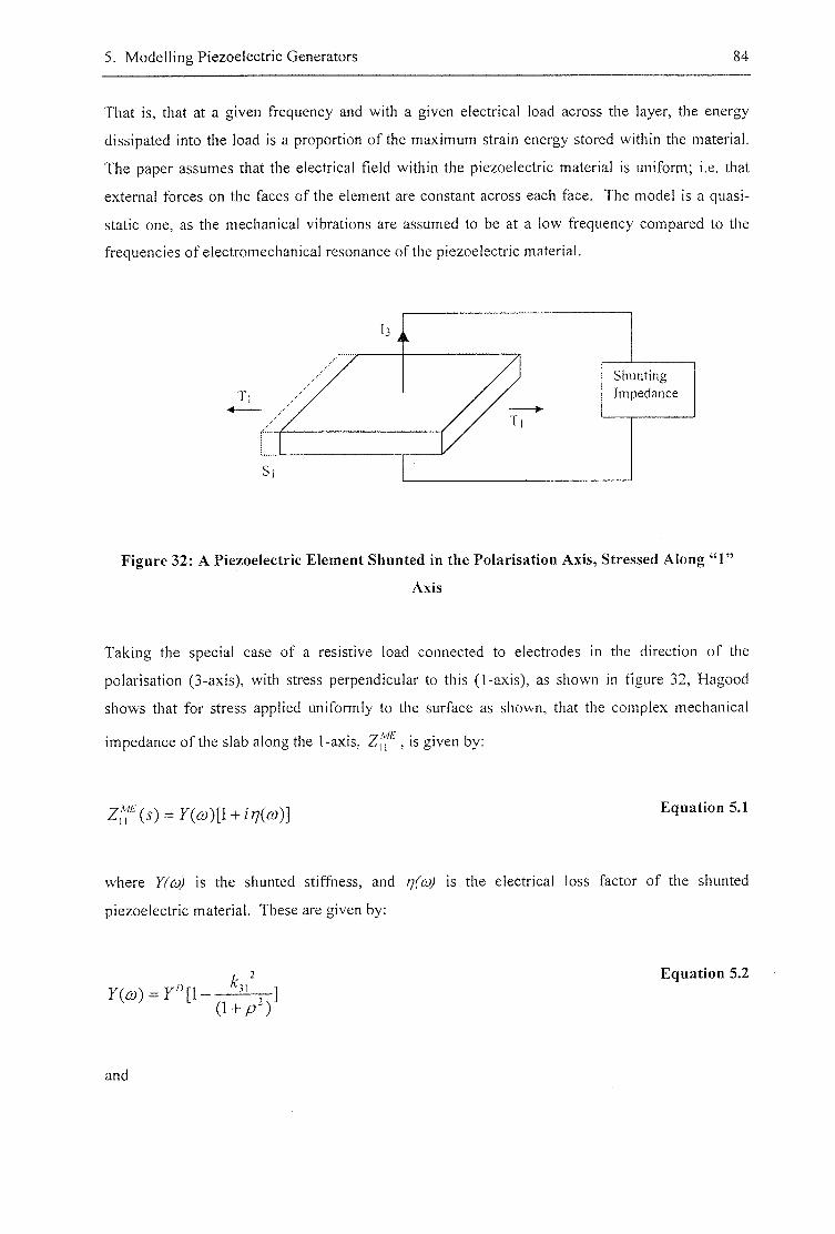
5. Modelling Piezoelectric Generators 84
That is, that at a given frequency and with a given electrical load across the layer, the energy
dissipated into the load is a proportion of the maximum strain energy stored within the material.
The paper assumes that the electrical field within the piezoelectric material is uniform; i.e. that
external forces on the faces of the element are constant across each face. The model is a quasi-
static one, as the mechanical vibrations are assumed to be at a low frequency compared to the
frequencies of electromechanical resonance of the piezoelectric material.
Shunting Impedance
Figure 32: A Piezoelectric Element Shunted in the Polarisation Axis, Stressed Along "1"
Axis
Taking the special case of a resistive load connected to electrodes in the direction of the
polarisation (3-axis), with stress perpendicular to this (1-axis), as shown in figure 32, Hagood
shows that for stress applied uniformly to the surface as shown, that the complex mechanical
impedance of the slab along the 1-axis, , is given by:
Equation 5.1
where Y(co) is the shunted stiffness, and ri(co) is the electrical loss factor of the shunted
piezoelectric material. These are given by:
Equation 5.2
and
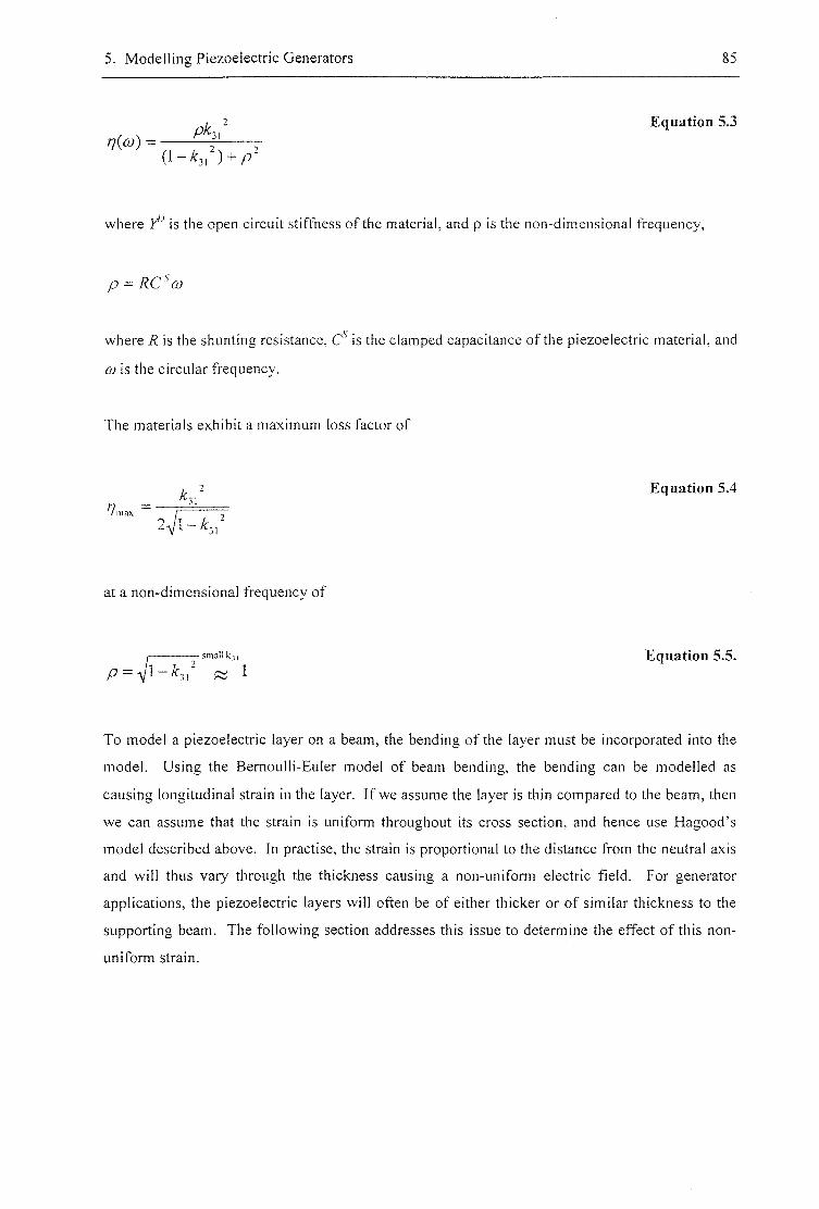
5. Modelling Piezoelectric Generators 85
1 2 Equation 5.3
where 7^ is the open circuit stiffness of the material, and p is the non-dimensional frequency,
p = /ZC'Vu
where R is the shunting resistance, is the clamped capacitance of the piezoelectric material, and
co is the circular frequency.
The materials exhibit a maximum loss factor of
I 2 Equation 5.4 n = ^ /mM / r
2 ^ 1
at a non-dimensional frequency of
p - -Jl - ^3," ~ 1 small k,, Equation 5.5.
To model a piezoelectric layer on a beam, the bending of the layer must be incorporated into the
model. Using the Bernoulli-Euler model of beam bending, the bending can be modelled as
causing longitudinal strain in the layer. If we assume the layer is thin compared to the beam, then
we can assume that the strain is uniform throughout its cross section, and hence use Hagood's
model described above. In practise, the strain is proportional to the distance from the neutral axis
and will thus vary through the thickness causing a non-uniform electric field. For generator
applications, the piezoelectric layers will often be of either thicker or of similar thickness to the
supporting beam. The following section addresses this issue to determine the effect of this non-
uniform strain.
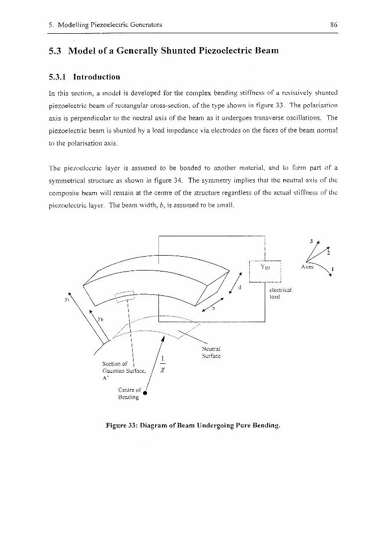
5. Modelling Piezoelectric Generators 86
5.3 Model of a Generally Shunted Piezoelectric Beam
5.3.1 Introduction
In this section, a model is developed for the complex bending stiffness of a resistively shunted
piezoelectric beam of rectangular cross-section, of the type shown in figure 33. The polarisation
axis is perpendicular to the neutral axis of the beam as it undergoes transverse oscillations. The
piezoelectric beam is shunted by a load impedance via electrodes on the faces of the beam normal
to the polarisation axis.
The piezoelectric layer is assumed to be bonded to another material, and to form part of a
symmetrical structure as shown in figure 34. The symmetry implies that the neutral axis of the
composite beam will remain at the centre of the structure regardless of the actual stiffness of the
piezoelectric layer. The beam width, 6, is assumed to be small.
e l e c t r i c a l
l o a d
N e u t r a l
S u r f a c e
S e c t i o n o f |
G a u s s i a n S u r f a c e ,
C e n t r e o f
B e n d i n g
.Axes
Figure 33; Diagram of Beam Undergoing Pure Bending.
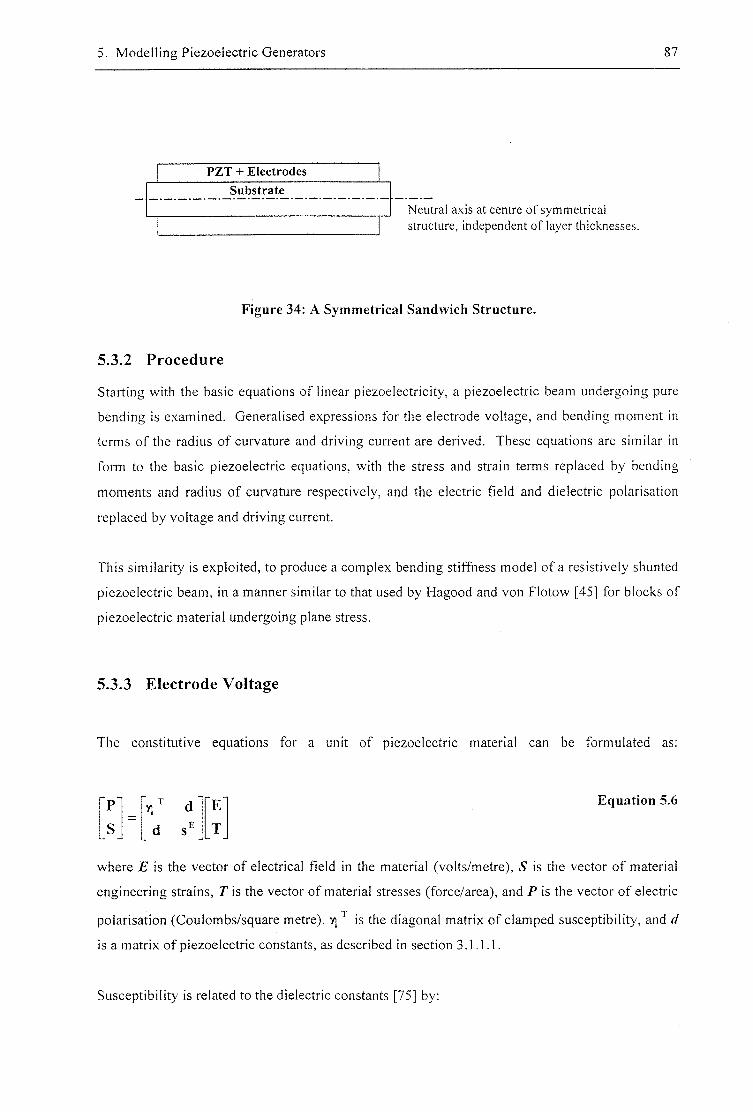
5. Modelling Piezoelectric Generators 87
PZT + Electrodes
Substrate
N e u t r a l ax i s at c e n t r e o f s y m m e t r i c a l
s t r uc tu re , i n d e p e n d e n t o f l ayer t h i c k n e s s e s
Figure 34; A Symmetrical Sandwich Structure.
5.3.2 Procedure
Starting with the basic equations of linear piezoelectricity, a piezoelectric beam undergoing pure
bending is examined. Generalised expressions for the electrode voltage, and bending moment in
terms of the radius of curvature and driving current are derived. These equations are similar in
form to the basic piezoelectric equations, with the stress and strain terms replaced by bending
moments and radius of curvature respectively, and the electric field and dielectric polarisation
replaced by voltage and driving current.
This similarity is exploited, to produce a complex bending stiffness model of a resistively shunted
piezoelectric beam, in a manner similar to that used by Hagood and von Flotow [45] for blocks of
piezoelectric material undergoing plane stress.
5.3.3 Electrode Voltage
The constitutive equations for a unit of piezoelectric material can be formulated as:
Equation 5.6 P d ' 'E'
S_ d T
where E is the vector of electrical field in the material (volts/metre), S is the vector of material
engineering strains, T is the vector of material stresses (force/area), and P is the vector of electric
polarisation (Coulombs/square metre), y] is the diagonal matrix of clamped susceptibility, and d
is a matrix of piezoelectric constants, as described in section 3.1.1.1.
Susceptibility is related to the dielectric constants [75] by:
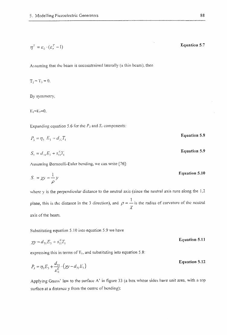
5. Modelling Piezoelectric Generators
- 1 ) Equation 5.7
Assuming that the beam is unconstrained laterally (a thin beam), then
T2 = Tlr=0.
By symmetry,
Ei=Ei=0.
Expanding equation 5.6 for the P j and Si components:
^ =7/^ ^3 +^31^1 Equation 5.8
Assuming Bernoulli-Euler bending, we can write [76]:
c I = —A'
p
Equation 5.9
Equation 5.10
where y is the perpendicular distance to the neutral axis (since the neutral axis runs along the 1,2
plane, this is the distance in the 3 direction), and / ) = — is the radius of curvature of the neutral Z
axis of the beam.
Substituting equation 5.10 into equation 5.9 we have
Zy ~ ^31^3
expressing this in terms o f T , , and substituting into equation 5.8:
^ = % ^ 3 + 4 ' ( z y - ^ 3 , 4 )
Equation 5.11
Equation 5.12
Applying Gauss' law to the surface A' in figure 33 (a box whose sides have unit area, with a top
surface at a distance y from the centre of bending):
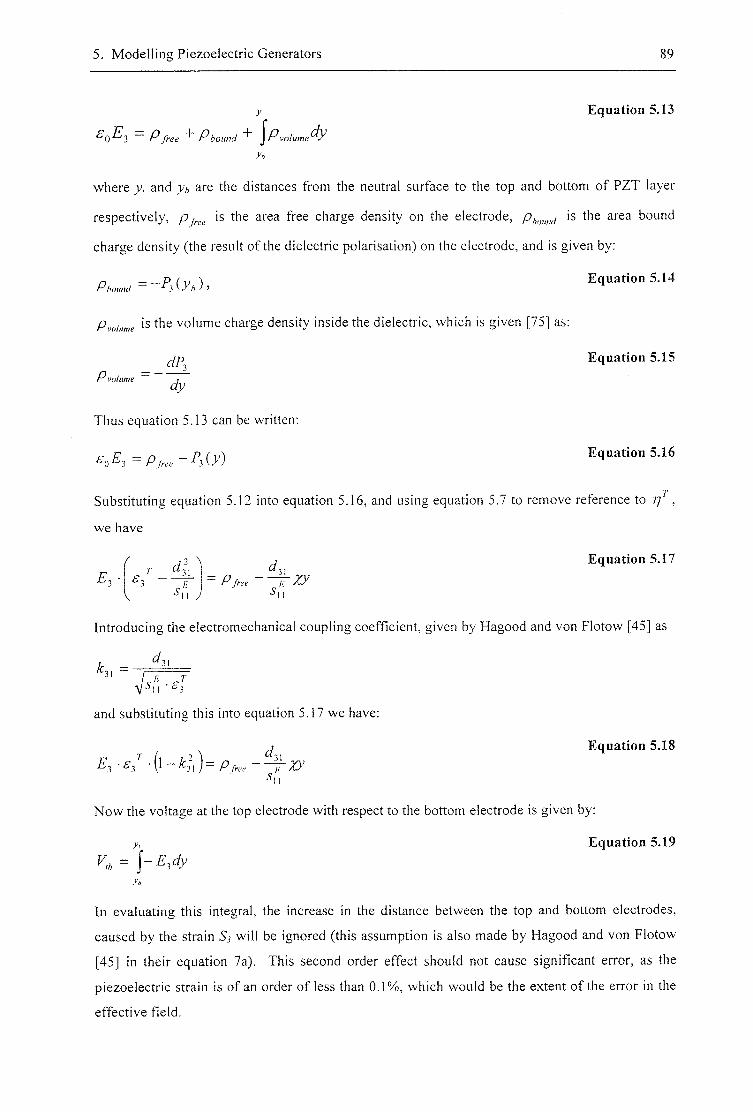
5. Modelling Piezoelectric Generators 89
y Equation 5.13
^0-^3 Pfree Pbound ^Pvohme^y
%
where yi and y* are the distances from the neutral surface to the top and bottom of PZT layer
respectively, is the area free charge density on the electrode, is the area bound
charge density (the result of the dielectric polarisation) on the electrode, and is given by:
A , ' ~ P , ( y , ) , Equation 5.14
Pvoiume is the volume charge density inside the dielectric, which is given [75] as:
Equation 5.15
P vaiume ,
Thus equation 5.13 can be written;
e,E,=p„„-P,{y) Equation 5.16
Substituting equation 5.12 into equation 5.16, and using equation 5.7 to remove reference io rj' ,
we have
E,
Equation 5.17
Introducing the electromechanical coupling coefficient, given by Hagood and von Flotow [45] as
A: -/Cji
and substituting this into equation 5.17 we have:
-^3 '^3^ ' ( ^ - ^ 3 i ) -I I
^ Equation 5.18
Now the voltage at the top electrode with respect to the bottom electrode is given by:
Equation 5.19
K, = j - E,dy
In evaluating this integral, the increase in the distance between the top and bottom electrodes,
caused by the strain Ss will be ignored (this assumption is also made by Hagood and von Flotow
[45] in their equation 7a). This second order effect should not cause significant error, as the
piezoelectric strain is of an order of less than 0.1%, which would be the extent of the error in the
effective field.

5. Modelling Piezoelectric Generators 90
Evaluating equation 5.19, and substituting the relation [45];
where £•3' is the permittivity in the 3 direction, of a piezoelectric block clamped in the 1
direction, we have:
d ^ „.V, 'Pfrc
Equation 5.20
where d = - yi,, the height of the piezoelectric layer, and ^ , the distance to the
centre of the piezoelectric layer from the neutral surface.
5.3.4 Bending Moments
Defining M, as the moment required at the right-hand side of the beam to maintain the curvature,
then
where b is the width of the piezoelectric layer
Equation 5.21
Now, substituting equation 5.18 into equation 5.11 to eliminate Ej, we have:
T. ^,1 V - ^ 1 1 ^ 3 ' V ^ 3 \ J J
d-31
P fn
Equation 5.22
Substituting this into equation 5.21, and solving, we have:
/ . d,,-b-d-y„
11 (1 - ^31 ) f u f 11*3
Equation 5.23
where =b ^y'dy, the 2"'' moment of area of the piezoelectric layer about the neutral axis.
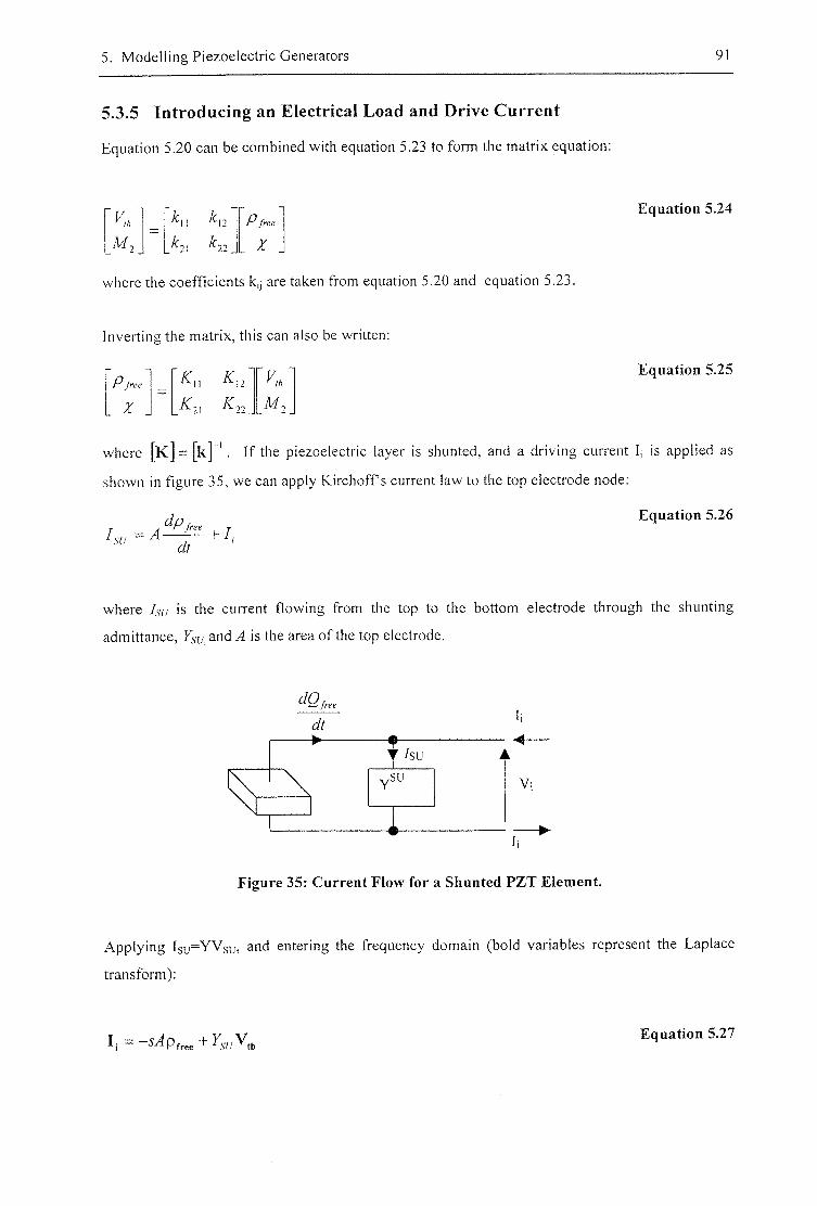
5. Modelling Piezoelectric Generators 91
5.3.5 Introducing an Electrical Load and Drive Current
Equation 5.20 can be combined with equation 5.23 to form the matrix equation:
k^2 P free
_^2l _ Z -
Equation 5.24
where the coefficients k|j are taken from equation 5.20 and equation 5.23.
Inverting the matrix, this can also be written:
P free K , ;
_ % - ^22 _
Equation 5.25
where [ K ] = [k] ' . If the piezoelectric layer is shunted, and a driving current Ij is applied as
shown in figure 35, we can apply Kirchoff s current law to the top electrode node:
Equation 5.26
where Isu is the current flowing from the top to the bottom electrode through the shunting
admittance, }^(/_andv4 is the area of the top electrode.
.su V i
Figure 35: Current Flow for a Shunted PZT Element.
Applying Isu-YVsu, and entering the frequency domain (bold variables represent the Laplace
transform):
I | — •y^pfrec Equation 5.27
5. Modelling Piezoelectric Generators 92
where s is tiie Laplace frequency variable. Substituting the top partition of equation 5.25 into
equation 5.27, we have
Combining this with the bottom partition of equation 5.25, we can write
Equation 5.28
h - A!!,, + FYf/
_ A , M ,
Equation 5.29
This is a governing equation for a shunted piezoelectric beam, with arbitrary shunting impedance,
driving current, and mechanical boundary conditions.
5.3.6 Resistive Shunting
Taking the top partition of equation 5.29, and setting the driving current to zero:
V . sAK^,
- M , Equation 5.30
Taking the bottom partition of equation 5.29 and substituting equation 5.30 to eliminate V*:
Equation 5.31
su M .
This gives the mechanical response of a resistively shunted piezoelectric layer. All electrical
terms have been eliminated. It is analogous to the Bernoulli-Euler law of elementary bending
[76]:
1 1 ,, " n
Equation 5.32
where Y is the young's modulus of the beam. In our case, the bending stiffness has been
modified by the piezoelectric coupling, and the resistive shunt, has introduced a complex
component to the stiffness.
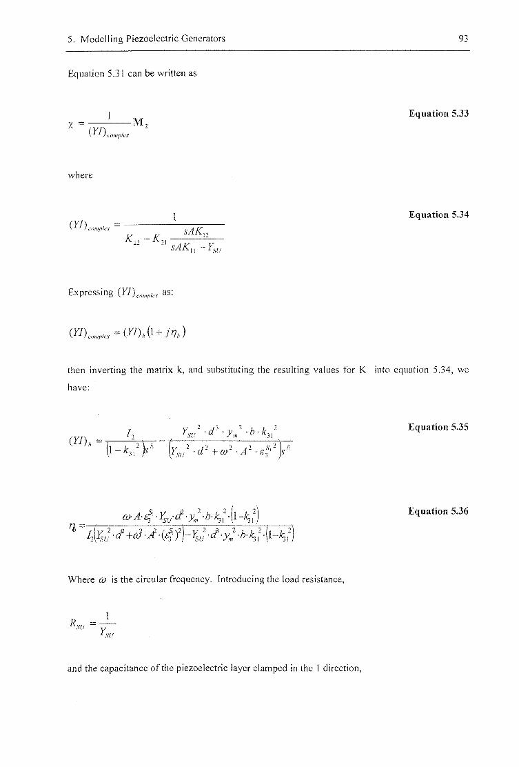
5. Modelling Piezoelectric Generators 93
Equation 5.31 can be written as
ciiltipkx
- M . Equation 5.33
where
complex
1 Equation 5.34
sAKf I
Expressing as:
then inverting the matrix k, and substituting the resulting values for K into equation 5.34, we
have:
31
V'
Equation 5.35
-6-^1 - M Equation 5.36
Where co is the circular frequency. Introducing the load resistance,
^su rsa
and the capacitance of the piezoelectric layer clamped in the 1 direction,
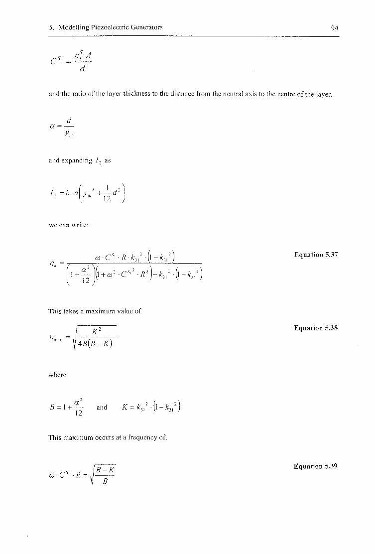
5. Modelling Piezoelectric Generators 94
d
and the ratio of the layer thickness to the distance from the neutral axis to the centre of the layer,
a d
y,„
and expanding / j as
^ 0 1 y„r +
12
we can write:
Ih (U C"' A:;/ ( l - A ; ; / )
V 1 2 , 1 + 0)- C" ' - ygN-A: ) /
Equation 5.37
This takes a maximum value of
Equation 5.38
where
B = l + ^ and =
This maximum occurs at a frequency of,
G). c B
Equation 5.39
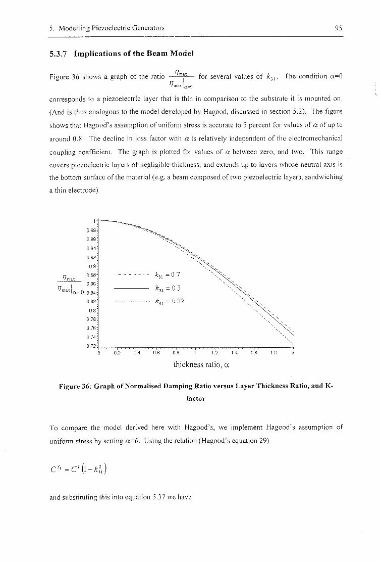
5. Modelling Piezoelectric Generators 95
5.3.7 Implications of the Beam Model
Figure 36 shows a graph of the ratio — — for several values of . The condition a = 0 77 /max |g(_o
corresponds to a piezoelectric layer that is thin in comparison to the substrate it is mounted on.
(And is thus analogous to the model developed by Hagood, discussed in section 5.2). The figure
shows that Hagood's assumption of uniform stress is accurate to 5 percent for values of a of up to
around 0.8. The decline in loss factor with a is relatively independent of the electromechanical
coupling coefficient. The graph is plotted for values of a between zero, and two. This range
covers piezoelectric layers of negligible thickness, and extends up to layers whose neutral axis is
the bottom surface of the material (e.g. a beam composed of two piezoelectric layers, sandwiching
a thin electrode)
I 0 . 9 3
096
0 . 9 4
0 . 9 2
0.9
0.88
j 0.86
i a = 0 0.84
0 82
0.8
078
076
074
0 72
31 =0.7
^31 = 0.3
= 0.02
0 . 2 0 . 4 0 . 6 0.8 t 1 . 2 1 . 4 1 . 6 I .
thickness ratio, a
Figure 36: Graph of Normalised Damping Ratio versus Layer Thickness Ratio, and K-
factor
To compare the model derived here with Hagood's, we implement Hagood's assumption of
uniform stress by setting a-O. Using the relation (Hagood's equation 29)
and substituting this into equation 5.37 we have
5. Modelling Piezoelectric Generators 96
7/,
C Jg A:,/ Equation 5.40
This is similar to the result derived by Hagood, although his model gives the result for a different
set of boundary conditions.
The prototype generator developed in chapter 4 has a value for a of 0.583. This model predicts
that this will result in a damping ratio that is 3 percent lower than that predicted by Hagood's
theory. This value will be used in the following analyses.
5.4 Harmonic Response of a Piezoelectric Generator
By representing the piezoelectric layer mechanically as having a complex stiffness, as described
above, conventional mechanical models can be used to predict the mechanical response of a
composite piezoelectric-steel beam, of the type described in section 4.3. Once this response has
been determined, damping theory can be used to determine the electrical power produced.
For rectangular beams, Bernoulli-Euler approximations can be used in conjunction with Rayleigh-
Ritz methods to predict the amplitude of vibration, and resulting stresses in a piezo-generator.
The beams described in section 4.3, however, are of a tapered nature, and show significant edge
effects. The shape causes a concentration of stress near the centre of the beam, away from the
lateral edges (See figure 40, Section 5.5). Further edge effects are introduced by the thickness of
the piezo-electric layer, which is not clamped at its root. Including these effects in this model is
not straightforward, and the resulting mode shapes will not yield solutions that are easy to grasp
intuitively (a motivation for using this method).
Comparing the results obtained by this method to the Finite Element Analysis described below,
for the test device described, this method is found to give a natural frequency that is around 6%
higher than the FEA result. Thus, finite element analysis is judged to give more reliable results.
A third option is described by Hagood et al [77]. In this model, the dynamic piezoelectric
coupling between a structure and an electrical network is predicted. The governing equations are
derived, and discretised with assumed elastic and electrical field shapes in a Rayleigh-Ritz
formulation. This model is well suited to the problem of piezoelectric generators described here,
however, the simpler models described above offer sufficient accuracy, and are simpler as they
reflect the quasi-static nature of the piezoelectric coupling in the generators.

5. Modelling Piezoelectric Generators 97
5.4.1 Finite Element Analysis (FEA)
To determine the mechanical response of a piezo-generator to being shaken, and the proportion of
the strain energy stored within the piezoelectric layer, the finite element package ANSYS"^' was
used. Finite element analysis has an advantage over analytical methods based on Bernoulli-Euler
approximations (see above), as it takes account of edge effects, and the shear lag caused by thin
layers such as the electrodes, and the dielectric insulator.
Modelling piezo-generators is complicated by the small thickness of the individual layers in
comparison to the overall lateral dimensions of the devices. For an accurate analysis, the
elements used in a model must not typically be more than around 20 times longer than they are
thick [78]. This means that many elements are required when simulating thin layers, which
causes long computation times for the models. To reduce the number of elements, a composite
element type SOLID46 is used which represents a number of laminated layers in a single element.
This element type is used to model the combination of the substrate and dielectric layers on either
side of the substrate. A planar mesh was also initially considered to reduce the computation time,
however this does not allow for the edge effects described in section 5.5.
Figure 37 shows the mesh of finite elements employed for calculating the amplitude of vibration
of the beam, and the amount of strain energy stored within the piezoelectric layer. The program
listing used to generate the mesh, is listed in appendix B. The symmetry of the model about its
central axis was exploited, so that only half of the structure was modelled, reducing computation
time. Three different types of material are defined for the beam: substrate only, substrate covered
with a dielectric film, and piezoelectric material. The top electrode is not modelled, as it is
assumed that the compliant polymer material has a small effect on the stiffer ceramic layers that it
is printed upon. The effect of the bottom electrode is included by increasing the thickness of the
piezoelectric layer by the thickness of the bottom electrode. Since the bottom electrode is of
similar stiffness to the piezoelectric layer, this will not affect the overall stiffness of the beam,
however, it will overestimate the energy available from the piezoelectric layer. For the cases
considered here, where the bottom electrode is thin in comparison to the piezoelectric layer, this
should not introduce significant errors. The substrate nodes are constrained in all directions at the
root of the beam to model the beam clamping. The nodes along central axis are constrained in the
Y-di recti on to model the missing half of the mesh. The mass is modelled by stiff but light
elements, connected to a short line of dense elements placed at the centre of mass of the mass. It
should be noted that this ignores any rotational inertia of the mass, however, when the model is
compared to experimental results the model is seen to be sufficiently accurate.
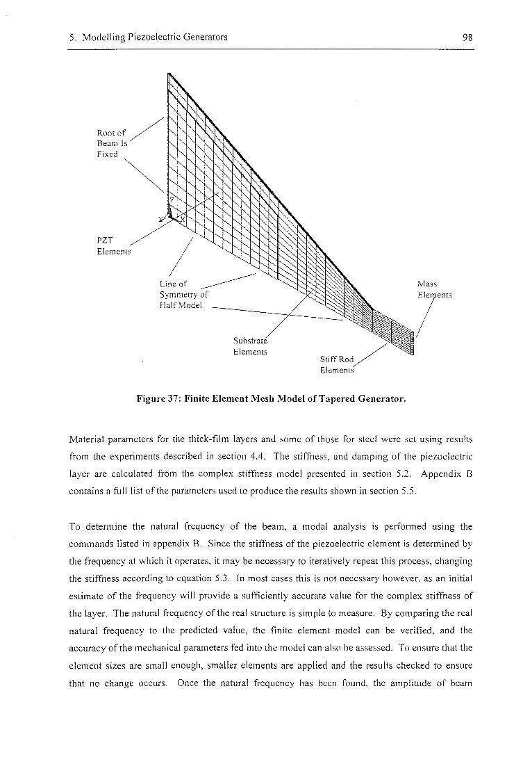
5. Modelling Piezoelectric Generators 98
Root of Beam Is Fixed
PZT Elements
Line of Symmetr Half Model
Mass Elenients
Substrate
Elements Stiff Rod Elements
Figure 37: Finite Element Mesh Model of Tapered Generator.
Material parameters for the thick-film layers and some of those for steel were set using results
from the experiments described in section 4.4. The stiffness, and damping of the piezoelectric
layer are calculated from the complex stiffness model presented in section 5.2. Appendix B
contains a full list of the parameters used to produce the results shown in section 5.5.
To determine the natural frequency of the beam, a modal analysis is performed using the
commands listed in appendix B. Since the stiffness of the piezoelectric element is determined by
the frequency at which it operates, it may be necessary to iteratively repeat this process, changing
the stiffness according to equation 5.3. In most cases this is not necessary however, as an initial
estimate of the frequency will provide a sufficiently accurate value for the complex stiffness of
the layer. The natural frequency of the real structure is simple to measure. By comparing the real
natural frequency to the predicted value, the finite element model can be verified, and the
accuracy of the mechanical parameters fed into the model can also be assessed. To ensure that the
element sizes are small enough, smaller elements are applied and the results checked to ensure
that no change occurs. Once the natural frequency has been found, the amplitude of beam

5. Modelling Piezoelectric Generators 99
vibration can be determined using an harmonic analysis. The analysis is performed using the
commands listed in appendix B.
To find the energy produced at a particular amplitude of vibration, it is necessary to determine the
amount of strain energy stored in the structure when the beam is at the point in is vibration cycle
of maximum deflection. This is done using a static analysis. The beam tip is held at a deflection,
equivalent to the vibration amplitude, and the energy stored within the different layers is
calculated. This makes the approximation that the mode shape of the vibration at the resonant
frequency is identical to this static shape. This is reasonable since we are only working around
the natural frequency of the beam and most of the mass is concentrated at the tip of the beam.
This approximation has been tested by comparing the two shapes; the maximum error in the
displacement of any node is found to be only 0.3% of the tip deflection. The analysis is set up,
and the results derived as detailed in appendix B.
5.4.2 The Electrical Energy Available to a Resistive Load
Damping theory can be applied to find how much of the strain energy stored within the
piezoelectric layer is released as electrical energy. Treating the shunted piezoelectric material as a
material with a complex stiffness, as described in section 5.2, the electrical power dissipated in
the load, P, is given [52] by:
f = 2;^ Equation 5.41
where r j f f ) is the frequency dependant loss factor of the shunted piezoelectric material, and U,,,
the peak strain energy stored within the piezoelectric material, and f, the frequency of vibration.
The energy dissipated electrically is a combination of the energy dissipated in both the shunting
resistance, and the series resistance of the electrodes. However, the series resistance of the
electrodes is of an order of a few ohms, much smaller than the tens or hundreds of kilo-ohms of
the shunting resistance, and can be ignored here.
5.5 Analysis of a Piezoelectric Generator Beam
Figure 38 shows the sequence of calculations used to find the energy available from a piezo-
generator.
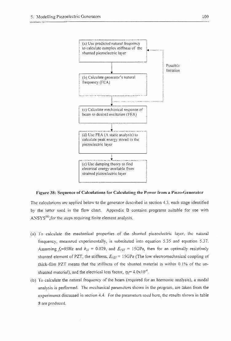
5. Modelling Piezoelectric Generators 100
(a) Use predicted natural frequency to calculate complex stiffness of the shunted piezoelectric layer
(a) Use predicted natural frequency to calculate complex stiffness of the shunted piezoelectric layer
(b) Calculate generator's natural frequency (FEA)
(c) Calculate mechanical response of beam to desired excitation (FEA)
(d) Use FEA (A static analysis) to calculate peak energy stored in the piezoelectric layer
(e) Use damping theory to find electrical energy available from strained piezoelectric layer
Possible Iteration
Figure 38: Sequence of Calculations for Calculating the Power from a Piezo-Generator
The calculations are applied below to the generator described in section 4.3, each stage identified
by the letter used in the flow chart. Appendix B contains programs suitable for use with
ANSYS"^',for the steps requiring finite element analysis.
(a) To calculate the mechanical properties of the shunted piezoelectric layer, the natural
frequency, measured experimentally, is substituted into equation 5.35 and equation 5.37.
Assuming / ,=95Hz and kn = 0.029, and Epzr ~ 15GPa, then for an optimally resistively
shunted element of PZT, the stiffness, E,>zt- 15GPa (The low electromechanical coupling of
thick-film PZT means that the stiffness of the shunted material is within 0.1% of the un-
shunted material), and the electrical loss factor, 4.0x10"''.
(b) To calculate the natural frequency of the beam (required for an harmonic analysis), a modal
analysis is performed. The mechanical parameters shown in the program, are taken from the
experiments discussed in section 4.4. For the parameters used here, the results shown in table
8 are produced.
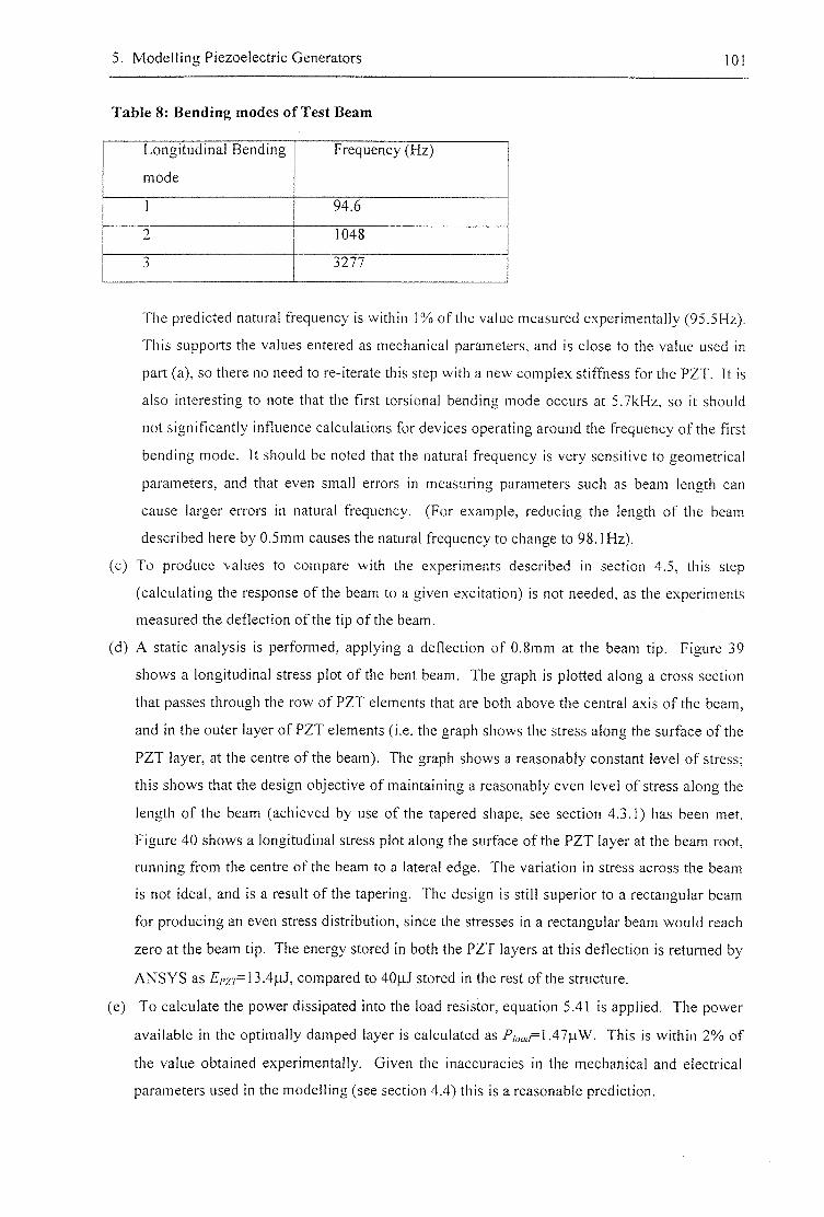
5. Modelling Piezoelectric Generators 101
Table 8: Bending modes of Test Beam
Longitudinal Bending
mode
Frequency (Hz)
1 9 4 ^
2 1048
3 3277
The predicted natural frequency is within 1% of the value measured experimentally (95.5Hz).
This supports the values entered as mechanical parameters, and is close to the value used in
part (a), so there no need to re-iterate this step with a new complex stiffness for the PZT. It is
also interesting to note that the first torsional bending mode occurs at 5.7kHz, so it should
not significantly influence calculations for devices operating around the frequency of the first
bending mode. It should be noted that the natural frequency is very sensitive to geometrical
parameters, and that even small errors in measuring parameters such as beam length can
cause larger errors in natural frequency, (For example, reducing the length of the beam
described here by 0.5mm causes the natural frequency to change to 98.1Hz).
(c) To produce values to compare with the experiments described in section 4.5, this step
(calculating the response of the beam to a given excitation) is not needed, as the experiments
measured the deflection of the tip of the beam.
(d) A static analysis is performed, applying a deflection of 0.8mm at the beam tip. Figure 39
shows a longitudinal stress plot of the bent beam. The graph is plotted along a cross section
that passes through the row of PZT elements that are both above the central axis of the beam,
and in the outer layer of PZT elements (i.e. the graph shows the stress along the surface of the
PZT layer, at the centre of the beam). The graph shows a reasonably constant level of stress;
this shows that the design objective of maintaining a reasonably even level of stress along the
length of the beam (achieved by use of the tapered shape, see section 4.3.1) has been met.
Figure 40 shows a longitudinal stress plot along the surface of the PZT layer at the beam root,
running from the centre of the beam to a lateral edge. The variation in stress across the beam
is not ideal, and is a result of the tapering. The design is still superior to a rectangular beam
for producing an even stress distribution, since the stresses in a rectangular beam would reach
zero at the beam tip. The energy stored in both the PZT layers at this deflection is returned by
ANSYS as £/vr=13.4|iJ, compared to 4 0 p j stored in the rest of the structure.
(e) To calculate the power dissipated into the load resistor, equation 5.41 is applied. The power
available in the optimally damped layer is calculated as .47)j.W. This is within 2% of
the value obtained experimentally. Given the inaccuracies in the mechanical and electrical
parameters used in the modelling (see section 4.4) this is a reasonable prediction.
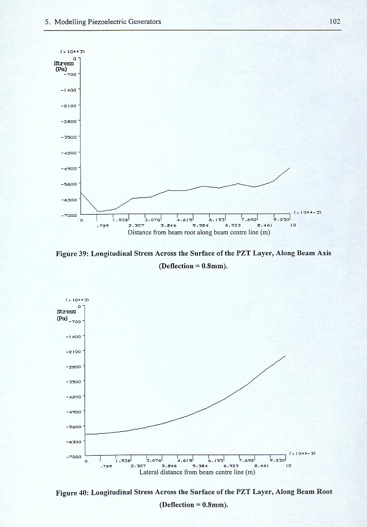
5. Modelling Piezoelectric Generators 102
f > ia**3> Q
Stress (Pa)
- T O O
T T f > 1 0*l-3> 1 .S3Sl 3.0761 4.6151 6.I 53' 7.692' 9.230'
.769 2.307 3.34 6 5.334 6.923 S.4<H lO Distance from beam root along beam centre line (m)
Figure 39: Longitudinal Stress Across the Surface of the PZT Layer, Along Beam Axis
(Deflection = 0.8mm).
f > 1 0 * * 3 )
O ' Stress (Pa). , . ,
( > ) 0»*-3>
Lateral distance from beam centre line (m)
Figure 40; Longitudinal Stress Across the Surface of the PZT Layer, Along Beam Root
(Deflection = 0.8mm).
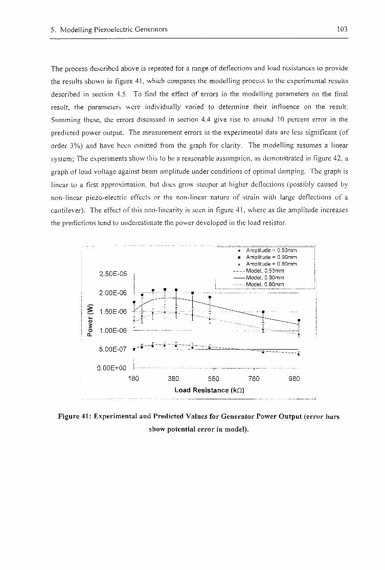
5. Modelling Piezoelectric Generators 103
The process described above is repeated for a range of deflections and load resistances to provide
the results shown in figure 41, which compares the modelling process to the experimental results
described in section 4.5. To fmd the effect of errors in the modelling parameters on the fmal
result, the parameters were individually varied to determine their influence on the result.
Summing these, the errors discussed in section 4,4 give rise to around 10 percent error in the
predicted power output. The measurement errors in the experimental data are less significant (of
order 3%) and have been omitted from the graph for clarity. The modelling assumes a linear
system; The experiments show this to be a reasonable assumption, as demonstrated in figure 42, a
graph of load voltage against beam amplitude under conditions of optimal damping. The graph is
linear to a first approximation, but does grow steeper at higher deflections (possibly caused by
non-linear piezo-electric effects or the non-linear nature of strain with large deflections of a
cantilever). The effect of this non-linearity is seen in figure 41, where as the amplitude increases
the predictions tend to underestimate the power developed in the load resistor.
2.505-06
2.00E-06
5 1.502-06
I o 1.005-06 CL
5.00E-07
0,00E+00
i 'i-- :3 'zkzs' nt
180
Amplitude = 0.53mm Amplitude - 0.90mm Amplitude = 0.80mm Model, 0.53mm Model, 0.90mm Model, 0.80mm
380 580 780
Load Resistance (kQ)
i
980
Figure 41: Experimental and Predicted Values for Generator Power Output (error bars
show potential error in model).
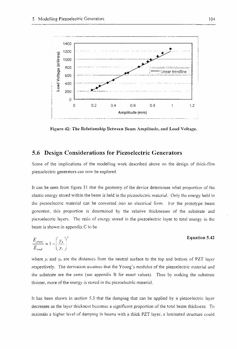
5. Modelling Piezoelectric Generators 104
</) E >
& 0) O)
T! re o
1200
1000
Linear trendline
200
&2 CM &6 0 8
Amplitude (mm)
1.2
Figure 42: The Relationship Between Beam Amplitude, and Load Voltage.
5.6 Design Considerations for Piezoelectric Generators
Some of the implications of the modelling work described above on the design of thick-film
piezoelectric generators can now be explored.
It can be seen from figure 31 that the geometry of the device determines what proportion of the
elastic energy stored within the beam is held in the piezoelectric material. Only the energy held in
the piezoelectric material can be converted into an electrical form. For the prototype beam
generator, this proportion is determined by the relative thicknesses of the substrate and
piezoelectric layers. The ratio of energy stored in the piezoelectric layer to total energy in the
beam is shown in appendix C to be
E
E. 1
/ Equation 5.42
where y, and y* are the distances from the neutral surface to the top and bottom of PZT layer
respectively. The derivation assumes that the Young's modulus of the piezoelectric material and
the substrate are the same (see appendix B for exact values). Thus by making the substrate
thinner, more of the energy is stored in the piezoelectric material.
It has been shown in section 5.3 that the damping that can be applied by a piezoelectric layer
decreases as the layer thickness becomes a significant proportion of the total beam thickness. To
maintain a higher level of damping in beams with a thick PZT layer, a laminated structure could
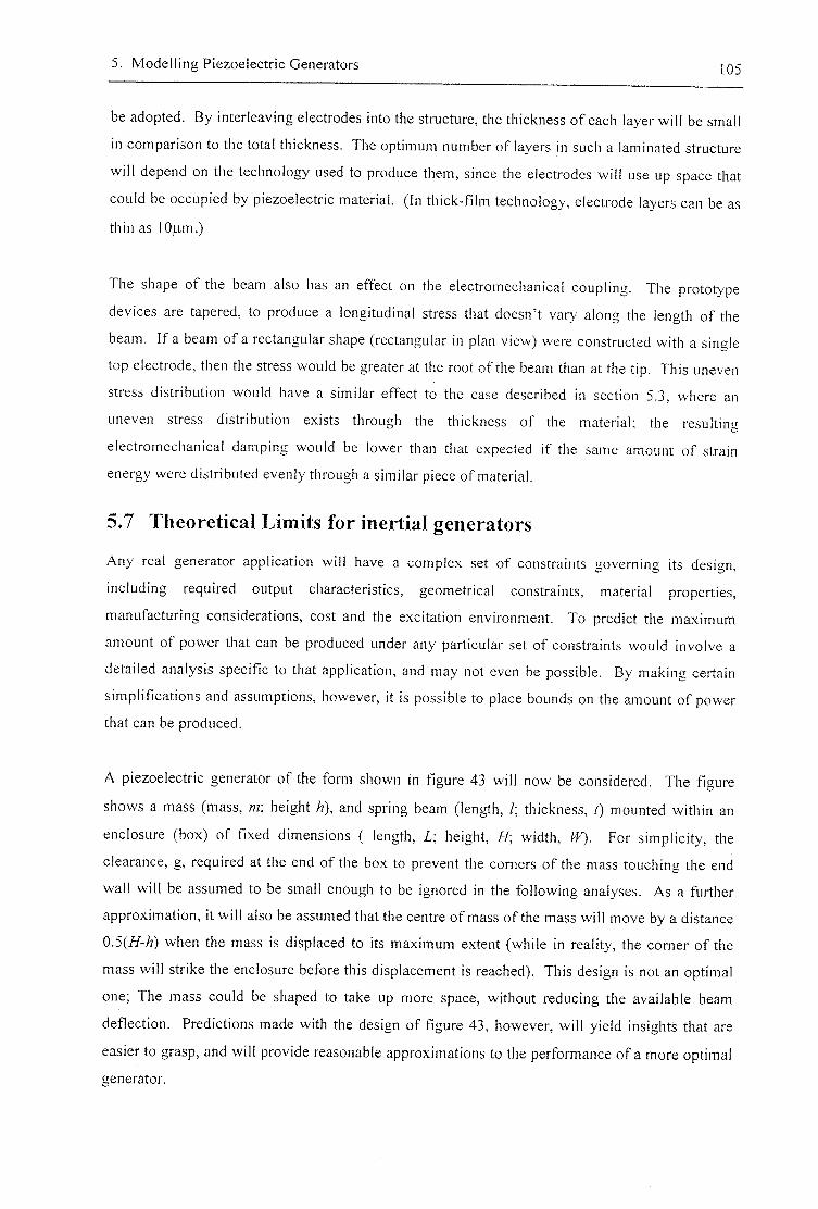
5. Modelling Piezoelectric Generators 105
be adopted. By interleaving electrodes into the structure, the thickness of each layer will be small
in comparison to the total thickness. The optimum number of layers in such a laminated structure
will depend on the technology used to produce them, since the electrodes will use up space that
could be occupied by piezoelectric material. (In thick-film technology, electrode layers can be as
thin as lOjim.)
The shape of the beam also has an effect on the electromechanical coupling. The prototype
devices are tapered, to produce a longitudinal stress that doesn't vary along the length of the
beam. If a beam of a rectangular shape (rectangular in plan view) were constructed with a single
top electrode, then the stress would be greater at the root of the beam than at the tip. This uneven
stress distribution would have a similar effect to the case described in section 5.3, where an
uneven stress distribution exists through the thickness of the material; the resulting
electromechanical damping would be lower than that expected if the same amount of strain
energy were distributed evenly through a similar piece of material.
5.7 Theoretical Limits for inertial generators
Any real generator application will have a complex set of constraints governing its design,
including required output characteristics, geometrical constraints, material properties,
manufacturing considerations, cost and the excitation environment. To predict the maximum
amount of power that can be produced under any particular set of constraints would involve a
detailed analysis specific to that application, and may not even be possible. By making certain
simplifications and assumptions, however, it is possible to place bounds on the amount of power
that can be produced.
A piezoelectric generator of the form shown in figure 43 will now be considered. The figure
shows a mass (mass, m; height A), and spring beam (length, /; thickness, mounted within an
enclosure (box) of fixed dimensions ( length, height, width, fF). For simplicity, the
clearance, g, required at the end of the box to prevent the comers of the mass touching the end
wall will be assumed to be small enough to be ignored in the following analyses. As a further
approximation, it will also be assumed that the centre of mass of the mass will move by a distance
0.5(/A/z) when the mass is displaced to its maximum extent (while in reality, the comer of the
mass will strike the enclosure before this displacement is reached). This design is not an optimal
one; The mass could be shaped to take up more space, without reducing the available beam
deflection. Predictions made with the design of figure 43, however, will yield insights that are
easier to grasp, and will provide reasonable approximations to the performance of a more optimal
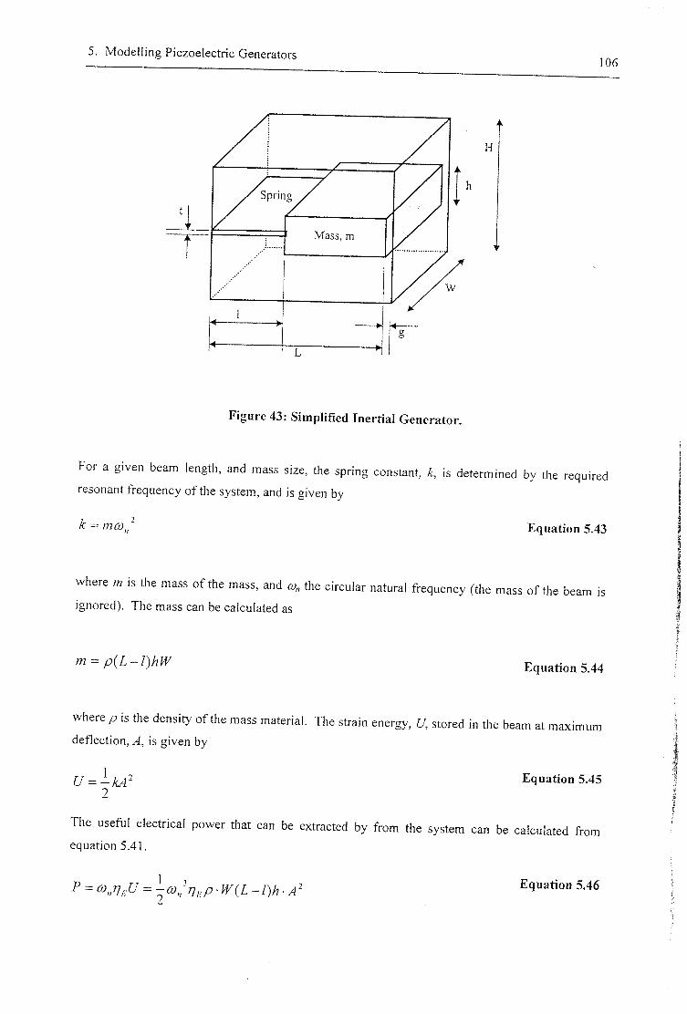
5. Modelling Piezoelectric Generators 106
Mass, m
H
Figure 43: Simplified Inertial Generator.
For a given beam length, and mass size, the spring constant, A:, is determined by the required
resonant frequency of the system, and is given by
k = mco' Equation 5.43
where m is the mass of the mass, and a,, the circular natural frequency (the mass of the beam is
ignored). The mass can be calculated as
7M = Equation 5.44
where/ ) i s thedensi tyofthemassmateria l . Thestrainenergy,[ / , s toredinthebeamatmaximum
deflection, A, is given by
2 Equation 5.45
The useful electrical power that can be extracted by from the system can be calculated from
equation 5.41.
^ - / ) A . Equation 5.46
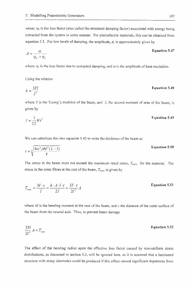
5. Modelling Piezoelectric Generators 107
where % is the loss factor (also called the structural damping factor) associated with energy being
extracted from the system in some manner. For piezoelectric materials, this can be obtained from
equation 5.3. For low levels of damping, the amplitude, A, is approximately given by
a Equation 5.47 =
where rji is the loss factor due to unwanted damping, and a is the amplitude of base excitation.
Using the relation
3 7 / Equation 5.48 k
where 7 is the Young's modulus of the beam, and /, the second moment of area of the beam, is
given by
/ = Equation 5.49
12
We can substitute this into equation 5.43 to write the thickness of the beam as
^ ^ Equation 5.50
The stress in the beam must not exceed the maximum rated stress, r„,av, for the material. The
stress in the outer fibres at the root of the beam, r„„„, is given by
_ M-c k-A-l-t 3Y-t ^ Equation 5.51
where M i s the bending moment at the root of the beam, and c the distance of the outer surface of
the beam from the neutral axis. Thus, to prevent beam damage
2Yt Equation 5.52
The effect of the bending radius upon the effective loss factor caused by non-uniform stress
distributions, as discussed in section 5.3, will be ignored here, as it is assumed that a laminated
structure with many electrodes could be produced if this effect caused significant departures from
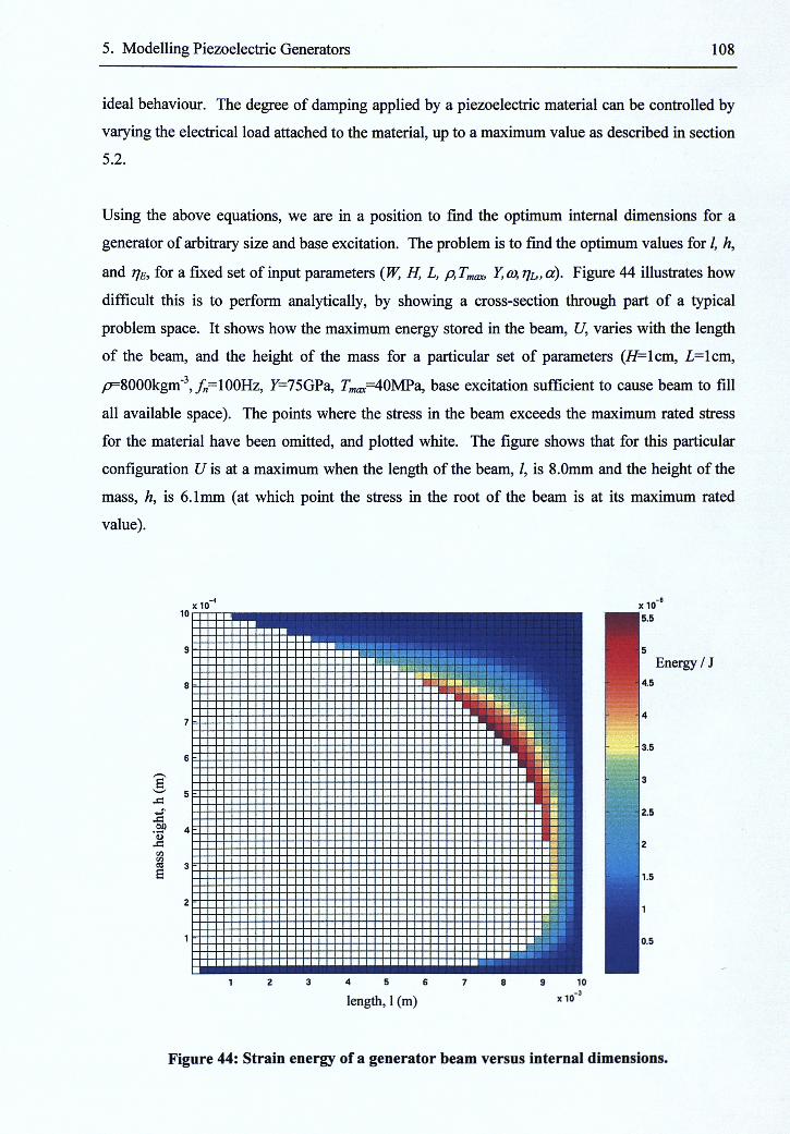
5. Modelling Piezoelectric Generators 108
ideal behaviour. The degree of damping applied by a piezoelectric material can be controlled by
varying the electrical load attached to the material, up to a maximum value as described in section
5.2.
Using the above equations, we are in a position to find the optimum internal dimensions for a
generator of arbitrary size and base excitation. The problem is to find the optimum values for /, h,
and r]E, for a fixed set of input parameters {W, H, L, p,Tmax, Y,a), Figure 44 illustrates how
difficult this is to perform analytically, by showing a cross-section through part of a typical
problem space. It shows how the maximum energy stored in the beam, U, varies with the length
of the beam, and the height of the mass for a particular set of parameters (^f=lcm, 2= 1cm,
/7=8000kgm'^,/,=100Hz, 7=75 GPa, 7L;a%=40MPa, base excitation sufficient to cause beam to fill
all available space). The points where the stress in the beam exceeds the maximum rated stress
for the material have been omitted, and plotted white. The figure shows that for this particular
configuration LA is at a maximum when the length of the beam, /, is 8.0mm and the height of the
mass, h, is 6.1mm (at which point the stress in the root of the beam is at its maximum rated
value).
Energy / J
length, 1 (m) x10
Figure 44: Strain energy of a generator beam versus internal dimensions.
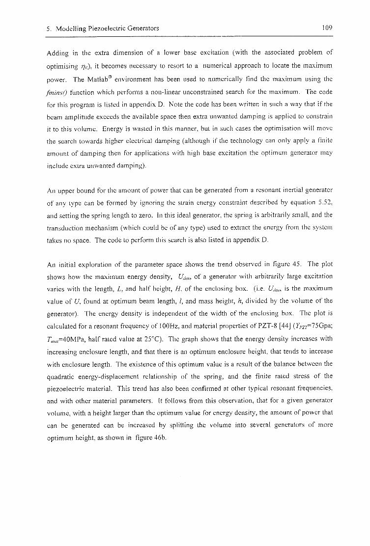
5. Modelling Piezoelectric Generators 109
Adding in the extra dimension of a lower base excitation (with the associated problem of
optimising %), it becomes necessary to resort to a numerical approach to locate the maximum
power. The Matlab® environment has been used to numerically find the maximum using the
fminsQ function which performs a non-linear unconstrained search for the maximum. The code
for this program is listed in appendix D. Note the code has been written in such a way that if the
beam amplitude exceeds the available space then extra unwanted damping is applied to constrain
it to this volume. Energy is wasted in this manner, but in such cases the optimisation will move
the search towards higher electrical damping (although if the technology can only apply a finite
amount of damping then for applications with high base excitation the optimum generator may
include extra unwanted damping).
An upper bound for the amount of power that can be generated from a resonant inertial generator
of any type can be formed by ignoring the strain energy constraint described by equation 5.52,
and setting the spring length to zero. In this ideal generator, the spring is arbitrarily small, and the
transduction mechanism (which could be of any type) used to extract the energy from the system
takes no space. The code to perform this search is also listed in appendix D.
An initial exploration of the parameter space shows the trend observed in figure 45. The plot
shows how the maximum energy density, Uj^n, of a generator with arbitrarily large excitation
varies with the length, I , and half height, H, of the enclosing box. (i.e. [/,/„„ is the maximum
value of U, found at optimum beam length, /, and mass height, h, divided by the volume of the
generator). The energy density is independent of the width of the enclosing box. The plot is
calculated for a resonant frequency of lOOHz, and material properties of PZT-8 [44] (}fZ7=75Gpa;
7'/»av="40MPa, half rated value at 25°C). The graph shows that the energy density increases with
increasing enclosure length, and that there is an optimum enclosure height, that tends to increase
with enclosure length. The existence of this optimum value is a result of the balance between the
quadratic energy-displacement relationship of the spring, and the finite rated stress of the
piezoelectric material. This trend has also been confirmed at other typical resonant frequencies,
and with other material parameters. It follows from this observation, that for a given generator
volume, with a height larger than the optimum value for energy density, the amount of power that
can be generated can be increased by splitting the volume into several generators of more
optimum height, as shown in figure 46b.
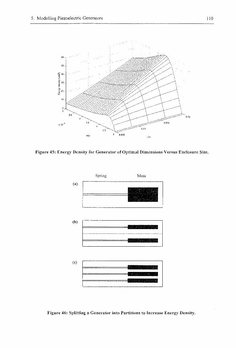
5. Modelling Piezoelectric Generators 10
0 0 , 0 0 5
Figure 45; Energy Density for Generator of Optimal Dimensions Versus Enclosure Size.
(a)
Spring Mass
(b)
(c)
Figure 46: Splitting a Generator into Partitions to Increase Energy Density.
5. Modelling Piezoelectric Generators 11
To take account of this multi-beam possibility the code listed in appendix B optimises for power
density, then returns the power that would be produced by a multi-beam generator by multiplying
this power density by the available volume. In practice, the beams could be moved closer
together as shown in figure 46c, taking advantage of that fact that all the beams will move
together (although some clearance would still be necessary, to allow for the rotation of the masses
as the beam deflects). Laminated piezoelectric elements may be required to maintain ideal
behaviour due to the varying stress through the beam thickness (see section 5.3). The multi-beam
configuration described here would require thinner laminations than a design with only a single
beam, and the technology used to produce the laminations vyill limit the lamination thickness.
The above methods have been applied to the example applications listed in table 9, to produce the
results listed in table 1 1, Table 10 lists the material parameters used in the analysis.
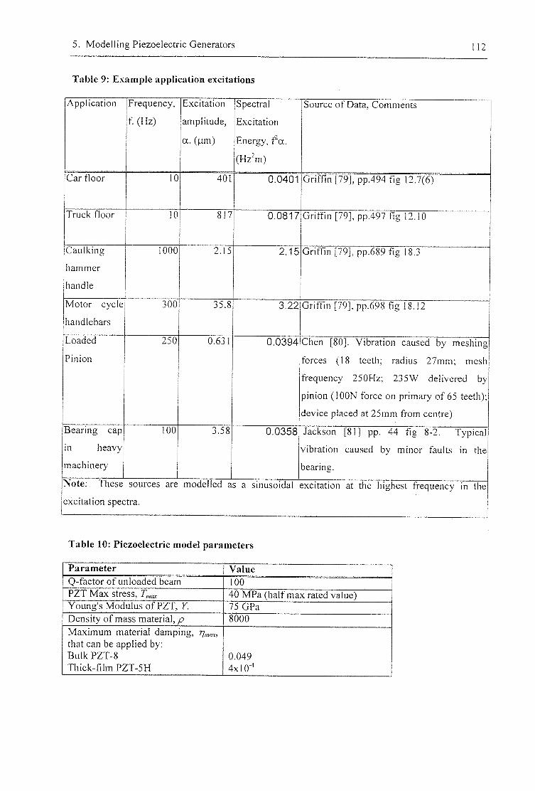
5. Modelling Piezoelectric Generators
Table 9: Example application excitations
. 1 2
Application Frequency,
R f H b )
Excitation
amplitude,
a . (jim)
Spectral
Excitation
Energy, f"a.
(Hz'm)
Source of Data, Comments
Car floor 10 401 0 .0401 Griffin [79], pp.494 fig 12,7(6)
Truck floor 10 817 0 0 8 1 7 Griffin [79], pp.497 fig 12.10
Caulking
hammer
handle
1000 2T5 2 J 5 Grifnn[79], pp.689 fig 18.3
Motor cycle
handlebars
300 3 5 ^ 3 22 GrifOn [79], pp.698 fig 18.12
Loaded
Pinion
250 0.631 0 . 0 3 9 4 Chen [80]. Vibration caused by meshing
forces (18 teeth; radius 27mm; mesh
frequency 250Hz; 235W delivered by
pinion (lOON force on primary of 65 teeth);
device placed at 25mm from centre)
Bearing cap
in heavy
machinery
100 3 J 8 0 . 0 3 5 8 Jackson [81] pp. 44 fig 8-2. Typical
vibration caused by minor faults in the
bearing.
Wote: ihese sources are modelled as a smusoidal excitation at the highest frequency in the
excitation spectra.
Table 10: Piezoelectric model parameters
Parameter Value Q-factor of unloaded beam 100 PZT Max stress, T„,ax 40 MPa (half max rated value) Young's Modulus of PZT, Y. 75GPa Density of mass material, p 8000
Maximum material damping, that can be applied by: Bulk PZT-8 0.049 Thick-film PZT-5H 4x10^
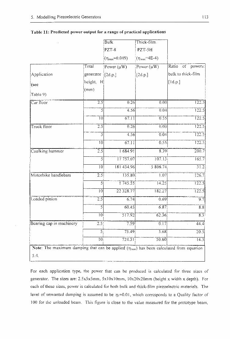
5. Modelling Piezoelectric Generators 113
Table 11: Predicted power output for a range of practical applications
B u k
PZT-8
(nmax=0.049)
Thick-film
PZT-5H
(T |maME-4)
Application
(see
Table 9)
Total
generator
height, H
(mm)
Power (|iW)
[2d.p.]
Power (jiW)
[2d.p.]
Ratio of powers:
bulk to thick-film
[Id.p.]
Car floor 2.5 0^:6 0.00 12Z5 Car floor
5 4.56 0.04 12Z5
Car floor
10 67T1 0 J 5 12Z5
Truck floor 2.5 0.00 122J Truck floor
5 4.56 0.04 12Z5
Truck floor
10 6 7 T ] 0.55 122^
Caulking hammer 2.5 1 68441 8 J 9 200/7 Caulking hammer
5 17 757.07 107T3 165.7
Caulking hammer
10 181 4 3 4 4 6 5 806.74 3L2
Motorbike handlebars 2.5 135^0 1.07 12&7 Motorbike handlebars
5 1745.55 14J^ 12Z5
Motorbike handlebars
10 22 32&77 18Z27 122.5
Loaded pinion 2.5 6 J 4 0 69 9.7 Loaded pinion
5 6&45 6.87 8.8
Loaded pinion
10 5 1 7 4 2 6 2 J 6 8.3
Bearing cap in machinery 2.5 7 J 9 0.17 4 4 ^ Bearing cap in machinery
5 75.49 3.68 2&5
Bearing cap in machinery
10 724J1 5&60 14J
Note: The maximum damping that can be applied (^m^) has been calculated from equation
5.4.
For each application type, the power that can be produced is calculated for three sizes of
generator. The sizes are: 2.5x5x5mm, 5x10x10mm, 10x20x20mm (height x width x depth). For
each of these sizes, power is calculated for both bulk and thick-film piezoelectric materials. The
level of unwanted damping is assumed to be %-0 .01 , which corresponds to a Quality factor of
100 for the unloaded beam. This figure is close to the value measured for the prototype beam,
5. Modelling Piezoelectric Generators 114
and to permit comparison, is the same as that used for predictions for magnet-coil generators in
section 7.4.
The table shows a wide variation in the amount of power that can be generated from the various
applications. A column shows the ratio between the power that could be produced from a
generator using bulk PZT-8, and one using the thick-film PZT-5H material discussed in the
previous chapter. It can be seen that the bulk PZT offers much higher power output, and that the
thick-film PZT produces a useful amount of power in only a few cases that have a high excitation
energy. The table only contains data for piezoceramic materials, PVDF has been omitted as it
will produce even less energy than the thick-film PZT (due to its low activity).
The same program has been used to produce the graph shown in figure 47a. The graph shows
data for a generator of fixed size (5mm high x 10mm x 10mm) using the material PZT-8. The
power for a device of optimum internal dimensions is plotted for a range of excitation amplitudes
and frequencies. To permit simpler comparison between frequencies, the x-axis shows the
spectral energy of the excitation (the product of the frequency squared and the excitation
amplitude). Figure 48 shows the value of the parameters that correspond to each point on the
graph. An interesting feature of these graphs is that they show a sudden transition between a
multi-beam configuration (ratio of cell height to total height < 1.0 ) to a single beam (cell height
equals total height). It can be seen that a multi-beam configuration becomes optimum at higher
frequencies, and lower excitations, and that the optimum cell height is almost independent of
excitation. As the excitation is increased the height of the mass decreases, and the length of the
beam increases until a critical point is reached when a single beam becomes the better design.
The small maxima seen in the power graph are thought to be artefacts of the optimisation process
around this transition, although they are not large enough to detract from the utility of these
results as 'ball-park' estimates (the assumptions used in the derivation above mean that these
results are for an ideal generator; in practice non-ideal elements will reduce the actual power
produced).
Figure 47(a) can be compared to (b) which shows the theoretical limit for the maximum power
that could be produced from a resonant generator of any type, as discussed above. It can be seen
that at higher frequencies and lower excitation, the piezoelectric generators approach this
maximum. A reason that causes the piezoelectric generators to fail to reach this upper bound in
other cases can be seen from figure 48(c). The piezoelectric material is operating by applying as
much damping as is possible. To approach the maximum more damping is required, which could
only be achieved by finding a material with a higher electromechanical coupling factor, k (see
section 5.2).
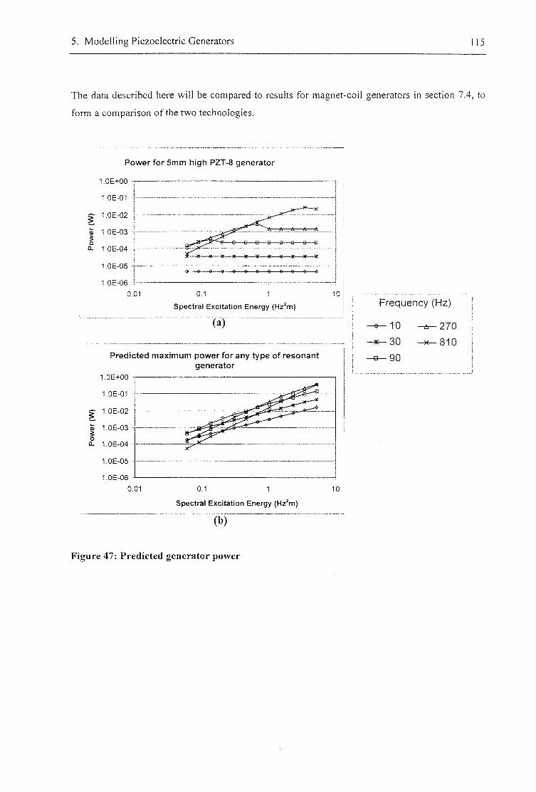
5. Modelling Piezoelectric Generators 15
The data described here will be compared to results for magnet-coil generators in section 7.4, to
form a comparison of the two technologies.
Power for 5mm high PZT-8 generator
1.0E+00
1.0E-01
1.0E-02
0) 1.06-03
tt- 1.0E-04
,0E-05 -
1^646 0 , 0 1 01 1
Spectral Excitation Energy (Hz^m)
(a)
1.0E+00 -
1.0E-01 -
5 1.0E-02 -
1.0E-03 -1 Q.
1.0E-05 -
1.0E-06 -
(b)
10
Predicted maximum power for any type of resonant generator
0.01 0.1 1 10
Spectral Excitation Energy (Hz'm)
Frequency (Hz)
10 2 7 0
^ 3 0 - 4 < - 8 1 0
- B - 9 0
Figure 47: Predicted generator power
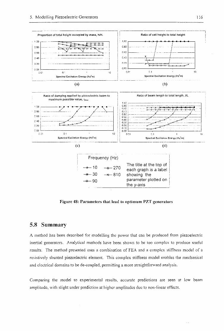
5. Modelling Piezoelectric Generators 16
Proportion of total height occupied by mass, h/H.
1 ,00
0,80
0,60
0 . 4 0
020
0.00 0 1 1
Spectral Excitation Energy (Hz'm)
(a)
Ratio of damping applied by piezoelectric beam to maximum possible value, nmmx
0.1 1
spectral Excitation Energy (Hz'm)
(C)
1.00 0.90 0.80 0.70 0.60 0.50 0.40 0.30 0.20 0 10 0.00
Ratio of cell height to total height
0.1 1
spectral Excitation Energy (Hz'm)
(b)
Ratio of beam length to total length, l/L
-- - - .— ^ 9 t .. H
—
—
0.1 1
Spectral Excitation Energy (Hz'm)
(d)
Frequency (Hz)
10 2 7 0
30
- B - 9 0
- x - 8 1 0
The title at the top of each graph is a label showing the parameter plotted on the y-axis
Figure 48: Parameters that lead to optimum PZT generators
5.8 Summary
A method has been described for modelling the power that can be produced from piezoelectric
inertial generators. Analytical methods have been shown to be too complex to produce useful
results. The method presented uses a combination of FEA and a complex stiffness model of a
resistively shunted piezoelectric element. This complex stiffness model enables the mechanical
and electrical domains to be de-coupled, permitting a more straightforward analysis.
Comparing the model to experimental results, accurate predictions are seen at low beam
amplitude, with slight under prediction at higher amplitudes due to non-linear effects.
5. Modelling Piezoelectric Generators 117
The power output from the prototype generators reaches a maximum of only a few microwatts.
This power output is too low to be of practical use (see section 3.3). The model (see equation 5.4)
reveals that this low power is due to the low electromagnetic coupling produced by thick-film
piezoceramics when they are operated in a 3-1 coupling mode. If bulk PZT were used in place of
the thick-film material, the model predicts a 100 fold increase in generated power, Thus, research
(e.g. Glynne-Jones a/ [82] and Kosec er a/ [83]) to improve thick-film piezoelectric materials
has the potential to significantly improve the performance of the prototype.
The model has been applied to a simplified generator structure to make predictions of how much
power a piezoelectric generator of an arbitrary size might produce under ideal conditions. These
calculations have been applied to a range of example applications, and reveal that the generated
power varies widely from application to application, and that bulk PZT offers superior
performance. The same examples will be used in chapter 7 to enable a comparison between
piezoelectric and magnet-coil generators.
6. Ageing Characteristics of Thick-Film PZT 118
CHAPTER 6
Ageing Characteristics of Thick-Film PZT
6.1 Introduction
It has long been known that piezoelectric ceramics suffer a long term ageing process after
polarisation [84]. When these materials are used in sensors, actuators, and generators there is a
concern that this ageing will decrease the efficiency, sensitivity or accuracy of the devices. It is
thus important to characterise the ageing process so that designs can be made which allow for
degradation over the lifetime of a device.
Owing to the difficulties in measuring the coupling coefficients of thick-film piezoelectric
ceramics, which stem from the presence of an underlying substrate, there are no reports in the
literature of any attempts to measure the ageing of these thick-film properties. Making a
preliminary study of this effect was thus deemed important for piezoelectric generators. This
section does not attempt to explore the ageing process in detail, but to provide some confidence in
the long-term stability of thick-film PZT.
Methods for studying two types of ageing process are presented. The first measures the decrease
in magnitude of the d], coefficient (which relates stress applied perpendicular to the polarisation
direction to charge displaced along the polar axis) and the dielectric constant, Ksj, with time after
polarisation. Finally, a method to examine the effect of cyclical stress on the dsi coefficient is
explored.
6.2 Background
From the time that a sample of bulk PZT is cooled after polarisation, it can be noted that the
ageing cycles described in table 12 begins.
Jaffe et at [43] state that for any of these properties the effect can be expressed for practical time
intervals as K-K,) - m log(t) where K is the value of the constant, Ko its value at t=I, and t the
time elapsed since cooling. Jaffe also notes that by mathematical necessity the ageing rate must
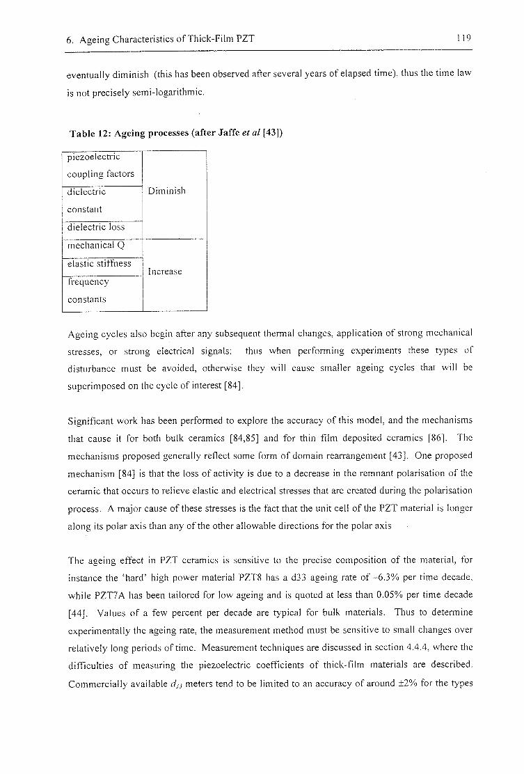
6. Ageing Characteristics of Thick-Film PZT 19
eventually diminish (this has been observed after several years of elapsed time), thus the time law
is not precisely semi-logarithmic.
Table 12: Ageing processes (after Jaffe et al [43])
piezoelectric
coupling factors
Diminish dielectric
constant
Diminish
dielectric loss
Diminish
mechanical Q
Increase elastic stiffness
Increase frequency
constants
Increase
Ageing cycles also begin after any subsequent thermal changes, application of strong mechanical
stresses, or strong electrical signals; thus when performing experiments these types of
disturbance must be avoided, otherwise they will cause smaller ageing cycles that will be
superimposed on the cycle of interest [84].
Significant work has been performed to explore the accuracy of this model, and the mechanisms
that cause it for both bulk ceramics [84,85] and for thin film deposited ceramics [86]. The
mechanisms proposed generally reflect some form of domain rearrangement [43]. One proposed
mechanism [84] is that the loss of activity is due to a decrease in the remnant polarisation of the
ceramic that occurs to relieve elastic and electrical stresses that are created during the polarisation
process. A major cause of these stresses is the fact that the unit cell of the PZT material is longer
along its polar axis than any of the other allowable directions for the polar axis
The ageing effect in PZT ceramics is sensitive to the precise composition of the material, for
instance the 'hard ' high power material PZT8 has a d33 ageing rate o f - 6 . 3 % per time decade,
while PZT7A has been tailored for low ageing and is quoted at less than 0.05% per time decade
[44]. Values of a few percent per decade are typical for bulk materials. Thus to determine
experimentally the ageing rate, the measurement method must be sensitive to small changes over
relatively long periods of time. Measurement techniques are discussed in section 4.4.4, where the
difficulties of measuring the piezoelectric coefficients of thick-film materials are described.
Commercially available dj} meters tend to be limited to an accuracy of around ±2% for the types
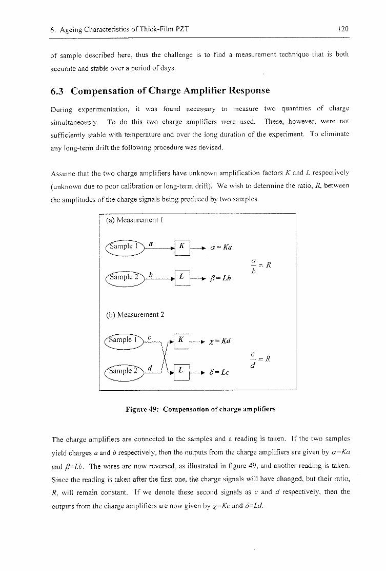
6. Ageing Characteristics of Thick-Film PZT 120
of sample described here, thus the challenge is to find a measurement technique that is both
accurate and stable over a period of days.
6.3 Compensation of Charge Amplifier Response
During experimentation, it was found necessary to measure two quantities of charge
simultaneously. To do this two charge amplifiers were used. These, however, were not
sufficiently stable with temperature and over the long duration of the experiment. To eliminate
any long-term drift the following procedure was devised.
Assume that the two charge amplifiers have unknown amplification factors K and L respectively
(unknown due to poor calibration or long-term drift). We wish to determine the ratio, R, between
the amplitudes of the charge signals being produced by two samples.
(a) Measurement
a K *
(b) Measurement 2
ample^~V—
K
-p- a = Ka
/3 = Lb
-• 5=Lc
a R
c
d R
Figure 49: Compensation of charge amplifiers
The charge amplifiers are connected to the samples and a reading is taken. If the two samples
yield charges a and b respectively, then the outputs from the charge amplifiers are given by a-Ka
and /3=Lb. The wires are now reversed, as illustrated in figure 49, and another reading is taken.
Since the reading is taken after the first one, the charge signals will have changed, but their ratio,
R, will remain constant. If we denote these second signals as c and d respectively, then the
outputs from the charge amplifiers are now given by and S-Ld.
6. Ageing Characteristics of Thick-Film PZT 121
It can be shown that the ratio between the input signals, R, can be determined by the following
equation that is in terms of the measured outputs from the charge amplifiers, and is independent of
K and L.
Equation 6.1
6.4 Temporal ageing after polling
The experiments described here use the composite steel / dielectric / PZT beams described in
chapter 4. When these beams are mounted in a clamp and shaken the resulting signal at the
electrodes is a function of the dji coefficient of the PZT. Thus, by examining this signal after
polarisation, the ageing of the coefficient can be observed. The ageing of the dielectric
constant, K33, of the PZT layer can also be measured through the capacitance of the sample.
6.4.1 Experimental procedure
The composite beams were produced as described in section 4,3, including attaching a mass to the
tips of the beams, and wires to the electrodes. A device is polarised as described in section 4.2.7.3
using a temperature of 150°C for a period of 35 minutes. Immediately following polarisation the
beam is clamped at one end of the clamp of the shaker rig described in section 4.5.1.
Preliminary experiments showed that both the base excitation supplied by the shaker and the
response of a clamped sample to shaking varied with environmental temperature; this variation
obscured the ageing present in the sample (see figure 51). To compensate for this effect, a
reference sample was used. The reference sample was mounted at the opposite end of the clamp
to the main sample. This reference sample was prepared in an identical manner to the main
sample, except that it was polarised one month before the experiment. If the system is assumed to
be linear, then if the base acceleration is increased, the ratio between the signals from the
reference sample and the main sample should remain unchanged. Similarly, the reference sample
should compensate for any linear temperature dependence of the dn coefficient with temperature.
By polarising the reference sample one month before the experiment, it should not age more than
a further -0.12% over the course of a 2-day experiment (given the rate of ageing found
experimentally).
The shaker was driven by the amplifier and frequency source described above. The frequency of
excitation was set at 60Hz, around two thirds of the 90Hz natural frequencies of the sample and
reference beams. Preliminary experiments had been performed operating at the resonant
frequency of the sample; it was found, however, that as temperature variations occurred the
6. Ageing Characteristics of Thick-Film PZT 122
natural frequencies of the beams would change causing large variations in the beams' amplitudes.
It was also found that at resonance the positions of the connecting wires had large effects on the
beams' amplitudes, leading to unreliable results (at resonance the amplitude is controlled by the
amount of damping present; the connecting wires cause a significant part of this damping).
Operating at 60Hz is a compromise between using higher frequencies with the associated
damping problems, and lower frequencies which would produce a smaller signal to noise ratio.
The main sample was placed in the clamp immediately after it was polarised. The amplitude of
the acceleration applied by the shaker was set to 28ms"^ (measured using the accelerometer),
which produced a strong signal without being large enough to cause mechanical change in the test
apparatus. The amplitude of the beam at this excitation was measured as 0.3mm. Using the finite
element model described in section 5.4.1, it was found that this results in a maximum longitudinal
stress in the PZT layer of 2.7 MPa. This is in the linear range described for bulk PZT5A [44],
which is given a maximum rated static compressive stress perpendicular to the polar axis of
13.8MPa. It is thus reasonable to assume that the device is operating in its linear range, and that
the shaking should not contribute any stress-induced ageing cycles.
To measure the charge displaced by the two beams a pair of Kistler Charge Amplifiers (model
5001) were used. The charge amplifiers were set to a sensitivity of lOOOpC/V with a feedback
resistance of lO'Q. The signal analyser monitored the output from the charge amplifiers, and was
used with a flat-top (sinusoidal) windowing function, which gave better amplitude accuracy than
the other available functions. The signal analyser was set to a sampling rate of 256Hz, with a
total number of 512 samples. The analyser performed Fourier transforms to show the average
signal amplitude over the sampling period.
Once the sample was polarised and clamped, and the shaker activated, then a set of measurements
were taken periodically. To take a set of measurements, first the charge signals were measured
with the main sample connected to charge amplifier 'A ' , and the reference connected to charge
amplifier 'B ' . A reading was taken simultaneously of both quantities. (The signal analyser has
two input channels that are logged concurrently. Both can be paused simultaneously to allow this
measurement). The connecting leads were then switched so that the main sample was connected
to charge amplifier 'B ' , and the reference connected to charge amplifier 'A ' ; readings of the
charge signals were again taken simultaneously. Equation 6.1 was then used to determine the
ratio of sample response to reference response. The experiments described here continued for up
to 2 days, with the interval between readings increasing to provide suitable data to plot a semi-
logarithmic graph of the results.
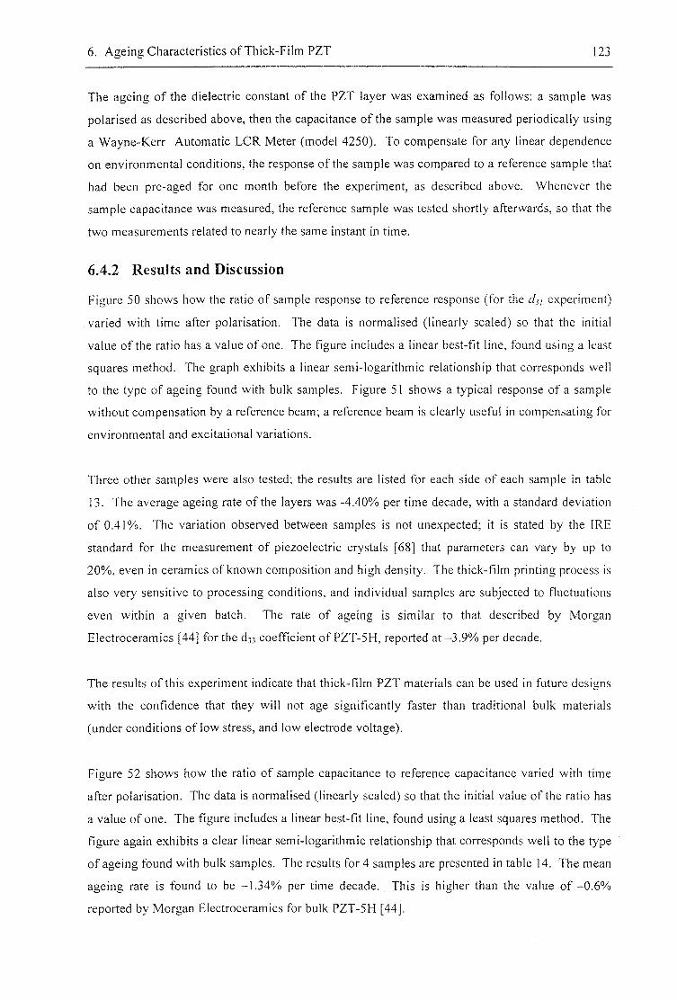
6. Ageing Characteristics of Thick-Film PZT 123
The ageing of the dielectric constant of the PZT layer was examined as follows: a sample was
polarised as described above, then the capacitance of the sample was measured periodically using
a Wayne-Kerr Automatic LCR Meter (model 4250). To compensate for any linear dependence
on environmental conditions, the response of the sample was compared to a reference sample that
had been pre-aged for one month before the experiment, as described above. Whenever the
sample capacitance was measured, the reference sample was tested shortly afterwards, so that the
two measurements related to nearly the same instant in time.
6.4.2 Results and Discussion
Figure 50 shows how the ratio of sample response to reference response (for the experiment)
varied with time after polarisation. The data is normalised (linearly scaled) so that the initial
value of the ratio has a value of one. The figure includes a linear best-fit line, found using a least
squares method. The graph exhibits a linear semi-logarithmic relationship that corresponds well
to the type of ageing found with bulk samples. Figure 51 shows a typical response of a sample
without compensation by a reference beam; a reference beam is clearly useful in compensating for
environmental and excitational variations.
Three other samples were also tested; the results are listed for each side of each sample in table
13. The average ageing rate of the layers was -4.40% per time decade, with a standard deviation
of 0.41%. The variation observed between samples is not unexpected; it is stated by the IRE
standard for the measurement of piezoelectric crystals [68] that parameters can vary by up to
20%, even in ceramics of known composition and high density. The thick-film printing process is
also very sensitive to processing conditions, and individual samples are subjected to fluctuations
even within a given batch. The rate of ageing is similar to that described by Morgan
Electroceramics [44] for the d]) coefficient of PZT-5H, reported a t - 3 . 9 % per decade.
The results of this experiment indicate that thick-film PZT materials can be used in future designs
with the confidence that they will not age significantly faster than traditional bulk materials
(under conditions of low stress, and low electrode voltage).
Figure 52 shows how the ratio of sample capacitance to reference capacitance varied with time
after polarisation. The data is normalised (linearly scaled) so that the initial value of the ratio has
a value of one. The figure includes a linear best-fit line, found using a least squares method. The
figure again exhibits a clear linear semi-logarithmic relationship that corresponds well to the type
of ageing found with bulk samples. The results for 4 samples are presented in table 14. The mean
ageing rate is found to be -1 .34% per time decade. This is higher than the value of - 0 . 6 %
reported by Morgan Electroceramics for bulk PZT-5H [44],
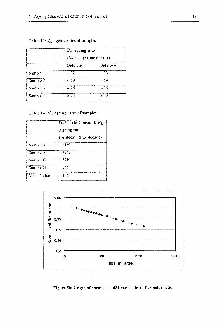
6. Ageing Characteristics of Thick-Film PZT 124
Table 13: dn ageing rates of samples
dj! Ageing rate
(% decay/ time decade)
Side one Side two
Sample! 4 J 2 4.93
Sample 2 4.69 4.59
Sample 3 4 2 6 4 3 5
Sample 4 3.94 3 J 3
Table 14: K}} ageing rates of samples
Dielectric Constant,
Ageing rate
(% decay/ time decade)
Sample A 1.1194
Sample B 1.33%
Sample C 1.37%
Sample D 1.54%
Mean Value 1.34%
IV 0.95
2 0.85
10 100 1000
Time (minutes)
10000
Figure 50: Graph of normalised d31 versus time after polarisation
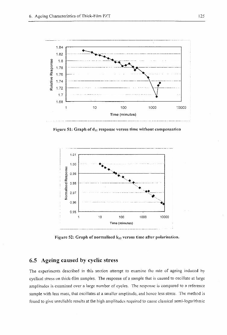
6. Ageing Characteristics of Thick-Film PZT 125
10 100 1000
Time (minutes)
10000
Figure 51: Graph of d], response versus time without compensation
1.01
1.00
I •o 0.98
to
E 0.97 o z 0.96
0.95
1 10 100
Time (minutes)
1000 10000
Figure 52: Graph of normalised k]3 versus time after polarisation.
6.5 Ageing caused by cyclic stress
The experiments described in this section attempt to examine the rate of ageing induced by
cyclical stress on thick-film samples. The response of a sample that is caused to oscillate at large
amplitudes is examined over a large number of cycles. The response is compared to a reference
sample with less mass, that oscillates at a smaller amplitude, and hence less stress. The method is
found to give unreliable results at the high amplitudes required to cause classical semi-logarithmic
6. Ageing Characteristics of Thick-Film PZT 126
ageing of the sample; lower amplitudes are, however, found to cause a small linear ageing effect
that is presented as interesting and potentially important.
6.5.1 Method
Sample and reference composite beams were prepared and equipped with wires as described in
the previous experiment. Both beams were polarised, then left for 60 days so that the amount of
natural ageing over the course of the experiment would be negligible (over the course of an 8 day
experiment the dji of these samples will decrease by only a further 0.2%, assuming an ageing rate
o f - 4 % per decade).
The two beams were mounted in the shaker rig as before. In this experiment, a tip mass was
placed on the sample beam, but not the reference beam. This means that when the clamp was
shaken, the sample oscillates with a much higher amplitude than the reference beam. The sample
beam was thus being shaken at an amplitude that may cause it to age due to the cyclic stresses
induced in it. The reference beam should not age in this manner, and should allow for
compensation of any variation in the excitation amplitude and linear temperature-related
coefficient changes.
For the reasons described in the previous experiment, the shaker was operated at 55Hz. Samples
were tested at two different excitation amplitudes. Table 15 lists the beam amplitudes, and the
associated base excitation, and the maximum stress in the PZT at these amplitudes predicted using
the FEA model. The longitudinal stresses predicted in the PZT layer would place the samples in
the linear region of operation were they formed from bulk material (PZT-5A has a maximum
rated compressive stress perpendicular to the polar axis of 13.8MPa)
Larger beam amplitudes were investigated, but it was found that at such amplitudes there were
large variations in the results that obscured any meaningful trends. These variations could be due
to the large amount of base excitation required to achieve these beam amplitudes in a sub-resonant
beam causing mechanical changes in the clamping arrangement, or perhaps that the strength of the
thick-film layer in tension or compression is exceeded.
The charge signals from the two samples were fed into the pair of charge amplifiers. These were
set to sensitivities of 1 OOOpC/V and 50pC/V for the sample and reference beams respectively.
The output from the charge amplifiers was monitored by the signal analyser described above. As
before, a flat-top windowing function was used. The signal analyser was set to a sampling rate of
128Hz, with a total number of 512 samples.
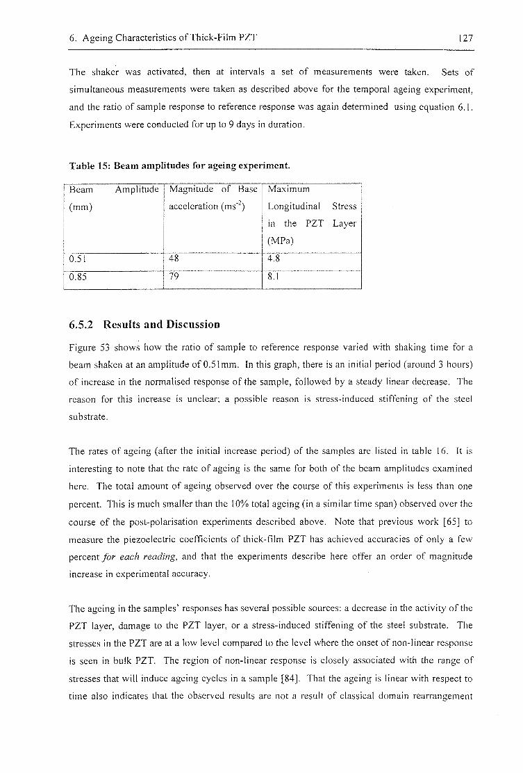
6. Ageing Characteristics of Thictc-Film PZT 127
The shaker was activated, then at intervals a set of measurements were taken. Sets of
simultaneous measurements were taken as described above for the temporal ageing experiment,
and the ratio of sample response to reference response was again determined using equation 6.1.
Experiments were conducted for up to 9 days in duration.
Table 15: Beam amplitudes for ageing experiment.
Beam Amplitude
(mm)
Magnitude of Base
acceleration (ms'")
Maximum
Longitudinal Stress
in the PZT Layer
(MPa)
0.51 48 4.8
0.85 79 8.1
6.5.2 Results and Discussion
Figure 53 shows how the ratio of sample to reference response varied with shaking time for a
beam shaken at an amplitude of 0.51mm. In this graph, there is an initial period (around 3 hours)
of increase in the normalised response of the sample, followed by a steady linear decrease. The
reason for this increase is unclear; a possible reason is stress-induced stiffening of the steel
substrate.
The rates of ageing (after the initial increase period) of the samples are listed in table 16. It is
interesting to note that the rate of ageing is the same for both of the beam amplitudes examined
here. The total amount of ageing observed over the course of this experiments is less than one
percent. This is much smaller than the 10% total ageing (in a similar time span) observed over the
course of the post-polarisation experiments described above. Note that previous work [65] to
measure the piezoelectric coefficients of thick-film PZT has achieved accuracies of only a few
percent for each reading, and that the experiments describe here offer an order of magnitude
increase in experimental accuracy.
The ageing in the samples' responses has several possible sources; a decrease in the activity of the
PZT layer, damage to the PZT layer, or a stress-induced stiffening of the steel substrate. The
stresses in the PZT are at a low level compared to the level where the onset of non-linear response
is seen in bulk PZT. The region of non-linear response is closely associated with the range of
stresses that will induce ageing cycles in a sample [84]. That the ageing is linear with respect to
time also indicates that the observed results are not a result of classical domain rearrangement
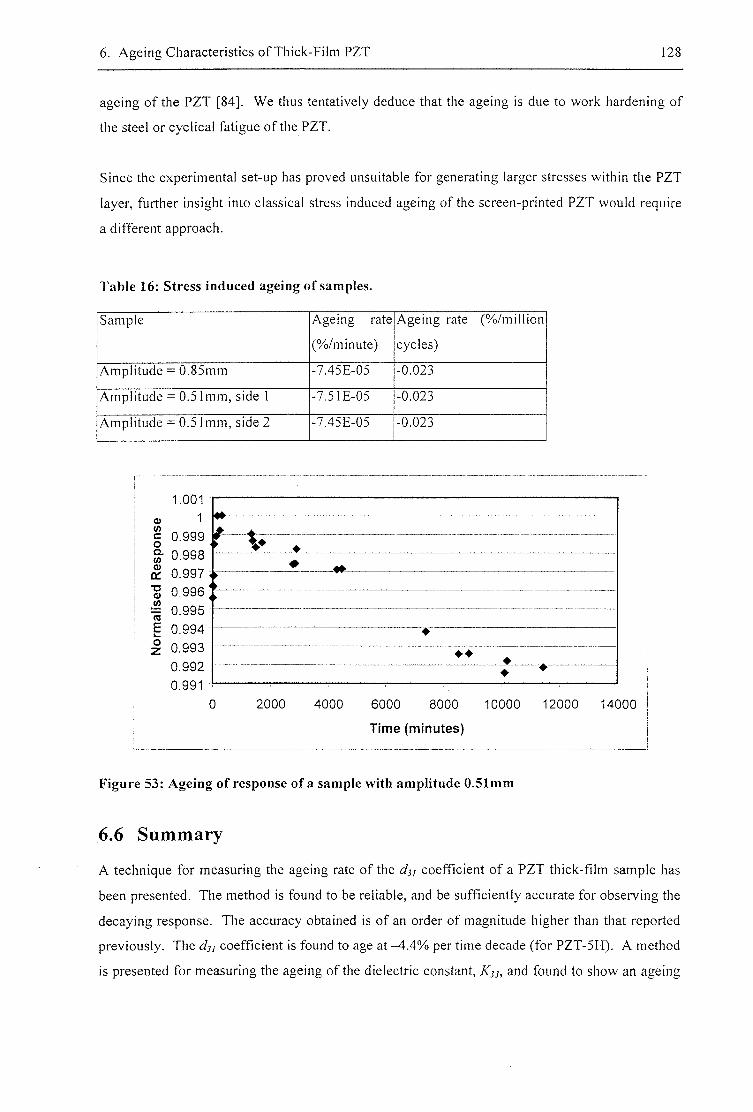
6. Ageing Characteristics of Thick-Film PZT 128
ageing of the PZT [84]. We thus tentatively deduce that the ageing is due to work hardening of
the steel or cyclical fatigue of the PZT.
Since the experimental set-up has proved unsuitable for generating larger stresses within the PZT
layer, further insight into classical stress induced ageing of the screen-printed PZT would require
a different approach.
Table 16: Stress induced ageing of samples.
Sample Ageing rate
(%/minute)
Ageing rate (%/miilion
cycles)
Amplitude = 0.85mm -7.45E-05 -0.023
Amplitude = 0.51mm, side 1 .7.5115-05 -0.023
Amplitude == 0.51mm, side 2 -7.45E-05 -0.023
<u (/) c o Q. S o;
"S « 75 E o z
1.001
1
0,999
0.998
0.997
0.996
0.995
0.994
0.993
0.992
0.991
> > r V •
•
0 •
•
• • _ • • •
2000 4000 6000 8000 10000 12000 14000
Time (minutes)
Figure 53: Ageing of response of a sample with amplitude 0.51mm
6.6 Summary
A technique for measuring the ageing rate of the d^i coefficient of a PZT thick-film sample has
been presented. The method is found to be reliable, and be sufficiently accurate for observing the
decaying response. The accuracy obtained is of an order of magnitude higher than that reported
previously. The dj i coefficient is found to age at - 4 . 4 % per time decade (for PZT-5H). A method
is presented for measuring the ageing of the dielectric constant, K33, and found to show an ageing
6. Ageing Characteristics of Thick-Film PZT 129
rate of - 1 .34% per time decade. Future studies into the effect of polarisation conditions and other
processing parameters on the rate of ageing are recommended.
A technique for exploring the ageing induced by cyclical stress has also been described. The
method has been found to be unreliable at the higher stresses required to induce classical ageing,
however, at lower amplitudes, a small linear ageing effect has been found that warrants further
study.
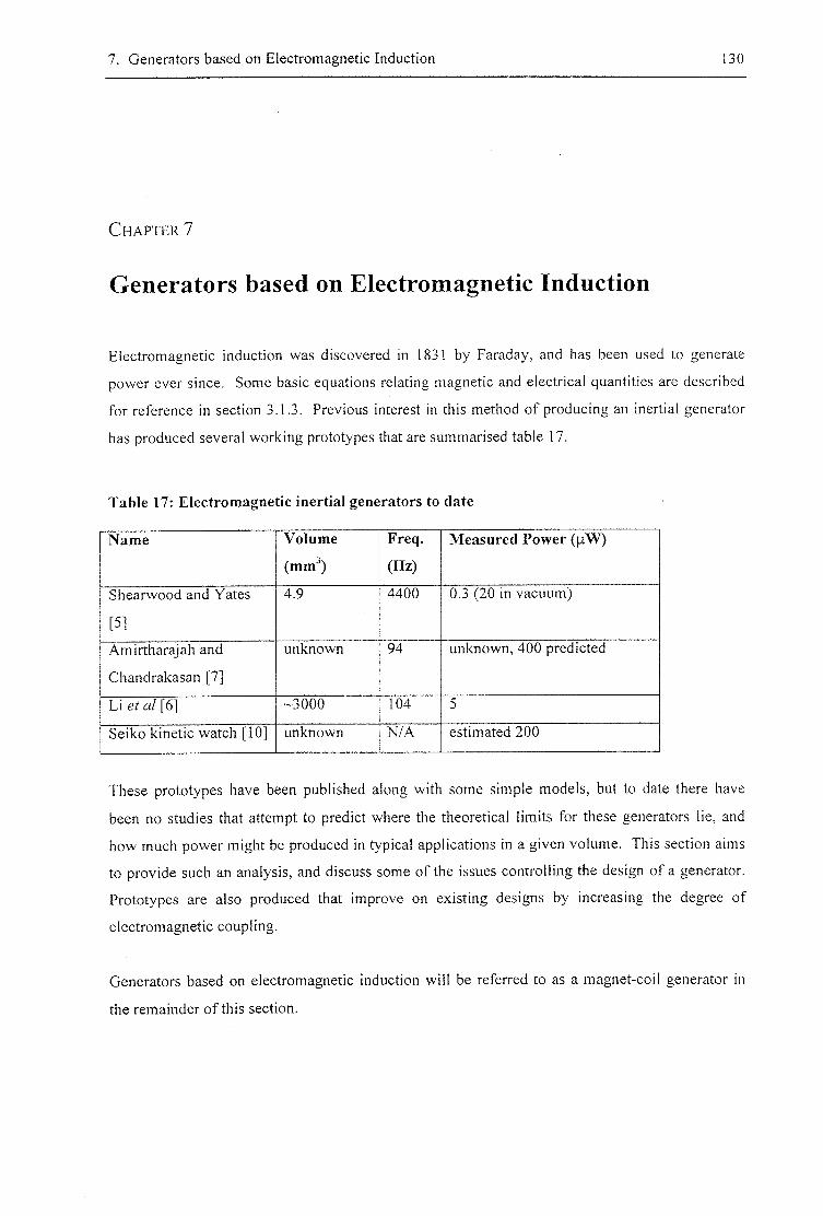
7. Generators based on Electromagnetic Induction 130
CHAPTER 7
Generators based on Electromagnetic Induction
Electromagnetic induction was discovered in 1831 by Faraday, and has been used to generate
power ever since. Some basic equations relating magnetic and electrical quantities are described
for reference in section 3.1.3. Previous interest in this method of producing an inertial generator
has produced several working prototypes that are summarised table 17.
Table 17: Electromagnetic inertial generators to date
Name Volume
(mm^)
Freq.
(Hz)
Measured Power (^W)
Shearwood and Yates
[5]
4.9 4400 0.3 (20 in vacuum)
Amirtharajah and
Chandrakasan [7]
unknown 94 unknown, 400 predicted
Li et al [6] -3000 104 5
Seiko kinetic watch [10] unknown N/A estimated 200
These prototypes have been published along with some simple models, but to date there have
been no studies that attempt to predict where the theoretical limits for these generators lie, and
how much power might be produced in typical applications in a given volume. This section aims
to provide such an analysis, and discuss some of the issues controlling the design of a generator.
Prototypes are also produced that improve on existing designs by increasing the degree of
electromagnetic coupling.
Generators based on electromagnetic induction will be referred to as a magnet-coil generator in
the remainder of this section.
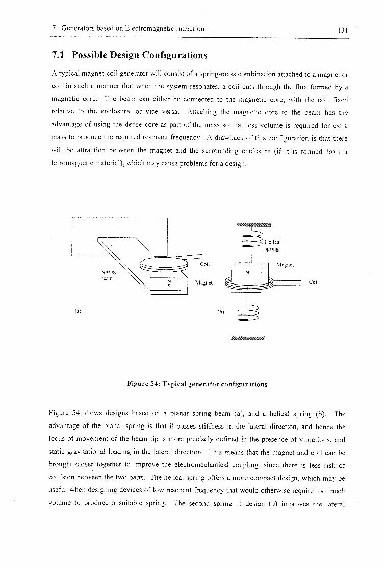
7. Generators based on Electromagnetic Induction 131
7.1 Possible Design Configurations
A typical magnet-coil generator will consist of a spring-mass combination attached to a magnet or
coil in such a manner that when the system resonates, a coil cuts through the flux formed by a
magnetic core. The beam can either be connected to the magnetic core, with the coil fixed
relative to the enclosure, or vice versa. Attaching the magnetic core to the beam has the
advantage of using the dense core as part of the mass so that less volume is required for extra
mass to produce the required resonant frequency. A drawback of this configuration is that there
will be attraction between the magnet and the surrounding enclosure (if it is formed from a
ferromagnetic material), which may cause problems for a design.
Spnng beam
CoH
Magnet
(»)
Helical
spring
Magnet
CoH
Figure 54: Typical generator configurations
Figure 54 shows designs based on a planar spring beam (a), and a helical spring (b). The
advantage of the planar spring is that it posses stiffness in the lateral direction, and hence the
locus of movement of the beam tip is more precisely defined in the presence of vibrations, and
static gravitational loading in the lateral direction. This means that the magnet and coil can be
brought closer together to improve the electromechanical coupling, since there is less risk of
collision between the two parts. The helical spring offers a more compact design, which may be
useful when designing devices of low resonant frequency that would otherwise require too much
volume to produce a suitable spring. The second spring in design (b) improves the lateral
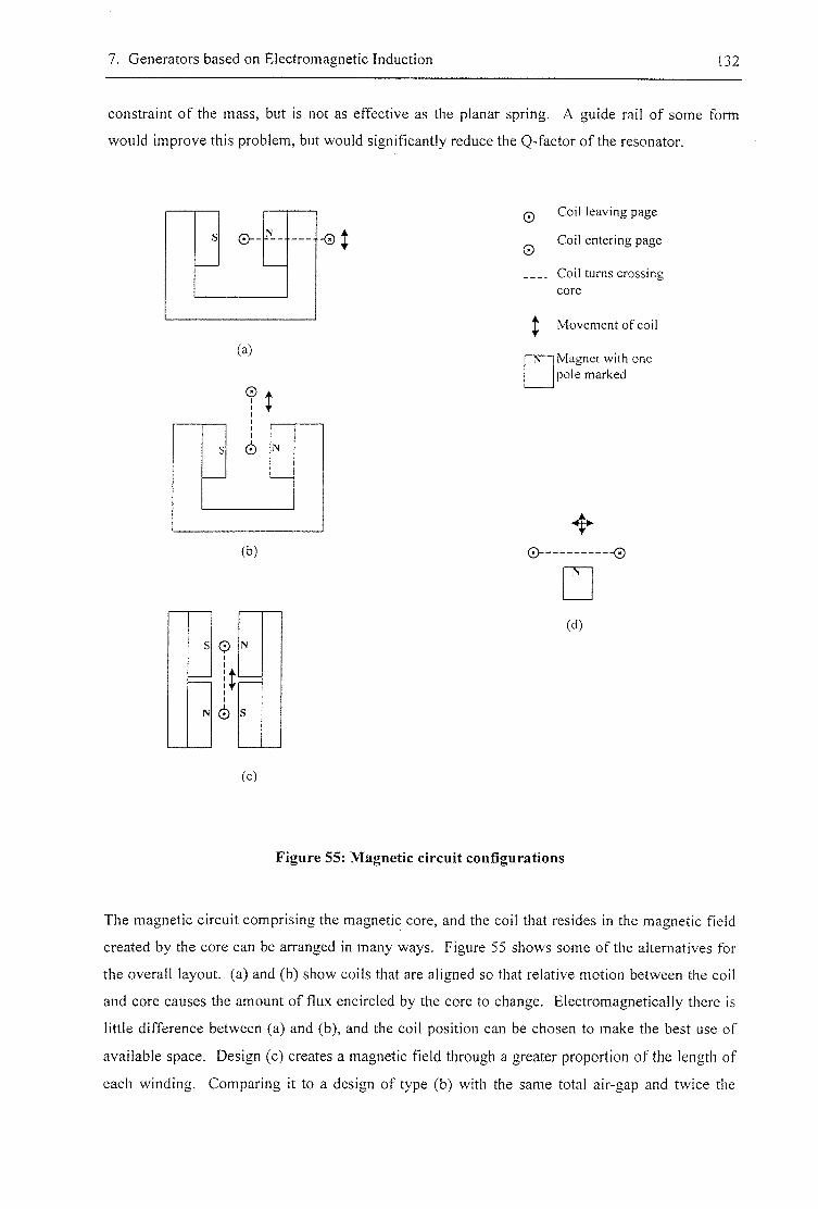
7. Generators based on Electromagnetic Induction 132
constraint of the mass, but is not as effective as the planar spring. A guide rail of some form
would improve this problem, but would significantly reduce the Q-factor of the resonator.
0 - -
(a)
0
6
(b)
0
6
(c)
I
0 Coil leaving page
Coil entering page
Coil turns crossing
core
I Movement of coil
Magnet with one pole marked
0 - - - - 0
(d)
Figure 55: Magnetic circuit configurations
The magnetic circuit comprising the magnetic core, and the coil that resides in the magnetic field
created by the core can be arranged in many ways. Figure 55 shows some of the alternatives for
the overall layout, (a) and (b) show coils that are aligned so that relative motion between the coil
and core causes the amount of flux encircled by the core to change. Electromagnetically there is
little difference between (a) and (b), and the coil position can be chosen to make the best use of
available space. Design (c) creates a magnetic field through a greater proportion of the length of
each winding. Comparing it to a design of type (b) with the same total air-gap and twice the
7. Generators based on Electromagnetic Induction 133
number of coils to achieve the degree of electromagnetic coupling, it can be seen that the total
length of coil is twice that required for design (c) (assuming that the height of the coil, h, is not
significant). Thus, design (c) has the potential to reduce the resistive losses in the coil windings
by shortening the coil. However, this comparison is not wholly accurate as the clearance required
at the side of the coil is ignored, and the coil height will often be significant. Design (d) is of the
type used by Chan [87]. The advantage of this design is its ease of manufacture, especially during
MEMS processes, however, the degree of electromagnetic coupling achieved with this layout will
be much smaller than the other layouts described here (especially for small coil amplitudes). To
achieve suitable output voltages with this configuration, Chan had to use a torsional vibration
mode. In some higher source amplitude applications this may not be a problem, as the best design
is not always the one that provides the highest degree of coupling (see section 7.4.5).
To improve the degree of coupling, it is important to choose a type of magnet that will produce a
strong flux density. Rare earth magnets are ideal for this application, and offer up to 5 times the
magnetic energy density of conventional AInico magnets. "Neodymium Iron Boron magnets have
the most powerful magnetic properties per cubic cm known at this time [2001]"[88], and can
operate at up to 120°C. If higher temperature operation is required, the less powerful Samarium
Cobalt can be used, with a working temperature of up to 250°C.
The coil is characterised by the proportion of the coil that passes through the magnetic field, the
number of turns in the coil, and its series resistance. Second-order effects such as coil inductance
can often be ignored due to the low frequency of many applications. Two types of coil have been
used in the past: wound coils, and printed coils (as used by Chan [87]). A printed coil can be
formed by screen printing layers of conductive materials and insulators onto a substrate in much
the same manner as PCBs are produced. (Printed coils are sometimes known as planar coils -
although here, both coils will tend to be essentially planar in nature as a consequence of the
advantage of having a thin air-gap.) A printed coil can be made very thin (printed layers will
typically be lOjim thick), which makes it particularly attractive for small scale devices (see
section 7.5.2). A printed coil may also be easier to manufacture as it only involves standard thick-
film printing processes, as opposed to a wound coil, which becomes more difficult to manufacture
as the scale decreases. The disadvantage of a printed coil is that the small thickness of each layer
will result in a high series resistance for the coil. If windings of a larger thickness than are
traditionally available from thick-film technology (e.g. >50)j.m) are required, it is anticipated that
a wound coil will be more economic to manufacture. Printed coils have the added advantage of
already being connected to a substrate, which may add rigidity to the coil, and hence decrease the
clearance required between the coil and the magnetic core.
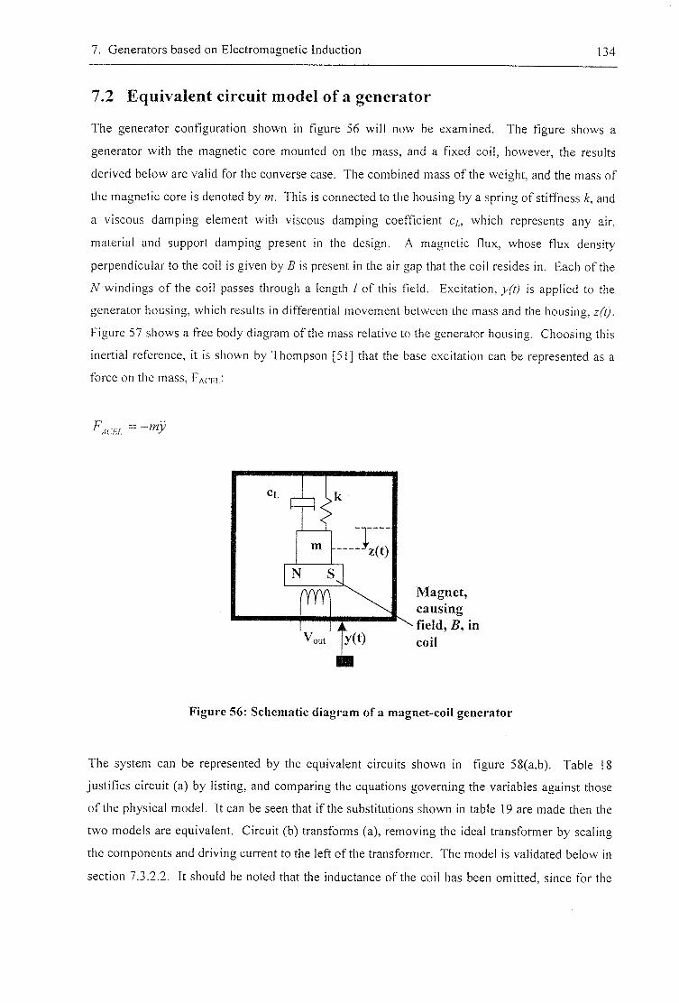
7. Generators based on Electromagnetic Induction 134
7.2 Equivalent circuit model of a generator
The generator configuration shown in figure 56 will now be examined. The figure shows a
generator with the magnetic core mounted on the mass, and a fixed coil, however, the results
derived below are valid for the converse case. The combined mass of the weight, and the mass of
the magnetic core is denoted by m. This is connected to the housing by a spring of stiffness k, and
a viscous damping element with viscous damping coefficient c/,, which represents any air,
material and support damping present in the design. A magnetic flux, whose flux density
perpendicular to the coil is given by B is present in the air gap that the coil resides in. Each of the
N windings of the coil passes through a length / of this field. Excitation, y(t) is applied to the
generator housing, which results in differential movement between the mass and the housing, z f t j .
Figure 57 shows a free body diagram of the mass relative to the generator housing. Choosing this
inertial reference, it is shown by Thompson [51] that the base excitation can be represented as a
force on the mass, pACEL:
F
m
>k
N
Vo
Magnet, causing field, B, in coil
Figure 56: Schematic diagram of a magnet-coil generator
The system can be represented by the equivalent circuits shown in figure 58(a,b). Table 18
justifies circuit (a) by listing, and comparing the equations governing the variables against those
of the physical model. It can be seen that if the substitutions shown in table 19 are made then the
two models are equivalent. Circuit (b) transforms (a), removing the ideal transformer by scaling
the components and driving current to the left of the transformer. The model is validated below in
section 7.3.2.2. It should be noted that the inductance of the coil has been omitted, since for the
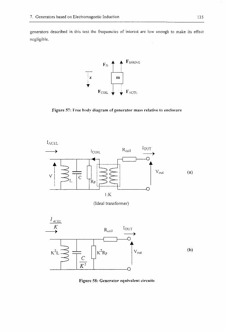
7. Generators based on Electromagnetic Induction 135
generators described in this text the frequencies of interest are low enough to make its effect
negligible.
Fd Fspring
m
F c o i l t t Face l
Figure 57: Free body diagram of generator mass relative to enclosure
lACEL » loUT
V C U
out
l : K
(Ideal t r ans fo rmer )
(a)
I AC EL K
K ^ L
Rc coil loUT
- O
c K'
K^Rp V, out
- o
(b)
Figure 58: Generator equivalent circuits
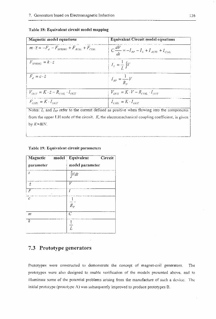
7. Generators based on Electromagnetic Induction 136
Table 18: Equivalent circuit model mapping
Magnetic model equations Equivalent Circuit model equations
m • z = —Fj — ^ac/;i ^coil RP ~ ^^Acm h'on
K)ur = K • z — R( qii^ • Iquj Knrr = K - V — Rcq,,^ ' I our
F - K • I
Notes; //, and Irp refer to the current defined as positive when f lowing into the components
f rom the upper LH node of the circuit. K, the electromechanical coupling coefficient, is given
by
Table 19: Equivalent circuit parameters
Magnetic model Equivalent Circuit
parameter model parameter
z jPWf
z F
F I
c 1
R,,
m C
k 1
L
7.3 Prototype generators
Prototypes were constructed to demonstrate the concept of magnet-coil generators. The
prototypes were also designed to enable verification of the models presented above, and to
illuminate some of the potential problems arising from the manufacture of such a device. The
initial prototype (prototype A) was subsequently improved to produce prototypes B.
7. Generators based on Electromagnetic Induction 137
7.3.1 Prototype: A
A diagram and photo of the generator is shown in figure 59. The device consists of a cantilever
beam supported in a clamp. At the tip of this stainless steel beam, a C-shaped core is mounted,
with two magnets inside each end of the core. Attached to the clamp block, a coil consisting of 27
turns of 0.2mm diameter enamelled copper wire was wound so that each turn passes around the
beam, including passing through the magnetic field in the core gap. The core was attached to the
beam using double sided adhesive tape. It is acknowledged that this would be inadequate for a
practical generator, however, for the short tests described here it performed well.
To test the device the shaker and measurement apparatus described in section 4.5.1 was used. The
following experiments were performed:
(a) The resonant frequency was determined using the technique described in section 4.5.2. The
following experiments were all performed with excitation at the resonant frequency.
(b) The open circuit coil voltage was measured for a range of different amplitudes of base
vibration (base amplitude measured using an accelerometer; see section 4.5.1).
(c) Various load resistors were applied across the coil terminals, and the resulting load voltage,
and electrical power measured for a fixed base excitation.
(d) The load voltage across an optimum load resistance was measured for a range of different
amplitudes of base vibration
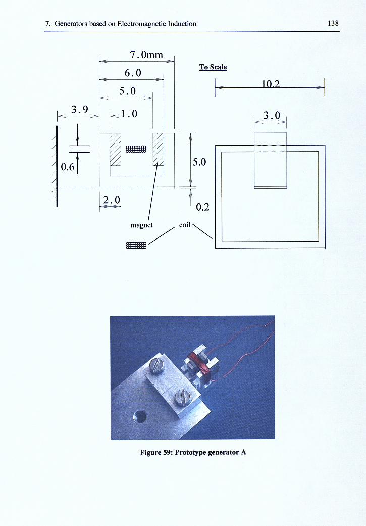
7. Generators based on Electromagnetic Induction 138
1 O m m
To Scale
magnet
m m
Figure 59: Prototype generator A
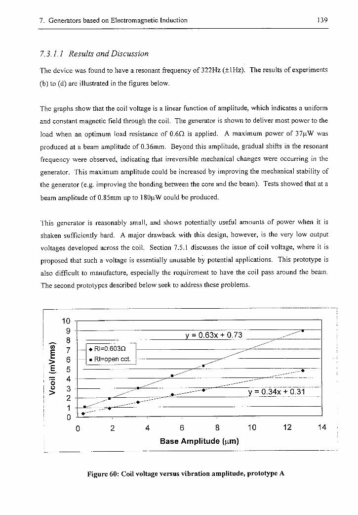
7. Generators based on Electromagnetic Induction 139
7.3.1.1 Results and Discussion
The device was found to have a resonant frequency of 322Hz (±lHz). The results of experiments
(b) to (d) are illustrated in the figures below.
The graphs show that the coil voltage is a linear function of amplitude, which indicates a uniform
and constant magnetic field through the coil. The generator is shown to deliver most power to the
load when an optimum load resistance of 0.6Q is applied. A maximum power of 37p.W was
produced at a beam amplitude of 0.36mm. Beyond this amplitude, gradual shifts in the resonant
frequency were observed, indicating that irreversible mechanical changes were occurring in the
generator. This maximum amplitude could be increased by improving the mechanical stability of
the generator (e.g. improving the bonding between the core and the beam). Tests showed that at a
beam amplitude of 0.85mm up to 180p.W could be produced.
This generator is reasonably small, and shows potentially useful amounts of power when it is
shaken sufficiently hard. A major drawback with this design, however, is the very low output
voltages developed across the coil. Section 7.5.1 discusses the issue of coil voltage, where it is
proposed that such a voltage is essentially unusable by potential applications. This prototype is
also difficult to manufacture, especially the requirement to have the coil pass around the beam.
The second prototypes described below seek to address these problems.
V)
E L. > E
I 8 >
10 9
8 7
6 5
4
3
2 1 0
y = 0.63x + 0.73
• RI=0.603Q
• RI=open cct.
y = 0.34x + 0.31
0 4 6 8 10
Base Amplitude (jam)
12 14
Figure 60: Coil voltage versus vibration amplitude, prototype A
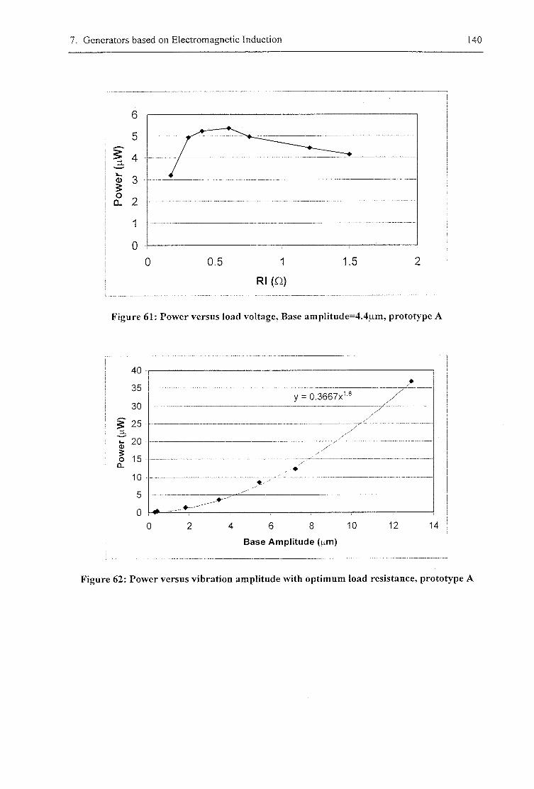
7. Generators based on Electromagnetic Induction 140
0.5
Rl (O)
1.5
Figure 61: Power versus load voltage, Base amplitude=4.4^in, prototype A
40
35
30
g 25
& 20
o 15 Q.
10
0 !-#_
0
y = 0.3667x1
4 6 8 10
Base Amplitude ((am)
12 14
Figure 62: Power versus vibration amplitude with optimum load resistance, prototype A
7. Generators based on Electromagnetic Induction 141
7.3.2 Prototypes: B
This section describes three prototypes of different designs that are based on a similar
construction method. Figure 63 shows the design of the prototypes, with the dimensions listed in
table 20. There are three designs:
(1) B1 is a small cantilever beam generator.
(2) 8 2 is a larger cantilever beam generator.
(3) B3 is of a similar size to B2, but is a torsional resonator.
Figure 64 shows a photograph of a completed B2. The resonant frequency of the cantilever
designs can be varied by adjusting the point at which they are clamped.
The common element in each design is the arrangement of the magnetic circuit (previously
illustrated in figure 55c ). On each generator, four magnets are mounted around a rectangular
slot, and the flux guided around the outside by means of two steel keeper plates. Thus arranged, a
magnetic circuit with two air-gaps is formed. The coil is passed through the slot so that when the
beam rests in a central position, both the upper and lower portions of each turn pass through the
magnetic field. The prototypes are designed so that during normal operation, the beam amplitude
is never large enough to cause the coil to leave the magnetic gaps. The coils can thus be modelled
as always remaining within a constant magnetic field. This arrangement is examined in more
depth in section 7.4.3; the finite element model described in that section was used to iteratively
pick core dimensions that provide both a gap wide enough for the coil, and a useful magnetic field
strength in the gap. The predictions are compared to the measured values below.
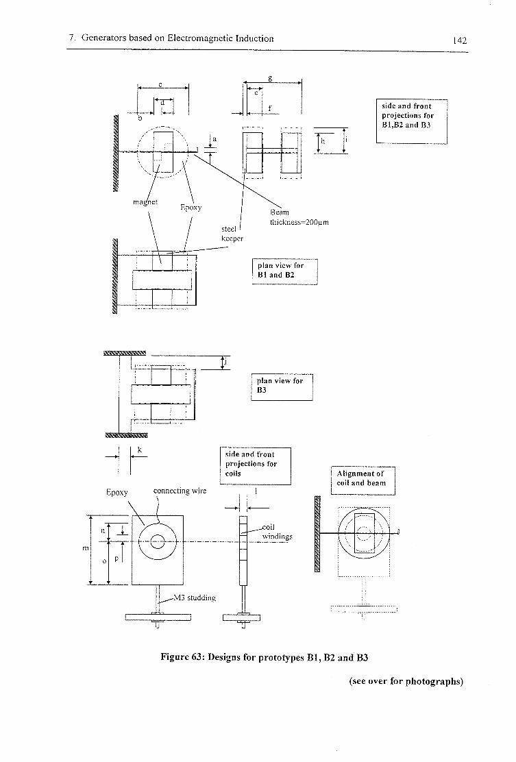
7. Generators based on Electromagnetic Induction 142
m a g n e t
Beam t h i c k n e s s = 2 0 0 | - i m
plan view for B1and B2
side and front projections for B1,B2 and B3
Epoxy connecting wire
n ; J L
0 p
plan view for B3
side and front projections for coils
- M 3 s t u d d i n g
jzoil w i n d i n g s
T "
Alignment of coil and beam
Figure 63: Designs for prototypes B l , B2 and B3
(see over for photographs)
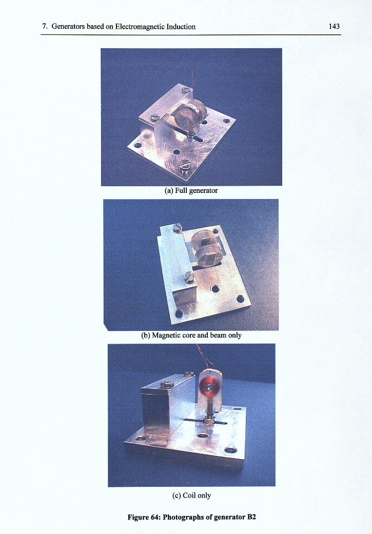
7. Generators based on Electromagnetic Induction 143
(a) Full generator
(b) Magnetic core and beam only
(c) Coil only
Figure 64: Photographs of generator B2
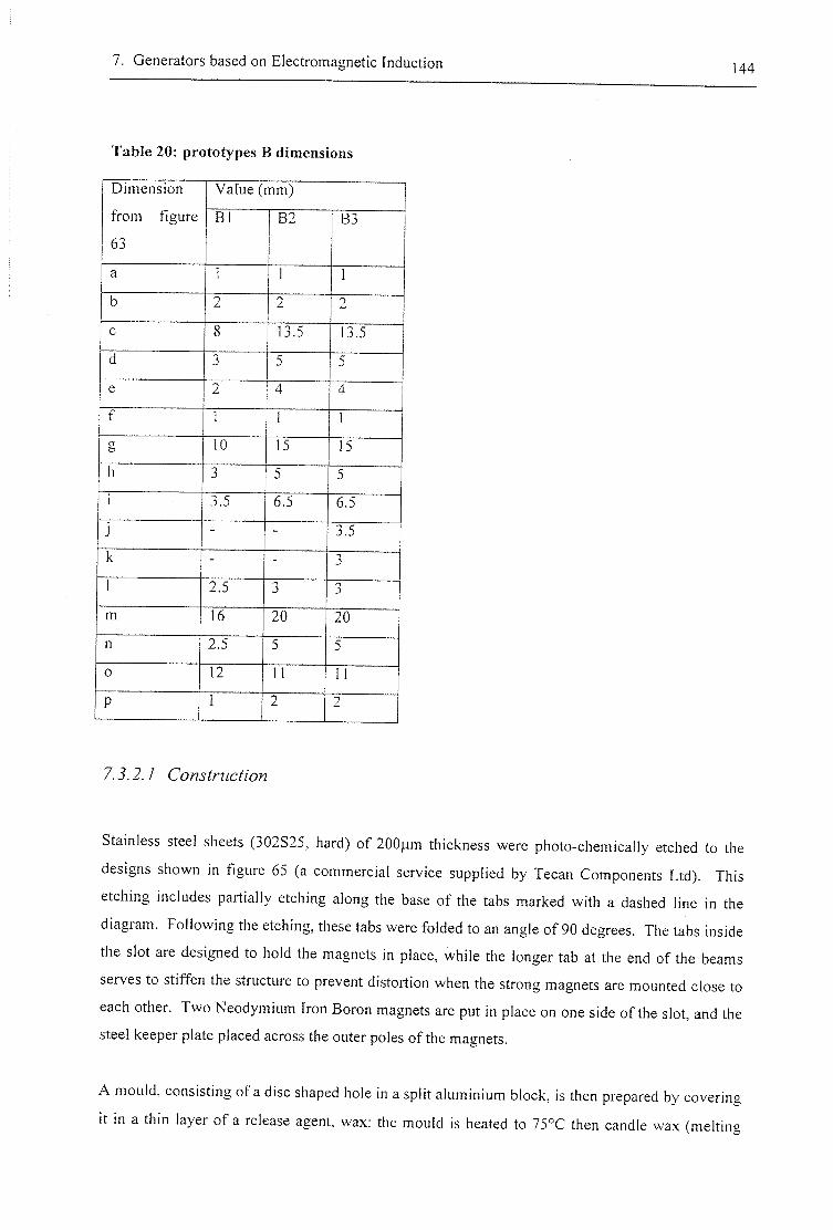
7. Generators based on Electromagnetic Induction 144
Table 20: prototypes B dimensions
Dimension
from figure
63
Value (mm) Dimension
from figure
63
8 1 B2 B3
a 1 1 I
b 2 2 2
c 8 13.5 13.5
d 3 5 5
e 2 4 4
f 1 1 1
g 10 15 15
ii 3 5 5
1 3.5 6.5 6.5
J - - 3.5
k - - 3
1 2.5 3 3
m 16 20 20
n 2.5 5 5
0 12 11 11
P 1 2 2
7.3.2.1 Construction
Stainless steel sheets ( j02S25 , hard) of 200(am thickness were photo-chemically etched to the
designs shown in figure 65 (a commercial service supplied by Tecan Components Ltd). This
etching includes partially etching along the base of the tabs marked with a dashed line in the
diagram. Following the etching, these tabs were folded to an angle of 90 degrees. The tabs inside
the slot are designed to hold the magnets in place, while the longer tab at the end of the beams
serves to stiffen the structure to prevent distortion when the strong magnets are mounted close to
each other. Two Neodymium Iron Boron magnets are put in place on one side of the slot, and the
steel keeper plate placed across the outer poles of the magnets.
A mould, consisting of a disc shaped hole in a split aluminium block, is then prepared by covering
it in a thin layer of a release agent, wax: the mould is heated to 75°C then candle wax (melting
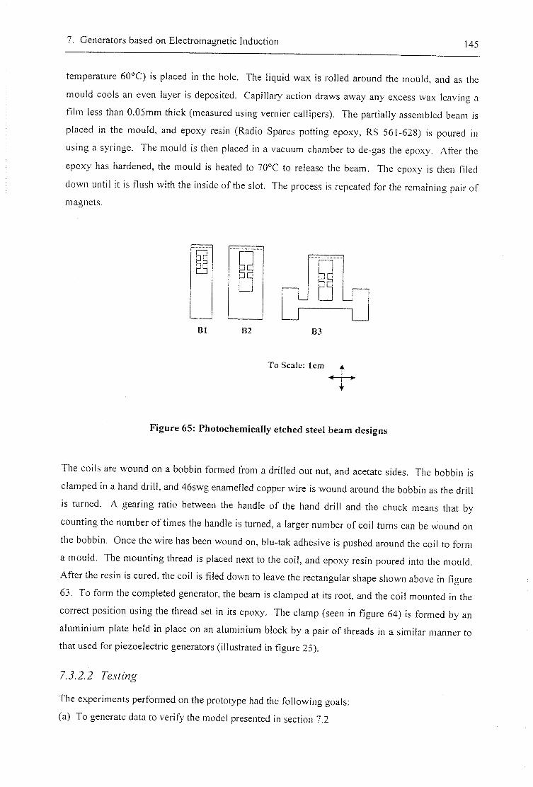
7. Generators based on Electromagnetic Induction 145
temperature 60°C) is placed in the hole. The liquid wax is rolled around the mould, and as the
mould cools an even layer is deposited. Capillary action draws away any excess wax leaving a
f i lm less than 0.05mm thick (measured using vernier callipers). The partially assembled beam is
placed in the mould, and epoxy resin (Radio Spares potting epoxy, RS 561-628) is poured in
using a syringe. The mould is then placed in a vacuum chamber to de-gas the epoxy. After the
epoxy has hardened, the mould is heated to 70°C to release the beam. The epoxy is then filed
dov/n until it is flush with the inside of the slot. The process is repeated for the remaining pair of
magnets.
B1 83
To Scale: 1cm
Figure 65: Photochemically etched steel beam designs
The coils are wound on a bobbin formed from a drilled out nut, and acetate sides. The bobbin is
clamped in a hand drill, and 46swg enamelled copper wire is wound around the bobbin as the drill
is turned. A gearing ratio between the handle of the hand drill and the chuck means that by
counting the number of times the handle is turned, a larger number of coil turns can be wound on
the bobbin. Once the wire has been wound on, blu-tak adhesive is pushed around the coil to form
a mould. The mounting thread is placed next to the coil, and epoxy resin poured into the mould.
After the resin is cured, the coil is filed down to leave the rectangular shape shown above in figure
63. To form the completed generator, the beam is clamped at its root, and the coil mounted in the
correct position using the thread set in its epoxy. The clamp (seen in figure 64) is formed by an
aluminium plate held in place on an aluminium block by a pair of threads in a similar manner to
that used for piezoelectric generators (illustrated in figure 25).
7.j.2.2
The experiments performed on the prototype had the following goals:
(a) To generate data to verify the model presented in section 7.2
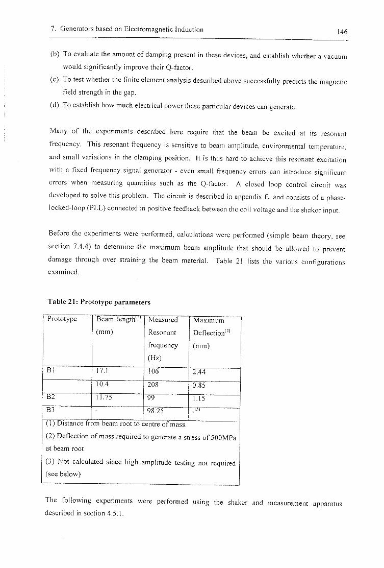
7. Generators based on Electromagnetic Induction 146
(b) To evaluate the amount of damping present in these devices, and establish whether a vacuum
would significantly improve their Q-factor.
(c) To test whether the finite element analysis described above successfully predicts the magnetic
field strength in the gap.
(d) To establish how much electrical power these particular devices can generate.
Many of the experiments described here require that the beam be excited at its resonant
frequency. This resonant frequency is sensitive to beam amplitude, environmental temperature,
and small variations in the clamping position. It is thus hard to achieve this resonant excitation
with a fixed frequency signal generator - even small frequency errors can introduce significant
errors when measuring quantities such as the Q-factor. A closed loop control circuit was
developed to solve this problem. The circuit is described in appendix E, and consists of a phase-
locked-loop (PLL) connected in positive feedback between the coil voltage and the shaker input.
Before the experiments were performed, calculations were performed (simple beam theory, see
section 7.4.4) to determine the maximum beam amplitude that should be allowed to prevent
damage through over straining the beam material. Table 21 lists the various configurations
examined.
Table 21: Prototype parameters
Prototype Beam length^'' Measured Maximum
(mm) Resonant Defiection'"^
frequency (mm)
(Hz)
B l 17.1 106 2.44
10.4 208 0.85
82 11.75 99 1.15
83 - 98.25
( I ) Distance from beam root to centre of mass.
(2) Deflection of mass required to generate a stress of 500MPa
at beam root
(3) Not calculated since high amplitude testing not required
(see below)
The following experiments were performed using the shaker and measurement apparatus
described in section 4.5.1.
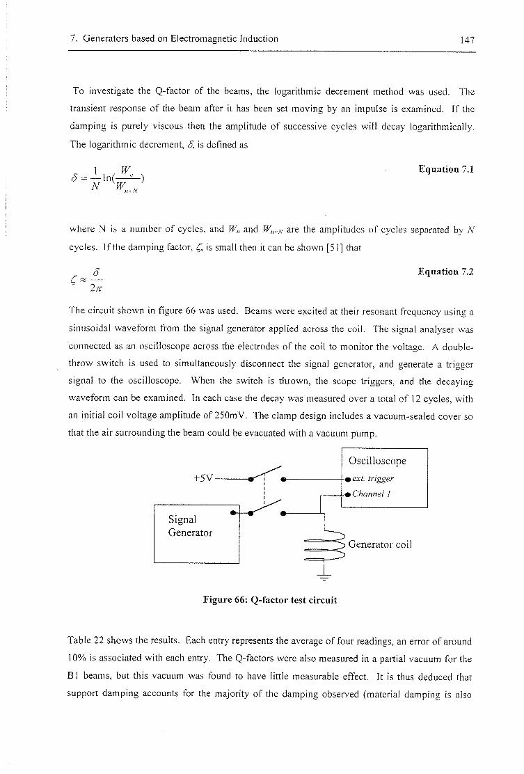
7. Generators based on Electromagnetic Induction 147
To investigate the Q-factor of the beams, the logarithmic decrement method was used. The
transient response of the beam after it has been set moving by an impulse is examined. If the
damping is purely viscous then the amplitude of successive cycles will decay logarithmically.
The logarithmic decrement, S, is defined as
J Equation 7.1
n+N
where N is a number of cycles, and W„ and W„+f^ are the amplitudes of cycles separated by N
cycles. If the damping factor, is small then it can be shown [51] that
2;T
Equation 7.2
The circuit shown in figure 66 was used. Beams were excited at their resonant frequency using a
sinusoidal waveform from the signal generator applied across the coil. The signal analyser was
connected as an oscilloscope across the electrodes of the coil to monitor the voltage. A double-
throw switch is used to simultaneously disconnect the signal generator, and generate a trigger
signal to the oscilloscope. When the switch is thrown, the scope triggers, and the decaying
waveform can be examined. In each case the decay was measured over a total of 12 cycles, with
an initial coil voltage amplitude of 250mV. The clamp design includes a vacuum-sealed cover so
that the air surrounding the beam could be evacuated with a vacuum pump.
+5V
Generator coil
Signal Generator
Oscilloscope
•9 ext. trigger
•9 Channel I
Figure 66: Q-factor test circuit
Table 22 shows the results. Each entry represents the average of four readings, an error of around
10% is associated with each entry. The Q-factors were also measured in a partial vacuum for the
B1 beams, but this vacuum was found to have little measurable effect. It is thus deduced that
support damping accounts for the majority of the damping observed (material damping is also
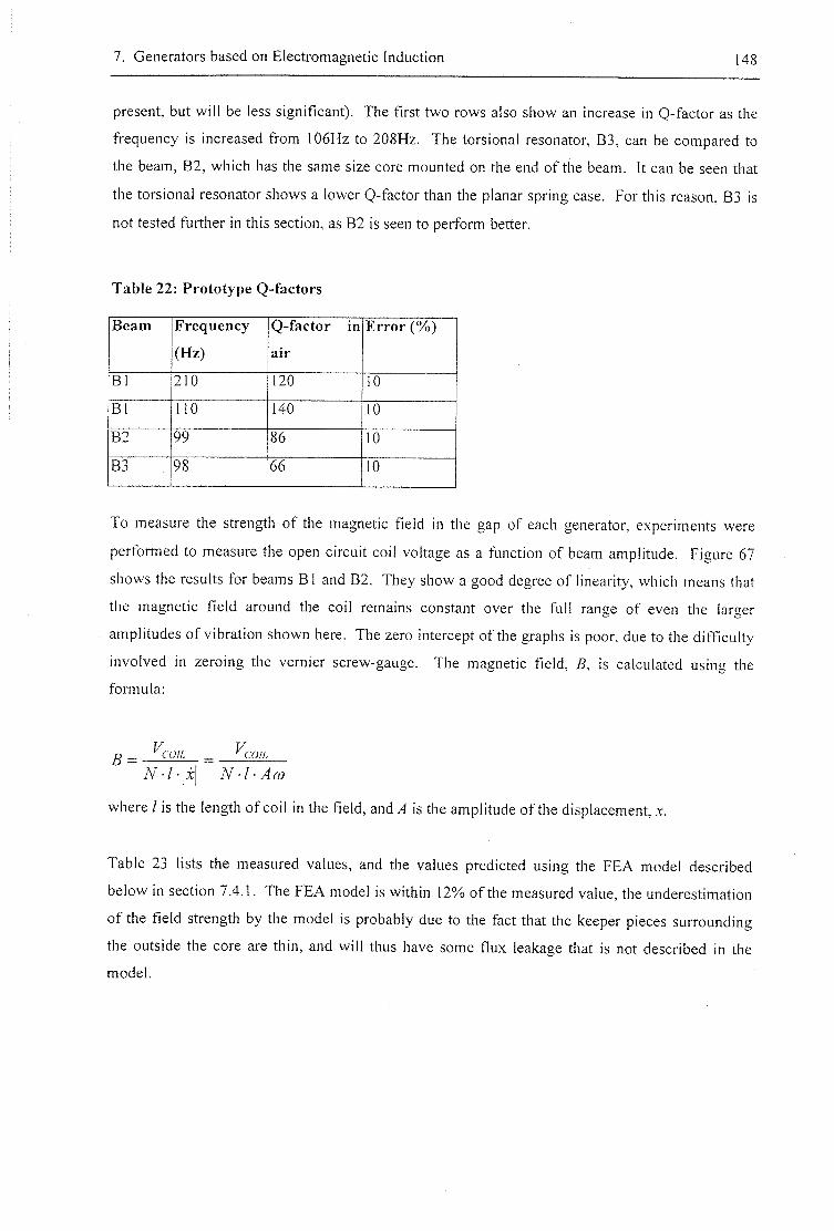
7. Generators based on Electromagnetic Induction 148
present, but will be less significant). The first two rows also show an increase in Q-factor as the
frequency is increased from 106Hz to 208Hz. The torsional resonator, B3, can be compared to
the beam, B2, which has the same size core mounted on the end of the beam. It can be seen that
the torsional resonator shows a lower Q-factor than the planar spring case. For this reason, B3 is
not tested further in this section, as 8 2 is seen to perform better.
Table 22: Prototype Q-factors
Beam Frequency Q-factor in Er ror (%)
(Hz) air
8 1 210 120 1 0
8 1 1 1 0 140 10
B2 99 86 1 0
B3 98 66 1 0
To measure the strength of the magnetic field in the gap of each generator, experiments were
performed to measure the open circuit coil voltage as a function of beam amplitude. Figure 67
shows the results for beams B l and B2. They show a good degree of linearity, which means that
the magnetic field around the coil remains constant over the full range of even the larger
amplitudes of vibration shown here. The zero intercept of the graphs is poor, due to the difficulty
involved in zeroing the vernier screw-gauge. The magnetic field, 8, is calculated using the
formula:
B • / • |x| N -l • Aco
where / is the length of coil in the field, and/Sl is the amplitude of the displacement, x.
Table 23 lists the measured values, and the values predicted using the FEA model described
below in section 7.4.1. The FEA model is within 12% of the measured value, the underestimation
of the field strength by the model is probably due to the fact that the keeper pieces surrounding
the outside the core are thin, and wi l l thus have some flux leakage that is not described in the
model.
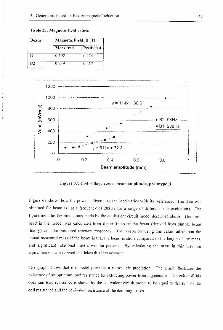
7. Generators based on Electromagnetic Induction 149
Table 23: Magnetic field values
Beam Magnetic Field, B (T) Beam
Measured Predicted
B1 0.192 0.214
B2 0.239 0.267
1200
1000
l/T E
800
> £ 600
o
> 400
200
y = 114X + 36.6 . •
* 82, 98Hz
m B1, 208Hz •
•
* 82, 98Hz
m B1, 208Hz
•
* y = 611x4-32.3
0 0.2 0.4 0.6
Beam amp l i t ude (mm)
0.8 1
Figure 67: Coil voltage versus beam amplitude, prototype B
Figure 68 shows how the power delivered to the load varies with its resistance. The data was
obtained for beam B1 at a frequency of 208Hz for a range of different base excitations. The
figure includes the predictions made by the equivalent circuit model described above. The mass
used in the model was calculated from the stiffness of the beam (derived from simple beam
theory), and the measured resonant frequency. The reason for using this value rather than the
actual measured mass of the beam is that the beam is short compared to the length of the mass,
and significant rotational inertia will be present. By calculating the mass in this way, an
equivalent mass is derived that takes this into account.
The graph shows that the model provides a reasonable prediction. The graph illustrates the
existence of an optimum load resistance for extracting power from a generator. The value of this
optimum load resistance is shown by the equivalent circuit model to be equal to the sum of the
coil resistance and the equivalent resistance of the damping losses.
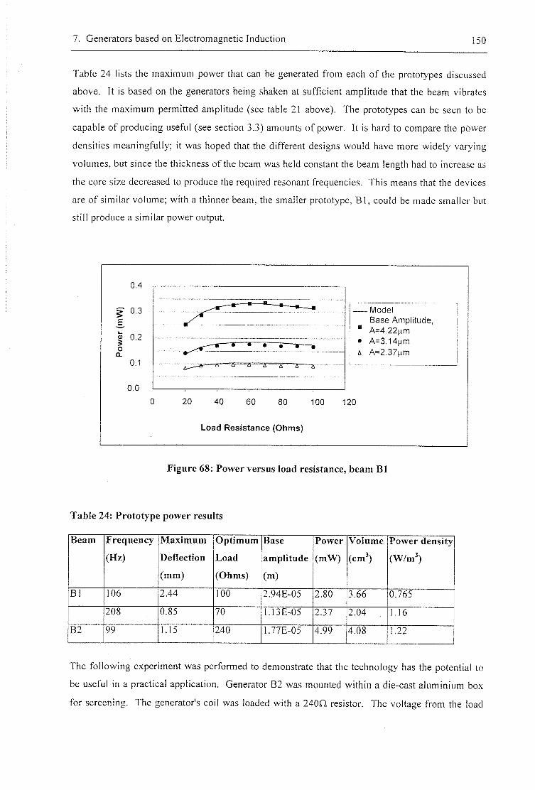
7. Generators based on Electromagnetic Induction 150
Table 24 lists the maximum power that can be generated from each of the prototypes discussed
above. It is based on the generators being shaken at sufficient amplitude that the beam vibrates
with the maximum permitted amplitude (see table 21 above). The prototypes can be seen to be
capable of producing useful (see section 3.3) amounts of power. It is hard to compare the power
densities meaningfully; it was hoped that the different designs would have more widely varying
volumes, but since the thickness of the beam was held constant the beam length had to increase as
the core size decreased to produce the required resonant frequencies. This means that the devices
are of similar volume; with a thinner beam, the smaller prototype, B l , could be made smaller but
still produce a similar power output.
m 0.2
Model Base Amplitude,
' A=4.22^m • A=3.14(im a A=2.37um
20 40 60 80 100 120
Load Resistance (Ohms)
Figure 68: Power versus load resistance, beam B l
Table 24: Prototype power results
Beam Frequency
(Hz)
Maximum
Deflection
(mm)
Opt imum
Load
(Ohms)
Base
amplitude
(m)
Power
(mW)
Volume
(cm^)
Power density
(W/m^)
Bl 106 2.44 100 2.94E-05 2.80 3.66 0.765
208 0.85 70 1.1313-05 Z37 2.04 1.16
B2 99 1.15 240 L77E-05 4.99 4.08 L22
The following experiment was performed to demonstrate that the technology has the potential to
be useful in a practical application. Generator B2 was mounted within a die-cast aluminium box
for screening. The generator's coil was loaded with a 240Q resistor. The voltage from the load
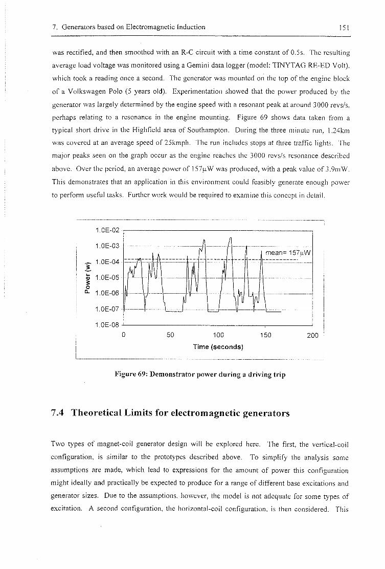
7. Generators based on Electromagnetic Induction 151
was rectified, and then smoothed with an R-C circuit with a time constant of 0.5s. The resulting
average load voltage was monitored using a Gemini data logger (model: TINYTAG RE-ED Volt),
which took a reading once a second. The generator was mounted on the top of the engine block
of a Volkswagen Polo (5 years old). Experimentation showed that the power produced by the
generator was largely determined by the engine speed with a resonant peak at around 3000 revs/s,
perhaps relating to a resonance in the engine mounting. Figure 69 shows data taken from a
typical short drive in the Highfield area of Southampton. During the three minute run, 1.24km
was covered at an average speed of 25kmph. The run includes stops at three traffic lights. The
major peaks seen on the graph occur as the engine reaches the 3000 revs/s resonance described
above. Over the period, an average power of 157p.W was produced, with a peak value of 3.9mW.
This demonstrates that an application in this environment could feasibly generate enough power
to perform useful tasks. Further work would be required to examine this concept in detail.
1.0E-02
1.0E-03 mean= 157fiW
1.0E-04
I 1.0E-05
1.0E-06
1.0E-07
1.0E-08
50 100
Time (seconds)
150 200
Figure 69: Demonstrator power dur ing a dr iv ing t r ip
7,4 Theoretical Limits for electromagnetic generators
Two types of magnet-coil generator design will be explored here. The first, the vertical-coil
configuration, is similar to the prototypes described above. To simplify the analysis some
assumptions are made, which lead to expressions for the amount of power this configuration
might ideally and practically be expected to produce for a range of different base excitations and
generator sizes. Due to the assumptions, however, the model is not adequate for some types of
excitation. A second configuration, the horizontal-coil configuration, is then considered. This
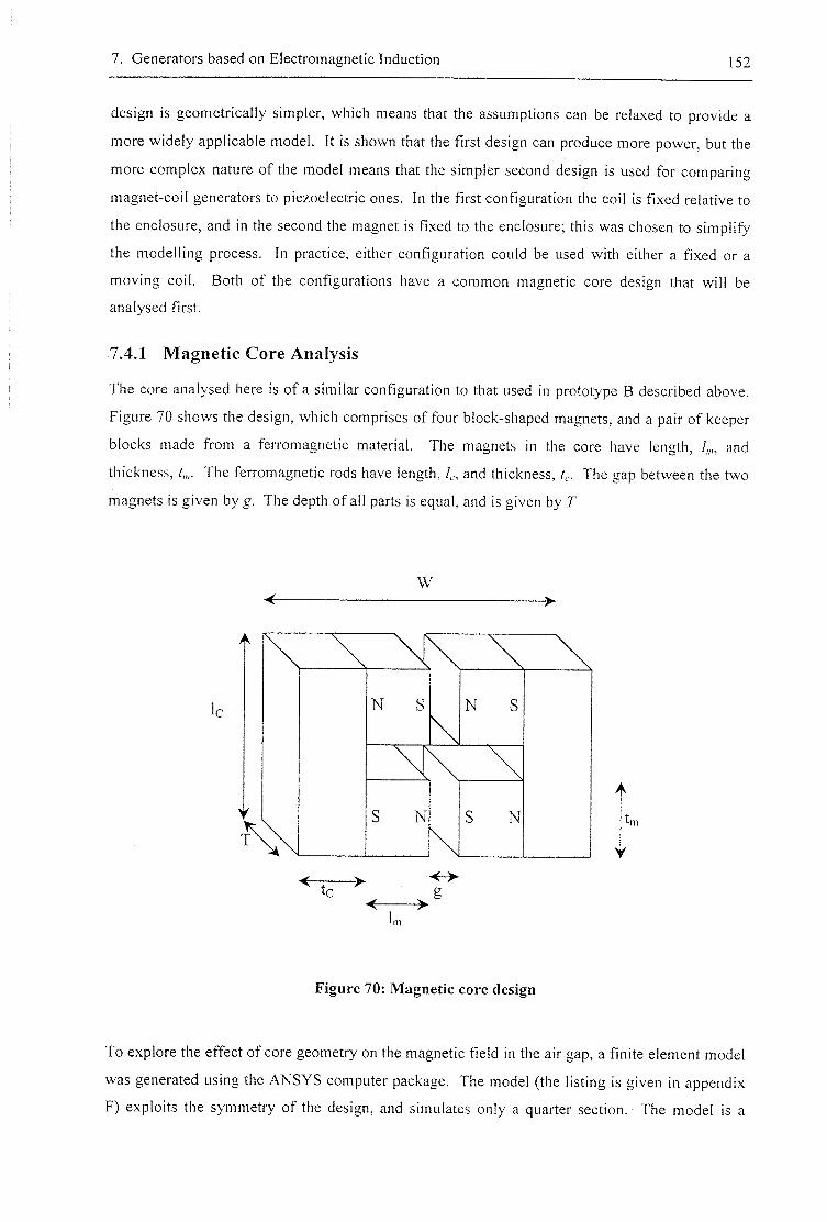
7. Generators based on Electromagnetic Induction 152
design is geometrically simpler, which means that the assumptions can be relaxed to provide a
more widely applicable model. It is shown that the first design can produce more power, but the
more complex nature of the model means that the simpler second design is used for comparing
magnet-coil generators to piezoelectric ones. In the first configuration the coil is fixed relative to
the enclosure, and in the second the magnet is fixed to the enclosure; this was chosen to simplify
the modelling process. In practice, either configuration could be used with either a fixed or a
moving coil. Both of the configurations have a common magnetic core design that will be
analysed first.
7.4.1 Magnetic Core Analysis
The core analysed here is of a similar configuration to that used in prototype B described above.
Figure 70 shows the design, which comprises of four block-shaped magnets, and a pair of keeper
blocks made from a ferromagnetic material. The magnets in the core have length, and
thickness, L - The ferromagnetic rods have length, and thickness, r,.. The gap between the two
magnets is given by g. The depth of all parts is equal, and is given by T
W
Ic
T
N S
\ N S
\ \ S N
\ S N
< > L
Figure 70: Magnetic core design
To explore the effect of core geometry on the magnetic field in the air gap, a finite element model
was generated using the ANSYS computer package. The model (the listing is given in appendix
F) exploits the symmetry of the design, and simulates only a quarter section. The model is a
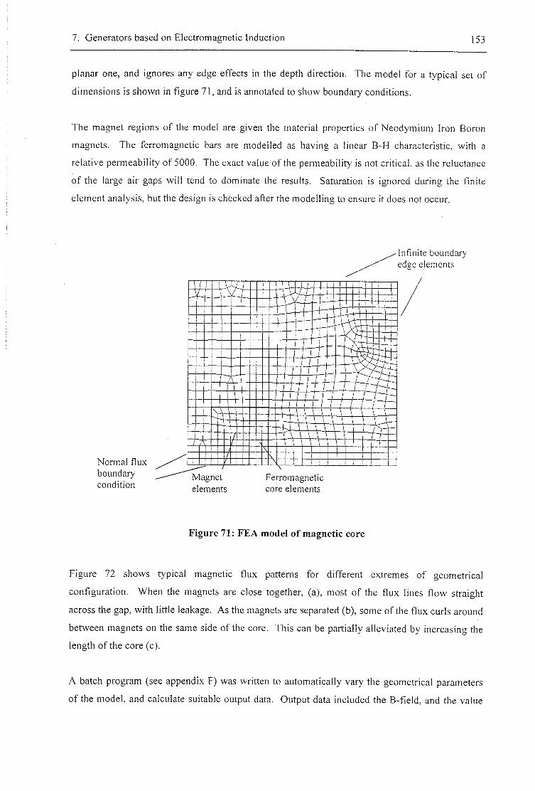
7. Generators based on Electromagnetic Induction 153
planar one, and ignores any edge effects in the depth direction. The model for a typical set of
dimensions is shown in figure 71, and is annotated to show boundary conditions.
The magnet regions of the model are given the material properties of Neodymium Iron Boron
magnets. The ferromagnetic bars are modelled as having a linear B-H characteristic, with a
relative permeability of 5000. The exact value of the permeability is not critical, as the reluctance
of the large air gaps will tend to dominate the results. Saturation is ignored during the finite
element analysis, but the design is checked after the modelling to ensure it does not occur.
Normal flux boundary condition
M a g n e t
Inf in i te b o u n d a r y
e d g e e l e m e n t s
elements Ferromagnetic core elements
Figure 71: FEA model of magnetic core
Figure 72 shows typical magnetic flux patterns for different extremes of geometrical
configuration. When the magnets are close together, (a), most of the flux lines flow straight
across the gap, with little leakage. As the magnets are separated (b), some of the flux curls around
between magnets on the same side of the core. This can be partially alleviated by increasing the
length of the core (c).
A batch program (see appendix F) was written to automatically vary the geometrical parameters
of the model, and calculate suitable output data. Output data included the B-field, and the value
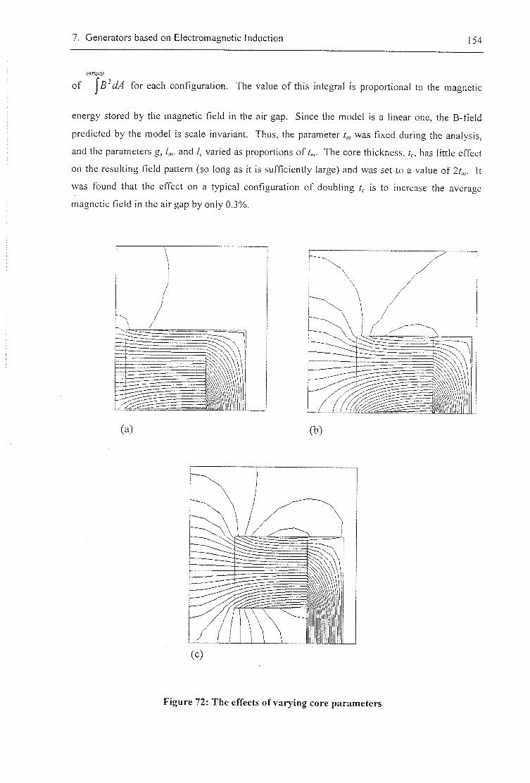
7. Generators based on Electromagnetic Induction 154
of ^B^dA for each configuration. The value of this integral is proportional to the magnetic
energy stored by the magnetic field in the air gap. Since the model is a linear one, the B-field
predicted by the model is scale invariant. Thus, the parameter t,„ was fixed during the analysis,
and the parameters g, and 4 varied as proportions of/,,,. The core thickness, rc, has little effect
on the resulting field pattern (so long as it is sufficiently large) and was set to a value of 2/,,,. ft
was found that the effect on a typical configuration of doubling is to increase the average
magnetic field in the air gap by only 0.3%.
—
—
mm (a) (b)
Figure 72: The effects of varying core parameters
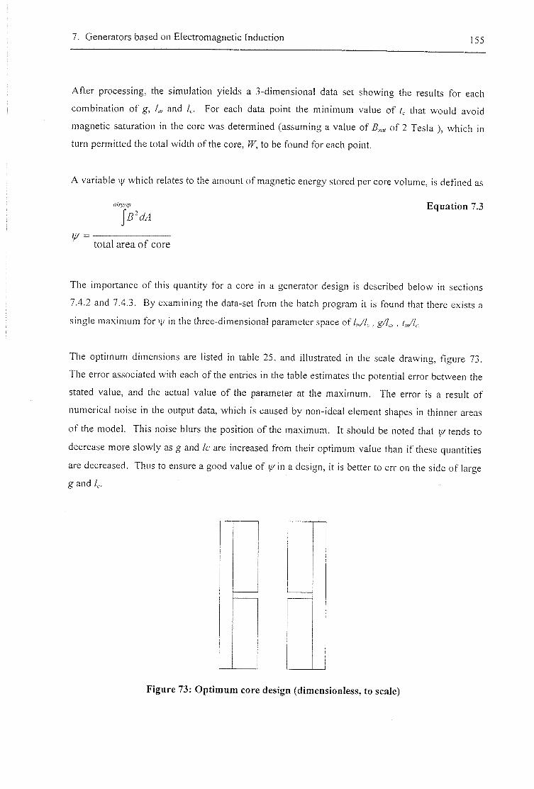
7. Generators based on Electromagnetic Induction 155
After processing, the simulation yields a 3-dimensional data set showing the results for each
combination of g, /„, and 4. For each data point the minimum value of 4. that would avoid
magnetic saturation in the core was determined (assuming a value of of 2 Tesia ), which in
turn permitted the total width of the core, W, to be found for each point.
A variable v|; which relates to the amount of magnetic energy stored per core volume, is defined as
Equation 7.3
¥ total area o f core
The importance of this quantity for a core in a generator design is described below in sections
7.4.2 and 7.4.3. By examining the data-set from the batch program it is found that there exists a
single maximum for in the three-dimensional parameter space o f g / 7 , , . ^,,/4
The optimum dimensions are listed in table 25, and illustrated in the scale drawing, figure 73.
The error associated with each of the entries in the table estimates the potential error between the
stated value, and the actual value of the parameter at the maximum. The error is a result of
numerical noise in the output data, which is caused by non-ideal element shapes in thinner areas
of the model. This noise blurs the position of the maximum. It should be noted that ^ tends to
decrease more slowly as g and /c are increased from their optimum value than i f these quantities
are decreased. Thus to ensure a good value of (y in a design, it is better to err on the side of large
g and 4.
Figure 73: Opt imum core design (dimensionless, to scale)
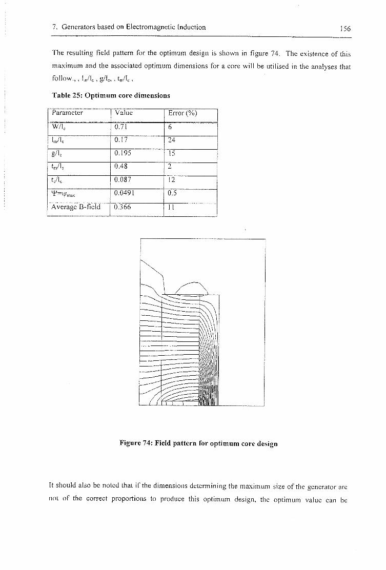
7. Generators based on Electromagnetic Induction 156
The resulting field pattern for the optimum design is shown in figure 74. The existence of this
maximum and the associated optimum dimensions for a core will be utilised in the analyses that
follow., , l,n/lc , g/lc, , V i c ,
Table 25: Opt imum core dimensions
Parameter Value Error (%)
W/l, O J I 6
Im/lc 0.17 24
g/lc 0U95 15
tm/lc 0.48 2
tc/lc 0.087 12
0IW91 0.5
Average B-field 0 J 6 6 11
Figure 74: Field pattern for opt imum core design
It should also be noted that if the dimensions determining the maximum size of the generator are
not of the correct proportions to produce this optimum design, the optimum value can be
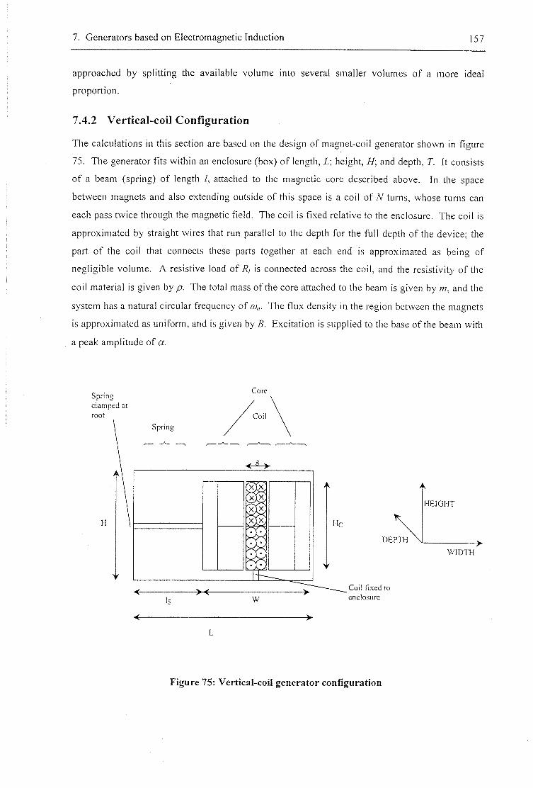
7. Generators based on Electromagnetic Induction 157
approached by splitting the available volume into several smaller volumes of a more ideal
proportion.
7.4.2 Vertical-coil Configuration
The calculations in this section are based on the design of magnet-coil generator shown in figure
75. The generator fits within an enclosure (box) of length, Z; height, / / ; and depth, T. It consists
of a beam (spring) of length /, attached to the magnetic core described above. In the space
between magnets and also extending outside of this space is a coil of # turns, whose turns can
each pass twice through the magnetic field. The coil is fixed relative to the enclosure. The coil is
approximated by straight wires that run parallel to the depth for the full depth of the device; the
part of the coil that connects these parts together at each end is approximated as being of
negligible volume. A resistive load of Rt is connected across the coil, and the resistivity of the
coil material is given by p. The total mass of the core attached to the beam is given by w, and the
system has a natural circular frequency of 03,,. The flux density in the region between the magnets
is approximated as uniform, and is given by B. Excitation is supplied to the base of the beam with
a peak amplitude of a .
Spring c l a m p e d at
r o o t
S p r i n g
< ^ >
He
DEPTH
Coil f i x e d to
e n c l o s u r e
HEIGHT
VWDTH
Figure 75: Vertical-coil generator configuration
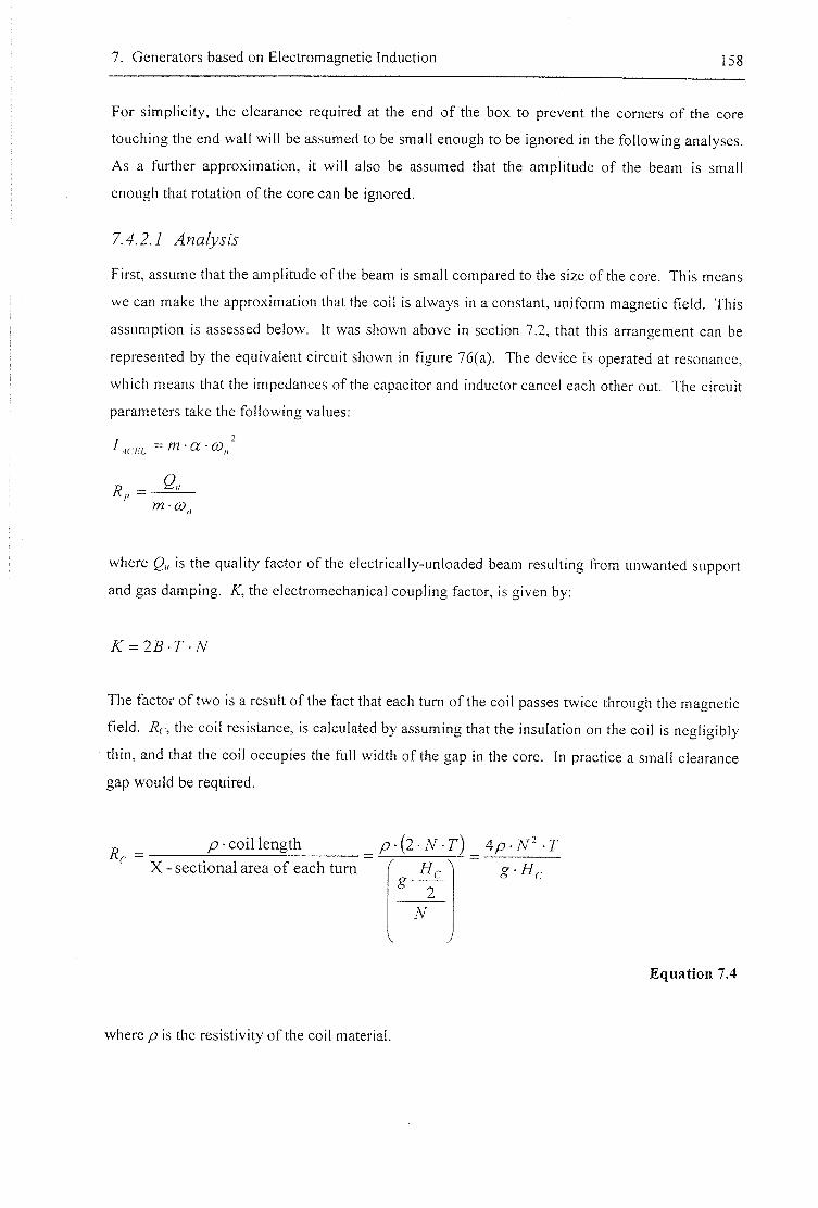
7. Generators based on Electromagnetic Induction 158
For simplicity, the clearance required at the end of the box to prevent the comers of the core
touching the end wall will be assumed to be small enough to be ignored in the following analyses.
As a further approximation, it will also be assumed that the amplitude of the beam is small
enough that rotation of the core can be ignored.
7 . ^ .2 .7
First, assume that the amplitude of the beam is small compared to the size of the core. This means
we can make the approximation that the coil is always in a constant, uniform magnetic field. This
assumption is assessed below. It was shown above in section 7.2, that this arrangement can be
represented by the equivalent circuit shown in figure 76(a). The device is operated at resonance,
which means that the impedances of the capacitor and inductor cancel each other out. The circuit
parameters take the following values:
R,, Q.,
where is the quality factor of the electrically-unloaded beam resulting from unwanted support
and gas damping. K, the electromechanical coupling factor, is given by:
^ = 2 ^ . r . TV
The factor of two is a result of the fact that each turn of the coil passes twice through the magnetic
field. Rc, the coil resistance, is calculated by assuming that the insulation on the coil is negligibly
thin, and that the coil occupies the full width of the gap in the core. In practice a small clearance
gap would be required.
R, p • coil length
X - sectional area of each turn
/ ) ( 2 . 7 v . r )
g -He
N
Equation 7.4
where p is the resistivity of the coil material.
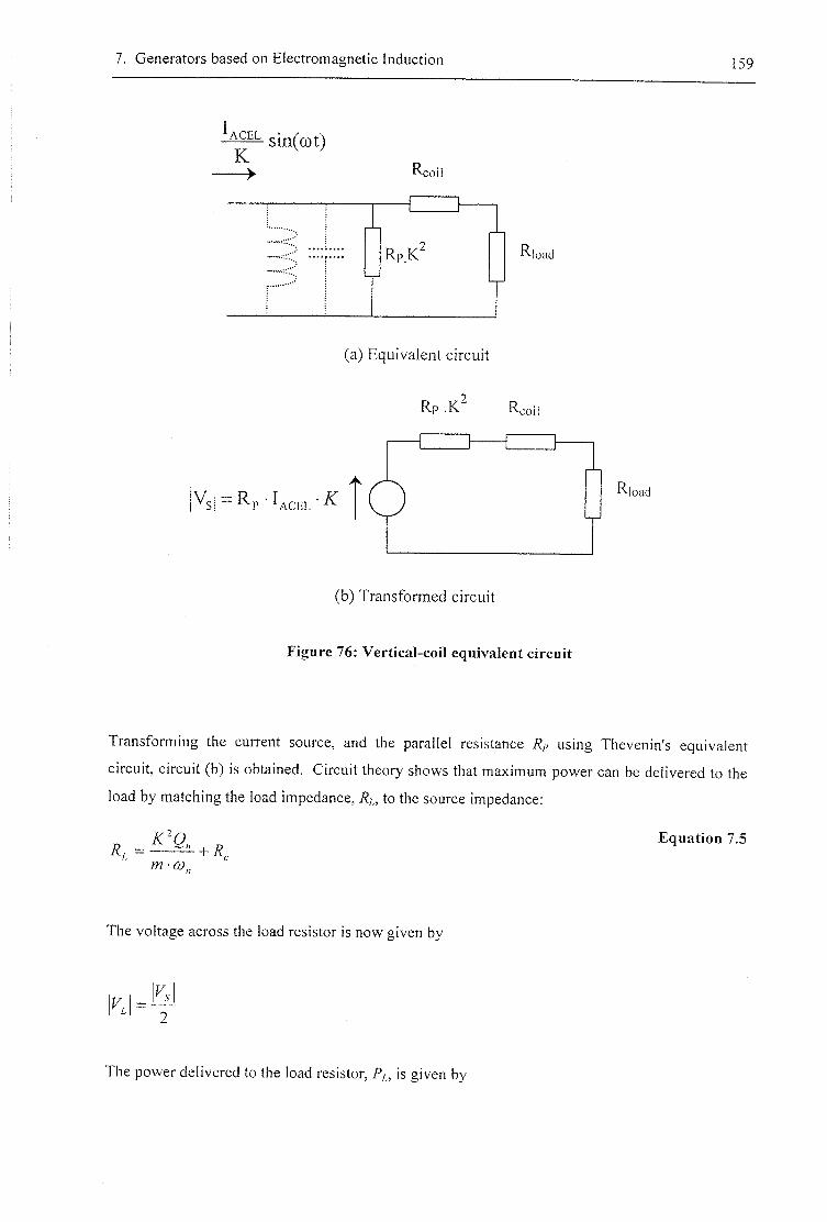
7. Generators based on Electromagnetic Induction 159
" - A C E L
K sin(mt)
R-coil
I Rp.K' R-load
(a) Equivalent circuit
Rp Rc COli
V s = R p - l A C E L - ^ R|oad
(b) Transformed circuit
Figure 76: Vertical-coil equivalent circuit
Transforming the current source, and the parallel resistance using Thevenin's equivalent
circuit, circuit (b) is obtained. Circuit theory shows that maximum power can be delivered to the
load by matching the load impedance, to the source impedance:
R.
The voltage across the load resistor is now given by
Equation 7.5
V, K.
The power delivered to the load resistor, P/,, is given by
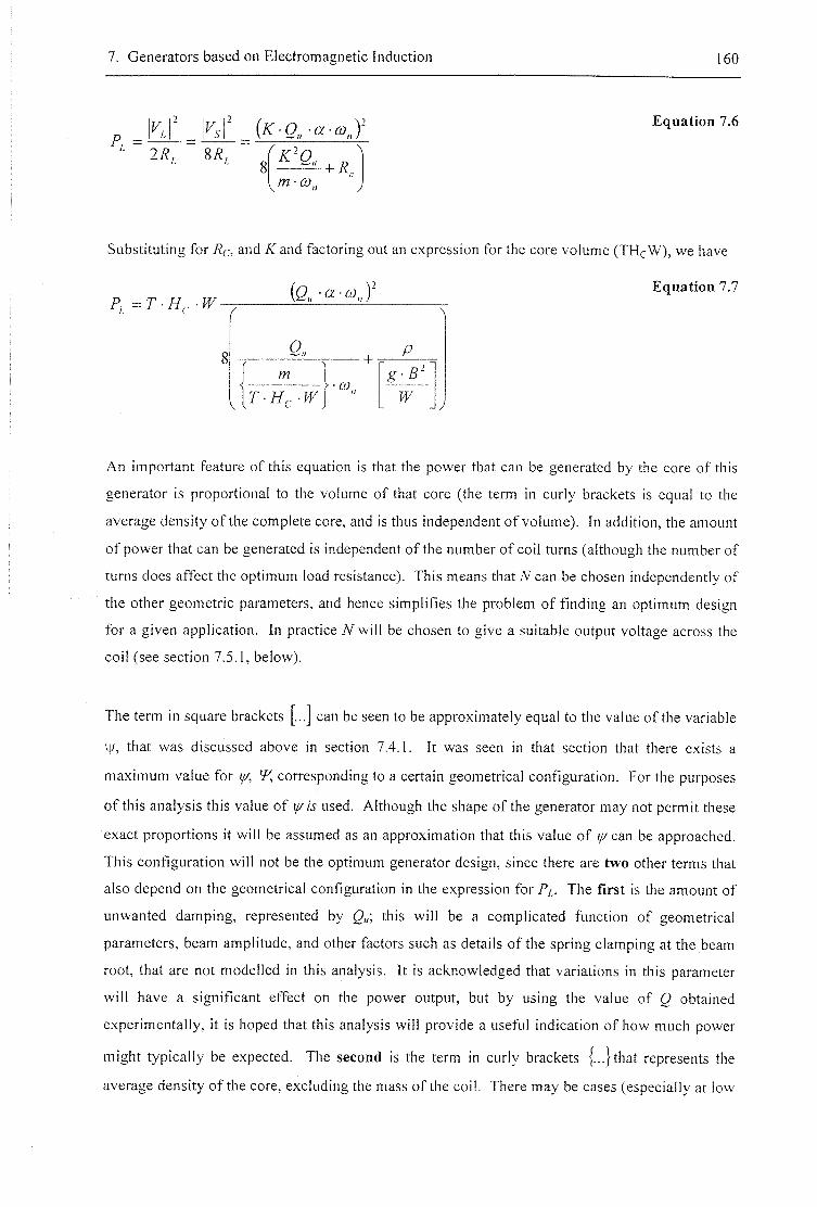
7. Generators based on Electromagnetic Induction 160
P, K Equation 7.6
8 ^ , - + &
Substituting for jRc, and K and factoring out an expression for the core volume (THgW), we have
Equation 7.7
o , ,
/M • +
p
CO., g a '
W
An important feature of this equation is that the power that can be generated by the core of this
generator is proportional to the volume of that core (the term in curly brackets is equal to the
average density of the complete core, and is thus independent of volume). In addition, the amount
of power that can be generated is independent of the number of coil turns (although the number of
turns does affect the optimum load resistance). This means that # can be chosen independently of
the other geometric parameters, and hence simplifies the problem of finding an optimum design
for a given application. In practice # wi l l be chosen to give a suitable output voltage across the
coil (see section 7.5.1, below).
The term in square brackets [...] can be seen to be approximately equal to the value of the variable
\\j, that was discussed above in section 7.4.1. It was seen in that section that there exists a
maximum value for t//, % corresponding to a certain geometrical configuration. For the purposes
of this analysis this value of \f/is used. Although the shape of the generator may not permit these
exact proportions it will be assumed as an approximation that this value of ^ c a n be approached.
This configuration will not be the optimum generator design, since there are two other terms that
also depend on the geometrical configuration in the expression for Pi . The first is the amount of
unwanted damping, represented by g„; this will be a complicated function of geometrical
parameters, beam amplitude, and other factors such as details of the spring clamping at the beam
root, that are not modelled in this analysis. It is acknowledged that variations in this parameter
will have a significant effect on the power output, but by using the value of Q obtained
experimentally, it is hoped that this analysis will provide a useful indication of how much power
might typically be expected. The second is the term in curly brackets {...}that represents the
average density of the core, excluding the mass of the coil. There may be cases (especially at low
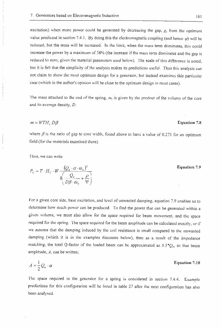
7. Generators based on Electromagnetic Induction 161
excitation) when more power could be generated by decreasing the gap, g, from the optimum
value predicted in section 7.4.1. By doing this the electromagnetic coupling (and hence y/) will be
reduced, but the mass will be increased. In the limit, when the mass term dominates, this could
increase the power by a maximum of 38% (the increase if the mass term dominates and the gap is
reduced to zero, given the material parameters used below). The scale of this difference is noted,
but it is felt that the simplicity of the analysis makes its predictions useful. Thus this analysis can
not claim to show the most optimum design for a generator, but instead examines this particular
case (which in the author's opinion will be close to the optimum design in most cases).
The mass attached to the end of the spring, m, is given by the product of the volume of the core
and its average density, D.
m = WTH^.Dp Equation 7.8
where is the ratio of gap to core width, found above to have a value of 0.275 for an optimum
field (for the materials examined there).
Thus, we can write
Equation 7.9
8| + - ^
For a given core size, base excitation, and level of unwanted damping, equation 7.9 enables us to
determine how much power can be produced. To find the power that can be generated within a
given volume, we must also allow for the space required for beam movement, and the space
required for the spring. The space required for the beam amplitude can be calculated exactly, or if
we assume that the damping induced by the coil resistance is small compared to the unwanted
damping (which it is in the examples discusses below), then as a result of the impedance
matching, the total Q-factor of the loaded beam can be approximated as so that beam
amplitude, A, can be written;
, 1 „ Equation 7.10
The space required in the generator for a spring is considered in section 7.4.4. Example
predictions for this configuration wil l be listed in table 27 after the next configuration has also
been analysed.
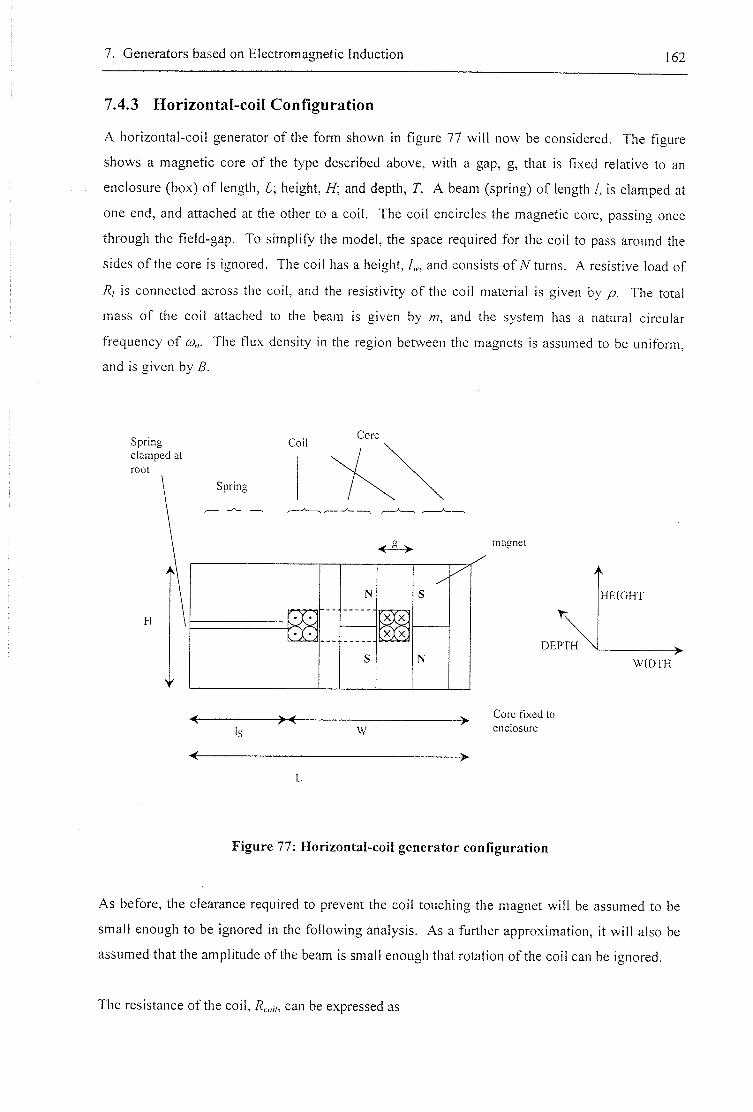
7. Generators based on Electromagnetic Induction 162
7.4.3 Horizontal-coil Configuration
A horizontal-coil generator of the form shown in figure 77 will now be considered. The figure
shows a magnetic core of the type described above, with a gap, g, that is fixed relative to an
enclosure (box) of length, L\ height, H\ and depth, T. A beam (spring) of length /, is clamped at
one end, and attached at the other to a coil. The coil encircles the magnetic core, passing once
through the field-gap. To simplify the model, the space required for the coil to pass around the
sides of the core is ignored. The coil has a height, L , and consists of / / turns. A resistive load of
is connected across the coil, and the resistivity of the coil material is given by /?. The total
mass of the coil attached to the beam is given by m, and the system has a natural circular
frequency of (Um- The flux density in the region between the magnets is assumed to be uniform,
and is given by B.
Spring c l a m p e d at
r oo t
Spring
C o r e
H
-X-
<" >
w
m a g n e t
s
fx)
k'X'J tx) xj
s N DEPTH
C o r e fixed to
e n c l o s u r e
HEIGHT
WIDTH
Figure 77: Horizontal-coil generator configuration
As before, the clearance required to prevent the coil touching the magnet will be assumed to be
small enough to be ignored in the following analysis. As a further approximation, it will also be
assumed that the amplitude of the beam is small enough that rotation of the coil can be ignored.
The resistance of the coil, /?„„/, can be expressed as
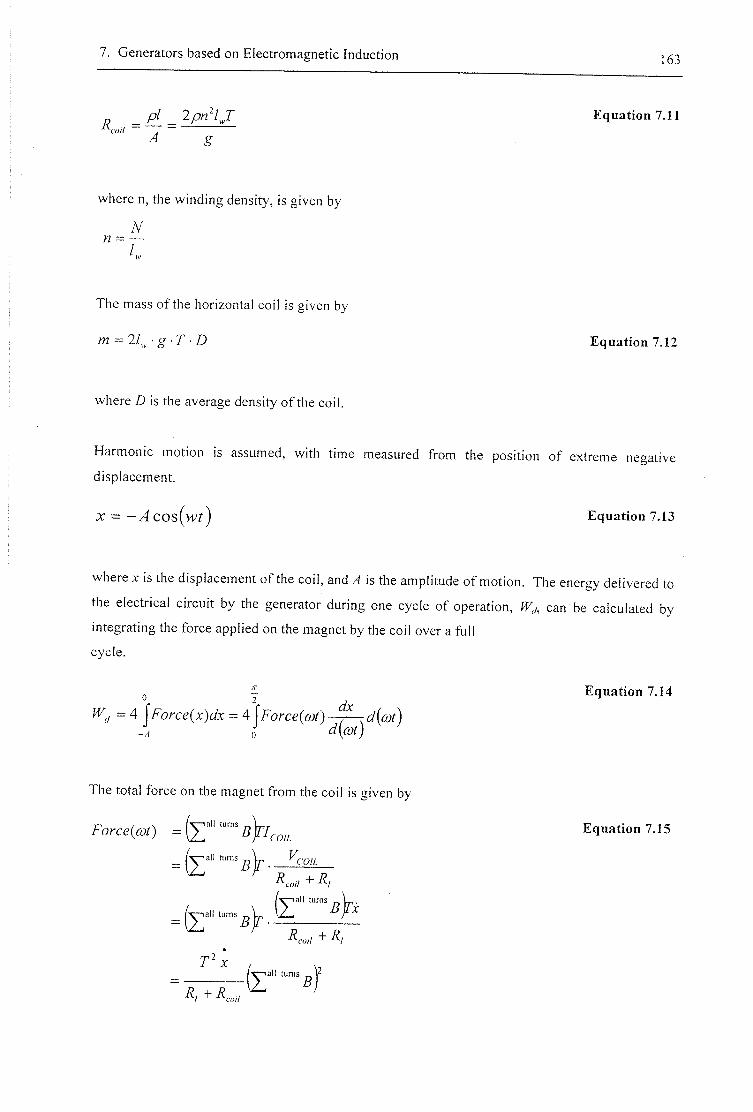
7. Generators based on Electromagnetic Induction 163
A g
Equation 7.11
where n, the winding density, is given by
N n
The mass of the horizontal coil is given by
Equation 7.12
where D is the average density of the coil.
Harmonic motion is assumed, with time measured from the position of extreme negative
displacement.
z = - y 4 c o s ( w ) Equation 7.13
where is the displacement of the coil, and ,4 is the amplitude of motion. The energy delivered to
the electrical circuit by the generator during one cycle of operation, can be calculated by
integrating the force applied on the magnet by the coil over a full
cycle.
-A 0 d\(X)tj
Equation 7.14
The total force on the magnet from the coil is given by
Force(a,) =fe-""s)rW
^coH +
-"Bh
l^a i l turns
Equation 7.15

7. Generators based on Electromagnetic Induction
Thus,
164
0 \ ^ l + ^coi! )
Equation 7.16
The summation ( ^ B) depends of the displacement of the coil.
direction of magnetic field
(a)
>
M R
/ , - / /
2 2
(b)
z = 0
(c)
Figure 78: Coil positions relative to core
If the coil lies entirely in one half of the core, as depicted in any of the positions lying between the
states shows in figure 78(a) and (b), then we have
= - W < % < /„ Equation 7.17
I f the coil crosses between the two halves of the core (positions lying between states shown in
figure 78(b) and (c), then we have
X" ""fi= \Bndh- \Bndh
Equation 7.18
< X < 0
The two integrals evaluate the field in the portions of the coil in the two halves of the magnetic
core. The sign change between the integrals reflects the field changing direction between the two
halves. Evaluating the integrals we have,
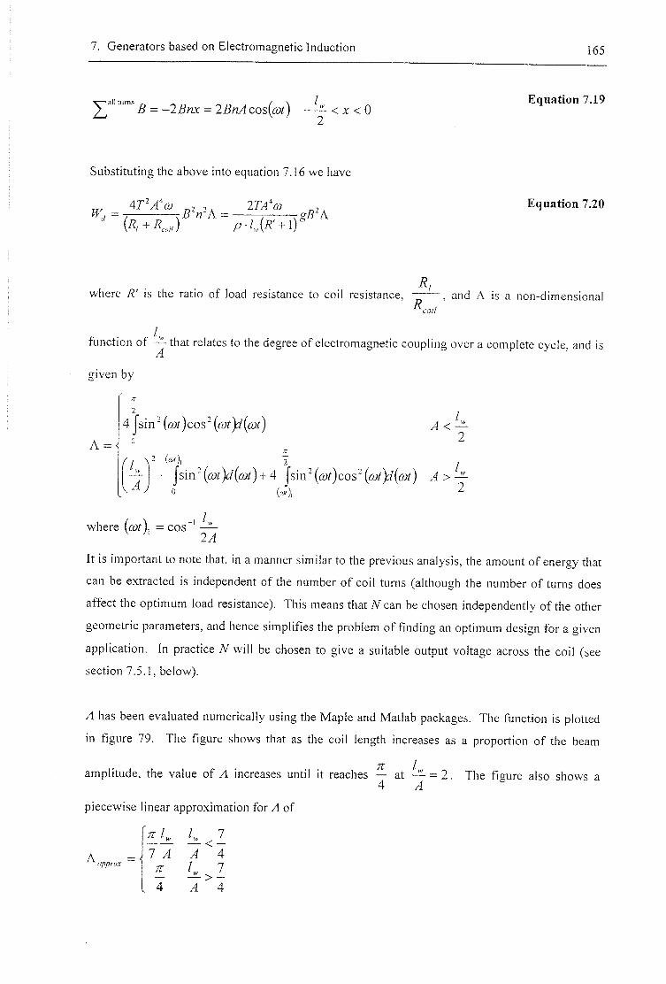
7. Generators based on Electromagnetic Induction 165
^nii turns ^ _ _2j^^ _ 2BnA cos{a)t) - ^ < x < 0 Equa t ion 7.19
Substituting the above into equation 7.16 we have
Equa t ion 7.20
where R' is the ratio of load resistance to coil resistance, R,
R , and A is a non-dimensional
function of ^ that relates to the degree of electromagnetic coupling over a complete cycle, and is
given by
I r
4 j s i n ^ ) cos 4 < —
A
6
/„
W)i
where ((ur), = cos' & 2v4
It is important to note that, in a manner similar to the previous analysis, the amount of energy that
can be extracted is independent of the number of coil turns (although the number of turns does
a fkc t the optimum load resistance). This means that # can be chosen independently of the other
geometric parameters, and hence simplifies the problem of finding an optimum design for a given
application. In practice # w i l l be chosen to give a suitable output voltage across the coil (see
section 7.5.1, below).
/ I has been evaluated numerically using the Maple and Matlab packages. The function is plotted
in figure 79. The figure shows that as the coil length increases as a proportion of the beam
TV I
amplitude, the value of A increases until it reaches — at - ^ = 2. The figure also shows a
piecewise linear approximation for A of
A
& 1 < — 7 A A 4 n K, 7
> — 4 4 A
7 > —
4
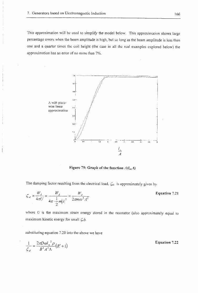
7. Generators based on Electromagnetic Induction 166
This approximation will be used to simplify the model below. This approximation shows large
percentage errors when the beam amplitude is high, but so long as the beam amplitude is less than
one and a quarter times the coil height (the case in all the real examples explored below) the
approximation has an error of no more than 7%.
A with piece-wise linear approximation
/ - / - /
//
/ -
A
Figure 79: Graph of the function A(l„,A)
The damping factor resulting from the electrical load, is approximately given by
c -W., Equation 7.21
2 ' '
where is the maximum strain energy stored in the resonator (also approximately equal to
maximum kinetic energy for small i^/).
substituting equation 7.20 into the above we have
Equation 7.22
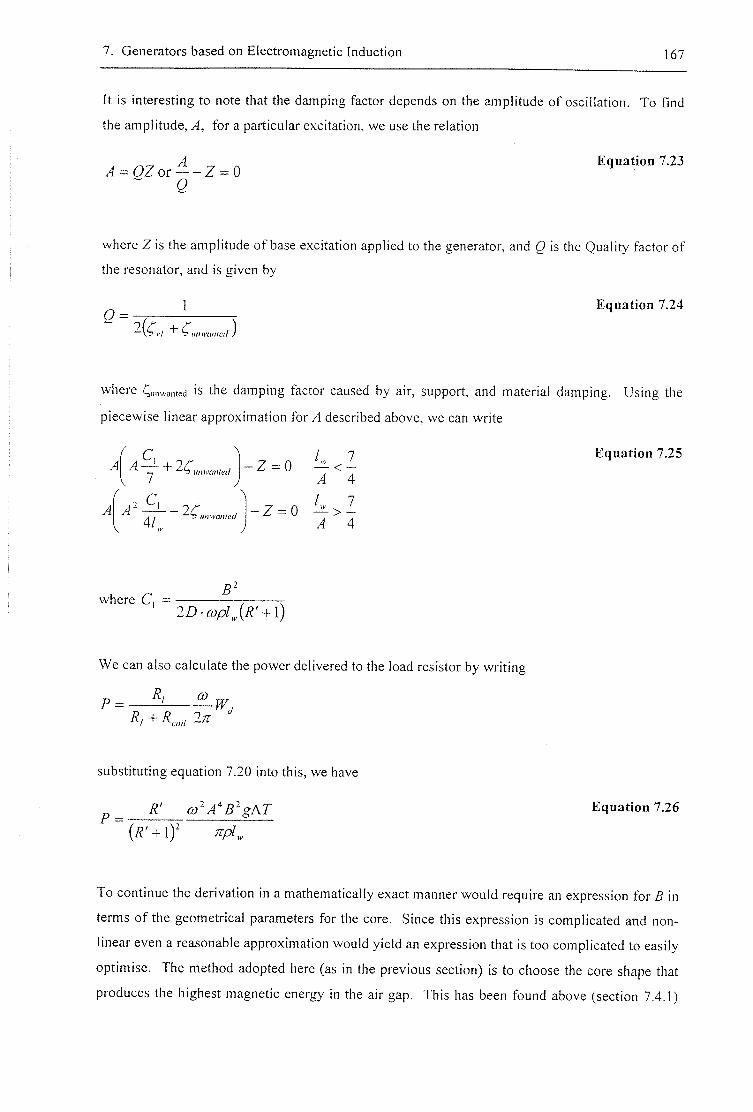
7. Generators based on Electromagnetic Induction 167
It is interesting to note that the damping factor depends on the amplitude of oscillation. To find
the amplitude, A, for a particular excitation, we use the relation
.4 = OZ or = 0 Eq„a«o„7 .23
~ Q
where Z is the amplitude of base excitation applied to the generator, and Q is the Quality factor of
the resonator, and is given by
1 Equation 7.24
Ciinwcmlcil )
where i unwankd is the damping factor caused by air, support, and material damping. Using the
piecewise linear approximation for A described above, we can write
A
A
^ C ^ y unwatHed
A J S unwamed V I" V
Z = 0 4
/ 7 - Z = 0 ^ > -
A 4
/ 7 Equation 7.25
where C,
We can also calculate the power delivered to the load resistor by writing
f — f F ,
substituting equation 7.20 into this, we have
.R' Equation 7.26
+ 1 ) '
To continue the derivation in a mathematically exact manner would require an expression for B in
terms of the geometrical parameters for the core. Since this expression is complicated and non-
linear even a reasonable approximation would yield an expression that is too complicated to easily
optimise. The method adopted here (as in the previous section) is to choose the core shape that
produces the highest magnetic energy in the air gap. This has been found above (section 7.4.1)
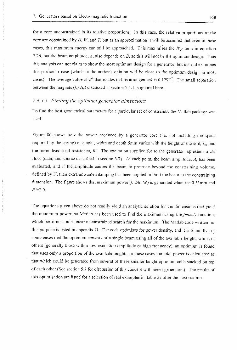
7. Generators based on Electromagnetic Induction 168
for a core unconstrained in its relative proportions. In this case, the relative proportions of the
core are constrained by H, W, and T, but as an approximation it will be assumed that even in these
cases, this maximum energy can still be approached. This maximises the B~g term in equation
7.26, but the beam amplitude. A, also depends on B, so this will not be the optimum design. Thus
this analysis can not claim to show the most optimum design for a generator, but instead examines
this particular case (which in the author's opinion will be close to the optimum design in most
cases). The average value of B' that relates to this arrangement is 0 .179T\ The small separation
between the magnets (/,,,-2/c) discussed in section 7.4.1 is ignored here.
7. 7
To find the best geometrical parameters for a particular set of constraints, the Matlab package was
used.
Figure 80 shows how the power produced by a generator core (i.e. not including the space
required by the spring) of height, width and depth 5mm varies with the height of the coil, 7 , and
the normalised load resistance, The excitation supplied for to the generator represents a car
floor (data, and source described in section 5.7). At each point, the beam amplitude, A, has been
evaluated, and i f the amplitude causes the beam to protrude beyond the constraining volume,
defined by H, then extra unwanted damping has been applied to limit the beam to the constraining
dimension. The figure shows that maximum power (0.24mW) is generated when /w=0.53mm and
; ; '=2.o.
The equations given above do not readily yield an analytic solution for the dimensions that yield
the maximum power, so Matlab has been used to find the maximum using the fminsQ function,
which performs a non-linear unconstrained search for the maximum. The Matlab code written for
this purpose is listed in appendix G. The code optimises for power density, and it is found that in
some cases that the optimum consists of a single beam using all of the available height, whilst in
others (generally those with a low excitation amplitude or high frequency), an optimum is found
that uses only a proportion of the available height. In these cases the total power is calculated as
that which could be generated from several of these smaller height optimum cells stacked on top
of each other (See section 5.7 for discussion of this concept with piezo-generators). The results of
this optimisation are listed for a selection of real examples in table 27 after the next section.
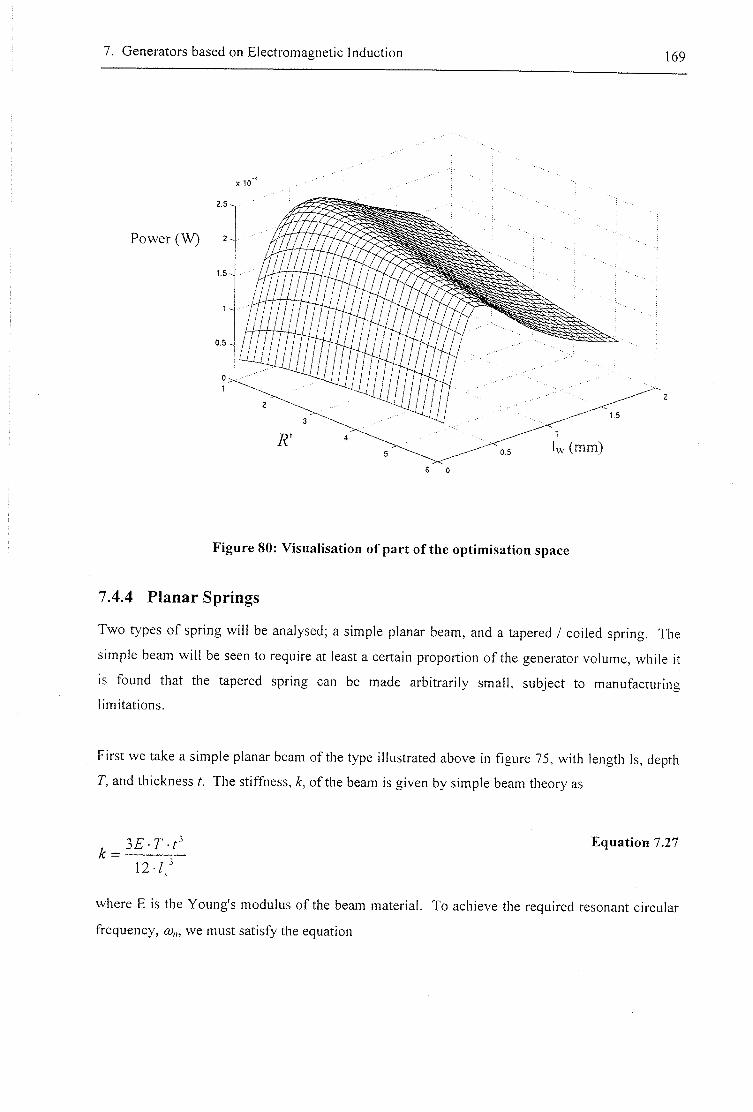
7. Generators based on Electromagnetic Induction 169
Power (W)
6 0
Figure 80: Visualisation of part of the optimisation space
7.4.4 Planar Springs
Two types of spring will be analysed; a simple planar beam, and a tapered / coiled spring. The
simple beam will be seen to require at least a certain proportion of the generator volume, while it
is found that the tapered spring can be made arbitrarily small, subject to manufacturing
limitations.
First we take a simple planar beam of the type illustrated above in figure 75, with length Is, depth
T, and thickness t. The stiffness, k, of the beam is given by simple beam theory as
k = Equation 7.27
where E is the Young's modulus of the beam material. To achieve the required resonant circular
frequency, co,,, we must satisfy the equation
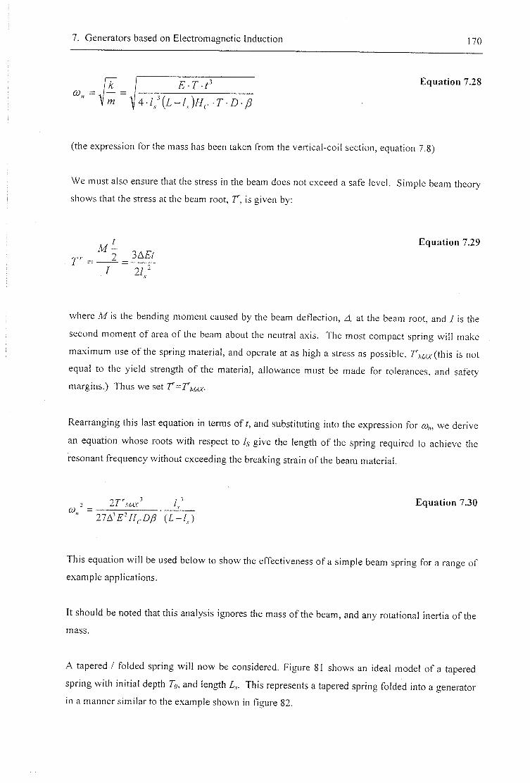
7. Generators based on Electromagnetic Induction 170
1^ I E-T-t^ Equation 7.28
(the expression for the mass has been taken from the vertical-coil section, equation 7.8)
We must also ensure that the stress in the beam does not exceed a safe level. Simple beam theory
shows that the stress at the beam root, T, is given by:
, , t Equation 7.29
/ 2 / '
where M is the bending moment caused by the beam deflection, zl, at the beam root, and / is the
second moment of area of the beam about the neutral axis. The most compact spring will make
maximum use of the spring material, and operate at as high a stress as possible, 2\M_y(this is not
equal to the yield strength of the material, allowance must be made for tolerances, and safety
margins.) Thus we set T-Tmax-
Rearranging this last equation in terms of and substituting into the expression for a;,,, we derive
an equation whose roots with respect to /g give the length of the spring required to achieve the
resonant frequency without exceeding the breaking strain of the beam material.
2 / / Equation 7.30 6; ^
This equation will be used below to show the effectiveness of a simple beam spring for a range of
example applications.
It should be noted that this analysis ignores the mass of the beam, and any rotational inertia of the
mass.
A tapered / folded spring will now be considered. Figure 81 shows an ideal model of a tapered
spring with initial depth To, and length Z,.- This represents a tapered spring folded into a generator
in a manner similar to the example shown in figure 82.
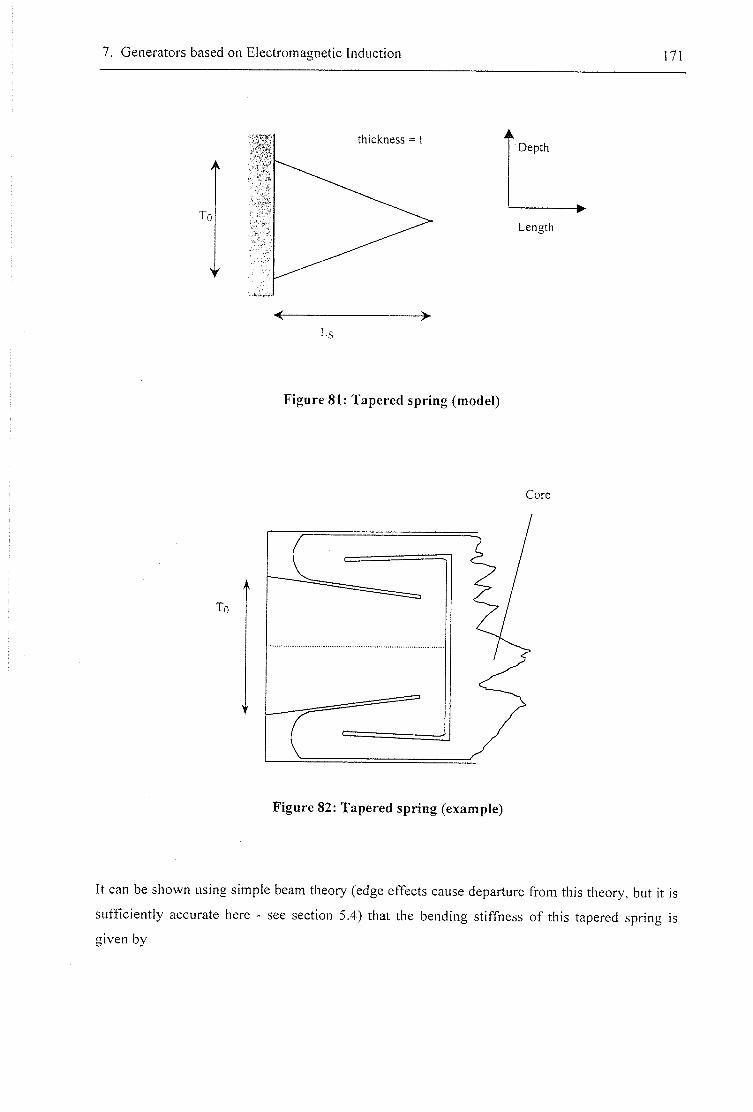
7. Generators based on Electromagnetic Induction 171
To
thickness = t Depth
Length
Ls
Figure 81: Tapered spring (model)
Core
To
Figure 82: Tapered spring (example)
It can be shown using simple beam theory (edge effects cause departure from this theory, but it is
sufficiently accurate here - see section 5.4) that the bending stiffness of this tapered spring is
given by
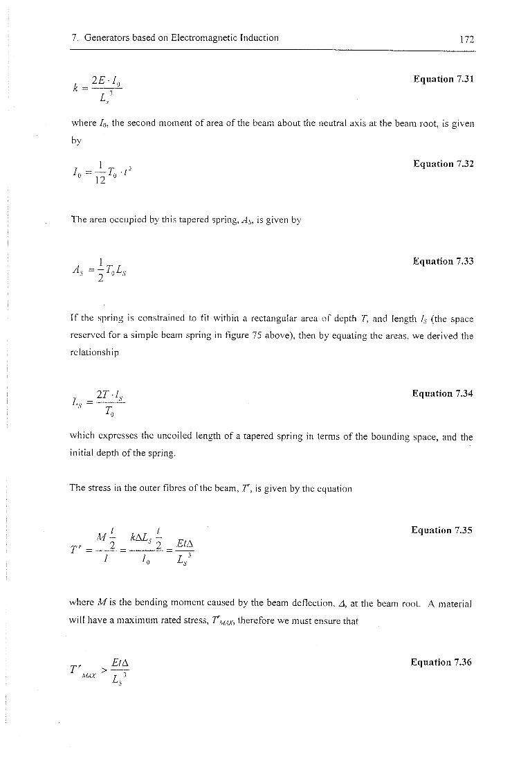
7. Generators based on Electromagnetic Induction 172
k 2E • /{, Equation 7.31
l '
where I„, the second moment of area of the beam about the neutral axis at the beam root, is given
by
1 , Equation 7.32
The area occupied by this tapered spring, As, is given by
1 Equation 7.33 / I '
If the spring is constrained to fit within a rectangular area of depth T, and length /.v (the space
reserved for a simple beam spring in figure 75 above), then by equating the areas, we derived the
relationship
2T • /,. Equation 7.34 Z . = ^
T,
which expresses the uncoiled length of a tapered spring in terms of the bounding space, and the
initial depth of the spring.
The stress in the outer fibres of the beam, T, is given by the equation
, , f . t Equation 7.35
where M is the bending moment caused by the beam deflection. A, at the beam root. A material
will have a maximum rated stress, T Ad4x, therefore we must ensure that
^ £ / A Equation 7.36
Ls
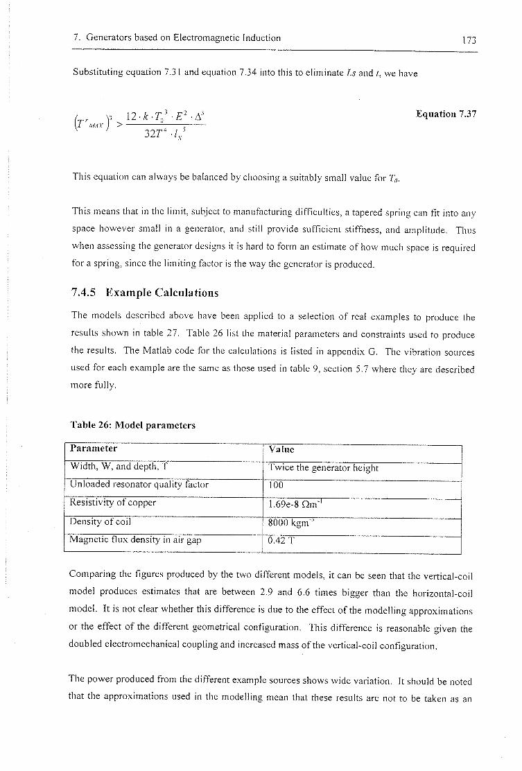
7. Generators based on Electromagnetic Induction I73
Substituting equation 7.3 1 and equation 7.34 into this to eliminate Ls and t, we have
Arr V 12 ' &' ICqiiation 7.37 U MAX ) > ——
This equation can always be balanced by choosing a suitably small value for T,,.
This means that in the limit, subject to manufacturing difficulties, a tapered spring can fit into any
space however small in a generator, and still provide sufficient stiffness, and amplitude. Thus
when assessing the generator designs it is hard to form an estimate of how much space is required
for a spring, since the limiting factor is the way the generator is produced,
7.4.5 Example Calculations
The models described above have been applied to a selection of real examples to produce the
results shown in table 27. Table 26 list the material parameters and constraints used to produce
the results. The Matlab code for the calculations is listed in appendix G. The vibration sources
used for each example are the same as those used in table 9, section 5.7 where they are described
more fully.
Table 26: Model parameters
Parameter Value
Width, W, and depth, T Twice the generator height
Unloaded resonator quality factor 100
Resistivity of copper 1.696-8 Qm
Density of coil 8000 kgm"
Magnetic flux density in air gap 0.42 T
Comparing the figures produced by the two difkrent models, it can be seen that the vertical-coil
model produces estimates that are between 2.9 and 6.6 times bigger than the horizontal-coil
model. It is not clear whether this difference is due to the effect of the modelling approximations
or the effect of the different geometrical configuration. This difference is reasonable given the
doubled electromechanical coupling and increased mass of the vertical-coil configuration.
The power produced from the different example sources shows wide variation. It should be noted
that the approximations used in the modelling mean that these results are not to be taken as an
7. Generators based on Electromagnetic Induction 174
exact measure of how much power can be generated, but rather an indication of the order of
magnitude that is possible. The sources represent a range of different extremes - from the low-
frequency, low-amplitude car case, to the high-frequency, high amplitude caulking hammer. The
power generated reflects this. For each sample vibration source, the power available is seen to
grow rapidly with increasing generator height. Even at the smaller 2.5mm height, however, the
more vigorous sources can be seen to be capable of producing useful power (see section 3.3 for a
discussion of what might constitute useful power).
These figures are misleading if taken without consideration of the spring size. A column is
presented in the table that shows the power that would be produced by the horizontal-coil
configuration when a simple planar beam spring is used (as calculated from equation 7.30). As
discussed above, a coiled spring could be constructed to occupy less space than this, but this
column gives an idea of how challenging it would be to produce a smaller spring. In several of
the low frequency and high vibration cases, over 90% of the space needs to be set aside for a
beam spring.
It should be noted that the assumption of a small amplitude of vibration used in the vertical-coil
analysis is violated in some cases (those left blank on the table). This assumption was used to
approximate the field around the coils as always constant, thus this model cannot be used in these
cases.
For each analysis, a column shows how many turns would be required on the coil to provide a
2volt peak-peak amplitude output signal. Calculations show that if polyester coated copper wire
were used with a total diameter of 24p.m (commercially available), then the required number of
turns could be produced (at a cost) for all but the two largest of the table entries. The difficulty
involved in extracting power from cases where only low output voltages are available is discussed
below.
The horizontal-coil model will be used below to produce further predictions for direct comparison
with piezoelectric generators.
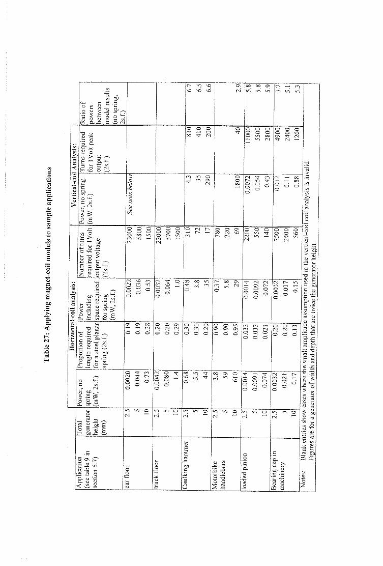
% c
.S V
CL
"o. £
o
o u
C CQ s OA c
A CL < t^' (S
z H
cq
c M (D
QJ U 13
1 I I I
S Q,
O X
73 Y (U (3 O 3 CL rr O >
H s-O
(+_ c/i CL
W) a
(N VI \0 \d \o \6
o\ ni
(/) o
I I I i l l Z 2 o M
13 cj
bA O' SP 0)
^ _2 o S*
& O
<5 a Q S
I o o o o o o O oo un (N
M m (N m m g s =
m vn (N
8 vn
(N ^ O S g "
: -
s i i n .2 o _c: w] &0 & % a . S & 5^ ^
(N bD ^
c H
§ (> FT
Q. (D CL OJ <
c o
o\ o\ oo r—I ^
O C> C)
o ^ m
i s S
VI (N
o o o 00 ^ cs
m m o ^ r .
C) (N r~"
00 00
3 -
o
oo oo o\ v4 vi
o o o o o o O VI oo v (N
o o oo (N r " (N
O O G\ (N M (N <3 C> ci
(N O ^ 00
§ S
o o c
vn VI (N
o o o m m cN C) C) C)
oo v4
o o o\ 0\ C> C)
vi
VI IT) ni
g -C bA •S 3 (0 U
o
V) tT) (N
II
(N r~"
i §
rn v4 VI
o o o o o o o\ Tf- rs -rj- (N ^
o o o O vn ^ (N
fN (N o\ r~ § 3
s 8 C) (3
O O O O O O V-) ^ r~ (N
(N
i §
o o M rs c> o
I—I ^ o\ § S
o 5
CL
O
CN '— m rs o o O r<
vn vn (N
CL 3 Er
# 1 CQ S
tu a£) > 'S
S %
II l l I ' (8 <D <D CO -a 3 (0
t | = T3
<D _C -B -S
« 2 0 §
c
OA
- g c « 1) (/) C 5 ra 00
CQ Z
7. Generators based on Electromagnetic Induction 176
7.5 Producing practical generators
This section has focussed on modelling generators, and making theoretical predictions concerning
how applicable the technology is to potential applications. Other issues must be considered
before these generators can become a reality.
7.5.1 Extracting power
The requirement for extracting and storing the energy produced places strong constraints on the
generator design. Further work is required in this area, however some initial thoughts are
discussed below.
Before the power can be stored in an electrochemical cell, capacitor, or super-capacitor, it will
need to be rectified. Rectifiers based on junction diodes are the most conventional solution,
however, they require a forward voltage of a least a few hundred milli-volts to provide a
reasonable forward current (the HP HSCH-3486 schottky diode would be a good low-voltage
rectifier with a forward current of 0.1mA at F,,-100mV). Other possibilities include active
(switched) rectification with either micro-relays (expensive) or semiconductor devices such as
FETs (hard to produce low 'on' resistance without consuming too much power). Another
possibility is to use a transformer to boost the voltage before rectification. For the low
frequencies seen in many of the potential applications described above, producing an efficient
wound transformer in the space available would be difficult. Also, since the voltage is already
being derived from an electromagnetic interaction, perhaps it would be more efficient to focus on
increasing the voltage at source by improving the number of coil turns. A piezoelectric
transformer [89] has also been considered, however, these devices become inefficient at typical
generator dimensions, and their working frequency is typically in the region of tens of kilohertz.
[t is thus suggested that in general a generator will need to produce a peak voltage of at least a few
hundred milli-volts before the power can usefully be stored. The calculations above show that the
number of turns can be increased without decreasing the potential power, thus the challenge is to
produce a significant number of sufficiently thin windings. In some situations, however, the
output voltage may be so low that no practical way of extracting the power can be found.
7.5.2 Micro-devices
Many potential applications would benefit from a small generator. As the dimensions are reduced
we must consider how the power scales with volume, and how small devices might be
manufactured.
7. Generators based on Electromagnetic Induction 177
The predictions made above in section 7.4.5 show that devices of total height 2.5mm could only
provide useful power in certain high amplitude applications. The power scales as a function of
approximately the third power of height, thus even smaller generators are unlikely to produce
useful power. These high amplitude applications seem rare, and it is anticipated that a generator
height of 5mm is the smallest that is likely to be required.
M E M S technologies are currently an area of intense research, and it is natural and fashionable to
ask whether a micro-generator could be produced in this way. MEMS devices typically range in
size between an order of micrometres to orders of millimetres. Thus, the device sizes described
above are at the larger (and hence more expensive) end of the spectrum. There are three main
parts to the generators described above:
(a) Spring: Silicon is a good material for producing springs. Both equation 7.30 and equation
7.37 show that springs can be made smaller and withstand a higher amplitude if the quantity
\3 T ^
' is increased. Taking Tmax as the yield strength, this takes a value of 9,500Pa for E -
Silicon compared to 12,000Pa for some Be-Copper alloys, and 52,000Pa for precipitation
hardened 17Cr-4Ni Cu Stainless steel. The photochemical processes that can be used in
silicon micromachining mean that detailed tapered spring designs of the type described above
in chapter 4 could be produced. An advantage with photochemical etching processes is that
the dimensions of devices can be controlled to very high tolerances. A possible drawback with
silicon springs would be the brittle nature of the material. Small defects, and sharp edges can
cause stress concentrations that will cause fracture of the spring. Both Silicon and Copper
springs have been used by Chan [87], he concludes that copper is a more suitable material in
his context.
(b) Magnets: The modelling described above shows that strong magnetic fields are required to
produce good generators. Techniques for depositing thick film magnets which are suited to
M E M S processing techniques are not capable of producing either the field strength or the
dimensions required. It would thus be necessary to apply pre-formed magnets to a structure
using some more conventional approach.
(c) Coil: The modelling work shows that there is a requirement for a relatively thick coil
structure with a high density of turns. As discussed above, it is possible to create this type of
structure using thick-film printing (Chan uses this approach). For large numbers of turns,
printed coils may be uneconomic compared to winding coils mechanically from wire. The coil
will typically lie out of the plane of the spring; micromachining is best suited to semi-planar
structures, and would probably require complex processing to produce a suitable configuration.
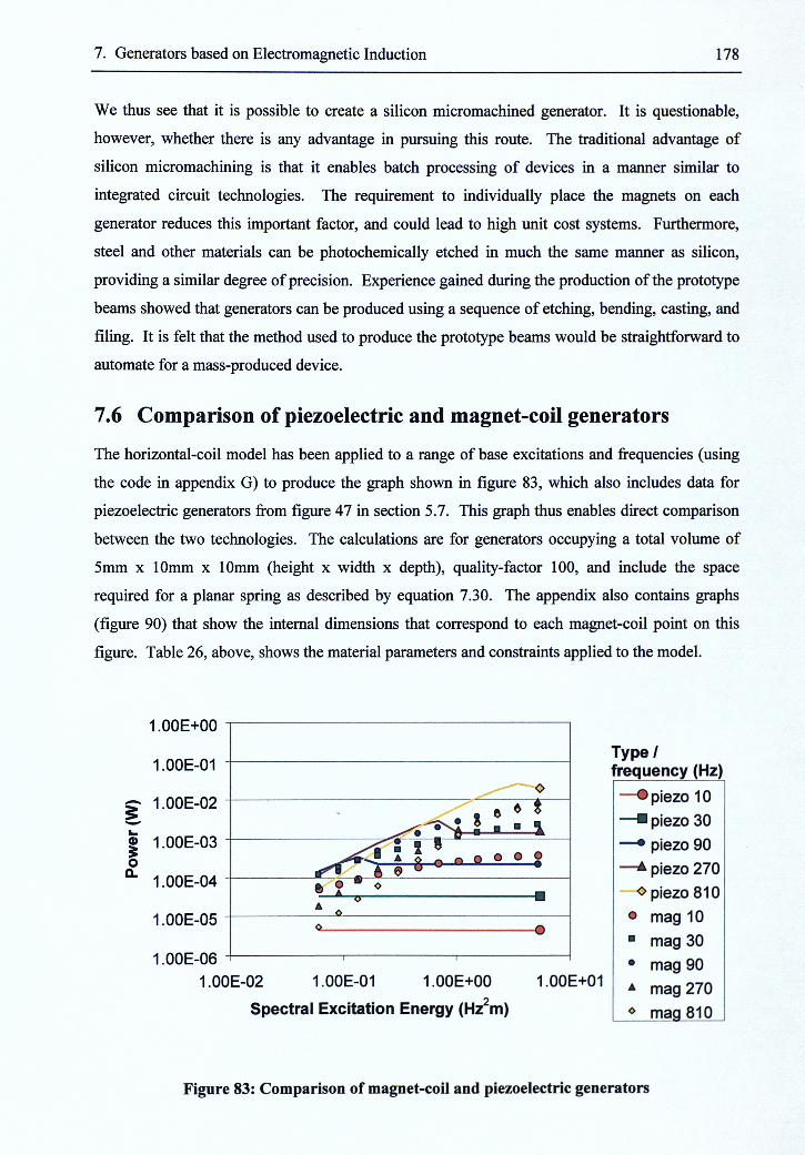
7. Generators based on Electromagnetic Induction 178
We thus see that it is possible to create a silicon micromachined generator. It is questionable,
however, whether there is any advantage in pursuing this route. The traditional advantage of
silicon micromachining is that it enables batch processing of devices in a manner similar to
integrated circuit technologies. The requirement to individually place the magnets on each
generator reduces this important factor, and could lead to high unit cost systems. Furthermore,
steel and other materials can be photochemically etched in much the same manner as silicon,
providing a similar degree of precision. Experience gained during the production of the prototype
beams showed that generators can be produced using a sequence of etching, bending, casting, and
filing. It is felt that the method used to produce the prototype beams would be straightforward to
automate for a mass-produced device.
7.6 Comparison of piezoelectric and magnet-coil generators
The horizontal-coil model has been applied to a range of base excitations and frequencies (using
the code in appendix G) to produce the graph shown in figure 83, which also includes data for
piezoelectric generators from figure 47 in section 5.7. This graph thus enables direct comparison
between the two technologies. The calculations are for generators occupying a total volume of
5mm x 10mm x 10mm (height x width x depth), quality-factor 100, and include the space
required for a planar spring as described by equation 7.30. The appendix also contains graphs
(figure 90) that show the internal dimensions that correspond to each magnet-coil point on this
figure. Table 26, above, shows the material parameters and constraints applied to the model.
1.00E+00
1.00E-01
^ 1.00E-02
1.00E-03
1.00E-04
1 .OOE-05
1 .OOE-06
1.00E-02 1.00E-01 1.00E+00
Spectral Excitation Energy (Hz m)
1.00E+01
Type/ frequency (Hz)
—•p iezo 10
— • piezo 30
—• piezo 90
—^ piezo 270
- o piezo 810
o mag 10
• mag 30
• mag 90
^ mag 270
mag 810
Figure 83: Comparison of magnet-coil and piezoelectric generators
7. Generators based on Electromagnetic Induction 179
As an example of how to use the graph, the vibration data from a bearing cap in heavy machinery
listed in table 9 will be used to determine how much power could be generated, as estimated by
the graph. The frequency of base excitation is lOOHz, at an amplitude of 3.58^im. Forming the
product of frequency squared and amplitude we obtain the spectral excitation energy as
0.0358Hz"m. Since the frequency of 100Hz does not have a data series on the graph, the
frequency will be approximated as 90Hz (to be more thorough, we could interpolate between 90
and 270Hz). Calculations for 90Hz are plotted on the graph as a blue line (piezoelectric) and blue
circles (magnet-coil). Extending a line from the x-axis at 0.0358 Hz^m and intersecting with these
two blue series, we find that powers of l . l m W and 0.25mW are predicted from the magnet-coil
and piezoelectric generators respectively. In this case it would thus seem that a magnet-coil
generator would be the best design, and that enough power could be generated to perform useful
work. To find the geometric proportions of the best generator in this case figure 90 should be
examined (this will be a good starting point for generator design, but the final design will be
different due to non-ideal parameters that are not modelled here).
The graphs above show the power that could be delivered to a resistive load of an optimum value.
Further work is required to examine methods of extracting and storing the power generated by
both technologies; it is not clear in which of the technologies this will be more efficient.
It can be seen that the technology that generates the most power depends on the excitation
conditions. The piezoelectric generators produce more power at the highest frequency examined
(810Hz) and for the lower excitation amplitudes of the 270 and 90Hz cases. For the cases
examined, the magnet-coil generator never supplies less than a tenth of the power of the
piezoelectric case. The most marked difference can be seen at lower amplitudes and lower
frequencies, when the magnet-coil generator is seen to be up to 90 times more powerful. Under
these conditions, the piezoelectric generators are unable to apply as much damping as the magnet-
coil ones. Note that the horizontal-coil configuration (as modelled in the above figure) is shown
above to be around one quarter as powerful as the vertical-coil configuration, thus, if the vertical-
coil configuration were compared to piezoelectric generators, the piezoelectric generators would
be more powerful in even fewer cases.
When choosing which technology is most suitable for a given application, other factors must be
considered. Piezoelectric generators are not easy to manufacture. Thick-film generators
discussed in chapter 4 are currently limited by the low activity of the PZT material used (although
materials research may solve this problem in the future). Bulk devices are required to produce the
power shown above, however producing (often multi-beam, multi-layer) devices of the size found
to be optimum is difficult. The lifetime and reliability of the devices must also be examined; the
7. Generators based on Electromagnetic Induction gneiicinauciion jgQ
piezoelectric devices use a brittle ceramic material as a spring, compared to the metallic springs of
the magnet-coil devices. Finding a suitable method to clamp the piezoelectric beams at their root
without introducing extra potentially damaging stresses would be difficult. Thus, it is envisaged
that piezoelectric generators will rarely be the best choice, except perhaps in particularly high
frequency (several kilo-Hertz) applications.
7.7 Summary
Typical design configurations for inertial generators based on electromagnetic induction have
been examined. An electrical equivalent circuit model has been described, and verified by
producing a prototype generator. The prototypes produced a maximum power of 2.4 and 5.0mW
in volumes of 2.0 and 4.1cm^ respectively.
Generators have a specific optimum load resistance, which depends on both the amount of
damping present, and the coil resistance. The unwanted damping present in the prototypes
described here is dominated by support damping, and is thus hard to predict theoretically. The
prototypes have revealed that output voltages can be very low. This is important as once power
has been generated it must also be rectified and stored in a suitable medium such as a battery.
Both batteries and rectifiers require voltages of at least a few hundred milli-volts. Thus,
producing reasonable output voltages will often require a large number of fine turns on the coil.
The concept has been validated using a demonstrator mounted on a car engine block that has been
shown to be capable of producing a useful amount of power.
An analysis of two possible generator structures has provided a method of calculating theoretical
limits on the power that can be generated within a given volume for a particular excitation. The
resulting equations can be used to predict (to an order of magnitude) power output for any
application. The equations have been applied to a number of existing vibration sources to show
typical output powers. These show that the power delivered is very application specific, with
figures ranging from IjuW to 35mW.
The model has also been used to provide a graph of power output for a range of different
excitations. This graph permits direct comparison between magnet-coil generators and
piezoelectric ones. The comparison shows that both technologies have merits, and that the
excitation conditions determine which will produce the most power. It is suggested that even in
cases where a magnet-coil generator may be predicted to generate less power, it will often be the
best choice due to the difficulties of manufacturing piezoelectric devices. Magnet-coil generators
are also likely to be more reliable.
I. Conclusions and Suggestions for Further Work 131
CHAPTER 8
Conclusions and Suggestions for Further Work
8.1 Conclusions
Vibration powered devices provide an alternative to batteries, and offer a solution to the power
requirements of distributed sensor systems. In combination with suitable wireless
communications techniques vibration power has the potential to permit fully wireless and
autonomous sensors with operational lifetimes that are not constrained by built in power sources.
Two main technologies have been identified as ways of harvesting vibration power: piezoelectric
materials, and magnet-coil combinations using electromagnetic induction. While both ideas can
be found in the existing literature, no existing studies have sought to provide a framework upon
which these techniques can be evaluated and compared. Engineers have had no way to answer the
questions 'For which applications is vibration power suitable?' and 'Which technology should I
use?'. This thesis has addressed these issues, culminating in calculations typified by figure 84
below.
It has been shown that in some applications, vibration-powered generators can produce energy at
a rate comparable to other self-powered technologies such as solar power. The decision to use
vibration power will be a result of having considered what other sources of power are available
and weighing up the issues of output power, cost, long-term stability, etc. Vibration power has an
advantage over solar power in dark, vibrating environments such as car engines and other heavy
machinery. Potential disadvantages of vibration-powered generators include their higher
production costs, moving parts that are more likely to fail than solid-state devices, and the lack of
existing development of devices of this type.
Initially, thick-film PZT was explored as a potential technology for a generator. A process to
form a multi-layered thick-film device has been developed. The devices consist of two thick-film
PZT layers, with electrodes, sandwiching a steel beam. By clamping the beams at their root, and
attaching a mass to the tip of the structure, power is generated when the base is shaken.
Producing the devices required overcoming some materials problems. It was found that PZT
films react with the steel substrate during the firing processes, to prevent this interaction glassy
8. Conclusions and Suggestions for Further Work 182
dielectric layers were incorporated into the structure. Also, thermal mismatch between the layers
causes warping to occur during the firing process. The warping was reduced by producing
symmetrical structures, however, variations in the screen printing process meant that some
warping still occurs which places a lower limit on the thickness of the steel. The material
properties of the device layers have been measured, since mechanical data is not commonly
available for thick-film materials. Methods to measure the piezoelectric constants of the PZT
have been developed. Measuring these constants is not trivial, and the methods presented here are
more accurate that any reported in the literature to date for thick-film piezoelectric materials.
The thick-film devices were tested using an electromechanical shaker. Working in linear regions
of operation, the results showed that small amounts of power could be generated (around 3|LLW).
Modelling was undertaken to examine why such small amounts of power were generated, and also
to predict the power output from piezoelectric generators of arbitrary dimensions. It was found
that analytic models became too complex when such factors as edge effects and varying stresses
through the piezoelectric material were incorporated. It was also found that commercially
available finite element modelling packages, will not at this time simulate resistively shunted
piezoelectric elements. The problem was made more tractable by decoupling the electrical and
mechanical domains, representing the resistively shunted piezoelectric material as exhibiting a
frequency dependant stiffness and loss factor. The existing model of a shunted piezoelectric
element, however, did not include the effect of non-uniform strain through the piezoelectric layer
that is a feature of generator designs. A new model of a resistively shunted piezoelectric element
undergoing pure bending was therefore developed. The model shows that this effect can cause a
reduction in available damping of up to 30%. This reduction can be reduced by using laminated
piezoelectric / electrode structures. Comparing the model to experimental results, accurate
predictions are seen at low beam amplitude, with slight under prediction at higher amplitudes due
to non-linear effects.
The model reveals that the reason for the low power produced by the thick-film generator, is the
low electromechanical coupling coefficient of thick-film PZT. If this technology is to be useful,
devices must be constructed with either bulk PZT, or densified thick-film PZT. The model was
also used in conjunction with numerical methods to find optimum generator dimensions for a
range of excitations that might be found in practice. These figures show that bulk PZT generators
could produce useful amounts of power in many applications.
Experiments have been devised to assess the long-term stability of thick film PZT materials.
Prior research has shown that bulk piezoelectric ceramics suffer a long term ageing process after
polarisation, however, no studies have been reported that measure this important process in thick-
Conclusions and Suggestions for Further Work 183
film piezoceramics. A technique for measuring the ageing rate of the d), coefficient of a PZT
thick-film sample has been presented. The method has been found to be reliable, and be
sufficiently accurate for observing the decaying response. The accuracy obtained is of an order of
magnitude higher than that reported previously. The d), coefficient is found to age at - 4 . 4 % per
time decade (for PZT-5H). A method is presented for measuring the ageing of the dielectric
constant, K33, and found to show an ageing rate o f -1 .34% per time decade.
Turning to generators based on electromagnetic induction, typical design configurations have
been examined. An electrical equivalent circuit model has been described, and verified by
producing a prototype generator. The prototypes produced a maximum power of 2.4 and 5.0mW
in volumes of 2.0 and 4.1cm^ respectively. The prototypes have revealed that output voltages can
be very low. This is important as once power has been generated it must also be rectified and
stored in a suitable medium such as a battery. Both batteries and rectifiers require voltages of at
least a few hundred milli-volts. Thus, producing reasonable output voltages will often require a
large number of fine turns on the coil. The concept has been validated using a demonstrator
mounted on a car engine block that has been shown to be capable of producing an average of
160^V/.
An analysis of two possible magnet-coil generator structures has provided a method of calculating
theoretical upper limits on the power that can be generated within a given volume for a particular
excitation. The resulting equations can be used to predict (to an order of magnitude) power output
for any application. The equations have been applied to a number of existing vibration sources to
show typical output powers. These show that the power delivered is very application specific,
with figures ranging from lp.W to 35mW.
The model has also been used to predict power output for a range of different excitations. This
data has been combined with similar results for a piezoelectric generator, to permit direct
comparison between the two technologies. Figure 84 shows the power that can be produced by
both technologies from generators occupying a total volume of 5mm x 10mm x 10mm (height x
width X depth). See section 7.6 for a description of how to use this graph. The comparison shows
that both technologies have merits, and that the excitation conditions determine which will
produce the most power. Piezoelectric generators, however, would not be easy to manufacture.
The lifetime and reliability of the devices must also be examined; the piezoelectric devices use a
brittle ceramic material as a spring, compared to the metallic springs of the magnet-coil devices.
For these reasons it is envisaged that piezoelectric generators will rarely be the best choice, except
perhaps in particularly high frequency (several kilo-Hertz) applications.
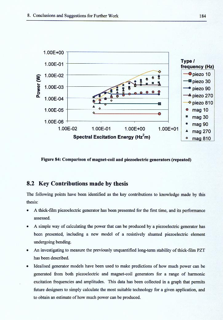
8. Conclusions and Suggestions for Further Work 184
1.00E+00
1.00E-01
s 1.00E-02
1 1.00E-03 o tL
1.00E-04
1.00E-05
1.00E-06
1.00E-02 1.00E-01 1.00E+00
Type/ frequency (Hz)
1.00E+01
Spectral Excitation Energy (Hz^m)
piezo 10
— • piezo 30
piezo 90
piezo 270
o piezo 810
o mag 10
• mag 30
• mag 90
A mag 270
O map 810
Figure 84: Comparison of magnet-coil and piezoelectric generators (repeated)
8.2 Key Contributions made by thesis
The following points have been identified as the key contributions to knowledge made by this
thesis:
• A thick-film piezoelectric generator has been presented for the first time, and its performance
assessed.
• A simple way of calculating the power that can be produced by a piezoelectric generator has
been presented, including a new model of a resistively shunted piezoelectric element
undergoing bending.
• An investigating to measure the previously unquantified long-term stability of thick-film PZT
has been described.
• Idealised generator models have been used to make predictions of how much power can be
generated from both piezoelectric and magnet-coil generators for a range of harmonic
excitation frequencies and amplitudes. This data has been collected in a graph that permits
future designers to simply calculate the most suitable technology for a given application, and
to obtain an estimate of how much power can be produced.

8. Conclusions and Suggestions for Further Work 185
8.3 Suggestions for Further Work
The future for self-powered systems seems bright, and interest in self-power is currently growing
rapidly. Caution is also important though, as this is a subject where misplaced optimism can last
for a long time. Consider, for example, the work on generating power from vibrations in road
bridges; much work was done before it was realised that small devices could not generate useful
power. In contrast self-winding wristwatches are a widespread success, with a power source that
is well matched to its intended application. The message is that before continuing research into
the areas mentioned below, it is important to choose a target application and tailor designs
accordingly.
This thesis presents a background that should enable future designers to choose a suitable
technology, and estimate how much power it will produce for a given application. Piezoelectric
generators are unlikely to feature much in future research, unless a superb high frequency
application is found for them. If they are used further, then significant effort will need to be
expended in producing a design that can be economically manufactured. If current research into
thick-film piezoelectric materials yields materials comparable in activity to bulk ones (possible)
then producing generators would be much simpler. Magnet-coil generators have been explored in
some depth here. The question of which configuration is best has been approached, but it is found
that the results depend on many practical considerations that will vary from application to
application. Thus, further fundamental research is unlikely to yield further useful insights in this
area. It is the author's opinion that the double-gap core design will be found to be superior in
most cases. Further work in this area is more likely to be concerned with producing generators
for practical applications, and discovering how closely the theoretical predictions made here can
be approached through careful and inspired engineering.
This thesis focuses on linear resonant generators. Another type of design [8] which may be
particularly suitable for impulse type excitations could be explored; Power can be generated
through impacts between an inertial mass, and a piezoelectric element. This type of generator is
non-linear, and will require a different type of analysis to that presented here. Another
unexplored possibility is that resonant generators can be modified to allow electrical tuning of
their resonant frequency through the addition of reactive loads, which would allow higher power
generation in environments where a narrow excitation frequency is not stable in time.
The question of how power is to be extracted and stored has not been addressed in detail in this
thesis. It must be appreciated that the power generated (as the term has been used in this thesis,
referring to the power that can be delivered to an optimum resistive load) is not the same as the
Conclusions and Suggestions for Furtiier Work 185
amount of power that will be ultimately delivered to a storage device such as a battery following
rectification and voltage scaling. Impedance matching will be important here to ensure optimum
power transfer. The cause of this disparity Is the low output voltages that may be produced by
small generators in weak vibration applications. Section 7.5.1 points out some possible ways of
tackling this problem, but it is acknowledged that in some cases it may not be possible to 'get
hold' of the power.
Power extraction is important, but the most interesting problems lie with systems issues:
Producing a miniature system that can gather, process and transmit data using only the small
amounts of power that will be present. The electronics is unlikely to be particularly novel,
innovation must come in finding a solid application, and using the system in an adroit manner (for
instance making use of the fact that data processing is power efficient to reduce the amount of
power hungry data transmission that must be used). There is potential for arrays of self-powered
systems working together, since communications power can be reduced when neighbour to
neighbour communications are used. There is also scope for novel communications methods
since communications is likely to consume the largest proportion of a power budget. An ultra-
low power communications technique could open up many potential applications, even if it were
only capable of very poor data rates. Systems will also require ultra-low power sensors, another
area that has not been examined in this thesis.
Finally, vibration power is not the only solution! There is no single technological answer to self-
power: To realise the vision of a world filled with tiny wireless and autonomous sensor systems,
each potential application must be evaluated to determine where power might be derived.
Applying such solutions will require devices to be carefully tailored to each specific application,
with devices often needing to search for power at the edges of feasibility.
Appendix A 187
APPENDICES
Appendix A: Publications List
1. p. Glynne-Jones, S. P. Beeby, P. Dargie, T. Papakostas and N. M. White, "An Investigation
Into The Effect Of Modified Firing Profiles On The Piezoelectric Properties Of Thick-Film
PZT Layers On Silicon.", / O f a W Tgc/zMo/ogy, Vol. II, pp. 526-
531,2000.
2. P. Glynne-Jones, S. P. Beeby, and N. M. White, "Towards a Piezoelectric Vibration-Powered
Microgenerator", MeofWA-g/MeMf a W TgcAMoZogy, Kb/ 2,
MarcA 2007.
3. P. Glynne-Jones, S. P. Beeby and N. M. White, "A Method to Determine the Ageing Rate of
Thick-Film PZT Layers", Accepted: lOP./. Measurement Science and Technology.
4. P. Glynne-Jones and N. M. White, "Self-powered Systems: A Review of Energy Sources",
Sensor Review, Vol 21, No 2, pp. 91 -97, 2000.
5. M. El-hami, P. Glynne Jones, E. James, S. Beeby, N. M. White, A. D. Brown, and M. Hill,
"Design and fabrication of a new vibration-based electromechanical power generator",
Accepted for
6. E. P. James, P. Glynne-Jones, M. El-Hami, S. P. Beeby, J. N. Ross, and N. M. White, "Planar
signal extraction techniques for a self-powered microsystem", JWem'w/'e/Memr a W CoMfro/ ,
Vol 34, No. 2, March 2001.
7. P. Glynne-Jones, S. P. Beeby and N. M. White, "A Novel Thick-Film Piezoelectric Micro-
Generator", Accepted for Smart Materials and Structures
8. P. Glynne-Jones, S. P. Beeby, E. P. James, and N. M. White, "The Modelling of a
Piezoelectric Vibration Powered Generator for Microsystems", Proc. 1T'' Int. Conf. on Solid-
2007 Munich 2001.
Appendix A 188
9. P. Glynne-Jones, M. El-hami, S. P. Beeby, E. P. James, A. D. Brown, M. Hill, and N. M.
White, "A vibration-powered generator for wireless microsystems", Proc. Int. Symp on Smart
2000, Hong Kong, October 2000.
10. M. El-hami, P. Glynne Jones, S. Beeby, and N. M. White, "Design analysis of a self-powered
micro-renewable power-supply", Proc. Int. Conf. on Electrical Machines (ICEM 2000),
Helsinki, Finland, Vol. 3, pp. 1466-1470, ZS' -SO* August 2000.
11. M. El-hami, P. Glynne Jones, E. James, S. Beeby, N, M. White, A. D. Brown, and M. Hill,
"A new approach towards the design of a vibration-based microelectromechanical generator",
f/"oc. OM (CE'wro.ygMfO/'j; 2000) Denmark,
pp. 483-486, 27"'-3r' August 2000.
12. E. P. James, P. Glynne-Jones, M. El-hami, S. P. Beeby, J. N. Ross and N. M. White, "Planar
signal extraction techniques for a self-powered microsystem", - froc. /Mf OM
j'em.yo/'.y a W 2000^, Sensors Measurement Instrumentation and Control
Exhibition, NEC, Birmingham, 15"' February 2001,
Appendix B 189
Appendix B: Finite element programs for thick-film
generator analysis
Program to generate a finite element model of a generator using the ANSYS® package (See
section 4.3 for details of the devices that this program models, and section 5.5 for how the results
f rom this program are used).
IFILE B12A3.TXT
!Model of a piezo generator beam of type made in Batch 12
!Includes layered elements to represent the ip222 dielectric layer
!Model exploits symmetry across width: HALF MODEL ONLY
finish ILeave any existing modules
/clear,start !reset
/FILNAM,TRIPLAN3 IFile name for run
/TITLE,Plane comp beam
/UNITS,SI lUse SI units
/PREP7
! Dimensional parameters
IPTHK=22E-6 IIP THICKNESS
PZTTHK=70E-6 IPZT THICKNESS
PZTWIDl=(20E-3)/2 IHALF PZT WIDTH at root
PZTWID2=(10E-3)/2 IHALF PZT WIDTH at end of pzt
PZTLEN=10E-3 IPZT LENGTH
SITHK=104E-6 ISI THICKNESS (Steel not silicon, bi^ its easier to
leave the names)
SIWIDl=(22.5e-3)/2 IHALF SI WIDTH at root
SIWID2=(3.5e-3)/2 IHALF SI WIDTH at end of taper
SILEN=18.5E-3 ISI LENGTH
SIBORDER=0.1e-3 I Substrate length before pzt starts
Appendix B 190
R0DWID=SIWID2 IHALF ROD WIDTH in stiff rod area
RODTHK^SITHK !ROD Thickness
R0DLEN=3.5e-3 IROD LENGTH
MASSLEN=0.1e-3
MASS=0.5e-3 IMass in kg of tip mass
MSHSIZE=le-3 IMESH SPACING IN LENGTH DIRECTION
! Material properties
! LAYERED SOLID ELEMENT:
I 3 LAYERS (IP222 then substrate then IP222)
ET,1,S0LID46,,,,,2,4
R, 1,3
RMORE
RMORE,1,0,IPTHK,2,0,SITHK
RMORE,3,0,IPTHK ! RELATIVE LAYER THICKNESSES
exip=74E9 IModulous of Elasticity of ip222
densip=2640 Idensity OF ip222
exsi=162E9 IModulous of Elasticity of Substrate (Steel)
denssi=7690 Idensity OF Substrate
MP,EX,l,exip
MP,NUXY,1,0.3
MP,DENS,l,densip
I MATERIAL 1, 1st ip222 layer PROPERTIES
MP,EX,2,exsi
MP,NUXY,2,0.3
MP,DENS,2,denssi
I MATERIAL 2, Steel PROPERTIES
MP,EX,3,exip
MP,NUXY,3,0.3
MP,DENS,3,densip
I MATERIAL 3, 2nd ip222 layer PROPERTIES
ET,4,45 Ipiezo layer
MP,EX,4,15E9 IModulous of Elasticity of PZT
mp,nuxy,4,0.3
mp,dens,4,5440
Appendix B
ET,5,45 !stiff rod material
MP,EX,5,1000E9 'Modulus of Elasticity of stiff area
mp,nuxy,5,0.3
mp,dens,5,1 'almost weightless
ET,6,4S 'stiff mass material
MP,EX,6,1000E9 'Modulus of Elasticity of stiff area
mp,nuxy,6,0.3
mp,dens,6,MASS/((SITHK+2+IPTHK}*MASSLEN*(SIWID2+2)) !density fixed to
give right mass
! Build model
!X-Length Y-Width Z-Thickness
sitop=(SITHK/2+IPTHK)
(Defining key points around the model
K,1,0,SIWID1,-SITOP
K,5,0,PZTWID1,-SITOP
K,2,0,-SIWID1,-SITOP
K,6,0,-PZTWID1,-SITOP
K,3,SILEN,SIWID2,-SIT0P
K,7,PZTLEN,PZTWID2,-SIT0P
K,4,SILEN,-SIWID2,-SIT0P
K,8,PZTLEN,-PZTWID2,-SIT0P
K,9,SILEN+R0DLEN,SIWID2,-SIT0P
K,10,SILEN+RODLEN,-SIWID2,-SITOP
K,11,SILEN+R0DLEN+MASSLEN,SIWID2,-SIT0P
K,12,SILEN+R0DLEN+MASSLEN,-SIWID2,-SIT0P
K, 13,-SIBORDER,SIWID1,-SITOP !the border at the root
K,14,-SIBORDER,PZTWID1,-SIT0P
K,15,-SIBORDER,-PZTWID1,-SIT0P
K,16,-SIBORDER,-SIWID1,-SIT0P
Appendix B 192
K,17,PZTLEN,SIWID2+(SILEN-PZTLEN)*((SIWID1-SIWID2)/SILEN),-SIT0P
side node levevel with node 7
K,18,PZTLEN,-(SIWID2+(SILEN-PZTLEN)*((SIWID1-SIWID2)/SILEN)),-SIT0P !mid
side node levevel with
K,24,-SIBORDER,0,-SITOP
K,19,0,0,-SITOP
K,20,PZTLEN,0,-SITOP
K,21,SILEN,0,-SITOP
K,22,SILEN+RODLEN,0,-SITOP
K,23,SILEN+RODLEN+MASSLEN,0,-SITOP
a,1,5,7,17 luncovered si area on bottom of block normal direction is z
+ve
*get,A.Rl,area,,num,max
a,17,7,20,21,3 luncovered si area on bottom of block normal direction
is z +ve
*get,AR10,area,,num,max
A,5,19,20,7 (covered si area on bottom of block
*get,AR2,area,,num,max
A,3,21,22,9 !rod bottom area
*get,AR4,area,,num,max
A,9,22,23,11 Imass bottom area
*get,AR5,area,,num,max
A,13,14,5,1 I SI border a
*get,AR6,area,,num,max
A,14,24,19,5 !SI border a
*get,AR7,area,,num,max
asel,all
Aoffst,AR2,SIT0P*2 larea to be extruded to make top pzt block
*get,AR3,area,,num,max
vext,ARl,,,,,SIT0P*2,1,1,1 !extrude ARl to make uncovered si volume
Appendix B 193
*get,VJ,volume,,num,max
vext,AR10,,,,,SITOP*2,1,1,1 !extrude ARIO to make uncovered si volume B
*get,VB,volume,,num,max
vext,AR2,,,,,SIT0P*2,1,1,1 !extrude AR2 to make covered si volume A
*get,VA,volume,,num,max
vext,AR6,,,,,SIT0P*2,1,1,1 !extrude AR6 to make border vol G
*get,VG,volume,,num,max
vext,AR7,,,,,SIT0P*2,l,l,l !extrude AR7 to make border vol H
*get,VH,volume,,num,max
VATT,,,1 lATTATCH VOLUMES TO ELEMENT TYPE 1, material type
done automatically
vsel,none
vext,AR2,,,,,-PZTTHK,1,1,1 'extrude AR2 to make bottom pzt volume D
*get,VD,volume,,num,max
vext,AR3,,,,,PZTTHK,1,1,1 !extrude AR3 to make top pzt volume D
*get,VC,volume,,num,max
VATT,4,,4 'ATTACH VOLUMES TO ELEMENT TYPE 4,MATERIAL 4
vsel,none
vext,AR4,,,,,SIT0P*2,1,1,1 !extrude AR4 to make rod volume E
*get,VE,volume,,num,max
VATT,5,,5 lATTACH VOLUMES TO ELEMENT TYPE 5,MATERIAL 5
vsel,none
vext,AR5,,,,,SIT0P*2,1,1,1 'extrude AR5 to make mass volume E
*get,VE,volume,,num,max
VATT,6,,6 'ATTACH VOLUMES TO ELEMENT TYPE 4,MATERIAL 4
allsel
LSEL,S,LOC,Z,0 !SELECT ALL RISERS IN SI BLOCK/ ROD/MASS
LESIZE,ALL,(SITHK+2+IPTHK)/l 'SPACING ON MESH IN Z-DIRECTION
(one element)

Appendix B 194
LSEL,S,L0C,Z,SIT0P+PZTTHK/2 !SELECT some RISERS IN pztBLOCK
LSEL,a,L0C,Z,-(SITHK/2+IPTHK+PZTTHK/2) 'SELECT rest of RISERS IN
pztBLOCK
LESIZE,ALL,PZTTHK/1 !SPACING MESH IN Z-DIRECTION (one
element)
ALLSEL
NUMMRG,KP,le-8 IMERGE DUPLICATE THINGS closer than le-8
ASEL,S,LOC,X,PZTLEN
ASEL,R,LOC,Z,0 IGET AREAS IN SI /M4D COMBINE TO MAKE (WE FACE EDR
MESHING
ACCAT,ALL
LSEL,S,LOC,X,PZTLEN
LSEL,R,LOC,Z,SITOP
LCCAT,ALL
LSEL,S,LOC,X,PZTLEN
LSEL,R,LOC,Z,-SITOP
LCCAT,ALL
VSEL,ALL
ESIZEfMSHSIZE 'DEFAULT SPACING ON REST OF STRUCTURE
VMESH,ALL
/VIEW,1,1,1,1
IMESH REMAINING volumes
ASEL,S,LOC,X,-SIBORDER 'SELECT END FACEs
NSLA,S,1 !GET ITS NODES
D,ALL,ALL ICONSTRAIN THEM IN ALL DIRECTIONS
ALLSEL
asel,s,loc,y,0 !GET THE AREAS ALONG THE JOIN WITH THE NON-EXISTENT HALF
NSLA,S,1 'GET ITS NODES
d,all,uy ICONSTRAIN THEM TO MOVE ONLY IN X,Z DIRECTIONS
ALLSEL
save
FINISH

Appendix B I95
!Modal analysis commands
/solu
ANTYPE,MODAL IModal analysis
M0D0PT,REDUC,3 [extract only 3 modes
MXPAND,3,,,YES !expand them all, and generate element results
TOTAL,30,1 !automatic generation of structural DOF (exclude volt
DOFs)
SAVE
SOLVE
*GET,myfreq,MODE,l,FRE0 !get freq of 1st mode
FINISH
!/postl
!set,1,1 !choose first mode
Ipldisp !display mode shape
! To find the harmonic response of beam from file B12A3 to base excitaion
*ask,AMPLIT,Amplitude of Aceleration to apply:, 0.1
!*a5k,myfreq,Frequency to evaluate:, 78
*ask,mydamp,Beta Damping in PZT layer:,0.1
!setup damping in the piezolayer
finish
/prep7
mp,damp,4,mydamp
finish
/SOLU
ANTYPE,HARMIC
HROPT,full
HROUT,ON IReal/imag output
outres,all,all Isave all to file.rst
Appendix B ipg
HARFRQ,myfreq llook at response between these frequencies
NSUBST,! (number of steps in this range
KBC,1 'stepped load - load is constant over all freq steps
ACEL,,,AMPLIT 'applies a harmonic excitation to beam of given amplitude
in z direction
SAVE
SOLVE
FINISH
/postl
nsel,s,loc,x,SILEN+R0DLEN+MASSLEN/2 !get a node at beam tip
prnsol,UZ Iprint amplitude of beam tip
!to find energy stored at a given displacement for beam modeled in file
B12A3
/prep?
nsel,s,loc,x,SILEN+R0DLEN+MASSLEN/2
*get,tip,node,,num,max 'get a node at beam tip, call it "tip"
NSEL,S,NODE,,tip
d,all,uz,0.80e-3 'apply a fixed displacement to node
!f,all,fz,le-4 !(or apply a fixed force to node)
ALLSEL
FINISH
/solu
ANTYPE,static I do static analysis
OUTPR,VENG,ALL !calculate output energies
SAVE
SOLVE
FINISH
/postl
not forget that this is a half model, energies must be doubled
to get
Appendix B 197
lvalues for full structure
ESEL,s,mat,,4
etable,enpzt,sene 'Print energy stored in PZT layers
ssum
e5el,s,mat,,l
esel,a,mat,,2
esel,a,mat,,3
esel,a,mat,,5
esel,a,mat,,6
etable,enrest,sene 'Print sum of energy in other layers
ssum
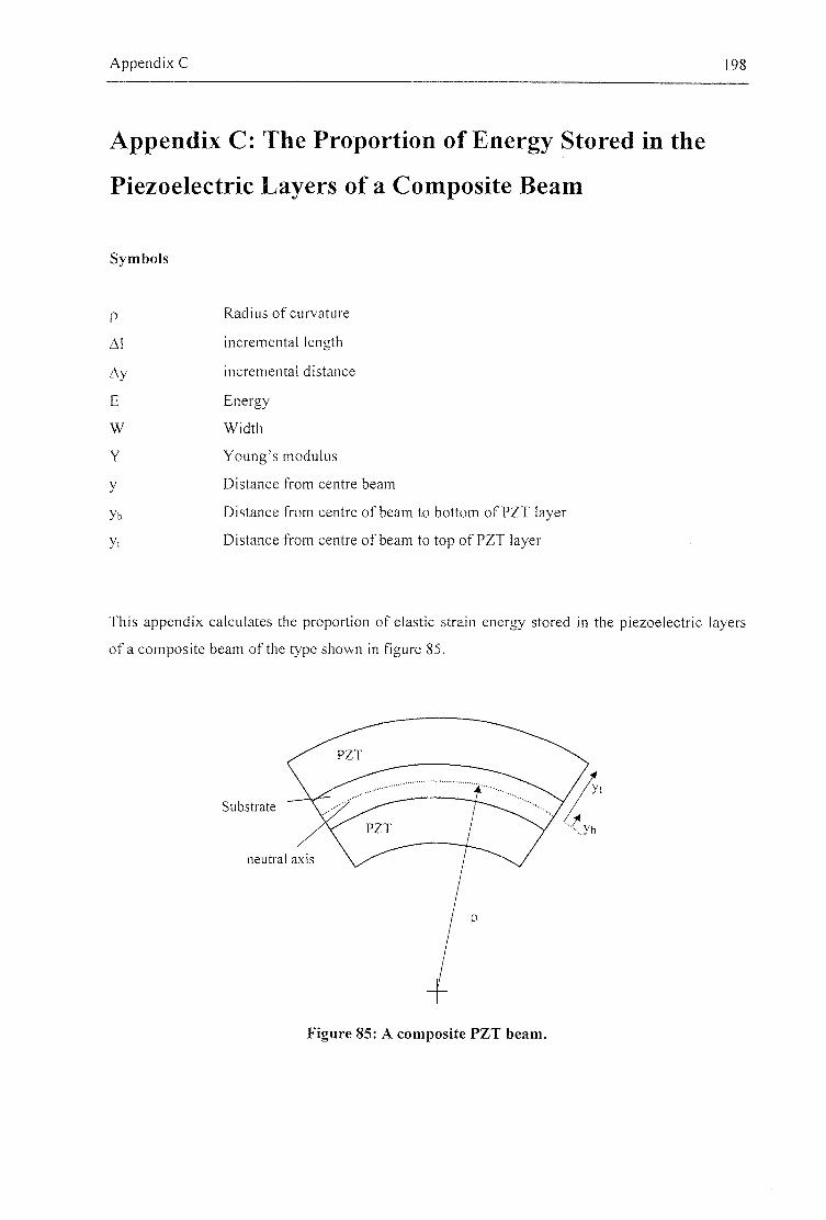
Appendix C 198
Appendix C: The Proportion of Energy Stored in the
Piezoelectric Layers of a Composite Beam
Symbols
P
Al
A y
E
W
Y
y
Yb
y,
Radius of curvature
incremental length
incremental distance
E n e r g y
W i d t h
Young's modulus
Distance from centre beam
Distance from centre of beam to bottom of PZT layer
Distance from centre of beam to top of PZT layer
This appendix calculates the proportion of elastic strain energy stored in the piezoelectric layers
of a composite beam of the type shown in figure 85.
Subs t ra te
neutral axis
Figure 85: A composite P Z T beam.
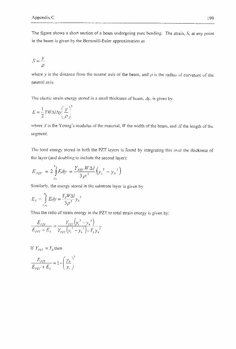
Appendix C 199
The figure shows a short section of a beam undergoing pure bending. The strain, S, at any point
in the beam is given by the Bernoulli-Euier approximation as
p
where is the distance from the neutral axis o f the beam, and is the radius o f curvature o f the
neutral axis.
The elastic strain energy stored in a small thickness of beam, Ay, is given by
.p)
where 7 is the Young's modulus of the material, the width of the beam, and Al the length of the
segment.
The total energy stored in both the PZT layers is found by integrating this over the thickness o f
the layer (and doubling to include the second layer):
= z j J T a y = [ y ' - y / )
Similarly, the energy stored in the substrate layer is given by
E , = 3
Thus the ratio of strain energy in the PZT to total strain energy is given by:
^I'ZT _ '^j'zrjyi ~yh)
If then
Ej,2T + V . / J
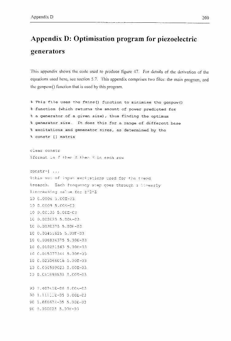
Appendix D 200
Appendix D: Optimisation program for piezoelectric
generators
This appendix shows the code used to produce figure 47. For details of the derivation of the
equations used here, see section 5.7. This appendix comprises two files: the main program, and
the genpow() function that is used by this program.
% This file uses the fmins() function to minimise the genpowO
% function (which returns the amount of power predicted for
% a generator of a given size), thus finding the optimum
% generator size. It does this for a range of different base
% excitations and generator sizes, as determined by the
% constr [] matrix
clear constr
%format is f then Z then H in each row
constr=[ ...
%this set of input excitations used for the trend
%search. Each frequency step goes through a linearly
%increasing value for f^2*Z
10 0.0006 5.00E-03
10 0.0009 5.00E-03
10 0.00135 5.00E-03
10 0.002025 5.00E-03
10 0.0030375 5.00E-03
10 0.00455625 5.00E-03
10 0.006834375 5.00E-03
10 0.010251563 5.00E-03
10 0.015377344 5.00E-03
10 0.023066016 5.00E-03
10 0.034599023 5.00E-03
10 0.051898535 5.00E-03
90 7.40741E-06 5.00E-03
90 l.lllllE-05 5.00E-03
90 1.66667E-05 5.00E-03
90 0.000025 5.00E-03
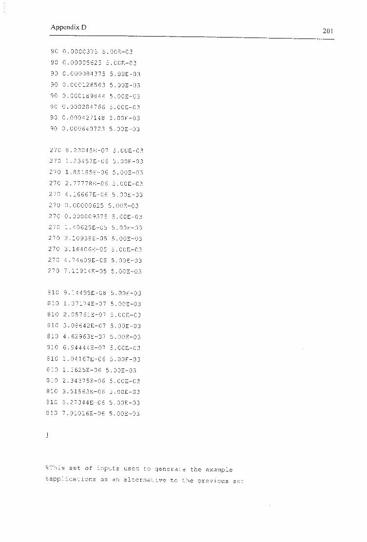
Appendix D
90 0.0000375 5.00E-03
90 0.00005625 5.00E-03
90 0.000084375 5.00E-03
90 0.000126563 5.00E-03
90 0.000189844 5.00E-03
90 0.000284766 5.00E-03
90 0.000427148 5.00E-03
90 0.000640723 S.OOE-03
270 8.23045E-07 5.00E-03
270 1.23457E-06 5.00E-03
270 1.85185E-06 5.00E-03
270 2.77778E-06 5.00E-03
270 4.16667E-06 5.00E-03
270 0.00000625 5.00E-03
270 0.000009375 5.00E-03
270 1.40625E-05 5.00E-03
270 2.10938E-05 5.00E-03
270 3.16406E-05 5.00E-03
270 4.74609E-05 5.00E-03
270 7.11914E-05 5.00E-03
810 9.14495E-08 5.00E-03
810 1.37174E-07 5.00E-03
810 2.05761E-07 5.00E-03
810 3.08642E-07 5.00E-03
810 4.62963E-07 5.00E-03
810 6.94444E-07 5.00E-03
810 1.04167E-06 5.00E-03
810 1.5625E-06 5.00E-03
810 2.34375E-06 5.00E-03
810 3.51563E-06 5.00E-03
810 5.27344E-06 5.00E-03
810 7.91016E-06 5.00E-03
201
&This set of inputs used to generate the example
5cipp^icaLions as an alternative to the previous set
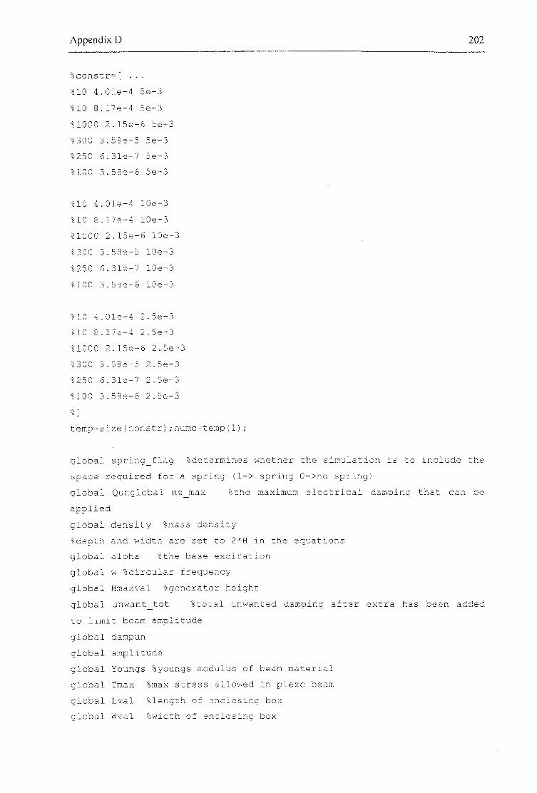
Appendix D 202
%constr=[ ...
%10 4Xn.e-4 5e-3
%10 5e-3
%1000 2.15e-6 5e-3
%300 3.58e-5 5e-3
%250 6.31e-7 5e-3
%100 3.58e-6 5e-3
%10 4.01e-4 lOe-3
%10 8.17e-4 lOe-3
%1000 2.15e-6 lOe-3
%300 3.58e-5 lOe-3
%250 6.31e-7 lOe-3
%100 3.58e-6 lOe-3
%10 4.01e-4 2.5e-3
%10 8.17e-4 2.5e-3
SIOOO 2.15e-6 2.5e-3
%300 3.58e-5 2.5e-3
%250 6.31e-7 2.5e-3
%100 3.58e-6 2.5e-3
%]
temp=size(constr);numc=temp(l);
global spring_flag %determines whether the simulation is to include the
space required for a spring (l-> spring 0->no spring)
global Qunglobal ne_max %the maximum electrical damping that can be
applied
global density %mass density
%depth and width are set to 2*H in the equations
global alpha %the base excitation
global w %circular frequency
global Hmaxval %generator height
global unwant_tot %total unwanted damping after extra has been added
to limit beam amplitude
global dampun
global amplitude
global Youngs %youngs modulus of bezHn material
global Tmax %max stress allowed in piezo beam
global Lval %length of enclosing box
global Wval %width of enclosing box

Appendix D 203
global stress %output: stress in beam
global aflag %stress too big flag.
global afactor %how much correction has been applied to the amplitude
for stress reasons
%determines whether the simulation is to include the space required for
a spring (l-> spring 0->no spring)
spring_flag=l;
%spring_flag=0; %this option used to get the maximum power for any type
of generator
Youngs=75e9;
Tmax=40e6;
Qun=100;
density=8000; %steel density
%three possibilities: (only uncomment one of them)
%ne_max=10000 %this is unlimited to find max for any
%transducer use with 5pring_flag=0
ne_max=0.049 %bulk pztS
%ne_max=4e-4 %thick-film pzt
% max iteration steps in search, minimisation, tolerance [x f(x)]
op(14)=20000;op(l:3)=[0,le-5,le-5];
clear powden hratio damp h hratio flagnum d_un amp lenb power lenratio
disp('Total table entries=');
disp(numc)
for ind=l:numc
%set the parameters corresponding to this step f z h q
w=constr(ind,l)*2*pi;
Hmaxval=constr(ind,3);
Lval=Hmaxval*2;
Wval=Hmaxval*2;
alpha=constr(ind,2);
disp('first try:');
disp(genpow([Hmaxval*0.99,ne_max/200,Lval*0.99]));
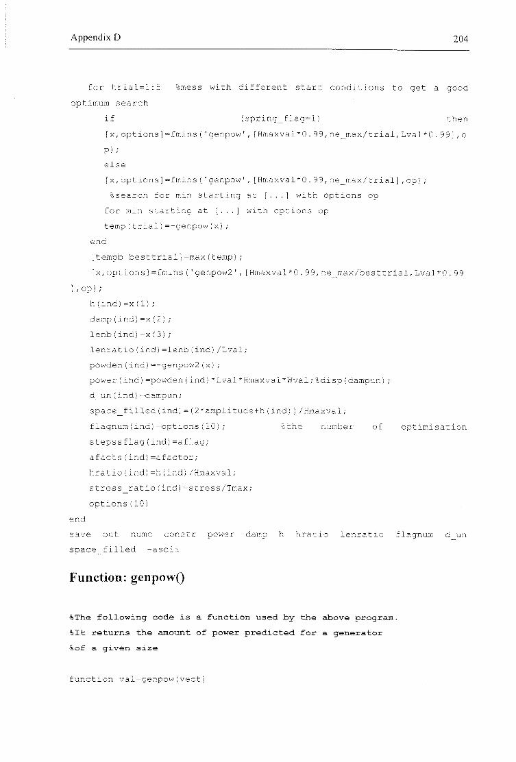
Appendix D 204
for trial=l:5 %mess with different start conditions to get a good
optimum search
if (spring_flag=l) then
[x,options]=fmins('genpow',[Hmaxval*0.99,ne_max/trial,Lval*0.99],o
p);
else
[x,options]=fmins('genpow',[Hmaxval*0.99,ne_max/trial],op);
%search for min starting at [...] with options op
for min starting at [...] with options op
temp(trial)=-genpow(x);
end
[tempb besttrial]=max(temp);
[x,options]=fmins('genpow2',[Hmaxval*0.99,ne_max/besttrial,Lval*0.99
],op);
h(ind)=x(l);
damp(ind)=x(2);
lenb(ind)=x(3);
lenratio(ind)=lenb(ind)/Lval;
powden(ind)=-genpow2(x);
power(ind)=powden(ind)*Lval*Hmaxval*Wval;%di5p(dampun);
d_un(ind)=dampun;
space_filled(ind)=(2*amplitude+h(ind))/Hmaxval;
flagnum(ind)=options(10); %the number of optimisation
stepssflag(ind)=aflag;
afacts(ind)=afactor;
hratio(ind)=h(ind)/Hmaxval;
stress_ratio(ind)=stress/Tmax;
options(10)
end
save out numc constr power damp h hratio lenratio flagnum d_un
space filled -ascii
Function: genpowQ
%Ths following code is a function used by the above program.
%It returns the amount of power predicted for a generator
%of a given size
function val=genpow(vect)
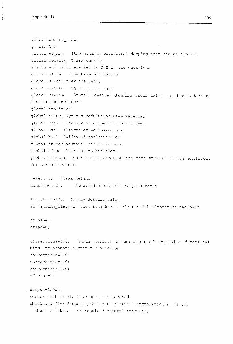
Appendix D 205
global spring_flag;
global Qun
global ne_max %the maximum electrical damping that can be applied
global density %mass density
%depth and width are set to 2*H in the equations
global alpha %the base excitation
global w %circular frequency
global Hmaxval %generator height
global dampun %total unwanted damping after extra has been added to
limit beam amplitude
global amplitude
global Youngs %youngs modulus of beam material
global Tmax %max stress allowed in piezo beam
global Lval %length of enclosing box
global Wval %width of enclosing box
global stress %output: stress in beam
global aflag %stress too big flag.
global afactor %how nmch correction has been applied to the amplitude
for stress reasons
h=vect(l); %beam height
damp=vect(2); %applied electrical damping ratio
length=Lval/2; %dummy default value
if (spring_flag==l) then length=vect(3); end %the length of the beam
stress=0;
aflag=0;
correctiona=1.0; %this permits a smoothing of non-valid functional
bits, to promote a good minimisation
correctionb=1.0;
correctionc=1.0
correctiond=1.0
afactor=l;
dampun=l/Qun;
%check that limits have not been reached
thickness=(4*w*2*density*h*length*3*(Lval-length)/Youngs)^(1/3);
%beam thickness for required natural frequency
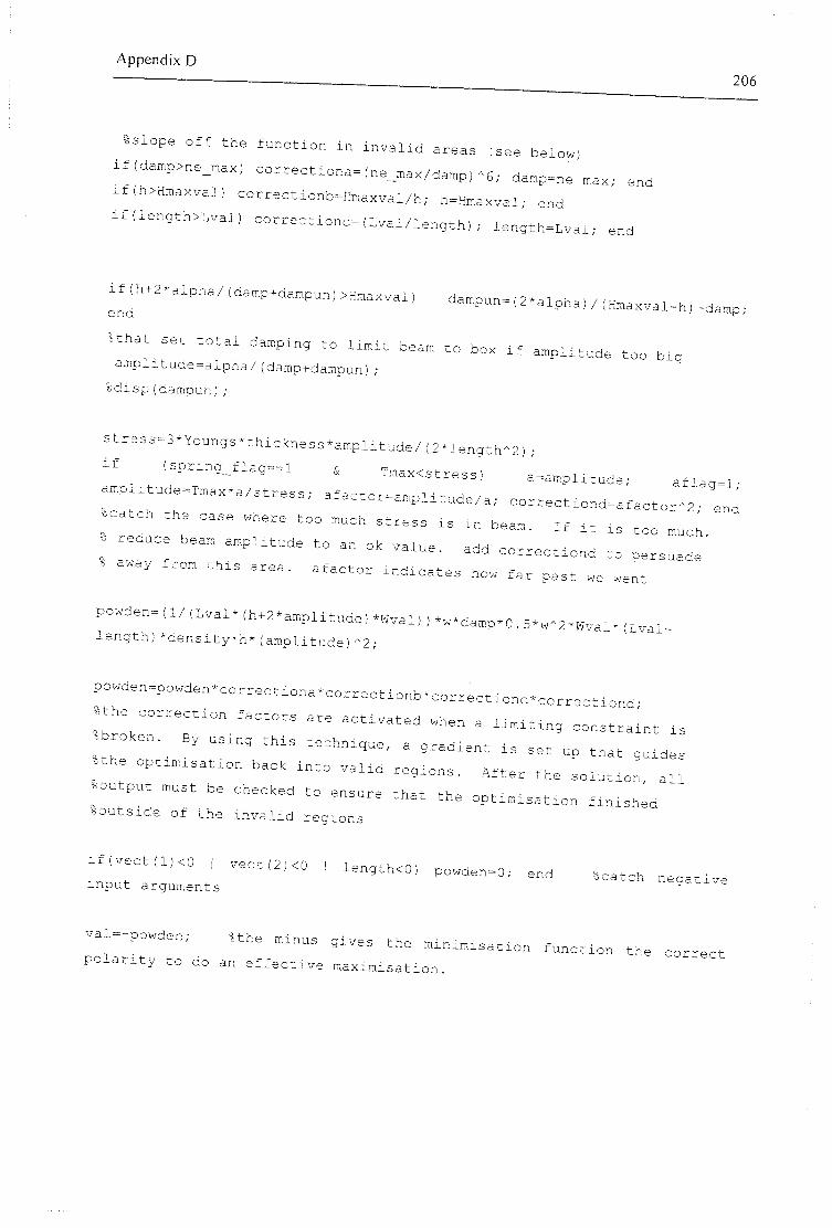
Appendix D
206
%slope off the function in invalid areas (see below)
if(damp>ne_max, correctional(ne_max/damp)^6; damp=ne_max; end
if(h>Hmaxval) correctionb=Hmaxval/h; h^Hmaxval; end
if(length>Lval) correctionc=(Lval/length); length=Lval; end
i , ^ h . 2 . , l p h . / ( c k . p + d . . p u n , ,
%that set total damping to limit beam to box if
amplitude=alp
disp(dampun);
, amplitude too bic amplitude-alpha/(damp+dampun);
stress 3*Youngs+thickness»amplitude/(2*lengfh"2)'
powde„^,l/,Lval-,h+2-a .p l i tude) .w™i,,.„.da„p.0.5.„-2.Bv . i.,Lval^
length)*density*h*(amplitude)*2;
. . u p u t . u . t b . . n , u r . t h a t t h . f i . i . h . d
ooutside of the invalid regions
.r::.:;:;: ..........
Appendix E 207
Appendix E: Phase Locked Loop (PLL) test circuit
This appendix describes the design of the Phase Locked Loop (PLL) circuit used to drive the
electromechanical shaker at the resonant frequency o f the generator beam for the experiments
described in section 7.3.2.2.
Figure 86 shows a block diagram of the arrangement, with each block expanded in the fo l lowing
figures. The circuit comprises a PLL connected in positive feedback to the generator structure.
The positive feedback is designed to operate in a manner similar to the situation found when a
microphone and speaker arrangement produces a feedback whistle. The difference here is that the
PLL produces an output o f f ixed amplitude, so the 'feedback whistle' is o f a controlled amplitude.
To produce positive feedback in the circuit, the PLL is required to lock-on in phase with the input
signal derived from the generator core. To fulfil this requirement, the PLL was built from discrete
components with a phase-detector of the author's own design.
The comparators ICl and [C2 take the sine wave inputs from the coil and VCO, and form them
into a TTL 5 V square wave. Resistors R2, 3, 5 and 6 introduce a small amount of hysteresis. The
high-pass filters formed by RIM and C l / 2 remove any DC component in the inputs. IC4 is set-up
so that it produces a pulse approximately 0.75 o f the period o f the input waveform. The logic
formed by IC4 and IC5 is arranged so that if the output from ICl is in advance of that from [C2
then IC5a will produce short pulses, and if the reverse condition is true then IC5b will produce
short pulses. The output from iC5b is inverted, then summed with that from IC5a and a DC
offset . The resulting signal from IC7 indicates the relative phase o f the two input signals with
s h o r t p o s i t i v e o r n e g a t i v e p u l s e s a b o u t a D C level. Tlie DC level i s u s e d t o i n t r o d u c e a p e r m a n e n t
phase of fset in the circuit which can be adjusted to compensate for any phase leads or lags in the
remainder o f t h e positive feedback loop. A A e r t h e s i g n a l i s s m o o t h e d b y t h e l o o p - f i l t e r , k p a s s e s
into the V C O block. The output from the loop-filter is summed in [C9 with a DC offset that
determines the center frequency o f t h e oscillator. I C I O i s a V C O chip that produces the sine wave
required to c lose the P L L loop.
To set-up the circuit it may be necessary to experiment with the polarity o f the generator coil so
that Its output IS m-phase with the signal supplied to the shaker. To achieve correct c losed loop
performance from the PLL care must be taken with which o f the phase detector inputs is
connected to the VCO. Operating with a generator with a resonant frequency o f l 0 5 H z , the
circuit was found to achieve a resonant lock over a centre frequency range o f ±25Hz. Lock time
(t ime for the outer positive feedback loop to produce 90% o f final beam amplitude) was around
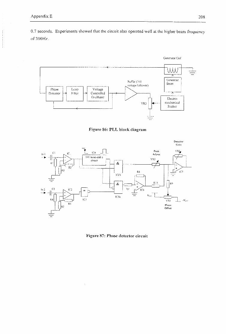
Appendix E 208
0.7 seconds. Experiments showed that the circuit also operated well at the higher beam frequency
o f 3 0 0 H z .
Generator Coil
P h a s e
D e t e c t o r
L o o p
Fi l ter
V o l t a g e
C o n t r o l l e d
Osc i l l a to r
Buffer (741 voltage follower)
VR3
Generator
Beam
1
Elec t ro -
S h a k e r
F i g u r e 86: P L L b l o c k d i a g r a m
In 2
Detector Cam
VR2 Peak Adjust
VR3
IC4 ICI
IC7
RIO
R7 IC2 IC6
IC5a R4 IC3 VRI
Phase Offset
F i g u r e 87: P h a s e d e t e c t o r c ircui t
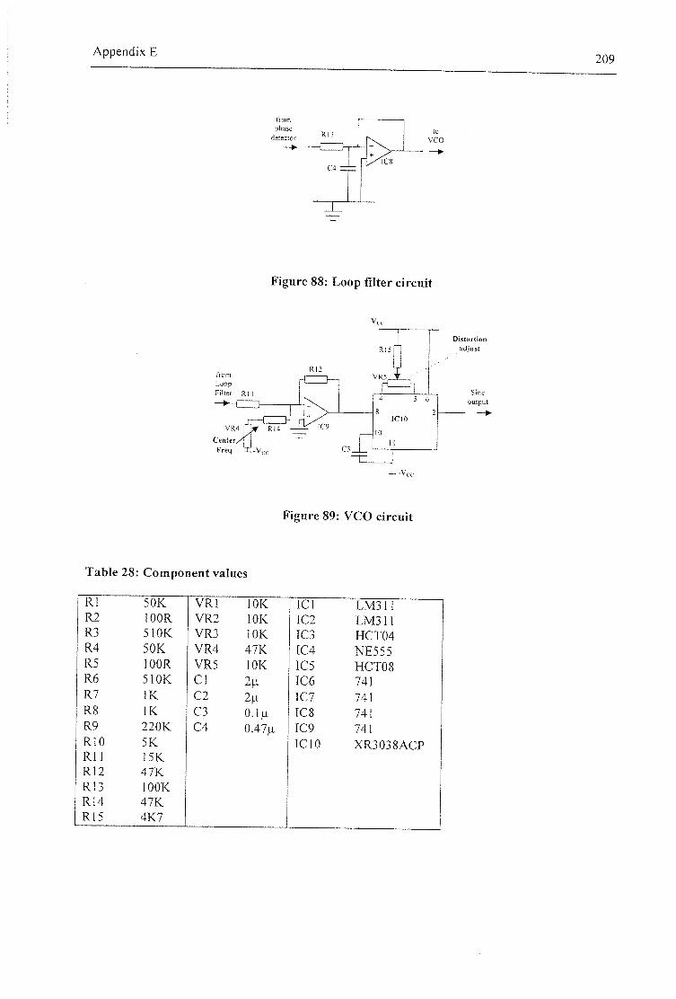
Appendix E 2 0 9
from phaw
detector R|j
C4
to VCO
nC8
Figure 88: L o o p filter c ircui t
Distortion
output
* ^4 Center
from Loop FHwr R |
T a b l e 28 : C o m p o n e n t v a l u e s
F i g u r e 89: V C O c ircu i t
R1 5 0 K V R l lOK ICl L&43II R 2 lOOR V R 2 lOK IC2 L M 3 1 1 R3 SIOK VR3 lOK IC3 H C T 0 4 R4 5 0 K V R 4 4 7 K [C4 1VE555 R5 lOOR V R 5 lOK IC5 H C T 0 8 R6 5 1 0 K CI IC6 741 R7 IK C2 2H IC7 741 R8 IK C3 O J ^ ICS 741 R9 2 2 0 K C4 0 . 4 7 ^ IC9 741 RIO 5 K ICIO X R 3 0 3 8 A C P R l l I5K R 1 2 4 7 K
R13 lOOK R I 4 4 7 K R15 4 K 7
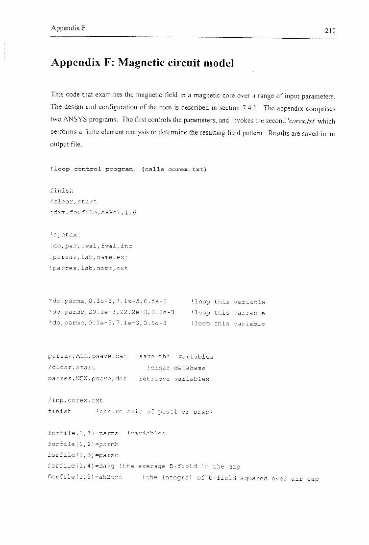
A p p e n d i x F 210
Appendix F: Magnetic circuit model
This code that examines the magnet ic f ield in a magne t ic core over a range of input parameters .
The design and configuration o f the core is described in section 7.4.1. The appendix comprises
two A N S Y S programs. The first controls the parameters, and invokes the second 'coz-ez./Air' which
performs a finite element analysis to determine the resulting field pattern. Results are saved in an
output f i le.
!loop control program: (calls corex.txt)
finish
/ c l e a r , s t a r t
* d i m , f o r f i l e , A R R A Y , 1 , 6
! s y n t a x :
! d o , p a r , i v a l , f v a l , i n c
! p a r s a v , l a b , n a m e , e x t
! p a r r e s , l a b , n a m e , e x t
*do,parma,0.1e-3,7.1e-3,0.5e-3
*do,parmb,20.1e-3,22.2e-3,0.3e-3
*do,parmc,0.1e-3,7.1e-3,0.5e-3
loop this variable
loop this variable
loop this variable
parsav,ALL,psave,dat Isave the variables
/clear,start !clear database
parres,NEW,psave,dat !retrieve variables
/inp,corex,txt
finish 'ensure exit of postl or prep7
forfile(l,l)=parma Ivariables
forfile(1,2)=parmb
forfile(l,3)=parmc
forfile(l,4)=Bavg !the average B-field in the gap
forfile(l,5)=ab2tot Ithe integral of b-field squared over air gap

Appendix F 211
forfile(l,6)=ab2tot2 Ithe integral of b-field squared over all air-
regions
/com,done
/out,magresS,dak,/APPEND
! write the contents of the forfile results array to file the (...) line-
is a format string
IformaT (prepointFspace.afterpoint) (4F10.5) works!
*vwrite,forfile(1,1)
(4E10.5)
*vwrite,forfile(1,2)
(4E10.5)
*vwrite,forfile(1,3)
(4E10.5)
*vwrite,forfile(1,4)
(4E10.5)
*vwrite,forfile(1,5)
(4E10.5)
*vwrite,forfile(1,6)
(4E10.5)
/com delimiter,
/out
*enddo
*enddo
*enddo
Batch File: corex.txt
!receives model parameters parma,parmb,parmc and returns magnetic field
Ithis file takes parameters parma,parmb,parmc and feeds then into
! g (gap), lc( length of core) and Im (length of magnet)
! tm is fixed at lOe-3. The core is kept thick, to avoid any saturation
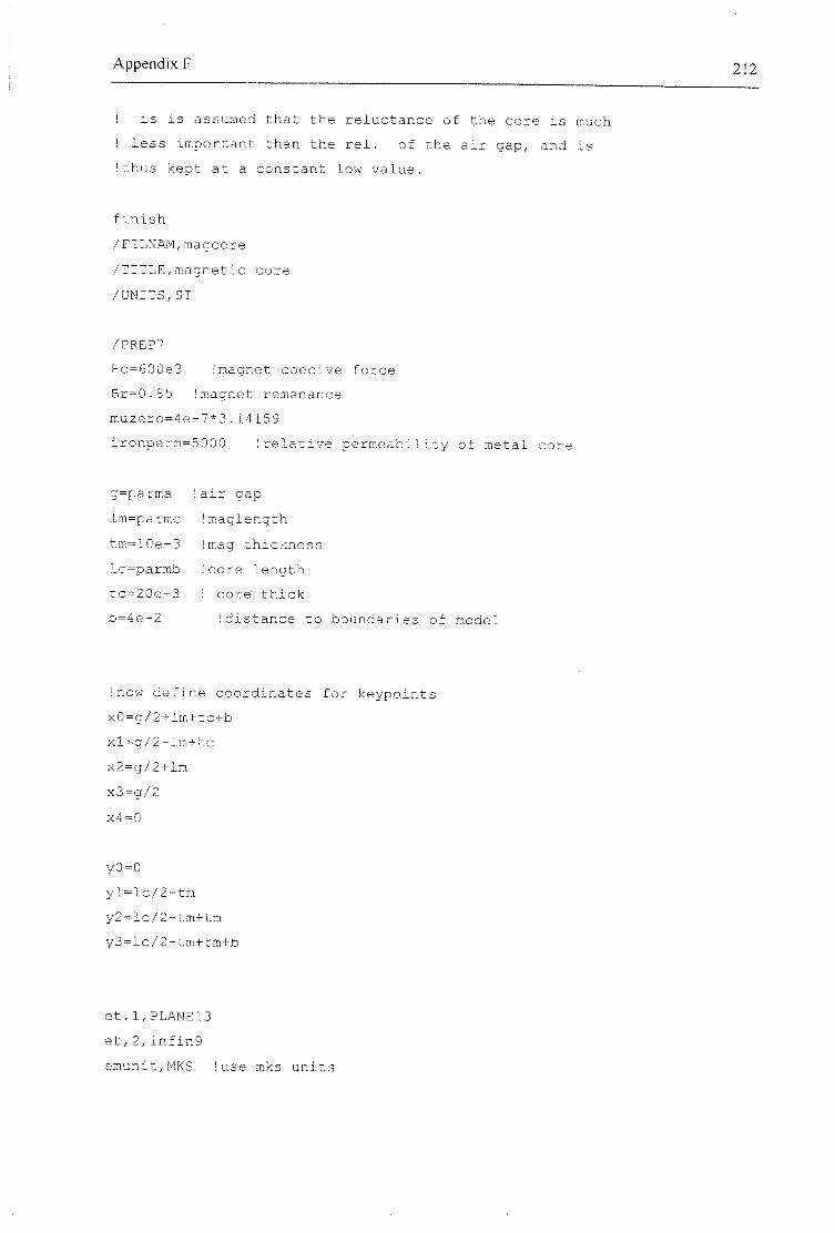
Appendix F 212
I is is assumed that the reluctance of the core is much
! less important than the rel. of the air gap, and is
Ithus kept at a constant low value.
finish
/FILNAM,magcore
/TITLE,magnetic core
/UNITS,SI
/PREP7
Hc=600e3 Imagnet coecive force
Br=0.85 Imagnet remenance
muzero=4e-7*3.14159
ironperm=5000 'relative permeability of metal core
g=parma
lm=parmc
tm=10e-3
lc=parmb
tc=20e-3
b=4e-2
air gap
maglength
mag thickness
core length
core thick
'distance to boundaries of model
!now define coordinates for keypoints
xO=g/2+lm+tc+b
xl=g/2+lm+tc
x2=g/2+lm
x3=g/2
x4=0
y0=0
yl=lc/2-tm
y2=lc/2-tm+tm
y3=lc/2-tm+tm+b
et,l,PLANE13
et,2,infin9
emunit,MKS !use mks units
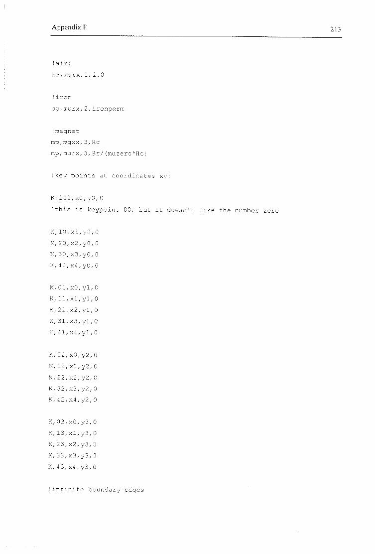
Appendix F 213
! air:
MP,murx,1,1.0
'iron
mp,murx,2,ironperm
Imagnet
mp,mgxx,3,Hc
mp,murx,3,Br/(muzero*Hc)
!key points at coordinates xy:
K,100,x0,y0,0
'this is keypoint 00, but it doesn't like the number zero
K,10,xl,y0,0
K,20,x2,y0,0
K,30,x3,y0,0
K,40,x4,y0,0
K,01,x0,yl,0
K,ll,xl,yl,0
K,21,x2,yl,0
K, 31,x3,yl,0
K, 41,x4,yl,0
K,02,x0,y2,0
K, 12,xl,y2,0
K,22,x2,y2,0
K,32,x3,y2,0
K, 42,x4,y2,0
K, 03,x0,y3,0
K, 13,xl,y3,0
K,23,x2,y3,0
K, 33,x3,y3,0
K,43,x4,y3,0
!infinite boundary edges
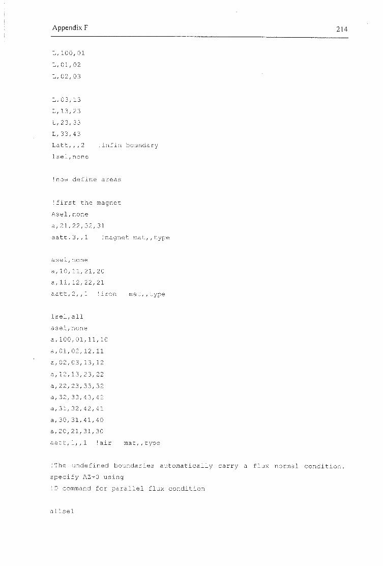
Appendix F 214
L, 100,01
L,01,02
L,02,03
L,03,13
L,13,23
L,23,33
L,33,43
Latt,,,2 linfin boundary
lsel,none
!now define areas
!first the magnet
Asel,none
a,21,22,32,31
aatt,3,,l 'magnet mat,,type
asel,none
3,10,11,21,20
a,11,12,22,21
aatt,2,,l 'iron mat,,type
Isel,all
asel,none
a,100,01,11,10
a,01,02,12,11
a,02,03,13,12
a,12,13,23,22
a,22,23,33,32
a,32,33,43,42
a,31,32,42,41
a,30,31,41,40
a,20,21,31,30
aatt,l,,l lair mat,,type
MThe undefined boundaries automatically carry a flux normal condition,
specify AZ=0 using
ID command for parallel flux condition
allsel
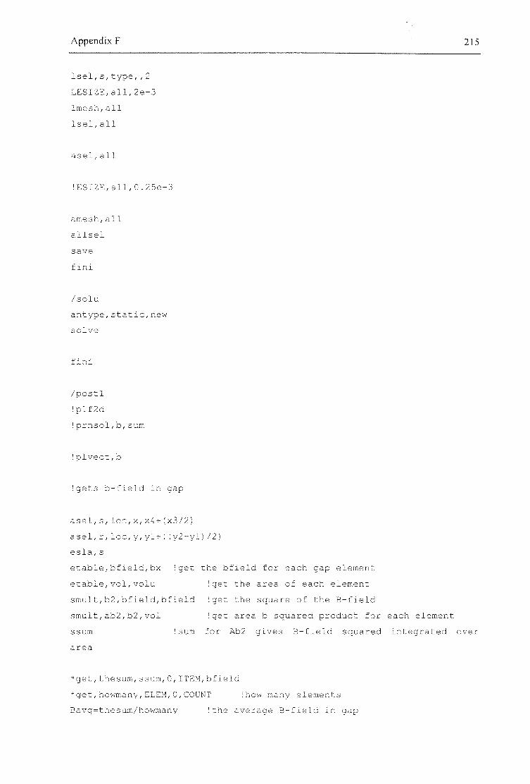
Appendix F 215
lsel,s,type,,2
LESIZE,all,2e-3
lmesh,all
Isel,all
asel,all
!ESIZE,all,0.25e-3
amesh,all
allsel
save
f ini
/solu
antype,static,new
solve
f ini
/postl
!plf2d
!prnsol,b,sum
!plvect,b
Igets b-field in gap
asel,s,loc,x,x4+(x3/2)
asel,r,loc,y,yl+((y2-yl)/2)
esla,s
etable,bfield,bx Iget the bfield for each gap element
etable,vol,volu Iget the area of each element
smult,b2,bfield,bfield Iget the square of the B-field
smult,ab2,b2,vol Iget area b squared product for each element
ssimi hsim for ZU32 gives B-field squared integrated over
3. xTG a.
*get,thesum,ssum,0,ITEM,bfield
*get,howmany,ELEM,0,COUNT I how many elements
Bavg=thesum/howmany I the average B-field in gap
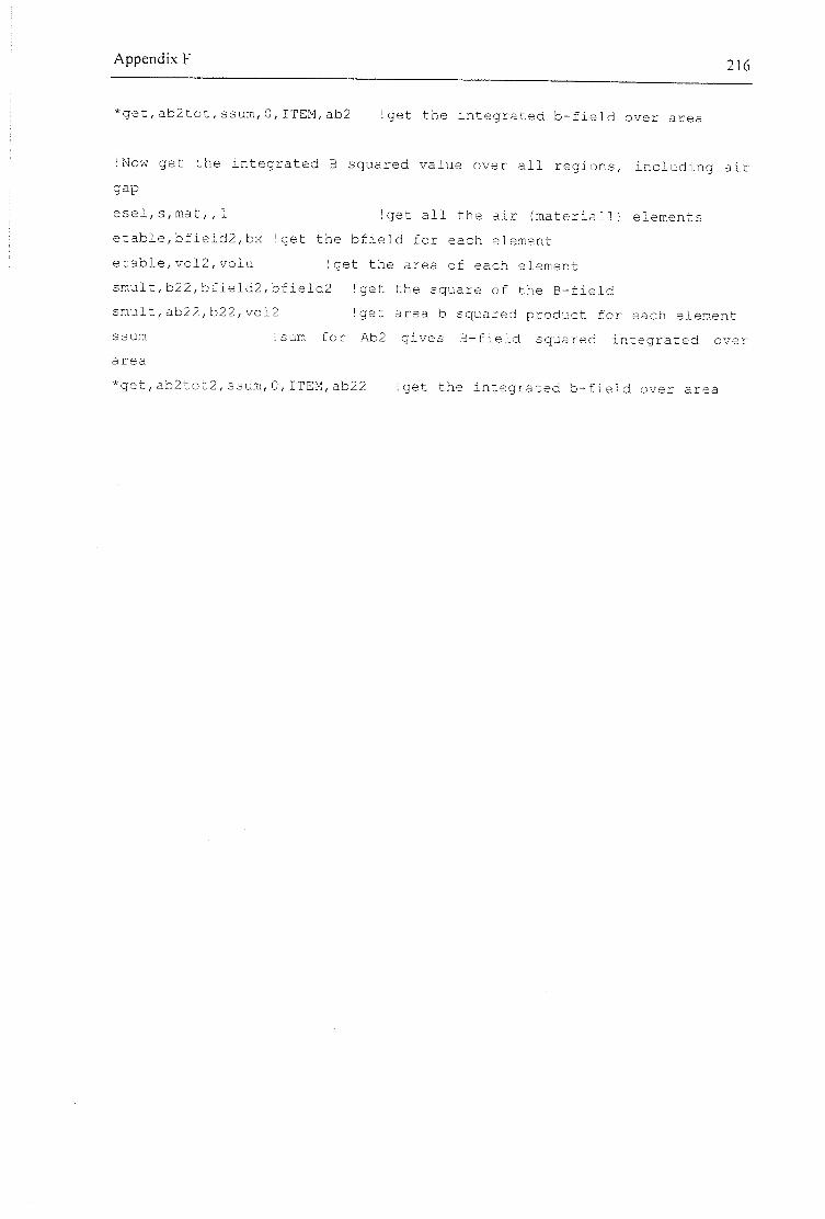
Appendix F 216
*get,ab2tot,ssum,0,ITEM,ab2 !get the integrated b-field over area
MNow get the integrated B squared value over all regions, including air
gap
esel,s,mat,,l !get all the air (materiall) elements
etable,bfield2,bx !get the bfield for each element
etable,vol2,volu I get the area of each element
smult,b22,bfield2,bfield2 !get the square of the B-field
smult,ab22,b22,vol2 I get area b squared product for each element
ssum Isum for fU]2 gives B-field squared integrated over
area
*get,ab2tot2,ssum,0,ITEM,ab22 !get the integrated b-field over area
A p p e n d i x G 217
Appendix G: Optimisation program for magnet-coil
generators
This appendix shows the code used to produce the magnet-coil data for figure 83. It implements
the equations derived in section 7.4.3 to optimise the horizontal-coil model described there. This
appendix comprises three flies: the main program, the coi lpow() function that is used by the main
program, and finally a program to calculate the space required in each generator for a planar
spring. At the end of the appendix a set o f graphs shows the internal dimensions that correspond
to the magnet-coil data.
% This file uses the fmins() function to minimise the coilopt()
% function (which returns the amount of power predicted for
% a generator of a given size), thus finding the optimum
% generator size. It does this for a range of different base
% excitations and generator sizes, as determined by the
% constr [] matrix
clear constr
% format f Z H Qunwnat
%this matrix is the set of input excitations that are examined
%see Appendix D for the excitations used in the trend search.
constr=[ ...
10 4.01e-4 5e-3 100
10 8.17e-4 5e-3 100
1000 2.15e-6 5e-3 100
300 3.58e-5 5e-3 100
250 6.31e-7 5e-3 100
100 3.58e-6 5e-3 100
10 4.01e-4 lOe-3 100
10 8.17e-4 lOe-3 100
1000 2.15e-6 lOe-3 100
300 3.58e-5 lOe-3 100
250 6.31e-7 lOe-3 100
100 3.58e-6 lOe-3 100
10 4.01e-4 2.5e-3 100
Appendix G 218
10 8.17e-4 2.5e-3 100
1000 2.15e-6 2.5e-3 100
300 3.58e-5 2.5e-3 100
250 6.31e-7 2.5e-3 100
100 3.58e-6 2.5e-3 100
temp=size(con5tr);
numc=temp(1);
:lear Abest
global invQun
global g_ratio dens B2 rho
global pow_5ub flags Abest
global Z f Hmaxval
global K1 K5 K2 pi4
global Abest lam
pi4=pi/4;
g_ratio=0.195/(0.195+0.71); %magnetic gap as proportion of total width
dens=8000; %density of coil
82=0.04 91*0.71/0.195; Sis psi * Wopt/gopt %value of 8*2 in gap
rho=1.69e-8; %resistivity of copper
8 =sqrt(B2);
% max iteration steps in search, minimisation, tolerance [x f(x)]
op(14)^1000;
op(1:3)=[0,le-4,0.00001];
clear powres flagnum lenc Resload flagop lambda Voltload powcube
Qfact
disp('Total table entries=');
disp(numc)
for ind=l:numc
Appendix G 219
ind
%set the parameters corresponding to this step f z h q
w=constr(ind,l)*2*pi;
Hmaxval=constr(ind,3);
Z=^onstr(ind,2);
invQun=l/constr(ind,4);
%partial calculations
Kl=pi*g_ratio*dens*w/(2*B2);
K5=w"2/(2*pi);
K2=Z*Kl+7/pi;
Itrial^Hmaxval; %find a value oflenc that lies in the non-
zero solution set
ptrial=0;
while (ptrial==0 & ltrial>le-10)
ltrial=ltrial/2;
ptrial=coilpow2([ltrial 1]);
end
[x,options]=fmins('coilpow',[0.9*Hmaxval,3],op); %search for
min starting at [...] with options op
lenc(ind)=x(l);
Resload(ind)=x(2};
powres(ind)=-coilpow2(x);
flagnum(ind)=options(10); %the number of optimisation steps
flagop(ind)=flags; %records which t )e of root was found in
coilpowl
Amp(ind)=Abest;
lambda{ind)=lam;
options(10)
end
Appendix G 220
for i=l:numc
powcube(i)=powres(i)*constr(i,3)^2; %calculate the power that
would be generated from a cube of side H
Voltload(i)=Resload(i)/(l+Resload(i))*B_*(constr(i,3)-
2*Amp(i))*2*pi*constr(i,l)*Amp(i};
%Voltload(i,ifk)=Resload(i,j,k)/(l+Resload(i,i,k))*B_*wrange(i)*Amp(i,i,
k) ;
Qfact(i)=Amp(i)/constr(i,2);
end
save out TKHnc constr powres flagnum lenc Resload lambda Voltload
powcube Qfact -ascii
Function: coilpowQ
%The following code is a function used by the above program.
%It returns the amount of power predicted for a generator
%of a given size
function val=coilpowl(vect)
if (size(vect)-=2) error('minim: wrong number of parameters: need
(l,h)'); end
lc=:vect(l);
r=vect(2);
global rl r2 vail val2
global invQun %this is 1/Qunwanted
global g_ratio dens B2 rho
global pow_sub flags Abest
global Z w Hmaxval
global K1 K5 K2 pi4
global Abest lam

Appendix G 221
K3=2*rho*lc/g_ratio;
Aregion=4 *lc/7;
%K4=K2*Aregion;
pi71c=pi*lc/7;
Rl=(2*rho*lc/(g_ratio))*r;
K8=pi/(K1*(K3+Rl));
pl=[K8/7 invQun -Z]; %the polynomial for lc/A<(7/4)
p2=[K8/(4*lc) 0 invQun -Z]; % the > region
rl=roots(pl); %rl has two roots
r2=roots(p2); %r2 has 3 roots
vall=rl>Aregion; %these tell us wheteher the roots (assuming they are
real) are in valid ranges
val2=r2<Aregion;
%the following will find the root with the largest amplitude
%ie it returns root for pi first if they are real and valid
%Justification: the optimum design is expected to lie on the larger of
any two possibilities - trying to return more than
%one root would confuse the optimisation routine.
A ^ ^ s t = 0 ;
lam=0;
if (isreal(rl))
if (vall(l) & vail(2)) Abest=max(rl); flags=l; end
if (vall(l) & -vail(2)) Abest=rl(l); flags=2; end
if (-vall(l) & vail(2)) Abest=rl(2); flags=3; end
if (Abest>0) Iam=pi71c/Abest; end
end
if (Abest==0) %if no good roots yet....
if (val2(l) & isreal(r2(l))) Abest=r2(l); flags=4; end
if (val2(2) & isreal(r2(2)) & r2(2)>Abest) flags=5; Abest=r2(2); end
if (val2(3) & isreal(r2(3)) & r2(3)>Abest) flags^G; Abest=r2(3); end
lam=pi4;
end

Appendix G 222
if (Abest==0) %if no good roots yet....
flags=7;
end
if (2*Abest+lc>Hmaxval) Abest=(Hmaxval-lc)/2; end %does the amplitude
exceed allowed space?
power=Rl/((Rl+K3)*2)*K5*4*B2*Abest^4*lam; %calculates Power/(T*W)
% if (2*Abest+lc>Hmaxval) power=0; %does the amplitude exceed allowed
space?
% else power=Rl/((Rl+K3)^2)*K5*4*B2*Abest*4*lam; %calculates
Power/(T*W)
% end
if(vect(l)<0 I vect(2)<0) power=0; end %catch negative input
arguments
val^^power; %the minus gives the minimisation function the correct
polarity
Program: beamsize.m
% This file has output data from the previous program built
%into its input data. It calculates the proportion of the
%enclosure length that is required to form a planar spring
%finds minimum straight beam length for Sm constraints . See logS pp.
Ill
%constants
%GMlOO
E=2.1E11
Sm=4.2E8
Density=8000
beta=0.5
Appendix G 223
%inputdata
HG=[5.00E-03 5.00E-03 5.00E-03 5.00E-03 5.00E-03 5.00E-03 l.OOE-02
l.OOE-02 l.OOE-02 l.OOE-02 l.OOE-02 l.OOE-02 2.50E-03 2.50E-03 2.50E-03
2.50E-03 2.50E-03 2.50E-03]; %generator enclosure height
L=2*HG; %generator enclosure length
fn=[1.00E+01 l.OOE+01 l.OOE+03 3.00E+02 2.50E+02 l.OOE+02 l.OOE+01
l.OOE+01 l.OOE+03 3.00E+02 2.50E+02 l.OOE+02 l.OOE+01 l.OOE+01 l.OOE+03
3.00E+02 2.50E+02 l.OOE+02];
wn=2*pi*fn;
%the frequencies of each data set
Ampl=[1.48E-03 1.62E-03 1.79E-04 1.4 6E-03 5.26E-05 2.98E-04 2.72E-03
2.96E-03 1.79E-04 2.26E-03 5.26E-05 2.98E-04 8.06E-04 8.88E-04 1.79E-04
8.76E-04 5.26E-05 2.77E-04];
%the beam amplitude
HC=[2.05E-03 1.77E-03 5.31E-04 2.09E-03 3.11E-04 2.79E-03 4.55E-03
4.08E-03 5.31E-04 5.48E-03 3.11E-04 2.79E-03 8.88E-04 7.24E-04 5.31E-04
7.48E-04 3.11E-04 1.95E-03];
%the core height Ic
numdataitems=18
for i=l:numdataitems
A(i)=27*(Ampl(i))"3*E*2+HC(i)*Density*beta*(wn(i))*2/(2*&m^3);
poly(i,:)=[l 0 A(i) -A(i)*L(i)];
solns(:,i)=roots(poly(i,:));
end
%solves the equation for spring length Is from equation given in
%main text
propn=solns(3,:)./L
save out.txt propn -ascii
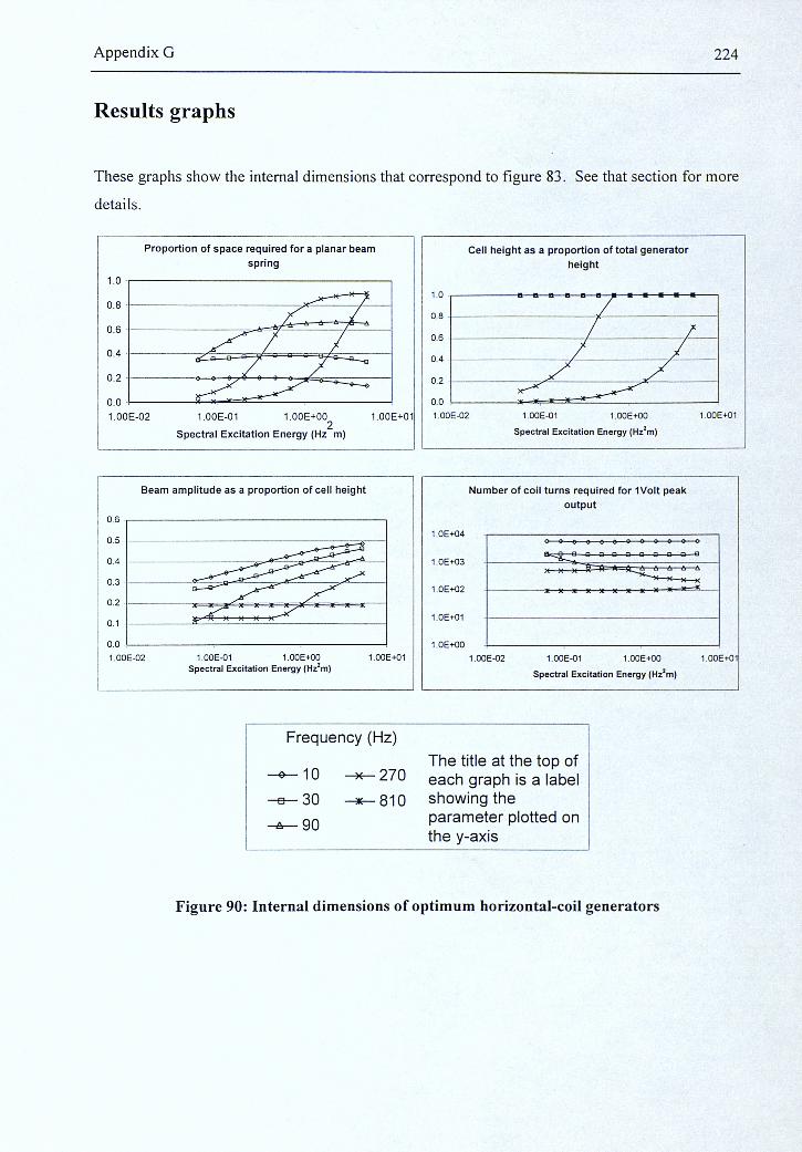
Appendix G 224
Results graphs
These graphs show the internal dimensions that correspond to figure 83. See that section for more
details.
Proportion of space required for a planar beam spring
1.0
0.8
0.6
0.4
0.2
0.0
1.00E-02 1.00E-01 140E+00 1.00E+01
Spectral Excitation Energy (Hz m)
Cell height as a proportion of total generator height
0.6
0.4
0.2
I.OOE^ 1.00E-01 1.00E+00
Spectral Excitation Energy (Hz^m)
1,006+01
Beam amplitude as a proportion of cell height
1.00E^2 1.00E-01 1.00E+00 1.00E+01 Spectral Excitation Energy (Hz^m)
Number of coil turns required for 1Volt peak output
l.OE+04
1.0E+03
1.0E+02
1.0E+01
1.0E+00 1 .OOE-02 1 .OGE-01 1 .OOE+00 1.00E+01
Spectral Excitation Energy (Hz^m)
Frequency (Hz)
The title at the top of 270 each graph is a label
- a — 3 0 -4*— 8 1 0 showing the parameter plotted on the y-axis
-A—90
Figure 90: Internal dimensions of optimum horizontal-coil generators
References 225
References
[1] A home page for the company Perrelet 1777:
http://vvww.perrelet.com.au/
[2] '07 / .Ewrojgmof.y vYF and the Tm/.
2000 both had sessions devoted to self-powered devices.
[3] C. B. Williams and R. B. Yates, Analysis of a micro-electric generator for microsystems",
52, No.1-3, pp.8-11, 1996.
[4] C. B. Williams, A. Pavic, R. S. Crouch, and R. C. Wood, "Feasibility study of vibration-
electric generator for bridge vibration sensors", 7677 /W. CoA^,
Vol 3243, p p l U 1-1117, 1998,
[5] C, Shearwood and R. B. Yates, "Development of a Resonant Electromagnetic Micro-
Generator", .E/gc/ron/c Vol.33, No.22, pp.1883-1884, 1997.
[6] W. J. Li, Z. Wen, P. K. Wong, G. M. H. Chan, and P. H. W. Leong, "A micromachined
vibration-induced power generator for low power sensors of robotic systems",
CoMgrg.yj.- om 7(o6o^fc.y M/fYAvi/yZ/caf/om, June 16-21, Hawaii, USA,
2000.
[7] R. Amirtharajah and A. P. Chandrakasan, "Self-powered signal processing using vibration-
based power generation", Vol 33, No 5pp 687-695, 1998.
[8] M. Umeda, K. Nakamura, and S. Ueha, "Energy storage characteristics of a piezo-generator
using impact induced vibration", J f Vol 36, pp. 3146-3151, 1997.
[9] Personal communications with Manabu Aoyagi, May 2000.
[10] M. Hayakawa, E/gc/roMzc WMnvafc/z mYAggmgrn/or, United States Patent, number 5001685,
March 19th, 1991.

References 226
[11] P. B. Koeneman, H. J. Busch-Vishniac, K. L. Wood, "Feasibility of Micro Power Supplies
for MEMS", Journal of Microelectromechanical Systems, Vol 6, No 4, pp 355-362, 1997.
[12] M. J. Konak, 1. G. Powlesland, S. P. van der Velden, and S. C. Galea, "A Self-Powered
Discrete Time Piezoelectric Vibration Damper", Smart Materials Structures & Integrated
Systems, Vol 3241, pp 270-279, 1997.
[13] T. Starner, "Human Powered Wearable Computing", IBM System J., Vol 35 [3&4, pp 618-
29], 1996.
[14] Shi-Hiu Chen, Dynamoelectric shoes. United States Patent, number 5495682, March 5th,
1996.
[15] N. Lakie, Inflatable boot liner with electrical generator and heater. United States Patent,
number 4845338, July 4th, 1989.
[16] J. Kymissis, C. Kendall, J. Paradiso, and N. Gershenfeld, "Parasitic Power Harvesting in
Shoes", 2nd Int. Symp. Wearable Computers, Digest of Papers, Ch. 28 pp. 132-139, 1998.
[17] E. Hausler and L. Stein, "Implantable Physiological Power Supply with PVDF Film",
Ferroelectrics, Vol, 60, pp.277-282, 1984.
[18] A page dedicated to Trevor Baylis supported by the company "Innovative Technologies" :
http://windupradio.com/bavlis.htm
[19] D. Segal, I. Bran sky, "Testing of a piezoelectric generator for in-flight electrical powering of
projectile guidance systems", Ferroelectrics, Vol 202, pp.81-85, 1997.
[20] J. B. Lee, Z. Chen, M. G. Allen, A. Rohatgi, and R. Arya, "A Miniturized High-Voltage
Solar Cell Array as an Electrostatic MEMS Power Supply", Journal of Microelectromechanical
Systems, Vol. 4 No. 3, pp 102-108, 1995.
[21] A. C. van der Woerd, M. A. Bais, L. P. de Jong, and A. van Roermund, "A highly efficient
micro-power converter between a solar cell and a rechargeable lithium-ion battery", SPIE
Conference on Smart Electronics and MEMS, Vol 3328, pp. 315-325, 1998.
References 227
[22] J.N. Ross, "Optical power for sensor interfaces", Meas. Sci. Technol. Vol 3, pp 651-655,
1992.
[23] W. Kuntz and R. Mores, "Electrically Insulated Smart Sensors: Principles for Operation and
Supply", 25-27, pp 497-505, 1991.
[24] W. Gross, "Optical Power Supply for Fibre-optic Hybrid Sensors", /(,
Vol 25-27, pp. 475-480, 1991.
[25] M. R, Al-Mohanadi, J. N. Ross, and J. E. Brignell, "Optical power and intelligent sensors",
60, pp 142-146, 1997.
[26] T. Renner, G. Rittmayer, D. Falkenberg, and G. Grubmuller, "An Isotropic Thermoelectric
Battery for Cardiac Pacemakers", q / fAg /m/erMar/oMa/ OM fowe/-
Radioisotopes, Madrid, pp.207-216, 1972.
[27] Personal communications with Wolfgang K. Scheibelhofer (cardiologist in Vienna, Austria),
03 February 1999.
[28] M. Stordeur and I. Stark, "Low Power Thermoelectric Generator - self sufficient energy
supply for micro systems", fz-oc. /CZ'PZ Z&A W. TTze/'/Mog/gc/r/c.y, pp 575-577, 1997.
[29] Texas Instruments TIKIS homepage: http://www.ti.com/mc/docs/tiris/docs/index.htm
[30] U. Kaiser, W. Steinhagen, "A Low Power Transponder IC for High-Performance
Identification Systems", / E f E Vol. 30 No. 3, 1995.
[31] D. Friedman, H. Heinrich, and D-W. Duan, "A Low-Power CMOS Integrated Circuit for
Field-Powered Radio Frequency Identification Tags", IEEE International Solid-State Circuits
Conference, pp. 294-295, 1997.
[32] Department of cybernetics, Reading university:
http://www.cvber.rdg.ac .Uk/K.Warwick/WWW/fpage.htm
References 228
[33] J. Bouvier, Y. Thorigne, S. Abou Hassan, M.J. Revillet, and P. Senn, "A Smart Card CMOS
Circuit with Magnetic Power and Communications Interface", IEEE International Solid-State
Circuits Conference, pp. 296-297, 1997.
[34] H. Matsuki, M Yamaguchi, T. Watanabe, K. Murakami, K. Nadehara, and T. Yamamoto,
"Implantable transformer for an artificial heart utilizing amorphous magnetic fibres", J. Appl.
f Vol 64 (10), pp. 5859-5861, 1988.
[35] Ultralife Batteries Inc., product data sheet:
http://www.ultralifebatteries.com/
[36] J.B. Bates, G.R. Gruzalski, and C.F. Luck, "Rechargeable Solid State Lithium
Microbatteries", Proc. IEEE Micro Electro Mechanical Syst. Workshop, pp. 82-86, 1993.
[37] N. M. White and J. E. Brignell, Institute of Physics Publishing,
[38] K. S. J. Pister, J. M. fCahn, and B. E. Boser, "Smart Dust: Wireless Networks of Millimeter-
Scale Sensor Nodes", jy/gA/zgA/ /Irnc/e 7999
Summary, 1999.
[39] P. B. Chu, N. R. Lo, E. C. Berg, and K. S. J. Pister, "Optical Communication Using Micro
Corner Cube Reflectors", froc . MEMS' fFbrA:$Aop, Nagoya, Japan, pp. 350-355, 1997.
[40] G. Asada, M. Dong, T. S. Lin, F. Newberg, G. Pottie, W. J. Kaiser, and H. O. Marcy,
"Wireless Integrated Network Sensors: Low Power Systems on a Chip.", Proceedings of the 1998
EwrqpeaM 5'o/zW Aafe C/rcwzY.* 1998.
[41] K. Bult, A. Burstein, D. Chang, M. Dong, M. Fielding, E. Kruglick, J. Ho, F. Lin, T.-H. Lin,
W. J. Kaiser, H. Marcy, R. Mukai, P. Nelson, F. Newberg, K. S. J. Pister, G. Pottie, H. Sanchez,
O. M. Stafsudd, K. B. Tan, C. M. Ward, S. Xue, J. Yao, "A Distributed Wireless MEMS
Technology for Condition Based Maintenance.", Proceedings of the 1996 Integrated Monitoring,
rgcAWogy Mobile, Alabama, USA, pp. 373-380, 24 April 1996.
References
[42] See MIT's "Ultra Low Power Wireless Sensor Project";
http://www-mtl.i'nit.edu/research/sodini/ultra low power wireless sensor.html
[43] B. JafTe, W. R. Cook, and H. JafFe, f/gzoeZec/T-K Cem/Mzcf. Academic Press, 197]
[44] Piezoelectric Ceramics Data Book for Designers, Morgan Electroceramics, 1999.
[45] N. W. Hagood and A. von Flotow, "Damping of Structural Vibrations with Piezoelectric
Materials and Passive Electrical Networks", Jowma/ of Sound and Vibration, 146(2), pp. 243-268,
199].
[A6] IEEE Standard on Piezoelectricity. ANSI/IEEE Standard 176-1987, 1988.
[47] J. F. Shackleford, /M/roc/wc/zoM ro Mz/grzaZ .EMgrnegz-f, New York: McMillan
Publishing Co., pp5]6-518, 1988.
[48] H.R. Gallantree, "Review of transducer applications of polyvinylidene fluoride", 7EJE f m c . .
130,219-224, 1983.
[49] W.G. Cady, Piezoelectricity, New York: Dover Publications, vol. 1, 1964.
[50] R. Kombluh, R. Pelrine, J. Eckerle, and J. Joseph, "Electrostrictive Polymer Artificial
Muscle Actuators", Proc. of the lEE, pp. 2147-2154, 1998.
[51] W.T. Thomson, Theory of Vibration with Applications, 3rd Edition, London: Allen & Unwin,
1988.
[52] A. D. Nashif, D. L G. Jones, and J. P. Henderson, XiWf/OM Dampmg. New York: John
Wiley & Sons, 1985.
[53] T. Priede, "Road vehicle noise", Noise and Vibration, ed R.. G. White, and J. G. Walker,
New York: John Wiley & Sons, pp. 389-437, 1986.
[54] E, A. Vittoz, "Low-Power Design : Ways to Approach the Limits", IEEE Int. Solid-State
Circuits Conf, pp. 14-18, 1994.
References 230
[55] K. Aoki, Y. Fukuda, and A. Nishimura, Jpn. J. Appl. Phys 32 4147-4149, 1993.
[56] V. Tvarozek, I. Novotny, I. Cerv-en, J. Kovac, and T. Lacko, Sensors and Actuators A 30
123-127, 1992.
[57] W. C. Hendricks, S. B. Desu, J. Si, and C. H. Peng, Mat. Res. Soc. Symp. Proc. 310 241-247,
1993.
[58] N. M. White and JD Turner, "Thick-film sensors: Past, present and future", Measurement
Science and Technology, 8, pp. 1-20, 1997.
[59] D. Peckner and I. M. Bernstein, Handbook of stainless steels, New-York: McGraw-Hill,
1977.
[60] S. P. Beeby, A. Blackburn, and N. M. White, "Processing of PZT piezoelectric thick-films on
silicon for microelectromechanlcal system". Journal of Micromechanics and Microengineering, 9
pp.218-29,1999.
[61] Heraeus Silica and Metals Ltd, Preliminary Data Sheet: IP222L Dielectric Paste for
Chromium-Steel. Undated.
[62] Heraeus Silica and Metals Ltd, Data Sheet: Steel Preparation. Undated.
[63] Electro-Science Laboratories Inc., Datasheet: 9635-C, Cermet Silver/Palladium Conductor.
1998.
[64] Electro-Science Laboratories Inc., Data Sheet: 9633-B, Cermet Silver/Palladium Conductor.
1998.
[65] P. G. Dargie, A Study of the Effect of Process Parameter Variation Upon the Characteristics
of Screen Printed Piezoelectric Materials, MPhil thesis. University of Southampton, 1998.
[66] L. L. Hench and J. K. West, Principles of Electronic Ceramics, New York: John Wiley &
Sons, pp22-27, 1990.
References 231
[67] W. P. Mason and H. Jaffe, "Methods for measuring piezoelectric, elastic, and dielectric
coefficients of crystals and ceramics", Proceedings of the IRE, 1954.
[68] B. Jaffe "Measurement of piezoelectric ceramics", /RE OM cfyjWa,
1961.
[69] Personal communications with P. Dargie, 17th September, 1999.
[70] D. Berlincourt and H. A. F, Krueger,./. Applied Physics 30 (11) 1804-1810, 1959.
[71] Y. Nemirovsky, A. Nemirovsky, P. Muralt, and N. Setter, 56 239-
2 4 9 J 9 9 6 .
[72] KjO Mt:/, Goodmans Industries
Limited Vibrator Division, Publication No. V50 Mk. l , 1964.
[73] J. Soderkvist, "Dynamic behaviour of a piezoelectric beam", J. Acoust. Soc. Am.. 90 (2), Pt.
1, pp.686-691, August 1991.
[74] J. Soderkvist, "Using FEA To Treat Piezoelectric Low-frequency Resonators", IEEE trans,
on Ultrasonics, Ferroelectrics, and Frequency Control. 45 (3) , May 1998.
[75] P. Lorrain, D. R. Corson, and F. Lorrain, Electromagnetic Fields and Waves, New York:
W.H. Freeman and Company, 1988.
[76] A. C. Ugural and S. K. Fenester, Advanced Strength, and Applied Elasticity, London:
Elsevier, 1987.
[77] N. W. Hagood, W. H. Chung, and A. von Flowtow, "Modelling of Piezoelectric Actuator
Dynamics for Active Structural Control", Proc. of the 31st Struct. Dynamics, & Mat'Is Conf,
Long Beach, CA, May 1990.
[78] VWoMW. ANSYS [nc, 1998.
References 232
[79] M. J. Griffin, Handbook of human vibration, London: Academic Press, 1990.
[80] M. H. Chen, Co/MAmmg /Ae ac/zve coM/ro/ coMcfz'rzoM moM/formg.
Southampton University PhD Thesis, 1999.
[81] C. Jackson, The Practical vibration primer, Houston: Gulf Pub. Co., 1979.
[82] P. Giynne-Jones, S. P. Beeby, P. Dargie, T. Papakostas, and N M White, "An Investigation
Into The Effect Of Modified Firing Profiles On The Piezoelectric Properties Of Thick-Film PZT
Layers On Silicon", lOP J. Measurement Science and Technology, Vol. 11, pp. 526-531, 2000.
[83] M.Kosec, J. Hole, B. Malic, M. Hrovat, "Processing and Characterisation of High Quality
(Pb,La,)(Ti,Zr)03 Thick Films", 12th European Microelectronics and Packaging Conf., pp. 175-
181, 1999.
[84] W. Mason, "Aging of the properties of Barium Titanate and Related Ferroelectric Cermaics",
27 (I) 73-84, 1955.
[85] Q. M. Zhang and J. Zhao, "Electromechanical Properties of Lead Zirconate Titanate
Piezoceramics Under the Influence of Mechanical Stresses", ZraMj, [/Z/rojOMzcf,
Ferroelectrics and Frequency Control 46 (6) 1518-1526, 1999.
[86] J. F. Shepard, Chu Fan, and S. Trolier-McKinstry, "Characterisation and aging response of
the d31 piezoelectric coefficient of lead zirconate titanate thin films", v/bwrna/
8 5 ( 9 ) 6711-6716,1999.
[87] Chan Ming-Ho Gordon, Design and Modeling of a Micro Vibration-Based Power Generator,
PhD thesis, Chinese University of Hong Kong, June 2000.
[88] Eclipse rare earth magnetics Limited:
http://www.eclipse-magnetics.co.uk/rare earth.html
[89] H. W. Kalz, Solid State Magnetic and Dielectric Devices, pp.171, 1959.

The following published papers were included in the bound thesis. These have not been digitised due to copyright restrictions, but the links are provided. P.Glynne-Jones, et al. (2000) “An investigation into the effect of modified firing profiles on the piezoelectric properties of thick-film PZT layers on silicon.” Measurement Science and Technology, Vol. 12, pp. 663-670 https://doi.org/10.1088/0957-0233/12/6/302
Related Documents