Modelling and Simulations Minor Project

UNIVERSITY COLLEGE DUBLIN EEEN30150 MODELLING AND SIMULATION

Minor Project I Report Minjie Lu 11450458

1

Minor Project Report

Primary Problem 3: Pratt Truss Bridge

To start the problem, A 3-D visualisation of the Truss Bridge is needed, it was primarily did by hand sketch. After code was used

in Matlab, the graphical representation of the bridge below was obtained.

From Figure MP1.1, I can see due to the symmetry of the truss and the force in the steel bar across the bridge slab and the top of

the bridge can be neglected, therefore this truss can be analysed as a planar truss (the truss in which all members lie in one plane).

Figure MP1.1

Figure MP1.2

Unit in cm



2

Step 1 (Methodology):

In order to determine the forces in different members of the truss, the first step is to check if the structure is statically determinate

(i.e. 2j=m+3), where j is the number of joints and m is the number of members.

m=29 and j=16 in this case (Figure MP.2). Since 2×16=29+3, therefore the truss is statically determinate.

In the analysis of trusses, in general we assume that all loads are applied at joints only, Matrix Based Approach is a good method

to use here to analysis this truss.

Step 2 (Calculation of Matrix of coefficients [A]):

The following calculation was done by hand to obtain the 32×32 Matrix of coefficients [A],(𝑭𝑎 = Internal Force in that bar a)

Cos45=Sin45=0.707

For Node 1 ∑ Horizontal Force => 𝑭1 +0.707 × 𝑭15 + 𝑯1=0

∑Vertical Force => 𝑽1 +0.707 × 𝑭15= 0

For Node 2 ∑ Horizontal Force => −𝑭1 + 𝑭2=0

∑Vertical Force => 𝑭16=0

For Node 3 ∑ Horizontal Force => −𝑭2 +0.707 × 𝑭17 + 𝑭3= 0

∑Vertical Force => 𝑭18 + 0.707× 𝑭17= 0

For Node 4 ∑ Horizontal Force => −𝑭3 − 0.707 × 𝑭19 + 𝑭4= 0

∑Vertical Force => 𝑭20 +0.707 × 𝑭19= 0

For Node 5 ∑ Horizontal Force => −𝑭4 − 0.707 × 𝑭21 + 0.707 × 𝑭23 + 𝑭5= 0

∑Vertical Force => 0.707 × 𝑭21 + 𝑭22 + 0.707 × 𝑭23= 0

For Node 6 ∑ Horizontal Force => −𝑭5 + 0.707 × 𝑭22 + 𝑭6= 0

∑Vertical Force => 𝑭24 + 0.707 × 𝑭25= 0

For Node 7 ∑ Horizontal Force => −𝑭6 + 0.707 × 𝑭27 + 𝑭7= 0

∑Vertical Force => 𝑭26+ 0.707+ 𝑭27= 0

For Node 8 ∑ Horizontal Force => −𝑭7 + 𝑭8=0


For Node 9 ∑ Horizontal Force => −𝑭8 + 0.707× 𝑭29= 0

∑Vertical Force => 𝑽9 + 0.707× 𝑭29= 0

For Node 10 ∑ Horizontal Force => 0.707× 𝑭29 −0.707× 𝑭27 − 𝑭9= 0

∑Vertical Force => −0.707× 𝑭27 − 𝑭28 − 0.707× 𝑭29= 0

For Node 11 ∑ Horizontal Force => − 𝑭10 −0.707 × 𝑭25 + 𝑭9= 0

∑Vertical Force => − 𝑭26 − 0.707× 𝑭25= 0

Reference: Dr Arturo Gonzalez, ‘Statically determinate trusses, calculation of internal forces.’ School

of Civil Structural and Environmental Engineering, UCD



3

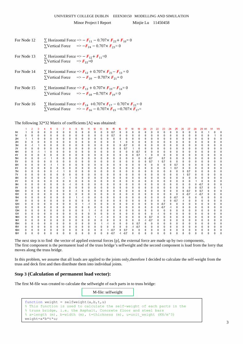
For Node 12 ∑ Horizontal Force => − 𝑭11 − 0.707× 𝑭23+ 𝑭10= 0

∑Vertical Force => −𝑭24 − 0.707× 𝑭23= 0

For Node 13 ∑ Horizontal Force => − 𝑭12+ 𝑭11=0


For Node 14 ∑ Horizontal Force => 𝑭12 + 0.707× 𝑭21− 𝑭13 = 0

∑Vertical Force => − 𝑭20 − 0.707× 𝑭21= 0

For Node 15 ∑ Horizontal Force => 𝑭13 + 0.707× 𝑭19− 𝑭14= 0

∑Vertical Force => − 𝑭18 −0.707× 𝑭19= 0

For Node 16 ∑ Horizontal Force => 𝑭14 +0.707× 𝑭17 − 0.707× 𝑭15= 0

∑Vertical Force => − 𝑭16 − 0.707× 𝑭15 −0.707× 𝑭17=

The following 32*32 Matrix of coefficients [A] was obtained:

The next step is to find the vector of applied external forces [p], the external force are made up by two components,

The first component is the permanent load of the truss bridge’s selfweight and the second component is load from the lorry that

moves along the truss bridge.

In this problem, we assume that all loads are applied to the joints only,therefore I decided to calculate the self-weight from the

truss and deck first and then distribute them into individual joints.

Step 3 (Calculation of permanent load vector):

The first M-file was created to calculate the selfweight of each parts in to truss bridge:

function weight = selfweight(a,b,t,u)

% This function is used to calculate the self-weight of each parts in the

% truss bridge, i.e. the Asphalt, Concrete floor and steel bars

% a=length (m), b=width (m), t=thickness (m), u=unit_weight (KN/m^3)

weight=a*b*t*u;

M-file: selfweight



4

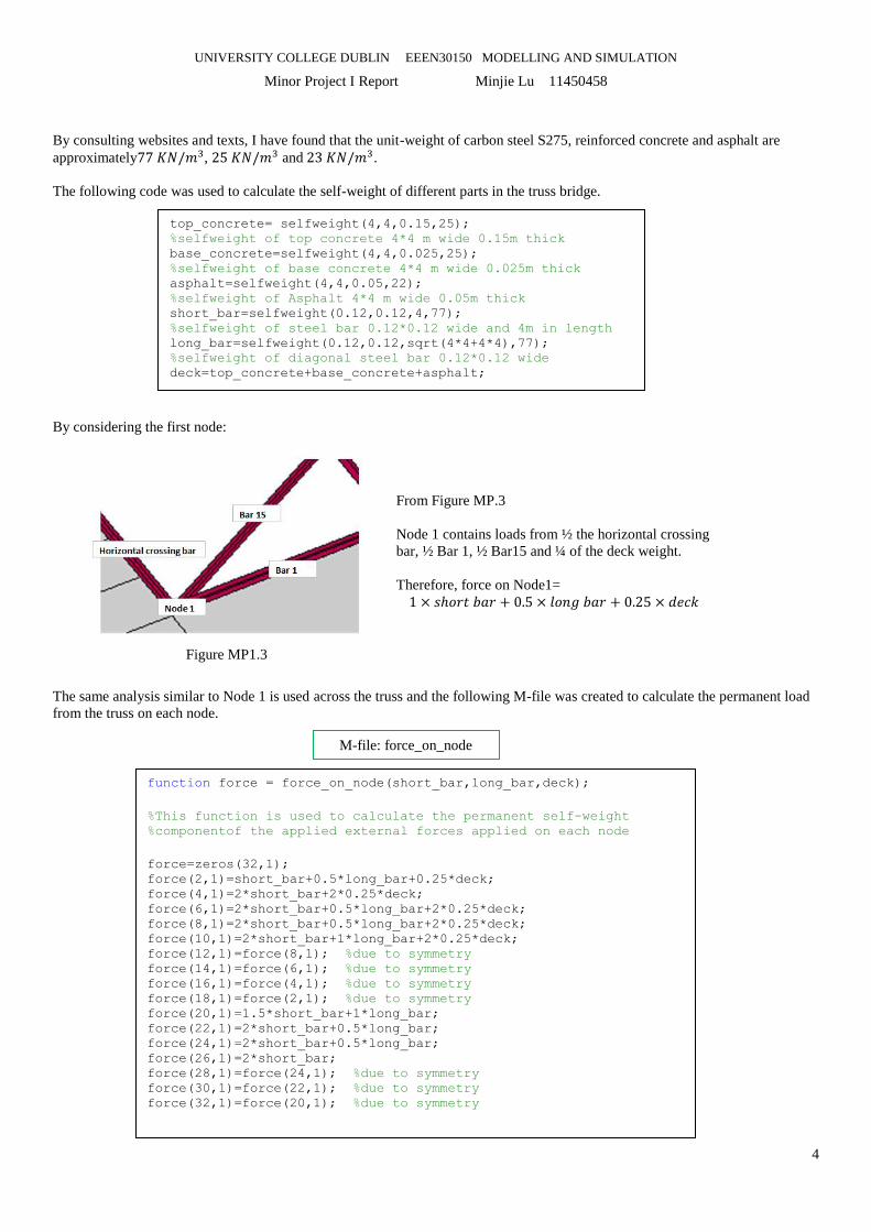
By consulting websites and texts, I have found that the unit-weight of carbon steel S275, reinforced concrete and asphalt are

approximately77 𝐾𝑁/𝑚3, 25 𝐾𝑁/𝑚3 and 23 𝐾𝑁/𝑚3.

The following code was used to calculate the self-weight of different parts in the truss bridge.

By considering the first node:

The same analysis similar to Node 1 is used across the truss and the following M-file was created to calculate the permanent load

from the truss on each node.

top_concrete= selfweight(4,4,0.15,25);

%selfweight of top concrete 4*4 m wide 0.15m thick

base_concrete=selfweight(4,4,0.025,25);

%selfweight of base concrete 4*4 m wide 0.025m thick

asphalt=selfweight(4,4,0.05,22);

%selfweight of Asphalt 4*4 m wide 0.05m thick

short_bar=selfweight(0.12,0.12,4,77);

%selfweight of steel bar 0.12*0.12 wide and 4m in length

long_bar=selfweight(0.12,0.12,sqrt(4*4+4*4),77);

%selfweight of diagonal steel bar 0.12*0.12 wide

deck=top_concrete+base_concrete+asphalt;

From Figure MP.3

Node 1 contains loads from ½ the horizontal crossing

bar, ½ Bar 1, ½ Bar15 and ¼ of the deck weight.

Therefore, force on Node1=

1 × 𝑠ℎ𝑜𝑟𝑡 𝑏𝑎𝑟 + 0.5 × 𝑙𝑜𝑛𝑔 𝑏𝑎𝑟 + 0.25 × 𝑑𝑒𝑐𝑘

Figure MP1.3

M-file: force_on_node

function force = force_on_node(short_bar,long_bar,deck);

%This function is used to calculate the permanent self-weight

%componentof the applied external forces applied on each node

force=zeros(32,1); force(2,1)=short_bar+0.5*long_bar+0.25*deck; force(4,1)=2*short_bar+2*0.25*deck; force(6,1)=2*short_bar+0.5*long_bar+2*0.25*deck; force(8,1)=2*short_bar+0.5*long_bar+2*0.25*deck; force(10,1)=2*short_bar+1*long_bar+2*0.25*deck; force(12,1)=force(8,1); %due to symmetry force(14,1)=force(6,1); %due to symmetry force(16,1)=force(4,1); %due to symmetry force(18,1)=force(2,1); %due to symmetry force(20,1)=1.5*short_bar+1*long_bar; force(22,1)=2*short_bar+0.5*long_bar; force(24,1)=2*short_bar+0.5*long_bar; force(26,1)=2*short_bar; force(28,1)=force(24,1); %due to symmetry force(30,1)=force(22,1); %due to symmetry force(32,1)=force(20,1); %due to symmetry



5

The permanent self-weight component of the applied external forces [p] now can be calculated:

The 32 × 1 matrix of the permanent self-weight force applied on each node is now obtained.

Step 4 (Calculation of variable load vector):

This step is to calculate the variable external forces that apply on different node while the lorry makes its way across the bridge.

In this problem, the front axle load is given as 10KN and the rear axle load is given as 36KN.

Now I can calculate the second component the vector of applied external forces [p] which is variable load from the Lorry,

For example, when the front axle of the lorry reaches Node1. The full load from the front axle applies on node 1.

When the front axle of the lorry moves 6m pass Node1 (the rear axle of the lorry at 2m pass Node1), ½ of the rear axle load

applies on Node1, and ½ applies on Node2, ½ of the front axle load applies on Node2, and ½ applies on Node3.

This analyisis is used across the truss for 37 different positions while the lorry moves across the truss bridge with 1 meter

increment. i.e. From d0to d36.

For example, the code for the front axle of the lorry moves 9m pass Node1 (i.e. for d9):

Code for the front axle of the lorry moves 24m pass Node1(i.e. for d24):

The 36 vector matrices for 37 different positions while the lorry moves across the truss with 1 meter increment are now obtained.

The vector of applied external forces [p] can be obtained: [p] = permanent_external_force + variable_force_𝑑𝑥

where 𝑑𝑥 is the distance between lorry’s front axle and Node1

permanent_external_force=force_on_node(short_bar,long_bar,deck);

M-file: force_on_node

function axleforce=axle_force(w); % this function can be used to calculate the axle force will apply on the 2D truss % where w= the axle load axleforce=0.5*1.45*w;

%multiplied by 0.5 since only half of the axle load will act on one plane truss %multiplied by 1.45 due to the dynamical effect

front_axle_force=axle_force(10) rear_axle_force=axle_force(36)

%variable external force when the front axle of lorry is 9m pass node 1, %where d is the distance between front axle and node 1 variable_force_d9= zeros(32,1); variable_force_d9(4,1)=rear_axle_force*0.75+front_axle_force*0; variable_force_d9(6,1)=rear_axle_force*0.25+front_axle_force*0.75; variable_force_d9(8,1)=rear_axle_force*0+front_axle_force*0.25; variable_force_d9;

%variable external force when the front axle of lorry is 24m pass node 1, %where d is the distance between front axle and node 1 variable_force_d24= zeros(32,1); variable_force_d24(12,1)=rear_axle_force*1+front_axle_force*0; variable_force_d24(14,1)=rear_axle_force*0+front_axle_force*1; variable_force_d24;



6

Step 5 (Gaussian Elimination):

So far, in order to determine the forces in the varies number bar of the truss {𝑈} = [𝐴]−1{𝑃}

I have already obtained the 32*32 Matrix of coefficients [A],the vector of applied external forces {p}. Now I can solve the forces

vector in bars {U} by Gaussian elimination. As Matlab already has an in-built function for this form of elimination that is

{Inv(A)*B},it can be used to help check my results of Gaussian Elimination.

The following M-file was created to solve the above equation by implementing Gaussian Elimination.

function [x] = GaussianEliminate(A,b) % SolvesAx = b by Gaussian elimination

N = length(b); %work out the number of equations need

for column=1:(N-1) %swap rows so that the row we are using to eliminate %the entries in the rows below is larger than the %values to be eliminated.

[alphea,beta] = max(abs(A(column:end,column))); beta=beta+column-1; temp = A(column,:); A(column,:) = A(beta,:); A(beta,:) = temp; temp = b(column) ; b(column)= b(beta); b(beta) = temp;

%work on all the rows below the diagonal element for row =(column+1):N

%work out the value of d d = A(row,column)/A(column,column);

%do the row operation (result displayed on screen) A(row,column:end) = A(row,column:end)-d*A(column,column:end) ; b(row) = b(row)-d*b(column); end% end of loop through rows end% end of loop through columns

%back substitution

for row=N:-1:1

x(row) = b(row);

for i=(row+1):N x(row) = x(row)-A(row,i)*x(i); end

x(row) = x(row)/A(row,row); end

x = x' ;

return

Reference: ‘Numerical Methods in Chemical Engineering’, Department of Chemical Engineering and Biotechnology, University

of Cambridge. Available at http://laser.cheng.cam.ac.uk/wiki/images/d/d8/Handout2.pdf(Accessed 24 March 2014)

M-file: GaussiaElimination

http://laser.cheng.cam.ac.uk/wiki/images/d/d8/Handout2.pdf



7

Internal force in

Step 6 (Calculation of vector of applied external forces [p]):

The above M-file can be used to solve the forces vector in bars {U}for a given position by using general code:

where 𝑑𝑥 is the distance between lorry’s front axle and Node1.

The permanent_external_force and variable_force_𝒅𝒙 have already been obtained in step3 and step4.

Now I can use the results from step3 and step4 to find the corresponding forces vector in bars {U}:

For example, if I want to find the interal force vector in bars while the front axle of lorry is 6m pass node1,

Now, I can obtain the 37 interal force vector matrices {U} for 36 different positions while the lorry moves across the truss with 1

meter increment. i.e. From d0to d36.

For example,

while the front axle of the lorry is at Node1, i.e. at d0: while the front axle of the lorry is 25 meters pass Node1, i.e. at d25:

internal_force_in_bar_𝒅𝒙=GaussianEliminate((internal_force),

(permanent_external_force+variable_force_𝒅𝒙))

internal_force_in_bar_d6=GaussianEliminate((internal_force),

(permanent_external_force+variable_force_d6))

235.1283

235.1283

404.6611

506.3808

506.3808

404.6611

235.1283

235.1283

-404.6611

-506.3808

-540.2874

-540.2874

-506.3808

-404.6611

-332.5719

52.6704

239.7918

-113.7262

143.8751

-45.9131

47.9584

-8.8704

47.9584

-45.9131

143.8751

-113.7262

239.7918

52.6704

-332.5719

0

271.8497

264.5997

Bar1

Bar2

Bar3

Bar4

Bar5

Bar6

Bar7

Bar8

Bar9

Bar10

Bar11

Bar12

Bar13

Bar14

Bar15

Bar16

Bar17

Bar18

Bar19

Bar20

Bar21

Bar22

Bar23

Bar24

Bar25

Bar26

Bar27

Bar28

Bar29

H1

V1

V9

245.6861

245.6861

425.7767

538.0542

559.1699

448.4330

257.9205

257.9205

-448.4330

-559.1699

-582.5186

-582.5186

-538.0542

-425.7767

-347.5051

52.6704

254.7251

-124.2841

158.8083

-56.4709

62.8916

-8.8704

33.0251

-35.3553

156.6292

-122.7434

269.4660

54.4829

-364.8098

0

275.1575

287.3919

Note: the unit is in KN,

While the front axle of the lorry is at Node1, the internal force in bar1 is 235.12 KN (in tension),

the internal force in bar20 is -45.91 KN (in compression).



8

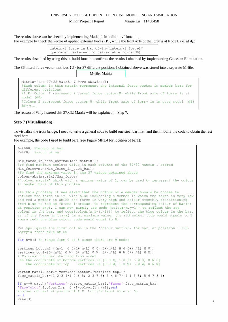
The results above can be check by implementing Matlab’s in-build ‘inv’ function,

For example to check the vector of applied external forces {P}, while the front axle of the lorry is at Node1, i.e. at d0:

The results abstained by using this in-build function confirms the results I obtained by implementing Gaussian Elimination.

The 36 interal force vector matrices {U} for 37 different positions I obtained above was stored into a separate M-file:

The reason of Why I stored this 37×32 Matrix will be explained in Step 7.

Step 7 (Visualisation):

To visualise the truss bridge, I need to write a general code to build one steel bar first, and then modify the code to obtain the rest

steel bars.

For example, the code I used to build bar1 (see Figure MP1.4 for location of bar1):

internal_force_in_bar_d0=inv(internal_force)*

(permanent_external_force+variable_force_d0)

L=4000; %Length of bar W=120; %width of bar

Max_force_in_each_bar=max(abs(matrix)); %To find maximum abslute value in each columns of the 37*32 matrix I stored Max_force=max(Max_force_in_each_bar); %To find the maximum value in the 37 values abtained above colour=abs(matrix)/Max_force;

%‘colour matrix’ which with a maximum value of 1, can be used to represent the colour

in member bars of this problem

%In this problem, it was asked that the colour of a member should be chosen to

reflect the force in it, with blue indicating a member in which the force is very low

and red a member in which the force is very high and colour smoothly transitioning

from blue to red as forces increase. To represent the corresponding colour of bar(x)

at position d(y), I can now simply use code {colour(x,y-1)} to reflect the red colour in the bar, and code{colour(x,1-(y-1))} to reflect the blue colour in the bar,

as if the force in bar(x) is at maximum value, the red colour code would equals to 1 (pure red),the blue colour code would equal to 0.

P=1 %p=1 gives the first column in the ‘colour matrix’, for bar1 at position 1 I.E.

Lorry’s front axle at D0

for n=0:8 %n range from 0 to 8 since there are 9 nodes

vertices_bottom1=[(n*L) 0 0;L+(n*L) 0 0; L+(n*L) W 0;0+(n*L) W 0]; vertices_top1=[0+(n*L) 0 W; L+(n*L) 0 W; L+(n*L) W W;0+(n*L) W W];

% To construct bar starting from node1

as the coordinate of bottom vertices is [0 0 0; L 0 0; L W 0; 0 W 0]

the coordinate of top vertices is [0 0 W; L 0 W; L W W; 0 W W]

vertex_matrix_bar1=[vertices_bottom1;vertices_top1]; face_matrix_bar=[1 2 3 4;1 2 6 5; 2 3 7 6; 3 4 8 7; 4 1 5 8; 5 6 7 8 ];

if n==0 patch('Vertices',vertex_matrix_bar1,'Faces',face_matrix_bar,

'FaceColor',[colour(1,p) 0 (1-colour(1,p))]);end

%colour of bar1 at position1 I.E. Lorry’s front axle at D0 end

View(3)

Matrix=[the 37*32 Matrix I have obtained];

%Each column in this matrix represent the internal force vector in member bars for different positions. %I.E. Column 1 represent internal force vector{U} while front axle of lorry is at node1 (d0)

%Column 2 represent force vector{U} while front axle of lorry is 1m pass node1 (d1)

%Etc……

M-file: Matrix



9

From above code I can now obtain the drawing of bar1 shown in Figure MP1.5

For another example, the vertices and patch code I used for creating bar16 (see Figure MP1.4 for location of bar16):

Bar16 now can be obtained, shown in Figure MP1.6.

Similar code used for creating the diagonal bar, bar15:

code used for creating the crossing bar:

To creating the symmetrical bar1 is even more simply by changing the Z coordinate of the vertices code of bar1.

Figure MP1.5

Figure MP1.4

vertices_bottom2=[0+(n*L) 0 0;W+(n*L) 0 0; W+(n*L) W 0;0+(n*L) W 0]; vertices_top2=[0+(n*L) 0 L; W+(n*L) 0 L; W+(n*L) W L;0+(n*L) W L]; vertex_matrix_bar2=[vertices_bottom2;vertices_top2];

% n starts from 1 since no vertical bar at nodeo if n==1 patch('Vertices',vertex_matrix_bar2,'Faces',face_matrix_bar,


%colour code is colour(16,p), because I want Matlab to pick up the ‘colour

matrix’ for bar16, which is row16 in each column for different positions.

Figure MP1.6

vertices_bottom4=[0+(n*L) 0 0; W+(n*L) 0 0; W+(n*L) W 0; 0+(n*L) W 0]; vertices_top4= [0+((n+1)*L) 0 L; W+((n+1)*L) 0 L; W+((n+1)*L) W L; 0+((n+1)*L) W L];

vertex_matrix_bar4=[vertices_bottom4;vertices_top4];

if n==0 patch('Vertices',vertex_matrix_bar4,'Faces',face_matrix_bar,


vertices_bottom6=[(n*L) 0 0;W+(n*L) 0 0; W+(n*L) L+W 0;0+(n*L) L+W 0]; vertices_top6=[0+(n*L) 0 W; W+(n*L) 0 W; W+(n*L) L+W W;0+(n*L) L+W W];

vertex_matrix_bar6=[vertices_bottom6;vertices_top6]; patch('Vertices',vertex_matrix_bar6,'Faces',face_matrix_bar, 'FaceColor',[0.5 0 0.5]);



10

Now by changing the Vertices code and patching code for different bar members I can now obtain a full drawing of the truss with

colour reflect the internal forces in member bars for the position of 𝑑0 (front axle of Lorry at node1):

To help the visualisation, I decided to create a graphical representation of the lorry on the truss. I.E. for the given position of the

lorry the truss’s colour reflect the force in various member bars. (Due to complexity of create a graphical representation of the

lorry, I created a block with 4m length and 2m wide instead).

Combine the above code with the code I created for graphical representation of the truss.

Now I can create an M-file for the graphical represention of the truss bridge with the movement of the lorry across the bridge with

different p value (which represent the lorry’s position).

The movie which animates the movement of the lorry across the bridge, with changing member colours indicating the changing

forces within the various members has been uploaded on https://www.youtube.com/watch?v=9YItOzFkZfI&feature=youtu.be

Figure MP1.7

TW=2000; %Truck width 2m

TH=2000; %Truck height 2m

L=4000; %Truck length 4m

for k=p/4

%since I want the block to move with increment of 1 meter, which is 1/4 of its length

%where the p is the assigned column value to the 37*32 ‘colour matrix’ which reflects the

colour in member bars explained previously

vertices_Lorrybottom=[(k-1.25)*L TW/2 0;(k-0.25)*L TW/2 0;(k-0.25)*L (3/2)*TW 0;

(k-1.25)*L (3/2)*TW 0];

vertices_Lorrytop=[(k-1.25)*L TW/2 TH;(k-0.25)*L TW/2 TH;(k-0.25)*L (3/2)*TW TH;

(k-1.25)*L (3/2)*TW TH];

vertex_matrix_Lorry=[vertices_Lorrybottom;vertices_Lorrytop];

face_matrix_Lorry=[1 2 3 4;1 2 6 5; 2 3 7 6; 3 4 8 7; 4 1 5 8; 5 6 7 8 ];

patch('Vertices',vertex_matrix_Lorry,'Faces',face_matrix_Lorry, 'FaceColor',[0 1 0]);

end

https://www.youtube.com/watch?v=9YItOzFkZfI&feature=youtu.be



11

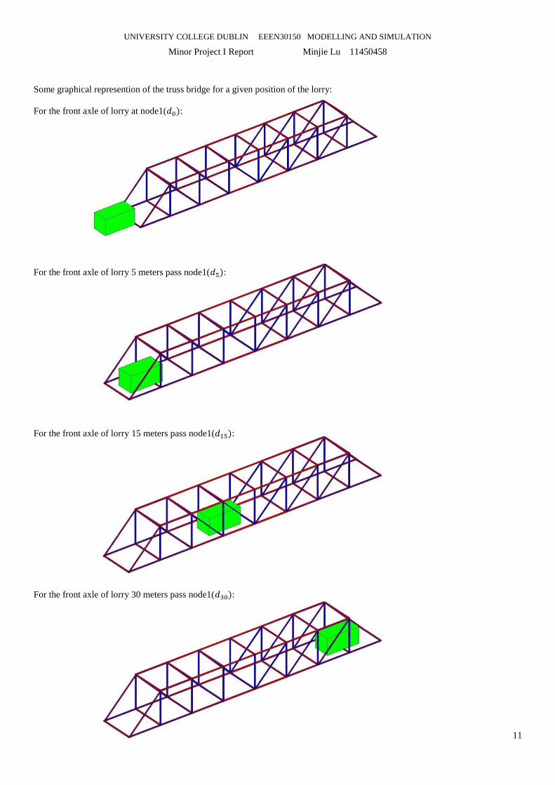
Some graphical represention of the truss bridge for a given position of the lorry:

For the front axle of lorry at node1(𝑑0):

For the front axle of lorry 5 meters pass node1(𝑑5):



Modelling and Simulations Minor Project

Documents