Modellierung und numerische Simulation einer Kette neutraler ...

Diese Arbeit wurde vorgelegt amLehrstuhl fur Mathematik (MathCCES)

Modellierung und numerische Simulation einer Ketteneutraler Atome, welche mittels Anregung durch einenLaser koharent an Rydberg Zustande gekoppelt werden

Modelling and numerical Simulation of a chain ofneutral atoms coherently coupled to highly excited

Rydberg states

BachelorarbeitPhysik

Dezember 2020

Vorgelegt von Nigel NellesPresented by Rue du Bayehon 41, Ovifat, 4950 Weismes, Belgien

Matrikelnummer: [email protected]

Erstprufer Prof. Dr. Benjamin StammFirst examiner Lehrstuhl fur Mathematik (MathCCES)

RWTH Aachen University

Zweitprufer Prof. Dr. Stefan WeßelSecond examiner Lehr- und Forschungsgebiet Theoretische Physik (kondensierte Materie)


Koreferent Loris Di CairanoCo-supervisor Lehrstuhl fur Mathematik (MathCCES)


Eigenstandigkeitserklarung

Hiermit versichere ich, dass ich diese Bachelorarbeit selbstandig verfasst und keineanderen als die angegebenen Quellen und Hilfsmittel benutzt habe. Die Stellen meinerArbeit, die dem Wortlaut oder dem Sinn nach anderen Werken entnommen sind, habeich in jedem Fall unter Angabe der Quelle als Entlehnung kenntlich gemacht. Dasselbegilt sinngemaß fur Tabellen und Abbildungen. Diese Arbeit hat in dieser oder einerahnlichen Form noch nicht im Rahmen einer anderen Prufung vorgelegen.

Aachen, im Dezember 2020

Nigel Nelles

II

Contents

List of Figures V

List of Tables VII

1. Abstract 1

2. Introduction 1

3. Model 33.1. Dirac-Formalism . . . . . . . . . . . . . . . . . . . . . . . . . . . . . . 3

3.1.1. Hilbert Space . . . . . . . . . . . . . . . . . . . . . . . . . . . . 33.1.2. Linear Operators . . . . . . . . . . . . . . . . . . . . . . . . . . 53.1.3. Eigenvalue Problem . . . . . . . . . . . . . . . . . . . . . . . . . 73.1.4. Linear Operators as Matrices . . . . . . . . . . . . . . . . . . . 8

3.2. Physical Interpretation . . . . . . . . . . . . . . . . . . . . . . . . . . . 93.3. Many-Body Hilbert Space for Two-Level Particles . . . . . . . . . . . . 10

3.3.1. Two-Level System . . . . . . . . . . . . . . . . . . . . . . . . . 103.3.2. Transition to the many Particle Hilbert Space . . . . . . . . . . 11

3.4. Rabi Oscillations . . . . . . . . . . . . . . . . . . . . . . . . . . . . . . 123.5. Array of strongly interacting neutral Atoms excited to Rydberg states . 17

4. Computation 194.1. Constructing the Hamiltonian . . . . . . . . . . . . . . . . . . . . . . . 194.2. Implicitly Restarted Lanzcos Method . . . . . . . . . . . . . . . . . . . 214.3. Singular Value Decomposition . . . . . . . . . . . . . . . . . . . . . . . 21

5. Results 235.1. Performance of Ground State Computation . . . . . . . . . . . . . . . . 245.2. Reducing computation time through SVD approximation . . . . . . . . 255.3. Computation of the Spectrum . . . . . . . . . . . . . . . . . . . . . . . 28

6. Conclusion 36

7. Outlook 36

A. Tables representing the ground state spectrum for different number ofatoms 37A.1. NAtoms = 11 . . . . . . . . . . . . . . . . . . . . . . . . . . . . . . . . . 37A.2. NAtoms = 12 . . . . . . . . . . . . . . . . . . . . . . . . . . . . . . . . . 38A.3. NAtoms = 13 . . . . . . . . . . . . . . . . . . . . . . . . . . . . . . . . . 39A.4. NAtoms = 14 . . . . . . . . . . . . . . . . . . . . . . . . . . . . . . . . . 40A.5. NAtoms = 15 . . . . . . . . . . . . . . . . . . . . . . . . . . . . . . . . . 41

III

B. Diagrams showing the Number of non-converging Ground State compu-tations 43B.1. NAtoms = 11 . . . . . . . . . . . . . . . . . . . . . . . . . . . . . . . . . 43B.2. NAtoms = 12 . . . . . . . . . . . . . . . . . . . . . . . . . . . . . . . . . 44B.3. NAtoms = 13 . . . . . . . . . . . . . . . . . . . . . . . . . . . . . . . . . 45B.4. NAtoms = 14 . . . . . . . . . . . . . . . . . . . . . . . . . . . . . . . . . 46B.5. NAtoms = 15 . . . . . . . . . . . . . . . . . . . . . . . . . . . . . . . . . 47

C. Plots showing the Speedup of the SVD Approximation with StandardDeviation 48C.1. NAtoms = 11 . . . . . . . . . . . . . . . . . . . . . . . . . . . . . . . . . 48C.2. NAtoms = 12 . . . . . . . . . . . . . . . . . . . . . . . . . . . . . . . . . 49C.3. NAtoms = 13 . . . . . . . . . . . . . . . . . . . . . . . . . . . . . . . . . 50C.4. NAtoms = 14 . . . . . . . . . . . . . . . . . . . . . . . . . . . . . . . . . 51C.5. NAtoms = 15 . . . . . . . . . . . . . . . . . . . . . . . . . . . . . . . . . 52

D. Plots showing the mean Accuracy of SVD Approximations depending onNSing 53D.1. NAtoms = 11 . . . . . . . . . . . . . . . . . . . . . . . . . . . . . . . . . 53D.2. NAtoms = 12 . . . . . . . . . . . . . . . . . . . . . . . . . . . . . . . . . 54D.3. NAtoms = 13 . . . . . . . . . . . . . . . . . . . . . . . . . . . . . . . . . 55D.4. NAtoms = 14 . . . . . . . . . . . . . . . . . . . . . . . . . . . . . . . . . 56D.5. NAtoms = 15 . . . . . . . . . . . . . . . . . . . . . . . . . . . . . . . . . 57

References 58

IV

List of Figures

1. Plot showing the Rabi oscillation for different ∆. This plot was inspiredby a plot in [11] depicting the same functions. . . . . . . . . . . . . . . 16

2. Plot showing the time needed to construct the Hamiltonian and to com-pute the ground state, depending on the system size. Time was mea-sured for specific parameter values. . . . . . . . . . . . . . . . . . . . . 24

3. Plot showing the time needed to compute the ground state, dependingon the system size. Time was measured for several parameter values.The parameter values chosen are shown in figure 4 as ~pi,test . . . . . 25

4. Parameter values used for SVD approximation and for testing. . . . . . 275. Singular Values of A. . . . . . . . . . . . . . . . . . . . . . . . . . . . . 276. Accuracy of the SVD approximation depending on the number NSing of

singular values considered. σmax is the biggest relative inaccuracy acrossall the test points (see figure 4). . . . . . . . . . . . . . . . . . . . . . . 27

7. Plot showing the relationship tgs,exact/tgs,approx for different numbers ofatoms. tgs,exact is the average time needed to compute an exact groundstate. tgs,approx is the average time needed to compute an approximatedground state, depending on NSing. NSing is the number of singular valuesconsidered for the SVD approximation. . . . . . . . . . . . . . . . . . . 27

8. Diagram depicting |c|2max for a system of size NAtoms = 11 . . . . . . . . 319. Diagram depicting |c|2max for a system of size NAtoms = 12 . . . . . . . . 3210. Diagram depicting |c|2max for a system of size NAtoms = 13 . . . . . . . . 3311. Diagram taken from [2], it depicts the ground state phase diagram for

an array of 13 atoms. Comparison with figure 10 shows that we getsimilar results. . . . . . . . . . . . . . . . . . . . . . . . . . . . . . . . . 33

12. Diagram depicting |c|2max for a system of size NAtoms = 14 . . . . . . . . 3413. Diagram depicting |c|2max for a system of size NAtoms = 15 . . . . . . . . 3514. Plot showing for 3 < NSing < 40 how many of the 32 approximated

ground state computations did not converge. The system is of sizeNAtoms = 11 . . . . . . . . . . . . . . . . . . . . . . . . . . . . . . . . . 43

15. Plot showing 3 < NSing < 40 how many of the 32 approximated groundstate computations did not converge. The system is of size NAtoms = 12 44




19. Plot showing the relationship between tgs,exact and tgs,approx with un-certainty for 11 atoms. tgs,exact is the mean time it takes to computean exact ground state. tgs,approx is the mean time it takes to computean approximated ground state. NSing is the number of singular valuesconsidered for the SVD approximation. . . . . . . . . . . . . . . . . . 48

V





24. Plot showing the mean accuracy σmean of the SVD approximation withstandard deviation across all test points ~pi ∈ ~pi,test, depending onNSing for NAtoms = 11 . . . . . . . . . . . . . . . . . . . . . . . . . . . . 53





VI

List of Tables

VII

1. Abstract

In this thesis we have modeled a system consisting of an array of neutral atoms thatare driven by lasers to highly excited Rydberg states. A numerical method to solvethe model has been implemented and we were able to compute the ground state forsystems of up to 20 atoms, which corresponds to a Hilbert space of more than amillion dimensions. For systems of up to 15 atoms we successfully used the singularvalue decomposition to generate a reduced approximation space and to reduce thetime needed to compute the ground state in a many-query context by more than afactor 500 while maintaining a precision of 99%. Using this decrease in computationtime we plotted a diagram depicting information of 200× 200 different ground states,corresponding to systems with different parameter values. For a system consisting of 15atoms, the computation of this diagram took about 40 minutes on an average desktopcomputer. These diagrams depicting the ground state spectrum for different systemsreveal that for certain sizes and parameter ranges, a specific kind of translationallysymmetric states makes up most of the ground state, with probabilities of ∼ 85%.

2. Introduction

Let us first make an introduction on the topic, most information in this section comesfrom the two papers [2, 3]. The study of coherent many-body dynamics in artificialsystems is relatively new, since it is made possible by recent advances in technologyallowing the control of the quantum state of individual quantum objects.One of its uses would be to hopefully gain new insights in the field of solid state physics.This could be done by quantum simulation, which means constructing systems thatsimulate the behavior of quantum objects in real matter. One advantage of these ar-tificial systems would be that it is possible to change the external parameters of thesetup in ways that would not be possible with real matter. The parameters could forexample be set to very high levels or be changed very suddenly. This could lead tothe observation of new phenomenon that help us to better understand the behavior ofmatter on a quantum mechanical level.These systems can also be used to simulate theoretical models, like the Ising model.Since the numerical simulation of quantum mechanical many-body systems is at themoment limited to about 50 particles, due to the exponential growth of the Hilbertspace, simulation using interacting quantum objects can make it possible to examinelarger systems than possible through numerical computation.These artificial systems also form the basis for the development of quantum comput-ers. Basic elements of quantum processors have already been realized with differentapproaches, although only for a small number of coupled qubits. One example istrapped ions interacting through Coulomb interaction [25] where the qubits are en-coded in atomic hyperfine levels. Two other examples are spins in semiconductors [1]and superconducting circuits [13]. Realizing quantum processors for a higher numberof qubits proves to be a difficult challenge, the different requirements for this can be

1

found in [14].

One promising way to do quantum computing/quantum simulation is coherent cou-pling of neutral atoms to highly excited Rydberg states. The Rydberg state is a statewhere the outer electron is excited to a very high principal quantum number n. Sinceatoms in this state form a dipole they interact with each other through repulsive van-der-Waals interaction. As stated in [2] about the interaction between Rydberg atoms:”Such interactions have recently been used to realize quantum gates [33, 20, 29], toimplement strong photon-photon interactions [28] and to study quantum many-bodyphysics of Ising spin systems in optical lattices [30, 31, 34] and in probabilisticallyloaded dipole trap arrays [22].” The system that we are examining in this thesis is thesame system constructed in [2], an array of several such atoms. The physical realiza-tion of this system can be done by locking atoms in a certain position with opticaltweezers and exciting them with a laser.

Aside from the physical realization, it is also important to compute the theoreticalbehavior of such a system so that there is something to compare the real behavior to.The first part of the theoretical/numerical simulation would be to solve the stationarySchrodinger equation, which is what we will do in this thesis.We will begin by introducing the mathematical framework needed to describe a quan-tum mechanical system, then we will look at the physics of an atom that is driven bya laser and see how that leads us to the Hamiltonian describing a multitude of suchatoms interacting with each other. Before we proceed to the numerical analysis ofthe Hamiltonian we introduce the techniques used for the computation. Our simula-tion consists of computing the ground state spectrum of the Hamiltonian in a certainparameter range for different system sizes. Since every atom can be considered as atwo-level quantum mechanical system, we find that the number of dimensions of theHilbert space is 2N , where N is the number of atoms in the array. We can see thatthe size of the Hilbert space is growing exponentially with the number of atoms and sois the time and memory needed for computations. Aside from the mathematical andphysical perspective of the topic, the thesis will also deal with techniques to reducethe time and memory consumption of the computation within a many-query context.This will be just as important as the physical results, since the same techniques couldbe used to allow for more complex computations later on, like computing the tempo-ral evolution of the system and maybe even use time-dependent parameters for theHamiltonian.

2

3. Model

3.1. Dirac-Formalism

In this section we want to introduce the mathematical formalism that is used in quan-tum mechanics, the Dirac-Formalism. This section will focus solely on the mathemat-ics, how it is used in physics will be covered in the section 3.2. The content of thissection comes from different books [26, 18, 19, 32].

3.1.1. Hilbert Space

Let us begin by introducing the Hilbert space. It is the framework for the mathematicsof quantum mechanics. We will start by introducing some definitions that are neededfor the Hilbert space. The definition of the Vector space is [19]:

Definition 1 (Vector Space) A vector space over C consists of a set V along with twooperations, the vector addition + and the scalar multiplication ·. These two operationsare subject to the conditions that for all vectors ~α, ~β,~γ ∈ V and all scalars c, d ∈ C:

1. the set V is closed under vector addition, that is, ~α + ~β ∈ V

2. vector addition is commutative, ~α + ~β = ~β + ~α

3. vector addition is associative, (~α + ~β) + ~γ = ~α + (~β + ~γ)

4. there is a zero vector ~0 ∈ V such that ~α +~0 = ~α for all ~α ∈ V

5. each ~α ∈ V has an additive inverse ~β ∈ V such that ~α + ~β = ~0

6. the set V is closed under scalar multiplication, that is, c · ~α ∈ V

7. scalar multiplication distributes over scalar addition, (c+ d) · ~α = c · ~α + d · ~α.

8. scalar multiplication distributes over vector addition, c · (~α + ~β) = c · ~α + c · ~β

9. ordinary multiplication of scalars associates with scalar multiplication, (cd) · ~α =c · (d · ~α)

10. multiplication by the scalar 1 is the identity operation, 1 · ~α = ~α

Note that for item (7), the + on the left side means the addition of two complexnumbers, while the + on the right side means the addition introduced in the definition.

Definition 2 (Inner Product Space) An inner product space over C is a vector space

over C with an inner product 〈·, ·〉 that, for all vectors ~α, ~β ∈ V and all scalars c ∈ C,has the following properties [26]:

1. 〈~α, ~β〉 = 〈~β, ~α〉∗ (∗ means the complex conjugate)

3

2. 〈~α, ~β1 + ~β2〉 = 〈~α, ~β1〉+ 〈~α, ~β2〉

3. 〈~α, c~β1〉 = c〈~α, ~β1〉 = 〈c∗~α, ~β1〉

4. 〈~α, ~α〉 ≥ 0 ∀ ~α ∈ V (= 0 only for ~α = ~0)

At this point we want to introduce the Dirac notation. In this notation, vectors arewritten as |α〉, |β〉 instead of ~α, ~β. We can write the sum of two vectors |α〉, |β〉 as|α〉+|β〉 = |α+β〉 and the product of a scalar c and a vector |α〉 as c·|α〉 = c|α〉 = |cα〉.For |α〉 ∈ V we write the dual vector 〈α| ∈ V∗ where V∗ is the dual space. For adefinition of the dual space, refer to [18]. For |α〉, |β〉 ∈ V , the inner product is written〈α|β〉.In order to be able to define the Hilbert space, we need to introduce some more concepts[26].

Definition 3 (Norm) The norm of a vector |α〉 is defined as

‖α‖ =√〈α|α〉 ∈ R. (1)

Definition 4 (Convergence) The sequence |αn〉n∈N ⊂ V converges strongly towards|α〉 ∈ V if

limn→∞

‖αn − α‖ = 0. (2)

Definition 5 (Cauchy Sequence) A Cauchy sequence is defined as a sequence |αn〉n∈N ⊂V where there exists for each ε > 0, an N(ε) ∈ N so that

‖αn − αm‖ < ε ∀ n,m > N(ε). (3)

Definition 6 (Complete Vector Space) A vector space V is called complete, if everyCauchy sequence |αn〉n∈N ⊂ V converges towards an element inside V.

Now we have everything we need to define the Hilbert space [18]

Definition 7 (Hilbert Space) A Hilbert space H is an inner product space over C whichis also complete.

From now on we will be working in H instead of V . We will not specifically point outelements from H, H∗, or C most of the time. If not specified otherwise, every vectorwritten in Dirac notation is meant to be an element of H or H∗, depending on thenotation, and every lower case latin letter, with or without subscript, is an element ofC. Let us continue with some further definitions and theorems [26].

Definition 8 (Linear Independence) The vectors |α1〉, |α2〉, ..., |αn〉 are called linearlyindependent if the relation

n∑j=1

cj|αj〉 = |0〉 (4)

can only be fulfilled for c1 = c2 = ... = cn = 0.

4

Definition 9 (Dimension of a Vector Space) The dimension of a Vector space H isdefined as the maximum number of linearly independent vectors in H.

Definition 10 (Orthogonality) |α〉, |β〉 are orthogonal if:

〈α|β〉 = 0. (5)

Definition 11 A vector |α〉 is said to be normalized if ‖α‖ = 1.

Definition 12 (Complete Orthonormal System) A complete orthonormal system (CONS)is defined as a set |αj〉 of orthonormal vectors for which there does not exist an ele-ment in H, that does not belong to |αj〉, but is orthogonal to all elements of |αj〉.

We will sometimes call a CONS a complete set of orthonormal basis vectors or evenjust basis vectors. Orthonormal means orthogonal and normalized.

Theorem 1 If |αj〉 ⊂ H is a CONS, then we can write every vector |β〉 ∈ H as alinear combination of |αj〉:

|β〉 =∑j

cj|αj〉. (6)

For a proof of the finite-dimensional case, refer to [26], a proof of the infinite-dimensionalcase can be found in [32].

3.1.2. Linear Operators

In this section we want to define the different types of operators that we will be usinglater. The content of this section and the two sections that follow comes from [26],especially the definitions. In order to distinguish operators from complex numbers, wewill use capital letters for operators.

Definition 13 (Operator A) Mapping relation, which assigns to each element |α〉 fromthe partial set DA ⊆ H uniquely an element |β〉 ∈ WA ⊆ H:

|β〉 = A|α〉 = |Aα〉. (7)

Sum and product of an operator are defined as

(A1 + A2)|α〉 = A1|α〉+ A2|α〉, |α〉 ∈ DA1 ∩DA2 , (8)

(A1A2)|α〉 = A1(A2|α〉), |α〉 ∈ DA2 , WA2 ⊆ DA1 . (9)

Definition 14 (Operator A† adjoint to A)

1. DA†: Set of all |γ〉 for which a |γ〉 exists with:

〈γ|A|α〉 = 〈γ|α〉, ∀ |α〉 ∈ DA. (10)

5

2. Mapping condition:A†|γ〉 = |γ〉. (11)

The adjoint operator has the following properties

1. There holds〈γ|A|α〉 = 〈α|A†|γ〉∗, |α〉 ∈ DA, |γ〉 ∈ DA† . (12)

2. The adjoint operator A† acts on 〈α| just like A acts on |α〉

〈α|A† = 〈Aα|. (13)

3. For suitable domains of definition, which will not be indicated anymore from nowon, we get

(A†)† = A. (14)

4. The following identity holds,

(AB)† = B†A†, (15)

5. as well as(A+B)† = A† +B†, (16)

(cA)† = c∗A†. (17)

Definition 15 (Linear Operator A) An operator A : DA → WA is called linear if:

1. DA is a linear subspace of H,

2. for arbitrary |α1〉, |α2〉 ∈ DA it holds:

A(c1|α1〉+ c2|α2〉) = c1A|α1〉+ c2A|α2〉. (18)

Definition 16 (Hermitian Operator A) An operator A : DA → WA is called hermitianif:

1. DA = DA† = H,

2. A = A† ⇐⇒ A|α〉 = A†|α〉 ∀ |α〉 ∈ H.

Definition 17 (Expectation Value) The expectation value of an operator A and a vec-tor |α〉 is defined as 〈α|A|α〉.

6

3.1.3. Eigenvalue Problem

Now we want to treat the eigenvalue problem for operators and specifically look at theproperties of the eigenspectrum of hermitian operators.

Definition 18 (Eigenvalue and Eigenvector) If A|a〉 = a|a〉, then |a〉 is called an eigen-vector of A with eigenvalue a.

Hermitian operators play a special role in quantum mechanics, this is because of fourproperties concerning their eigenvalues and eigenvectors.

Theorem 2 If A is a hermitian operator, then:

1. its expectation values are real.

2. its eigenvalues are real.

3. its eigenvectors are orthogonal.

4. its eigenvectors build a CONS.

Proof:

1. Let A be a hermitian operator and |α〉 an element of H. Then

〈α|A|α〉 = 〈α|A†|α〉∗ = 〈α|A|α〉∗ ⇒ 〈α|A|α〉 ∈ R ∀ |α〉 ∈ H. (19)

2. Let A be a hermitian operator and |a〉 an eigenvector of A with eigenvalue a.Then

〈a|A|a〉 = 〈a|a|a〉 ⇒ a =〈a|A|a〉〈a|a〉

. (20)

Since numerator and denominator are both real, a is also real.

3. For a proof, refer to [26].

4. For a proof, refer to [26] for the finite-dimensional case and [32] to find a deeperanalysis for the infinite-dimensional case.

Theorem 3 It is possible to describe a hermitian operator A by its eigenvalues aj andeigenvectors |aj〉, this is called the spectral representation:

A =∑j

aj|aj〉〈aj|. (21)

Proof: Let A be a hermitian operator and |aj〉 its eigenvectors which will alwaysform a CONS. We can then write every vector |ψ〉 ∈ H in this basis:

|ψ〉 =∑j

|aj〉〈aj|ψ〉. (22)

7

If we let the operator A act on |ψ〉 we get

A|ψ〉 =∑j

aj|aj〉〈aj|ψ〉. (23)

Since this is true for every vector |ψ〉 ∈ H we find

A =∑j

aj|aj〉〈aj|. (24)

Definition 19 (Identity Operator) The identity operator 1 is the operator that mapsevery state onto itself:

1|α〉 = |α〉 ∀ |α〉 ∈ H. (25)

It can be expressed in the spectral representation:

1 =∑j

|aj〉〈aj|. (26)

We can insert the spectral representation of the identity operator in any expressionwithout changing it.

3.1.4. Linear Operators as Matrices

Let |uj〉 be a CONS, for an arbitrary vector |α〉 ∈ H we can then assign a possiblyinfinite-dimensional column vector

|α〉 ←→

a1

a2...am...

, (27)

where aj = 〈uj|α〉 are the projections of that vector onto the basis |uj〉. To the dualvector 〈α| we can now assign a possibly infinite-dimensional row vector

〈α| ←→(a∗1 a∗2 · · · a∗m · · ·

). (28)

We can define the inner product of two such vectors, where |β〉 =∑

j bj|uj〉, as

〈α|β〉 =(a∗1 a∗2 · · · a∗m · · ·

)b1

b2...bm...

=∑j

a∗jbj. (29)

8

and also define an outer product

|a〉〈b| =

a1

a2...am...

(b∗1 b∗2 · · · b∗m · · ·

)=

a1b∗1 a1b

∗2 · · · a1b

∗m · · ·

a2b∗1 a2b

∗2 · · · a2b

∗m · · ·

......

. . ....

amb∗1 amb

∗2 · · · amb

∗m · · ·

......

.... . .

. (30)

For an operator A we can write

A = 1A1 =∑n,m

|un〉〈un|A|um〉〈um|, (31)

which takes the form of a matrix

A =

A11 A12 · · · A1m · · ·A21 A22 · · · A2m · · ·

......

. . ....

An1 An2 · · · Anm · · ·...

......

. . .

, (32)

where the matrix elements are defined as Anm = 〈un|A|um〉. We can get the elementsof the adjoint operator A† from (A†)nm = A∗mn. For hermitian operators we find therequirement Anm = A∗mn.

3.2. Physical Interpretation

Now that we have defined the mathematical formalism, we want to specify how it isused in quantum mechanics. [26]

1. A quantum mechanical system is described by a Hilbert space.

2. A state in that system is described by a vector in that space.The number of dimensions that the Hilbert space has corresponds to the numberof base states that the physical state can be made of.

3. An observable that can be measured is described by a hermitian operator.The reason we have to use operators to conduct a measurement is that in quan-tum mechanics, the influence that the measurement has on the system can notbe neglected. This is reflected in the fact that applying an operator to a vector,which describes the state, may alter it. We have to use hermitian operators, be-cause its eigenvalues and expectation values, which also describe physical values,are real.

4. The possible results of the measurement are the eigenvalues of that operator.

9

5. When measuring the state of the system, the state gets filtered. If we have anoperator A =

∑i

ai|ai〉〈ai| and a state |β〉 =∑i

bi|ai〉, then after measuring ai we

have |β〉 = |ai〉.

6. The probabilities for measuring ai are |〈ai|β〉|2.For this reason, we will always consider normalized vectors.

There are some more concepts we want to introduce. The equation

H|ψ〉 = E|ψ〉, (33)

where E is the energy of |ψ〉, is called the time-independent Schrodinger equation. Itis also the eigenvalue equation of the operator H, which is called Hamiltonian. Theeigenvalues of H are the possible measurements for the energy of the system. Thereexists also a time-dependent Schrodinger equation, which is written

H|ψ(t)〉 = i~|ψ(t)〉. (34)

The time-dependent Schrodinger equation describes the temporal evolution of a quan-tum mechanical state. If the Hamiltonian is not time-dependent, we can write thesolutions of the time-dependent Schrodinger equation in terms of the solution to thetime-independent one:

|ψi(t)〉 = |ψi(t = 0)〉e−iEit/~. (35)

With H|ψi(t = 0)〉 = Ei|ψi(t = 0)〉 being a solution to the time-independent Schrodingerequation.

3.3. Many-Body Hilbert Space for Two-Level Particles

In this section we want to introduce the Hilbert space that describes a physical systemcomposed of many two-level particles. Let us first begin with the Hilbert space of onesuch particle, it is a two-dimensional complex vector space.

3.3.1. Two-Level System

The two possible base states of our particle are the two orthonormal base vectors

|1〉 =

(10

)and |2〉 =

(01

). Every possible state of that particle can be described as a

combination of those two base states.

|ψ〉 = c1|1〉+ c2|2〉, c1, c2 ∈ C, ||ψ||2 = 1. (36)

This system is equivalent to a two state spin system with | ↑〉 =

(10

)and | ↓〉 =

(01

).

Some important operators in a two-level system are the Pauli matrices. In a spin

10

system they can for example be used to measure the spin in any of the three spatialdimensions. The three Pauli matrices and the unit matrix are defined as:

11 := |1〉〈1|+ |2〉〈2| =(

1 00 1

)σx := |1〉〈2|+ |2〉〈1| =

(0 11 0

)σy := i(−|1〉〈2|+ |2〉〈1|) =

(0 −ii 0

)σz := |1〉〈1| − |2〉〈2| =

(1 00 −1

).

(37)

The pauli matrices have two eigenvalues each, +1 and −1, which are the possiblemeasurements of the spin in the corresponding direction. The normalized eigenvectorscorresponding to these eigenvalues are:

|ψ+x 〉 =

1√2

(11

)=

1√2

(|1〉+ |2〉) |ψ−x 〉 =1√2

(1−1

)=

1√2

(|1〉 − |2〉)

|ψ+y 〉 =

1√2

(1i

)=

1√2

(|1〉+ i|2〉) |ψ−y 〉 =1√2

(1−i

)=

1√2

(|1〉 − i|2〉)

|ψ+z 〉 =

(10

)= |1〉 |ψ−z 〉 =

(01

)= |2〉.

(38)

3.3.2. Transition to the many Particle Hilbert Space

The notation H(i)1 used in this section is taken from [27]. In [16] it is shown that

Hilbert spaces can be combined using the tensor product ⊗ and that ⊗ is used as theKronecker product when using the matrix formalism for operators. The definition ofthe Kronecker product is:

Definition 20 (Kronecker Product ⊗) Let A be a m × n matrix and B be a p × qmatrix. The matrix C = A ⊗ B will then be an mp × nq matrix with coefficientsCi′j′ = AijBkl where i′ = (i− 1) · p+ k and j′ = (j − 1) · q + l.

Let us specifically look at a composite Hilbert space that is the combination of Ntwo-dimensional Hilbert spaces like the one we have just introduced. This compositeHilbert space will describe N particles that have two possible base states each. LetH(i)

1 ' C2 be the Hilbert space of particle i and |u(i)1 〉, |u

(i)2 〉 the orthonormal base of

that Hilbert space H(1)1 . Then the Hilbert space of the N -particle system is defined by

HN = H(1)1 ⊗H

(2)1 ⊗ ...⊗H

(N)1 ' C2N . The complete set of orthonormal base vectors of

the N -particle Hilbert space is composed of every possible combination of H(i)1 ’s base

vectors.N⊗i=1

|u(i)αi〉 = |u(1)

α1〉 ⊗ |u(2)

α2〉 ⊗ · · · ⊗ |u(N)

αN〉 = |u(1)

α1u(2)α2...u(N)

αN〉

∣∣∣∣∣ αi ∈ 1, 2. (39)

Every possible state |ψ〉 ∈ HN can then be written as a linear product of these basevectors:

|ψ〉 =∑

α1,α2,...,αN

C(α1, ..., αN)|u(1)α1u(2)α2...u(N)

αN〉. (40)

11

The inner product of the N -particle Hilbert space is defined as,

〈φ|ψ〉 =

( ∑β1,β2,...,βN

C∗(β1, ..., βN)〈u(1)β1u

(2)β2...u

(N)βN|

)( ∑α1,α2,...,αN

C(α1, ..., αN)|u(1)α1u(2)α3...u(N)

αN〉

)=

∑α1,β1,α2,β2,...,αN ,βN

C∗(β1, ..., βN)C(α1, ..., αN)δα1β1δα2β2 ...δαNβN .

(41)

where|φ〉 =

∑β1,β2,...,βN

C(β1, ..., βN)|u(1)β1u

(2)β2...u

(N)βN〉. (42)

If A(i)1 is an operator in H(i)

1 . Then the corresponding one-particle operator in HN isdefined as,

A(i)N = 1(1)

1 ⊗ ...⊗ 1(i−1)1 ⊗ A(i)

1 ⊗ 1(i+1)1 ⊗ ...⊗ 1(N)

1 (43)

3.4. Rabi Oscillations

In this section, by using the same derivation as presented in [11], we will examinethe physics of a two-level quantum mechanical system interacting with an oscillatoryperturbation. More specifically, we will study the case of an atom that is excited by alaser. We set the frequency of the laser close to the resonance frequency between theground state |1〉 and a highly excited state |2〉. This way we can neglect the probabil-ities of the atom being in a different state than |1〉 or |2〉, making it an approximatetwo-level system. We can split the Hamiltonian of the system in an unperturbed partH(0) which comes from the atom itself and a perturbation part H(1)(t) which describesthe excitation by a laser. The Hamiltonian H(0) is defined as

H(0) = E1|1〉〈1|+ E2|2〉〈2|. (44)

|1〉 and |2〉 are the eigenstates of the Hamiltonian and E1 and E2 are the correspondingenergies. We can write the temporal evolution of these states, which arises from thetime-dependent Schrodinger equation:

|ψ(0)1 〉 = |1〉e−iE1t/~

|ψ(0)2 〉 = |2〉e−iE2t/~.

(45)

The perturbed Hamiltonian, containing the excitation by a laser is written as

H = H(0) + H(1)(t). (46)

Since the eigenfunctions (45) of the unperturbed Hamiltonian form a complete set, wecan write any solution of the Schrodinger equation as a linear combination of thoseeigenfunctions:

|ψ(1)〉 = a1(t)|1〉e−iE1t/~ + a2(t)|2〉e−iE2t/~. (47)

12

Note that the coefficients are time-dependent, the composition of states changes overtime. We will not further specify the time dependence of a1 and a2 from now on, as wellas the time dependence of |ψ(1)〉. We can insert equation (47) into the time-dependentSchrodinger equation of the perturbed Hamiltonian (46) to get

(H(0) + H(1)(t))|ψ(1)〉 = i~|ψ(1)〉⇒ a1H

(0)|ψ(0)1 〉+ a2H

(0)|ψ(0)2 〉+ a1H

(1)|ψ(0)1 〉+ a2H

(1)|ψ(0)2 〉

=i~(a1|ψ(0)1 〉+ a2|ψ(0)

2 〉+ a1|ψ(0)1 〉+ a2|ψ(0)

2 〉)⇒ a1H

(1)|ψ(0)1 〉+ a2H

(1)|ψ(0)2 〉 = i~(a1|ψ(0)

1 〉+ a2|ψ(0)2 〉),

(48)

where we have used the Schrodinger equation of the unperturbed Hamiltonian in thelast step. We can further transform this equation by using (45), multiplying with 〈1|and 〈2| from the left and defining the resonance frequency ω0 = E2−E1

~ ,

i~a1 = a1〈1|H(1)|1〉+ a2e−iω0t〈1|H(1)|2〉

i~a2 = a1eiω0t〈2|H(1)|1〉+ a2〈2|H(1)|2〉

(49)

Since the laser isn’t changing the two energy levels E1 and E2 but only the occupationprobabilities of the two states |1〉 and |2〉, the diagonal entries of H(1) need to be 0 atanytime:

〈n|H|n〉 = En = 〈n|H(0)|n〉 ⇒ 〈n|H(1)|n〉 = 0. (50)

This simplifies the two equations (49) to

i~a1 = a2〈1|H(1)|2〉e−iω0t,

i~a2 = a1〈2|H(1)|1〉eiω0t.(51)

Let us now look more closely at H(1). A laser can be described as an electromagneticwave of the form

~E(~r, t) = ~E0ei(~k·~r−ωt). (52)

Since the wavelength of the laser is much larger than the size of an atom, we canapproximate the electromagnetic field to be constant over the space we are considering.We can simplify this expression further by only taking into account the real part, sincethe imaginary part does not influence our system.

~E(t) = ~E0 cos (−ωt) = ~E0 cos (ωt). (53)

The outer electron forms a dipole with the core atom. The energy V of a dipole ~p inan electric field ~E(t) is

V (t) = −~p · ~E(t) = −q~r · ~E(t) (54)

13

In our case, ~r becomes the operator r representing the direction and length of thedipole and the charge q is equal to e. This leads us to our Hamiltonian H(1)(t):

H(1)(t) = −e ~E(t) · r = −e ~E0 · r cos (ωt). (55)

We are interested in the matrix elements of this Hamiltonian:

〈2|H(1)|1〉 = −e ~E0 cos (ωt)〈2|r|1〉 = ~Ω cos (ωt), (56)

where we have defined

Ω =−e ~E0〈2|r|1〉

~(57)

as the Rabi frequency. As we will see later, the Rabi frequency is the frequency atwhich the probabilities of |1〉 and |2〉 oscillate back and forth, in the case of resonantdriving. We can insert (56) into equation (51):

a1 = −iΩ∗a2e−iω0t cos (ωt) =

−iΩ∗

2a2(e−i(ω0+ω)t + e−i(ω0−ω)t),

a2 = −iΩa1eiω0t cos (ωt) =

−iΩ2a1(ei(ω0+ω)t + ei(ω0−ω)t).

(58)

The frequency ω of our laser will be very close to the resonance frequency ω0, this meansthat ω0−ω ω0 +ω. The two differential equations above show a superposition of twowaves that differ in their frequency by several orders of magnitude. In the timescale ofthe oscillation ei(ω0+ω)t, the other oscillation ei(ω0−ω)t will appear stationary because itis a lot slower. Whereas in the timescale of ei(ω0−ω)t, the faster oscillation will just evenout because it is much faster. Since we are interested in the slower timescale, we will beneglecting the fast rotating terms, which is the so called rotating wave approximation(RWA). Without the fast rotating terms ei(ω0+ω)t, the equations become

a1 '−iΩ∗

2a2e

i∆t,

a2 '−iΩ

2a1e−i∆t,

(59)

where we have defined the detuning of the laser from the resonance frequency as

∆ = ω − ω0. (60)

In order to solve this system of differential equations, we differentiate one and thensubstitute the other:

a2 = −ia1Ω

2e−i∆t − a1∆

Ω

2e−i∆t = −|Ω|

2

4a2 − i∆a2. (61)

14

We can solve this equation by using the ansatz a2 = e−i∆t/2(AeiGt/2 +Be−iGt/2), whichyields, (

i

2G− i

2∆

)2

Aei(G−∆)t/2 +

(− i

2G− i

2∆

)2

Bei(−G−∆)t/2

= −|Ω|2

4(Aei(G−∆)t/2 +Bei(−G−∆)t/2)

−i∆[(

i

2G− i

2∆

)Aei(G−∆)t/2 +

(− i

2G− i

2∆

)Bei(−G−∆)t/2

].

(62)

We can split this equation into parts with A and parts with B, which gives the sameresults both times, (

i

2G− i

2∆

)2

= −|Ω|2

4− i∆

(i

2G− i

2∆

)⇒− 1

4(G2 + ∆2 − 2G∆) = −1

4(|Ω|2 − 2G∆ + 2∆2)

⇒ G2 = |Ω|2 + ∆2.

(63)

G is the generalized Rabi frequency. If we choose our initial condition to be a1(0) = 1and a2(0) = 0, we get,

a2(0) = A+B = 0⇒ B = −A⇒ a2 = 2iAe−i∆t/2 sin (Gt/2).

(64)

We can insert this into the other differential equation of (59),

a1 = −iΩ∗

2a2e

i∆t = Ω∗Aei∆t/2 sin (Gt/2). (65)

Integration of this expression gives us,

a1(t) =

∫ t

0

Ω∗Aei∆t′/2 sin (Gt′/2)dt′ = −2A

Ωei∆t/2(G cos (Gt/2)− i∆ sin (Gt/2)). (66)

We can use the normalization condition on these two functions,

|a1|2 + |a2|2 =

∣∣∣∣−2A

Ωei∆t/2(G cos (Gt/2)− i∆ sin (Gt/2))

∣∣∣∣2 +∣∣2iAe−i∆t/2 sin (Gt/2)

∣∣2=

4A2

|Ω|2(G2 cos2 (Gt/2) + ∆2 sin2 (Gt/2)) + 4A2 sin2 (Gt/2) = 4A2 G

2

|Ω|2!

= 1,

(67)

which gives us A = Ω/2G if we choose Ω to be real. Inserting this into our Ansatz weget the final solution

a1(t) = −ei∆t/2(cos (Gt/2)− i∆

Gsin (Gt/2)), a2(t) = e−i∆t/2

iΩ

Gsin (Gt/2). (68)

15

If we analyze these expressions, we can see that the probabilities |a1|2 and |a2|2 areoscillating back and forth with the generalized Rabi frequency G. For the special case∆ = 0, we have G = Ω. In that case the system is driven by its resonant frequency,it completely oscillates back and forth between |1〉 and |2〉. The angular frequency ofthat oscillation between |1〉 and |2〉 is the Rabi frequency Ω. If we have a detuningfrom the resonant frequency, ∆ 6= 0, the oscillation back and forth gets faster, but theamplitude of the oscillation decreases, which means that the probability |a2|2 neverreaches one. This can be seen in figure 1.

Figure 1: Plot showing the Rabi oscillation for different ∆. This plot was inspired bya plot in [11] depicting the same functions.

We also want to find the Hamiltonian of the system. To do that, we start again at theset of differential equations (51) and transform these by substituting a2 = ei∆ta2:

ia1 =1

2Ω∗a2,

i ˙a2 =1

2Ωa1 −∆a2.

(69)

16

If we write these equations in matrix form, we get a time dependent Schrodingerequation (

ia1

i ˙a2

)=

(0 1

2Ω∗

12Ω −∆

)(a1

a2

)=

1

~H

(a1

a2

), (70)

with a Hamiltonian defined as

H

~=

(0 1

2Ω∗

12Ω −∆

). (71)

This is our final result for the Hamiltonian of a two level system driven by a laser. Theparameter Ω is a measure of the lasers intensity and ∆ is a measure of its frequency.

3.5. Array of strongly interacting neutral Atoms excited toRydberg states

Some of the content/expressions in this section is deducted from previous sections,some is taken from [2, 3]. The system that we want to analyze in this thesis is achain of equally spaced neutral atoms, that are coherently coupled to highly excitedRydberg states, with the help of lasers. It is the same system that is set up andexamined in [2]. The laser is adjusted in a way that the atoms can only be in twostates or a superposition of those, the ground state and the so called Rydberg state.The Rydberg state is a state in which the outer electron has a very high principalquantum number n. Each of these atoms can be seen as a two-level system but insteadof |1〉 and |2〉 we will describe the states with |g〉 = |1〉 and |r〉 = |2〉. Rabi oscillations,which we have introduced in the previous section, describe the dynamics of the atomsdriven by lasers. We have found that the one-particle Hamiltonian takes the form

H

~=

Ω

2σx −∆n. (72)

where the operator n is defined as n = |r〉〈r|, and Ω is real. In order to find theHamiltonian for N particles, we first have to transform the single-particle Hamiltonianof every atom to the N-particle Hilbert space HN . This transformation can be doneaccording to (43). For atom i we get the Hamiltonian inside HN

H(i)

~=

Ω

2σix −∆ni, (73)

where σix and ni are the one-particle operators inside HN , which are transformed fromσx and n according to (43). The Hamiltonian H for the whole system can be found byadding all of the single-atom Hamiltonians H(i) ∈ HN together:

H

~=

Ω

2

∑i

σix −∆∑i

ni. (74)

17

In this thesis we are only considering the case where all of the atoms are driven withthe same Rabi frequency and detuning, that is why we write Ω and ∆ instead of Ωi

and ∆i. There is an additional term that we have to take into account, the interactionbetween atoms. At the distances we are examining, ground state atoms don’t interactwith each other, but Rydberg atoms form dipoles that interact through van-der-Waalsinteraction. Considering this interaction between Rydberg atoms, the Hamiltonianbecomes

H

~=

Ω

2

∑i

σix −∆∑i

ni +∑i<j

Vijninj. (75)

The interaction factor is defined as Vij = C/R6ij [2, 3], where C is a constant and Rij is

the distance between the two atoms with index i and j. As we can see, the interactionfactor decreases very rapidly as Rij increases. This strong spatial variation of theinteraction will prevent two atoms from being excited simultaneously if they are tooclose. The range at which two atoms can still be excited is specified by the Rydbergblockade radius Rb which is defined as the range for which Vij = Ω [2, 3], thus we find

Rb = 6√C/Ω. If two atoms are closer to one another than Rb, only one of the two will

usually be excited, this effect is called Rydberg blockade. Since our atoms are equallyspaced, we can change the term Vij to Vij = C

((j−i)a)6, where a is the spacing between

two neighbouring atoms. We can transform this further by introducing nS = Rb

a, which

gives us the Rydberg blockade range in number of atoms. nS = 2 would for examplemean that if an atom is excited to the Rydberg state, two neighbouring atoms oneach side would have their excitation suppressed. With nS we can transform Vij toVij = Ω · ( nS

j−i)6 which eliminates C. Our Hamiltonian then becomes

H

~=

Ω

2

∑i

σix −∆∑i

ni + Ω∑i<j

(nSj − i

)6

ninj. (76)

Since the ground state spectrum is independent of a factor in front of H, we cansimplify it further:

1

~ΩH

(∆

Ω, nS

)=

1

2

∑i

σix −∆

Ω

∑i

ni +∑i<j

(nSj − i

)6

ninj. (77)

This is the final form of the Hamiltonian. A physical construction of this system wouldhave three external parameters, the intensity of the laser, which dictates Ω, the fre-quency of the laser, which dictates ∆ and the spacing a between the atoms. In ourmodel we chose to use ∆

Ωand nS(Ω, a, C) as our two parameters, since only those in-

fluence the ground state.

We are now finished constructing the model of the system we want to examine, theHamiltonian (77) and the space HN fully describe the system. In the next section,Computation, we are going to describe our approach to simulate the system. For usthis will be equivalent to solving the eigenvalue problem of the constructed Hamiltonian

18

for different parameters. This would seem trivial at first glance, but since the dimen-sionality of H ' C2N grows exponentially with the number of atoms, it is importantto use every possible way of speeding up the computation.

4. Computation

4.1. Constructing the Hamiltonian

The first step of the computation is to construct the Hilbert space and the Hamiltonianacting on it. Since the Hamiltonian we are interested in acts on a real-valued finite-dimensional space, we choose to work in the space H ' R2N , where N is the numberof atoms in our system. As stated in section 3.3.2, we can use the Kronecker productto construct the basis and operators of the many-particle Hilbert space based on theone-particle space and operators. If we choose the basis vectors of the one-particlesystems to be

|g(i)〉 =

(10

), |r(i)〉 =

(01

), (78)

then we can construct the set of natural basis vectors

|ui〉, 1 ≤ i ≤ 2N (79)

for the composite Hilbert space, where |ui〉 denotes the vector with a 1 in ith coordinateand a 0 everywhere else. We find that the binary representation of the index i − 1corresponds to the state that base vector represents, if we replace 0 with g and 1 withr. If we take for example the case N = 4 and i = 9:

|u9〉 = |rggg〉 ←→ bin(9− 1) = bin(8) = 1000→ rggg (80)

This fact is quite convenient for the coding process, when having to make large vectorsreadable.Now that we have covered the basis of the Hilbert space, let us look at how to constructthe many-particle operators and with them the Hamiltonian. For σix, according to (43),we find

σix =

σx ⊗ 12N−1 , i = 1

12i−1 ⊗ σx ⊗ 12N−i , 1 < i < N

12N−1 ⊗ σx, i = N

(81)

where σx =

(0 11 0

)and 1k is the identity matrix in Rk. For ni we find equally

ni =

n⊗ 12N−1 , i = 1

12i−1 ⊗ n⊗ 12N−i , 1 < i < N

12N−1 ⊗ n, i = N

(82)

19

where n =

(0 00 1

). With these building blocks we can construct the Hamiltonian (77).

The computation time just to construct this Hamiltonian increases quite drasticallywith the number of atoms. For the matrix multiplication ninj for example, there are(2N)2 · 2N = (2N)3 multiplications and (2N)2 · (2N − 1) ≈ (2N)3 additions to be done.Together with the sum

∑i<j ninj this becomes approximately N ! ·2 · (2N)3 operations.

For N = 10 that makes approximately 7.8 · 1015 operations, for N = 13 it is already6.8 ·1021 operations. It is quite obvious that the computation will not get very far withsuch a high number of operations needed for

∑i<j ninj alone.

Another problem is the amount of memory that is needed per matrix. For N = 15 wewould need more than 8 GB for every single matrix, assuming that the matrices need8 Byte per entry. The 30 single particle operators σix and ni would already need morethan 240 GB together.

The size of the matrices, as well as the number of operations needed for Kroneckerproducts and matrix multiplications can be drastically reduced however by using datastructures and algorithms that make use of the fact that the matrices are quite sparse,which means that most of the matrices’ elements are zero. An environment that iswell suited for our needs is the programming language Python together with packageslike NumPy [6, 5] and SciPy [9, 8]. SciPy offers, amongst a lot of other things, toolsto construct and handle sparse matrices, this greatly reduces the time and memoryneeded to construct large Hamiltonians.

When we want to construct a lot of different Hamiltonians, we can reduce the timeto do so further by constructing the Hamiltonian as a linear combination:

1

~ΩH

(∆

Ω, nS

)=

1

2H1 −

∆

ΩH2 + (nS)6H3, (83)

where

H1 =∑i

σix, H2 =∑i

ni, H3 =∑i<j

(1

j − i

)6

ninj. (84)

If we want to construct the Hamiltonian for different parameter values, we only needto construct the three matrices H1, H2 and H3 once and can then add them togetherfor a lot of different parameter values ∆

Ωand nS. The sum (83) takes significantly less

time to calculate than the whole calculation (77) and since H1, H2 and H3 are storedas sparse matrices, they need very little memory.

That concludes the construction of the Hamiltonian, next we will describe how wecompute its ground state.

20

4.2. Implicitly Restarted Lanzcos Method

In order to get the ground state of a constructed Hamiltonian, we are using a built-infunction [10] of the SciPy package [8, 9]. As stated on the documentation page [10]:This function is a wrapper to the ARPACK [12] SSEUPD and DSEUPD functionswhich use the Implicitly Restarted Lanczos Method(IRLM) to find the eigenvalues andeigenvectors. The Lanczos method is an iterative algorithm designed to find a smallnumber k of eigenvalues and corresponding eigenvectors of large symmetric matrices.A noteworthy feature of the Lanczos method is that the matrix coefficients do not needto be known, only its effect when performing a matrix-vector multiplication. It wouldtake quite long to properly introduce the method, which is why we are not treating itbut use it as an established numerical method. Information on the original Lanczosmethod can be found in the paper by Cornelius Lanczos himself [23], for the modernimplementation and the implicitly restarted variant refer to [24, 4].

4.3. Singular Value Decomposition

In this section we would like to describe the singular value decomposition(SVD) to-gether with some of its properties [17], and how we can use it to speed up the compu-tation of ground state vectors. First we would like to establish a specific notation todescribe a matrix A that is constructed of column vectors ~ai:

A = [~a1|...|~an]. (85)

Then we can define some elementary notions [17].

Definition 21 (Orthogonal Matrix) A matrix A ∈ Rn×n is said to be orthogonal, ifAAT = 1. If A = [~a1|...|~an], then the vectors ~ai ∈ Rn form a CONS.

Definition 22 (span) Given a collection of vectors ~a1, ...,~an ∈ R, the set of all linearcombinations of these vectors is a subspace referred to as the span of ~a1, ...,~an:

span~a1, ...,~an =

n∑j=1

βj~aj : βj ∈ R

(86)

Definition 23 (Range) The range of a matrix A = [~a1|...|~an] is the subspace

range(A) = span~a1, ...,~an (87)

Definition 24 (Rank) The rank of a matrix A is defined by

rank(A) = dim(range(A)), (88)

where dim(range(A)) is the dimension of range(A).

21

Theorem 4 If A ∈ Rm×n is a real-valued matrix, then there exist orthogonal matrices

U ∈ Rm×m, V ∈ Rn×n (89)

such thatA = USV T (90)

where S = diag(s1, s2, ..., sp) ∈ Rm×n, s1 ≤ s2 ≤ ... ≤ sp p = min(m,n).

This decomposition is called the SVD. The SVD is a generalization of the eigenvaluedecomposition for non square matrices. Since U is orthogonal, its columns are basisvectors of Rm. The entries si of the diagonal matrix S are called singular values.As stated by Carl Eckart and Gale Young (Eckart-Young-Theorem) [15, 21], the SVDis the optimal way to approximate a matrix A ∈ Rm×n of rank p = min(m,n), by amatrix B ∈ Rm×n of rank r < p. The approximation can be done by first writing theSVD of A:

A = USV T (91)

where S = diag(s1, s2, ..., sp) ∈ Rm×n and U = [~u1|...|~um]. The approximated matrix Bof rank r is then

B = US ′V T , (92)

where S ′ = diag(s′1, s′2, ..., s

′p) ∈ Rm×n with

s′i = si ∀i ≤ r

s′i = 0 ∀i > r(93)

A very useful property of a SVD of a matrix B with rank r < p is that the set ofvectors ~u1, ..., ~ur is an orthonormal basis of the subspace range(B) [17].

Now that we have established these properties of the SVD and the SVD itself, wewant to look at how we can use it to speedup the computation in a many-query context.We will be sticking to the normal vector notation in this section and write the groundstate vector as ~g instead of |g〉.Let us assume we have a Hamiltonian whose l parameters p1, ..., pl belong to a set W

H(p1, ..., pl) = H(~p) ∈ Rn×n, ~p =l∑

i=0

pi~ei, ~p ∈ W ⊆ Rl, (94)

and that we wish to analyze the ground-state spectrum of this Hamiltonian as a func-tion of the parameter ~p. We could then compute the ground state ~gi of H(~pi) for acertain number k of values ~pi ∈ W . The points ~pi should be equally distributed overW . If for a SVD of the matrix A that is constructed from these different ground states~gi

A = USV T , A = [~g1|...|~gk] (95)

22

we find that the singular values decay quickly enough:

sr s1, for an r < k n, (96)

then it is possible to approximate the matrix A with a matrix B of a lower rank, asstated by the Eckart-Young-Theorem. The set of vectors ~u1, ..., ~ur, which forms a ba-sis of range(B) can then be used to approximately describe range(A) = span(~g1, ..., ~gk).This would mean that the k ground state vectors ~g1, ..., ~gk can be described by a fewbasis vectors ~u1, ..., ~ur where r < k. If this basis is suited to describe ~g1, ..., ~gk itcould hopefully be used to describe any ground state ~g of H(~p) where ~p ∈ W . Ifwe assume that this is the case, we can project the Hamiltonian H(~p) onto the spacerange(B) = span(~u1, ..., ~ur):

HR(~p) = UTRH(~p)UR ∈ Rr×r, UR = [~u1|...|~ur] ∈ Rn×r, (97)

and compute the ground state of this reduced Hamiltonian HR(~p) instead. If ~gR ∈ Rr

is the ground state of HR(~p), then we can find the approximated ground state ~gA ∈ Rn

of H(~p) by projecting ~gR to Rn:~gA = UR~gR (98)

Since r n, this method would greatly reduce the dimension of the eigenvalue equa-tion and with it the computation time.We can not just assume that the basis vectors ~u1, ..., ~ur are suited to describe anyground state for ~p ∈ W however. The validity of the approximation ~gA ≈ ~g has tobe verified. Before relying on the results ~gA it is important to check ‖~gA − ~g‖ for ameaningful number of ground states ~g that are different from the ~gi that were used tofind the basis ~u1, ..., ~ur.

For the actual computation of the SVD we use a built-in method [7] of the packageNumPy.

5. Results

In the previous part, Computation, we have talked about the methods used to constructand analyze our Hamiltonian. In this part we are going to put those methods to useand analyze the results. First we will check for how big of a system we are able toconstruct the Hamiltonian and compute the ground state in an acceptable time. Thenwe will look at how well the SVD is suited to reduce the time of the ground statecomputation and how close these approximated ground states are to the exact ones.Finally we are going to compute the ground state spectrum of the Hamiltonian withthe help of the SVD approximation by applying it in a many-query context.

23

5.1. Performance of Ground State Computation

In this section we want to look at how well our Code performs and at what system sizeit comes to its limits. For our computation we are using an Intel Core i5-7500 and 24GB of DDR4 RAM clocked at 2400 MHz.

As described in the two sections 4.1 and 4.2, we construct the Hamiltonian

1

~ΩH

(∆

Ω, nS

)=

1

2

∑i

σix −∆

Ω

∑i

ni +∑i<j

(nSj − i

)6

ninj. (99)

and compute its ground state using the implicitly restarted Lanczos method. For theparameters we choose the following:

∆Ω

nS1 2.5

We measure the time it takes to construct this Hamiltonian and to compute the groundstate, depending on the number of atoms. The results of the measurements are shownin figure 2. The construction time and the computation time are increasing exponen-

Figure 2: Plot showing the time needed to construct the Hamiltonian and to computethe ground state, depending on the system size. Time was measured forspecific parameter values.

tially with the number of atoms, as was to be expected, since the size of the Hilbertspace H ' R2N is increasing exponentially with the size as well.

24

The relationship between the ground state computation time and the two parameters∆Ω

and nS is not so straightforward. Depending on the value of those parameters, theground state computation time varies over several orders magnitudes. The averagedcomputation time over different parameter values can be seen in figure 3. Note thatsince the standard deviation of the computation time is larger than the arithmeticmean, the error bar goes below zero. The time it takes to construct the Hamiltonianis independent of the parameters ∆

Ωand nS.

Figure 3: Plot showing the time needed to compute the ground state, depending on thesystem size. Time was measured for several parameter values. The parametervalues chosen are shown in figure 4 as ~pi,test

5.2. Reducing computation time through SVD approximation

In this section we are going to look at how well the SVD is suited to approximate andspeedup our computation. Our approach will be as described in section 4.3. We wantto analyze the ground state spectrum for the following parameter and particle numberrange:

∆Ω

nS NAtoms

0− 5 0.5− 4.5 11-15

Our parameter range forms a two-dimensional space W , with ∆/Ω on the x-axis andnS on the y-axis. We choose equally spaced points ~pi,SV D in this parameter range

25

to build our matrix A. In order to test the accuracy of the SVD approximation after-wards, we use the points ~pi,test which are located between the points ~pi,SV D. Arepresentation of these points can be seen in figure 4.

First we compute the ground state |gi〉 of every Hamiltonian H(~pi), ~pi ∈ ~pi,SV D.Then we construct the matrix A which has all the ground states |gi〉 as columns:

A = [g1|...|g45]. (100)

When A is constructed, we compute the SVD of A = USV T , the singular values wehave obtained this way are shown in figure 5. The decay of these singular values isgood for every system size and almost does not grow while increasing the number ofparticles. This has an important consequence: the physics that is explored by theground state under variation of the two parameters is not becoming more complexwhile increasing the number of particles. This is quite surprising as the dimension ofthe Hilbert space increases exponentially.Now we want to test how well the first NSing columns of the matrix U work as basisto describe the ground states for our parameter range. To do this, we first computethe ground states |gi〉 of every Hamiltonian H(~pi) where ~pi ∈ ~pi,test. Then, for a spe-cific NSing, we compute the approximated ground states |gi〉 of the same HamiltoniansH(~pi), ~pi ∈ ~pi,test, as described in the equations (97) and (98), where r = NSing.

We want to check how well the approximation performs in the worst case, whichis why we are examining the maximum relative inaccuracy σmax(NSing) over all ourapproximated ground states:

σmax(NSing) = max(σi),

σi =‖gi − gi‖‖gi‖

.(101)

Since ‖g‖ = 1 for any ground state, the division by ‖g‖ is redundant, but it showsthat the inaccuracy is relative. The results can be seen in figure 6, plots showing σmeaninstead, with standard deviation, are in the Appendix section.

In figure 7, we have plotted the relationship tgs,exact/tgs,approx for different values ofNSing. tgs,exact is the average computation time for an exact ground state and tgs,approxis the average computation time for an approximated ground state. The times tgs,exactand tgs,approx were measured for all the different parameter values ~pi ∈ ~pi,test. Thedifferent measurements tgs,exact vary over several orders of magnitude which is why thestandard deviation of tgs,exact is bigger than tgs,exact itself. This high deviation resultsin very large error bars for tgs,exact/tgs,approx, plots showing these can be found in theAppendix section.

26

Figure 4: Parameter values used for SVDapproximation and for testing.

Figure 5: Singular Values of A.

Figure 6: Accuracy of the SVD approxima-tion depending on the numberNSing of singular values consid-ered. σmax is the biggest rela-tive inaccuracy across all the testpoints (see figure 4).

Figure 7: Plot showing the relationshiptgs,exact/tgs,approx for differentnumbers of atoms. tgs,exact is theaverage time needed to computean exact ground state. tgs,approxis the average time neededto compute an approximatedground state, depending onNSing. NSing is the number ofsingular values considered for theSVD approximation.

The results of the SVD approximation are good, it can definitely be used to speedup the computation while still beeing accurate enough. We choose NSing = 20, this

27

gives us an accuracy of about 99% while speeding up the computation by a factor500 − 1000. In the following table we can see the times of the different parts of thecomputation for the chosen number of singular values NSing = 20:

NAtoms tMatrix tSV D tconstr tgs,exact tgs,approx11 34.7s 0.3s (0.57± 0.05)ms (0.67± 0.95)s (0.90± 0.02)ms12 77.2s 1.2s (0.82± 0.11)ms (1.47± 2.02)s (2.16± 0.15)ms13 161.8s 5.1s (1.70± 0.16)ms (3.18± 5.07)s (3.78± 0.25)ms14 388.0s 20.8s (3.20± 0.10)ms (6.94± 12.10)s (8.09± 0.79)ms15 1256.0s 87.7s (7.36± 2.53)ms (21.53± 31.74)s (18.07± 3.86)ms

tSV D is the time needed to compute the SVD A = USV T and tMatrix is the time ittakes to compute the 45 ground states |gi〉 of H(~pi), ~pi ∈ ~pi,SV D and to construct thematrix

A = [g1|...|g45]. (102)

tconstr is the average time it takes to construct the Hamiltonian, by using the linearcombination (83). The time needed to compute H1, H2 and H3 is very small comparedto the total computation time, so it can be neglected. The different measurements oftconstr correspond to the parameter values ~pi ∈ ~pi,test. tgs,exact and tgs,approx are asdescribed before, in the table we can see quite well how large the standard deviationof computation time for exact ground states is.

It is important to mention that the ground state computation sometimes did notconverge, this happened only for NSing ≥ 30. The corresponding times and accuracieswere removed from the calculations. In the Appendix section are diagrams showingfor each value of NSing how much of approximated ground state computations did notconverge.

For a number n of ground state computations, we find the time tFull needed withoutSVD approximation and the time tapprox needed with SVD approximation:

tFull(n) = n · (tconstr + tgs,exact)

tapprox(n) = tMatrix + tSV D + n · (tconstr + tgs,approx).(103)

The much faster computation time quickly makes up for the SVD’s preparation time,the proportionality to n is about 300 times higher for tFull than it is for tapprox.

5.3. Computation of the Spectrum

Now that we have found a way to quickly construct the Hamiltonian and compute itsground state, we can do so for a large number of parameter values and see what effect

28

the parameters have on the ground state. Another challenge however, is depicting therelation between the parameters and the ground state. Since every ground state is a2N -dimensional vector

|gi〉 =2N∑j=0

cj|uj〉, (104)

there is no way to clearly represent such a vector as a whole. The most obvious way toexamine a single ground state would be to sort the base states |uj〉 by their probabili-ties |cj|2 and to look at the base states having the highest probability. In some cases,a single or a few base states make up the majority of the ground state |gi〉. In othercases the ground state is a superposition of a lot of different possible base states withlow probabilities each, then it is in a very uncertain state.

The way we have chosen to be the best to visually represent the relationship betweenthe parameters and the ground state of the Hamiltonian is the following: We chooseour two parameters ∆

Ωand nS as our two axes. For every point (∆

Ω, nS) we represent a

scalar |c|2max(∆Ω, nS) using colors. This scalar is calculated the following way: For our

two parameters (∆Ω, nS) we construct the Hamiltonian and compute its ground state

|gi〉 =2N∑j=0

cj|uj〉. (105)

For this ground state we find the highest probability |cj|2 which will then be our scalar|c|2max(∆

Ω, nS). These plots can be seen in figures 8 to 13. The problem with this rep-

resentation is that it doesn’t show which base state’s probability is being depicted atwhat point, but the base state remains the same over larger areas and these areas arevisually distinguishable from one another. We will add a small table to every plot thatshows which areas correspond to which base states. In addition to this, there are largertables in the Appendix section. These tables contain the probabilities of the 5 mostprobable base states for a number of points covering all of the different areas visible inthe plots.

Before treating the plots of specific system sizes, let us make some general observa-tions. There are two parts in the Hamiltonian that are competing, the sum −∆

Ω

∑i ni

makes it favorable for the system to have as many excited atoms as possible in orderto reduce the energy, but the sum

∑i<j(

nS

j−i)6ninj makes it favorable to reduce the

number of closeby excitations. Depending on the number nS, it will be favorable fortwo atoms with index i and j to be both excited if |i− j| > nS, this effect scales with∆Ω

. For low ∆Ω

, the ground state will be a superposition of a lot of low probability basestates. With increasing ∆

Ω, the ground states will consist of fewer, higher probability

base states, as certain patterns start to become a lot more favorable than others.Let us take a closer look at this case of higher ∆

Ω. For nS < 1, the ground state

29

tends towards the single base state |rrr...rrr〉, independent of the system size. For1 < nS < 2 we find that for systems with an odd number of atoms, the ground statetends to go towards |rgr...rgr〉, for an even number of atoms it becomes a superposi-tion of states where half of the atoms are excited. In the case of 2 < nS < 3, we findthat for system sizes N = 3 · k + 1, k ∈ N, the ground state becomes for the mostpart |rggrggrg...grggr〉. For other system sizes the ground state becomes a complexsuperposition of different base states.

We can generalize this concept, for m − 1 < nS < m, a system with a numberof atoms N = m · k + 1, k ∈ N will form ground states that consist majorily of abase state having an excited atom at each end and forming a recurring pattern of oneexcited atom followed by m− 1 ground state atoms and starting again with an excitedatom. Let us designate this pattern as Zm symmetry. For system sizes that are notof the type N = m · k + 1, k ∈ N, in the range m − 1 < nS < m, the ground statewill form a superposition of several different base states. If a system size allows forZm symmetry, the ground state for m− 1 < nS < m will always converge towards thecorresponding base state.

Let us now look at specific system sizes. For every plot there will be a table showingwhich base states are being depicted in the different areas. In order to indicate thearea, a single point in that area is specified, the base state corresponds to the wholearea and not just the single point.

30

Figure 8: Diagram depicting |c|2max for a system of size NAtoms = 11

nS∆Ω

|uj〉0.5 4.5 |rrrrrrrrrrr〉 (Z1)1.5 4.5 |rgrgrgrgrgr〉 (Z2)2.7 4.5 |rggrgggrggr〉4 4.5 |rggggrggggr〉 (Z5)

Starting with the case NAtoms = 11 (figure 8). The base states corresponding to thedifferent areas can be seen in the attached table. For this system size we can haveground states that form Z1, Z2 and Z5 symmetry, as can be seen by the yellow areasin the plot. The phase of Z5 symmetry goes even below ns = 4. That is because thestate |rggggrggggr〉 is the most energy efficient state, even when excited atoms withonly three non-excited atoms between are allowed. The purple lines on the top andright border are due to non converging Lanczos computations.

31


nS∆Ω

|uj〉0.5 4.5 |rrrrrrrrrrrr〉 (Z1)1.6 4.5 |rgrgrggrgrgr〉2.3 4.5 |rggrggrgrggr〉 and |rggrgrggrggr〉2.55 4.5 |rggrggggrggr〉3.2 4.5 |rgggrggrgggr〉4.5 4.5 |rgggggrggggr〉 and |rggggrgggggr〉

The plot for NAtoms = 12 together with a table showing the corresponding basestates can be seen in figure 9.

For this system size there can only be Z1 symmetry, all other areas are relativelyuncertain. In the table we can see quite well how the system tries to maximize thenumber of excited atoms and tries to minimize the interaction between excited atoms.

32


nS∆Ω

|uj〉0.5 4.5 |rrrrrrrrrrrrr〉 (Z1)1.6 4.5 |rgrgrgrgrgrgr〉 (Z2)2.7 4.5 |rggrggrggrggr〉 (Z3)3.7 4.5 |rgggrgggrgggr〉 (Z4)4.7 4.5 |rgggggrgggggr〉 (Z6)

Figure 11: Diagram taken from [2], it depicts the ground state phase diagram for anarray of 13 atoms. Comparison with figure 10 shows that we get similarresults.

33

The diagram for NAtoms = 13 is depicted in figure 10, as well as the correspondingtable. For this system the ground state will be quite predictable for most parameters,since most of the time there is a configuration that is a lot more efficient than all others,which are the possible symmetries Z1, Z2, Z3, Z4 and Z6. We can see that the areawith Z6 symmetry stretches down below nS = 5, that is because this is also the mostefficient way in the range 4 < nS < 5. When arranging excited atoms with at leastfour ground state atoms between, the best way to do so for maximizing the number ofexcited atoms and minimizing interaction between them is |rgggggrgggggr〉.In the paper [2] they have shown a ground state phase diagram for the same system,it is shown in figure 11. Comparison with figure 10 shows that we get similar results.


nS∆Ω

|uj〉0.7 4.5 |rrrrrrrrrrrrrr〉 (Z1)1.6 4.5 |rgrgrgrggrgrgr〉 and |rgrgrggrgrgrgr〉2.2 4.5 |rggrgrggrgrggr〉2.6 4.5 |rggrggrgggrggr〉 and |rggrgggrggrggr〉3.7 4.5 |rgggrggggrgggr〉4.7 4.5 |rggggggrgggggr〉 and |rgggggrggggggr〉

The case NAtoms = 14 (figure 12) is similar to NAtoms = 12, we find no possible sym-

34

metries except Z1 and thus no base states that are dominant, except |rrrrrrrrrrrrrr〉.


nS∆Ω

|uj〉0.5 4.5 |rrrrrrrrrrrrrrr〉 (Z1)1.6 4.5 |rgrgrgrgrgrgrgr〉 (Z2)2.25 4.5 |rggrggrgrggrggr〉2.5 4.5 |rggrggrggggrggr〉 and |rggrggggrggrggr〉3 4.5 |rggggrgggrggggr〉4 4.5 |rggggrgggrggggr〉

Finally NAtoms = 15 (figure 13). For this system size only Z1 and Z2 symmetry ispossible, thus we find no other base states being dominant.

Let us briefly mention the time needed to compute these diagrams. Each of thesediagrams contains 200×200 pixels, for each pixel the Hamiltonian had to be constructedand the ground state computed as well as the highest probability found. In the followingtable we can see the computation times for different system sizes:

35

NAtoms tcomp11 103.45s12 181.92s13 384.91s14 854.26s15 2236.8s

6. Conclusion

After setting up the basic mathematical formalism used in quantum mechanics we havemodeled the system of an array of neutral atoms excited by lasers. Our Hamiltonianwas parametrized by two parameters, the relation ∆/Ω between the detuning and theRabi frequency, as well as the number of suppressed Rydberg excitations nS. TheHilbert space the Hamiltonian acts on grows exponentially with the number of atoms,which leads to the computation of the ground state becoming prohibitively expensivein a many-query context. In order to solve the computation time problem we projectedthe ground states onto a reduced space with lower dimension. We did this by applyinga SVD to the space spanned by a set of different ground state vectors correspondingto Hamiltonians within a certain parameter range. This gave us a speedup of abouttwo to three orders of magnitude which allowed us to reproduce observations of Zm-symmetry reported in [2]. The reduced space that we find does not grow significantlywith the number of atoms when demanding the same accuracy and staying in thesame parameter range. This suggests that the physics behind the ground states of thesystem does not get significantly more complex with the number of atoms, althoughthe size of the Hilbert space grows exponentially.

7. Outlook

Since we reduced the computation time to a very low level, we would now have thefreedom to add complexity to the computation. We could for example expand ourcomputation to try to solve the time dependent Schrodinger equation. Another stepcould be to simulate the effect that a time-dependent Hamiltonian has on the systemand simulate how the system behaves under quickly changing parameters.

36

A. Tables representing the ground state spectrum fordifferent number of atoms

A.1. NAtoms = 11∆Ω

= 0.5, nS = 0.5 ∆Ω

= 2.5, nS = 0.5 ∆Ω

= 4.5, nS = 0.5|uj〉 |cj|2 |uj〉 |cj|2 |uj〉 |cj|2

|rrrrrrrrrrr〉 0.027 |rrrrrrrrrrr〉 0.674 |rrrrrrrrrrr〉 0.869|grrrrrrrrrr〉 0.018 |rrrrrrrrgrr〉 0.025 |grrrrrrrrrr〉 0.012|rrrrrrrrrrg〉 0.018 |rrgrrrrrrrr〉 0.025 |rrrrrrrrrrg〉 0.012|rgrrrrrrrrr〉 0.011 |rrrrrrgrrrr〉 0.025 |rgrrrrrrrrr〉 0.011|rrrrrrrrrgr〉 0.011 |rrrrgrrrrrr〉 0.025 |rrrrrrrrrgr〉 0.011

∆Ω

= 0.5, nS = 1.5 ∆Ω

= 2.5, nS = 1.5 ∆Ω

= 4.5, nS = 1.5|uj〉 |cj|2 |uj〉 |cj|2 |uj〉 |cj|2

|rgggrgrgrgr〉 0.015 |rgrgrgrgrgr〉 0.769 |rgrgrgrgrgr〉 0.901|rgrgrgrgggr〉 0.015 |rgrgggrgrgr〉 0.037 |rgggrgrgrgr〉 0.018|rgggggggggr〉 0.015 |rgrgrgggrgr〉 0.037 |rgrgrgrgggr〉 0.018|rgrgrgggrgr〉 0.015 |rgggrgrgrgr〉 0.037 |rgrgrgggrgr〉 0.018|rgrgggrgrgr〉 0.015 |rgrgrgrgggr〉 0.037 |rgrgggrgrgr〉 0.018

∆Ω

= 0.5, nS = 2.7 ∆Ω

= 2.5, nS = 2.7 ∆Ω

= 4.5, nS = 2.7|uj〉 |cj|2 |uj〉 |cj|2 |uj〉 |cj|2

|ggggggggggg〉 0.054 |rggrgggrggr〉 0.288 |rggrgggrggr〉 0.431|rgggggggggg〉 0.050 |rgggrggrggr〉 0.206 |rgggrggrggr〉 0.235|ggggggggggr〉 0.050 |rggrggrgggr〉 0.206 |rggrggrgggr〉 0.235|rgggggggggr〉 0.049 |rggggggrggr〉 0.053 |rggggggrggr〉 0.024|ggggggrgggr〉 0.023 |rggrggggggr〉 0.053 |rggrggggggr〉 0.024

∆Ω

= 0.5, nS = 4 ∆Ω

= 2.5, nS = 4 ∆Ω

= 4.5, nS = 4|uj〉 |cj|2 |uj〉 |cj|2 |uj〉 |cj|2

|ggggggggggg〉 0.126 |rggggrggggr〉 0.661 |rggggrggggr〉 0.902|ggggggggggr〉 0.081 |rgggggggggr〉 0.095 |rgggggggggr〉 0.023|rgggggggggg〉 0.081 |rgggggrgggr〉 0.043 |rgggrgggggr〉 0.016|rgggggggggr〉 0.062 |rgggrgggggr〉 0.043 |rgggggrgggr〉 0.016|grggggggggg〉 0.040 |rggggrggggg〉 0.036 |rggggrggggg〉 0.015

37


= 0.5, nS = 0.5 ∆Ω

= 2.5, nS = 0.5 ∆Ω

= 4.5, nS = 0.5|uj〉 |cj|2 |uj〉 |cj|2 |uj〉 |cj|2

|rrrrrrrrrrrr〉 0.020 |rrrrrrrrrrrr〉 0.653 |rrrrrrrrrrrr〉 0.855|rrrrrrrrrrrg〉 0.015 |rrgrrrrrrrrr〉 0.024 |rrrrrrrrrrrg〉 0.012|grrrrrrrrrrr〉 0.015 |rrrrrrrrrgrr〉 0.024 |grrrrrrrrrrr〉 0.012|rrrrrrrrrrgr〉 0.008 |rrrrgrrrrrrr〉 0.024 |rrrrrrrrgrrr〉 0.011|rgrrrrrrrrrr〉 0.008 |rrrrrrrgrrrr〉 0.024 |rrrgrrrrrrrr〉 0.011

∆Ω

= 0.5, nS = 1.6 ∆Ω

= 2.5, nS = 1.6 ∆Ω

= 4.5, nS = 1.6|uj〉 |cj|2 |uj〉 |cj|2 |uj〉 |cj|2

|rggggggggggr〉 0.014 |rgrgrggrgrgr〉 0.210 |rgrgrggrgrgr〉 0.277|rggggggrgggr〉 0.009 |rgrggrgrgrgr〉 0.169 |rgrggrgrgrgr〉 0.215|rgggrggggggr〉 0.009 |rgrgrgrggrgr〉 0.169 |rgrgrgrggrgr〉 0.215|rggggggggrgr〉 0.009 |rggrgrgrgrgr〉 0.076 |rggrgrgrgrgr〉 0.085|rgrggggggggr〉 0.009 |rgrgrgrgrggr〉 0.076 |rgrgrgrgrggr〉 0.085

∆Ω

= 0.5, nS = 2.3 ∆Ω

= 2.5, nS = 2.3 ∆Ω

= 4.5, nS = 2.3|uj〉 |cj|2 |uj〉 |cj|2 |uj〉 |cj|2

|rggggggggggr〉 0.036 |rggrggggrggr〉 0.159 |rggrggrgrggr〉 0.242|gggggggggggg〉 0.029 |rggrggrgrggr〉 0.103 |rggrgrggrggr〉 0.242|gggggggggggr〉 0.028 |rggrgrggrggr〉 0.103 |rggrggrggrgr〉 0.118|rggggggggggg〉 0.028 |rggrggrggggr〉 0.103 |rgrggrggrggr〉 0.118|rggrgggggggr〉 0.020 |rggggrggrggr〉 0.103 |rggrggggrggr〉 0.061

∆Ω

= 0.5, nS = 2.55 ∆Ω

= 2.5, nS = 2.55 ∆Ω

= 4.5, nS = 2.55|uj〉 |cj|2 |uj〉 |cj|2 |uj〉 |cj|2

|rggggggggggr〉 0.042 |rgggrgggrggr〉 0.134 |rggrggggrggr〉 0.228|gggggggggggg〉 0.039 |rggrgggrgggr〉 0.134 |rggrggrggggr〉 0.131|rggggggggggg〉 0.035 |rggrggggrggr〉 0.124 |rggggrggrggr〉 0.131|gggggggggggr〉 0.035 |rgggrggrgggr〉 0.107 |rggrggrgrggr〉 0.119|rgggrggggggg〉 0.019 |rggrggrggggr〉 0.071 |rggrgrggrggr〉 0.119

∆Ω

= 0.5, nS = 3.2 ∆Ω

= 2.5, nS = 3.2 ∆Ω

= 4.5, nS = 3.2|uj〉 |cj|2 |uj〉 |cj|2 |uj〉 |cj|2

|gggggggggggg〉 0.074 |rgggrggrgggr〉 0.241 |rgggrggrgggr〉 0.394|rggggggggggg〉 0.054 |rggrgggrgggr〉 0.133 |rggrgggrgggr〉 0.231|gggggggggggr〉 0.054 |rgggrgggrggr〉 0.133 |rgggrgggrggr〉 0.231|rggggggggggr〉 0.053 |rggggggrgggr〉 0.128 |rggggggrgggr〉 0.040|ggggggggggrg〉 0.024 |rgggrggggggr〉 0.128 |rgggrggggggr〉 0.040

38

∆Ω

= 0.5, nS = 4.5 ∆Ω

= 2.5, nS = 4.5 ∆Ω

= 4.5, nS = 4.5|uj〉 |cj|2 |uj〉 |cj|2 |uj〉 |cj|2

|gggggggggggg〉 0.139 |rgggggrggggr〉 0.340 |rgggggrggggr〉 0.442|rggggggggggg〉 0.077 |rggggrgggggr〉 0.340 |rggggrgggggr〉 0.442|gggggggggggr〉 0.077 |rggggggggggr〉 0.100 |rggggggggggr〉 0.044|rggggggggggr〉 0.064 |rgggggrggggg〉 0.021 |rgggggrggggg〉 0.009|grgggggggggg〉 0.038 |gggggrgggggr〉 0.021 |gggggrgggggr〉 0.009


= 0.5, nS = 0.5 ∆Ω

= 2.5, nS = 0.5 ∆Ω

= 4.5, nS = 0.5|uj〉 |cj|2 |uj〉 |cj|2 |uj〉 |cj|2

|rrrrrrrrrrrrr〉 0.014 |rrrrrrrrrrrrr〉 0.633 |rrrrrrrrrrrrr〉 0.838|rgrrrrrrrrrrr〉 0.008 |rrgrrrrrrrrrr〉 0.023 |rrrrrrrrrgrrr〉 0.012|rrrrrrrrrrrgr〉 0.008 |rrrrrrrrrrgrr〉 0.023 |rrrgrrrrrrrrr〉 0.012|rrrgrrrrrrrrr〉 0.007 |rrrrgrrrrrrrr〉 0.023 |rrrrrgrrrrrrr〉 0.012|rrrrrrrrrgrrr〉 0.007 |rrrrrrrrgrrrr〉 0.023 |rrrrrrrgrrrrr〉 0.012

∆Ω

= 0.5, nS = 1.6 ∆Ω

= 2.5, nS = 1.6 ∆Ω

= 4.5, nS = 1.6|uj〉 |cj|2 |uj〉 |cj|2 |uj〉 |cj|2

|rgggggggggggr〉 0.011 |rgrgrgrgrgrgr〉 0.719 |rgrgrgrgrgrgr〉 0.873|rgggggrgggggr〉 0.007 |rgrgrgggrgrgr〉 0.036 |rgrgggrgrgrgr〉 0.019|rgggggggggggg〉 0.007 |rgrgrgrgggrgr〉 0.036 |rgrgrgrgggrgr〉 0.019|ggggggggggggr〉 0.007 |rgrgggrgrgrgr〉 0.036 |rgrgrgggrgrgr〉 0.019|rggggggggrggr〉 0.007 |rgrgrgrgrgggr〉 0.036 |rgrgrgrgrgggr〉 0.019

∆Ω

= 0.5, nS = 2.7 ∆Ω

= 2.5, nS = 2.7 ∆Ω

= 4.5, nS = 2.7|uj〉 |cj|2 |uj〉 |cj|2 |uj〉 |cj|2

|ggggggggggggg〉 0.036 |rggrggrggrggr〉 0.722 |rggrggrggrggr〉 0.877|rgggggggggggr〉 0.035 |rggrgggggrggr〉 0.047 |rggrggrgggggr〉 0.026|rgggggggggggg〉 0.033 |rgggggrggrggr〉 0.046 |rgggggrggrggr〉 0.026|ggggggggggggr〉 0.033 |rggrggrgggggr〉 0.046 |rggrgggggrggr〉 0.026|rgggggggrgggr〉 0.016 |gggrggrggrggr〉 0.027 |gggrggrggrggr〉 0.018

∆Ω

= 0.5, nS = 3.7 ∆Ω

= 2.5, nS = 3.7 ∆Ω

= 4.5, nS = 3.7|uj〉 |cj|2 |uj〉 |cj|2 |uj〉 |cj|2

|ggggggggggggg〉 0.081 |rgggrgggrgggr〉 0.598 |rgggrgggrgggr〉 0.902|rgggggggggggr〉 0.060 |rgggrgggggggr〉 0.095 |rgggggggrgggr〉 0.027|ggggggggggggr〉 0.060 |rgggggggrgggr〉 0.095 |rgggrgggggggr〉 0.027|rgggggggggggg〉 0.060 |ggggrgggrgggr〉 0.035 |ggggrgggrgggr〉 0.016|grggggggggggg〉 0.026 |rgggrgggrgggg〉 0.035 |rgggrgggrgggg〉 0.016

39

∆Ω

= 0.5, nS = 4.7 ∆Ω

= 2.5, nS = 4.7 ∆Ω

= 4.5, nS = 4.7|uj〉 |cj|2 |uj〉 |cj|2 |uj〉 |cj|2

|ggggggggggggg〉 0.135 |rgggggrgggggr〉 0.467 |rgggggrgggggr〉 0.791|ggggggggggggr〉 0.067 |rggggggrggggr〉 0.090 |rggggrggggggr〉 0.049|rgggggggggggg〉 0.067 |rggggrggggggr〉 0.090 |rggggggrggggr〉 0.049|rgggggggggggr〉 0.045 |rgggggggggggr〉 0.087 |rgggggggggggr〉 0.038|grggggggggggg〉 0.036 |rgggggrgggggg〉 0.028 |rgggggrgggggg〉 0.017

A.4. NAtoms = 14

∆Ω

= 0.5, nS = 0.5 ∆Ω

= 2.5, nS = 0.5 ∆Ω

= 4.5, nS = 0.5|uj〉 |cj|2 |uj〉 |cj|2 |uj〉 |cj|2

|rrrrrrrrrrrrrr〉 0.010 |rrrrrrrrrrrrrr〉 0.615 |rrrrrrrrrrrrrr〉 0.823|rgrrrrrrrrrrrr〉 0.006 |rrgrrrrrrrrrrr〉 0.021 |rrrgrrrrrrrrrr〉 0.012|rrrrrrrrrrrrgr〉 0.006 |rrrrrrrrrrrgrr〉 0.021 |rrrrrrrrrrgrrr〉 0.012|rrrgrrrrrrrrrr〉 0.006 |rrrrrrrrrgrrrr〉 0.021 |rrrrrgrrrrrrrr〉 0.012|rrrrrrrrrrgrrr〉 0.006 |rrrrgrrrrrrrrr〉 0.021 |rrrrrrrrgrrrrr〉 0.012

∆Ω

= 0.5, nS = 1.6 ∆Ω

= 2.5, nS = 1.6 ∆Ω

= 4.5, nS = 1.6|uj〉 |cj|2 |uj〉 |cj|2 |uj〉 |cj|2

|rggggggggggggr〉 0.006 |rgrgrgrggrgrgr〉 0.168 |rgrgrgrggrgrgr〉 0.223|rggrgggggggggr〉 0.004 |rgrgrggrgrgrgr〉 0.168 |rgrgrggrgrgrgr〉 0.223|rgggggggggrggr〉 0.004 |rgrgrgrgrggrgr〉 0.118 |rgrgrgrgrggrgr〉 0.150|gggggggggggggr〉 0.004 |rgrggrgrgrgrgr〉 0.118 |rgrggrgrgrgrgr〉 0.150|rggggggggggggg〉 0.004 |rggrgrgrgrgrgr〉 0.049 |rggrgrgrgrgrgr〉 0.055

∆Ω

= 0.5, nS = 2.2 ∆Ω

= 2.5, nS = 2.2 ∆Ω

= 4.5, nS = 2.2|uj〉 |cj|2 |uj〉 |cj|2 |uj〉 |cj|2

|rggggggggggggr〉 0.017 |rggrggrgggrggr〉 0.149 |rggrgrggrgrggr〉 0.114|rggggggggggggg〉 0.015 |rggrgggrggrggr〉 0.149 |rggrgrgrggrggr〉 0.078|gggggggggggggr〉 0.015 |rggrggrggrgggr〉 0.071 |rggrggrgrgrggr〉 0.078|gggggggggggggg〉 0.014 |rgggrggrggrggr〉 0.071 |rggrgrggrggrgr〉 0.071|rgggggggggrggr〉 0.011 |rggrggggggrggr〉 0.030 |rgrggrggrgrggr〉 0.071

∆Ω

= 0.5, nS = 2.6 ∆Ω

= 2.5, nS = 2.6 ∆Ω

= 4.5, nS = 2.6|uj〉 |cj|2 |uj〉 |cj|2 |uj〉 |cj|2

|gggggggggggggg〉 0.028 |rggrggrgggrggr〉 0.218 |rggrggrgggrggr〉 0.304|rggggggggggggr〉 0.027 |rggrgggrggrggr〉 0.218 |rggrgggrggrggr〉 0.304|rggggggggggggg〉 0.025 |rggrggrggrgggr〉 0.115 |rggrggrggrgggr〉 0.130|gggggggggggggr〉 0.025 |rgggrggrggrggr〉 0.115 |rgggrggrggrggr〉 0.130|rgggrggggggggr〉 0.014 |rggrggggggrggr〉 0.038 |rggrggggggrggr〉 0.023

40

∆Ω

= 0.5, nS = 3.7 ∆Ω

= 2.5, nS = 3.7 ∆Ω

= 4.5, nS = 3.7|uj〉 |cj|2 |uj〉 |cj|2 |uj〉 |cj|2

|gggggggggggggg〉 0.076 |rgggrggggrgggr〉 0.240 |rgggrggggrgggr〉 0.411|rggggggggggggg〉 0.050 |rggggrgggrgggr〉 0.187 |rgggrgggrggggr〉 0.232|gggggggggggggr〉 0.050 |rgggrgggrggggr〉 0.187 |rggggrgggrgggr〉 0.232|rggggggggggggr〉 0.046 |rggggggggrgggr〉 0.057 |rgggrggggggggr〉 0.028|ggggggggggggrg〉 0.023 |rgggrggggggggr〉 0.057 |rggggggggrgggr〉 0.028

∆Ω

= 0.5, nS = 4.7 ∆Ω

= 2.5, nS = 4.7 ∆Ω

= 4.5, nS = 4.7|uj〉 |cj|2 |uj〉 |cj|2 |uj〉 |cj|2

|gggggggggggggg〉 0.112 |rggggggrgggggr〉 0.234 |rggggggrgggggr〉 0.329|rggggggggggggg〉 0.059 |rgggggrggggggr〉 0.234 |rgggggrggggggr〉 0.329|gggggggggggggr〉 0.059 |rggggggggggggr〉 0.088 |rggggrgggggggr〉 0.061|rggggggggggggr〉 0.041 |rgggggggrggggr〉 0.051 |rgggggggrggggr〉 0.061|ggggggggggggrg〉 0.032 |rggggrgggggggr〉 0.051 |rggggggggggggr〉 0.052

A.5. NAtoms = 15

∆Ω

= 0.5, nS = 0.5 ∆Ω

= 2.5, nS = 0.5 ∆Ω

= 4.5, nS = 0.5|uj〉 |cj|2 |uj〉 |cj|2 |uj〉 |cj|2

|rrrrrrrrrrrrrrr〉 0.008 |rrrrrrrrrrrrrrr〉 0.598 |rrrrrrrrrrrrrrr〉 0.809|rgrrrrrrrrrrrrr〉 0.005 |rrrrrrrrrrrrgrr〉 0.020 |rrrrrrrrrrrgrrr〉 0.012|rrrrrrrrrrrrrgr〉 0.005 |rrgrrrrrrrrrrrr〉 0.020 |rrrgrrrrrrrrrrr〉 0.012|rrrrrrrrrrrgrrr〉 0.005 |rrrrrrrrrrgrrrr〉 0.020 |rrrrrgrrrrrrrrr〉 0.012|rrrgrrrrrrrrrrr〉 0.005 |rrrrgrrrrrrrrrr〉 0.020 |rrrrrrrrrgrrrrr〉 0.012

∆Ω

= 0.5, nS = 1.6 ∆Ω

= 2.5, nS = 1.6 ∆Ω

= 4.5, nS = 1.6|uj〉 |cj|2 |uj〉 |cj|2 |uj〉 |cj|2

|rgggggggggggggr〉 0.005 |rgrgrgrgrgrgrgr〉 0.696 |rgrgrgrgrgrgrgr〉 0.846|ggggggggggggggr〉 0.004 |rgrgrgggrgrgrgr〉 0.032 |rgrgrgggrgrgrgr〉 0.020|rgggggggggggggg〉 0.004 |rgrgrgrgggrgrgr〉 0.032 |rgrgrgrgggrgrgr〉 0.020|rggggggggrggggr〉 0.003 |rgrgggrgrgrgrgr〉 0.032 |rgrgggrgrgrgrgr〉 0.020|rggggrggggggggr〉 0.003 |rgrgrgrgrgggrgr〉 0.032 |rgrgrgrgrgggrgr〉 0.020

41

∆Ω

= 0.5, nS = 2.25 ∆Ω

= 2.5, nS = 2.25 ∆Ω

= 4.5, nS = 2.25|uj〉 |cj|2 |uj〉 |cj|2 |uj〉 |cj|2

|rgggggggggggggr〉 0.014 |rggrggrggggrggr〉 0.099 |rggrggrgrggrggr〉 0.158|ggggggggggggggg〉 0.012 |rggrggggrggrggr〉 0.099 |rggrgrggrggrggr〉 0.135|ggggggggggggggr〉 0.012 |rggrggrgrggrggr〉 0.087 |rggrggrggrgrggr〉 0.135|rgggggggggggggg〉 0.012 |rggrggrggrgrggr〉 0.069 |rgrggrggrggrggr〉 0.066|rggggggggggrggr〉 0.010 |rggrgrggrggrggr〉 0.069 |rggrggrggrggrgr〉 0.066

∆Ω

= 0.5, nS = 2.5 ∆Ω

= 2.5, nS = 2.5 ∆Ω

= 4.5, nS = 2.5|uj〉 |cj|2 |uj〉 |cj|2 |uj〉 |cj|2

|ggggggggggggggg〉 0.019 |rggrgggrgggrggr〉 0.107 |rggrggrggggrggr〉 0.137|rgggggggggggggr〉 0.019 |rggrgggrggrgggr〉 0.076 |rggrggggrggrggr〉 0.137|ggggggggggggggr〉 0.017 |rgggrggrgggrggr〉 0.076 |rggrggrgrggrggr〉 0.093|rgggggggggggggg〉 0.017 |rggrggrggggrggr〉 0.064 |rggrggrggrgrggr〉 0.070|rgggggggggrgggr〉 0.009 |rggrggggrggrggr〉 0.064 |rggrgrggrggrggr〉 0.070

∆Ω

= 0.5, nS = 3 ∆Ω

= 2.5, nS = 3 ∆Ω

= 4.5, nS = 3|uj〉 |cj|2 |uj〉 |cj|2 |uj〉 |cj|2

|ggggggggggggggg〉 0.034 |rgggrggrggrgggr〉 0.116 |rggrgggrggrgggr〉 0.169|rgggggggggggggr〉 0.031 |rggrgggrggrgggr〉 0.094 |rgggrggrgggrggr〉 0.169|ggggggggggggggr〉 0.029 |rgggrggrgggrggr〉 0.094 |rggrgggrgggrggr〉 0.161|rgggggggggggggg〉 0.029 |rggrgggrgggrggr〉 0.069 |rgggrggrggrgggr〉 0.142|rgggrgggggggggr〉 0.013 |rgggrgggggrgggr〉 0.059 |rgggrgggrggrggr〉 0.070

∆Ω

= 0.5, nS = 4 ∆Ω

= 2.5, nS = 4 ∆Ω

= 4.5, nS = 4|uj〉 |cj|2 |uj〉 |cj|2 |uj〉 |cj|2

|ggggggggggggggg〉 0.075 |rggggrgggrggggr〉 0.242 |rggggrgggrggggr〉 0.377|ggggggggggggggr〉 0.048 |rgggrggggrggggr〉 0.147 |rgggrggggrggggr〉 0.236|rgggggggggggggg〉 0.048 |rggggrggggrgggr〉 0.147 |rggggrggggrgggr〉 0.236|rgggggggggggggr〉 0.038 |rggggggggrggggr〉 0.092 |rggggrggggggggr〉 0.031|grggggggggggggg〉 0.023 |rggggrggggggggr〉 0.092 |rggggggggrggggr〉 0.031

42

B. Diagrams showing the Number of non-convergingGround State computations

For some combinations of ∆Ω

, nS and NSing the implicitly restarted Lanczos methoddoes not converge and thus aborts. This happens mostly for higher values of ∆

Ω, nS

and NSing. For NSing < 30 this didn’t happen, since we have chosen NSing = 20 thisproblem doesn’t affect us. The diagrams show for every value of 3 < NSing < 40 howmany of the 32 ground state computations corresponding to ~pi,test did not converge.

B.1. NAtoms = 11

Figure 14: Plot showing for 3 < NSing < 40 how many of the 32 approximated groundstate computations did not converge. The system is of size NAtoms = 11

43

B.2. NAtoms = 12

Figure 15: Plot showing 3 < NSing < 40 how many of the 32 approximated groundstate computations did not converge. The system is of size NAtoms = 12

44

B.3. NAtoms = 13


45

B.4. NAtoms = 14


46

B.5. NAtoms = 15


47

C. Plots showing the Speedup of the SVDApproximation with Standard Deviation

The following plots show the relationship between computation time for exact groundstates and approximated ground states. The errorbars go into the negative, becausethe standard deviation for tgs,exact is bigger than tgs,exact itself. This is because thevalues of tgs,exact span several orders of magnitude depending on the two parameters∆Ω

and nS.

C.1. NAtoms = 11

Figure 19: Plot showing the relationship between tgs,exact and tgs,approx with uncertaintyfor 11 atoms. tgs,exact is the mean time it takes to compute an exact groundstate. tgs,approx is the mean time it takes to compute an approximatedground state. NSing is the number of singular values considered for theSVD approximation.

48

C.2. NAtoms = 12


49

C.3. NAtoms = 13


50

C.4. NAtoms = 14


51

C.5. NAtoms = 15


52

D. Plots showing the mean Accuracy of SVDApproximations depending on NSing

D.1. NAtoms = 11

Figure 24: Plot showing the mean accuracy σmean of the SVD approximation withstandard deviation across all test points ~pi ∈ ~pi,test, depending on NSing

for NAtoms = 11

53

D.2. NAtoms = 12


for NAtoms = 12

54

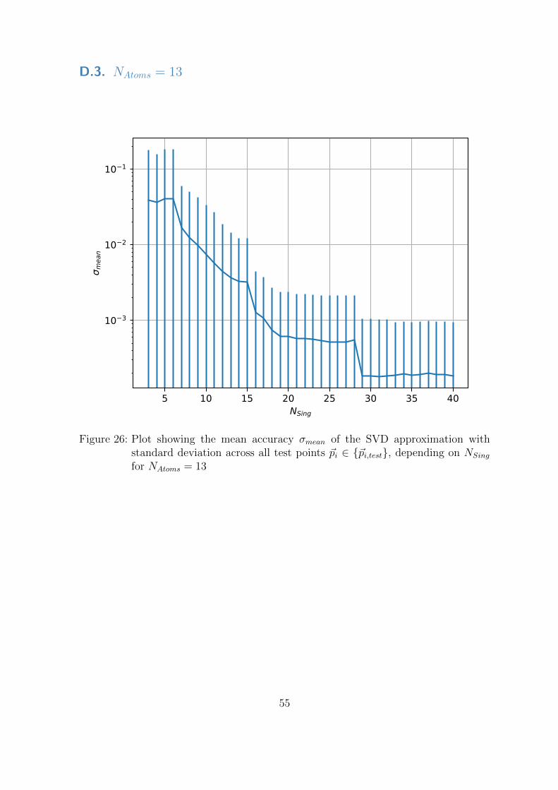
D.3. NAtoms = 13


for NAtoms = 13

55

D.4. NAtoms = 14


for NAtoms = 14

56

D.5. NAtoms = 15


for NAtoms = 15

57

References

[1] David D Awschalom, Lee C Bassett, Andrew S Dzurak, Evelyn L Hu, and Jason RPetta. Quantum spintronics: engineering and manipulating atom-like spins insemiconductors. Science, 339(6124):1174–1179, 2013.

[2] Hannes Bernien, Sylvain Schwartz, Alexander Keesling, Harry Levine, AhmedOmran, Hannes Pichler, Soonwon Choi, Alexander S Zibrov, Manuel Endres,Markus Greiner, et al. Probing many-body dynamics on a 51-atom quantumsimulator. Nature, 551(7682):579–584, 2017.

[3] Antoine Browaeys and Thierry Lahaye. Many-body physics with individuallycontrolled Rydberg atoms. Nature Physics, pages 1–11, 2020.

[4] Daniela Calvetti, L Reichel, and And Sorensen. An implicitly restarted Lanczosmethod for large symmetric eigenvalue problems. Electronic Trans. Numer. Anal.,2:1–21, 04 1994.

[5] The NumPy Community. Numpy (version 1.18.5), 2020. URL https://github.

com/numpy/numpy.

[6] The SciPy Community. Numpy v1.19 manual, 2020. URL https://numpy.org/

doc/stable/. (accessed: 14.11.2020).

[7] The SciPy Community. numpy.linalg.svd, 2020. URL https://numpy.

org/doc/stable/reference/generated/numpy.linalg.svd.html. (accessed:22.11.2020).

[8] The SciPy Community. Scipy (version 1.4.1), 2020. URL https://github.com/

scipy/scipy.

[9] The SciPy Community. Scipy reference guide, 2020. URL https://docs.scipy.

org/doc/scipy/reference/. (accessed: 02.11.2020).

[10] The SciPy Community. scipy.sparse.linalg.eigsh, 2020. URL https:

//docs.scipy.org/doc/scipy/reference/generated/scipy.sparse.linalg.

eigsh.html. (accessed: 02.11.2020).

[11] Ph. W. Courteille. Interaction of light with cold atoms, 2019. URL http://www.

ifsc.usp.br/~strontium/Publication/Scripts/LightAtomsLecture.pdf.(accessed: 26.10.2020).

[12] D.C. Sorensen, R.B. Lehoucq, C. Yang, and K. Maschhoff. Arpack software, 2008.URL https://www.caam.rice.edu/software/ARPACK/.

[13] Michel H Devoret and Robert J Schoelkopf. Superconducting circuits for quantuminformation: an outlook. Science, 339(6124):1169–1174, 2013.

58

https://github.com/numpy/numpy

https://github.com/numpy/numpy

https://numpy.org/doc/stable/

https://numpy.org/doc/stable/

https://numpy.org/doc/stable/reference/generated/numpy.linalg.svd.html

https://numpy.org/doc/stable/reference/generated/numpy.linalg.svd.html

https://github.com/scipy/scipy

https://github.com/scipy/scipy

https://docs.scipy.org/doc/scipy/reference/

https://docs.scipy.org/doc/scipy/reference/

https://docs.scipy.org/doc/scipy/reference/generated/scipy.sparse.linalg.eigsh.html



http://www.ifsc.usp.br/~strontium/Publication/Scripts/LightAtomsLecture.pdf

http://www.ifsc.usp.br/~strontium/Publication/Scripts/LightAtomsLecture.pdf

https://www.caam.rice.edu/software/ARPACK/

[14] David P DiVincenzo. The physical implementation of quantum computation.Fortschritte der Physik: Progress of Physics, 48(9-11):771–783, 2000.

[15] Carl Eckart and Gale Young. The approximation of one matrix by another oflower rank. Psychometrika, 1(3):211–218, 1936.

[16] Francisco Fernandez. The Kronecker product and some of its physical applications.European Journal of Physics, 37:065403, 11 2016. doi: 10.1088/0143-0807/37/6/065403.

[17] Gene H Golub and Charles F Van Loan. Matrix computations, 4th. JohnsHopkins, 2013.

[18] Paul R Halmos. Finite-dimensional vector spaces. Courier Dover Publications,2017.

[19] Jim Hefferon. Linear algebra fourth edition. 2020.

[20] L Isenhower, E Urban, XL Zhang, AT Gill, T Henage, Todd A Johnson,TG Walker, and M Saffman. Demonstration of a neutral atom controlled-NOTquantum gate. Physical review letters, 104(1):010503, 2010.

[21] Richard M Johnson. On a theorem stated by Eckart and Young. Psychometrika,28(3):259–263, 1963.

[22] Henning Labuhn, Daniel Barredo, Sylvain Ravets, Sylvain De Leseleuc, TommasoMacrı, Thierry Lahaye, and Antoine Browaeys. Tunable two-dimensional arraysof single Rydberg atoms for realizing quantum Ising models. Nature, 534(7609):667–670, 2016.

[23] Cornelius Lanczos. An iteration method for the solution of the eigenvalue problemof linear differential and integral operators. United States Governm. Press OfficeLos Angeles, CA, 1950.

[24] Richard B Lehoucq, Danny C Sorensen, and Chao Yang. ARPACK users’guide: solution of large-scale eigenvalue problems with implicitly restarted Arnoldimethods. SIAM, 1998.

[25] Christopher Monroe and Jungsang Kim. Scaling the ion trap quantum processor.Science, 339(6124):1164–1169, 2013.

[26] Wolfgang Nolting. Theoretical Physics 6. Springer, 2017.

[27] Wolfgang Nolting. Theoretical Physics 7: Quantum Mechanics-Methods andApplications. Springer, 2017.

[28] Jonathan D Pritchard, D Maxwell, Alexandre Gauguet, Kevin J Weatherill, MPAJones, and Charles S Adams. Cooperative atom-light interaction in a blockadedRydberg ensemble. Physical review letters, 105(19):193603, 2010.

59

[29] Mark Saffman. Quantum computing with atomic qubits and Rydberg interactions:progress and challenges. Journal of Physics B: Atomic, Molecular and OpticalPhysics, 49(20):202001, 2016.

[30] Peter Schauß, Marc Cheneau, Manuel Endres, Takeshi Fukuhara, Sebastian Hild,Ahmed Omran, Thomas Pohl, Christian Gross, Stefan Kuhr, and Immanuel Bloch.Observation of spatially ordered structures in a two-dimensional Rydberg gas.Nature, 491(7422):87–91, 2012.

[31] Peter Schauß, Johannes Zeiher, Takeshi Fukuhara, Sebastian Hild, Marc Cheneau,Tommaso Macrı, Thomas Pohl, Immanuel Bloch, and Christian Groß. Crystal-lization in Ising quantum magnets. Science, 347(6229):1455–1458, 2015.

[32] John Von Neumann. Mathematical foundations of quantum mechanics: New edition.Princeton university press, 2018.

[33] Tatjana Wilk, A Gaetan, C Evellin, J Wolters, Y Miroshnychenko, P Grangier,and A Browaeys. Entanglement of two individual neutral atoms using Rydbergblockade. Physical Review Letters, 104(1):010502, 2010.

[34] Johannes Zeiher, Jae-yoon Choi, Antonio Rubio-Abadal, Thomas Pohl, Rick vanBijnen, Immanuel Bloch, and Christian Gross. Coherent many-body spin dy-namics in a long-range interacting Ising chain. Physical Review X, 7(4):041063,2017.

60

Modellierung und numerische Simulation einer Kette neutraler ...

Documents