Modeling the Global Economic and Environmental Implications of Biofuels Production: Preliminary Results for the Medium Term

Modeling the Global Economic and Environmental Implications of

Biofuels Production: Preliminary Results for the Medium Term

Jorge Fernandez-Cornejo Agapi Somwaru

Henry An, Michael Brady

Ruben Lubowski*

For presentation at the 11th Annual GTAP Conference, Helsinki, Finland, June 12-14, 2008.

* Economic Research Service, U.S. Department of Agriculture, 1800 M Street, NW, Washington DC, 20036. Please do not cite, reproduce, or distribute without permission of the authors. The views expressed are those of the authors and do not necessarily correspond to the views or policies of the Economic Research Service or the U.S. Department of Agriculture

2

I. Introduction The recent global expansion of biofuel production led by the U.S. and Brazil, has had a

large effect on production, prices, and trade in the agricultural sector. Rapid growth of

U.S. ethanol production that relies on corn as feedstock is using an increasing share of the

corn crop. As Westcott (2007) shows, about 14 percent of the total corn crop in the U.S.

was used in ethanol production in 2005/2006. The increased demand for corn has also

led to higher corn prices and to an expansion in the total amount of cropland used to grow

corn at the expense of soybeans, cotton, and other crops, whose price consequently also

rose.

Biofuel production in Brazil has also had a large effect on global agricultural and

energy markets. Brazil began producing ethanol from sugar cane to use as fuel in the

1970s. Agricultural land in Brazil for sugar cane and other crops (particularly soybeans)

grew rapidly as cropland and pasture replaced forest and cerrado in the Brazilian

Amazonia. From 1980 to 1995, around 7 million hectares were converted to agriculture

(Cardille and Foley, 2003). However, Brazilian agricultural officials assert that future

increases in cropland devoted to sugar cane will come from pastureland rather than from

forestland (Guimaraes, 2007).1

While other countries and regions do not produce a large amount of ethanol, some

of these regions, such as the European Union (EU), affect world markets as consumers of

ethanol. For example, F.O. Licht estimates that the EU consumption of fuel ethanol

1 Guimaraes points out that currently 210 million hectares of pasture land are able to sustain 206 million heads of livestock. He adds that with the expected increases in livestock productivity, the same amount of livestock will need only 147 million hectares of pastures, freeing up 63 million hectares for other agricultural uses.

3

under the EU biofuel directive will be nearly 2 billion gallons per year in 2010 (F.O.

Licht, 2006).2

Given the complexity of agricultural markets, their interaction with other markets,

and their global nature, evaluating the repercussions of a growing market for biofuels is

not simple. Economists found very quickly that most existing agricultural models lacked

the necessary components and data to account for biofuel production at this scale

exposing a need to improve the current analytical modeling frameworks and data

systems. To help cover this gap, the Economic Research Service (ERS) of the U.S.

Department of Agriculture developed FARM II, a revised and updated version of the

Future Agricultural Resources Model (FARM).

This research further revises FARM II to examine the impacts of biofuel

development and production on a global basis under a set of economic, policy, and

technological scenarios and examines the economic and environmental tradeoffs, as well

as the distribution of benefits and costs across countries, regions, producers, and

consumers. This is the first of two papers that summarize results from the FARM II

model adapted to incorporate biofuels. This paper focuses on ethanol on the medium

term; that is, around year 2015. We assume that while improvements in current

technology and the impact of biotechnology will improve yields and technical plant

efficiency, the medium term impact of ethanol from cellulose and other technological

breakthroughs will be small. A second paper will examine the longer term with the

impact of ethanol from cellulose as the main focus.

This paper begins by summarizing the energy picture to provide some context for

the growing global importance of biofuels. Then we examine the major technical and 2 However, the EU is a significant producer of biodiesel.

4

policy drivers of biofuels production. A brief review of recent efforts to model biofuel

production is presented next and we follow this with a description of the revised FARM

II model and databases used in this study. Then we describe the scenarios examined, and

present preliminary results and conclusions.

II Biofuels in Perspective

Why Biofuels?

In 2005, a total of 460 quadrillion BTUs (Quads) of energy (equivalent to 49.4 billion

barrels of oil) were produced globally for various uses, up from 287 Quads in 1980

(USDOE, 2005).3 Petroleum is the largest energy source, accounting for 35 percent of

the total, followed by coal with 26 percent, natural gas (23 percent), hydroelectric power

(6.2 percent), natural gas plant liquids (2.5 percent), and other sources (1.4 percent).

Most primary energy production goes towards transportation and electricity generation.

Coal and natural gas are primarily used for the latter and petroleum for the prior (about

50 percent of oil demand is used for transportation, USDOE, 2007). Energy demand

across countries depends on their Gross Domestic Product (GDP), which varies widely,

and energy intensity (e.g., BTUs per dollar GDP), which is more uniform (when using

purchasing power parities). For example, 2005 energy intensity for India was 7000 BTU

per dollar, for Brazil 6300, Japan 6500, China 7900, and the U.S. 9100 (USDOE, 2007).

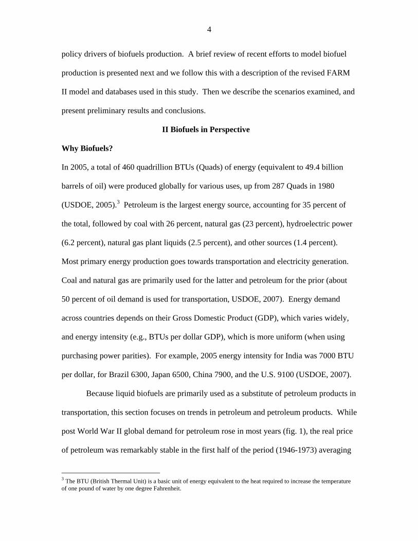
Because liquid biofuels are primarily used as a substitute of petroleum products in

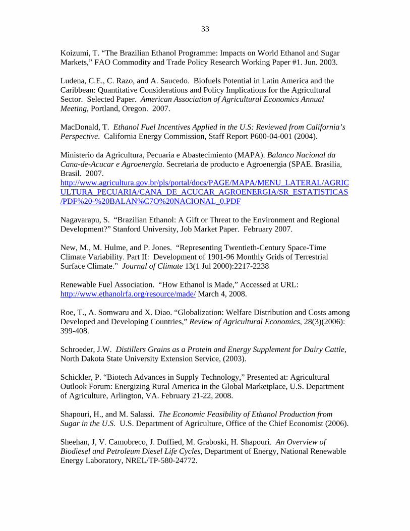
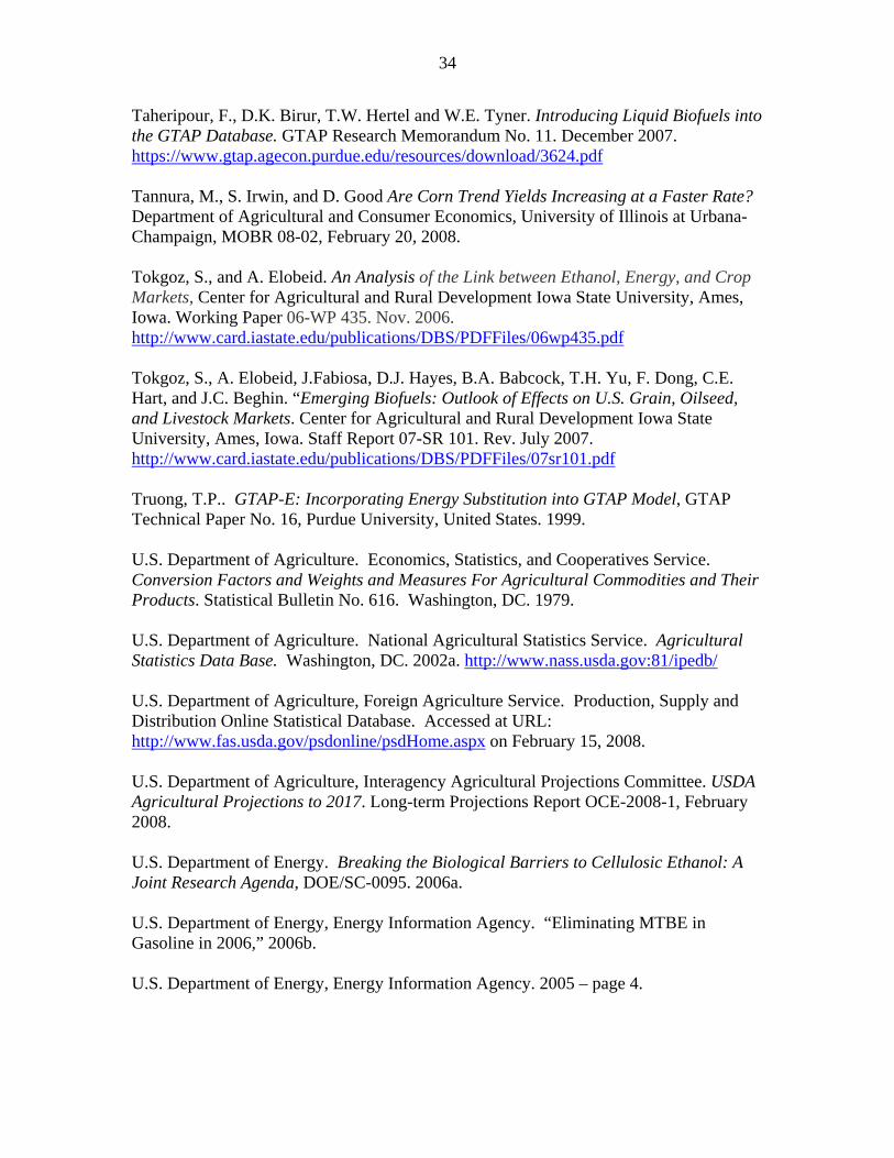
transportation, this section focuses on trends in petroleum and petroleum products. While

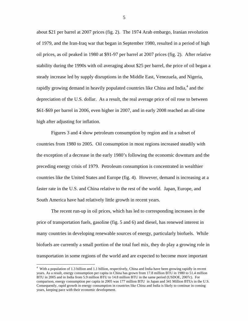
post World War II global demand for petroleum rose in most years (fig. 1), the real price

of petroleum was remarkably stable in the first half of the period (1946-1973) averaging

3 The BTU (British Thermal Unit) is a basic unit of energy equivalent to the heat required to increase the temperature of one pound of water by one degree Fahrenheit.

5

about $21 per barrel at 2007 prices (fig. 2). The 1974 Arab embargo, Iranian revolution

of 1979, and the Iran-Iraq war that began in September 1980, resulted in a period of high

oil prices, as oil peaked in 1980 at $91-97 per barrel at 2007 prices (fig. 2). After relative

stability during the 1990s with oil averaging about $25 per barrel, the price of oil began a

steady increase led by supply disruptions in the Middle East, Venezuela, and Nigeria,

rapidly growing demand in heavily populated countries like China and India,4 and the

depreciation of the U.S. dollar. As a result, the real average price of oil rose to between

$61-$69 per barrel in 2006, even higher in 2007, and in early 2008 reached an all-time

high after adjusting for inflation.

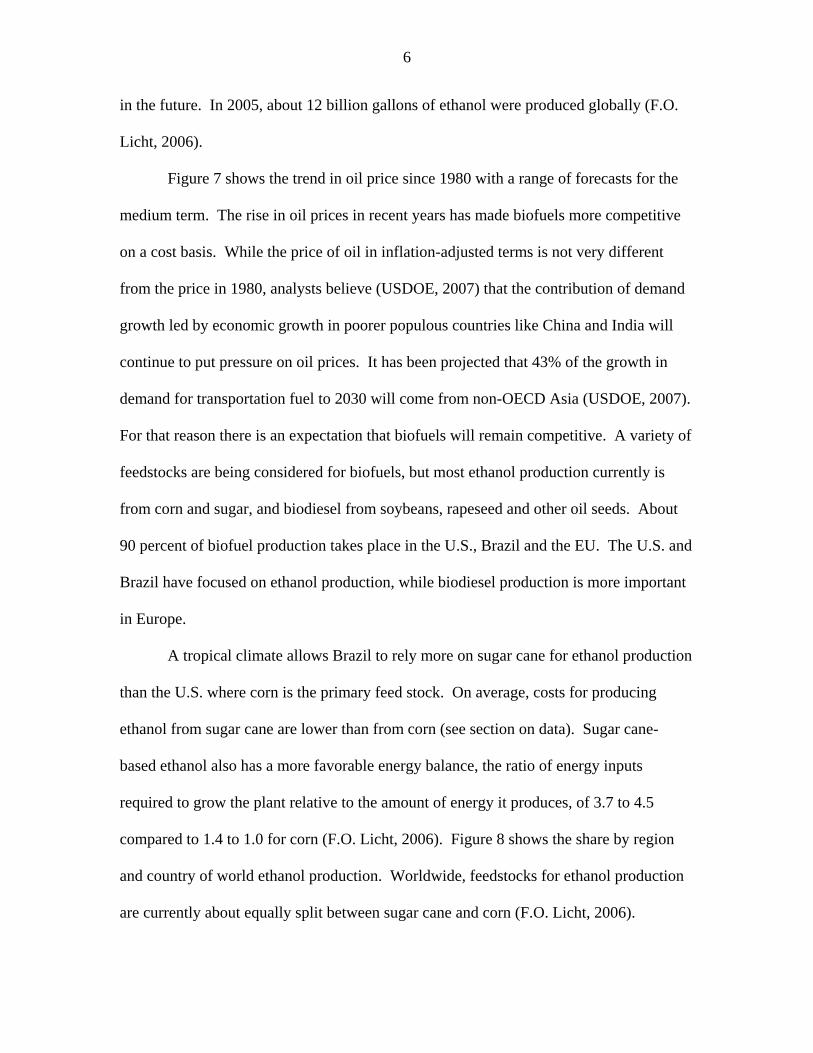
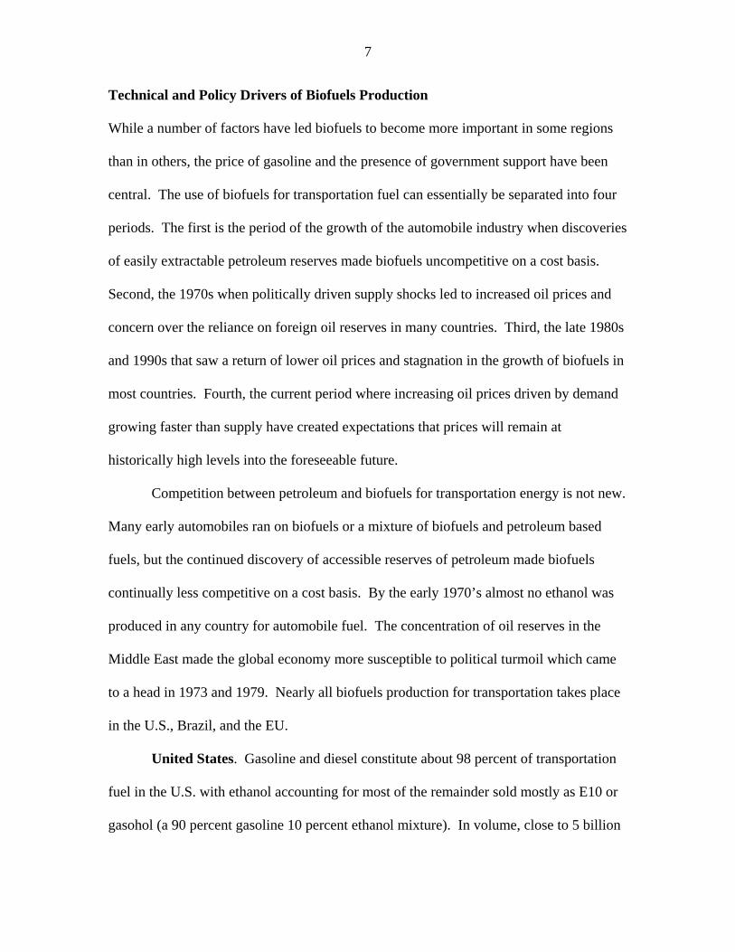
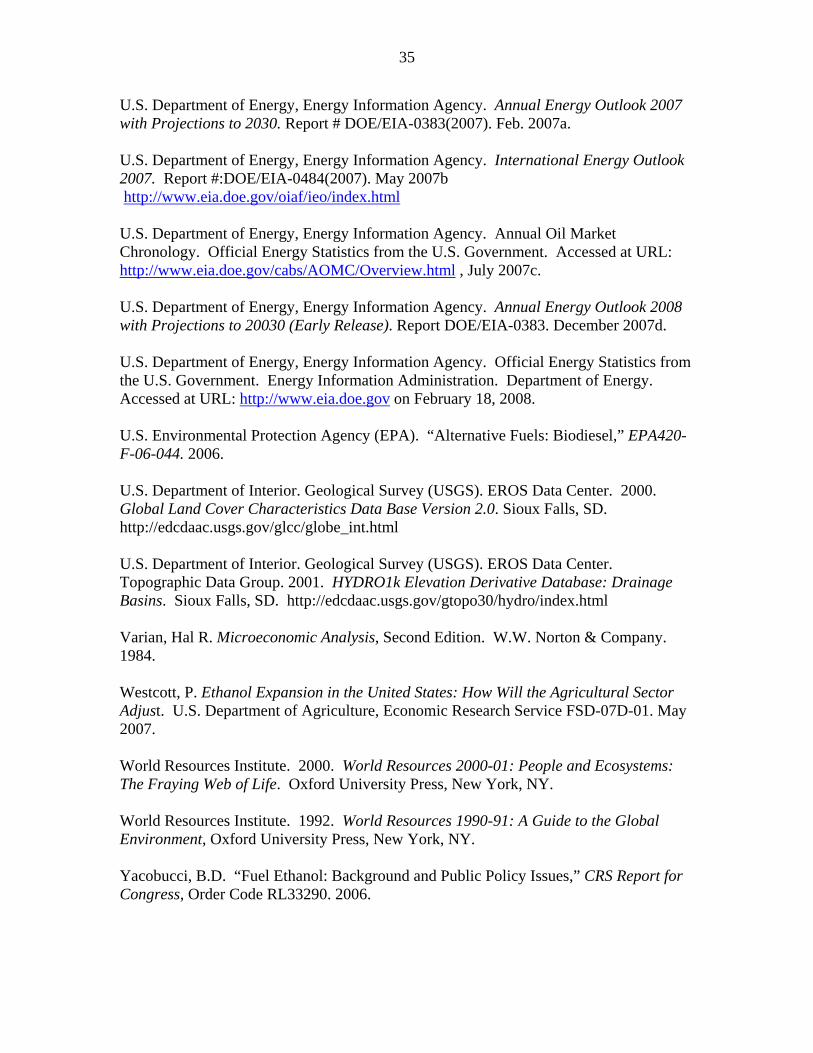
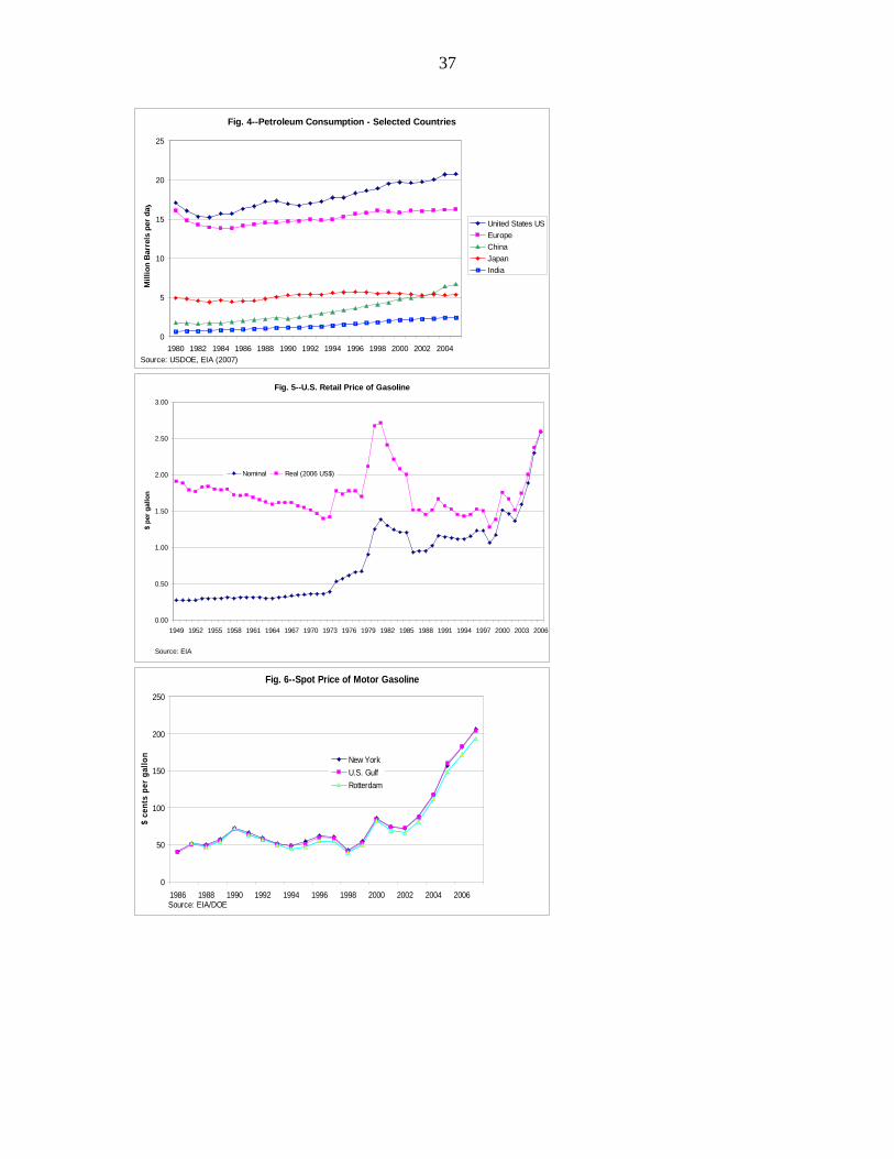
Figures 3 and 4 show petroleum consumption by region and in a subset of

countries from 1980 to 2005. Oil consumption in most regions increased steadily with

the exception of a decrease in the early 1980’s following the economic downturn and the

preceding energy crisis of 1979. Petroleum consumption is concentrated in wealthier

countries like the United States and Europe (fig. 4). However, demand is increasing at a

faster rate in the U.S. and China relative to the rest of the world. Japan, Europe, and

South America have had relatively little growth in recent years.

The recent run-up in oil prices, which has led to corresponding increases in the

price of transportation fuels, gasoline (fig. 5 and 6) and diesel, has renewed interest in

many countries in developing renewable sources of energy, particularly biofuels. While

biofuels are currently a small portion of the total fuel mix, they do play a growing role in

transportation in some regions of the world and are expected to become more important

4 With a population of 1.3 billion and 1.1 billion, respectively, China and India have been growing rapidly in recent years. As a result, energy consumption per capita in China has grown from 17.8 million BTU in 1980 to 51.4 million BTU in 2005 and in India from 5.9 million BTU to 14.8 million BTU in the same period (USDOE, 2007c). For comparison, energy consumption per capita in 2005 was 177 million BTU in Japan and 341 Million BTUs in the U.S. Consequently, rapid growth in energy consumption in countries like China and India is likely to continue in coming years, keeping pace with their economic development.

6

in the future. In 2005, about 12 billion gallons of ethanol were produced globally (F.O.

Licht, 2006).

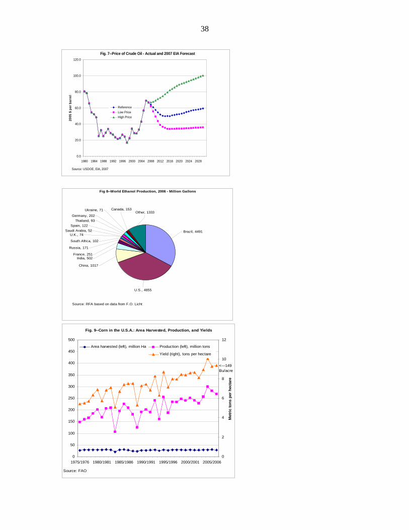
Figure 7 shows the trend in oil price since 1980 with a range of forecasts for the

medium term. The rise in oil prices in recent years has made biofuels more competitive

on a cost basis. While the price of oil in inflation-adjusted terms is not very different

from the price in 1980, analysts believe (USDOE, 2007) that the contribution of demand

growth led by economic growth in poorer populous countries like China and India will

continue to put pressure on oil prices. It has been projected that 43% of the growth in

demand for transportation fuel to 2030 will come from non-OECD Asia (USDOE, 2007).

For that reason there is an expectation that biofuels will remain competitive. A variety of

feedstocks are being considered for biofuels, but most ethanol production currently is

from corn and sugar, and biodiesel from soybeans, rapeseed and other oil seeds. About

90 percent of biofuel production takes place in the U.S., Brazil and the EU. The U.S. and

Brazil have focused on ethanol production, while biodiesel production is more important

in Europe.

A tropical climate allows Brazil to rely more on sugar cane for ethanol production

than the U.S. where corn is the primary feed stock. On average, costs for producing

ethanol from sugar cane are lower than from corn (see section on data). Sugar cane-

based ethanol also has a more favorable energy balance, the ratio of energy inputs

required to grow the plant relative to the amount of energy it produces, of 3.7 to 4.5

compared to 1.4 to 1.0 for corn (F.O. Licht, 2006). Figure 8 shows the share by region

and country of world ethanol production. Worldwide, feedstocks for ethanol production

are currently about equally split between sugar cane and corn (F.O. Licht, 2006).

7

Technical and Policy Drivers of Biofuels Production

While a number of factors have led biofuels to become more important in some regions

than in others, the price of gasoline and the presence of government support have been

central. The use of biofuels for transportation fuel can essentially be separated into four

periods. The first is the period of the growth of the automobile industry when discoveries

of easily extractable petroleum reserves made biofuels uncompetitive on a cost basis.

Second, the 1970s when politically driven supply shocks led to increased oil prices and

concern over the reliance on foreign oil reserves in many countries. Third, the late 1980s

and 1990s that saw a return of lower oil prices and stagnation in the growth of biofuels in

most countries. Fourth, the current period where increasing oil prices driven by demand

growing faster than supply have created expectations that prices will remain at

historically high levels into the foreseeable future.

Competition between petroleum and biofuels for transportation energy is not new.

Many early automobiles ran on biofuels or a mixture of biofuels and petroleum based

fuels, but the continued discovery of accessible reserves of petroleum made biofuels

continually less competitive on a cost basis. By the early 1970’s almost no ethanol was

produced in any country for automobile fuel. The concentration of oil reserves in the

Middle East made the global economy more susceptible to political turmoil which came

to a head in 1973 and 1979. Nearly all biofuels production for transportation takes place

in the U.S., Brazil, and the EU.

United States. Gasoline and diesel constitute about 98 percent of transportation

fuel in the U.S. with ethanol accounting for most of the remainder sold mostly as E10 or

gasohol (a 90 percent gasoline 10 percent ethanol mixture). In volume, close to 5 billion

8

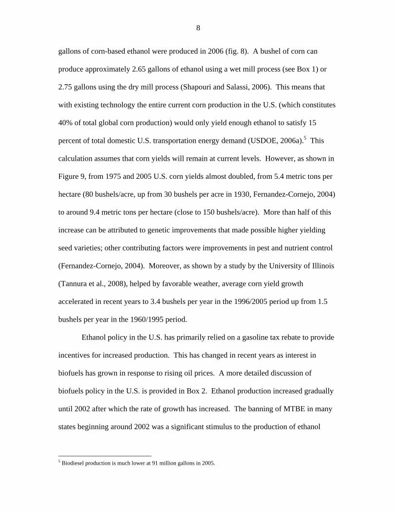
gallons of corn-based ethanol were produced in 2006 (fig. 8). A bushel of corn can

produce approximately 2.65 gallons of ethanol using a wet mill process (see Box 1) or

2.75 gallons using the dry mill process (Shapouri and Salassi, 2006). This means that

with existing technology the entire current corn production in the U.S. (which constitutes

40% of total global corn production) would only yield enough ethanol to satisfy 15

percent of total domestic U.S. transportation energy demand (USDOE, 2006a).5 This

calculation assumes that corn yields will remain at current levels. However, as shown in

Figure 9, from 1975 and 2005 U.S. corn yields almost doubled, from 5.4 metric tons per

hectare (80 bushels/acre, up from 30 bushels per acre in 1930, Fernandez-Cornejo, 2004)

to around 9.4 metric tons per hectare (close to 150 bushels/acre). More than half of this

increase can be attributed to genetic improvements that made possible higher yielding

seed varieties; other contributing factors were improvements in pest and nutrient control

(Fernandez-Cornejo, 2004). Moreover, as shown by a study by the University of Illinois

(Tannura et al., 2008), helped by favorable weather, average corn yield growth

accelerated in recent years to 3.4 bushels per year in the 1996/2005 period up from 1.5

bushels per year in the 1960/1995 period.

Ethanol policy in the U.S. has primarily relied on a gasoline tax rebate to provide

incentives for increased production. This has changed in recent years as interest in

biofuels has grown in response to rising oil prices. A more detailed discussion of

biofuels policy in the U.S. is provided in Box 2. Ethanol production increased gradually

until 2002 after which the rate of growth has increased. The banning of MTBE in many

states beginning around 2002 was a significant stimulus to the production of ethanol

5 Biodiesel production is much lower at 91 million gallons in 2005.

9

beyond the ethanol tax rebate that was responsible for growth previously.6 Just from

2003 to 2005 the use of ethanol mixed in gasoline increased 70% (USDOE, 2007).

Continued diffusion of automobiles that can run on higher ethanol gasoline mixes is

important for growth in the market for E85 that remains limited to date. Five million

flexible fuel vehicles (FFVs) were sold in the U.S. from 1992 to 2005 (USDOE, 2007).

FFVs can run on up to 85% ethanol but few do currently due to the limited availability of

refilling stations with E85. The growth of biofuels has significant governmental support

going into the future through the 2007 version of the Renewable Fuel Standard (RFS) in

the Energy Bill and also in the Farm Bill (see Box 2). Projections for biofuels production

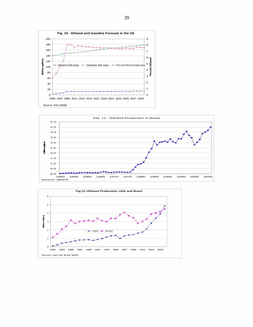
over the next 15 years under the RFS are shown in table 1.7

Brazil. Due to a combination of climate and government policy, Brazil has

substituted biofuels for fossil fuels in transportation far more than any other country. As

shown in Figure 11, the decision of the Brazilian government to expand ethanol

production following the first oil crisis in 1973 set off a significant and sustained growth

that has accelerated in the past few years. From 1975 through the late 1990s Brazilian

policy relied on direct intervention into production and consumption decisions in a

number of ways. A discussion of Brazilian biofuels policy is summarized in Box 3.

Following 15 years of slowing growth, the policy was realigned towards the use of tax

rebates and subsidies to move towards a market based market-based approach.

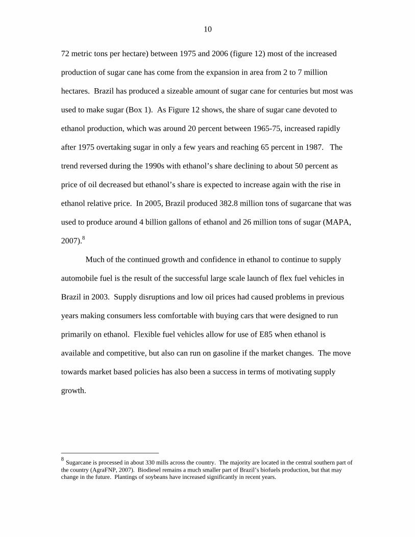
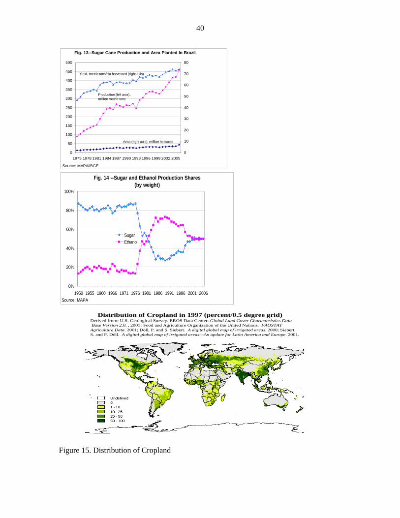
While there was approximately a 50% increase in sugar cane yields (from 47 to

6 MTEB was banned for environmental (water quality) reasons after it was found in groundwater following leaks in pipelines and underground storage tanks (USDOE, 2003). 7 It appears that the ethanol production forecast in the most recent Energy Outlook prepared by the Energy Information Administration (USDOE, 2007) shown in fig. 10 will already be exceeded by the ethanol production shown in the most recent RFS (table 1). For example, the Energy Information Agency forecast 12 billion gallons of ethanol production for 2015 (which represents a 7.7 percent of U.S. gasoline use), while the RFS calls for 15 billion gallons of corn-starch ethanol (plus additional amounts of cellulosic ethanol and biodiesel).

10

72 metric tons per hectare) between 1975 and 2006 (figure 12) most of the increased

production of sugar cane has come from the expansion in area from 2 to 7 million

hectares. Brazil has produced a sizeable amount of sugar cane for centuries but most was

used to make sugar (Box 1). As Figure 12 shows, the share of sugar cane devoted to

ethanol production, which was around 20 percent between 1965-75, increased rapidly

after 1975 overtaking sugar in only a few years and reaching 65 percent in 1987. The

trend reversed during the 1990s with ethanol’s share declining to about 50 percent as

price of oil decreased but ethanol’s share is expected to increase again with the rise in

ethanol relative price. In 2005, Brazil produced 382.8 million tons of sugarcane that was

used to produce around 4 billion gallons of ethanol and 26 million tons of sugar (MAPA,

2007).8

Much of the continued growth and confidence in ethanol to continue to supply

automobile fuel is the result of the successful large scale launch of flex fuel vehicles in

Brazil in 2003. Supply disruptions and low oil prices had caused problems in previous

years making consumers less comfortable with buying cars that were designed to run

primarily on ethanol. Flexible fuel vehicles allow for use of E85 when ethanol is

available and competitive, but also can run on gasoline if the market changes. The move

towards market based policies has also been a success in terms of motivating supply

growth.

8 Sugarcane is processed in about 330 mills across the country. The majority are located in the central southern part of the country (AgraFNP, 2007). Biodiesel remains a much smaller part of Brazil’s biofuels production, but that may change in the future. Plantings of soybeans have increased significantly in recent years.

11

Whether the biofuels sector can continue to grow without a considerable

expansion in land for corn in the U.S. (or sugar cane in Brazil) depends on whether yields

will continue to increase as they have done in recent decades.

European Union. The history of biofuels in the EU is relatively short compared

to the U.S. and Brazil. In 2004, the EU produced about 768 million gallons of biofuels

(CRS, 2006). The Biofuels Directive put forth in 2003 promotes meeting a quarter of all

transportation energy demands from biofuels by 2030 (Box 3). The EU started producing

a measurable amount of biofuels in the early 1990’s. Total production had increased to

500,000 tons in 1997. Following a brief drop in 1998, production has increased steadily

to the current levels. Over this time both biodiesel and ethanol productions have

increased steadily with the former constituting a bulk of production. Rapeseed

production is the feedstock for most of this and is primarily grown in Italy, Germany, and

France (USDA, 2008). In contrast to the U.S., the ethanol that is produced in the EU

relies primarily on wheat.

An additional challenge in coordinating biofuels production in the EU is the

diversity of countries that are member states. There is a wide range in targets for each

country. The UK target is 0.3% of transportation energy while the Czech Republic has a

target of 2.9%. The fact that diesel automobiles are relatively more common in the EU

has avoided having to rely on the spread of flex fuel vehicles with ethanol since a car that

can run on petroleum diesel can typically run on biodiesel as well.

Rest of the World. While the effect of biofuels on food prices remains a concern

in many poorer countries there is increasing interest in developing the sector in some

regions. According to F.O. Licht (2006), Canada produces 60 to 66 million gallons of

12

ethanol using corn, wheat, and barley, although it is still a net importer. Mexico produces

about 16 million gallons of ethanol, but imports more than 30 million gallons per year.

Interest in ethanol is also growing in some South American countries. Argentina’s

government enacted a mixture requirement, while corn producers in Chile have seen

ethanol as a solution to overproduction problems. In Africa nearly all ethanol production

occurs in South Africa where molasses is the major feed tock for hydrous ethanol.

China is the fourth largest producer of ethanol behind the U.S., Brazil, and the

EU. India also has the potential for large scale ethanol production from sugar cane given

that it is one of the largest sugar producers in the world. Thailand currently has limited

ethanol for fuel production, but it does have a favorable climate for sugar production and

the government has become involved in promoting the growth of the industry (F.O. Licht,

2006).

III An Overview of Recent Biofuels Models

In response to increased interest in biofuels in recent years, a number of partial and

general equilibrium models have been adapted or developed to consider potential

implications of an expanding biofuels sector. This section provides a summary of the

most recent studies based on these models and describes their basic structure,

assumptions, scenarios, and main findings.

Birur, Hertel, and Tyner (2007)(BHT) examine the implications of a growing

biofuels industry on the agriculture sector and land use globally using a global

computable general equilibrium framework (CGE). More specifically, BHT incorporate

biofuels into GTAP-E (Truong, 1999; Burniaux and Truong, 2002; McDougal and Golub,

2007), a version of GTAP that includes a global energy database and model. Biofuels are

13

integrated into the model from both the consumption and production side, and agro-

ecological zones (AEZs) are integrated to model land use change following Lee et al.

(2005). Three types of biofuels are considered; ethanol from sugar cane, ethanol from

corn, and biodiesel from oilseeds.9 Factors influencing the biofuels sector include crude

oil prices, the replacement of MTBE with ethanol, and ethanol subsidies.

BHT validate their model by using 2001 as a baseline and compare model

predictions with actual 2006 data. The model predicts a 178% increase in ethanol

production for the U.S. from 2001 to 2006 compared to the actual observed increase of

174 percent. Prediction for corn production growth was 7 percent compared to an

observed 11 percent. For Brazil, the model predicted a 38 percent increase in production

of ethanol from sugarcane, while the actual increase was 24 percent. For EU biodiesel,

the observed change from 2001 to 2006 was 410 percent and the model predicted 415

percent. The share of oilseeds predicted to go towards biodiesel ranged from 5.6% to

27.2% over the time period. All non-biofuel agricultural outputs are predicted to

decrease except for coarse grains. Most of the changes in agricultural outputs in Brazil

and the EU can be attributed to oil prices. So, the MTBE and ethanol subsidy shocks in

the U.S. do not significantly reverberate to other regions. Oil seed production is

predicted to go up by 16% in the EU. Non-oilseed grains are predicted to drop in total

production by 4%. As expected, oil prices have the largest effect on global prices.

However, the prices of agricultural commodities only increased slightly with coarse

grains being the exception. The largest expansion of land as a result of higher oil prices

9 Taheripour, Birur, Hertel, and Tyner (2007) document the process of introducing these three types of biofuels into version 6 of GTAP (Dimarana, 2007). The biofuels are introduced in three databases. One assumes there are no intermediate uses for biofuels. The second assumes that a portion of ethanol from corn is used as an additive for gasoline. The third allows for byproducts in biofuels production by accounting for distillers dried grains with solubles (DDGS) for ethanol generated from corn.

14

is in less-productive AEZs. Land for coarse grain production in the U.S. was predicted to

increase by 4%, which mostly drew from other grain sectors that lost 7%. The same story

held for Canada and the EU that increased acreage in biofuel feedstock grains at the

expense of other agricultural outputs.

In a related paper, Birur, Hertel, and Tyner (2007b) examine the 2006-2010

period using the same modeling structure and scenarios. They predict that ethanol

capacity will reach 13.4 billion gallons, which is used as a binding production level in the

model projections to 2010. It is projected that the share of corn going to produce ethanol

will more than double at the expense of feed grain and exports (16% to 38%). The

production of all other agricultural goods decreases by a significant amount. Land

allocated to the production of coarse grains increases to meet the increased demand.

Acreage in the corn belt goes up by 10%, but the largest increases are in less productive

areas. The EU mandate to 2010 represents a 281% increase over current biofuel

production. Oilseed production increases by 26% as prices double, although this is far

short of what is needed to meet the mandate. Exports in oilseeds are almost completely

eliminated. Across AEZs in Europe, land used for oilseed production increases from 7

percent to 30 percent. Trade in oilseeds is expected to increase sharply as countries like

Brazil expand production to meet the increase in demand.

Tokgoz et al. (2007 revised) use a multi-product multi-country deterministic

partial equilibrium model to consider the effect of growth in U.S. ethanol production on

various aspects of the agriculture sector including planted acreage, crop prices, livestock

production and prices, and trade. Within this framework three scenarios are considered:

higher oil prices with large-scale adoption of FFVs; 7 million acres are removed from the

15

Conservation Reserve Program; and a drought equivalent to that of 1988 occurs together

with a 14.7 billion gallon ethanol mandate. This study is an extension of Elobeid et al.

(2006) that found that the production of ethanol would grow until the incentive to expand

disappear by elevated corn prices. Additional assumptions made in Tokgoz are that the

demand for ethanol mixed with gasoline at greater than 10% will be minimal to at least

2017, and the price of distillers’ grains determined by demand from domestic and

international markets for feed grains is made endogenous in contrast to Elobeid’s.

The baseline predicts that meeting this scale of ethanol production will require

corn acreage to expand to 94 million acres as a result of prices reaching $3.40 per bushel.

Corn expands primarily at the expense of soybeans. Livestock production shrinks and the

higher costs are passed on to consumers. U.S. agriculture is not made less competitive

relative to other countries since higher prices are expected to be a global phenomenon.

The high oil price scenario assumes that prices are $10 per barrel greater than the

baseline. Land use change depends critically on the rate of adoption of FFVs that can run

on E85. If adoption is high, ethanol production would reach 29 billion gallons requiring

112 million acres of corn. Soybean and wheat planting go down as a result. Corn prices

are projected to reach $4.40 per bushel. Food prices would increase 1.1 percent overall

while meat prices go up by 5 percent and eggs go up 7 percent. The scenario involving a

removal of 7 million acres of land from CRP lowers crop prices only in the short run.

The third scenario that combines a severe drought with an ethanol mandate finds that

price inflation is moderated by the presence of international trade and a decrease in

carryover stocks of corn and wheat. Livestock producers would make moderate

production cuts.

16

Elobeid and Hart (2007) examine the connection between increasing oil prices

and increasing production of ethanol and inflation in agricultural commodity prices using

the same multi-commodity, multi-country modeling system as Tokgoz. The central focus

of the paper is to assess the downstream effects of these changes in the energy markets on

food prices and food security focusing on developing countries. The model is partial

equilibrium, econometric, and non-spatial. It also endogenously includes supply and

demand for agricultural products from temperate climates in all countries. It includes an

extension to the international market for ethanol, which provides a link to energy

markets. Other endogenous variables include prices, production, consumption and trade

in ethanol. The baseline is constructed using the U.S. and international commodity

models calibrated on 2006 historic data, which is then projected to the period 2007-16.

The first scenario involves a $10 increase in oil per barrel and FFVs are limited.

The second scenario is the same as the first but assumes greater penetration of FFVs. As

expected, countries that rely more heavily on rice are less vulnerable to the effects of

increased corn demand for ethanol. Countries that rely on wheat and sorghum fall in

between. So, Sub-Saharan Africa and Latin America are more negatively affected than

Southeast Asia.

Gurgel, Reilly, and Paltsev (2007)(GRP) focus on the long-run (2000 to 2100)

land use implications of growth in the global biofuels industry in a CGE framework

based on MIT’s Emissions Prediction and Policy Analysis model (EPPA). EPPA is a

recursive-dynamic multi-regional CGE model. GRP consider both current corn and sugar

based ethanol and the development of viable cellulosic ethanol production technology by

adapting EPPA to include multiple agricultural sectors, multiple land types, and explicitly

17

account for natural areas. The set of model runs also vary whether there is a greenhouse

gas mitigation policy.

EPPA uses GTAP data for base information aggregating the data into 16 regions

and 21 sectors. The base year of the model is 1997, and then the economy is simulated

recursively at 5-year intervals from 2000 to 2100. Given its original motivation, EPPA

models the energy sector in detail. Productivity growth in labor, energy, and land are

exogenously determined (1% per year for land). The role of bioenergy in both electricity

production and uses that currently rely on petroleum are both included. The arrival of

cellulosic technology is endogenous. Five types of land are identified: cropland, pasture,

harvested forest, natural grasslands, and natural forest. Both liquid and electric biomass

compete with crops for cropland. GRP differ from most other studies that model land

transformation. GRP find that the liquid biofuels technology dominates electricity

generation from biomass in both the scenario with a climate policy and without. Total

biofuel production with a climate policy is more than 6 fold greater than without by the

year 2100. Also notable, tropical and subtropical regions in the Americas become

significant biofuel production regions. Comparing the different land transformation

approaches, there was not a significant difference in total biofuels production, but there

was a difference in which types of land tended to be brought into biofuel production.

Using the land supply elasticity, increased intensification avoids the loss of natural area

land. So, the essential finding of GRP is that if cellulosic technologies for creating

ethanol become viable there will be widespread expansion of plantings of these crops,

comparable to the amount of land currently under crops globally, over the next century.

18

Ludena, Razo, and Saucedo (2007) estimate the potential for biofuels in Latin

America using current production and cropland area and then estimate how much

production could expand to 2025 while still meeting food production and security needs.

They find that there is enough land for the production of both food and biofuels, although

smaller countries may need to decide which to produce domestically and which to import.

Nagavarapu (2007) uses a CGE model of regional agricultural and labor markets

to look at the effect of a change in U.S. trade barriers to ethanol on Brazil. Data on labor

choices is taken from household surveys, land use and production decisions, and output

prices. A baseline is estimated on data from 1982 to 2005. In a scenario where ethanol

demand is perfectly elastic at a price 5 percent above the baseline, sugar cane and ethanol

production increase 28 percent and 94 percent, respectively. Changing the perfect

elasticity point to 10 percent above the baseline increases sugar cane production 56

percent.

Dixon et al. (2007) use a dynamic CGE model to assess the effect of policy aimed

at reducing the cost of biomass-based transportation fuel on the wider economy. The

baseline is constructed from observed data from 1992 to 2004 that is projected to 2020.

The treatment scenario then compares the projection assuming a substitution of biofuels

for petroleum. It is found that a 25 percent replacement leads to a reduction in oil prices,

an increase in employment, and an increase in export prices.

Banse, van Meijl, and Woltjer (2007) look at the global and regional effects of the

EU Biofuel directive in a CGE model that is a modification of the GTAP-E multi-sector

multi-region AGE model. Intermediate inputs are separated into energy and non-energy

sectors. The energy inputs are a capital-energy composite that accounts explicitly for

19

inputs of cereals, vegetable oils, and sugar beet or cane to produce biofuels. Land as an

input is included by modeling land demand assuming a degree of substitutability between

uses for different land types. They also model agricultural labor and capital markets

separate from non-agricultural markets.

The baseline scenario in Banse et al. is based on an elaboration of one of the four

IPCC emissions scenarios. The policy scenarios include blending requirements of 5.75

percent (low) and 11.5 percent (high) that each member state would have to meet.

Sensitivity analysis is done with respect to the price of crude oil and the elasticity of

substitution between different biofuel feedstocks. In the baseline case food prices decline

as a result of productivity outpacing demand growth even though biofuel production does

increase due to an increase in crude oil prices. Although biofuels would not reach the

5.75 percent target. Under the low blending requirement the share of biofuels in Brazil

would decrease by 7 percent as a result of the relative increase in biofuels crops relative

to oil. As expected, growth in oilseed production in the EU increases from 5 percent in

the baseline case to 29 percent in the low scenario and 49% in the high scenario. Global

land in agriculture increases in the high scenario.

IV The Model and Data

By generating stress on natural resources, global increases in human populations and

economic activities may threaten long-run agricultural and environmental sustainability.

Evaluations of how economic growth may be maintained without sacrificing

environmental amenities in the 21st century are hampered, however, by the lack of

appropriate modeling tools. To help overcome this problem, the Economic Research

20

Service (ERS) of the U.S. Department of Agriculture developed the Future Agricultural

Resources Model (FARM).

The FARM Database

The Future Agricultural Resources Model (FARM) is an integrated modeling framework

designed to analyze global changes related to long-run agricultural and environmental

resources. This model was originally developed by Roy Darwin and others (Darwin et

al., 1995; Darwin and Kennedy, 2002). Darwin and his collaborators were among the

first to model global economic production by agro-ecological zones (AEZ), where land is

divided into classes based on climate and other physical characteristics that affect the

suitability of land to grow different crops and the productivity of land for different uses.

Previous versions of FARM have been used primarily to analyze the impacts of

greenhouse gas emissions on agriculture (Darwin et al., 1994, 1995; Darwin, 1999, 2003,

2004b; Darwin and Kennedy, 2000). Other applications include: costs of sea level rise

(Darwin and Tol, 2001); the impacts of changes in agricultural technology on land use

(Ianchovichina et al., 2001); the costs of protecting global ecosystem diversity

(Lewandrowski et al., 1999); and the effects of trade deregulation and population growth

on tropical forests (Darwin et al., 1996).

The FARM framework can be visualized in terms of an environmental and

economic component (Darwin et al., 1995). The environmental component consists of a

geographic information system (GIS) that links land cover and climate data with land and

water resources. Climate is linked with land resources by agro-ecological zones defined

primarily in terms of the length of the growing season. Growing season is the period

21

during a year that soil temperature and moisture conditions support plant growth.10

Climate is linked with water resources through surface and subsurface runoff—the

amount of precipitation that is not evapotranspirated back into the atmosphere.

Evapotranspiration is the combined loss of water from a given area in a specific time by

evaporation from the soil surface and by transpiration from plants.

As more precise data have become available since FARM’s inception, ERS

revised the FARM modeling framework and updated its underlying database. The

current version of FARM, also called FARM II, includes a revised database with a new

land and water resources database linked with production of agricultural and forestry

commodities by enhanced agro-ecological zones (AEZs). Major updates include: First,

the environmental data are calibrated to 1997 values, rather than 1990. Second, the land-

cover characteristics are organized by country and 0.5° lat.-long. grid, rather than 12

aggregate regions and 0.5° latitude-longitude grid.11 Third, because the initial resolution

of the land-cover characteristics data is 1.0 km2, each country-grid combination may have

multiple land-cover characteristics, rather than just one. Fourth, agro-ecological zones,

which were initially called land classes, are derived from actual contemporary monthly

temperature and precipitation data, and plant hardiness zones (PHZ) and thermal regimes

are used in conjunction with length of growing season to distribute commodities to land

10AEZs defined primarily by length of growing season but also defined by thermal regime (TR) and plant hardiness zones (PHZ). The length of growing season is the number of days with soil temperature higher or equal than 5 ºC, where soil temperature is calculated from air temperature using 21 and 10 day lags in spring and fall, respectively. There are 6 classes of growing seasons: 0-60 days, 61-120 days, 121-180 days, 181-240 days, 241-300 days, and 301-365 days. Thermal regime is the average daily temperature during growing season and divided into 7 classes (TR1 less than or equal to10 ºC, in increments of 5 ºC until TR7 greater than 35 ºC. Moisture regime is the average daily precipitation during the growing season. Plant hardiness zones derived from minimum monthly temperatures. There are a total of 9 PHZs, starting with min monthly temp. less than or equal to -45 ºC (PHZ=1) and moving up in intervals of 10 ºC and ending with greater than or equal to 25 ºC (PHZ=9). There are two types of AEZs: irrigated and rainfed (indicated by prefix ‘i’ or ‘r’). Irrigated cropland refers to areas equipped to provide water to crops. Data are from Doll and Siebert (1999) in 0.5º lat-long resolution. 11 Land cover classes included are Cropland, Grassland, Tundra, Coniferous Forest, Nonconiferous Forest, Mixed Forest, Scattered Trees, Shrubland, Built-Up Land, and Other Land.

22

covers.12 Finally, data on U.S. agricultural water withdrawals are organized by U.S.

State, rather than for the U.S. as a whole and data on population density help define

actual land use.

The database includes the following information on land and water resources:

basic land covers by country and 0.5° lat.-long. grid; rainfed and irrigated agro-ecological

zones, thermal regimes, and plant hardiness zones by 0.5° lat.-long. grid; freshwater

withdrawals by country and sector, and agricultural withdrawals by U.S. State; and

potential irrigation water requirements by 0.5° lat.-long. grid. The database also contains

the following information linking these resources with world economic production: crop,

livestock, and forestry commodity production by country; population density by country

and 0.5° lat.-long. grid; estimated average commodity product of land by length of

growing season and thermal regime; estimated commodity production by country, land

cover, and 0.5° lat.-long. grid; and agricultural water withdrawals for livestock and

irrigation by country, land cover, and 0.5° lat.-long. grid. To illustrate, figures 15-21

show the global distribution by land cover, thermal regime, plant hardiness, and length of

the growing season.

FARM’s economic component consists of a multi-sector global computable

general equilibrium (CGE) model of the global economy implemented in the General

Algebraic Modeling System (GAMS). Both the static and dynamic versions of this

model have been previously described and applied to diverse issues relating to trade

liberalization (Roe, Somwaru and Diao, 2006; Diao, Roe and Somwaru 2002; Diao,

Somwaru and Roe 2001; Diao and Somwaru 2000).

12 The meteorological data were prepared by the University of East Anglia’s Climate Research Unit (New et al., 2000). There are 67,420 grids with weather observations.

23

As a CGE modeling framework, FARM II, accounts for all production and

expenditures within each of its country/regions. A representative household in each

region supplies primary factors to producers and maximizes utility with respect to

household consumption, government consumption, and saving. Representative producers

in each sector maximize profits associated with the utilization of four primary factors—

land, water, labor, and capital. FARM II explicitly models production systems including

land by AEZ. Assuming constant returns to scale, capital and labor are freely mobile

among national sectors while land and water endowments are fixed by agro-ecological

zones. For simplicity, no independent government savings or borrowing is assumed,

with the government spending all its tax revenues on consumption or household transfers.

Investment is assumed to exactly equal depreciation so the capital stock remains constant.

Government policies are typically simulated by imposing charges on inputs and outputs.

FARM II incorporates the latest version of the Global Trade Analysis Project

(GTAP) database, version 7, which represents the world economy as of 2004. The CGE

model is calibrated using the GTAP database but modified so that national production

and value-added data is distributed proportionally as per FARM’s environmental

database, by land use and AEZ. Table 2 summarizes the sectors and country/regions used

in this study.

For this application, the GTAP sector data were aggregated into 25 sectors,

including 8 agricultural commodities (six crops—paddy rice, wheat, other grains,

oilseeds, sugar crops, other crops—cattle and other livestock). In addition, we include 17

other sectors: forestry products, coal, oil, gas, other minerals; fish, meat and dairy; other

processed food; vegetable oils and fats; sugar; lumber; manufacturing non-metallic;

24

chemical, rubber, and plastic products; petroleum and coal products; other

manufacturing; transportation services; services; and capital goods.

For the Biofuels study it was necessary to split some of the GTAP existing sectors

to explicitly account for corn, soybeans, and ethanol. For example, the sector “other

grains” was split into corn and “rest of other grains,” and the sector “oilseeds” was split

into the sectors “soybean” and “other oil seeds.” Two ethanol sectors were created based

on the two major sources of the feedstock: Corn ethanol produced mostly in the U.S. and

sugar-cane ethanol produced mostly in Brazil. Figures 22 and 23 summarize the cost of

production of ethanol in the two major ethanol-producing countries, the U.S. and Brazil,

and also show the dependence of ethanol cost on the price of their respective feedstocks.

Key agricultural and non-agricultural sectors data, especially for those sectors

related to biofuels in the global GTAP database, were expanded because detailed and

accurate data are necessary to simulate consistent commodity impacts. Given the

importance of input requirements (such as purchased variable inputs) in the production of

individual commodities, we use alternative data sources to develop these cost flows as

well as returns to the factors of production of all new commodities introduced in the

database. In particular, for the U.S. we use data from the Agricultural Resource

Management Surveys (ARMS) and from ERS’ official farm income and productivity

accounts to reflect updated production and intermediate cost of farm commodity

activities intermediate cost of farm commodity activities. Utilizing the environmental

database we improved the accuracy of resource allocation globally, especially land use,

by farm activity in the production of the various farm outputs. A benefit of such detailed

25

data on costs and supply-response is that it allows complete specification and interaction

of the sectors/commodities in the model.

Unlike other global modeling platforms that utilize elasticities in nested

production specification to accommodate the lack of detailed commodity data on

intermediates and factors of production, we were in the position to augment the global

database to estimate directly own and cross effects of the commodities and industries

specified. A benefit of such up-to-date detail on costs and supply-side requirements for

specific crops and livestock is that it allows us to capture more accurately the impacts of

future biofuel expansion. For example, the farm resources needed to produce corn

determine the supply response not only for corn but for all other related commodities that

compete for similar resources. We also attempt to capture the interaction of upstream

and downstream industries related to biofuels, such as dry corn milling sector/industry

and similar sugar/ethanol activities in the U.S. and Brazil, respectively, in a consistent

manner. In sum, we introduce disaggregated industries to capture the farm and

downstream industries linkages and interactions that are essential for the FARM II model

in order to simulate and accurately quantify the impacts on the farm sector.

Given the farm sector’s dynamic changes and especially the relevance of biofuels

for the global FARM II model, we replaced aggregated farm activities with detailed

commodity/ industry activities and specific value-added accounts and the entire global

environmental and economic database was rebalanced.

For the biofuel study, the data are aggregated into 15 countries/regions: Canada,

United States, Mexico, Brazil, other Western Hemisphere, European Union (EU25),

Russia, China, India, other East Asia, other South Asia, OPEC countries, Oceania, Africa,

26

and the rest of the world (table 2). Finally, we consider the following endowments: land,

unskilled labor, skilled labor, capital, natural resources, and irrigation water.

Scenarios

In this preliminary analysis we consider two scenarios, both for the medium term. The

basic scenario with trend productivity assumes that the U.S. producers attempt to meet

the Revised Renewable Fuels Standard for the medium term (around 2015); that is, the

U.S. will have a total production target of around 15 billion gallons per year of

conventional biofuels (ethanol from corn starch). In the case of the U.S., the productivity

gains for the basic scenario are consistent with USDA’s baseline projections (USDA.

2008). The basic scenario also assumes that Brazilian producers will attempt to meet the

ethanol production estimates set up in the national energy plan published by the Brazilian

Government (EPE, 2007), which implies that there will be moderate increases in

productivity (table 3).

In the second scenario, we assume the there will be additional productivity gains

in the U.S. as predicted by some experts (Schicker, 2008). For Brazil we assume

productivity gains with respect the basic Brazilian scenario of 10 percent. It is also

assumed that for the medium term there will not be a substantial amount of cellulosic

ethanol. Table 3 shows the yields and other technical data related to the production of

corn-based ethanol in the U.S. and sugar cane-based ethanol in Brazil in accordance with

the two medium-term scenarios considered.

Preliminary Results

Selected preliminary results from the model simulations are summarized in table 4 and

figures 24-25. All impacts resulting from the two scenarios are measured as percentage

27

changes from the model baseline for the 2004/2005 world economy. Overall global

welfare change effects are presented in Table 4.13 In both scenarios, greater production

of corn-based and sugar cane-based ethanol leads to moderate global welfare gains led by

Brazil. The U.S. has small gains. Main losers are OPEC countries.

As a result of the 220 percent increase in production of corn-based ethanol in the

U.S. and 120 percent increase of sugar cane-based ethanol in Brazil, U.S. corn production

increases by about 33 percent, U.S. corn prices increase by 23 percent while corn ethanol

prices decrease by about 8 percent. U.S. land devoted to corn increases by 18 percent

(fig. 24). In Brazil, the 120 percent increase in sugar cane-based ethanol leads to an

increase in sugar cane production of 53 percent. Sugar cane prices rise by about 24, sugar

ethanol price decrease by about 20 percent, and land use increases by 52 percent (fig. 25).

In the alternative (higher productivity scenario), as corn-based ethanol raises by

about 220 percent, U.S. corn production increases by 39 percent, U.S. corn prices

increase by 23 percent while corn ethanol prices decrease by 9 percent. Corn acreage

increases by 16 percent (fig. 24). In Brazil, the increase (120 percent) in sugar cane-based

ethanol leads to sugar cane production increases of almost 55 percent and sugar cane

prices increase by 24 percent. Land used to grow sugar cane increases by about 51

percent (fig. 25).

Summary and Concluding Comments

This paper presents the first part of an effort to evaluate the global potential for biofuel

adoption under different economic, policy, and technological assumptions. The analysis

13 This paper uses the widely accepted equivalent variation (i.e., consumers’ willingness to pay) to measure the social welfare gains or losses due to the increased ethanol production (e.g., to meet the Renewable Fuel Standard-- in the U.S.) The EV measurement of welfare uses the status-quo (pre-policy) prices as the base and addresses the question: what income would be equivalent to the change brought about by the policy (Varian, 1984).

28

is based on the revised Future Agricultural Resources Model (FARM II), which is an

integrated modeling framework developed by USDA’s Economic Research Service

designed for analyzing global changes related to long-run agricultural and environmental

sustainability. FARM II includes a new land and water resources database linked to the

production of agricultural and forestry commodities according to agro-ecological zones

characterized by irrigated or rain-fed production conditions, length of growing seasons,

temperature regime, and plant hardiness zones. This database has been incorporated into

a computable general equilibrium (CGE) model of the global economy based on the

GTAP 7 database modified to reflect FARM II economic structure. FARM II has been

adapted for the analysis of the implications of biofuel production and provides a global

framework with links between the agricultural and energy sectors, trade policy, and land

resource use at a fine spatial scale. This paper includes preliminary simulation results of

a controlled experiment under two technological and policy scenarios focusing on the

medium term.

Further work, currently under development, includes addition in the model of

biodiesel component and second generation feedstocks.

References AgraFNP. Sugar and Ethanol in Brazil: A Study of the Brazilian Sugarcane, Sugar and Ethanol Industries. Special Report No. 140. AgraFNP, Sao Paulo, Brazil and Agra Informa Ltd, Kent, UK. 2007. Banse, M.A.H.; Meijl, H. van; Tabeau, A.A.; Woltjer, G.B. Impact of Biofuel Policies on World Agricultural and Food Markets. Paper presented at the Tenth Annual Conference on Global Economics Analysis, Assessing the Foundations of Global Economic Analysis, Purdue University, West Lafayette, IN, USA, 7-9 June, 2007. https://www.gtap.agecon.purdue.edu/resources/download/3428.pdf

29

Bamberger, R. “Automobile and Light Truck Fuel Economy: The CAFÉ Standards,” CRS Issue Brief for Congress, Order Code IB90122, (2003). Birur, D.K., T.W. Hertel, W. E. Tyner. The Biofuels Boom: Implications for World Food Markets. Center for Global Trade Analysis Department of Agricultural Economics, Purdue University. Paper prepared for presentation at the Food Economy Conference Sponsored by the Dutch Ministry of Agriculture, The Hague, October 18-19, 2007. http://www.agecon.purdue.edu/papers/biofuels/LEI_paper.pdf Birur, D.K., T.W. Hertel and W.E. Tyner. “Impact of Biofuel Production on World Agricultural Markets: A Computable General Equilibrium Analysis.” GTAP Working Paper, Purdue University. November 2007 Bolter, I., D. Bacovsky, and M. Worgetter. “Biofuels in the European Union: An Overview of the European Biofuels Policy,” IEA Task 39 Report T39-B7. 2007. BP. BP Statistical Review of World Energy 2007. Historical data. Download historical data from 1965-2006. Accessed at: http://www.bp.com/statisticalreview on Feb. 2008. Burniaux, J. and T. Truong. "GTAP-E: An Energy-Environmental Version of the GTAP Model", GTAP Technical Paper No. 16, Center for Global Trade Analysis. 2002. Cardille, J.A., and J.A. Foley. “Agricultural land-use change in Brazilian Amazonia between 1980 and 1995: Evidence from integrated satellite and census data.” Remote Sensing of Environment 87 (2003) 551–562 Commission of European Communities) “Directive 2003/30/EC of the European Parliament and of the Council of 8 May 2003 on the Promotion of the Use of Biofuels or Other Renewable Fuels for Transport,” Official Journal of the European Union, L123/42-46. 2003. Accessed at: http://ec.europa.eu/energy/res/legislation/doc/biofuels/en_final.pdf Commission of the European Communities, The European Union (EU). Biomass Action Plan {SEC(2005) 1573} 628 final. Congressional Research Service (CRS), The Library of Congress. “European Union Biofuels Policy and Agriculture: An Overview,” CRS Report for Congression, Order Code RS22404. Mar. 16, 2006. Darwin, R.F. 2004a. Creating Global Economic Models with Water and Heterogeneous Land Resources. U.S. Department of Agriculture, Economic Research Service, Washington, DC. Forthcoming. Darwin, R.F. 2004b. “Effects of Greenhouse Gas Emissions on World Agriculture, Food Consumption, and Economic Welfare”, forthcoming in Climatic Change.

30

Darwin, R.F. 2003. “Impacts of Rising Concentrations Greenhouse Gases.” Chapter 7.2 in: Agricultural Resources and Environmental Indicators, 2003. U.S. Department of Agriculture, Economic Research Service, Washington, DC. Darwin, R. F. 1999. “A FARMer=s View of the Ricardian Approach to Measuring Effects of Climatic Change on Agriculture.” Climatic Change 41(3-4):371-411. Darwin, R. F. and D. Kennedy. 2000. “Economic Effects of CO2 Fertilization of Crops: Transforming Changes in Yield into Changes in Supply.” Environmental Modeling and Assessment 5(3):157-168. Darwin, R. F., J. Lewandrowski, B. McDonald, and M. Tsigas. 1994. “Global Climate Change: Analyzing Environmental Issues and Agricultural Trade within a Global Context.” Chapter 14 in: Sullivan, J., ed., Environmental Policies: Implications for Agricultural Trade. (Foreign Agricultural Economic Report Number 252) U.S. Department of Agriculture, Economic Research Service, Washington, DC, pp. 122-145. Darwin, R.F., and J. Sullivan. 2004. A Global Economic Database with Water and Heterogeneous Land Resources. U.S. Department of Agriculture, Economic Research Service, Washington, DC. Forthcoming. Darwin, R.F., J. Sullivan, and K. Ingram. 2004. Linking Land and Water Resources with World Economic Production. U.S. Department of Agriculture, Economic Research Service, Washington, DC. Forthcoming. Darwin, R. F. and R. S. J. Tol. 2001. “Estimates of the Economic Effects of Sea Level Rise.” Environmental and Resource Economics 19(2):113-129 Darwin, R. F., M. Tsigas, J. Lewandrowski, and A. Raneses. 1996 “Land Use and Cover in Ecological Economics,” Ecological Economics 17(3):157-181. Darwin, R. F., M. Tsigas, J. Lewandrowski, and A. Raneses. 1995. World Agriculture and Climate Change: Economic Adaptation. (U.S. Department of Agriculture, Economic Research Service, Agricultural Economic Report No. 703) Washington, DC. Diao, X., T. Roe, and A. Somwaru. “Developing Country Interests in Agricultural Reforms Under the World Trade Organization,” American Journal of Agricultural Economics, 84(3)(2002).: 782-790. Diao, X., A. Somwaru, and T. Roe. “A Global Analysis of Agricultural Reform in WTO Member Countries,” in Agricultural Policy Reform in the WTO: The Road Ahead, Agricultural Economic Report No. 802. U.S. Department of Agriculture, Economic Research Service, Washington, DC. 2001. Dimaranan, B.V., Editor. Global Trade, Assistance, and Production: The GTAP 6 Data Base. Center for Global Trade Analysis, Purdue University. 2006. https://www.gtap.agecon.purdue.edu/databases/v6/v6_doco.asp

31

Dixon, P.B., S. Osborne, M.T. Rimmer. “The Economy-Wide Effects in the United States of Replacing Crude Petroleum with Biomass,” Monash University (2007). Döll, P. and S. Siebert. 1999. A Digital Global Map of Irrigated Areas: Documentation. Center for Environmental Systems Research, University of Kassel, Kassel, Germany. Duffield, J.A, and K. Collins. “Evolution of Renewable Energy Policy,” Choices 21(1)(2006):9-14. Duffield, J., H. Shapouri, M. Graboski, R. McCormick, and R. Wilson. Biodiesel Development: New Markets for Conventional and Genetically Modified Agricultural Products. U.S. Department of Agriculture, Economic Research Service, Agricultural Economic Report Number 770. Sep. 1998. Elobeid, A., S. Tokgoz. Removal of U.S. Ethanol Domestic and Trade Distortions: Impact on U.S. and Brazilian Ethanol Markets. Center for Agricultural and Rural Development Iowa State University, Ames, Iowa. Working Paper 06-WP 427. October 2006 (Revised) http://www.card.iastate.edu/publications/DBS/PDFFiles/06wp427.pdf Elobeid, A., S. Tokgoz, D. J. Hayes, B.A. Babcock, C.E. Hart. The Long-Run Impact of Corn-Based Ethanol on the Grain, Oilseed, and Livestock Sectors: A Preliminary Assessment. The Center for Agricultural and Rural Development Iowa State University, Ames, Iowa. CARD Briefing paper 06-BP 49. Nov. 2006. http://www.card.iastate.edu/publications/DBS/PDFFiles/06bp49.pdf Elobeid, A., C.E. Hart. “Ethanol Expansion in the Food versus Fuel Debate: How Will Developing World Fare?” Journal of Agricultural & Food Industrial Organization. 5(2)(2007): Article 6 http://www.bepress.com/jafio/vol5/iss2/art6/ Eswaran, H., E. Van den Berg, P. Reich, R. Almaraz, B. Smallwood, and P. Zdruli. 1995. Global Soil Moisture and Temperature Regimes. World Soil Resources Office, Natural Resources Conservation Service, U.S. Department of Agriculture, Washington, DC. Fernandez-Cornejo, J. The Seed Industry in U.S. Agriculture: An Exploration of Data and Information on Crop Seed Markets, Regulation, Industry Structure, and Research and Development. U.S. Department of Agriculture, Economic Research Service, AIB-786. Feb. 2004. Food and Agriculture Organization of the United Nations (FAO). Online Statistical Database (FAOSTAT). Accessed at URL: http://faostat.fao.org/site/526/default.aspx on March 4, 2008.

32

F.O. Licht. World Ethanol Markets: The Outlook to 2015. A Special Study from F.O. Lich in Conjunction with Agra CEAS Consulting. Special Report No. 132. Published and Distributed by Agra Informa Ltd, Kent, UK and F.O. Licht, Ratzeburg, Germany. 2004. F.O. Licht. Ethanol Production Costs: A Worldwide Survey. An F.O. Licht Special Study. Special Report No. 138. Published and Distributed by F.O. Licht, Kent. UK. 2006. Food and Agriculture Organization of the United Nations (FAO). 2002. FAOSTAT Agriculture Data. Rome, Italy. Food and Agriculture Organization of the United Nations (FAO). 1996. Agro-ecological zoning: Guidelines. (FAO Soils Bulletin 73) Rome, Italy. Guimaraes, E. “Brazilian Agribusiness,” Presented at: Agricultural Outlook Forum: Energizing Rural America in the Global Marketplace, U.S. Department of Agriculture, Arlington, VA. February 21-22, 2008. Gleick, Peter H., ed. 1993. Water in Crisis: A Guide to the World’s Fresh Water Resources. Oxford University Press, Oxford, United Kingdom.

Gurgel, A., J.M. Reilly, and S. Paltsev. “Potential Land Use Implications of a Global Biofuels Industry.” Journal of Agricultural & Food Industrial Organization. 5(2)(2007): Article 9. Available at:: http://www.bepress.com/jafio/vol5/iss2/art9/

Ianchovichina, E., R.F. Darwin, and R. Shoemaker. “Resource Use and Technological Progress in Agriculture: A Dynamic General Equilibrium Analysis.” Ecological Economics 38(2)(2001):275-291. Lee, H.L., T.W. Hertel, B. Sohngen, and N. Ramankutty. Towards An Integrated Land Use Data Base for Assessing the Potential for Greenhouse Gas Mitigation. GTAP Technical Paper No.25. Center for Global Trade Analysis. December, 2005 Leemans, R. and W.P. Cramer. The IIASA Database for Mean Monthly Values of Temperature, Precipitation, and Cloudiness on a Global Terrestrial Grid. Digital Raster Data on a 30-minute Geographic (lat/long) 360x720 grid. International Institute for Applied Systems Analysis, Luxemburg, Austria. 1991. Lewandrowski, J., R. F. Darwin, M. Tsigas, and A. Raneses. “Estimating Costs of Protecting Global Ecosystem Diversity,” Ecological Economics 29(1)(1999):111-125. Klein, K., R. Romain, M. Olar, and N. Bergeron. “Ethanol Policies, Programs, and Production in Canada.” Presented at “Agriculture as a Producer and Consumer of Energy,” Sponsored by the Farm Foundation, OSDA, and OFPNV. 2004. http://www.farmfoundation.org/projects/documents/klein-ethanol.ppt.

33

Koizumi, T. “The Brazilian Ethanol Programme: Impacts on World Ethanol and Sugar Markets,” FAO Commodity and Trade Policy Research Working Paper #1. Jun. 2003. Ludena, C.E., C. Razo, and A. Saucedo. Biofuels Potential in Latin America and the Caribbean: Quantitative Considerations and Policy Implications for the Agricultural Sector. Selected Paper. American Association of Agricultural Economics Annual Meeting, Portland, Oregon. 2007. MacDonald, T. Ethanol Fuel Incentives Applied in the U.S: Reviewed from California’s Perspective. California Energy Commission, Staff Report P600-04-001 (2004).

Ministerio da Agricultura, Pecuaria e Abastecimiento (MAPA). Balanco Nacional da Cana-de-Acucar e Agroenergia. Secretaria de producto e Agroenergia (SPAE. Brasilia, Brasil. 2007. http://www.agricultura.gov.br/pls/portal/docs/PAGE/MAPA/MENU_LATERAL/AGRICULTURA_PECUARIA/CANA_DE_ACUCAR_AGROENERGIA/SR_ESTATISTICAS/PDF%20-%20BALAN%C7O%20NACIONAL_0.PDF

Nagavarapu, S. “Brazilian Ethanol: A Gift or Threat to the Environment and Regional Development?” Stanford University, Job Market Paper. February 2007. New, M., M. Hulme, and P. Jones. “Representing Twentieth-Century Space-Time Climate Variability. Part II: Development of 1901-96 Monthly Grids of Terrestrial Surface Climate.” Journal of Climate 13(1 Jul 2000):2217-2238 Renewable Fuel Association. “How Ethanol is Made,” Accessed at URL: http://www.ethanolrfa.org/resource/made/ March 4, 2008. Roe, T., A. Somwaru and X. Diao. “Globalization: Welfare Distribution and Costs among Developed and Developing Countries,” Review of Agricultural Economics, 28(3)(2006): 399-408. Schroeder, J.W. Distillers Grains as a Protein and Energy Supplement for Dairy Cattle, North Dakota State University Extension Service, (2003). Schickler, P. “Biotech Advances in Supply Technology,” Presented at: Agricultural Outlook Forum: Energizing Rural America in the Global Marketplace, U.S. Department of Agriculture, Arlington, VA. February 21-22, 2008. Shapouri, H., and M. Salassi. The Economic Feasibility of Ethanol Production from Sugar in the U.S. U.S. Department of Agriculture, Office of the Chief Economist (2006). Sheehan, J, V. Camobreco, J. Duffied, M. Graboski, H. Shapouri. An Overview of Biodiesel and Petroleum Diesel Life Cycles, Department of Energy, National Renewable Energy Laboratory, NREL/TP-580-24772.

34

Taheripour, F., D.K. Birur, T.W. Hertel and W.E. Tyner. Introducing Liquid Biofuels into the GTAP Database. GTAP Research Memorandum No. 11. December 2007. https://www.gtap.agecon.purdue.edu/resources/download/3624.pdf Tannura, M., S. Irwin, and D. Good Are Corn Trend Yields Increasing at a Faster Rate? Department of Agricultural and Consumer Economics, University of Illinois at Urbana- Champaign, MOBR 08-02, February 20, 2008. Tokgoz, S., and A. Elobeid. An Analysis of the Link between Ethanol, Energy, and Crop Markets, Center for Agricultural and Rural Development Iowa State University, Ames, Iowa. Working Paper 06-WP 435. Nov. 2006. http://www.card.iastate.edu/publications/DBS/PDFFiles/06wp435.pdf Tokgoz, S., A. Elobeid, J.Fabiosa, D.J. Hayes, B.A. Babcock, T.H. Yu, F. Dong, C.E. Hart, and J.C. Beghin. “Emerging Biofuels: Outlook of Effects on U.S. Grain, Oilseed, and Livestock Markets. Center for Agricultural and Rural Development Iowa State University, Ames, Iowa. Staff Report 07-SR 101. Rev. July 2007. http://www.card.iastate.edu/publications/DBS/PDFFiles/07sr101.pdf Truong, T.P.. GTAP-E: Incorporating Energy Substitution into GTAP Model, GTAP Technical Paper No. 16, Purdue University, United States. 1999. U.S. Department of Agriculture. Economics, Statistics, and Cooperatives Service. Conversion Factors and Weights and Measures For Agricultural Commodities and Their Products. Statistical Bulletin No. 616. Washington, DC. 1979. U.S. Department of Agriculture. National Agricultural Statistics Service. Agricultural Statistics Data Base. Washington, DC. 2002a. http://www.nass.usda.gov:81/ipedb/ U.S. Department of Agriculture, Foreign Agriculture Service. Production, Supply and Distribution Online Statistical Database. Accessed at URL: http://www.fas.usda.gov/psdonline/psdHome.aspx on February 15, 2008. U.S. Department of Agriculture, Interagency Agricultural Projections Committee. USDA Agricultural Projections to 2017. Long-term Projections Report OCE-2008-1, February 2008. U.S. Department of Energy. Breaking the Biological Barriers to Cellulosic Ethanol: A Joint Research Agenda, DOE/SC-0095. 2006a. U.S. Department of Energy, Energy Information Agency. “Eliminating MTBE in Gasoline in 2006,” 2006b. U.S. Department of Energy, Energy Information Agency. 2005 – page 4.

35

U.S. Department of Energy, Energy Information Agency. Annual Energy Outlook 2007 with Projections to 2030. Report # DOE/EIA-0383(2007). Feb. 2007a. U.S. Department of Energy, Energy Information Agency. International Energy Outlook 2007. Report #:DOE/EIA-0484(2007). May 2007b http://www.eia.doe.gov/oiaf/ieo/index.html U.S. Department of Energy, Energy Information Agency. Annual Oil Market Chronology. Official Energy Statistics from the U.S. Government. Accessed at URL: http://www.eia.doe.gov/cabs/AOMC/Overview.html , July 2007c. U.S. Department of Energy, Energy Information Agency. Annual Energy Outlook 2008 with Projections to 20030 (Early Release). Report DOE/EIA-0383. December 2007d. U.S. Department of Energy, Energy Information Agency. Official Energy Statistics from the U.S. Government. Energy Information Administration. Department of Energy. Accessed at URL: http://www.eia.doe.gov on February 18, 2008. U.S. Environmental Protection Agency (EPA). “Alternative Fuels: Biodiesel,” EPA420-F-06-044. 2006. U.S. Department of Interior. Geological Survey (USGS). EROS Data Center. 2000. Global Land Cover Characteristics Data Base Version 2.0. Sioux Falls, SD. http://edcdaac.usgs.gov/glcc/globe_int.html U.S. Department of Interior. Geological Survey (USGS). EROS Data Center. Topographic Data Group. 2001. HYDRO1k Elevation Derivative Database: Drainage Basins. Sioux Falls, SD. http://edcdaac.usgs.gov/gtopo30/hydro/index.html Varian, Hal R. Microeconomic Analysis, Second Edition. W.W. Norton & Company. 1984. Westcott, P. Ethanol Expansion in the United States: How Will the Agricultural Sector Adjust. U.S. Department of Agriculture, Economic Research Service FSD-07D-01. May 2007. World Resources Institute. 2000. World Resources 2000-01: People and Ecosystems: The Fraying Web of Life. Oxford University Press, New York, NY. World Resources Institute. 1992. World Resources 1990-91: A Guide to the Global Environment, Oxford University Press, New York, NY. Yacobucci, B.D. “Fuel Ethanol: Background and Public Policy Issues,” CRS Report for Congress, Order Code RL33290. 2006.

36

Fig. 1--World Petroleum Consumption

0

10

20

30

40

50

60

70

80

90

100

1965 1968 1971 1974 1977 1980 1983 1986 1989 1992 1995 1998 2001 20040

1

2

3

4

5

6

7

8

9

10(Million Barrels per day)

World (left scale) Brazil China India

Source: BP, 2007 Fig. 2--The Price of Petroleum in Real 2007 Dollars

0

20

40

60

80

100

120

1946 1952 1958 1964 1970 1976 1982 1988 1994 2000 2006

US$

per

bar

rel

Illinois IOGA (U.S)

Dubai

Brent

Nigerian Forcados

West TexasIntermediate (U.S.)

Source: Platts as reported by BP; Inlationdata. Fig. 3--World Petroleum Comsumption by Region, 1980-2005

0

10

20

30

40

50

60

70

80

90

1980 1982 1984 1986 1988 1990 1992 1994 1996 1998 2000 2002 2004

Mill

on B

arre

ls p

er D

ay

AfricaAsia & OceaniaMiddle EastEuropeCentral & South AmericaNorth America

Source: USDOE, EIA (2007)

37

Fig. 4--Petroleum Consumption - Selected Countries

0

5

10

15

20

25

1980 1982 1984 1986 1988 1990 1992 1994 1996 1998 2000 2002 2004

Mill

ion

Bar

rels

per

day

United States USEuropeChinaJapanIndia

Source: USDOE, EIA (2007) Fig. 5--U.S. Retail Price of Gasoline

0.00

0.50

1.00

1.50

2.00

2.50

3.00

1949 1952 1955 1958 1961 1964 1967 1970 1973 1976 1979 1982 1985 1988 1991 1994 1997 2000 2003 2006

$ pe

r ga

llon

Nominal Real (2006 US$)

Source: EIA Fig. 6--Spot Price of Motor Gasoline

0

50

100

150

200

250

1986 1988 1990 1992 1994 1996 1998 2000 2002 2004 2006

$ ce

nts

per

gallo

n New YorkU.S. GulfRotterdam

Source: EIA/DOE

38

Fig. 7--Price of Crude Oil - Actual and 2007 EIA Forecast

0.0

20.0

40.0

60.0

80.0

100.0

120.0

1980 1984 1988 1992 1996 2000 2004 2008 2012 2016 2020 2024 2028

2005

$ p

er b

arre

l

ReferenceLow PriceHigh Price

Source: USDOE, EIA, 2007

Fig 8--World Ethanol Production, 2006 - Million Gallons

Brazil, 4491

U.S., 4855

China, 1017

India, 502

Russia, 171

France, 251

Other, 1333Canada, 153Ukraine, 71

Germany, 202

South Africa, 102

U.K., 74Saudi Arabia, 52

Thailand, 93Spain, 122

Source: RFA based on data from F.O. Licht

Fig. 9--Corn in the U.S.A.: Area Harvested, Production, and Yields

0

50

100

150

200

250

300

350

400

450

500

1975/1976 1980/1981 1985/1986 1990/1991 1995/1996 2000/2001 2005/20060

2

4

6

8

10

12

Met

ric to

ns p

er h

ecta

re

Area harvested (left), million Ha Production (left), million tons

Yield (right), tons per hectare

Source: FAO

<---149 Bu/acre

39

Fig. 10-- Ethanol and Gasoline Forecast in the US

0

20

40

60

80

100

120

140

160

180

200

2005 2007 2009 2011 2013 2015 2017 2019 2021 2023 2025 2027 2029

Bill

ion

gallo

ns

0

1

2

3

4

5

6

7

8

9

Perc

ent E

than

ol

Ethanol (left axis) Gasoline (left axis) Percent Ethanol (right axis)

Source: EIA (2008)

Fig. 11 --Ethanol Production in Brazil

0.0

0.5

1.0

1.5

2.0

2.5

3.0

3.5

4.0

4.5

5.0

1950 1955 1960 1965 1970 1975 1980 1985 1990 1995 2000 2005

Billion gallons

Source: MAPA

Fig.12--Ethanol Production, USA and Brazil

0

1

2

3

4

5

6

1981 1983 1985 1987 1989 1991 1993 1995 1997 1999 2001 2003 2005

Bill

ion

Gal

lons

USA Brazil

Sources: USA: EIA; Brazil: MAPA

40

Fig. 13--Sugar Cane Production and Area Planted In Brazil

0

50

100

150

200

250

300

350

400

450

500

1975 1978 1981 1984 1987 1990 1993 1996 1999 2002 20050

10

20

30

40

50

60

70

80

Source: MAPA/IBGE

Yield, metric tons/Ha harvested (right axis)

Production (left axis), million metric tons

Area (right axis), million hectares

Fig. 14 --Sugar and Ethanol Production Shares

(by weight)

0%

20%

40%

60%

80%

100%

1950 1955 1960 1966 1971 1976 1981 1986 1991 1996 2001 2006

SugarEthanol

Source: MAPA Distribution of Cropland in 1997 (percent/0.5 degree grid)

Derived from: U.S. Geological Survey. EROS Data Center. Global Land Cover Characteristics DataBase Version 2.0. , 2001; Food and Agriculture Organization of the United Nations. FAOSTAT

Agriculture Data. 2001; Döll, P. and S. Siebert. A digital global map of irrigated areas. 2000; Siebert,S. and P. Döll. A digital global map of irrigated areas—An update for Latin America and Europe. 2001.

Figure 15. Distribution of Cropland

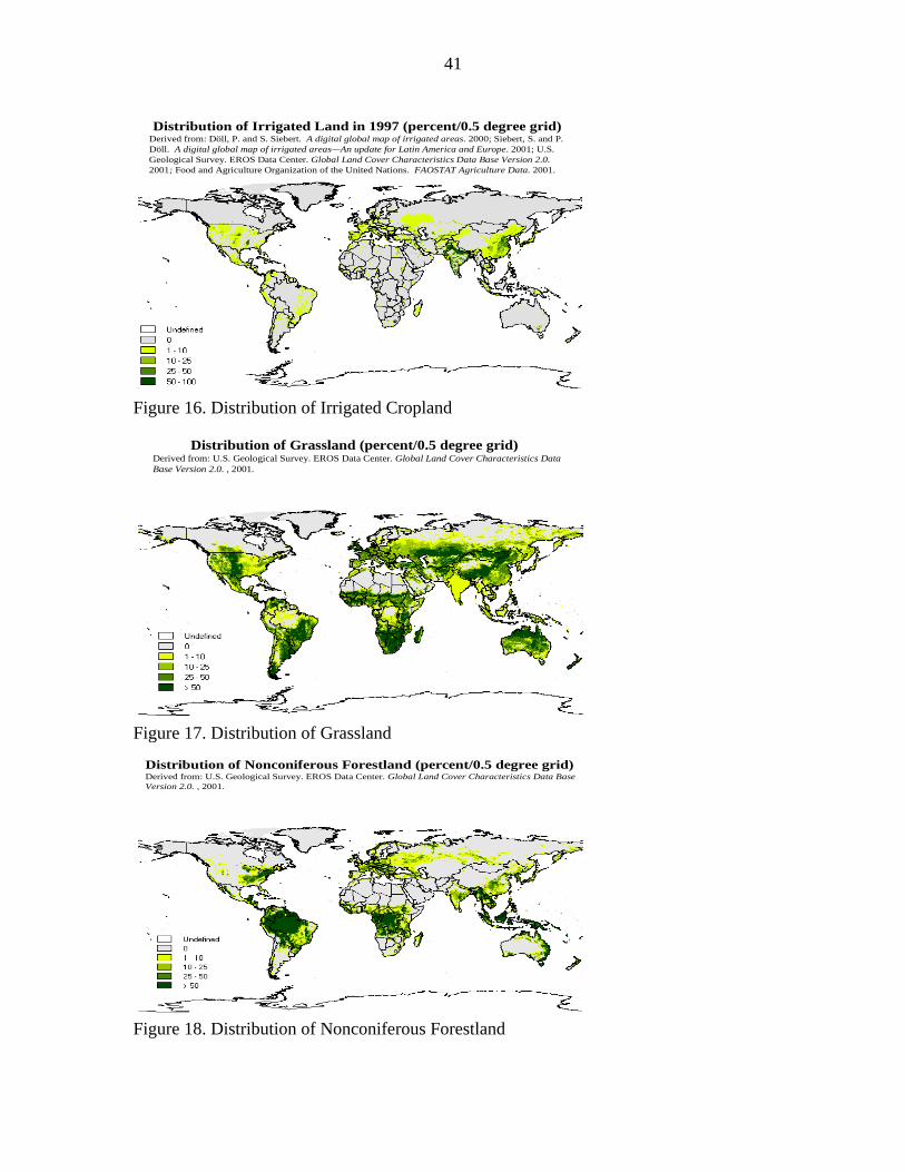
41

Distribution of Irrigated Land in 1997 (percent/0.5 degree grid)Derived from: Döll, P. and S. Siebert. A digital global map of irrigated areas. 2000; Siebert, S. and P. Döll. A digital global map of irrigated areas—An update for Latin America and Europe. 2001; U.S. Geological Survey. EROS Data Center. Global Land Cover Characteristics Data Base Version 2.0. 2001; Food and Agriculture Organization of the United Nations. FAOSTAT Agriculture Data. 2001.

Figure 16. Distribution of Irrigated Cropland

Distribution of Grassland (percent/0.5 degree grid)Derived from: U.S. Geological Survey. EROS Data Center. Global Land Cover Characteristics Data Base Version 2.0. , 2001.

Figure 17. Distribution of Grassland

Distribution of Nonconiferous Forestland (percent/0.5 degree grid)Derived from: U.S. Geological Survey. EROS Data Center. Global Land Cover Characteristics Data Base Version 2.0. , 2001.

Figure 18. Distribution of Nonconiferous Forestland

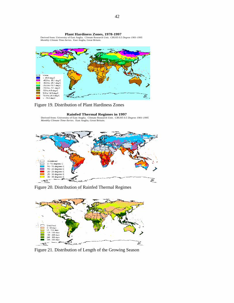
42

Plant Hardiness Zones, 1978-1997

Derived from: University of East Anglia. Climate Research Unit. CRU05 0.5 Degree 1901-1995 Monthly Climate Time-Series. East Anglia, Great Britain.

Figure 19. Distribution of Plant Hardiness Zones

Rainfed Thermal Regimes in 1997Derived from: University of East Anglia. Climate Research Unit. CRU05 0.5 Degree 1901-1995 Monthly Climate Time-Series. East Anglia, Great Britain.

Figure 20. Distribution of Rainfed Thermal Regimes y g ,

Figure 21. Distribution of Length of the Growing Season

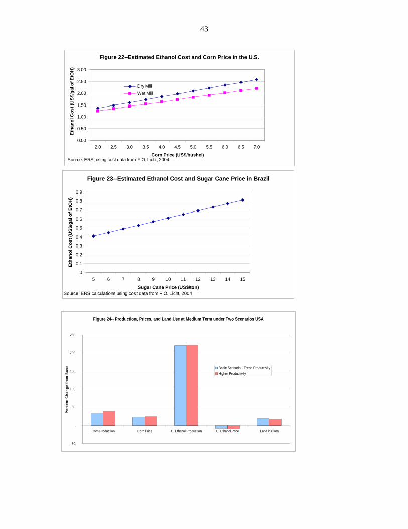
43

Figure 22--Estimated Ethanol Cost and Corn Price in the U.S.

0.00

0.50

1.00

1.50

2.00

2.50

3.00

2.0 2.5 3.0 3.5 4.0 4.5 5.0 5.5 6.0 6.5 7.0

Corn Price (US$/bushel)

Etha

nol C

ost (

US$

/gal

of E

tOH

)

Dry MillWet Mill

Source: ERS, using cost data from F.O. Licht, 2004

Figure 23--Estimated Ethanol Cost and Sugar Cane Price in Brazil

0

0.1

0.2

0.3

0.4

0.5

0.6

0.7

0.8

0.9

5 6 7 8 9 10 11 12 13 14 15

Sugar Cane Price (US$/ton)

Etha

nol C

ost (

US

$/ga

l of E

tOH

)

Source: ERS calculations using cost data from F.O. Licht, 2004

Figure 24-- Production, Prices, and Land Use at Medium Term under Two Scenarios USA

-50.

.

50.

100.

150.

200.

250.

Corn Production Corn Price C. Ethanol Production C. Ethanol Price Land in Corn

Perc

ent C

hang

e fro

m B

ase Basic Scenario - Trend Productivity

Higher Productivity

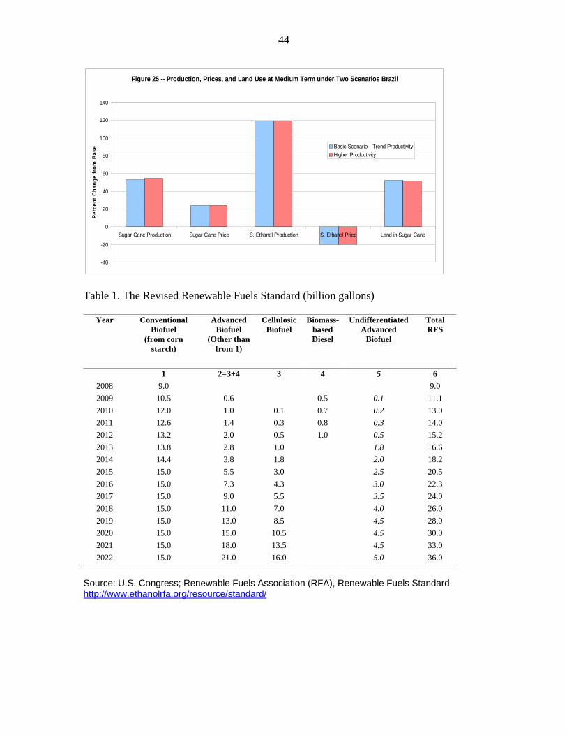
44

Figure 25 -- Production, Prices, and Land Use at Medium Term under Two Scenarios Brazil

-40

-20

0

20

40

60

80

100

120

140

Sugar Cane Production Sugar Cane Price S. Ethanol Production S. Ethanol Price Land in Sugar Cane

Perc

ent C

hang

e fr

om B

ase Basic Scenario - Trend Productivity

Higher Productivity

Table 1. The Revised Renewable Fuels Standard (billion gallons)

Year Conventional Biofuel

(from corn starch)

Advanced Biofuel

(Other than from 1)

Cellulosic Biofuel

Biomass-based Diesel

Undifferentiated Advanced

Biofuel

Total RFS

1 2=3+4 3 4 5 6 2008 9.0 9.0 2009 10.5 0.6 0.5 0.1 11.1 2010 12.0 1.0 0.1 0.7 0.2 13.0 2011 12.6 1.4 0.3 0.8 0.3 14.0 2012 13.2 2.0 0.5 1.0 0.5 15.2 2013 13.8 2.8 1.0 1.8 16.6 2014 14.4 3.8 1.8 2.0 18.2 2015 15.0 5.5 3.0 2.5 20.5 2016 15.0 7.3 4.3 3.0 22.3 2017 15.0 9.0 5.5 3.5 24.0 2018 15.0 11.0 7.0 4.0 26.0 2019 15.0 13.0 8.5 4.5 28.0 2020 15.0 15.0 10.5 4.5 30.0 2021 15.0 18.0 13.5 4.5 33.0 2022 15.0 21.0 16.0 5.0 36.0

Source: U.S. Congress; Renewable Fuels Association (RFA), Renewable Fuels Standard http://www.ethanolrfa.org/resource/standard/

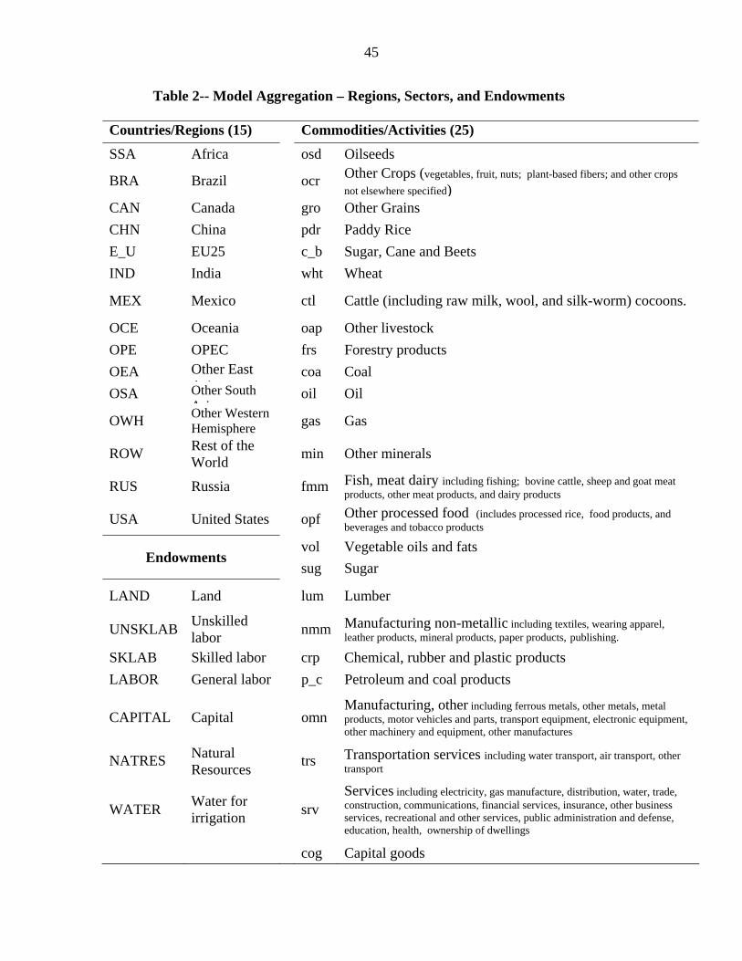
45

Table 2-- Model Aggregation – Regions, Sectors, and Endowments

Countries/Regions (15) Commodities/Activities (25)

SSA Africa osd Oilseeds

BRA Brazil ocr Other Crops (vegetables, fruit, nuts; plant-based fibers; and other crops not elsewhere specified)

CAN Canada gro Other Grains CHN China pdr Paddy Rice E_U EU25 c_b Sugar, Cane and Beets IND India wht Wheat

MEX Mexico ctl Cattle (including raw milk, wool, and silk-worm) cocoons.

OCE Oceania oap Other livestock OPE OPEC frs Forestry products OEA Other East

A i coa Coal

OSA Other South Asia

oil Oil

OWH Other Western Hemisphere gas Gas

ROW Rest of the World min Other minerals

RUS Russia fmm Fish, meat dairy including fishing; bovine cattle, sheep and goat meat products, other meat products, and dairy products

USA United States opf Other processed food (includes processed rice, food products, and beverages and tobacco products

vol Vegetable oils and fats Endowments

sug Sugar

LAND Land lum Lumber

UNSKLAB Unskilled labor nmm Manufacturing non-metallic including textiles, wearing apparel,

leather products, mineral products, paper products, publishing. SKLAB Skilled labor crp Chemical, rubber and plastic products LABOR General labor p_c Petroleum and coal products

CAPITAL Capital omn Manufacturing, other including ferrous metals, other metals, metal products, motor vehicles and parts, transport equipment, electronic equipment, other machinery and equipment, other manufactures

NATRES Natural Resources trs Transportation services including water transport, air transport, other

transport

WATER Water for irrigation srv

Services including electricity, gas manufacture, distribution, water, trade, construction, communications, financial services, insurance, other business services, recreational and other services, public administration and defense, education, health, ownership of dwellings

cog Capital goods

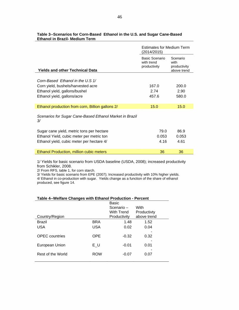
46

Table 3--Scenarios for Corn-Based Ethanol in the U.S. and Sugar Cane-Based Ethanol in Brazil- Medium Term

Estimates for Medium Term (2014/2015)

Yields and other Technical Data

Basic Scenario with trend productivity

Scenario with productivity above trend

Corn-Based Ethanol in the U.S 1/ Corn yield, bushels/harvested acre 167.0 200.0 Ethanol yield, gallons/bushel 2.74 2.90 Ethanol yield, gallons/acre 457.6 580.0 Ethanol production from corn, Billion gallons 2/ 15.0 15.0 Scenarios for Sugar Cane-Based Ethanol Market in Brazil 3/ Sugar cane yield, metric tons per hectare 79.0 86.9 Ethanol Yield, cubic meter per metric ton 0.053 0.053 Ethanol yield, cubic meter per hectare 4/ 4.16 4.61 Ethanol Production, million cubic meters 36 36 1/ Yields for basic scenario from USDA baseline (USDA, 2008); increased productivity from Schikler, 2008. 2/ From RFS, table 1, for corn starch. 3/ Yields for basic scenario from EPE (2007); Increased productivity with 10% higher yields. 4/ Ethanol in co-production with sugar. Yields change as a function of the share of ethanol produced, see figure 14.

Table 4--Welfare Changes with Ethanol Production - Percent

Country/Region

Basic Scenario – With Trend Productivity

With Productivty above trend

Brazil BRA 1.48 1.52 USA USA 0.02 0.04

OPEC countries OPE -0.32-

0.32

European Union E_U -0.01-

0.01

Rest of the World ROW -0.07-

0.07

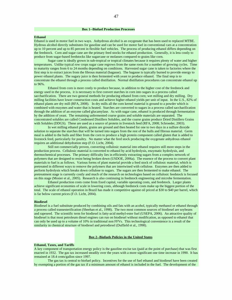
47

Box 1--Biofuel Production Processes

Ethanol Ethanol is used in motor fuel in two ways. Anhydrous alcohol is an oxygenate that has been used to replaced MTBE. Hydrous alcohol directly substitutes for gasoline and can be used for motor fuel in conventional cars at a concentration up to 10 percent and up to 85 percent in flexible fuel vehicles. The process of producing ethanol differs depending on the feedstock. Corn and sugar cane are the primary feed stocks for ethanol production. Generally, it is less costly to produce from sugar-based feedstocks like sugarcane or molasses compared to grains like corn. Sugar cane is ideally grown in sub-tropical or tropical climates because it requires plenty of water and higher temperatures. Unlike typical row crops sugar cane regrows from the same roots for a number of growing cycles. Time to maturity ranges from 6 to 24 months depending on conditions. Harvested sugar cane is taken to factories where the first step is to extract juices from the fibrous material (bagasse). The bagasse is typically burned to provide energy to power ethanol plants. The sugary juice is then fermented with yeast to produce ethanol. The final step is to concentrate the ethanol through a process called distillation. Normal distillation procedures can concentrate ethanol up to 96%.

Ethanol from corn is more costly to produce because, in addition to the higher cost of the feedstock and energy used in the process, it is necessary to first convert starches in corn into sugars in a process called saccharification. There are two general methods for producing ethanol from corn; wet milling and dry milling. Dry milling facilities have lower construction costs and achieve higher ethanol yields per unit of input. In the U.S., 82% of ethanol plants are dry mill (RFA, 2008). In dry mills all the corn kernel material is ground to a powder which is combined with enzymes and water that is heated. Starches are converted to sugars in a process called saccharification through the addition of an enzyme called glucamylase. As with sugar cane, ethanol is produced through fermentation by the addition of yeast. The remaining unfermented coarse grains and soluble materials are separated. The concentrated solubles are called Condensed Distillers Solubles, and the coarse grains produce Dried Distillers Grains with Solubles (DDGS). These are used as a source of protein in livestock feed (RFA, 2008; Schroeder, 2003).

In wet milling ethanol plants, grains are ground and then heated for one to two days in a sulfure dioxide solution to separate the starches that will be turned into sugars from the rest of the hulls and fibrous material. Germ meal is added to the hulls and fiber from the corn to produce a high protein component called gluten that is added to livestock feed, particularly for poultry. No matter what the feed stock producing the oxygenate anhydrous ethanol requires an additional dehydration step (F.O. Licht, 2004). Still not commercially proven, converting cellulosic material into ethanol requires still more steps in the production process. Cellulosic material is converted to ethanol by acid hydrolysis, enzymatic hydrolysis, and thermochemical processes. The primary difficulty lies in efficiently extracting sugars from a complex network of polymers that are designed to resist being broken down (USDOE, 2006a). The essence of the process to convert plant materials to fuel is as follows. Various forms of plant material provide a feed stock of cellulosic material, which is pretreated in different ways to remove the polymers that are intertwined with cellulose. Enzymes are then added to perform hydrolysis which breaks down cellulose to sugars. The sugars are then fermented to make ethanol. The pretreatment stage is currently costly and much of the research on technologies based on cellulosic feedstock is focused on this stage (Mosier et al., 2005). Research is also continuing in feedstock engineering and microbe fermentation. Ethanol production costs come from fixed capital, variable operating costs, and feedstock. Larger plants achieve significant economies of scale in lowering costs, although feedstock costs make up the biggest portion of the total. The scale of ethanol operation in Brazil has made it competitive against oil priced at $30 to $40 per barrel, which is far below current prices (F.O. Licht, 2004). Biodiesel Biodiesel is a fuel substitute produced by combining oils and fats with an acohol, typically methanol or ethanol through a process called transesterification (Sheehan et al., 1998). The two most common sources of biodiesel are soybeans and rapeseed. The scientific term for biodiesel is fatty-acid methyl-ester fuel (USEPA, 2006). An attractive quality of biodiesel is that most petroleum diesel engines can run on biodiesel without modification, as opposed to ethanol that can only be used up to a volume of 10% in traditional non FFVs. This technological convenience is a result of the similarity in chemical structure of biodiesel and petrodiesel (Duffield et al., 1998).

Box 2--Biofuels Policies in the United States

Ethanol, Taxes, and Tariffs A key component of transportation energy policy is the gasoline excise tax (paid at the point of purchase) that was first enacted in 1932. The gas tax increased steadily over the years with a more significant one time increase in 1990. It has remained at 18.4 cents/gallon since 1997.

The gas tax is central to biofuel policy. Incentives for the use of fuel ethanol and biodiesel have been created by exempting a portion of the gas tax if a minimum amount of ethanol is included in the fuel. The development of the

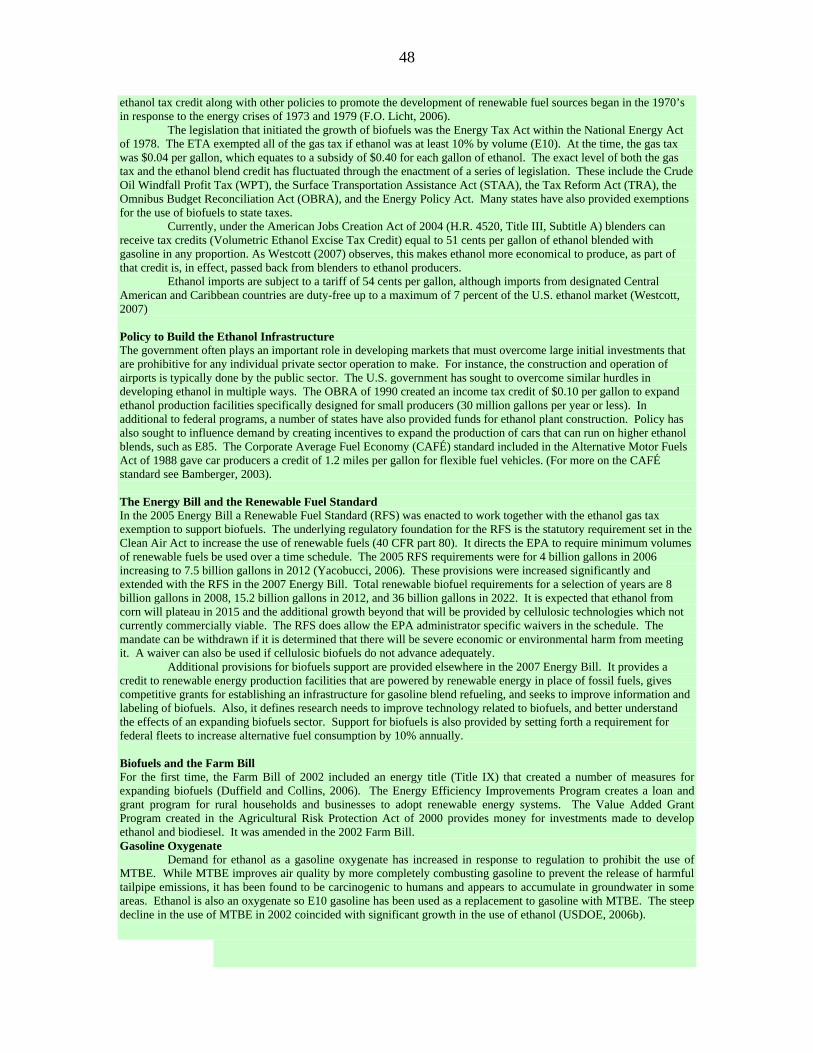
48

ethanol tax credit along with other policies to promote the development of renewable fuel sources began in the 1970’s in response to the energy crises of 1973 and 1979 (F.O. Licht, 2006).

The legislation that initiated the growth of biofuels was the Energy Tax Act within the National Energy Act of 1978. The ETA exempted all of the gas tax if ethanol was at least 10% by volume (E10). At the time, the gas tax was $0.04 per gallon, which equates to a subsidy of $0.40 for each gallon of ethanol. The exact level of both the gas tax and the ethanol blend credit has fluctuated through the enactment of a series of legislation. These include the Crude Oil Windfall Profit Tax (WPT), the Surface Transportation Assistance Act (STAA), the Tax Reform Act (TRA), the Omnibus Budget Reconciliation Act (OBRA), and the Energy Policy Act. Many states have also provided exemptions for the use of biofuels to state taxes.

Currently, under the American Jobs Creation Act of 2004 (H.R. 4520, Title III, Subtitle A) blenders can receive tax credits (Volumetric Ethanol Excise Tax Credit) equal to 51 cents per gallon of ethanol blended with gasoline in any proportion. As Westcott (2007) observes, this makes ethanol more economical to produce, as part of that credit is, in effect, passed back from blenders to ethanol producers.

Ethanol imports are subject to a tariff of 54 cents per gallon, although imports from designated Central American and Caribbean countries are duty-free up to a maximum of 7 percent of the U.S. ethanol market (Westcott, 2007) Policy to Build the Ethanol Infrastructure The government often plays an important role in developing markets that must overcome large initial investments that are prohibitive for any individual private sector operation to make. For instance, the construction and operation of airports is typically done by the public sector. The U.S. government has sought to overcome similar hurdles in developing ethanol in multiple ways. The OBRA of 1990 created an income tax credit of $0.10 per gallon to expand ethanol production facilities specifically designed for small producers (30 million gallons per year or less). In additional to federal programs, a number of states have also provided funds for ethanol plant construction. Policy has also sought to influence demand by creating incentives to expand the production of cars that can run on higher ethanol blends, such as E85. The Corporate Average Fuel Economy (CAFÉ) standard included in the Alternative Motor Fuels Act of 1988 gave car producers a credit of 1.2 miles per gallon for flexible fuel vehicles. (For more on the CAFÉ standard see Bamberger, 2003). The Energy Bill and the Renewable Fuel Standard In the 2005 Energy Bill a Renewable Fuel Standard (RFS) was enacted to work together with the ethanol gas tax exemption to support biofuels. The underlying regulatory foundation for the RFS is the statutory requirement set in the Clean Air Act to increase the use of renewable fuels (40 CFR part 80). It directs the EPA to require minimum volumes of renewable fuels be used over a time schedule. The 2005 RFS requirements were for 4 billion gallons in 2006 increasing to 7.5 billion gallons in 2012 (Yacobucci, 2006). These provisions were increased significantly and extended with the RFS in the 2007 Energy Bill. Total renewable biofuel requirements for a selection of years are 8 billion gallons in 2008, 15.2 billion gallons in 2012, and 36 billion gallons in 2022. It is expected that ethanol from corn will plateau in 2015 and the additional growth beyond that will be provided by cellulosic technologies which not currently commercially viable. The RFS does allow the EPA administrator specific waivers in the schedule. The mandate can be withdrawn if it is determined that there will be severe economic or environmental harm from meeting it. A waiver can also be used if cellulosic biofuels do not advance adequately.

Additional provisions for biofuels support are provided elsewhere in the 2007 Energy Bill. It provides a credit to renewable energy production facilities that are powered by renewable energy in place of fossil fuels, gives competitive grants for establishing an infrastructure for gasoline blend refueling, and seeks to improve information and labeling of biofuels. Also, it defines research needs to improve technology related to biofuels, and better understand the effects of an expanding biofuels sector. Support for biofuels is also provided by setting forth a requirement for federal fleets to increase alternative fuel consumption by 10% annually. Biofuels and the Farm Bill For the first time, the Farm Bill of 2002 included an energy title (Title IX) that created a number of measures for expanding biofuels (Duffield and Collins, 2006). The Energy Efficiency Improvements Program creates a loan and grant program for rural households and businesses to adopt renewable energy systems. The Value Added Grant Program created in the Agricultural Risk Protection Act of 2000 provides money for investments made to develop ethanol and biodiesel. It was amended in the 2002 Farm Bill. Gasoline Oxygenate Demand for ethanol as a gasoline oxygenate has increased in response to regulation to prohibit the use of MTBE. While MTBE improves air quality by more completely combusting gasoline to prevent the release of harmful tailpipe emissions, it has been found to be carcinogenic to humans and appears to accumulate in groundwater in some areas. Ethanol is also an oxygenate so E10 gasoline has been used as a replacement to gasoline with MTBE. The steep decline in the use of MTBE in 2002 coincided with significant growth in the use of ethanol (USDOE, 2006b).

49

Box 3--Biofuels Policies in Other Countries

While concerns about reliance on foreign oil and rural employment led Brazil to aggressively and directly support the growth of sugar based ethanol in the 1970’s, climate change mitigation has been central to the European Union’s effort to increase the use of biofuels in the last ten years. At the same time, political support for biofuels remains limited in many developing countries like China and Mexico due to concerns over rising food prices. Brazil Brazil’s status as the global leader in biofuels and the second largest producer of ethanol is the result of more than 30 years of active policy intervention. Support for biofuels started during the energy crisis in 1973 with a national ethanol program called Proálcool (Koizumi, 2003). Besides providing the country with greater protection from global oil supply disruptions Proálcool addressed the overproduction problems that had existed in its sugarcane industry in the early part of the 20th century that led to the creation of production quotas to maintain higher prices (Koizumi, 2003). The Brazilian government heavily subsidized loans for expanding sugarcane fields and constructing ethanol distilleries through the National Economic and Social Development Bank (BNDES). The World Bank also provided investment funds (AgraFNP, 2007). The direct control of the ethanol market maintained the industry through the 1980’s and 90’s by mandating ethanol blend requirements as oil prices decreased significantly.

Brazil deregulated the ethanol program in the late 1990’s by eliminating Proálcool, which removed ethanol price standards and subsidies. Also, Petrobras was no longer given a monopoly over distribution. Without direct control of production and prices the government influences ethanol markets in response to supply and demand side factors by adjusting the ethanol gas blending requirement between 20 and 25% (USDOE, 2007). The introduction of flex-fuel vehicles in 2003 has also been important for the more recent growth in the ethanol industry. The ability to run on any gas ethanol mixture provides flexibility that the ethanol-only cars introduced in the 1980’s lacked. With the combination of aggressive ethanol policies and a favorable climate for producing sugarcane Brazil now produces half of the world’s supply of sugar-based ethanol and also has the lowest unit cost of production (F.O. Lichts, 2004). The European Union The biofuels sector in the EU differs markedly from Brazil in both policy and production. Growing conditions are not as favorable for corn or sugarcane, making ethanol less attractive, so biodiesel from rapeseed makes up a majority of production. Also, the diversity among Member States in terms of economy and agriculture requires that directives allow some flexibility in meeting standards. The first important biofuels document in the EU was the 1997 White Paper on Renewable Energy that outlined the potential for biofuels in the European Union (COM 599 final). The first substantive policy was the EU Biofuels Directive (2003/30/EC) published in 2003 that required Member States to have biofuels account for 2% of transportation fuel use by the end of 2005, and 5.75% by December, 2010.

The Energy Taxation Directive (2003/96/EC), also adopted in 2003, encouraged EU Member States to provide either tax reductions or tax exemptions for biofuels, although no uniform standard is set allowing flexibility across states (COM(2005) 628 final, Annex 9). Some Member States including France and Austria have enacted a requirement for fuel to contain a required ethanol mix, which is likely to be adopted in other countries (COM(2005) 628 final, Annex 9). Biofuels are also supported in the 2003 Common Agriculture Policy (CAP) that designates a maximum of 45€ per ha in aid for growing energy crops on non set-aside land with a maximum total area of 1.5 million ha for the EU as a whole (CAP Action Plan, 2003). In 2005, 1.8 million ha of the 97 million ha of arable land in the EU were used for growing raw materials for biofuels (COM(2005) 628 final, Annex 7).

Action Plans for biomass and biofuels in 2005 and 2007 updated projections for potential growth. The “Renewable Energy Roadmap” and the “The Energy Policy for Europe” released in 2007 have set a goal for 20% of energy to be renewable by 2020 and half of that to come from biofuels (Bolter et al., 2007). Other Countries Support for biofuels in Canada has grown since the government ratified the Kyoto Protocol in 2002. A Renewable Fuel Standard has been the central policy approach proposed to achieve a 5% renewables level for gasoline by 2010 (F.O. Lichts, 2006). Already in place is a federal excise tax exemption in proportion to the ethanol mix (F.O. Licht, 2006). Some provinces have taken additional measures, such as minimum ethanol blends, to promote biofuels. The initial goal was for 35% of fuel consumption to contain 10% ethanol using corn as the primary feedstock. To expand ethanol production a gasoline exemption tax of US $0.28/gallon was enacted together with subsidies for production facilities valued at $73 million (Klein et al., 2004). Argentina enacted in April, 2006 a 5% biofuel mix requirement accompanied by tax breaks for producers (F.O. Licht, 2006). Thailand, which has favorable conditions for growing sugar cane, looks to follow Brazil’s lead by mandating gasoline to contain 10% ethanol. China is also focusing on developing biofuels through the development of E10 gasoline blends, although this exists on a trial basis currently.