Modeling Seashell Morphology - Academicsacademics.smcvt.edu/jellis-monaghan/papers/papers/teaching papers... · 5.1 Handout I (highly independent) ... Modeling Seashell Morphology

Modeling Seashell Morphology

George L. Ashline

Department of Mathematics

Saint Michael’s CollegeColchester, VT 05439

[email protected]

Joanna A. Ellis-Monaghan



[email protected]

Zsuzsanna M. Kadas



[email protected]

Declan J. McCabe

Department of Biology


[email protected]

June 23, 2009

Abstract

Modeling the beautiful and varied shapes of seashells sculpted by nature is an

aesthetically appealing application of several concepts typically introduced in multi-

variable calculus. We use vector calculus tools to generate three-dimensional models of

mollusk shells from growth measurements. We suggest a method for measuring shell

specimens to determine necessary model parameters. We also provide Maple code

for the modeling and several project handouts designed for various levels of student

independence and preparation.

MATHEMATICAL FIELD: Calculus.

APPLICATION FIELDS: Malacology, paleontology, and marine biology.

TARGET AUDIENCE: Students in multivariable calculus.

PREREQUISITES: Multivariable calculus including space curves, parameterized

surfaces, Frenet frames. Use of a computer algebra system for curve-fitting and

generating three-dimensional graphics.

1

Contents

1 Introduction 5

2 Developing the Model 6

3 Measuring the Shells and Fitting the Model 9

4 Parameter Effects and Surface Ornamentation 13

5 Project Handouts 16

5.1 Handout I (highly independent) . . . . . . . . . . . . . . . . . . . . . . . . . 16

5.2 Handout II (breaking the problem into steps) . . . . . . . . . . . . . . . . . 17

5.3 Handout III (structured format) . . . . . . . . . . . . . . . . . . . . . . . . . 17

5.4 Handout IV (writing component) . . . . . . . . . . . . . . . . . . . . . . . . 18

6 Maple Code 19

6.1 Part I: the procedure “Shell” . . . . . . . . . . . . . . . . . . . . . . . . . . . 20

6.2 Part II: modeling a shell specimen from data . . . . . . . . . . . . . . . . . . 22

6.3 Generating the color plate shells . . . . . . . . . . . . . . . . . . . . . . . . . 25

7 References and Sources 27

7.1 Print shell modeling resources . . . . . . . . . . . . . . . . . . . . . . . . . . 27

7.2 Online shell modeling resources . . . . . . . . . . . . . . . . . . . . . . . . . 29

7.3 Online sources for shells, pictures, and X-rays . . . . . . . . . . . . . . . . . 31

Modeling Seashell Morphology 2



1 Introduction

The elegant shape of seashells has always attracted the eye of the artist, the scientist, and themathematician. Despite the staggering variety of shell shapes found in nature, the growthof almost all seashells can be described in terms of three exponential functions and a closedcurve that describes the shape of the shell’s aperture, or opening. The model developedhere is an aesthetically appealing application of several concepts typically introduced inmultivariable calculus; it reinforces students’ understanding of curves and surfaces in three-dimensional space, in particular, Frenet frames and parameterized surfaces. It also offers ataste of the challenges of collecting and using data in the modeling process. To model themorphology of specific shells, students take measurements from shell X-rays or photographsof cross-sections. They use these data to estimate several growth parameters that determinethe overall three-dimensional shape of the shell. Curve-fitting is then used to more accuratelymodel the aperture, enhancing the detail of the final model.

We focus on mollusks in the class Gastropoda. This class includes the familiar gardensnails, slugs, and edible snails as well as a diverse array of freshwater and marine species,including periwinkles and whelks. Most shelled gastropods have a shell consisting of onepiece, which is typically coiled or spiral in shape. Mollusks with one shell are referred to asunivalves, while those with shells consisting of two parts, such as clams, mussels, and oysters,are called bivalves. Gastropods enlarge their helical shells by depositing fresh material atthe lip of the aperture, or opening of the shell. The turns of the spiral of the shell are calledwhorls; the last-deposited and largest whorl of the shell is termed the body whorl, and theolder, smaller whorls constitute the spire of the shell. Gastropod shells are composed largelyof calcium carbonate overlaid by a tough protinaceous material called conchin or conchiolin.The protinaceous layer or periostracum imparts shell color in most cases [Rupert and Barnes1994].

While the majority of shells have the asymmetrical helico-spiral shape described elo-quently by D’Arcy Thompson (see Section 2), some shells such as the limpet are moresymmetrical, and others like the cowrie shells are superficially bilaterally symmetric becauseeach new whorl completely envelops previous whorls. We will work with the more typicalhelico-spiral shells, since their growth parameters may be more readily approximated.

From a strictly biological point of view, mathematical models of gastropod shells are ofinterest for several reasons. Extrapolations beyond the size of a particular shell can be con-structed and viewed to determine whether the resulting shape retains its integrity or resultsin a loose spiral no longer connected to previous whorls. One can also determine if additionalwhorls would continue to increase the cross-sectional area of the aperture or if the aperturewould be impinged upon by previous whorls, thus making the shell uninhabitable. Thiswould indicate whether the particular growth parameters limit the range of sizes possible fora given species. The parameters can also aid in classifying the organisms by locating eachspecies in a parameter space where each axis corresponds to one of the growth parameters.This helps to determine the spectrum of possible shell forms and may elucidate the relation-ship between different species [Raup 1966]. Finally, cross-sections of embedded fossils can


be measured and modeled to produce three-dimensional renderings without risking damageto valuable specimens.

In Section 2, we develop the parametric equations that model the surface of the shell.Section 3 describes the process of measuring a shell X-ray to determine the growth parametersand create a model of a particular specimen of Epitonium magnificum. The effects of varyingthe model parameters are discussed in Section 4, as are modifications to include surfaceornamentation. Project handouts are included in Section 5. Section 6 provides Maple codefor computing and plotting shell models; the process of modeling E. magnificum is includedas a sample. Maple code for generating all of the color plates is also included here. The finalsection is an annotated list of references and resources for seashell modeling.

2 Developing the Model

The model we develop below is largely based on Prusinkiewicz and Fowler [2003], or Chapter10 in Meinhardt [2003], particularly in the use of a Frenet frame to position the aperture.However, we loosely follow Jirapong and Krawczyk [2003] in taking measurements from across-section of the shell and using curve-fitting methods to fit exponential functions to thedata. The underlying idea, captured by D’Arcy Thompson in his classic work On Growth

and Form, is this:

The surface of any shell...may be imagined to be generated by the revolutionabout a fixed axis of a closed curve, which, remaining always geometrically similarto itself, increases its dimensions continually.... In turbinate shells, [any givenpoint on the generating curve]... partakes, therefore, of the character of a helix, aswell as a logarithmic spiral; it may be strictly entitled a helico-spiral [Thompson1961, 189].

To visualize the growth of the seashell, we begin with a helical spiral rotating aboutthe z-axis. Both the radius and the height increase as the animal grows, so the shell growsupwards along the z-axis, with the small end toward the origin, and the large open endfurther up the z-axis. The aperture is a closed curve that sweeps along this helical spiral,growing larger, but remaining geometrically self-similar as it moves along. See Figure 1,where we have flipped the image upside down to present a more typical view of the shell.

Seashell growth is in principle self-similar; the rate of change of both the radius andheight of the helical spiral are proportional to their size, that is, both grow exponentially.Thus, if t is the angle of rotation about the z axis, the radius and height functions are givenby:

Radius: r(t) = r0ekrt;

Vertical Displacement: z(t) = z0ekzt.


Figure 1: Growing circles sweep along the helical spiral to generate the shell surface.

Here kr and kz are the nonnegative growth constants. The constants r0 and z0 are initialradius and height values. The helical spiral is then given by the space curve:

H (t) = 〈r(t) cos t, r(t) sin t, z(t)〉 .

Note that this helical spiral grows in the clockwise direction and thus produces a right-handed, or dextral, shell. This is by far the most common form, although a few generanormally produce sinistral shells, and rarely, a sinistral specimen of a normally dextralgenus may occur [Oliver, 2004].

Just like the height and radius, the size of the aperture grows exponentially as the aper-ture sweeps along the helical spiral. We model the aperture as the product of an exponentialgrowth function a(t) and a ‘shape’ function P (s). Here, as above, t is the angle of rotationabout the z-axis. P (s) is a polar function where s is a radial angle measured about thecenter of the aperture (a point on the helical spiral). Thus, the aperture is modeled by:

P (s) · a(t), with a(t) = a0ekat,

where ka is the nonnegative growth rate and a0 is the initial aperture size. If P (s) is set equalto the constant 1, the aperture is simply a circle whose radius increases exponentially witht, as in Figure 1. It is easiest to begin by modeling a shell with a nearly circular aperture, orto use a circle as a first approximation of the aperture shape. When the rough overall formof the shell has been achieved, the aperture shape can be modified to give a more accurateimage. The parameters r0, z0 , a0, kr, kz and ka for a particular gastropod may be estimatedfrom measurements taken from the shell, as described in Section 3. The effects of varyingthese parameters are discussed in Section 4.

The shapes of shell apertures vary widely: some are nearly circular or elliptical, othersnearly triangular, and still others quite irregular. Currently, there is no known elementary


function model for the aperture, as there is for the helical spiral. Thus, the aperture istypically approximated by using a variety of curve-fitting techniques, as discussed in Section3.

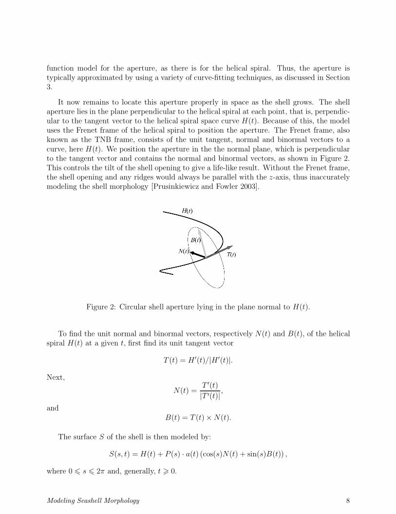
It now remains to locate this aperture properly in space as the shell grows. The shellaperture lies in the plane perpendicular to the helical spiral at each point, that is, perpendic-ular to the tangent vector to the helical spiral space curve H(t). Because of this, the modeluses the Frenet frame of the helical spiral to position the aperture. The Frenet frame, alsoknown as the TNB frame, consists of the unit tangent, normal and binormal vectors to acurve, here H(t). We position the aperture in the the normal plane, which is perpendicularto the tangent vector and contains the normal and binormal vectors, as shown in Figure 2.This controls the tilt of the shell opening to give a life-like result. Without the Frenet frame,the shell opening and any ridges would always be parallel with the z-axis, thus inaccuratelymodeling the shell morphology [Prusinkiewicz and Fowler 2003].

Figure 2: Circular shell aperture lying in the plane normal to H(t).

To find the unit normal and binormal vectors, respectively N(t) and B(t), of the helicalspiral H(t) at a given t, first find its unit tangent vector

T (t) = H ′(t)/|H ′(t)|.

Next,

N(t) =T ′(t)

|T ′(t)|,

andB(t) = T (t)× N(t).

The surface S of the shell is then modeled by:

S(s, t) = H(t) + P (s) · a(t) (cos(s)N(t) + sin(s)B(t)) ,

where 0 6 s 6 2π and, generally, t > 0.


The equation for the two-parameter surface S(s, t) makes it easy to visualize how thesurface is traced out: for each value of t, the tip of the vector H(t) is a point on the helicalspiral; the second term is a radial vector that traces the aperture curve centered at thatpoint in the normal plane. See Figure 3.

Figure 3: The shell surface traced out as the sum of two vectors.

Ultimately, six parameters and one function are used in this equation for modeling shellmorphology: the initial value parameters r0, z0, a0 and the growth parameters kr , kz, ka forthe exponential functions that fit the shell measurements, together with the radial apertureshape function P (s). By adjusting the parameters that control the helical spiral and aperturegrowth and specifying P (s), a large variety of naturally occurring shells can be modeled andfantasy shells can be created as well.

3 Measuring the Shells and Fitting the Model

This section gives explicit directions for measuring shell specimens to determine the necessarymodel parameters r0, z0, a0, kr , kz, ka and to approximate P (s). It is possible to work directlyfrom an actual seashell to obtain the parameters, either by taking external incremental calipermeasurements or by cutting the shell lengthwise through its axis in order to reveal the interiorstructure. Both of these methods have been used by prior modelers [Jirapong and Krawczyk2003, Prusinkiewicz and Fowler 2003], but both require access to the actual shell. To simplifythe process, we chose to work with X-ray images of shells available for purchase [Crow 2009],and we used a hard copy of a shell image large enough to be easily measured with a ruler(about 15 centimeters tall works well). The measuring and fitting process is illustrated inFigures 4 and 5 for E. magnificum, a shell with nearly circular apertures. The Maple codein Section 6 carries out the calculations and renders the final image.


We begin by drawing the (vertical) axis through the image of the shell and choosing thepoint that will be designated the “apex” or tip of the shell. It is impossible to locate the apexdefinitively, and in some cases the true apex has been worn away, so we simply approximateas best we can. The variable t is set to zero at this point, and it increases by 2π each timethe aperture completes a rotation about the axis, thus creating another whorl of the shell.Our model is “upside down” from the way shell images are typically depicted; this is becausewe think of our shells as growing upward from the origin. When we display the images, wetypically rotate them to put the apex at the top again, as in Figure 1 and the color plates.

To determine the parameters kr and kz, we first need to locate the center of each ofthe cross-sectional apertures. Strictly speaking, the shell has only one aperture, the actualopening, but the cross-sections of the shell chamber visible in the X-ray image were theapertures at some times in the past as the shell was growing, so we refer to these cross-sections as apertures as well. Caution is needed in taking measurements of the smallest fewapertures. Not only are the apical whorls of the shell hard to measure due to their size, butthey were laid down by the animal in its larval stage and are typically structurally differentfrom the rest of the shell. Furthermore, when modeling a cut shell, the chambers near theapex may be distorted as the cut is often somewhat off-center. Finally, at the opposite endof the shell, the actual opening of the body whorl of the shell may deviate from the shapeof the other cross-sections, so, if possible, it is best not to use it for measurements either.There should be at least 4 feasible cross-sections, using the actual opening and the apexchambers only as a last resort.

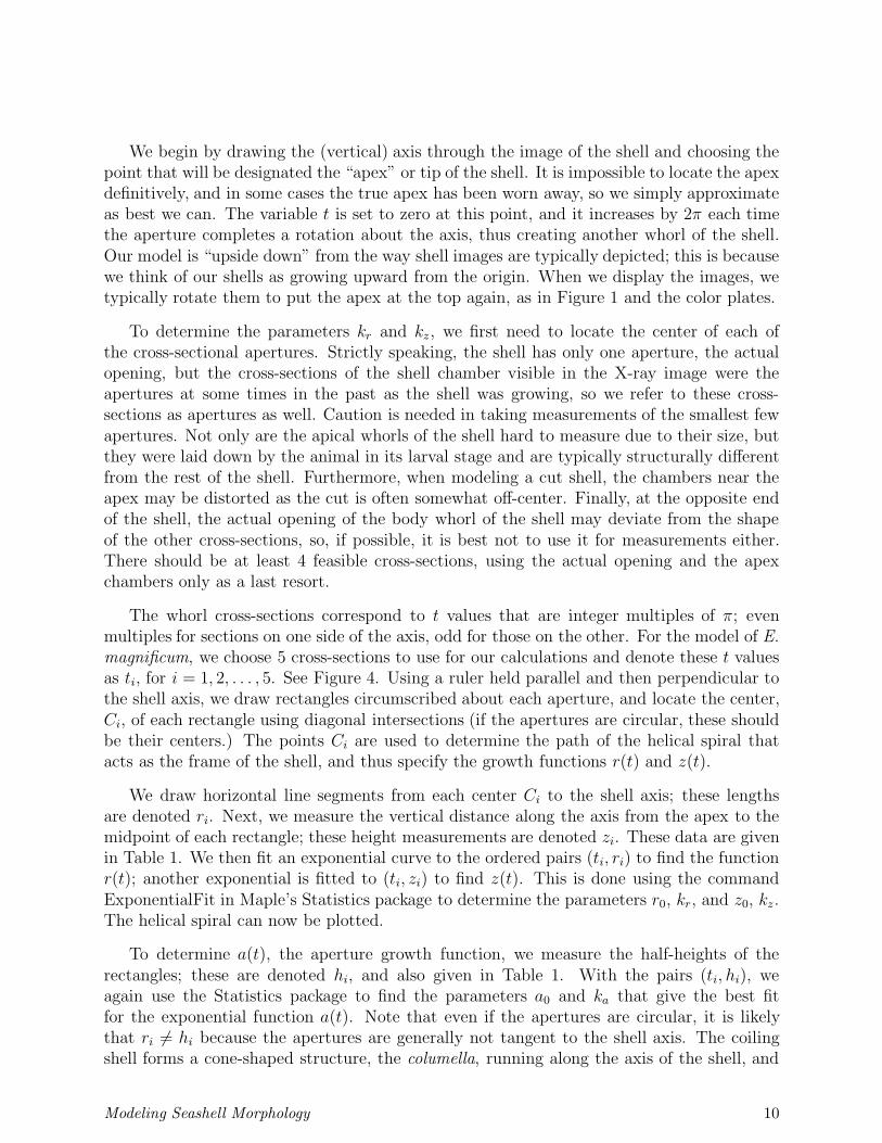
The whorl cross-sections correspond to t values that are integer multiples of π; evenmultiples for sections on one side of the axis, odd for those on the other. For the model of E.

magnificum, we choose 5 cross-sections to use for our calculations and denote these t valuesas ti, for i = 1, 2, . . . , 5. See Figure 4. Using a ruler held parallel and then perpendicular tothe shell axis, we draw rectangles circumscribed about each aperture, and locate the center,Ci, of each rectangle using diagonal intersections (if the apertures are circular, these shouldbe their centers.) The points Ci are used to determine the path of the helical spiral thatacts as the frame of the shell, and thus specify the growth functions r(t) and z(t).

We draw horizontal line segments from each center Ci to the shell axis; these lengthsare denoted ri. Next, we measure the vertical distance along the axis from the apex to themidpoint of each rectangle; these height measurements are denoted zi. These data are givenin Table 1. We then fit an exponential curve to the ordered pairs (ti, ri) to find the functionr(t); another exponential is fitted to (ti, zi) to find z(t). This is done using the commandExponentialFit in Maple’s Statistics package to determine the parameters r0, kr, and z0, kz.The helical spiral can now be plotted.

To determine a(t), the aperture growth function, we measure the half-heights of therectangles; these are denoted hi, and also given in Table 1. With the pairs (ti, hi), weagain use the Statistics package to find the parameters a0 and ka that give the best fitfor the exponential function a(t). Note that even if the apertures are circular, it is likelythat ri 6= hi because the apertures are generally not tangent to the shell axis. The coilingshell forms a cone-shaped structure, the columella, running along the axis of the shell, and


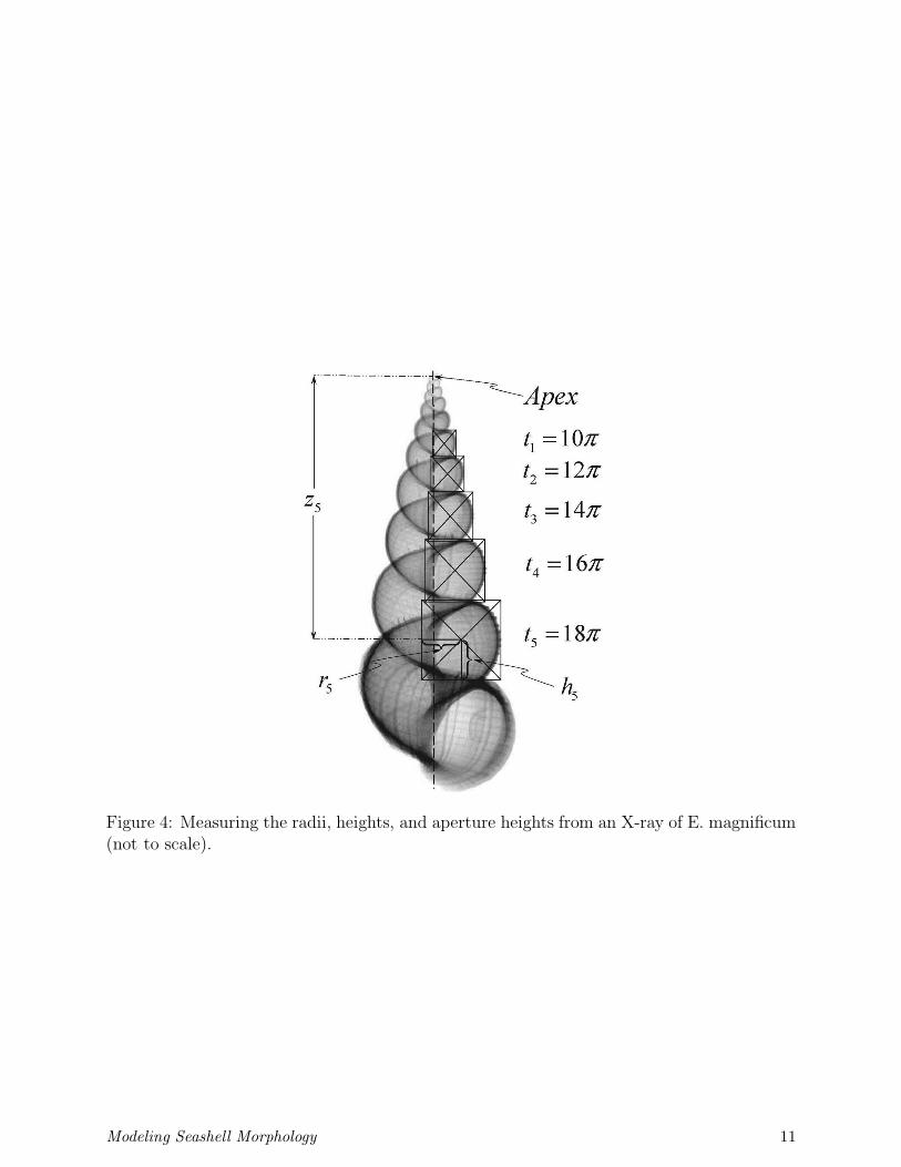
Figure 4: Measuring the radii, heights, and aperture heights from an X-ray of E. magnificum(not to scale).


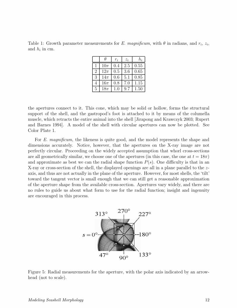
Table 1: Growth parameter measurements for E. magnificum, with θ in radians, and ri, zi,and hi in cm.

θ ri zi hi

1 10π 0.4 2.5 0.552 12π 0.5 3.6 0.653 14π 0.6 5.1 0.854 16π 0.8 7.0 1.155 18π 1.0 9.7 1.50

the apertures connect to it. This cone, which may be solid or hollow, forms the structuralsupport of the shell, and the gastropod’s foot is attached to it by means of the columellamuscle, which retracts the entire animal into the shell [Jirapong and Krawczyk 2003; Rupertand Barnes 1994]. A model of the shell with circular apertures can now be plotted. SeeColor Plate 1.

For E. magnificum, the likeness is quite good, and the model represents the shape anddimensions accurately. Notice, however, that the apertures on the X-ray image are notperfectly circular. Proceeding on the widely accepted assumption that whorl cross-sectionsare all geometrically similar, we choose one of the apertures (in this case, the one at t = 18π)and approximate as best we can the radial shape function P (s). One difficulty is that in anX-ray or cross-section of the shell, the displayed openings are all in a plane parallel to the z-axis, and thus are not actually in the plane of the aperture. However, for most shells, the ‘tilt’toward the tangent vector is small enough that we can still get a reasonable approximationof the aperture shape from the available cross-section. Apertures vary widely, and there areno rules to guide us about what form to use for the radial function; insight and ingenuityare encouraged in this process.

Figure 5: Radial measurements for the aperture, with the polar axis indicated by an arrow-head (not to scale).


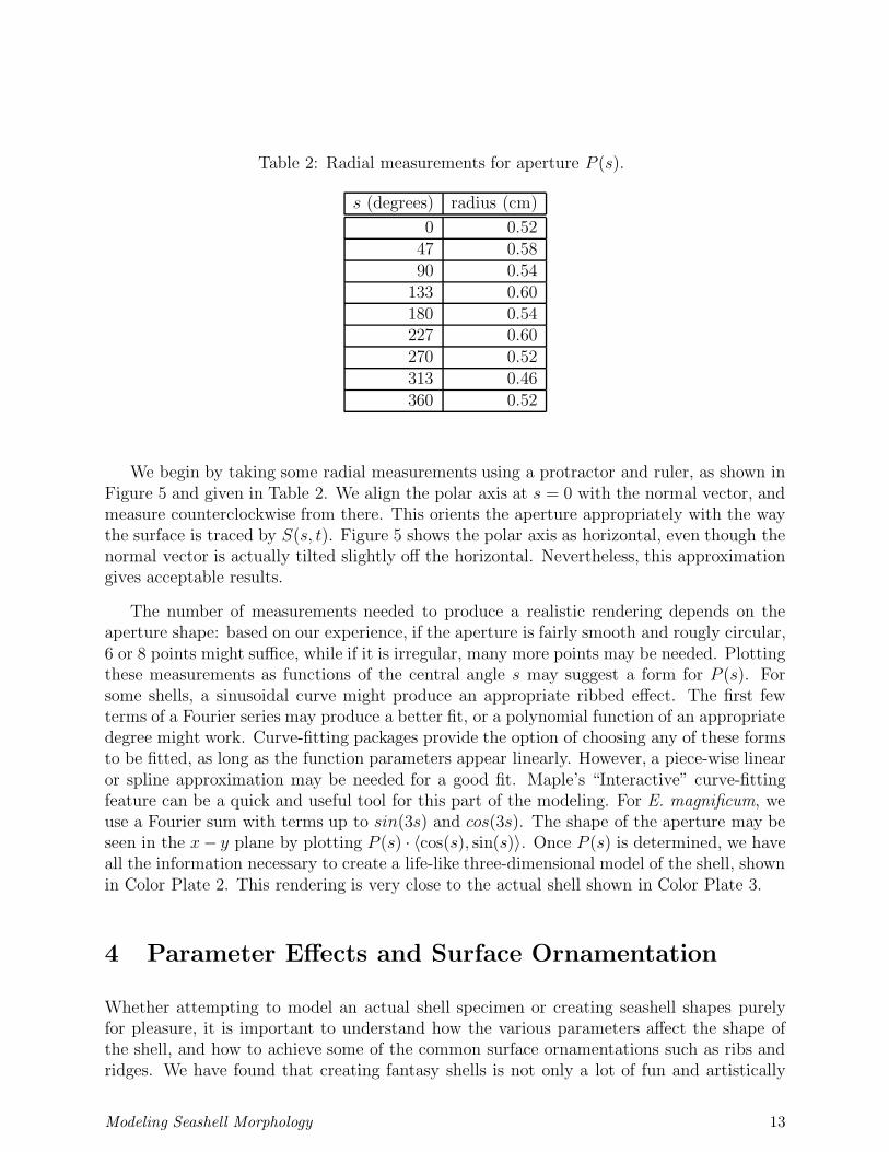
Table 2: Radial measurements for aperture P (s).

s (degrees) radius (cm)

0 0.5247 0.5890 0.54

133 0.60180 0.54227 0.60270 0.52313 0.46360 0.52

We begin by taking some radial measurements using a protractor and ruler, as shown inFigure 5 and given in Table 2. We align the polar axis at s = 0 with the normal vector, andmeasure counterclockwise from there. This orients the aperture appropriately with the waythe surface is traced by S(s, t). Figure 5 shows the polar axis as horizontal, even though thenormal vector is actually tilted slightly off the horizontal. Nevertheless, this approximationgives acceptable results.

The number of measurements needed to produce a realistic rendering depends on theaperture shape: based on our experience, if the aperture is fairly smooth and rougly circular,6 or 8 points might suffice, while if it is irregular, many more points may be needed. Plottingthese measurements as functions of the central angle s may suggest a form for P (s). Forsome shells, a sinusoidal curve might produce an appropriate ribbed effect. The first fewterms of a Fourier series may produce a better fit, or a polynomial function of an appropriatedegree might work. Curve-fitting packages provide the option of choosing any of these formsto be fitted, as long as the function parameters appear linearly. However, a piece-wise linearor spline approximation may be needed for a good fit. Maple’s “Interactive” curve-fittingfeature can be a quick and useful tool for this part of the modeling. For E. magnificum, weuse a Fourier sum with terms up to sin(3s) and cos(3s). The shape of the aperture may beseen in the x− y plane by plotting P (s) · 〈cos(s), sin(s)〉. Once P (s) is determined, we haveall the information necessary to create a life-like three-dimensional model of the shell, shownin Color Plate 2. This rendering is very close to the actual shell shown in Color Plate 3.

4 Parameter Effects and Surface Ornamentation

Whether attempting to model an actual shell specimen or creating seashell shapes purelyfor pleasure, it is important to understand how the various parameters affect the shape ofthe shell, and how to achieve some of the common surface ornamentations such as ribs andridges. We have found that creating fantasy shells is not only a lot of fun and artistically


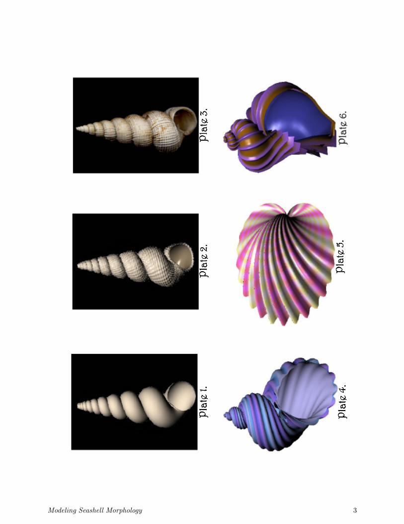
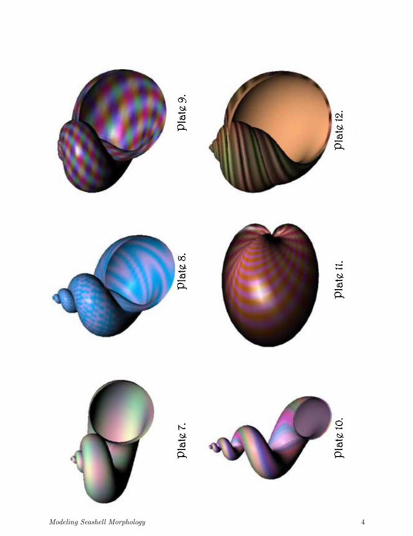
appealing, but also develops a sense of the parameter interactions. Color Plates 4 through12 show “designer shells” that have been created to illustrate various parameter interactions,apertures, and surface orientation.

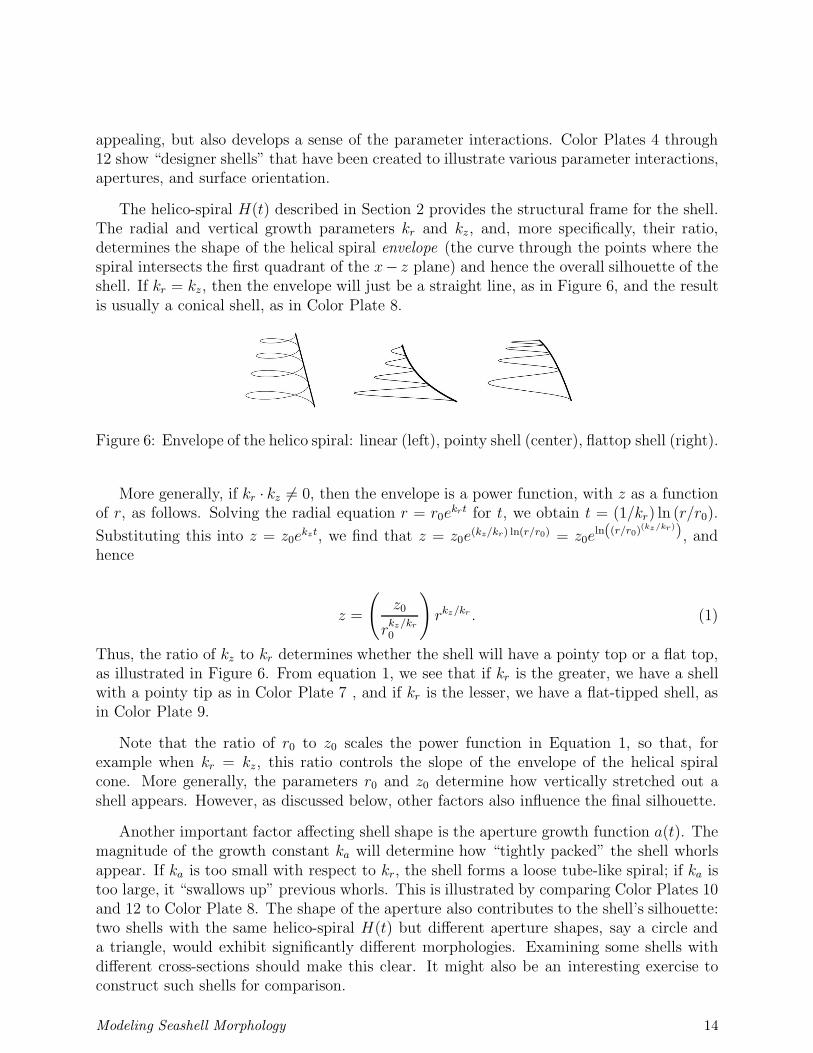
The helico-spiral H(t) described in Section 2 provides the structural frame for the shell.The radial and vertical growth parameters kr and kz, and, more specifically, their ratio,determines the shape of the helical spiral envelope (the curve through the points where thespiral intersects the first quadrant of the x− z plane) and hence the overall silhouette of theshell. If kr = kz, then the envelope will just be a straight line, as in Figure 6, and the resultis usually a conical shell, as in Color Plate 8.

Figure 6: Envelope of the helico spiral: linear (left), pointy shell (center), flattop shell (right).

More generally, if kr · kz 6= 0, then the envelope is a power function, with z as a functionof r, as follows. Solving the radial equation r = r0e

krt for t, we obtain t = (1/kr) ln (r/r0).

Substituting this into z = z0ekzt, we find that z = z0e

(kz/kr) ln(r/r0) = z0eln((r/r0)

(kz /kr)), andhence

z =

(

z0

rkz/kr

0

)

rkz/kr . (1)

Thus, the ratio of kz to kr determines whether the shell will have a pointy top or a flat top,as illustrated in Figure 6. From equation 1, we see that if kr is the greater, we have a shellwith a pointy tip as in Color Plate 7 , and if kr is the lesser, we have a flat-tipped shell, asin Color Plate 9.

Note that the ratio of r0 to z0 scales the power function in Equation 1, so that, forexample when kr = kz, this ratio controls the slope of the envelope of the helical spiralcone. More generally, the parameters r0 and z0 determine how vertically stretched out ashell appears. However, as discussed below, other factors also influence the final silhouette.

Another important factor affecting shell shape is the aperture growth function a(t). Themagnitude of the growth constant ka will determine how “tightly packed” the shell whorlsappear. If ka is too small with respect to kr, the shell forms a loose tube-like spiral; if ka istoo large, it “swallows up” previous whorls. This is illustrated by comparing Color Plates 10and 12 to Color Plate 8. The shape of the aperture also contributes to the shell’s silhouette:two shells with the same helico-spiral H(t) but different aperture shapes, say a circle anda triangle, would exhibit significantly different morphologies. Examining some shells withdifferent cross-sections should make this clear. It might also be an interesting exercise toconstruct such shells for comparison.


Shells exhibit surface sculpting of many different types, described by terms such as ribs,grooves, cords, granules, nodules and scales [Egerton 2008]. Spiral and axial ribs are themost basic of these. Spiral ribs run parallel to the helico-spiral H(t). Adding a periodicfunction in s, such as a sine function of appropriate period and amplitude, to an aperturefunction will create spiral ribs. Axial ribs, or ridges, are orthogonal to H(t). On first glance,it may seem that ridges are vertical, that is, parallel to the z axis. But closer examinationof shell specimens shows that ridges occurring in nature, in fact, lie in planes perpendicularto the helico-spiral H(t) [Prusinkiewicz and Fowler 2003]. Some of these ridges are, actuallyvarices, thickenings that result from pauses in the growth of the shell, so they must liein the aperture plane [Oliver and Nicholls 2004]. This confirms that the Frenet frame isthe appropriate method for modeling shells, and it allows ridges to be incorporated in astraightforward way. In modeling the shell exterior, ridges may be regarded as periodic (orat least recurrent) changes in the aperture. Ridges can thus be incorporated by modifyingthe shape function so that it varies with t as well as s. Letting P (s, t) = P (s) · Q(t), withthe variables separated, keeps the aperture shape geometrically similar along the length ofthe helico-spiral, but allows t-variations that may create ridges. Allowing P to be a moregeneral function of s and t would permit aperture shape to vary in all sorts of ways and notremain geometrically self-similar. Shells with ribs and ridges are illustrated in Color Plates4, 5, and 6.

Some shells have highly convoluted apertures that may simply not be expressible as apolar function. Other methods for defining the generating curve, such as Bezier curves,have been used [Prusinkiewicz and Fowler 2003], but these are beyond the scope of ourtwo-parameter model.

Despite careful measuring, the resulting models often differ somewhat from the chosenspecimen. One source of error we have noticed is that the model can be quite sensitive to theinitial values r0 and z0. The helical spiral might seem to have the correct proportions basedon the measurements, but the final shell appears too elongated or too squat. In that case,some minor ad hoc adjustments may be necessary to achieve a good rendering. Anotherdifficulty is that, for both shell X-rays and cross-sections of actual shells, the visible cross-sections lie in a plane containing the z-axis, not in a plane determined by the Frenet frame,so the aperture curve derived from measurements is distorted. A nice extra-credit problemis to adjust the measurements for distortion by taking into account how far the Frenet frameis tilted away from the vertical. A third caution is that some shells with elongated apertures(Cymantium Clandestina for example) may have have a small narrow portion of the aperturethat does not lie in the normal plane, but rather inclines toward the z-axis.

We initially estimated designer shell parameters from photographs, but then also gavefree rein to artistic license. Our color patterns result from specifying RGB colors as functionsof s and t in our Maple plots. Although it is fun to play with the color patterns this way, itgenerally does not replicate actual shell coloration (except stripes). See Meinhardt [2003] forfurther information, and stay tuned for a seashell patterning sequel to this module! Bivalves(such as clams or cockles) may also be modeled using the methods shown here, as in ColorPlates 11 and 5, but we have not yet found a satisfactory way to estimate the parametersfrom shell measurements. However, eyeball estimates and a good understanding of how


the parameters control the shape of the shell can still lead to lovely renderings. The shellparameters and aperture functions used to generate the designer shells in Color Plates 4through 12 are given in Section 6.3

5 Project Handouts

The handouts below offer several possible approaches for this project, ranging from highlyindependent to quite structured. For an independent approach, we provide Handout I only.For classes or students needing more guidance, we also provide Handout II, which breaksdown the problem into smaller steps. Handout III further assists students with organizingtheir work. We have successfully used the Handout I only approach in class and weregratified by the enthusiasm with which students grappled with the problem. They werevery excited by having an open-ended application and not being led by the hand throughit. We encourage such independent students to share model drafts with us, if they wish tocheck their progress. However, as project work contiues, some students need suggestions forbreaking down the steps and we then provide Handout II to them. Handout III can helpstreamline assessment, particularly with less prepared students. Handout IV adds a writingcomponent to the project.

Developing the model itself can be a valuable experience for well-prepared, self-motivatedstudents. In this case, we provide students only with Handout I and part of the resourcelist from Section 7. We require students to gain morphology and modeling informationdirectly from the literature without the benefit of the discussions contained in this module.By including Handout IV, we give students an opportunity to develop mathematical writingskills and more closely replicate a real-world experience in applied mathematics. Studentscompleting a literature search can explore the range of works on this topic and may wellimprove on the model presented in this module.

In our courses, we begin this project after students have learned about space curvesand Frenet frames. To facilitate the shell modeling, we introduce parameterized surfacesearlier than our textbook. We also loosely describe how a shell model is formed by theaperture curve sliding along the helical spiral, but mostly leave students to the satisfactionof independent discovery.

5.1 Handout I (highly independent)

Choose a seashell, either an intact shell or some form of cross-section, and develop theequations to model it. Write a program with course software to generate a three-dimensionalmodel of the shell. The code must be well-documented (i.e. contain detailed explanationsdescribing each line of code). In addition, demonstrate your understanding of how the variousparameters in your model control shell morphology in a brief written explanation.


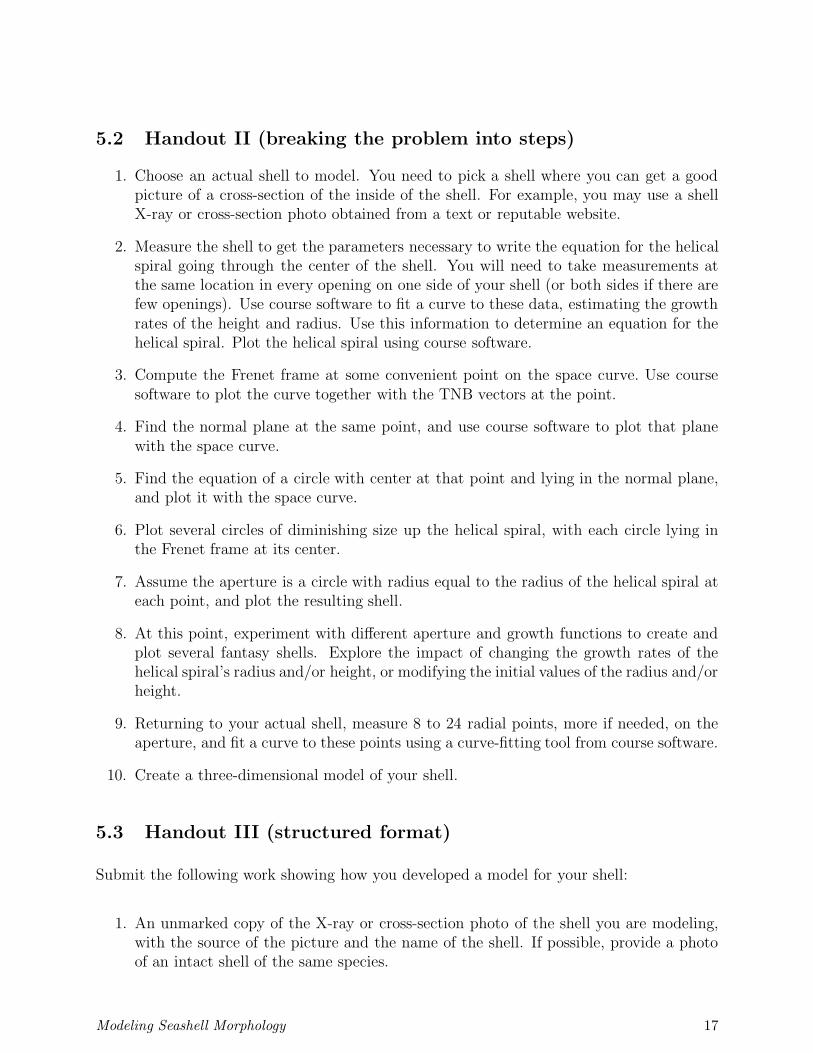
5.2 Handout II (breaking the problem into steps)

1. Choose an actual shell to model. You need to pick a shell where you can get a goodpicture of a cross-section of the inside of the shell. For example, you may use a shellX-ray or cross-section photo obtained from a text or reputable website.

2. Measure the shell to get the parameters necessary to write the equation for the helicalspiral going through the center of the shell. You will need to take measurements atthe same location in every opening on one side of your shell (or both sides if there arefew openings). Use course software to fit a curve to these data, estimating the growthrates of the height and radius. Use this information to determine an equation for thehelical spiral. Plot the helical spiral using course software.

3. Compute the Frenet frame at some convenient point on the space curve. Use coursesoftware to plot the curve together with the TNB vectors at the point.

4. Find the normal plane at the same point, and use course software to plot that planewith the space curve.

5. Find the equation of a circle with center at that point and lying in the normal plane,and plot it with the space curve.

6. Plot several circles of diminishing size up the helical spiral, with each circle lying inthe Frenet frame at its center.

7. Assume the aperture is a circle with radius equal to the radius of the helical spiral ateach point, and plot the resulting shell.

8. At this point, experiment with different aperture and growth functions to create andplot several fantasy shells. Explore the impact of changing the growth rates of thehelical spiral’s radius and/or height, or modifying the initial values of the radius and/orheight.

9. Returning to your actual shell, measure 8 to 24 radial points, more if needed, on theaperture, and fit a curve to these points using a curve-fitting tool from course software.

10. Create a three-dimensional model of your shell.

5.3 Handout III (structured format)

Submit the following work showing how you developed a model for your shell:

1. An unmarked copy of the X-ray or cross-section photo of the shell you are modeling,with the source of the picture and the name of the shell. If possible, provide a photoof an intact shell of the same species.


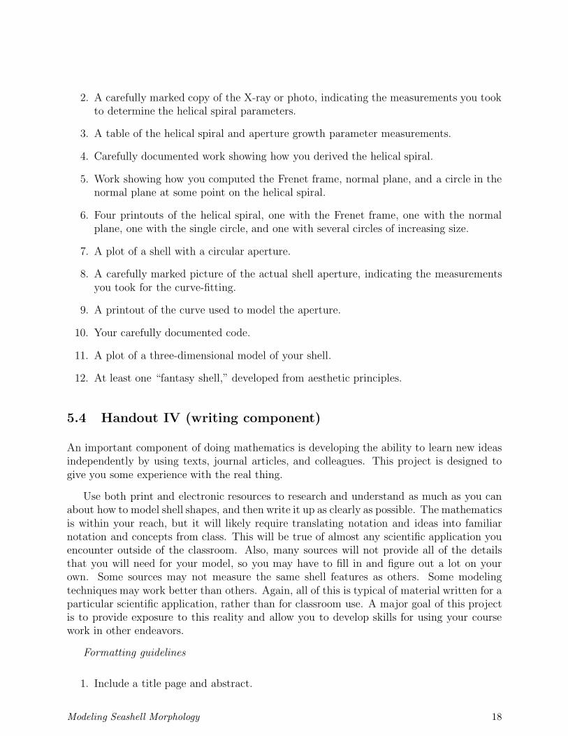
2. A carefully marked copy of the X-ray or photo, indicating the measurements you tookto determine the helical spiral parameters.

3. A table of the helical spiral and aperture growth parameter measurements.

4. Carefully documented work showing how you derived the helical spiral.

5. Work showing how you computed the Frenet frame, normal plane, and a circle in thenormal plane at some point on the helical spiral.

6. Four printouts of the helical spiral, one with the Frenet frame, one with the normalplane, one with the single circle, and one with several circles of increasing size.

7. A plot of a shell with a circular aperture.

8. A carefully marked picture of the actual shell aperture, indicating the measurementsyou took for the curve-fitting.

9. A printout of the curve used to model the aperture.

10. Your carefully documented code.

11. A plot of a three-dimensional model of your shell.

12. At least one “fantasy shell,” developed from aesthetic principles.

5.4 Handout IV (writing component)

An important component of doing mathematics is developing the ability to learn new ideasindependently by using texts, journal articles, and colleagues. This project is designed togive you some experience with the real thing.

Use both print and electronic resources to research and understand as much as you canabout how to model shell shapes, and then write it up as clearly as possible. The mathematicsis within your reach, but it will likely require translating notation and ideas into familiarnotation and concepts from class. This will be true of almost any scientific application youencounter outside of the classroom. Also, many sources will not provide all of the detailsthat you will need for your model, so you may have to fill in and figure out a lot on yourown. Some sources may not measure the same shell features as others. Some modelingtechniques may work better than others. Again, all of this is typical of material written for aparticular scientific application, rather than for classroom use. A major goal of this projectis to provide exposure to this reality and allow you to develop skills for using your coursework in other endeavors.

Formatting guidelines

1. Include a title page and abstract.


2. Use a mathematical typesetting tool such as LaTeX or MathType for all equations andsymbols, and prepare all figures carefully.

3. The paper must be properly referenced, with a complete bibliography at the end andreferences in the text. Internet resources must be used with caution and must beproperly documented. Use MathSciNet http://www.ams.org/mathscinet as muchas possible for citation formats. Use MLA formatting for Internet sites http://www.wisc.edu/writing/Handbook/elecmla.html, and for anything not on MathSciNet.

4. Model your paper on articles you read in your research, and consider both their struc-ture and their content.

5. Proofread carefully. Use campus writing resources and peer review, and appropriatelyedit/revise your paper before submission.

Evaluation criteria

The overall goal is a clear model describing what measurements are needed from theshell, a formula for generating the shell, and a description of the effect of each variable in theformula. Clarity of exposition is as important as the underlying mathematics. Indicationsof a well-written paper: clear equations with careful discussions of which physical propertiesof the shell are controlled by which parameters, figures that illustrate the concepts you arediscussing, and clear evidence that you understand basic vector calculus concepts and howthey pertain to this application.

Indications of a paper that needs more work: equations and/or figures copied with inade-quate explanation, disorganized composition, poor spelling or grammar, lack of proofreading,over-reliance on Internet sources, and inadequate referencing.

6 Maple Code

This project assumes a reasonable amount of familiarity with a computer algebra system thatgenerates three-dimensional graphics. We use Maple throughout our calculus curriculum, soour students are familiar with basic function manipulation, plotting commands, and syntaxwhen starting this project. As part of normal multivariable calculus class work, we alsoprovide examples in Maple of generating space curves, parameterized surfaces, planes, andthe Frenet frame, so this project also offers excellent synthesis and application opportunities.

Below is the Maple 12 code that we developed for this project. The generic Mapleprocedure, which may be used with any shell parameters, is provided first, followed by asample of modeling a shell of the species E. magnificum. We do not necessarily expectstudents to be familiar with the procedure (proc) command used in the worksheet. Somestudents use it (particularly those with some computer science background), while othersare more comfortable generating each shell plot individually. Both approaches seem to workequally well.


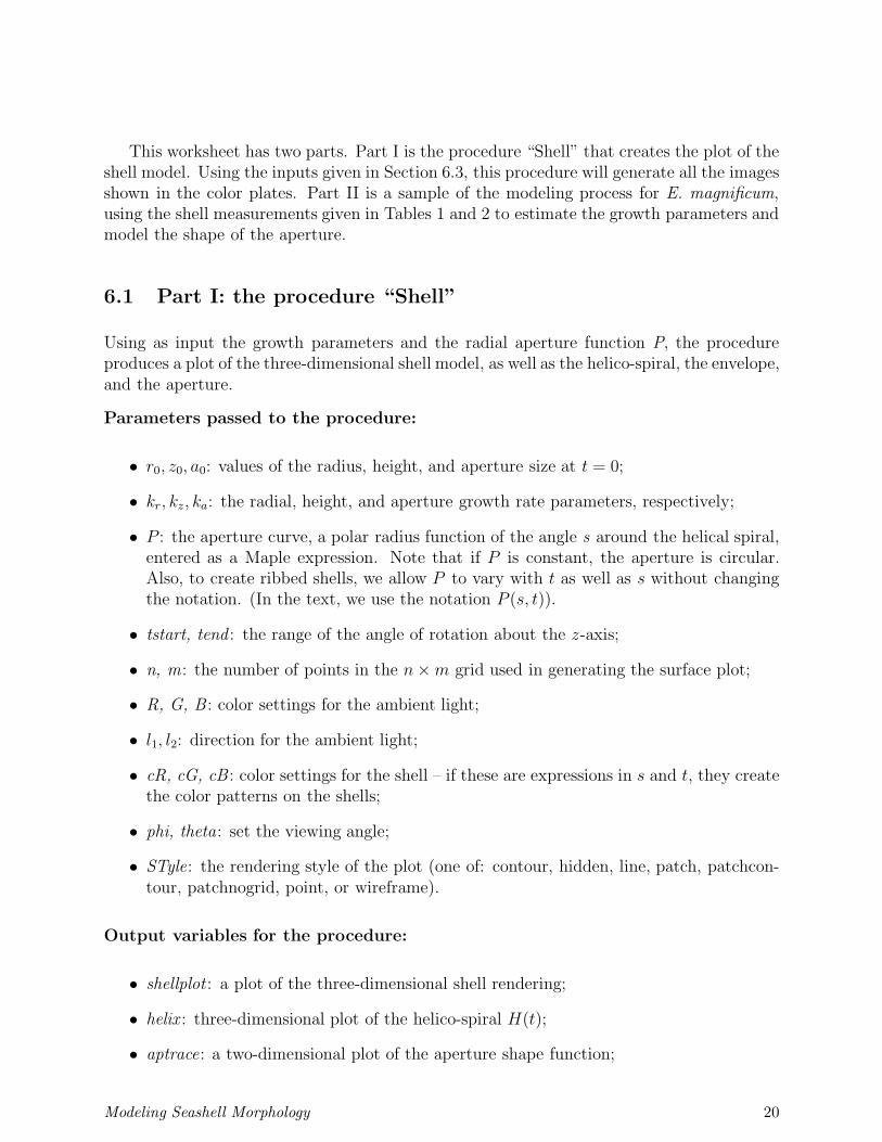
This worksheet has two parts. Part I is the procedure “Shell” that creates the plot of theshell model. Using the inputs given in Section 6.3, this procedure will generate all the imagesshown in the color plates. Part II is a sample of the modeling process for E. magnificum,using the shell measurements given in Tables 1 and 2 to estimate the growth parameters andmodel the shape of the aperture.

6.1 Part I: the procedure “Shell”

Using as input the growth parameters and the radial aperture function P, the procedureproduces a plot of the three-dimensional shell model, as well as the helico-spiral, the envelope,and the aperture.

Parameters passed to the procedure:

• r0, z0, a0: values of the radius, height, and aperture size at t = 0;

• kr, kz, ka: the radial, height, and aperture growth rate parameters, respectively;

• P : the aperture curve, a polar radius function of the angle s around the helical spiral,entered as a Maple expression. Note that if P is constant, the aperture is circular.Also, to create ribbed shells, we allow P to vary with t as well as s without changingthe notation. (In the text, we use the notation P (s, t)).

• tstart, tend : the range of the angle of rotation about the z -axis;

• n, m : the number of points in the n × m grid used in generating the surface plot;

• R, G, B : color settings for the ambient light;

• l1, l2: direction for the ambient light;

• cR, cG, cB : color settings for the shell – if these are expressions in s and t, they createthe color patterns on the shells;

• phi, theta : set the viewing angle;

• STyle: the rendering style of the plot (one of: contour, hidden, line, patch, patchcon-tour, patchnogrid, point, or wireframe).

Output variables for the procedure:

• shellplot : a plot of the three-dimensional shell rendering;

• helix : three-dimensional plot of the helico-spiral H(t);

• aptrace: a two-dimensional plot of the aperture shape function;


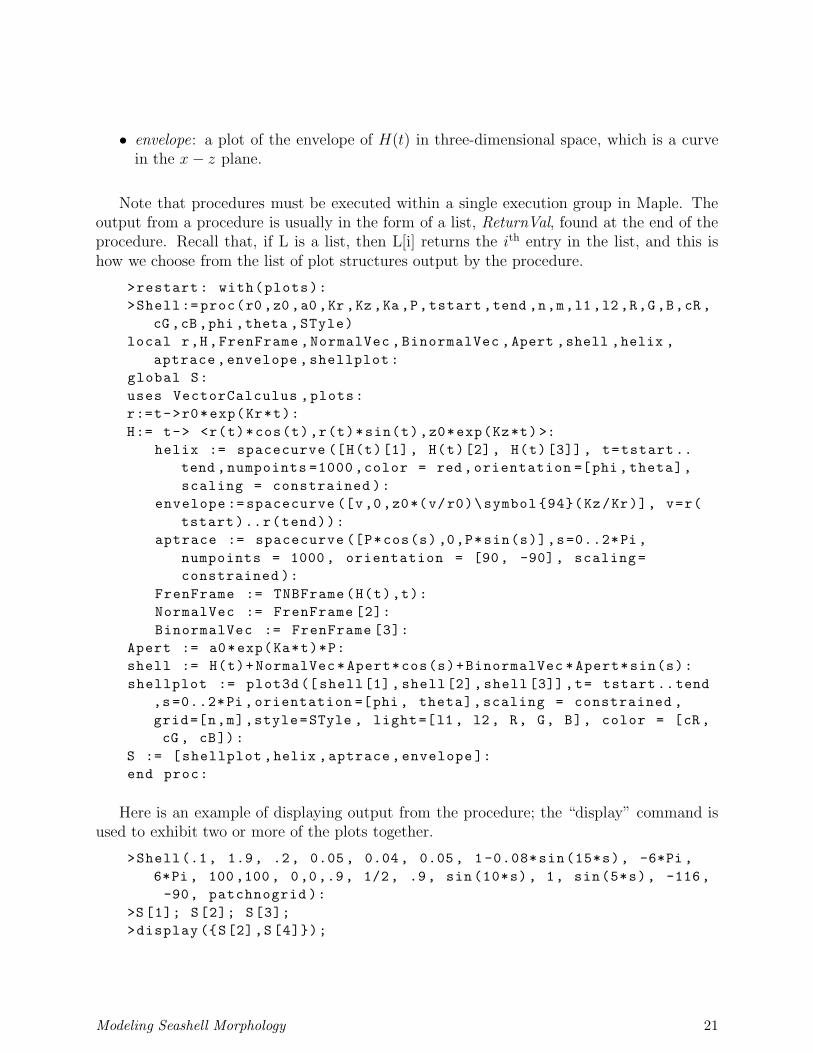
• envelope: a plot of the envelope of H(t) in three-dimensional space, which is a curvein the x − z plane.

Note that procedures must be executed within a single execution group in Maple. Theoutput from a procedure is usually in the form of a list, ReturnVal, found at the end of theprocedure. Recall that, if L is a list, then L[i] returns the ith entry in the list, and this ishow we choose from the list of plot structures output by the procedure.

>restart: with(plots):

>Shell:=proc(r0,z0,a0,Kr,Kz,Ka,P,tstart,tend ,n,m,l1,l2,R,G,B,cR,

cG,cB,phi ,theta ,STyle)

local r,H,FrenFrame ,NormalVec ,BinormalVec ,Apert ,shell ,helix ,

aptrace,envelope ,shellplot:

global S:

uses VectorCalculus ,plots:

r:=t->r0*exp(Kr*t):

H:= t-> <r(t)*cos(t),r(t)*sin(t),z0*exp(Kz*t)>:

helix := spacecurve ([H(t)[1], H(t)[2], H(t)[3]], t=tstart..

tend ,numpoints =1000,color = red,orientation =[phi,theta],

scaling = constrained ):

envelope :=spacecurve ([v,0,z0*(v/r0)\symbol {94}(Kz/Kr)], v=r(

tstart)..r(tend)):

aptrace := spacecurve ([P*cos(s),0,P*sin(s)],s=0..2*Pi,

numpoints = 1000, orientation = [90, -90], scaling=

constrained ):

FrenFrame := TNBFrame(H(t),t):

NormalVec := FrenFrame [2]:

BinormalVec := FrenFrame [3]:

Apert := a0*exp(Ka*t)*P:

shell := H(t)+NormalVec*Apert*cos(s)+BinormalVec *Apert*sin(s):

shellplot := plot3d([shell[1], shell[2],shell[3]],t= tstart..tend

,s=0..2*Pi,orientation =[phi, theta],scaling = constrained ,

grid=[n,m],style=STyle , light=[l1, l2, R, G, B], color = [cR,

cG , cB]):

S := [shellplot ,helix ,aptrace,envelope ]:

end proc:

Here is an example of displaying output from the procedure; the “display” command isused to exhibit two or more of the plots together.

>Shell(.1, 1.9, .2, 0.05, 0.04, 0.05, 1-0.08*sin(15*s), -6*Pi ,

6*Pi, 100,100, 0,0,.9, 1/2, .9, sin(10*s), 1, sin(5*s), -116,

-90, patchnogrid ):

>S[1]; S[2]; S[3];

>display ({S[2],S[4]});


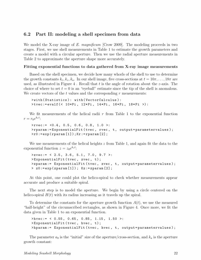
6.2 Part II: modeling a shell specimen from data

We model the X-ray image of E. magnificum [Crow 2009]. The modeling proceeds in twostages. First, we use shell measurements in Table 1 to estimate the growth parameters andcreate a model with a circular aperture. Then we use the radial aperture measurements inTable 2 to approximate the aperture shape more accurately.

Fitting exponential functions to data gathered from X-ray image measurements

Based on the shell specimen, we decide how many whorls of the shell to use to determinethe growth constants kr, kz, ka. In our shell image, five cross-sections at t = 10π, . . . , 18π areused, as illustrated in Figure 4 . Recall that t is the angle of rotation about the z-axis. Thechoice of where to set t = 0 is an “eyeball” estimate since the tip of the shell is anomalous.We create vectors of the t values and the corresponding r measurements:

>with(Statistics ): with(VectorCalculus ):

>tvec:=evalf(< 10*Pi , 12*Pi, 14*Pi, 16*Pi, 18*Pi >):

We fit measurements of the helical radii r from Table 1 to the exponential functionr = r0e

krt:

>rvec:= <0.4, 0.5, 0.6, 0.8, 1.0 >:

>rparam:= ExponentialFit (tvec , rvec , t, output=parametervalues );

>r0:=exp(rparam [1]);Kr:=rparam[2];

We use measurements of the helical heights z from Table 1, and again fit the data to theexponential function z = z0e

kzt:

>zvec:= < 2.5, 3.6, 5.1, 7.0, 9.7 >:

>ExponentialFit (tvec , zvec , t);

>zparam:= ExponentialFit (tvec , zvec , t, output=parametervalues );

> z0:=exp(zparam[1]); Kz:=zparam [2];

At this point, one could plot the helico-spiral to check whether measurements appearaccurate and produce a suitable spiral.

The next step is to model the aperture. We begin by using a circle centered on thehelico-spiral H(t) with its radius increasing as it travels up the spiral.

To determine the constants for the aperture growth function A(t), we use the measured“half-height” of the circumscribed rectangles, as shown in Figure 4. Once more, we fit thedata given in Table 1 to an exponential function.

>hvec:= < 0.55, 0.65, 0.85, 1.15, 1.50 >:

>ExponentialFit (tvec , hvec , t);

>hparam:= ExponentialFit (tvec , hvec , t, output=parametervalues );

The parameter a0 is the “initial” size of the aperture/cross-section, and ka is the aperturegrowth constant:


>a0:= exp(hparam[1]); Ka:= hparam [2];

Shell model with circular aperture

We can now plot a model of the shell with circular apertures using the “Shell” procedureand the growth parameters we have determined.

Using P = 1 produces a circular aperture with size corresponding to the measurementstaken.

>Shell(r0 ,z0,a0, Kr,Kz,Ka , 1, 0,20*Pi, 500,50, 60,0, 1,1,1,

0.98,0.9,0.8, -90, -80, patchnogrid ):

>S[1];

To see an image that resembles the X-ray, right click and view the shell without thewireframe and with transparency adjusted to about 50%. Displaying the shell with STyleset to wireframe helps determine the appropriate ratio of n to m in the grid setting. Adjustn and m so that the wireframe cells on the shell surface are roughly square.

Also, the shell grows with increasing z, so the graph has been turned upside down (usingviewing angles phi and theta) to get the usual view.

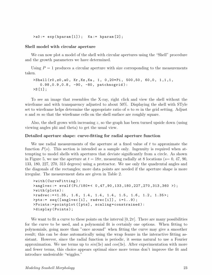
Detailed aperture shape: curve-fitting for radial aperture function

We use radial measurements of the aperture at a fixed value of t to approximate thefunction P (s). This section is intended as a sample only. Ingenuity is required when at-tempting to model shells with apertures that deviate significantly from a circle. As shownin Figure 5, we use the aperture at t = 18π, measuring radially at 8 locations (s= 0, 47, 90,133, 180, 227, 270, 313 degrees) using a protractor. We use only the quadrental angles andthe diagonals of the rectangles; more data points are needed if the aperture shape is moreirregular. The measurement data are given in Table 2.

>with(CurveFitting ):

>anglvec := evalf(Pi/180*< 0,47,90,133,180,227,270,313,360 >);

>with(plots):

>radvec:=<1.35, 1.6, 1.4, 1.4, 1.4, 1.5, 1.6, 1.2, 1.35>;

>pts:= seq([anglvec[i], radvec[i]], i=1..9);

>Points:=pointplot ([pts], scaling=constrained ):

>display(Points);

We want to fit a curve to these points on the interval [0, 2π]. There are many possibilitiesfor the curve to be used, and a polynomial fit is certainly one options. When fitting topolynomials, going more than ”once around” when fitting the curve may give a smootherresult; this can be done automatically using the wrap feaure in the interactive fitting as-sistant. However, since the radial function is periodic, it seems natural to use a Fourierapproximation. We use terms up to sin(3s) and cos(3s). After experimentation with moreand fewer terms, this choice appears optimal since more terms don’t improve the fit andintroduce undesirable “wiggles.”


>FourierForm := k+a*sin(s) + b*cos(s) +c*sin(2*s) +d*cos(2*s)+e*

sin(3*s) +f*cos(3*s):

>ApFit:= LeastSquares (anglvec, radvec, s, curve=FourierForm );

>FitCurve :=plot(ApFit ,s=-Pi/2..5*Pi/2, color=blue , scaling=

constrained ):

>display ({Points,FitCurve });

This curve specifies the aperture at the chosen value t = 18π.

To find the expression for P (s), note that this aperture is A(t)×P (s) = a0eka18πP (s), so

we need to divide by a0eka18π to solve for the aperture shape function P .

>a:=t-> a0*exp(Ka*t);

>P:=ApFit/a(18*Pi);

The procedure “Shell” with the growth parameters determined above and the aperturecurve P now produces a refined model:

>Shell(r0 ,z0,a0, Kr,Kz,Ka , P, 0,20*Pi, 500,50, 60,0, 1,1,1,

0.98,0.9,0.8, -90,-80, patchnogrid ):

>S[1];

>S[3];

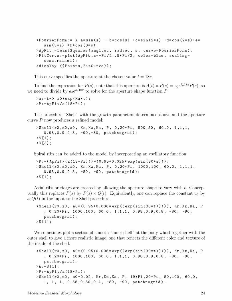
Spiral ribs can be added to the model by incorporating an oscillatory function:

>P:=(ApFit/(a(18*Pi)))*(0.95+0.025* exp(sin(30*s)));

>Shell(r0 ,z0,a0, Kr,Kz,Ka , P, 0,20*Pi, 1000,100, 60,0, 1,1,1,

0.98,0.9,0.8, -80, -90, patchnogrid ):

>S[1];

Axial ribs or ridges are created by allowing the aperture shape to vary with t. Concep-tually this replaces P (s) by P (s) × Q(t). Equivalently, one can replace the constant a0 bya0Q(t) in the input to the Shell procedure.

>Shell(r0 ,z0, a0*(0.95+0.006* exp((exp(sin(30*t))))), Kr,Kz ,Ka , P

, 0,20*Pi , 1000,100, 60,0, 1,1,1, 0.98,0.9,0.8, -80, -90,

patchnogrid ):

>S[1];

We sometimes plot a section of smooth “inner shell” at the body whorl together with theouter shell to give a more realistic image, one that reflects the different color and texture ofthe inside of the shell.

>Shell(r0 ,z0, a0*(0.95+0.006* exp((exp(sin(30*t))))), Kr,Kz ,Ka , P

, 0,20*Pi , 1000,100, 60,0, 1,1,1, 0.98,0.9,0.8, -80, -90,

patchnogrid ):

>A:=S[1]:

>P:=ApFit/a(18*Pi):

>Shell(r0 ,z0, a0 -0.02, Kr ,Kz ,Ka , P, 19*Pi ,20*Pi , 50,100, 60,0,

1, 1, 1, 0.58,0.50,0.4, -80, -90, patchnogrid ):


>B:=S[1]:

>display ({A,B});

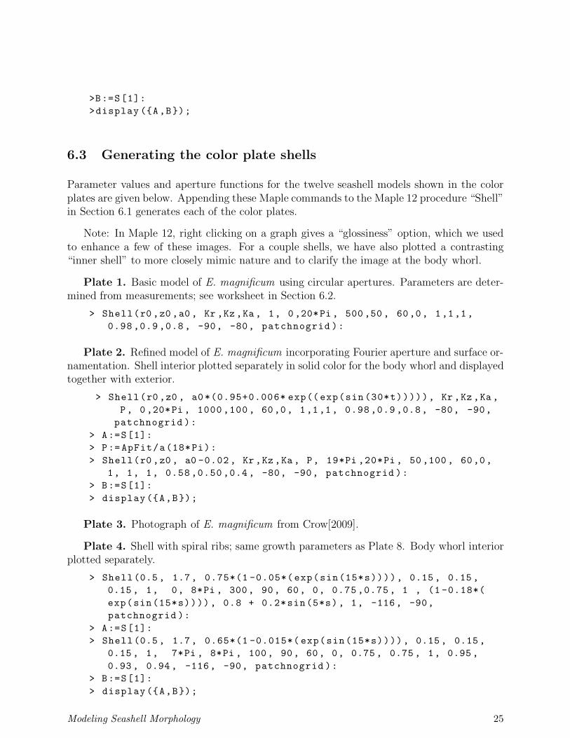
6.3 Generating the color plate shells

Parameter values and aperture functions for the twelve seashell models shown in the colorplates are given below. Appending these Maple commands to the Maple 12 procedure “Shell”in Section 6.1 generates each of the color plates.

Note: In Maple 12, right clicking on a graph gives a “glossiness” option, which we usedto enhance a few of these images. For a couple shells, we have also plotted a contrasting“inner shell” to more closely mimic nature and to clarify the image at the body whorl.

Plate 1. Basic model of E. magnificum using circular apertures. Parameters are deter-mined from measurements; see worksheet in Section 6.2.

> Shell(r0,z0,a0, Kr ,Kz,Ka, 1, 0,20*Pi, 500,50, 60,0, 1,1,1,

0.98,0.9,0.8, -90, -80, patchnogrid ):

Plate 2. Refined model of E. magnificum incorporating Fourier aperture and surface or-namentation. Shell interior plotted separately in solid color for the body whorl and displayedtogether with exterior.

> Shell(r0,z0 , a0*(0.95+0.006* exp((exp(sin(30*t))))), Kr,Kz,Ka,

P, 0,20*Pi, 1000,100, 60,0, 1,1,1, 0.98,0.9,0.8, -80, -90,

patchnogrid ):

> A:=S[1]:

> P:=ApFit/a(18*Pi):

> Shell(r0,z0, a0 -0.02, Kr,Kz,Ka, P, 19*Pi ,20*Pi, 50,100, 60,0,

1, 1, 1, 0.58,0.50,0.4, -80, -90, patchnogrid ):

> B:=S[1]:

> display({A,B});

Plate 3. Photograph of E. magnificum from Crow[2009].

Plate 4. Shell with spiral ribs; same growth parameters as Plate 8. Body whorl interiorplotted separately.

> Shell(0.5, 1.7, 0.75*(1 -0.05*(exp(sin(15*s)))), 0.15, 0.15,

0.15, 1, 0, 8*Pi , 300, 90, 60, 0, 0.75,0.75, 1 , (1 -0.18*(

exp(sin(15*s)))), 0.8 + 0.2*sin(5*s), 1, -116, -90,

patchnogrid ):

> A:=S[1]:

> Shell(0.5, 1.7, 0.65*(1 -0.015*( exp(sin(15*s)))), 0.15, 0.15,

0.15, 1, 7*Pi , 8*Pi , 100, 90, 60, 0, 0.75, 0.75, 1, 0.95,

0.93, 0.94, -116, -90, patchnogrid ):

> B:=S[1]:

> display({A,B});


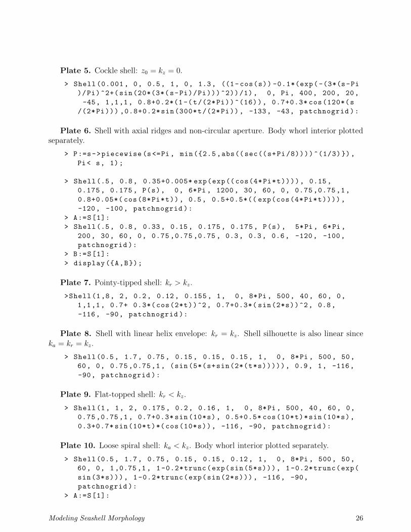
Plate 5. Cockle shell: z0 = kz = 0.

> Shell(0.001, 0, 0.5, 1, 0, 1.3, ((1-cos(s)) -0.1*(exp(-(3*(s-Pi

)/Pi)^2+(sin(20*(3*(s-Pi)/Pi)))^2))/1), 0, Pi, 400, 200, 20,

-45, 1,1,1, 0.8+0.2*(1-(t/(2*Pi))^(16)), 0.7+0.3* cos(120*(s

/(2*Pi))) ,0.8+0.2*sin(300*t/(2*Pi)), -133, -43, patchnogrid ):

Plate 6. Shell with axial ridges and non-circular aperture. Body whorl interior plottedseparately.

> P:=s->piecewise (s<=Pi, min({2.5,abs((sec((s+Pi/8))))^(1/3)}),

Pi< s, 1);

> Shell(.5, 0.8, 0.35+0.005* exp(exp((cos(4*Pi*t)))), 0.15,

0.175, 0.175, P(s), 0, 6*Pi , 1200, 30, 60, 0, 0.75,0.75,1,

0.8+0.05*( cos(8*Pi*t)), 0.5, 0.5+0.5*(( exp(cos(4*Pi*t)))),

-120, -100, patchnogrid ):

> A:=S[1]:

> Shell(.5, 0.8, 0.33, 0.15, 0.175, 0.175, P(s), 5*Pi, 6*Pi,

200, 30, 60, 0, 0.75 ,0.75 ,0.75 , 0.3, 0.3, 0.6, -120, -100,

patchnogrid ):

> B:=S[1]:

> display({A,B});

Plate 7. Pointy-tipped shell: kr > kz.

>Shell(1,8, 2, 0.2, 0.12, 0.155, 1, 0, 8*Pi, 500, 40, 60, 0,

1,1,1, 0.7+ 0.3*(cos(2*t))^2, 0.7+0.3*( sin(2*s))^2, 0.8,

-116, -90, patchnogrid ):

Plate 8. Shell with linear helix envelope: kr = kz. Shell silhouette is also linear sinceka = kr = kz.

> Shell(0.5, 1.7, 0.75, 0.15, 0.15, 0.15, 1, 0, 8*Pi , 500, 50,

60, 0, 0.75,0.75,1, (sin(5*(s+sin(2*(t*s))))), 0.9, 1, -116,

-90, patchnogrid ):

Plate 9. Flat-topped shell: kr < kz.

> Shell(1, 1, 2, 0.175, 0.2, 0.16, 1, 0, 8*Pi, 500, 40, 60, 0,

0.75,0.75,1, 0.7+0.3* sin(10*s), 0.5+0.5* cos(10*t)*sin(10*s),

0.3+0.7* sin(10*t)*(cos(10*s)), -116, -90, patchnogrid ):

Plate 10. Loose spiral shell: ka < kz. Body whorl interior plotted separately.

> Shell(0.5, 1.7, 0.75, 0.15, 0.15, 0.12, 1, 0, 8*Pi , 500, 50,

60, 0, 1,0.75,1, 1-0.2*trunc(exp(sin(5*s))), 1-0.2*trunc(exp(

sin(3*s))), 1-0.2*trunc(exp(sin(2*s))), -116, -90,

patchnogrid ):

> A:=S[1]:


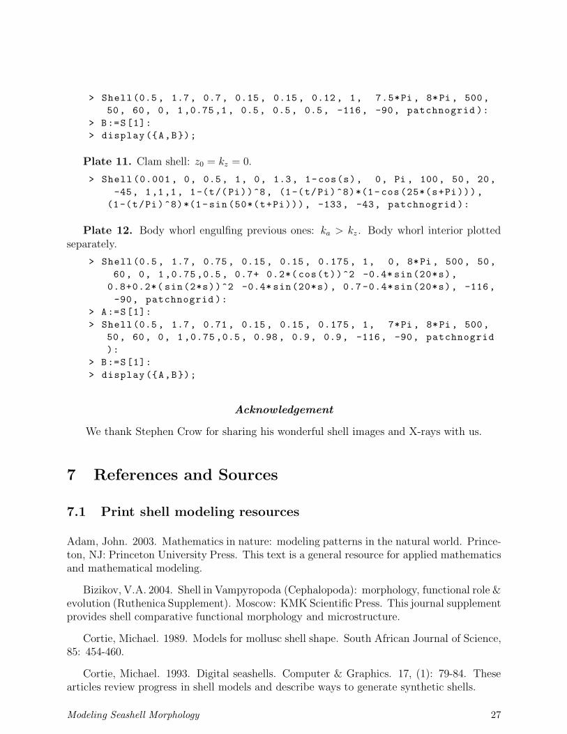
> Shell(0.5, 1.7, 0.7, 0.15, 0.15, 0.12, 1, 7.5*Pi, 8*Pi, 500,

50, 60, 0, 1,0.75,1, 0.5, 0.5, 0.5, -116, -90, patchnogrid ):

> B:=S[1]:

> display({A,B});

Plate 11. Clam shell: z0 = kz = 0.

> Shell(0.001, 0, 0.5, 1, 0, 1.3, 1-cos(s), 0, Pi , 100, 50, 20,

-45, 1,1,1, 1-(t/(Pi))^8, (1-(t/Pi)^8)*(1-cos(25*(s+Pi))),

(1-(t/Pi)^8)*(1-sin(50*(t+Pi))), -133, -43, patchnogrid ):

Plate 12. Body whorl engulfing previous ones: ka > kz . Body whorl interior plottedseparately.

> Shell(0.5, 1.7, 0.75, 0.15, 0.15, 0.175, 1, 0, 8*Pi, 500, 50,

60, 0, 1,0.75,0.5, 0.7+ 0.2*(cos(t))^2 -0.4* sin(20*s),

0.8+0.2*( sin(2*s))^2 -0.4* sin(20*s), 0.7-0.4*sin(20*s), -116,

-90, patchnogrid ):

> A:=S[1]:

> Shell(0.5, 1.7, 0.71, 0.15, 0.15, 0.175, 1, 7*Pi, 8*Pi, 500,

50, 60, 0, 1,0.75,0.5, 0.98, 0.9, 0.9, -116, -90, patchnogrid

):

> B:=S[1]:

> display({A,B});

Acknowledgement

We thank Stephen Crow for sharing his wonderful shell images and X-rays with us.

7 References and Sources

7.1 Print shell modeling resources

Adam, John. 2003. Mathematics in nature: modeling patterns in the natural world. Prince-ton, NJ: Princeton University Press. This text is a general resource for applied mathematicsand mathematical modeling.

Bizikov, V.A. 2004. Shell in Vampyropoda (Cephalopoda): morphology, functional role &evolution (Ruthenica Supplement). Moscow: KMK Scientific Press. This journal supplementprovides shell comparative functional morphology and microstructure.

Cortie, Michael. 1989. Models for mollusc shell shape. South African Journal of Science,85: 454-460.

Cortie, Michael. 1993. Digital seashells. Computer & Graphics. 17, (1): 79-84. Thesearticles review progress in shell models and describe ways to generate synthetic shells.


Dawkins, Richard. 1996. Climbing mount improbable. New York: W. W. Norton &Company. This popular science book discusses probability and its applications to evolution.

Flower, Rousseau H. 1964. Nautiloid shell morphology. New Mexico Institute of Miningand Technology, Bureau of Mines and Mineral Resources Memoir: Soccoro. This founda-tional work focuses on external shell morphology and thin sections.

Fowler, Deborah, Hans Meinhardt, Przemyslaw Prusinkiewicz. 1992. Modeling seashells.Proceeding of SIGGRAPH ’92 (Chicago, Illinois, July 26-31), In Computer Graphics, 26, (2):379-387. ACM SIGGRAPH, New York. This article offers shell modeling analysis similar toChapter 10 of [Meinhardt, 2003].

Galbraith, Callum, Przemyslaw Prusinkiewicz, and Brian Wyvill. 2002. Modeling aMurex cabritii sea shell with a structured implicit surface modeler. The Visual Computer,18: 70-80. This article gives a modeler to help capture shell surface perturbations and shellwall thickness.

Illert, Chris and Ruggero Santilli. 1995. Foundations of theoretical conchology. 2nd ed.Florida: Hadronic Press. This text argues that shells require a structurally general geometry.

Mandelbrot, Benoit. 1982. The fractal geometry of nature. New York: W. H. Freemanand Co. This text offers a definitive overview of fractal geometry and its applications.

McGhee, George, Jr. 1999. Theoretical morphology: the concept and its applications(The critical moments and perspectives in Earth history and paleobiology). New York:Columbia University Press. This text offers an overview of theoretical morphology and itsfuture challenges.

Meinhardt, Hans. 2003. The algorithmic beauty of sea shells, 3rd ed. New York:Springer-Verlag. This book gives a rigorous study of modeling and computer simulations ofseashell patterns.

Meinhardt, Hans and Martin Klinger. 1987. A model for pattern formation on the shellsof molluscs. Journal of Theoretical Biology, 126: 63-89. This article offers models to generatemollusk shell pigmentation and relief-like patterns.

Oliver, Arthur P. H. and James Nicholls. 2004. Guide to seashells of the world. Buffalo,NY: Firefly Books. This is a comprehensive seashell identification resource.

Pickover, Clifford. 1989. A short recipe for seashell synthesis. IEEE Computer Graphicsand Applications 9, (6): 8-11. This article provides artistic examples of seashell-like formsfrom a graphics supercomputer.

Prusinkiewicz, Przemyslaw and Deborah R. Fowler. 2003. Shell models in three dimen-sions. Chapter 10 of [Meinhardt 2003]. We significantly use this resource in our modelingapproach in this module.

Raup, David. 1962. Computer as aid in describing form in gastropod shells. Science,138: 150-152.


Raup, David. 1966. Geometrical analysis of shell coiling: general problems. Journal ofPaleontology, 40, (5): 1178-1190.

Raup, David. 1969. Modeling and simulation of morphology by computer. In Proceed-ings of the North American Paleontology Convention, 71-83.

Raup, David and Arnold Michelson. 1965. Theoretical morphology of the coiled shell.Science, 147: 1294-1296. Raup’s articles analyze shell morphology and computer-aided shellmodeling.

Rupert, Edward and Robert Barnes. 1994. Invertebrate zoology. 6th ed. Fort Worth:Saunders College Publishing/Harcourt Brace Publishing. This introductory invertebratebiology text emphasizes adaptive morphology and physiology.

Stone, Jon R. 1995. CerioShell; a computer program designed to simulate variation inshell form. Paleobiology, 21: 509-519.

Stone, Jon R. 1996. The evolution of ideas: a phylogeny of shell models. The AmericanNaturalist, 148: 904-929.

Stone, Jon R. 1997. The spirit of D’Arcy Thompson dwells in empirical morphospace.Mathematical Biosciences, 142: 13-30. Stone’s articles describe shell model evolution andrecent connections to classic approaches.

Thompson, DArcy. 1961. On Growth and Form. Great Britain: University Press,Cambridge. This work explores form and structure in living organisms from a mathematicalperspective.

Wilbur, Karl, E.R. Trueman, and M.R. Clarke (Eds.). 1988. The mollusca: form andfunction, Volume 11. San Diego, CA: Academic Press. This text reviews advances in inter-preting the structure and function of mollusk systems.

7.2 Online shell modeling resources

American Mathematical Society. 2004. The mathematical study of mollusk shells. Avail-able at: http://www.ams.org/featurecolumn/archive/shell1.html, accessed 27, Jan-uary, 2009. This column describes how logarithmic spirals can help develop mollusk shellgeometry.

Coombes, Stephen. 2000. The geometry of sea ghells. Available at: http://www.maths.nott.ac.uk/personal/sc/SeaShells.pdf , accessed 27, January, 2009. This University ofNottingham document offers mathematical background for shell models.

Duke University. 1997-2003. “Connected Curriculum Project.” Available at: http:

//www.math.duke.edu/education/ccp/materials/biology.html, accessed 27, January,2009. This site offers two modules that create equiangular spirals using a CAS.

Ferraro, Roberto. 2000. LS sketchbook by example: Sea shells and horns. Available at:


http://coco.ccu.uniovi.es/malva/sketchbook/lssketchbook/examples/seashell/seashell.

htm, accessed 27, January, 2009. This page presents some software/code for sketching spiralsand shell models.

International Educational Software. 2003. Snail shell Manipula Math with Java. Avail-able at http://www.ies.co.jp/math/java/misc/oum/oum.html, accessed 27, January, 2009.This site provides a java applet for creating a snail shell according to a log clock model.

Jirapong, Kamon, Robert J. Krawczyk. 2003. Seashell architectures. Paper given atISAMA/Bridges Conference. Available at: http://www.iit.edu/~krawczyk/kjbrdg03.

pdf, accessed 27, January, 2009. This site describes a study to apply seashell form toarchitecture.

Kazlev, M. Alan. 2002. Palaeos invertebrates: Mollusca: Mollusc shell morphology.”Available at: http://www.palaeos.com/Invertebrates/Molluscs/Mollusca.Shell.html,accessed 27, January, 2009. This site offers information on mollusk shell modeling and Raup’smodels from the 1960s.

Lee, Xah. 1995-2008. Mathematics of seashell shapes. and Equiangular spiral. Availableat: http://xahlee.org/SpecialPlaneCurves_dir/Seashell_dir/index.html, accessed27, January, 2009. These pages provide information and some CAS/graphing calculatorcode to model seashells.

Lucca, G. 2003. Representing seashells surface. Visual Mathematics. 5: 1. Availableat http://www.mi.sanu.ac.yu/vismath/lucca/, accessed 27, January, 2009. This paperpresents a general algorithm to model various seashell shapes and some examples.

Moidel, Chuck. Sea shells. WPI. Available at: http://www.cs.wpi.edu/~emmanuel/

courses/cs563/write_ups/chuckm/seashells.htm, accessed 27, January, 2009. This ar-ticle offers information on shell modeling, pigmentation, and relevant biochemistry.

Peterson, Ivars. 2005. Sea shell spirals. Science News. Available at: http://www.

sciencenews.org/view/generic/id/6030/title/Math_Trek__Sea_Shell_Spirals, accessed27, January, 2009. This column argues that nautilus shell growth is not based on a goldenratio equiangular spiral.

Phillips, Tony. 2001. The mathematical study of mollusk shells. Available at: http://

www.math.sunysb.edu/~tony/whatsnew/column/shells-0201/shell1.html, accessed 27,January, 2009. This column describes how equiangular spirals can generate mollusk shellgeometry.

Picado, Jorge. 2009. Seashells: the plainness and beauty of their mathematical descrip-tion. Loci (the online digital magazine of the MathDL). Available at http://mathdl.maa.org/mathDL/23/?pa=content&sa=viewDocument&nodeId=3294, accessed 19, May 2009. Thisarticle includes a simple model to describe and generate many types of seashell shapes.

TONMO.com. 2000-2009. The octopus news magazine online. Available at: http:

//www.tonmo.com/science/fossils/morphology/, accessed 27, January, 2009. This site


offers a variety of shell morphology information.

Wang, Ngai-Ming. 1997. Modeling seashells in openGL. Cornell University. Availableat: http://www.nbb.cornell.edu/neurobio/land/OldStudentProjects/cs490-96to97/wang/re2.html, accessed 27, January, 2009. The author models various seashells by sweep-ing a curve along a helico spiral in Open GL.

7.3 Online sources for shells, pictures, and X-rays

American Malacological Society homepage. 2009. Available at: http://www.malacological.org/, accessed 27, January, 2009. The AMS is an international society interested in the con-servation and study of mollusks.

Beechey, Des. The sea shells of New South Wales. Available at: http://seashellsofnsw.org.au/, accessed 27, January, 2009. This site offers information about various shell speciesand a handy shell glossary.

Bourquin, Avril. 2009. Man and Mollusc/Mollusk. Available at: http://manandmollusc.net/, accessed 27, January, 2009. This comprehensive site provides various shell articles anda handy Internet resource zone.

Conchking store homepage. 2009. Available at: http://conchking.com/Seashells.

htm, accessed 27, January, 2009. This online store offers a wide range of Caribbean seashells.

Conch-Net or Conchologists Information Network homepage. 1996-2009. Available at:http://www.conchologistsofamerica.org/home/, accessed 27, January, 2009. This siteprovides American Conchologist shell articles and other relevant information.

Crowncity seashell posters. 2009. Available at: http://www.crowncity.com/shellfish/,accessed 27, January, 2009. This page offers shell printer made using an X-ray machine.

Crow, Stephen. 2009. Seashell architecture. Available at: http://www.seashellarchitecture.com/, accessed 27, January, 2009. Offering a large collection of seashell X-rays, this site isthe source of the CD for our X-rays.

Cummings, Kevin, Anton Oleinik, and John Slapcinsky. 2008. Systemic research col-lections.” Available at: http://www.inhs.uiuc.edu/cbd/main/collections/mollusk_

links/museumlist.html, accessed 27, January, 2009. This page details research collectionsof recent and fossil mollusks from around the world.

Egerton, Peter. 2000. Peters sea shells homepage. Available at: http://www.petersseashells.ca/shellcore.html, accessed 27, January, 2009. This site offers morphology and seashellinformation and a useful page with pertinent links.

University of California Museum of Paleontology. 2001. Mollia homepage. Available at:http://www.ucmp.berkeley.edu/mologis/mollia.html, accessed 27, January, 2009. Thissite offers information about various malacological journals, a listserve, and newsletter.


Poppe, Guido and Philippe Poppe. 1996-2009. Conchology, Inc. Available at http:

//www.conchology.be/en/home/home.php, accessed 27, January, 2009. This site presentsfor sale thousands of shell photographs.

Power, Emilio. The macalogical cabinet. 2005. Available at: http://pw1.netcom.com/

~ejpower/macab/malcabinet.htm, accessed 27, January, 2009. This site displays some raremollusks and links to other informational/education sites.

Schultz, Randolf. 2008. The shelly lib homepage. Available at: http://www.shelly.

de/sl.html, accessed 27, January, 2009. This is a small library with applications to createshapes and textures of seashells and snails.

Worldwide Conchology. 2009. Conchology: The art and science of nature. Available at:http://www.worldwideconchology.com/MainFrames.shtml, accessed 27, January, 2009.This site offers a family index for mollusks and high quality digital images of various shells.

Biographies

George Ashline received his B.S. from Saint Lawrence University, his M.S. from theUniversity of Notre Dame, and his Ph.D. from the University of Notre Dame in complexanalysis. He has taught at Saint Michael’s College for many years. He is a participant andconsultant in Project NExT, a program created for new or recent Ph.D.s in the mathematicalsciences. He is also actively involved in mathematics professional development programs forelementary and middle level educators.


Joanna Ellis-Monaghan received a B.A. in visual arts and mathematics from BenningtonCollege, an M.S. in mathematics from the University, and a Ph.D. from the University ofNorth Carolina at Chapel Hill in 1995 in algebraic combinatorics. Her current research areasare algebraic combinatorics and applied graph theory, with an emphasis on bioinformaticsand statistical mechanics. She is a proponent of active learning and has developed a broadrange of classroom materials, much of it technology-based, to augment a variety of courses.She is also involved in undergraduate student research, is a Project NeXT consultant, andis on the Maple Academic Advisory Board.

Zsuzsanna Kadas received her B.S. in Mathematics and Physics from St. John’s Uni-versity (1974) and her M.S. and Ph.D. in Applied Mathematics from Rutgers University(1982). She taught at the University of Vermont and has been Professor of Mathematics atSaint Michael’s College for many years. Her specialty is differential equations and mathe-matical models in biology, and she especially enjoys teaching students about the power ofmathematics to describe nature and the physical world.

Declan McCabe earned his B.S. in Biology at St. Joseph’s University in Philadelphia,M.S. in Ecology and Evolution at the University of Pittsburgh, and his Ph.D. in Ecology fromthe University of Vermont. He teaches introductory and upper-level courses in the BiologyDepartment at Saint Michael’s College. As a science advisor for the Vermont EPSCoRstreams project (http://www.uvm.edu/~streams/), he has combined research and outreachin a program that involves high school and undergraduate students in ecological research.Teaching materials developed by future primary school teachers in his Biology in ElementarySchools course are at: http://www.wikieducator.org/Biology_in_elementary_schools.


Modeling Seashell Morphology - Academicsacademics.smcvt.edu/jellis-monaghan/papers/papers/teaching papers... · 5.1 Handout I (highly independent) ... Modeling Seashell Morphology

Documents