Modeling of the cure fraction in survival studies · i i i i i i i i The Stata Journal (2007) 7, Number 3, pp. 1{25 Modeling of the cure fraction in survival studies Paul C. Lambert

$Page 1: Modeling of the cure fraction in survival studies · i i i i i i i i The Stata Journal (2007) 7, Number 3, pp. 1{25 Modeling of the cure fraction in survival studies Paul C. Lambert$
i

i

i

i

i

i

i

i

The Stata Journal (2007)7, Number 3, pp. 1–25

Modeling of the cure fraction in survival studies

Paul C. LambertCentre for Biostatistics and Genetic Epidemiology

Department of Health SciencesUniversity of Leicester

Leicester, UK

[email protected]

Abstract. Cure models are a special type of survival analysis model where itis assumed that there are a proportion of subjects who will never experience theevent and thus the survival curve will eventually reach a plateau. In population-based cancer studies, cure is said to occur when the mortality (hazard) rate inthe diseased group of individuals returns to the same level as that expected inthe general population. The cure fraction is of interest to patients and a usefulmeasure to monitor trends and differences in survival of curable disease. I willdescribe the strsmix and strsnmix commands, which fit the two main types ofcure fraction model, namely, the mixture and nonmixture cure fraction models.These models allow incorporation of the expected background mortality rate andthus enable the modeling of relative survival when cure is a possibility. I give anexample to illustrate the commands.

Keywords: st0001, strsmix, strsnmix, predict, relative survival, cure models, splitpopulation models, postestimation

1 Introduction

In survival analysis, having subjects with censored observations is common. These aresubjects who are either lost to follow-up or, more usually, have not yet experiencedthe event of interest at the time of analysis. For some outcomes, there may be sub-jects who never experience the event. For example, when one is modeling time toreoffending for released prisoners, a proportion may never experience the event. Or formodeling the recurrence of disease, some patients may be cured of their disease andnever have a recurrence. In these situations, interest often lies in estimating the pro-portion of subjects who do not experience the event. Special survival analysis modelsknown as cure models attempt to fit this proportion. For a review of various types ofthese models, see Maller and Zhou (2001) or Ibrahim, Chen, and Sinha (2001, chap. 5).Economists and other social scientists sometimes call these models split populationmodels (Schmidt and Witte 1989).

In cancer studies, there may be interest in the proportion of patients cured of theirdisease: the cure fraction. However, when one investigates cure in these studies, severalsubjects will die of other causes. Here I will describe a particular type of cure modelthat incorporates the expected (or background) mortality for each individual and thusenables estimation of the cure fraction in situations where some patients will die of

c© 2007 StataCorp LP st0001

i

i

i

i

i

i

i

i

2 Modeling cure in relative survival

other causes. Information of cure at the individual level will rarely be available, and soin these models we are concerned with population (or statistical) cure. Although thisarticle concentrates on cure models that incorporate background mortality, the methods(and Stata commands) described also apply in other areas and for fitting standard curemodels.

Most cure models in cancer have either analyzed data from children, where othercauses of death can effectively be ignored because they are so rare, or analyzed nonfataloutcomes such as disease recurrence. In population-based cancer studies, using relative

survival methods is becoming standard. Relative survival is the ratio of the observed(all cause) survival to the expected survival from a comparable group in the generalpopulation and provides a measure of the excess mortality experienced by patientsdiagnosed with the disease of interest, irrespective of whether the excess mortality isdirectly or indirectly attributable to the disease. If reliable information on cause ofdeath is available, then one can perform a cause-specific analysis where deaths not dueto the disease of interest can be treated as censored observations. However, the cause ofdeath may either not be recorded or obtained from death certificates, which are ofteninaccurately recorded (Begg and Schrag 2002). One can obtain the expected survivaland/or the expected mortality rate from national mortality statistics, and such is usuallycalculated after matching for age, sex, year of diagnosis, and possibly other covariates(Coleman, Babb, Damiecki, et al. 1999). There are many proposed models for relativesurvival that generally model on the hazard scale, which enables modeling of the excessmortality (hazard) rate. In these models, covariate effects are usually summarized asexcess hazard ratios, the relative survival equivalent of a hazard ratio. Several relativesurvival models split the time scale to fit piecewise effects for the excess hazard (seeDickman et al. 2004 for a review). Recently, there has been interest in modeling both thebaseline excess hazard rate and time-dependent covariate effects continuously by usingsplines (Giorgi et al. 2003) or fractional polynomials (Lambert et al. 2005). However,none of these models assume that a proportion of the patients may be cured of disease.

For most cancers, the relative survival curve appears to plateau after several years.This plateau effect occurs when the mortality rate of the diseased individuals is thesame as the expected mortality rate in the general population, or equivalently, theexcess mortality rate is equal to zero; i.e., there is population cure.

For cure models that do not consider the background mortality rate, two main typesof models have been proposed. Most work has concentrated on the mixture cure model,where it is assumed that a proportion, π, of patients are cured and are not at risk ofexperiencing the event of interest, with the remaining proportion, 1−π, being uncured,and that these subjects will eventually experience the event of interest and thus theirsurvival function will tend to zero. The second type of cure fraction model is the nonmix-ture cure model, which defines an asymptote for the cumulative hazard, and hence forthe cure fraction. One of the advantages of the nonmixture cure fraction model is that ithas a proportional hazards model as a special case. This article describes two commandsfor cure models that incorporate background mortality rates. The command strsmix

fits and extends the mixture cure fraction model incorporating background mortality,described by De Angelis et al. (1997), and the command strsnmix extends the nonmix-

i

i

i

i

i

i

i

i

P. C. Lambert 3

ture cure fraction to incorporate background mortality (Lambert et al. 2007). Section 2briefly describes these models; for more details, see the original references.

Other user-written Stata commands that fit cure models are lncure, spsurv, andcureregr (these can be found using findit). The lncure command fits a lognormalmixture model, but there is no facility to model parameters other than the cure fraction.The spsurv command fits mixture cure models to discrete survival data. One can modelcovariates that affect the hazard rate of the uncured group, but it is not possible to modelthe cure fraction. The cureregr fits both mixture and nonmixture cure models with thechoice of exponential Weibull, lognormal, and gamma parametric distributions with thedistributional parameters allowed to vary by covariates. There is also a choice of linkfunctions for the cure fraction. The strsmix and strsmix commands extend the featuresavailable in these commands to enable the incorporation of background mortality rates,more flexible parametric distributions, and extended prediction options.

2 Model specifications

2.1 Relative survival and excess mortality

In relative survival, the all-cause survival function, S(t), can be expressed as the productof the expected survival function, S∗(t), and the relative survival function, R(t):

S(t) = S∗(t)R(t)

On the hazard scale, this expression is equivalent to

h(t) = h∗(t) + λ(t)

where h(t) is the all-cause hazard (mortality) rate, h∗(t) is the expected hazard (mor-tality) rate, and λ(t) is the excess hazard (mortality) rate associated with the disease ofinterest. Thus the total mortality rate is the sum of two components, the background(or expected) mortality rate, and the excess mortality rate associated with the disease ofinterest. Both h∗(t) and S∗(t) are obtained from external sources, usually from routinedata. Because these are usually calculated at a national, or large regional, level theseare treated as known and not as stochastic variables.

For parametric cure fraction models, choose a function for R(t) that has an asymp-tote at the cure fraction, π, or equivalently, the excess mortality rate, λ(t), has anasymptote at zero. The most common methods of defining these functions are themixture and nonmixture cure fraction models.

i

i

i

i

i

i

i

i


2.2 Mixture cure fraction models

In the mixture cure fraction model, the all-cause survival is

S(t) = S∗(t){π + (1 − π)Su(t)}

where π is the proportion cured and Su(t) is the survival function for the uncuredindividuals. On the hazard scale, this expression becomes

h(t) = h∗(t) +(1 − π)fu(t)

π + (1 − π)Su(t)

In a strict sense, the mixture cure fraction model assumes that at diagnosis thereis a group of individuals who experience no excess mortality compared to the generalpopulation. In a discussion of cure models in clinical trials, Sposto (2002) argues thatthe splitting of the study subjects into cured and uncured at t = 0 is not appropriatein an era when treatment can last many years and that cure could occur at any timetherein. When one is modeling from time of diagnosis, assuming that there is a “cured”and “uncured” group defined at this time point is not sensible. This warning doesnot invalidate the use of this model, since it may fit the data well and is a usefulmathematical function with an asymptote at the cure fraction, π. The mixture curefraction model has also been used to obtain useful summary measures for those who are“bound to die” (Verdecchia et al. 1998), although these measures are available for thenonmixture model as well.

2.3 Nonmixture cure fraction models

The nonmixture model has a background in modeling of tumor recurrence, wherethe cure fraction is the probability that no clonogenic cancer cells remain (Tsodikov,Ibrahim, and Takovlev 2003). However, as for the mixture model, it can be considereda useful mathematical function with an asymptote that can be applied to estimate thecure fraction and is useful for data that do not fit the above biological definition as longas assuming cure is reasonable (Ibrahim, Chen, and Sinha 2001). In the nonmixturecure fraction model, the all-cause survival is

S(t) = S∗(t)πFz(t)

or equivalently

S(t) = S∗(t) exp{ln(π)Fz(t)}

where π is the cure fraction and Fz is a cumulative distribution function generallychosen to be 1 − Sz(t), where Sz(t) is a standard parametric survival function, such

i

i

i

i

i

i

i

i

P. C. Lambert 5

as the Weibull or lognormal distribution function. Thus the survival function has anasymptote at the cure fraction, π, and the cumulative hazard is proportional to Fz andhas an asymptote at − ln(π).

On the hazard scale, we can write this as

h(t) = h∗(t) − ln(π)fz(t)

where fz(t) is the probability distribution function for Fz, and thus the excess mortalityrate is proportional to this function. When one is fitting models, if the parameterscontained in fz(t) do not vary by covariates, then the above is a proportional excesshazards model. The mixture cure fraction model does not have proportional excesshazards as a special case, and thus this is a potential advantage of the nonmixtureapproach, making it comparable to other models proposed for relative survival whereproportional excess hazards may initially be assumed (Dickman et al. 2004).

We can also express the nonmixture cure fraction model as

S(t) = S∗(t)

{

π + (1 − π)

(

πFz(t) − π

1 − π

)}

This is a mixture cure fraction model, and thus the survival function of uncured patientscan also be obtained from a nonmixture model by a simple transformation of the modelparameters.

2.4 Parametric distributions

Various parametric distributions can be considered for both the mixture and nonmixturecure fraction model. The Weibull, lognormal, and (generalized) gamma distributionsare all implemented in the commands described here. These survival distributions areimplemented using the same parameterization as those for streg (see [ST] streg).

The estimate of the cure fraction can be sensitive to the choice of parametric dis-tribution. In my experience, the Weibull distribution works well for most examples,except when there is a high cure fraction (e.g., >80%) or a high excess mortality ratein the first few weeks of follow-up. This latter problem often occurs in elderly pa-tients. The lognormal distribution rarely provides a good estimate of the cure fractionin cancer studies because of its having a long tail and an imposed rise and fall of the(excess) hazard function. This leads to the estimate of the cure fraction being basedon extrapolating well past the end of the follow-up period. The (generalized) gammadistribution is potentially useful because it has the Weibull, exponential, lognormal,and standard gamma distributions as special cases. However, there may be problemswith convergence, and unfortunately these problems are most likely to occur when theWeibull distribution does not provide a good estimate of the cure fraction.

i

i

i

i

i

i

i

i


Sometimes both the mixture and nonmixture cure fraction models do not providegood estimates of the cure fraction, such as when there is a high excess hazard rate inthe first few weeks after diagnosis. More flexible approaches to the choice of parametricdistribution can overcome these problems. I describe two such approaches below.

Split-time models

The problem of poor-fitting models is often associated with the oldest age groups wherethe excess hazard is notably higher in the first few weeks than in other age groups andthen sharply decreases. One solution is to split the time scale into two and estimatethe excess hazard rate separately in these two intervals. Within the first interval, up totime k, a simple parametric model is fitted. In the second interval, a nonmixture curefraction model is fitted conditional on survival to time k. The two components can thenbe combined to give the overall cure fraction. For example, when one uses a Weibulldistribution for the early period, the overall hazard rate then becomes

h(t) = h∗(t) + λeγetγe−1 if t ≤ k

h(t) = h∗(t) − ln(πc)fz(t − k) if t > k

with survival function

S(t) = S∗(t) exp(−λetγe) if t ≤ k

S(t) = S∗(t) exp(−λekγe)π

Fz(t−k)c if t > k

The overall cure fraction estimate can be obtained using

π = exp(−λekγe)πc

Using a mixture of distributions

The split-time model described in the previous section has some limitations. First,the choice of the cutpoint k is subjective, and second, interpreting model parameters isharder since the overall cure fraction is not directly modeled. Another method to pick upmore complex shapes of the excess hazard function is to use a mixture of distributionsfor the excess hazard rate for the nonmixture cure fraction model and a mixture ofdistributions for the survival distribution for the uncured for the mixture cure fractionmodel.

For the nonmixture cure fraction model, the parametric distribution becomes a mix-ture of two distributions; i.e.,

i

i

i

i

i

i

i

i

P. C. Lambert 7

fz(t) = pf1(t) + (1 − p)f2(t)

For the mixture cure fraction model, the survival distribution of the uncured becomesa mixture of two survival distributions; i.e.,

Su(t) = pS1(t) + (1 − p)S2(t)

Using a mixture of distributions provides great flexibility in the shape of excesshazard and relative survival functions. For a review of using finite mixture models insurvival analysis, see McLachlan and McGiffin (1994). A variety of choices of distri-butions could be used, but at present the commands described here allow a mixtureof two Weibull distributions or a mixture of a Weibull distribution and an exponentialdistribution.

2.5 Link functions

Three different link functions are considered for modeling the cure fraction, π, whenincluding covariates, X. These are

• The identity link π = β′X. This has the advantage that covariate effects are inunits of the cure fraction and are thus relatively easy to interpret. However, theremay be boundary problems for low or high cure fractions, but given the usual sizeof datasets used with population-based cancer studies, this is rarely a problem.

• The logistic link ln(π/1 − π) = β′X. Covariate effects are expressed as log oddsratios and thus have a similar interpretation to those in logistic regression.

• The log(-log) link, ln{− ln(π)} = β′X. This link function is particularly useful forthe nonmixture model since covariate effects are expressed as log excess mortalityrate ratios if the parameters in the distribution function do not vary by covariates,i.e., if proportional excess hazards are assumed.

The parameters contained within the parametric distributions may also vary by co-variates, for example, the scale (λ) and shape (γ) parameters of the Weibull distribution.In fact, failing to model these parameters can lead to biased estimates of the cure frac-tion (Lambert et al. 2007). When one is modeling these parameters, a log link is usedfor positive parameters and an identity link for unbounded parameters. For the modelsthat use a mixture of distributions, a logistic link is used for the mixture parameter, p.

2.6 Period analysis

Estimates of long-term survival, for example, 5- or 10-year survival, are often used inpopulation-based cancer studies to monitor trends and to compare prognostic groups.

i

i

i

i

i

i

i

i


Over the last few years there has been growing interest in the use of period analysis

as a method to obtain up-to-date estimates of long-term survival (Brenner and Gefeller1997). Period analysis restricts the analysis to survival experience during some recentinterval. Usually, this analysis is performed with the standard life-table method, wherethe number at risk and the number of deaths within each interval are calculated, takingaccount of the defined period. However, from a modeling viewpoint, period analysisis merely artificially left-truncating the survival times before a selected cutoff date andright-censoring survival times at the end of the interval. Thus, a patient becomes at riskonly after a certain date. Therefore, period analysis models can be fitted using standarddelayed-entry techniques and, when implemented for the cure models presented here,enable one to obtain up-to-date estimates of the cure fraction.

2.7 Time-varying covariates

One can include time-varying covariates in the models, though there are no such covari-ates in the examples presented here. An example of such a covariate is if a biomarkerwas recorded at various time points. These would be incorporated by splitting the datafor each subject at the time of the biomarker measurements.

2.8 Estimation

All parameters are estimated by using maximum likelihood implemented through theml commands with method lnf so that first and second derivatives of the log-likelihoodfunction are obtained numerically. If the ith subject has survival/censoring time ti,censoring indicator di, and entry time t0i, we can obtain their contribution to the loglikelihood by using

ln Li = di ln{h(ti)} + ln{S(ti)} − ln{S(t0i)}

If delayed-entry models are not being fitted, then the last term can be droppedbecause it will be zero for all subjects.

For the mixture cure fraction model, the hazard and survival functions defined insection 2.2 are used in the above equation to obtain the log-likelihood contribution ofthe ith subject as

ln Li = di ln

{

h∗(ti) +(1 − π)fu(ti)

π + (1 − π)Su(ti)

}

+ ln {S∗(ti)} + ln {πi + (1 − πi)Su(ti)}

− ln{S∗(t0i)} − ln {πi + (1 − πi)Su(t0i)}

Similarly, the contribution of the ith subject to the log likelihood for the nonmixturecure fraction model is

i

i

i

i

i

i

i

i

P. C. Lambert 9

ln Li = di ln {h∗(ti) − ln(πi)fz(ti)} + ln {S∗(ti)} + {ln(πi) − ln(πi)Sz(ti)}

− ln{S∗(t0i)} − {ln(πi) − ln(πi)Sz(t0i)}

For the log-likelihood functions for both the mixture and nonmixture cure fractionmodels, the terms ln{S∗(ti)} and ln{S∗(t0i)} do not depend on the model parametersand are not required when maximizing to obtain parameter estimates. This simplifiesthings somewhat since we need only the expected hazard at the event time for thosethat die.

3 strsmix and strsnmix commands

3.1 Syntax

strsmix[

varlist] [

if] [

in]

, distribution(distribution) link(link function)

bhazard(varname)[

k1(varlist) k2(varlist) k3(varlist) k4(varlist)

pmix(varlist) noconstant noconsk1 noconsk2 noconsk3 noconsk4 noconspmix

init(matrix name) skip inititer(#) stopconstraint valconstraint(#)

eform]

strsnmix[

varlist] [

if] [

in]

, distribution(distribution) link(link function)

bhazard(varname)[

k1(varlist) k2(varlist) k3(varlist) k4(varlist)

pmix(varlist) split(#) earlydist(distribution) earlyk1(varlist)

earlyk2(varlist) noconstant noconsk1 noconsk2 noconsk3 noconsk4

noconspmix earlynoconsk1 earlynoconsk2 init(matrix name) skip

inititer(#) stopconstraint valconstraint(#) eform]

strsmix and strsnmix are both st commands and the data must be stset before usingthem.

3.2 Options

Options for both strsmix and strsnmix

distribution(distribution) specifies the parametric distribution. distribution is oneof the following: weibull, lognormal, or gamma. One can also fit a mixture oftwo Weibull distributions, weibweib, or a mixture of a Weibull and exponentialdistribution, weibexp. For the strsnmix command, this distribution corresponds toan additive mixture on the excess hazard scale, and for the strsmix command, itcorresponds to an additive mixture on the relative survival scale.

i

i

i

i

i

i

i

i


link(link function) specifies the link function for the cure fraction. link function is oneof the following: identity, logistic, or loglog. loglog is ln{− ln(π)}.

bhazard(varname) gives the variable name for the baseline hazard, h∗(t), at death orcensoring. This option is compulsory, but standard cure models can be fitted bymaking varname a column of zeros.

k1(varlist) gives any covariates for the first auxiliary parameter. For the Weibull dis-tribution this refers to ln(λ), for the lognormal distribution it refers to µ, for thegamma distribution it refers to ln(γ), and for the Weibull–Weibull and Weibull–exponential mixture distributions it refers to ln(λ1) (see [ST] streg for details of theparameterization of these distributions).

k2(varlist) gives any covariates for the second auxiliary parameter. For the Weibulldistribution, this refers to ln(γ), for the lognormal distribution it refers to ln(σ), forthe gamma distribution it refers to κ, and for the Weibull–Weibull and Weibull–exponential mixture distributions it refers to ln(γ1) (see [ST] streg for details of theparameterization of these distributions).

k3(varlist) gives any covariates for the third auxiliary parameter. For the gamma distri-bution, it refers to µ and for the Weibull–Weibull and Weibull–exponential mixturedistributions it refers to ln(λ2) (see [ST] streg for details of the parameterization ofthese distributions).

k4(varlist) gives any covariates for the fourth auxiliary parameter. Applicable only forthe Weibull–Weibull mixture distribution where it refers to ln(γ2) (see [ST] streg

for details of the parameterization of this distribution).

pmix(varlist) gives any covariates for the mixture parameter, for the Weibull–Weibull,and for the Weibull–exponential mixture distributions.

noconstant specifies that a constant term is not included in the cure fraction part ofthe model.

noconsk1 specifies that a constant term is not included for the first auxiliary parameter.

noconsk2 specifies that a constant term is not included for the second auxiliary param-eter.

noconsk3 specifies that a constant term is not included for the third auxiliary parameter.

noconsk4 specifies that a constant term is not included for the fourth auxiliary param-eter.

noconspmix specifies that a constant term is not included for the mixture componentfor the Weibull–Weibull and Weibull–exponential mixture distributions.

init(matrix name) uses a parameter vector of starting values.

skip requests that any parameters found in the initialization vector but not found inthe model are ignored. The default is to issue an error message.

i

i

i

i

i

i

i

i

P. C. Lambert 11

inititer(#) requests how many iterations are used when obtaining starting values forthe Weibull–Weibull and Weibull–exponential mixture distributions. By default, themixture parameter is held constant at 0 on the logistic scale (this can be changedusing the valconstraint() option).

stopconstraint requests not to constrain the mixture parameter to obtain initial val-ues.

valconstraint(#) gives the value of the constraint on the mixture parameter on thelogistic scale. The default is valconstraint(0), i.e., 0.5 on the probability scale.

eform displays the coefficient table in exponentiated form. This is useful when usingthe logistic and loglog options for the link function.

Options unique to strsnmix

split(#) specifies the split-point for split-time models.

earlydist(distribution) specifies the distribution for the first period in a split-timemodel. distribution is exponential or weibull.

earlyk1(varlist) gives any covariates for the first auxiliary parameter for the survivalfunction in the period before the split point(k). For both the exponential and Weibulldistributions, this option refers to ln(λe). Use this option only with split-time mod-els.

earlyk2(varlist) gives any covariates for the second auxiliary parameter for the survivalfunction in the period before the split point(k). This option applies only to theWeibull distribution, where it refers to ln(γe). Use this option only with split-timemodels.

earlynoconsk1 specifies that a constant term is not included for the first auxiliaryparameter for the first period in the parametric split-time model.

earlynoconsk2 specifies that a constant term is not included for the second auxiliaryparameter model for the first period in the parametric split-time model.

3.3 Postestimation

Both strsmix and strsnmix are estimation commands and thus share most of the fea-tures of estimation commands; see help estcom. There are several prediction options,which I briefly describe below.

Syntax for predict

predict varname[

if] [

in]

,[

cure survival hazard uncured centile

centval(#) pcuretime pcure pcureval(#) mix1 mix2 incpmix

timevar(varname) ci level(#) cfrom(#) cto(#) ctol(#) citer(#)]

i

i

i

i

i

i

i

i


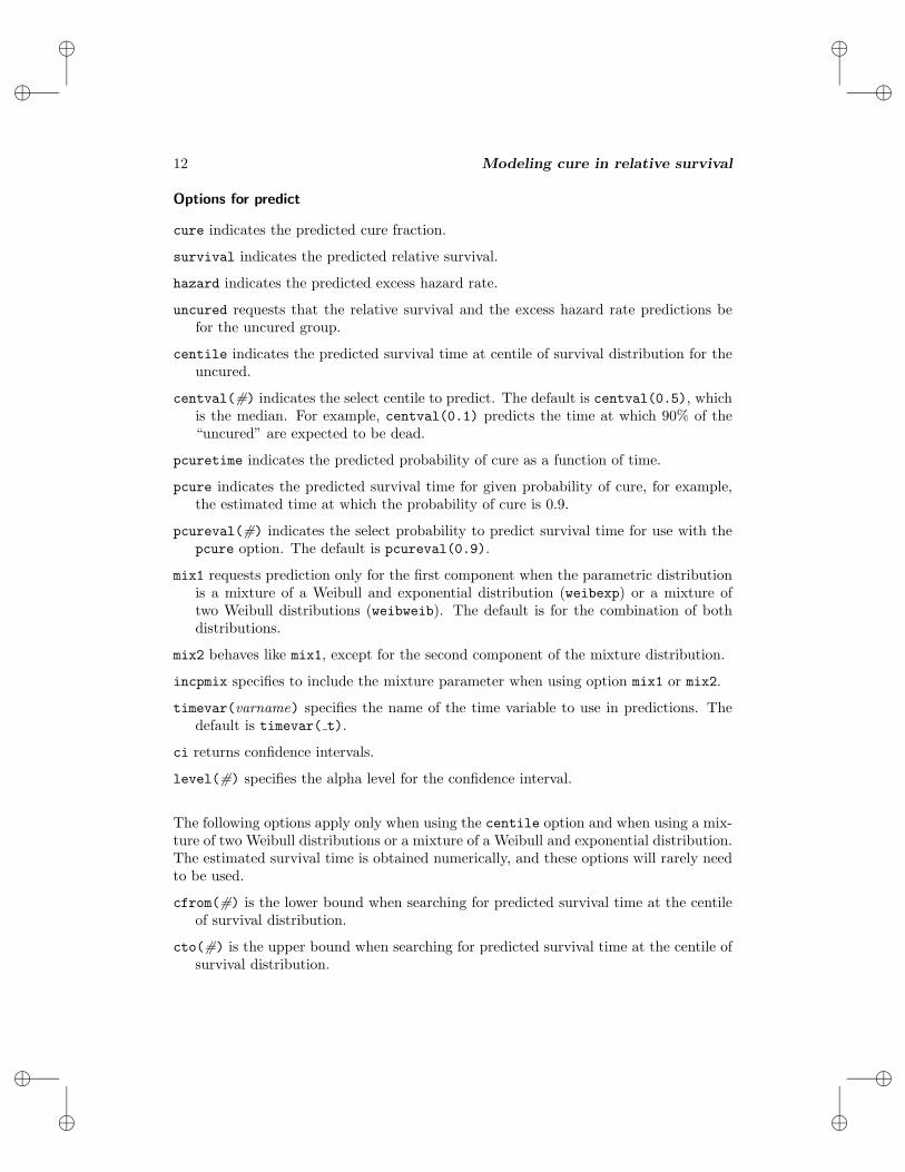
Options for predict

cure indicates the predicted cure fraction.

survival indicates the predicted relative survival.

hazard indicates the predicted excess hazard rate.

uncured requests that the relative survival and the excess hazard rate predictions befor the uncured group.

centile indicates the predicted survival time at centile of survival distribution for theuncured.

centval(#) indicates the select centile to predict. The default is centval(0.5), whichis the median. For example, centval(0.1) predicts the time at which 90% of the“uncured” are expected to be dead.

pcuretime indicates the predicted probability of cure as a function of time.

pcure indicates the predicted survival time for given probability of cure, for example,the estimated time at which the probability of cure is 0.9.

pcureval(#) indicates the select probability to predict survival time for use with thepcure option. The default is pcureval(0.9).

mix1 requests prediction only for the first component when the parametric distributionis a mixture of a Weibull and exponential distribution (weibexp) or a mixture oftwo Weibull distributions (weibweib). The default is for the combination of bothdistributions.

mix2 behaves like mix1, except for the second component of the mixture distribution.

incpmix specifies to include the mixture parameter when using option mix1 or mix2.

timevar(varname) specifies the name of the time variable to use in predictions. Thedefault is timevar( t).

ci returns confidence intervals.

level(#) specifies the alpha level for the confidence interval.

The following options apply only when using the centile option and when using a mix-ture of two Weibull distributions or a mixture of a Weibull and exponential distribution.The estimated survival time is obtained numerically, and these options will rarely needto be used.

cfrom(#) is the lower bound when searching for predicted survival time at the centileof survival distribution.

cto(#) is the upper bound when searching for predicted survival time at the centile ofsurvival distribution.

i

i

i

i

i

i

i

i

P. C. Lambert 13

ctol(#) is the absolute tolerance when searching for predicted survival time at thecentile of survival distribution.

citer(#) is the number of iterations when searching for predicted survival time at thecentile of survival distribution.

4 Examples

To illustrate the strsmix and strsnmix commands, I use the data for 33,874 femalesaged 50 and over diagnosed with ovarian cancer. The data were obtained from thepublic-use dataset of all England and Wales cancer registrations between January 1,1981, and December 31, 1990, with follow-up until December 31, 1995 (Coleman, Babb,Damiecki, et al. 1999; Coleman, Babb, Mayer, et al. 1999). Background mortalityrates were obtained from England and Wales national mortality statistics by age, ge-ographical region, period of diagnosis, and deprivation group (Coleman, Babb, Mayer,et al. 1999). Although the background mortality rates also contain mortality asso-ciated with the disease, in practice this has little effect on the parameter estimates(Ederer, Axtell, and Cutler 1961). Given the length of follow-up (maximum 15 years),one would expect to observe the cure fraction within this time scale. The covariatesinvestigated are deprivation, defined in terms of the area-based Carstairs score and ageat diagnosis. There are five deprivation categories ranging from the least deprived (af-fluent) to the most deprived quintile in the population. Age is split into four groups,50–59, 60–69, 70–79, and 80+.

4.1 Estimation in one sample

Estimating the cure fraction in one sample may be of interest. Below are the commandsand output from fitting the mixture cure fraction model with strsmix to the 50–59 agegroup by using a Weibull distribution for the survival of the uncured and an identitylink function.

. use Ovary_Cancer, clear

. stset survtime, failure(dead==1) id(ident) exit(time 15)

id: identfailure event: dead == 1

obs. time interval: (survtime[_n-1], survtime]exit on or before: time 15

33874 total obs.0 exclusions

33874 obs. remaining, representing33874 subjects28685 failures in single failure-per-subject data

88539.89 total analysis time at risk, at risk from t = 0earliest observed entry t = 0

last observed exit t = 14.992

i

i

i

i

i

i

i

i


. strsmix if cage == 1, dist(weibull) link(identity) bhazard(rate)

initial: log likelihood = -33701.229alternative: log likelihood = -19189.062rescale: log likelihood = -17405.714rescale eq: log likelihood = -15006.234

(output omitted )Iteration 3: log likelihood = -14992.964

Number of obs = 8905Wald chi2(0) = .

Log likelihood = -14992.964 Prob > chi2 = .

_t Coef. Std. Err. z P>|z| [95% Conf. Interval]

pi_cons .2674759 .0053773 49.74 0.000 .2569365 .2780152

ln_lambda_cons -.4326249 .016389 -26.40 0.000 -.4647467 -.400503

ln_gamma_cons -.147681 .0119269 -12.38 0.000 -.1710573 -.1243047

The data are stset in the usual way, with the variable survtime denoting survivaltime in years and dead denoting the censoring indicator. The exit option is used torestrict follow-up time to 15 years. The rate variable is the expected hazard rate atthe death or censoring time, obtained from Coleman, Babb, Mayer, et al. (1999), andhas previously been merged into the dataset.

The model converged after three iterations. The cure fraction is estimated at 0.267for this age group, with a narrow confidence interval due to the large sample size.Using the predict command after strsmix or strsnmix provides predictions of thecure fraction, the excess hazard function, and relative survival function for the sampleas a whole or for the uncured group, the probability of cure as a function of time, thesurvival time for a given centile of the survival function for the uncured group, and thesurvival time for a given probability of cure. The predictions are conditional on anycovariates and evaluated at each observed survival time ( t), but this can be changedusing the timevar option. For example,

. predict exhaz_all, hazard

. predict rs_all, survival

. predict exhaz_uncured, hazard uncured

. predict rs_uncured, survival uncured

One can obtain confidence intervals for the various predictions. The standard er-rors of the predictions are obtained using the delta method and implemented usingpredictnl. The standard errors for relative survival are obtained on the log(-log) scale(i.e., log cumulative excess hazard scale), the standard error for excess hazard is ob-tained on the log excess hazard scale, and the standard errors for the cure fraction areobtained on the scale selected from the link() option, except for split-time models,where the standard error is obtained on the cure fraction scale.

i

i

i

i

i

i

i

i

P. C. Lambert 15

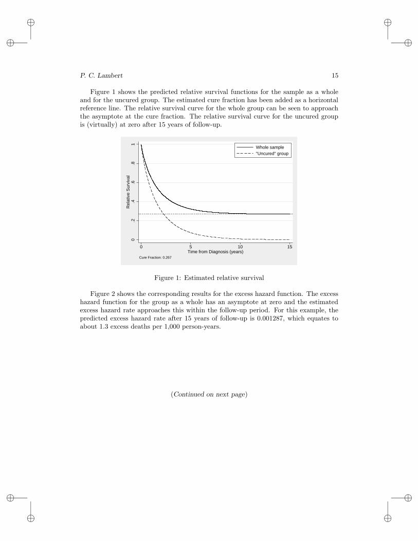
Figure 1 shows the predicted relative survival functions for the sample as a wholeand for the uncured group. The estimated cure fraction has been added as a horizontalreference line. The relative survival curve for the whole group can be seen to approachthe asymptote at the cure fraction. The relative survival curve for the uncured groupis (virtually) at zero after 15 years of follow-up.

0.2

.4.6

.81

Rel

ativ

e S

urvi

val

0 5 10 15Time from Diagnosis (years)

Whole sample"Uncured" group

Cure Fraction: 0.267

Figure 1: Estimated relative survival

Figure 2 shows the corresponding results for the excess hazard function. The excesshazard function for the group as a whole has an asymptote at zero and the estimatedexcess hazard rate approaches this within the follow-up period. For this example, thepredicted excess hazard rate after 15 years of follow-up is 0.001287, which equates toabout 1.3 excess deaths per 1,000 person-years.

(Continued on next page)

i

i

i

i

i

i

i

i


0.5

11.

5E

xces

s H

azar

d R

ate


Whole sample"Uncured" group

Figure 2: Estimated excess hazard functions

4.2 Modeling the cure fraction

Fitting models for the cure fraction is of interest. In this section, we will fit nonmixturecure fraction models with strsnmix. The covariates to be included are age group anddeprivation group. Initially, we will assume proportional excess hazards for the groupas a whole. Calculating proportional excess hazards for the group as a whole is notpossible using the mixture cure fraction model. A proportional excess hazards modelcan be fitted using

. strsnmix cage2-cage4 dep2-dep5, dist(weibull) link(loglog) bhazard(rate) eform

(output omitted )Iteration 4: log likelihood = -43631.03

Number of obs = 33874Wald chi2(7) = 2335.74

Log likelihood = -43631.03 Prob > chi2 = 0.0000

_t exp(b) Std. Err. z P>|z| [95% Conf. Interval]

picage2 1.302542 .0219722 15.67 0.000 1.260182 1.346327cage3 1.80924 .0317526 33.78 0.000 1.748064 1.872557cage4 2.553791 .0558784 42.85 0.000 2.446586 2.665693dep2 1.033701 .0200523 1.71 0.088 .9951367 1.073759dep3 1.074588 .0208841 3.70 0.000 1.034426 1.116309dep4 1.091107 .0216229 4.40 0.000 1.04954 1.134321dep5 1.139311 .0244794 6.07 0.000 1.092329 1.188315

ln_lambda_cons -.6297643 .013746 -45.81 0.000 -.656706 -.6028226

ln_gamma_cons -.2542385 .0059823 -42.50 0.000 -.2659635 -.2425134

i

i

i

i

i

i

i

i

P. C. Lambert 17

The model converges after four iterations. The use of the log{− log(π)} link functionmeans that the parameter estimates are log excess hazard ratios. The eform option hasbeen used to obtain exponentiated parameter estimates, i.e., the excess hazard ratios.There is a clear association with age group, with older age groups having a higherexcess hazard rate. Because this is a relative survival model, this survival model istaking account of the fact that there is also an increase in the background mortalityrate with increasing age. There is also an association of the deprivation group, withmore deprived groups having a higher excess hazard rate; the most deprived group hasa 14% higher excess mortality rate than that of the most affluent group.

When quantifying any differences in the cure fraction is of direct interest, modelingusing the identity or logistic link functions may be preferable. Below is the output fromusing the identity link function.

. strsnmix cage2-cage4 dep2-dep5, dist(weibull) link(identity) bhazard(rate)

(output omitted )




picage2 -.0908007 .005786 -15.69 0.000 -.1021411 -.0794603cage3 -.1830008 .0054337 -33.68 0.000 -.1936507 -.1723508cage4 -.2459081 .0053425 -46.03 0.000 -.2563792 -.235437dep2 -.0086246 .0050806 -1.70 0.090 -.0185825 .0013332dep3 -.0182842 .0049411 -3.70 0.000 -.0279686 -.0085999dep4 -.0192701 .0049738 -3.87 0.000 -.0290185 -.0095216dep5 -.0308327 .0050601 -6.09 0.000 -.0407503 -.0209152_cons .3033963 .0061608 49.25 0.000 .2913213 .3154714

ln_lambda_cons -.6288331 .0137149 -45.85 0.000 -.6557139 -.6019524

ln_gamma_cons -.2541574 .0059797 -42.50 0.000 -.2658774 -.2424374

The constant term is 0.303 and is the estimated cure fraction for patients aged 50–59 years at diagnosis in the least deprived group. Covariate effects are now expressedin differences in the cure fraction; for example, in patients of the same age, the curefraction in the most deprived group (dep5) is 0.031 lower than that in the least deprivedgroup. This is still a proportional excess hazards model since the Weibull distributionparameters do not vary by covariates. However, now covariate effects for the curefraction are assumed to be additive on the cure fraction scale, whereas in the previousmodel they were assumed to be multiplicative on the excess hazard scale. In population-based cancer studies, proportional excess hazards are rare and models that allow fornonproportionality are often required. The following output shows the effect of allowingboth the Weibull parameters to vary by age and deprivation group.

i

i

i

i

i

i

i

i


. strsnmix cage2-cage4 dep2-dep5, dist(weibull) link(identity) bhazard(rate)> k1(cage2-cage4 dep2-dep5) k2(cage2-cage4 dep2-dep5)

(output omitted )




picage2 -.0607861 .0074988 -8.11 0.000 -.0754835 -.0460887cage3 -.1072302 .0077687 -13.80 0.000 -.1224565 -.0920038cage4 -.1052487 .0100726 -10.45 0.000 -.1249907 -.0855067dep2 -.0105491 .0084903 -1.24 0.214 -.0271898 .0060917dep3 -.0102564 .0084892 -1.21 0.227 -.026895 .0063822dep4 -.0046395 .0086344 -0.54 0.591 -.0215625 .0122836dep5 -.0183708 .0094453 -1.94 0.052 -.0368833 .0001417_cons .2674146 .0076815 34.81 0.000 .2523591 .2824701

ln_lambdacage2 .2770222 .0304632 9.09 0.000 .2173154 .3367291cage3 .6212965 .035035 17.73 0.000 .5526292 .6899638cage4 1.203913 .0534578 22.52 0.000 1.099138 1.308689dep2 .0070544 .0378794 0.19 0.852 -.0671879 .0812967dep3 .0868296 .0381024 2.28 0.023 .0121503 .1615089dep4 .1614986 .0385736 4.19 0.000 .0858958 .2371014dep5 .149896 .0434601 3.45 0.001 .0647157 .2350763_cons -1.006311 .0312836 -32.17 0.000 -1.067626 -.9449965

ln_gammacage2 -.1044376 .0158949 -6.57 0.000 -.135591 -.0732842cage3 -.2046917 .0163687 -12.51 0.000 -.2367738 -.1726096cage4 -.2227369 .0204895 -10.87 0.000 -.2628956 -.1825781dep2 -.021792 .017239 -1.26 0.206 -.0555797 .0119958dep3 -.0369464 .0173383 -2.13 0.033 -.0709288 -.002964dep4 -.0525448 .0176128 -2.98 0.003 -.0870653 -.0180243dep5 -.0976965 .0192059 -5.09 0.000 -.1353394 -.0600535_cons -.0255061 .0160773 -1.59 0.113 -.057017 .0060048

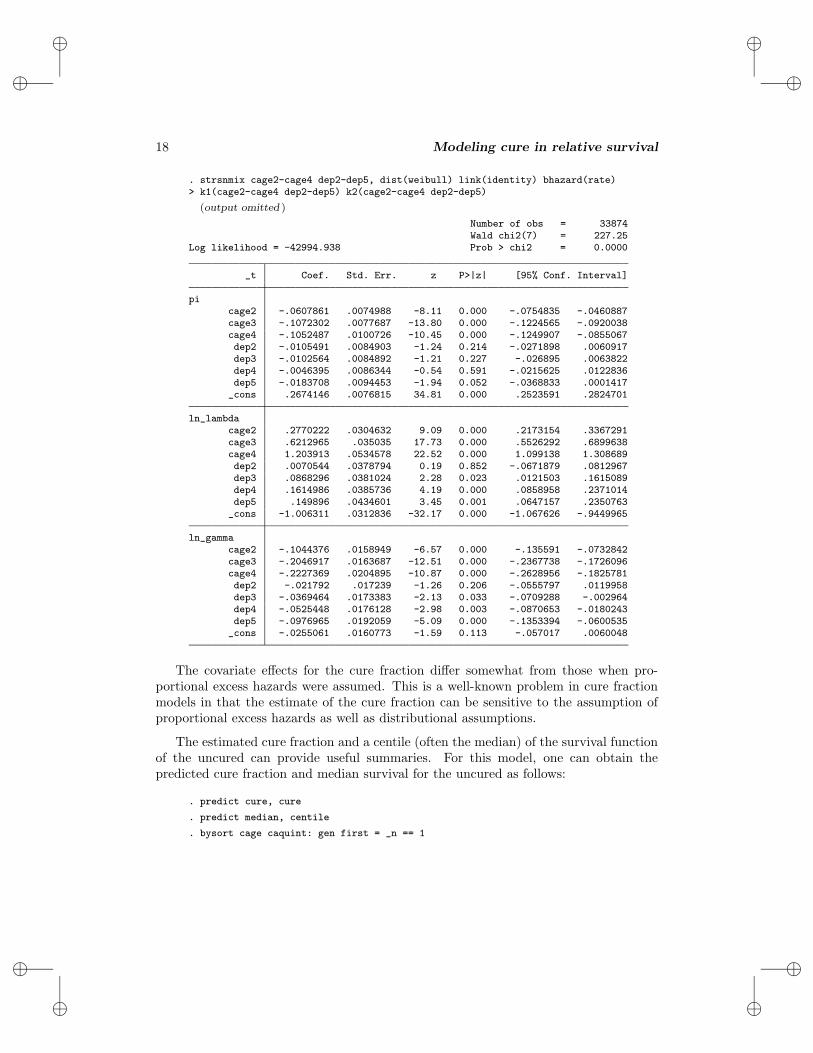
The covariate effects for the cure fraction differ somewhat from those when pro-portional excess hazards were assumed. This is a well-known problem in cure fractionmodels in that the estimate of the cure fraction can be sensitive to the assumption ofproportional excess hazards as well as distributional assumptions.

The estimated cure fraction and a centile (often the median) of the survival functionof the uncured can provide useful summaries. For this model, one can obtain thepredicted cure fraction and median survival for the uncured as follows:

. predict cure, cure

. predict median, centile

. bysort cage caquint: gen first = _n == 1

i

i

i

i

i

i

i

i

P. C. Lambert 19

. tabdisp cage caquint if first, c(cure median) f(%5.3fc)

GB quintile Carstairs scoreAge Group leastdep 2 3 4 mostdep

50-59 0.267 0.257 0.257 0.263 0.2491.166 1.143 1.053 0.980 0.970

60-69 0.207 0.196 0.196 0.202 0.1880.777 0.750 0.680 0.625 0.601

70-79 0.160 0.150 0.150 0.156 0.1420.438 0.413 0.367 0.333 0.308

80+ 0.162 0.152 0.152 0.158 0.1440.205 0.191 0.167 0.150 0.133

The top number in each cell shows the estimated cure fraction, with the bottomcell showing the estimated median survival for the uncured. Both the cure fractionand median survival for the uncured decrease with increasing age and with increasingdeprivation. Confidence intervals for these estimates can be obtained using the ci

option.

4.3 Split-time models

When either the mixture or nonmixture cure fraction model provides poor estimates ofthe cure fraction, a more flexible approach may be required. Using the split() optionin the strsnmix command fits the split-time models described in section 2.4. Forillustration, I will use the oldest age group, 80+, for the ovary cancer example with nomodeling of covariates. The standard mixture models sometimes fits poorly to the oldestage group because this group has a high excess hazard in the first few weeks/monthsafter diagnosis. The distribution for the early period before time k is selected using theearlydist() option, where arguments are weibull and exponential.

Generally, including the same covariates for the initial high hazard rate as for theconditional cure fraction model seems sensible. However, one can model the differentparameters separately. In fact, often the nonproportionality of the excess hazards isdue to larger differences early on in the time scale, and assuming proportional excesshazards after some time point may sometimes be sensible.

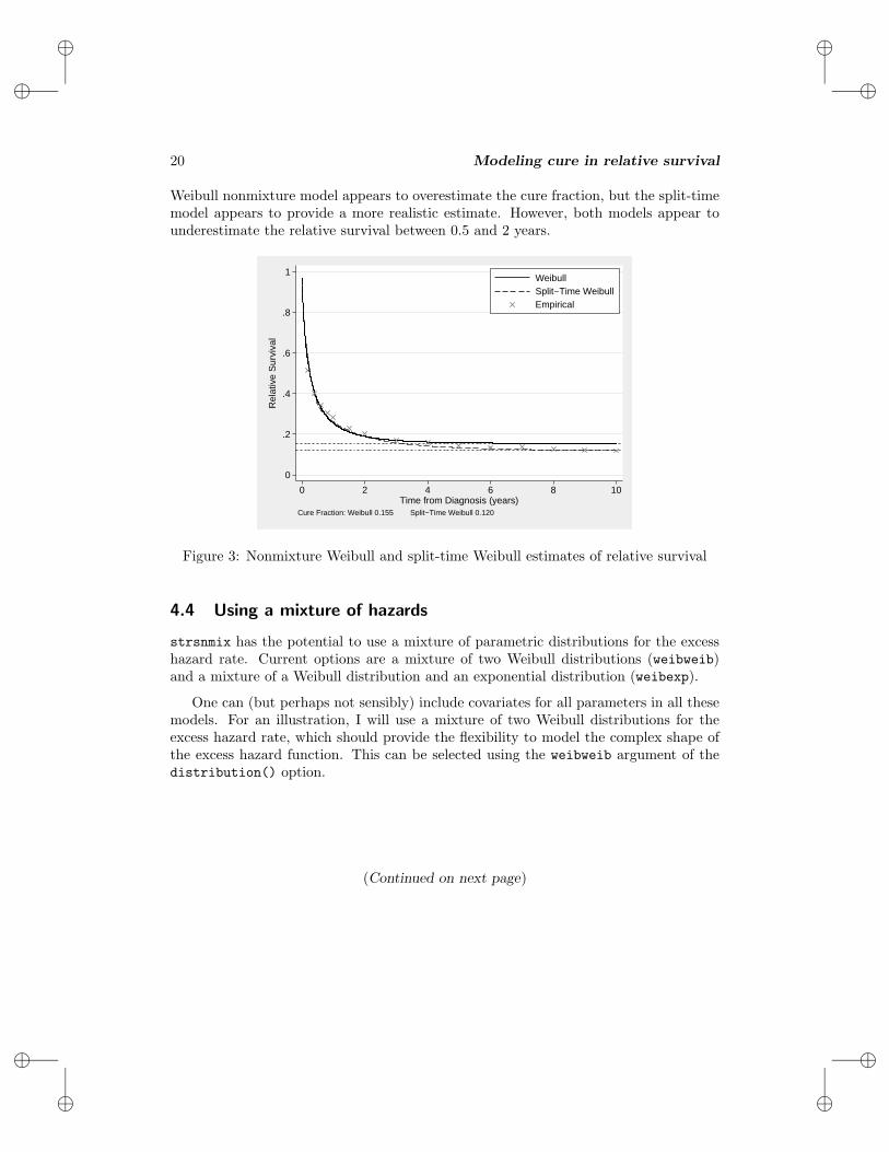
Figure 3 shows the estimated relative survival curves for a nonmixture cure fractionmodel with a Weibull distribution and a split-time model with a Weibull distribu-tion for the survival before 0.5 years combined with a nonmixture cure fraction modelconditional on surviving to 0.5 years. Also shown on the plot are the empirical esti-mates (using the Hakulinen method) of relative survival obtained using the life-tablemethod implemented in strs (http://www.pauldickman.com/rsmodel/stata colon). Inthis simple one-sample problem, one would expect the cure fraction estimate to be closeto where the empirical estimate appeared to reach a plateau. The figure shows that the

i

i

i

i

i

i

i

i


Weibull nonmixture model appears to overestimate the cure fraction, but the split-timemodel appears to provide a more realistic estimate. However, both models appear tounderestimate the relative survival between 0.5 and 2 years.

0

.2

.4

.6

.8

1R

elat

ive

Sur

viva

l

0 2 4 6 8 10Time from Diagnosis (years)

WeibullSplit−Time WeibullEmpirical

Cure Fraction: Weibull 0.155 Split−Time Weibull 0.120

Figure 3: Nonmixture Weibull and split-time Weibull estimates of relative survival

4.4 Using a mixture of hazards

strsnmix has the potential to use a mixture of parametric distributions for the excesshazard rate. Current options are a mixture of two Weibull distributions (weibweib)and a mixture of a Weibull distribution and an exponential distribution (weibexp).

One can (but perhaps not sensibly) include covariates for all parameters in all thesemodels. For an illustration, I will use a mixture of two Weibull distributions for theexcess hazard rate, which should provide the flexibility to model the complex shape ofthe excess hazard function. This can be selected using the weibweib argument of thedistribution() option.


i

i

i

i

i

i

i

i

P. C. Lambert 21

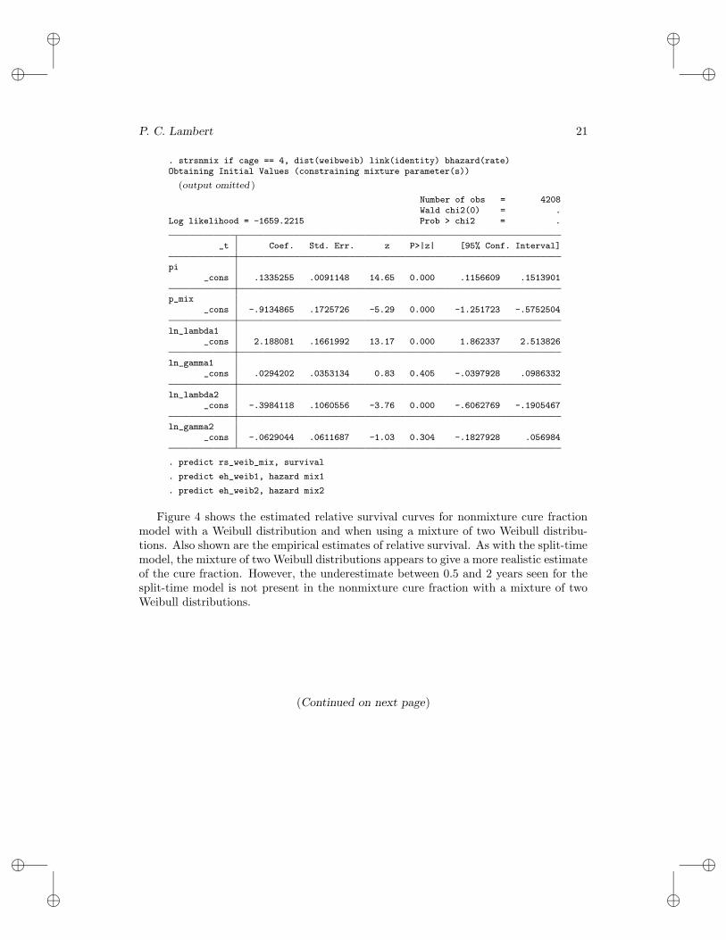
. strsnmix if cage == 4, dist(weibweib) link(identity) bhazard(rate)Obtaining Initial Values (constraining mixture parameter(s))

(output omitted )




pi_cons .1335255 .0091148 14.65 0.000 .1156609 .1513901

p_mix_cons -.9134865 .1725726 -5.29 0.000 -1.251723 -.5752504

ln_lambda1_cons 2.188081 .1661992 13.17 0.000 1.862337 2.513826

ln_gamma1_cons .0294202 .0353134 0.83 0.405 -.0397928 .0986332

ln_lambda2_cons -.3984118 .1060556 -3.76 0.000 -.6062769 -.1905467

ln_gamma2_cons -.0629044 .0611687 -1.03 0.304 -.1827928 .056984

. predict rs_weib_mix, survival

. predict eh_weib1, hazard mix1

. predict eh_weib2, hazard mix2

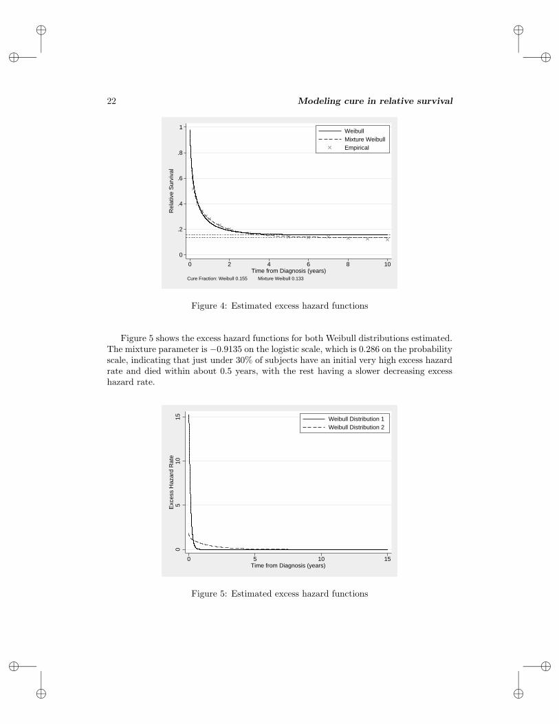
Figure 4 shows the estimated relative survival curves for nonmixture cure fractionmodel with a Weibull distribution and when using a mixture of two Weibull distribu-tions. Also shown are the empirical estimates of relative survival. As with the split-timemodel, the mixture of two Weibull distributions appears to give a more realistic estimateof the cure fraction. However, the underestimate between 0.5 and 2 years seen for thesplit-time model is not present in the nonmixture cure fraction with a mixture of twoWeibull distributions.


i

i

i

i

i

i

i

i


0

.2

.4

.6

.8

1

Rel

ativ

e S

urvi

val

0 2 4 6 8 10Time from Diagnosis (years)

WeibullMixture WeibullEmpirical

Cure Fraction: Weibull 0.155 Mixture Weibull 0.133


Figure 5 shows the excess hazard functions for both Weibull distributions estimated.The mixture parameter is −0.9135 on the logistic scale, which is 0.286 on the probabilityscale, indicating that just under 30% of subjects have an initial very high excess hazardrate and died within about 0.5 years, with the rest having a slower decreasing excesshazard rate.

05

1015

Exc

ess

Haz

ard

Rat

e


Weibull Distribution 1Weibull Distribution 2


i

i

i

i

i

i

i

i

P. C. Lambert 23

4.5 Period analysis

Period analysis models can simply be fitted using delayed-entry techniques. The dataneed to be stset; doing so is easiest when the dates of diagnosis and the date of the eventor censoring are available. For the one-sample example using the 50–59 age group fromsection 4.1, I will use only survival experience after January 1, 1990. This informationcan be incorporated using stset and then the strsmix and strsnmix commands areused the same way as in the previous analyses. For example,

. stset dateexit, failure(dead==1) enter(time mdy(1,1,1990)) origin(datediag)> id(ident) scale(365.25)

id: identfailure event: dead == 1

obs. time interval: (dateexit[_n-1], dateexit]enter on or after: time mdy(1,1,1990)exit on or before: failure

t for analysis: (time-origin)/365.25origin: time datediag

33874 total obs.21560 obs. end on or before enter()

12314 obs. remaining, representing12314 subjects7140 failures in single failure-per-subject data

41693.25 total analysis time at risk, at risk from t = 0earliest observed entry t = 0

last observed exit t = 14.99247

. strsmix if cage == 1, dist(weibull) link(identity) bhazard(rate)note: delayed entry models are being fitted

(output omitted )




pi_cons .2788979 .0094126 29.63 0.000 .2604496 .2973461

ln_lambda_cons -.4975554 .0405256 -12.28 0.000 -.576984 -.4181267

ln_gamma_cons -.1552354 .0282638 -5.49 0.000 -.2106315 -.0998393

The period estimate of the cure fraction is slightly higher using period analysis at0.279 (compared with 0.267 in the previous analysis). The more up-to-date estimateindicates that there was a slight improvement in the proportion of patients cured. Thenthe difference is small and the confidence intervals for the two estimates overlap. Ifadvances in patient care had been more dramatic, then one would have expected tosee a greater difference between the standard and period estimates. However, includingperiod analysis when modeling survival data to obtain up-to-date parameter estimates

i

i

i

i

i

i

i

i


is simple. Period analysis clearly has several assumptions; for a discussion of theseassumptions, see Brenner and Gefeller (1997).

5 Conclusion

The cure fraction is an important measure in providing information to patients andmonitoring trends and differences in survival over time. The commands strsmix andstrsnmix allow one to estimate the cure fraction in population-based cancer studiesbut also allow one to fit standard cure models. Although fitting these models to datawhere cure has not been reached is possible, doing so is generally not recommended. Theestimated cure fraction will be based on extrapolating the relative survival curve beyondthe time of follow-up with the data and thus is sensitive to distributional assumptions.

6 Acknowledgments

I thank Paul Dickman, John Thompson, and Claire Weston for their helpful commentsand suggestions when developing these commands. I also thank an anonymous reviewerof the manuscript for helpful comments.

Part of this work was carried out while on study leave from the University of Le-icester visiting the Department of Medical Epidemiology and Biostatistics, KarolinskaInstitutet, Stockholm, Sweden, a visit partly funded by the Swedish Cancer Society(Cancerfonden).

7 References

Begg, C. B., and D. Schrag. 2002. Attribution of deaths following cancer treatment.Journal of the National Cancer Institute 94: 1044–1045.

Brenner, H., and O. Gefeller. 1997. Deriving more up-to-date estimates of long-termpatient survival. Journal of Clinical Epidemiology 50: 211–216.

Coleman, M., P. Babb, P. Damiecki, P. Grosclaude, S. Honjo, J. Jones, G. Knerer,A. Pitard, M. J. Quinn, A. Sloggett, and B. De Stavola. 1999. Cancer survival trendsin England and Wales, 1971–1995, deprivation and NHS Region. Office for NationalStatistics, London, UK.

Coleman, M., P. Babb, D. Mayer, M. J. Quinn, and A. Sloggett. 1999. Cancer survivaltrends in England and Wales, 1971–1995, deprivation and NHS Region (CD-ROM).Office for National Statistics, London, UK.

De Angelis, R., R. Capocaccia, T. Hakulinen, B. Soderman, and A. Verdecchia. 1997.Mixture models for cancer survival analysis: Application to population-based datawith covariates. Statistics in Medicine 18: 441–454.

i

i

i

i

i

i

i

i

P. C. Lambert 25

Dickman, P., A. Sloggett, M. Hills, and T. Hakulinen. 2004. Regression models forrelative survival. Statistics in Medicine 23: 51–64.

Ederer, F., L. M. Axtell, and S. J. Cutler. 1961. The relative survival rate: A statisticalmethodology. National Cancer Institute Monograph 6: 101–121.

Giorgi, R., M. Abrahamowicz, C. Quantin, P. Bolard, J. Esteve, J. Gouvernet, andJ. Faivre. 2003. A relative survival regression model using B-spline functions tomodel non-proportional hazards. Statistics in Medicine 22: 2767–2784.

Ibrahim, J. G., M. H. Chen, and D. Sinha. 2001. Bayesian Survival Analysis. New York:Springer.

Lambert, P., L. K. Smith, D. R. Jones, and J. Botha. 2005. Additive and multiplicativecovariate regression models for relative survival incorporating fractional polynomialsfor time-dependent effects. Statistics in Medicine 24: 3871–3885.

Lambert, P. C., J. R. Thompson, C. L. Weston, and P. W. Dickman. 2007. Estimatingand modeling the cure fraction in population-based cancer survival analysis. Bio-

statistics 8: 576–594.

Maller, R. A., and X. Zhou. 2001. Survival Analysis with Long-term Survivors. NewYork: Wiley.

McLachlan, G. J., and D. C. McGiffin. 1994. On the role of finite mixture models insurvival analysis. Statistical Methods in Medical Research 3: 211–226.

Schmidt, P., and D. Witte. 1989. Predicting criminal recidivism using split populationsurvival time models. Journal of Econometrics 40: 141–159.

Sposto, R. 2002. Cure model analysis in cancer: An application to data from theChildren’s Cancer Group. Statistics in Medicine 21: 293–312.

Tsodikov, A., J. G. Ibrahim, and A. Takovlev. 2003. Estimating cure rates from survivaldata: An alternative to two-component mixture models. Journal of the American

Statistical Association 98: 1063–1078.

Verdecchia, A., R. De Angelis, R. Capocaccia, M. Sant, A. Micheli, G. Gatta, andF. Berrino. 1998. The cure for colon cancer: Results from the EUROCARE study.International Journal of Cancer 77: 322–329.

About the author

Paul Lambert is a senior lecturer in medical statistics at the University of Leicester, Leicester,UK.

Modeling of the cure fraction in survival studies · i i i i i i i i The Stata Journal (2007) 7, Number 3, pp. 1{25 Modeling of the cure fraction in survival studies Paul C. Lambert

Documents