Cure Fraction, Modelling and Estimating in a Population ...einspem.upm.edu.my/journal/fullpaper/vol2no1/8. MJMS Vol 2 (1) page 113... · Cure Fraction, Modelling and Estimating in

Malaysian Journal of Mathematical Sciences 2 (1): 113-134 (2008)

Cure Fraction, Modelling and Estimating

in a Population-Based Cancer Survival Analysis

1Mohd Rizam Abu Bakar,

2Khalid A. Salah,

1Noor Akma Ibrahim

and 1Kassim Haron

1Department of Mathematics, Universiti Putra Malaysia and

Institute for Mathematical Research, Universiti Putra Malaysia 2Department of Mathematics, Al-Quds University, Jerusalem, Palestine

E-mail: [email protected]

ABSTRACT

In population-based cancer studies, cure is said to occur when the mortality (hazard) rate in the diseased group of individuals returns to the same level as that expected in the general population. The optimal method for monitoring the progress of patient care across the full spectrum of provider settings is through the population-based study of cancer patient survival, which is only possible using data collected by population-based cancer registries. The probability of cure, statistical cure, is defined for a cohort of cancer patients as the percent of patients whose annual death rate

equals the death rate of general cancer-free population. Recently models have been introduced, so called cure fraction models, that estimates the cure fraction as well as the survival time distribution for those uncured. The colorectal cancer survival data from the Surveillance, Epidemiology and End Results (SEER) program, USA, is used. The aim is to evaluate the cure fraction models and compare these methods to other methods used to monitor time trends in cancer patient survival, and to highlight some problems using these models. Keywords: Relative survival, Survival mixture cure rate model, Cure fraction, SEER

Stat, CANSURV.

INTRODUCTION

An important way of analyzing the improvements in cancer treatment

is to look at time trends in cancer patient survival. When analyzing time trends in cancer patient survival the focus lies on estimating the change in

net survival. The net survival at a certain point in time is the proportion of

patients who would have survived up to that point if the cancer of interest

was the only possible cause of death. There are two ways to estimate the net survival, using cause-specific survival or relative survival. In cause-specific

survival the time from diagnosis until death from the cancer of interest is

studied and all individuals that die from something else are censored. In relative survival all deaths are considered events and the whole mortality in

the cancer group is compared to the mortality in the general population to

find the excess mortality due to the cancer of interest. Relative survival is

Mohd Rizam Abu Bakar et al.

114 Malaysian Journal of Mathematical Sciences

the method mostly used when analyzing cancer patient survival, and the

most common estimate for the net survival is the 5-year relative survival ratio (RSR). Cure models have been introduced that estimate the cure

fraction and the survival for the uncured. Many countries today have

population-based cancer registries. In Malaysia, as well as the other modern countries, it is been notify the registry of all new cancer cases by the

National Cancer Registry (NCR) which supported by the Ministry of Health

(MOH). The Malaysian cancer registry contains data on virtually all most

cancers diagnosed. The registry holds data about the patient as age at diagnosis, sex and birth date as well as information about the tumor,

anatomical location, histology, stage and basis of registration. The

underlying cause of death is recorded for all cases, using death certificate information from Malaysian National Registry Department (MNRD).

Several approaches to modelling relative survival exist, section 2 briefly

describes the most commonly used regression approaches and gives an

outline of the theory for the fitting methods used. The two most common cure models, the Mixture model and the Non-mixture model are presented in

section 3. An application on female breast cancer presented in section 4

followed by results and conclusion in section 5.

RELATIVE SURVIVAL

Relative survival is becoming the method of choice for estimating cancer patient survival using population-based cancer registries although its

utility is not restricted to studying cancer (Dickman and Adami 2006).

Estimating cause-specific mortality (and its analogue cause-specific survival) using cancer registry data is problematic because information on

cause-of-death is often unreliable or unavailable (Gamel and Vogel 2001).

We instead estimate the net mortality associated with a diagnosis of cancer in terms of excess mortality, the difference between the total mortality

experienced by the patients and the expected mortality of a comparable

group from the general population. Relative survival is the observed

survival among the cancer patients (when all deaths are considered as events) divided by the expected survival in a comparable group of the

general population. The expected survival is usually estimated from

nationwide population life tables stratified by age, sex, calendar time and where, applicable, race. Even though these tables include the mortality from

the cancer of interest, it has been shown that this doesn't effect the

estimations in practice.

Cure Fraction, Modelling and Estimating in a Population-Based Cancer Survival Analysis


Estimating expected survival

Expected survival can be thought of as being calculated for a cohort of patients from the general population matched by age, sex and calendar

period. There are three different methods for estimating the expected

survival, with the differences between them being how long each individual is considered to be 'at risk' for the purpose of estimating expected survival.

In practice there are small differences between the methods, and in most

cases they give similar results. The three methods are Ederer I, Ederer II

(Ederer et al. 1961), and the Hakulinen (Hakulinen 1982).

Ederer I: The matched individuals are considered to be at risk indefinitely

(even beyond the closing date of the study). The time at which a cancer patient dies or is censored has no effect on the expected survival. Under this

method, the cumulative expected survival proportion from the date of

diagnosis to the end of the ith interval is given by

1

1

1

1( )

n

hi iH H h

n

∗ ∗== ∑

where 1

n is the total number of patients alive at the start of follow-up and

( )i

H h∗ is the expected probability of surviving to the end of the ith interval

for a person in the general population and, given by

1( ) ( )i

ji jH h H h

∗== ∏

where ( )j

H h is the expected survival probability for the hth patient in the

jth interval. That is, the expected 5-year survival proportion is estimated as

the average of the expected 5-year survival probabilities for every individual

in the life table.

Ederer II: The matched individuals are considered to be at risk until the

corresponding cancer patient dies or is censored, which allows for heterogeneous observed follow-up times. It estimates interval-specific

expected survival proportions for each interval, based on those patients alive

at the start of the interval. The cumulative expected survival is then estimated as the product of the interval-specific survival proportions. The

cumulative expected survival is given by

1 ,i

ji jH G

∗ ∗== ∏



where 11 ( )i

i

n

hj jnG G h

∗== ∑ is the average of the annual expected survival

probabilities ( )j

G h of the patients alive at the start of the jth interval.

Note, both Ederer I and Ederer II give a biased estimate of the relative

survival ratio.

Hakulinen: If the survival time of a cancer patient is censored then so is the

survival time of the matched individual. However, if a cancer patient dies

the matched individual is assumed to be `at risk' until the closing date of the

study. This method was proposed to get an unbiased estimate of the relative survival ratio, Hakulinen (1982). It creates a biased estimate of the expected

relative survival, but the bias is similar to the bias of the observed survival

proportion and therefore the biases cancel each other out and results in an unbiased estimate. If the survival time of a cancer patient is censored so is

the survival time of the matched individual, but if a cancer patient dies the

matched individual remains 'at risk' until the end of the study. The following steps were used to derive the expected survival proportion using the

Hakulinen method. Let j

k be the number of patients with a potential

follow-up time which extends beyond the beginning of the jth interval. Let

the rest ja

k of these j

k patients have a potential follow-up time which

extends past the end of the jth interval and the last jb

k be potential

withdrawals during the jth interval. It follows that 1 1,k n= 1j jak k+ = and

j ja jbk k k= + . We will use the notation

jaK to refer to the set of

jak

patients and h to index the ja

k patients in the set ja

K . The expected

number of patients alive and under observation at the beginning of the jth

interval is given by

1

1

( ) if 2

if 1.

jh K j

j

H h jn

n j

∗∈ −∗

≥∑=

=

For the jb

k patients with potential follow-up times ending during the jth

interval, it is assumed that each patient is at risk for half of the interval, so

the expected probability of dying during the interval is given by *

1i

H− .

The expected number of patients withdrawing alive during the jth interval is

therefore given by



1

*

1

*

1

( ) ( ) if 2

( ) if 1.

jb

b

h K j j

j

h K

H h H h jw

H h j

∗∈ −∗

∈

≥∑= =∑

The expected number of patients dying during the jth interval, among the

jbk patients with potential follow-up time ending during the same interval is

given by

( )( )1

*

1

*

1

( ) 1 ( ) if 2

1 ( ) if 1,

jb

b

h K j j

j

h K

H h H h j

H h j

δ

∗∈ −

∗

∈

− ≥∑

= − =∑

and the expected total number of patients dying during the jth interval is

given by

( )

( )1

*

1

*

1 1

( ) 1 ( ) if 2

1 ( ) if 1.

ja

a

h K j j j

j

h K

H h H h jd

H h j

δ

δ

∗ ∗∈ −

∗

∗∈

− + ≥∑ =

− + =∑

The expected interval-specific survival proportion is then written as

1 ,/ 2

j

j

j j

dg

n w

∗

∗

∗ ∗= −

−

and, finally, the expected survival proportion from the beginning of follow-

up (usually diagnosis) to the end of the ith interval is obtained by calculating

1 .i

ji jH g

∗ ∗== ∏

All three methods give similar estimates for follow-up times up to 10 years,

but for longer follow-up the Hakulinen method is slightly better. If the

estimates are done separately for different age groups the methods give similar results even for follow-up beyond 10 years. It doesn't matter what

method is used, but in practice Ederer II estimates are usually used.



The relative survival ratio (RSR) is defined as the observed survival divided

by the expected survival. The cumulative relative survival ratio at time t ,

ir , is calculated as the observed survival proportion at time t ,

iB , divided

by the expected survival proportion at time t , .i

H ∗ That is,

.∗

=i

ii

H

Br

It can be interpreted as the proportion of patients still alive after i years of

follow-up if the cancer of interest was the only possible cause of death. This is a useful measure for showing the cumulative probability of surviving up

to a given time. An often used measure of cancer patient survival is the 5-

year cumulative RSR. Another useful measure is the interval-specific relative survival ratio, that describes the RSR in specific intervals from

follow-up (usually annual intervals). For most cancers a plot of the

cumulative RSR will flatten out after some time from diagnosis, this is when the interval-specific RSR is equal to one. This indicates that the mortality in

the patient group is the same as the mortality in the general population and

they experience no excess mortality. This point is called the cure point and

the patients still alive are considered statistically cured as shown in Figure 1.

Figure 1: Hypothetical cumulative relative survival curve

This does not mean, however, that the patients are actually medically cured.

Statistical cure applies at a group level, when the mortality is the same as in the general population, and there might be individuals that are not medically

cured. For some cancers the patients continue to experience excess mortality

and the interval-specific RSR never becomes one (and the cumulative RSR



doesn't flatten out), this can be because of excess mortality due to the cancer

or due to other causes. The interval-specific RSR can also level out at a value greater than one. This may happen when deaths have been missing in

the follow-up process, but it might also be explained by the 'healthy patient

effect', these patients experience lower mortality than the general population because of having greater than average contact with the health system.

Modelling Excess Mortality

The relative survival model can be written as

( | ) ( | ) ( | ),S t S t R t∗= ×Z Z Z (1)

where ( | ),S t Z ( | )S t∗ Z and ( | )R t Z are observed, expected and

relative survival, t is time since diagnosis and Z is the covariate vector.

That is, the relative survival is the ratio between the observed survival in the

cancer patient group and the expected survival. The mortality associated

with relative survival is excess mortality. The hazard for a person diagnosed with cancer is modelled as

( | ) ( | ) ( | ),h t h t v t∗= +Z Z Z (2)

where ( | )h t∗ Z is the expected hazard, and ( | )v t Z is the excess hazard

due to the cancer. The extended covariate matrix including the interval

variables is called X . The interest lies in modelling the excess hazard

component, v , which is assumed to be a multiplicative function of the

covariates, written as exp( )βX . The basic relative survival model is then

written as

( ) ( ) exp( ).h h β∗= +X X X (3)

This means that the parameters representing the effect in each follow-up

interval are estimated and interpreted in the same way as all the other parameters. Model (3) assumes proportional excess hazards, but non-

proportional excess hazards can be modelled by including time by covariate

interactions in the model. To estimate the model in equation (3), the method

used is modelling excess mortality using Poisson regression. The relative survival model assumes piecewise constant hazards which implies a Poisson

process for the number of deaths in each interval. Since the Poisson



distribution belongs to the exponential family the relative survival model can

then be estimated in the framework of generalized linear models using a Poisson assumption for the observed number of deaths. Model (3) is then

written as

ln( ) ln( )j j j

d yµ β∗− = + X (4)

where j

d∗ is the expected and

jd is the observed number of deaths for

observation j and ( )j j

d Poisson µ∼ where j j j

yµ λ= , j

λ is the

average hazard for an interval ,j and j

y is the person-time at risk in the

interval. Model (4) implies a generalized linear model with outcome j

d ,

Poisson error structure, link ln( )j j

dµ ∗− and offset ln( )j

y . The

observations can be life table intervals, individual patients or subject-bands.

The advantage of the Poisson regression approach is that since it is a

generalized linear model we have regression diagnostics and can assess goodness of fit.

CURE MODELS

Recently new methods have been introduced to estimate the cure fraction. These new methods extend the earlier cure fraction models to

incorporate the ideas of relative survival. The cure fraction is of big interest

to patients and is a useful measure when looking at trends in cancer patient

survival. Cure models estimate both the cure fraction and the survival function for the uncured. The two most common cure models are the

Mixture model and the Non-mixture model.

The Mixture Cure Fraction Model

The most popular type of cure rate model is the mixture cure fraction model

(mixture model) discussed by Berkson and Gage (1952). In this model, they

assume a certain fraction θ of the population is "cured" and the remaining

(1 )θ− are not cured.

The survival function for the entire population, denoted by ( )S t for this

model is given by



),()1()( 1 tStS θθ −+= (5)

where 1( )S t denotes the survivor function for the non-cured group in the

population. Common choices for ( )S t are the exponential and Weibull

distributions. We shall refer to the model in (5) as the standard cure rate

model. Model (5) can be extended to include relative survival. In that case

the overall survival for the patient group is written as

{ },)()1()()( 1 tStStS θθ −+= ∗

where ( )S t∗ is the expected survival. Similarly the overall hazard is the

sum of the background mortality rate and the excess mortality rate

associated with the cancer of interest

,)()1(

)()1()()(

1

1

tS

tfthth

θθ

θ

−+

−+= ∗

where ( )h t∗ is the expected mortality rate and 1( )f t is the density

function associated with 1( )S t . For survival models, the log-likelihood

contribution for the ith subject with survival or censoring time i

t and

censoring indicator i

d , in terms of relative survival, can be defined as

( )lni

L =

( ) ( )11

1

(1 ) ( )ln ( ) ln ( ) ln (1 ) ( ) .

(1 ) ( )

i

i i i i

i

f td h t S t S t

S t

θθ θ

θ θ∗ ∗ −

+ + + + − + −

(6)

As noted by De Angelis et al. (1997), ( )i

S t∗ is independent from the model

parameters and can be removed. Since ( )i

h t∗ is assumed to be known the

likelihood can be simply defined for any standard distribution given the

density function 1( )f t , and the survival function, 1( )S t , for the uncured

group.



The Non-Mixture Cure Fraction Model

The second type of cure fraction model is the non-mixture cure fraction model (non-mixture model), which defines an asymptote for the cumulative

hazard, and hence for the cure fraction. The non-mixture model assumes that

after treatment a patient is left with i

N 'metastatic-competent' cancer cells.

iN is assumed to have a Poisson distribution with mean λ . That gives the

cure fraction as ( 0)P λ = . When λ is not equal to 0 , let j

C denote the

time for the jth metastatic-competent cell to produce a metastatic tumor

with distribution function ( ) 1 ( ).C C

F t S t= − The survival function can be

written as

( )( )( ) exp ln( ) ( ) ,CF t

CS t F tθ θ= = (7)

also referred to as promotion time cure model. The hazard function is

( ) ln( ) ( ),C

h t f tθ= −

where ( )C

f t is a probability density function for ( )C

F t . To enable

relative survival cure models to be fitted the overall survival can be

expressed as the product of the expected survival and disease related

(relative) survival

( )( )( ) ( ) ( )exp ln( ) ln( ) ( )CF t

CS t S t S t S tθ θ θ∗ ∗= = − (8)

and the overall hazard rate as

( ) ( ) ln( ) ( ).C

h t h t f tθ∗= − (9)

Equation (8) can be rewritten as ( )

( ) ( ) (1 )1

CF t

S t S tθ θ

θ θθ

∗ −

= + − −

which is a mixture model and thus the survival distribution of the uncured

patients can also be obtained from a non-mixture model by a simple transformation of the model parameters. The log-likelihood contribution for

the ith subject with survival or censoring time i

t and censoring indicator

id is for the non-mixture model written as



( ) ( ) ( ) ( ) ( )( )ln ln ( ) ln( ) ( ) ln ( ) ln ln ( ) .i i i i C i i i i C iL d h t f t S t S tθ θ θ∗ ∗= + + + −

As for the mixture model the likelihood can be simply defined for any given

standard parametric distribution given ( )f t and ( )S t . If the parameters

in ( )C

f t do not vary by covariates, equation (9) is a proportional hazards

model. This is an advantage of the non-mixture model over the mixture

model, as the mixture model does not have a proportional hazards model for

the whole group as a special case.

The parametric and semiparametric distributions and link function

The survival function 1( )S t for the non-cured group can takes the form of

parametric or semiparametric distributions. Among the parametric models,

lognormal (LN), loglogistic (LL), Weibull (WB), and Gompertz (GP)

distributions are widely used to model the survival time. After reparameterization (Gamel et al 2000), these survival functions can be

expressed as

1

1

ln1 , LN

ln1 exp , LL

( | , )ln

exp exp , WB

(1 exp( )exp , GP

t

t

S tt

t

µφ

σ

µ

σµ σ

µ

σ

σ µ

µ

−

− −

− +

= − −

−

where φ denotes for normal function. The parameters (θ, µ, σ) may depend on the covariates as

{ }( )

{ }

1( )

( )

( )

( ) 1 exp

( )

( ) exp ,

T

T

T

X X

X X

X X

θθ

µµ

σσ

θ β

µ β

σ β

−

= + −

=

=



where ,θβ ,µβ σβ are vectors of regression parameters, in model (5),

covariates X can appear in ( )

Xθ

, ( )

Xµ

, ( )

Xσ

simultaneously. Moreover,

when ( ) 0,Xθ = this model reduces to the standard parametric survival

models.

The survival function 1( )S t can also be a semiparametric proportional

hazards model,

( )exp

1 0( | ) ( ) ,

TX

S t X S tµβ

=

where the baseline 0( )S t is modeled by piecewise exponential distribution.

A generalization of model (5) with a power function δ can be written as

{ } ,)()1()( 1δθθ tStS −+=

where the power function ( )( )( ) exp ,

Tx X

δδδ β= used in the estimation of

completeness index of cancer prevalence.

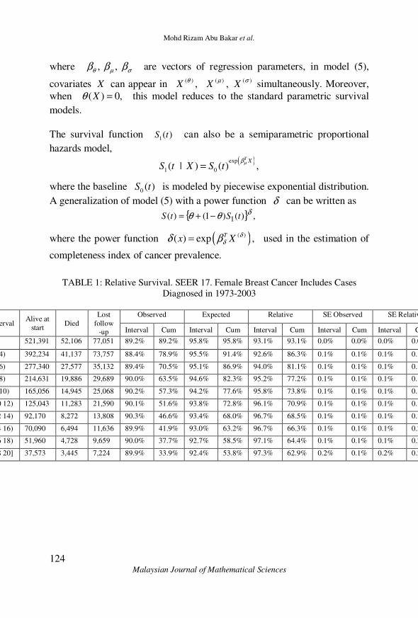
TABLE 1: Relative Survival. SEER 17. Female Breast Cancer Includes Cases

Diagnosed in 1973-2003

Interval Alive at

start Died

Lost

follow

-up

Observed Expected Relative SE Observed SE Relative

Interval Cum Interval Cum Interval Cum Interval Cum Interval Cum

<2 521,391 52,106 77,051 89.2% 89.2% 95.8% 95.8% 93.1% 93.1% 0.0% 0.0% 0.0% 0.0%

[2 4) 392,234 41,137 73,757 88.4% 78.9% 95.5% 91.4% 92.6% 86.3% 0.1% 0.1% 0.1% 0.1%

[4 6) 277,340 27,577 35,132 89.4% 70.5% 95.1% 86.9% 94.0% 81.1% 0.1% 0.1% 0.1% 0.1%

[6 8) 214,631 19,886 29,689 90.0% 63.5% 94.6% 82.3% 95.2% 77.2% 0.1% 0.1% 0.1% 0.1%

[8 10) 165,056 14,945 25,068 90.2% 57.3% 94.2% 77.6% 95.8% 73.8% 0.1% 0.1% 0.1% 0.1%

[10 12) 125,043 11,283 21,590 90.1% 51.6% 93.8% 72.8% 96.1% 70.9% 0.1% 0.1% 0.1% 0.1%

[12 14) 92,170 8,272 13,808 90.3% 46.6% 93.4% 68.0% 96.7% 68.5% 0.1% 0.1% 0.1% 0.1%

[14 16) 70,090 6,494 11,636 89.9% 41.9% 93.0% 63.2% 96.7% 66.3% 0.1% 0.1% 0.1% 0.2%

[16 18) 51,960 4,728 9,659 90.0% 37.7% 92.7% 58.5% 97.1% 64.4% 0.1% 0.1% 0.1% 0.2%

[18 20] 37,573 3,445 7,224 89.9% 33.9% 92.4% 53.8% 97.3% 62.9% 0.2% 0.1% 0.2% 0.2%



APPLICATION

Aim of the study

The purpose of this study is to analyze time trends in breast cancer patient

survival. The interest lies in survival after diagnosis of cancer, and how the

survival has changed over time. The focus lies on analyzing time trends using mixture cure models with different link functions. This is done by

applying cure models to real data from the Incidence - SEER 17 Regs

Public-Use, Nov 2005 Sub (1973-2003 varying), National Cancer Institute, USA, DCCPS, released April 2006. Recently developed methodology and

the new SEER Stata and CANSURV software commands created by

National Cancer Institute are used to estimate the cure fraction for many types of cancer. The aim is to evaluate in which cases the cure models work

and when they do not, and to see what kind of information about the survival

can be obtained using cure models that is not available using standard

methods.

Data description

The Surveillance, Epidemiology, and End Results (SEER) Program of the

National Cancer Institute annually collects cancer incidence and survival data from population-based cancer registries across the United States. These

data are distributed in the SEER Public-Use databases. The SEER Registries

routinely collect data on patient demographics, primary tumor site, morphology, stage at diagnosis, first course of treatment, and follow-up for

vital status. The SEER Program is a comprehensive source of population-

based information in the United States that includes stage of cancer at the

time of diagnosis and survival rates within each stage. In this study we are interested to include all female patients diagnosed with breast cancer

between 1973 and 2003. The survival time is the time between diagnose and

death, in this application, survival times are grouped into two annual intervals. The maximum follow-up time is 20 years, so the interval takes a

value from {1,…,10}. When a patient is still alive at the end of the study or

at the time the patient is lost to follow-up, then her survival time is censored. After excluding all death certificate only and autopsy only observations,

since they have zero survival time 521,391 observations were left. These

were divided into 7 age groups, less than 30 years (< 30), (30 – 39) years,

(40 – 49) years, (50 -59) years, (60 – 69) years, (70 – 79) years, and 80 years and over (80 +), and the data were stratified upon these age groups.

Moreover, four covariates were used in this study; diagnosis year (1973 –

2003), race (all, White, Black, Other), Martial status (All status, Married,



Single, Divorced/Separated, Widow/Other) and stage, SEER uses a staging

scheme; "SEER historic stage" which categorizes stage at diagnosis into (localized, regional, distant) and unstaged based on the extent of the cancer

at the time of diagnosis.

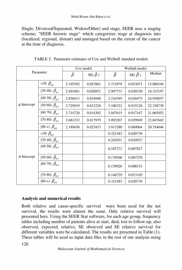
TABLE 2: Parameter estimates of Cox and Weibull standard models

Parameter Cox model Weibull model

β̂ SE( β̂ ) β̂ SE( β̂ ) Median

µ Intercept

<30 0µβ 2.195392 0.053961 2.713979 0.053071 15.089194

[30 40) 1µβ 2.491001 0.020951 2.907731 0.020330 18.315197

[40 50) 2µβ 2.830413 0.014948 3.216395 0.016475 24.938057

[50 60) 3µβ 2.725019 0.013226 3.106322 0.015126 22.338739

[60 70) 4µβ 2.714720 0.014302 3.047615 0.017167 21.065052

[70 80) 5µβ 2.681233 0.017979 3.093207 0.029949 22.047662

[80 +) 6µβ 2.189458 0.023437 3.013280 0.069064 20.354046

σ Intercept

<30 0σβ 0.321583 0.029739

[30 40) 1σβ 0.243651 0.010937

[40 50) 2σβ

0.187371 0.007827

[50 60) 3σβ 0.178560 0.007270

[60 70) 4σβ

0.139026 0.008331

[70 80) 5σβ 0.146729 0.013105

[80 +) 6σβ 0.321583 0.029739

Analysis and numerical results

Both relative and cause-specific survival were been used for the net

survival, the results were almost the same. Only relative survival will presented here. Using the SEER Stat software, for each age group, frequency

tables including number of patients alive at start, died, lost to follow-up, also

observed, expected, relative, SE observed and SE relative survival for different variables were be calculated. The results are presented in Table (1).

These tables will be used as input data files in the rest of our analysis using



CANSURV and S-Plus software.

In order to look at survival by age groups over a long period of time, the

analysis was done separately for these groups to see if the improvements in

survival over time were different for different age groups. We fit the standard survival models (assumed no cure present) and cure models to the

data. Table (2) shows the parameter estimates for the standard survival

models include the Weibull model and the Cox proportional hazards model.

TABLE 3: Parameter estimates, Cure rate (%) and Median survival time of

Weibull mixed cure model

Parameter Age group

<30 30-39 40-49 50-59 60-69 70-79 80+

Cure (θ)

Intercept θβ̂ 0.116 0.343 0.659 0.543 0.195 -2.733 -16.955

SE( θβ̂ ) 0.051 0.021 0.019 0.022 0.058 4.316 3656.1

µ Intercept µβ̂ 1.072 1.212 1.377 1.405 1.785 2.999 3.013

SE( µβ̂ ) 0.040 0.018 0.019 0.022 0.051 0.393 0.069

σ Intercept σβ̂ -0.169 -0.190 -0.172 -0.144 -0.037 0.141 0.319

SE( σβ̂ ) 0.034 0.013 0.011 0.011 0.014 0.030 0.027

Cure (%) 52.21 58.33 65.76 63.72 55.41 5.72 0.00

Median 2.92 3.36 3.96 4.08 5.96 20.08 20.35

The relative risk (hazard ratio) of dying of breast cancer is exp( )βµ− for

the Cox model and ( ){ }exp exp σβµ β− for the standard Weibull model.

For example, the risk of breast cancer death for the age group (40 – 50)

relative to the age group (< 30) is exp(2.830413) exp(2.195392) 1.8871÷ =

from the Cox model and

exp(3.216395/ exp(0.187371)) exp(2.713979/ exp(0.321583)) 2.0121÷ =

from Weibull model. The median survival time for the Weibull model is

exp( )(ln 2)σµ which is presented in the last column of Table 2. The

parameter estimates from the Weibull mixture cure model are listed in Table

3, all the covariates are significant (p < 0.0007), it is included in all



parameters (θ, µ, σ). In the last two rows the cure rates and the median survival times for uncured patients for each age group are calculated from

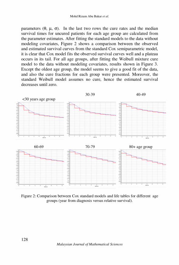
the parameter estimates. After fitting the standard models to the data without

modeling covariates, Figure 2 shows a comparison between the observed and estimated survival curves from the standard Cox semiparametric model,

it is clear that Cox model fits the observed survival curves well and a plateau

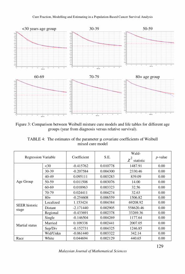
occurs in its tail. For all age groups, after fitting the Weibull mixture cure model to the data without modeling covariates, results shown in Figure 3.

Except the oldest age group, the model seems to give a good fit of the data,

and also the cure fractions for each group were presented. Moreover, the standard Weibull model assumes no cure, hence the estimated survival

decreases until zero.

<30 years age group 30-39 40-49

60-69 70-79 80+ age group

Figure 2: Comparison between Cox standard models and life tables for different age

groups (year from diagnosis versus relative survival).




60-69 70-79 80+ age group

Figure 3: Comparison between Weibull mixture cure models and life tables for different age

groups (year from diagnosis versus relative survival).

TABLE 4: The estimates of the parameter µ covariate coefficients of Weibull mixed cure model

Regression Variable Coefficient S.E. Wald-

2χ statistic p-value

Age Group

<30 -0.415762 0.010778 1487.91 0.00

30-39 -0.207584 0.004300 2330.46 0.00

40-49 0.095111 0.003283 839.09 0.00

50-59 0.011508 0.003076 14.00 0.00

60-69 0.018963 0.003323 32.56 0.00

70-79 0.024411 0.004274 32.63 0.00

80+ -0.254608 0.006559 1506.82 0.00

SEER historic stage

Localized 1.153424 0.004384 69208.92 0.00

Distant -2.171440 0.002905 558620.46 0.00

Regional -0.433691 0.002378 33269.36 0.00

Martial status

Single -0.146504 0.004269 1177.64 0.00

Married 0.109338 0.002441 2007.05 0.00

Sep/Div -0.152731 0.004325 1246.85 0.00

Wid/Unkn -0.061440 0.003322 342.14 0.00

Race White 0.044694 0.002129 440.65 0.00



Black -0.428422 0.004158 10615.83 0.00

Other 0.137656 0.006127 504.74 0.00

Log-Likelihood Value = -7592515.8

Table

The Wald-2χ test was used as part of our exploratory data analysis, in

order to identify of which covariates correlate with subsequent survival and

then cure fraction θ and the parameters µ and σ. As shown in Table 4, all

covariates were found to be significant and affect the parameter µ in the Weibull cure model. These are the covariates associated with a p-value less

than 0.05. For the parameter θ all covariates were found to be significant except the stage (distant) with p-value equal 0.986953. Also, the log-

likelihood value was calculated.

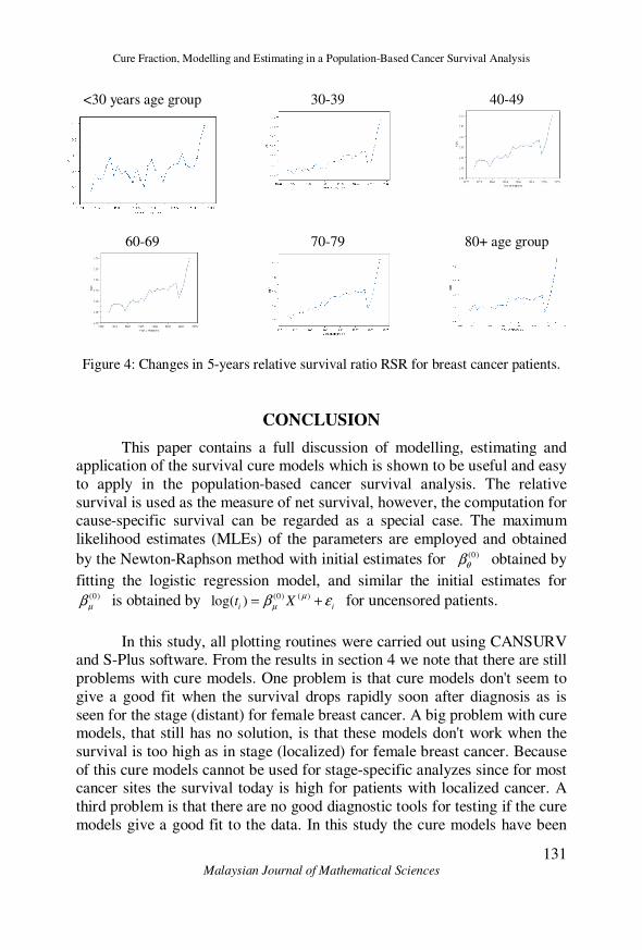
Graphs over the change in 5-years relative survival ratio (RSR) for different

age groups are presented in Figure 4. There is much random variation for the age group (< 30) but it easy to see that the 5-year RSR has increased for all

ages and are now around one for all age groups.

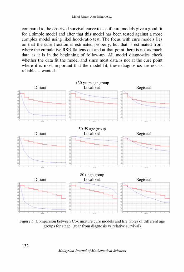
A big problem with cure models, is that these models don't fit the data and work well when the survival is too high. To overcome this problem, for each

age group the data is stratified into localized, regional and distant stages.

Figure 6 shows observed and estimated survival curves from the Cox

mixture cure model, it doesn't seems to give a good fit specially in the stages (distant) and (localized), since the survival drops rapidly soon after

diagnosis in the first stage, and the survival is too high in the second stage.

In summary, cure modelling was carried out using both standard and mixture cure fraction model. Both methods gave similar results. For the oldest age

group cure models don't seem to give a good fit, also these models don't

work well when the survival drops rapidly soon after diagnosis and when the

survival is too high. Because of this cure models cannot be used for stage-specific analyzes since for most cancer sites the survival today is high for

patients with localized cancer.




60-69

70-79

80+ age group

Figure 4: Changes in 5-years relative survival ratio RSR for breast cancer patients.

CONCLUSION

This paper contains a full discussion of modelling, estimating and application of the survival cure models which is shown to be useful and easy

to apply in the population-based cancer survival analysis. The relative

survival is used as the measure of net survival, however, the computation for cause-specific survival can be regarded as a special case. The maximum

likelihood estimates (MLEs) of the parameters are employed and obtained

by the Newton-Raphson method with initial estimates for (0)

θβ obtained by

fitting the logistic regression model, and similar the initial estimates for (0)

µβ is obtained by (0) ( )log( )

i it X

µµβ ε= + for uncensored patients.

In this study, all plotting routines were carried out using CANSURV and S-Plus software. From the results in section 4 we note that there are still

problems with cure models. One problem is that cure models don't seem to

give a good fit when the survival drops rapidly soon after diagnosis as is

seen for the stage (distant) for female breast cancer. A big problem with cure models, that still has no solution, is that these models don't work when the

survival is too high as in stage (localized) for female breast cancer. Because

of this cure models cannot be used for stage-specific analyzes since for most cancer sites the survival today is high for patients with localized cancer. A

third problem is that there are no good diagnostic tools for testing if the cure

models give a good fit to the data. In this study the cure models have been



compared to the observed survival curve to see if cure models give a good fit

for a simple model and after that this model has been tested against a more complex model using likelihood-ratio test. The focus with cure models lies

on that the cure fraction is estimated properly, but that is estimated from

where the cumulative RSR flattens out and at that point there is not as much data as it is in the beginning of follow-up. All model diagnostics check

whether the data fit the model and since most data is not at the cure point

where it is most important that the model fit, these diagnostics are not as

reliable as wanted.

<30 years age group

Distant Localized Regional

50-59 age group


80+ age group


Figure 5: Comparison between Cox mixture cure models and life tables of different age

groups for stage. (year from diagnosis vs relative survival)



Despite the problems associated with cure models, as long as these

models are used with a critical mind and the results are compared with other estimates as life table estimates they give very interesting information. Most

important when using cure models is that statistical cure can be assumed

even when statistical cure is not reasonable. The benefits of using cure models when analyzing trends in cancer survival is that the cure fraction is

not influenced by lead-time, that is usually a big problem in cancer patient

survival analysis, and that looking at both the cure fraction and the survival

of the 'uncured' can reveal a lot of information that looking at only one estimate can not. One of the most important reasons for using cure models is

that it gives valuable information to cancer patients. Since many cancer

patients today actually get cured of their cancer, the cure fraction is a very interesting measure for someone diagnosed with cancer. If and when the

problems with the cure models are solved this will probably be the way of

analyzing time trends in cancer patient survival in the future.

ACKNOWLEDGEMENT

The authors gratefully acknowledge the Surveillance, Epidemiology,

and End Results (SEER) Program (www.seer.cancer.gov) SEER*Stat Database: Incidence - SEER 17 Regs Public-Use, Nov 2005 Sub (1973-2003

varying), National Cancer Institute, DCCPS, Surveillance Research

Program, Cancer Statistics Branch, released April 2006, based on the November 2005 submission.

REFERENCES

Berkson, J. and Gage, R. P. (1952). Survival curve for cancer patients

following treatment. Journal of the American Statistical Association,

47, 501–515.

De Angelis, R., Capocaccia, R., Hakulinen, T., Soderman, B. and

Verdecchia, A. (1999). Mixture Models for Cancer Survival Analysis: Application to Population-Based Data with Covariates.

Statistics in Medicine, 18, 441-454.

Dickman, P. W., Adami, H. O. (2006). Interpreting trends in cancer patient

survival. Journal of Internal Medicine, 260, 103-117.

Ederer, F., Axtell, L. M. and Cutler, S. J. (1961). The Relative Survival



Rate: A Statistical Methodology. National Cancer Institute

Monograph, 6, 101-121.

Gamel, J. W., Weller, E. A., Wesley, M. N., and Feuer, E. J. (2000).

Parametric cure models of relative and cause-specific survival for

grouped survival times. Computer Methods and Programs in

Biomedicine, 61, 99-110.

Gamel, J. W. and Vogel, R. L. (2001). Non-parametric comparison of

relative versus cause-specific survival in Surveillance, Epidemiology

and End Results (SEER) programme breast cancer patients.

Statistical Methods in Medical Research, 10(5), 339-352.

Hakulinen, T. (1982), Cancer Survival Corrected for Heterogeneity in

Patient Withdrawal. Biometrics, 38, 933-942.

Cure Fraction, Modelling and Estimating in a Population ...einspem.upm.edu.my/journal/fullpaper/vol2no1/8. MJMS Vol 2 (1) page 113... · Cure Fraction, Modelling and Estimating in

Documents