Modeling Lexical Tones for Mandarin Large Vocabulary Continuous Speech Recognition Xin Lei A dissertation submitted in partial fulfillment of the requirements for the degree of Doctor of Philosophy University of Washington 2006 Program Authorized to Offer Degree: Electrical Engineering

Welcome message from author
This document is posted to help you gain knowledge. Please leave a comment to let me know what you think about it! Share it to your friends and learn new things together.
Transcript

Modeling Lexical Tones for Mandarin Large VocabularyContinuous Speech Recognition
Xin Lei
A dissertation submitted in partial fulfillmentof the requirements for the degree of
Doctor of Philosophy
University of Washington
2006
Program Authorized to Offer Degree: Electrical Engineering


University of WashingtonGraduate School
This is to certify that I have examined this copy of a doctoral dissertation by
Xin Lei
and have found that it is complete and satisfactory in all respects,and that any and all revisions required by the final
examining committee have been made.
Chair of the Supervisory Committee:
Mari Ostendorf
Reading Committee:
Mari Ostendorf
Mei-Yuh Hwang
Li Deng
Date:


In presenting this dissertation in partial fulfillment of the requirements for the doctoraldegree at the University of Washington, I agree that the Library shall make its copiesfreely available for inspection. I further agree that extensive copying of this dissertation isallowable only for scholarly purposes, consistent with “fair use” as prescribed in the U.S.Copyright Law. Requests for copying or reproduction of this dissertation may be referredto Proquest Information and Learning, 300 North Zeeb Road, Ann Arbor, MI 48106-1346,1-800-521-0600, to whom the author has granted “the right to reproduce and sell (a) copiesof the manuscript in microform and/or (b) printed copies of the manuscript made frommicroform.”
Signature
Date


University of Washington
Abstract
Modeling Lexical Tones for Mandarin Large VocabularyContinuous Speech Recognition
Xin Lei
Chair of the Supervisory Committee:Professor Mari Ostendorf
Electrical Engineering
Tones in Mandarin carry lexical meaning to distinguish ambiguous words. Therefore,
some representation of tone is considered to be an important component of an automatic
Mandarin speech recognition system. In this dissertation, we propose several new strate-
gies for tone modeling and explore their effectiveness in state-of-the-art HMM-based Man-
darin large vocabulary speech recognition systems in two domains: conversational telephone
speech and broadcast news.
A scientific study of tonal patterns in different domains is performed first, showing the
different levels of tone coarticulation effects. Then we investigate two classes of approaches
to tone modeling for speech recognition: embedded and explicit tone modeling. In embedded
tone modeling, a novel spline interpolation algorithm is proposed for continuation of the
F0 contour in unvoiced regions, and more effective pitch features are extracted from the
interpolated F0 contour. Since tones span syllables rather than phonetic units, we also
investigate the use of a multi-layer perceptron and long-term F0 windows to extract tone-
related posterior probabilities for acoustic modeling. Experiments reveal the new tone
features can improve the recognition performance significantly. To address the different
natures of spectral and tone features, multi-stream adaptation is also explored.
To further exploit the suprasegmental nature of tones, we combine explicit tone modeling
with the embedded tone modeling by lattice rescoring. Explicit tone models allow the use


of variable windows to synchronize feature extraction with the syllable. Oracle experiments
reveal that there is substantial room for improvement by adding explicit tone modeling (30%
reduction in character error rate). Pursuing that potential improvement, syllable-level tone
models are first trained and used to provide an extra knowledge source in the lattice. Then
we extend the syllable-level tone modeling to word-level modeling with a hierarchical backoff.
Experimental results show the proposed word-level tone modeling outperforms the syllable-
level modeling consistently and leads to significant gains over embedded tone modeling
alone. An important aspect of this work is that the methods are evaluated in the context
of a high performance, continuous speech recognition system. Hence, our development of
two state-of-the-art Mandarin large vocabulary speech recognition systems to incorporate
the tone modeling techniques is also described.


TABLE OF CONTENTS
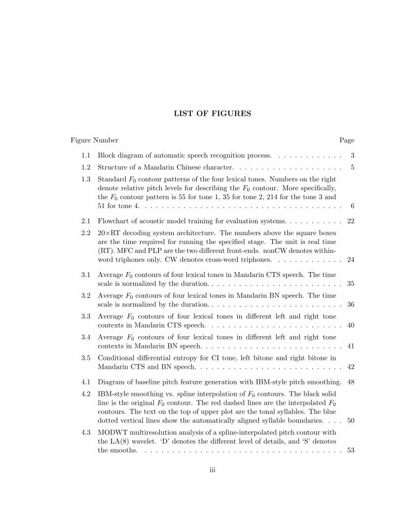
List of Figures . . . . . . . . . . . . . . . . . . . . . . . . . . . . . . . . . . . . . . . . iii
List of Tables . . . . . . . . . . . . . . . . . . . . . . . . . . . . . . . . . . . . . . . . . v
Chapter 1 Introduction . . . . . . . . . . . . . . . . . . . . . . . . . . . . . . . . . 1
1.1 Motivation . . . . . . . . . . . . . . . . . . . . . . . . . . . . . . . . . . . . . 2
1.2 Review of Tone Modeling in Chinese LVCSR . . . . . . . . . . . . . . . . . . 9
1.3 Main Contributions . . . . . . . . . . . . . . . . . . . . . . . . . . . . . . . . . 11
1.4 Dissertation Outline . . . . . . . . . . . . . . . . . . . . . . . . . . . . . . . . 13
Chapter 2 Corpora and Experimental Paradigms . . . . . . . . . . . . . . . . . . 15
2.1 Mandarin Corpora . . . . . . . . . . . . . . . . . . . . . . . . . . . . . . . . . 15
2.2 CTS Experimental Paradigm . . . . . . . . . . . . . . . . . . . . . . . . . . . 20
2.3 BN/BC Experimental Paradigm . . . . . . . . . . . . . . . . . . . . . . . . . 26
2.4 Summary . . . . . . . . . . . . . . . . . . . . . . . . . . . . . . . . . . . . . . 27
Chapter 3 Study of Tonal Patterns in Mandarin Speech . . . . . . . . . . . . . . 29
3.1 Review of Linguistic Studies . . . . . . . . . . . . . . . . . . . . . . . . . . . . 29
3.2 Comparative Study of Tonal Patterns in CTS and BN . . . . . . . . . . . . . 34
3.3 Summary . . . . . . . . . . . . . . . . . . . . . . . . . . . . . . . . . . . . . . 39
Chapter 4 Embedded Tone Modeling with Improved Pitch Features . . . . . . . . 44
4.1 Related Research . . . . . . . . . . . . . . . . . . . . . . . . . . . . . . . . . . 45
4.2 Tonal Acoustic Units and Pitch Features . . . . . . . . . . . . . . . . . . . . . 47
4.3 Spline Interpolation of Pitch Contour . . . . . . . . . . . . . . . . . . . . . . . 49
4.4 Decomposition of Pitch Contour with Wavelets . . . . . . . . . . . . . . . . . 51
4.5 Normalization of Pitch Features . . . . . . . . . . . . . . . . . . . . . . . . . . 54
4.6 Experiments . . . . . . . . . . . . . . . . . . . . . . . . . . . . . . . . . . . . . 55
4.7 Summary . . . . . . . . . . . . . . . . . . . . . . . . . . . . . . . . . . . . . . 57
i

Chapter 5 Tone-related MLP Posteriors in the Feature Representation . . . . . . 595.1 Motivation and Related Research . . . . . . . . . . . . . . . . . . . . . . . . . 595.2 Tone/Toneme Classification with MLPs . . . . . . . . . . . . . . . . . . . . . 615.3 Incorporating Tone/Toneme Posteriors . . . . . . . . . . . . . . . . . . . . . . 635.4 Experiments . . . . . . . . . . . . . . . . . . . . . . . . . . . . . . . . . . . . . 645.5 Summary . . . . . . . . . . . . . . . . . . . . . . . . . . . . . . . . . . . . . . 69
Chapter 6 Multi-stream Tone Adaptation . . . . . . . . . . . . . . . . . . . . . . 706.1 Review of Adaptation . . . . . . . . . . . . . . . . . . . . . . . . . . . . . . . 706.2 Multi-stream Adaptation of Mandarin Acoustic Models . . . . . . . . . . . . 726.3 Experiments . . . . . . . . . . . . . . . . . . . . . . . . . . . . . . . . . . . . . 746.4 Summary . . . . . . . . . . . . . . . . . . . . . . . . . . . . . . . . . . . . . . 76
Chapter 7 Explicit Syllable-level Tone Modeling for Lattice Rescoring . . . . . . 807.1 Related Research . . . . . . . . . . . . . . . . . . . . . . . . . . . . . . . . . . 817.2 Oracle Experiment . . . . . . . . . . . . . . . . . . . . . . . . . . . . . . . . . 827.3 Context-independent Tone Models . . . . . . . . . . . . . . . . . . . . . . . . 837.4 Supra-tone Models . . . . . . . . . . . . . . . . . . . . . . . . . . . . . . . . . 867.5 Estimating Tone Accuracy of the Lattices . . . . . . . . . . . . . . . . . . . . 887.6 Integrating Syllable-level Tone Models . . . . . . . . . . . . . . . . . . . . . . 917.7 Summary . . . . . . . . . . . . . . . . . . . . . . . . . . . . . . . . . . . . . . 93
Chapter 8 Word-level Tone Modeling with Hierarchical Backoff . . . . . . . . . . 948.1 Motivation and Related Research . . . . . . . . . . . . . . . . . . . . . . . . . 948.2 Word Prosody Models . . . . . . . . . . . . . . . . . . . . . . . . . . . . . . . 958.3 Backoff Strategies . . . . . . . . . . . . . . . . . . . . . . . . . . . . . . . . . . 978.4 Experimental Results . . . . . . . . . . . . . . . . . . . . . . . . . . . . . . . . 988.5 Summary . . . . . . . . . . . . . . . . . . . . . . . . . . . . . . . . . . . . . . 103
Chapter 9 Summary and Future Directions . . . . . . . . . . . . . . . . . . . . . 1049.1 Contributions . . . . . . . . . . . . . . . . . . . . . . . . . . . . . . . . . . . . 1049.2 Future Directions . . . . . . . . . . . . . . . . . . . . . . . . . . . . . . . . . . 113
Bibliography . . . . . . . . . . . . . . . . . . . . . . . . . . . . . . . . . . . . . . . . . 115
Appendix A Pronunciations of Initials and Finals . . . . . . . . . . . . . . . . . . . 125
ii
LIST OF FIGURES
Figure Number Page
1.1 Block diagram of automatic speech recognition process. . . . . . . . . . . . . 3
1.2 Structure of a Mandarin Chinese character. . . . . . . . . . . . . . . . . . . . 5
1.3 Standard F0 contour patterns of the four lexical tones. Numbers on the rightdenote relative pitch levels for describing the F0 contour. More specifically,the F0 contour pattern is 55 for tone 1, 35 for tone 2, 214 for the tone 3 and51 for tone 4. . . . . . . . . . . . . . . . . . . . . . . . . . . . . . . . . . . . . 6
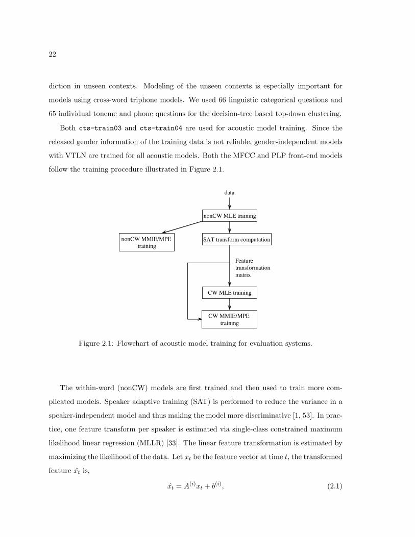
2.1 Flowchart of acoustic model training for evaluation systems. . . . . . . . . . . 22
2.2 20×RT decoding system architecture. The numbers above the square boxesare the time required for running the specified stage. The unit is real time(RT). MFC and PLP are the two different front-ends. nonCW denotes within-word triphones only. CW denotes cross-word triphones. . . . . . . . . . . . . 24
3.1 Average F0 contours of four lexical tones in Mandarin CTS speech. The timescale is normalized by the duration. . . . . . . . . . . . . . . . . . . . . . . . . 35
3.2 Average F0 contours of four lexical tones in Mandarin BN speech. The timescale is normalized by the duration. . . . . . . . . . . . . . . . . . . . . . . . . 36
3.3 Average F0 contours of four lexical tones in different left and right tonecontexts in Mandarin CTS speech. . . . . . . . . . . . . . . . . . . . . . . . . 40
3.4 Average F0 contours of four lexical tones in different left and right tonecontexts in Mandarin BN speech. . . . . . . . . . . . . . . . . . . . . . . . . . 41
3.5 Conditional differential entropy for CI tone, left bitone and right bitone inMandarin CTS and BN speech. . . . . . . . . . . . . . . . . . . . . . . . . . . 42
4.1 Diagram of baseline pitch feature generation with IBM-style pitch smoothing. 48
4.2 IBM-style smoothing vs. spline interpolation of F0 contours. The black solidline is the original F0 contour. The red dashed lines are the interpolated F0
contours. The text on the top of upper plot are the tonal syllables. The bluedotted vertical lines show the automatically aligned syllable boundaries. . . . 50
4.3 MODWT multiresolution analysis of a spline-interpolated pitch contour withthe LA(8) wavelet. ‘D’ denotes the different level of details, and ‘S’ denotesthe smooths. . . . . . . . . . . . . . . . . . . . . . . . . . . . . . . . . . . . . 53
iii

4.4 Raw F0 contour and the final processed F0 features. The vertical dashed linesshow the forced aligned tonal syllable boundaries. . . . . . . . . . . . . . . . . 56
5.1 Schematic of a single hidden layer, feed-forward neural network. . . . . . . . . 625.2 Block diagram of the tone-related MLP posterior feature extraction stage. . . 64
6.1 Multi-stream adaptation of Mandarin acoustic models. The regression classtrees (RCT) can be either manually designed or clustered by acoustics. . . . . 73
6.2 The decision tree clustering of the regression class tree (RCT) of MFCCstream. “EQ” denotes “equal to”, “IN” denotes “belong to”, and “-” denotesthe silence phone. . . . . . . . . . . . . . . . . . . . . . . . . . . . . . . . . . . 75
6.3 The decision tree clustering of the regression class tree (RCT) of pitch stream.“EQ” denotes “equal to”, “IN” denotes “belong to”, and “-” denotes thesilence phone. . . . . . . . . . . . . . . . . . . . . . . . . . . . . . . . . . . . . 76
7.1 Aligning a lattice arc i to oracle tone alignments. . . . . . . . . . . . . . . . . 837.2 Illustration of frame-level tone posteriors. . . . . . . . . . . . . . . . . . . . . 897.3 Illustration of insertion of dummy tone links for lattice expansion. . . . . . . 93
8.1 Backoff hierarchy of Mandarin tone modeling. . . . . . . . . . . . . . . . . . . 96
9.1 Mandarin BN decoding system architecture. . . . . . . . . . . . . . . . . . . . 111
iv

LIST OF TABLES
Table Number Page
2.1 Mandarin CTS acoustic data for acoustic model training and testing. . . . . . 16
2.2 Mandarin CTS text data for language model training. . . . . . . . . . . . . . 18
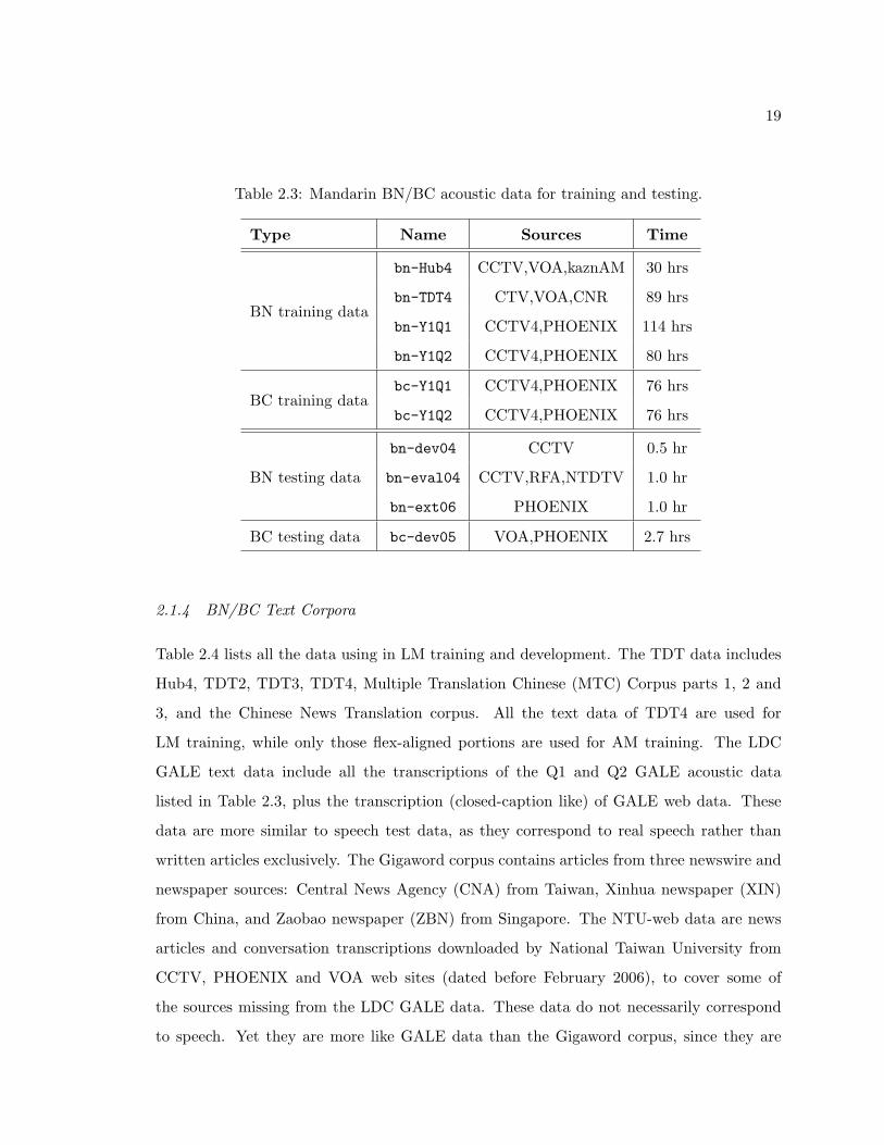
2.3 Mandarin BN/BC acoustic data for training and testing. . . . . . . . . . . . . 19
2.4 Mandarin BN/BC text data for language model training and development,in number of words. . . . . . . . . . . . . . . . . . . . . . . . . . . . . . . . . 20
4.1 The 22 syllable initials and 38 finals in Mandarin. In the list of initials, NULLmeans no initial. In the list of finals, (z)i denotes the final in /zi/, /ci/, /si/;(zh)i denotes the final in /zhi/, /chi/, /shi/, /ri/. . . . . . . . . . . . . . . . . 46
4.2 Phone set in our 2004 Mandarin CTS speech recognition system. ‘sp’ is thephone model for silence; ‘lau’ is for laughter; ‘rej’ is for noise. The numbers1-5 denote the tone of the phone. . . . . . . . . . . . . . . . . . . . . . . . . . 47
4.3 Phone set in our 2006 Mandarin BN speech recognition system. ‘sp’ is thephone model for silence; ‘rej’ is for noise. The numbers 1-4 denote the toneof the phone. . . . . . . . . . . . . . . . . . . . . . . . . . . . . . . . . . . . . 48
4.4 Mandarin speech recognition character error rates (%) of different pitch fea-tures on bn-eval04. ‘D’ denotes the different level of details, and ‘S’ denotesthe smooth. SI means speaker-independent results and SA means speaker-adapted results. . . . . . . . . . . . . . . . . . . . . . . . . . . . . . . . . . . . 57
4.5 CER results (%) on bn-dev04 and bn-eval04 using different pitch featureprocessing. SI means speaker-independent results and SA means speaker-adapted results. . . . . . . . . . . . . . . . . . . . . . . . . . . . . . . . . . . . 58
4.6 CER results (%) on cts-dev04 using different pitch feature processing. . . . 58
5.1 Frame accuracy of tone and toneme MLP classifiers on the cross validationset of cts-train04. IBM F0 denotes IBM-style F0 features; spline F0 de-notes spline+MWN+MA processed F0 features. The tone target in IBM F0
approach is phone-level tone and in spline F0 approach is syllable-level tone. . 66
5.2 CER of CTS systems on cts-dev04 using tone posteriors. IBM F0 denotesIBM-style F0 features; spline F0 denotes spline+MWN+MA processed F0
features. The tone in IBM F0 approach is at the phone level and at thesyllable level in spline F0 approach. . . . . . . . . . . . . . . . . . . . . . . . . 67
v

5.3 CER of CTS systems on cts-dev04 using toneme posteriors. IBM F0 denotesIBM-style F0 features; spline F0 denotes spline+MWN+MA processed F0
features. . . . . . . . . . . . . . . . . . . . . . . . . . . . . . . . . . . . . . . . 685.4 CER of BN system on bn-eval04 with toneme posteriors (ICSI features). In
this table, F0 denotes spline+MWN+MA processed F0 features. SI meansspeaker-independent results and SA means speaker-adapted results. . . . . . . 69
6.1 Definitions of some phone classes in decision tree questions of RCTs. Thesedefinitions are for BN task. . . . . . . . . . . . . . . . . . . . . . . . . . . . . 77
6.2 CER on bn-eval04 using different MLLR adaptation strategies with MFCC+F0
model. RCT means the type of regression class trees. . . . . . . . . . . . . . . 786.3 CER on bn-eval04 using different MLLR adaptation strategies with MFCC+F0+ICSI
model. . . . . . . . . . . . . . . . . . . . . . . . . . . . . . . . . . . . . . . . . 78
7.1 Baseline and oracle recognition error rate results (%) of tones, base syl-lables (BS), tonal syllables (TS), and characters (Char) on the CTV sub-set of bn-eval04. The baseline system uses embedded tone modeling withspline+MWN+MA pitch features. . . . . . . . . . . . . . . . . . . . . . . . . 83
7.2 Four-tone classification tone error rate (TER) results (%) on cross validationset of bn-Hub4. “PRC” means polynomial regression coefficients. “RRC”means robust regression coefficients. “dur” denotes syllable duration. . . . . . 86
7.3 Four-tone classification results on long tones in CTV subset of bn-eval04.TER denotes tone error rate. . . . . . . . . . . . . . . . . . . . . . . . . . . . 87
7.4 CER of tone model integration on CTV test set. The baseline system usesembedded tone modeling with spline+MWN+MA pitch features. . . . . . . . 92
8.1 CER(%) using word prosody models with CI tone models as backoff. Thebaseline system uses embedded tone modeling with spline+MWN+MA pitchfeatures. . . . . . . . . . . . . . . . . . . . . . . . . . . . . . . . . . . . . . . . 101
8.2 CER (%) using word prosody models with CD tone models as backoff. ”l -”denotes left-tone context-dependent models. The baseline system uses em-bedded tone modeling with spline+MWN+MA pitch features. . . . . . . . . . 102
8.3 CER (%) on bn-eval04 and bn-ext06 using word prosody models trainedwith 465 hours of data. The baseline system uses embedded tone modelingwith spline+MWN+MA pitch features. . . . . . . . . . . . . . . . . . . . . . 103
9.1 CER results (%) of the Mandarin CTS system for NIST 2004 evaluation. . . 1099.2 CER results (%) of the Mandarin BN/BC system for NIST 2006 evaluation. . 112
vi

ACKNOWLEDGMENTS
First and foremost, I would like to express my deepest gratitude to my advisor Profes-
sor Mari Ostendorf, for her encouragement and guidance in my study. Her insights and
meticulous reading and editing of this dissertation and every other publication resulting
from this research, have definitely improved the quality of my work. I must thank Mei-Yuh
Hwang for her technical expertise and detailed understanding of speech recognition sys-
tems, which have made it possible for the development of the two state-of-the-art Mandarin
speech recognition systems during my study. I also want to thank the other members of
my supervisory committee: Jeff Bilmes, Les Atlas, Li Deng, and Hank Levy. I thank Jeff
Bilmes for his help on turning my course project report into my first ICASSP paper. I
thank Les Atlas for his interesting course on digital signal processing, which attracted me
to the speech processing field. I thank Li Deng for being in my thesis reading committee. I
thank Hank Levy for serving as GSR for both my general and final exams.
I also want to thank Tim Ng for working together with me in the early stage when we
developed the first Mandarin CTS system. I want to thank Manhung Siu for providing
the opportunity of my visit to Hong Kong. Thanks to both Manhung and Tan Lee for the
many useful discussions on my work. I must thank our collaborators at SRI: Wen Wang,
Jing Zheng and Andreas Stolcke. Thanks to them for providing the SRI decipher speech
recognition system and support. It has been an intellectually rewarding experience working
with the SRI folks to build the systems that I am really proud of.
There are many people in the SSLI lab I would like to thank for various reasons. Xiao Li
and Gang Ji for being my friends ever since I came to UW. Jon Malkin and Arindam Mandal
for the numerous discussions related and unrelated to research. Karim, Chris and Scott for
working in the lab with me on many weekends. Dustin for getting us the continuous supply
of soda and for the support of Condor. Mei Yang for her curiosity about everything. Kevin
vii

for organizing the reading groups and seminars. Jeremy Kahn for his knowledge on Unix
and Perl. Thanks to all the members in SSLI lab for helping me through and making my
time here better.
Finally, I want to thank my family. My parents taught me the value of education and
have always pushed me and supported me. My sister for her encouragement and advice.
Most importantly, of course, I want to thank my wife Cindy for her patience and love, and
for always being there for me. Without the constant love and support from my dear family,
this piece of work would not have been possible.
This dissertation is based upon the work supported by DARPA grant MDA972-02-C-
0038 from the EARS program, and by DARPA under Contract No. HR0011-06-C-0023
from the GALE program.
viii

1
Chapter 1
INTRODUCTION
Mandarin is a category of related Chinese dialects spoken across most of northern and
southwestern China. Mandarin is the most widely spoken form of the Chinese language and
has the largest number of speakers in the world. One distinctive characteristic of Mandarin
is that it is a tone language [18]. While most languages use intonation or pitch to convey
grammatical structure or emphasis, their tones do not carry lexical information. In tone
languages, a tone is called a lexical tone which is an integral part of a word itself. The
Mandarin lexical tones, just like consonants and vowels, are used to distinguish words from
each other.
Tone languages can be classified into two broad categories: register tone systems and con-
tour tone systems. Mandarin has a contour tone system, where the tones are distinguished
by their shifts in pitch (their pitch shapes or contours, such as rising, falling, dipping and
peaking) rather than simply their pitch levels relative to each other as in a register tone
system. The primary physiological cause of pitch in speech is the vibration rate of the
vocal folds, the acoustic correlate of which is fundamental frequency (F0). Although the
correlation between pitch and fundamental frequency is non-linear, pitch can for practical
purposes be equated with F0 as F0 frequencies are relatively low (e.g., below 500Hz) [17].
Therefore, the F0 contour of the syllable is the most prominent acoustic cue of Mandarin
tones. In isolated Mandarin speech, the F0 contour corresponds well with the canonical
patterns of its lexical tone. However, in continuous Mandarin speech, the F0 contour is
subject to many variations such as tone sandhi1 [18] and tone coarticulation.
In the past decade, there has been significant progress on English large vocabulary con-
1Tone sandhi refers to the phenomenon that, in continuous speech, some lexical tones may change theirtone category in certain tone contexts.
2
tinuous speech recognition (LVCSR) in the hidden Markov model (HMM) framework. It
is natural to want to extend the English automatic speech recognition (ASR) systems to
Mandarin, one of the world’s most spoken languages. In addition, the difficulty of inputting
Chinese by keyboard presents a great opportunity for Mandarin ASR to improve computer
usability. Many studies have been conducted to extend the progress to Mandarin speech
recognition. However, the performance of the state-of-the-art Mandarin LVCSR systems is
still much worse than that of English systems. An important reason is that Mandarin is a
tone language that requires special treatment for modeling the tones. The same Mandarin
syllable with different tones usually represent completely different characters. This intro-
duces more complexity on the acoustic modeling side of Mandarin speech recognition. In
this dissertation, we are mainly concerned with improving the tone modeling of Mandarin
speech recognition within the HMM framework. We focus on developing tone modeling
techniques which can be easily integrated in a state-of-the-art Mandarin speech recognition
system and improving the speech recognition performance in the conversational telephone
speech (CTS), broadcast news (BN) and broadcast conversation (BC) domains.
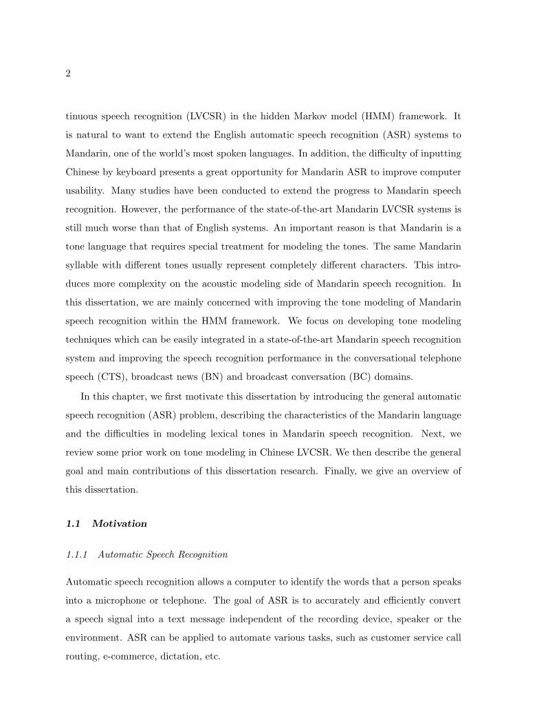
In this chapter, we first motivate this dissertation by introducing the general automatic
speech recognition (ASR) problem, describing the characteristics of the Mandarin language
and the difficulties in modeling lexical tones in Mandarin speech recognition. Next, we
review some prior work on tone modeling in Chinese LVCSR. We then describe the general
goal and main contributions of this dissertation research. Finally, we give an overview of
this dissertation.
1.1 Motivation
1.1.1 Automatic Speech Recognition
Automatic speech recognition allows a computer to identify the words that a person speaks
into a microphone or telephone. The goal of ASR is to accurately and efficiently convert
a speech signal into a text message independent of the recording device, speaker or the
environment. ASR can be applied to automate various tasks, such as customer service call
routing, e-commerce, dictation, etc.

3
Most modern speech recognition systems are based on the HMM framework. Fig-
ure 1.1 illustrates the general process of most HMM-based speech recognition systems.
Let X = {x1, x2, . . . , xN} denote the acoustic observation (feature vector) sequence and
W = {w1, w2, . . . , wM} be the corresponding word sequence. The decoder chooses the word
sequence with the maximum a posteriori probability:
W = argmaxW
p(W |X) = argmaxW
p(X|W )p(W ), (1.1)
where p(X|W ) is called the acoustic model and p(W ) is known as the language model.
Feature Analysis(Spectral Analysis)
Feature Analysis(Spectral Analysis)
Pattern Classification(Decoding)
Pattern Classification(Decoding)
WordLexicon
WordLexicon
Language Model
Language Model
Acoustic Model (HMM)
Acoustic Model (HMM)
Input Speech
DecodedWords
Figure 1.1: Block diagram of automatic speech recognition process.
The feature analysis module extracts feature vectors X that represent the input speech
signal for statistical modeling and decoding. The commonly used standard types of speech
feature vectors include mel-frequency cepstral coefficients (MFCCs) [19] and perceptual
linear predictive coefficients (PLPs) [39]. HMMs are used to model the speech signal in terms
of piecewise stationary regions. In the training phase, an inventory of sub-phonetic HMM
acoustic models are trained using a corpus of labeled speech data. The statistical language
model is also trained on the text data. For a sequence of words W = {w1, w2, . . . wM}, the
prior probability p(W ) is given by
p(W ) = p(w1, w2, . . . wM ) =M∏i=1
p(wi|w1, w2, . . . wi−1). (1.2)

4
In practice, the most commonly used language model is called an N -gram, where each
word depends only on its previous N − 1 words. In the decoding phase, the acoustic proba-
bility score p(X|W ), also called a likelihood score, is combined with the prior probabilities
of each utterance p(W ) to compute the posterior probability p(W |X). Finally, the word
sequence W with the maximum posterior probability is decoded as the hypothesized speech
text.
Figure 1.1 shows only the very essential components of modern speech recognition sys-
tems. There has been a substantial amount of research and dramatic progress in English
ASR in recent years [70, 36, 26]. Advanced technologies such as discriminative training
methods [74] and speaker adaptation techniques [56, 1] have significantly decreased the
word error rate (WER) of ASR systems.
1.1.2 Characteristics of Mandarin Chinese
Quite different from English and some other Western languages, Mandarin is a tonal-syllabic
and ideographic language. Chinese vocabulary consists of characters instead of words in
English. Each Mandarin Chinese character is a tonal syllable. One or multiple Chinese
characters form a “word”. To describe the pronunciation of a Chinese character, both the
base syllable and the tone need to be defined. There are several different ways to represent
the pronunciation of the Mandarin Chinese characters. The most popular way is to use tonal
Pinyin2 which combines the base syllable and a tone mark to represent the pronunciation
of a character. The syllable structure of Mandarin Chinese is illustrated in Figure 1.2
with an example. The base syllable structure is conventionally decomposed into an initial
and a final3 [8]: the syllable initial is an optional consonant; the syllable final includes an
optional medial glide, a nucleus (vowel) and an optional coda (final nasal consonant, /n/ or
/ng/). There are a total of 22 initials and 38 finals in Mandarin Chinese, which are listed
in Chapter 4.
2“Pinyin” is a system which uses Roman letters to represent syllables in standard Mandarin. The toneof a syllable is indicated by a diacritical mark above the nucleus vowel or diphthong, e.g. ba, ba, ba, ba.Another common convention is to append a digit representing the tone to the end of individual syllables,e.g. ba1, ba2, ba3, ba4. For simplicity, we adopt the second annotation in this dissertation.
3Although these two terms are seemingly awkward in English, they are standard in the literature.

5
character: circle
tonal syllable/yuan2/
base syllable/yuan/
tone2
initial/y/
final/uan/
nucleus/a/
coda/n/
medial/u/
Figure 1.2: Structure of a Mandarin Chinese character.
There are four lexical tones plus one neutral tone in Mandarin Chinese. The five tones
are commonly characterized as high-level (tone 1), mid-rising (tone 2), low-dipping (tone 3),
high-falling (tone 4) and neutral (tone 5). Lexical tones are essential in Mandarin speech.
For example, the characters “Ë”(yan1, cigarette), “Δ(yan2, strict), “Ú”(yan3, eye),
“É”(yan4, swallow) share the same syllable “yan” (“y” is the syllable initial and “an”
is the syllable final) and only differ in tones, but their meanings are completely different.
Another interesting example is “o”(mai3, buy) and “q”(mai4, sell), which also differ only
in tones but they have the opposite meanings. The neutral tone, on the other hand, often
occurs in unstressed positions with reduced duration and energy.
Mandarin has a contour tone system, in which tones depend on the shape of the pitch
contour instead of the relative pitch levels. The standard F0 contour patterns of the four
lexical tones using a 5-level scale [7] are shown in Figure 1.3. Unlike the four lexical tones,
the neutral tone does not have a stable F0 contour pattern. Its F0 contour largely depends
on the contextual tones.
There are around 6500 commonly used Chinese characters in GB codes4. These Man-
4GB and Big5 are the two most commonly used coding schemes. GB is used in mainland China andis associated with simplified characters. Big5 is used in Taiwan and Hong Kong and is associated with

6
Figure 1.3: Standard F0 contour patterns of the four lexical tones. Numbers on the rightdenote relative pitch levels for describing the F0 contour. More specifically, the F0 contourpattern is 55 for tone 1, 35 for tone 2, 214 for the tone 3 and 51 for tone 4.
darin characters map to around 410 base syllables, or around 1340 tonal syllables. Since
a lot of characters share the same base syllable or tonal syllable, the disambiguation of
Chinese characters heavily relies on the tones and the context characters.
1.1.3 Difficulties in Tone Modeling
There are several key language-specific challenges in Mandarin ASR, such as modeling
tones and lack of word segmentation. Since tone plays a critical role in Mandarin speech
in distinguishing ambiguous characters, we will focus on the tone modeling problem in this
dissertation work.
The most important acoustic cue of tone is the F0 contour. Some other acoustic features
such as duration and energy also contribute to modeling of the tones. Tone modeling for
Mandarin continuous speech recognition is generally a difficult problem due to many factors:
• Speaker variations
Different people have different pitch ranges. The typical F0 range for a male is 80-
200 Hz, and 150-350 Hz for females. Even within the same gender, the pitch level
and dynamic range may vary significantly. Speakers with a southern accent also
traditional characters.

7
exhibit much different tonal patterns than the northern speakers. Therefore, speaker
normalization of F0 features is necessary for tone modeling.
• Coarticulation constraints
In continuous Mandarin speech, the tones are also influenced by the neighboring tones
due to coarticulation constraints. As a result, the phonetic5 realization of a tone may
vary. In [103] Xu used the Mandarin syllable sequence /ma ma/ as the tone carrier
to examine how two tones are produced next to each other. He found that there exist
carry-over effects from the left context and anticipatory effects from the right context.
The anticipatory and carry-over effects differ both in magnitude and in nature: the
carry-over effects are much larger in magnitude and mostly assimilatory, i.e., the onset
F0 value of a tone is assimilated to the offset F0 value of its previous tone; on the
other hand, the anticipatory effects are relatively small and mostly dissimilatory, i.e.,
a low onset value of a tone raises the maximum F0 value of a preceding tone. In
more natural speech such as BN/BC and CTS, there are also much more frequent
appearances of neutral tones. Since the neutral tone does not have a stable pitch
contour, it is very difficult to model.
• Linguistic constraints
The F0 contour of a tone is significantly affected by many linguistic constraints such
as tone sandhi and intonation, sometimes referred to as phonological effects. Tone
sandhi refers to the categorical change of a tone when spoken in certain tone contexts.
In Mandarin Chinese, the most common tone sandhi rule is the third-tone-sandhi rule:
the leading syllable in a set of two third-tone syllables is raised to the second tone.
Intonation refers to the phrase-level structure on top of lexical tone sequences. The
intonation of an utterance also affects the F0 contour significantly. It was found in [79]
that both the pitch contour shape and the scale of a given tone are influenced by the
intonation. The F0 contour is also affected by the speaker’s emotion and mood when
5Phonetics is distinguished from phonology. Phonetics is the study of the production, perception, andphysical properties of speech sounds, while phonology attempts to account for how they are combined,organized, and convey meaning in particular languages.
8
uttering the sentence.
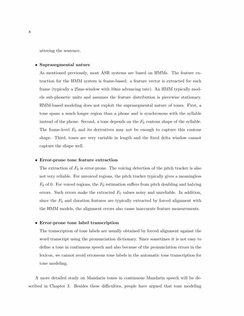
• Suprasegmental nature
As mentioned previously, most ASR systems are based on HMMs. The feature ex-
traction for the HMM system is frame-based: a feature vector is extracted for each
frame (typically a 25ms-window with 10ms advancing rate). An HMM typically mod-
els sub-phonetic units and assumes the feature distribution is piecewise stationary.
HMM-based modeling does not exploit the suprasegmental nature of tones. First, a
tone spans a much longer region than a phone and is synchronous with the syllable
instead of the phone. Second, a tone depends on the F0 contour shape of the syllable.
The frame-level F0 and its derivatives may not be enough to capture this contour
shape. Third, tones are very variable in length and the fixed delta window cannot
capture the shape well.
• Error-prone tone feature extraction
The extraction of F0 is error-prone. The voicing detection of the pitch tracker is also
not very reliable. For unvoiced regions, the pitch tracker typically gives a meaningless
F0 of 0. For voiced regions, the F0 estimation suffers from pitch doubling and halving
errors. Such errors make the extracted F0 values noisy and unreliable. In addition,
since the F0 and duration features are typically extracted by forced alignment with
the HMM models, the alignment errors also cause inaccurate feature measurements.
• Error-prone tone label transcription
The transcription of tone labels are usually obtained by forced alignment against the
word transcript using the pronunciation dictionary. Since sometimes it is not easy to
define a tone in continuous speech and also because of the pronunciation errors in the
lexicon, we cannot avoid erroneous tone labels in the automatic tone transcription for
tone modeling.
A more detailed study on Mandarin tones in continuous Mandarin speech will be de-
scribed in Chapter 3. Besides these difficulties, people have argued that tone modeling

9
would not help continuous Mandarin speech recognition since the tone information becomes
less informative (more variable) and performance is mainly determined by the Chinese lan-
guage model [30]. Language models give positive constraints on the possible contextual
characters, which effectively means that they also reduce the influence of tone modeling.
Especially in a very good Mandarin ASR system with strong language models, there is the
potential for tone modeling to be less important [69]. Due to the various difficulties and
the overlap with language modeling, achieving significant ASR gain from tone modeling has
been a challenging task for Mandarin speech recognition systems.
1.2 Review of Tone Modeling in Chinese LVCSR
Many studies have been conducted on how to incorporate tone information in Chinese speech
recognition, mainly including Mandarin ASR [62, 10, 6, 45, 5] and Cantonese6 ASR [55, 72,
76]. Quite different from Mandarin, Cantonese has 6 lexical tones and a register tone
system where tones depend on their relative pitch level [76]. Different tasks in Chinese ASR
have been explored and can be categorized into isolated word recognition, dictation-based
continuous speech recognition and spontaneous speech recognition. Here we will briefly
review some prior work in tone modeling in Chinese LVCSR.
The approaches to Mandarin tone modeling fall into two major categories: explicit tone
modeling and embedded tone modeling. Explicit tone modeling means that tone recognition
is done as an independent process to HMM-based phonetic recognition. In this approach,
separate tone classifiers are used to model the tonal patterns carried by the acoustic signal.
Features for explicit tone recognition include F0, duration, polynomial coefficients, etc. For
example, Legendre coefficients were used to encode the pitch contour of the tones in [90]
and orthogonal polynomial coefficients were used in [98]. Various pattern recognition models
have been tried for Chinese tone recognition. Neural networks were successfully used in [14]
for Mandarin tone recognition. Hidden Markov models were tried in [93, 55] and Gaussian
mixture models were tried in [76] for Cantonese tone recognition. The authors of [98]
also proposed a decision-tree based Mandarin tone classifier using duration, log energy and
6Cantonese is a Chinese dialect spoken by tens of millions of speakers in southern China and Hong Kong.

10
other features. More recently, support vector machines have been used for Cantonese tone
recognition [72]. Besides these traditional classifiers, in [5] the authors proposed a mixture
stochastic polynomial tone model for continuous Mandarin tone patterns.
Typically there are several different ways to use the explicit tone classifier in the Man-
darin LVCSR system:
1. The tone recognition and phonetic recognition are carried out separately and then
merged together to generate the final tonal syllable sequence [93];
2. The phonetic recognition is performed first and then the tone models are used to post-
process the N -best lists or word graphs generated from the first pass decoding [90, 76];
3. The tone models can be applied in the first-pass searching process to integrate the
tone scores into the Viterbi score [90, 55, 98, 5, 72].
The post-processing approach has minimal computation and introduces fairly small de-
lays, without having to modify the speech recognizer to be a language-specific decoder.
But the disadvantage is that the effectiveness depends on the quality of the N -best lists or
word graphs such as the confusion networks and word lattices. For example, if the correct
hypothesis is not in the N -best lists, it will not be recovered from resorting the N -best
lists. Therefore, rescoring the word lattices is a better option since a lattice is a much richer
representation of the entire search space.
The embedded tone modeling approach, on the other hand, incorporates pitch features
directly into the feature vector and merges tone and phonetic units to form tonal acoustic
models [10, 6, 45, 99]. This method is straight-forward and easy to apply in the general
HMM framework. It also has proved to be quite powerful in various Mandarin ASR tasks.
In [45], around 30% relative improvement in character error rate (CER) has been achieved
by taking this approach on three different continuous Mandarin speech corpora, including a
telephone speech corpora and two dictation speech corpora. This work also confirms a good
correspondence between tone recognition accuracy and character recognition accuracy.
The major challenges in embedded tone modeling are the extraction of effective pitch
features and selection of tonal acoustic units. Since F0 is not defined for unvoiced regions, the

11
post-processing of F0 features is essential to avoid variance problems. Difference smoothing
techniques have been proposed [10, 45, 101] with different levels of success. On the model
side, the selection of appropriate tonal acoustic units is also important. Initials and tonal
finals were used in [6]; tonal phoneme (toneme) based on the main vowel idea was proposed
by [10]; and extended initials and segmental tonal finals were designed in [44].
In most of the state-of-the-art Mandarin LVCSR systems in recent NIST evaluations,
the embedded tone modeling approach has been adopted: the toneme phone set is used and
the F0 and its delta features are appended to the spectral feature vector [48, 34, 101]. Very
good speech recognition performance can be achieved with this tone modeling approach.
We will build our baseline system under this framework and investigate the explicit tone
modeling approaches on top of it.
1.3 Main Contributions
The general goal of this dissertation is to improve the performance of state-of-the-art Man-
darin LVCSR systems. Towards this goal, we investigate various tone modeling strategies
to enhance Mandarin continuous speech recognition. More specifically, we focus on tone
modeling of Mandarin LVCSR in the CTS and BN/BC domains. There are six main con-
tributions of this dissertation work:
• Scientific study of tonal patterns in Mandarin BN/BC and CTS speech
The tonal patterns in isolated speech correspond well with the standard F0 contour
patterns. However, in more natural speech such as BN/BC and CTS, the tonal pat-
terns are significantly different due to the coarticulation and linguistic variations. We
perform a scientific study to see how the tonal patterns change in these speech do-
mains. This study helps us gain more insight into statistical tone modeling.
• Effective pitch feature processing for embedded tone modeling
The F0 features are not defined in unvoiced regions, causing modeling problems in
Mandarin ASR. Inspired by F0 contour modeling in speech synthesis [41], we propose
a spline interpolation method to solve this discontinuity problem. This interpolation

12
method also makes the system less sensitive to the misalignment between F0 and
phone boundaries given by HMMs. Next, we decompose the interpolated F0 contour
into different scales by wavelet analysis. Different scales of F0 decomposition charac-
terize different scales of variations. By combining the useful levels, we obtain more
meaningful features for lexical tone modeling. We also develop an approximate fast
F0 normalization method which achieves significant CER reduction.
• Incorporation of tone-related MLP posteriors in Mandarin ASR
The HMM-based modeling only uses frame-level F0 and its delta features. Since tone
depends on a longer span than the phonetic units, we explore using longer windows to
extract tone features. Multi-layer perceptron (MLP) is used to classify the tone-related
acoustic units with a fixed window. We then append the MLP posterior probabilities
to the original feature vector. Experiments show that with a longer window to model
tonal patterns, recognition performance can be significantly improved.
• Multi-stream based tone adaptation
The fundamental frequency is the carrier frequency of the speech signal. The spectral
features are represented by the spectral envelope of the signal. These two streams are
different in nature. We also explore different adaptation strategies for adaptation of
acoustic models in embedded modeling. Different streams are adapted separately using
different adaptation regression class trees. This offers more flexibility for adaptation
of multiple streams of different natures.
• Combination of explicit and embedded tone modeling
The nature of Mandarin tones is suprasegmental. Therefore, it makes more sense to
model the tones in the segment-level instead of a fixed window as used in HMMs.
However, we do not want to lose the established good performance of embedded tone
modeling. Therefore, we propose to build explicit tone models and rescore the lat-
tices output from embedded modeling. We choose lattice rescoring instead of N -best
rescoring because a lattice is a much richer representation of the decoding space.
Through the oracle experiments, we find there is plenty of room for improvement by

13
complementary explicit tone modeling. In recognition experiments, we find that even
with a simple four-tone model, a small improvement can be achieved.
• Word-level tone modeling with hierarchical backoff
Due to the many errors in the pronunciation dictionary, tone sandhi and tone coar-
ticulation effects in continuous Mandarin speech, it is very hard to build reliable
syllable-level tone models. We extend the syllable-level tone modeling to word level.
We explore modeling word-dependent F0 and duration patterns, using the explicit tone
models as a backoff for less frequently observed and unseen words. In this way, the
tone coarticulation is more explicitly modeled for the same word, and the constrained
context offers more stability. Experimental results demonstrate that word-level tone
modeling consistently outperforms syllable-level modeling.
1.4 Dissertation Outline
This dissertation consists of three major parts and is structured as follows: Part I involves
the preliminary materials that include Chapter 2 and Chapter 3. In Chapter 2 we introduce
the Mandarin corpora and experimental paradigms that are used in this work. In Chapter
3 we study the tonal patterns in Mandarin CTS and BN speech domains. Part II of the
dissertation, on embedded tone modeling techniques, are studied in Chapter 4, 5 and 6.
In Chapter 4, we describe our baseline embedded tone modeling system and present the
improved pitch feature processing method. In Chapter 5, we discuss the use of tone-related
MLP posteriors in Mandarin speech recognition and show that the tone and toneme MLP
posteriors significantly improve the performance. In Chapter 6, we describe our work in
tone adaptation and show that it extends to general multi-stream adaptation. Chapter 7
and 8 comprise Part III of this study, on explicit tone modeling. In Chapter 7, the explicit
tone modeling framework is explored to complement embedded tone modeling. Different
syllable-level explicit tone models and tone recognition experiments are proposed and then
evaluated in lattice rescoring to further improve the ASR performance. In Chapter 8, we
propose the word-level tone modeling approach. Finally, Chapter 9 summarizes the key
findings and contributions of this dissertation and suggests directions for future work.

14
PART I
PRELIMINARIES
In the first part of the dissertation, we are concerned about the preliminary materials
for this study. In Chapter 2, we describe the Mandarin CTS and BN/BC corpora that are
used in the experiments. Several experimental paradigms are presented for investigations
in different domains. In Chapter 3, a linguistic review of Mandarin tones is performed first.
The goal is to gain some some insight into statistical modeling of tones. Then a scientific
study of tonal patterns and coarticulation effects in different domains is presented.

15
Chapter 2
CORPORA AND EXPERIMENTAL PARADIGMS
In this chapter, we describe the Mandarin corpora and experimental paradigms used in
this dissertation study. Two types of corpora are used in our experiments: the Mandarin
CTS corpora from NIST 2004 Mandarin CTS evaluation, and the Mandarin BN/BC corpora
from NIST 2006 Mandarin BN/BC evaluation. Compared to isolated words and dictation
speech, CTS and BN/BC speech are more natural and spontaneous. Therefore, the tonal
patterns are generally harder to model. Both of the full CTS and BN/BC corpora contain
a sizable amount of data: more than 100 hours of CTS speech and more than 450 hours
of BN/BC speech. For quick turnaround time, development experiments conducted in this
dissertation used only a portion of the data with good transcriptions. However, the full
training data sets were used in the formal NIST evaluations to achieve the best possible
performance, which will be discussed in Chapter 9.
For CTS and BN/BC experiments, we have used different decoding architectures due
to different task characteristics, real-time constraints and the time period of development.
CTS is a more difficult task and more complicated decoding structure is used. BN/BC are
relatively easier and we adopt simpler decoding structure for close to real-time performance,
since the system will ultimately be used to transcribe large amounts of speech for information
extraction. We first describe the experiment architecture for CTS experiments and then
present the experiment architecture for BN/BC experiments.
2.1 Mandarin Corpora
The Mandarin corpora include all the data used for training acoustic models (AM) and
language models (LM). They are classified into following four categories: CTS acoustic
corpora, CTS text corpora, BN/BC acoustic corpora and BN/BC text corpora.

16
2.1.1 CTS Acoustic Corpora
The acoustic data available for the NIST 2004 CTS task are listed in Table 2.1. All these
data are from the Effective Affordable Reusable Speech-To-Text (EARS) program sponsored
by DARPA. The training data consists of two parts, 45.9 hours of cts-train03 and 57.7
hours of cts-train04, yielding a total of around 103 hours. The acoustic waveforms were
sampled at 8KHz.
Table 2.1: Mandarin CTS acoustic data for acoustic model training and testing.
Type Name Time
training datacts-train03 45.9 hrs
cts-train04 57.7 hrs
testing datacts-dev04 2.5 hrs
cts-eval04 1.0 hr
The data set cts-train03 was from NIST 2003 Rich Transcription Mandarin CTS
task and includes the CallHome and CallFriend databases. The CallHome and CallFriend
(CH&CF) corpora were collected in North America, mostly spoken by overseas Chinese
graduate students calling home or friends. These were phone calls from the U.S. (usually
one speaker) to mainland China (often more than one speaker) without any specific topic.
As families and friends tried to convey as much information about their lives as possible,
many speakers talked fast and many conversations involved abundant English words, such
as “yeah”, “okay”, “email”, “visa” “Thanksgiving”, etc. The training set cts-train04 was
collected by Hong Kong University of Science and Technology (HKUST) in 2004. There
are 251 conversations (or 502 conversation sides) in cts-train04. These were phone calls
within mainland China and Hong Kong by mostly college students, limited to 40 topics
such as professional sports on TV, life partners, movies, computer games, etc. There are no
multiple speakers on any conversation side.
The testing data for CTS experiments includes cts-dev04 and cts-eval04. The devel-
opment set cts-dev04 has 24 conversations with a total length of roughly 2.5 hours. The
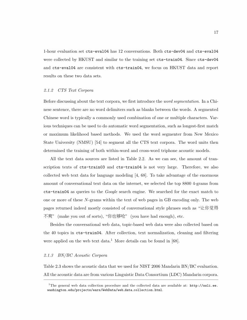
17
1-hour evaluation set cts-eval04 has 12 conversations. Both cts-dev04 and cts-eval04
were collected by HKUST and similar to the training set cts-train04. Since cts-dev04
and cts-eval04 are consistent with cts-train04, we focus on HKUST data and report
results on these two data sets.
2.1.2 CTS Text Corpora
Before discussing about the text corpora, we first introduce the word segmentation. In a Chi-
nese sentence, there are no word delimiters such as blanks between the words. A segmented
Chinese word is typically a commonly used combination of one or multiple characters. Var-
ious techniques can be used to do automatic word segmentation, such as longest-first match
or maximum likelihood based methods. We used the word segmenter from New Mexico
State University (NMSU) [54] to segment all the CTS text corpora. The word units then
determined the training of both within-word and cross-word triphone acoustic models.
All the text data sources are listed in Table 2.2. As we can see, the amount of tran-
scription texts of cts-train03 and cts-train04 is not very large. Therefore, we also
collected web text data for language modeling [4, 68]. To take advantage of the enormous
amount of conversational text data on the internet, we selected the top 8800 4-grams from
cts-train04 as queries to the Google search engine. We searched for the exact match to
one or more of these N -grams within the text of web pages in GB encoding only. The web
pages returned indeed mostly consisted of conversational style phrases such as “t�úz
Xw” (make you out of sorts), “��ê ” (you have had enough), etc.
Besides the conversational web data, topic-based web data were also collected based on
the 40 topics in cts-train04. After collection, text normalization, cleaning and filtering
were applied on the web text data.1 More details can be found in [68].
2.1.3 BN/BC Acoustic Corpora
Table 2.3 shows the acoustic data that we used for NIST 2006 Mandarin BN/BC evaluation.
All the acoustic data are from various Linguistic Data Consortium (LDC) Mandarin corpora.
1The general web data collection procedure and the collected data are available at: http://ssli.ee.
washington.edu/projects/ears/WebData/web data collection.html.

18
Table 2.2: Mandarin CTS text data for language model training.
Source # of Words
cts-train03 479K
cts-train04 398K
conversational web data 100M
topic-based web data 244M
The training data includes several major parts: bn-Hub4, bn-TDT4, bn-Y1Q1, bn-Y1Q2,
bc-Y1Q1 and bc-Y1Q2. The total amount of the training data is around 465 hours of
speech: 313 hours of BN speech and 152 hours of BC speech. The 30 hours of bn-Hub4
data has accurate manual transcriptions and was released for the NIST 2004 evaluation.
The bn-TDT4 data has different sources: CTV, VOA, CNR2 and other sources (e.g. from
Taiwan). Since we focus on mainland accent, only the data from the first three sources
were used. The bn-TDT4 data comes with closed captions, but not accurate transcriptions.
Therefore, we used the flexible alignment algorithm described in [88] to select the segments
with high confidence in the closed captions. After selection, there are in total about 89 hrs
of TDT4 data: 25 hours of CTV, 43 hours of VOA and 21 hours of CNR. The bn-Y1Q1 and
bc-Y1Q1 were the BN and BC data released by LDC in January 2006. The bn-Y1Q2 and
bc-Y1Q2 data were from the second LDC release in May 2006. Both of these releases are for
the Global Autonomous Language Exploitation (GALE) program sponsored by DARPA.
These two batches of data include acoustic waveforms from CCTV4 and PHOENIX sources.
For testing, there are 4 major test sets: 2004 BN development set bn-dev04 (0.5 hour),
2004 BN evaluation set bn-eval04 (1 hour), 2006 BN extended dryrun test set bn-ext06 (1
hour), and the BC development set bc-dev05 (2.7 hours) created by Cambridge University
(CU). All BN/BC training and testing acoustic data were sampled at 16KHz.
2CTV, VOA, CNR and the later mentioned CCTV4, RFA, PHOENIX are all Mandarin broadcast radioor TV stations.
19
Table 2.3: Mandarin BN/BC acoustic data for training and testing.
Type Name Sources Time
BN training data
bn-Hub4 CCTV,VOA,kaznAM 30 hrs
bn-TDT4 CTV,VOA,CNR 89 hrs
bn-Y1Q1 CCTV4,PHOENIX 114 hrs
bn-Y1Q2 CCTV4,PHOENIX 80 hrs
BC training databc-Y1Q1 CCTV4,PHOENIX 76 hrs
bc-Y1Q2 CCTV4,PHOENIX 76 hrs
BN testing data
bn-dev04 CCTV 0.5 hr
bn-eval04 CCTV,RFA,NTDTV 1.0 hr
bn-ext06 PHOENIX 1.0 hr
BC testing data bc-dev05 VOA,PHOENIX 2.7 hrs
2.1.4 BN/BC Text Corpora
Table 2.4 lists all the data using in LM training and development. The TDT data includes
Hub4, TDT2, TDT3, TDT4, Multiple Translation Chinese (MTC) Corpus parts 1, 2 and
3, and the Chinese News Translation corpus. All the text data of TDT4 are used for
LM training, while only those flex-aligned portions are used for AM training. The LDC
GALE text data include all the transcriptions of the Q1 and Q2 GALE acoustic data
listed in Table 2.3, plus the transcription (closed-caption like) of GALE web data. These
data are more similar to speech test data, as they correspond to real speech rather than
written articles exclusively. The Gigaword corpus contains articles from three newswire and
newspaper sources: Central News Agency (CNA) from Taiwan, Xinhua newspaper (XIN)
from China, and Zaobao newspaper (ZBN) from Singapore. The NTU-web data are news
articles and conversation transcriptions downloaded by National Taiwan University from
CCTV, PHOENIX and VOA web sites (dated before February 2006), to cover some of
the sources missing from the LDC GALE data. These data do not necessarily correspond
to speech. Yet they are more like GALE data than the Gigaword corpus, since they are
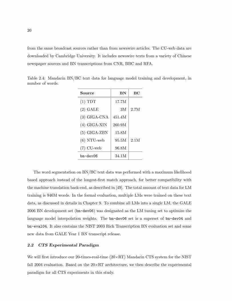
20
from the same broadcast sources rather than from newswire articles. The CU-web data are
downloaded by Cambridge University. It includes newswire texts from a variety of Chinese
newspaper sources and BN transcriptions from CNR, BBC and RFA.
Table 2.4: Mandarin BN/BC text data for language model training and development, innumber of words.
Source BN BC
(1) TDT 17.7M
(2) GALE 3M 2.7M
(3) GIGA-CNA 451.4M
(4) GIGA-XIN 260.9M
(5) GIGA-ZBN 15.8M
(6) NTU-web 95.5M 2.1M
(7) CU-web 96.8M
bn-dev06 34.1M
The word segmentation on BN/BC text data was performed with a maximum likelihood
based approach instead of the longest-first match approach, for better compatibility with
the machine translation back-end, as described in [49]. The total amount of text data for LM
training is 946M words. In the formal evaluation, multiple LMs were trained on these text
data, as discussed in details in Chapter 9. To combine all LMs into a single LM, the GALE
2006 BN development set (bn-dev06) was designated as the LM tuning set to optimize the
language model interpolation weights. The bn-dev06 set is a superset of bn-dev04 and
bn-eval04. It also contains the NIST 2003 Rich Transcription BN evaluation set and some
new data from GALE Year 1 BN transcript release.
2.2 CTS Experimental Paradigm
We will first introduce our 20-times-real-time (20×RT) Mandarin CTS system for the NIST
fall 2004 evaluation. Based on the 20×RT architecture, we then describe the experimental
paradigm for all CTS experiments in this study.

21
2.2.1 Mandarin CTS 20×RT System
In NIST fall 2004 evaluation, University of Washington (UW) has collaborated with SRI
International (SRI) to port the techniques in SRI decipher speech recognition system to
Mandarin Chinese as well as exploring language-specific problems such as tone modeling,
pronunciation modeling and language modeling. An SRI-UW Mandarin CTS recognition
system was developed during January - September 2004.3 The goal was to achieve the lowest
possible CER in Mandarin telephone speech recognition. We first describe the front-end,
then acoustic and language model design, followed by the 20×RT decoding paradigm.
Front-End Processing: The input speech signal is processed using a 25ms Hamming
window, with the frame rate of 10ms. There are two front-ends in our system. One uses the
standard 39-dimensional Mel-scale cepstrum coefficients (MFCCs) and 3-dimensional pitch
features including the 1st and 2nd derivatives. The other uses 39-dimensional Perceptual
Linear Predictive (PLP) coefficients plus the same 3-dimensional pitch features. Mean and
variance normalization (CMN/CVN) is applied to both MFCC/PLP and pitch features
per conversational side. Vocal tract length normalization (VTLN) is also applied in both
front-ends to reduce the variability among speakers [95].
Acoustic Modeling: For phonetic pronunciation, we started from BBN’s 2003 Mandarin
pronunciation dictionary, which was based on the LDC Mandarin pronunciation lexicon.
The dictionary consists of approximately 12,000 words and associated phonetic transcrip-
tions. The BBN dictionary used 83 tonal phones, in addition to 6 non-speech phones to
model silence and other non-speech events. Some improvement was obtained by using a few
simple rules to merge rare phones [47]. The resulting phone set consists of 65 speech phones,
including one silence phone, one for laughter, and one for all other non-speech events. Our
initial system adopts the bottom-up clustered genone models [21]. However, we moved to
decision-tree based state-level parameter sharing [71, 46], primarily due to its better pre-
3This work was in collaboration with Dr. Mei-Yuh Hwang, Tim Ng, Prof. Mari Ostendorf from UW andDr. Wen Wang from SRI. We have used tools in SRI’s decipher speech recognition system to developeour Mandarin system. In the development of this system, the author’s major contributions include theacoustic data segmentation, pitch feature extraction, discriminative acoustic model training and speakeradaptive training.
22
diction in unseen contexts. Modeling of the unseen contexts is especially important for
models using cross-word triphone models. We used 66 linguistic categorical questions and
65 individual toneme and phone questions for the decision-tree based top-down clustering.
Both cts-train03 and cts-train04 are used for acoustic model training. Since the
released gender information of the training data is not reliable, gender-independent models
with VTLN are trained for all acoustic models. Both the MFCC and PLP front-end models
follow the training procedure illustrated in Figure 2.1.
nonCW MLE training
data
SAT transform computation
Feature transformation matrix
CW MLE training
CW MMIE/MPE training
nonCW MMIE/MPE training
Figure 2.1: Flowchart of acoustic model training for evaluation systems.
The within-word (nonCW) models are first trained and then used to train more com-
plicated models. Speaker adaptive training (SAT) is performed to reduce the variance in a
speaker-independent model and thus making the model more discriminative [1, 53]. In prac-
tice, one feature transform per speaker is estimated via single-class constrained maximum
likelihood linear regression (MLLR) [33]. The linear feature transformation is estimated by
maximizing the likelihood of the data. Let xt be the feature vector at time t, the transformed
feature xt is,
xt = A(i)xt + b(i), (2.1)

23
where the linear transformation parameters A(i) and b(i) are trained for each speaker i. To
better model the coarticulation across word boundaries, we also trained cross-word (CW)
triphone models. The CW models are used in lattice rescoring stages, but less expensive
nonCW models are used in stages that generate the lattices.
Discriminative training methods like maximum mutual information estimation (MMIE)
and minimum phone error (MPE) training have been explored in our system. First, the
maximum likelihood estimated (MLE) models are trained. Then we performed MMIE
training on top of the existing MLE model [109]. MPE training was also applied on top
of the MLE model [74]. In our experiments, we have found that MPE models outperform
MMIE models, which outperform the original MLE models, similar to the results reported
by others [74].
Language Modeling: Since the two training corpora were quite different, two different
trigrams are trained based on cts-train03 and cts-train04. Trigram language models
are also trained for the conversational web data and the topic-based web data. Then the
final LM is built by interpolating the four LMs to minimize the perplexity on a held out
set. It is found that the web data significantly improves the system performance [68]. The
final trigram LM is given by
LM3 = 0.04 LM3train03 + 0.64 LM3
train04 + 0.16 LM3cWeb + 0.16 LM3
tWeb (2.2)
where cWeb denotes conversational web data, and tWeb denotes topic-based web data.
20×RT Decoding: The decoding structure used for the formal benchmark evaluation was
based on SRI’s 2004 English CTS 20×RT decoding system. The system architecture is
shown in Figure 2.2. Multiple acoustic models, cross adaptations and confusion network
based system combinations [64] have been used in the system. The total run time of the
system is around 17-times real-time on a machine with a single Pentium 3.2GHz CPU, 4GB
RAM and hyperthreading enabled.
For evaluation, the acoustic segmentation is not provided and therefore an automatic
segmentation is performed using gender-independent Gaussian mixture models (GMMs).
Two GMM models are trained, each with 100 Gaussians of 39-dimensional MFCC cepstra

24
MFCnonCW
Thinlattices
PLPCW
MFCCW
PLPCW
MFCnonCW
MFCCW
PLPCW
20xRTOutput
5xRTOutput
Thicklattices
2.6
1.0
2.1
1.3
0.1
4.9 2.6
0.2
2.1
Decoding/rescoring stepLegend
Hyps for MLLR or outputLattice generation/useLattice or 1-best outputConfusion network combination
Figure 2.2: 20×RT decoding system architecture. The numbers above the square boxes arethe time required for running the specified stage. The unit is real time (RT). MFC and PLPare the two different front-ends. nonCW denotes within-word triphones only. CW denotescross-word triphones.
and deltas: a foreground model for speech and a background model for silence. We keep
0.5 seconds of silence at the beginning and the ending of each utterance segment. After
the acoustic waveforms are segmented, a clustering algorithm based on the mixture weights
of a MFCC-based Gaussian mixture model is used to group all utterances within the same
conversation channel into acoustically homogeneous clusters. Based on these pseudo-speaker
clusters, VTLN and component-wise mean and variance normalization are applied.
In the CTS 20×RT decoding system, three sets of gender-independent acoustic models
(both ML models and MPE models) are used: MFCC within-word triphone models, MFCC
cross-word triphone models and PLP cross-word triphone models. The MFCC nonCW
triphone acoustic model is used to generate word lattices with a bigram language model.
The word lattices are then expanded into more grammar states with trigram scores by a
trigram LM. Finally, three N-best lists are generated from the trigram lattices using three
different adapted acoustic models: MFCC nonCW triphones, MFCC CW triphones, and
PLP CW triphones. The N-best word lists are then combined to generate a character-based

25
confusion network for ROVER [28], to obtain the final recognition result. For more details
about the 20×RT system, the reader can be referred to [85]. The main differences of our
Mandarin system from the SRI English system include: pitch features in the front-end, no
duration modeling, no alternative pronunciations, no SuperARV language modeling4 [94],
no Gaussian short lists for speeding up the decoding, and neither LDA/HLDA nor voicing
features nor ICSI features were used. The performance of the CTS evaluation system is
described in Chapter 9.
2.2.2 Mandarin CTS Experimental Paradigm
As we can see from Figure 2.2, the 20×RT system is very complicated. It takes a very long
time to train the ML and MPE acoustic models on all of the training data and run the full
20×RT decoding template. To evaluate the tone modeling in CTS task more efficiently, we
only use cts-train04 to train ML models and run decoding from the thick lattices of the
20×RT decoding system.
For CTS experiments, we evaluate the improved tone modeling in the feature domain.
The CTS experimental paradigm is shown in the following Procedure 1. This experiment
setup is referred as CTS-EBD experimental paradigm afterwards. In training phase, we train
the new acoustic models with the improved tone features. In decoding phase, we use the new
acoustic models with the same acoustic segmentation and language models. First, we do a
7-class MLLR adaptation on the new models. The adaptation is unsupervised based on the
recognition hypotheses from an earlier pass (5×RT output as shown in Figure 2.2). With
the speaker adapted (SA) models, we then rescore the thick word lattices generated from
the 20×RT system. Since the thick word lattices are of good quality and offer a constrained
search space for the new acoustic models, both good performance and fast speed can be
achieved through this CTS-EBD experimental paradigm.
4SuperARV language model is an almost-parsing language model based on the constraint dependencygrammar formalism.
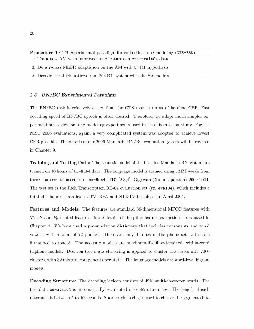
26
Procedure 1 CTS experimental paradigm for embedded tone modeling (CTS-EBD)1: Train new AM with improved tone features on cts-train04 data
2: Do a 7-class MLLR adaptation on the AM with 5×RT hypothesis
3: Decode the thick lattices from 20×RT system with the SA models
2.3 BN/BC Experimental Paradigm
The BN/BC task is relatively easier than the CTS task in terms of baseline CER. Fast
decoding speed of BN/BC speech is often desired. Therefore, we adopt much simpler ex-
periment strategies for tone modeling experiments used in this dissertation study. For the
NIST 2006 evaluations, again, a very complicated system was adopted to achieve lowest
CER possible. The details of our 2006 Mandarin BN/BC evaluation system will be covered
in Chapter 9.
Training and Testing Data: The acoustic model of the baseline Mandarin BN system are
trained on 30 hours of bn-Hub4 data. The language model is trained using 121M words from
three sources: transcripts of bn-Hub4, TDT[2,3,4], Gigaword(Xinhua portion) 2000-2004.
The test set is the Rich Transcription RT-04 evaluation set (bn-eval04), which includes a
total of 1 hour of data from CTV, RFA and NTDTV broadcast in April 2004.
Features and Models: The features are standard 39-dimensional MFCC features with
VTLN and F0 related features. More details of the pitch feature extraction is discussed in
Chapter 4. We have used a pronunciation dictionary that includes consonants and tonal
vowels, with a total of 72 phones. There are only 4 tones in the phone set, with tone
5 mapped to tone 3. The acoustic models are maximum-likelihood-trained, within-word
triphone models. Decision-tree state clustering is applied to cluster the states into 2000
clusters, with 32 mixture components per state. The language models are word-level bigram
models.
Decoding Structure: The decoding lexicon consists of 49K multi-character words. The
test data bn-eval04 is automatically segmented into 565 utterances. The length of each
utterance is between 5 to 10 seconds. Speaker clustering is used to cluster the segments into

27
pseudo-speakers for normalization, as in CTS decoding. In BN task, we have investigated
both embedded tone modeling and explicit tone modeling. The decoding setup for embedded
tone modeling experiments is shown as experimental paradigm BN-EBD in Procedure 2. After
we train the new acoustic models with improved tone features, we do a first-pass decoding
with the speaker independent (SI) model. Using the decoded first-pass hypothesis, we do
a 3-class MLLR adaptation. Fewer classes are used because the amount of speech from a
hypothesized speaker is less than in CTS. Then we use the SA models to decode the data
again.
Procedure 2 BN/BC experimental paradigm for embedded tone modeling (BN-EBD)1: Train new AM with improved tone features on bn-Hub4 data
2: First-pass decoding with the SI model
3: Do a 3-class MLLR adaptation on the SI model with the first-pass hypothesis
4: Decode with the SA models
For explicit tone modeling, we use the decoding setup as shown in Procedure 3. This
experiment setup is referred to as experimental paradigm BN-EPL afterwards. Explicit tone
models are trained and used to rescore the SA lattices generated from the SA decoding.
Procedure 3 BN/BC experimental paradigm for explicit tone modeling (BN-EPL)1: Train explicit tone models on bn-Hub4 data
2: Perform SI decoding with embedded tone modeling
3: Adapt the AM by unsupervised MLLR
4: Use the SA models to decode and generate word lattices
5: Rescore the SA lattices with the explicit tone models
2.4 Summary
In this chapter, we have described all the acoustic and text data that are used in the
Mandarin CTS and BN/BC experiments. We then introduce the experimental paradigms
for CTS task and BN/BC task, respectively. In the more difficult CTS task, to achieve good

28
performance as well as efficiency, we designed the experimental paradigm to be based on a
complicated 20×RT system. The improved acoustic models are adapted first with the output
hypothesis from the 5×RT system, and then used to rescore the word lattices from a late
stage of the 20×RT system. For the relatively easier BN/BC task where faster response is
needed, we designed a simple two-pass decoding paradigm. The improved acoustic models
are used for speaker-independent decoding and the output hypothesis is used for MLLR
adaptation. The adapted models are then used for a second-pass decoding. The word
lattices are generated in the final decoding and further used for rescoring with explicit tone
models.
29
Chapter 3
STUDY OF TONAL PATTERNS IN MANDARIN SPEECH
In continuous Mandarin speech, the F0 contour patterns of lexical tones are much dif-
ferent from their citation forms. In this chapter, we first review some linguistic studies on
tones in continuous Mandarin speech. The questions we try to answer are:
• What linguistic units does a tone align to?
• What are the major sources of tonal variation in connected speech?
• How much do the tonal variation sources affect the F0 contours?
After reviewing the literature, we then perform an empirical study of the tonal patterns
of Mandarin speech in the CTS and BN domains. The goal of this study is to get some un-
derstanding of the linguistic side of tones, and to gain some insight into statistical modeling
of Mandarin tones as described in the later chapters of this dissertation.
3.1 Review of Linguistic Studies
Before we review some related linguistic studies on tones, there are three terms that need
to be distinguished in the context of speech1: fundamental frequency (F0), pitch and tone.
The first term, F0, is an acoustic term referring to the rate of cycling (opening and closing)
of the vocal folds in the larynx during phonation of voiced sounds. The second term, pitch,
is a perceptual term: it is the auditory attribute according to which sounds can be ordered
on a scale from low to high. The existence of F0 differences may not be enough to result in
the perception of pitch differences. However, in many papers, pitch and F0 are often used
interchangeably, as mentioned in Chapter 1. The final term, tone, is a linguistic term. It
1These terms may also be used in some other contexts such as music.

30
refers to a phonological category that distinguishes two words or utterances for languages
where pitch plays some sort of linguistic role. In this dissertation work, we focus on the
lexical tones that distinguish words.
In the following of this section, we will describe four aspects of related linguistic study
on tones: 1) the domain of tone; 2) tone coarticulation; 3) the neutral tone and tone sandhi;
and 4) tone and intonation.
3.1.1 Domain of tone
How the tones and their F0 contours align with other linguistic units in speech is an impor-
tant issue for processing and modeling of F0 contours in speech recognition. At the phonetic
level, there have been many arguments as to whether a tone is carried by the entire syllable
or only a portion of the syllable.
Mandarin syllables have a simple consonant and vowel (CV) structure or consonant,
vowel and nasal (CVN) structure. Early in 1974, Howie [43] reported that tones in Mandarin
are carried by only the syllable rhyme (vowel and nasal), while the portion of the F0 contour
corresponding to an initial voiced consonant or glide is merely an adjustment for the voicing
of initial consonants. He argued that the domain of a tone is limited to the rhyme of the
syllable because there is much F0 perturbation in the early portion of a syllable due to the
initial consonant. In 1995, Lin [61] also argued that neither initial consonants and glides
nor final nasals play any tone-carrying role in Mandarin.
However, more recently in [104], Xu has found experimentally that the implementation
of each tone in a tone sequence always starts from the onset of the syllable and proceeds
until the end of the syllable. He found the F0 contour during the entire syllable is contin-
uously approaching the most ideal contour for the corresponding lexical tone. The large
perturbation in the early portion of the F0 contour is due to both the initial consonant and
the coarticulation influence of the preceding tone. He also confirmed that the tone-syllable
alignment is consistent across different syllable structures (CV or CVN) and speaking rates
(slow, normal or fast). Therefore Xu argued that syllable is the reference domain for tone
alignment.
31
In Mandarin tone modeling, what segmental unit that tone aligns with determines the
region to extract tone features. While most previous studies on Mandarin tone modeling
adopt the syllable final for extracting tone features, in contrast to Xu’s finding, this may be
partly because in syllables with unvoiced consonants, the F0 is not defined for the unvoiced
region and partly due to tone coarticulation. To deal with the unvoiced regions, we develop
a spline interpolation technique in Chapter 4 to interpolate the F0 contour in order to
approximate the coarticulation of tones. In this way, the F0 features for explicit tone
modeling can be extracted from the syllable level consistently, which facilitates automatic
recognition since categories are more separable when the data is less noisy.
3.1.2 Tone coarticulation
When the Mandarin tones are produced in isolation, their F0 contours seem quite stable
and correspond well with the canonical patterns. However, when the tones are produced
in context, the tonal contours undergo variations depending on the preceding and following
tones [8, 103]. The coarticulation effect from the preceding tone is called the carry-over
effect and the coarticulation effect from the following tone is called the anticipatory effect.
In 1990, Shen [80] analyzed all possible Mandarin tri-tonal combinations on the “ba ba
ba” sequence embedded in a carrier sentence. She found both carry-over and anticipatory
effects exist, and that the bi-directional effects are symmetric and assimilatory in nature.
However, Xu [103] studied the F0 contours of bi-tonal combinations on the “ma ma” se-
quence embedded in a number of carrier sentences and had somewhat different findings.
He found the most apparent influence is from the preceding tone rather than the following
tone, i.e. the carry-over effect is much more significant than anticipatory effects in terms of
magnitude. In addition, he found that the carry-over effects and anticipatory effects are due
to different mechanisms: carry-over effects are mostly assimilatory, e.g. the onset F0 value
of a tone is assimilated to the offset value of the previous tone; but anticipatory effects are
mostly dissimilatory, e.g. a low onset F0 value of a tone raises the F0 of the preceding tone.
Since both of these two studies are based on relatively small databases, the discrepancies
of the findings are probably due to the insufficient data. In [90] Wang conducted an empirical

32
study of tone coarticulation using a larger Mandarin digit corpus. She had similar findings
to Xu’s observations: carry-over effects are more significant in magnitude and assimilatory
in nature; anticipatory effects are more complex with both assimilatory and dissimilatory
effects. In this work, we will further study the tonal patterns and coarticulation effects in
more natural Mandarin broadcast news and conversational speech corpora.
3.1.3 Neutral tone and tone sandhi
Besides the four citation tones, there exists a toneless neutral tone in connected Chinese
speech [8]. The syllables with neutral tones are substantially shorter than toned syllables
and show all the symptoms of being unstressed [107]. They are mainly affixes or non-initial
sylables of some bisyllabic words. They either are inherently toneless or may lose their own
tones depending on the context. For example, the suffix “{”(de) used to mark possessives
has no tone of its own in any context. In some reduplicated forms, like “��”(jie3 jie,
elder sister), the second syllable loses its tone. The general consensus is that there are no
phonological (categorical) specifications for the neutral tone and its F0 contour pattern is
completely dependent on the context tones.
In addition to the neutral tone, there are several other special situations called tone
sandhi where the basic tone is modified. Tone sandhi refers to the tone category change
when several tones are pronounced together. Sandhi comes from Sanskrit2 and means
”putting together”. The tone sandhi effect is different from the tone coarticulation effects
in that it involves a phonological change of the intended tone category.
There are three well-cited sandhi rules in Mandarin [8]. The most well-known rule is
the third-tone-sandhi rule, which states that the leading syllable in a set of two third-tone
syllables is raised to the second tone. For example, the most common Chinese greeting
“�P”(ni3 hao3, how are you) is pronounced as “ni2 hao3”. However, when there are
more than two contiguous third tones, the third-tone-sandhi becomes quite complicated and
the expression of the rule is found to depend on the prosodic structure rather than on the
syntax [82].
2Sanskrit is the classical literary language of India.

33
The second common sandhi rule also relates to the third tone: when a third tone syllable
is followed by a syllable with a tone other than third tone, it changes to a new tone with
the pitch contour 21 using the scale in Figure 1.3. This is called the ”half third tone” in [8].
Different from the third tone, the half third tone dips during the syllable but never rises.
For example, in the word “i°”(hen3 gao1, very tall) the first syllable changes to a half
third tone.
The third sandhi rule is concerned with tone 2 (rising tone): in a 3 syllable string, when
a tone 2 syllable is preceded by a tone 1 or 2 and followed by any tone other than the neutral
tone, the 2nd syllable changes to tone 1. For example, the word “®#ÿ”(san1 nian2 ji2,
the third grade) is pronounced as “san1 nian1 ji2”. This tone sandhi rule is somewhat
debatable. Some linguistic researchers have found that most of the rising tones after a
tone 1 are still perceived as the rising tone, although the F0 contours are flattened [81, 102].
Therefore, there is an argument that this phenomenon is actually due to tone coarticulation,
instead of a phonological change as in tone sandhi.
There are also some other more complicated tone sandhi rules in connected Mandarin
speech, but this is beyond the scope of our study. To model the tone coarticulation and
tone sandhi effects, we have used context-dependent tone models in this dissertation study,
as discussed in Chapter 7 and Chapter 8. Some phonological changes of neutral tone and
tone sandhi are also encoded directly in the lexicon as the surface form pronunciations.
3.1.4 Tone and intonation
While lexical tones use F0 to distinguish between words, intonation uses F0 to convey
discourse structure and intent that are separate from the meanings of the words in the spoken
utterances. Because the same acoustic parameter F0 is being used, tone and intonation will
inevitably interact with each other. A study was conducted in [79] by Shen to investigate if
intonation can change the F0 contour of lexical tones to beyond recognition. She observed
that intonation perturbs the F0 values of the lexical tones, e.g. interrogative intonation raises
the F0 value of the sentence-final syllable as well as the overall pitch level. Nevertheless,
the basic F0 contour shape of lexical tones remain intact.

34
Two important phenomena in intonation study are: downstep and declination. Downstep
refers to the phenomenon that in a HLH sequence3, the second H has a lower F0 level than
the first. Declination refers to the tendency for F0 to gradually decline over the course of an
utterance. Declination is also known as an overall F0 downtrend. Downstep and declination
phenomena occur in both tone and non-tone languages. Prieto et al. [75] suggests that
declination is probably equivalent to a series of of downsteps. In [105] Xu also argues that
downstep is probably due to the combined effects of anticipatory variation and carry-over
variation, and that declination may be due to the combined effects of downstep, sentence
focus and new topic initiation.
Overall, intonation is mainly associated with long-term trends of F0. While there are
some local effect from intonation, the lexical tones are primarily responsible for determin-
ing the local F0 contours. Since the intonation does not carry any lexical information, it
should be normalized out for ASR purposes. We will discuss the decomposition of utter-
ance F0 contour via wavelets analysis and other normalization methods for extracting more
meaningful lexical tone features in Chapter 4.
3.2 Comparative Study of Tonal Patterns in CTS and BN
As described in the review of linguistic studies, the tonal F0 contour patterns are influenced
by different sorts of variations in connected speech. While most previous studies were done
on short tone sequences, Wang [90] also conducted empirical studies of tonal patterns on
small read and spontaneous corpora. In this section we perform a similar comparative study
of mean patterns of tones in Mandarin CTS and BN domains. We are mainly concerned
about the tone coarticulation effects and how much they differ in CTS and BN speech.
For this study, we have interpolated the F0 contour with splines to approximately recover
the full syllable pitch pattern. Details of the spline interpolation are in Chapter 4. For
comparison with the previous work [90], no F0 normalization is performed.
3Here we use H for high pitch target, L for low pitch target.
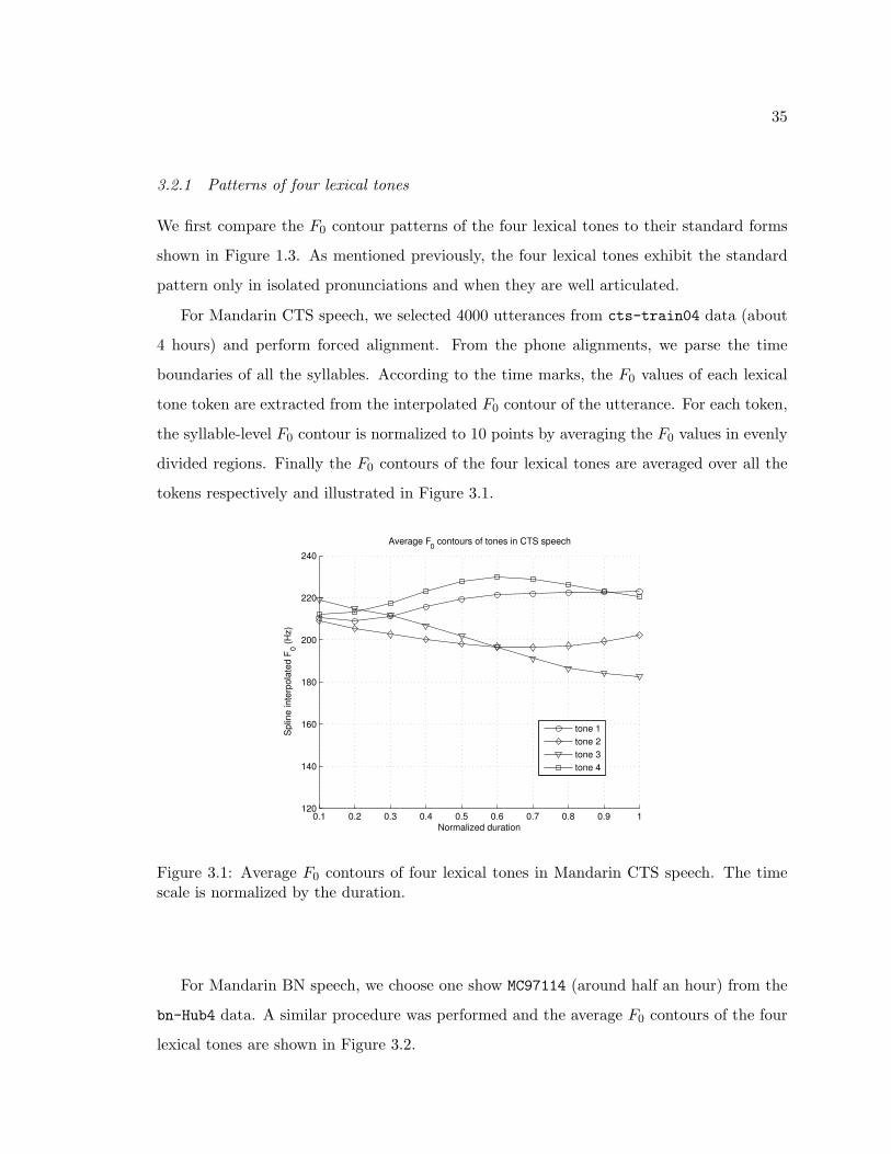
35
3.2.1 Patterns of four lexical tones
We first compare the F0 contour patterns of the four lexical tones to their standard forms
shown in Figure 1.3. As mentioned previously, the four lexical tones exhibit the standard
pattern only in isolated pronunciations and when they are well articulated.
For Mandarin CTS speech, we selected 4000 utterances from cts-train04 data (about
4 hours) and perform forced alignment. From the phone alignments, we parse the time
boundaries of all the syllables. According to the time marks, the F0 values of each lexical
tone token are extracted from the interpolated F0 contour of the utterance. For each token,
the syllable-level F0 contour is normalized to 10 points by averaging the F0 values in evenly
divided regions. Finally the F0 contours of the four lexical tones are averaged over all the
tokens respectively and illustrated in Figure 3.1.
0.1 0.2 0.3 0.4 0.5 0.6 0.7 0.8 0.9 1120
140
160
180
200
220
240
Normalized duration
Spl
ine
inte
rpol
ated
F0 (H
z)
Average F0 contours of tones in CTS speech
tone 1tone 2tone 3tone 4
Figure 3.1: Average F0 contours of four lexical tones in Mandarin CTS speech. The timescale is normalized by the duration.
For Mandarin BN speech, we choose one show MC97114 (around half an hour) from the
bn-Hub4 data. A similar procedure was performed and the average F0 contours of the four
lexical tones are shown in Figure 3.2.

36
0.1 0.2 0.3 0.4 0.5 0.6 0.7 0.8 0.9 1120
140
160
180
200
220
240
Normalized duration
Spl
ine
inte
rpol
ated
F0 (H
z)
Average F0 contours of tones in BN speech
tone 1tone 2tone 3tone 4
Figure 3.2: Average F0 contours of four lexical tones in Mandarin BN speech. The timescale is normalized by the duration.
Comparing the lexical tonal patterns in Figure 3.1 and Figure 3.2, we have the following
findings:
• Similarities
The lexical tonal patterns in both CTS and BN cases are significantly different from
their standard patterns in Figure 1.3 but they share several similarities. First of all,
especially in the early region of the F0 contours, all four tones seem to start from
around the same pitch level. This can be explained by the strong influence of the
carry-over effect from the left context. Since the onset of the F0 contour depends on
its left tone context, after averaging all the possible left contexts the onset is close
to the mean of the offset of the previous tone. On the other hand, the offsets of the
contours ends at different levels. This confirms that the coarticulation effect from the
right context (usually anticipatory) is not very significant and the four tonal patterns
still keep their own offset values. Second, in most cases, the latter half of a tone
contour pattern looks more like its corresponding standard pattern. It is much easier

37
to tell the tonal patterns from the relative pitch levels and derivatives of the latter half
of the contours in both CTS and BN. The first half captures more of the coarticulation
effects. Third, in particular, the third tone in both cases shows no symptoms of rising
after dipping like its standard pattern shown in Figure 1.3. This can be explained by
the second tone sandhi rule introduced in the previous section: except when followed
by another third tone, the current third tone will change to a “half third tone” without
rising. Since a majority of the third tone cases are followed by a non-third tone, the
averaged contour of third tone exhibits a pattern of no rising.
• Dissimilarities
There are also some dissimilarities between the CTS and BN tonal patterns. Note
that we did not encode the third-tone-sandhi in the CTS lexicon, but we encode most
of the within-word third-tone-sandhi in the BN lexicon. This means that the tone 3
contour in Figure 3.1 was computed with both instances of tone 3 and some instances
of tone 2, causing the tone 3 contour to be lifted towards tone 2 contour slightly. The
most obvious difference is that the range of the tonal patterns in BN speech seems
to be much larger than that of the CTS speech. This might suggest that the tones
are better articulated and there is less reduction in tone articulation in BN speech.
Since CTS speech is more spontaneous than BN speech, this difference is reasonable.
Another dissimilarity is: the offset of tone 4 in CTS is almost in high pitch level
instead of low as in its standard pattern. It might also be explained by the reduction
in articulation that tone 4 cannot reach its underlying pitch targets in CTS. These
differences suggest that the tone modeling in CTS speech could be more difficult than
in BN speech.
3.2.2 Tone coarticulation effects
To further study the tone coarticulation effects, for each lexical tone, we compare its tone
contour in different left and right tone contexts together. Figure 3.3 shows the average
F0 contour comparisons in Mandarin CTS speech. Figure 3.4 shows the comparisons in
Mandarin BN speech. In both cases the onset of the pitch contours is more dependent on
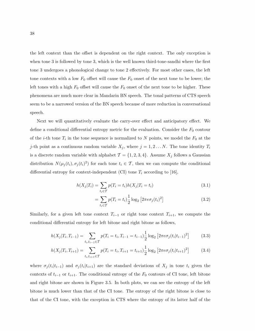
38
the left context than the offset is dependent on the right context. The only exception is
when tone 3 is followed by tone 3, which is the well known third-tone-sandhi where the first
tone 3 undergoes a phonological change to tone 2 effectively. For most other cases, the left
tone contexts with a low F0 offset will cause the F0 onset of the next tone to be lower; the
left tones with a high F0 offset will cause the F0 onset of the next tone to be higher. These
phenomena are much more clear in Mandarin BN speech. The tonal patterns of CTS speech
seem to be a narrowed version of the BN speech because of more reduction in conversational
speech.
Next we will quantitatively evaluate the carry-over effect and anticipatory effect. We
define a conditional differential entropy metric for the evaluation. Consider the F0 contour
of the i-th tone Ti in the tone sequence is normalized to N points, we model the F0 at the
j-th point as a continuous random variable Xj , where j = 1, 2 . . . N . The tone identity Ti
is a discrete random variable with alphabet T = {1, 2, 3, 4}. Assume Xj follows a Gaussian
distribution N(µj(ti), σj(ti)2) for each tone ti ∈ T , then we can compute the conditional
differential entropy for context-independent (CI) tone Ti according to [16],
h(Xj |Ti) =∑ti∈T
p(Ti = ti)h(Xj |Ti = ti) (3.1)
=∑ti∈T
p(Ti = ti)12
log2
[2πeσj(ti)2
](3.2)
Similarly, for a given left tone context Ti−1 or right tone context Ti+1, we compute the
conditional differential entropy for left bitone and right bitone as follows,
h(Xj |Ti, Ti−1) =∑
ti,ti−1∈Tp(Ti = ti, Ti−1 = ti−1)
12
log2
[2πeσj(ti|ti−1)2
](3.3)
h(Xj |Ti, Ti+1) =∑
ti,ti+1∈Tp(Ti = ti, Ti+1 = ti+1)
12
log2
[2πeσj(ti|ti+1)2
](3.4)
where σj(ti|ti−1) and σj(ti|ti+1) are the standard deviations of Xj in tone ti given the
contexts of ti−1 or ti+1. The conditional entropy of the F0 contours of CI tone, left bitone
and right bitone are shown in Figure 3.5. In both plots, we can see the entropy of the left
bitone is much lower than that of the CI tone. The entropy of the right bitone is close to
that of the CI tone, with the exception in CTS where the entropy of its latter half of the

39
contour is significantly lowered. This might be explained by the tone sandhi effect: we did
not encode the tone sandhi in the CTS lexicon, but we encode most of the within-word tone
sandhi in the BN lexicon. In addition, the entropy in BN speech is much higher than CTS
speech, which is probably due to the larger dynamic range of F0 distribution in BN.
3.3 Summary
In this chapter, we first had a literature review of linguistic studies on Mandarin tones. In
early work, tone was thought to be aligned with syllable final, but more recent linguistic
research on Mandarin tones have suggested the tone is aligned with the full syllable instead
of the final. Many tone variations in connected speech have been found, such as tone
coarticulation, neutral tone, tone sandhi and intonation effects. It was found that the
carry-over effect from the left tone context is much more significant than the anticipatory
effect from the right context. Then we did an empirical study of tonal patterns in Mandarin
CTS and BN speech. We confirmed that there is tone coarticulation information from the
F0 contour of the full syllable. We qualitatively and quantitatively evaluate the difference
of tone coarticulation effects in both domains. Our findings in CTS and BN domains are
consistent with the past work: carry-over effect is much more significant than anticipatory
effect. We also confirmed that there are more tone coarticulation and reduction in CTS
speech than in BN speech, which suggests tone modeling in CTS speech might be more
difficult.

40
0.1 0.2 0.3 0.4 0.5 0.6 0.7 0.8 0.9120
140
160
180
200
220
240
Normalized duration
Spl
ine
inte
rpol
ated
F0 (H
z)
Average F0 contours of tone 1 in different right contexts
tone 1tone 2tone 3tone 4
0.1 0.2 0.3 0.4 0.5 0.6 0.7 0.8 0.9120
140
160
180
200
220
240
Normalized duration
Spl
ine
inte
rpol
ated
F0 (H
z)
Average F0 contours of tone 1 in different left contexts
tone 1tone 2tone 3tone 4
0.1 0.2 0.3 0.4 0.5 0.6 0.7 0.8 0.9120
140
160
180
200
220
240
Normalized duration
Spl
ine
inte
rpol
ated
F0 (H
z)
Average F0 contours of tone 2 in different right contexts
tone 1tone 2tone 3tone 4
0.1 0.2 0.3 0.4 0.5 0.6 0.7 0.8 0.9120
140
160
180
200
220
240
Normalized duration
Spl
ine
inte
rpol
ated
F0 (H
z)
Average F0 contours of tone 2 in different left contexts
tone 1tone 2tone 3tone 4
0.1 0.2 0.3 0.4 0.5 0.6 0.7 0.8 0.9120
140
160
180
200
220
240
Normalized duration
Spl
ine
inte
rpol
ated
F0 (H
z)
Average F0 contours of tone 3 in different right contexts
tone 1tone 2tone 3tone 4
0.1 0.2 0.3 0.4 0.5 0.6 0.7 0.8 0.9120
140
160
180
200
220
240
Normalized duration
Spl
ine
inte
rpol
ated
F0 (H
z)
Average F0 contours of tone 3 in different left contexts
tone 1tone 2tone 3tone 4
0.1 0.2 0.3 0.4 0.5 0.6 0.7 0.8 0.9120
140
160
180
200
220
240
Normalized duration
Spl
ine
inte
rpol
ated
F0 (H
z)
Average F0 contours of tone 4 in different right contexts
tone 1tone 2tone 3tone 4
0.1 0.2 0.3 0.4 0.5 0.6 0.7 0.8 0.9120
140
160
180
200
220
240
Normalized duration
Spl
ine
inte
rpol
ated
F0 (H
z)
Average F0 contours of tone 4 in different left contexts
tone 1tone 2tone 3tone 4
Figure 3.3: Average F0 contours of four lexical tones in different left and right tone contextsin Mandarin CTS speech.

41
0.1 0.2 0.3 0.4 0.5 0.6 0.7 0.8 0.9120
140
160
180
200
220
240
Normalized duration
Spl
ine
inte
rpol
ated
F0 (H
z)
Average F0 contours of tone 1 in different right contexts
tone 1tone 2tone 3tone 4
0.1 0.2 0.3 0.4 0.5 0.6 0.7 0.8 0.9120
140
160
180
200
220
240
Normalized duration
Spl
ine
inte
rpol
ated
F0 (H
z)
Average F0 contours of tone 1 in different left contexts
tone 1tone 2tone 3tone 4
0.1 0.2 0.3 0.4 0.5 0.6 0.7 0.8 0.9120
140
160
180
200
220
240
Normalized duration
Spl
ine
inte
rpol
ated
F0 (H
z)
Average F0 contours of tone 2 in different right contexts
tone 1tone 2tone 3tone 4
0.1 0.2 0.3 0.4 0.5 0.6 0.7 0.8 0.9120
140
160
180
200
220
240
Normalized duration
Spl
ine
inte
rpol
ated
F0 (H
z)
Average F0 contours of tone 2 in different left contexts
tone 1tone 2tone 3tone 4
0.1 0.2 0.3 0.4 0.5 0.6 0.7 0.8 0.9120
140
160
180
200
220
240
Normalized duration
Spl
ine
inte
rpol
ated
F0 (H
z)
Average F0 contours of tone 3 in different right contexts
tone 1tone 2tone 3tone 4
0.1 0.2 0.3 0.4 0.5 0.6 0.7 0.8 0.9120
140
160
180
200
220
240
Normalized duration
Spl
ine
inte
rpol
ated
F0 (H
z)
Average F0 contours of tone 3 in different left contexts
tone 1tone 2tone 3tone 4
0.1 0.2 0.3 0.4 0.5 0.6 0.7 0.8 0.9120
140
160
180
200
220
240
Normalized duration
Spl
ine
inte
rpol
ated
F0 (H
z)
Average F0 contours of tone 4 in different right contexts
tone 1tone 2tone 3tone 4
0.1 0.2 0.3 0.4 0.5 0.6 0.7 0.8 0.9120
140
160
180
200
220
240
Normalized duration
Spl
ine
inte
rpol
ated
F0 (H
z)
Average F0 contours of tone 4 in different left contexts
tone 1tone 2tone 3tone 4
Figure 3.4: Average F0 contours of four lexical tones in different left and right tone contextsin Mandarin BN speech.
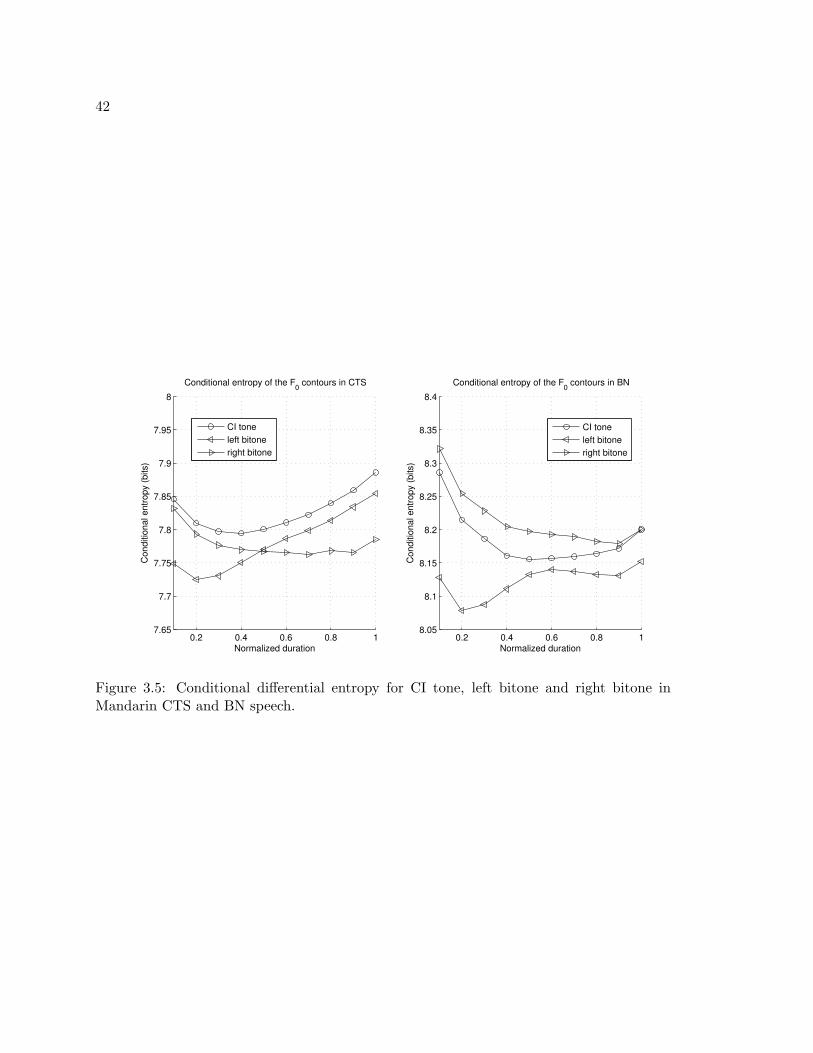
42
0.2 0.4 0.6 0.8 17.65
7.7
7.75
7.8
7.85
7.9
7.95
8
Conditional entropy of the F0 contours in CTS
Normalized duration
Con
ditio
nal e
ntro
py (b
its)
CI toneleft bitoneright bitone
0.2 0.4 0.6 0.8 18.05
8.1
8.15
8.2
8.25
8.3
8.35
8.4
Conditional entropy of the F0 contours in BN
Normalized duration
Con
ditio
nal e
ntro
py (b
its)
CI toneleft bitoneright bitone
Figure 3.5: Conditional differential entropy for CI tone, left bitone and right bitone inMandarin CTS and BN speech.

43
PART II
EMBEDDED TONE MODELING
The second part of the dissertation is concerned with embedded tone modeling. In
embedded tone modeling, tonal acoustic units are used and tone features are appended to
the original spectral feature vector as the new feature for the HMM-based modeling. A
fixed-window is used to extract F0-related tone features.
In Chapter 4, more effective pitch features are explored. A spline interpolation algorithm
is proposed for continuation of the F0 contour. Wavelet-based analysis is performed on the
interpolated contour and an effective F0 normalization algorithm is presented. In Chapter
5, we increase the length of the feature extraction window to generate more effective tone-
related features with MLPs. Both tone posteriors and toneme posteriors are investigated. In
Chapter 6, multi-stream adaptation of Mandarin acoustic models is pursued. The spectral
feature stream and tone feature stream are adapted with different regression class trees.
This offers more flexibility for adaptation of multiple streams of different natures.

44
Chapter 4
EMBEDDED TONE MODELING WITH IMPROVED PITCHFEATURES
There have been a lot of studies on both embedded and explicit tone modeling in Man-
darin speech recognition in the past. In embedded tone modeling, the sub-syllabic acoustic
units and the tones are jointly modeled whereas in explicit tone modeling they are mod-
eled separately. Especially in the past ten years, the embedded tone modeling approach
has gained popularity due to its good performance and convenience of porting from an
established English LVCSR system. In this study, we have built our baseline system with
embedded tone modeling. In embedded tone modeling, tonal acoustic units are used and the
F0 related pitch features are appended to the spectral feature vector. The selection of tonal
acoustic units and extraction of effective pitch features are the main issues in embedded
tone modeling.
Based on the concept that the syllable is the domain of tone, we propose a novel spline
interpolation algorithm for F0 continuation. The spline interpolation of F0 contour not
only alleviates the variance problem1 in embedded tone modeling, but also enables us to
extract consistent syllable-level pitch contours for explicit tone modeling in latter part of this
dissertation. Then we decompose the spline interpolated F0 contour by wavelet analysis and
show that different scales correspond to different levels of variation. Inspired by the wavelet
decomposition, we propose an empirical normalization method that is less computationally
expensive. Experimental results reveal that the new pitch feature processing algorithm
improves the Mandarin ASR performance significantly.
In the remaining part of this chapter, we review the past work on embedded tone mod-
eling in Section 4.1. In Section 4.2, we describe the tonal acoustic units and baseline pitch
features used in our system. Then in Section 4.3, we propose the spline smoothing of the
1If we use 0’s or other constants as the F0 values in unvoiced regions, very small variances of acousticmodels will be caused and the system performance will be significantly degraded.
45
pitch contour. In Section 4.4, the wavelet analysis is presented. In Section 4.5, the empirical
pitch feature normalization algorithm is described. In Section 4.6, experiments are carried
out to show the effectiveness of the improved pitch features. Finally in Section 4.7, we
conclude and summarize our embedded tone modeling work.
4.1 Related Research
For embedded tone modeling, we will describe past studies in terms of two aspects: acoustic
unit selection and tone feature extraction. Most earlier Mandarin ASR systems have used
sub-syllabic initial and final as basic acoustic units [60, 62]. The typical inventory of initials
and finals are listed in Table 4.1. Liu et al. [62] tried both toneless and toned finals on
a Mandarin CTS task and and found improved performance with initial and toned final
acoustic units. The authors in [100] compared the performance of different acoustic units:
syllables, initials and finals, context-independent phones, and context-dependent phones
(diphones or triphones). They found the best performance is achieved with the generalized
triphone system on a dictation task. The authors argued that the triphone units can bet-
ter model the coarticulation effects in continuous speech. However, in their work, toneless
phones were used and only syllable recognition was performed. In 1997, Chen et al. [10] from
IBM proposed to associate the tone with only the latter part of the final and decompose
the syllable into a preme and a toneme2. Later in 2001, Chen [11] proposed another way
to associate the tone with the main vowel of the final. Both methods significantly reduce
the number of toned acoustic units and achieved improved ASR performance. To further
reduce the size of toned acoustic units, researchers from Microsoft Research Asia proposed
to quantize the pitch onset and offset into 3 levels (high/low/middle) [44]. A similar quan-
tization strategy was used in [111] to model tone coarticulation by designing a new phone
set.
On the tone feature side for embedded tone modeling, the most intuitive way is to
use F0 and its deltas as features, since F0 is the most prominent acoustic cue for lexical
tones. However, to use F0 as one of the acoustic features, special treatment is required.
2A preme is a combination of the initial consonant with the glide if it exists. A toneme is a phonemeassociated with a specific tone in a tone language.

46
Table 4.1: The 22 syllable initials and 38 finals in Mandarin. In the list of initials, NULLmeans no initial. In the list of finals, (z)i denotes the final in /zi/, /ci/, /si/; (zh)i denotesthe final in /zhi/, /chi/, /shi/, /ri/.
Category Units
Initials b, p, m, f, d, t, n, l, g, k, h, j, q, x, zh, ch, sh, r, z, c, s, NULL
Finals
a, ai, an, ang, ao, e, ei, en, eng, er, i, (z)i, (zh)i, ia, ian, iang,
iao, ie, in, ing, iong, iu, o, ong, ou, u, ua, uai, uan, uang, ueng,
ui, un, uo, u, uan, ue, un
According to general understanding, F0 is not defined for unvoiced regions. Setting the
F0 values of unvoiced frames to 0 or a constant will result in very large derivatives at the
boundaries of unvoiced and voiced segments, and derivatives of 0 in unvoiced regions. This
typically brings serious variance problems in acoustic modeling. Some research has shown
that directly adding the extracted pitch track into the feature vector in this way brings
no accuracy improvement [6]. To solve this problem, an F0 continuation algorithm was
proposed in [10]. Chang in [6] proposed an empirical F0 smoothing algorithm for online
purposes. To compensate for the sentence intonation effects, the author of [90] computed
the mean of sentence F0 contour and subtracted it from the F0 features. A long-term pitch
normalization (LPN) method was proposed [45] to subtract the moving average of the F0 to
normalize the speaker and phrase effects. A similar F0 normalization method called moving
window normalization (MWN) was adopted in [55] for Cantonese speech recognition.
In our state-of-the-art Mandarin CTS system in recent NIST 2004 evaluation, the toneme
based tonal phone set and IBM-style smoothing similar to [10] have been adopted. In the
next section, we will discuss the details about the embedded tone modeling in our baseline
system, which achieves very good performance [48].
47
4.2 Tonal Acoustic Units and Pitch Features
4.2.1 Acoustic units
The acoustic inventory of our Mandarin systems are based on the main vowel idea in [11].
Our CTS phone set is shown in Table 4.2. We started with BBN’s tonal pronunciation phone
set and mapped some rare phones to common phones to make them more trainable [47]. For
example, both /(z)i/ and /(zh)i/ in Table 4.1 are mapped to /i/. Besides this pronunciation
phone set of 62 phones, we included 3 additional phones to model the nonspeech sounds:
silence, noise and laughter. Some common neutral tones (tone 5) are encoded in the CTS
lexicon.
Table 4.2: Phone set in our 2004 Mandarin CTS speech recognition system. ‘sp’ is thephone model for silence; ‘lau’ is for laughter; ‘rej’ is for noise. The numbers 1-5 denote thetone of the phone.
Category Units
Non-tonal phonessp, C, S, W, Z, b, c, d, f, g, h, j, k, l, lau, m, n, p, q, r,
rej, s, t, w, x, y, z
Tonemes
E1, E2, E3, E4, EE1, EE2, EE3, EE4, EE5, N1, N2,
N3, N4, N5, R2, R4, a1, a2, a3, a4, a5, ey1, ey2, ey3,
ey4, i1, i2, i3, i4, o1, o2, o3, o4, o5, u1, u2, u3, u4
In our Mandarin BN system for NIST 2006 evaluation, we also used a phone set modified
from BBN’s BN phone set. The phone set has 72 phones as shown in Table 4.3. In the
BBN dictionary, the neutral tones are mapped to tone 3. The pronunciations of the initials
and finals in terms of our CTS and BN phone set are attached in Appendix A.
4.2.2 Pitch features
In our baseline systems, we have used a pitch feature smoothing algorithm similar to
IBM [10] with the first and second derivatives. The diagram for generating the baseline
pitch features is shown in Figure 4.1.

48
Table 4.3: Phone set in our 2006 Mandarin BN speech recognition system. ‘sp’ is the phonemodel for silence; ‘rej’ is for noise. The numbers 1-4 denote the tone of the phone.
Category Units
Non-tonal phonessp, N, NG, W, Y, b, c, ch, d, f, g, h, rej, j, k, l, m, n,
p, q, r, s, sh, t, v, w, x, y, z, zh
Tonemes
A1, A2, A3, A4, E1, E2, E3, E4, I1, I3, I4, IH1, IH2, IH3,
IH4, a1, a2, a3, a4, e1, e2, e3, e4, er2, er3, er4, i1, i2, i3,
i4, o1, o2, o3, o4, u1, u2, u3, u4, yu1, yu2, yu3, yu4
ESPS get_f0
input wav SRI robust pitch filtering
wav average + random noise forunvoiced/silence pitch
Compute log pitch
Low-pass filtering∆ + ∆∆
Mean/Variance normalization per speaker
output pitch features
IBM-style smoothing
Figure 4.1: Diagram of baseline pitch feature generation with IBM-style pitch smoothing.
The F0 is extracted with ESPS pitch tracker get f0 [25]. Then it is processed by SRI’s
robust pitch filter graphtrack, which uses a log-normal tied mixture model to eliminate
halving and doubling errors [83], followed by a median filter for smoothing. Since pitch
values are only defined for voiced frames, we then smooth the F0 contour similar to [10].
Specifically, the pitch feature is computed as:
pt =
ln (pt) if voiced at t;
ln (pt + 0.1 · r) if unvoiced or silence at t.(4.1)
where pt is the pitch at time t, pt is the utterance mean of the voiced pitch, r is a random
number between 0 and 1. Then this pitch feature pt is smoothed with a low-pass moving

49
average filter which simply computes the average of the 5-point context window. After the
smoothing by the moving average filter, we compute the derivative of the pitch feature using
a standard regression formula over a ±2 frame window. In the beginning and the end of the
utterance, the first or the last pitch feature value is replicated for computing the derivatives.
The double derivative of the pitch feature is computed in the same fashion. Finally, the
3-dimensional pitch features are mean and variance normalized per speaker and appended
to the standard 39-dimensional MFCC/ PLP features, resulting in a 42-dimensional feature
vector for acoustic modeling.
4.3 Spline Interpolation of Pitch Contour
Although the IBM-style pitch continuation algorithm alleviates the variance problem in
modeling and gives improved ASR performance, it might not be optimal to use the same
waveform average F0 for all the unvoiced regions in the utterance. Inspired by the spline
modeling of F0 contours for speech coding and synthesis [41], we explored interpolating the
pitch contour with spline polynomials. The spline-interpolated pitch contour also alleviates
the variance problem. Furthermore, it can approximate the F0 coarticulation during the
unvoiced consonants to some extent, which enables us to extract consistent pitch contours
at the syllable level (the domain of tone, as discussed in Chapter 3). Finally the spline inter-
polation is more amenable to the wavelet decomposition and moving window normalization
described in the next two sections.
We have used the piecewise cubic Hermite interpolating polynomial (PCHIP) [29] for
spline smoothing. This method preserves monotonicity and the shape of the data. Com-
pared with the general cubic spline interpolation, PCHIP spline interpolation has no over-
shoots and less oscillation if the data are not smooth. An implementation of PCHIP inter-
polation from the open source package octave-forge3 [23] was used in this work.
A comparison of IBM-style smoothing and spline interpolation of pitch contours is illus-
trated in Figure 4.2. To compare with the original F0 contour, we have omitted the step
of taking the log. As we can see from Figure 4.2, the spline interpolation preserves the
3http://octave.sf.net

50
0.2 0.4 0.6 0.8 1 1.2 1.40
50
100
150
200
250
300
time (sec)
F 0 (Hz)
IBM−style F0 smoothing
fu2 he2 zhong1 mei3 liang3 guo2 gen1 ben3 li4 yi4
0.2 0.4 0.6 0.8 1 1.2 1.40
50
100
150
200
250
300
time (sec)
F 0 (Hz)
Spline F0 interpolation
Figure 4.2: IBM-style smoothing vs. spline interpolation of F0 contours. The black solidline is the original F0 contour. The red dashed lines are the interpolated F0 contours. Thetext on the top of upper plot are the tonal syllables. The blue dotted vertical lines showthe automatically aligned syllable boundaries.
shape of the F0 contour, while some artifacts are introduced in the IBM-style smoothing.
For example, in the second syllable “he2” and the third syllable “zhong1”, the earlier half
of the syllable F0 contours are artificially changed due to the use of the average F0 before
smoothing. In the end of the utterance, the IBM-style smoothing causes a F0 raise, which
is contrary to the F0 downtrend over the utterance and could change the intonation inter-
pretation. The spline interpolation, on the other hand, does not introduce such artifacts.

51
4.4 Decomposition of Pitch Contour with Wavelets
In contrast to many wavelet-based methods, our goal is not to use the wavelet coefficients
for data compression or denoising. Instead, we want to extract relevant features for lexical
tone modeling by examining the signal content in a scale-by-scale manner. The discrete
wavelet transform (DWT) has been used to decompose the pitch contour in speaker verifi-
cation task [12] and pitch stylization task [91]. In this section, we first apply the maximal
overlap discrete wavelet transform (MODWT) [73] to decompose the F0 contour of an ut-
terance. Based on the decomposition, we extract more effective pitch features from multiple
resolution levels for modeling the lexical tones.
4.4.1 Maximal overlap discrete wavelet transform
A wavelet function is a real-valued function ψ(·) defined over the real axis (−∞,∞) and
satisfies two basic properties that∫∞−∞ ψ(u)du = 0 and
∫∞−∞ ψ2(u)du = 1. A continuous
wavelet transform (CWT) is defined as the inner product of a function x(·) with a collection
of wavelet functions ψλ,t(u)
W (λ, t) ≡∫ ∞
−∞ψλ,t(u)x(u)du, where ψλ,t(u) ≡
1√λ
(u− t
λ
). (4.2)
The functions ψλ,t(u) are scaled (by λ) and translated (by t) versions of the prototype
wavelet ψ(u). The DWT can be considered as a subsampling of the CWT in both dyadic
scales and time. The DWT coefficients are W dwtj,k = W (2j , 2jk), where j is the discrete scale
and k is the discrete time.
The maximal overlap DWT (MODWT) is also called translation-invariant DWT, station-
ary DWT, or time invariant DWT. The MODWT is time invariant in the sense that: if the
function x(t) = x(t−τ) is a shifted version of x(t), then its MODWT is Wmodwtj,t = Wmodwt
j,t−τ .
Due to the time invariance, it is not critical to choose the starting point for analysis with
MODWT. The MODWT is also a subsampling of the CWT, but only sampling the CWT at
dyadic scales 2j while keeping all times t: Wmodwtj,t = W (2j , t). In contrast to the orthonor-
mal DWT, the MODWT is a nonorthogonal transform. It is highly redundant because of its
subsampling of the CWT is based on all times t but not just multiples of 2j as in the DWT.

52
This eliminates the alignment artifacts that arise from the DWT subsampling in the time
domain. In addition, the DWT of level J restricts the sample size to an integer multiple of
2J , while the MODWT of level J is well defined for any sample size N . Therefore, with the
MODWT we do not have to decimate the sample size as with DWT.
4.4.2 Multi-resolution analysis
A time series can be decomposed with wavelet analysis into a sum of constituent functions,
each containing a particular scale of events. A J-level decomposition of a signal X(t) is
given by:
X(t) = SJ(t) +J∑
j=1
Dj(t), 0 ≤ t ≤ T. (4.3)
where SJ(t) is called J-th level wavelet smooth and Dj(t) is called the j-th level wavelet
detail for X(t). The scale index j can range from j = 1 (the level of finest detail) to a
maximum of J (typically J ≤ blog2 T c). Heuristically, the wavelet smooth can be thought
of as the local averages in X(t) at a given scale, while the wavelet detail can be taken as the
local differences in X(T ) at a specific scale. Therefore, equation 4.3 defines a multiresolution
analysis (MRA) of X(T ).
As is true for the DWT, the MODWT can be used to form an MRA. In contrast to the
usual DWT, the MODWT details Dj and smooths SJ are associated with zero phase filters,
thus making it easy to align features in an MRA with the original time series meaningfully.
More details and illustration about analysis with MODWT can be found in [73].
Using the MODWT, we perform an MRA on the utterance level F0 contours. Figure 4.3
illustrates a 6-level MRA of the spline interpolated F0 contour generated in Figure 4.2. The
LA(8) wavelet filter was used for this study (LA stands for ‘least asymmetric’, refer to [73]
for more details).
Since the length of each frame is 10ms, the time scale of j-th level detail or smooth is
2jms. For example, level j = 1 denotes the time scale of 20ms, and level j = 6 denotes the
time scale of 640ms. The different levels of wavelet details represent the F0 variations at
different scales, while the wavelet smooth represents the F0 local average at a given scale,
e.g. S6 corresponds to the local average of a scale of 640ms. Therefore, the decomposition

53
0 20 40 60 80 100 120 140 16050
100150200250
F 0 (Hz)
0 20 40 60 80 100 120 140 160
100
150S
6
0 20 40 60 80 100 120 140 160
−505
D1
Frames
0 20 40 60 80 100 120 140 160
−5
05
D2
0 20 40 60 80 100 120 140 160
−100
10
D3
0 20 40 60 80 100 120 140 160−40−20
02040
D4
0 20 40 60 80 100 120 140 160
−200
20
D5
0 20 40 60 80 100 120 140 160
−200
2040
D6
Figure 4.3: MODWT multiresolution analysis of a spline-interpolated pitch contour withthe LA(8) wavelet. ‘D’ denotes the different level of details, and ‘S’ denotes the smooths.
of the original spline interpolated F0 contour can be classified into 3 main categories: Type
I represents large-scale variations related to intonation and carries various linguistic infor-
mation (the wavelet smooth); type II refers to the medium-scale variations accounting for
the lexical tonal patterns (the mid-level wavelet details); type III includes small variations
from estimation error, segmental and phonetic effects, and other noise (the low-level wavelet
details). Among these three types of F0 variations, only type II variation is useful for mod-
eling the lexical tones in Mandarin speech. Since the typical length of a syllable is around
200ms, this might suggest the components of D4 (160ms) and D5 (320ms) in the wavelet

54
decomposition are more useful for context-independent tone modeling, while component D6
(640ms) might be relevant to characterize the tritone contexts. We will experimentally try
different combinations of the decomposed components to find out the best pitch features
for tone modeling.
4.5 Normalization of Pitch Features
While wavelet-based MRA provides a structured method to analyze the F0 contour decom-
positions and extract meaningful components for tone modeling, it is somewhat complicated
and computationally expensive. In this section, we describe a similar but more efficient way
to extract pitch features for embedded tone modeling.
From Figure 4.2, we can see there is an overall F0 downtrend over the utterance (type
I variation). This F0 downtrend affects the F0 levels of the lexical tones. For example, the
F0 level of the second tone 1 (in “gen1”) is much lower than the first tone 1 (in “zhong1”)
due to the F0 declination. To normalize for the intonation effect, Wang [90] models the
F0 downtrend as a straight line and then subtracts the downtrend from the F0 contour
of each utterance. However, this linear approximation might not be enough to capture
more complicated intonation effects especially in longer utterances. A better normalization
method has been proposed to associate each tone with a window that extends to a few
neighboring syllables and compute the moving average of F0 in the window [45, 55]. Then
the average F0 over this window is subtracted from the F0 of the current frame. This method
is called “long-term pitch normalization (LPN)” in [45] and “moving window normalization
(MWN)” in [55]. In our study, we adopt a similar method to normalize the type I F0
variations with a fixed-length window and will refer it as MWN as well. To normalize the
type III variations in F0 contour, we simply use a low-pass filter which is the moving average
(MA) of a 5-point window.
The resulting pitch feature extraction algorithm is shown in Algorithm 4. Figure 4.4
illustrates the original raw F0 and the pitch feature finally used in embedded tone modeling.
As we can see, the pitch level difference between the first tone 1 (in “zhong1”) and the second
tone 1 (in “gen1”) has been somewhat alleviated through the normalization. Experimental
results are given in the next section.
55
Algorithm 4 Pitch feature extraction algorithm1: Generate raw F0 with ESPS get f0
2: Process raw F0 with SRI graphtrack
3: Interpolate the F0 contour with PCHIP spline
4: Take the log of F0
5: Normalize with MWN
6: Smooth the pitch feature with 5-point MA filter
7: Mean and variance normalization per speaker
4.6 Experiments
Experiments were carried out to evaluate the effectiveness of the pitch features. First we
present the experimental results in the Mandarin BN domain. Then we describe the results
in the Mandarin CTS domain.
4.6.1 BN experiments
In Mandarin BN, we used the BN embedded modeling experimental paradigm BN-EBD de-
scribed in Chapter 2. We first compare the IBM-style processing of F0, spline interpolated
F0 and the pitch features composed of wavelet components. The CER results on bn-eval04
are listed in Table 4.4. We find out the IBM-style smoothing improves the MFCC baseline
by 2.4% in speaker independent (SI) decoding and 1.9% absolute in speaker adapted (SA)
decoding. The spline-interpolated F0 features give similar performance to the IBM-style
features. By removing the wavelet smooth component S6 from the F0 contour, we get
0.3% better. The best performance is achieved with (D3+D4+D5+D6) for SA decoding
and (D2+D3+D4+D5+D6) for SI decoding, i.e., removing at least components D1 and S6.
This result is consistent with our conjecture that D4, D5 and D6 might contain the most
tone information. In the last row of Table 4.4, we also tried to concatenate the details into a
multi-dimension feature. However, the performance is not as good as the combination of the
details. Therefore, it seems that the wavelet smooth S6 represents the type I variation of F0,
D3-D6 details represent the type II variations, and the type III variations are represented
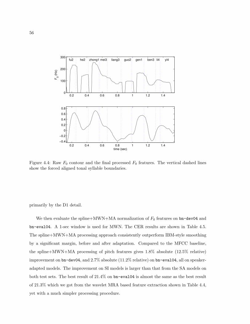
56
0.2 0.4 0.6 0.8 1 1.2 1.40
100
200
300F 0 (H
z)fu2 he2 zhong1 mei3 liang3 guo2 gen1 ben3 li4 yi4
0.2 0.4 0.6 0.8 1 1.2 1.4−0.4
−0.2
0
0.2
0.4
0.6
0.8
time (sec)
Figure 4.4: Raw F0 contour and the final processed F0 features. The vertical dashed linesshow the forced aligned tonal syllable boundaries.
primarily by the D1 detail.
We then evaluate the spline+MWN+MA normalization of F0 features on bn-dev04 and
bn-eval04. A 1-sec window is used for MWN. The CER results are shown in Table 4.5.
The spline+MWN+MA processing approach consistently outperform IBM-style smoothing
by a significant margin, before and after adaptation. Compared to the MFCC baseline,
the spline+MWN+MA processing of pitch features gives 1.8% absolute (12.5% relative)
improvement on bn-dev04, and 2.7% absolute (11.2% relative) on bn-eval04, all on speaker-
adapted models. The improvement on SI models is larger than that from the SA models on
both test sets. The best result of 21.4% on bn-eval04 is almost the same as the best result
of 21.3% which we got from the wavelet MRA based feature extraction shown in Table 4.4,
yet with a much simpler processing procedure.

57
Table 4.4: Mandarin speech recognition character error rates (%) of different pitch featureson bn-eval04. ‘D’ denotes the different level of details, and ‘S’ denotes the smooth. SImeans speaker-independent results and SA means speaker-adapted results.
Pitch Feature SI SA
MFCC only 26.4 24.1
+ IBM-style F0 24.0 22.2
+ spline F0 23.8 22.0
+ (D1+D2+D3+D4+D5+D6) F0 23.6 21.7
+ (D2+D3+D4+D5+D6) F0 23.1 21.4
+ (D3+D4+D5+D6) F0 23.4 21.3
+ (D2+D3+D4+D5) F0 24.1 21.7
+ (D2+D3+D4) F0 24.8 22.6
+ [D2 D3 D4 D5 D6] F0 24.3 22.4
4.6.2 CTS experiments
We also examined the pitch feature processing on Mandarin CTS cts-dev04 test set,
used the CTS embedded modeling experimental paradigm CTS-EBD presented in Chap-
ter 2. The wavelet-based pitch features were not explored since the gain is not significant
enough for the cost. Table 4.6 shows the CER results with a 1-sec window for MWN. The
spline+MWN+MA processing consistently outperforms the IBM-style processing by 0.5%
absolute, although the relative improvement is smaller than in the BN task. This can be
explained by that the more significant tone coarticulation in CTS makes it more difficult
for modeling the tones.
4.7 Summary
In this chapter, we presented the baseline embedded tone modeling with tonal acoustic
units and IBM-style pitch features. We then proposed a spline interpolation algorithm for
continuation of the F0 contour. Based on the spline interpolated F0 contour, we performed
wavelet based multiresolution analysis and decompose the F0 contour into three categories

58
Table 4.5: CER results (%) on bn-dev04 and bn-eval04 using different pitch featureprocessing. SI means speaker-independent results and SA means speaker-adapted results.
Featurebn-dev04 bn-eval04
SI SA SI SA
MFCC only 16.6 14.5 26.4 24.1
+ IBM-style F0 15.7 14.0 24.0 22.2
+ spline F0 15.2 13.5 23.8 22.0
+ (spline+MWN+MA) F0 14.5 12.7 23.2 21.4
Table 4.6: CER results (%) on cts-dev04 using different pitch feature processing.
Feature CER
PLP only 36.8
+ IBM-style F0 35.7
+ spline F0 35.9
+ (spline+MWN+MA) F0 35.2
representing the intonation, lexical tone variation and other noises. By combining different
levels of decomposed components, we found out primarily the F0 variation on the scales of
3 to 6 (corresponding to 80ms to 640ms) can improve the tone modeling in Mandarin BN
task. We then described an approximated algorithm to extract the useful components from
the F0 contour. Experimental results show that the spline+MWN+MA processing gives
consistent performance improvements on both Mandarin BN and CTS tasks. Compared
to the no-pitch baseline, the improved pitch features obtain 2.7% absolute improvement on
Mandarin BN and 1.6% absolute improvement on Mandarin CTS.

59
Chapter 5
TONE-RELATED MLP POSTERIORS IN THE FEATUREREPRESENTATION
Most state-of-the-art Mandarin speech recognition systems use F0 related features for
embedded tone modeling. This approach achieves significant improvement in various Man-
darin ASR tasks [45, 48]. In the last chapter, we proposed novel F0 processing techniques to
get more effective pitch features for lexical tone modeling, by normalizing out the intonation
effects and noises. In this chapter, we investigate alternative tone features extracted from a
longer time window than F0 related features, using a multi-layer perceptron (MLP). These
discriminative features include tone posteriors and toneme posteriors.
This chapter is organized as follows. In Section 5.1, we describe the motivation for
using tone-related MLP posteriors and introduce some related research. In Section 5.2,
MLP-based tone and toneme classification are introduced. In Section 5.3, we present how
the tone and toneme posteriors are incorporated in the feature representation for an HMM
back-end. In Section 5.4, experiments are carried out to show the effectiveness of various
schemes. Finally, we summarize the key findings in Section 5.5.
5.1 Motivation and Related Research
The pitch features used in embedded tone modeling include processed F0, its derivative and
second derivative. F0 captures the instantaneous pitch for a specific frame (typically 25ms
with 10ms step size). The derivatives capture the change of F0 over the neighboring frames.
In our system, the F0 delta features are computed from a 5-frame window (±2 frames) and
the second derivative features capture the F0 change over a window of 9 frames. However,
a tone depends on the F0 contour at the syllable-level. The average duration of a syllable is
around 200ms, which corresponds to 20 frames. Hence, the windows for computing short-
time F0 features and the associated derivatives might not be enough to cover the entire span
of the tone and to depict the shape of the F0 contours, especially when the F0 contours

60
become more complicated in continuous speech. Therefore, we explore alternative tone
features that contain more information than frame-level F0 values and derivatives.
In [40], Hermansky et al. proposed the tandem approach which uses neural network
(MLP) based phone posterior outputs as the input features for Gaussian mixture models of
a conventional speech recognizer. The resulted system effectively has two acoustic models in
tandem: a neural network and a GMM. The tandem acoustic modeling achieves significant
improvement on a noisy digit recognition task. Later in [24], the authors found that tandem-
style neural network feature preprocessors can offer considerable WER reduction for context-
independent modeling in a spontaneous large-vocabulary task compared to the MFCC or
PLP features, but the improvements do not carry over to context-dependent models. An
error analysis of tandem MLP features [77] showed that the errors of the system using MLP
features are different from the system with cepstral features. This suggested that it might
be better to combine the cepstral and MLP features. In [2], ICSI and OGI researchers
found it is preferable to augment the original spectral features with the discriminative MLP
posteriors in the Aurora task, especially in the case of mismatched training and testing
conditions. Significant improvement can be achieved in English large vocabulary speech
recognition by using variations of MLP-based features [66, 9]. In these research efforts,
MLPs are used to compute phoneme posteriors given the original spectral features or long-
span log critical band energy trajectories. The posteriors are then transformed by principle
component analysis (PCA) [22] and appended to the spectral feature vector as a new input
feature.
Inspired by the tandem style approaches, we propose to use an MLP to generate tone-
related posteriors as tone features and combine them with the original acoustic feature
vector. The advantages of using MLP-based posteriors are two-fold: first, by using a longer
time window, we can probably get more information of the current tone; second, the MLP
generated posterior features are discriminative in nature and may be more useful than the
F0 features or complement the F0 features. In this study, we consider two different types
of MLP targets: tones and tonemes. Then we append the tone-related posteriors to the
original feature vector for HMM-based acoustic modeling. Some of the work on CTS task
with IBM-style F0 features in this chapter has been reported in [57].
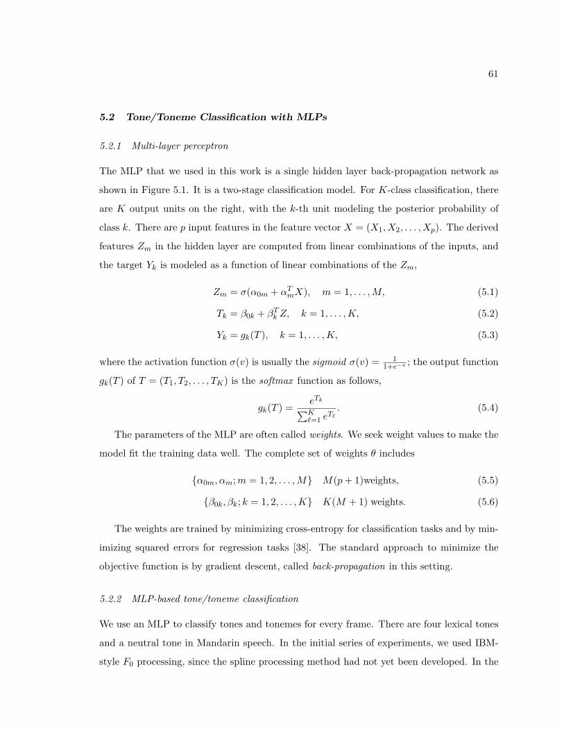
61
5.2 Tone/Toneme Classification with MLPs
5.2.1 Multi-layer perceptron
The MLP that we used in this work is a single hidden layer back-propagation network as
shown in Figure 5.1. It is a two-stage classification model. For K-class classification, there
are K output units on the right, with the k-th unit modeling the posterior probability of
class k. There are p input features in the feature vector X = (X1, X2, . . . , Xp). The derived
features Zm in the hidden layer are computed from linear combinations of the inputs, and
the target Yk is modeled as a function of linear combinations of the Zm,
Zm = σ(α0m + αTmX), m = 1, . . . ,M, (5.1)
Tk = β0k + βTk Z, k = 1, . . . ,K, (5.2)
Yk = gk(T ), k = 1, . . . ,K, (5.3)
where the activation function σ(v) is usually the sigmoid σ(v) = 11+e−v ; the output function
gk(T ) of T = (T1, T2, . . . , TK) is the softmax function as follows,
gk(T ) =eTk∑K`=1 e
T`
. (5.4)
The parameters of the MLP are often called weights. We seek weight values to make the
model fit the training data well. The complete set of weights θ includes
{α0m, αm;m = 1, 2, . . . ,M} M(p+ 1)weights, (5.5)
{β0k, βk; k = 1, 2, . . . ,K} K(M + 1) weights. (5.6)
The weights are trained by minimizing cross-entropy for classification tasks and by min-
imizing squared errors for regression tasks [38]. The standard approach to minimize the
objective function is by gradient descent, called back-propagation in this setting.
5.2.2 MLP-based tone/toneme classification
We use an MLP to classify tones and tonemes for every frame. There are four lexical tones
and a neutral tone in Mandarin speech. In the initial series of experiments, we used IBM-
style F0 processing, since the spline processing method had not yet been developed. In the

62
X1
X2
Xp
Xp-1
X3
Z1
Y1
Z2
Z3
ZM
Y2
YK
Figure 5.1: Schematic of a single hidden layer, feed-forward neural network.
IBM-style F0 processing approach, silence and unvoiced regions use waveform F0 average
for interpolation and do not have reliable tonal patterns. The assumption of IBM-style
smoothing is that the tone of a syllable only resides in the main vowel of the syllable [10].
Therefore, we train a tone MLP classifier with six targets: five tones and a no-tone target,
where the no-tone target is somewhat like a garbage model. The MLP is trained to distin-
guish the six categories according to the input MFCC and F0 features of the current and
neighboring frames. All the results reported in this chapter use single hidden layer MLPs
and a 9-frame context window. For each frame, we extract 39+3 dimension MFCC+F0
features. Therefore, the input size of the MLP is 378 for MFCC+F0 features. In training,
the MLP output units have target values of 1 for the tone associated with the tonal phone
that current frame belongs to, and 0 for others. The phonetic-level tone target labels of the
training data are assigned automatically by parsing the Viterbi alignments with an existing
set of HMMs.
After the spline processing was developed, a similar series of experiments were carried
out with the spline+MWN+MA processed F0 features and the syllable-level tone labels.
The spline processing of F0 assumes that the tone aligns with the entire syllable. Therefore,

63
in these experiments we have used syllable-level tone targets where the tone target remains
the same for all the phones within the syllable.
A toneme is defined as a phoneme consisting of a specific tone in a tone language [10].
For example, a1, a2, a3, a4 and a5 are five different tonemes associated with the same main
vowel “a”. Consonants can be regarded as special tonemes without tones. In our Mandarin
CTS speech recognition system, we have 62 speech tonemes plus one silence phone, one for
laughter and one for all other nonspeech events as listed in Table 4.2. The 62 speech phones
consists of 27 non-tonal phones and 35 tonal phones. For toneme classification, we train an
MLP to classify the 64 sub-word units (all the phones except the one for all other nonspeech
events). The same input features are used as in tone classification.
5.3 Incorporating Tone/Toneme Posteriors
The overall configuration of our tone feature extraction stage is illustrated in Figure 5.2.
Three different features, including their first order and second order derivatives, are ex-
tracted from the input speech: MFCC, F0 and PLP. Both MFCC and PLP front ends
are used to exploit the cross-system benefits. The F0 features (post-processed F0 plus the
first two derivatives) are appended to the MFCC features to form at new feature vector
for each frame. By concatenating the feature vectors from neighboring frames, we form
a 378-dimension feature vector and feed it into the MLP to classify tone-related targets.
Because the MLP output posterior has a very non-Gaussian distribution (between 0 and
1 by the sigmoid operation), we take the log of the posterior to make it more Gaussian-
like [66]. After that, PCA is performed to decorrelate and reduce the dimensions of the
posterior feature vector. The resulting tone-related features are then appended with PLP
and optionally F0 features to form the final feature vector for the back-end HMM-based
SRI decipher recognizer.
In the tone posterior system, we want to explore several questions. First, since the tone
MLP classifier is trained with spectral and F0 features from a much longer time span than
a single frame, we want to find out whether the tone posterior features perform better than
using frame-level F0 features. Second, given that the dimension of the tone posteriors is
small (6), we want to find out whether further PCA dimension reduction is helpful at all.

64
Inputspeech
PLP featureextraction
MFCC featureextraction
Pitch featureextraction
Concatenatecontextframes
MLPclassifier
Take logand PCA
tone-relatedposterior features
ConcatenateOutputfeature
Concatenate
Figure 5.2: Block diagram of the tone-related MLP posterior feature extraction stage.
Finally, we want to explore whether syllable-level tone posteriors trained with spline F0
features are better than phone-level tone posteriors trained with IBM-style F0 features.
In the toneme posterior system, PCA is performed on the log of the 64-dimensional
output MLP features and the first 25 principle components are taken, as suggested in [66].
This system is quite similar to the PLP/MLP feature based system in [9], except that we are
using F0 features combined with MFCC features to classify tone-dependent acoustic units.
In this case, the questions we want to answer is that whether the toneme posteriors are more
effective, and whether they are complementary to the tone posteriors or the frame-based
features.
5.4 Experiments
After the MLP classifiers are trained, we use them to generate tone-related posterior features
for a back-end HMM system as described in the last section. The posteriors are also mean
and variance normalized per speaker. All HMM systems here are maximum likelihood
trained using decision-tree state clustering. The CTS pronunciation phone set includes
consonants and tonal vowels, with a total of 65 phones as listed in Table 4.2. All triphones
of the same base phone with different tones are in the same tree. Categorical questions
include tone questions, in addition to other phone classes and individual phone questions,
state ID, etc. Unless noted, all systems use within-word triphones.
Most experiments were carried out on the Mandarin CTS task. The decoding lexicon
consists of 11.5K multi-character words. The language model is a trigram model trained

65
from training data transcriptions and text data collected from the web [48]. We follow the
experimental paradigm CTS-EBD described in Chapter 2 for decoding. Besides the CTS
experiments, we also present a brief experiment on Mandarin BN task.
5.4.1 MLP training for CTS experiments
For tone and toneme MLP classifier training, we first randomize the order of the training
utterances lest the MLP training fall into a local optimum. A portion (10%) of the training
data cts-train04 is held out as a cross validation set in MLP training. The tone and
toneme training targets are generated from forced alignment with the recognizer using an
existing set of triphone HMMs. We tune the number of context frames and hidden nodes for
the best frame classification accuracy. Frame accuracy is defined as the ratio of the number
of correctly classified frames to the total number of frames, where classification is deemed
to be correct if the highest output of the MLP corresponds to the correct target. This is a
good preliminary indicator of system performance and provides an efficient way to tune the
parameters without running the whole system.
It is found that for both tone and toneme classification, a 9-frame window gives satis-
factory results, although a longer time window provides a marginal gain in frame accuracy.
Considering the context frames used in computing the delta features, the effective span of
the input features is 17-frame, i.e. 170ms which is close to the average syllable span of
200ms. In the tone MLP classifier, 900 hidden nodes are enough.1 In the toneme MLP
classifier, 1500 hidden nodes provide good performance. The frame accuracy scores of the
tone and toneme MLP classifiers on the cross validation set are listed in Table 5.1. By
using the spline-processed F0 features, the tone classification accuracy is much lower than
with IBM-style F0 features, probably because the tone targets are at the syllable level and
more difficult to classify with the same window length. The toneme frame accuracy is not
affected significantly because toneme is a phonetic unit. The toneme accuracies are slightly
better than the published English phoneme frame accuracy results on a similar CTS task
[12], where 46 phoneme targets are used.
1The number of hidden nodes is large for 6-tone classification, since the input size is also large.

66
Table 5.1: Frame accuracy of tone and toneme MLP classifiers on the cross validation set ofcts-train04. IBM F0 denotes IBM-style F0 features; spline F0 denotes spline+MWN+MAprocessed F0 features. The tone target in IBM F0 approach is phone-level tone and in splineF0 approach is syllable-level tone.
Targets CardinalityFrame Acc.
IBM F0 spline F0
tone 6 80.3% 71.8%
toneme 64 68.8% 68.6%
5.4.2 CTS experiments with tone posteriors
The CER results from tone posterior systems are listed in Table 5.2. As we can see, the
system with PLP+(tone posterior) features outperforms the PLP+F0 system by 0.3% ab-
solute in IBM-style F0 approach, and 0.5% absolute in spline+MWN+MA F0 approach.
This shows that the tone posterior offers more tone information beyond using F0 features
directly. By combining the F0 and tone posteriors, the performance is not significantly
different from the system with only tone posteriors. We also find that PCA on the small
dimension (6) is not necessary: there is no reduction in CER, though it slightly reduces the
computation and memory requirements. Finally, the experiments show that the syllable-
level tone posteriors with spline F0 features outperform the phonetic-level tone posteriors
with IBM-style F0 features by 0.7% absolute, which supports our hypothesis that it is useful
to maintain the contour through the unvoiced regions.
A critical detail in decoding with the posteriors augmented models is to optimize the
Gaussian weight parameter [112], which is a scaling factor of log likelihood computation
of individual Gaussian components in the mixture. For an augmented feature vector, log
likelihood has a larger dynamic range and the models are sharper. Therefore, smaller
Gaussian weights should be used compared to the baseline systems. For tone posterior
systems, we used a Gaussian weight of 0.6 instead of the Gaussian weight of 0.7 in baseline
systems.

67
Table 5.2: CER of CTS systems on cts-dev04 using tone posteriors. IBM F0 denotes IBM-style F0 features; spline F0 denotes spline+MWN+MA processed F0 features. The tone inIBM F0 approach is at the phone level and at the syllable level in spline F0 approach.
Feature Dim.CER
IBM F0 spline F0
PLP only 39 36.8% 36.8%
+F0 42 35.7% 35.2%
+(tone posterior) 45 35.4% 34.7%
+F0+(tone posterior) 48 35.2% 34.8%
5.4.3 CTS experiments with toneme posteriors
We also experimented with the toneme posteriors and the posteriors combined from both
tone and toneme posteriors. The CER results are shown in Table 5.3. In all experiments
reported here, PCA is performed to reduce the MLP log posteriors down to 25 dimensions.
The PLP+PCA(toneme posterior) feature systems have an impressive improvement of more
than 2.0% absolute in CER over the baseline PLP+F0 systems. Because the toneme pos-
terior contains discriminative information for both phone units (as in English experiments)
and tones, the significant performance improvement is reasonable and consistent with the
English results reported in [9]. Adding F0 features to the system provides a further 0.5%
improvement in IBM-style F0 system, but no significant difference in spline F0 system. For
toneme posterior systems, even lower Gaussian weights of 0.3 to 0.5 are used.
We then try to combine the tone and toneme posterior features. The performance is
essentially the same as the PLP+F0+PCA(toneme posterior) system. Finally, we combine
all features together (PLP, F0 and PCA of tone and toneme posterior features) in a single
system but no further improvement is obtained. The last two experiments probably indicate
that the information provided by the tone posterior is covered by the combination of F0
and toneme posterior; or alternatively the F0 information is covered by the combination of

68
tone posterior and toneme posterior.2 The best results of the IBM F0 system and spline F0
system are not significantly different, probably because the toneme target is at the phonetic
level and depends more on the phonetic information than the tone information.
Table 5.3: CER of CTS systems on cts-dev04 using toneme posteriors. IBM F0 denotesIBM-style F0 features; spline F0 denotes spline+MWN+MA processed F0 features.
Feature Dim.CER
IBM F0 spline F0
PLP only 39 36.8% 36.8%
+F0 42 35.7% 35.2%
+PCA(toneme posterior) 64 33.7% 33.1%
+F0+PCA(toneme posterior) 67 33.2% 33.2%
+PCA(tone, toneme posterior) 64 33.3% 33.1%
We have also trained cross-word triphone systems based on the best feature combi-
nation of PLP+F0+PCA(toneme posterior). The performance improvement compared to
the corresponding PLP+F0 system is 2.0% absolute, which is consistent with that in the
within-word systems.
5.4.4 BN experiment with toneme posteriors
An experiment with the toneme posteriors is also carried out on the BN task. The toneme
posteriors used in this experiment are the more complicated ICSI features, which are the
combined output of two types of MLPs. A higher dimension of 32 for the ICSI features
is chosen for its better performance. Spline-interpolated F0 features are used in the ex-
periment. More details are referred to our Mandarin BN evaluation system description in
Chapter 9. The experimental paradigm BN-EBD is adopted, except that all 465 hours of
training data are used for AM training. The results are shown in Table 5.4. The 1.8%
absolute improvement in SI decoding and 1.0% in SA decoding are consistent with those in
2We increased the output dimension after PCA, but it did not help.

69
the CTS experiments.
Table 5.4: CER of BN system on bn-eval04 with toneme posteriors (ICSI features). In thistable, F0 denotes spline+MWN+MA processed F0 features. SI means speaker-independentresults and SA means speaker-adapted results.
Feature Dim. SI SA
MFCC+F0 42 18.7% 17.2%
MFCC+F0+ICSI 74 16.9% 16.2%
5.5 Summary
In this work, we have tried different approaches to incorporate tone-related MLP posteriors
in the feature representation for Mandarin CTS and BN recognition tasks. More specifi-
cally, tone posteriors, toneme posteriors and their combinations with F0 and PLP features
are explored. We found that tone posteriors outperforms plain F0 features significantly.
Much more significant improvement is achieved by using toneme posterior features, which
is probably in part because of incorporating segmental cues, known to be important from
other work [9]. By combining toneme posteriors with either F0 features or tone posteriors,
we have reduced CER by 2-2.5% absolute (or 6-7% relative) on a Mandarin CTS task, and
achieved similar improvement on a Mandarin BN task.
70
Chapter 6
MULTI-STREAM TONE ADAPTATION
The Mandarin ASR system with embedded tone modeling uses a single-stream feature
vector. However, the spectral features and the pitch features are quite different feature
streams in nature, although higher order cepstral features may contain some pitch informa-
tion. Spectral features tend to have more rapid (and sometimes abrupt) changes over time,
while pitch changes more slowly. The spectral features are mainly associated with the base
phones and syllables, and the pitch features are mainly associated with the tones. To exploit
the stream-specific model dependence, a two-stream modeling approach was tried in [42, 78].
A similar dynamic Bayesian network (DBN) based multi-stream model was proposed in our
previous work [58] for Mandarin tonal phoneme recognition. Recently, multi-space proba-
bility distribution (MSD) methods [92] were also tried for stream-dependent tone modeling.
As pointed out by these researchers, multi-stream modeling offers flexible parameter tying
mechanisms at the stream level, and the acoustic model size is much smaller. In several
Mandarin LVCSR tasks [78], multi-stream modeling gives slightly better performance than
single-stream modeling.
In this chapter, we will exploit the multi-stream nature of Mandarin speech in the
speaker adaptation stage. The spectral feature stream and the pitch feature stream are
adapted separately using different adaptation regression class trees. In Section 6.1, we review
the general adaptation strategy, which is based on maximum likelihood linear regression
(MLLR). In Section 6.2, the modification for multi-stream adaptation is described. The
experiments are presented in Section 6.3, and the key findings are summarized in Section 6.4.
6.1 Review of Adaptation
Unsupervised speaker adaptation is essential for modern HMM-based speech recognizers.
Many adaptation methods have been proposed to compensate for the mismatch between

71
training and decoding conditions. The most popular approaches are maximum a poste-
riori (MAP) adaptation [37] and maximum likelihood linear regression (MLLR) adapta-
tion [56, 33]. MAP-based adaptation incorporates prior knowledge about the distribution
of the model parameters to help robust adaptation of model parameters, and it converges
to maximum likelihood estimates when adaptation data increases. In MLLR adaptation, a
set of linear transformation matrices are estimated to transform the model parameters and
maximize the likelihood of the adaptation data. The transforms can be shared by different
classes of phones, making the approach effective even when there is little adaptation data
available. In our system, MLLR is adopted for rapid adaptation with limited adaptation
data.
Within the MLLR framework, different types of adaptation techniques can be used,
such as unconstrained model-space adaptation of mean or variance parameters, constrained
model-space adaptation, feature-space adaptation, and speaker adaptive training [33]. We
will focus on linear transformations of the model mean vectors, which has a much bigger
impact on performance than the variance adaptation [35]. Let OT = {o(1), . . . , o(T )} denote
the adaptation data, the general model-space transform parameters are found by optimizing
the following auxiliary function
Q(M,M) =
K − 12
M∑m=1
T∑τ=1
γm(τ)[K(m) + log(|Σ(m)|) + (o(τ)− µ(m))T Σ(m)−1(o(τ)− µ(m))
](6.1)
where µ(m) and Σ(m) are the transformed mean and variance for Gaussian component m;
M is the total number of Gaussian components associated with the particular transform;
and the posterior probability γm(τ) is
γm(τ) = p(qm(τ)|M, OT ) (6.2)
qm(τ) indicates o(τ) belongs to Gaussian component m; K is a constant related to the
transition probabilities; and K(m) is the normalization constant associated with Gaussian
component m.

72
Assume we adapt the n-dimensional model mean vectors with a linear transform,
µ = b+Aµ = Wξ (6.3)
where ξ = [1 µT ]T is the (n+1)×1 extended mean vector, and W = [b A] is the n×(n+1)
extended transformation matrix. For an acoustic model with diagonal covariance Gaussians,
the mean MLLR transformation can be solved computationally efficiently as shown in [56].
The i-th row of the transform is given by
wTi = G(i)−1k(i)T (6.4)
where the sufficient statistics are the (n+1)× (n+1) matrix G(i) and the 1× (n+1) vector
k(i) as follows:
G(i) =M∑
m=1
1
σ(m)2i
ξ(m)ξ(m)TT∑
τ=1
γm(τ) (6.5)
k(i) =M∑
m=1
T∑τ=1
γm(τ)1
σ(m)2i
oi(τ)ξ(m)T . (6.6)
Since the data available for adaptation is generally limited, it is necessary to cluster
model parameters together into regression classes. All components in a given regression
class are assumed to transform in a similar fashion. The regression classes are typically
determined dynamically according to the amount of available adaptation data using a re-
gression class tree (RCT). When more data is available, more detailed classes can be used
from deeper levels in the RCT. The regression class tree can be built either by phonetic
knowledge or by automatic data-driven acoustic clustering, as discussed in [32].
6.2 Multi-stream Adaptation of Mandarin Acoustic Models
As mentioned earlier, the feature vector of our Mandarin system is composed of 39-dimensional
MFCC features and 3-dimensional pitch features. In the typical MLLR adaptation, the
MFCC and pitch streams are transformed together with a single regression class tree. In
our baseline system, a phone class tree is manually designed. It has three base classes:
non-speech, vowels and consonants. For example, all the Gaussian components in the vowel
regression class share the same transform. This might be true for the MFCC parameters

73
since they are used to model the phonetic information. However, for the pitch stream it
might not be suitable: it is constrained that all tones share the same MLLR transform.
Therefore, we want to find out whether it is helpful to adapt the MFCC and pitch
streams separately, as illustrated in Figure 6.1. The RCTs shown in Figure 6.1 are general
trees which could be either the manual trees or automatically derived trees. Each stream
can be adapted with Equation 6.4 and the corresponding statistics in Equation 6.5 and
Equation 6.6. The posterior probabilities γm(τ) for two streams are assumed to be the
same, and are computed with the full feature vector. However, the sufficient statistics
{G(i), k(i)} for two streams are accumulated according to different adaptation regression
classes. If using the manually designed classes, the MFCC stream can use the 3-class tree
as used in the baseline system, but the pitch stream can use a regression class tree which
classifies all the phones into 5 base classes: no-tone, tone 1 to tone 4. Alternatively, the
regression class tree for each stream can be built by acoustic clustering separately.
mfccµ
pitchµ
mfcc mfcc mfccA bµ +
pitch pitch pitchA bµ +
MFCC RCT
pitch RCT
Figure 6.1: Multi-stream adaptation of Mandarin acoustic models. The regression classtrees (RCT) can be either manually designed or clustered by acoustics.
Some decoupling of the spectral stream and pitch stream can be achieved by using block
diagonal transforms in MLLR adaptation. The difference between using block diagonal
transforms and multi-stream MLLR adaptation is that the multi-stream adaptation offers
the ability to share transforms among units differently. For example, for three models “a1”,
“a2” and “e1”, the spectral stream of “a1” and “a2” can be share a transform because they

74
have the same base phone, while the pitch stream of “a1” can share a transform with that
of “e1” because they have the same tone.
6.3 Experiments
Experiments were carried out to compare the multi-stream adaptation to the single-stream
adaptation. We used the acoustic models trained on bn-Hub4 and do 2-pass decoding with
adaptation. The state clustering of the acoustic models is slightly different from the previous
models in order that all the triphones within a senone1 [46] share the same tone. The reason
is that the adaptation transform is shared for all triphones within a senone. If there are
triphones with different tones in a senone, it will not be possible to transform the different
tones with different transformation matrices.
We first generated the regression class trees automatically for MFCC and pitch streams
by clustering the acoustic subvectors separately. In all our experiments, the automatically
derived RCTs were grown with techniques described in [63]. The top 5 levels of the RCTs
for MFCC stream and pitch stream are shown in Figure 6.2 and Figure 6.3, respectively.
The definitions of the phone classes in the decision trees in Figure 6.2 and Figure 6.3 are
listed in Table 6.1. As we can see, the RCT for MFCC stream and the RCT for pitch stream
are quite different in structure. In the top levels of MFCC RCT, more questions about the
base phone are asked, while more questions about the tones are asked in the pitch RCT.
Then we performed the experiments on multi-stream adaptation for MFCC+F0 model.
The experimental results on bn-eval04 are shown in Table 6.2. By using full transform
matrices A in single-stream adaptation, the MLLR adaptation improves the performance
from 22.9% to 21.1%. If we use two-block-diagonal matrices for adaptation, the perfor-
mance is slightly improved to 20.9%. The improvement of 0.2% absolute is not statistically
significant according to matched pair sentence segment test, but the improvement is consis-
tent across several different test sets. This shows the MFCC stream and the pitch stream
are uncorrelated to some extent. However, by doing multi-stream adaptation with either
manual RCT or automatically clustered RCT, no further improvement is achieved. This is
1A senone is a clustered output distribution.
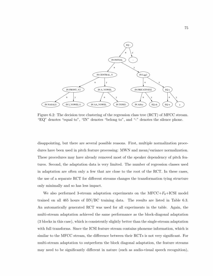
75
EQ -
IN INITIAL
n
-
y
IN CENTRAL_V
n
IN Lqg2
y
IN FRONT_V2
n
IN A_VOWEL
y
IN FRICATIVES2
n
EQ y
y
IN NASALS
n
IN I_VOWEL11
y
IN AA_VOWEL
n
IN TONE1
y
IN Affric
n
EQ sh
y
EQ w
n
y
y
Figure 6.2: The decision tree clustering of the regression class tree (RCT) of MFCC stream.“EQ” denotes “equal to”, “IN” denotes “belong to”, and “-” denotes the silence phone.
disappointing, but there are several possible reasons. First, multiple normalization proce-
dures have been used in pitch feature processing: MWN and mean/variance normalization.
These procedures may have already removed most of the speaker dependency of pitch fea-
tures. Second, the adaptation data is very limited. The number of regression classes used
in adaptation are often only a few that are close to the root of the RCT. In these cases,
the use of a separate RCT for different streams changes the transformation tying structure
only minimally and so has less impact.
We also performed 3-stream adaptation experiments on the MFCC+F0+ICSI model
trained on all 465 hours of BN/BC training data. The results are listed in Table 6.3.
An automatically generated RCT was used for all experiments in the table. Again, the
multi-stream adaptation achieved the same performance as the block-diagonal adaptation
(3 blocks in this case), which is consistently slightly better than the single-stream adaptation
with full transforms. Since the ICSI feature stream contains phoneme information, which is
similar to the MFCC stream, the difference between their RCTs is not very significant. For
multi-stream adaptation to outperform the block diagonal adaptation, the feature streams
may need to be significantly different in nature (such as audio-visual speech recognition),

76
EQ -
IN TONE4
n
-
y
IN TONE1
n
IN LOW_V
y
IN TONE3
n
IN CENTRAL_V
y
EQ IH4
n
EQ A4
y
IN FINAL2
n
IN MID_V
y
IN ROUNDED21
n
EQ a1
y
EQ er4
n
IH4
y
a4
n
A4
y
Figure 6.3: The decision tree clustering of the regression class tree (RCT) of pitch stream.“EQ” denotes “equal to”, “IN” denotes “belong to”, and “-” denotes the silence phone.
and the adaptation data may need to be sufficiently large to enable the use of more regression
classes in the separate RCTs.
6.4 Summary
In this chapter, we investigated the multi-stream adaptation framework for modeling the
spectral features and pitch features separately. In the adaptation stage, the sufficient sta-
tistics of the MFCC stream and pitch stream are used to compute the MLLR transforms
according to different regression class trees. This allows the components in the pitch stream
that have the same tone to share the same adaptation transforms. However, experimental
results show that this multi-stream adaptation strategy has the same performance as using
block diagonal transforms in MLLR adaptation. This might suggest that our pitch feature
normalization techniques have already removed most of the speaker dependency, or the
amount of adaptation data is too limited to make full use of more classes in the regression
class tree.

77
Table 6.1: Definitions of some phone classes in decision tree questions of RCTs. Thesedefinitions are for BN task.
Phone Class Phones
AA VOWEL A1,A2,A3,A4
Affric c,ch,j,q,z,zh
A VOWEL a1,a2,a3,a4
CENTRAL V A1,A2,A3,A4,a1,a2,a3,a4,er2,er3,er4
FRICATIVE f,h,r,s,sh,x
FRONT V2 E1,E2,E3,E4,I1,I3,I4,IH1,IH2,IH3,IH4,i1,i2,i3,i4,yu1,yu2,yu3,yu4
INITIAL b,c,ch,d,f,g,h,j,k,l,m,n,p,q,r,s,sh,t,v,w,x,y,z,zh
I VOWEL11 i1,i2,i3,i4
LOW V A1,A2,A3,A4,a1,a2,a3,a4
Lqg2 l,r,w,y
MID V E1,E2,E3,E4,e1,e2,e3,e4,er2,er3,er4,o1,o2,o3,o4
NASALS N,NG,m,n
ROUNDED21 o1,o2,o3,o4,u1,u2,u3,u4
TONE1 A1,E1,I1,IH1,a1,e1,i1,o1,u1,yu1
TONE3 A3,E3,I3,IH3,a3,e3,er3,i3,o3,u3,yu3
TONE4 A4,E4,I4,IH4,a4,e4,er4,i4,o4,u4,yu4

78
Table 6.2: CER on bn-eval04 using different MLLR adaptation strategies with MFCC+F0
model. RCT means the type of regression class trees.
Adaptation Strategy RCT CER
No adaptation – 22.9%
Single-stream, full transformmanual 21.1%
automatic 21.0%
Single-stream, block diagonalmanual 20.9%
automatic 21.0%
Multi-streammanual 20.9%
automatic 20.9%
Table 6.3: CER on bn-eval04 using different MLLR adaptation strategies withMFCC+F0+ICSI model.
Adaptation Strategy CER
No adaptation 16.9%
Single-stream, full transform 16.2%
Single-stream, block diagonal 16.0%
Multi-stream 16.0%

79
PART III
EXPLICIT TONE MODELING
The third part of the dissertation is concerned with explicit tone modeling to complement
embedded tone modeling. Although embedded tone modeling has improved the recognition
performance significantly, it does not exploit the suprasegmental nature of tones: a tone
aligns with the syllable instead of the phonetic unit. Therefore, explicit tone modeling
techniques can be used to complement the embedded modeling system.
In Chapter 7, the syllable-level tone models are used to rescore the lattices output from
the embedded modeling system. Oracle experiments reveal there is substantial room for
improvement by using explicit tone models to rescore the lattices (30% relative reduction
in character error rate). Neural network based context-independent tone models and supra-
tone models are used for rescoring and a small improvement is obtained. In Chapter 8,
word-level tone models are explored to more explicitly model the tone coarticulation and
sandhi effects within the word. Hierarchical backoff schemes are used for less frequent and
unseen word-level models. Consistent improvement is achieved by using word-level tone
models compared to the syllable-level models.

80
Chapter 7
EXPLICIT SYLLABLE-LEVEL TONE MODELINGFOR LATTICE RESCORING
In Chapter 4 and Chapter 5, we have explored different tone features for use in HMM-
based embedded tone modeling. The pitch features capture the F0 contour of a small
fixed-length window. The MLPs can be used to extract tone-related features from a longer
fixed-length window. Both methods have achieved significant improvements in Mandarin
speech recognition. However, the features extracted from a fixed-rate analysis cannot exploit
the fact that a tone is synchronous with the syllable. First, the center of the window for tone
feature extraction should be aligned to the center of the syllable, instead of to any specific
frame. Second, the window should have a variable length that is equal to the length of the
target syllable. Finally, the acoustic unit of HMM state of tonal phones cannot exploit the
dependency between tones and syllables.
In this chapter, we investigate explicit syllable-level tone models and use them for lattice
rescoring in Mandarin ASR systems. In Section 7.1, previous research on explicit tone
modeling is described. In Section 7.2, an experiment is presented to evaluate the upper
bound for explicit tone modeling by rescoring the output lattices from the embedded tone
modeling system that uses improved pitch features, demonstrating the potential for further
improved performance. In Section 7.3, we discuss the context-independent (CI) tone models
used. In Section 7.4, context dependency of tones is explored by using supra-tone models.
In Section 7.5, we describe a new method to estimate the tone classification accuracy of the
lattice by using frame-level tone posteriors. In Section 7.6, lattice rescoring experiments
with syllable-level tone models are presented. Finally, we summarize the key findings in
Section 7.7. The part on rescoring with CI tone models has been reported in [59].

81
7.1 Related Research
Much research has been done on explicit syllable-level tone modeling in the past several
decades. Various statistical tone models have been tried for tone classification and tone
recognition. Tone classification is to classify a tone (or a sequence of tones) into different
categories given the syllable boundaries. Tone recognition means to recognize a sequence
of tones without knowing the syllable boundaries. The tone classification or recognition
results can be used to aid the Mandarin speech recognition in post-processing or directly
integrated in the first-pass search process [90], or can be combined with the separate syllable
recognition results to get the final output characters.
In 1988, Yang et al. [106] proposed a lexical tone recognition technique by combining
vector quantization and hidden Markov models. A very high tone accuracy was reported
for isolated syllables. In 1995, Chen et al. [14] used neural networks to do tone recognition
in continuous Mandarin speech. Energy and F0 features from the target [90] syllable and
neighboring syllables are extracted to take into account the coarticulation effect. Then
a hidden control neural net and a hidden state multi-layer perceptron were proposed to
model the global intonation pattern of a sentential utterance as a hidden Markov chain,
and effectively use a separate MLP in each state for tone discrimination. A recognition
accuracy of 86.7% was achieved on a speaker-independent tone recognition task. However,
in both studies the tone recognition results were not used for speech recognition.
The authors of [93] in 1997 presented a complete recognition of continuous Mandarin
speech with large vocabulary. In this work, the tones and base syllables were recognized
separately with two different sets of HMMs. Each context-dependent tone model (tritone)
was represented with an HMM with seven states. A concatenated syllable matching algo-
rithm was used to integrate the separate tone and base syllable recognizers and output tonal
syllable lattices. The tonal syllable lattices were passed through a linguistic processor and
character output was generated. The HMM-based tone models were also used in [55] on a
Cantonese speech recognition task.
More recently, the author of [90] used Legendre coefficients as tone features to train
Gaussian mixture model (GMM) based tone models. She then applied the tone models

82
in post-processing the N-best lists as well as first pass decoding. With simple four-tone
models, post-processing approach provided around 10% relative improvement in syllable
error rate on a spontaneous Mandarin speech recognition task. The first pass decoding
method was slightly better than the post-processing approach. Besides HMM and GMM,
decision trees [98] and support vector machines [72] have also been investigated for Mandarin
or Cantonese tone modeling. Other than these traditional pattern classification methods,
a novel mixture stochastic polynomial tone model (SPTM) [5] was also proposed for tone
modeling. In this chapter, we investigate applying the neural-network-based explicit tone
models to rescore the lattices that already incorporate the improvements from embedded
tone modeling.
7.2 Oracle Experiment
In our embedded tone modeling system, the improved pitch features already provide more
than 10% relative improvement in CER. In this work, we first hope to find out whether
additional explicit tone modeling can further improve the ASR performance. We choose to
rescore word lattices instead of N-best lists since a lattice is a much richer representation of
the entire search space. The word lattices used here are in HTK Standard Lattice Format
(SLF) [108]. In the SLF lattices, each lattice node corresponds to a point in time and
each lattice link (arc) is labeled with a word hypothesis and the associated log likelihoods
(acoustic and language model). In order to parse the syllable boundaries for each word, the
backtrace phones and their durations are also generated and labeled in the word links.
An error analysis was performed on the CTV portion of the bn-eval04 test set. The
second row of Table 7.1 shows the baseline recognition error rate results of tones, base
syllables (BS), tonal syllables (TS) and characters, computed from the same decoding run
as in the last row of Table 4.5. We find the character errors with correct base syllable but
wrong tone account for only 0.6% absolute (BS vs. TS). This might lead to the conclusion
that by using perfect tone information, we can at most achieve 0.6% improvement. However,
different tone decisions might change the phonetic decision since the acoustic units are
context-dependent tonal phones.
To more effectively evaluate the upperbound for tone modeling, we incorporate the per-

83
Table 7.1: Baseline and oracle recognition error rate results (%) of tones, base syllables(BS), tonal syllables (TS), and characters (Char) on the CTV subset of bn-eval04. Thebaseline system uses embedded tone modeling with spline+MWN+MA pitch features.
Tone BS TS Char
Baseline 9.3 10.4 11.0 12.0
+ Oracle tone 5.5 7.4 7.6 8.2
fect tone information in lattice search. Forced alignment is performed against the references
to get the oracle tone alignments. For each character in the lattice, we get the oracle tone
label according to the center time of the character. As shown in Figure 7.1, character Ci
is aligned to oracle tone T oj−1. If the tone Ti of Ci is different from the oracle tone T o
j−1,
the corresponding arc is pruned in the lattice via applying a large penalty score. Then we
re-decode the lattice with the Viterbi algorithm.
st etlattice arc
oracle tone alignment
iC
1ojT −
ojT
Figure 7.1: Aligning a lattice arc i to oracle tone alignments.
The re-decoded top best hypothesis achieves 8.2% CER compared to the baseline 12.0%,
as shown in the last row of Table 7.1. This indicates the upperbound for improvement is
3.8% absolute (or 32% relative) if we have a perfect tone recognizer.
7.3 Context-independent Tone Models
The oracle experiment shows that there is still substantial room for improvement in the
character recognition performance by rescoring the lattices from the embedded tone mod-
eling system. Therefore, we investigated the use of explicit syllable-level tone models to

84
rescore the lattices in the Mandarin BN task.
7.3.1 Model selection
The commonly used parametric classifiers include neural networks (MLPs), Gaussian mix-
ture models (GMMs) and support vector machines (SVMs). For many applications, SVMs
have the best performance. However, the training of SVMs is much slower than the other
two classifiers. In practice, we found the training of SVMs is more than an order of magni-
tude higher than MLPs or GMMs, even with a linear kernel. Considering the large amount
of data we are processing in LVCSR tasks, we choose to use MLPs and GMMs for ex-
plicit tone modeling. First we try MLPs due to its discriminative nature, fast training and
straightforward integration. The MLP we use is a single-hidden-layer neural network.
7.3.2 Feature selection
Various features can be used for explicit tone modeling. In our work we have tried the
following: syllable duration, polynomial regression coefficients (PRC), robust regression
coefficients [97] (RRC) and normalized F0 contour. First, we introduce the polynomial
coefficients.
Let F = [F1 F2 . . . FN ]′ be a sequence of F0 values of a particular syllable F0 contour
with N points. The objective is to find the polynomial of order d− 1 with coefficients βk’s
that best fit F . Let F = [F1 F2 . . . Fn]′ be an estimate of F. Then the estimated Fi is
given as,
Fi = β0 + β1ti + β2t2i + · · ·+ βd−1t
d−1i , i = 0, 1, . . . , N − 1 (7.1)
where ti = iN is the normalized time scale so that durations are normalized to 1 for all the
syllable durations. Equation 7.1 can be formulated in the matrix form as below,F0
F1
...
FN−1
=
1 t1 t21 . . . td−1
1
1 t2 t22 . . . td−12
......
.... . .
...
1 tN t2N . . . td−1N
β0
β1
...
βd−1
(7.2)

85
or noted as F = T ~β. By minimizing the sum of squared errors E = (F − F )′(F − F ), the
regression coefficients can be estimated by,
~β = (T ′T )−1T ′F (7.3)
Due to the F0 estimation errors and alignment errors when extracting syllable F0 con-
tours, the estimated polynomial regression coefficients may be affected by these outliers. We
tried the robust regression algorithm as proposed in [97]. The basic idea is to throw away
a portion (20% in our case) of the F0 contour values that have the largest fitting errors,
and re-estimate the regression coefficients with the remaining points. Instead of PRC and
RRC, the Legendre orthogonal polynomials were used in [20, 90]. They may provide better
performance but were not investigated in this study.
We also tried the features of the normalized F0 contour. Each syllable F0 contour is
normalized into a fixed number of points by averaging the evenly divided regions. These
features are very intuitive and easy to extract.
7.3.3 Tone classification
All the features are tested in a Mandarin BN tone classification task with an MLP-based 4-
tone model. The bn-Hub4 training data is forced aligned. The tone labels and the boundaries
of the syllables are parsed from the alignments. Then the syllable-level tone features are
extracted to train an MLP. All features are globally mean- and variance-normalized using
the syllable vector mean and variance computed from the training data. The quicknet
package from ICSI is used in the implementation. To compare the performance of different
features, we held out the last 10% of the training data for cross validation (CV). The number
of hidden nodes is optimized for each feature set. The tone error rate (TER) results of tone
classification are listed in Table 7.2.
As we can see from Table 7.2, the best result is achieved with normalized spline+MWN
processed F0 features. The MA processing, which helps in embedded tone modeling, seems
to hurt the explicit tone classification. Combinations of different feature sets are also tried,
but only minor improvement has been achieved. For simplicity, we have used the 6-point
normalized spline+MWN F0 contour plus duration as features for explicit tone modeling.

86
Table 7.2: Four-tone classification tone error rate (TER) results (%) on cross validationset of bn-Hub4. “PRC” means polynomial regression coefficients. “RRC” means robustregression coefficients. “dur” denotes syllable duration.
Feature Dim #of nodes TER
d=4 PRC + dur 5 20 36.59
d=4 RRC + dur 5 20 36.33
normalized spline F0 + dur 7 25 36.69
normalized spline+MWN F0 + dur 7 35 34.42
normalized spline+MWN+MA F0 + dur 7 25 35.37
After fixing the feature set, we also use GMMs as classification models. Since it is almost
impossible to distinguish the very short tones due to coarticulation effects, we also re-train
the model and test with only the tones longer than 15 frames. One GMM with 128 Gaussian
components is trained for each tone using EM algorithm as described in [3]. The results
on the CTV portion of bn-eval04 are compared in Table 7.3. The neural net performs
better than the GMM classifier with the same features. In addition, another experiment
with GMMs is carried out to evaluate the classification performance without interpolation
of the F0 contour, i.e., the raw F0 contour is used instead of the spline interpolated F0
contour. The MWN is applied only in the voiced regions of the raw F0 contour and the F0
values of the unvoiced regions are treated as missing features. The marginalization approach
in [15] is taken to handle the missing feature problem in both GMM training and testing.
The GMM classification result with missing F0 features is 2.6% worse than that with spline
interpolation, which suggests the interpolated contours offer meaningful information for
syllable-level CI tone classification.
7.4 Supra-tone Models
7.4.1 Models and features
Since tone context affects the syllable F0 contour significantly, as we found in Chapter 3, we
also investigate tone models with context features. The models we use are the supra-tone

87
Table 7.3: Four-tone classification results on long tones in CTV subset of bn-eval04. TERdenotes tone error rate.
Model Feature TER
Neural Net normalized spline+MWN F0 25.7%
GMM normalized spline+MWN F0 29.1%
GMMnormalized raw+MWN F0
31.7%(with missing features)
models proposed in [76]. Different from the traditional context-dependent tone models,
each supra-tone model covers a number of syllables in succession. The supra-tone model
characterizes not only the tone contours of individual syllables but also the transitions
among them, using features from both the current and neighboring syllables. Because the
carry-over coarticulation effect from the left context is much more significant than from the
right context, we use left di-tone models. Different from [76] where GMMs are used, we use
neural networks due to its better performance in the context-independent (CI) tone study
as shown in Table 7.3.
We classify the left tone context into 5 categories: tone 1 - 4, and other (pause, noise,
etc). We only consider the classification of tone 1 - 4 for the current syllable. Therefore,
the cardinality of supra-tone models is 5 × 4 = 20. The features of the supra-tone model
are 14-dimensional, obtained by concatenating the 7-dimensional CI tone features of the
current and the previous syllable.
7.4.2 Tone classification
To evaluate the tone classification performance with supra-tone models, we perform a
Viterbi-style decoding. As in the previous study, the syllable boundaries are extracted
from the forced alignment of the oracle transcriptions. The goal is to decode the tone
sequence T = {t1, t2, . . . , tN} that maximizes the probability,
T = argmaxT
P (T |O,M) (7.4)
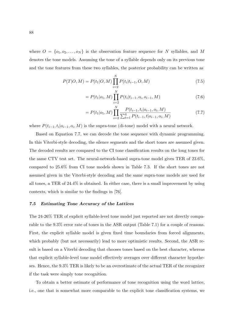
88
where O = {o1, o2, . . . , oN} is the observation feature sequence for N syllables, and M
denotes the tone models. Assuming the tone of a syllable depends only on its previous tone
and the tone features from these two syllables, the posterior probability can be written as
P (T |O,M) = P (t1|O,M)N∏
i=2
P (ti|ti−1, O,M) (7.5)
= P (t1|o1,M)N∏
i=2
P (ti|ti−1, oi, oi−1,M) (7.6)
= P (t1|o1,M)N∏
i=2
P (ti−1, ti|oi−1, oi,M)∑4t=1 P (ti−1, t|oi−1, oi,M)
(7.7)
where P (ti−1, ti|oi−1, oi,M) is the supra-tone (di-tone) model with a neural network.
Based on Equation 7.7, we can decode the tone sequence with dynamic programming.
In this Viterbi-style decoding, the silence segments and the short tones are assumed given.
The decoded results are compared to the CI tone classification results on the long tones for
the same CTV test set. The neural-network-based supra-tone model gives TER of 23.6%,
compared to 25.6% from CI tone models shown in Table 7.3. If the short tones are not
assumed given in the Viterbi-style decoding and the same supra-tone models are used for
all tones, a TER of 24.4% is obtained. In either case, there is a small improvement by using
contexts, which is similar to the findings in [76].
7.5 Estimating Tone Accuracy of the Lattices
The 24-26% TER of explicit syllable-level tone model just reported are not directly compa-
rable to the 9.3% error rate of tones in the ASR output (Table 7.1) for a couple of reasons.
First, the explicit syllable model is given fixed time boundaries from forced alignments,
which probably (but not necessarily) lead to more optimistic results. Second, the ASR re-
sult is based on a Viterbi decoding that chooses tones based on the best character, whereas
that explicit syllable-level tone model effectively averages over different character hypothe-
ses. Hence, the 9.3% TER is likely to be an overestimate of the actual TER of the recognizer
if the task were simply tone recognition.
To obtain a better estimate of performance of tone recognition using the word lattice,
i.e., one that is somewhat more comparable to the explicit tone classification systems, we

89
computed frame-level tone posteriors (averaging over the lattice) and used these to classify
the same fixed-time syllable segmentations as in the previous experiments by looking at the
posterior at the midpoint of the syllable.
The frame-level tone posterior (FLTP) probability is computed similarly to the time
frame error idea introduced in [96]. For example, as shown in Figure 7.2, there are many
possible hypothesis with different tone sequence and boundaries in the lattice. For a given
time frame i, we compute the frame-level tone posterior (FLTP) probability by summing
up all the posterior probabilities of the words crossing time i and corresponding to the same
tone Ti,
p(Ti|X) =1S
∑wk,`:
t(k)≤i≤t(`)
δ(T (wk,`, i), Ti)p(wk,`|X) (7.8)
where t(·) denotes the corresponding time of a lattice node, T (wk,`, i) represents the tone
of word wk,` at time i, δ(·) denotes whether the two values are the same, p(wk,`|X) is the
word posterior probability, and S is a constant to normalize the total probability to 1.
0 1 2 3 4 time
T1 T4 T3 T2
T1 T2 T2 T2
T1 T2 T3 T1
top best:
i
Figure 7.2: Illustration of frame-level tone posteriors.
For a word link wk,` with starting node k and ending node `, the link posterior p(wk,`|X)
is defined as the sum of the probabilities of all paths q passing through the link wk,` nor-
malized by the probability of the signal p(X):
p(wk,`|X) =
∑q∈Qwk,`
p(q,X)
p(X)(7.9)

90
where p(X) is approximated by the sum over all paths through the lattice. The summation
in the numerator can be performed efficiently using a variant of the forward-backward
algorithm on the lattice.
Similar to the approach used in [87], first the forward probabilities α and backward
probabilities β are computed for all the nodes in the lattice. In analogy to Baum-Welch
re-estimation, the forward probabilities are computed in a recursive fashion starting from
the beginning of the lattice. For each node ` with preceding word links wk,`, the forward
probability is given by
α` =∑
k
αk [pAM (wk,`)]1γ pLM (wk,`), (7.10)
where PAM is the acoustic likelihood of word wk,`, PLM is the language model probability
of word wk,`, and γ is the factor that is used to scale down the acoustic scores. Contrary to
normal practice in Viterbi decoding where the LM scores are scaled, it is better to reduce
the dynamic range of the acoustic scores than to increase that of language model, as found
by many previous studies [86, 64, 27]. The backward probabilities βk are computed in a
similar fashion starting from the end of the lattice.
After the forward and backward probabilities are computed, the word posterior proba-
bility is given by,
p(wk,`|X) =αk [pAM (wk,`)]
1γ pLM (wk,`)β`
p(X)(7.11)
where p(X) is simply the forward probability of the final node (or the backward probability
of the initial node).
After the frame-level tone posteriors are computed, we can use them to compute the tone
accuracy of the decoder given the oracle syllable boundaries. For each syllable segment, we
choose the frame-level tone posterior probability in the middle of the segment as the tone
decision from the decoder.1 For the same long tones in CTV test set, the tone accuracy is
95.1% (TER is 4.9%). Including the short tones, the overall TER is 7.3%. Compared to the
9.3% TER of the top best listed in the first row of Table 7.1, the frame-level tone posterior
method gives a much better estimate of the tone accuracy of the lattice.
1Other methods such as averaging the tone posteriors over the segment may also be used.

91
7.6 Integrating Syllable-level Tone Models
As we found in the last section, the speech recognizer (with both acoustic and language
model knowledge sources) has a TER of less than 10% while the TER of the explicit tone
models is above 20%. But since the explicit tone classifiers are trained with suprasegmental
acoustic features, we hope the explicit tone classifiers can be used as a complementary
knowledge source in lattice rescoring.
7.6.1 CI tone model integration
We first integrate the context-independent tone classifiers. For each lattice arc i, which has
tone Ti associated with character Ci, the tone score is computed as:
ψi = λdi log p(Ti|fi) (7.12)
where λ is the weight for the tone score, di is the number of frames in Ti, and p(Ti|fi) is
the posterior probability of Ti given the tone features fi. For short tones, a constant score
is used, approximating the posterior probability with a uniform distribution.
A tone weight of smaller than 0.5 gives improved performance. As listed in Table 7.4,
the best CER is 11.5%, achieved with w = 0.35. Compared with the embedded modeling
CER result of 12.0%, this 0.5% absolute improvement is statistically significant at the level
p < 0.04 according to the matched pair sentence segment test. It shows that the inferior
explicit tone classifier provides complementary information for recognition and improves the
system performance significantly. However, there is still a lot of room to improve compared
with the oracle bound.
We also tried to combine the FLTPs with the explicit tone decisions to increase the ro-
bustness. When the entropy of the output of explicit tone models is higher than a threshold,
the FLTP corresponding to the word link is used as tone score. But in our experiments, no
improvement has been achieved, as shown in Table 7.4. It is probably due to the lack of
extra knowledge from FLTPs.

92
Table 7.4: CER of tone model integration on CTV test set. The baseline system usesembedded tone modeling with spline+MWN+MA pitch features.
Integration Method CER
Baseline 12.0%
CI tone model 11.5%
CI tone model + FLTP 11.5%
Supra-tone model 11.6%
7.6.2 Supra-tone model integration
Integration of the supra-tone models is not as straightforward as that of the CI tone models,
since it requires a unique left tone context for each word. Therefore, we need to expand
the lattice according to its left tone context. Expansion for all possible left tone categories
and durations will cause a huge lattice. Therefore, we only expand lattices according to
the left tone categories. The same tone with different durations are treated as the same
left context. Then we can use the average duration of all the left context tones to find the
effective supra-tone boundaries. In the implementation of lattice expansion, we used the
lattice-tool from SRILM [84] with the following procedure:2
1. Save the orignal LM scores in one of the extra score fields, e.g., ”x1”.
2. Insert a new link after every word link that encodes the tone label(s) for the last
character of that word, as illustrated in Figure 7.3. There are no scores on these new
links.
3. Expand the lattice with an artificial bigram LM that contains all the bigrams formed
by a tone label in the first position and a word label in the second position. It will
have the effect of making the predecessor tone label for each word link unique.
After the lattice expansion is done, we can then assign tone scores with supra-tone
models based on the expanded lattices. Finally, we rescore the final lattices based on all
2Thanks to Dr. Andreas Stolcke for suggestions on this lattice expansion method.

93
st et st et etT2
Figure 7.3: Illustration of insertion of dummy tone links for lattice expansion.
scores, including the original LM scores. The CER result is also listed in Table 7.4. No
improvement is achieved from supra-tone modeling, probably because the improvement in
tone accuracy is not enough to translate to CER improvement, or the treatment of short
tones in our approach is sub-optimal.
7.7 Summary
In this chapter, we have evaluated the oracle upper bound for explicit tone modeling based
on the output lattices from the embedded tone modeling system. By using perfect tone
information to rescore the lattices, more than 30% relative improvement can be achieved on
the CTV test set. Then we train two syllable-level tone models, context-independent tone
models, and supra-tone models3, to rescore the lattices. We also develop the frame-level
tone posterior probabilities to estimate the tone classification accuracy of the recognizer,
for comparison with the syllable-level models. Different methods have been tried to rescore
the lattice with the explicit tone models as a complementary knowledge source. Significant
ASR improvement can be obtained with the CI tone models, but the supra-tone models did
not bring further improvement.
3Supra-tone models actually contain more than one syllable. But since supra-tone models have a fixednumber of syllables (in our case, two), we still refer to them as syllable-level. This is compared with theword-level tone models in the next chapter, which have a variable number of syllables.

94
Chapter 8
WORD-LEVEL TONE MODELING WITH HIERARCHICALBACKOFF
In this chapter, we extend previous approaches to explicit tone modeling from the syl-
lable level to the word level, incorporating a hierarchical backoff. Word-dependent tone
models are trained to explicitly model the tone coarticulation within the word. For less fre-
quent words, syllable-level tone models are used as backoff. Under this framework, different
types of tone modeling strategies are compared experimentally on a Mandarin broadcast
news speech recognition task, showing significant gains from the word-level tone modeling
approach on top of embedded tone modeling.
The rest of the chapter is organized as follows: In Section 8.1, we motivate this work. In
Section 8.2, we introduce the word-level tone models and the modified decoding criteria. In
Section 8.3, different backoff strategies for infrequent words are described. In Section 8.4,
experiments are carried out and the recognition results are discussed. Finally, we summarize
the key points in Section 8.5.
8.1 Motivation and Related Research
From the oracle experiments in Chapter 7, we found that by rescoring the first pass recogni-
tion output lattices of the embedded tone modeling with perfect tone information, around
30% relative improvement could be achieved. Using a neural network, even a simple syllable-
level 4-tone model can improve the recognition performance by 4% relative in a Mandarin
broadcast news (BN) experiment, but no further gain was obtained from more complex
supra-tone models. When the amount of training data becomes larger, more complicated
tone models could be used. However, it may also be possible to use more complex models
with a fixed amount of training data, if only for the well-trained cases.
Inspired by the word duration modeling approach [31, 52] and other word-level prosody
modeling techniques [89], we propose to extend the syllable-level tone modeling to a word-

95
level tone modeling framework with a hierarchical backoff: word-level tone models (word
prosody models) are trained for the frequent words, and tonal syllable (TS) or plain tone
models are used as backoff for the infrequent or unseen words. In addition, context-
dependent tone models can be used as backoff. These prosody models represent both
duration and F0 characteristics of a word. The word prosody models and the backoff tone
models can then be used in word lattice rescoring as a complementary knowledge source.
The word-dependent tone modeling framework can be viewed as a generalization of the
traditional context-independent and context-dependent tone modeling for rescoring. To
facilitate implementation of the word-dependent model with different backoff alternatives,
we use a class-conditional model, specifically Gaussian mixtures, that is a generalization of
the word duration model introduced in [31].
There are several advantages of the proposed approach. The tone coarticulation within
the word is more explicitly modeled. In addition, the different backoff strategies offer the
flexibility to model the dependencies between the tone and different linguistic units. Finally,
the word prosody models are less susceptible to tone labeling errors in the pronunciation
dictionary as long as the errors are consistent between the training and decoding dictionaries.
8.2 Word Prosody Models
In a Chinese sentence, there are no word delimiters such as blanks between the words.
Longest-first match or maximum likelihood based methods can be used to do word segmen-
tation [49]. A segmented Chinese word is typically a commonly used combination of one or
multiple characters. As illustrated in Figure 8.1, for a word wi = ci1ci2 · · · ciM which con-
sists of M characters, we denote the corresponding tonal syllable sequence as si1si2 · · · siM
and the tone sequence as ti1ti2 · · · tiM . In a given word, each Chinese character has a unique
pronunciation of a tonal syllable. In this study, we focus on the tone-related prosodic fea-
tures. In all our experiments, the feature fij for each character cij is a 4-dimensional vector:
the syllable duration plus 3 F0 values sampled from the syllable F0 contour.1 The feature fi
1A 4-dimensional feature vector is used instead of 7-dim in the previous chapter. This is to decrease thedimensionality of the word prosody models. In practice, no significant difference has been found by usingthe two different dimensionalities.
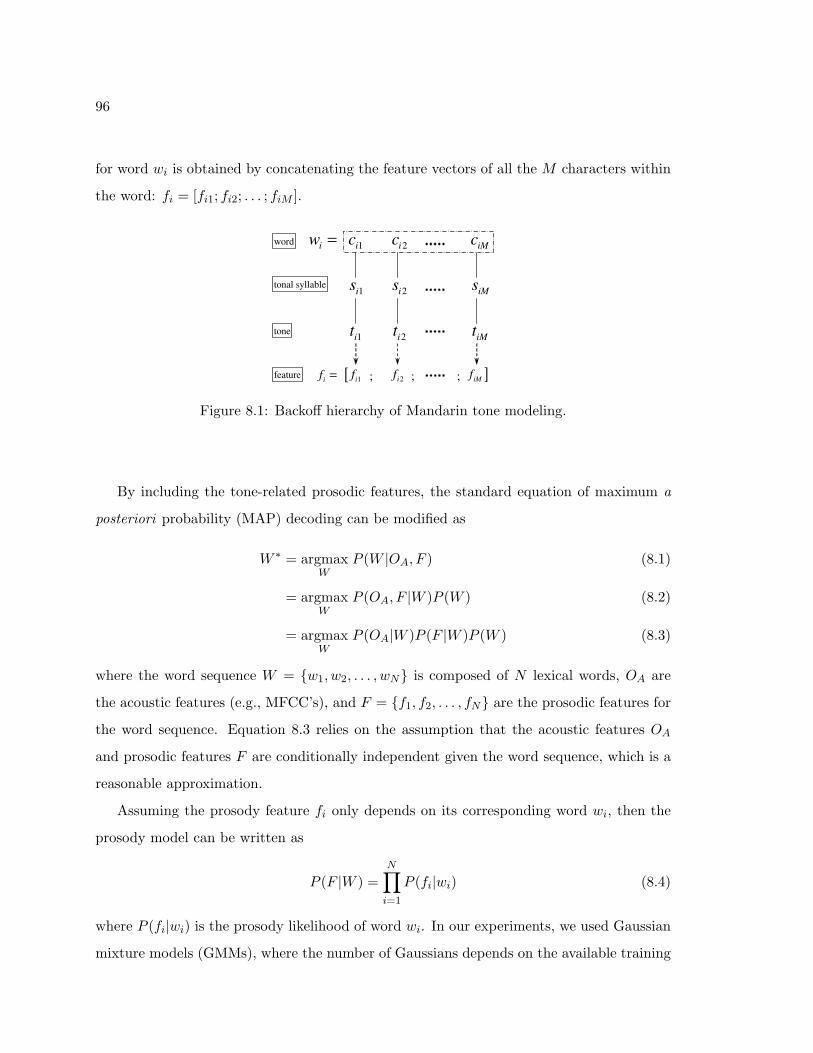
96
for word wi is obtained by concatenating the feature vectors of all the M characters within
the word: fi = [fi1; fi2; . . . ; fiM ].
1ic 2ic iMc
1is 2is iMs
1it 2it iMt
word
tonal syllable
tone
[ 1if 2if ]iMf; ; ;if =feature
iw =
Figure 8.1: Backoff hierarchy of Mandarin tone modeling.
By including the tone-related prosodic features, the standard equation of maximum a
posteriori probability (MAP) decoding can be modified as
W ∗ = argmaxW
P (W |OA, F ) (8.1)
= argmaxW
P (OA, F |W )P (W ) (8.2)
= argmaxW
P (OA|W )P (F |W )P (W ) (8.3)
where the word sequence W = {w1, w2, . . . , wN} is composed of N lexical words, OA are
the acoustic features (e.g., MFCC’s), and F = {f1, f2, . . . , fN} are the prosodic features for
the word sequence. Equation 8.3 relies on the assumption that the acoustic features OA
and prosodic features F are conditionally independent given the word sequence, which is a
reasonable approximation.
Assuming the prosody feature fi only depends on its corresponding word wi, then the
prosody model can be written as
P (F |W ) =N∏
i=1
P (fi|wi) (8.4)
where P (fi|wi) is the prosody likelihood of word wi. In our experiments, we used Gaussian
mixture models (GMMs), where the number of Gaussians depends on the available training

97
data for each model. One diagonal Gaussian is trained for 20 observations and a maximum
of 100 Gaussians is used for the GMMs.
As with the traditional syllable-level tone models, the word prosody models can be used
to rescore the recognition hypotheses in an N-best list or a word lattice. We choose to
rescore lattices since a lattice is a much richer representation of the entire search space.
8.3 Backoff Strategies
With a whole-word prosody model, the F0 contour and duration of the syllables within the
word are explicitly modeled. For unseen words or infrequent words that appear less than a
certain amount of times in the training data, we use the product of syllable-level models.
The particular syllable model is chosen according to a hierarchical backoff illustrated in
Figure 8.1. Within this framework, there are several different backoff strategies that we can
take. We first study the context-independent (CI) tone models as backoff. Then we study
the context-dependent (CD) tone models as backoff.
8.3.1 Context-independent tone models
To compute the prosody likelihood P (fi|wi) of the infrequent or unseen word wi with
context-independent component models, we use:
P (fi|wi)=⇒
C(wi)<Ct
M∏j=1
P (fij |sij). (8.5)
where “⇒” denotes backoff, C(wi) denotes the frequency of the word wi in the training
corpus and Ct is the frequency count threshold. Depending on the amount of training data
for the particular TS sij , the actual tone model used may be TS dependent or simply tone
dependent. The backoff strategy in this case is
P (fij |sij)=⇒
C(sij)<Ct P (fij |tij). (8.6)
When the frequency count of a tonal syllable is larger than the count threshold, an explicit
TS-dependent tone model is trained. Otherwise, the likelihood computation is backed off
to tone models. For simplicity, we have used the same count threshold Ct = 20 for training
all tone models including word and CI or CD tonal syllable models.
98
Similar to the word prosody models, these syllable-level models are trained as GMMs
except with fixed 4-dimensional features.
8.3.2 Context-dependent tone models
More generally, the word prosody models could be backed off to CD syllable-level models
such as tone-context-dependent TS models, bitones or tritones. As we have found in [59] and
Chapter 3, the carry-over coarticulation effect from the left context is much more significant
than from the right context. Therefore, as an alternative to Equation 8.5, we have used
left-tone context-dependent tone models as follows:
P (fi|wi)=⇒
C(wi)<Ct
M∏j=1
P (fij |ti(j−1), sij). (8.7)
Again, depending on the amount of training data for the particular CD models, a backoff
model may be used, where here we follow the strategy
P (fij |ti(j−1), sij)=⇒
C(ti(j−1),sij)<Ct P (fij |ti(j−1), tij) (8.8)
=⇒C(ti(j−1),tij)<Ct P (fij |tij) (8.9)
For a reasonably large training corpus, there are enough samples for training all possible
bitone models. Therefore, the backoff from left bitone to tone models is usually not used.
For the special case of the first tonal syllable of the word, it is often not straightforward
to find the unique left tone context of a word arc in the lattice. We can either use its
CI backoff models or expand the lattices according to the crossword left tone context as
mentioned in Chapter 7. Since no significant improvement was found by lattice expansion
in Chapter 7, in our experiments in this chapter, the former approach has been taken.
8.4 Experimental Results
Experiments are then carried out to find out the performance of the proposed word-level
tone modeling approach. We will compare word-level modeling to syllable-level modeling,
and various backoff strategies within the same proposed framework. First, we describe the
baseline system. Then we introduce the training and decoding with prosody models. Next

99
we present the experiments and results with different tone modeling techniques. Finally,
we investigate the data scalability of the prosody modeling in a Mandarin BN task with
several hundred hours of training data.
8.4.1 Baseline system
The baseline system is the Mandarin BN system with embedded tone modeling, as used in
the previous chapter. Details of the BN/BC baseline system have been described in Chapter
2. For testing, we use the NIST RT-04 evaluation set (bn-eval04) collected in April 2004.
There are three shows: CTV, NTDTV and RFA. Each show contains around 20 minutes of
speech data. The RFA data has a significant mismatch with the bn-Hub4 training data.
8.4.2 Training of prosody models
Forced alignment is performed to align all the training data. The F0 features are generated
similar to those used in embedded tone modeling, but without the final step of low-pass
filtering since the results in Table 7.2 show that it is better for the explicit tone modeling to
omit the low-pass filtering. Based on the forced alignment and the processed F0 features, the
feature vectors for word prosody models and other syllable-level tone models are extracted.
The features are mean- and variance-normalized per speaker as follows. As previously
mentioned, the feature vector fi is obtained by concatenating all feature vectors of the
M characters within the word: fi = [fi1; fi2, . . . ; fiM ]. Each sub feature vector fij is 4-
dimensional. The normalization is done for each sub vector:
fij =fij − µs
σs(8.10)
where fij is the normalized sub vector, µs and σs are the sample mean and standard
deviation of all the syllable feature vectors for a specific speaker s. Then GMMs with
diagonal Gaussians are trained for all the models that have a frequency count more than
the threshold (20 observations per Gaussian in our experiments).

100
8.4.3 Decoding with prosody models
The prosody models are used to rescore the word lattices from baseline system. For each
word arc in the lattice, the new score is computed based on acoustic model (AM), language
model (LM) and prosody model (PM) scores,
ψ(wi) = ψAM (wi) + αψLM (wi) + βψPM (wi), (8.11)
where α is the language model weight, β is the prosody model weight, and the prosody
score ψPM (wi) is given by
ψPM (wi) =1M
M∑j=1
dij logP (fi|wi), (8.12)
where dij is the duration of the j-th character in word wi. The average syllable duration
is used to weight the prosody likelihood, since in practice we find it effective to balance
insertion and deletion errors. To more explicitly control the deletion errors, we can introduce
an additive constant proportional to the number of characters in the word, similar to that
used in duration rescoring [52]. However, in our experiments we have not used this penalty
constant. The weights α and β are determined by grid search for the system trained on
bn-Hub4 data.
As in training, the feature vector fi for word arc wi is extracted from the F0 features
and the time marks in the lattice. However, the speaker-based normalization is not as
straightforward as in training, since no oracle transcription is available for getting the syl-
lables and their boundary time marks in order to extract the speaker-dependent feature
mean and variance normalization vectors. There are two options: the first is to use a global
mean and variance normalization factor from the training data; the second way is to use
the top hypothesis to compute the speaker mean and variance normalization factors. In our
experiments with the system trained on bn-Hub4 data, for simplicity, we have used global
normalization factors in decoding but speaker-based normalization in training.
8.4.4 Results and discussions
Since both the word-level prosody models and different syllable-level tone models have been
trained, we have the flexibility to choose different models and backoff strategies during

101
lattice decoding.
Table 8.1 shows the decoding results of different models.2 Since RFA has a significant
mismatch with the training data (as can be seen from the high CER), the prosody modeling
does not improve the performance on the RFA subset. The plain tone models can improve
the performance slightly for all subsets, while the word prosody models with backoff provide
a much larger improvement for subsets that are better matched to the training data. We
also find that the TS-dependent tone modeling is not significantly different from the tone
modeling, neither in rescoring directly nor as backoff models.
Table 8.1: CER(%) using word prosody models with CI tone models as backoff. The baselinesystem uses embedded tone modeling with spline+MWN+MA pitch features.
Model CTV NTDTV RFA Overall
Baseline 11.7 19.2 34.3 21.2
tone 11.5 18.8 34.2 20.9
TS ⇒ tone 11.5 18.8 34.7 21.1
word ⇒ tone 11.2 18.2 34.7 20.8
word ⇒ TS ⇒ tone 11.1 18.4 34.6 20.8
Table 8.2 shows the decoding results with CD tone models as backoff. Again, the RFA
subset does not benefit from explicit tone modeling. Excluding this set and comparing
Table 8.2 and Table 8.1, we can see the left bitone models are more effective than CI tone
models, due to the better modeling of tone coarticulation. However, the results between CI
backoff and CD backoff are not significantly different, probably because much of the tone
coarticulation has been modeled by the word prosody models. In Table 8.2, the left-context-
dependent TS models perform worse than the bitone models. This might be explained by
a lack of dependency between tones and base syllables, or the backoff may not have been
properly tuned. The lack of dependency is consistent with results in Table 8.1. With the
2The baseline results are slightly different from the results in Chapter 4, since a cleaner and more consis-tent decoding lexicon has been used.

102
3-level CD backoff modeling, performance on bn-eval04 can be improved by 0.6% absolute,
with 0.7% absolute on the CTV show and 1.0% absolute on the NTDTV show.
Table 8.2: CER (%) using word prosody models with CD tone models as backoff. ”l -” denotes left-tone context-dependent models. The baseline system uses embedded tonemodeling with spline+MWN+MA pitch features.
Model CTV NTDTV RFA Overall
Baseline 11.7 19.2 34.3 21.2
l -tone 11.3 18.4 34.4 20.8
l -TS ⇒ l -tone 11.4 18.7 34.4 20.9
word ⇒ l -tone 11.2 18.2 34.6 20.7
word ⇒ l -TS ⇒ l -tone 11.0 18.2 34.4 20.6
8.4.5 Performance scalability with training data
To test the effectiveness of the word-level tone modeling approach, we also train the prosody
models with all 465 hours of training data which was used in NIST 2006 GALE evaluation
system. The new language model is trained with around 946 million words. The decoding
lexicon is augmented to 60K words.
In this larger system, we only perform the first pass decoding. The baseline acoustic
model is maximum likelihood trained with 465 hours of data. The model size is 3000 senones
with 128 Gaussian components per senone. Since the larger system can generate a better top
hypothesis for computing the speaker-dependent normalization factors, per speaker mean
and variance normalization is used in decoding instead of global normalization. Different
from the grid search that is used in the smaller system in last section, the weights of the
acoustic models, language models, prosody models and word insertion penalty are optimized
to minimize the CER on bn-eval04 by the simplex downhill method [67], also known as
amoeba search. The best 3-level CD backoff model is used. The results on bn-eval04 and
bn-ext06 are shown in Table 8.3.
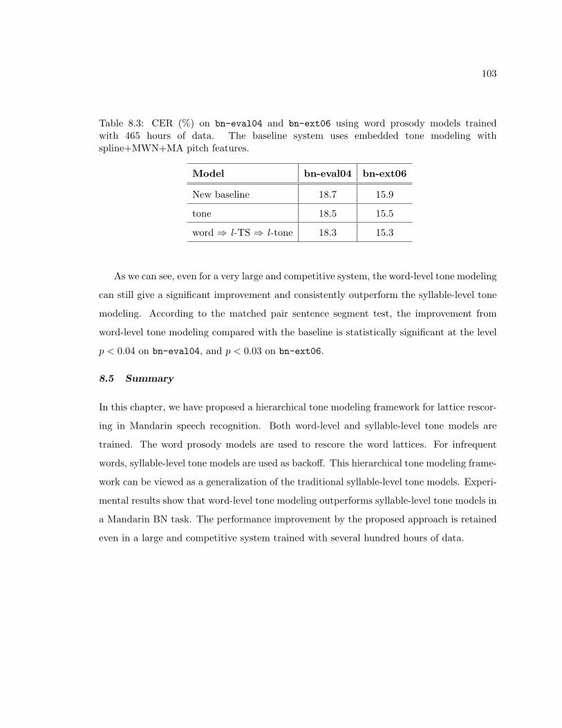
103
Table 8.3: CER (%) on bn-eval04 and bn-ext06 using word prosody models trainedwith 465 hours of data. The baseline system uses embedded tone modeling withspline+MWN+MA pitch features.
Model bn-eval04 bn-ext06
New baseline 18.7 15.9
tone 18.5 15.5
word ⇒ l -TS ⇒ l -tone 18.3 15.3
As we can see, even for a very large and competitive system, the word-level tone modeling
can still give a significant improvement and consistently outperform the syllable-level tone
modeling. According to the matched pair sentence segment test, the improvement from
word-level tone modeling compared with the baseline is statistically significant at the level
p < 0.04 on bn-eval04, and p < 0.03 on bn-ext06.
8.5 Summary
In this chapter, we have proposed a hierarchical tone modeling framework for lattice rescor-
ing in Mandarin speech recognition. Both word-level and syllable-level tone models are
trained. The word prosody models are used to rescore the word lattices. For infrequent
words, syllable-level tone models are used as backoff. This hierarchical tone modeling frame-
work can be viewed as a generalization of the traditional syllable-level tone models. Experi-
mental results show that word-level tone modeling outperforms syllable-level tone models in
a Mandarin BN task. The performance improvement by the proposed approach is retained
even in a large and competitive system trained with several hundred hours of data.

104
Chapter 9
SUMMARY AND FUTURE DIRECTIONS
This chapter summarizes the main contributions of the dissertation, including research
findings, general observations about effective tone modeling, and the state-of-the-art Man-
darin LVCSR systems developed for the NIST evaluations. Some directions are also sug-
gested for future research on tone modeling.
9.1 Contributions
The contributions of this dissertation lie in three aspects: 1) specific research findings and
modeling advances, 2) general observations, and 3) development of competitive Mandarin
ASR systems for NIST evaluations. The first aspect includes improvements of feature rep-
resentation and development of novel modeling techniques for tone modeling in Mandarin
speech recognition. The second aspect is concerned with the general observations about
effective tone modeling in state-of-the-art Mandarin LVCSR systems, based on pulling
together findings from different types of experiments. The third aspect involves the co-
development of SRI-UW’s first state-of-the-art Mandarin CTS system in the NIST 2004
evaluation, and Mandarin BN system in NIST 2006 evaluation.1 Much of the tone model-
ing research work was done on systems that were not state-of-the-art (e.g., used less training
data), since this has faster experiment turnaround. However, to achieve the best possible
performance, all data were used and multiple passes of recognition were performed in the
evaluation systems. Due to the time period of the development of the tone modeling tech-
niques, only those techniques available at the time of evaluation were incorporated in the
evaluation systems.
1This has been a joint effort with Dr. Mei-Yuh Hwang, Prof. Mari Ostendorf, Tim Ng, Dr. Gang Pengfrom SSLI lab at UW, Dr. Ozgur Cetin from ICSI, and Dr. Wen Wang, Dr. Jing Zheng and Dr. AndreasStolcke from STAR lab at SRI International.

105
9.1.1 Research findings and modeling advances
Unlike most western languages, tones in Mandarin carry lexical meanings to distinguish
ambiguous words. Therefore, tone modeling is an important aspect for Mandarin ASR.
In natural Mandarin speech such as CTS and BN/BC speech, the tonal patterns are sig-
nificantly different from the standard F0 contour patterns, due to the coarticulation and
linguistic variations. We were able to find out experimentally that the carry-over effect from
the left tone context is much more significant than the anticipatory effect from the right
context in both CTS and BN/BC speech domains. We also found that the tone reduction
and coarticulation are more significant in CTS speech than in BN speech, which suggests
the tone modeling in CTS might be more difficult.
Various tone modeling strategies have been explored to enhance the performance of
Mandarin LVCSR systems. According to the time window used for feature selection, our
tone modeling approaches can be classified into two categories: fixed-window methods and
variable-window methods. These two categories of methods are complementary and we
tried to combine them to achieve improved performance.
The fixed-window approaches use a fixed-length time window to extract the features for
tones. The advantage is that these methods can be easily integrated in the HMM-based
embedded modeling framework for first pass decoding. First, we explored more effective
pitch features for embedded tone modeling. A spline interpolation algorithm was proposed
for continuation of the F0 contour. Based on the interpolated F0 contour, we performed
wavelet-based multiresolution analysis and decomposed the F0 contour into three categories
representing the intonation, lexical tone variation and other noises. By combining different
levels of the decomposed components, we were able to find out primarily the F0 variation
on the scales of 80ms to 640ms can improve the tone modeling in Mandarin BN task. An
approximate fast algorithm was developed to extract the useful components from the F0
contour and shown to achieve significant CER reduction in both Mandarin BN and CTS
tasks. Second, since tone depends on a longer span than the phonetic units, the frame-
level F0 features for HMM-based modeling may not be enough for tone modeling. We then
investigated using a longer time window to extract more effective tone features. MLP was

106
used to classify the tone-related acoustic units with features from a longer fixed-window.
The MLP posterior probabilities were appended to the original feature vector for HMM
modeling. We found the tone posteriors can improve the system performance, and much
more significant improvements were achieved by using toneme posterior features since they
also carry segmental information.
To exploit the stream-specific model dependence for spectral feature stream and tone
feature stream in the HMM modeling, we proposed a multi-stream adaptation technique
where the two streams are adapted separately using different adaptation regression class
trees. The adaptation regression class trees can be generated separately in a data-driven
manner from the training data, and used for MLLR adaptation. However, no significant
improvement has been achieved in our evaluation task with the multi-stream MLLR adap-
tation, probably because of the limited amount of adaptation data or that the pitch feature
processing, which includes long term normalization, has already removed most of the speaker
dependency.
The fixed-window methods cannot exploit the suprasegmental nature of tones. A tone
depends on the F0 contour of the syllable which has a variable length. Therefore, we in-
vestigated explicit tone modeling with features extracted from the syllable segments. We
first demonstrate that by rescoring the word lattices of the embedded tone modeling system
with perfect tone information, more than 30% improvement in CER could be achieved.
Syllable-level explicit tone models were trained and used to rescore the lattices. A small im-
provement can be achieved by this approach. Then we extended the explicit tone modeling
from the syllable level to the word level to take advantage of the large amount of training
data in LVCSR tasks. Word-dependent tone models are trained to explicitly model the
tone coarticulation and tone sandhi within the word. For less frequent or unseen words, we
used different syllable-level tone models as backoff. This hierarchical tone modeling frame-
work is a generalization of the syllable-level tone models for rescoring. In this framework,
different explicit tone modeling strategies can be adopted in a very flexible way. We were
able to demonstrate the word-level tone modeling approach consistently outperforms the
syllable-level tone models in a Mandarin BN task.

107
9.1.2 General Observations
From this study, we have the following cross-cutting findings about effective tone modeling
in state-of-the-art Mandarin LVCSR systems:
1. Filling in the gaps for unvoiced regions
When using F0 features, it is better to fill in the gaps for the unvoiced regions of the F0
contour by shape-preserving interpolation, rather than treating these as uninformative
regions and ignoring them or filling the gaps with mean values. Interpolation of F0
in the unvoiced regions can avoid variance problems in embedded tone modeling, and
can also facilitate extracting syllable-level tone features in explicit tone modeling. In
addition, spline-based interpolation is more effective than IBM-style F0 processing for
removal of utterance-level F0 downtrend, which is important for extracting effective
tone features. In Chapter 4 and Chapter 5, it was shown that significant improvement
can be obtained by using improved F0 features over IBM-style features. In Chapter 7,
it was shown that interpolation improves the explicit tone classification over treating
F0 in unvoiced regions as missing features.
2. Interdependence of pitch and spectral features
F0 features alone are not very powerful acoustic cues in comparison to the combined
effect of F0, spectral and context cues, i.e. F0 and spectral cues are not independently
characterizing tone and base syllables, respectively. It is generally better to integrate
all cues for good performance. In embedded tone modeling with MLP posteriors, as
described in Chapter 5, we found the toneme posteriors are much more effective than
tone posteriors, since the toneme contains both tone and segmental information. In
Chapter 6, we found that there was little advantage to decoupling the transform tying
for F0 and spectral features for speaker adaptation. In explicit tone modeling with
syllable-level tone models, as described in Chapter 7, we found the tone accuracy of
the lattices are remarkably higher than explicit tone models. Part of the reason is
that the lattices include acoustic cues from both F0 and spectral features, as well as
context cues in the language models.
108
3. Significance of coarticulation
The tone reduction and coarticulation effects in running speech greatly impact the
measured F0 contours as illustrated by the contrast between Figure 1.3 and Figures 3.1
and 3.2. The changes in CTS are more significant than in BN speech. Analysis of
contours in Chapter 3 suggests a lesser impact of tone modeling for CTS compared
to BN, because of the differences between average tone contours. Indeed, as found in
Chapter 4, for spontaneous speech like CTS, the impact of tone modeling on CER is
smaller. Different news sources also have different amounts of conversational speech
and perhaps other speaking style differences that impact tone variability. By modeling
the tone coarticulation effects, as presented in Chapter 8, better ASR performance
can be obtained for matched training and test conditions. However, there is no benefit
for a news source that is less well matched to the style of shows in the training data,
suggesting that adapting the word-level models may be useful.
9.1.3 Evaluation Systems
During this study, we have contributed to two state-of-the-art Mandarin speech recognition
systems: the Mandarin CTS system in NIST 2004 evaluation and the Mandarin BN/BC
system in NIST 2006 evaluation. Most state-of-the-art speech recognition techniques in the
SRI decipher English systems have been ported to both Mandarin Chinese ASR systems
successfully. We also explored some language-specific problems such as tone modeling,
pronunciation modeling and language modeling. Both systems have achieved performances
that are comparable to the best systems in the world. Since we have already covered the
Mandarin CTS system in Chapter 2, here we only describe the results for that system, and
give both the details and performance results of the Mandarin BN system.
SRI-UW 2004 Mandarin CTS system
The SRI-UW 2004 Mandarin CTS system for NIST 2004 evaluation was developed during
January - September 2004. The details of this system have been described in Chapter
2. The only tone modeling technique incorporated in this system was the embedded tone

109
modeling with IBM-style F0 processing, since the time period of development of the other
tone modeling techniques is after September 2004. Three sites participated in Mandarin
CTS evaluation: BBN, CU and SRI-UW. The released Mandarin speech-to-text (STT)
performance results on cts-eval04 data are listed in Table 9.1. All three competing sites
got a final CER of around 29.5% in Mandarin CTS task. In terms of CER, the difference
between SRI-UW system and other sites is statistically insignificant.
Table 9.1: CER results (%) of the Mandarin CTS system for NIST 2004 evaluation.
System cts-eval04
SRI-UW 29.7
CU 29.5
BBN 29.3
SRI-UW 2006 Mandarin BN/BC system
The SRI-UW 2006 Mandarin BN/BC system for NIST 2006 evaluation was developed during
October 2005 - July 2006. The tone modeling techniques incorporated in this system include
spline+MWN+MA F0 processing and toneme posteriors, representing the best embedded
tone modeling techniques. The explicit tone modeling work is more recent and was not
available at the time of evaluation. The details of this system are referred to [50]. We
briefly describe the system as follows.
Training and Testing Data: In the Mandarin BN/BC system for evaluation, we have
used all the 465 hours of BN and BC acoustic training data listed in Table 2.3. All the
946M words of text data listed in Table 2.4 are used in language model training. The final
evaluation set bnbc-eval06 contains about 1.2 hours of BN data and 1.0 hours of BC data.
Features and Acoustic Models: Two different front ends were used: one uses MFCC+F0,
and the other uses MFCC+F0+ICSI features. The F0 features in both front ends are

110
processed with spline+MWN+MA as in Chapter 4. The ICSI features are combined ver-
sion of the toneme posterior features used in Chapter 5 and the hidden activation temporal
pattern-MLPs (HATs) [66] features. Two types of MLPs are used generate the ICSI fea-
tures. A PLP/MLP, which focuses on medium-term information, was trained on 9 consec-
utive frames of PLP features and their derivatives. On the other hand, the HATs features
extract information from 500ms windows of critical band energies. Both PLP/MLP and
HATs systems generate toneme posteriors and are combined using inverse-entropy weight-
ing [65]. The combined posteriors are then projected down to 32-dimensional features via
PCA.
The AMs used in the final system were all gender-independent, MPE trained with fMPE
feature transforms. For the MFCC front end, there are 3000 decision-tree clustered states
with 128 Gaussians per state. Crossword triphones were used in the MFCC system with
feature-space speaker adaptive training (SAT), via single-class constrained MLLR. For the
MLP-feature front end, we did not have enough time to train an equally complex system as
with the MFCC-feature system. Instead, we trained a 3000×64 within-word triphone model
without SAT. For more details about combining the MLP features, fMPE transforms and
MPE training, please refer to [110].
Language Models: The most frequent 60K words in the training text were then chosen
as our decoding vocabulary. Seven N-gram LMs were independently trained on all seven
sources listed in Table 2.4, and then interpolated to maximize the likelihood on bn-dev06
transcriptions. Each individual LM was trained with Kneser-Ney smoothing [13].
There were five LMs used in decoding: one highly pruned bigram and one highly pruned
trigram for fast decoding in the first pass recognition, one full trigram for lattice expansion
and N-best generation, and two 5-gram LMs for N-best rescoring. The first 5-gram is class-
based, and the second 5-gram used count-based Jelinek-Mercer smoothing [51, 13]. More
details are described in [50].
Decoding Structure: The decoding structure consists of two iterations of cross-adaptation,
as illustrated in Figure 9.1. In the first iteration, first-pass decoding is performed using the
within-word MLP-feature AM with a pruned trigram. The top hypothesis is used to cross
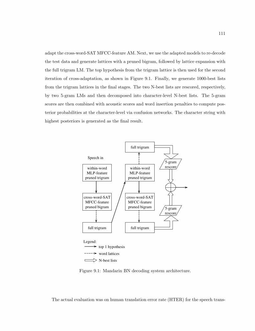
111
adapt the cross-word-SAT MFCC-feature AM. Next, we use the adapted models to re-decode
the test data and generate lattices with a pruned bigram, followed by lattice expansion with
the full trigram LM. The top hypothesis from the trigram lattice is then used for the second
iteration of cross-adaptation, as shown in Figure 9.1. Finally, we generate 1000-best lists
from the trigram lattices in the final stages. The two N-best lists are rescored, respectively,
by two 5-gram LMs and then decomposed into character-level N-best lists. The 5-gram
scores are then combined with acoustic scores and word insertion penalties to compute pos-
terior probabilities at the character-level via confusion networks. The character string with
highest posteriors is generated as the final result.
within-wordMLP-feature
pruned trigram
Speech in
cross-word-SATMFCC-featurepruned bigram
full trigram
within-wordMLP-feature
pruned trigram
cross-word-SATMFCC-featurepruned bigram
full trigram
full trigram
5-gramrescore
5-gramrescore
Legend:top 1 hypothesis
word lattices
N-best lists
Figure 9.1: Mandarin BN decoding system architecture.
The actual evaluation was on human translation error rate (HTER) for the speech trans-

112
lation task. Here we only report the intermediate ASR results. Three systems participated
in the Mandarin BN/BC NIST 2006 evaluation: UW-SRI-ICSI system, IBM system and
CU-BBN system. The ASR performance results of the final evaluation systems are listed
in Table 9.2.2 For computing the CER of the final evaluation test set bnbc-eval06, we
have used the reference transcription file provided by IBM with some cleaning. During our
development, we have focused on optimizing the system performance on BN (vs. BC) data
since BN was the major task for evaluation. The final BN performance of our system is
0.3% better than IBM and 0.5% worse than CU-BBN. Note that in our system, a smaller
amount of training data was used and fewer subsystems were used in ROVER combination.
In terms of CER, the 0.3% and the 0.5% differences are statistically significant. However,
the HTER results are in fact better for UW though the machine translation (MT) systems
are not better on text, which suggests that the ASR differences are not significant in terms
of their impact on MT.
Table 9.2: CER results (%) of the Mandarin BN/BC system for NIST 2006 evaluation.
Systembnbc-eval06
BN BC Overall
UW-SRI-ICSI 12.8 22.9 17.8
IBM 13.1 22.4 17.6
CU-BBN 12.3 21.0 16.5
After the word-level tone modeling was developed, we tried to integrate it in the final
evaluation system. However, no performance gain was obtained using the acoustic models
with fMPE and MPE training. There are several possible reasons. First, the combination
of discriminative feature, discriminative transform and discriminative model training [110]
may have diminished the impact from explicit tone modeling. The word-level tone models
may also need to be trained discriminatively instead of using the maximum likelihood cri-
terion. Second, the mismatch between the training and testing data might have limited the
2The listed results of UW-SRI-ICSI system are after a small bug fix.

113
effectiveness of the word-level tone models. Therefore, adaptation of the word-level tone
models may be necessary to minimize this mismatch.
9.2 Future Directions
While in this dissertation study we focused on modeling the tones for Mandarin Chinese, the
embedded and explicit tone modeling techniques developed should be applicable to other
tone languages such as Cantonese, Thai and Vietnamese. The approaches developed in this
dissertation study can also be extended in a number of ways. We briefly suggest several
directions for future research as follows.
The spline+MWN+MA pitch processing presented in Chapter 4 used a fixed window for
normalization. However, different speakers have different speaking rates and the intonation
effects may be on different scales. For example, in some regions of speech where the speak-
ing rate is higher, a shorter time window should be used for MWN. Also, the processing
technique for F0 contour could be used for processing the energy contour and extract useful
features for acoustic modeling.
The MLP-based tone-related posteriors, as described in Chapter 5, could be extended to
predict posteriors of context-dependent tone models such as bitones and tritones. Features
from a longer time window should be used to classify these context-dependent tones. Since
the cardinality of tritones is large (216 if using tone 1 to tone 5, neutral tone and no-tone) and
quite some tritones share similar F0 patterns, these tritones could be divided into different
groups. Either linguistic knowledge can be used to manually cluster the tritones, or they
can be clustered in a data-driven way. For example, according to the statistics accumulated
from the training data, these tritones can be clustered with maximum likelihood criterion.
The clustered tritone classes then can be used as the new targets for MLP training. The
MLP posteriors generated in this way may offer more information about tone than that
already incorporated in the toneme posteriors. Hence they may be combined to achieve
better performance.
In Chapter 6, we only considered the multi-stream adaptation of the mean parameters
of the acoustic models. The multi-stream adaptation technique can be extended to adapt
the variance parameters. In general, multi-stream adaptation offers more flexible adapta-

114
tion strategies and could be applied in other modeling tasks such as audio-visual speech
recognition.
In Chapter 7, the neural network based syllable-level tone models presented may be
improved with separate short-tone modeling. Different statistical models can be used for CI
or CD tone modeling and the decisions of these models may be combined to achieve better
performance.
The word-level tone modeling method presented in Chapter 8 may be improved in several
different ways. First, more tone features such as energy features and regression coefficients
can be used. The syllable duration features used in the word prosody models can be sub-
stituted by the duration features of the initials and finals to obtain more detailed modeling
of durations. Second, the right context can be taken into consideration for syllable-level
tone models, i.e., tritone models may be used instead of the left-bitone models. Third,
the word prosody models can be combined with duration modeling [31] to achieve better
performance. Finally, discriminative training and speaker adaptation of the word-level tone
models may also be explored.
115
BIBLIOGRAPHY
[1] T. Anastasakos, J. McDonough, R. Schwartz, and J. Makhoul. A compact modelfor speaker-adaptive training. In Proc. Int. Conf. on Spoken Language Processing,volume 2, pages 1137–1140, 1996.
[2] C. Benitez, L. Burget, B. Chen, S. Dupont, H. Garudadri, H. Hermansky, P. Jain,S. Kajarekar, and S. Sivadas. Robust ASR front-end using spectral-based and dis-criminant features: experiments on the Aurora tasks. In Proc. Eur. Conf. SpeechCommunication Technology, volume 1, pages 429–432, 2001.
[3] J. Bilmes. A gentle tutorial on the EM algorithm and its application to parameterestimation for Gaussian mixture and hidden Markov models. Technical Report ICSI-TR-97-021, University of Berkeley, 1997.
[4] I. Bulyko, M. Ostendorf, and A. Stolcke. Getting more mileage from web text sourcesfor conversational speech language modeling using class-dependent mixtures. In Proc.HLT/NAACL, pages 7–9, 2003.
[5] Y. Cao, S. Zhang, T. Huang, and B. Xu. Tone modeling for continuous Mandarinspeech recognition. International Journal of Speech Technology, 7:115–128, 2004.
[6] E. Chang, J. Zhou, S. Di, C. Huang, and K.-F. Lee. Large vocabulary Mandarinspeech recognition with different approaches in modeling tones. In Proc. Int. Conf.on Spoken Language Processing, volume 2, pages 983–986, 2000.
[7] Y.R. Chao. A system of tone letters. Le Maıtre Phonetique, 45:24–27, 1930.
[8] Y.R. Chao. A Grammar of Spoken Chinese. University of California Press, 1968.
[9] B. Chen, Q. Zhu, and N. Morgan. Tonotopic multi-layered perceptron: a neuralnetwork for learning long-term temporal features for speech recognition. In Proc. Int.Conf. on Acoustics, Speech and Signal Processing, volume 1, pages 945–948, 2005.
[10] C.J. Chen, R.A. Gopinath, M.D. Monkowski, M.A. Picheny, and K. Shen. New meth-ods in continuous Mandarin speech recognition. In Proc. Eur. Conf. Speech Commu-nication Technology, volume 3, pages 1543–1546, 1997.
[11] C.J. Chen, H. Li, L. Shen, and G. Fu. Recognize tone languages using pitch informa-tion on the main vowel of each syllable. In Proc. Int. Conf. on Acoustics, Speech andSignal Processing, volume 1, pages 61–64, 2001.
116
[12] J. Chen, B. Dai, and J. Sun. Prosodic features based on wavelet analysis for speakerverification. In Proc. Interspeech, pages 3093–3096, 2005.
[13] S. Chen and J. Goodman. An empirical study of smoothing techniques for languagemodeling. Technical Report TR-10-98, Computer Science Group, Harvard University,1998.
[14] S.H. Chen and Y.R. Wang. Tone recognition of continuous Mandarin speech basedon neural networks. IEEE Trans. on Speech and Audio Processing, 3:146–150, 1995.
[15] M. Cooke, P. Green, L. Josifovski, and A. Vizinho. Robust automatic speech recogni-tion with missing and unreliable acoustic data. Speech Communication, 34:267–285,2001.
[16] T.M. Cover and J.A. Thomas. Elements of Information Theory. Wiley-Interscience,1991.
[17] A. Cruttenden. Intonation. Cambridge University Press, 1986.
[18] D. Crystal. The Cambridge Encyclopedia of Language. Cambridge University Press,1997.
[19] S.B. Davis and P. Mermelstein. Comparison of parametric representation for monosyl-labic word recognition in continuously spoken sentences. IEEE Trans. on Acoustics,Speech and Signal Processing, 28:357–366, 1980.
[20] L. Deng, M. Aksmanovic, X. Sun, and C.F.J. Wu. Speech recognition using hiddenMarkov models with polynomial regression functions as nonstationary states. IEEETrans. on Speech and Audio Processing, 2(4):507–520, 1994.
[21] V. Digalakis and H. Murveit. GENONES: Optimizing the degree of mixture tying ina large vocabulary hidden Markov model based speech recognizer. In Proc. Int. Conf.on Acoustics, Speech and Signal Processing, volume 1, pages 537–540, 1994.
[22] R.O. Duda, P.E. Hart, and D.G. Stork. Pattern Classification. John Wiley and Sons,Inc., 2000.
[23] J.W. Eaton. GNU Octave Manual. Network Theory Limited, 2002.
[24] D.P.W. Ellis, R. Singh, and S. Sivadas. Tandem acoustic modeling in large-vocabularyrecognition. In Proc. Int. Conf. on Acoustics, Speech and Signal Processing, volume 1,pages 517–520, 2001.
[25] Entropic Research Laboratory. ESPS Version 5.0 Programs Manual, 1993.
117
[26] G. Evermann, H.Y. Chan, M.J.F. Gales, T. Hain, X. Liu, D. Mrva, L. Wang, andP.C. Woodland. Development of the 2003 CU-HTK conversational telephone speechtranscription system. In Proc. Int. Conf. on Acoustics, Speech and Signal Processing,volume 1, pages 249–252, 2004.
[27] G. Evermann and P.C. Woodland. Large vocabulary decoding and confidence estima-tion using word posterior probabilities. In Proc. Int. Conf. on Acoustics, Speech andSignal Processing, volume 3, pages 1655–1658, 2000.
[28] J.G. Fiscus. A post-processing system to yield reduced word error rates: Recognizeroutput voting error reduction (ROVER). In Proc. IEEE Automatic Speech Recognitionand Understanding Workshop, pages 347–352, 1997.
[29] F.N. Fritsch and R.E. Carlson. Monotone Piecewise Cubic Interpolation. SIAM J.Numerical Analysis, 17:238–246, 1980.
[30] S.W.K. Fu, C.H. Lee, and O.L. Clubb. A survey on Chinese speech recognition.Communications of COLIPS, 6(1):1–17, 1996.
[31] V.R.R. Gadde. Modeling word durations. In Proc. Int. Conf. on Spoken LanguageProcessing, volume 1, pages 601–604, 2000.
[32] M.J.F. Gales. The generation and use of regression class trees for MLLR adaptation.Technical Report CUED/F-INFENG/TR263, Cambridge University, August 1996.
[33] M.J.F. Gales. Maximum likelihood linear transformations for HMM-based speechrecognition. Computer Speech and Language, 12:75–98, 1998.
[34] M.J.F. Gales, B. Jia, X. Liu, K.C. Sim, P.C. Woodland, and K. Yu. Development ofthe CUHTK 2004 Mandarin conversational telephone speech transcription system. InProc. Int. Conf. on Acoustics, Speech and Signal Processing, volume 1, pages 841–844,2005.
[35] M.J.F. Gales and P.C. Woodland. Mean and variance adaptation within the MLLRframework. Computer Speech and Language, 10:249–264, 1996.
[36] J. Gauvain, L. Lamel, and G. Adda. The LIMSI broadcast news transcription system.Speech Communication, 37(1-2):89–108, May 2002.
[37] J.-L. Gauvain and C.-H. Lee. Maximum a posteriori estimation for multivariateGaussian mixture observations of Markov chains. IEEE Trans. on Speech and Au-dio Processing, 2(2):291–298, April 1994.
118
[38] T. Hastie, R. Tibshirani, and J. Friedman. The Elements of Statistical Learning.Springer, 2001.
[39] H. Hermansky. Perceptual linear predictive (PLP) analysis of speech. Journal of theAcoustic Society of America, 87:1738–1752, 1990.
[40] H. Hermansky, D. Ellis, and S. Sharma. Tandem connectionist feature extractionfor conventional HMM systems. In Proc. Int. Conf. on Acoustics, Speech and SignalProcessing, pages 1635–1638, 2000.
[41] D. Hirst and R. Espesser. Automatic modelling of fundamental frequency using aquadratic spline function. Travaux de l’Institut de Phonetique d’Aixen -Provence, 15,75-85, 1993.
[42] T.H. Ho, C.J. Liu, H. Sun, M.Y. Tsai, and L.S. Lee. Phonetic state tied-mixture tonemodeling for large vocabulary continuous Mandarin speech recognition. In Proc. Eur.Conf. Speech Communication Technology, pages 883–886, 1999.
[43] J.M. Howie. On the domain of tone in Mandarin. Phonetica, 30:129–148, 1974.
[44] C. Huang, Y. Shi, J. Zhou, M. Chu, T. Wang, and E. Chang. Segmental tonal modelingfor phone set design in Mandarin LVCSR. In Proc. Int. Conf. on Acoustics, Speechand Signal Processing, volume 1, pages 901–904, 2004.
[45] H.C. Huang and F. Seide. Pitch tracking and tone features for Mandarin speechrecognition. In Proc. Int. Conf. on Acoustics, Speech and Signal Processing, volume 3,pages 1523–1526, 2000.
[46] M.Y. Hwang, X. Huang, and F. Alleva. Predicting unseen triphones with senones.IEEE Trans. on Speech and Audio Processing, 4(6):412–419, 1996.
[47] M.Y. Hwang, X. Lei, T. Ng, I. Bulyko, M. Ostendorf, A. Stolcke, W. Wang, J. Zheng,V.R.R. Gadde, M. Graciarena, M. Siu, and Y. Huang. Progress on Mandarin conver-sational telephone speech recognition. In International Symposium on Chinese SpokenLanguage Processing, 2004.
[48] M.Y. Hwang, X. Lei, T. Ng, M. Ostendorf, A. Stolcke, W. Wang, J. Zheng, andV. Gadde. Porting DECIPHER from English to Mandarin. Technical ReportUWEETR-2006-0013, University of Washington, 2006.
[49] M.Y. Hwang, X. Lei, W. Wang, and T. Shinozaki. Investigation on Mandarin broad-cast news speech recognition. In Proc. Interspeech, pages 1233–1236, 2006.

119
[50] M.Y. Hwang, X. Lei, J. Zheng, O. Cetin, W. Wang, G. Peng, and A. Stolcke. Advancesin Mandarin broadcast speech recognition. In submitted to ICASSP, 2007.
[51] F. Jelinek and R. Mercer. Interpolated estimation of Markov source parameters fromsparse data. In Workshop on Pattern Recognition in Practice, 1980.
[52] N. Jennequin and J.-L. Gauvain. Lattice rescoring experiments with duration models.In TC-STAR Workshop on Speech-to-Speech Translation, pages 155–158, Barcelona,Spain, June 2006.
[53] H. Jin, S. Matsoukas, R. Schwartz, and F. Kubala. Fast robust inverse transform SATand multi-stage adaptation. In Proceedings DARPA Broadcast News Transcriptionand Understanding Workshop, pages 105–109, 1998.
[54] W. Jin. Chinese segmentation and its disambiguation. Technical Report MCCS-92-227, New Mexico State University, 1992.
[55] T. Lee, W. Lau, Y.W. Wong, and P.C. Ching. Using tone information in Cantonesecontinuous speech recognition. ACM Trans. Asian Language Info. Process., 1:83–102,2002.
[56] C. Leggetter and P. Woodland. Maximum likelihood linear regression for speakeradaptation of HMMs. Computer Speech and Language, 9:171–186, 1995.
[57] X. Lei, M. Hwang, and M. Ostendorf. Incorporating tone-related MLP posteriors inthe feature representation for Mandarin ASR. In Proc. Eur. Conf. Speech Communi-cation Technology, pages 2981–2984, 2005.
[58] X. Lei, G. Ji, T. Ng, J. Bilmes, and M. Ostendorf. DBN-based multi-stream modelsfor Mandarin toneme recognition. In Proc. Int. Conf. on Acoustics, Speech and SignalProcessing, volume 1, pages 349–352, 2005.
[59] X. Lei, M. Siu, M.Y. Hwang, M. Ostendorf, and T. Lee. Improved tone modeling forMandarin broadcast news speech recognition. In Proc. Interspeech, pages 1237–1240,2006.
[60] C.-H. Lin, L.-S. Lee, and P.-Y. Ting. A new framework for recognition of mandarinsyllables with tones using sub-syllabic units. In IEEE Trans. on Acoustics, Speechand Signal Processing, volume 2, pages 227–230, 1993.
[61] M. Lin. A perceptual study on the domain of tones in standard Chinese. Chinese J.Acoust., 14:350–357, 1995.

120
[62] F.H. Liu, M. Picheny, P. Srinivasa, M. Monkowski, and J. Chen. Speech recognitionon Mandarin Call Home: a large-vocabulary, conversational, and telephone speechcorpus. In Proc. Int. Conf. on Acoustics, Speech and Signal Processing, volume 7,pages 157–160, 1996.
[63] A. Mandal, M. Ostendorf, and A. Stolcke. Speaker clustered regression-class trees forMLLR adaptation. In Proc. Interspeech, pages 1133–1136, 2006.
[64] L. Mangu, E. Brill, and A. Stolcke. Finding consensus in speech recognition: worderror minimization and other applications of confusion networks. Computer Speechand Language, 14(4):373–400, 2000.
[65] H. Misra, H. Bourlard, and V. Tyagi. New entropy based combination rules inHMM/ANN multi-stream ASR. In Proc. Int. Conf. on Acoustics, Speech and Sig-nal Processing, volume 2, pages 741–744, 2003.
[66] N. Morgan, B. Chen, Q. Zhu, and A. Stolcke. TRAPping conversational speech:Extending TRAP/Tandem approaches to con versational telephone speech recogni-tion. In Proc. Int. Conf. on Acoustics, Speech and Signal Processing, volume 1, pages537–540, 2004.
[67] J.A. Nelder and R. Mead. A simplex method for function minimization. ComputerJournal, 7:308–313, 1965.
[68] T. Ng, M. Ostendorf, M. Hwang, I. Bulyko, M. Siu, and X. Lei. Web-data augmentedlanguage model for Mandarin speech recognition. In Proc. Int. Conf. on Acoustics,Speech and Signal Processing, volume 1, pages 589–592, 2005.
[69] T. Ng, M. Siu, and M. Ostendorf. A quantitative assessment of the importance oftone in Mandarin speech recognition. Signal Processing Letters, IEEE, 12(12):867–870, Dec. 2005.
[70] L. Nguyen, S. Matsoukas, J. Davenport, F. Kubala, R. Schwartz, and J. Makhoul.Progress in transcription of Broadcast News using Byblos. Speech Communication,38(12):213–230, Sep 2002.
[71] J.J. Odell, P.C. Woodland, and S.J. Young. Tree-based state clustering for large vo-cabulary speech recognition. In International Symposium on Speech, Image Processingand Neural Networks, volume 2, pages 690–693, 1994.
[72] G. Peng and W.S.-Y. Wang. Tone recognition of continuous Cantonese speech basedon support vector machines. Speech Communication, 45:49–62, 2005.
[73] D.B. Percival and A.T. Walden. Wavelet Methods for Time Series Analysis. Cam-bridge University Press, 2000.

121
[74] D. Povey and P.C. Woodland. Minimum phone error and I-smoothing for improveddiscriminative training. In Proc. Int. Conf. on Acoustics, Speech and Signal Processing,volume 1, pages 105–108, 2002.
[75] P. Prieto, C. Shih, and H. Nibert. Pitch downtrend in Spanish. Journal of Phonetics,24:445–473, 1996.
[76] Y. Qian. Use of Tone Information in Cantonese LVCSR Based on Generalized Pos-terior Probability Decoding. PhD thesis, The Chinese University of Hong Kong, 2005.
[77] M.J. Reyes-Gomez and D.P.W. Ellis. Error visualization for tandem acoustic modelingon the Aurora task. In Proc. Int. Conf. on Acoustics, Speech and Signal Processing,volume 4, pages 13–17, 2002.
[78] F. Seide and N.J.C. Wang. Two-stream modeling of Mandarin tones. In Proc. Int.Conf. on Spoken Language Processing, pages 495–498, 2000.
[79] X.-N. Shen. Interplay of the four citation tones and intonation in Mandarin Chinese.Journal of Chinese Linguistics, 17(1):61–74, 1989.
[80] X. S. Shen. Tonal coarticulation in Mandarin. Journal of Phonetics, 18:281–295, 1990.
[81] C. Shih and R. Sproat. Variations of the Mandarin rising tone. In Proceedings of theIRCS Research in Cognitive Science, 1992.
[82] C.-L. Shih. The Prosodic Domain of Tone Sandhi in Chinese. PhD thesis, Universityof California, San Diego, 1986.
[83] M.K. Sonmez, L. Heck, M. Weintraub, and E. Shriberg. A lognormal tied mixturemodel of pitch for prosody-based speaker recognition. In Proc. Eur. Conf. SpeechCommunication Technology, volume 3, pages 1391–1394, 1997.
[84] A. Stolcke. SRILM – an extensible language modeling toolkit. In Proc. Int. Conf. onSpoken Language Processing, volume 2, pages 901–904, 2002.
[85] A. Stolcke, B. Chen, H. Franco, R. Gadde, M. Graciarena, M.-Y. Hwang, K. Kirchhoff,X. Lei, A. Mandal, N. Morgan, T. Ng, M. Ostendorf, K. Sonmez, A. Venkataraman,D. Vergyri, W. Wang, J. Zheng, and Q. Zhu. Recent innovations in speech-to-texttranscription at SRI-ICSI-UW. IEEE Trans. on Audio, Speech and Language Process-ing, 14(5):1729–1744, 2006.
[86] A. Stolcke, Y. Konig, and M. Weintraub. Explicit word error minimization in N-bestlist rescoring. In Proc. Eur. Conf. Speech Communication Technology, volume 1, pages163–166, 1997.

122
[87] V. Valtchev, J.J. Odell, P.C. Woodland, and S.J. Young. MMIE training of largevocabulary recognition systems. Speech Communication, 22:303–314, 1997.
[88] A. Venkataraman, A. Stolcke, W. Wang, D. Vergyri, V. Gadde, and J. Zheng. An effi-cient repair procedure for quick transcription. In Proc. Int. Conf. on Spoken LanguageProcessing, volume 2, pages 901–904, 2004.
[89] D. Vergyri, A. Stolcke, V.R.R. Gadde, L. Ferrer, and E. Shriberg. Prosodic knowledgesources for automatic speech recognition. In Proc. Int. Conf. on Acoustics, Speech andSignal Processing, volume 1, pages 208–211, 2003.
[90] C. Wang. Prosodic Modeling for Improved Speech Recognition and Understanding.PhD thesis, Massachusetts Institute of Technology, 2001.
[91] D. Wang and S. Narayanan. Piecewise linear stylization of pitch via wavelet analysis.In Proc. Interspeech, pages 3277–3280, 2005.
[92] H. Wang, Y. Qian, F.K. Soong, J. Zhou, and J. Han. A multi-space distribution(MSD) approach to speech recognition of tonal languages. In Proc. Interspeech, pages125–128, 2006.
[93] H.M. Wang, T.H. Ho, R.C. Yang, J.L. Shen, B.R. Bai, J.C. Hong, W.P. Chen, T.L.Yu, and L.S. Lee. Complete recognition of continuous Mandarin speech for Chineselanguage with very large vocabulary. IEEE Trans. on Speech and Audio Processing,5:195–200, March 1997.
[94] W. Wang and M. Harper. The SuperARV language model: Investigating the effec-tiveness of tightly integrating multiple knowledge sources. In Proc. Conf. EmpiricalMethods Natural Language Process., pages 238–247, 2002.
[95] S. Wegmann, D. McAllaster, J. Orloff, and B. Peskin. Speaker normalization onconversational telephone speech. In Proc. Int. Conf. on Acoustics, Speech and SignalProcessing, volume 1, pages 339–341, 1996.
[96] F. Wessel, R. Schluter, and H. Ney. Explicit word error minimization using wordhypothesis posterior probabilities. In Proc. Int. Conf. on Acoustics, Speech and SignalProcessing, volume 1, pages 33–36, 2001.
[97] P.F. Wong. The use of prosodic features in Chinese speech recognition and spoken lan-guage processing. Master’s thesis, Hong Kong University of Science and Technology,2003.
[98] P.F. Wong and M.H. Siu. Decision tree based tone modeling for Chinese speechrecognition. In Proc. Int. Conf. on Acoustics, Speech and Signal Processing, volume 1,pages 905–908, 2004.

123
[99] Y.W. Wong and E. Chang. The effect of pitch and lexical tone on different Mandarinspeech recognition tasks. In Proc. Eur. Conf. Speech Communication Technology,volume 4, pages 2741–2744, 2001.
[100] J. Wu, L. Deng, and J. Chan. Modeling context-dependent phonetic units in a contin-uous speech recognition system for Mandarin Chinese. In Proc. Int. Conf. on SpokenLanguage Processing, volume 4, pages 2281–2284, 1996.
[101] B. Xiang, L. Nguyen, X. Guo, and D. Xu. The BBN Mandarin broadcast newstranscription system. In Proc. Eur. Conf. Speech Communication Technology, pages1649–1652, 2005.
[102] Y. Xu. Production and perception of coarticulated tones. Journal of the AcousticSociety of America, 95:2240–2253, 1994.
[103] Y. Xu. Contextual tonal variations in Mandarin. Journal of Phonetics, 25:61–83,1997.
[104] Y. Xu. Consistency of tone-syllable alignment across different syllable structures andspeaking rates. Phonetica, 55:179–203, 1998.
[105] Y. Xu. Sources of tonal variations in connected speech. Journal of Chinese Linguistics,17:1–31, 2001.
[106] W.-J. Yang, J.-C. Lee, Y.-C. Chang, and H.-C. Wang. Hidden Markov model forMandarin lexical tone recognition. IEEE Trans. on Acoustics, Speech and SignalProcessing, 36(7):988–992, July 1988.
[107] M. Yip. Tone. Cambridge University Press, 2002.
[108] S. Young, G. Evermann, D. Kershaw, G. Moore, J. Odell, D. Ollason, D. Povey,V. Valtchev, and P. Woodland. The HTK Book (version 3.2). Cambridge UniversityEngineering Department, 2002.
[109] J. Zheng, J. Butzberger, H. Franco, and A. Stolcke. Improved maximum mutualinformation estimation training of continuous density HMMs. In Proc. Eur. Conf.Speech Communication Technology, volume 2, pages 679–682, 2001.
[110] J. Zheng, O. Cetin, M.Y. Hwang, X. Lei, A. Stolcke, and N. Morgan. Combiningdiscriminative feature, transform, and model training for large vocabulary speechrecognition. In submitted to ICASSP, 2007.
[111] J. Zhou, Y. Tian, Y. Shi, C. Huang, and E. Chang. Tone articulation modeling forMandarin spontaneous speech recognition. In Proc. Int. Conf. on Acoustics, Speechand Signal Processing, volume 1, pages 997–1000, 2004.

124
[112] Q. Zhu, B. Chen, N. Morgan, and A. Stolcke. On using MLP features in LVCSR. InProc. Int. Conf. on Spoken Language Processing, pages 921–924, 2004.

125
Appendix A
PRONUNCIATIONS OF INITIALS AND FINALS
The pronunciations of 21 initials in terms of the CTS and BN phone sets are listed in
the following table.
Initial CTS BN
b b b
p p p
m m m
f f f
d d d
t t t
n n n
l l l
g g g
k k k
h h h
j j j
q q q
x x x
zh Z zh
ch C ch
sh S sh
r r r
z z z
c c c
s s s

126
The pronunciations of 38 finals in terms of the CTS and BN phone sets are listed in the
following table (assume all finals have tone 1).
Final CTS BN Final CTS BN
a a1 a1 ing i1 N1 i1 NG
ai a1 y A1 Y iong y o1 N1 y o1 NG
an a1 n A1 N iu y o1 w y o1 W
ang a1 N1 a1 NG o o1 o1
ao a1 w a1 W ong o1 N1 o1 NG
e EE1 e1 ou o1 w o1 W
ei ey1 E1 Y u u1 u1
en EE1 n e1 N ua w a1 w a1
eng EE1 N1 e1 NG uai w a1 y w A1 Y
er R1 er1 uan w a1 n w A1 N
i i1 i1 uang w a1 N1 w a1 NG
(z)i i1 I1 ueng o1 N1 w o1 NG
(zh)i i1 IH1 ui w ey1 w E1 Y
ia y a1 y a1 un w EE1 n w e1 N
ian y a1 n y A1 N uo w o1 w o1
iang y a1 N1 y a1 NG u W u1 v yu1
iao y a1 w y a1 W uan W a1 n v A1 N
ie y E1 y E1 ue W E1 v E1
in i1 n i1 N un W u1 n v e1 N

127
VITA
Xin Lei was born in Hubei Province, PR China. He obtained his bachelor’s degrees
from both Department of Mechanical Engineering and Department of Automation at Ts-
inghua University, China, in 1999. He got his Master’s degree in 2003 from the Electrical
Engineering department at the University of Washington, Seattle, USA. His master’s thesis
was on automatic in-capillary magnetic bead purification of DNA. He continued his PhD
study in SSLI lab in March 2003, where he initially worked on speech enhancement for low
rate speech coding. He then conducted his doctoral dissertation on lexical tone modeling
for Mandarin conversational telephone speech, broadcast news and broadcast conversation
speech recognition tasks. He was awarded the PhD degree in December 2006.
Related Documents


