Modeling and Forecasting long-term Natural Gas (NG) consumption in Iran, using Particle Swarm Optimization (PSO) Ebrahim Kamrani 2010

Welcome message from author
This document is posted to help you gain knowledge. Please leave a comment to let me know what you think about it! Share it to your friends and learn new things together.
Transcript

Modeling and Forecasting long-term
Natural Gas (NG) consumption in Iran,
using Particle Swarm Optimization (PSO)
Ebrahim Kamrani
2010

Programme
Masters Programme in Computer
Artificial Intelligence
Name of student
Ebrahim Kamrani
Supervisor
Dr. Pascal Rebreyend
Company/Department
Title
Modeling and Forecasting long
Particle Swarm Optimization (PSO)
Keywords Modeling
Masters Programme in Computer
Artificial Intelligence
Name of student
Ebrahim Kamrani
Dr. Pascal Rebreyend
Company/Department
ling and Forecasting long
Particle Swarm Optimization (PSO)
ing, Forecasting, Natural Gas (NG), Particle Swarm Intelligence (PSO), Iran
DEGREE PROJECT
Computer Engineering
Masters Programme in Computer
Artificial Intelligence
Ebrahim Kamrani
Dr. Pascal Rebreyend
ling and Forecasting long
Particle Swarm Optimization (PSO)
, Forecasting, Natural Gas (NG), Particle Swarm Intelligence (PSO), Iran
DEGREE PROJECT
Computer Engineering
Masters Programme in Computer Engineering
ling and Forecasting long-term Natural Gas (NG) consumption in Iran, using
Particle Swarm Optimization (PSO)
, Forecasting, Natural Gas (NG), Particle Swarm Intelligence (PSO), Iran
II
DEGREE PROJECT
Computer Engineering
Engineering - Applied
term Natural Gas (NG) consumption in Iran, using
, Forecasting, Natural Gas (NG), Particle Swarm Intelligence (PSO), Iran
DEGREE PROJECT
Computer Engineering
Reg number
Applied E3714
Year-Month
2010-
Examiner
Dr. Hasan Fleyeh
Supervisor at the C
term Natural Gas (NG) consumption in Iran, using
, Forecasting, Natural Gas (NG), Particle Swarm Intelligence (PSO), Iran
DEGREE PROJECT
Computer Engineering
Reg number
3714D
Month-Day
-11-17
Examiner
Dr. Hasan Fleyeh
Supervisor at the Company/Department
term Natural Gas (NG) consumption in Iran, using
, Forecasting, Natural Gas (NG), Particle Swarm Intelligence (PSO), Iran
Extent
15 ECTS
Dr. Hasan Fleyeh
ompany/Department
term Natural Gas (NG) consumption in Iran, using
, Forecasting, Natural Gas (NG), Particle Swarm Intelligence (PSO), Iran
ompany/Department

Ebrahim Kamrani Degree Project November, 2010 E3714D
�
��������������� � � ���������������������
����������� ��!���� � "�#������������������
$%�������&��� � � '��(�))&&&*�+*��
III
Abstract
The gradual changes in the world development have brought energy issues back into high profile. An ongoing challenge for countries around the world is to balance the development gains against its effects on the environment. The energy management is the key factor of any sustainable development program. All the aspects of development in agriculture, power generation, social welfare and industry in Iran are crucially related to the energy and its revenue.
Forecasting end-use natural gas consumption is an important Factor for efficient system operation and a basis for planning decisions.
In this thesis, particle swarm optimization (PSO) used to forecast long run natural gas consumption in Iran. This approach is relatively simple compared with other forecasting approaches. In some unusual situations, such as abnormal temperature changes, the forecasting error is high. Although this error might seem high, one does not need to be deeply concerned about the overall results since these unusual situations could be filtered out to yield more reliable predictions. Gas consumption data in Iran for the previous 34 years is used to predict the consumption for the coming years. Four linear and nonlinear models proposed and six factors such as Gross Domestic Product (GDP), Population, National Income (NI), Temperature, Consumer Price Index (CPI) and yearly Natural Gas (NG) demand investigated.

IV
Acknowledgment
I am very grateful to my advisor, Dr. Pascal Rebreyend, and my thesis examiner,
Dr. Hasan Fleyeh for their inspiring guidance, patient support and constant encouragement
throughout my research.
I would like to thank the Swedish Government for giving me an opportunity to study in
Sweden and Department of computer science at Dalarna University for providing all the
resources to complete my work.
Also I would like to express my gratitude to my professors in Dalarna university, Dr. Hasan
Fleyeh , Dr. Siril Yella and Dr. Jerker Westin. Also a special thanks to Prof. Mark Dougherty
for bringing enjoying moments on Cook's theorem proof! I have learnt a lot from them, not
only about the knowledge relevant to this thesis, but also the professional ethics.
Special gratitude to all my friends back there in my country and also my colleagues here at Dalarna University with whom I had great experience in DU. Last, but not least, I would like to thank my family, for their understanding and constant support, without which I would not be able to pursue my dream.

Ebrahim Kamrani Degree Project November, 2010 E3714D
�
��������������� � � ���������������������
����������� ��!���� � "�#������������������
$%�������&��� � � '��(�))&&&*�+*��
V
Dedications
This thesis is dedicated to my father, who taught me that the best kind of knowledge
to have is that which is learned for its own sake. It is also dedicated to my mother,
who taught me that even the largest task can be accomplished if it is done one step
at a time.
For Bahar who offered me unconditional love and support throughout the course of
this thesis.
Also this thesis is dedicated to the memories of Prof. Albert Hoffman for bringing
inspiration. Finally, it is dedicated to No.1 DJ in the world, Armin van buuren who
shares his passion on music with others and changed my path of life during past 3
years.
Armin van buuren No.1 DJ in the world in 2007, 2008, 2009 and 2010 [DJ]
Ebrahim Kamrani Degree Project November, 2010 E3714D
�
��������������� � � ���������������������
����������� ��!���� � "�#������������������
$%�������&��� � � '��(�))&&&*�+*��
VI
TABLE OF CONTENTS
CHAPTER 1: PROBLEM DEFINITION ………………………………………...………..1
CHAPTER 2: PREVIOUS WORKS……………………………………………………...…2
CHAPTER 3: OPTIMIZATION METHODS…………………………….………………10
3 Heuristic/Metaheuristic Methods……………………………………..………...….10 3.1 Point-Based Metaheuristics (Trajectory Methods) …...……………….…11
3.1.1 Tabu Search………………………………...…...................……11 3.1.2 Simulated Annealing………………........…………..…….…….11 3.1.3 Greedy Randomized Adaptive Search Procedure (GRASP)...…12 3.1.4 Iterative Local Search………...…………………………..…….12 3.1.5 Guided Local Search…………...……….………………...…….12
3.2 Population-Based Metaheuristics………...………….……………………12 3.2. 1 Genetic Algorithms………………...….………………….……12 3.2.2 Ant Colony Optimization (ACO) ...………………………….…12 3.2.3 Particle Swarm Optimization (PSO)...........................................13 3.2.4 Genetic Programming (GP) ……..….……………….…………13 3.2.5 Evolutionary Strategies (ES) …...………………………………13 3.2.6 Memetic Algorithms (MA) …..…….……………..……………13
CHAPTER 4: SWARM INTELLIGENCE (SI) AND PARTICLE SWARM
OPTIMIZATION (PSO) IN DETAILS………………….…………………….………..…14
4.1 Introduction to Swarm Intelligence………………………………….……………14
4.1.1 Definition………………………..…………………………………...…14
4.1.2 Specifications……………………………………………………...……14
4.2 Swarm Intelligence Types…………………………………………………...……14
4.3 Introduction to Particle Swarm Optimization (PSO) ……………………….……14
4.4 Particle Swarm Optimization (PSO) algorithms………………………...………..15
4.4.1 Algorithm description……………………...…………………...………15
4.4.2 PSO parameters initialization…………………………………………...16
4.4.3 PSO Pseudo code……………………………………………….………17
4.5 Defined Neighborhoods…………………..............................................…………19
4.6 PSO comparison with GA…………………………………………………...……20
4.6.1: Similarities…………………………………………………...……...…20
4.6.2: Discriminations ……………………………………………..…………20
4.7 Pros and cons of using PSO………………………………………………………20
4.7.1: Pros………………………………………………………...……..……20
4.7.2: Cons……………………………………………………....……………20
4.8 PSO extensions…………………………………………………………...………20
4.8.1 Hybrid algorithm…………………………………………...……...……20
4.8.2 Local Algorithm………………………………………………...………20
4.8.3 ARPSO Algorithm………………………………………...……………21
4.8.4 FARPSO Algorithm………………………………….…………………21
4.8.5 FRANDPSO Algorithm…………………………...……………………21

Ebrahim Kamrani Degree Project November, 2010 E3714D
�
��������������� � � ���������������������
����������� ��!���� � "�#������������������
$%�������&��� � � '��(�))&&&*�+*��
VII
4.8.6 ARANDPSO Algorithm…………………………...………………...…22
CHAPTER 5: FORECASTING METHODOLOGY …………………………….………23
CHAPTER 6: MODELING AND DATA FEATURES STRUCTURE…………….……25
CHAPTER 7: RUNNING MODES AND RESULTS………………………...…..…….…29
CHAPTER 8: DATA ANALYSIS AND DISCUSSION…………………….…….………32
CONCLUSION…………………………………………………………..……….….………40
FUTURE WORKS……………………………………………………...………….…..……40
REFERENCES…………………………………………………...…………………..…...…41
APPENDIX A.Particle Swarm Intelligence (PSO) MATLAB Implementation……………..45
APPENDIX B.Mean Absolute Percentage Error (MAPE) function Excel Implementation1.47

Ebrahim Kamrani Degree Project November, 2010 E3714D
�
��������������� � � ���������������������
����������� ��!���� � "�#������������������
$%�������&��� � � '��(�))&&&*�+*��
VIII
LIST OF FIGURES
Fig 1: Worldwide Energy Sources graph in 2004 (World Energy Council)...............................5 Fig 2: World NG consumption, 2007-2035 (tcf) (International Energy Outlook 2010).............6 Fig 3: Puzzle of optimization methods.....................................................................................10 Fig 4: Search Space and optimums...........................................................................................10 Fig 5: Particle position update in Search Space........................................................................15 Fig 6: Particle vectors update in Search Space.........................................................................16 Fig 7: PSO Flowchart................................................................................................................18 Fig 8: Circle..............................................................................................................................19 Fig 9: Wheel..............................................................................................................................19 Fig 10: Star................................................................................................................................19 Fig 11: Model 1 Results (Linear Model)..................................................................................33 Fig 12: Model 1 Results (Underestimation, Average Error Percent is % 85.7819025)….......33 Fig 13: Model 2 Results (Linear Model)..................................................................................35 Fig 14: Model 2 Results (Underestimation, Average Error Percent is % 61.2057075)…........35 Fig 15: Model 3 Results (Linear Model)..................................................................................37 Fig 16: Model 3 Results (Underestimation, Average Error Percent is % 4.0299355)……......37 Fig 17: Model 4 Results (Non-Linear Model)..........................................................................39 Fig 18: Model 4 Results (Underestimation, Average Error Percent is % 5.237114)................39
LIST OF TABLES
Table 1: Natural Gas Production in cubic meters (cu m). [CIA World Factbook]……............6 Table 2: World Natural Gas reserves by country (International Energy Outlook 2010) ...........7 Table 3: Data for 34 years of Iran Natural Gas (NG) and six features…...............……….….27 Table 4: Model 1 Results…...........................…………………………………………..…….29 Table 5: Model 2 Results…….....................………………………………………………….30 Table 6: Model 3 Results…….....................………………………………………………….30 Table 7: Model 4 Results…….................…………………………………………………….31 Table 8: Model 1 Analysis……...................………………………………………………….32 Table 9: Model 2 Analysis……..…….................…………………………………………….34 Table 10: Model 3 Analysis…….............................………………………………………….36 Table 11: Model 4 Analysis…….................………………………………………………….38

Ebrahim Kamrani Degree Project November, 2010 E3714D
�
��������������� � � ���������������������
����������� ��!���� � "�#������������������
$%�������&��� � � '��(�))&&&*�+*��
IX
This page intentionally left blank.
1
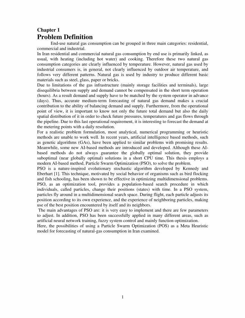
Chapter 1
Problem Definition End-use natural gas consumption can be grouped in three main categories: residential,
commercial and industrial. In Iran residential and commercial natural gas consumption by end use is primarily linked, as usual, with heating (including hot water) and cooking. Therefore these two natural gas consumption categories are clearly influenced by temperature. However, natural gas used by industrial consumers is, in general, not clearly influenced by outdoor air temperature, and follows very different patterns. Natural gas is used by industry to produce different basic materials such as steel, glass, paper or bricks. Due to limitations of the gas infrastructure (mainly storage facilities and terminals), large disequilibria between supply and demand cannot be compensated in the short term operation (hours). As a result demand and supply have to be matched by the system operator in advance (days). Thus, accurate medium-term forecasting of natural gas demand makes a crucial contribution to the ability of balancing demand and supply. Furthermore, from the operational point of view, it is important to know not only the future total demand but also the daily spatial distribution of it in order to check future pressures, temperatures and gas flows through the pipeline. Due to this last operational requirement, it is interesting to forecast the demand at the metering points with a daily resolution. For a realistic problem formulation, most analytical, numerical programming or heuristic methods are unable to work well. In recent years, artificial intelligence based methods, such as genetic algorithms (GAs), have been applied to similar problems with promising results. Meanwhile, some new AI-based methods are introduced and developed. Although these AI-based methods do not always guarantee the globally optimal solution, they provide suboptimal (near globally optimal) solutions in a short CPU time. This thesis employs a modern AI-based method, Particle Swarm Optimization (PSO), to solve the problem. PSO is a nature-inspired evolutionary stochastic algorithm developed by Kennedy and Eberhart [1]. This technique, motivated by social behavior of organisms such as bird flocking and fish schooling, has been shown to be effective in optimizing multidimensional problems. PSO, as an optimization tool, provides a population-based search procedure in which individuals, called particles, change their positions (states) with time. In a PSO system, particles fly around in a multidimensional search space. During flight, each particle adjusts its position according to its own experience, and the experience of neighboring particles, making use of the best position encountered by itself and its neighbors. The main advantages of PSO are: it is very easy to implement and there are few parameters to adjust. In addition, PSO has been successfully applied in many different areas, such as artificial neural network training, fuzzy system control and mainly function optimization. Here, the possibilities of using a Particle Swarm Optimization (POS) as a Meta Heuristic model for forecasting of natural-gas consumption in Iran examined.
Ebrahim Kamrani Degree Project November, 2010 E3714D
�
��������������� � � ���������������������
����������� ��!���� � "�#������������������
$%�������&��� � � '��(�))&&&*�+*��
2
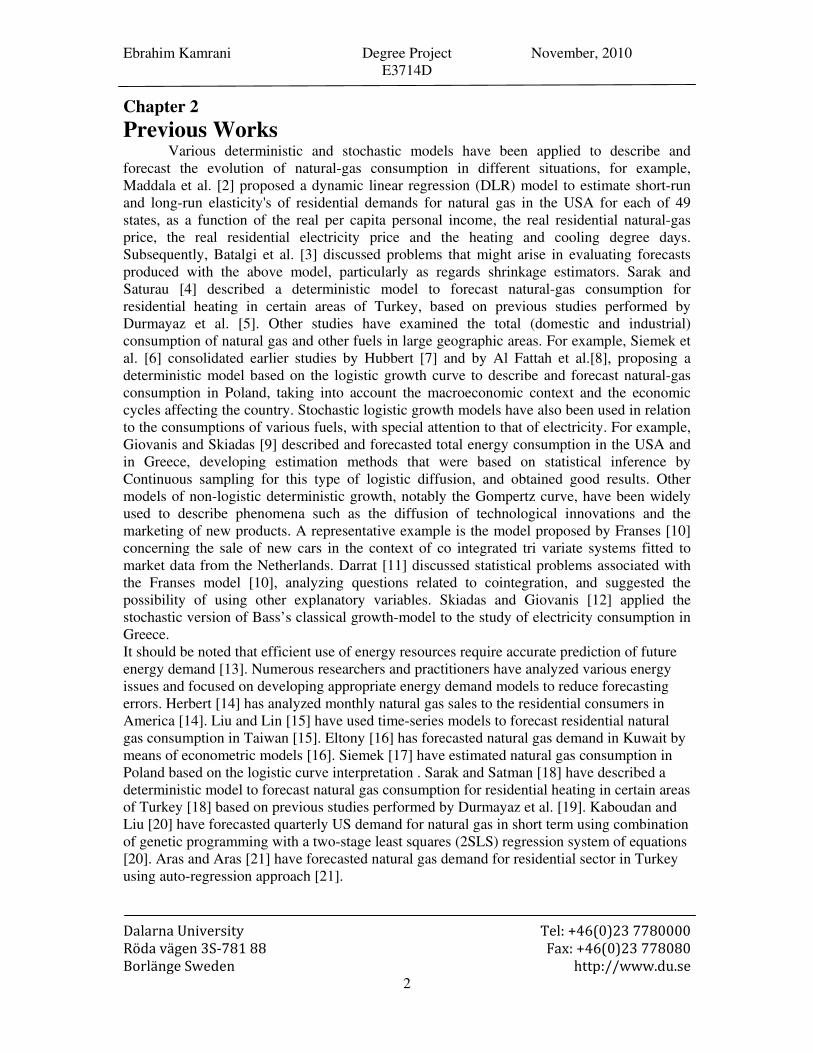
Chapter 2
Previous Works Various deterministic and stochastic models have been applied to describe and
forecast the evolution of natural-gas consumption in different situations, for example, Maddala et al. [2] proposed a dynamic linear regression (DLR) model to estimate short-run and long-run elasticity's of residential demands for natural gas in the USA for each of 49 states, as a function of the real per capita personal income, the real residential natural-gas price, the real residential electricity price and the heating and cooling degree days. Subsequently, Batalgi et al. [3] discussed problems that might arise in evaluating forecasts produced with the above model, particularly as regards shrinkage estimators. Sarak and Saturau [4] described a deterministic model to forecast natural-gas consumption for residential heating in certain areas of Turkey, based on previous studies performed by Durmayaz et al. [5]. Other studies have examined the total (domestic and industrial) consumption of natural gas and other fuels in large geographic areas. For example, Siemek et al. [6] consolidated earlier studies by Hubbert [7] and by Al Fattah et al.[8], proposing a deterministic model based on the logistic growth curve to describe and forecast natural-gas consumption in Poland, taking into account the macroeconomic context and the economic cycles affecting the country. Stochastic logistic growth models have also been used in relation to the consumptions of various fuels, with special attention to that of electricity. For example, Giovanis and Skiadas [9] described and forecasted total energy consumption in the USA and in Greece, developing estimation methods that were based on statistical inference by Continuous sampling for this type of logistic diffusion, and obtained good results. Other models of non-logistic deterministic growth, notably the Gompertz curve, have been widely used to describe phenomena such as the diffusion of technological innovations and the marketing of new products. A representative example is the model proposed by Franses [10] concerning the sale of new cars in the context of co integrated tri variate systems fitted to market data from the Netherlands. Darrat [11] discussed statistical problems associated with the Franses model [10], analyzing questions related to cointegration, and suggested the possibility of using other explanatory variables. Skiadas and Giovanis [12] applied the stochastic version of Bass’s classical growth-model to the study of electricity consumption in Greece. It should be noted that efficient use of energy resources require accurate prediction of future energy demand [13]. Numerous researchers and practitioners have analyzed various energy issues and focused on developing appropriate energy demand models to reduce forecasting errors. Herbert [14] has analyzed monthly natural gas sales to the residential consumers in America [14]. Liu and Lin [15] have used time-series models to forecast residential natural gas consumption in Taiwan [15]. Eltony [16] has forecasted natural gas demand in Kuwait by means of econometric models [16]. Siemek [17] have estimated natural gas consumption in Poland based on the logistic curve interpretation . Sarak and Satman [18] have described a deterministic model to forecast natural gas consumption for residential heating in certain areas of Turkey [18] based on previous studies performed by Durmayaz et al. [19]. Kaboudan and Liu [20] have forecasted quarterly US demand for natural gas in short term using combination of genetic programming with a two-stage least squares (2SLS) regression system of equations [20]. Aras and Aras [21] have forecasted natural gas demand for residential sector in Turkey using auto-regression approach [21].
Ebrahim Kamrani Degree Project November, 2010 E3714D
�
��������������� � � ���������������������
����������� ��!���� � "�#������������������
$%�������&��� � � '��(�))&&&*�+*��
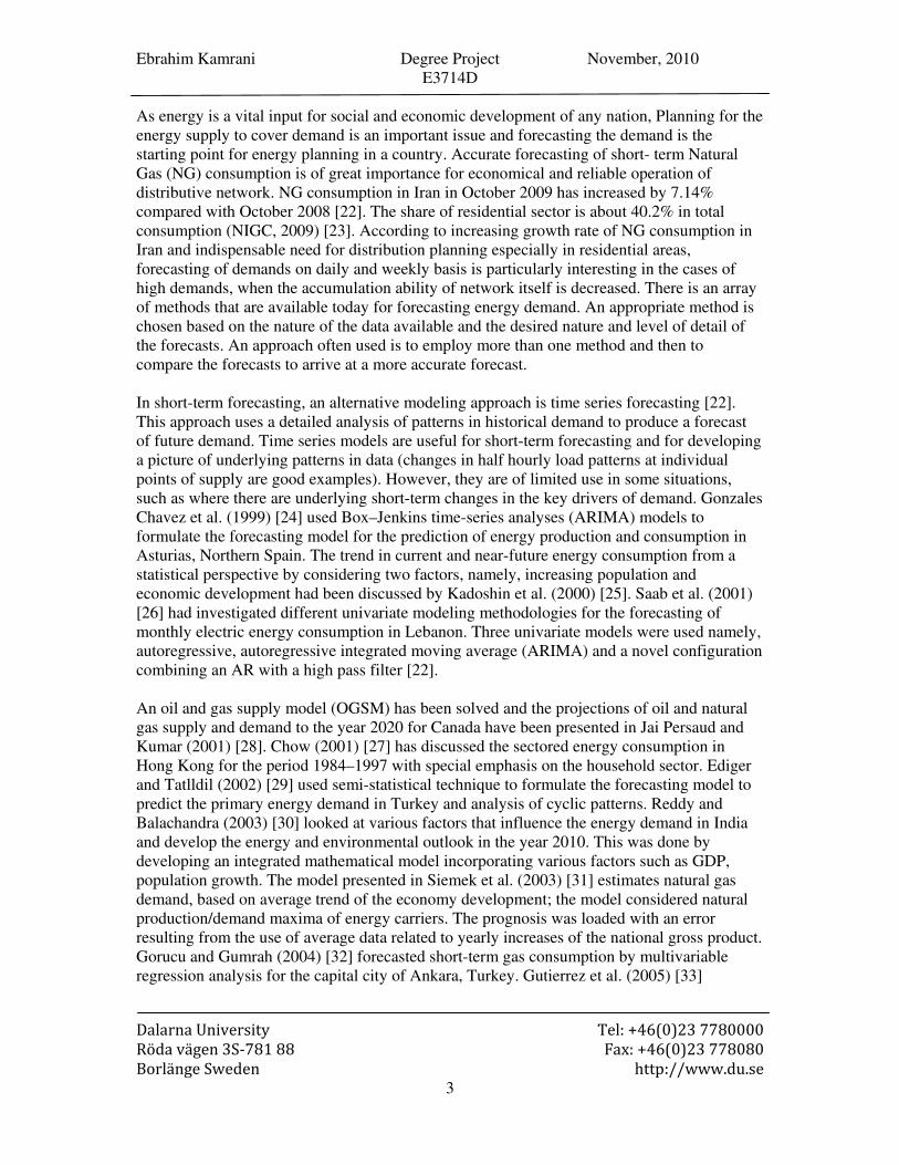
3
As energy is a vital input for social and economic development of any nation, Planning for the energy supply to cover demand is an important issue and forecasting the demand is the starting point for energy planning in a country. Accurate forecasting of short- term Natural Gas (NG) consumption is of great importance for economical and reliable operation of distributive network. NG consumption in Iran in October 2009 has increased by 7.14% compared with October 2008 [22]. The share of residential sector is about 40.2% in total consumption (NIGC, 2009) [23]. According to increasing growth rate of NG consumption in Iran and indispensable need for distribution planning especially in residential areas, forecasting of demands on daily and weekly basis is particularly interesting in the cases of high demands, when the accumulation ability of network itself is decreased. There is an array of methods that are available today for forecasting energy demand. An appropriate method is chosen based on the nature of the data available and the desired nature and level of detail of the forecasts. An approach often used is to employ more than one method and then to compare the forecasts to arrive at a more accurate forecast. In short-term forecasting, an alternative modeling approach is time series forecasting [22]. This approach uses a detailed analysis of patterns in historical demand to produce a forecast of future demand. Time series models are useful for short-term forecasting and for developing a picture of underlying patterns in data (changes in half hourly load patterns at individual points of supply are good examples). However, they are of limited use in some situations, such as where there are underlying short-term changes in the key drivers of demand. Gonzales Chavez et al. (1999) [24] used Box–Jenkins time-series analyses (ARIMA) models to formulate the forecasting model for the prediction of energy production and consumption in Asturias, Northern Spain. The trend in current and near-future energy consumption from a statistical perspective by considering two factors, namely, increasing population and economic development had been discussed by Kadoshin et al. (2000) [25]. Saab et al. (2001) [26] had investigated different univariate modeling methodologies for the forecasting of monthly electric energy consumption in Lebanon. Three univariate models were used namely, autoregressive, autoregressive integrated moving average (ARIMA) and a novel configuration combining an AR with a high pass filter [22]. An oil and gas supply model (OGSM) has been solved and the projections of oil and natural gas supply and demand to the year 2020 for Canada have been presented in Jai Persaud and Kumar (2001) [28]. Chow (2001) [27] has discussed the sectored energy consumption in Hong Kong for the period 1984–1997 with special emphasis on the household sector. Ediger and Tatlldil (2002) [29] used semi-statistical technique to formulate the forecasting model to predict the primary energy demand in Turkey and analysis of cyclic patterns. Reddy and Balachandra (2003) [30] looked at various factors that influence the energy demand in India and develop the energy and environmental outlook in the year 2010. This was done by developing an integrated mathematical model incorporating various factors such as GDP, population growth. The model presented in Siemek et al. (2003) [31] estimates natural gas demand, based on average trend of the economy development; the model considered natural production/demand maxima of energy carriers. The prognosis was loaded with an error resulting from the use of average data related to yearly increases of the national gross product. Gorucu and Gumrah (2004) [32] forecasted short-term gas consumption by multivariable regression analysis for the capital city of Ankara, Turkey. Gutierrez et al. (2005) [33]

Ebrahim Kamrani Degree Project November, 2010 E3714D
�
��������������� � � ���������������������
����������� ��!���� � "�#������������������
$%�������&��� � � '��(�))&&&*�+*��
4
examined the application of a Gompertz-type innovation diffusion process for stochastic modeling and capturing the growth process of natural gas consumption in Spain. Sanchez-Ubeda and Berzosa (2007) [34] forecasted industrial end-use natural gas consumption in a medium-term horizon (1–3 years) with a very high resolution (days) based on a decomposition approach. The forecast was obtained by the combination of three different components: one that captures the trend of the time series, a seasonal component and a transitory component. Parikh et al. (2007) [35] estimated demand projections of petroleum products and natural gas in India. They considered GDP and population as inputs of their NG estimation model. Yoo et al. (2009) [36] estimated households’ demand function for natural gas by applying a sample selection model using data from a survey of households in Seoul. There are also alternative approaches available such as neural network and hybrid models. These typically use multiple techniques and inputs, and produce forecasts based on the mix that produces the best results given the input data available at the time. Hybrid and neural network models have the potential to produce forecasts that perform well compared to the more traditional modeling approaches. Their main disadvantage is their ‘‘black box’’ nature because a forecasting model needs to be intuitive and easily explained to ‘‘non-experts’’. Khotanzad et al. (2000) [37] focused on combination of artificial neural network (ANN) forecasters with application to the prediction of daily natural gas consumption needed by gas utilities. Gorucu et al. (2004) [38] trained the ANNs to decide the optimum parameters to be used in forecasting the gas consumption for short-term applications. Also [39] employed an ANN approach for annual electricity consumption in high energy consumption industrial sectors. Azadeh et al. (2008) [40] developed an integrated algorithm for forecasting monthly electrical energy consumption based on ANN, computer simulation and design of experiments using stochastic procedures. Azadeh et al. (2009) [41] proposed a new hybrid ANFIS computer simulation for improvement of electricity consumption estimation. The proposed algorithm uses the most important relative error estimation method which is mean absolute percentage error (MAPE). All error estimation methods except MAPE have scaled output. As input data used for the model estimation have different scales, MAPE method is the preferred method to estimate relative errors. MAPE is calculated via:
Such that xt is the actual data, ^xt is the estimated value for xt and n is the sample size. Excel implementation of mean absolute percentage error (MAPE) function is in Appendix B.
Natural gas (NG) is one of the most important energy sources in the world [13]. The natural gas consumption growth has been the fastest of all the fossil fuels in recent years. While the share of oil in the world’s total energy produced declined to 38% in 2004 from 45% in 1970 [42], the share of natural gas has gone up to 23% from 17.2% for the same period. In the last

Ebrahim Kamrani Degree Project November, 2010 E3714D
�
��������������� � � ���������������������
����������� ��!���� � "�#������������������
$%�������&��� � � '��(�))&&&*�+*��
5
20 years, global production of natural gas has increased about 1.7 times and the US Energy Information Administration predicts its use to double by 2020 [42].
Fig 1: Worldwide Energy Sources graph in 2004 (World Energy Council).
Iran’s primary energy sources include oil, natural gas, electric power (three-quarters or more was natural gas fired, with the remainder either being hydroelectric or oil fired), solar, wood, animal and plant waste [43]. Oil and natural gas are the major source of primary energy in Iran. The known oil reserves are estimated to be about 90 billion barrels [43]. The major oil field of Iran is located in the southwest region and in the Persian Gulf. Iran produced about 3.5 million bbl/d of oil during past years. Iran’s current sustainable crude oil production capacity is estimated to be around 3.75 million bbl/d. The domestic oil consumption is about 1 million bbl/d in 2002. Iran’s oil export was about 2.5 million bbl/d in 2002, of which 28% went to Europe, 20% to Japan, and under 10% to South Korea, and other large customers including China and India [44]. Iran’s domestic oil consumption has been increasing rapidly as the economy and population grow (about 7% per year). The price of oil products is heavily subsidized to the tune of $ 3 billion or so per year [44]. This causes a large amount of waste and inefficiency in oil consumption; in addition, a substantial amount of petroleum products (mainly gasoline) is also smuggled to the neighboring countries since petroleum products are much cheaper in Iran than in neighboring countries [43]. Iran also imports around $1 billion per year worth oil products (mainly gasoline). Gasoline price is raised by 30–35% every year in early April. This is a part of an effort to curtail the rise in gasoline subsidy expenditure, gasoline consumption and imports (both are growing rapidly). The consumption trend is expected to continue in an unsustainable manner [45]. Besides public awareness of energy conservation methods, domestic supply and demand may be balanced by changing the price structure of oil products in Iran. Since Iran has nationalized oil resources, there is a general feeling among people that the government should ensure that oil products are available to the public at lower prices [43].

Ebrahim Kamrani Degree Project November, 2010 E3714D
�
��������������� � � ���������������������
����������� ��!���� � "�#������������������
$%�������&��� � � '��(�))&&&*�+*��
6
Fig 2: World NG consumption, 2007-2035 (tcf) (International Energy Outlook 2010) [104]
Table 1: Natural Gas�Production in cubic meters (cu m). [CIA World Factbook]

Ebrahim Kamrani Degree Project November, 2010 E3714D
�
��������������� � � ���������������������
����������� ��!���� � "�#������������������
$%�������&��� � � '��(�))&&&*�+*��
7
Iran owns the second largest oil and gas reservoir in the world. Iran is also the fourth largest producer and consumer of gas and the fourth largest producer and exporter of oil in the world [46]. A strong dependency has been created between the oil and gas sectors and the economic growth in the country during the hundred years of oil production and the forty years of development of gas consumption network. Oil revenue is also the biggest provider of the government’s budget and the growth of all sectors of the economy directly and indirectly is effected by petro-dollars (Central Bank of Iran Report, 2010) [46].
Table 2: World Natural Gas reserves by country (International Energy Outlook 2010) [104]
Numerous elements have caused the nature and structure of the relationships in Iran energy sector to be different from other countries. For example [46] has mentioned some of the characteristics of some developing countries that should be taken into account when modeling energy policies. Another study was carried out by Urban et al. (2007) [Also in 46] on modeling of Energy systems for developing countries. They have indicated how to improve energy models for increasing their suitability for developing countries and have given advice on modeling techniques and data requirements.
The structural difference in Iran’s energy sector is different from the industrialized countries that most energy models have been developed for. In Iran the causal relationships have some major differences [46]. For example, the energy price for consumers is not a function of

Ebrahim Kamrani Degree Project November, 2010 E3714D
�
��������������� � � ���������������������
����������� ��!���� � "�#������������������
$%�������&��� � � '��(�))&&&*�+*��
8
production costs or the rate of exploration and oil production is not a function of global oil price but is according to OPEC’s share. Therefore the energy model for Iran must be developed based on particular relationships that exist in this country [46]. Some of the specifications of Iran that makes the energy relationships structure different from industrial countries [46] are as follows:
1- Governmental management of oil and gas production and its particular decisions and policies.
2- Low energy prices and very high energy intensity and the existence of illogical and uneconomical relation in consumption because of low energy prices.
3- Lack of technical and financial abilities for developing the oil and gas production due to political sanctions, difficulties caused by war, etc.
4- Existence of huge undeveloped resources and the slow development of the resources regardless of their final production capacity.
5- A high potential for oil and gas export in the future with the realization that there is a limit on these resources in the world.
6- Existence of high potential for energy conservation and possibility of decrease in domestic consumption due to the high amount of waste in various stages of oil and gas consumption since long ago, which has been continued to the present.
7- Very low final production costs of oil and gas in comparison to other countries and the possibility of competition with low world oil prices.
8- High effectiveness of oil revenue on the economy and the effects of oil revenue on investments in oil and gas productions.
Knowing the above facts, there are some weaknesses and strengths that affect the energy sector of Iran. Major policies should go towards demand side management and optimal production strategies [46]. The relationship framework and priorities used in the model are based on major policies to increase the productivity in the country. Based on this fact, gas consumption has been prioritized [46] as follows:
1. Domestic consumption. 2. Injection into the oil reservoirs in order to increase oil production. 3. Gas and LNG export.
Oil production is based on the country’s share in OPEC and OPEC’s share of oil production is related to global demand [46]. The policy to substitute oil consumption by gas in different sectors depends on the trend in gas production and the peak demand in the cold season of the country. The policies [46] defined in this model can be considered in the following groups:
1. How to increase the productivity of energy in different sectors of economy and decrease the energy intensities of these sectors.
2. How to introduce policies related to improving the efficiency of production, refining and distribution of oil, gas and electricity.

Ebrahim Kamrani Degree Project November, 2010 E3714D
�
��������������� � � ���������������������
����������� ��!���� � "�#������������������
$%�������&��� � � '��(�))&&&*�+*��
9
3. Policies to introduce nuclear energy, hydroelectric power, decrease the associated flare gas.
The resources that supply peak demand for gas in Iran [46] are as follows:
1- The underground gas reservoirs, which reserve surplus gas during non-peak period.
2- Increasing production at some gas fields (mostly gas fields in central regions of Iran).
3- Substitution of gas with oil in power plants during cold season peak demand. 4- Not injecting gas in the oil fields during cold season and using the gas in
residential and commercial sector.

Ebrahim Kamrani Degree Project November, 2010 E3714D
�
��������������� � � ���������������������
����������� ��!���� � "�#������������������
$%�������&��� � � '��(�))&&&*�+*��
10
Chapter 3
Optimization Methods
Fig 3: Puzzle of optimization methods
Optimization Methods Here, some of the optimization methods will briefly introduce, We classify these methods in two major categories where exact methods will find optimal solutions and heuristic methods will find reasonable (not necessarily optimal) solutions in a reasonable computation cost. Although lots of optimization techniques developed in literature, here we address most famous ones in huristic methods which applied on most combinatorial optimization problems.
Fig 4: Search Space and optimums
Ebrahim Kamrani Degree Project November, 2010 E3714D
�
��������������� � � ���������������������
����������� ��!���� � "�#������������������
$%�������&��� � � '��(�))&&&*�+*��
11
3 Heuristic Methods When we are going to deal with NP-hard problems (problem class that their complexity and computational cost increase exponentially with the size of data), exact methods are impractical, so we use methods called heuristics where they use domain knowledge to solve problems in a more efficient way. However, heuristics will not guarantee optimality of the solution as exact methods do, but they are fast methods which provide good enough solutions. A vast number of Modern heuristics developed in the past years called metaheuristics with capabilities to escape from local optima toward the global optima. Hill climbing or iterative improvement move to a solution which should always be better than the current one until it finds local optima (the solution that is better among other neighborhoods). This method will stick very quickly in local optima that may be much worse than the global optimum. The idea of metaheuristics roughly is to accept solutions even if they are worse than the current one with the hope of finding better solutions on the search process [47]. Metaheuristics should make a balance between two main features known as intensification and diversification where the first one is a thorough check in promising region of search space and the latter discover and explore other parts of search space in hope of finding better solutions. A roughly classification of metaheuristics could be trajectory based and population based metaheuristics where in a trajectory metaheuristic, just one solution will consider and in a population based metaheuristics, a population of solutions will maintain. In the past few years metaheuristics applied on different combinatorial optimization problems successfully.
3.1 Point-Based Metaheuristics (Trajectory Methods)
3.1.1 Tabu Search Glover [102] proposed this method in 1977 which is an adaptive memory based method. In iterative improvement of local search process, there is possibility of getting stuck in local optima; however tabu search tries to prevent getting stuck in local optima by accepting non-improving moves to even worse neighbors. This procedure may cause a cycle on previously visited solutions. Tabu search will use a short term memory structure (tabu list) to avoid this problem. Length of tabu list and different tabu lists for each type of neighborhood moves proposed in [48]. At some points tabu list prohibit search process from better moves where there is no risk of cycling, to override tabu list, aspiration criteria defined to accept a move even if it is in the tabu list. Tabu search hybridize with other metaheuristics methods.
3.1.2 Simulated Annealing Kirkpatrick et all. [49] Propose this method in 1983. Origins of idea come from the physical annealing process of metals in Metropolis [50]. Intensification is possible by accepting a solution if it is better than the current solution, however diversification will provide by a probability of accepting a worse solution. An interesting point about this method is that there is a theoretical convergence proof. Also it is easy to implement comparing other metaheuristic methods. The probability of accepting worse solutions decrease during the search and it called cooling schedule implemented as a static schedule which should define before the search process and also in a dynamic way where could be based on information obtained during the search process. Similar methods to simulated annealing proposed in literature like Threshold Accepting [51, 52], noising method [53]. Some recent issues on simulated annealing

Ebrahim Kamrani Degree Project November, 2010 E3714D
�
��������������� � � ���������������������
����������� ��!���� � "�#������������������
$%�������&��� � � '��(�))&&&*�+*��
12
addressed in [54, 55]. Also a full review of different problem domains and applications where simulated annealing applied on could be found in [56].
3.1.3 Greedy Randomized Adaptive Search Procedure (GRASP) This method is a multi-start metaheuristic with constructive and improvement phase on each iteration. Constructive heuristic applies on different seeds to generate different random starting points and in improvement phase it will greedy select the best candidate. These solutions after constructive phase are not necessarily optimal, so in improvement phase it uses a local search strategy based on a neighborhood structure. GRASP usually applies these two phases repeatedly to obtain optimal solution. It also calls adaptive because of updating the evaluation of other candidates when an element selected. A recent survey of greedy randomized adaptive search procedure is in [57] where it can be hybridize with other approaches [58].
3.1.4 Iterative Local Search This method is similar to GRASP because of applying a local search repeatedly on different solutions. It starts with an initial solution which is a local optimum by itself, then perform a perturbation of solution and again apply a local search on new solution and it continues. Acceptance criteria will apply to decide whether the new one or the previous local optima should be accepted. A full investigation on method is in [59].
3.1.5 Guided Local Search The idea is to change the objective function value when it finds local optima, so it diversifies search process to other parts of search space. It developed by Tsang and Voudouris [60, 61].
3.2 Population-Based Metaheuristics
3.2. 1 Genetic Algorithms (GA) Genetic algorithms mimic the evolution of biological species in nature. It first introduced in late 1950’s, [62, 63, 64] contributes to method and John Holland [65, 66] carried out much of the main work on genetic algorithms. Chromosomes simulated by a population of strings where crossover and mutation operators will recombine them. It guided by the objective function for all strings in maintained population. Individuals with higher fitness value have a better opportunity to breed according to survival of the fittest. From generation to generation, new solutions (offspring) repeatedly will improve to obtain optima. Genetic algorithms need to be set for some parameters like the initial population (mostly obtained at random), population size and mutation and crossover rate and type to apply, the selection mechanism for next generation, the stopping condition. [67], [68] by Davis and [69] by Goldberg are a part of most important literature in the field.
3.2.2 Ant Colony Optimization (ACO) An early form of Ant Colony Optimization (ACO) called ant systems where developed by Dorigo. Ant Colony Optimization is a nature inspired optimization method that was developed based on real ants searching for food in nature. Ant Colony Optimization is based on indirect communication of ants as artificial agents by artificial pheromone trails

Ebrahim Kamrani Degree Project November, 2010 E3714D
�
��������������� � � ���������������������
����������� ��!���� � "�#������������������
$%�������&��� � � '��(�))&&&*�+*��
13
which mimics by numerical values ants use to construct solutions to a given problem probabilistically. This pheromone trails are updating as search continues to reflect experience of ants in search process. Ant Colony Optimization is a constructive heuristic which starts with a population of empty solutions and add new elements to partial solution to form the complete feasible solution for the problem. Usually problem will model by a graph with vertices and edges where ants start from vertices to other adjacent vertices of problem. The ants should decide on which vertex visit next. The amount of pheromone will guide other ants to choose a better path in the graph model. A level of pheromone evaporation defined to prevent early convergence. The evaporation rate and updating rules for pheromone trails is important for the balance between intensification and diversification of ACO method.
3.2.3 Particle Swarm Optimization (PSO) This method have discussed in details in chapter 4.
3.2.4 Genetic Programming (GP) This approach uses Darwinian principles of natural selection, crossover, mutation, gene duplication, gene deletion, etc. Genetic programming starts from a randomly created computer programs with composition of the functions and terminals of the problem, then it evaluate each program by executing them based on a fitness function iteratively. The programs will select for the next generation based on their fitness and this process continues until some stopping criteria met.
3.2.5 Evolutionary Strategies (ES) Basic form of Evolutionary Strategies [70] is very close to genetic algorithms with two
main features; first, ES is mostly applied to optimize real-valued variables, second is in its usage of just mutation. ES also applied on discrete variables and used crossover feature [71]. In [72, 73, 74, 75, 76, and 77] more details are discussed.
3.2.6 Memetic Algorithms (MA) Basically, memetic algorithms are a combination of evolutionary strategies (also
genetic algorithms) with one or more local search methods in the hope of more improvement for individuals. [78, 79] are two good starting points for memetic algorithms in literature.

Ebrahim Kamrani Degree Project November, 2010 E3714D
�
��������������� � � ���������������������
����������� ��!���� � "�#������������������
$%�������&��� � � '��(�))&&&*�+*��
14
Chapter 4
Swarm Intelligence (SI) and
Particle Swarm Optimization (PSO) in details
4.1 Introduction to Swarm Intelligence (SI)
4.1.1 Definition In many years, researchers of different fields explored many interesting behavior of
insects and animals in nature. Inspirations provided by the natural phenomena like bird flocking or fish schooling, which has been an interesting area of study in artificial life for quite some time now [80, 81]. Swarm intelligence theory developed by Dorigo, Bonabeau and Theraulaz. It can be applied in many different applications including but not limited to optimization methods in communication systems, robotics, traffic control systems and other applications [82, 83 and 84].
4.1.2 Specifications The most important characteristic of these swarms is their Self Organization behavior
where there is no central controlling system for them and they behave as a group or swarm of intelligent agents. Robustness and Flexibility are two other important characteristics of swarms. [85, 86] Some of the general specifications of swarm come as below:
• each member of group has interactions with other members;
• each member of group has interactions with the environment;
• each member of group coordinate its own movement path based on other members;
• each member of group tries to be near to other neighbors/members;
• there is no collision between group members;
• there is no leader to command members;
• each member of group can move in any space (front, center and rear);
• Using social behavior, all members can achieve food and defense against hunters.
4.2 Swarm Intelligence (SI) Types Swarm intelligence (SI) describes the collective behavior of decentralized, self-
organized systems, natural or artificial. There are different types of swarm in nature. Ant colonies, Bee hives, Bird flocking, Bacteria molding and Fish schooling are samples of these swarm. Among them two groups find more attraction between scientists. Bird flocking which Particle Swarm Optimization (PSO) is based on that and Ant colony makes Ant Colony Optimization (ACO) method. [87, 88] In my work, Particle Swarm Optimization (PSO) used as preferred method.
4.3 Introductions to Particle Swarm Optimization (PSO) Particle swarm optimization (PSO) is a population based stochastic optimization
technique developed by Dr. Eberhart and Dr. Kennedy in 1995, inspired by social behavior of bird flocking or fish schooling. Recently, PSO has been applied successfully in many areas such as continuous function optimization (Eberhart & Kennedy, 1995; Kennedy & Eberhart, 1995) [89, 90], flowshop scheduling (Tasgetiren, Liang, Sevkli, & Gencyilmaz, 2007) [91], job shop scheduling,
Ebrahim Kamrani Degree Project November, 2010 E3714D
�
��������������� � � ���������������������
����������� ��!���� � "�#������������������
$%�������&��� � � '��(�))&&&*�+*��
15
resource constrained project scheduling, part-machine grouping, task allocation, and neural network training (Shen, Shi, Yang, & Ye, 2006) [92]. PSO has many desirable characteristics:
• the concept of PSO is very simple and it can be implemented easily for many applications;
• it is versatile, robust and general purpose in that it can be applied to similar versions of a problem with minor modification;
• it is computationally efficient in the sense that reasonable solutions can be obtained in short computational time;
• unlike genetic algorithms it involves only a few parameters so that it is easier to find the best combination of parameter values;
• it is easily integrated with many local search techniques to improve the solution quality;
• the algorithm is well suited to parallelization by implementation on a cluster of workstations.
4.4 Particle Swarm Optimization (PSO) algorithms
4.4.1 Algorithm description PSO is based on the interaction and the social communication of the group of
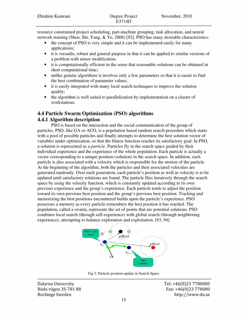
particles. PSO, like GA or ACO, is a population based random search procedure which starts with a pool of possible particles and finally attempts to determine the best solution vector of variables under optimization, so that the fitness function reaches its satisfactory goal. In PSO, a solution is represented as a particle. Particles fly in the search space guided by their individual experience and the experience of the whole population. Each particle is actually a vector corresponding to a unique position (solution) in the search space. In addition, each particle is also associated with a velocity which is responsible for the motion of the particle. At the beginning of the algorithm, both the particles and their associated velocities are generated randomly. Over each generation, each particle’s position as well as velocity is to be updated until satisfactory solutions are found. The particle flies iteratively through the search space by using the velocity function, which is constantly updated according to its own previous experience and the group’s experience. Each particle tends to adjust the position toward its own previous best position and the group’s previous best position. Tracking and memorizing the best positions encountered builds upon the particle’s experience. PSO possesses a memory as every particle remembers the best position it has reached. The population, called a swarm, represents the set of points that are potential solutions. PSO combines local search (through self-experience) with global search (through neighboring experience), attempting to balance exploration and exploitation. [93, 94]
Fig 5: Particle position update in Search Space

Ebrahim Kamrani Degree Project November, 2010 E3714D
�
��������������� � � ���������������������
����������� ��!���� � "�#������������������
$%�������&��� � � '��(�))&&&*�+*��
16
Each particle has a valuation function should be optimized; its value is based on distance to the goal. First it is initialized by random numbers and search will start. Each member will use its best experience (pbest) and also best of other experiences (gbest). In some other variation of PSO, particles will use the best experience of their neighbor (lbest). [93, 86] Particles will update values using relations below:
( ) ( )ttttt presentgbestrandcpresentpbestrandcvwv −⋅+−⋅+⋅=+
()() 211
11 ++ += ttt vpresentpresent
Such that, C1 and C2 are learning parameters and usually assumed equal to 2. rand() is a random number generator function in [0,1] range. presentt is the current position and vt is the velocity of particles. wt is a control parameter for ratio of current velocity (vt ) on the next velocity and is a balance parameter between global search and local search and will decrease to have a global search for first part of search and gradually toward local search. Updating vectors comes below:
�
Fig 6: Particle vectors update in Search Space
4.4.2 PSO parameters initialization As mentioned in [93, 84 and 86], Population size (number of particles) usually assign
between [20, 40] for normal problems. For most problems 10 is enough but in complicated cases [100, 200] is also used. All vectors like present position, pbest, gbest and vt can be with more than one component which is number of parameters should be optimize. Each component of present position should be in the range of searching space such that:
max1min presentpresentpresent t ≤≤+
Using relation below, we can update w in each step:
Iter
iterwwww
max
]*)[( minmaxmax
−−=
Also, C1 and C2 parameters can have different values, based on that we have different modes for our PSO as below: [84, 86, 93 and 94]
• Full Model (c1, c2 > 0)
• Cognition Only (c1 > 0 and c2 = 0)
• Social Only (c1 = 0 and c2 > 0)
• Selfless (c1 = 0 and c2 > 0, and g ≠ i)

Ebrahim Kamrani Degree Project November, 2010 E3714D
�
��������������� � � ���������������������
����������� ��!���� � "�#������������������
$%�������&��� � � '��(�))&&&*�+*��
17
4.4.3 PSO Pseudo code For each particle
Initialize particle
END
Do
For each particle
Calculate fitness value
If the fitness value is better than the best fitness
value (pBest) in history
set current value as the new pBest
End
Choose the particle with the best fitness value of all the
particles as the gBest
For each particle
Calculate particle velocity
Update particle position
End
While maximum iterations or minimum error criteria is not
attained

Ebrahim Kamrani Degree Project November, 2010 E3714D
�
��������������� � � ���������������������
����������� ��!���� � "�#������������������
$%�������&��� � � '��(�))&&&*�+*��
18
Fig 7: PSO Flowchart
�����
���������� ������������������������ ����
���������������������������������� ���!""�
���������� ������������#�$�����%����&��������������
'�#���(��������"�
���������� ������������#�$�����%����&�������������
'�#���(��������"�
������������������
������� ����)����*��+(������,�(��������"�
������� ��&�����-�������$����
.&#���� ������������#�$�����%������������
���� �����&&�������#�������������#/�+'�� ����
�����������&��0����%����1�����'�� ����
&��#��������#��������������������,�
������2������������������&����������
3�#

Ebrahim Kamrani Degree Project November, 2010 E3714D
�
��������������� � � ���������������������
����������� ��!���� � "�#������������������
$%�������&��� � � '��(�))&&&*�+*��
19
4.5: Defined Neighborhoods PSO algorithm can have different versions of Local and Global based on radius of
searching neighbors of particle. Global version will assume gbest for each particle. It is fast but, trapping in local optima is possible. Local version will assume lbest for each particle and use a neighborhood radius; it is slower comparing to global version but probability of getting trapped in local optima decreased. So it is better to use global version for starting the algorithm and gradually use the local one [82, 83]. Three well known topologies for neighborhood in local version defined as below:
• Fig 8: Circle
• Fig 9: Wheel
• Fig 10: Star
Ebrahim Kamrani Degree Project November, 2010 E3714D
�
��������������� � � ���������������������
����������� ��!���� � "�#������������������
$%�������&��� � � '��(�))&&&*�+*��
20
4.6 PSO comparisons with GA
4.6.1 Similarities Both methods are population based, stochastic and use fitness function for evaluating
population. As both are metaheuristic methods, there is no guaranty for optimal solution. Both methods share information in population using chromosome in GA and gBest (lBest) in PSO.
4.6.2 Discriminations There is no evolutionary operator (mutation, crossover) in PSO. Particle will converge
to optimal solution using memory for best visited position. Also basic PSO algorithm is a continuous one comparing to basic GA which is for discrete optimization.
4.7 Pros and cons of using PSO
4.7.1 Pros PSO implementation is easy and number of parameters to choose is low. Number of
particles comparing to GA is not that much important, PSO with a few number of particles can be compared with GA with a big population size. Using global search and local search combined in PSO is one of the most important features. w factor make a good balance between global and local search.
4.7.2 Cons It is possible for PSO to be converged in a short time and trap in local optima. Another
problem is fast sharing information caused to similar particle which increase probability of getting trapped in local optima and more iteration of algorithm cannot solve this problem. For solving this problem hybrid PSO model and lBest defined. Also the performance of algorithm is dependant to problem domain.
4.8 PSO extensions
4. 8.1 Hybrid algorithms This method is a hybrid of particles movement in basic PSO and particle movement
with Evolutionary Algorithm (EA) suing tournament algorithm for selecting particles. First evaluation function will calculate for each particle, then each value of particle will compare to other k particles and a rank number will assign to each particles. Then particles sort based on their rank value (notice that particles are not sort based on their pbest or lbest). When all particles sorted, position and velocity of half of particles will update using the better half set. Although, changes in hybrid PSO are small and it has overhead of calculations and ranking but can improve results.
4.8.2 Local Algorithm Basic PSO also called gBest model algorithm. In local algorithm each particle have
access to pBest and lBest which is best results of its neighbors comparing to global algorithm

Ebrahim Kamrani Degree Project November, 2010 E3714D
�
��������������� � � ���������������������
����������� ��!���� � "�#������������������
$%�������&��� � � '��(�))&&&*�+*��
21
that particles have access to the global best. So in the local algorithm, gBest is substitute by lBest.
4.8.3 Attractive and Repulsive PSO (ARPSO) Algorithm All particles update their position and velocity based on others in basic PSO. Particles
attract each other in the basic method, here in ARPSO there is a repulsive phase where particle velocity will update based on relation below: [86, 93 and 103]
Where in this phase an explosion happens and particles go far from gBest and pBest. In attract phase particles will be near each other and when diversity become less than dlow , it switches to repulsive phase and again when diversity become more than dhigh , it switches to attract phase. So we have an algorithm in two different phases with using different diversity in each step. These phases can be identified using setDirection function as below: [81]
In above function, flying direction of particles can be identified by assigning dir variable. Diversity of particles will calculate using calculateDiversity function as below:
Where S is Swarm, |S| is size of Swarm, |L| is length of diameter of search space, N is
dimension size of problem, pij is jth value and ith particle and jp is jth value average of
particle p. [93]
4.8.4 Fuzzy diversity-guided Attractive/Repulsive (FARPSO) Algorithm In ARPSO, when diversity reaches less than dlow, all particles start searching in search
space of problem. To avoid this, a group of particles exploit environment and for defining their number, the diversity value is used. So Swarm will divide in two groups, one for searching in search space and the other for using current knowledge. When diversity of swarm is less than dlow , exploit group size will be zero and when it is more than dhigh, the size of exploit group becomes the size of swarm as below: [95, 103]
This method use fuzzy diversity-guided attractive/repulsive PSO (FARPSO) and is similar to previous method (ARPSO).
4.8.5 Fuzzy diversity-guided Random walk (FRANDPSO) Algorithm Explosion behavior of above algorithm will send exploit group to the borders of search
space, to improve this issue in ARPSO algorithm, Random walk cab apply. In FRANDPSO

Ebrahim Kamrani Degree Project November, 2010 E3714D
�
��������������� � � ���������������������
����������� ��!���� � "�#������������������
$%�������&��� � � '��(�))&&&*�+*��
22
algorithm, first a random number as scaling factor add to previous velocity. Then s initialize as a random number in [1,vmax] and for each particle velocity will be checked to be valid based on relation below:
Using this method, s will not be less than 1 unless maximum velocity is less than 1. The updating algorithm for velocities comes below: [81, 95]
And algorithm for updating particle positions is:
In this algorithm, beside updating positions of basic PSO, when particle is on the borders of search space it will come back to search space (vj := -vj) [98, 101, 102, 104 and 108]
4.8.6 Attractive/Random-walk (ARANDPSO) Algorithm Above algorithm is not using fuzzy information, so using FARPSO another algorithm
called ARPSO random attract-repulsive proposed. This algorithm uses different threshold levels, called attractive/random-walk PSO when random walk substitute repulsive phase. [95]
Ebrahim Kamrani Degree Project November, 2010 E3714D
�
��������������� � � ���������������������
����������� ��!���� � "�#������������������
$%�������&��� � � '��(�))&&&*�+*��
23
Chapter 5
Forecasting Methodology As mentioned we use the PSO algorithm for solving this forecasting problem. In this problem we have linear and nonlinear estimates. Thus in a large dimension problem, we can't rely on simple LP or NLP Methods. As mentioned before, Particle Swarm Optimization (PSO), as an optimization tool, provides a population-based search procedure in which individuals, called particles, change their positions (states) with time. In a PSO system, particles fly around in a multidimensional search space. During flight, each particle adjusts its position according to its own experience, and the experience of neighboring particles, making use of the best position encountered by itself and its neighbors. Particle Swarm Optimization (PSO) shares many similarities with evolutionary computation techniques such as Genetic Algorithms (GA). The system is initialized with a population of random solutions and searches for optima by updating generations. However, unlike GA, PSO has no evolution operators such as crossover and mutation. The main advantages of PSO are: it is very easy to implement and there are few parameters to adjust. In addition, PSO has been successfully applied in many different areas, such as artificial neural network training, fuzzy system control and mainly function optimization.
The language used to explain the PSO follows from the analogy of particles in a swarm. These key terms are:
1. Particle (individual, agent): each individual in the swarm; 2. position/location: a particle’s n-dimensional coordinates which represents a solution
to the problem; 3. Swarm: the entire collection (population) of particles; 4. Fitness: the fitness function provides the interface between the physical problem
and the optimization problem. The fitness function is a number representing the goodness of a given solution given by a position in solution space;
5. Generation: each iteration of optimization procedure using the PSO; 6. pbest (personal best): the position in parameter space of the best fitness returned for
a specific particle; 7. gbest (global best): the position in parameter space of the best fitness returned for
the entire swarm; 8. Vmax: the maximum velocity value allowed in a given direction.
Similar to the other population-based evolutionary algorithms, PSO is initialized with a population of random solutions (particles) using uniform distribution. However, each particle in PSO traces a trajectory in an n-dimensional search space, updating constantly a velocity vector based on best solutions found so far by that particle as well as others in the population (swarm). Each particle keeps track of its coordinates in the problem space, which are associated with the best solution (fitness) it has achieved so far, pbest. Another ‘‘best” value tracked by the global version of the particle swarm optimizer is the overall best value, gbest, and its location, obtained so far by any particle in the population.

Ebrahim Kamrani Degree Project November, 2010 E3714D
�
��������������� � � ���������������������
����������� ��!���� � "�#������������������
$%�������&��� � � '��(�))&&&*�+*��
24
The Particle Swarm Optimization (PSO) algorithm, at each time step, changes the velocity of each particle moving towards its pbest and gbest locations. Velocity is weighted by random terms, with separate random numbers being generated for acceleration toward pbest and gbest locations, respectively. [96] Each particle updates its velocity Vt to catch up with the best particle g, as follows:
( ) ( )ttttt presentgbestrandcpresentpbestrandcvwv −⋅+−⋅+⋅=+
()() 211
V [] is the particle velocity, persent [] is the current particle (solution). Pbest [] and Gbest [] are defined as stated before. Rand () is a random number between (0,1). c1, c2 are two positive constants named learning factors. Usually c1 = c2 = 2. As such, using the new velocity Vt, the particle’s updated.
11 ++ += ttt vpresentpresent

Ebrahim Kamrani Degree Project November, 2010 E3714D
�
��������������� � � ���������������������
����������� ��!���� � "�#������������������
$%�������&��� � � '��(�))&&&*�+*��
25
Chapter 6
Modeling and Data Features Structure In our Data, we have six types of features for 34 years of Iran and we want find a Liner or Non-linear model for our forecasting methodology, respect of below features to forecast the Gas Consumption of Iran.
1- Population 2- National Income (NI) 3- Gross Domestic Product (GDP) 4- Consumer Price Index (CPI) 5- Demand Of Previous Year 6- Temperature
For example, to model this problem, in the first attempt we use: F (Population, GDP) = A1+A2*Population+A3*GDP
We inject the Data (for example 25 years) to model and find A1, A2, and A3. In this thesis, MATLAB software is used for implementing the method. The main code is in Appendix A. After Running the code and finding the solutions, we check the answers with 4 rests of our data to see the correctness of the solution. Then we change the main function and repeat these steps until we have a satisfactory solution to our problem. While electricity demand has been the focus of the research community, studies on natural gas demand modeling and forecasting have not been reported in the scientific literature to the same extent. Furthermore most papers address the problem of very short-term forecasting (typically one-step-ahead), while medium and long-term energy demand forecasting is quite unusual. For example, Hippert et al [97] examined nearly 100 papers (published between 1991 and 1999) concerning only short-term electricity demand forecasting. One of the main difficulties in accurate medium-term forecasting of demand is the determination of effective explanatory variables to use and the future prediction of them. Studies on energy consumption show that the energy consumption can be influenced mainly by calendar, climate-related and socioeconomic factors. Weather factors include temperature, relative humidity, wind speed, luminosity and rainfall (e.g Mirasgedis et al. [98]), being temperature the main driving weather factor for electricity demand. This non-linear influence is usually captured by using two temperature-derived variables: the heating degree days and the cooling degree days. Total Natural Gas demand is also affected by socioeconomic factors such as the population growth, the gross domestic product (GDP), or the price. Now we discuss important factor for proposed model in more detail:
1. Temperature
One of the most important factors in gas consumption is temperature. Most of our heating instruments use natural gas as a source of energy, so we can assume

Ebrahim Kamrani Degree Project November, 2010 E3714D
�
��������������� � � ���������������������
����������� ��!���� � "�#������������������
$%�������&��� � � '��(�))&&&*�+*��
26
that decreasing the temperature leads to increasing gas consumption (especially in home use). By severely decreasing the temperature, we saw extremely shortage of natural gas. We have so many methods for forecasting the temperature, so we can use average temperature of next years in our model. But we have two challenges: a. Type of average temperature: there are several indexes of temperature such as
Average temperature, average max temperature, average min temperature and etc. Among these factors it seems that average min temperature is the best factor. By going temperature less than zero, use of natural gas will increases severely.
b. Average temperature of Cities: there are several stations in Iran that we can use their measures. But because home natural gas consumption depends on population, we use average temperature of 10 most populated cities.
2. Population Clearly, increasing in population will lead to more energy consumption. Natural gas is an important energy factor, so we can assume more population leads to more consumption of natural gas.
3. Gross Domestic Product (GDP)
One of the most important factors that help us to forecast industrial use of natural gas is Gross Domestic Product (GDP). Increasing this factor shows more production occurred, so this leads to more use of energy (also natural gas) by Factories.
4. Consumer Price Index (CPI)
It seems that price of energy is very important in consumption. But because of subsidy in Iran, price is that low that we can ignore this factor.
Proposed Models According to mentioned factors and importance of them, we propose four linear and nonlinear models:
1. �0 + �1*Pop + �2*GDP + �3*Temperature
2. �0 + �1*Pop + �2*CPI + �3*GDP + �4*NI + �5*Temperature
3. Demand of previous Year + �1*Pop + �2*CPI + �3*GDP + �4*NI + �5*Temperature
4. Demand of previous Year + �1*Pop + �2* 3 ** NIGDPCPI + �3*Temperature
Ebrahim Kamrani Degree Project November, 2010 E3714D
�
��������������� � � ���������������������
����������� ��!���� � "�#������������������
$%�������&��� � � '��(�))&&&*�+*��
27
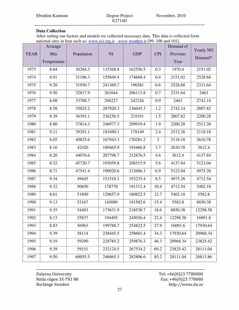
Data Collection
After setting our factors and models we collected necessary data. This data is collected form national sites in Iran such as: www.sci.org.ir , www.weather.ir [99, 100 and 101].
YEAR
Average
Min
Temperature
Population NI GDP CPI
Demand of
Previous
Year
Yearly NG
Demand*
1973 8.64 30284.3 115368.8 162556.5 0.3 1970.4 2151.02
1974 8.91 31106.3 155649.4 174668.4 0.4 2151.02 2528.68
1975 9.20 31950.7 241369.7 196581 0.6 2528.68 2331.64
1976 9.50 32817.9 261044 206113.8 0.7 2331.64 2463
1977 8.88 33708.7 298227 242326 0.9 2463 2742.14
1978 8.58 35025.2 287920.3 236645.3 1.2 2742.14 2807.82
1979 8.38 36393.1 236256.5 219191 1.5 2807.82 2200.28
1980 8.80 37814.3 246977.3 209919.4 1.9 2200.28 2512.26
1981 9.11 39291.1 181690.1 178149 2.4 2512.26 2118.18
1982 8.05 40825.6 167943.3 170281.2 3 2118.18 2610.78
1983 8.16 42420 189465.9 191666.8 3.7 2610.78 3612.4
1984 8.20 44076.6 207798.7 212876.5 4.6 3612.4 4137.84
1985 8.52 45720.7 193059.8 208515.9 5.6 4137.84 5123.04
1986 8.71 47541.4 190020.6 212686.3 6.9 5123.04 4975.26
1987 9.34 49445 151510.1 193235.4 8.5 4975.26 4712.54
1988 9.32 50650 178770 191312.4 10.4 4712.54 5402.18
1989 8.61 51890 129657.9 180822.5 12.7 5402.18 5582.8
1990 9.13 53167 145080 191502.6 15.4 5582.8 8850.38
1991 9.35 54483 175631.9 218538.7 18.6 8850.38 12298.58
1992 8.13 55837 194495 245036.4 22.4 12298.58 16091.6
1993 8.83 56963 199788.7 254822.5 27.9 16091.6 17930.64
1994 9.39 58114 238445.5 258601.4 34.3 17930.64 20968.34
1995 9.19 59290 228785.2 259876.3 46.3 20968.34 23825.42
1996 9.39 59151 232124.5 267534.2 69.2 23825.42 28111.04
1997 9.50 60055.5 246865.3 283806.6 85.2 28111.04 26813.86

Ebrahim Kamrani Degree Project November, 2010 E3714D
�
��������������� � � ���������������������
����������� ��!���� � "�#������������������
$%�������&��� � � '��(�))&&&*�+*��
28
1998 10.05 60936.5 244857.4 291768.7 100 26813.86 29211.18
1999 10.06 61830 234347.4 300139.6 118.1 29211.18 29178.34
2000 9.86 62736 259203.6 304941.2 141.8 29178.34 34498.42
2001 10.43 63663.9 271785.4 320068.9 159.7 34498.42 36682.28
2002 10.02 64528.2 282526.5 330623.6 177.9 36682.28 37897.36
2003 10.07 65540.2 317877.7 355554 206 37897.36 43233.86
2004 9.55 66991.6 341161 379838 238.2 43233.86 47306.02
2005 7.55 67477.5 373506 398235 274.5 47306.02 56139.98
2006 8.65 68467.4 357594.1 387392 307.6 56139.98 60392.76
Table 3: Data for 34 years of Iran Natural Gas (NG) including six features
Ebrahim Kamrani Degree Project November, 2010 E3714D
�
��������������� � � ���������������������
����������� ��!���� � "�#������������������
$%�������&��� � � '��(�))&&&*�+*��
29
Chapter 7
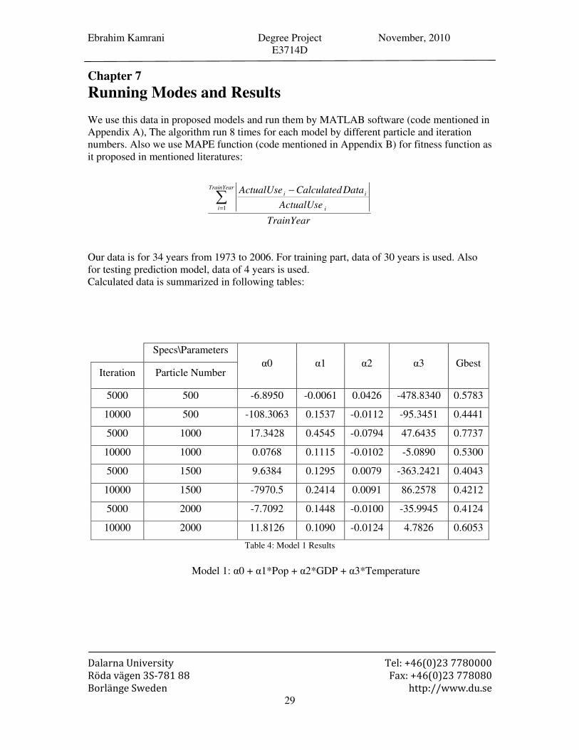
Running Modes and Results We use this data in proposed models and run them by MATLAB software (code mentioned in Appendix A), The algorithm run 8 times for each model by different particle and iteration numbers. Also we use MAPE function (code mentioned in Appendix B) for fitness function as it proposed in mentioned literatures:
TrainYear
ActualUse
DataCalculatedActualUseTrainYear
i i
ii�
=
−
1
Our data is for 34 years from 1973 to 2006. For training part, data of 30 years is used. Also for testing prediction model, data of 4 years is used. Calculated data is summarized in following tables:
Gbest �3 �2 �1 �0
Specs\Parameters
Particle Number Iteration
0.5783 -478.8340 0.0426 -0.0061 -6.8950 500 5000
0.4441 -95.3451 -0.0112 0.1537 -108.3063 500 10000
0.7737 47.6435 -0.0794 0.4545 17.3428 1000 5000
0.5300 -5.0890 -0.0102 0.1115 0.0768 1000 10000
0.4043 -363.2421 0.0079 0.1295 9.6384 1500 5000
0.4212 86.2578 0.0091 0.2414 -7970.5 1500 10000
0.4124 -35.9945 -0.0100 0.1448 -7.7092 2000 5000
0.6053 4.7826 -0.0124 0.1090 11.8126 2000 10000
Table�4: Model 1 Results
Model 1: �0 + �1*Pop + �2*GDP + �3*Temperature

Ebrahim Kamrani Degree Project November, 2010 E3714D
�
��������������� � � ���������������������
����������� ��!���� � "�#������������������
$%�������&��� � � '��(�))&&&*�+*��
30
Gbest �5 �4 �3 �2 �1 �0
Specs\Parameters
Particle
Number Iteration
3.3536 -
362.8567 -0.0034 0.0585 -12.2257 0.3217 -10.0928 500 5000
3.2257 932.0010 -0.4366 0.4587 39.8980 -0.4917 163.4144 500 10000
1.9684 -22.6196 -0.1579 0.1978 -54.6686 -0.2813 7.3529 1000 5000
1.7945 1943.9 0.0782 -0.4349 229.5585 1.4174 30.5722 1000 10000
0.6454 8.2013 0.0114 -0.0211 143.9911 0.1914 8.0635 1500 5000
0.8208 57.3520 -0.1012 0.1762 2.6805 -0.2155 4.5909 1500 10000
0.5390 58.4994 -0.0154 -0.0182 17.5303 0.2582 175.8150 2000 5000
1.3973 -11.6640 -0.2389 0.3679 7.4754 -0.6316 8.6960 2000 10000
Table�5: Model 2 Results
Model 2: �0 + �1*Pop + �2*CPI + �3*GDP + �4*NI + �5*Temperature
best �5 �4 �3 �2 �1
Specs\Parameters
Particle
Number Iteration
0.1034 -101.7891 -0.0013 0.0026 6.1186 0.0253 500 5000
0.1033 -113.0266 -0.0020 0.0044 11.3883 0.0223 500 10000
0.1045 -198.0347 -0.0042 0.0082 3.7234 0.0335 1000 5000
0.1030 -107.3546 -0.0015 0.0032 7.7092 0.0251 1000 10000
0.1032 -85.9110 -0.0014 0.0023 11.6457 0.0236 1500 5000
0.1032 -78.0451 -0.0008 0.0014 7.3269 0.0237 1500 10000
0.1048 -18.7125 -0.0006 -0.0022 12.5147 0.0263 2000 5000
0.1032 -91.9696 -0.0014 0.0028 9.8789 0.0227 2000 10000
Table�6: Model 3 Results
Model 3: Demand of previous Year + �1*Pop + �2*CPI + �3*GDP + �4*NI +
�5*Temperature

Ebrahim Kamrani Degree Project November, 2010 E3714D
�
��������������� � � ���������������������
����������� ��!���� � "�#������������������
$%�������&��� � � '��(�))&&&*�+*��
31
Gbest �3 �2 �1
Specs\Parameters
Particle
Number Iteration
0.1092 -0.8186 0.1476 -0.0094 10 100
0.1060 -81.6813 0.0623 0.0201 10 200
0.1088 -10.5017 0.1671 -0.0096 20 100
0.1061 -43.9315 0.0959 0.0070 20 200
0.1084 -48.8668 0.1049 0.0090 30 100
0.1059 -69.7949 0.0460 0.0195 30 200
0.1065 -39.9476 0.0872 0.0075 40 100
0.1058 -61.2409 0.0692 0.0143 40 200
Table�7: Model 4 Results
Model 4: Demand of previous Year + �1*Pop + �2* 3 ** NIGDPCPI + �3*Temperature

Ebrahim Kamrani Degree Project November, 2010 E3714D
�
��������������� � � ���������������������
����������� ��!���� � "�#������������������
$%�������&��� � � '��(�))&&&*�+*��
32
Chapter 8
Data Analysis and discussion Here is the analysis of obtained data after running the algorithm several times with different parameters for each model.
Model 1: Fitness Function (�0 + �1*Pop + �2*GDP + �3*Temperature)
In this model that we used most important factors, we didn't have good result. The main idea for explaining this large error is because our model was trained with data that doubled or maximum tripled over 30 years, natural gas consumption is multiplied by 20. So our model can’t predict satisfactorily. The following formula is average of coefficient that is calculated 8 times for each model:
-14.0195 + 0.167288*Pop - 0.00795 * GDP + -104.978 * Temperature
So in model 1 average of coefficients are:
• �0 = -14.0195
• �1 = 0.167288
• �2 = -0.00795
• �3 = -104.978 By using these average coefficients in test years, we have these predications and error percent:
Error Percent Distance
Between Data
Estimated Use
Of Natural Gas
Actual Use Of
Natural Gas Year
83.65567 36167.57 7066.287 43233.86 2003
84.84206 40135.4 7170.619 47306.02 2004
86.96899 48824.38 7315.604 56139.98 2005
87.66089 52940.83 7451.929 60392.76 2006
Table�8: Model 1 Analysis
Average Error Percent is % 85.7819025 that shows our model can’t predict satisfactorily.

Ebrahim Kamrani Degree Project November, 2010 E3714D
�
��������������� � � ���������������������
����������� ��!���� � "�#������������������
$%�������&��� � � '��(�))&&&*�+*��
33
Fig 11: Model 1 Results (Linear Model)
Fig 12: Model 1 Results (Underestimation, Average Error Percent is % 85.7819025)
As we can see, Model 1 which is a linear model can’t predict satisfactorily with a considerable underestimation issue.

Ebrahim Kamrani Degree Project November, 2010 E3714D
�
��������������� � � ���������������������
����������� ��!���� � "�#������������������
$%�������&��� � � '��(�))&&&*�+*��
34
Model 2: Fitness Function (�0 + �1*Pop + �2*CPI + �3*GDP + �4*NI +
�5*Temperature)
In this model that we use all of our factors except demand of previous year, we didn't have good results too. It is because of same reason in previous model. But we have slight improvement. The main idea for explaining this improvement is using Consumer Price Index (CPI) parameter that multiplied by 3000 during these 30 years. The following formula is average of coefficient that is calculated 8 times for each model:
48.55151+ 0.071075*Pop + 46.77994*CPI + 0.098113*GDP + -0.10798*NI +
325.3517*Temperature
So in model 2 averages of coefficients are:
• �0 = 48.55151
• �1 = 0.071075
• �2 = 46.77994
• �3 = 0.098113
• �4 = -0.10798
• �5 = 325.3517
By using these coefficients in test years, we have these predications and error percent:
Error Percent Distance
Between Data
Estimated Use
Of Natural Gas
Actual Use Of
Natural Gas Year
57.95005 25054.04 18179.82 43233.86 2003
58.80323 27817.47 19488.55 47306.02 2004
63.69278 35757.11 20382.87 56139.98 2005
64.37677 38878.91 21513.85 60392.76 2006
Table�9: Model 2 Analysis
Average Error Percent is % 61.2057075 that shows our model can’t predict satisfactorily.

Ebrahim Kamrani Degree Project November, 2010 E3714D
�
��������������� � � ���������������������
����������� ��!���� � "�#������������������
$%�������&��� � � '��(�))&&&*�+*��
35
Fig 13: Model 2 Results (Linear Model)
Fig 14: Model 2 Results (Underestimation, Average Error Percent is % 61.2057075)
As we can see, Model 2 which is a linear model can’t predict satisfactorily with a considerable underestimation issue.
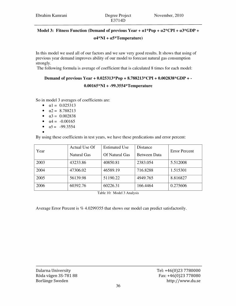
Ebrahim Kamrani Degree Project November, 2010 E3714D
�
��������������� � � ���������������������
����������� ��!���� � "�#������������������
$%�������&��� � � '��(�))&&&*�+*��
36
Model 3: Fitness Function (Demand of previous Year + �1*Pop + �2*CPI + �3*GDP +
�4*NI + �5*Temperature)
In this model we used all of our factors and we saw very good results. It shows that using of previous year demand improves ability of our model to forecast natural gas consumption strongly. The following formula is average of coefficient that is calculated 8 times for each model:
Demand of previous Year + 0.025313*Pop + 8.788213*CPI + 0.002838*GDP + -
0.00165*NI + -99.3554*Temperature
So in model 3 averages of coefficients are:
• �1 = 0.025313
• �2 = 8.788213
• �3 = 0.002838
• �4 = -0.00165
• �5 = -99.3554
• By using these coefficients in test years, we have these predications and error percent:
Error Percent Distance
Between Data
Estimated Use
Of Natural Gas
Actual Use Of
Natural Gas Year
5.512008 2383.054 40850.81 43233.86 2003
1.515301 716.8288 46589.19 47306.02 2004
8.816827 4949.765 51190.22 56139.98 2005
0.275606 166.4464 60226.31 60392.76 2006
Table�10: Model 3 Analysis
Average Error Percent is % 4.0299355 that shows our model can predict satisfactorily.
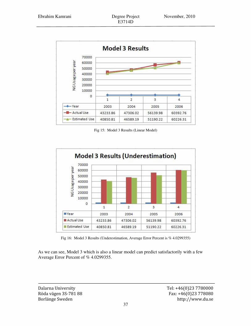
Ebrahim Kamrani Degree Project November, 2010 E3714D
�
��������������� � � ���������������������
����������� ��!���� � "�#������������������
$%�������&��� � � '��(�))&&&*�+*��
37
Fig 15: Model 3 Results (Linear Model)
Fig 16: Model 3 Results (Underestimation, Average Error Percent is % 4.0299355)
As we can see, Model 3 which is also a linear model can predict satisfactorily with a few Average Error Percent of % 4.0299355.
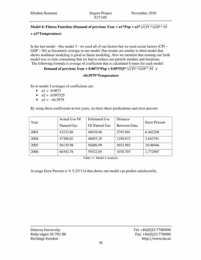
Ebrahim Kamrani Degree Project November, 2010 E3714D
�
��������������� � � ���������������������
����������� ��!���� � "�#������������������
$%�������&��� � � '��(�))&&&*�+*��
38
Model 4: Fitness Function (Demand of previous Year + �1*Pop + �2* 3 ** NIGDPCPI
+ �3*Temperature)
In the last model - like model 3 - we used all of our factors but we used social factors (CPI – GDP – NI) as Geometric average in our model. Our results are similar to third model that shows nonlinear modeling is good as linear modeling. Also we mention that running our forth model was so time consuming that we had to reduce our particle number and iterations. The following formula is average of coefficient that is calculated 8 times for each model:
Demand of previous Year + 0.0073*Pop + 0.097525* 3 ** NIGDPCPI +
-44.5979*Temperature
So in model 3 averages of coefficients are:
• �1 = 0.0073
• �2 = 0.097525
• �3 = -44.5979
By using these coefficients in test years, we have these predications and error percent:
Error Percent Distance
Between Data
Estimated Use
Of Natural Gas
Actual Use Of
Natural Gas Year
6.462298 2793.901 40439.96 43233.86 2003
2.643791 1250.672 46055.35 47306.02 2004
10.06946 5652.992 50486.99 56139.98 2005
1.772907 1070.707 59322.05 60392.76 2006
Table�11: Model 4 Analysis
Average Error Percent is % 5.237114 that shows our model can predict satisfactorily.

Ebrahim Kamrani Degree Project November, 2010 E3714D
�
��������������� � � ���������������������
����������� ��!���� � "�#������������������
$%�������&��� � � '��(�))&&&*�+*��
39
Fig 17: Model 4 Results (Non-Linear Model)
Fig 18: Model 4 Results (Underestimation, Average Error Percent is % 5.237114)
As we can see, Model 3 which is also a linear model can predict satisfactorily with a few Average Error Percent of % 5.237114.
Ebrahim Kamrani Degree Project November, 2010 E3714D
�
��������������� � � ���������������������
����������� ��!���� � "�#������������������
$%�������&��� � � '��(�))&&&*�+*��
40
Conclusion
All the aspects of development in agriculture, power generation, social welfare and industry in Iran are crucially related to the energy and its revenue. Forecasting end-use natural gas consumption is an important Factor for efficient system operation and a basis for planning decisions. Both Modeling and long-term Forecasting covered for end-use natural gas consumption in Iran. Particle swarm optimization (PSO) used to forecast long run natural gas consumption in Iran. In some unusual situations, such as abnormal temperature changes, the forecasting error is high. Although this error might seem high, one does not need to be deeply concerned about the overall results since these unusual situations could be filtered out to yield more reliable predictions. Gas consumption data in Iran for the previous 30 years is used to predict the consumption for four years. Four linear and nonlinear models proposed for this purpose Six factors such as Gross Domestic Product (GDP), Population, National Income (NI), Temperature, Consumer Price Index (CPI) and yearly Natural Gas (NG) demand investigated. Models 1, 2 and 3 are linear models where model 4 is a non-linear model, the first and second model can’t predict satisfactorily with high Average Error Percent by order % 85.7819025 and % 61.2057075. Model 3 and 4 can predict satisfactorily with a low Average Error Percent by order % 4.0299355 and % 5.237114. Although model 3 is a linear model and model 4 is a non-linear model, but both can predict satisfactorily. Model 4 uses just three coefficients where model 3 uses five coefficients. Best prediction for model 3 is with 1000 particles in 10,000 iterations where best prediction for model 4 is with 40 particles in just 200 iterations.
Future Works
All four models for prediction suffer from underestimation (although it is with a very low Average Error Percent of % 4.0299355 or % 5.237114); in future we continue to build other robust models (by using more experts’ opinion) for better estimation of long-term natural gas usage in Iran. It is also possible to add more features to our prediction model, for example the effect of other political issues (such as sanction), Interest Rate, Rate of Inflation, National Power Index (NPI), relative humidity, wind speed, luminosity, rainfall, etc. Also we can use some other metaheuristic models Such as ACO, GA. Also Using different forecasting methods such as ANN [Back propagation, Recurrent], Time series [ARIMA, AR, MA, MAAR, ARMA], Regression, to apply them as a forecasting module Another approach besides above is to use Particle Swarm Intelligence (PSO) as a tool for other optimization problems like long-term electricity usage estimation. Furthermore, from the operational point of view, it is important to know not only the future total demand but also the daily spatial distribution of it in order to check future pressures, temperatures and gas flows through the pipeline. Due to this last operational requirement, it is interesting to forecast the demand at the metering points with a daily resolution.
Ebrahim Kamrani Degree Project November, 2010 E3714D
�
��������������� � � ���������������������
����������� ��!���� � "�#������������������
$%�������&��� � � '��(�))&&&*�+*��
41
References [1] J. Kennedy, R.C. Eberhart, Particle Swarm Optimization, Proc. IEEE Int. Conf. Neural Networks (1995) 1942–1948. [2] Maddala GS, Trost RP, Li H, Joutz F. Estimation of short-run and long-run elasticities of energy demand from panel data using shrinkage estimators. J Bus Econ Stat 1997;15:90–100. [3] Baltagi BH, Bresson G, Pirotte A. Comparison of forecasting performance for homogeneous, heterogeneous and shrinkage estimators. Some empirical evidence from US electricity and natural-gas consumption. Econ Lett 2002;76:375–82. [4] Sarak H, Satman A. The degree-day method to estimate the residential heating natural-gas consumption in Turkey: a case study. Energy 2003;28:929–39. [5] Durmayaz A, Kadioglu M, Sen Z. An application of the degree-hours method to estimate the residential heating energy requirement and fuel consumption in Istanbul. Energy 2000;25(12):1245–56. [6] Siemek J, Stanislaw N, Stanislaw R. Estimation of natural-gas consumption in Poland based on the logistic-curve interpolation. Appl Energy 2003;75:1–7. [7] Hubbert MK. Energy resources [Publ. 1000-D]. Natl Acad Sci/Natl Res Council; 1962. [8] Al-Fattah SM, Startzman RA. Forecasting world natural gas-supply [SPE 59798]; 2000. [9] Giovanis AN, Skiadas CH. A stochastic logistic innovation diffusion-model studying the electricity consumption in Greece and the United States. Technol Forecast Soc Change 1999;61:253–64. [10] Franses PH. Modeling new products sales: an application of cointegration analysis. Int J Res Market 1994;11:491–502. [11] Darrat AF. On the Gompertz process and new product sales: some further results from cointegration analysis. Q J Bus Econ 2002;39(1):49–56. [12] Skiadas CH, Giovani AN. A stochastic Bass innovation diffusion model for studying the growth of electricity consumption in Greece. Appl Stoch Models Data Anal 1997;13:085–101. [13] Forouzanfar M., Doustmohammadi A., Menhaj M., Hasanzadeh S., 2010, Modeling and estimation of the natural gas consumption for residential and commercial sectors in Iran, Applied Energy 87 (2010) 268–274 [14] Herbert JH. An analysis of monthly sales of natural gas to residential customers in the US. Energy Syst Policy J 1987;10(2):127–48. [15] Liu LM, Lin MW. Forecasting residential consumption of natural gas using monthly and quarterly time series. Int J Forecast 1991;7(1):3–16. [16] Eltony MN. Demand for natural gas in Kuwait: an empirical analysis using two econometric models. Int J Energy Res 1996;20:957–63. [17] Siemek J, Nagy S, Rychliki. Estimation of natural-gas consumption in Poland based on the logistic-curve interpretation. Appl Energy 2003;75(1–2):1–7. [18] Sarak H, Satman A. The degree-day method to estimate the residential heating natural-gas consumption in Turkey: a case study. Energy J 2003;28:929–39. [19] Durmayaz A, Kadioglu M, Sen Z. An application of the degree-hour method to estimate the residential heating energy requirement and fuel consumption in Istanbul. Sci Direct J Energy 2000;25(12):1245–56. [20] Kaboudan MA, Liu QW. Forecasting quarterly US demand for natural gas. E-J: Inform Technol Econ Manage 2004;2(1):1–14. Paper 4. [21] Aras H, Aras N. Forecasting residential natural gas demand. Energy Sources 2004;26(5):463–72. [22] A. Azadeh, S.M.Asadzadeh, A.Ghanbari, 2010, An adaptive network-based fuzzy inference system for short-termnatural gas demandestimation:Uncertainandcomplexenvironments, Energy Policy 38 (2010)1529–1536 [23] NIGC, 2009. National Iranian Gas Company website. www.nigc.ir [24] Gonzales Chavez,S., XibertaBernat,J., LlanezaCoalla,H.,1999. Forecastingof energy production and consumption in Asturias (NorthernSpain). Energy24, 183–198. [25] Kadoshin, S., Nishiyama, T.,Toshihide,I., 2000.The trend in current and near future of energy consumption from a statistical perspective. AppliedEnergy 67, 407–417. [26] Saab, S.,Badr,E.,Nasr,G., 2001. Univariate modeling and forecasting of energy consumption: the case of electricity in Lebanon. Energy26,1–14. [27] Chow, L.C.H.,2001.A study of sectoral energy consumption in HongKong (1984–97) with special emphasis on the house hold sector.Energy Policy 29, 1099–1110. [28] Jai Persaud,A.,Kumar,U.,2001. An eclectic approach in energy forecasting: a case of natural resources Canada’s(NRCan’s) oil and gas outlook. Energy Policy 29, 303–313.

Ebrahim Kamrani Degree Project November, 2010 E3714D
�
��������������� � � ���������������������
����������� ��!���� � "�#������������������
$%�������&��� � � '��(�))&&&*�+*��
42
[29] Ediger, V.S.,Tatlldil,H.,2002. Forecasting the primary energy demand in Turkey and analysis of cyclic patterns. Energy Conversion and Management 43, 473–487. [30] Reddy, B.S.,Balachandra,P.,2003.Integrated energy–environment-policy analysis: a case study of India. Utility Policy 11 (2),59–73. [31] Siemek, J.,Nagy,S.,Rychlicki,S.,2003. Estimation of natural-gas consumption in Poland based on the logistic-curve interpretation. Applied Energy 75 (1–2), 1–7. [32] Gorucu, F.B.,Gumrah,F.,2004. Evaluation and forecasting of gas consumption by statistical analysis. Energy Sources 26 (3),267–276. [33] Gutierrez, R.,Nafidi,A.,Sanchez,R.G.,2005. Forecasting total natural-gas consumption in Spain by using the stochastic Gompertz innovation diffusion model. Applied Energy 80 (2),115–124. [34] Sanchez-Ubeda, E.F.,Berzosa,A.,2007. Modeling and forecasting industrial end-use natural gas consumption. Energy Economics 29 (4), 710–742. [35] Parikh, J.,Purohit,P.,Maitra,P.,2007. Demand projections of petroleum products and natural gas in India. Energy 32, 1825–1837. [36] Yoo, S.,Lim,H.J.,Kwak,S.J.,2009. Estimating the residential demand function for natural gas in Seoul with correction for samples election bias. Applied Energy 86 (4),460–465. [37] Khotanzad, A.,Elragal,H.,Lu,T.,2000. Combination of artificial neural network forecasters for prediction of natural gas consumption. IEEE Transactionson Neural Networks 11 (2), 464–473. [38] Gorucu, F.B.,Geris,P.U.,Gumrah,F.,2004. Artificial neural network modeling for forecasting gas consumption. Energy Sources 26 (3),299–307. [39] Azadeh, A.,Ghaderi,S.F.,Sohrabkhani,S.,2008. Annual electricity consumption forecasting by neural network in high energy consuming industrial sectors. Energy Conversion and Management 49 (8), 2272–2278. [40] Azadeh, A.,Saberi,M.,Ghaderi,S.F.,Gitiforouz,A.,Ebrahimipour,V.,2008. Improved estimation of electricity demand function by integration of fuzzy system and data mining approach. Energy Conversion and Management 49, 2165–2177. [41] Azadeh, A.,Saberi,M.,Gitiforouz,A.,Saberi,Z.,2009. Ahybrid simulation adaptive network-based fuzzy inference system for improvement of electricity consumption estimation. Expert Systems with Applications 36, 11108–11117. [42] Iman A, Startzman RA, Barrufet MA. Multi-cyclic Hubbert model shows global conventional gas output peaking in 2019. Oil Gas J 2004;16(August):20–8. [43] F.A. Hessari, 2005, Sectoral energy consumption in Iran, Renewable and Sustainable Energy Reviews 9 (2005) 203–214 [44] Available from: www.nioc.com; Persian version, news and reports 2002–2003. [45] Oil consumption and production in Iran. Energy Statistical Review of Iran 2002;2:103–28. [46] Kiani B. & Pourfakhraei M., 2010, A system dynamic model for production and consumption policy in Iran oil and gas sector, Energy Policy 2010 [47] . H. Osman and G. Laporte. Metaheuristics: a bibliography. Annals of Operations Research, pages 513–623, 1996. [48] K. Dowsland. Nurse scheduling with tabu search and strategic oscillation. European Journal of Operational Research, 106:393–407, 1998. [49] S. Kirkpatrick, C. D. Gelatt, and M. P. Vecchi. Optimization by simulated annealing. Science, 220:671–680, 1983. [50] N. Metropolis, A. W. Rosenbluth, A. H. Teller, and E. Teller. Equation of state calculation by fast computing machines. Journal of Chemical Physics, 21:1087–1091, 1953. [51] . Dueck and T. Scheuer. Threshold accepting - a general-purpose optimisation algorithm appearing superior to simulated annealing. Journal of Computational Physics, 90:161–175, 1990. [52] P. Moscato and J. F. Fontanari. Convergence and finite-time behavior of simulated annealing. Advances in Applied Probability, 18:747–771, 1990. [53] I. Charon and O. Hudry. The noising method: a new method for combinatorial optimisation. Operations Research Letters, 14:133–137, 1993. [54] M. Duque-Ant´on. Constructing efficient simulated annealing algorithms. Discrete Applied Mathematics, 77:139–159, 1997. [55] V. Fabian. Simulated annealing simulated. Computers Math. Applic., 33(1/2):81–94, 1997. [56] C. Koulamas, S. R. Antony, and R. Jaen. A survey of simulated annealing applications to operations research problems. Omega International journal of Management Science, 22(1):41–56, 1994.

Ebrahim Kamrani Degree Project November, 2010 E3714D
�
��������������� � � ���������������������
����������� ��!���� � "�#������������������
$%�������&��� � � '��(�))&&&*�+*��
43
[57] P. Festa and M. G. C. Resende. Grasp: an annoted bibliography. In P. Hansen C. C. Ribeiro, editor, Essays and Surveys in Metaheuristics, pages 325–367. Kluwer Academic Publishers, 2002. [58] L. S. Pitsoulis and M. G. C. Greedy randomized adaptive search procedures. Technical report, AT&T Labs Research, 2001. [59] H. R. Louren¸co, O. C. Martin, and T. St¨utzle. Iterated local search. In F. Glover and G. A. Kochenberger, editors, Handbook of Metaheuristics, pages 321–353. Kluwer Academic Publishers, 2003. [60] C. Voudouris and E. Tsang. Guided local search. Technical Report CSM-247, Department of Computer Science, University of Essex, 1997. [61] E. Tsang and C. Voudouris. Fast local search and guided local search and their application to british telecom’s workforce scheduling problem. Operations Research Letters, 20:119–127, 1997. [62] . S. Fraser. Simulation of genetic systems by automatic digital computers. ii. effects of linkage on rates under selection. Australian Journal of Biological Sciences, 10:492–499, 1957. [63] A. S. Fraser. Simulation of genetic systems by automatic digital computers. iv. epistasis. Australian Journal of Biological Sciences, 13:329–346, 1960. [64] H. J. Bremermann. The evolution of intelligence. the nervous system as a model of its environment. Technical Report 1, Contract 477(17), Department of Mathematics, University of Washington, Seattle, 1958. [65] J. H. Holland, editor. Adaptation in natural and artificial systems. University of Michigan Press, 1975. [66] J. H. Holland, editor. Adaptation in natural and artificial systems. University of Michigan Press, 1992. Second edition, MIT Press 1992. [67] C. R. Reeves and J. E. Rowe, editors. Genetic Algorithms: Principles and perspectives. Kluwer, Norwell, MA, 2001. [68] L. D. Davis, editor. Handbook of genetic algorithms. Van Nostrand Reinhold, 1991. [69] David E. Goldberg. Genetic algorithms in search, optimization & machine learning. Addison Wesley, 1989. [70] L. J. Fogel, A. J. Owens, and M. J. Walsh, editors. Artificial intelligence through simulated evolution. Wiley, New York, 1966. [71] M. Herdy. Application of the evolution strategy to discrete optimization problems. In First International Conference on Parallel Problem Solving from Nature (PPSN), volume 496 of Lecture Notes in Computer Science, pages 188–192. Springer-Verlag, 1991. [72] T. B¨ack, F. Hoffmeister, and H. P. Schwefel. A survey of evolution strategies. In Proceedings of the Fourth Conference on Genetic Algorithms, pages 2–9. Morgan Kauffman, 1991. [73] T. Back, F. Hoffmeister, and H. P. Schwefel. A survey of evolution strategies. In Proceedings of the Fourth Conference on Genetic Algorithms, pages 2–9. Morgan Kauffman, 1991. [74] D. B. Fogel, editor. Evolutionary computation: The Fossil Record. IEEE Press, 1998. [75] D. B. Fogel. An introduction to simulated evolutionary optimization. IEEE Transactions on Neural Networks, 5:3, 1994. [76] D. B. Fogel. Asymptotic convergence properties of genetic algorithms and evolutionary programming. analysis and experiments. Cybernetics and Systems, 25:389, 1994. [77] G. B. Fogel and D. B. Fogel. Continuous evolutionary programming. Analysis and experiments. Cybernetics and Systems, 26:79, 1995. [78] D. Corne, M. Dorigo, and F. Glover, editors. New Ideas in Optimization. McGraw-Hill Publishing Company, 1999. [79] P. Moscato. On evolution, search, optimisation, genetic algorithms and martial arts: Towards memetic algorithms. Technical Report 826, California Institute of Technology, Caltech Concurrent Computation Program, 1989. [80] Shi, Y., & Eberhart, R. C. (1999). Empirical study of particle swarm optimization. In Proceedings of 1999 congress on evolutionary computation (pp. 1945–1950). Piscataway, NJ: IEEE Service Center. [81] Clerc, M., & Kennedy, J. (2002). The particle swarm-explosion, stability, and convergence in a multidimensional complex space. IEEE Transactions on Evolutionary Computation, 6(1), 58–73. [82] Shi, Y., & Eberhart, R. C. (1999). Empirical study of particle swarm optimization. In Proceedings of 1999 congress on evolutionary computation (pp. 1945–1950). Piscataway, NJ: IEEE Service Center. [83] Clerc, M., & Kennedy, J. (2002). The particle swarm-explosion, stability, and convergence in a multidimensional complex space. IEEE Transactions on Evolutionary Computation, 6(1), 58–73. [84] Shi, Y., & Eberhart, R. C. (1998). Parameter selection in particle swarm optimization. In Proceedings of the seventh annual conference on evolutionary programming (pp. 591–600). New York: Springer-Verlag. [85] Eberhart, R. C., & Shi, Y. (2000). Comparing inertia weights and constriction factors in particle swarm optimization. Proceeding of the 2000 Congress Evolutionary Computation, San Diego, CA, July. pp. 84–88.

Ebrahim Kamrani Degree Project November, 2010 E3714D
�
��������������� � � ���������������������
����������� ��!���� � "�#������������������
$%�������&��� � � '��(�))&&&*�+*��
44
[86] Trelea, C. (2003). The particle swarm optimization algorithm: Convergence analysis and parameter selection. Information Processing Letters, 85, 317–325. [87] Yang Liu, Kevin M. Passino, "Swarm Intelligence: Literature Overview," Dept. of Electrical Engineering, Ohio State University, March 30, 2000. [88] Jonas Pfeil, "Swarm Intelligence," Communication and Operating Systems Group, Berlin University of Technology [89] Eberhart, R., & Kennedy, J. (1995). A new optimizer using particle swarm theory. In Proceeding of the sixth international symposium on micro machine and human science (pp. 39–43). Nagoya, Japan: Piscataway, NJ IEEE service center. [90] Kennedy, J., & Eberhart, R. (1995). Particle swarm optimization. In: Proceeding of IEEE international conference on neural networks IV (pp. 1942–1948). Piscataway, NJ IEEE service center. [91] Tasgetiren, M. F., Liang, Y. C., Sevkli, M., & Gencyilmaz, G. (2007). Particle swarm optimization algorithm for makespan and total flowtime minimization in permutation flowshop sequencing problem. European Journal of Operational Research, 177, 1930–1947. [92] Shen, Q., Shi, W., Yang, X., & Ye, B. (2006). Particle swarm algorithm trained neural network for QSAR studies of inhibitors of plateletderived growth factor receptor phosphorylation. European Journal of Pharmaceutical Sciences, 28(5), 369–376. [93] Eberhart, R. C., Shi, Y. (2001). Particle swarm optimization: Developments, applications, and resources. In Proceeding of the IEEE congress on evolutionary computation (pp. 81–86). Seoul Korea: Piscataway, NJ IEEE service center. [94] Lopes, H. S., Coelho, L. S. (2005). Particle swarm optimization with fast local search for the blind traveling salesman problem. In Proceedings of the fifth international conference on hybrid intelligent systems (HIS’05) (pp. 245–250). IEEE computer society. [95] Søren Gjellerup Christiansen, "Fuzzy diversity-guidance and random-walk behavior in Particle Swarm Optimization," July 3, 2005. [96] L.d.S. Coelho, C.A. Sierakowski / Advances in Engineering Software 39 (2008) 877–887 [97] Hippert, H.S., Pedreira, C.E., Souza, R.C., 2001. Neural networks for short-term load forecasting: a review and evaluation. IEEE Transactions on Power Systems 16 (1), 44–55. [98] Makridakis, S., Wheelwright, S., Hyndman, R., 1998. Forecasting Methods and Applications. Wiley, New York. [99] NIGC, 2010. National Iranian Gas Company: www.nigc.ir [100] Statistical Center of Iran: http://www.amar.org.ir [101] Iran Meteorological Organization: http://www.irimo.ir [102] F. Glover. Heuristics for integer programming using surrogate constraints. Decision Science, 8:156–166, 1977. [103] Jacques Riget, Jakob Svaneborg Vesterstrøm, "A diversity-guided particle swarm optimizer - the ARPSO," Technical report, no. 2002-02, 2002. [104] International Energy Outlook 2010: http://www.eia.doe.gov/oiaf/ieo/nat_gas.html [CIA] The World Factbook 2010 (ISSN 1553-8133; also known as the CIA World Factbook) https://www.cia.gov/library/publications/the-world-factbook/index.html [DJ] DJ Magazine: http://www.djmag.com

Ebrahim Kamrani Degree Project November, 2010 E3714D
�
��������������� � � ���������������������
����������� ��!���� � "�#������������������
$%�������&��� � � '��(�))&&&*�+*��
45
Appendix A Particle Swarm Intelligence (PSO) MATLAB Implementation %Parameters of the PSO
MaxIterationsNo = 5000;
ParticleNum = 1000;
Dim = 4;
% if we Use Minimum or Maximum Distance with Goal we can Use:
%MinDelta = -0.0001;
%MaxDelta = 0.0001;
c1 = 2;
c2 = 2;
TemperatureData = xlsread('NaturalGasData.xls', 'Yearly NG', 'C4:C37');
PopulationData = xlsread('NaturalGasData.xls', 'Yearly NG', 'D4:D37');
NIData = xlsread('NaturalGasData.xls', 'Yearly NG', 'E4:E37');
GDPData = xlsread('NaturalGasData.xls', 'Yearly NG', 'F4:F37');
CPIData = xlsread('NaturalGasData.xls', 'Yearly NG', 'G4:G37');
DPreviousYearData = xlsread('NaturalGasData.xls', 'Yearly NG', 'H4:H37');
YearlyNGDemandData = xlsread('NaturalGasData.xls', 'Yearly NG', 'I4:I37');
TrainYear = 30;
TestYear = 4;
%Initialize the Position and Velocity of Particles
for Cnt1 = 1:ParticleNum
for Cnt2 = 1:Dim
ParticlePos(Cnt1,Cnt2) = rand*10;
ParticleV(Cnt1,Cnt2) = rand;
PBest(Cnt1,Cnt2) = ParticlePos(Cnt1,Cnt2);
end
end
%Initialize PBestFitness Array
%Because Our goal is to minimize, we use a large number for initializing
for Cnt = 1:ParticleNum
PBestFitness(Cnt) = 1000000;
end
GBestValue = 1000000;
%Main PSO Routine
for Cnt = 1:MaxIterationsNo
%find the fitness of each particle
%The Fitness Function Depend On Dimension of Problem (Currently 4)
for Cnt1 = 1:ParticleNum
CurrentFitness(Cnt1)=0;
for Cnt2 = 1:TrainYear
A0 = ParticlePos(Cnt1,1);
A1 = ParticlePos(Cnt1,2);
A2 = ParticlePos(Cnt1,3);
A3 = ParticlePos(Cnt1,4);

Ebrahim Kamrani Degree Project November, 2010 E3714D
�
��������������� � � ���������������������
����������� ��!���� � "�#������������������
$%�������&��� � � '��(�))&&&*�+*��
46
% A4 = ParticlePos(Cnt1,5);
% A5 = ParticlePos(Cnt1,6);
%Different fitness functions for Models 1 - 4
MyEquation = A0 + ...
PopulationData(Cnt2) * A1 + ...
GDPData(Cnt2) * A2 + ...
TemperatureData(Cnt2) * A3;
% MyEquation = A0 + ...
% PopulationData(Cnt2) * A1 + ...
% CPIData(Cnt2) * A2 + ...
% GDPData(Cnt2) * A3 + ...
% NIData(Cnt2) * A4 + ...
% TemperatureData(Cnt2) * A5;
% MyEquation = DPreviousYearData(Cnt2) + ...
% PopulationData(Cnt2) * A0 + ...
% CPIData(Cnt2) * A1 + ...
% GDPData(Cnt2) * A2 + ...
% NIData(Cnt2) * A3 + ...
% TemperatureData(Cnt2) * A4;
% MyEquation = DPreviousYearData(Cnt2) + ...
% PopulationData(Cnt2) * A0 + ...
% nthroot(CPIData(Cnt2) * GDPData(Cnt2) *
NIData(Cnt2),3) * A1 + ...
% TemperatureData(Cnt2) * A2;
%
CurrentFitness(Cnt1) = CurrentFitness(Cnt1) + ...
abs((YearlyNGDemandData(Cnt2) - MyEquation)) / ...
YearlyNGDemandData(Cnt2);
end
CurrentFitness(Cnt1)=CurrentFitness(Cnt1) / TrainYear;
end
%Find PBest for each particle
for Cnt1 = 1:ParticleNum
if CurrentFitness(Cnt1) <PBestFitness(Cnt1)
PBestFitness(Cnt1) = CurrentFitness(Cnt1);
for Cnt2 = 1:Dim
PBest(Cnt1,Cnt2) = ParticlePos(Cnt1,Cnt2);
end
end
end
%Find the global best among all of the particles
if min(CurrentFitness) < GBestValue
[GBestValue,GBestIndex] = min(CurrentFitness);
for Cnt2 = 1:Dim
GBest(Cnt2) = ParticlePos(GBestIndex,Cnt2);
end
end
%GBest contains the position of global best
%Update the position and velocity of Particles
for Cnt1 = 1:ParticleNum
for Cnt2 = 1:Dim

Ebrahim Kamrani Degree Project November, 2010 E3714D
�
��������������� � � ���������������������
����������� ��!���� � "�#������������������
$%�������&��� � � '��(�))&&&*�+*��
47
PCurrent(Cnt2) = ParticlePos(Cnt1,Cnt2);
end
for Cnt2 = 1:Dim
ParticleV(Cnt2) = 0.01*ParticleV(Cnt2)+ c1*rand*(PBest(Cnt2)-
PCurrent(Cnt2)) + c2*rand*(GBest(Cnt2)-PCurrent(Cnt2));
ParticlePos(Cnt1,Cnt2) = PCurrent(Cnt2) +ParticleV(Cnt2);
end
end
end
GBest
GBestValue Appendix B Mean Absolute Percentage Error (MAPE) function Excel Implementation
mean absolute percentage error (MAPE)
Function MAPE(Original As Range, Revised As Range)
Dim Divisor As Long
Dim x As Long
Dim Change As Double
Dim TotalChange As Double
Divisor = Original.Rows.Count
Change = 0
TotalChange = 0
For x = 1 To Divisor
Change = Abs(((Revised.Cells(x, 1) / Original.Cells(x, 1)) - 1) * 100)
TotalChange = TotalChange + Change
Next x
MAPE = TotalChange / Divisor
End Function
The end.�
Related Documents