Model Reduction Of An Aircraft

Model Reduction Of An Aircraft

P. S. Khuntia Dr. A. S. Chaudhuri Dr Smita Sadhu

Dr. B.C Roy Engineering College Jadavpur University Fuljhore, Durgapur – 713206 Kolkata 700 032

West Bengal

Abstract: The determination of closed loop transfer function often results in an eight or higher order

system of equations with a little or no coupling between the longitudinal or lateral dynamics of an

aircraft. For this reason, the longitudinal and lateral dynamics can be decoupled completely in most

cases and studied separately. This needs transfer function reduction in linear time-invariant systems

and the corresponding control theories have become cornerstones for important new theoretical

developments with far-reaching implications. The key computational problem there is the calcula-

tion of a balancing transformation and the matrices of the balanced realization. In this paper we shall

concentrate on describing numerical algorithms for computing state-space balancing

transformations for transfer function reduction. Simple linear controllers are normally preferred

over complex linear controllers for linear time-invariant plants. It is therefore necessary to

reduce the order of the physical plant transfer function. There are fewer things to go wrong in

the hardware or bugs to fix in the software; they are easier to understand; and the computational

requirements are less if the order of transfer function is less. A great deal of

qualitative/quantitative knowledge exists which is vital in the applications of the design

algorithms to practical procedures. Development of controllability and observability grammians

is key to reduction procedures. Such procedures are the subject of this paper. MATLAB

procedures are extensively used in this work.

Key Words : balancing transformation, controllability ,observability, grammians, model reduction

Introduction

The equations of motion of an aircraft are a set of coupled nonlinear ordinary equations in the

longitudinal and lateral state variables. The standard procedure which is often employed to derive

these nonlinear equations and is based on the free-body-diagram of the aircraft. In this diagram, all

fundamental aerodynamic forces acting on the aircraft are included and balanced. These equations

are then linearized about some nominal values using perturbational analysis. Finally, the linearized

equations are described in the state space form and are augmented by adding additional states for

2

actuators, gusts, and so forth if necessary. This procedure often results in an eight order system of

equations with a little or no coupling between the longitudinal or lateral dynamics. For this reason,

the longitudinal and lateral dynamics can be decoupled completely in most cases and studied

separately.

For this reason system transfer function reduction in linear time-invariant systems and the

corresponding control theory have become a cornerstone for important new theoretical

developments with far-reaching implications. Some early ideas were discussed by Moore in [1] and

further refinements, extensions. and applications have appeared in. for example. [2], [3 - 5], [6], [7], [8], [9 -

11], [12-13], [21] and the references therein.

One of the main reasons why balancing is of interest in control and one of its principal applications

is in model reduction. For state-space models, a methodology for deriving reduced-order models is

provided in terms of a system's realization in balanced coordinates. The key computational problem

there is the calculation of a balancing transformation and the matrices of the balanced realization.

Other applications include a solution to the problem in frequency domain and frequency response

approximation of the problems. The key paper by Glover [5] provides many further details and

references. Some important new advances are described in [5] and much of the previous work is tied

together in a very readable and coherent presentation.

In this paper we shall concentrate on describing a numerical algorithm for computing a state-space

balancing transformation for transfer function reduction.

Simple linear controllers are normally preferred over complex linear controllers for linear time-

invariant plants. It is therefore necessary to reduce the order of the physical plant transfer

function. There are fewer things to go wrong in the hardware or bugs to fix in the software; they

are easier to understand; and the computational requirements are less. For this reason, there is a

desire to have methods available for designing low-order reliable approximation for high-order

plants. Such methods can broadly be divided into two classes: direct, in which the parameters

defining a low-order controller are computed by some optimization or other procedure; and

indirect, in which a high-order controller is first found, and then a procedure used to simplify it

[5]. Examples of such methods include the work of Gangsaas et al. [ 14] which draws on [15], and of

Bernstein and Hyland [16]-[17]. A great deal of qualitative/conceptual knowledge exists which is

3

vital in the applications of the design algorithms to practical procedures. Such procedures are the

subject of this paper.

Transfer function reduction amounts to representing a stable transfer function matrix in

operational form, and approximating by throwing away the summand with the smallest value of

magnitude order. This method becomes equivalent asymptotically to a scheme known as

approximation based on balanced realization truncation. See [18],[19].

Then a low-order controller is designed using a low order of approximation of the plant, with the

low-order controller then used on the correct plant. There is both a general and a specific

criticism of this idea. The general criticism is that in the overall design process leading to the

controller, the approximation is carried out at an earlier step in the process than if the controller is

approximated; each subsequent step in a design after an approximation propagates the effects of

that approximation, and the ultimate effect at the end can be unclear, the more so the greater the

number of design steps subsequent to the approximation. The specific criticism is that, as argued

in [10], satisfactory approximation of the plant requires some knowledge in advance of the

controller. So the designer is caught in an awkward logical loop. Iteration may be one way out.

Also, the advance knowledge of the controller may in practice not have to be precise, but

equivalent to or deducible from the knowledge embedded in closed-loop specifications supplied

in advance. Our original motivation for undertaking this work came from the works of with

Boeing engineers, especially D. Gangsaas [14]. Specific motivating examples have had plant orders

between 8 and 55.

The model reduction is based on closed-loop considerations. Order reduction should after all

preserve closed-loop stability, and the closed-loop performance. Throughout this paper, we have

exhibited many choices facing those seeking to reduce the order of a plant. It is crucial that the

plant be taken into account in the choice of method for controller design. However, the main

procedure we would advance is, in relation to any one problem to check a multiplicity of

approaches. Just as in classical control, it is recognized that different control objectives can

conflict, and different controller designs can all be legitimate, so is this true with more

complicated control problems.

4

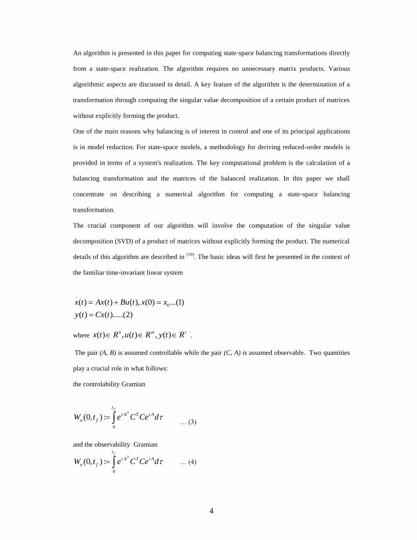
An algorithm is presented in this paper for computing state-space balancing transformations directly

from a state-space realization. The algorithm requires no unnecessary matrix products. Various

algorithmic aspects are discussed in detail. A key feature of the algorithm is the determination of a

transformation through computing the singular value decomposition of a certain product of matrices

without explicitly forming the product.

One of the main reasons why balancing is of interest in control and one of its principal applications

is in model reduction. For state-space models, a methodology for deriving reduced-order models is

provided in terms of a system's realization. The key computational problem is the calculation of a

balancing transformation and the matrices of the balanced realization. In this paper we shall

concentrate on describing a numerical algorithm for computing a state-space balancing

transformation.

The crucial component of our algorithm will involve the computation of the singular value

decomposition (SVD) of a product of matrices without explicitly forming the product. The numerical

details of this algorithm are described in [19]. The basic ideas will first be presented in the context of

the familiar time-invariant linear system

.

0( ) ( ) ( ), (0) ...(1)

( ) ( ).....(2)

x t Ax t Bu t x x

y t Cx t

where ( ) , ( ) , ( )n m rx t R u t R y t R ‘.

The pair (A, B) is assumed controllable while the pair (C, A) is assumed observable. Two quantities

play a crucial role in what follows:

the controlability Gramian

0

(0, ) :f

T

t

A T Ao fW t e C Ce d … (3)

and the observability Gramian

0

(0, ) :f

T

t

A T Ao fW t e C Ce d … (4)

5

where tf is some fixed final time. Frequently, A is assumed asymptotically stable and tr = + is

considered.

We shall make that assumption in this paper and in that case W, and W, satisfy the algebraic

Lyapunov equations

AWc+WcAT+BBT=0 … (5)

ATWo+WoA

T+C TC=0 …. (6) and these finite-time Gramians can be computed by the methods suggested in [21].

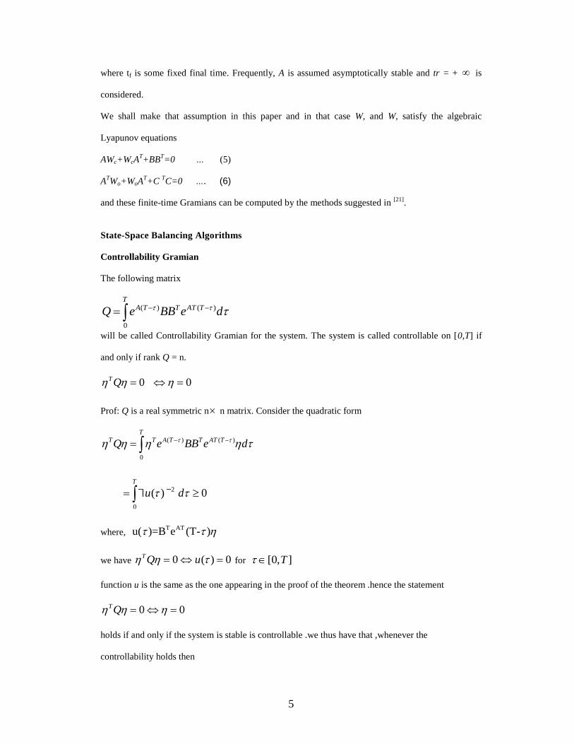
State-Space Balancing Algorithms

Controllability Gramian The following matrix

( ) ( )

0

TA T T AT TQ e BB e d

will be called Controllability Gramian for the system. The system is called controllable on [0,T] if

and only if rank Q = n.

0 0

T Q

Prof: Q is a real symmetric n n matrix. Consider the quadratic form

( ) ( )

0

TT T A T T AT TQ e BB e d

2

0

( ) 0T

u d

where, T ATu( )=B e (T- )

we have 0 ( ) 0TQ u for [0, ]T

function u is the same as the one appearing in the proof of the theorem .hence the statement

0 0TQ

holds if and only if the system is stable is controllable .we thus have that ,whenever the

controllability holds then

6

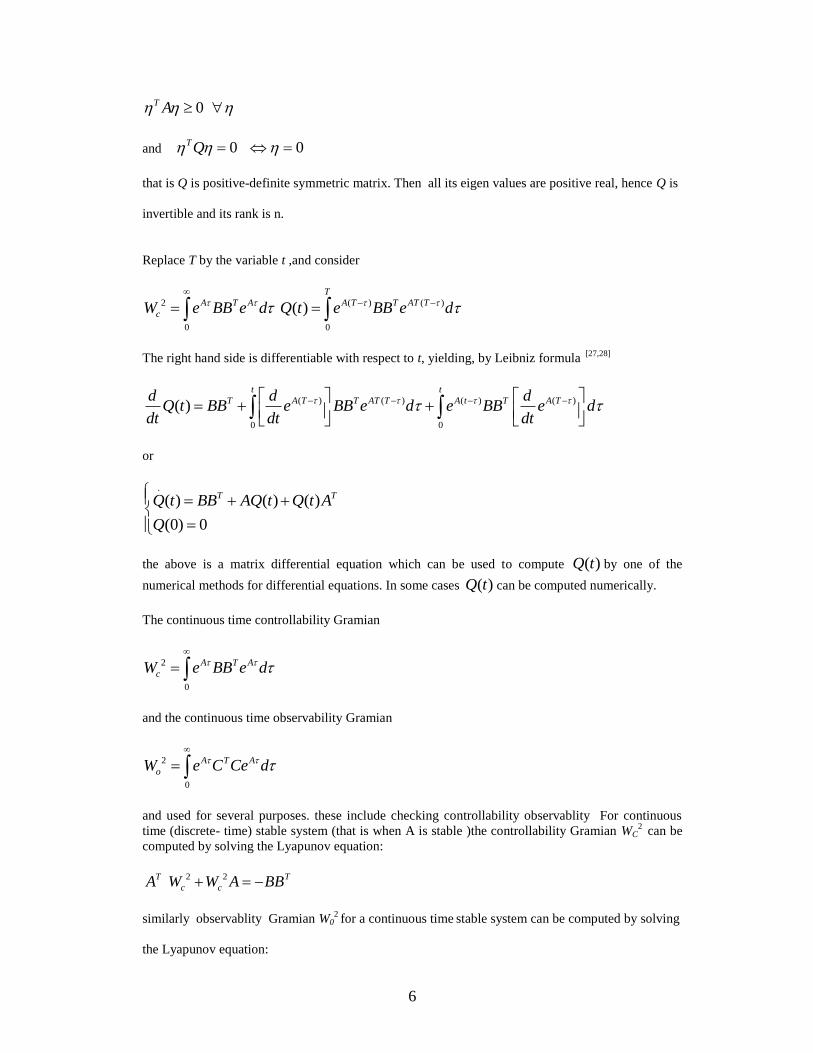
0 T A

and 0 0TQ

that is Q is positive-definite symmetric matrix. Then all its eigen values are positive real, hence Q is

invertible and its rank is n.

Replace T by the variable t ,and consider

2

0

A T AcW e BB e d

( ) ( )

0

( )T

A T T AT TQ t e BB e d

The right hand side is differentiable with respect to t, yielding, by Leibniz formula [27,28]

( ) ( ) ( ) ( )

0 0

( )t t

T A T T AT T A t T A Td d dQ t BB e BB e d e BB e d

dt dt dt

or

.

( ) ( ) ( )

(0) 0

T TQ t BB AQ t Q t A

Q

the above is a matrix differential equation which can be used to compute ( )Q t by one of the

numerical methods for differential equations. In some cases ( )Q t can be computed numerically.

The continuous time controllability Gramian

2

0

A T AcW e BB e d

and the continuous time observability Gramian

2

0

A T AoW e C Ce d

and used for several purposes. these include checking controllability observablity For continuous time (discrete- time) stable system (that is when A is stable )the controllability Gramian WC

2 can be computed by solving the Lyapunov equation:

2 2 T Tc cA W W A BB

similarly observablity Gramian W02 for a continuous time stable system can be computed by solving

the Lyapunov equation:

7

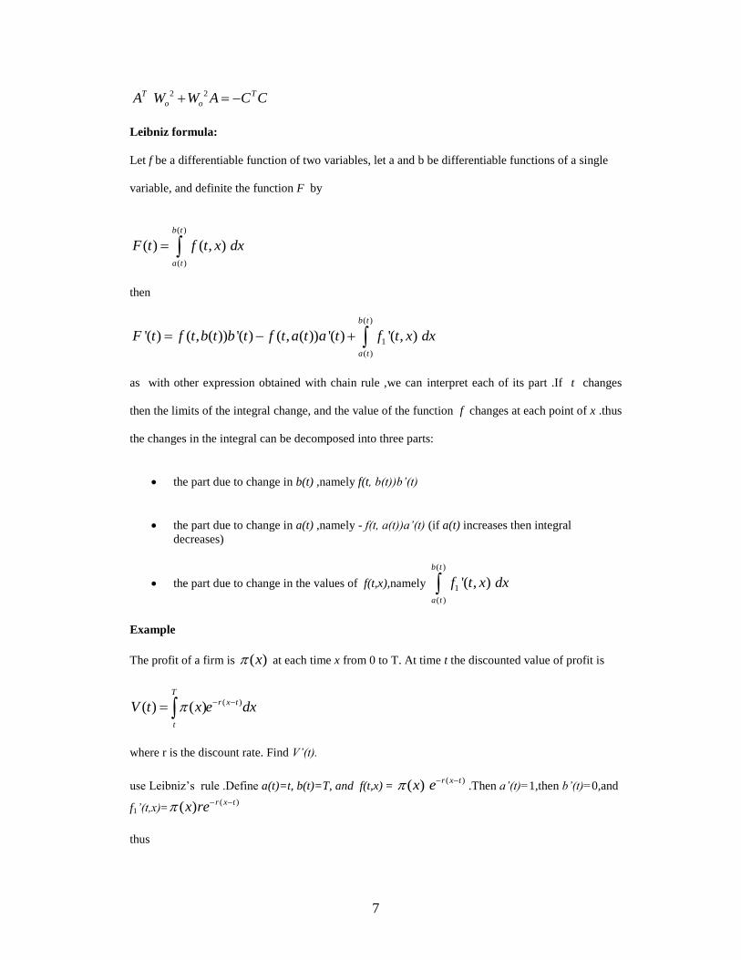
2 2 T To oA W W A C C

Leibniz formula:

Let f be a differentiable function of two variables, let a and b be differentiable functions of a single

variable, and definite the function F by

( )

( )

( ) ( , ) b t

a t

F t f t x dx

then

( )

1

( )

'( ) ( , ( )) '( ) ( , ( )) '( ) '( , ) b t

a t

F t f t b t b t f t a t a t f t x dx

as with other expression obtained with chain rule ,we can interpret each of its part .If t changes

then the limits of the integral change, and the value of the function f changes at each point of x .thus

the changes in the integral can be decomposed into three parts:

the part due to change in b(t) ,namely f(t, b(t))b’(t)

the part due to change in a(t) ,namely - f(t, a(t))a’(t) (if a(t) increases then integral decreases)

the part due to change in the values of f(t,x),namely

( )

1

( )

'( , ) b t

a t

f t x dx

Example

The profit of a firm is ( )x at each time x from 0 to T. At time t the discounted value of profit is

( )( ) ( )T

r x t

t

V t x e dx

where r is the discount rate. Find V’(t).

use Leibniz’s rule .Define a(t)=t, b(t)=T, and f(t,x) = ( )x ( )r x te .Then a’(t)=1,then b’(t)=0,and

f1’(t,x)= ( )( ) r x tx re

thus

8

( ) ( )'( ) ( ) ( ) ( ) ( )T

r t t r x t

t

V t t e x re dx t rV t

the first term reflects the fact that the future is shortened when t increases and the second term

reflects the fact that as time advances future profit at any given time is obtained sooner, and is thus

worth more.

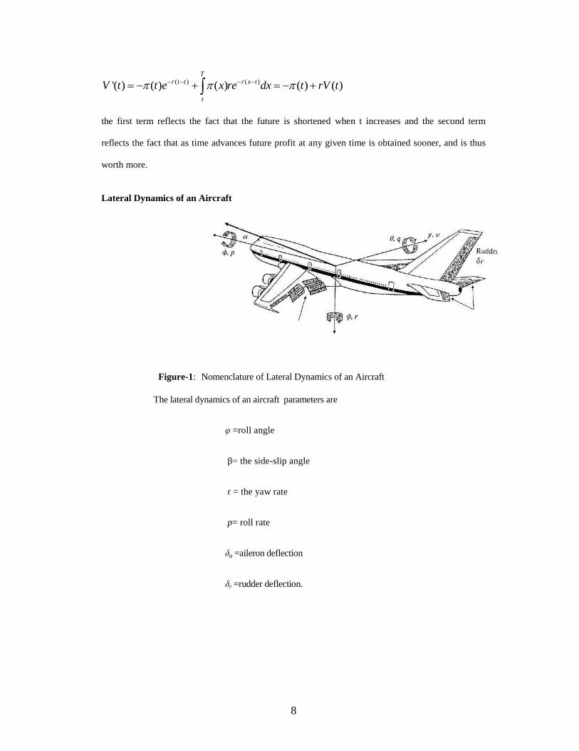
Lateral Dynamics of an Aircraft

Figure-1: Nomenclature of Lateral Dynamics of an Aircraft

The lateral dynamics of an aircraft parameters are

φ =roll angle

β= the side-slip angle

r = the yaw rate

p= roll rate

δa =aileron deflection

δr =rudder deflection.

9

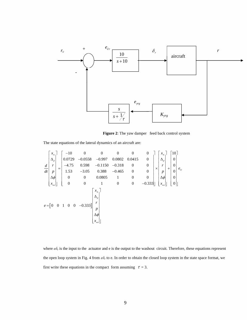
Figure 2: The yaw damper feed back control system

The state equations of the lateral dynamics of an aircraft are:

10 0 0 0 0 0 10

0.0729 0.0558 0.997 0.0802 0.0415 0 0

4.75 0.598 0.1150 0.318 0 0

1.53 3.05 0.388 0.465 0 0

0 0 0.0805 1 0 0

0 0 1 0 0 0.333

A A

wo wo

x x

r rd

p pdt

x x

0

0

0

0

0 0 1 0 0 0.333

r

A

wo

e

x

re

p

x

where eδr is the input to the actuator and e is the output to the washout circuit. Therefore, these equations represent

the open loop system in Fig. 4 from eδr to e. In order to obtain the closed loop system in the state space format, we

first write these equations in the compact form assuming = 3.

aircraft

1s

s

Kyrg

rc

+

-

r re

10

10s

r

yrge

10

.

( ) ( )

( ) ( )c cx A x t Br t

e t Cx t

.( ) ( )

( ) ( )rx Ax t Be t

e t Cx t

where T

wox xA r p x

noting that

( ) ( ) ( )

= ( ) ( )r c

c

e t r t e t

r t Cx t

We finally obtained the closed loop system

.

( ) ( )

( ) ( )c cx A x t Br t

e t Cx t

where AC =A-BC is the closed loop system matrix.

Compensator Transfer Function of the Yaw Damper System

Swept-wing aircraft have a natural tendency to be highly damped in one of the lateral modes of

motion. A typical commercial-aircraft cruising speeds and altitudes, this dynamic mode is sufficiently

difficult to control that virtually every swept-wing aircraft has a feedback system to help the pilot.

Therefore, the goal of our control system is to modify the natural dynamics so that the plane is

pleasant for the pilot to fly. Studies have shown that pilots like natural frequencies ωn ≤ 0.5 and

damping ratio of ζ ≥ 0.5. Aircraft with dynamics that violate these guidelines are generally

considered fatiguing to fly and highly undesirable. Thus our system specifications are to achieve lateral

dynamics that meet these specification. Study of the lightly damped lateral mode indicates that it is

primarily a yawing phenomenon, so measurement of the yaw rate is the logical starting point

for the design. Most new aircraft systems have relied on a laser device (called a ring-laser

11

gyroscope) for the measurement. Here two laser beams transverse a closed path (often a

triangle) in opposite directions. As the triangular device rotates, the detected frequencies of the

two beams shift according to Doppler effect, and this frequency shift is measured, producing a

measure of rotational rate. These devices have fewer moving parts and are more reliable at low

cost. Two aerodynamic surfaces typically influence the lateral aircraft motion: the rudder and

the ailerons. The highly damped yaw mode that will be stabilized by the yaw damper is most

affected by the rudder. Therefore, use of that single control input is a logical starting point for

the design. Hydraulic devices are universally employed in large aircraft to provide the force

that moves the aerodynamic surfaces. No other kind of device has been developed to provide

the combination of high force, high speed, and light weight desirable for the actuation of the

controlling aerodynamic surfaces. On the other hand, the low-speed flaps, which are extended

slowly prior to landing, are typically actuated by an electric motor with a worm gear. The

linearized lateral equations of motion in horizontal flight at 40,000(ft) and nominal forward

speed V0 = 774(ft/sec) (Mach 0.8) are stated above [26].

The simple physical fact is that a positive or clockwise rudder motion causes a negative or

counterclockwise yaw rate. In other words, turning the rudder left (clockwise) causes the

front of the aircraft to rotate left (counterclockwise). The natural motion corresponding to the

complex poles is referred to as the Dutch roll (s = — 0.033 ±j'O.95). The motion corresponding to the

stable real poles is referred to as the spiral mode (si = —0.0073) and the roll mode (s2 = —0.563).

From looking at the system poles, we see that the offending mode that needs repair for good pilot

handling is the Dutch roll. The roots have an acceptable frequency, but their damping ratio £ = 0.03 is

far short of the desired value £ = 0.5. As a first try at the design, consider proportional feedback of the

yaw rate to the rudder. Plot the root locus and the frequency response with respect to the gain of this

feedback. From these plots show that a damping of £ = 0.45 is achievable and this damping occurs at a

gain of about 3.0.

In practice, however, we find that this simple feedback changes the overall gain from the pilot to the

roll rate at low frequencies from about 15 to one over the feedback gain or about 0.33. The change in

DC or zero-frequency gain creates an objectionable situation during a steady turn. Because the

feedback produces a steady rudder input opposite the pilot's input, the pilot must introduce a much

12

larger steady command for the same yaw rate than is necessary in the open-loop case. The dilemma is

solved by feeding back not the yaw rate but the derivative of the yaw rate, since the derivative-feedback is

approximated by including in the feedback path a lead compensation with its zero at the origin (called a

washout circuit). The result is a feedback that passes transients and provides the desired damping but

washes out steady and low-frequency signals. If we augment the dynamic model of the system by

adding the actuator and washout circuit with τ = 3, we obtain the state-variable model as given above

in equations .

From the root locus it is observed that the addition of the washout circuit allows the damping ratio

to be increased from 0.03 to about 0.35. Although feedback of yaw rate through the washout circuit

results in a considerable improvement over the original aircraft control, the response needs to be

improved.

An optimal design using the pole placement has been tried and the corresponding state feedback gain

vector has been incorporated in the transfer function. An optimal design using an estimator has been

tried and the estimator gain vector has been included in the transfer function model.

The compensator transfer function , GC(s) =

-844(s + 10.0)(s - 1.04)(s2 + 1.948s + 1.261)(s + .023) (s + 0.0272)(s2 + 1.674s + 1.151)(s2 + 8.14s + 118.575)(s + 51.3)

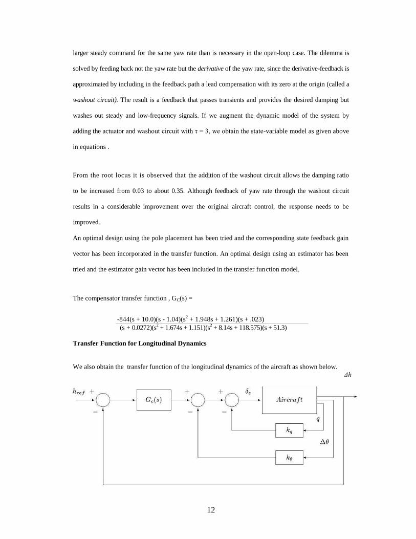
Transfer Function for Longitudinal Dynamics We also obtain the transfer function of the longitudinal dynamics of the aircraft as shown below.

Δh

13

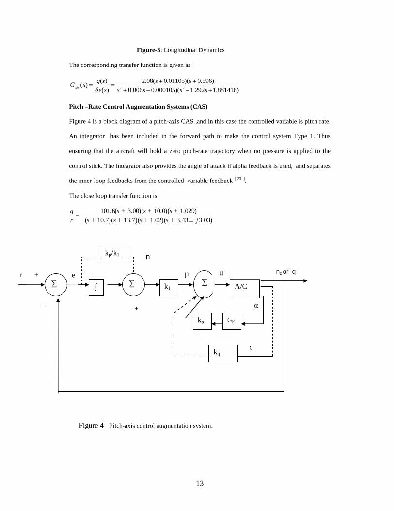
Figure-3: Longitudinal Dynamics The corresponding transfer function is given as

2 2

( ) 2.08( 0.01105)( 0.596)( )

( ) 0.006 0.000105)( 1.292 1.881416)q e

q s s sG s

e s s s s s

Pitch –Rate Control Augmentation Systems (CAS) Figure 4 is a block diagram of a pitch-axis CAS ,and in this case the controlled variable is pitch rate.

An integrator has been included in the forward path to make the control system Type 1. Thus

ensuring that the aircraft will hold a zero pitch-rate trajectory when no pressure is applied to the

control stick. The integrator also provides the angle of attack if alpha feedback is used, and separates

the inner-loop feedbacks from the controlled variable feedback [ 23 ].

The close loop transfer function is q

r=

101.6( 3.00)( 10.0)( 1.029)

( 10.7)( 13.7)( 1.02)( 3.43 3.03)

s s s

s s s s j

+ + +

+ + + + ±

∑

∑ k1

kp/k1

kα GF

kq

A/C

Figure 4 Pitch-axis control augmentation system.

ee

n

nz or q

u

q

+

+

_

r

α

∑

µ

14

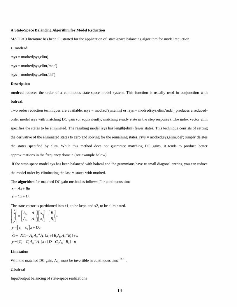
A State-Space Balancing Algorithm for Model Reduction MATLAB literature has been illustrated for the application of state-space balancing algorithm for model reduction. 1. moderd

rsys = modred(sys,elim)

rsys = modred(sys,elim,'mdc')

rsys = modred(sys,elim,'del')

Description modred reduces the order of a continuous state-space model system. This function is usually used in conjunction with

balreal.

Two order reduction techniques are available: rsys = modred(sys,elim) or rsys = modred(sys,elim,'mdc') produces a reduced-

order model rsys with matching DC gain (or equivalently, matching steady state in the step response). The index vector elim

specifies the states to be eliminated. The resulting model rsys has length(elim) fewer states. This technique consists of setting

the derivative of the eliminated states to zero and solving for the remaining states. rsys = modred(sys,elim,'del') simply deletes

the states specified by elim. While this method does not guarantee matching DC gains, it tends to produce better

approximations in the frequency domain (see example below).

If the state-space model sys has been balanced with balreal and the grammians have m small diagonal entries, you can reduce

the model order by eliminating the last m states with modred.

The algorithm for matched DC gain method as follows. For continuous time

x Ax Bu

y Cx Du

The state vector is partitioned into x1, to be kept, and x2, to be eliminated.

11 12 1 1

21 22 2 2

1 2

A A x Bxu

A A x By

y c c x Du

1 1

12 22 21 1 1 12 22 21 [ 11 ] [ ]x A A A A x B A A B u 1 1

1 2 22 21 2 22 2[ ] [ ]y C C A A x D C A B u

Limitation With the matched DC gain, A22 must be invertible in continuous time [7, 1] . 2.balreal Input/output balancing of state-space realizations

15

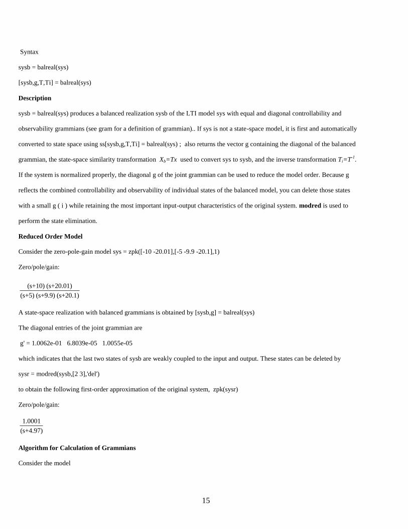
Syntax sysb = balreal(sys) [sysb,g,T,Ti] = balreal(sys) Description

sysb = balreal(sys) produces a balanced realization sysb of the LTI model sys with equal and diagonal controllability and

observability grammians (see gram for a definition of grammian).. If sys is not a state-space model, it is first and automatically

converted to state space using ss[sysb,g,T,Ti] = balreal(sys) ; also returns the vector g containing the diagonal of the balanced

grammian, the state-space similarity transformation Xb=Tx used to convert sys to sysb, and the inverse transformation Ti=T-1.

If the system is normalized properly, the diagonal g of the joint grammian can be used to reduce the model order. Because g

reflects the combined controllability and observability of individual states of the balanced model, you can delete those states

with a small g ( i ) while retaining the most important input-output characteristics of the original system. modred is used to

perform the state elimination.

Reduced Order Model

Consider the zero-pole-gain model sys = zpk([-10 -20.01],[-5 -9.9 -20.1],1) Zero/pole/gain:

(s+10) (s+20.01)

(s+5) (s+9.9) (s+20.1)

A state-space realization with balanced grammians is obtained by [sysb,g] = balreal(sys) The diagonal entries of the joint grammian are g' = 1.0062e-01 6.8039e-05 1.0055e-05 which indicates that the last two states of sysb are weakly coupled to the input and output. These states can be deleted by sysr = modred(sysb,[2 3],'del') to obtain the following first-order approximation of the original system, zpk(sysr) Zero/pole/gain:

1.0001

(s+4.97)

Algorithm for Calculation of Grammians Consider the model

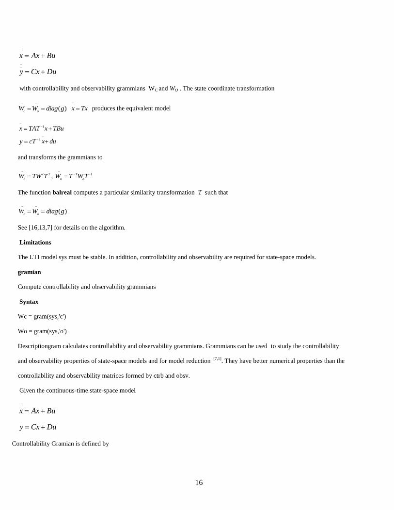
16

x Ax Bu

y Cx Du

with controllability and observability grammians WC and WO . The state coordinate transformation

( ) c oW W diag g

x Tx

produces the equivalent model

1

1

x TAT x TBu

y cT x du

and transforms the grammians to

1, c T T

c o oW TW T W T W T

The function balreal computes a particular similarity transformation T such that

( )c oW W diag g

See [16,13,7] for details on the algorithm. Limitations The LTI model sys must be stable. In addition, controllability and observability are required for state-space models. gramian Compute controllability and observability grammians Syntax Wc = gram(sys,'c') Wo = gram(sys,'o') Descriptiongram calculates controllability and observability grammians. Grammians can be used to study the controllability

and observability properties of state-space models and for model reduction [7,1]. They have better numerical properties than the

controllability and observability matrices formed by ctrb and obsv.

Given the continuous-time state-space model

x Ax Bu

y Cx Du

Controllability Gramian is defined by

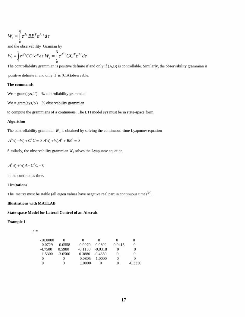
17

0

T

cA T A dW e BB e

and the observability Gramian by

0

T

o

A T A dW e CC e

0

T

oA T A dW e CC e

The controllability grammian is positive definite if and only if (A,B) is controllable. Similarly, the observability grammian is

positive definite if and only if is (C,A)observable.

The commands

Wc = gram(sys,'c') % controllability grammian

Wo = gram(sys,'o') % observability grammian

to compute the grammians of a continuous. The LTI model sys must be in state-space form.

Algorithm

The controllability grammian WC is obtained by solving the continuous-time Lyapunov equation

0T T

o oA W W C C 0T T

c cAW W A BB

Similarly, the observability grammian Wo solves the Lyapunov equation

0T T

o oA W W A C C

in the continuous time. Limitations The matrix must be stable (all eigen values have negative real part in continuous time)[24]. Illustrations with MATLAB State-space Model for Lateral Control of an Aircraft Example 1

a = -10.0000 0 0 0 0 0 0.0729 -0.0558 -0.9970 0.0802 0.0415 0 -4.7500 0.5980 -0.1150 -0.0318 0 0 1.5300 -3.0500 0.3880 -0.4650 0 0 0 0 0.0805 1.0000 0 0 0 0 1.0000 0 0 -0.3330

18

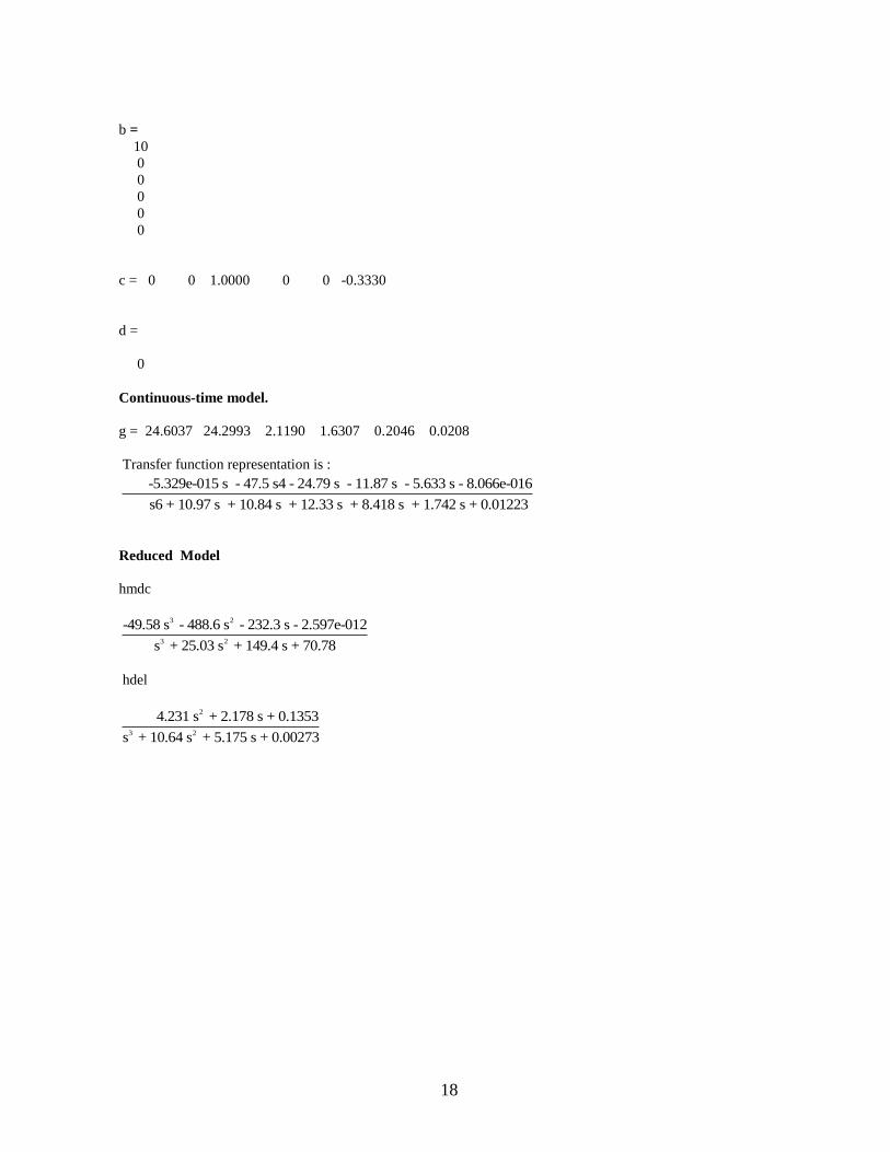
b = 10 0 0 0 0 0 c = 0 0 1.0000 0 0 -0.3330 d = 0 Continuous-time model. g = 24.6037 24.2993 2.1190 1.6307 0.2046 0.0208 Transfer function representation is :

5 3 2

5 4 3 2

-5.329e-015 s - 47.5 s4 - 24.79 s - 11.87 s - 5.633 s - 8.066e-016

s6 + 10.97 s + 10.84 s + 12.33 s + 8.418 s + 1.742 s + 0.01223

Reduced Model hmdc

3 2

3 2

-49.58 s - 488.6 s - 232.3 s - 2.597e-012

s + 25.03 s + 149.4 s + 70.78

hdel

2

3 2

4.231 s + 2.178 s + 0.1353

s + 10.64 s + 5.175 s + 0.00273

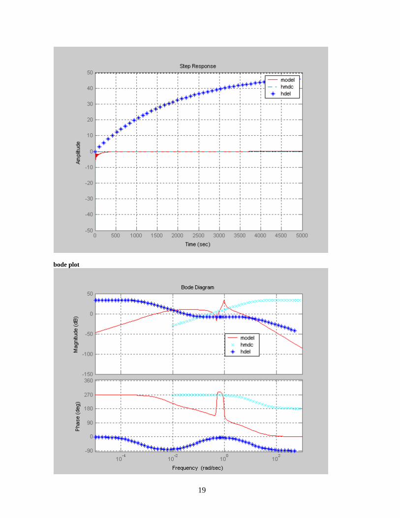
19

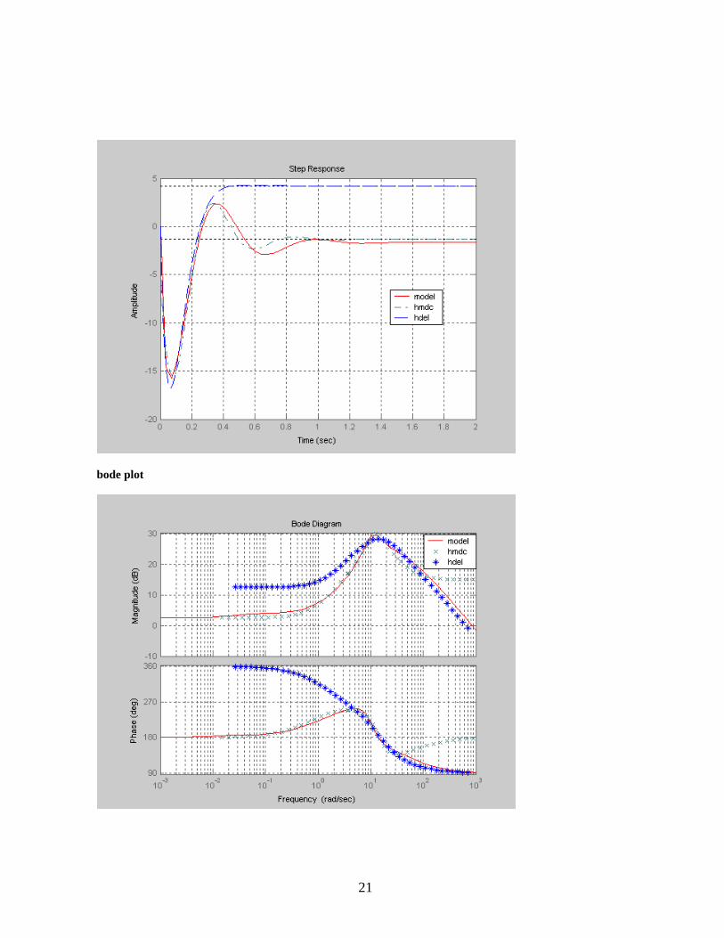
bode plot

20

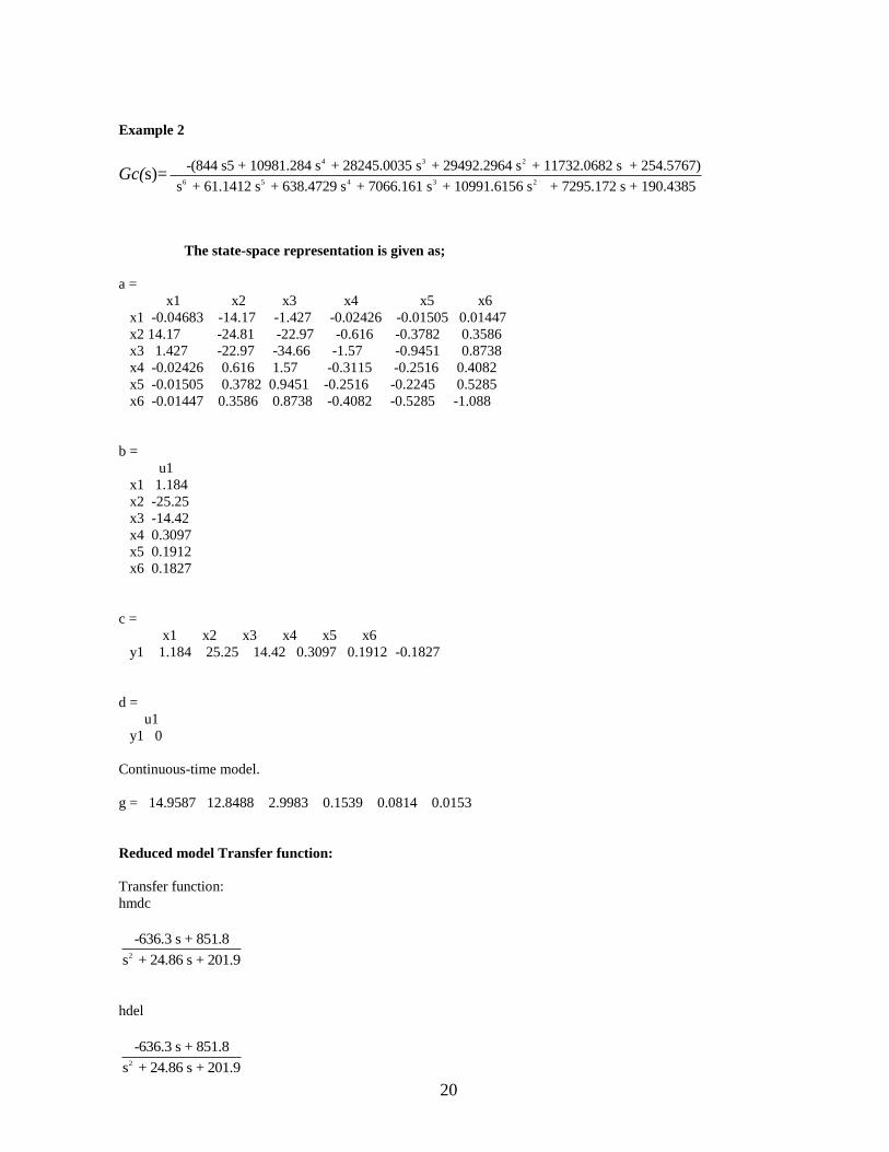
Example 2

Gc(s)=4 3 2

6 5 4 3 2

-(844 s5 + 10981.284 s + 28245.0035 s + 29492.2964 s + 11732.0682 s + 254.5767)

s + 61.1412 s + 638.4729 s + 7066.161 s + 10991.6156 s + 7295.172 s + 190.4385

The state-space representation is given as; a = x1 x2 x3 x4 x5 x6 x1 -0.04683 -14.17 -1.427 -0.02426 -0.01505 0.01447 x2 14.17 -24.81 -22.97 -0.616 -0.3782 0.3586 x3 1.427 -22.97 -34.66 -1.57 -0.9451 0.8738 x4 -0.02426 0.616 1.57 -0.3115 -0.2516 0.4082 x5 -0.01505 0.3782 0.9451 -0.2516 -0.2245 0.5285 x6 -0.01447 0.3586 0.8738 -0.4082 -0.5285 -1.088 b = u1 x1 1.184 x2 -25.25 x3 -14.42 x4 0.3097 x5 0.1912 x6 0.1827 c = x1 x2 x3 x4 x5 x6 y1 1.184 25.25 14.42 0.3097 0.1912 -0.1827 d = u1 y1 0 Continuous-time model. g = 14.9587 12.8488 2.9983 0.1539 0.0814 0.0153 Reduced model Transfer function: Transfer function: hmdc

2

-636.3 s + 851.8

s + 24.86 s + 201.9

hdel

2

-636.3 s + 851.8

s + 24.86 s + 201.9

21

bode plot

22

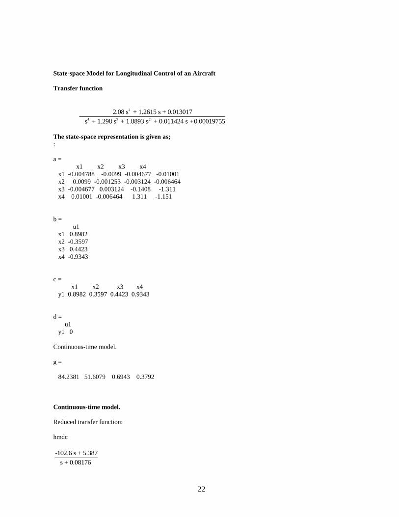
State-space Model for Longitudinal Control of an Aircraft Transfer function

2

4 3 2

2.08 s + 1.2615 s + 0.013017

s + 1.298 s + 1.8893 s + 0.011424 s + 0.00019755

The state-space representation is given as; : a = x1 x2 x3 x4 x1 -0.004788 -0.0099 -0.004677 -0.01001 x2 0.0099 -0.001253 -0.003124 -0.006464 x3 -0.004677 0.003124 -0.1408 -1.311 x4 0.01001 -0.006464 1.311 -1.151 b = u1 x1 0.8982 x2 -0.3597 x3 0.4423 x4 -0.9343 c = x1 x2 x3 x4 y1 0.8982 0.3597 0.4423 0.9343 d = u1 y1 0 Continuous-time model. g = 84.2381 51.6079 0.6943 0.3792 Continuous-time model. Reduced transfer function: hmdc -102.6 s + 5.387

s + 0.08176

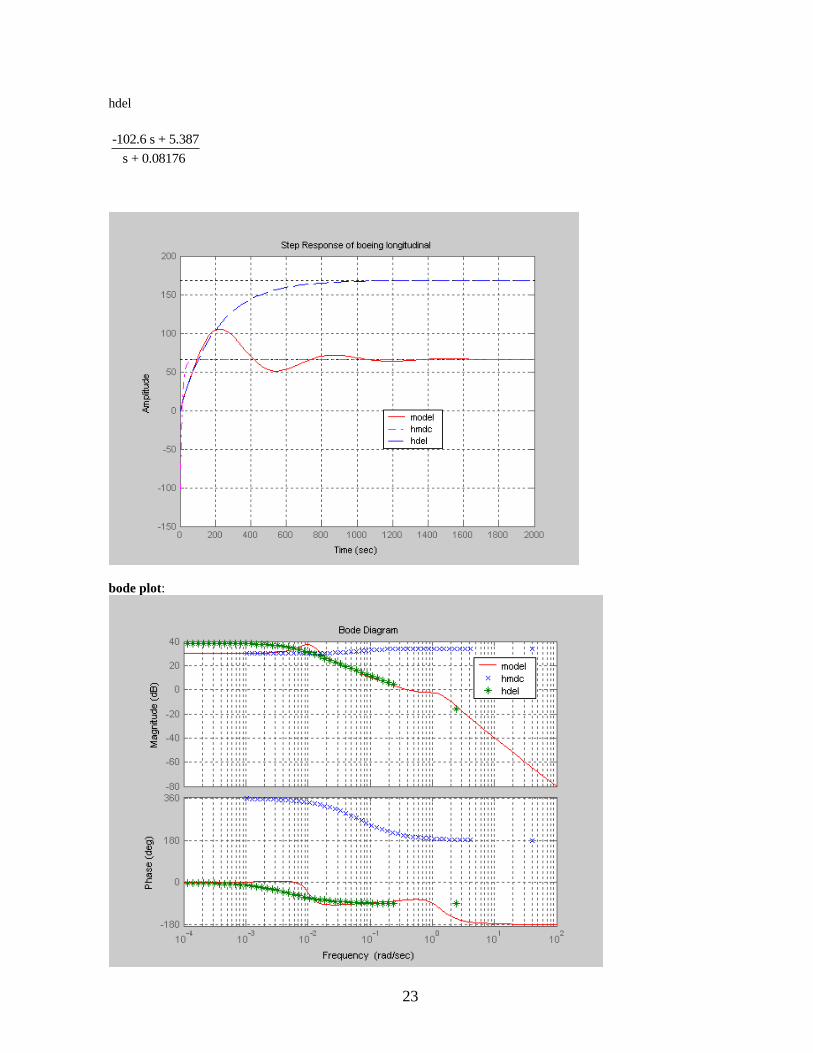
23

hdel -102.6 s + 5.387

s + 0.08176

bode plot:

24

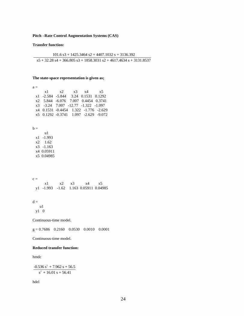
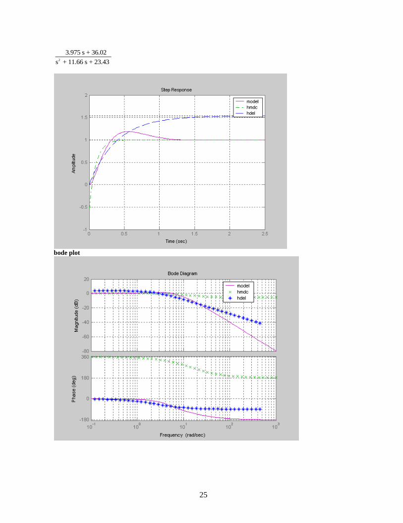
Pitch –Rate Control Augmentation Systems (CAS) Transfer function:

101.6 s3 + 1425.3464 s2 + 4407.1032 s + 3136.392

s5 + 32.28 s4 + 366.805 s3 + 1858.3031 s2 + 4617.4634 s + 3131.8537

The state-space representation is given as; a = x1 x2 x3 x4 x5 x1 -2.584 -5.844 3.24 0.1531 0.1292 x2 5.844 -6.076 7.007 0.4454 0.3741 x3 -3.24 7.007 -12.77 -1.322 -1.097 x4 0.1531 -0.4454 1.322 -1.776 -2.629 x5 0.1292 -0.3741 1.097 -2.629 -9.072 b = u1 x1 -1.993 x2 1.62 x3 -1.163 x4 0.05911 x5 0.04985 c = x1 x2 x3 x4 x5 y1 -1.993 -1.62 1.163 0.05911 0.04985 d = u1 y1 0 Continuous-time model. g = 0.7686 0.2160 0.0530 0.0010 0.0001 Continuous-time model. Reduced transfer function: hmdc

2

2

-0.536 s + 7.962 s + 56.5

s + 16.01 s + 56.41

hdel

25

2

3.975 s + 36.02

s + 11.66 s + 23.43

bode plot

26

Conclusion

The primary focus in this paper has been on the principal application of computing of state-space balancing

transformations directly from a state-space realization (A, B, C) for continuous-time linear systems. Under a

balancing transformation T the equivalent realization has controllability and observability Gramians. Higher

order models of lateral and longitudinal dynamics of an aircraft have been reduced extensively using MATLAB.

It has been found that reduced models both in time domain and frequency domain compare favourably with

higher order models suggesting fewer things to go wrong in the hardware or bugs to fix in the software.

References:

[1] B. C. Moore, "Principal component analysis in linear systems:Controllability, observability, and model reduction," IEEE Trans.Automat. Contr., vol. AC-26, pp. 17-32, 1981. [2] D. Enns. "Model reduction for control system design," Ph.D. dissertation. Dep. Aeronautics and Astronautics, Stanford Univ.,Stanford, CA. June 1984. [3] K. V. Fernando and H. Nicholson, "Minimality of SISO linear systems."Proc.IEEE,vol.70,pp.1241- 1242,1982. [4] ---------, "On the cross-Grammian for symmetric MIMO systems," IEEE Trans. Circuits Syst., vol. CAS-32, pp. 487-489, 1985. [5] K. Glover, "All optimal Hankel-norm approximations of linear multivariable systems and their L "-error bounds”, Int. J. Contr., vol. 39, pp. 1115-1193. 1984.

[6] E. A. Jonckheere and L. M. Silverman. "A new set of invariants for linear systems—Application to reduced order compensator design," IEEE Trans. Automat. Contr., vol. AC-28. pp. 953-964, 1983. [7] A. J. Laub. L. M. Silverman, and M. Verma, "A note on cross-Grammians for symmetric realizations:" Proc. IEEE, vol. 71, pp. 9M-905, 1983. [8] P. Opdenacker, "Balanced model order reduction techniques and their applications to large space structures problems." Ph.D. dissertation.Dep. Elec. Eng.-Syst.. Univ. Southern Calif., Aug. 1985 [9] L. Pernebo and L. M. Silverman, "Model reduction via balanced state space representations," IEEE Trans. Automat. Contr., vol. AC-27,pp. 382-387, 1982.

[10] S. Shokoohi. L. M. Silverman, and P. Van Dooren, "Linear time-variable systems: Balancing and model reduction," IEEE Trans.Autoinat. Contr., vol. AC-28, pp. 810-822, 1983. [11] J. R. Sveinsson and F. W. Fairman, "Minimal balanced realization of transfer function matrices using Markov parameters," IEEE Trans.Automat. Contr., vol. AC-30, pp. 1014-1016, 1985.

[12] N. J. Young, "Balanced realizations via model operators," Int. J.Contr., vol. 42, pp. 369-389

[13] Alan J. Laub, Michael T. Heath, Chris C. Paige, And Robert C. Ward, “Computation of System Balancing Transformations and Other Applications of Simultaneous Diagonalization Algorithms”, IEEE VOL. AC-32. NO. 2, February 1987 pp. 115-122

27

[14] D. Gangsaas. K. R. Bruce, J. D. Blight, and U. -L. Ly, "Application of modern synthesis to aircraft control: Three case studies," IEEETrans. Automat. Contr., vol. AC-31, pp. 995-1104, Nov. 1986.

[15] U. L. Ly, "A design algorithm for robust low order controller," Ph.D. dissertation, Dep. Aeronaut. Astronaut., Stanford Univ.,Stanford, CA, 1982. [16] D. S. Bernstein and D. C. Hyland, "The optimal projection equations for fixed-order dynamic compensation," IEEE Trans. Automat.Contr., vol. AC-29, pp. 1034-1037, Nov. 1985.

[17] D. C. Hyland and D. S. Bernstein, "The optimal projection equations for model reduction and the relationships among the methods of Wilson, Skclton, and Moore," IEEE Trans. Automat. Contr., vol.AC-30, pp. 1201-1211, Dec. 1985. [18] R. E. Skelton, Dynamic Systems Control. New York: Wiley. 1988. [19] E. A. Jonckheere and L. M. Silverman. “A new set of invariants for IEEE Trans. Automat. Contr., vol. AC-28. pp. 953-964, 1983.

[20] C. Van Loan, “Computing integrals involving the matrix exponential,” IEEE Trans. Automat. Conrr., vol. AC-23, pp. 395-404, 1978. [21] Bartle, Robert G., “A modern theory of integration”, Graduate Studies in Math., vol. 32., American Math. Soc., Providence, 2001.

[22] Gordon, Russell A., “The Integrals of Lebesgue, Denjoy, Perron and Henstock”, Graduate Studies in Math., vol. 4., American Math. Soc., Providence, 1994. [23] P S Khuntia et al, “Response Acceleration of an Aircraft”, submitted for possible publication in the Journal of the Institution of Engineers(India).

[24] Kailath, T., Linear Systems, Prentice-Hall, 1980. [25] B D O Anderson and Yi Liu, “Controllers reduction: concepts and approaches”, IEEE Trans. Automat.Contr., vol. AC-34, pp. 802-812, August ,1989. [26] Hossein M Oloomi, Laboratory Manual for Lab 4 and Lab 5for Lateral Control of a Boeing 747 and Longitudinal Control of a Boeing 747 , Department of Electrical Engineering, Purdue University Fort Wayne, USA [27] Bartle, Robert G., “A modern theory of integration”, Graduate Studies in Math., vol. 32.,American Math. Soc.,

Providence, 2001. [28] Gordon, Russell A., “The Integrals of Lebesgue, Denjoy, Perron and Henstock”, Graduate Studies in Math.,

vol. 4., American Math. Soc., Providence, 1994.

28