Model for Traffic Emissions Estimation

Pergamon Atmospheric Environment Vol. 27B, No. 4, pp. 435-446, 1993. Copyright ~ 1994 Elsevier Science Ltd

Printed in Great Britain. All fights reserved 0957-1272/93 $6.00+0.00

MODEL FOR TRAFFIC EMISSIONS ESTIMATION

A. ALEXOPOULOS and D. ASSIMACOPOULOS

Department of Chemical Engineering, Section II, National Technical University of Athens, Zographou 157 73, Athens, Greece

and

E. MITSOULIS* Department of Chemical Engineering, University of Ottawa, Ottawa, Ontario, K1N 6N5, Canada

(First received 15 December 1991 and in final form 25 April 1993)

A~tmct--A model is developed for the spatial and temporal evaluation of traffic emissions in metropolitan areas based on sparse measurements. All traffÉc data available are fully employed and the pollutant emissions are determined with the highest precision possible. The main roads are regarded as line sources of constant traffic parameters in the time interval considered. The method is flexible and allows for the estimation of distributed small traffic sources (non-line/area sources). The emissions from the latter are assumed to be proportional to the local population density as well as to the traffic density leading to local main arteries. The contribution of moving vehicles to air pollution in the Greater Athens Area for the period 1986-1988 is analysed using the proposed model. Emissions and other related parameters are evaluated. Emissions from area sources were found to have a noticeable share of the overall air pollution.

Key word index: Traffic emissions, traffic pollution, urban emission modelling.

1. INTRODUCTION

In recent years, urban pollution has emerged as the most acute problem, because of its negative effects on health and deterioration in living conditions. To pre- vent further exacerbation, a thorough environmental policy is required based on scientific planning of pollution control. Within this framework it is necessary:

- - to analyse and specify all pollution sources and their contribution to air pollution;

- - to study the different factors which cause the phenomenon;

- - to develop tools to reduce pollution by intro- ducing control measures and alternatives to existing practices.

An appraisal of the existing pollution sources con- stitutes the first step of tackling the problem. A precise knowledge of their location, temporal distribution, level of activity and their interconnection with the massive flow of pollutants in the atmosphere, com- prise the most crucial elements in the overall formula- tion of a model, which can be used for quantitative predictions concerning real situations (Ciaggett et al., 1981; Matzoros, 1990).

Estimates of emissions from traffic (moving sources) is a demanding problem. It requires coordination of a large number of data and measurements in the area of interest. This work presents a model, which evalu-

* To whom correspondence should be addressed.

ates the pollutant emissions from traffic in urban areas in a detailed manner. In our attempt to model the emissions, we have tried to make as much as possible use of existing raw data. The present model is flexible enough so that it can be used in cases where raw data are not complete and a network/trip matrix is difficult to generate.

Special attention has been paid to the evaluation of traffic area sources, i.e. to those emissions which do not originate in the big arteries and for which traffic load data are usually missing. Modelling of these sources presents major difficulties and is possible only when detailed data are available. Such an example was given by Psaraki-Kalouptsidis (1976) in the case of St Louis, U.S.A. This model is based on a special probability law which is assumed to govern traffic, when the latter has as a determining parameter the average travelled distance. Different routes are grouped into categories with common traffic charac- teristics and emission factors.

In the present work there are no such data available. The proposed method groups together small line sources into area sources. For area sources, fuel consumption is estimated from an overall balance in the study area and according to data for population density and local traffic intensity. The structure of the model is independent of the time period of its implementation and it can be updated with new traffic data. Thus, in connection with similar emission models for central heating (Kozaris et al., 1984) and for industrial emissions, it can be used as a tool for pollution control policies.

435

436 A. ALEXOPOULOS et al.

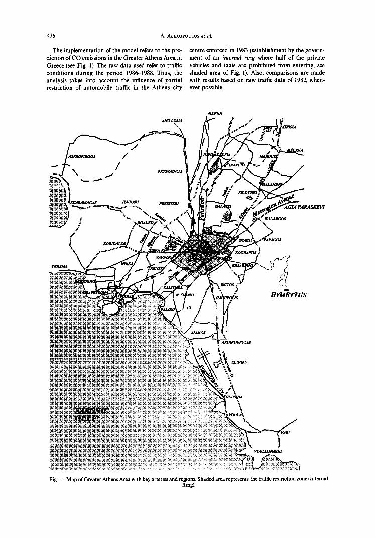
The implementation of the model refers to the prediction of CO emissions in the Greater Athens Area in Greece (see Fig. 1). The raw data used refer to traffic conditions during the period 1986-1988. Thus, the analysis takes into account the influence of partial restriction of automobile traffic in the Athens city

centre enforced in 1983 (establishment by the govern- ment of an internal ring where half of the private vehicles and taxis are prohibited from entering, see shaded area of Fig. 1). Also, comparisons are made with results based on raw traffic data of 1982, when- ever possible.

ME31ID1

ANO LOSIA , ~

¢~PROPIRGOS

, /

/

R i ~ 4 P J

PET~OUPOZJ

PERZSTEPJ

¥ 1 L O ~

MELISIA

~OLARGO~

P~MMA

HYMETTU$

AJ~GIROUPOLi$

VOULIAO~

Fig. 1. Map of Greater Athens Area with key arteries and regions. Shaded area represents the traffic restriction zone (Internal Ring).

Model for traffic emissions estimation 437

2. M O D E L F O R M U L A T I O N FOR E M I S S I O N S E V A L U A T I O N

2.1. Emissions evaluation

Pollutant emissions at a point of a traffic artery is a function of many variables, which can be grouped into two categories: (a) traffic variables (x,), such as traffic load, traffic composition, speed, driving model, etc. and (b) vehicle variables (y,), related to vehicle engine and its driving conditions. The emission of a pollutant p during the time interval t will be:

Ept='w~pt(Xl, x2 . . . . . Xn; Y l , Y2 . . . . . Yn)' (1)

The spatial and temporal distribution of traffic load is an essential factor in the emission model. In most cases there is a total lack of data for arteries of light traffic, and the evaluation of their contribution to air pollution is based on simplifying assumptions (Roth and Roberts, 1974).

Traffic composition, i.e. the percentage distribution of traffic load per vehicle category, differs from the corresponding composition of vehicle fleet due to different usage of various vehicle categories. In cases where data on traffic composition are missing or inad- equate, vehicles are grouped into two categories according to fuel type used. In the case of a total lack of data on traffic composition, some information can be obtained from the relative consumption of gasoline and diesel in the area or from literature sources (EPA Report, 1979).

Simulation of the motion of a certain vehicle category leads to the driving model and gives the average operating times of the vehicle engine while stationary, in constant speed, acceleration, or deceleration for a typical route of constant distance. The emission factors used for the calculation of vehicle emissions depend on driving conditions (EPA Report, 1978). Road driving conditions can be expressed, apart from the driving model, as a function of the average speed of the vehicles during the time period under consideration (Roth and Roberts, 1974).

The pollutant vehicle emissions also depend on several engine parameters, the most important of which are the engine volume (co) and age, the ratio air/fuel, the ignition procedure, the ratio area/volume of the cylinders, the compression ratio, etc. Emissions are also sensitive to a large number of parameters concerning driving conditions such as engine charge and temperature.

It is evident that in a large-scale model it is impossible to take into account all different parameters. For simplification, we proceed with the following categories:

- - vehicles with similar engine parameters, - - arteries with similar traffic conditions.

Such categories can be expressed by the parameters referred to as "traffic composition" and "traffic artery category" and be taken into account as such in the model.

2.2. Line sources modelling

In order to implement Equation (1), some approx- imations should be made such as that all variables therein are kept constant along distance I of the route and during the time period under consideration. Prac- tically this is impossible to achieve since traffic arteries transverse areas with different urban activities and cross many smaller roads.

In the present model, the arteries for which traffic data exist are divided into small linear segments (corresponding to measurements). These, in turn, are considered as independent line sources with constant traffic variables. Under these assumptions, the pollutant quantity Ep emitted from a segment of an artery (hence line source) of length I during a time period t is given by:

N

Ep= ~ Q.ai. l-epi. (2) i=1

The quantity Q-a/expresses the traffic load of vehicles of category i in the time period studied. The quantity Q-a~-I represents the number of vehicle- kilometres that were travelled by the vehicle category i during time t and along distance I of the line source.

In the emission model of line sources all roads for which traffic data are available, are taken into account. Line sources are divided into appropriate linear segments for which traffic load, traffic composition and emission factors of the pollutants are assumed constant. Road splitting is made according to changes in traffic load along its length. The line segments derived this way are studied as independent line sources with a traffic composition corresponding to the category which each line source belongs to.

Raw data collected on traffic load present many shortcomings, either because of bad scheduling practices or because of problems during measurement or because of lack of adequate technical equipment. In order to resolve better these inadequacies, the following submodels for handling traffic data were developed.

(a) FILL. Submodel FILL fills up missing data in traffic load files. The method used averages data of similar road categories with complete data records. The averaging procedure generates non-dimensional values for traffic loads of each line source (using the average value). Then, it applies a curve fitting procedure in order to find suitable adjusting factors express- ing the traffic load variation in the time period under examination.

(b) EXTEND. The duration of measurements is usually one week and the data collected refers either to weekdays or to weekends. The number of traffic load data related to weekends is significantly lower than that related to weekdays. It is essential to extend the traffic load data, so that they can cover the same number of weekend periods as that of weekdays. Sub- model EXTEND creates weekday/weekend propor- tionality factors for the roads, for which data from


J "-'t TM~

l l

T ~

F m

T ~

I..

l EQUATION

(2)

I Emlutons

L~S~

Ooo¢0tnate Data

=~

LlmbSc~rce Data

pe¢ ~l. Ion

Fig. 2. Structure of the model estimating line-source emissions (LINE-S).

both categories are available and provides an estimation of the weekend traffic load values.

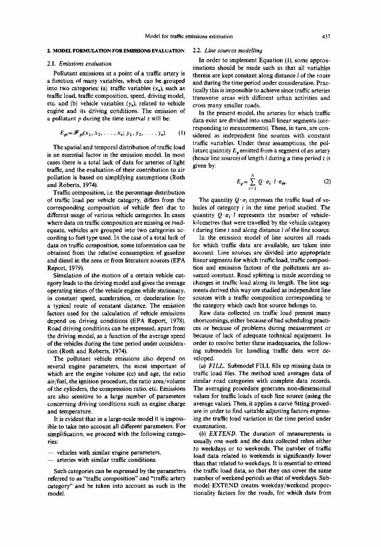
(c) S T R E E T . Estimation of emissions, in the form of pollutant quantity per unit area, can be achieved if all partial emissions from the line sources are added in each grid cell. For this, it is necessary to locate the line sources on the grid, so that their contribution to each cell can be identified. Then, the intersections of line sources with grid lines are determined and the inter- ceptvd lengths of line sources are calculated and enter the corresponding grid cell.

Figure 2 shows the structure of the overall model for calculating emissions from line sources, called LINE-S. The user initially chooses (with subroutine TIME) the time period for which emissions are to be calculated. Then subroutine SPACE determines whether the results will be emissions per unit length of line source or emissions per unit area. In the second case it is necessary to handle the output files from submodel STREET. Necessary input data also com- prise: the coordinates of line sources, the emission factors, and the traffic composition for each vehicle category.

2.3. Area sources modell ing

It is evident that the previous modelling procedure does not take into consideration that part of the traffic which occurs in secondary roads and for which there are no data available. Depending on the density of measurements, the traffic percentage which is not considered as line sources may be quite important. This shortcoming can be surmounted, to a degree, by intro- ducing the concept of mobile area source. In fact, it is a grouping of disperse small line sources transformed

into an area source having as emission point the centre of the corresponding cell.

The model of line sources (which is solved first) estimates fuel consumption (gasoline and diesel) of vehicles, using the consumption factors for each vehicle category. Then from the overall fuel consumption in the area, the extra fuel quantities are distributed to that part of traffic (small roads without traffic data) not processed in the line-source model.

The distribution procedure should discriminate among different urban activities. For the proposed model, these are divided into:

- - activities that lead to vehicle traffic in the grid cell under consideration;

- - activities that lead vehicle traffic to big arteries.

The first type of activity is usually proportional to the urban activities of the area, which as a first approximation can be assumed to be in direct proportion to the population of the area under consideration. The second type has an intensity proportional to the traffic load of local line sources.

For the implementation of the above traffic model, a percentage a of the fuel consumed in the area-traffic sources, is distributed to all grid cells and in proportion to their local population density. This fuel quantity corresponds to all constant traffic activities of the area. The remaining fuel (1 - a ) is distributed proportionally to the corresponding vehicle-kilometres travelled by each vehicle category in the neigh- bouring line-traffic source.

The fuel quantities (gasoline and diesel) annually consumed in the line sources of the area of interest are calculated using the consumption factors for each


Traffic Load Data

7 Coordlneta

Data

Traffic ComposllJon

r l

t EQUATION ~_~ Con~Jmpt~ (3) Factors

. . . . . . . . . . . . . . . . . . . . . . . . . . . . . . . . . . . . . . . . . . . . . . . . . . . . . . . . . . . . . . . . . .

Factor m Fuel end Cell [

Consumption Consuml~on [ tJae-Setu~ of Area Sourc~ Emlulons

Consumption (7) Eml~Ions F ~ o r s p t

T

Factors Factors

Subroutine

CONSUMPTION

Total Pollutant

Emissions

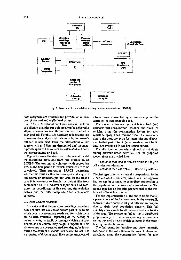
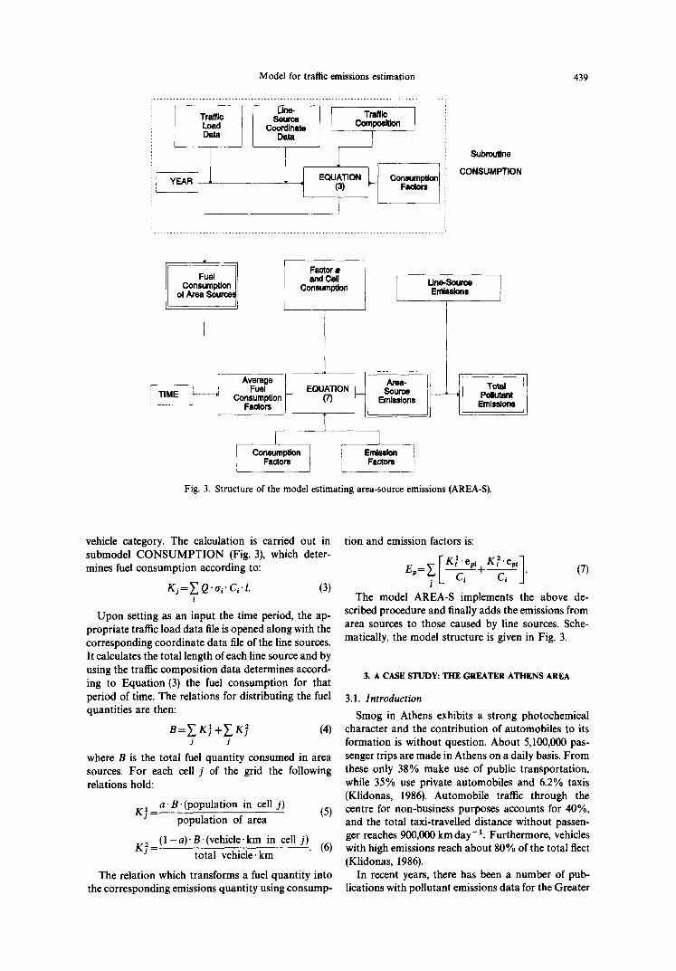
Fig. 3. Structure of the model estimating area-source emissions (AREA-S).

vehicle category. The calculation is carried out in submodel CONSUMPTION (Fig. 3), which determines fuel consumption according to:

K~ = ~, Q. a~" Ci" I. (3) i

Upon setting as an input the time period, the appropriate traffic load data file is opened along with the corresponding coordinate data file of the line sources. It calculates the total length of each line source and by using the traffic composition data determines according to Equation (3) the fuel consumption for that period of time. The relations for distributing the fuel quantities are then:

1 2 B = ~ Kj + ~ Kj (4) J J

where B is the total fuel quantity consumed in area sources. For each cell j of the grid the following relations hold:

a. B. (population in cell j) K] = population of area (5)

K2=(1-a).B.(vehicle.km in cell j) (6) j - total vehicle, km

The relation which transforms a fuel quantity into the corresponding emissions quantity using consurnp-

tion and emission factors is:

_ r K ~ ' % i K 2"%{]

The model AREA-S implements the above de- scribed procedure and finally adds the emissions from area sources to those caused by line sources. Sche- matically, the model structure is given in Fig. 3.

3. A CASE STUDY: THE GREATER ATHENS AREA

3.1. Introduction Smog in Athens exhibits a strong photochemical

character and the contribution of automobiles to its formation is without question. About 5,100,000 passenger trips are made in Athens on a daily basis. From these only 38% make use of public transportation, while 35% use private automobiles and 6.2% taxis (Klidonas, 1986). Automobile traffic through the centre for non-business purposes accounts for 40%, and the total taxi-travelled distance without passenger reaches 900,000 km day- 1. Furthermore, vehicles with high emissions reach about 80% of the total fleet (Klidonas, 1986).

In recent years, there has been a number of pub- lications with pollutant emissions data for the Greater


Athens Area. According to PERPA (1990), vehicle traffic is responsible for 64% of smoke, 8% of SO2, 67% of NO~, 68% of HCs and almost 100% of CO. Based on this evidence, the Greek State introduced at the end of 1982 traffic restrictions prohibiting half of the fleet of private automobiles to enter the city centre. The area of restricted circulation is demar- cated by the Internal Ring road (see Fig. 1). It is clear that emissions from moving sources are of great interest, and therefore a precise analysis of their contribution to overall air pollution as well as their spatial and temporal distribution is necessary.

The relation between emissions and automobiles for the Greek capital has been the subject of some studies by Pattas and co-workers (1983, 1985a, b,c). However, a thorough model for emissions prediction based on traffic sources has not been developed as yet. Dracopoulos (1986) attempted a determination of the mean yearly pollutant emissions in the Greater Athens Area for traffic conditions prevailing in 1982. In a similar study, Bonazoundas and Tsibidis (1987) determined the lead emissions from gasoline-employ- ing vehicles moving in the main arteries of the Greater Athens Area according to traffic data of 1983.

3.2. Input data

3.2.1. Model geometry. The area under consideration corresponds to a surface of 693 km 2 (21 km x 33 km), which is covered with an evenly distributed

square grid of 1 km 2 unit cells. The limits of the study area extend to mountains Egaleo, Parnitha, Penteli, Hymettus and the Saronic Gulf. The axes of the coordinate system used coincide with geographical direc- tions of North-South (y) and East-West (x), respectively. This coordinate system was also the basis for the calculation of the coordinates of main arteries used in the present model.

3.2.2. Traffic load data. The case study was based on traffic data for years 1986 and 1987, as well as the first 9 months of 1988, and concerns calculation of CO emissions from traffic in the Greater Athens area. The choice of CO was based on two reasons: (a) CO is relatively inert and (b) CO may be considered as the best tracer for determining the traffic contribution to the overall atmospheric pollution of the area since it is almost solely emitted by vehicles (PERPA, 1990).

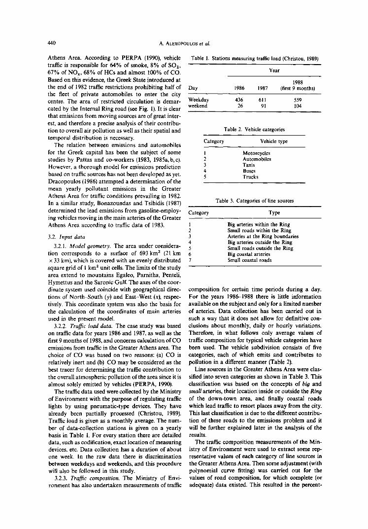
The traffic data used were collected by the Ministry of Environment with the purpose of regulating traffic lights by using pneumatic-type devices. They have already been partially processed (Christou, 1989). Traffic load is given as a monthly average. The number of data-collection stations is given on a yearly basis in Table 1. For every station there are detailed data, such as codification, exact location of measuring devices, etc. Data collection has a duration of about one week. In the raw data there is discrimination between weekdays and weekends, and this procedure will also be followed in this study.

3.2.3. Traffic composition. The Ministry of Envi- ronment has also undertaken measurements of traffic

Table 1. Stations measuring traffic load (Christou, 1989)

Year

1988 Day 1986 1987 (first 9 months)

Weekday 436 611 559 weekend 26 91 104

Table 2. Vehicle categories

Category Vehicle type

1 Motorcycles 2 Automobiles 3 Taxis 4 Buses 5 Trucks

Table 3. Categories of line sources

Category Type

Big arteries within the Ring Small roads within the Ring Arteries at the Ring boundaries Big arteries outside the Ring Small roads outside the Ring Big coastal arteries Small coastal roads

composition for certain time periods during a day. For the years 1986-1988 there is little information available on the subject and only for a limited number of arteries. Data collection has been carried out in such a way that it does not allow for definitive conclusions about monthly, daily or hourly variations. Therefore, in what follows only average values of traffic composition for typical vehicle categories have been used. The vehicle subdivision consists of five categories, each of which emits and contributes to pollution in a different manner (Table 2).

Line sources in the Greater Athens Area were clas- sifted into seven categories as shown in Table 3. This classification was based on the concepts of big and small arteries, their location inside or outside the Ring of the down-town area, and finally coastal roads which lead traffic to resort places away from the city. This last classification is due to the different contribution of these roads to the emissions problem and it will be further explained later in the analysis of the results.

The traffic composition measurements of the Min- istry of Environment were used to extract some rep- resentative values of each category of line sources in the Greater Athens Area. Then some adjustment (with polynomial curve fitting) was carried out for the values of road composition, for which complete (or adequate) data existed. This resulted in the percent-


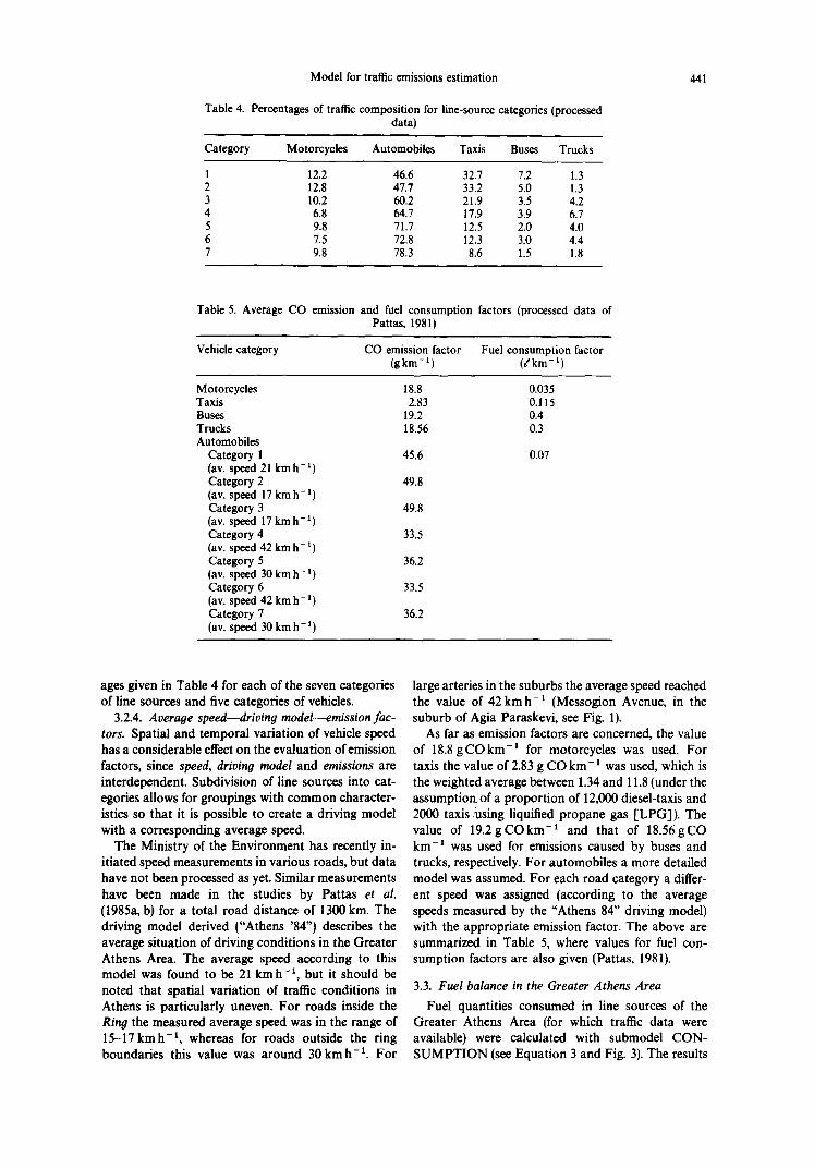
Table 4. Percentages of traffic composition for line-source categories (processed data)

Category Motorcycles Automobiles T a x i s B u s e s Trucks

1 12.2 46.6 32.7 7.2 1.3 2 12.8 47.7 33.2 5.0 1.3 3 10.2 60.2 21.9 3.5 4.2 4 6.8 64.7 17.9 3.9 6.7 5 9.8 71.7 12.5 2.0 4.0 6 7.5 72.8 12.3 3.0 4.4 7 9.8 78.3 8.6 1.5 1.8

Table 5. Average CO emission and fuel consumption factors (processed data of Pattas, 1981)

Vehicle category CO emission factor Fuel consumption factor (gkm -1) (•km -1)

Motorcycles Taxis Buses Trucks Automobiles

Category 1 (av. speed 21 kmh -1 Category 2 (av. speed 17 kmb -1 Category 3 (av. speed 17 km h- 1 Category 4 (av. speed 42 km h- 1 Category 5 (av. speed 30 km h- 1 Category 6 (av. speed 42 km h - 1

Category 7 (av. speed 30 km h - 1

18.8 2.83

19.2 18.56

45.6

49.8

49.8

33.5

36.2

33.5

36.2

0.035 0.115 0.4 0.3

0.07

ages given in Table 4 for each of the seven categories of line sources and five categories of vehicles.

3.2.4. Average speed--driving model---emission factors. Spatial and temporal variation of vehicle speed has a considerable effect on the evaluation of emission factors, since speed, driving model and emissions are interdependent. Subdivision of line sources into categories allows for groupings with common character- istics so that it is possible to create a driving model with a corresponding average speed.

The Ministry of the Environment has recently in- itiated speed measurements in various roads, but data have not been processed as yet. Similar measurements have been made in the studies by Pattas et al. (1985a, b) for a total road distance of 1300 km. The driving model derived ("Athens '84") describes the average situation of driving conditions in the Greater Athens Area. The average speed according to this model was found to be 21 kmh -~, but it should be noted that spatial variation of traffic conditions in Athens is particularly uneven. For roads inside the Ring the measured average speed was in the range of 15-17kmh -~, whereas for roads outside the ring boundaries this value was around 30 kmh-1. For

large arteries in the suburbs the average speed reached the value of 42 kmh -1 (Messogion Avenue, in the suburb of Agia Paraskevi, see Fig. 1).

As far as emission factors are concerned, the value of 18.8gCOkm -1 for motorcycles was used. For taxis the value of 2.83 g CO km- 1 was used, which is the weighted average between 1.34 and 11.8 (under the assumption, of a proportion of 12,000 diesel-taxis and

. ~ . . .

2000 taxis .Using hqmfied propane gas [LPG]). The value of 19.2gCOkm -1 and that of 18.56gCO km-~ was used for emissions caused by buses and trucks, respectively. For automobiles a more detailed model was assumed. For each road category a different speed was assigned (according to the average speeds measured by the "Athens 84" driving model) with the appropriate emission factor. The above are summarized in Table 5, where values for fuel consumption factors are also given (Pattas, 1981).

3.3. Fuel balance in the Greater Athens Area

Fuel quantities consumed in line sources of the Greater Athens Area (for which traffic data were available) were calculated with submodel CON- SUMPTION (see Equation 3 and Fig. 3). The results


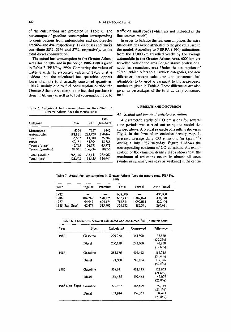
of the calculations are presented in Table 6. The percentages of gasoline consumption corresponding to contributions from automobiles and motorcycles are 96% and 4%, respectively. Taxis, buses and trucks contribute 28%, 35% and 37%, respectively, to the total diesel consumption.

The actual fuel consumption in the Greater Athens Area during 1982 and in the period 1986-1988 is given in Table 7 (PERPA, 1990). Comparing the values of Table 6 with the respective values of Table 7, it is evident that the calculated fuel quantities appear lower than the total actually consumed quantities. This is mainly due to fuel consumption outside the Greater Athens Area (despite the fact that purchase is done in Athens) as well as to fuel consumption due to

traffic on small roads (which are not included in the line-sources model).

In order to balance the fuel consumption, the extra fuel quantities were distributed to the grid cells used in the model. According to PERPA (1990) estimations, from the 15,000 km travelled yearly by the average automobile in the Greater Athens Area, 6000 km are travelled outside the area (long-distance professional activities, excursions, etc.). Under the assumption of "9/15", which refers to all vehicle categories, the new differences between calculated and consumed fuel quantities (to be used as an input to the area-source model) are given in Table 8. These differences are also given as percentages of the total actually consumed fuel.

Table 6. Calculated fuel consumption in line-source in Greater Athens Area (in metric tons)

1988 Category 1986 1987 (Jan-Sept)

Motorcycle 6324 7987 6442 Automobiles 181,821 223,420 178,469 Taxis 35,562 43,380 35,287 Buses 42,151 54,304 43,886 Trucks (diesel) 45,795 56,771 45,771 Trucks (gasoline) 97,031 106,734 88,056

Total gasoline 285,176 338,141 272,967 Total diesel 121,508 154,455 124,944

4. RESULTS AND DISCUSSION

4.1. Spatial and temporal emissions variation

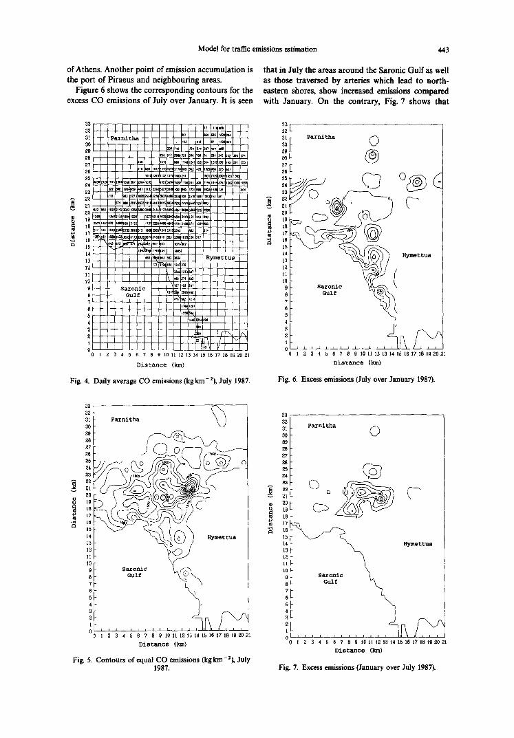
A parametric study of CO emissions for several time periods was carried out using the model de- scribed above. A typical example of results is shown in Fig. 4, in the form of an emission density map. It presents average daily CO emissions (in kgkm -2) during a July 1987 weekday. Figure 5 shows the corresponding contours of CO emissions. An examination of the emission density maps shows that the maximum of emissions occurs in almost all cases (winter or summer, weekday or weekend) in the centre

Table 7. Actual fuel consumption in Greater Athens Area (in metric tons, PERPA, 1990)

Year Regular Premium Total Diesel Auto Diesel

1982 - - - - 608,000 - - 406,000 1986 104,262 578,175 682,437 1,387,074 401,390 1987 94,047 624,474 718,521 1,097,013 329,104 1988 (Jan-Sept) 62,479 513,903 576,382 885,371 265,611

Table 8. Differences between calculated and consumed fuel (in metric tons)

Year Fuel Calculated Consumed Difference

1982 Gasoline 229,220 364,800 135,580 (37.2%)

Diesel 200,750 243,600 42,850 (17.6%)

1986 Gasoline 285,176 409,462 165,715 (30.4%)

Diesel 121,508 240,834 119,326 (49.5%)

1987 Gasoline 338,141 431,113 123,963 (21.6%)

Diesel 154,455 197,462 43,007 (21.8%)

1988 (Jan-Sept) Gasoline 272,967 345,829 97,149 (21.1%)

Diesel 124,944 159,367 34,423 (21.6%)


of Athens. Another point of emission accumulation is the port of Piracus and ncighboudng areas.

Figure 6 shows the corresponding contours for the excess CO emissions of July over January. It is seen

that in July the areas around the Saronic Gulf as well as those traversed by arteries which lead to north- eastern shores, show increased emissions compared with January. On the contrary, Fig. 7 shows that

0 1 2 3 4 5 6 7 8 9 10 11 I2 13 14 15 16 17 18 19 20 21

Distance (km)

33 32 3 t Par ni tha

k_/ 30

g8 g,'/

26

~3

~2 (3

i

0 l 2 3 4 5 B ? 8 g 10 11 12 13 14 15 16 17 18 Ig 20 21

Distance (km)

Fig. 4. Daily average CO emissions (kgkm-2), July 1987. Fig. 6. Excess emissions (July over January 1987).

33 32 31 30 29 28 27 26 25 24 23

20 U 19

17

15 14 13 12 lI lO 9 8 7 6 5 4 3 2 [ g

0 1 2 3 4 5 6 7 8 9 10 11 12 13 14 15 18 17 18 19 20 21

Distance (kin)

Fig. 5. C o n t o u r s o f e q u a l C O e m i s s i o n s ( k g k m - 2 ) , Ju ly 1987.

33 321 31i 3ol 99 28 27 26 25 24i 83 22 21

19 18 17 16 15 14 13 12 l l tO 9 8 7 6 5 4 3 2 ! 0

Parnltha O

~ H F m e t t u s

1 2 3 4 5 6 7 8 9 t0 1I 12 13 14 15 18 17 ]8 19 Z0 21

D i s t a n c e (kin)

Fig. 7. Excess emissions (January over July 1987).

• Po~ddtmm Avenue • P ~ ' ~ 1 (i~d= R~0 [ ] Patission 3 (on the Ring)

Thousand of vehicles per day

4O

35

'i


Jan Feb M~r Apt May Jun Jul Aug Sep Oct Nov Dec

Mordh

Fig. 8. Traffic load variation in three different line-source categories (weekend, 1987).

CO l l ~ n l l 4 ~ (weekday, July 1987)

10 o a - 0.2J

i • a - 0.50 8 o a - 0.75

0

Cell N ~ (2lst line)

Fig. 9. Sensitivity analysis of fuel amount a in Equa- tions (5) and (6).

Table 9. Calculated CO emissions (kgd -1)

Year January July

1982 Typical day: 513,899 1986 372,660 382,998 1987 391,623 406,074 1988 395,597 430,582

emissions in January are highest in the city centre, compared with that of July.

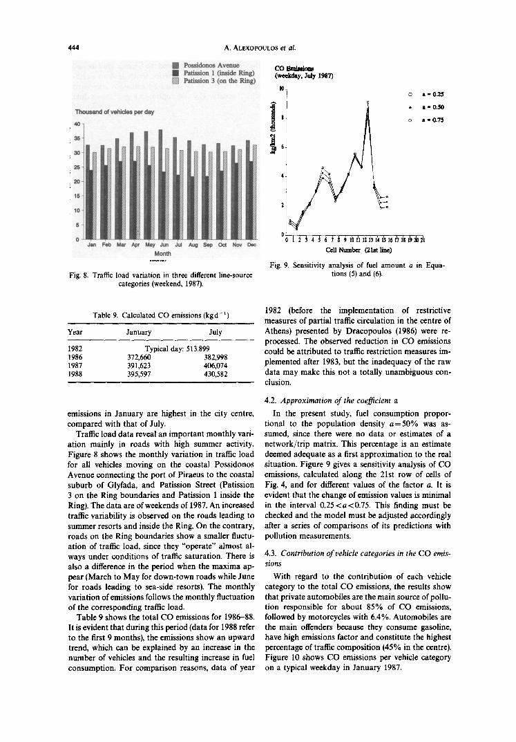
Traffic load data reveal an important monthly variation mainly in roads with high summer activity. Figure 8 shows the monthly variation in traffic load for all vehicles moving on the coastal Possidonos Avenue connecting the port of Piraeus to the coastal suburb of Glyfada, and Patission Street (Patission 3 on the Ring boundaries and Patission 1 inside the Ring). The data are of weekends of 1987. An increased traffic variability is observed on the roads leading to summer resorts and inside the Ring. On the contrary, roads on the Ring boundaries show a smaller fluctuation of traffic load, since they "operate" almost al- ways under conditions of traffic saturation. There is also a difference in the period when the maxima appear (March to May for down-town roads while June for roads leading to sea-side resorts). The monthly variation of emissions follows the monthly fluctuation of the corresponding traffic load.

Table 9 shows the total CO emissions for 1986-88. It is evident that during this period (data for 1988 refer to the first 9 months), the emissions show an upward trend, which can be explained by an increase in the number of vehicles and the resulting increase in fuel consumption. For comparison reasons, data of year

1982 (before the implementation of restrictive measures of partial traffic circulation in the centre of Athens) presented by Dracopoulos (1986) were re- processed. The observed reduction in CO emissions could be attributed to traffic restriction measures implemented after 1983, but the inadequacy of the raw data may make this not a totally unambiguous con- clusion.

4.2. Approximation of the coefficient a

In the present study, fuel consumption proportional to the population density a = 5 0 % was assumed, since there were no data or estimates of a network/trip matrix. This percentage is an estimate deemed adequate as a first approximation to the real situation. Figure 9 gives a sensitivity analysis of CO emissions, calculated along the 21st row of cells of Fig. 4, and for different values of the factor a. It is evident that the change of emission values is minimal in the interval 0.25<a<0.75. This finding must be checked and the model must be adjusted accordingly after a series of comparisons of its predictions with pollution measurements.

4.3. Contribution of vehicle categories in the CO emissions

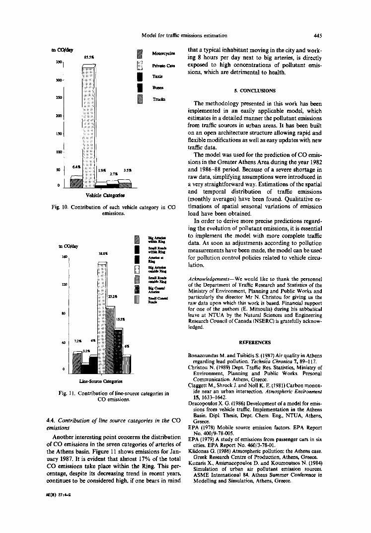
With regard to the contribution of each vehicle category to the total CO emissions, the results show that private automobiles are the main source of pollution responsible for about 85% of CO emissions, followed by motorcycles with 6.4%. Automobiles are the main offenders because they consume gasoline, have high emissions factor and constitute the highest percentage of traffic composition (45% in the centre). Figure 10 shows CO emissions per vehicle category on a typical weekday in January 1987.


m CO/day

3~o

2 5 0 .

200.

150.

I00

6.4.~ JO

oN

8S.5~

:+:+:.:.:,:,:~

i!:~ii!,:~:?ii!i

::!!!>:,i!:!i

::iii,lii~i!i!,!i: ,::!!~!i!?iLi

i!~:]il]::~iii!:i i]!iiii:!i!iill

!i]i:]ii::i]:~: 1.9~ s.ss ii~ii~i~iiiii!i~i~ 2.7~

iiiiiiii!iii i!i i Vehicle CateSories

W Mo~we.lea

Private Cam

I Taxis

Buses

[~ Trucks

Fig. 10. Contribution of each vehicle category in CO emissions.

m COIday 3S.B%

160

. . . . • :.: : : : , , : : : . : . : . . , . .

. . , . . . • :.:.: :

::::::: ::

: i : i : i :

.:: .: .: .:

: : : : : : :5 : .:::::::

~i::ii!!i: ii !i!i:~

4o 7~s e~ :/i::i:::]: ......

: : : : : : 5

80

l l sm,II llm~ A t t m t m a t

,,ease g~

R m ~

Fig. 11. Contribution of line-source categories in CO emissions.

4.4. Contribution of line source categories in the CO emissions

Another interesting point concerns the distribution of CO emissions in the seven categories of arteries of the Athens basin. Figure 11 shows emissions for Jan- uary 1987. It is evident that almost 17% of the total CO emissions take place within the Ring. This percentage, despite its decreasing trend in recent years, continues to be considered high, if one bears in mind

that a typical inhabitant moving in the city and work- ing 8 hours per day next to big arteries, is directly exposed to high concentrations of pollutant emissions, which are detrimental to health.

5. CONCLUSIONS

The methodology presented in this work has been implemented in an easily applicable model, which estimates in a detailed manner the pollutant emissions from traffic sources in urban areas. It has been built on an open architecture structure allowing rapid and flexible modifications as well as easy updates with new traffic data.

The model was used for the prediction of CO emissions in the Greater Athens Area during the year 1982 and 1986-88 period. Because of a severe shortage in raw data, simplifying assumptions were introduced in a very straightforward way. Estimations of the spatial and temporal distribution of traffic emissions (monthly averages) have been found. Qualitative estimations of spatial seasonal variations of emission load have been obtained.

In order to derive more precise predictions regarding the evolution of pollutant emissions, it is essential to implement the model with more complete traffic data. As soon as adjustments according to pollution measurements have been made, the model can be used for pollution control policies related to vehicle circulation.

Acknowledgements--We would like to thank the personnel of the Department of Traffic Research and Statistics of the Ministry of Environment, Planning and Public Works and particularly the director Mr N. Christou for giving us the raw data upon which this work is based. Financial support for one of the authors (E. Mitsoulis) during his sabbatical leave at NTUA by the Natural Sciences and Engineering Research Council of Canada (NSERC) is gratefully acknow- ledged.

REFERENCES

Bonazoundas M. and Tsibidis S. (1987) Air quality in Athens regarding lead pollution. Techni'ca Chronica 7, 89-117.

Christou N. (1989) Dept. Traffic Res. Statistics, Ministry of Environment, Planning and Public Works. Personal Communication. Athens, Greece.

Claggett M., Shrock J. and Nell K. E. (1981) Carbon monox- ide near an urban intersection. Atmospheric Environment 15, 1633-1642.

Dracopoulos X. G. (1986) Development of a model for emissions from vehicle traffic. Implementation in the Athens Basin. Dipl. Thesis, Dept. Chem. Eng., NTUA, Athens, Greece.

EPA (1978) Mobile source emission factors. EPA Report No. 400/9-78-005.

EPA (1979) A study of emissions from passenger cars in six cities. EPA Report No. 460/3-78-01,

Klidonas G. (1986) Atmospheric pollution: the Athens case. Greek Research Centre of Production, Athens, Greece.

Kozaris X., Assimacopoulos D. and Koumoutsos N. (1984) Simulation of urban air pollutant emission sources. ASME International 84. Athens Summer Conference in Modelling and Simulation, Athens, Greece.

.~(0) 27:4-6


Matzoros A. (1990) Results from a model of road traffic air pollution, featuring junction effects and vehicle operating modes. Tra.~c Engineerina and Control. January issue.

Pattas K. N. (1981) Environmental pollution from vehicles. Int. Conf. Environ. Pollution, September, Thessaloniki, Greece.

Pattas K. N. and Kyriakis N. A. (1983) Exhaust car emissions study of current vehicle fleet in Athens, Technical Report to the Ministry of Environment, Planning and Public Works-EEC/DG XI. Thessaloniki.

Pattas K. N., Kyriakis N. A. and Samaras Z. X. (1985a) Emission study of existing vehicle fleet in Athens (Phase lI). Vol. I: Development of the driving model Athens 84. Technical Report to the Ministry of Environment, Plann- ing and Public Works--EEC/DG XI, Thessaloniki, Greece.

Pattas K. N., Kyriakis N. A. and Samaras Z. X. (1985b) Emission study of existing vehicle fleet in Athens (Phase II). Vol. II: Appraisal of total atmospheric pollution from traffic per vehicle category. Technical Report to the Minis- try of Environment, Planning and Public Works-- EEC/DG XI, Thessaloniki, Greece.

Pattas K. N., Kyriakis N. A. and Samaras Z. X. (1985c)

Emission study of existing vehicle fleet in Athens (Phase II). Voi. III: Techniques for pollutants reduction of existing vehicle fleet in Athens (Phase II). Vol. III. Techniques for pollutants reduction of existing vehicle fleet. Technical Report to the Ministry of Environment, Planning and Public Works--EEC/DG XI, Tbessaloniki, Greece.

Pattas K. N., Psoinos P. D. and Samaras Z. X. (1987) Technical and economic study for installing devices to reduce emissions in existing vehicles. Ministry of Environ- ment, Planning and Public Works-EEC, Contract No. 86- B6642-11-011-11-8, Thessaloniki, Greece.

PERPA Annual Report (1990) Air pollution in the Athens area. Ministry of Environment, Planning and Public Works, Direction of Environmental Protection (PERPA), Athens, Greece.

Psaraki-Kalouptsidis P. (1976) A methodology for the determination of non-line/area source emissions from motor vehicles. M.Sc. Thesis, Washington University, Sever In- stitute of Technology, St Louis, Missouri, U.S.A.

Roth P. M. and Roberts, J. W. (1974) A model and inventory of pollutant emissions. Atmospheric Environment 8, 97-130.

Model for Traffic Emissions Estimation

Documents