Model-based diagnosis of continuous static systems

Annals of Mathematics and Artificial Intelligence 11(1994)367-380 367

Model-based diagnosis of continuous static systems

Stefano Cermignani and Giorgio Tornielli Cise SpA, P.O. Box 12081, 1-20134 Milano, Italy

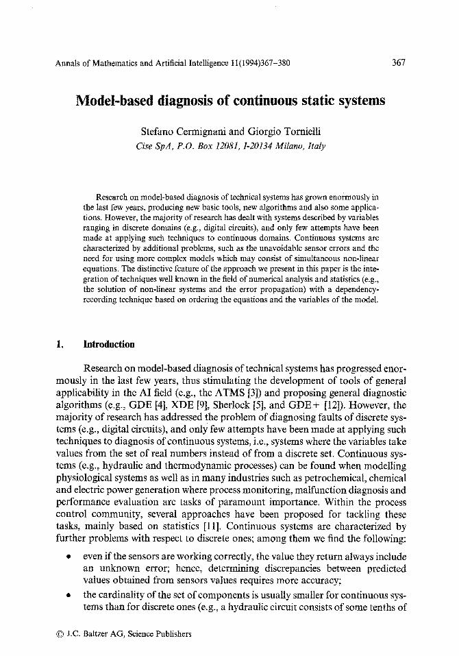
Research on model-based diagnosis of technical systems has grown enormously in the last few years, producing new basic tools, new algorithms and also some applica- tions. However, the majority of research has dealt with systems described by variables ranging in discrete domains (e.g., digital circuits), and only few attempts have been made at applying such techniques to continuous domains. Continuous systems are characterized by additional problems, such as the unavoidable sensor errors and the need for using more complex models which may consist of simultaneous non-linear equations, The distinctive feature of the approach we present in this paper is the integration of techniques well kno~aa in the field of numerical analysis and statistics (e.g., the solution of non-linear systems and the error propagation) with a dependency- recording technique based on ordering the equations and the variables of the model.

1. Introduction

Research on model-based diagnosis of technical systems has progressed enormously in the last few years, thus stimulating the development of tools of general applicability in the AI field (e.g., the ATMS [3]) and proposing general diagnostic algorithms (e.g., GDE [4], XDE [9], Sherlock [5], and GDE+ [12]). However, the majority of research has addressed the problem of diagnosing faults of discrete systems (e.g., digital circuits), and only few attempts have been made at applying such techniques to diagnosis of continuous systems, i.e., systems where the variables take values from the set of real numbers instead of from a discrete set. Continuous systems (e.g., hydraulic and thermodynamic processes) can be found when modelling physiological systems as well as in many industries such as petrochemical, chemical and electric power generation where process monitoring, malfunction diagnosis and performance evaluation are tasks of paramount importance. Within the process control community, several approaches have been proposed for tackling these tasks, mainly based on statistics [11]. Continuous systems are characterized by further problems with respect to discrete ones; among them we find the following:

�9 even if the sensors are working correctly, the value they return always include an unknown error; hence, determining discrepancies between predicted values obtained from sensors values requires more accuracy;

�9 the cardinality of the set of components is usually smaller for continuous systems than for discrete ones (e.g., a hydraulic circuit consists of some tenths of

�9 J.C. Baltzer AG, Science Publishers

368 S. Cermignani, G. Tornielli, Diagnosis of continuous static systems

components against some thousands of components of a digital circuit), but the models of the former are much more complex than the ones of the latter since, often, they consist of simultaneous non-linear equations.

Diagnosis may be interpreted as an iterative process consisting of two steps: generation of a candidate diagnosis (i.e., an assignment of a mode of behaviour, either correct or faulty, to each component and sensor), and its evaluation. Evalua- tion of a candidate is performed by checking whether the logical conjunction of the equational model denoted by the candidate and of the observations is consistent: if this is the case, the candidate is a correct diagnosis. The current most popular model-based diagnostic algorithms, yet aiming at being "general", suffer of some drawbacks when applied to continuous systems. One of the causes is the locality of constraint propagation [13], the mechanism usually adopted for implementing the evaluator, which prevents solution of simultaneous equations (unless the expen- sive symbolic constraint propagation is applied [2]). Finally, these algorithms always assume that the values gathered by the data acquisition system do not include any error.

The candidate evaluator we present in this paper has been designed for cop- ing with the above mentioned difficulties. In particular, for evaluating candidates we adopt well known numerical algorithms (e.g., the Newton-Raphson algorithm), we perform error propagation using techniques based on statistical analysis and, assuming that observations are actually ~ statistical variables of known distribution, we adopt statistical tests for determining discrepancies between different predicted values. These techniques are coupled with a dependency tracing mechanism embedded into the evaluator which allows determining the minimal sets of modes on which a given discrepancy depends on (i.e., conflicts). Conflicts are then used by the candidate generator as a basis for generating new candidates. The dependency mechanism is achieved by arranging the equations of the model into a lattice which represents a partial ordering between the equations and the variables of the model, and exploiting this ordering for determining the sets of conflicting modes.

The aim of this paper is to show how the above mentioned techniques may be combined within the candidate evaluator of a model-based diagnostic system. The paper is organized as follows: section 2 describes the kind of diagnostic problem that we have to solve, section 3 introduces the overall diagnostic system; sections 4-8 are focused on the candidate evaluator and give a thorough description of how the equations are ordered and how this ordering is used for checking whether the observations are consistent with the model and for determining the conflicts. Finally, section 9 discusses on open issues and on future work.

2. Diagnosis of continuous static systems

Processes of industrial interest are dynamic. Their behaviour can be modelled by a set of differential equations relating the rate of change of the state vector to the

S. Cermignani, G. Tornielli, Diagnosis of continuous static systems 369

input vector and to the state vector itself. However, when the system dynamics is fast with respect to the dynamics of the input variables, the system may be approxi- mated by a static model.

In this situation, we assume that the output variables (y) depend, through known physical laws, on a set of proper input variables (u) and on a set of parameters (p) of the process (see fig. 1). The values o f p are defined when the system is designed and should be kept constant in order to maintain the process at the desired state.

Y v

ables arises

Fig. 1.

In the most general case, only some of the input and some of the output vari- are measured and parameters p are not observable. A diagnostic problem when one of the following three situations occurs:

�9 The output changes due to disturbances affecting one or more process parameters without modifying the structure of the process. For instance, pipe crusting changes the load loss factor of a pipe, but the law relating input and output pressures, load loss factor and flow rate remains the same. In this case the diagnosis system has to determine which variations in parameters p may have caused the displacement in the observed output.

�9 The output changes due to abnormal events that change the equational structure of the process, i.e., some of the components behave according to laws different from the expected ones. For instance, the law of a blocked valve is different from the one of a correctly working valve. In this case the diagnostic system has to identify the faulty components as well as the new laws that they exhibit.

�9 One or more sensors are broken and either they do not return any value or the values that they return cannot be trusted in. In this latter case the monitoring system has to detect the broken sensor(s) and their outcome values have to be discarded.

3. The diagnostic process

According to ODS-PI [7], we view the overall diagnostic process as an iterative process consisting of two steps: generation of a candidate diagnosis and its sub-


sequent evaluation (the modules actually composing the diagnostic system are shown in fig. 2).

In the framework of our work, a candidate consists of an assignment of a behavioural mode to each component and to each sensor of the system. For instance, a hydraulic pump may be described in the component library as consisting of two modes of behaviour: the correct behaviour and the faulty behaviour due to blade erosion. In the same way, sensors may be either working correctly, thus the data that they return may be trusted in (even if they are affected by the physiological sensor errorl), or may be broken and either no value is returned or, worse, the value that they return is completely unreliable and has to be discarded.

Comp~en! L~a~

Plant DescriptiOCt

plant Data-Ba~ [

Conflicts

, i .......

Generator Candidate '1 I com~,,.,t / ~~ @ Modes ,~ Status

Model I I Observation L ~176 '

.~ I I i- M' I ...... Se~set~ 1 ode I Observations

Candidate Evaluator

Fig. 2.

Generation of candidate diagnoses may be achieved by exploiting several types of knowledge such as the prior probability of observing a given fault, or experiential knowledge. However, it is important that candidates be conflict free where a conflict is the minimal set of modes which have been used for determining a discrepancy. Con- flicts are incrementally computed by the evaluator, and when they are available, the generator has not to generate candidates including already discovered conflict since this candidate would be surely rejected by the evaluator. A longer discussion of the overall diagnostic process and on the candidate generator is outside the scope of this paper. A discussion on these topics can be found in [5, 6].

In conclusion, the interaction between the generator and the evaluator is as follows: the former feeds the generator with a candidate to be evaluated, and the latter returns to the generator the conflict sets that possibly it has discovered.

x The term physiological sensor error refers to the error due to the normal functioning of the sensor. This kind o f er ror cannot be avoided, but is assumed to be statistically known (i.e., normal ly distributed with zero mean and fixed s tandard deviation).


In order to be used by the evaluator, the candidates proposed by the generator have to be translated into a set of equations and into a set of known values and unknown variables. This is achieved by means of the Model Builder and by the Observation Selector modules. The former translates each component mode into the corresponding set of equations and unknowns (e.g., the correct mode of behaviour of a pipe denotes the equation which relates input and output pressure and flow rate to the load loss factor with a known value for the load loss factor, while the crusting mode denotes the same equation but with an unknown value for the load loss factor). The latter uses the status of each sensor in order to filter the observations: only the ones corresponding to correctly working sensors are used as known values to be given in input to the evaluator.

4. The candidate evaluator

As argued in the introduction, designing an evaluator for continuous systems requires to take into account that their models often consist of non-linear simultaneous equations, and that the values returned by correctly working sensors include an unknown error. Furthermore, the evaluator has to be designed in such a way that the number of known values be not fixed a priori since different candidates may denote different known values. The solution that we propose for these problems is herein described.

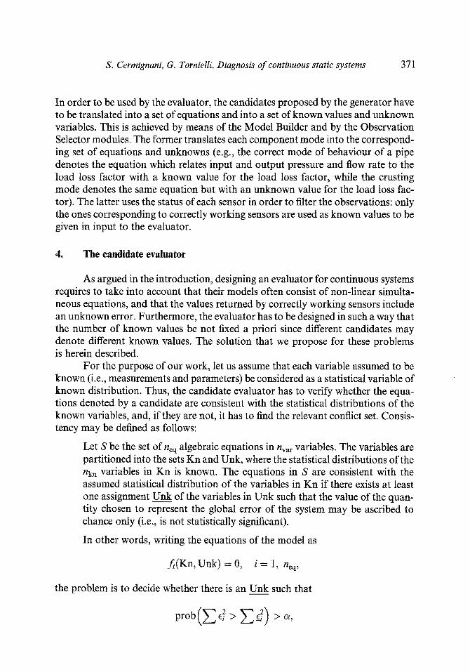
For the purpose of our work, let us assume that each variable assumed to be known (i.e., measurements and parameters) be considered as a statistical variable of known distribution. Thus, the candidate evaluator has to verify whether the equations denoted by a candidate are consistent with the statistical distributions of the known variables, and, if they are not, it has to find the relevant conflict set. Consis- tency may be defined as follows:

Let S be the set of neq algebraic equations in nvar variables. The variables are partitioned into the sets Kn and Unk, where the statistical distributions of the nkn variables in Kn is known. The equations in S are consistent with the assumed statistical distribution of the variables in Kn if there exists at least one assignment Unk of the variables in Unk such that the value of the quantity chosen to represent the global error of the system may be ascribed to chance only (i.e., is not statistically significant).

In other words, writing the equations of the model as

j~(Kn, Unk) = 0, i = 1, neq,

the problem is to decide whether there is an Unk such that

2 Pr~ ~


where ei = J} (Kn, Unk), _el = J} (Kn, Unk), Kn is the expected value of Kn and a is the maximum accepted probability for false positive cases, for instance 5%.

In order to determine whether such a Unk exists, we have devised a procedure consisting of the following main steps:

1. Consider each equation of S as having the variables in Unk only as unknown quantities, while those in Kn are set to their expected values (i.e., the measured values for the observable variables and the design values for the parameters).

2. Determine a subset (WC) of the equations which is well constrained, i.e., which allows the computation of all its unknowns. The cardinality of WC has to be the greatest possible.

3. Arrange the equations in WC according to a partial ordering (see section 4.2). The ordering is exploited for two reasons: firstly, it reduces the complexity of the computation by making easier the convergence of the numerical algorithms, and, secondly, it allows the minimal conflict set to be determined.

4. Highlight the subset (OC) of the remaining equations that contains redun- dant equations only, i.e., equations in which all unknown quantities become known as the equations in WC are solved.

5. Solve the equations in WC with respect to the unknowns exploiting the ordering computed in 3.

6. Estimate the distributions of the computed quantities as functions of the distribution of the variables in Kn.

7. For each equation in OC, verify whether, as the unknown quantities are sub- stituted with their values computed in 5, the outcoming error may be ascribed to chance only.

8. If this is the case, then the system may be considered consistent with the assumed statistical distributions for the variables in Kn.

9. Otherwise, for the first equation in OC that does not verify the test in 7, exploit the ordering defined in 3 for finding the relevant conflict set.

This procedure becomes tractable if some further assumptions about the equations and the statistical properties of the known quantities are considered. Namely, we assume that all the functions associated to the equations are piecewise continuous and provided with left and right partial derivatives with respect to all the variables, at least in the interesting domain. All the errors associated to each known quantity, i.e., the differences between the expected value (which is assumed) and the actual value (which is actually unknown), are supposed to be statistically independent. Each error is also supposed to be distributed according to a Gaussian curve with mean equal to zero and known standard deviation. Finally, each difference is supposed to be small enough to allow the linearization of the equations around the expected values. All these assumptions seem to be acceptable for realistic cases. In the following sections the main steps of this procedure are detailed, using the simplified mixing plant described in section 5.

S. Cermignani, G. Tornielli, Diagnosis o f continuous static systems 373

5. A reference example

Let us consider the physical system shown in fig. 3. This consists of twenty interconnected components belonging to two different classes, namely pumps and pipes. The correct behaviour of each of these components may be expressed as a parameterized relation between input pressure (Pi), output pressure (Po) and flow rate (G) as follows:

Pump: Po - Pi - aG2 - bG - c = O,

Pipe: Pi - Po - rG2 = O,

GI

G2

G3 v

G4 ~ G5 . ~

PrO P f l P12 P13

Fig. 3.

) G8

z ~ > ,,, i--r;-] ~,

where a, b and c are the characteristic parameters of each pump and r is the characteristic parameter of each pipe. In addition, in force of the mass balance princi- ple, an equation is associated to each of the nodes, stating that the sum of the flows entering the node minus the sum of the flows exiting the node equals to zero. In our example the node equations are the following:

Node 1: G1 + G2 + G3 - G4 : 0,

Node 2: G4 -- G5 - G6 = 0,

Node 3 : G 5 + G6 + G7 - G8 : O.

Let us assume that P1, P2,/'3, P7, /9 , Ptl , P12, P15, P16, PI8 and P20 are measured, and let us also assume that we are performing fault detection hence the candidate to evaluate is the one which states that all the components and all the sensors work correctly. In this case the system model consists of 23 equations in 68 variables; the subset Unk consists of 17 variables, since 11 pressures are measured and all the 40 parameters are supposed to be known.

6. How to structure the equations (steps 2-3-4)

The i%q equations of the system S can be partitioned into three disjoint; and possibly empty, subsets:

374 S. Cermignani, G. Tornietli, Diagnosis of continuous static systems

�9 The subset of the Well Constrained (WC) equations, consisting of nwc equations in nwe unknowns. This set has to be chosen with the largest cardinality, i.e., in such a way that there is not another set with the same property and with a larger cardinality. Under the above mentioned assumption about the properties of theJ~'s, the equations in WC admit one and only one solution.

�9 The subset of the Over Constrained (OC) equations, consisting of no~ equations, each of them referring only to some of the unknowns belonging to the set computable by the equations in WC. Each of the equations in OC may be used in order to check whether the assumed statistical distributions of the variables in Kn and the values computed by WC is consistent.

�9 The subset of the Under Constrained (UC) equations, consisting of the remaining ( n ~ - nwc- noc) equations. Our diagnostic algorithm does not use this set, since it is always possible to find out an assignment to all the unknown quantities such that the equations in UC are satisfied.

The procedure for determining these three subsets builds a partial ordering of the equations that can be represented as a directed lattice whose nodes are either computer-nodes o r checker-nodes (see fig. 4). A computer-node is characterized by a set of input variables, a set of output variables and a set of known quantities, while a checker-node has no output variables. All the nodes are connected in such a way that there is a link from a node to another if an output variable of the former is an input variable for the latter. Each computer-node represents a system of equations which allows all the unknowns listed as output variables to be computed, given the input variables and the known quantities. Each checker-node represents exactly one equation in which all the variables are known, assuming known the ones listed as input variables. Thus, the union of all the equations associated to the computer-nodes is the WC subset, the union of all the equations associated to the checker-nodes is the OC subset, and all the remaining equations belong to the UC subset.

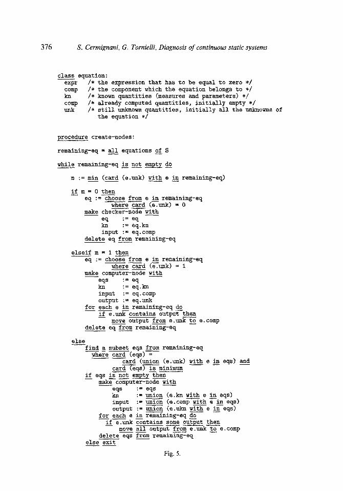
A simplified description of the procedure that creates the nodes is given in fig. 5. The process of linking these nodes is straightforward and, then, it is not described. Let us note this procedure above described is strongly related to the Iwasaki and

class computer-node: eqs /* list of equations */ kn /* known quantities (measures and parameters) */ input /* already computed quantities needed as input */ output /* quantities computed by this node */

class checker-node: eq /* equation */ kn /* known quantities (measures and parameters) */ input /* already computed quantities needed as input */

Fig. 4.

S. Cermignani, G. Tornielli, Diagnosis of continuous static s~,stems 375

Simon's procedure for computing a causal ordering among the variables of a well- constrained set of equations [10]. In fact, our procedure, when supplied with a well- constrained set S of equations, exactly produces Iwasaki and Simon's causal ordering; however, in our case, we are able to compute a partial ordering even if S is not welt-constrained.

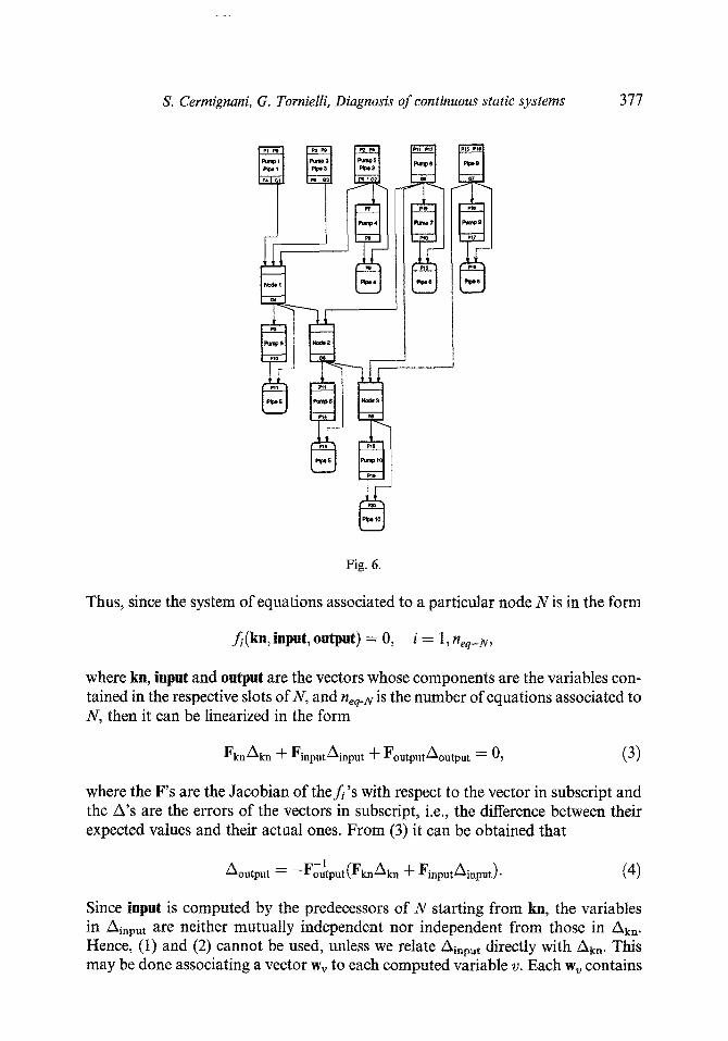
The output of our procedure applied to the mixing plant is shown in fig. 6. In this picture, ehecker-nodez are drawn as rounded corner rectangles, while computer-nodes as squared corner rectangles. In the upper side of each node are shown the measured variables of the components associated to that node, in the lower side the output variables and, since in our example there is a one to one relationship between components and equations, the nodes are labelled with the component names only. Furthermore, the parameters associated to each node are unambiguously denoted by the component names and thus are not explicitly shown.

7. How to solve the structured system (steps 5-6)

The ordering determined in the previous steps of the procedure may now be exploited for computing the expected values of all the computable variables and for estimating the variance of their associated en'ors. The problem described in this section deals with the processing of the computer-nodes of the lattice. The sequence according to which they are processed is given by the ordering fixed by the lattice. In other words, a particular node may be processed only after that each of its predecessors have been processed too.

The expected value of the unknowns listed in the output slot of a node may be computed by solving the equations associated to it by means of a numerical algorithm, such as the Newton-Raphson method. 2

The variance of the errors may be obtained starting from the variances of the errors associated to the input variables and of the errors associated to the known quantities in Kn. This is easy to be performed if all the errors associated to the variables in Kn are supposed to be normally distributed, and to be small enough to allow the linearization of the system around their expected values. In fact, it is well known that if vi are n statistical variables normally distributed and mutually independent with means #i and variances ~ , then also the statistical variable

V = Z Wi'Oi~ i = 1, n,

is normally distributed with mean # and variance a 2 given by

# = i = 1,n (I)

2 "~ ~2 = Z . w i ~ , i = 1,n. (2)

2 The choice of the particular algorithm may be decided at run-time, possibly using information about the symbolic nature of the equations. However, this issue is outside of the scope of this paper.


class equation: expr /* the expression that has to be equal to zero */ comp /* the component which the equation belongs to */ kn / * known quantities (measures and parameters) * / comp /* already computed quantities, initially empty */ unk /* still unknown quantities, initially all the unknowns of

the equation */

procedure create-nodes :

remaining-eq = all equations of S

while remaining-eq is not empty do

m := min (card (e.unk) with e in remaining-eq)

if m = 0 then eq := choose from e in remaining-eq

where card (e.Lmk) = 0 make checker-node with

eq : = eq kn := eq.kn input := eq.comp

delete eq fro m remaining-eq

elseif m = I then eq := choose from e in remaining-eq

where card (~.unk) = 1 make computer-node wit___hh

eqs := eq kn := eq.kn input : = eq. comp output : = eq.unk

for each e in remaining-eq d_~o if e.unk contains output then

move output from e.unk to e.comp delete eq from remaining-eq

else find a subset eqs from remaining-eq

where card (eqs) = card (union (e.ttnk) with e in eqs) and

card (eqs) is minimt~ i_ff eqs is not empty then

make computer-node wit__~h eqs := eqs kn := union (e.kn with e in eqs) input := union (e.comp with e in eqs) output := union (e,ukn with e in eqs)

for each e in remaining-eq do i_ff e.unk contains some output then

move all output from e.unk to e.comp delete eqs from remaining-eq

else exit

Fig. 5.


Fig. 6.

Thus, since the system of equations associated to a particular node N is in the form

f (kn , input, output) = 0, i = 1, neq_N,

where kn, input and output are the vectors whose components are the variables contained in the respective slots of N, and neq-N is the number of equations associated to N, then it can be linearized in the form

FknAkn q- FinputAinput -]- FoutputAoutput = 0, (3)

where the F's are the Jacobian of thef. 's with respect to the vector in subscript and the A's are the errors of the vectors in subscript, i.e., the difference between their expected values and their actual ones. From (3) it can be obtained that

- -Foutput(FknAkn + FinputAinput). (4) Aoutpu t _ -I

Since input is computed by the predecessors of N starting from ku, the variables in Ainpu t a re neither mutually independent nor independent from those in Akn. Hence, (t) and (2) cannot be used, unless we relate Ainpu t directly with Akn. This may be done associating a vector wv to each computed variable v. Each wv contains


nkn components, representing the value of the partial derivatives of v with respect to every variable in Kn. These derivatives are evaluated in the point corresponding to the expected values of each variable, In order to obtain the w,v's for the variables computed by the node N, from the wv's for the variables computed by its predecessors, it is sufficient to substitute

in (4), obtaining

Ainpu t = Winput~kn (5)

= -Foutput(Fkn + FinputWinput)Akn, Aoutpu t -1

where Winput is defined as the matrix built putting the wv associated to each input in each row. Hence, Woutput (defined analogously to Winput) is given by

Woutput = -Foultput(Fkn -+- FinputWinput).

Since Aoutput is represented now as linear combination of the independent variables in Akn, the best estimate of the variance of the output errors is given by applying (2)

2 2 2 O'output ----- WoutputO-kn ,

where W2output is the matrix obtained from Woutput, squaring each of its element. However, as it will be clear in the next section, only the w,'s associated to the output variables are actually computed. Indeed this is the only information needed for detecting discrepancies in the checker-nodes.

8. How to detect an inconsistency and the relative conflict set (steps 7 -8 -9 )

As already described, a checker-node N denotes an equation of the following form:

f(kn, input) = O,

where kn and input are the vectors whose components are the variables contained in the respective Slots of N. Evaluating the function f in the point denoted by the expected values of kn and input, an error e is obtained. Using the previous assumptions about the errors in Kn, e can be expressed as follows:

c = FknAkn + VinputAinpu t : 0, (6)

where the F's and the A's are defined as above. Substituting (5) in (6), it is possible to express e as a linear combination of Akn,

E : (Fkn + FinputWinput)Akn : 0.


Hence, defining

W e = Fkn q- FinputWinput,

the best estimate of the variance of e is given by 2 2 2

(re : WE ffkn

where W~ is the matrix obtained from W,, squaring each of its element. At this point, in order to decide whether the obtained value of e is consistent

with the assumption that it should be equal to zero, it is sufficient to compare the ratio between e and cr~ with the characteristic values of a normalized gaussian distribution. For instance, if the maximum accepted probability for false negative cases is 0.05, then the absolute value of this ratio must be less than 1.96.

When a discrepancy is discovered by a given checker-node, the set of components involved in the determination of the discrepancy (i.e., the conflict set) have to be collected 3. This is achieved by traversing the lattice starting from the checker- node which discovers the discrepancy, back to the root nodes: all the components associated to the computer-nodes found along the path are included in the conflict. Thus, if the checker-node of fig. 6 labelled with component pJ.pe8 discovers a discrepancy, then at least one component among p• p• and pump9 is faulty or one measure among P15, P16 and P18 is incorrect.

9. Conclusions and future work

The distinctive feature of the approach to diagnosis we have presented in this paper is the integration of techniques well known in the field of numerical analysis and statistics (e.g., the solution of non-linear systems and the error propagation) with dependency-recording. The latter is a powerful technique adopted by model- based diagnostic algorithms for determining the sources of the observed symp- toms, only exploiting the model of the physical system to be diagnosed. The need for this integration arises from the difficulty experimented when applying the most popular model-based diagnostic algorithms (e.g., GDE) to the application domains in which we are interested in, namely, hydraulics and thermodynamics.

The approach that we have proposed for evaluating candidate diagnoses consists in determining a partial ordering of the equations of the system model and in exploiting it in order to verify the consistency of a fault hypothesis. If the latter is not consistent, then the ordering can be used to determine the possible sources of the inconsistency.

This approach may be easily implemented if some simplifying assumptions may be made which seem realistic for practical cases.

Future work will consist in applying this algorithm to real size industrial cases. We expect that this activity will better evidence possible limitations of the

3 Actually, a conflict is defined as a set of component modes, but here we can unambiguously talk of components since in a candidate each component is associated with one and only one mode.


design and possible areas of improvement. However, we believe that such improve- ments will be mainly concerned with optimization of the computation of the partial ordering when the system of equations is over-constrained and with the choice of the best algorithm for solving a given set of numerical equations.

Acknowledgements

The work described in this paper has been undertaken in Esprit Project ARTIST (P5143) by the following partners: Cise, Cepsa, Delphi, Heriot-Watt Uni- versity, Labein and Siemens. The authors wish to acknowledge the contribution of all members of the project team whilst taking full responsibility for the views expressed in this paper. The work is partly supported by the C.E.C. under the ESPRIT programme and by the Automatica Research Center (CRA) of the Italian Electricity Board (ENEL).

References

[1] R. Davis, Diagnostic reasoning based on structure and behaviour, Artificial Intelligence 24 (1984) 347-410.

[2] J. de Kleer and G.J. Sussman, Propagation of constraints applied to circuit synthesis, Circuit Theor. Appl. 8 (1980) 127-144.

[3] J. de Kleer, An assumption-based truth maintenance system, Artificial Intelligence 28 (1986) 127-162.

[4] J. de Kleer and B.C. Williams, Diagnosing multiple faults, Artificial Intelligence 32 (1987) 97- 130.

[5] J. de Kleer and B.C. Williams, Diagnosis with behavioral modes, in: Proc. 11th Int. Conf. on Arti- ficial Intelligence, 1989, pp. 1324-1330.

[6] J. de Kleer and B.C. Williams, Focusing the diagnosis engine, in: Proc. 1st Int. Workshop on Prin- ciples of Diagnosis, Stanford, CA, 1990.

[7] M. Gallanti, M. Roncato, A. Stefanini and G. Tornielli, A diagnostic algorithm based on models at different levels of abstraction, in: Proc. 11th Int. Conf. on Artificiatlntelligence, 1989, pp. 1350- 1355.

[8] B.J. Glass and C.M. Wong, A knowledge-based approach to identification and adaptation in dynamic systems control, in: Proc. 27th IEEE Conf. on Decision and Control, Austin, TX, 1988, pp. 881-886.

[9] W.C. Hamscher, Model-based troubleshooting of digital systems, Technical Report 1074, MIT Artificial InteUigence Lab. (August 1988).

[10] Y. Iwasaki and H.A. Simon, Causality in device behaviour, Artificial Intelligence 29 (1986) 3-32. [11] S. Narasimhan and R.S.H. Mall, Generalized likelihood ratio method for gross error identifica-

tion, AIChE J. 33 (1987) 1514-1521. [12] P. Struss and O. Dressier, Physical negation - Integrating fault models into the General Diagnos-

tic Engine, in: Proc. 11th Int. Conf. on Artificial Intelligence, 1989, pp. 1318-1323. [13] G.J. Sussman and G.L. Steele, CONSTRAINTS - A language for expressing almost-hierarchical

descriptions, Artificial Intelligence 14(1) (1980).

Model-based diagnosis of continuous static systems

Documents