Mobile fading channels modelling, analysis & simulation,( patzold 2002)
Aug 15, 2015
Welcome message from author
This document is posted to help you gain knowledge. Please leave a comment to let me know what you think about it! Share it to your friends and learn new things together.
Transcript


MOBILE FADING CHANNELS


MOBILE FADING CHANNELS Matthias Pätzold Professor of Mobile Communications Agder University College, Grimstad, Norway

Originally published in the German language by Friedr. Vieweg & Sohn Verlagsgesellschaft mbH, D-65189 Wiesbaden, Germany, under the title “Matthias Pätzold: Mobilfunkkanäle. 1. Auflage (1st Edition)”. Copyright © Friedr. Vieweg & Sohn Verlagsgesellschaft mbH, Braunschweig/Wiesbaden, 1999. Copyright © 2002 by John Wiley & Sons, Ltd Baffins Lane, Chichester, West Sussex, PO19 1UD, England National 01243 779777 International (+44) 1243 779777 e-mail (for orders and customer service enquiries): [email protected] Visit our Home Page on http://www.wiley.co.uk or http://www.wiley.com All Rights Reserved. No part of this publication may be reproduced, stored in a retrieval system, or transmitted, in any form or by any means, electronic, mechanical, photocopying, recording, scanning or otherwise, except under the terms of the Copyright Designs and Patents Act 1988 or under the terms of a licence issued by the Copyright Licensing Agency, 90 Tottenham Court Road, London, W1P 9HE, UK, without the permission in writing of the Publisher, with the exception of any material supplied specifically for the purpose of being entered and executed on a computer system, for exclusive use by the purchaser of the publication. Neither the author(s) nor John Wiley & Sons, Ltd accept any responsibility or liability for loss or damage occasioned to any person or property through using the material, instructions, methods or ideas contained herein, or acting or refraining from acting as a result of such use. The author(s) and Publisher expressly disclaim all implied warranties, including merchantability of fitness for any particular purpose. Designations used by companies to distinguish their products are often claimed as trademarks. In all instances where John Wiley & Sons, Ltd is aware of a claim, the product names appear in initial capital or capital letters. Readers, however, should contact the appropriate companies for more complete information regarding trademarks and registration. Other Wiley Editorial Offices John Wiley & Sons, Inc., 605 Third Avenue, New York, NY 10158-0012, USA WILEY-VCH Verlag GmbH Pappelallee 3, D-69469 Weinheim, Germany John Wiley & Sons Australia Ltd, 33 Park Road, Milton, Queensland 4064, Australia John Wiley & Sons (Canada) Ltd, 22 Worcester Road Rexdale, Ontario, M9W 1L1, Canada John Wiley & Sons (Asia) Pte Ltd, 2 Clementi Loop #02-01, Jin Xing Distripark, Singapore 129809 A catalogue record for this book is available from the British Library ISBN 0471 49549 2 Produced from PostScript files supplied by the author. Printed and bound in Great Britain by Biddles Ltd, Guildford and King’s Lynn. This book is printed on acid-free paper responsibly manufactured from sustainable forestry, in which at least two trees are planted for each one used for paper production.

V
Preface
This book results from my teaching and research activities at the Technical Uni-versity of Hamburg-Harburg (TUHH), Germany. It is based on my German book“Mobilfunkkanale — Modellierung, Analyse und Simulation” published by Vieweg &Sohn, Braunschweig/Wiesbaden, Germany, in 1999. The German version served as atext for the lecture Modern Methods for Modelling of Networks, which I gave at theTUHH from 1996 to 2000 for students in electrical engineering at masters level.
The book mainly is addressed to engineers, computer scientists, and physicists, whowork in the industry or in research institutes in the wireless communications field andtherefore have a professional interest in subjects dealing with mobile fading channels.In addition to that, it is also suitable for scientists working on present problems ofstochastic and deterministic channel modelling. Last, but not least, this book also isaddressed to master students of electrical engineering who are specialising in mobileradio communications.
In order to be able to study this book, basic knowledge of probability theory andsystem theory is required, with which students at masters level are in generalfamiliar. In order to simplify comprehension, the fundamental mathematical tools,which are relevant for the objectives of this book, are recapitulated at the beginning.Starting from this basic knowledge, nearly all statements made in this book arederived in detail, so that a high grade of mathematical unity is achieved. Thanksto sufficient advice and help, it is guaranteed that the interested reader can verifythe results with reasonable effort. Longer derivations interrupting the flow of thecontent are found in the Appendices. There, the reader can also find a selectionof MATLAB-programs, which should give practical help in the application of themethods described in the book. To illustrate the results, a large number of figureshave been included, whose meanings are explained in the text. Use of abbreviationshas generally been avoided, which in my experience simplifies the readability consid-erably. Furthermore, a large number of references is provided, so that the reader is ledto further sources of the almost inexhaustible topic of mobile fading channel modelling.
My aim was to introduce the reader to the fundamentals of modelling, analysis,and simulation of mobile fading channels. One of the main focuses of this book isthe treatment of deterministic processes. They form the basis for the developmentof efficient channel simulators. For the design of deterministic processes with givencorrelation properties, nearly all the methods known in the literature up to noware introduced, analysed, and assessed on their performance in this book. Furtherfocus is put on the derivation and analysis of stochastic channel models as wellas on the development of highly precise channel simulators for various classes offrequency-selective and frequency-nonselective mobile radio channels. Moreover, aprimary topic is the fitting of the statistical properties of the designed channel models
VI
to the statistics of real-world channels.
At this point, I would like to thank those people, without whose help this bookwould never have been published in its present form. First, I would like to expressmy warmest thanks to Stephan Kraus and Can Karadogan, who assisted me withthe English translation considerably. I would especially like to thank Frank Laue forperforming the computer experiments in the book and for making the graphical plots,which decisively improved the vividness and simplified the comprehension of the text.Sincerely, I would like to thank Alberto Dıaz Guerrero and Qi Yao for reviewing mostparts of the manuscript and for giving me numerous suggestions that have helped meto shape the book into its present form. Finally, I am also grateful to Mark Hammondand Sarah Hinton my editors at John Wiley & Sons, Ltd.
Matthias Patzold
GrimstadJanuary 2002
VII
Contents
1 INTRODUCTION . . . . . . . . . . . . . . . . . . . . . . . . . . . . . . . 11.1 THE EVOLUTION OF MOBILE RADIO SYSTEMS . . . . . . . . . 11.2 BASIC KNOWLEDGE OF MOBILE RADIO CHANNELS . . . . . . 31.3 STRUCTURE OF THIS BOOK . . . . . . . . . . . . . . . . . . . . . 7
2 RANDOM VARIABLES, STOCHASTIC PROCESSES, ANDDETERMINISTIC SIGNALS . . . . . . . . . . . . . . . . . . . . . . . 112.1 RANDOM VARIABLES . . . . . . . . . . . . . . . . . . . . . . . . . . 11
2.1.1 Important Probability Density Functions . . . . . . . . . . . . 152.1.2 Functions of Random Variables . . . . . . . . . . . . . . . . . . 19
2.2 STOCHASTIC PROCESSES . . . . . . . . . . . . . . . . . . . . . . . 202.2.1 Stationary Processes . . . . . . . . . . . . . . . . . . . . . . . . 222.2.2 Ergodic Processes . . . . . . . . . . . . . . . . . . . . . . . . . 252.2.3 Level-Crossing Rate and Average Duration of Fades . . . . . . 25
2.3 DETERMINISTIC CONTINUOUS-TIME SIGNALS . . . . . . . . . . 272.4 DETERMINISTIC DISCRETE-TIME SIGNALS . . . . . . . . . . . . 29
3 RAYLEIGH AND RICE PROCESSES AS REFERENCE MODELS 333.1 GENERAL DESCRIPTION OF RICE AND RAYLEIGH PROCESSES 343.2 ELEMENTARY PROPERTIES OF RICE AND RAYLEIGH PRO-
CESSES . . . . . . . . . . . . . . . . . . . . . . . . . . . . . . . . . . . 353.3 STATISTICAL PROPERTIES OF RICE AND RAYLEIGH PRO-
CESSES . . . . . . . . . . . . . . . . . . . . . . . . . . . . . . . . . . . 393.3.1 Probability Density Function of the Amplitude and the Phase . 393.3.2 Level-Crossing Rate and Average Duration of Fades . . . . . . 413.3.3 The Statistics of the Fading Intervals of Rayleigh Processes . . 46
4 INTRODUCTION TO THE THEORY OF DETERMINISTICPROCESSES . . . . . . . . . . . . . . . . . . . . . . . . . . . . . . . . . . 554.1 PRINCIPLE OF DETERMINISTIC CHANNEL MODELLING . . . . 564.2 ELEMENTARY PROPERTIES OF DETERMINISTIC PROCESSES 594.3 STATISTICAL PROPERTIES OF DETERMINISTIC PROCESSES . 63
4.3.1 Probability Density Function of the Amplitude and the Phase . 644.3.2 Level-Crossing Rate and Average Duration of Fades . . . . . . 724.3.3 Statistics of the Fading Intervals at Low Levels . . . . . . . . . 77
VIII Contents
4.3.4 Ergodicity and Criteria for the Performance Evaluation . . . . 78
5 METHODS FOR THE COMPUTATION OF THE MODELPARAMETERS OF DETERMINISTIC PROCESSES . . . . . . . . 815.1 METHODS FOR THE COMPUTATION OF THE DISCRETE
DOPPLER FREQUENCIES AND DOPPLER COEFFICIENTS . . . 835.1.1 Method of Equal Distances (MED) . . . . . . . . . . . . . . . . 835.1.2 Mean-Square-Error Method (MSEM) . . . . . . . . . . . . . . . 905.1.3 Method of Equal Areas (MEA) . . . . . . . . . . . . . . . . . . 955.1.4 Monte Carlo Method (MCM) . . . . . . . . . . . . . . . . . . . 1045.1.5 Lp-Norm Method (LPNM) . . . . . . . . . . . . . . . . . . . . 1135.1.6 Method of Exact Doppler Spread (MEDS) . . . . . . . . . . . . 1285.1.7 Jakes Method (JM) . . . . . . . . . . . . . . . . . . . . . . . . 133
5.2 METHODS FOR THE COMPUTATION OF THE DOPPLER PHASES1435.3 FADING INTERVALS OF DETERMINISTIC RAYLEIGH PROCESSES145
6 FREQUENCY-NONSELECTIVE STOCHASTIC AND DETER-MINISTIC CHANNEL MODELS . . . . . . . . . . . . . . . . . . . . . 1556.1 THE EXTENDED SUZUKI PROCESS OF TYPE I . . . . . . . . . . 157
6.1.1 Modelling and Analysis of the Short-Term Fading . . . . . . . 1576.1.1.1 Probability Density Function of the Amplitude and the
Phase . . . . . . . . . . . . . . . . . . . . . . . . . . . 1656.1.1.2 Level-Crossing Rate and Average Duration of Fades . 166
6.1.2 Modelling and Analysis of the Long-Term Fading . . . . . . . . 1696.1.3 The Stochastic Extended Suzuki Process of Type I . . . . . . . 1726.1.4 The Deterministic Extended Suzuki Process of Type I . . . . . 1766.1.5 Applications and Simulation Results . . . . . . . . . . . . . . . 181
6.2 THE EXTENDED SUZUKI PROCESS OF TYPE II . . . . . . . . . 1856.2.1 Modelling and Analysis of the Short-Term Fading . . . . . . . 186
6.2.1.1 Probability Density Function of the Amplitude and thePhase . . . . . . . . . . . . . . . . . . . . . . . . . . . 190
6.2.1.2 Level-Crossing Rate and Average Duration of Fades . 1936.2.2 The Stochastic Extended Suzuki Process of Type II . . . . . . 1966.2.3 The Deterministic Extended Suzuki Process of Type II . . . . . 2006.2.4 Applications and Simulation Results . . . . . . . . . . . . . . . 205
6.3 THE GENERALIZED RICE PROCESS . . . . . . . . . . . . . . . . . 2086.3.1 The Stochastic Generalized Rice Process . . . . . . . . . . . . . 2096.3.2 The Deterministic Generalized Rice Process . . . . . . . . . . . 2136.3.3 Applications and Simulation Results . . . . . . . . . . . . . . . 217
6.4 THE MODIFIED LOO MODEL . . . . . . . . . . . . . . . . . . . . . 2186.4.1 The Stochastic Modified Loo Model . . . . . . . . . . . . . . . 218
6.4.1.1 Autocorrelation Function and Doppler Power SpectralDensity . . . . . . . . . . . . . . . . . . . . . . . . . . 222
6.4.1.2 Probability Density Function of the Amplitude and thePhase . . . . . . . . . . . . . . . . . . . . . . . . . . . 225
6.4.1.3 Level-Crossing Rate and Average Duration of Fades . 2286.4.2 The Deterministic Modified Loo Model . . . . . . . . . . . . . 230
Contents IX
6.4.3 Applications and Simulation Results . . . . . . . . . . . . . . . 236
7 FREQUENCY-SELECTIVE STOCHASTIC AND DETERMIN-ISTIC CHANNEL MODELS . . . . . . . . . . . . . . . . . . . . . . . . 2417.1 THE ELLIPSES MODEL OF PARSONS AND BAJWA . . . . . . . . 2447.2 SYSTEM THEORETICAL DESCRIPTION OF FREQUENCY-
SELECTIVE CHANNELS . . . . . . . . . . . . . . . . . . . . . . . . . 2457.3 FREQUENCY-SELECTIVE STOCHASTIC CHANNEL MODELS . . 250
7.3.1 Correlation Functions . . . . . . . . . . . . . . . . . . . . . . . 2507.3.2 The WSSUS Model According to Bello . . . . . . . . . . . . . . 251
7.3.2.1 WSS Models . . . . . . . . . . . . . . . . . . . . . . . 2517.3.2.2 US Models . . . . . . . . . . . . . . . . . . . . . . . . 2537.3.2.3 WSSUS Models . . . . . . . . . . . . . . . . . . . . . 253
7.3.3 The Channel Models According to COST 207 . . . . . . . . . . 2597.4 FREQUENCY-SELECTIVE DETERMINISTIC CHANNEL MODELS 267
7.4.1 System Functions of Frequency-Selective Deterministic ChannelModels . . . . . . . . . . . . . . . . . . . . . . . . . . . . . . . 267
7.4.2 Correlation Functions and Power Spectral Densities of DGUSModels . . . . . . . . . . . . . . . . . . . . . . . . . . . . . . . 272
7.4.3 Delay Power Spectral Density, Doppler Power Spectral Density,and Characteristic Quantities of DGUS Models . . . . . . . . . 276
7.4.4 Determination of the Model Parameters of DGUS Models . . . 2817.4.4.1 Determination of the discrete propagation delays and
delay coefficients . . . . . . . . . . . . . . . . . . . . . 2817.4.4.2 Determination of the discrete Doppler frequencies and
Doppler coefficients . . . . . . . . . . . . . . . . . . . 2837.4.4.3 Determination of the Doppler phases . . . . . . . . . 284
7.4.5 Deterministic Simulation Models for the Channel ModelsAccording to COST 207 . . . . . . . . . . . . . . . . . . . . . . 284
8 FAST CHANNEL SIMULATORS . . . . . . . . . . . . . . . . . . . . . 2898.1 DISCRETE DETERMINISTIC PROCESSES . . . . . . . . . . . . . . 2908.2 REALIZATION OF DISCRETE DETERMINISTIC PROCESSES . . 292
8.2.1 Tables System . . . . . . . . . . . . . . . . . . . . . . . . . . . 2928.2.2 Matrix System . . . . . . . . . . . . . . . . . . . . . . . . . . . 2958.2.3 Shift Register System . . . . . . . . . . . . . . . . . . . . . . . 297
8.3 PROPERTIES OF DISCRETE DETERMINISTIC PROCESSES . . . 2978.3.1 Elementary Properties of Discrete Deterministic Processes . . . 2988.3.2 Statistical Properties of Discrete Deterministic Processes . . . 305
8.3.2.1 Probability Density Function and Cumulative Distri-bution Function of the Amplitude and the Phase . . . 306
8.3.2.2 Level-Crossing Rate and Average Duration of Fades . 3138.4 REALIZATION EXPENDITURE AND SIMULATION SPEED . . . . 3158.5 COMPARISON WITH THE FILTER METHOD . . . . . . . . . . . . 317
X Contents
Appendix A DERIVATION OF THE JAKES POWER SPECTRALDENSITY AND THE CORRESPONDING AUTOCORRELA-TION FUNCTION . . . . . . . . . . . . . . . . . . . . . . . . . . . . . . 321
Appendix B DERIVATION OF THE LEVEL-CROSSING RATE OFRICE PROCESSES WITH DIFFERENT SPECTRAL SHAPESOF THE UNDERLYING GAUSSIAN RANDOM PROCESSES . 325
Appendix C DERIVATION OF THE EXACT SOLUTION OF THELEVEL-CROSSING RATE AND THE AVERAGE DURATIONOF FADES OF DETERMINISTIC RICE PROCESSES . . . . . . . 329
Appendix D ANALYSIS OF THE RELATIVE MODEL ERROR BYUSING THE MONTE CARLO METHOD IN CONNECTIONWITH THE JAKES POWER SPECTRAL DENSITY . . . . . . . 341
Appendix E SPECIFICATION OF FURTHER L-PATH CHANNELMODELS ACCORDING TO COST 207 . . . . . . . . . . . . . . . . . 343
MATLAB-PROGRAMS . . . . . . . . . . . . . . . . . . . . . . . . . . . . . 347
ABBREVIATIONS . . . . . . . . . . . . . . . . . . . . . . . . . . . . . . . . 377
SYMBOLS . . . . . . . . . . . . . . . . . . . . . . . . . . . . . . . . . . . . . 379
BIBLIOGRAPHY . . . . . . . . . . . . . . . . . . . . . . . . . . . . . . . . . 391
INDEX . . . . . . . . . . . . . . . . . . . . . . . . . . . . . . . . . . . . . . . . 409

1
INTRODUCTION
1.1 THE EVOLUTION OF MOBILE RADIO SYSTEMS
For several years, the mobile communications sector has definitely been the fastest-growing market segment in telecommunications. Experts agree that today we arejust at the beginning of a global development, which will increase considerablyduring the next years. Trying to find the factors responsible for this development,one immediately discovers a broad range of reasons. Certainly, the liberalizationof the telecommunication services, the opening and deregulation of the Europeanmarkets, the topping of frequency ranges around and over 1GHz, improved modu-lation and coding techniques, as well as impressive progress in the semiconductortechnology (e.g., large-scale integrated CMOS- and GaAs-technology), and, last butnot least, a better knowledge of the propagation processes of electromagnetic wavesin an extraordinary complex environment have made their contribution to this success.
The beginning of this turbulent development now can be traced to more than 40years ago. The first generation mobile radio systems developed at that time wereentirely based on analog technique. They were strictly limited in their capacity ofsubscribers and their accessibility. The first mobile radio network in Germany was inservice between 1958 and 1977. It was randomly named A-net and was still based onmanual switching. Direct dialling was at first possible with the B-net, introduced in1972. Nevertheless, the calling party had to know where the called party was locatedand, moreover, the capacity limit of 27 000 subscribers was reached fairly quickly. TheB-net was taken out of service on the 31st of December 1994. Automatic localizationof the mobile subscriber and passing on to the next cell was at first possible with thecellular C-net introduced in 1986. It operates at a frequency range of 450MHz andhas a Germany-wide accessibility with a capacity of 750 000 subscribers.
Second generation mobile radio systems are characterized by digitalization of thenetworks. The GSM standard (GSM: Groupe Special Mobile)1 developed in Europeis generally accepted as the most elaborated standard worldwide. The D-net, broughtinto service in 1992, is based on the GSM standard. It operates at a frequency rangeof 900MHz and offers all subscribers a Europe-wide coverage. In addition to this,the E-net (Digital Cellular System, DCS 1800) has been running parallel to the
1 By now GSM stands for “Global System for Mobile Communications”.

2 INTRODUCTION
D-net since 1994, operating at a frequency range of 1800 MHz. Mainly, these twonetworks only differ in their respective frequency range. In Great Britain, however,the DCS 1800 is known as PCN (Personal Communications Network). Estimates saythe amount of subscribers using mobile telephones will in Europe alone grow from 92million at present to 215 million at the end of 2005. In consequence, it is expectedthat in Europe the number of employees in this branch will grow from 115 000 atpresent to 1.89 million (source of information: Lehman Brothers Telecom Researchestimates). The originally European GSM standard has in the meantime becomea worldwide mobile communication standard that has been accepted by 129 (110)countries at the end of 1998 (1997). The network operators altogether ran 256 GSMnetworks with over 70.3 million subscribers at the end of 1997 worldwide. But onlyone year later (at the end of 1998), the amount of GSM networks had increased to324 with 135 million subscribers. In addition to the GSM standard, a new standardfor cordless telephones, the DECT standard (DECT: Digital European CordlessTelephone), was introduced by the European Telecommunications Standard Institute(ETSI). The DECT standard allows subscribers moving at a fair pace to use cordlesstelephones at a maximum range of about 300 m.
In Europe, third generation mobile radio systems is expected to be practically readyfor use at the beginning of the twenty-first century with the introduction of theUniversal Mobile Telecommunications System (UMTS) and the Mobile BroadbandSystem (MBS). With UMTS, in Europe one is aiming at integrating the variousservices offered by second generation mobile radio systems into one universal system[Nie92]. An individual subscriber can then be called at any time, from any place(car, train, aircraft, etc.) and will be able to use all services via a universal terminal.With the same aim, the system IMT 2000 (International Mobile Telecommunications2000)2 is being worked on worldwide. Apart from that, UMTS/IMT 2000 will alsoprovide multimedia services and other broadband services with maximum data ratesup to 2 Mbit/s at a frequency range of 2 GHz. MBS plans mobile broadband servicesup to a data rate of 155 Mbit/s at a frequency range between 60 and 70GHz. Thisconcept is aimed to cover the whole area with mobile terminals, from fixed opticalfibre networks over optical fibre connected base stations to the indoor area. ForUMTS/IMT 2000 as for MBS, communication by satellites will be of vital importance.
From future satellite communication it will be expected — besides supplying areaswith weak infrastructure — that mobile communication systems can be realizedfor global usage. The present INMARSAT-M system, based on four geostationarysatellites (35 786 km altitude), will at the turn of the century be replaced by satellitesflying on non-geostationary orbits at medium height (Medium Earth Orbit, MEO)and at low height (Low Earth Orbit, LEO). The MEO satellite system is representedby ICO with 12 satellites circling at an altitude of 10 354 km, and typical represen-tatives of the LEO satellite systems are IRIDIUM (66 satellites, 780 km altitude),GLOBALSTAR (48 satellites, 1 414 km altitude), and TELEDESIC (288 satellites,
2 IMT 2000 was formally known as FPLMTS (Future Public Land Mobile TelecommunicationsSystem).

BASIC KNOWLEDGE OF MOBILE RADIO CHANNELS 3
1 400 km altitude)3 [Pad95]. A coverage area at 1.6 GHz is intended for hand-portableterminals that have about the same size and weight as GSM mobile telephones today.On the 1st of November 1998, IRIDIUM took the first satellite telephone networkinto service. An Iridium satellite telephone cost 5 999DM in April 1999, and the pricefor a call was, depending on the location, settled at 5 to 20 DM per minute. Despitethe high prices for equipment and calls, it is estimated that in the next ten yearsabout 60 million customers worldwide will buy satellite telephones.
At the end of this technical evolution from today’s point of view is the developmentof the fourth generation mobile radio systems. The aim of this is integration ofbroadband mobile services, which will make it necessary to extend the mobilecommunication to frequency ranges up to 100GHz.
Before the introduction of each newly developed mobile communication systems a largenumber of theoretical and experimental investigations have to be made. These help toanswer open questions, e.g., how existing resources (energy, frequency range, labour,ground, capital) can be used economically with a growing number of subscribers andhow reliable, secure data transmission can be provided for the user as cheaply and assimple to handle as possible. Also included are estimates of environmental and healthrisks that almost inevitably exist when mass-market technologies are introduced andthat are only to a certain extent tolerated by a public becoming more and more critical.Another boundary condition growing in importance during the development of newtransmission techniques is often the demand for compatibility with existing systems.To solve the technical problems related to these boundary conditions, it is necessaryto have a firm knowledge of the specific characteristics of the mobile radio channel.The term mobile radio channel in this context is the physical medium that is usedto send the signal from the transmitter to the receiver [Pro95]. However, when thechannel is modelled, the characteristics of the transmitting and the receiving antennaare in general included in the channel model. The basic characteristics of mobile radiochannels are explained later. The thermal noise is not taken into consideration in thefollowing and has to be added separately to the output signal of the mobile radiochannel, if necessary.
1.2 BASIC KNOWLEDGE OF MOBILE RADIO CHANNELS
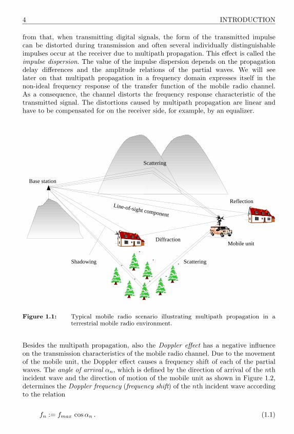
In mobile radio communications, the emitted electromagnetic waves often do notreach the receiving antenna directly due to obstacles blocking the line-of-sight path. Infact, the received waves are a superposition of waves coming from all directions due toreflection, diffraction, and scattering caused by buildings, trees, and other obstacles.This effect is known as multipath propagation. A typical scenario for the terrestrialmobile radio channel is shown in Figure 1.1. Due to the multipath propagation, thereceived signal consists of an infinite sum of attenuated, delayed, and phase-shiftedreplicas of the transmitted signal, each influencing each other. Depending on thephase of each partial wave, the superposition can be constructive or destructive. Apart
3 Originally TELEDESIC planned to operate 924 satellites circling at an altitude between 695 and705 km.
4 INTRODUCTION
from that, when transmitting digital signals, the form of the transmitted impulsecan be distorted during transmission and often several individually distinguishableimpulses occur at the receiver due to multipath propagation. This effect is called theimpulse dispersion. The value of the impulse dispersion depends on the propagationdelay differences and the amplitude relations of the partial waves. We will seelater on that multipath propagation in a frequency domain expresses itself in thenon-ideal frequency response of the transfer function of the mobile radio channel.As a consequence, the channel distorts the frequency response characteristic of thetransmitted signal. The distortions caused by multipath propagation are linear andhave to be compensated for on the receiver side, for example, by an equalizer.
Line-of-sight component
Diffraction
Base station
Scattering
Scattering
Mobile unit
Reflection
Shadowing
Figure 1.1: Typical mobile radio scenario illustrating multipath propagation in aterrestrial mobile radio environment.
Besides the multipath propagation, also the Doppler effect has a negative influenceon the transmission characteristics of the mobile radio channel. Due to the movementof the mobile unit, the Doppler effect causes a frequency shift of each of the partialwaves. The angle of arrival αn, which is defined by the direction of arrival of the nthincident wave and the direction of motion of the mobile unit as shown in Figure 1.2,determines the Doppler frequency (frequency shift) of the nth incident wave accordingto the relation
fn := fmax cos αn . (1.1)

BASIC KNOWLEDGE OF MOBILE RADIO CHANNELS 5
In this case, fmax is the maximum Doppler frequency related to the speed of the mobileunit v, the speed of light c0, and the carrier frequency f0 by the equation
fmax =vc0
f0 . (1.2)
The maximum (minimum) Doppler frequency, i.e., fn = fmax (fn = −fmax), isreached for αn = 0 (αn = π). In comparison, though, fn = 0 for αn = π/2 andαn = 3π/2. Due to the Doppler effect, the spectrum of the transmitted signalundergoes a frequency expansion during transmission. This effect is called thefrequency dispersion. The value of the frequency dispersion mainly depends on themaximum Doppler frequency and the amplitudes of the received partial waves. In thetime domain, the Doppler effect implicates that the impulse response of the channelbecomes time-variant. One can easily show that mobile radio channels fulfil theprinciple of superposition [Opp75, Lue90] and therefore are linear systems. Due tothe time-variant behaviour of the impulse response, mobile radio channels thereforegenerally belong to the class of linear time-variant systems.
α
Direction of motion
n
x
thof the n incident wave
y
Direction of arrival
Figure 1.2: Angle of arrival αn of the nth incident wave illustrating the Doppler effect.
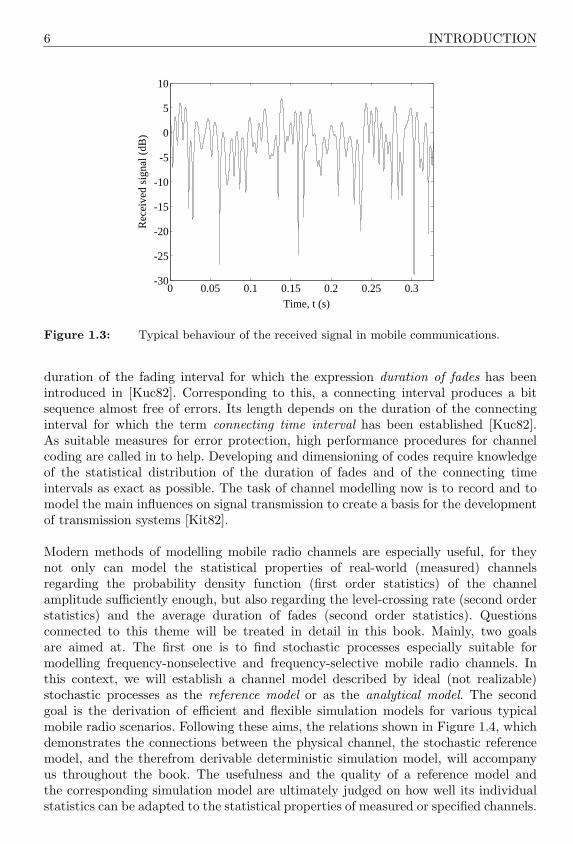
Multipath propagation in connection with the movement of the receiver and/or thetransmitter leads to drastic and random fluctuations of the received signal. Fades of30 to 40 dB and more below the mean value of the received signal level can occurseveral times per second, depending on the speed of the mobile unit and the carrierfrequency [Jak93]. A typical example of the behaviour of the received signal in mobilecommunications is shown in Figure 1.3. In this case, the speed of the mobile unitis v = 110 km/h and the carrier frequency is f0 = 900MHz. According to (1.2),this corresponds to a maximum Doppler frequency of fmax = 91 Hz. In the presentexample, the distance covered by the mobile unit during the chosen period of timefrom 0 to 0.327 s is equal to 10m.
In digital data transmission, the momentary fading of the received signal causes bursterrors, i.e., errors with strong statistical connections to each other [Bla84]. Therefore,a fading interval produces burst errors, where the burst length is determined by the
6 INTRODUCTION
0 0.05 0.1 0.15 0.2 0.25 0.3-30
-25
-20
-15
-10
-5
0
5
10
Time, t (s)
Rec
eive
d si
gnal
(dB
)
Figure 1.3: Typical behaviour of the received signal in mobile communications.
duration of the fading interval for which the expression duration of fades has beenintroduced in [Kuc82]. Corresponding to this, a connecting interval produces a bitsequence almost free of errors. Its length depends on the duration of the connectinginterval for which the term connecting time interval has been established [Kuc82].As suitable measures for error protection, high performance procedures for channelcoding are called in to help. Developing and dimensioning of codes require knowledgeof the statistical distribution of the duration of fades and of the connecting timeintervals as exact as possible. The task of channel modelling now is to record and tomodel the main influences on signal transmission to create a basis for the developmentof transmission systems [Kit82].
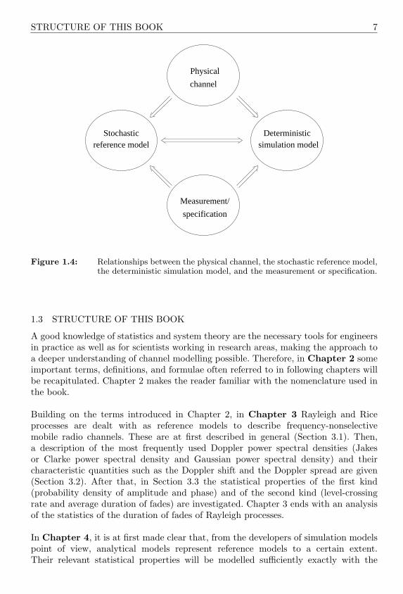
Modern methods of modelling mobile radio channels are especially useful, for theynot only can model the statistical properties of real-world (measured) channelsregarding the probability density function (first order statistics) of the channelamplitude sufficiently enough, but also regarding the level-crossing rate (second orderstatistics) and the average duration of fades (second order statistics). Questionsconnected to this theme will be treated in detail in this book. Mainly, two goalsare aimed at. The first one is to find stochastic processes especially suitable formodelling frequency-nonselective and frequency-selective mobile radio channels. Inthis context, we will establish a channel model described by ideal (not realizable)stochastic processes as the reference model or as the analytical model. The secondgoal is the derivation of efficient and flexible simulation models for various typicalmobile radio scenarios. Following these aims, the relations shown in Figure 1.4, whichdemonstrates the connections between the physical channel, the stochastic referencemodel, and the therefrom derivable deterministic simulation model, will accompanyus throughout the book. The usefulness and the quality of a reference model andthe corresponding simulation model are ultimately judged on how well its individualstatistics can be adapted to the statistical properties of measured or specified channels.
STRUCTURE OF THIS BOOK 7
Measurement/
channel
simulation modelreference model
specification
Stochastic
Physical
Deterministic
Figure 1.4: Relationships between the physical channel, the stochastic reference model,the deterministic simulation model, and the measurement or specification.
1.3 STRUCTURE OF THIS BOOK
A good knowledge of statistics and system theory are the necessary tools for engineersin practice as well as for scientists working in research areas, making the approach toa deeper understanding of channel modelling possible. Therefore, in Chapter 2 someimportant terms, definitions, and formulae often referred to in following chapters willbe recapitulated. Chapter 2 makes the reader familiar with the nomenclature used inthe book.
Building on the terms introduced in Chapter 2, in Chapter 3 Rayleigh and Riceprocesses are dealt with as reference models to describe frequency-nonselectivemobile radio channels. These are at first described in general (Section 3.1). Then,a description of the most frequently used Doppler power spectral densities (Jakesor Clarke power spectral density and Gaussian power spectral density) and theircharacteristic quantities such as the Doppler shift and the Doppler spread are given(Section 3.2). After that, in Section 3.3 the statistical properties of the first kind(probability density of amplitude and phase) and of the second kind (level-crossingrate and average duration of fades) are investigated. Chapter 3 ends with an analysisof the statistics of the duration of fades of Rayleigh processes.
In Chapter 4, it is at first made clear that, from the developers of simulation modelspoint of view, analytical models represent reference models to a certain extent.Their relevant statistical properties will be modelled sufficiently exactly with the
8 INTRODUCTION
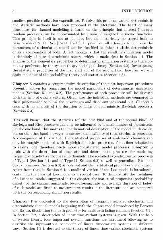
smallest possible realization expenditure. To solve this problem, various deterministicand statistic methods have been proposed in the literature. The heart of manyprocedures for channel modelling is based on the principle that filtered Gaussianrandom processes can be approximated by a sum of weighted harmonic functions.This principle in itself is not at all new, but can historically be traced back tobasic works of S. O. Rice [Ric44, Ric45]. In principle, all attempts to compute theparameters of a simulation model can be classified as either statistic, deterministicor as a combination of both. A fact though is that the resulting simulation modelis definitely of pure deterministic nature, which is made clear in Section 4.1. Theanalysis of the elementary properties of deterministic simulation systems is thereforemainly performed by the system theory and signal theory (Section 4.2). Investigatingthe statistical properties of the first kind and of the second kind, however, we willagain make use of the probability theory and statistics (Section 4.3).
Chapter 5 contains a comprehensive description of the most important procedurespresently known for computing the model parameters of deterministic simulationmodels (Sections 5.1 and 5.2). The performance of each procedure will be assessedwith the help of quality criteria. Often, also the individual methods are compared intheir performance to allow the advantages and disadvantages stand out. Chapter 5ends with an analysis of the duration of fades of deterministic Rayleigh processes(Section 5.3).
It is well known that the statistics (of the first kind and of the second kind) ofRayleigh and Rice processes can only be influenced by a small number of parameters.On the one hand, this makes the mathematical description of the model much easier,but on the other hand, however, it narrows the flexibility of these stochastic processes.A consequence of this is that the statistical properties of real-world channels canonly be roughly modelled with Rayleigh and Rice processes. For a finer adaptationto reality, one therefore needs more sophisticated model processes. Chapter 6deals with the description of stochastic and deterministic processes for modellingfrequency-nonselective mobile radio channels. The so-called extended Suzuki processesof Type I (Section 6.1) and of Type II (Section 6.2) as well as generalized Rice andSuzuki processes (Section 6.3) are derived and their statistical properties are analysed.Apart from that, in Section 6.4, a modified version of the Loo model is introduced,containing the classical Loo model as a special case. To demonstrate the usefulnessof all channel models suggested in this chapter, the statistical properties (probabilitydensity of the channel amplitude, level-crossing rate and average duration of fades)of each model are fitted to measurement results in the literature and are comparedwith the corresponding simulation results.
Chapter 7 is dedicated to the description of frequency-selective stochastic anddeterministic channel models beginning with the ellipses model introduced by Parsonsand Bajwa, illustrating the path geometry for multipath fading channels (Section 7.1).In Section 7.2, a description of linear time-variant systems is given. With the helpof system theory, four important system functions are introduced allowing us todescribe the input-output behaviour of linear time-variant systems in differentways. Section 7.3 is devoted to the theory of linear time-variant stochastic systems

STRUCTURE OF THIS BOOK 9
going back to Bello [Bel63]. In connection with this, stochastic system functionsand characteristic quantities derivable from these are defined. Also the referenceto frequency-selective stochastic channel models is established and, moreover, thechannel models for typical propagation areas specified in the European work groupCOST 207 [COS89] are given. Section 7.4 deals with the derivation and analysisof frequency-selective deterministic channel models. Chapter 7 ends with the de-sign of deterministic simulation models for the channel models according to COST 207.
Chapter 8 deals with the derivation, analysis, and realization of fast channelsimulators. For the derivation of fast channel simulators, the periodicity of harmonicfunctions is exploited. It is shown how alternative structures for the simulation ofdeterministic processes can be derived. In particular, for complex Gaussian randomprocesses it is extraordinarily easy to derive simulation models merely based onadders, storage elements, and simple address generators. During the actual simulationof the complex-valued channel amplitude, time-consuming trigonometric operations aswell as multiplications are then no longer required. This results in high-speed channelsimulators, which are suitable for all frequency-selective and frequency-nonselectivechannel models dealt with in previous chapters. Since the proposed principle can begeneralized easily, we will in Chapter 8 restrict our attention to the derivation of fastchannel simulators for Rayleigh channels. Therefore, we will exclusively employ thediscrete-time representation and will introduce so-called discrete-time deterministicprocesses in Section 8.1. With these processes there are new possibilities for indirectrealization. The three most important of them are introduced in Section 8.2. In thefollowing Section 8.3, the elementary and statistical properties of discrete deter-ministic processes are examined. Section 8.4 deals with the analysis of the requiredrealization expenditure and with the measurement of the simulation speed of fastchannel simulators. Chapter 8 ends with a comparison between the Rice method andthe filter method (Section 8.5).


2
RANDOM VARIABLES,STOCHASTIC PROCESSES,AND DETERMINISTICSIGNALS
Besides clarifying the used nomenclature, we will in this chapter introduce someimportant terms, which will later often be used in the context of describing stochasticand deterministic channel models. However, the primary aim is to familiarize thereader with some basic principles and definitions of probability, random signals,and systems theory, as far as it is necessary for the understanding of this book.A complete and detailed description of these subjects will not be presented here;instead, some relevant technical literature will be recommended for further studies.As technical literature for the subject of probability theory, random variables, andstochastic processes, the books by Papoulis [Pap91], Peebles [Pee93], Therrien [The92],Dupraz [Dup86], as well as Shanmugan and Breipohl [Sha88] are recommended.Also the classical works of Middleton [Mid60], Davenport [Dav70], and the bookby Davenport and Root [Dav58] are even nowadays still worth reading. A modernGerman introduction to the basic principles of probability and stochastic processescan be found in [Boe98, Bei97, Hae97]. Finally, the excellent textbooks by Oppenheimand Schafer [Opp75], Papoulis [Pap77], Rabiner and Gold [Rab75], Kailath [Kai80],Unbehauen [Unb90], Schußler [Sch91], and Fettweis [Fet96] provide a deep insight intosystems theory as well as into the principles of digital signal processing.
2.1 RANDOM VARIABLES
In the context of this book, random variables are of central importance, not only to thestatistical but also to the deterministic modelling of mobile radio channels. Therefore,we will at first review some basic definitions and terms which are frequently used inconnection with random variables.
An experiment whose outcome is not known in advance is called a random experiment.We will call points representing the outcomes of a random experiment sample pointss. A collection of possible outcomes of a random experiment is an event A. Theevent A = s consisting of a single element s is an elementary event. The set of
12 STOCHASTIC PROCESSES AND DETERMINISTIC SIGNALS
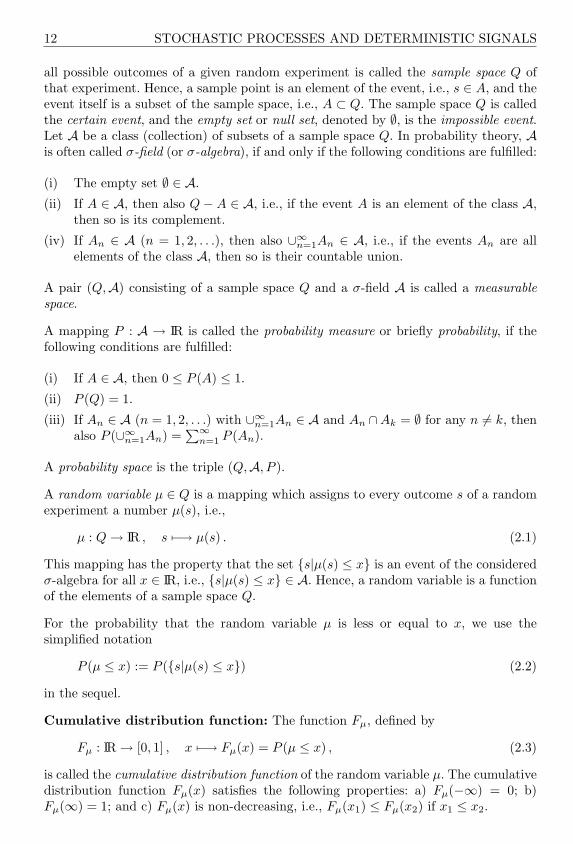
all possible outcomes of a given random experiment is called the sample space Q ofthat experiment. Hence, a sample point is an element of the event, i.e., s ∈ A, and theevent itself is a subset of the sample space, i.e., A ⊂ Q. The sample space Q is calledthe certain event, and the empty set or null set, denoted by ∅, is the impossible event.Let A be a class (collection) of subsets of a sample space Q. In probability theory, Ais often called σ-field (or σ-algebra), if and only if the following conditions are fulfilled:
(i) The empty set ∅ ∈ A.
(ii) If A ∈ A, then also Q− A ∈ A, i.e., if the event A is an element of the class A,then so is its complement.
(iv) If An ∈ A (n = 1, 2, . . .), then also ∪∞n=1An ∈ A, i.e., if the events An are allelements of the class A, then so is their countable union.
A pair (Q,A) consisting of a sample space Q and a σ-field A is called a measurablespace.
A mapping P : A → IR is called the probability measure or briefly probability, if thefollowing conditions are fulfilled:
(i) If A ∈ A, then 0 ≤ P (A) ≤ 1.
(ii) P (Q) = 1.
(iii) If An ∈ A (n = 1, 2, . . .) with ∪∞n=1An ∈ A and An ∩Ak = ∅ for any n 6= k, thenalso P (∪∞n=1An) =
∑∞n=1 P (An).
A probability space is the triple (Q,A, P ).
A random variable µ ∈ Q is a mapping which assigns to every outcome s of a randomexperiment a number µ(s), i.e.,
µ : Q → IR , s 7−→ µ(s) . (2.1)
This mapping has the property that the set s|µ(s) ≤ x is an event of the consideredσ-algebra for all x ∈ IR, i.e., s|µ(s) ≤ x ∈ A. Hence, a random variable is a functionof the elements of a sample space Q.
For the probability that the random variable µ is less or equal to x, we use thesimplified notation
P (µ ≤ x) := P (s|µ(s) ≤ x) (2.2)
in the sequel.
Cumulative distribution function: The function Fµ, defined by
Fµ : IR → [0, 1] , x 7−→ Fµ(x) = P (µ ≤ x) , (2.3)
is called the cumulative distribution function of the random variable µ. The cumulativedistribution function Fµ(x) satisfies the following properties: a) Fµ(−∞) = 0; b)Fµ(∞) = 1; and c) Fµ(x) is non-decreasing, i.e., Fµ(x1) ≤ Fµ(x2) if x1 ≤ x2.
RANDOM VARIABLES 13
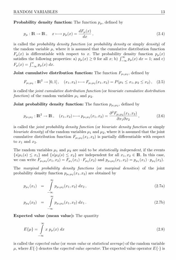
Probability density function: The function pµ, defined by
pµ : IR → IR , x 7−→ pµ(x) =dFµ(x)
dx, (2.4)
is called the probability density function (or probability density or simply density) ofthe random variable µ, where it is assumed that the cumulative distribution functionFµ(x) is differentiable with respect to x. The probability density function pµ(x)satisfies the following properties: a) pµ(x) ≥ 0 for all x; b)
∫∞−∞ pµ(x) dx = 1; and c)
Fµ(x) =∫ x
−∞ pµ(x) dx.
Joint cumulative distribution function: The function Fµ1µ2 , defined by
Fµ1µ2 : IR2 → [0, 1] , (x1, x2) 7−→ Fµ1µ2(x1, x2) = P (µ1 ≤ x1, µ2 ≤ x2) , (2.5)
is called the joint cumulative distribution function (or bivariate cumulative distributionfunction) of the random variables µ1 and µ2.
Joint probability density function: The function pµ1µ2 , defined by
pµ1µ2 : IR2 → IR , (x1, x2) 7−→ pµ1µ2(x1, x2) =∂2Fµ1µ2(x1, x2)
∂x1∂x2, (2.6)
is called the joint probability density function (or bivariate density function or simplybivariate density) of the random variables µ1 and µ2, where it is assumed that the jointcumulative distribution function Fµ1µ2(x1, x2) is partially differentiable with respectto x1 and x2.
The random variables µ1 and µ2 are said to be statistically independent, if the eventss|µ1(s) ≤ x1 and s|µ2(s) ≤ x2 are independent for all x1, x2 ∈ IR. In this case,we can write Fµ1µ2(x1, x2) = Fµ1(x1) · Fµ2(x2) and pµ1µ2(x1, x2) = pµ1(x1) · pµ2(x2).
The marginal probability density functions (or marginal densities) of the jointprobability density function pµ1µ2(x1, x2) are obtained by
pµ1(x1) =
∞∫
−∞pµ1µ2(x1, x2) dx2 , (2.7a)
pµ2(x2) =
∞∫
−∞pµ1µ2(x1, x2) dx1 . (2.7b)
Expected value (mean value): The quantity
Eµ =
∞∫
−∞x pµ(x) dx (2.8)
is called the expected value (or mean value or statistical average) of the random variableµ, where E· denotes the expected value operator. The expected value operator E· is

14 STOCHASTIC PROCESSES AND DETERMINISTIC SIGNALS
linear, i.e., the relations Eαµ = αEµ (α ∈ IR) and Eµ1 +µ2 = Eµ1+Eµ2hold. Let f(µ) be a function of the random variable µ. Then, the expected value off(µ) can be determined by applying the fundamental relationship
Ef(µ) =
∞∫
−∞f(x) pµ(x) dx . (2.9)
The generalization to two random variables µ1 and µ2 leads to
Ef(µ1, µ2) =
∞∫
−∞
∞∫
−∞f(x1, x2) pµ1µ2(x1, x2) dx1 dx2 . (2.10)
Variance: The value
Var µ = E(µ− Eµ)2
= Eµ2 − (Eµ)2 (2.11)
is called the variance of the random variable µ, where Var · denotes the varianceoperator. The variance of a random variable µ is a measure of the concentration of µnear its expected value.
Covariance: The covariance of two random variables µ1 and µ2 is defined by
Cov µ1, µ2 = E(µ1 − Eµ1)(µ2 − Eµ2) (2.12a)= Eµ1µ2 − Eµ1 · Eµ2 . (2.12b)
Moments: The kth moment of the random variable µ is defined by
Eµk =
∞∫
−∞xk pµ(x) dx , k = 0, 1, . . . (2.13)
Characteristic function: The characteristic function of a random variable µ isdefined as the expected value
Ψµ(ν) = Eej2πνµ
=
∞∫
−∞pµ(x) ej2πνx dx , (2.14)
where ν is a real-valued variable. It should be noted that Ψµ(−ν) is the Fouriertransform of the probability density function pµ(x). The characteristic function oftenprovides a simple technique for determining the probability density function of a sumof statistically independent random variables.
Chebyshev inequality: Let µ be an arbitrary random variable with a finite expectedvalue and a finite variance. Then, the Chebyshev inequality
P (|µ− Eµ| ≥ ε) ≤ Var µε2
(2.15)

RANDOM VARIABLES 15
holds for any ε > 0. The Chebyshev inequality is often used to obtain bounds on theprobability of finding µ outside of the interval Eµ ± ε
√Var µ.
Central limit theorem: Let µn (n = 1, 2, . . . , N) be statistically independentrandom variables with Eµn = mµn and Var µn = σ2
µn. Then, the random variable
µ = limN→∞
1√N
N∑n=1
(µn −mµn) (2.16)
is asymptotically normally distributed with the expected value Eµ = 0 and thevariance Var µ = σ2
µ = limN→∞
1N
∑Nn=1 σ2
µn.
The central limit theorem plays a fundamental role in statistical asymptotic theory.The density of the sum (2.16) of merely seven statistically independent randomvariables with almost identical variance often results in a good approximation of thenormal distribution.
2.1.1 Important Probability Density Functions
In the following, a summary of some important probability density functions often usedin connection with channel modelling will be presented. The corresponding statisticalproperties such as the expected value and the variance will be dealt with as well. Atthe end of this section, we will briefly present some rules of calculation, which are ofimportance to the addition, multiplication, and transformation of random variables.
Uniform distribution: Let θ be a real-valued random variable with the probabilitydensity function
pθ(x) =
12π
, x ∈ [−π, π) ,
0 , else .
(2.17)
Then, pθ(x) is called the uniform distribution and θ is said to be uniformly distributedin the interval [−π, π). The expected value and the variance of a uniformly distributedrandom variable θ are Eθ = 0 and Var θ = π2/3, respectively.
Gaussian distribution (normal distribution): Let µ be a real-valued randomvariable with the probability density function
pµ(x) =1√
2πσµ
e− (x−mµ)2
2σ2µ , x ∈ IR . (2.18)
Then, pµ(x) is called the Gaussian distribution (or normal distribution) and µ is said tobe Gaussian distributed (or normally distributed). In the equation above, the quantitymµ ∈ IR denotes the expected value and σ2
µ ∈ (0,∞) is the variance of µ, i.e.,
Eµ = mµ (2.19a)

16 STOCHASTIC PROCESSES AND DETERMINISTIC SIGNALS
and
Var µ = Eµ2 −m2µ = σ2
µ . (2.19b)
To describe the distribution properties of Gaussian distributed random variables µ, weoften use the short notation µ ∼ N(mµ, σ2
µ) instead of giving the complete expression(2.18). Especially, for mµ = 0 and σ2
µ = 1, N(0, 1) is called the standard normaldistribution.
Multivariate Gaussian distribution: Let us consider n real-valued Gaussiandistributed random variables µ1, µ2, . . . , µn with the expected values mµi (i =1, 2, . . . , n) and the variances σ2
µi(i = 1, 2, . . . , n). The multivariate Gaussian
distribution (or multivariate normal distribution) of the Gaussian random variablesµ1, µ2, . . . , µn is defined by
pµ1µ2...µn(x1, x2, . . . , xn) =
1(√2π
)n √detCµ
e−12 (x−mµ)T C−1
µ (x−mµ) , (2.20)
where T denotes the transpose of a vector (or a matrix). In the above expression, xand mµ are column vectors, which are given by
x =
x1
x2
...xn
∈ IRn×1 (2.21a)
and
mµ =
Eµ1Eµ2
...Eµn
=
mµ1
mµ2
...mµn
∈ IRn×1, (2.21b)
respectively, and det Cµ (C−1µ ) denotes the determinant (inverse) of the covariance
matrix
Cµ =
Cµ1µ1 Cµ1µ2 · · · Cµ1µn
Cµ2µ1 Cµ2µ2 · · · Cµ2µn
......
. . ....
Cµnµ1 Cµnµ2 · · · Cµnµn
∈ IRn×n . (2.22)
The elements of the covariance matrix Cµ are given by
Cµiµj = Cov µi, µj = E(µi −mµi)(µj −mµj ) , ∀ i, j = 1, 2, . . . , n . (2.23)
If the n random variables µi are normally distributed and uncorrelated in pairs, thenthe covariance matrix Cµ results in a diagonal matrix with diagonal entries σ2
µi. In
this case, the joint probability density function (2.20) decomposes into a product of n

RANDOM VARIABLES 17
Gaussian distributions of the normally distributed random variables µi ∼ N(mµi , σ2µi
).This implies that the random variables µi are statistically independent for all i =1, 2, . . . , n.
Rayleigh distribution: Let us consider two zero-mean statistically independentnormally distributed random variables µ1 and µ2, each having a variance σ2
0 , i.e.,µ1, µ2 ∼ N(0, σ2
0). Furthermore, let us derive a new random variable from µ1 and µ2
according to ζ =√
µ21 + µ2
2. Then, ζ represents a Rayleigh distributed random variable.The probability density function pζ(x) of Rayleigh distributed random variables ζ isgiven by
pζ(x) =
x
σ20
e− x2
2σ20 , x ≥ 0 ,
0 , x < 0 .
(2.24)
Rayleigh distributed random variables ζ have the expected value
Eζ = σ0
√π
2(2.25a)
and the variance
Var ζ = σ20
(2− π
2
). (2.25b)
Rice distribution: Let µ1, µ2 ∼ N(0, σ20) and ρ ∈ IR. Then, the random variable
ξ =√
(µ1 + ρ)2 + µ22 is a so-called Rice distributed random variable. The probability
density function pξ(x) of Rice distributed random variables ξ is
pξ(x) =
x
σ20
e− x2+ρ2
2σ20 I0
(xρ
σ20
), x ≥ 0 ,
0 , x < 0 ,
(2.26)
where I0(·) denotes the modified Bessel function of 0th order. For ρ = 0, the Ricedistribution pξ(x) results in the Rayleigh distribution pζ(x) described above. The firstand second moment of Rice distributed random variables ξ are [Wol83a]
Eξ = σ0
√π
2e− ρ2
4σ20
(1 +
ρ2
2σ20
)I0
(ρ2
4σ20
)+
ρ2
2σ20
I1
(ρ2
4σ20
)(2.27a)
and
Eξ2 = 2σ20 + ρ2 , (2.27b)
respectively, where In(·) denotes the modified Bessel function of nth order. From(2.27a), (2.27b), and by using (2.11), the variance of Rice distributed random variablesξ can easily be calculated.
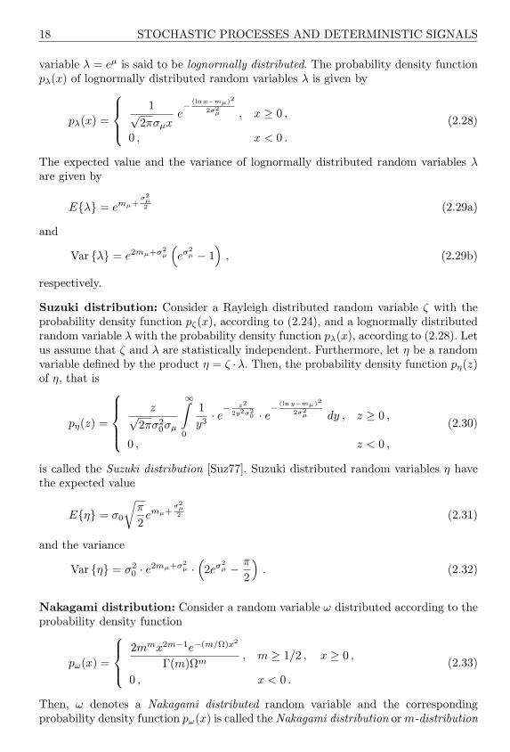
Lognormal distribution: Let µ be a Gaussian distributed random variable withthe expected value mµ and the variance σ2
µ, i.e., µ ∼ N(mµ, σ2µ). Then, the random
18 STOCHASTIC PROCESSES AND DETERMINISTIC SIGNALS
variable λ = eµ is said to be lognormally distributed. The probability density functionpλ(x) of lognormally distributed random variables λ is given by
pλ(x) =
1√2πσµx
e− (ln x−mµ)2
2σ2µ , x ≥ 0 ,
0 , x < 0 .
(2.28)
The expected value and the variance of lognormally distributed random variables λare given by
Eλ = emµ+σ2
µ2 (2.29a)
and
Var λ = e2mµ+σ2µ
(eσ2
µ − 1)
, (2.29b)
respectively.
Suzuki distribution: Consider a Rayleigh distributed random variable ζ with theprobability density function pζ(x), according to (2.24), and a lognormally distributedrandom variable λ with the probability density function pλ(x), according to (2.28). Letus assume that ζ and λ are statistically independent. Furthermore, let η be a randomvariable defined by the product η = ζ ·λ. Then, the probability density function pη(z)of η, that is
pη(z) =
z√2πσ2
0σµ
∞∫
0
1y3· e−
z2
2y2σ20 · e−
(ln y−mµ)2
2σ2µ dy , z ≥ 0 ,
0 , z < 0 ,
(2.30)
is called the Suzuki distribution [Suz77]. Suzuki distributed random variables η havethe expected value
Eη = σ0
√π
2emµ+
σ2µ2 (2.31)
and the variance
Var η = σ20 · e2mµ+σ2
µ ·(2eσ2
µ − π
2
). (2.32)
Nakagami distribution: Consider a random variable ω distributed according to theprobability density function
pω(x) =
2mmx2m−1e−(m/Ω)x2
Γ(m)Ωm, m ≥ 1/2 , x ≥ 0 ,
0 , x < 0 .
(2.33)
Then, ω denotes a Nakagami distributed random variable and the correspondingprobability density function pω(x) is called the Nakagami distribution or m-distribution
RANDOM VARIABLES 19
[Nak60]. In (2.33), the symbol Γ(·) represents the Gamma function, the second momentof the random variable ω has been introduced by Ω = Eω2, and the parameterm denotes the reciprocal value of the variance of ω2 normalized to Ω2, i.e., m =Ω2/E(ω2−Ω)2. From the Nakagami distribution, we obtain the one-sided Gaussiandistribution and the Rayleigh distribution as special cases if m = 1/2 and m = 1,respectively. In certain limits, the Nakagami distribution, moreover, approximatesboth the Rice distribution and the lognormal distribution [Nak60, Cha79].
2.1.2 Functions of Random Variables
In some parts of this book, we will deal with functions of two and more randomvariables. In particular, we will often make use of fundamental rules in connection withthe addition, multiplication, and transformation of random variables. In the sequel,the mathematical principles necessary for this will briefly be reviewed.
Addition of two random variables: Let µ1 and µ2 be two random variables, whichare statistically characterized by the joint probability density function pµ1µ2(x1, x2).Then, the probability density function of the sum µ = µ1 + µ2 can be obtained asfollows
pµ(y) =
∞∫
−∞pµ1µ2(x1, y − x1) dx1
=
∞∫
−∞pµ1µ2(y − x2, x2) dx2 . (2.34)
If the two random variables µ1 and µ2 are statistically independent, then it followsthat the probability density function of µ is given by the convolution of the probabilitydensities of µ1 and µ2. Thus,
pµ(y) = pµ1(y) ∗ pµ2(y)
=
∞∫
−∞pµ1(x1)pµ2(y − x1) dx1
=
∞∫
−∞pµ1(y − x2)pµ2(x2) dx2 , (2.35)
where ∗ denotes the convolution operator.
Multiplication of two random variables: Let ζ and λ be two random variables,which are statistically described by the joint probability density function pζλ(x, y).Then, the probability density function of the random variable η = ζ · λ is equal to
pη(z) =
∞∫
−∞
1|y|pζλ
(z
y, y
)dy . (2.36)
20 STOCHASTIC PROCESSES AND DETERMINISTIC SIGNALS
From this relation, we obtain the expression
pη(z) =
∞∫
−∞
1|y|pζ
(z
y
)· pλ(y) dy (2.37)
for statistically independent random variables ζ, λ.
Functions of random variables: Let us assume that µ1, µ2, . . . , µn are randomvariables, which are statistically described by the joint probability density functionpµ1µ2...µn
(x1, x2, . . . , xn). Furthermore, let us assume that the functions f1, f2, . . . , fn
are given. If the system of equations fi(x1, x2, . . . , xn) = yi (i = 1, 2, . . . , n) has real-valued solutions x1ν , x2ν , . . . , xnν (ν = 1, 2, . . . , m), then the joint probability densityfunction of the random variables ξ1 = f1(µ1, µ2, . . . , µn), ξ2 = f2(µ1, µ2, . . . , µn), . . . ,ξn = fn(µ1, µ2, . . . , µn) can be expressed by
pξ1ξ2...ξn(y1, y2, . . . , yn) =m∑
ν=1
pµ1µ2...µn(x1ν , x2ν , . . . , xnν)|J(x1ν , x2ν , . . . , xnν)| , (2.38)
where
J(x1, x2, . . . , xn) =
∣∣∣∣∣∣∣∣∣∣∣∣
∂f1∂x1
∂f1∂x2
· · · ∂f1∂xn
∂f2∂x1
∂f2∂x2
· · · ∂f2∂xn
......
. . ....
∂fn
∂x1
∂fn
∂x2· · · ∂fn
∂xn
∣∣∣∣∣∣∣∣∣∣∣∣
(2.39)
denotes the Jacobian determinant.
Furthermore, we can compute the joint probability density function of the randomvariables ξ1, ξ2, . . . , ξk for k < n by using (2.38) as follows
pξ1ξ2...ξk(y1, y2, . . . , yk) =
∞∫
−∞
∞∫
−∞. . .
∞∫
−∞pξ1ξ2...ξn(y1, y2, . . . , yn) dyk+1 dyk+2 . . . dyn .
(2.40)
2.2 STOCHASTIC PROCESSES
Let (Q,A, P ) be a probability space. Now let us assign to every particular outcomes = si ∈ Q of a random experiment a particular function of time µ(t, si) according toa rule. Hence, for a particular si ∈ Q, the function µ(t, si) denotes a mapping from IRto IR (or C) according to
µ(·, si) : IR → IR (or C) , t 7→ µ(t, si) . (2.41)
STOCHASTIC PROCESSES 21
The individual functions µ(t, si) of time are called realizations or sample functions. Astochastic process µ(t, s) is a family (or an ensemble) of sample functions µ(t, si), i.e.,µ(t, s) = µ(t, si)|si ∈ Q = µ(t, s1), µ(t, s2), . . ..On the other hand, at a particular time instant t = t0 ∈ IR, the stochastic processµ(t0, s) only depends on the outcome s and, thus, equals a random variable. Hence,for a particular t0 ∈ IR, µ(t0, s) denotes a mapping from Q to IR (or C) according to
µ(t0, ·) : Q → IR (or C) , s 7→ µ(t0, s) . (2.42)
The probability density function of the random variable µ(t0, s) is determined by theoccurrence of the outcomes.
Therefore, a stochastic process is a function of two variables t ∈ IR and s ∈ Q, so thatthe correct notation is µ(t, s). Henceforth, however, we will drop the second argumentand simply write µ(t) as in common practice.
From the statements above, we can conclude that a stochastic process µ(t) can beinterpreted as follows [Pap91]:
(i) If t is a variable and s is a random variable, then µ(t) represents a family or anensemble of sample functions µ(t, s).
(ii) If t is a variable and s = s0 is a constant, then µ(t) = µ(t, s0) is a realization ora sample function of the stochastic process.
(iii) If t = t0 is a constant and s is a random variable, then µ(t0) is a random variableas well.
(iv) If both t = t0 and s = s0 are constants, then µ(t0) is a real-valued (complex-valued) number.
The relationships following from the statements (i)–(iv) made above are illustrated inFigure 2.1.
Complex-valued stochastic processes: Let µ′(t) and µ′′(t) be two real-valuedstochastic processes, then a (complex-valued) stochastic process is defined by µ(t) =µ′(t) + jµ′′(t).
We have stated above that a stochastic process µ(t) can be interpreted as a randomvariable for fixed values of t ∈ IR. This random variable can again be described bya distribution function Fµ(x; t) = P (µ(t) ≤ x) or a probability density functionpµ(x; t) = dFµ(x; t)/dx. The extension of the concept of the expected value, whichwas introduced for random variables, to stochastic processes leads to the expectedvalue function
mµ(t) = Eµ(t) . (2.43)
Let us consider the random variables µ(t1) and µ(t2), which are assigned to thestochastic process µ(t) at the time instants t1 and t2, then
rµµ(t1, t2) = Eµ∗(t1)µ(t2) (2.44)

22 STOCHASTIC PROCESSES AND DETERMINISTIC SIGNALS
µ µ(t ) (t ,s)ooRandom
variableµ (t) = µ (t,s )o
Sample
function
=µ µo(t )
=
(t ,s )
Stochastic process
o o
Real (complex) number
t=t o os=s
os=s t=t o
µ (t) µ (t,s)=
Figure 2.1: Relationships between stochastic processes, random variables, samplefunctions, and real-valued (complex-valued) numbers.
is called the autocorrelation function of µ(t), where the superscripted asterisk ∗ denotesthe complex conjugation. Note that the complex conjugation is associated with thefirst independent variable in rµµ(t1, t2).1 The so-called variance function of a complex-valued stochastic process µ(t) is defined as
σ2µ(t) = Var µ(t) = E|µ(t)− Eµ(t)|2
= Eµ∗(t)µ(t) − Eµ∗(t)Eµ(t)= rµµ(t, t)− |mµ(t)|2 , (2.45)
where rµµ(t, t) denotes the autocorrelation function (2.44) at the time instant t1 =t2 = t, and mµ(t) represents the expected value function according to (2.43). Finally,the expression
rµ1µ2(t1, t2) = Eµ∗1(t1)µ2(t2) (2.46)
introduces the cross-correlation function of the stochastic processes µ1(t) and µ2(t) atthe time instants t1 and t2.
2.2.1 Stationary Processes
Stationary processes are of crucial importance to the modelling of mobile radiochannels and will therefore be dealt with briefly here. One often distinguishes betweenstrict-sense stationary processes and wide-sense stationary processes.
1 It should be noted that in the literature, the complex conjugation is often also associated withthe second independent variable of the autocorrelation function rµµ(t1, t2), i.e., rµµ(t1, t2) =Eµ(t1)µ∗(t2).

STOCHASTIC PROCESSES 23
A stochastic process µ(t) is said to be strict-sense stationary, if its statistical propertiesare invariant to a shift of the origin, i.e., µ(t1) and µ(t1 + t2) have the same statisticsfor all t1, t2 ∈ IR. This leads to the following conclusions:
(i) pµ(x; t) = pµ(x) , (2.47a)(ii) Eµ(t) = mµ = const. , (2.47b)(iii) rµµ(t1, t2) = rµµ(|t1 − t2|) . (2.47c)
A stochastic process µ(t) is said to be wide-sense stationary if (2.47b) and (2.47c) arefulfilled. In this case, the expected value function Eµ(t) is independent of t and, thus,simplifies to the expected value mµ introduced for random variables. Furthermore, theautocorrelation function rµµ(t1, t2) merely depends on the time difference t1−t2. From(2.44) and (2.47c), with t1 = t and t2 = t + τ , it then follows for τ > 0
rµµ(τ) = rµµ(t, t + τ) = Eµ∗(t)µ(t + τ) , (2.48)
where rµµ(0) represents the mean power of µ(t). Analogously, for the cross-correlationfunction (2.46) of two wide-sense stationary processes µ1(t) and µ2(t), we obtain
rµ1µ2(τ) = Eµ∗1(t)µ2(t + τ) = r∗µ2µ1(−τ) . (2.49)
Let µ1(t), µ2(t), and µ(t) be three wide-sense stationary stochastic processes. TheFourier transform of the autocorrelation function rµµ(τ), defined by
Sµµ(f) =
∞∫
−∞rµµ(τ) e−j2πfτ dτ , (2.50)
is called the power spectral density (power density spectrum). The general relationgiven above between the power spectral density and the autocorrelation function isalso known as the Wiener-Khinchine relationship. The Fourier transform of the cross-correlation function rµ1µ2(τ), defined by
Sµ1µ2(f) =
∞∫
−∞rµ1µ2(τ) e−j2πfτ dτ , (2.51)
is called the cross-power spectral density (cross-power density spectrum). Taking (2.49)into account, we immediately realize that Sµ1µ2(f) = S∗µ2µ1
(f) holds.
Let ν(t) be the input process and µ(t) the output process of a linear time-invariantstable system with the impulse response h(t). Furthermore, let us assume that thesystem is deterministic, meaning that it only operates on the time variable t. Then,the output process µ(t) is the convolution of the input process ν(t) and the impulseresponse h(t), i.e., µ(t) = ν(t) ∗ h(t). It is well known that the transfer function H(f)of the system is the Fourier transform of the impulse response h(t). Moreover, thefollowing relations hold:
24 STOCHASTIC PROCESSES AND DETERMINISTIC SIGNALS
rνµ(τ) = rνν(τ) ∗ h(τ) —• Sνµ(f) = Sνν(f) ·H(f) , (2.52a, b)rµν(τ) = rνν(τ) ∗ h∗(−τ) —• Sµν(f) = Sνν(f) ·H∗(f) , (2.52c, d)
rµµ(τ) = rνν(τ) ∗ h(τ) ∗ h∗(−τ) —• Sµµ(f) = Sνν(f) · |H(f)|2 , (2.52e, f)
where the symbol —• denotes the Fourier transform. We will assume in the sequelthat all systems under consideration are linear, time-invariant, and stable.
It should be noted that, strictly speaking, no stationary processes can exist. Stationaryprocesses are merely used as mathematical models for processes, which hold theirstatistical properties over a relatively long time. From now on, a stochastic processwill be assumed as a strict-sense stationary stochastic process, as long as nothing elseis said.
A system with the transfer function
H(f) = −j sgn (f) (2.53)
is called the Hilbert transformer. We observe that this system causes a phase shift of−π/2 for f > 0 and a phase shift of +π/2 for f < 0. It should also be observed thatH(f) = 1 holds. The inverse Fourier transform of the transfer function H(f) resultsin the impulse response
h(t) =1πt
. (2.54)
Since h(t) 6= 0 holds for t < 0, it follows that the Hilbert transformer is not causal.Let ν(t) with Eν(t) = 0 be a real-valued input process of the Hilbert transformer,then the output process
ν(t) = ν(t) ∗ h(t) =1π
∞∫
−∞
ν(t′)t− t′
dt′ (2.55)
is said to be the Hilbert transform of ν(t). One should note that the computation ofthe integral in (2.55) must be performed according to Cauchy’s principal value.
With (2.52) and (2.54), the following relations hold:
rνν(τ) = rνν(τ) —• Sνν(f) = −j sgn (f) · Sνν(f) , (2.56a, b)rνν(τ) = −rνν(τ) —• Sνν(f) = −Sνν(f) , (2.56c, d)
rνν(τ) = rνν(τ) —• Sνν(f) = Sνν(f) . (2.56e, f)

STOCHASTIC PROCESSES 25
2.2.2 Ergodic Processes
The description of the statistical properties of stochastic processes, like the expectedvalue or the autocorrelation function, is based on ensemble means (statistical means),which takes all possible sample functions of the stochastic process into account. Inpractice, however, one almost always observes and records only a finite number ofsample functions (mostly even only one single sample function). Nevertheless, in orderto make statements on the statistical properties of stochastic process, one refers tothe ergodicity hypothesis.
The ergodicity hypothesis deals with the question, whether it is possible to evaluateonly a single sample function of a stationary stochastic process instead of averagingover the whole ensemble of sample functions at one or more specific time instants.Of particular importance is the question whether the expected value and theautocorrelation function of a stochastic process µ(t) equal the temporal means takenover any arbitrarily sample function µ(t, si). According to the ergodic theorem, theexpected value Eµ(t) = mµ equals the temporal average of µ(t, si), i.e.,
mµ = mµ := limT→∞
12T
+T∫
−T
µ(t, si) dt , (2.57)
and the autocorrelation function rµµ(τ) = Eµ∗(t)µ(t + τ) equals the temporalautocorrelation function of µ(t, si), i.e.,
rµµ(τ) = rµµ(τ) := limT→∞
12T
+T∫
−T
µ∗(t, si) µ(t + τ, si) dt . (2.58)
A stationary stochastic process µ(t) is said to be strict-sense ergodic, if all expectedvalues, which take all possible sample functions into account, are identical to therespective temporal averages taken over an arbitrary sample function. If this conditionis only fulfilled for the expected value and the autocorrelation function, i.e., if only(2.57) and (2.58) are fulfilled, then the stochastic process µ(t) is said to be wide-senseergodic. A strict-sense ergodic process is always stationary. The inverse statement isnot always true, although commonly assumed.
2.2.3 Level-Crossing Rate and Average Duration of Fades
Apart from the probability density function and the autocorrelation function, othercharacteristic quantities describing the statistics of mobile fading channels are ofimportance. These quantities are the level-crossing rate and the average duration offades.
As we know, the received signal in mobile radio communications often undergoesheavy statistical fluctuations, which can reach as high as 30 dB and more. In digitalcommunications, a heavy decline of the received signal directly leads to a drasticincrease of the bit error rate. For the optimization of coding systems, which arerequired for error correction, it is not only important to know how often the received
26 STOCHASTIC PROCESSES AND DETERMINISTIC SIGNALS
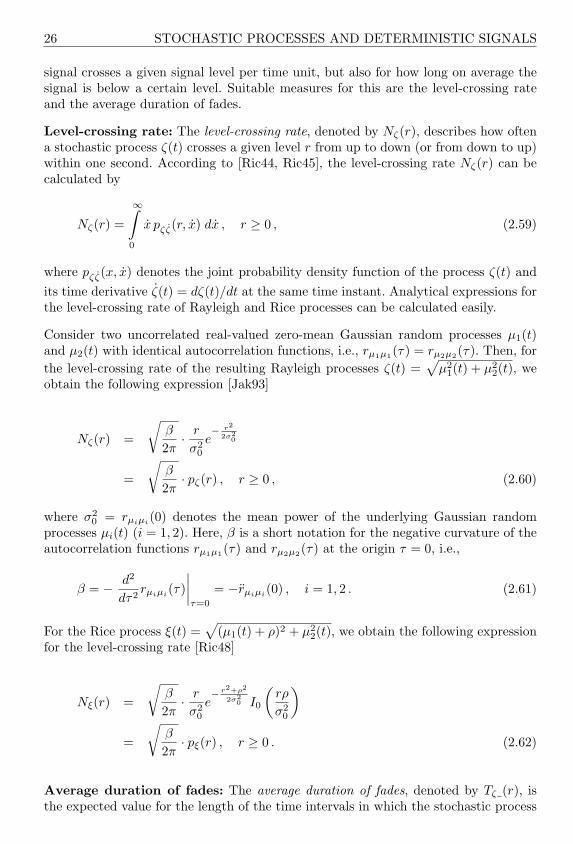
signal crosses a given signal level per time unit, but also for how long on average thesignal is below a certain level. Suitable measures for this are the level-crossing rateand the average duration of fades.
Level-crossing rate: The level-crossing rate, denoted by Nζ(r), describes how oftena stochastic process ζ(t) crosses a given level r from up to down (or from down to up)within one second. According to [Ric44, Ric45], the level-crossing rate Nζ(r) can becalculated by
Nζ(r) =
∞∫
0
x pζζ(r, x) dx , r ≥ 0 , (2.59)
where pζζ(x, x) denotes the joint probability density function of the process ζ(t) andits time derivative ζ(t) = dζ(t)/dt at the same time instant. Analytical expressions forthe level-crossing rate of Rayleigh and Rice processes can be calculated easily.
Consider two uncorrelated real-valued zero-mean Gaussian random processes µ1(t)and µ2(t) with identical autocorrelation functions, i.e., rµ1µ1(τ) = rµ2µ2(τ). Then, forthe level-crossing rate of the resulting Rayleigh processes ζ(t) =
õ2
1(t) + µ22(t), we
obtain the following expression [Jak93]
Nζ(r) =
√β
2π· r
σ20
e− r2
2σ20
=
√β
2π· pζ(r) , r ≥ 0 , (2.60)
where σ20 = rµiµi(0) denotes the mean power of the underlying Gaussian random
processes µi(t) (i = 1, 2). Here, β is a short notation for the negative curvature of theautocorrelation functions rµ1µ1(τ) and rµ2µ2(τ) at the origin τ = 0, i.e.,
β = − d2
dτ2rµiµi(τ)
∣∣∣∣τ=0
= −rµiµi(0) , i = 1, 2 . (2.61)
For the Rice process ξ(t) =√
(µ1(t) + ρ)2 + µ22(t), we obtain the following expression
for the level-crossing rate [Ric48]
Nξ(r) =
√β
2π· r
σ20
e− r2+ρ2
2σ20 I0
(rρ
σ20
)
=
√β
2π· pξ(r) , r ≥ 0 . (2.62)
Average duration of fades: The average duration of fades, denoted by Tζ (r), isthe expected value for the length of the time intervals in which the stochastic process

DETERMINISTIC CONTINUOUS-TIME SIGNALS 27
ζ(t) is below a given level r. The average duration of fades Tζ (r) can be calculatedby means of [Jak93]
Tζ (r) =Fζ (r)Nζ(r)
, (2.63)
where Fζ (r) denotes the cumulative distribution function of the stochastic processζ(t) being the probability that ζ(t) is less or equal to the level r, i.e.,
Fζ (r) = P (ζ(t) ≤ r) =
r∫
0
pζ(x) dx . (2.64)
For the Rayleigh processes ζ(t), the average duration of fades is given by
Tζ (r) =√
2π
β· σ2
0
r
(e
r2
2σ20 − 1
), r ≥ 0 , (2.65)
where the quantity β is again given by (2.61).
For Rice processes ξ(t), however, we find by substituting (2.26), (2.64), and (2.62) in(2.63) the following integral expression
Tξ (r) =√
2π
β· e
r2
2σ20
r I0
(rρσ20
)r∫
0
x e− x2
2σ20 I0
(xρ
σ20
)dx , r ≥ 0 , (2.66)
which has to be evaluated numerically.
Analogously, the average connecting time interval Tζ+(r) can be introduced. Thisquantity describes the expected value for the length of the time intervals, in which thestochastic process ζ(t) is above a given level r. Thus,
Tζ+(r) =Fζ+(r)Nζ(r)
, (2.67)
where Fζ+(r) is called the complementary cumulative distribution function of ζ(t). Thisfunction describes the probability that ζ(t) is larger than r, i.e., Fζ+(r) = P (ζ(t) >r). The complementary cumulative distribution function Fζ+ and the cumulativedistribution function Fζ−(r) are related by Fζ+(r) = 1− Fζ−(r).
2.3 DETERMINISTIC CONTINUOUS-TIME SIGNALS
In principle, one distinguishes between continuous-time and discrete-time signals. Fordeterministic signals, we will in what follows use the continuous-time representationwherever it is possible. Only in those sections where the numerical simulations ofchannel models play a significant role, is the discrete-time representation of signalschosen.
A deterministic (continuous-time) signal is usually defined over IR. The set IR isconsidered as the time space in which the variable t takes its values, i.e., t ∈ IR.

28 STOCHASTIC PROCESSES AND DETERMINISTIC SIGNALS
A deterministic signal is described by a function (mapping) in which each value oft is definitely assigned to a real-valued (or complex-valued) number. Furthermore,in order to distinguish deterministic signals from stochastic processes better, we willput the tilde-sign onto the symbols chosen for deterministic signals. Thus, under adeterministic signal µ(t), we will understand a mapping of the kind
µ : IR → IR (or C) , t 7−→ µ(t) . (2.68)
In connection with deterministic signals, the following terms are of importance.
Mean value: The mean value of a deterministic signal µ(t) is defined by
mµ := limT→∞
12T
T∫
−T
µ(t)dt . (2.69)
Mean power: The mean power of a deterministic signal µ(t) is defined by
σ2µ := lim
T→∞1
2T
T∫
−T
|µ(t)|2dt . (2.70)
From now on, we will always assume that the power of a deterministic signal is finite.
Autocorrelation function: Let µ(t) be a deterministic signal. Then, theautocorrelation function of µ(t) is defined by
rµµ(τ) := limT→∞
12T
T∫
−T
µ∗(t) µ(t + τ)dt , τ ∈ IR . (2.71)
Comparing (2.70) with (2.71), we realize that the value of rµµ(τ) at τ = 0 is identicalto the mean power of µ(t), i.e., the relation rµµ(0) = σ2
µ holds.
Cross-correlation function: Let µ1(t) and µ2(t) be two deterministic signals. Then,the cross-correlation function of µ1(t) and µ2(t) is defined by
rµ1µ2(τ) := limT→∞
12T
T∫
−T
µ∗1(t) µ2(t + τ) dt , τ ∈ IR . (2.72)
Here, rµ1µ2(τ) = r∗µ2µ1(−τ) holds.
Power spectral density: Let µ(t) be a deterministic signal. Then, the Fouriertransform of the autocorrelation function rµµ(τ), defined by
Sµµ(f) :=
∞∫
−∞rµµ(τ)e−j2πfτdτ , f ∈ IR , (2.73)

DETERMINISTIC DISCRETE-TIME SIGNALS 29
is called the power spectral density (or power density spectrum) of µ(t).
Cross-power spectral density: Let µ1(t) and µ2(t) be two deterministic signals.Then, the Fourier transform of the cross-correlation function rµ1µ2(τ)
Sµ1µ2(f) :=
∞∫
−∞rµ1µ2(τ)e−j2πfτdτ , f ∈ IR , (2.74)
is called the cross-power spectral density (or cross-power density spectrum). From (2.74)and the relation rµ1µ2(τ) = r∗µ2µ1
(−τ) it follows that Sµ1µ2(f) = S∗µ2µ1(f) holds.
Let ν(t) and µ(t) be the deterministic input signal and the deterministic output signal,respectively, of a linear time-invariant stable system with the transfer function H(f).Then, the relationship
Sµµ(f) = |H(f)|2Sνν(f) (2.75)
holds.
2.4 DETERMINISTIC DISCRETE-TIME SIGNALS
By equidistant sampling of a continuous-time signal µ(t) at the discrete time instantst = tk = kTs, where k ∈ Z and Ts symbolizes the sampling interval, we obtain thesequence of numbers µ(kTs) = . . . , µ(−Ts), µ(0), µ(Ts), . . .. In specific questions ofmany engineering fields, it is occasionally strictly distinguished between the sequenceµ(kTs) itself, which is then called a discrete-time signal, and the kth elementµ(kTs) of it. For our purposes, however, this differentiation is not connected toany advantage worth mentioning. In what follows, we will therefore simply writeµ(kTs) for discrete-time signals or sequences, and we will make use of the notationµ[k] := µ(kTs) = µ(t)|t=kTs .
It is clear that by sampling a deterministic continuous-time signal µ(t), we obtain adiscrete-time signal µ[k], which is deterministic as well. Under a deterministic discrete-time signal µ[k], we understand a mapping of the kind
µ : Z→ IR (or C) , k 7−→ µ[k] . (2.76)
The terms such as mean value, autocorrelation function, and power spectral density,which were previously introduced for deterministic continuous-time signals, can alsobe applied to deterministic discrete-time signals. The most important definitions andrelationships will only be introduced here, as far as they are actually used, especiallyin Chapter 8. The reader can find a detailed presentation of the relationships, e.g., in[Opp75, Kam98, Unb90].
Mean value: The mean value of a deterministic sequence µ[k] is defined by
mµ := limK→∞
12K + 1
K∑
k=−K
µ[k] . (2.77)

30 STOCHASTIC PROCESSES AND DETERMINISTIC SIGNALS
Mean power: The mean power of a deterministic sequence µ[k] is defined by
σ2µ := lim
K→∞1
2K + 1
K∑
k=−K
|µ[k]|2 . (2.78)
Autocorrelation sequence: Let µ[k] be a deterministic sequence, then thecorresponding autocorrelation sequence is defined by
rµµ[κ] := limK→∞
12K + 1
K∑
k=−K
µ∗[k] µ[k + κ] , κ ∈ Z . (2.79)
Thus, in connection with (2.78), it follows σ2µ = rµµ[0].
Cross-correlation sequence: Let µ1[k] and µ2[k] be two deterministic sequences,then the cross-correlation sequence is defined by
rµ1µ2 [κ] := limK→∞
12K + 1
K∑
k=−K
µ∗1[k] µ2[k + κ] , κ ∈ Z . (2.80)
Here, the relation rµ1µ2 [κ] = r∗µ2µ1[−κ] holds.
Power spectral density: Let µ[k] be a deterministic sequence, then the discreteFourier transform of the autocorrelation sequence rµµ[κ], defined by
Sµµ(f) :=∞∑
κ=−∞rµµ[κ] e−j2πfTsκ , f ∈ IR , (2.81)
is called the power spectral density or power density spectrum of µ[k].
Between (2.81) and (2.73), the relation
Sµµ(f) :=1Ts
∞∑m=−∞
Sµµ(f −mfs) (2.82)
holds, where fs = 1/Ts is called the sampling frequency or the sampling rate.Obviously, the power spectral density Sµµ(f) is periodic with the period fs, sinceSµµ(f) = Sµµ(f −mfs) holds for all m ∈ Z. The relation (2.82) states that the powerspectral density Sµµ(f) of µ[k] follows from the power spectral density Sµµ(f) of µ(t),if the latter one is weighted by 1/Ts and periodically continued at instants mfs, wherem ∈ Z.
The inverse discrete Fourier transform of the power spectral density Sµµ(f) againresults in the autocorrelation sequence rµµ[κ] of µ[k], i.e.,
rµµ[κ] :=1fs
fs/2∫
−fs/2
Sµµ(f) ej2πfTsκ df , κ ∈ Z . (2.83)

DETERMINISTIC DISCRETE-TIME SIGNALS 31
Cross-power spectral density: Let µ1[k] and µ2[k] be two deterministic sequences.Then, the discrete Fourier transform of the cross-correlation sequence rµ1µ2 [κ], definedby
Sµ1µ2(f) :=∞∑
κ=−∞rµ1µ2 [κ] e−j2πfTsκ , f ∈ IR , (2.84)
is called the cross-power spectral density or the cross-power density spectrum. From theabove equation and rµ1µ2 [κ] = r∗µ2µ1
[−κ] it follows that Sµ1µ2(f) = S∗µ2µ1(f) holds.
Sampling theorem: Let µ(t) be a band-limited continuous-time signal with the cut-off frequency fc. If this signal is sampled with a sampling frequency fs greater thanthe double of its cut-off frequency fc, i.e.,
fs > 2fc , (2.85)
then µ(t) is completely determined by the corresponding sampling values µ[k] =µ(kTs). In particular, the continuous-time signal µ(t) can be reconstructed from thesequence µ[k] by means of the relation
µ(t) =∞∑
k=−∞µ[k] sinc
(π
t− kTs
Ts
), (2.86)
where sinc (·) denotes the sinc function, which is defined by sinc (x) = sin(x)/x.
It should be added that the sampling condition (2.85) can be replaced by theless restrictive condition fs ≥ 2fc, if the power spectral density Sµµ(f) has no δ-components at the limits f = ±fc [Fet96]. In this case, even on condition that fs ≥ 2fc
holds, the validity of the sampling theorem is absolutely guaranteed.


3
RAYLEIGH AND RICEPROCESSES AS REFERENCEMODELS
From now on, we assume that the transmitter is stationary. The transmitted electro-magnetic waves mostly do not, at least in urban areas, arrive at the vehicle antennaof the receiver over the direct path. On the other hand, due to reflections frombuildings, from the ground, and from other obstacles with vast surfaces, as well asscatters from trees and other scatter-objects, a multitude of partial waves arriveat the receiver antenna from different directions. This effect is known as multipathpropagation. Due to multipath propagation, the received partial waves increase orweaken each other, depending on the phase relations of the waves. Consequently, thereceived electromagnetic field strength and, thus, also the received signal are bothstrongly fluctuating functions of the receiver’s position [Lor85] or, in case of a movingreceiver, strongly fluctuating functions of time. Besides, as a result of the Dopplereffect, the motion of the receiver leads to a frequency shift (Doppler shift)1 of thepartial waves hitting the antenna. Depending on the direction of arrival of these partialwaves, different Doppler shifts occur, so that for the sum of all scattered (and reflected)components, we finally obtain a continuous spectrum of Doppler frequencies, which iscalled the Doppler power spectral density.
If the propagation delay differences among the scattered signal components at thereceiver are negligible compared to the symbol interval, what we will assume in thefollowing, then the channel is said to be frequency-nonselective. In this case, thefluctuations of the received signal can be modelled by multiplying the transmittedsignal with an appropriate stochastic model process. After extensive measurementsof the envelope of the received signal [You52, Nyl68, Oku68] in urban and suburbanareas, i.e., in regions where the line-of-sight component is often blocked by obstacles,the Rayleigh process was suggested as suitable stochastic model process. In ruralregions, however, the line-of-sight component is often a part of the received signal, so
1 In the two-dimensional horizontal plane, the Doppler shift (Doppler frequency) of an elementarywave is equal to f = fmax cos α, where α is the angle of arrival as illustrated in Figure 1.2 andfmax =vf0/c0 denotes the maximum Doppler frequency (v: velocity of the vehicle, f0: carrierfrequency, c0: speed of light) [Jak93].
34 RAYLEIGH AND RICE PROCESSES AS REFERENCE MODELS
that the Rice process is the more suitable stochastic model for these channels.
However, the validity of these models is limited to relatively small areas withdimensions in the order of about some few tens of wavelengths, where the local meanof the envelope is approximately constant [Jak93]. In larger areas, however, the localmean fluctuates due to shadowing effects and is approximately lognormally distributed[Oku68, Par92].
The knowledge of the statistical properties of the received signal envelope is necessaryfor the development of digital communication systems and for planning mobile radionetworks. Usually, Rayleigh and Rice processes are preferred for modelling fast-term fading, whereas slow-term fading is modelled with a lognormal process [Par92].Slow-term fading not only has a strong influence on channel availability, selectionof the carrier frequency, handover, etc., but is also important in the planning ofmobile radio networks. For the choice of the transmission technique and the design ofdigital receivers, however, the properties of the fast-term statistics, on which we willconcentrate in this chapter, are of vital importance [Fec93b].
In order to better assess the performance of deterministic processes and deterministicsimulation models derivable from these, we will often refer to stochastic referencemodels. As reference models — depending on the objective — the respective referencemodels for Gaussian, Rayleigh or Rice processes will be used. The aim of this chapteris to describe these reference models. At first, an introductory description of thereference models is given in Section 3.1. After some elementary properties of thesemodels have been examined closer in Section 3.2, we will finally analyse in Section 3.3the statistical properties of the first order (Subsection 3.3.1) and of the second order(Subsection 3.3.2), as far as it is necessary for the further aims of this book. Chapter 3ends with an analysis of the fading intervals of Rayleigh processes (Subsection 3.3.3).
3.1 GENERAL DESCRIPTION OF RICE AND RAYLEIGH PROCESSES
The sum of all scattered components of the received signal is — when transmittingan unmodulated carrier over a frequency-nonselective mobile radio channel — inthe equivalent complex baseband often described by a zero-mean complex Gaussianrandom process
µ(t) = µ1(t) + jµ2(t) . (3.1)
Usually, it is assumed that the real-valued Gaussian random processes µ1(t) andµ2(t) are statistically uncorrelated. Let the variance of the processes µi(t) be equal toVar µi(t) = σ2
0 for i = 1, 2, then the variance of µ(t) is given by Var µ(t) = 2σ20 .
The line-of-sight component of the received signal will in the following be describedby a general time-variant part
m(t) = m1(t) + jm2(t) = ρej(2πfρt+θρ) , (3.2)
where ρ, fρ, and θρ denote the amplitude, the Doppler frequency, and the phase ofthe line-of-sight component, respectively. One should note about this that, due to the

ELEMENTARY PROPERTIES OF RICE AND RAYLEIGH PROCESSES 35
Doppler effect, the relation fρ = 0 only holds if the direction of arrival of the incidentwave is orthogonal to the direction of motion of the mobile user. Consequently, (3.2)then becomes a time-invariant component, i.e.,
m = m1 + jm2 = ρejθρ . (3.3)
At the receiver antenna, we have the superposition of the sum of the scatteredcomponents with the line-of-sight component. In the model chosen here, thissuperposition is equal to the addition of (3.1) and (3.2). For this reason, we introducea further complex Gaussian random process
µρ(t) = µρ1(t) + jµρ2(t) = µ(t) + m(t) (3.4)
with time-variant mean value m(t).
As we know, forming the absolute values of (3.1) and (3.4) leads to Rayleigh and Riceprocesses [Ric48], respectively. In order to distinguish these processes clearly from eachother, we will in the following denote Rayleigh processes by
ζ(t) = |µ(t)| = |µ1(t) + jµ2(t)| (3.5)
and Rice processes by
ξ(t) = |µρ(t)| = |µ(t) + m(t)| . (3.6)
3.2 ELEMENTARY PROPERTIES OF RICE AND RAYLEIGH PROCESSES
The shape of the power spectral density of the complex Gaussian random process (3.4)is identical to the Doppler power spectral density, which is obtained from both thepower of all electromagnetic waves arriving at the receiver antenna and the distributionof the angles of arrival. In addition to that, the antenna radiation pattern of thereceiving antenna has a decisive influence on the shape of the Doppler power spectraldensity.
By modelling mobile radio channels, one frequently simplifies matters by assumingthat the propagation of electromagnetic waves occurs in the two-dimensional plane,hence, horizontally. Furthermore, mostly the idealized assumption is made that theangles of incidence of the waves arriving at the antenna of the mobile participant(receiver) are uniformly distributed from 0 to 2π. For omnidirectional antennas, wecan then easily calculate the (Doppler) power spectral density Sµµ(f) of the scatteredcomponents µ(t) = µ1(t) + jµ2(t). For Sµµ(f), one finds the following expression[Cla68, Jak93]
Sµµ(f) = Sµ1µ1(f) + Sµ2µ2(f) , (3.7)
where
Sµiµi(f) =
σ20
πfmax
√1− (f/fmax)2
, |f | ≤ fmax ,
0 , |f | > fmax ,
(3.8)
36 RAYLEIGH AND RICE PROCESSES AS REFERENCE MODELS
holds for i = 1, 2 and fmax denotes the maximum Doppler frequency. In the literature,(3.8) is often called Jakes power spectral density (Jakes PSD), although it was originallyderived by Clarke [Cla68]. The reader can find a full derivation of the Jakes powerspectral density in Appendix A.
In principle, the electromagnetic waves arriving at the receiver have besides thevertical also a horizontal component. The latter is considered in the three-dimensionalpropagation model derived in [Aul79]. The only difference between the resulting powerspectral density and (3.8) is that there are no poles at f = ±fmax. Apart from that,the course of the curve is similar to that of (3.8).
A stochastic model for a land mobile radio channel with communication between twomoving vehicles (mobile-to-mobile communication) was introduced in [Akk86]. It wasshown there that the channel can again be represented by a narrow-band complexGaussian random process with symmetrical Doppler power spectral density, whichhas poles though at the points f = ±(fmax1 − fmax2). Here, fmax1 (fmax2) denotesthe maximum Doppler frequency due to the motion of the receiver (transmitter). Theshape of the curve differs considerably from the Jakes power spectral density (3.8),but contains it as a special case for fmax1 = 0 or fmax2 = 0. The statistical properties(of second order) for this channel model were analysed in a further paper [Akk94].
Considering (3.7) and (3.8), we see that Sµµ(f) is an even function. This propertyno longer exists, however, as soon as either a spatially limited shadowing preventsan isotropic distribution of the received waves or sector antennas with a formativedirectional antenna radiation pattern are used at the receiver [Cla68, Gan72]. Theelectromagnetic reflecting power of the environment can also be in such a conditionthat waves from certain directions are reflected with different intensities. In this case,the Doppler power spectral density Sµµ(f) of the complex Gaussian random process(3.1) is also unsymmetrical [Kra90b]. We will return to this subject in Chapter 5.
The inverse Fourier transform of Sµµ(f) results for the Jakes power spectral density(3.8) in the autocorrelation function derived in Appendix A
rµµ(τ) = rµ1µ1(τ) + rµ2µ2(τ) , (3.9)
where
rµiµi(τ) = σ20J0(2πfmaxτ) , i = 1, 2 , (3.10)
holds, and J0(·) denotes the 0th-order Bessel function of the first kind.
By way of illustration, the Jakes power spectral density (3.8) is presented togetherwith the corresponding autocorrelation function (3.10) in Figures 3.1(a) and 3.1(b),respectively.
Besides the Jakes power spectral density (3.8), the so-called Gaussian power spectraldensity (Gaussian PSD)
Sµiµi(f) =σ2
0
fc
√ln 2π
e− ln 2( ffc
)2
, i = 1, 2 , (3.11)

ELEMENTARY PROPERTIES OF RICE AND RAYLEIGH PROCESSES 37
(a)
-100 -50 0 50 1000
0.005
0.01
0.015
0.02
0.025
0.03
0.035
0.04
f (Hz)
Sµ
iµi(f
)
(b)
0 0.01 0.02 0.03 0.04 0.05-0.5
0
0.5
1
τ (s)
r µiµ
i(τ)
Figure 3.1: (a) Jakes power spectral density Sµiµi(f) and (b) the correspondingautocorrelation function rµiµi(τ) (fmax = 91Hz, σ2
0 = 1).
will play an important role in the following, where fc denotes the 3-dB-cut-offfrequency.
Theoretical investigations in [Bel73] have shown that the Doppler power spectraldensity of aeronautical channels has a Gaussian shape. Further information on themeasurements concerning the propagation characteristics of aeronautical satellitechannels can be found, for example, in [Neu87]. Although no absolute correspondenceto the obtained measurements could be proved, (3.11) can in most cases very well beused as a sufficiently good approximation [Neu89]. For signal bandwidths up to some10 kHz, the aeronautical satellite channel belongs to the class of frequency-nonselectivemobile radio channels [Neu89].
Especially for frequency-selective mobile radio channels, it has been shown [Cox73]that the Doppler power spectral density of the far echoes deviates strongly fromthe shape of the Jakes power spectral density. Hence, the Doppler power spectraldensity is approximately Gaussian shaped and is generally shifted from the origin ofthe frequency plane, because the far echoes mostly dominate from a certain directionof preference. Specifications for frequency-shifted Gaussian power spectral densitiesfor the pan-European, terrestrial, cellular GSM system can be found in [COS86].
The inverse Fourier transform results for the Gaussian power spectral density (3.11)in the autocorrelation function
rµiµi(τ) = σ20 e−
π fc√ln 2
τ2
. (3.12)
In Figure 3.2, the Gaussian power spectral density (3.11) is illustrated with thecorresponding autocorrelation function (3.12).
Characteristic quantities for the Doppler power spectral density Sµiµi(f) are theaverage Doppler shift B
(1)µiµi and the Doppler spread B
(2)µiµi [Bel63]. The average Doppler
shift (Doppler spread) describes the average frequency shift (frequency spread) that

38 RAYLEIGH AND RICE PROCESSES AS REFERENCE MODELS
(a)
-200 -100 0 100 2000
1
2
3
4
5
6
7x 10⁻³
f (Hz)
Sµ
iµi(f
)
(b)
0 0.01 0.02 0.03 0.04 0.050
0.2
0.4
0.6
0.8
1
τ (s)
r µiµ
i(τ)
Figure 3.2: (a) Gaussian power spectral density Sµiµi(f) and (b) corresponding
autocorrelation function rµiµi(τ) (fc =√
ln 2fmax, fmax = 91Hz, σ20 = 1).
a carrier signal experiences during transmission. The average Doppler shift B(1)µiµi is
the first moment of Sµiµi(f) and the Doppler spread B(2)µiµi is the square root of the
second central moment of Sµiµi(f). Consequently, B(1)µiµi and B
(2)µiµi are defined by
B(1)µiµi
:=
∫∞−∞ fSµiµi(f)df∫∞−∞ Sµiµi(f)df
(3.13a)
and
B(2)µiµi
:=
√√√√∫∞−∞(f −B
(1)µiµi)2Sµiµi(f)df∫∞
−∞ Sµiµi(f)df, (3.13b)
for i = 1, 2, respectively. Equivalent — but often easier to calculate — expressions for(3.13a) and (3.13b) can be obtained by using the autocorrelation function rµiµi(τ) aswell as its first and second time derivative at the origin, i.e.,
B(1)µiµi
:=1
2πj· rµiµi(0)rµiµi(0)
and B(2)µiµi
=12π
√(rµiµi(0)rµiµi(0)
)2
− rµiµi(0)rµiµi(0)
,(3.14a, b)
for i = 1, 2, respectively.
For the important special case where the Doppler power spectral densities Sµ1µ1(f)and Sµ2µ2(f) are identical and symmetrical, rµiµi(0) = 0 (i = 1, 2) holds. Hence, byusing (3.7), we obtain the following expressions for the corresponding characteristicquantities of the Doppler power spectral density Sµµ(f)
B(1)µµ = B(1)
µiµi= 0 and B(2)
µµ = B(2)µiµi
=√
β
2πσ0, (3.15a, b)

STATISTICAL PROPERTIES OF RICE AND RAYLEIGH PROCESSES 39
where σ20 = rµiµi
(0) ≥ 0 and β = −rµiµi(0) ≥ 0.
By making use of (3.15a, b), especially for the Jakes power spectral density [see (3.8)]and the Gaussian power spectral density [see (3.11)], the expressions
B(1)µiµi
= B(1)µµ = 0 and B(2)
µiµi= B(2)
µµ =
fmax√2
, Jakes PSD ,
fc√2 ln 2
, Gaussian PSD ,(3.16a, b)
for i = 1, 2 follow for the average Doppler shift B(1)µiµi and the Doppler spread B
(2)µiµi ,
respectively. From (3.16b), it follows that the Doppler spread of the Jakes powerspectral density is identical to the Doppler spread of the Gaussian power spectraldensity, if the 3-dB-cut-off frequency fc and the maximum Doppler frequency fmax
are related by fc =√
ln 2fmax.
3.3 STATISTICAL PROPERTIES OF RICE AND RAYLEIGH PROCESSES
Besides the probability density of the amplitude and the phase, we will in this sectionalso analyse the level-crossing rate as well as the average duration of fades of Riceprocesses ξ(t) = |µ(t) + m(t)| [see (3.6)] with time-variant line-of-sight componentsm(t). Analysing the influence of the power spectral density Sµµ(f) of the complexGaussian random process µ(t) on the statistical properties of ξ(t), we will restrictourselves to the Jakes and Gaussian power spectral densities introduced above.
3.3.1 Probability Density Function of the Amplitude and the Phase
The probability density function of the Rice process ξ(t), pξ(x), is described by the socalled Rice distribution [Ric48]
pξ(x) =
x
σ20
e− x2+ρ2
2σ20 I0
(xρ
σ20
), x ≥ 0 ,
0 , x < 0 ,
(3.17)
where I0(·) is the 0th-order modified Bessel function of the first kind and σ20 =
rµiµi(0) = rµµ(0)/2 again denotes the power of the real-valued Gaussian randomprocess µi(t) (i = 1, 2). Obviously, neither the time variance of the mean (3.2) causedby the Doppler frequency of the line-of-sight component nor the exact shape of theDoppler power spectral density Sµµ(f) influences the probability density functionpξ(x). Merely the amplitude of the line-of-sight component ρ and the power σ2
0 of thereal part or the imaginary part of the scattered component determine the behaviourof pξ(x).
Of particular interest is in this context the Rice factor, denoted by cR, which describesthe ratio of the power of the line-of-sight component to the sum of the power of all

40 RAYLEIGH AND RICE PROCESSES AS REFERENCE MODELS
scattered components. Thus, the Rice factor is defined by
cR :=ρ2
2σ20
. (3.18)
From the limit ρ → 0, i.e., cR → 0, the Rice process ξ(t) results in the Rayleigh processζ(t), whose statistical amplitude variations are described by the Rayleigh distribution[Pap91]
pζ(x) =
x
σ20
e− x2
2σ20 , x ≥ 0 ,
0 , x < 0 .
(3.19)
The probability density functions pξ(x) and pζ(x) according to (3.17) and (3.19) areshown in the Figures 3.3(a) and 3.3(b), respectively.
(a)
0 1 2 3 40
0.1
0.2
0.3
0.4
0.5
0.6
0.7
x
pξ(
x)
ρ= 0 (Rayleigh)
ρ= 1/2
ρ= 1 σo2=1
(b)
0 1 2 3 40
0.1
0.2
0.3
0.4
0.5
0.6
0.7
0.8
0.9
x
pζ(
x)
σo2=1/2
σo2= 1
σo2= 2
Figure 3.3: The probability density function of (a) Rice and (b) Rayleigh processes.
As mentioned before, the exact shape of the Doppler power spectral density Sµµ(f)has no effect on the probability density of the absolute value of the complex Gaussianrandom process, i.e., ξ(t) = |µρ(t)|. Analogously, this statement is also valid forthe probability density function of the phase ϑ(t) = argµρ(t), where ϑ(t) can beexpressed with (3.1), (3.2), and (3.4) as follows
ϑ(t) = arctan
µ2(t) + ρ sin (2πfρt + θρ)µ1(t) + ρ cos (2πfρt + θρ)
. (3.20)
In order to confirm this statement, we study the probability density function pϑ(θ; t)of the phase ϑ(t) given by the following relation [Pae98d]

STATISTICAL PROPERTIES OF RICE AND RAYLEIGH PROCESSES 41
pϑ(θ; t) =e− ρ2
2σ20
2π
1 +
ρ
σ0
√π
2cos(θ − 2πfρt− θρ)e
ρ2 cos2(θ−2πfρt−θρ)
2σ20
[1 + erf
(ρ cos(θ − 2πfρt− θρ)
σ0
√2
)], −π < θ ≤ π , (3.21)
where erf (·) is called the error function.2 The dependence of the probability densityfunction pϑ(θ; t) on the time t is due to the Doppler frequency fρ of the line-of-sightcomponent m(t). According to Subsection 2.2.1, the stochastic process ϑ(t) is notstationary in the strict sense, because the condition (2.47a) is not fulfilled. Only forthe special case that fρ = 0 (ρ 6= 0), the phase ϑ(t) is a strict-sense stationary processwhich is then described by the probability density function shown in [Par92]
pϑ(θ) =e− ρ2
2σ20
2π
1 +
ρ
σ0
√π
2cos(θ − θρ)e
ρ2 cos2(θ−θρ)
2σ20
[1 + erf
(ρ cos(θ − θρ)
σ0
√2
)], −π < θ ≤ π . (3.22)
As ρ → 0, it follows µρ(t) → µ(t) and, thus, ξ(t) → ζ(t), and from (3.22), we obtainthe uniform distribution
pϑ(θ) =12π
, −π < θ ≤ π . (3.23)
Therefore, the phase of zero-mean complex Gaussian random processes withuncorrelated real and imaginary parts is always uniformly distributed. Finally, itshould be mentioned that in the limit ρ →∞, (3.22) tends to pϑ(θ) = δ(θ − θρ).
By way of illustration, the probability density function pϑ(θ) is depicted in Figure 3.4for several values of ρ.
3.3.2 Level-Crossing Rate and Average Duration of Fades
As further statistical quantities, we will in this subsection study the level-crossingrate and the average duration of fades. Therefore, we at first turn to the Rice processξ(t) introduced by (3.6), and we impose on our reference model that the real-valuedzero-mean Gaussian random processes µ1(t) and µ2(t) are uncorrelated and both haveidentical autocorrelation functions, i.e., rµ1µ2(τ) = 0 and rµ1µ1(τ) = rµ2µ2(τ). Whencalculating the level-crossing rate Nξ(r) of the Rice process ξ(t) = |µρ(t)|, however,it must be taken into consideration that a correlation exists between the real andimaginary part of the complex Gaussian random process µρ(t) [see (3.4)] due to thetime-variant line-of-sight component (3.2).
2 The error function is defined as erf (x) = 2√π
R x0 e−t2dt.

42 RAYLEIGH AND RICE PROCESSES AS REFERENCE MODELS
-π 0 π 0
0.05
0.1
0.15
0.2
0.25
0.3
0.35
0.4
0.45
θ
pϑ
(θ)
ρ= 1
ρ=1/2
ρ= 0 (Rayleigh)
Figure 3.4: The probability density function of the phase pϑ(θ) (fρ = 0, θρ = 0, σ20 = 1).
For the level-crossing rate Nξ(r) it then holds [Pae98d]
Nξ(r) =r√
2β
π3/2σ20
e− r2+ρ2
2σ20
π/2∫
0
cosh(
rρ
σ20
cos θ
)
e−(αρ sin θ)2 +
√παρ sin(θ) · erf (αρ sin θ)
dθ , r ≥ 0 , (3.24)
where the quantities α and β are given by
α = 2πfρ
/√2β (3.25)
and
β = βi = −rµiµi(0) , i = 1, 2 , (3.26)
respectively. Considering (3.25), we notice that the Doppler frequency fρ of the line-of-sight component m(t) has an influence on the level-crossing rate Nξ(r). However, iffρ = 0, and, thus, α = 0, it follows from (3.24) the relation (2.62), which will at thispoint be given again for completeness, i.e.,
Nξ(r) =
√β
2π· pξ(r) , r ≥ 0 . (3.27)
Therefore, (3.27) describes the level-crossing rate of Rice processes with a time-invariant line-of-sight component. For ρ → 0, it follows pξ(r) → pζ(r), and for thelevel-crossing rate Nζ(r) of Rayleigh processes ζ(t), we obtain the relation
Nζ(r) =
√β
2π· pζ(r) , r ≥ 0 . (3.28)
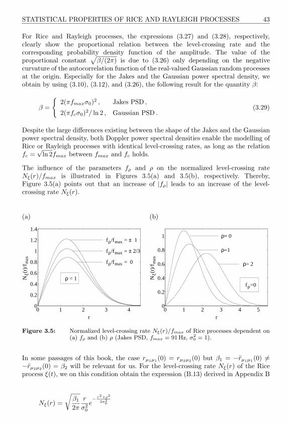
STATISTICAL PROPERTIES OF RICE AND RAYLEIGH PROCESSES 43
For Rice and Rayleigh processes, the expressions (3.27) and (3.28), respectively,clearly show the proportional relation between the level-crossing rate and thecorresponding probability density function of the amplitude. The value of theproportional constant
√β/(2π) is due to (3.26) only depending on the negative
curvature of the autocorrelation function of the real-valued Gaussian random processesat the origin. Especially for the Jakes and the Gaussian power spectral density, weobtain by using (3.10), (3.12), and (3.26), the following result for the quantity β:
β =
2(πfmaxσ0)2 , Jakes PSD ,
2(πfcσ0)2/ ln 2 , Gaussian PSD .(3.29)
Despite the large differences existing between the shape of the Jakes and the Gaussianpower spectral density, both Doppler power spectral densities enable the modelling ofRice or Rayleigh processes with identical level-crossing rates, as long as the relationfc =
√ln 2fmax between fmax and fc holds.
The influence of the parameters fρ and ρ on the normalized level-crossing rateNξ(r)/fmax is illustrated in Figures 3.5(a) and 3.5(b), respectively. Thereby,Figure 3.5(a) points out that an increase of |fρ| leads to an increase of the level-crossing rate Nξ(r).
(a)
0 1 2 3 40
0.2
0.4
0.6
0.8
1
1.2
1.4
r
Nξ(
r)/f
max
fρ/fmax = ± 1
fρ/fmax = ± 2/3
fρ/fmax = 0
ρ = 1
(b)
0 1 2 3 4 50
0.2
0.4
0.6
0.8
1
r
Nξ(
r)/f
max
ρ= 0
ρ=1
ρ= 2
fρ=0
Figure 3.5: Normalized level-crossing rate Nξ(r)/fmax of Rice processes dependent on(a) fρ and (b) ρ (Jakes PSD, fmax = 91Hz, σ2
0 = 1).
In some passages of this book, the case rµ1µ1(0) = rµ2µ2(0) but β1 = −rµ1µ1(0) 6=−rµ2µ2(0) = β2 will be relevant for us. For the level-crossing rate Nξ(r) of the Riceprocess ξ(t), we on this condition obtain the expression (B.13) derived in Appendix B
Nξ(r) =
√β1
2π
r
σ20
e− r2+ρ2
2σ20

44 RAYLEIGH AND RICE PROCESSES AS REFERENCE MODELS
· 1π
π∫
0
cosh[
rρ
σ20
cos(θ − θρ)] √
1− k2 sin2 θ dθ , r ≥ 0 , (3.30)
where k =√
(β1 − β2)/β1, β1 ≥ β2. In this case, the level-crossing rate is in generalno longer proportional to the probability density function of the Rice distribution.
On the other hand, we again obtain the usual relations for Rayleigh processes ζ(t),whose level-crossing rate Nζ(r) is obtained from (3.30) by taking the limit ρ → 0, i.e.,
Nζ(r) =
√β1
2π· r
σ20
e− r2
2σ20 · 1
π
∫ π
0
√1− k2 sin2 θ dθ , r ≥ 0 . (3.31)
In the literature (see [Gra81, vol. II, eq. (8.111.3)]), the above integral with the form
E(ϕ, k) =
ϕ∫
0
√1− k2 sin2 θ dθ (3.32)
is known as elliptic integral of the second kind. The parameter k denotes the modulusof the integral. For ϕ = π/2 these integrals are also called the complete elliptic integralsof the second kind and we write E(k) = E(π
2 , k).
Let us use (3.19). Then, the level-crossing rate for Rayleigh processes can now be putin the following form
Nζ(r) =
√β1
2πpζ(r) · 2
πE(k) , r ≥ 0 , (3.33)
where for the modulus k again k =√
(β1 − β2)/β1 , β1 ≥ β2, holds. Thus, forRayleigh processes the level-crossing rate is proportional to the probability densityfunction of the amplitude even for the case β1 6= β2. The proportional constant is herenot only determined by β1, but also by the difference β1 − β2.
Furthermore, we are interested in the level-crossing rate Nζ(r) for the case that therelative deviation between β1 and β2 is very small. Therefore, let us assume that apositive number ε = β1 − β2 ≥ 0 with ε/β1 << 1 exists, so that
k =
√β1 − β2
β1=
√ε
β1<< 1 (3.34)
holds. Next, we make use of the relation (see [Gra81, vol. II, eq. (8.114.1)])
E(k) =π
2F
(−1
2,12; 1; k2
)
=π
2
1−
∞∑n=1
[1 · 3 · 5 · . . . · (2n− 1)
2n n!
]2k2n
2n− 1
, (3.35)

STATISTICAL PROPERTIES OF RICE AND RAYLEIGH PROCESSES 45
where F (., .; .; .) is called the hypergeometric function. By using the first two terms ofthe series for E(k), we obtain the following approximation formula
E(k) ≈ π
2
(1− k2
4
)≈ π
2
√1− k2
2, k << 1 . (3.36)
Now, substituting (3.34) into (3.36) and taking (3.33) into account, leads for the level-crossing rate Nζ(r) to the approximation
Nζ(r) ≈√
β
2π· pζ(r) , r ≥ 0 , (3.37)
which is valid for the case (β1 − β2)/β1 << 1, where in (3.37) the quantity β is givenby β = (β1 + β2)/2. Hence, (3.28) approximately keeps its validity if the relativedeviations between β1 and β2 are small and if β = β1 = β2 is in (3.28) replaced bythe arithmetical mean β = (β1 + β2)/2.
The average duration of fades, i.e., the average length of the duration while the channelamplitude is below a level r, is defined by the quotient of the distribution function ofthe channel amplitude over the level-crossing rate, according to (2.63). The probabilitydensity function and the level-crossing rate of Rice and Rayleigh processes consideredhere have already been analysed in detail, so that the analysis of the correspondingaverage duration of fades can easily be carried out. For completeness, however, theresulting relations will again be given here. For Rice processes with fρ = 0 andRayleigh processes, we obtain for the average duration of fades [see also (2.66) and(2.65), respectively]:
Tξ−(r) =Fξ−(r)Nξ(r)
=√
2π
β· e
r2
2σ20
r I0
(rρσ20
)r∫
0
x e− x2
2σ20 I0
(xρ
σ20
)dx , r ≥ 0 , (3.38a)
and
Tζ−(r) =Fζ−(r)Nζ(r)
=√
2π
β· σ2
0
r
(e
r2
2σ20 − 1
), r ≥ 0 , (3.38b)
respectively, where Fξ−(r) = P (ξ(t) ≤ r) and Fζ−(r) = P (ζ(t) ≤ r) denote thecumulative distribution function of the Rice and Rayleigh process, respectively.
In channel modelling, we are especially interested in the behaviour of the averageduration of fades at low levels r. We therefore wish to analyse this case separately.For this purpose, let r << 1, so that for moderate Rice factors, we may writerρ/σ2
0 << 1 and, consequently, both I0(rρ/σ20) and I0(xρ/σ2
0) can be approximatedby one in (3.38a), since the independent variable x is within the relevant interval [0, r].After a series expansion of the integrand in (3.38a), Tξ (r) can be given in a closedform. By this means, it quickly turns out that for low levels r, Tξ (r) converges toTζ (r) given by (3.38b). Furthermore, the relation(3.38b) can be simplified by usingex ≈ 1 + x (x << 1), so that we finally obtain the approximations
Tξ−(r) ≈ Tζ−(r) ≈ r
√π
2β, r << 1 , (3.39)
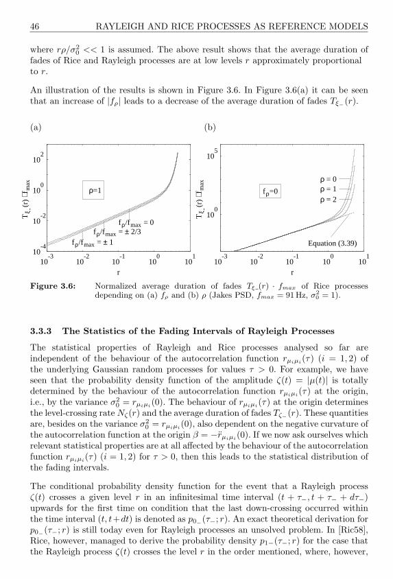
46 RAYLEIGH AND RICE PROCESSES AS REFERENCE MODELS
where rρ/σ20 << 1 is assumed. The above result shows that the average duration of
fades of Rice and Rayleigh processes are at low levels r approximately proportionalto r.
An illustration of the results is shown in Figure 3.6. In Figure 3.6(a) it can be seenthat an increase of |fρ| leads to a decrease of the average duration of fades Tξ−(r).
(a)
10-3
10-2
10-1
100
101
10-4
10-2
100
102
r
Tξ -
(r)
⋅ fm
ax
ρ=1
fρ/fmax = ± 1fρ/fmax = ± 2/3
fρ/fmax = 0
(b)
10-3
10-2
10-1
100
101
100
105
r
Tξ -
(r)
⋅ fm
ax
fρ=0
ρ = 0ρ = 1ρ = 2
Equation (3.39)
Figure 3.6: Normalized average duration of fades Tξ (r) · fmax of Rice processesdepending on (a) fρ and (b) ρ (Jakes PSD, fmax = 91Hz, σ2
0 = 1).
3.3.3 The Statistics of the Fading Intervals of Rayleigh Processes
The statistical properties of Rayleigh and Rice processes analysed so far areindependent of the behaviour of the autocorrelation function rµiµi(τ) (i = 1, 2) ofthe underlying Gaussian random processes for values τ > 0. For example, we haveseen that the probability density function of the amplitude ζ(t) = |µ(t)| is totallydetermined by the behaviour of the autocorrelation function rµiµi(τ) at the origin,i.e., by the variance σ2
0 = rµiµi(0). The behaviour of rµiµi(τ) at the origin determinesthe level-crossing rate Nζ(r) and the average duration of fades Tζ−(r). These quantitiesare, besides on the variance σ2
0 = rµiµi(0), also dependent on the negative curvature ofthe autocorrelation function at the origin β = −rµiµi(0). If we now ask ourselves whichrelevant statistical properties are at all affected by the behaviour of the autocorrelationfunction rµiµi(τ) (i = 1, 2) for τ > 0, then this leads to the statistical distribution ofthe fading intervals.
The conditional probability density function for the event that a Rayleigh processζ(t) crosses a given level r in an infinitesimal time interval (t + τ−, t + τ− + dτ−)upwards for the first time on condition that the last down-crossing occurred withinthe time interval (t, t+dt) is denoted as p0−(τ−; r). An exact theoretical derivation forp0−(τ−; r) is still today even for Rayleigh processes an unsolved problem. In [Ric58],Rice, however, managed to derive the probability density p1−(τ−; r) for the case thatthe Rayleigh process ζ(t) crosses the level r in the order mentioned, where, however,
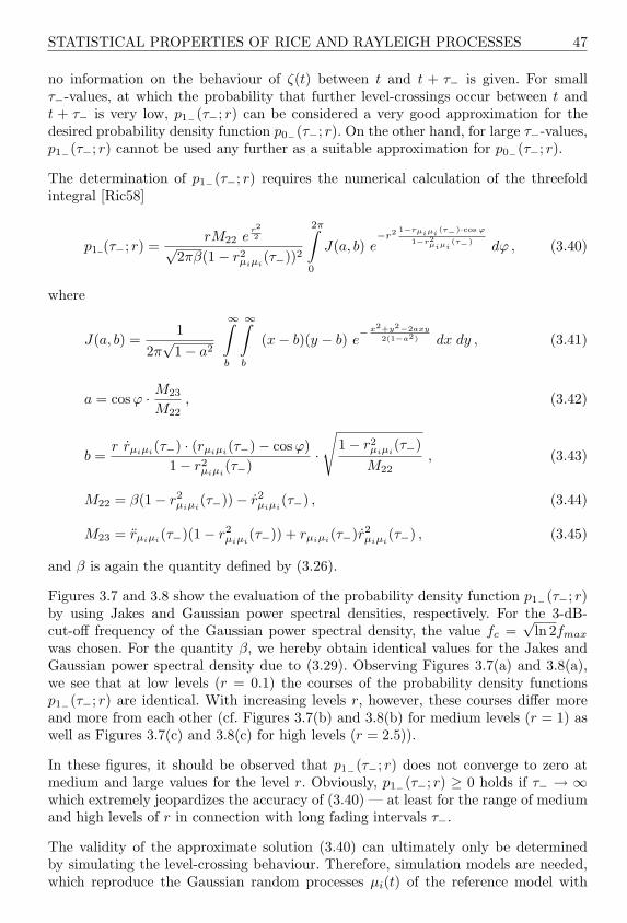
STATISTICAL PROPERTIES OF RICE AND RAYLEIGH PROCESSES 47
no information on the behaviour of ζ(t) between t and t + τ− is given. For smallτ−-values, at which the probability that further level-crossings occur between t andt + τ− is very low, p1−(τ−; r) can be considered a very good approximation for thedesired probability density function p0−(τ−; r). On the other hand, for large τ−-values,p1−(τ−; r) cannot be used any further as a suitable approximation for p0−(τ−; r).
The determination of p1−(τ−; r) requires the numerical calculation of the threefoldintegral [Ric58]
p1 (τ−; r) =rM22 e
r22√
2πβ(1− r2µiµi
(τ−))2
2π∫
0
J(a, b) e−r2 1−rµiµi
(τ−)·cos ϕ
1−r2µiµi
(τ−) dϕ , (3.40)
where
J(a, b) =1
2π√
1− a2
∞∫
b
∞∫
b
(x− b)(y − b) e− x2+y2−2axy
2(1−a2) dx dy , (3.41)
a = cos ϕ · M23
M22, (3.42)
b =r rµiµi(τ−) · (rµiµi(τ−)− cos ϕ)
1− r2µiµi
(τ−)·√
1− r2µiµi
(τ−)M22
, (3.43)
M22 = β(1− r2µiµi
(τ−))− r2µiµi
(τ−) , (3.44)
M23 = rµiµi(τ−)(1− r2µiµi
(τ−)) + rµiµi(τ−)r2µiµi
(τ−) , (3.45)
and β is again the quantity defined by (3.26).
Figures 3.7 and 3.8 show the evaluation of the probability density function p1−(τ−; r)by using Jakes and Gaussian power spectral densities, respectively. For the 3-dB-cut-off frequency of the Gaussian power spectral density, the value fc =
√ln 2fmax
was chosen. For the quantity β, we hereby obtain identical values for the Jakes andGaussian power spectral density due to (3.29). Observing Figures 3.7(a) and 3.8(a),we see that at low levels (r = 0.1) the courses of the probability density functionsp1−(τ−; r) are identical. With increasing levels r, however, these courses differ moreand more from each other (cf. Figures 3.7(b) and 3.8(b) for medium levels (r = 1) aswell as Figures 3.7(c) and 3.8(c) for high levels (r = 2.5)).
In these figures, it should be observed that p1−(τ−; r) does not converge to zero atmedium and large values for the level r. Obviously, p1−(τ−; r) ≥ 0 holds if τ− → ∞which extremely jeopardizes the accuracy of (3.40) — at least for the range of mediumand high levels of r in connection with long fading intervals τ−.
The validity of the approximate solution (3.40) can ultimately only be determinedby simulating the level-crossing behaviour. Therefore, simulation models are needed,which reproduce the Gaussian random processes µi(t) of the reference model with

48 RAYLEIGH AND RICE PROCESSES AS REFERENCE MODELS
(a) Low level:r = 0.1
0 0.5 1 1.5 20
500
1000
1500
2000
2500
3000
3500
τ- (ms)
p1
-(τ-;
r)
τ90 τ95 τ99
Equation (3.40)Equation (3.47)Equation (3.52)
(b) Medium level:r = 1
0 5 10 15 200
50
100
150
200
250
300
350
τ- (ms)
p1
-(τ-;
r)
Non-convergent
(c) High level:r = 2.5
0 50 100 150 2000
20
40
60
80
100
τ- (ms)
p1
-(τ-;
r)
Non-convergent
Figure 3.7: The probability density function p1−(τ−; r) when using the Jakes power
spectral density (fmax = 91Hz, σ20 = 1).
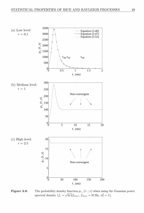
STATISTICAL PROPERTIES OF RICE AND RAYLEIGH PROCESSES 49
(a) Low level:r = 0.1
0 0.5 1 1.5 20
500
1000
1500
2000
2500
3000
3500
τ- (ms)
p1
-(τ-;
r)
τ90 τ95 τ99
Equation (3.40)Equation (3.47)Equation (3.52)
(b) Medium level:r = 1
0 5 10 15 200
50
100
150
200
250
300
τ- (ms)
p1
-(τ-;
r)
Non-convergent
(c) High level:r = 2.5
0 50 100 150 2000
5
10
15
20
τ- (ms)
p1
-(τ-;
r)
Non-convergent
Figure 3.8: The probability density function p1−(τ−; r) when using the Gaussian power
spectral density (fc =√
ln 2fmax, fmax = 91 Hz, σ20 = 1).

50 RAYLEIGH AND RICE PROCESSES AS REFERENCE MODELS
respect to the probability density function pµi(x) and the autocorrelation functionrµiµi
(τ) extremely accurate. We will return to this subject in Section 5.3. For ourpurposes, at first only the discovery that the probability density function of the fadingintervals of Rayleigh channels at medium and high levels r decisively depends on thebehaviour of the autocorrelation function rµiµi
(τ) for τ ≥ 0 is of importance.
In the following, we will analyse the statistics of the deep fades. The knowledge of thestatistics of the deep fades is of great importance in mobile radio communications,since the bit and symbol error probability are mainly determined by the occurrence ofdeep fades. Hence, let r << 1. In this case, the duration of fades τ− are short. Thus,the probability that further level-crossings occur between t and t+ τ− is very low, andthe approximation p0−(τ−; r) ≈ p1−(τ−; r) is very good. In [Ric58] it is shown thatthe probability density function (3.40) converges to
p1−(τ−; r) = − 1Tζ−(r)
d
du
[2u
I1(z) e−z
](3.46)
as r → 0, where z = 2/(πu2) and u = τ−/Tζ−(r) hold. After some algebraicmanipulations, we find the following expression for this
p1−(τ−; r) =2πz2e−z
Tζ−(r)
[I0(z)−
(1 +
12z
)I1(z)
], r → 0 , (3.47)
where z = 2[Tζ−(r)/τ−
]2/π. Considering (3.46) or (3.47), we see that, besides on the
level r, p1−(τ−; r) only depends on the average duration of fades Tζ−(r) and, hence, onσ2
0 = rµiµi(0) and β = −rµiµi(0). Consequently, the probability density of the fadingintervals at low levels (r << 1) is independent of the shape of the autocorrelationfunction rµiµi(τ) for τ > 0. The numerical evaluation of the probability densityfunction (3.47) for the level r = 0.1 is also depicted in Figures 3.7(a) and 3.8(a).These figures clearly show that the deviations between (3.40) and (3.47) are negligiblefor low levels r.
In the limits τ− → 0 and τ− → ∞, (3.47) converges to p1−(0; r) = p1−(∞; r) = 0.Finally, it should be mentioned that by using (3.47) one finds – after a short side-calculation – the following result for the expected value of the fading intervals τ−
Eτ− =
∞∫
0
τ− p1−(τ−; r) dτ− = Tζ−(r) . (3.48)
With τq, we will in the following denote the time interval of the duration of fadeswhich includes q per cent of all fading intervals. Thus, by τq the lower bound of theintegral
∞∫
τq
p0−(τ−; r) dτ− = 1− q
100(3.49)
is determined. The knowledge of the quantities τ90, τ95, and τ99 is of great importanceto the (optimal) design of the interleaver/deinterleaver as well as for the channel

STATISTICAL PROPERTIES OF RICE AND RAYLEIGH PROCESSES 51
coder/decoder. With the approximation p0−(τ−; r) ≈ p1−(τ−; r), we are now able toderive an approximate solution for τq in an explicit form. We at first proceed bydeveloping (3.47) into a power series, where we make use of the series expansions[Abr72, eq. (4.2.1)]
e−z =∞∑
n=0
(−z)n
n!(3.50)
and [Abr72, eq. (9.6.10)]
Iν(z) =(z
2
)ν ∞∑n=0
(z2/4)n
n! Γ(ν + n + 1), ν = 0, 1, 2, . . . (3.51)
In the latter expression Γ(·) denotes the gamma function.3 Terminating the resultingseries after the second term, leads for the right-sided tail of the distribution p1−(τ−; r)to the approximation usable for our purposes
p1−(τ−; r) ≈ πz2
2(3− 5z)/Tζ−(r) , (3.52)
where z again represents z = 2[Tζ−(r)/τ−
]2/π. If we now replace the probability
density p0−(τ−; r) in (3.49) by (3.52), then an explicit expression for the quantityτq = τq(r) can be derived from the result of the integration.
Finally, we obtain the approximation valid for 75 ≤ q ≤ 100 [Pae96e]
τq(r) ≈Tζ−(r)
π4 [1−√
1− 4(1− q100 )] 1
3, r << 1 . (3.53)
This equation clearly shows that the quantity τq(r) is at deep fades proportional tothe average duration of fades. Especially for τ90(r), τ95(r), and τ99(r), we obtain from(3.53):
τ90(r) ≈ 1.78 · Tζ−(r) , (3.54)τ95(r) ≈ 2.29 · Tζ−(r) , (3.55)τ99(r) ≈ 3.98 · Tζ−(r) . (3.56)
Further simplifications are possible if we approximate the average duration of fadesTζ−(r) for r << 1 by Tζ−(r) ≈ r
√π/(2β) [cf. (3.39)]. If β is in this relation now
replaced by the formula (3.29) found for the Jakes and Gaussian power spectral density,then we obtain, e.g., for the quantity τ90(r) the approximation
τ90(r) ≈
r
2 σ0 fmax, Jakes PSD ,
r√
ln 22 σ0 fc
, Gaussian PSD ,
(3.57)
3 According to Euler the gamma function Γ(x) is defined for real numbers x > 0 by Γ(x) :=R∞0 e−t tx−1 dt . If x is a natural number, then Γ(x) = (x− 1)! holds.

52 RAYLEIGH AND RICE PROCESSES AS REFERENCE MODELS
which is valid for all r << 1. By means of this result, we see that the quantityτ90(r) and, hence, the general quantity τq(r) (75 ≤ q ≤ 100) are proportional to rand reciprocally proportional to fmax or fc for low levels r. Hereby, it is of majorimportance that the exact form of the power spectral density of the complex Gaussianrandom process, which generates the Rayleigh process, does not have any influenceon the behaviour of τq(r). Hence, for the Jakes and the Gaussian power spectraldensity, we again obtain identical values for τq(r) by choosing fc =
√ln 2 fmax.
Therefore, one may also compare Figures 3.7(a) and 3.8(a), where the approximation(3.52) and the quantities τ90(r), τ95(r), and τ99(r) [see (3.54)–(3.56)] derived from thatare illustrated. It should be noted that at the level r = 0.1, the relative deviationsof the approximations (3.54)–(3.56) from the corresponding quantities τq(r), whichwere calculated over (3.49) in a numerical way, are less than one per thousand. Thevalidity of all these approximate solutions for τq(r) can again ultimately only bejudged by simulating the level-crossing behaviour. In Section 5.3, we will see thatthe approximations introduced in this section match the simulation results obtainedthere quite well.
In [Wol83a], computer simulations of probability density functions p0−(τ−; r) werealso performed for Rice processes. Thereby, it has turned out that a Rice processhas practically the same probability density function of the fading intervals as thecorresponding Rayleigh process. These results are at least for low levels not surprisingany more, because from (3.47) it follows that p1−(τ−; r) merely depends on Tζ−(r),and on the other hand, we have seen in Subsection 3.3.2 that Tξ−(r) ≈ Tζ−(r) holdsif r << 1 and rρ/σ2
0 << 1. The analytical approximations obtained for Rayleighprocesses for p0−(τ−; r) and τq(r) can in such cases be directly taken over for Riceprocesses.
At this point it should be mentioned that the calculation of the probability densityfunction of fading intervals carried out by Rice [Ric58] caused various further researchactivities in this field (e.g., [McF56, McF58, Lon62, Rai65, Bre70]). They followed thegoal of deriving new and more precise approximations than the approximate solutions(3.40) given by Rice. The mathematical treatment of the so-called level-crossingproblem is even for Rayleigh channels connected with considerable difficulties and anexact general solution is still to be found. Special attention in this field should be paidto the works [Bre78, Mun82, Mun83, Wol83a, Wol83b, Mun86, Tez87] carried out atthe Institute for Applied Physics of Frankfurt University, led by Prof. Wolf. In [Mun82],data have been reported about a 4-state model which gives a valid approximation forthe probability density p0−(τ−; r) over a much greater region than (3.40) [Wol83a]. Theobtained approximate solutions could again be noticeably improved by extending the4-state model to 6- and 8-state models [Mun83, Wol83b, Mun86, Tez87]. However,investigations on generalized Gaussian random processes, the so-called sphericalinvariant stochastic processes [Bre78], have shown [Bre89] that the 4- and 6-statemodels in this process class — especially for negative levels — often do not achievesatisfying results, whereas the approximation suggested in [Bre70] does quite well. Inspite of all the progress in this field, the expenditure of mathematical and numericalcalculation is considerable. Moreover, the reliability of all theoretically obtainedapproximations is not guaranteed from the start, so that we cannot get by without an

STATISTICAL PROPERTIES OF RICE AND RAYLEIGH PROCESSES 53
experimental verification of the results.
From this point of view, it seems more sensible to give up the lavish numericalcalculations and instead only carry out simulations on (however precisely) generatedsample processes [Bre89]. This background will be taken into consideration in thefollowing two chapters, where we will introduce and analyse methods for the efficientrealization of highly precise simulation models for the generation of sample processes.
4
INTRODUCTION TO THETHEORY OF DETERMINISTICPROCESSES
All channel models studied in the sequel of this book are based on the use of at least tworeal-valued coloured Gaussian random processes. In the previous chapter, for example,we have seen that the modelling of the classical Rayleigh or Rice processes requiresthe realization of two real-valued coloured Gaussian random processes. Whereas for aSuzuki process [Suz77], which is defined by the product process of a Rayleigh processand a lognormal process, three real-valued coloured Gaussian random processes areneeded. In connection with digital data transmission over land mobile radio channels,we often refer to such processes (Rayleigh, Rice, Suzuki) as appropriate stochasticmodels in order to describe the random amplitude fluctuations of the received signal inthe equivalent complex baseband. Mobile radio channels, whose statistical amplitudebehaviour can be described by Rayleigh, Rice or Suzuki processes, consequentlywill be denoted as Rayleigh, Rice or Suzuki channels. These models can be classedinto the group of frequency-nonselective channels [Pro95]. A further example can begiven by the modelling of frequency-selective channels [Pro95] using finite impulseresponse (FIR) filters with L time-variant complex-valued coefficients. This requiresthe realization of 2L real-valued coloured Gaussian random processes. With the help ofthese few examples, it already becomes clear that the development of efficient methodsfor the realization of coloured Gaussian random processes is of the utmost importancein the modelling of both frequency-nonselective and frequency-selective mobile radiochannels.
For the solution of this problem, we will introduce in this chapter a fundamentalmethod which is based on a superposition of a finite number of harmonic functions.The principle of this procedure is based on an approach of Rice [Ric44, Ric45]. InSection 4.1, we will first explain the principle of deterministic channel modelling.The following Section 4.2 deals with elementary properties of deterministic processessuch as the autocorrelation function, power spectral density, Doppler spread, etc. Thestatistical properties of these processes are the subject of the discussions in Section 4.3.In this connection, we will also introduce suitable quality criteria, on the basis of whicha fair assessment of the performance for all design methods, which are introduced laterin Chapter 5, can be carried out. The application of these criteria allows us to state

56 INTRODUCTION TO THE THEORY OF DETERMINISTIC PROCESSES
some rules for certain design methods. On the other hand, also the problems occurringwhen less suitable methods are used can be made clear.
4.1 PRINCIPLE OF DETERMINISTIC CHANNEL MODELLING
In the literature, one essentially finds two fundamental methods for the modelling ofcoloured Gaussian random processes: the filter method and the Rice method.
When using the filter method, as shown in Figure 4.1(a), white Gaussian noise (WGN)νi(t) is given to the input of a linear time-invariant filter, whose transfer functionis denoted by Hi(f). In the following, we assume that the filter is ideal, i.e., thetransfer function Hi(f) can be fitted to any given frequency response with arbitraryprecision. If νi(t) ∼ N(0, 1), then we have a zero-mean stochastic Gaussian randomprocess µi(t) at the filter output, where according (2.52e, f) the power spectral densitySµiµi(f) of µi(t) matches the square of the absolute value of the transfer function, i.e.,Sµiµi
(f) = |Hi(f)|2. Hence, by filtering of white Gaussian noise νi(t), we obtain acoloured Gaussian random process µi(t).
The principle of the Rice method [Ric44, Ric45] is illustrated in Figure 4.1(b). It isbased on a superposition of an infinite number of weighted harmonic functions withequidistant frequencies and random phases. According to this principle, a stochasticGaussian process µi(t) can be described mathematically as
µi(t) = limNi→∞
Ni∑n=1
ci,n cos (2πfi,nt + θi,n) , (4.1)
where
ci,n = 2√
∆fiSµiµi(fi,n) , (4.2a)
fi,n = n ·∆fi . (4.2b)
The phases θi,n (n = 1, 2, . . . , Ni) are random variables, which are uniformlydistributed in the interval (0, 2π], and the quantity ∆fi is here chosen in such a waythat (4.2b) covers the whole relevant frequency range, where it is furthermore assumedthat the following property holds: ∆fi → 0 as Ni →∞.
As we know, a Gaussian random process is completely characterized by its meanvalue and its colour, which can be described either by the power spectral densityor, alternatively, by the autocorrelation function. According to Rice [Ric44, Ric45],the expression (4.1) represents a zero-mean Gaussian random process with the powerspectral density Sµiµi(f). Consequently, the analytical models shown in Figures 4.1(a)and 4.1(b) are equivalent, i.e., the two introduced methods — the filter method and theRice method — result in identical stochastic processes. For both methods, however, oneshould take into account that these processes are not exactly realizable. When usingthe filter method, an exact realization is prevented by the assumption that the filtershould be ideal. Strictly speaking, the input signal of the filter — the white Gaussiannoise — can also not be realized exactly. When using the Rice method, a realization is

PRINCIPLE OF DETERMINISTIC CHANNEL MODELLING 57
(a)
(t) ~ N(0,1)i
WGN
ν
i
µ i (t)H (f)
(b)
+
+
+f
πcos(2 f i,1
∞
i,1 θc
c
i,1
i,2
)
πcos(2 f i,2 t
t
i,2 θ )
c
πcos(2 t θ )
µ i (t)
i,
i,
∞
∞ i,
Figure 4.1: Stochastic reference models for coloured Gaussian random processes µi(t):(a) filter method and (b) Rice method.
impossible because an infinite number of harmonic functions Ni is not implementableon a computer or on a hardware platform. Hence, for a coloured Gaussian randomprocess, the filter method and the Rice method only result in a stochastic analytical(ideal) model, which will be considered as reference model throughout the book.
As is well known, when using the filter method, the use of non-ideal but thereforerealizable filters makes the realization of stochastic simulation models possible.Here, depending on the extent of the realization expenditure, one should take intoconsideration that the statistics of the filter output signal deviates more or less fromthat of the desired ideal Gaussian random process. In numerous publications (e.g.,[Bre86a, Sch89, Fec93a, Mar94b, Lau94]), this method has been applied in order todesign simulation models for mobile radio channels. In Section 8.5, we will return tothe filter method once more. In the following sections, however, we will first presenta detailed analysis of the Rice method. It should be noted that many of the resultsfound for the Rice method can be applied directly to the filter method.
If the Rice method is applied by using only a finite number of harmonic functions Ni,then we obtain a further stochastic process denoted by
µi(t) =Ni∑
n=1
ci,n cos(2πfi,nt + θi,n) , (4.3)
where we assume for the moment that the parameters ci,n and fi,n are still givenby (4.2a) and (4.2b), respectively, and θi,n are again uniformly distributed randomvariables. Now, this method can be applied to the realization of a simulation modelwhose general structure is shown in Figure 4.2(a). It is obvious that µi(t) → µi(t)holds as Ni → ∞. At this point, it should be emphasized that the simulation modelis still of stochastic nature, since the phases θi,n are uniformly distributed randomvariables for all n = 1, 2, . . . , Ni.
Only after the phases θi,n (n = 1, 2, . . . , Ni) are taken out of a random generatorwith a uniform distribution in the interval (0, 2π], the phases θi,n no longer representrandom variables but constant quantities, since they are now realizations (outcomes)of a random variable. Thus, in connection with (4.2a), (4.2b), and (4.3), it becomes

58 INTRODUCTION TO THE THEORY OF DETERMINISTIC PROCESSES
obvious that
µi(t) =Ni∑
n=1
ci,n cos(2πfi,nt + θi,n) (4.4)
is a deterministic process or a deterministic function. Hence, from the stochasticsimulation model shown in Figure 4.2(a), a deterministic simulation model follows,whose structure is presented in Figure 4.2(b) in its continuous-time form ofrepresentation. Note that in the limit Ni → ∞, the deterministic process µi(t) tendsto a sample function of the stochastic process µi(t).
(a)
+
+
+f
πcos(2 f i,1 i,1
^
θc
c
i,1
i,2
)
πcos(2 f i,2 t
t
i,2 θ )
ci,Ni
πcos(2 i,N t θ )i i,Ni
µ i (t)
(b)
+
+
+f
πcos(2 f i,1 i,1
(t)
θc
c
i,1
i,2
)
πcos(2 f i,2 t
t
i,2 θ )
ci,Ni
πcos(2 i,N t θ )i i,Ni
µ~ i
Figure 4.2: Simulation models for coloured Gaussian random processes: (a) stochasticsimulation model (random phases θi,n) and (b) deterministic simulationmodel (constant phases θi,n).
In Section 4.3 and Chapter 5, it will be shown that by choosing the parametersdescribing the deterministic process (4.4) appropriately, a very good approximationcan be achieved in such a way that the statistical properties of µi(t) are very close tothose of the underlying zero-mean coloured Gaussian random process µi(t). For thisreason, µi(t) will be called real deterministic Gaussian process and
µ(t) = µ1(t) + jµ2(t) (4.5)
will be named complex deterministic Gaussian process. With reference to (3.5), a so-called deterministic Rayleigh process
ζ(t) = |µ(t)| = |µ1(t) + jµ2(t)| . (4.6)
follows from the absolute value of (4.5). Logically, by taking the absolute value ofµρ(t) = µ(t) + m(t), a deterministic Rice process
ξ(t) = |µρ(t)| = |µ(t) + m(t)| (4.7)
can be introduced, where m(t) again describes the line-of-sight component of thereceived signal, as defined by (3.2). The resulting structure of the simulation modelfor deterministic Rice processes is shown in Figure 4.3.

ELEMENTARY PROPERTIES OF DETERMINISTIC PROCESSES 59
.
cos(2 π f + θ 1,11,1 t )
cos(2 + θπ f )t 1,21,2
cos(2 + θπ f t )1,N1 1,N1
ρf θρ2 π t +
ρf θρ2 π t +
m (t) =1
µ1
2
(t)~ µ1(t)~
ρ
~µρ(t)
ξ~(t)
µ~ρ2(t)µ~
2(t)c
c. .
.
c
c. .
.
c1,1
1,N1
1,2
c
ρ cos( . .
.)
ρ sin( )
cos(2 π f + θt
cos(2 + θπ f t
. . .
cos(2 + θπ f t
2,1
2,2
2,N
2,1
2,2
2,N2
2,1
2,2
2,N2
)
)
) m (t) =2
Figure 4.3: A deterministic simulation model for Rice processes.
The discrete-time simulation model, which is required for computer simulations, candirectly be obtained by substituting the time variable t with t = kTs, where Ts denotesthe sampling interval and k is an integer. To carry out computer simulations, onegenerally proceeds by determining the parameters of the simulation model ci,n, fi,n,and θi,n for n = 1, 2, . . . , Ni during the simulation set-up phase. During the simulationrun phase following this, all parameters are kept constant for the whole duration ofthe simulation.
Since for our purpose the deterministic processes are exclusively used for the modellingof the time-variant fading behaviour caused by the Doppler effect, we will in thefollowing call the parameters ci,n, fi,n, and θi,n describing the deterministic process(4.4) the Doppler coefficients, discrete Doppler frequencies, and Doppler phases,respectively.
One aim of this book is to present methods by which the model parameters(ci,n, fi,n, θi,n) can be determined in such a way that the statistical properties ofthe deterministic process µi(t) or µi(kT ) match those of the (ideal) stochastic processµi(t) as closely as possible. Of course, this aim is pursued under the boundary conditionthat the realization expenditure should be kept as low as possible. Here, the realizationexpenditure is mainly determined by the number of harmonic functions Ni. However,before turning to this topic, we will first of all present some fundamental propertiesof deterministic processes.
4.2 ELEMENTARY PROPERTIES OF DETERMINISTIC PROCESSES
The interpretation of µi(t) as a deterministic process, i.e., as a mapping of the form
µi : IR → IR , t 7→ µi(t) , (4.8)

60 INTRODUCTION TO THE THEORY OF DETERMINISTIC PROCESSES
enables us to derive for these kind of processes simple analytical closed-form solutionsfor most of the fundamental characteristic quantities like autocorrelation function,power spectral density, Doppler spread, etc.
First, a discussion of the terms introduced in Section 2.3 follows, where the definitionsof these terms are now applied to the deterministic processes µi(t) (i = 1, 2) definedby (4.4).
Mean value: Let µi(t) be a deterministic process with fi,n 6= 0 (n = 1, 2, . . . , Ni).Then, it follows from (2.69) that the mean value of µi(t) is given by
mµi= 0 . (4.9)
In the following, it is always assumed that fi,n 6= 0 holds for all n = 1, 2, . . . , Ni andi = 1, 2.
Mean power: Let µi(t) be a deterministic process. Then, it follows from (2.70) thatthe mean power of µi(t) is given by
σ2µi
=Ni∑
n=1
c2i,n
2. (4.10)
Obviously, the mean power σ2µi
depends on the Doppler coefficients ci,n but not onthe discrete Doppler frequencies fi,n and the Doppler phases θi,n.
Autocorrelation function: For the autocorrelation function of deterministicprocesses µi(t), the following closed-form expression follows from (2.71)
rµiµi(τ) =Ni∑
n=1
c2i,n
2cos(2πfi,nτ) . (4.11)
One should note that rµiµi(τ) depends on the Doppler coefficients ci,n and the discreteDoppler frequencies fi,n, but not on the Doppler phases θi,n. Note also that themean power σ2
µiis identical to the autocorrelation function rµiµi(τ) at τ = 0, i.e.,
σ2µi
= rµiµi(0).
Cross-correlation function: Let µ1(t) and µ2(t) be two deterministic processes.Then, it follows from (2.72) that the cross-correlation function of µ1(t) and µ2(t) canbe written as
rµ1µ2(τ) = 0 , if f1,n 6= ±f2,m , (4.12)
holds for all n = 1, 2, . . . , N1 and m = 1, 2, . . . , N2. This result shows that thedeterministic processes µ1(t) and µ2(t) are uncorrelated if the absolute values ofthe respective discrete Doppler frequencies are different from each other. However, iff1,n = ±f2,m holds for some or all pairs of (n,m), then µ1(t) and µ2(t) are correlated,and we obtain the following expression for the cross-correlation function
rµ1µ2(τ) =N∑
n=1f1,n=±f2,m
c1,nc2,m
2cos(2πf1,nτ − θ1,n ± θ2,m) , (4.13)

ELEMENTARY PROPERTIES OF DETERMINISTIC PROCESSES 61
where N denotes the largest number of N1 and N2, i.e., N = maxN1, N2. Oneshould note that in this case rµ1µ2(τ) also depends on the Doppler phases θi,n.The cross-correlation function rµ2µ1(τ) can be obtained from the relation rµ2µ1(τ) =r∗µ1µ2
(−τ) = rµ1µ2(−τ).
Power spectral density: Let µi(t) be a deterministic process. Then, it followsfrom (2.73) in connection with (4.11) that the power spectral density of µi(t) canbe expressed as
Sµiµi(f) =Ni∑
n=1
c2i,n
4[δ(f − fi,n) + δ(f + fi,n)] . (4.14)
Hence, the power spectral density of µi(t) is a symmetrical line spectrum, i.e.,Sµiµi
(f) = Sµiµi(−f). The spectral lines are located at the discrete points f = ±fi,n
and weighted by the factor c2i,n/4.
Cross-power spectral density: Let µ1(t) and µ2(t) be two deterministic processes.Then, it follows from (2.74) with (4.12) and (4.13) that the cross-power spectral densityof µ1(t) and µ2(t) is given by
Sµ1µ2(f) = 0 , if f1,n 6= ±f2,m , (4.15)
and
Sµ1µ2(f) =N∑
n=1f1,n=±f2,m
c1,nc2,m
4[δ(f − f1,n) · e−j(θ1,n∓θ2,m)
+ δ(f + f1,n) · ej(θ1,n∓θ2,m)] (4.16)
for all n = 1, 2, . . . , N1 and m = 1, 2, . . . , N2, where N = maxN1, N2. Thecross-power spectral density Sµ2µ1(f) can directly be obtained from the relationSµ2µ1(f) = S∗µ1µ2
(f).
Average Doppler shift: Let µi(t) be a deterministic process with the power spectraldensity Sµiµi(f). Then, by analogy to (3.13a), the average Doppler shift B
(1)µiµi of µi(t)
is defined by
B(1)µiµi
:=
∫∞−∞ f Sµiµi(f) df∫∞−∞ Sµiµi(f) df
=1
2πj·
˙rµiµi(0)rµiµi(0)
. (4.17)
Due to the symmetry property Sµiµi(f) = Sµiµi(−f), it follows that
B(1)µiµi
= 0 . (4.18)

62 INTRODUCTION TO THE THEORY OF DETERMINISTIC PROCESSES
On condition that the real and imaginary parts are uncorrelated, one analogouslyobtains for complex deterministic processes µ(t) = µ1(t)+jµ2(t), the following relationbetween the average Doppler shifts of µ(t) and µi(t)
B(1)µµ = B(1)
µiµi= 0 , i = 1, 2 . (4.19)
By considering the relations (4.19) and (3.15a), it turns out that the average Dopplershift of the simulation model is identical to that of the reference model.
Doppler spread: Let µi(t) be a deterministic process with the power spectral densitySµiµi(f). Then, analogous to (3.13b), the Doppler spread B
(2)µiµi of µi(t) is defined by
B(2)µiµi
:=
√√√√∫∞−∞(f − B
(1)µiµi)2 Sµiµi(f) df∫∞
−∞ Sµiµi(f) df
=12π
√( ˙rµiµi(0)rµiµi(0)
)2
−¨rµiµi(0)rµiµi(0)
. (4.20)
Using (4.10) and (4.11), the last equation can be written as
B(2)µiµi
=
√βi
2πσµi
, (4.21)
where
βi = −¨rµiµi(0) = 2π2Ni∑
n=1
(ci,nfi,n)2 . (4.22)
The comparison of the equation (3.15b) with (4.21) shows that the Doppler spreadsB
(2)µiµi and B
(2)µiµi are always identical, if the Doppler coefficients ci,n and the discrete
Doppler frequencies fi,n are determined in such a way that σ2µi
= σ20 and βi = β hold.
(In particular, it is sufficient that the condition βi/σ20 = β/σ2
0 is fulfilled.)
Analogously, the Doppler spread B(2)µµ corresponding to the power spectral density
Sµµ(f) of the complex deterministic process µ(t) = µ1(t) + jµ2(t) can be determined.On condition that µ1(t) and µ2(t) are uncorrelated, the Doppler spread B
(2)µµ can be
expressed as
B(2)µµ =
√β
2πσµ, (4.23)
where σ2µ = σ2
µ1+ σ2
µ2> 0 and β = β1 + β2 > 0 hold. In Chapter 5, we will get
acquainted with methods for the design of deterministic processes µ1(t) and µ2(t)
STATISTICAL PROPERTIES OF DETERMINISTIC PROCESSES 63
having the properties σ2µ1
= σ2µ2
and β1 6= β2. Especially in this case, the Doppler
spread B(2)µµ can be calculated from the quadratic mean of B
(2)µ1µ1 and B
(2)µ2µ2 , i.e.,
B(2)µµ =
√√√√(B
(2)µ1µ1
)2
+(B
(2)µ2µ2
)2
2. (4.24)
Finally, it should be mentioned that if σ20 = σ2
µ1= σ2
µ2and β = β1 = β2 hold, then
we obtain the result
B(2)µµ = B(2)
µiµi=
√β
2πσ0, i = 1, 2 (4.25)
which is closely related to (3.15b). However, if the deviations between β1 and β2 aresmall, which is often the case, then the above expression is a very good approximationfor B
(2)µµ if β is replaced by β = β1 ≈ β2 there.
Periodicity: Let µi(t) be a deterministic process with arbitrary but nonzeroparameters ci,n, fi,n (and θi,n). If the greatest common divisor of the discrete Dopplerfrequencies
Fi = gcdfi,1, fi,2, . . . , fi,Ni 6= 0 (4.26)
exists, then µi(t) is periodic with the period Ti = 1/Fi, i.e., it holds µi(t+ Ti) = µi(t)and rµiµi(τ + Ti) = rµiµi(τ).
The proof of this theorem is relatively simple and will therefore be presented here onlybriefly. Since Fi is the greatest common divisor of fi,1, fi,2, . . . , fi,Ni , there are integersqi,n ∈ Z, so that fi,n = qi,n · Fi holds for all n = 1, 2, . . . , Ni and i = 1, 2. By puttingfi,n = qi,n · Fi = qi,n/Ti into (4.4) and (4.11), the validity of µi(t + Ti) = µi(t) andrµiµi(τ + Ti) = rµiµi(τ), respectively, can be proved directly.
4.3 STATISTICAL PROPERTIES OF DETERMINISTIC PROCESSES
Even though a discussion of the elementary properties of deterministic processescould be performed in the previous section without any problems, an analysis ofthe statistical properties first seems to be absurd, since statistical methods canmeaningfully be applied only on random variables and stochastic processes. But, onthe other hand, their application to deterministic processes (4.4) makes no sense. Inorder in this case to gain access to statistical quantities like the probability densityfunction, the level-crossing rate, and the average duration of fades, we will study thebehaviour of deterministic processes µi(t) at random time instants t. If nothing elseis explicitly mentioned, we will assume throughout this section that the time variablet is a random variable uniformly distributed within the interval IR. It should also benoted that both the time variable t and the Doppler phases θi,n are in the argument ofthe cosine functions of (4.4). Therefore, we could alternatively assume that the timet = t0 is a constant and the phases θi,n are uniformly distributed random variables.In both cases, however, we would obtain exactly the same results for the followingcomputations.

64 INTRODUCTION TO THE THEORY OF DETERMINISTIC PROCESSES
4.3.1 Probability Density Function of the Amplitude and the Phase
In this subsection, we will analyse the probability density function of the amplitudeand phase of complex deterministic processes µ(t) = µ1(t) + jµ2(t). It will be shownthat these probability density functions are completely determined by the number ofharmonic functions Ni and the choice of the Doppler coefficients ci,n.
Therefore, we first consider a single weighted harmonic elementary function of theform
µi,n(t) = ci,n cos(2πfi,nt + θi,n) , (4.27)
where ci,n, fi,n, and θi,n are arbitrary but constant parameters different from zero andt is a uniformly distributed random variable. Due to the periodicity of µi,n(t), it issufficient to restrict t on the open interval (0, f−1
i,n ) with fi,n 6= 0. Since t was assumedto be a uniformly distributed random variable, µi,n(t) is no longer a deterministicfunction but a random variable as well, whose probability density function is given by[Pap91, p. 98]
pµi,n(x) =
1π ci,n
√1− (x/ci,n)2
, |x| < ci,n ,
0 , |x| ≥ ci,n .
(4.28)
The expected value and the variance of µi,n(t) are equal to 0 and c2i,n/2, respectively. If
the random variables µi,n(t) are statistically independent, then the probability densityfunction pµi(x) of the sum
µi(t) = µi,1(t) + µi,2(t) + . . . + µi,Ni(t) (4.29)
can be obtained from the convolution of the individual probability density functionspµi,n(x), i.e.,
pµi(x) = pµi,1(x) ∗ pµi,2(x) ∗ . . . ∗ pµi,Ni(x). (4.30)
The expected value mµi and the variance σ2µi
of µi(t) are then given by
mµi = 0 (4.31a)
and
σ2µi
=Ni∑
n=1
c2i,n
2, (4.31b)
respectively. In principle, a rule for the computation of pµi(x) is given by (4.30). Butwith regard to the following procedure, it is more advantageous to apply the conceptof the characteristic function [see (2.14)]. After substituting (4.28) into (2.14), wefind the following expression for the characteristic function Ψµi,n(ν) of the randomvariables µi,n(t)
Ψµi,n(ν) = J0(2πci,nν) . (4.32)

STATISTICAL PROPERTIES OF DETERMINISTIC PROCESSES 65
The Ni-fold convolution (4.30) of the probability density functions pµi,n(x) can nowbe formulated as the Ni-fold product of the corresponding characteristic functionsΨµi,n
(ν)
Ψµi(ν) = Ψµi,1(ν) · Ψµi,2(ν) · . . . · Ψµi,Ni
(ν)
=Ni∏
n=1
J0(2πci,nν) . (4.33)
Concerning (4.30), an alternative expression for the probability density function pµi(x)
is then given by the inverse Fourier transform of Ψµi(−ν) = Ψµi(ν) [Ben48]
pµi(x) =∫ ∞
−∞Ψµi(ν) ej2πνx dν
= 2∫ ∞
0
[Ni∏
n=1
J0(2πci,nν)
]cos(2πνx) dν , i = 1, 2 . (4.34)
It is important to realize that the probability density function pµi(x) of µi(t) iscompletely determined by the number of harmonic functions Ni and by the Dopplercoefficients ci,n, whereas the discrete Doppler frequencies fi,n and the Doppler phasesθi,n have no influence on pµi(x).
In the following, let ci,n = σ0
√2/Ni and fi,n 6= 0 for all n = 1, 2, . . . , Ni and i = 1, 2.
Then, due to (4.31a) and (4.31b), the sum µi(t) introduced by (4.29) is a randomvariable with the expected value 0 and the variance
σ20 = σ2
µ1= σ2
µ2= σ2
0 . (4.35)
Regarding the central limit theorem [see (2.16)], it turns out that in the limit Ni →∞,the sum µi(t) tends to a normally distributed random variable having the expectedvalue 0 and the variance σ2
0 , i.e.,
limNi→∞
pµi(x) = pµi(x) =1√
2πσ0
e− x2
2σ20 . (4.36)
Hence, after computing the Fourier transform of this equation, one obtains thefollowing relation for the corresponding characteristic functions
limNi→∞
Ψµi(ν) = Ψµi(ν) = e−2(πσ0ν)2 , (4.37)
from which — by using (4.33) — the remarkable property
limNi→∞
[J0
(2πσ0
√2Ni
ν
)]Ni
= e−2(πσ0ν)2 (4.38)
finally follows.

66 INTRODUCTION TO THE THEORY OF DETERMINISTIC PROCESSES
Of course, for a finite number of harmonic functions Ni, we have to write: pµi(x) ≈pµi
(x) and Ψµi(ν) ≈ Ψµi
(ν). From Figure 4.4(a), illustrating pµi(x) according to
(4.34) with ci,n = σ0
√2/Ni for Ni ∈ 3, 5, 7,∞, it follows that in fact for Ni ≥ 7,
the approximation pµi(x) ≈ pµi(x) is astonishingly good. An appropriate measure ofthe approximation error is the mean-square error of the probability density functionpµi(x) defined by
Epµi:=
∫ ∞
−∞
(pµi(x)− pµi(x)
)2dx . (4.39)
The behaviour of the mean-square error Epµias a function of the number of harmonic
functions Ni is shown in Figure 4.4(b). This figure gives us an impression of how fastpµi
(x) converges to pµi(x) if Ni increases.
(a)
-4 -2 0 2 40
0.05
0.1
0.15
0.2
0.25
0.3
0.35
0.4
x
pµ
i(x)
Ni → ∞Ni = 7 Ni = 5 Ni = 3
(b)
0 10 20 30 40 500
0.5
1
1.5
2
2.5
3
3.5
4x 10⁻⁴
Ni
Ep
µi
Figure 4.4: (a) Probability density function pµi(x) for Ni ∈ 3, 5, 7,∞, (b) mean-square error Epµi
as a function of Ni. (Analytical results obtained with
ci,n = σ0
p2/Ni, σ2
0 = 1.)
Due to the good convergence behaviour that pµi(x) exhibits in conjunction withci,n = σ0
√2/Ni, we will occasionally assume (without causing too large an error)
that the identity
pµi(x) = pµi(x) , if Ni ≥ 7 , (4.40)
holds. In this case, many analytical problems, which are otherwise difficult toovercome, can then be solved in a relatively easy way.
Next, we will derive the probability density function of the absolute value and thephase of the complex-valued random variable
µρ(t) = µρ1(t) + jµρ2(t) , (4.41)
where µρi(t) = µi(t) + mi(t) (i = 1, 2). Here, concerning mi(t) according to (3.2), wehave to discuss the cases fρ = 0 and fρ 6= 0 separately.
STATISTICAL PROPERTIES OF DETERMINISTIC PROCESSES 67
At first, we consider the case fρ = 0. By doing this, mi becomes independent of therandom variable t. Consequently, mi is a constant whose probability density functionis described by pmi
(x) = δ(x−mi). Furthermore, it follows that the probability densityfunction pµρi
(x) of µρi(t) can now be expressed directly by using pµi(x) as
pµρi(x) = pµi(x) ∗ pmi(x)
= pµi(x−mi) . (4.42)
On the assumption that µρ1(t) and µρ2(t) are statistically independent, and, thus,f1,n 6= ±f2,m holds for all n = 1, 2, . . . , N1 and m = 1, 2, . . . , N2, the joint probabilitydensity function of the random variables µρ1(t) and µρ2(t), denoted by pµρ1µρ2
(x1, x2),can be expressed by
pµρ1µρ2(x1, x2) = pµρ1
(x1) · pµρ2(x2) . (4.43)
The transform of the Cartesian coordinates (x1, x2) into polar coordinates (z, θ) bymeans of
x1 = z cos θ , x2 = z sin θ (4.44a, b)
allows us to calculate the joint probability density function pξϑ(z, θ) of the amplitudeξ(t) = |µρ(t)| and the phase ϑ(t) = argµρ(t) as follows:
pξϑ(z, θ) = z pµρ1µρ2(z cos θ, z sin θ) (4.45a)
= z pµρ1(z cos θ) · pµρ2
(z sin θ) (4.45b)
= z pµ1(z cos θ − ρ cos θρ) · pµ2(z sin θ − ρ sin θρ) . (4.45c)
By using (2.40), we obtain the probability density functions of the amplitude pξ(z)and phase pϑ(θ) from the preceding equation in the form:
pξ(z) = z
∫ π
−π
pµ1(z cos θ − ρ cos θρ) · pµ2(z sin θ − ρ sin θρ) dθ , (4.46a)
pϑ(θ) =∫ ∞
0
z pµ1(z cos θ − ρ cos θρ) · pµ2(z sin θ − ρ sin θρ) dz . (4.46b)
Putting (4.34) into the last two expressions gives us the following threefold integralsfor the desired probability density functions:
pξ(z) = 4z
∫ π
−π
∫ ∞
0
[N1∏
n=1
J0(2πc1,nν1)
]g1(z, θ, ν1) dν1
·∫ ∞
0
[N2∏
m=1
J0(2πc2,mν2)
]g2(z, θ, ν2) dν2
dθ , (4.47a)

68 INTRODUCTION TO THE THEORY OF DETERMINISTIC PROCESSES
pϑ(θ) = 4∫ ∞
0
z
∫ ∞
0
[N1∏
n=1
J0(2πc1,nν1)
]g1(z, θ, ν1) dν1
·∫ ∞
0
[N2∏
m=1
J0(2πc2,mν2)
]g2(z, θ, ν2) dν2
dz , (4.47b)
where
g1(z, θ, ν1) = cos[2πν1(z cos θ − ρ cos θρ)] , (4.48a)
g2(z, θ, ν2) = cos[2πν2(z sin θ − ρ sin θρ)] . (4.48b)
Up to now, there are no further simplifications known for (4.47b), so that the remainingthree integrals must be solved numerically. In comparison with that, it is possible toreduce the threefold integral on the right-hand side of (4.47a) to a double integral bymaking use of the expression [Gra81, eq. (3.876.7)]
∫ 1
0
cos(2πν2z
√1− x2
)√
1− x2cos(2πν1zx) dx =
π
2J0
(2πz
√ν21 + ν2
2
). (4.49)
After some algebraic manipulations, we finally come to the result
pξ(z) = 4πz
∫ π
0
∫ ∞
0
[N1∏
n=1
J0(2πc1,ny cos θ)
][N2∏
m=1
J0(2πc2,my sin θ)
]
· J0(2πzy) cos[2πρy cos(θ − θρ)
]y dy dθ . (4.50)
The results of the numerical evaluations of pξ(z) and pϑ(θ) for the special caseci,n = σ0
√2/Ni (σ2
0 = 1) are illustrated in Figures 4.5(a) and 4.5(b), respectively.These illustrations again make clear that the approximation error can in general beignored if Ni ≥ 7.
We also want to show that if the Doppler coefficients ci,n are given by ci,n = σ0
√2/Ni,
then it follows in the limit Ni → ∞ from (4.47a) and (4.47b) the expected result:pξ(z) → pξ(z) and pϑ(θ) → pϑ(θ), respectively. To show this, we apply the property(4.38) enabling us to express (4.47a) and (4.47b) as
limNi→∞
pξ(z) = 4z
∫ π
−π
[∫ ∞
0
e−2(πσ0ν1)2
g1(z, θ, ν1) dν1
]
·[∫ ∞
0
e−2(πσ0ν2)2
g2(z, θ, ν2) dν2
]dθ (4.51)
and

STATISTICAL PROPERTIES OF DETERMINISTIC PROCESSES 69
(a)
0 1 2 3 40
0.1
0.2
0.3
0.4
0.5
0.6
z
pξ(
z)
ρ= 0 (Rayleigh)ρ=0.5ρ= 1
pξ(z) pξ(z)
(b)
-π 0 π 0
0.1
0.2
0.3
0.4
0.5
θ
pϑ
(θ)
ρ= 0 (Rayleigh)
ρ=0.5
ρ= 1 pϑ(θ) pϑ(θ)
Figure 4.5: (a) Probability density function pξ(z) of the amplitude ξ(t) = |µρ(t)| and
(b) probability density function pϑ(θ) of the phase ϑ(t) = argµρ(t) for
N1 = N2 = 7. (Analytical results obtained with ci,n = σ0
p2/Ni and
σ20 = 1.)
limNi→∞
pϑ(θ) = 4∫ z
0
z
[∫ ∞
0
e−2(πσ0ν1)2
g1(z, θ, ν1) dν1
]
·[∫ ∞
0
e−2(πσ0ν2)2
g2(z, θ, ν2) dν2
]dz , (4.52)
respectively. The use of the integral [Gra81, eq. (3.896.2)]∫ ∞
−∞e−q2x2
cos(px) dx =√
π
qe− p2
4q2 (4.53)
allows us to present the expressions (4.51) and (4.52) in the form
limNi→∞
pξ(z) =z
σ20
e− z2+ρ2
2σ20 · 1
π
∫ π
0
ezρ
σ20
cos(θ−θρ)dθ (4.54)
and
limNi→∞
pϑ(θ) =1
2πσ20
e− ρ2
2σ20
∫ ∞
0
z e− z2
2σ20+ zρ
σ20
cos(θ−θρ)dz , (4.55)
respectively. With the integral representation of the modified Bessel function of zerothorder [Abr72, eq. (9.6.16)]
I0(z) =1π
π∫
0
e ±z cos θ dθ , (4.56)
we can immediately identify (4.54) with the Rice distribution pξ(z) defined by (3.17),and from (4.55), using [Gra81, eq. (3.462.5)]
70 INTRODUCTION TO THE THEORY OF DETERMINISTIC PROCESSES
∞∫
0
z e−qz2−2pzdz =12q− p
2q
√π
qe
p2
q
[1− erf
(p√q
)],
| argp| < π
2, Re q > 0 , (4.57)
we obtain, after elementary calculations, the probability density function pϑ(θ) givenby (3.22).
Furthermore, we will pay attention to the general case, where fρ 6= 0. The line-of-sightcomponent m(t) = m1(t) + jm2(t) [see (3.2)] will now be considered as time-variantmean value, whose real and imaginary parts can consequently be described by theprobability density functions
pm1(x1 ; t) = δ(x1 −m1(t)) = δ(x1 − ρ cos(2πfρt + θρ)) (4.58)
and
pm2(x2 ; t) = δ(x2 −m2(t)) = δ(x2 − ρ sin(2πfρt + θρ)) , (4.59)
respectively. The derivation of the probability density functions pξ(z; t) and pϑ(θ; t)can be performed analogously to the case fρ = 0. For these functions, oneobtains expressions, which coincide with the right-hand side of (4.47a) and (4.47b),respectively, if there the functions gi(z, θ, νi) for i = 1, 2 are substituted by
g1(z, θ, ν1) = cos 2πν1[z cos θ − ρ cos(2πfρt + θρ)] (4.60a)
and
g2(z, θ, ν2) = cos 2πν2[z sin θ − ρ sin(2πfρt + θρ)] . (4.60b)
Concerning the convergence behaviour, it can be shown that for Ni → ∞ withci,n = σ0
√2/Ni, it follows pξ(z; t) → pξ(z) and pϑ(θ; t) → pϑ(θ; t) as expected, where
pξ(z) and pϑ(θ; t) are the probability density functions described by (3.17) and (3.21),respectively.
In order to complete this topic, we will verify the derived analytical expressions forthe probability density functions pξ(z) and pϑ(θ) by simulation. In principle, we canproceed here by making use of the simulation model shown in Figure 4.3, where wehave to substitute the time variable t by a uniformly distributed random variable,which already helped us to achieve our aim in deriving the analytical expressions. Inthe following, however, we will keep the conventional approach, i.e., we replace t byt = kTs, where Ts denotes the sampling interval and k = 1, 2, . . . , K. One shouldnote here that the sampling interval Ts is chosen sufficiently small enough to assurethat the statistical analysis and the evaluation of the deterministic sequences ξ(kTs) =|µρ(kTs)| and ϑ(kTs) = arg µρ(kTs) can be performed as precisely as possible. It willnot be sufficient in this context if the sampling frequency fs = 1/Ts is merely givenby the value fs = 2 ·max fi,nNi
n=1; although this value would be completely sufficient
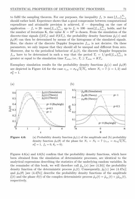
STATISTICAL PROPERTIES OF DETERMINISTIC PROCESSES 71
to fulfil the sampling theorem. For our purposes, the inequality fs À max fi,nNi
n=1should rather hold. Experience shows that a good compromise between computationalexpenditure and attainable precision is achieved, if — depending on the case ofapplication — fs ≈ 20 · maxfi,nNi
n=1 up to fs ≈ 100 · maxfi,nNin=1 holds, and for
the number of iterations K, the value K = 106 is chosen. From the simulation of thediscrete-time signals ξ(kTs) and ϑ(kTs), the probability density functions pξ(z) andpϑ(θ) can then be determined by means of the histograms of the simulated signals.Here, the choice of the discrete Doppler frequencies fi,n is not decisive. On theseparameters, we only impose that they should all be unequal and different from zero.Moreover, due to the periodical behaviour of µi(t), the discrete Doppler frequenciesfi,n have to be determined in such a way that the period Ti = 1/ gcdfi,nNi
n=1 isgreater or equal to the simulation time Tsim, i.e., Ti ≥ Tsim = KTs.
Exemplary simulation results for the probability density functions pξ(z) and pϑ(θ)are depicted in Figure 4.6 for the case ci,n = σ0
√2/Ni, where Ni = 7 (i = 1, 2) and
σ20 = 1.
(a)
0 1 2 3 40
0.1
0.2
0.3
0.4
0.5
0.6
z
pξ(
z)
ρ= 0 (Rayleigh)
ρ=0.5ρ= 1
pξ(z) (Simulation) pξ(z) (Theory) pξ(z) (Theory)
(b)
-π 0 π 0
0.1
0.2
0.3
0.4
0.5
θ
pϑ
(θ)
ρ= 0 (Rayleigh)
ρ=0.5
ρ= 1 pϑ(θ) (Simulation) pϑ(θ) (Theory)
pϑ(θ) (Theory)
Figure 4.6: (a) Probability density function pξ(z) of the amplitude and (b) probability
density function pϑ(θ) of the phase for N1 = N2 = 7 (ci,n = σ0
p2/Ni,
σ20 = 1, fρ = 0, θρ = 0).
Figures 4.6(a) and 4.6(b) confirm that the probability density functions, which havebeen obtained from the simulation of deterministic processes, are identical to theanalytical expressions describing the statistics of the underlying random variables. Inthe remainder of this book, we will therefore call pµi(x) [see (4.34)] the probabilitydensity function of the deterministic process µi(t). Consequently, pξ(z) [see (4.47a)]and pϑ(θ) [see (4.47b)] describe the probability density functions of the amplitudeξ(t) and the phase ϑ(t) of the complex deterministic process µρ(t) = µρ1(t) + jµρ2(t),respectively.

72 INTRODUCTION TO THE THEORY OF DETERMINISTIC PROCESSES
4.3.2 Level-Crossing Rate and Average Duration of Fades
In this subsection, we will derive general analytical expressions for the level-crossingrate Nξ(r) and the average duration of fades Tξ−(r) of the deterministic simulationmodel for Rice processes shown in Figure 4.3. The knowledge of analytical solutionsmakes the determination of Nξ(r) and Tξ−(r) from time-consuming simulationssuperfluous. Moreover, they enable a deeper insight into the cause and the effect ofstatistical degradations, which can be attributed to the finite number of used harmonicfunctions Ni, on the one hand, but also to the applied method for the determinationof the model parameters, on the other.
In the preceding Subsection 4.3.1, we have seen that the probability density functionpµi(x) of the deterministic process µi(t) is almost identical to the probability densityfunction pµi
(x) of the (ideal) stochastic process µi(t), provided that the number ofharmonic functions Ni is sufficiently high, let us say Ni ≥ 7. On condition that therelations
(i) pµi(x) = pµi(x) , (4.61a)
(ii) β = β1 = β2 (4.61b)
hold, then the level-crossing rate Nξ(r) is still given by (3.24), if there the quantities αand β of the stochastic reference model are replaced by the corresponding quantities αand β of the deterministic simulation model. Thus, one obtains the following expressionfor deterministic Rice processes ξ(t) with fρ 6= 0:
Nξ(r) =r
√2β
π3/2σ20
e− r2+ρ2
2σ20
π/2∫
0
cosh(
rρ
σ20
cos θ
)
·
e−(αρ sin θ)2 +√
παρ sin(θ) erf (αρ sin θ)
dθ , r ≥ 0 , (4.62)
where
α = 2πfρ
/√2β , (4.63a)
β = βi = −¨rµiµi(0) = 2π2Ni∑
n=1
(ci,nfi,n)2 . (4.63b)
For the special case fρ = 0, it follows from (4.63a) that α = 0 holds, so that (4.62)simplifies to the following expression
Nξ(r) =
√β
2π· pξ(r) , r ≥ 0 , (4.64)
which is identical to (3.27) after replacing β by β there. Obviously, the quality of theapproximation β ≈ β quite decisively determines the deviation of the level-crossing
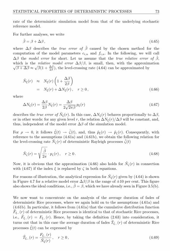
STATISTICAL PROPERTIES OF DETERMINISTIC PROCESSES 73
rate of the deterministic simulation model from that of the underlying stochasticreference model.
For further analyses, we write
β = β + ∆β , (4.65)
where ∆β describes the true error of β caused by the chosen method for thecomputation of the model parameters ci,n and fi,n. In the following, we will call∆β the model error for short. Let us assume that the true relative error of β,which is the relative model error ∆β/β, is small, then, with the approximation√
β + ∆β ≈ √β(1 + ∆β
2β ), the level-crossing rate (4.64) can be approximated by
Nξ(r) ≈ Nξ(r)(
1 +∆β
2β
)
= Nξ(r) + ∆Nξ(r) , r ≥ 0 , (4.66)
where
∆Nξ(r) =∆β
2βNξ(r) =
∆β
2√
2πβpξ(r) (4.67)
describes the true error of Nξ(r). In this case, ∆Nξ(r) behaves proportionally to ∆β,or in other words: for any given level r, the relation ∆Nξ(r)/∆β will be constant, and,thus, independent of the model error ∆β of the simulation model.
For ρ → 0, it follows ξ(t) → ζ(t), and, thus pξ(r) → pζ(r). Consequently, withreference to the assumptions (4.61a) and (4.61b), we obtain the following relation forthe level-crossing rate Nζ(r) of deterministic Rayleigh processes ζ(t)
Nζ(r) =
√β
2π· pζ(r) , r ≥ 0 . (4.68)
Now, it is obvious that the approximation (4.66) also holds for Nζ(r) in connectionwith (4.67) if the index ξ is replaced by ζ in both equations.
For reasons of illustration, the analytical expression for Nξ(r) given by (4.64) is shownin Figure 4.7 for a relative model error ∆β/β in the range of ±10 per cent. This figurealso shows the ideal conditions, i.e., β = β, which we have already seen in Figure 3.5(b).
We now want to concentrate on the analysis of the average duration of fades ofdeterministic Rice processes, where we again hold on to the assumptions (4.61a) and(4.61b). In particular, it follows from (4.61a) that the cumulative distribution functionFξ−(r) of deterministic Rice processes is identical to that of stochastic Rice processes,i.e., Fξ−(r) = Fξ−(r). Hence, by taking the definition (2.63) into consideration, itturns out that in this case the average duration of fades Tξ−(r) of deterministic Riceprocesses ξ(t) can be expressed by
Tξ−(r) =Fξ−(r)
Nξ(r), r ≥ 0 , (4.69)
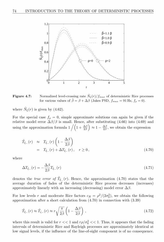
74 INTRODUCTION TO THE THEORY OF DETERMINISTIC PROCESSES
0 1 2 3 4 50
0.2
0.4
0.6
0.8
1
1.2
ρ=0 ρ=2
β=1.1 ββ=1.0 ββ=0.9 β
r
Nξ(
r)/f
max
Figure 4.7: Normalized level-crossing rate Nξ(r)/fmax of deterministic Rice processes
for various values of β = β + ∆β (Jakes PSD, fmax = 91Hz, fρ = 0).
where Nξ(r) is given by (4.62).
For the special case fρ = 0, simple approximate solutions can again be given if therelative model error ∆β/β is small. Hence, after substituting (4.66) into (4.69) andusing the approximation formula 1
/(1 + ∆β
2β
)≈ 1− ∆β
2β , we obtain the expression
Tξ−(r) ≈ Tξ−(r)(
1− ∆β
2β
)
= Tξ−(r) + ∆Tξ−(r) , r ≥ 0 , (4.70)
where
∆Tξ−(r) = −∆β
2βTξ−(r) (4.71)
denotes the true error of Tξ−(r). Hence, the approximation (4.70) states that theaverage duration of fades of the deterministic Rice process decreases (increases)approximately linearly with an increasing (decreasing) model error ∆β.
For low levels r and moderate Rice factors cR = ρ2/(2σ20), we obtain the following
approximation after a short calculation from (4.70) in connection with (3.39)
Tξ−(r) ≈ Tζ−(r) ≈ r
√π
2β
(1− ∆β
2β
), (4.72)
where this result is valid for r << 1 and rρ/σ20 << 1. Thus, it appears that the fading
intervals of deterministic Rice and Rayleigh processes are approximately identical atlow signal levels, if the influence of the line-of-sight component is of no consequence.

STATISTICAL PROPERTIES OF DETERMINISTIC PROCESSES 75
By comparing (3.39) with (4.72) it also becomes clearer that the relative model erroragain determines the deviation from the average duration of fades of the correspondingreference model.
An interesting statement can also be made on the product Nξ(r) · Tξ−(r). Namely,from (2.63) and (4.69), the model error law of deterministic channel modelling
Nξ(r) · Tξ−(r) = Nξ(r) · Tξ−(r) (4.73)
follows, which means that the product of the level-crossing rate and the averageduration of fades of deterministic Rice processes is independent of the model error∆β. With an increasing model error ∆β, the level-crossing rate Nξ(r) may rise, butthe average duration of fades Tξ−(r) decreases by the same extent, so that the productNξ(r) · Tξ−(r) remains constant at any given level r = const. This result is alsoapproximately obtained from the product of the approximations (4.66) and (4.70) ifwe ignore in the resulting product the quadratic term [∆β/(2β)]2.
Since Rayleigh processes can naturally be considered as Rice processes for the specialcase ρ = 0, the relations (4.69)–(4.71) and (4.73) in principle hold for Rayleighprocesses as well. Only the indices ξ and ξ− have to be replaced by ζ and ζ−,respectively.
The evaluation of the analytical expression for Tξ−(r) [see (4.69)] is shown in Figure 4.8for ∆β/β ∈ −0.1, 0,+0.1.
0 1 2 3 4 50
10
20
30
40
50
r
Tξ -
(r)
f max
ρ=2
ρ=0
β=1.1 ββ=1.0 ββ=0.9 β
Figure 4.8: Normalized average duration of fades Tξ−(r) · fmax of deterministic Rice
processes for various values of β = β + ∆β (Jakes PSD, fmax = 91Hz,fρ = 0).
In Chapter 5, where the individual methods for the determination of the simulation
76 INTRODUCTION TO THE THEORY OF DETERMINISTIC PROCESSES
model parameters are analysed, we will see that the condition (4.61b) can often notbe fulfilled exactly. In most cases, however, the relative deviation between β1 and β2
is very small. Due to the analysis of the level-crossing rate and the average durationof fades of Rice and Rayleigh processes, which was dealt with in Subsection 3.3.2, wealready know that for small relative deviations between β1 and β2, the ideal relationsderived on condition that β = β1 = β2 holds will still keep their validity in a verygood approximation, if we replace the quantity β = β1 = β2 by the arithmetical meanβ = (β1 + β2)/2 [see (3.37)] in the corresponding expressions or if we directly identifyβ with β1, i.e., β = β1 ≈ β2 [see also Appendix B, eq. (B.17)]. Analogous resultscan be found for the deterministic model as well. For further simplification, we willtherefore set β = β1 ≈ β2 in the following, in case the relative deviation between β1
and β2 is small.
Finally, concerning this subject, it should be noted that even without the statedconditions (4.61a) and (4.61b), the level-crossing rate and, thus, also the averageduration of fades of deterministic Rice processes can be calculated exactly. However,the numerical expenditure for the solution of the obtained integral equations isconsiderably high. Apart from that the achievable improvements are often only low,even for a small number of harmonic functions Ni, so that the comparatively highnumerical expenditure does not seem to be justified. Not only against this background,it turns out that especially the condition (4.61a) is meaningful, even though — strictlyspeaking — this condition is only fulfilled exactly as Ni →∞.
For completeness, the exact calculation of both the level-crossing rate and the averageduration of fades of deterministic Rice processes for any number of harmonic functionsNi is presented in Appendix C, where both conditions (4.61a) and (4.61b) have beendropped. In Appendix C, one finds the following analytical closed-form expression forthe level-crossing rate Nξ(r)
Nξ(r) = 2r
∞∫
0
π∫
−π
w1(r, θ) w2(r, θ)
∞∫
0
j1(z, θ) j2(z, θ) z cos(2πzz) dz dθ dz , (4.74)
where
w1(r, θ) = pµ1(r cos θ − ρ cos θρ) , (4.75a)w2(r, θ) = pµ2(r sin θ − ρ sin θρ) , (4.75b)
j1(z, θ) =N1∏
n=1
J0(4π2c1,nf1,nz cos θ) , (4.75c)
j2(z, θ) =N2∏
n=1
J0(4π2c2,nf2,nz sin θ) . (4.75d)
Now, if we substitute (4.74) into (4.69) and replace the cumulative distributionfunction Fξ−(r) by Fξ−(r) in the latter equation and using for Fξ−(r) the expression(C.40) derived in Appendix C, then we also find an exact analytical expression for theaverage duration of fades Tξ−(r) of deterministic Rice processes ξ(t).

STATISTICAL PROPERTIES OF DETERMINISTIC PROCESSES 77
4.3.3 Statistics of the Fading Intervals at Low Levels
In this subsection, we will discuss the statistical properties of the fading intervals ofdeterministic Rayleigh processes. We will restrict ourselves to low levels here, becausein this case very precise approximate solutions can be derived by analytical means.At medium and high levels, however, we have to rely on simulations to which we willcome back in Section 5.3.
At first, we will study the probability density function of the fading intervals ofdeterministic Rayleigh processes p0−(τ−; r). This density characterizes the conditionalprobability density function for the case that a deterministic Rayleigh process ζ(t)crosses a level r for the first time at the time instant t2 = t1 + τ−, provided that thelast down-crossing occurred at the time instant t1. If no further statements are madeabout the level-crossing behaviour of ζ(t) between t1 and t2, then the correspondingprobability density function is denoted by p1−(τ−; r). During the analysis proceededfor the stochastic reference model in Subsection 3.3.3, it was pointed out that,according to (3.47), p1−(τ−; r) can be regarded as a very good approximation forp0−(τ−; r) if the level r is low. Consequently, it also holds for the deterministic model:p0−(τ−; r) → p1−(τ−; r) if r → 0, where p1−(τ−; r) follows directly from (3.47) if thereTζ−(r) is substituted by Tζ−(r) [Pae96e], i.e.,
p1−(τ−; r) =2πz2 e−z
Tζ−(r)
[I0(z)−
(1 +
12z
)I1(z)
], 0 ≤ r << 1 , (4.76)
where z = 2[Tζ−(r)/τ−
]2/π. The use of the result (4.70) now gives us the opportunity
to investigate the influence of the model error ∆β on the probability density functionof the fading intervals of deterministic Rayleigh processes at deep signal levelsanalytically. The evaluation of p1−(τ−; r) according to (4.76) for various values ofβ = β+∆β is shown in Figure 4.9 for a level r of r = 0.1. In this figure, one recognizesthat a positive model error ∆β > 0 is always connected with a distinct decrease(increase) of the probability density function p1−(τ−; r) in the range of relatively large(small) fading intervals τ−. With a negative model error ∆β < 0, logically, the inversebehaviour occurs.
In a similar way, we obtain an expression for τq describing the length of the timeinterval of those fading intervals of deterministic Rayleigh processes ζ(t) which includeq per cent of all fading intervals. The quantity τq = τq(r) follows directly from (3.53)if we again replace Tζ−(r) by Tζ−(r), i.e., for 75 ≤ q ≤ 100 it follows that
τq(r) ≈Tζ−(r)
π4
[1−
√1− 4
(1− q
100
)]1/3, r << 1 . (4.77)
In order to make the influence of the model error ∆β easily identifiable, we useTζ−(r) = Tζ−(r)[1 − ∆β/(2β)] and in connection with (3.53), we write the relationabove in the form
τq(r) ≈ τq(r)(
1− ∆β
2β
), r << 1 . (4.78)
78 INTRODUCTION TO THE THEORY OF DETERMINISTIC PROCESSES
0 0.5 1 1.50
1000
2000
3000
4000
5000
β = 0.5 β
β = 0.75 β
β = 1 β
β = 1.5 β
β = 2 β
τ- (ms)
p1
-(τ-;
r)
ρ = 0
r = 0.1
Figure 4.9: The influence of β = β +∆β on the probability density function p1−(τ−; r)
of the fading intervals τ− at low levels (Jakes PSD, fmax = 91 Hz, σ20 = 1).
This relation makes clear that a relative error of β in the order of ±ε approximatelycauses a relative error of τq(r) in the order of ∓ε/2.
In particular, after putting (3.54)–(3.56) into (4.78), the quantities τ90(r), τ95(r), andτ99(τ) can now approximately be expressed by:
τ90(r) ≈ 1.78 · Tζ−(r)[1−∆β/(2β)] , (4.79a)τ95(r) ≈ 2.29 · Tζ−(r)[1−∆β/(2β)] , (4.79b)τ99(r) ≈ 3.98 · Tζ−(r)[1−∆β/(2β)] . (4.79c)
At this point, it should be explicitly emphasized that all approximations for p0−(τ−; r)and τq(r), which were specially derived in this subsection for deterministic Rayleighprocesses, are also valid for deterministic Rice processes with moderate Rice factors.This statement becomes clear immediately if we take into consideration that p1−(τ−; r)[see (4.76)] and τq(r) [see (4.77)] only depend on the average duration of fades Tζ−(r),and, due to (4.72), Tζ−(r) can approximately be replaced at low signal levels r by theaverage duration of fades Tξ−(r) of Rice processes.
4.3.4 Ergodicity and Criteria for the Performance Evaluation
As already mentioned, a deterministic process µi(t), defined by (4.4), is a samplefunction of the corresponding stochastic process µi(t). In this subsection, we willdiscuss the ergodic properties of the stochastic process µi(t). Hence, we first distinguishbetween the ergodicity with respect to the mean value and the ergodicity with respectto the autocorrelation function [Pap91]. After that, we will look at some criteria forthe assessment of the performance, which will play a significant role in the followingchapter.

STATISTICAL PROPERTIES OF DETERMINISTIC PROCESSES 79
Ergodicity with respect to the mean value: A stochastic process µi(t) is said tobe ergodic with respect to the mean value if the temporal mean value of µi(t) computedover the interval [-T,T] converges in the limit T → ∞ to the statistical mean valuemµi := Eµi(t), i.e.,
mµi= mµi
:= limT→∞
12T
∫ T
−T
µi(t) dt . (4.80)
Since the Doppler phases θi,n of the stochastic process µi(t) are random variablesuniformly distributed in the interval (0, 2π], the left-hand side of the equation aboveis equal to zero. The right-hand side is also equal to zero if all discrete Dopplerfrequencies fi,n are unequal to zero, i.e., if fi,n 6= 0 for all n = 1, 2, . . . , Ni and i = 1, 2.That requirement (fi,n 6= 0) can be fulfilled without any difficulty by all parametercomputation methods introduced in the next chapter. Hence, mµi = mµi = 0 holds,and, thus, the stochastic process µi(t) is ergodic with respect to the mean value.
Ergodicity with respect to the autocorrelation function: A stochastic processµi(t) is said to be ergodic with respect to the autocorrelation function if the temporalmean of µi(t)µi(t+τ) computed over the interval [−T, T ] converges in the limit T →∞to the statistical mean rµiµi(τ) := Eµi(t)µi(t + τ), i.e.,
rµiµi(τ) = rµiµi(τ) := limT→∞
12T
∫ T
−T
µi(t) µi(t + τ) dt . (4.81)
If the discrete Doppler frequencies fi,n and the Doppler coefficients ci,n of thestochastic process µi(t) are constant quantities and merely the Doppler phasesθi,n ∈ (0, 2π] are uniformly distributed random variables, then the left-hand side ofthe equation above leads to
rµiµi(τ) =Ni∑
n=1
c2i,n
2cos(2πfi,nτ) . (4.82)
Due to (4.11), we are already familiar with the solution of the right-hand side of(4.81). The comparison of (4.11) with (4.82) shows us that rµiµi(τ) = rµiµi(τ) holds,and, thus, the stochastic process µi(t) is ergodic with respect to the autocorrelationfunction.
Without wanting to jump ahead, it should be noted here that for the Monte Carlomethod described in Subsection 5.1.4, the discrete Doppler frequencies fi,n of thestochastic process µi(t) are not constants but random variables. We will see that inthis case rµiµi(τ) 6= rµiµi(τ) holds, and, thus, the stochastic process µi(t) is not ergodicwith respect to the autocorrelation function.
Indeed, for channel modelling it is not the crucial factor whether the stochastic processµi(t) is ergodic with respect to the mean value or the autocorrelation function. Thedeviations of statistical properties of the deterministic process µi(t) from the statisticalproperties of the underlying ideal stochastic process µi(t) are decisive. From thesedeviations, criteria can be gained for the performance evaluation of the methods forthe computation of the model parameters presented in the next chapter.
80 INTRODUCTION TO THE THEORY OF DETERMINISTIC PROCESSES
Since the process µi(t) was introduced here as a zero-mean normally distributedstochastic process, i.e., µi(t) ∼ N(0, σ2
0), the mean-square error of the probabilitydensity function pµi
(x) [cf. (4.39)]
Epµi:=
∞∫
−∞(pµi
(x)− pµi(x))2 dx (4.83)
defines the first important criterion for the performance evaluation [Pae98b].
As is well known, real-valued Gaussian random processes are described completelyby their probability density function and their autocorrelation function. A furtherimportant criterion for the performance evaluation is therefore the mean-square errorof the autocorrelation function rµiµi
(τ) defined by
Erµiµi:=
1τmax
τmax∫
0
(rµiµi(τ)− rµiµi(τ))2 dτ . (4.84)
For the parameter τmax, the value τmax = Ni/(2fmax) has turned out to be suitable,especially for the Jakes power spectral density, as we will see in the next chapter.
Meanwhile, it has already been mentioned several times that the statistical propertiesof deterministic simulation models can deviate considerably from those of theunderlying ideal stochastic reference model. We have seen that for many importantstatistical quantities, the model error ∆β could be held responsible for this. Therefore,a good parameter computation procedure should only cause a small relative modelerror ∆β/β, even when the realization expenditure is low, i.e., for a small numberof harmonic functions Ni. Hence, the model error ∆β and its convergence property∆β → 0 or β → β for Ni → ∞ will be paid attention to in the subsections of thefollowing chapter as well.

5
METHODS FOR THECOMPUTATION OF THEMODEL PARAMETERS OFDETERMINISTIC PROCESSES
By now there is a multitude of various methods for the computation of the primaryparameters of the simulation model (Doppler coefficients ci,n and discrete Dopplerfrequencies fi,n). Exactly like the original Rice method [Ric44, Ric45], the method ofequal distances [Pae94b, Pae96d] as well as the mean-square-error method [Pae96d]are characterized by the fact that the distances between two neighbouring discreteDoppler frequencies are equidistant. These three methods merely differ in the specificway of how the Doppler coefficients are adapted to the desired Doppler powerspectral density. Due to the equidistant property of discrete Doppler frequencies,which are in neighbouring pairs, all three procedures have one decisive disadvantagein common, namely the comparatively small period of the designed deterministicGaussian processes, and, thus, of the resulting simulation model. This disadvantagecan be avoided, e.g., by using the method of equal areas [Pae94b, Pae96d], whichhas an acceptable performance when applied to the Jakes power spectral density.However, this method fails or leads to a comparatively high realization expenditure,if the procedure is used in connection with Gaussian shaped power spectral densities.In German-speaking countries, the Monte Carlo method [Schu89, Hoe92] has becomequite popular. In comparison with other methods, however, the performance of thismethod is poor [Pae96d, Pae96e] if the approximation precision of the autocorrelationfunction of the resulting deterministic Gaussian processes is used as a criterion for theevaluation of the performance. The principle of the Monte Carlo method is that thediscrete Doppler frequencies of the stochastic simulation system are obtained from themapping of a uniformly distributed random variable into a random variable with adistribution proportional to the desired Doppler power spectral density. Consequently,the discrete Doppler frequencies themselves are random variables. The realization of aset fi,n of discrete Doppler frequencies can thus result in a deterministic Gaussianprocess µi(t), whose statistical properties may largely deviate from the desiredproperties of the (ideal) stochastic Gaussian random process µi(t). This even holds ifthe number of harmonic functions Ni chosen is very large, let us say Ni = 100 [Pae96e].A quasi-optimal procedure is the method of exact Doppler spread [Pae98b, Pae96c].
82 METHODS FOR THE COMPUTATION OF THE MODEL PARAMETERS
This method is almost ideally suitable for Jakes shaped power spectral densities. Theperformance of the method of exact Doppler spread can only be outperformed by theLp-norm method [Pae98b, Pae96c]. Unfortunately, the arising numerical complexityof this method is comparatively high, so that an application, especially in connectionwith the Jakes and Gaussian power spectral density, is often not worth the effort.The Lp-norm method only unfolds its full performance when the statistical propertiesof the deterministic simulation model have to be adapted to snapshot measurementsof real-world mobile radio channels. A further design method is the Jakes method[Jak93], which, however, does not fulfil the often imposed requirement that the realand imaginary part of the complex Gaussian random processes describing the Rayleigh(Rice) process should be uncorrelated.
For an infinite number of harmonic functions, all these methods result in deterministicprocesses with identical statistical properties, which even match the ones of thereference model exactly. However, as soon as only a finite number of harmonicfunctions is used, we obtain deterministic processes with completely different statisticalproperties, which in particular cases can considerably deviate from those of thereference model. The discussion of these properties will be one objective of thefollowing Section 5.1. Thus, in order to compute the model parameters ci,n and fi,n,we will proceed by deriving the seven design procedures mentioned just in such a waythat they are generally applicable. Afterwards, the methods are respectively appliedto both of the often used Jakes and Gaussian power spectral densities. In general, weobtain simple equations allowing us to quickly determine the desired model parametersfor the most important practical application cases. For each method, the characteristicproperties as well as the advantages and disadvantages will be discussed. For a fairjudgement of the performance, the criteria of assessment introduced in the precedingSubsection 4.3.4 will be made use of. At places in the text, where relations among theindividual methods occur, these connections will be pointed out.
The computation of the Doppler phases θi,n can be carried out independently ofthese methods. Without restriction of generality, we at first assume that the elements ofthe set θi,n are generated from Ni statistically independent realizations of a randomvariable uniformly distributed in the interval [0, 2π). Afterwards, in Section 5.2, wewill discover a deterministic design method for the computation of the set θi,n. Atthat stage, the relevance of the Doppler phases θi,n with regard to the statisticalproperties of µi(t) will also be analysed more precisely.
Finally, we will again deal with the analysis of the probability density function of thefading intervals of deterministic Rayleigh processes in Section 5.3.

DISCRETE DOPPLER FREQUENCIES AND DOPPLER COEFFICIENTS 83
5.1 METHODS FOR THE COMPUTATION OF THE DISCRETE DOPPLERFREQUENCIES AND DOPPLER COEFFICIENTS
5.1.1 Method of Equal Distances (MED)
One of the main characteristics of the method of equal distances (MED) [Pae94b,Pae96d] is that discrete Doppler frequencies, which are found in neighbouring pairs,have the same distance. This property is achieved by defining the discrete Dopplerfrequencies fi,n as
fi,n :=∆fi
2(2n− 1) , n = 1, 2, . . . , Ni , (5.1)
where
∆fi = fi,n − fi,n−1 , n = 2, 3, . . . , Ni , (5.2)
denotes the distance between two neighbouring discrete Doppler frequencies of the ithdeterministic process µi(t) (i = 1, 2).
In order to compute the Doppler coefficients ci,n, we take a look at the frequencyinterval
Ii,n :=[fi,n − ∆fi
2, fi,n +
∆fi
2
), n = 1, 2, . . . , Ni , (5.3)
and demand that within this interval, the mean power of the power spectral densitySµiµi(f) of the stochastic reference model is identical to that of the power spectraldensity Sµiµi(f) of the deterministic simulation model, i.e.,
∫
fεIi,n
Sµiµi(f) df =∫
fεIi,n
Sµiµi(f) df (5.4)
for all n = 1, 2, . . . , Ni and i = 1, 2. Thus, after substituting (4.14) into the aboveequation, the Doppler coefficients ci,n are determined by the expression
ci,n = 2
√∫
fεIi,n
Sµiµi(f) df . (5.5)
After substituting (5.5) into (4.11), one can easily prove that rµiµi(τ) → rµiµi(τ) holdsas Ni →∞. Referring to the central limit theorem, it can furthermore be shown thatthe convergence property pµi(x) → pµi(x) holds as Ni → ∞. Thus, for an infinitenumber of harmonic functions, the deterministic processes designed according to themethod of equal distances can be interpreted as sample functions of the underlyingideal Gaussian random process.
The major disadvantage of this method is the resulting poor periodicity property ofµi(t). To make this clear, we start from (4.26), and in connection with (5.1) it followsthat the greatest common divisor of the discrete Doppler frequencies is
Fi = gcdfi,nNin=1 =
∆fi
2. (5.6)
84 METHODS FOR THE COMPUTATION OF THE MODEL PARAMETERS
Consequently, µi(t) is periodical with the period Ti = 1/Fi = 2/∆fi. To obtain a largevalue for Ti, a small value for ∆fi is required, which is in general involved with a highrealization amount as we will see below.
Jakes power spectral density: The frequency range of the Jakes power spectraldensity [see (3.8)] is limited to the range |f | ≤ fmax, so that for a given number ofharmonic functions Ni, a reasonable value for the difference between two neighbouringdiscrete Doppler frequencies ∆fi is given by ∆fi = fmax/Ni. Consequently, from (5.1)we obtain the following relation for the discrete Doppler frequencies fi,n
fi,n =fmax
2Ni(2n− 1) (5.7)
for all n = 1, 2, . . . , Ni and i = 1, 2. The corresponding Doppler coefficients ci,n
can now easily be computed with (3.8), (5.3), (5.5), and (5.7). After an elementarycomputation, we find the expression
ci,n =2σ0√
π
[arcsin
(n
Ni
)− arcsin
(n− 1Ni
)]1/2
(5.8)
for all n = 1, 2, . . . , Ni and i = 1, 2.
The deterministic processes µi(t) designed with (5.7) and (5.8) obviously have themean value mµi = 0 and the mean power
σ2µi
= rµiµi(0) =Ni∑
n=1
c2i,n
2= σ2
0 . (5.9)
Hence, both the mean value and the mean power of the deterministic process µi(t)exactly match the corresponding quantities of the stochastic process µi(t), i.e., theexpected value and the variance.
Designing the complex deterministic processes µ(t) = µ1(t) + jµ2(t), the uncor-relatedness of µ1(t) and µ2(t) must be guaranteed. This can be ensured withoutdifficulty by choosing N2 in accordance with N2 = N1 + 1, so that due to (5.7) itfollows: f1,n 6= f2,m for n = 1, 2, . . . , N1 and m = 1, 2, . . . , N2. This again leads to thedesired property that µ1(t) and µ2(t) are uncorrelated [cf. (4.12)].
As an example, the power spectral density Sµiµi(f) and the correspondingautocorrelation function rµiµi(τ) are depicted in Figure 5.1, where the value 25 hasbeen chosen for the number of harmonic functions Ni.
For comparison, the autocorrelation function rµiµi(τ) of the reference model is alsopresented in Figure 5.1(b). The shape of rµiµi(τ) shown in this figure makes theperiodical behaviour clearly recognizable. In general, the following relation holds
rµiµi(τ + mTi/2) =
rµiµi(τ) , m even ,
−rµiµi(τ) , m odd ,(5.10)

DISCRETE DOPPLER FREQUENCIES AND DOPPLER COEFFICIENTS 85
(a)
-100 -50 0 50 1000
0.02
0.04
0.06
0.08
0.1
f (Hz)
Sµ
iµi(f
)
(b)
0 0.05 0.1 0.15 0.2 0.25-1
-0.5
0
0.5
1
τ (s)
r µiµ
i(τ)
rµiµi(τ) [see (4.11)]
rµiµi(τ) [see (3.10)]
Figure 5.1: (a) Power spectral density Sµiµi(f) and (b) autocorrelation functionrµiµi(τ) for Ni = 25 (MED, Jakes PSD, fmax = 91Hz, σ2
0 = 1).
where Ti = 1/Fi = 2/∆fi = 2Ni/fmax. If we now choose the value τmax = Ti/4 =Ni/(2fmax) for the upper limit of the integral (4.84), the mean-square error Erµiµi
[see (4.84)] can thus be usefully evaluated, particularly since Erµiµirepresents a
measure of the performance of the method of equal distances as a function of therealization complexity determined by Ni. The evaluation of the performance criteriaErµiµi
and Epµiaccording to (4.84) and (4.83), respectively, were performed on
the basis of the method of equal distances. The obtained results are presented inFigures 5.2(a) and 5.2(b) showing the influence of the used number of harmonicfunctions Ni. For a better classification of the performance of this method, the resultsobtained for ci,n = σ0
√2/Ni are also shown in Figure 5.2(b). Hence, one realizes
that the approximation of the Gaussian distribution using the Doppler coefficientsci,n according to (5.8) is worse in comparison with the results obtained by usingci,n = σ0
√2/Ni.
Finally, we will also study the model error ∆βi = βi−β. With (5.7), (5.8), (3.29), and(4.22), we find the closed-form expression
∆βi = β
[1 +
1− 4Ni
2N2i
− 8πN2
i
Ni−1∑n=1
n · arcsin(
n
Ni
)], (5.11)
whose right-hand side tends to 0 as Ni →∞, i.e., it holds limNi→∞∆βi = 0. Figure 5.3depicts the relative model error ∆βi/β. It should be observed that the ratio ∆βi/βmerely depends on Ni.
Gaussian power spectral density: The frequency range of the Gaussian powerspectral density (3.11) must first be limited to the relevant range. Therefore, weintroduce the quantity κc which is chosen in such a way that the mean power ofthe Gaussian power spectral density obtained within the frequency range |f | ≤ κcfc
makes up at least 99.99 per cent of its total mean power. This demand is fulfilled with

86 METHODS FOR THE COMPUTATION OF THE MODEL PARAMETERS
(a)
0 10 20 30 40 500
1
2
3
4
5
6
7
8
9x 10⁻³
Ni
Er µ
iµi
(b)
0 10 20 30 40 500
1
2
3
4
5
6
7x 10⁻⁴
Ni
Ep
µi
ci,n [see (5.8)]
ci,n=σo (2/Ni)1/2
Figure 5.2: Mean-square errors: (a) Erµiµiand (b) Epµi
(MED, Jakes PSD, fmax =
91Hz, σ20 = 1, τmax = Ni/(2fmax)).
0 20 40 60 80 100-0.06
-0.05
-0.04
-0.03
-0.02
-0.01
0
Ni
∆βi /
β
Figure 5.3: Relative model error ∆βi/β (MED, Jakes PSD).

DISCRETE DOPPLER FREQUENCIES AND DOPPLER COEFFICIENTS 87
κc = 2√
2/ ln 2. Depending on the number of harmonic functions Ni, the differencebetween two neighbouring discrete Doppler frequencies ∆fi can then be described by∆fi = κcfc/Ni. Thus, with (5.1), we obtain the following expression for the discreteDoppler frequencies fi,n
fi,n =κcfc
2Ni(2n− 1) (5.12)
for all n = 1, 2, . . . , Ni and i = 1, 2. Now, using (3.11), (5.3), and (5.5), this enablesthe computation of the Doppler coefficients ci,n. As a result, we find the formula
ci,n = σ0
√2
[erf
(nκc
√ln 2
Ni
)− erf
((n− 1)κc
√ln 2
Ni
)] 12
(5.13)
for all n = 1, 2, . . . , Ni and i = 1, 2. Deterministic processes µi(t) designed with (5.12)and (5.13) have a mean value of zero and a mean power of
σ2µi
= rµiµi(0) =Ni∑
n=1
c2i,n
2
= σ20 erf
(κc
√ln 2
)
= 0.9999366 · σ20 ≈ σ2
0 , (5.14)
provided that κc is chosen as suggested, i.e., κc = 2√
2/ ln 2. In the present case, theperiod of µi(t) is given by Ti = 2/∆fi = 2Ni/(κcfc).
Figure 5.4(a) shows the power spectral density Sµiµi(f) for Ni = 25 and Figure 5.4(b)illustrates the corresponding behaviour of the autocorrelation function rµiµi(τ) incomparison with the autocorrelation function rµiµi(τ) of the reference model in therange 0 ≤ τ ≤ Ti/2.
A suitable value for the upper limit of the integral (4.84) is also in this case a quarterof the period Ti, i.e., τmax = Ti/4 = Ni/(2κcfc). If the mean-square error Erµiµi
[see(4.84)] is evaluated with respect to the upper limit τmax prescribed in this way, thenwe obtain the graph presented in Figure 5.5(a) showing the influence of the numberof harmonic functions Ni. Figure 5.5(b) presents the results of the evaluation of theperformance criterion Epµi
according to (4.83). For comparison, the results obtainedby using ci,n = σ0
√2/Ni are shown in this figure as well.
Finally, we will also analyse the model error ∆βi. Using (4.22), (5.12), (5.13), and(3.29), we find the following closed-form solution for ∆βi = βi − β
∆βi = β
2 ln 2κ2
c
[(1− 1
2Ni
)2
erf(κc
√ln 2
)− 2
N2i
Ni−1∑n=1
n erf
(nκc
√ln 2
Ni
)]−1
.
(5.15)

88 METHODS FOR THE COMPUTATION OF THE MODEL PARAMETERS
(a)
-300 -200 -100 0 100 200 3000
0.01
0.02
0.03
0.04
0.05
0.06
0.07
f (Hz)
Sµ
iµi(f
)
(b)
0 0.02 0.04 0.06 0.08-1
-0.5
0
0.5
1
τ (s)
r µiµ
i(τ)
rµiµi(τ) [see (4.11)]
rµiµi(τ) [see (3.12)]
Figure 5.4: (a) Power spectral density Sµiµi(f) and (b) autocorrelation function
rµiµi(τ) for Ni = 25 (MED, Gaussian PSD, fc =√
ln 2fmax, fmax = 91 Hz,
σ20 = 1, κc = 2
p2/ ln 2).
(a)
0 10 20 30 40 500
0.5
1
1.5x 10⁻⁴
Ni
Er µ
iµi
(b)
0 10 20 30 40 500
0.5
1
1.5
2
2.5
3x 10⁻³
Ni
Ep
µi
ci,n [see (5.13)]
ci,n=σo (2/Ni)1/2
Figure 5.5: Mean-square errors: (a) Erµiµiand (b) Epµi
(MED, Gaussian PSD, fc =√ln 2 fmax, fmax = 91Hz, σ2
0 = 1, τmax = Ni/(2κcfc), κc = 2p
2/ ln 2).
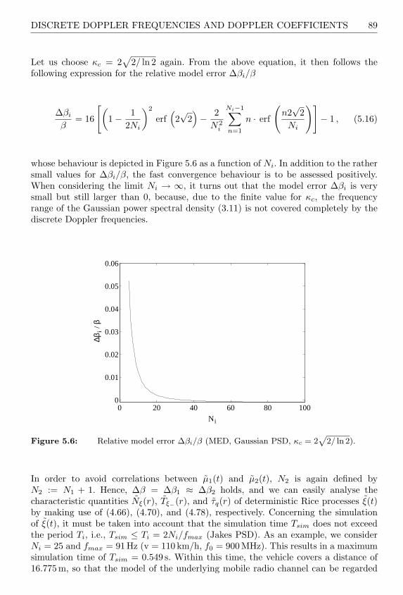
DISCRETE DOPPLER FREQUENCIES AND DOPPLER COEFFICIENTS 89
Let us choose κc = 2√
2/ ln 2 again. From the above equation, it then follows thefollowing expression for the relative model error ∆βi/β
∆βi
β= 16
[(1− 1
2Ni
)2
erf(2√
2)− 2
N2i
Ni−1∑n=1
n · erf
(n2√
2Ni
)]− 1 , (5.16)
whose behaviour is depicted in Figure 5.6 as a function of Ni. In addition to the rathersmall values for ∆βi/β, the fast convergence behaviour is to be assessed positively.When considering the limit Ni → ∞, it turns out that the model error ∆βi is verysmall but still larger than 0, because, due to the finite value for κc, the frequencyrange of the Gaussian power spectral density (3.11) is not covered completely by thediscrete Doppler frequencies.
0 20 40 60 80 1000
0.01
0.02
0.03
0.04
0.05
0.06
Ni
∆βi /
β
Figure 5.6: Relative model error ∆βi/β (MED, Gaussian PSD, κc = 2p
2/ ln 2).
In order to avoid correlations between µ1(t) and µ2(t), N2 is again defined byN2 := N1 + 1. Hence, ∆β = ∆β1 ≈ ∆β2 holds, and we can easily analyse thecharacteristic quantities Nξ(r), Tξ−(r), and τq(r) of deterministic Rice processes ξ(t)by making use of (4.66), (4.70), and (4.78), respectively. Concerning the simulationof ξ(t), it must be taken into account that the simulation time Tsim does not exceedthe period Ti, i.e., Tsim ≤ Ti = 2Ni/fmax (Jakes PSD). As an example, we considerNi = 25 and fmax = 91 Hz (v = 110 km/h, f0 = 900 MHz). This results in a maximumsimulation time of Tsim = 0.549 s. Within this time, the vehicle covers a distance of16.775m, so that the model of the underlying mobile radio channel can be regarded

90 METHODS FOR THE COMPUTATION OF THE MODEL PARAMETERS
as wide-sense stationary.1 Nevertheless, this simulation time is not by a long waysufficient to determine typical characteristic quantities such as Nξ(r), Tξ−(r), and τq(r)with acceptable precision. A more exact measurement of these quantities for the sameparameter sets fi,n and ci,n can be achieved by ensemble averaging (statisticalaveraging). Therefore, various realizations of ξ(t) are required, which can be generatedby means of various sets for the Doppler phases θi,n. Due to the relatively smallperiod Ti, which only increases linearly with Ni, the method of equal distances isnot recommendable for long-time simulations. For this reason, the properties of thismethod will not be investigated here in any detail. Further results of this approachcan be found in [Pae96d].
5.1.2 Mean-Square-Error Method (MSEM)
The mean-square-error method (MSEM) is based on the idea that the model parametersets ci,n and fi,n are computed in such a way that the mean-square error (4.84)
Erµiµi=
1τmax
∫ τmax
0
(rµiµi(τ)− rµiµi(τ))2 dτ (5.17)
becomes minimal [Pae96d]. Here, rµiµi(τ) can be any autocorrelation function of theprocess µi(t) describing a theoretical reference model. Alternatively, rµiµi(τ) can alsobe obtained from the measurement data of a real-world channel. The autocorrelationfunction rµiµi(τ) of the deterministic model is again given by (4.11). In the equationgiven above, τmax describes an appropriate time interval over which the approximationof the autocorrelation function rµiµi(τ) is of interest. Unfortunately, a simple andclosed-form solution for this problem only exists, if the discrete Doppler frequenciesfi,n are again defined by (5.1) and, consequently, they are equidistant.
After substituting (4.11) into (5.17) and setting the partial derivatives of Erµiµiwith
respect to the Doppler coefficients ci,n equal to zero, i.e., ∂Erµiµi/∂ci,n = 0, we obtain,
in connection with (5.1), the following formula for ci,n [Pae96d]:
ci,n = 2
√1
τmax
∫ τmax
0
rµiµi(τ) cos(2πfi,nτ) dτ (5.18)
for all n = 1, 2, . . . , Ni (i = 1, 2), where τmax shall again be given by τmax = Ti/4 =1/(2∆fi).
In case of the limit ∆fi → 0, one can show that from (5.18) the expression
ci,n = lim∆fi→0
2√
∆fiSµiµi(fi,n) (5.19)
follows, which is identical to the relation (4.2a) given by Rice [Ric44, Ric45]. Numericalanalysis have shown that for ∆fi > 0, the formula
ci,n = 2√
∆fiSµiµi(fi,n) , (5.20)
1 Measurements have shown [Cox73] that in urban areas mobile radio channels can appropriatelybe modelled for signal bandwidths up to 10MHz and covered distances up to 30m by so-calledGWSSUS channels (“Gaussian wide-sense stationary uncorrelated scattering”).
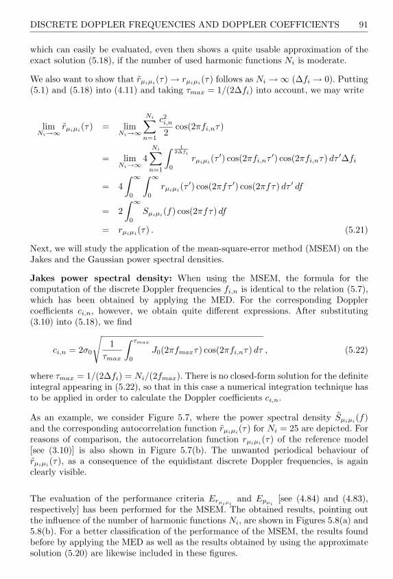
DISCRETE DOPPLER FREQUENCIES AND DOPPLER COEFFICIENTS 91
which can easily be evaluated, even then shows a quite usable approximation of theexact solution (5.18), if the number of used harmonic functions Ni is moderate.
We also want to show that rµiµi(τ) → rµiµi
(τ) follows as Ni →∞ (∆fi → 0). Putting(5.1) and (5.18) into (4.11) and taking τmax = 1/(2∆fi) into account, we may write
limNi→∞
rµiµi(τ) = lim
Ni→∞
Ni∑n=1
c2i,n
2cos(2πfi,nτ)
= limNi→∞
4Ni∑
n=1
∫ 12∆fi
0
rµiµi(τ′) cos(2πfi,nτ ′) cos(2πfi,nτ) dτ ′∆fi
= 4∫ ∞
0
∫ ∞
0
rµiµi(τ ′) cos(2πfτ ′) cos(2πfτ) dτ ′ df
= 2∫ ∞
0
Sµiµi(f) cos(2πfτ) df
= rµiµi(τ) . (5.21)
Next, we will study the application of the mean-square-error method (MSEM) on theJakes and the Gaussian power spectral densities.
Jakes power spectral density: When using the MSEM, the formula for thecomputation of the discrete Doppler frequencies fi,n is identical to the relation (5.7),which has been obtained by applying the MED. For the corresponding Dopplercoefficients ci,n, however, we obtain quite different expressions. After substituting(3.10) into (5.18), we find
ci,n = 2σ0
√1
τmax
∫ τmax
0
J0(2πfmaxτ) cos(2πfi,nτ) dτ , (5.22)
where τmax = 1/(2∆fi) = Ni/(2fmax). There is no closed-form solution for the definiteintegral appearing in (5.22), so that in this case a numerical integration technique hasto be applied in order to calculate the Doppler coefficients ci,n.
As an example, we consider Figure 5.7, where the power spectral density Sµiµi(f)and the corresponding autocorrelation function rµiµi(τ) for Ni = 25 are depicted. Forreasons of comparison, the autocorrelation function rµiµi(τ) of the reference model[see (3.10)] is also shown in Figure 5.7(b). The unwanted periodical behaviour ofrµiµi(τ), as a consequence of the equidistant discrete Doppler frequencies, is againclearly visible.
The evaluation of the performance criteria Erµiµiand Epµi
[see (4.84) and (4.83),respectively] has been performed for the MSEM. The obtained results, pointing outthe influence of the number of harmonic functions Ni, are shown in Figures 5.8(a) and5.8(b). For a better classification of the performance of the MSEM, the results foundbefore by applying the MED as well as the results obtained by using the approximatesolution (5.20) are likewise included in these figures.

92 METHODS FOR THE COMPUTATION OF THE MODEL PARAMETERS
(a)
-100 -50 0 50 1000
0.01
0.02
0.03
0.04
0.05
0.06
0.07
0.08
f (Hz)
Sµ
iµi(f
)
(b)
0 0.05 0.1 0.15 0.2 0.25-1
-0.5
0
0.5
1
τ (s)
r µiµ
i(τ)
rµiµi(τ) [see (4.11)]
rµiµi(τ) [see (3.10)]
Figure 5.7: (a) Power spectral density Sµiµi(f) and (b) autocorrelation functionrµiµi(τ) for Ni = 25 (MSEM, Jakes PSD, fmax = 91Hz, σ2
0 = 1).
(a)
0 10 20 30 40 500
1
2
3
4
5
6
7
8
9x 10⁻³
Ni
Er µ
iµi
MSEM
MED
Approximation (5.20)
(b)
0 10 20 30 40 50
1
2
3
4
5
6
7x 10
-4
Ni
Ep
µi
MSEM
MED
Approximation (5.20)
Figure 5.8: Mean-square errors: (a) Erµiµiand (b) Epµi
(MSEM, Jakes PSD, fmax =
91Hz, σ20 = 1, τmax = Ni/(2fmax)).

DISCRETE DOPPLER FREQUENCIES AND DOPPLER COEFFICIENTS 93
In case of the MSEM, a simple solution for the model error ∆βi does not exist. Bymeans of (5.7), (5.22), (3.29), and (4.22), the following formula for βi is obtained aftera short computation
βi = β1Ni
Ni∑n=1
(2n− 1)2∫ 1
0
J0(πNiu) cos[π
2(2n− 1)u
]du . (5.23)
With this expression and by making use of β = 2(πfmaxσ0)2, the model error∆βi = βi − β can be calculated. Figure 5.9 depicts the resulting relative model error∆βi/β in terms of Ni. This figure also shows the results which can be found when theapproximate solution (5.20) is used. For reasons of comparison, the graph of ∆βi/βobtained by applying the MED is also presented here once again.
0 20 40 60 80 100-0.25
-0.2
-0.15
-0.1
-0.05
0
Ni
∆βi /
β
MSEM
MED
Approximation (5.20)
Figure 5.9: Relative model error ∆βi/β (MSEM, Jakes PSD).
Gaussian power spectral density: The discrete Doppler frequencies fi,n are givenby (5.12). For the Doppler coefficients ci,n, we now obtain, after substituting (3.12)into (5.18), the expression
ci,n = 2σ0
√1
τmax
∫ τmax
0
e−(πfcτ)2/ ln 2 cos(2πfi,nτ) dτ (5.24)
for all n = 1, 2, . . . , Ni (i = 1, 2), where τmax = 1/(2∆fi) = Ni/(2κcfc). Let thequantity κc again be defined by κc = 2
√2/ ln 2, so that the period Ti is given by
Ti = Ni/(√
2/ ln 2fc). The definite integral under the square root of (5.24) has to besolved numerically.
As an example, the power spectral density Sµiµi(f) for Ni = 25 is shown inFigure 5.10(a). Figure 5.10(b) presents the corresponding autocorrelation function
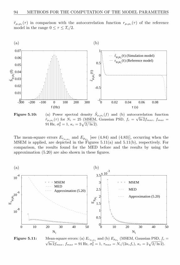
94 METHODS FOR THE COMPUTATION OF THE MODEL PARAMETERS
rµiµi(τ) in comparison with the autocorrelation function rµiµi(τ) of the referencemodel in the range 0 ≤ τ ≤ Ti/2.
(a)
-300 -200 -100 0 100 200 3000
0.01
0.02
0.03
0.04
0.05
0.06
0.07
f (Hz)
Sµ
iµi(f
)
(b)
0 0.02 0.04 0.06 0.08-1
-0.5
0
0.5
1
τ (s)
r µiµ
i(τ)
rµiµi(τ) (Simulation model)
rµiµi(τ) (Reference model)
Figure 5.10: (a) Power spectral density Sµiµi(f) and (b) autocorrelation function
rµiµi(τ) for Ni = 25 (MSEM, Gaussian PSD, fc =√
ln 2fmax, fmax =
91Hz, σ20 = 1, κc = 2
p2/ ln 2).
The mean-square errors Erµiµiand Epµi
[see (4.84) and (4.83)], occurring when theMSEM is applied, are depicted in the Figures 5.11(a) and 5.11(b), respectively. Forcomparison, the results found for the MED before and the results by using theapproximation (5.20) are also shown in these figures.
(a)
0 10 20 30 40 50
10-8
10-6
10-4
Ni
Er µ
iµi
MSEMMEDApproximation (5.20)
(b)
0 10 20 30 40 500
0.5
1
1.5
2
2.5
3
3.5x 10⁻³
Ni
Ep
µi
MSEM
MED
Approximation (5.20)
Figure 5.11: Mean-square errors: (a) Erµiµiand (b) Epµi
(MSEM, Gaussian PSD, fc =√ln 2fmax, fmax = 91Hz, σ2
0 = 1, τmax = Ni/(2κcfc), κc = 2p
2/ ln 2).

DISCRETE DOPPLER FREQUENCIES AND DOPPLER COEFFICIENTS 95
We briefly turn to the model error ∆βi. Putting (5.12) and (5.24) into the formula forβi [see (4.22)] and making use of (3.29), the expression
βi = βκ2
c ln 2N2
i
Ni∑n=1
(2n− 1)2∫ 1
0
e−
πNi2κc
√ln 2
u2
cos[π
2(2n− 1)u
]du (5.25)
follows, making the computation of the model error ∆βi = βi−β possible. Figure 5.12displays the resulting relative model error ∆βi/β as a function of Ni. This figure alsopresents the results which can be found by using the approximate solution (5.20)derived for the Doppler coefficients ci,n. For comparison, this figure also shows thegraph previously obtained for the MED.
0 20 40 60 80 1000
0.01
0.02
0.03
0.04
0.05
Ni
∆βi /
β
MSEM
MED
Approximation (5.20)
Figure 5.12: Relative model error ∆βi/β (MSEM, Gaussian PSD, κc = 2p
2/ ln 2).
5.1.3 Method of Equal Areas (MEA)
The method of equal areas (MEA) [Pae94b] is characterized by the fact that thediscrete Doppler frequencies fi,n are determined in such a way that the area underthe Doppler power spectral density Sµiµi(f) is equal to σ2
0/(2Ni) within the frequencyrange fi,n−1 < f ≤ fi,n, i.e.,
∫ fi,n
fi,n−1
Sµiµi(f) df =σ2
0
2Ni(5.26)
for all n = 1, 2, . . . , Ni and i = 1, 2, where fi,0 := 0. For an explicit computation ofthe discrete Doppler frequencies fi,n, the introduction of the auxiliary function
Gµi(fi,n) :=∫ fi,n
−∞Sµiµi(f) df (5.27)

96 METHODS FOR THE COMPUTATION OF THE MODEL PARAMETERS
turns out to be helpful. In case of symmetrical Doppler power spectral densities, i.e.,Sµiµi
(f) = Sµiµi(−f), and by using (5.26), we may express Gµi
(fi,n) in the form
Gµi(fi,n) =σ2
0
2+
n∑ν=1
∫ fi,ν
fi,ν−1
Sµiµi(f) df
=σ2
0
2
(1 +
n
Ni
). (5.28)
If the inverse function of Gµi , denoted by G−1µi
, exists, then the discrete Dopplerfrequencies fi,n are given by
fi,n = G−1µi
[σ2
0
2
(1 +
n
Ni
)](5.29)
for all n = 1, 2, . . . , Ni and i = 1, 2.
The Doppler coefficients ci,n are now determined by imposing on both the referencemodel and the simulation model that within the frequency interval Ii,n := (fi,n−1, fi,n],the mean power of the stochastic process µi(t) is identical to that of the deterministicprocess µi(t), i.e.,
∫
fεIi,n
Sµiµi(f) df =∫
fεIi,n
Sµiµi(f) df . (5.30)
From the equation above and by using the relations (4.14) and (5.26), it now followsthe following simple formula for the Doppler coefficients
ci,n = σ0
√2Ni
, (5.31)
where n = 1, 2, . . . , Ni and i = 1, 2. Just as with the previous methods, we will alsoapply this procedure to the Jakes and Gaussian power spectral density.
Jakes power spectral density: With the Jakes power spectral density (3.8), weobtain the following expression for (5.27)
Gµi(fi,n) =σ2
0
2
[1 +
2π
arcsin(
fi,n
fmax
)], (5.32)
where 0 < fi,n ≤ fmax, ∀n = 1, 2, . . . , Ni and i = 1, 2. If we set up a relation betweenthe right-hand side of (5.32) and (5.28), then the discrete Doppler frequencies fi,n canbe computed explicitly. As a result, we find the equation
fi,n = fmax sin(
πn
2Ni
), (5.33)
which is valid for all n = 1, 2, . . . , Ni and i = 1, 2. The corresponding Dopplercoefficients ci,n are furthermore given by (5.31). Theoretically, for all relevant values ofNi, say Ni ≥ 5, the greatest common divisor Fi := gcdfi,nNi
n=1 is equal to zero, and,thus, the period Ti = 1/Fi is infinite. Hence, in this idealized case, the deterministic

DISCRETE DOPPLER FREQUENCIES AND DOPPLER COEFFICIENTS 97
process µi(t) is nonperiodic. In practical cases of application, however, the discreteDoppler frequencies fi,n can only be calculated with a finite precision. Let us assumethat the discrete Doppler frequencies fi,n, according to (5.33), are representable upto the lth decimal place after the comma, then the greatest common divisor is equalto Fi = gcdfi,nNi
n=1 = 10−l s−1. Consequently, the period Ti of the deterministicprocess µi(t) is Ti = 1/Fi = 10l s, so that µi(t) can be considered as quasi-nonperiodicif l ≥ 10.
Deterministic processes µi(t) designed with (5.31) and (5.33) are characterized by themean value mµi = 0 and the mean power
σ2µi
= rµiµi(0) =Ni∑
n=1
c2i,n
2= σ2
0 . (5.34)
When designing the complex deterministic processes µ(t) = µ1(t)+jµ2(t), the demandfor uncorrelatedness of the real part and the imaginary part can be fulfilled sufficiently,if the number of harmonic functions N2 is defined by N2 := N1 + 1. However, the factthat f1,N1 = f2,N2 = fmax always holds for any chosen values of N1 and N2 hasthe consequence that µ1(t) and µ2(t) are not completely uncorrelated. But even formoderate values of Ni, the resulting correlation is very small, so that this effect willbe ignored in order to simplify matters.
Let us choose Ni = 25, for example, then we obtain the results shown in Figures 5.13(a)for the power spectral density Sµiµi(f). The corresponding autocorrelation functionrµiµi(τ) is presented in 5.13(b).
(a)
-100 -50 0 50 1000
0.005
0.01
0.015
0.02
0.025
f (Hz)
Sµ
iµi(f
)
(b)
0 0.05 0.1 0.15 0.2 0.25
-0.4
-0.2
0
0.2
0.4
0.6
0.8
1
τ (s)
r µiµ
i(τ)
rµiµi(τ) (Simulation model)
rµiµi(τ) (Reference model)
Figure 5.13: (a) Power spectral density Sµiµi(f) and (b) autocorrelation functionrµiµi(τ) for Ni = 25 (MEA, Jakes PSD, fmax = 91Hz, σ2
0 = 1).
Without any difficulty, it can be proved that rµiµi(τ) → rµiµi(τ) holds as Ni → ∞.To prove this property, we substitute (5.31) and (5.33) into (4.11), so that we maywrite

98 METHODS FOR THE COMPUTATION OF THE MODEL PARAMETERS
limNi→∞
rµiµi(τ) = lim
Ni→∞
Ni∑n=1
c2i,n
2cos(2πfi,nτ)
= limNi→∞
σ20
1Ni
Ni∑n=1
cos[2πfmaxτ sin
(πn
2Ni
)]
= σ20
2π
∫ π/2
0
cos(2πfmaxτ sin α) dα
= σ20J0(2πfmaxτ)
= rµiµi(τ) . (5.35)
In Subsection 4.3.1, we have furthermore proved that for ci,n = σ0
√2/Ni it holds:
pµi(x) → pµi
(x) as Ni → ∞. Consequently, for an infinite number of harmonicfunctions, the deterministic Gaussian process µi(t) represents a sample function ofthe stochastic Gaussian random process µi(t). Note that the same relation also existsbetween the deterministic Rice process ξ(t) and the stochastic Rice process ξ(t).
A deeper insight into the performance of the MEA can again be gained by evaluatingthe performance criteria (4.83) and (4.84). Both of the resulting mean-square errorsErµiµi
and Epµiare shown in Figures 5.14(a) and 5.14(b), respectively.
(a)
0 10 20 30 40 500
0.005
0.01
0.015
Ni
Er µ
iµi
MEA
(b)
0 10 20 30 40 500
0.5
1
1.5
2
2.5
3
3.5
4x 10⁻⁴
Ni
Ep
µi
MEA
Figure 5.14: Mean-square errors: (a) Erµiµiand (b) Epµi
(MEA, Jakes PSD, fmax =
91Hz, σ20 = 1, τmax = Ni/(2fmax)).
Now, let us analyse the model error ∆βi as well. With (5.31), (5.33), and (3.29), weat first find the following expression for βi [see (4.22)]
βi = β2Ni
Ni∑n=1
sin2
(πn
2Ni
)
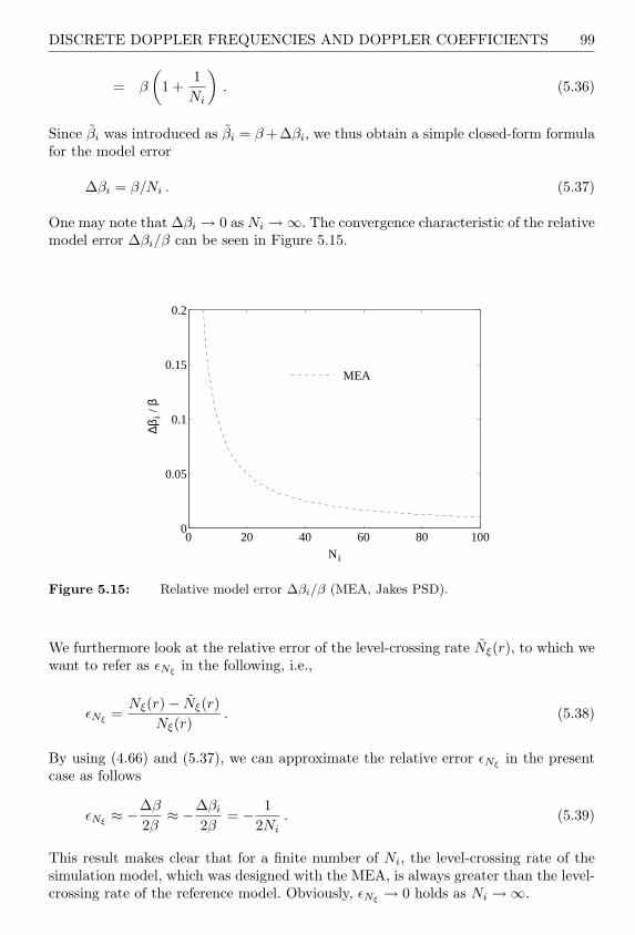
DISCRETE DOPPLER FREQUENCIES AND DOPPLER COEFFICIENTS 99
= β
(1 +
1Ni
). (5.36)
Since βi was introduced as βi = β +∆βi, we thus obtain a simple closed-form formulafor the model error
∆βi = β/Ni . (5.37)
One may note that ∆βi → 0 as Ni →∞. The convergence characteristic of the relativemodel error ∆βi/β can be seen in Figure 5.15.
0 20 40 60 80 1000
0.05
0.1
0.15
0.2
Ni
∆βi /
β
MEA
Figure 5.15: Relative model error ∆βi/β (MEA, Jakes PSD).
We furthermore look at the relative error of the level-crossing rate Nξ(r), to which wewant to refer as εNξ
in the following, i.e.,
εNξ=
Nξ(r)− Nξ(r)Nξ(r)
. (5.38)
By using (4.66) and (5.37), we can approximate the relative error εNξin the present
case as follows
εNξ≈ −∆β
2β≈ −∆βi
2β= − 1
2Ni. (5.39)
This result makes clear that for a finite number of Ni, the level-crossing rate of thesimulation model, which was designed with the MEA, is always greater than the level-crossing rate of the reference model. Obviously, εNξ
→ 0 holds as Ni →∞.
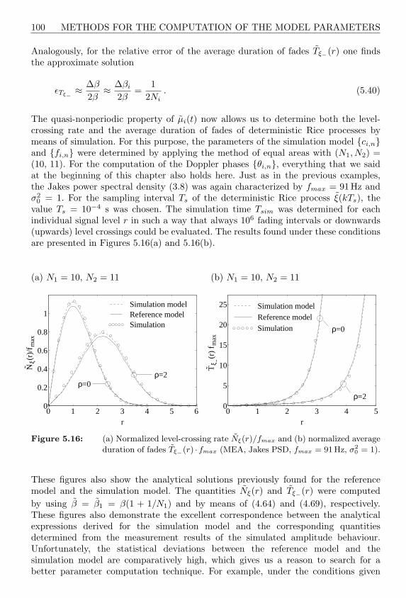
100 METHODS FOR THE COMPUTATION OF THE MODEL PARAMETERS
Analogously, for the relative error of the average duration of fades Tξ−(r) one findsthe approximate solution
εTξ− ≈∆β
2β≈ ∆βi
2β=
12Ni
. (5.40)
The quasi-nonperiodic property of µi(t) now allows us to determine both the level-crossing rate and the average duration of fades of deterministic Rice processes bymeans of simulation. For this purpose, the parameters of the simulation model ci,nand fi,n were determined by applying the method of equal areas with (N1, N2) =(10, 11). For the computation of the Doppler phases θi,n, everything that we saidat the beginning of this chapter also holds here. Just as in the previous examples,the Jakes power spectral density (3.8) was again characterized by fmax = 91Hz andσ2
0 = 1. For the sampling interval Ts of the deterministic Rice process ξ(kTs), thevalue Ts = 10−4 s was chosen. The simulation time Tsim was determined for eachindividual signal level r in such a way that always 106 fading intervals or downwards(upwards) level crossings could be evaluated. The results found under these conditionsare presented in Figures 5.16(a) and 5.16(b).
(a) N1 = 10, N2 = 11
0 1 2 3 4 5 60
0.2
0.4
0.6
0.8
1
r
Nξ(
r)/f
max
ρ=0ρ=2
Simulation modelReference modelSimulation
(b) N1 = 10, N2 = 11
0 1 2 3 4 50
5
10
15
20
25
r
Tξ -
(r)
f max
ρ=0
ρ=2
Simulation modelReference modelSimulation
Figure 5.16: (a) Normalized level-crossing rate Nξ(r)/fmax and (b) normalized average
duration of fades Tξ−(r) ·fmax (MEA, Jakes PSD, fmax = 91Hz, σ20 = 1).
These figures also show the analytical solutions previously found for the referencemodel and the simulation model. The quantities Nξ(r) and Tξ−(r) were computedby using β = β1 = β(1 + 1/N1) and by means of (4.64) and (4.69), respectively.These figures also demonstrate the excellent correspondence between the analyticalexpressions derived for the simulation model and the corresponding quantitiesdetermined from the measurement results of the simulated amplitude behaviour.Unfortunately, the statistical deviations between the reference model and thesimulation model are comparatively high, which gives us a reason to search for abetter parameter computation technique. For example, under the conditions given

DISCRETE DOPPLER FREQUENCIES AND DOPPLER COEFFICIENTS 101
here, where N1 = 10 and N2 = 11, the percentage of the relative error of the level-crossing rate Nξ(r) and the average duration of fades Tξ−(r) is about εNξ
≈ −5 percent and εTξ− ≈ +5 per cent, respectively.
Gaussian power spectral density: With the Gaussian power spectral density(3.11), we obtain the following expression for (5.27)
Gµi(fi,n) =
σ20
2
[1 + erf
(fi,n
fc
√ln 2
)](5.41)
for all n = 1, 2, . . . , Ni and i = 1, 2. Since the inverse function erf−1(·) of the Gaussianerror function does not exist, the discrete Doppler frequencies fi,n cannot be in thiscase computed explicitly. Nevertheless, from the difference of both relations, (5.28)and (5.41), we obtain the equation
n
Ni− erf
(fi,n
fc
√ln 2
)= 0 , ∀n = 1, 2, . . . , Ni (i = 1, 2) , (5.42)
from which the discrete Doppler frequencies fi,n can be determined by means of aproper numerical root-finding technique.
Since the difference between two neighbouring discrete Doppler frequencies ∆fi,n =fi,n − fi,n−1 depends on the index n over a strongly nonlinear relation, it can beassumed that the greatest common divisor Fi = gcdfi,nNi
n=1 is quite small, so thatthe period Ti = 1/Fi of µi(t) is quite high. We can therefore assume that µi(t) isquasi-nonperiodic.
For the corresponding Doppler coefficients ci,n, (5.31) moreover holds. Thus, thedeterministic processes µi(t) designed in this way have the mean power σ2
µi= σ2
0 . Inthe same way as with the Jakes power spectral density, here also the uncorrelatednessof the deterministic processes µ1(t) and µ2(t) can be guaranteed sufficiently by definingN2 according to N2 := N1 + 1.
For example, for Ni = 25, both the power spectral density Sµiµi(f) [cf. (4.14)] andthe corresponding autocorrelation function rµiµi(τ) [cf. (4.11)] will be computed again.For these two functions, we obtain the results shown in Figures 5.17(a) and 5.17(b).
For the performance assessment, the criteria introduced by (4.84) and (4.83) will againbe evaluated for Ni = 5, 6, . . . , 50 at this point. The results obtained for Erµiµi
andEpµi
are depicted in Figures 5.18(a) and 5.18(b), respectively. Figure 5.18(a) alsoshows the graph of Erµiµi
obtained by applying the modified method of equal areas(MMEA), which will be described below.
We now come to the analysis of the model error ∆βi. Since the discrete Dopplerfrequencies fi,n are not given in an explicit form, no closed-form solution can bederived for the model error ∆βi either. Therefore, we proceed as follows. At first,the parameter sets ci,n and fi,n will be computed by using (5.31) and (5.42).Then, the quantity βi can be determined by means of (4.22). In connection with
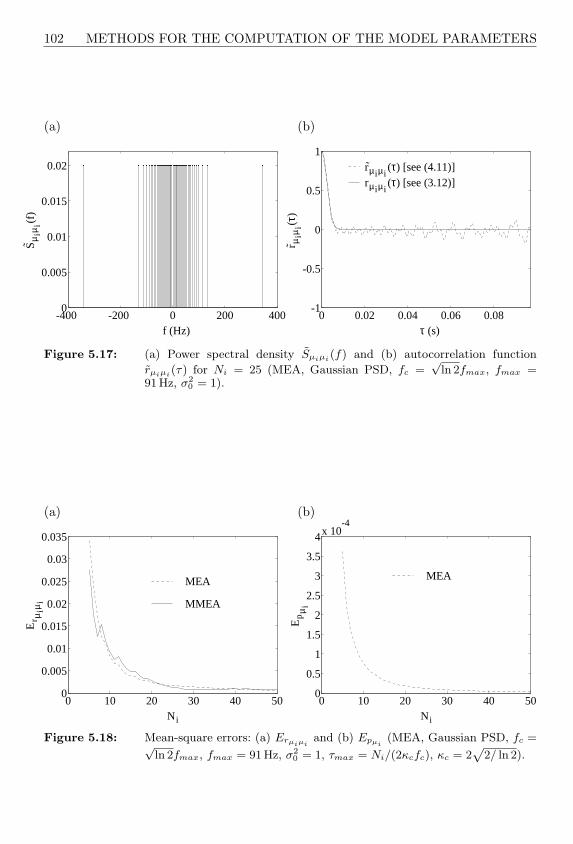
102 METHODS FOR THE COMPUTATION OF THE MODEL PARAMETERS
(a)
-400 -200 0 200 4000
0.005
0.01
0.015
0.02
f (Hz)
Sµ
iµi(f
)
(b)
0 0.02 0.04 0.06 0.08-1
-0.5
0
0.5
1
τ (s)
r µiµ
i(τ)
rµiµi(τ) [see (4.11)]
rµiµi(τ) [see (3.12)]
Figure 5.17: (a) Power spectral density Sµiµi(f) and (b) autocorrelation function
rµiµi(τ) for Ni = 25 (MEA, Gaussian PSD, fc =√
ln 2fmax, fmax =91Hz, σ2
0 = 1).
(a)
0 10 20 30 40 500
0.005
0.01
0.015
0.02
0.025
0.03
0.035
Ni
Er µ
iµi
MEA
MMEA
(b)
0 10 20 30 40 500
0.5
1
1.5
2
2.5
3
3.5
4x 10⁻⁴
Ni
Ep
µi
MEA
Figure 5.18: Mean-square errors: (a) Erµiµiand (b) Epµi
(MEA, Gaussian PSD, fc =√ln 2fmax, fmax = 91Hz, σ2
0 = 1, τmax = Ni/(2κcfc), κc = 2p
2/ ln 2).
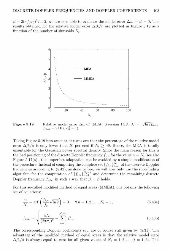
DISCRETE DOPPLER FREQUENCIES AND DOPPLER COEFFICIENTS 103
β = 2(πfcσ0)2/ ln 2, we are now able to evaluate the model error ∆βi = βi − β. Theresults obtained for the relative model error ∆βi/β are plotted in Figure 5.19 as afunction of the number of sinusoids Ni.
0 20 40 60 80 1000
1
2
3
4
5
6
Ni
∆βi /
β
MEAMEA
MMEA
Figure 5.19: Relative model error ∆βi/β (MEA, Gaussian PSD, fc =√
ln 2fmax,fmax = 91 Hz, σ2
0 = 1).
Taking Figure 5.19 into account, it turns out that the percentage of the relative modelerror ∆βi/β is only lower than 50 per cent if Ni ≥ 49. Hence, the MEA is totallyunsuitable for the Gaussian power spectral density. Since the main reason for this isthe bad positioning of the discrete Doppler frequency fi,n for the value n = Ni [see alsoFigure 5.17(a)], this imperfect adaptation can be avoided by a simple modification ofthe procedure. Instead of computing the complete set fi,nNi
n=1 of the discrete Dopplerfrequencies according to (5.42), as done before, we will now only use the root-findingalgorithm for the computation of fi,nNi−1
n=1 and determine the remaining discreteDoppler frequency fi,Ni in such a way that βi = β holds.
For this so-called modified method of equal areas (MMEA), one obtains the followingset of equations:
n
Ni− erf
(fi,n
fc
√ln 2
)= 0 , ∀n = 1, 2, . . . , Ni − 1 , (5.43a)
fi,Ni =
√√√√ βNi
(2πσ0)2−
Ni−1∑n=1
f2i,n . (5.43b)
The corresponding Doppler coefficients ci,n are of course still given by (5.31). Theadvantage of the modified method of equal areas is that the relative model error∆βi/β is always equal to zero for all given values of Ni = 1, 2, . . . (i = 1, 2). This

104 METHODS FOR THE COMPUTATION OF THE MODEL PARAMETERS
is graphically demonstrated in Figure 5.19. However, the effects on the mean-squareerror Erµiµi
are small, as can be seen from Figure 5.18(a).
For the determination of the level-crossing rate Nξ(r) and the average duration offades Tξ−(r), we proceed in the same way as described in connection with the Jakespower spectral density before. The results obtained for Nξ(r) and Tξ−(r) by choosing(N1, N2) = (10, 11) are presented in Figures 5.20(a) and 5.20(b), respectively. Here,the modified method of equal areas was used for the computation of the modelparameters.
(a) N1 = 10, N2 = 11
0 1 2 3 4 5 60
0.2
0.4
0.6
0.8
1
1.2
r
Nξ(
r)/f
max
ρ=0ρ=2
Simulation modelReference modelSimulation
(b) N1 = 10, N2 = 11
0 1 2 3 4 50
5
10
15
20
25
r
Tξ -
(r)
f max
ρ=0
ρ=2
Simulation modelReference modelSimulation
Figure 5.20: (a) Normalized level-crossing rate Nξ(r)/fmax and (b) normalized average
duration of fades Tξ−(r) · fmax (MMEA, Gaussian PSD, fc =√
ln 2fmax,
fmax = 91 Hz, σ20 = 1).
Closed-form analytical expressions for the relative error of both the level-crossing rateNξ(r) and the average duration of fades Tξ−(r) cannot be derived for the MEA in thecase of the Gaussian power spectral density. The reason for this is to be sought in theimplicit equation (5.42) for the determination of the discrete Doppler frequencies fi,n.For the MMEA, however, both relative errors εNξ
and εTξ− are equal to zero.
5.1.4 Monte Carlo Method (MCM)
The Monte Carlo method was first proposed in [Schu89] for the stochastic modellingand the digital simulation of mobile radio channels. Based on this paper, a model forthe equivalent discrete-time channel [For72] in the complex baseband was introduced in[Hoe90, Hoe92]. In the following, we will use this method for the design of deterministicprocesses and will afterwards analyse their statistical properties.
The principle of the Monte Carlo method is based on the realization of the discreteDoppler frequencies fi,n according to a given probability density function pµi(f), whichis related to the power spectral density Sµiµi(f) of the coloured Gaussian random

DISCRETE DOPPLER FREQUENCIES AND DOPPLER COEFFICIENTS 105
process µi(t) by
pµi(f) =
1σ2
0
Sµiµi(f) . (5.44)
Again, σ20 here denotes the mean power (variance) of the Gaussian random process
µi(t).
For the computation of the discrete Doppler frequencies fi,n, we will be guided bythe procedure presented in [Hoe90, Hoe92]. Let un be a random variable uniformlydistributed within the interval (0,1]. Furthermore, let gµi
(un) be a mapping thatis chosen in such a way that the distribution of the discrete Doppler frequenciesfi,n = gµi(un) is equal to the desired cumulative distribution function
Fµi(fi,n) =∫ fi,n
−∞pµi(f) df . (5.45)
According to [Pap91], gµi(un) can then be identified with the inverse function ofFµi(fi,n) = un. Consequently, for the discrete Doppler frequencies fi,n, the relation
fi,n = gµi(un) = F−1µi
(un) (5.46)
holds for all n = 1, 2, . . . , Ni (i = 1, 2). Generally, we obtain positive as well asnegative values for fi,n. In cases where the probability density function pµi(f) is aneven function, i.e., pµi(f) = pµi(−f), we can confine ourselves to positive values forfi,n without restriction of generality. This will be made possible by substituting theuniformly distributed random variable un ∈ (0, 1] in (5.45) by (1 + un)/2 ∈ ( 1
2 , 1].
Since it follows from un > 0 that fi,n > 0 holds, the time average of µi(t) is equal tozero, i.e., mµi = mµi = 0.
The Doppler coefficients ci,n are chosen so that the mean power of µi(t) is identicalto the variance of µi(t), i.e., σ2
0 = rµiµi(0) = σ20 , which is guaranteed by choosing ci,n
according to (5.31). Hence, it then follows
ci,n = σ0
√2Ni
(5.47)
for all n = 1, 2, . . . , Ni (i = 1, 2).
One may consider that with the Monte Carlo method, not only the Doppler phasesθi,n, but also the discrete Doppler frequencies fi,n are random variables. In principle,there is no difference whether statistical or deterministic methods are applied for thedetermination of the model parameters (ci,n, fi,n, θi,n), because the process µi(t),which matters here, is a deterministic function per definition. (We refer to Section 4.1,where deterministic processes µi(t) have been introduced as sample functions or asrealizations of stochastic processes µi(t).) However, especially for a small number ofharmonic functions, the ergodic properties of the stochastic process µi(t) are poor,if the Monte Carlo method is applied for the computation of the discrete Dopplerfrequencies fi,n [Pae96e]. The consequence is that many important characteristic

106 METHODS FOR THE COMPUTATION OF THE MODEL PARAMETERS
quantities of the deterministic process µi(t), like the Doppler spread, the level-crossingrate, and the average duration of fades become random values, which in particularcases can considerably deviate from the desired characteristic quantities prescribed bythe reference model. In the following, we want to put this into concrete terms withthe example of the Jakes and Gaussian power spectral density.
Jakes power spectral density: The application of the Monte Carlo method inconnection with the Jakes power spectral density (3.8) results in the followingexpression for the discrete Doppler frequencies fi,n
fi,n = fmax sin(π
2un
), (5.48)
where un ∈ (0, 1] for all n = 1, 2, . . . , Ni (i = 1, 2). For the Doppler coefficients ci,n,furthermore (5.47) holds. It should be observed that the substitution of un in (5.48)by the deterministic quantity n/Ni exactly leads to the relation (5.33) that we foundfor the method of equal areas.
Since the discrete Doppler frequencies fi,n are random variables, the greatest commondivisor Fi = gcdfi,nNi
n=1 is a random variable as well. However, for a given realizationof the set fi,n with Ni elements, the greatest common divisor Fi is a constant thatcan be determined by applying the Euclidian algorithm on fi,n, where we haveto take into account that the discrete Doppler frequencies fi,n are real numbers.Generally, one can assume that the greatest common divisor Fi is very small, and,thus, the period Ti = 1/Fi is very large, so that µi(t) can be considered as a quasi-nonperiodical function. Obviously, this holds even more, the greater the number ofharmonic functions Ni is chosen.
The demand for uncorrelatedness of the real and the imaginary part generallyalso does not cause any difficulty when designing complex deterministic processesµ(t) = µ1(t) + jµ2(t). The reason for this is that even for N1 = N2, the realized setsf1,n and f2,n are in general mutually exclusive events, leading to the result thatµ1(t) and µ2(t) are uncorrelated with respect to time averaging.
An example of the power spectral density Sµiµi(f), obtained with Ni = 25 harmonicfunctions, is shown in Figure 5.21(a). The autocorrelation function rµiµi(τ), which wascomputed according to (4.11), is plotted in Figure 5.21(b) for two different realizationsof the sets fi,n.
Regarding Figure 5.21(b), one can see that even in the range 0 ≤ τ ≤ τmax,the autocorrelation function rµiµi(τ) of the deterministic process µi(t) can deviateconsiderably from the ideal autocorrelation function rµiµi(τ) of the stochastic processµi(t).2
On the other hand, if we analyse the autocorrelation function rµiµi(τ) of the stochasticprocess µi(t), then, by using (4.82), we obtain
2 Using the Jakes power spectral density, furthermore, let τmax = Ni/(2fmax).

DISCRETE DOPPLER FREQUENCIES AND DOPPLER COEFFICIENTS 107
(a)
-100 -50 0 50 1000
0.005
0.01
0.015
0.02
0.025
f (Hz)
Sµ
iµi(f
)
(b)
0 0.05 0.1 0.15 0.2 0.25
-0.6
-0.4
-0.2
0
0.2
0.4
0.6
0.8
1
τ (s)
r µiµ
i(τ)
rµiµi(τ) (Simulation model)
rµiµi(τ) (Reference model)
1. Realization2. Realization
Figure 5.21: (a) Power spectral density Sµiµi(f) and (b) autocorrelation functionrµiµi(τ) for Ni = 25 (MCM, Jakes PSD, fmax = 91Hz, σ2
0 = 1).
rµiµi(τ) := Eµi(t)µi(t + τ)
=Ni∑
n=1
c2i,n
2Ecos(2πfi,nτ)
=Ni∑
n=1
c2i,n
2J0(2πfmaxτ)
= σ20J0(2πfmaxτ)
= rµiµi(τ) . (5.49)
Summarizing, we can say that the autocorrelation function rµiµi(τ) of the stochasticsimulation model is equal to the ideal autocorrelation function rµiµi(τ) of the referencemodel, whereas the autocorrelation function rµiµi(τ) of the deterministic simulationmodel is different from both of the first-mentioned autocorrelation functions, i.e.,rµiµi(τ) = rµiµi(τ) 6= rµiµi(τ) [Pae96e]. Due to rµiµi(τ) 6= rµiµi(τ), the stochasticprocess µi(t) is therefore not ergodic with respect to the autocorrelation function [cf.Subsection 4.3.4].
The performance of the Monte Carlo method can again be assessed more preciselywith the help of the mean-square error Erµiµi
[see (4.84)]. Figure 5.22 illustrates theevaluation of Erµiµi
as a function of Ni for a single realization of the autocorrelationfunction rµiµi(τ) as well as for the expected value obtained by averaging Erµiµi
overa thousand realizations of rµiµi(τ).
Figure 5.22 also shows the results found for the method of equal areas, which areobviously better compared to the results obtained for the Monte Carlo method. Therelation (5.47) for the computation of the Doppler coefficients ci,n matches (5.31)exactly. Hence, for the mean-square error Epµi
[cf. (4.83)], we obtain exactly the sameresults as presented in Figure 5.14(b).

108 METHODS FOR THE COMPUTATION OF THE MODEL PARAMETERS
0 10 20 30 40 500
0.02
0.04
0.06
0.08
0.1
0.12
0.14
Ni
Er µ
iµi
MCM, #=1
MCM, #=103
MEA
Figure 5.22: Mean-square error Erµiµi(MCM, Jakes PSD, fmax = 91Hz, σ2
0 = 1,
τmax = Ni/(2fmax)).
The discussion on the model error ∆βi follows. Let us start with (4.22). Then, byusing (3.29) and (5.47), the quantity βi = β + ∆βi can be expressed as a function ofthe discrete Doppler frequencies fi,n as follows
βi =2β
f2maxNi
Ni∑n=1
f2i,n . (5.50)
For the Monte Carlo method, the discrete Doppler frequencies fi,n are randomvariables, so that βi is also a random variable. In what follows, we will determinethe probability density function of βi.
Starting from the uniform distribution of un ∈ (0, 1] and noting that the mappingfrom un to fi,n is defined by (5.48), it follows that the probability density function ofthe discrete Doppler frequencies fi,n can be written as
pfi,n(fi,n) =
2
πfmax
√1−
(fi,n
fmax
)2, 0 < f ≤ fmax ,
0 , else .
(5.51)
Now, with the probability density function of fi,n, the density of f2i,n can easily be
computed, and in order to compute the density of the sum of these squares, wepreferably apply the concept of the characteristic function. After some straightforwardcomputations, we obtain the result for the probability density function of βi in the

DISCRETE DOPPLER FREQUENCIES AND DOPPLER COEFFICIENTS 109
following form [Pae96e]
pβi(βi) =
2
∞∫
0
[J0
(2πβν
Ni
)]Ni
cos[2π(βi − β)ν] dν , if βi ∈ (0, 2β] ,
0 , if βi /∈ (0, 2β] .
(5.52)
By way of illustration, the probability density function pβi(βi) of βi is plotted in
Figure 5.23 with Ni as a parameter.
0 0.5 1 1.5 20
1
2
3
4x 10
-5
βi/β
pβ i
(βi)
Ni → ∞
Ni=100
Ni= 20
Ni= 7
Figure 5.23: Probability density function pβi(βi) of βi by using the Monte Carlo method
(Jakes PSD, fmax = 91Hz, σ20 = 1).
The expected value Eβi and the variance Var βi of βi are as follows:
Eβi = β , (5.53a)
Var βi =β2
2Ni. (5.53b)
It will also be shown that for large values of Ni, the random variable βi isapproximately normally distributed with a mean value and a variance according to(5.53a) and (5.53b), respectively. Using the approximation for the Bessel function of0th order [Abr72, eq. (9.1.12)]
J0(x) ≈ 1− x2
4(5.54)
and taking into account that the relation [Abr72, eq. (4.2.21)]
e−x = limNi→∞
(1− x
Ni
)Ni
(5.55)
110 METHODS FOR THE COMPUTATION OF THE MODEL PARAMETERS
can be approximated by e−x ≈ (1 − x/Ni) if Ni is sufficiently large, we may expresspβi
(βi) [see (5.52)] approximately by
pβi(βi) ≈
∫ ∞
−∞e− (πβν)2
Ni e−j2π(βi−β)ν dν , βi ∈ (0, 2β] . (5.56)
Finally, using the integral [Gra81, vol. I, eq. (3.323.2)]∫ ∞
−∞e−(ax)2±bx dx =
√π
ae( b
2a )2 , a > 0 , (5.57)
the desired approximation directly follows
pβi(βi) ≈ 1√
2πβ/√
2Ni
e− (βi−β)2
2β2/(2Ni) , βi ∈ (0, 2β] . (5.58)
Hence, for large values of Ni, the quantity βi is approximately normally distributed,and we may write βi ∼ N(β, β2/(2Ni)) without making too large an error. It should beobserved that in the limit Ni →∞, it obviously follows pβi
(βi) → δ(βi−β). Evidently,the model error ∆βi = βi − β is likewise approximately normally distributed, i.e.,∆βi ∼ N(0, β2/(2Ni)), so that the random variable ∆βi is in fact zero-mean, butunfortunately its variance merely behaves proportionally to the reciprocal value ofthe number of harmonic functions Ni. Finally, we also investigate the relative modelerror ∆βi/β, for which it approximately holds: ∆βi/β ∼ N(0, 1/(2Ni)). Hence, thestandard deviation of ∆βi/β is equal to 1/
√2Ni and for Ni > 2 it is thus always
greater than the relative model error ∆βi/β = 1/Ni obtained by using the method ofequal areas [cf. (5.37)]. Figure 5.24 demonstrates the random behaviour of the relativemodel error ∆βi/β in terms of the number of harmonic functions Ni. The evaluationof ∆βi/β was performed here by means of (5.50), where five events of the set fi,nNi
n=1
were processed for every value of Ni ∈ 5, 6, . . . , 100.
Due to (4.66), (4.70), and (4.78), it now becomes clear that the level-crossing rateNξ(r), the average duration of fades Tξ−(r), and the time intervals τq(r) likewisedeviate in a random manner from the corresponding quantities of the reference model.For example, if we choose the pair (10, 11) for the couple (N1, N2), then for twodifferent realizations of each of the sets f1,nN1
n=1 and f2,nN2n=1, the behaviours
shown in Figures 5.25(a) and 5.25(b) could occur for Nξ(r) and Tξ−(r), respectively.Here, the simulations were carried out in the same way as previously described inSubsection 5.1.3.
With the Chebyshev inequality (2.15), one can show [see Appendix C] that even ifNi = 2500 harmonic functions are used, the probability that the absolute value of therelative model error |∆βi/β| exceeds a value of more than 2 per cent is merely less orequal to 50 per cent.
Gaussian power spectral density: If we apply the Monte Carlo method inconnection with the Gaussian power spectral density (3.11), then it is not possible
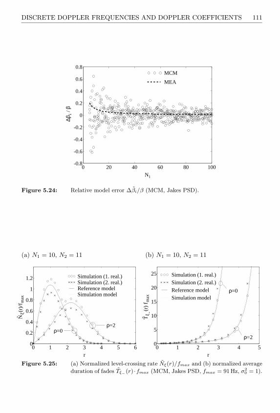
DISCRETE DOPPLER FREQUENCIES AND DOPPLER COEFFICIENTS 111
0 20 40 60 80 100-0.8
-0.6
-0.4
-0.2
0
0.2
0.4
0.6
0.8
Ni
∆βi /
βMCM
MEA
Figure 5.24: Relative model error ∆βi/β (MCM, Jakes PSD).
(a) N1 = 10, N2 = 11
0 1 2 3 4 5 60
0.2
0.4
0.6
0.8
1
1.2
r
Nξ(
r)/f
max
ρ=0ρ=2
Reference modelSimulation model
Simulation (1. real.)Simulation (2. real.)
(b) N1 = 10, N2 = 11
0 1 2 3 4 50
5
10
15
20
25
r
Tξ -
(r)
f max
ρ=0
ρ=2
Reference modelSimulation model
Simulation (1. real.)Simulation (2. real.)
Figure 5.25: (a) Normalized level-crossing rate Nξ(r)/fmax and (b) normalized average
duration of fades Tξ−(r) ·fmax (MCM, Jakes PSD, fmax = 91Hz, σ20 = 1).
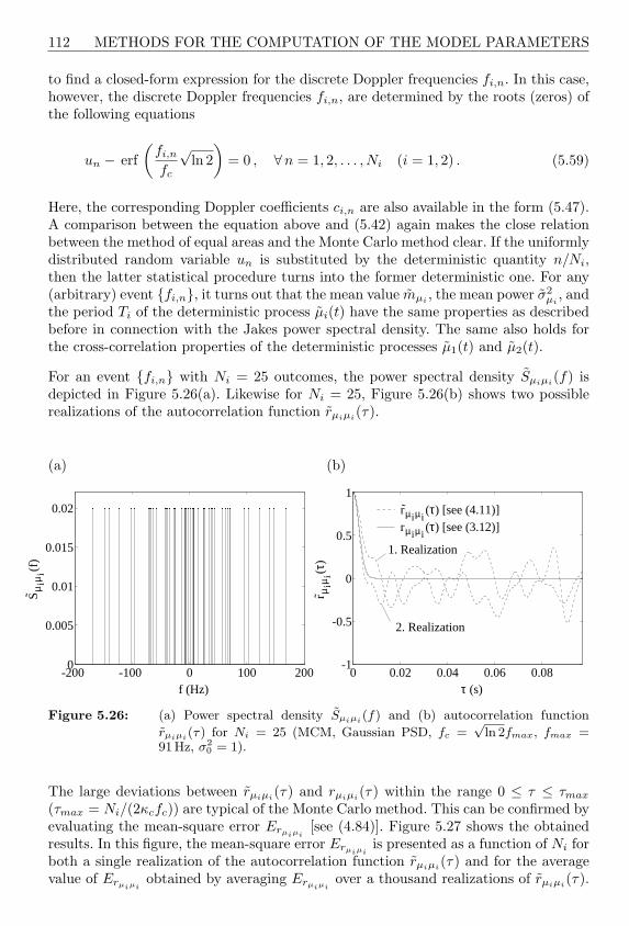
112 METHODS FOR THE COMPUTATION OF THE MODEL PARAMETERS
to find a closed-form expression for the discrete Doppler frequencies fi,n. In this case,however, the discrete Doppler frequencies fi,n, are determined by the roots (zeros) ofthe following equations
un − erf(
fi,n
fc
√ln 2
)= 0 , ∀n = 1, 2, . . . , Ni (i = 1, 2) . (5.59)
Here, the corresponding Doppler coefficients ci,n are also available in the form (5.47).A comparison between the equation above and (5.42) again makes the close relationbetween the method of equal areas and the Monte Carlo method clear. If the uniformlydistributed random variable un is substituted by the deterministic quantity n/Ni,then the latter statistical procedure turns into the former deterministic one. For any(arbitrary) event fi,n, it turns out that the mean value mµi , the mean power σ2
µi, and
the period Ti of the deterministic process µi(t) have the same properties as describedbefore in connection with the Jakes power spectral density. The same also holds forthe cross-correlation properties of the deterministic processes µ1(t) and µ2(t).
For an event fi,n with Ni = 25 outcomes, the power spectral density Sµiµi(f) isdepicted in Figure 5.26(a). Likewise for Ni = 25, Figure 5.26(b) shows two possiblerealizations of the autocorrelation function rµiµi(τ).
(a)
-200 -100 0 100 2000
0.005
0.01
0.015
0.02
f (Hz)
Sµ
iµi(f
)
(b)
0 0.02 0.04 0.06 0.08-1
-0.5
0
0.5
1
τ (s)
r µiµ
i(τ)
rµiµi(τ) [see (4.11)]
rµiµi(τ) [see (3.12)]
1. Realization
2. Realization
Figure 5.26: (a) Power spectral density Sµiµi(f) and (b) autocorrelation function
rµiµi(τ) for Ni = 25 (MCM, Gaussian PSD, fc =√
ln 2fmax, fmax =91Hz, σ2
0 = 1).
The large deviations between rµiµi(τ) and rµiµi(τ) within the range 0 ≤ τ ≤ τmax
(τmax = Ni/(2κcfc)) are typical of the Monte Carlo method. This can be confirmed byevaluating the mean-square error Erµiµi
[see (4.84)]. Figure 5.27 shows the obtainedresults. In this figure, the mean-square error Erµiµi
is presented as a function of Ni forboth a single realization of the autocorrelation function rµiµi(τ) and for the averagevalue of Erµiµi
obtained by averaging Erµiµiover a thousand realizations of rµiµi(τ).

DISCRETE DOPPLER FREQUENCIES AND DOPPLER COEFFICIENTS 113
0 10 20 30 40 500
0.02
0.04
0.06
0.08
0.1
0.12
Ni
Er µ
iµi
MCM, #=1
MCM, #=103
MMEA
Figure 5.27: Mean-square error Erµiµi(MCM, Gaussian PSD, fc =
√ln 2fmax, fmax =
91Hz, σ20 = 1, τmax = Ni/(2κcfc), κc = 2
p2/ ln 2).
In this case, the analysis of the model error ∆βi cannot be carried out analytically.Therefore, we proceed in such a way that for a given realization of fi,n, at firstthe corresponding elementary event of the random variable βi is determined bymeans of (4.22). Afterwards, with β = 2(πfcσ0)2/ ln 2, the computation of the modelerror ∆βi = βi − β will be performed. Figure 5.28 presents the evaluation of therelative model error ∆βi/β, where the obtained results are shown for each value ofNi ∈ 5, 6, . . . , 100 on the basis of five realizations of the set fi,n.
The determination as well as the investigation of the properties of the level-crossingrate Nξ(r) and the average duration of fades Tξ−(r) are also performed on the basisof several realizations of the set fi,n. To illustrate the obtained results, we takea look at Figures 5.29(a) and 5.29(b), where two different realizations of Nξ(r) andTξ−(r) are shown, respectively. All the presented results have been obtained by using(N1, N2) = (10, 11).
5.1.5 Lp-Norm Method (LPNM)
The Lp-norm method (LPNM) is based on the idea that the sets ci,n and fi,n areto be determined in such a way that the following requirements will be fulfilled for agiven number of harmonic functions Ni [Pae98b, Pae96c]:
(i) With respect to the following Lp-norm
E(p)pµi
:=∫ ∞
−∞|pµi(x)− pµi(x)|p dx
1/p
, p = 1, 2, . . . , (5.60)
the probability density function pµi(x) of the deterministic process µi(t) will be an
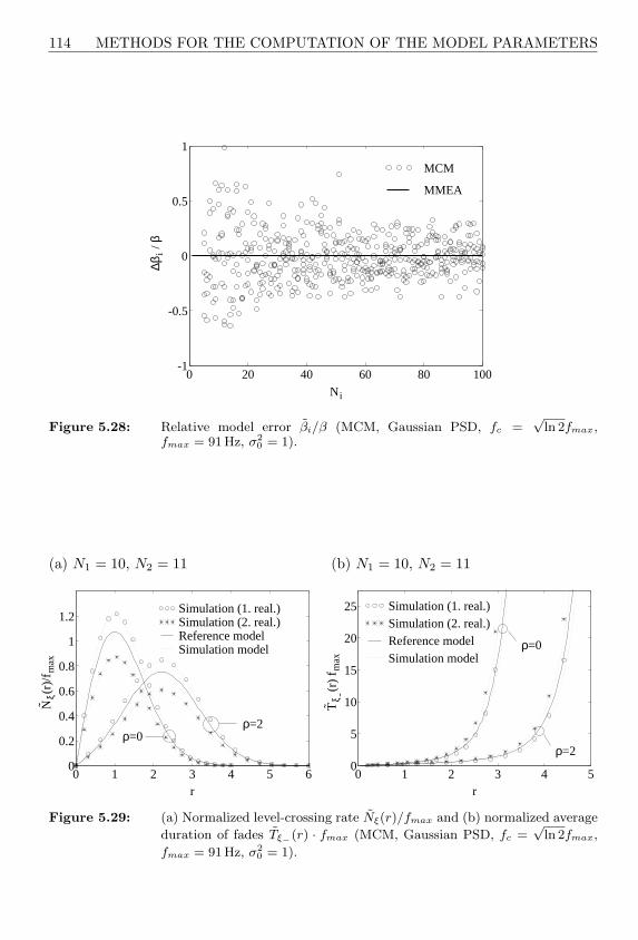
114 METHODS FOR THE COMPUTATION OF THE MODEL PARAMETERS
0 20 40 60 80 100-1
-0.5
0
0.5
1
Ni
∆βi /
βMCM
MMEA
Figure 5.28: Relative model error βi/β (MCM, Gaussian PSD, fc =√
ln 2fmax,fmax = 91 Hz, σ2
0 = 1).
(a) N1 = 10, N2 = 11
0 1 2 3 4 5 60
0.2
0.4
0.6
0.8
1
1.2
r
Nξ(
r)/f
max
ρ=0ρ=2
Reference modelSimulation model
Simulation (1. real.)Simulation (2. real.)
(b) N1 = 10, N2 = 11
0 1 2 3 4 50
5
10
15
20
25
r
Tξ -
(r)
f max
ρ=0
ρ=2
Reference modelSimulation model
Simulation (1. real.)Simulation (2. real.)
Figure 5.29: (a) Normalized level-crossing rate Nξ(r)/fmax and (b) normalized average
duration of fades Tξ−(r) · fmax (MCM, Gaussian PSD, fc =√
ln 2fmax,
fmax = 91 Hz, σ20 = 1).

DISCRETE DOPPLER FREQUENCIES AND DOPPLER COEFFICIENTS 115
optimal approximation of the Gaussian distribution pµi(x) of the stochastic processµi(t).
(ii) With respect to the following Lp-norm
E(p)rµiµi
:=
1τmax
∫ τmax
0
|rµiµi(τ)− rµiµi(τ)|p dτ
1/p
, p = 1, 2, . . . , (5.61)
the autocorrelation function rµiµi(τ) of the deterministic process µi(t) will be fittedas close as possible to a given (desired) autocorrelation function rµiµi
(τ) of thestochastic process µi(t), where τmax again defines an appropriate time interval[0, τmax] over which the approximation of rµiµi
(τ) is of interest.
We first pay attention to the requirement (i). Since, according to (4.34), pµi(x)merely depends on the Doppler coefficients ci,n, we ask ourselves: does an optimalsolution for the set of Doppler coefficients ci,n exist, for which the Lp-norm E
(p)pµi
becomes minimal? In order to answer this question, we first substitute (4.34) and(4.36) into (5.60), and afterwards perform a numerical optimization of the Dopplercoefficients ci,n, so that E
(p)pµi
becomes minimal. As a numerical optimization technique,for example, the Fletcher-Powell algorithm [Fle63] is particularly well suited for thiskind of problem. After the minimization of (5.60), the optimized Doppler coefficientsci,n = c
(opt)i,n are available for the realization of deterministic simulation models.
Figure 5.30(a) shows the resulting probability density function pµi(x) by using theoptimized quantities c
(opt)i,n . For the choice of suitable starting values for the Doppler
coefficients, we appropriately fall back to the quantities ci,n = σ0
√2/Ni. For a better
assessment of the obtained results, the probability density function pµi(x), which isobtained by using the starting values ci,n = σ0
√2/Ni [cf. also Figure 4.4(a)], is again
presented in Figure 5.30(b).
More meaningful than the comparison of Figures 5.30(a) and 5.30(b) are the results ofFigure 5.31, where the mean-square error Epµi
[see (4.39)] is presented for ci,n = c(opt)i,n
as well as for ci,n = σ0
√2/Ni. One can clearly realize that the optimization gain
decreases strictly monotonously if the number of sinusoids Ni increases.
It is also worth mentioning that after the minimization of (5.60), all optimized Dopplercoefficients c
(opt)i,n are in fact identical (due to the central limit theorem). But for a finite
number of harmonic functions Ni, they are always smaller than the pre-set startingvalues, i.e., c
(opt)i,n < σ0
√2/Ni, ∀Ni = 1, 2, . . . Since the optimized Doppler coefficients
c(opt)i,n are identical, which is even the case when arbitrary starting values are chosen,
it is probable that the Lp-norm (5.60) has a global minimum at ci,n = c(opt)i,n , and,
thus, the Doppler coefficients ci,n = c(opt)i,n are optimal. For finite values of Ni, one
may also take into account that due to ci,n = c(opt)i,n < σ0
√2/Ni, the mean power of
the deterministic process µi(t) is always smaller than the variance of the stochasticprocess µi(t), i.e., it holds σ2
0 < σ20 . This can be realized by considering Figure 5.32.
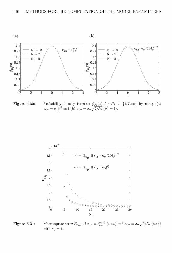
116 METHODS FOR THE COMPUTATION OF THE MODEL PARAMETERS
(a)
-3 -2 -1 0 1 2 30
0.05
0.1
0.15
0.2
0.25
0.3
0.35
0.4
pµ
i(x)
x
Ni → ∞Ni = 7Ni = 5
ci,n = c(opt)i,n
(b)
-3 -2 -1 0 1 2 30
0.05
0.1
0.15
0.2
0.25
0.3
0.35
0.4
pµ
i(x)
x
Ni → ∞Ni = 7Ni = 5
ci,n=σo (2/Ni)1/2
Figure 5.30: Probability density function pµi(x) for Ni ∈ 5, 7,∞ by using: (a)
ci,n = c(opt)i,n and (b) ci,n = σ0
p2/Ni (σ2
0 = 1).
0 5 10 15 20 25 300
0.5
1
1.5
2
2.5
3
3.5
4x 10
-4
Ni
Ep
µi
Epµi if ci,n = σo (2/Ni)
1/2
Epµi if ci,n = c(opt)
i,n
Figure 5.31: Mean-square error Epµi, if ci,n = c
(opt)i,n (∗ ∗ ∗) and ci,n = σ0
p2/Ni ( )
with σ20 = 1.

DISCRETE DOPPLER FREQUENCIES AND DOPPLER COEFFICIENTS 117
0 5 10 15 20 25 300.5
0.6
0.7
0.8
0.9
1
1.1
Ni
σ2 o
σ2o if ci,n = σo (2/Ni)
1/2
σ2o if ci,n = c(opt)
i,n
Figure 5.32: Mean power σ20 of the deterministic process µi(t), if ci,n = c
(opt)i,n (∗ ∗ ∗)
and ci,n = σ0
p2/Ni ( ) with σ2
0 = 1.
Obviously, a compromise between the attainable approximation precision of pµi(x) ≈pµi(x) and σ2
0 ≈ σ20 has to be made here. Let us try to avoid this compromise by
imposing the so-called power constraint defined by σ20 = σ2
0 on the simulation model.Then, we have to optimize, e.g., the first Ni−1 Doppler coefficients ci,1, ci,2, . . . , ci,Ni−1
and the remaining parameter ci,Ni is determined in such a way that the imposed powerconstraint σ2
0 = σ20 is always fulfilled. In this case, the optimization results in c
(opt)i,n =
σ0
√2/Ni for all n = 1, 2, . . . , Ni. Thus, by including the power constraint σ2
0 = σ20 in
the parameter design, an optimal approximation of the Gaussian distribution pµi(x)for any number of harmonic functions Ni can only become possible if the Dopplercoefficients ci,n are given by ci,n = c
(opt)i,n = σ0
√2/Ni. Therefore, when modelling
Gaussian random processes and other processes derivable from these, such as Rayleighprocesses, Rice processes, and lognormal processes, we will usually make use of therelation ci,n = σ0
√2/Ni in the following.
The suggested method is still quite useful and advantageous for the approximationof probability density functions which are not derivable from Gaussian distributions,e.g., like the Nakagami distribution (2.33). The Nakagami distribution [Nak60] is moreflexible than the frequently used Rayleigh or Rice distribution and often enables abetter adaptation to probability density functions which follow from experimentalmeasurement results [Suz77].
In order to be able to determine the set of Doppler coefficients ci,n in such a way thatthe probability density function of the deterministic simulation model approximatesthe Nakagami distribution, we perform the optimization of the Doppler coefficientsin a similar manner as described before in connection with the normal distribution.The only difference is that in (5.60) we have to substitute the Gaussian distribution
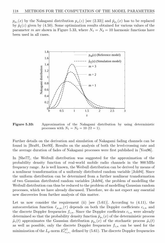
118 METHODS FOR THE COMPUTATION OF THE MODEL PARAMETERS
pµi(x) by the Nakagami distribution pω(z) [see (2.33)] and pµi(x) has to be replacedby pξ(z) given by (4.50). Some optimization results obtained for various values of theparameter m are shown in Figure 5.33, where N1 = N2 = 10 harmonic functions havebeen used in all cases.
0 0.5 1 1.5 2 2.5 30
0.2
0.4
0.6
0.8
1
1.2
1.4
1.6
1.8
z
Nak
agam
i dis
trib
utio
n
m = 1
m = 2
m = 3
pξ(z) (Simulation model)
pω(z) (Reference model)
Figure 5.33: Approximation of the Nakagami distribution by using deterministicprocesses with N1 = N2 = 10 (Ω = 1).
Further details on the derivation and simulation of Nakagami fading channels can befound in [Bra91, Der93]. Results on the analysis of both the level-crossing rate andthe average duration of fades of Nakagami processes were first published in [You96].
In [She77], the Weibull distribution was suggested for the approximation of theprobability density function of real-world mobile radio channels in the 900MHzfrequency range. As is well known, the Weibull distribution can be derived by means ofa nonlinear transformation of a uniformly distributed random variable [Joh94]. Sincethe uniform distribution can be determined from a further nonlinear transformationof two Gaussian distributed random variables [Joh94], the problem of modelling theWeibull distribution can thus be reduced to the problem of modelling Gaussian randomprocesses, which we have already discussed. Therefore, we do not expect any essentialnew discoveries from further analysis of this matter.
Let us now consider the requirement (ii) [see (5.61)]. According to (4.11), theautocorrelation function rµiµi(τ) depends on both the Doppler coefficients ci,n andthe discrete Doppler frequencies fi,n. Since the Doppler coefficients ci,n were alreadydetermined so that the probability density function pµi(x) of the deterministic processµi(t) approximates the Gaussian distribution pµi(x) of the stochastic process µi(t)as well as possible, only the discrete Doppler frequencies fi,n can be used for theminimization of the Lp-norm E
(p)rµiµi
defined by (5.61). The discrete Doppler frequencies
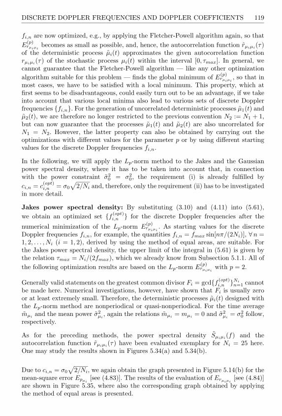
DISCRETE DOPPLER FREQUENCIES AND DOPPLER COEFFICIENTS 119
fi,n are now optimized, e.g., by applying the Fletcher-Powell algorithm again, so thatE
(p)rµiµi
becomes as small as possible, and, hence, the autocorrelation function rµiµi(τ)
of the deterministic process µi(t) approximates the given autocorrelation functionrµiµi
(τ) of the stochastic process µi(t) within the interval [0, τmax]. In general, wecannot guarantee that the Fletcher-Powell algorithm — like any other optimizationalgorithm suitable for this problem — finds the global minimum of E
(p)rµiµi
, so that inmost cases, we have to be satisfied with a local minimum. This property, which atfirst seems to be disadvantageous, could easily turn out to be an advantage, if we takeinto account that various local minima also lead to various sets of discrete Dopplerfrequencies fi,n. For the generation of uncorrelated deterministic processes µ1(t) andµ2(t), we are therefore no longer restricted to the previous convention N2 := N1 + 1,but can now guarantee that the processes µ1(t) and µ2(t) are also uncorrelated forN1 = N2. However, the latter property can also be obtained by carrying out theoptimizations with different values for the parameter p or by using different startingvalues for the discrete Doppler frequencies fi,n.
In the following, we will apply the Lp-norm method to the Jakes and the Gaussianpower spectral density, where it has to be taken into account that, in connectionwith the power constraint σ2
0 = σ20 , the requirement (i) is already fulfilled by
ci,n = c(opt)i,n = σ0
√2/Ni and, therefore, only the requirement (ii) has to be investigated
in more detail.
Jakes power spectral density: By substituting (3.10) and (4.11) into (5.61),we obtain an optimized set f (opt)
i,n for the discrete Doppler frequencies after the
numerical minimization of the Lp-norm E(p)rµiµi
. As starting values for the discreteDoppler frequencies fi,n, for example, the quantities fi,n = fmax sin[nπ/(2Ni)], ∀n =1, 2, . . . , Ni (i = 1, 2), derived by using the method of equal areas, are suitable. Forthe Jakes power spectral density, the upper limit of the integral in (5.61) is given bythe relation τmax = Ni/(2fmax), which we already know from Subsection 5.1.1. All ofthe following optimization results are based on the Lp-norm E
(p)rµiµi
with p = 2.
Generally valid statements on the greatest common divisor Fi = gcdf (opt)i,n Ni
n=1 cannotbe made here. Numerical investigations, however, have shown that Fi is usually zeroor at least extremely small. Therefore, the deterministic processes µi(t) designed withthe Lp-norm method are nonperiodical or quasi-nonperiodical. For the time averagemµi and the mean power σ2
µi, again the relations mµi = mµi = 0 and σ2
µi= σ2
0 follow,respectively.
As for the preceding methods, the power spectral density Sµiµi(f) and theautocorrelation function rµiµi(τ) have been evaluated exemplary for Ni = 25 here.One may study the results shown in Figures 5.34(a) and 5.34(b).
Due to ci,n = σ0
√2/Ni, we again obtain the graph presented in Figure 5.14(b) for the
mean-square error Epµi[see (4.83)]. The results of the evaluation of Erµiµi
[see (4.84)]are shown in Figure 5.35, where also the corresponding graph obtained by applyingthe method of equal areas is presented.

120 METHODS FOR THE COMPUTATION OF THE MODEL PARAMETERS
(a)
-100 -50 0 50 1000
0.005
0.01
0.015
0.02
f (Hz)
Sµ
iµi(f
)
(b)
0 0.05 0.1 0.15 0.2 0.25-0.4
-0.2
0
0.2
0.4
0.6
0.8
1
τ (s)
r µiµ
i(τ)
rµiµi(τ) (Simulation model)
rµiµi(τ) (Reference model)
τmax
Figure 5.34: (a) Power spectral density Sµiµi(f) and (b) autocorrelation functionrµiµi(τ) for Ni = 25 (LPNM, Jakes PSD, fmax = 91Hz, σ2
0 = 1).
0 10 20 30 40 500
0.005
0.01
0.015
Ni
Er µ
iµi
MEA
LPNM
Figure 5.35: Mean-square error Erµiµi(LPNM, Jakes PSD, fmax = 91Hz, σ2
0 = 1,
τmax = Ni/(2fmax)).
In order to compute the model error ∆βi = βi − β, the expression (4.22) has to beevaluated for ci,n = σ0
√2/Ni and fi,n = f
(opt)i,n . In comparison with the method of
equal areas, we then obtain the graphs illustrated in Figure 5.36 for the relative modelerror ∆βi/β.
The simulation of the level-crossing rate and the average duration of fades is carriedout in the same way as already described in Subsection 5.1.3. For reasons of unity, wehere again choose the pair (10, 11) for the couple (N1, N2). The simulation results for
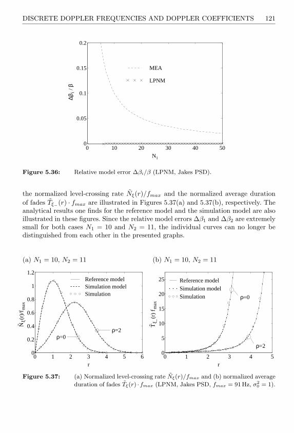
DISCRETE DOPPLER FREQUENCIES AND DOPPLER COEFFICIENTS 121
0 10 20 30 40 500
0.05
0.1
0.15
0.2
Ni
∆βi /
βMEA
LPNM
Figure 5.36: Relative model error ∆βi/β (LPNM, Jakes PSD).
the normalized level-crossing rate Nξ(r)/fmax and the normalized average durationof fades Tξ−(r) · fmax are illustrated in Figures 5.37(a) and 5.37(b), respectively. Theanalytical results one finds for the reference model and the simulation model are alsoillustrated in these figures. Since the relative model errors ∆β1 and ∆β2 are extremelysmall for both cases N1 = 10 and N2 = 11, the individual curves can no longer bedistinguished from each other in the presented graphs.
(a) N1 = 10, N2 = 11
0 1 2 3 4 5 60
0.2
0.4
0.6
0.8
1
1.2
r
Nξ(
r)/f
max
ρ=0ρ=2
Simulation modelReference model
Simulation
(b) N1 = 10, N2 = 11
0 1 2 3 4 50
5
10
15
20
25
r
Tξ -
(r)
f max
ρ=0
ρ=2
Reference modelSimulation modelSimulation
Figure 5.37: (a) Normalized level-crossing rate Nξ(r)/fmax and (b) normalized average
duration of fades Tξ(r) ·fmax (LPNM, Jakes PSD, fmax = 91 Hz, σ20 = 1).

122 METHODS FOR THE COMPUTATION OF THE MODEL PARAMETERS
Gaussian power spectral density: The previously analysed methods for thedetermination of the model parameters of the deterministic processes have made itquite clear that the Gaussian power spectral density causes much greater problemsthan the Jakes power spectral density. In this subsection, we will find out how toget these problems under control by using the Lp-norm method. Therefore, we fullyexploit the degrees of freedom which this method has to offer. All in all, this leadsus to three fundamental variants [Pae97d] of the Lp-norm method. In the following,these variants will be briefly described and afterwards analysed with respect to theirperformances.
First variant of the Lp-norm method (LPNM I): In the first variant, the Dopplercoefficients ci,n are again computed according to the equation ci,n = σ0
√2/Ni for
all n = 1, 2, . . . , Ni, whereas the discrete Doppler frequencies fi,n are optimized forn = 1, 2, . . . , Ni − 1 in such a way that the Lp-norm E
(p)rµiµi
[see (5.61)] results in a(local) minimum, i.e.,
E(p)rµiµi
(f i) = Min! , (5.62)
where f i stands for the parameter vector f i = (fi,1, fi,2, . . . , fi,Ni−1)T ∈ IRNi−1.Boundary conditions, like the restriction that the components of the parameter vectorf i shall be positive, do not need to be imposed on the procedure, since the Gaussianpower spectral density is symmetrical. The remaining discrete Doppler frequency fi,Ni
is defined by
fi,Ni :=
√√√√ βNi
(2πσ0)2−
Ni−1∑n=1
f2i,n , (5.63)
so that we have guaranteed in a simple manner that the model error ∆βi is alwayszero for all chosen values of Ni = 1, 2, . . . (i = 1, 2). With the corresponding quantityβ, we can of course make use of this possibility when dealing with the Jakes powerspectral density (or any other given power spectral density) as well. Quite suitablestarting values for the optimization of the involved discrete Doppler frequencies arethe quantities found with the method of equal areas [cf. Subsection 5.1.3]. For theevaluation of the Lp-norm E
(p)rµiµi
, it is sufficient for our objectives to restrict ourselvesto the case p = 2. In this connection, for the parameter τmax, we return to the relationτmax = Ni/(2κcfc) with κc = 2
√2/ ln 2 and fc =
√ln 2fmax, which has already been
employed several times in preceding investigations. For the quantities Fi, mµi , and σ2µi
,the statements made for the Jakes power spectral density are still valid in the presentcase. Uncorrelated deterministic processes µ1(t) and µ2(t) can also be obtained forN1 = N2 by optimizing the parameter vectors f1 and f2 under different conditions.Therefore, it is sufficient to change, for example, τmax or p slightly and then to repeatthe optimization once again.
We choose Ni = 25 and with the first variant of the Lp-norm method, we obtain thepower spectral density Sµiµi(f) presented in Figure 5.38(a). Figure 5.38(b) shows thecorresponding autocorrelation function rµiµi(τ).
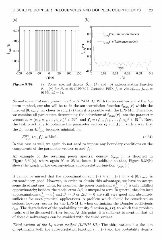
DISCRETE DOPPLER FREQUENCIES AND DOPPLER COEFFICIENTS 123
(a)
-150 -100 -50 0 50 100 1500
0.005
0.01
0.015
0.02
f (Hz)
Sµ
iµi(f
)
(b)
0 0.02 0.04 0.06 0.08 0.1-0.2
0
0.2
0.4
0.6
0.8
1
τ (s)
r µiµ
i(τ)
rµiµi(τ) (Simulation model)
rµiµi(τ) (Reference model)
τmax
Figure 5.38: (a) Power spectral density Sµiµi(f) and (b) autocorrelation function
rµiµi(τ) for Ni = 25 (LPNM I, Gaussian PSD, fc =√
ln 2fmax, fmax =91Hz, σ2
0 = 1).
Second variant of the Lp-norm method (LPNM II): With the second variant of the Lp-norm method, our aim will be to fit the autocorrelation function rµiµi(τ) within theinterval [0, τmax] far closer to rµiµi(τ) than it is possible with the LPNM I. Therefore,we combine all parameters determining the behaviour of rµiµi(τ) into the parametervectors ci = (ci,1, ci,2, . . . , ci,Ni)
T ∈ IRNi and f i = (fi,1, fi,2, . . . , fi,Ni)T ∈ IRNi . Now,
the task is actually to optimize the parameter vectors ci and f i in such a way thatthe Lp-norm E
(p)rµiµi
becomes minimal, i.e.,
E(p)rµiµi
(ci, f i) = Min! . (5.64)
In this case as well, we again do not need to impose any boundary conditions on thecomponents of the parameter vectors ci and f i.
An example of the resulting power spectral density Sµiµi(f) is depicted inFigure 5.39(a), where again Ni = 25 is chosen. In addition to that, Figure 5.39(b)shows the graph of the corresponding autocorrelation function rµiµi(τ).
It cannot be missed that the approximation rµiµi(τ) ≈ rµiµi(τ) for τ ∈ [0, τmax] isextraordinary good. However, in order to obtain this advantage, we have to acceptsome disadvantages. Thus, for example, the power constraint σ2
µi= σ2
0 is only fulfilledapproximately; besides, the model error ∆βi is unequal to zero. In general, the obtainedapproximations σ2
µi≈ σ2
0 and βi ≈ β or ∆βi ≈ 0 are still very good and absolutelysufficient for most practical applications. A problem which should be considered asserious, however, occurs for the LPNM II when optimizing the Doppler coefficientsci,n. The degradation of the probability density function pµi(x), to which this problemleads, will be discussed further below. At this point, it is sufficient to mention that allof these disadvantages can be avoided with the third variant.
Third variant of the Lp-norm method (LPNM III): The third variant has the aimof optimizing both the autocorrelation function rµiµi(τ) and the probability density

124 METHODS FOR THE COMPUTATION OF THE MODEL PARAMETERS
(a)
-300 -200 -100 0 100 200 3000
0.005
0.01
0.015
0.02
0.025
f (Hz)
Sµ
iµi(f
)
(b)
0 0.02 0.04 0.06 0.08 0.1-0.2
0
0.2
0.4
0.6
0.8
1
τ (s)
r µiµ
i(τ)
rµiµi(τ) (Simulation model)
rµiµi(τ) (Reference model)
τmax
Figure 5.39: (a) Power spectral density Sµiµi(f) and (b) autocorrelation function
rµiµi(τ) for Ni = 25 (LPNM II, Gaussian PSD, fc =√
ln 2fmax, fmax =91Hz, σ2
0 = 1).
function pµi(x). An error function suitable for this purpose has the form
E(ci, f i) = W1 · E(p)rµiµi
(ci, f i) + W2 · E(p)pµi
(ci) , (5.65)
where E(p)rµiµi
(·) and E(p)pµi
(·) denote the Lp-norms introduced by (5.61) and (5.60),respectively. The quantities W1 and W2 are appropriate weighting factors, which willbe defined by W1 = 1/4 and W2 = 3/4 in the sequel. To have both constraints σ2
µi= σ2
0
and βi = β exactly fulfilled now, we will define the parameter vectors ci and f i by
ci = (ci,1, ci,2, . . . , ci,Ni−1)T ∈ IRNi−1 (5.66a)
and
f i = (fi,1, fi,2, . . . , fi,Ni−1)T ∈ IRNi−1 , (5.66b)
respectively, and calculate the remaining model parameters ci,Ni and fi,Ni as follows:
ci,Ni =
√√√√2σ20 −
Ni−1∑n=1
c2i,n , (5.67a)
fi,Ni =1
ci,Ni
√√√√ β
2π2−
Ni−1∑n=1
(ci,nfi,n)2 , (5.67b)
where β = −rµiµi(0) = 2(πfcσ0)2/ ln 2 (i = 1, 2). Correlations between thedeterministic processes µ1(t) and µ2(t) can now be avoided for N1 = N2 by performingthe minimization of the error function (5.65) for i = 1 and i = 2 with differentweighting factors of the respective Lp-norms E
(p)rµiµi
and E(p)pµi
.

DISCRETE DOPPLER FREQUENCIES AND DOPPLER COEFFICIENTS 125
As in the preceding examples, we choose Ni = 25 and observe the resultingpower spectral density Sµiµi
(f) in Figure 5.40(a). The corresponding autocorrelationfunction rµiµi
(τ) is shown in Figure 5.40(b).
(a)
-400 -200 0 200 4000
0.005
0.01
0.015
0.02
0.025
0.03
f (Hz)
Sµ
iµi(f
)
(b)
0 0.02 0.04 0.06 0.08 0.1-0.2
0
0.2
0.4
0.6
0.8
1
τ (s)
r µiµ
i(τ)
rµiµi(τ) (Simulation model)
rµiµi(τ) (Reference model)
τmax
Figure 5.40: (a) Power spectral density Sµiµi(f) and (b) autocorrelation function
rµiµi(τ) for Ni = 25 (LPNM III, Gaussian PSD, fc =√
ln 2fmax,fmax = 91 Hz, σ2
0 = 1).
Finally, we will also analyse the performance of these three variants of the Lp-normmethod. Here, we are especially interested in the mean-square errors Erµiµi
and Epµi
[see (4.84) and (4.83), respectively], both of which are shown as a function of Ni inFigures 5.41(a) and 5.41(b), respectively. For the starting values, the parameters tobe optimized were in all cases computed with the method of equal areas.
Studying Figure 5.41(a) it becomes obvious that the quality of the approximationrµiµi(τ) ≈ rµiµi(τ) can be improved enormously, if, besides the discrete Dopplerfrequencies fi,n, also the Doppler coefficients ci,n are included in the optimization, as itis intended for the LPNM II and III. It should be noted that among the three variantsof the Lp-norm method introduced here, the LPNM I has in fact the largest mean-square error Erµiµi
[see Figure 5.41(a)], but on the other hand the mean-square errorEpµi
[see Figure 5.41(b)] is the smallest. Exactly the opposite statement applies to theLPNM II. Only the LPNM III is a guarantee of a successful compromise between theminimization of both Erµiµi
and Epµi. With a suitable choice of the weighting factors
in (5.65), the minimization of E(p)rµiµi
always turns out well with this method, i.e., wedo not have to come to terms with the fact that considerable degradations concerningE
(p)pµi
occur. Not only due to this property, but also because the boundary conditionsσ2
µi= σ2
0 and βi = β can be fulfilled exactly with the LPNM III, this variant of theLp-norm method is without doubt the most efficient one.

126 METHODS FOR THE COMPUTATION OF THE MODEL PARAMETERS
(a)
0 10 20 30 40 50
10-6
10-4
10-2
Ni
Er µ
iµi
MEALPNM ILPNM IILPNM III
(b)
0 10 20 30 40 5010
-6
10-5
10-4
10-3
10-2
Ni
Ep
µi
MEALPNM ILPNM IILPNM III
Figure 5.41: Mean-square errors: (a) Erµiµiand (b) Epµi
(LPNM I–III, Gaussian
PSD, fc =√
ln 2fmax, fmax = 91Hz, σ20 = 1, τmax = Ni/(2κcfc),
κc = 2p
2/ ln 2).
Concerning the evaluation of the model error ∆βi = βi − β for the three variantsof the Lp-norm method, we recall that during the introduction of the LPNM I andIII we set great store on the fact that the model error ∆βi is always equal to zero.This is guaranteed by (5.63) for the LPNM I and by (5.67b) for the LPNM III. Inorder to get the model error for the LPNM II, we substitute the optimized Dopplercoefficients ci,n = c
(opt)i,n and the optimized discrete Doppler frequencies fi,n = f
(opt)i,n
into (4.22). All the results obtained for the relative model error ∆βi/β are presentedin Figure 5.42. It can be seen that the model error ∆βi corresponding to the LPNM IIis different from zero. In the present case, the autocorrelation function rµiµi(τ) wasoptimized over the interval [0, τmax] with a constant weighting factor. However, if theapproximation error of rµiµi(τ) is weighted higher within an infinitesimal ε-intervalaround τ = 0, then the model error ∆βi can once more be reduced remarkably. Since itcan still be seen clearly in Figure 5.42 that the relative model error ∆βi/β is sufficientlysmall, we will accept the results found for this subject so far and continue with theanalysis of the level-crossing rate and the average duration of fades.
For the analysis of the level-crossing rate Nξ(r) and the average duration of fadesTξ−(r), we will confine ourselves to the LPNM III. Again, the simulation of thequantities Nξ(r) and Tξ−(r) will be performed on the conditions described inSubsection 5.1.3. For the normalized level-crossing rate Nξ(r)/fmax, the simulationresults as well as the analytical results are depicted in Figure 5.43(a), where the pair(10, 10) was chosen for the couple (N1, N2), exactly as in the preceding examples.Figure 5.43(b) next to it shows the corresponding normalized average duration offades Tξ−(r)fmax.
We want to close this subsection with some general remarks about the Lp-normmethod. The decisive advantage of this method lies in the possibility to design

DISCRETE DOPPLER FREQUENCIES AND DOPPLER COEFFICIENTS 127
0 10 20 30 40 50-0.16
-0.14
-0.12
-0.1
-0.08
-0.06
-0.04
-0.02
0
Ni
∆βi /
β
LPNM I
LPNM II
LPNM III
Figure 5.42: Relative model error ∆βi/β (LPNM I–III, Gaussian PSD, fc =√
ln 2fmax,fmax = 91 Hz, σ2
0 = 1).
(a) N1 = N2 = 10
0 1 2 3 4 5 60
0.2
0.4
0.6
0.8
1
1.2
r
Nξ(
r)/f
max
ρ=0ρ=2
Simulation modelReference modelSimulation
(b) N1 = N2 = 10
0 1 2 3 4 50
5
10
15
20
25
r
Tξ -
(r)
f max
ρ=0
ρ=2
Simulation modelReference modelSimulation
Figure 5.43: (a) Normalized level-crossing rate Nξ(r)/fmax and (b) normalized average
duration of fades Tξ−(r)·fmax (LPNM III, Gaussian PSD, fc =√
ln 2fmax,
fmax = 91 Hz, σ20 = 1).
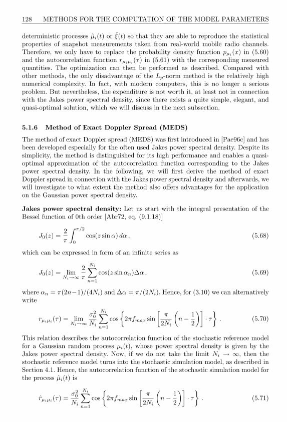
128 METHODS FOR THE COMPUTATION OF THE MODEL PARAMETERS
deterministic processes µi(t) or ξ(t) so that they are able to reproduce the statisticalproperties of snapshot measurements taken from real-world mobile radio channels.Therefore, we only have to replace the probability density function pµi
(x) in (5.60)and the autocorrelation function rµiµi(τ) in (5.61) with the corresponding measuredquantities. The optimization can then be performed as described. Compared withother methods, the only disadvantage of the Lp-norm method is the relatively highnumerical complexity. In fact, with modern computers, this is no longer a seriousproblem. But nevertheless, the expenditure is not worth it, at least not in connectionwith the Jakes power spectral density, since there exists a quite simple, elegant, andquasi-optimal solution, which we will discuss in the next subsection.
5.1.6 Method of Exact Doppler Spread (MEDS)
The method of exact Doppler spread (MEDS) was first introduced in [Pae96c] and hasbeen developed especially for the often used Jakes power spectral density. Despite itssimplicity, the method is distinguished for its high performance and enables a quasi-optimal approximation of the autocorrelation function corresponding to the Jakespower spectral density. In the following, we will first derive the method of exactDoppler spread in connection with the Jakes power spectral density and afterwards, wewill investigate to what extent the method also offers advantages for the applicationon the Gaussian power spectral density.
Jakes power spectral density: Let us start with the integral presentation of theBessel function of 0th order [Abr72, eq. (9.1.18)]
J0(z) =2π
∫ π/2
0
cos(z sin α) dα , (5.68)
which can be expressed in form of an infinite series as
J0(z) = limNi→∞
2π
Ni∑n=1
cos(z sin αn)∆α , (5.69)
where αn = π(2n−1)/(4Ni) and ∆α = π/(2Ni). Hence, for (3.10) we can alternativelywrite
rµiµi(τ) = limNi→∞
σ20
Ni
Ni∑n=1
cos
2πfmax sin[
π
2Ni
(n− 1
2
)]· τ
. (5.70)
This relation describes the autocorrelation function of the stochastic reference modelfor a Gaussian random process µi(t), whose power spectral density is given by theJakes power spectral density. Now, if we do not take the limit Ni → ∞, then thestochastic reference model turns into the stochastic simulation model, as described inSection 4.1. Hence, the autocorrelation function of the stochastic simulation model forthe process µi(t) is
rµiµi(τ) =σ2
0
Ni
Ni∑n=1
cos
2πfmax sin[
π
2Ni
(n− 1
2
)]· τ
. (5.71)

DISCRETE DOPPLER FREQUENCIES AND DOPPLER COEFFICIENTS 129
The stochastic process µi(t) will be ergodic with respect to the autocorrelationfunction. Then, regarding Subsection 4.3.4, it follows that rµiµi
(τ) = rµiµi(τ) holds.
Consequently, for the autocorrelation function of the deterministic process µi(t), weobtain the equation
rµiµi(τ) =
σ20
Ni
Ni∑n=1
cos
2πfmax sin[
π
2Ni
(n− 1
2
)]· τ
. (5.72)
If we now compare the above relation with the general expression (4.11), then theDoppler coefficients ci,n and the discrete Doppler frequencies fi,n can be identifiedwith the equations
ci,n = σ0
√2Ni
(5.73)
and
fi,n = fmax sin[
π
2Ni
(n− 1
2
)], (5.74)
respectively, for all n = 1, 2, . . . , Ni (i = 1, 2). A deterministic process µi(t) designedwith these parameters, has the time average mµi = mµi = 0 and the mean powerσ2
µi= σ2
0 . For all relevant values of Ni, the greatest common divisor Fi = gcdfi,nNin=1
is equal to zero (or very small), so that the period Ti = 1/Fi becomes infinite (or verylarge). The uncorrelatedness of two deterministic processes µ1(t) and µ2(t) is againguaranteed by the convention N2 := N1 + 1.
The autocorrelation function rµiµi(τ) computed according to (5.72) is presented inFigure 5.44(a) for Ni = 7 and in Figure 5.44(b) for Ni = 21.
(a) Ni = 7
0 0.02 0.04 0.06 0.08
-0.5
0
0.5
1
τ (s)
r µiµ
i(τ)
rµiµi(τ) (Simulation model)
rµiµi(τ) (Reference model)
τmax
(b) Ni = 21
0 0.05 0.1 0.15-0.4
-0.2
0
0.2
0.4
0.6
0.8
1
τ (s)
r µiµ
i(τ)
rµiµi(τ) (Simulation model)
rµiµi(τ) (Reference model)
τmax
Figure 5.44: Autocorrelation function rµiµi(τ) for (a) Ni = 7 and (b) Ni = 21 (MEDS,Jakes PSD, fmax = 91Hz, σ2
0 = 1).

130 METHODS FOR THE COMPUTATION OF THE MODEL PARAMETERS
In connection with the Jakes power spectral density, the following rule of thumbapplies: let there be Ni harmonic functions are given, then the approximationrµiµi
(τ) ≈ rµiµi(τ) is quite good up to the Nith zero-crossing of rµiµi
(τ).
Since the relation ci,n = σ0
√2/Ni, which has already been obtained several times for
the Doppler coefficients, also applies here, the mean-square error Epµi[see (4.83)]
is again identical to the results shown in Figure 5.14(b). The evaluation of themean-square error Erµiµi
[see (4.84)] in terms of Ni results in the graph depictedin Figure 5.45. As shown in this figure, the comparison with the Lp-norm methodclearly demonstrates that even by applying numerical optimization techniques, onlyminor improvements can be achieved.
0 10 20 30 40 500
0.2
0.4
0.6
0.8
1x 10
-5
Ni
Er µ
iµi
MEDS
LPNM
Figure 5.45: Mean-square error Erµiµi(MEDS, Jakes PSD, fmax = 91Hz, σ2
0 =
1, τmax = Ni/(2fmax)).
Putting the equations (5.73) and (5.74) into (4.22) and making use of the relation(3.29), we can easily show that βi = β holds. In other words, the model error ∆βi isequal to zero for all Ni ∈ N \ 0. Since we have σ2
µi= σ2
0 and βi = β = β in thepresent case, it follows from (3.15b) and (4.25) that
B(2)µµ = B(2)
µiµi= B(2)
µiµi= B(2)
µµ (5.75)
holds. Hence, the Doppler spread of the simulation model is identical to that of thereference model. This is exactly the reason why this procedure is called the ‘methodof exact Doppler spread’.
The time-domain simulation will be restricted here to the emulation of the level-crossing rate, where we now choose the couple (N1, N2) = (5, 6) and proceed, apartfrom that, exactly as in Subsection 5.1.3. Even for such small numbers of harmonicfunctions, the simulation results match the analytical results very well, as can be seen
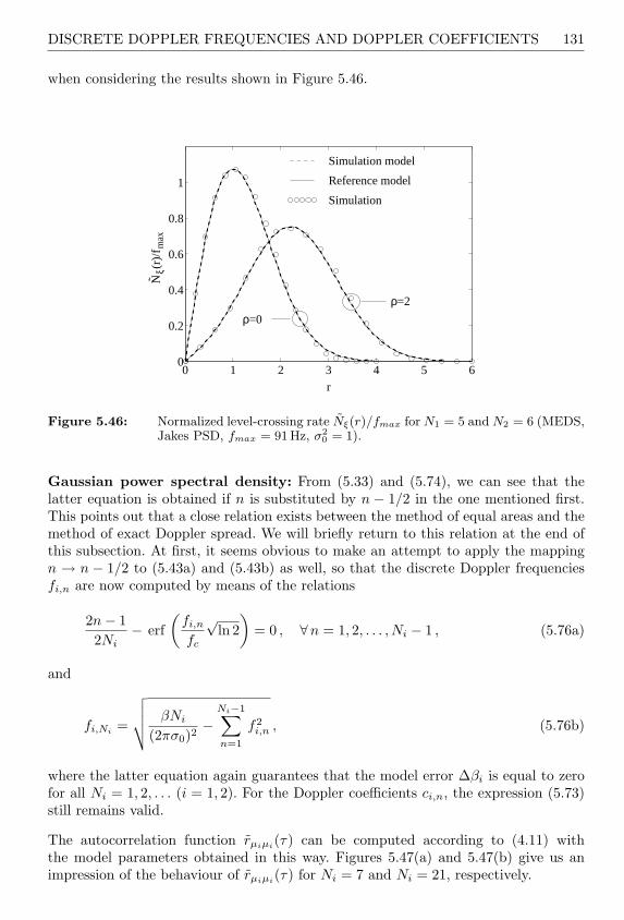
DISCRETE DOPPLER FREQUENCIES AND DOPPLER COEFFICIENTS 131
when considering the results shown in Figure 5.46.
0 1 2 3 4 5 60
0.2
0.4
0.6
0.8
1
r
Nξ(
r)/f
max
ρ=0
ρ=2
Simulation model
Reference model
Simulation
Figure 5.46: Normalized level-crossing rate Nξ(r)/fmax for N1 = 5 and N2 = 6 (MEDS,Jakes PSD, fmax = 91Hz, σ2
0 = 1).
Gaussian power spectral density: From (5.33) and (5.74), we can see that thelatter equation is obtained if n is substituted by n − 1/2 in the one mentioned first.This points out that a close relation exists between the method of equal areas and themethod of exact Doppler spread. We will briefly return to this relation at the end ofthis subsection. At first, it seems obvious to make an attempt to apply the mappingn → n − 1/2 to (5.43a) and (5.43b) as well, so that the discrete Doppler frequenciesfi,n are now computed by means of the relations
2n− 12Ni
− erf(
fi,n
fc
√ln 2
)= 0 , ∀n = 1, 2, . . . , Ni − 1 , (5.76a)
and
fi,Ni =
√√√√ βNi
(2πσ0)2−
Ni−1∑n=1
f2i,n , (5.76b)
where the latter equation again guarantees that the model error ∆βi is equal to zerofor all Ni = 1, 2, . . . (i = 1, 2). For the Doppler coefficients ci,n, the expression (5.73)still remains valid.
The autocorrelation function rµiµi(τ) can be computed according to (4.11) withthe model parameters obtained in this way. Figures 5.47(a) and 5.47(b) give us animpression of the behaviour of rµiµi(τ) for Ni = 7 and Ni = 21, respectively.

132 METHODS FOR THE COMPUTATION OF THE MODEL PARAMETERS
(a) Ni = 7
0 0.02 0.04 0.06 0.08-0.5
0
0.5
1
τ (s)
r µiµ
i(τ)
rµiµi(τ) (Simulation model)
rµiµi(τ) (Reference model)
τmax
(b) Ni = 21
0 0.05 0.1 0.15
-0.2
0
0.2
0.4
0.6
0.8
1
τ (s)
r µiµ
i(τ)
rµiµi(τ) (Simulation model)
rµiµi(τ) (Reference model)
τmax
Figure 5.47: Autocorrelation function rµiµi(τ) for (a) Ni = 7 and (b) Ni = 21 (MEDS,
Gaussian PSD, fc =√
ln 2fmax, fmax = 91 Hz, σ20 = 1).
The mean-square error Erµiµi[see (4.84)], which results from the application of the
present method and the standard Lp-norm method, is presented in the succeedingFigure 5.48 as a function of Ni. Unlike the case of the Jakes power spectral density,for a small number of harmonic functions Ni, the method of exact Doppler spreaddelivers clearly higher values for Erµiµi
than the Lp-norm method does. However,if Ni ≥ 25, no considerable improvements are achievable by means of numericaloptimization techniques.
0 10 20 30 40 500
0.5
1
1.5
2
2.5
3
3.5
4x 10
-3
Ni
Er µ
iµi
MEDSLPNM
Figure 5.48: Mean-square error Erµiµi(MEDS, Gaussian PSD, fc =
√ln 2fmax,
fmax = 91 Hz, σ20 = 1, τmax = Ni/(2κcfc), κc = 2
p2/ ln 2).
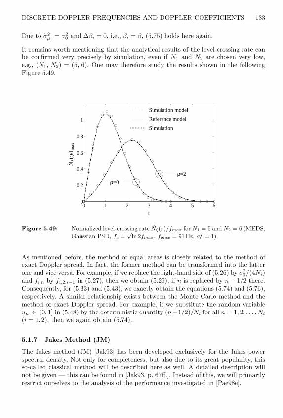
DISCRETE DOPPLER FREQUENCIES AND DOPPLER COEFFICIENTS 133
Due to σ2µi
= σ20 and ∆βi = 0, i.e., βi = β, (5.75) holds here again.
It remains worth mentioning that the analytical results of the level-crossing rate canbe confirmed very precisely by simulation, even if N1 and N2 are chosen very low,e.g., (N1, N2) = (5, 6). One may therefore study the results shown in the followingFigure 5.49.
0 1 2 3 4 5 60
0.2
0.4
0.6
0.8
1
r
Nξ(
r)/f
max
ρ=0
ρ=2
Simulation model
Reference model
Simulation
Figure 5.49: Normalized level-crossing rate Nξ(r)/fmax for N1 = 5 and N2 = 6 (MEDS,
Gaussian PSD, fc =√
ln 2fmax, fmax = 91 Hz, σ20 = 1).
As mentioned before, the method of equal areas is closely related to the method ofexact Doppler spread. In fact, the former method can be transformed into the latterone and vice versa. For example, if we replace the right-hand side of (5.26) by σ2
0/(4Ni)and fi,n by fi,2n−1 in (5.27), then we obtain (5.29), if n is replaced by n− 1/2 there.Consequently, for (5.33) and (5.43), we exactly obtain the equations (5.74) and (5.76),respectively. A similar relationship exists between the Monte Carlo method and themethod of exact Doppler spread. For example, if we substitute the random variableun ∈ (0, 1] in (5.48) by the deterministic quantity (n−1/2)/Ni for all n = 1, 2, . . . , Ni
(i = 1, 2), then we again obtain (5.74).
5.1.7 Jakes Method (JM)
The Jakes method (JM) [Jak93] has been developed exclusively for the Jakes powerspectral density. Not only for completeness, but also due to its great popularity, thisso-called classical method will be described here as well. A detailed description willnot be given — this can be found in [Jak93, p. 67ff.]. Instead of this, we will primarilyrestrict ourselves to the analysis of the performance investigated in [Pae98e].

134 METHODS FOR THE COMPUTATION OF THE MODEL PARAMETERS
Jakes power spectral density: After rewriting the expressions for the parametersof the simulation model given in [Jak93, p. 70] by taking the notation chosen hereinto account, the following relations hold for the Doppler coefficients ci,n, the discreteDoppler frequencies fi,n, and the Doppler phases θi,n:
ci,n =
2σ0√Ni − 1
2
sin(
πn
Ni − 1
), n = 1, 2, . . . , Ni − 1 , i = 1 ,
2σ0√Ni − 1
2
cos(
πn
Ni − 1
), n = 1, 2, . . . , Ni − 1 , i = 2 ,
σ0√Ni − 1
2
, n = Ni , i = 1, 2 ,
(5.77)
fi,n =
fmax cos(
nπ
2Ni − 1
), n = 1, 2, . . . , Ni − 1 , i = 1, 2 ,
fmax , n = Ni , i = 1, 2(5.78)
θi,n = 0 , n = 1, 2, . . . , Ni , i = 1, 2 , (5.79)
where N1 = N2. The Doppler coefficients ci,n were scaled here in such a way that themean power σ2
µiof µi(t) meets the relation σ2
µi= σ2
0 for i = 1, 2. Due to fi,n 6= 0, thefollowing relation holds for the time average: mµi = mµi = 0 (i = 1, 2).
The resulting power spectral densities Sµ1µ1(f) and Sµ2µ2(f) as well as thecorresponding autocorrelation functions rµ1µ1(τ) and rµ2µ2(τ) are shown inFigures 5.50(a)–5.50(d) for N1 = N2 = 9. Even for small values of τ , it can beseen from Figures 5.50(b) and 5.50(d) that the autocorrelation functions of thedeterministic processes µ1(t) and µ2(t) strongly deviate from the ideal autocorrelationfunction rµiµi(τ) = σ2
0J0(2πfmaxτ). On the other hand, as Figure 5.50(f) reveals, theautocorrelation function rµµ(τ) of the complex deterministic process µ(t) over theinterval τ ∈ [0, τmax] matches rµµ(τ) = 2σ2
0J0(2πfmaxτ) very well. Figure 5.50(e)shows the power spectral density Sµµ(f) that corresponds to the autocorrelationfunction rµµ(τ).
It is interesting that even for Ni →∞, the autocorrelation function rµiµi(τ) does nottend to rµiµi(τ). Instead of this, after substituting (5.77) and (5.78) into (4.11) andtaking the limit Ni →∞ afterwards, we rather obtain the functions
limN1→∞
rµ1µ1(τ) =2σ2
0
π
∫ π/2
0
[1− cos(4z)
]cos(2πfmaxτ cos z) dz (5.80a)
and
limN2→∞
rµ2µ2(τ) =2σ2
0
π
∫ π/2
0
[1 + cos(4z)
]cos(2πfmaxτ cos z) dz , (5.80b)
which, by making use of [Gra81, eq. (3.715.19)]∫ π/2
0
cos(z cos x) cos(2nx) dx = (−1)n · π
2J2n(z) , (5.81)
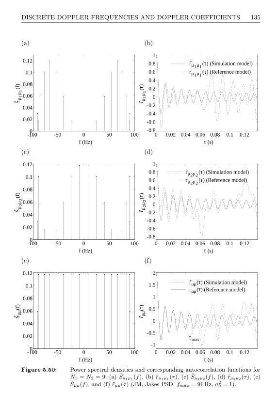
DISCRETE DOPPLER FREQUENCIES AND DOPPLER COEFFICIENTS 135
(a)
-100 -50 0 50 1000
0.02
0.04
0.06
0.08
0.1
0.12
f (Hz)
Sµ
1µ
1(f
)
(b)
0 0.02 0.04 0.06 0.08 0.1 0.12-0.8
-0.6
-0.4
-0.2
0
0.2
0.4
0.6
0.8
1
τ (s)r µ
1µ
1(τ
)
rµ1µ1(τ) (Simulation model)
rµ1µ1(τ) (Reference model)
(c)
-100 -50 0 50 1000
0.02
0.04
0.06
0.08
0.1
0.12
f (Hz)
Sµ
2µ
2(f
)
(d)
0 0.02 0.04 0.06 0.08 0.1 0.12-0.8
-0.6
-0.4
-0.2
0
0.2
0.4
0.6
0.8
1
τ (s)
r µ2
µ2
(τ)
rµ2µ2(τ) (Simulation model)
rµ2µ2(τ) (Reference model)
(e)
-100 -50 0 50 1000
0.02
0.04
0.06
0.08
0.1
0.12
f (Hz)
Sµµ
(f)
(f)
0 0.02 0.04 0.06 0.08 0.1 0.12-1
-0.5
0
0.5
1
1.5
2
τ (s)
r µµ(τ
)
rµµ(τ) (Simulation model)rµµ(τ) (Reference model)
τmax
Figure 5.50: Power spectral densities and corresponding autocorrelation functions forN1 = N2 = 9: (a) Sµ1µ1(f), (b) rµ1µ1(τ), (c) Sµ2µ2(f), (d) rµ2µ2(τ), (e)
Sµµ(f), and (f) rµµ(τ) (JM, Jakes PSD, fmax = 91 Hz, σ20 = 1).

136 METHODS FOR THE COMPUTATION OF THE MODEL PARAMETERS
can also be brought into the form
limN1→∞
rµ1µ1(τ) = σ20
[J0(2πfmaxτ)− J4(2πfmaxτ)
](5.82a)
and
limN2→∞
rµ2µ2(τ) = σ20
[J0(2πfmaxτ) + J4(2πfmaxτ)
], (5.82b)
as shown in [Pae98e]. Thus, even after taking the limit Ni → ∞, the inequalityrµiµi(τ) 6= rµiµi(τ) (i = 1, 2) holds. On the contrary, the autocorrelation functionrµµ(τ) of the complex deterministic process µ(t) = µ1(t) + jµ2(t) does tend very wellto the autocorrelation function rµµ(τ) of the reference model, as Ni → ∞. This factbecomes immediately evident after substituting (5.82a) and (5.82b) into the generalexpression
rµµ(τ) = rµ1µ1(τ) + rµ2µ2(τ) + j(rµ1µ2(τ)− rµ2µ1(τ)
)(5.83)
following from (2.71), and then making use of the relation rµ1µ2(τ) = rµ2µ1(τ), whichholds here, as we will see subsequently. Hence, one directly realizes that
limNi→∞
rµµ(τ) = rµµ(τ) = 2σ20 J0(2πfmaxτ) (5.84)
holds.
We furthermore want to analyse to which functions the power spectral densitiesSµ1µ1(f) and Sµ2µ2(f) tend to in the limits N1 → ∞ and N2 → ∞, respectively.Therefore, we transform (5.82a) and (5.82b) into the spectral domain by means of theFourier transform and obtain
limN1→∞
Sµ1µ1(f) =
σ20 ·
1− cos[4 arcsin(f/fmax)
]
πfmax
√1− (f/fmax)2
, |f | ≤ fmax ,
0 , |f | > fmax ,
(5.85a)
limN2→∞
Sµ2µ2(f) =
σ20 ·
1 + cos[4 arcsin(f/fmax)
]
πfmax
√1− (f/fmax)2
, |f | ≤ fmax ,
0 , |f | > fmax .
(5.85b)
Of course, we might as well have substituted (5.77) and (5.78) in Sµiµi(f) given by(4.14). Then, after taking the limit Ni → ∞, we would have obtained the results(5.85a) and (5.85b) stated above in an alternative way. If we now put these resultsinto the Fourier transform of (5.83), then we obtain the Jakes power spectral densityas expected, i.e.,
limNi→∞
Sµµ(f) = Sµµ(f) =
2σ20
πfmax
√1− (f/fmax)2
, |f | ≤ fmax ,
0 , |f | > fmax .
(5.86)
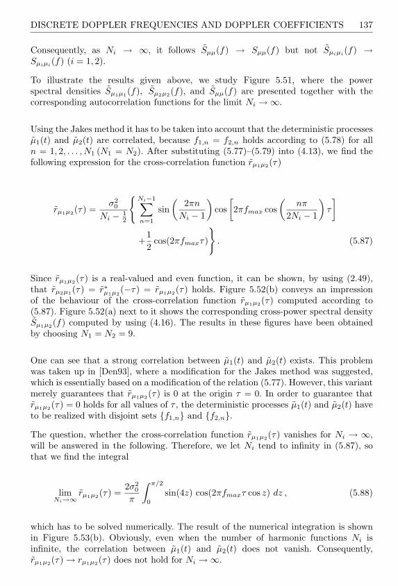
DISCRETE DOPPLER FREQUENCIES AND DOPPLER COEFFICIENTS 137
Consequently, as Ni → ∞, it follows Sµµ(f) → Sµµ(f) but not Sµiµi(f) →Sµiµi
(f) (i = 1, 2).
To illustrate the results given above, we study Figure 5.51, where the powerspectral densities Sµ1µ1(f), Sµ2µ2(f), and Sµµ(f) are presented together with thecorresponding autocorrelation functions for the limit Ni →∞.
Using the Jakes method it has to be taken into account that the deterministic processesµ1(t) and µ2(t) are correlated, because f1,n = f2,n holds according to (5.78) for alln = 1, 2, . . . , N1 (N1 = N2). After substituting (5.77)–(5.79) into (4.13), we find thefollowing expression for the cross-correlation function rµ1µ2(τ)
rµ1µ2(τ) =σ2
0
Ni − 12
Ni−1∑n=1
sin(
2πn
Ni − 1
)cos
[2πfmax cos
(nπ
2Ni − 1
)τ
]
+12
cos(2πfmaxτ)
. (5.87)
Since rµ1µ2(τ) is a real-valued and even function, it can be shown, by using (2.49),that rµ2µ1(τ) = r∗µ1µ2
(−τ) = rµ1µ2(τ) holds. Figure 5.52(b) conveys an impressionof the behaviour of the cross-correlation function rµ1µ2(τ) computed according to(5.87). Figure 5.52(a) next to it shows the corresponding cross-power spectral densitySµ1µ2(f) computed by using (4.16). The results in these figures have been obtainedby choosing N1 = N2 = 9.
One can see that a strong correlation between µ1(t) and µ2(t) exists. This problemwas taken up in [Den93], where a modification for the Jakes method was suggested,which is essentially based on a modification of the relation (5.77). However, this variantmerely guarantees that rµ1µ2(τ) is 0 at the origin τ = 0. In order to guarantee thatrµ1µ2(τ) = 0 holds for all values of τ , the deterministic processes µ1(t) and µ2(t) haveto be realized with disjoint sets f1,n and f2,n.The question, whether the cross-correlation function rµ1µ2(τ) vanishes for Ni → ∞,will be answered in the following. Therefore, we let Ni tend to infinity in (5.87), sothat we find the integral
limNi→∞
rµ1µ2(τ) =2σ2
0
π
∫ π/2
0
sin(4z) cos(2πfmaxτ cos z) dz , (5.88)
which has to be solved numerically. The result of the numerical integration is shownin Figure 5.53(b). Obviously, even when the number of harmonic functions Ni isinfinite, the correlation between µ1(t) and µ2(t) does not vanish. Consequently,rµ1µ2(τ) → rµ1µ2(τ) does not hold for Ni →∞.
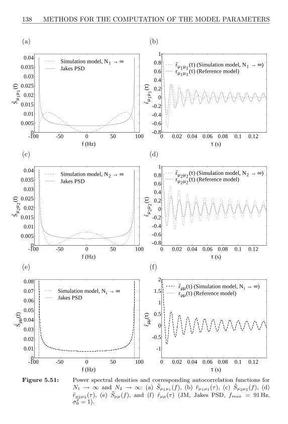
138 METHODS FOR THE COMPUTATION OF THE MODEL PARAMETERS
(a)
-100 -50 0 50 1000
0.005
0.01
0.015
0.02
0.025
0.03
0.035
0.04
f (Hz)
Sµ
1µ
1(f
)
Simulation model, N1 → ∞Jakes PSD
(b)
0 0.02 0.04 0.06 0.08 0.1 0.12-0.8
-0.6
-0.4
-0.2
0
0.2
0.4
0.6
0.8
1
τ (s)r µ
1µ
1(τ
)
rµ1µ1(τ) (Simulation model, N1 → ∞)
rµ1µ1(τ) (Reference model)
(c)
-100 -50 0 50 1000
0.005
0.01
0.015
0.02
0.025
0.03
0.035
0.04
f (Hz)
Sµ
2µ
2(f
)
Simulation model, N2 → ∞Jakes PSD
(d)
0 0.02 0.04 0.06 0.08 0.1 0.12-0.8
-0.6
-0.4
-0.2
0
0.2
0.4
0.6
0.8
1
τ (s)
r µ2
µ2
(τ)
rµ2µ2(τ) (Simulation model, N2 → ∞)
rµ2µ2(τ) (Reference model)
(e)
-100 -50 0 50 1000
0.01
0.02
0.03
0.04
0.05
0.06
0.07
0.08
f (Hz)
Sµµ
(f)
Simulation model, Ni → ∞Jakes PSD
(f)
0 0.02 0.04 0.06 0.08 0.1 0.12
-1
-0.5
0
0.5
1
1.5
2
τ (s)
r µµ(τ
)
rµµ(τ) (Simulation model, Ni → ∞)rµµ(τ) (Reference model)
Figure 5.51: Power spectral densities and corresponding autocorrelation functions forN1 → ∞ and N2 → ∞: (a) Sµ1µ1(f), (b) rµ1µ1(τ), (c) Sµ2µ2(f), (d)
rµ2µ2(τ), (e) Sµµ(f), and (f) rµµ(τ) (JM, Jakes PSD, fmax = 91 Hz,σ2
0 = 1).

DISCRETE DOPPLER FREQUENCIES AND DOPPLER COEFFICIENTS 139
(a)
-100 -50 0 50 1000
0.01
0.02
0.03
0.04
0.05
0.06
f (Hz)
Sµ
1µ
2(f
)
(b)
-0.06 -0.04 -0.02 0 0.02 0.04 0.06-0.4
-0.2
0
0.2
0.4
0.6
τ (s)
r µ1
µ2
(τ)
Figure 5.52: (a) Cross-power spectral density Sµ1µ2(f) and (b) cross-correlationfunction rµ1µ2(τ) for N1 = N2 = 9 (JM, Jakes PSD, fmax = 91Hz,σ2
0 = 1).
In case of the limit Ni → ∞, we obtain the following closed-form expression for thecross-power spectral density Sµ1µ2(f) after performing the Fourier transform of (5.88)
limNi→∞
Sµ1µ2(f) =
σ20 ·
sin[4 arccos(|f |/fmax)
]
πfmax
√1− (f/fmax)2
, |f | ≤ fmax ,
0 , |f | > fmax .
(5.89)
The evaluation result of this equation is illustrated in Figure 5.53(a). In contrast to theJakes power spectral density (3.8), which becomes singular at f = ±fmax, the cross-power spectral density (5.89) takes on the finite value 4/(πfmax) at these points, i.e.,Sµ1µ2(±fmax) = 4/(πfmax) holds, which can easily be proven by using the rule ofde l’Hospital [Bro91].
Expediently, the mean-square error (4.84) of the autocorrelation function is in thiscase evaluated with respect to rµ1µ1(τ), rµ2µ2(τ), and rµµ(τ). The obtained results aredepicted in Figure 5.54(a) as a function of Ni. Using the Jakes method, the Dopplercoefficients ci,n partly deviate considerably from the (quasi-)optimal quantities ci,n =σ0
√2/Ni. This inevitably leads to an increase in the mean-square error Epµi
[see(4.83)], as can clearly be seen in Figure 5.54(b).
For the Jakes method, we have: N1 = N2 and f1,n = f2,n ∀n = 1, 2, . . . , N1 (N2). But,on the other hand, c1,n 6= c2,n still holds for almost all n = 1, 2, . . . , N1 (N2). Thus, itis to be expected that the model errors ∆β1 and ∆β2 are different for a given numberof harmonic functions Ni. One should therefore study Figure 5.55, where the relativemodel errors ∆β1/β and ∆β2/β are presented.
Due to ∆β1 6= ∆β2, we must use the expression (B.13) for the computation of thelevel-crossing rate Nξ(r), where β1 and β2 have to be substituted by β1 = β+∆β1 and

140 METHODS FOR THE COMPUTATION OF THE MODEL PARAMETERS
(a)
-100 -50 0 50 100
0
5
10
15x 10
-3
Ni → ∞
f (Hz)
Sµ
1µ
2(f
)
(b)
-0.06 -0.04 -0.02 0 0.02 0.04 0.06-0.6
-0.4
-0.2
0
0.2
0.4
0.6
0.8
τ (s)
r µ1
µ2
(τ)
rµ1µ2(τ) (Simulation model, Ni → ∞)
rµ1µ2(τ) (Reference model)
Figure 5.53: (a) Cross-power spectral density Sµ1µ2(f) and (b) cross-correlationfunction rµ1µ2(τ) for Ni →∞ (JM, Jakes PSD, fmax = 91Hz, σ2
0 = 1).
(a)
0 10 20 30 40 500
0.01
0.02
0.03
0.04
0.05
Ni
Er µ
iµi
Erµ1µ1Erµ2µ2Erµµ
(b)
0 10 20 30 40 500
0.2
0.4
0.6
0.8
1
x 10-3
Ni
Ep
µi
c1,n according to (5.77)c2,n according to (5.77)ci,n = σo (2/Ni)
1/2
Figure 5.54: (a) Mean-square errors Erµ1µ1, Erµ2µ2
, and Erµµ with τmax = Ni/(2fmax)
and (b) mean-square error Epµi(JM, Jakes PSD, fmax = 91Hz, σ2
0 = 1).

DISCRETE DOPPLER FREQUENCIES AND DOPPLER COEFFICIENTS 141
0 10 20 30 40 50
-0.2
-0.15
-0.1
-0.05
0
0.05
0.1
0.15
0.2
Ni
∆βi /
β
∆β1/β
∆β2/β
Figure 5.55: Relative model errors ∆β1/β and ∆β2/β (JM, Jakes PSD, fmax = 91 Hz,σ2
0 = 1).
β2 = β + ∆β2, respectively. Generally speaking, in case of a correlation between µ1(t)and µ2(t), the level-crossing rate Nξ(r) also depends on the quantities ˙rµ1µ2(0) and¨rµ1µ2(0). Since it follows immediately from (5.87) that ˙rµ1µ2(0) is equal to zero, andfurthermore the influence of ¨rµ1µ2(0) on Nξ(r) is quite small, this dependency will beignored here. Figure 5.56(a) presents the analytical results for Nξ(r)/fmax as well as forNξ(r)/fmax with N1 = N2 = 9. This figure also shows the corresponding simulationresults, which match the analytical solutions for Nξ(r)/fmax and Nξ(r)/fmax verywell.
(a)
0 1 2 3 4 5 60
0.2
0.4
0.6
0.8
1
1.2
r
Nξ(
r)/f
max
ρ=0
ρ=2
Reference modelSimulation model
Simulation
(b)
0 1 2 3 4 50
5
10
15
20
25
r
Tξ -
(r)
f max
ρ=0
ρ=2
Simulation modelReference modelSimulation
Figure 5.56: (a) Normalized level-crossing rate Nξ(r)/fmax and (b) normalized average
duration of fades Tξ−(r) · fmax for N1 = N2 = 9 (JM, Jakes PSD,
fmax = 91 Hz, σ20 = 1).

142 METHODS FOR THE COMPUTATION OF THE MODEL PARAMETERS
When using the Jakes method, it seems that the relatively large deviations betweenthe autocorrelation functions rµiµi
(τ) and rµiµi(τ) as well as the cross-correlation
function rµ1µ2(τ) different from zero, do not have an excessively negative influenceon Nξ(r). By the way, this also holds for the average duration of fades Tξ−(r) [seeFigure 5.56(b)] as well as for the probability density function p0−(τ−; r) of the fadingintervals τ− at low levels r [see Figure 5.57]. From this, however, we may not concludethat especially the influence of the cross-correlation function rµ1µ2(τ) on Nξ(r) andtherefore also on Tξ−(r) can be ignored in all cases. This rather depends on the specifictype of the cross-correlation function rµ1µ2(τ). In the following Chapter 6, we will seethat certain classes of cross-correlation functions really exist, which not only affect thestatistical properties of higher orders, but also have an influence on the probabilitydensity function of the signal amplitude. In this way, it is possible to increase theflexibility of the statistical properties of mobile fading channel models considerably.
0 0.5 1 1.50
500
1000
1500
2000
2500
3000
3500
τ-/ms
p0
-(τ-;
r)
Approximation p1-(τ-;r) [see (3.47)]
Approximation p1-(τ-;r) [see (4.76)]
Simulation
Ni=9
Figure 5.57: Probability density function p0−(τ−; r) of the fading intervals τ− at the
level r = 0.1 (JM, Jakes PSD, fmax = 91Hz, σ20 = 1).
Summarizing, we can record the fact that the essential disadvantage of the Jakesmethod is not to be seen in the cross-correlation function different from zero, but inthe fact that the deterministic processes µ1(t) and µ2(t) are not optimally Gaussiandistributed [cf. Figure 5.54(b)] for a given number of harmonic functions Ni. Sincethe loss of performance is not too high and can easily be compensated by a slightincrease of the number of harmonic functions Ni, we can all in all say that in case Ni
is chosen higher or equal to nine, the Jakes method is quite suitable for the modellingof Rayleigh and Rice processes with the classical Doppler power spectral density givenby (3.8) [Pae98e]. Finally, it should also be noted that an implementation techniqueof the Jakes method on a signal processor has been described in [Cas88, Cas90].
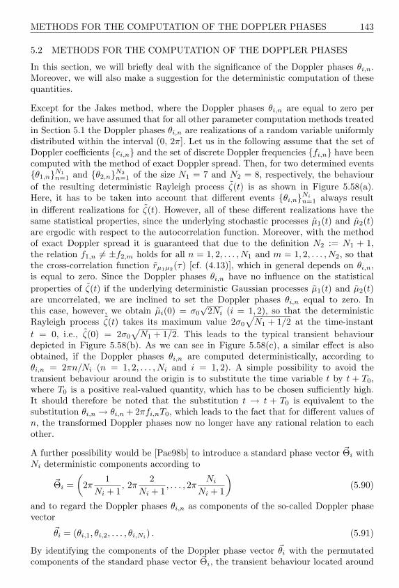
METHODS FOR THE COMPUTATION OF THE DOPPLER PHASES 143
5.2 METHODS FOR THE COMPUTATION OF THE DOPPLER PHASES
In this section, we will briefly deal with the significance of the Doppler phases θi,n.Moreover, we will also make a suggestion for the deterministic computation of thesequantities.
Except for the Jakes method, where the Doppler phases θi,n are equal to zero perdefinition, we have assumed that for all other parameter computation methods treatedin Section 5.1 the Doppler phases θi,n are realizations of a random variable uniformlydistributed within the interval (0, 2π]. Let us in the following assume that the set ofDoppler coefficients ci,n and the set of discrete Doppler frequencies fi,n have beencomputed with the method of exact Doppler spread. Then, for two determined eventsθ1,nN1
n=1 and θ2,nN2n=1 of the size N1 = 7 and N2 = 8, respectively, the behaviour
of the resulting deterministic Rayleigh process ζ(t) is as shown in Figure 5.58(a).Here, it has to be taken into account that different events θi,nNi
n=1 always resultin different realizations for ζ(t). However, all of these different realizations have thesame statistical properties, since the underlying stochastic processes µ1(t) and µ2(t)are ergodic with respect to the autocorrelation function. Moreover, with the methodof exact Doppler spread it is guaranteed that due to the definition N2 := N1 + 1,the relation f1,n 6= ±f2,m holds for all n = 1, 2, . . . , N1 and m = 1, 2, . . . , N2, so thatthe cross-correlation function rµ1µ2(τ) [cf. (4.13)], which in general depends on θi,n,is equal to zero. Since the Doppler phases θi,n have no influence on the statisticalproperties of ζ(t) if the underlying deterministic Gaussian processes µ1(t) and µ2(t)are uncorrelated, we are inclined to set the Doppler phases θi,n equal to zero. Inthis case, however, we obtain µi(0) = σ0
√2Ni (i = 1, 2), so that the deterministic
Rayleigh process ζ(t) takes its maximum value 2σ0
√N1 + 1/2 at the time-instant
t = 0, i.e., ζ(0) = 2σ0
√N1 + 1/2. This leads to the typical transient behaviour
depicted in Figure 5.58(b). As we can see in Figure 5.58(c), a similar effect is alsoobtained, if the Doppler phases θi,n are computed deterministically, according toθi,n = 2πn/Ni (n = 1, 2, . . . , Ni and i = 1, 2). A simple possibility to avoid thetransient behaviour around the origin is to substitute the time variable t by t + T0,where T0 is a positive real-valued quantity, which has to be chosen sufficiently high.It should therefore be noted that the substitution t → t + T0 is equivalent to thesubstitution θi,n → θi,n + 2πfi,nT0, which leads to the fact that for different values ofn, the transformed Doppler phases now no longer have any rational relation to eachother.
A further possibility would be [Pae98b] to introduce a standard phase vector ~Θi withNi deterministic components according to
~Θi =(
2π1
Ni + 1, 2π
2Ni + 1
, . . . , 2πNi
Ni + 1
)(5.90)
and to regard the Doppler phases θi,n as components of the so-called Doppler phasevector
~θi = (θi,1, θi,2, . . . , θi,Ni) . (5.91)
By identifying the components of the Doppler phase vector ~θi with the permutatedcomponents of the standard phase vector ~Θi, the transient behaviour located around

144 METHODS FOR THE COMPUTATION OF THE MODEL PARAMETERS
the origin of the time axis can be avoided from the start. In this connection, one mayobserve the simulation results of ζ(t) shown in Figure 5.58(d).
(a)
0 0.2 0.4 0.6 0.8 1-40
-30
-20
-10
0
10
20
t (s)
20 lo
g ζ(
t)
(b)
0 0.2 0.4 0.6 0.8 1-50
-40
-30
-20
-10
0
10
20
t (s)
20 lo
g ζ(
t)
(c)
0 0.2 0.4 0.6 0.8 1-50
-40
-30
-20
-10
0
10
t (s)
20 lo
g ζ(
t)
(d)
0 0.2 0.4 0.6 0.8 1-40
-30
-20
-10
0
10
t (s)
20 lo
g ζ(
t)
Figure 5.58: Influence of the phases θi,n on the transient behaviour of ζ(t) around theorigin: (a) random phases θi,n ∈ (0, 2π], (b) θi,n = 0, (c) θi,n = 2πn/Ni
(n = 1, 2, . . . , Ni), and (d) permutated phases (MEDS, Jakes PSD,fmax = 91 Hz, σ2
0 = 1, N1 = 21, N2 = 22).
By permuting the components of (5.90), it is possible to construct Ni! different setsθi,n of Doppler phases. Thus, for any given sets of ci,n and fi,n, altogetherN1! · N2! deterministic Rayleigh processes ζ(t) with different time behaviour butidentical statistical properties can be realized.
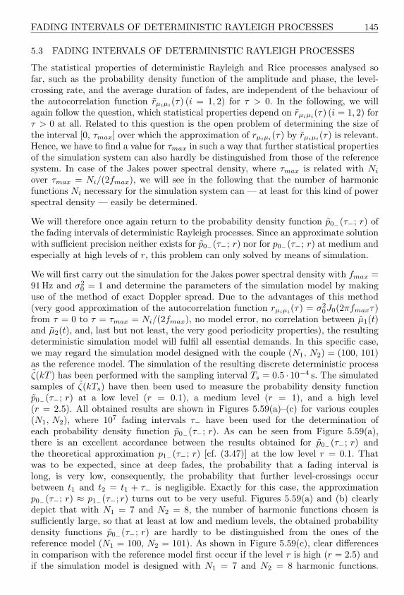
FADING INTERVALS OF DETERMINISTIC RAYLEIGH PROCESSES 145
5.3 FADING INTERVALS OF DETERMINISTIC RAYLEIGH PROCESSES
The statistical properties of deterministic Rayleigh and Rice processes analysed sofar, such as the probability density function of the amplitude and phase, the level-crossing rate, and the average duration of fades, are independent of the behaviour ofthe autocorrelation function rµiµi(τ) (i = 1, 2) for τ > 0. In the following, we willagain follow the question, which statistical properties depend on rµiµi
(τ) (i = 1, 2) forτ > 0 at all. Related to this question is the open problem of determining the size ofthe interval [0, τmax] over which the approximation of rµiµi(τ) by rµiµi(τ) is relevant.Hence, we have to find a value for τmax in such a way that further statistical propertiesof the simulation system can also hardly be distinguished from those of the referencesystem. In case of the Jakes power spectral density, where τmax is related with Ni
over τmax = Ni/(2fmax), we will see in the following that the number of harmonicfunctions Ni necessary for the simulation system can — at least for this kind of powerspectral density — easily be determined.
We will therefore once again return to the probability density function p0−(τ−; r) ofthe fading intervals of deterministic Rayleigh processes. Since an approximate solutionwith sufficient precision neither exists for p0−(τ−; r) nor for p0−(τ−; r) at medium andespecially at high levels of r, this problem can only solved by means of simulation.
We will first carry out the simulation for the Jakes power spectral density with fmax =91Hz and σ2
0 = 1 and determine the parameters of the simulation model by makinguse of the method of exact Doppler spread. Due to the advantages of this method(very good approximation of the autocorrelation function rµiµi(τ) = σ2
0J0(2πfmaxτ)from τ = 0 to τ = τmax = Ni/(2fmax), no model error, no correlation between µ1(t)and µ2(t), and, last but not least, the very good periodicity properties), the resultingdeterministic simulation model will fulfil all essential demands. In this specific case,we may regard the simulation model designed with the couple (N1, N2) = (100, 101)as the reference model. The simulation of the resulting discrete deterministic processζ(kT ) has been performed with the sampling interval Ts = 0.5 · 10−4 s. The simulatedsamples of ζ(kTs) have then been used to measure the probability density functionp0−(τ−; r) at a low level (r = 0.1), a medium level (r = 1), and a high level(r = 2.5). All obtained results are shown in Figures 5.59(a)–(c) for various couples(N1, N2), where 107 fading intervals τ− have been used for the determination ofeach probability density function p0−(τ−; r). As can be seen from Figure 5.59(a),there is an excellent accordance between the results obtained for p0−(τ−; r) andthe theoretical approximation p1−(τ−; r) [cf. (3.47)] at the low level r = 0.1. Thatwas to be expected, since at deep fades, the probability that a fading interval islong, is very low, consequently, the probability that further level-crossings occurbetween t1 and t2 = t1 + τ− is negligible. Exactly for this case, the approximationp0−(τ−; r) ≈ p1−(τ−; r) turns out to be very useful. Figures 5.59(a) and (b) clearlydepict that with N1 = 7 and N2 = 8, the number of harmonic functions chosen issufficiently large, so that at least at low and medium levels, the obtained probabilitydensity functions p0−(τ−; r) are hardly to be distinguished from the ones of thereference model (N1 = 100, N2 = 101). As shown in Figure 5.59(c), clear differencesin comparison with the reference model first occur if the level r is high (r = 2.5) andif the simulation model is designed with N1 = 7 and N2 = 8 harmonic functions.

146 METHODS FOR THE COMPUTATION OF THE MODEL PARAMETERS
However, if the differences from the reference model will be negligible for this leveltoo, then at least N1 = 21 and N2 = 22 harmonic functions will be required. A furtherincrease of Ni makes no sense!
At this point, it should be noted that N1 = 7 and N2 = 8 harmonic functions are ingeneral sufficient for the modelling of mobile radio channels, where channel models areoften required to determine the bit error probability of digital transmission systemsconsisting of a transmitter, a channel model, and a receiver. Of course, N1 = 7 andN2 = 8 are only sufficient, if the parameter design of the harmonic functions has beencarried out correctly. This can be attributed to the fact that the bit error probabilityis essentially determined by the statistical properties (i.e., the probability densityfunction of the amplitude, the level-crossing rate, the average duration of fades, andthe probability density function of the fading intervals) of ζ(t) at low levels r. Thebehaviour of ζ(t) at high levels is in this case not of particular importance.
A comparison of Figures 3.7(a)–(c) and Figures 5.59(a)–(c) shows that the theoreticalapproximation p1−(τ−; r) at all levels r only fits the measured probability densitiesp0(τ−; r) at small fading intervals τ− very well. One should also note that for τ− →∞,it always follows p0−(τ−; r) → 0 ∀ r ∈ 0.1, 1, 2.5. However, this convergence propertyis not fulfilled by p1−(τ−; r) for the levels r = 1 and r = 2.5 [see Figures 3.7(b) and3.7(c)]. From the convergence behaviour of p0−(τ−; r), we can now approximatelyconclude the interval [0, τmax], over which the approximation rµiµi(τ) ≈ rµiµi(τ) hasto be as good as possible. We will therefore make use of the quantity τq = τq(r),introduced in Subsection 3.3.3, where we substitute p0−(τ−; r) into (3.49) by theprobability density function p0−(τ−; r) of the fading intervals of the reference model(N1 = 100, N2 = 101) and choose q so large that for all fading intervals τ− ≥ τq, theprobability density function p0−(τ−; r) becomes sufficiently small. Furthermore, wedemand that τmax must fulfil the inequality τmax ≥ τq. We remember that by usingthe method of exact Doppler spread, rµiµi(τ) represents a very good approximationfor rµiµi(τ) within the range 0 ≤ τ ≤ τmax, where τmax is related with Ni overthe equation τmax = Ni/(2fmax). Therefore, for the estimation of the requirednumber of harmonic functions Ni, we can obtain the following simple formula byusing τmax = Ni/(2fmax) ≥ τq(r)
Ni ≥ d2fmaxτq(r)e . (5.92)
For example, if we choose q = 90, then we find the value 135.7ms for τ90 = τ90(r)at the high level r = 2.5 [see Figure 5.59(c)]. With respect to (5.92) it then followsNi ≥ 25. This result matches the one obtained before by experimental means verywell. Now, in reverse order, let us assume that Ni is given (for example, by Ni ≥ 7),then the resulting probability density function p0(τ−; r) matches the correspondingprobability density function of the reference model within the range 0 ≤ τ− ≤ 38.5msvery well. This is also confirmed by considering Figure 5.59(c).
For low and medium levels, where usually τ90 < 1/fmax holds, (5.92) does not provideany admissible values for Ni, since in these cases the obtained values fall below thelower limit Ni = 7, which is considered to be the necessary number of harmonicfunctions for a sufficient approximation of the Gaussian probability density function
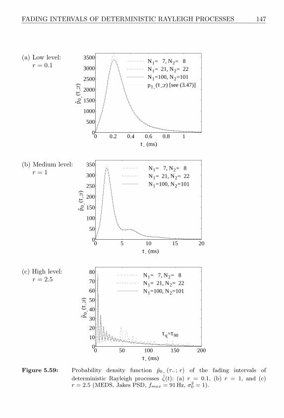
FADING INTERVALS OF DETERMINISTIC RAYLEIGH PROCESSES 147
(a) Low level:r = 0.1
0 0.2 0.4 0.6 0.8 10
500
1000
1500
2000
2500
3000
3500
τ- (ms)
p0
-(τ-;
r)
N1= 7, N2= 8N1= 21, N2= 22N1=100, N2=101p1-
(τ-;r) [see (3.47)]
(b) Medium level:r = 1
0 5 10 15 200
50
100
150
200
250
300
350
τ- (ms)
p0
-(τ-;
r)
N1= 7, N2= 8N1= 21, N2= 22N1=100, N2=101
(c) High level:r = 2.5
0 50 100 150 2000
10
20
30
40
50
60
70
80
τ- (ms)
p0
-(τ-;
r)
τq=τ90
N1= 7, N2= 8N1= 21, N2= 22N1=100, N2=101
Figure 5.59: Probability density function p0−(τ−; r) of the fading intervals of
deterministic Rayleigh processes ζ(t): (a) r = 0.1, (b) r = 1, and (c)r = 2.5 (MEDS, Jakes PSD, fmax = 91Hz, σ2
0 = 1).

148 METHODS FOR THE COMPUTATION OF THE MODEL PARAMETERS
pµi(x). Therefore, as a useful estimation, which is valid for all levels r ≥ 0, theinequality
Ni ≥ max7, d2fmaxτq(r)e (5.93)
is suggested.
Next, we will study the statistics of the fading intervals of deterministic Rayleighprocesses ζ(t) with underlying Gaussian shaped coloured processes µ1(t) and µ2(t).The Gaussian power spectral density (3.11) is characterized by the parametersfc =
√ln 2fmax, fmax = 91 Hz, and σ2
0 = 1. The parameters of the simulationmodel are again determined with respect to the method of exact Doppler spread.Exactly as in the preceding case, we consider the simulation model for the couple(N1, N2) = (100, 101) as reference model. The repetition of the measurement of theprobability density function p0−(τ−; r), which was carried out on the simulated fadingbehaviour of ζ(kTs) for low, medium, and high levels r, now leads to the results shownin Figures 5.60(a)–(c). For all levels, the sampling interval Ts was thereby again givenby the constant quantity Ts = 0.5 · 10−4 s. Here again 107 fading intervals τ− wereevaluated for the determination of each probability density function p0−(τ−; r).
From the comparison of Figures 5.60(a) and 5.59(a), it follows that the respectiveprobability density functions p0−(τ−; r) are identical. That was to be expected, sincethe exact shape of the power spectral density of the processes µ1(t) and µ2(t) has noinfluence on the density p0(τ−; r) at low levels r. Only the values of the quantitiesσ2
0 = rµiµi(0) and βi = −¨rµiµi(0) are of importance here. In the present case, theyare identical for the Jakes and the Gaussian power spectral density. Only with anincreasing level r, the behaviour of rµiµi(τ) gains more and more influence on thedensity p0−(τ−; r) for values τ > 0. Therefore, one should compare Figures 5.60(b)and 5.60(c) with Figures 5.59(b) and 5.59(c), respectively. Obviously, the followingfundamental relation exists between p0−(τ−; r) and rµµ(τ): the probability densityfunction p0−(τ−; r) only has several maxima if this also holds for the autocorrelationfunction rµµ(τ) of the underlying complex deterministic process µ(t) = µ1(t)+ jµ2(t).
At the end of this section, we will study the two-dimensional joint probabilitydensity function of the fading and connecting intervals, which will be denoted hereby p0−+(τ−, τ+; r). The function p0−+(τ−, τ+; r) describes the density of the jointprobability that the fading interval τ− and the connecting interval τ+ occur in pairs.This is the probability density for the case that a deterministic Rayleigh process ζ(t)crosses a constant level r upwards after the time duration τ− for the first time withinthe interval (t + τ−, t + τ− + dτ−) and afterwards falls below that level again afterthe duration τ+ within the interval (t + τ− + τ+, t + τ− + τ+ + dτ+) for the first time,provided that a level-crossing through r has already appeared from up to down at thetime instant t.
Some simulation results for the two-dimensional joint probability density functionp0−+(τ−, τ+; r) are shown in Figures 5.61(a)–(c) and 5.62(a)–(c) for the case ofJakes and Gaussian shaped coloured deterministic processes µi(t), respectively. Thenumerical integration of these probability densities over the connecting interval τ+,

FADING INTERVALS OF DETERMINISTIC RAYLEIGH PROCESSES 149
(a) Low level:r = 0.1
0 0.5 1 1.50
500
1000
1500
2000
2500
3000
3500
4000
τ- (ms)
p0
-(τ-;
r)
N1= 7, N2= 8N1= 21, N2= 22N1=100, N2=101
(b) Medium level:r = 1
0 5 10 15 200
50
100
150
200
250
300
350
τ- (ms)
p0
-(τ-;
r)
N1= 7, N2= 8N1= 21, N2= 22N1=100, N2=101
(c) High level:r = 2.5
0 50 100 150 2000
5
10
15
20
τ- (ms)
p0
-(τ-;
r)
N1= 7, N2= 8N1= 21, N2= 22N1=100, N2=101
Figure 5.60: Probability density function p0−(τ−; r) of the fading intervals of
deterministic Rayleigh processes ζ(t): (a) r = 0.1, (b) r = 1, and (c)
r = 2.5 (MEDS, Gaussian PSD, fc =√
ln 2fmax, fmax = 91Hz, σ20 = 1).
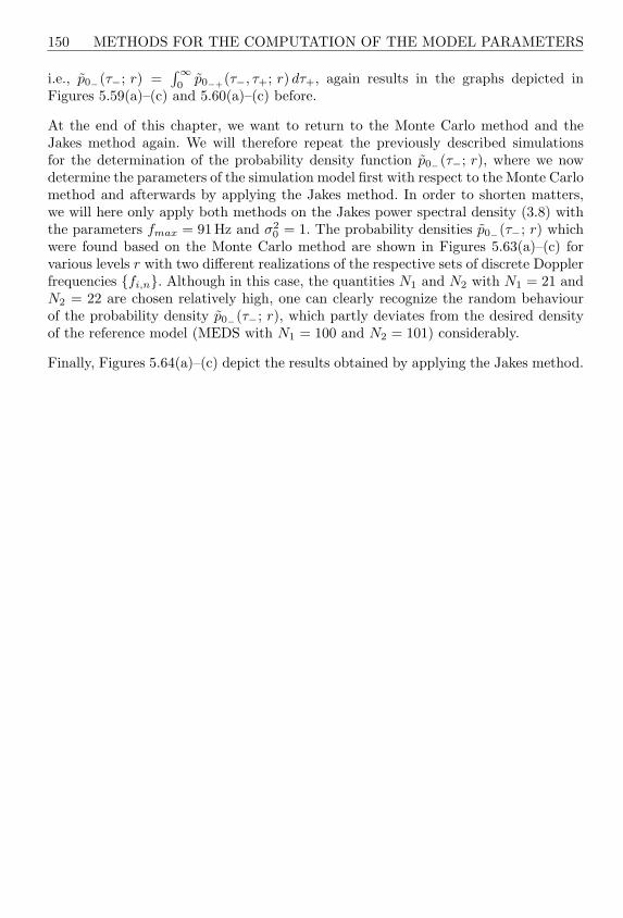
150 METHODS FOR THE COMPUTATION OF THE MODEL PARAMETERS
i.e., p0−(τ−; r) =∫∞0
p0−+(τ−, τ+; r) dτ+, again results in the graphs depicted inFigures 5.59(a)–(c) and 5.60(a)–(c) before.
At the end of this chapter, we want to return to the Monte Carlo method and theJakes method again. We will therefore repeat the previously described simulationsfor the determination of the probability density function p0−(τ−; r), where we nowdetermine the parameters of the simulation model first with respect to the Monte Carlomethod and afterwards by applying the Jakes method. In order to shorten matters,we will here only apply both methods on the Jakes power spectral density (3.8) withthe parameters fmax = 91 Hz and σ2
0 = 1. The probability densities p0−(τ−; r) whichwere found based on the Monte Carlo method are shown in Figures 5.63(a)–(c) forvarious levels r with two different realizations of the respective sets of discrete Dopplerfrequencies fi,n. Although in this case, the quantities N1 and N2 with N1 = 21 andN2 = 22 are chosen relatively high, one can clearly recognize the random behaviourof the probability density p0−(τ−; r), which partly deviates from the desired densityof the reference model (MEDS with N1 = 100 and N2 = 101) considerably.
Finally, Figures 5.64(a)–(c) depict the results obtained by applying the Jakes method.

FADING INTERVALS OF DETERMINISTIC RAYLEIGH PROCESSES 151
(a) Low level:r = 0.1
050
100150
00.5
10
2
4
6
8
10
τ+ (ms)τ- (ms)
po
- +
(τ-,
τ +;r
)
(b) Medium level:r = 1
05
1015
05
10150
2
4
6
8
τ+ (ms)τ- (ms)
po
- +
(τ-,
τ +;r
)
(c) High level:r = 2.5
0
2
4
6
010203040500
1
2
3
4
5
6
τ+ (ms)τ- (ms)
po
- +
(τ-,
τ +;r
)
Figure 5.61: Joint probability density function p0−+(τ−, τ+; r) of the fading and
connecting intervals of deterministic Rayleigh processes ζ(t): (a) r = 0.1,(b) r = 1, and (c) r = 2.5 (MEDS, Jakes PSD, fmax = 91Hz, σ2
0 = 1).

152 METHODS FOR THE COMPUTATION OF THE MODEL PARAMETERS
(a) Low level:r = 0.1
0
100
200
0
0.5
10
1
2
3
4
5
6
τ+ (ms)τ- (ms)
po
- +
(τ-,
τ +;r
)
(b) Medium level:r = 1
0
10
20
05
100
1
2
3
4
5
6
τ+ (ms)τ- (ms)
po
- +
(τ-,
τ +;r
)
(c) High level:r = 2.5
02
46
050
100150
2000
0.1
0.2
0.3
0.4
0.5
0.6
τ+ (ms)τ- (ms)
po
- +
(τ-,
τ +;r
)
Figure 5.62: Joint probability density function p0−+(τ−, τ+; r) of the fading and
connecting intervals of deterministic Rayleigh processes ζ(t): (a) r = 0.1,
(b) r = 1, and (c) r = 2.5 (MEDS, Gaussian PSD, fc =√
ln 2fmax,fmax = 91 Hz, σ2
0 = 1).

FADING INTERVALS OF DETERMINISTIC RAYLEIGH PROCESSES 153
(a) Low level:r = 0.1
0 0.5 1 1.50
500
1000
1500
2000
2500
3000
3500
4000
p0
-(τ-;
r)
τ- (ms)
p1-(τ-;r) [see (3.47)]
MCM (N1=21, N2=22)
1. Realization2. Realization
(b) Medium level:r = 1
0 5 10 15 200
50
100
150
200
250
300
350
400
450
p0
-(τ-;
r)
τ- (ms)
MEDS (N1= 100, N2= 101)MCM (N1= 21, N2= 22)
1. Realization
2. Realization
(c) High level:r = 2.5
0 20 40 60 80 100 1200
20
40
60
80
100
120
140
160
180
τ- (ms)
p0
-(τ-;
r)
MEDS (N1= 100, N2= 101)MCM (N1= 21, N2= 22)
1. Realization2. Realization
Figure 5.63: Probability density function p0−(τ−; r) of the fading intervals of
deterministic Rayleigh processes ζ(t): (a) r = 0.1, (b) r = 1, and (c)r = 2.5 (MCM, Jakes PSD, fmax = 91Hz, σ2
0 = 1).
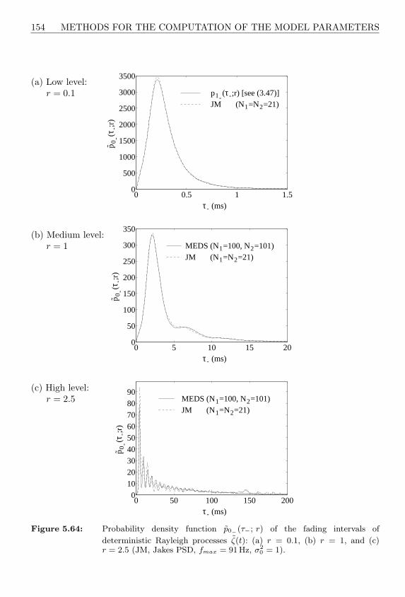
154 METHODS FOR THE COMPUTATION OF THE MODEL PARAMETERS
(a) Low level:r = 0.1
0 0.5 1 1.50
500
1000
1500
2000
2500
3000
3500
τ- (ms)
p0
-(τ-;
r)
p1-(τ-;r) [see (3.47)]
JM (N1=N2=21)
(b) Medium level:r = 1
0 5 10 15 200
50
100
150
200
250
300
350
τ- (ms)
p0
-(τ-;
r)
MEDS (N1=100, N2=101)JM (N1=N2=21)
(c) High level:r = 2.5
0 50 100 150 2000
10
20
30
40
50
60
70
80
90
τ- (ms)
p0
-(τ-;
r)
MEDS (N1=100, N2=101)JM (N1=N2=21)
Figure 5.64: Probability density function p0−(τ−; r) of the fading intervals of
deterministic Rayleigh processes ζ(t): (a) r = 0.1, (b) r = 1, and (c)r = 2.5 (JM, Jakes PSD, fmax = 91Hz, σ2
0 = 1).

6
FREQUENCY-NONSELECTIVESTOCHASTIC ANDDETERMINISTIC CHANNELMODELS
For frequency-nonselective, terrestrial, cellular land mobile radio channels andfrequency-nonselective satellite mobile radio channels, meaning channels, in whichthe propagation delay differences of the reflected and scattered signal componentsat the receiver antenna are negligible in comparison with the symbol interval, therandom fluctuations of the received signal can be modelled by a multiplication of thetransmitted signal with a suitable stochastic model process. The discovery and thedescription of suitable stochastic model processes and their adaptation to real-worldchannels have been the subject of research [Suz77, Loo85, Loo91, Lut91, Cor94] for aconsiderable time.
The simplest stochastic model processes to be applied to this are Rayleigh and Riceprocesses described in the third chapter. The flexibility of these models is, however,too limited and often not large enough for a sufficient adaptation to the statisticsof real-world channels. For the frequency-nonselective land mobile radio channel, ithas turned out that the Suzuki process [Suz77, Han77] is a more suitable stochasticmodel in many cases. The Suzuki process is a product process of a Rayleigh processand a lognormal process. The slow signal fading, stated for real-world channels, ishere modelled by the lognormal process taking the slow time variation of the averagelocal received power into account. The Rayleigh process here models the fast fadingas always. By modelling the channel on the basis of the Suzuki process, it is assumedthat no line-of-sight component exists due to shadowing. Usually, it is also assumedthat the two narrow-band real-valued Gaussian random processes, which produce theRayleigh process, are uncorrelated. If we drop the last assumption, then this leads tothe so-called modified Suzuki process analysed in [Kra90a, Kra90b].
Although the Suzuki process and its modified version were originally suggestedas a model for the terrestrial, cellular land mobile radio channel, these stochasticprocesses are also quite suitable for modelling satellite mobile radio channels in urbanregions, where the assumption that the line-of-sight signal component is shadowed, is

156 FREQUENCY-NONSELECTIVE CHANNEL MODELS
justified for most of the time. Suburban and rural regions or even open areas withpartial or no shadowing of the line-of-sight component, however, make further modelextensions necessary. A contribution to this was made in the publication [Cor94].The stochastic model introduced there is based on a product process of a Riceprocess and a lognormal process. Such a product process is suitable for modelling alarge class of environments (urban, suburban, rural, open). Here, the two real-valuedGaussian random processes producing the Rice process are again assumed to beuncorrelated. If this assumption is dropped, then the flexibility of this model canbe improved considerably with respect to the statistics of higher order. Accordingto the specification of the cross-correlation, we distinguish between extended Suzukiprocesses of Type I [Pae98d] and such of Type II [Pae97a].
Moreover, in [Pae97c] a so-called generalized Suzuki process was suggested, whichcontains the classical Suzuki process [Suz77, Han77], the modified Suzuki process[Kra90a, Kra90b], as well as the two extended Suzuki processes [Pae98d, Pae97a] ofType I and Type II as special cases. As a rule, the first and second order statisticalproperties of generalized Suzuki processes are very flexible and can therefore beadapted to given measurement results of real-world channels very well.
A further stochastic model was introduced by Loo [Loo85, Loo87, Loo90, Loo91].Loo’s model is designated for a satellite mobile radio channel in rural environments,where a line-of-sight component between the satellite and the vehicle exists for most ofthe time of the transmission. The model is based on a Rayleigh process with constantmean power for the absolute value of the sum of all scattered and reflected multipathcomponents. For the amplitude of the line-of-sight component, it is assumed that thestatistics of this amplitude behaves like a lognormal process. In this way, the slowamplitude variations of the line-of-sight component caused by foliage (shadowing) aretaken into account.
All the stochastic channel models described up to now have one property in common:They are stationary, i.e., they are based on stationary stochastic processes withconstant parameters. A non-stationary model, which is valid for very large areas,was introduced by Lutz et al. [Lut91]. This model has especially been developedfor frequency-nonselective, land mobile satellite channels. One distinguishes betweenregions, in which the line-of-sight component is shadowed (bad channel state), andregions without shadowing (good channel state). The important thing is that theproposed channel model is a 2-state model, for which the amplitude of the fadingsignal is modelled by the classical Suzuki process in the bad channel state and by aRice process in the good channel state. This procedure can easily be generalized andleads to an M-state model, where each state is represented by a specific stationarystochastic model process. In this sense, the fading behaviour of non-stationarychannels can be approximated by M stationary channel models [Vuc92, Mil95].Experimental measurements have shown that a 4-state model is sufficient for mostchannels [Vuc90]. After all, as it has been shown in [Pae99a], even one and the samestationary channel model can be applied for each state, provided that the flexibilityof this model is sufficiently high. Then, a specific set of coefficients will be assignedto each channel state. A change of a channel state is thus equivalent to a new

THE EXTENDED SUZUKI PROCESS OF TYPE I 157
configuration of a universal stationary channel model.
In this chapter, we will in detail deal with the description of the extended Suzukiprocess of Type I (Section 6.1) and of Type II (Section 6.2) as well as with thegeneralized Suzuki process (Section 6.3). Also, we will get to know a modified versionof the Loo model in Section 6.4. The modified Loo model contains the classical Loomodel as a special case. Moreover, in Section 6.5, some methods for the modelling ofnonstationary mobile radio channels will be introduced. In each section, we will alwaysproceed in such a way that a description of the respective reference model takes placeat first. Afterwards, the corresponding deterministic simulation model derivable fromthe reference model will be presented. For the purpose of demonstrating the usefulnessof the suggested reference models, the statistical properties like the probability densityfunction of the amplitude, the level-crossing rate, and the average duration of fadesare always fitted to measurement results available from the literature. All conformitiesachieved between the reference model, the simulation model, and the underlyingmeasurements are usually astonishingly good, as will be clearly demonstrated byvarious examples.
6.1 THE EXTENDED SUZUKI PROCESS OF TYPE I
As mentioned at the beginning, the product process of a Rayleigh process and alognormal process is said to be a Suzuki process. For these kind of processes, anextension is suggested in the text that follows. The Rayleigh process is in this casesubstituted by a Rice process taking the influence of a line-of-sight componentinto account. In the proposed model, the line-of-sight component can definitelybe Doppler-shifted. Also, a cross-correlation between the two real-valued Gaussianrandom processes determining the Rice process can be admitted. In this way, thenumber of the grades of freedom increases, which in fact increases the mathematicalcomplexity to be pursued, but on the other hand clearly improves the flexibilityof the stochastic model in the end. The resulting product process from a Riceprocess with cross-correlated underlying Gaussian random processes and a lognormalprocess was introduced as extended Suzuki process (of Type I) [Pae95a, Pae98d]. Thisprocess is suitable as a stochastic model for a large class of satellite and land mobileradio channels in environments, where a direct line-of-sight connection between thetransmitter and the receiver cannot be ignored.
The description of the reference model and the derivation of the statistical propertiesare carried out here by using the (complex) baseband notation as usual. At first, wewill deal with the Rice process, which is used for the modelling of the short-termfading.
6.1.1 Modelling and Analysis of the Short-Term Fading
For the modelling of the short-term fading, thus, the fast fading, we will consider theRice process (3.6), i.e.,
ξ(t) = |µρ(t)| = |µ(t) + m(t)| , (6.1)
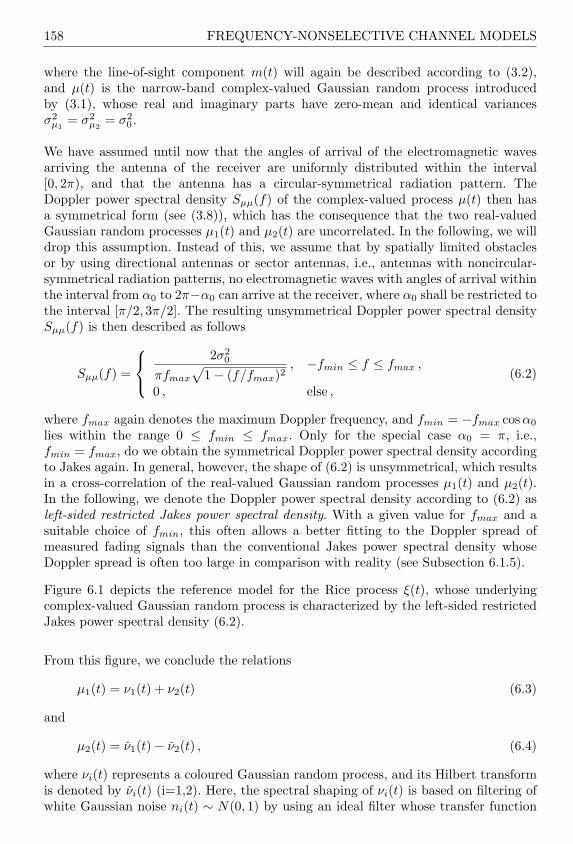
158 FREQUENCY-NONSELECTIVE CHANNEL MODELS
where the line-of-sight component m(t) will again be described according to (3.2),and µ(t) is the narrow-band complex-valued Gaussian random process introducedby (3.1), whose real and imaginary parts have zero-mean and identical variancesσ2
µ1= σ2
µ2= σ2
0 .
We have assumed until now that the angles of arrival of the electromagnetic wavesarriving the antenna of the receiver are uniformly distributed within the interval[0, 2π), and that the antenna has a circular-symmetrical radiation pattern. TheDoppler power spectral density Sµµ(f) of the complex-valued process µ(t) then hasa symmetrical form (see (3.8)), which has the consequence that the two real-valuedGaussian random processes µ1(t) and µ2(t) are uncorrelated. In the following, we willdrop this assumption. Instead of this, we assume that by spatially limited obstaclesor by using directional antennas or sector antennas, i.e., antennas with noncircular-symmetrical radiation patterns, no electromagnetic waves with angles of arrival withinthe interval from α0 to 2π−α0 can arrive at the receiver, where α0 shall be restricted tothe interval [π/2, 3π/2]. The resulting unsymmetrical Doppler power spectral densitySµµ(f) is then described as follows
Sµµ(f) =
2σ20
πfmax
√1− (f/fmax)2
, −fmin ≤ f ≤ fmax ,
0 , else ,
(6.2)
where fmax again denotes the maximum Doppler frequency, and fmin = −fmax cos α0
lies within the range 0 ≤ fmin ≤ fmax. Only for the special case α0 = π, i.e.,fmin = fmax, do we obtain the symmetrical Doppler power spectral density accordingto Jakes again. In general, however, the shape of (6.2) is unsymmetrical, which resultsin a cross-correlation of the real-valued Gaussian random processes µ1(t) and µ2(t).In the following, we denote the Doppler power spectral density according to (6.2) asleft-sided restricted Jakes power spectral density. With a given value for fmax and asuitable choice of fmin, this often allows a better fitting to the Doppler spread ofmeasured fading signals than the conventional Jakes power spectral density whoseDoppler spread is often too large in comparison with reality (see Subsection 6.1.5).
Figure 6.1 depicts the reference model for the Rice process ξ(t), whose underlyingcomplex-valued Gaussian random process is characterized by the left-sided restrictedJakes power spectral density (6.2).
From this figure, we conclude the relations
µ1(t) = ν1(t) + ν2(t) (6.3)
and
µ2(t) = ν1(t)− ν2(t) , (6.4)
where νi(t) represents a coloured Gaussian random process, and its Hilbert transformis denoted by νi(t) (i=1,2). Here, the spectral shaping of νi(t) is based on filtering ofwhite Gaussian noise ni(t) ∼ N(0, 1) by using an ideal filter whose transfer function

THE EXTENDED SUZUKI PROCESS OF TYPE I 159
H (f)1
H (f)2
ν (t)1(t)1n
(t)n2 Hilbert transformer
µ (t)2
µ (t)1
µ (t)ρ
fρ
fρ
ρ
ν (t)2
-WGN
WGN
m = sin2
ξ (t)
ρ
m =1 cosρ
(2 π + θ ) t ρ
(2 π + θ ) t
Figure 6.1: Reference model for Rice processes ξ(t) with cross-correlated underlyingGaussian random processes µ1(t) and µ2(t).
is given by Hi(f) =√
Sνiνi(f). In the following, we will assume that the whiteGaussian random processes n1(t) and n2(t) are uncorrelated.
The autocorrelation function of µ(t) = µ1(t) + jµ2(t), which is generally defined by(2.48), can be expressed in terms of the autocorrelation and cross-correlation functionsof µ1(t) and µ2(t) as follows [Kam96]
rµµ(τ) = rµ1µ1(τ) + rµ2µ2(τ) + j(rµ1µ2(τ)− rµ2µ1(τ)) . (6.5)
Using the relations rνiνi(τ) = rνiνi(τ) and rνiνi(τ) = rνiνi(−τ) = −rνiνi(τ) (cf. also(2.56e) and (2.56c), respectively), we may write:
rµ1µ1(τ) = rν1ν1(τ) + rν2ν2(τ) = rµ2µ2(τ) , (6.6a)
rµ1µ2(τ) = rν1ν1(τ)− rν2ν2(τ) = −rµ2µ1(τ) , (6.6b)
so that (6.5) can be expressed by
rµµ(τ) = 2[rν1ν1(τ) + rν2ν2(τ) + j(rν1ν1(τ)− rν2ν2(τ))] . (6.7)
After the Fourier transform of (6.5) and (6.7), we obtain the following expressions forthe Doppler power spectral density
Sµµ(f) = Sµ1µ1(f) + Sµ2µ2(f) + j(Sµ1µ2(f)− Sµ2µ1(f)) , (6.8a)
Sµµ(f) = 2[Sν1ν1(f) + Sν2ν2(f) + j(Sν1ν1(f)− Sν2ν2(f))] . (6.8b)
For the Doppler power spectral densities Sνiνi(f) and Sνiνi(f) as well as for thecorresponding autocorrelation functions rνiνi(τ) and rνiνi(τ), the following relationshold:
Sν1ν1(f) =σ2
0
2πfmax
√1− (f/fmax)2
, (6.9a)

160 FREQUENCY-NONSELECTIVE CHANNEL MODELS
•∣∣
rν1ν1(τ) =σ2
0
2J0(2πfmaxτ) , (6.9b)
Sν2ν2(f) = rect (f/fmin) · Sν1ν1(f) , (6.9c)•∣∣
rν2ν2(τ) = fminσ20J0(2πfmaxτ) ∗ sinc (2πfminτ) , (6.9d)
Sν1ν1(f) = −j sgn (f) · Sν1ν1(f) , (6.9e)•∣∣
rν1ν1(τ) =σ2
0
2H0(2πfmaxτ) , (6.9f)
Sν2ν2(f) = −j sgn (f) · Sν2ν2(f) , (6.9g)•∣∣
rν2ν2(τ) = fminσ20H0(2πfmaxτ) ∗ sinc (2πfminτ) , (6.9h)
where J0(·) and H0(·) denote the 0th order Bessel function of the first kind and theStruve’s function of 0th order, respectively.1 If we now substitute (6.9e) and (6.9g)into (6.8b), then we can express Sµµ(f) in terms of Sνiνi(f) as follows
Sµµ(f) = 2[(1 + sgn (f)) · Sν1ν1(f) + (1− sgn (f)) · Sν2ν2(f)] . (6.10)
Figure 6.2 illustrates the shapes of Sν1ν1(f) and Sν2ν2(f) as well as the correspondingleft-sided restricted Jakes power spectral density Sµµ(f).
In the following derivation of the statistical properties of ξ(t) = |µρ(t)| and ϑ(t) =argµρ(t), we often make use of the abbreviations
ψ(n)0 :=
dn
dτnrµ1µ1(τ)
∣∣∣∣τ=0
=dn
dτnrµ2µ2(τ)
∣∣∣∣τ=0
(6.11a)
and
φ(n)0 :=
dn
dτnrµ1µ2(τ)
∣∣∣∣τ=0
(6.11b)
for n = 0, 1, 2. Using (6.6) and (6.9), these characteristic quantities can be expressedas follows:
1 The rectangular function used in (6.9c) is defined by
rect (x) =
8<:
1 for |x| < 11/2 for x = ±10 for |x| > 1
and sinc (x) = sin(x)/x in (6.9d) denotes the sinc function.

THE EXTENDED SUZUKI PROCESS OF TYPE I 161
(a)
-fmax 0 fmax
f
Sν 1
ν 1(f
)
(b)
-fmax -fmin 0 fmin fmax
f
Sν 2
ν 2(f
)
(c)
-fmin 0 fmax
f
Sµµ
(f)
Figure 6.2: Doppler power spectral densities: (a) Sν1ν1(f), (b) Sν2ν2(f), and (c) theresulting left-sided restricted Jakes power spectral density.

162 FREQUENCY-NONSELECTIVE CHANNEL MODELS
ψ(0)0 = ψ0 =
σ20
2
[1 +
2π
arcsin(κ0)]
, (6.12a)
ψ(1)0 = ψ0 = 0 , (6.12b)
ψ(2)0 = ψ0 = −(πσ0fmax)2
1 +
2π
[arcsin(κ0)− 1
2sin(2 arcsin(κ0))
], (6.12c)
φ(0)0 = φ0 = 0 , (6.12d)
φ(1)0 = φ0 = 2σ2
0fmax
√1− κ2
0 , (6.12e)
φ(2)0 = φ0 = 0 , (6.12f)
where the overdot indicates the time derivative, and the parameter κ0 denotes thefrequency ratio
κ0 = fmin/fmax , 0 ≤ κ0 ≤ 1 . (6.13)
One should note that the shape of Sµµ(f) is only symmetrical for the special caseκ0 = 1. In this case, the processes µ1(t) and µ2(t) are uncorrelated, and from(6.12a)–(6.12f), the relations ψ0 = σ2
0 , ψ0 = −2(πσ0fmax)2, and φ0 = 0, which wealready know from Subsection 3.3.2, follow.
A starting point for the derivation of the statistical properties of Rice processes ξ(t)with unsymmetrical Doppler power spectral densities is given by the joint probabilitydensity function of the processes µρ1(t), µρ2(t), µρ1(t), and µρ2(t) [see (3.4)] at thesame point within the time t. This joint probability density function will be denotedby pµρ1µρ2 µρ1 µρ2
(x1, x2, x1, x2) here. It should be noted that µρi(t) is a real-valuedGaussian random process with the time variant mean value Eµρi(t) = mi(t)and the variance Var µρi(t) = Var µi(t) = rµiµi(0) = ψ0. Consequently, itstime derivative µρi(t) is a real-valued Gaussian random process too. However, thisprocess is characterized by the mean value Eµρi(t) = mi(t) and the varianceVar µρi(t) = Var µi(t) = rµiµi(0) = −rµiµi(0) = −ψ0. It is also worth mentioningthat the processes µρi(t) and µρi(t) are in pairs correlated at the same time instantt. The joint probability density function pµρ1µρ2 µρ1 µρ2
(x1, x2, x1, x2) can therefore beexpressed by the multivariate Gaussian distribution (2.20), i.e.,
pµρ1µρ2 µρ1 µρ2(x1, x2, x1, x2) =
e− 1
2 (x − m)T C−1µρ
(x − m)
(2π)2√
det Cµρ
, (6.14)
where x and m are the column vectors defined by
x =
x1
x2
x1
x2
(6.15)

THE EXTENDED SUZUKI PROCESS OF TYPE I 163
and
m =
E µρ1(t)E µρ2(t)E µρ1(t)E µρ2(t)
=
m1(t)m2(t)m1(t)m2(t)
=
ρ cos(2πfρt + θρ)ρ sin(2πfρt + θρ)
−2πfρρ sin(2πfρt + θρ)2πfρρ cos(2πfρt + θρ)
, (6.16)
respectively, and det Cµρ ( C−1µρ
) denotes the determinant (inverse) of the covariancematrix
Cµρ =
Cµρ1µρ1Cµρ1µρ2
Cµρ1 µρ1Cµρ1 µρ2
Cµρ2µρ1Cµρ2µρ2
Cµρ2 µρ1Cµρ2 µρ2
Cµρ1µρ1Cµρ1µρ2
Cµρ1 µρ1Cµρ1 µρ2
Cµρ2µρ1Cµρ2µρ2
Cµρ2 µρ1Cµρ2 µρ2
. (6.17)
The entries of the covariance matrix Cµρ can be calculated as follows
Cµ
(k)ρi
µ(`)ρj
= Cµ
(k)ρi
µ(`)ρj
(ti, tj) (6.18a)
= E(µ(k)
ρi(ti)−m
(k)i (ti)
)(µ(`)
ρj(tj)−m
(`)j (tj)
) (6.18b)
= Eµ(k)i (ti)µ
(`)j (tj) (6.18c)
= rµ
(k)i µ
(`)j
(ti, tj) (6.18d)
= rµ
(k)i µ
(`)j
(τ) , (6.18e)
for all i, j = 1, 2 and k, ` = 0, 1. The transition from (6.18d) to (6.18e) is possible ifwe take into account that µi(t) and µi(t) are Gaussian random processes, which arestrict-sense stationary per definition. As a consequence, for the autocorrelation andcross-correlation functions, it follows that these correlation functions only depend onthe time difference τ = tj − ti, i.e., r
µ(k)i µ
(`)j
(ti, tj) = rµ
(k)i µ
(`)j
(ti, ti + τ) = rµ
(k)i µ
(`)j
(τ).
Studying the equations (6.17) and (6.18e), it now becomes clear that the covariancematrix Cµρ of the processes µρ1(t), µρ2(t), µρ1(t), and µρ2(t) is identical to thecorrelation matrix Rµ of the processes µ1(t), µ2(t), µ1(t), and µ2(t), i.e., we maywrite
Cµρ(τ) = Rµ(τ) =
rµ1µ1(τ) rµ1µ2(τ) rµ1µ1(τ) rµ1µ2(τ)
rµ2µ1(τ) rµ2µ2(τ) rµ2µ1(τ) rµ2µ2(τ)
rµ1µ1(τ) rµ1µ2(τ) rµ1µ1(τ) rµ1µ2(τ)
rµ2µ1(τ) rµ2µ2(τ) rµ2µ1(τ) rµ2µ2(τ)
. (6.19)
For the entries of the correlation matrix Rµ(τ), the following relations hold [Pap91]:
rµjµi(τ) = rµiµj (−τ) , rµiµj (τ) = rµiµj (τ) , (6.20a, b)rµiµj (τ) = −rµiµj (τ) , rµiµj (τ) = −rµiµj (τ) , (6.20c, d)

164 FREQUENCY-NONSELECTIVE CHANNEL MODELS
for all i, j = 1, 2.
For the derivation of the level-crossing rate and the average duration of fades, we haveto consider the correlation properties of the processes µ
(k)ρi (ti) and µ
(`)ρj (tj) at the same
time instant, i.e., ti = tj , and, thus, the time-difference variable τ = tj − ti is equalto zero. Therefore, in connection with (6.12a)–(6.12f), we can profit from the notation(6.11) enabling us to present the covariance matrix and the correlation matrix (6.19)as follows
Cµρ(0) = Rµ(0) =
ψ0 0 0 φ0
0 ψ0 −φ0 0
0 −φ0 −ψ0 0
φ0 0 0 −ψ0
. (6.21)
After substituting (6.21) into the relation (6.14), we can now express the jointprobability density function pµρ1µρ2 µρ1 µρ2
(x1, x2, x1, x2) in terms of the quantities(6.12a)–(6.12f). For our intention, however, it is advisable to perform a transformationof the Cartesian coordinates (x1, x2) to polar coordinates (z, θ) first. For that purpose,we consider the following system of equations:
z =√
x21 + x2
2 , z =x1x1 + x2x2√
x21 + x2
2
, (6.22a)
θ = arctan(
x2
x1
), θ =
x1x2 − x2x1
x21 + x2
2
. (6.22b)
For z > 0, |z| < ∞, |θ| ≤ π, and |θ| < ∞, this system of equations has the real-valuedsolutions
x1 = z cos θ , x1 = z cos θ − θz sin θ , (6.23a)
x2 = z sin θ , x2 = z sin θ + θz cos θ . (6.23b)
Applying the transformation rule (2.38) leads to the joint probability density function
pξξϑϑ(z, z, θ, θ) = |J |−1pµρ1µρ2 µρ1 µρ2(z cos θ, z sin θ,
z cos θ − θz sin θ, z sin θ + θz cos θ) , (6.24)
where J denotes the Jacobian determinant
J =
∣∣∣∣∣∣∣∣∣∣∣
∂z∂x1
∂z∂x2
∂z∂x1
∂z∂x2
∂z∂x1
∂z∂x2
∂z∂x1
∂z∂x2
∂θ∂x1
∂θ∂x2
∂θ∂x1
∂θ∂x2
∂θ∂x1
∂θ∂x2
∂θ∂x1
∂θ∂x2
∣∣∣∣∣∣∣∣∣∣∣
=
∣∣∣∣∣∣∣∣∣∣∣
∂x1∂z
∂x1∂z
∂x1∂θ
∂x1
∂θ∂x2∂z
∂x2∂z
∂x2∂θ
∂x2
∂θ∂x1∂z
∂x1∂z
∂x1∂θ
∂x1
∂θ∂x2∂z
∂x2∂z
∂x2∂θ
∂x2
∂θ
∣∣∣∣∣∣∣∣∣∣∣
−1
= − 1z2
. (6.25)

THE EXTENDED SUZUKI PROCESS OF TYPE I 165
After some further algebraic manipulations, we are now in the position to bringthe desired joint probability density function pξξϑϑ(z, z, θ, θ) into the following form[Pae98d]
pξξϑϑ(z, z, θ, θ) =z2
(2π)2ψ0βe−
z2+ρ2
2ψ0 · e zρψ0
cos(θ−2πfρt−θρ)
·e− 12β [z−√2βαρ sin(θ−2πfρt−θρ)]2
·e− z22β
nθ− φ0
ψ0−√2β αρ
z cos(θ−2πfρt−θρ)o2
(6.26)
for z ≥ 0, |z| < ∞, |θ| ≤ π, and |θ| < ∞, where
α =
(2πfρ − φ0
ψ0
)/√2β , (6.27)
β = −ψ0 − φ20/ψ0 . (6.28)
The joint probability density function (6.26) represents a fundamental equation. Withthis, we will at first determine the probability density function of the amplitude andthe phase of the process µρ(t) in the following subsection, and will then proceed withthe derivation of the level-crossing rate and the average duration of fades of the processξ(t) = |µρ(t)| by again making use of (6.26).
6.1.1.1 Probability Density Function of the Amplitude and the Phase
Employing the rule (2.40) now allows us to calculate the probability density pξ(z)of the process ξ(t) from the joint probability density function pξξϑϑ(z, z, θ, θ). Wetherefore consider the threefold integral
pξ(z) =
∞∫
−∞
π∫
−π
∞∫
−∞pξξϑϑ(z, z, θ, θ) dθ dθ dz , z ≥ 0 . (6.29)
Putting (6.26) in the above expression results in the well-known Rice distribution
pξ(z) =
z
ψ0e−
z2+ρ2
2ψ0 I0
(zρ
ψ0
), z ≥ 0 ,
0 , z < 0 .
(6.30)
Due to the correlation of the processes µ1(t) and µ2(t), this result cannot be regardedas a matter of course, as we will see later in Subsection 6.2. Since the probabilitydensity (6.30) is independent of the quantity φ0 in the present case, it follows that thecorrelation between the processes µ1(t) and µ2(t) has no influence on the probabilitydensity function of the amplitude ξ(t). However, one should note that the parameterκ0 determining the Doppler bandwidth exerts an influence on the variance ψ0 of theprocesses µ1(t) and µ2(t) [cf. (6.12a)] and consequently determines the behaviour of(6.30) decisively.

166 FREQUENCY-NONSELECTIVE CHANNEL MODELS
The probability density function of the phase ϑ(t), denoted by pϑ(θ), can be calculatedin a similar way. Substituting (6.26) into
pϑ(θ) =
∞∫
0
∞∫
−∞
∞∫
−∞pξξϑϑ(z, z, θ, θ) dθ dz dz , −π ≤ θ ≤ π , (6.31)
results in
pϑ(θ) = pϑ(θ; t) =e−
ρ2
2ψ0
2π
1 +
√π
2ψ0ρ cos(θ − 2πfρt− θρ) · e
ρ2 cos2(θ−2πfρt−θρ)2ψ0
[1 + erf
(ρ cos(θ − 2πfρt− θρ)√
2ψ0
)] , −π ≤ θ ≤ π . (6.32)
One observes that also in this case, the cross-correlation function rµ1µ2(τ) has noinfluence on the probability density function pϑ(θ), since pϑ(θ) is independent of φ0.For the special case κ0 = 1, we have ψ0 = σ2
0 , and, thus, from (6.32) it follows (3.21).The investigation of further special cases, for example: (i) fρ = 0, (ii) ρ → 0, and (iii)ρ → ∞ leads to the statements made below the equation (3.21), which will not berevised again at this point.
6.1.1.2 Level-Crossing Rate and Average Duration of Fades
The derivation of the level-crossing rate using
Nξ(r) =∫ ∞
0
z pξξ(r, z) dz (6.33)
requires the knowledge of the joint probability density function pξξ(z, z) of thestationary processes ξ(t) and ξ(t) at the same time instant t at the level z = r.For the joint probability density function pξξ(z, z), one finds, after substituting (6.26)into
pξξ(z, z) =
π∫
−π
∞∫
−∞pξξϑϑ(z, z, θ, θ) dθ dθ , z ≥ 0 , |z| < ∞ , (6.34)
the result
pξξ(z, z) =z
ψ0
√β(2π)3/2
· e− z2+ρ2
2ψ0
∫ π
−π
ezρψ0
cos θ
·e− 12β [z−√2βαρ sin θ]2 dθ , z ≥ 0 , |z| < ∞ , (6.35)
where α, β, and ψ0 are the quantities introduced by (6.27), (6.28), and (6.12a),respectively. Obviously, the processes ξ(t) and ξ(t) are in general statistically

THE EXTENDED SUZUKI PROCESS OF TYPE I 167
dependent, because pξξ(z, z) 6= pξ(z) ·pξ(z) holds. Only for the special case α = 0, i.e.,(i) if the two real-valued Gaussian random processes µ1(t) and µ2(t) are uncorrelatedand fρ is equal to zero, or, (ii) if fρ and φ0 are related by fρ = φ0/(2πψ0), thenwe obtain statistically independent processes ξ(t) and ξ(t), since from (6.35) it nowfollows
pξξ(z, z) = pξ(z) · pξ(z)
=z
ψ0e−
z2+ρ2
2ψ0 I0
(zρ
ψ0
)· e−
z22β
√2πβ
, (6.36)
where β in this case again represents β = −ψ0 − φ20/ψ0 ≥ 0. Hence, for α = 0, the
joint probability density function pξξ(z, z) is equal to the product of the probabilitydensity functions of the stochastic processes ξ(t) and ξ(t), which are Rice and Gaussiandistributed, respectively.
With the joint probability density function (6.35), we are now able to calculatethe level-crossing rate of Rice processes whose underlying complex-valued Gaussianprocess has cross-correlated in-phase and quadrature components. In this way, aftersubstituting (6.35) in the definition (6.33) and performing some tedious algebraicmanipulations, we finally obtain the result [Pae98d]
Nξ(r) =r√
2β
π3/2ψ0e−
r2+ρ2
2ψ0
∫ π/2
0
cosh(
rρ
ψ0cos θ
)
·
e−(αρ sin θ)2 +√
παρ sin(θ) · erf (αρ sin θ)
dθ , r ≥ 0 , (6.37)
where the characteristic quantities α, β, and ψ0 are given in the form (6.27), (6.28),and (6.12a), respectively. Further simplifications are not possible; the remainingintegral has to be solved numerically. Let us again consider the special case κ0 = 1.Then, we obtain: α = 2πfρ/
√2β, β = −ψ0 = −rµiµi(0), and ψ0 = σ2
0 , so that thelevel-crossing rate Nξ(r) given above results in the expression introduced by (3.24),as was to be expected.
Let us assume that the line-of-sight component tends to zero, i.e., ρ → 0, which leadsto ξ(t) → ζ(t). Then, it follows that (6.37) tends to
Nξ(r) =
√β
2π· r
ψ0e−
r22ψ0 , r ≥ 0 , (6.38)
where the quantity β is given by (6.28). The above result shows us that the level-crossing rate is proportional to the Rayleigh distribution. This property has alsobeen mentioned in [Kra90b]. Due to (6.28), the proportionality factor
√β/(2π) is
not only determined by the curvature of the autocorrelation function at the originτ = 0 (ψ0 = rµiµi(0)), but also decisively by the gradient of the cross-correlationfunction at τ = 0 (φ0 = rµ1µ2(0)).

168 FREQUENCY-NONSELECTIVE CHANNEL MODELS
Now, let ρ 6= 0 and fρ = φ0/(2πψ0). Then, it follows α = 0 [see (6.27)], and from(6.37) we obtain the level-crossing rate Nξ(r) according to (3.27), if σ2
0 is substitutedby ψ0 in that equation, i.e.,
Nξ(r) =
√β
2π· r
ψ0e−
r2+ρ2
2φ0 I0
(rρ
ψ0
), r ≥ 0 , (6.39)
where β is again given by (6.28).
In connection with the Jakes power spectral density, the level-crossing rate Nξ(r)described by (6.37) is always proportional to the maximum Doppler frequency fmax.The normalization of Nξ(r) to fmax therefore eliminates the influence of both thevelocity of the vehicle and the carrier frequency. The influence of the parameters κ0
and σ20 on the normalized level-crossing rate Nξ(r)/fmax is illustrated in Figure 6.3(a)
and in Figure 6.3(b), respectively.
(a)
0 1 2 3 4 5 60
0.5
1
1.5
2
ρ=0ρ=3
κ0= 0 κ0=1/3κ0=2/3κ0= 1
r
Nξ(
r)/f
max
(b)
0 1 2 3 40
0.5
1
1.5
2
2.5
r
Nξ(
r)/f
max
σ20= 1
σ20=3/4
σ20=1/2
σ20=1/4
Figure 6.3: Normalized level-crossing rate Nξ(r)/fmax of Rice processes (with cross-correlated underlying Gaussian random processes): (a) κ0 = fmin/fmax
(σ20 = 1) and (b) σ2
0 (ρ = 0, κ0 = 1).
For the calculation of the average duration of fades Tξ−(r), we will be guided by thebasic relation (2.63), i.e.,
Tξ (r) =Fξ (r)Nξ(r)
, (6.40)
where Fξ−(r) denotes the cumulative distribution function of the Rice process ξ(t)and therefore states the probability that ξ(t) takes a value which is lower or equal tothe signal level r. Using (6.30), the following integral expression can be derived forFξ−(r)
Fξ (r) = P (ξ(t) ≤ r)

THE EXTENDED SUZUKI PROCESS OF TYPE I 169
=∫ r
0
pξ(z)dz
=e−
ρ2
2ψ0
ψ0
∫ r
0
ze−z22ψ0 I0
(zρ
ψ0
)dz . (6.41)
The average duration of fades of Rice processes ξ(t) with cross-correlated in-phaseand quadrature components µ1(t) and µ2(t) is, thus, the quotient (6.40) of theintegral expressions (6.41) and (6.37), which have to be solved numerically.
The influence of the parameters κ0 and σ20 on the normalized average duration of fades
Tξ−(r) · fmax is depicted in Figures 6.4(a) and 6.4(b), respectively.
(a)
10-1
100
10-3
10-2
10-1
100
101
ρ=0
ρ=3
r
Tξ -
(r)
⋅ fm
ax
κ0= 0 κ0=1/3 κ0=2/3 κ0= 1
(b)
10-1
100
10-2
10-1
100
r
Tξ -
(r)
⋅ fm
ax
σ02=1/4
σ02=1/2
σ02=3/4
σ02= 1
Figure 6.4: Normalized average duration of fades Tξ(r) · fmax of Rice processes(with cross-correlated underlying Gaussian random processes): (a) κ0 =fmin/fmax (σ2
0 = 1) and (b) σ20 (ρ = 0, κ0 = 1).
6.1.2 Modelling and Analysis of the Long-Term Fading
Measurements have shown that the slow fading behaves in its statistical propertiesquite similar to a lognormal process [Reu72, Bla72, Oku68]. With such a process, theslow fluctuations of the local mean value of the received signal, which are determinedby shadowing effects, can be reproduced. In the following, we will denote lognormalprocesses by λ(t). Lognormal processes can be derived by means of the nonlineartransform
λ(t) = eσ3ν3(t)+m3 (6.42)
from a third real-valued Gaussian random process ν3(t) with the expected valueEν3(t) = 0 and the variance Var ν3(t) = 1. Fitting the model behaviour tothe statistics of real-world channels, the model parameters m3 and σ3 can be used inconnection with the parameters of the Rice process (σ2
0 , fmax, fmin, ρ, fρ). We assume

170 FREQUENCY-NONSELECTIVE CHANNEL MODELS
henceforth that the stochastic process ν3(t) is statistically independent of the processesν1(t) and ν2(t). Figure 6.5 illustrates the reference model for the lognormal processλ(t) introduced this way.
H 3 (f)
σ3 m3
exp( ).µ3(t)ν
WGN(t)3n 3(t)
λ (t)
Figure 6.5: Reference model for lognormal processes λ(t).
Here, the process ν3(t) is obtained by filtering white Gaussian noise n3(t) ∼ N(0, 1)with a real-valued low-pass filter, whose transfer function H3(f) is related to thepower spectral density Sν3ν3(f) of the process ν3(t) according to (2.52f), i.e., H3(f) =√
Sν3ν3(f). For Sν3ν3(f), the Gaussian power spectral density is assumed in the form[cf. also (3.11)]
Sν3ν3(f) =1√
2πσc
e− f2
2σ2c , (6.43)
where the 3-dB-cut-off frequency fc = σc
√2 ln 2 is in general much smaller than the
maximum Doppler frequency fmax. In order to simplify the notation, we introduce thesymbol κc for the frequency ratio fmax/fc, i.e., κc = fmax/fc. A study on modifiedSuzuki processes has shown [Kra90b] that both the parameter κc as well as the exactshape of the power spectral density of ν3(t) have no considerable influence on therelevant statistical properties of modified Suzuki processes, if κc > 10. Other typesof power spectral densities Sν3ν3(f) than the form (6.43) studied here have beenproposed, for example, in [Kra90a, Kra90b] and [Loo91], where RC-low-pass filtersand Butterworth filters of third order have been applied, respectively.
The autocorrelation function rν3ν3(τ) of the process ν3(t) can be described aftercalculating the inverse Fourier transform of (6.43) by
rν3ν3(τ) = e−2(πσcτ)2 . (6.44)
Next, let us consider the lognormal process λ(t) [see (6.42)]. The autocorrelationfunction rλλ(τ) of this process can be expressed in terms of rν3ν3(τ) as follows
rλλ(τ) = Eλ(t) · λ(t + τ)= Ee2m3+σ3[ν3(t)+ν3(t+τ)]=
∫ ∞
−∞
∫ ∞
−∞e2m3+σ3(x1+x2) · pν3ν′3(x1, x2) dx1 dx2 , (6.45)

THE EXTENDED SUZUKI PROCESS OF TYPE I 171
where
pν3ν′3(x1, x2) =1
2π√
1− r2ν2ν3
(τ)e− x2
1−2rν3ν3 (τ) x1x2+x22
2[1−r2ν3ν3
(τ)] (6.46)
describes the joint probability density function of the Gaussian random process ν3(t)at two different time instants t1 = t and t2 = t + τ . After substituting (6.46) in (6.45)and solving the double integral, the autocorrelation function rλλ(τ) can be expressedin a closed form by
rλλ(τ) = e2m3+σ23 [1+rν3ν3 (τ)] . (6.47)
With this relation, the mean power of the lognormal process λ(t) can easily bedetermined. We obtain rλλ(0) = e2(m3+σ2
3).
The power spectral density Sλλ(f) of the lognormal process λ(t) can now be expressedin terms of the power spectral density Sν3ν3(f) of ν3(t) as follows [Pae98c]
Sλλ(f) =
∞∫
−∞rλλ(τ)e−j2πfτdτ
= e2m3+σ23 · δ(f) +
∞∫
−∞
(eσ2
3rν3ν3 (τ) − 1)
e−j2πfτdτ
= e2m3+σ23 ·
δ(f) +
∞∑n=1
σ2n3
n!·Sν3ν3
(f√n
)√
n
. (6.48)
This result shows us that the power spectral density Sλλ(f) of the lognormal processλ(t) consists of a weighted delta function at the origin f = 0 and of an infinite sumof strictly monotonously decreasing power spectral densities Sν3ν3(f/
√n)/
√n. One
should note that Sν3ν3(f/√
n)/√
n follows directly from (6.43), if the quantity σc isreplaced by
√nσ3 there.
The probability density function pλ(y) of the lognormal process λ(t) is described bythe lognormal distribution (2.28), i.e.,
pλ(y) =
1√2πσ3y
e− (ln y−m3)2
2σ23 , y ≥ 0 ,
0 , y < 0 ,
(6.49)
with the expected value and the variance according to (2.29a) and (2.29b), respectively.
For the calculation of the level-crossing rate and the average duration of fades of(extended) Suzuki processes, we require the knowledge of the joint probability density

172 FREQUENCY-NONSELECTIVE CHANNEL MODELS
function of the lognormal process λ(t) and its corresponding time derivative λ(t) atthe same time instant t. This joint probability density function will be denoted bypλλ(y, y) here and will briefly be derived in the following. We start from the underlyingGaussian random process ν3(t) and its time derivative ν3(t). For the cross-correlationfunction of these two processes it follows that rν3ν3(0) = 0 holds, i.e., ν3(t1) andν3(t2) are uncorrelated at the same time instant t = t1 = t2. Since ν3(t) and, hence,also ν3(t) are Gaussian random processes, it follows from the uncorrelatedness thatthese processes are statistically independent. For the joint probability density functionpν3ν3(x, x) of the processes ν3(t) and ν3(t), we can therefore write
pν3ν3(x, x) = pν3(x) · pν3(x) =e−
x22√
2π· e−
x22γ
√2πγ
, (6.50)
where
γ = rν3ν3(0) = −rν3ν3(0) = (2πσc)2 (6.51)
denotes the variance of the process ν3(t).
Similar to the scheme described in detail in Subsection 6.1.1, we can take pν3ν3(x, x) asour starting point to determine the desired joint probability density function pλλ(y, y).The nonlinear mapping (6.42) in connection with the following substitution of variables
x =ln y −m3
σ3, x =
y
σ3y(6.52a, b)
yields the expression J = (σ3y)2 for the Jacobian determinant (6.25). With thetransformation rule (2.38), we then obtain the following result for the joint probabilitydensity function pλλ(y, y)
pλλ(y, y) =e− (ln y−m3)2
2σ23√
2π σ3y· e− y2
2γ(σ3y)2
√2πγ σ3y
. (6.53)
This result shows us that the processes λ(t) and λ(t) are statistically dependent,although the underlying Gaussian processes ν3(t) and ν3(t) are statisticallyindependent.
6.1.3 The Stochastic Extended Suzuki Process of Type I
The extended Suzuki process (Type I), denoted by η(t), was introduced in [Pae98d]as a product process of a Rice process ξ(t) [see (6.1)] with cross-correlated underlyingGaussian random processes µ1(t) and µ2(t) and a lognormal process λ(t) [see (6.42)],i.e.,
η(t) = ξ(t) · λ(t) . (6.54)
Figure 6.6 shows the structure of the reference model belonging to η(t) for a frequency-nonselective mobile radio channel.

THE EXTENDED SUZUKI PROCESS OF TYPE I 173
H (f)1
ν (t)1(t)1n
Hilbert transformer
µ (t)2
µ (t)1
µ (t)ρ
fρ
fρ
H (f)2
(t)n2 ν (t)2
WGN
m3σ3
exp( ).
ξ (t)
1
-
WGN
sinρ
cosρ
(2 π + θ ) t ρ
(2 π + θ ) t ρ
ν (t)WGN
(t)n3 3
3H (f)
µ (t)3
(t)λ
(t)η
m (t) =
m (t) =2
Figure 6.6: Reference model for extended Suzuki processes (Type I).
The probability density function pη(z) of the extended Suzuki process η(t) can becalculated by means of the relation [Pap91]
pη(z) =∫ ∞
−∞
1|y| pξλ
(z
y, y
)dy , (6.55)
where pξλ(x, y) is the joint probability density function of the processes ξ(t) and λ(t) atthe same time instant t. According to our assumption, the coloured Gaussian randomprocesses ν1(t), ν2(t), and ν3(t) are in pairs statistically independent. Consequently,the Rice process ξ(t) and the lognormal process λ(t) are also statistically independent,so that for the joint probability density function pξλ(x, y) it follows: pξλ(x, y) =pξ(x) · pλ(y). Hence, the multiplicative relation between the processes ξ(t) and λ(t)leads to the following integral equation for the probability density function of extendedSuzuki processes
pη(z) =z√
2πψ0σ3
∫ ∞
0
1y3
e−(z/y)2+ρ2
2ψ0 I0
(zρ
yψ0
)e− (ln y−m3)2
2σ23 dy , z ≥ 0 . (6.56)
For ρ = 0, it should be noted that the probability density function (6.56) canbe reduced to the (classical) Suzuki distribution (2.30) introduced in [Suz77]. Theinfluence of the parameters ρ and σ3 on the behaviour of pξ(z) can be concluded fromFigure 6.7.
Studying (6.56), one can clearly see that pη(z) merely depends on the quantitiesψ0, ρ, σ3, and m3. Accordingly, the exact shape of the power spectral density of thecomplex-valued Gaussian random process µ(t) and especially the cross-correlation ofthe processes µ1(t) and µ2(t) have no influence on the probability density function

174 FREQUENCY-NONSELECTIVE CHANNEL MODELS
0 1 2 3 40
0.2
0.4
0.6
0.8
1
z
pη
(z)
ρ=0 ρ=3
σ3 = 1/3 σ3 = 2/3σ3 = 1
Figure 6.7: Probability density function pη(z) for various values of the parameters ρand σ3 (ψ0 = 1, m3 = −σ2
3/2).
of the extended Suzuki process. For the adaptation of (6.56) to a given measuredprobability density function by merely optimizing these model parameters, there isa risk that the statistics of real-world channels are reproduced insufficiently by thechannel model.
In the following, we therefore study the level-crossing rate Nη(r) of the process η(t),i.e.,
Nη(r) =∫ ∞
0
z pηη(r, z) dz , (6.57)
which requires the knowledge of the joint probability density function pηη(z, z) ofthe process η(t) and its time derivative η(t) at the same time instant t. This jointprobability density can be derived by substituting the equations (6.35) and (6.53)obtained for pξξ(x, x) and pλλ(y, y), respectively, into the relation [Kra90a]
pηη(z, z) =
∞∫
0
∞∫
−∞
1y2
pξξ
(z
y,z
y− z
y2y
)pλλ(y, y) dy dy , z ≥ 0, |z| < ∞ . (6.58)
Hence, after some tedious algebraic manipulations, we find the expression
pηη(z, z) =z
(2π)32 ψ0
√β
∫ ∞
0
e−(z/y)2+ρ2
2ψ0
y3K(z, y)· e− (ln y−m3)2
2σ23√
2π σ3y·
∫ 2π
0
ezρ
yψ0cos θ · e−
(z−√2βαyρ sin θ)2
2βy2K2(z,y) dθ dy , z ≥ 0 , |z| < ∞ , (6.59)

THE EXTENDED SUZUKI PROCESS OF TYPE I 175
where
K(z, y) =
√1 +
γ
β
(zσ3
y
)2
. (6.60)
After substituting (6.59) into (6.57), we then obtain the following final result for thelevel-crossing rate Nη(r) of the extended Suzuki process of Type I
Nη(r) =r√
2β
π3/2ψ0·∞∫
0
K(r, y)y
· e− (lny−m3)2
2σ23√
2π σ3ye−
(r/y)2+ρ2
2ψ0 ·π/2∫
0
cosh(
rρ
yψ0cos θ
)
e−(αρ sin θ
K(r,y) )2
+√
π αρsin θ
K(r, y)erf
[αρ
sin θ
K(r, y)
]dθ dy, (6.61)
where α, β, and γ again are the quantities introduced by (6.27), (6.28), and (6.51),respectively, and ψ0 is determined by (6.12a). Exactly due to α and β, the influenceof the shape of the Doppler power spectral density is now taken into consideration,because α depends on φ0 and β is a function of φ0 and ψ0. A detailed analysis of (6.61)here also shows that Nη(r) is again proportional to the maximum Doppler frequencyand, thus, to the speed of the vehicle as well.
Moreover, we are interested in some special cases. Assuming σ3 → 0, then thelognormal distribution (6.49) converges to the probability density function pλ(y) =δ(y − em3). Consequently, especially in case m3 = 0, the level-crossing rate Nη(r)tends to Nξ(r) according to (6.37).
In case of a missing line-of-sight component, i.e., ρ = 0, the level-crossing rate ofmodified Suzuki processes follows from (6.61)
Nη(r)|ρ=0 =
√β
2π
r
ψ0
∫ ∞
0
K(r, y)y
pλ(y) e− r2
2ψ0y2 dy
=
√β
2π
∫ ∞
0
K(r, y) pζ(r/y) pλ(y) dy (6.62)
as stated in [Kra90a, Kra90b]. It should also be mentioned that for ρ 6= 0, the twocases
(i) fρ = φ0/(2πψ0) , (6.63a)
(ii) fρ = 0 and φ0 = 0 (6.63b)
are equivalent with respect to the level-crossing rate Nη(r), because we then haveα = 0 due to (6.27), and from (6.61) the same expression
Nη(r)|α=0 =
√β
2π
r
ψ0
∫ ∞
0
K(r, y)y
pλ(y) e−(r/y)2+ρ2
2ψ0 I0
(rρ
yψ0
)dy
=
√β
2π
∫ ∞
0
K(r, y) pξ(r/y) pλ(y) dy (6.64)

176 FREQUENCY-NONSELECTIVE CHANNEL MODELS
always follows. One should note, however, that the cases (i) and (ii) result in differentvalues for β. Under the condition (i), the general relation (6.28) is valid for β, whereasthis equation can be simplified in case of (ii) to β = −ψ0.
At the end of this subsection, we also derive the cumulative distribution functionFη−(r) = P (η(t) ≤ r), which is required for the calculation of the average duration offades of extended Suzuki processes of Type I
Tη (r) =Fη (r)Nη(r)
. (6.65)
Thus, using (6.56), we obtain
Fη (r) =∫ r
0
pη(z) dz
=1√
2π ψ0σ3
∫ ∞
0
∫ r
0
z
y3e−
(z/y)2+ρ2
2ψ0 I0
(zρ
yψ0
)e− (ln y−m3)2
2σ23 dz dy
= 1−∫ ∞
0
Q1
(ρ√ψ0
,r
y√
ψ0
)pλ(y) dy , (6.66)
where Q1(., .) (see [Pro95, p. 44]) is the generalized Marcum’s Q-function defined by
Qm(a, b) =
∞∫
b
z(z
a
)m−1
e−z2+a2
2 Im−1(az) dz , m = 1, 2, . . . (6.67)
In order to illustrate the results found in this section, let us consider the parameterstudy shown in Figures 6.8(a)–6.8(d). Figures 6.8(a) and 6.8(b) depict the normalizedlevel-crossing rate Nη(r)/fmax calculated according to (6.61) for several values of theparameters m3 and σ3. The graphs of the corresponding normalized average durationof fades Tη−(r) · fmax are presented in Figures 6.8(c) and 6.8(d).
6.1.4 The Deterministic Extended Suzuki Process of Type I
In the preceding subsection, we have seen that the reference model for the extendedSuzuki process of Type I is based on the use of three real-valued coloured Gaussianrandom processes νi(t) or µi(t) (i = 1, 2, 3) (see Figure 6.6). We now make use of theprinciple of deterministic channel modelling explained in Section 4.1, and approximatethe ideal Gaussian random processes νi(t) by
νi(t) =Ni∑
n=1
ci,n cos(2πfi,nt + θi,n) , i = 1, 2, 3 . (6.68)
In the following, we therefore assume that the processes ν1(t), ν2(t), and ν3(t) areuncorrelated in pairs. The uncorrelatedness property can be guaranteed withoutproblems for nearly all parameter design methods discussed in Section 6.1. After

THE EXTENDED SUZUKI PROCESS OF TYPE I 177
(a)
10-1
100
10-3
10-2
10-1
100
r
Nη
(r)/
f max
ρ=3
ρ=0
m3 = 1/4 m3 = 1/2 m3 = 3/4 m3 = 1
(b)
10-1
100
10-3
10-2
10-1
100
r
Nη
(r)/
f max
ρ=3
ρ=0
σ3 = 1/4 σ3 = 1/2 σ3 = 3/4 σ3 = 1
(c)
10-1
100
10-2
10-1
100
101
m3 = 1/4
m3 = 1/2m3 = 3/4
m3 = 1
ρ = 0 ρ = 3
r
Tη
-(r)
⋅ fm
ax
(d)
10-1
100
10-1
100
σ3 = 1
σ3 = 3/4
σ3 = 1/2
σ3 = 1/4
r
Tη
-(r)
⋅ fm
ax
ρ = 0 ρ = 3
Figure 6.8: Normalized level-crossing rate Nη(r)/fmax of extended Suzuki processes(Type I) for several values of (a) m3gl6-68 (σ3 = 1/2) and (b) σ3 (m3 = 1/2)as well as (c) and (d) the corresponding normalized average duration offades Tη−(r) · fmax (κ0 = 1, ψ0 = 1).

178 FREQUENCY-NONSELECTIVE CHANNEL MODELS
a few elementary network transformations, the continuous-time structure shown inFigure 6.9 enabling the simulation of deterministic extended Suzuki processes of Type Ifollows from the stochastic reference model (see Figure 6.6).
.
c1,1
c11,N
c2,1
cos(2 π f + θ )t1,1 1,1
cos(2 +π f θt1
)11,N 1,N
cos(2 π f + θ )t 2,12,1
cos(2 + θπ f t2
)22,N 2,N
π f + θ )sin(2 t1,1 1,1
+ θπ fsin(2 t1 11,N 1,N
π f + θ )sin(2 t 2,12,1
+ θπ fsin(2 t2,N2 22,Nρ π
Deterministic lognormal process
ρf t + ) θρ=(t)m2
sin(2
.exp( )
ρ cos(2 π ρf t + ) θρ=(t)1
m
µ (t)1~
µ~ 2(t)
µ~ ρ(t)
ν~3(t)
σ3 m 3
µ~ 3 (t)
ξ (t)~
~(t)λ
η~ (t) .ξ (t)~
(t)~λ=
cos(2 π + θ )f
cos(2 π + θ )fc
3,1 3,1
3,1
t
t3,2 3,2
c3,2
cos(2 + θπ f
c
t3,N3 3,N3)
3,N3
c1
c
)
)1,N
1,1
22,N
- c 2,1
2- c 2,N
c
Deterministic Rice process with cross-correlated underlying components
Figure 6.9: Deterministic simulation model for extended Suzuki processes (Type I).
Studying Figure 6.9, we notice that not only the design of the digital filters, whichare usually employed for spectral shaping, but also the realization of the Hilberttransformer can be avoided. Moreover, deterministic simulation models offer theadvantage that all relations derived for the reference model before such as, for instance,the expressions for the probability density function pη(z), the level-crossing rate Nη(r),and the average duration of fades Tη−(r) can be used to approximately describe thebehaviour of deterministic extended Suzuki process η(t). In all those expressions, whichare of interest for us, we therefore only have to replace the characteristic quantities ofthe reference model ψ0, ψ0, and φ0 by the corresponding quantities of the simulationmodel, i.e.,
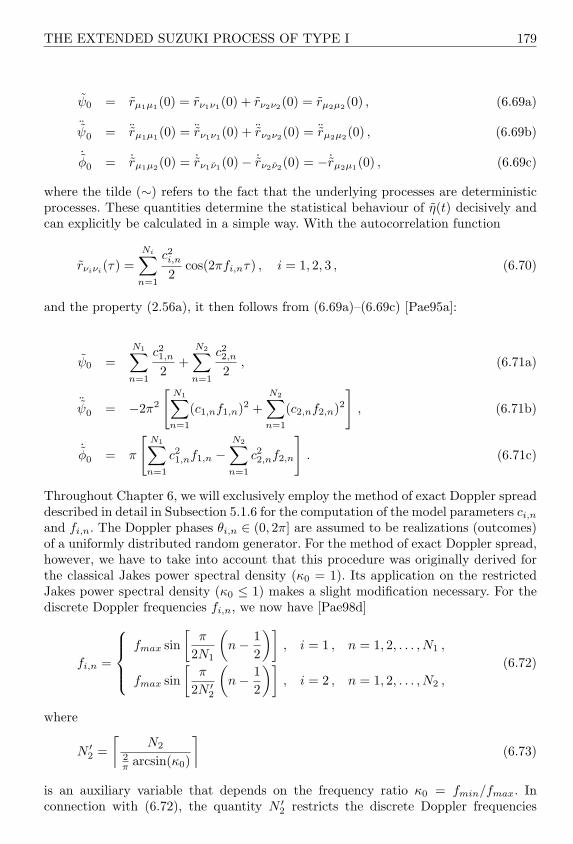
THE EXTENDED SUZUKI PROCESS OF TYPE I 179
ψ0 = rµ1µ1(0) = rν1ν1(0) + rν2ν2(0) = rµ2µ2(0) , (6.69a)
¨ψ0 = ¨rµ1µ1(0) = ¨rν1ν1(0) + ¨rν2ν2(0) = ¨rµ2µ2(0) , (6.69b)
˙φ0 = ˙rµ1µ2(0) = ˙rν1ν1(0)− ˙rν2ν2(0) = − ˙rµ2µ1(0) , (6.69c)
where the tilde (∼) refers to the fact that the underlying processes are deterministicprocesses. These quantities determine the statistical behaviour of η(t) decisively andcan explicitly be calculated in a simple way. With the autocorrelation function
rνiνi(τ) =
Ni∑n=1
c2i,n
2cos(2πfi,nτ) , i = 1, 2, 3 , (6.70)
and the property (2.56a), it then follows from (6.69a)–(6.69c) [Pae95a]:
ψ0 =N1∑
n=1
c21,n
2+
N2∑n=1
c22,n
2, (6.71a)
¨ψ0 = −2π2
[N1∑
n=1
(c1,nf1,n)2 +N2∑
n=1
(c2,nf2,n)2]
, (6.71b)
˙φ0 = π
[N1∑
n=1
c21,nf1,n −
N2∑n=1
c22,nf2,n
]. (6.71c)
Throughout Chapter 6, we will exclusively employ the method of exact Doppler spreaddescribed in detail in Subsection 5.1.6 for the computation of the model parameters ci,n
and fi,n. The Doppler phases θi,n ∈ (0, 2π] are assumed to be realizations (outcomes)of a uniformly distributed random generator. For the method of exact Doppler spread,however, we have to take into account that this procedure was originally derived forthe classical Jakes power spectral density (κ0 = 1). Its application on the restrictedJakes power spectral density (κ0 ≤ 1) makes a slight modification necessary. For thediscrete Doppler frequencies fi,n, we now have [Pae98d]
fi,n =
fmax sin[
π
2N1
(n− 1
2
)], i = 1 , n = 1, 2, . . . , N1 ,
fmax sin[
π
2N ′2
(n− 1
2
)], i = 2 , n = 1, 2, . . . , N2 ,
(6.72)
where
N ′2 =
⌈N2
2π arcsin(κ0)
⌉(6.73)
is an auxiliary variable that depends on the frequency ratio κ0 = fmin/fmax. Inconnection with (6.72), the quantity N ′
2 restricts the discrete Doppler frequencies
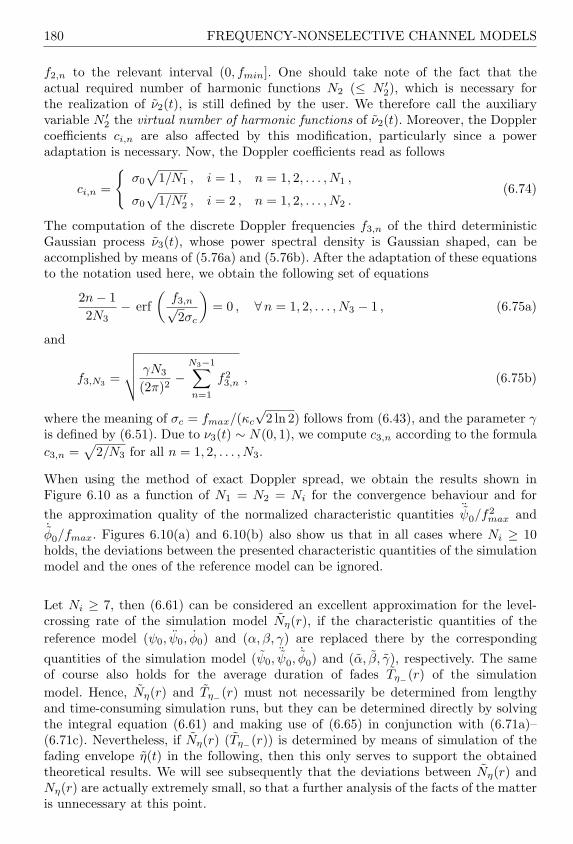
180 FREQUENCY-NONSELECTIVE CHANNEL MODELS
f2,n to the relevant interval (0, fmin]. One should take note of the fact that theactual required number of harmonic functions N2 (≤ N ′
2), which is necessary forthe realization of ν2(t), is still defined by the user. We therefore call the auxiliaryvariable N ′
2 the virtual number of harmonic functions of ν2(t). Moreover, the Dopplercoefficients ci,n are also affected by this modification, particularly since a poweradaptation is necessary. Now, the Doppler coefficients read as follows
ci,n =
σ0
√1/N1 , i = 1 , n = 1, 2, . . . , N1 ,
σ0
√1/N ′
2 , i = 2 , n = 1, 2, . . . , N2 .(6.74)
The computation of the discrete Doppler frequencies f3,n of the third deterministicGaussian process ν3(t), whose power spectral density is Gaussian shaped, can beaccomplished by means of (5.76a) and (5.76b). After the adaptation of these equationsto the notation used here, we obtain the following set of equations
2n− 12N3
− erf(
f3,n√2σc
)= 0 , ∀n = 1, 2, . . . , N3 − 1 , (6.75a)
and
f3,N3 =
√√√√ γN3
(2π)2−
N3−1∑n=1
f23,n , (6.75b)
where the meaning of σc = fmax/(κc
√2 ln 2) follows from (6.43), and the parameter γ
is defined by (6.51). Due to ν3(t) ∼ N(0, 1), we compute c3,n according to the formulac3,n =
√2/N3 for all n = 1, 2, . . . , N3.
When using the method of exact Doppler spread, we obtain the results shown inFigure 6.10 as a function of N1 = N2 = Ni for the convergence behaviour and forthe approximation quality of the normalized characteristic quantities ¨
ψ0/f2max and
˙φ0/fmax. Figures 6.10(a) and 6.10(b) also show us that in all cases where Ni ≥ 10holds, the deviations between the presented characteristic quantities of the simulationmodel and the ones of the reference model can be ignored.
Let Ni ≥ 7, then (6.61) can be considered an excellent approximation for the level-crossing rate of the simulation model Nη(r), if the characteristic quantities of thereference model (ψ0, ψ0, φ0) and (α, β, γ) are replaced there by the correspondingquantities of the simulation model (ψ0,
¨ψ0,
˙φ0) and (α, β, γ), respectively. The same
of course also holds for the average duration of fades Tη−(r) of the simulationmodel. Hence, Nη(r) and Tη−(r) must not necessarily be determined from lengthyand time-consuming simulation runs, but they can be determined directly by solvingthe integral equation (6.61) and making use of (6.65) in conjunction with (6.71a)–(6.71c). Nevertheless, if Nη(r) (Tη−(r)) is determined by means of simulation of thefading envelope η(t) in the following, then this only serves to support the obtainedtheoretical results. We will see subsequently that the deviations between Nη(r) andNη(r) are actually extremely small, so that a further analysis of the facts of the matteris unnecessary at this point.
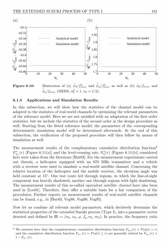
THE EXTENDED SUZUKI PROCESS OF TYPE I 181
(a)
0 10 20 30 40 50-10.46
-10.44
-10.42
-10.4
-10.38
-10.36
-10.34
-10.32
-10.3
ψo(2
) / f m
ax2
, ψ
o(2) /
f max
2
Ni
Analytical model
Simulation model
(b)
0 10 20 30 40 501.7
1.75
1.8
1.85
1.9
1.95
2
φ o(1) /
f max
,
φo(1
) / f m
ax
Ni
Analytical model
Simulation model
Figure 6.10: Illustration of (a) ψ0/f2max and
¨ψ0/f2
max as well as (b) φ0/fmax and˙φ0/fmax (MEDS, σ2
0 = 1, κ0 = 1/2).
6.1.5 Applications and Simulation Results
In this subsection, we will show how the statistics of the channel model can beadapted to the statistics of real-world channels by optimizing the relevant parametersof the reference model. Here we are not satisfied with an adaptation of the first orderstatistics, but we include the statistics of the second order in the design procedure aswell. Starting from the fitted reference model, the parameters of the correspondingdeterministic simulation model will be determined afterwards. At the end of thissubsection, the verification of the proposed procedure will then follow by means ofsimulation as well.
The measurement results of the complementary cumulative distribution function2
F ?η+
(r) [Figure 6.11(a)] and the level-crossing rate N?η (r) [Figure 6.11(b)] considered
here were taken from the literature [But83]. For the measurement experiments carriedout therein, a helicopter equipped with an 870 MHz transmitter and a vehiclewith a receiver were used to simulate a real-world satellite channel. Concerning therelative location of the helicopter and the mobile receiver, the elevation angle washeld constant at 15. One test route led through regions, in which the line-of-sightcomponent was heavily shadowed, another one through regions with light shadowing.The measurement results of this so-called equivalent satellite channel have also beenused in [Loo91]. Therefore, they offer a suitable basis for a fair comparison of theprocedures. Further reports on measurement results of real-world satellite channelscan be found, e.g., in [Huc83, Vog88, Vog90, Vog95].
Now let us combine all relevant model parameters, which decisively determine thestatistical properties of the extended Suzuki process (Type I), into a parameter vectordenoted and defined by Ω := (σ0, κ0, ρ, fρ, σ3, m3). In practice, the frequency ratio
2 We mention here that the complementary cumulative distribution function Fη+ (r) = P (η(t) > r)and the cumulative distribution function Fη− (r) = P (η(t) ≤ r) are generally related by Fη+ (r) =1− Fη− (r).

182 FREQUENCY-NONSELECTIVE CHANNEL MODELS
κc = fmax/fc is in general greater than 10. According to the statements made inSubsection 6.1.2, that parameter in this case exerts no influence on the statistics ofthe first and second order of η(t). This is the reason, why κc has not been included inthe parameter vector Ω. Without restriction of generality, we will therefore arbitrarilyfix the value of the frequency ratio κc to 20. Moreover, without having to take anyfurther restrictions into account, we also choose a priori θρ = 0.
As suitable measure of the deviations between the complementary distributionfunctions Fη+(r/ρ) and F ?
η+(r/ρ) as well as between the normalized level-crossing
rates Nη(r/ρ)/fmax and N?η (r/ρ)/fmax, we introduce the following error function
E2(Ω) :=
M∑
m=1
[W1
(rm
ρ
)(F ?
η+
(rm
ρ
)− Fη+
(rm
ρ
))]21/2
+1
fmax
M∑
m=1
[W2
(rm
ρ
)(N?
η
(rm
ρ
)−Nη
(rm
ρ
))]21/2
, (6.76)
where M is the number of different levels rm at which the measurements were taken.In addition, W1(·) and W2(·) denote two weighting functions, which we here wantto choose proportionally to the reciprocals of F ?
η+(·) and N?
η (·), respectively. Theoptimization of the components of the parameter vector Ω is carried out numericallyby applying the quasi-Newton procedure according to Fletcher-Powell [Fle63].
We first perform the optimization by using the classical Jakes power spectral density.Therefore, we keep the parameter κ0 = fmin/fmax constant at the value κ0 = 1during the minimization. Furthermore, we also fix fρ to the value fρ = 0, so thatthe extended Suzuki model simplifies to the conventional Rice-lognormal model. Now,we are confronted with the problem that there are no free parameters available forthe optimization of the normalized level-crossing rate Nη(r/ρ)/fmax, because all theremaining model parameters (σ0, ρ, σ3, m3) are completely used for the optimizationof the complementary cumulative distribution function Fη+(r/ρ). In other words, abetter approximation of the second order statistics is only possible at the expense of aworse approximation of the first order statistics. We will not yet make this compromiseat this point. For the moment, we will be content with the approximation of Fη+(r/ρ),and temporarily put W2(r/ρ) equal to 0. The results of the parameter optimizationfor regions with light and heavy shadowing are listed in Table 6.1.
Table 6.1: The optimized parameters of the reference model for areas with heavy andlight shadowing (without optimization of κ0 and fρ).
Shadowing σ0 ρ σ3 m3
heavy 0.1847 0.0554 0.1860 0.3515light 0.3273 0.9383 0.0205 0.1882

THE EXTENDED SUZUKI PROCESS OF TYPE I 183
Studying Figure 6.11(a), where the resulting complementary cumulative distributionfunction Fη+(r/ρ) is depicted, one can see that this function can be fitted very closelyto the given measurement results. However, it becomes clear from Figure 6.11(b)that these satisfying results cannot be obtained for the normalized level-crossing rateNη(r/ρ)/fmax. The deviations from the measurement results are partly more than 300per cent in this case. The deeper reason of this mismatching is due to the far too highDoppler spread of the Jakes power spectral density.
(a)
-30 -20 -10 0 100
0.2
0.4
0.6
0.8
1
r/ρ (dB)
Fη
+(r
/ρ)
Heavy shadowing
Light
shadowing
Measurement [But83]Analytical modelSimulation
(b)
-30 -25 -20 -15 -10 -5 0 510
-3
10-2
10-1
100
101
r/ρ (dB)
Nη
(r/ρ
)/f m
ax
Heavy shadowing
Light shadowing
Measurement [But83]Analytical modelSimulation
Figure 6.11: (a) Complementary cumulative distribution function Fη+(r/ρ) and (b)normalized level-crossing rate Nη(r/ρ)/fmax for regions with heavy andlight shadowing (without optimization of κ0 and fρ).
For comparison and in order to confirm the results found, Figures 6.11(a) and 6.11(b)also show the results obtained from a discrete-time simulation of the extended Suzukiprocess. The deterministic processes ν1(t), ν2(t), and ν3(t) were in this case designedby applying the techniques described in the preceding Subsection 6.1.4 (MEDS withN1 = 15, N2 = 16, and N3 = 15).
The next step is to enable a reduction of the Doppler bandwidth and, thus, of theDoppler spread as well, by including the parameter κ0 in the optimization procedure.In order to exploit the full flexibility of the channel model, the optimization of theparameter fρ will now also be permitted within the range −fmin ≤ fρ ≤ fmax. Thenumerical minimization of the error function (6.76) then yields for the components ofthe parameter vector Ω to the results presented in Table 6.2. With these parameters,which have been optimized with respect to both Fη+(r/ρ) and Nη(r/ρ)/fmax, thebehaviour of Fη+(r/ρ) remains almost unchanged (cf. Figures 6.11(a) and 6.12(a).)However, the actual advantages of the extended Suzuki model of Type I first becomeapparent by studying the statistics of second order. Observe that due to the modelextension, the normalized level-crossing rate Nη(r/ρ)/fmax of the reference model cannow obviously be fitted to the measurement results better than in the case κ0 = 1 andfρ = 0 (cf. Figures 6.11(b) and 6.12(b)).

184 FREQUENCY-NONSELECTIVE CHANNEL MODELS
Table 6.2: The optimized parameters of the reference channel model for areas withheavy and light shadowing (with optimization of κ0 and fρ).
Shadowing σ0 κ0 ρ σ3 m3 fρ/fmax
heavy 0.2022 4.4E-11 0.1118 0.1175 0.4906 0.6366light 0.4497 5.9E-08 0.9856 0.0101 0.0875 0.7326
(a)
-30 -20 -10 0 100
0.2
0.4
0.6
0.8
1
r/ρ (dB)
Fη
+(r
/ρ)
Heavy shadowing
Light
shadowing
Measurement [But83]Analytical modelSimulation
(b)
-30 -25 -20 -15 -10 -5 0 510
-3
10-2
10-1
100
r/ρ (dB)
Nη
(r/ρ
)/f m
ax
Heavy shadowing
Light shadowing
Measurement [But83]Analytical modelSimulation
Figure 6.12: (a) Complementary cumulative distribution function Fη+(r/ρ) and (b)normalized level-crossing rate Nη(r/ρ)/fmax for regions with heavy andlight shadowing (with optimization of κ0 and fρ).
It should also be mentioned that the Rice factor (3.18) of the extended Suzuki model(Type I) now reads as
cR =ρ2
2ψ0=
ρ2
σ20 [1 + 2
π arcsin(κ0)]. (6.77)
Using the parameters listed in Table 6.2, we obtain the values cR = −5.15 dB (heavyshadowing) and cR = 6.82 dB (light shadowing) for the Rice factor.
The verification of the analytical results is now again established by means ofsimulation. Due to the fact that κ0 = fmin/fmax is very small in both cases determinedby light and heavy shadowing (see Table 6.2), the influence of ν2(t) or ν2(t) canbe neglected, and, consequently, N2 can be set to zero, which is synonymous withan additional drastic reduction concerning the realization expenditure. The otherprocesses ν1(t) and ν3(t) are again realized by employing the method of exact Dopplerspread with N1 = 15 and N3 = 15 cosine functions, respectively. The simulationresults are also depicted in Figures 6.12(a) and 6.12(b). From these figures, it can berealized that there is nearly an absolute correspondence between the reference modeland the simulation model.

THE EXTENDED SUZUKI PROCESS OF TYPE II 185
In order to illustrate the results, the Figures 6.13(a) and 6.13(b) both show us apart of the simulated sequence of the deterministic extended Suzuki process η(t) forregions with heavy and light shadowing, respectively. One recognizes that for a heavilyshadowed line-of-sight component (see Figure 6.13(a)), the average signal level is, allin all, obviously smaller than for an only lightly shadowed line-of-sight component (seeFigure 6.13(b)). Also, the deep fades for heavy shadowing are much deeper than forlight shadowing.
(a)
0 0.5 1 1.5 2 2.5 3-50
-40
-30
-20
-10
0
10
t (s)
20 lo
g η(
t)
(b)
0 0.5 1 1.5 2 2.5 3-50
-40
-30
-20
-10
0
10
t (s)
20 lo
g η(
t)
Figure 6.13: Simulation of deterministic extended Suzuki processes η(t) of Type Ifor regions with (a) heavy shadowing and (b) light shadowing (MEDS,N1 = 15, N2 = 0, N3 = 15, fmax = 91Hz, κc = 20).
6.2 THE EXTENDED SUZUKI PROCESS OF TYPE II
In the preceding Section 6.1, it has been shown how a higher model class can be createdby introducing a correlation between the two Gaussian random processes determiningthe Rice process. In this way, the flexibility of the statistical properties of the secondorder could be increased. On the other hand, the statistical properties of the firstorder were not influenced. The model described in Section 6.1, however, is not theonly possible one for which cross-correlated Gaussian random processes can be used.A further possibility, which was first introduced in [Pae97a], will be discussed in thissection. We will see that a special type can be found for the cross-correlation functionof the real part and the imaginary part of a complex-valued Gaussian random process,which not only increases the flexibility of the statistical properties of the second orderof the stochastic model for modelling the short-term fading, but also the ones ofthe first order. In this model, the Rice, Rayleigh, and one-sided Gaussian randomprocesses are included as special cases. The long-term fading is again modelled bymeans of a lognormal process as usual. The product of both processes, which is usefulfor modelling short-term and long-term fading, is called extended Suzuki process ofType II.

186 FREQUENCY-NONSELECTIVE CHANNEL MODELS
The description of the extended Suzuki process (of Type II) and the derivation of itsstatistical properties of first and second order will be the aim of this section. We willat first deal with the modelling and analysis of short-term fading.
6.2.1 Modelling and Analysis of the Short-Term Fading
The modelling of short-term fading will be performed by considering the referencemodel depicted in Figure 6.14. In the following, this model will be described.
(t)µ2
θ ρ
(t)µρ (t)ξH (f)o
n ο (t) νο (t)
m1 = ρ θ ρcos
Hilbert
m = ρ sin2sin
cos θ o
θ o
(t)1µ
WGN
transformer
Figure 6.14: Reference model for stochastic processes ξ(t) with cross-correlatedGaussian random processes µ1(t) and µ2(t).
Regarding this figure, one should notice that the complex-valued Gaussian randomprocess
µ(t) = µ1(t) + jµ2(t) (6.78)
with the cross-correlated components µ1(t) and µ2(t) is derived from a single real-valued zero-mean Gaussian random process ν0(t). In order to simplify the model, wewill in the following assume that the Doppler frequency of the line-of-sight componentis equal to zero, and, thus, the line-of-sight component is described by the time-invariant expression (3.3), i.e.,
m = m1 + jm2 = ρejθρ . (6.79)
As for the preceding models, we will also derive a further stochastic process for thisone by taking the absolute value of the complex-valued Gaussian random processµρ(t) = µ(t) + m, i.e.,
ξ(t) = |µρ(t)| =√
(µ1(t) + m1)2 + (µ2(t) + m2)2 . (6.80)
We will see in Subsection 6.2.1.1 that Rice, Rayleigh, and one-sided Gaussian randomprocesses are merely special cases of this process. To do justice to this property, the
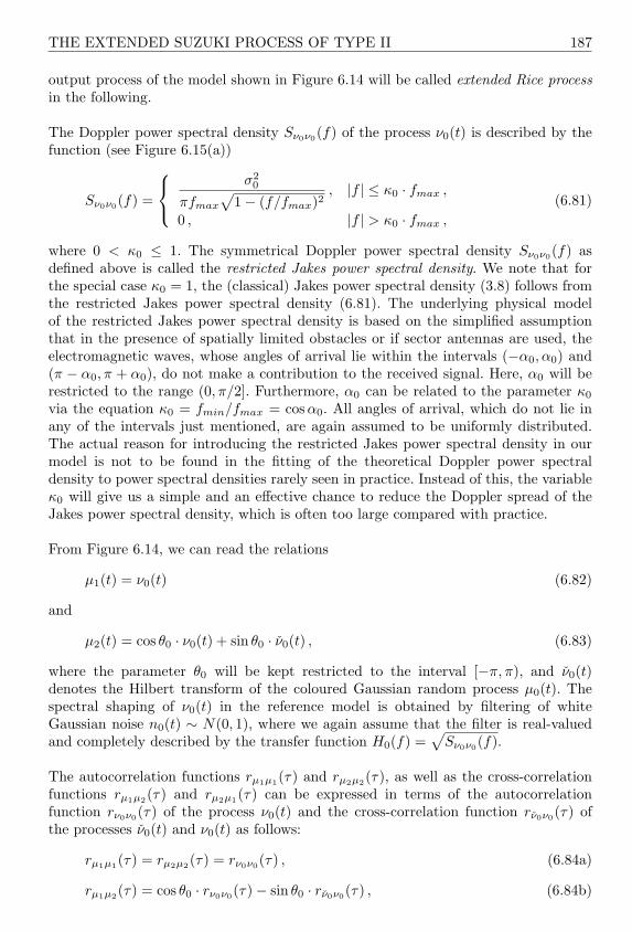
THE EXTENDED SUZUKI PROCESS OF TYPE II 187
output process of the model shown in Figure 6.14 will be called extended Rice processin the following.
The Doppler power spectral density Sν0ν0(f) of the process ν0(t) is described by thefunction (see Figure 6.15(a))
Sν0ν0(f) =
σ20
πfmax
√1− (f/fmax)2
, |f | ≤ κ0 · fmax ,
0 , |f | > κ0 · fmax ,
(6.81)
where 0 < κ0 ≤ 1. The symmetrical Doppler power spectral density Sν0ν0(f) asdefined above is called the restricted Jakes power spectral density. We note that forthe special case κ0 = 1, the (classical) Jakes power spectral density (3.8) follows fromthe restricted Jakes power spectral density (6.81). The underlying physical modelof the restricted Jakes power spectral density is based on the simplified assumptionthat in the presence of spatially limited obstacles or if sector antennas are used, theelectromagnetic waves, whose angles of arrival lie within the intervals (−α0, α0) and(π − α0, π + α0), do not make a contribution to the received signal. Here, α0 will berestricted to the range (0, π/2]. Furthermore, α0 can be related to the parameter κ0
via the equation κ0 = fmin/fmax = cos α0. All angles of arrival, which do not lie inany of the intervals just mentioned, are again assumed to be uniformly distributed.The actual reason for introducing the restricted Jakes power spectral density in ourmodel is not to be found in the fitting of the theoretical Doppler power spectraldensity to power spectral densities rarely seen in practice. Instead of this, the variableκ0 will give us a simple and an effective chance to reduce the Doppler spread of theJakes power spectral density, which is often too large compared with practice.
From Figure 6.14, we can read the relations
µ1(t) = ν0(t) (6.82)
and
µ2(t) = cos θ0 · ν0(t) + sin θ0 · ν0(t) , (6.83)
where the parameter θ0 will be kept restricted to the interval [−π, π), and ν0(t)denotes the Hilbert transform of the coloured Gaussian random process µ0(t). Thespectral shaping of ν0(t) in the reference model is obtained by filtering of whiteGaussian noise n0(t) ∼ N(0, 1), where we again assume that the filter is real-valuedand completely described by the transfer function H0(f) =
√Sν0ν0(f).
The autocorrelation functions rµ1µ1(τ) and rµ2µ2(τ), as well as the cross-correlationfunctions rµ1µ2(τ) and rµ2µ1(τ) can be expressed in terms of the autocorrelationfunction rν0ν0(τ) of the process ν0(t) and the cross-correlation function rν0ν0(τ) ofthe processes ν0(t) and ν0(t) as follows:
rµ1µ1(τ) = rµ2µ2(τ) = rν0ν0(τ) , (6.84a)
rµ1µ2(τ) = cos θ0 · rν0ν0(τ)− sin θ0 · rν0ν0(τ) , (6.84b)

188 FREQUENCY-NONSELECTIVE CHANNEL MODELS
rµ2µ1(τ) = cos θ0 · rν0ν0(τ) + sin θ0 · rν0ν0(τ) . (6.84c)
One should be aware of the influence of the parameter θ0 here. Note that thisparameter does not have any influence on the autocorrelation functions rµ1µ1(τ) andrµ2µ2(τ), but on the cross-correlation functions rµ1µ2(τ) and rµ2µ1(τ).
Substituting the relations (6.84a)–(6.84c) into (6.5), we obtain the following expressionfor the autocorrelation function rµµ(τ) of the complex-valued process µ(t) = µ1(t) +jµ2(t)
rµµ(τ) = 2rν0ν0(τ)− j2 sin θ0 · rν0ν0(τ) . (6.85)
The Fourier transform of the above result gives us the power spectral density in theform
Sµµ(f) = 2Sν0ν0(f)− j2 sin θ0 · Sν0ν0(f) . (6.86)
From (2.56b) and (2.56d), we obtain the relation Sν0ν0(f) = j sgn (f)·Sν0ν0(f), so thatSµµ(f) can now be expressed in terms of the restricted Jakes power spectral densitySν0ν0(f) as follows
Sµµ(f) = 2[1 + sgn (f) sin θ0] · Sν0ν0(f) . (6.87)
Note that Sµµ(f) is an unsymmetrical function for all values of θ0 ∈ (−π, π)\0. Anexample of the power spectral density Sµµ(f) is depicted in Figure 6.15(b), where thevalue 19.5 has been chosen for the parameter θ0.
(a)
0- κofmax κofmax
Sν o
ν o(f
)
f
(b)
- κofmax κofmax0
Sµµ
(f)
f
Figure 6.15: Doppler power spectral densities: (a) restricted Jakes PSD Sν0ν0(f) and(b) Sµµ(f) (θ0 = 19.5).
Deriving the statistical properties of ξ(t) = |µρ(t)| and ϑ(t) = argµρ(t), we willagain make use of the abbreviations (6.11a) and (6.11b). Therefore, we substitute(6.84a) into (6.11a) and (6.84b) into (6.11b), so that after some lengthy but simple

THE EXTENDED SUZUKI PROCESS OF TYPE II 189
algebraic computations, the characteristic quantities of the extended Rice model canbe written as follows:
ψ(0)0 = ψ0 =
2π
σ20 arcsin(κ0) , (6.88a)
ψ(1)0 = ψ0 = 0 , (6.88b)
ψ(2)0 = ψ0 = −ψ0 · 2(πfmax)2
1− sin[2 arcsin(κ0)]
2 arcsin(κ0)
, (6.88c)
φ(0)0 = φ0 = ψ0 · cos θ0 , (6.88d)
φ(1)0 = φ0 = 4σ2
0fmax(1−√
1− κ20 ) · sin θ0 , (6.88e)
φ(2)0 = φ0 = ψ0 · cos θ0 , (6.88f)
where 0 < κ0 ≤ 1 and −π ≤ θ0 < π. A comparison between the equations (6.88a)–(6.88f) and (6.12a)–(6.12f) shows us that for the present model even the quantitiesφ0 and φ0 are in general different from zero. Only for the special case θ0 = ±π/2,do we have φ0 = φ0 = 0. Hence, there are reasons for supposing that the statisticalproperties of the extended Rice process are different from those of the classical Riceprocess.
The starting point, which enables the analysis of the statistical properties of extendedRice processes, is again the multivariate Gaussian distribution of the processes µρ1(t),µρ2(t), µρ1(t), and µρ2(t) at the same time instant t [see (6.14)]. For the presentmodel, where it was assumed for simplification that fρ = 0, the multivariate Gaussiandistribution (6.14) is completely described by the column vectors
x =
x1
x2
x1
x2
and m =
m1
m2
m1
m2
=
ρ cos θρ
ρ sin θρ
00
(6.89a, b)
as well as by the covariance or correlation matrix
Cµρ(0) = Rµ(0) =
ψ0 φ0 0 φ0
φ0 ψ0 −φ0 0
0 −φ0 −ψ0 −φ0
φ0 0 −φ0 −ψ0
. (6.90)
Employing the relations (6.88d) and (6.88f) results in
Cµρ(0) = Rµ(0) =
ψ0 ψ0 cos θ0 0 φ0
ψ0 cos θ0 ψ0 −φ0 0
0 −φ0 −ψ0 −ψ0 cos θ0
φ0 0 −ψ0 cos θ0 −ψ0
. (6.91)

190 FREQUENCY-NONSELECTIVE CHANNEL MODELS
Now, after substituting (6.89a, b) and (6.91) into (6.14), the desired joint probabilitydensity function pµρ1µρ2 µρ1 µρ2
(x1, x2, x1, x2) of our model can be calculated. We thentransform the Cartesian coordinates (x1, x2) of this density to polar coordinates (z, θ)by means of (6.22a,b). After some further algebraic manipulations, we will succeed inconverting the joint probability density function (6.24) to the following form [Pae97a]
pξξϑϑ(z, z, θ, θ) =z2
(2π)2βψ0 sin2 θ0
· e−1
2ψ0 sin2 θ0[z2+ρ2−2zρ cos(θ−θρ)]
·ecos θ0
2ψ0 sin2 θ0[z2 sin 2θ+ρ2 sin 2θρ−2zρ sin(θ+θρ)]
·e−1
2β(1+cos θ0·sin 2θ) ·
z+φ0[ρ sin(θ−θρ)−cos θ0(z cos 2θ−ρ cos(θ+θρ))]
ψ0 sin2 θ0
2
·e−z2(1+cos θ0·sin 2θ)
2β sin2 θ0·
θ+φ0[ρ cos(θ−θρ)−z]−ψ0z cos θ0·cos 2θ
ψ0z(1+cos θ0·sin 2θ)
2
(6.92)
for z ≥ 0, |z| < ∞, |θ| ≤ π, and |θ| < ∞. Here, one should note that the quantity β in(6.92) is no longer given by (6.28), but is defined by the extended expression
β = −ψ0 − φ20
ψ0 sin2 θ0
. (6.93)
In the following subsection, we will derive the probability density function of theamplitude ξ(t) and the phase ϑ(t) from the joint probability density function (6.92).The analysis of the level-crossing rate and the average duration of fades of ξ(t) willthen follow subsequently.
6.2.1.1 Probability Density Function of the Amplitude and the Phase
For the probability density function of the extended Rice process ξ(t), denoted bypξ(z), we obtain the following result after substituting (6.92) into (6.29)
pξ(z) =z
2πψ0| sin θ0|e− z2+ρ2
2ψ0 sin2 θ0
·π∫
−π
ezρ cos(θ−θρ)
ψ0 sin2 θ0 · ecos θ0
2ψ0 sin2 θ0[z2 sin 2θ+ρ2 sin 2θρ−2zρ sin(θ+θρ)]
dθ, z ≥ 0 . (6.94)
Exactly as for conventional Rice processes, the probability density function pξ(z) inthis case also depends on the mean power of the processes µ1(t) and µ2(t), i.e., ψ0,as well as on the amplitude ρ of the line-of-sight component. Moreover, the densityof the extended Rice process is also determined by the parameter θ0 and — what issurprising at first — by the phase θρ of the line-of-sight component. We will understandthis property as soon as we have derived the corresponding simulation model (seeSubsection 6.2.3). In order to illustrate the results, we will study Figures 6.16(a) and6.16(b), where the probability density function (6.94) is shown for various values of

THE EXTENDED SUZUKI PROCESS OF TYPE II 191
the parameters θ0 and θρ, respectively. It should be pointed out that even for thismodel, the density pξ(z) neither depends on the first and second time derivative ofthe autocorrelation function (6.11a), i.e., ψ0 and ψ0, nor on the first and second timederivative of the cross-correlation function (6.11b), i.e., φ0 and φ0.
(a)
0 1 2 3 4 50
0.1
0.2
0.3
0.4
0.5
0.6
0.7
0.8
θ0 = 30o
θ0 = 75o
θ0 = 120o
θ0 = 165o
pξ(
z)
z
(b)
0 1 2 3 4 50
0.2
0.4
0.6
0.8
1
1.2 θρ = 30o, 90o
θρ = 45o
θρ = 135o
pξ(
z)
z
Figure 6.16: Probability density function pξ(z) of extended Rice processes ξ(t) forvarious values of the parameters (a) θ0 (ψ0 = 1, ρ = 1, θρ = 127) and(b) θρ (ψ0 = 1, ρ = 1, θ0 = 45).
In the text that follows, we will study some special cases. Especially, if we haveθ0 = ±π/2, then the integral in (6.94) can be solved explicitly, and it again followsthe Rice distribution
pξ(z) =z
ψ0e−
z2+ρ2
2ψ0 I0
(zρ
ψ0
), z ≥ 0 , (6.95)
with ψ0 according to (6.88a). For a shadowed line-of-sight component, i.e., ρ = 0, and,at first, for arbitrary values of θ0 ∈ [−π, π), the following density follows from (6.94)
pξ(z) =z
ψ0| sin θ0|e− z2
2ψ0 sin2 θ0 I0
(z2 cos θ0
2ψ0 sin2 θ0
), z ≥ 0 , (6.96)
from which, especially for θ0 = ±π/2, the Rayleigh distribution
pξ(z) =z
ψ0e−
z22ψ0 , z ≥ 0 , (6.97)
and for θ0 → 0, the one-sided Gaussian distribution
pξ(z) =1√πψ0
e−z24ψ0 , z ≥ 0 , (6.98)
follows. Consequently, the Rice distribution, the Rayleigh distribution, and theone-sided Gaussian distribution are special cases of the extended Rice distribution

192 FREQUENCY-NONSELECTIVE CHANNEL MODELS
(6.94).
For the probability density function of the phase ϑ(t), denoted by pϑ(θ), we obtain,after substituting (6.92) into (6.31), the expression
pϑ(θ) =| sin θ0|
2π(1− cos θ0 · sin 2θ)· e−
ρ2(1−cos θ0·sin 2θρ)
2ψ0 sin2 θ0
·
1 +√
πf(θ)ef2(θ)[1 + erf (f(θ))]
, −π ≤ θ ≤ π , (6.99)
where
f(θ) =ρ[cos(θ − θρ)− cos θ0 · sin(θ + θρ)]| sin θ0|
√2ψ0(1− cos θ0 · sin 2θ)
. (6.100)
Exactly like the probability density function of the amplitude [see (6.94)], theprobability density function of the phase merely depends on the parameters ψ0, ρ, θ0,and θρ, and not on the quantities ψ0, ψ0, φ0, and φ0.
The same probability density function of the phase, that we became acquainted withduring the analysis of Rice processes with uncorrelated Gaussian random processesµ1(t) and µ2(t) in Subsection 3.3.1 [see there (3.22)], also follows from (6.99) forthe special case θ0 = ±π/2. If the parameters ρ and θ0 are determined by ρ = 0and θ0 = ±π/2, then the phase ϑ(t) is uniformly distributed within the interval [−π, π].
Finally, the influence of the parameters θ0 and θρ on the behaviour of the densitypϑ(θ) shall be made clear by the Figures 6.17(a) and 6.17(b), respectively.
(a)
-π 0 π0
0.2
0.4
0.6
0.8
1
1.2 θ0 = 30o
θ0 = 75o
θ0 = 120o
θ0 = 165o
pϑ
(θ)
θ
(b)
-π 0 π0
0.2
0.4
0.6
0.8
1
θρ = - 60o
θρ = 0o
θρ = 60o
θρ = 120o
pϑ
(θ)
θ
Figure 6.17: Probability density function pϑ(θ) of the phase ϑ(t) for various valuesof the parameters (a) θ0 (ψ0 = 1, ρ = 1, θρ = 45) and (b) θρ
(ψ0 = 1, ρ = 1, θ0 = 45).

THE EXTENDED SUZUKI PROCESS OF TYPE II 193
6.2.1.2 Level-Crossing Rate and Average Duration of Fades
For the calculation of the level-crossing rate Nξ(r), the joint probability densityfunction pξξ(z, z) of the stochastic processes ξ(t) and ξ(t) have to be known at thesame time instant t. For this density, we obtain the following integral expression aftersubstituting (6.92) into (6.34)
pξξ(z, z) =z
(2π)3/2ψ0
√β| sin θ0|
e− z2+ρ2
2ψ0 sin2 θ0
∫ π
−π
1√1 + cos θ0 · sin 2θ
·ezρ cos(θ−θρ)
ψ0 sin2 θ0 · ecos θ0
2ψ0 sin2 θ0[z2 sin 2θ+ρ2 sin 2θρ−2zρ sin(θ+θρ)]
·e−1
2β(1+cos θ0·sin 2θ)
z+
φ0[ρ sin(θ−θρ)−cos θ0(z cos 2θ−ρ cos(θ+θρ))]
ψ0 sin2 θ0
2
dθ , (6.101)
for z ≥ 0 and |z| < ∞. Here, ψ0, φ0, and β again are the quantities defined by (6.88a),(6.88e), and (6.93), respectively. Within the interval (−π, π)\0, no value can befound for the parameter θ0 in such a way that the stochastic processes ξ(t) and ξ(t)become statistically independent, because pξξ(z, z) 6= pξ(z) · pξ(z) always holds. Evenfor the special case θ0 = ±π/2, the equation (6.35) may follow from (6.101), but hereit has to be taken into consideration that the relations (6.88a)–(6.88f) hold now, sothat we have φ0 6= 0 (α 6= 0), and, thus, (6.101) can never be brought into the form(6.36).
With the joint probability density function (6.101), all assumptions for the derivationof the level-crossing rate Nξ(r) of extended Rice processes ξ(t) are made. We substitute(6.101) into the definition (6.33), and, after some algebraic manipulations, obtain theresult
Nξ(r) =r√
β
(2π)3/2ψ0| sin θ0|· e−
r2+ρ2
2ψ0 sin2 θ0
∫ π
−π
√1 + cos θ0 · sin 2θ
·erρ cos(θ−θρ)
ψ0 sin2 θ0 ecos θ0
2ψ0 sin2 θ0[r2 sin 2θ+ρ2 sin 2θρ−2rρ sin(θ+θρ)]
·
e−g2(r,θ) +√
πg(r, θ)[1 + erf (g(r, θ))]
dθ , r ≥ 0 , (6.102)
where the function g(r, θ) stands for
g(r, θ) = − φ0ρ sin(θ − θρ)− cos θ0[r cos 2θ − ρ cos(θ + θρ)]ψ0 sin2 θ0
√2β(1 + cos θ0 · sin 2θ)
. (6.103)
The quantities ψ0, φ0, and β are again defined by (6.88a), (6.88e), and (6.93),respectively. It should be noted that we have made use of the integral [Gra81, vol. I,eq. (3.462.5)]
∫ ∞
0
x e−ax2−2bx dx =12a
1− b
√π
ae
b2a
[1− erf
(b√a
)], a > 0 , (6.104)

194 FREQUENCY-NONSELECTIVE CHANNEL MODELS
for the derivation of (6.102). Using (6.88a)–(6.88f), we easily find out that (6.102)is proportional to the maximum Doppler frequency fmax, i.e., the normalised level-crossing rate Nξ(r)/fmax is independent of the speed of the vehicle and the carrierfrequency, just as in the previous case. A brief parameter study, which makes theinfluence of the parameters κ0, ρ, θ0, and θρ on the normalised level-crossingrate Nξ(r)/fmax clear, is depicted in Figures 6.18(a)–6.18(d). The variation of κ0
(Figure 6.18(a)) and ρ (Figure 6.18 (b)) leads to curves, which are in principle similarto those shown in Figure 6.3(a) and Figure 3.5(b), respectively. A further, morepowerful parameter exists, namely θ0, which has a decisive influence on the behaviourof Nξ(r)/fmax, as can be seen in Figure 6.18(c). For the parameters (ψ0, κ0, ρ, θ0),which give rise to the results shown in Figure 6.18(d), the value of the quantity θρ isonly of secondary importance.
Now, attention is given to some special cases. On the assumption that θ0 = ±π/2holds, the level-crossing rate described by (6.37) follows from (6.102). If, in addition,ρ = 0 holds, then Nξ(r) becomes directly proportional to the Rayleigh distributionand can be brought into the form (6.38). Moreover, for the special case ρ = 0 andθ0 → 0, one can show that the level-crossing rate of one-sided Gaussian randomprocesses follows from (6.102), i.e.,
Nξ(r) =√
β
π√
ψ0e−
r24ψ0 , r ≥ 0 , (6.105)
where β is given by β = −ψ0 > 0 in the present case. Further special cases such as,e.g., ρ = 0 in connection with arbitrary values for θ0 ∈ [−π, π) can also be analysedeasily with the help of (6.102).
When calculating the average duration of fades Tξ−(r) [see (6.40)], we also need toknow the cumulative distribution function Fξ−(r) of the extended Rice process ξ(t),besides the level-crossing rate Nξ(r). For the former, we obtain the following doubleintegral by using the probability density function (6.94)
Fξ−(r) =∫ r
0
pξ(z) dz
=∫ r
0
z
2πψ0| sin θ0|e− z2+ρ2
2ψ0 sin2 θ0 ·∫ π
−π
ezρ cos(θ−θρ)
ψ0 sin2 θ0
·ecos θ0
2ψ0 sin2 θ0·[z2 sin 2θ+ρ2 sin 2θρ−2zρ sin(θ+θρ)]
dθ dz , r ≥ 0 . (6.106)
According to (6.40), the average duration of fades Tξ−(r) of extended Rice processesξ(t) is then the quotient of (6.106) and (6.102).
Figures 6.19(a) to 6.19(d) clearly show the influence which the parameters κ0, ρ, θ0,and θρ have on the normalised average duration of fades Tξ−(r) · fmax. The modelparameters, which lead to the results shown in Figures 6.18(a) to 6.18(d), have alsobeen used for the calculation of Tξ−(r) · fmax here. Varying the parameter κ0, we

THE EXTENDED SUZUKI PROCESS OF TYPE II 195
(a)
0 1 2 3 4 50
0.1
0.2
0.3
0.4
0.5
κo = 1/4 κo = 1/2κo = 3/4κo = 1
Nξ(
r)/f
max
r
(b)
0 1 2 3 4 50
0.2
0.4
0.6
0.8
1
ρ = 0ρ = 1/2ρ = 1ρ = 2
Nξ(
r)/f
max
r
(c)
0 1 2 3 4 50
0.2
0.4
0.6
0.8
1
1.2 θ0 = 30o
θ0 = 75o
θ0 = 120o
θ0 = 165o
Nξ(
r)/f
max
r
(d)
0 1 2 3 4 50
0.1
0.2
0.3
0.4
0.5
0.6
0.7
0.8
0.9
θρ = 0o
θρ = 45o
θρ = 90o
θρ = 135o
Nξ(
r)/f
max
r
Figure 6.18: Normalized level-crossing rate Nξ(r)/fmax of extended Rice processes(Type II) depending on: (a) κ0 (σ2
0 = 1, ρ = 0, θ0 = 45), (b)ρ (ψ0 = 1, κ0 = 1, θρ = 45, θ0 = 45), (c) θ0 (ψ0 = 1, κ0 = 1, ρ = 0),and (d) θρ (ψ0 = 1, κ0 = 1, ρ = 1, θ0 = 45).
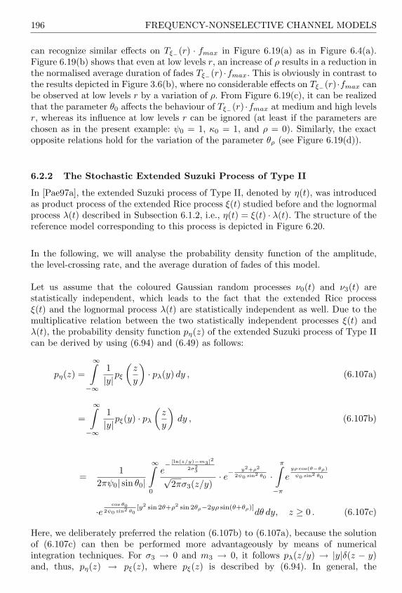
196 FREQUENCY-NONSELECTIVE CHANNEL MODELS
can recognize similar effects on Tξ−(r) · fmax in Figure 6.19(a) as in Figure 6.4(a).Figure 6.19(b) shows that even at low levels r, an increase of ρ results in a reduction inthe normalised average duration of fades Tξ−(r) ·fmax. This is obviously in contrast tothe results depicted in Figure 3.6(b), where no considerable effects on Tξ−(r)·fmax canbe observed at low levels r by a variation of ρ. From Figure 6.19(c), it can be realizedthat the parameter θ0 affects the behaviour of Tξ−(r) ·fmax at medium and high levelsr, whereas its influence at low levels r can be ignored (at least if the parameters arechosen as in the present example: ψ0 = 1, κ0 = 1, and ρ = 0). Similarly, the exactopposite relations hold for the variation of the parameter θρ (see Figure 6.19(d)).
6.2.2 The Stochastic Extended Suzuki Process of Type II
In [Pae97a], the extended Suzuki process of Type II, denoted by η(t), was introducedas product process of the extended Rice process ξ(t) studied before and the lognormalprocess λ(t) described in Subsection 6.1.2, i.e., η(t) = ξ(t) · λ(t). The structure of thereference model corresponding to this process is depicted in Figure 6.20.
In the following, we will analyse the probability density function of the amplitude,the level-crossing rate, and the average duration of fades of this model.
Let us assume that the coloured Gaussian random processes ν0(t) and ν3(t) arestatistically independent, which leads to the fact that the extended Rice processξ(t) and the lognormal process λ(t) are statistically independent as well. Due to themultiplicative relation between the two statistically independent processes ξ(t) andλ(t), the probability density function pη(z) of the extended Suzuki process of Type IIcan be derived by using (6.94) and (6.49) as follows:
pη(z) =
∞∫
−∞
1|y|pξ
(z
y
)· pλ(y) dy , (6.107a)
=
∞∫
−∞
1|y|pξ(y) · pλ
(z
y
)dy , (6.107b)
=1
2πψ0| sin θ0|
∞∫
0
e− [ln(z/y)−m3]2
2σ23√
2πσ3(z/y)· e−
y2+ρ2
2ψ0 sin2 θ0 ·π∫
−π
eyρ cos(θ−θρ)
ψ0 sin2 θ0
·ecos θ0
2ψ0 sin2 θ0[y2 sin 2θ+ρ2 sin 2θρ−2yρ sin(θ+θρ)]
dθ dy, z ≥ 0 . (6.107c)
Here, we deliberately preferred the relation (6.107b) to (6.107a), because the solutionof (6.107c) can then be performed more advantageously by means of numericalintegration techniques. For σ3 → 0 and m3 → 0, it follows pλ(z/y) → |y|δ(z − y)and, thus, pη(z) → pξ(z), where pξ(z) is described by (6.94). In general, the

THE EXTENDED SUZUKI PROCESS OF TYPE II 197
(a)
10-2
10-1
100
10-2
100
κo = 1/4 κo = 1/2κo = 3/4κo = 1
Tξ -
(r)
⋅ fm
ax
r
(b)
10-2
10-1
100
10-2
10-1
100
ρ = 0 ρ = 1/2ρ = 1ρ = 2
Tξ -
(r)
⋅ fm
ax
r
(c)
10-2
10-1
100
10-2
10-1
100
θ0 = 30o
θ0 = 75o
θ0 = 120o
θ0 = 165o
Tξ -
(r)
⋅ fm
ax
r
(d)
10-2
10-1
100
10-2
10-1
100
θρ = 0o
θρ = 45o
θρ = 90o
θρ = 135o
Tξ -
(r)
⋅ fm
ax
r
Figure 6.19: Normalized average duration of fades Tξ−(r) · fmax of extended Rice
processes (Type II) depending on: (a) κ0 (σ20 = 1, ρ = 0, θ0 = 45), (b)
ρ (ψ0 = 1, κ0 = 1, θρ = 45, θ0 = 45), (c) θ0 (ψ0 = 1, κ0 = 1, ρ = 0),and (d) θρ (ψ0 = 1, κ0 = 1, ρ = 1, θ0 = 45).
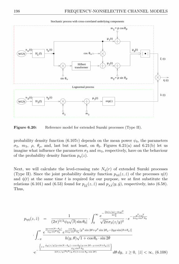
198 FREQUENCY-NONSELECTIVE CHANNEL MODELS
.exp( )
(t)µ2
θ ρ
(t)µρH (f)o
n ο (t) νο (t)
(t)ξ
m1 = ρ θ ρcos
σ3 m3
(t)λ
η (t)
Lognormal process
(t)µ3n (t)
H (f)ν (t)
WGN
m = ρ sin2sin
cos θ o
θ o
(t)1µ
WGN
transformer Hilbert
3 33
Stochastic process with cross-correlated underlying components
Figure 6.20: Reference model for extended Suzuki processes (Type II).
probability density function (6.107c) depends on the mean power ψ0, the parametersσ3, m3, ρ, θρ, and, last but not least, on θ0. Figures 6.21(a) and 6.21(b) let usimagine what influence the parameters σ3 and m3, respectively, have on the behaviourof the probability density function pη(z).
Next, we will calculate the level-crossing rate Nη(r) of extended Suzuki processes(Type II). Since the joint probability density function pηη(z, z) of the processes η(t)and η(t) at the same time t is required for our purpose, we at first substitute therelations (6.101) and (6.53) found for pξξ(z, z) and pλλ(y, y), respectively, into (6.58).Thus,
pηη(z, z) =1
(2π)3/2ψ0
√β| sin θ0|
·∫ ∞
0
e− [ln(z/y)−m3]2
2σ23√
2πσ3(z/y)2· e−
y2+ρ2
2ψ0 sin2 θ0
·∫ π
−π
eyρ cos(θ−θρ)
ψ0 sin2 θ0 ecos θ0
2ψ0 sin2 θ0[y2 sin 2θ+ρ2 sin 2θρ−2yρ sin(θ+θρ)]
h(y, θ)√
1 + cos θ0 · sin 2θ
·e−(
z+φ0(z/y)[ρ sin(θ−θρ)−cos θ0(y cos 2θ−ρ cos(θ+θρ))]
ψ0 sin2 θ0
)
2β(z/y)2h2(y,θ)(1+cos θ0·sin 2θ) dθ dy, z ≥ 0, |z| < ∞, (6.108)

THE EXTENDED SUZUKI PROCESS OF TYPE II 199
(a)
0 1 2 3 40
0.2
0.4
0.6
0.8
1
σ3 = 1/4σ3 = 1/2σ3 = 3/4σ3 = 1
pη
(z)
z
(b)
0 1 2 3 40
0.2
0.4
0.6
0.8
1
1.2
m3 = -1/2m3 = -1/4m3 = 0m3 = 1/4
pη
(z)
z
Figure 6.21: Probability density function pη(z) of extended Suzuki processes (Type II)for various values of the parameters (a) σ3 (m3 = 1, ψ0 = 0.0412, ρ =0.918, θρ = 86, θ0 = 97) and (b) m3 (σ3 = 0.5, ψ0 = 0.0412, ρ =0.918, θρ = 86, θ0 = 97).
where
h(y, θ) =
√1 +
γ(σ3y)2
β(1 + cos θ0 · sin 2θ). (6.109)
Here, ψ0, φ0, β, and γ again are the quantities introduced by (6.88a), (6.88e), (6.93),and (6.51), respectively. If we furthermore substitute (6.108) into (6.57), we obtainthe result for the level-crossing rate Nη(r) of extended Suzuki processes of Type IIas follows
Nη(r) =√
β
(2π)2σ3ψ0| sin θ0| ·∫ ∞
0
e− [ln(r/y)−m3]2
2σ23 · e−
y2+ρ2
2ψ0 sin2 θ0
·∫ π
−π
h(y, θ)√
1 + cos θ0 · sin 2θ
·eyρ cos(θ−θρ)
ψ0 sin2 θ0 · ecos θ0
2ψ0 sin2 θ0[y2 sin 2θ+ρ2 sin 2θρ−2yρ sin(θ+θρ)]
·
e−[ g(y,θ)h(y,θ) ]
2
+√
πg(y, θ)h(y, θ)
[1 + erf
(g(y, θ)h(y, θ)
)]dθ dy , r ≥ 0 , (6.110)
where the functions g(y, θ) and h(y, θ) are given by (6.103) and (6.109), respectively.
In the case σ3 → 0 and m3 → 0, it follows pλ(r/y) → |y|δ(r − y) and h(y, θ) → 1,so that Nη(r), according to (6.110), converges towards the expression (6.102), whichdescribes the level-crossing rate of extended Rice processes. This result was to beexpected. Furthermore, it should be taken into account that although (6.110) can bebrought into the form (6.61) for the special case θ0 = ±π/2, however, the definitions(6.88a)–(6.88f) still hold and not (6.12a)–(6.12f), so that, generally speaking, thelevel-crossing rate of extended Suzuki processes of Type II cannot be mapped exactly

200 FREQUENCY-NONSELECTIVE CHANNEL MODELS
onto that of Type I. The maximum Doppler frequency fmax is again proportional tothe level-crossing rate Nη(r), as can easily be shown by substituting (6.88a)–(6.88f)into (6.110).
For the computation of the average duration of fades Tη−(r), we again make use ofthe definition (6.65). For the necessary cumulative distribution function Fη−(r) =P (η(t) ≤ r), we obtain the following double integral by means of (6.107c)
Fη−(r) =∫ r
0
pη(z) dz
=1
2πψ0| sin θ0|∫ ∞
0
y
2
1 + erf
[ln(r/y)−m3
σ3
]· e−
y2+ρ2
2ψ0 sin2 θ0
·∫ π
−π
eyρ cos(θ−θρ)
ψ0 sin2 θ0 · ecos θ0
2ψ0 sin2 θ0[y2 sin 2θ+ρ2 sin 2θρ−2yρ sin(θ+θρ)]
dθ dy . (6.111)
According to (6.65), the quotient of (6.111) and (6.110) results in the average durationof fades Tη−(r) of extended Suzuki processes of Type II.
A few examples, which should help illustrate the results found for Nη(r) and Tη−(r) aredepicted in Figures 6.22(a) to 6.22(d). Figures 6.22(a) and 6.22(b) show the normalizedlevel-crossing rate Nη(r)/fmax, calculated according to (6.110) for various values ofthe parameter m3 and κc = fmax/fc, respectively. In the logarithmic representationof Figure 6.22(a), one can see that a change of the parameter m3 essentially causesa horizontal shift of the normalized level-crossing rate. Figure 6.22(b) makes it clearthat the influence of the parameter κc is absolutely negligible, if κc takes on realisticvalues, i.e., κc > 10. The normalized average duration of fades Tη−(r)·fmax, which wascalculated according to (6.65), is depicted in Figures 6.22(c) and 6.22(d) for differentvalues of m3 and κc, respectively.
6.2.3 The Deterministic Extended Suzuki Process of Type II
Referring to the stochastic model of the extended Suzuki process of Type II describedin the subsection before, we will now derive the corresponding deterministic model.Therefore, we again make use of the principle of deterministic channel modelling (seeSection 4.1), and approximate the coloured zero-mean Gaussian random process ν0(t)by a finite sum of weighted harmonic functions
ν0(t) =N1∑
n=1
c1,n cos(2πf1,nt + θ1,n) . (6.112)
With the Hilbert transform of the deterministic process above
ˇν0(t) =N1∑
n=1
c1,n sin(2πf1,nt + θ1,n) , (6.113)
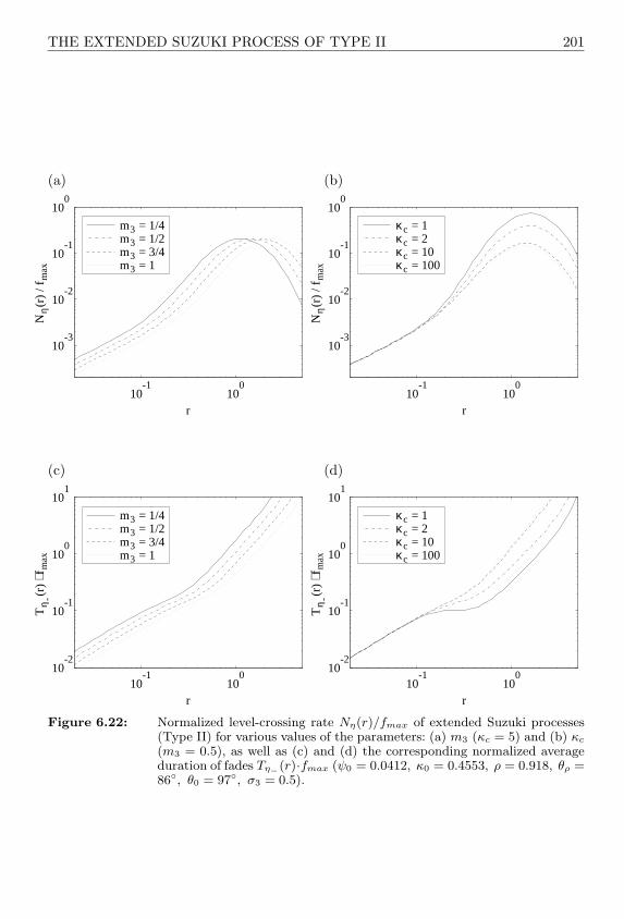
THE EXTENDED SUZUKI PROCESS OF TYPE II 201
(a)
10-1
100
10-3
10-2
10-1
100
m3 = 1/4m3 = 1/2m3 = 3/4m3 = 1
Nη
(r)
/ fm
ax
r
(b)
10-1
100
10-3
10-2
10-1
100
κc = 1κc = 2κc = 10κc = 100
Nη
(r)
/ fm
ax
r
(c)
10-1
100
10-2
10-1
100
101
m3 = 1/4m3 = 1/2m3 = 3/4m3 = 1
Tη
-(r)
⋅ fm
ax
r
(d)
10-1
100
10-2
10-1
100
101
κc = 1κc = 2κc = 10κc = 100
Tη
-(r)
⋅ fm
ax
r
Figure 6.22: Normalized level-crossing rate Nη(r)/fmax of extended Suzuki processes(Type II) for various values of the parameters: (a) m3 (κc = 5) and (b) κc
(m3 = 0.5), as well as (c) and (d) the corresponding normalized averageduration of fades Tη−(r)·fmax (ψ0 = 0.0412, κ0 = 0.4553, ρ = 0.918, θρ =86, θ0 = 97, σ3 = 0.5).
202 FREQUENCY-NONSELECTIVE CHANNEL MODELS
we can transform the two relations (6.82) and (6.83) to the deterministic model.Accordingly, we obtain
µ1(t) = ν0(t) (6.114)
and
µ2(t) = cos θ0 · ν0(t) + sin θ0 · ˇν0(t) . (6.115)
If we now substitute the deterministic process ν0(t) and its Hilbert transform ˇν0(t) bythe respective right-hand side of (6.112) and (6.113), then the generating deterministiccomponents can be written as follows:
µ1(t) =N1∑
n=1
c1,n cos(2πf1,nt + θ1,n) , (6.116)
µ2(t) =N1∑
n=1
c1,n cos(2πf1,nt + θ1,n − θ0) . (6.117)
At this point, the role of θ0 becomes clear: The parameter θ0 describes the phase shiftbetween the elementary harmonic functions µ1,n(t) and µ2,n(t) [see (4.27)]. Therefore,the Doppler phases θ2,n of the second deterministic process µ2(t) depend on theDoppler phases θ1,n of the first deterministic process µ1(t), because θ2,n = θ1,n − θ0
holds.
One may also take into account that for the Doppler coefficients ci,n and the Dopplerfrequencies fi,n the relations c1,n = c2,n and f1,n = f2,n hold. In particular, for thespecial case θ0 = ±90, the complex-valued deterministic process µ(t) = µ1(t)+jµ2(t)can be represented as
µ(t) =N1∑
n=1
c1,ne±j(2πf1,nt+θ1,n) . (6.118)
The deterministic lognormal process λ(t), which models the slow fading, is realizedexactly as shown in the bottom part of Figure 6.9. Accordingly, a further deterministicprocess ν3(t) is necessary, which has to be designed in such a way that it doesnot correlate with the process ν0(t). Since these two processes are (approximately)Gaussian distributed, the statistical independence of ν0(t) and ν3(t) follows from theuncorrelatedness. As a result, the deterministic processes ξ(t) and λ(t) derived fromthese are also statistically independent.
By using (6.116) and (6.117), the stochastic reference model for the extendedSuzuki process of Type II (see Figure 6.20) can now easily be transformed into thedeterministic simulation model shown in Figure 6.23.
The statistical properties of deterministic extended Suzuki processes η(t) of Type IIcan approximately be described by the relations pη(z), Nη(r), and Tη−(r) derived for

THE EXTENDED SUZUKI PROCESS OF TYPE II 203
.exp( )
.
cos(2 + θπ f )t 1,21,2
cos(2 + θπ f t )1,N1 1,N1
cos(2 π f )+ θ θ- 0t1,1 1,1
cos(2 + θπ f ) θ-1,2 1,2 0t
. . .
cos(2 + θπ f ) θ- 01,N1t 1,N1
cos(2 π f + θ 1,11,1 t )
µ3(t)~
3σ m 3
ν3
Deterministic lognormal process
~ (t)λ (t)~
ξ (t)~
(t)µ2ρ
~µ~2(t)
µ~1(t) (t)µρ1
~
(t)µρ~
η (t)~θρ
θρ
c
c. .
.
c
c. .
.
c
c. .
.
c
c1,1
1,N1
1,2
c1,1
1,2
1,N1
ρ1
m =. .
.. .
.
cos(2 π f + θt )
+ θπ f t )
cos(2 + θπ f t )
3,1 3,1
3,1
3,2 3,2
3,2
3,N3 3,N3
3,N3
cos(2
ρm =2
sin
cos
Deterministic process with cross-correlated underlyingcomponents
Figure 6.23: Deterministic simulation model for extended Suzuki processes (Type II).
the reference model before, if the characteristic quantities (6.88a)–(6.88f) are therereplaced by those corresponding to the simulation model. In the following, we willderive the characteristic quantities of the simulation model. We therefore need theautocorrelation functions of the processes µ1(t) and µ2(t)
rµ1µ1(τ) = rµ2µ2(τ) =N1∑
n=1
c21,n
2cos(2πf1,nτ) (6.119)
as well as the cross-correlation function calculated according to (4.13)
rµ1µ2(τ) = rµ2µ1(−τ) =N1∑
n=1
c21,n
2cos(2πf1,nτ − θ0) . (6.120)
With these two functions, the characteristic quantities of the simulation modelψ
(n)0 = r
(n)µ1µ1(0) and φ
(n)0 = r
(n)µ1µ2(0) can easily be determined for n = 0, 1, 2. We
immediately obtain the following closed-form expressions:

204 FREQUENCY-NONSELECTIVE CHANNEL MODELS
ψ(0)0 = ψ0 =
N1∑n=1
c21,n
2, (6.121a)
ψ(1)0 = ˙
ψ0 = 0 , (6.121b)
ψ(2)0 = ¨
ψ0 = −2π2N1∑
n=1
(c1,nf1,n)2 , (6.121c)
φ(0)0 = φ0 = ψ0 · cos θ0 , (6.121d)
φ(1)0 = ˙
φ0 = π
N1∑n=1
(c21,nf1,n) · sin θ0 , (6.121e)
φ(2)0 = ¨
φ0 = ¨ψ0 · cos θ0 . (6.121f)
Since this model uses the restricted Jakes power spectral density (κ0 ≤ 1), weappropriately return to the modified method of exact Doppler spread described inSubsection 6.4.1 in order to calculate the discrete Doppler frequencies f1,n and theDoppler coefficients c1,n. After adjusting the equations (6.72)–(6.74) to the presentmodel, we obtain
f1,n = fmax sin[
π
2N ′1
(n− 1
2
)]and c1,n = σ0
√2
N ′1
(6.122a, b)
for n = 1, 2, . . . , N1, where N1 denotes the actual (user defined) number of harmonicfunctions and
N ′1 =
⌈N1
2π arcsin(κ0)
⌉(6.123)
is the virtual number of harmonic functions.
For the Doppler phases θ1,n, it is assumed that they are realizations of a randomvariable uniformly distributed within the interval (0, 2π].
The calculation of the discrete Doppler frequencies f3,n of the deterministic Gaussianprocess ν3(t) is performed exactly according to (6.75a) and (6.75b). Accordingly, forc3,n again the formula c3,n =
√2/N3 for all n = 1, 2, . . . , N3 is used. The remaining
parameters of the simulation model (ρ, θρ,m3, σ3) are identical to those of the referencemodel.
With (6.122a) and (6.122b), the characteristic quantities of the simulation model(6.121a)–(6.121f) can now be evaluated. A comparison with the correspondingquantities of the reference model (6.88a)–(6.88f) then gives us the desired informationon the precision of the simulation model. As an example, the convergence behaviourof the normalized quantities ¨
ψ0/f2max and ˙
φ0/fmax is depicted in Figures 6.24(a) and6.24(b), respectively. Just as in Figures 6.10(a) and 6.10(b), one can here as well see

THE EXTENDED SUZUKI PROCESS OF TYPE II 205
that the deviations of the depicted quantities of the simulation model are negligiblecompared to the reference model for all cases relevant in practice (i.e., N1 ≥ 7).
(a)
0 10 20 30 40 50-2.3
-2.2
-2.1
-2
-1.9
-1.8
-1.7
ψo(2
) / f m
ax2
, ψ
o(2) /
f max
2
N1
Analytical model
Simulation model
(b)
0 10 20 30 40 500.756
0.758
0.76
0.762
0.764
0.766
0.768
φo(1
) / f m
ax
,
φ o(1) /
f max
N1
Analytical model
Simulation model
Figure 6.24: Illustration of (a) ψ0/f2max and
¨ψ0/f2
max as well as (b) φ0/fmax and˙φ0/fmax in terms of the N1 (MEDS, σ2
0 = 2, κ0 = 1/2, θ0 = 45).
For the level-crossing rate Nη(r) and the average duration of fades Tη−(r) of thesimulation model the statements made in Subsection 6.1.4 are also valid in the presentcase.
6.2.4 Applications and Simulation Results
This subsection intends to show us how the statistical properties of stochastic anddeterministic extended Suzuki processes of Type II can be brought into accordancewith those of measured channels. This is again performed by optimizing the primarymodel parameters. The basis for this is provided by the measurement results foundin the literature [But83] (F ?
η+(r), N?
η (r), T ?η−(r)), which we have already introduced in
Subsection 6.1.5. Only in this way, is a fair performance-comparison between extendedSuzuki processes of Type I and those of Type II possible.
In the present case, the parameter vector Ω is defined by
Ω := (σ0, κ0, θ0, ρ, θρ, σ3,m3, κc) . (6.124)
This time, the vector Ω contains all primary model parameters of the extended Suzukiprocess (Type II), also including κc, although exactly this parameter has no influenceworth mentioning on the first and second order statistics of the process η(t), if κc
exceeds the value 10. It will be left to the optimization procedure to find a suitablevalue for this quantity.
Since the error function E2(Ω) [see (6.76)] has turned out to be useful in our previousapplications, we will also make use of it in the present minimization problem, where we
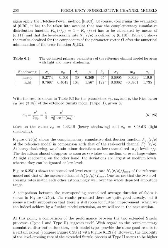
206 FREQUENCY-NONSELECTIVE CHANNEL MODELS
again apply the Fletcher-Powell method [Fle63]. Of course, concerning the evaluationof (6.76), it has to be taken into account that now the complementary cumulativedistribution function Fη+(r/ρ) = 1 − Fη−(r/ρ) has to be calculated by means of(6.111) and that the level-crossing rate Nη(r/ρ) is defined by (6.110). Table 6.3 showsthe results obtained for the components of the parameter vector Ω after the numericalminimization of the error function E2(Ω).
Table 6.3: The optimized primary parameters of the reference channel model for areaswith light and heavy shadowing.
Shadowing σ0 κ0 θ0 ρ θρ σ3 m3 κc
heavy 0.2774 0.506 30 0.269 45 0.0905 0.0439 119.9light 0.7697 0.4045 164 1.567 127 0.0062 -0.3861 1.735
With the results shown in Table 6.3 for the parameters σ0, κ0, and ρ, the Rice factorcR [see (3.18)] of the extended Suzuki model (Type II), given by
cR =ρ2
2ψ0=
π
4· ρ2
σ20 arcsin(κ0)
, (6.125)
takes on the values cR = 1.43 dB (heavy shadowing) and cR = 8.93 dB (lightshadowing).
Figure 6.25(a) shows the complementary cumulative distribution function Fη+(r/ρ)of the reference model in comparison with that of the real-world channel F ?
η+(r/ρ).
At heavy shadowing, we obtain minor deviations at low (normalized to ρ) levels r/ρ.The deviations almost disappear as soon as r/ρ takes on medium or even large values.At light shadowing, on the other hand, the deviations are largest at medium levels,whereas they can be ignored at low levels.
Figure 6.25(b) shows the normalized level-crossing rate Nη(r/ρ)/fmax of the referencemodel and that of the measured channel N?
η (r/ρ)/fmax. One can see that the two level-crossing rates match each other astonishingly well over the whole depicted amplituderange.
A comparison between the corresponding normalized average duration of fades isshown in Figure 6.25(c). The results presented there are quite good already, but itseems a likely supposition that there is still room for further improvement, which wecan indeed achieve by a further model extension, as we will see in the next section.
At this point, a comparison of the performance between the two extended Suzukiprocesses (Type I and Type II) suggests itself. With regard to the complementarycumulative distribution function, both model types provide the same good results toa certain extent (compare Figure 6.25(a) with Figure 6.12(a)). However, the flexibilityof the level-crossing rate of the extended Suzuki process of Type II seems to be higher

THE EXTENDED SUZUKI PROCESS OF TYPE II 207
(a)
-30 -25 -20 -15 -10 -5 0 50
0.2
0.4
0.6
0.8
1
Measurement [But83]
Analytical model
Simulation
Light shadowing
Heavy shadow
ing
Fη
+(r
/ρ)
r/ρ (dB)
(b)
-30 -25 -20 -15 -10 -5 0 510
-3
10-2
10-1
100
Measurement [But83]
Analytical model
Simulation
Nη
(r/ρ
)/f m
ax
r/ρ (dB)
Heavy shadowing
Light shad
owing
(c)
-30 -25 -20 -15 -10 -5 0 5
100
101
Measurement [But83]
Analytical model
Simulation
Tη
-(r/ρ
) ⋅ f
max
r/ρ (dB)
Heavy shadowing
Light shadowing
Figure 6.25: (a) Complementary cumulative distribution function Fη+(r/ρ), (b)normalized level-crossing rate Nη(r/ρ)/fmax, and (c) normalized averageduration of fades Tη−(r/ρ)·fmax for areas with heavy and light shadowing.
208 FREQUENCY-NONSELECTIVE CHANNEL MODELS
than that of Type I, which would explain the definitely better results of Figure 6.25(b)compared to those of Figure 6.12(b). To be fair though, we have to add that the higherflexibility comes along with a greater complexity of the reference model. Since theachievable improvements can only be reached with a higher numerical computationexpenditure, the user himself has to decide from case to case, i.e., in our terminology“from channel to channel”, whether the achievable improvements justify a higheranalytical and numerical computation expenditure or not.
However, if the parameters of the reference model have been determined, then thedetermination of the parameters of the corresponding deterministic simulation modelcan be regarded as trivial due to the closed-form formulas derived here.
If we once again study the simulation models depicted in Figures 6.9 and 6.23, itbecomes clear that the structure corresponding to the model Type II is, generallyspeaking, the more efficient one, and that the structure of Type I can only keep upwith it, if N2 is equal to zero, which is equivalent to the assumption that κ0 = 0 holds.
Finally, the verification of the analytical results by means of simulation remains.Therefore, we design the deterministic processes ν0(t) and ν3(t) by applying thetechniques described in the preceding Subsection 6.2.3 (modified MEDS with N1 = 25and N3 = 15). The measurement of the functions Fη+(r/ρ), Nη(r/ρ)/fmax, andTη−(r/ρ)·fmax N3 = 15) from a discrete-time simulation of the deterministic extendedSuzuki process (Type II) η(t) leads to the curves also depicted in Figures 6.25(a)–6.25(c). Again, there is a nearly complete correspondence between the reference modeland the simulation model, so that the graphs corresponding to these models can hardlybe distinguished from each other.
A small part of the sequence of the simulated deterministic process η(t) is depictedin Figure 6.26(a) for an area with heavy shadowing and in Figure 6.26(b) for an areawith light shadowing.
6.3 THE GENERALIZED RICE PROCESS
The extended Suzuki processes of Type I and Type II represent two classes ofstochastic processes with different statistical properties. Both models are identical,however, if κ0 = 0 holds in the former and if in the latter, the parameters κ0
and θ0 are given by κ0 = 1 and θ0 = π/2, respectively. But in general, we cansay that neither the extended Suzuki process of Type I is completely covered bythat of Type II nor that the reverse is true. In [Pae96b] it has been pointed out,and shown later in [Pae97c], that both models can be combined in a single model.This so-called generalized Suzuki model contains the extended Suzuki processes ofType I and of Type II as special cases. The mathematical expenditure required todescribe the generalized model is considerable, however, not much higher than thatof Type II. Without the lognormal process, the generalized Rice process follows fromthe generalized Suzuki process. The generalized Rice process is considerably easier todescribe and is in many cases sufficient for modelling frequency-nonselective mobileradio channels.
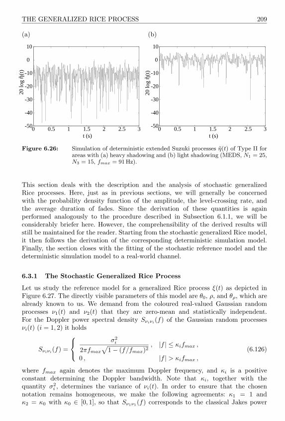
THE GENERALIZED RICE PROCESS 209
(a)
0 0.5 1 1.5 2 2.5 3-50
-40
-30
-20
-10
0
10
t (s)
20 lo
g η(
t)
(b)
0 0.5 1 1.5 2 2.5 3-50
-40
-30
-20
-10
0
10
t (s)
20 lo
g η(
t)Figure 6.26: Simulation of deterministic extended Suzuki processes η(t) of Type II for
areas with (a) heavy shadowing and (b) light shadowing (MEDS, N1 = 25,N3 = 15, fmax = 91 Hz).
This section deals with the description and the analysis of stochastic generalizedRice processes. Here, just as in previous sections, we will generally be concernedwith the probability density function of the amplitude, the level-crossing rate, andthe average duration of fades. Since the derivation of these quantities is againperformed analogously to the procedure described in Subsection 6.1.1, we will beconsiderably briefer here. However, the comprehensibility of the derived results willstill be maintained for the reader. Starting from the stochastic generalized Rice model,it then follows the derivation of the corresponding deterministic simulation model.Finally, the section closes with the fitting of the stochastic reference model and thedeterministic simulation model to a real-world channel.
6.3.1 The Stochastic Generalized Rice Process
Let us study the reference model for a generalized Rice process ξ(t) as depicted inFigure 6.27. The directly visible parameters of this model are θ0, ρ, and θρ, which arealready known to us. We demand from the coloured real-valued Gaussian randomprocesses ν1(t) and ν2(t) that they are zero-mean and statistically independent.For the Doppler power spectral density Sνiνi(f) of the Gaussian random processesνi(t) (i = 1, 2) it holds
Sνiνi(f) =
σ2i
2πfmax
√1− (f/fmax)2
, |f | ≤ κifmax ,
0 , |f | > κifmax ,
(6.126)
where fmax again denotes the maximum Doppler frequency, and κi is a positiveconstant determining the Doppler bandwidth. Note that κi, together with thequantity σ2
i , determines the variance of νi(t). In order to ensure that the chosennotation remains homogeneous, we make the following agreements: κ1 = 1 andκ2 = κ0 with κ0 ∈ [0, 1], so that Sν1ν1(f) corresponds to the classical Jakes power

210 FREQUENCY-NONSELECTIVE CHANNEL MODELS
spectral density (6.9a), and Sν2ν2(f) is identical to the restricted Jakes power spectraldensity (6.9c).
The reference model shown in Figure 6.27 includes two special cases:
(i) σ21 = σ2
2 = σ20 and θ0 = π/2 , (6.127a)
(ii) σ21 = 0 and σ2
2 = 2σ20 . (6.127b)
In case (i), exactly the Rice process depicted in Figure 6.1, whose underlying complex-valued Gaussian process is described by the left-hand side restricted Jakes powerspectral density (6.2), follows from the generalized Rice process. If we leave the missingminus sign in the lower branch of the structure shown in Figure 6.14 aside,3 then incase (ii) the extended Rice process (Figure 6.14) follows from the generalized Riceprocess (Figure 6.27).
H (f)1
H (f)2
ν (t)1(t)1n
(t)n2
m =1 θcos ρρ
WGN
ν (t)2
sin
cos
m = sin2 θρ
µ (t)
µ (t)
2
1
ξ (t)
ρ
-
(t)µρ
θo
θo
Hilbert transformerWGN
Figure 6.27: Reference model for generalized Rice processes ξ(t).
Next, we are interested in the autocorrelation function rµµ(τ) and the Doppler powerspectral density Sµµ(f) of the complex-valued process µ(t) = µ1(t) + jµ2(t). FromFigure 6.27, we first read the relations
µ1(t) = ν1(t) + ν2(t) (6.128)
and
µ2(t) = [ν1(t) + ν2(t)] cos θ0 + [ν1(t)− ν2(t)] sin θ0 . (6.129)
From these equations, we obtain the following relations for the autocorrelationfunctions rµ1µ1(τ) and rµ2µ2(τ), as well as for the cross-correlation functions rµ1µ2(τ)and rµ2µ1(τ)
rµ1µ1(τ) = rµ2µ2(τ) = rν1ν1(τ) + rν2ν2(τ) , (6.130a)
3 It should be noted that the minus sign has no influence on the statistics of ξ(t). Also, it can easilybe obtained by substituting θ0 with −θ0.

THE GENERALIZED RICE PROCESS 211
rµ1µ2(τ) = [rν1ν1(τ) + rν2ν2(τ)] cos θ0 + [rν1ν1(τ)− rν2ν2(τ)] sin θ0 , (6.130b)
rµ2µ1(τ) = [rν1ν1(τ) + rν2ν2(τ)] cos θ0 − [rν1ν1(τ)− rν2ν2(τ)] sin θ0 , (6.130c)
where rνiνi(τ) (i = 1, 2) denotes the inverse Fourier transform of (6.126), i.e,
rνiνi(τ) = σ2
i
2π
∫ arcsin(κi)
0
cos(2πfmaxτ sin ϕ) dϕ , (6.131)
and rνiνi(τ), due to (2.56a), denotes the Hilbert transform of rνiνi(τ), so that
rνiνi(τ) = σ2
i
2π
∫ arcsin(κi)
0
sin(2πfmaxτ sin ϕ) dϕ (6.132)
holds. By using the relation (6.5), the desired autocorrelation function rµµ(τ) can nowbe written as
rµµ(τ) = 2[rν1ν1(τ) + rν2ν2(τ)] + j2[rν1ν1(τ)− rν2ν2(τ)] sin θ0 . (6.133)
After performing the Fourier transform of (6.133) and taking the relation Sνiνi(f) =−j sgn (f)Sνiνi(f) into account, we can then express the Doppler power spectraldensity Sµµ(f) in terms of Sνiνi(f) [cf. (6.126)] as follows
Sµµ(f) = 2[1 + sgn (f) sin θ0] · Sν1ν1(f)+2[1− sgn (f) sin θ0] · Sν2ν2(f) . (6.134)
An example of this in general unsymmetrical Doppler power spectral density isdepicted in Figure 6.28.
It is obvious that for the two special cases (6.127a) and (6.127b) Figure 6.28 convertsto Figures 6.2(c) and 6.15(b), respectively. Also, the Doppler power spectral density(6.134) contains the classical Jakes power spectral density according to (3.7) asfurther special case, because we obtain the latter with the parameter constellationσ2
1 = σ22 = σ2
0 , κ1 = κ2 = 1, and θ0 = π/2.
Next follows the derivation of the characteristic quantities ψ(n)0 and φ
(n)0 (n = 0, 1, 2).
Therefore, we substitute (6.130a) into (6.11a) and (6.130b) into (6.11b), which leadsto the following expressions:
ψ(0)0 = ψ0 =
σ22
2
[(σ1
σ2
)2
+2π
arcsin(κ0)
], (6.135a)
ψ(1)0 = ψ0 = 0 , (6.135b)
ψ(2)0 = ψ0 =−(πσ2fmax)2
(σ1
σ2
)2
+2π
[arcsin(κ0)− 1
2sin(2 arcsin(κ0))
],(6.135c)

212 FREQUENCY-NONSELECTIVE CHANNEL MODELS
-fmax -κo⋅fmax fmaxκo⋅fmax0
Sµ
µ(f
)
f
Figure 6.28: Unsymmetrical Doppler power spectral density Sµµ(f) (σ21 = 0.25, σ2
2 = 1,θ0 = 15, κ0 = 0.4).
φ(0)0 = φ0 = ψ0 · cos θ0 , (6.135d)
φ(1)0 = φ0 = 2σ2
2fmax
[(σ1
σ2
)2
−(
1−√
1− κ20
)]· sin θ0 , (6.135e)
φ(2)0 = φ0 = ψ0 · cos θ0 , (6.135f)
where 0 ≤ κ0 ≤ 1 and −π ≤ θ0 < π. One may take into account that in the specialcase (i) described by (6.127a), the quantities presented above exactly result in theequations (6.12a)–(6.12f). On the other hand, the special case (ii) [cf. (6.127b)] leadsto the formulae4 (6.88a)–(6.88f).
With the characteristic quantities (6.135a)–(6.135f) the covariance matrix Cµρ(τ) ofthe vector process µρ(t) = (µρ1(t), µρ2(t), µρ1(t), µρ2(t)) at the same time t, i.e.,τ = 0, is completely determined. It holds
Cµρ(0) = Rµ(0) =
ψ0 ψ0 cos θ0 0 φ0
ψ0 cos θ0 ψ0 −φ0 0
0 −φ0 −ψ0 −ψ0 cos θ0
φ0 0 −ψ0 cos θ0 −ψ0
. (6.136)
For us it is important now to realize that the covariance matrix (6.136) has thesame form as (6.91). As a consequence of this, we again obtain the joint probabilitydensity function pξξϑϑ(z, z, θ, θ) described by (6.92), where we have to substitute thequantities ψ0, ψ0, and φ0 with the equations derived above, i.e., (6.135a), (6.135c), and
4 Due to the minus sign in the lower part of the sinal flow diagram shown in Figure 6.27, it has tobe taken into account that the equations (6.88e) and (6.135e) have different signs.

THE GENERALIZED RICE PROCESS 213
(6.135e), respectively. Consequently, all relations derivable from these, as for examplethose for pξ(z), pϑ(θ), Nξ(r), and Tξ−(r), exactly lead to the results already foundin Subsection 6.2.1. In the formulae given there, we merely have to replace ψ0, ψ0,and φ0 with (6.135a), (6.135c), and (6.135e), respectively. Therefore, all further cal-culations for the description of generalized Rice processes can at this point be omitted.
This fact, however, should not mislead us into concluding that extended Rice processesand generalized Rice processes are two different ways of describing one and the samestochastic process. The flexibility of generalized Rice processes is definitely higherthan that of extended Rice processes. The reason for this lies in the additionalprimary model parameter σ2
1 , which is zero per definition for the extended Rice processand which contributes to a further de-coupling of the secondary model parameters(ψ0, ψ0, ψ0, φ0, φ0, φ0) of the generalized Rice process. In order to make this clear withthe help of an example, we consider (6.88e). There, in the interval (0, 1] no real numberexists for the parameter κ0, so that φ0 = 0 holds. On the other hand, the quantityφ0 according to (6.135e) behaves differently. Let σ2
1 ∈ [σ22 , 2σ2
2), then a real-valuednumber
κ0 =σ1
σ2
√2−
(σ1
σ2
)2
(6.137)
always exists in the interval (0, 1], so that φ0 = 0 holds.
The multiplication of the generalized Rice process with a lognormal process resultsin the so-called generalized Suzuki process suggested in [Pae97c]. The generalizedSuzuki process contains the classical Suzuki process [Suz77], the modified Suzukiprocess [Kra90b], as well as the two extended Suzuki processes of Type I [Pae98d]and of Type II [Pae97a] as special cases. This product process is described by theprobability density function (6.107c), where we have to use the equation (6.135a)for ψ0. Similarly, for the level-crossing rate one finds the expression (6.110). Now,however, it has to be emphasized that the entries (ψ0, ψ0, ψ0, φ0, φ0, φ0) of thecovariance matrix Cµρ are defined by (6.135a)–(6.135f).
A detailed discussion of generalized Rice respectively Suzuki processes is not necessaryfor our purposes. Instead, we will continue with the design of deterministic generalizedRice processes.
6.3.2 The Deterministic Generalized Rice Process
We again proceed by at first replacing the coloured zero-mean Gaussian randomprocesses ν1(t) and ν2(t) by a finite sum of Ni weighted harmonic functions of theform
νi(t) =Ni∑
n=1
ci,n cos(2πfi,nt + θi,n) , i = 1, 2 . (6.138)
When designing the deterministic processes (6.138), it has to be taken into accountthat ν1(t) and ν2(t) have to be uncorrelated, i.e., f1,n 6= f2,m must hold for all

214 FREQUENCY-NONSELECTIVE CHANNEL MODELS
n = 1, 2, . . . , N1 and m = 1, 2, . . . , N2. With the deterministic processes designedin this way and the corresponding Hilbert transforms, i.e.,
ˇνi(t) =Ni∑
n=1
ci,n sin(2πfi,nt + θi,n) , i = 1, 2 , (6.139)
we can directly replace the stochastic processes µ1(t) and µ2(t) [cf. (6.128) and (6.129),respectively] with the corresponding deterministic processes µ1(t) and µ2(t). Thus, thelatter processes can be expressed as follows:
µ1(t) =N1∑
n=1
c1,n cos(2πf1,nt + θ1,n)
+N2∑
n=1
c2,n cos(2πf2,nt + θ2,n) , (6.140)
µ2(t) =N1∑
n=1
c1,n cos(2πf1,nt + θ1,n − θ0)
+N2∑
n=1
c2,n cos(2πf2,nt + θ2,n + θ0) . (6.141)
As a result, the deterministic generalized Rice process is completely determined, andwe obtain the simulation system in the continuous-time representation form depictedin Figure 6.29.
Now, let θ0 = π/2, then the structure of the deterministic Rice process with cross-correlated underlying components (cf. Figure 6.9) follows from Figure 6.29. Moreover,in the special case σ2
2 = 0, i.e., N2 = 0, we obtain the deterministic extended Riceprocess depicted in the top part of Figure 6.23.
In the following, we will derive the characteristic quantities of the simulation model,i.e., ψ
(n)0 = r
(n)µ1µ1(0) = r
(n)µ2µ2(0) and φ
(n)0 = r
(n)µ1µ2(0) for n = 0, 1, 2. The autocorrelation
functions rµ1µ1(τ) and rµ2µ2(τ) necessary for this can be expressed as
rµ1µ1(τ) = rµ2µ2(τ)
=N1∑
n=1
c21,n
2cos(2πf1,nτ) +
N2∑n=1
c22,n
2cos(2πf2,nτ) , (6.142)
and for the cross-correlation function rµ1µ2(τ) calculated according to (4.13) it holds
rµ1µ2(τ) = rµ2µ1(−τ)
=N1∑
n=1
c21,n
2cos(2πf1,nτ − θ0) +
N2∑n=1
c22,n
2cos(2πf2,nτ + θ0) . (6.143)

THE GENERALIZED RICE PROCESS 215
µρ (t)~
sin θρm =2 ρ
cos(2π
o
cos(2
cos(2
cos(2
cos(2
π
π
π
π
cos(2π
cos(2π
cos(2π
1,1
2,Ν2
2,1
1,N1 θ )
θ )1,1
1,N1
2,1 θ )
θ )2,Ν2
1,Ν1
1,1
2,1
2,Ν
1,1
11,Ν
2,1
2,Ν 22
c2,Ν
c
c
c
c
2,1
1,Ν
1,1
2,Ν
1
2
2
c
c
c
2,1
1,N1
1,1
m = ρ cos θ1 ρ
µ (t)
µ (t) 1
2
(t)ξ
f t +
f t +
f t +
f t +
f t +
f t +
f t +
f t +
~
~
~
θ + θ )
θ + θ )
θ − θ )
θ − θ )o
o
o
Figure 6.29: Deterministic simulation model for generalized Rice processes.
Thus, we obtain the following expressions for the characteristic quantities of thedeterministic simulation model:
ψ(0)0 = ψ0 =
N1∑n=1
c21,n
2+
N2∑n=1
c22,n
2, (6.144a)
ψ(1)0 = ˙
ψ0 = 0 , (6.144b)
ψ(2)0 = ¨
ψ0 = −2π2
[N1∑
n=1
(c1,nf1,n)2 +N2∑
n=1
(c2,nf2,n)2]
, (6.144c)
φ(0)0 = φ0 = ψ0 · cos θ0 , (6.144d)

216 FREQUENCY-NONSELECTIVE CHANNEL MODELS
φ(1)0 = ˙
φ0 = π
[N1∑
n=1
(c21,nf1,n)−
N2∑n=1
(c22,nf2,n)
]· sin θ0 , (6.144e)
φ(2)0 = ¨
φ0 = ¨ψ0 · cos θ0 . (6.144f)
With these quantities, β is also determined, because
β = − ¨ψ0 −
˙φ
2
0
ψ0 sin2 θ0
(6.145)
holds.
The calculation of the model parameters fi,n and ci,n is performed according to themethod of exact Doppler spread. As described in Subsection 6.1.4, however, thisprocedure must be slightly modified due to κ2 = κ0 ∈ (0, 1]. Therefore, the formula(6.72) is also valid for the discrete Doppler frequencies fi,n in the present case, wherewe have to take into account that (6.73) holds. Similarly, the calculation of theDoppler coefficients ci,n is performed by using (6.74), where σ0 has to be replacedby σi. Finally, for the Doppler phases θi,n it is assumed that these quantities arerealizations (outcomes) of a random variable uniformly distributed within (0, 2π].
Analysing the characteristic quantities of the simulation model, we restrict ourselvesto ψ0 and β/f2
max. If these quantities are calculated according to (6.144a) and (6.145),respectively, by means of (6.72) and (6.74), then the convergence behaviour in termsof Ni (N1 = N2) appears as depicted in Figures 6.30(a) and 6.30(b). The resultsshown are based on the primary model parameters σ2
1 , σ22 , and κ0, as they are listed
in the following subsection in Table 6.4.
(a)
0 10 20 30 40 500.02
0.04
0.06
0.08
0.1
0.12
Light shadowing
Heavy shadowing
Simulation modelAnalytical model
Ni
ψo ,
ψo
(b)
0 10 20 30 40 500.06
0.08
0.1
0.12
0.14
0.16
0.18
0.2
0.22
Light shadowing
Heavy shadowing
Simulation modelAnalytical model
Ni
β/f m
ax2
,
β/f
max
2
Figure 6.30: Illustration of (a) ψ0 and ψ0 as well as (b) β/f2max and β/f2
max (MEDS,σ2
i and κ2 according to Table 6.4).

THE GENERALIZED RICE PROCESS 217
Since the deviations between ψ0 and ψ0 as well as between β/f2max and β/f2
max arenegligible for all cases relevant in practice (Ni ≥ 7), it follows that the probabilitydensity function pξ(z), the level-crossing rate Nξ(r), and the average duration of fadesTξ−(r) of the simulation model are extremely close to the corresponding quantities ofthe reference model.
6.3.3 Applications and Simulation Results
In this subsection, it will be shown that the statistical properties of stochastic anddeterministic generalized Rice processes can be brought into astonishingly goodagreement with real-world measurement results, even without multiplying the Riceprocess with a lognormal process. Since a fair comparison of the performance betweendifferent channel models is intended, we here again use the measurement results forF ?
ξ+(r), N?
ξ (r), and T ?ξ−(r) from [But83], which were also the basis for the experiments
described in Subsections 6.1.5 and 6.2.4.
In the present case, the parameter vector Ω contains all six primary model parameters.Thus, Ω is defined by
Ω := (σ1, σ2, κ0, θ0 ρ, θρ) . (6.146)
The optimization of the components of Ω is again performed as described inSubsection 6.1.5 by minimizing the error function E2(Ω) [cf. (6.76)] by means ofthe Fletcher-Powell algorithm [Fle63]. The optimization results found are presentedin Table 6.4.
Table 6.4: The optimized primary model parameters of the reference model for areaswith heavy and light shadowing.
Shadowing σ1 σ2 κ0 θ0 ρ θρ
heavy 0.0894 0.7468 0.1651 0.3988 0.2626 30.3
light 0.1030 0.9159 0.2624 0.3492 1.057 53.1
The Rice factor cR [see (3.18)], i.e.,
cR =ρ2
2ψ0=
ρ2
σ22
[(σ1σ2
)2
+ 2π arcsin(κ2)
] , (6.147)
of the present model takes on the values cR = 0.134 dB (heavy shadowing) andcR = 8.65 dB (light shadowing), which are about as large as the Rice factorsdetermined for the extended Suzuki model of Type II (cf. Subsection 6.2.4).
Figure 6.31(a) shows us the complementary cumulative distribution function Fξ+(r/ρ)of the reference model and that of the measured channel F ?
ξ+(r/ρ). Clearly visible
deviations from the results depicted in Figure 6.25(a) do not seem to be apparent.

218 FREQUENCY-NONSELECTIVE CHANNEL MODELS
On the other hand, especially when considering the channel with heavy shadowing,we are able to achieve further improvement in view of fitting the normalized level-crossing rate of the reference model Nξ(r/ρ)/fmax to that of the measured channelN?
ξ (r/ρ)/fmax. This immediately becomes obvious if we compare Figure 6.31(b) withFigure 6.25(b). Especially with regard to the level-crossing rate, it seems as if thehigher flexibility of the generalized Rice model has a positive effect.
Clearly visible are also the improvements achieved for the adapting of the normalizedaverage duration of fades Tξ−(r/ρ)·fmax to T ?
ξ−(r/ρ)·fmax. Concerning this statement,one may compare the two Figures 6.31(c) and 6.25(c). Now the present model is invery good agreement with the measurements, even at low levels.
Finally, it should be pointed out that the corresponding simulation results are alsodepicted in Figures 6.31(a)–6.31(c). For the realization and the simulation of thechannel with heavy (light) shadowing, we have used N1 = N2 = 7 (N1 = N2 = 15)harmonic functions. In each of the two situations, a channel output sequence ξ(kTs)(k = 1, 2, . . . , Ns) with Ns = 3 · 106 sampling values was generated and used for theevaluation of the statistics. For the maximum Doppler frequency fmax, the value 91 Hzwas chosen here, and the sampling interval Ts was prescribed by Ts = 0.3ms.
6.4 THE MODIFIED LOO MODEL
Loo developed a stochastic model for the modelling of frequency-nonselectiveterrestrial mobile radio channels on the basis of measurements in [Loo85]. Thismodel was also the topic of further investigations in [Loo87, Loo90, Loo91, Loo96],which were summarized in [Loo98] at a later point. Loo’s model is based on thephysically plausibly reasoned assumption that the line-of-sight component underliesslow amplitude fluctuations caused by shadowing effects. In this model, it is assumedthat the slow amplitude fluctuations of the line-of-sight component are lognormallydistributed, while the fast fading, caused by the multipath propagation, behaves likea Rayleigh process.
In this section, we will combine Loo’s stochastic model and the Rice process withcross-correlated in-phase and quadrature components to a superordinate model. Theresulting model, which we will call the modified Loo model, then contains the originalmodel suggested by Loo and the extended Rice process as respective special case.
6.4.1 The Stochastic Modified Loo Model
The model with which we will deal with in this subsection is depicted in Figure 6.32. Itis a matter of the modified Loo model for which ν1(t), ν2(t), and ν3(t) are uncorrelatedzero-mean real-valued Gaussian random processes. Let the Doppler power spectraldensity Sνiνi(f) of the Gaussian random processes νi(t) for i = 1, 2 be given by therestricted Jakes power spectral density (6.126) with κi ∈ [0, 1], whereas we again usethe Gaussian power spectral density according to (6.43) for Sν3ν3(f).
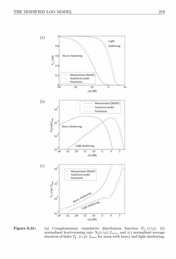
THE MODIFIED LOO MODEL 219
(a)
-30 -20 -10 0 100
0.2
0.4
0.6
0.8
1
r/ρ (dB)
Fξ +
(r/ρ
) Heavy shadowing
Light
shadowing
Measurement [But83]Analytical modelSimulation
(b)
-30 -25 -20 -15 -10 -5 0 510
-3
10-2
10-1
100
r/ρ (dB)
Nξ(
r/ρ)
/fm
ax
Heavy shadowing
Light shadowing
Measurement [But83]
Analytical model
Simulation
(c)
-30 -25 -20 -15 -10 -5 0 510
-1
100
101
102
Tξ -
(r/ρ
) ⋅ f
max
r/ρ (dB)
Measurement [But83] Analytical modelSimulation
Heavy shadowing
Light shadowing
Figure 6.31: (a) Complementary cumulative distribution function Fξ+(r/ρ), (b)normalized level-crossing rate Nξ(r/ρ)/fmax, and (c) normalized averageduration of fades Tξ−(r/ρ)·fmax for areas with heavy and light shadowing.

220 FREQUENCY-NONSELECTIVE CHANNEL MODELS
.exp( )
σ3 m3
(t)1µ
(t)µ2
(t)ρ
θ ρ+ )sin( 2 π fρ t
(t)1n
(t)m1
(t)µρθ ρ+ )
ρ (t)
2
(t)µ3n (t)
H (f)ν (t)
WGN3 3
3
WGN
ν (t)1H (f)1
transformerHilbert
WGN
n (t) ν (t)2 2H (f)2
2 π fρ tcos(
(t)m
Figure 6.32: The modified Loo model (reference model).
In this model, the fast signal fluctuations caused by the multipath propagation aremodelled in the equivalent complex baseband by a complex-valued Gaussian randomprocess
µ(t) = µ1(t) + jµ2(t) , (6.148)
where its real and imaginary part
µ1(t) = ν1(t) + ν2(t) , (6.149a)
µ2(t) = ν1(t)− ν2(t) , (6.149b)
are statistically uncorrelated. Here, νi(t) (i = 1, 2) again denotes the Hilbert transformof νi(t).
For the line-of-sight component m(t) = m1(t)+ jm2(t), we read from Figure 6.32 that
m(t) = ρ(t) · ej(2πfρt+θρ) (6.150)
holds, where fρ and θρ again denote the Doppler frequency and the Doppler phase ofthe line-of-sight component, respectively, and
ρ(t) = eσ3ν3(t)+m3 (6.151)
designates a lognormal process with which the slow amplitude fluctuations of theline-of-sight component are modelled. For the spectral and statistical properties ofthe lognormal process (6.151), the statements made in Subsection 6.1.2 hold. Let us

THE MODIFIED LOO MODEL 221
assume that the bandwidth of the Gaussian random process ν3(t) is very small incomparison with the bandwidth of µ(t), so that, consequently, the amplitude ρ(t) ofthe line-of-sight component (6.150) only varies relatively slowly compared to the fastsignal fading.
The sum of the scattered component and the line-of-sight component results in thecomplex-valued Gaussian random process
µρ(t) = µ(t) + m(t) , (6.152)
whose real and imaginary part can be expressed — by using (6.149a), (6.149b), and(6.150) — as follows:
µρ1(t) = ν1(t) + ν2(t) + ρ(t) · cos(2πfρt + θρ) , (6.153a)
µρ2(t) = ν1(t)− ν2(t) + ρ(t) · sin(2πfρt + θρ) . (6.153b)
The absolute value of (6.152) finally results in a new stochastic process
%(t) =√[
µ1(t)+ρ(t) cos(2πfρt+θρ)]2+
[µ2(t)+ρ(t) sin(2πfρt+θρ)
]2, (6.154)
which is called the modified Loo process. This process will in the following be used asa stochastic model to describe the fading behaviour of frequency-nonselective satellitemobile radio channels.
The modified Loo model introduced here contains the following three special cases:
(i) σ21 = σ2
2 = σ20 , κ1 = κ2 = 1 , and fρ = 0 , (6.155a)
(ii) σ22 = 0 or κ2 = 0 , (6.155b)
(iii) σ21 = σ2
2 = σ20 , κ1 = 1 , κ2 = κ0 , and σ2
3 = 0 . (6.155c)
Further on, we will see that in the special case (i), the power spectral density Sµµ(f)of the complex-valued Gaussian random process µ(t) [see (6.148)] is equal to theJakes power spectral density. Since the Gaussian random processes µ1(t) and µ2(t)are uncorrelated due to the symmetry of the Jakes power spectral density, the modifiedLoo model (Figure 6.32) can be reduced to the classical Loo model [Loo85, Loo91]depicted in Figure 6.33. One should take into account that also fρ = 0 holds, sothat the power spectral density of the line-of-sight component does not experience afrequency shift (Doppler shift) in this model. For the second special case (ii), where σ2
2
or κ2 are equal to zero, the coloured Gaussian random process ν2(t) can just as wellbe removed and one obtains the channel model proposed in [Pae98c], which standsout against the general variant due to its considerably smaller realization expense.Finally, the third special case (iii) leads to the Rice process depicted in Figure 6.1,for which the underlying Gaussian random processes µ1(t) and µ2(t) are, admittedly,also correlated, but for which the absolute value of the line-of-sight component m(t)is time-independent, i.e., it then holds |m(t)| = ρ(t) = ρ = em3 .

222 FREQUENCY-NONSELECTIVE CHANNEL MODELS
.exp( )
σ3 m3
(t)1µ
(t)µ2
(t)ρ
(t)1n
(t)m1
(t)µρ
ρ (t)
θ ρsin
θ ρcos
2
(t)µ3n (t)
H (f)ν (t)
WGN3 3
3
WGN H (f)1
WGN
n (t)2H (f)2
(t)m
Figure 6.33: The classical Loo model (reference model).
6.4.1.1 Autocorrelation Function and Doppler Power Spectral Density
We are now interested in the autocorrelation function rµρµρ(τ) and in thecorresponding Doppler power spectral density Sµρµρ(f) of the complex-valued randomprocess µρ(t) introduced by (6.152). Therefore, we at first calculate the autocorrelationfunction rµρi
µρi(τ) (i = 1, 2) of the processes µρi(t) as well as the cross-correlation
function rµρ1µρ2(τ) of the processes µρ1(t) and µρ2(t). By using (6.153a) and (6.153b),
we obtain the following relations for these correlation functions:
rµρ1µρ1(τ) = rµρ2µρ2
(τ) = rν1ν1(τ) + rν2ν2(τ) +12rρρ(τ) · cos(2πfρτ) , (6.156a)
rµρ1µρ2(τ) = r∗µρ2µρ1
(−τ) = rν1ν1(τ)− rν2ν2(τ) +12rρρ(τ) · sin(2πfρτ) , (6.156b)
where rνiνi(τ) (i = 1, 2) describes the autocorrelation function of the Gaussian randomprocess νi(t), and with rνiνi(τ) (i = 1, 2) exactly the cross-correlation function of νi(t)and νi(t) is meant. Recall that rνiνi(τ) and rνiνi(τ) are already known to us due to(6.131) and (6.132), respectively. Furthermore, rρρ(τ) describes the autocorrelationfunction of ρ(t) [cf. (6.151)] in (6.156a) and in (6.156b). One may take into accountthat ρ(t) has been introduced as lognormal process in this section. That is why theautocorrelation function rρρ(τ) of ρ(t) can be directly identified with the right-handside of (6.47). Hence, we can therefore directly write
rρρ(τ) = e2m3+σ23(1+rν3ν3 (τ)) . (6.157)
The autocorrelation function rµρµρ(τ) of the complex-valued process µρ(t) = µρ1(t) +jµρ2(t) will in imitation of (6.5) be expressed in terms of the autocorrelation functions
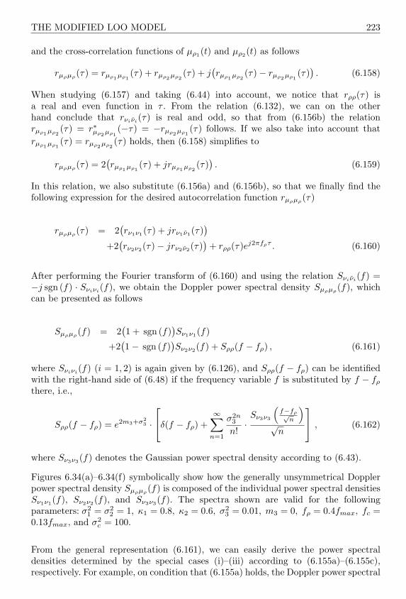
THE MODIFIED LOO MODEL 223
and the cross-correlation functions of µρ1(t) and µρ2(t) as follows
rµρµρ(τ) = rµρ1µρ1
(τ) + rµρ2µρ2(τ) + j
(rµρ1µρ2
(τ)− rµρ2µρ1(τ)
). (6.158)
When studying (6.157) and taking (6.44) into account, we notice that rρρ(τ) isa real and even function in τ . From the relation (6.132), we can on the otherhand conclude that rνiνi
(τ) is real and odd, so that from (6.156b) the relationrµρ1µρ2
(τ) = r∗µρ2µρ1(−τ) = −rµρ2µρ1
(τ) follows. If we also take into account thatrµρ1µρ1
(τ) = rµρ2µρ2(τ) holds, then (6.158) simplifies to
rµρµρ(τ) = 2(rµρ1µρ1
(τ) + jrµρ1µρ2(τ)
). (6.159)
In this relation, we also substitute (6.156a) and (6.156b), so that we finally find thefollowing expression for the desired autocorrelation function rµρµρ(τ)
rµρµρ(τ) = 2(rν1ν1(τ) + jrν1ν1(τ)
)
+2(rν2ν2(τ)− jrν2ν2(τ)
)+ rρρ(τ)ej2πfρτ . (6.160)
After performing the Fourier transform of (6.160) and using the relation Sνiνi(f) =−j sgn (f) · Sνiνi(f), we obtain the Doppler power spectral density Sµρµρ(f), whichcan be presented as follows
Sµρµρ(f) = 2(1 + sgn (f)
)Sν1ν1(f)
+2(1− sgn (f)
)Sν2ν2(f) + Sρρ(f − fρ) , (6.161)
where Sνiνi(f) (i = 1, 2) is again given by (6.126), and Sρρ(f − fρ) can be identifiedwith the right-hand side of (6.48) if the frequency variable f is substituted by f − fρ
there, i.e.,
Sρρ(f − fρ) = e2m3+σ23 ·
δ(f − fρ) +
∞∑n=1
σ2n3
n!·Sν3ν3
(f−fρ√
n
)√
n
, (6.162)
where Sν3ν3(f) denotes the Gaussian power spectral density according to (6.43).
Figures 6.34(a)–6.34(f) symbolically show how the generally unsymmetrical Dopplerpower spectral density Sµρµρ(f) is composed of the individual power spectral densitiesSν1ν1(f), Sν2ν2(f), and Sν3ν3(f). The spectra shown are valid for the followingparameters: σ2
1 = σ22 = 1, κ1 = 0.8, κ2 = 0.6, σ2
3 = 0.01, m3 = 0, fρ = 0.4fmax, fc =0.13fmax, and σ2
c = 100.
From the general representation (6.161), we can easily derive the power spectraldensities determined by the special cases (i)–(iii) according to (6.155a)–(6.155c),respectively. For example, on condition that (6.155a) holds, the Doppler power spectral
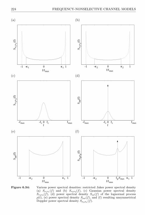
224 FREQUENCY-NONSELECTIVE CHANNEL MODELS
(a)
-1 -κ1 0 κ1 1f/fmax
Sν 1
ν 1(f
)
(b)
-1 -κ2 0 κ2 1f/fmax
Sν 2
ν 2(f
)(c)
-fmax -fc 0 fc fmaxf
Sν 3
ν 3(f
)
(d)S
ρρ(f
)
-fmax -fc 0 fc fmaxf
(e)
Sµµ
(f)
-1 -κ2 0 κ1 1f/fmax
(f)
Sµ
ρµρ
(f)
-1 -κ2 0 fρ/fmax κ1 1f/fmax
Figure 6.34: Various power spectral densities: restricted Jakes power spectral density(a) Sν1ν1(f) and (b) Sν2ν2(f), (c) Gaussian power spectral densitySν3ν3(f), (d) power spectral density Sρρ(f) of the lognormal processρ(t), (e) power spectral density Sµµ(f), and (f) resulting unsymmetricalDoppler power spectral density Sµρµρ(f).
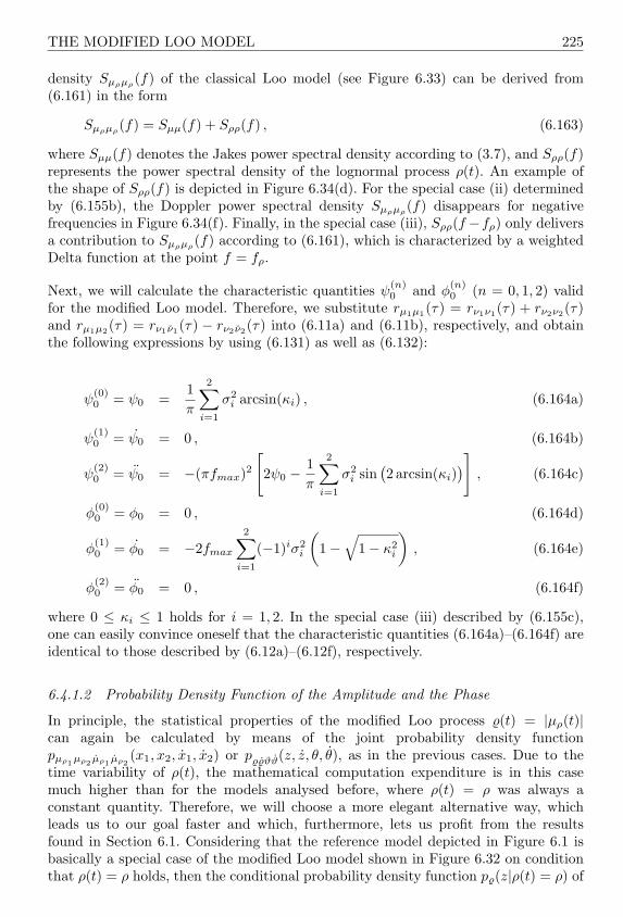
THE MODIFIED LOO MODEL 225
density Sµρµρ(f) of the classical Loo model (see Figure 6.33) can be derived from(6.161) in the form
Sµρµρ(f) = Sµµ(f) + Sρρ(f) , (6.163)
where Sµµ(f) denotes the Jakes power spectral density according to (3.7), and Sρρ(f)represents the power spectral density of the lognormal process ρ(t). An example ofthe shape of Sρρ(f) is depicted in Figure 6.34(d). For the special case (ii) determinedby (6.155b), the Doppler power spectral density Sµρµρ(f) disappears for negativefrequencies in Figure 6.34(f). Finally, in the special case (iii), Sρρ(f −fρ) only deliversa contribution to Sµρµρ
(f) according to (6.161), which is characterized by a weightedDelta function at the point f = fρ.
Next, we will calculate the characteristic quantities ψ(n)0 and φ
(n)0 (n = 0, 1, 2) valid
for the modified Loo model. Therefore, we substitute rµ1µ1(τ) = rν1ν1(τ) + rν2ν2(τ)and rµ1µ2(τ) = rν1ν1(τ) − rν2ν2(τ) into (6.11a) and (6.11b), respectively, and obtainthe following expressions by using (6.131) as well as (6.132):
ψ(0)0 = ψ0 =
1π
2∑
i=1
σ2i arcsin(κi) , (6.164a)
ψ(1)0 = ψ0 = 0 , (6.164b)
ψ(2)0 = ψ0 = −(πfmax)2
[2ψ0 − 1
π
2∑
i=1
σ2i sin
(2 arcsin(κi)
)]
, (6.164c)
φ(0)0 = φ0 = 0 , (6.164d)
φ(1)0 = φ0 = −2fmax
2∑
i=1
(−1)iσ2i
(1−
√1− κ2
i
), (6.164e)
φ(2)0 = φ0 = 0 , (6.164f)
where 0 ≤ κi ≤ 1 holds for i = 1, 2. In the special case (iii) described by (6.155c),one can easily convince oneself that the characteristic quantities (6.164a)–(6.164f) areidentical to those described by (6.12a)–(6.12f), respectively.
6.4.1.2 Probability Density Function of the Amplitude and the Phase
In principle, the statistical properties of the modified Loo process %(t) = |µρ(t)|can again be calculated by means of the joint probability density functionpµρ1µρ2 µρ1 µρ2
(x1, x2, x1, x2) or p%%ϑϑ(z, z, θ, θ), as in the previous cases. Due to thetime variability of ρ(t), the mathematical computation expenditure is in this casemuch higher than for the models analysed before, where ρ(t) = ρ was always aconstant quantity. Therefore, we will choose a more elegant alternative way, whichleads us to our goal faster and which, furthermore, lets us profit from the resultsfound in Section 6.1. Considering that the reference model depicted in Figure 6.1 isbasically a special case of the modified Loo model shown in Figure 6.32 on conditionthat ρ(t) = ρ holds, then the conditional probability density function p%(z|ρ(t) = ρ) of

226 FREQUENCY-NONSELECTIVE CHANNEL MODELS
the stochastic process %(t), which is defined by (6.154), has to be identical to (6.30).Therefore, we can write
p%(z|ρ(t) = ρ) = pξ(z) =
z
ψ0e−
z2+ρ2
2ψ0 I0
(zρ
ψ0
), z ≥ 0 ,
0 , z < 0 ,
(6.165)
where ψ0 describes the mean power of µi(t) (i = 1, 2) according to (6.164a). Since theamplitude ρ(t) of the line-of-sight component is lognormally distributed in the Loomodel, i.e., the density pρ(y) of ρ(t) is given by the lognormal distribution [cf. (2.28)]
pρ(y) =
1√2πσ3y
e− (ln y−m3)2
2σ23 , y ≥ 0 ,
0 , y < 0 ,
(6.166)
the probability density function p%(z) of the modified Loo process %(t) can be derivedfrom the joint probability density function p%ρ(z, y) of the stochastic processes %(t)and ρ(t) as follows:
p%(z) =∫ ∞
0
p%ρ(z, y) dy
=∫ ∞
0
p%(z|ρ(t) = y) · pρ(y) dy
=∫ ∞
0
pξ(z; ρ = y) · pρ(y) dy , z ≥ 0 . (6.167)
If we now substitute (6.30) (or (6.165)) and (6.166) into (6.167), then we obtain thefollowing expression for the probability density function p%(z) of the modified Looprocess %(t)
p%(z) =z√
2πψ0σ3
∫ ∞
0
1y
e−z2+y2
2ψ0 I0
(zy
ψ0
)e− (ln y−m3)2
2σ23 dy , z ≥ 0 , (6.168)
where ψ0 is given by (6.164a). We notice that the probability density function p%(z)depends on three parameters, namely ψ0, σ3, and m3. In connection with (6.155a),it now becomes apparent that (6.168) also holds for the classical Loo model, if weleave the influences of the parameters σ2
i and κi on ψ0 aside. The same statement alsoholds for the special case (ii) introduced by (6.155b). Therefore, it is not surprisingif one also finds the probability density function p%(z) in the form (6.168), e.g., in[Loo85, Loo91, Loo98] and [Pae98c]. Differences, however, do occur for the level-crossing rate and the average duration of fades, as we will see in the followingSubsection 6.4.1.3. For completeness, we will also briefly study the effects of thespecial case (iii) [see (6.155c)]. In the limit σ2
3 → 0, the lognormal distribution (6.166)converges to pρ(y) = δ(y − ρ), where ρ = em3 . In this case, the Rice distribution(6.165) follows directly from (6.167), where it has to be taken into account that ρ isequal to em3 .

THE MODIFIED LOO MODEL 227
In order to illustrate the probability density function p%(z) of the modified Loo process%(t), we study Figures 6.35(a) and 6.35(b), which allow the influence of the parametersσ3 and m3, respectively, to stand out.
(a)
0 1 2 3 4 50
0.1
0.2
0.3
0.4
0.5
0.6σ3 = 0.25σ3 = 0.5σ3 = 0.75σ3 = 1
z
pρ -(z
)
(b)
0 5 10 150
0.05
0.1
0.15
0.2
0.25
0.3
0.35
0.4
z
pρ -(z
)
m3 = 0.25
m3 = 0.5
m3 = 0.75
m3 = 1
Figure 6.35: Probability density function p%(z) of the amplitude %(t) of modified andclassical Loo processes depending on: (a) σ3 (ψ0 = 1, m3 = −σ2
3) and (b)m3 (ψ0 = 1, σ2
3 = 1).
Next, we will analyse the probability density function pϑ(θ) of the phase ϑ(t) =argµρ(t) of the modified Loo model. Here, we proceed in a similar way as for thecomputation of p%(z). In consideration of the present situation this means that weexploit the fact that the probability density function pϑ(θ) for ρ(t) = ρ = const. isidentical to the right-hand side of (6.32). Hence, we have
pϑ(θ; t|ρ(t) = ρ) =e−
ρ2
2ψ0
2π
1 +
√π
2ψ0ρ cos(θ − 2πfρt− θρ) e
ρ2 cos2(θ−2πfρt−θρ)2ψ0
[1 + erf
(ρ cos(θ − 2πfρt− θρ)√
2ψ0
)] , −π ≤ θ ≤ π . (6.169)
Since the conditional probability density function of the phase ϑ(t) for fρ 6= 0 is alwaysa function of the time t according to this equation, we first perform an averaging ofthe expression above with respect to the time t. This leads to the uniform distribution
pϑ(θ|ρ(t) = ρ) = limT→∞
12T
∫ T
−T
pϑ(θ; t|ρ(t) = ρ) dt
=12π
, −π ≤ θ ≤ π . (6.170)
The desired probability density function pϑ(θ) of the phase ϑ(t) = argµρ(t) can nowbe determined by means of the joint probability density function pϑρ(θ, y) of ϑ(t) and

228 FREQUENCY-NONSELECTIVE CHANNEL MODELS
ρ(t) as follows:
pϑ(θ) =∫ ∞
0
pϑρ(θ, y) dy
=∫ ∞
0
pϑ(θ|ρ(t) = y) · pρ(y) dy
=12π
∫ ∞
0
pρ(y) dy
=12π
, −π ≤ θ ≤ π . (6.171)
Thus, it is proven that the phase ϑ(t) of µρ(t) is uniformly distributed in the interval[−π, π], if the Doppler frequency fρ of the line-of-sight component m(t) is not equalto zero. Similarly, an expression for pϑ(θ) can be derived for the case fρ = 0. We will,however, refrain from a presentation of the resulting formula at this point.
6.4.1.3 Level-Crossing Rate and Average Duration of Fades
The derivation of the level-crossing rate N%(r) of the modified Loo process %(t) isperformed by means of the fundamental relation (6.33). Since the knowledge of thejoint probability density function p%%(z, z) of the processes %(t) and %(t) at the sametime t is necessary again, we will at first derive this. Therefore, we write
p%%(z, z) =∫ ∞
0
∫ ∞
−∞p%%ρρ(z, z, y, y) dy dy
=∫ ∞
0
∫ ∞
−∞p%%(z, z|ρ(t) = y, ρ(t) = y) · pρρ(y, y) dy dy . (6.172)
In the latter expression, pρρ(y, y) denotes the joint probability density function of ρ(t)and ρ(t) at the same time t. Since the process ρ(t) is lognormally distributed in themodified Loo model, we can directly identify pρρ(y, y) with the relation (6.53), i.e., wecan write
pρρ(y, y) =e− (ln y−m3)2
2σ23√
2π σ3y· e− y2
2γ(σ3y)2
√2πγ σ3y
, (6.173)
where γ = −rν3ν3(0) = (2πσc)2. At the beginning of Subsection 6.4.1, we assumedthat the amplitude ρ(t) of the line-of-sight component will itself only vary very slowly.Therefore, ρ(t) ≈ 0 must approximately hold, so that the probability density functionpρ(y) of ρ(t) can be approximated by pρ(y) ≈ δ(y). Since this always holds if γ issufficiently small or if the frequency ratio κc = fmax/fc is sufficiently large, we can inthis case replace (6.173) by the approximation
pρρ(y, y) ≈ pρ(y) · δ(y) , (6.174)
where pρ(y) again denotes the lognormal distribution according to (6.166). Regardingthe sifting property of the Delta function, we now substitute (6.174) into (6.172) andobtain the approximation

THE MODIFIED LOO MODEL 229
p%%(z, z) ≈∫ ∞
0
∫ ∞
−∞p%%(z, z|ρ(t) = y, ρ(t) = y) · pρ(y) δ(y) dy dy
=∫ ∞
0
p%%(z, z|ρ(t) = y, ρ(t) = 0) · pρ(y) dy . (6.175)
With this relation, we can now approximate the level-crossing rate N%(r) [cf. (6.33)]as follows:
N%(r) =∫ ∞
0
z p%%(r, z) dz
≈∫ ∞
0
∫ ∞
0
z p%%(z, z|ρ(t) = y, ρ(t) = 0) · pρ(y) dy dz
=∫ ∞
0
N%(r|ρ(t) = y, ρ(t) = 0) · pρ(y) dy . (6.176)
Here, we have to take into account that the level-crossing rate N%(r|ρ(t) = ρ, ρ(t) = 0)appearing under the integral of (6.176) exactly corresponds to the relation (6.37)derived in Subsection 6.1.1.2. If we now substitute this equation together with (6.166)into (6.176), then we obtain the following approximation for the level-crossing rate ofthe modified Loo process
N%(r) ≈∫ ∞
0
e− (ln y−m3)2
2σ23√
2πσ3y· r√
2β
π3/2ψ0e−
r2+y2
2ψ0 ·∫ π/2
0
cosh(
ry
ψ0cos θ
)
·[e−(αy sin θ)2 +
√παy sin(θ) erf (αy sin θ)
]dθ dy , (6.177)
where the relations (6.27) and (6.28) hold for α and β, respectively, if there theformulae (6.164a), (6.164c), and (6.164e) are used for the characteristic quantitiesψ0, ψ0, and φ0, respectively.
The investigation of the special case (i) [see (6.155a)] at first provides α = 0. Thisleads to the fact that the approximation (6.177) can be simplified considerably. Thus,on condition that α = 0 holds, the level-crossing rate N%(r) of the modified Loo modelsimplifies to that of the classical Loo model, which can be approximated as follows:
N%(r)|α=0 ≈√
β
2π· r
ψ0
∫ ∞
0
e− (ln y−m3)2
2σ23√
2πσ3y· e− r2+y2
2ψ0 I0
(ry
ψ0
)dy
=
√β
2π
∫ ∞
0
pξ(r; ρ = y) · pρ(y) dy , (6.178)
where the quantities β and ψ0 are in this case given by β = −2(πσ0fmax)2 andψ0 = σ2
0 , respectively, and pξ(r; ρ = y) denotes the Rice distribution (2.26), if ρ is
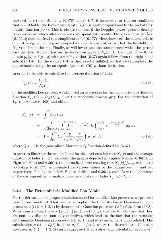
230 FREQUENCY-NONSELECTIVE CHANNEL MODELS
replaced by y there. Studying (6.178) and (6.167) it becomes clear that on conditionthat α = 0 holds, the level-crossing rate N%(r) is again proportional to the probabilitydensity function p%(r). This is always the case if the Doppler power spectral densityis symmetrical, which often does not correspond with reality. The special case (ii) [see(6.155b)] does not lead to a simplification of (6.177). Here, however, the characteristicquantities ψ0, ψ0, and φ0 are coupled stronger to each other, so that the flexibility ofN%(r) suffers in the end. Finally, we will investigate the consequences which the specialcase (iii) [see (6.155c)] has on the level-crossing rate N%(r). In the limit σ2
3 → 0, weobtain pρ(y) = δ(y−ρ) with ρ = em3 , so that (6.37) again follows from the right-handside of (6.176). By the way, (6.174) is then exactly fulfilled, so that we can replace theapproximations sign by an equals sign in (6.176) without hesitation.
In order to be able to calculate the average duration of fades
T%−(r) =F%−(r)N%(r)
(6.179)
of the modified Loo process, we still need an expression for the cumulative distributionfunction F%−(r) = P (%(t) ≤ r) of the stochastic process %(t). For the derivation ofF%−(r), we use (6.168) and obtain
F%−(r) =∫ r
0
p%(z) dz
=1√
2πψ0σ3
∫ r
0
∫ ∞
0
z
ye−
z2+y2
2ψ0 I0
(zy
ψ0
)e− (ln y−m3)2
2σ23 dy dz
= 1−∫ ∞
0
Q1
(y√ψ0
,r√ψ0
)pρ(y) dy , (6.180)
where Q1(·, ·) is the generalized Marcum’s Q-function defined by (6.67).
In order to illustrate the results found for the level-crossing rate N%(r) and the averageduration of fades T%−(r), we study the graphs depicted in Figures 6.36(a)–6.36(d). InFigures 6.36(a) and 6.36(b), the normalized level-crossing rate N%(r)/fmax, calculatedaccording to (6.177), is presented for various values of the parameters m3 and σ3,respectively. The figures below, Figures 6.36(c) and 6.36(d), each show the behaviourof the corresponding normalized average duration of fades T%−(r) · fmax.
6.4.2 The Deterministic Modified Loo Model
For the derivation of a proper simulation model for modified Loo processes, we proceedas in Subsection 6.1.4. That means, we replace the three stochastic Gaussian randomprocesses νi(t) (i = 1, 2, 3) by deterministic Gaussian processes νi(t) of the form (6.68).When constructing the sets f1,n, f2,n, and f3,n, one has to take care that theyare mutually disjoint (mutually exclusive), which leads to the fact that the resultingdeterministic Gaussian processes ν1(t), ν2(t), and ν3(t) are in pairs uncorrelated. Thesubstitution νi(t) → νi(t) leads to µi(t) → µi(t), where the deterministic Gaussianprocesses µi(t) (i = 1, 2, 3) can be expressed after a short side calculation as follows:
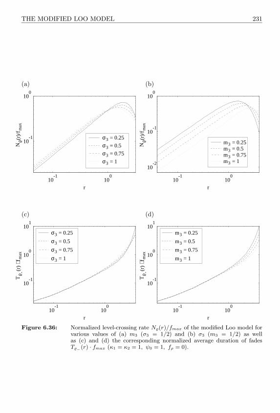
THE MODIFIED LOO MODEL 231
(a)
10-1
100
10-1
100
r
Nρ -(r
)/f m
ax
σ3 = 0.25
σ3 = 0.5
σ3 = 0.75
σ3 = 1
(b)
10-1
100
10-2
10-1
100
r
Nρ -(r
)/f m
axm3 = 0.25m3 = 0.5m3 = 0.75m3 = 1
(c)
10-1
100
10-1
100
101
r
Tρ --
(r)
⋅ fm
ax
σ3 = 0.25
σ3 = 0.5
σ3 = 0.75
σ3 = 1
(d)
10-1
100
10-1
100
101
r
Tρ --
(r)
⋅ fm
ax
m3 = 0.25
m3 = 0.5
m3 = 0.75
m3 = 1
Figure 6.36: Normalized level-crossing rate N%(r)/fmax of the modified Loo model forvarious values of (a) m3 (σ3 = 1/2) and (b) σ3 (m3 = 1/2) as wellas (c) and (d) the corresponding normalized average duration of fadesT%−(r) · fmax (κ1 = κ2 = 1, ψ0 = 1, fρ = 0).

232 FREQUENCY-NONSELECTIVE CHANNEL MODELS
µ1(t) =N1∑
n=1
c1,n cos(2πf1,nt + θ1,n) +N2∑
n=1
c2,n cos(2πf2,nt + θ2,n) , (6.181a)
µ2(t) =N1∑
n=1
c1,n sin(2πf1,nt + θ1,n)−N2∑
n=1
c2,n sin(2πf2,nt + θ2,n) , (6.181b)
µ3(t) = σ3
N3∑n=1
c3,n cos(2πf3,nt + θ3,n) + m3 . (6.181c)
With these relations, the stochastic reference model (see Figure 6.32) can be directlytransformed into the deterministic Loo model, shown in Figure 6.37. The outputprocess %(t) of this model is mnemonically named deterministic modified Loo process.
c1,1
c11,N
c2,1
cos(2 π f + θ )t1,1 1,1
cos(2 +π f θt1
)11,N 1,N
cos(2 π f + θ )t 2,12,1
cos(2 + θπ f t2
)22,N 2,N
π f + θ )sin(2 t1,1 1,1
+ θπ fsin(2 t1 11,N 1,N
π f + θ )sin(2 t 2,12,1
+ θπ fsin(2 t2,N2 22,N
.
sin(2
exp( )ν~3(t)
σ3 m 3
µ~ 3 (t)
cos(2 π ρf t + ) θρ
µ (t)1~
µ~ 2(t)
µ~ ρ(t)
.
(t)~ρ
~ρ (t)
cos(2 π + θ )f
cos(2 π + θ )fc
3,1 3,1
3,1
t
t3,2 3,2
c3,2
cos(2 + θπ f
c
t3,N3 3,N3)
3,N3
c1
c
)
)1,N
1,1
22,N
- c 2,1
2- c 2,N
c
π ρf t + ) θρ
Figure 6.37: The deterministic modified Loo model (simulation model).
For the special case (i), introduced in (6.155a), the structure of the so-calleddeterministic classical Loo model follows from Figure 6.37. Here, each of the twodeterministic processes µ1(t) and µ2(t), given by (6.181a) and (6.181b), respectively,

THE MODIFIED LOO MODEL 233
can be replaced by the fundamental relation (4.4), as a result of which the realizationexpenditure of the model reduces considerably. The special case (ii) [see (6.155b)] alsoleads to a simplification of the structure of the simulation model, because σ2
2 = 0 isequivalent to N2 = 0. It should be noted that, for this case, one obtains the simulationmodel introduced in [Pae98c]. Finally, we want to point out that in the specialcase (6.155c), the structure of the deterministic Rice process with cross-correlatedcomponents follows from Figure 6.37, as we have already discovered from the top partof Figure 6.9.
On condition that Ni ≥ 7 holds, the equations (6.168), (6.177), and (6.179) derivedfor the reference model in Subsection 6.4.1 approximately also hold for deterministicmodified Loo processes %(t), if the substitutions ψ0 → ψ0, ψ0 → ¨
ψ0, and φ0 → ˙φ0
are performed in the formulae concerned. Here, the characteristic quantities ψ0,¨ψ0,
and ˙φ0 of the simulation model are given by the relations (6.71a), (6.71b), and (6.71c)
derived in Subsection 6.1.4, respectively. This is not particularly surprising becausehere as well as in Subsection 6.1.4, the deterministic Gaussian processes µ1(t) and µ2(t)are based on the same expressions. Differences, however, only occur in the calculationof the model parameters fi,n and ci,n for i = 1, 2. In the present case, we have totake into account that the Jakes power spectral density is in general left-hand siderestricted as well as right-hand side restricted, due to κ1 ∈ [0, 1] and κ2 ∈ [0, 1]. If wetake this fact into account, when calculating the model parameters fi,n and ci,n, bymeans of the method of exact Doppler spread (MEDS), then the following expressionshold for the deterministic modified Loo model:
fi,n = fmax sin[
π
2N ′i
(n− 1
2
)], n = 1, 2, . . . , Ni (i = 1, 2) , (6.182a)
ci,n =σi√N ′
i
, n = 1, 2, . . . , Ni (i = 1, 2) , (6.182b)
where
N ′i =
⌈Ni
2π arcsin(κi)
⌉, i = 1, 2, (6.183)
describes the virtual number of harmonic functions, and Ni again denotes the actualnumber, i.e., the number of harmonic functions set by the user. For the Doppler phasesθi,n, we assume as usual that these quantities are outcomes (realizations) of a randomgenerator uniformly distributed in the interval (0, 2π].
The design of the third deterministic Gaussian process ν3(t) is performed exactlyaccording to the method described in Subsection 6.1.4. In particular, the calculationof the discrete Doppler frequencies f3,n is carried out by means of the relation(6.75a) in connection with (6.75b), and for the Doppler coefficients ci,n the formulac3,n =
√2/N3 again holds for all n = 1, 2, . . . , N3. The remaining parameters of the
simulation model (fρ, θρ,m3, σ3) of course correspond to those of the reference model,so that all parameters are now determined.
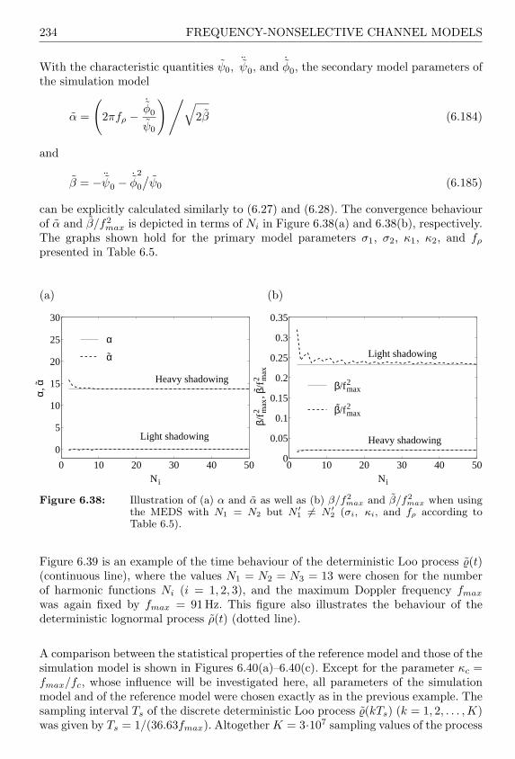
234 FREQUENCY-NONSELECTIVE CHANNEL MODELS
With the characteristic quantities ψ0,¨ψ0, and ˙
φ0, the secondary model parameters ofthe simulation model
α =
(2πfρ −
˙φ0
ψ0
)/√2β (6.184)
and
β = − ¨ψ0 − ˙
φ2
0
/ψ0 (6.185)
can be explicitly calculated similarly to (6.27) and (6.28). The convergence behaviourof α and β/f2
max is depicted in terms of Ni in Figure 6.38(a) and 6.38(b), respectively.The graphs shown hold for the primary model parameters σ1, σ2, κ1, κ2, and fρ
presented in Table 6.5.
(a)
0 10 20 30 40 50
0
5
10
15
20
25
30
Ni
α, α Heavy shadowing
Light shadowing
α
α
(b)
0 10 20 30 40 500
0.05
0.1
0.15
0.2
0.25
0.3
0.35
Light shadowing
Heavy shadowing
Ni
β/f2 m
ax, β
/f2 m
ax
β/f2max
β/f2max
Figure 6.38: Illustration of (a) α and α as well as (b) β/f2max and β/f2
max when usingthe MEDS with N1 = N2 but N ′
1 6= N ′2 (σi, κi, and fρ according to
Table 6.5).
Figure 6.39 is an example of the time behaviour of the deterministic Loo process %(t)(continuous line), where the values N1 = N2 = N3 = 13 were chosen for the numberof harmonic functions Ni (i = 1, 2, 3), and the maximum Doppler frequency fmax
was again fixed by fmax = 91 Hz. This figure also illustrates the behaviour of thedeterministic lognormal process ρ(t) (dotted line).
A comparison between the statistical properties of the reference model and those of thesimulation model is shown in Figures 6.40(a)–6.40(c). Except for the parameter κc =fmax/fc, whose influence will be investigated here, all parameters of the simulationmodel and of the reference model were chosen exactly as in the previous example. Thesampling interval Ts of the discrete deterministic Loo process %(kTs) (k = 1, 2, . . . , K)was given by Ts = 1/(36.63fmax). Altogether K = 3·107 sampling values of the process

THE MODIFIED LOO MODEL 235
0 1 2 3 4 5-50
-40
-30
-20
-10
0
10
20
t/s
20 lo
g ρ -
(t)
ρ(t)ρ- (t)
Figure 6.39: The deterministic processes %(t) and ρ(t) (σ21 = σ2
2 = 1, κ1 = 0.8, κ2 =0.5, σ3 = 0.5, m3 = 0.25, fρ = 0.2fmax, θρ = 0, κc = 50, andfmax = 91 Hz).
%(kTs) (k = 1, 2, . . . ,K) have been simulated and used for the determination of theprobability density function p%(z) [see Figure 6.40(a)], the normalized level-crossingrate N%(r)/fmax [see Figure 6.40(b)], and the normalized average duration of fadesT%−(r) · fmax [see Figure 6.40(c)] of the simulation model.
Figure 6.40(a) makes us recognize that the behaviour of the probability densityfunction p%(z) is not influenced by the quantity κc. This result was to be expected,because p%(z) is, according to (6.168), independent of the bandwidth of the processν3(t), which completely explains the missing influence of the frequency ratio κc =fmax/fc. The minor differences that can be observed between p%(z) and p%(z), aredue to the limited numbers of harmonic functions, which were here equal to Ni = 13for i = 1, 2, 3. It does not need to be explicitly emphasized that these deviationsdecrease if Ni increases, and that they converge against zero as Ni →∞.
The results of Figure 6.40(b) show us that the deviations between the level-crossingrate of the reference model and that of the simulation model are only relatively highfor unrealistically small values of κc, i.e., κc ≤ 5. On the contrary, for κc ≥ 20 thedifferences between the analytical approximate solution (6.177) and the correspondingsimulation results can be ignored.
Studying Figure 6.40(c), we notice that the same statements also hold for the averageduration of fades. Consequently, the approximate solutions derived for this model forthe level-crossing rate and the average duration of fades are very exact, provided thatthe frequency ratio κc = fmax/fc is greater than or equal to 20, i.e., if the amplitudeof the line-of-sight component changes relatively slowly compared to the amplitudevariations of the scattered component. We do not need to be afraid of a restrictionconnected with the boundary condition κc ≥ 20 for practically relevant cases, because

236 FREQUENCY-NONSELECTIVE CHANNEL MODELS
for real-world channels, κc À 1 holds anyway.
6.4.3 Applications and Simulation Results
In this subsection, we want to fit the statistic properties of the modified Loo modelto the statistics of real-world channels. Just as for the extended Suzuki process ofType I and Type II as well as for the generalized Rice process, we here also use themeasurement results presented in [But83] as a basis for the complementary cumulativedistribution function, the level-crossing rate, and the average duration of fades.
In the following, we will choose the realistic value κc = 20 for the frequency ratioκc = fmax/fc, so that the level-crossing rate N%(r) of the Loo model is approximatedby (6.177) very well. Without restriction of generality, we will also set the phase θρ ofthe line-of-sight component to the arbitrary value θρ = 0.
The remaining free model parameters of the modified Loo model are the quantitiesσ1, σ2, κ1, κ2, σ3, m3, and fρ, which are set for the model fitting procedure. Withthese primary model parameters, we defined the parameter vector
Ω :=(σ1, σ2, κ1, κ2, σ3, m3, fρ
), (6.186)
whose components are to be optimized according to the scheme described inSubsection 6.1.5. In order to minimize the error function E2(Ω) [cf. (6.76)], we againmake use of the Fletcher-Powell algorithm [Fle63]. The optimized components of theparameter vector Ω obtained in this way are presented in Table 6.5 for areas withlight and heavy shadowing.
Table 6.5: The optimized primary model parameters of the modified Loo model forareas with light and heavy shadowing.
Shadowing σ1 σ2 κ1 κ2 σ3 m3 fρ/fmax
heavy 0 0.3856 0 0.499 0.5349 -1.593 0.1857light 0.404 0.4785 0.6223 0.4007 0.2628 -0.0584 0.0795
For the modified Loo model, the Rice factor cR is calculated as follows:
cR =E
|m(t)|2
E |µ(t)|2 =E
%2(t)
2E µ2i (t)
(i = 1, 2)
=r%%(0)2ψ0
=π
2· e2(m3+σ2
3)
∑2i=1 σ2
i arcsin(κi). (6.187)
Thus, with the parameters taken from Table 6.5, the Rice factor cR is cR = 1.7 dB forheavy shadowing and cR = 8.96 dB for light shadowing.

THE MODIFIED LOO MODEL 237
(a)
0 1 2 3 4 50
0.1
0.2
0.3
0.4
0.5
0.6
z
pρ -(z
)
Simulation (κc = 2)Simulation (κc = 5)Simulation (κc = 20)Analytical model[see (6.168)]
(b)
0 1 2 3 4 50
0.1
0.2
0.3
0.4
0.5
0.6
0.7
r
Nρ -(r
)/f m
ax
Simulation (κc = 2)Simulation (κc = 5)Simulation (κc = 20)Analytical model[see (6.177)]
(c)
0 1 2 3 4 50
20
40
60
80
100
r
Tρ --
(r)
⋅ fm
ax
Simulation (κc = 2)Simulation (κc = 5)Simulation (κc = 20)Analytical model[see (6.179)]
Figure 6.40: Comparisons between: (a) p%(z) and p%(z), (b) N%(r)/fmax and
N%(r)/fmax, as well as (c) T%−(r) · fmax and T%−(r) · fmax (σ21 = σ2
2 =1, κ1 = 0.8, κ2 = 0.5, σ3 = 0.5, m3 = 0.25, fρ = 0.2fmax, θρ = 0, andfmax = 91 Hz).
238 FREQUENCY-NONSELECTIVE CHANNEL MODELS
In Figure 6.41(a), the complementary cumulative distribution function F%+(r) =1 − F%−(r) of the modified Loo model is depicted together with that of themeasured channel for the areas with light shadowing and with heavy shadowing.Figure 6.41(b) makes it clear that the differences between the normalized level-crossing rate N%(r)/fmax of the modified Loo model and the measured normalizedlevel-crossing rate used here are acceptable.
Finally, Figure 6.41(c) shows the corresponding normalized average duration of fades.Here, an excellent agreement is again observable between the reference model and themeasured channel.
For the verification of the analytical results, the corresponding simulation resultsare also depicted in Figures 6.41(a)–6.41(c). Therefore, the deterministic Gaussianprocesses ν1(t), ν2(t), and ν3(t) were designed according to the method described inSubsection 6.4.2 by using N1 = N2 = N3 = 15 cosine functions.
Finally, the deterministic modified Loo process %(t) is depicted in Figures 6.42(a)and 6.42(b) for areas with light shadowing and for areas with heavy shadowing,respectively.

THE MODIFIED LOO MODEL 239
(a)
-30 -20 -10 0 100
0.2
0.4
0.6
0.8
1
r (dB)
Fρ -+
(r)
Measurement [But83] Analytical modelSimulation
Heavy shadow
ing
Light shadow
ing
(b)
-30 -20 -10 0 1010
-3
10-2
10-1
100
101
r (dB)
Nρ -(r
)/f m
ax
Measurement [But83] Analytical modelSimulation
Heavy shadowing
Light shadowing
(c)
-30 -20 -10 0 10
100
101
102
r (dB)
Tρ --
(r)
⋅ fm
ax
Measurement [But83]
Analytical model
Simulation
Heavy shadowing
Light shadowing
Figure 6.41: (a) Complementary cumulative distribution function F%+(r), (b) normal-ized level-crossing rate N%(r)/fmax, and (c) normalized average durationof fades T%−(r/ρ) · fmax for areas with light and heavy shadowing.

240 FREQUENCY-NONSELECTIVE CHANNEL MODELS
(a)
0 1 2 3 4 5-50
-40
-30
-20
-10
0
10
t (s)
20 lo
gρ -(t)
(b)
0 1 2 3 4 5-50
-40
-30
-20
-10
0
10
t (s)
20 lo
gρ -(t)
Figure 6.42: Simulation of deterministic modified Loo processes %(t) for areas with (a)heavy shadowing and (b) light shadowing (MEDS, N1 = N2 = N3 =15, fmax = 91Hz, κc = 20).
7
FREQUENCY-SELECTIVESTOCHASTIC ANDDETERMINISTIC CHANNELMODELS
So far, we have been exclusively concerned with the description of frequency-nonselective mobile radio channels, which are characterized by the fact that thedifferences between the propagation delays of the received electromagnetic waves canbe ignored compared to the symbol interval. Obviously, this assumption is less andless justified the shorter the symbol interval or the higher the data rate becomes.Channels for which the propagation delay differences cannot be ignored in comparisonwith the symbol interval, therefore, represent a further important class of channels,namely the class of frequency-selective channels. The statistic and deterministicmodelling of this class of channels is the topic of this chapter.
In the literature, the number of publications merely dealing with frequency-selectivemobile radio channels has grown so much that even scientists mainly involvedwith this subject are running the risk of losing the overview. Therefore, it is hereimpossible to mention every author who has made a contribution to this subject,particularly since this introduction can only present a small selection of publications.In order to organize this group of themes systematically, it is sensible to make arough classification of the publications, dividing them into the following categories:theory, measurement, and simulation.
In the first category belong works in which the description and analysis of mobileradio channels are mainly treated theoretically. The most important article in thiscategory is indisputably [Bel63]. In this fundamental work on stochastic time-variantlinear systems, Bello introduces the WSSUS1 model that is employed almost ex-clusively for the description of frequency-selective mobile radio channels. With thismodel, the input-output behaviour of mobile radio channels can be described inthe equivalent complex baseband in a relatively simple manner, since the channel
1 WSSUS: wide-sense stationary uncorrelated scattering

242 FREQUENCY-SELECTIVE CHANNEL MODELS
is assumed to be quasi-stationary during the observation time interval. Empiricallygrounded statements have shown [Par82] that the assumption of quasi-stationarityis justified, when the mobile unit covers a distance in the order of less than a fewtens of the wavelength of the carrier signal. The articles [Par82, Ste87, Lor85] givea good overview of the most important characteristics of time-variant channels, towhich naturally mobile radio channels also belong. Books discussing this subject are,for example, [Ste94, Stu96, Pro95] and [Jun97]. A deep insight into the theory ofWSSUS models can be obtained by studying [Fle90]. A detailed analysis of WSSUSmodels can also be found in [Sad98] for instance, where correlation functions as wellas scattering functions are derived on the assumption of non-uniformly distributedangles of arrival. The article [Fle96] gives an overview of the state of research inthe field of channel modelling, carried out until 1996 by European research projectssuch as COST 207, RACE CODIT, and RACE ATDMA. In the meantime, intensiveresearch on spatial-temporal channel models for future mobile radio systems withadaptive antennas has been carried out [Lib99]. Detailed articles giving an overviewwith many references concerning this subject are the publications [Ert98] and [Mar99].
In the second category belong publications reporting on experimental measurementresults of mobile radio channels as well as works treating the technology of mobileradio channel measurement. Certainly, the works by Young [You52], NyLund [Nyl68],Cox [Cox72, Cox73], Nielson [Nie78], as well as by Bajwa and Parsons [Baj82] belongto the pioneering works in the field of channel measurements. The subject of channelmeasuring is treated in an easily understandable manner in the overview article byAndersen et al. [And95]. In this publication, mobile radio channels are divided intoclasses depending on the environment, and typical measured characteristic quantitiesfor different propagation scenarios are given. Particularly in connection with themeasurement of system functions of mobile radio channels, the papers [Wer91]and [Kat95] are interesting. For the measurement of the propagation properties ofmobile radio channels, special measuring devices are required. They are denotedas channel sounders. At the Telecommunications Institute of the University ofErlangen–Nuremberg, Germany, the three channel sounders RUSK 400, RUSK 5000,and RUSK X have been developed [Mar94a] as part of research projects in associationwith the Deutsche Telekom in Darmstadt, Germany. Detailed information on theprinciple of the applied measurement methods of the channel sounders can be foundin [Mar92, Mar94a, Mar94b]. Results of measurement campaigns performed withthe device type RUSK 5000 are, for example, reported in [Kad91, Goe92a, Goe92b].The channel sounders RUSK 400 and RUSK 5000 have been produced merely asprototypes, whereas RUSK X and the succeeding models RUSK SX and RUSK WLLhave for some time already been commercially sold by the company MEDAV GmbH.Recently, the device RUSK ATM also became part of the RUSK channel sounders’family. This device arose within the framework of the project ATMmobil, which waspromoted by the BMFT and supported by the company MEDAV [Tho99]. With thisvector channel sounder, in particular directional resolved measurements of mobileradio channels can be carried out in the frequency band of 5 GHz up to 6 GHz. Afurther channel sounder named SIMOCS 2000 has been produced by the Siemens AGin Munich, Germany. The principle of the functionality of SIMOCS 2000 is describedin [Fel94] and [Jun97]. Furthermore, it should be mentioned that Zollinger [Zol93]
FREQUENCY-SELECTIVE CHANNEL MODELS 243
has developed a channel sounder at the ETH (Swiss Federal Institute of TechnologyZurich) in Zurich, Switzerland. The channel sounder ECHO 24 (ETH ChannelSounder operating at 24 GHz) also traces its descent from the ETH. With thischannel sounder, complex channel impulse responses can be measured in buildingswith a temporal resolution of 2 ns [Hed99].
In the third and last category finally belong works stressing the development ofsimulation models of frequency-selective mobile radio channels. Concerning themethod of realization of these so-called channel simulators, one distinguishes betweenhardware realization and software realization. Hardware realizations can in additionbe divided into analog and digital channel simulators. Analog channel simulators (e.g.,[Cap80, Ber86]) model the channel in the high-frequency band or in the intermediate-frequency band, where surface acoustic wave (SAW) filters are applied to realizedifferent multipath propagation delays. Digital channel simulators in general performall arithmetic operations that become necessary in the complex baseband in real-timeusing digital signal processors [Sch89] or vector processors (e.g., [Ehr82, Sch90]). Inmost applications, however, the channel simulation does not take place under real-timeconditions, but is performed on a workstation or a PC. As design methods for therequired algorithms, in principle both the filter method (e.g., [Fec93a, Lau94]) andthe Rice method (e.g., [Schu89, Hoe90, Hoe92, Cre95, Yip95, Pae95b]) are possible.Incidentally, both of these methods are eligible for the design of channel simulators formobile communication systems with frequency-hopping capabilities, which has beenshown by using the filter method in [Lam97] and by using the Rice method in [Pae97b].
The present Chapter 7 is structured as follows. In order to illustrate the path geometryfor multipath fading channels with different propagation delays, we will at firstdescribe the ellipses model introduced by Parsons and Bajwa [Par82] in Section 7.1. InSection 7.2, we will be concerned with the system theoretical description of frequency-selective channels. In this context, we will discuss four system functions introducedby Bello [Bel63]. It will be pointed out how to get various insights with these systemfunctions into the input-output behaviour of linear time-variant systems. Section 7.3contains a description of the theory of frequency-selective stochastic channel models,which is also going back to Bello [Bel63]. Here, the WSSUS channel model is of centralimportance. In particular, stochastic system functions as well as the characteristicquantities derivable from these will be introduced to characterize the statisticalproperties of WSSUS channel models. These models are also suitable for modellingchannels specified by the European working group COST 207 [COS86, COS89]. Thedescription of the COST 207 channel models is the topic of Subsection 7.3.3. Section 7.4is dedicated to the mathematical description of frequency-selective deterministicchannel models. The mathematical methods applied in this section are an extensionof the theory of deterministic processes introduced in Chapter 4. Finally, Chapter 7ends with the derivation of deterministic simulation models for the channel modelsaccording to COST 207.
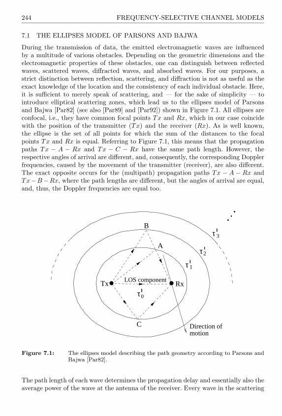
244 FREQUENCY-SELECTIVE CHANNEL MODELS
7.1 THE ELLIPSES MODEL OF PARSONS AND BAJWA
During the transmission of data, the emitted electromagnetic waves are influencedby a multitude of various obstacles. Depending on the geometric dimensions and theelectromagnetic properties of these obstacles, one can distinguish between reflectedwaves, scattered waves, diffracted waves, and absorbed waves. For our purposes, astrict distinction between reflection, scattering, and diffraction is not as useful as theexact knowledge of the location and the consistency of each individual obstacle. Here,it is sufficient to merely speak of scattering, and — for the sake of simplicity — tointroduce elliptical scattering zones, which lead us to the ellipses model of Parsonsand Bajwa [Par82] (see also [Par89] and [Par92]) shown in Figure 7.1. All ellipses areconfocal, i.e., they have common focal points Tx and Rx, which in our case coincidewith the position of the transmitter (Tx) and the receiver (Rx). As is well known,the ellipse is the set of all points for which the sum of the distances to the focalpoints Tx and Rx is equal. Referring to Figure 7.1, this means that the propagationpaths Tx − A − Rx and Tx − C − Rx have the same path length. However, therespective angles of arrival are different, and, consequently, the corresponding Dopplerfrequencies, caused by the movement of the transmitter (receiver), are also different.The exact opposite occurs for the (multipath) propagation paths Tx − A − Rx andTx−B−Rx, where the path lengths are different, but the angles of arrival are equal,and, thus, the Doppler frequencies are equal too.
τ0
τ 1
τ2
τ 3
Direction ofCmotion
LOS componentRxTx
B
A
Figure 7.1: The ellipses model describing the path geometry according to Parsons andBajwa [Par82].
The path length of each wave determines the propagation delay and essentially also theaverage power of the wave at the antenna of the receiver. Every wave in the scattering
SYSTEM THEORETICAL DESCRIPTION 245
zone characterized by the `th ellipses undergoes the same discrete propagation delay
τ ′` = τ ′0 + ` ∆τ ′ , ` = 0, 1, . . . , L − 1 , (7.1)
where τ ′0 is the propagation delay of the line-of-sight (LOS) component, ∆τ ′ is aninfinitesimal propagation delay, and L denotes the number of paths with differentpropagation delays. It is evident that the ellipses model increases in precision if Lincreases and ∆τ ′ becomes smaller. In the limit L → ∞ and ∆τ ′ → 0, the discretepropagation delay τ ′` results in the continuous propagation delay τ ′ restricted to theinterval [τ ′0, τ
′max]. Here, τ ′max characterizes the maximum propagation delay, which
depends on the environment. The maximum propagation delay τ ′max is chosen in sucha way that the contributions of the scattered components with propagation delays τ ′
greater than τ ′max can be ignored.
In the following discussion, we will see that the ellipses model forms to a certain extentthe physical basis for the modelling of frequency-selective channels. In particular, thenumber of paths L with different propagation delays exactly corresponds to the numberof delay elements required for the tapped-delay-line structure of the time-variant filterused for modelling frequency-selective channels. In order to achieve an economicalrealization, L should be kept as small as possible.
7.2 SYSTEM THEORETICAL DESCRIPTION OF FREQUENCY-SELECTIVECHANNELS
Using the system functions introduced by Bello [Bel63], the input and output signalsof frequency-selective channels can be related to each other in different ways. Thestarting point for the derivation of the system functions is based on the assumptionthat the channel is a linear time-variant system in the equivalent complex baseband.In time-variant systems, the impulse response — denoted by h0(t0, t) — is a functionof the time t0 at which the channel has been excited by the impulse δ(t − t0), andthe time t at which the effect of the impulse is observed at the output of the channel.The relation between the impulse δ(t − t0) and the corresponding impulse responseh0(t0, t) can therefore be expressed by
δ(t− t0) → h0(t0, t) . (7.2)
Since every physical channel is causal, the impulse cannot produce an effect beforethe impulse has excited the channel. This is the so-called law of causality that can beexpressed by
h0(t0, t) = 0 for t < t0 . (7.3)
Using the impulse response h0(t0, t), we now want to compute the output signal y(t)of the channel for an arbitrary input signal x(t). For this purpose, we at first representx(t) as an infinite densely superposition of weighted delta functions. By applying thesifting property of delta functions, this leads us to
x(t) =∫ ∞
−∞x(t0) δ(t− t0) dt0 . (7.4)
246 FREQUENCY-SELECTIVE CHANNEL MODELS
Alternatively, we can also use the expression
x(t) = lim∆t0→0
∑t0
x(t0) δ(t− t0) ∆t0 . (7.5)
Since the channel was assumed to be linear, we may employ the principle ofsuperposition [Lue90]. Hence, by using (7.2), the response to the sum in (7.5) canbe written as
∑t0
x(t0) δ(t− t0) ∆t0 →∑t0
x(t0)h0(t0, t) ∆t0 . (7.6)
For the desired relation
x(t) → y(t) , (7.7)
we obtain the following result from (7.6) in the limit ∆t0 → 0∫ ∞
−∞x(t0) δ(t− t0) dt0 →
∫ ∞
−∞x(t0) h0(t0, t) dt0 . (7.8)
If we now make use of the causality property (7.3), then the output signal is given by
y(t) =∫ t
−∞x(t0)h0(t0, t) dt0 . (7.9)
Next, we substitute the variable t0 by the propagation delay
τ ′ = t− t0 , (7.10)
which defines the time elapsed from the moment at which the channel was excited bythe impulse to the moment at which the response was observed at the output of thechannel. Substituting t0 by t− τ ′ in (7.9) results in
y(t) =∫ ∞
0
x(t− τ ′) h(τ ′, t) dτ ′ . (7.11)
In order to simplify the notation, the time-variant impulse response h0(t − τ ′, t) hasbeen replaced by h(τ ′, t) := h0(t− τ ′, t). Physically, the time-variant impulse responseh(τ ′, t) can be interpreted as the response of the channel at the time t to a deltaimpulse that stimulated the channel at the time t−τ ′. Considering (7.10), the causalityproperty (7.3) can be expressed by
h(τ ′, t) = 0 for τ ′ < 0 . (7.12)
From (7.11), we now directly obtain the tapped-delay-line model shown in Figure 7.2of a frequency-selective channel with the time-variant impulse response h(τ ′, t). Notethat the tapped-delay-line model can be interpreted as transversal filter with time-variant coefficients.
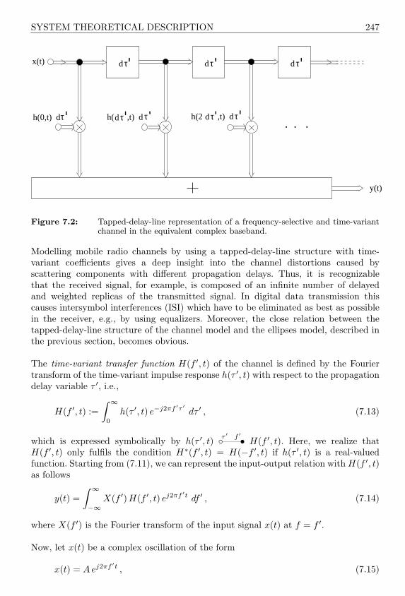
SYSTEM THEORETICAL DESCRIPTION 247
h(2 ,t) d
ττd d
ττd τd
τdx(t)
. . .
y(t)
τ τh(0,t) d h( ,t) d
Figure 7.2: Tapped-delay-line representation of a frequency-selective and time-variantchannel in the equivalent complex baseband.
Modelling mobile radio channels by using a tapped-delay-line structure with time-variant coefficients gives a deep insight into the channel distortions caused byscattering components with different propagation delays. Thus, it is recognizablethat the received signal, for example, is composed of an infinite number of delayedand weighted replicas of the transmitted signal. In digital data transmission thiscauses intersymbol interferences (ISI) which have to be eliminated as best as possiblein the receiver, e.g., by using equalizers. Moreover, the close relation between thetapped-delay-line structure of the channel model and the ellipses model, described inthe previous section, becomes obvious.
The time-variant transfer function H(f ′, t) of the channel is defined by the Fouriertransform of the time-variant impulse response h(τ ′, t) with respect to the propagationdelay variable τ ′, i.e.,
H(f ′, t) :=∫ ∞
0
h(τ ′, t) e−j2πf ′τ ′ dτ ′ , (7.13)
which is expressed symbolically by h(τ ′, t) τ ′ f ′——• H(f ′, t). Here, we realize thatH(f ′, t) only fulfils the condition H∗(f ′, t) = H(−f ′, t) if h(τ ′, t) is a real-valuedfunction. Starting from (7.11), we can represent the input-output relation with H(f ′, t)as follows
y(t) =∫ ∞
−∞X(f ′)H(f ′, t) ej2πf ′t df ′ , (7.14)
where X(f ′) is the Fourier transform of the input signal x(t) at f = f ′.
Now, let x(t) be a complex oscillation of the form
x(t) = Aej2πf ′t , (7.15)

248 FREQUENCY-SELECTIVE CHANNEL MODELS
where A denotes a complex-valued constant, then it follows from (7.11)
y(t) = A
∫ ∞
0
h(τ ′, t) ej2πf ′(t−τ ′) dτ ′ . (7.16)
Using (7.13), we may also write
y(t) = AH(f ′, t) ej2πf ′t . (7.17)
Therefore, the response of the channel can in this case be represented by the inputsignal (7.15) weighted by the time-variant transfer function H(f ′, t). The form (7.17)consequently makes clear that the time-variant transfer function H(f ′, t) can bemeasured directly in the relevant frequency band by sinusoidal excitation.
Neither the time-variant impulse response h(τ ′, t) nor the corresponding transferfunction H(f ′, t) allow an insight into the phenomena caused by the Doppler effect. Inorder to eliminate this disadvantage, we apply the Fourier transform on h(τ ′, t) withrespect to the time variable t. In this way, we obtain a further system function
s(τ ′, f) :=∫ ∞
−∞h(τ ′, t) e−j2πft dt , (7.18)
which is called the Doppler-variant impulse response.
Instead of (7.18), we may also write h(τ ′, t) t f——• s(τ ′, f). Expressing the time-variant impulse response h(τ ′, t) by the inverse Fourier transform of s(τ ′, f), allowsthe representation of (7.11) in the form
y(t) =∫ ∞
0
∫ ∞
−∞x(t− τ ′) s(τ ′, f) ej2πft df dτ ′ . (7.19)
This relation shows that the output signal y(t) can be represented by an infinitesum of delayed, weighted, and Doppler shifted replicas of the input signal x(t).Signals delayed during transmission in the range of [τ ′, τ ′ + dτ ′) and affected by aDoppler shift within [f, f + df) are weighted by the differential part s(τ ′, f) df dτ ′.The Doppler-variant impulse response s(τ ′, f), therefore, explicitly describes thedispersive behaviour of the channel as a function of both the propagation delays τ ′
and the Doppler frequencies f . Consequently, the physical interpretation of s(τ ′, f)directly leads to the ellipses model shown in Figure 7.1.
A further system function, the so-called Doppler-variant transfer function T (f ′, f), isdefined by the two-dimensional Fourier transform of the time-variant impulse responseh(τ ′, t) according to
T (f ′, f) :=∫ ∞
−∞
∫ ∞
0
h(τ ′, t) e−j2π(ft+f ′τ ′) dτ ′ dt . (7.20)
Due to (7.13) and (7.18), we may also write T (f ′, f) f t•—— H(f ′, t) or
T (f ′, f) f ′ τ ′•—— s(τ ′, f) for (7.20).

SYSTEM THEORETICAL DESCRIPTION 249
The computation of the Fourier transform of (7.11) with respect to the time variablet allows the representation of the spectrum Y (f) of the output signal y(t) in the form
Y (f) =∫ ∞
−∞X(f − f ′)T (f − f ′, f ′) df ′ . (7.21)
Finally, we exchange the frequency variables f and f ′ and obtain
Y (f ′) =∫ ∞
−∞X(f ′ − f)T (f ′ − f, f) df . (7.22)
This equation shows how a relation between the spectrum of the output-signal andthe input-signal can be established by making use of the Doppler-variant transferfunction T (f ′, f). Regarding (7.22), it becomes obvious that the spectrum of theoutput signal can be interpreted as a superposition of an infinite number of Dopplershifted and filtered replicas of the spectrum of the input signal.
At the end of this section, we keep in mind that the four system functions h(τ ′, t),H(f ′, t), s(τ ′, f), and T (f ′, f) are related in pairs by the Fourier transform. TheFourier transform relationships established above are illustrated in Figure 7.3.
f
fτ
τ
τ
f
τ f
τ
f
f
τ
transfer function
T( ,f)
H( ,t)s( ,f)
h( ,t)
t
f
f t
t
f
f
t
Time-variantimpulse response
impulse responseDoppler-variant
Doppler-varianttransfer function
Time-variant
Figure 7.3: Fourier transform relationships between the system functions according toBello [Bel63].

250 FREQUENCY-SELECTIVE CHANNEL MODELS
7.3 FREQUENCY-SELECTIVE STOCHASTIC CHANNEL MODELS
7.3.1 Correlation Functions
In the following, we consider the channel as a stochastic system. In this case, thefour functions h(τ ′, t), H(f ′, t), s(τ ′, f), and T (f ′, f) are stochastic system functions.Generally, these stochastic system functions can be described by the followingautocorrelation functions:
rhh(τ ′1, τ′2; t1, t2) := Eh∗(τ ′1, t1) h(τ ′2, t2) , (7.23a)
rHH(f ′1, f′2; t1, t2) := EH∗(f ′1, t1) H(f ′2, t2) , (7.23b)
rss(τ ′1, τ′2; f1, f2) := Es∗(τ ′1, f1) s(τ ′2, f2) , (7.23c)
rTT (f ′1, f′2; f1, f2) := ET ∗(f ′1, f1)T (f ′2, f2) . (7.23d)
Since the system functions are related by the Fourier transform, it is not surprisingthat analog relations are also valid for the autocorrelation functions. For example,(7.23a) and (7.23b) are related by
rHH(f ′1, f′2; t1, t2) :=EH∗(f ′1, t1)H(f ′2, t2)
= E
∫ ∞
−∞h∗(τ ′1, t1) ej2πf ′1τ ′1 dτ ′1
∫ ∞
−∞h(τ ′2, t2) e−j2πf ′2τ ′2 dτ ′2
=∫ ∞
−∞
∫ ∞
−∞Eh∗(τ ′1, t1)h(τ ′2, t2) ej2π(f ′1τ ′1−f ′2τ ′2) dτ ′1 dτ ′2
=∫ ∞
−∞
∫ ∞
−∞rhh(τ ′1, τ
′2; t1, t2) ej2π(f ′1τ ′1−f ′2τ ′2) dτ ′1 dτ ′2 . (7.24)
Finally, we replace the variable f ′1 by −f ′1 on both sides of the last equa-tion, to make clear that rHH(−f ′1, f
′2; t1, t2) is the two-dimensional Fourier
transform of rhh(τ ′1, τ′2; t1, t2) with respect to the two propagation delay
variables τ ′1 and τ ′2. This can be expressed symbolically by the notationrhh(τ ′1, τ
′2; t1, t2)
τ ′1,τ ′2 f ′1,f ′2————• rHH(−f ′1, f′2; t1, t2). The Fourier transform relationships
between all the other pairs of (7.23a)–(7.23d) can be derived in a similar way. Asa result, one finds the relationships between the autocorrelation functions of thestochastic system functions shown in Figure 7.4.
In order to describe the input-output relation of the stochastic channel, we assume thatthe input signal x(t) is a stochastic process with the known autocorrelation functionrxx(t1, t2) := Ex∗(t1)x(t2). As (7.11) is valid for deterministic systems as well asfor stochastic systems, we can express the autocorrelation function ryy(t1, t2) of theoutput signal y(t) as a function of rxx(t1, t2) and rhh(τ ′1, τ
′2; t1, t2) as follows:
ryy(t1, t2) := Ey∗(t1) y(t2)
= E
∫ ∞
0
∫ ∞
0
x∗(t1 − τ ′1)x(t2 − τ ′2)h∗(τ ′1, t1) h(τ ′2, t2) dτ ′1 dτ ′2

FREQUENCY-SELECTIVE STOCHASTIC CHANNEL MODELS 251
τ τ1 2,τ τ1 2, ,1t t2
τ τ1 2, ,1t t2r ( )hh ;
τ τ1 2, ,1 2t t
1 2,f f 1 2,f f1 2,f f
1 2,f f
1 2,f f 1 2,f f
1 2,f f
1 2,f f
1
ss
2,f f
τ τ1 2,, 2t t1
, 2t t1
τ τ1 2, , 2t t1
1 2,f frTT ( )1 2,f 1 2,f ff- ;-
r ( ; )- ( ;rHH )-
Figure 7.4: Relationships between the autocorrelation functions of the stochasticsystem functions.
=∫ ∞
0
∫ ∞
0
Ex∗(t1 − τ ′1)x(t2 − τ ′2)Eh∗(τ ′1, t1)h(τ ′2, t2) dτ ′1 dτ ′2
=
∞∫
0
∞∫
0
rxx(t1 − τ ′1; t2 − τ ′2) rhh(τ ′1, τ′2; t1, t2) dτ ′1 dτ ′2 . (7.25)
In the derivation above, we have implicitly assumed that the time-variant impulseresponse h(τ ′, t) of the channel and the input signal x(t) are statistically independent.
Significant simplifications can be made by assuming that the time-variant impulseresponse h(τ ′, t) is stationary in the wide sense with respect to t, and that thescattering components with different propagation delays are statistically uncorrelated.Basing on these assumptions, Bello introduced the so-called WSSUS model in hisessential work [Bel63] on stochastic time-variant linear systems. The description ofthe WSSUS model is the topic of the following subsection.
7.3.2 The WSSUS Model According to Bello
The WSSUS model enables the statistical description of the input-output relationof mobile radio channels for the transmission of bandpass signals in the equivalentcomplex baseband for observation periods in which the stationarity of the channel isensured in the wide sense. According to empirical studies [Par82], the channel can beconsidered as wide-sense stationary as long as the mobile unit covers a distance in thedimension of a few tens of the wavelength of the carrier signal.
7.3.2.1 WSS Models
A channel model with a wide-sense stationary impulse response is called WSS channelmodel (WSS, wide-sense stationary). Instead of the term WSS channel model, we

252 FREQUENCY-SELECTIVE CHANNEL MODELS
also use the short form WSS model, since it is evident that this model is exclusivelyused for modelling channels. The assumption of wide-sense stationarity leads to thefact that the two autocorrelation functions in (7.23a) and (7.23b) are invariant withrespect to a translation of time, i.e., the autocorrelation functions rhh(τ ′1, τ
′2; t1, t2) and
rHH(f ′1, f′2; t1, t2) merely depend on the time difference τ := t2 − t1. With t1 = t and
t2 = t + τ , we can therefore write in case of WSS models:
rhh(τ ′1, τ′2; t, t + τ) = rhh(τ ′1, τ
′2; τ) , (7.26a)
rHH(f ′1, f′2; t, t + τ) = rHH(f ′1, f
′2; τ) . (7.26b)
The restricted behaviour of these two autocorrelation functions certainly hasconsequences for the remaining autocorrelation functions (7.23c) and (7.23d). Toclarify this, we look at the Fourier transform relation between rhh(τ ′1, τ
′2; t1, t2) and
rss(τ ′1, τ′2; f1, f2) which can, by considering Figure 7.4, be formulated as follows
rss(τ ′1, τ′2; f1, f2) =
∫ ∞
−∞
∫ ∞
−∞rhh(τ ′1, τ
′2; t1, t2) ej2π(t1f1−t2f2) dt1 dt2 . (7.27)
The substitutions of the variables t1 → t and t2 → t + τ , in connection with (7.26a),result in
rss(τ ′1, τ′2; f1, f2) =
∫ ∞
−∞e−j2π(f2−f1)t dt
∫ ∞
−∞rhh(τ ′1, τ
′2; τ) e−j2πf2τ dτ . (7.28)
The first integral on the right-hand side of (7.28) can be identified with the deltafunction δ(f2 − f1). Consequently, rss(τ ′1, τ
′2; f1, f2) can be expressed by
rss(τ ′1, τ′2; f1, f2) = δ(f2 − f1)Sss(τ ′1, τ
′2; f1) , (7.29)
where Sss(τ ′1, τ′2; f1) is the Fourier transform of the autocorrelation function
rhh(τ ′1, τ′2; τ) with respect to the time separation variable τ . The assumption that the
time-variant impulse response h(τ ′, t) is wide-sense stationary therefore leads to thefact that the system functions s(τ ′1, f1) and s(τ ′2, f2) are statistically uncorrelated ifthe Doppler frequencies f1 and f2 are different.
It can be shown in a similar way that (7.23d) can be represented in the form
rTT (f ′1, f′2; f1, f2) = δ(f2 − f1)STT (f ′1, f
′2; f1) , (7.30)
where STT (f ′1, f′2; f1) denotes the Fourier transform of the autocorrelation function
rHH(f ′1, f′2; τ) with respect to τ . From (7.30), it can be realized that the system
functions T (f ′1, f1) and T (f ′2, f2) are statistically uncorrelated for different Dopplerfrequencies f1 and f2.
Since the time-variant impulse response h(τ ′, t) results from a superposition ofa multitude of scattered components, it can generally be stated that the WSSassumption leads to the fact that scattering components with different Dopplerfrequencies or different angles of arrival are statistically uncorrelated.
FREQUENCY-SELECTIVE STOCHASTIC CHANNEL MODELS 253
7.3.2.2 US Models
A second important class of channel models is obtained by assuming that scatteringcomponents with different propagation delays are statistically uncorrelated. Thesechannel models are called US channel models or US models (US, uncorrelatedscattering). The autocorrelation functions rhh(τ ′1, τ
′2; t1, t2) and rss(τ ′1, τ
′2; f1, f2) of
US models can first of all be described formally by
rhh(τ ′1, τ′2; t1, t2) = δ(τ ′2 − τ ′1)Shh(τ ′1; t1, t2) , (7.31a)
rss(τ ′1, τ′2; f1, f2) = δ(τ ′2 − τ ′1)Sss(τ ′1; f1, f2) . (7.31b)
The singular behaviour of the autocorrelation function (7.31a) has significant conse-quences on the tapped-delay-line model shown in Figure 7.2, because the time-variantcoefficients of this model are now uncorrelated as a result of the US assumption.In practice, the coefficients of the tapped-delay-line model are realized almostexclusively by coloured Gaussian random processes. It should be taken into accountthat uncorrelated Gaussian random processes are also statistically independent.
Formal expressions for the autocorrelation functions of the remaining stochastic systemfunctions H(f ′, t) and T (f ′, f) can easily be determined by using the relations shownin Figure 7.4. With the substitutions f ′1 = f ′ and f ′2 = f ′+υ′, the following equationscan be found:
rHH(f ′, f ′ + υ′; t1, t2) = rHH(υ′; t1, t2) , (7.32a)rTT (f ′, f ′ + υ′; f1, f2) = rTT (υ′; f1, f2) . (7.32b)
Obviously, the autocorrelation functions of the system functions H(f ′, t) and T (f ′, f)only depend on the frequency difference υ′ := f ′2 − f ′1. As a consequence, US modelsare wide-sense stationary with respect to the frequency f ′.
If we now compare the above mentioned autocorrelation functions of US models withthose derived for WSS models, then we notice that they are dual to each other.Therefore, we can say that the class of US models stands in a duality relationshipto the class of WSS models.
7.3.2.3 WSSUS Models
The most important class of stochastic time-variant linear channel models is rep-resented by models belonging to the class of WSS models as well as to the classof US models. These channel models with wide-sense stationary impulse responsesand uncorrelated scattering components are called WSSUS channel models or simplyWSSUS models (WSSUS, wide-sense stationary uncorrelated scattering). Due totheir simplicity, they are of great practical importance and are nowadays almostexclusively employed for modelling frequency-selective mobile radio channels.

254 FREQUENCY-SELECTIVE CHANNEL MODELS
In the case of the WSSUS assumption, the autocorrelation function of the time-variantimpulse response h(τ ′, t) has to be describable by (7.26a) as well as by (7.31a). Hence,we may formally write
rhh(τ ′1, τ′2; t, t + τ) = δ(τ ′2 − τ ′1)Shh(τ ′1, τ) , (7.33)
where Shh(τ ′1, τ) is called the delay cross-power spectral density. With this represen-tation it becomes obvious that the time-variant impulse response h(τ ′, t) of WSSUSmodels has the characteristic properties of non-stationary white noise with respectto the propagation delay τ ′, on the one hand, and is also wide-sense stationary withrespect to the time t, on the other hand.
By analogy, we can directly obtain the autocorrelation function of T (f ′, f) by bringing(7.30) and (7.32b) together. Thus, for WSSUS models, it holds
rTT (f ′, f ′ + υ′; f1, f2) = δ(f2 − f1)STT (υ′, f1) , (7.34)
where STT (υ′, f1) is called Doppler cross-power spectral density. This result showsthat the system function T (f ′, f) of WSSUS models behaves like non-stationarywhite noise with respect to the Doppler frequency f and like a wide-sense stationarystochastic process with respect to the frequency f ′.
Furthermore, we can combine the relations (7.29) and (7.31b) and obtain theautocorrelation function of s(τ ′, f) in the form
rss(τ ′1, τ′2; f1, f2) = δ(f2 − f1) δ(τ ′2 − τ ′1) S(τ ′1, f1) . (7.35)
From this, we conclude that the system function s(τ ′, f) of WSSUS models has thecharacter of non-stationary white noise with respect to τ ′ as well as with respect tof . In [Bel63], Bello called the function S(τ ′1, f1) appearing in (7.35) the scatteringfunction.
Finally, by combining (7.26b) and (7.32a), it follows for the autocorrelation functionof H(f ′, t) the relation
rHH(f ′, f ′ + υ′; t, t + τ) = rHH(υ′, τ) . (7.36)
The autocorrelation function rHH(υ′, τ) is called the time-frequency correlationfunction. Regarding (7.36) it becomes obvious that the system function H(f ′, t) ofWSSUS models has the properties of wide-sense stationary stochastic processes withrespect to f ′ and t.
Figure 7.4 shows the universally valid relationships between the autocorrelationfunctions of the four system functions. With the expressions (7.33)–(7.36), it is nowpossible to derive the specific relations valid for WSSUS models. One may thereforestudy Figure 7.5, where the relationships between the delay cross-power spectraldensity Shh(τ ′, τ), the time-frequency correlation function rHH(υ′, τ), the Dopplercross-power spectral density STT (υ′, f), and the scattering function S(τ ′, f) are shown.

FREQUENCY-SELECTIVE STOCHASTIC CHANNEL MODELS 255
υTT
fS ( , )
τhh τS ( , )
fτS ( , ) υ
τ
υ
υτ
υ
τ
τ
υ
power spectral density
τr ( , )HH
τ
τ
f
τ
f
τ
f
f
Delay cross-
Time-frequencycorrelation function
Scatteringfunction
power spectral density
Doppler cross-
Figure 7.5: Relationships between the delay cross-power spectral density Shh(τ ′, τ),the time-frequency correlation function rHH(υ′, τ), the Doppler cross-powerspectral density STT (υ′, f), and the scattering function S(τ ′, f) of WSSUSmodels.
Here, it should be noted that the substitutions f1 → f and τ ′1 → τ ′ have been carriedout for reasons of simplifying the notation.
Figure 7.5 makes clear that the knowledge of one of the four depicted functions issufficient to calculate the remaining three. For example, from the scattering functionS(τ ′, f), we can directly obtain the delay cross-power spectral density Shh(τ ′, τ) bycomputing the inverse Fourier transform with respect to the Doppler frequency f , i.e.,
Shh(τ ′, τ) =∫ ∞
−∞S(τ ′, f) ej2πfτ df , (7.37)
where τ = t2 − t1.
The delay cross-power spectral density Shh(τ ′, τ) at τ = 0 defines the so-called delaypower spectral density Sτ ′τ ′(τ ′), which is due to (7.37) related to the scattering functionS(τ ′, f) according to
Sτ ′τ ′(τ ′) := Shh(τ ′, 0) =∫ ∞
−∞S(τ ′, f) df . (7.38)
The delay power spectral density Sτ ′τ ′(τ ′) determines the average power of scatteringcomponents occurring with the propagation delay τ ′. It can easily be shown thatSτ ′τ ′(τ ′) is proportional to the probability density function of the propagation delaysτ ′. From the delay power spectral density Sτ ′τ ′(τ ′), two important characteristic

256 FREQUENCY-SELECTIVE CHANNEL MODELS
quantities for the characterization of WSSUS models can be derived: the averagedelay and the delay spread.
Average delay: The average delay B(1)τ ′τ ′ is defined by the first moment of Sτ ′τ ′(τ ′),
i.e.,
B(1)τ ′τ ′ :=
∫∞−∞ τ ′ Sτ ′τ ′(τ ′) dτ ′∫∞−∞ Sτ ′τ ′(τ ′) dτ ′
. (7.39)
It corresponds to the centre of gravity of the delay power spectral density Sτ ′τ ′(τ ′).The average delay B
(1)τ ′τ ′ is the statistical mean delay that a carrier signal experiences
during the transmission over a multipath fading channel.
Delay spread: The delay spread B(2)τ ′τ ′ is defined by the square root of the second
central moment of Sτ ′τ ′(τ ′), i.e.,
B(2)τ ′τ ′ :=
√√√√√∫∞−∞
(τ ′ −B
(1)τ ′τ ′
)2
Sτ ′τ ′(τ ′) dτ ′∫∞−∞ Sτ ′τ ′(τ ′) dτ ′
. (7.40)
The delay spread B(2)τ ′τ ′ provides us with a measure of the time spread of an impulse
passed through a multipath fading channel.
From Figure 7.5, we realize that the Doppler cross-power spectral density STT (υ′, f)is the Fourier transform of the scattering function S(τ ′, f) with respect to the delayτ ′, i.e., the relation
STT (υ′, f) =∫ ∞
−∞S(τ ′, f) e−j2πυ′τ ′ dτ ′ (7.41)
holds, where υ′ = f ′2 − f ′1.
For υ′ = 0, the already known Doppler power spectral density Sµµ(f) follows fromthe Doppler cross-power spectral density STT (υ′, f), because
Sµµ(f) := STT (0, f) =∫ ∞
−∞S(τ ′, f) dτ ′ (7.42)
holds. The Doppler power spectral density Sµµ(f) gives the average power of thescattering components occurring with the Doppler frequency f . In Appendix A, it isshown that Sµµ(f) is proportional to the probability density function of the Dopplerfrequencies f . Remember that two important characteristic quantities can be derivedfrom the Doppler power spectral density Sµµ(f), namely, the average Doppler shiftB
(1)µµ [cf. (3.13a)] and the Doppler spread B
(2)µµ [cf. (3.13b)].
According to Figure 7.5, the time-frequency correlation function rHH(υ′, τ) can becalculated from the scattering function S(τ ′, f) as follows:
rHH(υ′, τ) =∫ ∞
−∞
∫ ∞
−∞S(τ ′, f) e−j2π(υ′τ ′−fτ) dτ ′ df , (7.43)
FREQUENCY-SELECTIVE STOCHASTIC CHANNEL MODELS 257
where υ′ = f ′2− f ′1 and τ = t2− t1. Alternatively, we could have calculated rHH(υ′, τ)by applying the Fourier transform on Shh(τ ′, τ) with respect to the propagationdelays τ ′ or via the inverse Fourier transform of STT (υ′, f) with respect to theDoppler frequency f .
From the time-frequency correlation function rHH(υ′, τ), two further correlationfunctions can be derived. They are called frequency correlation function and timecorrelation function. From each of these functions, a further important characteristicquantity can be derived: the coherence bandwidth and the coherence time.
Frequency correlation function: The frequency correlation function rτ ′τ ′(υ′) isdefined by the time-frequency correlation function rHH(υ′, τ) at τ = t2 − t1 = 0, i.e.,
rτ ′τ ′(υ′) := rHH(υ′, 0)
=∫ ∞
−∞
∫ ∞
−∞S(τ ′, f) e−j2πυ′τ ′ dτ ′ df
=∫ ∞
−∞Sτ ′τ ′(τ ′) e−j2πυ′τ ′ dτ ′ . (7.44)
Obviously, the frequency correlation function rτ ′τ ′(υ′) is the Fourier transformof the delay power spectral density Sτ ′τ ′(τ ′). The frequency correlation functioncharacterizes the similarity of the time-variant transfer functions H(f ′1, t) and H(f ′2, t)as a function of the frequency separation variable υ′ = f ′2 − f ′1.
Coherence bandwidth: The frequency separation variable υ′ = BC that fulfils thecondition
|rτ ′τ ′(BC)| = 12|rτ ′τ ′(0)| (7.45)
is called the coherence bandwidth.
Since, referring to (7.44), the frequency correlation function rτ ′τ ′(υ′) and thedelay power spectral density Sτ ′τ ′(τ ′) form a Fourier transform pair, the coherencebandwidth BC is, according to the uncertainty principle of communicationsengineering [Lue90], approximately reciprocally proportional to the delay spread B
(2)τ ′τ ′ .
With an increasing ratio of signal bandwidth to coherence bandwidth, the expenditureof signal equalization in the receiver grows. An important special case occurs if thecoherence bandwidth BC is much greater than the symbol rate fsym, i.e., if
BC À fsym or B(2)τ ′τ ′ ¿ Tsym (7.46a, b)
holds, where Tsym = 1/fsym denotes the symbol interval. In this case, the effect ofthe impulse dispersion can be ignored and the time-variant impulse response h(τ ′, t)of the channel can approximately be represented by
h(τ ′, t) = δ(τ ′) · µ(t) , (7.47)
258 FREQUENCY-SELECTIVE CHANNEL MODELS
where µ(t) is a proper complex stochastic process. Using (7.11), the output signal y(t)may be expressed as
y(t) = µ(t) · x(t) . (7.48)
Due to the multiplicative relation between µ(t) and x(t), we speak of multiplicativefading in this context. After substituting (7.47) in (7.13), we obtain the followingexpression for the time-variant transfer function H(f ′, t)
H(f ′, t) = µ(t) , (7.49)
In this case, the time-variant transfer function is obviously independent of thefrequency f ′. Thus, the channel is said to be frequency-nonselective, because allfrequency components of the transmitted signal are subjected to the same variations.A frequency-nonselective modelling of the mobile radio channel is always adequateif the delay spread B
(2)τ ′τ ′ does not exceed 10 per cent to 20 per cent of the symbol
interval Tsym.
Time correlation function: The time correlation function rµµ(τ) is defined by thetime-frequency correlation function rHH(υ′, τ) at υ′ = f ′2 − f ′1 = 0, i.e.,
rµµ(τ) := rHH(0, τ)
=∫ ∞
−∞
∫ ∞
−∞S(τ ′, f) ej2πfτ dτ ′ df
=∫ ∞
−∞Sµµ(f) ej2πfτ df . (7.50)
This correlation function describes the correlation properties of the received scatteredcomponents as a function of the time difference τ = t2 − t1.
Coherence time: The time interval τ = TC that fulfils the condition
|rµµ(TC)| = 12|rµµ(0)| (7.51)
is called the coherence time.
According to (7.50), the time correlation function rHH(0, τ) and the Doppler powerspectral density Sµµ(f) form a Fourier transform pair. Consequently, the coherencetime TC behaves approximately reciprocally proportional to the Doppler spread B
(2)µµ .
The smaller the ratio of the coherence time TC and the symbol interval Tsym is, thehigher are the demands on the tracing performance of the channel estimator in thereceiver. If the coherence time TC is much larger than the symbol interval Tsym, i.e.,
TC À Tsym or B(2)µµ ¿ fsym , (7.52a, b)

FREQUENCY-SELECTIVE STOCHASTIC CHANNEL MODELS 259
then the impulse response of the channel may be regarded as approximately constantfor the duration of one symbol. In this case, we speak of slow fading.
Figure 7.6 once more shows the relationships between the correlation functions andthe power spectral densities introduced in this subsection in conjunction with thecharacteristic quantities of WSSUS models derived from these.
This figure vividly shows us that for WSSUS models the knowledge of the scatteringfunction S(τ ′, f) is sufficient to determine all correlation functions and power spectraldensities as well as their characteristic quantities such as the delay spread and Dopplerspread.
7.3.3 The Channel Models According to COST 207
In 1984, the European working group COST2 207 was established by CEPT.3 At thattime, this working group developed suitable channel models for typical propagationenvironments, in view of the planned pan-European mobile communication systemGSM. The typical propagation environments are classifiable into areas with ruralcharacter (RA, Rural Area), areas typical for cities and suburbs (TU, Typical Urban),densely built urban areas with bad propagation conditions (BU, Bad Urban), andhilly terrains (HT, Hilly Terrain). Basing on the WSSUS assumption, the workinggroup COST 207 developed specifications for the delay power spectral density andthe Doppler power spectral density for these four classes of propagation environments[COS86, COS89]. The main results will be presented subsequently.
The specification of typical delay power spectral densities Sτ ′τ ′(τ ′) is based on theassumption that the corresponding probability density function pτ ′(τ ′), which isproportional to Sτ ′τ ′(τ ′), can be represented by one or more negative exponentialfunctions. The delay power spectral density functions Sτ ′τ ′(τ ′) of the channel modelsaccording to COST 207 are shown in Table 7.1 and in Figure 7.7. The real-valuedconstant quantities cRA, cTU , cBU , and cHT introduced there can in principle bechosen arbitrarily. Hence, they can be determined in such a way that the averagedelay power is equal to one for example, i.e.,
∫∞0
Sτ ′τ ′(τ ′) dτ ′ = 1. In this case, itholds:
cRA =9.2
1− e−6.44, cTU =
11− e−7
, (7.53a, b)
cBU =2
3(1− e−5), cHT =
1(1− e−7)/3.5 + (1− e−5)/10
. (7.53c, d)
In the GSM system, the symbol interval Tsym is defined by Tsym = 3.7µs. If we
2 COST: European Cooperation in the Field of Scientific and Technical Research.3 CEPT: Conference of European Posts and Telecommunications Administrations.

260 FREQUENCY-SELECTIVE CHANNEL MODELS
bandwidth
time
ττ
ττυr ( )
µµ τr ( )
υTT
fS ( , )
µµS (f)
µµ(1)
µµ(2)
τhh ττ
υ
υ
υ
υ
τ
τ
τ
υ
τ
υ
τ
τ
τ τ
τ
T
τ = 0
τ = 0
υ = 0
υ = 0
τ
τS ( , )f τHH
r ( , )
f
τ
τ
f τ
f
f
τ
f
B
(1)
(2)
S ( )
S ( , )
B
B
B
B
: Delay spread
: Average delay
C
Time-frequencycorrelation function
correlation functionFrequency
Timecorrelation function
C
: Average Doppler shift
: Doppler spread
Dopplercross-powerspectral density
Delaycross-powerspectral density
power spectral densityDelay
Dopplerpower spectral density
Scatteringfunction
: Coherence
: Coherence
Figure 7.6: Relationships between the correlation functions, power spectral densities,and characteristic quantities of WSSUS models.

FREQUENCY-SELECTIVE STOCHASTIC CHANNEL MODELS 261
(a)
0 5 10 15 20-25
-20
-15
-10
-5
0
τ’ (µs)
10 lo
g10
(Sτ’
τ’(τ
’)/S
τ’τ’
(0))
Rural Area
(b)
0 5 10 15 20-30
-25
-20
-15
-10
-5
0
τ’ (µs)
10 lo
g10
(Sτ’
τ’(τ
’)/S
τ’τ’
(0)) Typical Urban
(c)
0 5 10 15 20-25
-20
-15
-10
-5
0
τ’ (µs)
10 lo
g10
(Sτ’
τ’(τ
’)/S
τ’τ’
(0))
Bad Urban
(d)
0 5 10 15 20-30
-25
-20
-15
-10
-5
0
τ’ (µs)
10 lo
g10
(Sτ’
τ’(τ
’)/S
τ’τ’
(0))
Hilly Terrain
Figure 7.7: Delay power spectral densities Sτ ′τ ′(τ′) of the channel models according to
COST 207 [COS89].
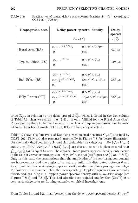
262 FREQUENCY-SELECTIVE CHANNEL MODELS
Table 7.1: Specification of typical delay power spectral densities Sτ ′τ ′(τ′) according to
COST 207 [COS89].
Propagation area Delay power spectral density Delayspread
Sτ ′τ ′(τ ′) B(2)τ ′τ ′
cRA e−9.2τ ′/µs, 0 ≤ τ ′ < 0.7µsRural Area (RA)
0, else0.1 µs
Typical Urban (TU)cTU e−τ ′/µs, 0 ≤ τ ′ < 7µs
0.98 µs0, else
cBU e−τ ′/µs, 0 ≤ τ ′ < 5µs
Bad Urban (BU) cBU12e(5−τ ′/µs), 5µs ≤ τ ′ < 10µs 2.53 µs
0, else
cHT e−3.5τ ′/µs, 0 ≤ τ ′ < 2µs
Hilly Terrain (HT) cHT 0.1e(15−τ ′/µs), 15µs ≤ τ ′ < 20µs 6.88 µs
0, else
bring Tsym in relation to the delay spread B(2)τ ′τ ′ , which is listed in the last column
of Table 7.1, then we realize that (7.46b) is only fulfilled for the Rural Area (RA).Consequently, the RA channel belongs to the class of frequency-nonselective channels,whereas the other channels (TU, BU, HT) are frequency-selective.
Table 7.2 shows the four types of Doppler power spectral densities Sµµ(f) specified byCOST 207. They are also presented graphically in Figure 7.8 for better illustration.For the real-valued constants A1 and A2, preferably the values A1 = 50/
(√2π3fmax
)
and A2 = 101.5/[√
2π(√
10 + 0.15)fmax
]are chosen, since it is then ensured that∫∞
−∞ Sµµ(f) df is equal to one. The classical Jakes power spectral density only occursin the case of very short propagation delays (τ ′ ≤ 0.5 µs) [see Figures 7.8(a) and 7.8(d)].Only in this case, the assumptions that the amplitudes of the scattering componentsare homogeneous and the angles of arrival are uniformly distributed between 0 and2π are justified. For scattering components with medium and long propagation delaysτ ′, however, it is assumed that the corresponding Doppler frequencies are normallydistributed, resulting in a Doppler power spectral density with a Gaussian shape [seeFigures 7.8(b) and 7.8(c)]. This had already been pointed out by Cox [Cox73] at avery early stage after performing extensive empirical investigations.
From Tables 7.1 and 7.2, it can be seen that the delay power spectral density Sτ ′τ ′(τ ′)
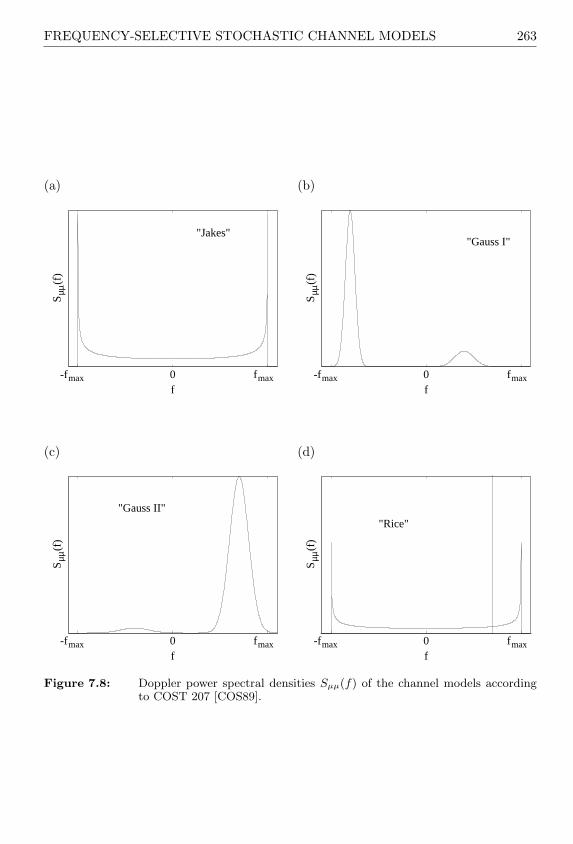
FREQUENCY-SELECTIVE STOCHASTIC CHANNEL MODELS 263
(a)
-fmax 0 fmax f
Sµµ
(f)
"Jakes"
(b)
-fmax 0 fmax f
Sµµ
(f)
"Gauss I"
(c)
-fmax 0 fmax f
Sµµ
(f)
"Gauss II"
(d)
-fmax 0 fmax f
Sµµ
(f)
"Rice"
Figure 7.8: Doppler power spectral densities Sµµ(f) of the channel models accordingto COST 207 [COS89].
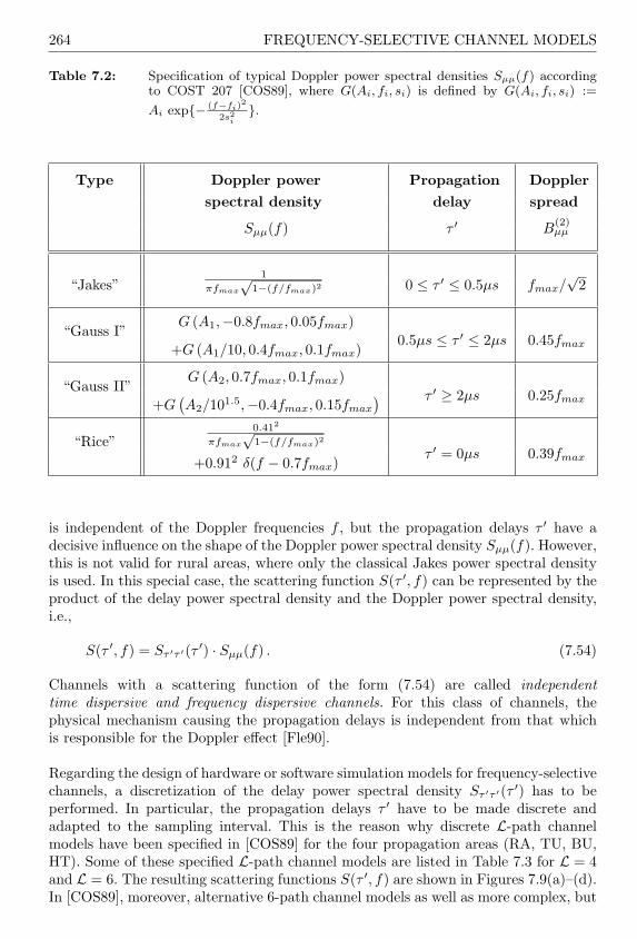
264 FREQUENCY-SELECTIVE CHANNEL MODELS
Table 7.2: Specification of typical Doppler power spectral densities Sµµ(f) accordingto COST 207 [COS89], where G(Ai, fi, si) is defined by G(Ai, fi, si) :=
Ai exp− (f−fi)2
2s2i.
Type Doppler power Propagation Dopplerspectral density delay spread
Sµµ(f) τ ′ B(2)µµ
“Jakes”1
πfmax
√1−(f/fmax)2 0 ≤ τ ′ ≤ 0.5µs fmax/
√2
“Gauss I”G (A1,−0.8fmax, 0.05fmax)
+G (A1/10, 0.4fmax, 0.1fmax)0.5µs ≤ τ ′ ≤ 2µs 0.45fmax
“Gauss II”G (A2, 0.7fmax, 0.1fmax)
+G(A2/101.5,−0.4fmax, 0.15fmax
) τ ′ ≥ 2µs 0.25fmax
“Rice”0.412
πfmax
√1−(f/fmax)2
+0.912 δ(f − 0.7fmax)τ ′ = 0µs 0.39fmax
is independent of the Doppler frequencies f , but the propagation delays τ ′ have adecisive influence on the shape of the Doppler power spectral density Sµµ(f). However,this is not valid for rural areas, where only the classical Jakes power spectral densityis used. In this special case, the scattering function S(τ ′, f) can be represented by theproduct of the delay power spectral density and the Doppler power spectral density,i.e.,
S(τ ′, f) = Sτ ′τ ′(τ ′) · Sµµ(f) . (7.54)
Channels with a scattering function of the form (7.54) are called independenttime dispersive and frequency dispersive channels. For this class of channels, thephysical mechanism causing the propagation delays is independent from that whichis responsible for the Doppler effect [Fle90].
Regarding the design of hardware or software simulation models for frequency-selectivechannels, a discretization of the delay power spectral density Sτ ′τ ′(τ ′) has to beperformed. In particular, the propagation delays τ ′ have to be made discrete andadapted to the sampling interval. This is the reason why discrete L-path channelmodels have been specified in [COS89] for the four propagation areas (RA, TU, BU,HT). Some of these specified L-path channel models are listed in Table 7.3 for L = 4and L = 6. The resulting scattering functions S(τ ′, f) are shown in Figures 7.9(a)–(d).In [COS89], moreover, alternative 6-path channel models as well as more complex, but

FREQUENCY-SELECTIVE STOCHASTIC CHANNEL MODELS 265
therefore more exact, 12-path channel models have been specified. They are presentedin Appendix E for the sake of completeness.
(a) Rural Area
00.2
0.40.6 -fmax
0 fmax -30
-20
-10
0
f (Hz)τ’ (µs)
10 lo
g10
S(τ’
,f)
(b) Typical Urban
0 1 2 3 4 5 −fmax
0 fmax −30
−25
−20
−15
f (Hz)
τ’ (µs)
10 lo
g10
S(τ’
,f)
(c) Bad Urban
02
46
8−fmax
0 fmax
−30
−25
−20
−15
f (Hz)
τ’ (µs)
10 lo
g10
S(τ’
,f)
(d) Hilly Terrain
05
1015 20 −fmax
0 fmax −30
−25
−20
−15
f (Hz)
τ’ (µs)
10 lo
g 10S
(τ’,f
)
Figure 7.9: Scattering functions S(τ ′, f) of the L-path channel models according toCOST 207 [COS89].

266 FREQUENCY-SELECTIVE CHANNEL MODELS
Table 7.3: Specification of the L-path channel models according to COST 207 [COS89],where L = 4 (RA) and L = 6 (TU, BU, HT).
Path no. Propagation Path Category of the Delay` delay power Doppler power spread
τ ′` (lin.) (dB) spectral density B(2)τ ′τ ′
(a) Rural Area
0 0.0 µs 1 0 “Rice”1 0.2 µs 0.63 -2 “Jakes”2 0.4 µs 0.1 -10 “Jakes”
0.1 µs
3 0.6 µs 0.01 -20 “Jakes”
(b) Typical Urban
0 0.0 µs 0.5 -3 “Jakes”1 0.2 µs 1 0 “Jakes”2 0.6 µs 0.63 -2 “Gauss I”3 1.6 µs 0.25 -6 “Gauss I”
1.1 µs
4 2.4 µs 0.16 -8 “Gauss II”5 5.0 µs 0.1 -10 “Gauss II”
(c) Bad Urban
0 0.0 µs 0.5 -3 “Jakes”1 0.4 µs 1 0 “Jakes”2 1.0 µs 0.5 -3 “Gauss I”3 1.6 µs 0.32 -5 “Gauss I”
2.4 µs
4 5.0 µs 0.63 -2 “Gauss II”5 6.6 µs 0.4 -4 “Gauss II”
(d) Hilly Terrain
0 0.0 µs 1 0 “Jakes”1 0.2 µs 0.63 -2 “Jakes”2 0.4 µs 0.4 -4 “Jakes”3 0.6 µs 0.2 -7 “Jakes”
5.0 µs
4 15.0 µs 0.25 -6 “Gauss II”5 17.2 µs 0.06 -12 “Gauss II”

FREQUENCY-SELECTIVE DETERMINISTIC CHANNEL MODELS 267
7.4 FREQUENCY-SELECTIVE DETERMINISTIC CHANNEL MODELS
In this section, we will deal with the derivation and the analysis of frequency-selectivedeterministic channel models. For this purpose, we again apply the principle ofdeterministic channel modelling described in Section 4.1.
7.4.1 System Functions of Frequency-Selective Deterministic ChannelModels
Starting point for the derivation of the system functions of frequency-selectivedeterministic channel models is the time-variant impulse response consisting of a sumof L discrete propagation paths
h(τ ′, t) =L−1∑
`=0
a` µ`(t) δ(τ ′ − τ ′`) . (7.55)
The quantities a` in (7.55) are real-valued and they are called the delay coefficients.As we will see later on, both the delay coefficients a` and the discrete propagationdelays τ ′` [see (7.1)] determine the delay power spectral density of frequency-selectivedeterministic channel models. Strictly speaking, the delay coefficient a` is a measureof the square root of the average delay power which is assigned to the `th discretepropagation path. In general, one can say that the delay coefficients a` and the discretepropagation delays τ ′` determine the frequency-selective behaviour of the channel,which can be attributed to the effect of multipath propagation. In the present case, itis assumed that elliptical scattering zones with different discrete axes are the reasonfor multipath propagation. The disturbances of the channel caused by the Dopplereffect, i.e., the disturbances caused by the motion of the receiver (transmitter), aremodelled in (7.55), according to the principle of deterministic channel modelling, bycomplex deterministic Gaussian processes
µ`(t) = µ1,`(t) + jµ2,`(t) , ` = 0, 1, . . . ,L − 1 , (7.56a)
where
µi,`(t) =Ni,`∑n=1
ci,n,` cos(2πfi,n,`t + θi,n,`) , i = 1, 2 . (7.56b)
Here, Ni,` denotes the number of harmonic functions belonging to the real part(i = 1) or the imaginary part (i = 2) of the `th propagation path. In (7.56b), ci,n,`
is the Doppler coefficient of the nth component of the `th propagation path, and theremaining model parameters fi,n,` and θi,n,` are, as stated before, called the Dopplerfrequencies and the Doppler phases, respectively.
Figure 7.10 shows the structure of the complex Gaussian random process µ`(t) in thecontinuous-time representation. To ensure that the simulation model derived belowhas the same striking properties as a US model, the complex deterministic Gaussianprocesses µ`(t) must be uncorrelated for different propagation paths. Therefore, it isinevitable that the deterministic Gaussian processes µ`(t) and µλ(t) are designed in

268 FREQUENCY-SELECTIVE CHANNEL MODELS
such a way that they are uncorrelated for ` 6= λ, where `, λ = 0, 1, . . . ,L − 1. Thisdemand can easily be fulfilled. One merely has to ensure that the discrete Dopplerfrequencies fi,n,` are designed so that the resulting sets fi,n,` are disjoint (mutuallyexclusive) for different propagation paths. For the simulation model, the demand foruncorrelated scattering (US) propagation can therefore be formulated as follows:
US ⇐⇒ fi,n,` 6= fj,m,λ for ` 6= λ , (7.57)
where i, j = 1, 2, n = 1, 2, . . . , Ni,`, m = 1, 2, . . . , Nj,λ, and `, λ = 0, 1, . . . ,L − 1.
"!$#&%'#&% )(+*#&%'#&% , #&%'#&%
"!$#&% -.% )(+*#&% -.% , #&% -.%
"!$#&% /1032 45% 6(7*#&% /1032 45% , #&% /1032 48%
"! -.%'#&% 9)(+* -.%'#&% :
"! -.% -.% 9)(+* -.% -.% :
"! -.% /<;82 45% =6(7* -.% /<;82 45% >
, -.%'#&%
, -.% -.%
, -.% /<;82 48%
#&% ?5
@-.% 5
Figure 7.10: Simulation model for complex deterministic Gaussian processes µ`(t).
In the following, we assume that the US condition (7.57) is always fulfilled. In thiscase, the correlation properties of the complex deterministic Gaussian processes µ`(t)introduced by (7.56a) can be described by
limT→∞
12T
∫ T
−T
µ∗` (t) µλ(t + τ) dt =
rµ`µ`
(τ) , if ` = λ ,
0 , if ` 6= λ ,(7.58)
where
rµ`µ`(τ) =
2∑
i=1
rµi,`µi,`(τ) , (7.59a)
rµi,`µi,`(τ) =
Ni,`∑n=1
c2i,n,`
2cos(2πfi,n,`τ) (7.59b)

FREQUENCY-SELECTIVE DETERMINISTIC CHANNEL MODELS 269
holds for i = 1, 2 and `, λ = 0, 1, . . . ,L − 1.
At this stage, it should be mentioned that all parameters determining the statisticalbehaviour of the time-variant impulse response h(τ ′, t) can be calculated in such away that the scattering function of the deterministic system approximates a givenspecified or measured scattering function. A procedure for this will be introducedin Subsection 7.4.4. We may therefore assume that the parameters mentioned aboveare not only known, but also constant quantities, which will not be changed duringthe channel simulation run. In this case, the time-variant impulse response h(τ ′, t)is a deterministic function (sample function) which will consequently be called thetime-variant deterministic impulse response. It defines a further important class ofchannel models. In the following, channel models with an impulse response accordingto (7.55) will be called DGUS4 models.
Since the discrete propagation delays τ ′` in (7.55) cannot become negative, h(τ ′, t)fulfils the causality condition, i.e., it holds
h(τ ′, t) = 0 for τ ′ < 0 . (7.60)
By analogy to (7.11), we can compute the output signal y(t) for any given input signalx(t) by applying
y(t) =∫ ∞
0
x(t− τ ′) h(τ ′, t) dτ ′ . (7.61)
If we now employ the expression (7.55) for the time-variant deterministic impulseresponse h(τ ′, t), we obtain
y(t) =L−1∑
`=0
a` µ`(t)x(t− τ ′`) . (7.62)
Hence, the output signal y(t) of the channel can be interpreted as a superpositionof L delayed versions of the input signal x(t − τ ′`), where each of the delayedversions is weighted by a constant delay coefficient a` and a time-variant complexdeterministic Gaussian process µ`(t). Without restriction of generality, we may ignorethe propagation delay of the line-of-sight component in this model. To simplifymatters, we define τ ′0 := 0. This does not cause any problem, because only thepropagation delay differences ∆τ ′` = τ ′` − τ ′`−1 (` = 1, 2, . . . ,L − 1) are relevant forthe system behaviour. From (7.62) follows the tapped-delay-line structure shown inFigure 7.11 of a deterministic simulation model for a frequency-selective mobile radiochannel in the continuous-time representation.
The discrete-time simulation model, required for computer simulations, can beobtained from the continuous-time structure, e.g., by substituting τ ′` → `T ′s,x(t) → x(kT ′s), y(t) → y(kT ′s) and µ`(t) → µ`(kTs), where Ts and T ′s denote sampling
4 DGUS is introduced here as an abbreviation for “deterministic Gaussian uncorrelated scattering”.

270 FREQUENCY-SELECTIVE CHANNEL MODELS
!#"$&%' !#"$&%( !)"$*%+, '
-/. -0 -/1 -23
4.5 6 417
Figure 7.11: Deterministic simulation model for a frequency-selective mobile radiochannel in the equivalent complex baseband.
intervals, k is an integer, and ` refers to the `th propagation path (` = 0, 1, . . . ,L−1).For the propagation delay differences ∆τ ′` = τ ′`− τ ′`−1, we in this case obtain ∆τ ′` → T ′sfor all ` = 1, 2, . . . ,L − 1. The sampling intervals Ts and T ′s have to be sufficientlysmall, but must not necessarily be identical. Between Ts and T ′s, we can thereforeestablish the general relation Ts = m′
s T ′s, where m′s ∈ N is in the following called
the sampling rate ratio. The larger (smaller) the sampling rate ratio m′s is chosen,
the higher (lower) the simulation speed of the channel simulator is and the larger(smaller) the error occurring due to the discretization of µ`(t) is. The sampling rateratio m′
s enables the user to find a good compromise between the simulation speedand the precision of the channel model. As a guideline, m′
s should be chosen so thatthe sampling interval Ts satisfies the condition T ′s ≤ Ts ≤ Tsym for any given symbolinterval Tsym. The upper limit Ts = Tsym corresponds to the often made assumptionthat the impulse response is constant for the duration of one data symbol. However,this assumption is only justified if the product fmax Tsym is very small.
From the general relation (7.62), two important special cases can be derived. Theseare characterized by
(i) a0 6= 0 , a1 = a2 = . . . = aL−1 = 0 (7.63a)
and
(ii) µ`(t) = µ` = const. , ∀ ` = 0, 1, . . . ,L − 1 . (7.63b)
The first special case (i) describes a channel for which all scattering componentscaused by obstacles situated relatively far away from the receiver can be ignored.Using µ(t) := a0µ0(t), we can in this case represent the time-variant deterministic
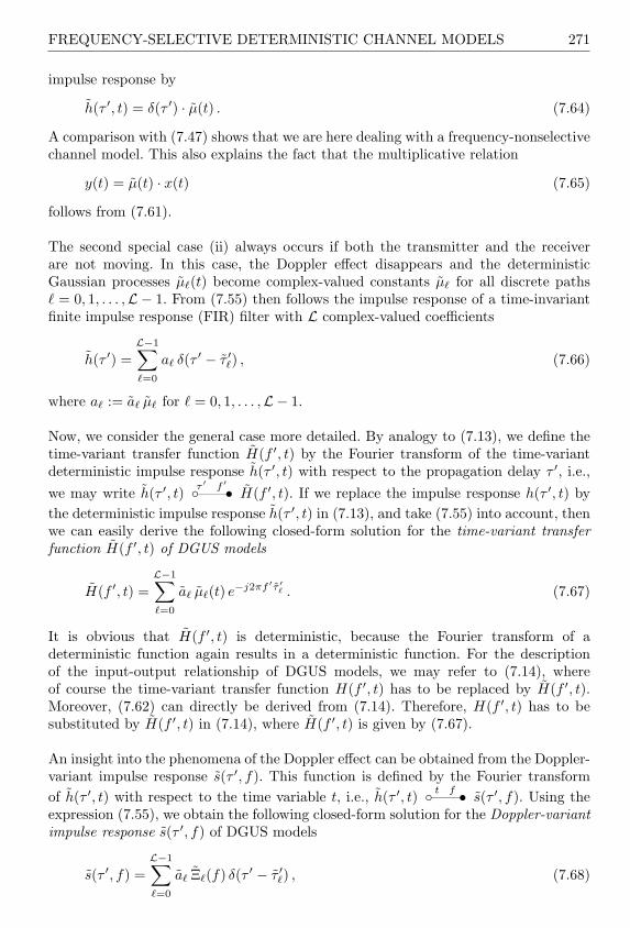
FREQUENCY-SELECTIVE DETERMINISTIC CHANNEL MODELS 271
impulse response by
h(τ ′, t) = δ(τ ′) · µ(t) . (7.64)
A comparison with (7.47) shows that we are here dealing with a frequency-nonselectivechannel model. This also explains the fact that the multiplicative relation
y(t) = µ(t) · x(t) (7.65)
follows from (7.61).
The second special case (ii) always occurs if both the transmitter and the receiverare not moving. In this case, the Doppler effect disappears and the deterministicGaussian processes µ`(t) become complex-valued constants µ` for all discrete paths` = 0, 1, . . . ,L − 1. From (7.55) then follows the impulse response of a time-invariantfinite impulse response (FIR) filter with L complex-valued coefficients
h(τ ′) =L−1∑
`=0
a` δ(τ ′ − τ ′`) , (7.66)
where a` := a` µ` for ` = 0, 1, . . . ,L − 1.
Now, we consider the general case more detailed. By analogy to (7.13), we define thetime-variant transfer function H(f ′, t) by the Fourier transform of the time-variantdeterministic impulse response h(τ ′, t) with respect to the propagation delay τ ′, i.e.,we may write h(τ ′, t) τ ′ f ′——• H(f ′, t). If we replace the impulse response h(τ ′, t) bythe deterministic impulse response h(τ ′, t) in (7.13), and take (7.55) into account, thenwe can easily derive the following closed-form solution for the time-variant transferfunction H(f ′, t) of DGUS models
H(f ′, t) =L−1∑
`=0
a` µ`(t) e−j2πf ′τ ′` . (7.67)
It is obvious that H(f ′, t) is deterministic, because the Fourier transform of adeterministic function again results in a deterministic function. For the descriptionof the input-output relationship of DGUS models, we may refer to (7.14), whereof course the time-variant transfer function H(f ′, t) has to be replaced by H(f ′, t).Moreover, (7.62) can directly be derived from (7.14). Therefore, H(f ′, t) has to besubstituted by H(f ′, t) in (7.14), where H(f ′, t) is given by (7.67).
An insight into the phenomena of the Doppler effect can be obtained from the Doppler-variant impulse response s(τ ′, f). This function is defined by the Fourier transformof h(τ ′, t) with respect to the time variable t, i.e., h(τ ′, t) t f——• s(τ ′, f). Using theexpression (7.55), we obtain the following closed-form solution for the Doppler-variantimpulse response s(τ ′, f) of DGUS models
s(τ ′, f) =L−1∑
`=0
a` Ξ`(f) δ(τ ′ − τ ′`) , (7.68)
272 FREQUENCY-SELECTIVE CHANNEL MODELS
where Ξ`(f) denotes the Fourier transform of µ`(t), i.e.,
Ξ`(f) = Ξ1,`(f) + jΞ2,`(f) , ` = 0, 1, . . . ,L − 1 , (7.69a)
Ξi,`(f) =Ni,`∑n=1
ci,n,`
2[δ(f − fi,n,`) ejθi,n,` + δ(f + fi,n,`) e−jθi,n,`
], i = 1, 2 .
(7.69b)
Thus, s(τ ′, f) is a two-dimensional discrete line spectrum, where the spectral linesare located at the discrete positions (τ ′, f) = (τ ′`,±fi,n,`) and weighted by thecomplex-valued factors 1
2 a`ci,n,`e±jθi,n,` . For the description of the input-output
behaviour, the relation (7.19) is useful, if the Doppler-variant impulse responses(τ ′, f) is substituted by s(τ ′, f) there. It should also be observed that (7.62) followsfrom (7.19), if in the latter equation s(τ ′, f) is replaced by (7.68).
Finally, we consider the Doppler-variant transfer function T (f ′, f) of DGUS modelswhich is defined by the two-dimensional Fourier transform of the time-variantdeterministic impulse response h(τ ′, t), i.e., h(τ ′, t) τ ′,t f ′,f————• T (f ′, f). Due to
h(τ ′, t) τ ′ f ′——• H(f ′, t) and h(τ ′, t) t f——• s(τ ′, f), the computation of an expressionfor T (f ′, f) can also be carried out via the one-dimensional Fourier transformH(f ′, t) t f——• T (f ′, f) or s(τ ′, f) τ ′ f ′——• T (f ′, f). No matter which procedure wedecide upon, we in any case obtain the following closed-form expression for theDoppler-variant transfer function T (f ′, f) of the deterministic system
T (f ′, f) =L−1∑
`=0
a` Ξ`(f) e−j2πf ′τ ′` . (7.70)
Summarizing, we should keep in mind that when the model parameters ci,n,`,fi,n,`, θi,n,`, a`, τ ′`, Ni,`, and L are known and constant quantities, the foursystem functions h(τ ′, t), H(f ′, t), s(τ ′, f), and T (f ′, f) can be calculated explicitly.By analogy to Figure 7.3, the system functions of deterministic channel models arerelated in pairs by the Fourier transform. The resulting relationships are illustratedin Figure 7.12.
7.4.2 Correlation Functions and Power Spectral Densities of DGUSModels
With reference to the WSSUS model, analog relations can be established in the generalsense for the correlation functions and power spectral densities of the frequency-selective deterministic channel model (DGUS model). In particular, the correlationfunctions of the four system functions h(τ ′, t), H(f ′, t), s(τ ′, f), and T (f ′, f) of thedeterministic system can be represented by the following relations:
rhh(τ ′1, τ′2; t, t + τ) = δ(τ ′2 − τ ′1) Shh(τ ′1, τ) , (7.71a)

FREQUENCY-SELECTIVE DETERMINISTIC CHANNEL MODELS 273
transfer function
Time-variantimpulse response
impulse responseDoppler-variant
f
fτ
τ τ
fτ
f
τ f
τ
f
Doppler-variant
f
transfer functionTime-variant
H( ,t)s( ,f)
T( ,f)
~
~
~
~
h( ,t)t
ft
f t
f t
Figure 7.12: Relationships between the system functions of frequency-selectivedeterministic channel models.
rHH(f ′, f ′ + υ′; t, t + τ) = rHH(υ′, τ) , (7.71b)rss(τ ′1, τ
′2; f1, f2) = δ(f2 − f1) δ(τ ′2 − τ ′1) S(τ ′1, f1) , (7.71c)
rTT (f ′, f ′ + υ′; f1, f2) = δ(f2 − f1) STT (υ′, f1) . (7.71d)
In these equations, Shh(τ ′1, τ) denotes the delay cross-power spectral density,rHH(υ′, τ) is the time-frequency correlation function, S(τ ′1, f1) is the scatteringfunction, and STT (υ′, f1) is the Doppler cross-power spectral density of thedeterministic system. Two of these quantities at a time form a Fourier transform pairin the same way as for the WSSUS model. By analogy to Figure 7.5, we obtain therelations depicted in Figure 7.13 for frequency-selective deterministic channel models.In order to simplify the notation, the variables τ ′1 and f1 have again been replaced byτ ′ and f , respectively.
The interpretation of h(τ ′, t) as time-variant deterministic function, enables us toderive closed-form solutions for the correlation functions (7.71a)–(7.71d), and, hence,also for the functions shown in Figure 7.13. This provides the basis for analysing thestatistical properties of the deterministic channel model analytically. We will dealwith this task in the following.
Therefore, we at first define the autocorrelation function of the time-variantdeterministic impulse response h(τ ′, t) as follows
rhh(τ ′1, τ′2; t, t + τ) := lim
T→∞1
2T
∫ T
−T
h∗(τ ′1, t) h(τ ′2, t + τ) dt . (7.72)
It should be taken into account that the time averaging, which has to be carried outhere, is in contrast to (7.23a), whereas the computation of the autocorrelation function

274 FREQUENCY-SELECTIVE CHANNEL MODELS
υTT
fS ( , )
τhh τS ( , )
fτS ( , ) υ
τ
υ
υτ
υ
τ
τ
υ
~τr ( , )
HH
τ
τ
f
τ
f
τ
f
f
Delay cross-
Time-frequencycorrelation function
Scatteringfunction
power spectral density
Doppler cross-power spectral density
~
~
~
Figure 7.13: Relationships between the delay cross-power spectral density Shh(τ ′, τ),the time-frequency correlation function rHH(υ′, τ), the scattering function
S(τ ′, f), and the Doppler cross-power spectral density STT (υ′, f) of DGUSmodels.
of the stochastic impulse response h(τ ′, t) requires statistical averaging (ensembleaverage). In the equation above, we use the expression (7.55) for h(τ ′, t), so thatwe may write
rhh(τ ′1, τ′2; t, t + τ) = lim
T→∞1
2T
∫ T
−T
[L−1∑
`=0
a` µ∗` (t) δ(τ ′1 − τ ′`)
]
·[L−1∑
λ=0
aλ µλ(t + τ) δ(τ ′2 − τ ′λ)
]dt
= limT→∞
L−1∑
`=0
L−1∑
λ=0
a` aλ δ(τ ′1 − τ ′`) δ(τ ′2 − τ ′λ)
· 12T
∫ T
−T
µ∗` (t) µλ(t + τ) dt . (7.73)
Using (7.58), it follows
rhh(τ ′1, τ′2; t, t + τ) =
L−1∑
`=0
a2` rµ`µ`
(τ) δ(τ ′1 − τ ′`) δ(τ ′2 − τ ′`) . (7.74)
Generally, the product of two delta functions is not defined. But in the present case,however, the first delta function appearing in (7.74) depends on the variable τ ′1 and the

FREQUENCY-SELECTIVE DETERMINISTIC CHANNEL MODELS 275
second one on τ ′2. Since τ ′1 and τ ′2 are independent variables, the product will not causeany problems in the two-dimensional (τ ′1, τ
′2)-plane. Furthermore, δ(τ ′1 − τ ′`) δ(τ ′2 − τ ′`)
is equivalent to δ(τ ′1 − τ ′`) δ(τ ′2 − τ ′1), so that (7.74) can be represented by
rhh(τ ′1, τ′2; t, t + τ) = δ(τ ′2 − τ ′1) Shh(τ ′1, τ) , (7.75)
where
Shh(τ ′, τ) =L−1∑
`=0
a2` rµ`µ`
(τ) δ(τ ′ − τ ′`) (7.76)
denotes the delay cross-power spectral density of frequency-selective deterministicchannel models. Note that (7.75) has the same form as (7.33). The delay cross-powerspectral density Shh(τ ′, τ) can be computed explicitly in connection with the auto-correlation functions (7.59a) and (7.59b) if all model parameters ci,n,`, fi,n,`,a`, τ ′`, Ni,`, and L are known.
The Fourier transform of the delay cross-power spectral density Shh(τ ′, τ) with respectto the propagation delay τ ′ results in the time-frequency correlation function
rHH(υ′, τ) =L−1∑
`=0
a2` rµ`µ`
(τ) e−j2πυ′τ ′` (7.77)
of the deterministic system.
Preferably, we also refer to the delay cross-power spectral density Shh(τ ′, τ) in orderto calculate an analytical expression for the scattering function. The Fourier transformof (7.76) with respect to τ immediately leads to the expression
S(τ ′, f) =L−1∑
`=0
a2` Sµ`µ`
(f) δ(τ ′ − τ ′`) , (7.78)
which describes the scattering function of frequency-selective deterministic channelmodels. In this equation,
Sµ`µ`(f) =
2∑
i=1
Ni,`∑n=1
c2i,n,`
4[δ(f − fi,n,`) + δ(f + fi,n,`)] , ` = 0, 1, . . . ,L− 1 ,(7.79)
represents the Doppler power spectral density of the `th scattering component, which isdefined by the Fourier transform of the autocorrelation function rµ`µ`
(τ) according to(7.59a). Now it becomes obvious that the scattering function S(τ ′, f) of deterministicchannel models can be represented by a finite sum of weighted delta functions.The delta functions are located in the two-dimensional (τ ′, f)-plain at the positions(τ ′`, ±fi,n,`), and are weighted by the constants (a`ci,n,`)2/4. Without restrictionof generality, we assume in the following that the scattering function S(τ ′, f) isnormalized to unity, so that the volume under S(τ ′, f) is equal to one, i.e.,
∫ ∞
−∞
∫ ∞
0
S(τ ′, f) dτ ′ df = 1 . (7.80)
276 FREQUENCY-SELECTIVE CHANNEL MODELS
To ensure that (7.80) is definitely fulfilled, the Doppler coefficients ci,n,` and the delaycoefficients a` have to fulfil the boundary conditions
Ni,`∑n=1
c2i,n,` = 1 and
L−1∑
`=0
a2` = 1 . (7.81a, b)
Finally, we determine the Fourier transform of the scattering function S(τ ′, f) withrespect to τ ′ in order to obtain the Doppler cross-power spectral density
STT (υ′, f) =L−1∑
`=0
a2` Sµ`µ`
(f) e−j2πυ′τ ′` (7.82)
of frequency-selective deterministic channel models. We can easily assure ourselves ofthe fact that one also obtains the Doppler cross-power spectral density STT (υ′, f) inthe presented form (7.82), if the alternative possibility — via the Fourier transformof the time-frequency correlation function rHH(υ′, τ) with respect to τ — is madeuse of, where in this case the relation (7.77) has to be used for rHH(υ′, τ).
Thus, it has been shown that the four functions Shh(τ ′, τ), rHH(υ′, τ), S(τ, f), andSTT (υ′, f) characterizing the deterministic system can be calculated analytically, ifthe relevant model parameters ci,n,`, fi,n,`, a`, τ ′`, Ni,`, and L are known.
7.4.3 Delay Power Spectral Density, Doppler Power Spectral Density,and Characteristic Quantities of DGUS Models
In this subsection, simple closed-form solutions will be derived for the fundamentalcharacteristic functions and quantities of DGUS models, such as the delay powerspectral density, Doppler power spectral density, and delay spread. For this purpose,we will here discuss the terms introduced for stochastic models (WSSUS models) inSubsection 7.3.2.3 for deterministic systems.
Delay power spectral density: Let S(τ ′, f) be the scattering function of adeterministic channel model, then, by analogy to (7.38), the corresponding Delaypower spectral density Sτ ′τ ′(τ ′) is defined by
Sτ ′τ ′(τ ′) := Shh(τ ′, 0)
=∫ ∞
−∞S(τ ′, f) df . (7.83)
After employing (7.78) and considering the boundary condition (7.81a), it follows
Sτ ′τ ′(τ ′) =L−1∑
`=0
a2` δ(τ ′ − τ ′`) . (7.84)

FREQUENCY-SELECTIVE DETERMINISTIC CHANNEL MODELS 277
Hence, the delay power spectral density Sτ ′τ ′(τ ′) is a discrete line spectrum, wherethe spectral lines are located at the discrete positions τ ′ = τ ′` and weighted by theconstants a2
` . Consequently, the behaviour of Sτ ′τ ′(τ ′) is completely determinedby the model parameters a`, τ ′`, and L. It should be pointed out that the areaunder the Delay power spectral density Sτ ′τ ′(τ ′) is equal to one due to (7.81b), i.e.,∫∞0
Sτ ′τ ′(τ ′) dτ ′ = 1.
Average delay: Let Sτ ′τ ′(τ ′) be the delay power spectral density of a deterministicchannel model, then the first moment of Sτ ′τ ′(τ ′) is called the average delay B
(1)τ ′τ ′ .
Thus, by analogy to (7.39), the definition
B(1)τ ′τ ′ :=
∫∞−∞ τ ′ Sτ ′τ ′(τ ′) dτ ′∫∞−∞ Sτ ′τ ′(τ ′) dτ ′
(7.85)
holds. Putting (7.84) in (7.85) and taking the boundary condition (7.81b) into account,then the average delay B
(1)τ ′τ ′ can be expressed in closed form as follows
B(1)τ ′τ ′ =
L−1∑
`=0
τ ′` a2` . (7.86)
Delay spread: The square root of the second central moment of Sτ ′τ ′(τ ′) is calledthe Delay spread B
(2)τ ′τ ′ , which is, by analogy to (7.40), defined by
B(2)τ ′τ ′ :=
√√√√√∫∞−∞
(τ ′ − B
(1)τ ′τ ′
)2
Sτ ′τ ′(τ ′) dτ ′∫∞−∞ Sτ ′τ ′(τ ′) dτ ′
. (7.87)
With (7.84) and (7.81b), the closed-form expression
B(2)τ ′τ ′ =
√√√√L−1∑
`=0
(τ ′` a`)2 −
(B
(1)τ ′τ ′
)2
(7.88)
can be derived, where B(1)τ ′τ ′ is the average delay according to (7.86).
Doppler power spectral density: Let S(τ ′, f) be the scattering function of adeterministic channel model, then — by analogy to (7.42) — the correspondingDoppler power spectral density Sµµ(f) can be determined via the relation
Sµµ(f) := STT (0, f)
=∫ ∞
−∞S(τ ′, f) dτ ′ . (7.89)
With the scattering function S(τ ′, f) given by (7.78), we can now derive a closed-formsolution for the Doppler power spectral density Sµµ(f) of the deterministic system.

278 FREQUENCY-SELECTIVE CHANNEL MODELS
Thus, we obtain
Sµµ(f) =L−1∑
`=0
a2` Sµ`µ`
(f) , (7.90)
where Sµ`µ`(f) denotes the Doppler power spectral density of the `th scattering
component determined by (7.79). This result shows that the Doppler power spectraldensity Sµµ(f) of frequency-selective deterministic channel models is given by thesum of the Doppler power spectral densities Sµ`µ`
(f) of all propagation paths` = 0, 1, . . . ,L, where each individual Doppler power spectral density Sµ`µ`
(f) has tobe weighted by the square of the corresponding delay coefficient. Here, the square ofthe delay coefficient a2
` represents the path power, that is the mean (average) powerof the `th scattering component.
With knowledge of the Doppler power spectral density Sµµ(f) or Sµ`µ`(f), the average
Doppler shift and the Doppler spread can be computed. The definition, derivation,and discussion of these characteristic quantities have already been performed inSection 4.2. We will refrain from a recapitulation of these results at this place.
Frequency correlation function: Let rHH(υ′, τ) be the time-frequency correlationfunction of a deterministic channel model. Then, by analogy to (7.44), the frequencycorrelation function rτ ′τ ′(υ′) is defined by the time-frequency correlation functionrHH(υ′, τ) at τ = t2 − t1 = 0, i.e.,
rτ ′τ ′(υ′) := rHH(υ′, 0)
=∫ ∞
−∞
∫ ∞
−∞S(τ ′, f) e−j2πυ′τ ′ dτ ′ df
=∫ ∞
−∞Sτ ′τ ′(τ ′) e−j2πυ′τ ′ dτ ′ . (7.91)
A closed-form expression for the frequency correlation function rτ ′τ ′(υ′) is obtainedin a simple way by setting τ = 0 in (7.77). Taking the boundary condition (7.81a)into consideration, which implies that rµ`µ`
(0) = 1 holds for all ` = 0, 1, . . . ,L− 1, wethen obtain
rτ ′τ ′(υ′) =L−1∑
`=0
a2` e−j2πυ′τ ′` . (7.92)
Coherence bandwidth: Let rτ ′τ ′(υ′) be the frequency correlation function given by(7.92), then the frequency separation variable υ′ = BC for which
|rτ ′τ ′(BC)| = 12|rτ ′τ ′(0)| (7.93)
holds, is called the coherence bandwidth of deterministic channel models. With(7.92) and taking the boundary condition (7.81b) into consideration, we obtain the
FREQUENCY-SELECTIVE DETERMINISTIC CHANNEL MODELS 279
transcendental equation∣∣∣∣∣L−1∑
`=0
a2` e−j2πBCτ ′`
∣∣∣∣∣−12
= 0 . (7.94)
The smallest positive value for BC which fulfils the equation above is the coherencebandwidth. Apart from simple special cases, (7.94) has generally to be solved bymeans of numerical root-finding techniques. The Newton-Raphson method is one of themost powerful and well-known numerical methods for solving root-finding problems.
Time correlation function: Let rHH(υ′, τ) be the time-frequency correlationfunction of a deterministic channel model. Then, by analogy to (7.50), the timecorrelation function rµµ(τ) is defined by the time-frequency correlation functionrHH(υ′, τ) at υ′ = f ′2 − f ′1 = 0, i.e.,
rµµ(τ) := rHH(0, τ)
=∫ ∞
−∞
∫ ∞
−∞S(τ ′, f) ej2πfτ dτ ′ df
=∫ ∞
−∞Sµµ(f) ej2πfτ df . (7.95)
We consider (7.77) at υ′ = 0 and, thus, obtain
rµµ(τ) =L−1∑
`=0
a2` rµ`µ`
(τ) . (7.96)
Coherence time: Let rµµ(τ) be the time correlation function given by (7.96), thenthe time interval τ = TC for which
|rµµ(TC)| = 12|rµµ(0)| (7.97)
holds, is called the coherence time of deterministic channel models. Substituting (7.96)in (7.97), and taking (7.59a) and (7.59b) into account, results in the transcendentalequation
∣∣∣∣∣∣
2∑
i=1
L−1∑
`=0
Ni,`∑n=1
(a`ci,n,`)2
2cos(2πfi,n,`TC)
∣∣∣∣∣∣− 1
2= 0 , (7.98)
from which the coherence time TC can be computed by applying numerical zerofinding techniques. The smallest positive value for TC which solves (7.98) is thecoherence time.
In order to facilitate an overview, the above derived relationships between thecorrelation functions and the power spectral densities as well as the characteristicquantities of frequency-selective deterministic channel models derivable from theseare depicted in Figure 7.14.
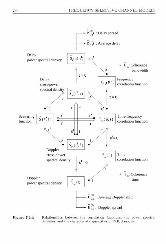
280 FREQUENCY-SELECTIVE CHANNEL MODELS
time
bandwidth
τ τ
τ τ~ υr ( )
~µµ
r ( )τ
υTT
fS ( , )
µµS (f)
µµ(1)
µµ(2)
τ
τυ
υ
υ
τ
τ
υ
τ
υ
τ
υ
τ
τ
τ
τ
τ(2)
T
τ = 0
τ = 0
υ = 0
υ = 0
~
~
~
~
~ ~
~
~
~
~
~
τ
fτS ( , ) τHH
r ( , )f
f
τ
S ( , )hh ττ
f
τ
f
τ
f
B
~S ( )
(1)
B
B
B
B
Time-frequencycorrelation function
correlation functionTime
Frequencycorrelation function
Delaycross-powerspectral density
Dopplercross-powerspectral density
Delaypower spectral density
C: Coherence
: Average delay
: Delay spread
C: CoherenceDopplerpower spectral density
: Average Doppler shift
: Doppler spread
Scatteringfunction
Figure 7.14: Relationships between the correlation functions, the power spectraldensities, and the characteristic quantities of DGUS models.
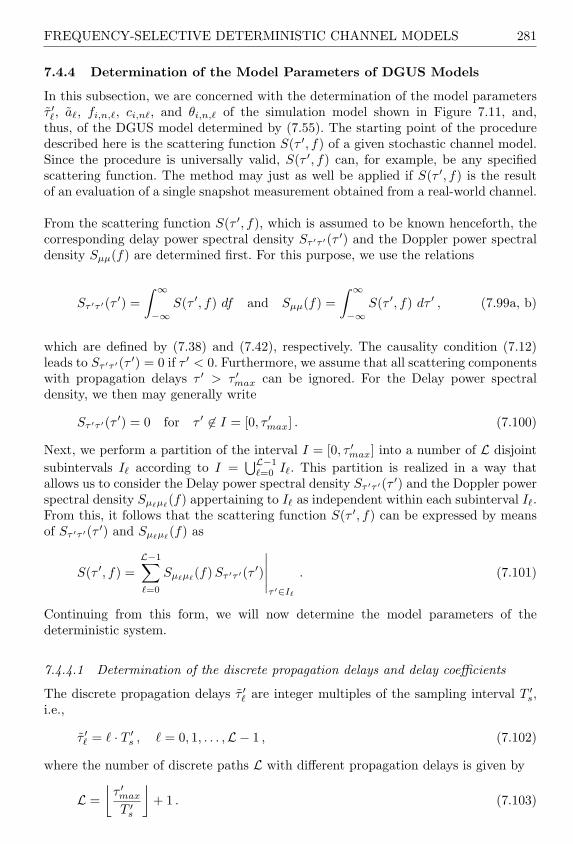
FREQUENCY-SELECTIVE DETERMINISTIC CHANNEL MODELS 281
7.4.4 Determination of the Model Parameters of DGUS Models
In this subsection, we are concerned with the determination of the model parametersτ ′`, a`, fi,n,`, ci,n`, and θi,n,` of the simulation model shown in Figure 7.11, and,thus, of the DGUS model determined by (7.55). The starting point of the proceduredescribed here is the scattering function S(τ ′, f) of a given stochastic channel model.Since the procedure is universally valid, S(τ ′, f) can, for example, be any specifiedscattering function. The method may just as well be applied if S(τ ′, f) is the resultof an evaluation of a single snapshot measurement obtained from a real-world channel.
From the scattering function S(τ ′, f), which is assumed to be known henceforth, thecorresponding delay power spectral density Sτ ′τ ′(τ ′) and the Doppler power spectraldensity Sµµ(f) are determined first. For this purpose, we use the relations
Sτ ′τ ′(τ ′) =∫ ∞
−∞S(τ ′, f) df and Sµµ(f) =
∫ ∞
−∞S(τ ′, f) dτ ′ , (7.99a, b)
which are defined by (7.38) and (7.42), respectively. The causality condition (7.12)leads to Sτ ′τ ′(τ ′) = 0 if τ ′ < 0. Furthermore, we assume that all scattering componentswith propagation delays τ ′ > τ ′max can be ignored. For the Delay power spectraldensity, we then may generally write
Sτ ′τ ′(τ ′) = 0 for τ ′ 6∈ I = [0, τ ′max] . (7.100)
Next, we perform a partition of the interval I = [0, τ ′max] into a number of L disjointsubintervals I` according to I =
⋃L−1`=0 I`. This partition is realized in a way that
allows us to consider the Delay power spectral density Sτ ′τ ′(τ ′) and the Doppler powerspectral density Sµ`µ`
(f) appertaining to I` as independent within each subinterval I`.From this, it follows that the scattering function S(τ ′, f) can be expressed by meansof Sτ ′τ ′(τ ′) and Sµ`µ`
(f) as
S(τ ′, f) =L−1∑
`=0
Sµ`µ`(f) Sτ ′τ ′(τ ′)
∣∣∣∣∣τ ′∈I`
. (7.101)
Continuing from this form, we will now determine the model parameters of thedeterministic system.
7.4.4.1 Determination of the discrete propagation delays and delay coefficients
The discrete propagation delays τ ′` are integer multiples of the sampling interval T ′s,i.e.,
τ ′` = ` · T ′s , ` = 0, 1, . . . ,L − 1 , (7.102)
where the number of discrete paths L with different propagation delays is given by
L =⌊
τ ′max
T ′s
⌋+ 1 . (7.103)
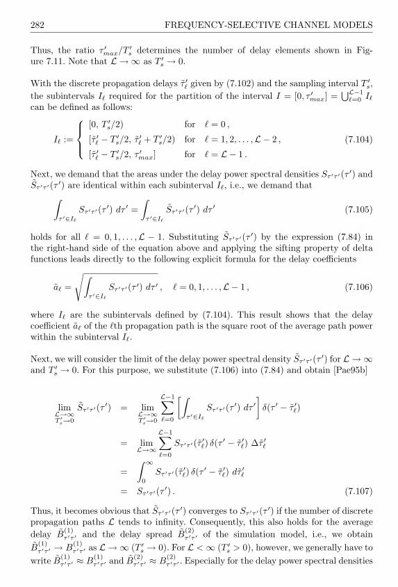
282 FREQUENCY-SELECTIVE CHANNEL MODELS
Thus, the ratio τ ′max/T ′s determines the number of delay elements shown in Fig-ure 7.11. Note that L → ∞ as T ′s → 0.
With the discrete propagation delays τ ′` given by (7.102) and the sampling interval T ′s,the subintervals I` required for the partition of the interval I = [0, τ ′max] =
⋃L−1`=0 I`
can be defined as follows:
I` :=
[0, T ′s/2) for ` = 0 ,
[τ ′` − T ′s/2, τ ′` + T ′s/2) for ` = 1, 2, . . . ,L − 2 ,
[τ ′` − T ′s/2, τ ′max] for ` = L − 1 .
(7.104)
Next, we demand that the areas under the delay power spectral densities Sτ ′τ ′(τ ′) andSτ ′τ ′(τ ′) are identical within each subinterval I`, i.e., we demand that
∫
τ ′∈I`
Sτ ′τ ′(τ ′) dτ ′ =∫
τ ′∈I`
Sτ ′τ ′(τ ′) dτ ′ (7.105)
holds for all ` = 0, 1, . . . ,L − 1. Substituting Sτ ′τ ′(τ ′) by the expression (7.84) inthe right-hand side of the equation above and applying the sifting property of deltafunctions leads directly to the following explicit formula for the delay coefficients
a` =
√∫
τ ′∈I`
Sτ ′τ ′(τ ′) dτ ′ , ` = 0, 1, . . . ,L − 1 , (7.106)
where I` are the subintervals defined by (7.104). This result shows that the delaycoefficient a` of the `th propagation path is the square root of the average path powerwithin the subinterval I`.
Next, we will consider the limit of the delay power spectral density Sτ ′τ ′(τ ′) for L → ∞and T ′s → 0. For this purpose, we substitute (7.106) into (7.84) and obtain [Pae95b]
limL→∞T ′s→0
Sτ ′τ ′(τ ′) = limL→∞T ′s→0
L−1∑
`=0
[∫
τ ′∈I`
Sτ ′τ ′(τ ′) dτ ′]
δ(τ ′ − τ ′`)
= limL→∞
L−1∑
`=0
Sτ ′τ ′(τ ′`) δ(τ ′ − τ ′`) ∆τ ′`
=∫ ∞
0
Sτ ′τ ′(τ ′`) δ(τ ′ − τ ′`) dτ ′`
= Sτ ′τ ′(τ ′) . (7.107)
Thus, it becomes obvious that Sτ ′τ ′(τ ′) converges to Sτ ′τ ′(τ ′) if the number of discretepropagation paths L tends to infinity. Consequently, this also holds for the averagedelay B
(1)τ ′τ ′ and the delay spread B
(2)τ ′τ ′ of the simulation model, i.e., we obtain
B(1)τ ′τ ′ → B
(1)τ ′τ ′ as L → ∞ (T ′s → 0). For L < ∞ (T ′s > 0), however, we generally have to
write B(1)τ ′τ ′ ≈ B
(1)τ ′τ ′ and B
(2)τ ′τ ′ ≈ B
(2)τ ′τ ′ . Especially for the delay power spectral densities
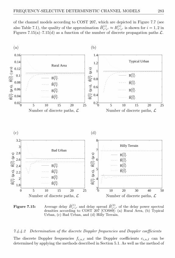
FREQUENCY-SELECTIVE DETERMINISTIC CHANNEL MODELS 283
of the channel models according to COST 207, which are depicted in Figure 7.7 (seealso Table 7.1), the quality of the approximation B
(i)τ ′τ ′ ≈ B
(i)τ ′τ ′ is shown for i = 1, 2 in
Figures 7.15(a)–7.15(d) as a function of the number of discrete propagation paths L.
(a)
0 5 10 15 20 250.02
0.04
0.06
0.08
0.1
0.12
0.14
0.16
B(1
)τ’
τ’ (
µ s)
, B
(2)
τ’τ’
( µ
s) Rural Area
B(1)τ’τ’
B(1)τ’τ’
B(2)τ’τ’
B(2)τ’τ’
Number of discrete paths, L
(b)
0 5 10 15 20 250.2
0.4
0.6
0.8
1
1.2
1.4
B(1
)τ’
τ’ (
µ s)
, B
(2)
τ’τ’
(µ
s)
Typical Urban
B(1)τ’τ’
B(1)τ’τ’
B(2)τ’τ’
B(2)τ’τ’
Number of discrete paths, L
(c)
0 5 10 15 20 25
1.8
2
2.2
2.4
2.6
2.8
3
3.2
B(1
)τ’
τ’ (
µ s)
, B
(2)
τ’τ’
(µ
s)
Bad Urban
B(1)τ’τ’
B(1)τ’τ’
B(2)τ’τ’
B(2)τ’τ’
Number of discrete paths, L
(d)
0 10 20 30 40 503
4
5
6
7
8
B(1
)τ’
τ’ (
µ s)
, B
(2)
τ’τ’
(µ
s)
Hilly Terrain
B(1)τ’τ’
B(1)τ’τ’
B(2)τ’τ’
B(2)τ’τ’
Number of discrete paths, L
Figure 7.15: Average delay B(1)
τ ′τ ′ and delay spread B(2)
τ ′τ ′ of the delay power spectraldensities according to COST 207 [COS89]: (a) Rural Area, (b) TypicalUrban, (c) Bad Urban, and (d) Hilly Terrain.
7.4.4.2 Determination of the discrete Doppler frequencies and Doppler coefficients
The discrete Doppler frequencies fi,n,` and the Doppler coefficients ci,n,` can bedetermined by applying the methods described in Section 5.1. As well as the method of

284 FREQUENCY-SELECTIVE CHANNEL MODELS
exact Doppler spread (MEDS), we preferably also use the Lp-norm method (LPNM).The first method mentioned is especially recommended for the Jakes power spectraldensity. However, it has to be taken into account that the complex deterministicGaussian processes µ`(t) are designed in such a way that µ`(t) and µλ(t) areuncorrelated for ` 6= λ (`, λ = 0, 1, . . . ,L − 1). This is always the case if the discreteDoppler frequencies fi,n,` fulfil the condition (7.57). Using the MEDS, this condition isalways fulfilled in case the number of harmonic functions Ni,` are chosen in such a waythat Ni,` 6= Nj,λ holds if ` 6= λ, where i, j = 1, 2 and `, λ = 0, 1, . . . ,L − 1. However,when using the LPNM method, we do not have to take the inequality Ni,` 6= Nj,λ
into account, because even for Ni,` = Nj,λ, disjoint sets fi,n,` and fj,m,λ with` 6= λ can easily be found, so that the resulting deterministic processes µ`(t) andµλ(t) are uncorrelated for ` 6= λ. For this purpose, it is sufficient to either minimizethe Lp-norm (5.61) by using different values for the parameter p, or by performing theoptimization of each set fi,n,` of discrete Doppler frequencies with different valuesfor the quantity τmax defining the upper limit of the integral in (5.61). Having thisin mind, the numerical optimization of the autocorrelation function rµi,`µi,`
(τ) [see(7.59b)] guarantees that the desired property
fi,n,`⋂fj,m,λ = ∅ ⇐⇒ ` 6= λ (7.108)
is usually fulfilled for all i, j = 1, 2, n = 1, 2, . . . , Ni,`, m = 1, 2, . . . , Nj,λ, and`, λ = 0, 1, . . . ,L − 1.
7.4.4.3 Determination of the Doppler phases
In Subsections 7.4.2 and 7.4.3, it was pointed out that the Doppler phases θi,n,` haveno influence on the system functions shown in Figure 7.14. Hence, we may concludethat the fundamental statistical properties of DGUS models are independent of thechoice of the Doppler phases θi,n,`. The statements made in Section 5.2 are still validfor the frequency-selective case. Therefore, we once again may assume that the Dopplerphases θi,n,` are realizations of a random variable, uniformly distributed in the interval(0, 2π]. Alternatively, θi,n,` can also be determined by applying the deterministicprocedure described in Section 5.2. In both cases different events (sets) θi,n,` alwaysresult in different realizations (sample functions) for the time-variant impulse responseh(τ ′, t) but, nevertheless, all impulse responses have the same statistical properties. Inother words: every realization of the impulse response h(τ ′, t) contains the completestatistical information.
7.4.5 Deterministic Simulation Models for the Channel ModelsAccording to COST 207
At the end of this chapter, we will once more pick up the channel models accordingto COST 207 [COS89] and will show how to develop efficient simulation models forthem. For this purpose, we restrict our attention to the 4-path and 6-path channelmodels (RA, TU, BU, HT) specified in Table 7.3. Due to the fact that these modelsare already presented in a discrete form with respect to τ ′, the discrete propagationdelays τ ′` can directly be equated with the values for τ ′`, presented in Table 7.3, i.e.,

FREQUENCY-SELECTIVE DETERMINISTIC CHANNEL MODELS 285
τ ′` = τ ′`. Adaptation of the sampling interval T ′s to the discrete propagation delays τ ′`is achieved here by τ ′` = q` · T ′s, where q` denotes an integer and T ′s is the greatestcommon divisor of τ ′1, τ
′2, . . . , τ
′L−1, i.e., T ′s = gcdτ ′`L−1
`=1 . The corresponding delaycoefficients a` are identical to the square root of the path power as listed in Table 7.3.
The specifications for the Doppler power spectral density can be found in Table 7.2. Inthe case of the Jakes power spectral density, we determine the model parameters fi,n,`
and ci,n,` by applying the Lp-norm method described in Subsection 5.1.5, taking intoaccount that (7.108) is fulfilled. For the Gaussian power spectral densities (Gauss Iand Gauss II), the third variant of the Lp-norm method (LPNM III) is of advantage.For the solution of the present problem, it is recommended to start with a Gaussianrandom process νi,`(t) having a symmetrical Gaussian power spectral density of theform
Sνi,`νi,`(f) = Ai,` e
− f2
2s2i,` , i = 1, 2 , (7.109)
and then perform a frequency shift of fi,0,`, which finally results in
Sµ`µ`(f) =
2∑
i=1
Sνi,`νi,`(f − fi,0,`) , (7.110)
where Ai,`, si,`, and fi,0,` denote the quantities specified in Table 7.2. Theautocorrelation function required for the minimization of the error function (5.65)is in the present case given by the inverse Fourier transform of (7.109), i.e.,
rνi,`νi,`(τ) = σ2
i,` e−2(πsi,`τ)2 , (7.111)
where σ2i,` =
√2π Ai,` si,` describes the variance of the Gaussian random process
νi,`(t). For the simulation model this means that we first have to determine the modelparameters fi,n,` and ci,n,` of the deterministic process
νi,`(t) =Ni,`∑n=1
ci,n,` cos(2πfi,n,` + θi,n,`) (7.112)
by using the LPNM III. The application of the frequency translation theorem of theFourier transform then provides the demanded complex deterministic Gaussian processin the form
µ`(t) =2∑
i=1
νi,`(t) e−j2πfi,0,`t
=2∑
i=1
νi,`(t) cos(2πfi,0,`t)− j
2∑
i=1
νi,`(t) sin(2πfi,0,`t) . (7.113)
The resulting simulation model for the complex deterministic process µ`(t) is shownin Figure 7.16.

286 FREQUENCY-SELECTIVE CHANNEL MODELS
! #"%$&"%$ ')(+*-,"%$&"%$ '/. 0 "%$&"%$ '
! #"%$ 12$ ')(+*-,"%$ 12$ '/. 0 "%$ 12$ '
! #"%$ 35476 89$ ':(;*<,"%$ 35476 89$ '=. 0 "%$ 35476 8>$ '
! 12$&"%$ ' (+*-, 12$&"%$ ' .
! 12$ 12$ ' (+*-, 12$ 12$ ' .
! 12$ 3@?>6 89$ ' (;*<, 12$ 3@?>6 89$ ' .
0 12$&"%$ '
0 12$ 12$ '
0 12$ 3@?>6 8>$ 'AB 12$ ' C(D.
AB "%$ ' C(D.
2E7F+GH 12$ I2$ ')(=.
JGH #"%$ I2$ ':(=.
! 12$ I2$ ')(D.
2E7F+! #"%$ I2$ ':(D.AKL'M9(D.
Figure 7.16: Simulation model for complex deterministic Gaussian processes µ`(t) byusing the frequency-shifted Gaussian power spectral densities accordingto COST 207 [see Table 7.2].
Using the Lp-norm method, we have the chance to choose an equal number of har-monic functions Ni,` not only for all propagation paths, but also for the correspondingreal and imaginary parts, without violating the condition (7.108). As an example,we fix Ni,` for the L-path channel models according to COST 207 by Ni,` = 10(∀ i = 1, 2, and ` = 0, 1, . . . ,L − 1). For the maximum Doppler frequency fmax, wechoose the value 91Hz. Now, the remaining model parameters can be computedby using the method described above. Knowing the model parameters, not onlythe scattering function S(τ ′, f) [see (7.78)], but also all other correlation functions,power spectral densities, and characteristic quantities shown in Figure 7.14 can bedetermined analytically. For example, the resulting scattering functions S(τ ′, f) ofthe deterministic simulation models are shown in Figures 7.17(a)–7.17(d) for theL-path channel models listed in Table 7.3.
At the end of this chapter it should be mentioned that the processing of the discreteinput signal x(kT ′s) and the corresponding output signal y(kT ′s) is performed withthe sampling rate f ′s = 1/T ′s, whereas the sampling of the complex deterministicGaussian process µ`(t) (` = 0, 1, . . . ,L − 1) takes place at the discrete time instantst = k Ts = k m′
s T ′s. It should be noted that the statements made in Subsection 7.4.1have to be taken into account for the choice of the sampling rate ratio m′
s.

FREQUENCY-SELECTIVE DETERMINISTIC CHANNEL MODELS 287
(a) Rural Area
00.2
0.40.6 -fmax
0
fmax -30
-20
-10
0
f (Hz)τ’ (µs)
10 lo
g10
S(τ’
,f)
(b) Typical Urban
02
46 -fmax
0
fmax -30-25-20-15-10
f (Hz)τ’ (µs)
10 lo
g10
S(τ’
,f)
(c) Bad Urban
02
46
8 -fmax
0
fmax -30-25-20-15-10
f (Hz)τ’ (µs)
10 lo
g10
S(τ’
,f)
(d) Hilly Terrain
05
1015
20 -fmax
0
fmax -30
-25
-20
-15
f (Hz)τ’ (µs)
10 lo
g10
S(τ’
,f)
Figure 7.17: Scattering function S(τ ′, f) of deterministic channel models on the basisof the L-path channel models according to COST 207 [COS89]: (a) RuralArea, (b) Typical Urban, (c) Bad Urban, and (d) Hilly Terrain.

8
FAST CHANNEL SIMULATORS
The description of the channel simulators considered up to now has always beenperformed by using the continuous-time representation. In Section 4.1, it was statedthat a discrete-time simulation model, which is required for computer simulations,can directly be obtained from the continuous-time simulation model by substitutingin the latter the time variable t by t = kTs, where Ts denotes the sampling interval.This way of implementation will henceforth be denoted by direct realization and thecorresponding simulation model will be called direct system. In order to realize a real-valued deterministic Gaussian process by using the direct realization, Ni harmonicfunctions as well as several multiplications and additions have to be computed ateach instant k. Since the number of harmonic functions Ni is the decisive quantitydetermining the computation time, the efficiency can only be increased essentiallyby reducing Ni. On the other hand, we know from our investigations in Chapter 5that a natural lower limit at Ni = 7 exists, and, consequently, choosing Ni < 7 willresult in heavy losses in quality. Thus, the possibilities for a further increase of thespeed of direct systems with Ni = 7 are exhausted to a large extent. A speed-up ofthe simulator without accepting losses in precision can only be attained with indirectrealization forms.
In this chapter, several ways of indirect implementation forms will be investigated.The basic idea which enables the derivation of new structures for the simulation ofdeterministic processes is based on taking advantage of the periodicity of harmonicfunctions. During the set-up phase, each of the Ni harmonic functions is sampled onlyonce within its basic period. The samples are then stored in Ni tables. During thesimulation run, the registers of each table are read out cyclically and summed up.
In this manner, it is possible to realize simulation models for complex-valued Gaussianrandom processes by merely using adders, storage elements, and a simple addressgenerator. Time-consuming trigonometric operations as well as the implementation ofmultiplications are then no longer required. This results in fast channel simulators[Pae98f, Pae00e, Pae99b], which are applicable for all frequency-nonselective andfrequency-selective channel models that can be derived from (complex-valued)Gaussian random processes. Since the proposed principle can be generalized easily, wewill restrict our attention in this chapter to the derivation of fast channel simulatorsfor Rayleigh channels.
For that purpose, we will employ the discrete-time representation to describe so-called

290 FAST CHANNEL SIMULATORS
discrete-time deterministic processes in Section 8.1. This class of processes opensup new possibilities to establish indirect realization forms, where three of the mostrelevant will be presented in Section 8.2. The elementary and statistical propertiesof discrete deterministic processes will then be examined in Section 8.3. Section 8.4deals with the analysis of the required realization expenditure as well as with themeasurement of the speed of fast channel simulators. Finally, a comparison with afilter method based simulation model for Rayleigh processes will be carried out inSection 8.5.
8.1 DISCRETE DETERMINISTIC PROCESSES
Our starting point is the deterministic Gaussian process µi(t) introduced by (4.4).Sampling this process at t = kTs will result in a discrete-time signal (sequence)
µi[k] := µi(kTs) =Ni∑
n=1
ci,n cos(2πfi,nkTs + θi,n) . (8.1)
With respect to a preferably efficient realization, the range of values has to be limitedfor the discrete Doppler frequencies fi,n as well as for the Doppler phases θi,n. Thus,for the reciprocal value of the discrete Doppler frequencies 1/fi,n, for example, onlyinteger multiples of the sampling interval Ts are henceforth permissible. The Dopplerphases θi,n are subject to a similar restriction. According to two mappings, definedbelow, we obtain from fi,n → fi,n and θi,n → θi,n quantized Doppler frequencies fi,n
and quantized Doppler phases θi,n, respectively. Provided that the deviations betweenfi,n and fi,n are sufficiently small, and, consequently, fi,n ≈ fi,n holds, then
µi[k] := µi(kTs) =Ni∑
n=1
ci,n cos(2πfi,nkTs + θi,n) (8.2)
describes a sequence, which is equivalent to (8.1) (with respect to the relevantstatistical properties). In the following, the sequence µi[k] is called discretedeterministic Gaussian process. Thereby, the Doppler coefficients in (8.2) are identicalto those in (8.1), whereas the quantized Doppler frequencies fi,n are related to thequantities fi,n and Ts according to
fi,n :=1
Ts round 1/(fi,nTs) (8.3)
for all n = 1, 2, . . . , Ni.1 We call
Li,n =1
fi,nTs= round
1
fi,nTs
(8.4)
the period of the individual discrete harmonic elementary function µi,n[k] =ci,n cos(2πfi,nkTs+ θi,n), i.e., it applies µi,n[k] = µi,n[k+Li,n]. Note that the rounding
1 The operator roundx in (8.3) rounds the real-valued number x to the nearest integer.

DISCRETE DETERMINISTIC PROCESSES 291
operation used in (8.4) always results in a natural number for the period Li,n. Inthe next section, we will see that this will turn out to be a clear advantage for therealization.
The quantized Doppler phases θi,n in (8.2) are calculated from the given quantitiesθi,n according to the expression
θi,n :=2π
Li,nround
Li,n
2πθi,n
(8.5)
for all n = 1, 2, . . . , Ni. Remember that the Doppler phases θi,n are real-valuednumbers within the interval (0, 2π], whereas the quantized values θi,n according to(8.5) are elements of the set
Θi,n =
2π1
Li,n, 2π
2Li,n
, . . . , 2πLi,n − 1
Li,n, 2π
. (8.6)
The mapping θi,n → θi,n according to (8.5) has been chosen in such a way thatθi,n ∈ Θi,n is as close as possible to θi,n.
By using x − 1/2 ≤ round x ≤ x + 1/2, one can show that in the limit Ts → 0from (8.3) and (8.5) it follows fi,n = fi,n and θi,n = θi,n, respectively. However, forsufficiently small sampling intervals Ts, we can write fi,n ≈ fi,n and θi,n ≈ θi,n. Atthis point, we want to note that the quality of the approximation θi,n ≈ θi,n underparticular conditions, which will be discussed in detail in Section 8.3, does not affectthe statistical properties of µi[k]. On the other hand, the deviations between fi,n andfi,n determined by the sampling interval Ts cannot be ignored without hesitation,which will also be substantiated in Section 8.3. As an appropriate measure of thedeviation between fi,n and fi,n, we consider the relative error
εfi,n=
fi,n − fi,n
fi,n(8.7)
represented in Figure 8.1. From this figure, it can be realized that the quality of theapproximation fi,n ≈ fi,n decreases if the sampling interval Ts increases. This resultindicates that the statistical properties of µi[k] depend on the size of the samplinginterval Ts. However, for Ts < 1/(10fi,n) the absolute value of the relative error |εfi,n
|is below a limit of 5 per cent, which can be tolerated in most practical applications.
Obviously, the discrete deterministic Gaussian process µi[k] introduced by (8.2) canbe derived from the continuous-time deterministic process µi(t) by sampling the latterat time instants t = kTs and, furthermore, by replacing the quantities fi,n and θi,n bytheir quantized versions fi,n and θi,n, respectively, i.e.,
µi(t)t → kTs
————–Â µi[k] := µi(kTs)
fi,n → fi,n
θi,n → θi,n
—————-Â µi[k] := µi(kTs) . (8.8)
From the fact that fi,n and θi,n converge to fi,n and θi,n, respectively, as Ts tendsto zero, it follows: µi[k] → µi(t) as Ts → 0. Considering the results of Chapter 4,

292 FAST CHANNEL SIMULATORS
0 0.2 0.4 0.6 0.8 1-0.05
0
0.05
Sampling interval, Ts (ms)
Rel
ativ
e er
ror,
εf i
,n
Figure 8.1: Relative error εfi,naccording to (8.7) for fi,n = 91Hz as a function of the
sampling interval Ts.
it becomes obvious that the discrete deterministic Gaussian process µi[k] tends to asample function of the Gaussian random process µi(t) as Ts → 0 and Ni →∞.
By analogy with (4.5), we here introduce the complex-valued sequence
µ[k] = µ1[k] + jµ2[k] (8.9)
as complex discrete deterministic Gaussian process and we call its absolute value
ζ[k] = |µ[k]| = |µ1[k] + jµ2[k]| (8.10)
discrete deterministic Rayleigh process. Moreover, we will in the following study thephase ϑ[k] = argµ[k] defined by the discrete deterministic process
ϑ[k] = arctan
µ2[k]µ1[k]
. (8.11)
8.2 REALIZATION OF DISCRETE DETERMINISTIC PROCESSES
The discrete deterministic processes introduced above open up new possibilities forthe development of fast channel simulators. In the following, three procedures will bepresented.
8.2.1 Tables System
The basic idea of the tables system is to store the samples of one period of the sequenceµi,n[k] = ci,n cos(2πfi,nkTs + θi,n) into a table and to read out the table entriescyclically during the simulation [Pae00e]. For the design of a simulation model of

REALIZATION OF DISCRETE DETERMINISTIC PROCESSES 293
Rayleigh channels, N1 +N2 tables instead of N1 +N2 harmonic functions are required.By means of an address generator, the values stored in the tables are accessed. At anydiscrete time k = 0, 1, 2, . . ., the discrete sequence µ[k] = µ1[k] + jµ2[k] can simply bereconstructed by summing up the selected entries of the table as shown in Figure 8.2.After taking the absolute value, the desired discrete deterministic Rayleigh processζ[k] is then available.
.
L 1,1-1
L 1,N1-1
2,1L -1
L 2,N2-1
a [k]2,N2
.
.
.
.
.
.
.
.
.
.
.
.
.
.
.
.
.
.
Tab2,1
Tab2,N2
Tab1,N1
Tab1,1
a1,N1
[k]
[k]a2,1
.
.
.
.
.
.
[k]a1,1
µ 1,1[k]
1,N1µ
Address
[k]
µ 2,1[k]
µ 2,N2[k]
µ 2[k]
µ [k]
µ 1[k]..
.
.
.
.
01
01
01
01
ζ [k]
generator
Figure 8.2: Tables system for the fast simulation of Rayleigh channels.
The table, in which the information of one period of a discrete harmonic elementaryfunction µi,n[k] is stored, will be denoted by Tabi,n. The entry of the table Tabi,n atposition l ∈ 0, 1, . . . , Li,n − 1 corresponds to the value of µi,n[k] at k = l, i.e., itholds
µi,n[l] = ci,n cos(2πfi,nlTs + θi,n) (8.12)
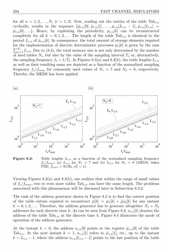
294 FAST CHANNEL SIMULATORS
for all n = 1, 2, . . . , Ni (i = 1, 2). Now, reading out the entries of the table Tabi,n
cyclically, results in the sequence µi,n[0], µi,n[1], . . . , µi,n[Li,n − 1], µi,n[Li,n] =µi,n[0], . . .. Hence, by exploiting the periodicity, µi,n[k] can be reconstructedcompletely for all k = 0, 1, 2, . . . The length of the table Tabi,n is identical to theperiod Li,n of µi,n[k]. In consequence, the total amount of storage elements requiredfor the implementation of discrete deterministic processes µi[k] is given by the sum∑Ni
n=1 Li,n. Due to (8.4), the total memory size is not only determined by the numberof used tables Ni, but also by the value of the sampling interval Ts or, alternatively,the sampling frequency fs = 1/Ts. In Figures 8.3(a) and 8.3(b), the table lengths Li,n
as well as their resulting sums are depicted as a function of the normalized samplingfrequency fs/fmax for commonly used values of N1 = 7 and N2 = 8, respectively.Thereby, the MEDS has been applied.
(a)
100
101
102
103
104
100
105
fs/fmax
L1,
n
L1,7L1,6
L1,5
L1,4L1,3
L1,2
L1,1
Σn L1,nN1=7
(b)
100
101
102
103
104
100
105
fs/fmax
L2,
n
L2,8L2,7
L2,6L2,5
L2,4
L2,3L2,2
L2,1
Σn L2,n
N2=8
Figure 8.3: Table lengths Li,n as a function of the normalized sampling frequencyfs/fmax: (a) L1,n for N1 = 7 and (b) L2,n for N2 = 8 (MEDS, JakesPSD, fmax = 91 Hz, σ2
0 = 1).
Viewing Figures 8.3(a) and 8.3(b), one realizes that within the range of small valuesof fs/fmax, two or even more tables Tabi,n can have the same length. The problemsassociated with this phenomenon will be discussed later in Subsection 8.3.2.
The task of the address generator shown in Figure 8.2 is to find the correct positionof the table entries required to reconstruct µ[k] = µ1[k] + jµ2[k] for any instantk = 0, 1, 2, . . .. Therefore, the address generator has to generate altogether N1 + N2
addresses for each discrete time k. As can be seen from Figure 8.2, ai,n[k] denotes theaddress of the table Tabi,n at the discrete time k. Figure 8.4 illustrates the mode ofoperation of the address generator.
At the instant k = 0, the address ai,n[0] points at the register µi,n[0] of the tableTabi,n. At the next instant k = 1, ai,n[1] refers to µi,n[1], etc., up to the instantk = Li,n − 1, where the address ai,n[Li,n − 1] points to the last position of the table
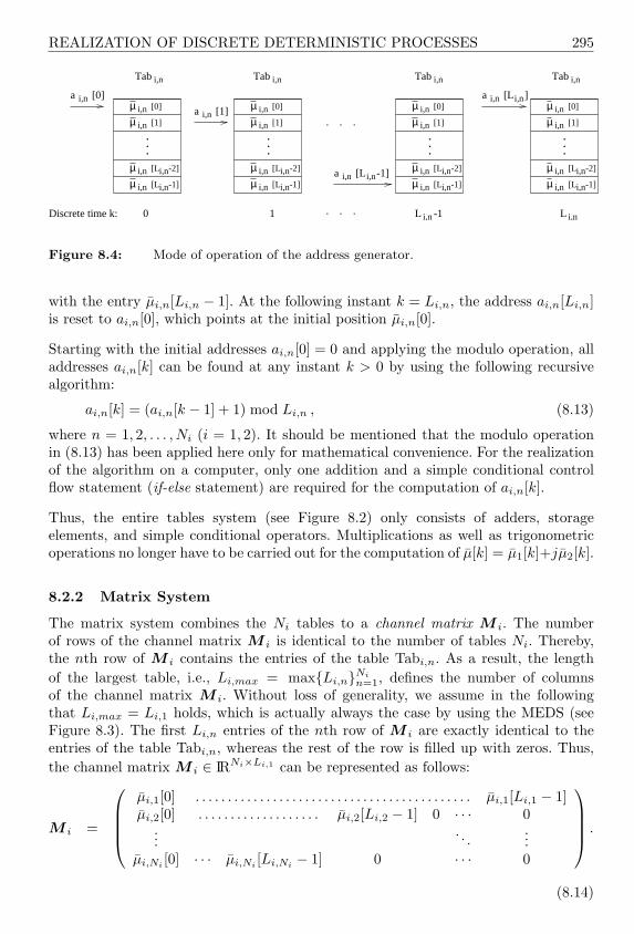
REALIZATION OF DISCRETE DETERMINISTIC PROCESSES 295
a i,n [0]
Tab i,n
a i,n [1]
Tab i,n
. .. L i,n
Tab i,n
a i,n i,n[L ]
L i,n -1
. ..
Tab i,n
......
......
a i,n i,n[L -1]
[1]
Discrete time k: 0 1
i,n [0]
i,n
i,n
i,nµ
µµ
µ i,n
i,n[L -1]
[L -2]
i,n [0]
i,n
i,n
i,nµ
µµ
µ i,n
i,n[L -1]
[L -2]
i,n [0]
i,n
i,n
i,nµ
µµ
µ i,n
i,n[L -1]
[L -2]
i,n [0]
i,n
i,n
i,nµ
µµ
µ i,n
i,n[L -1]
[L -2]
[1] [1] [1]
Figure 8.4: Mode of operation of the address generator.
with the entry µi,n[Li,n − 1]. At the following instant k = Li,n, the address ai,n[Li,n]is reset to ai,n[0], which points at the initial position µi,n[0].
Starting with the initial addresses ai,n[0] = 0 and applying the modulo operation, alladdresses ai,n[k] can be found at any instant k > 0 by using the following recursivealgorithm:
ai,n[k] = (ai,n[k − 1] + 1) mod Li,n , (8.13)
where n = 1, 2, . . . , Ni (i = 1, 2). It should be mentioned that the modulo operationin (8.13) has been applied here only for mathematical convenience. For the realizationof the algorithm on a computer, only one addition and a simple conditional controlflow statement (if-else statement) are required for the computation of ai,n[k].
Thus, the entire tables system (see Figure 8.2) only consists of adders, storageelements, and simple conditional operators. Multiplications as well as trigonometricoperations no longer have to be carried out for the computation of µ[k] = µ1[k]+jµ2[k].
8.2.2 Matrix System
The matrix system combines the Ni tables to a channel matrix M i. The numberof rows of the channel matrix M i is identical to the number of tables Ni. Thereby,the nth row of M i contains the entries of the table Tabi,n. As a result, the lengthof the largest table, i.e., Li,max = maxLi,nNi
n=1, defines the number of columnsof the channel matrix M i. Without loss of generality, we assume in the followingthat Li,max = Li,1 holds, which is actually always the case by using the MEDS (seeFigure 8.3). The first Li,n entries of the nth row of M i are exactly identical to theentries of the table Tabi,n, whereas the rest of the row is filled up with zeros. Thus,the channel matrix M i ∈ IRNi×Li,1 can be represented as follows:
M i =
µi,1[0] . . . . . . . . . . . . . . . . . . . . . . . . . . . . . . . . . . . . . . . . . . . µi,1[Li,1 − 1]µi,2[0] . . . . . . . . . . . . . . . . . . . µi,2[Li,2 − 1] 0 · · · 0
.... . .
...µi,Ni [0] · · · µi,Ni [Li,Ni − 1] 0 · · · 0
.
(8.14)

296 FAST CHANNEL SIMULATORS
The channel matrix M i contains the complete information needed for thereconstruction of µi[k]. In order to guarantee the correct reconstruction of µi[k] forall values of k = 0, 1, 2, . . ., it is necessary to select from each row of M i one entry atthe correct position. This can be achieved by introducing a further matrix Si, whichwill henceforth be called the selection matrix. The entries of the selection matrixSi are time variant quantities, which can only take the values 0 or 1. There is aclose relation between the address generator introduced in the previous subsectionand the selection matrix Si. This becomes obvious by noting that the entries ofSi = (sl,n) ∈ 0, 1Li,1×Ni can be calculated at any instant k by using the addressesai,n[k] (8.13) according to
sl,n = sl,n[k] =
1 if l = ai,n[k]0 if l 6= ai,n[k] (8.15)
for all l = 0, 1, . . . , Li,1 − 1 and n = 1, 2, . . . , Ni (i = 1, 2).
The discrete deterministic Gaussian process µi[k] can now be obtained from theproduct of the channel matrix M i and the selection matrix Si as follows:
µi[k] = tr (M i · Si) , (8.16)
where tr(·) denotes the trace2 [Zur92, Hor85].
Using (8.16), we can thus also express the complex discrete deterministic Gaussianprocess (8.9) in an alternative form
µ[k] = tr (M1 · S1) + j tr (M2 · S2) . (8.17)
It is worth mentioning that the number of columns (rows) of the channel matrix M i
(selection matrix Si) tends to infinity as Ts → 0 and, thus, µi[k] converges to µi(t).In the limits Ts → 0 and Ni → ∞, the number of columns and the number of rowsof both the channel matrix M i and the selection matrix Si tend to infinity. In thiscase, the complex discrete deterministic Gaussian process µ[k] converges, as it wasexpected, to a sample function of the complex stochastic Gaussian random processµ(t).
An equivalent representation of the discrete deterministic Rayleigh process ζ[k],introduced by (8.10), can be obtained by taking the absolute value of (8.17), i.e.,
ζ[k] = |µ[k]| = | tr (M1 · S1) + j tr (M2 · S2)| . (8.18)
For the sake of completeness, we write the phase ϑ[k] of µ[k] = µ1[k] + jµ2[k] in theform
ϑ[k] = arctan
tr (M2 · S2)tr (M1 · S1)
. (8.19)
2 The trace of a square matrix A = (an,m) ∈ IRN×N is defined by the sum of the main diagonalentries an,m, i.e., tr(A) =
PNn=1 an,n.
PROPERTIES OF DISCRETE DETERMINISTIC PROCESSES 297
It is evident that in the limit Ts → 0 it follows: ζ[k] → ζ(t) and ϑ[k] → ϑ(t).Furthermore, the sequences ζ[k] and ϑ[k] are converging for Ts → 0 and Ni →∞ to asample function of the corresponding stochastic processes ζ(t) and ϑ(t), respectively.
It should be mentioned that the computation of the discrete deterministic processes(8.16)–(8.19) by taking the trace of the product of two matrices is not a very efficientapproach due to the large number of multiplications and additions that have tobe carried out. However, considerable simplifications are possible if all unnecessaryoperations such as multiplications with zero and one are avoided at the beginning.In this case, the matrix system reduces to the tables system. In other words: thematrix system actually represents no genuine alternative realization form to the tablessystem, but provides some new aspects regarding the interpretation and representationof discrete-time deterministic processes.
8.2.3 Shift Register System
From the tables system (see Figure 8.2), we can derive the shift register systemdepicted in Figure 8.5 by replacing in the former the tables Tabi,n with feedback shiftregisters Regi,n. Instead of N1 +N2 tables, now N1 +N2 shift registers are required forthe realization of µ[k] = µ1[k]+jµ2[k]. The length of the shift register Regi,n is therebyidentical to the length Li,n of the corresponding table Tabi,n. During the simulationset-up phase, the shift registers Regi,n are filled at the positions l ∈ 0, 1, . . . , Li,n−1with the values µi,n[l] = ci,n cos(2πfi,nlTs + θi,n), where n = 1, 2, . . . , Ni and i = 1, 2.Throughout the simulation run phase, the contents of the shift registers are shiftedby one position to the right at every clock pulse (see Figure 8.5). Due to the linkscreated between the shift register outputs (positions 0) with their respective inputs(positions Li,n− 1), it is ensured that the discrete deterministic processes µi,n[k] and,consequently, also µ[k] = µ1[k] + jµ2[k] as well as ζ[k] = |µ[k]| can be reconstructedfor all k = 0, 1, 2, . . .
Note that in comparison with the tables system, no address generator is needed, butinstead of this,
∑2i=1
∑Ni
n=1 Li,n register entries have to be shifted at every clock pulse,which — especially for software realizations in connection with large register lengths— does not lead to a satisfying solution. For that reason, we will prefer the tablessystem to the shift register system and will turn our attention in the next section tothe analysis of the properties of discrete deterministic processes.
8.3 PROPERTIES OF DISCRETE DETERMINISTIC PROCESSES
By analogy to the analysis of continuous-time deterministic processes (Chapter 4), westart in Subsection 8.3.1 with the investigation of the elementary properties of discretedeterministic processes, and then we will continue with the analysis of the statisticalproperties in the following Subsection 8.3.2.

298 FAST CHANNEL SIMULATORS
[k]
L -1 2 1 0l
2 1 0lL -1
µReg
Reg
L1,1-1 2 1 0l
2 1 0lL1,N1-1
[k]
µ1,N1[k]
1,1µ
Reg1,N1
Reg1,1
2,1
2,N2
2,N2
2,1
2,N [k]2
[k]µ2,1
[k]2µ
[k]1µ
[k]µ
ζ
Figure 8.5: Realization of discrete deterministic Rayleigh processes ζ[k] by using shiftregisters.
8.3.1 Elementary Properties of Discrete Deterministic Processes
The interpretation of µi[k] as discrete deterministic process, i.e., as a mapping of theform
µi : Z→ IR , k 7→ µi[k] , (8.20)
allows us to establish a close relationship with the investigations performed inSection 4.2. Therefore, we proceed analogously to Section 4.2 and derive simple closedsolutions for the fundamental characteristic quantities of µi[k] such as mean value,mean power, autocorrelation sequence, etc.
Mean value: Let µi[k] be a discrete deterministic process with fi,n 6= 0 (n =1, 2, . . . , Ni). Then, by using (2.77) and (8.2), it can be shown that the mean value ofµi[k] is equal to
mµi = limK→∞
12K + 1
K∑
k=−K
µi[k] = 0 . (8.21)
It is henceforth assumed that fi,n 6= 0 holds for all n = 1, 2, . . . , Ni and i = 1, 2.

PROPERTIES OF DISCRETE DETERMINISTIC PROCESSES 299
Mean power: Let µi[k] be a discrete deterministic process. Then, it follows by using(2.78) and (8.2) that its mean power is given by
σ2µi
= limK→∞
12K + 1
K∑
k=−K
µ2i [k] =
Ni∑n=1
c2i,n
2. (8.22)
In particular, by applying the MEDS, we obtain due to (5.73) the desired resultσ2
µi= σ2
0 .
Autocorrelation sequence: Let µi[k] be a discrete deterministic process. Then,it follows from (2.79) and (8.2) that the autocorrelation sequence of µi[k] can beexpressed by
rµiµi[κ] = lim
K→∞1
2K + 1
K∑
k=−K
µi[k] µi[k + κ]
=Ni∑
n=1
c2i,n
2cos(2πfi,nTsκ) . (8.23)
A comparison with (4.11) shows that rµiµi [κ] can be obtained from rµiµi(τ) if rµiµi(τ)is sampled at τ = κTs and if additionally the quantities fi,n are substituted by fi,n.In addition, we realize that also in the discrete-time case, the quantized Dopplerphases θi,n have no influence on the behaviour of the autocorrelation sequence rµiµi [κ].Observe that from (8.22) and (8.23) the relation σ2
µi= rµiµi [0] can directly be
obtained.
The deviations between rµiµi [κ] := rµiµi(κTs) and rµiµi [κ], caused by the quantizationof the discrete Doppler frequencies fi,n, can be observed in Figure 8.6. Thereby, theMEDS has been applied by using Ni = 8 harmonic functions (tables). Figure 8.6(a)shows that for sufficiently small sampling intervals (Ts = 0.1ms) no significantdifferences occur between rµiµi [κ] and rµiµi [κ] if τ = κTs is within its range of interestτ =∈ [0, Ni/(2fmax)]. However, this does not apply for large values of Ts, as canbe seen when considering Figure 8.6(b), where the corresponding ratios in case ofTs = 1ms are shown.
Cross-correlation sequence: Let µ1[k] and µ2[k] be two discrete deterministicprocesses. Then, it follows from (2.80) in connection with (8.2) that the cross-correlation sequence is equal to
rµ1µ2 [κ] = 0 , (8.24)
if f1,n 6= ±f2,m is fulfilled for all n = 1, 2, . . . , N1 and m = 1, 2, . . . , N2, or
rµ1µ2 [κ] =maxN1,N2∑
n=1f1,n=±f2,m
c1,nc2,m
2cos(2πf1,nTsκ− θ1,n ± θ2,m) , (8.25)
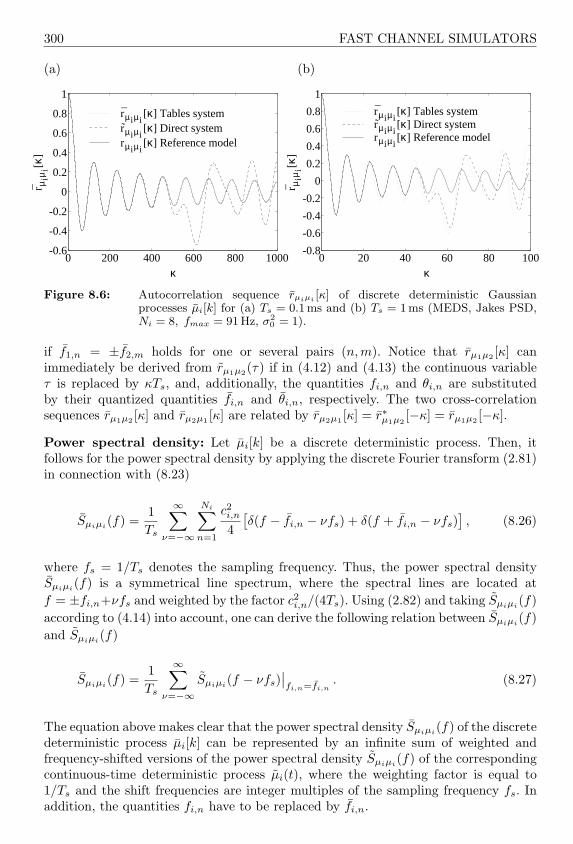
300 FAST CHANNEL SIMULATORS
(a)
0 200 400 600 800 1000-0.6
-0.4
-0.2
0
0.2
0.4
0.6
0.8
1
κ
r µiµ
i[κ]
rµiµi[κ] Tables system
rµiµi[κ] Direct system
rµiµi[κ] Reference model
(b)
0 20 40 60 80 100-0.8
-0.6
-0.4
-0.2
0
0.2
0.4
0.6
0.8
1
κr µ
iµi[κ
]
rµiµi[κ] Tables system
rµiµi[κ] Direct system
rµiµi[κ] Reference model
Figure 8.6: Autocorrelation sequence rµiµi [κ] of discrete deterministic Gaussianprocesses µi[k] for (a) Ts = 0.1ms and (b) Ts = 1ms (MEDS, Jakes PSD,Ni = 8, fmax = 91Hz, σ2
0 = 1).
if f1,n = ±f2,m holds for one or several pairs (n,m). Notice that rµ1µ2 [κ] canimmediately be derived from rµ1µ2(τ) if in (4.12) and (4.13) the continuous variableτ is replaced by κTs, and, additionally, the quantities fi,n and θi,n are substitutedby their quantized quantities fi,n and θi,n, respectively. The two cross-correlationsequences rµ1µ2 [κ] and rµ2µ1 [κ] are related by rµ2µ1 [κ] = r∗µ1µ2
[−κ] = rµ1µ2 [−κ].
Power spectral density: Let µi[k] be a discrete deterministic process. Then, itfollows for the power spectral density by applying the discrete Fourier transform (2.81)in connection with (8.23)
Sµiµi(f) =1Ts
∞∑ν=−∞
Ni∑n=1
c2i,n
4[δ(f − fi,n − νfs) + δ(f + fi,n − νfs)
], (8.26)
where fs = 1/Ts denotes the sampling frequency. Thus, the power spectral densitySµiµi(f) is a symmetrical line spectrum, where the spectral lines are located atf = ±fi,n+νfs and weighted by the factor c2
i,n/(4Ts). Using (2.82) and taking Sµiµi(f)according to (4.14) into account, one can derive the following relation between Sµiµi(f)and Sµiµi(f)
Sµiµi(f) =1Ts
∞∑ν=−∞
Sµiµi(f − νfs)∣∣fi,n=fi,n
. (8.27)
The equation above makes clear that the power spectral density Sµiµi(f) of the discretedeterministic process µi[k] can be represented by an infinite sum of weighted andfrequency-shifted versions of the power spectral density Sµiµi(f) of the correspondingcontinuous-time deterministic process µi(t), where the weighting factor is equal to1/Ts and the shift frequencies are integer multiples of the sampling frequency fs. Inaddition, the quantities fi,n have to be replaced by fi,n.
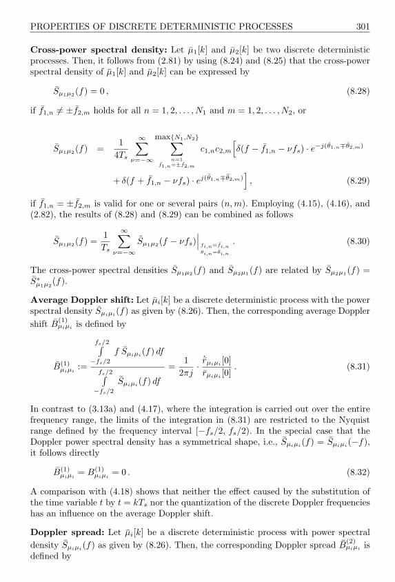
PROPERTIES OF DISCRETE DETERMINISTIC PROCESSES 301
Cross-power spectral density: Let µ1[k] and µ2[k] be two discrete deterministicprocesses. Then, it follows from (2.81) by using (8.24) and (8.25) that the cross-powerspectral density of µ1[k] and µ2[k] can be expressed by
Sµ1µ2(f) = 0 , (8.28)
if f1,n 6= ±f2,m holds for all n = 1, 2, . . . , N1 and m = 1, 2, . . . , N2, or
Sµ1µ2(f) =1
4Ts
∞∑ν=−∞
maxN1,N2∑n=1
f1,n=±f2,m
c1,nc2,m
[δ(f − f1,n − νfs) · e−j(θ1,n∓θ2,m)
+ δ(f + f1,n − νfs) · ej(θ1,n∓θ2,m)], (8.29)
if f1,n = ±f2,m is valid for one or several pairs (n,m). Employing (4.15), (4.16), and(2.82), the results of (8.28) and (8.29) can be combined as follows
Sµ1µ2(f) =1Ts
∞∑ν=−∞
Sµ1µ2(f − νfs)∣∣∣ fi,n=fi,n
θi,n=θi,n
. (8.30)
The cross-power spectral densities Sµ1µ2(f) and Sµ2µ1(f) are related by Sµ2µ1(f) =S∗µ1µ2
(f).
Average Doppler shift: Let µi[k] be a discrete deterministic process with the powerspectral density Sµiµi(f) as given by (8.26). Then, the corresponding average Dopplershift B
(1)µiµi is defined by
B(1)µiµi
:=
fs/2∫−fs/2
f Sµiµi(f) df
fs/2∫−fs/2
Sµiµi(f) df
=1
2πj· ˙rµiµi [0]rµiµi [0]
. (8.31)
In contrast to (3.13a) and (4.17), where the integration is carried out over the entirefrequency range, the limits of the integration in (8.31) are restricted to the Nyquistrange defined by the frequency interval [−fs/2, fs/2). In the special case that theDoppler power spectral density has a symmetrical shape, i.e., Sµiµi(f) = Sµiµi(−f),it follows directly
B(1)µiµi
= B(1)µiµi
= 0 . (8.32)
A comparison with (4.18) shows that neither the effect caused by the substitution ofthe time variable t by t = kTs nor the quantization of the discrete Doppler frequencieshas an influence on the average Doppler shift.
Doppler spread: Let µi[k] be a discrete deterministic process with power spectraldensity Sµiµi(f) as given by (8.26). Then, the corresponding Doppler spread B
(2)µiµi is
defined by

302 FAST CHANNEL SIMULATORS
B(2)µiµi
: =
√√√√√√√√√
fs/2∫−fs/2
(f − B(1)µiµi)2 Sµiµi(f) df
fs/2∫−fs/2
Sµiµi(f) df
=12π
√( ˙rµiµi[0]
rµiµi[0]
)2
− ¨rµiµi[0]
rµiµi[0]
. (8.33)
Using (8.31), (8.32), and σ2µi
= rµiµi[0], we can — especially for symmetrical Doppler
power spectral densities — express the last equation as follows
B(2)µiµi
=
√βi
2πσµi
, (8.34)
where
βi = −¨rµiµi [0] = 2π2Ni∑
n=1
(ci,nfi,n)2 . (8.35)
It should be remembered that the MEDS has been developed especially for the Jakespower spectral density. In Subsection 5.1.6, we learned that in this case the Dopplerspread of the continuous-time simulation model is identical to the Doppler spread ofthe reference model, i.e., B
(2)µiµi = B
(2)µiµi . This relationship is now only approximately
valid. The reason for this is that although σ2µi
= σ2µi
= σ20 holds, but due to fi,n ≈ fi,n
it follows βi ≈ βi = βi and, thus,
B(2)µiµi
≈ B(2)µiµi
= B(2)µiµi
. (8.36)
The deviation between B(2)µiµi and B
(2)µiµi or between βi and βi is basically determined
by the chosen value for the sampling interval Ts. We will find out more details aboutthis by analysing the model error of discrete-time systems.
Model error: Let µi[k] be a discrete deterministic process introduced by (8.2). Then,the model error ∆βi of the discrete-time system is defined by
∆βi := βi − βi . (8.37)
Using (3.29) and (8.35), the model error ∆βi can easily be evaluated for allparameter computation methods described in Chapter 5 as a function of Ni and Ts
or alternatively fs = 1/Ts. An example of the behaviour of the relative model error∆βi/βi of discrete-time systems is shown in Figure 8.7 as a function of the normalizedsampling frequency fs/fmax. Thereby, the MEDS has been applied with Ni = 7 (JakesPSD, fmax = 91 Hz, σ2
0 = 1).
Figure 8.7 clearly illustrates that the model error ∆βi/βi decreases if the samplingfrequency fs increases. In the limit fs → ∞ or Ts → 0, we obtain ∆βi/βi → 0
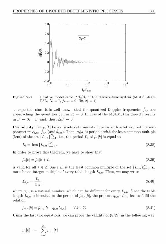
PROPERTIES OF DISCRETE DETERMINISTIC PROCESSES 303
100
101
102
103
104
-0.4
-0.2
0
0.2
0.4
0.6
0.8
fs/fmax
∆βi/
β iNi=7
Figure 8.7: Relative model error ∆βi/βi of the discrete-time system (MEDS, JakesPSD, Ni = 7, fmax = 91Hz, σ2
0 = 1).
as expected, since it is well known that the quantized Doppler frequencies fi,n areapproaching the quantities fi,n as Ts → 0. In case of the MSEM, this directly resultsin βi → βi = βi and, thus, ∆βi → 0.
Periodicity: Let µi[k] be a discrete deterministic process with arbitrary but nonzeroparameters ci,n, fi,n (and θi,n). Then, µi[k] is periodic with the least common multiple(lcm) of the set Li,nNi
n=1, i.e., the period Li of µi[k] is equal to
Li = lcm Li,nNin=1 . (8.38)
In order to prove this theorem, we have to show that
µi[k] = µi[k + Li] (8.39)
is valid for all k ∈ Z. Since Li is the least common multiple of the set Li,nNin=1, Li
must be an integer multiple of every table length Li,n. Thus, we may write
Li,n =Li
qi,n, (8.40)
where qi,n is a natural number, which can be different for every Li,n. Since the tablelength Li,n is identical to the period of µi,n[k], the product qi,n · Li,n has to fulfil therelation
µi,n[k] = µi,n[k + qi,nLi,n] ∀ k ∈ Z . (8.41)
Using the last two equations, we can prove the validity of (8.39) in the following way:
µi[k] =Ni∑
n=1
µi,n[k]

304 FAST CHANNEL SIMULATORS
=Ni∑
n=1
µi,n[k + qi,nLi,n]
=Ni∑
n=1
µi,n[k + Li]
= µi[k + Li] ∀ k ∈ Z . (8.42)
From Li being the least common multiple of the set Li,nNin=1, it follows that Li is
the smallest (positive) value for which (8.39) is valid. Consequently, Li is said to bethe period of the discrete deterministic process µi[k].
We will point out here that an upper bound on the period Li (8.38) is given by theproduct of all table lengths Li,n, i.e.,
Li =Ni∏
n=1
Li,n . (8.43)
Taking the above remarks into account, it can easily be shown that Li also fulfils(8.39). However, the period Li and its upper bound Li are related by Li ≥ Li.
From the fact that the table length Li,n depends on the sampling frequency fs, itfollows that the period Li depends on fs as well. This dependency is illustrated inFigure 8.8, where the period Li and its upper bound Li are presented as a functionof the normalized sampling frequency fs/fmax. Thereby, the results are deliberatelyshown for a small, medium, and large number of tables (Ni = 7, Ni = 14, Ni = 21)in order to make clear that both Ni and fs have a decisive influence on the periodLi. We can also note, especially for low values of Ni, that the period Li is often closeto its upper bound Li. The easily computable expression (8.43) therefore allows ingeneral to estimate the period Li with sufficient precision. Furthermore, it can berealized by considering Figure 8.8 that the period Li is very large even for smallvalues of fs/fmax. For that reason, we may denote µi[k] as quasi-nonperiodic discretedeterministic Gaussian process, provided that the sampling frequency fs is sufficientlylarge, i.e., fs > 20fmax.
Next, we will examine the period of discrete deterministic Rayleigh processes ζ[k].Therefore, we consider the following theorem:
Let µ1[k] and µ2[k] be two discrete deterministic Gaussian processes, which areperiodic with L1 and L2, respectively. Then, the discrete deterministic Rayleighprocess ζ[k] = |µ1[k] + jµ2[k]| is periodic with the period
L = lcm L1, L2 . (8.44)
The proof of this theorem is similar to the proof of (8.39) allowing us this time topresent an abridged version. Due to (8.44), two natural numbers q1 and q2 exist,which fulfil the equations L = q1L1 and L = q2L2, respectively. Thus, it follows
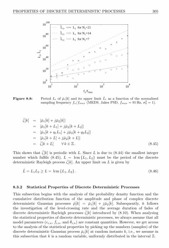
PROPERTIES OF DISCRETE DETERMINISTIC PROCESSES 305
101
102
103
104
100
1020
1040
1060
1080
10100
fs/fmax
Li,
Li
Li, Li for Ni=21
Li, Li for Ni=14
Li, Li for Ni=7
Figure 8.8: Period Li of µi[k] and its upper limit Li as a function of the normalizedsampling frequency fs/fmax (MEDS, Jakes PSD, fmax = 91 Hz, σ2
0 = 1).
ζ[k] = |µ1[k] + jµ2[k]|= |µ1[k + L1] + jµ2[k + L2]|= |µ1[k + q1L1] + jµ2[k + q2L2]|= |µ1[k + L] + jµ2[k + L]|= ζ[k + L] ∀ k ∈ Z . (8.45)
This shows that ζ[k] is periodic with L. Since L is due to (8.44) the smallest integernumber which fulfils (8.45), L = lcm L1, L2 must be the period of the discretedeterministic Rayleigh process ζ[k]. An upper limit on L is given by
L = L1L2 ≥ L = lcm L1, L2 . (8.46)
8.3.2 Statistical Properties of Discrete Deterministic Processes
This subsection begins with the analysis of the probability density function and thecumulative distribution function of the amplitude and phase of complex discretedeterministic Gaussian processes µ[k] = µ1[k] + jµ2[k]. Subsequently, it followsthe investigation of the level-crossing rate and the average duration of fades ofdiscrete deterministic Rayleigh processes ζ[k] introduced by (8.10). When analysingthe statistical properties of discrete deterministic processes, we always assume that allmodel parameters (ci,n, fi,n, and θi,n) are constant quantities. However, we get accessto the analysis of the statistical properties by picking up the numbers (samples) of thediscrete deterministic Gaussian process µi[k] at random instants k, i.e., we assume inthis subsection that k is a random variable, uniformly distributed in the interval Z.

306 FAST CHANNEL SIMULATORS
8.3.2.1 Probability Density Function and Cumulative Distribution Function of theAmplitude and the Phase
In this subsection, we will derive analytical expressions for the probability densityfunction and cumulative distribution function of the amplitude as well as the phaseof complex discrete deterministic Gaussian processes µ[k]. Let us start by consideringone single discrete harmonic elementary sequence of the form
µi,n[k] = ci,n cos(2πfi,nkTs + θi,n) , (8.47)
where the model parameters ci,n, fi,n, and θi,n are arbitrary but nonzero quantitiesand k is the uniformly distributed random variable mentioned above. Since µi,n[k]is periodic with Li,n, we can assume, without restriction of generality, that therandom variable k is limited to the half-open interval [0, Li,n). In this case, µi,n[k]has no longer to be regarded as a deterministic sequence but as a random variable,whose possible elementary events (outcomes or realizations) are the elements ofthe set µi,n[0], µi,n[1], . . . , µi,n[Li,n − 1]. Thereby, it should be noted that eachelementary event occurs with the probability 1/Li,n. Consequently, the probabilitydensity function of µi,n[k] can be written as
pµi,n(x) =1
Li,n
Li,n−1∑
l=0
δ(x− µi,n[l]) , (8.48)
where n = 1, 2, . . . , Ni (i = 1, 2). Since the discrete harmonic elementary sequenceµi,n[k] converges to the corresponding harmonic elementary function µi,n(t) [see (4.27)]as the sampling interval Ts tends to zero, the discrete probability density functionpµi,n(x) converges consequently to the continuous probability density function pµi,n(x)defined by (4.28), i.e., in the limit Ts → 0 it follows pµi,n(x) → pµi,n(x). An exampleof the probability density function pµi,n(x) of µi,n[k] is shown in Figure 8.9(a) for thecase Ts = 0.1 ms. As well as that, Figure 8.9(b) illustrates the results obtained aftertaking the limit Ts → 0.
Following the approach described above, we proceed with the derivation of theprobability density function pµi(x) of discrete deterministic Gaussian processes µi[k].Due to the periodicity of µi[k], we can restrict k to the half-open interval [0, Li).Therefore, let k be a random variable, uniformly distributed over [0, Li), then µi[k][see (8.2)] is also a random variable whose elementary events µi[0], µi[1], . . . , µi[Li−1]are uniformly distributed. By analogy to (8.48), the probability density function ofdiscrete deterministic Gaussian processes µi[k] can be expressed by
pµi(x) =1Li
Li−1∑
l=0
δ(x− µi[l]) . (8.49)
This result shows that the density pµi(x) of µi[k] can be represented as a weighted sumof delta functions. Thereby, the delta functions are located at µi[0], µi[1], . . . , µi[Li−1]and weighted by the reciprocal value of the period Li. Notice that pµi(x) doesnot result from the convolution pµi,1(x) ∗ pµi,2(x) ∗ . . . ∗ pµi,Ni
(x), because therandom variables µi,1[k], µi,2[k], . . . , µi,Ni [k] are, strictly speaking, not statistically

PROPERTIES OF DISCRETE DETERMINISTIC PROCESSES 307
(a)
-ci,n 0 ci,n
x
pµ
i,n(x
)
1/Li,n
(b)
-ci,n 0 ci,n0
0.5
1
1.5
2
2.5
3
3.5
4
4.5
x
pµ
i,n(x
)Figure 8.9: Probability density function pµi,n(x) of µi,n(x) with (a) Ts = 0.1ms and
(b) Ts → 0 (MEDS, Jakes PSD, Ni = 7, n = 7, fmax = 91Hz, σ20 = 1).
independent. Regarding the tables system, for example, the statistical dependencyfinds expression in the fact that the address generator in general does not producethe maximum number of different address combinations (states). This, in the ultimateanalysis, is the reason why the actual period Li and the maximum period Li arerelated by the inequality Li ≤ Li. It should also be noted that in the limit Ts → 0 itfollows pµi(x) → pµi(x), where pµi(x) [see (4.34)] is the probability density functionof µi(t). Moreover, pµi(x) approaches to the Gaussian probability density functionpµi(x) defined by (4.36) as Ts → 0 and Ni → ∞. For Ts > 0, it is not advisableto analyse the difference between the probability density functions pµi(x) and pµi(x)directly, because the former density is a discrete function, and the latter is a continuousfunction. However, this problem can easily be avoided by considering the cumulativedistribution function Fµi(r) of the discrete deterministic Gaussian process µi[k]. From(8.49), we obtain immediately
Fµi(r) =1Li
Li−1∑
l=0
∫ r
0
δ(x− µi[l]) dx , r ≥ 0 . (8.50)
A comparison of Fµi(r) with the cumulative distribution function Fµi(r) of thecorresponding continuous-time deterministic Gaussian process µi(t)
Fµi(r) =12
+ 2r
∫ ∞
0
[Ni∏
n=1
J0(2πci,nν)
]sinc (2πνr) dν , r ≥ 0 (8.51)
is shown in Figure 8.10. The analytical expression for the cumulative distributionfunction Fµi(r) given above can directly be obtained after substituting the probabilitydensity function (4.34) in Fµi(r) =
∫ r
−∞ pµi(x) dx and then solving the integral withrespect to the independent variable x.
In addition, the cumulative distribution function
Fµi(r) =12
[1 + erf
(r√2σ0
)], r ≥ 0 , (8.52)

308 FAST CHANNEL SIMULATORS
of the zero-mean Gaussian random process µi(t) represents in Figure 8.10 thebehaviour of the reference model.
-2 0 2 4 60
0.2
0.4
0.6
0.8
1
r
Fµ
i(r)
Fµi(r) (Tables system)
Fµi(r) (Direct system)
Fµi(r) (Reference model)
Figure 8.10: Cumulative distribution function Fµi(x) of discrete deterministic Gaussianprocesses µi[k] for Ts = 0.1ms (MEDS, Jakes PSD, Ni = 7, fmax = 91 Hz,σ2
0 = 1).
For sufficiently small values of the sampling interval Ts, the period Li becomes verylarge (see Figure 8.8) and, consequently, the sample space µi[l]Li−1
l=0 becomes verylarge as well. In such cases, it is not possible to evaluate the cumulative distributionfunction Fµi(r) according to (8.50) exactly without exceeding any reasonably chosentime-out interval for the computer simulation. Fortunately, this problem can beavoided, because one even obtains excellent results by merely evaluating K ¿ Li
elements of the subset µi[k]K−1k=0 , as demonstrated in Figure 8.10. This figure shows
an almost perfect correspondence between Fµi(r) and Fµi(r) or Fµi(x), although (8.50)has been evaluated by using only K = 50·103 ¿ Li samples µi[k] (k = 0, 1, . . . , K−1).
Next, we will examine the probability density function and the cumulative distributionfunction of discrete deterministic Rayleigh processes ζ[k]. Thereby, we take intoaccount that ζ[k] is periodic with L = lcm L1, L2. Let us assume until furthernotice that k is a random variable, uniformly distributed in the interval [0, L). Then,it follows that ζ[k] defined by (8.10) is also a random variable, where each of thepossible outcomes ζ[0], ζ[1], . . . , ζ[L− 1] occurs with the probability 1/L. By analogyto (8.49), we can thus write for the probability density function pζ(z) of discretedeterministic Rayleigh processes ζ[k]
pζ(z) =1L
L−1∑
l=0
δ(z − ζ[l]) , z ≥ 0 . (8.53)

PROPERTIES OF DISCRETE DETERMINISTIC PROCESSES 309
This result allows us to express the cumulative distribution function of ζ[k] as
Fζ−(r) =1L
L−1∑
l=0
∫ r
0
δ(z − ζ[l]) dz , r ≥ 0 . (8.54)
Note that due to ζ[k] → ζ(t) as Ts → 0, it follows pζ(z) → pζ(z) and Fζ−(r) → Fζ−(r).Thereby, pζ(z) results from (4.47a) with ρ = 0, which allows us to present thecumulative distribution function Fζ−(r) of ζ(t) as
Fζ−(r) =∫ r
0
pζ(z) dz
= 4r
∞∫
0
J1(2πrz)
π/2∫
0
[N1∏
n=1
J0(2πc1,nz cos θ)
]
[N2∏
n=1
J0(2πc2,nz sin θ)
]dθ dz , r ≥ 0 . (8.55)
Finally, it should be noted that after performing the limits Ts → 0 and Ni →∞, theidentity Fζ−(r) = Fζ−(r) is obtained, where
Fζ−(r) = 1− e− r2
2σ20 , r ≥ 0 , (8.56)
describes the cumulative distribution function of Rayleigh processes.
The cumulative distribution functions (8.54)–(8.56) are depicted in Figure 8.11. Forthe evaluation of Fζ−(r) according to (8.54), K = 50 · 103 ¿ L samples ζ[k](k = 0, 1, . . . , K − 1) have been used. The sampling interval Ts has been chosensufficiently small (Ts = 0.1 ms).
Now, let us analyse in detail the influence of the sampling interval Ts on the statisticsof ζ[k]. In particular, it is our intention to answer the following question: what is themaximum value of Ts for which Fζ−(r) does not perceptibly differ from Fζ−(r)? Up tonow, we have in general assumed that Ts is sufficiently small without concretely sayingwhat the phrase ‘sufficiently small’ really means. In the following, we want to make upfor this by deriving a lower limit for Ts. To illustrate the problem that occurs when Ts
exceeds a certain critical threshold, we consider the graphs presented in Figure 8.12.In contrast to the cumulative distribution function Fζ−(r) shown in Figure 8.11, wehave used in the present case K = L = 9240 samples ζ[k] (k = 0, 1, . . . , K − 1) forthe computation of Fζ−(r) by using (8.54). At the same time, the sampling intervalTs has been increased from Ts = 0.1ms up to Ts = 5 ms. Obviously, this seemsto be problematical, because different realizations of the quantized Doppler phasesθi,nNi
n=1 are now leading to different cumulative distribution functions Fζ−(r), whichmay differ considerably (see Figure 8.12). It should be observed that in this examplethe sampling theorem for low-pass signals [Fet96] is still fulfilled, because the chosenvalues Ts = 5ms, i.e., fs = 200 Hz, and fmax = 91Hz are sufficient for the sampling
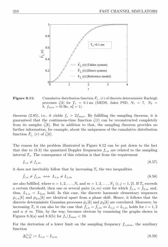
310 FAST CHANNEL SIMULATORS
0 1 2 3 40
0.2
0.4
0.6
0.8
1
r
Fζ -
(r)
Fζ-(r) (Tables system)
Fζ-(r) (Direct system)
Fζ-(r) (Reference model)
Ts=0.1 ms
Figure 8.11: Cumulative distribution function Fζ−(r) of discrete deterministic Rayleigh
processes ζ[k] for Ts = 0.1 ms (MEDS, Jakes PSD, N1 = 7, N2 =8, fmax = 91 Hz, σ2
0 = 1).
theorem (2.85), i.e., it yields fs > 2fmax. By fulfilling the sampling theorem, it isguaranteed that the continuous-time function ζ(t) can be reconstructed completelyfrom its samples ζ[k]. But in addition to that, the sampling theorem provides nofurther information, for example, about the uniqueness of the cumulative distributionfunction Fζ−(r) of ζ[k].
The reason for the problem illustrated in Figure 8.12 can be put down to the factthat due to (8.3) the quantized Doppler frequencies fi,n are related to the samplinginterval Ts. The consequence of this relation is that from the requirement
fi,n 6= fj,m (8.57)
it does not inevitably follow that by increasing Ts the two inequalities
fi,n 6= fj,m ⇐⇒ Li,n 6= Lj,m (8.58)
are also fulfilled, where n = 1, 2, . . . , Ni and m = 1, 2, . . . , Nj (i, j = 1, 2). If Ts exceedsa certain threshold, then one or several pairs (n,m) exist for which f1,n = f2,m and,thus, L1,n = L2,m hold. In this case, the discrete harmonic elementary sequencesµ1,n[k] and µ2,n[k] are identical apart from a phase shift. Hence, it follows that thediscrete deterministic Gaussian processes µ1[k] and µ2[k] are correlated. Moreover, byincreasing Ts it can also be the case that fi,n = fi,m ⇔ Li,n = Li,m holds for i = 1, 2and n 6= m. This, by the way, becomes obvious by examining the graphs shown inFigures 8.3(a) and 8.3(b) for fs/fmax < 10.
For the derivation of a lower limit on the sampling frequency fs,min, the auxiliaryfunction
∆(i,j)n,m := Li,n − Lj,m (8.59)
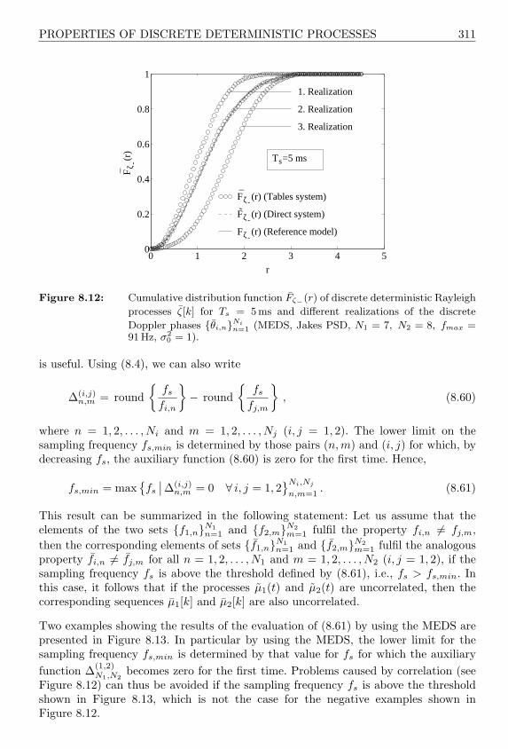
PROPERTIES OF DISCRETE DETERMINISTIC PROCESSES 311
0 1 2 3 4 50
0.2
0.4
0.6
0.8
1
Fζ-(r) (Tables system)
Fζ-(r) (Direct system)
Fζ-(r) (Reference model)
1. Realization
2. Realization
3. Realization
r
Fζ -
(r)
Ts=5 ms
Figure 8.12: Cumulative distribution function Fζ−(r) of discrete deterministic Rayleigh
processes ζ[k] for Ts = 5ms and different realizations of the discrete
Doppler phases θi,nNin=1 (MEDS, Jakes PSD, N1 = 7, N2 = 8, fmax =
91Hz, σ20 = 1).
is useful. Using (8.4), we can also write
∆(i,j)n,m = round
fs
fi,n
− round
fs
fj,m
, (8.60)
where n = 1, 2, . . . , Ni and m = 1, 2, . . . , Nj (i, j = 1, 2). The lower limit on thesampling frequency fs,min is determined by those pairs (n,m) and (i, j) for which, bydecreasing fs, the auxiliary function (8.60) is zero for the first time. Hence,
fs,min = maxfs
∣∣ ∆(i,j)n,m = 0 ∀ i, j = 1, 2
Ni,Nj
n,m=1. (8.61)
This result can be summarized in the following statement: Let us assume that theelements of the two sets f1,nN1
n=1 and f2,mN2m=1 fulfil the property fi,n 6= fj,m,
then the corresponding elements of sets f1,nN1n=1 and f2,mN2
m=1 fulfil the analogousproperty fi,n 6= fj,m for all n = 1, 2, . . . , N1 and m = 1, 2, . . . , N2 (i, j = 1, 2), if thesampling frequency fs is above the threshold defined by (8.61), i.e., fs > fs,min. Inthis case, it follows that if the processes µ1(t) and µ2(t) are uncorrelated, then thecorresponding sequences µ1[k] and µ2[k] are also uncorrelated.
Two examples showing the results of the evaluation of (8.61) by using the MEDS arepresented in Figure 8.13. In particular by using the MEDS, the lower limit for thesampling frequency fs,min is determined by that value for fs for which the auxiliaryfunction ∆(1,2)
N1,N2becomes zero for the first time. Problems caused by correlation (see
Figure 8.12) can thus be avoided if the sampling frequency fs is above the thresholdshown in Figure 8.13, which is not the case for the negative examples shown inFigure 8.12.

312 FAST CHANNEL SIMULATORS
0 10 20 30 40 5010
0
101
102
103
104
N1
f s,m
in/f
max
∆N1,N2
(1,2)
∆N1,N1-1
(1,1)
Figure 8.13: Lower limit on the sampling frequency fs,min as a function of N1 (MEDS,Jakes PSD, N2 = N1 + 1, fmax = 91 Hz, σ2
0 = 1).
It should finally be mentioned that the lower limit fs,min according to (8.61) issufficient, but not necessary in order to fulfil the condition (8.58), i.e., it cannot beexcluded that there exist values for fs which are below fs,min and even though the twoinequalities in (8.58) are fulfilled. Here, it is not our intention to discuss this problemin detail. Instead of this, we consider fs > 20fmax as a rule of thumb, which turnedout to be very useful for most practical applications. Hence, we say that the samplingfrequency fs is sufficiently large, if fs is larger than 20fmax.
We will proceed with the analysis of the probability density function pϑ(θ) of thephase of complex discrete deterministic Gaussian processes µ[k]. Of course, similararguments to those used for the derivation of (8.53) can be applied here to achievethe present aim. However, we prefer a more simple and straightforward approach bysubstituting in (8.53) the amplitude ζ[l] by the phase ϑ[l] allowing us directly toexpress the probability density function pϑ(θ) of the phase as
pϑ(θ) =1L
L−1∑
l=0
δ(θ − ϑ[l]) , |θ| ≤ π , (8.62)
where ϑ[l] = arctanµ2[l]/µ1[l] denotes the phase of the complex deterministicGaussian process µ[k] = µ1[k] + jµ2[k] at instants k = l ∈ 0, 1, . . . , L − 1. Using(8.62), the corresponding cumulative distribution function can be written as
Fϑ(ϕ) =1L
L−1∑
l=0
ϕ∫
−π
δ(θ − ϑ[l]) dϕ , |ϕ| ≤ π . (8.63)
It should be mentioned that due to ϑ[k] → ϑ(t) as Ts → 0, it also follows pϑ(θ) → pϑ(θ)and, thus, Fϑ(ϕ) → Fϑ(ϕ) as Ts → 0, where pϑ(θ) can be obtained from (4.47b)

PROPERTIES OF DISCRETE DETERMINISTIC PROCESSES 313
for ρ = 0, so that the cumulative distribution function Fϑ(ϕ) of the phase ϑ(t) ofµ(t) = µ1(t) + jµ2(t) can be expressed as
Fϑ(ϕ) =
ϕ∫
−π
pϑ(θ) dθ
= 4
ϕ∫
−π
∞∫
0
z
∞∫
0
[N1∏
n=1
J0(2πc1,nν1)
]cos(2πν1z cos θ) dν1
∞∫
0
[N2∏
m=1
J0(2πc2,mν2)
]cos(2πν2z sin θ) dν2
dz dθ , |ϕ| ≤ π .
(8.64)
As Ts → 0 and Ni →∞, it follows Fϑ(ϕ) → Fϑ(ϕ), where
Fϑ(ϕ) =12
(1 +
ϕ
π
), |ϕ| ≤ π , (8.65)
is the cumulative distribution function of the uniformly distributed phase of zero-meancomplex Gaussian random processes µ(t) = µ1(t) + jµ2(t).
Figure 8.14 illustrates the cumulative distribution functions (8.63)–(8.65). Theevaluation of (8.63) has been performed by using K = 50·103 ¿ L samples (outcomes)of the sample space ϑ[l]L−1
l=0 . For the sampling interval Ts, the value Ts = 0.1ms hasbeen chosen. Thus, by using the MEDS with the parameters specified in the figurecaption of Figure 8.14, the relation fs/fmax is close to the threshold fs,min/fmax (seeFigure 8.13).
8.3.2.2 Level-Crossing Rate and Average Duration of Fades
In contrast to continuous-time deterministic Rayleigh processes for which analyticalexpressions for both the level-crossing rate and the average duration of fades havebeen derived (see Appendix C), up to now no comparable solutions for discrete-timedeterministic Rayleigh processes exist. In the following, we restrict our investigationto the derivation of approximate formulas by assuming that the normalized samplingfrequency fs/fmax lies above the threshold shown in Figure 8.13. Thereby, the numberof harmonic functions (tables) Ni is assumed to be sufficiently large, i.e., Ni ≥ 7.Moreover, we assume that the relative model error ∆βi/βi of the discrete-time systemis small, which is in particular the case when the MEDS is applied on condition thatfs > fs,min is fulfilled (see Figure 8.7). Taking into account that the probability densityfunction pµi(x) of discrete deterministic processes µi[k] is asymptotically equal to theprobability density function pµi(x) of continuous-time deterministic processes µi(t),i.e., pµi(x) ∼ pµi(x), then we can summarize the above mentioned statements andassumptions as follows:

314 FAST CHANNEL SIMULATORS
-π 0 π 0
0.2
0.4
0.6
0.8
1
ϕ
Fϑ
(ϕ)
Fϑ(ϕ) (Tables system)
Fϑ(ϕ) (Direct system)
Fϑ(ϕ) (Reference model)
Figure 8.14: Cumulative distribution function Fϑ(ϕ) of the phase ϑ[k] of complexdiscrete deterministic Gaussian processes µ[k] = µ1[k] + jµ2[k] for Ts =0.1ms (MEDS, Jakes PSD, N1 = 7, N2 = 8, fmax = 91 Hz, σ2
0 = 1).
(i) pµi(x) ∼ pµi(x) ≈ pµi(x) , (8.66a)(ii) β = (β1 + β2)/2 ≈ β = β1 = β2 . (8.66b)
Taking these assumptions into account, the level-crossing rate Nζ(r) and the averageduration of fades Tζ−(r) of discrete deterministic Rayleigh processes ζ[k] are inprinciple still given by the approximations (4.66) and (4.70), respectively. However,we only have to evaluate these equations for the case ρ = 0 and after that, we have toreplace the model error ∆β by ∆β. This results in
Nζ(r) ≈ Nζ(r)(
1 +∆β
2β
), (8.67a)
Tζ−(r) ≈ Tζ−(r)(
1− ∆β
2β
), (8.67b)
where ∆β = β − β. In (8.67a), Nζ(r) denotes the level-crossing rate of Rayleighprocesses as defined by (2.60) and in (8.67b), Tζ−(r) refers to the average duration offades introduced by (2.65). As Ts → 0 and Ni → ∞ it follows Nζ(r) → Nζ(r) andTζ− → Tζ−(r).
Figure 8.15(a) shows an example for the normalized level-crossing rate Nζ(r)/fmax ofdiscrete deterministic Rayleigh processes ζ[k]. Just as in the previous examples, wecomputed here the model parameters by using the MEDS with N1 = 7 and N2 = 8.For the sampling interval Ts, again, the value Ts = 0.1ms has been chosen. Thecorresponding normalized average duration of fades Tζ−(r) · fmax is illustrated inFigure 8.15(b).

REALIZATION EXPENDITURE AND SIMULATION SPEED 315
(a)
0 1 2 3 4 5 60
0.2
0.4
0.6
0.8
1
1.2
r
Nζ(
r)/f
max
Nζ(r) (Tables system)Nζ(r) (Direct system)Nζ(r) (Reference model)
(b)
0 1 2 3 40
10
20
30
40
50
r
Tζ -
(r)
f max
Tζ-(r) (Tables system)
Tζ-(r) (Direct system)
Tζ-(r) (Reference model)
Figure 8.15: (a) Normalized level-crossing rate Nζ(r)/fmax and (b) normalized averageduration of fades Tζ−(r) ·fmax of discrete deterministic Rayleigh processes
ζ[k] for Ts = 0.1ms (MEDS, Jakes PSD, N1 = 7, N2 = 8, fmax = 91Hz,σ2
0 = 1).
8.4 REALIZATION EXPENDITURE AND SIMULATION SPEED
In this section, we will examine in detail the efficiency of the tables system (seeFigure 8.2). Moreover, the tables system’s efficiency will be compared to that ofthe corresponding discrete-time direct system, which is obtained by replacing thecontinuous-time variable t by kTs in Figure 4.3. For convenience, we ignore theinfluence of the line-of-sight component by choosing ρ = 0. Let us assume in thefollowing that the set-up phase has been completed, so that we can restrict ourinvestigations to the computation expenditure required for the generation of therespective complex-valued channel output sequence.
It can easily be seen from Figure 8.2 that the operations listed in Table 8.1 have to becarried out at each instant k in order to compute one sample of the complex discretedeterministic Gaussian process µ[k] = µ1[k]+jµ2[k]. One realizes that merely additionsand simple conditional control flow statements (if-else statements) are required. Theadditions are needed for the generation of the addresses within the address generatoras well as for adding up the tables outputs, whereas the conditional control flowstatements are only required for the generation of the addresses within the addressgenerator.
The number of operations required for the generation of the complex-valued sequenceµ[k] = µ1[k]+jµ2[k] by employing the direct system is also listed in Table 8.1. Thereby,normalized Doppler frequencies Ωi,n = 2πfi,nTs have been used in order to avoidunnecessary multiplications within the arguments of the harmonic functions.
The results shown in Table 8.1 can be summarized as follows: all multiplications can beavoided, the number of additions remains unchanged, and all trigonometric operationscan be substituted by simple if-else statements, when the tables system is used insteadof the direct system for the generation of complex-valued channel output sequences. It
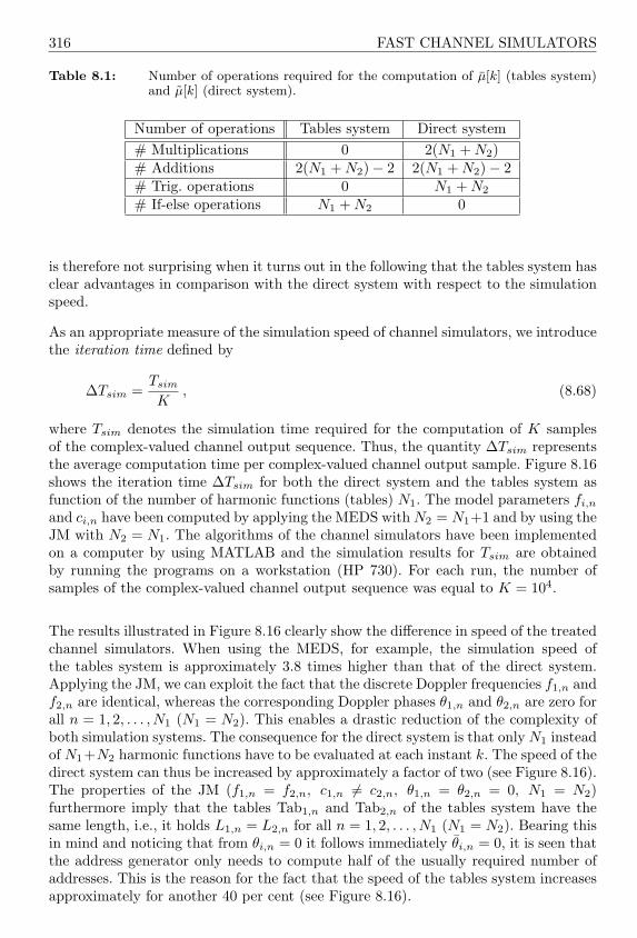
316 FAST CHANNEL SIMULATORS
Table 8.1: Number of operations required for the computation of µ[k] (tables system)and µ[k] (direct system).
Number of operations Tables system Direct system# Multiplications 0 2(N1 + N2)# Additions 2(N1 + N2)− 2 2(N1 + N2)− 2# Trig. operations 0 N1 + N2
# If-else operations N1 + N2 0
is therefore not surprising when it turns out in the following that the tables system hasclear advantages in comparison with the direct system with respect to the simulationspeed.
As an appropriate measure of the simulation speed of channel simulators, we introducethe iteration time defined by
∆Tsim =Tsim
K, (8.68)
where Tsim denotes the simulation time required for the computation of K samplesof the complex-valued channel output sequence. Thus, the quantity ∆Tsim representsthe average computation time per complex-valued channel output sample. Figure 8.16shows the iteration time ∆Tsim for both the direct system and the tables system asfunction of the number of harmonic functions (tables) N1. The model parameters fi,n
and ci,n have been computed by applying the MEDS with N2 = N1+1 and by using theJM with N2 = N1. The algorithms of the channel simulators have been implementedon a computer by using MATLAB and the simulation results for Tsim are obtainedby running the programs on a workstation (HP 730). For each run, the number ofsamples of the complex-valued channel output sequence was equal to K = 104.
The results illustrated in Figure 8.16 clearly show the difference in speed of the treatedchannel simulators. When using the MEDS, for example, the simulation speed ofthe tables system is approximately 3.8 times higher than that of the direct system.Applying the JM, we can exploit the fact that the discrete Doppler frequencies f1,n andf2,n are identical, whereas the corresponding Doppler phases θ1,n and θ2,n are zero forall n = 1, 2, . . . , N1 (N1 = N2). This enables a drastic reduction of the complexity ofboth simulation systems. The consequence for the direct system is that only N1 insteadof N1+N2 harmonic functions have to be evaluated at each instant k. The speed of thedirect system can thus be increased by approximately a factor of two (see Figure 8.16).The properties of the JM (f1,n = f2,n, c1,n 6= c2,n, θ1,n = θ2,n = 0, N1 = N2)furthermore imply that the tables Tab1,n and Tab2,n of the tables system have thesame length, i.e., it holds L1,n = L2,n for all n = 1, 2, . . . , N1 (N1 = N2). Bearing thisin mind and noticing that from θi,n = 0 it follows immediately θi,n = 0, it is seen thatthe address generator only needs to compute half of the usually required number ofaddresses. This is the reason for the fact that the speed of the tables system increasesapproximately for another 40 per cent (see Figure 8.16).

COMPARISON WITH THE FILTER METHOD 317
0 5 10 15 20 25 300
0.02
0.04
0.06
0.08
0.1
0.12
N1
∆TSi
m (
ms)
Direct system (MEDS)
Direct system (JM)
Tables system (MEDS)
Tables system (JM)
Figure 8.16: Iteration time ∆Tsim as a function of the number of harmonic functions(tables) N1 (MEDS with N2 = N1 + 1, JM with N2 = N1, fmax = 91Hz,σ2
0 = 1, Ts = 0.1ms).
Summing up, we can say that the tables system is — by using the MEDS (JM) —approximately four times (three times) faster than the corresponding direct system.The benefit of higher speed is confronted by the disadvantage of higher demand forstorage elements, but this, however, is the only disadvantage of the tables system worthmentioning. Remember that the total demand for storage elements is proportional tothe sampling frequency (see Figure 8.3). By choosing the sampling frequency fs justabove fs,min, then the minimum number of storage elements is obtained withoutaccepting appreciable losses in precision. However, a good compromise betweenthe model’s precision and complexity is obtained by choosing fs within the range20fmax ≤ fs ≤ 30fmax. When such a designed channel simulator is used as linkbetween the transmitter and the receiver of a mobile communication system, thena sampling rate conversion by means of an interpolation (a decimation) filter is ingeneral required in order to fit the sampling frequency of the channel simulator to thesampling frequency of the receiver’s input (transmitter’s output).
8.5 COMPARISON WITH THE FILTER METHOD
At this point, it is advisable to carry out a comparison with the filter method, which isalso often used in the design of simulation models for mobile radio channels. Here, werestrict our investigations to the modelling of Rayleigh processes. For that purpose,we consider the discrete-time structure depicted in Figure 8.17.
Since white Gaussian noise is, strictly speaking, not realizable, we consider ν1[k] andν2[k] as two realizable noise sequences whose statistical properties are sufficiently closeto those of ideal white Gaussian random processes. In particular, we demand that thesepseudo-random sequences νi[k] (i = 1, 2) are uncorrelated, having a very long period,and fulfilling the properties Eνi[k] = 0 and Var νi[k] = 1.

318 FAST CHANNEL SIMULATORS
Noise
Noise
~H(z)
~H(z)
[k]
~
.ζ~
1~ν
~2ν
~µ 2
µ 1
~µ
[k] [k]
[k][k]
[k]
Figure 8.17: A simulation model for Rayleigh processes on basis of the filter method.
In Figure 8.17, H(z) denotes the transfer function of a digital filter in the z-domain. Inpractice, recursive digital filters are widely in use for modelling of narrow-band randomprocesses. The transfer function of such filters can be represented in the z-domain asfollows
H(z) = A0
N0/2∏n=1
(z − ρ0n ejϕ0n
) (z − ρ0n e−jϕ0n
)
N0/2∏n=1
(z − ρ∞n ejϕ∞n) (z − ρ∞n e−jϕ∞n)
, (8.69)
where N0 denotes the order of the filter and A0 is a constant which will be determinedin such a way that the mean power at the output of the digital filter is equal to σ2
0 . Aswe already know, the principle of the filter method is to determine the coefficients of thetransfer function of the filter in such a way that the deviations between the magnitudeof the transfer function |H(ej2πfTs)| and the square root of the desired Doppler powerspectral density
√Sµiµi(f) are minimal, or at least as small as possible, with respect to
an appropriate error criterion. This problem is in general solved by applying numericaloptimization procedures such as, e.g., the Fletcher-Powell algorithm [Fle63] or theRemez exchange procedure. An overview of commonly used optimization procedurescan be found in [Fle87, Gro97, Ent76].
Particularly for the widely used Jakes power spectral density (3.8), a recursive digitalfilter of eighth order has been designed in [Bre86a], which very closely approximatesthe desired frequency response. In Table 8.2 the coefficients of the recursive digital filteradopted from [Hae88] are listed for a cut-off frequency fc that has been normalized tothe sampling frequency fs according to fc = fs/(110.5).
The resulting graph of the squared magnitude function |H(ej2πfTs)|2 and thedesired Jakes power spectral density are both presented in Figure 8.18(a). The verygood conformity between the corresponding autocorrelation functions is shown inFigure 8.18(b).
The cut-off frequency fc is in case of the Jakes power spectral density identifiedwith the maximum Doppler frequency fmax. This means that by changing of fmax

COMPARISON WITH THE FILTER METHOD 319
Table 8.2: Coefficients of the transfer function of the eighth order recursive filter[Hae88].
n ρ0n ϕ0n ρ∞n ϕ∞n
1 1.0 5.730778 · 10−2 0.991177 4.542547 · 10−2
2 1.0 7.151706 · 10−2 0.980664 1.912862 · 10−2
3 1.0 0.105841 0.998042 5.507401 · 10−2
4 1.0 0.264175 0.999887 5.670618 · 10−2
(a)
-0.015 -0.01 -0.005 0 0.005 0.01 0.0150
50
100
150
200
250
f/fs
|H(e
j2 π
f T
s )|2
Simulation model
Reference model
(b)
0 200 400 600 800 1000-0.6
-0.4
-0.2
0
0.2
0.4
0.6
0.8
1
1.2
κ
r µiµ
i[κ]
Simulation model
Reference model
Figure 8.18: (a) Squared magnitude function |H(ej2πfTs)|2 of the eighth order recursivefilter and (b) autocorrelation sequence rµiµi [κ] of the filtered randomprocess µi[k] (i = 1, 2) [Bre86a].
or fc, all coefficients of the transfer function H(z) have to be recalculated employingcommon lowpass-to-lowpass transformations [Opp75]. In this case it should be notedthat due to these frequency transformations nonlinear frequency distortions occur,which in particular cannot be ignored when the relation fc/fs is small. In practice,this problem is solved by employing sampling rate conversion. Thereby, the digital filteroperates with a small sampling rate that has to be converted afterwards by means ofan interpolation filter to the mostly much higher sampling rate of the transmissionsystem. We will not go into details of sampling rate conversion, since our aim here isto compare the computation speed of different channel simulators, which disregardsanyway the conversion of the sampling rate for the reason of fairness. Otherwise, aninterpolator would also be necessary for both the tables system and the direct system.Clearly, this is in principle always feasible, but with regard to a simple measurementof the computation speed, this will only lead to the fact that the computation speedbecomes dependent, aside from other factors, on the chosen interpolation factor.
In [Pae00e], the structure shown in Figure 8.17 of the eighth order recursive digitalfilter described above has been implemented by using MATLAB on a workstation(HP 730) and the iteration time ∆Tsim has been measured according to the rule(8.68). The result of this measurement was ∆Tsim = 0.02ms. It also turned out that
320 FAST CHANNEL SIMULATORS
approximately 70 per cent of the total computation time is required for the generationof the real-valued random sequences ν1[k] and ν2[k], whereas the filtering of thesesequences only occupies the remaining 30 per cent of the computation time. From thisresult we conclude that a reduction of the filter order does not automatically lead toa significant reduction in iteration time ∆Tsim.
Relating now the iteration time obtained for the filter system of eighth order tothe corresponding iteration time of the direct system and the tables system, itbecomes apparent that by using the MEDS (N1 = 7, N2 = 8) the direct systemis approximately 25 per cent slower than the filter system, whereas the speed of thetables system outperforms that of the filter system by approximately 300 per cent.
Appendix A
DERIVATION OF THE JAKESPOWER SPECTRAL DENSITYAND THE CORRESPONDINGAUTOCORRELATIONFUNCTION
The derivation of the Jakes power spectral density is based on the following threeassumptions:
(i) The propagation of the electromagnetic waves takes place in the two-dimensional(horizontal) plane, and the receiver is located in the centre of an isotropicscattering area.
(ii) The angles of arrival α of the waves arriving the receiving antenna are uniformlydistributed in the interval [−π, π).
(iii) The antenna radiation pattern of the receiving antenna is circular-symmetrical(omnidirectional antenna).
Due to the assumption that the angles of arrival α are random variables with theprobability density function
pα(α) =
12π
, α ∈ [−π, π) ,
0 , else ,
(A.1)
it follows that the Doppler frequencies, defined by
f = f(α) := fmax cos(α) , (A.2)
are also random variables. The probability density function of the Doppler frequenciesf , denoted by pf (f), can easily be computed by using (2.38). Applying (2.38) to thepresent problem enables us to write the probability density function pf (f) in thefollowing form
pf (f) =m∑
ν=1
pα(αν)∣∣ ddαf(α)
∣∣α=αν
, (A.3)

322 DERIVATION OF THE JAKES POWER SPECTRAL DENSITY
where m is the number of solutions of the equation (A.2) within the interval [−π, π).For |f | > fmax, the equation f = fmax cos(α) has no real-valued solution and,consequently, pf (f) = 0 for |f | > fmax. However, due to the ambiguity of the inversefunction of the cosine function within the interval [−π, π), two solutions exist for|f | < fmax, namely,
α1 = −α2 = arccos (f/fmax) , (A.4)
so that m = 2. After elementary computations and by using (A.1)–(A.4), we find thefollowing result for the probability density function pf (f) of the Doppler frequencies
pf (f) =
1πfmax
√1− (f/fmax)2
, |f | < fmax ,
0 , |f | > fmax .
(A.5)
It can easily be seen that the probability density function pf (f) of the Dopplerfrequencies has to be directly proportional to the power spectral density Sµµ(f) ofthe scattered components µ(t) = µ1(t) + jµ2(t), received at the receiving antenna.Therefore, we imagine that µ(t) can be represented by a superposition of an infinitenumber of exponential functions according to
µ(t) = limN→∞
N∑n=1
cn ej(2πfnt+θn) . (A.6)
As a consequence of the idealized assumption of isotropic scattering propagation, allamplitudes cn = σ0
√2/N have the same size. The Doppler frequencies fn in (A.6) are
random variables whose probability density function is determined by (A.5). Likewise,the phases θn are random variables, but they are uniformly distributed in the interval[0, 2π). One may note that the power spectral density Sµµ(f) of (A.6) is composed ofan infinite number of discrete spectral lines and that within an infinitesimal frequencyinterval df the average power Sµµ(f) df can be observed. This power has to beproportional to the number of spectral lines contained in df . On the other hand,with (A.5) the number of spectral lines contained in the frequency interval df can alsobe represented by pf (f) df . Hence, the following relation holds
Sµµ(f) df ∼ pf (f) df , (A.7)
and, thus,
Sµµ(f) ∼ pf (f) . (A.8)
Consequently, due to∫∞−∞ Sµµ(f) df = 2σ2
0 and∫∞−∞ pf (f) df = 1, it follows the
relation
Sµµ(f) = 2σ20 pf (f) . (A.9)
Thus, by taking (A.5) into account, we find the power spectral density
Sµµ(f) =
2σ20
πfmax
√1− (f/fmax)2
, |f | ≤ fmax ,
0 , |f | > fmax ,
(A.10)

DERIVATION OF THE JAKES POWER SPECTRAL DENSITY 323
which in the literature is often called Jakes power spectral density or Clarke powerspectral density. Strictly speaking, in the above equation, we should have used the lessstrict inequality |f | < fmax instead of |f | ≤ fmax. In other publications, however, thepoles at f = ±fmax are commonly assigned to the range of the Jakes power spectraldensity. Without wanting to go into a detailed analysis of Sµµ(f) at f = ±fmax, wewill follow the conventional notation, particularly since this small modification doesnot have any effect on the subsequent computations anyway.
For the power spectral density of the real part and the imaginary part of µ(t) =µ1(t) + jµ2(t), the relation
Sµiµi(f) =Sµµ(f)
2=
σ20
πfmax
√1− (f/fmax)2
, |f | ≤ fmax ,
0 , |f | > fmax ,
(A.11)
holds for i = 1 and i = 2, respectively.
Finally, we also compute the autocorrelation function rµµ(τ) of the scatteredcomponent µ(t) = µ1(t) + jµ2(t). At first, we choose the way over the inverse Fouriertransform of the Jakes power spectral density (A.10) and obtain — by taking intoaccount that Sµµ(f) is an even function — the expression
rµµ(τ) =
∞∫
−∞Sµµ(f) ej2πfτ df
=4σ2
0
πfmax
fmax∫
0
cos(2πfτ)√1− (f/fmax)2
df . (A.12)
The substitution of f by fmax cos(α) first of all leads to
rµµ(τ) = σ20
4π
π/2∫
0
cos(2πfmaxτ cosα) dα , (A.13)
from which, by using the integral representation of the zeroth-order Bessel function ofthe first kind [Gra81, eq. (3.715.19)]
J0(z) =2π
π/2∫
0
cos(z cosα) dα , (A.14)
the result
rµµ(τ) = 2σ20 J0(2πfmaxτ) (A.15)
immediately follows.
324 DERIVATION OF THE JAKES POWER SPECTRAL DENSITY
An alternative to this computation method is the following one. Starting with thedefinition of the autocorrelation function
rµµ(τ) := Eµ∗(t)µ(t + τ) , (A.16)
introduced by (2.48) and using (A.6), we find
rµµ(τ) = limN→∞
limM→∞
N∑n=1
M∑m=1
cncm E
ej[2π(fm−fn)t+2πfmτ+θm−θn]
. (A.17)
The calculation of the expected value has to be performed with respect to the uniformlydistributed phases as well as with respect to the Doppler frequencies distributedaccording to (A.5). Determining the expected value with respect to θm and θn resultsin rµµ(τ) = 0 for n 6= m and in
rµµ(τ) = limN→∞
N∑n=1
c2n E
ej2πfnτ
(A.18)
for n = m. With the probability density function (A.5), we can — after a shortintermediate computation similar to that of the first procedure — represent theexpected value appearing the right-hand side of (A.18) by
Eej2πfnτ
=
∞∫
−∞pf (f) ej2πfτ df
= J0(2πfmaxτ) . (A.19)
Finally, we recall that the amplitudes cn are determined, according to the assumptionsmade before, by cn = σ0
√2/N . Thus, from (A.18) and under consideration of (A.19),
it follows the expression
rµµ(τ) = 2σ20 J0(2πfmaxτ) , (A.20)
which is identical to the result (A.15) obtained by computing the inverse Fouriertransform of the Jakes power spectral density.

Appendix B
DERIVATION OF THELEVEL-CROSSING RATE OFRICE PROCESSES WITHDIFFERENT SPECTRALSHAPES OF THE UNDERLYINGGAUSSIAN RANDOMPROCESSES
Let µ1(t) and µ2(t) be two uncorrelated zero-mean Gaussian random processes withidentical variances but different spectral shapes, i.e., the corresponding autocorrelationfunctions are subject to the following conditions:
(i) rµ1µ1(0) = rµ2µ2(0) = σ20 , (B.1)
(ii) rµ1µ1(τ) 6= rµ2µ2(τ) , if τ > 0 , (B.2)
(iii)dn
dτnrµ1µ1(τ) 6= dn
dτnrµ2µ2(τ) , if τ ≥ 0 , n = 1, 2, . . . (B.3)
For the purpose of further simplification of the problem, we assume that fρ = 0,i.e., the line-of-sight component m is supposed to be time invariant and, thus, isdetermined by (3.3).
Starting point for the computation of the level-crossing rate of the resulting Riceprocess is the joint probability density function of the stationary processes µρ1(t),µρ2(t), µρ1(t), and µρ2(t) [see (3.4)] at the same time t. Here, we have to takethe following fact into account: if µρi(t) is a real-valued (stationary) Gaussianrandom process with mean value Eµρi
(t) = mi 6= 0 and variance Var µρi(t) =
Var µi(t) = rµiµi(0) = σ2
0 , then its derivative with respect to time, denotedby µρi(t), is also a real-valued (stationary) Gaussian random process but withmean value Eµρi
(t) = mi = 0 and variance Var µρi(t) = Var µi(t) =
rµiµi(0) = −rµiµi(0) = βi (i = 1, 2). Due to (B.3), the inequality β1 6= β2 holds

326 DERIVATION OF THE LCR OF RICE PROCESSES
for βi. Furthermore, the processes µρi(t) and µρi(t) are in pairs uncorrelated at thesame time t. From this fact, it follows that the joint probability density functionpµρ1µρ2 µρ1 µρ2
(x1, x2, x1, x2) is given by the multivariate Gaussian distribution, whichcan, by using (2.20), be represented by
pµρ1µρ2 µρ1 µρ2(x1, x2, x1, x2) =
e− (x1−m1)2
2σ20√
2π σ0
· e− (x2−m2)2
2σ20√
2π σ0
· e−x21
2β1√2πβ1
· e−x22
2β2√2πβ2
. (B.4)
The transformation of the Cartesian coordinates (x1, x2) into polar coordinates (z, θ),by means of z =
√x2
1 + x22 and θ = arctan(x2/x1), leads to the following system of
equations:
x1 = z cos θ , x1 = z cos θ − θz sin θ ,
x2 = z sin θ , x2 = z sin θ + θz cos θ ,(B.5)
for z ≥ 0 and |θ| ≤ π. The application of the transformation rule (2.38) then resultsin the joint probability density function
pξξϑϑ(z, z, θ, θ) = |J |−1pµρ1µρ2 µρ1 µρ2(z cos θ, z sin θ, z cos θ − θz sin θ, z sin θ + θz cos θ),
(B.6)
where
J = J(z) =
∣∣∣∣∣∣∣∣∣∣∣∣
∂x1∂z
∂x1∂z
∂x1∂θ
∂x1
∂θ
∂x2∂z
∂x2∂z
∂x2∂θ
∂x2
∂θ
∂x1∂z
∂x1∂z
∂x1∂θ
∂x1
∂θ
∂x2∂z
∂x2∂z
∂x2∂θ
∂x2
∂θ
∣∣∣∣∣∣∣∣∣∣∣∣
−1
= − 1z2
(B.7)
denotes the Jacobian determinant [see (2.39)]. Inserting (B.5) and (B.7) into (B.6)results, after some algebraic calculations, in the following expression for the jointprobability function pξξϑϑ(z, z, θ, θ)
pξξϑϑ(z, z, θ, θ) =z2
(2πσ0)2√
β1β2
e− 1
2σ20[z2+ρ2−2zρ cos(θ−θρ)]
· e − z22 ( cos2 θ
β1+ sin2 θ
β2)−z2θ2( cos2 θ
β2+ sin2 θ
β1)−zzθ(
β1−β2β1β2
) cos θ sin θ , (B.8)
for z ≥ 0, |z| < ∞, |θ| ≤ π and |θ| < ∞. Using (2.40), we can now compute the jointprobability density function of the processes ξ(t) and ξ(t) at the same time t by usingthe relation
pξξ(z, z) =
∞∫
−∞
π∫
−π
pξξϑϑ (z, z, θ, θ) dθ dθ , z ≥ 0 , |z| < ∞ . (B.9)

DERIVATION OF THE LCR OF RICE PROCESSES 327
Inserting (B.8) into (B.9) finally results in
pξξ(z, z) =z
(2π)3/2 σ20
e− z2+ρ2
2σ20
π∫
−π
ezρ
σ20
cos (θ−θρ) · e− z2
2(β1 cos2 θ+β2 sin2 θ)
√β1 cos2 θ + β2 sin2 θ
dθ .
(B.10)
Since the level-crossing rate Nξ(r) of Rice process ξ(t) is generally defined by
Nξ(r) :=
∞∫
0
z pξξ(r, z)dz , r ≥ 0 , (B.11)
we obtain, by using the above expression (B.10), the result
Nξ(r) =r e
− r2+ρ2
2σ20
(2π)3/2σ20
·π∫
−π
erρ
σ20
cos(θ−θρ)√
β1 cos2 θ + β2 sin2 θ dθ , (B.12)
which holds for β1 6= β2. Without restriction of generality, we may assume that β1 ≥ β2
holds. On this condition, we can also express (B.12) by
Nξ(r) =
√β1
2π· r
σ20
e− r2+ρ2
2σ20 · 1
π
π∫
0
cosh[
rρ
σ20
cos(θ − θρ)] √
1− k2 sin2 θ dθ , r ≥ 0 ,
(B.13)
where k =√
(β1 − β2)/β1.
It should be mentioned that for β = β1 = β2 6= 0, i.e., k = 0, and by using the relation[Abr72, eq. (9.6.16)]
I0(z) =1π
π∫
0
cosh(z cos θ) dθ , (B.14)
the above expression for the level-crossing rate Nξ(r) can be reduced to the form(3.27), as it was to be expected.
At the end of Appendix B, we consider an approximation for the case that therelative deviation between β1 and β2 is very small. Thus, for a positive number εwith ε/β1 << 1, it holds
β1 = β2 + ε . (B.15)
Due to k =√
(β1 − β2)/β1 =√
ε/β1 << 1, we may use the approximation
328 DERIVATION OF THE LCR OF RICE PROCESSES
√1− k2 sin2 θ ≈ 1− k2
2sin2 θ
= 1− ε
2β1sin2 θ , (B.16)
so that the relation (B.13) can be simplified for θρ = 0 by the following approximations
Nξ(r)|β1≈β2 ≈√
β1
2π· r
σ20
e− r2+ρ2
2σ20
[I0
(rρ
σ20
)− ε
2β1I1
(rρ
σ20
)/
(rρ
σ20
)]
≈√
β1
2π· r
σ20
e− r2+ρ2
2σ20 I0
(rρ
σ20
)
≈√
β1
2π· pξ(r) . (B.17)
For the derivation of this relation, we have made use of the integral representation ofthe first-order modified Bessel function of the first kind [Abr72, eq. (9.6.18)]
I1(z) =z
π
π∫
0
e±z cos θ sin2 θ dθ . (B.18)
Hence, (B.17) shows that in case β1 ≈ β2, the expression (3.27) approximately holdsfor the level-crossing rate of Rice processes ξ(t), if the quantity β is substituted by β1
in (3.27).

Appendix C
DERIVATION OF THE EXACTSOLUTION OF THELEVEL-CROSSING RATE ANDTHE AVERAGE DURATION OFFADES OF DETERMINISTICRICE PROCESSES
We start with the derivation of the exact solution of the level-crossing rate ofdeterministic Rice processes using a finite number of harmonic functions. Theassumptions (4.61a) and (4.61b), which were made in Subsection 4.3.2 for the purposeof simplification, will be dropped here. After that follows the computation of thecorresponding average duration of fades.
Let us consider two uncorrelated zero-mean deterministic Gaussian processes
µi(t) =Ni∑
n=1
ci,n cos(2πfi,nt + θi,n) , i = 1, 2 , (C.1)
with identical variances equal to Var µi(t) = σ2µi
=∑Ni
n=1 c2i,n/2, where the
parameters ci,n, fi,n, and θi,n are nonzero real-valued constants. We demand thatthe discrete Doppler frequencies have to be different from each other for all n =1, 2, . . . , Ni and i = 1, 2, so that in particular the sets f1,nN1
n=1 and f2,nN2n=1 are
disjoint, guaranteeing that the deterministic Gaussian processes µ1(t) and µ2(t) areuncorrelated. According to (4.34), the probability density function of µi(t) reads asfollows
pµi(x) = 2
∫ ∞
0
[Ni∏
n=1
J0(2πci,nν)
]cos(2πνx)dν , i = 1, 2 . (C.2)
Since the differentiation with respect to time is a linear operation, it follows from (C.1)

330 DERIVATION OF THE LCR OF DETERMINISTIC RICE PROCESSES
that
˙µi(t) = −2π
Ni∑n=1
ci,nfi,n sin(2πfi,nt + θi,n) , i = 1, 2 , (C.3)
also describes two uncorrelated zero-mean deterministic Gaussian processes, where thevariance of this processes is equal to Var ˙µi(t) = βi = 2π2
∑Ni
n=1(ci,nfi,n)2. For thecorresponding probability density function pµi
(x) of ˙µi(t), the expression
pµi(x) = 2
∫ ∞
0
[Ni∏
n=1
J0
[(2π)2ci,nfi,nν
]]
cos(2πνx) dν , i = 1, 2 , (C.4)
holds.
In this connection it has to be taken into account that with (4.13), the cross-correlationfunction of µi(t) and ˙µi(t) can be expressed by
rµiµi(τ) = ˙rµiµi(τ) = −π
Ni∑n=1
c2i,nfi,n sin(2πfi,nτ) , (C.5)
and, thus, it becomes clear that µi(t) and ˙µi(t) are in general correlated. For thecomputation of the level-crossing rate, however, we are only interested in the behaviourof µi(t1) and ˙µi(t2) at the same time instant t = t1 = t2, which is equivalent toτ = t2 − t1 = 0. Observe that from (C.5) it follows rµiµi(τ) = 0 for τ = 0, i.e.,the deterministic Gaussian processes µi(t) and ˙µi(t) are uncorrelated at the sametime t. Consequently, also the deterministic processes µ1(t), µ2(t), ˙µ1(t), and ˙µ2(t),are uncorrelated in pairs at the same time t. We know that if two random variablesare uncorrelated, then they are not necessarily statistically independent. However, forGaussian distributed random variables, uncorrelatedness is equivalent to independence[Pap91]. In the present case, the probability density functions pµi(xi) and pµi(x) [see(C.2) and (C.4), respectively] are both almost identical to the Gaussian distributionif Ni ≥ 7. Therefore, we may assume that µ1(t), µ2(t), ˙µ1(t), and ˙µ2(t) are mutuallystatistically independent at the same time t. As a consequence, the joint probabilitydensity function of these processes can be expressed by the product of the individualprobability density functions, i.e.,
pµ1µ2µ1µ2(x1, x2, x1, x2) = pµ1(x1) · pµ2(x2) · pµ1(x1) · pµ2(x2) . (C.6)
Considering the line-of-sight component (3.2), we assume — in order to simplify matter— that fρ = 0 holds, so that m = m1 + jm2 is a complex-valued constant, whosereal and imaginary part is characterized by the discrete probability density functionpmi(xi) = δ(xi −mi), i = 1, 2. For the probability density functions of the complexdeterministic processes µρi(t) = µi(t) + mi and ˙µρi
(t) = ˙µi(t) + mi = ˙µi(t), thefollowing relations hold for i = 1, 2:
pµρi(xi) = pµi(xi) ∗ pmi(xi) = pµi(xi −mi) , (C.7a)
pµρi(xi) = pµi(xi) ∗ pmi(xi) = pµi(xi) . (C.7b)
DERIVATION OF THE LCR OF DETERMINISTIC RICE PROCESSES 331
Thus, for the joint probability density function of the deterministic processes µρ1(t),µρ2(t), ˙µρ1
(t), and ˙µρ2(t), we may write
pµρ1µρ2 µρ1 µρ2(x1, x2, x1, x2) = pµ1(x1 −m1) · pµ2(x2 −m2) · pµ1(x1) · pµ2(x2) .
(C.8)
The transformation of the Cartesian coordinates (x1, x2, x1, x2) to polar coordinates(z, z, θ, θ) [cf. Appendix B, eq. (B.5)] results in the joint probability density functionof the processes ξ(t), ˙
ξ(t), ϑ(t), and ˙ϑ(t) at the same time t according to
pξξϑϑ(z, z, θ, θ) = z2·pµ1(z cos θ − ρ cos θρ) · pµ2(z sin θ − ρ sin θρ)
·pµ1(z cos θ − θz sin θ) · pµ2(z sin θ + θz cos θ) , (C.9)
for 0 ≤ z < ∞, |z| < ∞, |θ| ≤ π, and |θ| < ∞. From this expression, the jointprobability density function pξξ(z, z) of the deterministic processes ξ(t) and ˙
ξ(t) canbe obtained after applying the relation (2.40). Hence,
pξξ(z, z) = z2
∫ ∞
−∞
∫ π
−π
pµ1(z cos θ − ρ cos θρ) · pµ2(z sin θ − ρ sin θρ)
·pµ1(z cos θ − θz sin θ) · pµ2(z sin θ + θz cos θ) dθ dθ , (C.10)
where 0 ≤ z < ∞ and |z| < ∞. If we substitute the equation above into the definitionof the level-crossing rate for deterministic Rice processes ξ(t)
Nξ(r) :=∫ ∞
0
z pξξ(r, z) dz , r ≥ 0 , (C.11)
then we obtain the expression
Nξ(r) = r2
π∫
−π
pµ1(r cos θ − ρ cos θρ) · pµ2(r sin θ − ρ sin θρ)
·∞∫
0
z
∞∫
−∞pµ1(z cos θ − θr sin θ) · pµ2(z sin θ + θr cos θ) dθ dz dθ .
(C.12)
It is mathematically convenient to express (C.12) as
Nξ(r) = r2
∫ π
−π
w1(r, θ) w2(r, θ)∫ ∞
0
z f(r, z, θ) dz dθ , (C.13)
where w1(r, θ), w2(r, θ), and f(r, z, θ) are auxiliary functions defined by
332 DERIVATION OF THE LCR OF DETERMINISTIC RICE PROCESSES
w1(r, θ) := pµ1(r cos θ − ρ cos θρ) , (C.14a)w2(r, θ) := pµ2(r sin θ − ρ sin θρ) , (C.14b)
and
f(r, z, θ) := 2∫ ∞
0
[N1∏
n=1
J0(4π2c1,nf1,nν1)
] ∫ ∞
0
[N2∏
m=1
J0(4π2c2,mf2,mν2)
]
·∫ ∞
−∞
cos
[2πz(ν1 cos θ − ν2 sin θ)− 2πθr(ν1 sin θ + ν2 cos θ)
]
+ cos[2πz(ν1 cos θ + ν2 sin θ)− 2πθr(ν1 sin θ − ν2 cos θ)
]dθ dν1 dν2 , (C.15)
respectively. The integration over θ in (C.15) results in
∫ ∞
−∞cos
[2πz(ν1 cos θ ∓ ν2 sin θ)− 2πθr(ν1 sin θ ± ν2 cos θ)
]dθ
= cos[2πz(ν1 cos θ ∓ ν2 sin θ)] · δ[r(ν1 sin θ ± ν2 cos θ)] . (C.16)
Putting the relation
δ[r(ν1 sin θ ± ν2 cos θ)] =δ(tan θ ± ν1/ν2)
|rν1 cos θ| (C.17)
into (C.16) and using the transformation of the variables ϕ = tan θ, then (C.13) canbe represented by
Nξ(r) = 2r2
∫ ∞
−∞w1(r, arctanϕ) w2(r, arctan ϕ)
·∫ ∞
0
z f(r, z, arctan ϕ) cos2(arctanϕ) dz dϕ , (C.18)
where
f(r, z, arctan ϕ) = 2
∞∫
0
∞∫
0
[∏N1n=1 Jo(4π2c1,nf1,nν1)
] [∏N2m=1 Jo(4π2c2,mf2,mν2)
]
|rν1 cos(arctan ϕ)|
·
cos[2πzν2 cos(arctanϕ)
(ν1
ν2− ϕ
)]· δ
(ϕ +
ν2
ν1
)
+ cos[2πzν2 cos(arctanϕ)
(ν1
ν2+ ϕ
)]· δ
(ϕ− ν2
ν1
)dν1 dν2 . (C.19)

DERIVATION OF THE LCR OF DETERMINISTIC RICE PROCESSES 333
If we now substitute (C.19) into (C.18) and subsequently transform the Cartesiancoordinates (ν1, ν2) to polar coordinates (z, θ) by means of (ν1, ν2) → (z cos θ, z sin θ),then we obtain
Nξ(r) = 2r
∫ ∞
0
∫ π
0
w1(r, θ) [w2(r, θ) + w2(r,−θ)]
·∫ ∞
0
j1(z, θ) j2(z, θ) z cos(2πzz) dz dθ dz , (C.20)
where
j1(z, θ) =N1∏
n=1
J0(4π2c1,nf1,nz cos θ) , (C.21a)
j2(z, θ) =N2∏
n=1
J0(4π2c2,nf2,nz sin θ) , (C.21b)
and w1(r, θ), w2(r, θ) are the auxiliary functions introduced by (C.14a) and (C.14b),respectively. For the derivation of (C.20), we exploited the fact that w1(r, θ) is an evenfunction in θ, i.e., w1(r, θ) = w1(r,−θ). Since w2(r, θ) is neither even nor odd in θ ifρ 6= 0 (or θρ 6= kπ, k = 0,±1,±2, . . .), we may also write for the level-crossing rate ofdeterministic Rice processes [Pae99c]
Nξ(r) = 2r
∞∫
0
π∫
−π
w1(r, θ) w2(r, θ)
∞∫
0
j1(z, θ) j2(z, θ) z cos(2πzz) dz dθ dz . (C.22)
Further but only slight simplifications are possible for the level-crossing rate Nζ(r) ofdeterministic Rayleigh processes ζ(t). Since ρ = 0 holds in this case, it follows thatw2(r, θ) is an even function in θ as well, so that from (C.22), the expression
Nζ(r) = 4r
∞∫
0
π∫
0
w1(r, θ) w2(r, θ)
∞∫
0
j1(z, θ) j2(z, θ) z cos(2πzz) dz dθ dz (C.23)
can be obtained, where w1(r, θ) and w2(r, θ) have to be computed according to (C.14a)and (C.14b), respectively, by taking ρ = 0 into account. In (C.23), j1(z, θ) and j2(z, θ)again denote the functions (C.21a) and (C.21b), respectively.
By means of the exact solution of the level-crossing rate Nξ(r) of deterministic Riceprocesses ξ(t) it now becomes obvious that apart from ρ and the number of harmonicfunctions Ni, Nξ(r) also depends on the quantities ci,n and fi,n. In contrast to that, theDoppler phases θi,n have no influence on Nξ(r). Thus, for a given number of harmonicfunctions Ni, the deviations between the level-crossing rate of the simulation modeland that of the reference model are essentially determined by the method applied forthe computation of the model parameters ci,n and fi,n. For the purpose of illustration

334 DERIVATION OF THE LCR OF DETERMINISTIC RICE PROCESSES
and verification of the obtained results, the normalized level-crossing rates, computedaccording to (C.22) and (C.23), are depicted in Figure C.1 together with the pertinentsimulation results. The methods (MEDS, MEA, MCM) applied for the determinationof the model parameters ci,n and fi,n are described in detail in Chapter 5. For theMCM it should in addition be noted that the results shown in Figure C.1 are only validfor a certain realization of the set of discrete Doppler frequencies fi,nNi
n=1. Anotherrealization for fi,nNi
n=1 may give better or worse results for Nξ(r). The reason forthis is in the nature of the MCM, according to which the discrete Doppler frequenciesfi,n are random variables, so that the deviations between Nξ(r) and Nξ(r) can only bedescribed statistically. Further details on this subject are described in Subsection 5.1.4.
0 1 2 3 4 5 60
0.2
0.4
0.6
0.8
1
1.2
r
Nξ(
r)/f
max
MEA
MEA
MEDS
MEDS
MCM
MCM
Reference modelSimulation modelSimulation
ρ=0
ρ=2
Figure C.1: Normalized level-crossing rate of deterministic Rice and Rayleigh processesboth realized with N1 = 7 and N2 = 8 (Jakes PSD, fmax = 91Hz,σ2
0 = 1, θρ = π/4).
Next, we want to show that the level-crossing rate of deterministic Rice processesindeed converges to the level-crossing rate of the reference model as Ni →∞, i.e.,
Nξ(r) = Nξ(r) , Ni →∞ . (C.24)
Therefore, we merely assume that the autocorrelation function rµiµi(τ) of µi(t) fulfilsthe following two conditions:
(i) rµiµi(0) = rµiµi(0) ⇐⇒ σ2µi
= σ20 = σ2
0 , (C.25a)
(ii) ¨rµiµi(0) = rµiµi(0) ⇐⇒ βi = β = β . (C.25b)
The first condition (i) imposes the so-called power constraint on the simulation model.If the power constraint is fulfilled, then the mean power of the deterministic processµi(t) is identical to the variance of the stochastic process µi(t). By analogy to the power
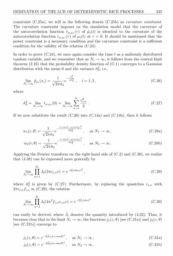
DERIVATION OF THE LCR OF DETERMINISTIC RICE PROCESSES 335
constraint (C.25a), we will in the following denote (C.25b) as curvature constraint.The curvature constraint imposes on the simulation model that the curvature ofthe autocorrelation function rµiµi
(τ) of µi(t) is identical to the curvature of theautocorrelation function rµiµi(τ) of µi(t) at τ = 0. It should be mentioned that thepower constraint is a necessary condition and the curvature constraint is a sufficientcondition for the validity of the relation (C.24).
In order to prove (C.24), we once again consider the time t as a uniformly distributedrandom variable, and we remember that as Ni →∞, it follows from the central limittheorem (2.16) that the probability density function of (C.1) converges to a Gaussiandistribution with the mean 0 and the variance σ2
0 , i.e.,
limNi→∞
pµi(xi) =
1√2πσ0
e− x2
i2σ2
0 , i = 1, 2 , (C.26)
where
σ20 = lim
Ni→∞rµiµi(0) = lim
Ni→∞
Ni∑n=1
c2i,n
2. (C.27)
If we now substitute the result (C.26) into (C.14a) and (C.14b), then it follows
w1(r, θ) =1√
2πσ0
e− (r cos θ−ρ cos θρ)2
2σ20 , as N1 →∞ , (C.28a)
w2(r, θ) =1√
2πσ0
e− (r sin θ−ρ sin θρ)2
2σ20 , as N2 →∞ . (C.28b)
Applying the Fourier transform on the right-hand side of (C.2) and (C.26), we realizethat (4.38) can be expressed more generally by
limNi→∞
Ni∏n=1
J0(2πci,nν) = e−2(πσ0ν)2 , (C.29)
where σ20 is given by (C.27). Furthermore, by replacing the quantities ci,n with
2πci,nfi,n in (C.29), the relation
limNi→∞
Ni∏n=1
J0(4π2fi,nci,nν) = e−2βi(πν)2 (C.30)
can easily be derived, where βi denotes the quantity introduced by (4.22). Thus, itbecomes clear that in the limit Ni →∞, the functions j1(z, θ) [see (C.21a)] and j2(z, θ)[see (C.21b)] converge to
j1(z, θ) = e−2β1(πz cos θ)2 , as N1 →∞ , (C.31a)
j2(z, θ) = e−2β2(πz sin θ)2 , as N2 →∞ , (C.31b)

336 DERIVATION OF THE LCR OF DETERMINISTIC RICE PROCESSES
respectively. If we now substitute the obtained results (C.28a), (C.28b), (C.31a), and(C.31b) into Nξ(r) according to (C.22), then — on the condition that β = β1 = β2
holds — it follows the expression
limNi→∞
Nξ(r) =r
πσ20
e− r2+ρ2
2σ20
∫ ∞
0
∫ π
−π
z erρ
σ20
cos(θ−θρ)
∫ ∞
0
e−2β(πz)2 cos(2πzz) dz dθ dz . (C.32)
Using the integral [Gra81, eq. (3.896.4)]
∫ ∞
0
e−ux2cos(bx) dx =
12
√π
ue−
b24u , Re u > 0 , (C.33)
(C.32) can be simplified to
limNi→∞
Nξ(r) =r√
2πβσ20
e− r2+ρ2
2σ20 · 1
2π
∫ π
−π
erρ
σ20
cos(θ−θρ)dθ ·
∫ ∞
0
z e− z2
2β dz . (C.34)
The remaining two integrals over θ and z can be solved without great expense byusing the integral representation of the zeroth-order modified Bessel function of thefirst kind [Abr72, eq. (9.6.16)]
I0(z) =1π
∫ π
0
e±z cos θ dθ (C.35)
and the integral [Gra81, eq. (3.461.3)]∫ ∞
0
x2n+1 e−px2dx =
n!2pn+1
, p > 0 . (C.36)
Finally, we obtain
limNi→∞
Nξ(r) =
√β
2π· r
σ20
e− r2+ρ2
2σ20 I0
(rρ
σ20
). (C.37)
Taking the power constraint (C.25a) and the curvature constraint (C.25b) intoaccount, the right-hand side of the above equation can now directly be identifiedwith (2.62), which proves the validity of (C.24).
For completeness, we will also give the exact solution for the average duration offades Tξ−(r) of deterministic Rice processes ξ(t). Since we need an expression forthe cumulative distribution function Fξ−(r) of ξ(t), we will first of all derive this bysubstituting (4.50) into
Fξ−(r) =∫ r
0
pξ(z) dz . (C.38)

DERIVATION OF THE LCR OF DETERMINISTIC RICE PROCESSES 337
The integration over z can be carried out by using the indefinite integral [Gra81,eq. (5.56.2)]
∫z J0(z) dz = z J1(z) , (C.39)
so that after some algebraic manipulations, the following result is obtained
Fξ−(r) = 2r
∫ ∞
0
J1(2πry)∫ π
0
h1(y, θ)h2(y, θ) cos[2πρy cos(θ − θρ)] dθ dy , (C.40)
where
h1(y, θ) =N1∏
n=1
J0(2πc1,ny cos θ) , (C.41a)
h2(y, θ) =N2∏
n=1
J0(2πc2,ny sin θ) . (C.41b)
With the cumulative distribution function (C.40) presented above and the solutionfor the level-crossing rate (C.22) found before, the average duration of fades Tξ−(r) ofdeterministic Rice processes ξ(t) can now be analysed analytically using
Tξ−(r) =Fξ−(r)
Nξ(r). (C.42)
In order to illustrate the obtained results, we consider Figure C.2, which shows thenormalized average duration of fades of deterministic Rice and Rayleigh processes,according to the theoretical results (C.42), in comparison with the correspondingsimulation results.
Subsequently, we want to prove that in the conditions (C.25a) and (C.25b), the averageduration of fades Tξ−(r) of deterministic Rice processes ξ(t) converges to the averageduration of fades Tξ−(r) of stochastic Rice processes ξ(t) as the number of harmonicfunctions Ni tends to infinity, i.e.,
Tξ−(r) = Tξ−(r) , as Ni →∞ . (C.43)
Due to (C.24) and the general relation (C.42), it is sufficient here to show that
Fξ−(r) = Fξ−(r) , as Ni →∞ , (C.44a)
or, equivalently, that
pξ(r) = pξ(r) , as Ni →∞ , (C.44b)
holds. Due to (C.29), we therefore first realize that the functions h1(y, θ) [see (C.41a)]and h2(y, θ) [see (C.41b)] tend to
h1(y, θ) = e−2(πσ0y cos θ)2 , as N1 →∞ , (C.45a)

338 DERIVATION OF THE LCR OF DETERMINISTIC RICE PROCESSES
-15 -10 -5 0 5
10-1
100
r (dB)
Tξ -
(r)
⋅ fm
ax
ρ=0
ρ=2
MEA: Theory, SimulationMEDS: Theory, SimulationMCM: Theory, Simulation
Reference model
Figure C.2: Normalized average duration of fades of deterministic Rice and Rayleighprocesses both realized with N1 = 7 and N2 = 8 (Jakes PSD, fmax = 91 Hz,σ2
0 = 1, θρ = π/4).
and
h2(y, θ) = e−2(πσ0ysinθ)2 , as N2 →∞ , (C.45b)
respectively. With this result it follows from (4.50)
limNi→∞
pξ(z) = (2π)2z
∞∫
0
e−2(πσ0y)2J0(2πzy)1π
π∫
0
cos[2πρy cos(θ − θρ)]dθ y dy .
(C.46)
The integral representation of the zeroth-order Bessel function [Abr72, eq. (9.1.18)]
J0(z) =1π
∫ π
0
cos(z cos θ) dθ (C.47)
enables us to write the expression (C.46) in the form
limNi→∞
pξ(z) = (2π)2z∫ ∞
0
e−2(πσ0y)2 J0(2πzy) J0(2πρy) y dy . (C.48)
The remaining integral can be solved by using [Gra81, eq. (6.633.2)]∫ ∞
0
e−(ax)2J0(αx) J0(βx) x dx =1
2a2e−
α2+β2
4a2 I0
(αβ
2a2
). (C.49)
Thus, we finally obtain
pξ(z) =z
σ20
e− z2+ρ2
2σ20 I0
(zρ
σ20
), Ni →∞ . (C.50)

DERIVATION OF THE LCR OF DETERMINISTIC RICE PROCESSES 339
With the power constraint (C.25a), i.e., σ20 = σ2
0 , the Rice distribution (2.26) followsfrom the right-hand side of (C.50) proving the validity of (C.44b) and, consequently,also the validity of (C.43).

Appendix D
ANALYSIS OF THE RELATIVEMODEL ERROR BY USING THEMONTE CARLO METHOD INCONNECTION WITH THEJAKES POWER SPECTRALDENSITY
We consider the relative model error
∆βi
β=
βi − β
β, i = 1, 2 , (D.1)
where the quantities β and βi are, especially for the Jakes power spectral density,given by
β = 2(πσ0fmax)2 (D.2)
and
βi =2β
f2maxNi
Ni∑n=1
f2i,n , (D.3)
respectively. If we use the Monte Carlo method for the computation of the modelparameter, then the discrete Doppler frequencies fi,n are random variables, whereeach random variable fi,n is characterized by the probability density function
pfi,n(fi,n) =
2πfmax
√1− (fi,n/fmax)2
, 0 < f ≤ fmax ,
0 , else .
(D.4)
With the Chebyshev inequality (2.15), the relation
P
(∣∣∣∣∆βi
β− E
∆βi
β
∣∣∣∣ ≥ ε
)≤ Var ∆βi/β
ε2(D.5)

342 ANALYSIS OF THE RELATIVE MODEL ERROR BY USING THE MCM
holds for all ε > 0. Using (D.4), we find
Ef2
i,n
=
f2max
2(D.6)
and
Varf2
i,n
= E
f4
i,n
− (E
f2
i,n
)2
=38f4
max −f4
max
4
=f4
max
8. (D.7)
Hence, for the mean value and the variance of the relative model error ∆βi/β [cf.(D.1)], we obtain the following expression in connection with (D.3)
E
∆βi
β
= 0 (D.8)
and
Var
∆βi
β
= Var
βi
β
=(
2f2
maxNi
)2
Var
Ni∑
n=1
f2i,n
=(
2f2
maxNi
)2 Ni∑n=1
Varf2
i,n
=1
2Ni, (D.9)
respectively. Thus, with the Chebyshev inequality (D.5) the relation
P
(∣∣∣∣∆βi
β
∣∣∣∣ ≥ ε
)≤ 1
2Niε2(D.10)
follows. For example, let ε = 0.02 and Ni = 2500 (!), then the above inequality canbe interpreted as follows: the probability that the absolute value of the relative modelerror |∆βi/β| is greater than or equal to 2 per cent is smaller than or equal to 50 percent.

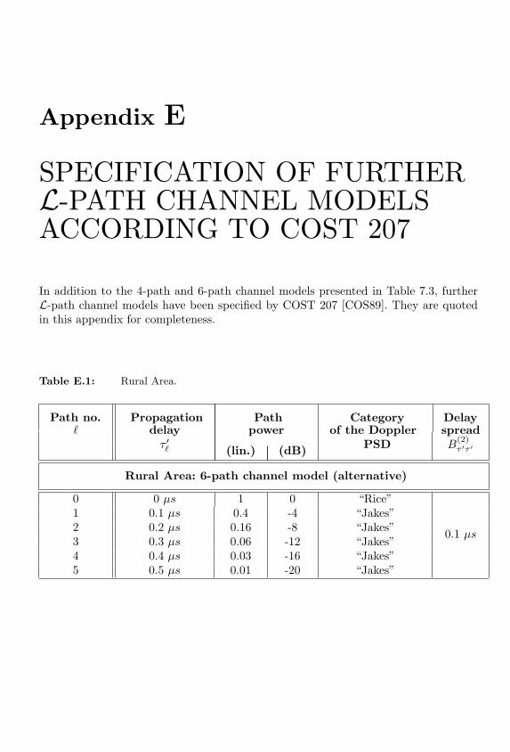
Appendix E
SPECIFICATION OF FURTHERL-PATH CHANNEL MODELSACCORDING TO COST 207
In addition to the 4-path and 6-path channel models presented in Table 7.3, furtherL-path channel models have been specified by COST 207 [COS89]. They are quotedin this appendix for completeness.
Table E.1: Rural Area.
Path no. Propagation Path Category Delay` delay power of the Doppler spread
τ ′` (lin.) (dB) PSD B(2)τ ′τ ′
Rural Area: 6-path channel model (alternative)
0 0 µs 1 0 “Rice”1 0.1 µs 0.4 -4 “Jakes”2 0.2 µs 0.16 -8 “Jakes”3 0.3 µs 0.06 -12 “Jakes”
0.1 µs
4 0.4 µs 0.03 -16 “Jakes”5 0.5 µs 0.01 -20 “Jakes”

344 L-PATH CHANNEL MODELS ACCORDING TO COST 207
Table E.2: Typical Urban.
Path no. Propagation Path Category Delay` delay power of the Doppler spread
τ ′` (lin.) (dB) PSD B(2)τ ′τ ′
(i) Typical Urban: 12-path channel model
0 0.0 µs 0.4 -4 “Jakes”1 0.2 µs 0.5 -3 “Jakes”2 0.4 µs 1 0 “Jakes”3 0.6 µs 0.63 -2 “Gauss I”4 0.8 µs 0.5 -3 “Gauss I”5 1.2 µs 0.32 -5 “Gauss I”6 1.4 µs 0.2 -7 “Gauss I”
1.0 µs
7 1.8 µs 0.32 -5 “Gauss I”8 2.4 µs 0.25 -6 “Gauss II”9 3.0 µs 0.13 -9 “Gauss II”10 3.2 µs 0.08 -11 “Gauss II”11 5.0 µs 0.1 -10 “Gauss II”
(ii) Typical Urban: 12-path channel model (alternative)
0 0.0 µs 0.4 -4 “Jakes”1 0.1 µs 0.5 -3 “Jakes”2 0.3 µs 1 0 “Jakes”3 0.5 µs 0.55 -2.6 “Jakes”4 0.8 µs 0.5 -3 “Gauss I”5 1.1 µs 0.32 -5 “Gauss I”6 1.3 µs 0.2 -7 “Gauss I”
1.0 µs
7 1.7 µs 0.32 -5 “Gauss I”8 2.3 µs 0.22 -6.5 “Gauss II”9 3.1 µs 0.14 -8.6 “Gauss II”10 3.2 µs 0.08 -11 “Gauss II”11 5.0 µs 0.1 -10 “Gauss II”
(iii) Typical Urban: 6-path channel model (alternative)
0 0.0 µs 0.5 -3 “Jakes”1 0.2 µs 1 0 “Jakes”2 0.5 µs 0.63 -2 “Jakes”3 1.6 µs 0.25 -6 “Gauss I”
1.0 µs
4 2.3 µs 0.16 -8 “Gauss II”5 5.0 µs 0.1 -10 “Gauss II”

L-PATH CHANNEL MODELS ACCORDING TO COST 207 345
Table E.3: Bad Urban.
Path no. Propagation Path Category Delay` delay power of the Doppler spread
τ ′` (lin.) (dB) PSD B(2)τ ′τ ′
(i) Bad Urban: 12-path channel model
0 0.0 µs 0.2 -7 “Jakes”1 0.2 µs 0.5 -3 “Jakes”2 0.4 µs 0.79 -1 “Jakes”3 0.8 µs 1 0 “Gauss I”4 1.6 µs 0.63 -2 “Gauss I”5 2.2 µs 0.25 -6 “Gauss II”6 3.2 µs 0.2 -7 “Gauss II”
2.5 µs
7 5.0 µs 0.79 -1 “Gauss II”8 6.0 µs 0.63 -2 “Gauss II”9 7.2 µs 0.2 -7 “Gauss II”10 8.2 µs 0.1 -10 “Gauss II”11 10.0 µs 0.03 -15 “Gauss II”
(ii) Bad Urban: 12-path channel model (alternative)
0 0.0 µs 0.17 -7.7 “Jakes”1 0.1 µs 0.46 -3.4 “Jakes”2 0.3 µs 0.74 -1.3 “Jakes”3 0.7 µs 1 0 “Gauss I”4 1.6 µs 0.59 -2.3 “Gauss I”5 2.2 µs 0.28 -5.6 “Gauss II”6 3.1 µs 0.18 -7.4 “Gauss II”
2.5 µs
7 5.0 µs 0.72 -1.4 “Gauss II”8 6.0 µs 0.69 -1.6 “Gauss II”9 7.2 µs 0.21 -6.7 “Gauss II”10 8.1 µs 0.1 -9.8 “Gauss II”11 10.0 µs 0.03 -15.1 “Gauss II”
(iii) Bad Urban: 6-path channel model (alternative)
0 0.0 µs 0.56 -2.5 “Jakes”1 0.3 µs 1 0 “Jakes”2 1.0 µs 0.5 -3 “Gauss I”3 1.6 µs 0.32 -5 “Gauss I”
2.5 µs
4 5.0 µs 0.63 -2 “Gauss II”5 6.6 µs 0.4 -4 “Gauss II”

346 L-PATH CHANNEL MODELS ACCORDING TO COST 207
Table E.4: Hilly Terrain.
Path no. Propagation Path Category Delay` delay power of the Doppler spread
τ ′` (lin.) (dB) PSD B(2)τ ′τ ′
(i) Hilly Terrain: 12-path channel model
0 0.0 µs 0.1 -10 “Jakes”1 0.2 µs 0.16 -8 “Jakes”2 0.4 µs 0.25 -6 “Jakes”3 0.6 µs 0.4 -4 “Gauss I”4 0.8 µs 1 0 “Gauss I”5 2.0 µs 1 0 “Gauss I”6 2.4 µs 0.4 -4 “Gauss II”
5.0 µs
7 15.0 µs 0.16 -8 “Gauss II”8 15.2 µs 0.13 -9 “Gauss II”9 15.8 µs 0.1 -10 “Gauss II”10 17.2 µs 0.06 -12 “Gauss II”11 20.0 µs 0.04 -14 “Gauss II”
(ii) Hilly Terrain: 12-path channel model (alternative)
0 0.0 µs 0.1 -10 “Jakes”1 0.1 µs 0.16 -8 “Jakes”2 0.3 µs 0.25 -6 “Jakes”3 0.5 µs 0.4 -4 “Jakes”4 0.7 µs 1 0 “Gauss I”5 1.0 µs 1 0 “Gauss I”6 1.3 µs 0.4 -4 “Gauss I”
5.0 µs
7 15.0 µs 0.16 -8 “Gauss II”8 15.2 µs 0.13 -9 “Gauss II”9 15.7 µs 0.1 -10 “Gauss II”10 17.2 µs 0.06 -12 “Gauss II”11 20.0 µs 0.04 -14 “Gauss II”
(iii) Hilly Terrain: 6-path channel model (alternative)
0 0.0 µs 1 0 “Jakes”1 0.1 µs 0.71 -1.5 “Jakes”2 0.3 µs 0.35 -4.5 “Jakes”3 0.5 µs 0.18 -7.5 “Jakes”
5.0 µs
4 15 µs 0.16 -8.0 “Gauss II”5 17.2 µs 0.02 -17.7 “Gauss II”
347
MATLAB-PROGRAMS
In the following, a selection of MATLAB-programs (m-files) is presented, whichsave the user from programming effort during the realization of the methods usedto design the model parameters of deterministic processes, and which will help himfind his way in the topic of simulation and analysis of mobile radio channel models.MATLAB stands for matrix laboratory, an interpreter language developed by TheMath Works, Inc., for the numerical computation and visualization of matrices. Them-files presented below require the Signal Processing Toolbox and the OptimizationToolbox.
References on necessary subroutines (functions) and a description of the input andoutput parameters of the individual programs can be found in the program headerblock of each program.
At first, the m-files for the computation of the model parameters are presentedby making use of the methods described in Chapter 5. Here, these methods aresubdivided depending on the type of power spectral density (Jakes/Gauss) of thedeterministic Gaussian processes to be realized. Subsequently, functions for thetime-domain simulation of various frequency-nonselective (Chapter 6) and frequency-selective (Chapter 7) mobile radio channels are presented. Finally, further tools areprovided, with the help of which the designed channel simulators can be analysedwith respect to their statistical properties such as the probability density function,the cumulative distribution function, the level-crossing rate, and the average durationof fades.
%--------------------------------------------------------------------% parameter_Jakes.m -------------------------------------------------%% Program for the computation of the discrete Doppler frequencies,% Doppler coefficients and Doppler phases by using the Jakes power% spectral density.%% Used m-files: LPNM_opt_Jakes.m, fun_Jakes.m,% grad_Jakes.m, acf_mue.m%--------------------------------------------------------------------% [f_i_n,c_i_n,theta_i_n]=parameter_Jakes(METHOD,N_i,sigma_0_2,...

348 MATLAB-PROGRAMS
% f_max,PHASE,PLOT)%--------------------------------------------------------------------% Explanation of the input parameters:%% METHOD:% |----------------------------------------------|------------------|% | Methods for the computation of the discrete | Input |% | Doppler frequencies and Doppler coefficients | |% |----------------------------------------------|------------------|% |----------------------------------------------|------------------|% | Method of equal distances (MED) | ’ed_j’ |% |----------------------------------------------|------------------|% | Mean square error method (MSEM) | ’ms_j’ |% |----------------------------------------------|------------------|% | Method of equal areas (MEA) | ’ea_j’ |% |----------------------------------------------|------------------|% | Monte Carlo method (MCM) | ’mc_j’ |% |----------------------------------------------|------------------|% | Lp-norm method (LPNM) | ’lp_j’ |% |----------------------------------------------|------------------|% | Method of exact Doppler spread (MEDS) | ’es_j’ |% |----------------------------------------------|------------------|% | Jakes method (JM) | ’jm_j’ |% |----------------------------------------------|------------------|%% N_i: number of harmonic functions% sigma_0_2: average power of the real deterministic Gaussian% process mu_i(t)% f_max: maximum Doppler frequency%% PHASE:% |----------------------------------------------|------------------|% | Methods for the computation of the Doppler | Input |% | phases | |% |----------------------------------------------|------------------|% |----------------------------------------------|------------------|% | Random Doppler phases | ’rand’ |% |----------------------------------------------|------------------|% | Permuted Doppler phases | ’perm’ |% |----------------------------------------------|------------------|%% PLOT: plot of the ACF and the PSD of mu_i(t), if PLOT==1
function [f_i_n,c_i_n,theta_i_n]=parameter_Jakes(METHOD,N_i,...sigma_0_2,f_max,PHASE,PLOT)
if nargin<6,

MATLAB-PROGRAMS 349
error(’Not enough input parameters’)end
sigma_0=sqrt(sigma_0_2);
% Method of equal distances (MED)if METHOD==’ed_j’,
n=(1:N_i)’;f_i_n=f_max/(2*N_i)*(2*n-1);c_i_n=2*sigma_0/sqrt(pi)*(asin(n/N_i)-asin((n-1)/N_i)).^0.5;K=1;
% Mean square error method (MSEM)elseif METHOD==’ms_j’,
n=(1:N_i)’;f_i_n=f_max/(2*N_i)*(2*n-1);Tp=1/(2*f_max/N_i);t=linspace(0,Tp,5E3);Jo=besselj(0,2*pi*f_max*t);c_i_n=zeros(size(f_i_n));for k=1:length(f_i_n),
c_i_n(k)=2*sigma_0*...sqrt(1/Tp*( trapz( t,Jo.*...cos(2*pi*f_i_n(k)*t )) ));
endK=1;
% Method of equal areas (MEA)elseif METHOD==’ea_j’
n=(1:N_i)’;f_i_n=f_max*sin(pi*n/(2*N_i));c_i_n=sigma_0*sqrt(2/N_i)*ones(size(n));K=1;
% Monte Carlo method (MCM)elseif METHOD==’mc_j’
n=rand(N_i,1);f_i_n=f_max*sin(pi*n/2);c_i_n=sigma_0*sqrt(2/N_i)*ones(size(n));
K=1;
% Lp-norm method (LPNM)elseif METHOD==’lp_j’,
if exist(’fminu’)~=2disp([’ =====> This method requires ’,...
’the Optimization Toolbox !!’])
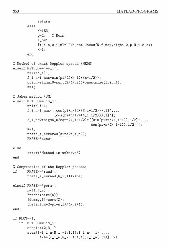
350 MATLAB-PROGRAMS
returnelse
N=1E3;p=2; % Norms_o=1;[f_i_n,c_i_n]=LPNM_opt_Jakes(N,f_max,sigma_0,p,N_i,s_o);K=1;
end
% Method of exact Doppler spread (MEDS)elseif METHOD==’es_j’,
n=(1:N_i)’;f_i_n=f_max*sin(pi/(2*N_i)*(n-1/2));c_i_n=sigma_0*sqrt(2/(N_i))*ones(size(f_i_n));K=1;
% Jakes method (JM)elseif METHOD==’jm_j’,
n=1:N_i-1;f_i_n=f_max*[[cos(pi*n/(2*(N_i-1/2))),1]’,...
[cos(pi*n/(2*(N_i-1/2))),1]’];c_i_n=2*sigma_0/sqrt(N_i-1/2)*[[sin(pi*n/(N_i-1)),1/2]’,...
[cos(pi*n/(N_i-1)),1/2]’];K=1;theta_i_n=zeros(size(f_i_n));PHASE=’none’;
elseerror(’Method is unknown’)
end
% Computation of the Doppler phases:if PHASE==’rand’,
theta_i_n=rand(N_i,1)*2*pi;
elseif PHASE==’perm’,n=(1:N_i)’;Z=rand(size(n));[dummy,I]=sort(Z);theta_i_n=2*pi*n(I)/(N_i+1);
end;
if PLOT==1,if METHOD==’jm_j’
subplot(2,3,1)stem([-f_i_n(N_i:-1:1,1);f_i_n(:,1)],...
1/4*[c_i_n(N_i:-1:1,1);c_i_n(:,1)].^2)

MATLAB-PROGRAMS 351
title(’i=1’)xlabel(’f (Hz)’)ylabel(’PSD’)subplot(2,3,2)stem([-f_i_n(N_i:-1:1,2);f_i_n(:,2)],...
1/4*[c_i_n(N_i:-1:1,2);c_i_n(:,2)].^2)title(’i=2’)xlabel(’f (Hz)’)ylabel(’PSD’)tau_max=N_i/(K*f_max);tau=linspace(0,tau_max,500);r_mm=sigma_0^2*besselj(0,2*pi*f_max*tau);
r_mm_tilde1=acf_mue(f_i_n(:,1),c_i_n(:,1),tau);subplot(2,3,4)plot(tau,r_mm,’r-’,tau,r_mm_tilde1,’g--’)title(’i=1’)xlabel(’tau (s)’)ylabel(’ACF’)r_mm_tilde2=acf_mue(f_i_n(:,2),c_i_n(:,2),tau);subplot(2,3,5)plot(tau,r_mm,’r-’,tau,r_mm_tilde2,’g--’)title(’i=2’)xlabel(’tau (s)’)ylabel(’ACF’)subplot(2,3,3)stem([-f_i_n(N_i:-1:1,1);f_i_n(:,1)],...
1/4*[c_i_n(N_i:-1:1,1);c_i_n(:,1)].^2+...1/4*[c_i_n(N_i:-1:1,2);c_i_n(:,2)].^2)
title(’i=1,2’)xlabel(’f (Hz)’)ylabel(’PSD’)subplot(2,3,6)plot(tau,2*r_mm,’r-’,tau,r_mm_tilde1+r_mm_tilde2,’g--’)title(’i=1,2’)xlabel(’tau (s)’)ylabel(’ACF’)
elsesubplot(1,2,1)stem([-f_i_n(N_i:-1:1);f_i_n],...
1/4*[c_i_n(N_i:-1:1);c_i_n].^2)xlabel(’f/Hz’)ylabel(’LDS’)tau_max=N_i/(K*f_max);tau=linspace(0,tau_max,500);r_mm=sigma_0^2*besselj(0,2*pi*f_max*tau);r_mm_tilde=acf_mue(f_i_n,c_i_n,tau);
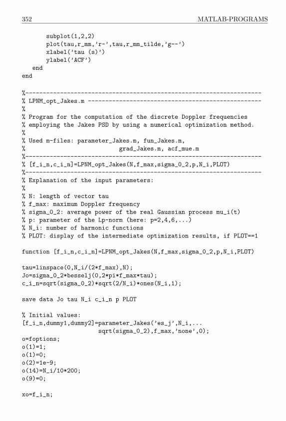
352 MATLAB-PROGRAMS
subplot(1,2,2)plot(tau,r_mm,’r-’,tau,r_mm_tilde,’g--’)xlabel(’tau (s)’)ylabel(’ACF’)
endend
%--------------------------------------------------------------------% LPNM_opt_Jakes.m --------------------------------------------------%% Program for the computation of the discrete Doppler frequencies% employing the Jakes PSD by using a numerical optimization method.%% Used m-files: parameter_Jakes.m, fun_Jakes.m,% grad_Jakes.m, acf_mue.m%--------------------------------------------------------------------% [f_i_n,c_i_n]=LPNM_opt_Jakes(N,f_max,sigma_0_2,p,N_i,PLOT)%--------------------------------------------------------------------% Explanation of the input parameters:%% N: length of vector tau% f_max: maximum Doppler frequency% sigma_0_2: average power of the real Gaussian process mu_i(t)% p: parameter of the Lp-norm (here: p=2,4,6,...)% N_i: number of harmonic functions% PLOT: display of the intermediate optimization results, if PLOT==1
function [f_i_n,c_i_n]=LPNM_opt_Jakes(N,f_max,sigma_0_2,p,N_i,PLOT)
tau=linspace(0,N_i/(2*f_max),N);Jo=sigma_0_2*besselj(0,2*pi*f_max*tau);c_i_n=sqrt(sigma_0_2)*sqrt(2/N_i)*ones(N_i,1);
save data Jo tau N_i c_i_n p PLOT
% Initial values:[f_i_n,dummy1,dummy2]=parameter_Jakes(’es_j’,N_i,...
sqrt(sigma_0_2),f_max,’none’,0);o=foptions;o(1)=1;o(1)=0;o(2)=1e-9;o(14)=N_i/10*200;o(9)=0;
xo=f_i_n;
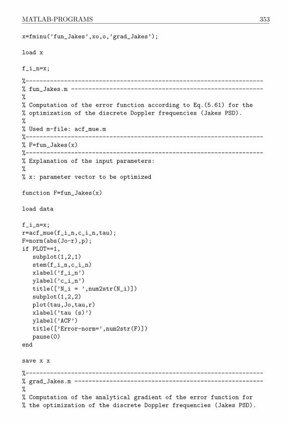
MATLAB-PROGRAMS 353
x=fminu(’fun_Jakes’,xo,o,’grad_Jakes’);
load x
f_i_n=x;
%--------------------------------------------------------------------% fun_Jakes.m -------------------------------------------------------%% Computation of the error function according to Eq.(5.61) for the% optimization of the discrete Doppler frequencies (Jakes PSD).%% Used m-file: acf_mue.m%--------------------------------------------------------------------% F=fun_Jakes(x)%--------------------------------------------------------------------% Explanation of the input parameters:%% x: parameter vector to be optimized
function F=fun_Jakes(x)
load data
f_i_n=x;r=acf_mue(f_i_n,c_i_n,tau);F=norm(abs(Jo-r),p);if PLOT==1,
subplot(1,2,1)stem(f_i_n,c_i_n)xlabel(’f_i_n’)ylabel(’c_i_n’)title([’N_i = ’,num2str(N_i)])subplot(1,2,2)plot(tau,Jo,tau,r)xlabel(’tau (s)’)ylabel(’ACF’)title([’Error-norm=’,num2str(F)])pause(0)
end
save x x
%--------------------------------------------------------------------% grad_Jakes.m ------------------------------------------------------%% Computation of the analytical gradient of the error function for% the optimization of the discrete Doppler frequencies (Jakes PSD).
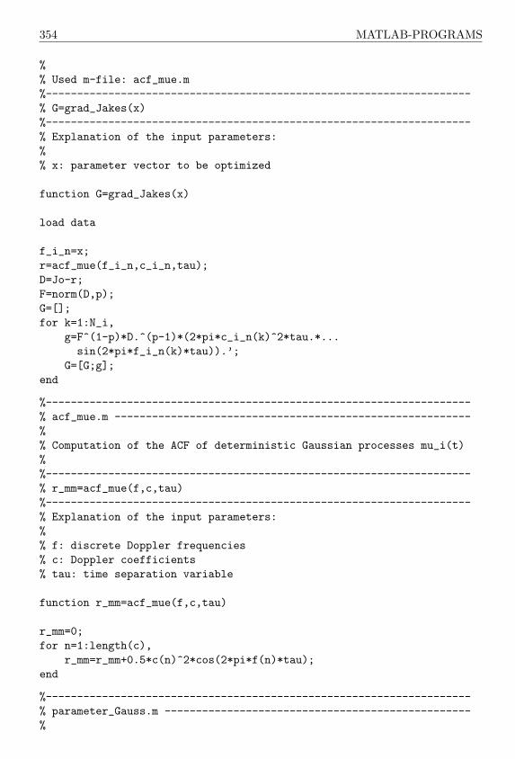
354 MATLAB-PROGRAMS
%% Used m-file: acf_mue.m%--------------------------------------------------------------------% G=grad_Jakes(x)%--------------------------------------------------------------------% Explanation of the input parameters:%% x: parameter vector to be optimized
function G=grad_Jakes(x)
load data
f_i_n=x;r=acf_mue(f_i_n,c_i_n,tau);D=Jo-r;F=norm(D,p);G=[];for k=1:N_i,
g=F^(1-p)*D.^(p-1)*(2*pi*c_i_n(k)^2*tau.*...sin(2*pi*f_i_n(k)*tau)).’;
G=[G;g];end
%--------------------------------------------------------------------% acf_mue.m ---------------------------------------------------------%% Computation of the ACF of deterministic Gaussian processes mu_i(t)%%--------------------------------------------------------------------% r_mm=acf_mue(f,c,tau)%--------------------------------------------------------------------% Explanation of the input parameters:%% f: discrete Doppler frequencies% c: Doppler coefficients% tau: time separation variable
function r_mm=acf_mue(f,c,tau)
r_mm=0;for n=1:length(c),
r_mm=r_mm+0.5*c(n)^2*cos(2*pi*f(n)*tau);end
%--------------------------------------------------------------------% parameter_Gauss.m -------------------------------------------------%
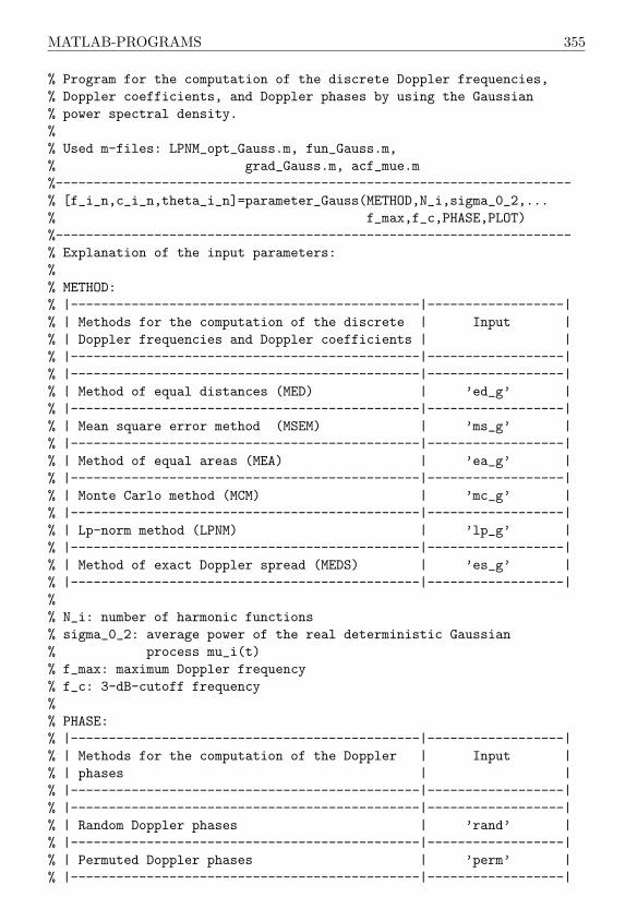
MATLAB-PROGRAMS 355
% Program for the computation of the discrete Doppler frequencies,% Doppler coefficients, and Doppler phases by using the Gaussian% power spectral density.%% Used m-files: LPNM_opt_Gauss.m, fun_Gauss.m,% grad_Gauss.m, acf_mue.m%--------------------------------------------------------------------% [f_i_n,c_i_n,theta_i_n]=parameter_Gauss(METHOD,N_i,sigma_0_2,...% f_max,f_c,PHASE,PLOT)%--------------------------------------------------------------------% Explanation of the input parameters:%% METHOD:% |----------------------------------------------|------------------|% | Methods for the computation of the discrete | Input |% | Doppler frequencies and Doppler coefficients | |% |----------------------------------------------|------------------|% |----------------------------------------------|------------------|% | Method of equal distances (MED) | ’ed_g’ |% |----------------------------------------------|------------------|% | Mean square error method (MSEM) | ’ms_g’ |% |----------------------------------------------|------------------|% | Method of equal areas (MEA) | ’ea_g’ |% |----------------------------------------------|------------------|% | Monte Carlo method (MCM) | ’mc_g’ |% |----------------------------------------------|------------------|% | Lp-norm method (LPNM) | ’lp_g’ |% |----------------------------------------------|------------------|% | Method of exact Doppler spread (MEDS) | ’es_g’ |% |----------------------------------------------|------------------|%% N_i: number of harmonic functions% sigma_0_2: average power of the real deterministic Gaussian% process mu_i(t)% f_max: maximum Doppler frequency% f_c: 3-dB-cutoff frequency%% PHASE:% |----------------------------------------------|------------------|% | Methods for the computation of the Doppler | Input |% | phases | |% |----------------------------------------------|------------------|% |----------------------------------------------|------------------|% | Random Doppler phases | ’rand’ |% |----------------------------------------------|------------------|% | Permuted Doppler phases | ’perm’ |% |----------------------------------------------|------------------|

356 MATLAB-PROGRAMS
%% PLOT: plot of the ACF and the PSD of mu_i(t), if PLOT==1
function [f_i_n,c_i_n,theta_i_n]=parameter_Gauss(METHOD,N_i,...sigma_0_2,f_max,f_c,PHASE,PLOT)
if nargin<7,error(’Not enough input parameters’)
end
sigma_0=sqrt(sigma_0_2);kappa_c=f_max/f_c;
% Method of equal distances (MED)if METHOD==’ed_g’,
n=(1:N_i)’;f_i_n=kappa_c*f_c/(2*N_i)*(2*n-1);c_i_n=sigma_0*sqrt(2)*sqrt(erf(n*kappa_c*...
sqrt(log(2))/N_i)-erf((n-1)*kappa_c*...sqrt(log(2))/N_i) );
K=1;
% Mean square error method (MSEM)elseif METHOD==’ms_g’,
n=(1:N_i)’;f_i_n=kappa_c*f_c/(2*N_i)*(2*n-1);tau_max=N_i/(2*kappa_c*f_c);N=1E3;tau=linspace(0,tau_max,N);f1=exp(-(pi*f_c*tau).^2/log(2));c_i_n=zeros(size(f_i_n));for k=1:length(c_i_n),
c_i_n(k)=2*sigma_0*sqrt(trapz(tau,f1.*...cos(2*pi*f_i_n(k)*tau))/tau_max);
endK=1;
% Method of equal areas (MEA)elseif METHOD==’ea_g’
n=(1:N_i)’;c_i_n=sigma_0*sqrt(2/N_i)*ones(size(n));f_i_n=f_c/sqrt(log(2))*erfinv(n/N_i);f_i_n(N_i)=f_c/sqrt(log(2))*erfinv(0.9999999);K=1;
% Monte Carlo method (MCM)elseif METHOD==’mc_g’

MATLAB-PROGRAMS 357
n=rand(N_i,1);f_i_n=f_c/sqrt(log(2))*erfinv(n);c_i_n=sigma_0*sqrt(2/N_i)*ones(size(n));K=1;
% Lp-norm method (LPNM)elseif METHOD==’lp_g’,
if exist(’fminu’)~=2disp([’ =====> This method requires ’,...
’the Optimization Toolbox !!’])return
elseN=1e3;p=2;[f_i_n,c_i_n]=LPNM_opt_Gauss(N,f_max,f_c,...
sigma_0_2,p,N_i,PLOT);K=2;
end
% Method of exact Doppler spread (MEDS)elseif METHOD==’es_g’,
n=(1:N_i)’;c_i_n=sigma_0*sqrt(2/N_i)*ones(size(n));f_i_n=f_c/sqrt(log(2))*erfinv((2*n-1)/(2*N_i));K=1;
elseerror([setstr(10),’Method is unknown’])
end
% Computation of the Doppler phases:if PHASE==’rand’,
theta_i_n=rand(N_i,1)*2*pi;elseif PHASE==’perm’,
n=(1:N_i)’;Z=rand(size(n));[dummy,I]=sort(Z);theta_i_n=2*pi*n(I)/(N_i+1);
end
if PLOT==1,subplot(1,2,1)stem([-f_i_n(N_i:-1:1);f_i_n],...
1/4*[c_i_n(N_i:-1:1);c_i_n].^2)xlabel(’f (Hz)’)ylabel(’PSD’)tau_max=N_i/(K*kappa_c*f_c);

358 MATLAB-PROGRAMS
tau=linspace(0,tau_max,500);r_mm=sigma_0_2*exp(-(pi*f_c/sqrt(log(2))*tau).^2);r_mm_tilde=acf_mue(f_i_n,c_i_n,tau);subplot(1,2,2)plot(tau,r_mm,’r-’,tau,r_mm_tilde,’g--’)xlabel(’tau (s)’)ylabel(’ACF’)
end
%--------------------------------------------------------------------% LPNM_opt_Gauss.m --------------------------------------------------%% Program for the computation of the discrete Doppler frequencies% employing the Gaussian PSD by using a numerical optimization% method.%% Used m-files: parameter_Gauss.m, fun_Gauss.m,% grad_Gauss.m, acf_mue.m%--------------------------------------------------------------------% [f_i_n,c_i_n]=LPNM_opt_Gauss(N,f_max,f_c,sigma_0_2,p,N_i,PLOT)%--------------------------------------------------------------------% Explanation of the input parameters:%% N: length of vector tau% f_max: maximum Doppler frequency% f_c: 3-dB-cutoff frequency% sigma_0_2: average power of the real Gaussian process mu_i(t)% p: parameter of the Lp-norm (here: p=2,4,6,...)% N_i: number of harmonic functions% PLOT: display of the intermediate optimization results, if PLOT==1
function [f_i_n,c_i_n]=LPNM_opt_Gauss(N,f_max,f_c,sigma_0_2,...p,N_i,PLOT)
kappa_c=f_max/f_c;
F_list=[];save F_list F_list
tau_max=N_i/(2*kappa_c*f_c);tau=linspace(0,tau_max,N);r_mm=sigma_0_2*exp(-(pi*f_c/sqrt(log(2))*tau).^2);
[f_i_n,c_i_n,dummy]=parameter_Gauss(’es_g’,N_i,sigma_0_2,f_max,...f_c,’none’,PLOT);
save data r_mm tau N_i c_i_n p PLOT

MATLAB-PROGRAMS 359
o=foptions;o(1)=1;o(1)=0;o(2)=1e-9;o(14)=N_i/10*200;o(9)=0;
xo=f_i_n;
x=fminu(’fun_Gauss’,xo,o,’grad_Gauss’);
load x
f_i_n=sort(abs(x));
%--------------------------------------------------------------------% fun_Gauss.m -------------------------------------------------------%% Computation of the error function according to Eq.(5.61) for the% optimization of the discrete Doppler frequencies (Gaussian PSD).%% Used m-file: acf_mue.m%--------------------------------------------------------------------% F=fun_Gauss(x)%--------------------------------------------------------------------% Explanation of the input parameters:%% x: parameter vector to be optimized
function F=fun_Gauss(x)
load data
f_i_n=x;
r=acf_mue(f_i_n,c_i_n,tau);F=norm(abs(r_mm-r),p);if PLOT==1,
subplot(1,2,1)stem(f_i_n,c_i_n)xlabel(’f_i_n’)ylabel(’c_i_n’)
title([’N_i = ’,num2str(N_i)])subplot(1,2,2)plot(tau,r_mm,tau,r)
360 MATLAB-PROGRAMS
xlabel(’tau (s)’)ylabel(’ACF’)title([’Error-norm=’,num2str(F)])pause(0)
end
save x x
%--------------------------------------------------------------------% grad_Gauss.m ------------------------------------------------------%% Computation of the analytical gradient of the error function for% the optimization of the discrete Doppler frequencies% (Gaussian PSD).%% Used m-file: acf_mue.%--------------------------------------------------------------------% G=grad_Gauss(x)%--------------------------------------------------------------------% Explanation of the input parameters:%% x: parameter vector to be optimized
function G=grad_Gauss(x)
load data
f_i_n=x;r=acf_mue(f_i_n,c_i_n,tau);D=r_mm-r;F=norm(D,p);G=[];for k=1:N_i,
g=F^(1-p)*D.^(p-1)*(2*pi*c_i_n(k)^2*tau.*...sin(2*pi*f_i_n(k)*tau)).’;
G=[G;g];end
%--------------------------------------------------------------------% Mu_i_t.m ----------------------------------------------------------%% Program for the simulation of real deterministic Gaussian processes% mu_i(t) [see Fig. 4.2(b)].%--------------------------------------------------------------------% mu_i_t=Mu_i_t(c,f,th,T_s,T_sim,PLOT)%--------------------------------------------------------------------% Explanation of the input parameters:

MATLAB-PROGRAMS 361
%% f: discrete Doppler frequencies% c: Doppler coefficients% th: Doppler phases% T_s: sampling interval% T_sim: duration of the simulation% PLOT: plot of the deterministic Gaussian process mu_i(t),% if PLOT==1
function mu_i_t=Mu_i_t(c,f,th,T_s,T_sim,PLOT)
if nargin==5,PLOT=0;
end
N=ceil(T_sim/T_s);t=(0:N-1)*T_s;mu_i_t=0;for k=1:length(f),
mu_i_t=mu_i_t+c(k)*cos(2*pi*f(k)*t+th(k));end
if PLOT==1,plot(t,mu_i_t)xlabel(’t (s)’)ylabel(’mu_i(t)’)
end
%--------------------------------------------------------------------% Rice_proc.m -------------------------------------------------------%% Program for the simulation of deterministic Rice processes xi(t)% (see Fig. 4.3).%% Used m-file: Mu_i_t.m%--------------------------------------------------------------------% xi_t=Rice_proc(f1,c1,th1,f2,c2,th2,rho,f_rho,theta_rho,...% T_s,T_sim,PLOT)%--------------------------------------------------------------------% Explanation of the input parameters:%% f1, c1, th1: discrete Doppler frequencies, Doppler coefficients,% and Doppler phases of mu_1(t)% f2, c2, th2: discrete Doppler frequencies, Doppler coefficients,% and Doppler phases of mu_2(t)% rho: amplitude of the LOS component m(t)% f_rho: Doppler frequency of the LOS component m(t)
362 MATLAB-PROGRAMS
% theta_rho: phase of the LOS component m(t)% T_s: sampling interval% T_sim: duration of the simulation% PLOT: plot of the deterministic Rice process xi(t), if PLOT==1
function xi_t=Rice_proc(f1,c1,th1,f2,c2,th2,rho,f_rho,theta_rho,...T_s,T_sim,PLOT)
if nargin==10,PLOT=0;
end
N=ceil(T_sim/T_s);t=(0:N-1)*T_s;arg=2*pi*f_rho*t+theta_rho;
xi_t=abs(Mu_i_t(c1,f1,th1,T_s,T_sim)+rho*cos(arg)+...j*(Mu_i_t(c2,f2,th2,T_s,T_sim)+rho*sin(arg)) );
if PLOT==1,plot(t,20*log10(xi_t))xlabel(’t (s)’)ylabel(’20 log xi(t)’)
end
%--------------------------------------------------------------------% Suzuki_Type_I.m ---------------------------------------------------%% Program for the simulation of deterministic extended Suzuki% processes of Type I (see Fig. 6.9).%% Used m-files: parameter_Jakes.m, parameter_Gauss.m, Mu_i_t.m%--------------------------------------------------------------------% eta_t=Suzuki_Type_I(N_1,N_2,N_3,sigma_0_2,kappa_0,f_max,sigma_3,...% m_3,rho,f_rho,theta_rho,f_c,T_s,T_sim,PLOT)%--------------------------------------------------------------------% Explanation of the input parameters:%% N_1, N_2, N_3: number of harmonic functions of the real deter-% ministic Gaussian processes nu_1(t), nu_2(t),% and nu_3(t), respectively% sigma_0_2: average power of the real deterministic Gaussian% processes mu_1(t) and mu_2(t)% kappa_0: frequency ratio f_min/f_max (0<=kappa_0<=1)% f_max: maximum Doppler frequency% sigma_3: square root of the average power of the real deterministic% Gaussian process nu_3(t)
MATLAB-PROGRAMS 363
% m_3: average value of the third real deterministic Gaussian% process mu_3(t)% rho: amplitude of the LOS component m(t)% f_rho: Doppler frequency of the LOS component m(t)% theta_rho: phase of the LOS component m(t)% f_c: 3-dB-cut-off frequency% T_s: sampling interval% T_sim: duration of the simulation% PLOT: plot of the deterministic extended Suzuki process eta(t) of% Type I, if PLOT==1
function eta_t=Suzuki_Type_I(N_1,N_2,N_3,sigma_0_2,kappa_0,f_max,...sigma_3,m_3,rho,f_rho,theta_rho,f_c,T_s,T_sim,PLOT)
if nargin==14,PLOT=0;
end
[f1,c1,th1]=parameter_Jakes(’es_j’,N_1,sigma_0_2,f_max,’rand’,0);c1=c1/sqrt(2);
N_2_s=ceil(N_2/(2/pi*asin(kappa_0)));[f2,c2,th2]=parameter_Jakes(’es_j’,N_2_s,sigma_0_2,f_max,’rand’,0);f2 =f2(1:N_2);c2 =c2(1:N_2)/sqrt(2);th2=th2(1:N_2);
[f3,c3,th3]=parameter_Gauss(’es_g’,N_3,1,f_max,f_c,’rand’,0);gaMma=(2*pi*f_c/sqrt(2*log(2)))^2;f3(N_3)=sqrt(gaMma*N_3/(2*pi)^2-sum(f3(1:N_3-1).^2));
N=ceil(T_sim/T_s);t=(0:N-1)*T_s;
arg=2*pi*f_rho*t+theta_rho;
xi_t=abs(Mu_i_t(c1,f1,th1,T_s,T_sim)+...Mu_i_t(c2,f2,th2,T_s,T_sim)+rho*cos(arg)+...j*(Mu_i_t(c1,f1,th1-pi/2,T_s,T_sim)-...Mu_i_t(c2,f2,th2-pi/2,T_s,T_sim)+rho*sin(arg)));
lambda_t=exp(Mu_i_t(c3,f3,th3,T_s,T_sim)*sigma_3+m_3);
eta_t=xi_t.*lambda_t;
if PLOT==1,plot(t,20*log10(eta_t),’b-’)xlabel(’t (s)’)

364 MATLAB-PROGRAMS
ylabel(’20 log eta(t)’)end
%--------------------------------------------------------------------% Suzuki_Type_II.m ------------------------------------------------------%% Program for the simulation of deterministic extended Suzuki% processes of Type II (see Fig. 6.23).%% Used m-files: parameter_Jakes.m, parameter_Gauss.m, Mu_i_t.m%--------------------------------------------------------------------% eta_t=Suzuki_Type_II(N_1,N_3,sigma_0_2,kappa_0,theta_0,f_max,...% sigma_3,m_3,rho,theta_rho,f_c,T_s,T_sim,PLOT)%--------------------------------------------------------------------% Explanation of the input parameters:%% N_1, N_3: number of harmonic functions of the real deterministic% Gaussian processes nu_0(t) and nu_3(t), respectively% sigma_0_2: average power of the real deterministic Gaussian% process mu_0(t) (for kappa_0=1)% kappa_0: frequency ratio f_min/f_max (0<=kappa_0<=1)% theta_0: phase shift between mu_1_n(t) and mu_2_n(t)% f_max: maximum Doppler frequency% sigma_3: square root of the average power of the real deterministic% Gaussian process nu_3(t)% m_3: average value of the real deterministic Gaussian% process mu_3(t)% rho: amplitude of the LOS component m(t)% theta_rho: phase of the LOS component m(t)% f_c: 3-dB-cut-off frequency% T_s: sampling interval% T_sim: duration of the simulation% PLOT: plot of the deterministic extended Suzuki process eta(t) of% Type II, if PLOT==1
function eta_t=Suzuki_Type_II(N_1,N_3,sigma_0_2,kappa_0,theta_0,...f_max,sigma_3,m_3,rho,theta_rho,f_c,...T_s,T_sim,PLOT)
if nargin==13,PLOT=0;
end
N_1_s=ceil(N_1/(2/pi*asin(kappa_0)));[f1,c1,th1]=parameter_Jakes(’es_j’,N_1_s,sigma_0_2,f_max,’rand’,0);f1 =f1(1:N_1);c1 =c1(1:N_1);th1=th1(1:N_1);

MATLAB-PROGRAMS 365
[f3,c3,th3]=parameter_Gauss(’es_g’,N_3,1,f_max,f_c,’rand’,0);gaMma=(2*pi*f_c/sqrt(2*log(2)))^2;f3(N_3)=sqrt(gaMma*N_3/(2*pi)^2-sum(f3(1:N_3-1).^2));
N=ceil(T_sim/T_s);t=(0:N-1)*T_s;
xi_t=abs(Mu_i_t(c1,f1,th1,T_s,T_sim)+rho*cos(theta_rho)+...j*(Mu_i_t(c1,f1,th1-theta_0,T_s,T_sim)+...
rho*sin(theta_rho) ) );
lambda_t=exp(Mu_i_t(c3,f3,th3,T_s,T_sim)*sigma_3+m_3);
eta_t=xi_t.*lambda_t;
if PLOT==1,plot(t,20*log10(eta_t),’b-’)xlabel(’t (s)’)ylabel(’20 log eta(t)’)
end
%--------------------------------------------------------------------% gen_Rice_proc.m ---------------------------------------------------%% Program for the simulation of deterministic generalized Rice% processes (see Fig. 6.29).%% Used m-files: parameter_Jakes.m, Mu_i_t.m%--------------------------------------------------------------------% xi_t=gen_Rice_proc(N_1,N_2,sigma_1_2,sigma_2_2,kappa_0,...% theta_0,rho,theta_rho,f_max,...% T_s,T_sim,PLOT)%--------------------------------------------------------------------% Explanation of the input parameters:%% N_1, N_2: number of harmonic functions of the real deterministic% Gaussian processes nu_1(t) and nu_2(t), respectively% sigma_1_2: average power of the real deterministic Gaussian% process nu_1(t)% sigma_2_2: average power of the real deterministic Gaussian% process nu_2(t)% kappa_0: frequency ratio f_min/f_max (0<=kappa_0<=1)% theta_0: phase shift between mu_1_n(t) and mu_2_n(t)% rho: amplitude of the LOS component m(t)% theta_rho: phase of the LOS component m(t)
366 MATLAB-PROGRAMS
% f_max: maximum Doppler frequency% T_s: sampling interval% T_sim: duration of the simulation% PLOT: plot of the deterministic generalized Suzuki process xi(t),% if PLOT==1
function xi_t=gen_Rice_proc(N_1,N_2,sigma_1_2,sigma_2_2,kappa_0,...theta_0,rho,theta_rho,f_max,T_s,...T_sim,PLOT)
if nargin==11,PLOT=0;
end
[f1,c1,th1]=parameter_Jakes(’es_j’,N_1,sigma_1_2,f_max,’rand’,0);c1=c1/sqrt(2);
N_2_s=ceil(N_2/(2/pi*asin(kappa_0)));[f2,c2,th2]=parameter_Jakes(’es_j’,N_2_s,sigma_2_2,f_max,’rand’,0);f2 =f2(1:N_2);c2 =c2(1:N_2)/sqrt(2);th2=th2(1:N_2);
N=ceil(T_sim/T_s);t=(0:N-1)*T_s;
xi_t=abs(Mu_i_t(c1,f1,th1,T_s,T_sim)+...Mu_i_t(c2,f2,th2,T_s,T_sim)+rho*cos(theta_rho)+...j*(Mu_i_t(c1,f1,th1-theta_0,T_s,T_sim)+...Mu_i_t(c2,f2,th2+theta_0,T_s,T_sim)+...rho*sin(theta_rho)));
if PLOT==1,plot(t,20*log10(xi_t),’b-’)xlabel(’t (s)’)ylabel(’20 log xi(t)’)
end
%--------------------------------------------------------------------% det_mod_Loo.m -----------------------------------------------------%% Program for the simulation of modified Loo processes.%% Used m-files: parameter_Jakes.m, parameter_Gauss.m, Mu_i_t.m%--------------------------------------------------------------------% rho_t=det_mod_Loo(N_1,N_2,N_3,sigma_1_2,kappa_1,sigma_2_2,...% kappa_2,f_max,sigma_3,m_3,f_rho,...

MATLAB-PROGRAMS 367
% theta_rho,f_c,T_s,T_sim,PLOT)%--------------------------------------------------------------------% Explanation of the input parameters:%% N_1, N_2, N_3: number of harmonic functions of the real determi-% nistic Gaussian processes nu_1(t), nu_2(t), and% nu_3(t), respectively% sigma_1_2: average power of the real deterministic Gaussian% process nu_1(t)% kappa_1: frequency ratio f_min/f_max (0<=kappa_0<=1) of nu_1(t)% sigma_2_2: average power of the real deterministic Gaussian% process nu_2(t)% kappa_2: frequency ratio f_min/f_max (0<=kappa_0<=1) of nu_2(t)% f_max: maximum Doppler frequency% sigma_3: square root of the average power of the real deterministic% Gaussian process nu_3(t)% m_3: average value of the third real deterministic Gaussian% process mu_3(t)% f_rho: Doppler frequency of the LOS component m(t)% theta_rho: phase of the LOS component m(t)% f_c: 3-dB-cut-off frequency% T_s: sampling interval% T_sim: duration of the simulation% PLOT: plot of the time-domain signal rho(t), if PLOT==1
function rho_t=det_mod_Loo(N_1,N_2,N_3,sigma_1_2,kappa_1,...sigma_2_2,kappa_2,f_max,sigma_3,m_3,f_rho,...theta_rho,f_c,T_s,T_sim,PLOT)
if nargin==15,PLOT=0;
end
sigma_1=sqrt(sigma_1_2);sigma_2=sqrt(sigma_2_2);
N_1_s=ceil(N_1/(2/pi*asin(kappa_1)));[f1,c1,th1]=parameter_Jakes(’es_j’,N_1_s,sigma_1_2,f_max,’rand’,0);f1 =f1(1:N_1);c1 =c1(1:N_1)/sqrt(2);th1=th1(1:N_1);
N_2_s=ceil(N_2/(2/pi*asin(kappa_2)));[f2,c2,th2]=parameter_Jakes(’es_j’,N_2_s,sigma_2_2,f_max,’rand’,0);f2 =f2(1:N_2);c2 =c2(1:N_2)/sqrt(2);th2=th2(1:N_2);

368 MATLAB-PROGRAMS
[f3,c3,th3]=parameter_Gauss(’es_g’,N_3,1,f_max,f_c,’rand’,0);gaMma=(2*pi*f_c/sqrt(2*log(2)))^2;f3(N_3)=sqrt(gaMma*N_3/(2*pi)^2-sum(f3(1:N_3-1).^2));
N=ceil(T_sim/T_s);t=(0:N-1)*T_s;
arg=2*pi*f_rho*t+theta_rho;
RHO_t=exp(Mu_i_t(c3,f3,th3,T_s,T_sim)*sigma_3+m_3);
rho_t=abs(Mu_i_t(c1,f1,th1,T_s,T_sim)+...Mu_i_t(c2,f2,th2,T_s,T_sim)+RHO_t.*cos(arg)+...j*(Mu_i_t(c1,f1,th1-pi/2,T_s,T_sim)-...Mu_i_t(c2,f2,th2-pi/2,T_s,T_sim)+RHO_t.*sin(arg)));
if PLOT==1,plot(t,20*log10(rho_t),’b-’,t,20*log10(RHO_t),’y--’)xlabel(’t (s)’)ylabel(’20 log rho(t)’)
end
%--------------------------------------------------------------------% F_S_K.m -----------------------------------------------------------%% Program for the simulation of deterministic frequency-selective% mobile radio channels.%%--------------------------------------------------------------------% [y_t,T,t_0]=F_S_K(x_t,f_max,m_s,T,t_0,q_l,...% C1,F1,TH1,C2,F2,TH2,F01,F02,RHO,F_RHO,PLOT)%--------------------------------------------------------------------% Explanation of the input parameters:%% x_t: time-domain input signal of the channel simulator (sampled% with T_s=0.2E-6 s)% f_max: maximum Doppler frequency% m_s: sampling rate ratio% T: contents of the delay elements of the time variant FIR filter% t_0: offset in time% q_l: q_l=tau_l/T_s+1%--------------------------------------------------------------------% The following matrices are generated in F_S_K_p.m:% F1, F2: discrete Doppler frequencies% C1, C2: Doppler coefficients% TH1, TH2: Doppler phases
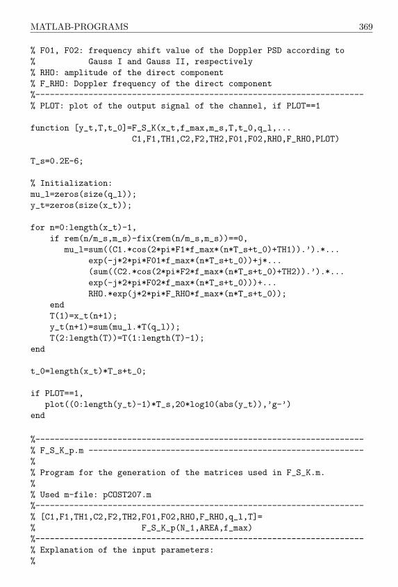
MATLAB-PROGRAMS 369
% F01, F02: frequency shift value of the Doppler PSD according to% Gauss I and Gauss II, respectively% RHO: amplitude of the direct component% F_RHO: Doppler frequency of the direct component%--------------------------------------------------------------------% PLOT: plot of the output signal of the channel, if PLOT==1
function [y_t,T,t_0]=F_S_K(x_t,f_max,m_s,T,t_0,q_l,...C1,F1,TH1,C2,F2,TH2,F01,F02,RHO,F_RHO,PLOT)
T_s=0.2E-6;
% Initialization:mu_l=zeros(size(q_l));y_t=zeros(size(x_t));
for n=0:length(x_t)-1,if rem(n/m_s,m_s)-fix(rem(n/m_s,m_s))==0,
mu_l=sum((C1.*cos(2*pi*F1*f_max*(n*T_s+t_0)+TH1)).’).*...exp(-j*2*pi*F01*f_max*(n*T_s+t_0))+j*...(sum((C2.*cos(2*pi*F2*f_max*(n*T_s+t_0)+TH2)).’).*...exp(-j*2*pi*F02*f_max*(n*T_s+t_0)))+...RHO.*exp(j*2*pi*F_RHO*f_max*(n*T_s+t_0));
endT(1)=x_t(n+1);y_t(n+1)=sum(mu_l.*T(q_l));T(2:length(T))=T(1:length(T)-1);
end
t_0=length(x_t)*T_s+t_0;
if PLOT==1,plot((0:length(y_t)-1)*T_s,20*log10(abs(y_t)),’g-’)
end
%--------------------------------------------------------------------% F_S_K_p.m ---------------------------------------------------------%% Program for the generation of the matrices used in F_S_K.m.%% Used m-file: pCOST207.m%--------------------------------------------------------------------% [C1,F1,TH1,C2,F2,TH2,F01,F02,RHO,F_RHO,q_l,T]=% F_S_K_p(N_1,AREA,f_max)%--------------------------------------------------------------------% Explanation of the input parameters:%

370 MATLAB-PROGRAMS
% N_1: minimum number of discrete Doppler frequencies% AREA: according to COST 207, 4 types of channels are specified:% 1) Rural Area: ’ra’% 2) Typical Urban: ’tu’% 3) Bad Urban: ’bu’% 4) Hilly Terrain: ’ht’% f_max: maximum Doppler frequency
function [C1,F1,TH1,C2,F2,TH2,F01,F02,RHO,F_RHO,q_l,T]=...F_S_K_p(N_1,AREA,f_max)
% The greatest common divisor of the discrete propagation delays% defines the sampling interval T_s:T_s=0.2E-6;
if all(lower(AREA)==’ra’),a_l=[1,0.63,0.1,0.01];tau_l=[0,0.2,0.4,0.6]*1E-6;DOPP_KAT=[’RI’;’JA’;’JA’;’JA’];
elseif all(lower(AREA)==’tu’),a_l=[0.5,1,0.63,0.25,0.16,0.1];tau_l=[0,0.2,0.6,1.6,2.4,5]*1E-6;DOPP_KAT=[’JA’;’JA’;’G1’;’G1’;’G2’;’G2’];
elseif all(lower(AREA)==’bu’),a_l=[0.5,1,0.5,0.32,0.63,0.4];tau_l=[0,0.4,1.0,1.6,5.0,6.6]*1E-6;DOPP_KAT=[’JA’;’JA’;’G1’;’G1’;’G2’;’G2’];
elseif all(lower(AREA)==’ht’),a_l=[1,0.63,0.4,0.2,0.25,0.06];tau_l=[0,0.2,0.4,0.6,15,17.2]*1E-6;DOPP_KAT=[’JA’;’JA’;’JA’;’JA’;’G2’;’G2’];
end
% Generate the parameters and assign them to the matrices:num_of_taps=length(DOPP_KAT);F1=zeros(num_of_taps,N_1+2*num_of_taps-1);F2=F1;C1=F1;C2=F1;TH1=F1;TH2=F1;F01=zeros(1,num_of_taps);F02=F01;RHO=zeros(1,num_of_taps);F_RHO=RHO;NN1=N_1+2*(num_of_taps-1):-2:N_1;for k=1:num_of_taps,
[f1,f2,c1,c2,th1,th2,rho,f_rho,f01,f02]=...pCOST207(DOPP_KAT(k,:),NN1(k));F1(k,1:NN1(k))=f1;C1(k,1:NN1(k))=c1*sqrt(a_l(k));TH1(k,1:NN1(k))=th1;F2(k,1:NN1(k)+1)=f2;
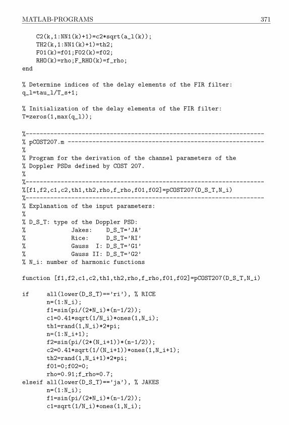
MATLAB-PROGRAMS 371
C2(k,1:NN1(k)+1)=c2*sqrt(a_l(k));TH2(k,1:NN1(k)+1)=th2;F01(k)=f01;F02(k)=f02;RHO(k)=rho;F_RHO(k)=f_rho;
end
% Determine indices of the delay elements of the FIR filter:q_l=tau_l/T_s+1;
% Initialization of the delay elements of the FIR filter:T=zeros(1,max(q_l));
%--------------------------------------------------------------------% pCOST207.m --------------------------------------------------------%% Program for the derivation of the channel parameters of the% Doppler PSDs defined by COST 207.%%--------------------------------------------------------------------%[f1,f2,c1,c2,th1,th2,rho,f_rho,f01,f02]=pCOST207(D_S_T,N_i)%--------------------------------------------------------------------% Explanation of the input parameters:%% D_S_T: type of the Doppler PSD:% Jakes: D_S_T=’JA’% Rice: D_S_T=’RI’% Gauss I: D_S_T=’G1’% Gauss II: D_S_T=’G2’% N_i: number of harmonic functions
function [f1,f2,c1,c2,th1,th2,rho,f_rho,f01,f02]=pCOST207(D_S_T,N_i)
if all(lower(D_S_T)==’ri’), % RICEn=(1:N_i);f1=sin(pi/(2*N_i)*(n-1/2));c1=0.41*sqrt(1/N_i)*ones(1,N_i);th1=rand(1,N_i)*2*pi;n=(1:N_i+1);f2=sin(pi/(2*(N_i+1))*(n-1/2));c2=0.41*sqrt(1/(N_i+1))*ones(1,N_i+1);th2=rand(1,N_i+1)*2*pi;f01=0;f02=0;rho=0.91;f_rho=0.7;
elseif all(lower(D_S_T)==’ja’), % JAKESn=(1:N_i);f1=sin(pi/(2*N_i)*(n-1/2));c1=sqrt(1/N_i)*ones(1,N_i);
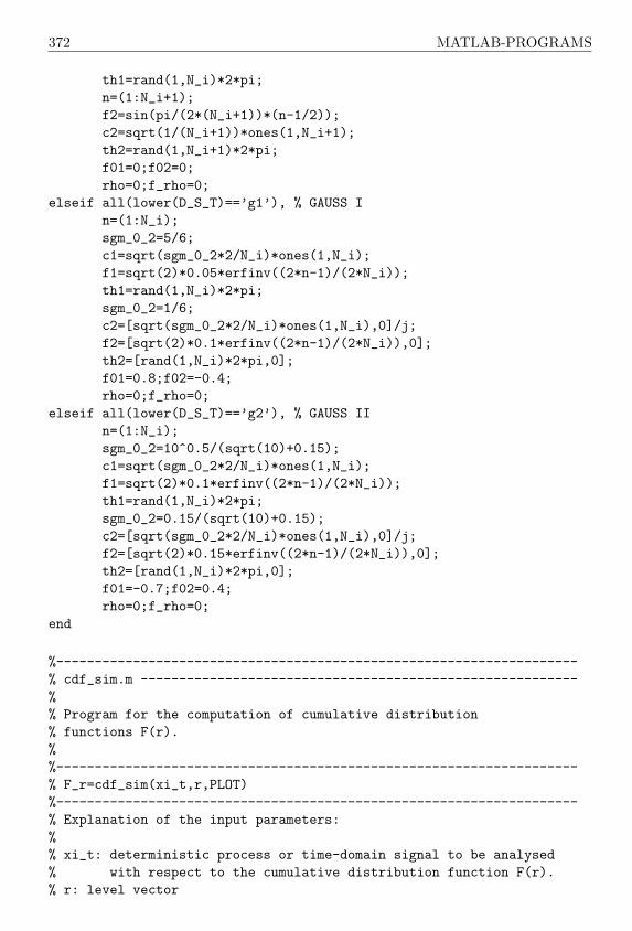
372 MATLAB-PROGRAMS
th1=rand(1,N_i)*2*pi;n=(1:N_i+1);f2=sin(pi/(2*(N_i+1))*(n-1/2));c2=sqrt(1/(N_i+1))*ones(1,N_i+1);th2=rand(1,N_i+1)*2*pi;f01=0;f02=0;rho=0;f_rho=0;
elseif all(lower(D_S_T)==’g1’), % GAUSS In=(1:N_i);sgm_0_2=5/6;c1=sqrt(sgm_0_2*2/N_i)*ones(1,N_i);f1=sqrt(2)*0.05*erfinv((2*n-1)/(2*N_i));th1=rand(1,N_i)*2*pi;sgm_0_2=1/6;c2=[sqrt(sgm_0_2*2/N_i)*ones(1,N_i),0]/j;f2=[sqrt(2)*0.1*erfinv((2*n-1)/(2*N_i)),0];th2=[rand(1,N_i)*2*pi,0];f01=0.8;f02=-0.4;rho=0;f_rho=0;
elseif all(lower(D_S_T)==’g2’), % GAUSS IIn=(1:N_i);sgm_0_2=10^0.5/(sqrt(10)+0.15);c1=sqrt(sgm_0_2*2/N_i)*ones(1,N_i);f1=sqrt(2)*0.1*erfinv((2*n-1)/(2*N_i));th1=rand(1,N_i)*2*pi;sgm_0_2=0.15/(sqrt(10)+0.15);c2=[sqrt(sgm_0_2*2/N_i)*ones(1,N_i),0]/j;f2=[sqrt(2)*0.15*erfinv((2*n-1)/(2*N_i)),0];th2=[rand(1,N_i)*2*pi,0];f01=-0.7;f02=0.4;rho=0;f_rho=0;
end
%--------------------------------------------------------------------% cdf_sim.m ---------------------------------------------------------%% Program for the computation of cumulative distribution% functions F(r).%%--------------------------------------------------------------------% F_r=cdf_sim(xi_t,r,PLOT)%--------------------------------------------------------------------% Explanation of the input parameters:%% xi_t: deterministic process or time-domain signal to be analysed% with respect to the cumulative distribution function F(r).% r: level vector
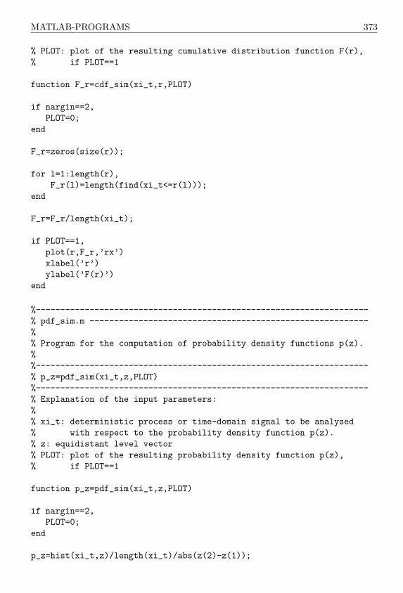
MATLAB-PROGRAMS 373
% PLOT: plot of the resulting cumulative distribution function F(r),% if PLOT==1
function F_r=cdf_sim(xi_t,r,PLOT)
if nargin==2,PLOT=0;
end
F_r=zeros(size(r));
for l=1:length(r),F_r(l)=length(find(xi_t<=r(l)));
end
F_r=F_r/length(xi_t);
if PLOT==1,plot(r,F_r,’rx’)xlabel(’r’)ylabel(’F(r)’)
end
%--------------------------------------------------------------------% pdf_sim.m ---------------------------------------------------------%% Program for the computation of probability density functions p(z).%%--------------------------------------------------------------------% p_z=pdf_sim(xi_t,z,PLOT)%--------------------------------------------------------------------% Explanation of the input parameters:%% xi_t: deterministic process or time-domain signal to be analysed% with respect to the probability density function p(z).% z: equidistant level vector% PLOT: plot of the resulting probability density function p(z),% if PLOT==1
function p_z=pdf_sim(xi_t,z,PLOT)
if nargin==2,PLOT=0;
end
p_z=hist(xi_t,z)/length(xi_t)/abs(z(2)-z(1));

374 MATLAB-PROGRAMS
if PLOT==1,plot(z,p_z,’mx’)xlabel(’z’)ylabel(’p(z)’)
end
%--------------------------------------------------------------------% lcr_sim.m ---------------------------------------------------------%% Program for the computation of the level-crossing rate N(r).%%--------------------------------------------------------------------% N_r=lcr_sim(xi_t,r,T_sim,PLOT)%--------------------------------------------------------------------% Explanation of the input parameters:%% xi_t: deterministic process or time-domain signal to be analysed% with respect to the level-crossing rate N(r)% r: level vector% T_sim: duration of the simulation% PLOT: plot of the resulting level-crossing rate N(r), if PLOT==1
function N_r=lcr_sim(xi_t,r,T_sim,PLOT)
if nargin==3,PLOT=0;
end
N_r=zeros(size(r));
for k=1:length(r),N_r(k)=sum(xi_t(2:length(xi_t)) < r(k) & ...
xi_t(1:length(xi_t)-1) >= r(k) );end
N_r=N_r/T_sim;
if PLOT==1,plot(r,N_r,’yx’)xlabel(’r’)ylabel(’N(r)’)
end
%--------------------------------------------------------------------% adf_sim.m ---------------------------------------------------------%% Program for the computation of the average duration of fades T_(r).%

MATLAB-PROGRAMS 375
% Used m-files: cdf_sim.m, lcr_sim.m%--------------------------------------------------------------------% adf=adf_sim(xi_t,r,T_sim,PLOT)%--------------------------------------------------------------------% Explanation of the input parameters:%% xi_t: deterministic process or time-domain signal to be analysed% with respect to the average duration of fades T_(r)% r: equidistant level vector% T_sim: duration of the simulation% PLOT: plot of the resulting average duration of fades T_(r),% if PLOT==1
function adf=adf_sim(xi_t,r,T_sim,PLOT)
cdf=cdf_sim(xi_t,r);lcr=lcr_sim(xi_t,r,T_sim);
adf=cdf./lcr;
if PLOT==1,plot(r,adf,’yx’)xlabel(’r’)ylabel(’T_(r)’)
end


377
ABBREVIATIONS
ACF autocorrelation function
ATDMA Advanced Time Division Multiple Access
BMFT Bundesministerium fur Forschung und Technologie
BU Bad Urban
CEPT Conference of European Posts and Telecommunications Administra-tions
COST European Cooperation in the Field of Scientific and Technical Research
DCS Digital Cellular System
DECT Digital European Cordless Telephone
DGUS deterministic Gaussian uncorrelated scattering
ETSI European Telecommunications Standards Institute
FIR finite impulse response
FPLMTS Future Public Land Mobile Telecommunications System
GSM Global System for Mobile Communications (former: Groupe SpecialMobile)
GWSSUS Gaussian wide-sense stationary uncorrelated scattering
HT Hilly Terrain
IMT 2000 International Mobile Telecommunications 2000
INMARSAT International Maritime Satellite Organisation
ISI intersymbol interference
JM Jakes method
LEO low earth orbit
LOS line-of-sight
LPNM Lp-norm method
MBS Mobile Broadband System
MCM Monte Carlo method
MEA method of equal areas
MED method of equal distances
378 ABBREVIATIONS
MEDS method of exact Doppler spread
MEO medium earth orbit
MMEA modified method of equal areas
MSEM mean-square-error method
PCN Personal Communications Network
PSD power spectral density
RA Rural Area
RACE Research on Advanced Communications in Europe
TU Typical Urban
UMTS Universal Mobile Telecommunications System
WGN white Gaussian noise
WSSUS wide-sense stationary uncorrelated scattering

379
SYMBOLS
SET THEORY
C set of complex numbers
N set of natural numbers
IR set of real numbers
Z set of integer numbers
∈ is an element of
6∈ is not an element of
∀ for all
⊂ subset
∪ union
∩ intersection
A \B difference of set A and set B
∅ empty set or null set
[a, b] set of real numbers within the closed interval from a to b, i.e.,[a, b] = x ∈ IR|a ≤ x ≤ b
[a, b) set of real numbers within the right-hand side open interval from a tob, i.e., [a, b) = x ∈ IR|a ≤ x < b
(a, b] set of real numbers within the left-hand side open interval from a tob, i.e., (a, b] = x ∈ IR|a < x ≤ b
xnNn=1 set of elements x1, x2, . . . , xN
OPERATORS AND MISCELLANEOUS SYMBOLS
argx argument of x = x1 + jx2
Cov x1, x2 covariance between x1 and x2
ex exponential function
Ex (statistical) mean value or expected value of x

380 SYMBOLS
Fx(t) Fourier transform of x(t)
expx exponential function
F−1X(f) inverse Fourier transform of X(f)
gcdxnNn=1 greatest common divisor (also known as highest common factor) of
x1, x2, . . . , xN
Imx imaginary part of x = x1 + jx2
lcm xnNn=1 least common multiple of x1, x2, . . . , xN
lim limit
ln x natural logarithm of x
loga x logarithm of x to base a
maxxnNn=1 largest element of the set x1, x2, . . . , xN
minxnNn=1 smallest element of the set x1, x2, . . . , xN
mod modulo operation
n! factorial function
P (µ ≤ x) probability that the event µ is less than or equal to x
Rex real part of x = x1 + jx2
roundx nearest integer to x
sgn (x) sign of the number x: 1 if x > 0, −1 if x < 0
Var x variance of x
x1(t) ∗ x2(t) convolution of x1(t) and x2(t)
x∗ complex conjugate of the complex number x = x1 + jx2
|x| absolute value of x√
x principal value of the square root of x, i.e.,√
x ≥ 0 for x ≥ 0∏N
n=1 multiple product∑N
n=1 multiple sum∫ b
ax(t)dt integral of the function x(t) over the interval [a, b]
x(t) derivative of the function x(t) with respect to time t
x(t) Hilbert transform of x(t)
x → a x tends to a or x approaches a
dxe ceiling function, the smallest integer greater than or equal to x
bxc floor function, the greatest integer less than or equal to x
≈ approximately equal
∼ distributed according to (statistics) or asymptotically equal (analysis)
≤ less than or equal to
¿ much less than

SYMBOLS 381
= equal
6= unequal
—• Fourier transform
MATRICES AND VECTORS
(am,n) matrix with am,n as the entry of the mth row and the nth column
AT transpose matrix of the matrix A
A−1 inverse matrix of the matrix A
Cµρcovariance matrix of the vector processµρ(t) = (µρ1(t), µρ2(t), µρ1(t), µρ2(t))
T
detA determinant of the matrix A
J Jacobian determinant
m column vector of m1, m2, m1, and m2, i.e., m = (m1,m2, m1, m2)T
Rµ autocorrelation matrix of the vector processµ(t) = (µ1(t), µ2(t), µ1(t), µ2(t))T
tr(A) trace of the matrix A = (am,n) ∈ IRN×N , i.e., tr(A) =∑N
n=1 an,n
x column vector of x1, x2, x1, and x2, i.e., x = (x1, x2, x1, x2)T
Ω parameter vector
SPECIAL FUNCTIONS
erf (·) error function
erfc (·) complementary error function
E(·, ·) elliptic integral of the second kind
E(·) complete elliptic integral of the second kind
F (·, ·; ·; ·) hypergeometric function
H0(·) Struve’s function of order zero
Iν(·) modified Bessel function of the first kind of order ν
Jν(·) Bessel function of the first kind of order ν
Qm(·, ·) generalized Marcum’s Q-function
rect (·) rectangular function
sinc (·) sinc function
δ(·) delta function
Γ(·) gamma function

382 SYMBOLS
STOCHASTIC PROCESSES
BC coherence bandwidth
B(1)µiµi average Doppler shift of µi(t)
B(2)µiµi Doppler spread of µi(t)
B(1)τ ′τ ′ average delay
B(2)τ ′τ ′ delay spread
c0 speed of light
cR Rice factor
E2(Ω) mean-square-error norm
f Doppler frequency
f0 carrier frequency
fc cut-off frequency
fmax maximum Doppler frequency
fmin lower cut-off frequency of the left-hand side restricted Jakes powerspectral density
fs sampling rate
fsym symbol rate
fρ Doppler frequency of the line-of-sight component m(t)
Fζ−(r) cumulative distribution function of Rayleigh processes ζ(t)
Fη−(r) cumulative distribution function of Suzuki processes η(t)
Fη+(r) complementary cumulative distribution function of Suzuki processesη(t)
Fϑ(ϕ) cumulative distribution function of the phase ϑ(t) ofµ(t) = µ1(t) + jµ2(t)
Fµi(r) cumulative distribution function of Gaussian random processes µi(t)
Fξ−(r) cumulative distribution function of Rice processes ξ(t)
Fξ+(r) complementary cumulative distribution function of Rice processes ξ(t)
F%−(r) cumulative distribution function of Loo processes %(t)
F%+(r) complementary cumulative distribution function of Loo processes %(t)
h(τ ′) time-invariant impulse response
h(τ ′, t) time-variant impulse response
H(f) transfer function of linear time-invariant systems
H(f ′, t) time-variant transfer function
H(f) Hilbert transformer
L number of discrete paths

SYMBOLS 383
m(t) (time-variant) line-of-sight component
m′s sampling rate ratio, i.e., m′
s = f ′s/fs = Ts/T ′smµi
mean value of µi(t)
Nζ(r) level-crossing rate of Rayleigh processes ζ(t)
Nη(r) level-crossing rate of Suzuki processes η(t)
Nξ(r) level-crossing rate of Rice processes ξ(t)
N%(r) level-crossing rate of Loo processes %(t)
p0−(τ−; r) probability density function of the fading intervals τ− of Rayleighprocesses ζ(t)
p1−(τ−; r) approximate solution for p0−(τ−; r)
pζ(z) Rayleigh distribution
pη(z) Suzuki distribution
pλ(z) lognormal distribution
pϑ(θ) probability density function of the phase ϑ(t)
pµi(x) Gaussian distribution
pµρ1µρ2 µρ1 µρ2joint probability density function of µρ1(t), µρ2(t), µρ1(t), and µρ2(t)
pξ(z) Rice distribution
p%(z) probability density function of Loo processes %(t)
pω(z) Nakagami distribution
pξξ(z, θ) joint probability density function of ξ(t) and ξ(t)
pξξϑϑ(z, z, θ, θ) joint probability density function of ξ(t), ξ(t), ϑ(t), and ϑ(t)
Qm(·, ·) generalized Marcum’s Q-function
r amplitude level
rhh(·, ·; ·, ·) autocorrelation function of h(τ ′, t)
rHH(υ′, τ) time-frequency correlation function of WSSUS models
rHH(·, ·; ·, ·) autocorrelation function of H(f ′, t)
rss(·, ·; ·, ·) autocorrelation function of s(τ ′, f)
rTT (·, ·; ·, ·) autocorrelation function of T (f ′, f)
rxx(t1, t2) autocorrelation function of x(t), i.e., rxx(t1, t2) = Ex∗(t1)x(t2)ryy(t1, t2) autocorrelation function of y(t), i.e., ryy(t1, t2) = Ey∗(t1)y(t2)rµµ(τ) autocorrelation function of µ(t) = µ1(t) + jµ2(t)
rµiµi(τ) autocorrelation function of µi(t)
rµiµi(τ) autocorrelation function of µi(t)
rµ1µ2(τ) cross-correlation function of µ1(t) and µ2(t)
rτ ′τ ′(υ′) frequency correlation function
s(τ ′, f) Doppler-variant impulse response

384 SYMBOLS
S(τ ′, f) scattering function of WSSUS models
Shh(τ ′, τ) delay cross-power spectral density of WSSUS models
STT (υ′, f) Doppler cross-power spectral density of WSSUS models
Sτ ′τ ′(τ ′) delay power spectral density
Sµµ(f) power spectral density of µ(t) = µ1(t) + jµ2(t)
Sµiµi(f) power spectral density of µi(t)
Sµ1µ2(f) cross-power spectral density of µ1(t) and µ2(t)
t time variable
T (f ′, f) Doppler-variant transfer function
TC coherence time
Ts sampling interval
Tsym symbol interval
Tζ−(r) average duration of fades of Rayleigh processes ζ(t)
Tη−(r) average duration of fades of Suzuki processes η(t)
Tξ−(r) average duration of fades of Rice processes ξ(t)
T%−(r) average duration of fades of Loo processes %(t)
un random variable, uniformly distributed in the interval (0, 1]
v speed of the mobile unit
Wi(·) weighting function
x(t) input signal
y(t) output signal
β negative curvature of the autocorrelation function rµiµi(τ) at theorigin, i.e., β = βi = −rµiµi(0) (i = 1, 2)
γ negative curvature of the autocorrelation function rν3ν3(τ) at theorigin, i.e., γ = −rν3ν3(0)
ζ(t) Rayleigh process
η(t) Suzuki process
θρ phase of the line-of-sight component m(t)
ϑ(t) phase of µρ(t), i.e., ϑ(t) = argµρ(t)κ0 frequency ratio fmin over fmax
κc frequency ratio fmax over fc
λ(t) lognormal process
µ(t) zero-mean complex Gaussian random process
µi(t) real Gaussian random process (stochastic reference model)
µi(t) real stochastic process (stochastic simulation model)
µρ(t) complex Gaussian random process with mean m(t)

SYMBOLS 385
νi(t) white Gaussian noise
ξ(t) Rice process
ρ amplitude of the line-of-sight component m(t)
%(t) Loo process
σ20 mean power of µi(t)
τ time difference between t2 and t1, i.e., τ = t2 − t1
τ− fading interval
τ+ connecting interval
τq(r) length of the time interval that comprises q % of all fading intervals ofthe process ζ(t) at level r
τ ′ continuous propagation delay
τ ′` discrete propagation delay of the `th path
τ ′max maximum propagation delay
∆τ ′` propagation delay difference between τ ′` and τ ′`−1, i.e., ∆τ ′` = τ ′`− τ ′`−1
φ0 symbol for the cross-correlation function rµ1µ2(τ) at τ = 0
ψ0 symbol for the autocorrelation function rµiµi(τ) at τ = 0
Ψµi(ν) characteristic function of µi(t)
DISCRETE-TIME DETERMINISTIC PROCESSES
ai,n[k] address of the table Tabi,n at the discrete time k
B(1)µiµi average Doppler shift of µi[k]
B(2)µiµi Doppler spread of µi[k]
ci,n Doppler coefficient of the nth component of µi[k]
fi,n quantised Doppler frequency of the nth component of µi[k]
fs sampling frequency
fs,min minimum sampling frequency
Fζ−(r) cumulative distribution function of discrete deterministic Rayleighprocesses ζ[k]
Fϑ(ϕ) cumulative distribution function of the phase ϑ[k] ofµ[k] = µ1[k] + jµ2[k]
Fµi(r) cumulative distribution function of discrete deterministic Gaussianprocesses µi[k]
k discrete time variable (t = kTs)
K number of simulated samples of a discrete deterministic process
L period of ζ[k]

386 SYMBOLS
L upper limit of the period of ζ[k]
Li period of µi[k]
Li upper limit of the period of µi[k]
Li,n period of the nth component of µi[k]
mµimean value of the sequence µi[k]
M i channel matrix; contains the complete information for the reconstruc-tion of µi[k]
Nζ(r) level-crossing rate of discrete deterministic Rayleigh processes ζ[k]
pζ(z) probability density function of discrete deterministic Rayleighprocesses ζ[k]
pϑ(θ) probability density function of the phase ϑ[k] of µ[k] = µ1[k] + jµ2[k]
pµi(x) probability density function of discrete deterministic Gaussian
processes µi[k]
Regi,n register; contains one period of the harmonic elementary sequenceµi,n[k]
rµiµi [κ] autocorrelation sequence of µi[k]
rµ1µ2 [κ] cross-correlation sequence of µ1[k] and µ2[k]
Si selection matrix
Sµiµi(f) power spectral density of µi[k]
Sµ1µ2(f) cross-power spectral density of µ1[k] and µ2[k]
Tabi,n table; contains one period of the harmonic elementary sequence µi,n[k]
Ts sampling interval
Tsim simulation time
∆Tsim iteration time
Tζ−(r) average duration of fades of discrete deterministic Rayleigh processesζ[k]
βi negative curvature of the autocorrelation sequence rµiµi [κ] at theorigin, i.e., βi = −¨rµiµi [0] (i = 1, 2)
∆βi model error of ¨rµiµi [0], i.e., ∆βi = βi − β
∆(i,j)n,m auxiliary function for the determination of the minimum sampling
frequency fA,min
εfi,nrelative error of the quantized Doppler frequencies fi,n
ζ[k] discrete-time deterministic Rayleigh process
θi,n quantized Doppler phase of the nth component of µi[k]
ϑ[k] phase of µ[k] = µ1[k] + jµ2[k], i.e., ϑ[k] = argµ[k]κ time difference between the instants k2 and k1, i.e., κ = k2 − k1
µ[k] complex discrete-time deterministic Gaussian process
SYMBOLS 387
µi[k] real discrete-time deterministic Gaussian process
µi,n[k] nth harmonic elementary function of µi[k]
σ2µi
mean power of µi[k]
CONTINUOUS-TIME DETERMINISTIC PROCESSES
a` delay coefficient of the `th path
BC coherence bandwidth of DGUS models
B(1)µiµi average Doppler shift of µi(t)
B(2)µiµi Doppler spread of µi(t)
B(1)τ ′τ ′ average delay of DGUS models
B(2)τ ′τ ′ delay spread of DGUS models
ci,n Doppler coefficient of the nth component of µi(t)
ci,n,` Doppler coefficient of the nth component of µi,`(t)
Epµimean-square error of pµi(x)
Erµiµimean-square error of rµiµi(τ)
fi,n discrete Doppler frequency of the nth component of µi(t)
fi,n,` discrete Doppler frequency of the nth component of µi,`(t)
Fi greatest common divisor fi,1, fi,2, . . . , fi,Ni , i.e., Fi = gcdfi,nNin=1
Fζ−(r) cumulative distribution function of deterministic Rayleigh processesζ(t)
Fη−(r) cumulative distribution function of deterministic Suzuki processes η(t)
Fϑ(ϕ) cumulative distribution function of the phase ϑ(t) ofµ(t) = µ1(t) + jµ2(t)
Fµi(r) cumulative distribution function of deterministic Gaussian processesµi(t)
Fξ−(r) cumulative distribution function of deterministic Rice processes ξ(t)
F%−(r) cumulative distribution function of deterministic Loo processes %(t)
h(τ ′) time-invariant impulse response of DGUS models
h(τ ′, t) time-variant impulse response of DGUS models
H(f ′, t) time-variant transfer function of DGUS models
mµi mean value of µi(t)
N smallest number of N1 and N2, i.e., N = minN1, N2Ns number of sampling values
Ni number of harmonic functions of µi(t)

388 SYMBOLS
Ni,` number of harmonic functions of µi,`(t)
N ′i virtual number of harmonic functions of µi(t)
Nζ(r) level-crossing rate of deterministic Rayleigh processes ζ(t)
Nη(r) level-crossing rate of deterministic Suzuki processes η(t)
Nξ(r) level-crossing rate of deterministic Rice processes ξ(t)
N%(r) level-crossing rate of deterministic Loo processes %(t)
p0−(τ−; r) probability density function of the fading intervals τ− of ζ(t)
p0−+(τ−, τ+; r) joint probability density function of fading and connecting intervals ofζ(t)
p1−(τ−; r) approximate solution for p0−(τ−; r)
pζ(z) probability density function of deterministic Rayleigh processes ζ(t)
pη(z) probability density function of deterministic Suzuki processes η(t)
pϑ(θ) probability density function of the phase ϑ(t) of µ(t) = µ1(t) + jµ2(t)
pµi(x) probability density function of deterministic Gaussian processes µi(t)
pξ(z) probability density function of deterministic Rice processes ξ(t)
p%(z) probability density function of deterministic Loo processes %(t)
pξξ(z, θ) joint probability density function of ξ(t) and ˙ξ(t)
rhh(·, ·; ·, ·) autocorrelation function h(τ ′, t)
rHH(υ′, τ) time-frequency correlation function of DGUS models
rss(·, ·; ·, ·) autocorrelation function of s(τ ′, f)
rTT (·, ·; ·, ·) autocorrelation function of T (f ′, f)
rµµ(τ) autocorrelation function of µ(t) = µ1(t) + jµ2(t)
rµiµi(τ) autocorrelation function of µi(t)
rµi,`µi,`(τ) autocorrelation function of µi,`(t)
rµ`µ`(τ) autocorrelation function of µ`(t)
rµ1µ2(τ) cross-correlation function of µ1(t) and µ2(t)
rτ ′τ ′(υ′) frequency correlation function of DGUS models
s(τ ′, f) Doppler-variant impulse response of DGUS models
S(τ ′, f) scattering function of DGUS models
Shh(τ ′, τ) delay cross-power spectral density of DGUS models
STT (υ′, f) Doppler cross-power spectral density of DGUS models
Sµiµi(f) power spectral density of µi(t)
Sµ`µ`(f) power spectral density of µ`(t)
Sµ1µ2(f) cross-power spectral density of µ1(t) and µ2(t)
Sτ ′τ ′(τ ′) delay power spectral density of DGUS models
SYMBOLS 389
T (f ′, f) Doppler-variant transfer function of DGUS models
TC coherence time of DGUS models
Ti period of µi(t)
Ts, T ′s sampling intervals
Tsim simulation time
Tζ−(r) average duration of fades of deterministic Rayleigh processes ζ(t)
Tη−(r) average duration of fades of deterministic Suzuki processes η(t)
Tξ−(r) average duration of fades of deterministic Rice processes ξ(t)
T%−(r) average duration of fades of deterministic Loo processes %(t)
βi negative curvature of the autocorrelation function rµiµi(τ) at theorigin, i.e., βi = −¨rµiµi(0) (i = 1, 2)
∆βi model error of the simulation model, i.e., ∆βi = βi − β
γ negative curvature of the autocorrelation function of rν3ν3(τ) at theorigin, i.e., γ = −¨rν3ν3(0)
εNξrelative error of the level-crossing rate Nξ(r)
εTξrelative error of the average duration of fades Tξ−(r)
ζ(t) continuous-time deterministic Rayleigh process
η(t) continuous-time deterministic Suzuki process
θ0 phase difference between µ1,n(t) and µ2,n(t)
θi,n Doppler phase of the nth component of µi(t)
θi,n,` Doppler phase der nth component of µi,`(t)~θi Doppler phase vector~Θi standard phase vector
ϑ(t) phase of µρ(t), i.e., ϑ(t) = argµρ(t)λ(t) continuous-time deterministic lognormal process
µ(t) zero-mean complex continuous-time deterministic Gaussian process
µi(t) zero-mean real continuous-time deterministic Gaussian process
µi,`(t) real deterministic Gaussian process of the `th path of DGUS models
µi,n(t) nth harmonic elementary function of µi(t)
µ`(t) complex deterministic Gaussian process of the `th path of DGUSmodels
µρ(t) complex deterministic Gaussian process with mean value m(t)
ξ(t) continuous-time deterministic Rice process
%(t) continuous-time deterministic Loo process
σ2µ mean power of µ(t)
390 SYMBOLS
σ2µi
mean power of µi(t)
τ ′` discrete propagation delay of the `th path
∆τ ′` propagation delay difference between τ ′` and τ ′`−1, i.e., ∆τ ′` = τ ′`− τ ′`−1
τq(r) length of the time interval that comprises q % of all fading intervals ofthe process ζ(t) at level r
φ0 symbol for the cross-correlation function rµ1µ2(τ) at τ = 0
ψ0 symbol for the autocorrelation function rµiµi(τ) at τ = 0
Ξ`(f) Fourier transform of µ`(t)
Ψµi(ν) characteristic function of µi(t)
Ωi,n normalized discrete Doppler frequency, i.e., Ωi,n = 2πfi,nTs
391
Bibliography
[Abr72] M. Abramowitz and I. A. Stegun, Handbook of Mathematical Functionswith Formulas, Graphs, and Mathematical Tables. Washington: NationalBureau of Standards, 1972.
[Aka97] Y. Akaiwa, Introduction to Digital Mobile Communication. New York:John Wiley & Sons, 1997.
[Akk86] A. S. Akki and F. Haber, “A statistical model of mobile-to-mobile landcommunication channel,” IEEE Trans. Veh. Technol., vol. 35, no. 1, pp.2–7, Feb. 1986.
[Akk94] A. S. Akki, “Statistical properties of mobile-to-mobile land communica-tion channels,” IEEE Trans. Veh. Technol., vol. 43, no. 4, pp. 826–831,Nov. 1994.
[Ald82] M. Aldinger, “Die Simulation des Mobilfunk-Kanals auf einem Digital-rechner,” FREQUENZ, vol. 36, no. 4/5, pp. 145–152, 1982.
[And92] J. B. Andersen and P. Eggers, “A heuristic model of power delay profiles inlandmobile communications,” in Proc. URSI Int. Symp. ElectromagneticTheory, Sydney, Australia, Aug. 1992, pp. 55–57.
[And95] J. B. Andersen, T. S. Rappaport, and S. Yoshida, “Propagationmeasurements and models for wireless communications channels,” IEEECommun. Mag., vol. 33, no. 1, pp. 42–49, Jan. 1995.
[Arr73] G. Arredondo, W. Chriss, and E. Walker, “A multipath fading simulatorfor mobile radio,” IEEE Trans. Veh. Technol., vol. 22, no. 4, pp. 241–244,May 1973.
[Aul79] T. Aulin, “A modified model for the fading signal at the mobile radiochannel,” IEEE Trans. Veh. Technol., vol. 28, no. 3, pp. 182–203, Aug.1979.
[Baj82] A. S. Bajwa and J. D. Parsons, “Small-area characterisation of UHF urbanand suburban mobile radio propagation,” Inst. Elec. Eng. Proc., vol. 129,no. 2, pp. 102–109, April 1982.
[Bei97] F. Beichelt, Stochastische Prozesse fur Ingenieure. Stuttgart: Teubner,1997.

392 Bibliography
[Bel63] P. A. Bello, “Characterization of randomly time-variant linear channels,”IEEE Trans. Comm. Syst., vol. 11, no. 4, pp. 360–393, Dec. 1963.
[Bel73] P. A. Bello, “Aeronautical channel characterization,” IEEE Trans.Commun., vol. 21, pp. 548–563, May 1973.
[Ben48] W. R. Bennett, “Distribution of the sum of randomly phasedcomponents,” Quart. Appl. Math., vol. 5, pp. 385–393, May 1948.
[Ber86] D. Berthoumieux and J. M. Pertoldi, “Hardware propagation simulator ofthe frequency-selective fading channel at 900 MHz,” in Proc. 2nd NordicSeminar on Land Mobile Radio Communications, Stockholm, Sweden,1986, pp. 214–217.
[Bla72] D. M. Black and D. O. Reudink, “Some characteristics of mobile radiopropagation at 836 MHz in the Philadelphia area,” IEEE Trans. Veh.Technol., vol. 21, pp. 45–51, Feb. 1972.
[Bla84] R. E. Blahut, Theory and Practice of Error Control Codes. Reading,Massachusetts: Addison-Wesley, 1984.
[Boe98] J. F. Bohme, Stochastische Signale. Stuttgart: Teubner, 2nd ed., 1998.
[Bra91] W. R. Braun and U. Dersch, “A physical mobile radio channel model,”IEEE Trans. Veh. Technol., vol. 40, no. 2, pp. 472–482, May 1991.
[Bre70] H. Brehm, Ein- und zweidimensionale Verteilungsdichten von Nulldurch-gangsabstanden stochastischer Signale. Ph.D. dissertation, UniversityFrankfurt/Main, Frankfurt, Germany, June 1970.
[Bre78] H. Brehm, Spharisch invariante stochastische Prozesse. Habilitationthesis, University Frankfurt/Main, Frankfurt, Germany, 1978.
[Bre86a] H. Brehm, W. Stammler, and M. Werner, “Design of a highly flexibledigital simulator for narrowband fading channels,” in Signal ProcessingIII: Theories and Applications, Amsterdam, The Netherlands: ElsevierScience Publishers (North-Holland), EURASIP, Sep. 1986, pp. 1113–1116.
[Bre86b] H. Brehm and M. Werner, “Generalized Rayleigh fading in a mobile radiochannel,” in Proc. 2nd Nordic Seminar on Digital Land Mobile RadioCommunication, Stockholm, Oct. 1986, pp. 210–214.
[Bre89] H. Brehm, “Pegelkreuzungen bei verallgemeinerten Gauß-Prozessen,”Archiv Elektr. Ubertr., vol. 43, no. 5, pp. 271–277, 1989.
[Bro91] I. N. Bronstein and K. A. Semendjajew, Taschenbuch der Mathematik.Frankfurt/Main: Harri Deutsch, 25th ed., 1991.
[But83] J. S. Butterworth and E. E. Matt, “The characterization of propagationeffects for land mobile satellite services,” in Inter. Conf. on SatelliteSystems for Mobile Communications and Navigations, June 1983, pp. 51–54.

Bibliography 393
[Cap80] E. Caples, K. Massad, and T. Minor, “A UHF channel simulator for digitalmobile radio,” IEEE Trans. Veh. Technol., vol. 29, no. 2, pp. 281–289,May 1980.
[Cas88] E. F. Casas and C. Leung, “A simple digital fading simulator for mobileradio,” in Proc. IEEE Vehicular Technology Conference, Sep. 1988, pp.212–217.
[Cas90] E. F. Casas and C. Leung, “A simple digital fading simulator for mobileradio,” IEEE Trans. Veh. Technol., vol. 39, no. 3, pp. 205–212, Aug. 1990.
[Cha79] U. Charash, “Reception through Nakagami fading multipath channelswith random delays,” IEEE Trans. Commun., vol. 27, no. 4, pp. 657–670,April 1979.
[Cla68] R. H. Clarke, “A statistical theory of mobile-radio reception,” Bell Syst.Tech. Journal, vol. 47, pp. 957–1000, July/Aug. 1968.
[Cor94] G. E. Corazza and F. Vatalaro, “A statistical model for land mobilesatellite channels and its application to nongeostationary orbit systemssystems,” IEEE Trans. Veh. Technol., vol. 43, no. 3, pp. 738–742, Aug.1994.
[COS86] COST 207 WG1, “Proposal on channel transfer functions to be used inGSM tests late 1986,” COST 207 TD (86)51 Rev. 3, Sep. 1986.
[COS89] COST 207, “Digital land mobile radio communications,” Office for OfficialPublications of the European Communities, Final Report, Luxembourg,1989.
[Cox72] D. C. Cox, “Delay Doppler characteristics of multipath propagationat 910 MHz in a suburban mobile radio environment,” IEEE Trans.Antennas Propagat., vol. 20, no. 5, pp. 625–635, Sep. 1972.
[Cox73] D. C. Cox, “910 MHz urban mobile radio propagation: Multipathcharacteristics in New York City,” IEEE Trans. Veh. Technol., vol. 22,no. 4, pp. 104–110, Nov. 1973.
[Cre95] P. M. Crespo and J. Jimenez, “Computer simulation of radio channelsusing a harmonic decomposition technique,” IEEE Trans. Veh. Technol.,vol. 44, no. 3, pp. 414–419, Aug. 1995.
[Cyg88] D. Cygan, M. Dippold, and J. Finkenzeller, “Kanalmodelle fur diesatellitengestutzte Kommunikation landmobiler Teilnehmer,” Archiv Elek.Ubertr., vol. 42, no. 6, pp. 329–339, Nov./Dec. 1988.
[Dav58] W. B. Davenport and W. L. Root, An Introduction to the Theory ofRandom Signals and Noise. New York: McGraw-Hill, 1958.
[Dav70] W. B. Davenport, Probability and Random Processes. New York: McGraw-Hill, 1970.
394 Bibliography
[Dav87] F. Davarian, “Channel simulation to facilitate mobile-satellite communi-cations research,” IEEE Trans. Commun., vol. 35, no. 1, pp. 47–56, Jan.1987.
[Den93] P. Dent, G. E. Bottomley, and T. Croft, “Jakes fading model revisited,”Electronics Letters, vol. 29, no. 13, pp. 1162–1163, June 1993.
[Der93] U. Dersch and R. J. Ruegg, “Simulations of the time and frequencyselective outdoor mobile radio channel,” IEEE Trans. Veh. Technol., vol.42, no. 3, pp. 338–344, Aug. 1993.
[Dup86] J. Dupraz, Probability, Signals, Noise. London: North Oxford AcademicPublishers, 1986.
[Ehr82] L. Ehrman, L. B. Bates, J. F. Eschle, and J. M. Kates, “Real-time softwaresimulation of the HF radio channel,” IEEE Trans. Commun., vol. 30, no.8, pp. 1809–1817, Aug. 1982.
[Ent76] W. Entenmann, Optimierungsverfahren. Heidelberg: Huthig-Verlag, 1976.
[Ert98] R. B. Ertel, P. Cardieri, K. W. Sowerby, T. S. Rappaport, and J. H. Reed,“Overview of spatial channel models for antenna array communicationsystems,” IEEE Personal Commun., pp. 10–22, Feb. 1998.
[Fec93a] S. A. Fechtel, “A novel approach to modeling and efficient simulationof frequency-selective fading radio channels,” IEEE J. Select. AreasCommun., vol. 11, no. 3, pp. 422–431, April 1993.
[Fec93b] S.A. Fechtel, Verfahren und Algorithmen der robusten Synchronisation furdie Datenubertragung uber dispersive Schwundkanale. Ph.D. dissertation,Rheinisch-Westfalische Technische Hochschule Aachen, Aachen, Germany,1993.
[Feh95] K. Feher, Wireless Digital Communications: Modulation and SpreadSpectrum Applications. Upper Saddle River, New Jersey: Prentice-Hall,1995.
[Fel94] T. Felhauer, Optimale erwartungstreue Algorithmen zur hochauflosendenKanalschatzung mit Bandspreizsignalformen. Dusseldorf: VDI-Verlag,Fortschritt-Berichte, series 10, no. 278, 1994.
[Fet96] A. Fettweis, Elemente nachrichtentechnischer Systeme. Stuttgart:Teubner, 2nd ed., 1996.
[Fle63] R. Fletcher and M. J. D. Powell, “A rapidly convergent descent methodfor minimization,” Computer Journal, vol. 6, no. 2, pp. 163–168, 1963.
[Fle87] R. Fletcher, Practical Methods of Optimization. New York: John Wiley &Sons, 2nd ed., 1987.
Bibliography 395
[Fle90] B. H. Fleury, Charakterisierung von Mobil- und Richtfunkkanalen mitschwach stationaren Fluktuationen und unkorrelierter Streuung (WSSUS).Ph.D. dissertation, Swiss Federal Institute of Technology Zurich, Zurich,Switzerland, 1990.
[Fle96] B. H. Fleury and P. E. Leuthold, “Radiowave propagation in mobile com-munications: An overview of European research,” IEEE Commun. Mag.,vol. 34, no. 2, pp. 70–81, Feb. 1996.
[Fli91] N. Fliege, Systemtheorie. Stuttgart: Teubner, 1991.
[Fon97] F. P. Fontan, J. Pereda, M. J. Sedes, M. A. V. Castro, S. Buonomo, andP. Baptista, “Complex-envelope three-state Markov chain simulator forthe LMS channel,” Int. J. Sat. Commun., pp. 1–15, Jan. 1997.
[For72] G. D. Forney, “Maximum-likelihood sequence estimation for digitalsequences in the presence of intersymbol interference,” IEEE Trans.Inform. Theory, vol. 18, pp. 363–378, May 1972.
[Gan72] M. J. Gans, “A power-spectral theory of propagation in the mobile-radioenvironment,” IEEE Trans. Veh. Technol., vol. 21, no. 1, pp. 27–38, Feb.1972.
[Gel82] H. J. Gelbrich, K. Low, and R. W. Lorenz, “Funkkanalsimulation undBitfehler-Strukturmessungen an einem digitalen Kanal,” FREQUENZ,vol. 36, no. 4/5, pp. 130–138, 1982.
[Gib96] J. D. Gibson, Ed., The Mobile Communications Handbook. CRC Press inCooperation with IEEE Press, 1996.
[Goe92a] M. Goller and K.D. Masur, “Ergebnisse von Funkkanalmessungenim 900 MHz Bereich auf Neubaustrecken der Deutschen Bundesbahn,”Nachrichtentechnik–Elektronik, vol. 42, no. 4, pp. 146–149, 1992.
[Goe92b] M. Goller and K. D. Masur, “Ergebnisse von Funkkanalmessungenim 900 MHz Bereich auf Neubaustrecken der Deutschen Bundesbahn,”Nachrichtentechnik–Elektronik, vol. 42, no. 5, pp. 206–210, 1992.
[Gol89] J. Goldhirsh and W. J. Vogel, “Mobile satellite system fade statistics forshadowing and multipath from roadside trees at UHF on L-band,” IEEETrans. Antennas Propagat., vol. 37, no. 4, pp. 489–498, April 1989.
[Gol92] J. Goldhirsh and W. J. Vogel, “Propagation effects for land mobilesatellite systems: Overview of experimental and modeling results,” NASAReference Publication 1274, Feb. 1992.
[Gol96] G. H. Golub and C. F. van Loan, Matrix Computations. Baltimore: TheJohns Hopkins University Press, 3rd ed., 1996.
[Gra81] I. S. Gradstein and I. M. Ryshik, Tables of Series, Products, and Integrals.Frankfurt: Harri Deutsch, 5th ed., vol. I and II, 1981.
396 Bibliography
[Gre78] L. J. Greenstein, “A multipath fading channel model for terrestrial digitalradio systems,” IEEE Trans. Commun., vol. 26, no. 8, pp. 1247–1250,1978.
[Gro97] C. Großmann and J. Terno, Numerik der Optimierung. Stuttgart:Teubner, 2nd ed., 1997.
[Hae88] R. Hab, Koharenter Empfang bei Datenubertragung uber nichtfrequenz-selektive Schwundkanale. Ph.D. dissertation, Rheinisch-WestfalischeTechnische Hochschule Aachen, Aachen, Germany, 1988.
[Hae97] E. Hansler, Statistische Signale. Berlin: Springer, 1997.
[Hag82] J. Hagenauer and W. Papke, “Der gespeicherte Kanal — Erfahrungenmit einem Simulationsverfahren fur Fading-Kanale,” FREQUENZ, vol.36, no. 4/5, pp. 122–129, 1982.
[Han77] F. Hansen and F. I. Meno, “Mobile fading — Rayleigh and lognormalsuperimposed,” IEEE Trans. Veh. Technol., vol. 26, no. 4, pp. 332–335,Nov. 1977.
[Hed99] R. Heddergott and P. Truffer, “Comparison of high resolution channelparameter measurements with ray tracing simulations in a multipathenvironment,” in Proc. 3rd European Personal Mobile CommunicationsConference, EPMCC’99, Paris, France, March 1999, pp. 167–172.
[Hes80] G. C. Hess, “Land-mobile satellite excess path loss measurements,” IEEETrans. Veh. Technol., vol. 29, no. 2, pp. 290–297, May 1990.
[Hes93] G. C. Hess, Land-Mobile Radio System Engineering. Boston, MA: ArtechHouse, 1993.
[Hoe90] P. Hoher, Koharenter Empfang trelliscodierter PSK-Signale auffrequenzselektiven Mobilfunkkanalen — Entzerrung, Decodierung undKanalparameterschatzung. Dusseldorf: VDI-Verlag, Fortschritt-Berichte,series 10, no. 147, 1990.
[Hoe92] P. Hoher, “A statistical discrete-time model for the WSSUS multipathchannel,” IEEE Trans. Veh. Technol., vol. 41, no. 4, pp. 461–468, Nov.1992.
[Hor85] R. A. Horn and C. R. Johnson, Matrix Analysis. New York: CambridgeUniversity Press, 1985.
[Huc83] R. W. Huck, J. S. Butterworth, and E. E. Matt, “Propagationmeasurements for land mobile satellite services,” in Proc. IEEE 33rdVehicular Technology Conference, Toronto, Canada, 1983, pp. 265–268.
[Jah95] A. Jahn, “Propagation data and channel model for LMS systems,”ESA Purchase Order 141742, Final Report, DLR, Institute forCommunications Technology, Jan. 1995.

Bibliography 397
[Jak93] W. C. Jakes, Ed., Microwave Mobile Communications. Piscataway, NJ:IEEE Press, 1993.
[Joh94] G. E. Johnson, “Constructions of particular random processes,” Proc. ofthe IEEE, vol. 82, no. 2, pp. 270–285, Feb. 1994.
[Jun97] P. Jung, Analyse und Entwurf digitaler Mobilfunksysteme. Stuttgart:Teubner, 1997.
[Kad91] G. Kadel and R. W. Lorenz, “Breitbandige Ausbreitungsmessungen zurCharakterisierung des Funkkanals beim GSM-System,” FREQUENZ, vol.45, no. 7/8, pp. 158–163, 1991.
[Kad92] G. Kadel and R. W. Lorenz, “Wideband propagation measurements ofthe mobile radio channel,” in Proc. ISAP-92, Sappore, Japan, 1992, pp.81–84.
[Kai80] T. Kailath, Linear Systems. Englewood Cliffs, New Jersey: Prentice-Hall,1980.
[Kam96] K. D. Kammeyer, Nachrichtenubertragung. Stuttgart: Teubner, 2nd ed.,1996.
[Kam98] K. D. Kammeyer and K. Kroschel, Digitale Signalverarbeitung. Stuttgart:Teubner, 4th ed., 1998.
[Kat95] R. Kattenbach and H. Fruchting, “Calculation of system and corre-lation functions for WSSUS channels from wideband measurements,”FREQUENZ, vol. 49, no. 3/4, pp. 42–47, 1995.
[Kit82] L. Kittel, “Analoge und diskrete Kanalmodelle fur die Signalubertragungbeim beweglichen Funk,” FREQUENZ, vol. 36, no. 4/5, pp. 153–160,1982.
[Kra88] A. Krantzik and D. Wolf, “Simulation and analysis of Suzuki fadingprocesses,” in Proc. of the 1988 IEEE Int. Conf. on Acoustics, Speech,and Signal Processing, New York, USA, 1988, pp. 2184–2187.
[Kra90a] A. Krantzik and D. Wolf, “Distribution of the fading-intervals of modifiedSuzuki processes,” in Signal Processing V: Theories and Applications,L. Torres, E. Masgrau, and M. A. Lagunas, Eds., Amsterdam, TheNetherlands: Elsevier Science Publishers, B.V, 1990, pp. 361–364.
[Kra90b] A. Krantzik and D. Wolf, “Statistische Eigenschaften von Fadingprozessenzur Beschreibung eines Landmobilfunkkanals,” FREQUENZ, vol. 44, no.6, pp. 174–182, June 1990.
[Kub00] E. Kubista, F. P. Fontan, M. A. V. Castro, S. Buonomo, B. R. Arbesser-Rastburg, and J. P. V. P. Baptista, “Ka-band propagation measurementsand statistics for land mobile satellite applications,” IEEE Trans. Veh.Technol., vol. 49, no. 3, pp. 973–983, May 2000.

398 Bibliography
[Kuc82] H. P. Kuchenbecker, “Statistische Eigenschaften von Schwund- undVerbindungsdauer beim Mobilfunk-Kanal,” FREQUENZ, vol. 36, no. 4/5,pp. 138–144, 1982.
[Lam97] U. Lambrette, S. Fechtel, and H. Meyer, “A frequency domain variabledata rate frequency hopping channel model for the mobile radio channel,”in Proc. IEEE 47th Veh. Technol. Conf., VTC’97, Phoenix, Arizona, USA,May 1997.
[Lau94] D. I. Laurenson and G. J. R. Povey, “Channel modelling for a predictiverake receiver system,” in Proc. 5th IEEE Int. Symp. Personal, Indoor andMobile Radio Commun., PIMRC’94, The Hague, The Netherlands, Sep.1994, pp. 715–719.
[Lee82] W. C. Y. Lee, Mobile Communications Engineering. New York: McGraw-Hill, 1982.
[Lee93] W. C. Y. Lee, Mobile Communications Design Fundamentals. New York:John Wiley & Sons, 2nd ed., 1993.
[Lee95] W. C. Y. Lee, Mobile Cellular Telecommunications: Analog and DigitalSystems. New York: McGraw-Hill, 2nd ed., 1995.
[Lib99] J. C. Liberty and T. S. Rappaport, Smart Antennas for WirelessCommunications: IS-95 and Third Generation CDMA Applications.Upper Saddle River, New Jersey: Prentice-Hall, 1999.
[Lon62] M. S. Longuet-Higgins, “The distribution of intervals between zeros ofa stationary random function,” Phil. Trans. Royal. Soc., vol. A 254, pp.557–599, 1962.
[Loo85] C. Loo, “A statistical model for a land mobile satellite link,” IEEE Trans.Veh. Technol., vol. 34, no. 3, pp. 122–127, Aug. 1985.
[Loo87] C. Loo, “Measurements and models of a land mobile satellite channel andtheir applications to MSK signals,” IEEE Trans. Veh. Technol., vol. 35,no. 3, pp. 114–121, Aug. 1987.
[Loo90] C. Loo, “Digital transmission through a land mobile satellite channel,”IEEE Trans. Commun., vol. 38, no. 5, pp. 693–697, May 1990.
[Loo91] C. Loo and N. Secord, “Computer models for fading channels withapplications to digital transmission,” IEEE Trans. Veh. Technol., vol.40, no. 4, pp. 700–707, Nov. 1991.
[Loo96] C. Loo, “Statistical models for land mobile and fixed satellitecommunications at Ka band,” in Proc. IEEE 46th Veh. Technol. Conf.,VTC’96, Atlanta, Georgia, USA, April/May 1996, pp. 1023–1027.
[Loo98] C. Loo and J. S. Butterworth, “Land mobile satellite channel measure-ments and modeling,” Proc. of the IEEE, vol. 86, no. 7, pp. 1442–1463,July 1998.

Bibliography 399
[Lor79] R. W. Lorenz, “Theoretische Verteilungsfunktionen von Mehrwege-schwundprozessen im beweglichen Funk und die Bestimmung ihrerParameter aus Messungen,” Technischer Bericht des Forschungsinstitutsder DBP beim FTZ, FI 455 TBr 66, March 1979.
[Lor85] R. W. Lorenz, “Zeit- und Frequenzabhangigkeit der Ubertragunsfunktioneines Funkkanals bei Mehrwegeausbreitung mit besondererBerucksichtigung des Mobilfunkkanals,” Der Fernmelde-Ingenieur,Verlag fur Wissenschaft und Leben Georg Heidecker, vol. 39, no. 4, April1985.
[Lor86] R. W. Lorenz, “Modell und Simulation des Mobilfunkkanals zur Analysevon Signalverzerrungen durch frequenzselektiven Schwund,” FREQUENZ,vol. 40, no. 9/10, pp. 241–248, 1986.
[Lue90] H. D. Luke, Signalubertragung — Grundlagen der digitalen und analogenNachrichtensysteme. Berlin: Springer, 1990.
[Lut85] E. Lutz and E. Plochinger, “Generating Rice processes with given spectralproperties,” IEEE Trans. Veh. Technol., vol. 34, no. 4, pp. 178–181, Nov.1985.
[Lut91] E. Lutz, D. Cygan, M. Dippold, F. Dolainsky, and W. Papke, “Theland mobile satellite communication channel — Recording, statistics, andchannel model,” IEEE Trans. Veh. Technol., vol. 40, no. 2, pp. 375–386,May 1991.
[Lut96] E. Lutz, “A Markov model for correlated land mobile satellite channels,”Int. J. Sat. Commun., vol. 13, pp. 333–339, 1996.
[Man95] Mannesmann Mobilfunk, Geschaftsbericht. Dusseldorf, Germany, 1995.
[Mar92] U. Martin, “Ein System zur Messung der Eigenschaften von Mobil-funkkanalen und ein Verfahren zur Nachverarbeitung der Meßdaten,”FREQUENZ, vol. 46, no. 7/8, pp. 178–188, 1992.
[Mar94a] U. Martin, Ausbreitung in Mobilfunkkanalen: Beitrage zum Entwurfvon Meßgeraten und zur Echoschatzung. Ph.D. dissertation, UniversityErlangen–Nuremberg, Erlangen, Germany, 1994.
[Mar94b] U. Martin, “Modeling the mobile radio channel by echo estimation,”FREQUENZ, vol. 48, no. 9/10, pp. 198–212, Sep./Oct. 1994.
[Mar99] U. Martin, J. Fuhl, I. Gaspard, M. Haardt, A. Kuchar, C. Math, A. F.Molisch, and R. Thoma, “Model scenarios for direction-selective adaptiveantennas in cellular mobile communication systems — Scanning theliterature,” Wireless Personal Communications, Special Issue on SpaceDivision Multiple Access, Kluwer Academic Publishers, pp. 109–129, Oct.1999.
[McF56] J. A. McFadden, “The axis-crossing intervals of random functions I,”Trans. Inst. Rad. Eng., vol. 2, pp. 146–150, 1956.
400 Bibliography
[McF58] J. A. McFadden, “The axis-crossing intervals of random functions II,”Trans. Inst. Rad. Eng., vol. 4, pp. 14–24, 1958.
[Meh94] A. Mehrotra, Cellular Radio Performance Engineering. Boston, MA:Artech House, 1994.
[Mey95] H. Mey, “Chancen der europaischen Industrie im Bereich mobilerEndgerate,” in Proc. 2. ITG-Fachtagung Mobile Kommunikation’95, Neu-Ulm, Germany, Sep. 1995, p. 11.
[Mid60] D. Middleton, An Introduction to Statistical Communication Theory. NewYork: McGraw-Hill, 1960.
[Mil95] M. J. Miller, B. Vucetic, and L. Berry, Eds., Satellite Communications:Mobile and Fixed Services. Boston, MA: Kluwer Academic Publishers, 3rded., 1995.
[Mun82] T. Munakata and D. Wolf, “A novel approach to the level-crossing problemof random processes,” in Proc. of the 1982 IEEE Int. Symp. on Inf.Theory, Les Arcs, France, 1982, vol. IEEE-Cat. 82 CH 1767-3 IT, pp. 149–150.
[Mun83] T. Munakata and D. Wolf, “On the distribution of the level-crossing time-intervals of random processes,” in Proc. of the 7th Int. Conf. on Noisein Physical Systems, Montpelier, USA, M. Savelli, G. Lecoy, and J. P.Nougier, Eds., North-Holland Publ. Co., Amsterdam, The Netherlands,1983, pp. 49–52.
[Mun86] T. Munakata, Mehr-Zustande-Modelle zur Beschreibung des Pegelkreu-zungsverhaltens stationarer stochastischer Prozesse. Ph.D. dissertation,University Frankfurt/Main, Frankfurt, Germany, March 1986.
[Nak60] M. Nakagami, “The m-distribution: A general formula of intensitydistribution of rapid fading,” in Statistical Methods in Radio WavePropagation, W. G. Hoffman, Ed., Oxford, UK: Pergamon Press, 1960.
[Neu87] A. Neul, J. Hagenauer, W. Papke, F. Dolainsky, and F. Edbauer,“Aeronautical channel characterization based on measurement flights,”IEEE Conf. GLOBECOM’87, Tokyo, Japan, pp. 1654–1659, Nov. 1987.
[Neu89] A. Neul, Modulation und Codierung im aeronautischen Satellitenkanal.Ph.D. dissertation, University of the Federal Armed Forces Munich,Munich, Germany, Sep. 1989.
[Nie78] D. Nielson, “Microwave propagation measurements for mobile digital radioapplication,” IEEE Trans. Veh. Technol., vol. 27, no. 3, pp. 117–131, Aug.1978.
[Nie92] M. J. J. Nielen, “UMTS: A third generation mobile system,” in Proc.3rd IEEE Int. Symp. Personal, Indoor and Mobile Radio Commun.,PIMRC’92, Boston, Massachusetts, USA, 1992, pp. 17–21.
Bibliography 401
[Nyl68] H. W. Nylund, “Characteristics of small-area signal fading on mobilecircuits in the 150 MHz band,” IEEE Trans. Veh. Technol., vol. 17, pp.24–30, Oct. 1968.
[Oht80] K. Ohtani and H. Omori, “Distribution of burst error lengths in Rayleighfading radio channels,” Electronics Letters, vol. 16, no. 23, pp. 889–891,1980.
[Oht81] K. Ohtani, K. Daikoku, and H. Omori, “Burst error performanceencountered in digital land mobile radio channel,” IEEE Trans. Veh.Technol., vol. 23, no. 1, pp. 156–160, 1981.
[Oku68] Y. Okumura, E. Ohmori, T. Kawano, and K. Fukuda, “Field strength andits variability in VHF and UHF land mobile radio services,” Rev. Elec.Commun. Lab., vol. 16, pp. 825–873, Sep./Oct. 1968.
[Olm99] J. J. Olmos, A. Gelonch, F. J. Casadevall, and G. Femenias, “Design andimplementation of a wide-band real-time mobile channel emulator,” IEEETrans. Veh. Technol., vol. 48, no. 3, pp. 746–764, May 1999.
[Opp75] A. V. Oppenheim and R. W. Schafer, Digital Signal Processing. EnglewoodCliffs, New Jersey: Prentice-Hall, 1975.
[Pad95] J. E. Padgett, C. G. Gunther, and T. Hattori, “Overview of wirelesspersonal communications,” IEEE Communication Magazine, vol. 33, no.1, pp. 28–41, Jan. 1995.
[Pae94a] M. Patzold, U. Killat, Y. Shi, and F. Laue, “A discrete simulationmodel for the WSSUS multipath channel derived from a specifiedscattering function,” in Proc. 8. Aachener Kolloquium uber MobileKommunikationssysteme, RWTH Aachen, Aachen, Germany, March 1994,pp. 347–351.
[Pae94b] M. Patzold, U. Killat, and F. Laue, “A deterministic model for a shadowedRayleigh land mobile radio channel,” in Proc. 5th IEEE Int. Symp.Personal, Indoor and Mobile Radio Commun., PIMRC’94, The Hague,The Netherlands, Sep. 1994, pp. 1202–1210.
[Pae95a] M. Patzold, U. Killat, and F. Laue, “Ein erweitertes Suzukimodell fur denSatellitenmobilfunkkanal,” in Proc. 40. Internationales WissenschaftlichesKolloquium, Technical University Ilmenau, Ilmenau, Germany, Sep. 1995,vol. I, pp. 321–328.
[Pae95b] M. Patzold, U. Killat, and F. Laue, “A new deterministic simulationmodel for WSSUS multipath fading channels,” in Proc. 2. ITG-FachtagungMobile Kommunikation ’95, Neu-Ulm, Germany, Sep. 1995, pp. 301–312.
[Pae96a] M. Patzold, U. Killat, Y. Shi, and F. Laue, “A deterministic methodfor the derivation of a discrete WSSUS multipath fading channel model,”European Trans. Telecommun. and Related Technologies (ETT), vol. 7,no. 2, pp. 165–175, March/April 1996.

402 Bibliography
[Pae96b] M. Patzold, U. Killat, F. Laue, and Y. Li, “An efficient deterministicsimulation model for land mobile satellite channels,” in Proc. IEEE 46thVeh. Technol. Conf., VTC’96, Atlanta, Georgia, USA, April/May 1996,pp. 1028–1032.
[Pae96c] M. Patzold, U. Killat, F. Laue, and Y. Li, “A new and optimal methodfor the derivation of deterministic simulation models for mobile radiochannels,” in Proc. IEEE 46th Veh. Technol. Conf., VTC’96, Atlanta,Georgia, USA, April/May 1996, pp. 1423–1427.
[Pae96d] M. Patzold, U. Killat, and F. Laue, “A deterministic digital simulationmodel for Suzuki processes with application to a shadowed Rayleigh landmobile radio channel,” IEEE Trans. Veh. Technol., vol. 45, no. 2, pp.318–331, May 1996.
[Pae96e] M. Patzold, U. Killat, F. Laue, and Y. Li, “On the problems of MonteCarlo method based simulation models for mobile radio channels,” in Proc.IEEE 4th Int. Symp. on Spread Spectrum Techniques & Applications,ISSSTA’96, Mayence, Germany, Sep. 1996, pp. 1214–1220.
[Pae97a] M. Patzold, U. Killat, Y. Li, and F. Laue, “Modeling, analysis,and simulation of nonfrequency-selective mobile radio channels withasymmetrical Doppler power spectral density shapes,” IEEE Trans. Veh.Technol., vol. 46, no. 2, pp. 494–507, May 1997.
[Pae97b] M. Patzold, F. Laue, and U. Killat, “A frequency hopping Rayleigh fadingchannel simulator with given correlation properties,” in Proc. IEEE Int.Workshop on Intelligent Signal Processing and Communication Systems,ISPACS’97, Kuala Lumpur, Malaysia, Nov. 1997, pp. S8.1.1–S8.1.6.
[Pae97c] M. Patzold and F. Laue, “Generalized Rice processes and generalizedSuzuki processes for modeling of frequency-nonselective mobile radiochannels,” unpublished, 1997.
[Pae97d] M. Patzold and F. Laue, “Fundamental design methods for fading channelmodels with Gaussian Doppler power spectrum,” unpublished, 1997.
[Pae98a] M. Patzold, Stochastische und deterministische Modelle zur Modellierungvon nichtfrequenzselektiven Mobilfunkkanalen. Habilitation thesis,Technical University Hamburg-Harburg, Hamburg, Germany, 1998.
[Pae98b] M. Patzold, U. Killat, F. Laue, and Y. Li, “On the statistical properties ofdeterministic simulation models for mobile fading channels,” IEEE Trans.Veh. Technol., vol. 47, no. 1, pp. 254–269, Feb. 1998.
[Pae98c] M. Patzold, Y. Li, and F. Laue, “A study of a land mobile satellite channelmodel with asymmetrical Doppler power spectrum and lognormallydistributed line-of-sight component,” IEEE Trans. Veh. Technol., vol.47, no. 1, pp. 297–310, Feb. 1998.

Bibliography 403
[Pae98d] M. Patzold, U. Killat, and F. Laue, “An extended Suzuki model for landmobile satellite channels and its statistical properties,” IEEE Trans. Veh.Technol., vol. 47, no. 2, pp. 617–630, May 1998.
[Pae98e] M. Patzold and F. Laue, “Statistical properties of Jakes’ fading channelsimulator,” in Proc. IEEE 48th Veh. Technol. Conf., VTC’98, Ottawa,Ontario, Canada, May 1998, pp. 712–718.
[Pae98f] M. Patzold and R. Garcıa, “A new procedure for the design of fastsimulation models for Rayleigh fading channels,” in Proc. IEEE Int. Symp.on Wireless Communications, ISWC’98, Montreal, Quebec, Canada, May1998, p. 28.
[Pae99a] M. Patzold, A. Szczepanski, and F. Laue, “Flexible stationare undnichtstationare Kanalmodelle fur den Satellitenmobilfunkkanal und derenAnpassung an die statistischen Eigenschaften von gemessenen Kanalen,”in Proc. ITG-Diskussionssitzung Meßverfahren im Mobilfunk, Gunzburg,Germany, March 1999, pp. 59–60.
[Pae99b] M. Patzold and R. Garcıa, “Design and performance of fast channelsimulators for Rayleigh fading channels,” in Proc. 3rd European PersonalMobile Communications Conference, EPMCC’99, Paris, France, March1999, pp. 280–285.
[Pae99c] M. Patzold and F. Laue, “Level-crossing rate and average duration offades of deterministic simulation models for Rice fading channels,” IEEETrans. Veh. Technol., vol. 48, no. 4, pp. 1121–1129, July 1999.
[Pae99d] M. Patzold, Mobilfunkkanale — Modellierung, Analyse und Simulation.Wiesbaden: Vieweg, 1999.
[Pae00a] M. Patzold, “Perfect channel modeling and simulation of measured wide-band mobile radio channels,” in Proc. 1st International Conference on 3GMobile Communication Technologies, IEE 3G2000, London, UK, March2000, pp. 288–293.
[Pae00b] M. Patzold, A. Szczepanski, S. Buonomo, and F. Laue, “Modelingand simulation on nonstationary land mobile satellite channels by usingextended Suzuki and handover processes,” in Proc. IEEE 51st Veh.Technol. Conf., VTC2000-Spring, Tokyo, Japan, May 2000, pp. 1787–1792.
[Pae00c] M. Patzold and A. Szczepanski, “Methods for modeling of specifiedand measured multipath power delay profiles,” in Proc. IEEE 51st Veh.Technol. Conf., VTC2000-Spring, Tokyo, Japan, May 2000, pp. 1828–1834.
[Pae00d] M. Patzold and F. Laue, “The performance of deterministic Rayleighfading channel simulators with respect to the bit error probability,” inProc. IEEE 51st Veh. Technol. Conf., VTC2000-Spring, Tokyo, Japan,May 2000, pp. 1998–2003.

404 Bibliography
[Pae00e] M. Patzold, R. Garcıa, and F. Laue, “Design of high-speed simulationmodels for mobile fading channels by using table look-up techniques,”IEEE Trans. Veh. Technol., vol. 49, no. 4, pp. 1178–1190, July 2000.
[Pae00f] M. Patzold, T. Jargstorff, and F. Laue, “A procedure for the design ofdeterministic spatial channel models,” in Proc. 3rd Int. Symp. on WirelessPersonal Multimedia Communications, WPMC’00, Bangkok, Thailand,Nov. 2000, pp. 452–459.
[Pae00g] M. Patzold, A. Szczepanski, and N. Youssef, “Methods for modeling ofspecified and measured multipath power delay profiles,” IEEE Trans. Veh.Technol., submitted for publication, 2000.
[Pap77] A. Papoulis, Signal Analysis. New York: McGraw-Hill, 1977.
[Pap91] A. Papoulis, Probability, Random Variables, and Stochastic Processes.New York: McGraw-Hill, 3rd ed., 1991.
[Par82] J. D. Parsons and A. S. Bajwa, “Wideband characterisation of fadingmobile radio channels,” Inst. Elec. Eng. Proc., vol. 129, no. 2, pp. 95–101,April 1982.
[Par89] J. D. Parsons and J. G. Gardiner, Mobile Communication Systems.Glasgow: Blackie & Son, 1989.
[Par92] J. D. Parsons, The Mobile Radio Propagation Channel. London: PentechPress, 1992.
[Ped00] K. I. Pedersen, P. E. Mogensen, and B. H. Fleury, “A stochastic model ofthe temporal and azimuthal dispersion seen at the base station in outdoorpropagation environments,” IEEE Trans. Veh. Technol., vol. 49, no. 2,March 2000.
[Pee93] P. Z. Peebles, Probability, Random Variables, and Random SignalPrinciples. New York: McGraw-Hill, 3rd ed., 1993.
[Poo98] H. V. Poor and G. W. Wornell, Eds., Wireless Communications: SignalProcessing Perspectives. Upper Saddle River, New Jersey: Prentice-Hall,1998.
[Pro95] J. Proakis, Digital Communications. New York: McGraw-Hill, 3rd ed.,1995.
[Qu99] S. Qu and T. Yeap, “A three-dimensional scattering model for fadingchannels in land mobile environment,” IEEE Trans. Veh. Technol., vol.48, no. 3, pp. 765–781, May 1999.
[Rab75] L. R. Rabiner and B. Gold, Theory and Applications of Digital SignalProcessing. Englewood Cliffs, New Jersey: Prentice-Hall, 1975.
[Rai65] A. J. Rainal, “Axis-crossing intervals of Rayleigh processes,” Bell Syst.Tech. J., vol. 44, pp. 1219–1224, 1965.

Bibliography 405
[Rap96] T. S. Rappaport, Wireless Communications: Principles and Practice.Upper Saddle River, New Jersey: Prentice-Hall, 1996.
[Red95] S. M. Redl, M. K. Weber, and M. W. Oliphant, An Introduction to GSM.Boston, MA: Artech House, 1995.
[Reu72] D. O. Reudink, “Comparison of radio transmission at X-Band frequenciesin suburban and urban areas,” IEEE Trans. Ant. Prop., vol. 20, pp. 470–473, July 1972.
[Ric44] S. O. Rice, “Mathematical analysis of random noise,” Bell Syst. Tech. J.,vol. 23, pp. 282–332, July 1944.
[Ric45] S. O. Rice, “Mathematical analysis of random noise,” Bell Syst. Tech. J.,vol. 24, pp. 46–156, Jan. 1945.
[Ric48] S. O. Rice, “Statistical properties of a sine wave plus random noise,” BellSyst. Tech. J., vol. 27, pp. 109–157, Jan. 1948.
[Ric58] S. O. Rice, “Distribution of the duration of fades in radio transmission:Gaussian noise model,” Bell Syst. Tech. J., vol. 37, pp. 581–635, May1958.
[Sad98] J. S. Sadowsky and V. Kafedziski, “On the correlation and scatteringfunctions of the WSSUS channel for mobile communications,” IEEETrans. Veh. Technol., vol. 47, no. 1, pp. 270–282, Feb. 1998.
[Sch89] H. W. Schußler, J. Thielecke, K. Preuss, W. Edler, and M. Gerken, “Adigital frequency-selective fading simulator,” FREQUENZ, vol. 43, no. 2,pp. 47–55, 1989.
[Sch90] R. Schwarze, Ein Systemvorschlag zur Verkehrsinformationsubertragungmittels Rundfunksatelliten. Ph.D. dissertation, Universitat-Gesamthoch-schule-Paderborn, Paderborn, Germany, 1990.
[Sch91] H. W. Schußler, Netzwerke, Signale und Systeme, Bd. 2: Theoriekontinuierlicher und diskreter Systeme. Berlin: Springer, 1991.
[Schu89] H. Schulze, “Stochastische Modelle und digitale Simulation vonMobilfunkkanalen,” in U.R.S.I/ITG Conf. in Kleinheubach 1988,Germany (FR), Proc. Kleinheubacher Reports of the German PTT,Darmstadt, Germany, 1989, vol. 32, pp. 473–483.
[Sha88] K. S. Shanmugan and A. Breipohl, Random Signals: Detection,Estimation, and Data Analysis. New York: John Wiley & Sons, 1988.
[She77] N. H. Shepherd, “Radio wave loss deviation and shadow loss at 900 MHz,”IEEE Trans. Veh. Technol., vol. 26, no. 4, Nov. 1977.
[Ste87] S. Stein, “Fading channel issues in system engineering,” IEEE J. Select.Areas Commun., vol. 5, no. 2, pp. 68–89, Feb. 1987.

406 Bibliography
[Ste94] H. Steffan, “Adaptive generative radio channel models,” in Proc. 5th IEEEInt. Symp. Personal, Indoor and Mobil Radio Commun., PIMRC’94, TheHague, The Netherlands, Sep. 1994, pp. 268–273.
[Stee94] R. Steele, Ed., Mobile Radio Communications. Piscataway NJ: IEEEPress, 1994.
[Stu96] G. L. Stuber, Principles of Mobile Communications. Boston, MA: KluwerAcademic Publishers, 1996.
[Suz77] H. Suzuki, “A statistical model for urban radio propagation,” IEEETrans. Commun., vol. 25, no. 7, pp. 673–680, July 1977.
[Tez87] R. Tetzlaff, J. Wehhofer, and D. Wolf, “Simulation and analysis ofRayleigh fading processes,” in Proc. of the 9th Int. Conf. on Noise inPhysical Systems, Montreal, Canada, 1987, pp. 113–116.
[The92] C. W. Therrien, Discrete Random Signals and Statistical Signal Process-ing. Englewood Cliffs, New Jersey: Prentice-Hall, 1992.
[Tho99] R. S. Thoma and U. Martin, “Richtungsaufgeloste Messung vonMobilfunkkanalen,” in Proc. ITG-Diskussionssitzung Meßverfahren imMobilfunk, Gunzburg, March 1999, pp. 34–36.
[Unb90] R. Unbehauen, Systemtheorie. Munchen: R. Oldenbourg Verlag, 5th ed.,1990.
[Vog88] W. J. Vogel and J. Goldhirsh, “Fade measurements at L-band and UHFin mountainous terrain for land mobile satellite systems,” IEEE Trans.Antennas Propagat., vol. 36, no. 1, pp. 104–113, Jan. 1988.
[Vog90] W. J. Vogel and J. Goldhirsh, “Mobile satellite system propagationmeasurements at L-band using MARECS-B2,” IEEE Trans. AntennasPropagat., vol. 38, no. 2, pp. 259–264, Feb. 1990.
[Vog95] W. J. Vogel and J. Goldhirsh, “Multipath fading at L band for lowelevation angle, land mobile satellite scenarios,” IEEE J. Select. AreasCommun., vol. 13, no. 2, pp. 197–204, Feb. 1995.
[Vuc90] B. Vucetic and J. Du, “Channel modeling and simulation in satellitemobile communication systems,” in Proc. Int. Conf. Satel. MobileCommun., Adelaide, Australia, Aug. 1990, pp. 1–6.
[Vuc92] B. Vucetic and J. Du, “Channel modeling and simulation in satellitemobile communication systems,” IEEE J. Select. Areas in Commun., vol.10, no. 8, pp. 1209–1218, Oct. 1992.
[Wer91] M. Werner, Modellierung und Bewertung von Mobilfunkkanalen. Ph.D.dissertation, Technical Faculty of the University Erlangen–Nuremberg,Erlangen, Germany, 1991.
Bibliography 407
[Wit97] M. Wittmann, J. Marti, and T. Kurner, “Impact of the power delay profileshape on the bit error rate in mobile radio systems,” IEEE Trans. Veh.Technol., vol. 46, no. 2, pp. 329–339, May 1997.
[Wol83a] D. Wolf, T. Munakata, and J. Wehhofer, “Die Verteilungsdichte derPegelunterschreitungszeitintervalle bei Rayleigh-Fadingkanalen,” NTG-Fachberichte 84, pp. 23–32, 1983.
[Wol83b] D. Wolf, T. Munakata, and J. Wehhofer, “Statistical properties of Ricefading processes,” in Signal Processing II: Theories and Applications,Proc. EUSIPCO’83 Second European Signal Processing Conference,H. W. Schußler, Erlangen, Ed., Elsevier Science Publishers B.V. (North-Holland), 1983, pp. 17–20.
[Xie00] Y. Xie and Y. Fang, “A general statistical channel model for mobilesatellite systems,” IEEE Trans. Veh. Technol., vol. 49, no. 3, pp. 744–752, May 2000.
[Yac99] M. D. Yacoub, J. E. V. Bautista, and L. G. de Rezende Guedes, “Onhigher order statistics of the Nakagami-m distribution,” IEEE Trans.Veh. Technol., vol. 48, no. 3, pp. 790–794, May 1999.
[Yip95] K.-W. Yip and T.-S. Ng, “Efficient simulation of digital transmission overWSSUS channels,” IEEE Trans. Commun., vol. 43, no. 12, pp. 2907–2913,Dec. 1995.
[You52] W. R. Young, “Comparison of mobile radio transmission at 150, 450, 900,and 3700 MHz,” Bell Syst. Tech. J., vol. 31, pp. 1068–1085, Nov. 1952.
[You96] N. Youssef, T. Munakata, and M. Takeda, “Fade statistics in Nakagamifading environments,” in Proc. IEEE 4th Int. Symp. on Spread SpectrumTechniques & Applications, ISSSTA’96, Mayence, Germany, Sep. 1996,pp. 1244–1247.
[Zol93] E. Zollinger, Eigenschaften von Funkubertragungsstrecken in Gebauden.Ph.D. dissertation, Swiss Federal Institute of Technology Zurich, Zurich,Switzerland, 1993.
[Zur92] R. Zurmuhl and S. Falk, Matrizen und ihre Anwendungen — 1. Grund-lagen. Berlin: Springer, 6th ed., 1992.


409
INDEX
Addition of random variables, 19Address generator, 293, 294Analytical model, 6
for Gaussian random processes, 56Angle of arrival, 4, 158, 187, 244, 321Autocorrelation function
of deterministic processes, 60, 268of deterministic signals, 28of DGUS models, 272ffof lognormal processes, 171of stochastic processes, 22of the output signal of frequency-
selective stochastic channel mod-els, 250
of time-variant deterministic impulseresponses, 273
of US models, 253ffof WSS models, 251ffof WSSUS models, 253ff
Autocorrelation sequenceof deterministic sequences, 30of discrete deterministic processes,
299Average connecting time interval, 27Average delay, 256
of DGUS models, 277of WSSUS models, 256
Average Doppler shiftdefinition, 37of deterministic processes, 61of DGUS models, 278of discrete deterministic processes,
301of WSSUS models, 256
Average duration of fades, 25ffdefinition, 26of deterministic Rice processes, 72ff,
73, 337
derivation, 329ffexact analytical solution, 76
of extended Rice processes, 194of extended Suzuki processes of
Type I, 176of extended Suzuki processes of
Type II, 200of generalized Rice processes, 213of modified Loo processes, 230of Rayleigh processes, 27, 45ffof Rice processes, 27, 45ffof Rice processes with cross-corre-
lated components, 168
Bad Urban, 259, 345Baseband representation, 157Bessel function, 36, 160
approximation, 109integral representation, 128, 323, 338modified, 17
integral representation, 69, 327,328
series representation, 51Bivariate cumulative distribution func-
tion, see Joint cumulative distribu-tion function
Bivariate probability density function,see Joint probability density func-tion
Burst error, 5
Cartesian coordinates, 67, 164, 326Causality, see Law of causalityCentral limit theorem, 15, 65Certain event, 12Channel matrix, 295Channel models
COST 207 models, 259ff
410 INDEX
DGUS models, 269frequency-nonselective models, 155fffrequency-selective models, 241ff
deterministic, 267ffstochastic, 250ff
L-path models, 266, 343ffUS models, 253ffWSS models, 251ffWSSUS models, 251, 253ff
Channel simulatorfast, 289ff
Channel sounder, 242Channel state, 156Channels
frequency-nonselective, see Fre-quency-nonselective channels
frequency-selective, see Frequency-selective channels
independent time dispersive andfrequency dispersive, 264
Characteristic functiondefinition, 14of deterministic Gaussian processes,
65of Gaussian distributed random vari-
ables, 65of harmonic elementary functions, 64
Characteristic quantitiesof deterministic Gaussian processes,
178, 203, 215of stochastic Gaussian processes,
160, 211, 225Chebyshev inequality, 14, 341Clarke power spectral density, 323Coherence bandwidth
of DGUS models, 278of WSSUS models, 257
Coherence timeof DGUS models, 279of WSSUS models, 258
Coloured Gaussian random process, 56Complementary cumulative distribu-
tion function, 27, 181Component
line-of-sight, 34, 58, 158, 186, 218,220
Connecting time interval, 6
average, see Average connecting timeinterval
Convolutionof probability density functions, 19,
64Convolution operator, 19Coordinates
Cartesian, see Cartesian coordinatespolar, see Polar coordinates
Correlation functionsof DGUS models, 272ffof frequency-selective stochastic
channel models, 250ffof WSSUS models, 253ffrelations for DGUS models, 280relations for frequency-selective
stochastic channel models, 251relations for WSSUS models, 260
Correlation matrix, 163, 189Covariance
definition, 14Covariance matrix, 16, 163, 189, 212Cross-correlation function
of deterministic processes, 60of deterministic signals, 28of stochastic processes, 22
Cross-correlation sequenceof deterministic sequences, 30of discrete deterministic processes,
299Cross-power density spectrum, see
Cross-power spectral densityCross-power spectral density
of deterministic processes, 61of deterministic sequences, 31of deterministic signals, 29of discrete deterministic processes,
301of stochastic processes, 23
Cumulative distribution functionbivariate, see Joint cumulative distri-
bution functioncomplementary, 181definition, 12of continuous-time deterministic
Gaussian processes, 307

INDEX 411
of continuous-time deterministicRayleigh processes, 309
of deterministic Rice processes, 336of discrete deterministic Gaussian
processes, 307of discrete deterministic Rayleigh
processes, 309of extended Rice processes, 194of extended Suzuki processes of
Type I, 176of extended Suzuki processes of
Type II, 200of modified Loo processes, 230of Rayleigh processes, 309of Rice processes, 168of the phase of complex continuous-
time deterministic Gaussian pro-cesses, 313
of the phase of complex discretedeterministic Gaussian pro-cesses, 312
of zero-mean Gaussian random pro-cesses, 307
Curvature constraint, 335Cut-off frequency, 31
3-dB-cut-off frequency, 170
Delayaverage, see Average delaycontinuous propagation, 245discrete propagation, 245, 267, 281ffinfinitesimal propagation, 245maximum propagation, 245
Delay coefficient, 267, 281ffDelay cross-power spectral density
of DGUS models, 273, 275of WSSUS models, 254
Delay power spectral densityof DGUS models, 276of WSSUS models, 255specification according to COST 207,
261, 262Delay spread, 256
of DGUS models, 277of WSSUS models, 256
Density, see Probability density func-tion
bivariate, see Joint probability den-sity function
DeterminantJacobian, see Jacobian determinant
Deterministic Gaussian uncorrelatedscattering (DGUS) models, 269
Deterministic process, 55ffdefinition, 58elementary properties, 59ffstatistical properties, 63ff
DGUS models, 269Direct system, 289Doppler coefficients, 59, 283
by using the Jakes method, 134by using the Lp-norm method, 115ffby using the mean-square-error
method, 90, 91, 93by using the method of equal areas,
96, 101by using the method of equal distan-
ces, 83, 84, 87by using the method of exact Dopp-
ler spread, 129, 131by using the Monte Carlo method,
105, 106, 112of the `th propagation path, 267
Doppler cross-power spectral densityof DGUS models, 273, 276of WSSUS models, 254, 256
Doppler effect, 4Doppler frequencies, 244, 321
discrete, 59, 283by using the Jakes method, 134by using the Lp-norm method, 118by using the mean-square-error
method, 90, 91, 93by using the method of equal areas,
96, 101by using the method of equal dis-
tances, 83, 84, 87by using the method of exact
Doppler spread, 129, 131by using the Monte Carlo method,
105, 106, 112of the `th propagation path, 267
quantized, 290Doppler frequency, 33

412 INDEX
definition, 4maximum, 5, 33
Doppler phases, 59, 284methods for the computation, 143ffof the `th propagation path, 267quantized, 290
Doppler power spectral density, 33, 35ffof DGUS models, 277of WSSUS models, 256specification according to COST 207,
263, 264unsymmetrical, 158ff, 188, 211, 224
Doppler shift, 33average, see Average Doppler shift
Doppler spreaddefinition, 37of deterministic processes, 62of DGUS models, 278of discrete deterministic processes,
301of WSSUS models, 256
Duration of fades, 6
Elementary event, 11Elementary function
discrete harmonic, 290harmonic, 64
Ellipses model, 244ffElliptic integral of the second kind, 44
complete, 44Empty set, 12Ensemble of sample functions, 21Ergodic processes, 25ff
strict-sense, 25wide-sense, 25with respect to the autocorrelation
function, 79with respect to the mean value, 79
Ergodic theorem, 25Ergodicity
with respect to the autocorrelationfunction, 79
with respect to the mean value, 79Ergodicity hypothesis, 25Error
mean-square, see Mean-square errorError function, 41, 182
Event, 11certain, 12elementary, 11impossible, 12
Expected valuedefinition, 13of Gaussian distributed random vari-
ables, 15of lognormally distributed random
variables, 18of Rayleigh distributed random vari-
ables, 17of Rice distributed random variables,
17of Suzuki distributed random vari-
ables, 18Expected value function, 21Expected value operator, 13
Fading, 5fast, 155multiplicative, see Multiplicative
fadingslow, 155, 259
Family of sample functions, 21Fast channel simulator, 289ffFast-term fading, 34Filter method, 56, 57, 317Finite impulse response (FIR) filter,
271Fourier transform, 23
discrete, 30inverse discrete, 30
Frequency correlation functionof DGUS models, 278of WSSUS models, 257
Frequency dispersion, 5Frequency ratio, 162, 170Frequency shift, see Doppler shiftFrequency-nonselective channels, 33,
55, 155ff, 258Frequency-selective channels, 55, 241ff
system theoretical description, 245fftapped-delay-line representation,
247Function
INDEX 413
characteristic, see Characteristicfunction
deterministic, see Deterministic pro-cess
error, see Error functionharmonic, see Harmonic functionshypergeometric, see Hypergeometric
functioninverse, see Inverse functionStruve’s, see Struve’s function
Functions of random variables, 19ff
Gamma function, 51Gaussian distribution, 15, 65
multivariate, 16, 162, 326one-sided, 19, 191
Gaussian noisewhite, see White Gaussian noise
Gaussian power spectral density, 36,38, 170, 224, 262
Gaussian processcomplex deterministic, 58, 267complex discrete deterministic, 292discrete deterministic, 290real deterministic, 58, 267stochastic, 56
Gaussian random processcoloured, see Coloured Gaussian
random processcomplex, 34real, 34
Harmonic elementary function, seeElementary function, harmonic
Harmonic functionsnumber, 59number of the `th propagation path,
267virtual number, 180, 204, 233
Hilbert transform, 24Hilbert transformer, 24Hilly Terrain, 259, 346Hypergeometric function, 45
Impossible event, 12Impulse dispersion, 4Impulse response
Doppler-variant, 248of DGUS models, 271
of frequency-nonselective determinis-tic channels, 271
of frequency-nonselective stochasticchannels, 257
of time-invariant finite impulse re-sponse (FIR) filters, 271
time-variant, 245ffof DGUS models, 269
time-variant deterministic, 267Integral
elliptic, see Elliptic integralIntersymbol interference, 247Inverse function, 105Iteration time, 316
Jacobian determinant, 20, 164, 326Jakes method, 82, 133ffJakes power spectral density, 36, 37,
262, 323derivation, 321ffleft-sided restricted, 158, 161restricted, 187, 188, 210, 224
JM, see Jakes methodJoint cumulative distribution function
definition, 13Joint probability density function, 13,
67, 162, 172, 174, 190, 198, 228,326, 330
of fading and connecting intervals,148ff
L-path channel modelsspecification according to COST 207,
266, 343ffLand mobile radio channels, 155Law of causality, 245, 246Level-crossing problem, 52Level-crossing rate, 25ff
definition, 26of classical Loo processes, 229of deterministic Rayleigh processes,
73, 333of deterministic Rice processes, 72ff,
333derivation, 329ff
414 INDEX
exact analytical solution, 76of extended Rice processes, 193of extended Suzuki processes of
Type I, 175of extended Suzuki processes of
Type II, 199of generalized Rice processes, 213of modified Loo processes, 229of modified Suzuki processes, 175of Rayleigh processes, 26, 41ffof Rice processes, 26, 41ff, 327
derivation, 325ffof Rice processes with cross-corre-
lated components, 167Line-of-sight component, 34, 58, 158,
186, 218, 220Lognormal distribution, 17, 171Lognormal process, 169
deterministic, 202reference model, 170
Long-term fading, 169Loo model, 156, 218
classical, 222deterministic modified, 232modified, 218ff
Loo processdeterministic modified, 232ffmodified, 221
average duration of fades, 230cumulative distribution function,
230deterministic simulation model,
232level-crossing rate, 229probability density function, 226reference model, 220
Lp-norm method, 82, 113fffirst variant, 122second variant, 123third variant, 123
LPNM, see Lp-norm methodLutz model, 156
Marcum’s Q-functiongeneralized, 176, 230
Marginal density, see Marginal proba-bility density function
Marginal probability density function,13
Matrix system, 295ffMCM, see Monte Carlo methodm-distribution, see Nakagami distribu-
tionMEA, see Method of equal areasMean power
of deterministic processes, 60of deterministic sequences, 30of deterministic signals, 28of discrete deterministic processes,
299of lognormal processes, 171
Mean valuedefinition, 13of deterministic processes, 60of deterministic sequences, 29of deterministic signals, 28of discrete deterministic processes,
298Mean-square error
of autocorrelation functions, 80of probability density functions, 66,
80Mean-square-error method, 81, 90ffMeasurable space, 12MED, see Method of equal distancesMEDS, see Method of exact Doppler
spreadMethod
of equal areas, 81, 95ffof equal distances, 81, 83ffof exact Doppler spread, 81, 128ffof mean-square error, 81, 90ff
MMEA, see Modified method of equalareas
Modelanalytical, see Analytical modelreference, see Reference model
Model error, 73, 77, 80by using the Jakes method, 139by using the Lp-norm method, 120,
126by using the mean-square-error
method, 93, 95

INDEX 415
by using the method of equal areas,98, 101
by using the method of equal distan-ces, 85, 87
by using the method of exact Dopp-ler spread, 130, 131
by using the Monte Carlo method,108ff, 113, 341ff
of discrete-time systems, 302relative, 73, 74
Model error law, 75Modified method of equal areas, 103Moments
definition, 14Monte Carlo method, 81, 104ff, 341ffMSEM, see Mean-square-error methodMultipath propagation, 3, 33Multiplication of random variables, 19Multiplicative fading, 258Multivariate Gaussian distribution, 16
Nakagami distribution, 18, 117Noise
white Gaussian, see White Gaussiannoise
Normal distribution, see Gaussian dis-tribution
Null set, 12
Parameter vector, 181, 205, 217, 236Path power, 278Paths
number of, 245propagation paths, 244
Performance evaluationcriteria, 79ff
Periodof deterministic processes, 63, 96of discrete deterministic processes,
303Phase of complex Gaussian random
processes, 40Polar coordinates, 67, 164, 326Power
mean, see Mean powerPower constraint, 334
Power density spectrum, see Powerspectral density
Power spectral densityof deterministic processes, 61of deterministic sequences, 30of deterministic signals, 28of DGUS models, 272ffof discrete deterministic processes,
300of lognormal processes, 171, 224of stochastic processes, 23of WSSUS models, 253ffrelations for DGUS models, 280relations for WSSUS models, 260
Principleof deterministic channel modelling,
56ffProbability
definition, 12Probability density, see Probability
density functionProbability density function
bivariate, see Joint probability den-sity function
definition, 13of classical Loo processes, 226of deterministic Gaussian processes,
65of deterministic Rice processes, 67,
68of discrete deterministic Rayleigh
processes, 308of Doppler frequencies, 322of extended Rice processes, 190of extended Suzuki processes of
Type I, 173of extended Suzuki processes of
Type II, 196of fading intervals of deterministic
Rayleigh processes, 77ff, 145ffof Gaussian distributed random vari-
ables, 15of generalized Rice processes, 213of harmonic elementary functions, 64of lognormal processes, 171of lognormally distributed random
variables, 18

416 INDEX
of modified Loo processes, 226of multivariate Gaussian distributed
random variables, 16of multivariate normally distributed
random variables, 16of Nakagami distributed random
variables, 18of normally distributed random vari-
ables, 15of Rayleigh distributed random vari-
ables, 17of Rayleigh processes, 40of Rice distributed random variables,
17of Rice processes, 39of Rice processes with cross-corre-
lated components, 165of Suzuki distributed random vari-
ables, 18of the amplitude of complex deter-
ministic Gaussian processes, 64ffof the fading intervals of Rayleigh
processes, 46ffof the fading intervals of Rice
processes, 52of the line-of-sight component, 67of the phase of complex deterministic
Gaussian processes, 64ff, 67of the phase of complex discrete de-
terministic Gaussian processes,312
of the phase of complex Gaussianrandom processes, 40
of the phase of complex Gaussianrandom processes with cross-correlated components, 166, 192,227
of uniformly distributed randomvariables, 15
Probability measure, 12Probability space, 12, 20Processes
deterministic, 55ff, 58ffelementary properties, 59ffstatistical properties, 63ff
discrete deterministic, 290ffergodic, see Ergodic processes
stationary, see Stationary processesstochastic, see Stochastic processes
Random variables, 11ffaddition of, 19definition, 12functions of, 19ffmultiplication of, 19
Rayleigh channel, 55Rayleigh distribution, 17Rayleigh process, 35
deterministic, 58discrete deterministic, 292statistical properties, 39ff
Realization, 21direct, 289
Rectangular function, 160Reference model, 6
for classical Loo processes, 222for extended Suzuki processes of
Type I, 173for extended Suzuki processes of
Type II, 198for Gaussian random processes, 57for generalized Rice processes, 210for modified Loo processes, 220
Rice channel, 55Rice distribution, 17Rice factor, 39
of extended Suzuki models of Type I,184
of extended Suzuki models ofType II, 206
of generalized Rice processes, 217of modified Loo models, 236
Rice method, 56, 81Rice process, 35
deterministic, 58deterministic generalized, 213ffextended, 187generalized, 208ffstatistical properties, 39ffwith cross-correlated components,
157ffanalytical model, 159
Rural Area, 259, 343

INDEX 417
Sample function, 21Sample points, 11Sample space, 12Sampling condition, 31Sampling frequency, 30, 70, 294Sampling interval, 29, 59, 70, 270, 289Sampling rate, 30Sampling rate ratio, 270, 286Sampling theorem, 31, 310Satellite mobile radio channels, 155Scattering function
of DGUS models, 273, 275of L-path channel models according
to COST 207, 265of WSSUS models, 254
Scattering zoneselliptical, 244
Selection matrix, 296Shift register, 297Shift register system, 297ffShort-term fading, 157, 186σ-algebra, 12σ-field, 12Signals
deterministic continuous-time, 27ffdeterministic discrete-time, 29ff
Simulationof deterministic extended Suzuki
processes of Type I, 185of deterministic extended Suzuki
processes of Type II, 209of deterministic modified Loo pro-
cesses, 235, 240Simulation model
for complex deterministic Gaussianprocesses, 268
for deterministic extended Suzukiprocesses of Type I, 178
for deterministic extended Suzukiprocesses of Type II, 203
for deterministic Gaussian processes,58
for deterministic generalized Riceprocesses, 215
for deterministic modified Loo pro-cesses, 232
for deterministic Rice processes, 59
for discrete-time deterministic Riceprocesses, 59
for frequency-selective mobile radiochannels, 270
for stochastic Gaussian processes, 58for the channel models according to
COST 207, 284ffSimulation time, 71Sinc function, 31, 160Slow-term fading, 34Standard normal distribution, 16State model, 156Stationary processes, 22ff
strict-sense, 23wide-sense, 23
Stochastic processes, 20ffcomplex-valued, 21
Struve’s function, 160Suzuki channel, 55Suzuki distribution, 18Suzuki process, 155
classical, 156deterministic extended of Type I,
178ffdeterministic extended of Type II,
200ffextended of Type I, 156, 157ff, 172ff
average duration of fades, 176cumulative distribution function,
176deterministic simulation model,
178level-crossing rate, 175probability density function, 173reference model, 173
extended of Type II, 156, 185ff, 196ffaverage duration of fades, 200cumulative distribution function,
200deterministic simulation model,
203level-crossing rate, 199probability density function, 196reference model, 198
generalized, 156, 213modified, 155
System functions
418 INDEX
of frequency-selective channels, 245ffof frequency-selective deterministic
channel models, 267ffrelations for DGUS models, 273relations for frequency-selective
channels, 249
Tables system, 292ffTapped-delay-line model, 247Tchebycheff inequality, see Chebyshev
inequalityTime correlation function
of DGUS models, 279of WSSUS models, 258
Time-frequency correlation functionof DGUS models, 273, 275of WSSUS models, 254, 256
Transfer function, 56Doppler-variant, 248
of DGUS models, 272time-variant, 247
of DGUS models, 271Transversal filter, 246Typical Urban, 259, 344
Uncorrelated scattering (US) models,253ff
Uniform distribution, 15US models, 253ff
Variancedefinition, 14of Gaussian distributed random vari-
ables, 16of lognormally distributed random
variables, 18of Rayleigh distributed random vari-
ables, 17of Rice distributed random variables,
17of Suzuki distributed random vari-
ables, 18Variance function, 22Variance operator, 14
Weibull distribution, 118WGN, see White Gaussian noiseWhite Gaussian noise, 56
Wide-sense stationary (WSS) models,251ff
Wide-sense stationary uncorrelatedscattering (WSSUS) models, 251,253ff
Wiener-Khinchine relationship, 23WSS models, 251ffWSSUS models, 251, 253ff

Related Documents