Mixed-Mode Oscillations with Multiple Time Scales

MIXED-MODE OSCILLATIONS WITH MULTIPLE TIME SCALES

MATHIEU DESROCHES∗, JOHN GUCKENHEIMER†, BERND KRAUSKOPF∗, CHRISTIAN KUEHN‡,HINKE M. OSINGA∗, MARTIN WECHSELBERGER§

Abstract. Mixed-mode oscillations (MMOs) are trajectories of a dynamical system in which there is an altern-ation between oscillations of distinct large and small amplitudes. MMOs have been observed and studied for overthirty years in chemical, physical and biological systems. Few attempts have been made thus far to classify differentpatterns of MMOs, in contrast to the classification of the related phenomena of bursting oscillations. This papergives a survey of different types of MMOs, concentrating its analysis on MMOs whose small-amplitude oscillationsare produced by a local, multiple-time-scale “mechanism.” Recent work gives substantially improved insight intothe mathematical properties of these mechanisms. In this survey, we unify diverse observations about MMOs andestablish a systematic framework for studying their properties. Numerical methods for computing different types ofinvariant manifolds and their intersections are an important aspect of the analysis described in this paper.

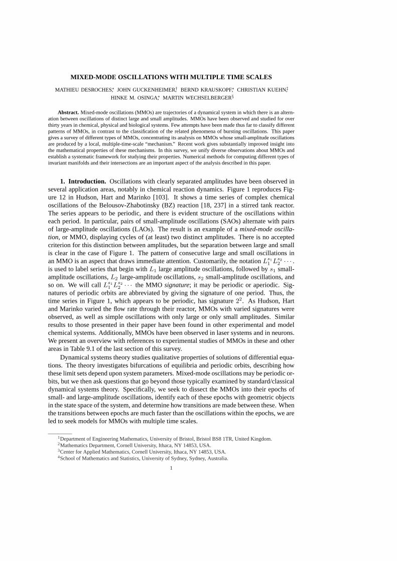
1. Introduction. Oscillations with clearly separated amplitudes have been observed inseveral application areas, notably in chemical reaction dynamics. Figure 1 reproduces Fig-ure 12 in Hudson, Hart and Marinko [103]. It shows a time series of complex chemicaloscillations of the Belousov-Zhabotinsky (BZ) reaction [18, 237] in a stirred tank reactor.The series appears to be periodic, and there is evident structure of the oscillations withineach period. In particular, pairs of small-amplitude oscillations (SAOs) alternate with pairsof large-amplitude oscillations (LAOs). The result is an example of amixed-mode oscilla-tion, or MMO, displaying cycles of (at least) two distinct amplitudes. There is no acceptedcriterion for this distinction between amplitudes, but the separation between large and smallis clear in the case of Figure 1. The pattern of consecutive large and small oscillations inan MMO is an aspect that draws immediate attention. Customarily, the notationLs1

1 Ls22 · · · .

is used to label series that begin withL1 large amplitude oscillations, followed bys1 small-amplitude oscillations,L2 large-amplitude oscillations,s2 small-amplitude oscillations, andso on. We will callLs1

1 Ls22 · · · the MMO signature; it may be periodic or aperiodic. Sig-

natures of periodic orbits are abbreviated by giving the signature of one period. Thus, thetime series in Figure 1, which appears to be periodic, has signature22. As Hudson, Hartand Marinko varied the flow rate through their reactor, MMOs with varied signatures wereobserved, as well as simple oscillations with only large or only small amplitudes. Similarresults to those presented in their paper have been found in other experimental and modelchemical systems. Additionally, MMOs have been observed in laser systems and in neurons.We present an overview with references to experimental studies of MMOs in these and otherareas in Table 9.1 of the last section of this survey.

Dynamical systems theory studies qualitative properties of solutions of differential equa-tions. The theory investigates bifurcations of equilibria and periodic orbits, describing howthese limit sets depend upon system parameters. Mixed-mode oscillations may be periodic or-bits, but we then ask questions that go beyond those typically examined by standard/classicaldynamical systems theory. Specifically, we seek to dissect the MMOs into their epochs ofsmall- and large-amplitude oscillations, identify each of these epochs with geometric objectsin the state space of the system, and determine how transitions are made between these. Whenthe transitions between epochs are much faster than the oscillations within the epochs, we areled to seek models for MMOs with multiple time scales.

1Department of Engineering Mathematics, University of Bristol, Bristol BS8 1TR, United Kingdom.2Mathematics Department, Cornell University, Ithaca, NY 14853, USA.3Center for Applied Mathematics, Cornell University, Ithaca, NY 14853, USA.4School of Mathematics and Statistics, University of Sydney, Sydney, Australia.

1

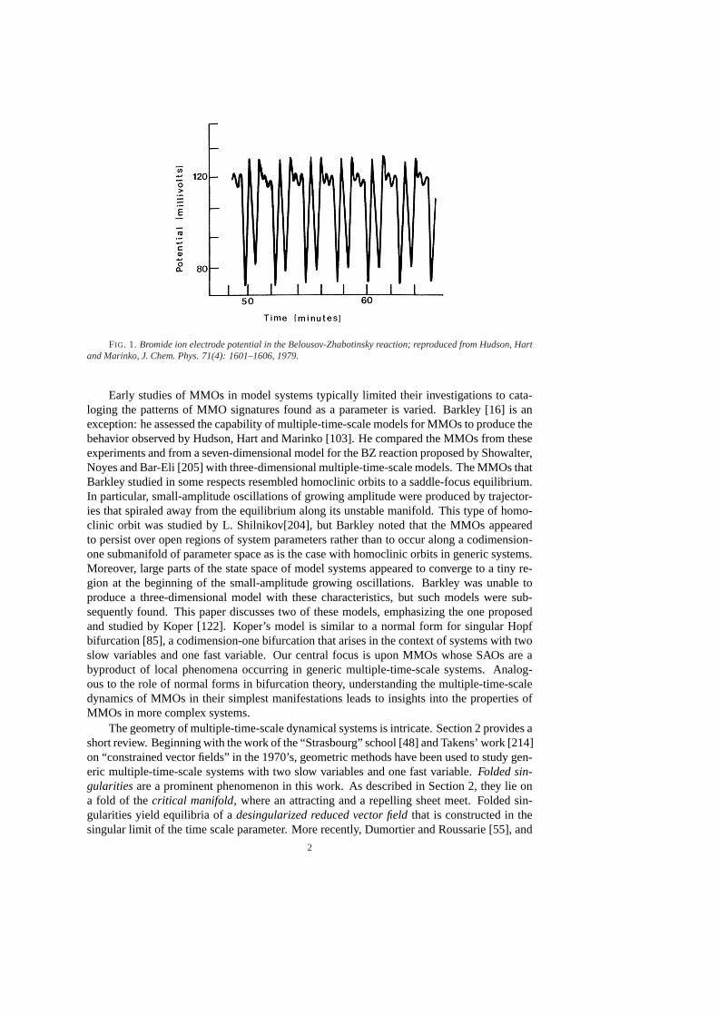
FIG. 1. Bromide ion electrode potential in the Belousov-Zhabotinsky reaction; reproduced from Hudson, Hartand Marinko, J. Chem. Phys. 71(4): 1601–1606, 1979.

Early studies of MMOs in model systems typically limited their investigations to cata-loging the patterns of MMO signatures found as a parameter is varied. Barkley [16] is anexception: he assessed the capability of multiple-time-scale models for MMOs to produce thebehavior observed by Hudson, Hart and Marinko [103]. He compared the MMOs from theseexperiments and from a seven-dimensional model for the BZ reaction proposed by Showalter,Noyes and Bar-Eli [205] with three-dimensional multiple-time-scale models. The MMOs thatBarkley studied in some respects resembled homoclinic orbits to a saddle-focus equilibrium.In particular, small-amplitude oscillations of growing amplitude were produced by trajector-ies that spiraled away from the equilibrium along its unstable manifold. This type of homo-clinic orbit was studied by L. Shilnikov[204], but Barkley noted that the MMOs appearedto persist over open regions of system parameters rather than to occur along a codimension-one submanifold of parameter space as is the case with homoclinic orbits in generic systems.Moreover, large parts of the state space of model systems appeared to converge to a tiny re-gion at the beginning of the small-amplitude growing oscillations. Barkley was unable toproduce a three-dimensional model with these characteristics, but such models were sub-sequently found. This paper discusses two of these models, emphasizing the one proposedand studied by Koper [122]. Koper’s model is similar to a normal form for singular Hopfbifurcation [85], a codimension-one bifurcation that arises in the context of systems with twoslow variables and one fast variable. Our central focus is upon MMOs whose SAOs are abyproduct of local phenomena occurring in generic multiple-time-scale systems. Analog-ous to the role of normal forms in bifurcation theory, understanding the multiple-time-scaledynamics of MMOs in their simplest manifestations leads to insights into the properties ofMMOs in more complex systems.

The geometry of multiple-time-scale dynamical systems is intricate. Section 2 provides ashort review. Beginning with the work of the “Strasbourg” school [48] and Takens’ work [214]on “constrained vector fields” in the 1970’s, geometric methods have been used to study gen-eric multiple-time-scale systems with two slow variables and one fast variable.Folded sin-gularitiesare a prominent phenomenon in this work. As described in Section 2, they lie ona fold of thecritical manifold, where an attracting and a repelling sheet meet. Folded sin-gularities yield equilibria of adesingularized reduced vector fieldthat is constructed in thesingular limit of the time scale parameter. More recently, Dumortier and Roussarie [55], and

2

Szmolyan and Wechselberger [212] introduced singular blow-up techniques for the analyt-ical study of the dynamics near folded singularities. These methods give information aboutcanard orbitsthat connect attracting and repellingslow manifolds.

Canard orbits organize the number of small-amplitude oscillations for MMOs associatedwith folded nodes. The unfoldings of folded nodes [86, 233], folded saddle-nodes [84, 143]and singular Hopf bifurcations [85] give insight into the characteristics of MMOs and howthey are formed as system parameters vary. Passage of trajectories through the region of afolded node is one mechanism for generating MMOs that we discuss at length in Section 3.1and illustrate with examples in Sections 4 and 5.Singular Hopf bifurcationand the closelyrelatedfolded saddle-node bifurcation of type IItogether constitute a second mechanism thatproduces SAOs and MMOs in a robust manner within systems having two slow variables andone fast variable. These bifurcations occur when a (true) equilibrium of the slow-fast systemcrosses a fold curve of a critical manifold. Singular Hopf bifurcation is discussed in Sec-tion 3.2 and also illustrated in Sections 4 and 5. We discuss a third mechanism for producingsmall-amplitude oscillations in slow-fast systems that is organized by aHopf bifurcation inthe layer equationsand requires two fast variables. We call this mechanism adynamic Hopfbifurcationand distinguish trajectories that pass by a dynamic Hopf bifurcation with adelayand trajectories with atourbillion [232] whose small-amplitude oscillations have larger mag-nitude than those of a delayed Hopf bifurcation. Dynamic Hopf bifurcation is discussed inSection 3.4 and illustrated in Sections 6 and 7.

Complementary to theoretical advances in the analysis of slow-fast systems, numericalmethods have been developed to compute and visualize geometric structures that shape thedynamics of these systems. Slow manifolds and canard orbits can now be computed in con-crete systems; see Guckenheimer [85, 89] and Desroches, Krauskopf and Osinga [40, 41, 42,43]. The combination of new theory and new numerics has produced new understanding ofMMOs in many examples that have been previously studied. This paper reviews and synthes-izes these advances. It is organized as follows. Section 2 gives background about relevantparts of geometric singular perturbation theory. Multiple-time-scale mechanisms that produceSAOs in MMOs are then discussed and illustrated in Section 3. The four subsequent sectionsprovide case studies that illustrate and highlight recent theoretical advances and computa-tional techniques. More details on the computational methods used in this paper can be foundin Section 8. The final Section 9 includes a brief survey of the MMO literature and discussesother mechanisms that are not associated with a split between slow and fast variables.

2. Geometric singular perturbation theory of slow-fast systems.We consider here aslow-fast vector field that takes the form

{ε x = ε dx

dτ = f(x, y, λ, ε),

y = dydτ = g(x, y, λ, ε),

(2.1)

where(x, y) ∈ Rm × Rn are state space variables,λ ∈ Rp are system parameters, andε is a small parameter0 < ε ¿ 1 representing the ratio of time scales. The functionsf : Rm × Rn × Rp × R → Rm and g : Rm × Rn × Rp × R → Rn are assumed tobe sufficiently smooth, typicallyC∞. The variablesx are fast and the variablesy are slow.System (2.1) can be rescaled to

{x′ = dx

dt = f(x, y, λ, ε),

y′ = dydt = ε g(x, y, λ, ε),

(2.2)

by switching from the slow time scaleτ to the fast time scalet = τ/ε.

3

Several viewpoints have been adopted to study slow-fast systems, starting with asymp-totic analysis [56, 164] using techniques such as matched asymptotic expansions [118, 148].Geometric Singular Perturbation Theory (GSPT) takes a geometric point of view and fo-cuses upon invariant manifolds, normal forms for singularities and analysis of their unfold-ings [10, 69, 110, 111, 215]. Fenichel’s seminal work [69] on invariant manifolds was aninitial foundation of GSPT and it is also called Fenichel theory. A third viewpoint was ad-opted by a group of French mathematicians in Strasbourg. Using nonstandard analysis, theymade many important discoveries [19, 20, 22, 23, 47, 48] about slow-fast systems. This paperadopts the GSPT viewpoint. We only focus on the results of GSPT that are necessary to studyMMOs. There are other important techniques that are part of GSPT, such as the ExchangeLemma [110, 112], the blow-up method [55, 142, 233] and slow-fast normal form theory [10]that are not described in this paper.

2.1. The critical manifold and the slow flow. Solutions of a slow-fast system fre-quently exhibit slow and fast epochs characterized by the speed at which the solution ad-vances. Asε → 0, the trajectories of (2.1) converge during fast epochs to solutions of thefastsubsystemor layer equations

{x′ = f(x, y, λ, 0),y′ = 0.

(2.3)

During slow epochs, on the other hand, trajectories of (2.2) converge to solutions of{

0 = f(x, y, λ, 0),y = g(x, y, λ, 0), (2.4)

which is a differential-algebraic equation (DAE) called theslow flowor reduced system. Onegoal of GSPT is to use the fast and slow subsystems, (2.3) and (2.4), to understand the dy-namics of the full system (2.1) or (2.2) forε > 0. The algebraic equation in (2.4) defines thecritical manifold

S := {(x, y) ∈ Rm × Rn | f(x, y, λ, 0) = 0}.We remark thatS may have singularities [141], but we assume here that this does not hap-pen so thatS is a smooth manifold. The points ofS are equilibrium points for the layerequations (2.3).

Fenichel theory [69] guarantees persistence ofS (or a subsetM ⊂ S) as a slow manifoldof (2.1) or (2.2) forε > 0 small enough ifS (or M ) is normally hyperbolic. The notion ofnormal hyperbolicity is defined for invariant manifolds more generally, effectively statingthat the attraction to and/or repulsion from the manifold is stronger than the dynamics on themanifold itself; see [66, 67, 68, 95] for the exact definition. Normal hyperbolicity is oftendifficult to verify when there is only a single time scale. However, in our slow-fast setting,S consists entirely of equilibria and the requirement of normal hyperbolicity ofM ⊂ Sis satisfied as soon as allp ∈ M are hyperbolic equilibria of the layer equations, that is, theJacobian(Dxf)(p, λ, 0) has no eigenvalues with zero real part. We call a normally hyperbolicsubsetM ⊂ S attracting if all eigenvalues of(Dxf)(p, λ, 0) have negative real parts forp ∈ M ; similarly M is calledrepelling if all eigenvalues have positive real parts. IfM isnormally hyperbolic and neither attracting nor repelling we say it is ofsaddle type.

Hyperbolicity of the layer equations fails at points onS where its projection onto thespace of slow variables is singular. Generically, such points are folds in the sense of singu-larity theory [10]. At a fold pointp∗, we havef(p∗, λ, 0) = 0 and(Dxf)(p∗, λ, 0) has rankm−1 with left and right null vectorsw andv, such thatw · [(D2

xxf)(p∗, λ, 0) (v, v)] 6= 0 and

4

w · [(Dyf)(p∗, λ, 0)] 6= 0. The set of fold points forms a submanifold of codimension one inthen-dimensional critical manifoldS. In particular, whenm = 1 andn = 2, the fold pointsform smooth curves that separate attracting and repelling sheets of the two-dimensional crit-ical manifoldS. In this paper we do not consider more degenerate singular points of theprojection ofS onto the space of slow variables.

Away from fold points the implicit function theorem implies thatS is locally the graphof a functionh(y) = x. Then the reduced system (2.4) can be expressed as

y = g(h(y), y, λ, 0). (2.5)

We can also keep the DAE structure and write (2.4) as the restriction toS of the vector field

{x = − (Dxf)−1 (Dyf) g,y = g,

(2.6)

on Rm × Rn by observing thatf = 0 and y = g imply x = − (Dxf)−1 (Dyf) g. Thevector field (2.6) blows up whenf is singular. It can bedesingularizedby scaling time by− det (Dxf), at the expense of changing the direction of the flow in the region where thisdeterminant is positive. This desingularized system plays a prominent role in much of ouranalysis. IfS is normally hyperbolic, not onlyS, but also the slow flow onS persists forε > 0; this is made precise in the following fundamental theorem.

THEOREM 2.1 (Fenichel’s Theorem [69]). SupposeM = M0 is a compact normallyhyperbolic submanifold (possibly with boundary) of the critical manifoldS of (2.2)and thatf, g ∈ Cr, r < ∞. Then forε > 0 sufficiently small the following holds:

(F1) There exists a locally invariant manifoldMε diffeomorphic toM0. Local invariancemeans thatMε can have boundaries through which trajectories enter or leave.

(F2) Mε has a Hausdorff distance ofO(ε) fromM0.(F3) The flow onMε converges to the slow flow asε → 0.(F4) Mε is Cr-smooth.(F5) Mε is normally hyperbolic and has the same stability properties with respect to the

fast variables asM0 (attracting, repelling or saddle type).(F6) Mε is usually not unique. In regions that remain at a fixed distance from the bound-

ary ofMε, all manifolds satisfying (F1)–(F5) lie at a Hausdorff distanceO(e−K/ε)from each other for someK > 0 with K = O(1).

The normally hyperbolic manifoldM0 has associated local stable and unstable manifolds

W sloc(M0) =

⋃

p∈M0

W sloc(p), and Wu

loc(M0) =⋃

p∈M0

Wuloc(p),

whereW sloc(p) andWu

loc(p) are the local stable and unstable manifolds ofp as a hyperbolicequilibrium of the layer equations, respectively. These manifolds also persist forε > 0sufficiently small: there exist local stable and unstable manifoldsW s

loc(Mε) andWuloc(Mε),

respectively, for which conclusions (F1)–(F6) hold if we replaceMε andM0 by W sloc(Mε)

andW sloc(M0) (or similarly byWu

loc(Mε) andWuloc(M0)).

We callMε a Fenichel manifold. Fenichel manifolds are a subclass ofslow manifolds,invariant manifolds on which the vector field has speed that tends to0 on the fast time scaleasε → 0. We use the convention that objects in the singular limit have subscript0, whereasthe associated perturbed objects have subscriptsε.

2.1.1. The critical manifold and the slow flow in the Van der Pol equation.Let usillustrate these general concepts of GSPT with an example. One of the simplest systems in

5

−2 −1 0 1 2−1

0

1

−2 −1 0 1 2−1

0

1

x

y

p−

Sa,− Sr Sa,+

p+

(a)

x

y•

p−

Sa,− Sr Sa,+

p+

(b)

.

.

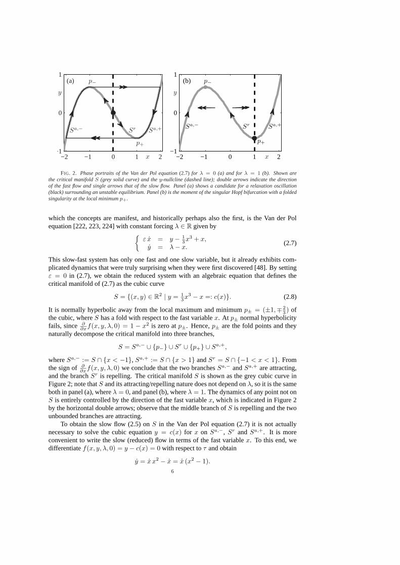
FIG. 2. Phase portraits of the Van der Pol equation(2.7) for λ = 0 (a) and forλ = 1 (b). Shown arethe critical manifoldS (grey solid curve) and they-nullcline (dashed line); double arrows indicate the directionof the fast flow and single arrows that of the slow flow. Panel (a) shows a candidate for a relaxation oscillation(black) surrounding an unstable equilibrium. Panel (b) is the moment of the singular Hopf bifurcation with a foldedsingularity at the local minimump+.

which the concepts are manifest, and historically perhaps also the first, is the Van der Polequation [222, 223, 224] with constant forcingλ ∈ R given by

{ε x = y − 1

3x3 + x,y = λ− x.

(2.7)

This slow-fast system has only one fast and one slow variable, but it already exhibits com-plicated dynamics that were truly surprising when they were first discovered [48]. By settingε = 0 in (2.7), we obtain the reduced system with an algebraic equation that defines thecritical manifold of (2.7) as the cubic curve

S = {(x, y) ∈ R2 | y = 13x3 − x =: c(x)}. (2.8)

It is normally hyperbolic away from the local maximum and minimump± = (±1,∓ 23 ) of

the cubic, whereS has a fold with respect to the fast variablex. At p± normal hyperbolicityfails, since ∂

∂xf(x, y, λ, 0) = 1 − x2 is zero atp±. Hence,p± are the fold points and theynaturally decompose the critical manifold into three branches,

S = Sa,− ∪ {p−} ∪ Sr ∪ {p+} ∪ Sa,+,

whereSa,− := S ∩ {x < −1}, Sa,+ := S ∩ {x > 1} andSr = S ∩ {−1 < x < 1}. Fromthe sign of ∂

∂xf(x, y, λ, 0) we conclude that the two branchesSa,− andSa,+ are attracting,and the branchSr is repelling. The critical manifoldS is shown as the grey cubic curve inFigure 2; note thatS and its attracting/repelling nature does not depend onλ, so it is the sameboth in panel (a), whereλ = 0, and panel (b), whereλ = 1. The dynamics of any point not onS is entirely controlled by the direction of the fast variablex, which is indicated in Figure 2by the horizontal double arrows; observe that the middle branch ofS is repelling and the twounbounded branches are attracting.

To obtain the slow flow (2.5) onS in the Van der Pol equation (2.7) it is not actuallynecessary to solve the cubic equationy = c(x) for x on Sa,−, Sr andSa,+. It is moreconvenient to write the slow (reduced) flow in terms of the fast variablex. To this end, wedifferentiatef(x, y, λ, 0) = y − c(x) = 0 with respect toτ and obtain

y = x x2 − x = x (x2 − 1).6

Combining this result with the equation fory we get:

(x2 − 1) x = λ− x or x =λ− x

x2 − 1. (2.9)

The direction of the slow flow onS is indicated in Figure 2 by the arrows on the grey curve;panel (a) is forλ = 0 and panel (b) forλ = 1. The slow flow does depend onλ, because thedirection of the flow is partly determined by the location of the equilibrium atx = λ on S.The slow flow is well defined onSa,−, Sr andSa,+, but not atx = ±1 (as long asλ 6= ±1).We can desingularize the slow flow nearx = ±1 by rescaling time with the factor(x2 − 1).This gives the equationx = λ − x of thedesingularized flow. Note that this time rescalingreverses the direction of time on the repelling branchSr, so care must be taken when relatingthe phase portrait of the desingularized system to the phase portrait of the slow flow.

Let us now focus specifically on the case forλ = 0, shown in Figure 2(a), because it isrepresentative for the range|λ| < 1. They-nullcline of (2.7) is shown as the dashed blackvertical line (thex-nullcline isS) and the origin is the only equilibrium, which is a source forthis value ofλ. The closed curve is a singular orbit composed of two fast trajectories startingat the two fold pointsp± concatenated with segments ofS. Such continuous concatenationsof trajectories of the layer equations and the slow flow are calledcandidates[20]. The singularorbit follows the slow flow onS to a fold point, then itjumps, that is, it makes a transitionto a fast trajectory segment that flows to another branch ofS. The same mechanism returnsthe singular orbit to the initial branch ofS. It can be shown [142, 164] that the singular orbitperturbs forε > 0 to a periodic orbit of the Van der Pol equation that liesO(ε) close to thiscandidate. Van der Pol introduced the termrelaxation oscillationto describe periodic orbitsthat alternate between epochs of slow and fast motion.

2.2. Singular Hopf bifurcation and canard explosion. The dynamics of slow-fast sys-tems in the vicinity of points on the critical manifold where normal hyperbolicity is lost canbe surprisingly complicated and nothing like what we know from systems with a single timescale. This section addresses the phenomenon known as acanard explosion, which occursin planar slow-fast systems after asingular Hopf bifurcation. We discuss this first for theexample of the Van der Pol equation (2.7).

2.2.1. Canard explosion in the Van der Pol equation.As mentioned above, the phaseportrait in Figure 2(a) is representative for a range ofλ-values. However, the phase portraitfor λ = 1, shown in Figure 2(b), is degenerate. Linear stability analysis shows that forε > 0 the unique equilibrium point(x, y) = (λ, 1

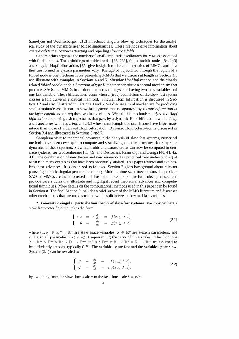
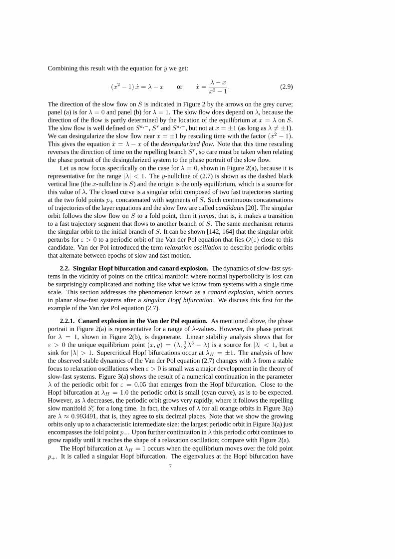
3λ3 − λ) is a source for|λ| < 1, but asink for |λ| > 1. Supercritical Hopf bifurcations occur atλH = ±1. The analysis of howthe observed stable dynamics of the Van der Pol equation (2.7) changes withλ from a stablefocus to relaxation oscillations whenε > 0 is small was a major development in the theory ofslow-fast systems. Figure 3(a) shows the result of a numerical continuation in the parameterλ of the periodic orbit forε = 0.05 that emerges from the Hopf bifurcation. Close to theHopf bifurcation atλH = 1.0 the periodic orbit is small (cyan curve), as is to be expected.However, asλ decreases, the periodic orbit grows very rapidly, where it follows the repellingslow manifoldSr

ε for a long time. In fact, the values ofλ for all orange orbits in Figure 3(a)areλ ≈ 0.993491, that is, they agree to six decimal places. Note that we show the growingorbits only up to a characteristic intermediate size: the largest periodic orbit in Figure 3(a) justencompasses the fold pointp−. Upon further continuation inλ this periodic orbit continues togrow rapidly until it reaches the shape of a relaxation oscillation; compare with Figure 2(a).

The Hopf bifurcation atλH = 1 occurs when the equilibrium moves over the fold pointp+. It is called a singular Hopf bifurcation. The eigenvalues at the Hopf bifurcation have

7

−2 −1 0 1 2−1

0

1

x

y

S

(a)

λλH

A(c)

λλH

A(b)

.

.

FIG. 3. Numerical continuation of periodic orbits in the Van der Pol’s equation(2.7) for ε = 0.05. Panel (a)shows a selection of periodic orbits: the cyan orbit is a typical small limit cycle near the Hopf bifurcation atλ = λH ,whereas all the orange orbits occur in a very small parameter interval atλ ≈ 0.993491. Panels (b) and (c) aresketched bifurcation diagrams corresponding to supercritical and subcritical singular Hopf bifurcations; hereAdenotes the amplitude of the limit cycle.

magnitudeO(ε−1/2), so that the periodic orbit is born at the Hopf bifurcation with an inter-mediate period between the fastO(ε−1) and slowO(1) time scales. The size of this periodicorbit grows rapidly from diameterO(ε1/2) to diameterO(1) in an interval of parameter val-uesλ of lengthO(exp(−K/ε)) (for someK > 0 fixed) that isO(ε) close toλH . Figures 3(b)and (c) are sketches of possible bifurcation diagrams inλ for the singular Hopf bifurcationin a supercritical case (which one finds in the Van der Pol system) and in a subcritical case,respectively; the vertical axis represents the maximal amplitude of the periodic orbits. Thetwo bifurcation diagrams are sketches that highlight the features described above. There is avery small interval ofλ where the amplitude of the oscillation grows in a square-root fashion,as is to be expected near a Hopf bifurcation. However, the amplitude then grows extremelyrapidly until it reaches a plateau that corresponds to relaxation oscillations.

The rapid growth in amplitude of the periodic orbit near the Hopf bifurcation is called acanard explosion. The name canard derives originally from the fact that some periodic orbitsduring the canard explosion look a bit like a duck [48]. In fact, the largest periodic orbit inFigure 3(a) is an example of such a “duck-shaped” orbit. More generally, and irrespective ofits actual shape, one now refers to a trajectory as acanard orbitif it follows a repelling slowmanifold for a time ofO(1) on the slow time scale. A canard orbit is called amaximal canardif it joins attracting and repelling slow manifolds. Since the slow manifolds are not unique,this definition depends upon the selection of specific attracting and repelling slow manifolds;compare (F6) of Theorem 2.1. Other choices yield trajectories that are exponentially close toone another. In the Van der Pol equation (2.7) the canard explosion occursO(e−K/ε)-close inparameter space to the point where the manifoldsSa,+

ε andSrε intersect in a maximal canard.

It is associated with the parameter valueλ = 1 where the equilibrium lies at the fold pointp+ of the critical manifoldS; see Figure 2(b).

2.3. Singular Hopf bifurcation and canard explosion in generic planar systems.Inthe Van der Pol equation (2.7) the singular Hopf bifurcation takes place atλ = 1 where theequilibrium lies at a fold point. In a generic family of slow-fast planar systems a singularHopf bifurcation does not happen exactly at a fold point, but at a distanceO(ε) in both phasespace and parameter space from the coincidence of the equilibrium and fold point. One can

8

obtain a generic family by modifying the slow equation of the Van der Pol equation (2.7) to

y = λ− x + a y.

In this modified system the equilibrium and fold point still coincide atx = 1, but the Hopfbifurcation occurs forx =

√1 + ε a. A detailed dynamical analysis of canard explosion and

the associated singular Hopf bifurcation using geometric or asymptotic methods exists forplanar slow-fast systems [12, 13, 55, 56, 140, 142]; we summarize these results as follows.

THEOREM 2.2 (Canard Explosion inR2 [142]). Suppose a planar slow-fast system hasa generic fold pointp∗ = (xp, yp) ∈ S, that is,

f(p∗, λ, 0) = 0,∂

∂xf(p∗, λ, 0) = 0,

∂2

∂x2f(p∗, λ, 0) 6= 0,

∂

∂yf(p∗, λ, 0) 6= 0.

(2.10)Assume the critical manifold is locally attracting forx < xp and repelling forx > xp andthere exists a folded singularity forλ = 0 at p∗, namely,

g(p∗, 0, 0) = 0,∂

∂xg(p∗, 0, 0) 6= 0,

∂

∂λg(p∗, 0, 0) 6= 0. (2.11)

Then a singular Hopf bifurcation and a canard explosion occur at

λH = H1 ε + O(ε3/2) and (2.12)

λc = (H1 + K1) ε + O(ε3/2). (2.13)

The coefficientsH1 andK1 can be calculated explicitly from normal form transformations [142]or by considering the first Lyapunov coefficient of the Hopf bifurcation [144].

In the singular limit we haveλH = λc. For anyε > 0 sufficiently small, the linearizedsystem [88, 147] at the Hopf bifurcation point has a pair ofsingular eigenvalues[27]

σ(λ; ε) = α(λ; ε) + i β(λ; ε),

with α(λH ; ε) = 0, ∂∂λα(λH ; ε) 6= 0 and

limε→0

β(λH ; ε) = ∞, on the slow time scaleτ , and

limε→0

β(λH ; ε) = 0, on the fast time scalet.

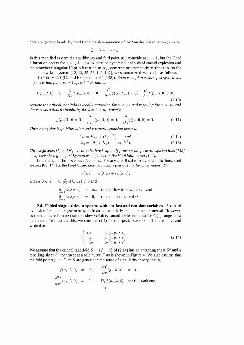
2.4. Folded singularities in systems with one fast and two slow variables.A canardexplosion for a planar system happens in an exponentially small parameter interval. However,as soon as there is more than one slow variable, canard orbits can exist forO(1) ranges of aparameter. To illustrate this, we consider (2.1) for the special casem = 1 andn = 2, andwrite it as

ε x = f(x, y, λ, ε),y1 = g1(x, y, λ, ε),y2 = g2(x, y, λ, ε).

(2.14)

We assume that the critical manifoldS = {f = 0} of (2.14) has an attracting sheetSa and arepelling sheetSr that meet at a fold curveF as is shown in Figure 4. We also assume thatthe fold pointsp∗ ∈ F onS are generic in the sense of singularity theory, that is,

f(p∗, λ, 0) = 0,∂f

∂x(p∗, λ, 0) = 0,

∂2f

∂x2(p∗, λ, 0) 6= 0, Dyf(p∗, λ, 0) has full rank one.

9

Sr

F

Sa

•

y1

x

y2

.

.

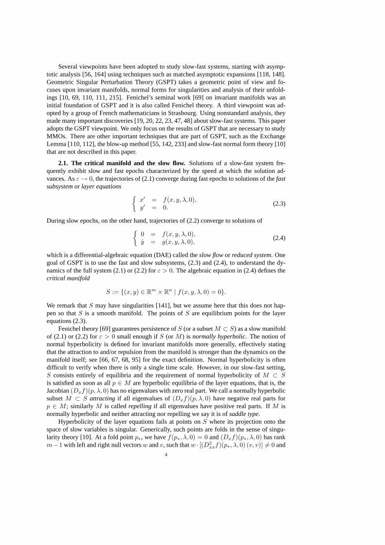
FIG. 4. The critical manifoldS with attracting sheetSa (red) and repelling sheetSr (blue) that meet at a foldcurveF (grey). The fast flow transverse toS is indicated by double (large) arrows and the slow flow onS near afolded node by single (small) arrows; see also Figure 5(b).

The slow flow is not defined on the fold curve before desingularization. At most fold points,trajectories approach or depart from both the attracting and repelling sheets ofS. In genericsystems, there may be isolated points, calledfolded singularities, where the trajectories ofthe slow flow switch from incoming to outgoing. Figure 4 shows an example of the slow flowon S and the thick dot onF is the folded singularity at whichF changes from attracting torepelling (with respect to the slow flow).

Folded singularities are equilibrium points of the desingularized slow flow. As describedabove, the desingularized slow flow can be expressed as

x =(

∂∂y1

f)

g1 +(

∂∂y2

f)

g2 ,

y1 = − (∂∂xf

)g1,

y2 = − (∂∂xf

)g2,

(2.15)

restricted toS. A fold point p∗ ∈ F is a folded singularity if

g1(p∗, λ, 0)∂f

∂y1(p∗, λ, 0) + g2(p∗, λ, 0)

∂f

∂y2(p∗, λ, 0) = 0.

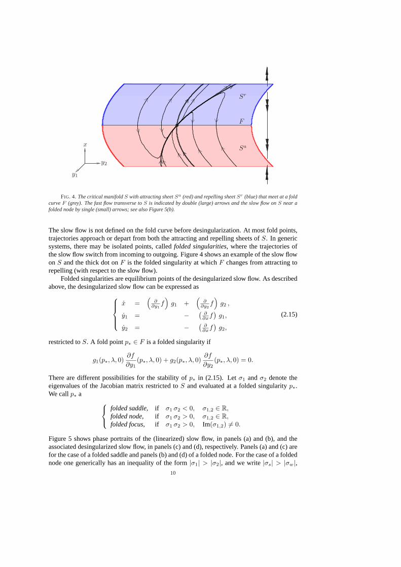
There are different possibilities for the stability ofp∗ in (2.15). Letσ1 andσ2 denote theeigenvalues of the Jacobian matrix restricted toS and evaluated at a folded singularityp∗.We callp∗ a

folded saddle, if σ1 σ2 < 0, σ1,2 ∈ R,folded node, if σ1 σ2 > 0, σ1,2 ∈ R,folded focus, if σ1 σ2 > 0, Im(σ1,2) 6= 0.

Figure 5 shows phase portraits of the (linearized) slow flow, in panels (a) and (b), and theassociated desingularized slow flow, in panels (c) and (d), respectively. Panels (a) and (c) arefor the case of a folded saddle and panels (b) and (d) of a folded node. For the case of a foldednode one generically has an inequality of the form|σ1| > |σ2|, and we write|σs| > |σw|,

10

x

y

Sr

F

Sa

(c)

x

y

Sr

F

Sa

(d)

x

y

Sr

F

Sa

γ1 γ2

(a)

x

y

Sr

F

Sa

γw

γs(b)

.

.

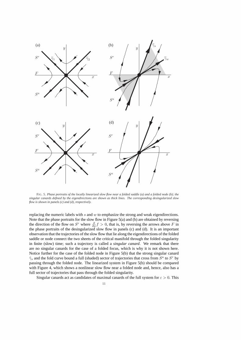
FIG. 5. Phase portraits of the locally linearized slow flow near a folded saddle (a) and a folded node (b); thesingular canards defined by the eigendirections are shown as thick lines. The corresponding desingularized slowflow is shown in panels (c) and (d), respectively.

replacing the numeric labels withs andw to emphasize the strong and weak eigendirections.Note that the phase portraits for the slow flow in Figure 5(a) and (b) are obtained by reversingthe direction of the flow onSr where ∂

∂xf > 0, that is, by reversing the arrows aboveF inthe phase portraits of the desingularized slow flow in panels (c) and (d). It is an importantobservation that the trajectories of the slow flow that lie along the eigendirections of the foldedsaddle or node connect the two sheets of the critical manifold through the folded singularityin finite (slow) time; such a trajectory is called asingular canard. We remark that thereare no singular canards for the case of a folded focus, which is why it is not shown here.Notice further for the case of the folded node in Figure 5(b) that the strong singular canardγs and the fold curve bound a full (shaded) sector of trajectories that cross fromSa to Sr bypassing through the folded node. The linearized system in Figure 5(b) should be comparedwith Figure 4, which shows a nonlinear slow flow near a folded node and, hence, also has afull sector of trajectories that pass through the folded singularity.

Singular canards act as candidates of maximal canards of the full system forε > 0. This

11

is described in the next theorem [19, 23, 31, 212, 233].THEOREM 2.3 (Canards inR3). For the slow-fast system(2.14)with ε > 0 sufficiently

small the following holds:(C1) There are no maximal canards generated by a folded focus.(C2) For a folded saddle the two singular canardsγ1,2 perturb to maximal canardsγ1,2.

(C3.1) For a folded node letµ := σw/σs < 1. The singular canardγs (“the strongcanard”) always perturbs to a maximal canardγs. If µ−1 6∈ N then the singularcanardγw (“the weak canard”) also perturbs to a maximal canardγw. We callγs

andγw primary canards.(C3.2) For a folded node supposek > 0 is an integer such that2k + 1 < µ−1 < 2k + 3

andµ−1 6= 2(k + 1). Then, in addition toγs,w, there arek other maximal canards,which we call secondary canards.

(C3.3) The primary weak canard of a folded node undergoes a transcritical bifurcation foroddµ−1 ∈ N and a pitchfork bifurcation for evenµ−1 ∈ N.

3. Slow-fast mechanisms for MMOs.In this section we present key theoretical resultsof how MMOs arise in slow-fast systems with SAOs occurring in a localized region of thephase space. The LAOs, on the other hand, are associated with large excursions away fromthe localized region of SAOs. More specifically, we discuss four local mechanisms that giverise to such SAOs:

• passage near a folded node, discussed in Section 3.1;• singular Hopf bifurcation, discussed in Section 3.2;• three-time-scale problems with a singular Hopf bifurcation, discussed in Section 3.3;• tourbillion, discussed in Section 3.4.

Each of these local mechanisms has its distinctive characteristics and can give rise to MMOswhen combined with aglobal return mechanismthat takes the trajectory back to the regionwith SAOs. Such global return mechanisms arise naturally in models from applications anda classic example is an S-shaped slow manifold; see Section 3.2 and the examples in Sec-tions 4–6. We do not discuss global returns in detail, but rather concentrate on the nature ofthe local mechanisms. From the analysis of normal forms we estimate quantities that can bemeasured in examples of MMOs produced from both numerical simulations and experimentaldata. Specifically, we consider the number of SAOs and the changes in their amplitudes fromcycle to cycle. We also consider in model systems the geometry of nearby slow manifoldsthat are associated with the approach to and departure from the SAO regions.

3.1. MMOs due to a folded node.Folded nodes are only defined for the singularlimit (2.4) of system (2.1) on the slow time scale. However, they are directly relevant toMMOs because forε > 0 small enough, trajectories of (2.1) that flow through a region wherethe reduced system has a folded node, undergo small oscillations. Benoit [19, 20] first re-cognized these oscillations. Wechselberger and collaborators [31, 212, 233] gave a detailedanalysis of folded nodes while Guckenheimer and Haiduc [86] and Guckenheimer [84] com-puted intersections of slow manifolds near a folded node and maps along trajectories passingthrough these regions. From Theorem 2.3 we know that the eigenvalue ratio0 < µ < 1 atthe folded node is a crucial quantity that determines the dynamics in a neighborhood of thefolded node. In particular,µ controls the maximal number of oscillations. The studies men-tioned above use normal forms to describe the dynamics of oscillations near a folded node.Two equivalent versions of these normal forms are

ε x = y − x2,y = z − x,z = −ν,

(3.1)

12

and

ε x = y − x2,y = −(µ + 1)x− z,z = 1

2µ.(3.2)

Note thatµ is the eigenvalue ratio of system (3.2) and thatν 6= 0 andµ 6= 0 imply that noequilibria exist in (3.1) and (3.2). If we replace(x, y, z) in system (3.1) by(u, v, w) and callthe time variableτ1, then we obtain system (3.2) via the coordinate change

x = (1 + µ)1/2 u, y = (1 + µ) v, z = −(1 + µ)3/2 w,

and the rescaling of timeτ = τ1/√

1 + µ, which gives

ν =µ

2(1 + µ)2or µ =

−1 +√

1− 8ν

−1−√1− 8ν.

Therefore, in system (3.1) the number of secondary canards changes with the parameterν.Whenν is small,µ ≈ 2ν. If the “standard” scaling [212]x = ε1/2 x, y = ε y, z = ε1/2 z,andt = ε1/2 t, is applied to system (3.1), we obtain

x′ = y − x2,y′ = z − x,

z′ = −ν .

(3.3)

Hence, the phase portraits of system (3.1) for different values ofε are topologically equivalentvia linear maps. The normal form (3.3) describes the dynamics in the neighborhood of afolded node, which is at the origin here. Trajectories that come fromy = ∞ with x > 0and pass through the folded-node region make a number of oscillations in the process, beforegoing off toy = ∞ with x < 0. There are no returns to the folded-node region in this system.

Let us first focus on the number of small oscillations. If2k + 1 < µ−1 < 2k + 3, forsomek ∈ N, andµ−1 6= 2(k + 1) then the primary strong canardγs twists once and thei-th secondary canardξi, 1 ≤ i ≤ k, twists2i + 1 times around the primary weak canardγw

in anO(1) neighborhood of the folded node singularity in system (3.3), which correspondsto anO(

√ε) neighborhood in systems (3.1) and (3.2) [212, 233]. (A twist corresponds to

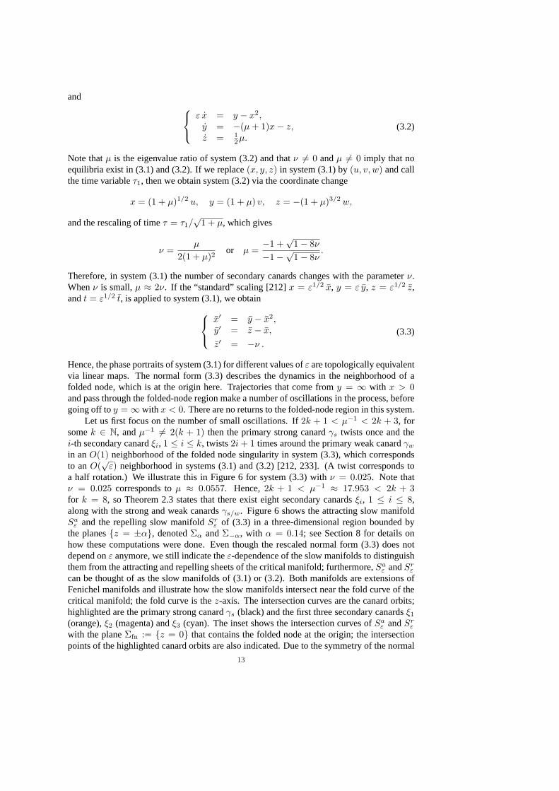
a half rotation.) We illustrate this in Figure 6 for system (3.3) withν = 0.025. Note thatν = 0.025 corresponds toµ ≈ 0.0557. Hence,2k + 1 < µ−1 ≈ 17.953 < 2k + 3for k = 8, so Theorem 2.3 states that there exist eight secondary canardsξi, 1 ≤ i ≤ 8,along with the strong and weak canardsγs/w. Figure 6 shows the attracting slow manifoldSa

ε and the repelling slow manifoldSrε of (3.3) in a three-dimensional region bounded by

the planes{z = ±α}, denotedΣα andΣ−α, with α = 0.14; see Section 8 for details onhow these computations were done. Even though the rescaled normal form (3.3) does notdepend onε anymore, we still indicate theε-dependence of the slow manifolds to distinguishthem from the attracting and repelling sheets of the critical manifold; furthermore,Sa

ε andSrε

can be thought of as the slow manifolds of (3.1) or (3.2). Both manifolds are extensions ofFenichel manifolds and illustrate how the slow manifolds intersect near the fold curve of thecritical manifold; the fold curve is thez-axis. The intersection curves are the canard orbits;highlighted are the primary strong canardγs (black) and the first three secondary canardsξ1

(orange),ξ2 (magenta) andξ3 (cyan). The inset shows the intersection curves ofSaε andSr

ε

with the planeΣfn := {z = 0} that contains the folded node at the origin; the intersectionpoints of the highlighted canard orbits are also indicated. Due to the symmetry of the normal

13

−0.40.10.6−1.1

0

1.1

z

y

x

Σα

Σ-α

Sr

ε

Sa

ε

Sr

ε∩ Σα

Sa

ε∩ Σα

Sr

ε∩ Σ-α

Sa

ε∩ Σ-α

γs

ξ1

ξ2

ξ3

(a)

y

x

γsξ1 ξ2ξ3

Sr

ε∩ Σfn

Sa

ε∩ Σfn

(b)

.

.

FIG. 6. Invariant slow manifolds of(3.3) with ν = 0.025 in a neighborhood of the folded node. Both theattracting slow manifoldSa

ε (red) and the repelling slow manifoldSrε (blue) are extensions of Fenichel manifolds.

The primary strong canardγs (black curve) and three secondary canardsξ1 (orange),ξ2 (magenta) andξ3 (cyan)are the first four intersection curves ofSa

ε and Srε ; the inset shows how these objects intersect a cross-section

orthogonal to the fold curve{x = 0, y = 0}.

form (3.3), the two slow manifoldsSaε andSr

ε are each other’s image under rotation byπabout they-axis in Figure 6(a).

A trajectory entering the fold region becomes trapped in a region bounded by stripsof Sa

ε and Srε and two of their intersection curves. The intersection curves are maximal

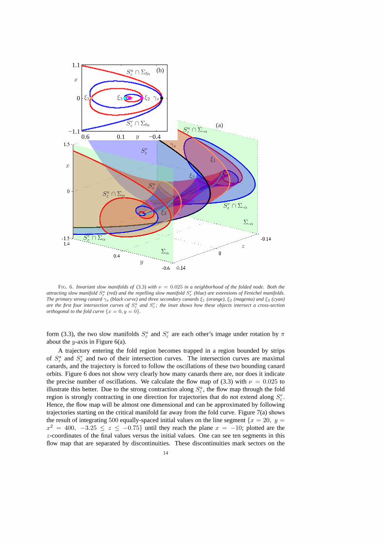
canards, and the trajectory is forced to follow the oscillations of these two bounding canardorbits. Figure 6 does not show very clearly how many canards there are, nor does it indicatethe precise number of oscillations. We calculate the flow map of (3.3) withν = 0.025 toillustrate this better. Due to the strong contraction alongSa

ε , the flow map through the foldregion is strongly contracting in one direction for trajectories that do not extend alongSr

ε .Hence, the flow map will be almost one dimensional and can be approximated by followingtrajectories starting on the critical manifold far away from the fold curve. Figure 7(a) showsthe result of integrating500 equally-spaced initial values on the line segment{x = 20, y =x2 = 400, −3.25 ≤ z ≤ −0.75} until they reach the planex = −10; plotted are thez-coordinates of the final values versus the initial values. One can see ten segments in thisflow map that are separated by discontinuities. These discontinuities mark sectors on the

14

−1 0 1−0.4

0.3

1

−1 0 1−0.4

0.3

1

−1 0 1−0.4

0.3

1

−1 0 1−0.4

0.3

1

−3.5 −2.5 −1.5 −0.50

0.45

0.9

1.35

zin

zout

���(b1)

���

(b2)

���

(b3)

���

(b4)

I0I1I2

I3I4

I5

I6I7

I8

I9

(a)

x

yI2 (b1)

x

yI5 (b2)

x

yI7 (b3)

x

yI9 (b4)

.

.

FIG. 7. Numerical study of the number of rotational sectors for system(3.3) with ν = 0.025. Panel (a)illustrates the flow map through the folded node by plotting thez-coordinatesz out of the first return to a cross-sectionx = −10 of 500 trajectories with equally-spaced initial values(x, y, z) = (20, 400, z in), where−3.25 ≤z in ≤ −0.75. Panels (b1)–(b4) show four trajectories projected onto the(x, y)-plane that correspond to the pointslabeled in panel (c), wherez in = −1.25 in panel (b1),z in = −1.5 in panel (b2),z in = −2 in panel (b3), andz in = −2.25 in panel (b4).

line segment{x = 20, y = x2 = 400, −3.25 ≤ z ≤ −0.75} that correspond to anincreasing number of SAOs; in fact, each segment corresponds to a two-dimensional sectorIi, 0 ≤ i ≤ 9, on the attracting sheetSa

ε of the slow manifold. The outer sectorI0 on the rightin Figure 7(a) is bounded on the left by the primary strong canardγs; sectorI1 is boundedby γs and the first maximal secondary canardξ1; sectorsIi, i = 2, . . . , 8, are bounded bymaximal secondary canard orbitsξi−1 andξi; and the last (left outer) sectorI9 is boundedon the right byξ8. On one side of the primary strong canardγs and each maximal secondarycanardξi, 1 ≤ i ≤ 8, trajectories follow the repelling slow manifoldSr

ε and then jump withdecreasing values ofx. On the other side ofγs andξi, trajectories jump back to the attractingslow manifold and make one more oscillation through the folded node region before flowingtowardx = −∞. The four panels (b1)–(b4) in Figure 7 show portions of four trajectoriesprojected onto the(x, y)-plane; their initial values are(x, y, z) = (20, 400, z in) with z in asmarked in panel (a), that is,z in = −1.25, z in = −1.5, z in = −2 andz in = −2.25 for(b1)–(b4), respectively. The trajectory in panel (b1) was chosen from the sectorI2, boundedby ξ1 andξ2; this trajectory makes two oscillations. The trajectory in panel (b2) comes fromI5 and, indeed, it makes five oscillations. The other two trajectories, in panel (b3) and (b4),make seven and nine oscillations, respectively, but some of these oscillations are too small tobe visible.

The actual widths of the rotational sectors in Figure 7 are very similar due to theε-dependent rescaling used to obtain (3.3). When the equations depend onε as in (3.1) and(3.2), however, the widths of the sectors depend onε. In fact, every sector is very smallexcept for the sector corresponding to maximal rotation, which is bounded byξk and the foldcurve. For an asymptotic analysis of the widths of the rotational sectors that organize the

15

Γc

γsγw

Sr

F

Sa

δ

•

•

y1

x

y2

.

.

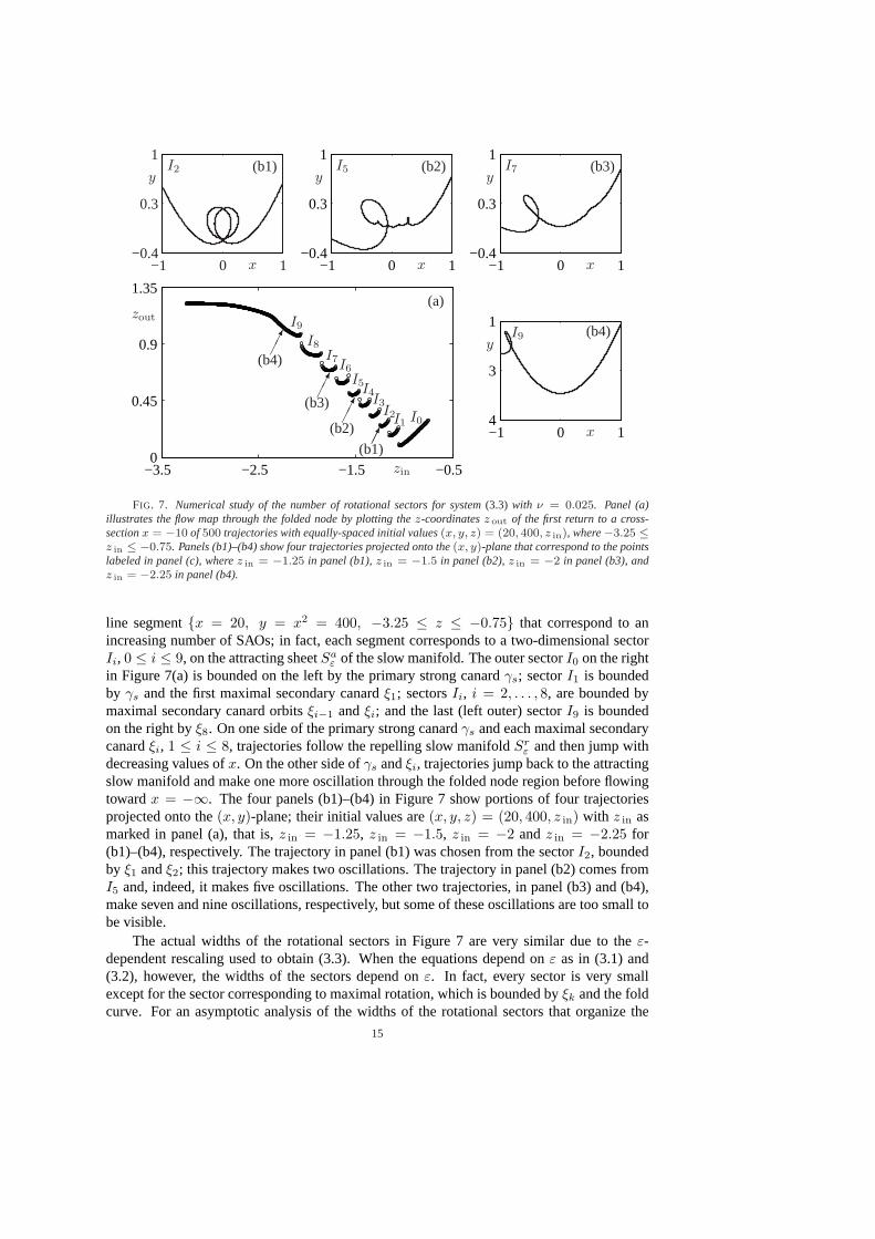
FIG. 8. Schematic diagram of the candidate periodic orbitΓc that gives rise to MMOs with SAOs produced bya folded node singularity. The candidateΓc approaches the folded node along the attracting sheetSa (red) of thecritical manifold (red) in the sector of maximal rotation associated with the weak singular canardγw. The distanceto the strong singular canardγs is labeledδ. When the trajectory reaches the folded node (filled circle) it jumpsalong a layer and proceeds to make a global return.

oscillations, system (3.2) is more convenient, because the eigenvalues of the desingularizedslow flow are−µ and−1. Brøns, Krupa and Wechselberger [31] found the following.

THEOREM 3.1. Consider system(2.14) and assume it has a folded node singularity.At an O(1)-distance from the fold curve, all secondary canards are in anO(ε(1−µ)/2)-neighborhood of the primary strong canard. Hence, the widths of the rotational sectorsIi,1 ≤ i ≤ k, is O(ε(1−µ)/2) and the width of sectorIk+1 is O(1).

Note that, asµ → 0 (the folded saddle-node limit), the number of rotational sectorsincreases indefinitely, and the upper bounds on their widths decrease toO(ε1/2).

3.1.1. Folded node with a global return mechanism.A global return mechanism mayreinject trajectories to the folded node funnel to create an MMO. Assuming that the returnhappensO(1) away from the fold curve, Theorem 3.1 predicts the number of SAOs thatfollow. We create a candidate trajectory by following the fast flow starting at the foldednode until it returns to the folded node region; this is sketched in Figure 8. The globalreturn mechanism produces one LAO. Letδ denote the distance of the global return pointof a trajectory from the singular strong canardγs measured on a cross-section at a distanceO(1) away from the fold; we use the convention thatδ > 0 indicates a return into the funnelregion. Providedδ is large enough, so that the global return point lands in the sectorIk+1 ofmaximal rotation, one can show the existence of astableMMO with signature1k+1, wherek is determined byµ [31]. We summarize this existence result (in a more general setting) inthe following theorem.

THEOREM 3.2 (Generic1k+1 MMOs). Consider system(2.14)with the following as-sumptions:

(A0) Assume that0 < ε ¿ 1 is sufficiently small,ε1/2 ¿ µ and k ∈ N is such that2k + 1 < µ−1 < 2k + 3.

(A1) The critical manifoldS is (locally) a folded surface.

16

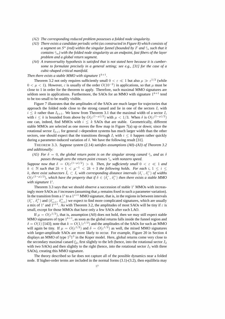
(A2) The corresponding reduced problem possesses a folded node singularity.(A3) There exists a candidate periodic orbit (as constructed in Figure 8) which consists of

a segment onSa (red) within the singular funnel (bounded byF and γs such that itcontainsγw) with the folded node singularity as an endpoint, fast fibers of the layerproblem and a global return segment.

(A4) A transversality hypothesis is satisfied that is not stated here because it is cumber-some to formulate precisely in a general setting; see e.g., [31] for the case of acubic-shaped critical manifold.

Then there exists a stable MMO with signature1k+1.Theorem 3.2 not only requires sufficiently small0 < ε ¿ 1 but alsoµ À ε1/2 (while

0 < µ < 1). However,ε is usually of the orderO(10−2) in applications, so thatµ must beclose to 1 in order for the theorem to apply. Therefore, such maximal MMO signatures areseldom seen in applications. Furthermore, the SAOs for an MMO with signature1k+1 tendto be too small to be readily visible.

Figure 7 illustrates that the amplitudes of the SAOs are much larger for trajectories thatapproach the folded node close to the strong canard and lie in one of the sectorsIi withi ≤ k rather thanIk+1. We know from Theorem 3.1 that the maximal width of a sectorIi

with i ≤ k is bounded from above byO(ε(1−µ)/2) with µ < 1/3. Whenδ is O(ε(1−µ)/2)one can, indeed, find MMOs withi ≤ k SAOs that are stable. Geometrically, differentstable MMOs are selected as one moves the flow map in Figure 7(a) up or down; since therotational sectorIk+1 for generalε-dependent systems has much larger width than the othersectors, one should expect that the transitions throughIi with i ≤ k happen rather quicklyduring a parameter-induced variation ofδ. We have the following result [31].

THEOREM 3.3. Suppose system(2.14)satisfies assumptions (A0)–(A3) of Theorem 3.2and additionally:

(A5) For δ = 0, the global return point is on the singular strong canardγs and asδpasses through zero the return point crossesγs with nonzero speed.

Suppose now thatδ = O(ε(1−µ)/2) > 0. Then, for sufficiently small0 < ε ¿ 1 andk ∈ N such that2k + 1 < µ−1 < 2k + 3 the following holds. For eachi, 1 ≤ i ≤k, there exist subsectorsIi ⊂ Ii with corresponding distance intervals(δ−i , δ+

i ) of widthsO(ε(1−µ)/2), which have the property that ifδ ∈ (δ−i , δ+

i ) then there exists a stable MMOwith signature1i.

Theorem 3.3 says that we should observe a succession of stable1i MMOs with increas-ingly more SAOs asδ increases (assuming thatµ remains fixed in such a parameter variation).In the transition from a1i to a1i+1 MMO signature, that is, in the regions in between intervals(δ−i , δ+

i ) and(δ−i+1, δ+i+1) we expect to find more complicated signatures, which are usually

a mix of 1i and1i+1. As with Theorem 3.2, the amplitudes of most SAOs will be tiny ifε issmall, except for those MMOs that have only a few SAOs after each LAO.

If µ = O(ε1/2), that is, assumption (A0) does not hold, then we may still expect stableMMO signatures of type1k+1, as soon as the global returns falls inside the funnel region andδ = O(1) [143]; note thatk = O(1/ε1/2) and the amplitudes of the SAOs for such an MMOwill again be tiny. Ifµ = O(ε1/2) andδ = O(ε1/2) as well, the mixed MMO signatureswith larger-amplitude SAOs are more likely to occur. For example, Figure 20 in Section 4displays an MMO of type1213 in the Koper model. Here, global returns come very close tothe secondary maximal canardξ2, first slightly to the left (hence, into the rotational sectorI2

with two SAOs) and then slightly to the right (hence, into the rotational sectorI3 with threeSAOs), creating this MMO signature.

The theory described so far does not capture all of the possible dynamics near a foldednode. If higher-order terms are included in the normal forms (3.1)-(3.2), then equilibria may

17

appear in anO(ε1/2) neighborhood of the folded node as soon asµ = O(ε1/2) or smaller.This observation motivates our study of the singular Hopf bifurcation in three dimensions.

3.2. MMOs due to a singular Hopf bifurcation. Equilibria of a slow-fast system (2.1)always satisfyf(x, y, λ, ε) = 0; generically, they are located in regions where the associatedcritical manifoldS is normally hyperbolic. However, in generic one-parameter families ofslow-fast systems, the equilibrium may cross a fold ofS. In generic families with two slowvariables, the fold point (including the specific parameter value) at which the equilibriumcrosses the fold curve of the critical manifold has been called afolded saddle-node of typeII [161]. Folded nodes and saddles of the reduced system are not projections of equilibria ofthe full slow-fast system, but the folded saddle-nodes of type II are. Whenε > 0, the systemhas a singular Hopf bifurcation, which occurs generically at a distanceO(ε) in parameterspace from the folded saddle-node of type II [85].

In order to obtain a normal form for the singular Hopf bifurcation, we follow [85] andadd higher-order terms to the normal form (3.1) of the folded node, to obtain

ε x = y − x2,y = z − x,z = −ν − a x− b y − c z.

(3.4)

As with (3.1), we apply the standard scaling [212]x = ε1/2 x, y = ε y, z = ε1/2 z, andt = ε1/2 t; system (3.4) then becomes

x′ = y − x2,y′ = z − x,

z′ = −ν − ε1/2 a x− ε b y − ε1/2 c z.

(3.5)

This scaled vector field provides anO(ε1/2)-zoom of the neighborhood of the folded sin-gularity where SAOs are expected to occur. The scaling removesε from the first equationswhile the coefficientsa, b andc of the third equation becomeε-dependent;ν remains fixed.Note that the coefficient ofy tends to0 faster than those ofx, z asε → 0. This feature makesthe definition of normal forms for slow-fast systems somewhat problematic: scalings of thestate-space variables and the singular perturbation parameterε interact with each other. Theseε-dependent scalings play an important role in “blow-up” analysis of fold points and foldedsingularities.

In contrast to the normal form (3.1) of a folded node, system (3.5) possesses equilibriafor all values ofν. If ν = O(1) then these equilibria are far from the origin, with coordinatesthat areO(ε−1/2) or larger. Since we want to study the dynamics near a folded singularity,theε-dependent terms in (3.5) play little role in this parameter regime and the system can beregarded as an inconsequential perturbation of the folded node normal form (3.3) and Theor-ems 3.2 and 3.3 apply. On the other hand, ifν = O(ε1/2) or smaller then one equilibriumlies within anO(1)-size domain of the phase space. This equilibrium is determined by thecoefficientsa andc (to leading order) and plays an important role in the local dynamics near afolded singularity [85, 143]. In particular, the equilibrium undergoes a singular Hopf bifurca-tion for ν = O(ε) [85]. Thus, for parameter valuesν = O(ε1/2) or smaller, the higher-orderterms in the third equation of (3.5) are crucial.

So what is the most appropriate normal form of a system that undergoes a singular Hopfbifurcation? Several groups have derived system (3.4), but drop the termby because it hashigher order inε after the scaling. However, this term appears in the formula for the lowest-order term inε of the first Lyapunov coefficient of the Hopf bifurcation of (3.4) and, hence,

18

−0.020.10.22−1

−0.3

0.4

y

x

zSa

Sr

SaSa

Γ

¡¡¡µ

(a)

y

x

S

Γ

XXXz (b)

.

.

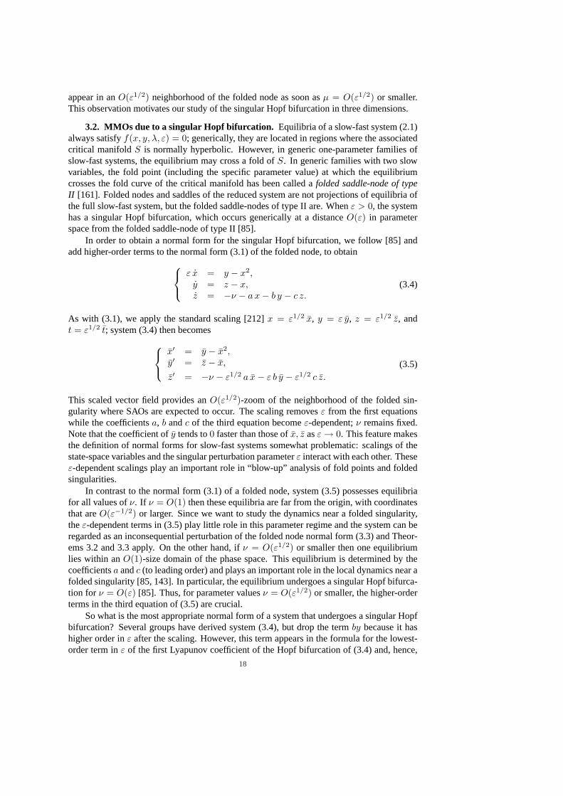
FIG. 9. Phase portrait of an MMO periodic orbitΓ (black curve) for system(3.6) with (ν, a, b, c, ε) =(0.0072168,−0.3872,−0.3251, 1.17, 0.01). The critical manifoldS (grey) is the S-shaped surface with folds atx = 0 andx = − 2

3. The orbitΓ is composed of two slow segments near the two attracting sheets ofS and two fast

segments, with SAOs in the region near the equilibriump on the repelling sheetSr of S just past the fold atx = 0.Panel (a) shows a three-dimensional view and panel (b) the projection onto the(x, y)-plane.

must be retained if we hope to determine a complete unfolding of the singular Hopf bifurca-tion [85].

The MMOs that occur close to the singular Hopf bifurcation have a somewhat dif-ferent character than those generated via the folded node mechanism. Guckenheimer andWillms [93] observed that a subcritical (ordinary) Hopf bifurcation may result in large regionsof the parameter space being funneled into a small neighborhood of a saddle equilibrium withunstable complex eigenvalues. After trajectories come close to the equilibrium, SAOs growin magnitude as the trajectory spirals away from the equilibrium. Similar MMOs may passnear a singular Hopf bifurcation. Then the equilibrium is a saddle-focus and trajectories onthe attracting Fenichel manifold are funneled into a region close to the one-dimensional stablemanifold of the equilibrium. SAOs occur as the trajectory spirals away from the equilibrium.We review here our incomplete understanding of singular Hopf bifurcations and the MMOspassing nearby.

The normal form (3.4) does not yield MMOs because there is no global return mech-anism; trajectories that leave the vicinity of the equilibrium point and the fold curve flow toinfinity in finite time. This property can be changed by adding a cubic term to the normalform that makes the critical manifold S-shaped, similar to the Van der Pol equation:

ε x = y − x2 − x3,y = z − x,z = −ν − a x− b y − c z.

(3.6)

This version of the normal form for singular Hopf bifurcation with global reinjection has been

19

−0.8 −0.2 0.40

0.1

0.2

100 150 200−0.9

−0.2

0.5

t

x

(a)

x

y

(b)

.

.

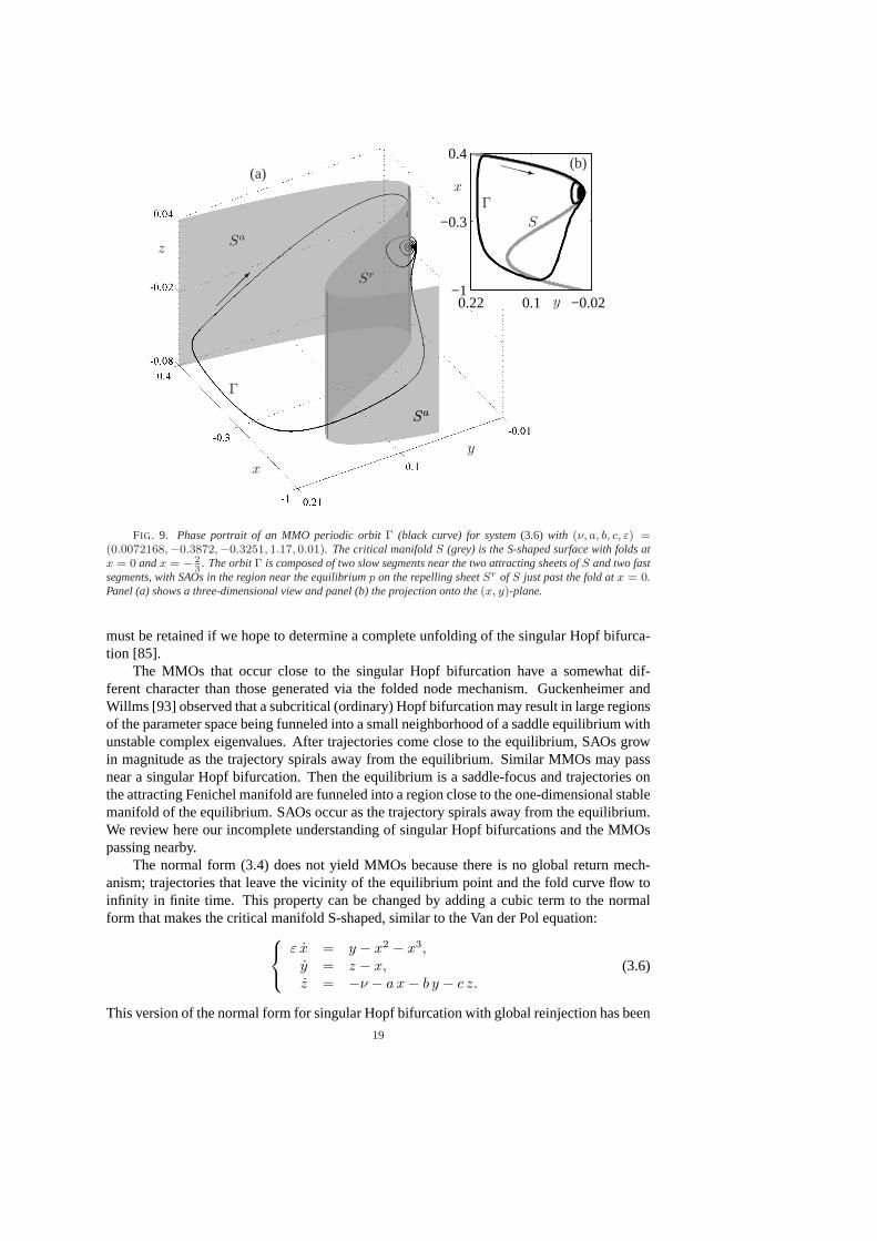
FIG. 10. A chaotic MMO trajectory of system (3.6) with (ν, a, b, c, ε) =(0.004564,−0.2317, 0.2053, 1.17, 0.01). Panel (a) shows the time series of thex-coordinate of the tra-jectory fromt = 100 to t = 200, and panel (b) the projection of the trajectory onto the(x, y)-plane.

derived repeatedly as a “reduced” model for MMOs [122, 138]. An example of the overallstructure of MMOs in system (3.6) with smallν is shown in Figure 9 for(ν, a, b, c, ε) =(0.0072168,−0.3872,−0.3251, 1.17, 0.01); note thatν = O(ε). The S-shaped critical man-ifold S is the grey surface in Figure 9(a); a top view is shown in panel (b). The manifoldS hastwo fold curves, one atx = 0 and one atx = − 2

3 , that decomposeS into one repelling andtwo attracting sheets. For our choice of parameters there exists a saddle-focus equilibriumpon the repelling sheet that is close to the origin (which is the folded node singularity). Theequilibriump has a pair of unstable complex conjugate eigenvalues. A stable MMO periodicorbit Γ, shown as the black curve in Figure 9, interacts withp as follows. Starting just pastthe fold atx = 0, that is, in the region near the origin withx < 0, the orbitΓ spirals awayfrom p along its two-dimensional unstable manifold and repeatedly intersects the repellingsheetSr of S. As soon asΓ intersects the repelling slow manifold (not shown), it jumps tothe attracting sheet ofS with x < − 2

3 . The orbitΓ then follows this sheet to the fold atx = − 2

3 , after which it jumps to the attracting sheet ofS with x > 0. ThenΓ returns to theneighborhood ofp and the periodic motion repeats.

The MMO periodic orbitΓ displayed in Figure 9 is only one of many types of complexdynamics present in system (3.6). One aspect of the complex dynamics in system (3.6) isthe fate of the periodic orbits created in the Hopf bifurcation. There are parameter regimesfor (3.6) with stable periodic orbits of small amplitude created by a supercritical Hopf bi-furcation. Subsequent bifurcations of these periodic orbits may be period-doubling or torusbifurcations [85]. Period-doubling cascades can give rise to small-amplitude chaotic invariantsets that may be associated with chaotic MMOs. For example, Figure 10 plots a chaotic MMOtrajectory for (3.6) with(ν, a, b, c, ε) = (0.004564,−0.2317, 0.2053, 1.17, 0.01) that arisesfrom such a period-doubling cascade of the periodic orbit emerging from the singular Hopfbifurcation. It appears that it is chaotic because of the nonperiodicity of its time series, shownfor the x-coordinate in Figure 10(a). A two-dimensional projection onto the(x, y)-planeis shown in panel (b). Note that this trajectory does not come close to either the equilibriumpointp or the folded singularity at the origin. Asν decreases from the value used in Figure 10(whereν is already of orderO(ε)), the large-amplitude epochs of the trajectories become lessfrequent and soon disappear, resulting in a small-amplitude chaotic attractor. Section 4 dis-cusses a rescaled subfamily of (3.6), giving further examples of complex dynamics and someanalysis of the organization of MMOs associated with this system.

We would like to characterize the parameter regimes with MMOs for which the SAOs

20

y

x

z

Wu(p)

Sr

ε

Σ

(a)

Wu

Sr

ε

Σ

(b)

.

.

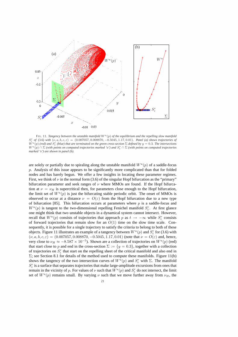
FIG. 11. Tangency between the unstable manifoldW u(p) of the equilibrium and the repelling slow manifoldSr

ε of (3.6) with (ν, a, b, c, ε) = (0.007057, 0.008870,−0.5045, 1.17, 0.01). Panel (a) shows trajectories ofW u(p) (red) andSr

ε (blue) that are terminated on the green cross-sectionΣ defined byy = 0.3. The intersectionsW u(p) ∩ Σ (with points on computed trajectories marked ’o’) andSr

ε ∩ Σ (with points on computed trajectoriesmarked ’x’) are shown in panel (b).

are solely or partially due to spiraling along the unstable manifoldWu(p) of a saddle-focusp. Analysis of this issue appears to be significantly more complicated than that for foldednodes and has barely begun. We offer a few insights in locating these parameter regimes.First, we think ofν in the normal form (3.6) of the singular Hopf bifurcation as the “primary”bifurcation parameter and seek ranges ofν where MMOs are found. If the Hopf bifurca-tion at ν = νH is supercritical then, for parameters close enough to the Hopf bifurcation,the limit set ofWu(p) is just the bifurcating stable periodic orbit. The onset of MMOs isobserved to occur at a distanceν = O(ε) from the Hopf bifurcation due to a new typeof bifurcation [85]. This bifurcation occurs at parameters wherep is a saddle-focus andWu(p) is tangent to the two-dimensional repelling Fenichel manifoldSr

ε . At first glanceone might think that two unstable objects in a dynamical system cannot intersect. However,recall thatWu(p) consists of trajectories that approachp as t → −∞ while Sr

ε consistsof forward trajectories that remain slow for anO(1) time on the slow time scale. Con-sequently, it is possible for a single trajectory to satisfy the criteria to belong to both of theseobjects. Figure 11 illustrates an example of a tangency betweenWu(p) andSr

ε for (3.6) with(ν, a, b, c, ε) = (0.007057, 0.008870,−0.5045, 1.17, 0.01) (note thatν = O(ε) and, hence,very close toνH ≈ −8.587 × 10−5). Shown are a collection of trajectories onWu(p) (red)that start close top and end in the cross-sectionΣ := {y = 0.3}, together with a collectionof trajectories onSr

ε that start on the repelling sheet of the critical manifold and also end inΣ; see Section 8.1 for details of the method used to compute these manifolds. Figure 11(b)shows the tangency of the two intersection curves ofWu(p) andSr

ε with Σ. The manifoldSr

ε is a surface that separates trajectories that make large-amplitude excursions from ones thatremain in the vicinity ofp. For values ofν such thatWu(p) andSr

ε do not intersect, the limitset ofWu(p) remains small. By varyingν such that we move further away fromνH , the

21

MMOs arise as soon asWu(p) andSrε begin to intersect; see also Section 4.

The number of SAOs that an MMO periodic orbitΓ makes alongWu(p) is determinedby how closeΓ comes top and by the ratio of real to imaginary parts of the complex eigen-values ofp. The only way to approachp is along its stable manifoldW s(p), so an MMOlike that displayed in Figure 9 must come very close toW s(p). The minimum distancedbetween an MMO andW s(p) is analogous to the distanceδ of a trajectory from the primarystrong canard in the case of folded nodes. Unlike the case of a folded node, the maximalamplitude of the SAOs observed nearWu(p) is largely independent ofd. What does changeasd → 0 is that the epoch of SAOs increases in length and begins with oscillations that aretoo small to be detectable. There has been little investigation of how the parameters of thenormal form (3.6) influenced, but Figure 8 in Guckenheimer [85] illustrates thatd dependsupon the parameterc in a complex manner. There are parameter regions where the globalreturns of MMO trajectories are funneled close toW s(p). Since MMOs are not found im-mediately adjacent to supercritical Hopf bifurcations, the ratio of real to imaginary parts ofthe complex eigenvalues remains bounded away from0 on MMO trajectories. This preventsthe appearance of extraordinarily long transients with oscillations that grow arbitrarily slowlylike those found near a subcritical Hopf bifurcation; see Section 5 and also [87, Figure 5].

The singular-Hopf and folded-node mechanisms for creating SAOs are not mutually ex-clusive and can be present in a single MMO in the transition regime withν = O(ε1/2). Thespecific behavior that one finds depends in part on whether the equilibriump near the singularHopf bifurcation is a saddle-focus with a pair of complex eigenvalues or a saddle with tworeal eigenvalues. The MMO displayed in Figure 21 contains some SAOs that lie inside therotational sectors between the attracting and repelling slow manifolds and some SAOs thatfollow the unstable manifold of the saddle-focus equilibrium. On the other hand, we notethat SAOs cannot be associated with a saddle equilibrium that has only real eigenvalues; thisoccurs in a parameter region withν > (a + c)ε1/2 (to leading order), butν = O(ε1/2).In this case, SAOs are solely associated with the folded node-type mechanism described forν = O(1) (that is,µ = O(1)). Krupa and Wechselberger [143] analyzed the transition regimeν = O(ε1/2) and showed that the folded node theory can be extended into this parameter re-gime provided the global return mechanism projects into the funnel region.

3.3. MMOs in three-time-scale systems.When the coefficientsν, a, b and c in thenormal forms (3.4) and (3.6) of the singular Hopf bifurcation are of orderO(ε) or smaller,thenz evolves slowly relative toy and the system actually has three time scales: fast, slowand super slow. Krupa et al. [138] studied this regime with geometric methods and asymptoticexpansions for the casea = c = 0. They observed MMOs for which the amplitudes of theSAOs remain relatively large. Their analysis is based upon rescaling the system such that ithas two fast variables and one slow variable. To make the three-time-scale structure explicit,we setν = εν, a = εa, b = εb andc = εc. Rescaling the singular-Hopf normal form (3.6) ofSection 3.2 byx = ε1/2 x, y = ε y, z = ε1/2 z, andt = ε1/2 t yields

x = y − x2 − ε1/2x3,y = z − x,

z = ε(−ν − ε1/2 a x− ε b y − ε1/2 c z),(3.7)

which is still a singularly perturbed system, but now with two fast variables,x andy, and aslow variablez. An equilibrium lies within anO(1)-size domain around the origin ifν =O(ε1/2) or smaller, i.e.,ν = O(ε3/2) or smaller. This equilibrium plays an important role inthe dynamics if it is of saddle-focus type. In particular, it undergoes a Hopf bifurcation forν = O(ε), i.e.,ν = O(ε2).

22

10x0−10

y

−4

8

2

(a)

10x0−10

y

−4

8

2

(b)

100−10 x

y

−4

2

10 (c)

•

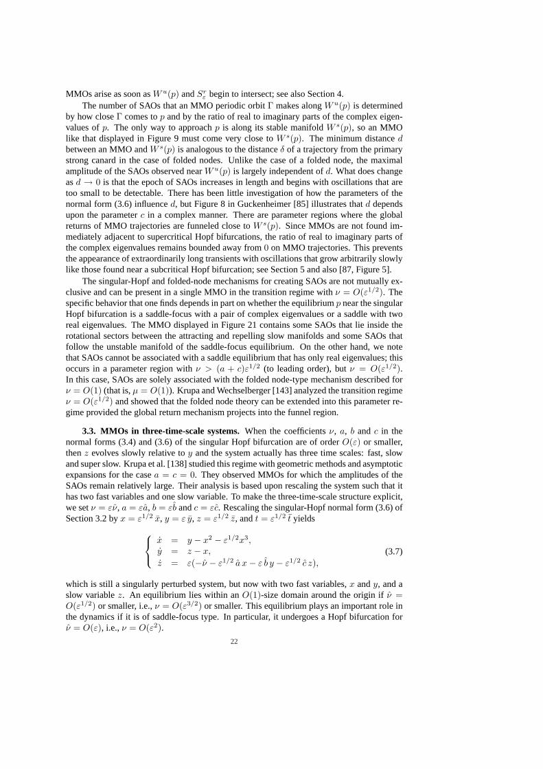
FIG. 12. Phase portraits of system(3.8) for three different values ofz. Shown are several trajectories (blue)and one trajectory (red) that approximates a separatrix. For eachz, there is a single equilibrium pointp at (x, y) =(z, z2). Panels (a)–(c) are forz = 2, z = 0.25 and z = 0, for whichp is a stable node, a stable focus and acenter surrounded by a continuous family of periodic orbits, respectively. The boundary of this family is the maximalcanard.

The two-dimensional layer problem of (3.7)

x = y − x2,y = z − x,z = 0,

(3.8)

in which z acts as a parameter, is exactly the same system obtained in the analysis of theplanar canard problem, where the parameterλ is replaced byz; compare with system (2.7).

Note that (3.8) has a unique equilibriump for each value ofz, given by(x, y) = (z, z2).Figure 12 shows phase portraits of (3.8) in the(x, y)-plane for three different values ofz,namelyz = 2, z = 0.25 andz = 0 in panels (a), (b) and (c), respectively. Forz > 0,the equilibriump is an attracting fixed point in the(x, y)-plane; it is a node forz > 1 anda focus for0 < z < 1; note that this information also determines the type of equilibriumof (3.7) obtained forν = O(ε1/2) to leading order — the same argument can also be usedto determine the basin boundary of the saddle-focus equilibrium in Section 3.2. The basinboundary ofp is an unbounded trajectory that is shown in red in panels (a) and (b). Whenz = 0, the vector field (3.8) has a time-reversing symmetry that induces the existence ofa family of periodic orbits. Indeed, the functionH(x, y) = exp(−2y) (y − x2 + 1

2 ) is anintegral of the motion and the level curveH = 0 is a parabola that separates periodic orbitssurroundingp (the origin) from unbounded orbits that lie below the parabola and becomeunbounded withx → ±∞ in finite time.

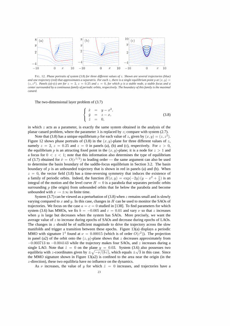
System (3.7) can be viewed as a perturbation of (3.8) whenz remains small and is slowlyvarying compared tox andy. In this case, changes inH can be used to monitor the SAOs oftrajectories. We focus on the casea = c = 0 studied in [138]. To find parameters for whichsystem (3.6) has MMOs, we fixb = −0.005 andε = 0.01 and varyν so thatz increaseswhen y is large but decreases when the system has SAOs. More precisely, we want theaverage value ofz to increase during epochs of SAOs and decrease during epochs of LAOs.The changes inz should be of sufficient magnitude to drive the trajectory across the slowmanifolds and trigger a transition between these epochs. Figure 13(a) displays a periodicMMO with signature14 found atν = 0.00015 (which is of orderO(ε2)). The projectionin panel (a2) of the orbit onto the(z, y)-plane shows thatz decreases approximately from−0.003713 to −0.004143 while the trajectory makes four SAOs, andz increases during asingle LAO. Note thatz = 0 on the planey = 0.03. System (3.6) also possesses twoequilibria withz-coordinates given by±

√−ν/(b ε), which equals±√3 in this case. Since

the MMO signature shown in Figure 13(a2) is confined to the area near the origin (in thez-direction), these two equilibria have no influence on the dynamics.

As ν increases, the value ofy for which z = 0 increases, and trajectories have a

23

250 275 300−0.95

−0.2

0.55

−0.0046 −0.00405 −0.0035−0.02

0.1

0.22

250 275 300−0.95

−0.2

0.55

−0.0046 −0.00405 −0.0035−0.02

0.1

0.22

t

x

(b1)

t

x

(a1)

z

y

91

(b2)

z

y 14

(a2)

.

.

FIG. 13. Stable periodic MMOs of system(3.6) with (a, b, c, ε) = (0,−0.005, 0, 0.01). Row (a) shows theperiodic MMO with signature14 for ν = 0.00015 as a time series ofx in panel (a1) and in projection onto the(z, y)-plane in panel (a2); similar projections are shown in row (b) forν = 0.00032, where the periodic MMO hassignature91.

propensity to pass more quickly through the region of SAOs. Figure 13(b) shows a peri-odic MMO with signature91 obtained forν = 0.00032. This value ofν lies close to theupper end of the range in which MMOs seem to exist for the chosen values of(a, b, c, ε) =(0,−0.005, 0, 0.01). As the projection in panel (b2) illustrates, the average value ofz in-creases (|z| decreases) during each LAO, but it takes nine LAOs before it crosses the thresholdinto the region of SAOs. On the other hand, a single SAO takes the trajectory back to the re-gion of LAOs.

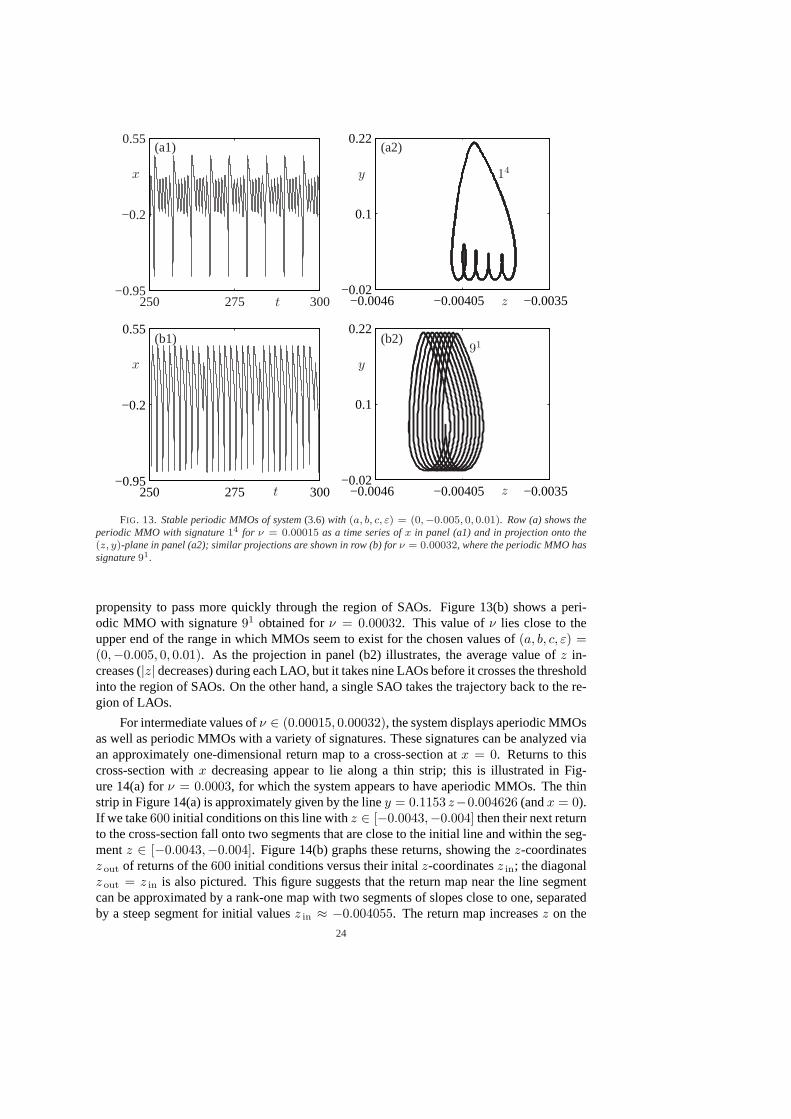
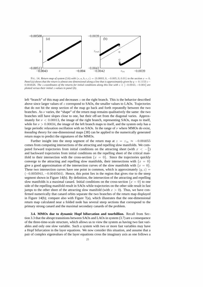
For intermediate values ofν ∈ (0.00015, 0.00032), the system displays aperiodic MMOsas well as periodic MMOs with a variety of signatures. These signatures can be analyzed viaan approximately one-dimensional return map to a cross-section atx = 0. Returns to thiscross-section withx decreasing appear to lie along a thin strip; this is illustrated in Fig-ure 14(a) forν = 0.0003, for which the system appears to have aperiodic MMOs. The thinstrip in Figure 14(a) is approximately given by the liney = 0.1153 z−0.004626 (andx = 0).If we take600 initial conditions on this line withz ∈ [−0.0043,−0.004] then their next returnto the cross-section fall onto two segments that are close to the initial line and within the seg-mentz ∈ [−0.0043,−0.004]. Figure 14(b) graphs these returns, showing thez-coordinatesz out of returns of the600 initial conditions versus their initalz-coordinatesz in; the diagonalz out = z in is also pictured. This figure suggests that the return map near the line segmentcan be approximated by a rank-one map with two segments of slopes close to one, separatedby a steep segment for initial valuesz in ≈ −0.004055. The return map increasesz on the

24

−0.0042 −0.0039−0.0043

−0.0039

−0.0043 −0.004−0.00513

−0.00508

zin

zout

(a)

z

y

(b)

.

.

FIG. 14. Return map of system(3.6)with (ν, a, b, c, ε) = (0.0003, 0,−0.005, 0, 0.01) to the sectionx = 0.Panel (a) shows that the return is almost one dimensional along a line that is approximately given byy = 0.1153 z−0.004626. Thez-coordinates of the returns for initial conditions along this line withz ∈ [−0.0043,−0.004] areplotted versus their initialz-values in panel (b).

left “branch” of this map and decreasesz on the right branch. This is the behavior describedabove since larger values ofz correspond to SAOs, the smaller values to LAOs. Trajectoriesthat do not hit the steep section of the map go back and forth repeatedly between the twobranches. Asν varies, the “shape” of the return map remains qualitatively the same: the twobranches still have slopes close to one, but their off-set from the diagonal varies. Approx-imately forν < 0.00013, the image of the right branch, representing SAOs, maps to itself,while for ν > 0.00034, the image of the left branch maps to itself, and the system only has alarge periodic relaxation oscillation with no SAOs. In the range ofν where MMOs do exist,kneading theoryfor one-dimensional maps [38] can be applied to the numerically generatedreturn maps to predict the signatures of the MMOs.

Further insight into the steep segment of the return map atz = z in ≈ −0.004055comes from computing intersections of the attracting and repelling slow manifolds. We com-puted forward trajectories from initial conditions on the attracting sheet (withx < − 2

3 )and backward trajectories from initial conditions on the repelling sheet of the critical man-ifold to their intersection with the cross-section{x = 0}. Since the trajectories quicklyconverge to the attracting and repelling slow manifolds, their intersections with{x = 0}give a good approximation of the intersection curves of the slow manifolds with{x = 0}.These two intersection curves have one point in common, which is approximately(y, z) =(−0.0050941,−0.0040564). Hence, this point lies in the region that gives rise to the steepsegment shown in Figure 14(b). By definition, the intersection of the attracting and repellingslow manifolds is a maximal canard. Initial conditions on the cross-section{x = 0} to oneside of the repelling manifold result in SAOs while trajectories on the other side result in fastjumps to the other sheet of the attracting slow manifold (withx > 0). Thus, we have con-firmed numerically that canard orbits separate the two branches of the return map displayedin Figure 14(b); compare also with Figure 7(a), which illustrates that the one-dimensionalreturn map calculated near a folded node has several steep sections that correspond to theprimary strong canard and the maximal secondary canards of the problem.

3.4. MMOs due to dynamic Hopf bifurcation and tourbillion. Recall from Sec-tion 3.3 that the abrupt transitions between SAOs and LAOs in system (3.7) are a consequenceof the three-time-scale structure, which allows us to view the system as having two fast vari-ables and only one slow variable. Such a system with two or more fast variables may havea Hopf bifurcation in the layer equations. We now consider this situation, and assume that apair of complex eigenvalues of the layer equations cross the imaginary axis as one follows a

25

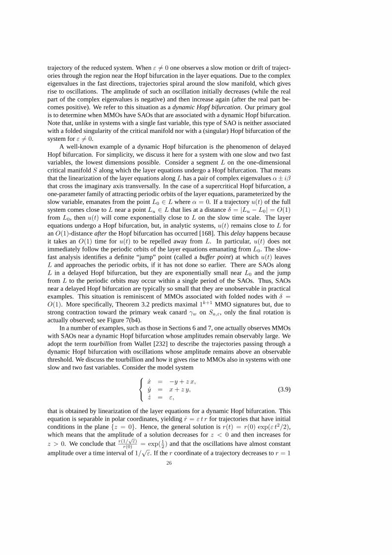
trajectory of the reduced system. Whenε 6= 0 one observes a slow motion or drift of traject-ories through the region near the Hopf bifurcation in the layer equations. Due to the complexeigenvalues in the fast directions, trajectories spiral around the slow manifold, which givesrise to oscillations. The amplitude of such an oscillation initially decreases (while the realpart of the complex eigenvalues is negative) and then increase again (after the real part be-comes positive). We refer to this situation as adynamic Hopf bifurcation. Our primary goalis to determine when MMOs have SAOs that are associated with a dynamic Hopf bifurcation.Note that, unlike in systems with a single fast variable, this type of SAO is neither associatedwith a folded singularity of the critical manifold nor with a (singular) Hopf bifurcation of thesystem forε 6= 0.

A well-known example of a dynamic Hopf bifurcation is the phenomenon of delayedHopf bifurcation. For simplicity, we discuss it here for a system with one slow and two fastvariables, the lowest dimensions possible. Consider a segmentL on the one-dimensionalcritical manifoldS along which the layer equations undergo a Hopf bifurcation. That meansthat the linearization of the layer equations alongL has a pair of complex eigenvaluesα± iβthat cross the imaginary axis transversally. In the case of a supercritical Hopf bifurcation, aone-parameter family of attracting periodic orbits of the layer equations, parameterized by theslow variable, emanates from the pointL0 ∈ L whereα = 0. If a trajectoryu(t) of the fullsystem comes close toL near a pointLu ∈ L that lies at a distanceδ = |Lu − L0| = O(1)from L0, thenu(t) will come exponentially close toL on the slow time scale. The layerequations undergo a Hopf bifurcation, but, in analytic systems,u(t) remains close toL foranO(1)-distanceafter the Hopf bifurcation has occurred [168]. Thisdelayhappens becauseit takes anO(1) time for u(t) to be repelled away fromL. In particular,u(t) does notimmediately follow the periodic orbits of the layer equations emanating fromL0. The slow-fast analysis identifies a definite “jump” point (called abuffer point) at whichu(t) leavesL and approaches the periodic orbits, if it has not done so earlier. There are SAOs alongL in a delayed Hopf bifurcation, but they are exponentially small nearL0 and the jumpfrom L to the periodic orbits may occur within a single period of the SAOs. Thus, SAOsnear a delayed Hopf bifurcation are typically so small that they are unobservable in practicalexamples. This situation is reminiscent of MMOs associated with folded nodes withδ =O(1). More specifically, Theorem 3.2 predicts maximal1k+1 MMO signatures but, due tostrong contraction toward the primary weak canardγw on Sa,ε, only the final rotation isactually observed; see Figure 7(b4).

In a number of examples, such as those in Sections 6 and 7, one actually observes MMOswith SAOs near a dynamic Hopf bifurcation whose amplitudes remain observably large. Weadopt the termtourbillion from Wallet [232] to describe the trajectories passing through adynamic Hopf bifurcation with oscillations whose amplitude remains above an observablethreshold. We discuss the tourbillion and how it gives rise to MMOs also in systems with oneslow and two fast variables. Consider the model system

x = −y + z x,y = x + z y,z = ε,

(3.9)

that is obtained by linearization of the layer equations for a dynamic Hopf bifurcation. Thisequation is separable in polar coordinates, yieldingr = ε t r for trajectories that have initialconditions in the plane{z = 0}. Hence, the general solution isr(t) = r(0) exp(ε t2/2),which means that the amplitude of a solution decreases forz < 0 and then increases forz > 0. We conclude thatr(1/

√ε)

r(0) = exp( 12 ) and that the oscillations have almost constant

amplitude over a time interval of1/√

ε. If the r coordinate of a trajectory decreases tor = 126

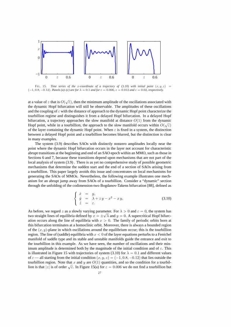
0 0.6−1

0

1

0 0.6 0 0.6z

x

z z

.

.

FIG. 15. Time series of thex-coordinate of a trajectory of(3.10) with initial point (x, y, z) =(−1, 0.8,−0.12). Panels (a)–(c) are forλ = 0.1 and forε = 0.006, ε = 0.012 andε = 0.02, respectively.

at a value ofz that isO(√

ε), then the minimum amplitude of the oscillations associated withthe dynamic Hopf bifurcation will still be observable. The amplitudes of these oscillationsand the coupling ofε with the distance of approach to the dynamic Hopf point characterize thetourbillion regime and distinguishes it from a delayed Hopf bifurcation. In a delayed Hopfbifurcation, a trajectory approaches the slow manifold at distanceO(1) from the dynamicHopf point, while in a tourbillion, the approach to the slow manifold occurs withinO(

√ε)

of the layer containing the dynamic Hopf point. Whenε is fixed in a system, the distinctionbetween a delayed Hopf point and a tourbillion becomes blurred, but the distinction is clearin many examples.

The system (3.9) describes SAOs with distinctly nonzero amplitudes locally near thepoint where the dynamic Hopf bifurcation occurs in the layer not account for characteristicabrupt transitions at the beginning and end of an SAO epoch within an MMO, such as those inSections 6 and 7, because these transitions depend upon mechanisms that are not part of thelocal analysis of system (3.9) . There is as yet no comprehensive study of possible geometricmechanisms that determine the sudden start and the end of a section of SAOs arising froma tourbillion. This paper largely avoids this issue and concentrates on local mechanisms forgenerating the SAOs of MMOs. Nevertheless, the following example illustrates one mech-anism for an abrupt jump away from SAOs of a tourbillion. Consider a “dynamic” sectionthrough the unfolding of the codimension-two Bogdanov-Takens bifurcation [88], defined as

x = y,y = λ + z y − x2 − x y,z = ε.

(3.10)

As before, we regardz as a slowly varying parameter. Forλ > 0 andε = 0, the system hastwo straight lines of equilibria defined byx = ±

√λ andy = 0. A supercritical Hopf bifurc-

ation occurs along the line of equilibria withx > 0. The family of periodic orbits born atthis bifurcation terminates at a homoclinic orbit. Moreover, there is always a bounded regionof the(x, y)-plane in which oscillations around the equilibrium occur; this is the tourbillionregion. The line of (saddle) equilibria withx < 0 of the layer equations perturbs to a Fenichelmanifold of saddle type and its stable and unstable manifolds guide the entrance and exit tothe tourbillion in this example. As we have seen, the number of oscillations and their min-imum amplitude is determined both by the magnitude of the initial condition and ofε. Thisis illustrated in Figure 15 with trajectories of system (3.10) forλ = 0.1 and different valuesof ε — all starting from the initial condition(x, y, z) = (−1, 0.8,−0.12) that lies outside thetourbillion region. Note thatx andy areO(1) quantities, and so the condition for a tourbil-lion is that|z| is of order

√ε. In Figure 15(a) forε = 0.006 we do not find a tourbillion but

27

observe oscillations that decay rapidly, are very small for a while and then grow rapidly againbefore the trajectory jumps away. In panel (b) forε = 0.012, on the other hand, the oscil-lations decay and then grow more gradually and they remain of observable size throughout.We conclude thatε is now just about large enough to speak of a tourbillion region, passagethrough which results in seven SAOs before the jump occurs. For even larger values ofε thesame initial condition results in oscillations that maintain an almost constant amplitiude; seeFigure 15(c) forε = 0.02. Observe that, owing to the faster drift through the region near theHopf bifurcation in the layer system, we now find only four SAOs before the trajectory jumpsaway.

It is interesting to compare the SAOs associated with a tourbillion with those occurringnear a folded node or near a singular Hopf bifurcation. One difference is that the period of theoscillations isO(ε) (slow time) for the tourbillion, while it isO(

√ε) for the other two cases.

In each of the cases, the data that determines the number of SAOs is slightly different. Forthe folded node, the eigenvalue rationµ determines the number of rotational sectors, and thedistance of the global return to the weak canard relative to the singular perturbation parameterdetermines which rotational sector a trajectory enters. For the singular Hopf bifurcation, thedistance of the global return to the stable manifold of the saddle-focus equilibrium sets theminimum amplitude and duration of the SAOs. For a tourbillion, the number of SAOs isgoverned by the singular perturbation parameter and the distance of the global return to thedelayed Hopf bifurcation point. Moreover, the termination of the SAOs for a tourbilliondepends upon either a global mechanism or an arbitrary threshold for the amplitude of SAOs.In contrast, the oscillations of a folded node end “on their own,” while the intersections ofthe unstable manifold of the equilibrium and the repelling slow manifold typically limit theamplitude of SAOs near a singular Hopf bifurcation.

3.5. Summary of local mechanisms for SAOs.We now summarize the main resultsof this review section on the local mechanisms that give rise to MMOs. For systems with asingle fast variable, the local mechanisms responsible for SAOs must involve a mixture of thetwo time scales. We distinguish three regions near folded nodes and folded saddle-nodes thatyield MMOs:

1. Folded Nodes:If the parameters satisfy suitable order conditions (ν = O(1)) sothat no equilibrium of the full system is near the folded node then the theory ofSection 3.1 applies and SAOs are due to thetwisting of slow manifolds.

2. Singular Hopf:As is shown in the Section 3.2, the dynamics near a singular Hopf bi-furcation (ν = O(ε)) tends to be quite complicated. SAOs occur when the trajectoryfollows theunstable manifold of a saddle-focus.

3. Transition Regime:The folded-node and singular-Hopf regimes are separated by atransition regime with intermediate values ofν = O(

√ε). Extensions of the folded

node theory have been developed in [143]; note that the parameterµ in [143] notonly represents the eigenvalue ratio but also describes the distance of the equilibriumto the folded node in a blown-up system. In this transition regime, it is possible forthe SAOs to pass through the rotational sectors of the folded nodeas well asspiralalong the unstable manifold of the saddle-focus equilibrium.

In systems with at least two fast variables the tourbillion provides a different local mech-anism that generates SAOs. Here, the layer equations have complex eigenvalues and theSAOs are aligned with the fast directions of the system. Little systematic study of the tour-billion as a mechanism that generates MMOs has been carried out, and the theory remainsfragmentary.

Finally, three-dimensional systems with three time scales can exhibit all of the mech-anisms discussed in this section. Namely a three-time-scale system may be considered as

28

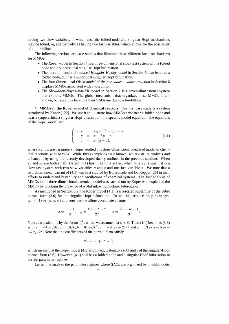
having two slow variables, in which case the folded-node and singular-Hopf mechanismsmay be found, or, alternatively, as having two fast variables, which allows for the possibilityof a tourbillion.

The following sections are case studies that illustrate these different local mechanismsfor MMOs:

• TheKoper modelin Section 4 is a three-dimensional slow-fast system with a foldednode and a supercritical singular Hopf bifurcation.

• The three-dimensionalreduced Hodgkin–Huxley modelin Section 5 also features afolded node, but has a subcritical singular Hopf bifurcation.

• The four-dimensionalOlsen model of the peroxidase-oxidase reactionin Section 6displays MMOs associated with a tourbillion.

• The Showalter–Noyes–Bar-Eli modelin Section 7 is a seven-dimensional systemthat exhibits MMOs. The global mechanism that organizes these MMOs is un-known, but we show here that their SAOs are due to a tourbillion.

4. MMOs in the Koper model of chemical reactors. Our first case study is a systemintroduced by Koper [122]. We use it to illustrate how MMOs arise near a folded node andnear a (supercritical) singular Hopf bifurcation in a specific model equation. The equationsof the Koper model are

ε1 x = k y − x3 + 3 x− λ,y = x− 2 y + z,z = ε2 (y − z),

(4.1)

whereλ andk are parameters. Koper studied this three-dimensional idealized model of chem-ical reactions with MMOs. While this example is well known, we revisit its analysis andenhance it by using the recently developed theory outlined in the previous sections. Whenε1 andε2 are both small, system (4.1) has three time scales; when onlyε1 is small, it is aslow-fast system with two slow variablesy andz and one fast variablex. We note that atwo-dimensional variant of (4.1) was first studied by Boissonade and De Kepper [26] in theirefforts to understand bistability and oscillations of chemical systems. The first analysis ofMMOs in the three-dimensional extended model was carried out by Koper who explained theMMOs by invoking the presence of a Shil′nikov homoclinic bifurcation.

As mentioned in Section 3.2, the Koper model (4.1) is a rescaled subfamily of the cubicnormal form (3.6) for the singular Hopf bifurcation. To see this, replace(x, y, z) in sys-tem (4.1) by(u, v, w) and consider the affine coordinate change

x =u− 1

3, y =

k v − λ + 227

, z =2 v − w − 1

3.

Now also scale time by the factor−k9 , where we assume thatk < 0. Then (4.1) becomes (3.6)

with ε = −k ε1/81, a = 18/k, b = 81 ε2/k2, c = −9 (ε2 + 2)/k andν = (3 ε2 λ − 6 ε2 −3 k ε2/k2. Note that the coefficients of the normal form satisfy

2 b− a c + a2 = 0,

which means that the Koper model (4.1) is only equivalent to a subfamily of the singular-Hopfnormal form (3.6). However, (4.1) still has a folded node and a singular Hopf bifurcation incertain parameter regimes.

Let us first analyze the parameter regimes where SAOs are organized by a folded node.

29

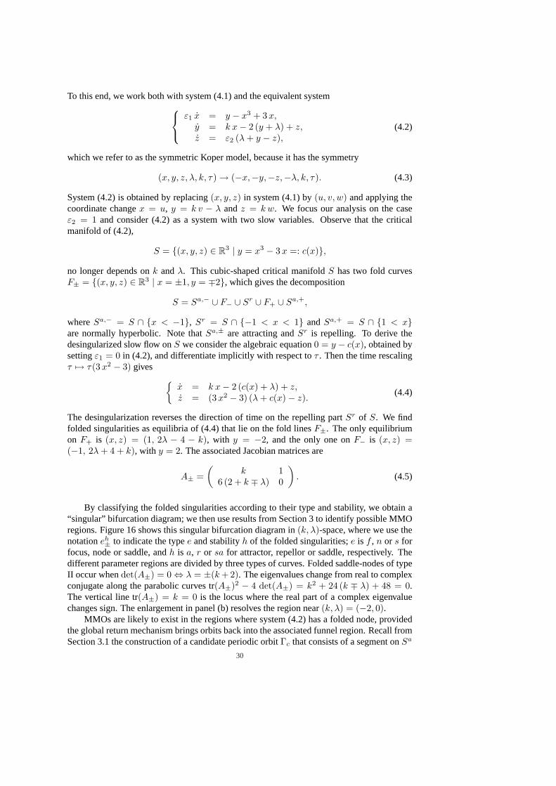
To this end, we work both with system (4.1) and the equivalent system

ε1 x = y − x3 + 3 x,y = k x− 2 (y + λ) + z,z = ε2 (λ + y − z),

(4.2)

which we refer to as the symmetric Koper model, because it has the symmetry

(x, y, z, λ, k, τ) → (−x,−y,−z,−λ, k, τ). (4.3)

System (4.2) is obtained by replacing(x, y, z) in system (4.1) by(u, v, w) and applying thecoordinate changex = u, y = k v − λ andz = k w. We focus our analysis on the caseε2 = 1 and consider (4.2) as a system with two slow variables. Observe that the criticalmanifold of (4.2),

S = {(x, y, z) ∈ R3 | y = x3 − 3 x =: c(x)},

no longer depends onk andλ. This cubic-shaped critical manifoldS has two fold curvesF± = {(x, y, z) ∈ R3 | x = ±1, y = ∓2}, which gives the decomposition

S = Sa,− ∪ F− ∪ Sr ∪ F+ ∪ Sa,+,

whereSa,− = S ∩ {x < −1}, Sr = S ∩ {−1 < x < 1} andSa,+ = S ∩ {1 < x}are normally hyperbolic. Note thatSa,± are attracting andSr is repelling. To derive thedesingularized slow flow onS we consider the algebraic equation0 = y − c(x), obtained bysettingε1 = 0 in (4.2), and differentiate implicitly with respect toτ . Then the time rescalingτ 7→ τ(3x2 − 3) gives

{x = k x− 2 (c(x) + λ) + z,z = (3 x2 − 3) (λ + c(x)− z). (4.4)

The desingularization reverses the direction of time on the repelling partSr of S. We findfolded singularities as equilibria of (4.4) that lie on the fold linesF±. The only equilibriumon F+ is (x, z) = (1, 2λ − 4 − k), with y = −2, and the only one onF− is (x, z) =(−1, 2λ + 4 + k), with y = 2. The associated Jacobian matrices are

A± =(

k 16 (2 + k ∓ λ) 0

). (4.5)

By classifying the folded singularities according to their type and stability, we obtain a“singular” bifurcation diagram; we then use results from Section 3 to identify possible MMOregions. Figure 16 shows this singular bifurcation diagram in(k, λ)-space, where we use thenotationeh

± to indicate the typee and stabilityh of the folded singularities;e is f , n or s forfocus, node or saddle, andh is a, r or sa for attractor, repellor or saddle, respectively. Thedifferent parameter regions are divided by three types of curves. Folded saddle-nodes of typeII occur whendet(A±) = 0 ⇔ λ = ±(k + 2). The eigenvalues change from real to complexconjugate along the parabolic curves tr(A±)2 − 4 det(A±) = k2 + 24 (k ∓ λ) + 48 = 0.The vertical line tr(A±) = k = 0 is the locus where the real part of a complex eigenvaluechanges sign. The enlargement in panel (b) resolves the region near(k, λ) = (−2, 0).

MMOs are likely to exist in the regions where system (4.2) has a folded node, providedthe global return mechanism brings orbits back into the associated funnel region. Recall fromSection 3.1 the construction of a candidate periodic orbitΓc that consists of a segment onSa

30

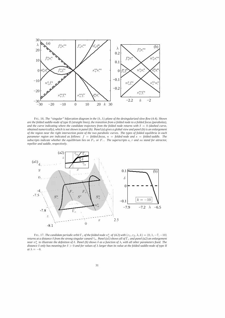
−30 −20 −10 0 10 20 30−30

−20

−10

0

10

20

30

−2.2 −2

−0.2

−0.1

0

0.1

0.2

k

λ (a)

na

+na

-

fa

+na

-

na

+fa

-

fa

+ssa

-

fa

+fa

-

ssa

+fa

-

fr

+ssa

-

ssa

+fr

-

nr

+ssa-

ssa+nr

-

ssa

+ssa

-

k

λ (b)

fa

+fa

-

fa

+na

-

na

+fa

-

fa

+ssa

-

na

+na

-

ssa

+fa

-

na

+ssa

-

ssa

+ na

-

ssa+ssa-

.

.

FIG. 16. The “singular” bifurcation diagram in the(k, λ)-plane of the desingularized slow flow(4.4). Shownare the folded saddle-node of type II (straight lines), the transition from a folded node to a folded focus (parabolas),and the curve indicating where the candidate trajectory from the folded node returns withδ = 0 (dashed curve,obtained numerically), which is not shown in panel (b). Panel (a) gives a global view and panel (b) is an enlargementof the region near the right intersection point of the two parabolic curves. The types of folded equilibria in eachparameter region are indicated as follows:f = folded focus,n = folded node ands = folded saddle. Thesubscripts indicate whether the equilibrium lies onF+ or F−. The superscriptsa, r and sa stand for attractor,repellor and saddle, respectively.

−7.9 −7.2 −6.5

−0.1

0

0.1

δ

γ0

γs

γw

z

x

(a2)

xz

y

F+F−

γ0

C0

(a1)

λ

δ

k = −10

H

(b)

.

.

•na

+

Sa

+SrSa

−

Γc

Γcγw

γs

.

.

FIG. 17. The candidate periodic orbitΓc of the folded nodena+ of (4.2)with (ε1, ε2, λ, k) = (0, 1,−7,−10)

returns at a distanceδ from the strong singular canardγs. Panel (a1) shows all ofΓc and panel (a2) an enlargementnearna

+ to illustrate the definition ofδ. Panel (b) showsδ as a function ofλ, with all other parameters fixed. Thedistanceδ only has meaning forδ > 0 and for values ofλ larger than its value at the folded saddle-node of type IIat λ = −8.

31

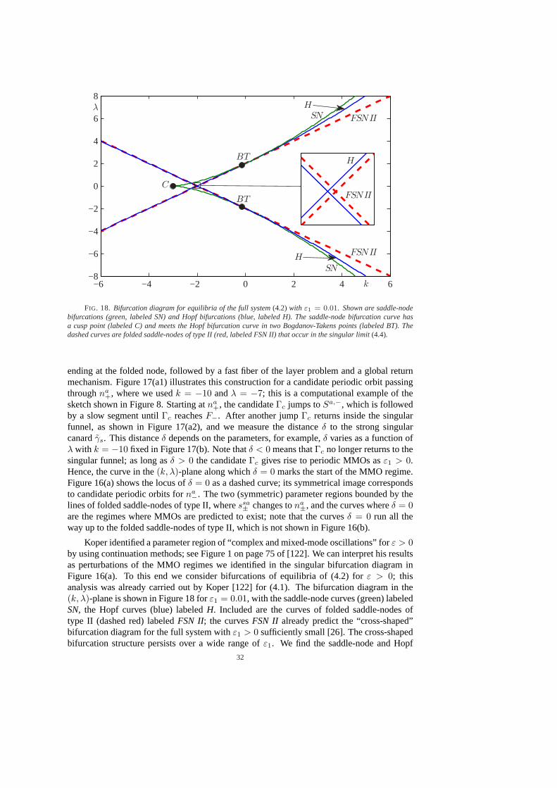
−6 −4 −2 0 2 4 6−8

−6

−4

−2

0

2

4

6

8

k

λ

BT

BT

C

FSNII

H

SN

SN

HFSNII

FSNII

H

.

.

FIG. 18. Bifurcation diagram for equilibria of the full system(4.2) with ε1 = 0.01. Shown are saddle-nodebifurcations (green, labeled SN) and Hopf bifurcations (blue, labeled H). The saddle-node bifurcation curve hasa cusp point (labeled C) and meets the Hopf bifurcation curve in two Bogdanov-Takens points (labeled BT). Thedashed curves are folded saddle-nodes of type II (red, labeled FSN II) that occur in the singular limit(4.4).

ending at the folded node, followed by a fast fiber of the layer problem and a global returnmechanism. Figure 17(a1) illustrates this construction for a candidate periodic orbit passingthroughna

+, where we usedk = −10 andλ = −7; this is a computational example of thesketch shown in Figure 8. Starting atna

+, the candidateΓc jumps toSa,−, which is followedby a slow segment untilΓc reachesF−. After another jumpΓc returns inside the singularfunnel, as shown in Figure 17(a2), and we measure the distanceδ to the strong singularcanardγs. This distanceδ depends on the parameters, for example,δ varies as a function ofλ with k = −10 fixed in Figure 17(b). Note thatδ < 0 means thatΓc no longer returns to thesingular funnel; as long asδ > 0 the candidateΓc gives rise to periodic MMOs asε1 > 0.Hence, the curve in the(k, λ)-plane along whichδ = 0 marks the start of the MMO regime.Figure 16(a) shows the locus ofδ = 0 as a dashed curve; its symmetrical image correspondsto candidate periodic orbits forna

−. The two (symmetric) parameter regions bounded by thelines of folded saddle-nodes of type II, wheressa

± changes tona±, and the curves whereδ = 0

are the regimes where MMOs are predicted to exist; note that the curvesδ = 0 run all theway up to the folded saddle-nodes of type II, which is not shown in Figure 16(b).

Koper identified a parameter region of “complex and mixed-mode oscillations” forε > 0by using continuation methods; see Figure 1 on page 75 of [122]. We can interpret his resultsas perturbations of the MMO regimes we identified in the singular bifurcation diagram inFigure 16(a). To this end we consider bifurcations of equilibria of (4.2) forε > 0; thisanalysis was already carried out by Koper [122] for (4.1). The bifurcation diagram in the(k, λ)-plane is shown in Figure 18 forε1 = 0.01, with the saddle-node curves (green) labeledSN, the Hopf curves (blue) labeledH. Included are the curves of folded saddle-nodes oftype II (dashed red) labeledFSN II; the curvesFSN II already predict the “cross-shaped”bifurcation diagram for the full system withε1 > 0 sufficiently small [26]. The cross-shapedbifurcation structure persists over a wide range ofε1. We find the saddle-node and Hopf

32

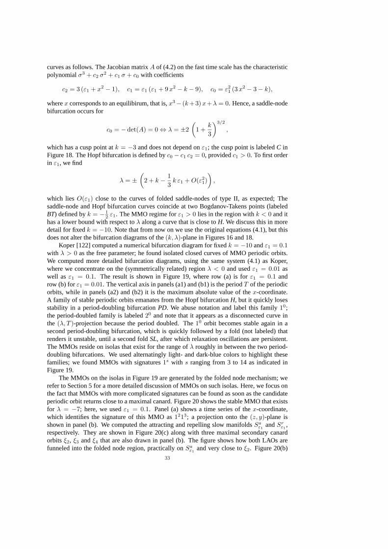
curves as follows. The Jacobian matrixA of (4.2) on the fast time scale has the characteristicpolynomialσ3 + c2 σ2 + c1 σ + c0 with coefficients

c2 = 3 (ε1 + x2 − 1), c1 = ε1 (ε1 + 9 x2 − k − 9), c0 = ε21 (3x2 − 3− k),

wherex corresponds to an equilibirum, that is,x3− (k +3) x+λ = 0. Hence, a saddle-nodebifurcation occurs for

c0 = − det(A) = 0 ⇔ λ = ±2(

1 +k

3

)3/2

,

which has a cusp point atk = −3 and does not depend onε1; the cusp point is labeledC inFigure 18. The Hopf bifurcation is defined byc0 − c1 c2 = 0, providedc1 > 0. To first orderin ε1, we find

λ = ±(

2 + k − 13

k ε1 + O(ε21)

),

which lies O(ε1) close to the curves of folded saddle-nodes of type II, as expected; Thesaddle-node and Hopf bifurcation curves coincide at two Bogdanov-Takens points (labeledBT) defined byk = − 1

2 ε1. The MMO regime forε1 > 0 lies in the region withk < 0 and ithas a lower bound with respect toλ along a curve that is close toH. We discuss this in moredetail for fixedk = −10. Note that from now on we use the original equations (4.1), but thisdoes not alter the bifurcation diagrams of the(k, λ)-plane in Figures 16 and 18.

Koper [122] computed a numerical bifurcation diagram for fixedk = −10 andε1 = 0.1with λ > 0 as the free parameter; he found isolated closed curves of MMO periodic orbits.We computed more detailed bifurcation diagrams, using the same system (4.1) as Koper,where we concentrate on the (symmetrically related) regionλ < 0 and usedε1 = 0.01 aswell as ε1 = 0.1. The result is shown in Figure 19, where row (a) is forε1 = 0.1 androw (b) forε1 = 0.01. The vertical axis in panels (a1) and (b1) is the periodT of the periodicorbits, while in panels (a2) and (b2) it is the maximum absolute value of thex-coordinate.A family of stable periodic orbits emanates from the Hopf bifurcationH, but it quickly losesstability in a period-doubling bifurcationPD. We abuse notation and label this family10;the period-doubled family is labeled20 and note that it appears as a disconnected curve inthe (λ, T )-projection because the period doubled. The10 orbit becomes stable again in asecond period-doubling bifurcation, which is quickly followed by a fold (not labeled) thatrenders it unstable, until a second foldSL, after which relaxation oscillations are persistent.The MMOs reside on isolas that exist for the range ofλ roughly in between the two period-doubling bifurcations. We used alternatingly light- and dark-blue colors to highlight thesefamilies; we found MMOs with signatures1s with s ranging from 3 to 14 as indicated inFigure 19.

The MMOs on the isolas in Figure 19 are generated by the folded node mechanism; werefer to Section 5 for a more detailed discussion of MMOs on such isolas. Here, we focus onthe fact that MMOs with more complicated signatures can be found as soon as the candidateperiodic orbit returns close to a maximal canard. Figure 20 shows the stable MMO that existsfor λ = −7; here, we usedε1 = 0.1. Panel (a) shows a time series of thex-coordinate,which identifies the signature of this MMO as1213; a projection onto the(z, y)-plane isshown in panel (b). We computed the attracting and repelling slow manifoldsSa

ε1andSr

ε1,

respectively. They are shown in Figure 20(c) along with three maximal secondary canardorbits ξ2, ξ3 andξ4 that are also drawn in panel (b). The figure shows how both LAOs arefunneled into the folded node region, practically onSa

ε1and very close toξ2. Figure 20(b)

33

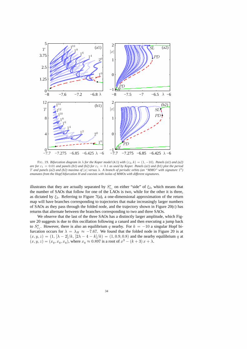
−6−6.425−6.85−7.275−7.70

4

8

12

−6.8−7.2−7.6−80

1.25

2.5

3.75

5

−6−6.425−6.85−7.275−7.7−1

0

1

2

−6−6.5−7−7.5−8−1

0

1

2

T

λ

10

201

2

14

16

18

110

112

114 (b1)

|x|

λ

HPD

PD

SL

(b2)

T

λ

10

20

14

16

18

110 (a1)

|x|

λ

HPD

PD

SL (a2)

.

.

FIG. 19. Bifurcation diagram inλ for the Koper model(4.1) with (ε2, k) = (1,−10). Panels (a1) and (a2)are for ε1 = 0.01 and panels (b1) and (b2) forε1 = 0.1 as used by Koper. Panels (a1) and (b1) plot the periodT and panels (a2) and (b2) maxima of|x| versusλ. A branch of periodic orbits (an “MMO” with signature10)emanates from the Hopf bifurcation H and coexists with isolas of MMOs with different signatures.

illustrates that they are actually separated bySrε1

on either “side” ofξ2, which means thatthe number of SAOs that follow for one of the LAOs is two, while for the other it is three,as dictated byξ3. Referring to Figure 7(a), a one-dimensional approximation of the returnmap will have branches corresponding to trajectories that make increasingly larger numbersof SAOs as they pass through the folded node, and the trajectory shown in Figure 20(c) hasreturns that alternate between the branches corresponding to two and three SAOs.

We observe that the last of the three SAOs has a distinctly larger amplitude, which Fig-ure 20 suggests is due to this oscillation following a canard and then executing a jump backto Sa

ε1. However, there is also an equilibriumq nearby. Fork = −10 a singular Hopf bi-

furcation occurs forλ = λH ≈ −7.67. We found that the folded node in Figure 20 is at(x, y, z) = (1, [λ − 2]/k, [2λ − 4 − k]/k) = (1, 0.9, 0.8) and the nearby equilibriumq at(x, y, z) = (xq, xq, xq), wherexq ≈ 0.897 is a root ofx3 − (k + 3) x + λ.

34

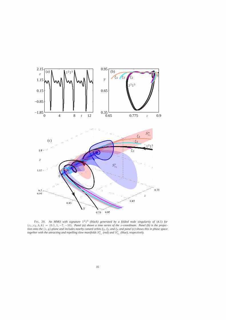
0.65 0.775 0.90.35

0.65

0.95

0 4 8 12−1.85

−0.85

0.15

1.15

2.15

z

y

x

Sr

ε1

Sa

ε1ξ4

ξ3

ξ2

1213

q

(c)

t

x 1213(a)

z

y

1213

ξ2ξ3ξ4q

(b)

.

.

FIG. 20. An MMO with signature1213 (black) generated by a folded node singulartiy of(4.1) for(ε1, ε2, λ, k) = (0.1, 1,−7,−10). Panel (a) shows a time series of thex-coordinate. Panel (b) is the projec-tion onto the(z, y)-plane and includes nearby canard orbitsξ2, ξ3 andξ4 and panel (c) shows this in phase spacetogether with the attracting and repelling slow manifoldsSa

ε1(red) andSr

ε1(blue), respectively.

35

0 15 30 45−1.7

0.3

2.3

−10.2 −10 −9.8−8.4

−7.6

−6.8

zy

xSr

ε

q

(d)

z

y

xSr

ε

Sa

ε

q

116

(c)

t

x116

(a)

k

λ

FSNII

H

Fig. 20(b)

.

.

FIG. 21. An MMO near a singular Hopf bifurcation for(4.1) with (ε1, ε2, λ, k) = (0.1, 1,−7.52,−10).Panel (a) shows the time series of thex-coordinate. The bifurcation diagram in panel (b) illustrates how closethe parameters are to a tangency bifurcation betweenW u(q) and Sr

ε (dashed cyan); the Hopf H (solid blue),folded saddle-node of type II FSN II (dashed red), andδ = 0 (dashed black) curves are shown as well; seealso Figure 16. The slow manifoldsSa

ε and Srε shown in panel (c) guide the MMO toward the equilibrium

q ≈ (0.951, 0.951, 0.951), after whichW u(q) organizes the SAOs. The high compression and twisting ofSrε

nearW u(q) is highlighted in panel (d).

36

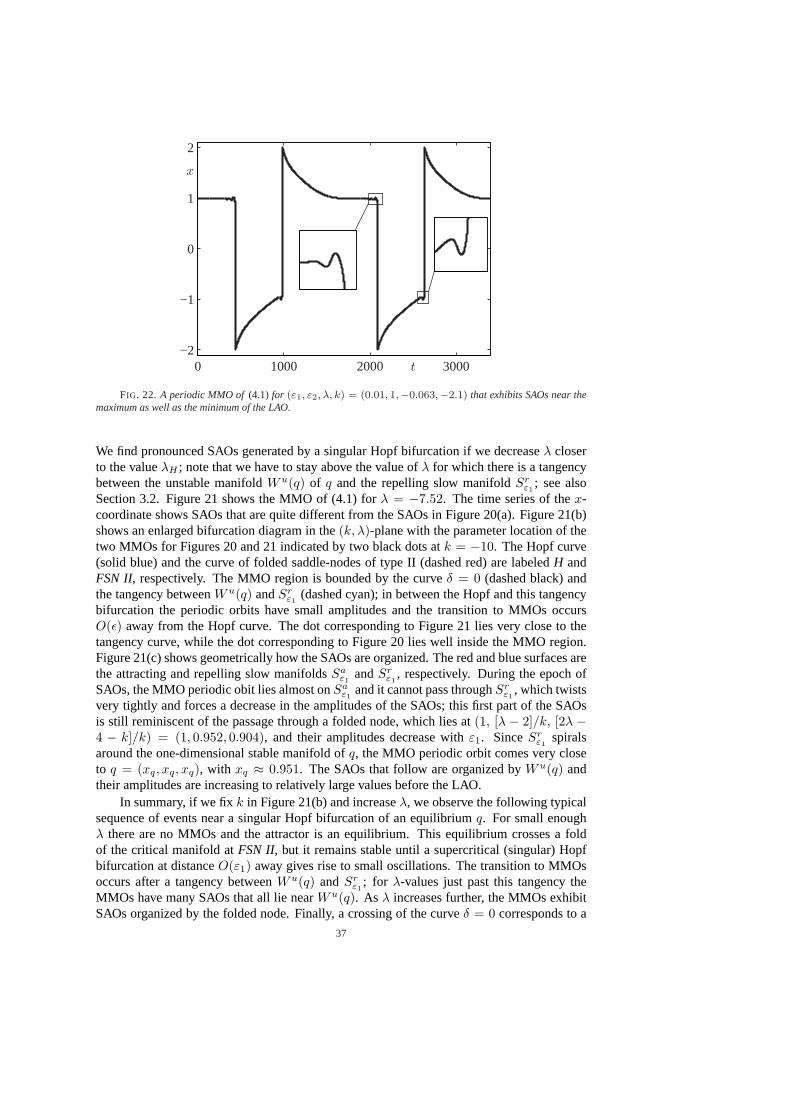
0 1000 2000 3000−2

−1

0

1

2

t

x

.

.

FIG. 22. A periodic MMO of(4.1) for (ε1, ε2, λ, k) = (0.01, 1,−0.063,−2.1) that exhibits SAOs near themaximum as well as the minimum of the LAO.

We find pronounced SAOs generated by a singular Hopf bifurcation if we decreaseλ closerto the valueλH ; note that we have to stay above the value ofλ for which there is a tangencybetween the unstable manifoldWu(q) of q and the repelling slow manifoldSr

ε1; see also

Section 3.2. Figure 21 shows the MMO of (4.1) forλ = −7.52. The time series of thex-coordinate shows SAOs that are quite different from the SAOs in Figure 20(a). Figure 21(b)shows an enlarged bifurcation diagram in the(k, λ)-plane with the parameter location of thetwo MMOs for Figures 20 and 21 indicated by two black dots atk = −10. The Hopf curve(solid blue) and the curve of folded saddle-nodes of type II (dashed red) are labeledH andFSN II, respectively. The MMO region is bounded by the curveδ = 0 (dashed black) andthe tangency betweenWu(q) andSr

ε1(dashed cyan); in between the Hopf and this tangency

bifurcation the periodic orbits have small amplitudes and the transition to MMOs occursO(ε) away from the Hopf curve. The dot corresponding to Figure 21 lies very close to thetangency curve, while the dot corresponding to Figure 20 lies well inside the MMO region.Figure 21(c) shows geometrically how the SAOs are organized. The red and blue surfaces arethe attracting and repelling slow manifoldsSa

ε1andSr

ε1, respectively. During the epoch of

SAOs, the MMO periodic obit lies almost onSaε1

and it cannot pass throughSrε1

, which twistsvery tightly and forces a decrease in the amplitudes of the SAOs; this first part of the SAOsis still reminiscent of the passage through a folded node, which lies at(1, [λ − 2]/k, [2λ −4 − k]/k) = (1, 0.952, 0.904), and their amplitudes decrease withε1. SinceSr

ε1spirals

around the one-dimensional stable manifold ofq, the MMO periodic orbit comes very closeto q = (xq, xq, xq), with xq ≈ 0.951. The SAOs that follow are organized byWu(q) andtheir amplitudes are increasing to relatively large values before the LAO.

In summary, if we fixk in Figure 21(b) and increaseλ, we observe the following typicalsequence of events near a singular Hopf bifurcation of an equilibriumq. For small enoughλ there are no MMOs and the attractor is an equilibrium. This equilibrium crosses a foldof the critical manifold atFSN II, but it remains stable until a supercritical (singular) Hopfbifurcation at distanceO(ε1) away gives rise to small oscillations. The transition to MMOsoccurs after a tangency betweenWu(q) andSr

ε1; for λ-values just past this tangency the

MMOs have many SAOs that all lie nearWu(q). As λ increases further, the MMOs exhibitSAOs organized by the folded node. Finally, a crossing of the curveδ = 0 corresponds to a

37

transition to relaxation oscillations.To end this case study, we report the existence of a different type of MMO not found

by Koper; it is shown in Figure 22. The MMO has SAOs both near the maximum and theminimum of the LAO. Hence, this MMO passes near folded nodesna

± on both fold curves.The parameter region where this occurs is quite small, so that it is difficult to locate such anMMO using simulation; it is the region in Figure 16 neark = −2 that can only be seen inthe enlargement in panel (b). We found the MMO by selecting parametersk = −2.1 andλ = −0.063 in this region and chooseε1 = 0.01 rather small; a more detailed study of therange of parameters for which such MMOs with two SAO epochs remains future work.

5. MMOs in a reduced Hodgkin–Huxley system.As the next case study we considera three-dimensional reduced version of the famous Hodgkin–Huxley equations [102] thatdescribe the generation of action potentials in the squid giant axon; see [115, 196] for thederivation and also [43], where the same example was used. The reduced model only de-scribes the dynamics for voltage (V ), the activation of the potassium channels (n) and theinactivation of the sodium channels (h); the activation of the sodium channels (m) is veryfast and it reaches its equilibrum statem = m∞(V ) (almost) instantaneously which can bejustified mathematically by a center-manifold reduction [196]. The evolution of the gatesnandh is considered slow while the evolution of the voltageV is considered fast. To justifythis time-scale separation, we nondimensionalize the Hodgkin–Huxley equations by introdu-cing a dimensionless voltage variablev = V/kv and a dimensionless timeτ = t/kt wherekv = 100 mV is a reference voltage scale andkt = 1 ms is a fast reference time scale; thisgives

εv = f(v, h, n) := I −m3∞(v)h (v − ENa)

− gk n4 (v − EK)− gl (v − EL),

h = g1(v, h) :=kt

τh

(h∞(v)− h)th(v)

,

n = g2(v, n) :=kt

τn

(n∞(v)− n)tn(v)

,

(5.1)

with dimensionless parametersEx = Ex/kv, gx = gx/gNa, with x ∈ {m, n, h}, I =I/(kvgNa) andε = C/(ktgNa) =: τv/kt. The original Hodgkin–Huxley parameter valuesare given in Table 5.1. Thus,ε = 1

120 ≈ 0.01 ¿ 1 and system (5.1) represents a singularlyperturbed system withv as a fast variable and(n, h) as slow variables. The functionsx∞(v)andtx(v), with x ∈ {m, n, h}, describe the (dimensionless) steady-state values and timeconstants of the gating variables, respectively; they are given by

x∞(v) =αx(v)

αx(v) + βx(v)and tx(v) =

1αx(v) + βx(v)

,

with

αm(v) = (kvv+40)/101−exp(−(kvv+40)/10) , βm(v) = 4 exp(−(kvv + 65)/18),

αh(v) = 0.07 exp(−(kvv + 65)/20), βh(v) = 11+exp(−(kvv+35)/10) ,

αn(v) = (kvv+55)/1001−exp(−(kvv+55)/10) , βn(v) = 0.125 exp(−(kvv + 65)/80).

The orginal Hodgkin–Huxley equations with scaling parametersτh = τn = τm = 1shows no MMOs [102], but ifτh > τh,e > 1 or τn > τn,e > 1 are beyond certain threshold

38

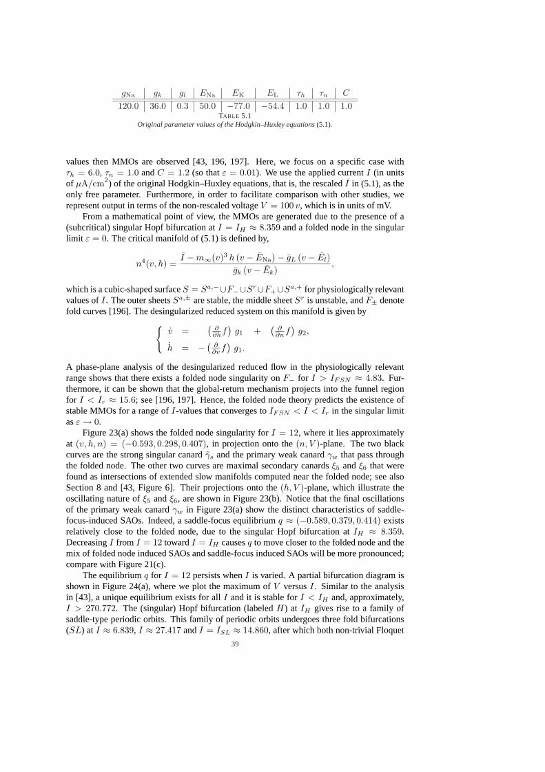
gNa gk gl ENa EK EL τh τn C

120.0 36.0 0.3 50.0 −77.0 −54.4 1.0 1.0 1.0TABLE 5.1

Original parameter values of the Hodgkin–Huxley equations(5.1).

values then MMOs are observed [43, 196, 197]. Here, we focus on a specific case withτh = 6.0, τn = 1.0 andC = 1.2 (so thatε = 0.01). We use the applied currentI (in unitsof µA/cm2) of the original Hodgkin–Huxley equations, that is, the rescaledI in (5.1), as theonly free parameter. Furthermore, in order to facilitate comparison with other studies, werepresent output in terms of the non-rescaled voltageV = 100 v, which is in units of mV.

From a mathematical point of view, the MMOs are generated due to the presence of a(subcritical) singular Hopf bifurcation atI = IH ≈ 8.359 and a folded node in the singularlimit ε = 0. The critical manifold of (5.1) is defined by,

n4(v, h) =I −m∞(v)3 h (v − ENa)− gL (v − El)

gk (v − Ek),

which is a cubic-shaped surfaceS = Sa,−∪F−∪Sr∪F+∪Sa,+ for physiologically relevantvalues ofI. The outer sheetsSa,± are stable, the middle sheetSr is unstable, andF± denotefold curves [196]. The desingularized reduced system on this manifold is given by

{v =

(∂

∂hf)

g1 +(

∂∂nf

)g2,

h = − (∂∂v f

)g1.

A phase-plane analysis of the desingularized reduced flow in the physiologically relevantrange shows that there exists a folded node singularity onF− for I > IFSN ≈ 4.83. Fur-thermore, it can be shown that the global-return mechanism projects into the funnel regionfor I < Ir ≈ 15.6; see [196, 197]. Hence, the folded node theory predicts the existence ofstable MMOs for a range ofI-values that converges toIFSN < I < Ir in the singular limitasε → 0.

Figure 23(a) shows the folded node singularity forI = 12, where it lies approximatelyat (v, h, n) = (−0.593, 0.298, 0.407), in projection onto the(n, V )-plane. The two blackcurves are the strong singular canardγs and the primary weak canardγw that pass throughthe folded node. The other two curves are maximal secondary canardsξ5 andξ6 that werefound as intersections of extended slow manifolds computed near the folded node; see alsoSection 8 and [43, Figure 6]. Their projections onto the(h, V )-plane, which illustrate theoscillating nature ofξ5 andξ6, are shown in Figure 23(b). Notice that the final oscillationsof the primary weak canardγw in Figure 23(a) show the distinct characteristics of saddle-focus-induced SAOs. Indeed, a saddle-focus equilibriumq ≈ (−0.589, 0.379, 0.414) existsrelatively close to the folded node, due to the singular Hopf bifurcation atIH ≈ 8.359.DecreasingI from I = 12 towardI = IH causesq to move closer to the folded node and themix of folded node induced SAOs and saddle-focus induced SAOs will be more pronounced;compare with Figure 21(c).

The equilibriumq for I = 12 persists whenI is varied. A partial bifurcation diagram isshown in Figure 24(a), where we plot the maximum ofV versusI. Similar to the analysisin [43], a unique equilibrium exists for allI and it is stable forI < IH and, approximately,I > 270.772. The (singular) Hopf bifurcation (labeledH) at IH gives rise to a family ofsaddle-type periodic orbits. This family of periodic orbits undergoes three fold bifurcations(SL) at I ≈ 6.839, I ≈ 27.417 andI = ISL ≈ 14.860, after which both non-trivial Floquet

39

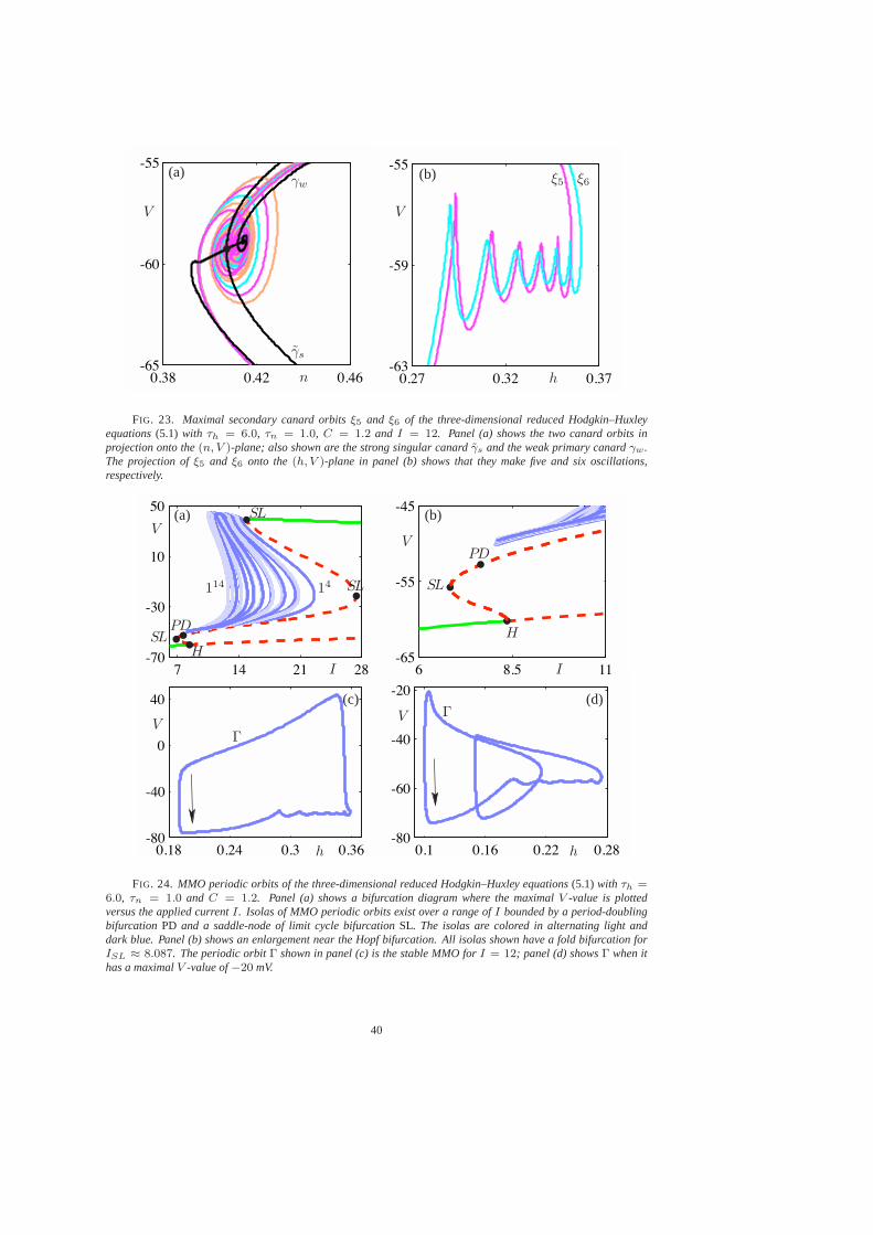
0.38 0.42 0.46 -65

-60

-55

0.27 0.32 0.37 -63

-59

-55

V

n

γs

γw(a)

V

h

ξ5 ξ6(b)

.

.

FIG. 23. Maximal secondary canard orbitsξ5 and ξ6 of the three-dimensional reduced Hodgkin–Huxleyequations(5.1) with τh = 6.0, τn = 1.0, C = 1.2 and I = 12. Panel (a) shows the two canard orbits inprojection onto the(n, V )-plane; also shown are the strong singular canardγs and the weak primary canardγw.The projection ofξ5 and ξ6 onto the(h, V )-plane in panel (b) shows that they make five and six oscillations,respectively.

0.18 0.24 0.3 0.36 -80

-40

0

40

0.1 0.16 0.22 0.28 -80

-60

-40

-20

7 14 21 28 -70

-30

10

50

6 8.5 11 -65

-55

-45

h

VΓ

(c)

h

V Γ

(d)

I

V

14

114

H

SLPD

SL

SL(a)

I

V

H

SL

PD

(b).

.

FIG. 24. MMO periodic orbits of the three-dimensional reduced Hodgkin–Huxley equations(5.1) with τh =6.0, τn = 1.0 and C = 1.2. Panel (a) shows a bifurcation diagram where the maximalV -value is plottedversus the applied currentI. Isolas of MMO periodic orbits exist over a range ofI bounded by a period-doublingbifurcation PD and a saddle-node of limit cycle bifurcationSL. The isolas are colored in alternating light anddark blue. Panel (b) shows an enlargement near the Hopf bifurcation. All isolas shown have a fold bifurcation forISL ≈ 8.087. The periodic orbitΓ shown in panel (c) is the stable MMO forI = 12; panel (d) showsΓ when ithas a maximalV -value of−20 mV.

40

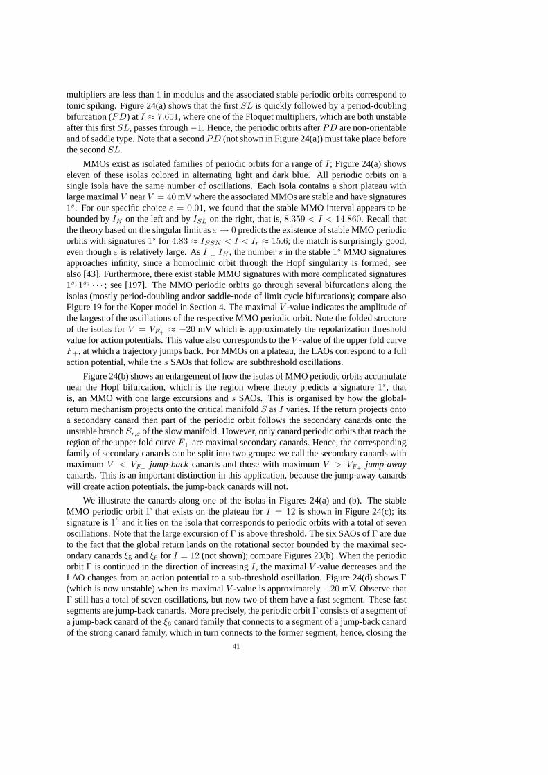
multipliers are less than 1 in modulus and the associated stable periodic orbits correspond totonic spiking. Figure 24(a) shows that the firstSL is quickly followed by a period-doublingbifurcation (PD) atI ≈ 7.651, where one of the Floquet multipliers, which are both unstableafter this firstSL, passes through−1. Hence, the periodic orbits afterPD are non-orientableand of saddle type. Note that a secondPD (not shown in Figure 24(a)) must take place beforethe secondSL.

MMOs exist as isolated families of periodic orbits for a range ofI; Figure 24(a) showseleven of these isolas colored in alternating light and dark blue. All periodic orbits on asingle isola have the same number of oscillations. Each isola contains a short plateau withlarge maximalV nearV = 40 mV where the associated MMOs are stable and have signatures1s. For our specific choiceε = 0.01, we found that the stable MMO interval appears to bebounded byIH on the left and byISL on the right, that is,8.359 < I < 14.860. Recall thatthe theory based on the singular limit asε → 0 predicts the existence of stable MMO periodicorbits with signatures1s for 4.83 ≈ IFSN < I < Ir ≈ 15.6; the match is surprisingly good,even thoughε is relatively large. AsI ↓ IH , the numbers in the stable1s MMO signaturesapproaches infinity, since a homoclinic orbit through the Hopf singularity is formed; seealso [43]. Furthermore, there exist stable MMO signatures with more complicated signatures1s11s2 · · · ; see [197]. The MMO periodic orbits go through several bifurcations along theisolas (mostly period-doubling and/or saddle-node of limit cycle bifurcations); compare alsoFigure 19 for the Koper model in Section 4. The maximalV -value indicates the amplitude ofthe largest of the oscillations of the respective MMO periodic orbit. Note the folded structureof the isolas forV = VF+ ≈ −20 mV which is approximately the repolarization thresholdvalue for action potentials. This value also corresponds to theV -value of the upper fold curveF+, at which a trajectory jumps back. For MMOs on a plateau, the LAOs correspond to a fullaction potential, while thes SAOs that follow are subthreshold oscillations.

Figure 24(b) shows an enlargement of how the isolas of MMO periodic orbits accumulatenear the Hopf bifurcation, which is the region where theory predicts a signature1s, thatis, an MMO with one large excursions ands SAOs. This is organised by how the global-return mechanism projects onto the critical manifoldS asI varies. If the return projects ontoa secondary canard then part of the periodic orbit follows the secondary canards onto theunstable branchSr,ε of the slow manifold. However, only canard periodic orbits that reach theregion of the upper fold curveF+ are maximal secondary canards. Hence, the correspondingfamily of secondary canards can be split into two groups: we call the secondary canards withmaximumV < VF+ jump-backcanards and those with maximumV > VF+ jump-awaycanards. This is an important distinction in this application, because the jump-away canardswill create action potentials, the jump-back canards will not.

We illustrate the canards along one of the isolas in Figures 24(a) and (b). The stableMMO periodic orbitΓ that exists on the plateau forI = 12 is shown in Figure 24(c); itssignature is16 and it lies on the isola that corresponds to periodic orbits with a total of sevenoscillations. Note that the large excursion ofΓ is above threshold. The six SAOs ofΓ are dueto the fact that the global return lands on the rotational sector bounded by the maximal sec-ondary canardsξ5 andξ6 for I = 12 (not shown); compare Figures 23(b). When the periodicorbit Γ is continued in the direction of increasingI, the maximalV -value decreases and theLAO changes from an action potential to a sub-threshold oscillation. Figure 24(d) showsΓ(which is now unstable) when its maximalV -value is approximately−20 mV. Observe thatΓ still has a total of seven oscillations, but now two of them have a fast segment. These fastsegments are jump-back canards. More precisely, the periodic orbitΓ consists of a segment ofa jump-back canard of theξ6 canard family that connects to a segment of a jump-back canardof the strong canard family, which in turn connects to the former segment, hence, closing the

41

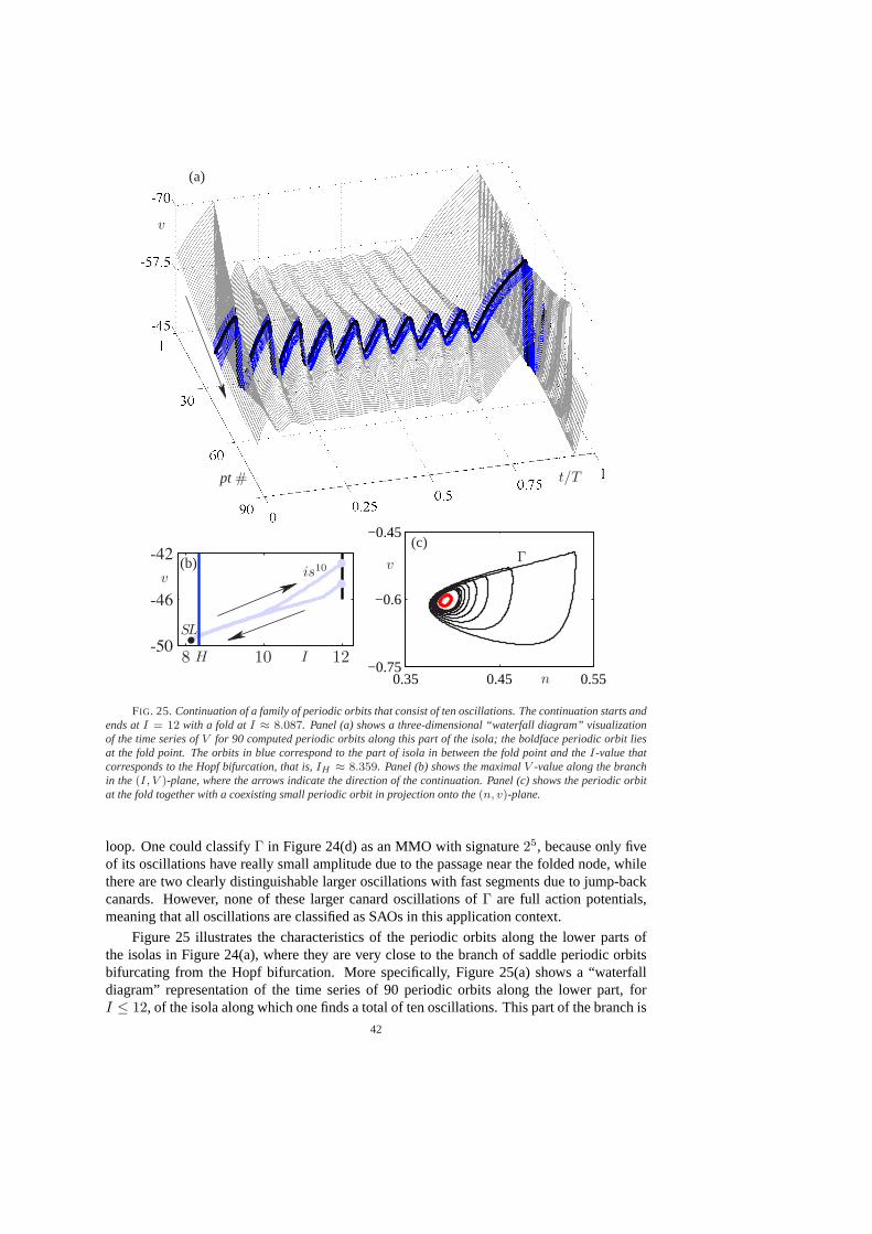
-50

-46

-42

8 10 12

0.35 0.45 0.55−0.75

−0.6

−0.45

I

v is10

•

SL

H

(b)

n

v Γ(c)

t/Tpt #

v

(a)

.

.

FIG. 25. Continuation of a family of periodic orbits that consist of ten oscillations. The continuation starts andends atI = 12 with a fold atI ≈ 8.087. Panel (a) shows a three-dimensional “waterfall diagram” visualizationof the time series ofV for 90 computed periodic orbits along this part of the isola; the boldface periodic orbit liesat the fold point. The orbits in blue correspond to the part of isola in between the fold point and theI-value thatcorresponds to the Hopf bifurcation, that is,IH ≈ 8.359. Panel (b) shows the maximalV -value along the branchin the(I, V )-plane, where the arrows indicate the direction of the continuation. Panel (c) shows the periodic orbitat the fold together with a coexisting small periodic orbit in projection onto the(n, v)-plane.

loop. One could classifyΓ in Figure 24(d) as an MMO with signature25, because only fiveof its oscillations have really small amplitude due to the passage near the folded node, whilethere are two clearly distinguishable larger oscillations with fast segments due to jump-backcanards. However, none of these larger canard oscillations ofΓ are full action potentials,meaning that all oscillations are classified as SAOs in this application context.

Figure 25 illustrates the characteristics of the periodic orbits along the lower parts ofthe isolas in Figure 24(a), where they are very close to the branch of saddle periodic orbitsbifurcating from the Hopf bifurcation. More specifically, Figure 25(a) shows a “waterfalldiagram” representation of the time series of 90 periodic orbits along the lower part, forI ≤ 12, of the isola along which one finds a total of ten oscillations. This part of the branch is

42

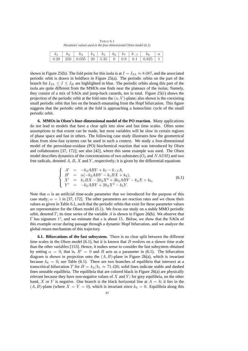
TABLE 6.1Parameter values used in the four-dimensional Olsen model(6.1)

k1 k2 k3 k4 k5 k6 k7 k−7 k8 α0.28 250 0.035 20 5.35 0 0.8 0.1 0.825 1

shown in Figure 25(b). The fold point for this isola is atI = ISL ≈ 8.087, and the associatedperiodic orbit is drawn in boldface in Figure 25(a). The periodic orbits on the part of thebranch forISL ≤ I ≤ IH are highlighted in blue. The periodic orbits along this part of theisola are quite different from the MMOs one finds near the plateaux of the isolas; Namely,they consist of a mix of SAOs and jump-back canards, ten in total. Figure 25(c) shows theprojection of the periodic orbit at the fold onto the(n, V )-plane; also shown is the coexistingsmall periodic orbit that lies on the branch emanating from the Hopf bifurcation. This figuresuggests that the periodic orbit at the fold is approaching a homoclinic cycle of the smallperiodic orbit.

6. MMOs in Olsen’s four-dimensional model of the PO reaction.Many applicationsdo not lead to models that have a clear split into slow and fast time scales. Often someassumptions to that extent can be made, but most variables will be slow in certain regionsof phase space and fast in others. The following case study illustrates how the geometricalideas from slow-fast systems can be used in such a context. We study a four-dimensionalmodel of the peroxidase-oxidase (PO) biochemical reaction that was introduced by Olsenand collaborators [37, 172]; see also [42], where this same example was used. The Olsenmodel describes dynamics of the concentrations of two substrates (O2 andNADH) and twofree radicals, denotedA, B, X andY , respectively; it is given by the differential equations

A′ = −k3ABY + k7 − k−7A,B′ = α(−k3ABY − k1BX + k8),X ′ = k1BX − 2k2X

2 + 3k3ABY − k4X + k6,Y ′ = −k3ABY + 2k2X

2 − k5Y.

(6.1)

Note thatα is an artificial time-scale parameter that we introduced for the purpose of thiscase study;α = 1 in [37, 172]. The other parameters are reaction rates and we chose theirvalues as given in Table 6.1, such that the periodic orbits that exist for these parameter valuesare representative for the Olsen model (6.1). We focus our study on a stable MMO periodicorbit, denotedΓ; its time series of the variableA is shown in Figure 26(b). We observe thatΓ has signature1s, and we estimate thats is about15. Below, we show that the SAOs ofthis example occur during passage through a dynamic Hopf bifurcation, and we analyze theglobal return mechanism of this trajectory.

6.1. Bifurcations of the fast subsystem.There is no clear split between the differenttime scales in the Olsen model (6.1), but it is known thatB evolves on a slower time scalethan the other variables [153]. Hence, it makes sense to consider the fast subsystem obtainedby settingα = 0, that is,B′ = 0 and B acts as a parameter in (6.1). The bifurcationdiagram is shown in projection onto the(A, B)-plane in Figure 26(a), which is invariantbecausek6 = 0; see Table (6.1). There are two branches of equilibria that intersect at atranscritical bifurcationT for B = k4/k1 ≈ 71.426; solid lines indicate stable and dashedlines unstable equilibria. The equilibria that are colored black in Figure 26(a) are physicallyrelevant because they have non-negative values ofX andY ; for grey equilibria, on the otherhand,X or Y is negative. One branch is the black horizontal line atA = 8; it lies in the(A,B)-plane (whereX = Y = 0), which is invariant sincek6 = 0. Equilibria along this

43

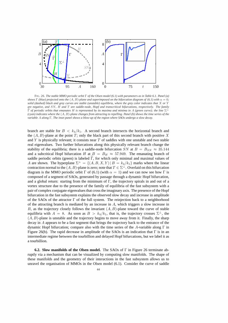
30 95 1600

4

8

0 75 1500

4

8

A

B Γ

H

SN

T

Γ

Σ⊥

H

SN

H

(a)

t

A Γ

(b).

.

FIG. 26. The stable MMO periodic orbitΓ of the Olsen model(6.1)with parameters as in Table 6.1. Panel (a)showsΓ (blue) projected onto the(A, B)-plane and superimposed on the bifurcation diagram of(6.1)with α = 0;solid (dashed) black and grey curves are stable (unstable) equilibria, where the grey color indicates thatX or Yare negative, andSN , H and T are saddle-node, Hopf and transcritical bifurcations, respectively. The familybΓ of periodic orbits that emanatesH is represented by its maxima and minima inA (green curve); the lineΣ⊥(cyan) indicates where the(A, B)-plane changes from attracting to repelling. Panel (b) shows the time series of thevariableA alongΓ. The inset panel shows a blow-up of the region where SAOs undergo a slow decay.

branch are stable forB < k4/k1. A second branch intersects the horizontal branch andthe (A, B)-plane at the pointT ; only the black part of this second branch with positiveXandY is physically relevant; it consists nearT of saddles with one unstable and two stablereal eigenvalues. Two further bifurcations along this physically relevant branch change thestability of the equilibria; there is a saddle-node bifurcationSN at B = BSN ≈ 35.144and a subcritical Hopf bifurcationH at B = BH ≈ 57.949. The emanating branch ofsaddle periodic orbits (green) is labeledΓ, for which only minimal and maximal values ofA are shown. The hyperplaneΣ⊥ = {(A,B, X, Y ) |B = k4/k1} marks where the linearcontraction normal to the(A,B)-plane is zero; note thatT ∈ Σ⊥. Overlaid on this bifurcationdiagram is the MMO periodic orbitΓ of (6.1) (with α = 1) and we can now see howΓ iscomposed of a segment of SAOs, generated by passage through a dynamic Hopf bifurcation,and a global return: starting from the minimum ofΓ, the trajectory spirals in and out of avortex structure due to the presence of the family of equilibria of the fast subsystem with apair of complex conjugate eigenvalues that cross the imaginary axis. The presence of the Hopfbifurcation in the fast subsystem explains the observed slow decay and increase in amplitudeof the SAOs of the attractorΓ of the full system. The reinjection back to a neighborhoodof the attracting branch is mediated by an increase inA, which triggers a slow increase inB, as the trajectory closely follows the invariant(A, B)-plane toward the curve of stableequilibria with A = 8. As soon asB > k4/k1, that is, the trajectory crossesΣ⊥, the(A,B)-plane is unstable and the trajectory begins to move away from it. Finally, the sharpdecay inA appears to be a fast segment that brings the trajectory back to the entrance of thedynamic Hopf bifurcation; compare also with the time series of theA-variable alongΓ inFigure 26(b). The rapid decrease in amplitude of the SAOs is an indication thatΓ is in anintermediate regime between the tourbillion and delayed Hopf bifurcations, but we label it asa tourbillion.

6.2. Slow manifolds of the Olsen model.The SAOs ofΓ in Figure 26 terminate ab-ruptly via a mechanism that can be visualized by computing slow manifolds. The shape ofthese manifolds and the geometry of their interactions in the fast subsystem allows us tounravel the organisation of MMOs in the Olsen model (6.1). Consider the curve of saddle

44

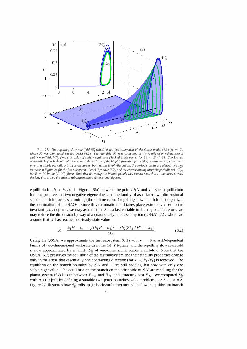
2468

0

0.25

0.5

0.75

B

A

Y

Sr

B

HW s

53

W s

63

(a)

A

Y

Γ60

W s

60(b)

.

.

FIG. 27. The repelling slow manifoldSrB (blue) of the fast subsystem of the Olsen model(6.1) (α = 0),

whereX was eliminated via the QSSA(6.2). The manifoldSrB was computed as the family of one-dimensional

stable manifoldsW sB (one side only) of saddle equilibria (dashed black curve) for53 ≤ B ≤ 63. The branch

of equilibria (dashed/solid black curve) in the vicinity of the Hopf bifurcation point (dot) is also shown, along withseveral unstable periodic orbits (green curves) born at this Hopf bifurcation; the periodic orbits are almost the sameas those in Figure 26 for the fast subsystem. Panel (b) showsW s

60 and the corresponding unstable periodic orbitcΓ60

for B = 60 in the(A, Y )-plane. Note that the viewpoint in both panels was chosen such thatA increases towardthe left; this is also the case in subsequent three-dimensional figures.

equilibria forB < k4/k1 in Figure 26(a) between the pointsSN andT . Each equilibriumhas one positive and two negative eigenvalues and the family of associated two-dimensionalstable manifolds acts as a limiting (three-dimensional) repelling slow manifold that organizesthe termination of the SAOs. Since this termination still takes place extremely close to theinvariant(A,B)-plane, we may assume thatX is a fast variable in this region. Therefore, wemay reduce the dimension by way of a quasi steady-state assumption (QSSA) [72], where weassume thatX has reached its steady-state value

X =k1B − k4 +

√(k1B − k4)2 + 8k2(3k3ABY + k6)

4k2. (6.2)

Using the QSSA, we approximate the fast subsystem (6.1) withα = 0 as aB-dependentfamily of two-dimensional vector fields in the(A, Y )-plane, and the repelling slow manifoldis now approximated by a familySr

B of one-dimensional stable manifolds. Note that theQSSA (6.2) preserves the equilibria of the fast subsystem and their stability properties changeonly in the sense that essentially one contracting direction (forB < k4/k1) is removed. Theequilibria on the branch bounded bySN and T are still saddles, but now with only onestable eigenvalue. The equilibria on the branch on the other side ofSN are repelling for theplanar system ifB lies in betweenBSN andBH , and attracting pastBH . We computedSr

B

with AUTO [50] by defining a suitable two-point boundary value problem; see Section 8.2.Figure 27 illustrates howSr

B rolls up (in backward time) around the lower equilibrium branch

45

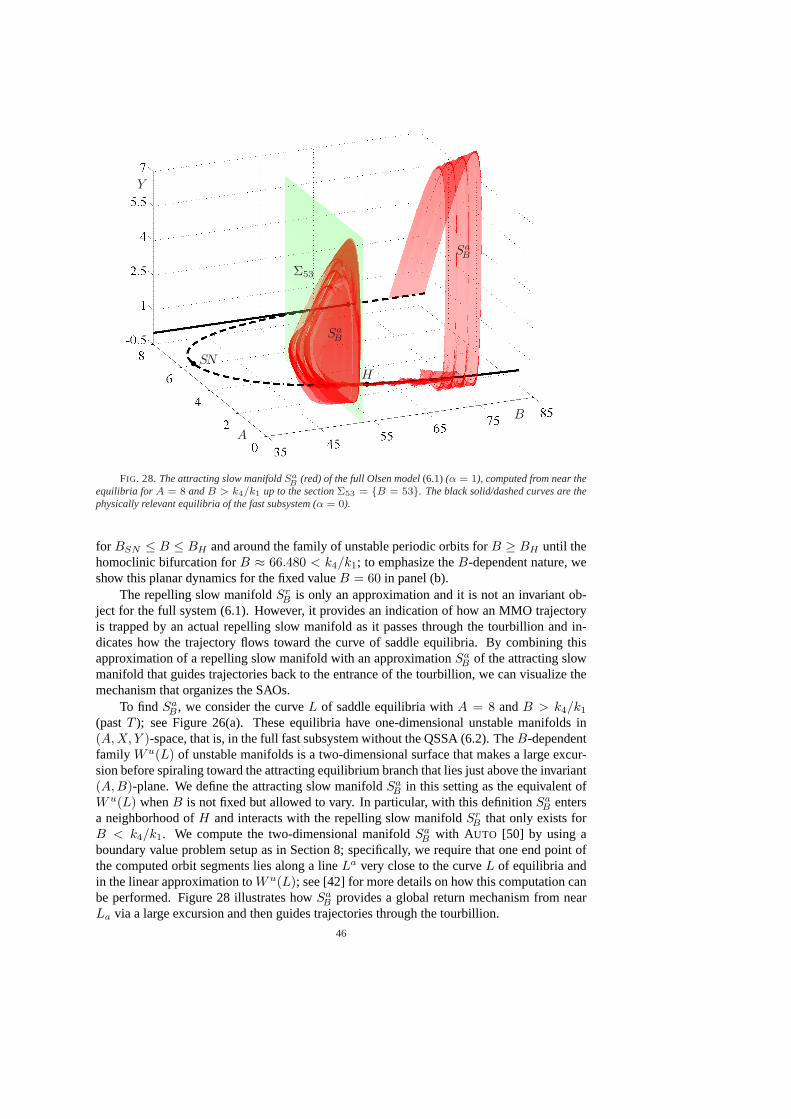
B

A

Y

Σ53

Sa

B

Sa

B

H

SN

.

.

FIG. 28. The attracting slow manifoldSaB (red) of the full Olsen model(6.1) (α = 1), computed from near the

equilibria for A = 8 andB > k4/k1 up to the sectionΣ53 = {B = 53}. The black solid/dashed curves are thephysically relevant equilibria of the fast subsystem (α = 0).

for BSN ≤ B ≤ BH and around the family of unstable periodic orbits forB ≥ BH until thehomoclinic bifurcation forB ≈ 66.480 < k4/k1; to emphasize theB-dependent nature, weshow this planar dynamics for the fixed valueB = 60 in panel (b).

The repelling slow manifoldSrB is only an approximation and it is not an invariant ob-

ject for the full system (6.1). However, it provides an indication of how an MMO trajectoryis trapped by an actual repelling slow manifold as it passes through the tourbillion and in-dicates how the trajectory flows toward the curve of saddle equilibria. By combining thisapproximation of a repelling slow manifold with an approximationSa

B of the attracting slowmanifold that guides trajectories back to the entrance of the tourbillion, we can visualize themechanism that organizes the SAOs.

To find SaB , we consider the curveL of saddle equilibria withA = 8 andB > k4/k1

(pastT ); see Figure 26(a). These equilibria have one-dimensional unstable manifolds in(A,X, Y )-space, that is, in the full fast subsystem without the QSSA (6.2). TheB-dependentfamily Wu(L) of unstable manifolds is a two-dimensional surface that makes a large excur-sion before spiraling toward the attracting equilibrium branch that lies just above the invariant(A,B)-plane. We define the attracting slow manifoldSa

B in this setting as the equivalent ofWu(L) whenB is not fixed but allowed to vary. In particular, with this definitionSa

B entersa neighborhood ofH and interacts with the repelling slow manifoldSr

B that only exists forB < k4/k1. We compute the two-dimensional manifoldSa

B with AUTO [50] by using aboundary value problem setup as in Section 8; specifically, we require that one end point ofthe computed orbit segments lies along a lineLa very close to the curveL of equilibria andin the linear approximation toWu(L); see [42] for more details on how this computation canbe performed. Figure 28 illustrates howSa

B provides a global return mechanism from nearLa via a large excursion and then guides trajectories through the tourbillion.

46

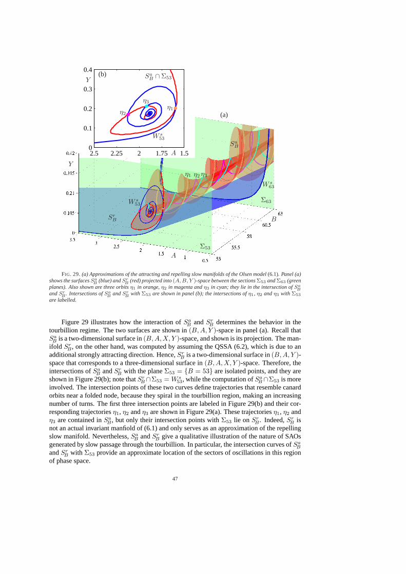
1.51.7522.252.50

0.1

0.2

0.3

0.4

B

A

Y

Σ53

Σ63

Sr

B

W s

53

W s

63

Sa

B

η1 η2 η3

(a)

A

Y

W s

53

Sa

B∩ Σ53

η1η2

η3

(b)

.

.

FIG. 29. (a) Approximations of the attracting and repelling slow manifolds of the Olsen model(6.1). Panel (a)shows the surfacesSa

B (blue) andSrB (red) projected into(A, B, Y )-space between the sectionsΣ53 andΣ63 (green

planes). Also shown are three orbitsη1 in orange,η2 in magenta andη3 in cyan; they lie in the intersection ofSaB

andSrB . Intersections ofSa

B andSrB with Σ53 are shown in panel (b); the intersections ofη1, η2 andη3 with Σ53

are labelled.

Figure 29 illustrates how the interaction ofSaB andSr

B determines the behavior in thetourbillion regime. The two surfaces are shown in(B, A, Y )-space in panel (a). Recall thatSa

B is a two-dimensional surface in(B, A,X, Y )-space, and shown is its projection. The man-ifold Sr

B , on the other hand, was computed by assuming the QSSA (6.2), which is due to anadditional strongly attracting direction. Hence,Sr

B is a two-dimensional surface in(B, A, Y )-space that corresponds to a three-dimensional surface in(B,A, X, Y )-space. Therefore, theintersections ofSa

B andSrB with the planeΣ53 = {B = 53} are isolated points, and they are

shown in Figure 29(b); note thatSrB ∩Σ53 = W s

53, while the computation ofSaB ∩Σ53 is more

involved. The intersection points of these two curves define trajectories that resemble canardorbits near a folded node, because they spiral in the tourbillion region, making an increasingnumber of turns. The first three intersection points are labeled in Figure 29(b) and their cor-responding trajectoriesη1, η2 andη3 are shown in Figure 29(a). These trajectoriesη1, η2 andη3 are contained inSa

B , but only their intersection points withΣ53 lie on SrB . Indeed,Sr

B isnot an actual invariant manfiold of (6.1) and only serves as an approximation of the repellingslow manifold. Nevertheless,Sa

B andSrB give a qualitative illustration of the nature of SAOs

generated by slow passage through the tourbillion. In particular, the intersection curves ofSaB

andSrB with Σ53 provide an approximate location of the sectors of oscillations in this region

of phase space.

47

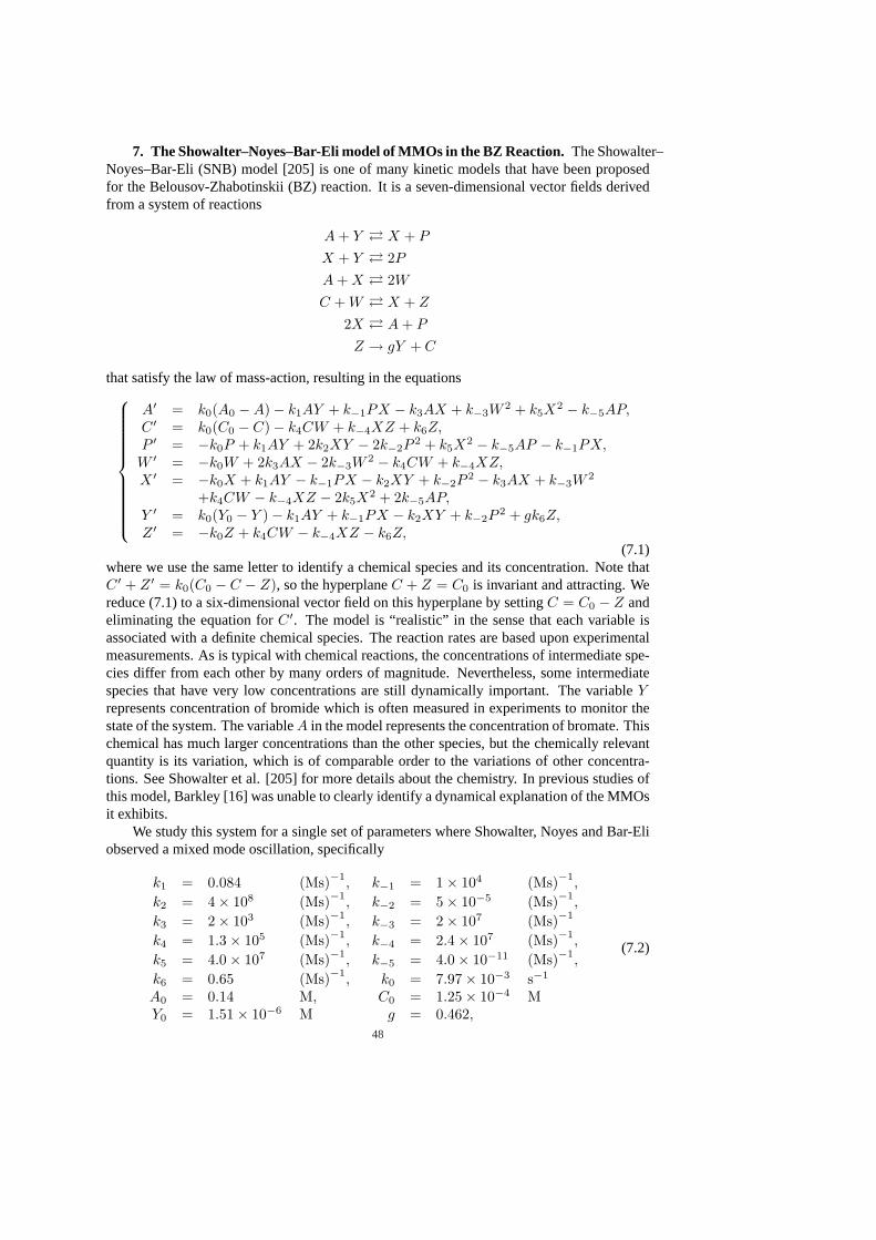
7. The Showalter–Noyes–Bar-Eli model of MMOs in the BZ Reaction.The Showalter–Noyes–Bar-Eli (SNB) model [205] is one of many kinetic models that have been proposedfor the Belousov-Zhabotinskii (BZ) reaction. It is a seven-dimensional vector fields derivedfrom a system of reactions

A + Y À X + P

X + Y À 2P

A + X À 2W

C + W À X + Z

2X À A + P

Z → gY + C

that satisfy the law of mass-action, resulting in the equations

A′ = k0(A0 −A)− k1AY + k−1PX − k3AX + k−3W2 + k5X

2 − k−5AP,C ′ = k0(C0 − C)− k4CW + k−4XZ + k6Z,P ′ = −k0P + k1AY + 2k2XY − 2k−2P

2 + k5X2 − k−5AP − k−1PX,

W ′ = −k0W + 2k3AX − 2k−3W2 − k4CW + k−4XZ,

X ′ = −k0X + k1AY − k−1PX − k2XY + k−2P2 − k3AX + k−3W

2

+k4CW − k−4XZ − 2k5X2 + 2k−5AP,

Y ′ = k0(Y0 − Y )− k1AY + k−1PX − k2XY + k−2P2 + gk6Z,

Z ′ = −k0Z + k4CW − k−4XZ − k6Z,(7.1)

where we use the same letter to identify a chemical species and its concentration. Note thatC ′ + Z ′ = k0(C0 − C − Z), so the hyperplaneC + Z = C0 is invariant and attracting. Wereduce (7.1) to a six-dimensional vector field on this hyperplane by settingC = C0 − Z andeliminating the equation forC ′. The model is “realistic” in the sense that each variable isassociated with a definite chemical species. The reaction rates are based upon experimentalmeasurements. As is typical with chemical reactions, the concentrations of intermediate spe-cies differ from each other by many orders of magnitude. Nevertheless, some intermediatespecies that have very low concentrations are still dynamically important. The variableYrepresents concentration of bromide which is often measured in experiments to monitor thestate of the system. The variableA in the model represents the concentration of bromate. Thischemical has much larger concentrations than the other species, but the chemically relevantquantity is its variation, which is of comparable order to the variations of other concentra-tions. See Showalter et al. [205] for more details about the chemistry. In previous studies ofthis model, Barkley [16] was unable to clearly identify a dynamical explanation of the MMOsit exhibits.

We study this system for a single set of parameters where Showalter, Noyes and Bar-Eliobserved a mixed mode oscillation, specifically

k1 = 0.084 (Ms)−1, k−1 = 1× 104 (Ms)−1

,

k2 = 4× 108 (Ms)−1, k−2 = 5× 10−5 (Ms)−1

,

k3 = 2× 103 (Ms)−1, k−3 = 2× 107 (Ms)−1

k4 = 1.3× 105 (Ms)−1, k−4 = 2.4× 107 (Ms)−1

,

k5 = 4.0× 107 (Ms)−1, k−5 = 4.0× 10−11 (Ms)−1

,

k6 = 0.65 (Ms)−1, k0 = 7.97× 10−3 s−1

A0 = 0.14 M, C0 = 1.25× 10−4 MY0 = 1.51× 10−6 M g = 0.462,

(7.2)

48

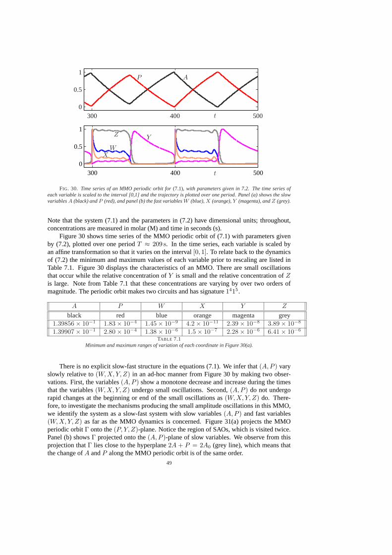
300 400 5000

0.5

1

300 400 5000

0.5

1

t

ZY

W

X

t

P A

.

.

FIG. 30. Time series of an MMO periodic orbit for(7.1), with parameters given in 7.2. The time series ofeach variable is scaled to the interval [0,1] and the trajectory is plotted over one period. Panel (a) shows the slowvariablesA (black) andP (red), and panel (b) the fast variablesW (blue),X (orange),Y (magenta), andZ (grey).

Note that the system (7.1) and the parameters in (7.2) have dimensional units; throughout,concentrations are measured in molar (M) and time in seconds (s).

Figure 30 shows time series of the MMO periodic orbit of (7.1) with parameters givenby (7.2), plotted over one periodT ≈ 209 s. In the time series, each variable is scaled byan affine transformation so that it varies on the interval[0, 1]. To relate back to the dynamicsof (7.2) the minimum and maximum values of each variable prior to rescaling are listed inTable 7.1. Figure 30 displays the characteristics of an MMO. There are small oscillationsthat occur while the relative concentration ofY is small and the relative concentration ofZis large. Note from Table 7.1 that these concentrations are varying by over two orders ofmagnitude. The periodic orbit makes two circuits and has signature1415.

A P W X Y Z

black red blue orange magenta grey1.39856× 10−1 1.83× 10−4 1.45× 10−9 4.2× 10−11 2.39× 10−8 3.89× 10−8

1.39907× 10−1 2.80× 10−4 1.38× 10−6 1.5× 10−7 2.28× 10−6 6.41× 10−6

TABLE 7.1Minimum and maximum ranges of variation of each coordinate in Figure 30(a).

There is no explicit slow-fast structure in the equations (7.1). We infer that(A,P ) varyslowly relative to(W,X, Y, Z) in an ad-hoc manner from Figure 30 by making two obser-vations. First, the variables(A,P ) show a monotone decrease and increase during the timesthat the variables(W,X, Y, Z) undergo small oscillations. Second,(A,P ) do not undergorapid changes at the beginning or end of the small oscillations as(W,X, Y, Z) do. There-fore, to investigate the mechanisms producing the small amplitude oscillations in this MMO,we identify the system as a slow-fast system with slow variables(A, P ) and fast variables(W,X, Y, Z) as far as the MMO dynamics is concerned. Figure 31(a) projects the MMOperiodic orbitΓ onto the(P, Y, Z)-plane. Notice the region of SAOs, which is visited twice.Panel (b) showsΓ projected onto the(A,P )-plane of slow variables. We observe from thisprojection thatΓ lies close to the hyperplane2A + P = 2A0 (grey line), which means thatthe change ofA andP along the MMO periodic orbit is of the same order.

49

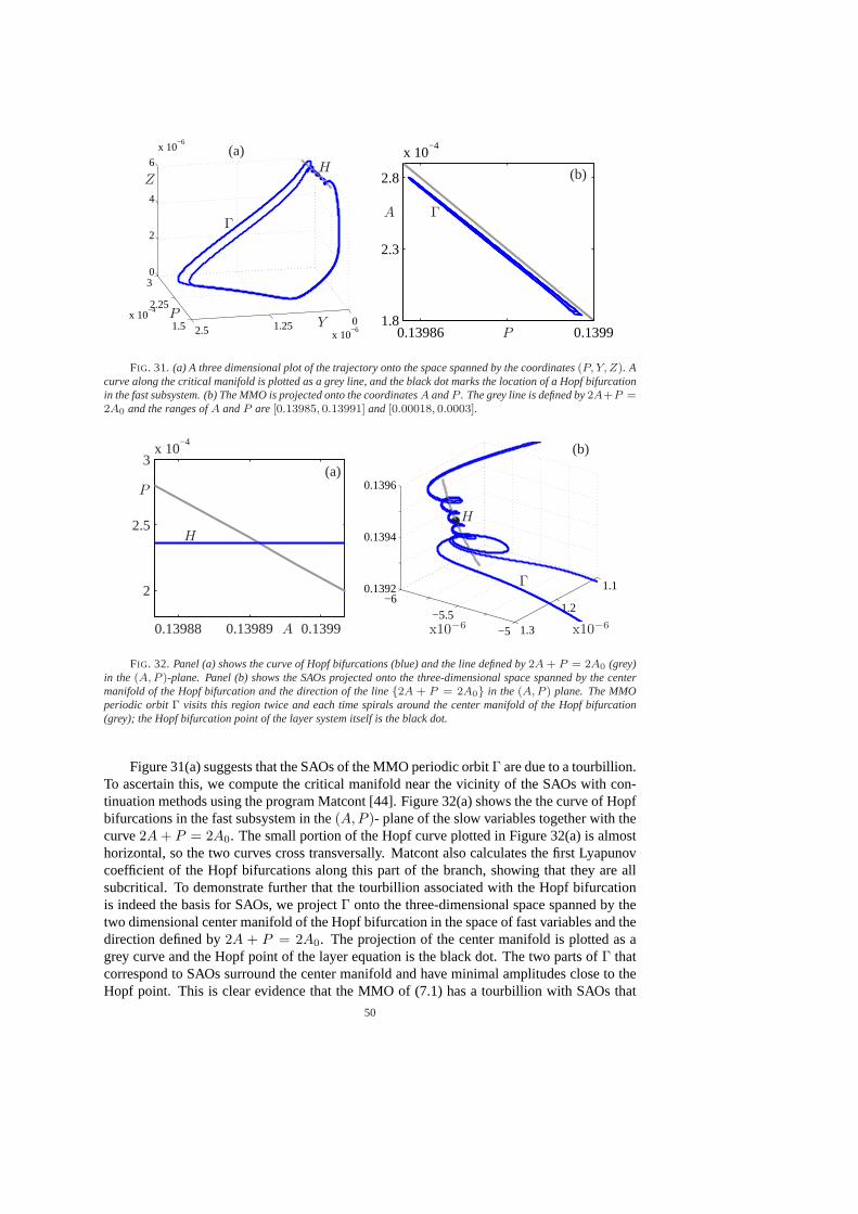
1.5

2.25

3

x 10−4

01.252.5 x 10−6

0

2

4

6

x 10−6

0.13986 0.13991.8

2.3

2.8

x 10−4

YP

ZH

Γ

(a)

P

A Γ

(b)

.

.

FIG. 31. (a) A three dimensional plot of the trajectory onto the space spanned by the coordinates(P, Y, Z). Acurve along the critical manifold is plotted as a grey line, and the black dot marks the location of a Hopf bifurcationin the fast subsystem. (b) The MMO is projected onto the coordinatesA andP . The grey line is defined by2A+P =2A0 and the ranges ofA andP are [0.13985, 0.13991] and[0.00018, 0.0003].

0.13988 0.13989 0.1399

2

2.5

3x 10

−4

1.1

1.2

1.3

−6−5.5

−5

0.1392

0.1394

0.1396

A

P

H

(a)

x10−6

x10−6

H

Γ

(b).

.

FIG. 32. Panel (a) shows the curve of Hopf bifurcations (blue) and the line defined by2A + P = 2A0 (grey)in the (A, P )-plane. Panel (b) shows the SAOs projected onto the three-dimensional space spanned by the centermanifold of the Hopf bifurcation and the direction of the line{2A + P = 2A0} in the (A, P ) plane. The MMOperiodic orbitΓ visits this region twice and each time spirals around the center manifold of the Hopf bifurcation(grey); the Hopf bifurcation point of the layer system itself is the black dot.

Figure 31(a) suggests that the SAOs of the MMO periodic orbitΓ are due to a tourbillion.To ascertain this, we compute the critical manifold near the vicinity of the SAOs with con-tinuation methods using the program Matcont [44]. Figure 32(a) shows the the curve of Hopfbifurcations in the fast subsystem in the(A,P )- plane of the slow variables together with thecurve2A + P = 2A0. The small portion of the Hopf curve plotted in Figure 32(a) is almosthorizontal, so the two curves cross transversally. Matcont also calculates the first Lyapunovcoefficient of the Hopf bifurcations along this part of the branch, showing that they are allsubcritical. To demonstrate further that the tourbillion associated with the Hopf bifurcationis indeed the basis for SAOs, we projectΓ onto the three-dimensional space spanned by thetwo dimensional center manifold of the Hopf bifurcation in the space of fast variables and thedirection defined by2A + P = 2A0. The projection of the center manifold is plotted as agrey curve and the Hopf point of the layer equation is the black dot. The two parts ofΓ thatcorrespond to SAOs surround the center manifold and have minimal amplitudes close to theHopf point. This is clear evidence that the MMO of (7.1) has a tourbillion with SAOs that

50

are generated by the passage through a dynamic Hopf bifurcation, similar to the one observedfor the Olsen model in Section 6. This example illustrates how the methods described in thispaper can be applied effectively to a system of higher dimension than just three or four.

8. Numerical methods for slow-fast systems.This section discusses numerical meth-ods that we used to compute the two-dimensional slow manifolds shown in many of thefigures, as well as stable and unstable manifolds of equilibrium points. The slow manifoldcomputations choose an end point of each orbit segment on the critical manifold away froma fold; this approximation yields errors that areO(ε) but decay quickly as one moves awayfrom the end point. For stable or unstable manifolds of equilibria, orbit segments are chosento lie in the linear eigenspace associated with the stable or unstable eigenvalues, respectively.The computational error associated with this approximation also decays quickly as one movesaway from the endpoint; see [41, 130] for analysis of these approximation errors .

A simple and effective method for computing invariant manifolds as families of orbitsegments is to use initial value solvers as the basic algorithm with initial conditions chosenon a mesh of points transverse to the flow in the invariant manifold; we call this the “sweep-ing” method. Despite its simplicity, this sweeping method fails to produce satisfactory resultsin some cases. In particular, strong convergence or divergence of trajectories toward one an-other makes the choice of the initial mesh problematic and can produce very non-uniform“coverage” of the desired manifold; see [59, 60]. In multiple-time-scale systems, the fast ex-ponential instability of Fenichel manifolds that are not attracting makes initial value solversincapable of tracking these manifolds by forward integration. These issues prompt the use ofboundary value methods combined with continuation as an alternate strategy for computinginvariant manifolds [131, 132] . We have used both strategies in this paper. This sectionpresents more details of the techniques used to compute attracting and repelling slow mani-folds of systems with one fast and two slow variables, as well as the continuation of canardorbits when a parameter is varied.

8.1. Sweeping invariant manifolds.The Fenichel manifolds of systems with a singlefast variable are either attracting or repelling. As a result, forward trajectories with initial con-ditions on the critical manifold will converge quickly to an attracting Fenichel manifold andbackward trajectories with initial conditions on the critical manifold will converge quicklyto a repelling Fenichel manifold. Thus, one way to compute two-dimensional attracting andrepelling Fenichel manifolds of a three-dimensional flow is to apply an initial value solver inthe appropriate time direction to a mesh of initial conditions along a curve of the critical man-ifold transverse to the slow flow. We used this sweeping method to computeSr

ε in Figure 11;see also [162] for an early use of this method to compute two-dimensional invariant mani-folds and Wechselberger [233] and Guckenheimer and Haiduc [86] for an example involvingfolded nodes.

When incorporated into a continuation framework, the sweeping method can also be usedif the critical manifold is not known in closed form and the mesh of initial conditions can-not be selected beforehand. Continuation methods [49] provide well-established algorithmsthat augment equation solvers like Newton’s method with strategies for choosing new start-ing points when solving under-determined systems of equations. More precisely, supposeF : Rm+n → Rm is a smooth function given bym equations ofm + n variables. The impli-cit function theorem states that the zeros ofF form a smoothn-dimensional manifoldM nearpoints where the matrixDF of partial derivatives has full rankm. Moreover, the theoremgives a formula for the tangent space ofM . Most continuation methods treat the casen = 1where the set of solutions is a curve; see [101] for the casen > 1. In general, the methodsare based on a predictor-corrector procedure: given a point onM , tangent (or higher-order)information is used to choose a new seed for the solver to find a new point onM . The sweep-

51

ing method described above selects the continuation step size based on equal increments ofa specific coordinate or direction, but more sophisticated step size adaptations can be usedas well. For example,pseudo-arclengthcontinuation as implemented in AUTO [50] choosespoints based on their distances from each other inRm+n.

We also used a sweeping method to compute the global unstable manifoldWu(p) inFigure 11. The mesh of initial conditions was taken to lie along a ray in the tangent space ofWu(p), with endpoints of the mesh at successive intersections of a trajectory of the linear-ized system with this ray. The sweeping method works well here, because the selected orbitsegments provide adequate “coverage” ofWu(p).

8.2. Continuation of orbit segments with boundary value solvers.The core algorithmsof AUTO [50] are boundary value solvers and continuation methods. The sweeping methoddescribed in the previous section can also be implemented in AUTO [50], so that the initialvalue problems are solved using a collocation method; see [49] for details. The techniques de-scribed in this section impose boundary conditions on both end points of the orbit segments,which makes the method more versatile and suitable in a wider context; see also [131]. Wedescribe here how to formulate two-point boundary value problems (BVP) in order to com-pute slow manifolds and associated canard orbits.

We consider two-point boundary value problems of the form

u = Tg(u, λ),u(0) ∈ L,u(1) ∈ Σ,

(8.1)

whereg : Rn × Rp → Rn is sufficiently smooth,T ∈ R, λ ∈ Rp are parameters andL andΣ are submanifolds ofRn. The parameterT rescales time so that the orbit segments alwayscorrespond to trajectories in the time interval[0, 1]. Hence, the boundary conditions at thetwo end points always apply tou(0) andu(1). In order to have a well-posed problem withisolated solutions, the number of boundary conditions should equal the number of equations(n, because(u) ∈ Rn) plus the number of free parameters (at mostp + 1 for the parameterλ and the total integration timeT ). We are interested in one-parameter families of solutionsof (8.1), which means that we allow one fewer boundary condition (or one additional freeparameter). Note thatT is typically unknown and we may viewT as the extra free parameter.

Let us first consider the computation of two-dimensional attracting and repelling slowmanifoldsSa

ε andSrε . To simplify the explanation, we assume that we have a three-dimensional

slow-fast system with two slow variables and a folded node. In this context, the parameterλ remains fixed, and we obtain a one-parameter family of orbit segments (with unkown totalintegration timesT ) by imposing a total of three boundary conditions. This means that thedimensions ofL andΣ in (8.1) sum up ton = 3. Our approach is to chooseL as a curve(or straight line) on the critical manifold, which requires two boundary conditions, andΣ asa surface (or plane), which requires one boundary condition, such that the associated one-parameter family of orbit segments covers the desired portion of the slow manifold. Forexample, in order forSa

ε to come into the folded node region, we letL be a curve on theattracting sheet of the critical manifold transverse to the slow flow andΣ be a surface ortho-gonal to the fold curveF at the folded node. The same approach works forSr

ε , where wechooseL on the repelling sheet of the critical manifold; note thatT < 0 for such a familyof orbit segments. We remark that these choices can also be used with the sweeping methodand an initial value solver that detects a “stopping condition” defined by the level set of afunction. With the boundary value solvers, we can exchange the roles ofL andΣ, whichis more appropriate for finding canard orbits; see Section 8.3. The slow manifolds can be

52

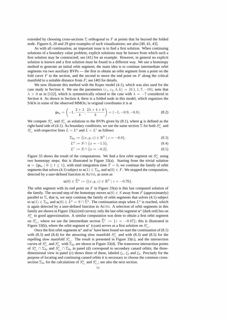
extended by choosing cross-sectionsΣ orthogonal toF at points that lie beyond the foldednode. Figures 6, 20 and 29 give examples of such visualizations; see also [40, 41, 43].

As with all continuation, an important issue is to find a first solution. When continuingsolutions of a boundary value problem, explicit solutions may be known from which such afirst solution may be constructed; see [41] for an example. However, in general no explicitsolution is known and a first solution must be found in a different way. We use a homotopymethod to generate an initial orbit segment; the main idea is to continue intermediate orbitsegments via two auxiliary BVPs — the first to obtain an orbit segment from a point on thefold curveF to the section, and the second to move the end point onF along the criticalmanifold to a suitable distance fromF ; see [40] for details.

We now illustrate this method with the Koper model (4.1), which was also used for thecase study in Section 4. We use the parameters(ε1, ε2, λ, k) = (0.1, 1, 7,−10); note thatλ > 0 as in [122], which is symmetrically related to the case withλ = −7 considered inSection 4. As shown in Section 4, there is a folded node in this model, which organizes theSAOs in some of the observed MMOs; in original coordinates it is at

pfn =(−1,

2 + λ

k,2λ + 4 + k

k

)= (−1,−0.9,−0.8). (8.2)

We computeSaε1

andSrε1

as solutions to the BVPs given by (8.1), whereg is defined as theright-hand side of (4.1). As boundary conditions, we use the same sectionΣ for bothSa

ε1and

Srε1

with respective linesL = La andL = Lr as follows

Σfn := {(x, y, z) ∈ R3 | z = −0.8}, (8.3)

La := S ∩ {x = −1.5}, (8.4)

Lr := S ∩ {x = −0.2}. (8.5)

Figure 33 shows the result of the computations. We find a first orbit segment onSaε1

usingtwo homotopy steps; this is illustrated in Figure 33(a). Starting from the trivial solutionu = {pfn | 0 ≤ t ≤ 1}, with total integration timeT = 0, we continue the family of orbitsegments that solves (4.1) subject tou(1) ∈ Σfn andu(0) ∈ F . We stopped the computation,detected by a user-defined function inAUTO, as soon as

u(0) ∈ Σa := {(x, y, z) ∈ R3 | z = −0.76}.The orbit segment with its end point onF in Figure 33(a) is this last computed solution ofthe family. The second step of the homotopy movesu(0) ∈ S away fromF (approximately)parallel toΣ, that is, we next continue the family of orbit segments that solves (4.1) subjectto u(1) ∈ Σfn andu(0) ∈ La = S ∩ Σa. The continuation stops whenLa is reached, whichis again detected by a user-defined function inAUTO. A selection of orbit segments in thisfamily are shown in Figure 33(a) (red curves); only the last orbit segmentua (dark red) lies onSa

ε1to good approximation. A similar computation was done to obtain a first orbit segment

on Srε1

, where we use the intermediate sectionΣr := {z = −0.87}; this is illustrated inFigure 33(b), where the orbit segmentur (cyan) serves as a first solution onSr

ε1.

Once the first orbit segmentsua andur have been found we start the continuation of (8.1)with (8.3) and (8.4) for the attracting slow manifoldSa

ε1and with (8.3) and (8.5) for the

repelling slow manifoldSrε1

. The result is presented in Figure 33(c), and the intersectioncurves ofSa

ε1andSr

ε1with Σfn are shown in Figure 33(d). The transverse intersection points

of Saε1∩ Σfn andSr

ε1∩ Σfn in panel (d) correspond to secondary canard orbits; the three-

dimensional view in panel (c) shows three of these, labeledξ1, ξ2 andξ3. Precisely for thepurpose of locating and continuing canard orbits it is necessary to choose the common cross-sectionΣfn for the calculations ofSa

ε1andSr

ε1; see also the next section.

53

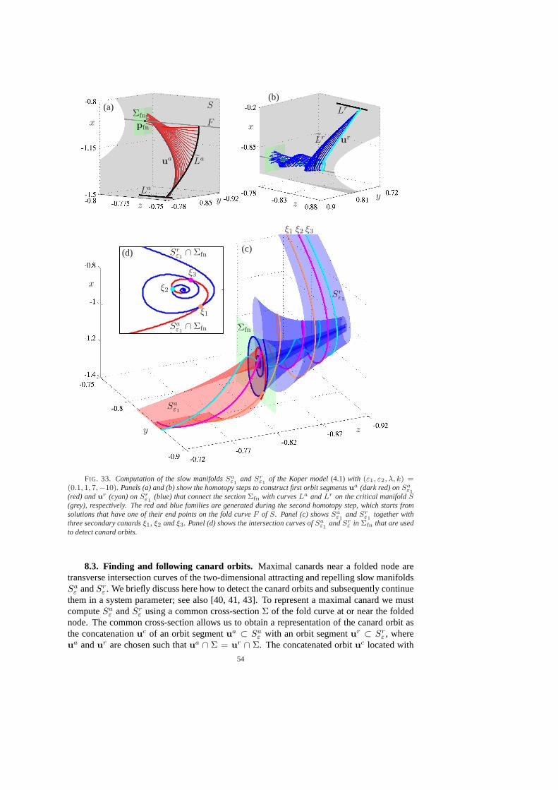
zy

x

Σfn

Sr

ε1

Sa

ε1

ξ1 ξ2 ξ3

(c)

ξ1

ξ2

ξ3

Sr

ε1∩ Σfn

Sa

ε1∩ Σfn

(d)

yz

x

La

pfn

Σfn

S

F

Lau

a

(a)

yz

x

Lr

Lru

r

(b).

.

FIG. 33. Computation of the slow manifoldsSaε1

and Srε1

of the Koper model(4.1) with (ε1, ε2, λ, k) =(0.1, 1, 7,−10). Panels (a) and (b) show the homotopy steps to construct first orbit segmentsua (dark red) onSa

ε1(red) andur (cyan) onSr

ε1(blue) that connect the sectionΣfn with curvesLa andLr on the critical manifoldS

(grey), respectively. The red and blue families are generated during the second homotopy step, which starts fromsolutions that have one of their end points on the fold curveF of S. Panel (c) showsSa

ε1andSr

ε1together with

three secondary canardsξ1, ξ2 andξ3. Panel (d) shows the intersection curves ofSaε1

andSrε in Σfn that are used

to detect canard orbits.

8.3. Finding and following canard orbits. Maximal canards near a folded node aretransverse intersection curves of the two-dimensional attracting and repelling slow manifoldsSa

ε andSrε . We briefly discuss here how to detect the canard orbits and subsequently continue

them in a system parameter; see also [40, 41, 43]. To represent a maximal canard we mustcomputeSa

ε andSrε using a common cross-sectionΣ of the fold curve at or near the folded

node. The common cross-section allows us to obtain a representation of the canard orbit asthe concatenationuc of an orbit segmentua ⊂ Sa

ε with an orbit segmentur ⊂ Srε , where

ua andur are chosen such thatua ∩ Σ = ur ∩ Σ. The concatenated orbituc located with

54

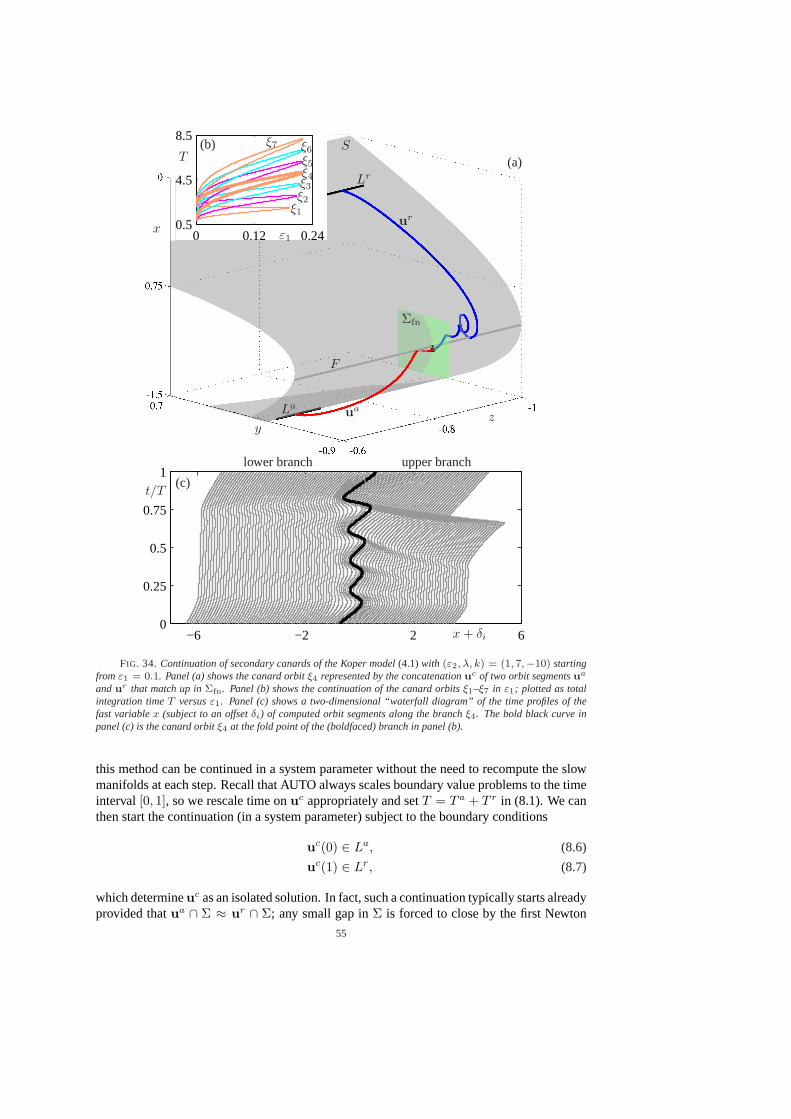
0 0.12 0.240.5

4.5

8.5

−6 −2 2 60

0.25

0.5

0.75

1

t/T

x + δi

lower branch upper branch

(c)

zy

x

La

Lr

Σfn

F

ua

ur

S

(a)T

ε1

ξ1

ξ2

ξ3

ξ4

ξ5

ξ6ξ7(b)

.

.

FIG. 34. Continuation of secondary canards of the Koper model(4.1)with (ε2, λ, k) = (1, 7,−10) startingfrom ε1 = 0.1. Panel (a) shows the canard orbitξ4 represented by the concatenationuc of two orbit segmentsua

andur that match up inΣfn. Panel (b) shows the continuation of the canard orbitsξ1–ξ7 in ε1; plotted as totalintegration timeT versusε1. Panel (c) shows a two-dimensional “waterfall diagram” of the time profiles of thefast variablex (subject to an offsetδi) of computed orbit segments along the branchξ4. The bold black curve inpanel (c) is the canard orbitξ4 at the fold point of the (boldfaced) branch in panel (b).

this method can be continued in a system parameter without the need to recompute the slowmanifolds at each step. Recall that AUTO always scales boundary value problems to the timeinterval [0, 1], so we rescale time onuc appropriately and setT = T a + T r in (8.1). We canthen start the continuation (in a system parameter) subject to the boundary conditions

uc(0) ∈ La, (8.6)

uc(1) ∈ Lr, (8.7)

which determineuc as an isolated solution. In fact, such a continuation typically starts alreadyprovided thatua ∩ Σ ≈ ur ∩ Σ; any small gap inΣ is forced to close by the first Newton

55

step. These two boundary conditions (8.6) and (8.7) force the orbit segmentuc to stay veryclose to the attracting sheet of the critical manifoldS until near the fold curveF , and thenstay close to the repelling sheet ofS up toLr.

Figure 34 illustrates canard continuation with the Koper model (4.1), where we usedε1 as the second free parameter (together withT ) and kept(ε2, λ, k) = (1, 7,−10) fixed.Figure 34(a) shows the two orbit segmentsua andur with (almost) equal end points in thesectionΣ = Σfn; they have been detected as a good approximation of the maximal secondarycanard orbitξ4, which is then represented by the concatenated orbituc. We continuedξ4,along with six other maximal secondary canards, for increasing and decreasingε1; see alsoFigure 33. Figure 34(b) shows these seven branches, labeledξ1–ξ7; here, the vertical axisshows the total integration timeT because it clearly distinguishes the branches. Whenξ1–ξ7 are continued in the direction of increasingε1, a fold in ε1 is detected for each branch;we have already seen this in Section 5 and it has also been observed in other systems [43].Figure 34(c) is a “waterfall diagram” that shows how the maximal secondary canard orbitξ4

evolves along the branch asε1 is varied; specifically, the time profile of the fast variablex ofconsecutively computed orbit segments along the branchξ4 are plotted with a suitable off-setδi. The orbit segment that corresponds to the fold ofξ4 is highlighted in bold black. Observethat the orbit segments to the left of the fold have four SAOs, whereas past the fold there areonly three SAOs followed by a fast segment. Hence the canard orbits past the fold are nolonger maximal canards; see also Section 5.

9. Discussion. We described several mechanisms in slow-fast systems that producemixed-mode oscillations, namely the twisting of slow invariant manifolds near a folded node,oscillations that follow the two-dimensional unstable manifold of a saddle-focus equilibriumnear a singular Hopf bifurcation, and the tourbillion mechanism of a dynamic Hopf bifurc-ation. Geometric singular perturbation theory provides tools to identify the geometry asso-ciated with each mechanism, to quantify the MMO signatures, and to describe associatedbifurcations. Analysis of the folded node case is more complete than the other cases. Re-cent work on singular Hopf bifurcation [85] and the transition from singular Hopf to foldednodes [143] provides substantial detail on the second case, but much remains to be discoveredabout the unfolding of a singular Hopf bifurcation that is relevant to MMOs. Historically, thedynamic Hopf bifurcation was discovered first, and detailed analysis exists for the case of adelayed Hopf bifurcation of the layer equations [168]. Together, these mechanisms constitutea partial framework for classifying MMOs in multiple-time-scale systems that can be furtherextended. Perhaps the most surprising aspect of the theory we have described is that oscilla-tions can appear from the interaction of fast and slow time scales even when neither of thesetime scales individually displays oscillations.

We have used four case studies to illustrate theoretical concepts and they serve as a test-bed for the development of numerical methods. The MMOs in the Koper model and thethree-dimensional reduction of the Hodgkin–Huxley equations have SAOs that occur on in-termediate time scales due to folded nodes and singular Hopf bifurcations. In the folded-nodemechanism, three parameters play key roles in determining the geometry of the small oscilla-tions: the ratioε of time scales, the eigenvalue ratioµ of the folded node in the desingularizedreduced system, and the distanceδ of global return trajectories from certain invariant man-ifolds. Intersections of invariant manifolds are prerequisite to global returns that produceMMOs in these examples, and tangencies between these manifolds constitutes a new type ofbifurcation that is found on the boundaries of parameter regions yielding MMOs. We foundfast oscillations of the layer equations in the Olsen and Showalter–Noyes–Bar-Eli models ofchemical reactions. Both models exhibit MMOs due to the dynamic Hopf mechanism. Thesetwo case studies also illustrate how the theory applies in higher dimensions and how numer-

56

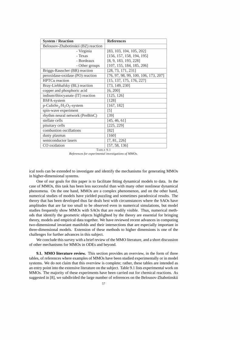
System / Reaction ReferencesBelousov-Zhabotinskii (BZ) reaction

- Virginia [83, 103, 104, 105, 202]- Texas [156, 157, 158, 194, 195]- Bordeaux [8, 9, 183, 193, 228]- Other groups [107, 155, 184, 185, 206]

Briggs-Rauscher (BR) reaction [28, 73, 171, 231]peroxidase-oxidase (PO) reaction [76, 97, 98, 99, 100, 106, 173, 207]HPTCu reaction [15, 137, 175, 176, 227]Bray-Liebhafsky (BL) reaction [73, 149, 230]copper and phosphoric acid [6, 200]indium/thiocyanate (IT) reaction [125, 126]BSFA-system [128]p-CuInSe2/H2O2-system [167, 182]spin-wave experiment [5]rhythm neural network (PreBotC) [39]stellate cells [45, 46, 61]pituitary cells [225, 229]combustion oscillations [82]dusty plasmas [160]semiconductor lasers [7, 81, 226]CO oxidation [57, 58, 136]

TABLE 9.1References for experimental investigations of MMOs.

ical tools can be extended to investigate and identify the mechanisms for generating MMOsin higher-dimensional systems.

One of our goals for this paper is to facilitate fitting dynamical models to data. In thecase of MMOs, this task has been less successful than with many other nonlinear dynamicalphenomena. On the one hand, MMOs are a complex phenomenon, and on the other hand,numerical studies of models have yielded puzzling and sometimes paradoxical results. Thetheory that has been developed thus far deals best with circumstances where the SAOs haveamplitudes that are far too small to be observed even in numerical simulations, but modelstudies frequently show MMOs with SAOs that are readily visible. Thus, numerical meth-ods that identify the geometric objects highlighted by the theory are essential for bringingtheory, models and empirical data together. We have reviewed recent advances in computingtwo-dimensional invariant manifolds and their intersections that are especially important inthree-dimensional models. Extension of these methods to higher dimensions is one of thechallenges for further advances in this subject.

We conclude this survey with a brief review of the MMO literature, and a short discussionof other mechanisms for MMOs in ODEs and beyond.

9.1. MMO literature review. This section provides an overview, in the form of threetables, of references where examples of MMOs have been studied experimentally or in modelsystems. We do not claim that this overview is complete; rather, these tables are intended asan entry point into the extensive literature on the subject. Table 9.1 lists experimental work onMMOs. The majority of these experiments have been carried out for chemical reactions. Assuggested in [8], we subdivided the large number of references on the Belousov-Zhabotinskii

57

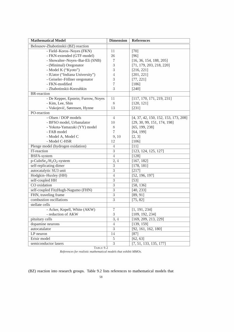
Mathematical Model Dimension ReferencesBelousov-Zhabotinskii (BZ) reaction

- Field–Koros–Noyes (FKN) 11 [70]- FKN-extended (GTF-model) 26 [96]- Showalter–Noyes–Bar-Eli (SNB) 7 [16, 36, 154, 188, 205]- (Minimal) Oregonator 3 [71, 179, 203, 218, 220]- Model K (“Kyoto”) 3 [216, 221]- IUator (“Indiana University”) 4 [201, 221]- Geiseler–Follner oregonator 3 [77, 221]- FKN-modified 7 [186]- Zhabotinskii-Korzuhkin 3 [240]

BR-reaction- De Kepper, Epstein; Furrow, Noyes 11 [117, 170, 171, 219, 231]- Kim, Lee, Shin 8 [120, 121]- Vukojevic, Sørensen, Hynne 13 [231]

PO-reaction- Olsen / DOP models 4 [4, 37, 42, 150, 152, 153, 173, 208]- BFSO model, Urbanalator 10 [29, 30, 99, 151, 174, 198]- Yokota-Yamazaki (YY) model 8 [65, 199, 238]- FAB model 7 [64, 199]- Model A, Model C 9, 10 [2, 3]- Model C-HSR 12 [106]

Plenge model (hydrogen oxidation) 4 [11]IT-reaction 3 [123, 124, 125, 127]BSFA-system 4 [128]p-CuInSe2/H2O2-system 2, 4 [167, 182]self-replicating dimer 3 [178, 181]autocatalytic SU3 unit 3 [217]Hodgkin–Huxley (HH) 4 [52, 196, 197]self-coupled HH 3 [53]CO oxidation 3 [58, 136]self-coupled FitzHugh-Nagumo (FHN) 3 [40, 233]FHN, traveling frame 3 [89, 91]combustion oscillations 3 [75, 82]stellate cells

- Acker, Kopell, White (AKW) 7 [1, 191, 234]- reduction of AKW 3 [109, 192, 234]

pituitary cells 3, 4 [169, 209, 213, 229]dopamine neurons 4 [139, 159]autocatalator 3 [92, 161, 162, 180]LP neuron 14 [87]Erisir model 5 [62, 63]semiconductor lasers 3 [7, 51, 133, 135, 177]

TABLE 9.2References for realistic mathematical models that exhibit MMOs.

(BZ) reaction into research groups. Table 9.2 lists references to mathematical models that

58

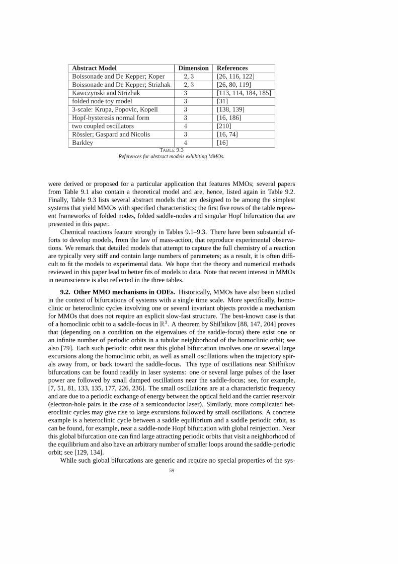
Abstract Model Dimension ReferencesBoissonade and De Kepper; Koper 2, 3 [26, 116, 122]Boissonade and De Kepper; Strizhak 2, 3 [26, 80, 119]Kawczynski and Strizhak 3 [113, 114, 184, 185]folded node toy model 3 [31]3-scale: Krupa, Popovic, Kopell 3 [138, 139]Hopf-hysteresis normal form 3 [16, 186]two coupled oscillators 4 [210]Rossler; Gaspard and Nicolis 3 [16, 74]Barkley 4 [16]

TABLE 9.3References for abstract models exhibiting MMOs.

were derived or proposed for a particular application that features MMOs; several papersfrom Table 9.1 also contain a theoretical model and are, hence, listed again in Table 9.2.Finally, Table 9.3 lists several abstract models that are designed to be among the simplestsystems that yield MMOs with specified characteristics; the first five rows of the table repres-ent frameworks of folded nodes, folded saddle-nodes and singular Hopf bifurcation that arepresented in this paper.

Chemical reactions feature strongly in Tables 9.1–9.3. There have been substantial ef-forts to develop models, from the law of mass-action, that reproduce experimental observa-tions. We remark that detailed models that attempt to capture the full chemistry of a reactionare typically very stiff and contain large numbers of parameters; as a result, it is often diffi-cult to fit the models to experimental data. We hope that the theory and numerical methodsreviewed in this paper lead to better fits of models to data. Note that recent interest in MMOsin neuroscience is also reflected in the three tables.

9.2. Other MMO mechanisms in ODEs. Historically, MMOs have also been studiedin the context of bifurcations of systems with a single time scale. More specifically, homo-clinic or heteroclinic cycles involving one or several invariant objects provide a mechanismfor MMOs that does not require an explicit slow-fast structure. The best-known case is thatof a homoclinic orbit to a saddle-focus inR3. A theorem by Shil′nikov [88, 147, 204] provesthat (depending on a condition on the eigenvalues of the saddle-focus) there exist one oran infinite number of periodic orbits in a tubular neighborhood of the homoclinic orbit; seealso [79]. Each such periodic orbit near this global bifurcation involves one or several largeexcursions along the homoclinic orbit, as well as small oscillations when the trajectory spir-als away from, or back toward the saddle-focus. This type of oscillations near Shil′nikovbifurcations can be found readily in laser systems: one or several large pulses of the laserpower are followed by small damped oscillations near the saddle-focus; see, for example,[7, 51, 81, 133, 135, 177, 226, 236]. The small oscillations are at a characteristic frequencyand are due to a periodic exchange of energy between the optical field and the carrier reservoir(electron-hole pairs in the case of a semiconductor laser). Similarly, more complicated het-eroclinic cycles may give rise to large excursions followed by small oscillations. A concreteexample is a heteroclinic cycle between a saddle equilibrium and a saddle periodic orbit, ascan be found, for example, near a saddle-node Hopf bifurcation with global reinjection. Nearthis global bifurcation one can find large attracting periodic orbits that visit a neighborhood ofthe equilibrium and also have an arbitrary number of smaller loops around the saddle-periodicorbit; see [129, 134].

While such global bifurcations are generic and require no special properties of the sys-

59

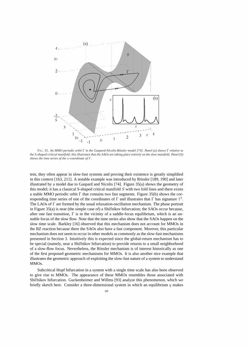
xy2

y1S

Γ

(a)

t

x (b)

.

.

FIG. 35. An MMO periodic orbitΓ in the Gaspard-Nicolis-Rossler model [74]. Panel (a) showsΓ relative tothe S-shaped critical manifold; this illustrates that the SAOs are taking place entirely on the slow manifold. Panel (b)shows the time series of thex-coordinate ofΓ.

tem, they often appear in slow-fast systems and proving their existence is greatly simplifiedin this context [163, 211]. A notable example was introduced by Rossler [189, 190] and laterillustrated by a model due to Gaspard and Nicolis [74]. Figure 35(a) shows the geometry ofthis model; it has a classical S-shaped critical manifoldS with two fold lines and there existsa stable MMO periodic orbitΓ that contains two fast segments. Figure 35(b) shows the cor-responding time series of one of the coordinates ofΓ and illustrates thatΓ has signature12.The LAOs ofΓ are formed by the usual relaxation-oscillation mechanism. The phase portraitin Figure 35(a) is near (the simple case of) a Shil′nikov bifurcation; the SAOs occur because,after one fast transition,Γ is in the vicinity of a saddle-focus equilibrium, which is an un-stable focus of the slow flow. Note that the time series also show that the SAOs happen on theslow time scale. Barkley [16] observed that this mechanism does not account for MMOs inthe BZ reaction because there the SAOs also have a fast component. Morever, this particularmechanism does not seem to occur in other models as commonly as the slow-fast mechanismspresented in Section 3. Intuitively this is expected since the global-return mechanism has tobe special (namely, near a Shil′nikov bifurcation) to provide returns to a small neighborhoodof a slow-flow focus. Nevertheless, the Rossler mechanism is of interest historically as oneof the first proposed geometric mechanisms for MMOs. It is also another nice example thatillustrates the geometric approach of exploiting the slow-fast nature of a system to understandMMOs.

Subcritical Hopf bifurcation in a system with a single time scale has also been observedto give rise to MMOs. The appearance of these MMOs resembles those associated withShil′nikov bifurcation. Guckenheimer and Willms [93] analyze this phenomenon, which webriefly sketch here. Consider a three-dimensional system in which an equilibriumq makes

60

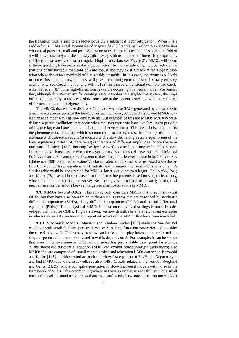
the transition from a sink to a saddle-focus via a subcritical Hopf bifurcation. Whenq is asaddle-focus, it has a real eigenvalue of magnitudeO(1) and a pair of complex eigenvalueswhose real parts are small and positive. Trajectories that come close to the stable manifold ofq will flow close toq and then slowly spiral away with oscillations of increasing magnitude,similar to those observed near a singular Hopf bifurcation; see Figure 21. MMOs will occurif these spiraling trajectories make a global return to the vicinity ofq. Global returns forportions of the unstable manifold ofq are robust and may exist already at the Hopf bifurc-ation where the center manifold ofq is weakly unstable. In this case, the returns are likelyto come close enough toq that they will give rise to long epochs of small, slowly growingoscillations. See Guckenheimer and Willms [93] for a three-dimensional example and Guck-enheimer et al. [87] for a high-dimensional example occurring in a neural model. We remarkthat, although this mechanism for creating MMOs applies to a single-time system, the Hopfbifurcation naturally introduces a slow time scale in the system associated with the real partsof the unstable complex eigenvalues.

The MMOs that we have discussed in this survey have SAOs generated by a local mech-anism near a special point of the limiting system. However, SAOs and associated MMOs mayalso arise in other ways in slow-fast systems. An example of this are MMOs with two well-defined separate oscillations that occur when the layer equations have two families of periodicorbits, one large and one small, and fast jumps between them. This scenario is analogous tothe phenomenon of bursting, which is common in neural systems. In bursting, oscillationsalternate with quiescent epochs (associated with a slow drift along a stable equilibrium of thelayer equations) instead of there being oscillations of different amplitudes. Since the sem-inal work of Rinzel [187], bursting has been viewed as a multiple-time-scale phenomenon.In this context, bursts occur when the layer equations of a model have both equilibria andlimit-cycle attractors and the full system makes fast jumps between these in both directions.Izhikevich [108] compiled an extensive classification of bursting patterns based upon the bi-furcations of the layer equations that initiate and terminate the oscillations in a burst. Asimilar table could be constructed for MMOs, but it would be even larger. Golubitsky, Josicand Kaper [78] use a different classification of bursting patterns based on singularity theory,which is more in the spirit of this survey. Section 6 gives a brief taste of the analysis of globalmechanisms for transitions between large and small oscillations in MMOs.

9.3. MMOs beyond ODEs. This survey only considers MMOs that arise in slow-fastODEs, but they have also been found in dynamical systems that are described by stochasticdifferential equations (SDEs), delay differential equations (DDEs) and partial differentialequations (PDEs). The analysis of MMOs in these more involved settings is much less de-veloped than that for ODEs. To give a flavor, we now describe briefly a few recent examplesin which a slow-fast structure is an important aspect of the MMOs that have been identified.

9.3.1. Stochastic MMOs.Muratov and Vanden-Eijnden [165] study the Van der Poloscillator with small (additive) noise; they useλ as the bifurcation parameter and considerthe case0 < ε ¿ 1. Their analysis shows an intricate interplay between the noise and thesingular perturbation parameterε, and how this depends onλ. For example, it can be shownthat even if the deterministic limit without noise has just a stable fixed point for suitableλ, the stochastic differential equation (SDE) can exhibit relaxation-type oscillations; alsoMMOs that are composed of “small canard orbits” and relaxation LAOs can occur. Borowskiand Kuske [145] consider a similar stochastic slow-fast equation of FitzHugh–Nagumo typeand find MMOs due to noise as well; see also [146]. Closely related is the work by Berglundand Gentz [24, 25] who study spike generation in slow-fast neural models with noise in theframework of SDEs. The common ingredient in these examples is excitability: while smallnoise only leads to small irregular oscillations, a sufficiently large noise perturbation can kick

61

the system beyond a threshold that results in a large excursion. There is a noise level whenthe system is most coherent or regular and, hence, shows well-defined but irregular MMOs.Excitability as a mechanism to generate large pulses as the result of external and/or internalnoise has also been observed and studied in several laser systems [54, 133].

Another possible mechanism for noise-induced MMOs was investigated by Yu et al. [239],who consider a system of coupled-oscillator SDEs. If the deterministic limit is at least bistablethen noise can provide a mechanism for sample paths to alternate between the basins of at-traction of deterministically stable invariant sets. The simplest way to visualize this idea is toconsider two stable limit cycles for an ODE, one with a small and the other with a large amp-litude. If the basins of attraction are suitably located, noise can induce repeated transitionsbetween tubular neighborhoods of each cycle. Hence, a typical sample path will then be anirregular MMO.

9.3.2. MMOs in delay differential equations. One can ask the question what happenswhen one adds delay terms to a slow-fast system. Sriram and Gopinathan [206] considerthe Belousov-Zhabotinskii reaction with delay in an experiment. They compare the resultswith a version of the classical three-dimensional Oregonator model [71, 203] with delay andclaim that the delay induces MMOs [206]. This prompts the question whether DDEs haveslow-fast phenomena, such as canards, similar to their ODE counterparts. In principle, thisshould be expected at least for the case of a finite number of fixed delays, for which theDDE does not feature a continuous spectrum [94]. Indeed a positive answer was recentlyobtained by Campbell, Stone and Erneux [32] for a two-dimensional DDE model of high-speed machining. In their system a small delay induces perturbation from a degenerate Hopfbifurcation, which results in a canard explosion as discussed in Section 2.2; see also [34] fordetails of the underlying theory for slow-fast DDEs with small delay.

9.3.3. MMOs in partial differential equations. Given a time-dependent PDE on a do-main inRn, one can look for MMOs in space, time or a mixture of space and time. Nagumo’sequation [166], which models the evolution of an activatorv(x, t) and a slow inhibitoru(x, t),is an example that has been studied extensively as an idealized model for propagation of ac-tion potentials. Traveling-wave profiles are found via the ansatzv(x, t) = v(x + σt) = v(τ)andw(x, t) = w(x + σt) = w(τ) as homoclinic solutions of a three-dimensional ODE withtwo fast variables and one slow variable [90]; hereσ is the wave speed. It has been shownthat MMOs exist as solutions of this reduced ODE [91]. More generally, work on evolutionequations given by PDEs suggests that oscillatory patterns with alternating amplitudes [35]and slow-fast structures [17] exist in many common models. Hence, the study of this type ofMMOs for PDEs will benefit from multiple-time-scale methods.

62

Acknowledgments. We thank the following organizations for their support during thepreparation of this paper. M.D. was supported by grants EP/C54403X/1 and EP/E032249/1from the Engineering and Physical Sciences Research Council (EPSRC); J.G. by the NationalScience Foundation, the Department of Energy and by an International Visiting Fellowshipfrom Sydney University; B.K. by a visitor grant from the Center for Applied Mathemat-ics (CAM) at Cornell University; C.K. by the National Science Foundation; H.M.O. by anEPSRC Advanced Research Fellowship grant and by the IGERT programme of CAM at Cor-nell University; and M.W. by sabbatical support from the Institute for Analysis and ScientificComputing at the Vienna University of Technology and from the Mathematical BiosciencesInstitute at Ohio State University. Furthermore, our collaboration was made possible by re-search visits of M.D., B.K. and H.M.O. at CAM; of J.G, B.K. and H.M.O. at Sydney Uni-versity; and of C.K. and M.W. at the Bristol Centre for Applied Nonlinear Mathematics. Wehereby thank these institutions for their hospitality and support.

REFERENCES

[1] C. D. ACKER, N. KOPELL, AND J. A. WHITE, Synchronization of strongly coupled excitatory neurons:Relating network behaviour to biophysics, J. Comput. Neurosci., 15:71–90, 2003.

[2] B. D. AGUDA, AND B. L. CLARKE, Bistability in chemical reaction networks: theory and application to theperoxidase-oxidase reaction, J. Chem. Phys., 87(6):3461–3470, 1987.

[3] B. D. AGUDA, AND R. LARTER, Periodic-chaotic sequences in a detailed mechanism of the peroxidase-oxidase reaction, J. Am. Chem. Soc., 113:7913–7916, 1991.

[4] B. D. AGUDA, R. LARTER, AND B. L. CLARKE, Dynamic elements of mixed-mode oscillations and chaosin a peroxidase-oxidase network, J. Chem. Phys., 90(8):4168–4175, 1989.

[5] F. M. DE AGUIAR, S. ROSENBLATT, A. AZEVEDO, AND S. M. REZENDE, Observation of mixed-modeoscillations in spin-wave experiments, J. Appl. Phys., 85(8):5086–5087, 1999.

[6] F. N. ALBAHADILY , J. RINGLAND , AND M. SCHELL, Mixed-mode oscillations in an electrochemical system.I. A Farey sequence which does not occur on a torus, J. Chem. Phys., 90:813–821, 1989.

[7] K. A L-NAIMEE , F. MARINO, M. CISZAK , R. MEUCCI, AND F. T. ARECCHI, Chaotic spiking and incom-plete homoclinic scenarios in semiconductor lasers with optoelectric feedback, New Journal of Physics,11:073022, 2009.

[8] F. ARGOUL, A. ARNEODO, P. RICHETTI, AND J. C. ROUX, From quasiperiodicity to chaos in the Belousov-Zhabotinskii reaction. I. Experiment, J. Chem. Phys., 86(6):3325–3338, 1987.

[9] F. ARGOUL AND J. C. ROUX, Quasiperiodicity in chemistry: An experimental path in the neighbourhood ofa codimension-two bifurcation, Phys. Lett. A, 108(8):426–430, 1985.

[10] V. I. A RNOLD (ED.), Encyclopedia of mathematical sciences: Dynamical systems V, Springer-Verlag, Ber-lin/New York, 1994.

[11] N. BABA AND K. K RISCHER, Mixed-mode oscillations and cluster patterns in an electrochemical relaxationoscillator under galvanostatic control, Chaos, 18(1):015103, 2008.

[12] S. M. BAER AND T. ERNEUX, Singular Hopf bifurcation to relaxation oscillations I, SIAM J. Appl. Mathem.,46(5):721–739, 1986.

[13] S. M. BAER AND T. ERNEUX, Singular Hopf bifurcation to relaxation oscillations II, SIAM J. Appl.Mathem., 52(6):1651–1664, 1992.

[14] S. M. BAER, T. ERNEUX, AND J. RINZEL, The slow passage through a Hopf bifurcation: delay, memoryeffects, and resonance, SIAM J. Appl. Math. 49(1):55–71, 1989.

[15] D. BAKES, L. SCHREIBEROVA, I. SCHREIBER, AND M. J. B. HAUSER, Mixed-mode oscillations in a ho-mogeneous ph-oscillatory chemical reaction system, Chaos, 18(1):015102, 2008.

[16] D. BARKLEY , Slow manifolds and mixed-mode oscillations in the Belousov-Zhabotinskii reaction, J. Chem.Phys., 89(9):5547–5559, 1988.

[17] D. BARKLEY , Linear stability analysis of rotating spiral waves in excitable media, Phys. Rev. Lett.,68(13):2090–2093, 1992.

[18] B. P. BELOUSOV, A periodically acting reaction and its mechanism, in Collection of short papers on RadiationMedicine for 1958, Med. Publ., Moscow, 1959, pp 145–147.

[19] E BENOIT, Systems lents-rapides dansR3 et leurs canards, in Third Schnepfenried geometry conference,volume 2, pp 159–191. Soc. Math. France, 1982.

[20] E BENOIT, Enlacements de canards, C.R. Acad. Sc. Paris, 300(8):225–230, 1985.[21] E BENOIT, Canards et enlacements, Inst. HautesEtudes Sci. Publ. Math. 72:63–91, 1990.[22] E BENOIT , J.-L. CALLOT, F. DIENER, AND M. D IENER, Chasse au canards, Collect. Math., 31:37–119,

63

1981.[23] E BENOIT, AND C. LOBRY, Les canards deR3, C.R. Acad. Sc. Paris, 294:483–488, 1982.[24] N. BERGLUND AND B. GENTZ, Noise-induced phenomena in slow-fast dynamical systems: a sample-paths

approach, Springer-Verlag, Berlin/New York, 2005.[25] N. BERGLUND AND B. GENTZ, Stochastic dynamic bifurcations and excitability, in C. Laing and G. Lord,

editors, Stochastic methods in neuroscience, Oxford University Press, 2008, pp 65–93.[26] J. BOISSONADE AND P. DEKEPPER, Transitions from bistability to limit cycle oscillations. Theoretical ana-

lysis and experimental evidence in an open chemical system, J. Phys. Chem., 84:501–506, 1980.[27] B. BRAAKSMA , Singular Hopf bifurcation in systems with fast and slow variables, J. Nonlinear Science,

8(5):457–490, 1998.[28] T.S. BRIGGS, AND W.C. RAUSCHER, An oscillating iodine clock, J. Chem. Educ., 50:496, 1973.[29] T. V. BRONNIKOVA , V. R. FED’ KINA , W. M. SCHAFFER, AND L. F. OLSEN, Period-doubling bifurcations

and chaos in a detailed model of the peroxidase-oxidase reaction, J. Phys. Chem., 99(23):9309–9312,1995.

[30] T. V. BRONNIKOVA , W. M. SCHAFFER, AND L. F. OLSEN, Nonlinear dynamics of the peroxidase-oxidasereaction. I. Bistability and bursting oscillations at low enzyme concentrations, J. Phys. Chem. B,105:310–321, 2001.

[31] M. BRØNS, M. KRUPA, AND M. WECHSELBERGER, Mixed mode oscillations due to the generalized canardphenomenon, Fields Institute Communications, 49:39–63, 2006.

[32] S. A. CAMPBELL , E. STONE, AND T. ERNEUX, Delay induced canards in a model of high speed machining,Dynamical Systems, 24(3):373–392, 2009.

[33] J. CARR, Applications of centre manifold theory. Springer-Verlag, Berlin/New York, 1981.[34] C. CHICONE, Inertial and slow manifolds for delay differential equations, J. Diff. Eqs., 190:364–406, 2003.[35] P. COULLET, Localized patterns and fronts in nonequilibrium systems, Int. J. Bif. Chaos, 12(11):2445–2457,

2002.[36] M. F. CROWLEY AND R. J. FIELD, Electrically coupled Belousov-Zhabotisnky oscillators: a potential chaos

generator, in C. Vidal and A. Pacault, editors, Nonlinear phenonema in chemical dynamics, Springer-Verlag, Berlin/New York, 1981, pp 147–153.

[37] H. DEGN, L. F. OLSEN, AND J. W. PERRAM, Bistability, oscillation, and chaos in an enzyme reaction,Annals of the New York Academy of Sciences, 316(1):623–637, 1979.

[38] W. DE MELO, AND S. VAN STRIEN, One-dimensional dynamics, Springer-Verlag, Berlin/New York, 1993.[39] C. A. DEL NEGRO, C. G. WILSON, R. J. BUTERA, H. RIGATTO, AND J. C. SMITH , Periodicity, mixed-

mode oscillations, and quasiperiodicity in a rhythm-generating neural network, Biophysical Journal,82:206–214, 2002.

[40] M. DESROCHES, B. KRAUSKOPF, AND H. M. OSINGA, Mixed-mode oscillations and slow manifolds in theself-coupled FitzHugh-Nagumo system, Chaos, 18(1):015107, 2008.

[41] M. DESROCHES, B. KRAUSKOPF, AND H. M. OSINGA, The geometry of slow manifolds near a folded node,SIAM J. Appl. Dyn. Syst., 7(4):1131–1162, 2008.

[42] M. DESROCHES, B. KRAUSKOPF, AND H. M. OSINGA, The geometry of mixed-mode oscillations in theOlsen model for the perioxidase-oxidase reaction, Discr. Cont. Dyn. Sys. S, 2(4): 807–827, 2009.

[43] M. DESROCHES, B. KRAUSKOPF, AND H. M. OSINGA, Numerical continuation of canard orbits in slow-fastdynamical systems, Nonlinearity, 23(3): 739–765, 2010.

[44] A. DHOOGE, W. GOVAERTS, AND YU. A. KUZNETSOV, MatCont: A Matlab package for numerical bifurc-ation analysis of ODEs, ACM TOMS 29(2): 141–164, 2003. Available viahttp://www.matcont.ugent.be/ .

[45] C. T. DICKSON, J. MAGISTRETTI, M. H. SHALISNKY, E. FRANSEN, M. E. HASSELMO, AND A. A LONSO,Properties and role ofIh in the pacing of subtreshold oscillations in entorhinal cortex layer II neurons,J. Neurophysiol., 83:2562–2579, 2000.

[46] C. T. DICKSON, J. MAGISTRETTI, M. H. SHALISNKY, B. HAMAM , AND A. A LONSO, Oscillatory activityin entorhinal neurons and circuits: Mechanisms and function, Ann. N.Y. Acad. Sci., 911:127–150, 2006.

[47] F. DIENER, AND M. D IENER, Nonstandard analysis in practice, Springer-Verlag, Berlin/New York, 1995.[48] M. D IENER, The canard unchained or how fast/slow dynamical systems bifurcate, The Mathematical Intelli-

gencer, 6:38–48, 1984.[49] E. J. DOEDEL, Lecture notes on numerical analysis of nonlinear equations, in B. Krauskopf, H. M. Osinga

and J. Galan-Vioque, editors, Numerical continuation methods for dynamical systems: path followingand boundary value problems, Springer-Verlag, Berlin/New York, 2007, pp 117–54.

[50] E. J. DOEDEL, R. C. PAFFENROTH, A. C. CHAMPNEYS, T. F. FAIRGRIEVE, YU. A. KUZNET-SOV, B. E. OLDEMAN , B. SANDSTEDE AND X. J. WANG, AUTO-07p: Con-tinuation and Bifurcation Software for Ordinary Differential Equations; available athttp://cmvl.cs.concordia.ca/auto/.

[51] E. J. DOEDEL, B. E. OLDEMAN , AND C. L. PANDO L., Bifurcation structures in a model of a CO2 laserwith a fast saturable absorber, Int. J. Bifurc. Chaos, in press.

64

[52] S. DOI, J. INOUE, AND S. KUMAGAI , Chaotic spiking in the Hodgkin–Huxley nerve model with slow inac-tivation in the sodium current, J. Integr. Neurosci., 3(2):207–225, 2004.

[53] J. DROVER, J. RUBIN , J. SU, AND B. ERMENTROUT, Analysis of a canard mechanism by which excitatorysynaptic coupling can synchronize neurons at low firing frequencies, SIAM J. Appl. Math., 65(1):69–92,2004.

[54] J.L.A. DUBBELDAM , B. KRAUSKOPF AND D. LENSTRA, Excitability and coherence resonance in laserswith saturable absorber, Phys. Rev. E 60(6):6580–6588, 1999.

[55] F. DUMORTIER AND R. ROUSSARIE, Canard cycles and center manifolds, Mem. Amer. Math. Soc., 577,1996.

[56] W. ECKHAUS, Relaxation oscillations including a standard chase on french ducks, Lec. Notes Math.,985:449–494, 1983.

[57] M. EISWIRTH AND G. ERTL Kinetic oscillations in the catalytic CO oxidation on a Pt(110) surface, Surf.Sci., 177(1):90–100, 1986.

[58] M. EISWIRTH, K. KRISCHER, AND G. ERTL, Nonlinear dynamics in the CO-oxidation on Pt single crystalsurfaces, Appl. Phys. A, 51:79–90, 1990.

[59] J. P. ENGLAND , B. KRAUSKOPF, AND H . M. OSINGA, Computing one-dimensional global manifold ofPoincare maps by continuation, SIAM J. Appl. Dyn. Syst., 4(4):1008–1041, 2005.

[60] J. P. ENGLAND , B. KRAUSKOPF, AND H .M. OSINGA, Computing two-dimensional global invariant mani-folds in slow-fast systems, Int. J. Bif. Chaos, 17(3): 805–822, 2007.

[61] I. ERCHOVA AND D. J. MCGONIGLE, Rhythms of the brain: An examination of mixed mode oscillationapproaches to the analysis of neurophysiological data, Chaos, 18(1):015115, 2008.

[62] A. ERISIR, D. LAU , B. RUDY, AND C. S. LEONARD, Function of specificK+ channels in sustained high-frequency firing of fast-spiking interneurons, J. Neurophysiol., 82:2476–2489, 1999.

[63] B. ERMENTROUT AND M. WECHSELBERGER, Canards, clusters and synchronization in a weakly coupledinterneuron model, SIAM J. Appl. Dyn. Syst., 8(1):253–278, 2009.

[64] V. R. FED′KINA , F. I. ATAULLAKHANOV , AND T. V. BRONNIKOVA, Computer simulations of sustainedoscillations in the peroxidase-oxidase reaction, Biophysical Chemistry, 19:259–264, 1984.

[65] V. R. FED′KINA , F. I. ATAULLAKHANOV , AND T. V. BRONNIKOVA, Stimulated regimens in the peroxidase-oxidase reaction, Theor. Exp. Chem., 24(2):172–178, 1988.

[66] N. FENICHEL, Persistence and smoothness of invariant manifolds for flows, Indiana University MathematicalJournal, 21:193–225, 1971.

[67] N. FENICHEL, Asymptotic stability with rate conditions, Indiana University Mathematical Journal, 23:1109–1137, 1974.

[68] N. FENICHEL, Asymptotic stability with rate conditions II, Indiana University Mathematical Journal, 26:81–93, 1977.

[69] N. FENICHEL, Geometric singular perturbation theory for ordinary differential equations, J. Diff. Eqs.,31:53–98, 1979.

[70] R.J. FIELD , E. KOROS, AND R.M. NOYES, Oscillations in chemical systems II. Thorough analysis of tem-poral oscillations in theCe−BrO3-malonic acid system, J. Am. Chem. Soc., 94:8649–8664, 1972.

[71] R. J. FIELD AND R. M. NOYES, Oscillations in chemical systems IV. Limit cycle behavior in a model of areal chemical reaction, J. Chem. Phys., 60:1877–1884, 1974.

[72] S. J. FRASER, The steady state and equilibrium approximations: A geometrical picture, J. Chem. Phys.,88:4732–4738, 1988.

[73] S. D. FURROW, Chemical oscillators based on iodate ion and hydrogen peroxide, in R. J. Field and M. Burger,editors, Oscillations and traveling waves in chemical systems, Wiley-Interscience, 1985, pp 171–192.

[74] P. GASPARD AND G. NICOLIS, What can we learn from homoclinic orbits in chaotic dynamics?, J. Stat.Phys., 31(3):499–518, 1983.

[75] P. GASPARD AND X.-J. WANG, Homoclinic orbits and mixed-mode oscillations in far-from-equilibrium sys-tems, J. Stat. Phys., 48:151–199, 1987.

[76] T. GEEST, C. G. STEINMETZ, R. LARTER, AND L. F. OLSEN, Period-doubling bifurcations and chaos inan enzyme reaction, J. Phys. Chem., 96:5678–5680, 1992.

[77] W. GEISELER AND H. H. FOLLNER, Three steady state situation in an open chemical reaction system. I,Biophys. Chem., 6(1):107–115, 1977.

[78] M. GOLUBITSKY, K. JOSIC, AND T. J. KAPER, An unfolding theory approach to bursting in fast-slowsystems, in H.W. Broer, B. Krauskopf, and G. Vegter, editors, Analysis of dynamical systems: Festschriftdedicated to Floris Takens on the occasion of his 60th birthday, Institute of Physics Publ., Bristol, 2001,pp 277–308.

[79] S. V. GONCHENKO, D. V. TURAEV, P. GASPARD, AND G. NICOLIS, Complexity in the bifurcation structureof homoclinic loops to a saddle-focus, Nonlinearity, 10:409–423, 1997.

[80] A. GORYACHEV, P. STRIZHAK , AND R. KAPRAL, Slow manifold structure and the emergence of mixed-modeoscillations, J. Chem. Phys., 107(18):2881–2889, 1997.

[81] D. GOULDING, S.P. HEGARTY, O. RASSKAZOV, S. MELNIK , M. HARTNETT, G. GREENE, J. G. MCINER-

65

NEY, D. RACHINSKII , AND G. HUYET Excitability in a quantum dot semiconductor laser with opticalinjection, Phys. Rev. Lett., 98(15):153903, 2007.

[82] P. GRAY, J. F. GRIFFITHS, S. M. HASKO, AND P.-G. LIGNOLA, Oscillatory ignitions and cool flamesaccompanying the non-isothermal oxidation of acetaldehyde in a well stirred, flow reactor, Proc. R. Soc.Lond., 374(1758):313–339, 1981.

[83] K. R. GRAZIANI , J. L. HUDSON, AND R. A. SCHMITZ, The Belousov-Zhabotinskii reaction in a continuousflow reactor, The Chemical Engineering Journal, 12(1):9–21, 1976.

[84] J. GUCKENHEIMER, Return maps of folded nodes and folded saddle-nodes, Chaos, 18(1):015108, 2008.[85] J. GUCKENHEIMER, Singular hopf bifurcation in systems with two slow variables, SIAM J. Appl. Dyn. Syst.,

7(4):1355–1377, 2008.[86] J. GUCKENHEIMER AND RADU HAIDUC, Canards at folded nodes, Moscow Mathematical Journal,25, 91–

103, 2005.[87] J. GUCKENHEIMER, R. HARRIS-WARRICK, J. PECK, AND A. R. WILLMS , Bifurcation, bursting, and spike

frequency adaptation, J. Comp. Neuosci., 4:257–277, 1997.[88] J. GUCKENHEIMER AND P. HOLMES, Nonlinear oscillations, dynamical systems, and bifurcations of vector

fields. Springer-Verlag, Berlin/New York, 1983.[89] J. GUCKENHEIMER AND C. KUEHN, Computing slow manifolds of saddle-type, SIAM J. Appl. Dyn. Syst.,

8(3):854–879, 2009.[90] J. GUCKENHEIMER AND C. KUEHN, Homoclinic orbits of the FitzHugh-Nagumo equation: The singular

limit, Discr. Cont. Dyn. Sys. Ser. S, 2(4):851–872, 2009.[91] J. GUCKENHEIMER AND C. KUEHN, Homoclinic orbits of the FitzHugh-Nagumo equation: Bifurcations in

the full system, SIAM J. Appl. Dyn. Syst., 8(3):138–153, 2009.[92] J. GUCKENHEIMER AND C. SCHEPER, A geometric model for mixed-mode oscillations in a chemical system,

Preprint, 2009.[93] J. GUCKENHEIMER AND A. W ILLMS , Asymptotic analysis of subcritical Hopf-homoclinic bifurcation, Phys-

ica D, 139, 195–216, 2000.[94] J. HALE AND S. M. VERDUYN LUNEL, Introduction to functional differential equations, Springer-Verlag,

Berlin/New York, 1993.[95] M. W. HIRSCH, C. C. PUGH, AND M. SHUB, Invariant manifolds, Springer-Verlag, Berlin/New York, 1977.[96] L. GYORGI, T. TURANYI , AND R. J. FIELD, Mechanistic details of the oscillatory Belousov-Zhabotinskii

reaction, J. Phys. Chem., 94:7162–7170, 1990.[97] T. HAUCK AND F. W. SCHNEIDER, Mixed-mode and quasiperiodic oscillations in the peroxidase-oxidase

reaction, J. Phys. Chem., 97:391–397, 1993.[98] T. HAUCK AND F. W. SCHNEIDER, Chaos in a Farey sequence through period doubling in the peroxidase-

oxidase reaction, J. Phys. Chem., 98:2072–2077, 1994.[99] M. J. B. HAUSER AND L. F. OLSEN, Mixed-mode oscillations and homoclinic chaos in an enzyme reaction,

J. Chem. Soc. Faraday Trans., 92(16):2857–2863, 1996.[100] M. J. B. HAUSER, L. F. OLSEN, T. V. BRONNIKOVA , AND W. M. SCHAFFER, Routes to chaos in the

peroxdiase-oxidase reaction: period-doubling and period-adding, J. Phys. Chem. B, 101:5075–5083,1997.

[101] M. HENDERSON, Multiple parameter continuation: Computing implicitly definedk-manifolds, Int. J. Bif.Chaos, 12(3): 451–476, 2002.

[102] A. L. HODGKIN AND A. F. HUXLEY , A quantitative description of membrane current and its application toconduction and excitation in nerve, J. Physiology 117:500–544, 1952.

[103] J. L. HUDSON, M. HART, AND D. MARINKO, An experimental study of multiple peak periodic and nonperi-odic oscillations in the Belousov-Zhabotinskii reaction, J. Chem. Phys., 71(4):1601–1606, 1979.

[104] J. L. HUDSON, J. MANKIN , J. MCCULLOUGH, AND P. LAMBA , Experiment on chaos in a continu-ous stirred reactor, in C. Vidal and A. Pacault, editors, Nonlinear phenonema in chemical dynamics,Springer-Verlag, Berlin/New York, 1981, pp 44–48.

[105] J. L. HUDSON AND J. C. MANKIN , Chaos in the Belousov-Zhabotinskii reaction, J. Chem. Phys., 74:6171–6177, 1981.

[106] Y.-F. HUNG, I. SCHREIBER, AND J. ROSS, New reaction mechanism for the oscillatory peroxidase-oxidasereaction and comparison with experiments, J. Phys. Chem., 99:1980–1987, 1995.

[107] P. IBISON AND K. SCOTT, Detailed bifurcation structure and new mixed-mode oscillations of the Belousov-Zhabotinskii reaction in a stirred flow reactor, J. Chem. Soc. Faraday Trans., 86(22):3695–3700, 1990.

[108] E. IZHIKEVICH , Neural excitability, spiking, and bursting, Int. J. Bif. Chaos, 10:1171–1266, 2000.[109] J. JALICS, M. KRUPA, AND H. G. ROTSTEIN, Mixed-mode oscillations in a three time-scale sys-

tem of ODEs motivated by a neuronal model, Dynamical Systems, an International Journal, DOI10.1080/14689360903535760, 2010.

[110] C. K. R. T. JONES, Geometric singular perturbation theory, in Dynamical systems (Montecatini Terme,1994). Springer-Verlag, Berlin/New York, 1995.

[111] T. J. KAPER, An introduction to geometric methods and dynamical systems theory for singular perturbation

66

problems. analyzing multiscale phenomena using singular perturbation methods, Proc. Sympos. Appl.Math., 56:85–131, 1999.

[112] T. J. KAPER AND C. K. R. T. JONES, A primer on the exchange lemma for fast-slow systems, In Multiple-Time-Scale Dynamical Systems, IMA Vol. 122:65–88, 2001.

[113] A. L. K AWCZYNSKI , V. O. KHAVRUS, AND P. E. STRIZHAK , Complex mixed-mode periodic and chaoticoscillations in a simple three-variable model of nonlinear system, Chaos, 10(2):299–310, 2000.

[114] A. L. K AWCZYNSKI AND P. E. STRIZHAK , Period adding and broken Farey tree sequences of bifurcationsfor mixed-mode oscillations and chaos in the simplest three-variable nonlinear system, J. of Chem. Phys.,112(14):6122–6130, 2000.

[115] J. KEENER AND J. SNEYD, Mathematical physiology, (Interdisciplinary Applied Mathematicsvol 8)Springer-Verlag, Berlin/New York, 1998.

[116] P. DE KEPPER ANDJ. BOISSONADE, From bistability to sustained oscillations in homogeneous chemicalsystems in flow reactor mode, in R.J. Field and M. Burger, editors, Oscillations and traveling waves inchemical systems, Wiley-Interscience, 1985, pp 223–256.

[117] P. DE KEPPER ANDI. R. EPSTEIN, A mechanistic study of oscillations and bistability in the Briggs-Rauscherreaction, J. A. Chem. Soc., 104:49–55, 1982.

[118] J. KEVORKIAN AND J. D. COLE, Multiple scale and singular perturbation methods. Springer-Verlag, Ber-lin/New York, 1996.

[119] V. O. KHAVRUS, H. FARKAS, AND P. E. STRIZHAK , Conditions for mixed-mode oscillations and determ-inistic chaos in nonlinear chemical systems, Theoretical and Experimental Chemistry, 38(5):301–307,2002.

[120] K.-R. KIM , D. J. LEE, AND K. J. SHIN, A simplified model for the Briggs-Rauscher reaction mechanism, J.Chem. Phys., 117(6):2710–2717, 2002.

[121] K.-R. KIM , K. J. SHIN , AND D. J. LEE, Complex oscillations in a simple model for the Briggs-Rauscherreaction. J. Chem. Phys., 121(6):2664–2672, 2004.

[122] M. T. M. KOPER, Bifurcations of mixed-mode oscillations in a three-variable autonomous Van der Pol-Duffing model with a cross-shaped phase diagram. Physica D, 80:72–94, 1995.

[123] M. T. M. KOPER AND P. GASPARD, Mixed-mode and chaotic oscillations in a simple model of an electro-chemical oscillator, J. Chem. Phys., 95:4945–4947, 1991.

[124] M. T. M. KOPER ANDP. GASPARD, The modeling of mixed-mode and chaotic oscillations in electrochemicalsystems, J. Chem. Phys., 96(10):7797–7813, 1992.

[125] M. T. M. KOPER, P. GASPARD, AND J. H. SLUYTERS, Mixed-mode oscillations and incomplete homo-clinic scenarios to a saddle-focus in the indium/thiocyanate electrochemical oscillator, J. Chem. Phys.,97(11):8250–8260, 1992.

[126] M. T. M. KOPER AND J. H. SLUYTERS, Electrochemical oscillators: an experimental study of the in-dium/thiocyanate oscillator, J. Electroanal. Chem., 303:65–72, 1991.

[127] M. T. M. KOPER AND J. H. SLUYTERS, Electrochemical oscillators: their description through a mathem-atical model, J. Electroanal. Chem., 303:73–94, 1991.

[128] K. KOVACS, M. LEDA, V. K. VANAG , AND I. R. EPSTEIN, Small-amplitude and mixed-mode oscillationsin the Bromate-Sulfite-Ferrocyanide-Aluminium(III) system. J. Phys. Chem., 113:146–156, 2009.

[129] B. KRAUSKOPF AND B.E. OLDEMAN , Bifurcations of global reinjection orbits near a saddle-node Hopfbifurcation, Nonlinearity 19(9):2149–2167, 2006.

[130] B. KRAUSKOPF ANDH. M. OSINGA, Computing geodesic level sets on global (un)stable manifolds of vectorfields.SIAM J. Appl. Dynam. Syst., 2(4): 546–569, 2003.

[131] B. KRAUSKOPF AND H. M. OSINGA, Computing invariant manifolds via the continuation of orbit seg-ments, in B. Krauskopf, H.M. Osinga and J. Galan-Vioque, editors, Numerical continuation methods fordynamical systems: path following and boundary value problems, Springer-Verlag, Berlin/New York,2007, pp 117–54, 2007.

[132] B. KRAUSKOPF, H. M. OSINGA, E. DOEDEL, M. HENDERSON, J. GUCKENHEIMER, A. VLADIMIRSKY ,M. DELLNITZ , AND O. JUNGE, A survey of methods for computing (un)stable manifolds of vector fields.Int. J. Bif. Chaos, 15, 763–792, 2005.

[133] B. KRAUSKOPFK. R. SCHNEIDER, J. SIEBER, S. M. WIECZOREK, AND M. WOLFRUM, Excitability andself-pulsations near homoclinic bifurcations in semiconductor laser systems, Optics Communications215(4-6):367–379, 2003.

[134] B. KRAUSKOPF AND T. RIESS, A Lin’s method approach to finding and continuing heteroclinic connectionsinvolving periodic orbits, Nonlinearity, 21(8):1655–1690, 2008.

[135] B. KRAUSKOPF ANDS.M. WIECZOREK, Accumulating regions of winding periodic orbits in optically drivenlasers, Physica D 173(1-2):97–113, 2002.

[136] K. K RISCHER, M. EISWIRTH, AND G. ERTL, Oscillatory CO oxidation on Pt(110): modeling of temporalself-organization. J. Chem. Phys., 96(12):9161–9172, 1992.

[137] K. K RISCHER, M. LUEBKE, M. EISWIRTH, W. WOLF, J. L. HUDSON, AND G. ERTL, A hierarchy oftransitions to mixed mode oscillations in an electrochemical system, Physica D, 62:123–133, 1993.

67

[138] M. K RUPA, N. POPOVIC, AND N. KOPELL, Mixed-mode oscillations in three time-scale systems: A proto-typical example, SIAM J. Applied Dynamical Systems, 7(2):361–420, 2008.

[139] M. K RUPA, N. POPOVIC, N. KOPELL, AND H. G. ROTSTEIN, Mixed-mode oscillations in a three time-scalemodel for the dopaminergic neuron, Chaos, 18:015106, 2008.

[140] M. K RUPA AND P. SZMOLYAN , Extending geometric singular perturbation theory to nonhyperbolic points— fold and canard points in two dimensions, SIAM J. Math. Anal., 33(2):286–314, 2001.

[141] M. K RUPA AND P. SZMOLYAN , Extending slow manifolds near transcritical and pitchfork singularities,Nonlinearity, 14:1473–1491, 2001.

[142] M. K RUPA AND P. SZMOLYAN , Relaxation oscillation and canard explosion, J. Diff. Eqs., 174:312–368,2001.

[143] M. K RUPA AND M. WECHSELBERGER, Local analysis near a folded saddle-node singularity, J. DifferentialEquations, DOI:10.1016/j.jde.2010.02.006 2010.

[144] C. KUEHN, From first Lyapunov coefficients to maximal canards, Int. J. Bif. Chaos, in press, 2010.[145] R. KUSKE AND R. BOROWSKI, Survival of subthreshold oscillations: the interplay of noise, bifurcation

structure, and return mechanism, Discrete and Continous Dynamical Systems S, 2(4):873–895, 2009.[146] R. KUSKE, R. BOROWSKI, Y-.X. L I , AND J.L. CABRERA, Characterizing mixed mode oscillations shaped

by noise and bifurcation structure, Preprint 2010, arXiv:1003.5260v1 [nlin.AO][147] YU. A. KUZNETSOV, Elements of applied bifurcation theory -3rd edition, Springer-Verlag, Berlin/New

York, 2004.[148] P. A. LAGERSTROM, Matched asymptotic expansions: Ideas and techniques, Springer-Verlag, Berlin/New

York, 1988.[149] B. LA NOVA AND J. VREST’ AL , Study of the Bray-Liebhafsky reaction by on-line mass spectrometry, J. Phys.

Chem. A, 106:1228–1232, 2002.[150] R. LARTER, C. L. BUSH, T. R. LONIS, AND B. D. AGUDA, Multiple steady states, complex oscillations,

and the devil’s staircase in the peroxidase-oxidase reaction, J. Chem. Phys., 87(10):5765–5771, 1987.[151] R. LARTER AND S. HEMKIN , Further refinements of the peroxidase-oxidase oscillator mechanism: Mixed-

mode oscillations and chaos, J. Phys. Chem., 100:18924–18930, 1996.[152] R. LARTER AND C. G. STEINMETZ, Chaos via mixed-mode oscillations, Phil. Trans. R. Soc. Lond. A,

337:291–298, 1991.[153] R. LARTER, C. G. STEINMETZ, AND B. AGUDA, Fast-slow variable analysis of the transition to mixed-

mode oscillations and chaos in the peroxidase reaction, J. Chem. Phys., 89(10):6506–6514, 1988.[154] D. L INDBERG, J. S. TURNER, AND D. BARKLEY , Chaos in the showalter-noyes-bar-eli model of the

belousov-zhabotinskii reaction, J. Chem. Phys., 92(5):3238–3239, 1990.[155] J. MASEŁKO, Experimental studies of complicated oscillations. The system Mn2+-malonic acid-KBrO3-

H2SO4, Chem. Phys., 51(3):473–480, 1980.[156] J. MASEŁKO AND H. L. SWINNEY, A complex transition sequence in the Belousov-Zhabotinskii reaction,

Physica Scripta, T9:35–39, 1985.[157] J. MASEŁKO AND H. L. SWINNEY, A Farey triangle in the Belousov-Zhabotinskii reaction, Phys. Lett. A,

119(8):403–406, 1986.[158] J. MASEŁKO AND H.L. SWINNEY, Complex periodic oscillation and Farey arithmetic in the Belousov-

Zhabotinskii reaction, J. Chem. Phys., 85:6430–6441, 1986.[159] G. S. MEDVEDEV AND J. E. CISTERNAS, Multimodal regimes in a compartmental model of the dopamine

neuron, Physica D, 194(3-4):333–356, 2004.[160] M. M IKIKIAN , M. CAVARROC, L. COUEDEL, Y. TESSIER, AND L. BOUFENDI, Mixed-mode oscillations

in complex plasma instabilities, Phys. Rev. Lett., 100(22), 2008.[161] A. M ILIK AND P. SZMOLYAN , Multiple time scales and canards in a chemical oscillator, in C. Jones and A.

Khibnik, editors, Multiple time scale dynamical systems, IMA Volumes in Mathematics and Its Applic-ations, Vol. 122, Springer-Verlag, Berlin/New York, 2001, pp 117–140.

[162] A. M ILIK , P. SZMOLYAN , H. LOEFFELMANN, AND E. GROELLER, Geometry of mixed-mode oscillationsin the 3-d autocatalator, Int. J. of Bif. and Chaos, 8(3):505–519, 1998.

[163] K. M ISCHAIKOW, M. MROZEK, AND J. F. REINECK, Singular index pairs, J. Dynamics and DifferentialEquations, 11(3):399–425, 1999.

[164] E. F. MISHCHENKO AND N. KH. ROZOV, Differential Equations with Small Parameters and RelaxationOscillations (translated from Russian), Plenum Press, 1980.

[165] C. B. MURATOV AND E. VANDEN-EIJNDEN, Noise-induced mixed-mode oscillations in a relaxation oscil-lator near the onset of a limit cycle, Chaos, 18(1):015111, 2008.

[166] J. NAGUMO, S. ARIMOTO, AND S. YOSHIZAWA, An active pulse transmission line simulating nerve axon,Proc. IRE, 50:2061–2070, 1962.

[167] G. NEHER, L. POHLMANN , AND H. TRIBUTSCH, Mixed-mode oscillations self-similarity and time-transientchaotic behaviour in the (photo-) electrochemical systemp − CuInSe2/H2O2, J. Phys. Chem.,99:17763–17771, 1995.

[168] A. I. NEISHTADT, Asymptotic investigation of the loss of stability as a pair of eigenvalues slowly cross the

68

imaginary axis, Usp. mat. Nauk 40, 190–191, 1985.[169] J. NOWACKI , S. H. MAZLAN , H. M. OSINGA AND K. T. TSANEVA-ATANASOVA, The role of large-

conductance Calcium-activatedK+ (BK) channels in shaping bursting oscillations of a somatotrophcell model, Physica D, 239(9):485–493, 2010.

[170] R. M. NOYES AND S. D. FURROW, The oscillatory Briggs-Rauscher reaction. 3. A skeleton mechanism foroscillations, J. Am. Chem. Soc., 104:45–48, 1982.

[171] N. OKAZAKI AND I. HANAZAKI , Photo-induced chaos in the Briggs-Rauscher reaction, J. Chem. Phys.,109(2):637–642, 1998.

[172] L. F. OLSEN, An enzyme reaction with a strange attractor, Physics Letters A, 94(9):454–457, 1983.[173] L. F. OLSEN AND H. DEGN, Oscillatory kinetics of the peroxidase-oxidase reaction in an open system.

Experimental and theoretical studies, Biochim. Biophys. Acta, 523(2):321–334, 1978.[174] D. L. OLSON, E. P. WILLIKSEN , AND A. SCHEELINE, An experimentally based model of the Peroxidase-

NADH biochemical oscillator: An enzyme-mediated chemical switch, J. Am. Chem. Soc., 117:2–15,1995.

[175] M. ORBAN AND I. R. EPSTEIN, Chemical oscillators in group VIA: The Cu(II)-catalyzed reaction betweenhydrogen peroxide and thiosulfate ion, J. Am. Chem. Soc., 109:101–106, 1987.

[176] M. ORBAN, K. KURIN-CSORGEI, G. RABAI , AND I. R. EPSTEIN, Mechanistic studies of oscillatory cop-per(II) catalyzed oxidation reactions of sulfour compounds, Chem. Eng. Sci., 55:267–273, 2000.

[177] C. L. PANDO L., Recurrent synchronism in the internal dynamics of CO2 lasers, Phys. Lett. A, 210(6):391–401, 1996.

[178] E. PEACOCK-LOPEZ, D. B. RADOV, AND C. S. FLESNER, Mixed-mode oscillations in a self-replicatingdimerization mechanism, Biophysical Chemistry, 65:171–178, 1997.

[179] B. PENG, V. GASPAR, AND K. SHOWALTER, False bifurcations in chemical systems: canards, Phil. Trans.R. Soc. Lond. A, 337:275–289, 1991.

[180] V. PETROV, S. K. SCOTT, AND K. SHOWALTER, Mixed-mode oscillations in chemical systems, J. Chem.Phys., 97(9):6191–6198, 1992.

[181] F. PLENGE, H. VARELA , AND K. K RISCHER, Asymmetric target patterns in one-dimensional oscillatorymedia with genuine nonlocal coupling, Phys. Rev. Lett., 94, 2005.

[182] L. POHLMANN , G. NEHER, AND H. TRIBUTSCH, A model for oscillating hydrogen liberation at CuInSe2 inthe presence of H2O2, J. Phys. Chem., 98:11007–11010, 1994.

[183] Y. POMEAU, J.-C. ROUX, A. ROSSI, S. BACHELART, AND C. VIDAL , Intermittent behaviour in theBelousov-Zhabotinsky reaction, Journal de Physique Lettres, 42:271–273, 1981.

[184] M. RACHWALSKA AND A. L. K AWCZYNSKI, New types of mixed-mode oscillations in the Belousov-Zhabotinsky reaction in continuously stirred tank reactors, J. Chem. Phys. A, 103:3455–3457, 1999.

[185] M. RACHWALSKA AND A. L. K AWCZYNSKI, Period-adding bifurcations in mixed-mode oscillations in theBelousov-Zhabotinsky reaction at various residence times in a CTSR, J. Chem. Phys. A, 105:7885–7888,2001.

[186] P. RICHETTI, J. C. ROUX, F. ARGOUL, AND A. A RNEODO, From quasiperiodicity to chaos in the Belousov-Zhabotinskii reaction. II. Modeling and theory, J. Chem. Phys., 86(6):3339–3355, 1987.

[187] J. RINZEL, A formal classification of bursting mechanisms in excitable systems, Proc. Int. Congress Math.,Berkeley, 1986, pp 1578–1593.

[188] J. RINZEL AND I. B. SCHWARTZ, One variable map prediction of the belousov-zhabotinskii mixed modeoscillations, J. Chem. Phys., 80(11):5610–5615, 1984.

[189] O. E. ROSSLER, Different types of chaos in two simple differential equations, Zeitschrift Naturforschung TeilA, 31:1664, 1976.

[190] O. E. ROSSLER, Different types of chaos in two simple differential equations, Bull. of Math. Biol., 39:275–289, 1977.

[191] H. G. ROTSTEIN, T. OPPERMANN, J. A. WHITE, AND N. KOPELL, The dynamic structure underlyingsubthreshold oscillatory activity and the onset of spikes in a model of medial entorhinal cortex stellatecells, J. Comput. Neurosci., 21:271–292, 2006.

[192] H. G. ROTSTEIN, M. WECHSELBERGER, AND N. KOPELL, Canard induced mixed-mode oscillations in amedial entorhinal cortex layer ii stellate cell model, SIAM J. Appl. Dyn. Syst., 7(4):1582–1611, 2008.

[193] J.-C. ROUX, A. ROSSI, S. BACHELART, AND C. VIDAL , Experimental observations of complex dynamicalbehaviour during a chemical reaction, Physica D, 2(2):395–403, 1981.

[194] J.-C. ROUX, R. H. SIMOYI , AND H. L. SWINNEY, Observation of a strange attractor, Physica D, 8(1):257–266, 1983.

[195] J.-C. ROUX AND H. L. SWINNEY, Topology of chaos in a chemical reaction, in C. Vidal and A. Pacault,editors, Nonlinear phenonema in chemical dynamics, Springer-Verlag, Berlin/New York, 1981, pp 38–43.

[196] J. RUBIN AND M. WECHSELBERGER, Giant squid — hidden canard: the 3D geometry of the Hodgkin-Huxley model, Biol. Cyb., 97(1):5–32, 2007.

[197] J. RUBIN AND M. WECHSELBERGER, The selection of mixed-mode oscillations in a Hodgkin-Huxley model

69

with multiple timescales, Chaos, 18(1):015105, 2008.[198] W. M. SCHAFFER, T. V. BRONNIKOVA , AND L. F. OLSEN, Nonlinear dynamics of the peroxidase-oxidase

reaction. II. Compatibility of an extended model with previously reported model-data correspondences,J. Phys. Chem., 105:5331–5340, 2001.

[199] A. SCHEELINE, D. L. OLSON, E. P. WILLIKSEN , G. A. HORRAS, M. L. K LEIN , AND R. LARTER, Theperoxidase-oxidase oscillator and its constituent chemistries, Chem. Rev., 97:739–756, 1997.

[200] M. SCHELL AND F. N. ALBAHADILY , Mixed-mode oscillations in an electrochemical system. II. A periodic-chaotic sequence, J. Chem. Phys., 90:822–828, 1989.

[201] S. SCHMIDT AND P. ORTOLEVA, Electric field effects on propagating BZ waves: preditions of an oregonatorand new pulse supporting models, J. Chem. Phys., 74:4488–4500, 1981.

[202] R. A. SCHMITZ , K. R. GRAZIANI , AND J. L. HUDSON, Experimental evidence of chaotic states in theBelousov-Zhabotinskii reaction, J. Chem. Phys., 67(6):3040–3044, 1977.

[203] S. K. SCOTT, Oscillations, waves, and chaos in chemical kinetics. Oxford University Press, 1994.[204] L. P. SHILNIKOV , A case of the existence of a denumerable set of periodic motions, Sov. Math. Dokl. 6:163–

166, 1965.[205] K. SHOWALTER, R.M. NOYES, AND K. BAR-ELI , A modified oregonator model exhibiting complicated

limit cycle behaviour in a ow system, J. Chem. Phys., 69:2514–2524, 1978.[206] K. SRIRAM AND M. S. GOPINATHAN, Effects of delayed linear electrical perturbation of the Belousov-

Zhabotinsky reaction: A case of complex mixed mode oscillations in a batch reactor, React. Kinet. Catal.Lett., 79(2):341–349, 2003.

[207] C. G. STEINMETZ, T. GEEST, AND R. LARTER, Universality in the peroxidase-oxidase reaction: perioddoublings, chaos, period three, and unstable limit cycles, J. Phys. Chem., 97:5649–5653, 1993.

[208] C. G. STEINMETZ AND R. LARTER, The quasiperiodic route to chaos in a model of the peroxidase-oxidasereaction, J. Phys. Chem., 94(2):1388–1396, 1991.

[209] J. V. STERN, H. M. OSINGA, A. LEBEAU AND A. SHERMAN, Resetting behavior in a model of bursting insecretory pituitary cells: Distinguishing plateaus from pseudo-plateaus, Bull. Math. Biol., 70(1): 68–88,2008.

[210] M. N. STOLYAROV, V. A. ROMANOV, AND E. I. VOLKOV, Out-of-phase mixed-mode oscillations of twostrongly coupled identical relaxation oscillators, Phys. Rev. E, 54(1):163–169, 1995.

[211] P. SZMOLYAN , Transversal heteroclinic and homoclinic orbits in singular perturbation problems, J. Diff.Eqs., 92:252–281, 1991.

[212] P. SZMOLYAN AND M. WECHSELBERGER, Canards inR3, J. Diff. Eqs., 177:419–453, 2001.[213] J. TABAK , N. TOPORIKOVA, M. E. FREEMAN AND R. BERTRAM, Low dose of dopamine may stimulate

prolactin secretion by increasing fast potassium currents, J. Comput. Neurosci., 22:211–222, 2007.[214] F. TAKENS, Constrained equations; a study of implicit differential equations and their discontinuous solu-

tions, in Structural stability, the theory of catastrophes, and applications in the sciences, LNM 525,Springer-Verlag, Berlin/New York, 1976.

[215] A. N. TIKHONOV, A. B. VASIL’ EVA , AND A. G. SVESHNIKOV, Differential equations. Springer Series inSoviet Mathematics. Springer-Verlag, Berlin/New York, 1985.

[216] K. TOMITA , A. ITO, AND T. OHTA, Simplified model for Belousov-Zhabotinsky reaction, J. Theor. Biol.,68(1):459–481, 1977.

[217] P. TRACQUI, Mixed-mode oscillation genealogy in a compartmental model of bonde mineral metabolism, J.Nonlinear Science, 4:69–103, 1994.

[218] W. C. TROY, Mathematical analysis of the oregonator model of the Belousov-Zhabotinskii reaction, In R.J.Field and M. Burger, editors, Oscillations and traveling waves in chemical systems, Wiley-Interscience,1985, pp 145–170.

[219] T. TURANYI , Rate sensitivity analysis of a model of the Briggs-Rauscher reaction, React. Kinet. Lett.,45:235–241, 1991.

[220] J. J. TYSON, On scaling the oregonator equations, in C. Vidal and A. Pacault, editors, Nonlinear phenonemain chemical dynamics, Springer-Verlag, Berlin/New York, 1981, pp 222–227.

[221] J. J. TYSON, A quantitative account of oscillations, bistability, and traveling waves in the Belousov-Zhabotinskii reaction, in R.J. Field and M. Burger, editors, Oscillations and traveling waves in chemicalsystems, Wiley-Interscience, 1985, pp 93–144.

[222] B. VAN DER POL, A theory of the amplitude of free and forced triode vibrations, Radio Review, 1:701–710,1920.

[223] B. VAN DER POL, On relaxation oscillations, Philosophical Magazine, 7:978–992, 1926.[224] B. VAN DER POL, The nonlinear theory of electric oscillations, Proc. IRE, 22:1051–1086, 1934.[225] F. VAN GOOR, D. ZIVADINOVIC , A. J. MARTINEZ-FUENTES AND S. S. STOJILKOVIC, Dependence of

pituitary hormone secretion on the pattern of spontaneous voltage-gated calcium influx, J. Biol. Chem.,276: 33840–33846, 2001.

[226] O. VAUDEL , N. PERAUD, AND P. BESNARD Synchronization on excitable pulses in optically injected semi-conductor lasersProc. SPIE, Vol. 6997:0F, 2008.

70

[227] T. G. J.VAN VENROOIJ AND M.T.M. KOPER, Bursting and mixed-mode oscillations during the hydrogenperoxide reduction on a platinum electrodeElectrochimica Acta, 40(11):1689–1696, 1995.

[228] C. VIDAL , J.-C. ROUX, S. BACHELART, AND A. ROSSI, Experimental study of the transition to turbulencein the Belousov-Zhabotinskii reaction, Annals of the New York Academy of Sciences, 357(1):377–396,1980.

[229] T. VO, R. BERTRAM, J. TABAK AND M. WECHSELBERGER, Mixed-mode oscillations as a mechanism forpseudo-plateau bursting, J. Comp. Neurosci., DOI: 10.1007/s10827-010-0226-7, 2010.

[230] V. V UKOJEVIC, S. ANIC, AND LJ. KOLAR-ANIC, Investigation of dynamic dehaviour of the Bray-Liebhafsky reaction in the CSTR. Determination of bifurcation points, J. Phys. Chem. A, 104:10731–10739, 2000.

[231] V. V UKOJEVIC, P.G. SØRENSEN, AND F. HYNNE, Predictive value of a model of the Briggs-Rauscherreaction fitted to quenching experiments, J. Phys. Chem., 100:17175–17185, 1996.

[232] G. WALLET , Entree-sortie dans un tourbillon, Ann. Inst. Fourier (Grenoble) 36, 157–184, 1986.[233] M. WECHSELBERGER, Existence and bifurcation of canards inR3 in the case of a folded node, SIAM J.

Appl. Dyn. Syst., 4(1):101–139, 2005.[234] M. WECHSELBERGER ANDW. WECKESSER, Bifurcations of mixed-mode oscillations in a stellate cell

model, Physica D, 238:1598–1614, 2009.[235] M. WECHSELBERGER ANDW. WECKESSER, Homoclinic clusters and chaos associated with a folded node

in a stellate cell model, Discr. Cont. Dyn. Sys. Ser. S, 2(4):829–850, 2009.[236] S. WIECZOREK AND B. KRAUSKOPF, Bifurcations of n-homoclinic orbits in optically injected lasers, Non-

linearity18(3):1095–1120, 2006.[237] A. W INFREE, Spiral Waves of Chemical Activity, Science 175, 634–36, 1972.[238] K. YOKOTA AND I. YAMAZAKI , Analysis and computer simulation of aerobic oxidation of reduced nicotin-

amide adenine dinucleotide catalyzed by horseradish peroxidase, Biochemistry, 16(9):1913–1920, 1977.[239] N. YU, R. KUSKE, AND Y. X. L I, Stochastic phase dynamics and noise-induced mixed-mode oscillations in

coupled oscillators, Chaos, 18(1):15, 2008.[240] A. M. ZHABOTINSKII , The early period of systematic studies of oscillations and waves in chemical sys-

tems, in R.J. Field and M. Burger, editors, Oscillations and traveling waves in chemical systems, Wiley-Interscience, 1985, pp 1–6.

71