minfi

The minfi User’s GuideAnalyzing Illumina 450k Methylation Arrays

Kasper D. Hansen Martin J. Aryee

Modified: October 9, 2011. Compiled: April 16, 2015

1 Introduction

The minfi package provides tools for analyzing Illumina’s Methylation arrays, with a specialfocus on the new 450k array for humans. At the moment Illumina’s 27k methylation arraysare not supported.

The tasks addressed in this package include preprocessing, QC assessments, identificationof interesting methylation loci and plotting functionality. Analyzing these types of arraysis ongoing research in ours and others groups. In general, the analysis of 450k data is notstraightforward and we anticipate many advances in this area in the near future.

The input data to this package are IDAT files, representing two different color channels priorto normalization. It is possible to use Genome Studio files together with the data structurescontained in this package, but in general Genome Studio files are already normalized and wedo not recommend this.

If you are using minfi in a publication, please cite (author?) [1]. The SWAN normalizationmethod is described in [2].

Chip design and terminology

The 450k array has a complicated design. What follows is a quick overview.

Each sample is measured on a single array, in two different color channels (red and green).Each array measures roughly 450,000 CpG positions. Each CpG is associated with twomeasurements: a methylated measurement and an “un”-methylated measurement. Thesetwo values can be measured in one of two ways: using a “Type I” design or a “Type IIdesign”. CpGs measured using a Type I design are measured using a single color, with twodifferent probes in the same color channel providing the methylated and the unmethylatedmeasurements. CpGs measured using a Type II design are measured using a single probe, and

1

two different colors provide the methylated and the unmethylated measurements. Practically,this implies that on this array there is not a one-to-one correspondence between probes andCpG positions. We have therefore tried to be precise about this and we refer to a“methylationposition” (or “CpG”) when we refer to a single-base genomic locus. The previous generation27k methlation array uses only the Type I design.

In this package we refer to differentially methylated positions (DMPs) by which we meana single genomic position that has a different methylation level in two different groups ofsamples (or conditions). This is different from differentially methylated regions (DMRs)which imply more that more than one methylation positions are different between conditions.

Physically, each sample is measured on a single “array”. There are 12 arrays on a singlephysical “slide” (organized in a 6 by 2 grid). Slides are organized into “plates” containing atmost 8 slides (96 arrays).

Workflow and R data classes

A set of 450k data files will initially be read into an RGChannelSet, representing the rawintensities as two matrices: one being the green channel and one being the red channel. Thisis a class which is very similar to an ExpressionSet or an NChannelSet.

The RGChannelSet is, together with a IlluminaMethylationManifest object, preprocessedinto a MethylSet. The IlluminaMethylationManifest object contains the array design,and describes how probes and color channels are paired together to measure the methylationlevel at a specific CpG. The object also contains information about control probes (alsoknown as QC probes). The MethylSet contains normalized data and essentially consists oftwo matrices containing the methylated and the unmethylated evidence for each CpG. Onlythe RGChannelSet contains information about the control probes.

The process described in the previous paragraph is very similar to the paradigm for analyzingAffymetrix expression arrays using the affy package (an AffyBatch is preprocessed into anExpressionSet using array design information stored in a CDF environment (package)).

A MethylSet is the starting point for any post-normalization analysis, such as searching forDMPs or DMRs.

Getting Started

> require(minfi)

> require(minfiData)

2

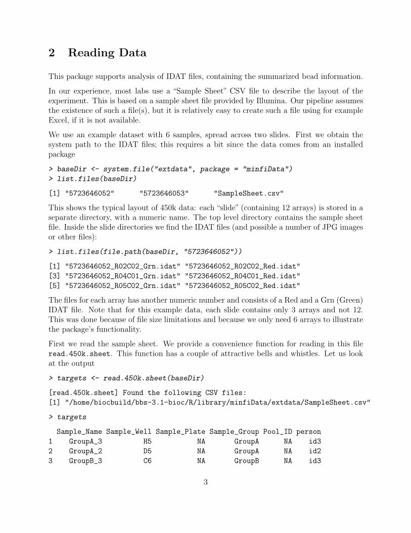
2 Reading Data

This package supports analysis of IDAT files, containing the summarized bead information.

In our experience, most labs use a “Sample Sheet” CSV file to describe the layout of theexperiment. This is based on a sample sheet file provided by Illumina. Our pipeline assumesthe existence of such a file(s), but it is relatively easy to create such a file using for exampleExcel, if it is not available.

We use an example dataset with 6 samples, spread across two slides. First we obtain thesystem path to the IDAT files; this requires a bit since the data comes from an installedpackage

> baseDir <- system.file("extdata", package = "minfiData")

> list.files(baseDir)

[1] "5723646052" "5723646053" "SampleSheet.csv"

This shows the typical layout of 450k data: each “slide” (containing 12 arrays) is stored in aseparate directory, with a numeric name. The top level directory contains the sample sheetfile. Inside the slide directories we find the IDAT files (and possible a number of JPG imagesor other files):

> list.files(file.path(baseDir, "5723646052"))

[1] "5723646052_R02C02_Grn.idat" "5723646052_R02C02_Red.idat"

[3] "5723646052_R04C01_Grn.idat" "5723646052_R04C01_Red.idat"

[5] "5723646052_R05C02_Grn.idat" "5723646052_R05C02_Red.idat"

The files for each array has another numeric number and consists of a Red and a Grn (Green)IDAT file. Note that for this example data, each slide contains only 3 arrays and not 12.This was done because of file size limitations and because we only need 6 arrays to illustratethe package’s functionality.

First we read the sample sheet. We provide a convenience function for reading in this fileread.450k.sheet. This function has a couple of attractive bells and whistles. Let us lookat the output

> targets <- read.450k.sheet(baseDir)

[read.450k.sheet] Found the following CSV files:

[1] "/home/biocbuild/bbs-3.1-bioc/R/library/minfiData/extdata/SampleSheet.csv"

> targets

Sample_Name Sample_Well Sample_Plate Sample_Group Pool_ID person

1 GroupA_3 H5 NA GroupA NA id3

2 GroupA_2 D5 NA GroupA NA id2

3 GroupB_3 C6 NA GroupB NA id3

3

4 GroupB_1 F7 NA GroupB NA id1

5 GroupA_1 G7 NA GroupA NA id1

6 GroupB_2 H7 NA GroupB NA id2

age sex status Array Slide

1 83 M normal R02C02 5723646052

2 58 F normal R04C01 5723646052

3 83 M cancer R05C02 5723646052

4 75 F cancer R04C02 5723646053

5 75 F normal R05C02 5723646053

6 58 F cancer R06C02 5723646053

Basename

1 /home/biocbuild/bbs-3.1-bioc/R/library/minfiData/extdata/5723646052/5723646052_R02C02

2 /home/biocbuild/bbs-3.1-bioc/R/library/minfiData/extdata/5723646052/5723646052_R04C01

3 /home/biocbuild/bbs-3.1-bioc/R/library/minfiData/extdata/5723646052/5723646052_R05C02

4 /home/biocbuild/bbs-3.1-bioc/R/library/minfiData/extdata/5723646053/5723646053_R04C02

5 /home/biocbuild/bbs-3.1-bioc/R/library/minfiData/extdata/5723646053/5723646053_R05C02

6 /home/biocbuild/bbs-3.1-bioc/R/library/minfiData/extdata/5723646053/5723646053_R06C02

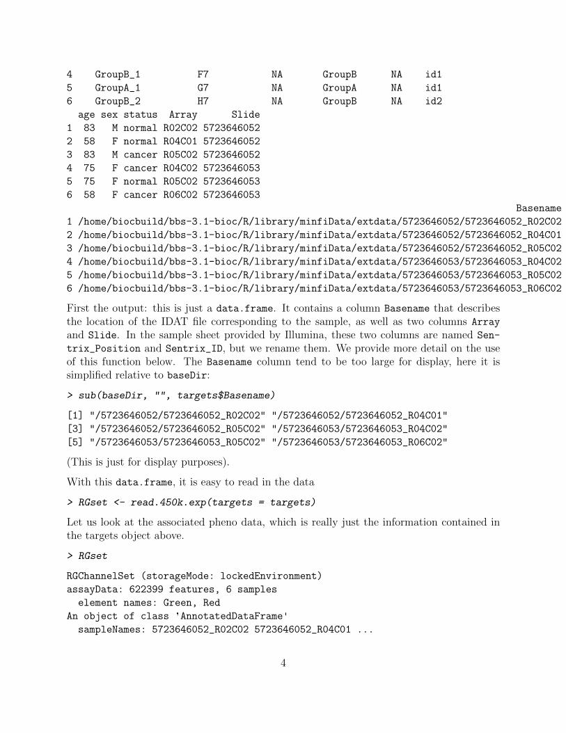
First the output: this is just a data.frame. It contains a column Basename that describesthe location of the IDAT file corresponding to the sample, as well as two columns Array

and Slide. In the sample sheet provided by Illumina, these two columns are named Sen-

trix_Position and Sentrix_ID, but we rename them. We provide more detail on the useof this function below. The Basename column tend to be too large for display, here it issimplified relative to baseDir:

> sub(baseDir, "", targets$Basename)

[1] "/5723646052/5723646052_R02C02" "/5723646052/5723646052_R04C01"

[3] "/5723646052/5723646052_R05C02" "/5723646053/5723646053_R04C02"

[5] "/5723646053/5723646053_R05C02" "/5723646053/5723646053_R06C02"

(This is just for display purposes).

With this data.frame, it is easy to read in the data

> RGset <- read.450k.exp(targets = targets)

Let us look at the associated pheno data, which is really just the information contained inthe targets object above.

> RGset

RGChannelSet (storageMode: lockedEnvironment)

assayData: 622399 features, 6 samples

element names: Green, Red

An object of class 'AnnotatedDataFrame'

sampleNames: 5723646052_R02C02 5723646052_R04C01 ...

4

5723646053_R06C02 (6 total)

varLabels: Sample_Name Sample_Well ... filenames (13 total)

varMetadata: labelDescription

Annotation

array: IlluminaHumanMethylation450k

annotation: ilmn12.hg19

> pd <- pData(RGset)

> pd[,1:4]

Sample_Name Sample_Well Sample_Plate Sample_Group

5723646052_R02C02 GroupA_3 H5 NA GroupA

5723646052_R04C01 GroupA_2 D5 NA GroupA

5723646052_R05C02 GroupB_3 C6 NA GroupB

5723646053_R04C02 GroupB_1 F7 NA GroupB

5723646053_R05C02 GroupA_1 G7 NA GroupA

5723646053_R06C02 GroupB_2 H7 NA GroupB

The read.450k.exp also makes it possible to read in an entire directory or directory tree(with recursive set to TRUE) by using the function just with the argument base and tar-

gets=NULL, like

> RGset2 = read.450k.exp(file.path(baseDir, "5723646052"))

> RGset3 = read.450k.exp(baseDir, recursive = TRUE)

Advanced notes on Reading Data

The only important column in sheet data.frame used in the targets argument for theread.450k.exp function is a column names Basename. Typically, such an object would alsohave columns named Array, Slide, and (optionally) Plate.

We used sheet data files build on top of the Sample Sheet data file provided by Illumina.This is a CSV file, with a header. In this case we assume that the phenotype data startsafter a line beginning with [Data] (or that there is no header present).

It is also easy to read a sample sheet “manually”, using the function read.csv. Here, weknow that we want to skip the first 7 lines of the file.

> targets2 <- read.csv(file.path(baseDir, "SampleSheet.csv"),

+ stringsAsFactors = FALSE, skip = 7)

> targets2

Sample_Name Sample_Well Sample_Plate Sample_Group Pool_ID

1 GroupA_3 H5 NA GroupA NA

2 GroupA_2 D5 NA GroupA NA

3 GroupB_3 C6 NA GroupB NA

5

4 GroupB_1 F7 NA GroupB NA

5 GroupA_1 G7 NA GroupA NA

6 GroupB_2 H7 NA GroupB NA

Sentrix_ID Sentrix_Position person age sex status

1 5723646052 R02C02 id3 83 M normal

2 5723646052 R04C01 id2 58 F normal

3 5723646052 R05C02 id3 83 M cancer

4 5723646053 R04C02 id1 75 F cancer

5 5723646053 R05C02 id1 75 F normal

6 5723646053 R06C02 id2 58 F cancer

We now need to populate a Basename column. On possible approach is the following

> targets2$Basename <- file.path(baseDir, targets2$Sentrix_ID,

+ paste0(targets2$Sentrix_ID,

+ targets2$Sentrix_Position))

Finally, minfi contains a file-based parser: read.450k. The return object represents the redand the green channel measurements of the samples. A useful function that we get from thepackage Biobase is combine that combines (“adds”) two sets of samples. This allows the userto manually build up an RGChannelSet.

3 Quality Control

minfi provides several plots that can be useful for identifying samples with data qualityproblems. These functions can display summaries of signal from the array (e.g. densityplots) as well as the values of several types of control probes included on the array. Ourunderstanding of the expected sample behavior in the QC plots is still evolving and willimprove as the number of available samples from the array increases. A good rule of thumbis to be wary of samples whose behavior deviates from that of others in the same or similarexperiments.

The wrapper function qcReport function can be used to produce a PDF QC report of themost common plots. If provided, the optional sample name and group options will be usedto label and color plots. Samples within a group are assigned the same color. The samplegroup option can also be used as a very cursory way to check for batch effects (e.g. by settingit to a processing day variable.)

> qcReport(RGset, sampNames = pd$Sample_Name,

+ sampGroups = pd$Sample_Group, pdf = "qcReport.pdf")

The components of the QC report can also be customized and produced individually asdetailed below.

6

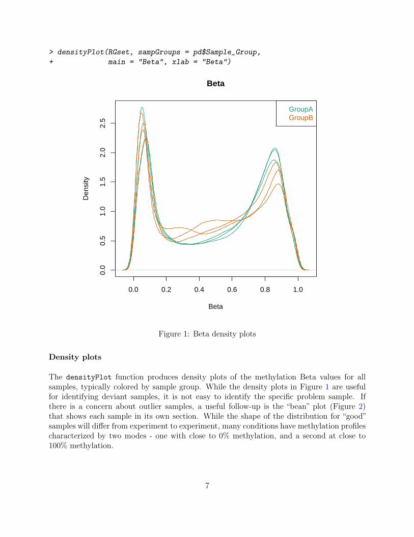
> densityPlot(RGset, sampGroups = pd$Sample_Group,

+ main = "Beta", xlab = "Beta")

0.0 0.2 0.4 0.6 0.8 1.0

0.0

0.5

1.0

1.5

2.0

2.5

Beta

Beta

Den

sity

GroupAGroupB

Figure 1: Beta density plots

Density plots

The densityPlot function produces density plots of the methylation Beta values for allsamples, typically colored by sample group. While the density plots in Figure 1 are usefulfor identifying deviant samples, it is not easy to identify the specific problem sample. Ifthere is a concern about outlier samples, a useful follow-up is the “bean” plot (Figure 2)that shows each sample in its own section. While the shape of the distribution for “good”samples will differ from experiment to experiment, many conditions have methylation profilescharacterized by two modes - one with close to 0% methylation, and a second at close to100% methylation.

7

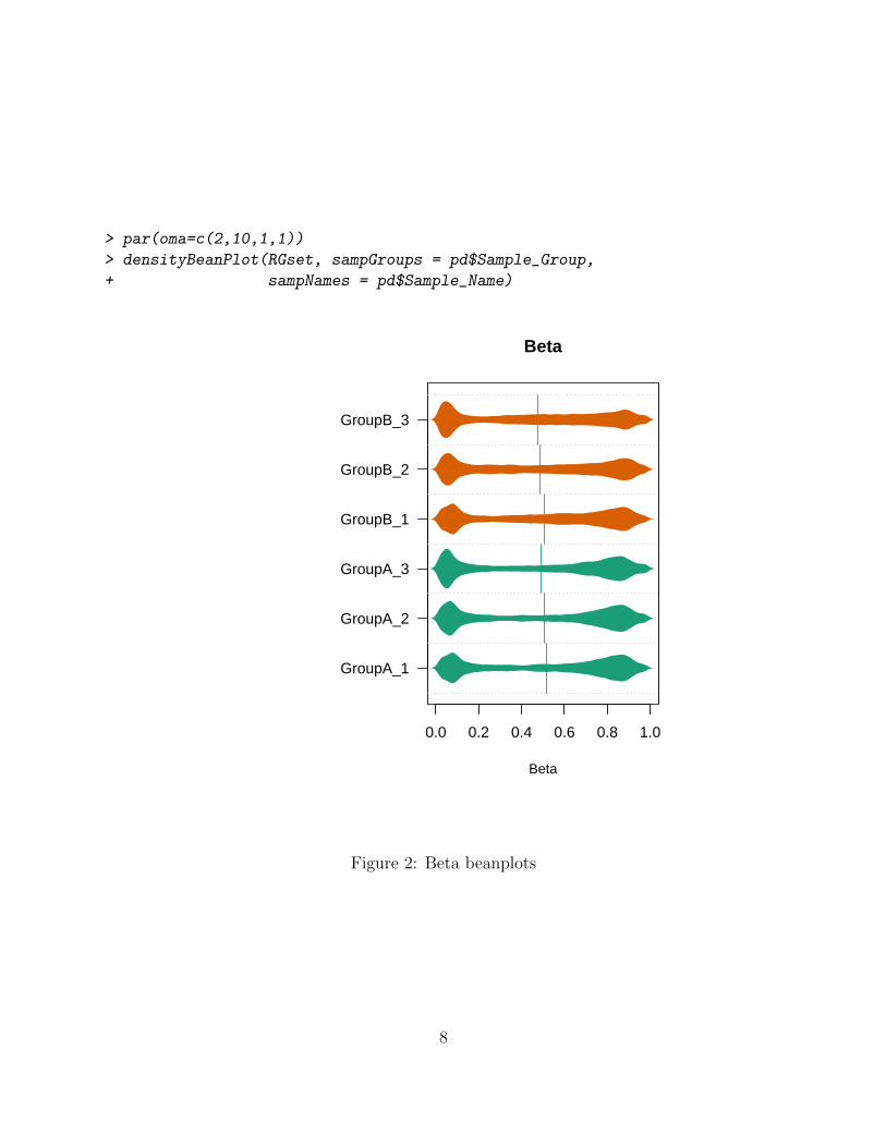
> par(oma=c(2,10,1,1))

> densityBeanPlot(RGset, sampGroups = pd$Sample_Group,

+ sampNames = pd$Sample_Name)

0.0 0.2 0.4 0.6 0.8 1.0

GroupA_1

GroupA_2

GroupA_3

GroupB_1

GroupB_2

GroupB_3

Beta

Beta

Figure 2: Beta beanplots

8

Control probe plots

The controlStripPlot function allows plotting of individual control probe types (Figure3). The following control probes are available on the array:

BISULFITE CONVERSION I 12

BISULFITE CONVERSION II 4

EXTENSION 4

HYBRIDIZATION 3

NEGATIVE 614

NON-POLYMORPHIC 4

NORM_A 32

NORM_C 61

NORM_G 32

NORM_T 61

SPECIFICITY I 12

SPECIFICITY II 3

STAINING 6

TARGET REMOVAL 2

4 Preprocessing (normalization)

Preprocessing (normalization) takes as input a RGChannelSet and returns a MethylSet.

A number of preprocessing options are available (and we are working on more methods).Each set of methods are implemented as a function preprocessXXX with XXX being thename of the method. Each method may have a number of tuning parameters.

“Raw” preprocessing means simply converting the Red and the Green channel into a Methy-lated and Unmethylated signal

> MSet.raw <- preprocessRaw(RGset)

We have also implemented preprocessing choices as available in Genome Studio. Thesechoices follow the description provided in the Illumina documentation and has been validatedby comparing the output of Genome Studio to the output of these algorithms, and this showsthe two approaches to be roughly equivalent (for a precise statement, see the manual pages).

Genome studio allows for background subtraction (also called background normalization) aswell as something they term control normalization. Both of these are optional and turningboth of them off is equivalent to raw preprocessing (preprocessRaw).

> MSet.norm <- preprocessIllumina(RGset, bg.correct = TRUE,

+ normalize = "controls", reference = 2)

9

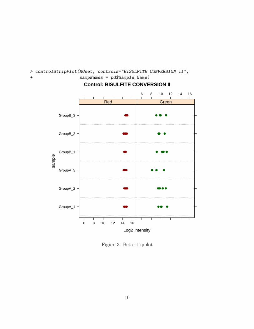
> controlStripPlot(RGset, controls="BISULFITE CONVERSION II",

+ sampNames = pd$Sample_Name)

Control: BISULFITE CONVERSION II

Log2 Intensity

sam

ple

GroupA_1

GroupA_2

GroupA_3

GroupB_1

GroupB_2

GroupB_3

6 8 10 12 14 16

●●●●

●●●●

●●●●

●●●●

●●●●

●●●●

Red

6 8 10 12 14 16

●● ●●

●● ●●

●● ●●

●● ●●

●● ●●

●● ●●

Green

Figure 3: Beta stripplot

10

The reference = 2 selects which array to use as “reference” which is an arbitrary array (weare not sure how Genome Studio makes its choice of reference).

Operating on a MethylSet

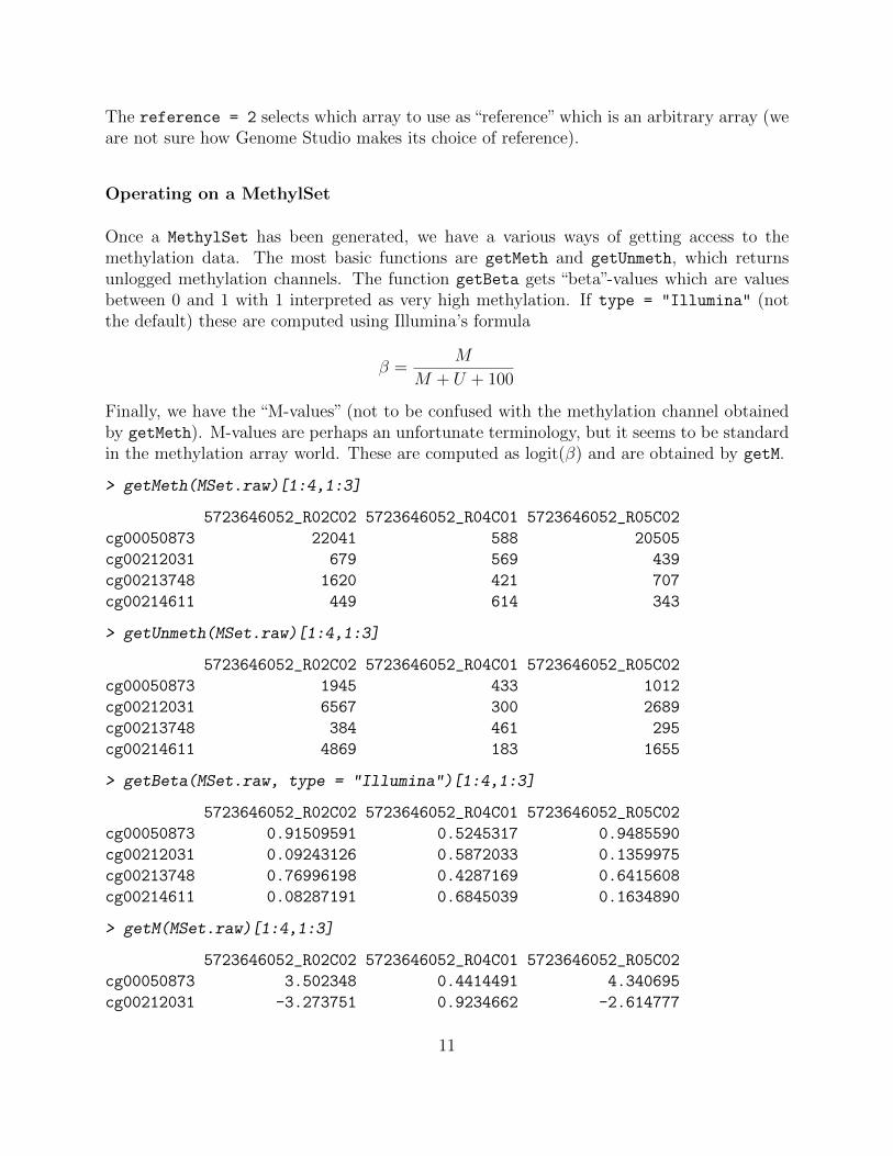
Once a MethylSet has been generated, we have a various ways of getting access to themethylation data. The most basic functions are getMeth and getUnmeth, which returnsunlogged methylation channels. The function getBeta gets “beta”-values which are valuesbetween 0 and 1 with 1 interpreted as very high methylation. If type = "Illumina" (notthe default) these are computed using Illumina’s formula

β =M

M + U + 100

Finally, we have the “M-values” (not to be confused with the methylation channel obtainedby getMeth). M-values are perhaps an unfortunate terminology, but it seems to be standardin the methylation array world. These are computed as logit(β) and are obtained by getM.

> getMeth(MSet.raw)[1:4,1:3]

5723646052_R02C02 5723646052_R04C01 5723646052_R05C02

cg00050873 22041 588 20505

cg00212031 679 569 439

cg00213748 1620 421 707

cg00214611 449 614 343

> getUnmeth(MSet.raw)[1:4,1:3]

5723646052_R02C02 5723646052_R04C01 5723646052_R05C02

cg00050873 1945 433 1012

cg00212031 6567 300 2689

cg00213748 384 461 295

cg00214611 4869 183 1655

> getBeta(MSet.raw, type = "Illumina")[1:4,1:3]

5723646052_R02C02 5723646052_R04C01 5723646052_R05C02

cg00050873 0.91509591 0.5245317 0.9485590

cg00212031 0.09243126 0.5872033 0.1359975

cg00213748 0.76996198 0.4287169 0.6415608

cg00214611 0.08287191 0.6845039 0.1634890

> getM(MSet.raw)[1:4,1:3]

5723646052_R02C02 5723646052_R04C01 5723646052_R05C02

cg00050873 3.502348 0.4414491 4.340695

cg00212031 -3.273751 0.9234662 -2.614777

11

cg00213748 2.076816 -0.1309465 1.260995

cg00214611 -3.438838 1.7463950 -2.270551

MDS plots

After preprocessing the raw data to obtain methylation estimates, Multi-dimensional scaling(MDS) plots provide a quick way to get a first sense of the relationship between samples.They are similar to the more familiar PCA plots and display a two-dimensional approxima-tion of sample-to-sample Euclidean distance. Note that while the plot visualizes the distancein epigenomic profiles between samples, the absolute positions of the points is not meaning-ful. One often expects to see greater between-group than within-group distances (althoughthis clearly depends on the particular experiment). The most variable locations are usedwhen calculating sample distances, with the number specified by the numPositions option.Adding sample labels to the MDS plot is a useful way of identifying outliers (figure 4) thatbehave differently from their peers.

The validation of preprocessIllumina

By validation we mean “yielding output that is equivalent to Genome Studio”.

Illumina offers two steps: control normalization and background subtraction (normalization).Using output from Genome Studio we are certain that the control normalization step isvalidated, with the following caveat: control normalization requires the selection of one arrayamong the 12 arrays on a chip as a reference array. It is currently unclear how Genome Studioselects the reference; if you know the reference array we can recreate Genome Studio exactly.Background subtraction (normalization) is almost correct: for 18 out of 24 arrays we seeexact equivalence and for the remaining 6 out of 24 arrays we only see small discrepancies(a per-array max difference of 1-4 for unlogged intensities). A script for doing this is inscripts/GenomeStudio.R.

Subset-quantile within array normalisation (SWAN)

SWAN (subset-quantile within array normalisation) is a new normalization method for Illu-mina 450k arrays. What follows is a brief description of the methodology (written by theauthors of SWAN):

Technical differences have been demonstrated to exist between the Type I and Type II assaydesigns within a single 450K array[3, 4]. Using the SWAN method substantially reduces thetechnical variability between the assay designs whilst maintaining the important biologicaldifferences. The SWAN method makes the assumption that the number of CpGs within the50bp probe sequence reflects the underlying biology of the region being interrogated. Hence,

12

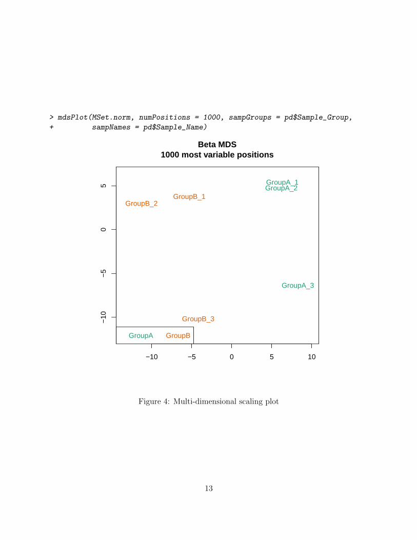
> mdsPlot(MSet.norm, numPositions = 1000, sampGroups = pd$Sample_Group,

+ sampNames = pd$Sample_Name)

−10 −5 0 5 10

−10

−5

05

Beta MDS1000 most variable positions

GroupA_3

GroupA_2

GroupB_3

GroupB_1

GroupA_1

GroupB_2

GroupA GroupB

Figure 4: Multi-dimensional scaling plot

13

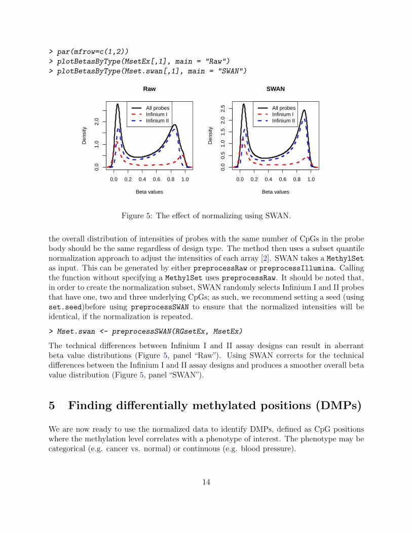
> par(mfrow=c(1,2))

> plotBetasByType(MsetEx[,1], main = "Raw")

> plotBetasByType(Mset.swan[,1], main = "SWAN")

0.0 0.2 0.4 0.6 0.8 1.0

0.0

1.0

2.0

Raw

Beta values

Den

sity

All probesInfinium IInfinium II

0.0 0.2 0.4 0.6 0.8 1.0

0.0

0.5

1.0

1.5

2.0

2.5

SWAN

Beta values

Den

sity

All probesInfinium IInfinium II

Figure 5: The effect of normalizing using SWAN.

the overall distribution of intensities of probes with the same number of CpGs in the probebody should be the same regardless of design type. The method then uses a subset quantilenormalization approach to adjust the intensities of each array [2]. SWAN takes a MethylSet

as input. This can be generated by either preprocessRaw or preprocessIllumina. Callingthe function without specifying a MethylSet uses preprocessRaw. It should be noted that,in order to create the normalization subset, SWAN randomly selects Infinium I and II probesthat have one, two and three underlying CpGs; as such, we recommend setting a seed (usingset.seed)before using preprocessSWAN to ensure that the normalized intensities will beidentical, if the normalization is repeated.

> Mset.swan <- preprocessSWAN(RGsetEx, MsetEx)

The technical differences between Infinium I and II assay designs can result in aberrantbeta value distributions (Figure 5, panel “Raw”). Using SWAN corrects for the technicaldifferences between the Infinium I and II assay designs and produces a smoother overall betavalue distribution (Figure 5, panel “SWAN”).

5 Finding differentially methylated positions (DMPs)

We are now ready to use the normalized data to identify DMPs, defined as CpG positionswhere the methylation level correlates with a phenotype of interest. The phenotype may becategorical (e.g. cancer vs. normal) or continuous (e.g. blood pressure).

14

We will create a 20,000 CpG subset of our dataset to speed up the demo:

> mset <- MSet.norm[1:20000,]

Categorical phenotypes

The dmpFinder function uses an F-test to identify positions that are differentially methylatedbetween (two or more) groups. Tests are performed on logit transformed Beta values asrecommended in Pan et al. Care should be taken if you have zeroes in either the Meth orthe Unmeth matrix. One possibility is to threshold the beta values, so they are always inthe interval [ε, 1 − ε]. We call ε the betaThreshold

Here we find the differences between GroupA and GroupB.

> table(pd$Sample_Group)

GroupA GroupB

3 3

> M <- getM(mset, type = "beta", betaThreshold = 0.001)

> dmp <- dmpFinder(M, pheno=pd$Sample_Group, type="categorical")

> head(dmp)

intercept f pval qval

cg10805483 -9.964341 1706.1212 2.053224e-06 0.02639720

cg20386875 -5.434480 1445.1107 2.859882e-06 0.02639720

cg07155336 -5.799521 550.9746 1.952772e-05 0.05148498

cg13059719 -2.505878 549.6611 1.962059e-05 0.05148498

cg08343042 -3.565042 506.2230 2.310839e-05 0.05148498

cg23098069 1.532107 497.6219 2.390872e-05 0.05148498

dmpFinder returns a table of CpG positions sorted by differential methylation p-value.

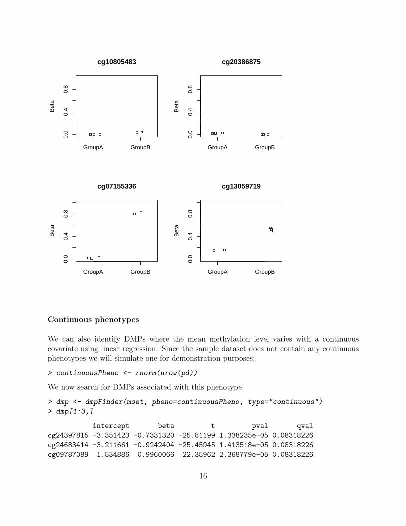
We can use the plotCpG function to plot methylation levels at individual positions:

> cpgs <- rownames(dmp)[1:4]

> par(mfrow=c(2,2))

> plotCpg(mset, cpg=cpgs, pheno=pd$Sample_Group)

15

GroupA GroupB

0.0

0.4

0.8

cg10805483

Bet

a

GroupA GroupB

0.0

0.4

0.8

cg20386875

Bet

a

GroupA GroupB

0.0

0.4

0.8

cg07155336

Bet

a

GroupA GroupB

0.0

0.4

0.8

cg13059719

Bet

a

Continuous phenotypes

We can also identify DMPs where the mean methylation level varies with a continuouscovariate using linear regression. Since the sample dataset does not contain any continuousphenotypes we will simulate one for demonstration purposes:

> continuousPheno <- rnorm(nrow(pd))

We now search for DMPs associated with this phenotype.

> dmp <- dmpFinder(mset, pheno=continuousPheno, type="continuous")

> dmp[1:3,]

intercept beta t pval qval

cg24397815 -3.351423 -0.7331320 -25.81199 1.338235e-05 0.08318226

cg24683414 -3.211661 -0.9242404 -25.45945 1.413518e-05 0.08318226

cg09787089 1.534886 0.9960066 22.35962 2.368779e-05 0.08318226

16

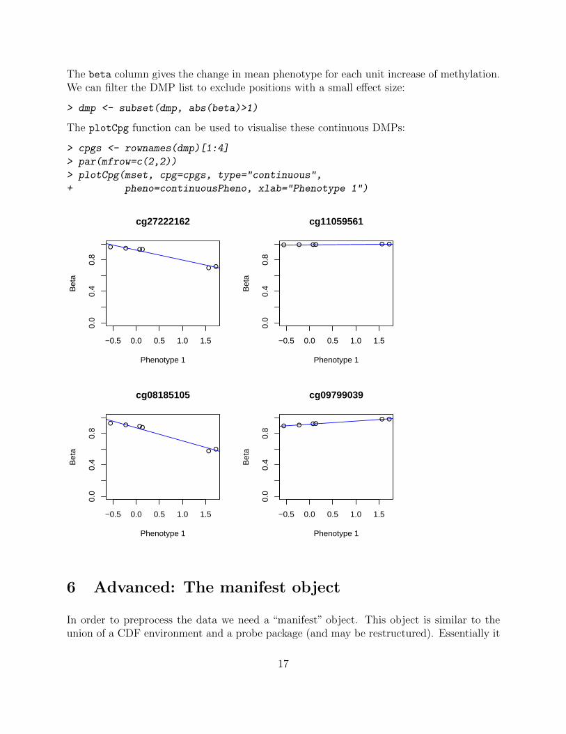
The beta column gives the change in mean phenotype for each unit increase of methylation.We can filter the DMP list to exclude positions with a small effect size:

> dmp <- subset(dmp, abs(beta)>1)

The plotCpg function can be used to visualise these continuous DMPs:

> cpgs <- rownames(dmp)[1:4]

> par(mfrow=c(2,2))

> plotCpg(mset, cpg=cpgs, type="continuous",

+ pheno=continuousPheno, xlab="Phenotype 1")

● ●

●

●●

●

−0.5 0.0 0.5 1.0 1.5

0.0

0.4

0.8

cg27222162

Phenotype 1

Bet

a

● ● ●●● ●

−0.5 0.0 0.5 1.0 1.5

0.0

0.4

0.8

cg11059561

Phenotype 1

Bet

a

● ●

●

●●

●

−0.5 0.0 0.5 1.0 1.5

0.0

0.4

0.8

cg08185105

Phenotype 1

Bet

a

● ●●

●●●

−0.5 0.0 0.5 1.0 1.5

0.0

0.4

0.8

cg09799039

Phenotype 1

Bet

a

6 Advanced: The manifest object

In order to preprocess the data we need a “manifest” object. This object is similar to theunion of a CDF environment and a probe package (and may be restructured). Essentially it

17

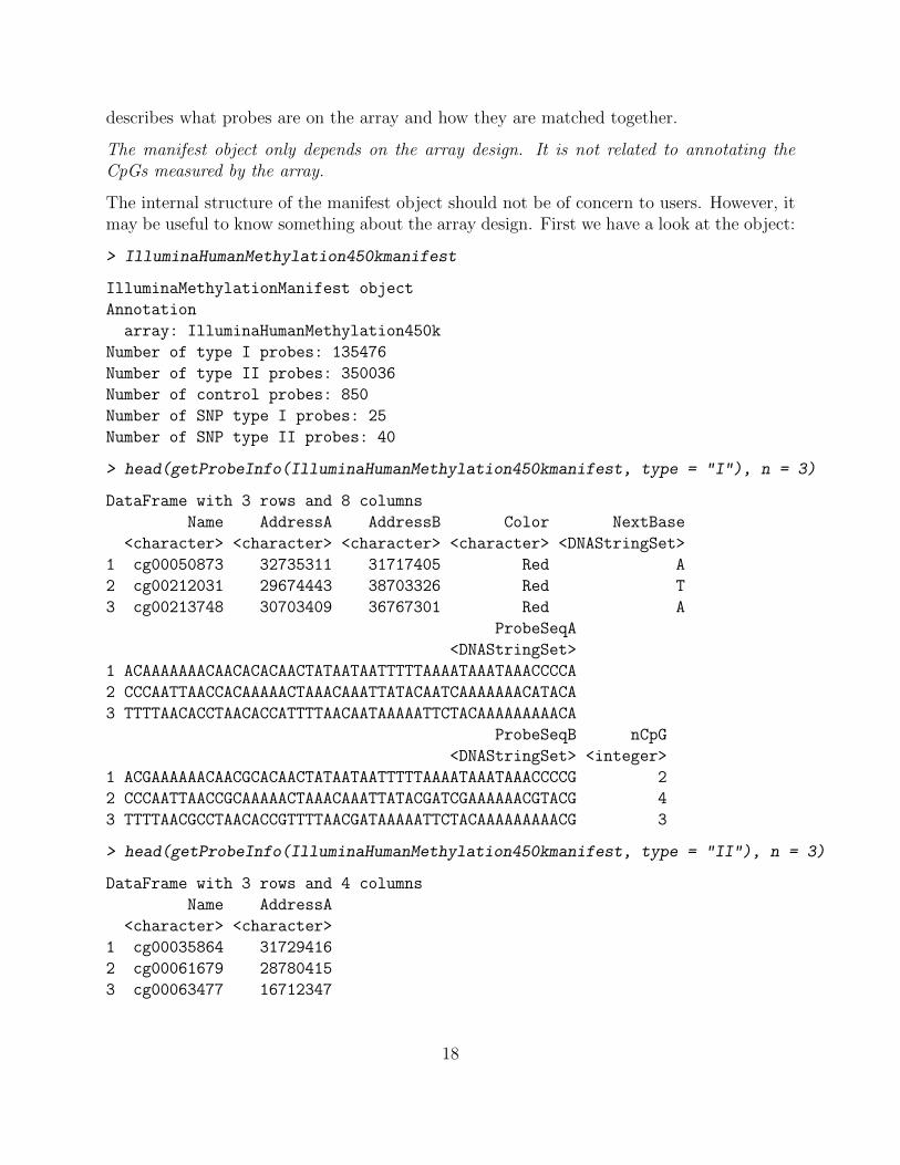
describes what probes are on the array and how they are matched together.

The manifest object only depends on the array design. It is not related to annotating theCpGs measured by the array.

The internal structure of the manifest object should not be of concern to users. However, itmay be useful to know something about the array design. First we have a look at the object:

> IlluminaHumanMethylation450kmanifest

IlluminaMethylationManifest object

Annotation

array: IlluminaHumanMethylation450k

Number of type I probes: 135476

Number of type II probes: 350036

Number of control probes: 850

Number of SNP type I probes: 25

Number of SNP type II probes: 40

> head(getProbeInfo(IlluminaHumanMethylation450kmanifest, type = "I"), n = 3)

DataFrame with 3 rows and 8 columns

Name AddressA AddressB Color NextBase

<character> <character> <character> <character> <DNAStringSet>

1 cg00050873 32735311 31717405 Red A

2 cg00212031 29674443 38703326 Red T

3 cg00213748 30703409 36767301 Red A

ProbeSeqA

<DNAStringSet>

1 ACAAAAAAACAACACACAACTATAATAATTTTTAAAATAAATAAACCCCA

2 CCCAATTAACCACAAAAACTAAACAAATTATACAATCAAAAAAACATACA

3 TTTTAACACCTAACACCATTTTAACAATAAAAATTCTACAAAAAAAAACA

ProbeSeqB nCpG

<DNAStringSet> <integer>

1 ACGAAAAAACAACGCACAACTATAATAATTTTTAAAATAAATAAACCCCG 2

2 CCCAATTAACCGCAAAAACTAAACAAATTATACGATCGAAAAAACGTACG 4

3 TTTTAACGCCTAACACCGTTTTAACGATAAAAATTCTACAAAAAAAAACG 3

> head(getProbeInfo(IlluminaHumanMethylation450kmanifest, type = "II"), n = 3)

DataFrame with 3 rows and 4 columns

Name AddressA

<character> <character>

1 cg00035864 31729416

2 cg00061679 28780415

3 cg00063477 16712347

18

ProbeSeqA nCpG

<DNAStringSet> <integer>

1 AAAACACTAACAATCTTATCCACATAAACCCTTAAATTTATCTCAAATTC 0

2 AAAACATTAAAAAACTAATTCACTACTATTTAATTACTTTATTTTCCATC 0

3 TATTCTTCCACACAAAATACTAAACRTATATTTACAAAAATACTTCCATC 1

> head(getProbeInfo(IlluminaHumanMethylation450kmanifest, type = "Control"), n = 3)

DataFrame with 3 rows and 4 columns

Address Type Color ExtendedType

<character> <character> <character> <character>

1 21630339 STAINING -99 DNP(20K)

2 27630314 STAINING Red DNP (High)

3 43603326 STAINING Purple DNP (Bkg)

The 450k array has a rather special design. It is a two-color array, so each array will havean associated Green signal and a Red signal.

On the 450k array, a CpG may be measured by a “type I” or “type II” design. The literatureoften uses the term“type I/II probes” which we believe is unfortunate (see next paragraph).

Each CpG has an associated methylated and un-methylated signal. If the CpG is of “type I”,the methylation and un-methylation signal are originating from two different probes (physicallocation on the array). There is one set of “type I” CpGs where the signal comes from theGreen channel for both probes (and the Red channel measures nothing) and another setwhere the signal comes from the Red channel. If the CpG is of “type II”, a single probe(physical location) is being used to measure the methylated/un-methylated signal and themethylated signal is always measured in the Green channel.

This is reflected in the manifest object seen above: “type I” CpGs have “AddressA”, “Ad-dressB” (this is a link to the physical location on the array) as well as “ProbeSeqA” and“ProbeSeqB”. They also have a “Col” indicator (which channel is the methylated signal com-ing from). In contrast “type II” CpGs have a single “Address”, one “ProbeSeq” and no colorinformation.

Because CpGs of “type I” are measured using two different physical probes, we dislike callingthe probes “type I/II” and instead attaches the type to the CpG itself.

Note that Illumina uses a special “cgXXX” name for the CpGs. There is actually a meaningto this, not unlike the meaning associated with “rsXXX” numbers for SNPs. Essentially theXXX is a hash of the bases surrounding the CpG, making the cgXXX numbers independentof genome version. Illumina has a technical note describing this.

19

7 SessionInfo

� R version 3.2.0 (2015-04-16), x86_64-unknown-linux-gnu

� Locale: LC_CTYPE=en_US.UTF-8, LC_NUMERIC=C, LC_TIME=en_US.UTF-8,LC_COLLATE=C, LC_MONETARY=en_US.UTF-8, LC_MESSAGES=en_US.UTF-8,LC_PAPER=en_US.UTF-8, LC_NAME=C, LC_ADDRESS=C, LC_TELEPHONE=C,LC_MEASUREMENT=en_US.UTF-8, LC_IDENTIFICATION=C

� Base packages: base, datasets, grDevices, graphics, methods, parallel, stats, stats4,utils

� Other packages: Biobase 2.28.0, BiocGenerics 0.14.0, Biostrings 2.36.0,GenomeInfoDb 1.4.0, GenomicRanges 1.20.0, IRanges 2.2.0,IlluminaHumanMethylation450kanno.ilmn12.hg19 0.2.1,IlluminaHumanMethylation450kmanifest 0.4.0, S4Vectors 0.6.0, XVector 0.8.0,bumphunter 1.8.0, foreach 1.4.2, iterators 1.0.7, lattice 0.20-31, locfit 1.5-9.1,minfi 1.14.0, minfiData 0.9.1

� Loaded via a namespace (and not attached): AnnotationDbi 1.30.0,BiocParallel 1.2.0, DBI 0.3.1, GEOquery 2.34.0, GenomicAlignments 1.4.0,GenomicFeatures 1.20.0, MASS 7.3-40, RColorBrewer 1.1-2, RCurl 1.95-4.5,RSQLite 1.0.0, Rcpp 0.11.5, Rsamtools 1.20.0, XML 3.98-1.1, annotate 1.46.0,base64 1.1, beanplot 1.2, biomaRt 2.24.0, bitops 1.0-6, codetools 0.2-11, digest 0.6.8,doRNG 1.6, futile.logger 1.4, futile.options 1.0.0, genefilter 1.50.0, grid 3.2.0,illuminaio 0.10.0, lambda.r 1.1.7, limma 3.24.0, matrixStats 0.14.0, mclust 5.0.0,multtest 2.24.0, nlme 3.1-120, nor1mix 1.2-0, pkgmaker 0.22, plyr 1.8.1,preprocessCore 1.30.0, quadprog 1.5-5, registry 0.2, reshape 0.8.5, rngtools 1.2.4,rtracklayer 1.28.0, siggenes 1.42.0, splines 3.2.0, stringr 0.6.2, survival 2.38-1,tools 3.2.0, xtable 1.7-4, zlibbioc 1.14.0

References

[1] Martin J Aryee, Andrew E Jaffe, Hector Corrada Bravo, Christine Ladd-Acosta, An-drew P Feinberg, Kasper D Hansen, and Rafael A Irizarry. Minfi: a flexible and com-prehensive Bioconductor package for the analysis of Infinium DNA methylation microar-rays. Bioinformatics, 30(10):1363–1369, 2014. doi:10.1093/bioinformatics/btu049,PMID:24478339.

[2] Jovana Maksimovic, Lavinia Gordon, and Alicia Oshlack. SWAN: Subset quantileWithin-Array Normalization for Illumina Infinium HumanMethylation450 BeadChips.Genome Biology, 13(6):R44, 2012. doi:10.1186/gb-2012-13-6-r44, PMID:22703947.

20

[3] Marina Bibikova, Bret Barnes, Chan Tsan, Vincent Ho, Brandy Klotzle, Jennie M Le,David Delano, Lu Zhang, Gary P Schroth, Kevin L Gunderson, Jian-Bing Fan, andRichard Shen. High density DNA methylation array with single CpG site resolution.Genomics, 98(4):288–295, 2011. doi:10.1016/j.ygeno.2011.07.007, PMID:21839163.

[4] Sarah Dedeurwaerder, Matthieu Defrance, Emilie Calonne, Helene Denis, ChristosSotiriou, and Francois Fuks. Evaluation of the Infinium Methylation 450K technology.Epigenomics, 3(6):771–784, 2011. doi:10.2217/epi.11.105, PMID:22126295.

[5] Jean-Philippe Fortin, Aurelie Labbe, Mathieu Lemire, Brent W Zanke, Thomas J Hud-son, Elana J Fertig, Celia MT Greenwood, and Kasper D Hansen. Functional normaliza-tion of 450k methylation array data improves replication in large cancer studies. GenomeBiology, 15(11):503, 2014. doi:10.1186/s13059-014-0503-2, PMID:25599564.

[6] Timothy J Triche, Daniel J Weisenberger, David Van Den Berg, Peter W Laird, andKimberly D Siegmund. Low-level processing of Illumina Infinium DNA MethylationBeadArrays. Nucleic Acids Research, 41(7):e90, 2013. doi:10.1093/nar/gkt090, PMID:23476028.

[7] Juan Sandoval, Holger Heyn, Sebastian Moran, Jordi Serra-Musach, Miguel A Pujana,Marina Bibikova, and Manel Esteller. Validation of a DNA methylation microarrayfor 450,000 CpG sites in the human genome. Epigenetics, 6(6):692–702, 2011. doi:

10.4161/epi.6.6.16196, PMID:21593595.

[8] Pan Du, Xiao Zhang, Chiang-Ching Huang, Nadereh Jafari, Warren A Kibbe, LifangHou, and Simon M Lin. Comparison of Beta-value and M-value methods for quantifyingmethylation levels by microarray analysis. BMC Bioinformatics, 11:587, 2010. doi:

10.1186/1471-2105-11-587, PMID:21118553.

21