Michael Murray SUR and SES

Sections 14.10 and 14.11; Appendix 14.A

More Estimators for Systemsof Equations

14.10 Seemingly Unrelated RegressionsIn learning about simultaneous equations models, our centralfocus has been on the endogenous explanators that make or-dinary least squares (OLS) inconsistent and that threaten theidentification of the equations. What about systems of equa-tions in which there are only untroublesome explanators?OLS is consistent when applied to such equations because theexplanators are contemporaneously uncorrelated with the dis-turbances. Is there anything more to be said about suchseemingly unrelated regressions?1 Econometrician ArnoldZellner of the University of Chicago, who first examined suchmultiple equations, did find more to say. Zellner found thatsystems of equations sometimes permit more efficient estima-tion than if the individual equations were estimated one at atime, separately from one another. Unrelated systems of equa-tions with no troublesome explanators, but with contempora-neous correlations across the disturbances of the equationsZellner named seemingly unrelated regressions SUR. Zellnershowed how we can estimate such equations more efficientlyby estimating them all together rather than by using OLS toestimate each equation separately. This section introduces

EXT 5-1

Web Extension 5

WHAT IS THE DGP?

EXT 5-2 Web Extension 5

SUR here as a stepping stone to the next section, in which we examine simultane-ous equations models with disturbances that are correlated across equations.

The DGPTo illustrate a system of seemingly unrelated equations, consider a sample offirms, all of which produce two products, quilts and mattresses. The per unit costof producing quilts, depends on the price of linen, and the price of dyes, .The per unit cost of producing mattresses, depends on the price of linen andthe price of foam,

Thus we have a DGP with two equations:

14.14

and

14.15

in which and both satisfy the Gauss–Markov Assumptions individually andhave the further shared characteristics that cov for i not equal to j,and cov for all i. We further assume that the price variables are in-dependent of the disturbances, on the assumption that the small producers in oursample have no effect on the prices they face for their inputs.

It is the correlation of disturbances that earmarks seemingly unrelated regres-sions. In this example, the intuition for a correlation is the notion that firms ableto produce quilts more cheaply than average may also tend to produce mattressesmore cheaply than average—producers efficient in one operation tend to be effi-cient in other operations, as well. (According to this intuition, but thecovariance need only be nonzero for seemingly unrelated regression estimation tobe appropriate.)

The SUR Estimation ProcedureIndividually, Equations 14.14 and 14.15 satisfy the Gauss–Markov Assumptions.OLS would seem the appropriate estimation procedure for either equation. What,then, is the intuition for why OLS might not be the efficient estimation procedurefor the seemingly unrelated Equations 14.14 and 14.15? Recall our reason forweighting some observations more heavily than others. In the model with no in-tercept, we saw that disturbances of a given size misled us less about the slopewhen they were attached to observations with larger X’s. In the model with an in-tercept, this intuition applied to observations that lay further from the mean X inthe sample. The Gauss–Markov Assumptions of homoskedasticity and no serialcorrelation assured us that any one observation was as likely as any other to havea disturbance of a given size. Hence, we found that the OLS weights were optimal.

sqm 7 0,

(eqi , em

i ) = sqm

(eqi , em

j ) = 0em

ieqi

Cmi = b0 + b1Pl

i + b2Pfi + em

i ,

Cqi = a0 + a1Pl

i + a2Pdi + eq

i

Pfi.

Cmi ,

PidPl

iCqi ,

More Estimators for Systems of Equations EXT 5-3

Suppose, however, we knew the correlation between the disturbances and thevariances of the disturbances, and we knew the actual value of the first distur-bance in the quilt equation, but not the value of the first disturbance in the mat-tress equation. Let us further assume the first observation has explanators thattake on the sample average values. Would we use OLS to estimate the mattressequation? Not if we think this observation lies closer to the true line than doother observations. The assumed information about the quilt disturbance, cou-pled with the information about the covariance between the disturbances, under-mines the presumption that all observations are equally likely to have distur-bances of a given size, and therefore undermines the rationale for the optimalityof OLS. Suppose, for example, that the disturbance on the first observation forthe cost of quilts is very small in magnitude, suggesting that the underlying distur-bance in the mattresses equation for the first observation is also very small. Be-cause this observation probably lies closer to the true line than we would other-wise think, we want to use that information in estimating the line.

How does this intuition apply in the actual circumstances in which we do notknow the size of a given residual? The choice of weighting the first observation inthe mattress regression will depend in part on how well we think we can mimicthe first observation’s disturbance in the quilt regression. If we can mimic the dis-turbances particularly well, we may decide to consider that information when weweight the first observation in the mattress equation. Because unbiased estimationwill impose constraints on the weights we use, weighting one observation moreheavily than in OLS requires weighting another observation less heavily, if we areto maintain unbiasedness.

Residuals mimic disturbances, but they are not equal to them. How reliablyresiduals mimic the disturbances for a given observation depends, in part, on howwell we estimate the true parameters (the variances of the parameter estimators),and, in part, on how far the explanators for that observation are from their aver-age values. (We are less confident in our estimates of the expected value of Y forX’s far from the mean X’s.) Therefore, how the quilt information influences ourmattress equation weight for the first observation will depend on the values of theexplanators in the quilt equation. Similarly, how influenced our weight for thefirst observation in the quilt equation will be depends on the values of the ex-planators in the mattress equation.

There are special cases in which OLS efficiently estimates seemingly unrelatedregressions. For one, if both equations suggest the same weights for an explana-tor, there is no reason to choose one over the other. One special case is that inwhich the explanators in one equation are identical to those in the other equa-tions; OLS is the efficient estimator for seemingly unrelated regressions in thiscase. A further special case applies when an equation contains only a subset of theexplanators that appear in other equations. If that subset takes on the same values


in every equation, then OLS efficiently estimates the equation containing the sub-set of explanators.

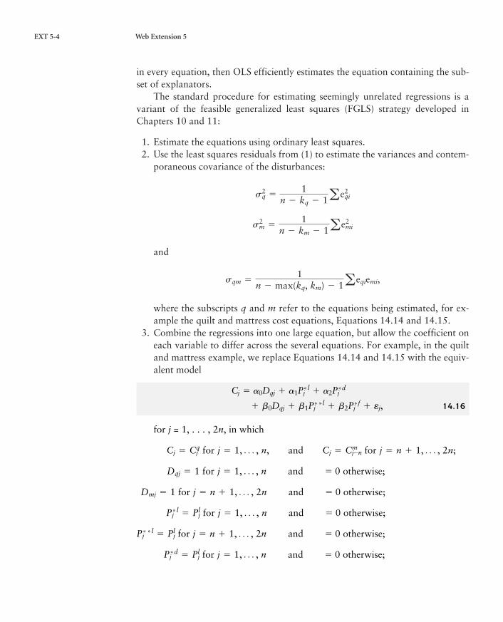
The standard procedure for estimating seemingly unrelated regressions is avariant of the feasible generalized least squares (FGLS) strategy developed inChapters 10 and 11:

1. Estimate the equations using ordinary least squares.2. Use the least squares residuals from (1) to estimate the variances and contem-

poraneous covariance of the disturbances:

and

where the subscripts q and m refer to the equations being estimated, for ex-ample the quilt and mattress cost equations, Equations 14.14 and 14.15.

3. Combine the regressions into one large equation, but allow the coefficient oneach variable to differ across the several equations. For example, in the quiltand mattress example, we replace Equations 14.14 and 14.15 with the equiv-alent model

14.16

for j = 1, . . . , 2n, in which

for and for

for otherwise;

for otherwise;

for otherwise;

for otherwise;

for otherwise;j = 1, Á , n and = 0P*dj = Pl

j

j = n + 1, Á , 2n and = 0P* *lj = Pl

j

j = 1, Á , n and = 0P*lj = Pl

j

j = n + 1, Á , 2n and = 0Dmj = 1

j = 1, Á , n and = 0Dqj = 1

j = n + 1, Á , 2n;Cj = Cmj-nj = 1, Á , n,Cj = Cq

j

+ b0Dqj + b1P**lj + b2P*f

j + ej,

Cj = a0Dqj + a1P*lj + a2P*d

j

sqm =1

n - max(kq, km) - 1aeqiemi,

s2m =

1n - km - 1a

e2mi

s2q =

1n - kq - 1a

e2qi


and for otherwise;

for for

This is called a “stacked” regression because several equations are stacked to-gether in a single regression equation. OLS applied to Equation 14.16 obtainsthe same results as OLS applied to Equations 14.14 and 14.15 separately.

4. Perform GLS on the stacked regression, using the estimated variances and co-variances in place of the actual.

Although FGLS can improve the efficiency with which each equation is esti-mated, there is a risk incurred by treating equations as a seemingly unrelated sys-tem. Specification errors, such as omitted variables, in one equation can bias thecoefficient estimates in all the equations. OLS applied one equation at a time willbe biased when applied to the misspecified equations, but the other equations willbe unbiasedly estimated. Many researchers shy away from SUR estimation be-cause they do not want to risk tainting all their estimates with the misspecifica-tion of a single equation.

14.11 Full Information Estimation MethodsIn simultaneous equations models, our central concern has been the simultaneitybias of OLS. In seemingly unrelated regression models, our concern has been withthe efficiency of estimators when the disturbances are contemporaneously corre-lated across equations. In this section, we discuss the joining of these two con-cerns. Just as FGLS methods can sometimes improve on the efficiency of OLS,sometimes they can also improve on the efficiency of IV estimators.

Estimators of simultaneous systems that jointly estimate all the structuralequations of a system are called full information estimators. Three-stage leastsquares and full information maximum likelihood are two full information esti-mators described in this section. Procedures that estimate individual structuralequations of a system separately from one another, such as OLS and 2SLS, arecalled limited information estimators. Another limited information estimator, in-troduced in this section, is the limited information maximum likelihood estimator.

Three-Stage Least SquaresThree-stage least squares is the most commonly used full information estimator.Three-stage least squares (3SLS) combines two-stage least squares and the FGLSestimator for seemingly unrelated regressions. The three steps of 3SLS are asfollows:

j = n + 1, Á , 2n.j = 1, Á , n and ej = emjej = eq

j

j = n + 1, Á , 2n and = 0P*fj = Pl

j

HOW DO WE MAKE

AN ESTIMATOR?


1. Estimate the reduced form equations by OLS and form fitted values for eachtroublesome explanator based on the variable’s reduced form equation.

2. Replace each troublesome explanator in each equation by its fitted valuefrom (1) and perform OLS for each structural equation. As in the second stepof the seemingly unrelated regressions equation, estimate the variances andcontemporaneous covariances of the equations’ disturbances, this time usingthe 2SLS residuals, instead of OLS residuals.

3. Perform FGLS as for seemingly unrelated regressions, using the estimatedvariances and contemporaneous correlations among the disturbances of theseveral structural equations, but replace any endogenous explanators withtheir fitted values from (1) before performing the SUR estimation.

Three-stage least squares consistently estimates systems of identified equa-tions but does not consistently estimate systems of equations that include one ormore underidentified equations. Consequently, before beginning the three steps of3SLS, we must determine which equations are underidentified, and not includethem in the 3SLS procedure.

Notice that in estimating the variances and cross-equation correlation of thedisturbances, 3SLS relies on fitted values of the reduced forms, in place of the en-dogenous variables themselves. But these OLS reduced form estimates do not in-corporate the information embodied in the exclusion restrictions of the structuralequations. This observation points the way to yet another estimator for simulta-neous equations, full information maximum likelihood (FIML). We’ll further dis-cuss the FIML estimator after we explore an example of 3SLS.

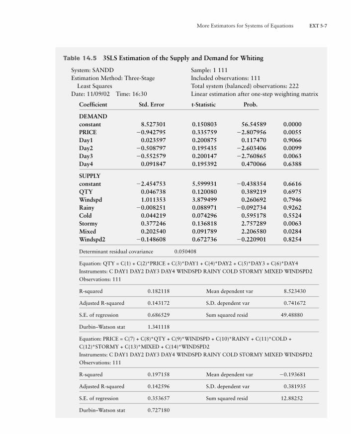
3SLS and the Fulton Fish MarketMost econometric software packages perform 3SLS on request. To better under-stand 3SLS, let’s return to Graddy’s Fulton Fish Market data, which are in the filewhiting.*** on this book’s Web site (www.aw-bc.com/murray). Table 14.5 con-tains the three-stage least squares estimates of the supply and demand for whitingfish in the Fulton Fish Market. We still find a significant effect of price on demandand still do not precisely measure the effect of quantity on the supply price—andstill do not reject the null hypothesis of perfectly elastic supply.

The parameter estimates do not change much between 2SLS (Table 14.3) and3SLS (Table 14.5) in this particular case. Nor do the estimated standard errors.Neither change much because the disturbances are only weakly correlated con-temporaneously across equations. The reported estimated covariance of the resid-uals is 0.05. The estimated standard deviations of the disturbances in the demandand supply equations are 0.69 and 0.35, respectively (the standard errors of theregressions in Table 14.5). Thus the correlation coefficient of the contemporane-ous disturbances is 0.05>(0.69 # 0.35) = 0.21.


Table 14.5 3SLS Estimation of the Supply and Demand for Whiting

System: SANDD Sample: 1 111Estimation Method: Three-Stage Included observations: 111

Least Squares Total system (balanced) observations: 222Date: 11/09/02 Time: 16:30 Linear estimation after one-step weighting matrix

Coefficient Std. Error t-Statistic Prob.

DEMANDconstant 8.527301 0.150803 56.54589 0.0000PRICE 0.942795 0.335759 2.807956 0.0055Day1 0.023597 0.200875 0.117470 0.9066Day2 0.508797 0.195435 2.603406 0.0099Day3 0.552579 0.200147 2.760865 0.0063Day4 0.091847 0.195392 0.470066 0.6388

SUPPLYconstant 2.454753 5.599931 0.438354 0.6616QTY 0.046738 0.120080 0.389219 0.6975Windspd 1.011353 3.879499 0.260692 0.7946Rainy 0.008251 0.088971 0.092734 0.9262Cold 0.044219 0.074296 0.595178 0.5524Stormy 0.377246 0.136818 2.757289 0.0063Mixed 0.202540 0.091789 2.206580 0.0284Windspd2 0.148608 0.672736 0.220901 0.8254

Determinant residual covariance 0.050408

Equation: QTY = C(1) + C(2)*PRICE + C(3)*DAY1 + C(4)*DAY2 + C(5)*DAY3 + C(6)*DAY4

Instruments: C DAY1 DAY2 DAY3 DAY4 WINDSPD RAINY COLD STORMY MIXED WINDSPD2

Observations: 111

R-squared 0.182118 Mean dependent var 8.523430

Adjusted R-squared 0.143172 S.D. dependent var 0.741672

S.E. of regression 0.686529 Sum squared resid 49.48880

Durbin–Watson stat 1.341118

Equation: PRICE = C(7) + C(8)*QTY + C(9)*WINDSPD + C(10)*RAINY + C(11)*COLD +

C(12)*STORMY + C(13)*MIXED + C(14)*WINDSPD2

Instruments: C DAY1 DAY2 DAY3 DAY4 WINDSPD RAINY COLD STORMY MIXED WINDSPD2

Observations: 111






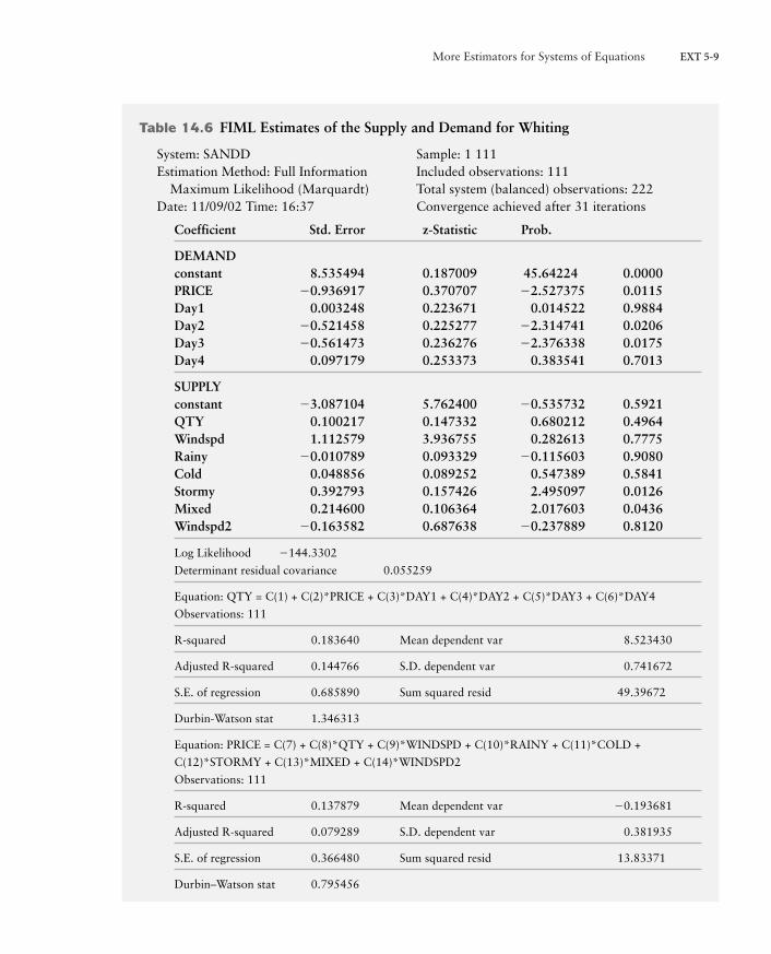
Full Information Maximum LikelihoodThree-stage least squares does not incorporate all the identifying informationfound in an overidentified model. The reduced form estimates used in the firststage are not forced to match the reduced form implied by the parameter esti-mates from the third stage. Full information maximum likelihood uses all of theidentifying information found in an overidentified model. Full information maxi-mum likelihood (FIML) jointly estimates all the structural parameters of a modelby maximum likelihood, subject to all the identifying restrictions contained in themodel. Maximum likelihood estimation is a strategy that estimates parameters byselecting the parameter values that make the observed sample data least surpris-ing; that is, the observed data would be less likely to arise for any alternative pa-rameter values than they are for the maximum likelihood estimates of the param-eters. (Supplement 4 on this book’s companion Web site, www.aw-bc.com/murray, contains an extensive discussion of maximum likelihood estimation.) Fullinformation maximum likelihood estimates the covariance structure of the distur-bances across equations jointly with the parameters of the equations themselves.Table 14.6 contains the FIML estimates of the whiting fish demand and supplyequations. There is little difference between the 3SLS and FIML estimates in thiscase.

Three-stage least squares yields different estimates than does full informationmaximum likelihood, but when the disturbances are normally distributed, both3SLS and FIML are asymptotically efficient estimators. Full information maxi-mum likelihood is computationally burdensome to perform, so three-stage leastsquares is the most commonly used full information estimator.

Full information estimators jointly estimate all the parameters of a system inone procedure. A peril of this approach is that misspecifications of one equationgenerally undermine the consistency of the estimates for all the equations. Econo-metricans have, over time, grown increasingly wary of this pitfall of full informa-tion methods, and they consequently rely on full information methods less andless. However, when the specification of the entire system of equations is particu-larly trustworthy, the efficiency gains of full information methods sometimes war-rant their use.

Limited Information Maximum LikelihoodFIML has a limited information estimator cousin, called limited informationmaximum likelihood. To avoid contagion from misspecified equations, LIML es-timates each structural equation separately. Limited information maximum likeli-hood (LIML) couples each structural equation with the reduced form equationsfor that equation’s endogenous explanators to create a mini-system of equations,and it estimates the parameters of that system by maximum likelihood.


Table 14.6 FIML Estimates of the Supply and Demand for Whiting

System: SANDD Sample: 1 111Estimation Method: Full Information Included observations: 111

Maximum Likelihood (Marquardt) Total system (balanced) observations: 222Date: 11/09/02 Time: 16:37 Convergence achieved after 31 iterations

Coefficient Std. Error z-Statistic Prob.

DEMANDconstant 8.535494 0.187009 45.64224 0.0000PRICE 0.936917 0.370707 2.527375 0.0115Day1 0.003248 0.223671 0.014522 0.9884Day2 0.521458 0.225277 2.314741 0.0206Day3 0.561473 0.236276 2.376338 0.0175Day4 0.097179 0.253373 0.383541 0.7013

SUPPLYconstant 3.087104 5.762400 0.535732 0.5921QTY 0.100217 0.147332 0.680212 0.4964Windspd 1.112579 3.936755 0.282613 0.7775Rainy 0.010789 0.093329 0.115603 0.9080Cold 0.048856 0.089252 0.547389 0.5841Stormy 0.392793 0.157426 2.495097 0.0126Mixed 0.214600 0.106364 2.017603 0.0436Windspd2 0.163582 0.687638 0.237889 0.8120

Log Likelihood 144.3302

Determinant residual covariance 0.055259

Equation: QTY = C(1) + C(2)*PRICE + C(3)*DAY1 + C(4)*DAY2 + C(5)*DAY3 + C(6)*DAY4

Observations: 111




Durbin-Watson stat 1.346313

Equation: PRICE = C(7) + C(8)*QTY + C(9)*WINDSPD + C(10)*RAINY + C(11)*COLD +

C(12)*STORMY + C(13)*MIXED + C(14)*WINDSPD2

Observations: 111






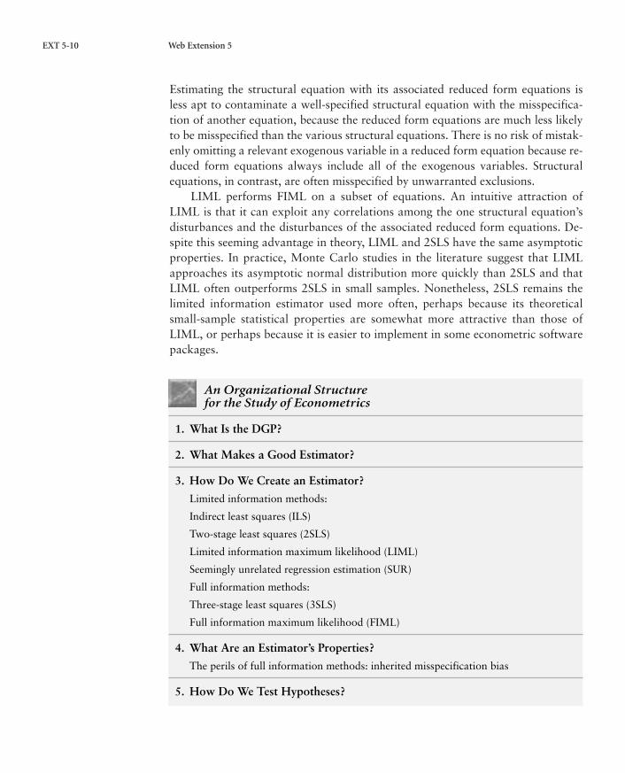
Estimating the structural equation with its associated reduced form equations isless apt to contaminate a well-specified structural equation with the misspecifica-tion of another equation, because the reduced form equations are much less likelyto be misspecified than the various structural equations. There is no risk of mistak-enly omitting a relevant exogenous variable in a reduced form equation because re-duced form equations always include all of the exogenous variables. Structuralequations, in contrast, are often misspecified by unwarranted exclusions.

LIML performs FIML on a subset of equations. An intuitive attraction ofLIML is that it can exploit any correlations among the one structural equation’sdisturbances and the disturbances of the associated reduced form equations. De-spite this seeming advantage in theory, LIML and 2SLS have the same asymptoticproperties. In practice, Monte Carlo studies in the literature suggest that LIMLapproaches its asymptotic normal distribution more quickly than 2SLS and thatLIML often outperforms 2SLS in small samples. Nonetheless, 2SLS remains thelimited information estimator used more often, perhaps because its theoreticalsmall-sample statistical properties are somewhat more attractive than those ofLIML, or perhaps because it is easier to implement in some econometric softwarepackages.

An Organizational Structure for the Study of Econometrics

1. What Is the DGP?

2. What Makes a Good Estimator?

3. How Do We Create an Estimator?

Limited information methods:

Indirect least squares (ILS)

Two-stage least squares (2SLS)

Limited information maximum likelihood (LIML)

Seemingly unrelated regression estimation (SUR)

Full information methods:

Three-stage least squares (3SLS)

Full information maximum likelihood (FIML)

4. What Are an Estimator’s Properties?

The perils of full information methods: inherited misspecification bias

5. How Do We Test Hypotheses?


Summary

This extension of Chapter 14 first introduces an estimation procedure for jointlyestimating several nonsimultaneous regression equations when their disturbancesare correlated. It then introduces two more estimators, three-stage least squares(3SLS) and full information maximum likelihood (FIML) estimators, which esti-mate all the parameters of a system of simultaneous equations jointly. Although3SLS and FIML are more efficient than 2SLS, they also risk transmitting specifi-cation biases across equations. A correctly specified equation is consistently esti-mated by 2SLS, even if all the other equations in the model are misspecified. But3SLS and FIML estimates of properly specified equations may be biased by a sin-gle misspecified equation in the system.

Concepts for ReviewFull information estimators

Full information maximum likelihood(FIML)

Limited information estimators

Limited information maximumlikelihood (LIML)

Seemingly unrelated regressions (SUR)

Three-stage least squares (3SLS)

(*** indicates a file on this book’s companion Web site,www.aw-bc.com/murray.)

Questions for Discussion1. Are any variables truly exogenous? Discuss.

2. When might FIML be inferior to 3SLS? Discuss.

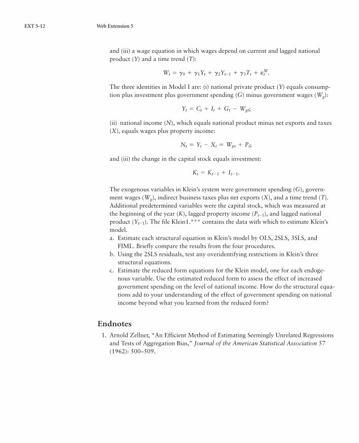
Problems for Analysis1. Lawrence Klein built one of the earliest models of the macro economy and estimated

it for the United States. Klein’s Model I contains (i) a consumption function in whichconsumption (C) depends on wages and salaries in the public and private sectors (Wg

and Wp) and on property income (P):

(ii) an investment equation in which investment (I) depends on current and laggedproperty income and on the initial stock of capital (K):

It = b0 + b1Pt + btPt-1 + b3Kt + elt;

Ct = a0 + a1(Wgt + Wpt) + a2Pt + etC;


and (iii) a wage equation in which wages depend on current and lagged nationalproduct (Y) and a time trend (T):

The three identities in Model I are: (i) national private product (Y) equals consump-tion plus investment plus government spending (G) minus government wages (Wg):

(ii) national income (N), which equals national product minus net exports and taxes(X), equals wages plus property income:

and (iii) the change in the capital stock equals investment:

The exogenous variables in Klein’s system were government spending (G), govern-ment wages (Wg), indirect business taxes plus net exports (X), and a time trend (T).Additional predetermined variables were the capital stock, which was measured atthe beginning of the year (K), lagged property income and lagged nationalproduct The file Klein1.*** contains the data with which to estimate Klein’smodel.a. Estimate each structural equation in Klein’s model by OLS, 2SLS, 3SLS, and

FIML. Briefly compare the results from the four procedures.b. Using the 2SLS residuals, test any overidentifying restrictions in Klein’s three

structural equations.c. Estimate the reduced form equations for the Klein model, one for each endoge-

nous variable. Use the estimated reduced form to assess the effect of increasedgovernment spending on the level of national income. How do the structural equa-tions add to your understanding of the effect of government spending on nationalincome beyond what you learned from the reduced form?

Endnotes1. Arnold Zellner, “An Efficient Method of Estimating Seemingly Unrelated Regressions

and Tests of Aggregation Bias,” Journal of the American Statistical Association 57(1962): 500–509.

(Yt-1).(Pt-1),

Kt = Kt-1 + It-1.

Nt = Yt - Xt = Wpt + Pt;

Yt = Ct + It + Gt - Wgt;

Wt = g0 + g1Yt + g2Yt-1 + g3Tt + eWt .


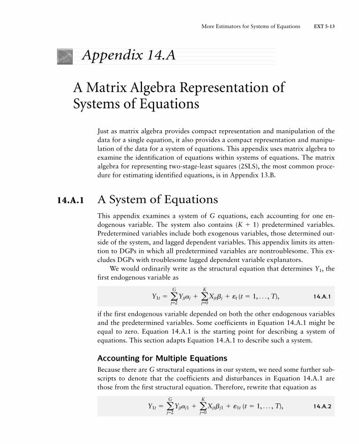
Appendix 14.A

A Matrix Algebra Representation ofSystems of Equations

Just as matrix algebra provides compact representation and manipulation of thedata for a single equation, it also provides a compact representation and manipu-lation of the data for a system of equations. This appendix uses matrix algebra toexamine the identification of equations within systems of equations. The matrixalgebra for representing two-stage-least squares (2SLS), the most common proce-dure for estimating identified equations, is in Appendix 13.B.

14.A.1 A System of EquationsThis appendix examines a system of G equations, each accounting for one en-dogenous variable. The system also contains predetermined variables.Predetermined variables include both exogenous variables, those determined out-side of the system, and lagged dependent variables. This appendix limits its atten-tion to DGPs in which all predetermined variables are nontroublesome. This ex-cludes DGPs with troublesome lagged dependent variable explanators.

We would ordinarily write as the structural equation that determines Y1, thefirst endogenous variable as

14.A.1

if the first endogenous variable depended on both the other endogenous variablesand the predetermined variables. Some coefficients in Equation 14.A.1 might beequal to zero. Equation 14.A.1 is the starting point for describing a system ofequations. This section adapts Equation 14.A.1 to describe such a system.

Accounting for Multiple EquationsBecause there are G structural equations in our system, we need some further sub-scripts to denote that the coefficients and disturbances in Equation 14.A.1 arethose from the first structural equation. Therefore, rewrite that equation as

14.A.2Y1t = aG

j=2Yjtaj1 + a

K

j=0Xjtbj1 + e1t (t = 1, Á , T),

Y1t = aG

j=2Yjtaj + a

K

j=0Xjtbj + et (t = 1, Á , T),

(K + 1)


and rewrite it again for symmetry as

or, even more symmetrically, as

14.A.3

in which Y1i is swallowed into the summation expression. Equation 14.A.3 is aform that could apply equally well to any structural equation, if we replace the 1’sin Equation 14.A.3 with a number appropriate to the structural equation in ques-tion. We could, for example, write the i-th structural equation as

14.A.4

For convenience, we define so that Equation 14.A.4 becomes

14.A.5

To express Equation 14.A.5 in matrix form, define

and

in which the Yi, the Xi, and the are column vectors containing the ob-servations for the corresponding variables, and

Notice that in We can rewrite Equation 14.A.5 as

An even more compact notation combines all G structural equations into one ma-trix formulation. Define

Ω = [Ω1Ω2 ÁΩG]

YΩi = XBi + Ei.

Ωi,gii = 1.

Bi = [b0b2i Á bKi]¿.

Ωi = [g1ig2i Á gGi]¿

(T * 1)Ei

E = [E1E2 Á EG],

X = [X0X1 Á XK],Y = [Y1Y2 Á YG],

aG

j=1Yjtgji = a

K

j=0Xjtbji + eit (t = 1, Á , T).

gji = -aji,

- aG

j=1Yjtaji = a

K

j=0Xjtbji + eit (t = 1, Á , T).

- aG

j=1Yjtaj1 = a

K

j=0Xjtbj1 + e1t (t = 1, Á , T),

Y1t - aG

j=2Yjtaj1 = a

K

j=0Xjtbj1 + e1t (t = 1, Á , T),


and

and write

14.A.6a

or

14.A.6b

Equation 14.A.6a is a matrix representation of G structural equations with K pre-determined variables in the system. The matrix in Equation14.A.6b is a matrix. Its columns contain the G structural relationships,with each row corresponding to one observation on all G structural relationships.

The Reduced FormIf the endogenous variables are genuinely determined in the system of equationsdefined by Equation 14.A.6, then we can solve that equation to express each en-dogenous variable as a function of the predetermined variables alone. When thisis true, we say that the model in 14.A.6 is complete. We assume our system iscomplete, so we can solve Equation 14.A.6 for Y:

or

14.A.7

where and Equation 14.A.7 is the reduced form for themodel in Equation 14.A.6. Equation 14.A.7 implies that

14.A.8

If the predetermined variables are not perfectly collinear, the reduced formequations are identified. Because the reduced form equations’ explanators are allpredetermined variables, we can consistently estimate the coefficients of thoseequations, the elements of , by OLS. In contrast, we may be unable to consis-tently estimate the coefficients of a structural equation like that in Equation14.A.2,

Y1t = aG

j=2Yjtaj1 + a

K

j=0Xjtbj1 + e1t (t = 1, Á , T),

∑

B = ∑Ω.

N = EΩ-1.∑ = BΩ-1

Y = XBΩ-1

+ EΩ-1= X∑ + N,

YΩΩ-1

= XBΩ-1

+ EΩ-1

(T * G)(YΩ - XB - E)

YΩ - XB - E = 0.

YΩ = XB + E,

B = [B1B2 Á BG]


because the endogenous explanators may be correlated with the disturbances. Ifnone of the predetermined variables are excluded from this equation, for exam-ple, there are no available instrumental variables for the endogenous variableswith which to consistently estimate the equation’s coefficients.

It is only the co-movement of the endogenous variables with the predeter-mined variables that can tell us about an individual structural equation’s coeffi-cients. Any co-movements among endogenous variables may be affected by feed-backs among the endogenous variables across equations. Consequently, all theinformation we have with which to identify the structural equations is containedin the reduced form relationships of Equation 14.A.7.

Structural Equations and Reduced Form Equations RevisitedThe structural relationships of Equation 14.A.6 (a and b) contain co-efficients in each of the G structural relationships, or coefficientsin all. The reduced-form equations, on the other hand, contain coefficientsin each of G equations, or coefficients in all. Because the number of re-duced form parameters is smaller than the number of structural coefficients, thereare infinitely many different matrices that could serve as and and satisfy

In general, the reduced form does not uniquely determine the structural model.This is the essence of the identification problem in simultaneous equations mod-els. Because it is the reduced form parameters that we know we can consistentlyestimate, we can only consistently estimate the structural parameters when theyare retrievable from the reduced form. But when can we retrieve the reduced coef-ficients for a particular structural equation from the reduced form equation?

The key to identifying the i-th structural equation lies in the i-th reduced formequation. Just as the i-th columns of the right- and left-hand sides of 14.A.6byield the i-th structural equation, with dependent variable Yi:

14.A.9

the i-th column of yields the reduced form equation for the i-th endogenousvariable, Yi. We know that the i-th element of is 1. Identification requires fur-ther restrictions on and . Consider, for example, the first structural equation.

Not all endogenous variables need appear in the first structural equation, nordo all predetermined variables need appear in the first equation. Let’s divide en-dogenous variables into three groups, itself, and contains allthe endogenous variables that appear as explanators with nonzero coefficients inthe first structural equation. contains all the endogenous variables with zerocoefficients in the first structural equation. is a matrix and is aYout1Gin1 * TYin1

Yout1

Yin1Yout1.Yin1,Y1

BiΩi

Ωi

∑i,∑,

YΩi - XBi - Ei = 0,

∑ = BΩ-1.

BΩ

GK + GK + 1

G2+ GK + G

G + K + 1


matrix; For convenience, suppose that Y isarranged such that

14.A.10

Similarly, suppose

14.A.11

in which contains all the predetermined variables that appear with nonzerocoefficients in the first structural equation and contains all the predeterminedvariables with zero coefficients in the first structural equation. is a matrix and is a matrix.

It proves informative to rewrite 14.A.9 with the explicit division of Y and Xinto the groups given by Equations 14.A.10 and 14.A.11:

14.A.12

in which is a matrix containing the first structural equation’s coeffi-cients for the endogenous variables in , is a matrix containingthe first structural equation’s coefficients for the endogenous variables in and and are similarly defined. Because excluded variables have zero co-efficients, we can rewrite Equation 14.A.12 as

We can similarly rewrite the reduced form equation

as

in which

B Pin11 ∑in1in ∑in1out

Pout11 ∑out1in ∑out1outR = ∑

[Y1Yin1Yout1] = [Xin1Xout1]B Pin11 ∑in1in ∑in1out

Pout11 ∑out1in ∑out1outR + Ni,

Y = X∑ + N

[Y1Yin1Yout1]C 1Ωin1

0S - [Xin1Xout1]BBin1

0R - Ei.

Bout1Bin1

Yout1,Gout1 * TΩout1Yin1

Gin1 * TΩin1

[Y1Yin1Yout1C 1Ωin1

Ωout1S - [Xin1Xout1]B Bin1

Bout1R - Ei,

Kin1 + Kout1 = K + 1.Kout1 * TXout1

Kin1 * TXin1

Xout

Xin1

X = [Xin1Xout1],

Y = [Y1Yin1Yout1].

Gin1 + Gout1 + 1 = G.Gout1 * T


and

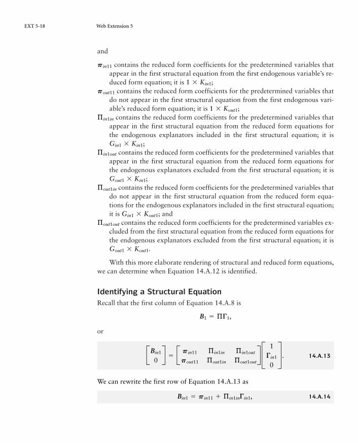
contains the reduced form coefficients for the predetermined variables thatappear in the first structural equation from the first endogenous variable’s re-duced form equation; it is ;

contains the reduced form coefficients for the predetermined variables thatdo not appear in the first structural equation from the first endogenous vari-able’s reduced form equation; it is ;

contains the reduced form coefficients for the predetermined variables thatappear in the first structural equation from the reduced form equations forthe endogenous explanators included in the first structural equation; it is

;contains the reduced form coefficients for the predetermined variables that

appear in the first structural equation from the reduced form equations forthe endogenous explanators excluded from the first structural equation; it is

;contains the reduced form coefficients for the predetermined variables that

do not appear in the first structural equation from the reduced form equa-tions for the endogenous explanators included in the first structural equation;it is ; and

contains the reduced form coefficients for the predetermined variables ex-cluded from the first structural equation from the reduced form equations forthe endogenous explanators excluded from the first structural equation; it is

.

With this more elaborate rendering of structural and reduced form equations,we can determine when Equation 14.A.12 is identified.

Identifying a Structural EquationRecall that the first column of Equation 14.A.8 is

or

14.A.13

We can rewrite the first row of Equation 14.A.13 as

14.A.14Bin1 = Pin11 + ∑in1inΩin1,

BBin1

0R = B Pin11 ∑in1in ∑in1out

Pout11 ∑out1in ∑out1outR C 1

Ωin1

0S .

B1 = ∑Ω1,

Gout1 * Kout1

∑out1out

Gin1 * Kout1

∑out1in

Gout1 * Kin1

∑in1out

Gin1 * Kin1

∑in1in

1 * Kout1

Pout11

1 * Kin1

Pin11


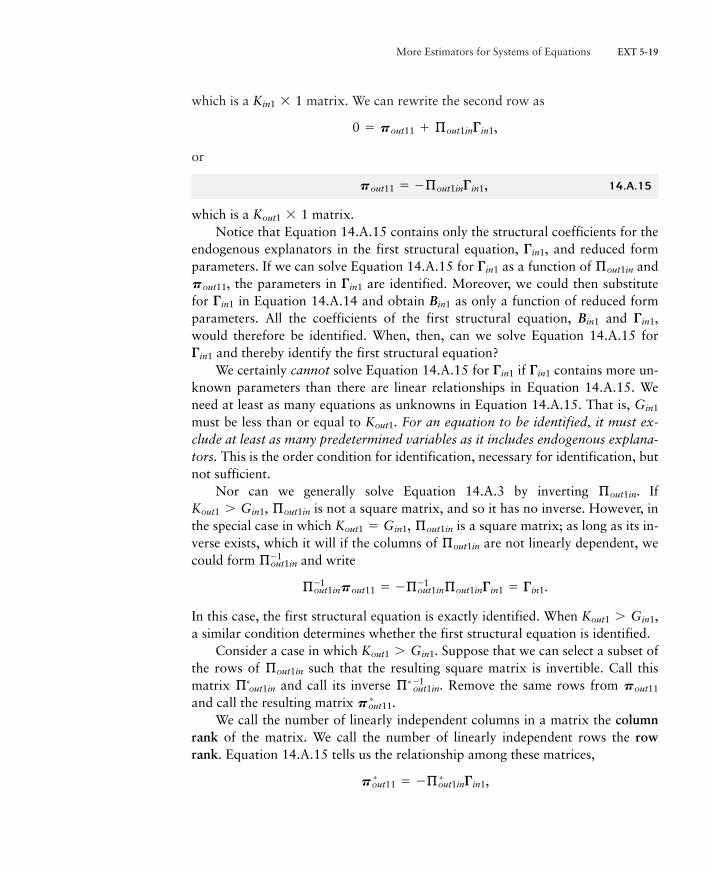
which is a matrix. We can rewrite the second row as

or

14.A.15

which is a matrix.Notice that Equation 14.A.15 contains only the structural coefficients for the

endogenous explanators in the first structural equation, and reduced formparameters. If we can solve Equation 14.A.15 for as a function of and

the parameters in are identified. Moreover, we could then substitutefor in Equation 14.A.14 and obtain as only a function of reduced formparameters. All the coefficients of the first structural equation, and would therefore be identified. When, then, can we solve Equation 14.A.15 for

and thereby identify the first structural equation?We certainly cannot solve Equation 14.A.15 for if contains more un-

known parameters than there are linear relationships in Equation 14.A.15. Weneed at least as many equations as unknowns in Equation 14.A.15. That is, must be less than or equal to . For an equation to be identified, it must ex-clude at least as many predetermined variables as it includes endogenous explana-tors. This is the order condition for identification, necessary for identification, butnot sufficient.

Nor can we generally solve Equation 14.A.3 by inverting . Ifis not a square matrix, and so it has no inverse. However, in

the special case in which is a square matrix; as long as its in-verse exists, which it will if the columns of are not linearly dependent, wecould form and write

In this case, the first structural equation is exactly identified. When a similar condition determines whether the first structural equation is identified.

Consider a case in which Suppose that we can select a subset ofthe rows of such that the resulting square matrix is invertible. Call thismatrix and call its inverse Remove the same rows from and call the resulting matrix

We call the number of linearly independent columns in a matrix the columnrank of the matrix. We call the number of linearly independent rows the rowrank. Equation 14.A.15 tells us the relationship among these matrices,

Pout11* = - ∑*out1inΩin1,

P*out11.Pout11∑*-1

out1in.∑*out1in

∑out1in

Kout1 7 Gin1.

Kout1 7 Gin1,

∑-1out1inPout11 = - ∑

-1out1in∑out1inΩin1 = Ωin1.

∑-1out1in

∑out1in

Kout1 = Gin1, ∑out1in

Kout1 7 Gin1, ∑out1in

∑out1in

Kout1

Gin1

Ωin1Ωin1

Ωin1

Ωin1,Bin1

Bin1Ωin1

Ωin1Pout11,∑out1inΩin1

Ωin1,

Kout1 * 1

Pout11 = - ∑out1inΩin1,

0 = Pout11 + ∑out1inΩin1,

Kin1 * 1


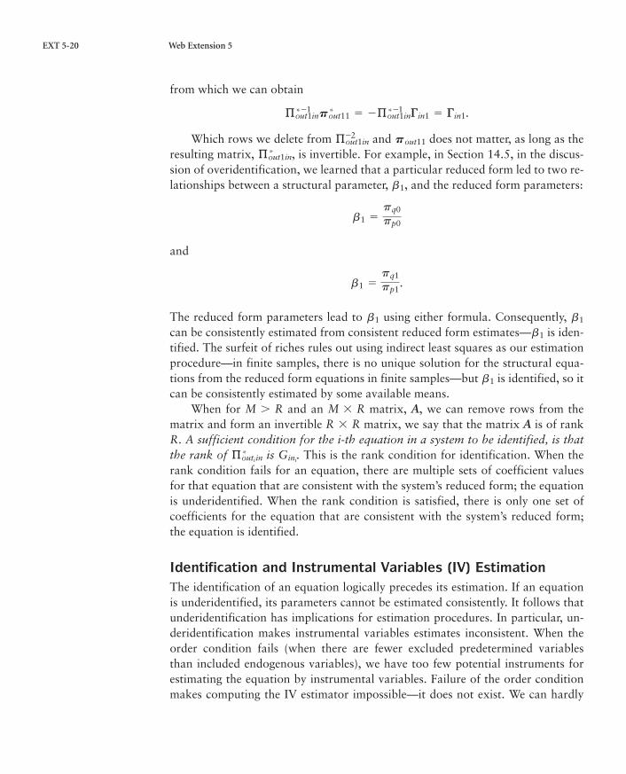
from which we can obtain

Which rows we delete from and does not matter, as long as theresulting matrix, , is invertible. For example, in Section 14.5, in the discus-sion of overidentification, we learned that a particular reduced form led to two re-lationships between a structural parameter, , and the reduced form parameters:

and

The reduced form parameters lead to using either formula. Consequently, can be consistently estimated from consistent reduced form estimates— is iden-tified. The surfeit of riches rules out using indirect least squares as our estimationprocedure—in finite samples, there is no unique solution for the structural equa-tions from the reduced form equations in finite samples—but is identified, so itcan be consistently estimated by some available means.

When for and an matrix, A, we can remove rows from thematrix and form an invertible matrix, we say that the matrix A is of rankR. A sufficient condition for the i-th equation in a system to be identified, is thatthe rank of is . This is the rank condition for identification. When therank condition fails for an equation, there are multiple sets of coefficient valuesfor that equation that are consistent with the system’s reduced form; the equationis underidentified. When the rank condition is satisfied, there is only one set ofcoefficients for the equation that are consistent with the system’s reduced form;the equation is identified.

Identification and Instrumental Variables (IV) EstimationThe identification of an equation logically precedes its estimation. If an equationis underidentified, its parameters cannot be estimated consistently. It follows thatunderidentification has implications for estimation procedures. In particular, un-deridentification makes instrumental variables estimates inconsistent. When theorder condition fails (when there are fewer excluded predetermined variablesthan included endogenous variables), we have too few potential instruments forestimating the equation by instrumental variables. Failure of the order conditionmakes computing the IV estimator impossible—it does not exist. We can hardly

Gini∑*outiin

R * RM * RM 7 R

b1

b1

b1b1

b1 =

pq1

pp1.

b1 =

pq0

pp0

b1

∑*out1in

Pout11∑-2out1in

∑*-1out1inP*out11 = - ∑*-1

out1inΩin1 = Ωin1.


miss failures of the order condition when we perform IV estimation; the computerwill tell us that we have tried to divide by zero or that some matrix is “singular”(that is, does not have an inverse).

When the order condition is satisfied, but the rank condition fails, we havethe needed number of potential instruments, but we cannot form enough linearlyindependent combinations of them to make ( X) invertible in large samples. Afailure of the rank condition when the order condition is satisfied does not stop usfrom computing the IV estimator, even in very large samples; the sampling errorsin estimating the reduced-form coefficients will probably lead us to construct in-struments that are not perfectly correlated within our samples. Nevertheless, theIV estimates are inconsistent in this case because the equation is not identified.

Concepts for ReviewColumn rank

Row rank

Z¿

Michael Murray SUR and SES

Documents

unrelated equations

individual equations

thatsystems of equations

suchmultiple equations

simultaneous equations

unrelated systems

simultaneous equations

correlation of disturbances