Study on global AGEing and adult health (SAGE), Wave 1 MEXICO MEXICO Study on global AGEing and adult health (SAGE), Wave 1 WHO SAGE WAVE 1

Welcome message from author
This document is posted to help you gain knowledge. Please leave a comment to let me know what you think about it! Share it to your friends and learn new things together.
Transcript
Study on glob
al AG
Eing and adult health (SAG
E), Wave 1
The Study on global AGEing and adult health (SAGE) is sup-
ported by WHO’s Surveys, Measurement and Analysis unit.
SAGE compiles comparable longitudinal information on the
health and well-being of adult populations and the ageing
process from nationally representative samples in six coun-
tries (China, Ghana, India, Mexico, Russian Federation and
South Africa). Financial support for SAGE was provided by
the US National Institute on Aging and the World Health
Organization. Mexico’s national report is a descriptive sum-
mary of SAGE Wave 1 results. Wave 2 was implemented in
2015 and Wave 3 in 2016. More information is available at:
www.who.int/healthinfo/sage
Cover images: iStockphoto
MEX
ICO
MEXICO
Study on global AGEing and adult health (SAGE), Wave 1
WHO SAGE WAVE 1
Study on global AGEing and adult health (SAGE) Wave 1
Mexico National Report
Instituto Nacional de Salud Pública (INSP)
Study Report March 2014
SAGE is supported by the US National Institute on Aging (NIA) through Interagency Agreements (OGHA 04034785; YA1323–08-CN-0020; Y1-AG-1005–01) and through a research grant (R01-AG034479). The NIA’s Division of Behavioral and Social Research, under the directorship of Dr Richard Suzman, has been instrumental in providing continuous intellectual and other technical support to SAGE, and has made the entire endeavour possible.
2 SAGE Mexico Wave 1
© World Health Organization 2014
All rights reserved.
The designations employed and the presentation of the material in this publication do not imply the expression of any opinion whatsoever on the part of the World Health Organization concerning the legal status of any country, territory, city or area or of its authorities, or concerning the delimitation of its frontiers or boundaries. Dotted lines on maps represent approximate border lines for which there may not yet be full agreement.
The mention of specific companies or of certain manufacturers’ prod-ucts does not imply that they are endorsed or recommended by the World Health Organization in preference to others of a similar nature that are not mentioned. Errors and omissions excepted, the names of proprietary products are distinguished by initial capital letters.
All reasonable precautions have been taken by the World Health Organization to verify the information contained in this publication. However, the published material is being distributed without war-ranty of any kind, either expressed or implied. The responsibility for the interpretation and use of the material lies with the reader. In no event shall the World Health Organization be liable for damages aris-ing from its use.
Photo: © Eperales/Flickr. https://creativecommons.org/licenses/by-nc-sa/2.0/
Copyediting: Dr Wynne Russell
Design and layout: Rick Jones, Exile: Design & Editorial Services, London (United Kingdom)
Copyright
3SAGE Mexico Wave 1
Acknowledgements
The authors wish to thank:
The Secretaría de Salud for their support for the study;
The states and communities participating in the study for their help in organising the work;
All respondents who consented to participate in the study;
All the fieldwork supervisors and their teams of interviewers for collecting the data;
The INSP institutional and administrative support;
Centro de Investigación en Salud Poblacional for long-term storage of DBS;
Dr Wynne Russell for editing, Dr Rebecca Peters for translations and editing, and Mr Richard Jones for designing the report;
The World Health Organization (WHO) for initiat-ing the study, financial and technical support, and provision of materials and instrumentation for the conduct of the study; and,
SAGE is supported by the US National Institute on Aging (NIA) through Interagency Agreements (OGHA 04034785; YA1323–08-CN-0020; Y1-AG-1005–01) and a research grant (R01-AG034479).
4 SAGE Mexico Wave 1
Contents
1. Introduction ......................................................................................................................................................................................................................... 6
1.1 Health and socio-demographic situation 6
1.2 Ageing issues and policy goals 6
1.3 Ageing related studies, data and policy gap 10
1.4 World Health Survey (SAGE Wave 0 in Mexico) and SAGE Wave 1 11
1.5 SAGE goals and objectives 11
2. Methodology .................................................................................................................................................................................................................. 13
2.1 Sampling design, implementation and size 13
2.2 Questionnaires 14
2.3 Data collection procedures 14
2.4 Survey metrics and data quality 16
2.5 Response rate 19
3. Characteristics of Households and Individuals ................................................................................................................ 20
3.1 Household characteristics 20
3.2 Individual respondent characteristics 23
4. Income, Consumption, Transfers and Retirement ........................................................................................................ 27
4.1 Work history 27
4.2 Income and transfers (household level) 27
5. Health Risks and Behaviours ..................................................................................................................................................................... 34
5.1 Tobacco and alcohol consumption 34
5.2 Diet and physical activity 36
5.3 Access to improved water sources and sanitation 40
5.4 Solid fuel use and indoor air pollution 41
6. Health State ...................................................................................................................................................................................................................... 42
6.1 Self-reported overall general health and day-to-day activity 42
6.2 Composite health state score and disability score 42
5SAGE Mexico Wave 1
6.3 Functioning and health: ADLs and IADLs 45
6.4 Measured cognitive function 45
7. Chronic Conditions and Interventions .......................................................................................................................................... 50
7.1 Chronic conditions 50
7.2 Injuries 59
7.3 Cervical and breast cancer 60
8. Health Examination and Biomarkers ............................................................................................................................................. 62
8.1 Anthropometry 62
8.2 Measured performance tests 65
9. Health Care Utilization and Health System Responsiveness .......................................................................... 76
9.1 Health service utilization 76
9.2 Health system responsiveness 79
10. Well-being and Quality of Life ............................................................................................................................................................. 81
10.1 Quality of life and life satisfaction (WHOQoL) 81
10.2 Happiness and well-being (Day Reconstruction Method) 82
11. Mortality ............................................................................................................................................................................................................................ 85
References ................................................................................................................................................................................................................................. 86
Appendices ............................................................................................................................................................................................................................... 88
6 SAGE Mexico Wave 1
1. Introduction
Mexico is ageing. The first phase of the ongoing demo-graphic transition took place in the 1930s, when mortality began to decline in conjunction with persistent high birth rates, leading to a sustained period of high pop-ulation growth. However, policy and cultural changes have led to steady and rapid declines in birth rates from 46 births per thousand population in 1960 to 21 per thousand in 2000. Over the same period, average fer-tility fell from 7.0 to 2.4 children per woman. The birth rate is expected to continue its downward trend to reach 11 births per thousand population by 2050 (CONAPO).
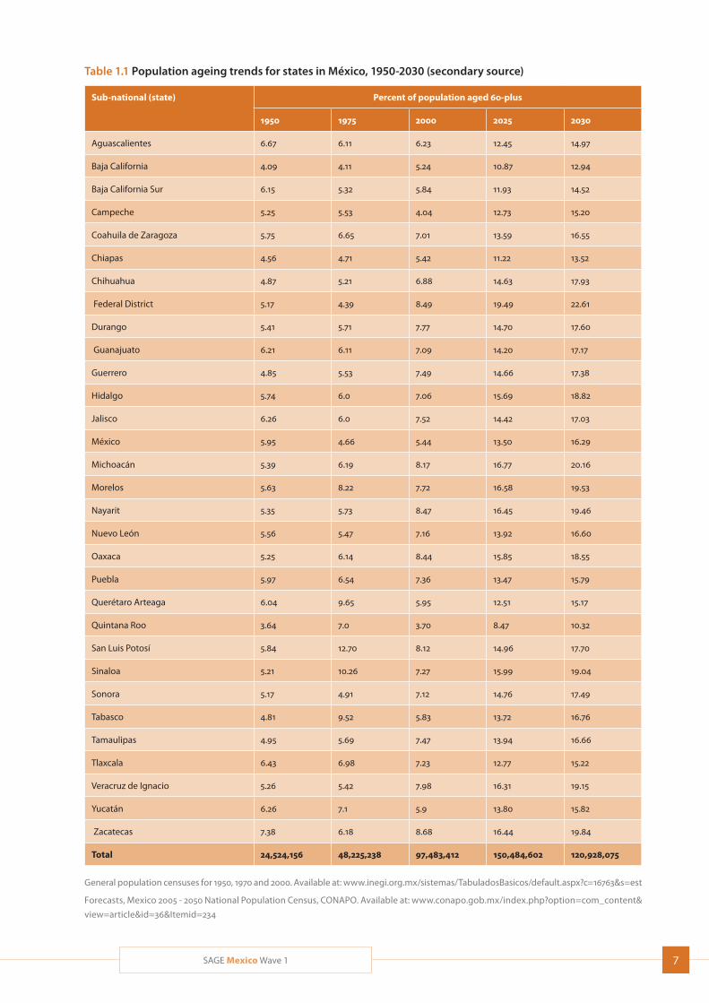
Meanwhile, the average life expectancy of Mexicans doubled during the second half of the twentieth cen-tury; it rose from 36 years in 1950 to 74 years in 2000. This trend is expected to continue over the next few decades allowing average life expectancy at birth to reach 80 years in 2050. As is the case in almost every country in the world, women in Mexico tend to live longer than men. In 2012, female life expectancy at birth was 79.4 years and male 74.5 years (Atun, 2014). Trends in the proportion of the total population aged 60-plus are provided by state in Table 1.1.
1.1 Health and socio-demographic situation
In recent decades, there has been an improvement in the living conditions of Mexico’s population, together with a decline in overall mortality and a transformation in the profile of causes of death, all of which have had a profound impact on society. The transition is at an advanced stage among the better-off strata of the population, while less well-off groups are at an earlier stage in the process (CONAPO, 2010).
Nevertheless, life expectancy in Mexico is the lowest amongst OECD countries (OECD, 2014), impacted by
harmful health-related behaviors, road traffic acci-dents and homicides. Ischemic heart disease, diabetes, chronic kidney disease and interpersonal violence were the top contributors to premature mortality in Mexico in 2010 (IHME, 2013). The leading causes of dis-ability in the country were lower back pain, depression, diabetes and neck pain. Compared to 1990, a higher proportion of the burden of disease in 2010 was from non-communicable disease and injuries, and a lower proportion of the disease burden was contributed by infectious diseases. High body mass index (BMI), high blood sugar, dietary risks, alcohol use and high blood pressure were the leading health risks contributing to disease burden in 2010.
1.2 Ageing issues and policy goals
Socio-economic aspects of health among older adultsPrevalence of disability gradually increases among both men and women after the age of 45 years and becomes considerable after the age of 79, when there is a greater likelihood of experiencing functional impairment in association with the inability to independently perform everyday tasks. As people grow older, the proportion of individuals in high-risk age groups will increase, making it likely that prevalence of disability will also increase (CONAPO).
One of the policy challenges presented by an ageing population is to adopt and introduce preventive measures and programmes to make it possible to reduce rates of morbidity and disability so as to increase disability-free life expectancy and enable more people to live longer in a satisfactory state of physical and mental health (CONAPO). In 2010, a man who reached the age of 60 years was expected to live an average of 2.5 of his
7SAGE Mexico Wave 1
Table 1.1 Population ageing trends for states in México, 1950-2030 (secondary source)
Sub-national (state) Percent of population aged 60-plus
1950 1975 2000 2025 2030
Aguascalientes 6.67 6.11 6.23 12.45 14.97
Baja California 4.09 4.11 5.24 10.87 12.94
Baja California Sur 6.15 5.32 5.84 11.93 14.52
Campeche 5.25 5.53 4.04 12.73 15.20
Coahuila de Zaragoza 5.75 6.65 7.01 13.59 16.55
Chiapas 4.56 4.71 5.42 11.22 13.52
Chihuahua 4.87 5.21 6.88 14.63 17.93
Federal District 5.17 4.39 8.49 19.49 22.61
Durango 5.41 5.71 7.77 14.70 17.60
Guanajuato 6.21 6.11 7.09 14.20 17.17
Guerrero 4.85 5.53 7.49 14.66 17.38
Hidalgo 5.74 6.0 7.06 15.69 18.82
Jalisco 6.26 6.0 7.52 14.42 17.03
México 5.95 4.66 5.44 13.50 16.29
Michoacán 5.39 6.19 8.17 16.77 20.16
Morelos 5.63 8.22 7.72 16.58 19.53
Nayarit 5.35 5.73 8.47 16.45 19.46
Nuevo León 5.56 5.47 7.16 13.92 16.60
Oaxaca 5.25 6.14 8.44 15.85 18.55
Puebla 5.97 6.54 7.36 13.47 15.79
Querétaro Arteaga 6.04 9.65 5.95 12.51 15.17
Quintana Roo 3.64 7.0 3.70 8.47 10.32
San Luis Potosí 5.84 12.70 8.12 14.96 17.70
Sinaloa 5.21 10.26 7.27 15.99 19.04
Sonora 5.17 4.91 7.12 14.76 17.49
Tabasco 4.81 9.52 5.83 13.72 16.76
Tamaulipas 4.95 5.69 7.47 13.94 16.66
Tlaxcala 6.43 6.98 7.23 12.77 15.22
Veracruz de Ignacio 5.26 5.42 7.98 16.31 19.15
Yucatán 6.26 7.1 5.9 13.80 15.82
Zacatecas 7.38 6.18 8.68 16.44 19.84
Total 24,524,156 48,225,238 97,483,412 150,484,602 120,928,075
General population censuses for 1950, 1970 and 2000. Available at: www.inegi.org.mx/sistemas/TabuladosBasicos/default.aspx?c=16763&s=est
Forecasts, Mexico 2005 - 2050 National Population Census, CONAPO. Available at: www.conapo.gob.mx/index.php?option=com_content&
view=article&id=36&Itemid=234
8 SAGE Mexico Wave 1
remaining life-years (20.2 on average) with some form of disability. This figure was 3.1 years among women, whose life expectancy at 60 was 22.1 years. In other words, after the age of 60 years, the average person will spend more than 10% of his or her remaining life years with some form of disability. The age-standardized prevalence of disability was estimated by the 2003 World Health Survey in Mexico to be 7.5% (http://who.int/disabilities/world_report/2011/technical_ appendices.pdf). The predominant form of disability among older adults was with mobility, which affected 56% of men and 62% of women, followed by visual impairment (33% and 32%, respectively) and hearing impairment (27% and 19%, respectively). One social factor affecting the older population that has to be considered is migration by Mexicans to the United States in search of economic support. This has affected both older adults and their families. For this reason, migration plays a very important role in any study of health and ageing (Wong, 2007).
It is noteworthy that in the data produced by the 2001 National Survey of Health and Ageing in Mexico (ENASEM), self-evaluation of health for the population aged over 50 years was closely associated with self-reporting of chronic diseases (of the heart, lungs, cancer or stroke) and with functional disability. This would seem to indicate that self-reporting may be a valuable global indicator of health in studies among the community. The exception is for obesity, which is not closely associated with self-reporting of health (INSP/SEDESOL).
Public policy and programmes for older adultsActivities that have been proposed to improve our
understanding of the health needs of older adults and
to improve health programmes for this population
include the following (Ham-Chande, 2007):
Setting up a health surveillance system for older
adults, based on morbidity and disability indicators;
Bolstering the programme of research into ageing
and health;
Including older adults in health promotion and pre-
ventive health strategies with precise and verifiable
targets that emphasize functional independence;
Establishing a policy to train human resources to
care for older adults;
Improving governance of the health system as regards regulation of establishments providing long-term care; and,
Expanding health-care services for older adults to cover community and home care.
The provision of services for older adults in Mexico is regulated by NOM-167-SSA1-1997, “On provision of social welfare services for minors and older adults”. A patchwork of different programmes have been imple-mented at the federal and state levels to provide finan-cial support to older adults; these generally suffer from the lack of an overall framework and government policy to define basic strategies for meeting older adults’ considerable needs. Some programmes have focused on ensuring the participation of the population living in extreme poverty, while others have emphasized a universal approach within a specific geographical area.
The three main programmes addressing this population group are the Over 70s Allowance in the Federal District; the component of Oportunidades (now Prospera) pro-viding support for older adults; and the 70+ Programme (Rubio 2010). Prospera is a selective intervention target-ing the population living in extreme poverty, while the Over 70s Allowance in the Federal District and the 70+ Programme are designed to provide universal cover-age within specific geographical areas (Secretaría de Salud). Since 2006, families benefiting from Prospera and with family members aged over 70 years have received additional financial support for each older family member. The level of support is adjusted every six months on the basis of variations in the National Basic Basket Price indicator, and since 2007 the component’s geographical coverage has gradually been limited so as to gradually transfer beneficiaries to the new 70+ Programme (Secretaría de Salud). In 2009, the support for the older adult component of Prospera had an authorized budget of 47.8 billion pesos – approximately 0.4% of GDP – and benefited more than 5 million fami-lies, almost two-thirds of whom were in the three lowest income deciles of the population. Prospera also pro-vides members of the families concerned with a basic package of free health services determined by their age, sex and life history. Persons of over 60 years of age ben-efit from health promotion measures and early diagnosis of diseases such as diabetes, high blood pressure, visual and hearing deficiencies, cognitive impairment.
At the Federal level, the 70+ Programme is a universal non-contributory allowance for older persons, initially intended for those living in rural localities of up to 2,500
9SAGE Mexico Wave 1
inhabitants. Each year, the Chamber of Deputies has increased the programme’s budget and its catchment area. In 2009, the allowance benefited older persons living in localities of up to 30,000 inhabitants and operated with a budget of slightly more than 13 billion pesos (approximately 0.1% of GDP); it was the social development programme with the second largest budget after Prospera. This programme involves a monthly cash payment of $500 (US$38.5), with two-monthly payments to older persons of more than 70 years of age. In 2009, there were 1.8 million active participants in more than 75,000 towns and villages throughout Mexico (Secretaría de Salud).
In 2001, the Over 70s Allowance in the Federal District Programme began to provide food support, medical care and free medicine for persons living in the Federal District. Initially, it focused on older persons living in areas that were highly or very highly marginal, but later became universal. In 2003, a law was established that provided the right of Mexico City residents to a daily allowance of no less than half the current minimum wage in the Federal District, provided they meet the age requirement and obliged the executive and legis-lative authorities to make available the necessary bud-get (Secretaría de Salud). In 2009, it was estimated to include at least 470,000 older persons with an annual Budget of at least 4.34 billion pesos. The allowance amounted to 822 pesos (US$63) per month.
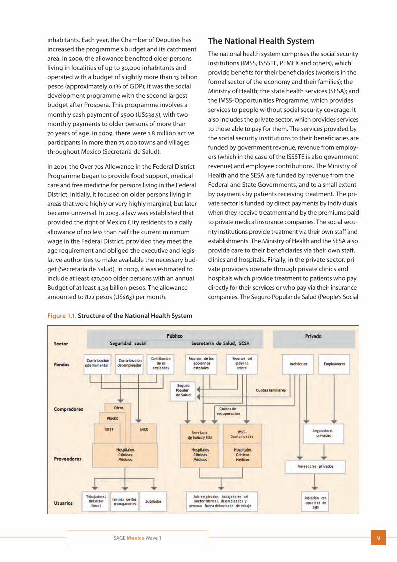
The National Health SystemThe national health system comprises the social security institutions (IMSS, ISSSTE, PEMEX and others), which provide benefits for their beneficiaries (workers in the formal sector of the economy and their families); the Ministry of Health; the state health services (SESA); and the IMSS-Opportunities Programme, which provides services to people without social security coverage. It also includes the private sector, which provides services to those able to pay for them. The services provided by the social security institutions to their beneficiaries are funded by government revenue, revenue from employ-ers (which in the case of the ISSSTE is also government revenue) and employee contributions. The Ministry of Health and the SESA are funded by revenue from the Federal and State Governments, and to a small extent by payments by patients receiving treatment. The pri-vate sector is funded by direct payments by individuals when they receive treatment and by the premiums paid to private medical insurance companies. The social secu-rity institutions provide treatment via their own staff and establishments. The Ministry of Health and the SESA also provide care to their beneficiaries via their own staff, clinics and hospitals. Finally, in the private sector, pri-vate providers operate through private clinics and hospitals which provide treatment to patients who pay directly for their services or who pay via their insurance companies. The Seguro Popular de Salud (People’s Social
Figure 1.1. Structure of the National Health System
10 SAGE Mexico Wave 1
Security) receives funds from the Federal Government, the State Governments and family contributions, and purchases services from the Ministry of Health and the SESA for its members (Ham-Chande, 2007).
Financial resources In 2012, Mexico invested 6.2% of its gross domestic product (GDP) on health (Atun, 2014), up from 5.6% of GDP in 2000 but below the, 6.5% spent in 2005 (OECD 2014). This percentage is lower than the average figure for Latin America (6.9%) and far below the percentage of GDP spent on health by other medium-income coun-tries in Latin America, such as Argentina (8.9%), Brazil (7.6%), Colombia (7.6%) and Uruguay (9.8%).
This proportion may be insufficient to meet the demands arising from the epidemiological transition described above. Forty-nine percent of total health expenditure is from public sources; the remaining expenditure is pri-vate and for the most part out-of-pocket expenditure. If it is to meet the new health and social challenges it faces, Mexico will need to expand expenditure, and in particular public expenditure, on health and to strengthen social protection in this sphere (INSP/SEDESOL).
At the time of Wave 1 interviews, approximately one-third of the population, mainly the lowest income groups, had no health insurance. The Government reached universal health coverage in 2012 through Seguro Popular (Knaul, 2012), although continued work is needed on reform and reorganization of systems to create effective, equitable and responsive health services.
Public expenditure on healthPublic resources are used to fund the activities of the two basic types of public health institutions; the social security institutions (the Mexican Social Security Insti-tute (IMSS), the State Employees Social Security and Social Service Institute (ISSSTE), the Mexican Petroleum Company (PEMEX), the Ministry of Defence (SEDENA) and the Merchant Navy Ministry (SEMAR)); and the in-stitutions that cater for people without social security (the Ministry of Health and IMSS-Opportunities (IMSS-O)). Private resources fund the activities of numerous service providers operating in surgeries, clinics and hospitals (Ham-Chande, 2007).
Private expenditure on healthPrivate expenditure on health includes all direct and indirect expenditure by families on health care for
their members: out-of-pocket expenditure on care, payment for service or to purchase an item of health care, and payment of insurance premiums. Private expenditure has generally been increasing since the 1990s; however, in recent years the rate of growth has been lower than that of public expenditure. The effects of the attainment of universal health coverage in 2012 remain to be seen.
InfrastructureThe infrastructure of the Mexican health sector (treat-ment facilities, beds, operating theatres and equipment) is still inadequate; moreover, infrastructure is unequally distributed among the States, institutions and the pop-ulation. Drug supplies have improved considerably throughout the sector, especially in outpatient facilities, although availability of drugs in hospitals is a challenge that still has to be taken up (Ham-Chande, 2007).
Human resourcesIn order to satisfy the demands arising from the epide-miological profile of the population for which they are responsible, health systems need sufficient and prop-erly trained human resources. However, many of the world’s health systems are beset by two problems where human resources are concerned: a shortage of properly trained health workers and their unequal geo-graphical distribution. Mexico is no exception and faces a relative shortage of physicians and nurses, and above all a problem with distribution across the country.
1.3 Ageing related studies, data and policy gap
Mexico is unique in many ways, including the produc-tion of a number of high quality population studies on ageing and health. The multi-country Study on global AGEing and adult health (SAGE) in Mexico focuses on health and well-being in older adulthood, and also provides an opportunity for insights into the ageing process domestically and in comparison to five other middle-income countries.
The need for a more thorough study of processes of ageing and of the state of health of the over-60 age group in Mexico has been apparent for several decades. A number of surveys have been carried out to provide a clearer picture of the situation. This includes the Survey of the Older Adult Population in the metropolitan area
11SAGE Mexico Wave 1
of Monterrey, which was carried out in 1988 by the Nuevo Leon State Population Council, and the National Survey on Ageing in Mexico, carried out in 1994 by the National Population Council. Subsequently, a wider Latin Amer-ican project was coordinated by the Pan-American Health Organization, which in 2000 and 2001 carried out a survey of health, well-being and ageing (SABE) in seven urban areas in Latin America. In Mexico, the sample came from the metropolitan area of Mexico City (PAHO, 2001; Albala, 2005). In connection with this work, con-siderable progress was achieved by the survey included in the National Survey of Health and Ageing in Mexico (ENASEM; Albala, 2005). In 2001, the Mexican Health and Aging Study (MHAS) started as a prospective panel study of health and ageing in Mexico, and has completed three waves of data collection (http://www.mhasweb.org/). The Mexican Family Life Survey was launched in 2002, and has completed two additional waves of data collection (http://www.ennvih-mxfls.org/english/introduccion.html). In 2003, the National Performance Evaluation Survey (ENED) was carried out by the National Public Health Institute (INSP) in collaboration with the World Health Organization (WHO) as part of the technical cooperation undertaken between the Ministry of Health and WHO. This was also known as the World Health Survey, and in Mexico as SAGE Wave 0, with this report detailing the follow-up SAGE Wave 1 from 2009/10.
1.4 World Health Survey (SAGE Wave 0 in Mexico) and SAGE Wave 1
Between 2002 and 2004, WHO conducted the World Health Survey (WHS) in 70 countries, including Mexico (Ustun, 2003). In each country, health and health systems information was gathered on the adult population aged 18 years and older, including persons aged 50-plus. This one study is known by three names in Mexico: ENED, WHS and SAGE Wave 0. Representative state indicators for the rural and urban areas of each State were gener-ated from this study. Questionnaires were applied in 38,746 of the 40,000 households selected for the sample, with an average of 1250 households in each State. The response rate was 96.9%, with 3.1% failure to reply, in comparison with an expected 15%.
The next wave of this study, WHO’s Study on global AGEing and adult health (SAGE) Wave 1, was implemented in 2009/10 in Mexico (Kowal, 2012). Wave 1 focused more on older adults and included six geographically distrib-uted countries with and wide variations in demographic
and economic development: Mexico, China, Ghana, India, Russia and South Africa. Once again, INSP imple-mented the study in Mexico, which was carried out in 31 of Mexico’s 32 States. The tools used in SAGE Wave 1 built on SAGE Wave 0, with revisions and other topics added as a result of reviews of other major surveys of ageing.
1.5 SAGE goals and objectives
The SAGE study has the following objectives: to improve our empirical understanding of the effects of ageing on well-being, to examine changes in the health state of adults and to determine trends and patterns over time. It is also intended to improve investigators’ ability to analyse the impact of social and economic changes, and of health policy, on the population’s present and future state of health. The study was implemented in six developing countries and will yield reliable and valid data to allow an assessment of differences in health between individuals, countries and regions. Another major objective of SAGE is to supplement the information routinely provided by Health Information Systems (HIS).
The goal of SAGE is to generate high quality health data on older adults in order to inform responses to popula-tion health needs (policy, planning and research) with the following specific objectives, to:
Obtain reliable, valid and comparable data on levels of health in a range of key domains for adult populations;
Examine the patterns and dynamics of age-related changes in health using a longitudinal design;
Include measured performance tests for selected health domains as a means to better understand self-reported health measures;
Collect data on health examinations and biomarkers in order to improve the reliability morbidity and risk factor estimates, and monitor the effects of policy interventions;
Follow intermediate outcomes, monitor trends, examine transitions and life events, and address relationships between health determinants and health-related outcomes;
Build linkages with other national and cross-national ageing studies; and,
Provide a public-access information base for evidence-based policy debate among all stakeholders.
12 SAGE Mexico Wave 1
The SAGE national report will be structured to present data on the main dimensions of the health, social and economic conditions of the older population in Mexico, and will highlight the salient features of differences between the poor and the rich; differences in access to health care services; and particular social and economic issues confronting older adults. All results were broken down by standard socio-demographic characteristics (age, sex, education, rural/urban location, marital status and income quintiles).
Reports and publications from SAGE Wave 1 and WHS/SAGE Wave 0 will be available on the WHO website, www.who.int/healthinfo/sage/. These are provided as one aspect of ongoing dissemination activities.
13SAGE Mexico Wave 1
2.1 Sampling design, implementation and size
SAGE Wave 1 is a follow-up survey of the 2003 WHS/SAGE Wave 0 sample with two target populations: individuals aged 18-49 and those age 50-plus (in 2003). The target sample size for individuals aged 18-49 was 1,000, whereas the sample size for individuals aged 50-plus was 3,100; these sample sizes were defined under the assumption that the response rate would be 60%. Since SAGE is a follow-up survey, we start by describing the Wave 0 sampling design (see also Naidoo, 2012).
WHS/SAGE Wave 0 sampling designThe sampling design of SAGE Mexico Wave 0 had three elements: stratification, sample allocation and sample selection.
Stratification. The primary sampling units (PSU) were the Basic Geo-Statistical Areas defined by the Census Office of México (INEGI). PSU were classified according to two criteria: state and urbanicity. In Mexico, there are 32 states, and uerbanicity was defined as in Table 2.1. Therefore, PSU were classified into 32 (State) x 3 (urba-nicity) = 96 strata.
Sample allocation. A sample size of 1,250 households was allocated to each State. The sample was distributed proportionally among strata according to the census population of year 2000. Forty-nine households were
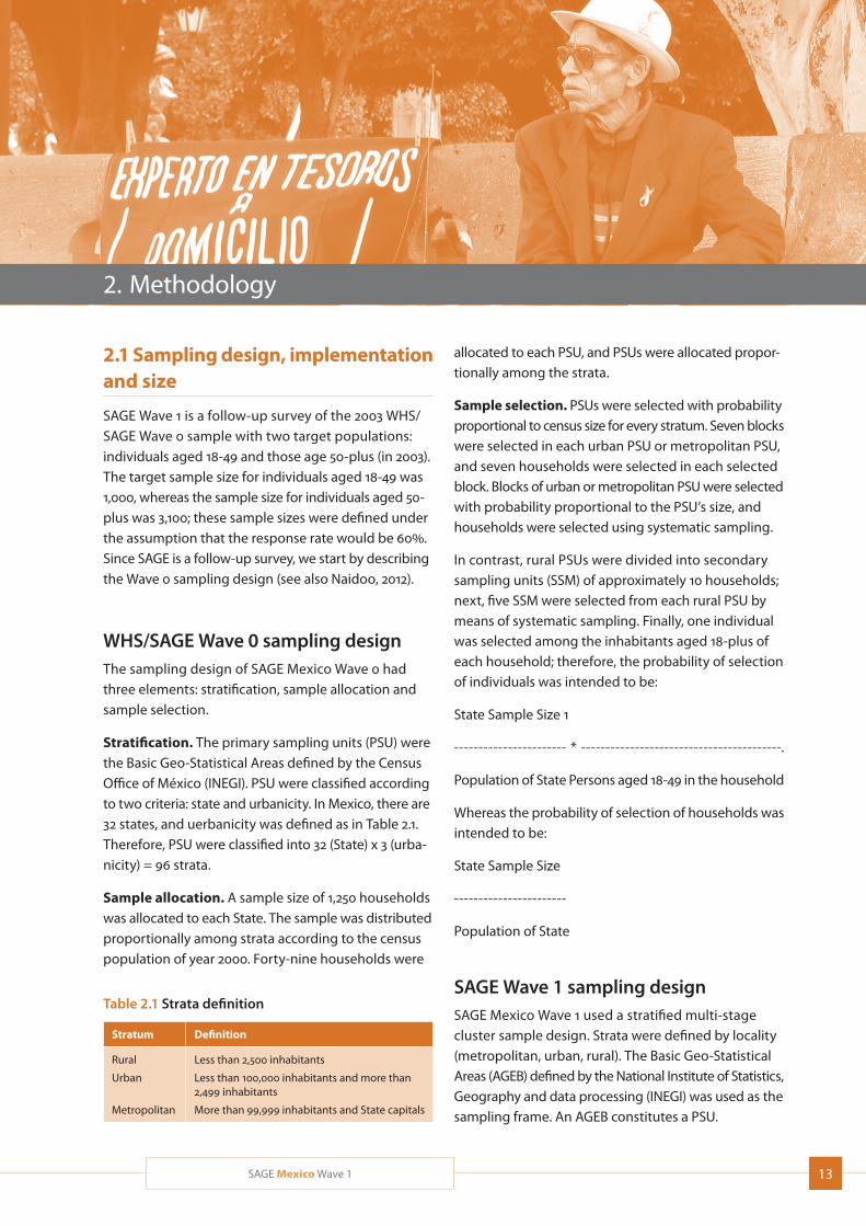
2. Methodology
allocated to each PSU, and PSUs were allocated propor-tionally among the strata.
Sample selection. PSUs were selected with probability proportional to census size for every stratum. Seven blocks were selected in each urban PSU or metropolitan PSU, and seven households were selected in each selected block. Blocks of urban or metropolitan PSU were selected with probability proportional to the PSU’s size, and households were selected using systematic sampling.
In contrast, rural PSUs were divided into secondary sampling units (SSM) of approximately 10 households; next, five SSM were selected from each rural PSU by means of systematic sampling. Finally, one individual was selected among the inhabitants aged 18-plus of each household; therefore, the probability of selection of individuals was intended to be:
State Sample Size 1
----------------------- * -----------------------------------------.
Population of State Persons aged 18-49 in the household
Whereas the probability of selection of households was intended to be:
State Sample Size
-----------------------
Population of State
SAGE Wave 1 sampling designSAGE Mexico Wave 1 used a stratified multi-stage cluster sample design. Strata were defined by locality (metropolitan, urban, rural). The Basic Geo-Statistical Areas (AGEB) defined by the National Institute of Statistics, Geography and data processing (INEGI) was used as the sampling frame. An AGEB constitutes a PSU.
Table 2.1 Strata definition
Stratum Definition
Rural
Urban
Metropolitan
Less than 2,500 inhabitants
Less than 100,000 inhabitants and more than 2,499 inhabitants
More than 99,999 inhabitants and State capitals
14 SAGE Mexico Wave 1
The sample size of SAGE Wave 1 is considerably smaller
than that of SAGE Wave 0; therefore, in order to obtain
a sample for SAGE Wave 1 with less geographical disper-
sion than that of the Wave 0 sample, a sub-sample of
211 PSUs were selected from the 797 Wave 0 PSUs.
PSUs were selected using probability proportional to
three factors:
a) (SAGE Wave 0 50-plus): number of SAGE Wave 0
participants aged 50-plus interviewed in the PSU
b) (State Population): population of the state to which
the PSU belongs
c) (SAGE Wave 0 PSU at county): number of PSUs
selected from the county to which the PSU belongs
for SAGE Wave 0.
For instance, if two PSUs in Aguascalientes State
were selected for SAGE Wave 0, then, for such a PSU,
the factor (SAGE Wave 0 PSU at county) would be
equal to two. The first and third factors were included
to reduce geographic dispersion. Factor two affords
states with larger populations a greater chance of
selection.
All SAGE Wave 0 individuals aged 50-plus in the selected
rural or urban PSUs and a random sample 90% of
individuals aged 50-plus in metropolitan PSUs who
had been interviewed in SAGE Wave 0 were included
in the SAGE Wave 1 primary sample. The remaining
10% of SAGE Wave 0 individuals aged 50-plus in metro-
politan areas were then allocated as a replacement
sample to replace individuals who could not be con-
tacted or did not consent to participate in SAGE Wave 1.
A systematic sample of 1000 SAGE Wave 0 individuals
aged 18-49 across all selected PSUs was selected as
the primary sample and 500 as a replacement sample.
Further sampling details and weighting strategies can
be found in Naidoo, 2012.
2.2 Questionnaires
The survey was carried out electronically using a CAPI
programme exclusively developed by SAGE Mexico.
Each interviewer had a laptop computer for conducting
face-to-face interviews. SAGE Wave 1 used five main
questionnaires in electronic format; these are described
in Table 2.1. GPS coordinates were collected from each
household using Garmin eTrex devices, with a minimum
of three satellite signals.
2.3 Data collection procedures
A total of 4326 households were targeted to achieve stated sample size goals. Households were included from 31 of Mexico’s 32 States, the exception being Colima. Details about the sample distribution by State, municipality and number of households is available online (http://apps.who.int/healthinfo/systems/survey data/index.php/catalog/67/study-description#page= sampling&tab=study-desc).
The survey began in November 2009 and ended in the third week of January 2010. On account of the geo-graphical hurdles and the scattered habitat in some municipalities, visits to each State were conducted in three stages:
First stage
This involved administration of the household questionnaire, the individual questionnaire and/or the proxy questionnaire by direct interview in the selected households.
Second stage
This stage was used for anthropometry, function (walking, grasping, spirometry and visual acuity) and cognitive tests (verbal fluency, immediate and recent verbal memory and repetition of numbers) and to measure biomarkers (blood pressure and blood samples to determine sugar and cholesterol levels).
Third stage
This comprised the retest by the supervisor. It involved administration of some of the tests and questions from the household, individual or proxy question-naires to persons who had already been interviewed.
Each coordinator was supported by one computer support person who was responsible for back-up of the information obtained during interviews and for maintenance of the laptop computers assigned to each interviewer. The total staff involved in the survey con-sisted of five coordinators, five computer support staff, 10 supervisors, 36 interviewers and 20 staff responsible for anthropometric data (weight, height, waist and hip circumference), blood sample and spirometry, most of whom were specially trained nurses.
Strategy for transferring and backing up dataThe information obtained from the interviews was stored directly on each interviewer’s laptop computer. At the
15SAGE Mexico Wave 1
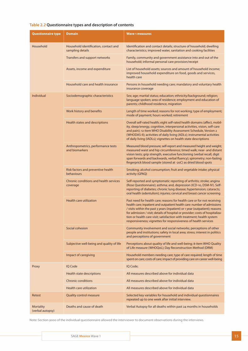
Table 2.2 Questionnaire types and description of contents
Questionnaire type Domain Wave 1 measures
Household Household identification, contact and sampling details
Identification and contact details; structure of household; dwelling characteristics; improved water, sanitation and cooking facilities
Transfers and support networks Family, community and government assistance into and out of the household; informal personal care provision/receipt
Assets, income and expenditure List of household assets; sources and amount of household income; improved household expenditure on food, goods and services, health care
Household care and health insurance Persons in household needing care; mandatory and voluntary health insurance coverage
Individual Sociodemographic characteristics Sex; age; marital status; education; ethnicity/background; religion; language spoken; area of residence; employment and education of parents; childhood residence, migration
Work history and benefits Length of time worked; reasons for not working; type of employment; mode of payment; hours worked; retirement
Health states and descriptions Overall self-rated health; eight self-rated health domains (affect, mobil-ity, sleep/energy, cognition, interpersonal activities, vision, self-care and pain); 12-item WHO Disability Assessment Schedule, Version 2 (WHODAS-II); activities of daily living (ADLs); instrumental activities of daily living (IADLs); vignettes on health state descriptions
Anthropometrics, performance tests and biomarkers
Measured blood pressure; self-report and measured height and weight; measured waist and hip circumference; timed walk; near- and distant vision tests; grip strength, executive functioning (verbal recall, digit span forwards and backwards, verbal fluency); spirometry; non-fasting fingerprick blood sample (stored at -20C) as dried blood spots
Risk factors and preventive health behaviours
Smoking; alcohol consumption; fruit and vegetable intake; physical activity (GPAQ)
Chronic conditions and health services coverage
Self-reported and symptomatic reporting of arthritis; stroke; angina (Rose Questionnaire); asthma; and, depression (ICD-10, DSM-IV). Self-reporting of diabetes; chronic lung disease; hypertension; cataracts; oral health (edentulism); injuries; cervical and breast cancer screening
Health care utilization Past need for health care; reasons for health care or for not receiving health care; inpatient and outpatient health care: number of admissions / visits within the past 3 years (inpatient) or 1 year (outpatient); reasons for admission / visit; details of hospital or provider; costs of hospitaliza-tion or health care visit; satisfaction with treatment; health system responsiveness; vignettes for responsiveness of health services
Social cohesion Community involvement and social networks; perceptions of other people and institutions; safety in local area; stress; interest in politics and perceptions of government
Subjective well-being and quality of life Perceptions about quality of life and well-being; 8-item WHO Quality of Life measure (WHOQoL); Day Reconstruction Method (DRM)
Impact of caregiving Household members needing care; type of care required; length of time spent on care; costs of care; impact of providing care on career well-being
Proxy IQ Code IQ Code;
Health state descriptions All measures described above for individual data
Chronic conditions All measures described above for individual data
Health care utilization All measures described above for individual data
Retest Quality control measure Selected key variables for household and individual questionnaires repeated up to one week after initial interview.
Mortality (verbal autopsy)
Deaths and cause of death Verbal Autopsy for all deaths within past 24 months in households
Note: Section 9000 of the individual questionnaire allowed the interviewer to document observations during the interviews.
16 SAGE Mexico Wave 1
end of each day, the data was backed up in coded form and compressed onto a ZIP archive protected by an encrypted 128-bit password.
The computer support person extracted the information from the interviewers’ computers and was transferred in encrypted form to a central server specifically used for storage. The server ensured that the files were un-damaged (uncorrupted). The files were then decrypted, decompressed and loaded into the project’s data base. A record of successful data upload was then sent via e-mail to the computer support person. The email contained receipts of the interview forms and result code for each interview. This information enabled the field coordinators and their supervisors to check the interview forms sent to the central office and to record productivity of each interviewer. Each com-puter support person was issued with a mobile wide-band device (MWB) to enable them to access the Web portal from anywhere and whenever necessary, thus averting the risk of introducing viruses into the files sent to the central server or into the computers used by the interviewers.
Follow-up systemIn order to obtain information on the progress of the survey in real time, a system was developed to permit advance reports to be produced routinely, together with ad hoc reports to check the quality of the survey. As soon as information was sent to the central server, these reports were generated automatically and in real time. Only staff authorized by the INSP’s Depart-ment of Surveys could assign keys for access to these systems. The main tables and graphs produced by the system were:
An overall report on interviews by results code, State, municipality and type of questionnaire
A graph showing the non-response rate per type of questionnaire.
Training strategyStandardized training materials were provided by WHO and were translated to Spanish and adapted for field work in Mexico.
The survey teams were trained during the last week of October and the first week of November 2009. The train-ing programme consisted of three modules taught in parallel:
1. Questionnaire (for supervisors and interviewers);
2. Anthropometry, function and cognitive tests and
biomarkers (for supervisors and staff responsible
for carrying out the function tests); and,
3. Use of the data entry programme on the laptop
computers (for all survey staff working in the field,
including supervisors, interviewers and staff record-
ing anthropometric data).
The staff responsible for training were all experienced
in carrying out surveys and in particular had experi-
ence with SAGE Mexico Wave 0. INSP staff specialized
in particular areas, such as verbal autopsies or IQ code,
were also asked to participate in the training. The train-
ers who taught anthropometrics came from various
hospitals and institutes specialized in the topic to be
taught. Details are given below:
Anthropometrics: Training and standardization
was provided by staff from INSP specialized in
anthropometrics. The training covered the tech-
niques for weighing, measuring height and waist
and thigh circumference.
Timed walk: Staff with experience of evaluation of
programmes for older adults (PAAM 70+) provided
training.
Grip strength: Training was provided by a geriatric
physician from the Salvador Zubirán National Insti-
tute of Medical Science and Nutrition (INNSZ).
Cognition tests: Training was provided by staff spe-
cialized in psychology and in performing this type
of test to assess the cognitive skills of adults aged
60-plus.
Spirometry: Training was provided by staff from the
National Institute of Respiratory Diseases who are
specialized in the use of spirometers in field settings.
Training in the remaining tests (capillary and venous
blood sample and evaluation of distant and near
vision) was provided by a colleague from the WHO
SAGE team.
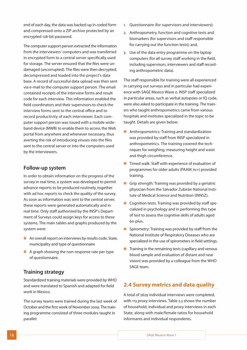
2.4 Survey metrics and data quality
A total of 2629 individual interviews were completed,
with 113 proxy interviews. Table 2.3 shows the number
of household, individual and proxy interviews in each
State, along with male/female ratios for household
informants and individual respondents.
17SAGE Mexico Wave 1
Table 2.3 Number of interviews completed, by type and M/F ratios for each area
Sub-national (region/province/state)
Household interviews
M/F Individual* Proxy* M/F
Aguascalientes 120 0.93 116 2 0.76
Baja California 127 1.10 75 0 0.49
Baja California Sur 26 1.00 18 1 0.47
Campeche 39 1.16 25 1 3.83
Coahuila de Zaragoza 51 1.10 47 3 1.22
Chiapas 28 1.06 24 1 1.31
Chihuahua 81 0.92 45 1 1.20
Federal District 191 0.94 166 5 1.21
Durango 129 0.95 138 6 1.39
Guanajuato 88 0.98 81 6 1.10
Guerrero 202 0.92 224 10 0.77
Hidalgo 86 0.95 79 5 1.74
Jalisco 184 0.90 161 8 1.07
México 164 0.84 142 8 1.28
Michoacán 98 0.81 123 4 0.08
Morelos 75 0.81 59 5 0.70
Nayarit 70 0.95 59 1 1.68
Nuevo León 187 1.02 149 7 0.97
Oaxaca 100 0.83 90 5 0.62
Puebla 57 0.81 50 2 0.96
Querétaro Arteaga 105 0.94 121 2 2.68
Quintana Roo 35 1.20 35 1 0.65
San Luis Potosí 94 0.87 83 2 0.53
Sinaloa 159 0.91 142 4 2.94
Sonora 120 1.09 96 2 0.24
Tabasco 54 1.14 50 3 0.28
Tamaulipas 68 0.69 55 6 0.34
Tlaxcala 14 0.88 12 1 1.32
Veracruz de Ignacio de 50 0.78 42 3 1.16
Yucatán 76 0.94 58 5 0.93
Zacatecas 57 0.93 64 3 1.08
Total ( pooled) 2935 0.94 2629 113 0.92
Note: Number of individual and proxy interviews completed and M/F ratios (fit to UN standard population)
18 SAGE Mexico Wave 1
Table 2.5 Household and individual response rates by selected background characteristics
Characteristics Household response rate
Householdscontacted
Individual* response rate
Individuals contacted
Age group in years
18-49 – – 28.0 429
50-59 – – 19.7 434
60-69 – – 57.1 937
70-79 – – 57.9 619
80+ – – 83.2 336
Residence
Urban 73.9 550 66.6 747
Rural 75.5 658 67.1 893
Metropolitan 57.3 2,036 49.0 2158
Wealth quintile*
Q1 (lowest) 90.6 498 83.0 617
Q2 60.1 507 56.8 627
Q3 44.8 469 42.6 585
Q4 41.7 552 36.8 658
Q5 (highest) 31.6 427 29.0 520
Total 2,453 2742
* Refers to completion of the full interview.
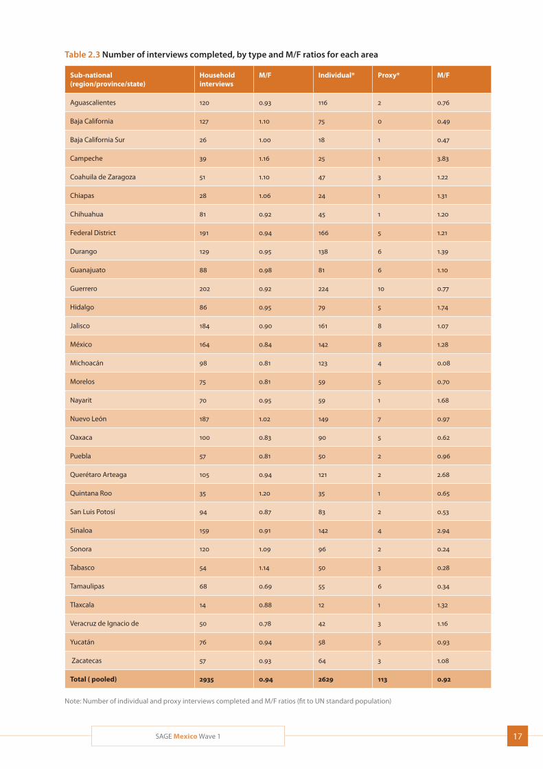
Table 2.4 Number of retest interviews, proxy retest, proxy validation and verbal autopsy interviews completed
Characteristics HH retest Individual retest Proxy retest Proxy validation Verbal Autopsy (VA)
Age group in years
18-49 7 6 0 11 4
50-59 9 7 0 5 8
60-69 11 8 1 10 20
70-79 10 10 0 8 34
80+ 6 6 1 4 53
Total 43 37 2 38 119
Retest interviews were conducted as one component of the quality assurance procedures, and verbal autopsies (VA) were used as a means to ascertain cause of death for deaths of household members. The numbers of completed retests (household, individual and proxy), proxy validation and verbal autopsy interviews are shown in Table 2.4. A total of 43 household retest inter-views were completed across the five age groups. A total
of 37 individual retest questionnaires were completed, and only two proxy retest interviews. A total of 38 inter-views were carried out to validate the use of a proxy test for a selected individual.
The largest number of verbal autopsies was obtained in the 80-plus age group, from whom 53 were obtained, in comparison with only four in the 18-49 year age group. The total number of verbal autopsies was 119.
19SAGE Mexico Wave 1
2.5 Response rate
The household response rate was higher in rural areas than in urban and metropolitan areas; the rates were 75.5%, 73.9% and 57.3%, respectively (Table 2.5).
For individual interviews, the response rate for the 18-49 years age group was 28.0%, for the 50-59 year age group was 19.7%, for the 60-69 age group was 57.1%, for the 70-79 years age group was 57.9%, and for those aged 80-plus was 83.2%. Final sample sizes for each age group are included in Table 2.5. The response rate was higher among women than among men, and higher in rural and urban areas than metropolitan areas. Response rates were generally higher in lower income quintiles than in higher income quintiles.
The total number of households in which an interview was completed was 2453 and the number of individuals interviewed was 2742.
20 SAGE Mexico Wave 1
3. Characteristics of Households and Individuals
3.1 Household characteristics
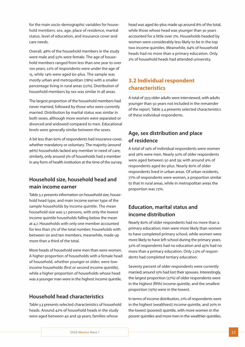
This chapter presents a profile of the selected house-holds and household members. The information on household members and housing characteristics was collected from household informants, usually the head of the household. The information collected from each of the households included a roster of household members; member composition and demographic characteristics, including marital status and education; insurance coverage and care needs of all residents stay-ing in the household for at least four months per year;
housing characteristics; and the income/economic situ-ation of the household. These basic household data play an important role in gaining an understanding of the issues related to adult health at the micro level, particu-larly of older persons.
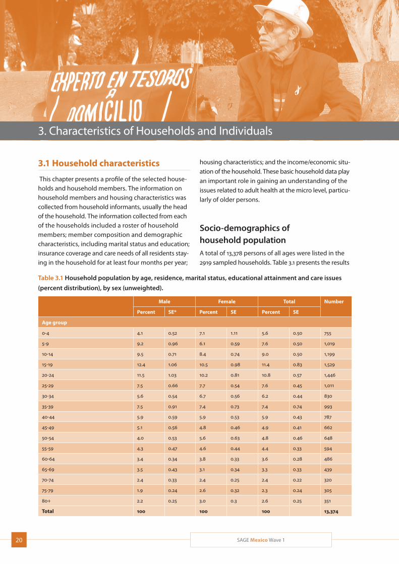
Socio-demographics of household populationA total of 13,378 persons of all ages were listed in the 2919 sampled households. Table 3.1 presents the results
Table 3.1 Household population by age, residence, marital status, educational attainment and care issues
(percent distribution), by sex (unweighted).
Male Female Total Number
Percent SE* Percent SE Percent SE
Age group
0-4 4.1 0.52 7.1 1.11 5.6 0.50 755
5-9 9.2 0.96 6.1 0.59 7.6 0.50 1,019
10-14 9.5 0.71 8.4 0.74 9.0 0.50 1,199
15-19 12.4 1.06 10.5 0.98 11.4 0.83 1,529
20-24 11.5 1.03 10.2 0.81 10.8 0.57 1,446
25-29 7.5 0.66 7.7 0.54 7.6 0.45 1,011
30-34 5.6 0.54 6.7 0.56 6.2 0.44 830
35-39 7.5 0.91 7.4 0.73 7.4 0.74 993
40-44 5.9 0.59 5.9 0.53 5.9 0.43 787
45-49 5.1 0.56 4.8 0.46 4.9 0.41 662
50-54 4.0 0.53 5.6 0.63 4.8 0.46 648
55-59 4.3 0.47 4.6 0.44 4.4 0.33 594
60-64 3.4 0.34 3.8 0.33 3.6 0.28 486
65-69 3.5 0.43 3.1 0.34 3.3 0.33 439
70-74 2.4 0.33 2.4 0.25 2.4 0.22 320
75-79 1.9 0.24 2.6 0.32 2.3 0.24 305
80+ 2.2 0.25 3.0 0.3 2.6 0.25 351
Total 100 100 100 13,374

21SAGE Mexico Wave 1
Male Female Total Number
Percent SE* Percent SE Percent SE
Residence
Urban/metropolitan 77.7 3.10 78.2 2.77 78.0 2.89 10,430
Rural 22.3 3.10 21.8 2.77 22.0 2.89 2,948
Total 100 100 100 13,378
Marital status
Never married 54.0 1.50 47.5 1.09 50.6 1.11 5,251
Currently married 38.0 1.63 34.9 1.43 36.3 1.42 3,772
Cohabitating 4.2 0.67 4.8 0.61 4.5 0.61 470
Separated/divorced 1.3 0.22 4.4 0.61 2.9 0.35 304
Widowed 2.1 0.28 8.2 0.71 5.3 0.44 551
Don’t know 0.4 0.23 0.2 0.09 0.3 0.12 34
Total 100 100 100 10,383
Education
No formal education 7.0 0.74 11.0 1.36 9.1 0.72 969
Less than primary school 28.7 2.13 29.2 1.52 28.9 1.65 3,069
Primary school completed 21.9 1.25 21.6 1.20 21.7 1.00 2,303
Secondary school completed 22.3 1.29 18.9 1.19 20.5 0.97 2,172
High school (or equivalent) completed 11.1 1.00 10.0 0.81 10.5 0.75 1,117
College/university completed 8.0 0.97 8.2 0.87 8.1 0.76 861
Post-graduate degree completed 1.0 0.29 1.1 0.52 1.0 0.37 111
Total 100 100 100 10,603
Insurance coverage
Mandatory 33.8 2.86 35.0 2.5 34.5 2.55 3,597
Voluntary 23.0 2.71 24.4 2.75 23.8 2.66 2,479
Both 0.2 0.08 0.2 0.06 0.2 0.06 18
None 43.0 2.81 40.4 2.72 41.6 2.65 4,343
Total 100 100 100 10,436
Household member needs care
Yes 3.1 0.57 5.3 0.83 4.2 0.56 443
No 96.9 0.57 94.7 0.83 95.8 0.56 9,993
Total 100 100 100 10,436
Household member institutionalized at time of interview
Yes 0 0.02 0.6 0.28 0.3 0.15 42
No 2.3 0.44 3.6 0.51 3.0 0.37 400
Not applicable 97.7 0.44 95.8 0.66 96.7 0.43 12,935
Total 100 100 100 13,378
Number 6,470 6,908 13,378
* SE = standard error
Table 3.1 Continued
22 SAGE Mexico Wave 1
Tab
le 3
.2 P
erce
nt d
istr
ibu
tion
of h
ouse
hol
d s
izes
, hou
seh
old
hea
d t
ypes
an
d m
ain
inco
me
earn
er t
ypes
, by
inco
me
qu
inti
le*
Inco
me
qu
inti
le
Nu
mb
er
Low
est
Seco
nd
Mid
dle
Fou
rth
Hig
hes
tTo
tal
Perc
ent
SE*
Perc
ent
SEPe
rcen
tSE
Perc
ent
SEPe
rcen
tSE
Perc
ent
Ho
use
ho
ld s
ize
(nu
mb
er o
f ho
use
ho
ld m
emb
ers)
148
.65.
7927
.44.
2812
.74.
658.
02.
643.
31.
8010
079
2-5
19.6
2.25
22.3
2.88
18.9
1.83
17.7
1.55
21.4
2.02
100
1,79
7
6-10
19.7
3.58
21.1
3.23
19.2
2.71
18.3
3.17
21.8
2.41
100
980
11+
18.3
6.17
16.1
6.18
7.9
4.01
22.9
7.66
34.8
9.74
100
58
Tota
l20
.42.
3021
.92.
2518
.61.
3917
.81.
6221
.31.
6410
02,
913
Nu
mb
er59
4
638
54
2
518
62
1
2,91
3
Mea
n h
ou
seh
old
siz
e4.
70.
185.
10.
275.
20.
225.
20.
175.
30.
155.
10.
12
Ho
use
ho
ld h
ead
Youn
ger w
oman
(age
d 18
-49)
16.8
6.44
16.7
6.24
31.8
11.4
715
.95.
1318
.85.
7110
016
7
Old
er w
oman
(50+
)27
.63.
7119
.31.
8022
.62.
9713
.11.
6817
.43.
7010
046
4
Youn
ger m
an (1
8-49
)20
.34.
0723
.54.
7616
.72.
8620
.43.
7119
.12.
9110
01,
002
Old
er m
an (5
0+)
18.4
2.16
22.4
2.77
16.8
1.68
17.6
1.55
24.8
2.35
100
1,27
6
Tota
l20
.42.
3021
.92.
2518
.61.
3917
.81.
6321
.31.
6410
02,
910
Nu
mb
er59
4
638
54
0
517
62
1
2,91
0
Mea
n a
ge
of h
ou
seh
old
hea
d56
.81.
255
.51.
9254
.71.
3854
.41.
2654
.80.
9955
.30.
75
Mai
n in
com
e ea
rner
Youn
ger w
oman
(age
d 18
-49)
25.6
5.81
20.1
5.92
15.9
3.49
19.1
4.76
19.3
4.66
100
338
Old
er w
oman
(50+
)24
.84.
1125
.66.
2719
.22.
7610
.91.
7519
.44.
5110
049
2
Youn
ger m
an (1
8-49
)16
.93.
8721
.13.
4321
.42.
9920
.63.
0620
.02.
6610
01,
014
Old
er m
an (5
0+)
17.4
2.52
21.5
2.32
16.2
1.71
19.1
1.78
25.8
2.54
100
951
Tota
l19
.52.
3121
.92.
3618
.61.
4118
.21.
6821
.81.
6810
02,
795
Nu
mb
er54
6
612
51
9
509
60
9
2,79
5
Mea
n a
ge
of m
ain
ear
ner
52.5
1.12
51.1
1.97
50.7
1.17
50.6
0.98
51.4
0.93
51.3
0.71
* SE
= s
tan
dar
d er
ror.
Inco
me
qui
ntile
Q1
is th
e lo
wes
t (p
oore
st) a
nd
Q5
the
hig
hest
(wea
lthi
est)
.
23SAGE Mexico Wave 1
Tab
le 3
.2 P
erce
nt d
istr
ibu
tion
of h
ouse
hol
d s
izes
, hou
seh
old
hea
d t
ypes
an
d m
ain
inco
me
earn
er t
ypes
, by
inco
me
qu
inti
le*
Inco
me
qu
inti
le
Nu
mb
er
Low
est
Seco
nd
Mid
dle
Fou
rth
Hig
hes
tTo
tal
Perc
ent
SE*
Perc
ent
SEPe
rcen
tSE
Perc
ent
SEPe
rcen
tSE
Perc
ent
Ho
use
ho
ld s
ize
(nu
mb
er o
f ho
use
ho
ld m
emb
ers)
148
.65.
7927
.44.
2812
.74.
658.
02.
643.
31.
8010
079
2-5
19.6
2.25
22.3
2.88
18.9
1.83
17.7
1.55
21.4
2.02
100
1,79
7
6-10
19.7
3.58
21.1
3.23
19.2
2.71
18.3
3.17
21.8
2.41
100
980
11+
18.3
6.17
16.1
6.18
7.9
4.01
22.9
7.66
34.8
9.74
100
58
Tota
l20
.42.
3021
.92.
2518
.61.
3917
.81.
6221
.31.
6410
02,
913
Nu
mb
er59
4
638
54
2
518
62
1
2,91
3
Mea
n h
ou
seh
old
siz
e4.
70.
185.
10.
275.
20.
225.
20.
175.
30.
155.
10.
12
Ho
use
ho
ld h
ead
Youn
ger w
oman
(age
d 18
-49)
16.8
6.44
16.7
6.24
31.8
11.4
715
.95.
1318
.85.
7110
016
7
Old
er w
oman
(50+
)27
.63.
7119
.31.
8022
.62.
9713
.11.
6817
.43.
7010
046
4
Youn
ger m
an (1
8-49
)20
.34.
0723
.54.
7616
.72.
8620
.43.
7119
.12.
9110
01,
002
Old
er m
an (5
0+)
18.4
2.16
22.4
2.77
16.8
1.68
17.6
1.55
24.8
2.35
100
1,27
6
Tota
l20
.42.
3021
.92.
2518
.61.
3917
.81.
6321
.31.
6410
02,
910
Nu
mb
er59
4
638
54
0
517
62
1
2,91
0
Mea
n a
ge
of h
ou
seh
old
hea
d56
.81.
255
.51.
9254
.71.
3854
.41.
2654
.80.
9955
.30.
75
Mai
n in
com
e ea
rner
Youn
ger w
oman
(age
d 18
-49)
25.6
5.81
20.1
5.92
15.9
3.49
19.1
4.76
19.3
4.66
100
338
Old
er w
oman
(50+
)24
.84.
1125
.66.
2719
.22.
7610
.91.
7519
.44.
5110
049
2
Youn
ger m
an (1
8-49
)16
.93.
8721
.13.
4321
.42.
9920
.63.
0620
.02.
6610
01,
014
Old
er m
an (5
0+)
17.4
2.52
21.5
2.32
16.2
1.71
19.1
1.78
25.8
2.54
100
951
Tota
l19
.52.
3121
.92.
3618
.61.
4118
.21.
6821
.81.
6810
02,
795
Nu
mb
er54
6
612
51
9
509
60
9
2,79
5
Mea
n a
ge
of m
ain
ear
ner
52.5
1.12
51.1
1.97
50.7
1.17
50.6
0.98
51.4
0.93
51.3
0.71
* SE
= s
tan
dar
d er
ror.
Inco
me
qui
ntile
Q1
is th
e lo
wes
t (p
oore
st) a
nd
Q5
the
hig
hest
(wea
lthi
est)
.
for the main socio-demographic variables for house-hold members: sex, age, place of residence, marital status, level of education, and insurance cover and care needs.
Overall, 48% of the household members in the study were male and 52% were female. The age of house-hold members ranged from less than one year to over 100 years; 22% of respondents were under the age of 15, while 14% were aged 60-plus. The sample was mostly urban and metropolitan (78%) with a smaller percentage living in rural areas (22%). Distribution of household members by sex was similar in all areas.
The largest proportion of the household members had never married, followed by those who were currently married. Distribution by marital status was similar in both sexes, although more women were separated or divorced and widowed compared to men. Educational levels were generally similar between the sexes.
A bit less than 60% of respondents had insurance cover, whether mandatory or voluntary. The majority (around 96%) households lacked any member in need of care; similarly, only around 3% of households had a member in any form of health institution at the time of the survey.
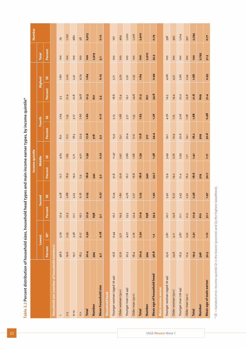
Household size, household head and main income earnerTable 3.2 presents information on household size, house-hold head type, and main income earner type of the sample households by income quintile. The mean household size was 5.1 persons, with only the lowest income quintile households falling below the mean at 4.7. Households with only one member accounted for less than 5% of the total number; households with between six and ten members, meanwhile, made up more than a third of the total.
More heads of household were men than were women. A higher proportion of households with a female head of household, whether younger or older, were low-income households (first or second income quintile), while a higher proportion of households whose head was a younger man were in the highest income quintile.
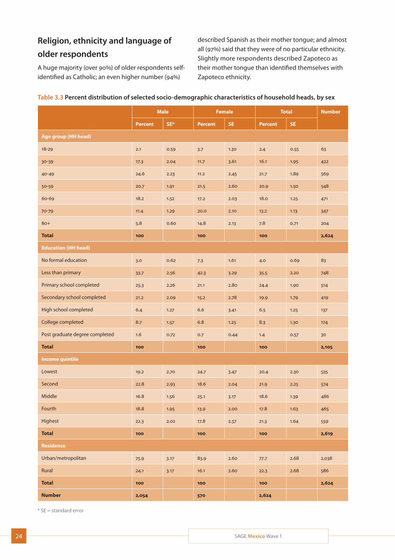
Household head characteristicsTable 3.3 presents selected characteristics of household heads. Around 42% of household heads in the study were aged between 40 and 59 years; families whose
head was aged 80-plus made up around 8% of the total, while those whose head was younger than 30 years accounted for a little over 2%. Households headed by women were considerably less likely to be in the top two income quintiles. Meanwhile, 64% of household heads had no more than a primary education. Only 2% of household heads had attended university.
3.2 Individual respondent characteristics
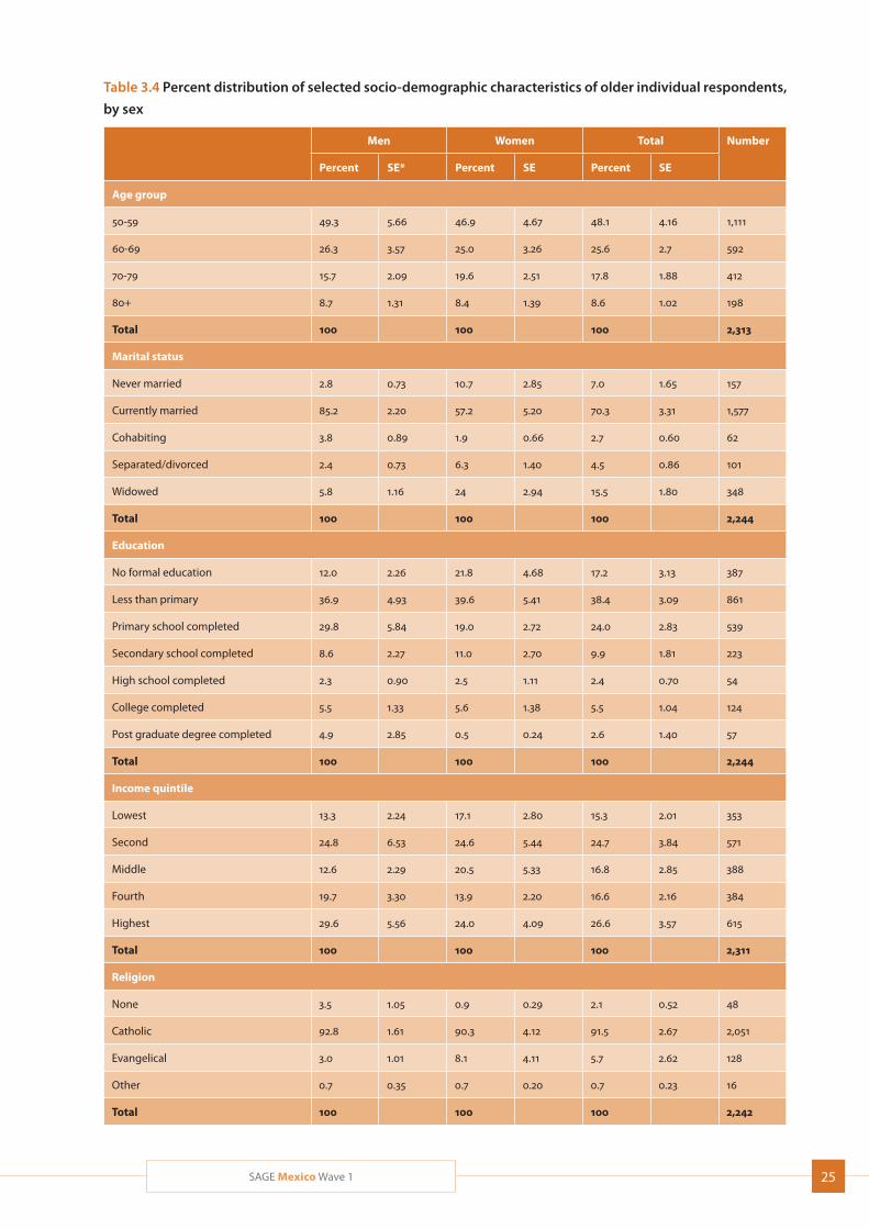
A total of 2313 older adults were interviewed, with adults younger than 50 years not included in the remainder of the report. Table 3.4 presents selected characteristics of these individual respondents.
Age, sex distribution and place of residenceA total of 74% of individual respondents were women and 26% were men. Nearly 50% of older respondents were aged between 50 and 59; with around 9% of respondents aged 80-plus. Nearly 80% of older respondents lived in urban areas. Of urban residents, 77% of respondents were women, a proportion similar to that in rural areas, while in metropolitan areas the proportion was 72%.
Education, marital status and income distributionNearly 80% of older respondents had no more than a primary education; men were more likely than women to have completed primary school, while women were more likely to have left school during the primary years. 32% of respondents had no education and 45% had no more than a primary education. Only 2.5% of respon-dents had completed tertiary education.
Seventy percent of older respondents were currently married; around 15% had lost their spouses. Interestingly, the largest proportion (27%) of older respondents were in the highest (fifth) income quintile, and the smallest proportion (15%) were in the lowest.
In terms of income distribution, 21% of respondents were in the highest (wealthiest) income quintile, and 20% in the lowest (poorest) quintile, with more women in the poorer quintiles and more men in the wealthier quintiles.
24 SAGE Mexico Wave 1
Table 3.3 Percent distribution of selected socio-demographic characteristics of household heads, by sex
Male Female Total Number
Percent SE* Percent SE Percent SE
Age group (HH head)
18-29 2.1 0.59 3.7 1.30 2.4 0.55 63
30-39 17.3 2.04 11.7 3.61 16.1 1.95 422
40-49 24.6 2.23 11.2 2.45 21.7 1.89 569
50-59 20.7 1.91 21.5 2.60 20.9 1.50 548
60-69 18.2 1.52 17.2 2.03 18.0 1.25 471
70-79 11.4 1.29 20.0 2.10 13.2 1.13 347
80+ 5.8 0.60 14.8 2.13 7.8 0.71 204
Total 100 100 100 2,624
Education (HH head)
No formal education 3.0 0.62 7.3 1.61 4.0 0.69 83
Less than primary 33.7 2.56 42.3 3.29 35.5 2.20 748
Primary school completed 25.3 2.26 21.1 2.80 24.4 1.90 514
Secondary school completed 21.2 2.09 15.2 2.78 19.9 1.79 419
High school completed 6.4 1.27 6.6 3.41 6.5 1.25 137
College completed 8.7 1.57 6.8 1.25 8.3 1.30 174
Post graduate degree completed 1.6 0.72 0.7 0.44 1.4 0.57 30
Total 100 100 100 2,105
Income quintile
Lowest 19.2 2.70 24.7 3.47 20.4 2.30 535
Second 22.8 2.93 18.6 2.04 21.9 2.25 574
Middle 16.8 1.56 25.1 3.17 18.6 1.39 486
Fourth 18.8 1.95 13.9 2.00 17.8 1.63 465
Highest 22.3 2.02 17.8 2.57 21.3 1.64 559
Total 100 100 100 2,619
Residence
Urban/metropolitan 75.9 3.17 83.9 2.60 77.7 2.68 2,038
Rural 24.1 3.17 16.1 2.60 22.3 2.68 586
Total 100 100 100 2,624
Number 2,054 570 2,624
* SE = standard error
Religion, ethnicity and language of
older respondents
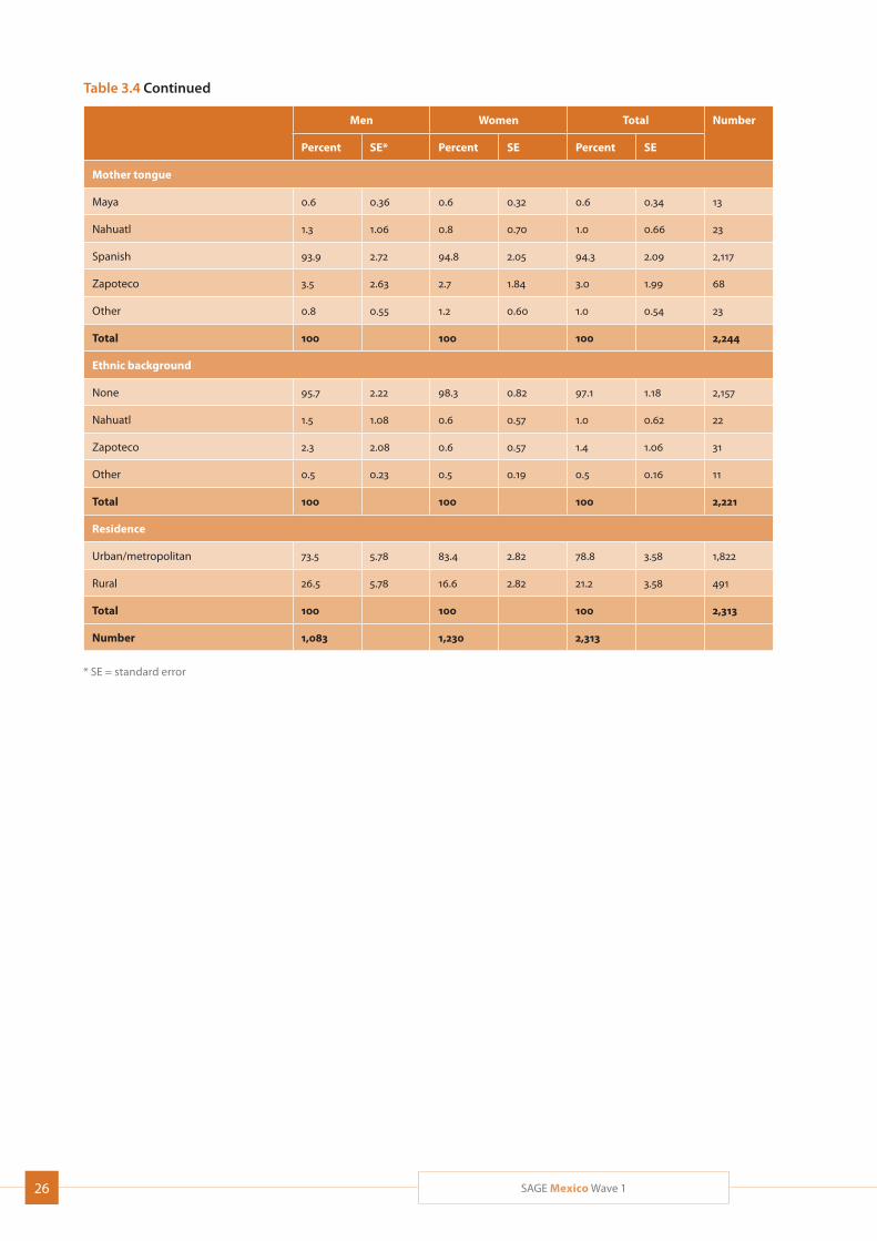
A huge majority (over 90%) of older respondents self-identified as Catholic; an even higher number (94%)
described Spanish as their mother tongue; and almost all (97%) said that they were of no particular ethnicity. Slightly more respondents described Zapoteco as their mother tongue than identified themselves with Zapoteco ethnicity.
25SAGE Mexico Wave 1
Table 3.4 Percent distribution of selected socio-demographic characteristics of older individual respondents,
by sex
Men Women Total Number
Percent SE* Percent SE Percent SE
Age group
50-59 49.3 5.66 46.9 4.67 48.1 4.16 1,111
60-69 26.3 3.57 25.0 3.26 25.6 2.7 592
70-79 15.7 2.09 19.6 2.51 17.8 1.88 412
80+ 8.7 1.31 8.4 1.39 8.6 1.02 198
Total 100 100 100 2,313
Marital status
Never married 2.8 0.73 10.7 2.85 7.0 1.65 157
Currently married 85.2 2.20 57.2 5.20 70.3 3.31 1,577
Cohabiting 3.8 0.89 1.9 0.66 2.7 0.60 62
Separated/divorced 2.4 0.73 6.3 1.40 4.5 0.86 101
Widowed 5.8 1.16 24 2.94 15.5 1.80 348
Total 100 100 100 2,244
Education
No formal education 12.0 2.26 21.8 4.68 17.2 3.13 387
Less than primary 36.9 4.93 39.6 5.41 38.4 3.09 861
Primary school completed 29.8 5.84 19.0 2.72 24.0 2.83 539
Secondary school completed 8.6 2.27 11.0 2.70 9.9 1.81 223
High school completed 2.3 0.90 2.5 1.11 2.4 0.70 54
College completed 5.5 1.33 5.6 1.38 5.5 1.04 124
Post graduate degree completed 4.9 2.85 0.5 0.24 2.6 1.40 57
Total 100 100 100 2,244
Income quintile
Lowest 13.3 2.24 17.1 2.80 15.3 2.01 353
Second 24.8 6.53 24.6 5.44 24.7 3.84 571
Middle 12.6 2.29 20.5 5.33 16.8 2.85 388
Fourth 19.7 3.30 13.9 2.20 16.6 2.16 384
Highest 29.6 5.56 24.0 4.09 26.6 3.57 615
Total 100 100 100 2,311
Religion
None 3.5 1.05 0.9 0.29 2.1 0.52 48
Catholic 92.8 1.61 90.3 4.12 91.5 2.67 2,051
Evangelical 3.0 1.01 8.1 4.11 5.7 2.62 128
Other 0.7 0.35 0.7 0.20 0.7 0.23 16
Total 100 100 100 2,242
26 SAGE Mexico Wave 1
Men Women Total Number
Percent SE* Percent SE Percent SE
Mother tongue
Maya 0.6 0.36 0.6 0.32 0.6 0.34 13
Nahuatl 1.3 1.06 0.8 0.70 1.0 0.66 23
Spanish 93.9 2.72 94.8 2.05 94.3 2.09 2,117
Zapoteco 3.5 2.63 2.7 1.84 3.0 1.99 68
Other 0.8 0.55 1.2 0.60 1.0 0.54 23
Total 100 100 100 2,244
Ethnic background
None 95.7 2.22 98.3 0.82 97.1 1.18 2,157
Nahuatl 1.5 1.08 0.6 0.57 1.0 0.62 22
Zapoteco 2.3 2.08 0.6 0.57 1.4 1.06 31
Other 0.5 0.23 0.5 0.19 0.5 0.16 11
Total 100 100 100 2,221
Residence
Urban/metropolitan 73.5 5.78 83.4 2.82 78.8 3.58 1,822
Rural 26.5 5.78 16.6 2.82 21.2 3.58 491
Total 100 100 100 2,313
Number 1,083 1,230 2,313
* SE = standard error
Table 3.4 Continued
27SAGE Mexico Wave 1
4. Income, Consumption, Transfers and Retirement
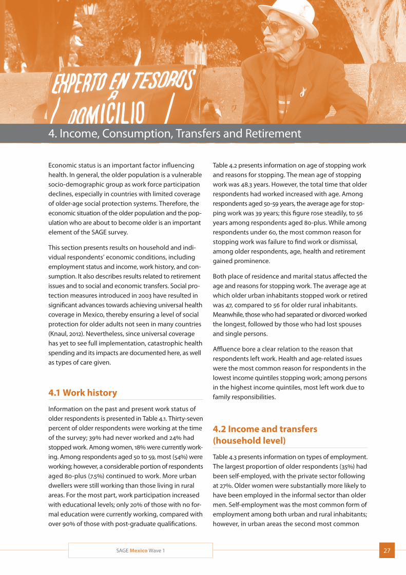
Economic status is an important factor influencing health. In general, the older population is a vulnerable socio-demographic group as work force participation declines, especially in countries with limited coverage of older-age social protection systems. Therefore, the economic situation of the older population and the pop-ulation who are about to become older is an important element of the SAGE survey.
This section presents results on household and indi-vidual respondents’ economic conditions, including employment status and income, work history, and con-sumption. It also describes results related to retirement issues and to social and economic transfers. Social pro-tection measures introduced in 2003 have resulted in significant advances towards achieving universal health coverage in Mexico, thereby ensuring a level of social protection for older adults not seen in many countries (Knaul, 2012). Nevertheless, since universal coverage has yet to see full implementation, catastrophic health spending and its impacts are documented here, as well as types of care given.
4.1 Work history
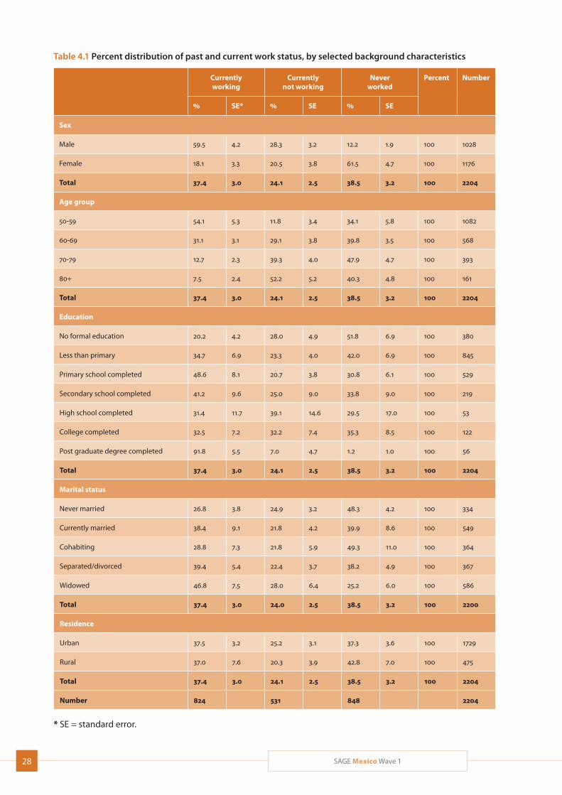
Information on the past and present work status of older respondents is presented in Table 4.1. Thirty-seven percent of older respondents were working at the time of the survey; 39% had never worked and 24% had stopped work. Among women, 18% were currently work-ing. Among respondents aged 50 to 59, most (54%) were working; however, a considerable portion of respondents aged 80-plus (7.5%) continued to work. More urban dwellers were still working than those living in rural areas. For the most part, work participation increased with educational levels; only 20% of those with no for-mal education were currently working, compared with over 90% of those with post-graduate qualifications.
Table 4.2 presents information on age of stopping work and reasons for stopping. The mean age of stopping work was 48.3 years. However, the total time that older respondents had worked increased with age. Among respondents aged 50-59 years, the average age for stop-ping work was 39 years; this figure rose steadily, to 56 years among respondents aged 80-plus. While among respondents under 60, the most common reason for stopping work was failure to find work or dismissal, among older respondents, age, health and retirement gained prominence.
Both place of residence and marital status affected the age and reasons for stopping work. The average age at which older urban inhabitants stopped work or retired was 47, compared to 56 for older rural inhabitants. Meanwhile, those who had separated or divorced worked the longest, followed by those who had lost spouses and single persons.
Affluence bore a clear relation to the reason that respondents left work. Health and age-related issues were the most common reason for respondents in the lowest income quintiles stopping work; among persons in the highest income quintiles, most left work due to family responsibilities.
4.2 Income and transfers (household level)
Table 4.3 presents information on types of employment. The largest proportion of older respondents (35%) had been self-employed, with the private sector following at 27%. Older women were substantially more likely to have been employed in the informal sector than older men. Self-employment was the most common form of employment among both urban and rural inhabitants; however, in urban areas the second most common
28 SAGE Mexico Wave 1
Table 4.1 Percent distribution of past and current work status, by selected background characteristics
Currently working
Currently not working
Never worked
Percent
Number
% SE* % SE % SE
Sex
Male 59.5 4.2 28.3 3.2 12.2 1.9 100 1028
Female 18.1 3.3 20.5 3.8 61.5 4.7 100 1176
Total 37.4 3.0 24.1 2.5 38.5 3.2 100 2204
Age group
50-59 54.1 5.3 11.8 3.4 34.1 5.8 100 1082
60-69 31.1 3.1 29.1 3.8 39.8 3.5 100 568
70-79 12.7 2.3 39.3 4.0 47.9 4.7 100 393
80+ 7.5 2.4 52.2 5.2 40.3 4.8 100 161
Total 37.4 3.0 24.1 2.5 38.5 3.2 100 2204
Education
No formal education 20.2 4.2 28.0 4.9 51.8 6.9 100 380
Less than primary 34.7 6.9 23.3 4.0 42.0 6.9 100 845
Primary school completed 48.6 8.1 20.7 3.8 30.8 6.1 100 529
Secondary school completed 41.2 9.6 25.0 9.0 33.8 9.0 100 219
High school completed 31.4 11.7 39.1 14.6 29.5 17.0 100 53
College completed 32.5 7.2 32.2 7.4 35.3 8.5 100 122
Post graduate degree completed 91.8 5.5 7.0 4.7 1.2 1.0 100 56
Total 37.4 3.0 24.1 2.5 38.5 3.2 100 2204
Marital status
Never married 26.8 3.8 24.9 3.2 48.3 4.2 100 334
Currently married 38.4 9.1 21.8 4.2 39.9 8.6 100 549
Cohabiting 28.8 7.3 21.8 5.9 49.3 11.0 100 364
Separated/divorced 39.4 5.4 22.4 3.7 38.2 4.9 100 367
Widowed 46.8 7.5 28.0 6.4 25.2 6.0 100 586
Total 37.4 3.0 24.0 2.5 38.5 3.2 100 2200
Residence
Urban 37.5 3.2 25.2 3.1 37.3 3.6 100 1729
Rural 37.0 7.6 20.3 3.9 42.8 7.0 100 475
Total 37.4 3.0 24.1 2.5 38.5 3.2 100 2204
Number 824 531 848 2204
* SE = standard error.
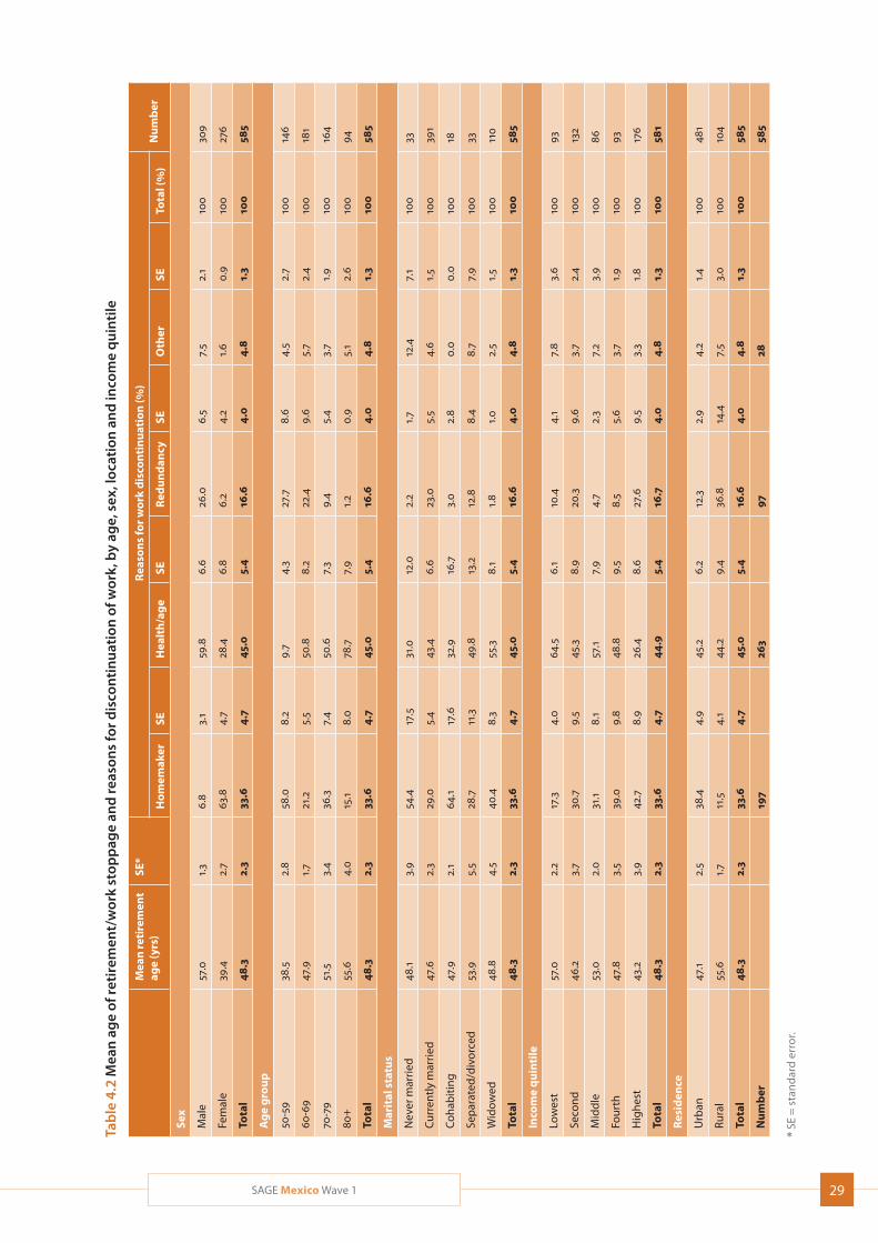
29SAGE Mexico Wave 1
Tab
le 4
.2 M
ean
ag
e of
reti
rem
ent/
wor
k st
opp
age
and
reas
ons
for d
isco
ntin
uat
ion
of w
ork,
by
age,
sex
, lo
cati
on a
nd
inco
me
qu
inti
le
Mea
n re
tire
men
t ag
e (y
rs)
SE*
Rea
son
s fo
r w
ork
dis
con
tin
uat
ion
(%)
Nu
mb
erH
om
emak
erSE
Hea
lth
/ag
eSE
Red
un
dan
cySE
Oth
erSE
Tota
l (%
)
Sex
Mal
e57
.01.
36.
83.
159
.86.
626
.06.
57.
52.
110
030
9
Fem
ale
39.4
2.7
63.8
4.7
28.4
6.8
6.2
4.2
1.6
0.9
100
276
Tota
l48
.32.
333
.64.
745
.05.
416
.64.
04.
81.
310
058
5
Ag
e g
rou
p
50-5
938
.52.
858
.08.
29.
74.
327
.78.
64.
52.
710
014
6
60-6
947
.91.
721
.25.
550
.88.
222
.49.
65.
72.
410
018
1
70-7
951
.53.
436
.37.
450
.67.
39.
45.
43.
71.
910
016
4
80+
55.6
4.0
15.1
8.0
78.7
7.9
1.2
0.9
5.1
2.6
100
94
Tota
l48
.32.
333
.64.
745
.05.
416
.64.
04.
81.
310
058
5
Mar
ital
sta
tus
Nev
er m
arrie
d48
.13.
954
.417
.531
.012
.02.
21.
712
.47.
110
033
Cur
rent
ly m
arrie
d47
.62.
329
.05.
443
.46.
623
.05.
54.
61.
510
039
1
Coh
abiti
ng47
.92.
164
.117
.632
.916
.73.
02.
80.
00.
010
018
Sep
arat
ed/d
ivor
ced
53.9
5.5
28.7
11.3
49.8
13.2
12.8
8.4
8.7
7.9
100
33
Wid
owed
48.8
4.5
40.4
8.3
55.3
8.1
1.8
1.0
2.5
1.5
100
110
Tota
l48
.32.
333
.64.
745
.05.
416
.64.
04.
81.
310
058
5
Inco
me
qu
inti
le
Low
est
57.0
2.2
17.3
4.0
64.5
6.1
10.4
4.1
7.8
3.6
100
93
Seco
nd46
.23.
730
.79.
545
.38.
920
.39.
63.
72.
410
013
2
Mid
dle
53.0
2.0
31.1
8.1
57.1
7.9
4.7
2.3
7.2
3.9
100
86
Four
th47
.83.
539
.09.
848
.89.
58.
55.
63.
71.
910
093
Hig
hest
43.2
3.9
42.7
8.9
26.4
8.6
27.6
9.5
3.3
1.8
100
176
Tota
l48
.32.
333
.64.
744
.95.
416
.74.
04.
81.
310
058
1
Res
iden
ce
Urb
an47
.12.
538
.44.
945
.26.
212
.32.
94.
21.
410
048
1
Rura
l55
.61.
711
.54.
144
.29.
436
.814
.47.
53.
010
010
4
Tota
l48
.32.
333
.64.
745
.05.
416
.64.
04.
81.
310
058
5
Nu
mb
er19
726
397
2858
5
* SE
= s
tan
dar
d er
ror.
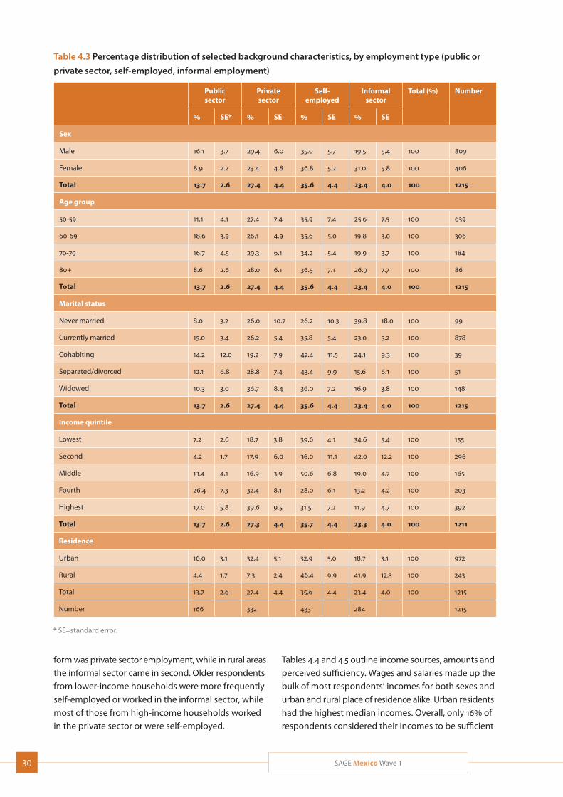
30 SAGE Mexico Wave 1
Table 4.3 Percentage distribution of selected background characteristics, by employment type (public or
private sector, self-employed, informal employment)
Public sector
Private sector
Self- employed
Informal sector
Total (%) Number
% SE* % SE % SE % SE
Sex
Male 16.1 3.7 29.4 6.0 35.0 5.7 19.5 5.4 100 809
Female 8.9 2.2 23.4 4.8 36.8 5.2 31.0 5.8 100 406
Total 13.7 2.6 27.4 4.4 35.6 4.4 23.4 4.0 100 1215
Age group
50-59 11.1 4.1 27.4 7.4 35.9 7.4 25.6 7.5 100 639
60-69 18.6 3.9 26.1 4.9 35.6 5.0 19.8 3.0 100 306
70-79 16.7 4.5 29.3 6.1 34.2 5.4 19.9 3.7 100 184
80+ 8.6 2.6 28.0 6.1 36.5 7.1 26.9 7.7 100 86
Total 13.7 2.6 27.4 4.4 35.6 4.4 23.4 4.0 100 1215
Marital status
Never married 8.0 3.2 26.0 10.7 26.2 10.3 39.8 18.0 100 99
Currently married 15.0 3.4 26.2 5.4 35.8 5.4 23.0 5.2 100 878
Cohabiting 14.2 12.0 19.2 7.9 42.4 11.5 24.1 9.3 100 39
Separated/divorced 12.1 6.8 28.8 7.4 43.4 9.9 15.6 6.1 100 51
Widowed 10.3 3.0 36.7 8.4 36.0 7.2 16.9 3.8 100 148
Total 13.7 2.6 27.4 4.4 35.6 4.4 23.4 4.0 100 1215
Income quintile
Lowest 7.2 2.6 18.7 3.8 39.6 4.1 34.6 5.4 100 155
Second 4.2 1.7 17.9 6.0 36.0 11.1 42.0 12.2 100 296
Middle 13.4 4.1 16.9 3.9 50.6 6.8 19.0 4.7 100 165
Fourth 26.4 7.3 32.4 8.1 28.0 6.1 13.2 4.2 100 203
Highest 17.0 5.8 39.6 9.5 31.5 7.2 11.9 4.7 100 392
Total 13.7 2.6 27.3 4.4 35.7 4.4 23.3 4.0 100 1211
Residence
Urban 16.0 3.1 32.4 5.1 32.9 5.0 18.7 3.1 100 972
Rural 4.4 1.7 7.3 2.4 46.4 9.9 41.9 12.3 100 243
Total 13.7 2.6 27.4 4.4 35.6 4.4 23.4 4.0 100 1215
Number 166 332 433 284 1215
* SE=standard error.
form was private sector employment, while in rural areas the informal sector came in second. Older respondents from lower-income households were more frequently self-employed or worked in the informal sector, while most of those from high-income households worked in the private sector or were self-employed.
Tables 4.4 and 4.5 outline income sources, amounts and perceived sufficiency. Wages and salaries made up the bulk of most respondents’ incomes for both sexes and urban and rural place of residence alike. Urban residents had the highest median incomes. Overall, only 16% of respondents considered their incomes to be sufficient
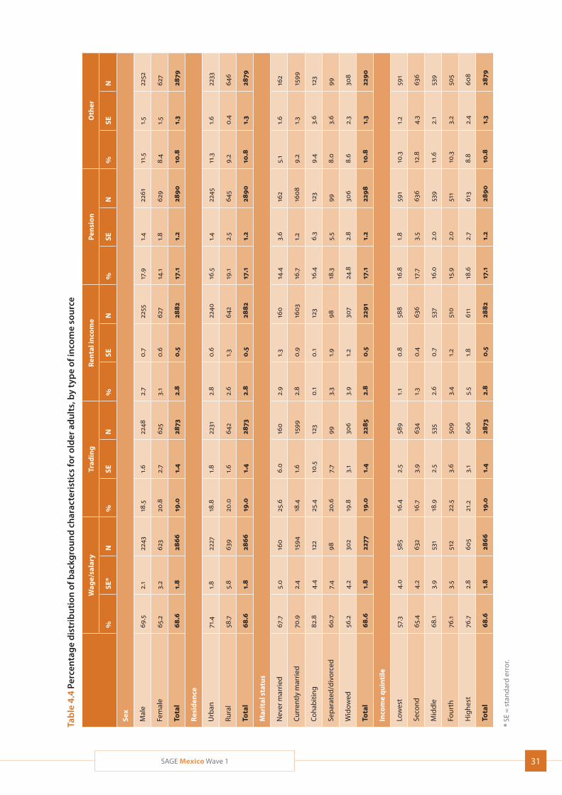
31SAGE Mexico Wave 1
Tab
le 4
.4 P
erce
ntag
e d
istr
ibu
tion
of b
ackg
rou
nd
ch
arac
teri
stic
s fo
r old
er a
du
lts,
by
typ
e of
inco
me
sou
rce
Wag
e/sa
lary
Trad
ing
Ren
tal i
nco
me
Pen
sio
nO
ther
%SE
*N
%SE
N%
SEN
%SE
N%
SEN
Sex
Mal
e69
.52.
122
4318
.51.
622
482.
70.
722
5517
.91.
422
6111
.51.
522
52
Fem
ale
65.2
3.2
623
20.8
2.7
625
3.1
0.6
627
14.1
1.8
629
8.4
1.5
627
Tota
l68
.61.
828
6619
.01.
428
732.
80.
528
8217
.11.
228
9010
.81.
328
79
Res
iden
ce
Urb
an71
.41.
822
2718
.81.
822
312.
80.
622
4016
.51.
422
4511
.31.
622
33
Rura
l58
.75.
863
920
.01.
664
22.
61.
364
219
.12.
564
59.
20.
464
6
Tota
l68
.61.
828
6619
.01.
428
732.
80.
528
8217
.11.
228
9010
.81.
328
79
Mar
ital
sta
tus
Nev
er m
arrie
d67
.75.
016
025
.66.
016
02.
91.
316
014
.43.
616
25.
11.
616
2
Cur
rent
ly m
arrie
d70
.92.
415
9418
.41.
615
992.
80.
916
0316
.71.
216
089.
21.
315
99
Coh
abiti
ng82
.84.
412
225
.410
.512
30.
10.
112
316
.46.
312
39.
43.
612
3
Sep
arat
ed/d
ivor
ced
60.7
7.4
9820
.67.
799
3.3
1.9
9818
.35.
599
8.0
3.6
99
Wid
owed
56.2
4.2
302
19.8
3.1
306
3.9
1.2
307
24.8
2.8
306
8.6
2.3
308
Tota
l68
.61.
822
7719
.01.
422
852.
80.
522
9117
.11.
222
9810
.81.
322
90
Inco
me
qu
inti
le
Low
est
57.3
4.0
585
16.4
2.5
589
1.1
0.8
588
16.8
1.8
591
10.3
1.2
591
Seco
nd65
.44.
263
216
.73.
963
41.
30.
463
617
.73.
563
612
.84.
363
6
Mid
dle
68.1
3.9
531
18.9
2.5
535
2.6
0.7
537
16.0
2.0
539
11.6
2.1
539
Four
th76
.13.
551
222
.53.
650
93.
41.
251
015
.92.
051
110
.33.
250
5
Hig
hest
76.7
2.8
605
21.2
3.1
606
5.5
1.8
611
18.6
2.7
613
8.8
2.4
608
Tota
l68
.61.
828
6619
.01.
428
732.
80.
528
8217
.11.
228
9010
.81.
328
79
* SE
= s
tan
dar
d er
ror.
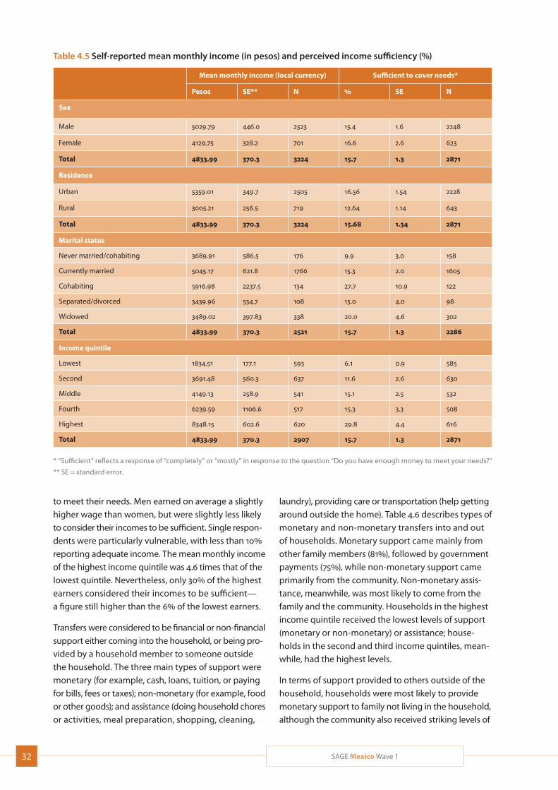
32 SAGE Mexico Wave 1
Table 4.5 Self-reported mean monthly income (in pesos) and perceived income sufficiency (%)
Mean monthly income (local currency) Sufficient to cover needs*
Pesos SE** N % SE N
Sex
Male 5029.79 446.0 2523 15.4 1.6 2248
Female 4129.75 328.2 701 16.6 2.6 623
Total 4833.99 370.3 3224 15.7 1.3 2871
Residence
Urban 5359.01 349.7 2505 16.56 1.54 2228
Rural 3005.21 256.5 719 12.64 1.14 643
Total 4833.99 370.3 3224 15.68 1.34 2871
Marital status
Never married/cohabiting 3689.91 586.5 176 9.9 3.0 158
Currently married 5045.17 621.8 1766 15.3 2.0 1605
Cohabiting 5916.98 2237.5 134 27.7 10.9 122
Separated/divorced 3439.96 534.7 108 15.0 4.0 98
Widowed 3489.02 397.83 338 20.0 4.6 302
Total 4833.99 370.3 2521 15.7 1.3 2286
Income quintile
Lowest 1834.51 177.1 593 6.1 0.9 585
Second 3691.48 560.3 637 11.6 2.6 630
Middle 4149.13 258.9 541 15.1 2.5 532
Fourth 6239.59 1106.6 517 15.3 3.3 508
Highest 8348.15 602.6 620 29.8 4.4 616
Total 4833.99 370.3 2907 15.7 1.3 2871
* “Sufficient” reflects a response of “completely” or “mostly” in response to the question “Do you have enough money to meet your needs?”
** SE = standard error.
to meet their needs. Men earned on average a slightly higher wage than women, but were slightly less likely to consider their incomes to be sufficient. Single respon-dents were particularly vulnerable, with less than 10% reporting adequate income. The mean monthly income of the highest income quintile was 4.6 times that of the lowest quintile. Nevertheless, only 30% of the highest earners considered their incomes to be sufficient— a figure still higher than the 6% of the lowest earners.
Transfers were considered to be financial or non-financial support either coming into the household, or being pro-vided by a household member to someone outside the household. The three main types of support were monetary (for example, cash, loans, tuition, or paying for bills, fees or taxes); non-monetary (for example, food or other goods); and assistance (doing household chores or activities, meal preparation, shopping, cleaning,
laundry), providing care or transportation (help getting around outside the home). Table 4.6 describes types of monetary and non-monetary transfers into and out of households. Monetary support came mainly from other family members (81%), followed by government payments (75%), while non-monetary support came primarily from the community. Non-monetary assis-tance, meanwhile, was most likely to come from the family and the community. Households in the highest income quintile received the lowest levels of support (monetary or non-monetary) or assistance; house-holds in the second and third income quintiles, mean-while, had the highest levels.
In terms of support provided to others outside of the household, households were most likely to provide monetary support to family not living in the household, although the community also received striking levels of
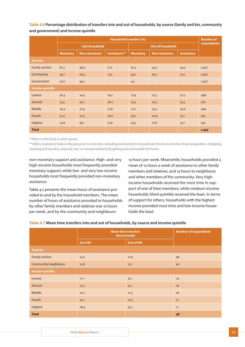
33SAGE Mexico Wave 1
non-monetary support and assistance. High- and very high-income households most frequently provided monetary support; while low- and very low-income households most frequently provided non-monetary assistance.
Table 4.7 presents the mean hours of assistance pro-vided to and by the household members. The mean number of hours of assistance provided to households by other family members and relatives was 15 hours per week, and by the community and neighbours
Table 4.6 Percentage distribution of transfers into and out of households, by source (family and kin, community
and government) and income quintile
Household transfers (%) Number of respondents Into household Out of household
Monetary Non-monetary* Assistance** Monetary Non-monetary Assistance
Sources
Family and kin 81.3 38.4 17.7 61.3 55.4 24.0 2,927
Community 35.7 64.3 12.5 43.7 63.7 21.5 2,927
Government 75.0 34.2 . 4.5 . . 2,927
Income quintile
Lowest 20.3 19.4 19.2 17.9 15.5 27.5 498
Second 23.5 29.1 28.2 23.5 22.5 23.5 507
Middle 24.3 27.4 21.8 11.0 23.3 19.6 469
Fourth 21.4 15.4 18.0 24.1 20.9 15.7 552
Highest 10.6 8.6 12.8 23.5 17.8 13.7 427
Total 2,453
* Refers to the food or other goods.
** Refers to physical help in the year prior to interview, including involvement in household chores or activities (meal preparation, shopping,
cleaning and laundry), physical care, or transportation/help getting around outside the home.
13 hours per week. Meanwhile, households provided a mean of 12 hours a week of assistance to other family members and relatives, and 13 hours to neighbours and other members of the community. Very high- income households received the most time in sup-port of one of their members, while medium-income households (third quintile) received the least. In terms of support for others, households with the highest income provided most time and low-income house-holds the least.
Table 4.7 Mean time transfers into and out of households, by source and income quintile
Mean time transfers (hours/week)
Number of respondents
Into HH Out of HH
Sources
Family and kin 15.0 11.6 98
Community/neighbours 12.8 13.1 90
Income quintile
Lowest 11.1 6.2 14
Second 15.5 9.2 19
Middle 10.7 11.5 18
Fourth 14.1 12.3 21
Highest 18.4 23.1 11
Total 98
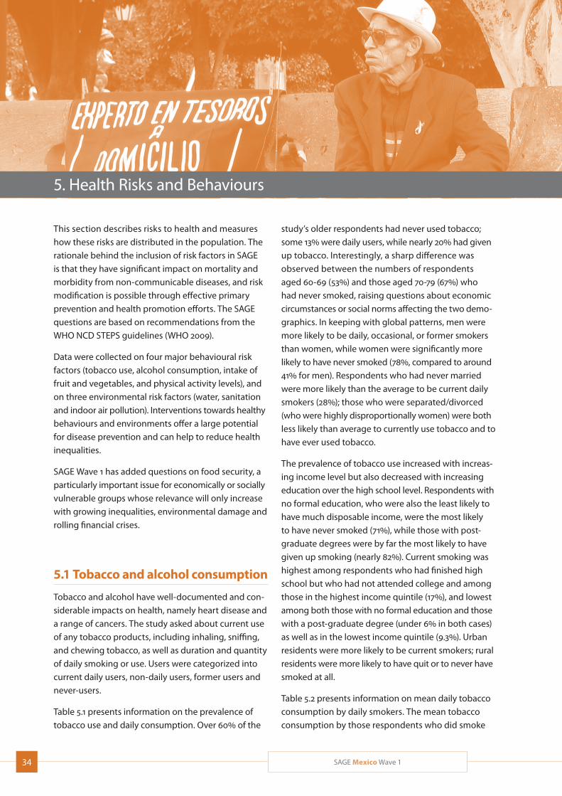
34 SAGE Mexico Wave 1
5. Health Risks and Behaviours
This section describes risks to health and measures how these risks are distributed in the population. The rationale behind the inclusion of risk factors in SAGE is that they have significant impact on mortality and morbidity from non-communicable diseases, and risk modification is possible through effective primary prevention and health promotion efforts. The SAGE questions are based on recommendations from the WHO NCD STEPS guidelines (WHO 2009).
Data were collected on four major behavioural risk factors (tobacco use, alcohol consumption, intake of fruit and vegetables, and physical activity levels), and on three environmental risk factors (water, sanitation and indoor air pollution). Interventions towards healthy behaviours and environments offer a large potential for disease prevention and can help to reduce health inequalities.
SAGE Wave 1 has added questions on food security, a particularly important issue for economically or socially vulnerable groups whose relevance will only increase with growing inequalities, environmental damage and rolling financial crises.
5.1 Tobacco and alcohol consumption
Tobacco and alcohol have well-documented and con-siderable impacts on health, namely heart disease and a range of cancers. The study asked about current use of any tobacco products, including inhaling, sniffing, and chewing tobacco, as well as duration and quantity of daily smoking or use. Users were categorized into current daily users, non-daily users, former users and never-users.
Table 5.1 presents information on the prevalence of tobacco use and daily consumption. Over 60% of the
study’s older respondents had never used tobacco; some 13% were daily users, while nearly 20% had given up tobacco. Interestingly, a sharp difference was observed between the numbers of respondents aged 60-69 (53%) and those aged 70-79 (67%) who had never smoked, raising questions about economic circumstances or social norms affecting the two demo-graphics. In keeping with global patterns, men were more likely to be daily, occasional, or former smokers than women, while women were significantly more likely to have never smoked (78%, compared to around 41% for men). Respondents who had never married were more likely than the average to be current daily smokers (28%); those who were separated/divorced (who were highly disproportionally women) were both less likely than average to currently use tobacco and to have ever used tobacco.
The prevalence of tobacco use increased with increas-ing income level but also decreased with increasing education over the high school level. Respondents with no formal education, who were also the least likely to have much disposable income, were the most likely to have never smoked (71%), while those with post-graduate degrees were by far the most likely to have given up smoking (nearly 82%). Current smoking was highest among respondents who had finished high school but who had not attended college and among those in the highest income quintile (17%), and lowest among both those with no formal education and those with a post-graduate degree (under 6% in both cases) as well as in the lowest income quintile (9.3%). Urban residents were more likely to be current smokers; rural residents were more likely to have quit or to never have smoked at all.
Table 5.2 presents information on mean daily tobacco consumption by daily smokers. The mean tobacco consumption by those respondents who did smoke
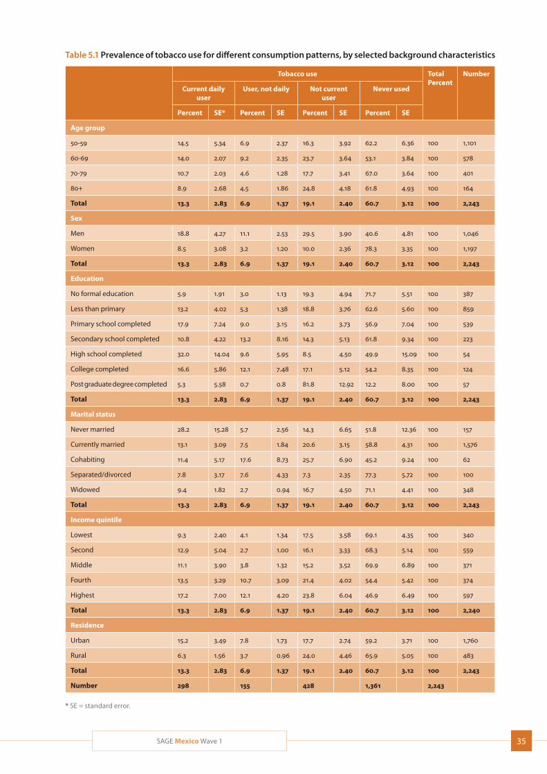
35SAGE Mexico Wave 1
Table 5.1 Prevalence of tobacco use for different consumption patterns, by selected background characteristics
Tobacco use TotalPercent
Number
Current daily user
User, not daily Not current user
Never used
Percent SE* Percent SE Percent SE Percent SE
Age group
50-59 14.5 5.34 6.9 2.37 16.3 3.92 62.2 6.36 100 1,101
60-69 14.0 2.07 9.2 2.35 23.7 3.64 53.1 3.84 100 578
70-79 10.7 2.03 4.6 1.28 17.7 3.41 67.0 3.64 100 401
80+ 8.9 2.68 4.5 1.86 24.8 4.18 61.8 4.93 100 164
Total 13.3 2.83 6.9 1.37 19.1 2.40 60.7 3.12 100 2,243
Sex
Men 18.8 4.27 11.1 2.53 29.5 3.90 40.6 4.81 100 1,046
Women 8.5 3.08 3.2 1.20 10.0 2.36 78.3 3.35 100 1,197
Total 13.3 2.83 6.9 1.37 19.1 2.40 60.7 3.12 100 2,243
Education
No formal education 5.9 1.91 3.0 1.13 19.3 4.94 71.7 5.51 100 387
Less than primary 13.2 4.02 5.3 1.38 18.8 3.76 62.6 5.60 100 859
Primary school completed 17.9 7.24 9.0 3.15 16.2 3.73 56.9 7.04 100 539
Secondary school completed 10.8 4.22 13.2 8.16 14.3 5.13 61.8 9.34 100 223
High school completed 32.0 14.04 9.6 5.95 8.5 4.50 49.9 15.09 100 54
College completed 16.6 5.86 12.1 7.48 17.1 5.12 54.2 8.35 100 124
Post graduate degree completed 5.3 5.58 0.7 0.8 81.8 12.92 12.2 8.00 100 57
Total 13.3 2.83 6.9 1.37 19.1 2.40 60.7 3.12 100 2,243
Marital status
Never married 28.2 15.28 5.7 2.56 14.3 6.65 51.8 12.36 100 157
Currently married 13.1 3.09 7.5 1.84 20.6 3.15 58.8 4.31 100 1,576
Cohabiting 11.4 5.17 17.6 8.73 25.7 6.90 45.2 9.24 100 62
Separated/divorced 7.8 3.17 7.6 4.33 7.3 2.35 77.3 5.72 100 100
Widowed 9.4 1.82 2.7 0.94 16.7 4.50 71.1 4.41 100 348
Total 13.3 2.83 6.9 1.37 19.1 2.40 60.7 3.12 100 2,243
Income quintile
Lowest 9.3 2.40 4.1 1.34 17.5 3.58 69.1 4.35 100 340
Second 12.9 5.04 2.7 1.00 16.1 3.33 68.3 5.14 100 559
Middle 11.1 3.90 3.8 1.32 15.2 3.52 69.9 6.89 100 371
Fourth 13.5 3.29 10.7 3.09 21.4 4.02 54.4 5.42 100 374
Highest 17.2 7.00 12.1 4.20 23.8 6.04 46.9 6.49 100 597
Total 13.3 2.83 6.9 1.37 19.1 2.40 60.7 3.12 100 2,240
Residence
Urban 15.2 3.49 7.8 1.73 17.7 2.74 59.2 3.71 100 1,760
Rural 6.3 1.56 3.7 0.96 24.0 4.46 65.9 5.05 100 483
Total 13.3 2.83 6.9 1.37 19.1 2.40 60.7 3.12 100 2,243
Number 298 155 428 1,361 2,243
* SE = standard error.
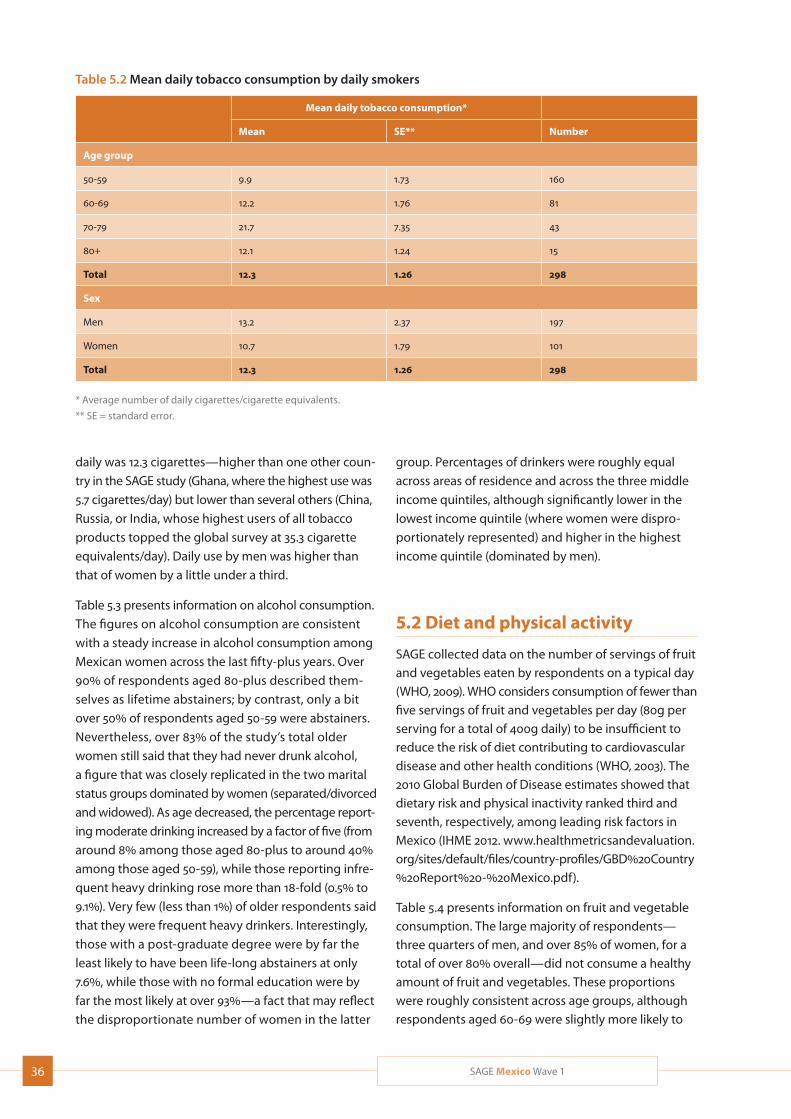
36 SAGE Mexico Wave 1
Table 5.2 Mean daily tobacco consumption by daily smokers
Mean daily tobacco consumption*
Mean SE** Number
Age group
50-59 9.9 1.73 160
60-69 12.2 1.76 81
70-79 21.7 7.35 43
80+ 12.1 1.24 15
Total 12.3 1.26 298
Sex
Men 13.2 2.37 197
Women 10.7 1.79 101
Total 12.3 1.26 298
* Average number of daily cigarettes/cigarette equivalents.
** SE = standard error.
daily was 12.3 cigarettes—higher than one other coun-
try in the SAGE study (Ghana, where the highest use was
5.7 cigarettes/day) but lower than several others (China,
Russia, or India, whose highest users of all tobacco
products topped the global survey at 35.3 cigarette
equivalents/day). Daily use by men was higher than
that of women by a little under a third.
Table 5.3 presents information on alcohol consumption.
The figures on alcohol consumption are consistent
with a steady increase in alcohol consumption among
Mexican women across the last fifty-plus years. Over
90% of respondents aged 80-plus described them-
selves as lifetime abstainers; by contrast, only a bit
over 50% of respondents aged 50-59 were abstainers.
Nevertheless, over 83% of the study’s total older
women still said that they had never drunk alcohol,
a figure that was closely replicated in the two marital
status groups dominated by women (separated/divorced
and widowed). As age decreased, the percentage report-
ing moderate drinking increased by a factor of five (from
around 8% among those aged 80-plus to around 40%
among those aged 50-59), while those reporting infre-
quent heavy drinking rose more than 18-fold (0.5% to
9.1%). Very few (less than 1%) of older respondents said
that they were frequent heavy drinkers. Interestingly,
those with a post-graduate degree were by far the
least likely to have been life-long abstainers at only
7.6%, while those with no formal education were by
far the most likely at over 93%—a fact that may reflect
the disproportionate number of women in the latter
group. Percentages of drinkers were roughly equal
across areas of residence and across the three middle
income quintiles, although significantly lower in the
lowest income quintile (where women were dispro-
portionately represented) and higher in the highest
income quintile (dominated by men).
5.2 Diet and physical activity
SAGE collected data on the number of servings of fruit and vegetables eaten by respondents on a typical day (WHO, 2009). WHO considers consumption of fewer than five servings of fruit and vegetables per day (80g per serving for a total of 400g daily) to be insufficient to reduce the risk of diet contributing to cardiovascular disease and other health conditions (WHO, 2003). The 2010 Global Burden of Disease estimates showed that dietary risk and physical inactivity ranked third and seventh, respectively, among leading risk factors in Mexico (IHME 2012. www.healthmetricsandevaluation.org/sites/default/files/country-profiles/GBD%20Country %20Report%20-%20Mexico.pdf).
Table 5.4 presents information on fruit and vegetable consumption. The large majority of respondents—three quarters of men, and over 85% of women, for a total of over 80% overall—did not consume a healthy amount of fruit and vegetables. These proportions were roughly consistent across age groups, although respondents aged 60-69 were slightly more likely to
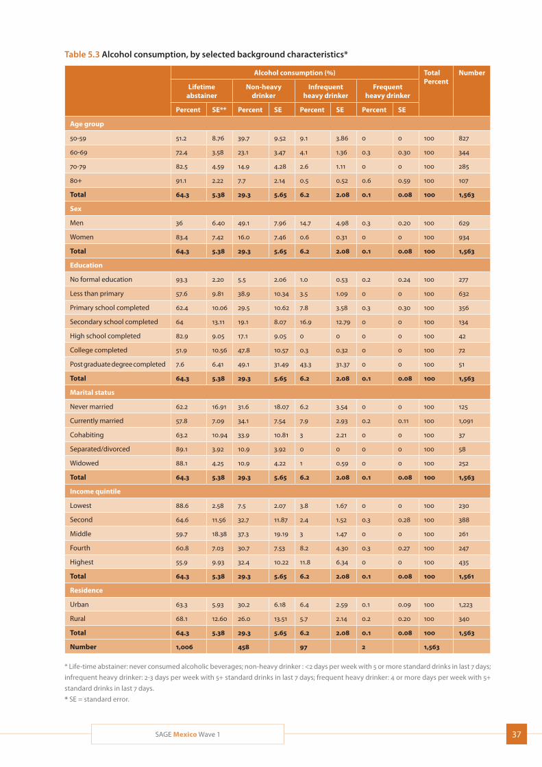
37SAGE Mexico Wave 1
Table 5.3 Alcohol consumption, by selected background characteristics*
Alcohol consumption (%) TotalPercent
Number
Lifetime abstainer
Non-heavy drinker
Infrequent heavy drinker
Frequent heavy drinker
Percent SE** Percent SE Percent SE Percent SE
Age group
50-59 51.2 8.76 39.7 9.52 9.1 3.86 0 0 100 827
60-69 72.4 3.58 23.1 3.47 4.1 1.36 0.3 0.30 100 344
70-79 82.5 4.59 14.9 4.28 2.6 1.11 0 0 100 285
80+ 91.1 2.22 7.7 2.14 0.5 0.52 0.6 0.59 100 107
Total 64.3 5.38 29.3 5.65 6.2 2.08 0.1 0.08 100 1,563
Sex
Men 36 6.40 49.1 7.96 14.7 4.98 0.3 0.20 100 629
Women 83.4 7.42 16.0 7.46 0.6 0.31 0 0 100 934
Total 64.3 5.38 29.3 5.65 6.2 2.08 0.1 0.08 100 1,563
Education
No formal education 93.3 2.20 5.5 2.06 1.0 0.53 0.2 0.24 100 277
Less than primary 57.6 9.81 38.9 10.34 3.5 1.09 0 0 100 632
Primary school completed 62.4 10.06 29.5 10.62 7.8 3.58 0.3 0.30 100 356
Secondary school completed 64 13.11 19.1 8.07 16.9 12.79 0 0 100 134
High school completed 82.9 9.05 17.1 9.05 0 0 0 0 100 42
College completed 51.9 10.56 47.8 10.57 0.3 0.32 0 0 100 72
Post graduate degree completed 7.6 6.41 49.1 31.49 43.3 31.37 0 0 100 51
Total 64.3 5.38 29.3 5.65 6.2 2.08 0.1 0.08 100 1,563
Marital status
Never married 62.2 16.91 31.6 18.07 6.2 3.54 0 0 100 125
Currently married 57.8 7.09 34.1 7.54 7.9 2.93 0.2 0.11 100 1,091
Cohabiting 63.2 10.94 33.9 10.81 3 2.21 0 0 100 37
Separated/divorced 89.1 3.92 10.9 3.92 0 0 0 0 100 58
Widowed 88.1 4.25 10.9 4.22 1 0.59 0 0 100 252
Total 64.3 5.38 29.3 5.65 6.2 2.08 0.1 0.08 100 1,563
Income quintile
Lowest 88.6 2.58 7.5 2.07 3.8 1.67 0 0 100 230
Second 64.6 11.56 32.7 11.87 2.4 1.52 0.3 0.28 100 388
Middle 59.7 18.38 37.3 19.19 3 1.47 0 0 100 261
Fourth 60.8 7.03 30.7 7.53 8.2 4.30 0.3 0.27 100 247
Highest 55.9 9.93 32.4 10.22 11.8 6.34 0 0 100 435
Total 64.3 5.38 29.3 5.65 6.2 2.08 0.1 0.08 100 1,561
Residence
Urban 63.3 5.93 30.2 6.18 6.4 2.59 0.1 0.09 100 1,223
Rural 68.1 12.60 26.0 13.51 5.7 2.14 0.2 0.20 100 340
Total 64.3 5.38 29.3 5.65 6.2 2.08 0.1 0.08 100 1,563
Number 1,006 458 97 2 1,563
* Life-time abstainer: never consumed alcoholic beverages; non-heavy drinker : <2 days per week with 5 or more standard drinks in last 7 days;
infrequent heavy drinker: 2-3 days per week with 5+ standard drinks in last 7 days; frequent heavy drinker: 4 or more days per week with 5+
standard drinks in last 7 days.
* SE = standard error.
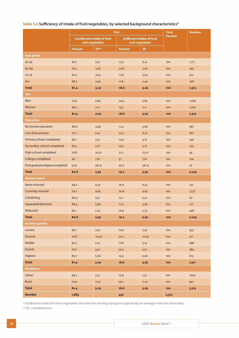
38 SAGE Mexico Wave 1
Table 5.4 Sufficiency of intake of fruit/vegetables, by selected background characteristics*
Diet TotalPercent
Number
Insufficient intake of fruit and vegetables
Sufficient intake of fruit and vegetables
Percent SE** Percent SE
Age group
50-59 82.7 6.21 17.3 6.21 100 1,111
60-69 76.2 3.56 23.8 3.56 100 592
70-79 82.2 3.03 17.8 3.03 100 412
80+ 88.2 2.40 11.8 2.40 100 198
Total 81.4 3.29 18.6 3.29 100 2,313
Sex
Men 75.6 5.85 24.4 5.85 100 1,083
Women 86.5 2.11 13.5 2.11 100 1,230
Total 81.4 3.29 18.6 3.29 100 2,313
Education
No formal education 88.6 3.66 11.4 3.66 100 387
Less than primary 77.7 6.41 22.3 6.41 100 861
Primary school completed 85.1 3.12 14.9 3.12 100 539
Secondary school completed 83.5 5.77 16.5 5.77 100 223
High school completed 78.8 10.31 21.2 10.31 100 54
College completed 69 7.61 31 7.61 100 124
Post graduate degree completed 52.6 28.14 47.4 28.14 100 57
Total 80.8 3.39 19.2 3.39 100 2,244
Marital status
Never married 84.0 6.47 16.0 6.47 100 157
Currently married 79.2 4.65 20.8 4.65 100 1,577
Cohabiting 89.9 3.51 10.1 3.51 100 62
Separated/divorced 88.4 3.58 11.6 3.58 100 101
Widowed 83.1 2.73 16.9 2.73 100 348
Total 80.8 3.39 19.2 3.39 100 2,244
Income quintile
Lowest 89.1 2.41 10.9 2.41 100 353
Second 79.8 10.50 20.2 10.50 100 571
Middle 82.2 5.13 17.8 5.13 100 388
Fourth 76.7 3.51 23.3 3.51 100 384
Highest 80.7 5.06 19.3 5.06 100 615
Total 81.4 3.29 18.6 3.29 100 2,311
Residence
Urban 84.2 2.31 15.8 2.31 100 1,822
Rural 70.9 11.31 29.1 11.31 100 491
Total 81.4 3.29 18.6 3.29 100 2,313
Number 1,883 430 2,313
* Insufficient intake of fruit or vegetables: less than five servings (400g) in a typical day on average in the last seven days.
** SE = standard error.
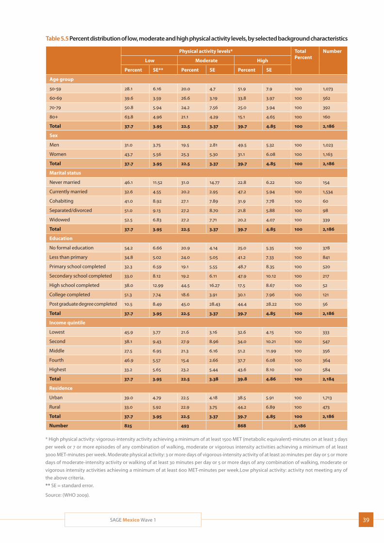
39SAGE Mexico Wave 1
Table 5.5 Percent distribution of low, moderate and high physical activity levels, by selected background characteristics
Physical activity levels* TotalPercent
Number
Low Moderate High
Percent SE** Percent SE Percent SE
Age group
50-59 28.1 6.16 20.0 4.7 51.9 7.9 100 1,073
60-69 39.6 3.59 26.6 3.19 33.8 3.97 100 562
70-79 50.8 5.94 24.2 7.56 25.0 3.94 100 392
80+ 63.8 4.96 21.1 4.29 15.1 4.65 100 160
Total 37.7 3.95 22.5 3.37 39.7 4.85 100 2,186
Sex
Men 31.0 3.75 19.5 2.81 49.5 5.32 100 1,023
Women 43.7 5.56 25.3 5.30 31.1 6.08 100 1,163
Total 37.7 3.95 22.5 3.37 39.7 4.85 100 2,186
Marital status
Never married 46.1 11.52 31.0 14.77 22.8 6.22 100 154
Currently married 32.6 4.55 20.2 2.95 47.2 5.94 100 1,534
Cohabiting 41.0 8.92 27.1 7.89 31.9 7.78 100 60
Separated/divorced 51.0 9.13 27.2 8.70 21.8 5.88 100 98
Widowed 52.5 6.83 27.2 7.71 20.2 4.07 100 339
Total 37.7 3.95 22.5 3.37 39.7 4.85 100 2,186
Education
No formal education 54.2 6.66 20.9 4.14 25.0 5.35 100 378
Less than primary 34.8 5.02 24.0 5.05 41.2 7.33 100 841
Primary school completed 32.3 6.59 19.1 5.55 48.7 8.35 100 520
Secondary school completed 33.0 8.12 19.2 6.11 47.9 10.12 100 217
High school completed 38.0 12.99 44.5 16.27 17.5 8.67 100 52
College completed 51.3 7.74 18.6 3.91 30.1 7.96 100 121
Post graduate degree completed 10.5 8.49 45.0 28.43 44.4 28.22 100 56
Total 37.7 3.95 22.5 3.37 39.7 4.85 100 2,186
Income quintile
Lowest 45.9 3.77 21.6 3.16 32.6 4.15 100 333
Second 38.1 9.43 27.9 8.96 34.0 10.21 100 547
Middle 27.5 6.95 21.3 6.16 51.2 11.99 100 356
Fourth 46.9 5.57 15.4 2.66 37.7 6.08 100 364
Highest 33.2 5.65 23.2 5.44 43.6 8.10 100 584
Total 37.7 3.95 22.5 3.38 39.8 4.86 100 2,184
Residence
Urban 39.0 4.79 22.5 4.18 38.5 5.91 100 1,713
Rural 33.0 5.92 22.9 3.75 44.2 6.89 100 473
Total 37.7 3.95 22.5 3.37 39.7 4.85 100 2,186
Number 825 493 868 2,186
* High physical activity: vigorous-intensity activity achieving a minimum of at least 1500 MET (metabolic equivalent)-minutes on at least 3 days
per week or 7 or more episodes of any combination of walking, moderate or vigorous intensity activities achieving a minimum of at least
3000 MET-minutes per week. Moderate physical activity: 3 or more days of vigorous-intensity activity of at least 20 minutes per day or 5 or more
days of moderate-intensity activity or walking of at least 30 minutes per day or 5 or more days of any combination of walking, moderate or
vigorous intensity activities achieving a minimum of at least 600 MET-minutes per week.Low physical activity: activity not meeting any of
the above criteria.
** SE = standard error.
Source: (WHO 2009).
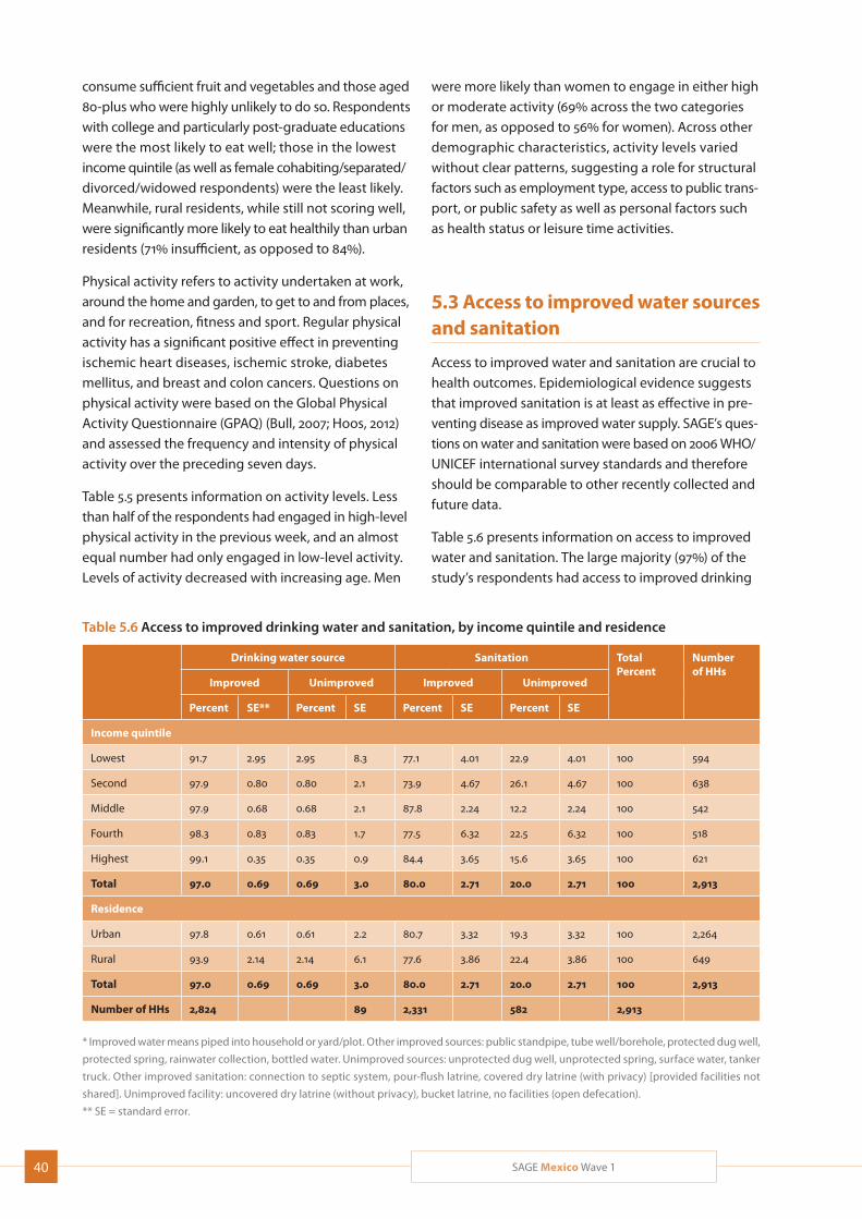
40 SAGE Mexico Wave 1
consume sufficient fruit and vegetables and those aged 80-plus who were highly unlikely to do so. Respondents with college and particularly post-graduate educations were the most likely to eat well; those in the lowest income quintile (as well as female cohabiting/separated/divorced/widowed respondents) were the least likely. Meanwhile, rural residents, while still not scoring well, were significantly more likely to eat healthily than urban residents (71% insufficient, as opposed to 84%).
Physical activity refers to activity undertaken at work, around the home and garden, to get to and from places, and for recreation, fitness and sport. Regular physical activity has a significant positive effect in preventing ischemic heart diseases, ischemic stroke, diabetes mellitus, and breast and colon cancers. Questions on physical activity were based on the Global Physical Activity Questionnaire (GPAQ) (Bull, 2007; Hoos, 2012) and assessed the frequency and intensity of physical activity over the preceding seven days.
Table 5.5 presents information on activity levels. Less than half of the respondents had engaged in high-level physical activity in the previous week, and an almost equal number had only engaged in low-level activity. Levels of activity decreased with increasing age. Men
were more likely than women to engage in either high or moderate activity (69% across the two categories for men, as opposed to 56% for women). Across other demographic characteristics, activity levels varied without clear patterns, suggesting a role for structural factors such as employment type, access to public trans-port, or public safety as well as personal factors such as health status or leisure time activities.
5.3 Access to improved water sources and sanitation
Access to improved water and sanitation are crucial to health outcomes. Epidemiological evidence suggests that improved sanitation is at least as effective in pre-venting disease as improved water supply. SAGE’s ques-tions on water and sanitation were based on 2006 WHO/UNICEF international survey standards and therefore should be comparable to other recently collected and future data.
Table 5.6 presents information on access to improved water and sanitation. The large majority (97%) of the study’s respondents had access to improved drinking
Table 5.6 Access to improved drinking water and sanitation, by income quintile and residence
Drinking water source Sanitation TotalPercent
Number of HHs
Improved Unimproved Improved Unimproved
Percent SE** Percent SE Percent SE Percent SE
Income quintile
Lowest 91.7 2.95 2.95 8.3 77.1 4.01 22.9 4.01 100 594
Second 97.9 0.80 0.80 2.1 73.9 4.67 26.1 4.67 100 638
Middle 97.9 0.68 0.68 2.1 87.8 2.24 12.2 2.24 100 542
Fourth 98.3 0.83 0.83 1.7 77.5 6.32 22.5 6.32 100 518
Highest 99.1 0.35 0.35 0.9 84.4 3.65 15.6 3.65 100 621
Total 97.0 0.69 0.69 3.0 80.0 2.71 20.0 2.71 100 2,913
Residence
Urban 97.8 0.61 0.61 2.2 80.7 3.32 19.3 3.32 100 2,264
Rural 93.9 2.14 2.14 6.1 77.6 3.86 22.4 3.86 100 649
Total 97.0 0.69 0.69 3.0 80.0 2.71 20.0 2.71 100 2,913
Number of HHs 2,824 89 2,331 582 2,913
* Improved water means piped into household or yard/plot. Other improved sources: public standpipe, tube well/borehole, protected dug well,
protected spring, rainwater collection, bottled water. Unimproved sources: unprotected dug well, unprotected spring, surface water, tanker
truck. Other improved sanitation: connection to septic system, pour-flush latrine, covered dry latrine (with privacy) [provided facilities not
shared]. Unimproved facility: uncovered dry latrine (without privacy), bucket latrine, no facilities (open defecation).
** SE = standard error.
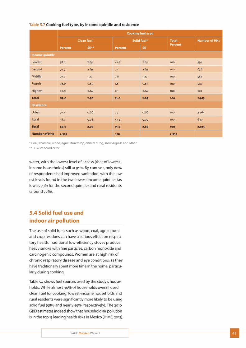
41SAGE Mexico Wave 1
water, with the lowest level of access (that of lowest-
income households) still at 91%. By contrast, only 80%
of respondents had improved sanitation, with the low-
est levels found in the two lowest income quintiles (as
low as 73% for the second quintile) and rural residents
(around 77%).
5.4 Solid fuel use and indoor air pollution
The use of solid fuels such as wood, coal, agricultural
and crop residues can have a serious effect on respira-
tory health. Traditional low-efficiency stoves produce
heavy smoke with fine particles, carbon monoxide and
carcinogenic compounds. Women are at high risk of
chronic respiratory disease and eye conditions, as they
have traditionally spent more time in the home, particu-
larly during cooking.
Table 5.7 shows fuel sources used by the study’s house-
holds. While almost 90% of households overall used
clean fuel for cooking, lowest-income households and
rural residents were significantly more likely to be using
solid fuel (58% and nearly 59%, respectively). The 2010
GBD estimates indeed show that household air pollution
is in the top 15 leading health risks in Mexico (IHME, 2012).
Table 5.7 Cooking fuel type, by income quintile and residence
Cooking fuel used
Clean fuel Solid fuel* TotalPercent
Number of HHs
Percent SE** Percent SE
Income quintile
Lowest 58.0 7.85 41.9 7.85 100 594
Second 92.9 2.89 7.1 2.89 100 638
Middle 97.2 1.22 2.8 1.22 100 542
Fourth 98.0 0.89 1.8 0.81 100 518
Highest 99.9 0.14 0.1 0.14 100 621
Total 89.0 2.70 11.0 2.69 100 2,913
Residence
Urban 97.7 0.66 2.3 0.66 100 2,264
Rural 58.5 9.08 41.3 9.05 100 649
Total 89.0 2.70 11.0 2.69 100 2,913
Number of HHs 2,592 320 2,912
* Coal, charcoal, wood, agriculture/crop, animal dung, shrubs/grass and other.
** SE = standard error.
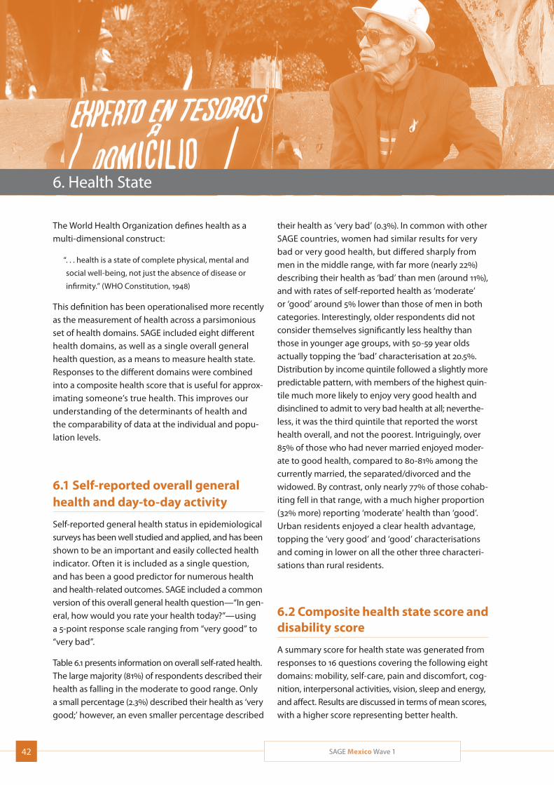
42 SAGE Mexico Wave 1
6. Health State
The World Health Organization defines health as a multi-dimensional construct:
“. . . health is a state of complete physical, mental and
social well-being, not just the absence of disease or
infirmity.” (WHO Constitution, 1948)
This definition has been operationalised more recently as the measurement of health across a parsimonious set of health domains. SAGE included eight different health domains, as well as a single overall general health question, as a means to measure health state. Responses to the different domains were combined into a composite health score that is useful for approx-imating someone’s true health. This improves our understanding of the determinants of health and the comparability of data at the individual and popu-lation levels.
6.1 Self-reported overall general health and day-to-day activity
Self-reported general health status in epidemiological surveys has been well studied and applied, and has been shown to be an important and easily collected health indicator. Often it is included as a single question, and has been a good predictor for numerous health and health-related outcomes. SAGE included a common version of this overall general health question—“In gen-eral, how would you rate your health today?”—using a 5-point response scale ranging from “very good” to “very bad”.
Table 6.1 presents information on overall self-rated health. The large majority (81%) of respondents described their health as falling in the moderate to good range. Only a small percentage (2.3%) described their health as ‘very good;’ however, an even smaller percentage described
their health as ‘very bad’ (0.3%). In common with other SAGE countries, women had similar results for very bad or very good health, but differed sharply from men in the middle range, with far more (nearly 22%) describing their health as ‘bad’ than men (around 11%), and with rates of self-reported health as ‘moderate’ or ‘good’ around 5% lower than those of men in both categories. Interestingly, older respondents did not consider themselves significantly less healthy than those in younger age groups, with 50-59 year olds actually topping the ‘bad’ characterisation at 20.5%. Distribution by income quintile followed a slightly more predictable pattern, with members of the highest quin-tile much more likely to enjoy very good health and disinclined to admit to very bad health at all; neverthe-less, it was the third quintile that reported the worst health overall, and not the poorest. Intriguingly, over 85% of those who had never married enjoyed moder-ate to good health, compared to 80-81% among the currently married, the separated/divorced and the widowed. By contrast, only nearly 77% of those cohab-iting fell in that range, with a much higher proportion (32% more) reporting ‘moderate’ health than ‘good’. Urban residents enjoyed a clear health advantage, topping the ‘very good’ and ‘good’ characterisations and coming in lower on all the other three characteri-sations than rural residents.
6.2 Composite health state score and disability score
A summary score for health state was generated from responses to 16 questions covering the following eight domains: mobility, self-care, pain and discomfort, cog-nition, interpersonal activities, vision, sleep and energy, and affect. Results are discussed in terms of mean scores, with a higher score representing better health.
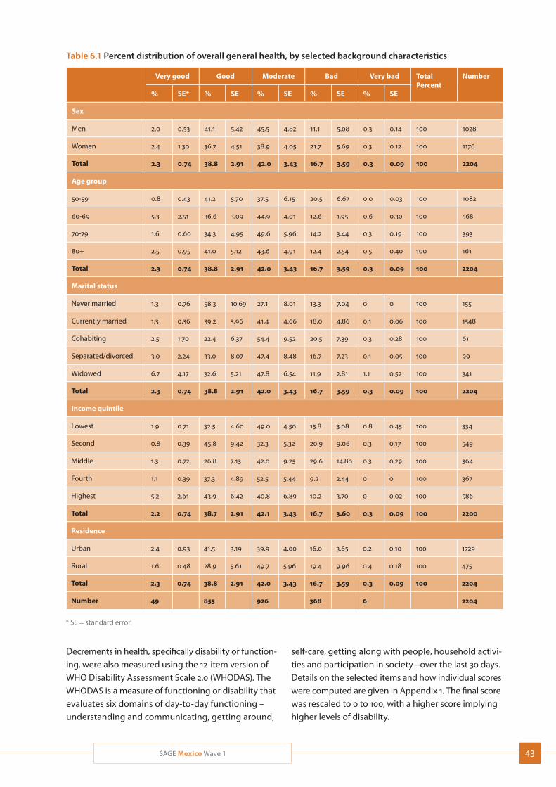
43SAGE Mexico Wave 1
Table 6.1 Percent distribution of overall general health, by selected background characteristics
Very good Good Moderate Bad Very bad TotalPercent
Number
% SE* % SE % SE % SE % SE
Sex
Men 2.0 0.53 41.1 5.42 45.5 4.82 11.1 5.08 0.3 0.14 100 1028
Women 2.4 1.30 36.7 4.51 38.9 4.05 21.7 5.69 0.3 0.12 100 1176
Total 2.3 0.74 38.8 2.91 42.0 3.43 16.7 3.59 0.3 0.09 100 2204
Age group
50-59 0.8 0.43 41.2 5.70 37.5 6.15 20.5 6.67 0.0 0.03 100 1082
60-69 5.3 2.51 36.6 3.09 44.9 4.01 12.6 1.95 0.6 0.30 100 568
70-79 1.6 0.60 34.3 4.95 49.6 5.96 14.2 3.44 0.3 0.19 100 393
80+ 2.5 0.95 41.0 5.12 43.6 4.91 12.4 2.54 0.5 0.40 100 161
Total 2.3 0.74 38.8 2.91 42.0 3.43 16.7 3.59 0.3 0.09 100 2204
Marital status
Never married 1.3 0.76 58.3 10.69 27.1 8.01 13.3 7.04 0 0 100 155
Currently married 1.3 0.36 39.2 3.96 41.4 4.66 18.0 4.86 0.1 0.06 100 1548
Cohabiting 2.5 1.70 22.4 6.37 54.4 9.52 20.5 7.39 0.3 0.28 100 61
Separated/divorced 3.0 2.24 33.0 8.07 47.4 8.48 16.7 7.23 0.1 0.05 100 99
Widowed 6.7 4.17 32.6 5.21 47.8 6.54 11.9 2.81 1.1 0.52 100 341
Total 2.3 0.74 38.8 2.91 42.0 3.43 16.7 3.59 0.3 0.09 100 2204
Income quintile
Lowest 1.9 0.71 32.5 4.60 49.0 4.50 15.8 3.08 0.8 0.45 100 334
Second 0.8 0.39 45.8 9.42 32.3 5.32 20.9 9.06 0.3 0.17 100 549
Middle 1.3 0.72 26.8 7.13 42.0 9.25 29.6 14.80 0.3 0.29 100 364
Fourth 1.1 0.39 37.3 4.89 52.5 5.44 9.2 2.44 0 0 100 367
Highest 5.2 2.61 43.9 6.42 40.8 6.89 10.2 3.70 0 0.02 100 586
Total 2.2 0.74 38.7 2.91 42.1 3.43 16.7 3.60 0.3 0.09 100 2200
Residence
Urban 2.4 0.93 41.5 3.19 39.9 4.00 16.0 3.65 0.2 0.10 100 1729
Rural 1.6 0.48 28.9 5.61 49.7 5.96 19.4 9.96 0.4 0.18 100 475
Total 2.3 0.74 38.8 2.91 42.0 3.43 16.7 3.59 0.3 0.09 100 2204
Number 49 855 926 368 6 2204
* SE = standard error.
Decrements in health, specifically disability or function-ing, were also measured using the 12-item version of WHO Disability Assessment Scale 2.0 (WHODAS). The WHODAS is a measure of functioning or disability that evaluates six domains of day-to-day functioning – understanding and communicating, getting around,
self-care, getting along with people, household activi-ties and participation in society –over the last 30 days. Details on the selected items and how individual scores were computed are given in Appendix 1. The final score was rescaled to 0 to 100, with a higher score implying higher levels of disability.
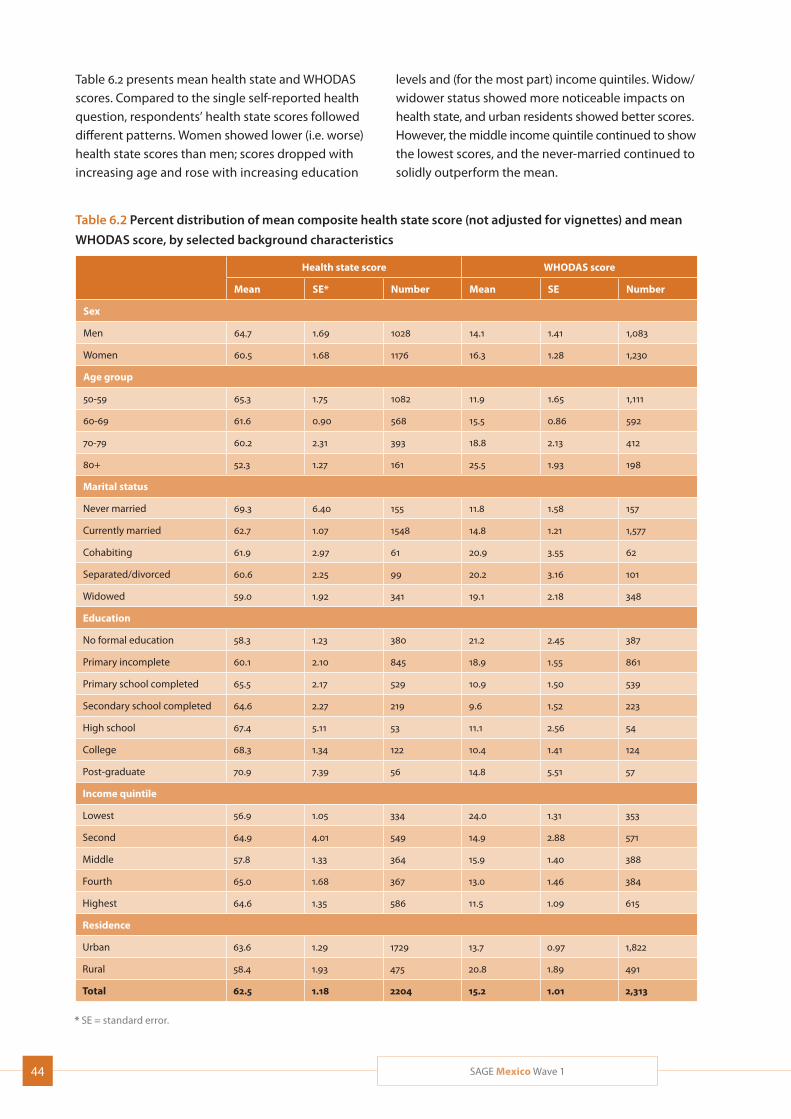
44 SAGE Mexico Wave 1
Table 6.2 Percent distribution of mean composite health state score (not adjusted for vignettes) and mean
WHODAS score, by selected background characteristics
Health state score WHODAS score
Mean SE* Number Mean SE Number
Sex
Men 64.7 1.69 1028 14.1 1.41 1,083
Women 60.5 1.68 1176 16.3 1.28 1,230
Age group
50-59 65.3 1.75 1082 11.9 1.65 1,111
60-69 61.6 0.90 568 15.5 0.86 592
70-79 60.2 2.31 393 18.8 2.13 412
80+ 52.3 1.27 161 25.5 1.93 198
Marital status
Never married 69.3 6.40 155 11.8 1.58 157
Currently married 62.7 1.07 1548 14.8 1.21 1,577
Cohabiting 61.9 2.97 61 20.9 3.55 62
Separated/divorced 60.6 2.25 99 20.2 3.16 101
Widowed 59.0 1.92 341 19.1 2.18 348
Education
No formal education 58.3 1.23 380 21.2 2.45 387
Primary incomplete 60.1 2.10 845 18.9 1.55 861
Primary school completed 65.5 2.17 529 10.9 1.50 539
Secondary school completed 64.6 2.27 219 9.6 1.52 223
High school 67.4 5.11 53 11.1 2.56 54
College 68.3 1.34 122 10.4 1.41 124
Post-graduate 70.9 7.39 56 14.8 5.51 57
Income quintile
Lowest 56.9 1.05 334 24.0 1.31 353
Second 64.9 4.01 549 14.9 2.88 571
Middle 57.8 1.33 364 15.9 1.40 388
Fourth 65.0 1.68 367 13.0 1.46 384
Highest 64.6 1.35 586 11.5 1.09 615
Residence
Urban 63.6 1.29 1729 13.7 0.97 1,822
Rural 58.4 1.93 475 20.8 1.89 491
Total 62.5 1.18 2204 15.2 1.01 2,313
* SE = standard error.
Table 6.2 presents mean health state and WHODAS scores. Compared to the single self-reported health question, respondents’ health state scores followed different patterns. Women showed lower (i.e. worse) health state scores than men; scores dropped with increasing age and rose with increasing education
levels and (for the most part) income quintiles. Widow/widower status showed more noticeable impacts on health state, and urban residents showed better scores. However, the middle income quintile continued to show the lowest scores, and the never-married continued to solidly outperform the mean.
45SAGE Mexico Wave 1
Some similar patterns were seen in the WHODAS results. Women showed higher disability than men; scores rose with age and roughly dropped with increas-ing income. The never-married continued to score well and urban residents had lower disability levels. However, respondents with post-graduate education actually scored worse than most other educational levels, and cohabiting, separated/divorced and widowed respondents scored noticeably worse than those currently married.
6.3 Functioning and health: ADLs and IADLs
Measures of functioning are common in surveys of older adults, and often include an assessment of the Activities of Daily Living (ADLs) and Instrumental Activi-ties of Daily Living (IADL). ADLs are considered basic tasks of everyday life, such as bathing, eating, dressing and toileting. IADLs include activities that are more complex than ADLs, such as meal preparation, doing housework, and travelling. Deficiencies or limitations in ADLs or IADLs suggest cognitive and/or physical decline signalling a need for assistance. WHODAS contains many of the most commonly asked ADL and IADL questions, as well as assessing severity of disability. SAGE included a fuller set of ADLs and IADLs widely used in surveys and studies of older populations to assess disability. A list of ADL and IADL items included in the study is given in Appendix 2. SAGE also compared deficiencies in ADLs and IADLs to WHODAS scores (Tables 6.3 and 6.4).
The overall level of disability in the community was low, which was to be expected from a community-based sample of older adults (Table 6.2). The level of disability was higher among women than among men on aver-age (16.3 in comparison to 14.1, respectively), and clearly increased with increasing age.
Table 6.3 presents information on ADL deficiencies. Overall, nearly 37% of respondents had one or more ADL limitations, and over one-fifth had two or more limitations. Women were noticeably more likely to suffer some limitation than men (40%, as opposed to 32.5%) as well as to suffer more severe levels of impair-ment than men (around one-quarter with two or more limitations, as opposed to around 17%). Levels of impair-ment rose steadily with age. The level of severe (2-plus) impairment was highest among the two oldest age groups (nearly 54% respondents aged 80-plus) and those in the lowest income quintile (around 40%); however, respondents who lacked a partner, either due
to separation/divorce or widowhood, were not far behind. The gap between the lowest and highest income quin-tiles was around 25%. Rural residents were noticeably more likely to suffer from one ADL limitation, but only slightly more likely to suffer from two or more.
Because the IADLs measure a more complex level of activities, deficiencies in these would suggest less severe impairment or disability than deficiencies in ADLs. Using them together may allow for general assessment of severity of disability.
Table 6.4 presents information on IADL deficiencies. A smaller percentage of respondents reported diffi-culties with IADLs than reported ADL limitations. Over 90% of respondents said that they had no difficulties with any IADL, and only 5.6% reported limitations in two or more IADLs. At greatest risk of severe impairment (deficiency in relation to two or more IADLs) were the oldest respondents (25% among those aged 80-plus), those in the lowest income quintile (nearly 15%), widows/widowers (over 12%), and those with no formal educa-tion (nearly 12%).
6.4 Measured cognitive function
Lower WHODAS scores and/or deficiencies in ADLs or IADLs often signal cognitive decline or dementia; the challenge is to differentiate normal age-related chang-es in cognition from cognitive impairment. In addition to ADL-type measures in SAGE, self-reported cognition and cognition tests were used.
Three cognition tests were used: verbal fluency (VF), verbal recall (VR), and digit span (DS). These tested learning ability, concentration and memory. The test used for verbal fluency challenged the respondent to produce as many words (animals) as possible in a one-minute time span. Immediate verbal and delayed verbal recall were used as tests of memory, wherein 10 words were successively presented after which the respondent was given the opportunity to recall as many of the words as possible. This was repeated three times to saturate the learning curve. After about 10 minutes of interview time, recall and recognition of the same 10 words were again tested. Digit span forward and backward were the last tests used for testing working memory and executive function.
A single composite cognition score was compiled using an exploratory and confirmatory factor analysis of cor-rect and erroneous replies to each of the immediate
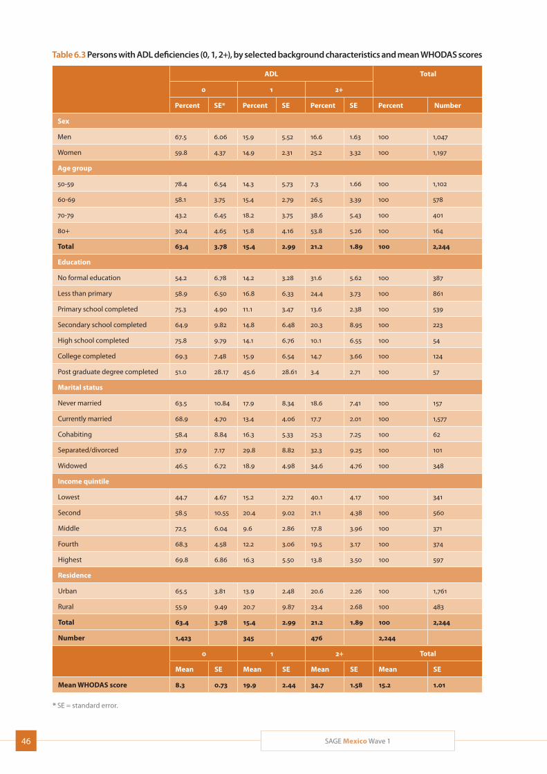
46 SAGE Mexico Wave 1
Table 6.3 Persons with ADL deficiencies (0, 1, 2+), by selected background characteristics and mean WHODAS scores
ADL Total
0 1 2+
Percent SE* Percent SE Percent SE Percent Number
Sex
Men 67.5 6.06 15.9 5.52 16.6 1.63 100 1,047
Women 59.8 4.37 14.9 2.31 25.2 3.32 100 1,197
Age group
50-59 78.4 6.54 14.3 5.73 7.3 1.66 100 1,102
60-69 58.1 3.75 15.4 2.79 26.5 3.39 100 578
70-79 43.2 6.45 18.2 3.75 38.6 5.43 100 401
80+ 30.4 4.65 15.8 4.16 53.8 5.26 100 164
Total 63.4 3.78 15.4 2.99 21.2 1.89 100 2,244
Education
No formal education 54.2 6.78 14.2 3.28 31.6 5.62 100 387
Less than primary 58.9 6.50 16.8 6.33 24.4 3.73 100 861
Primary school completed 75.3 4.90 11.1 3.47 13.6 2.38 100 539
Secondary school completed 64.9 9.82 14.8 6.48 20.3 8.95 100 223
High school completed 75.8 9.79 14.1 6.76 10.1 6.55 100 54
College completed 69.3 7.48 15.9 6.54 14.7 3.66 100 124
Post graduate degree completed 51.0 28.17 45.6 28.61 3.4 2.71 100 57
Marital status
Never married 63.5 10.84 17.9 8.34 18.6 7.41 100 157
Currently married 68.9 4.70 13.4 4.06 17.7 2.01 100 1,577
Cohabiting 58.4 8.84 16.3 5.33 25.3 7.25 100 62
Separated/divorced 37.9 7.17 29.8 8.82 32.3 9.25 100 101
Widowed 46.5 6.72 18.9 4.98 34.6 4.76 100 348
Income quintile
Lowest 44.7 4.67 15.2 2.72 40.1 4.17 100 341
Second 58.5 10.55 20.4 9.02 21.1 4.38 100 560
Middle 72.5 6.04 9.6 2.86 17.8 3.96 100 371
Fourth 68.3 4.58 12.2 3.06 19.5 3.17 100 374
Highest 69.8 6.86 16.3 5.50 13.8 3.50 100 597
Residence
Urban 65.5 3.81 13.9 2.48 20.6 2.26 100 1,761
Rural 55.9 9.49 20.7 9.87 23.4 2.68 100 483
Total 63.4 3.78 15.4 2.99 21.2 1.89 100 2,244
Number 1,423 345 476 2,244
0 1 2+ Total
Mean SE Mean SE Mean SE Mean SE
Mean WHODAS score 8.3 0.73 19.9 2.44 34.7 1.58 15.2 1.01
* SE = standard error.
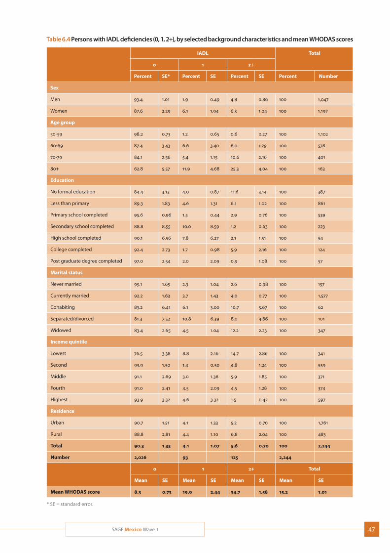
47SAGE Mexico Wave 1
Table 6.4 Persons with IADL deficiencies (0, 1, 2+), by selected background characteristics and mean WHODAS scores
IADL Total
0 1 2+
Percent SE* Percent SE Percent SE Percent Number
Sex
Men 93.4 1.01 1.9 0.49 4.8 0.86 100 1,047
Women 87.6 2.29 6.1 1.94 6.3 1.04 100 1,197
Age group
50-59 98.2 0.73 1.2 0.65 0.6 0.27 100 1,102
60-69 87.4 3.43 6.6 3.40 6.0 1.29 100 578
70-79 84.1 2.56 5.4 1.15 10.6 2.16 100 401
80+ 62.8 5.57 11.9 4.68 25.3 4.04 100 163
Education
No formal education 84.4 3.13 4.0 0.87 11.6 3.14 100 387
Less than primary 89.3 1.83 4.6 1.31 6.1 1.02 100 861
Primary school completed 95.6 0.96 1.5 0.44 2.9 0.76 100 539
Secondary school completed 88.8 8.55 10.0 8.59 1.2 0.63 100 223
High school completed 90.1 6.56 7.8 6.27 2.1 1.51 100 54
College completed 92.4 2.73 1.7 0.98 5.9 2.16 100 124
Post graduate degree completed 97.0 2.54 2.0 2.09 0.9 1.08 100 57
Marital status
Never married 95.1 1.65 2.3 1.04 2.6 0.98 100 157
Currently married 92.2 1.63 3.7 1.43 4.0 0.77 100 1,577
Cohabiting 83.2 6.41 6.1 3.00 10.7 5.67 100 62
Separated/divorced 81.3 7.52 10.8 6.39 8.0 4.86 100 101
Widowed 83.4 2.65 4.5 1.04 12.2 2.23 100 347
Income quintile
Lowest 76.5 3.38 8.8 2.16 14.7 2.86 100 341
Second 93.9 1.50 1.4 0.50 4.8 1.24 100 559
Middle 91.1 2.69 3.0 1.36 5.9 1.85 100 371
Fourth 91.0 2.41 4.5 2.09 4.5 1.28 100 374
Highest 93.9 3.32 4.6 3.32 1.5 0.42 100 597
Residence
Urban 90.7 1.51 4.1 1.33 5.2 0.70 100 1,761
Rural 88.8 2.81 4.4 1.10 6.8 2.04 100 483
Total 90.3 1.33 4.1 1.07 5.6 0.70 100 2,244
Number 2,026 93 125 2,244
0 1 2+ Total
Mean SE Mean SE Mean SE Mean SE
Mean WHODAS score 8.3 0.73 19.9 2.44 34.7 1.58 15.2 1.01
* SE = standard error.
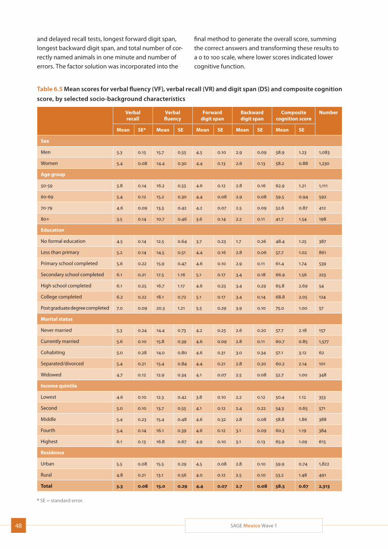
48 SAGE Mexico Wave 1
Table 6.5 Mean scores for verbal fluency (VF), verbal recall (VR) and digit span (DS) and composite cognition
score, by selected socio-background characteristics
Verbal recall
Verbal fluency
Forward digit span
Backward digit span
Composite cognition score
Number
Mean SE* Mean SE Mean SE Mean SE Mean SE
Sex
Men 5.3 0.15 15.7 0.55 4.5 0.10 2.9 0.09 58.9 1.23 1,083
Women 5.4 0.08 14.4 0.30 4.4 0.13 2.6 0.13 58.2 0.88 1,230
Age group
50-59 5.8 0.14 16.2 0.55 4.6 0.12 2.8 0.16 62.9 1.21 1,111
60-69 5.4 0.12 15.2 0.30 4.4 0.08 2.9 0.08 59.5 0.94 592
70-79 4.6 0.09 13.3 0.42 4.2 0.07 2.5 0.09 52.6 0.87 412
80+ 3.5 0.14 10.7 0.46 3.6 0.14 2.2 0.11 41.7 1.54 198
Education
No formal education 4.5 0.14 12.5 0.64 3.7 0.23 1.7 0.26 48.4 1.25 387
Less than primary 5.2 0.14 14.5 0.51 4.4 0.16 2.8 0.06 57.7 1.02 861
Primary school completed 5.6 0.22 15.9 0.47 4.6 0.10 2.9 0.11 61.4 1.74 539
Secondary school completed 6.1 0.21 17.5 1.16 5.1 0.17 3.4 0.18 66.9 1.56 223
High school completed 6.1 0.25 16.7 1.17 4.6 0.25 3.4 0.29 65.8 2.69 54
College completed 6.2 0.22 18.1 0.72 5.1 0.17 3.4 0.14 68.8 2.05 124
Post graduate degree completed 7.0 0.09 20.3 1.21 5.5 0.29 3.9 0.10 75.0 1.00 57
Marital status
Never married 5.3 0.24 14.4 0.73 4.2 0.25 2.6 0.20 57.7 2.18 157
Currently married 5.6 0.10 15.8 0.39 4.6 0.09 2.8 0.11 60.7 0.85 1,577
Cohabiting 5.0 0.28 14.0 0.80 4.6 0.31 3.0 0.34 57.1 3.12 62
Separated/divorced 5.4 0.21 15.4 0.84 4.4 0.21 2.8 0.20 60.2 2.14 101
Widowed 4.7 0.12 12.9 0.34 4.1 0.07 2.5 0.08 52.7 1.00 348
Income quintile
Lowest 4.6 0.10 12.3 0.42 3.8 0.10 2.2 0.12 50.4 1.12 353
Second 5.0 0.10 13.7 0.55 4.1 0.12 2.4 0.22 54.3 0.65 571
Middle 5.4 0.23 15.4 0.48 4.6 0.32 2.8 0.08 58.8 1.86 388
Fourth 5.4 0.14 16.1 0.39 4.6 0.12 3.1 0.09 60.3 1.19 384
Highest 6.1 0.13 16.8 0.67 4.9 0.10 3.1 0.13 65.9 1.09 615
Residence
Urban 5.5 0.08 15.5 0.29 4.5 0.08 2.8 0.10 59.9 0.74 1,822
Rural 4.8 0.21 13.1 0.56 4.0 0.12 2.5 0.10 53.2 1.48 491
Total 5.3 0.08 15.0 0.29 4.4 0.07 2.7 0.08 58.5 0.67 2,313
* SE = standard error.
and delayed recall tests, longest forward digit span, longest backward digit span, and total number of cor-rectly named animals in one minute and number of errors. The factor solution was incorporated into the
final method to generate the overall score, summing the correct answers and transforming these results to a 0 to 100 scale, where lower scores indicated lower cognitive function.
49SAGE Mexico Wave 1
Table 6.5 presents information on the results of the three individual cognition tests and composite cogni-tion scores. Composite cognition scores decreased with increasing age and increased with increasing ed-ucational level and income quintile. Men and women scored roughly equally, although with a very slight advantage towards men throughout. Urban residents topped rural ones, and the currently married came first among the different marital status groups. The lowest scores were found among respondents aged 80-plus, those from the lowest income quintile, and the widowed.
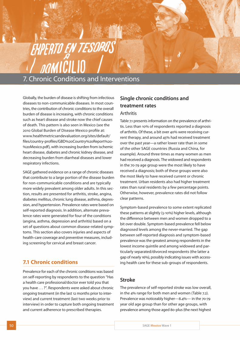
50 SAGE Mexico Wave 1
7. Chronic Conditions and Interventions
Globally, the burden of disease is shifting from infectious diseases to non-communicable diseases. In most coun-tries, the contribution of chronic conditions to the overall burden of disease is increasing, with chronic conditions such as heart disease and stroke now the chief causes of death. This pattern is also seen in Mexico (see the 2010 Global Burden of Disease Mexico profile at: www.healthmetricsandevaluation.org/sites/default/files/country-profiles/GBD%20Country%20Report%20- %20Mexico.pdf), with increasing burden from ischemic heart disease, diabetes and chronic kidney disease, and decreasing burden from diarrheal diseases and lower respiratory infections.
SAGE gathered evidence on a range of chronic diseases that contribute to a large portion of the disease burden for non-communicable conditions and are typically more widely prevalent among older adults. In this sec-tion, results are presented for arthritis, stroke, angina, diabetes mellitus, chronic lung disease, asthma, depres-sion, and hypertension. Prevalence rates were based on self-reported diagnosis. In addition, alternate preva-lence rates were generated for four of the conditions (angina, asthma, depression and arthritis) based on a set of questions about common disease-related symp-toms. This section also covers injuries and aspects of health-care coverage and preventive measures, includ-ing screening for cervical and breast cancer.
7.1 Chronic conditions
Prevalence for each of the chronic conditions was based on self-reporting by respondents to the question “Has a health care professional/doctor ever told you that you have . . . ?”. Respondents were asked about chronic ongoing treatment (in the last 12 months prior to inter-view) and current treatment (last two weeks prior to interview) in order to capture both ongoing treatment and current adherence to prescribed therapies.
Single chronic conditions and treatment ratesArthritis
Table 7.1 presents information on the prevalence of arthri-tis. Less than 10% of respondents reported a diagnosis of arthritis. Of these, a bit over 40% were receiving cur-rent therapy, and around 45% had received treatment over the past year—a rather lower rate than in some of the other SAGE countries (Russia and China, for example). Around three times as many women as men had received a diagnosis. The widowed and respondents in the 70-79 age group were the most likely to have received a diagnosis; both of these groups were also the most likely to have received current or chronic treatment. Urban residents also had higher treatment rates than rural residents by a few percentage points. Otherwise, however, prevalence rates did not follow clear patterns.
Symptom-based prevalence to some extent replicated these patterns at slightly (5-10%) higher levels, although the difference between men and women dropped to a bit over double. Symptom-based prevalence fell below diagnosed levels among the never-married. The gap between self-reported diagnosis and symptom-based prevalence was the greatest among respondents in the lowest income quintile and among widowed and par-ticularly separated/divorced respondents (the latter a gap of nearly 16%), possibly indicating issues with access-ing health care for these sub-groups of respondents.
StrokeThe prevalence of self-reported stroke was low overall, in the 4% range for both men and women (Table 7.2). Prevalence was noticeably higher—8.4%— in the 70-79 year old age group than for other age groups, with prevalence among those aged 80-plus (the next highest

51SAGE Mexico Wave 1
Table 7.1 Prevalence of arthritis (self-reported and symptom-reporting) and percentage receiving current and
chronic therapy, by selected background characteristics
Self-reported Symptom-based Current therapy* Chronic therapy*
% SE** N % SE N % SE N % SE N
Sex
Men 4.8 0.98 1028 8.4 1.69 960 42.0 8.77 93 47.9 9.44 93
Women 12.6 2.90 1176 19.8 3.21 1061 42.4 11.49 242 44.4 11.23 242
Age group
50-59 3.9 1.86 1082 9.1 2.74 974 16.9 7.74 102 20.0 7.89 102
60-69 10.6 1.71 568 17.9 2.62 521 43.3 8.33 107 44.6 8.29 107
70-79 18.4 6.09 393 22.1 6.44 371 67.6 13.3 95 71.1 12.16 95
80+ 14.3 3.33 161 17.8 3.49 155 44.1 11.99 32 52.8 11.79 32
Marital status
Never married 8.2 2.70 155 7.9 2.64 156 60.2 12.17 14 62.6 11.88 14
Currently married 6.4 1.40 1548 12.1 1.94 1387 31.6 6.36 194 35.4 6.55 194
Cohabiting 10.9 5.55 61 10.7 5.84 61 69.6 24.29 8 69.6 24.29 8
Separated/divorced 16.6 4.51 99 32.7 9.21 93 20.5 11.19 35 22.5 11.61 35
Widowed 18.6 7.23 341 22.7 7.61 323 70.1 13.47 85 72.8 12.38 85
Income quintile
Lowest 8.5 1.87 334 19.2 3.66 334 27.5 8.00 74 27.8 8.13 74
Second 12.9 4.66 549 15.6 4.84 544 69.8 12.63 98 74.3 11.13 98
Middle 6.9 2.44 364 10.0 2.22 277 45.5 12.68 32 50.2 12.29 32
Fourth 5.8 1.09 367 11.6 2.66 330 32.7 9.00 44 35.0 9.32 44
Highest 8.8 3.11 586 14.3 4.26 531 27.5 10.63 87 31.5 10.92 87
Residence
Urban 9.5 2.13 1729 15.1 2.37 1544 42.5 10.92 268 45.2 10.65 268
Rural 7.0 2.04 475 12.2 2.94 477 41.2 9.43 67 46.3 10.26 67
Total 9.0 1.74 2204 14.4 1.97 2021 42.2 8.97 335 45.4 8.76 335
* Current therapy = over previous two weeks; chronic therapy = over previous 12 months. ** SE = standard error.
group) a full two percentage points lower. Interestingly, respondents who had never married and who were widowed reported significantly higher prevalence rates than other marital status cohort. The three middle income quintiles were also much more likely to report having had a stroke than those in the lowest or highest quintiles, as to a lesser degree were urban residents compared to rural residents.
Among respondents who reported having had a stroke, just over half were currently receiving therapy, and just under half had received therapy in the last twelve
months. Those groups who were the most likely to have received either current or chronic therapy were the never-married (nearly 95%), those in the highest income quintile (over 90% of whom were receiving current therapy), and, for no clear reason, those in the second income quintile. By far the least likely to have received therapy were those in the lowest income quintile, whose treatment rates ranged between 20% (chronic) and 30% (current). Interestingly, urban residents were less likely to have received either current or chronic therapy than rural residents.
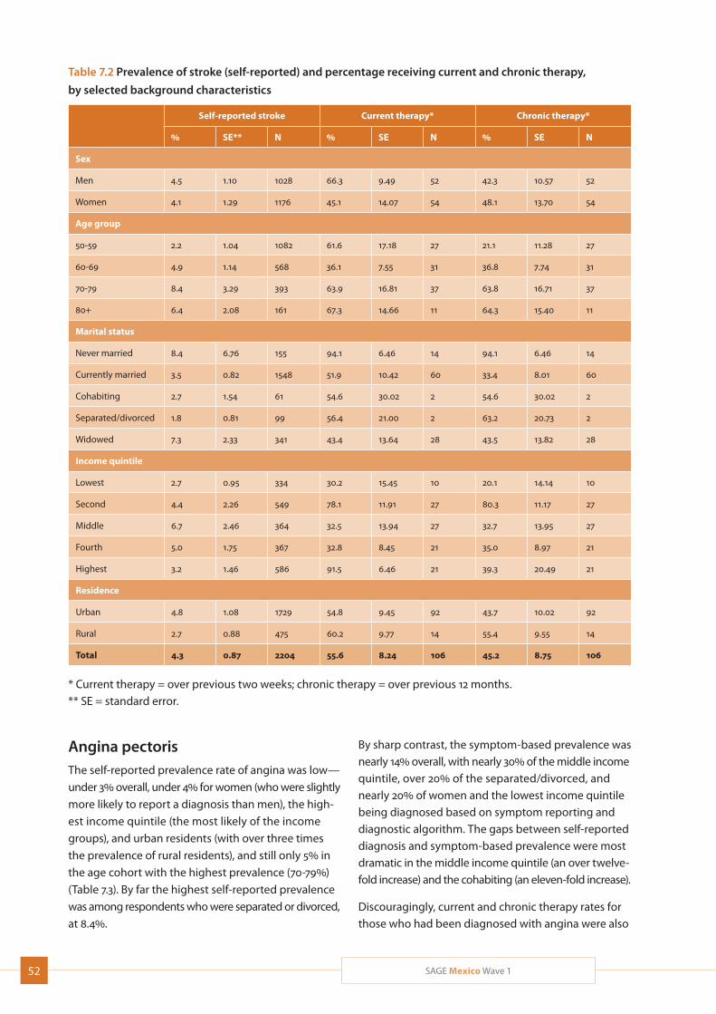
52 SAGE Mexico Wave 1
Table 7.2 Prevalence of stroke (self-reported) and percentage receiving current and chronic therapy,
by selected background characteristics
Self-reported stroke Current therapy* Chronic therapy*
% SE** N % SE N % SE N
Sex
Men 4.5 1.10 1028 66.3 9.49 52 42.3 10.57 52
Women 4.1 1.29 1176 45.1 14.07 54 48.1 13.70 54
Age group
50-59 2.2 1.04 1082 61.6 17.18 27 21.1 11.28 27
60-69 4.9 1.14 568 36.1 7.55 31 36.8 7.74 31
70-79 8.4 3.29 393 63.9 16.81 37 63.8 16.71 37
80+ 6.4 2.08 161 67.3 14.66 11 64.3 15.40 11
Marital status
Never married 8.4 6.76 155 94.1 6.46 14 94.1 6.46 14
Currently married 3.5 0.82 1548 51.9 10.42 60 33.4 8.01 60
Cohabiting 2.7 1.54 61 54.6 30.02 2 54.6 30.02 2
Separated/divorced 1.8 0.81 99 56.4 21.00 2 63.2 20.73 2
Widowed 7.3 2.33 341 43.4 13.64 28 43.5 13.82 28
Income quintile
Lowest 2.7 0.95 334 30.2 15.45 10 20.1 14.14 10
Second 4.4 2.26 549 78.1 11.91 27 80.3 11.17 27
Middle 6.7 2.46 364 32.5 13.94 27 32.7 13.95 27
Fourth 5.0 1.75 367 32.8 8.45 21 35.0 8.97 21
Highest 3.2 1.46 586 91.5 6.46 21 39.3 20.49 21
Residence
Urban 4.8 1.08 1729 54.8 9.45 92 43.7 10.02 92
Rural 2.7 0.88 475 60.2 9.77 14 55.4 9.55 14
Total 4.3 0.87 2204 55.6 8.24 106 45.2 8.75 106
* Current therapy = over previous two weeks; chronic therapy = over previous 12 months. ** SE = standard error.
Angina pectorisThe self-reported prevalence rate of angina was low—
under 3% overall, under 4% for women (who were slightly
more likely to report a diagnosis than men), the high-
est income quintile (the most likely of the income
groups), and urban residents (with over three times
the prevalence of rural residents), and still only 5% in
the age cohort with the highest prevalence (70-79%)
(Table 7.3). By far the highest self-reported prevalence
was among respondents who were separated or divorced,
at 8.4%.
By sharp contrast, the symptom-based prevalence was nearly 14% overall, with nearly 30% of the middle income quintile, over 20% of the separated/divorced, and nearly 20% of women and the lowest income quintile being diagnosed based on symptom reporting and diagnostic algorithm. The gaps between self-reported diagnosis and symptom-based prevalence were most dramatic in the middle income quintile (an over twelve-fold increase) and the cohabiting (an eleven-fold increase).
Discouragingly, current and chronic therapy rates for those who had been diagnosed with angina were also
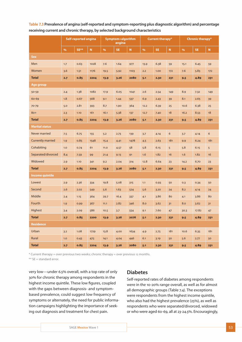
53SAGE Mexico Wave 1
Table 7.3 Prevalence of angina (self-reported and symptom-reporting plus diagnostic algorithm) and percentage
receiving current and chronic therapy, by selected background characteristics
Self-reported angina Symptom+algorithm angina
Current therapy* Chronic therapy*
% SE** N % SE N % SE N % SE N
Sex
Men 1.7 0.63 1028 7.6 1.64 977 13.9 6.38 59 15.1 6.45 59
Women 3.6 1.51 1176 19.5 5.92 1103 2.2 1.00 172 7.6 5.83 172
Total 2.7 0.85 2204 13.9 3.26 2080 5.1 2.30 231 9.5 4.89 231
Age group
50-59 2.4 1.38 1082 17.9 6.05 1041 2.6 2.54 149 8.9 7.32 149
60-69 1.8 0.67 568 9.1 1.44 537 6.9 2.43 39 8.1 2.65 39
70-79 5.0 2.81 393 8.7 1.90 364 12.2 6.39 25 10.6 6.38 25
80+ 2.3 1.10 161 16.1 5.38 137 12.7 7.40 18 16.2 8.53 18
Total 2.7 0.85 2204 13.9 3.26 2080 5.1 2.30 231 9.5 4.89 231
Marital status
Never married 7.5 6.75 155 5.2 2.73 139 3.7 4.14 6 3.7 4.14 6
Currently married 1.9 0.85 1548 15.4 4.41 1478 4.5 2.63 181 9.9 6.24 181
Cohabiting 1.0 0.74 61 11.0 4.57 58 5.8 6.15 5 5.8 6.15 5
Separated/divorced 8.4 7.59 99 21.4 9.13 91 1.6 1.82 16 1.6 1.82 16
Widowed 2.9 1.10 341 9.2 2.04 314 12.8 6.64 23 14.2 6.70 23
Total 2.7 0.85 2204 13.9 3.26 2080 5.1 2.30 231 9.5 4.89 231
Income quintile
Lowest 2.9 2.36 334 19.8 5.08 315 1.1 0.93 50 0.3 0.34 50
Second 2.6 2.02 549 5.6 1.63 524 5.6 3.20 24 8.2 4.14 24
Middle 2.4 1.15 364 29.7 16.4 337 4.1 3.86 80 4.1 3.86 80
Fourth 1.9 0.99 367 11.1 2.82 346 8.0 3.62 31 8.0 3.62 31
Highest 3.4 2.09 586 10.5 3.7 554 9.1 7.60 47 30.3 17.82 47
Total 2.7 0.85 2200 13.9 3.26 2076 5.1 2.30 231 9.5 4.89 231
Residence
Urban 3.2 1.08 1729 13.8 4.00 1634 4.9 2.75 181 10.6 6.35 181
Rural 1.0 0.43 475 14.1 4.04 446 6.1 3.19 50 5.6 2.77 50
Total 2.7 0.85 2204 13.9 3.26 2080 5.1 2.30 231 9.5 4.89 231
* Current therapy = over previous two weeks; chronic therapy = over previous 12 months.
** SE = standard error.
very low—under 6.5% overall, with a top rate of only 30% for chronic therapy among respondents in the highest income quintile. These low figures, coupled with the gaps between diagnosis- and symptom-based prevalence, could suggest low frequency of symptoms or alternately, the need for public informa-tion campaigns highlighting the importance of seek-ing out diagnosis and treatment for chest pain.
DiabetesSelf-reported rates of diabetes among respondents were in the 10-20% range overall, as well as for almost all demographic groups (Table 7.4). The exceptions were respondents from the highest income quintile, who also had the highest prevalence (25%), as well as respondents who were separated/divorced, widowed or who were aged 60-69, all at 23-24.5%. Encouragingly,
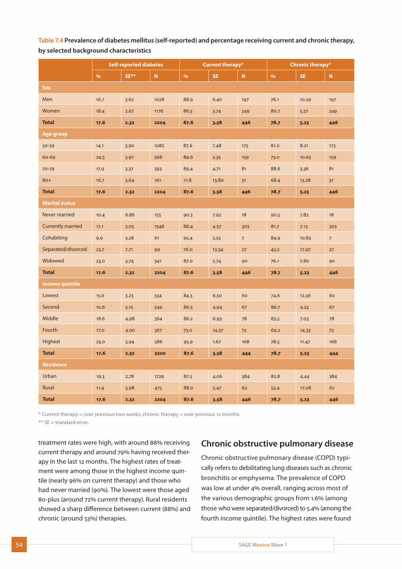
54 SAGE Mexico Wave 1
Table 7.4 Prevalence of diabetes mellitus (self-reported) and percentage receiving current and chronic therapy,
by selected background characteristics
Self-reported diabetes Current therapy* Chronic therapy*
% SE** N % SE N % SE N
Sex
Men 16.7 3.62 1028 88.9 6.40 197 76.1 10.29 197
Women 18.4 2.67 1176 86.5 3.74 249 80.7 5.27 249
Total 17.6 2.32 2204 87.6 3.58 446 78.7 5.23 446
Age group
50-59 14.1 3.90 1082 87.6 7.48 175 81.0 8.21 175
60-69 24.5 3.97 568 89.6 3.35 159 73.0 10.63 159
70-79 17.9 3.37 393 89.4 4.71 81 88.6 3.36 81
80+ 16.7 3.64 161 71.8 13.80 31 68.4 13.28 31
Total 17.6 2.32 2204 87.6 3.58 446 78.7 5.23 446
Marital status
Never married 10.4 6.86 155 90.3 7.92 18 90.5 7.82 18
Currently married 17.1 3.05 1548 88.4 4.57 303 81.7 7.13 303
Cohabiting 9.9 3.28 61 95.4 3.55 7 84.9 10.83 7
Separated/divorced 23.7 7.71 99 76.0 13.34 27 43.2 17.97 27
Widowed 23.0 3.74 341 87.0 5.74 90 76.1 7.80 90
Total 17.6 2.32 2204 87.6 3.58 446 78.7 5.23 446
Income quintile
Lowest 15.6 3.23 334 84.3 6.50 60 74.6 12.36 60
Second 10.6 3.15 549 86.5 4.94 67 86.7 4.23 67
Middle 18.6 4.98 364 86.2 6.93 78 83.5 7.03 78
Fourth 17.0 4.00 367 73.0 14.57 72 69.2 14.33 72
Highest 25.0 5.94 586 95.9 1.67 168 78.5 11.47 168
Total 17.6 2.32 2200 87.6 3.58 444 78.7 5.23 444
Residence
Urban 19.3 2.78 1729 87.5 4.06 384 82.8 4.44 384
Rural 11.4 3.98 475 88.0 5.47 62 53.4 17.08 62
Total 17.6 2.32 2204 87.6 3.58 446 78.7 5.23 446
* Current therapy = over previous two weeks; chronic therapy = over previous 12 months.
** SE = standard error.
treatment rates were high, with around 88% receiving current therapy and around 79% having received ther-apy in the last 12 months. The highest rates of treat-ment were among those in the highest income quin-tile (nearly 96% on current therapy) and those who had never married (90%). The lowest were those aged 80-plus (around 72% current therapy). Rural residents showed a sharp difference between current (88%) and chronic (around 53%) therapies.
Chronic obstructive pulmonary disease
Chronic obstructive pulmonary disease (COPD) typi-
cally refers to debilitating lung diseases such as chronic
bronchitis or emphysema. The prevalence of COPD
was low at under 4% overall, ranging across most of
the various demographic groups from 1.6% (among
those who were separated/divorced) to 5.4% (among the
fourth income quintile). The highest rates were found
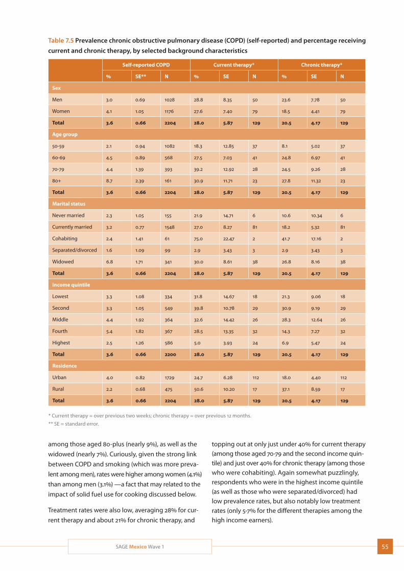
55SAGE Mexico Wave 1
Table 7.5 Prevalence chronic obstructive pulmonary disease (COPD) (self-reported) and percentage receiving
current and chronic therapy, by selected background characteristics
Self-reported COPD Current therapy* Chronic therapy*
% SE** N % SE N % SE N
Sex
Men 3.0 0.69 1028 28.8 8.35 50 23.6 7.78 50
Women 4.1 1.05 1176 27.6 7.40 79 18.5 4.41 79
Total 3.6 0.66 2204 28.0 5.87 129 20.5 4.17 129
Age group
50-59 2.1 0.94 1082 18.3 12.85 37 8.1 5.02 37
60-69 4.5 0.89 568 27.5 7.03 41 24.8 6.97 41
70-79 4.4 1.39 393 39.2 12.92 28 24.5 9.26 28
80+ 8.7 2.39 161 30.9 11.71 23 27.8 11.32 23
Total 3.6 0.66 2204 28.0 5.87 129 20.5 4.17 129
Marital status
Never married 2.3 1.05 155 21.9 14.71 6 10.6 10.34 6
Currently married 3.2 0.77 1548 27.0 8.27 81 18.2 5.32 81
Cohabiting 2.4 1.41 61 75.0 22.47 2 41.7 17.16 2
Separated/divorced 1.6 1.09 99 2.9 3.43 3 2.9 3.43 3
Widowed 6.8 1.71 341 30.0 8.61 38 26.8 8.16 38
Total 3.6 0.66 2204 28.0 5.87 129 20.5 4.17 129
Income quintile
Lowest 3.3 1.08 334 31.8 14.67 18 21.3 9.06 18
Second 3.3 1.05 549 39.8 10.78 29 30.9 9.19 29
Middle 4.4 1.92 364 32.6 14.42 26 28.3 12.64 26
Fourth 5.4 1.82 367 28.5 13.35 32 14.3 7.27 32
Highest 2.5 1.26 586 5.0 3.93 24 6.9 5.47 24
Total 3.6 0.66 2200 28.0 5.87 129 20.5 4.17 129
Residence
Urban 4.0 0.82 1729 24.7 6.28 112 18.0 4.40 112
Rural 2.2 0.68 475 50.6 10.20 17 37.1 8.59 17
Total 3.6 0.66 2204 28.0 5.87 129 20.5 4.17 129
* Current therapy = over previous two weeks; chronic therapy = over previous 12 months.
** SE = standard error.
among those aged 80-plus (nearly 9%), as well as the
widowed (nearly 7%). Curiously, given the strong link
between COPD and smoking (which was more preva-
lent among men), rates were higher among women (4.1%)
than among men (3.1%) —a fact that may related to the
impact of solid fuel use for cooking discussed below.
Treatment rates were also low, averaging 28% for cur-
rent therapy and about 21% for chronic therapy, and
topping out at only just under 40% for current therapy (among those aged 70-79 and the second income quin-tile) and just over 40% for chronic therapy (among those who were cohabiting). Again somewhat puzzlingly, respondents who were in the highest income quintile (as well as those who were separated/divorced) had low prevalence rates, but also notably low treatment rates (only 5-7% for the different therapies among the high income earners).
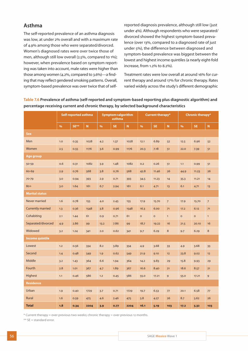
56 SAGE Mexico Wave 1
Table 7.6 Prevalence of asthma (self-reported and symptom-based reporting plus diagnostic algorithm) and
percentage receiving current and chronic therapy, by selected background characteristics
Self-reported asthma Symptom+algorithm asthma
Current therapy* Chronic therapy*
% SE** N % SE N % SE N % SE N
Sex
Men 1.0 0.35 1028 4.2 1.37 1028 12.1 6.89 52 12.5 6.96 52
Women 2.5 0.55 1176 3.6 0.99 1176 20.3 7.18 51 22.0 7.39 51
Age group
50-59 0.6 0.31 1082 3.9 1.48 1082 0.2 0.26 51 1.1 0.99 51
60-69 2.9 0.76 568 3.8 0.76 568 42.8 11.46 26 44.9 11.23 26
70-79 3.0 0.94 393 2.9 0.71 393 34.5 11.23 14 35.3 11.21 14
80+ 3.0 1.64 161 6.7 2.94 161 6.1 4.71 13 6.1 4.71 13
Marital status
Never married 1.6 0.78 155 4.0 2.45 155 17.9 15.70 7 17.9 15.70 7
Currently married 1.3 0.36 1548 3.8 0.96 1548 16.3 6.00 71 17.2 6.12 71
Cohabiting 2.1 1.44 61 0.9 0.71 61 0 0 1 0 0 1
Separated/divorced 4.9 2.86 99 13.2 7.86 99 18.7 19.22 16 21.5 20.10 16
Widowed 3.2 1.24 341 2.0 0.62 341 9.7 6.29 8 9.7 6.29 8
Income quintile
Lowest 1.2 0.56 334 8.2 3.89 334 4.9 3.68 33 4.9 3.68 33
Second 1.4 0.48 549 1.9 0.62 549 21.9 9.10 12 23.8 9.02 12
Middle 3.2 1.43 364 6.6 1.94 364 14.2 9.83 29 15.8 9.93 29
Fourth 2.8 1.01 367 4.7 1.89 367 16.6 8.40 21 18.6 8.57 21
Highest 1.1 0.46 586 1.2 0.45 586 55.0 17.21 9 55.0 17.21 9
Residence
Urban 1.9 0.40 1729 3.7 0.71 1729 19.7 6.53 77 20.1 6.58 77
Rural 1.6 0.59 475 4.6 2.46 475 5.8 4.27 26 8.7 5.62 26
Total 1.8 0.34 2204 3.9 0.77 2204 16.1 5.19 103 17.2 5.32 103
* Current therapy = over previous two weeks; chronic therapy = over previous 12 months.
** SE = standard error.
AsthmaThe self-reported prevalence of an asthma diagnosis was low, at under 2% overall and with a maximum rate of 4.9% among those who were separated/divorced. Women’s diagnosed rates were over twice those of men, although still low overall (2.5%, compared to 1%); however, when prevalence based on symptom report-ing was taken into account, male rates were higher than those among women (4.2%, compared to 3.6%)—a find-ing that may reflect gendered smoking patterns. Overall, symptom-based prevalence was over twice that of self-
reported diagnosis prevalence, although still low (just under 4%). Although respondents who were separated/divorced showed the highest symptom-based preva-lence (over 13%, compared to a diagnosed rate of just under 5%), the difference between diagnosed and symptom-based prevalence was biggest between the lowest and highest income quintiles (a nearly eight-fold increase, from 1.2% to 8.2%).
Treatment rates were low overall at around 16% for cur-rent therapy and around 17% for chronic therapy. Rates varied widely across the study’s different demographic
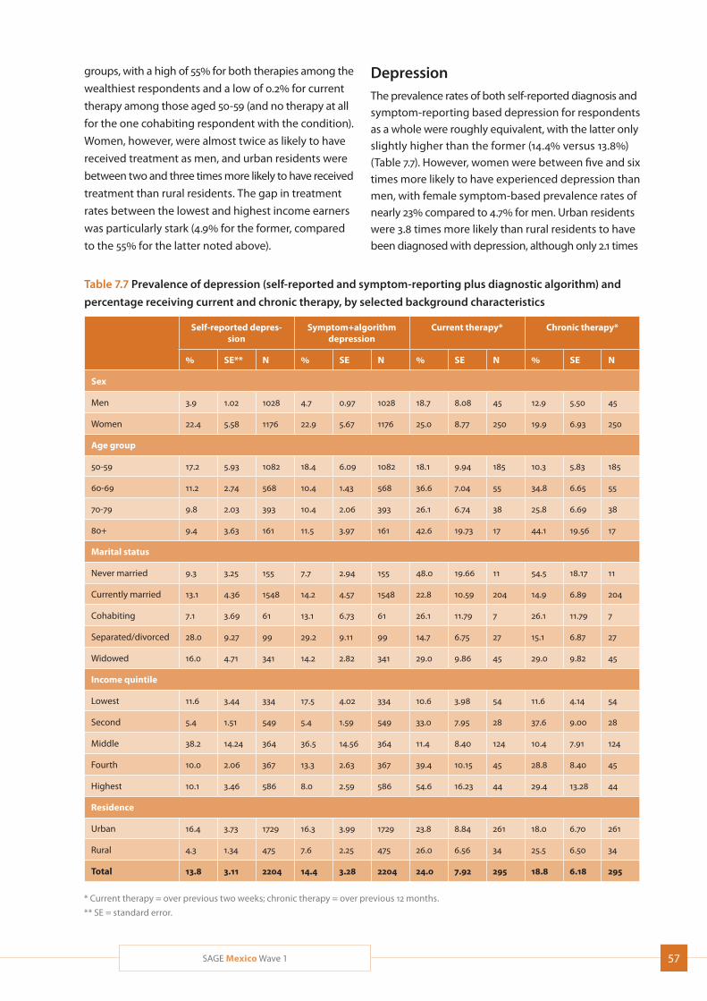
57SAGE Mexico Wave 1
groups, with a high of 55% for both therapies among the
wealthiest respondents and a low of 0.2% for current
therapy among those aged 50-59 (and no therapy at all
for the one cohabiting respondent with the condition).
Women, however, were almost twice as likely to have
received treatment as men, and urban residents were
between two and three times more likely to have received
treatment than rural residents. The gap in treatment
rates between the lowest and highest income earners
was particularly stark (4.9% for the former, compared
to the 55% for the latter noted above).
Table 7.7 Prevalence of depression (self-reported and symptom-reporting plus diagnostic algorithm) and
percentage receiving current and chronic therapy, by selected background characteristics
Self-reported depres-sion
Symptom+algorithm depression
Current therapy* Chronic therapy*
% SE** N % SE N % SE N % SE N
Sex
Men 3.9 1.02 1028 4.7 0.97 1028 18.7 8.08 45 12.9 5.50 45
Women 22.4 5.58 1176 22.9 5.67 1176 25.0 8.77 250 19.9 6.93 250
Age group
50-59 17.2 5.93 1082 18.4 6.09 1082 18.1 9.94 185 10.3 5.83 185
60-69 11.2 2.74 568 10.4 1.43 568 36.6 7.04 55 34.8 6.65 55
70-79 9.8 2.03 393 10.4 2.06 393 26.1 6.74 38 25.8 6.69 38
80+ 9.4 3.63 161 11.5 3.97 161 42.6 19.73 17 44.1 19.56 17
Marital status
Never married 9.3 3.25 155 7.7 2.94 155 48.0 19.66 11 54.5 18.17 11
Currently married 13.1 4.36 1548 14.2 4.57 1548 22.8 10.59 204 14.9 6.89 204
Cohabiting 7.1 3.69 61 13.1 6.73 61 26.1 11.79 7 26.1 11.79 7
Separated/divorced 28.0 9.27 99 29.2 9.11 99 14.7 6.75 27 15.1 6.87 27
Widowed 16.0 4.71 341 14.2 2.82 341 29.0 9.86 45 29.0 9.82 45
Income quintile
Lowest 11.6 3.44 334 17.5 4.02 334 10.6 3.98 54 11.6 4.14 54
Second 5.4 1.51 549 5.4 1.59 549 33.0 7.95 28 37.6 9.00 28
Middle 38.2 14.24 364 36.5 14.56 364 11.4 8.40 124 10.4 7.91 124
Fourth 10.0 2.06 367 13.3 2.63 367 39.4 10.15 45 28.8 8.40 45
Highest 10.1 3.46 586 8.0 2.59 586 54.6 16.23 44 29.4 13.28 44
Residence
Urban 16.4 3.73 1729 16.3 3.99 1729 23.8 8.84 261 18.0 6.70 261
Rural 4.3 1.34 475 7.6 2.25 475 26.0 6.56 34 25.5 6.50 34
Total 13.8 3.11 2204 14.4 3.28 2204 24.0 7.92 295 18.8 6.18 295
* Current therapy = over previous two weeks; chronic therapy = over previous 12 months.
** SE = standard error.
DepressionThe prevalence rates of both self-reported diagnosis and symptom-reporting based depression for respondents as a whole were roughly equivalent, with the latter only slightly higher than the former (14.4% versus 13.8%) (Table 7.7). However, women were between five and six times more likely to have experienced depression than men, with female symptom-based prevalence rates of nearly 23% compared to 4.7% for men. Urban residents were 3.8 times more likely than rural residents to have been diagnosed with depression, although only 2.1 times
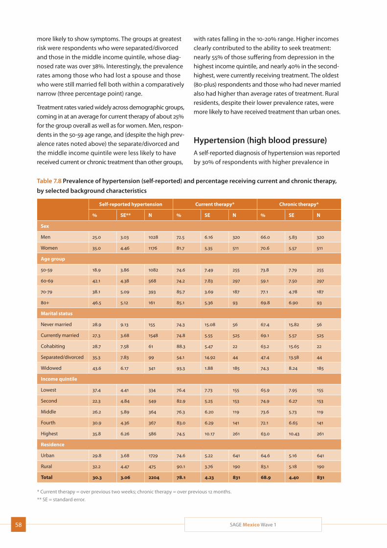
58 SAGE Mexico Wave 1
more likely to show symptoms. The groups at greatest risk were respondents who were separated/divorced and those in the middle income quintile, whose diag-nosed rate was over 38%. Interestingly, the prevalence rates among those who had lost a spouse and those who were still married fell both within a comparatively narrow (three percentage point) range.
Treatment rates varied widely across demographic groups, coming in at an average for current therapy of about 25% for the group overall as well as for women. Men, respon-dents in the 50-59 age range, and (despite the high prev-alence rates noted above) the separate/divorced and the middle income quintile were less likely to have received current or chronic treatment than other groups,
with rates falling in the 10-20% range. Higher incomes clearly contributed to the ability to seek treatment: nearly 55% of those suffering from depression in the highest income quintile, and nearly 40% in the second-highest, were currently receiving treatment. The oldest (80-plus) respondents and those who had never married also had higher than average rates of treatment. Rural residents, despite their lower prevalence rates, were more likely to have received treatment than urban ones.
Hypertension (high blood pressure)A self-reported diagnosis of hypertension was reported by 30% of respondents with higher prevalence in
Table 7.8 Prevalence of hypertension (self-reported) and percentage receiving current and chronic therapy,
by selected background characteristics
Self-reported hypertension Current therapy* Chronic therapy*
% SE** N % SE N % SE N
Sex
Men 25.0 3.03 1028 72.5 6.16 320 66.0 5.83 320
Women 35.0 4.46 1176 81.7 5.35 511 70.6 5.57 511
Age group
50-59 18.9 3.86 1082 74.6 7.49 255 73.8 7.79 255
60-69 42.1 4.38 568 74.2 7.83 297 59.1 7.50 297
70-79 38.1 5.09 393 85.7 3.69 187 77.1 4.78 187
80+ 46.5 5.12 161 85.1 5.36 93 69.8 6.90 93
Marital status
Never married 28.9 9.13 155 74.3 15.08 56 67.4 15.82 56
Currently married 27.3 3.68 1548 74.8 5.55 525 69.1 5.57 525
Cohabiting 28.7 7.58 61 88.3 5.47 22 63.2 15.65 22
Separated/divorced 35.3 7.83 99 54.1 14.92 44 47.4 13.58 44
Widowed 43.6 6.17 341 93.3 1.88 185 74.3 8.24 185
Income quintile
Lowest 37.4 4.41 334 76.4 7.73 155 65.9 7.95 155
Second 22.3 4.84 549 82.9 5.25 153 74.9 6.27 153
Middle 26.2 5.89 364 76.3 6.20 119 73.6 5.73 119
Fourth 30.9 4.36 367 83.0 6.29 141 72.1 6.65 141
Highest 35.8 6.26 586 74.5 10.17 261 63.0 10.43 261
Residence
Urban 29.8 3.68 1729 74.6 5.22 641 64.6 5.16 641
Rural 32.2 4.47 475 90.1 3.76 190 83.1 5.18 190
Total 30.3 3.06 2204 78.1 4.23 831 68.9 4.40 831
* Current therapy = over previous two weeks; chronic therapy = over previous 12 months.
** SE = standard error.
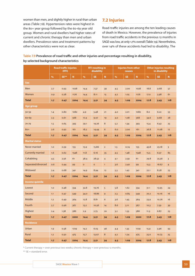
59SAGE Mexico Wave 1
women than men, and slightly higher in rural than urban areas (Table 7.8). Hypertension rates were highest in the 80+ year group followed by the 60-69 year old group. Women and rural dwellers had higher rates of current and chronic therapy than men and urban dwellers. Prevalence rates and treatment patterns by other characteristics were not as clear.
Table 7.9 Prevalence of road traffic and other injuries and percentage resulting in disability,
by selected background characteristics
Road traffic injuries (RTI)
RTI resulting in disability
Injuries from other causes
Other injuries resulting in disability
% SE** N % SE N % SE N % SE N
Sex
Men 2.7 0.93 1028 14.4 7.37 39 4.5 2.00 1028 18.8 9.68 57
Women 0.9 0.28 1176 14.4 8.11 15 4.2 1.05 1176 17.0 5.98 61
Total 1.7 0.47 2204 14.4 5.51 54 4.3 1.09 2204 17.8 5.43 118
Age group
50-59 1.4 0.80 1082 4.9 5.48 21 4.0 2.01 1082 8.0 6.22 53
60-69 2.3 0.61 568 17.4 9.07 19 4.0 1.08 568 34.6 9.68 28
70-79 1.5 0.65 393 29.1 19.26 8 5.2 1.34 393 15.4 6.42 25
80+ 2.6 0.92 161 18.2 14.44 6 6.0 2.00 161 26.8 11.08 12
Total 1.7 0.47 2204 14.4 5.51 54 4.3 1.09 2204 17.8 5.43 118
Marital status
Never married 1.0 0.59 155 15.9 15.86 2 1.5 0.74 155 43.8 23.18 3
Currently married 1.6 0.62 1548 11.8 6.16 35 4.5 1.48 1548 15.5 6.37 85
Cohabiting 4.5 2.56 61 38.4 28.52 4 4.1 2.59 61 29.8 25.56 3
Separated/divorced 0.6 0.44 99 0 0 1 3.6 2.40 99 15.3 16.67 4
Widowed 2.4 0.68 341 14.9 8.94 12 5.3 1.42 341 22.1 8.28 23
Total 1.7 0.47 2204 14.4 5.51 54 4.3 1.09 2204 17.8 5.43 118
Income quintile
Lowest 1.0 0.48 334 32.8 19.76 5 5.8 1.62 334 31.1 13.95 24
Second 1.1 0.47 549 34.0 18.86 9 2.3 0.85 549 20.2 10.16 16
Middle 1.2 0.49 364 12.8 8.81 6 3.6 1.45 364 23.9 10.76 16
Fourth 2.7 0.96 367 13.2 10.56 14 8.6 5.11 367 10.3 7.59 39
Highest 2.4 1.38 586 2.9 2.73 20 3.2 1.53 586 11.3 6.87 23
Total 1.7 0.47 2200 14.4 5.51 54 4.3 1.09 2200 17.8 5.43 118
Residence
Urban 1.9 0.58 1729 14.2 6.03 46 4.4 1.35 1729 15.9 5.96 93
Rural 1.2 0.50 475 15.7 13.07 8 4.2 1.24 475 25.0 10.73 25
Total 1.7 0.47 2204 14.4 5.51 54 4.3 1.09 2204 17.8 5.43 118
* Current therapy = over previous two weeks; chronic therapy = over previous 12 months.
** SE = standard error.
7.2 Injuries
Road-traffic injuries are among the ten leading causes of death in Mexico. However, the prevalence of injuries from road traffic accidents in the previous 12 months in SAGE was low, at only 1.7% overall (Table 7.9). Nevertheless, over 14% of these accidents had led to disability. The
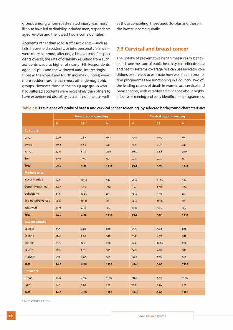
60 SAGE Mexico Wave 1
groups among whom road-related injury was most likely to have led to disability included men, respondents aged 70-plus and the lowest two income quintiles.
Accidents other than road-traffic accidents—such as falls, household accidents, or interpersonal violence—were more common, affecting a bit over 4% of respon-dents overall; the rate of disability resulting from such accidents was also higher, at nearly 18%. Respondents aged 80-plus and the widowed (and, interestingly, those in the lowest and fourth income quintiles) were more accident-prone than most other demographic groups. However, those in the 60-69 age group who had suffered accidents were more likely than others to have experienced disability as a consequence, as well
Table 7.10 Prevalence of uptake of breast and cervical cancer screening, by selected background characteristics
Breast cancer screening Cervical cancer screening
% SE** N % SE N
Age group
50-59 62.6 7.87 641 70.8 10.57 641
60-69 49.2 5.86 333 75.6 3.78 333
70-79 47.6 8.18 266 66.0 6.58 266
80+ 29.9 9.02 92 52.5 7.38 92
Total 54.0 4.28 1332 69.8 5.65 1332
Marital status
Never married 27.6 10.14 142 58.4 13.09 142
Currently married 64.7 5.53 762 73.7 8.96 762
Cohabiting 43.6 17.80 25 78.4 9.10 25
Separated/divorced 58.2 10.41 84 58.4 10.84 84
Widowed 39.9 7.32 319 67.8 5.90 319
Total 54.0 4.28 1332 69.8 5.65 1332
Income quintile
Lowest 33.5 4.82 226 63.7 5.42 226
Second 51.6 9.60 330 73.6 8.72 330
Middle 63.5 12.7 270 54.2 17.99 270
Fourth 56.2 6.11 185 74.9 4.99 185
Highest 61.7 8.03 319 80.2 6.78 319
Total 54.0 4.28 1330 69.8 5.65 1330
Residence
Urban 58.0 4.73 1109 68.6 6.70 1109
Rural 34.1 5.20 223 75.9 3.76 223
Total 54.0 4.28 1332 69.8 5.65 1332
* SE = standard error.
as those cohabiting, those aged 80-plus and those in the lowest income quintile.
7.3 Cervical and breast cancer
The uptake of preventative health measures or behav-iours is one measure of public health system effectiveness and health systems coverage. We can use indicator con-ditions or services to estimate how well health promo-tion programmes are functioning in a country. Two of the leading causes of death in women are cervical and breast cancer, with established evidence about highly effective screening and early identification programmes.
61SAGE Mexico Wave 1
As such, the use of pelvic examinations and mammog-raphy were assessed in women in Mexico.
Just over half (54%) of the women in this study had ever received screening for breast cancer (Table 7.10). Women in the 50-59 age group were most likely to have received mammograms (62%), while those aged 80-plus were significantly less likely, at under 30%. Urban resi-dents were 1.7 times more likely to have received screening than rural residents, approximately the same rate of difference as that between the lowest and highest income quintiles.
Meanwhile, 70% of women had been screened for cervical cancer. Rates of screening were highest in the 50-59 age bracket, as well as among the middle and highest income quintiles. In this instance, rural residents were more likely to have received screening than urban ones. Married women were most likely of the marital sta-tus groups to have received screening for both cancers.
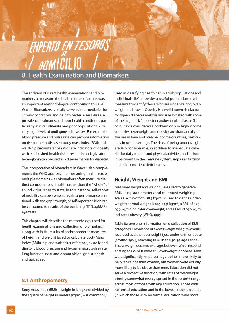
62 SAGE Mexico Wave 1
8. Health Examination and Biomarkers
The addition of direct health examinations and bio-
markers to measure the health status of adults was
an important methodological contribution to SAGE
Wave 1. Biomarkers typically serve as intermediaries for
chronic conditions and help to better assess disease
prevalence estimates and poor health conditions par-
ticularly in rural, illiterate and poor populations with
very high levels of undiagnosed diseases. For example,
blood pressure and pulse rate can provide information
on risk for heart diseases; body mass index (BMI) and
waist-hip circumference ratios are indicators of obesity
with established health risk thresholds; and, glycated
hemoglobin can be used as a disease marker for diabetes.
The incorporation of biomarkers in Wave 1 also comple-
ments the WHO approach to measuring health across
multiple domains – as biomarkers often measure dis-
tinct components of health, rather than the “whole” of
an individual’s health state. In this instance, self-report
of mobility can be assessed against performance on a
timed walk and grip strength, or self-reported vision can
be compared to results of the tumbling “E” (LogMAR)
eye tests.
This chapter will describe the methodology used for
health examinations and collection of biomarkers,
along with initial results of anthropometric measures
of height and weight (used to calculate Body Mass
Index (BMI)), hip and waist circumference, systolic and
diastolic blood pressure and hypertension, pulse rate,
lung function, near and distant vision, grip strength
and gait speed.
8.1 Anthropometry
Body mass index (BMI) – weight in kilograms divided by
the square of height in meters (kg/m2) – is commonly
used in classifying health risk in adult populations and
individuals. BMI provides a useful population-level
measure to identify those who are underweight, over-
weight and obese. Obesity is a well-known risk factor
for type-2 diabetes mellitus and is associated with some
of the major risk factors for cardiovascular disease (Lee,
2012). Once considered a problem only in high-income
countries, overweight and obesity are dramatically on
the rise in low- and middle-income countries, particu-
larly in urban settings. The risks of being underweight
are also considerable, in addition to inadequate calo-
ries for daily mental and physical activities, and include
impairments in the immune system, impaired fertility
and micro-nutrient deficiencies.
Height, Weight and BMIMeasured height and weight were used to generate
BMI, using stadiometers and calibrated weighing
scales. A cut-off of <18.5 kg/m2 is used to define under-
weight; normal weight is 18.5-24.9 kg/m2; a BMI of ≥25–
29.9 kg/m2 indicates overweight; and a BMI of ≥30 kg/m2
indicates obesity (WHO, 1995).
Table 8.1 presents information on distribution of BMI
categories. Prevalence of excess weight was 78% overall,
recorded as either overweight (just under 50%) or obese
(around 29%), reaching 86% in the 50-59 age range.
Excess weight declined with age, but over 52% of respond-
ents aged 80-plus were still overweight or obese. Men
were significantly (13 percentage points) more likely to
be overweight than women, but women were equally
more likely to be obese than men. Education did not
serve a protective function, with rates of overweight/
obesity somewhat evenly spread in the 70-80% range
across most of those with any education. Those with
no formal education and in the lowest income quintile
(in which those with no formal education were more
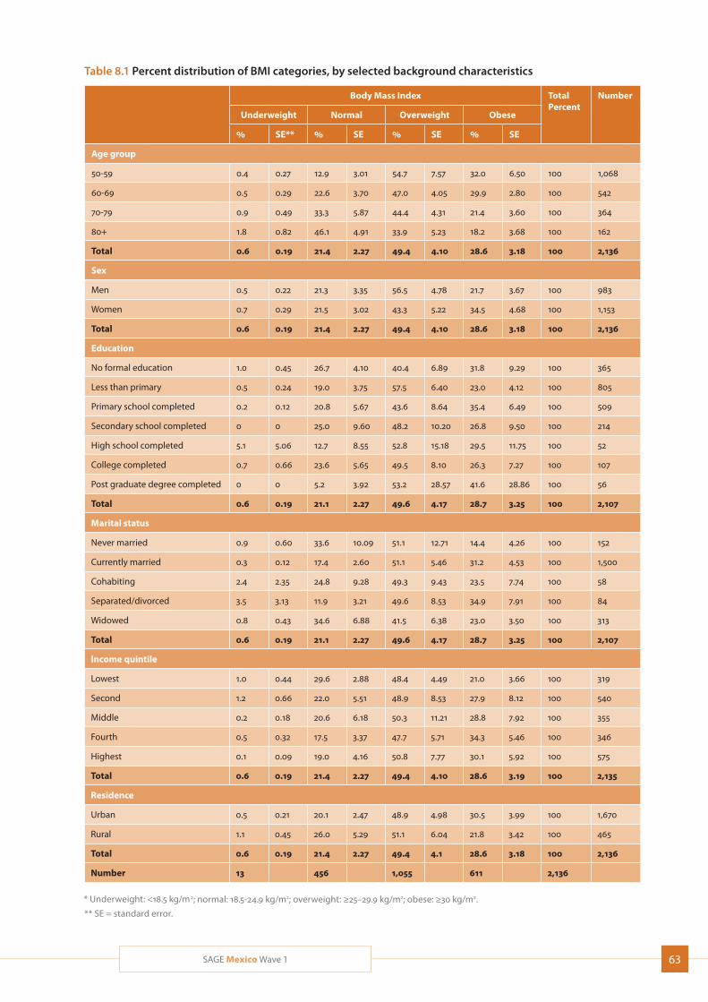
63SAGE Mexico Wave 1
Table 8.1 Percent distribution of BMI categories, by selected background characteristics
Body Mass Index TotalPercent
Number
Underweight Normal Overweight Obese
% SE** % SE % SE % SE
Age group
50-59 0.4 0.27 12.9 3.01 54.7 7.57 32.0 6.50 100 1,068
60-69 0.5 0.29 22.6 3.70 47.0 4.05 29.9 2.80 100 542
70-79 0.9 0.49 33.3 5.87 44.4 4.31 21.4 3.60 100 364
80+ 1.8 0.82 46.1 4.91 33.9 5.23 18.2 3.68 100 162
Total 0.6 0.19 21.4 2.27 49.4 4.10 28.6 3.18 100 2,136
Sex
Men 0.5 0.22 21.3 3.35 56.5 4.78 21.7 3.67 100 983
Women 0.7 0.29 21.5 3.02 43.3 5.22 34.5 4.68 100 1,153
Total 0.6 0.19 21.4 2.27 49.4 4.10 28.6 3.18 100 2,136
Education
No formal education 1.0 0.45 26.7 4.10 40.4 6.89 31.8 9.29 100 365
Less than primary 0.5 0.24 19.0 3.75 57.5 6.40 23.0 4.12 100 805
Primary school completed 0.2 0.12 20.8 5.67 43.6 8.64 35.4 6.49 100 509
Secondary school completed 0 0 25.0 9.60 48.2 10.20 26.8 9.50 100 214
High school completed 5.1 5.06 12.7 8.55 52.8 15.18 29.5 11.75 100 52
College completed 0.7 0.66 23.6 5.65 49.5 8.10 26.3 7.27 100 107
Post graduate degree completed 0 0 5.2 3.92 53.2 28.57 41.6 28.86 100 56
Total 0.6 0.19 21.1 2.27 49.6 4.17 28.7 3.25 100 2,107
Marital status
Never married 0.9 0.60 33.6 10.09 51.1 12.71 14.4 4.26 100 152
Currently married 0.3 0.12 17.4 2.60 51.1 5.46 31.2 4.53 100 1,500
Cohabiting 2.4 2.35 24.8 9.28 49.3 9.43 23.5 7.74 100 58
Separated/divorced 3.5 3.13 11.9 3.21 49.6 8.53 34.9 7.91 100 84
Widowed 0.8 0.43 34.6 6.88 41.5 6.38 23.0 3.50 100 313
Total 0.6 0.19 21.1 2.27 49.6 4.17 28.7 3.25 100 2,107
Income quintile
Lowest 1.0 0.44 29.6 2.88 48.4 4.49 21.0 3.66 100 319
Second 1.2 0.66 22.0 5.51 48.9 8.53 27.9 8.12 100 540
Middle 0.2 0.18 20.6 6.18 50.3 11.21 28.8 7.92 100 355
Fourth 0.5 0.32 17.5 3.37 47.7 5.71 34.3 5.46 100 346
Highest 0.1 0.09 19.0 4.16 50.8 7.77 30.1 5.92 100 575
Total 0.6 0.19 21.4 2.27 49.4 4.10 28.6 3.19 100 2,135
Residence
Urban 0.5 0.21 20.1 2.47 48.9 4.98 30.5 3.99 100 1,670
Rural 1.1 0.45 26.0 5.29 51.1 6.04 21.8 3.42 100 465
Total 0.6 0.19 21.4 2.27 49.4 4.1 28.6 3.18 100 2,136
Number 13 456 1,055 611 2,136
* Underweight: <18.5 kg/m2; normal: 18.5-24.9 kg/m2; overweight: ≥25–29.9 kg/m2; obese: ≥30 kg/m2.
** SE = standard error.
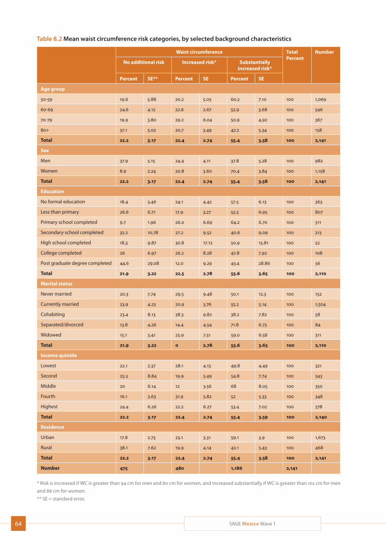
64 SAGE Mexico Wave 1
Table 8.2 Mean waist circumference risk categories, by selected background characteristics
Waist circumference TotalPercent
Number
No additional risk Increased risk* Substantially increased risk*
Percent SE** Percent SE Percent SE
Age group
50-59 19.6 5.88 20.2 5.05 60.2 7.10 100 1,069
60-69 24.6 4.12 22.6 2.67 52.9 3.68 100 546
70-79 19.9 3.80 29.2 6.04 50.9 4.92 100 367
80+ 37.1 5.02 20.7 3.49 42.2 5.34 100 158
Total 22.2 3.17 22.4 2.74 55.4 3.58 100 2,141
Sex
Men 37.9 5.15 24.4 4.11 37.8 5.28 100 982
Women 8.9 2.24 20.8 3.60 70.4 3.84 100 1,158
Total 22.2 3.17 22.4 2.74 55.4 3.58 100 2,141
Education
No formal education 18.4 3.46 24.1 4.42 57.5 6.13 100 363
Less than primary 26.6 6.71 17.9 3.27 55.5 6.95 100 807
Primary school completed 9.7 1.96 26.0 6.69 64.2 6.70 100 511
Secondary school completed 32.2 10.78 27.2 9.52 40.6 9.09 100 213
High school completed 18.3 9.87 30.8 17.12 50.9 15.81 100 52
College completed 26 6.97 26.2 8.28 47.8 7.92 100 108
Post graduate degree completed 44.6 29.08 12.0 9.29 43.4 28.86 100 56
Total 21.9 3.22 22.5 2.78 55.6 3.65 100 2,110
Marital status
Never married 20.3 7.74 29.5 9.48 50.1 12.3 100 152
Currently married 23.9 4.23 20.9 3.76 55.2 5.14 100 1,504
Cohabiting 23.4 8.13 38.3 9.82 38.2 7.82 100 58
Separated/divorced 13.8 4.26 14.4 4.54 71.8 6.73 100 84
Widowed 15.1 3.41 25.9 7.51 59.0 6.58 100 311
Total 21.9 3.22 0 2.78 55.6 3.65 100 2,110
Income quintile
Lowest 22.1 2.37 28.1 4.13 49.8 4.49 100 321
Second 25.3 8.84 19.9 5.49 54.8 7.74 100 543
Middle 20 6.14 12 3.56 68 8.05 100 350
Fourth 16.1 3.63 31.9 5.82 52 5.33 100 348
Highest 24.4 6.26 22.2 6.27 53.4 7.02 100 578
Total 22.2 3.17 22.4 2.74 55.4 3.59 100 2,140
Residence
Urban 17.8 2.73 23.1 3.31 59.1 3.9 100 1,673
Rural 38.1 7.62 19.9 4.14 42.1 5.43 100 468
Total 22.2 3.17 22.4 2.74 55.4 3.58 100 2,141
Number 475 480 1,186 2,141
* Risk is increased if WC is greater than 94 cm for men and 80 cm for women, and increased substantially if WC is greater than 102 cm for men
and 88 cm for women.
** SE = standard error.
65SAGE Mexico Wave 1
likely to be found) had the lowest rates of overweight/obesity—but in both cases, these were still around 70%. Separated/divorced respondents were the most likely of the marital groups to carry excess weight (nearly 85%), but also most likely (if still only at 3.5%) to be underweight. Rural residents were quite a bit less likely to be overweight/obese taken together (around 72%, compared to around 79% in urban areas), although slightly more likely to be overweight.
Hip and waist circumferenceWaist circumference (WC) and waist-to-hip ratio (WHR) are important indicators of overall health risk for cardio-vascular and metabolic diseases. People with more weight around their waists are at greater risk of heart disease and diabetes than those with weight around their hips. WC and WHR have been found to be more efficient predictors of mortality and other health out-comes in older people than BMI, as higher BMI in older adults is associated with lower mortality rates (Janssen, 2005; Huxley, 2010; Seidell, 2010; Heim 2011). Elevated WHR, as opposed to high BMI, has been associated with a greater risk of death (Price, 2006; Flicker, 2010). WC is a useful measure of fat distribution in the human body, and was measured midway between the lower rib cage and the iliac crest by trained interviewers.
Table 8.2 shows the distribution health risk from WC categories by selected demographic characteristics. The risk of metabolic complication from higher WC is based on WHO classifications as follows:
Increased if WC is greater than 94 cm for men and 80 cm for women;
Substantially increased if WC is greater than 102 cm for men and 88 cm for women (WHO, 2011).
Over 55% of respondents had a waist circumference that placed them at substantially increased risk of health problems, with an additional 22% at increased risk— a total of some 77%. In contrast to the results for over-weight/obesity, risky waist circumference (taken as increased risk plus substantially increased risk) did not show a straightforward decrease with age—although respondents aged 80-plus continued to show the lowest levels of risk overall. Similarly, the results by educational levels also did not conform to the overweight/obesity results, with respondents holding a post-graduate degree the least likely to have risky waist circumfer-ences, and those having no formal education sitting in the middle of the range. However, women were again
more likely to be at risk than men (particularly in the ‘substantially at risk’ category), as were the lowest income earners compared to other income quintiles. Rural residents, meanwhile, were substantially less likely to be at risk than their urban counterparts.
An alarming 84.5% of respondents overall had high-risk waist-to-hip ratios (WHR) (Table 8.3), with the figures rising to 90% or above among respondents aged 50-59, men, and those with post-graduate degrees. No demo-graphic group fell below 72%, the rough figure for respondents aged 70-79; in addition to this group, the never-married and the widowed were the only groups to come in below 75%. Most other demographic groups fell in the 80-89% range, with comparatively little vari-ation around income quintiles, place of residence, or (post-graduate degrees excepted) education. Notably, however, women came in at around 78% (compared, as noted above, to the men at nearly 92%).
8.2 Measured performance tests
The interviewers were trained to conduct face-to-face interviews, physical measurements and performance tests. A manual was available which contained instruc-tions on taking the different measurements, specifying the nature of each test, the instructions to be given before and during the measurement, the equipment to be used, the calibration of the equipment where necessary, and the importance of adhering to a proto-col throughout the activity in order to ensure inter-view consistency and reliability of the measurements obtained. Interviewers were also invited to report observations or problems arising in the administration of the tests.
Half of the respondents were accompanied by another person during the interview; 7% had hearing problems; 9% had problems with eyesight; 1% used a wheel chair; 7% used crutches, a cane or a walker; 14% had difficulty walking; fewer than 1% had paralysis; 2% had difficulty breathing or a chronic cough; fewer than 1% had an extremity amputated; and 7% reported having some other health condition that made performing a given test difficult.
Measured blood pressureThe current Official Mexican Standard (NOM-030-SSA2- 1999) considers normal blood pressure to be below
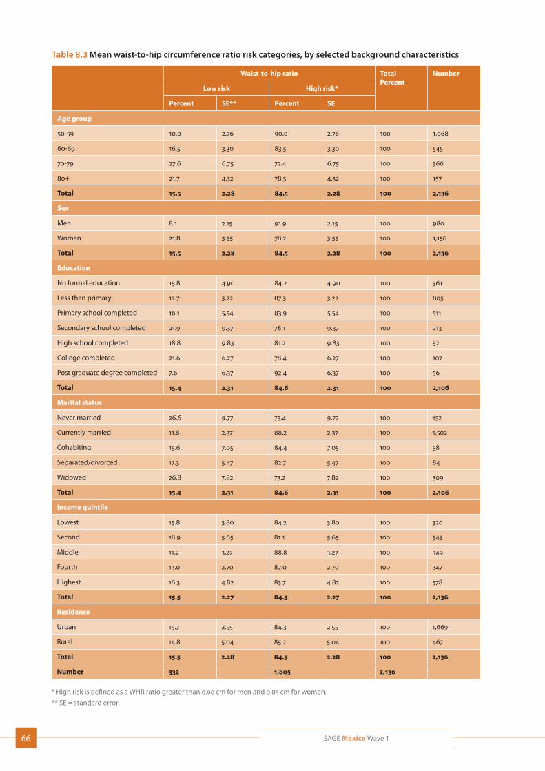
66 SAGE Mexico Wave 1
Table 8.3 Mean waist-to-hip circumference ratio risk categories, by selected background characteristics
Waist-to-hip ratio TotalPercent
Number
Low risk High risk*
Percent SE** Percent SE
Age group
50-59 10.0 2.76 90.0 2.76 100 1,068
60-69 16.5 3.30 83.5 3.30 100 545
70-79 27.6 6.75 72.4 6.75 100 366
80+ 21.7 4.32 78.3 4.32 100 157
Total 15.5 2.28 84.5 2.28 100 2,136
Sex
Men 8.1 2.15 91.9 2.15 100 980
Women 21.8 3.55 78.2 3.55 100 1,156
Total 15.5 2.28 84.5 2.28 100 2,136
Education
No formal education 15.8 4.90 84.2 4.90 100 361
Less than primary 12.7 3.22 87.3 3.22 100 805
Primary school completed 16.1 5.54 83.9 5.54 100 511
Secondary school completed 21.9 9.37 78.1 9.37 100 213
High school completed 18.8 9.83 81.2 9.83 100 52
College completed 21.6 6.27 78.4 6.27 100 107
Post graduate degree completed 7.6 6.37 92.4 6.37 100 56
Total 15.4 2.31 84.6 2.31 100 2,106
Marital status
Never married 26.6 9.77 73.4 9.77 100 152
Currently married 11.8 2.37 88.2 2.37 100 1,502
Cohabiting 15.6 7.05 84.4 7.05 100 58
Separated/divorced 17.3 5.47 82.7 5.47 100 84
Widowed 26.8 7.82 73.2 7.82 100 309
Total 15.4 2.31 84.6 2.31 100 2,106
Income quintile
Lowest 15.8 3.80 84.2 3.80 100 320
Second 18.9 5.65 81.1 5.65 100 543
Middle 11.2 3.27 88.8 3.27 100 349
Fourth 13.0 2.70 87.0 2.70 100 347
Highest 16.3 4.82 83.7 4.82 100 578
Total 15.5 2.27 84.5 2.27 100 2,136
Residence
Urban 15.7 2.55 84.3 2.55 100 1,669
Rural 14.8 5.04 85.2 5.04 100 467
Total 15.5 2.28 84.5 2.28 100 2,136
Number 332 1,805 2,136
* High risk is defined as a WHR ratio greater than 0.90 cm for men and 0.85 cm for women.
** SE = standard error.
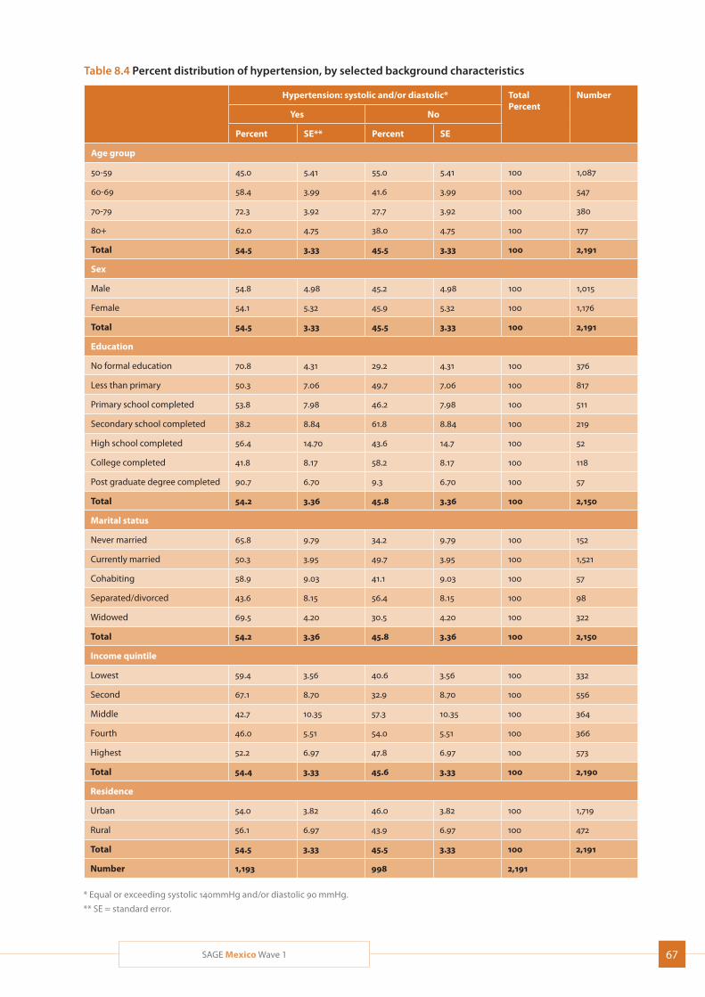
67SAGE Mexico Wave 1
Table 8.4 Percent distribution of hypertension, by selected background characteristics
Hypertension: systolic and/or diastolic* TotalPercent
Number
Yes No
Percent SE** Percent SE
Age group
50-59 45.0 5.41 55.0 5.41 100 1,087
60-69 58.4 3.99 41.6 3.99 100 547
70-79 72.3 3.92 27.7 3.92 100 380
80+ 62.0 4.75 38.0 4.75 100 177
Total 54.5 3.33 45.5 3.33 100 2,191
Sex
Male 54.8 4.98 45.2 4.98 100 1,015
Female 54.1 5.32 45.9 5.32 100 1,176
Total 54.5 3.33 45.5 3.33 100 2,191
Education
No formal education 70.8 4.31 29.2 4.31 100 376
Less than primary 50.3 7.06 49.7 7.06 100 817
Primary school completed 53.8 7.98 46.2 7.98 100 511
Secondary school completed 38.2 8.84 61.8 8.84 100 219
High school completed 56.4 14.70 43.6 14.7 100 52
College completed 41.8 8.17 58.2 8.17 100 118
Post graduate degree completed 90.7 6.70 9.3 6.70 100 57
Total 54.2 3.36 45.8 3.36 100 2,150
Marital status
Never married 65.8 9.79 34.2 9.79 100 152
Currently married 50.3 3.95 49.7 3.95 100 1,521
Cohabiting 58.9 9.03 41.1 9.03 100 57
Separated/divorced 43.6 8.15 56.4 8.15 100 98
Widowed 69.5 4.20 30.5 4.20 100 322
Total 54.2 3.36 45.8 3.36 100 2,150
Income quintile
Lowest 59.4 3.56 40.6 3.56 100 332
Second 67.1 8.70 32.9 8.70 100 556
Middle 42.7 10.35 57.3 10.35 100 364
Fourth 46.0 5.51 54.0 5.51 100 366
Highest 52.2 6.97 47.8 6.97 100 573
Total 54.4 3.33 45.6 3.33 100 2,190
Residence
Urban 54.0 3.82 46.0 3.82 100 1,719
Rural 56.1 6.97 43.9 6.97 100 472
Total 54.5 3.33 45.5 3.33 100 2,191
Number 1,193 998 2,191
* Equal or exceeding systolic 140mmHg and/or diastolic 90 mmHg.
** SE = standard error.
68 SAGE Mexico Wave 1
140/90 mmHg. Accordingly, optimal arterial pressure is considered to be below 120/80 mmHg, normal arterial pressure 120-129/80-84 mmHg and normal high arte-rial pressure 130-139/85-89 mmHg. According to this Standard, arterial hypertension is equal or exceeding 140/90 mmHg.1
Table 8.4 presents information on the prevalence of hypertension based on measured blood pressure. Over half (54.5%) of the respondents had systolic or diastolic hypertension, with rates peaking in the 70-79 age group (72.3%). Rates were almost identical among men and women and only differed slightly between urban and rural residents, with the latter only two percentage points more at risk. Rates varied more widely across income quintiles (a 15 percentage-point spread) and marital status (26 percentage points), with the widowed and the second income quintile at the greatest risk. They varied even more sharply (a spread of over 50 percent-age points) across education levels, with respondents at either end of the education spectrum (no formal education/post-graduate education) at the highest risk and those with a partial secondary education at the lowest.
Lung function (spirometry)Chronic obstructive pulmonary disease (COPD) is a lead-ing cause of premature death in Mexico (IHME, 2013). In addition, national statistics rank asthma and status asthmaticus 13th and bronchial pneumonia and pneu-monia 16th among the leading causes of illness by age group; these conditions were particularly prevalent among persons aged 65 and over (20%).2
Around 20% of respondents returned spirometry results indicating some degree of COPD, including around 18% of those respondents who said that they had never been diagnosed with the condition (Table 8.5). Rates of COPD went up with age (from 12.8% among 50-59 year olds to 36.5% among respondents aged 80-plus), were almost identical for men and women, and roughly equivalent among urban and rural residents and among the non-obese and the obese (the latter in fact showing slightly lower levels). Although current
1 Secretaria de Salud de México. NORMA Oficial Mexicana NOM-030-SSA2-1999, Para la prevención, tratamiento y control de la hipertensión arterial. Disponible en http://www.salud.gob.mx/unidades/cdi/nom/030ssa29.html consultada el 30 de julio del 2010.
2 Secretaría de Salud de México. Anuarios de morbilidad. Disponible en http://www.dgepi.salud.gob.mx/infoepi/infodigital.html, consultado el 30 de julio del 2010.
and former smokers had high rates, so did those who had never smoked. Prevalence was also lowest in the highest income quintile. Comparing the lung function test results to self-reported diagnosis (or not) of COPD, over 66% of respondents who said that they had been diagnosed with the condition showed no signs in the spirometry test, while over 13% of those who had never been diagnosed showed a moderate or more severe level of disease on the test. These discrepancies could be related to the small number reporting COPD, or inaccuracies in the administration of the spirometry test – a notoriously difficult test to complete.
Among respondents who returned spirometry results indicating some degree of COPD, most (57%) showed a moderate level of the condition, followed by those (28%) who showed only mild signs. The COPD of some 11% was severe, and that of around 4% very severe. Those very much at the greatest risk of severe or very severe COPD were respondents aged 80-plus (3.7% in each category, or 7.4% in total); no other demographic group showed a combined severe/very severe incidence of over 5.3% (the lowest income quintile). Respondents aged 80-plus were also by far the most likely to show moderate COPD. Among the risk category groups, interestingly, occasional smokers had the highest levels of severe/very severe incidence (again 5.3%); meanwhile, the non-obese were around half as likely as the obese to show severe/very severe incidence. The group with the highest incidence of moderate COPD was the middle income quintile at over 22%, followed by current daily smokers at nearly 16%.
Table 8.6 presents information on the distribution of asthma. The spirometry revealed asthma rates much higher than the rates derived from symptom reporting: fewer than 4% of respondents tested as completely free of asthma, and over 96% of those who said that they had no symptoms in fact showed some signs—mostly mild, but also moderate—of the condition. Spirometry-based incidence increased with age. Women were more likely than men to test as free from the condition, but also to show mild signs. Rural residents were more likely than their urban counterparts to show no signs of asthma in the spirometry; however, if they did show signs, they were more likely to be moderate or severe. Distribution of incidence across the income quintiles did not show strong patterns, although those in the highest income quintile were the least likely to show moderate or severe signs of the disease and those in the second and middle quintiles the most. Among risk factor groups, weight again did not provoke strong
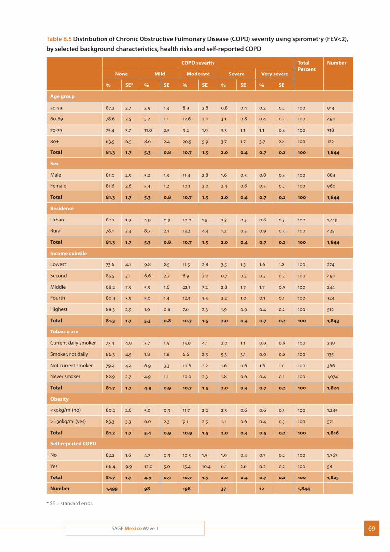
69SAGE Mexico Wave 1
Table 8.5 Distribution of Chronic Obstructive Pulmonary Disease (COPD) severity using spirometry (FEV<2),
by selected background characteristics, health risks and self-reported COPD
COPD severity TotalPercent
Number
None Mild Moderate Severe Very severe
% SE* % SE % SE % SE % SE
Age group
50-59 87.2 2.7 2.9 1.3 8.9 2.8 0.8 0.4 0.2 0.2 100 913
60-69 78.6 2.5 5.2 1.1 12.6 2.0 3.1 0.8 0.4 0.2 100 490
70-79 75.4 3.7 11.0 2.5 9.2 1.9 3.3 1.1 1.1 0.4 100 318
80+ 63.5 6.5 8.6 2.4 20.5 5.9 3.7 1.7 3.7 2.8 100 122
Total 81.3 1.7 5.3 0.8 10.7 1.5 2.0 0.4 0.7 0.2 100 1,844
Sex
Male 81.0 2.9 5.2 1.3 11.4 2.8 1.6 0.5 0.8 0.4 100 884
Female 81.6 2.6 5.4 1.2 10.1 2.0 2.4 0.6 0.5 0.2 100 960
Total 81.3 1.7 5.3 0.8 10.7 1.5 2.0 0.4 0.7 0.2 100 1,844
Residence
Urban 82.2 1.9 4.9 0.9 10.0 1.5 2.3 0.5 0.6 0.3 100 1,419
Rural 78.1 3.3 6.7 2.1 13.2 4.4 1.2 0.5 0.9 0.4 100 425
Total 81.3 1.7 5.3 0.8 10.7 1.5 2.0 0.4 0.7 0.2 100 1,844
Income quintile
Lowest 73.6 4.1 9.8 2.5 11.5 2.8 3.5 1.3 1.6 1.2 100 274
Second 85.5 3.1 6.6 2.2 6.9 2.0 0.7 0.3 0.3 0.2 100 490
Middle 68.2 7.3 5.3 1.6 22.1 7.2 2.8 1.7 1.7 0.9 100 244
Fourth 80.4 3.9 5.0 1.4 12.3 3.5 2.2 1.0 0.1 0.1 100 324
Highest 88.3 2.9 1.9 0.8 7.6 2.3 1.9 0.9 0.4 0.2 100 512
Total 81.3 1.7 5.3 0.8 10.7 1.5 2.0 0.4 0.7 0.2 100 1,843
Tobacco use
Current daily smoker 77.4 4.9 3.7 1.5 15.9 4.1 2.0 1.1 0.9 0.6 100 249
Smoker, not daily 86.3 4.5 1.8 1.8 6.6 2.5 5.3 3.1 0.0 0.0 100 135
Not current smoker 79.4 4.4 6.9 3.3 10.6 2.2 1.6 0.6 1.6 1.0 100 366
Never smoker 82.9 2.7 4.9 1.1 10.0 2.3 1.8 0.6 0.4 0.1 100 1,074
Total 81.7 1.7 4.9 0.9 10.7 1.5 2.0 0.4 0.7 0.2 100 1,824
Obesity
<30kg/m2 (no) 80.2 2.6 5.0 0.9 11.7 2.2 2.5 0.6 0.6 0.3 100 1,245
>=30kg/m2 (yes) 83.3 3.3 6.0 2.3 9.1 2.5 1.1 0.6 0.4 0.3 100 571
Total 81.2 1.7 5.4 0.9 10.9 1.5 2.0 0.4 0.5 0.2 100 1,816
Self-reported COPD
No 82.2 1.6 4.7 0.9 10.5 1.5 1.9 0.4 0.7 0.2 100 1,767
Yes 66.4 9.9 12.0 5.0 15.4 10.4 6.1 2.6 0.2 0.2 100 58
Total 81.7 1.7 4.9 0.9 10.7 1.5 2.0 0.4 0.7 0.2 100 1,825
Number 1,499 98 198 37 12 1,844
* SE = standard error.
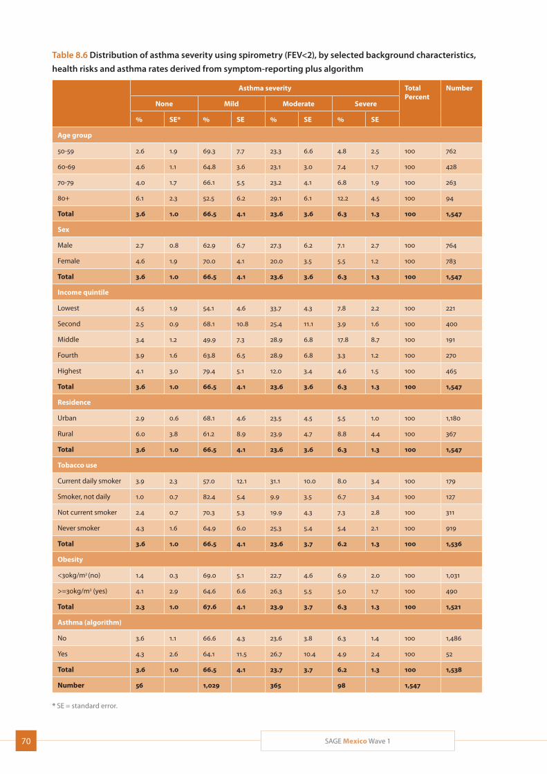
70 SAGE Mexico Wave 1
Table 8.6 Distribution of asthma severity using spirometry (FEV<2), by selected background characteristics,
health risks and asthma rates derived from symptom-reporting plus algorithm
Asthma severity TotalPercent
Number
None Mild Moderate Severe
% SE* % SE % SE % SE
Age group
50-59 2.6 1.9 69.3 7.7 23.3 6.6 4.8 2.5 100 762
60-69 4.6 1.1 64.8 3.6 23.1 3.0 7.4 1.7 100 428
70-79 4.0 1.7 66.1 5.5 23.2 4.1 6.8 1.9 100 263
80+ 6.1 2.3 52.5 6.2 29.1 6.1 12.2 4.5 100 94
Total 3.6 1.0 66.5 4.1 23.6 3.6 6.3 1.3 100 1,547
Sex
Male 2.7 0.8 62.9 6.7 27.3 6.2 7.1 2.7 100 764
Female 4.6 1.9 70.0 4.1 20.0 3.5 5.5 1.2 100 783
Total 3.6 1.0 66.5 4.1 23.6 3.6 6.3 1.3 100 1,547
Income quintile
Lowest 4.5 1.9 54.1 4.6 33.7 4.3 7.8 2.2 100 221
Second 2.5 0.9 68.1 10.8 25.4 11.1 3.9 1.6 100 400
Middle 3.4 1.2 49.9 7.3 28.9 6.8 17.8 8.7 100 191
Fourth 3.9 1.6 63.8 6.5 28.9 6.8 3.3 1.2 100 270
Highest 4.1 3.0 79.4 5.1 12.0 3.4 4.6 1.5 100 465
Total 3.6 1.0 66.5 4.1 23.6 3.6 6.3 1.3 100 1,547
Residence
Urban 2.9 0.6 68.1 4.6 23.5 4.5 5.5 1.0 100 1,180
Rural 6.0 3.8 61.2 8.9 23.9 4.7 8.8 4.4 100 367
Total 3.6 1.0 66.5 4.1 23.6 3.6 6.3 1.3 100 1,547
Tobacco use
Current daily smoker 3.9 2.3 57.0 12.1 31.1 10.0 8.0 3.4 100 179
Smoker, not daily 1.0 0.7 82.4 5.4 9.9 3.5 6.7 3.4 100 127
Not current smoker 2.4 0.7 70.3 5.3 19.9 4.3 7.3 2.8 100 311
Never smoker 4.3 1.6 64.9 6.0 25.3 5.4 5.4 2.1 100 919
Total 3.6 1.0 66.5 4.1 23.6 3.7 6.2 1.3 100 1,536
Obesity
<30kg/m2 (no) 1.4 0.3 69.0 5.1 22.7 4.6 6.9 2.0 100 1,031
>=30kg/m2 (yes) 4.1 2.9 64.6 6.6 26.3 5.5 5.0 1.7 100 490
Total 2.3 1.0 67.6 4.1 23.9 3.7 6.3 1.3 100 1,521
Asthma (algorithm)
No 3.6 1.1 66.6 4.3 23.6 3.8 6.3 1.4 100 1,486
Yes 4.3 2.6 64.1 11.5 26.7 10.4 4.9 2.4 100 52
Total 3.6 1.0 66.5 4.1 23.7 3.7 6.2 1.3 100 1,538
Number 56 1,029 365 98 1,547
* SE = standard error.
71SAGE Mexico Wave 1
patterns, although obese respondents were less likely to show no signs of the condition than their non-obese counterparts; among tobacco use groups, meanwhile, current daily smokers showed the highest levels of risk for moderate and severe signs of the disease.
Vision (near and distance, using Tumbling “E” chart)In addition to the complications associated with chronic degenerative illnesses and disability, alterations in motor coordination, space perception, sharpness of vision and hearing, walking, muscle and bone strength, mobility, and sensory perception of environmental stimuli such as cold and heat have been documented in persons over 60 years of age.
Over 80% of the study’s respondents had normal distant vision, while only slightly over 50% had normal near vision (Table 8.7). Distant vision declined steadily and fairly strongly with age; only some 50% of respondents aged 80-plus had normal distant vision, compared with over 85% in the 50-59 age bracket. Near vision declined slightly less regularly with age and did so across a narrower span (less than ten percentage points). Women showed fairly marked lower visual acuity at both the distant and near range than men, raising questions as to whether they might have been less inclined to use spectacles. Respondents in the highest two income quintiles and those higher up the educa-tional scale were notably more likely to show normal vision at both lengths; rural residents had better dis-tant vision than urban ones, but worse near vision. Respondents who had never married, meanwhile, had the best distant vision of the marital status groups, but the worst near vision.
Grip strength (dynamometer)Several studies of older people have shown that grip strength is a long-term predictor of mortality and dis-ability (Bohannon, 2008; Ling, 2010). Low hand-grip strength has been consistently linked to premature mortality, disability and other health complications in older people. Poor muscular strength has been shown to be associated with increased morbidity and mortal-ity in diverse samples of middle-aged and older adults. Grip strength in SAGE was assessed with the person in an upright seated position with the arm along the side, elbow bent at 90°, and the forearm and wrist were in the neutral position. The dynamometer handle was
adjusted to fit the hand size. Grip strength was assessed twice in each hand, with brief pauses between, and the final result a mean of the best result in each hand.
The mean grip strength for women was 19.3kg, while that for men was 30.3kg (Table 8.8). Grip strength declined with age, and was lower for rural residents than for urban ones; otherwise, it followed few pre-dictable patterns.
Gait speed (timed walk)Gait speed has been shown to be associated with sur-vival, disability, and cognitive impairment in older adults. Respondents were asked to complete a timed walk over 4 metres, once at a normal or usual pace, and once at a rapid pace. For normal/usual paced walking in community-dwelling older adults, speeds of less than 0.4-0.6 metres/second are considered slow, and possibly an indicator of health risk, but may also need adjustment based on cultural gait norms. Changes in gait speed at rapid pace may provide an early indicator of cognitive change.
The mean time to walk four meters at normal pace was 5.3 seconds, with the oldest respondents (aged 80-plus) at 8.3 seconds (0.48m/s). At rapid pace, even the oldest group was capable of walking four metres in six seconds (Table 8.9). Women were slower than men overall, and rural residents were slower than urban ones. Walking speeds increased with rising income quintiles and for the most part with education levels; meanwhile, widowed respondents were the slowest group, possibly due to their older average age.

72 SAGE Mexico Wave 1
Table 8.7 Level of visual acuity (distant and near), by selected background characteristics
Distant visual acuity TotalPercent
Number
Near visual acuity TotalPercent
Number
Normal Low vision Normal Low vision
Percent SE** Percent SE Percent SE Percent SE
Age group Age group
50-59 87.7 6.9 12.3 6.9 100 1,016 50-59 52.9 6.7 47.1 6.7 100 1,022
60-69 87.2 2.3 12.8 2.3 100 525 60-69 54.2 3.8 45.8 3.8 100 532
70-79 71.4 6.2 28.6 6.2 100 362 70-79 49.4 6.3 50.6 6.3 100 366
80+ 50.4 5.7 49.6 5.7 100 133 80+ 45.7 5.4 54.3 5.4 100 139
Total 82.2 3.4 17.8 3.4 100 2,036 Total 52.1 3.5 47.9 3.5 100 2,058
Sex Sex
Male 88.3 2.2 11.7 2.2 100 899 Male 55.4 5.3 44.6 5.3 100 913
Female 77.4 5.7 22.6 5.7 100 1,137 Female 49.5 4.7 50.5 4.7 100 1,145
Total 82.2 3.4 17.8 3.4 100 2,036 Total 52.1 3.5 47.9 3.5 100 2,058
Education Education
No formal education 79.1 5.9 20.9 5.9 100 350 No formal education 41.3 8.2 58.7 8.2 100 354
Less than primary 77.0 7.9 23.0 7.9 100 774 Less than primary 41.8 6.7 58.2 6.7 100 780
Primary school completed 82.7 6.0 17.3 6.0 100 447 Primary school completed 72.4 5.0 27.6 5.0 100 455
Secondary school completed 95.6 1.8 4.4 1.8 100 214 Secondary school completed 49.6 9.9 50.4 9.9 100 215
High school completed 96.2 2.3 3.8 2.3 100 51 High school completed 47.1 15.2 52.9 15.2 100 52
College completed 91.9 3.0 8.1 3.0 100 120 College completed 62.2 8.0 37.8 8.0 100 119
Post graduate degree completed 99.5 0.5 0.5 0.5 100 56 Post graduate degree completed 88.9 8.5 11.1 8.5 100 56
Total 82.6 3.5 17.4 3.5 100 2,011 Total 52.0 3.6 48.0 3.6 100 2,031
Marital status Marital status
Never married 90.4 3.4 9.6 3.4 100 148 Never married 36.2 9.5 63.8 9.5 100 151
Currently married 85.6 4.9 14.4 4.9 100 1,415 Currently married 52.2 4.9 47.8 4.9 100 1,428
Cohabiting 58.1 9.6 41.9 9.6 100 53 Cohabiting 47.3 9.6 52.7 9.6 100 53
Separated/divorced 88.8 3.7 11.2 3.7 100 96 Separated/divorced 60.2 9.4 39.8 9.4 100 95
Widowed 67.0 7.3 33.0 7.3 100 298 Widowed 57.4 5.5 42.6 5.5 100 305
Total 82.6 3.5 17.4 3.5 100 2,011 Total 52.0 3.6 48.0 3.6 100 2,031
Income quintile Income quintile
Lowest 78.3 4.7 21.7 4.7 100 292 Lowest 48.5 4.9 51.5 4.9 100 300
Second 78.8 5.8 21.2 5.8 100 478 Second 34.3 5.3 65.7 5.3 100 487
Middle 67.0 15.3 33.0 15.3 100 343 Middle 39.1 9.2 60.9 9.2 100 344
Fourth 85.9 3.0 14.1 3.0 100 353 Fourth 65.5 4.9 34.5 4.9 100 354
Highest 94.0 1.7 6.0 1.7 100 570 Highest 68.8 5.9 31.2 5.9 100 573
Total 82.2 3.4 17.8 3.4 100 2,035 Total 52.1 3.5 47.9 3.5 100 2,058
Residence Residence
Urban 81.1 4.2 18.9 4.2 100 1,594 Urban 54.4 4.1 45.6 4.1 100 1,613
Rural 86.1 4.0 13.9 4.0 100 441 Rural 43.8 5.9 56.2 5.9 100 445
Total 82.2 3.4 17.8 3.4 100 2,036 Total 52.1 3.5 47.9 3.5 100 2,058
Number 1,674 362 2,036 Number 1,073 985 2,058
* Vision tests include the respondent’s typical correcting aids (spectacles or other) if used. Normal distant and near visual acuity were classified
for values ranging from 0.3 to 2.0 on the LogMAR chart (better than 20/70 vision).
** SE = standard error.
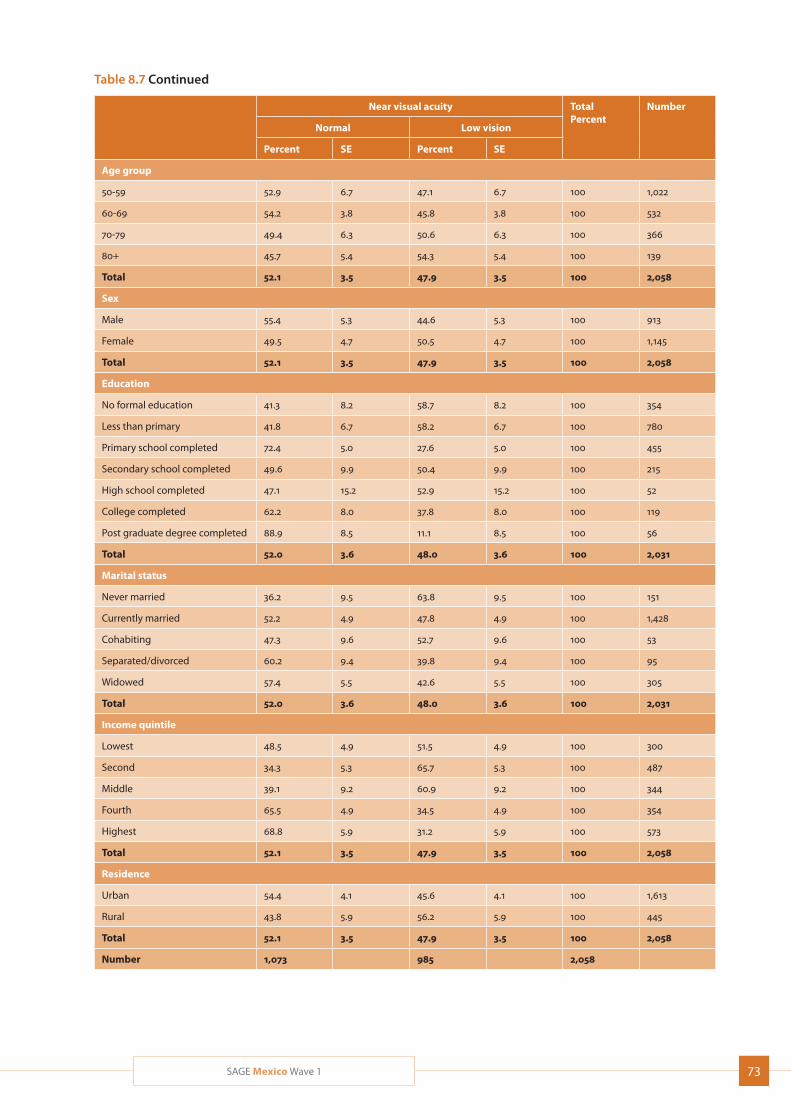
73SAGE Mexico Wave 1
Table 8.7 Level of visual acuity (distant and near), by selected background characteristics
Distant visual acuity TotalPercent
Number
Near visual acuity TotalPercent
Number
Normal Low vision Normal Low vision
Percent SE** Percent SE Percent SE Percent SE
Age group Age group
50-59 87.7 6.9 12.3 6.9 100 1,016 50-59 52.9 6.7 47.1 6.7 100 1,022
60-69 87.2 2.3 12.8 2.3 100 525 60-69 54.2 3.8 45.8 3.8 100 532
70-79 71.4 6.2 28.6 6.2 100 362 70-79 49.4 6.3 50.6 6.3 100 366
80+ 50.4 5.7 49.6 5.7 100 133 80+ 45.7 5.4 54.3 5.4 100 139
Total 82.2 3.4 17.8 3.4 100 2,036 Total 52.1 3.5 47.9 3.5 100 2,058
Sex Sex
Male 88.3 2.2 11.7 2.2 100 899 Male 55.4 5.3 44.6 5.3 100 913
Female 77.4 5.7 22.6 5.7 100 1,137 Female 49.5 4.7 50.5 4.7 100 1,145
Total 82.2 3.4 17.8 3.4 100 2,036 Total 52.1 3.5 47.9 3.5 100 2,058
Education Education
No formal education 79.1 5.9 20.9 5.9 100 350 No formal education 41.3 8.2 58.7 8.2 100 354
Less than primary 77.0 7.9 23.0 7.9 100 774 Less than primary 41.8 6.7 58.2 6.7 100 780
Primary school completed 82.7 6.0 17.3 6.0 100 447 Primary school completed 72.4 5.0 27.6 5.0 100 455
Secondary school completed 95.6 1.8 4.4 1.8 100 214 Secondary school completed 49.6 9.9 50.4 9.9 100 215
High school completed 96.2 2.3 3.8 2.3 100 51 High school completed 47.1 15.2 52.9 15.2 100 52
College completed 91.9 3.0 8.1 3.0 100 120 College completed 62.2 8.0 37.8 8.0 100 119
Post graduate degree completed 99.5 0.5 0.5 0.5 100 56 Post graduate degree completed 88.9 8.5 11.1 8.5 100 56
Total 82.6 3.5 17.4 3.5 100 2,011 Total 52.0 3.6 48.0 3.6 100 2,031
Marital status Marital status
Never married 90.4 3.4 9.6 3.4 100 148 Never married 36.2 9.5 63.8 9.5 100 151
Currently married 85.6 4.9 14.4 4.9 100 1,415 Currently married 52.2 4.9 47.8 4.9 100 1,428
Cohabiting 58.1 9.6 41.9 9.6 100 53 Cohabiting 47.3 9.6 52.7 9.6 100 53
Separated/divorced 88.8 3.7 11.2 3.7 100 96 Separated/divorced 60.2 9.4 39.8 9.4 100 95
Widowed 67.0 7.3 33.0 7.3 100 298 Widowed 57.4 5.5 42.6 5.5 100 305
Total 82.6 3.5 17.4 3.5 100 2,011 Total 52.0 3.6 48.0 3.6 100 2,031
Income quintile Income quintile
Lowest 78.3 4.7 21.7 4.7 100 292 Lowest 48.5 4.9 51.5 4.9 100 300
Second 78.8 5.8 21.2 5.8 100 478 Second 34.3 5.3 65.7 5.3 100 487
Middle 67.0 15.3 33.0 15.3 100 343 Middle 39.1 9.2 60.9 9.2 100 344
Fourth 85.9 3.0 14.1 3.0 100 353 Fourth 65.5 4.9 34.5 4.9 100 354
Highest 94.0 1.7 6.0 1.7 100 570 Highest 68.8 5.9 31.2 5.9 100 573
Total 82.2 3.4 17.8 3.4 100 2,035 Total 52.1 3.5 47.9 3.5 100 2,058
Residence Residence
Urban 81.1 4.2 18.9 4.2 100 1,594 Urban 54.4 4.1 45.6 4.1 100 1,613
Rural 86.1 4.0 13.9 4.0 100 441 Rural 43.8 5.9 56.2 5.9 100 445
Total 82.2 3.4 17.8 3.4 100 2,036 Total 52.1 3.5 47.9 3.5 100 2,058
Number 1,674 362 2,036 Number 1,073 985 2,058
* Vision tests include the respondent’s typical correcting aids (spectacles or other) if used. Normal distant and near visual acuity were classified
for values ranging from 0.3 to 2.0 on the LogMAR chart (better than 20/70 vision).
** SE = standard error.
Table 8.7 Continued
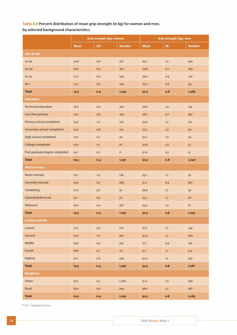
74 SAGE Mexico Wave 1
Table 8.8 Percent distribution of mean grip strength (in kg) for women and men,
by selected background characteristics
Grip strength (kg), women Grip strength (kg), men
Mean SE* Number Mean SE Number
Age group
50-59 20.8 0.6 577 33.2 1.2 534
60-69 18.9 0.4 307 29.8 0.7 285
70-79 17.3 0.9 242 26.0 0.9 170
80+ 15.2 0.6 104 20.2 0.9 94
Total 19.3 0.4 1,230 30.3 0.8 1,083
Education
No formal education 18.4 0.6 262 28.6 1.9 125
Less than primary 19.7 0.8 474 28.2 0.7 387
Primary school completed 19.5 1.0 227 33.6 1.5 312
Secondary school completed 19.6 0.8 132 27.5 1.9 90
High school completed 19.7 0.7 29 30.7 1.6 24
College completed 19.2 1.2 67 30.8 2.0 57
Post graduate degree completed 14.1 0.7 6 37.4 3.3 51
Total 19.3 0.4 1,197 30.3 0.8 1,047
Marital status
Never married 19.7 1.9 128 25.2 1.7 30
Currently married 19.9 0.5 685 31.2 0.9 891
Cohabiting 17.0 3.6 22 28.9 1.7 39
Separated/divorced 19.1 0.9 75 25.2 1.7 26
Widowed 18.0 0.6 287 23.4 1.0 61
Total 19.3 0.4 1,197 30.3 0.8 1,047
Income quintile
Lowest 17.3 0.6 210 27.0 1.7 144
Second 19.5 1.0 302 30.4 1.7 269
Middle 19.8 0.9 252 27.1 0.9 136
Fourth 18.8 0.7 171 31.1 1.1 213
Highest 20.1 0.8 295 32.4 1.5 320
Total 19.3 0.4 1,230 30.3 0.8 1,081
Residence
Urban 19.5 0.5 1,026 31.0 1.0 796
Rural 18.0 0.6 204 28.6 1.2 287
Total 19.3 0.4 1,230 30.3 0.8 1,083
* SE = Standard error.
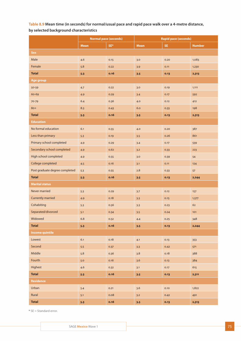
75SAGE Mexico Wave 1
Table 8.9 Mean time (in seconds) for normal/usual pace and rapid pace walk over a 4-metre distance,
by selected background characteristics
Normal pace (seconds) Rapid pace (seconds)
Mean SE* Mean SE Number
Sex
Male 4.6 0.15 3.0 0.20 1,083
Female 5.8 0.22 3.9 0.11 1,230
Total 5.3 0.16 3.5 0.13 2,313
Age group
50-59 4.7 0.22 3.0 0.19 1,111
60-69 4.9 0.29 3.4 0.17 592
70-79 6.4 0.36 4.0 0.12 412
80+ 8.3 0.43 6.0 0.33 198
Total 5.3 0.16 3.5 0.13 2,313
Education
No formal education 6.1 0.55 4.0 0.20 387
Less than primary 5.3 0.19 3.5 0.26 861
Primary school completed 4.9 0.29 3.4 0.17 539
Secondary school completed 4.9 0.62 3.2 0.33 223
High school completed 4.9 0.55 3.0 0.39 54
College completed 4.5 0.16 3.1 0.11 124
Post graduate degree completed 5.3 0.55 2.8 0.33 57
Total 5.3 0.16 3.5 0.13 2,244
Marital status
Never married 5.3 0.29 3.7 0.12 157
Currently married 4.9 0.18 3.3 0.15 1,577
Cohabiting 5.3 0.56 3.3 0.23 62
Separated/divorced 5.1 0.34 3.5 0.24 101
Widowed 6.8 0.52 4.4 0.25 348
Total 5.3 0.16 3.5 0.13 2,244
Income quintile
Lowest 6.1 0.18 4.1 0.13 353
Second 5.5 0.37 3.3 0.42 571
Middle 5.8 0.36 3.8 0.18 388
Fourth 5.0 0.16 3.6 0.13 384
Highest 4.6 0.32 3.1 0.17 615
Total 5.3 0.16 3.5 0.13 2,311
Residence
Urban 5.4 0.21 3.6 0.10 1,822
Rural 5.1 0.08 3.2 0.42 491
Total 5.3 0.16 3.5 0.13 2,313
* SE = Standard error.
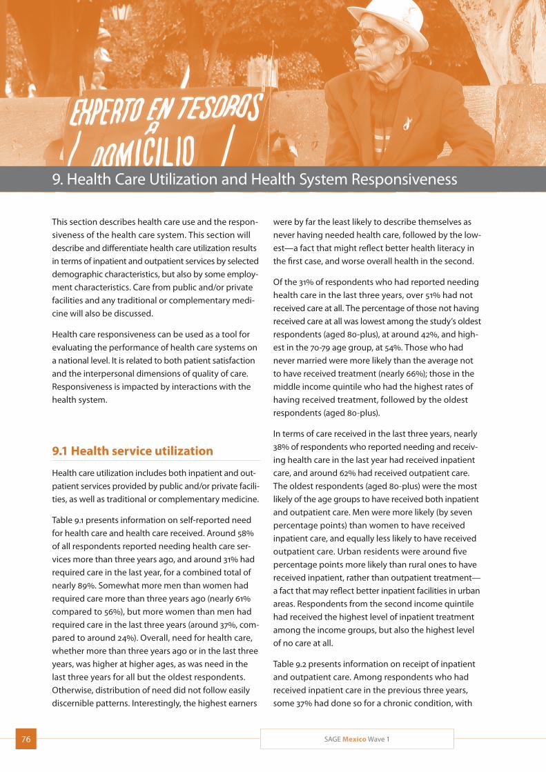
76 SAGE Mexico Wave 1
9. Health Care Utilization and Health System Responsiveness
This section describes health care use and the respon-
siveness of the health care system. This section will
describe and differentiate health care utilization results
in terms of inpatient and outpatient services by selected
demographic characteristics, but also by some employ-
ment characteristics. Care from public and/or private
facilities and any traditional or complementary medi-
cine will also be discussed.
Health care responsiveness can be used as a tool for
evaluating the performance of health care systems on
a national level. It is related to both patient satisfaction
and the interpersonal dimensions of quality of care.
Responsiveness is impacted by interactions with the
health system.
9.1 Health service utilization
Health care utilization includes both inpatient and out-
patient services provided by public and/or private facili-
ties, as well as traditional or complementary medicine.
Table 9.1 presents information on self-reported need
for health care and health care received. Around 58%
of all respondents reported needing health care ser-
vices more than three years ago, and around 31% had
required care in the last year, for a combined total of
nearly 89%. Somewhat more men than women had
required care more than three years ago (nearly 61%
compared to 56%), but more women than men had
required care in the last three years (around 37%, com-
pared to around 24%). Overall, need for health care,
whether more than three years ago or in the last three
years, was higher at higher ages, as was need in the
last three years for all but the oldest respondents.
Otherwise, distribution of need did not follow easily
discernible patterns. Interestingly, the highest earners
were by far the least likely to describe themselves as
never having needed health care, followed by the low-
est—a fact that might reflect better health literacy in
the first case, and worse overall health in the second.
Of the 31% of respondents who had reported needing
health care in the last three years, over 51% had not
received care at all. The percentage of those not having
received care at all was lowest among the study’s oldest
respondents (aged 80-plus), at around 42%, and high-
est in the 70-79 age group, at 54%. Those who had
never married were more likely than the average not
to have received treatment (nearly 66%); those in the
middle income quintile who had the highest rates of
having received treatment, followed by the oldest
respondents (aged 80-plus).
In terms of care received in the last three years, nearly
38% of respondents who reported needing and receiv-
ing health care in the last year had received inpatient
care, and around 62% had received outpatient care.
The oldest respondents (aged 80-plus) were the most
likely of the age groups to have received both inpatient
and outpatient care. Men were more likely (by seven
percentage points) than women to have received
inpatient care, and equally less likely to have received
outpatient care. Urban residents were around five
percentage points more likely than rural ones to have
received inpatient, rather than outpatient treatment—
a fact that may reflect better inpatient facilities in urban
areas. Respondents from the second income quintile
had received the highest level of inpatient treatment
among the income groups, but also the highest level
of no care at all.
Table 9.2 presents information on receipt of inpatient
and outpatient care. Among respondents who had
received inpatient care in the previous three years,
some 37% had done so for a chronic condition, with
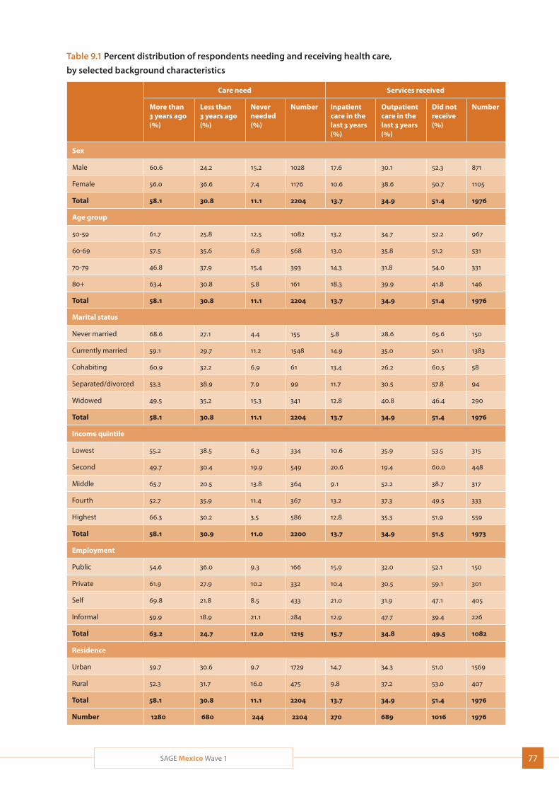
77SAGE Mexico Wave 1
Table 9.1 Percent distribution of respondents needing and receiving health care,
by selected background characteristics
Care need Services received
More than 3 years ago (%)
Less than 3 years ago (%)
Never needed (%)
Number Inpatient care in the last 3 years (%)
Outpatient care in the last 3 years (%)
Did not receive (%)
Number
Sex
Male 60.6 24.2 15.2 1028 17.6 30.1 52.3 871
Female 56.0 36.6 7.4 1176 10.6 38.6 50.7 1105
Total 58.1 30.8 11.1 2204 13.7 34.9 51.4 1976
Age group
50-59 61.7 25.8 12.5 1082 13.2 34.7 52.2 967
60-69 57.5 35.6 6.8 568 13.0 35.8 51.2 531
70-79 46.8 37.9 15.4 393 14.3 31.8 54.0 331
80+ 63.4 30.8 5.8 161 18.3 39.9 41.8 146
Total 58.1 30.8 11.1 2204 13.7 34.9 51.4 1976
Marital status
Never married 68.6 27.1 4.4 155 5.8 28.6 65.6 150
Currently married 59.1 29.7 11.2 1548 14.9 35.0 50.1 1383
Cohabiting 60.9 32.2 6.9 61 13.4 26.2 60.5 58
Separated/divorced 53.3 38.9 7.9 99 11.7 30.5 57.8 94
Widowed 49.5 35.2 15.3 341 12.8 40.8 46.4 290
Total 58.1 30.8 11.1 2204 13.7 34.9 51.4 1976
Income quintile
Lowest 55.2 38.5 6.3 334 10.6 35.9 53.5 315
Second 49.7 30.4 19.9 549 20.6 19.4 60.0 448
Middle 65.7 20.5 13.8 364 9.1 52.2 38.7 317
Fourth 52.7 35.9 11.4 367 13.2 37.3 49.5 333
Highest 66.3 30.2 3.5 586 12.8 35.3 51.9 559
Total 58.1 30.9 11.0 2200 13.7 34.9 51.5 1973
Employment
Public 54.6 36.0 9.3 166 15.9 32.0 52.1 150
Private 61.9 27.9 10.2 332 10.4 30.5 59.1 301
Self 69.8 21.8 8.5 433 21.0 31.9 47.1 405
Informal 59.9 18.9 21.1 284 12.9 47.7 39.4 226
Total 63.2 24.7 12.0 1215 15.7 34.8 49.5 1082
Residence
Urban 59.7 30.6 9.7 1729 14.7 34.3 51.0 1569
Rural 52.3 31.7 16.0 475 9.8 37.2 53.0 407
Total 58.1 30.8 11.1 2204 13.7 34.9 51.4 1976
Number 1280 680 244 2204 270 689 1016 1976
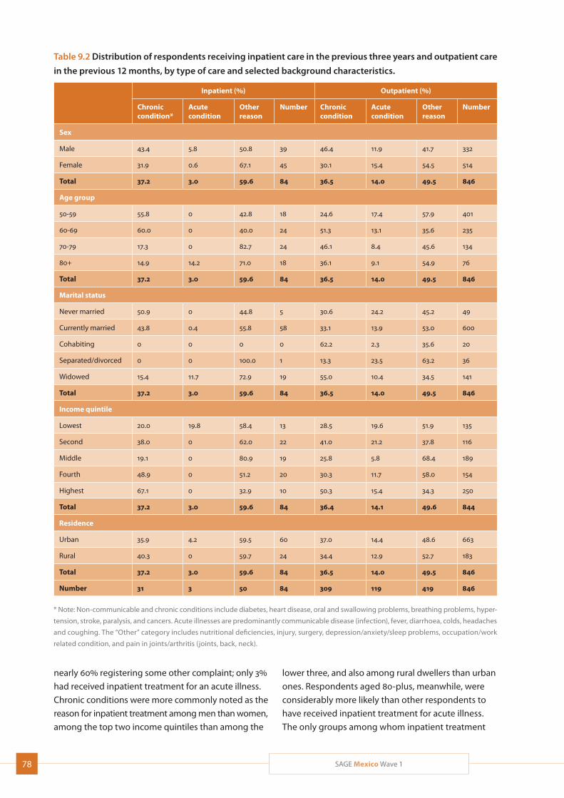
78 SAGE Mexico Wave 1
Table 9.2 Distribution of respondents receiving inpatient care in the previous three years and outpatient care
in the previous 12 months, by type of care and selected background characteristics.
Inpatient (%) Outpatient (%)
Chronic condition*
Acute condition
Other reason
Number Chronic condition
Acute condition
Other reason
Number
Sex
Male 43.4 5.8 50.8 39 46.4 11.9 41.7 332
Female 31.9 0.6 67.1 45 30.1 15.4 54.5 514
Total 37.2 3.0 59.6 84 36.5 14.0 49.5 846
Age group
50-59 55.8 0 42.8 18 24.6 17.4 57.9 401
60-69 60.0 0 40.0 24 51.3 13.1 35.6 235
70-79 17.3 0 82.7 24 46.1 8.4 45.6 134
80+ 14.9 14.2 71.0 18 36.1 9.1 54.9 76
Total 37.2 3.0 59.6 84 36.5 14.0 49.5 846
Marital status
Never married 50.9 0 44.8 5 30.6 24.2 45.2 49
Currently married 43.8 0.4 55.8 58 33.1 13.9 53.0 600
Cohabiting 0 0 0 0 62.2 2.3 35.6 20
Separated/divorced 0 0 100.0 1 13.3 23.5 63.2 36
Widowed 15.4 11.7 72.9 19 55.0 10.4 34.5 141
Total 37.2 3.0 59.6 84 36.5 14.0 49.5 846
Income quintile
Lowest 20.0 19.8 58.4 13 28.5 19.6 51.9 135
Second 38.0 0 62.0 22 41.0 21.2 37.8 116
Middle 19.1 0 80.9 19 25.8 5.8 68.4 189
Fourth 48.9 0 51.2 20 30.3 11.7 58.0 154
Highest 67.1 0 32.9 10 50.3 15.4 34.3 250
Total 37.2 3.0 59.6 84 36.4 14.1 49.6 844
Residence
Urban 35.9 4.2 59.5 60 37.0 14.4 48.6 663
Rural 40.3 0 59.7 24 34.4 12.9 52.7 183
Total 37.2 3.0 59.6 84 36.5 14.0 49.5 846
Number 31 3 50 84 309 119 419 846
* Note: Non-communicable and chronic conditions include diabetes, heart disease, oral and swallowing problems, breathing problems, hyper-
tension, stroke, paralysis, and cancers. Acute illnesses are predominantly communicable disease (infection), fever, diarrhoea, colds, headaches
and coughing. The “Other” category includes nutritional deficiencies, injury, surgery, depression/anxiety/sleep problems, occupation/work
related condition, and pain in joints/arthritis (joints, back, neck).
nearly 60% registering some other complaint; only 3%
had received inpatient treatment for an acute illness.
Chronic conditions were more commonly noted as the
reason for inpatient treatment among men than women,
among the top two income quintiles than among the
lower three, and also among rural dwellers than urban
ones. Respondents aged 80-plus, meanwhile, were
considerably more likely than other respondents to
have received inpatient treatment for acute illness.
The only groups among whom inpatient treatment
79SAGE Mexico Wave 1
was more likely to be related to chronic conditions than to other conditions were those aged 50-59 and 60-69, the never-married, and the highest income quin-tile, as noted above.
Among respondents who had received outpatient care in the previous 12 months, an almost identical percent-age as for inpatient care (nearly 37%) had done so for a chronic condition, while a much higher number had received outpatient than inpatient care for an acute illness (14% compared to the 3% noted above). Other reasons accounted for the remaining nearly 50% of outpatient care. Chronic conditions were more common as a reason for outpatient treatment among men than women, and for the highest income quintile. Apart from these two groups, the other groups among whom out-patient treatment was significantly more likely to be related to chronic conditions than to other conditions were those aged 60-69, the cohabiting and the widowed, and those in the second income quintile.
9.2 Health system responsiveness
The performance of the general health care system at the national level was evaluated against standards of health system responsiveness. Responsiveness has been defined as the way individuals are treated and their per-ceptions about the environment in which they receive care (Valentine, 2003). The measurement of health sys-tem responsiveness typically covers eight domains, which may be divided into two groups. The first group of indicators covers respect for the individual, including dignity, privacy, autonomy (involvement in decision-making about personal health care), choice (of provider) and communication (with provider); the second group is patient-centered, including timeliness/prompt atten-tion, social support, quality of care, infrastructure quality and access/selectiveness.
Health system responsiveness scores are quantitative indicators of the interaction between individuals and their health system. SAGE collected information on respondents’ impressions of their most recent inpatient and/or outpatient visit from seven domains, including waiting time, being treated respectfully, receiving clear explanations, being involved in making treatment decisions, talking privately, happiness with providers, and cleanliness of the health facility. Each indicator had one score. Factor analysis was applied to evaluate the total responsiveness score using factor scores. Responsiveness scores were converted to a range
between 0 and 100, with a higher score reflecting better system responsiveness.
Overall, respondents judged outpatient care as slightly more responsive than inpatient care (a mean respon-siveness score of 71.2, compared to 69.4 for inpatient care) (Table 9.3). Women found inpatient care quite a bit more responsive than did men, while men found outpatient care somewhat more responsive than did women; rural residents found inpatient care signifi-cantly more responsive than did urban ones, but regis-tered very similar scores for outpatient care. Overall, the separated/divorced, the never-married and those in the fourth income quintile rated the responsiveness of inpatient care the best; the cohabiting and the mid-dle income quintile rated it the worst. Meanwhile, the responsiveness of outpatient care was rated highest by the 50-59 age group, with scores fairly similar across the other demographic groups.
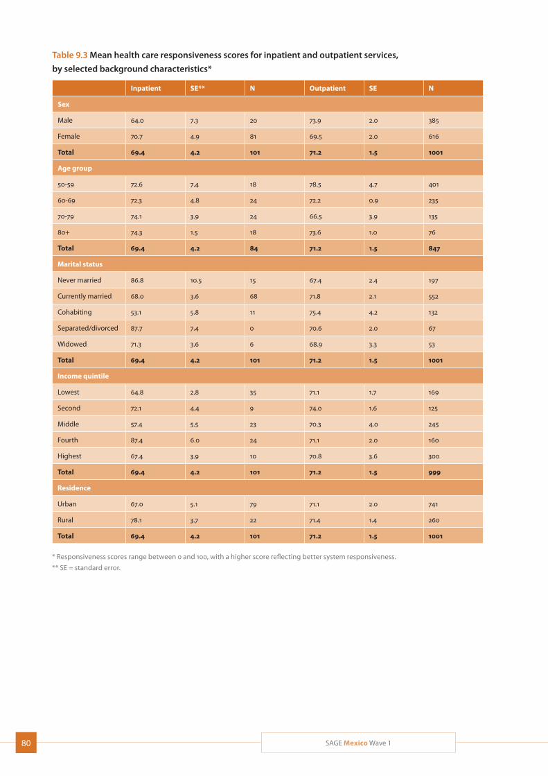
80 SAGE Mexico Wave 1
Table 9.3 Mean health care responsiveness scores for inpatient and outpatient services,
by selected background characteristics*
Inpatient SE** N Outpatient SE N
Sex
Male 64.0 7.3 20 73.9 2.0 385
Female 70.7 4.9 81 69.5 2.0 616
Total 69.4 4.2 101 71.2 1.5 1001
Age group
50-59 72.6 7.4 18 78.5 4.7 401
60-69 72.3 4.8 24 72.2 0.9 235
70-79 74.1 3.9 24 66.5 3.9 135
80+ 74.3 1.5 18 73.6 1.0 76
Total 69.4 4.2 84 71.2 1.5 847
Marital status
Never married 86.8 10.5 15 67.4 2.4 197
Currently married 68.0 3.6 68 71.8 2.1 552
Cohabiting 53.1 5.8 11 75.4 4.2 132
Separated/divorced 87.7 7.4 0 70.6 2.0 67
Widowed 71.3 3.6 6 68.9 3.3 53
Total 69.4 4.2 101 71.2 1.5 1001
Income quintile
Lowest 64.8 2.8 35 71.1 1.7 169
Second 72.1 4.4 9 74.0 1.6 125
Middle 57.4 5.5 23 70.3 4.0 245
Fourth 87.4 6.0 24 71.1 2.0 160
Highest 67.4 3.9 10 70.8 3.6 300
Total 69.4 4.2 101 71.2 1.5 999
Residence
Urban 67.0 5.1 79 71.1 2.0 741
Rural 78.1 3.7 22 71.4 1.4 260
Total 69.4 4.2 101 71.2 1.5 1001
* Responsiveness scores range between 0 and 100, with a higher score reflecting better system responsiveness.
** SE = standard error.
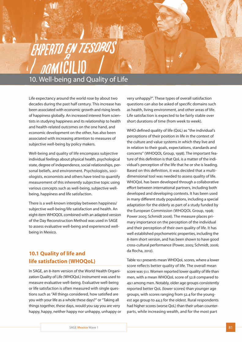
81SAGE Mexico Wave 1
10. Well-being and Quality of Life
Life expectancy around the world rose by about two decades during the past half century. This increase has been associated with economic growth and rising levels of happiness globally. An increased interest from scien-tists in studying happiness and its relationship to health and health-related outcomes on the one hand, and economic development on the other, has also been associated with increasing attention to measures of subjective well-being by policy makers.
Well-being and quality of life encompass subjective
individual feelings about physical health, psychological
state, degree of independence, social relationships, per-
sonal beliefs, and environment. Psychologists, soci-
ologists, economists and others have tried to quantify
measurement of this inherently subjective topic using
various concepts such as well-being, subjective well-
being, happiness and life satisfaction.
There is a well-known interplay between happiness/
subjective well-being/life satisfaction and health. An
eight-item WHOQOL combined with an adapted version
of the Day Reconstruction Method was used in SAGE
to assess evaluative well-being and experienced well-
being in Mexico.
10.1 Quality of life and life satisfaction (WHOQoL)
In SAGE, an 8-item version of the World Health Organi-
zation Quality of Life (WHOQoL) instrument was used to
measure evaluative well-being. Evaluative well-being
or life satisfaction is often measured with single ques-
tions such as “All things considered, how satisfied are
you with your life as a whole these days?” or “Taking all
things together, these days, would you say you are very
happy, happy, neither happy nor unhappy, unhappy or
very unhappy?”. These types of overall satisfaction questions can also be asked of specific domains such as health, living environment, and other areas of life. Life satisfaction is expected to be fairly stable over short durations of time (from week to week).
WHO defined quality of life (QoL) as “the individual’s perceptions of their position in life in the context of the culture and value systems in which they live and in relation to their goals, expectations, standards and concerns” (WHOQOL Group, 1998). The important fea-ture of this definition is that QoL is a matter of the indi-vidual’s perception of the life that he or she is leading. Based on this definition, it was decided that a multi-dimensional tool was needed to assess quality of life. WHOQoL has been developed through a collaborative effort between international partners, including both developed and developing contexts. It has been used in many different study populations, including a special adaptation for the elderly as part of a study funded by the European Commission (WHOQOL Group, 1998; Power 2005; Schmidt 2006). The measure places pri-mary importance on the perception of the individual and their perception of their own quality of life. It has well established psychometric properties, including the 8-item short version, and has been shown to have good cross-cultural performance (Power, 2005; Schmidt, 2006; da Rocha, 2012).
Table 10.1 presents mean WHOQoL scores, where a lower score reflects better quality of life. The overall mean score was 51.1. Women reported lower quality of life than men, with a mean WHOQoL score of 52.8 compared to 49.1 among men. Notably, older age groups consistently reported better QoL (lower scores) than younger age groups, with scores ranging from 52.4 for the young-est age group to 44.3 for the oldest. Rural respondents had higher scores (worse QoL) than their urban counter-parts, while increasing wealth, and for the most part
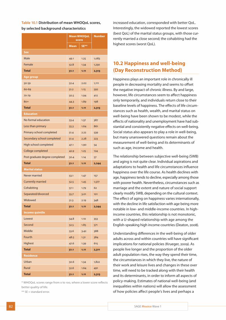
82 SAGE Mexico Wave 1
Table 10.1 Distribution of mean WHOQoL scores,
by selected background characteristics
Mean WHOQoL score
Number
Mean SE**
Sex
Male 49.1 1.25 1,083
Female 52.8 1.34 1,230
Total 51.1 1.11 2,313
Age group
50-59 52.4 2.02 1,111
60-69 51.2 1.15 592
70-79 50.5 1.94 412
80+ 44.3 1.89 198
Total 51.1 1.11 2,313
Education
No formal education 53.4 1.37 387
Less than primary 55.3 1.64 861
Primary school completed 51.4 2.22 539
Secondary school completed 51.4 2.28 223
High school completed 47.1 1.90 54
College completed 42.9 1.25 124
Post graduate degree completed 50.4 1.14 57
Total 51.1 1.11 2,244
Marital status
Never married 53.1 1.47 157
Currently married 52.5 1.45 1,577
Cohabiting 57.1 1.79 62
Separated/divorced 55.7 3.01 101
Widowed 51.3 2.19 348
Total 51.1 1.11 2,244
Income quintile
Lowest 54.8 1.10 353
Second 52.5 1.85 571
Middle 53.6 3.42 388
Fourth 48.5 1.31 384
Highest 47.6 1.39 615
Total 51.1 1.11 2,311
Residence
Urban 50.6 1.34 1,822
Rural 52.6 1.64 491
Total 51.1 1.11 2,313
* WHOQoL scores range from 0 to 100, where a lower score reflects
better quality of life.
** SE = standard error.
increased education, corresponded with better QoL. Interestingly, the widowed reported the lowest scores (best QoL) of the marital status groups, with those cur-rently married a close second; the cohabiting had the highest scores (worst QoL).
10.2 Happiness and well-being (Day Reconstruction Method)
Happiness plays an important role in chronically ill people in decreasing mortality and seems to offset the negative impact of chronic illness. By and large, however, life circumstances seem to affect happiness only temporarily, and individuals return close to their baseline levels of happiness. The effects of life circum-stances such as health, wealth, and marital status on well-being have been shown to be modest, while the effects of nationality and unemployment have had sub-stantial and consistently negative effects on well-being. Social status also appears to play a role in well-being, but many unanswered questions remain about the measurement of well-being and its determinants of such as age, income and health.
The relationship between subjective well-being (SWB) and aging is not quite clear. Individual aspirations and adaptations to health and life circumstances influence happiness over the life course. As health declines with age, happiness tends to decline, especially among those with poorer health. Nevertheless, circumstances such as marriage and the extent and nature of social support clearly modify SWB, depending on the cultural context. The effect of aging on happiness varies internationally, with the decline in life satisfaction with age being more notable in low- and middle-income countries. In high-income countries, this relationship is not monotonic, with a U-shaped relationship with age among the English-speaking high income countries (Deaton, 2008).
Understanding differences in the well-being of older adults across and within countries will have significant implications for national policies (Krueger, 2009). As people live longer and the proportion of the older adult population rises, the way they spend their time, the circumstances in which they live, the nature of their work and leisure lives and changes in these over time, will need to be tracked along with their health and its determinants, in order to inform all aspects of policy-making. Estimates of national well-being (and inequalities within nations) will allow the assessment of how policies affect people’s lives and perhaps a
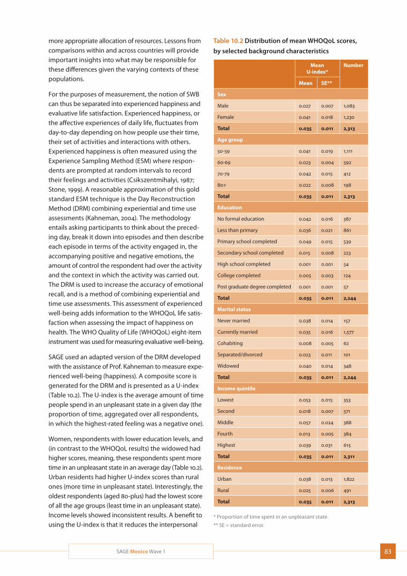
83SAGE Mexico Wave 1
more appropriate allocation of resources. Lessons from comparisons within and across countries will provide important insights into what may be responsible for these differences given the varying contexts of these populations.
For the purposes of measurement, the notion of SWB can thus be separated into experienced happiness and evaluative life satisfaction. Experienced happiness, or the affective experiences of daily life, fluctuates from day-to-day depending on how people use their time, their set of activities and interactions with others. Experienced happiness is often measured using the Experience Sampling Method (ESM) where respon-dents are prompted at random intervals to record their feelings and activities (Csikszentmihalyi, 1987; Stone, 1999). A reasonable approximation of this gold standard ESM technique is the Day Reconstruction Method (DRM) combining experiential and time use assessments (Kahneman, 2004). The methodology entails asking participants to think about the preced-ing day, break it down into episodes and then describe each episode in terms of the activity engaged in, the accompanying positive and negative emotions, the amount of control the respondent had over the activity and the context in which the activity was carried out. The DRM is used to increase the accuracy of emotional recall, and is a method of combining experiential and time use assessments. This assessment of experienced well-being adds information to the WHOQoL life satis-faction when assessing the impact of happiness on health. The WHO Quality of Life (WHOQoL) eight-item instrument was used for measuring evaluative well-being.
SAGE used an adapted version of the DRM developed with the assistance of Prof. Kahneman to measure expe-rienced well-being (happiness). A composite score is generated for the DRM and is presented as a U-index (Table 10.2). The U-index is the average amount of time people spend in an unpleasant state in a given day (the proportion of time, aggregated over all respondents, in which the highest-rated feeling was a negative one).
Women, respondents with lower education levels, and (in contrast to the WHOQoL results) the widowed had higher scores, meaning, these respondents spent more time in an unpleasant state in an average day (Table 10.2). Urban residents had higher U-index scores than rural ones (more time in unpleasant state). Interestingly, the oldest respondents (aged 80-plus) had the lowest score of all the age groups (least time in an unpleasant state). Income levels showed inconsistent results. A benefit to using the U-index is that it reduces the interpersonal
Table 10.2 Distribution of mean WHOQoL scores,
by selected background characteristics
Mean U-index*
Number
Mean SE**
Sex
Male 0.027 0.007 1,083
Female 0.041 0.018 1,230
Total 0.035 0.011 2,313
Age group
50-59 0.041 0.019 1,111
60-69 0.023 0.004 592
70-79 0.042 0.015 412
80+ 0.022 0.008 198
Total 0.035 0.011 2,313
Education
No formal education 0.042 0.016 387
Less than primary 0.036 0.021 861
Primary school completed 0.049 0.015 539
Secondary school completed 0.015 0.008 223
High school completed 0.001 0.001 54
College completed 0.005 0.003 124
Post graduate degree completed 0.001 0.001 57
Total 0.035 0.011 2,244
Marital status
Never married 0.038 0.014 157
Currently married 0.035 0.016 1,577
Cohabiting 0.008 0.005 62
Separated/divorced 0.023 0.011 101
Widowed 0.040 0.014 348
Total 0.035 0.011 2,244
Income quintile
Lowest 0.053 0.015 353
Second 0.018 0.007 571
Middle 0.057 0.024 388
Fourth 0.013 0.005 384
Highest 0.039 0.031 615
Total 0.035 0.011 2,311
Residence
Urban 0.038 0.013 1,822
Rural 0.025 0.006 491
Total 0.035 0.011 2,313
* Proportion of time spent in an unpleasant state.
** SE = standard error.
84 SAGE Mexico Wave 1
differences in the use of survey response scales; however, another way to examine the results of the DRM, is to break down the amount of time during the day that a person spends in a positive state, negative state, or a net affect based on amount of time spent in both pos-itive and negative states (duration-weighted net affect). Looking at the results this way, the DRM results showed that people were more likely to spend larger portions of their day in a positive emotional state (data not shown).
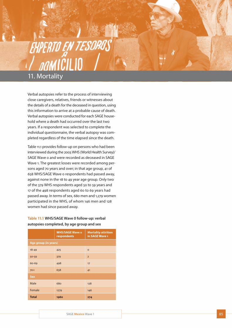
85SAGE Mexico Wave 1
11. Mortality
Verbal autopsies refer to the process of interviewing close caregivers, relatives, friends or witnesses about the details of a death for the deceased in question, using this information to arrive at a probable cause of death. Verbal autopsies were conducted for each SAGE house-hold where a death had occurred over the last two years. If a respondent was selected to complete the individual questionnaire, the verbal autopsy was com-pleted regardless of the time elapsed since the death.
Table 11.1 provides follow-up on persons who had been interviewed during the 2003 WHS (World Health Survey)/SAGE Wave 0 and were recorded as deceased in SAGE Wave 1. The greatest losses were recorded among per-sons aged 70 years and over; in that age group, 41 of 658 WHS/SAGE Wave 0 respondents had passed away, against none in the 18 to 49 year age group. Only two of the 379 WHS respondents aged 50 to 59 years and 17 of the 498 respondents aged 60 to 69 years had passed away. In terms of sex, 680 men and 1,279 women participated in the WHS, of whom 146 men and 128 women had since passed away.
Table 11.1 WHS/SAGE Wave 0 follow-up: verbal
autopsies completed, by age group and sex
WHS/SAGE Wave 0 respondents
Mortality attrition in SAGE Wave 1
Age group (in years)
18-49 425 0
50-59 379 2
60-69 498 17
70+ 658 41
Sex
Male 680 128
Female 1279 146
Total 1960 274
86 SAGE Mexico Wave 1
References
Albala C, Lebrão ML, León Díaz EM, Ham-Chande R, et al. Encuesta Salud, Bienestar y Envejecimiento (SABE): metodología de la encuesta y perfil de la población estudiada. Rev Panam Salud Publica. 2005;17(5/6):307–22.
Armstrong T, Bull F. Development of the World Health Organization Global Physical Activity Questionnaire (GPAQ). J Public Health. 2006;14(2):66-76.
Atun R, de Andrade LOM, Almeida G, Cotlear D, et al. Health-system reform and universal health coverage in Latin America. Lancet. 2014;dx.doi.org/10.1016/S0140-6736(14)61646-9
Bohannon RW. Hand-grip dynamometry predicts future outcomes in aging adults. J Geriatr Phys Ther. 2008;31(1):3-10.
Bull FC, Maslin TS, Armstrong T. Global Physical Activity Question-naire (GPAQ): nine country reliability and validity study. J Phys Act Health. 2009;6:790–804.
CONAPO. Envejecimiento de la Población de México Reto del siglo XXI. Disponible en: www.conapo.gob.mx/index.php?option= com_content&view=article&id=340&Itemid=15
CONAPO. Principales causas de mortalidad en México 1980 – 2007. Documento de Trabajo para el XLIII Periodo de Sesiones de la Comisión de Población y Desarrollo “Salud, morbilidad, mortalidad y desarrollo”. Nueva York, 2 a 16 de abril de 2010. Disponible en: www.conapo.gob.mx/publicaciones/mortalidad/Mortalidad xcausas_80_07.pdf
Csikszentmihalyi M, Larson R. Validity and reliability of the Experi-ence Sampling Method. J Nerv Ment Dis. 1987;175:526-36.
Deaton A. Income, health, and well-being around the world: evidence from the Gallup World Poll. J Econ Perspect. 2008;22(2):53-72.
ENASEM [Estudio Nacional sobre Salud y Envejecimiento en México]. Disponible en: www.bdsocial.org.mx/index.php?option=com_content&view=article&id=30&Itemid=85
Fillenbaum GG, Dellinger D, Maddox G, Pfieffer E. Assessment of individual functional status in a program evaluation and resource allocation model. In: Multidimensional Functional Assessment: The OARS Methodology, 2nd ed. Durham, NC: Duke University; 1978.
Flicker L, McCaul KA, Hankey GJ, Jamrozik K, Brown WJ, Byles JE, Almeida OP. Body mass index and survival in men and women aged 70 to 75. J Am Geriatr Soc. 2010;58(2):234-41.
2010 GBD Profile: Mexico. www.healthmetricsandevaluation.org/sites/default/files/country-profiles/GBD%20Country%20Report %20-%20Mexico.pdf. Seattle, WA: IHME. 2013.
Ham-Chande R, Gutiérrez-Robledo LM, PRESENTACIÓN: Salud y envejecimiento en el siglo XX. Salud Pública de México. 2007;49 (suplemento 4).
Heim N, Snijder MB, Heymans MW, Deeg DJ, Seidell JC, Visser M. Optimal cutoff values for high-risk waist circumference in older adults based on related health outcomes. Am J Epidemiol. 2011;174(4):479-89.
Hoos T, Espinoza N, Marshall S, Arrendondo EM. Validity of the Global Physical Activity Questionnaire (GPAQ) in adult Latinas. J Phys Act Health. 2012;9(5):698-705.
Huxley R, Mendis S, Zheleznyakov E, Reddy S, Chan J. Body mass index, waist circumference and waist:hip ratio as predictors of cardiovascular risk--a review of the literature. Eur J Clin Nutr. 2010;64(1):16-22.
INSP/SEDESOL. Primer seguimiento a la evaluación de impacto del programa de atención a adultos mayores de 70 años y más en zonas rurales (programa 70 y más). Informe de diseño meto-dológico del primer seguimiento a la evaluación de impacto. Estudio cuantitativo. Mexico City: INSP/SEDESOL. Disponible en: www.sedesol.gob.mx/archivos/802549/file/Planteamiento_Metodologico_Cuantitativo.pdf
Janssen I, Katzmarzyk PT, Ross R. Body Mass Index is inversely related to mortality in older people after adjustment for waist circum-ference. JAGS.2005;53(12):2112-8.
Kahneman D, Krueger AB, Schkade DA, Schwarz N, Stone AA. A survey method for characterizing daily life experience: The Day Reconstruction Method. Science. 2004;306(5702):1776-80.
Kane RA, Kane RL. Assessing the Elderly: A Practical Guide to Measurement. Lexington, MA: D.C. Health and Company; 1981.
Katz S, Ford AB, Moskowitz RW, Jackson BA, Jaffe MW. Studies of illness in the aged. JAMA. 1963;185:94-9.
Knaul FM, González-Pier E, Gómez-Dantés O, García-Junco D, et al. The quest for universal health coverage: achieving social pro-tection for all in Mexico. Lancet. 2012;380(9849):1259-79.
Kowal P, Chatterji S, Naidoo N, Biritwum R, et al. Data Resource Profile: The World Health Organization Study on global AGEing and adult health (SAGE). Int J Epidemiol. 2012;41(6):1639-49.
Krueger AB, Kahneman D, Schkade D, Schwarz N, Stone AA. National time accounting: The currency of life. In: Krueger AB (ed). Measuring the Subjective Well-Being of Nations: National Accounts of Time Use and Well-Being. Cambridge: NBER Books; 2009.
Lawson MP, Brody E. Assessment of older people: Self-maintaining and instrumental activities of daily living. Gerontologist. 1969;9:179-86.
Lee JM, Gebremariam A, Vijan S, Gurney JG. Excess body mass index-years, a measure of degree and duration of excess weight, and risk for incident diabetes. Arch Pediatr Adolesc Med. 2012;166(1):42-8.
87SAGE Mexico Wave 1
Ling CH, Taekema D, de Craen AJ, Gussekloo J, Westerndorp RG, Maier AB. Handgrip strength and mortality in the oldest old population: the Leiden 85-plus study. CMAJ. 2010;182(5):429-35.
McDowell I, Newell C. Measuring Health: A Guide to Rating Scales and Questionnaires. New York: Oxford University Press; 1987.
Naidoo N. SAGE Working Paper No. 5. WHO Study on global AGEing and adult health (SAGE) Waves 0 and 1 – Sampling information for China, Ghana, India, Mexico, Russia and South Africa. Geneva: WHO; 2012.
NORMA OFICIAL MEXICANA NOM-167-SSA1-1997, PARA LA PRESTA-CION DE SERVICIOS DE ASISTENCIA SOCIAL PARA MENORES Y ADULTOS MAYORES.
OCDE [ORGANIZACIÓN PARA LA COOPERACIÓN Y EL DESARROLLO ECONÓMICOS]. Síntesis: Estudio Económico de México 2009. Disponible en: www.cca.org.mx/funcionarios/emprendegestion publica/descargas/43557478.pdf
OECD Health Statistics 2014. How does Mexico compare? 2014. www.oecd.org/els/health-systems/Briefing-Note-MEXICO-2014.pdf
PAHO [Organización Panamericana de la Salud]. Encuesta Multicéntrica SALUD BIENESTAR Y ENVEJECIMIENTO (SABE) EN AMÉRICA LATINA Y EL CARIBE Informe Preliminar. DIVISIÓN DE PROMOCIÓN Y PROTECCIÓN DE LA SALUD (HPP). Washington, DC: PAHO; 2001.
Palma-Coca O, Olaiz-Fernández G. Metodología de la Encuesta Nacional de Evaluación del Desempeño. Salud Publica Mex. 2005;47(suppl 1):S66-S74.
Palmer M, Harley D. Models and measurement in disability: an inter-national review. Health Policy Plan. 2012;27(5):357-64.
Power M, Quinn K, Schmidt S; WHOQOL-OLD Group. Development of the WHOQOL-old module. Qual Life Res. 2005;14(10): 2197-214.
Price GM, Uauy R, Breeze E, Bulpitt CJ, Fletcher AE . Weight, shape, and mortality risk in older persons: elevated waist-hip ratio, not high body mass index, is associated with a greater risk of death. Am J Clin Nutr. 2006;84 (2):449–60.
da Rocha NS, Power MJ, Bushnell DM, Fleck MP. The EUROHIS-QOL 8-item index: comparative psychometric properties to its parent WHOQOL-BREF. Value Health. 2012;15(3):449-57.
Rubio GM, Garfias F. Análisis comparativo sobre los programas para adultos mayores en México. CEPAL Naciones Unidas 2010 - Serie Políticas sociales No 161.
Schmidt S, Muhlan H, Power M. The EUROHIS-QOL 8-item index: psychometric results of a cross-cultural field study. Eur J Public Health. 2006;16(4):420-8.
Secretaría de Salud. Programa Nacional de Salud 2007-2012. Disponible en: http://portal.salud.gob.mx/sites/salud/descargas/pdf/ pnscap1.pdf
Seidell JC. Waist circumference and waist/hip ratio in relation to all-cause mortality, cancer and sleep apnea. Eur J Clin Nutr. 2010;64(1):35-41.
Stone AA, Shiffman SS, DeVries MW. Ecological momentary assess-ment. In: Kahneman D, Diener E, Schwartz N (eds.). Wellbeing: The foundations of hedonic psychology. New York: Russell Sage Foundation; 1999 (pp. 26-39).
Üstün TB, Chatterji S, Villanueva M, Bendib L, et al. WHO Multi-country Survey Study on Health and Responsiveness 2000-2001. In: Murray CJL, Evans DB, (eds). Health system performance assess-ment: debates, methods and empiricism. Geneva: World Health Organization; 2003 (pp. 761-97).
Ustun TB, Chatterji S, Kostanjsek N, Rehm J, et al. Developing the World Health Organization Disability Assessment Schedule 2.0. Bull World Health Organ. 2010;88(11):815-23.
Valentine NB, De Silva A, Kawabata K, Darby C, Murray CJL, Evans D. Health system responsiveness: concepts, domains and opera-tionalization. In: Murray CJL, Evans DB (eds.). Health Systems Performance Assessment: Debates, Methods and Empiricism. Geneva: World Health Organization; 2003 (pp. 573–96).
Weiner JM, Hanley RJ, Clark R, Van Nostrand JF. Measuring the activities of daily living: Comparisons across national surveys. J Gerontol. 45(6):S237.
WHO [World Health Organization]. World report on disability. Geneva: WHO; 2011. http://who.int/disabilities/world_report/ 2011/technical_appendices.pdf
WHO [World Health Organization]. Waist Circumference and Waist–Hip Ratio: Report of a WHO Expert Consultation. Geneva: WHO; 2011.
WHO [World Health Organization]. STEPwise approach to risk factor surveillance. Geneva: WHO; 2009. www.who.int/chp/steps/resources/updates/en/index.html
WHO [World Health Organization]. Physical status: the use and interpretation of anthropometry. Report of a WHO Expert Committee. World Health Organ Tech Rep Ser. 1995;854:1-452.
WHO/UNICEF Joint Monitoring Programme core questions on drinking-water and sanitation for household surveys. Geneva: WHO; 2006. whqlibdoc.who.int/publications/2006/ 9789241563260_eng.pdf
WHOQOL Group. Development of the World Health Organization WHOQOL-BREF quality of life assessment. Psychol Med. 1998; 28(3):551-8.
Wong R, Espinoza M, Palloni A. Adultos mayores Mexicanos en contexto socioeconómico amplio: salud y envejecimiento. Salud Pública de México. 2007; 49(4):436-47.
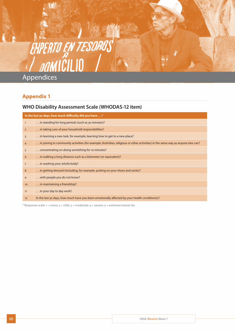
88 SAGE Mexico Wave 1
Appendices
Appendix 1
WHO Disability Assessment Scale (WHODAS-12 item)
In the last 30 days, how much difficulty did you have . . .*
1 . . . in standing for long periods (such as 30 minutes)?
2 . . . in taking care of your household responsibilities?
3 . . . in learning a new task, for example, learning how to get to a new place?
4 . . . in joining in community activities (for example, festivities, religious or other activities) in the same way as anyone else can?
5 . . . concentrating on doing something for 10 minutes?
6 . . . in walking a long distance such as a kilometer (or equivalent)?
7 . . . in washing your whole body?
8 . . . in getting dressed (including, for example, putting on your shoes and socks)?
9 . . . with people you do not know?
10 . . . in maintaining a friendship?
11 . . . in your day to day work?
12 In the last 30 days, how much have you been emotionally affected by your health condition(s)?
* Response scale: 1 = none; 2 = mild; 3 = moderate; 4 = severe; 5 = extreme/cannot do.
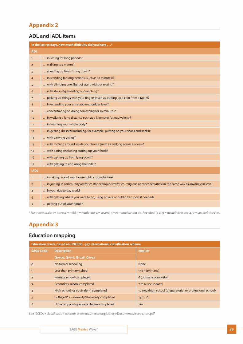
89SAGE Mexico Wave 1
Appendix 2
ADL and IADL items
In the last 30 days, how much difficulty did you have . . .*
ADL
1 . . . in sitting for long periods?
2 . . . walking 100 meters?
3 . . . standing up from sitting down?
4 . . . in standing for long periods (such as 30 minutes)?
5 . . . with climbing one flight of stairs without resting?
6 . . . with stooping, kneeling or crouching?
7 . . . picking up things with your fingers (such as picking up a coin from a table)?
8 . . . in extending your arms above shoulder level?
9 . . . concentrating on doing something for 10 minutes?
10 . . . in walking a long distance such as a kilometer (or equivalent)?
11 . . . in washing your whole body?
12 . . . in getting dressed (including, for example, putting on your shoes and socks)?
13 . . . with carrying things?
14 . . . with moving around inside your home (such as walking across a room)?
15 . . . with eating (including cutting up your food)?
16 . . . with getting up from lying down?
17 . . . with getting to and using the toilet?
IADL
1 . . . in taking care of your household responsibilities?
2 . . . in joining in community activities (for example, festivities, religious or other activities) in the same way as anyone else can?
3 . . . in your day to day work?
4 . . . with getting where you want to go, using private or public transport if needed?
5 . . . getting out of your home?
* Response scale: 1 = none; 2 = mild; 3 = moderate; 4 = severe; 5 = extreme/cannot do. Recoded: (1, 2, 3) = no deficiencies; (4, 5) = yes, deficiencies.
Appendix 3
Education mapping
Education levels, based on UNESCO 1997 international classification scheme
SAGE Code Description Mexico
Q0409, Q1016, Q1028, Q1032
0 No formal schooling None
1 Less than primary school 1 to 5 (primaria)
2 Primary school completed 6 (primaria completa)
3 Secondary school completed 7 to 9 (secundaria)
4 High school (or equivalent) completed 10 to12 (high school (preparatoria) or professional school)
5 College/Pre-university/University completed 13 to 16
6 University post-graduate degree completed 17+
See ISCED97 classification scheme, www.uis.unesco.org/Library/Documents/isced97-en.pdf
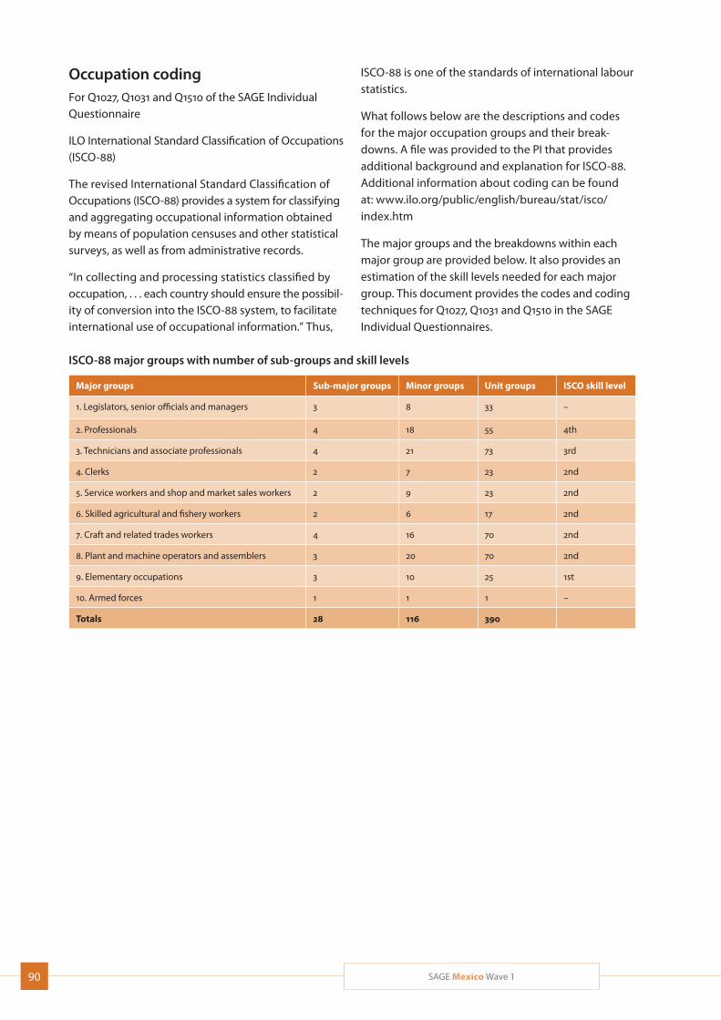
90 SAGE Mexico Wave 1
Occupation codingFor Q1027, Q1031 and Q1510 of the SAGE Individual Questionnaire
ILO International Standard Classification of Occupations (ISCO-88)
The revised International Standard Classification of Occupations (ISCO-88) provides a system for classifying and aggregating occupational information obtained by means of population censuses and other statistical surveys, as well as from administrative records.
“In collecting and processing statistics classified by occupation, . . . each country should ensure the possibil-ity of conversion into the ISCO-88 system, to facilitate international use of occupational information.” Thus,
ISCO-88 is one of the standards of international labour statistics.
What follows below are the descriptions and codes for the major occupation groups and their break-downs. A file was provided to the PI that provides additional background and explanation for ISCO-88. Additional information about coding can be found at: www.ilo.org/public/english/bureau/stat/isco/ index.htm
The major groups and the breakdowns within each major group are provided below. It also provides an estimation of the skill levels needed for each major group. This document provides the codes and coding techniques for Q1027, Q1031 and Q1510 in the SAGE Individual Questionnaires.
ISCO-88 major groups with number of sub-groups and skill levels
Major groups Sub-major groups Minor groups Unit groups ISCO skill level
1. Legislators, senior officials and managers 3 8 33 –
2. Professionals 4 18 55 4th
3. Technicians and associate professionals 4 21 73 3rd
4. Clerks 2 7 23 2nd
5. Service workers and shop and market sales workers 2 9 23 2nd
6. Skilled agricultural and fishery workers 2 6 17 2nd
7. Craft and related trades workers 4 16 70 2nd
8. Plant and machine operators and assemblers 3 20 70 2nd
9. Elementary occupations 3 10 25 1st
10. Armed forces 1 1 1 –
Totals 28 116 390
91SAGE Mexico Wave 1
Appendix 4
Text describing the income or wealth quintiles (permanent income)Income quintiles were derived from the household ownership of durable goods, dwelling characteristics (type of floors, walls and cooking stove), and access to services such as improved water, sanitation and cook-ing fuel. Durable goods included number of chairs, tables or cars, and if, for example, the household has electricity, a television, fixed line or mobile phone, a bucket or washing machine. A total of 21 assets were included with overlaps and differences in the asset lists by country. The results were recoded into dichotomous variables taking the value of 0 if the household did not possess or have access to the good or service, and 1 if it did. The data set was then reshaped, as though each household had multiple observations for wealth (each item being one observation), and was fit as a pure random effect model based on these multiple items per household. The result provides indicator specific thresholds on the latent income scale such that a household is more likely to respond affirmatively than not when its perma-nent income exceeds this threshold. This “asset ladder” was generated and it is country-specific. Using a Bayesian post-estimation (empirical Bayes) method, households were arranged on the asset ladder, where the raw con-tinuous income estimates are transformed in the final step into quintiles. The resulting estimates of household permanent income can be compared to the reported income and total house-hold expenditure. Though the correlation coefficients are not very high (both the Pearson and Spearman correlations are less than 0.5) there is a systematic ‘upper left triangular’ relationship across all countries. Namely, as self-reported income or expenditure increases, our permanent income estimate increases as well. However, our estimates can be high even when self-reported income or expenditure is low, which supports the well-known under-reporting or inadequacies of using income or expenditure indicators as opposed to wealth based on permanent income.
Text describing health scoreValid, reliable, and comparable health measures are essential components to inform clinical practice and health policy. The health module in SAGE included a self-assessment of health consisting of two to three questions pertaining to each of eight health domains (mobility, affect, cognition, self-care, pain, sleep/energy, interpersonal relations and vision). When deriving the SAGE health score, we used the 16 self-reported health state questions in Section 2000 of the questionnaire: Q2002-05, Q2007, Q2008, Q2010-13, Q2016-19, Q2023, and Q2024. Respondents could answer using a five-point scale, from 1=None; 2=Mild; 3=Moderate; 4=Severe; 5=Extreme/Cannot do. As this scale is an ordinal scale, we used an ordinal extension of the Rasch model, the Rating scale model in Winsteps, that keeps the thresholds fixed across items. The item Infit statistics were between 0.7 and 1.3 except for the vision domain, where it was slightly above 1.3. Based on the dimensionality map and the residual correlations, no significant second dimension was found. The item probability curves did not show any disordered thresh-old. Significant DIF (Differential Item Functioning) was found by country for which adjustments have not yet been made in the current results. The results were rescaled to 0 to 100 where zero is worst health and 100 is best health.
Related Documents


