Methodology for Developing Design Response …dap3.dot.ca.gov/ARS_Online/Tech_Docs/Methodology for Developing DRS...Methodology for Developing Design Response Spectrum for Use in Seismic

Methodology for Developing Design Response Spectrum for

Use in Seismic Design Recommendations

November 2012

DIVISION OF ENGINEERING SERVICES GEOTECHNICAL SERVICES

2

Introduction The Geotechnical Manual presents the requirements for determining and reporting seismic information and design response spectrum. This document presents the methodologies used to develop the deterministic, probabilistic and controlling design response spectra using the web tool ARS Online. Much of the information provided herein is based on the standards of the Caltrans Seismic Design Criteria Appendix B (SDC-B). Section 1: Definitions for Developing Deterministic Acceleration Response

Spectrum (ARS) Fault Parameters from the Caltrans Fault Database

MMax Maximum moment magnitude of fault - the largest earthquake a fault is capable of generating.

FRV Faults identified as a Reverse Fault “R” in the Caltrans Fault Database.

FNM Faults identified as a Normal Fault “N” in the Caltrans Fault Database. δ Fault dip angle (deg)

ZTOR Depth to top of rupture (km)

ZBOT Depth to bottom of rupture (km)

Distance Terms

RRUP Closest distance (km) to the fault rupture plane, as shown in Appendix B.

RJB Joyner-Boore distance - The shortest horizontal distance (km) to the surface projection of the rupture area. Think of this as the nearest horizontal distance to the area directly overlying the fault. RJB is zero if the site is located within that area.

RJB (RJB = 0) RJB Site A Site B RX Horizontal distance (km) to the fault trace or surface projection of the top of

rupture plane. It is measured perpendicular to the fault (or the fictitious extension of the fault). The diagram below shows when a site is located on the footwall side (Site A) or on hanging wall side (Site B).

RX RX Site A Site B Footwall Hanging Wall

3

Site Conditions

VS30 “Average” shear wave velocity for the upper 30m (100 feet) at the site (Appendix A).

Z1.0 Depth to rock with shear wave velocity = 1.0 km/sec [Caltrans defined deep sedimentary basin locations only; refer to SDC-B (Figures B.5-B.11)].

Z2.5 Depth to rock with shear wave velocity = 2.5 km/sec [Caltrans defined deep sedimentary basin locations only; refer to SDC-B (Figures B.5-B.11)].

Section 2: Design Policy and Available Design Tools The current Caltrans Seismic Design Criteria & Appendix B, and Memos to Designer (MTD) Section 20 shall be the basis for specifying the minimum seismic design requirements for Ordinary Standard Bridges (defined in SDC Section 1.1). For important bridges (defined in MTD Section 20-1) the requirements of project specific design criteria must be met. Design tools and references are available for use in developing response spectra for seismic design recommendations. These tools include, but are not limited to:

• Caltrans ARS Online Version 2 (web tool) • 2008 United States Geological Survey (USGS) National Seismic Hazard Map, 2008

National Seismic Hazard Map Gridded Data (static) • 2009 USGS Interactive Deaggregation Tool (Beta) • ARS Online Version 2 Report (Update to 2009 ARS Online Version 1 Report) • 2012 Caltrans Fault Database Report (Version 2a) • 2012 Caltrans Fault Database • Deterministic Response Spectrum Spreadsheet • Probabilistic Response Spectrum Spreadsheet • Fault & Site Data Input Sheet

A complete list of these documents and tools with web links are listed on Caltrans ARS Online V2 website (http://dap3.dot.ca.gov/shake_stable/v2/index.php) under the Technical References link. Section 3: Deterministic Acceleration Response Spectrum (ARS) The ARS Online Report (Version 2) hereafter referred to as the "ARS Online Report" was developed in 2012 and describes the methodologies used in creating the Caltrans Fault Database, fault locations, references and notes. It also discusses the development of ARS Online, a user-friendly web tool that is used to develop the design response spectrum. The report is an update of the 2009 ARS Online Report (Version 1) and discusses the changes in methodologies used in the 2012 ARS Online Report (Version 2), but the ground motion prediction equations and calculations remain unchanged.

4

The 2012 Caltrans Fault Database Report (Version 2a) discusses the faults used in ARS Online Version 2. Generally, the 2012 Caltrans Fault Database (CFD) builds on the 2007 Caltrans Fault Database used in ARS Online Version 1, and is updated to include several newly identified faults as well as updates provided in the Uniform California Earthquake Rupture Forecast –Version 3 (UCERF 3) database (prepublication copy). As was the case previously, faults included in the 2012 CFD are active within late Quaternary time (within the past 700,000 years) and capable of producing a maximum moment magnitude (MMax) earthquake of 6.0 or greater. The deterministic seismic site response is the average of two Next Generation Attenuation (NGA) ground motion prediction equations developed by Chiou & Youngs and Campbell & Bozorgnia (CY-CB) in 2008. The combined models are referred to as the CY-CB ground motion prediction equation (CY-CB GMPE). ARS Online is used to develop the acceleration response spectrum (ARS) curve. Results generated by ARS Online may be verified using the Deterministic Response Spectrum Spreadsheet. The Deterministic Response Spectrum Spreadsheet allows the geoprofessional to validate each deterministic ARS curve generated by ARS Online using input parameters from the Caltrans Fault Database, including fault characteristics, site-to-fault distances and site parameters (e.g. VS30, Z1.0 & Z2.5). Section 4: Procedure for Developing a Deterministic ARS using ARS Online Procedures and examples for developing an acceleration response spectrum (ARS) are based on the current criteria in the SDC, Appendix B, and require the user to be familiar with the ARS Online Report, Caltrans Fault Database, ARS Online web tool, and the Deterministic Response Spectrum Spreadsheet. The Fault & Site Data Input Sheet is also available to help users organize the data discussed below. The Fault & Site Data Input Sheet can also serve as a checklist to ensure that all relevant site factors and fault parameters have been considered. The following steps summarize how to develop a deterministic ARS using ARS Online.

1. Locate and “mark” the site on the ARS Online map and verify that the site is properly located using the satellite map view. • The ARS Online tool displays the active faults listed in the Caltrans Fault Database.

The simplified fault traces shown on the ARS Online tool are for estimating ground motions only and must NOT to be used for fault surface rupture evaluation. Uncertainties in the locations of the digital fault traces shown on the map are approximately ± 1 km. Uncertainty of the Google satellite map view is less than 140 meters.

2. Calculate, estimate, or use the measured VS30 value for the site (Refer to Appendix A). • The CY-CB ground motion prediction equations used in ARS Online are only

valid for VS30 values between 150 m/s and 1500 m/s. For sites with VS30 values less than 180 m/s or with soil profiles containing thick layers of very soft clay, refer to the VS30 section of the SDC, Appendix B.

3. Enter the VS30 value on ARS Online and push the “calculate” button to generate deterministic spectra.

5

4. Observe the resulting spectra shown in the lower plot and note fault(s) contributing to the design response spectrum.

5. Push the “tabular data” button to obtain the site, fault and response spectrum data. Section 5: Procedure for Verification of ARS Online Results using the

Deterministic Response Spectrum Spreadsheet This section presents steps to check the results of ARS Online using the Deterministic Response Spectrum Spreadsheet. Step 1: Obtain and Record Fault Parameters and Geometry

• In the map view of ARS Online, click on faults that contribute to the design response spectrum and obtain fault parameters (Fault ID, Maximum Moment Magnitude, fault type, fault dip angle, dip direction, and the top of rupture plane) from the pop-up fault information box.

• Draw a sketch in both plan and profile view that shows the site and fault-related geometry (e.g. footwall and hanging wall side of fault, perpendicular and/or off-set distance to fault). The Fault & Site Data Input Sheet can help organize the fault and site data used.

Step 2: Determine RX, RRUP, and RJB

• RX is the horizontal distance to the fault trace or surface projection of the top of rupture plane. It is measured perpendicular to the fault (or the fictitious extension of the fault).

• RRUP is the shortest distance to the fault rupture plane. • RJB is the distance to the vertical projection of the fault rupture plane. RJB is zero when

situated directly over the vertical projection of the fault plane. RX is typically measured using the ARS Online “ruler” tool. RRUP and RJB are typically calculated values that depend on the site location, its proximity to the fault, and the fault parameters. Appendix B presents various examples for determining RX, RRUP, and RJB. Step 3: Determine Z1.0, and/or Z2.5 Several deep sedimentary basins exist in California. In these regions, a depth to rock (Z) parameter is needed for prediction of the ground motion. The sedimentary basins are shown in SDC-B (Figures B.5-B.11) and on ARS Online by selecting the “overlay” button. These figures show depth to rock for shear wave velocities of 1000 and 2500 m/sec respectively. For a site that is located within one of these basins, determine the following:

• Z1.0: the vertical depth to rock (meters) with a shear wave velocity of 1000 m/s • Z2.5: the vertical depth to rock (km) with a shear wave velocity of 2500 m/s

Step 4: Input parameters into Deterministic Response Spectrum Spreadsheet Using the information gathered in the preceding steps, input the data into the “CY-CB Model Inputs” section of the Deterministic Response Spectrum Spreadsheet (shown below) to develop the deterministic ARS for each fault.

6

Step 5: Evaluate Special Cases The following special cases must be considered and may be verified by the deterministic response spectrum spreadsheet.

• A minimum deterministic spectrum (MDS) is imposed statewide, in recognition of the potential for earthquakes to occur on faults previously unknown or thought inactive. This minimum spectrum assumes a maximum moment magnitude 6.5, vertical strike-slip event occurring at a distance of 12 km (7.5 miles). A near-fault adjustment factor (Step 6) is NOT applied to the MDS. To plot the MDS using the spreadsheet, enter all the appropriate MDS parameters and VS30 for the site to obtain the CY-CB results then paste the data into the designated MDS cells.

• The Eastern California Shear Zone (ECSZ) (SDC-B, Figure B.2) minimum spectrum is

based on a vertical, strike-slip fault with a moment magnitude of 7.6 and a distance of 10 km. A near-fault adjustment factor (Step 6) is NOT applied to the ECSZ. To plot the ECSZ data using the spreadsheet, enter all the appropriate ECSZ parameters and VS30 for the site to obtain the CY-CB results then paste the data into the designated ECSZ cells.

• The Cascadia Subduction Zone (Fault Identification No. 8), is a large shallow dipping

thrust fault zone, that can generate large ground motions in northwestern California. It requires a separate attenuation model and modified analysis. The deterministic spectrum for the Cascadia Subduction zone is the median spectrum from the Youngs et al. (1997) ground motion prediction equation, with the added criterion that an arithmetic average of the Youngs et al. and CY-CB GMPE is used where the Youngs et al. spectrum is less than the average of the CY-CB GMPE (both without the hanging wall term applied).

7

o The Deterministic Response Spectrum Spreadsheet contains a tab to analyze the Cascadia Subduction Zone. First, the user will input fault and site data into the spreadsheet “input-compare” tab using the procedures listed in previous sections. The user then obtains the ARS Online spectral data and pastes the data into the designated cells of the deterministic spreadsheet. Once all the data have been entered, the user selects the spreadsheet tab “Cascadia” to analyze and compare spectra using the above procedure in order to obtain the appropriate design response spectrum.

Step 6: Apply Near-Fault Factors An increase in the calculated spectral acceleration to account for near-fault effects must be applied when RRUP is less than 25km. The increase is 20% for sites within 15 km of a causative fault and tapers linearly to zero at 25 km. The increase in spectral acceleration values is applied to periods longer than 1-second and linearly tapers to zero at a period of 0.5-second (see the figure below). The deterministic spreadsheet automatically applies this factor when the appropriate cell has been checked.

The near fault factor is not applied to the ECSZ or MDS. Refer to Step 5 for details. Step 7: Compare Deterministic Spectra The deterministic response spectrum is the upper envelope of all deterministic spectra developed by causative faults, the MDS and ECSZ (if applicable). The Deterministic Response Spectrum Spreadsheet uses the CY-CB ground motion prediction equations to generate spectral acceleration data for a site for a specific fault. It is recommended that deterministic response spectrum generated by ARS Online be checked using the Deterministic Response Spectrum Spreadsheet to ensure safety and cost-effective designs.

0%

5%

10%

15%

20%

25%

0 1 2 3 4 5

Nea

r Fau

lt F

acto

r,

(% in

crea

se)

Period (seconds)

Site to fault distance < 15km

Site to fault distance = 20 km

Site to fault distance > 25 km

8

When comparing deterministic spectrum it is most efficient to first address and enter the parameters for the MDS and the ECSZ (if applicable) prior to analyzing each potentially causative fault. After developing a response spectrum for the MDS and ECSZ (if applicable), paste the spectral data from the CY-CB spreadsheet results for each case in the designated cell in the spreadsheet. Systematically check each potentially causative fault against results generated by ARS Online. After entering the fault parameters and site information into the spreadsheet for each fault, compare the CY-CB spreadsheet results for each fault to the results generated by ARS Online by pasting the ARS Online data into the appropriate cells. After checking each result generated by ARS Online, the user may paste the CY-CB results into the designated cells for each fault so those results may be plotted on the spreadsheet graph before proceeding to checking the results of another fault. After all spectra have been developed for causative faults, MDS and ECSZ (if applicable), compare the results to determine the controlling deterministic response spectrum. In cases where more than one fault contributes to the maximum spectral values, use the upper envelope of the spectral values for the deterministic design response spectrum. Verification of the ARS Online results ensures quality seismic design recommendations. If a discrepancy of more than 10% exists between the ARS Online results and the Deterministic Response Spectrum Spreadsheet tool, then re-check input data. If the discrepancy cannot be resolved then email [email protected] to notify the ARS Online development team. Section 6: Probabilistic Acceleration Response Spectrum (ARS) The probabilistic response spectrum to be used for design of bridge structures is based on data from the 2008 USGS National Seismic Hazard Map for the 5% in 50 years probability of exceedance (or 975 year return period). Documentation, maps, data and tools are available at the USGS website, http://earthquake.usgs.gov/hazmaps/. In 2009, the USGS Interactive Deaggregation Tool (Beta) was made publicly available in the form of an interactive web tool. However, the development of a response spectrum requires 10 separate deaggregation calculations, so the process is relatively tedious when compared to ARS Online. ARS Online facilitates the development of the probabilistic analysis by utilizing the deaggregation data provided by the USGS to develop a probabilistic spectrum in one step. The probabilistic response spectrum developed by ARS Online also incorporates both the Caltrans near-fault and basin factors, if applicable. Determining R Distance for Near-Fault Factor in Probabilistic ARS Determine the appropriate distance to use for the near-fault factor by generating a site hazard deaggregation using the 2009 USGS Interactive Deaggregation Tool (Beta) for the period closest to the fundamental period of the structure. The fundamental period is provided by the structure designer. After generating a site hazard deaggregation, obtain the lesser of the R(mean) or R(mode) distance (from peak R, M bin) as shown in the figure below.

9

By default, ARS Online uses the RRUP distance to the closest “deterministic” fault for determining the near-fault factor for the initial probabilistic spectrum (see figure below). Consequently, the lesser of R(mean) or R(mode) must be entered in the “Near Fault” adjustment box (see figure below) so the appropriate R distance is applied. However, the R(mean) or R(mode) value should not be used if it is less than the RRUP distance reported by ARS Online, because a near-fault adjustment factor is not applied to the background seismic source used by the USGS Interactive Deaggregation Tool. The following figure shows an example of where a geoprofessional would override the default value in ARS Online by entering the appropriate R distance value of 47.8 km.

47.8

10

Although ARS Online provides a simple way of developing a probabilistic response spectrum, the use of the tool is not a requirement. As a result, the USGS Deaggregation Tool can be used as long as basin factors (as described in Section 8) and near-fault factor (as described in Section 10) are applied in the probabilistic spectrum. As discussed in the “ARS Online Report”, the probabilistic ARS developed by ARS Online uses interpolated USGS deaggregation data. The resulting probabilistic ARS is typically in close agreement (< 5% difference) with probabilistic data developed using the USGS interactive deaggregation tool. However, there may be a rare case where a larger discrepancy is observed. As a result, it is recommended that four spectral data points be compared to determine if the probabilistic ARS curve developed by ARS Online is acceptable. Section 7: Procedure for Developing the Probabilistic Response Spectrum

using ARS Online This section presents the steps to develop the probabilistic response spectrum.

1. Locate site using the ARS Online web tool. 2. Mark the site using the appropriate button or input Latitude and Longitude. 3. Input VS30 (Appendix A) 4. Generate the probabilistic ARS curve by pushing the “calculate” button. 5. Go to the USGS Interactive Deaggregation Tool (Beta): Input the data from steps 2 and 3

using the “5% in 50yr probability of exceedance” option. Run the USGS tool using structural periods of 0 sec, 0.3 sec, 1.0 sec, and 3.0 sec and save the results from each run (results to be used in Section 8).

6. Using the structure designer’s estimate of the fundamental period of the structure, obtain the lesser of R(mean) or R(mode) obtained from step 5 (for details refer to Section 6). This R distance is used to determine the appropriate near-fault factor to apply in ARS Online.

7. Go back to the ARS Online window: Enter the lesser of R(mean) or R(mode) (as obtained in step 6) into the ARS Online input box for near-fault adjustment for the probabilistic spectrum and push the “OK” button. After pushing the “OK” button, the probabilistic spectrum (graphical curve) will be updated.

8. Generate spectral acceleration data for the probabilistic spectrum by selecting the “tabular data” button

Section 8: Procedure for checking ARS Online results or to adjust the USGS

Deaggregation results: This section presents steps to verify the base spectrum of the probabilistic response spectrum.

1. Open the Probabilistic Response Spectrum Spreadsheet tool. 2. Copy the ARS Online “tabular data” from the probabilistic tab and paste the data into the

spreadsheet. 3. Enter the four USGS values (obtained in Section 7, step 5) into the probabilistic

spreadsheet.

11

4. Compare the ARS Online data with the four spectral values from USGS (see figure below).

5. If the discrepancy between the USGS spectral acceleration values and the ARS Online results is less than 10%, then the probabilistic ARS curve developed using ARS Online is acceptable for design.

6. If the discrepancy between the USGS spectral acceleration values and the ARS Online (base spectrum) results is greater than 10%, then the USGS Interactive Deaggregation Tool (beta) website must be used for development of the probabilistic response spectrum. In this case, the user must ensure that the USGS probabilistic spectrum is supplemented with applicable basin and near fault factors which can be obtained from ARS Online.

Checking the ARS Online results ensures quality seismic design recommendations. If a discrepancy of more than 10% exists between the ARS Online (base spectrum) data and the USGS Interactive Deaggregation Tool, then re-check input data. If the discrepancy cannot be resolved then develop the probabilistic ARS using the USGS Interactive Deaggregation Tool with the applicable near-fault and/or basin amplification factors obtained from ARS Online. Send an email to [email protected] to notify the ARS Online development team of the discrepancy.

Paste ARS Online Data Here

Input USGS Deaggregation Data Here

Observe % Difference

12

Section 9: Procedures for Design Response Spectrum Compare the probabilistic and the deterministic response spectra for all periods. The upper envelope of the spectral values must be used for the design response spectrum.

13

References Applied Technology Council, 1996, Improved Seismic Design Criteria for California Bridges: Resource Document, Publication 32-1, Redwood City, California. Boore, D., 2004, Estimating VS30 (or NEHRP Site Classes) from Shallow Velocity Models: Bulletin of the Seismological Society of America, Vol. 94, No. 2, pp. 591–597, April 2004 Boore, D., and Atkinson, G., 2008, Ground-motion prediction equations for the average horizontal component of PGA, PGV, and 5%-damped PSA at spectral periods between 0.01 s and 10.0 s: Earthquake Spectra, Vol.24, pp.99-138. Brandenberg, S.J., Bellana, N. and Shantz, T., 2010, Shear wave as function of standard penetration test resistance and vertical effective stress at California bridge sites: Soil Dynamics and Earthquake Engineering, vol. 30, pp. 1026-1035. Bryant, W. A. (compiler), 2005, Digital Database of Quaternary and Younger Faults from the Fault Activity Map of California, version 2.0: California Geological Survey Web Page, http://www.consrv.ca.gov/CGS/information/publications/QuaternaryFaults_ver2.htm Campbell, K., and Bozorgnia, Y., 2008, NGA ground motion model for the geometric mean horizontal component of PGA, PGV, PGD, and 5% damped linear elastic response spectra for periods ranging from 0.01 to 10 s.: Earthquake Spectra, Vol.24, pp.139-172. (http://www.eeri.org/cds_publications/catalog/product_info.php?products_id=293) Chiou, B., and Youngs, R., 2008, An NGA model for the average horizontal component of peak ground motion and response spectra: Earthquake Spectra, Vol.24, pp.173-216. (http://www.eeri.org/cds_publications/catalog/product_info.php?products_id=293) DeJong, J. T, 2007, Site Characterization – Guidelines for Estimating Vs Based on In-Situ Test, University of California at Davis, Soil Interactions Laboratory. pp 1-22. http://dap3.dot.ca.gov/shake_stable/reference/Vs30_Correlations_UC_Davis.pdf Dickenson, S.E., 1994, Dynamic Response of Soft and Deep Cohesive Soils During the Loma Prieta Earthquake of October 17, 1989: Dissertation for Doctor of Philosophy in Civil Engineering at the University of California at Berkley, pp. 104-112. Fumal, T.E., 1978, Correlations between seismic wave velocities and physical properties of near-surface geologic materials in the southern San Francisco Bay region, California: U.S. Geological Survey Open-File Report 78-1067, pp. 73-88. http://pubs.er.usgs.gov/djvu/OFR/1978/ofr_78_1067.djvu Fumal, T.E., Tinsley, J.C., 1985, Mapping Shear-Wave Velocities of Near-Surface Geologic Materials, U.S. Geological Survey Professional Paper 1360, pp. 127-149. http://pubs.er.usgs.gov/djvu/PP/pp_1360.djvu Imai T, Tonouchi K (1982) Correlation of N-value with S-wave velocity and shear modulus. In: Proceedings of the 2nd European symposium of penetration testing, Amsterdam, pp 57-72. Mayne, P.W., 2007, Cone Penetration Testing State-of-Practice. NCHRP Project 20-05 Topic 37- pp. 14.

14

Mayne P.W., Christopher, B.R, and DeJong, Jason, 2001, Manual on Subsurface Investigations, National Highway Institute, NHI-01-031. Mayne, P.W., and Rix, G.J.,1995, "Correlations between Shear Wave Velocity and Cone Tip Resistance in Natural Clays." Soils and Foundations, 35 (2), pp. 107-110. Merriam, M., 2012, Caltrans Fault Database (V2a) for ARS Online, California Department of Transportation, Sacramento, CA. http://dap3.dot.ca.gov/shake_stable/v2/display_resource.php?id=113 Ohta, Y., and Goto, N., 1978, "Empirical Shear Wave Velocity Equations in Terms of Characteristic Soil Indexes." Earthquake Engineering and Structural Dynamics. 6, pp. 167-187. Petersen, Mark D., Frankel, Arthur D., Harmsen, Stephen C., Mueller, Charles S., Haller, Kathleen M., Wheeler, Russell L., Wesson, Robert L., Zeng, Yuehua, Boyd, Oliver S., Perkins, David M., Luco, Nicolas, Field, Edward H., Wills, Chris J., and Rukstales, Kenneth S., 2008, Documentation for the 2008 Update of the United States National Seismic Hazard Maps: U.S. Geological Survey Open-File Report 2008–1128, pp. 61. Shantz, T., 2012, ARS Online 2.0: Discussion of New Features and Updated Source Data, California Department of Transportation, Sacramento, CA. http://dap3.dot.ca.gov/shake_stable/v2/display_resource.php?id=111 Shantz, T., Merriam, M., 2009, Development of the Caltrans Deterministic PGA Map and Caltrans ARS Online, California Department of Transportation, Sacramento, CA. http://dap3.dot.ca.gov/shake_stable/references/Deterministic_PGA_Map_and_ARS_Online_Report_071409.pdf Sykora, D.W., 1987, "Examination of Existing Shear Wave Velocity and Shear Modulus Correlations in Soils." Department of the Army, Waterways Experiment Station, Corps of Engineers, Miscellaneous Paper GL-87-22. Youngs, R.R., S.J. Chiou, W.J. Silva, and J.R. Humphrey (1997). Strong ground motion attenuation relationships for subduction zone earthquakes, Seism. Res. Letts., v. 68, no. 1, pp. 58-73.

15

Appendix A: Determination of Shear Wave Velocity and VS30 The average shear wave velocity (VS30) for the upper 30 meters (100 feet) of the soil/rock profile is required to determine the design ground motion at the ground surface of a project site using the attenuation relationships included in the SDC. The equation used for calculating VS30 within the upper 30m (100 ft) is:

n

nS

VD

VD

VD

VD

V++++

=...

ft 100

3

3

2

2

1

130 ;

The shear wave velocity (Vs) of each soil or rock layer may be measured in-situ or, where applicable, estimated based on empirical correlations with other parameters (e.g. field or lab data). In-situ measurements of Vs using geophysical methods, where feasible, are relatively simple and preferred for the purpose of estimating ground motions. The table below provides brief descriptions of some common geophysical methods for measuring Vs.

Geophysical Test Brief Description

PS Suspension logging

Shear wave measurements are made in an open or thermoplastic-cased borehole. Source and receivers have a fixed separation and are both within the borehole. Shear wave velocities are measured at discrete depth intervals.

Down-hole seismic The seismic source is fixed at the surface, and shear wave measurements are made with the receiver placed in the borehole at discrete intervals. Source to receiver separation varies with the receiver location.

Seismic CPT cone The CPT seismic cone method is similar to the down-hole seismic method. The source is at the surface, the receiver is in the CPT cone. No predrilled borehole is necessary. Measurements are at discrete intervals.

Rayleigh Wave Inversion

Measurements are made at the surface. Several geophysical methods are available, including Refraction Microtremor (ReMi), Multichannel Analysis of Surface Waves (MASW) and Spectral Analysis of Surface Waves (SASW).

Note: If geophysical methods are used, the Geophysics Branch or a Professional Geophysicist should provide the data and the results of the test in a report. In-situ measurements of Vs are generally required for project sites underlain by profile types that fall within the Type F category (as listed in SDC, Figure B.12), and in many cases Type E, or when site-specific dynamic ground response analyses are performed. For these cases, Vs measurements may need to extend to depths greater than 30 m depending on the site conditions and the appropriate depth of the input design base motion. Shear Wave Velocity Correlations In the absence of in-situ measurements, Vs for most soil layers and soft sedimentary rock layers can be estimated using established correlations. It should be noted that the correlations may contain significant uncertainty and geophysical measurements should be used when feasible. For cohesive soils, empirical correlations with laboratory measured undrained shear strength are preferred. For cohesionless soils, correlations with either the SPT (Standard Penetration Test – ASTM D1586) blow count value, N60 (blow count corrected for hammer efficiency but not for

where D is the layer thickness (ft) and V is the shear wave velocity (ft/s) for that layer. Note: VS30 input for attenuation models must be converted into meters/sec.

16

overburden), or the CPT tip resistance, qt, may be used. Recommended shear wave velocity correlations for soil layers for use in the development of ground motions for State projects are presented below. A correlation with SPT blow counts is also provided for estimating Vs for young sedimentary rocks. For stronger rock, the shear wave velocity for distinct zones may be evaluated based on correlations with other engineering and physical properties of rock mass and rock cores measured in the field or laboratory, or estimated by experienced geo-professionals using geologic correlations. Such properties include, but are not limited to, uniaxial compressive strength of rock, RQD of rock mass, elastic modulus, poisson’s ratio and ultrasonic shear velocity (see Mayne et al, 2001). Well documented and established empirical VS30 correlations specific to the earth material under consideration, or to the project site or the general area with similar earth material may be used by experienced geo-professionals provided adequate justifications of their use and the pertinent references are included in the report. In 2007, UC Davis (DeJong 2007) compiled published correlations between shear wave velocity and common in-situ geotechnical test parameters and presented recommended correlations for various soil types. In 2010, a research study done by UC Los Angeles (Brandenberg, Bellana and Shantz, 2010) was published that reviewed Caltrans P-S Log data and SPT data from 79 borings and presented recommended correlations for various soil types. Both studies were reviewed and compared by Caltrans for consistency with the ATC-32 profile types (SDC, Figure B.12) and the parameters and ranges used to define the profile types. The correlations provided below are recommended for State project sites, where applicable. The geo-professionals should be aware of the limitations of each correlation used. For example, penetration of the SPT sampler in earth material may be limited or affected by the presence of large particles (e.g. gravel, cobbles, boulders or rock fragments). Correlations, in particular using SPT data, should only be used with test data that are reliable and representative of the actual site conditions. If correlations are not applicable (e.g. SPT correlation used in a thick, coarse gravel deposit) or not available in a region, then in-situ measurements are recommended. The correlation equations below provide shear wave velocity in m/sec. and are valid for a range of 100 to 380 m/sec for cohesionless soil, and are valid for a range of 100 to 310 m/sec for cohesive soil. Higher velocities should be verified with in-situ measurements. Also, shear wave velocity correlations should not be applied to depths less than 5ft. Estimation of shear wave velocities (Vs) at depths less than 5ft can be approximated by a Vs value at a depth of 5ft. - Cohesionless Soil The shear wave velocity of cohesionless soil may be estimated by using correlations with SPT blow counts or CPT tip resistance. Correlations for cohesionless soil using SPT data and effective overburden stress developed in the 2010 UCLA study are: For Sand For Silt

( )( ) ( )( )vS NV 'ln236.0ln096.0045.4exp( 60 σ++=

( )( ) ( )( )vS NV 'ln231.0ln178.0783.3exp( 60 σ++=

17

Where N60 is the SPT blow count corrected only for the hammer energy and σ’v is the effective overburden stress (kPa). These correlations are valid where N60 ≤ 100 and σ’v ≤ 506 kPa. For CPT data, the correlation adapted by Mayne (2007) after Baldi et al, (1989) is recommended to calculate shear wave velocity for cohesionless soil:

( ) ( ) 27.013.0 ' 277 votS qV σ=

Where qt and σ’vo are the CPT tip resistance (MPa) and effective overburden stresses (MPa). - Cohesive Soil The correlation by Dickenson (1994) using undrained shear strength to calculate shear wave velocity is recommended for cohesive soil:

( ) 475.0/ 203 auS pSV = Where, Su is the undrained shear strength of cohesive soil and pa is the atmospheric pressure in the same unit as Su. In the absence of undrained shear strength data, the shear wave velocity of cohesive soil may be estimated by using the CPT correlation developed by Mayne and Rix (1995):

( ) 627.0 75.1 tS qV = where qt is the measured CPT tip resistance (kPa). When undrained shear strength or CPT tip resistance data are not available, use the correlation using SPT data and effective overburden developed in the 2010 UCLA study (where N60 ≥ 3): For Cohesive Soil - Young Sedimentary Rock Imai and Tonouchi (1982) reviewed over a hundred SPTs with corresponding Vs in young sedimentary rocks (Tertiary deposits). For these types of rock, their “Tertiary Sand/Clay” correlation may be used to estimate shear wave velocity.

( ) 319.060 109 NVS =

The Vs value estimated using the SPT correlation for young sedimentary rock layers should be limited to 560 m/sec.

( )( ) ( )( )vS NV 'ln164.0ln230.0996.3exp( 60 σ++=

18

Other Rocks While there are numerous studies that correlate shear wave velocity to in-situ geotechnical testing of soil, there are relatively few studies that correlate shear wave velocity to physical properties of rock. Two notable studies that may be useful to geo-professionals in developing approximations of shear wave velocities based on physical properties of rock are provided below. Fumal (1978) correlated shear wave velocity to weathering, hardness, fracture spacing, and lithology based on data from 27 sites in the upland areas of the San Francisco (Bay Area) region. Fumal and Tinsley (1985) extended the 1978 study to include 84 sites in the Los Angeles region. Some physical properties of the rock were more important than others depending on lithology, soil texture, rock hardness, but fracture spacing was found to be the most important factor affecting shear wave velocity. A thorough review of these studies will significantly aid geo-professionals in their estimations of shear velocity. In the absence of in-situ measurements of Vs, the VS30 for competent rock in California should be limited to 760 m/sec. - Estimating VS30 for sites with subsurface information less than 100 ft (30 m) For borings shallower than 100 feet (30 meters) are not available, VS30 can be determined by extrapolating shallower Vs data assuming that no significant changes in the subsurface occur to the extrapolated depth of 100 feet (David Boore (2004)): [ ] (d) s 30 V d) (0.015 - 1.45 ∗∗=SV ;

where d is the depth in meters to the bottom of the known soil column and Vs(d) is the average shear wave velocity (m/sec) for a known depth.

19

Appendix B: Determining RX, RRUP, and RJB The plan view and oblique view shown below present various site locations (A – F) relative to a fault. The following illustrations present scenarios for determining RX, RRUP, and RJB for various site locations relative to a fault as shown in the plan and oblique views below. Case 1 and Case 2 assume a site is situated similar to Site A with a vertical fault. Case 3 and Case 4 assume that a site is situated similar to Site A (footwall side of fault) with a dipping fault. Case 5 and Case 6 assume that a site is located as in Site B or C (hanging wall side of fault) with a dipping fault. For Sites D, E and F (shown below), which are offset from the fault plane, additional correction factors or measurements are required to determine the RX, RRUP & RJB. Plan View Site F Site D Site E

Site A Site C

Site B Oblique View

Exposed trace or vertical projection of the fault at the surface

Vertical Projection of Dipping Fault

Depth to Bottom of Fault Rupture

Projected Fault Width

) Fault Dip Angle

Site A

Site C

Site E Site F

Vertical Projection of Dipping Fault

Exposed trace or vertical projection of the fault at the surface Site B

Site D

20

Site is located on either side of vertical fault (Case 1 - 2) or site is located on footwall side of dipping fault (Case 3 – 4). Case 1: Fault dip = vertical; fault exposed at surface: ZTOR = 0 For vertical faults that intersect the surface (Sites A, B, C), RJB, RRUP, and RX are the same. It is the site-to-fault distance as measured in plan view (a.k.a map distance). Site RJB, RRUP, RX Fault Case 2: Fault dip = vertical; buried fault: ZTOR > 0) For vertical faults that do not intersect the surface (Sites A, B, C), RJB and RX are the same as the map distance, but RRUP must be calculated (see below) RJB, RX Site RRUP ZTOR Fault

( ) ( )2X2

TORRUP RZ R +=

21

Fault dip not vertical and site on footwall side For dipping faults, the calculations are different depending on whether the site is on the hanging wall side or footwall side, and if the fault intersects the surface (ZTOR = 0). For Cases 3 and 4, the sites are on the footwall side and are distinguished by whether or not the fault intersects the surface. Case 3: Site is on footwall side of the fault, ZTOR = 0 RJB, RRUP, RX Site A δ Footwall Hanging wall Case 4: Site is on the footwall side of the fault, ZTOR > 0 RJB and RX are the same as the map distance and RRUP must be calculated. RJB, RX

Site A ZTOR

. RRUP ) δ

( ) ( )2X2

TORRUP RZ R +=

22

Site is on hanging wall side of fault (Cases 5 & 6) In Cases 5 and 6, the site is on the hanging wall side of the fault and more calculations are required to determine the RX, RRUP & RJB distances than the previous cases. To assist in determining which of the following cases apply, some other pertinent distance parameters (FWP, X1, & X2) may be calculated to assist in determining the required RX, RRUP & RJB distances. Plan View Fault Width (FWP) Bottom of Dipping Fault (Vert. Projection) Exposed Dipping Fault at surface Site C Site B Case 5: Site is on the hanging wall side of the fault, ZTOR =0. In Case 5, the depth to top of rupture (ZTOR) is zero. Here it is necessary to know the depth to the bottom of fault rupture (ZBOT) in order to calculate the projected fault width (FWP), and to determine the X1 distance (shown below). The X1 distance is a geometric factor used only to determine if Case 5a or Case 5b applies. Case 5a: Rx is less than or equal to the sum of FWP and X1: Rx, where Rx ≤ FWP + X1 Fault Width (FWP) X1

RJB

RRUP

δtan

ZFW BOTP =

δtanZX BOT1 ∗=

0RJB = (Site B, when situated directly over fault plane)

PJB FW-RxR = where RJB ≥ 0, similar to Site C.

δsin R R XRUP ∗= for both Sites B & C

δ Site C

ZBOT

Site B

23

Case 5b: Rx is greater than the sum of FWP and X1: Rx, where Rx > FWP + X1 Fault Width (FWP) X1 Site C RRUP

tanδZFW BOT

P =

RJB δtanZX BOT1 ∗=

−=−=

tanδZRFWRR BOT

x PxJB ( ) ( )2JB2

BOTRUP RZ R +=

Case 6: Site is on the hanging wall side of the fault, ZTOR > 0. If the fault does not intersect the surface and the site is on the hanging wall side of the fault, there are three possible cases. To assist in determining which case applies, a geometric factor X2 is calculated. Case 6a: Rx is equal to or less than the geometric factor X2 δtanZX TOR2 ∗= 0RJB = when Rx is less than FWP

ZTOR

ZBOT

( ) ( )2TOR

2XRUP ZR R +=

FWP

δ

ZBOT

) δ

Rx

RRUP

X2

) δ

Site

)(tanδ

Z -ZFW TOR BOTP =

24

Case 6b: Site is between X2 and the outside edge X1; gray area shown below (e.g. Site B & Site C) RX, where Rx < FWp + X1 and Rx> X2 X2 ZTOR

RRUP ZBOT FWp __

)(

tanδZ -ZFW TOR BOT

P =

δtanZX TOR2 ∗=

δtanZX BOT1 ∗=

PJB FW-RxR = where RJB ≥ 0, similar to Site C; (For Site B, RJB = 0).

+= δδ

TOR

x RUP tanZ R sin R

Case 6c: Site to fault distance is greater than the sum of projected fault width (FWP) and the X1

distance as shown below. RX, where Rx > FWp + X1

FWP RJB X1 Site C ZTOR ) δ ZBOT RRUP

)(

tanδZ -ZFW TOR BOT

P =

PJB FW-RxR =

( ) ( )2JB2

BOTRUP RZ R +=

RJB X1

Site C

) δ

Site B

25

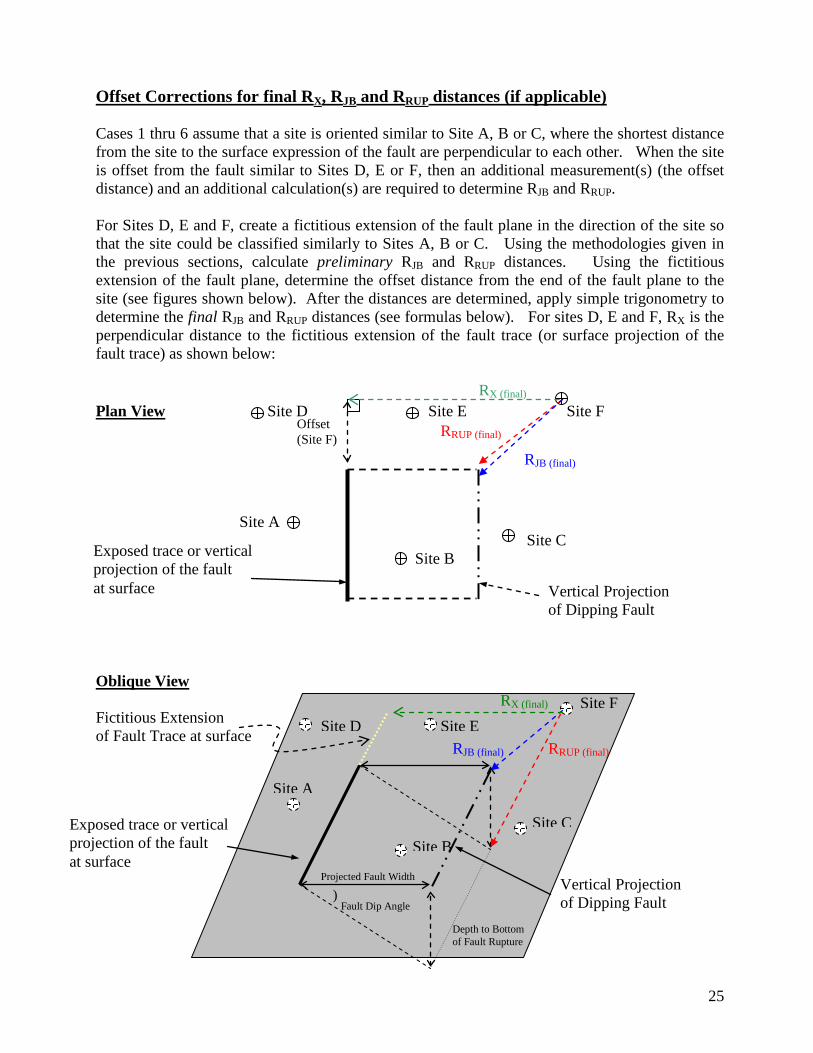
Offset Corrections for final RX, RJB and RRUP distances (if applicable) Cases 1 thru 6 assume that a site is oriented similar to Site A, B or C, where the shortest distance from the site to the surface expression of the fault are perpendicular to each other. When the site is offset from the fault similar to Sites D, E or F, then an additional measurement(s) (the offset distance) and an additional calculation(s) are required to determine RJB and RRUP. For Sites D, E and F, create a fictitious extension of the fault plane in the direction of the site so that the site could be classified similarly to Sites A, B or C. Using the methodologies given in the previous sections, calculate preliminary RJB and RRUP distances. Using the fictitious extension of the fault plane, determine the offset distance from the end of the fault plane to the site (see figures shown below). After the distances are determined, apply simple trigonometry to determine the final RJB and RRUP distances (see formulas below). For sites D, E and F, RX is the perpendicular distance to the fictitious extension of the fault trace (or surface projection of the fault trace) as shown below: RX (final) Plan View Site D . Site E Site F

Site A

Site C Site B Oblique View Fictitious Extension of Fault Trace at surface

Exposed trace or vertical projection of the fault at surface Vertical Projection

of Dipping Fault

Depth to Bottom of Fault Rupture

Projected Fault Width

) Fault Dip Angle

Site A

Site B

Site E

Site C

Vertical Projection of Dipping Fault

Exposed trace or vertical projection of the fault at surface

RRUP (final) RJB (final)

RX (final)

RRUP (final)

RJB (final)

Offset (Site F)

Site F Site D

26

Final Distance Measurements For Sites D, E & F

( ) ( )22RUP(final)RUP OffsetR R += For Site D, E & F

( ) ( )22JB(final)JB OffsetR R += For Site D & F

Offset R (final)JB = For Site E