Master’s Thesis 2019 30 ECTS Faculty of Science and Technology Methodology for Assessing Short-term Flexibility in Demand-side Assets Martin Haug MSc. Environmental Physics and Renewable Energy

Welcome message from author
This document is posted to help you gain knowledge. Please leave a comment to let me know what you think about it! Share it to your friends and learn new things together.
Transcript

Master’s Thesis 2019 30 ECTS
Faculty of Science and Technology
Methodology for Assessing
Short-term Flexibility in
Demand-side Assets
Martin Haug
MSc. Environmental Physics and Renewable Energy

i
This page is intentionally left blank.

Preface
This piece of paper means that my studies in As has come to an end. It has beena challenging, yet thrilling journey of my life and this last semester has not beenan exception.
First and foremost, I would like to express my gratitude to my supervisors HeidiSamuelsen Nygard and Stig Ødegaard Ottesen, whose help and guidance has beenessential for the shaping of this thesis, by providing constructive and encouragingfeedback. Thanks to Heidi for always keeping the door open, to always supportand guide a bewildered student. Thanks to Stig and eSmart for the warm welcome.I am grateful for getting the opportunity to dig into this exciting research field inmy last semester.
I want to thank my family for all the love, care and support throughout the years.Furthermore, I would like to let all my fellow students know that all these yearswould not have been as rich without you.
Some extra appreciation is given to the coffee culture in TF1-211, joy and weirdhumor at Nylenda and the many sunsets behind the oak tree which is soon to beworld famous in Christmas letters around the world.
My last wish is for all people to be aware of the consequences of their needs anddemands, and to be humble about the resources they do and do not have.
As, Dec 16th 2019
Martin Haug
ii
Summary
Global electricity grids, and especially the distribution grids, encounter new chal-lenges during the transmission to a sustainable energy chain. Decarbonizationinvolves electrification and a massive deployment of variable renewable energysources, which ultimately increase the complexity at the demand-side of the grid.There is a growing need to promote demand-side flexible power and to activelyutilize it to deal with an anticipated increase of local congestions and rampingproblems. Local flexibility markets have emerged to provide a platform where thedistribution grid operator or another flexibility buyer can activate demand-sideflexibility that is offered by prosumers, e.g. balance the grid.
In order for a prosumer to make its flexible power accessible on markets, new meth-odologies are needed. The main goal of this thesis is to develop a methodology forassessing short-term flexible power in a demand-side asset. Such a methodologyhas been developed for a generic flexible asset and consists of four stages: (1)load forecasts (2) physical asset models (3) estimation of available flexibility andat last (4) the shaping of a flexibility bid for flexibility markets. The thesis givesconceptual descriptions on how the methodology is implemented for each of fivedifferent flexible assets. Python is used as a tool for implementing the methodo-logy, using the package Keras to make RNN forecast models and object-orientedprogramming to create an Asset class framework.
The methodology is applied on a real use-case scenario where multi-step RNNforecast models are created, using real consumption data for an asset that powersa cooling storage. Data are provided by ASKO (end-user) and eSmart (smartgrid company). The forecast results seems promising even with relative shortdata, but must be optimized, tested on multiple test sets and include explanatoryvariables. Many assumptions had to be made for the asset parameters and thefinal hypothetical flexibility estimates were shown to be sensitive to these choices.Nevertheless, the methodology has been proven to work and is applied to a fulldemonstration of a bid procedure. Applied examples are also given for other assets,such as water heater and a battery.
The conclusion is that the methodology itself is stable and applicable to manydifferent assets. Its results however, being the flexibility estimates, are prone to bevery wrong if the constitutional stages in the methodology are weakly implemen-ted. A strength is that each stage is flexible to be changed or improved withoutdisturbing the flow of the methodology. For the methodology to work successfully,it is of utmost importance that accurate load (or production) forecasts and correctasset parameters are provided.
iii

Sammendrag
Overgangen til et bærekraftig energisystem fører meg seg nye utfordringer forkraftnettet. Distribusjonsnettet vil oppleve en mer kompleks strømflyt som følgeav elektrifisering og en massiv utrulling av uregulerbar, og til dels distribuert,strømproduksjon. Det er forventet en økning i lokale nettutfordringer i form avoverbelastning og hurtig ramping, noe som gir et økt behov for a fremme og aktivtta i bruk fleksibel effekt hos sluttbrukeren i operasjonen av distribusjonsnettet.Nye lokale fleksibilitetsmarkeder er i fremmarsj og har som mal a tilby en apenplattform der sluttbrukere kan selge sin fleksibilitet til en nettoperatør eller andrekjøpere som trenger denne fleksibiliteten, eksempelvis for a avlaste nettet.
For a frigjøre sluttbrukerfleksibilitet til slike markeder, er det nødvendig med nymetodikk. Hovedmalet med denne oppgaven er a utvikle en metodikk for a es-timere kortsiktig fleksibilitet i en distribuert strømkomponent, ogsa kalt asset. Enslik metodikk har blitt utviklet for en generell asset og bestar av fire trinn: (1) last-prediksjoner (2) fysisk modell av en asset (3) estimering av tilgjengelig fleksibilitetog (4) utforming av et bud mot et fleksibilitetsmarked. Oppgaven tar videre forseg hvordan metodikken kan implementeres for fem ulike asseter. Python brukessom et verktøy for a implementere metodikken, ved a bruke pakken Keras for alage RNN-modeller og objektorientert programmering for a lage en Asset-klasse.
Metodikken har blitt anvendt pa en reell asset som brukes til a kjøle et kjølelager.Forbruksdata er gitt av ASKO (sluttbruker) og eSmart (smart grid-selskap), oger brukt for a utvikle RNN-modeller til a prediktere assetens fremtidige forbruk.Modellene virker lovende, men ma optimaliseres, testes pa flere testsett og inkludereflere features. Det er gjort flere antagelser for asseten som har vært utslagsgivendefor fleksibilitetsestimatene. Det har blitt vist at metodikken fungerer og den harblitt anvendt videre i en hypotetisk budprosedyre. Eksempler for implementeringav metodikken pa andre relevante assets er ogsa gitt, nemlig en elektrokjele og etbatteri.
Sluttkonklusjonen er at selve metodikken er stabil og anvendelig for mange forskjel-lige asseter, men fleksibilitetsestimatene kan bare bli like gode som parameterene ogprediksjonene. Styrken til metodikken stegene kan endres uten a forstyrre flyteni metodikken, eksempelvis benytte en bedre lastprediksjonsmodell eller justereparameterene. For at metodikken skal fungere vellykket, sa trenger den nøyaktigelastprediksjoner og riktige parametere for asseten.
iv

Contents
1 Introduction 11.1 Background . . . . . . . . . . . . . . . . . . . . . . . . . . . . . . . 11.2 Motivation . . . . . . . . . . . . . . . . . . . . . . . . . . . . . . . . 41.3 Problem statement . . . . . . . . . . . . . . . . . . . . . . . . . . . 51.4 Tools, data, case and methods . . . . . . . . . . . . . . . . . . . . . 6
2 Theory 92.1 Electrical grids, power and energy . . . . . . . . . . . . . . . . . . . 9
2.1.1 The physical power system . . . . . . . . . . . . . . . . . . . 92.1.2 Regulating the power balance . . . . . . . . . . . . . . . . . 112.1.3 Flexible assets and definitions . . . . . . . . . . . . . . . . . 13
2.2 Energy markets . . . . . . . . . . . . . . . . . . . . . . . . . . . . . 142.2.1 Current power markets . . . . . . . . . . . . . . . . . . . . . 142.2.2 Mechanisms for solving emerging local problems . . . . . . . 152.2.3 NODES - A fully integrated marketplace for flexibility . . . 17
2.3 Modelling . . . . . . . . . . . . . . . . . . . . . . . . . . . . . . . . 202.3.1 Timeseries modelling . . . . . . . . . . . . . . . . . . . . . . 212.3.2 General machine learning . . . . . . . . . . . . . . . . . . . 222.3.3 Recurrent neural networks . . . . . . . . . . . . . . . . . . . 252.3.4 Multi-step forecasting . . . . . . . . . . . . . . . . . . . . . 292.3.5 Techniques for fighting overfitting . . . . . . . . . . . . . . . 30
v

vi CONTENTS
3 Preliminary methodology for assessing short-term demand-sideflexibility 333.1 Presenting the methodology . . . . . . . . . . . . . . . . . . . . . . 343.2 In-depth explanation of the methodology . . . . . . . . . . . . . . . 37
3.2.1 Preparation . . . . . . . . . . . . . . . . . . . . . . . . . . . 373.2.2 Forecast models (stage 1) . . . . . . . . . . . . . . . . . . . 383.2.3 Asset model (stage 2) . . . . . . . . . . . . . . . . . . . . . . 403.2.4 Flexibility estimation (stage 3) . . . . . . . . . . . . . . . . 443.2.5 Bid formatting (stage 4) . . . . . . . . . . . . . . . . . . . . 493.2.6 Aftermath and error measures . . . . . . . . . . . . . . . . . 503.2.7 Bid event line - time advancement . . . . . . . . . . . . . . . 51
3.3 Implementation of the methodology for selected assets . . . . . . . 533.3.1 Thermal energy storages and heat losses . . . . . . . . . . . 533.3.2 Implementation for batteries . . . . . . . . . . . . . . . . . . 543.3.3 Implementing a diesel generator . . . . . . . . . . . . . . . . 563.3.4 Implementing PV solar panels . . . . . . . . . . . . . . . . . 573.3.5 Implementing a water heater . . . . . . . . . . . . . . . . . . 583.3.6 Implementing a machine room for cooling storage . . . . . . 61
4 Use-case: Flexibility at a grocery warehouse 654.1 Introduction . . . . . . . . . . . . . . . . . . . . . . . . . . . . . . . 654.2 Methodology applied to the machine room asset . . . . . . . . . . . 69
4.2.1 Data investigation, analyses and preprocessing . . . . . . . . 694.2.2 Correlations . . . . . . . . . . . . . . . . . . . . . . . . . . . 714.2.3 One-step RNN forecasts . . . . . . . . . . . . . . . . . . . . 744.2.4 Multi-step RNN forecasts . . . . . . . . . . . . . . . . . . . 754.2.5 Example demonstration of a bidding event line . . . . . . . . 774.2.6 Behind the curtains of the bid event line . . . . . . . . . . . 78
4.3 Application for other assets . . . . . . . . . . . . . . . . . . . . . . 894.3.1 Battery . . . . . . . . . . . . . . . . . . . . . . . . . . . . . 894.3.2 Water heater w/ alternative energy source . . . . . . . . . . 914.3.3 Water heater w/ flexible heat storage . . . . . . . . . . . . . 93

CONTENTS vii
5 Discussion 955.1 RNN results . . . . . . . . . . . . . . . . . . . . . . . . . . . . . . . 955.2 Use-case results . . . . . . . . . . . . . . . . . . . . . . . . . . . . . 1035.3 Discussion of the methodology . . . . . . . . . . . . . . . . . . . . . 105
6 Conclusion and further work 1136.1 Conclusion . . . . . . . . . . . . . . . . . . . . . . . . . . . . . . . . 1136.2 Further work, summarized . . . . . . . . . . . . . . . . . . . . . . . 115
A An extensive selection of RNN model forecast results 121A.1 One-step forecasts 1 . . . . . . . . . . . . . . . . . . . . . . . . . . 122
A.1.1 Table of scores . . . . . . . . . . . . . . . . . . . . . . . . . 122A.1.2 Forecast plots . . . . . . . . . . . . . . . . . . . . . . . . . . 122
A.2 One-step forecasts 2 . . . . . . . . . . . . . . . . . . . . . . . . . . 127A.2.1 Table of scores . . . . . . . . . . . . . . . . . . . . . . . . . 127A.2.2 Forecast plots . . . . . . . . . . . . . . . . . . . . . . . . . . 128
A.3 Multi-step forecasts . . . . . . . . . . . . . . . . . . . . . . . . . . . 131A.3.1 Table of scores . . . . . . . . . . . . . . . . . . . . . . . . . 131A.3.2 Forecast plots . . . . . . . . . . . . . . . . . . . . . . . . . . 131
B Example Python Codes 135B.1 RNN model with Keras - Example Code . . . . . . . . . . . . . . . 135B.2 Asset class in Python . . . . . . . . . . . . . . . . . . . . . . . . . . 145B.3 Python Code for creating the flexplots in machine room use-case . . 152

viii CONTENTS

List of Figures
2.1 Illustration of a typical national power grid, including definitions ofpositive power flow direction, consumption and production. . . . . 10
2.2 NODES marketplace and its various market players, mainly theflexibility providers on the right, and the ones who would need theflexibility on the left. Graphic from NODES whitepaper [12]. . . . . 18
2.3 The terminology of a dataset used for creating machine learningmodels, here presented in a dataframe. This multivariate datasethas n features along the columns and has timestamps as instancesalong the rows, making it a timeseries. The figure also shows howthe data is usually divided into train, test and validation splits. . . 21
2.4 The process of building a machine learning model. Figure frombook Python Machine Learning, s. Raschka, V. Mirjalili [29]. . . . . 23
2.5 Architecture of a multilayer RNN, where the arrows indicate flowof data. Figure from book Python Machine Learning, s. Raschka,V. Mirjalili [29]. . . . . . . . . . . . . . . . . . . . . . . . . . . . . . 26
3.1 Workflow and the stages of the preliminary methodology for assess-ing short-term flexibility in a flexible asset. . . . . . . . . . . . . . . 34
3.2 An example of a multistep forecast plot. One line represents fore-casts at all current timesteps, t. Each line represents each forecaststep in the bidding horizon, t + h,∀h. To get an idea of how thisplot is made, refer to the text and figure 3.3. . . . . . . . . . . . . . 39
3.3 Real-time multistep forecast plots for different points in time. Thered dots represent the forecasted values in the bidding horizon. Truebaselines are also plotted. current timestep= (a) 800 (b) 804, (c)808 and (d) 818. As time advance, trajectories for each of the reddots that represent each forecast timestep, h, has been drawn togive an idea of how the multi-step forecast in figure 3.2 is made. . . 40
3.4 A sketch of a general physical model of a flexible asset with a flexibleenergy storage. The green arrows, and not the light red, indicatespositive power direction. . . . . . . . . . . . . . . . . . . . . . . . . 41
ix

x LIST OF FIGURES
3.5 An example of a flexplot, here using a Pixii battery as reference,with a passive load schedule. . . . . . . . . . . . . . . . . . . . . . . 46
3.6 An example of a flexplot, here using a Pixii battery as reference,with an active load schedule. . . . . . . . . . . . . . . . . . . . . . . 48
3.7 Example of a how a flexibility bid that is entered into the flexibilityplatform, may be illustrated. It is constituted of several slots in thebidding horizon h ∈ [1, H], here with H = 6. . . . . . . . . . . . . . 50
3.8 Example of a how a line of bidding events may look like duringtime advancement. Each subfigure represents successive events ofbidding, where each event involves assessing flexibility estimates bymeans of the methodology. The flexibility bids in (a) and (b) areignored. In (c), a part of the bid is thought activated, followed by(c) the dispatch process. . . . . . . . . . . . . . . . . . . . . . . . . 51
3.9 Simplistic physical model of a battery as a flexible asset. . . . . . . 553.10 Simplistic physical model of a diesel generator or of a PV panel. . . 563.11 Simplistic physical model of a water heater with a thermal energy
storage as a flexible asset. . . . . . . . . . . . . . . . . . . . . . . . 593.12 Simplistic physical model of a water heater with the opportunity to
replace electrical consumption with an alternative energy source, asa flexible asset. . . . . . . . . . . . . . . . . . . . . . . . . . . . . . 60
3.13 Simplistic physical model of the machine room and cooling storageas a flexible asset. . . . . . . . . . . . . . . . . . . . . . . . . . . . . 62
4.1 The system of ASKOs building and its considered assets. Powerflows and explanations are included in the figure. The main meterconnects to the grid. . . . . . . . . . . . . . . . . . . . . . . . . . . 66
4.2 Simplified illustration of the cooling storage setup, which is relev-ant for the machine room asset. The daily sunpath and cardinaldirections are indicated as well. . . . . . . . . . . . . . . . . . . . . 69
4.3 Plot showing historical consumption for the machine room assetfor Sept 26th, 2019. The volatile red line is the original timeser-ies with 5-min temporal resolution and the blue averaged line is adownsampled timeseries with 1-hour resolution. . . . . . . . . . . . 70
4.4 Plots of machine room consumption for different stages during theprocess of fixing missing data. Y-axis is consumption in kWh/h,x-axis indicates time in the range from Aug 13th to Sept 30th, 2019. 71
4.5 Correlation plots between outside temperatures near Vestby andmachine room consumption and its rolling means over 2, 3 and 4days (represented by ’2d’, ’3d’, and ’4d’ respectively). The usedtimeseries are daily values from Aug 13th to Sep 30th, 2019. Unitson x-axis is kWh/day, y-axis is ◦C. . . . . . . . . . . . . . . . . . . 72

LIST OF FIGURES xi
4.6 Plots of hourly values of machine room consumption and nearbyoutside temperatures (which is upscaled by factor 25), from Sept22nd till Sept 29th. A corresponding correlation plot is found onthe right. . . . . . . . . . . . . . . . . . . . . . . . . . . . . . . . . . 73
4.7 Correlation plots between the machine room consumption and in-side storage temperatures and its lagged values. The (+) and (-)indicate the forward lead respectively backward lagged values ofinside temperature. . . . . . . . . . . . . . . . . . . . . . . . . . . . 74
4.8 Forecast plot for machine room consumption, made with the one-step RNN model 10292019 1715, on the train (upper) and test set(lower) respectively. . . . . . . . . . . . . . . . . . . . . . . . . . . . 75
4.9 Forecast plot for train set and test set respectively, using the multi-step RNN model Model D. . . . . . . . . . . . . . . . . . . . . . . . 76
4.10 Corresponding real-time load forecast plots for events (a) to (d) forthe machine room. Each subfigure corresponds to the events of thebidding event line demonstration. Table 4.1 provides correspondingforecast results for each event. . . . . . . . . . . . . . . . . . . . . . 79
4.11 Corresponding flexplots for the events (a), (b), (c) and (d). . . . . . 814.12 Bidding event line plot. Example demonstration of a bid proced-
ure for the machine room asset, on Sept 26th, 2019. Real forecastbaselines are used, but assumptions on asset parameters are made.The bid event in each subfigure represent successive bidding hori-zons where the current time equals (a) 07:00 (b) 08:00 (c) 09:00 and(d) 10:00 → 13:00. . . . . . . . . . . . . . . . . . . . . . . . . . . . 82
4.13 Another example flexplot of machine room flexibility where Pmax
and Pmin are defined from a rolling mean of the baseline. . . . . . . 864.14 Multistep forecast plots from the use of three identical models that
have used a slightly different train test split size. The solid anddotted arrows in each figure indicate the same point of time, inorder to make a comparison. . . . . . . . . . . . . . . . . . . . . . . 88
4.15 Example bidding event line for a battery, example 1. . . . . . . . . 904.16 Example bidding event line for a battery, example 2. . . . . . . . . 904.17 Example bidding event line for a water heater that has an alternative
energy source. . . . . . . . . . . . . . . . . . . . . . . . . . . . . . . 914.18 An example flexplot for a water heater with an alternative energy
source. . . . . . . . . . . . . . . . . . . . . . . . . . . . . . . . . . . 924.19 Water heater with heat storage used as an example to present an
energy and flexibility plot in a step of the conceptual model. . . . . 94
A.1 Multi-step RNN forecast plots of model 10292019 1715 and model10292019 1851 . . . . . . . . . . . . . . . . . . . . . . . . . . . . . 123

xii LIST OF FIGURES
A.2 Multi-step RNN forecast plots of model 10292019 1915 and model10302019 1110 . . . . . . . . . . . . . . . . . . . . . . . . . . . . . 124
A.3 Multi-step RNN forecast plots of model 10302019 2000 and model10312019 0900 . . . . . . . . . . . . . . . . . . . . . . . . . . . . . 125
A.4 Multi-step RNN forecast plot of model 10312019 1000. Upper andlower plot is for train and test respectively. . . . . . . . . . . . . . . 126
A.5 Multistep forecast plots from model 11112019 1710. Upper andlower plot is for train and test respectively. As opposed to the com-ing models, this modesl used input data that was not preprocessedfor missing data points, as the dips to zero indicate. . . . . . . . . . 128
A.6 Multistep forecast plots from model 12112019 1327. Upper andlower plot is for train and test respectively. . . . . . . . . . . . . . . 129
A.7 Multistep forecast plots from model 12112019 1344. Upper andlower plot is for train and test respectively. . . . . . . . . . . . . . . 129
A.8 Multistep forecast plots from model 12112019 1410. Upper andlower plot is for train and test respectively. . . . . . . . . . . . . . . 130
A.9 Multistep forecast plots for model A and for model B . . . . . . . . 132A.10 Multistep forecast plots for model C and model D. . . . . . . . . . . 133A.11 Multistep forecast plots for model E and model F. . . . . . . . . . . 134

List of Tables
1.1 List of flexible assets in the scope of this thesis. . . . . . . . . . . . 6
3.1 Table of asset parameters that must be determined in order to fulfillstage 2 of the methodology. . . . . . . . . . . . . . . . . . . . . . . 43
4.1 Table of forecasted baselines and true values for machine room con-sumption on Sept 23th 2019. The table does provide relevant resultscorresponding to the events of the bidding event line demonstration.Each row in the table represent one current timestep and containsthe true value for that current timeslot, h = 0, and forecasted values
for the future timeslots in the bidding horizon, h ∈[1, H
]. . . . . . 80
A.1 Model architecture, parameters and forecast scores for various RNNone-step models, where lagged values of time features is createdexplicitly as new features. . . . . . . . . . . . . . . . . . . . . . . . 122
A.2 Model architecture, parameters and forecast scores for various RNNone-step models, where no features is made from algged time fea-tures, but instead, the lag memory is represented as the timestepdimension that Keras in Python want for RNNs. . . . . . . . . . . . 127
A.3 Model architecture, parameters and forecast scores for various RNNmulti-step models. . . . . . . . . . . . . . . . . . . . . . . . . . . . 131
xiii

xiv LIST OF TABLES

Abbreviations
Abbreviation Meaning
API Application Programming Interface
LV/MV/HV grid Low-/Medium-/High-Voltage grid
TSO/DSO Transmission/Distribution grid operator (operators of theHV transmission grid and MV/LV distribution grids re-spectively)
(vRES) RES (Variable) Renewable energy sources
DFS Decentral/Demand-side flexibility sources
ML Machine Learning
MLP Multiple Linear Regression
RNN Recurrent Neural Network
LSTM Long-short-term memory
PV panels Photovolatic solar panels
DA and ID market Day-Ahead and Intra-Day market for trading electricity
DRM Demand Response Management
MAE, MSE Mean Absolute Error, Mean Squared Error
SoC State of Charge
COP Coefficient of Performance
xv

xvi LIST OF TABLES

Mathematical notation
Mathematical symbol Meaning
~b =
[ˆb(1), ˆb(2), . . . , ˆb(t), . . . , ˆb(H)
]Forecasted baseline
~b =[b(1), b(2), . . . , b(t), . . . , b(H)
]True baseline
E(t) The energy storage level of the asset.
Emin/Emax The minimum/maximum allowed energy level ofthe asset’s energy storage.
∆Erange = Emax − Emin Total flexible energy level range for the asset’s en-ergy storage.
Pcons Electrical power consumption from the grid for theasset.
~Pmax The maximum possible power consumption of theasset.
~Pmin The minimum possible power consumption of theasset.
Pin = ePcons The share of consumption power that flows in tothe asset’s energy storage.
e Efficiency factor for converting grid electricity toinput power.
P(dis)charge = Pin + Plosses Net power flow in to the asset’s energy storage.
Plosses Power losses flowing out of the asset’s energy stor-age.
∆E(t) = P(t)(dis)charge∆t Change of energy level of the asset’s energy stor-
age, due to charging.
∆SoC(t) = n∆E(t) Change in the SoC level for an asset’s energy stor-age, due to charging.
xvii

xviii LIST OF TABLES
n = 1∆Erange
Normalization factor, convert from absolute en-ergy level to SoC level for the asset’s energystorage.
Pcons,SS The consumption which leads to a steady statesituation (no charging and no change in SoClevel).
~Fp = ~Pmax − ~
b Estimated maximum positive flexible power.~Fn = ~Pmin − ~
b Estimated maximum negative flexible power.~Fcommitted and ~Fdelivered Committed (bought) and delivered flexible
power.
R(h)delivered = F
(h)delivered − F
(h)committed Error of delivered flexibility.
t Current timestep/timeslot.
h or t + h, with h ∈ {1, 2, ...,H} Forecasted timestep/timeslot.
H Bidding horizon/number of timeslots.

Chapter 1
Introduction
This first chapter creates the framework, presenting the background and motiv-ation behind the work of this thesis. Then a problem statement is formulatedby means of one main goal and several sub goals. The tools, data, methods anduse-case that are used to address the goals are presented at last.
1.1 Background
Understanding our timeline of energy can be helpful for understanding the energysituation of today. Energy is a real evolutionary drug. Humans did once go frombeing wanderers to evolve around agriculture, a ”hack” of food supply enabling usto grow metropoles. Humans invented machines at a point, resulting in horses be-ing replaced by horsepower. Suddenly, this ”hack” of energy made a lot of cheapwork available for us, through fossil fuels. From that point, energy usage onlyescalated. Industry and cities could expand remotely from the rivers and electri-city was invented. Electricity, goods, transport, house appliances, and followinglyimproved health and wealth became achievable for many. Today, humankind hasdeveloped a very vulnerable relationship with the energy chain, which concern allsides of the globalized human society such as transport, health, water, food andcommunication to mention some. There are no doubts that we have built greatsocieties, however they depend upon a stable and secure source of energy supplyto maintain their vital functions.
1
2 CHAPTER 1. INTRODUCTION
In our age, the consensus about global warming is clear. There are huge socialforces, demonstrations in the streets which demand immediate climate action nowand the world leaders are taking responsibility, more or less. The reason lies in thataround 80% of world energy consumption is fossil-based (per 2018, electricity sectorexcluded) [1]. Of the world’s electricity production, around 66% is fossil-based[2]. This results in greenhouse gas emissions. Analyses estimate that postponingclimate action will end up several times more expensive than immediate focus andinvestments in low-carbon solutions [3][IEA through [4]]. EU as an example hascommitted to cut greenhouse gas emissions by 80-95% by 2050, compared to 1990levels, making it the fastest cutter [3].
Within the energy chain, two options are - to reverse our energy dependency byreducing energy demand - or to break the bond between energy and greenhousegas emissions. Both are valid solutions and both are being pledged. Electrifica-tion is an example of reducing overall energy usage, since electrical technology ismore energy efficient than fossil. Another plus of the electrification is that sectorsare given access to clean electricity from renewable energy sources (RES). Thuselectrification plays a vital role for cutting the bond between to greenhouse gasesand the energy chain. World electricity demand is expected to rise by 62% by2050 [2]. The fossil share of electricity production is expected to decrease fromcurrent 66% to around 31% by 2050, where solar and wind will constitute 48%[2]. Especially in Europe, wind and solar is expected to account for 80% of theelectricity mix within 2050 [2]. This illustrates the massive deployment of newvariable renewable energy sources (VRES) to come. On the downside, introducingnew electricity demand and increasing the VRES share of electricity productionwill induce trouble for power grids, in many ways new to traditional power gridoperation, outlined in the next paragraph. One prominent solution is to deploysmart grid technology with smart local flexibility markets. The work of this thesisfalls in under these categories.
A new energy era for power gridsPower grids face increased intermittency and at the same time an increased sens-itivity to intermittency [5]. At the supply side, power grids worldwide encounteran increased share of variable power production related to RES, where a signi-ficant share of it is at decentralized level unlike before [6]. On the demand side,we expect an increased high-intensive decentralized demand of electricity due toelectrification and increased energy usage. All in all, these are good actions forour sustainable, carbon-neutral future, however they impose new issues for theelectricity grid, issues that disturb the security of supply [5]. The complexityof the future electricity system will increase rapidly, particularly at distributionlevel, and this will result in more local congestions [7]. An increased VRES on
1.1. BACKGROUND 3
demand-side introduces a two-way power flow in the grid topography. In addition,the magnitude of the demand peaks are likely to increase, which initially anticip-ates grid capacity upgrades [6]. Quick changes in the power supply or demandwhich disturb the balance is also known as ramping. The new power grid trendswill cause more frequent and intense ramping situations because of variable pro-duction, both at national level and more at local level - which will cause costlydamages and blackouts unless the grid is made more flexible to handle it.
Balancing the grid have thus far been handled with traditional regulation methods.Regulation at the transmission level has many smart market-based mechanismswith a variety of backups, called reserves. A reserve is just another term for amajor flexible source that can offer up- or down-regulation at transmission levelwhen needed. Reservation and use of flexible reserves has mainly been a privilegefor transmission system operators (TSOs) [8]. This have worked so far, but thenew trends and the fact that the power flow changes from one-directional to bi-directional, requires more active approaches from the distribution grid operator(DSO) as well [8].
DFS marketsMore local problems give rise to the idea that local problems must be solved locally.With digitization and new methodologies, the intelligent market-based operationmethods at transmission level can be extended into the distribution grid and to theend-users. EU know this and has declared market-based congestion managementas default for future operation of the grids, both for the TSO and for DSOs [3].There are now many pilots and working cases on the rise in the field of market-based distribution grid operation. New smart flexibility market initiatives for DFSaim at offering local flexibility to DSOs for regulation of the grid and to othersin need of flexibility [9]. NODES [10] and GOPACS [11] are two examples ofplatforms for such local flexibility markets. Utilizing DFS through local flexibilitymarkets can be a key to shift and shed demand, providing a tool for solving localcongestions and extreme ramping [4]. Demand-side flexibility can either regulatepower up or down when it is necessary and the fine locational granularity of DFSis of uttermost importance [12]. The need for new DFS is well-documented. Onenice and comprehensive article to read about this is Flexibility in the 21st Centuryby Cochran et al. [13]. Markets for decentralized flexibility that have the rightfuldesign will both give added value to already existing DFS out there in addition togive incentives to further flourish DFS [8]. It is of importance that the design anddevelopment of such platforms are purposefully designed and is valuable for ALLparticipants. In addition to deploying smart and efficient marked-based operationmethods, new capacity will be built in order to increase the shared pool of reserveswhich is a way of increasing the overall flexibility of a grid [4]. This in turn, will
4 CHAPTER 1. INTRODUCTION
expand the reach of flexible resources and probably add value to DFS with theright trade-off.
Management of decentralized flexibility in a building and trading on local flexibilitymarkets requires expertise on the field. This is a task that smart grid companiesoften are engaged for. The smart grid company is called an aggregator if they tradeDFS volumes on flexibility markets on behalf of a prosumer. It is of importancethat the smart grid company has a methodology for assessing a building’s flexibilityin a precise manner. Being able to monitor and control flexible assets is necessaryas well. eSmart is such a smart grid company, and ASKO is an owner of a buildingwith flexible assets. In a reliable fashion, the smart grid company will offer thebuilding’s flexibility on a potential flexibility market on behalf of the building.NODES is an example of such a flexibility market platform.
1.2 Motivation
The recently mentioned need for distributed flexibility and flexibility marketsmakes this an interesting and new-born field to dig deeper into. The overarchedgoal is to identify and assess flexibility in demand-side assets so that it becomesaccessible for smart regulation of the distribution grid. For that to happen, newmethodologies are needed, a need confirmed by eSmart. The core motivation ofthe work in this thesis originates from this need. The success of flexibility marketsdepends on flexibility bids that are precise. Precise flexibility bids require pre-cise flexibility estimates. In addition to estimation, there are challenges related toshaping of flexibility bids and verification of deliverance.
There are many who has done work on quantifying flexibility. An article by DeConinck & Helsen from 2015 [14] showed that there were no common metric orindicator for quantifying flexibility. They proposed a method to do so, using costcurves which indicate costs for deviating from the planned load. Barth et al. [15]proposed an optimization algorithm for quantifying flexibility by simulating allvalid paths for the consumption throughout a day, but the bidding considerationsare left out. Ottesen et al. [16] has proposed optimization models for bidding andscheduling of flexible demand-side loads. Much of the literature propose optimiza-tion algorithms and optimization models for intelligent load control. To my presentknowledge, no literature looks into directly estimating short-term flexibility by us-ing load forecasts with flexibility markets and bid shaping in mind. Althoughoptimization methods may very well work, my motivation is to investigate a novelapproach.

1.3. PROBLEM STATEMENT 5
The work in this thesis is aimed at finding a methodology for assessing demand-sideflexibility for flexibility markets, where some parts of the work can be beneficialto other applications. Accurate load forecasts are of great value not only for themethodology developed here, but also for cost-optimization problems. Estimateson available demand-side flexibility are of interest to anyone who might use it.
1.3 Problem statement
In an attempt to address some of the necessary technical challenges related toassessing flexibility, most of the focus in this thesis is to develop a methodologyfor estimating short-term flexibility in assets for the making of flexibilioty bids.As a reference for the work in this thesis, ASKO is used regarding which flexibleassets to look at and NODES is used for the formalities around the local flexibilityplatform. The goals in the problem statement are formed in joint discussions withmy supervisors Stig and Heidi, whose knowledge in the field and about researchhas been of great value. A bullet list with the main goal and sub goals of thisthesis are presented below, in order to summarize the scope of this master thesis.
The main goal for the work of this thesis is as following:
(M) Develop a methodology to assess short-term flexibility for a set of variousflexible assets in a building, in order to generate a flexibility bid in conformitywith a local flexibility market platform. NODES and ASKO are used as pointof references.
The main goal has been analysed and is divided into several sub goals:
(S1) Conceptualize the workflow and steps required to achieve the main goal.
(S2) Develop load forecast models that enable accurate predictions of asset con-sumption.
(S3) Develop a method to model an asset, its properties and constraints regardingflexibility.
(S4) Identify the flexibility of a flexible asset. Model and estimate their flexibilityup to 6 timesteps ahead.
(S5) Suggest a bidding procedure, discuss the advancement in time and concep-tualize a bid activation procedure.

6 CHAPTER 1. INTRODUCTION
1.4 Tools, data, case and methods
A methodology for assessing short-term flexibility in five selected assets have beendeveloped. A lot of experimenting was done during this development process.Many of the choices throughout the work of this thesis is based on a use-case.
The use-case is a cooling storage for storing cold groceries in Vestby, Norway, whichis drifted by ASKO. eSmart is a smart grid company which intend to analyse andutilize the flexibility in ASKOs flexible assets. ASKO has multiple flexible assetssuch as a cooling system for the storage, PV panels and a water heater. Data onhistoric consumption for these three assets are provided with a temporal resolutionof at least 15 minutes. In addition, ASKO has a backup diesel generator at idleand do perhaps plan to invest in a battery bank.
The foundation is now set for which assets to look into at a conceptual level. Theflexible assets listed in table 1.1 will stay in the spotlight for the rest of the thesis.A walkthrough on how to implement the developed methodology for each assetspecifically, is included. Then a use-case will test the feasibility of the methodologyon real data of ASKO’s cooling consumption.
Table 1.1: List of flexible assets in the scope of this thesis.
Asset Abbreviation Type
Water heater WH Consumption
Machine room (for cooling a storage) MR Consumption
PV panels PV Production
Diesel generator DG Production
Battery BA Storage
An important fact-finding was that the flexibility of an asset is expressed by themagnitude it can deviate from its original load. Since we want to predict the futureflexibility, the logical line of thinking is that forecasts of the load are needed. Re-current neural networks (RNN) is a type of machine learning models and has beenexperimented with to make load forecasts. Python is used as the programminglanguage and the Python packages Keras and TensorFlow are used to implementRNN forecast models. A variety of RNN settings have been tested and experi-mented with. In addition, there are four different strategies for making multistepforecasts, whereas the one called direct multistep forecasting has been implemen-ted. A variety of hyperparameters for the RNN architecture is tested, however due

1.4. TOOLS, DATA, CASE AND METHODS 7
to computational complexity, the main focus is not to optimize them.
For modelling of an asset, a simplistic physical model of an asset with an energystorage has been made. During the implementation process, many assumptions onasset parameters must be done, because the information is unavailable or empiricaltests was not possible to conduct. Object-oriented programming in Python is usedto implement asset parameters in an asset class. The class is also used for flexibilityestimates and to make proper visualizations of the estimated flexibility and thelevel of energy in the asset’s storage.
før bakgrunnen kommer, bør intro sammenfatte klart malet med oppgave, hva somgjøres og hvordan. og hvilke verktøy som er brukt.hvilke ulike deler som bestar avhva.

8 CHAPTER 1. INTRODUCTION

Chapter 2
Theory
The theory chapter is structured in three parts. The first part is about the physicalpower grid and will present definitions on flexibility. The second part presentsexisting energy markets and the concept of novel flexibility markets, includingNODES. The third part contains all theory for load forecasting and practicalimplementation of recurrent neural networks.
2.1 Electrical grids, power and energy
2.1.1 The physical power system
The pure purpose of power grids is to make sure electricity is transported fromwherever it is produced to wherever it is consumed. It consists of a complex inter-connected system of generators (or producers/supply) and loads (or consumers/de-mand). Some are even both producing and consuming power, named prosumers.Everything is interconnected through a system of high-voltage (HV) and low-voltage (LV) power grids and voltage transformation stations.
Power grid topologyThe power grid consists of different voltage levels such as high voltage (HV) andmedium/low voltage (MV/LV), associated with the transmission grid and distri-bution grid respectively. The transmission grid covers a large geographical area,typically a country or large state, with high voltage to reduce losses and ensurehigh transmission capacity. Distribution grids operate at lower voltage levels to
9
10 CHAPTER 2. THEORY
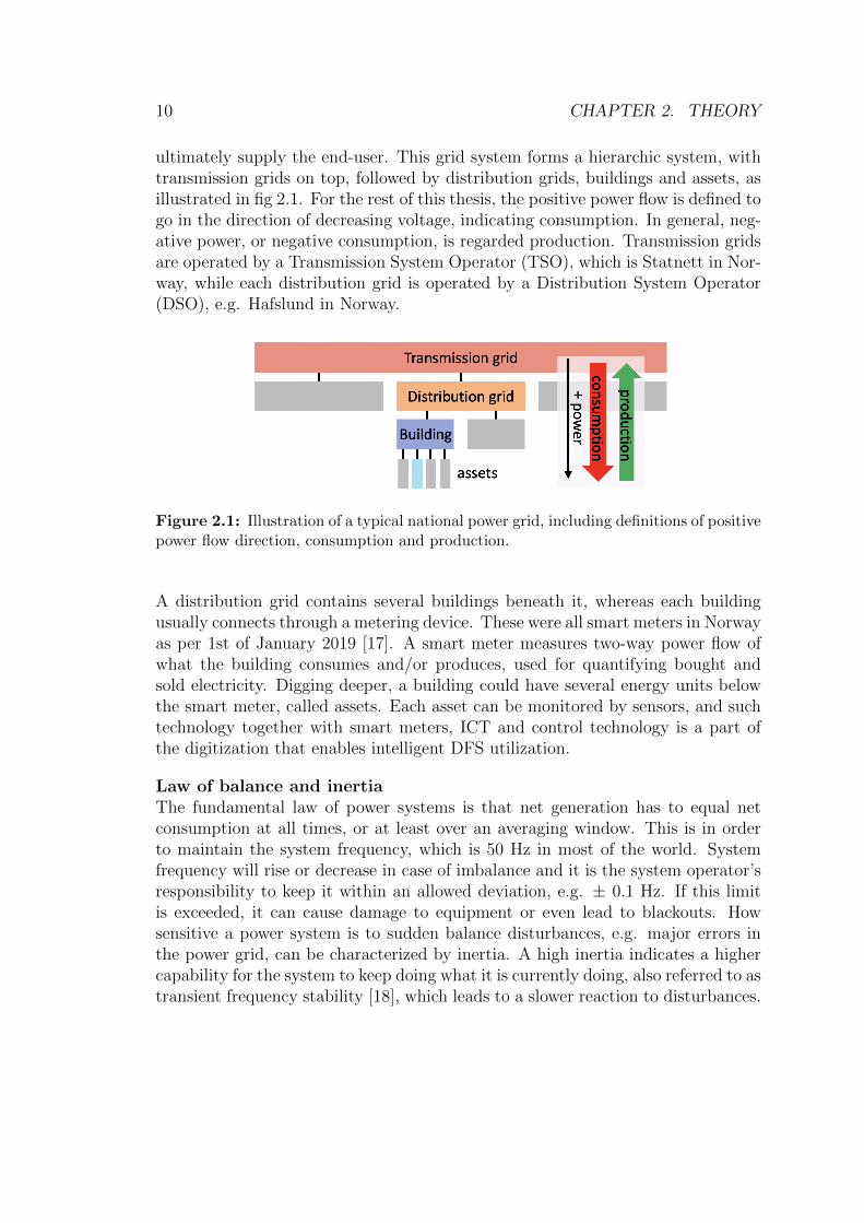
ultimately supply the end-user. This grid system forms a hierarchic system, withtransmission grids on top, followed by distribution grids, buildings and assets, asillustrated in fig 2.1. For the rest of this thesis, the positive power flow is defined togo in the direction of decreasing voltage, indicating consumption. In general, neg-ative power, or negative consumption, is regarded production. Transmission gridsare operated by a Transmission System Operator (TSO), which is Statnett in Nor-way, while each distribution grid is operated by a Distribution System Operator(DSO), e.g. Hafslund in Norway.
Figure 2.1: Illustration of a typical national power grid, including definitions of positivepower flow direction, consumption and production.
A distribution grid contains several buildings beneath it, whereas each buildingusually connects through a metering device. These were all smart meters in Norwayas per 1st of January 2019 [17]. A smart meter measures two-way power flow ofwhat the building consumes and/or produces, used for quantifying bought andsold electricity. Digging deeper, a building could have several energy units belowthe smart meter, called assets. Each asset can be monitored by sensors, and suchtechnology together with smart meters, ICT and control technology is a part ofthe digitization that enables intelligent DFS utilization.
Law of balance and inertiaThe fundamental law of power systems is that net generation has to equal netconsumption at all times, or at least over an averaging window. This is in orderto maintain the system frequency, which is 50 Hz in most of the world. Systemfrequency will rise or decrease in case of imbalance and it is the system operator’sresponsibility to keep it within an allowed deviation, e.g. ± 0.1 Hz. If this limitis exceeded, it can cause damage to equipment or even lead to blackouts. Howsensitive a power system is to sudden balance disturbances, e.g. major errors inthe power grid, can be characterized by inertia. A high inertia indicates a highercapability for the system to keep doing what it is currently doing, also referred to astransient frequency stability [18], which leads to a slower reaction to disturbances.

2.1. ELECTRICAL GRIDS, POWER AND ENERGY 11
Rotating generators, such as hydro or thermal power plants, contribute with inertiato a grid with their momentum, whilst solar power does not. System inertia is goodto have, but even grids with high inertia will eventually face frequency trouble incase of a sustained system imbalance, albeit in a less urgent manner. One of thedownsides of a power system with a high share of VRES is the low inertia and thevariability. Frequency is mostly balanced by the TSO, whereas the DSOs mostlyensure a stable voltage level and a reliable power flow in the LV grid. This hasthus far been handled through good regulation of the HV grid.
2.1.2 Regulating the power balance
Having presented the importance of system balance, there is a logical necessity forevery grid to have mechanisms for regulating the power balance. Such mechanismsare reflected by the flexibility of a grid. Flexibility in a power grid in general can bemany things. It revolves around the inherited ability of a grid to handle unforeseenincidents and imbalances, e.g. sudden ramping. This ability can be possessed byall participants in the grid. Ulbig & Andersson [19] has proposed a definition onoperational flexibility:
”Operational flexibility is the technical ability of a power system unit to modulateelectrical power feed-in to the grid and/or power out-feed from the grid over time.”
High flexibility will cause a grid system to withstand major error events or ramp-ing situations, thus sustaining a stable system balance. Power flexibility is notsomething new, but some may recognize it as regulation power or reserves. How-ever, the relatively new term decentral flexibility has received a lot of focus inlater time. Traditionally, regulation of the system was mostly done by centralizedgenerators, which matched supply against demand. That was usually sufficient foroperation of the entire power grid, but does not withstand the new complexity atdistribution level. Centralized flexibility will still play a major role in the future,however the need for intelligent operation methods at the distribution level withuse of DFS is evident.
The location of flexible sources matters, as electricity needs to be transportedthrough connections with capacity limits. Upgrading infrastructure, such as ca-pacity of transmission cables and transformers, is an effective countermeasure toincrease overall flexibility of a grid. The reason for this is that transmission ca-pacity become higher and the reach of reserves is extended. It adds options forbalancing the grid. A wider group of participants in need of or offering flexibilitygets access to a larger shared pool of flexible reserves. On the downside, upgrading

12 CHAPTER 2. THEORY
infrastructure is expensive, and will furthermore only serve a minority of incidentshaving extreme peaks and not add value to the normal operation. This fact res-ults in a worse capacity factor and is not a very socio-economical and acceptableoperation of the grid.
InterconnectorsThe power infrastructure in Europe has come a long way, and power grids in differ-ent countries are interconnected. The undersea cable NordLink between Norwayand Germany is soon finished, and UK will have cables to both Denmark andNorway by 2022 (Viking Link [20] and North Sea Link [21] respectively). If mostrenewable production can be regarded variable and dependent in weather, suchinterconnectors will increase production capacity, the share of loads and stabil-ity. Better connections will increase the variety of both power source types andgeographical location. As a result, the probability of coexistent production willdecrease which in turn provides stable generation. As a simple example, supposethe northern Germany has a high demand of electricity and that their only powersource, namely wind, is absent. With great interconnection, the demand would becovered by wind outside the British coast, south-German solar power and someFrench nuclear power, all well-balanced by Norwegian hydro power. This describesa scenario where grid management is done at transmission level, from the top.Good connections will be essential in the future, however there are opportunitiesgrowing from the bottom.
Pulsating end-usersThe share of decentralized flexibility grows in speed with the demand-side com-plexity. The future consists of active use and integration of DFS, where the lackof wind power in northern Germany potentially could be covered from flexibleprosumers within northern Germany. Interconnecting transmission capacity seeksto match the supply to the demand. The new and necessary tool is to controldemand and match it against supply with pulsating and dynamic end-users. Theidea is that prosumers regulate power in the grid with innovative integration oftheir flexible prosumption, which is one of the visions of smart grids. Smart gridsprovides a cost-effective alternative to infrastructure upgrades and aims at optim-izing already built capacity. This results in raising the capacity factor of existingtransmission lines and a more efficient operation of the grid.
Many of the traditional regulation mechanisms at transmission level are alreadymarket-based. Energy markets are considered cornerstones for maintaining balancebetween supply and demand in liberalized grid systems. They can be characterizedas intelligent. However, they are restricted to the TSO only and not for thedistribution grids. Distribution grids in past did not need such mechanisms in the

2.1. ELECTRICAL GRIDS, POWER AND ENERGY 13
traditional ”one-way power flow, centralized production, simple end-users”-grid.EU has declared marked-based solution as the standard operation method in thein the future, for distribution grids as well [3]. Before taking a dive into energymarkets and novel flexibility markets, some definitions for flexible power must besettled.
2.1.3 Flexible assets and definitions
All use of the term flexibility will refer to demand-side flexibility for a buildingand its assets. Assets in a building, represented in figure 2.1, are flexible if theyinherit the ability to deviate from their baseline. The baseline must be definedbefore flexibility can be quantified. The baseline is what would be ”the plan” inthe work of Peterson et al. [22]. The baseline is ”the reference” in the work ofConinck & Helsen [14], suggesting it to be the load schedule solution taken froma cost optimization model. FLexible assets must be monitored with sensors andtheir power must be controllable. Some definitions regarding the flexibility of aflexible asset are now presented. The definitions are inspired by Coninck & Helsen[14] and Pinto et al. [23] with some modifications to fit the methodology in thisthesis. Note that power is described in terms of consumption, whereas negativepower, or negative consumption, is production.
• Flexibility: The magnitude of power the asset can deviate with from itsbaseline consumption.
• Baseline consumption: Referring to the originally planned consumptionof an asset for the next H timesteps. This can be a load forecast or anoptimized load schedule.
• Positive flexibility: The ability to increase power consumption relative tothe baseline, thus providing positive flexible power. The upper boundary isdenoted maximum positive flexible power. Upward flexibility is an optionalterm.
• Negative flexibility: The ability of an asset to reduce power consumptionfrom its baseline (or increase production), thus providing negative flexiblepower. The lower boundary is denoted maximum negative flexible power.Downward flexibility is an optional term.
• Flexibility space: The feasible set of allowed choices of flexible power.

14 CHAPTER 2. THEORY
2.2 Energy markets
Energy markets are considered a cornerstone for maintaining balance between sup-ply and demand for power. The shared Nordic power system has several energymarkets to ensure system balance, such as the Day-Ahead (DA) market, Intra-Day (ID) market and reserve markets. In the markets, producers and consumerssell and buy their way into achieving balance, ranging from days to millisecondsbefore operation. These markets represent intelligent regulation systems. The re-serve markets offer close to real-time power regulation with trade and activationof balance reserves. These tools are however currently limited to the transmissionsystem level. With rising complexity on demand-side, there is a need for moreactive, intelligent regulation at distribution level as well. There are new localflexibility markets on the rise with a goal to expand intelligent market-based op-erations into the distribution grids. The goal is to integrate unrealized demandside flexibility for more precise regulation at distribution level. Upgrades of in-frastructure, curtailment of RES generation and shedding high-intensity industryare local options to achieve local system balance. However, smart solutions withsmart grids and ICT, along with connected energy markets will yield higher systemefficiency, stability and reliability, and fill the gap between supply and demand.This enables the transition into a low-carbon society in the future [4].
2.2.1 Current power markets
Day-Ahead market (spot market) is the main market for most of the physicalvolumes that are traded in the physical electricity grid. Before 12:00, all majorparticipants need to place bids and schedules of production and consumption foreach hour the next day [24]. Then, NordPool settles a system clearing price, whichis determined by a trade-off between demand and supply. Individual area pricesbased on bottlenecks will add or subtract to the system price for each affected area[25]. They apply to large regional areas, hence do not take local grid problems intoaccount. The ID market is a power trading platform which is closer to the real-time operation than the DA market. Participants left in personal imbalance afterthe DA market closure, can achieve balance through ID market trading. The IDmarket closes an hour before operation time [24]. Further imbalances that occurin the hour prior to the operation time are settled in the reserve/balance markets.Here, participants with flexibility offer regulation power that can be activated fromwithin 15 minutes or even seconds before operation time. Hence, reserve marketsare essential for securing the temporarily balance between supply and demand. The
2.2. ENERGY MARKETS 15
reserve markets can be divided further into primary market, secondary and tertiarymarkets, in which reserves must be activated automatically within seconds ormanually within minutes or 15 minutes respectively [24]. Participants outside themarket will be able to offer their reserves and be remunerated for their regulationservices [26]. Reserve markets are merely platforms developed for TSOs with toolsto tackle predicted and unforeseen critical grid events.
The emerging complexity at demand-side cause local problems at distribution level,which must be addressed by the DSO. The current market design with DA, IDand reserve markets are not aimed at operating distribution grids. In addition,the current, intelligent market-based operation methods at transmission level aresimply not granular enough to solve the arising local problems[12]. To solve localcongestions and other management issues related to the distribution grid requiremore active approaches from the DSO [8]. Local problems must be solved locally.
2.2.2 Mechanisms for solving emerging local problems
Innovative operation methods at distribution level is a highly active research field.There are alternatives which shows that deploying novel local flexibility marketsis not the only solution. There are various ways to utilize DFS. USA as an ex-ample has had many years of experience with distribution grid operation methods.There is demand response management (DRM) which aim at controlling demand-side consumption. Two subcategories of DRM would be direct control or indirectcontrol, both being so-called top-bottom approaches. The first, direct control givesthe DSO full access to control a flexible asset at demand-side, even shed its con-sumption, under given constraints. An example of such a mechanism is to includea contract module for dispatchable consumption, where the end-user is remuner-ated by a DSO that gain full access to shred/control their asset. Direct DRMcan be implemented in flexibility market platforms as well. Assessing short-termflexibility is important for direct DRM as well, as it will give the DSO knowledgeon how much flexible power they have dispatched. The second sub category ofDRM, indirect or intelligent control, nudge the end-user to change the consump-tion behaviour by means of price signals. Price signals may be added as tariffmodules in the electricity contract between the DSO and building. A building isgiven incentives to actively exploit price variations, through a cost-optimized loadcontrol system of their DFS. The indirect method has some limitations because itrequires planning and predictions of grid problems, at least a day but often weeksin advance. Indirect DRM may therefore have trouble to respond to more urgentgrid events. In addition, price signals may not give sufficient incentives for end-

16 CHAPTER 2. THEORY
users to invest in added flexibility in their assets. It is important to find solutionswhich also promotes more DFS, because that is needed in the future. It is believedthat flexibility markets will add value to DFS and flourish it.
EU has declared market-based congestion management as default for future real-time operations. Their reasoning is that, the alternative apporach, which is admin-istrative and cost-based where participants are obliged to help and remuneratedfor costs and forgone profits, is difficult to apply for DFS. The estimates that areneeded for costs and profits, for a vast amount of prosumers at demand-side, is toocomplex to get accurate and highly case-specific [9]. Such a top-bottom approachis hence favoured for the bottom-up approach where the slogan is to let the marketdo the job.
Local flexibility marketsFrom now on, local flexibility markets are the focus. When presenting the conceptof novel local flexibility markets, the reader may notice it draws parallels to reservemarkets. Flexible markets aim at extending intelligent marked-based operationmethods all the way into the distribution grid and end-users, which now has smartcontrol opportunities due to smart metering, IoT and digitization. The idea is thatbuildings bid their flexible power to the flexibility market platform. Here, DSOsand others who might need to buy local flexibility can activate that flexible power.In some cases, larger regions and even a TSO might need such flexibility as well,as with the example on northern Germany lacking wind production. DFS reservesare however small in volume, which could be unpractical on the market. Therefore,some smart grid companies specialize in aggregating small flexible volumes intobigger ones, e.g. a whole neighbourhood. A smart grid company possessing such arole is called an aggregator. Aggregator is also a term used in general for a smartgrid company that assess and trade a building’s flexibility on markets.
All the pilots and initiatives in the field of local flexibility markets are results ofthe rising complexity at distribution level. Local granularity is a key word. Asmentioned, reserve markets are limited to the transmission level, in addition to berestricted to major flexible volumes. DFS has a precise location in the distributiongrid, which is important. Active use of DFS provide finer granularity for DSOs tosolve local problems.
Initiatives in EuropeThere are many initiatives in Europe that investigate flexibility markets as a toolfor local grid operations. Some are pilots, however some have already been de-ployed at national level, such as GOPACS in the Netherlands, which is alreadyproved valuable. Radecke, 2019 gives a nice overview of pilots and working cases

2.2. ENERGY MARKETS 17
of market-based DFS solutions in Europe [9]. Many of the proposed markets alsocreate incentives to utilize unused potential DFS. Some examples of pilots andoperative flexibility markets in Europe are
• NODES (universal, pilots in Germany, Norway and soon U.K.)
• GOPACS (operative in the Netherlands)
• Bne Flexmarkt (Germany)
• SINTEG (multiple projects in Germany)
• Piclo (U.K.)
In the future, there could probably be many more market operators in competitionwith each other. In addition, each scenario probably requires a specialized marketdesign in order to be optimal for the case. However, the general concept of aflexibility market platform seems to be set. NODES, one of the many solutionsfor flexibility markets, is used further as a point of reference for the formalitiesaround flexibility market design, operation and flexibility bids.
2.2.3 NODES - A fully integrated marketplace for flexib-ility
NODES emerged as an initiative by NordPool and Agder Energi to address theconcurrent challenges that impact distribution grids. The information in this sec-tion is based on a NODES white-paper [12], unless other references are cited.
NODES is ”an universal platform for local, flexible electricity markets with featuresallowing for connecting to other markets”. It aims to increase the use of decentral-ized flexibility, as the European ID and DA markets alone do not provide sufficientgranularity for local congestion management nor allow integration of DFS. It alsoaims at increasing the amount of available DFS by adding value to it. A NODESplatform puts local flexibility as products on a shelf - up for take for buyers.The product, or a flexibility bid, is tagged with a location and includes a price, abaseline, the amount of offered flexible power and a duration.
The market-design
The design of the NODES marketplace and its market players is illustrated in

18 CHAPTER 2. THEORY
Figure 2.2: NODES marketplace and its various market players, mainly the flexibilityproviders on the right, and the ones who would need the flexibility on the left. Graphicfrom NODES whitepaper [12].
figure 2.2. The platform, as it is universal and meant to fit many scenarios, mustbe tailored to fit each unique scenario, in close cooperation with some thoughtmarket players. Fundamentally, the platform needs someone who can offer andsomeone who needs flexibility, e.g. prosumers and DSOs/TSOs respectively. Aflexibility provider can be a smart grid company (or aggregator), with access tothe flexible assets of a prosumer. They create a flexibility product and bid it intothe platform. The product can then be bought by either of the flexibility buyers.If bought and activated, the flexible power should be dispatched accordingly bythe provider. It could be positive of negative flexibility. Verification of deliveredflexibility happens through the same platform.
The relevant market players included in the scope of this thesis are the DSO,aggregator and a prosumer. These are shown as circles in the figure. A setup withthese market players is relevant for the use-case in this thesis, with the prosumerbeing a medium-sized industrial building possessing flexible assets. A pilotingNODES platform often start out this simple, before it eventually incorporatesmore market players and extend the platform, in everyone’s interest.
The aggregator will be important to bring DFS to the market. Aggregating smal-ler DFS volumes makes DFS more accessible. In addition, the aggregator will beresponsible for flexibility estimation, bidding to the NODES market platform, dis-patching of activated flexibility and verifying the delivered flexible power. NODES

2.2. ENERGY MARKETS 19
will be operating the market platform and offer an Application Programming In-terface (API) for trading. Both the flexibility buyer and the provider must be ableto communicate with the API.
Advantages of NODESThe NODES market platform, as well as other similar platforms, serves multiplebenefits. The first big advantage is that anticipated costly grid investments canbe avoided. Secondly, local congestions can be solved more precisely. Althoughmany of the new consumption assets impose problems, such as EVs, high-intensiveappliances and demand-side RES, they also provide possibilities which can be takeninto full advantage by flexibility aggregators and NODES.
NODES, in addition to other flexibility markets, claim to give incentives for build-ings to promote and make use their potential flexibility, by giving their flexibilityand increased value. Suppose that a building uses DFS for their internal use toexploit price variations. With NODES in addition, the building has more optionsto make profit from their flexibility. In addition, NODES platform want to expandlocal flexibility products into the reach of TSOs and other buyers that might needdecentralized flexibility, thus further raising the value of DFS. A broader set ofbuyers means a higher value for the DFS. Different buyers also often need flexib-ility at different times. If the need would be coincidental, the flexibility will beused where it is of most value - ideally where it is most needed. Many possibilitiesfor making profit of DFS will make it lucrative for prosumers to further realizeunused, potential flexibility.
Another important feature of the NODES market platform is that it can connectto other markets in the future, such as the ID-, DA- and reserve markets. Thatwould mean that a flexibility provider can access reserve markets more easily,so that they may buy back some balance. Suppose a flexibility provider is left inimbalance due to activation of its flexibility. The idea is that they should be able toautomatically re-balance their portfolio through cheaper trading in other marketsand still make profit. NODES, as an operator of the market, will make sure thatall bids and activations do not cause new troubles elsewhere in the grid. All inall, NODES do not aim to replace any excising markets, but merely complementthem to fully sustain a flexible smart grid all the way to the prosumers.
Working use-casesThe market-design of NODES is highly adaptable to different situations, locationsand conditions to resolve a diversity of cases. The platform has already provento be beneficial in real use-cases deployment both in Norway and Germany [27].In Germany, NODES is used to relief an overloaded 110kV line, using flexibility

20 CHAPTER 2. THEORY
that is localized and exploited on the LV grid. In Norway, a potential overloadedtransformer has postponed new investments, thanks to the NODES platform usingflexible resources beneath the transformer.
Market flexibility productsMost of the market-based flexibility platform initiatives in Europe, including NODES,define a flexibility product to be the deviation from the baseline, either by consum-ing more or less than what was planned. Some have remuneration by availability,where flexibility providers get paid to have their flexibility at standby, similar todirect DRM. Others have remuneration by activation, where providers get paidper single flexibility activation. NODES and a few others, offer both remunerationmethods [9].
NODES does not provide a specific product shape. Bids can look different fordifferent flexibility buyers and for different use-cases. However, NODES suggestsa modular design of a flexibility product. NODES support a contract to offer directcontrol of flexible asset, however the scope of this thesis focus on the competitiveflexibility market platform. A product on this platform must at least consist ofa baseline, offered flexible power, a time indicator, a price and the grid locationof the prosumer. Resolution of the bid offers can be adjusted, but 15 minuteresolution is often used. The focus of the work in this thesis will be on estimatingthe baseline and offered flexible power.
The forecasted baseline and the flexible power are constituted of several timeslots,denoted h. They indicate different times in the bidding horizon H. The bids ineach timeslot could have several bid shapes. Some traditional bid shapes in thetraditional energy markets can be linear, stepwise or block-based. A block bidconsist of a constant volume and price, allowing for no deviation (also referred toas full activation), whereas a step-wise bid consists of multiple block bids. A linearbid consist of a continuous range of flexible power that can be bought.
2.3 Modelling
This section will present theory for timeseries, sequence forecasting models andespecially recurrent neural networks. It will focus on practical implementationand application of RNNs for timeseries forecasting in Python.
2.3. MODELLING 21
2.3.1 Timeseries modelling
SequencesA sequence, including timeseries, is data that are structured in a certain or-der, where the order matters. Moreover, a timeseries is data structured alonga time axis, where a value is most likely to depend on prior values and to af-fect successive values. Timeseries can be represented mathematically as ~x =x0, x1, . . . , xt, . . . , xT−1, xT starting at 0 in order to be Python index friendly. xt
represent a value of the sequence at timestep t, for a total of T timesteps. If thereare multiple timeseries in the dataset, they can be distinct by a subscript, startingat 0 and counting, ~xt0, ~x
t1, . . . , ~x
ti, . . . , ~x
tn where n is total number of timeseries. Such
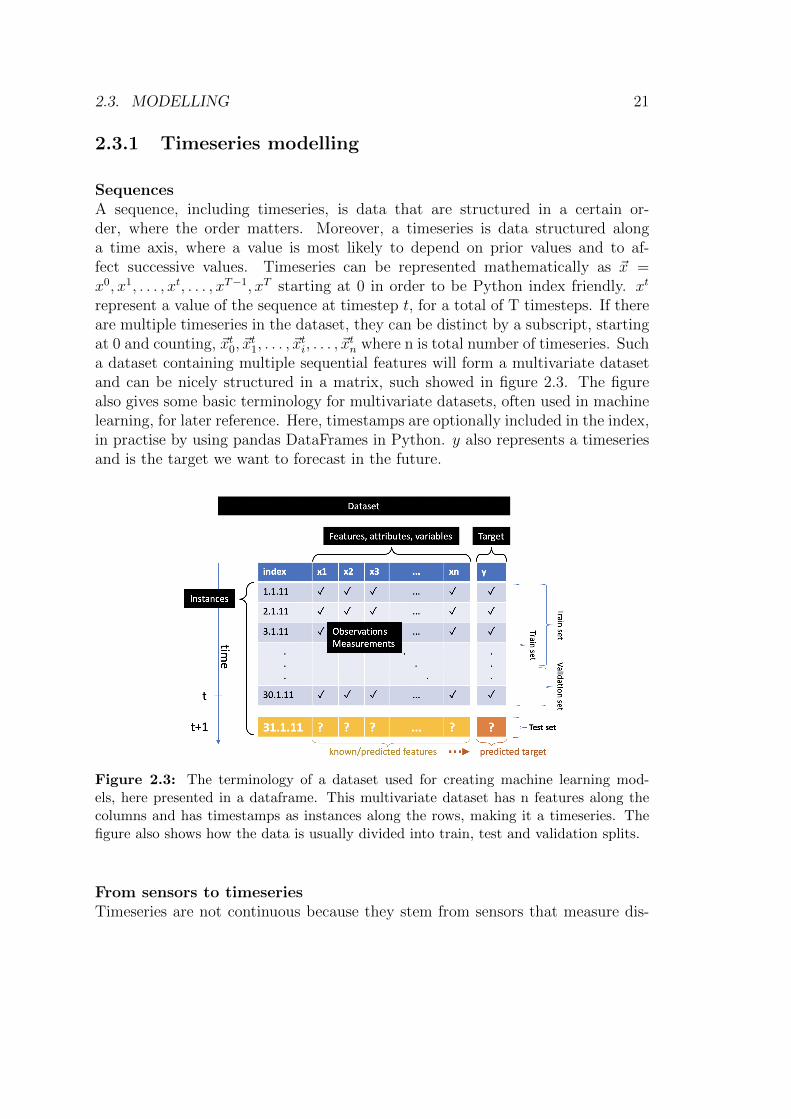
a dataset containing multiple sequential features will form a multivariate datasetand can be nicely structured in a matrix, such showed in figure 2.3. The figurealso gives some basic terminology for multivariate datasets, often used in machinelearning, for later reference. Here, timestamps are optionally included in the index,in practise by using pandas DataFrames in Python. y also represents a timeseriesand is the target we want to forecast in the future.
Figure 2.3: The terminology of a dataset used for creating machine learning mod-els, here presented in a dataframe. This multivariate dataset has n features along thecolumns and has timestamps as instances along the rows, making it a timeseries. Thefigure also shows how the data is usually divided into train, test and validation splits.
From sensors to timeseriesTimeseries are not continuous because they stem from sensors that measure dis-

22 CHAPTER 2. THEORY
crete signals. How well they represent a continuous measurement depends on thetemporal resolution, ∆t, of the measured timeseries. Power is originally an in-stantaneous value, measured in W or kW. If power is measured each minute, thesemeasurements could either be momentaneous measurements at each minute or thesensor could be sophisticated enough to provide an averaged value over the minute.Either way, the power is not momentaneous as it is assumed to represent a wholeminute. The unit becomes kWh/h, as in an averaged power.
Downsampling is an expression that means to resample the temporal resolution ofa timeseries to a lower resolution. For example, a timeseries of 1 minute resolutioncan be downsampled to 15 minute resolution. That is done by taking the averageof each of the 15 1-minute measurements.
Sequence forecastingSequence forecasting, or sequence predictions, can be done by the means of variousmethods. ARIMA models is a well-established and widely used timeseries forecast-ing method. Another option is to make use of a multiple linear regression method(MLR) for forecasting [16]. More novel methods are deep learning methods in thefield of machine learning (ML), such as neural networks, where especially recurrentneural networks (RNNs) are specifically designed for sequences.
According to Shi et al [28], RNN models have been shown to perform better atload forecasts compared to state-of-the-art techniques of ARIMA and SVM models.Others may mention they are equally good, which conforms with the well-knownfact that there is no outstanding ML model to each unique forecasting problem.The promising potential of RNNs and the fact that it is a quite novel approachfor forecasting load is the motivation for further exploring RNNs to perform theforecasting tasks in this thesis. The next sections present the process of buildingmachine learning models, followed by RNN theory.
2.3.2 General machine learning
ML is a field of data science, which differ from traditional programming algorithmsin one specific way. Instead of making rules to use on input data in the quest offinding answers, ML aims at using data and answers, in order to learn the rules.These rules can later be used to forecast future values.
The literature usually divide ML into three main subfields: supervised learning,unsupervised learning and reinforcement learning. Supervised learning is the relev-ant subfield for the work in this thesis, e.g. for making load forecasts. It describes
2.3. MODELLING 23
modelling machine learning models that are trained on datasets where the targetis known, in order to predict future targets.
Supervised learningOne of the main goals of supervised learning is to learn patterns in a historicdataset such that we can make correct predictions and decisions in the future.To learn these patterns, the algorithm needs to have features and the solution(target) as input. It learns trends between the feature dataset and the target, refx1, x2, ..., xn and y respectively in figure 2.3. Once the model is correctly trained,predictions can be made for the test set target, or unknown target, e.g. a futuretimestep. The features in the test set must be known in order to predict the finaltarget.
There are several models in the field of supervised learning, such as multi-linearregression (MLR), logistic regression, artificial neural networks (ANN), recurrentneural networks (RNN), decision trees, random forests, etc.
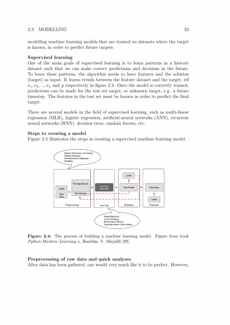
Steps to creating a modelFigure 2.4 illustrates the steps in creating a supervised machine learning model.
Figure 2.4: The process of building a machine learning model. Figure from bookPython Machine Learning, s. Raschka, V. Mirjalili [29].
Preprocessing of raw data and quick analysesAfter data has been gathered, one would very much like it to be perfect. However,
24 CHAPTER 2. THEORY
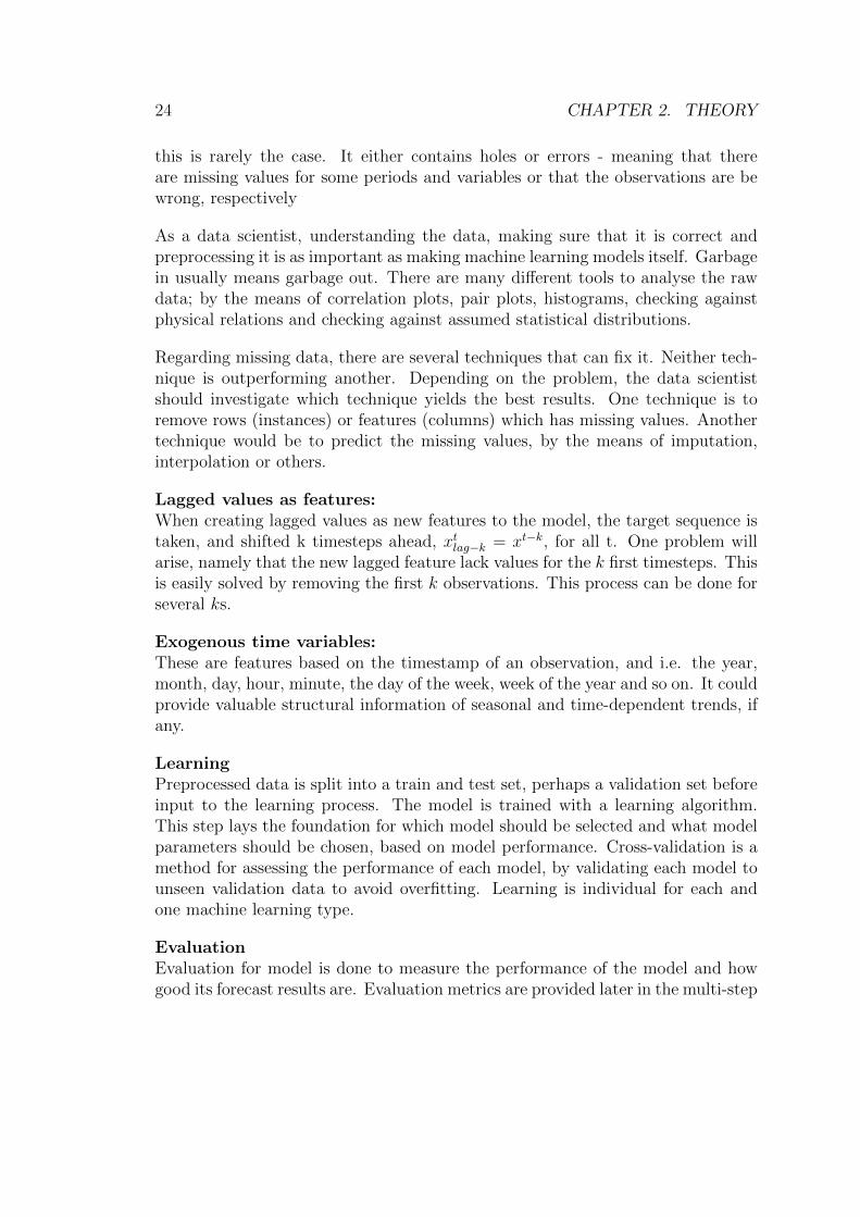
this is rarely the case. It either contains holes or errors - meaning that thereare missing values for some periods and variables or that the observations are bewrong, respectively
As a data scientist, understanding the data, making sure that it is correct andpreprocessing it is as important as making machine learning models itself. Garbagein usually means garbage out. There are many different tools to analyse the rawdata; by the means of correlation plots, pair plots, histograms, checking againstphysical relations and checking against assumed statistical distributions.
Regarding missing data, there are several techniques that can fix it. Neither tech-nique is outperforming another. Depending on the problem, the data scientistshould investigate which technique yields the best results. One technique is toremove rows (instances) or features (columns) which has missing values. Anothertechnique would be to predict the missing values, by the means of imputation,interpolation or others.
Lagged values as features:When creating lagged values as new features to the model, the target sequence istaken, and shifted k timesteps ahead, xtlag−k = xt−k, for all t. One problem willarise, namely that the new lagged feature lack values for the k first timesteps. Thisis easily solved by removing the first k observations. This process can be done forseveral ks.
Exogenous time variables:These are features based on the timestamp of an observation, and i.e. the year,month, day, hour, minute, the day of the week, week of the year and so on. It couldprovide valuable structural information of seasonal and time-dependent trends, ifany.
LearningPreprocessed data is split into a train and test set, perhaps a validation set beforeinput to the learning process. The model is trained with a learning algorithm.This step lays the foundation for which model should be selected and what modelparameters should be chosen, based on model performance. Cross-validation is amethod for assessing the performance of each model, by validating each model tounseen validation data to avoid overfitting. Learning is individual for each andone machine learning type.
EvaluationEvaluation for model is done to measure the performance of the model and howgood its forecast results are. Evaluation metrics are provided later in the multi-step

2.3. MODELLING 25
forecasts section.
OverfittingOverfitting is the case when a machine learning model is not generalized enoughto perform well on new unseen data. This happens when a model is trained verywell to training data, often prone to its noise, but results in bad forecasts for testdata.
Final predictionThis is the step for real-time forecasting. The model is fully trained and in oper-ation. When new data become available, the model could be retrained with thenew observations.
2.3.3 Recurrent neural networks
This section presents theory for RNN with focus and practical application. RNNscan be implemented in Python with the packages Keras and TensorFlow. Thetheory includes a high-level explanation of model architecture and the differentparameters of the model in addition to how the training and test data should beset up for training and forecasting.
All of the theory on recurrent neural networks in this subsection is based on thetwo books Python Machine Learning by S. Raschka and M. Vahid [29] and DeepLearning with Python by F. Chollet [30], unless else is mentioned.
Recurrent neural networks (RNNs) are widely used in many sequence applications,such as:
• classification of documents or timeseries, e.g. determine topics or authors ofbooks
• comparison of timeseries, e.g. investigate the relations
• sequence-to-sequence learning, much used in language translation
• analysing sentiments, e.g. classify the mood of a text or music (happy orsad)
• timeseries forecasting, e.g. predict electricity consumption
RNNs can be quite complex with advanced mathematical relations. The process
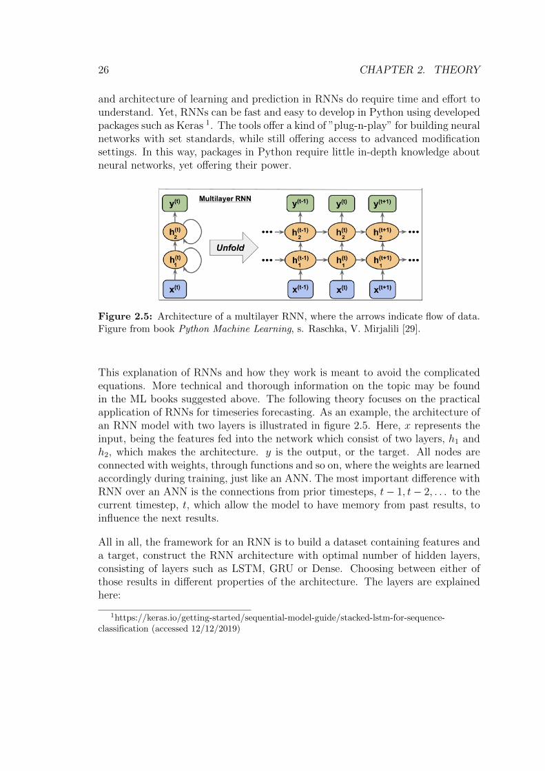
26 CHAPTER 2. THEORY
and architecture of learning and prediction in RNNs do require time and effort tounderstand. Yet, RNNs can be fast and easy to develop in Python using developedpackages such as Keras 1. The tools offer a kind of ”plug-n-play” for building neuralnetworks with set standards, while still offering access to advanced modificationsettings. In this way, packages in Python require little in-depth knowledge aboutneural networks, yet offering their power.
Figure 2.5: Architecture of a multilayer RNN, where the arrows indicate flow of data.Figure from book Python Machine Learning, s. Raschka, V. Mirjalili [29].
This explanation of RNNs and how they work is meant to avoid the complicatedequations. More technical and thorough information on the topic may be foundin the ML books suggested above. The following theory focuses on the practicalapplication of RNNs for timeseries forecasting. As an example, the architecture ofan RNN model with two layers is illustrated in figure 2.5. Here, x represents theinput, being the features fed into the network which consist of two layers, h1 andh2, which makes the architecture. y is the output, or the target. All nodes areconnected with weights, through functions and so on, where the weights are learnedaccordingly during training, just like an ANN. The most important difference withRNN over an ANN is the connections from prior timesteps, t− 1, t− 2, . . . to thecurrent timestep, t, which allow the model to have memory from past results, toinfluence the next results.
All in all, the framework for an RNN is to build a dataset containing features anda target, construct the RNN architecture with optimal number of hidden layers,consisting of layers such as LSTM, GRU or Dense. Choosing between either ofthose results in different properties of the architecture. The layers are explainedhere:
1https://keras.io/getting-started/sequential-model-guide/stacked-lstm-for-sequence-classification (accessed 12/12/2019)

2.3. MODELLING 27
LSTM (Long-short-term-memory) unit: Type of node unit, designed to over-come the vanishing gradient problem. It designed to carry information across manytimesteps and preventing older signals to completely vanish, hence it contributes tothe network by giving it a longer memory of the past. It is complex and combinesdifferent functions with different input and output combinations.
GRU (Gate Recurrent Units): A bit simpler architecture than LSTM, andis more computational efficient, due to fewer parameters. GRU layers may havebetter performance on smaller datasets.
Dense layer: Ultimately takes in all inputs from the previous layers and outputsa forecast, which is either a value or an array of values in the case of a multi-output.
HyperparametersIn addition to building the architecture, there are hyperparameters such as batchsize, number of epochs to train on and learning rate that influence model per-formance. The construction of data is of much importance as well. As with muchelse in the field of machine learning, there is no superior model to all problems,regarding choice of model, its architecture, its hyperparameters, data preparationetc. Therefore, finding a good model is experimentation itself and unique to eachproblem.
OptimizersAn optimizer is needed for training an RNN model and needed for finding optimalweights of a model during learning. Various optimizers can be chosen, such asadam and RMSprop. A brief introduction to optimization, with a comparisonbetween adam and RMSprop can be found on the webpage in the footnote 2.RMSprop is a simpler version of adam. Adam has been most used in the thesisand the standard optimizer for RNNs in Keras for Python 3. More on the adamoptimizer can be read in the article by Ruder [31]. Optimizers affect the successof the learning process and whether or not the optimal solution is found. It alsoaffects the time of the learning.
Preparing the dataset for RNN trainingDuring training of an RNN model in Python, the Keras model expects the traininginput data to have the following 3-dimensional shape:[
samples, timesteps, features]
This 3-dimensional matrix must be generated from the basis 2-dimensional dataset,
2https://blog.paperspace.com/intro-to-optimization-momentum-rmsprop-adam/ (accessed12/12/2019)
3https://keras.io/optimizers/ (accessed 12/12/2019)

28 CHAPTER 2. THEORY
like the one shown in figure 2.3, which has the shape[
samples, features]
. Thebasis 2-dimensional dataset represents the whole training and test data foundationwhich has been prepared and preprocessed. When the RNN model is trained inKeras, the timesteps dimension is introduced. This dimension represent how longthe memory of the RNN network should be.
During training, many smaller batches of the training data, having the 3-dimensionalshape, is fed into the network. Each batch generates a line of predictions in thetrain set. The amount of samples is set by the sequence length parameter and theamount of timesteps to form is set by the N lOOKBACK parameter.
As an example, a batch with input shape [1100, 7, 1] means that a training batch of1100 observations from the training set is chosen, in a kept sequential order, is fedinto the training network. It has 1 feature in the training set, e.g. the consumption.7 timesteps mean that the model shall use all 7 steps in the foundation for learningand predicting.
Each training batch fed into the learning algorithms, results in a forecast beingmade. This is compared against the true value. Based on this comparison, thelearnable weights of the RNN model are adjusted in order to improve the nextforecasts, through backpropagation.
When making a prediction for the test set, Keras wants only on batch with the3-dimension shape. For final prediction, sample=1 and the input data shape isnamely [1, timesteps, features]. The output forecast will be [1, 1]. If the modelis created so to output a multi-output forecast of H steps, the shape of this inputmatrix would have to be [H, timesteps, features]. It will then output an arrayof forecasted values of dimension [H, 1]. This array is a forecast for the forecasttimestep made for all timesteps, t+ 1∀t ∈ {testset}.
In order to create many batches for iterative learning for the whole train set and tofinally make predictions for the whole test set, various batch-generators are used.In the work of this thesis, a batch generator has been borrowed from an open Gitrepository 4, and the others are included in Keras, named TimeseriesGenerator.
Scaling:In order to improve model performance, RNNs benefit from having data scaledto the range between 0 and 1 or standardized. This can be done using MinMax-Scaler() provided by the sklearn package for Python.
4https://github.com/Hvass-Labs/TensorFlow-Tutorials/blob/master/23 Time-Series-Prediction.ipynb

2.3. MODELLING 29
Encoding categorical features to dummies:Dummies are needed to avoid letting the model think that a Sunday (value 6)has a higher value than Monday (value 0), and such, dummies is needed to bemade, by constructing a new feature for all of the values in the old feature, i.e.Monday,...,Sunday are the new dummy features which have values 0 or 1, wherea 1 assigns this feature to the given observation. Dummy creation can be doneeasily with pandas in Python.
2.3.4 Multi-step forecasting
As to this point, models were thought to predict only one timestep ahead. Thegoal is to make forecasts for multiple successive steps ahead. That means forecastseach of the forecast timesteps, t+1, t+2, ..., t+H, that we would like to forecast.A summary of various strategies for multi-step time series forecasting is given byBontempi et al. [32] and reviewed here:
1 Direct Multi-step Forecast Strategy: One unique model is made for eachforecast timestep.
2 Recursive Multi-step Forecast Strategy: The same one-step model is usedrecursively, where the prediction for the prior time step is used to predictthe next one.
3 Direct-Recursive Hybrid Multi-Step Forecast Strategies: Combines the twoabove strategies, e.g. creating individual models for each timestep ahead,where each model also uses predictions from models for prior timesteps.This may help overcome limitations of (1) and (2).
4 Multiple Output Forecast Strategy: Only one model is created and trained tomake a forecast for all timesteps at once.
(1) Direct Multi-step Forecast StrategyFor the work in this thesis, only the direct strategy has been implemented properly.For this strategy, multiple models are created in order to specialize on each of thelead timesteps that are to be forecasted, h. This happens relatively straightfor-ward. Many one-step models are used. Each model will use the same train set, X.There will however be different targets array per model, that are shifted one andone timestep from each other in lead time.

30 CHAPTER 2. THEORY
Evaluating multi-step forecastsThese evaluation metrics are used on regression problems, which is relevant for thisthesis. The most common ones are Mean Absolute Error (MAE), Mean AbsolutePercentage Error (MAPE), Mean Square Error( MSE), Root Mean Square Error(RMSE) and R Squared. The ones used in this thesis are mathematically expressedas following:
MAE =n∑
i=1
|yi − yi|n
(2.1)
MSE =∑
i = 1n (yi − yi)2
n(2.2)
A lower MSE or MAE value is a better score. Computing the score for each fore-casted timestep is often helpful. It gives valuable information on how a modelperformed on each seperate forecasted timestep. A summarized score can be com-puted as the average score across all forecasted steps.
2.3.5 Techniques for fighting overfitting
Some popular techniques to fight overfitting in neural nets are as following.
Validation data:During each training iteration, the model performance can be checked againstunseen data, named validation set, as seen in figure e2.3. Validating the trainingon an unseen validation set rather than the train set, will cause to model to nottry overfit parameters for the train set.
Early stopping:This technique is applied during model training. It monitors the validation scoreof each epoch, and if the validation score has not improved during a number ofsuccessive training epochs, called patience, it stops the training. Early stopping isoften used together with model checkpoints, which stores the latest best model.Using early stopping and model checkpoint enables us to reload the best modelfrom the point it stopped improving with respect to validation loss.
Dropout:Dropout is a technique to randomly drop a certain share of units (and learnableweights) in a layer and in such way ”thinning” the neural network. Their aimis to prevent units to be prone to overfitting. In Keras, the Dropout method isapplied by adding a Dropout layer after a layer that shall be thinned, e.g. after aLSTM layer. Correspondingly, a share of some random units will be dropped by

2.3. MODELLING 31
setting their unit output weights to 0, thus forcing use of other weights. The Dro-pout technique has in one case shown clear improvement over other regularizationtechniques [33].
Some techniques work better than others in certain cases, and sometimes the bestresult comes from a combination of them. Various techniques should be used withprudence in order to find the optimal method for the specific problem.

32 CHAPTER 2. THEORY
Chapter 3
Preliminary methodology forassessing short-term demand-sideflexibility
This chapter explains the concept of the developed methodology for assessingshort-term flexibility for an asset. It starts with a light explanation to let thereader get familiar with the overall methodology. Then, the methodology and itsconstitutional stages is thoroughly explained for a generic asset, including a bidevent line example to demonstrate its uaage during time advancement. The lastpart involves more specific descriptions on how the methodology is thought to beimplemented for each of the five chosen flexible assets that were presented in table1.1.
33
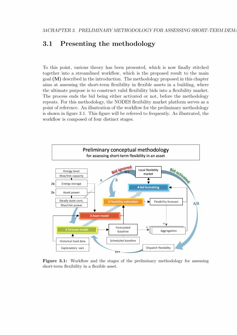
34CHAPTER 3. PRELIMINARYMETHODOLOGY FORASSESSING SHORT-TERMDEMAND-SIDE FLEXIBILITY
3.1 Presenting the methodology
To this point, various theory has been presented, which is now finally stitchedtogether into a streamlined workflow, which is the proposed result to the maingoal (M) described in the introduction. The methodology proposed in this chapteraims at assessing the short-term flexibility in flexible assets in a building, wherethe ultimate purpose is to construct valid flexibility bids into a flexibility market.The process ends the bid being either activated or not, before the methodologyrepeats. For this methodology, the NODES flexibility market platform serves as apoint of reference. An illustration of the workflow for the preliminary methodologyis shown in figure 3.1. This figure will be referred to frequently. As illustrated, theworkflow is composed of four distinct stages.
Figure 3.1: Workflow and the stages of the preliminary methodology for assessingshort-term flexibility in a flexible asset.

3.1. PRESENTING THE METHODOLOGY 35
A brief description of the stages
A generic, high-level description of the preliminary methodology will now bepresented, before each stage is explained in detail later. The methodology involvesthe use of timeseries data, forecasting models such as RNNs, physical models ofthe assets, object-oriented asset modelling in Python and bid formulations.
As we will see, and as previously defined, the flexibility is based on the baselineconsumption, and therefore a load forecast model (stage 1) is the first stage inmaking flexibility estimates. The load forecast model output a forecasted baseline.In some exceptions, an asset does not require a complicated forecasting model inorder to know its future baseline. An example is an optimized load schedule forbattery, where the forecasted baseline is simply a schedule or the plan. In othercases, the future baseline must be forecasted. The electrical consumption is inmany occasions influenced by external parameters, e.g. temperature or buildingactivity. A load forecast model uses historical timeseries data as input, in additionto any explanatory parameters which may improve predictive power of the forecastmodel. The goal is a model with high predictive accuracy for unseen data points,especially the first H timesteps in the bidding horizon, e.g. H = 6. A forecastmodel is developed and once a good model has been chosen, it outputs a forecasted
baseline, ~y or ~b .
Flexibility itself lies all in the asset and its characteristics, thus calling for an assetmodel (stage 2) . The asset has either flexible consumption, generation, storageor a combination of the three. In addition to a baseline forecast provided fromstage 1, it is necessary to investigate and quantify the inherited properties andconstraints of the asset regarding its power (2a) and energy storage (2b). Themaximum, minimum and steady state power, Pmax, Pmin and Pcons,SS respectively,are important for determining the magnitude of flexible power. Energy storageconstraints puts limits to the available flexibility regarding time and volume. Pro-vision of an energy level estimate, SoC, and the energy capacity limits, Emin andEmax, are necessary. This methodology does not provide a method to quantifysuch asset parameters, which may be a complex task to do. The asset parametersare nevertheless crucial input for the asset model in the task of estimating flexib-ility. A State-of-Charge (SoC) modelling framework is used to physically model aflexible asset with its parameters, power flows and states. Implementation is doneby means of object-orientated programming in Python.
Until this point, all necessary values are provided in order to calculate flexibilityestimates (stage 3). The forecasted baseline is input to the asset model and

36CHAPTER 3. PRELIMINARYMETHODOLOGY FORASSESSING SHORT-TERMDEMAND-SIDE FLEXIBILITY
combined with the asset parameters, in order to calculate of the flexibility forecast.A simple, yet effective way to assess the complete range of available flexibility isto calculate the upper and lower flexibility limits, denoted maximum positive andmaximum negative flexibility respectively. When this stage is done, the maximum
positive and negative flexibility, Fp
(h)and Fn
(h)respectively, is estimated for each
timestep in the bidding horizon. Simulation of the energy content levels reveal ifthe energy capacity limits are reached when activating Fn or Fp. The estimatedflexibility is therefore shredded accordingly, if energy storage limits are reached.This stage also visualizes the flexibility estimates and the possible energy storagetrajectories different choices of flexibility activations.
After available flexibility has been estimated, the next process is to format aflexibility bid (stage 4) to be offered on the market. Formulation of a bidhas many alternatives and should be developed with close cooperation with therespective participants. One choice is for the DSO to fully activate all negativeflexibility at once, which will probably completely discharge the assets energystorage. Another choice could be that the DSO activates just a portion of a bid,and thereby extending the duration. Another choice is for the building itself towithhold their flexibility fully or by parts, which they can freely do, for exampleif they believe the revenue is higher a couple of hours later. Since there are manyopportunities, the bid formulation stage must be done with prudence in orderto find the optimal solution for all parts. The bi-directional arrow between bidformatting and the Local flexibility market indicate that the flexibility buyer cangive feedback to the aggregator regarding the bids.
When a flexibility product has been offered to the market platform, there are twopossible outcomes. An ignored bid means that the bid is not bought by anyflexibility buyer and the building must prepare new flexibility estimates for the nextbidding period. t++ symbolize incrementation of time, indicating advancementto the next bidding period. Pathway B represent an update of flexibility estimateswithout retraining of the forecast model, whereas pathway A represent a full updateof flexibility estimates including retraining of the forecast model. Typically, thefrequency of model retraining needs to be found by experimentation and is limitedby computational complexity. In the case of an activated bid, the building iscommitted to dispatch the bought amount of flexible power. The success of thisdispatch process relies on the asset control system. As the dispatch process goeson, no bids are made until the end of the dispatch period. The process of makingnew flexibility bids then starts over with a repeated workflow cycle. One exceptionis in the case of rebound effects and rest time, which mean that the flexible assetmust recover from the dispatch process. Monitoring of the dispatch process willbe used in the aftermath to determine the level of dispatch success and potential

3.2. IN-DEPTH EXPLANATION OF THE METHODOLOGY 37
penalty fees.
Side notes:Aggregation: Currently, it is unknown whether the flexibility buyers at theNODES market platform would like individual flexibility products from each assetor an aggregated offer of available flexible power frmo mutliple assets. It couldalso be that different participants are in need of different bid aggregation levels,thus reflecting the need for multiple bid offers to NODES tailored for differentflexibility buyers. Whether or not an aggregation must be done by the flexibilityprovider itself or on the NODES platform is currently an open question.
Optimised load control: It should be mentioned that this model does notprovide any decision-support nor instructions for smart control system. The work-flow has as a goal to generate bids from flexibility forecasts, conducted from com-bining high-accuracy load forecast model forecasts together with information aboutasset properties and state. If the building is subject to an optimized smart controlsystem, the baseline in stage 1 could be replaced with the optimized load schedule.
3.2 In-depth explanation of the methodology
3.2.1 Preparation
Parameters such as the temporal resolution of a timeslot, ∆t, and the amountof timeslots in the bidding horizon H, should be defined first. ∆t could be onehour or less. The bidding horizon decides the total number of timesteps, or timeslots, in a bid such that h ∈ [1, H]. The temporal resolution determines the timebetween each timestep, or time duration of each time slot. The product of ∆tand H is the total time duration of the whole bid (in hours). Temporal resolutioncould in theory be set freely, however a lower limit is in practice set by sensordelays, computational time and the temporal resolution of the timeseries. Unlessanything else is mentioned in this short-term bidding methodology, ∆t = 1h andH = 6 timesteps as standard.

38CHAPTER 3. PRELIMINARYMETHODOLOGY FORASSESSING SHORT-TERMDEMAND-SIDE FLEXIBILITY
3.2.2 Forecast models (stage 1)
This methodology will proceed with a direct multistep RNN model, which waspresented in the theory chapter. All data is preprocessed in order to comply witha temporal resolution of 1 hour and the model is set to forecast 6 steps ahead.
EquationsThe goal is to predict the baseline consumption of the asset. Historical timeseriesof baseline consumption is used as a target ~y when training an RNN forecast modeland its lags and additional explanatory variables are included in the feature set.
The model outputs a vector of forecasted consumption values, ~y, which is hence-forth denoted as the forecasted baseline, expressed as following,
~b =
[ˆb(h)]Hh=1
=[
ˆb(1), ˆb(2), . . . , ˆb(t), . . . , ˆb(H)]
(3.1)
The vector of true consumption values ~y is henceforth denoted as the true baseline,expressed as following,
~b =[b(h)]Hh=1
=[b(1), b(2), . . . , b(t), . . . , b(H)
](3.2)
Units are kWh/h. The true baseline is available in historical data, in both testand train set. In real-time operation, the true baseline will tick in as datapoints ifbids keep getting ignored, however that is not the case with bid activation. In thetime after bid activation, it is impossible to know what the true baseline wouldbe because there is a flexibility dispatch going on. That should kept in mind forlater.
Visualizing multistep forecast plots
Multistep forecasts can be visualized as in figure 3.2. It may take some time tofully understand what it represents; therefore, a thorough explanation is given.The plot shows multi-step forecasts, t + h with h ∈ {1, 2, ..., H} with H=6, madeat all possible timesteps in the timeseries, ∀t. Ergo, there is one plotline for eachforecast horizon step h. Each of the red lines represent different forecasted steps,t+1, t+2,..., t+6. All the forecast lines aim at replicating the true line. They dohowever have different data foundations. Each forecasted value on the t+1 graphis based on all previous data points. Each forecasted value on the t+6 graphdoes not have its 5 prior values available for forecasting, thus yielding a differentforecast foundation. Ideally, all the forecast lines should thus be identical to each
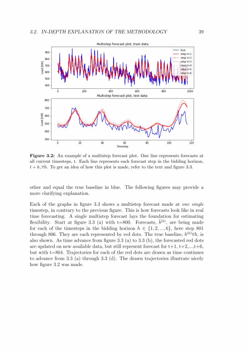
3.2. IN-DEPTH EXPLANATION OF THE METHODOLOGY 39
Figure 3.2: An example of a multistep forecast plot. One line represents forecasts atall current timesteps, t. Each line represents each forecast step in the bidding horizon,t + h,∀h. To get an idea of how this plot is made, refer to the text and figure 3.3.
other and equal the true baseline in blue. The following figures may provide amore clarifying explanation.
Each of the graphs in figure 3.3 shows a multistep forecast made at one singletimestep, in contrary to the previous figure. This is how forecasts look like in realtime forecasting. A single multistep forecast lays the foundation for estimatingflexibility. Start at figure 3.3 (a) with t=800. Forecasts, b(h), are being madefor each of the timesteps in the bidding horizon h ∈ {1, 2, ..., 6}, here step 801through 806. They are each represented by red dots. The true baseline, b(h)∀h, isalso shown. As time advance from figure 3.3 (a) to 3.3 (b), the forecasted red dotsare updated on new available data, but still represent forecast for t+1, t+2,...,t+6,but with t=804. Trajectories for each of the red dots are drawn as time continuesto advance from 3.3 (a) through 3.3 (d). The drawn trajectories illustrate nicelyhow figure 3.2 was made.
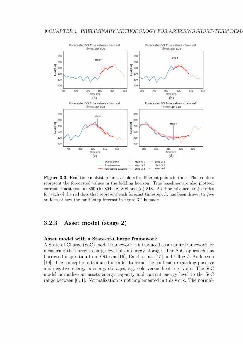
40CHAPTER 3. PRELIMINARYMETHODOLOGY FORASSESSING SHORT-TERMDEMAND-SIDE FLEXIBILITY
Figure 3.3: Real-time multistep forecast plots for different points in time. The red dotsrepresent the forecasted values in the bidding horizon. True baselines are also plotted.current timestep= (a) 800 (b) 804, (c) 808 and (d) 818. As time advance, trajectoriesfor each of the red dots that represent each forecast timestep, h, has been drawn to givean idea of how the multi-step forecast in figure 3.2 is made.
3.2.3 Asset model (stage 2)
Asset model with a State-of-Charge frameworkA State-of-Charge (SoC) model framework is introduced as an unite framework formeasuring the current charge level of an energy storage. The SoC approach hasborrowed inspiration from Ottesen [16], Barth et al. [15] and Ulbig & Andersson[19]. The concept is introduced in order to avoid the confusion regarding positiveand negative energy in energy storages, e.g. cold versus heat reservoirs. The SoCmodel normalize an assets energy capacity and current energy level to the SoCrange between [0, 1]. Normalization is not implemented in this work. The normal-

3.2. IN-DEPTH EXPLANATION OF THE METHODOLOGY 41
ization factor provides a conversion factor, n, between ∆SoC and absolute energy∆E. Along with the use of SoC, the terms charging and discharging will be usedinstead of increasing and decreasing energy content. Charging of an asset will in-crease the SoC, and vice versa for discharging. The asset consumption which leadsto a stable unchanged SoC level is defined as the steady state consumption, de-noted Pcons,SS. An increase or decrease of consumption relative to the steady stateconsumption results in charging or discharging the storage respectively. Coolingstorages are charged when they actually decrease their energy content, because ofadded electrical consumption. That is the purpose of the SoC framework.
The normalization factor, n, is defined to be
n =∆SoCrange
∆Erange
SoC∈[0,1]−→ 1
∆Erange
(3.3)
where ∆Erange = Emax−Emin is the allowed range of energy levels in the storage.If the energy storage is thermal, then ∆Erange will be provided by equation 3.20by inserting the maximum and minimum allowed temperatures. For a coolingstorage, ∆Erange will be negative and n < 0. In this thesis, n is set to be either+1 or -1, which means that SoC is still measured in kWh and not normalized tothe range [0, 1]. Further in this work, a n = −1 is used for the cooling storage andn = +1 is used for the other assets.
Figure 3.4: A sketch of a general physical model of a flexible asset with a flexible energystorage. The green arrows, and not the light red, indicates positive power direction.
A generic physical model of a flexible asset with a flexible energy storage is shownin figure 3.4. The SoC level and the relevant power flows are indicated. Pcons
represents the electrical power consumption of the asset. The share of consumptionthat interacts with the storage is expressed
Pin = ePcons (3.4)

42CHAPTER 3. PRELIMINARYMETHODOLOGY FORASSESSING SHORT-TERMDEMAND-SIDE FLEXIBILITY
with e > 0 being a power conversion efficiency factor and can be lower or greaterthan 1. Pin can be electrical or thermal power depending on the energy storagebeing chemical (battery) or thermal respectively. Often, e > 1 for heat pumps orcompressor systems, then often called coefficient of performance (COP). Or e < 1for chemical or direct thermal power conversion. A positive Pin will in isolationincrease the SoC level. In case of a cooling storage, a positive Pin do actuallyrepresent a negative power flow pure physically, but this confusion is now avoided.Another factor is the power losses, Plosses, which in isolation cause the SoC levelto decrease. The loss power could represent an intended outgoing power flow toan external purpose, e.g. heating offices. It also includes unwanted energy storagepower losses, for example heat losses. Plosses exclude electricity that flows backto the grid, as this is included in Pin/Pcons. The physical model also includes anoption to have an alternative power production source, e.g. diesel generator or PVpanels.
The net power flow into the energy storage is denoted as the charging power,P(dis)charge. It is defined as the net power flow that interacts with the energystorage’s system borders, expressed as following
P(dis)charge = Pin + Plosses
= ePcons + Plosses
(3.5)
The charge power is important for the evolution of the energy storage level. Achange in the SoC and energy level over time happens when the charge power iseither positive or negative, expressed
dSoC
dt= nP(dis)charge (3.6)
Integrating at both sides from one discrete timestep to the next timestep yields
∆SoC = n
∫ t+∆t
t
P(dis)charge(t)dt (3.7)
which for discrete timeseries simplifies to
∆SoC(t) = nP(t)(dis)charge∆t (3.8)
where ∆SoC(t) is denoted the change in SoC level at the timestep t, due to thecharge power at that timestep, P
(t)(dis)charge. ∆t is the temporal resolution, the
duration of a timestep (in hours).

3.2. IN-DEPTH EXPLANATION OF THE METHODOLOGY 43
Table 3.1: Table of asset parameters that must be determined in order to fulfill stage2 of the methodology.
Symbol Parameter Unit Description
∆t Temporal resolution, positiveinteger
hour example: ∆t=0.25 imply15min resolution
~Pmin a minimum possible assetpower (2a), array of length H
kW(kWh/h)
~Pmax a maximum possible assetpower (2a), array of length H
kW(kWh/h)
Emax Maximum energy capacity, in-teger
kWh
Emin Minimum energy capacity, in-teger
kWh
SoC0 An initial SoC value, ∈ [0, 1] -~b Forecasted baseline, array of
length HkWh/h provided from stage 1
Pcons,SS Steady state consumption, ar-ray of length H
kWh/h is equal to for ex. 0 or thebaseline
Having P(dis)charge = 0 will have the following implication
P(dis)charge = 0 =⇒ Pcons = Pcons,SS =⇒ ∆SoC = 0 (3.9)
where Pcons,SS is the steady state consumption, defined to be the consumption thatleads to an unchanged energy storage level. A steady state situation will accordingto eq. 3.5, lead to
Plosses,SS = −Pin,SS = −ePcons,SS
The losses are assumed to not be dependent on the consumption, namely Plosses,SS =Plosses. Using the above equation with a reformulation of eq. 3.5, P(dis)charge canalso be expressed
P(dis)charge = ePcons − ePcons,SS (3.10)
Asset model parametersDuring the development of the methodology, it is found that the asset parametersgiven in table 3.1 must be determined. In order to determine some of these para-meters, it may be necessary to conduct experiments and tests of the asset, e.g.step-tests.

44CHAPTER 3. PRELIMINARYMETHODOLOGY FORASSESSING SHORT-TERMDEMAND-SIDE FLEXIBILITY
The forecasted baseline, ref eq. 3.1, is provided by the forecast model in stage1. The minimum power ~Pmin sets a lower limit for the minimum possible powerconsumption of the asset. It can vary for different timeslots and is expressed
~Pmin =[
ˆP
(h)min
]Hh=1
(3.11)
Similarly, the maximum power ~Pmax sets an upper limit for the power consumptionof the asset, and is defined as
~Pmax =[
ˆP
(h)max
]Hh=1
(3.12)
The upper and lower power limits are found empirically or provided by the re-spective asset. Note that negative values always indicate production and notconsumption. The charge power is calculated according to equation 3.10.
Object-oriented programming for asset modellingFor the implementation of an asset model, a class called Asset has been made inPython. Making a class is beneficial, because one can create multiple objects fromit, e.g. many assets. The asset parameters defined in table 3.1 are provided as inputto the asset class, and will constitute the initial attributes (class variables) of theasset object. The class consists of many attributes and methods (class functions).The first important method, add energystorage() involves the possibility to attachan energy storage to the asset model, if it has any. The inputs to this method isthe energy storage parameters of the asset. The second and last important methodis make flexplot() which makes the final flexibility estimates and creates a flexplot.The flexplot is presented shortly.
The whole Python script for the class Asset, with commentaries and documenta-tion, is included in Appendix B.2. The bottom of the script show some exampleusage of the class, used for the making of the flexplots throughout this thesis.
Further work yet to be done is to implement a class for an aggregated groupof assets, e.g. Building, in order to provide aggregated flexplots and flexibilityestimates.
3.2.4 Flexibility estimation (stage 3)
Flex equationsThe flexibility lies in the ability to deviate from the baseline. Based on the baseline

3.2. IN-DEPTH EXPLANATION OF THE METHODOLOGY 45
forecasts~b, the forecasted maximum positive flexible power ~Fp is defined to be
~Fp = ~Pmax − ~b =
[P (h)max − ˆb(h)
]Hh=1
(3.13)
Similarly, the forecasted maximum negative flexible power is denoted
~Fn = ~Pmin − ~b =
[P
(h)min − ˆb(h)
]Hh=1
(3.14)
These values represent the estimated flexibility at each forecast timestep, h, in thebidding horizon H. Units are in kWh/h.
So far, the flexibility estimates do not take into consideration any limits set bythe energy storage or potential time restrictions. In the implementation programin Python, the ultimate estimated available flexible power is restrained by energystorage capacity limits, as soon illustrated.
Flexplot - visualizing available flexibility and energy storage trajectoriesVisualization provide better understanding for humans and is the first stage ofdecision support, on the road to a fully intelligent and automatized system. Plotshave been developed to visualize the estimated available flexibility and all possibleimpacts on the energy storage for all possible estimated outcomes. Simulationsfor the energy storage trajectories will reveal when activation of flexible powerwill result in hitting any energy storage limits. That is taken into considerationand the estimated available flexible power is shredded if simulations indicate thatenergy storage limits are reached. The plot is henceforth referred to as a flexplot,and an example flexplot is shown in figure 3.5.
Passive charge schedule
For the explanation of this flexplot, a Pixii battery [34] with the following specific-ations and assumptions is used:
• Temporal resolution is 15 minutes, ∆t = 0.25
• Max og min power, Pmax = −Pmin = 30kW
• Energy storage has a capacity of Emin = 0kWh and Emax = 65kWh
• Steady state consumption equals zero, since there are no power losses inbattery, ~PSS = ~0
• Forecasted baseline = inactive load schedule,~b = ~0
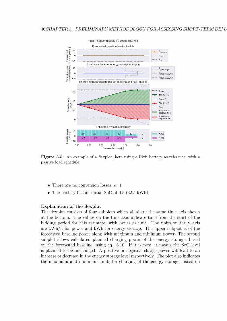
46CHAPTER 3. PRELIMINARYMETHODOLOGY FORASSESSING SHORT-TERMDEMAND-SIDE FLEXIBILITY
Figure 3.5: An example of a flexplot, here using a Pixii battery as reference, with apassive load schedule.
• There are no conversion losses, e=1
• The battery has an initial SoC of 0.5 (32.5 kWh)
Explanation of the flexplotThe flexplot consists of four subplots which all share the same time axis shownat the bottom. The values on the time axis indicate time from the start of thebidding period for this estimate, with hours as unit. The units on the y axisare kWh/h for power and kWh for energy storage. The upper subplot is of theforecasted baseline power along with maximum and minimum power. The secondsubplot shows calculated planned charging power of the energy storage, basedon the forecasted baseline, using eq. 3.10. If it is zero, it means the SoC levelis planned to be unchanged. A positive or negative charge power will lead to anincrease or decrease in the energy storage level respectively. The plot also indicatesthe maximum and minimum limits for charging of the energy storage, based on

3.2. IN-DEPTH EXPLANATION OF THE METHODOLOGY 47
the max and min power. The first and second subplots do in this case look similar,because of the chosen example (no storage losses), but this does not have to bethe case (as examples will show).
The third subplot is of importance to visualize what will happen with the energystorage level. The y axis represents stored energy. The limits of the energy storageare indicated. The graph reveals what is going to happen with the energy storagelevel for different choices of asset consumption. The blue solid line shows theplanned energy trajectory, Eplan(t), which is a simulation of energy level whenfollowing the forecasted baseline consumption. It is the path when choosing not toactivate any estimated available flexibility. For this specific example, the plannedenergy storage trajectory remains constant, because of the planned charging powerbeing zero. However, the planned baseline could very well involve charging, asshown later. Explaining the remaining content of this subfigure is postponed toafter explaining the fourth subplot.
The fourth subplot ultimately reveals the estimated flexibility, represented by theestimated max positive flexible power in striped cyan and estimated max negativeflexible power in solid purple. The estimates correspond to the difference betweenthe forecasted baseline and the power limits, as stated by the equations 3.13 and3.14. The estimated flexibility here are symmetric because of the chosen symmetriccase. It is 30 kWh/h both in the negative and positive direction. After timestep1.00 it sinks to 10 kWh/h and then to zero even, despite that the asset still hasa lot of choices to deviate from its baseline consumption, according to the firstsubplot. The reason is that the energy storage limits are reached and impose ashredding of the estimated flexibility.
Choosing to activate either Fp(t) or Fn(t) results in a change to the planned con-sumption, planned charging and the energy content. Referring to the energy stor-age subplot, the resulting energy trajectories of activating either all Fp(t) or allFn(t) is plotted in green or red respectively. These trajectories are represented byE(t, Fp(t)) and E(t, Fn(t)) respectively. The fact that the energy storage limitsare reached at timestep 1.00 is what impose the reduced flexibility seen in fourthsubplot. The dashed light grey line in the third subplot shows how the trajectorieswould be without considering energy storage limits.
Code snippets for creating this flexplot is found at the bottom of the Asset classscript in Appendix B.2, with EXAMPLE 1 as reference.
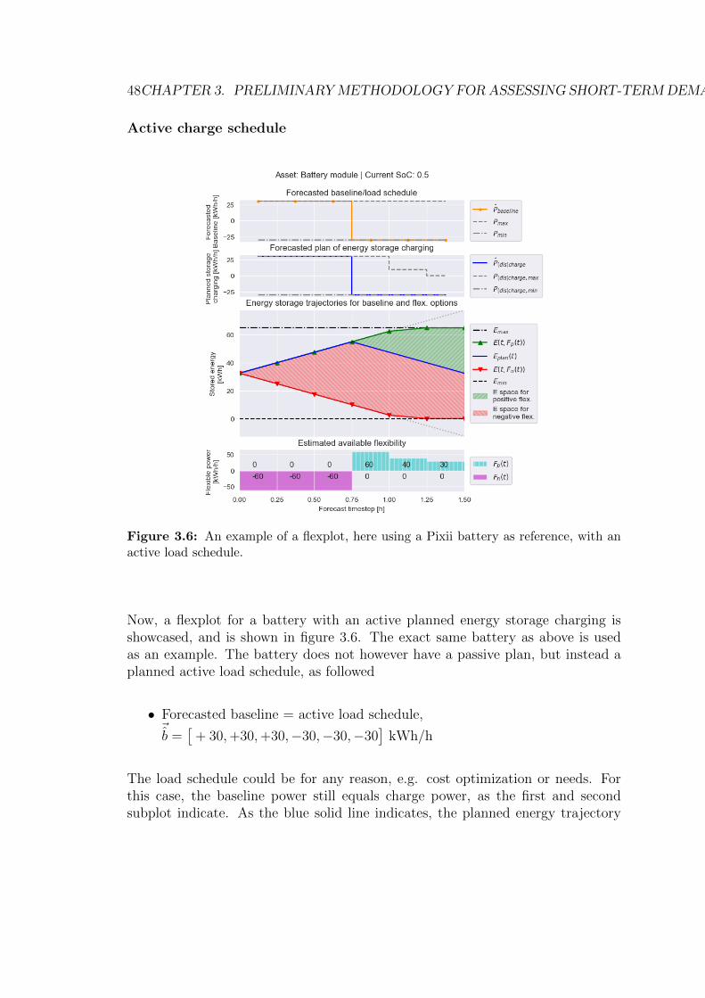
48CHAPTER 3. PRELIMINARYMETHODOLOGY FORASSESSING SHORT-TERMDEMAND-SIDE FLEXIBILITY
Active charge schedule
Figure 3.6: An example of a flexplot, here using a Pixii battery as reference, with anactive load schedule.
Now, a flexplot for a battery with an active planned energy storage charging isshowcased, and is shown in figure 3.6. The exact same battery as above is usedas an example. The battery does not however have a passive plan, but instead aplanned active load schedule, as followed
• Forecasted baseline = active load schedule,~b =
[+ 30,+30,+30,−30,−30,−30
]kWh/h
The load schedule could be for any reason, e.g. cost optimization or needs. Forthis case, the baseline power still equals charge power, as the first and secondsubplot indicate. As the blue solid line indicates, the planned energy trajectory

3.2. IN-DEPTH EXPLANATION OF THE METHODOLOGY 49
looks different now, due to planned charging. In addition, the flexibility estimatesare different. The forecasted baseline that is entered to the flexibility platform iswhat lays the basis for calculating the flexible power. Therefore, the estimatedflexible power is now -60 kWh/h in the first 3 timeslots. The plan was to chargethe battery with +30 kWh/h, while there is still an opportunity to discharge -30kWh/h. The resulting negative flexible power is the difference of - 60 kWh/h.There is no available positive flexibility for the first 3 slots, because the maximumpossible power/charge is already planned. This can be seen in the energy plot aswell, where the planned trajectory already follows the path of maximum positiveflex, which is 0. The last 3 slots offers positive flexible power. The fourth slotis +60kWh/ and the fifth has been imposed restrictions on because energy limitsare reached. Still, after the limits are reached, the sixth slot contain +30kWh/of offered flexible power. That is because the battery can have a consumption of0kWh/h, when -30kWh/h is planned.
Code snippets for creating this flexplot, figure 3.6, is found in Appendix B.2, withEXAMPLE 2 as reference.
3.2.5 Bid formatting (stage 4)
Based on the estimated flexible power, the ultimate bid is entered to the flexibilitymarket platform. It consist of H timeslots, each slot containing both a bid forpositive and negative flexible power, as seen in figure 3.7. The bid should com-ply with the flexibility product presented in the section underNODES Flexibilityproduct. Pricing of each flexibility bid slot is important, but is left out of the scopeof this thesis.
The bid in each slot could be linear, absolute or even contain a minimum activation,e.g. an absolute value above 30kWh/h. For the estimations in this thesis it isassumed an activation of the maximum bidded available flexible power, referredto as a full activation. Later, some alternatives will be briefly discussed, e.g.activating half the power of a bid.

50CHAPTER 3. PRELIMINARYMETHODOLOGY FORASSESSING SHORT-TERMDEMAND-SIDE FLEXIBILITY
Figure 3.7: Example of a how a flexibility bid that is entered into the flexibilityplatform, may be illustrated. It is constituted of several slots in the bidding horizonh ∈ [1, H], here with H = 6.
3.2.6 Aftermath and error measures
There are two different outcomes after the bid is formatted and entered intothe flexibility market platform. When a bid is ignored, we expect the realizedconsumption to follow the forecasted baseline,
P (h)cons = b(h) (3.15)
The realized consumption, however, does in fact become
P (h)cons = b(h) (3.16)
These values enables us to calculate the error of the baseline forecast, using eitherof the evaluation metrics mentioned in the section Evaluating multi-step forecasts.
When a bid is activated, the bought flexible power can be denoted F(h)committed.
The realized consumption is anticipated to be equal to the forecasted baselinepower with the added committed flexible power that is expected to be dispatched,expressed
ˆPcons
(h)= b(h) + F
(h)committed (3.17)
During the influence of the activated flexible power, the realized baseline, ~b, willnot become available, but the realized consumption P
(h)cons will be. That enables us
to calculate the delivered flexibility, F(h)delivered, which is expressed
F(h)delivered = P (h)
cons − b(h) (3.18)
The failed deliverance, or error of flexibility deliverance, can then be expressed
R(h)delivered = F
(h)delivered − F
(h)committed (3.19)
where the delivered flexibility is found with eq. 3.18 and the estimated flexibilityis the flexible power that is bought and committed.
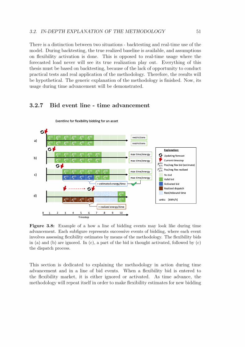
3.2. IN-DEPTH EXPLANATION OF THE METHODOLOGY 51
There is a distinction between two situations - backtesting and real-time use of themodel. During backtesting, the true realized baseline is available, and assumptionson flexibility activation is done. This is opposed to real-time usage where theforecasted load never will see its true realization play out. Everything of thisthesis must be based on backtesting, because of the lack of opportunity to conductpractical tests and real application of the methodology. Therefore, the results willbe hypothetical. The generic explanation of the methodology is finished. Now, itsusage during time advancement will be demonstrated.
3.2.7 Bid event line - time advancement
Figure 3.8: Example of a how a line of bidding events may look like during timeadvancement. Each subfigure represents successive events of bidding, where each eventinvolves assessing flexibility estimates by means of the methodology. The flexibility bidsin (a) and (b) are ignored. In (c), a part of the bid is thought activated, followed by (c)the dispatch process.
This section is dedicated to explaining the methodology in action during timeadvancement and in a line of bid events. When a flexibility bid is entered tothe flexibility market, it is either ignored or activated. As time advance, themethodology will repeat itself in order to make flexibility estimates for new bidding

52CHAPTER 3. PRELIMINARYMETHODOLOGY FORASSESSING SHORT-TERMDEMAND-SIDE FLEXIBILITY
horizons.
To demonstrate how the methodology works during time advancement, a concep-tual demonstration of the bidding procedure has been designed. It is designed toshow what happens in both outcomes of the methodology. For this purpose, 4successive bid events are created. Figure 3.8 shows 4 flexibility bids in the biddingprocedure. Each bid represents an event, where each event involves the use of themethodology for estimating flexibility to create the illustrated bids. Each event isas follows:
• Event (a): According to the methodology, a flexibility bid is made andentered into the platform, but the bid is ignored. We proceed to the nexttimestep.
• Event (b): Flexibility estimates are yet again formulated into a flexibilitybid and ignored again. We proceed to the next timestep to prepare for thenext bidding period.
• Event (c): The new flexibility bid that is entered is bought. As an example,the four first 4 slots for negative flexibility are activated, however this is onlyillustrative. The activated flexibility must match the given time and energyconstraints. We follow path bid activated in figure 3.1.
• Event (d): According to the methodology, the dispatch will try to deliverthe committed flexible power in its best fashion, however it may fail. Thevalues in the dark brown coloured slots, representing delivered flexible power,may therefore differ from the values of the activated flexibility. As the dis-patch period soon comes to an end, there are some alternatives. Either, newflexibility estimates are done right away or there is a rest or rebound period.
• The same process goes on and the methodology is repeated.
This set-up is used as a standard for later practical examples.

3.3. IMPLEMENTATION OF THEMETHODOLOGY FOR SELECTED ASSETS53
3.3 Implementation of the methodology for se-
lected assets
This is the third and last section of the chapter and will present specific descriptionson how the methodology can be implemented for the five following assets: Battery,diesel generator, PV panels, water heater (with heat tank or with alternativeenergy source) and machine room.
3.3.1 Thermal energy storages and heat losses
Before presenting the conceptual methodology for assets with thermal energy stor-ages, some theory on thermal physics must be presented. Equations for the energylevel and how heat transfer mechanisms change the energy level of a heat stor-age will therefore be presented. This section is aimed to support the modellingframework for flexible assets whose behaviour relies on underlying thermal physicalprocesses, such as a cooling storage and a water-based heat storage. Knowledgeabout heat losses will also provide information on which heat loss parameters toinclude as explanatory variables in load forecast models.
Most of following theory on thermodynamics is from the book by Sonntag & Bor-gnakke [35].
Heat and transfer mechanismsHeat is thermal energy and everything that have atoms with a temperature above0 Kelvin possess heat. In practice, one focus on relative change of heat in anobject. The change of thermal energy ∆Q (Wh) of an object with mass m (kg)subject to a temperature change ∆T (K), can be expressed
∆E = ∆Q = cpm∆T (3.20)
where cp ( WhkgK
) is the material-specific heat capacity of the object. The new thermal
energy in an object subject for a change in thermal energy would simply be E0 +∆E, where E0 usually is a constant that is set freely. Wh is a practical unit forenergy because electricity also uses this unit.
In order to change the thermal energy of an object, it needs to exchange heat powerwith the surroundings. Heat exchange happens through three heat transfer mech-anisms: conduction, convection and radiation. These mechanisms are presentedbelow, except for radiation, which can be neglected in the further work.

54CHAPTER 3. PRELIMINARYMETHODOLOGY FORASSESSING SHORT-TERMDEMAND-SIDE FLEXIBILITY
Heat conduction Qcond (W) is heat that transfer through a material, i.e. wall, andcan be described by Fourier’s law of heat conduction,
Qcond = −kA∆T
∆x(3.21)
where k ( WmKm2 ) is heat conductivity of the material, ∆T (K) is the linear temper-
ature gradient through the material, A (m2) the cross section and ∆x (m) thethickness of material.
Convection is heat transfer by motion of a fluid itself and is very complex todescribe in a mathematical way. The driver for convective heat flow is temperaturegradients in a fluid, which cause particle movement due to pressure differences. Agreat temperature gradient will cause high convective heat transfer until at last,when all air is mixed up and shares a common steady state temperature. As anaimed example, consider two enclosed rooms filled with air, having a difference intemperature ∆T . They are connected with a closed gate. When the gate opens,the temperature difference, ∆T , will be a driver for heat convection through thedoor, qconv, which can be expressed
Qconv ∝ ∆T (3.22)
A thermal energy storage raises or lowers its energy content by interacting withthe environments. In order to provide flexible electrical power, it is needed thatPlosses > 0 ⇒ Pcons > 0. The reason is that stored thermal energy itself cannotbe transformed back into providing electricity to grid. The asset can only deviateits consumption of there is a natural drainage of the thermal storage. Unwantedstorage heat losses stem from a warmer or colder environment to which heat istransferred according to the equations 3.22 and 3.21. Thermal energy storages aretherefore often insulated to avoid unwanted heat losses, reducing the coefficientof heat conduction. There should be mechanisms to avoid unwanted convectiveheat losses as well. Ideally, power losses should fully be going to its purpose, e.g.heating offices.
3.3.2 Implementation for batteries
Batteries big advantage of being charged and discharged with ease and precision,makes them the most ideal resource for flexibility and grid balancing purposes,when ignoring costs. From now on, a high-capacity battery will be considered. Al-though still being a more expensive alternative to other flexibility sources, utility-scale batteries are a serious competitor for offering flexibility services in the energy

3.3. IMPLEMENTATION OF THEMETHODOLOGY FOR SELECTED ASSETS55
chain. By 2050, around 360 GW of batteries are expected to be a part of the world’spower grids, and they expect to become a cost-competitive choice for load shiftingfrom the mid 2020’s [2]. A commercial battery available on today’s market canoffer 65 kWh of electrical energy storage with a 30 kW power conversion, packedin a half-tonne fridge-sized cabinet [34]. As batteries degrade over time with dif-ferent use patterns, current research is being done to gain a better understandingof operational related costs. For this thesis, a simplistic battery model is to beused, as presented in methodology chapter.
Batteries do perhaps offer the simplest and easiest source of flexibility and hasa smooth implementation of the conceptual model. A battery was chosen as anexample for the flexplot explanation.
Figure 3.9: Simplistic physical model of a battery as a flexible asset.
A physical model of a battery is shown in figure 3.9. A battery is subject todecisions, and the load schedule must be actively set, for example in order tominimize operational costs. The forecasted baseline is therefore set by a loadschedule. Steady state consumption is always equal to 0 for batteries, by assumingit has no storage losses. The charge power, Pcharge will thus be equal to the Pin,which transform power from the grid with a certain efficiency, e ∈ [0, 1]. Thecharging and discharging of a battery can be expressed
P(dis)charge = Pin = ePcons (3.23)
The action of storing energy in the battery for later extraction is associated withan efficiency loss, expressed by applying the above equation twice
Pcons,extraction = e2Pcons,storing (3.24)

56CHAPTER 3. PRELIMINARYMETHODOLOGY FORASSESSING SHORT-TERMDEMAND-SIDE FLEXIBILITY
Inserting the given parameters into eq. 3.8 yields an expression for increasing theenergy level, or SoC
∆SoC(t) = n∆E(t) = nP(t)in ∆t = neP (t)
cons∆t (3.25)
When a battery is charging, it is consuming power, Pcons > 0 and ∆SoC wouldhave to be positive. If they are negative, they indicate discharging and powerproduction. The maximum and minimum power of the battery is usually providedby the manufacturer. Estimation of flexibility is next. It has already been demon-strated and was shown for the case of both a passive and an active load schedule,figure 3.6 and 3.5 respectively.
As with the passive battery, the figure reveals that fully activating the maximumamount of either positive or negative flexibility, results in hitting the boundariesof the energy storage limit within 5 hours. The flexibility the last hour is thenshortened from this fact.
3.3.3 Implementing a diesel generator
A diesel generator generates electricity from running a combustion engine fuelledby diesel. It is ideal as a power backup, in case of power outages. Many dieselgenerators can also be fuelled by other liquid energy carriers, such as gasoline, biodiesel and colza oil, with different efficiencies.
Figure 3.10: Simplistic physical model of a diesel generator or of a PV panel.
A physical model of a diesel generator is shown in figure 3.9. A diesel generatoris always at backup to provide the alternative energy source as electricity to the

3.3. IMPLEMENTATION OF THEMETHODOLOGY FOR SELECTED ASSETS57
grid. It could have a minimum and maximum run time, and perhaps a rest timebetween runs. The forecasted baseline that is entered into the flexibility platformis simply equal to 0. The maximum power is determined by the specifications ofthe engine and how much electrical power it can deliver. The negative flexibilityis directly quantified as the maximum power and this information could thereforebe directly used to make bids. All the first stages of the methodology model couldbe skipped, and bids are entered directly to the platform. The diesel generatormay have a minimum power, thus the negative flexible power is
−Fn ∈[Pmax, Pmin
]
3.3.4 Implementing PV solar panels
Photovoltaic solar panels (PV panels) have the unique ability to transform irradi-ance to electrical power. They do so when they get lit by both direct solar raysand diffuse light. A typical commercial PV panel has an efficiency around 15-19% [36]. Solar power cannot be controlled, except from curtailing the productionwhich could provide positive flexibility, for example in the case of an extreme gridemergency. However, smart and interconnected flexibility markets aim at avoidingsuch curtailment. Alternatives to curtailment should always be sought, such ascharging other flexible assets in the building instead.
PV solar panels could provide flexible generation and their flexibility lies in cur-tailment of production. In the use-case, solar production assist to supply coolingpower which correlates with temperature and mostly sun. PV curtailment maytherefore lead to a high net building consumption that exceeds power tariff limits,thus resulting in a very high cost of the flexibility.
The PV panel asset can be modelled the same way as a diesel generator, as seen infigure 3.10. The forecasted production is entered to the flexibility platform as thebaseline. The maximum negative flexibility is to curtail all solar production. Forthis reason, the solar power production must be forecasted. This is somewhat easyon sunny and complete shaded days, but become tough on days with clouds thatcome and go. That applies to the flexibility estimates as well. This asset does nothave an energy storage or asset models, and the flexible power could directly beused to make flexibility bids. PV panel is not further investigated in this thesis.The implementation is clarified.

58CHAPTER 3. PRELIMINARYMETHODOLOGY FORASSESSING SHORT-TERMDEMAND-SIDE FLEXIBILITY
3.3.5 Implementing a water heater
A water heater consumes electricity to heat up an energy carrier, often water. Itcould have a tank for the energy carrier that stores thermal energy. Pipes transportthe energy carrier to ultimately heat up whatever needs to be heated externally.If the thermal energy storage is of a significant size, energy-wise, one can expectit to provide flexibility. Another source of flexibility can also be if the electricalconsumption has the opportunity to be replaced with another energy source. Aheat tank consisting of water can store a lot of energy. The specific heat capacityof water is around 4.2 kJ/kgK, in the liquid phase range, at 1 atm pressure [35].
We look at two cases. The first case is to look at a water heater whose consumptioncan be totally replaced by an alternative energy source. The second case is to lookat a water heater with a flexible thermal energy storage, which is providing theflexibility. In practice, the both can be combined. Using an alternative energysource will not result in any rebound effects, whereas discharging a thermal storagewill lead to a rebound effect to recover after activation period.
The first stage, settling the baseline forecast, must be done for either case. Waterheaters use electrical power to provide a heat power flow to an external purpose,which is considered a part of Plosses. From now on, it is assumed that the con-sumption equals steady state consumption
Predicting the baseline may require the creation of a load forecast model or, if theconsumption is very stable, an average or repeated value can be used. One canexpect the consumption to be influenced by the things that influence Plosses, suchas conduction losses through the isolated walls and parameters behind its externalpurpose, e.g. office space heating. Investigation of such processes may thereforebe helpful.
The ability to deviate from the consumption must be determined, which sets Pmin
and Pmax. The successive stages will differ for the case of an alternative energysource versus a heat reservoir. The case with a thermal storage will be treatedfirst, followed by the case with an alternative energy source.

3.3. IMPLEMENTATION OF THEMETHODOLOGY FOR SELECTED ASSETS59
Water heater with thermal storage
Figure 3.11: Simplistic physical model of a water heater with a thermal energy storageas a flexible asset.
A physical model of the water heater system with the heat reservoir can be seenin figure 3.11. Pmax would be some maximum value, most probably a constantand will make up the possibilities for charging the energy storage. Pmin can beassumed to be zero from now on, which means total consumption shut off. Thedrainage of the energy storage is thereby totally dependent on Plosses > 0.
The flexible range of energy levels in the heat storage is given by the equation
∆Erange = n∆SoC = cm∆T (3.26)
where ∆T = Tmax − Tmin is the allowed range of temperatures(K), c is the heatcapacity (kJ/kgK) and m is the mass (kg), of the medium. The latter can altern-atively be expressed m = ρV with ρ being the density (kg/m3) and V being thevolume (m3) of the medium. It is assumed no phase transitions. Temperature re-strictions, such as a minimum and maximum allowed temperature, Tmin and Tmax,sets a lower and upper boundary for the thermal energy content, Emin and Emax
respectively. The level of energy in the storage cannot exceed these limits.
An approach is to set Emin = 0 and let the maximum allowed energy level beexpressed
Emax = Emin + ∆Erange (3.27)
Now, all is set to estimate the flexibility.

60CHAPTER 3. PRELIMINARYMETHODOLOGY FORASSESSING SHORT-TERMDEMAND-SIDE FLEXIBILITY
Some notesIf Pmin = 0 and the asset consumption is shut off, the asset will provide negativeflexible energy and also discharge. As mentioned, the drainage will totally dependon Plosses. If the bottom energy level is reached, then the electrical consumptionmust be turned back on. From this fact, it is important to have good forecastsof the electrical consumption, assumed steady state. The forecasted baseline willonly be able to provide a forecast of the potential new energy level after activationand the time of a completely empty energy storage. A problem is that, if thebaseline forecast is wrong, especially when it has underestimated the forecastedsteady state consumption, it will thereby underestimate the losses. This wouldresult in an overestimated flexibility. It means that activation of that flexibility isexpected to drain the storage in a certain manner, but the energy storage will inpractice drain faster than anticipated. As a result, the flexibility activation willnot be able to last as long as committed, as the consumption must be turned backon when the bottom energy limit is reached before time.
Some ways to avoid this to happen is to provide more accurate, or even overestim-ated, forecasts or subtract a share of the estimated flexibility as a safety margin.That may help prevent failed deliverance of flexibility.
The rebound effect is a consideration that should be investigated. The reboundmust be analysed through experiments, and the rebound strength could perhapsbe controlled. Notes on implementation of rebound effects are for the discussionlater.
Water heater with alternative energy source
Figure 3.12: Simplistic physical model of a water heater with the opportunity toreplace electrical consumption with an alternative energy source, as a flexible asset.

3.3. IMPLEMENTATION OF THEMETHODOLOGY FOR SELECTED ASSETS61
A simple sketch of the water heater system with an alternative energy source isshown in figure 3.12. A twist in this case is that Pmax is equal to the baselineconsumption of the asset. That yields no positive flexible power. Pmin is simplyzero. Thus, the negative flexibility lies in shutting off the electrical power. Thealternative energy source still provides everything that is needed of power for thewater heater to continue delivering its functions, in Plosses. If there are any timeconstraints for the alternative energy source, regarding max runtime or rest timeafter activation, this can easily be implemented. All is set to estimate the negativeflexible power and make flexibility bids.
Some notes:The alternative energy source may have time constraints, which are taken care ofin the flexibility estimation or bid formulation. Rebound effects are not present,however there might be a rest time, in which a resting period must pass before thealternative energy source is yet again ready.
Aftermath:The realized baseline will not be available and the asset has not any energy storagethan can be drained. Therefore, the delivered flexibility is concluded to be perfectlyfulfilled.
3.3.6 Implementing a machine room for cooling storage
A complete conceptual description for implementing the preliminary methodologyon a machine room asset is now presented, including the steps for the making ofa forecast model. Figure 3.13 shows a simplistic model of the machine room assetwith its power flows and the SoC level of the cooling storage.
The first stage in the methodology is to create a load forecast model that can makepredictions for the future baseline consumption. Step one is in many ways the sameas forecasting the heat losses, since the baseline is assumed to be the steady statepower, Pcons = Pcons,SS ⇒ P(dis)charge,SS = 0. The ability to be flexible is to eitherblow up or ease down on electricity consumption from the forecasted baseline,thus charging or discharging the thermal storage respectively. According to themethodology, the second step would be to quantify the potential to deviate fromthe baseline. This must be done by analysing the ability to control the electricalconsumption and finding Pmax and Pmin. In addition, the storage parameters Emin
and Emax must be determined.

62CHAPTER 3. PRELIMINARYMETHODOLOGY FORASSESSING SHORT-TERMDEMAND-SIDE FLEXIBILITY
Figure 3.13: Simplistic physical model of the machine room and cooling storage as aflexible asset.
Settling the storage lossesSince understanding heat losses will increase predictive power for electrical con-sumption, heat losses for the cooling storage will now be analysed in the comingparagraphs.
Figure 3.13 is now referred to. The cooling power, represented by Pin (W), mustequal the net losses, Plosses (W) to maintain the set-temperature and SoC levelof the storage. There is convection losses through a potential open gate andconduction losses through the walls, roof and closed gates. The power loss is solelyconstituted by heat losses that can explained by the two heat transfer mechanisms,equations 3.22 and 3.21. Combined, this yields
− Pin = Plosses = Qcond + Qconv (3.28)
One unit of electricity consumption Pcons (W) that is needed to create one unitof storage cooling Pin (W) is in fact lower, due to a usually high Coefficient ofPerformance (COP) of above 4, e > 4 . Combined with the latter equation, thiscan be expressed
Pcons =Pin
e(3.29)
To conclude, the electrical consumption becomes dependent on heat losses
Pcons =1
e(Qcond + Qconv) (3.30)
The variables of the respective heat transfer mechanisms indicate that outsidetemperature will play a key role in both heat loss mechanisms. In addition, thefrequency of open gates will be essential for the presence of convective heat losses.
3.3. IMPLEMENTATION OF THEMETHODOLOGY FOR SELECTED ASSETS63
Thus, these variables should be included as explanatory features in a forecastmodel in order to improve the performance and predictions of the consumption.e must not be determined, because it will be found by the RNN model. If thefrequency of the gates can be modelled, this would be a valuable feature. Oncea good forecast model is realized, good forecasts gives a good foundation for theestimating flexibility. Note that the load forecast also is a forecast of the steadystate consumption.
stage 2 Next step in the methodology is to determine the asset parameters. Acooling storage for groceries needs to maintain a desired air temperature, calledthe set-temperature, Tset, which can be manipulated within an allowed deviation.Temperature restrictions are set for food safety regulations, under strict laws. Therange of allowed temperatures will yield a range of a flexible energy storage levels.This makes the asset possess flexible power. One needs to decide the range ofallowed temperatures. The lower and upper temperature limits, Tmin and Tmax
will define the maximum and minimum allowed energy storage capacity, Emax andEmin respectively, according to equation 3.20. The other variables in the equation,heat capacity and mass, could be assumed constant or be variables. If they arevariable, it is because groceries are moved in and out of the cooling storage. Theresulting range of allowed energy levels will be a function of the grocery volume andperhaps other variables. One could create physical models incorporating groceryvolume, but this may be a complex task. For the rest of this thesis, the combinedheat capacity is assumed constant. Finding this constant must be done by experts,however, step-tests have been proposed to investigate how the storage energy levelreacts to charging and discharging.
Even though the COP is not necessary to know in RNNs as they learn the weightsbetween the relations automatically, it may nevertheless be beneficial to have real-time information on a changing COP value as a feature, if it is known.
Analysing the ability to deviate and storage properties may be a complex taskto do. A suggested method is to carry out step-response tests, where temperat-ure set points are manipulated in order to monitor the response of the electricalconsumption. Then, a known change in electrical consumption will provide a meas-ured change in temperature. The heat capacity can be calculated and the assetsmaximum ability to deviate from its baseline can be mapped and provide Pmin
and Pmax. Step-down and step-up responses may look different in both time andamplitude. Charging of a cooling storage may probably take longer as opposed todischarging, since compressors often are dimensioned to maintain a temperatureand not to boost it.

64CHAPTER 3. PRELIMINARYMETHODOLOGY FORASSESSING SHORT-TERMDEMAND-SIDE FLEXIBILITY
A simplificationWithout practial analysis and knowledge on the asset parameters, some reasonablesimplifications must be made. From now on, a constant heat capacity and aconstant mass is assumed. Combined, they are referred to as a constant combinedheat capacity. Different assumptions for Pmax and Pmin will be looked at. First, itcould be assumed that Pmax and Pmin are purely defined out of the baseline andequals the baseline plus or minus a constant respectively. Another assumptionthat is looked into is that Pmax and Pmin are defined from a rolling mean of thebaseline. Then, a rolling mean over 3 timesteps is made from the baseline. Addingor subtracting a constant to this yield Pmax and Pmin respectively.
Once the asset parameters have been determined, stage 3 will calcualte and es-timate the available flexibility and create a flexplot. Based on this, a flexibilityproduct has to be shaped at stage 4. Eventual error margins are considered inthe bid before the forecasted baseline and the flexibility bid is entered into theNODES platform.

Chapter 4
Use-case: Flexibility at a grocerywarehouse
4.1 Introduction
This entire chapter is about applying the aforementioned theory and methodologyon a real-case scenario building. The goal is to investigate the feasibility of thepreliminary methodology for assessing short-term flexibility in a flexible asset andto demonstrate the use of the methodology with some real numbers and examples.
The structure of this chapter is as follows. Information about the use-case will begiven at first. The main part of the use-case is application of the methodology on amachine room asset for a cooling storage with real consumption data. The datasetis explored for correlations and then preprocessed before forecast models are built.The results from one-step and multi-step RNN forecast models are a major part ofthe use-case. Then, these baseline forecasts will lay the foundation for the furtherstages in the implementation of the methodology. Some assumptions has to bedone. Each stage will be explained, before a demonstration of a bid event linefinishes the whole use-case for the machine room asset. At end, some other shortrelevant examples for some of the other assets are shown, for the case of diversity.Figure 4.1 shows that assets in this use-case building, along with the internal powerflows.
65

66 CHAPTER 4. USE-CASE: FLEXIBILITY AT A GROCERY WAREHOUSE
Figure 4.1: The system of ASKOs building and its considered assets. Power flows andexplanations are included in the figure. The main meter connects to the grid.
About the use-case
The considered use-case involves a grocery warehouse in Vestby belonging to ASKOØST AS. Their main task is storage and distribution of groceries in the foodtransport chain. In other words, groceries - room-tempered, chilled or frozen -arrive here, get temporarily stored until they are sent away. In the era of smartgrids and the fact that ASKO ØST is a major power consumer in the local grid,has made them pay attention to demand response management and utilizing theirflexibility. This is both of their own economic interest and of interest for the localDSO in order to operate the local grid efficiently. The local DSO is HafslundAS and operates the distribution grid. They have interest in the digitization ageand are exploring new innovative ways to operate the grid, including NODES andflexibility markets. A third party, the smart grid company eSmart, plays the roleas the aggregator for ASKO. Their task is to analyse and optimize the use offlexible resources within ASKO and potentially to a future local flexibility market,thought to be NODES.
ASKO already has incentives to utilize their flexibility to make profit by exploitingprice variations and the power tariffs. A proposal is to investigate a flexibilitymarket platform with NODES as the operator, where the DSO, Hafslund, is athought flexibility buyer. ASKO is thought of as a flexibility provider with eSmartin the aggregator role.
All in all, the overarched goal for this use-case is to provide a methodology foreSmart and ASKO to assess short-term flexibility in their flexible assets. The use-case focus mainly on making flexibility bids according to the NODES flexibilitymarket. However, parts of the applied methodology in this use-case may be ad-

4.1. INTRODUCTION 67
vantageous for other scenarios as well. For example, precise RNN load forecastsand asset models are also needed in the process for exploiting price-variations withcost-optimization methods. Good short-term flexibility estimates are needed in thecase of direct DRM as well.
Shortly about the electricity contractThe first layer of the electricity price is the area price set by NordPool the dayahead. Power tariff modules comes in addition, and they intend to punish ASKOfor extra consumption during the periods where Hafslund wants lower consump-tion. One power tariff module adds an additional power cost at certain timesduring the day. Another power tariff does give incentives for ASKO to not exceeda certain monthly peak, where exceeding it involves a penalty power price thatapplies to all consumption of that month. Shaving of peaks and load shifting istherefore already in ASKOs interest because of the contract.
The NODES flexibility market platform will only add to the incentives for ASKOto use their flexibility. In addition, it will increase the intelligence and precisenessof Hafslunds grid operation. The above-mentioned contractual incentives are stillin place, but with a flexibility market in place, ASKO will have more opportunitiesto revenue from their DFS.
AssumptionsThere are some restrictions for fully applying a practical implementation of themethodology to the use-case. In lack of data and practical experiments, many sim-plifications must be made for the asset parameters and for the dispatch process.For the machine room asset especially, that means that important informationabout its behaviour, storage parameters, etc. is not available, which call for as-sumptions. A second effect from the lack of experiments is that the dispatchprocess itself cannot be measured. The results for the success of delivered flex-ibility is therefore hypothetical and based on the assumptions. Nevertheless, theapplication is conducted and will show that the methodology to work.
Building assets and parametersFigure 4.1 gives a nice overview of the building with its assets, showing their placein the hierarchical structure and the power flows. The main meter measures netbuilding power, and represents the bought and sold power with the grid contractorrespectively. The building contains the same assets as the selected assets whichwere presented in the methodology chapter. The following list will further describeeach asset for this specific use-case.

68 CHAPTER 4. USE-CASE: FLEXIBILITY AT A GROCERY WAREHOUSE
• Machine room: a complex cooling system, consisting of compressors,pumps, valves etc. to provide cooling for the frozen and chilled section ofthe warehouses, where the rest-heat is reused for comfort heating in officesetc. These components are placed in a machine room, whose net consump-tion is referred to as machine room consumption. It is a power demandingprocess which could provide 2-way flexibility, if carefully studied. Flexibil-ity potentials, max and minimum power, energy storage capacity and otherparameters are currently unknown.
• Electrical water heater, whose warm water is used to either defrosting orheating of office space. The asset can replace its electricity consumptionby an alternative energy source. It may also consist of a significantly sizedflexible thermal energy storage, however its parameters are unknown duringthe work of this thesis. Both alternative energy source and a flexible thermalstorage will both provide negative flexibility, whereas positive flexible powercould only be provided with a heat storage.
• PV panels on the rooftop, which produces electricity during a sunny day.It produces electricity when the need for cooling is most likely present. Thepositive flexibility lies in curtailment of production and does therefore dependon solar irradiance forecasts.
• A diesel generator, serves as a back-up power source, and need to be testrun once each month. It can provide negative flexibility that is limited by amaximum power of 2 MW and an unknown minimum power, for a maximumof unknown hours. Rest time is unknown.
• A high-capacity battery bank is still at the planning stage and may bebuilt in order to provide flexibility. For the purpose of this use-case, a Pixiibattery is relevant, which has 65kWh of energy capacity and maximum of30 kW of charging/discharging power. Multiple batteries can be stacked inorder to upscale these parameters.
Provided data:eSmart and ASKO has provided a dataset that contains timeseries of historicconsumption for all of the above assets and for the main meter, except the battery.The timeseries has a temporal resolution of at least 15 minutes. The consumptionfor machine room is used. In addition, inspiration of water heater consumption istaken from the dataseries. Temperature data is gathered from Yr.
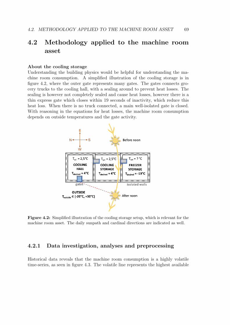
4.2. METHODOLOGY APPLIED TO THE MACHINE ROOM ASSET 69
4.2 Methodology applied to the machine room
asset
About the cooling storageUnderstanding the building physics would be helpful for understanding the ma-chine room consumption. A simplified illustration of the cooling storage is infigure 4.2, where the outer gate represents many gates. The gates connects gro-cery trucks to the cooling hall, with a sealing around to prevent heat losses. Thesealing is however not completely sealed and cause heat losses, however there is athin express gate which closes within 19 seconds of inactivity, which reduce thisheat loss. When there is no truck connected, a main well-isolated gate is closed.With reasoning in the equations for heat losses, the machine room consumptiondepends on outside temperatures and the gate activity.
Figure 4.2: Simplified illustration of the cooling storage setup, which is relevant for themachine room asset. The daily sunpath and cardinal directions are indicated as well.
4.2.1 Data investigation, analyses and preprocessing
Historical data reveals that the machine room consumption is a highly volatiletime-series, as seen in figure 4.3. The volatile line represents the highest available
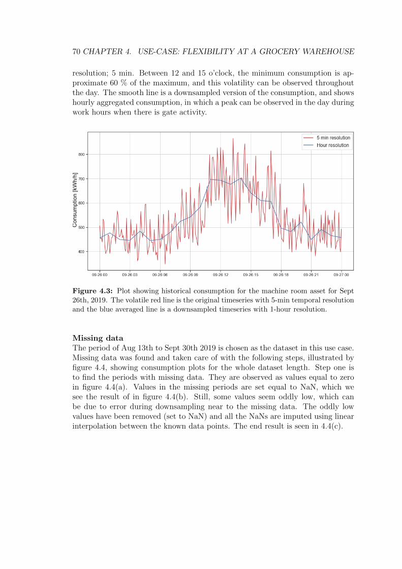
70 CHAPTER 4. USE-CASE: FLEXIBILITY AT A GROCERY WAREHOUSE
resolution; 5 min. Between 12 and 15 o’clock, the minimum consumption is ap-proximate 60 % of the maximum, and this volatility can be observed throughoutthe day. The smooth line is a downsampled version of the consumption, and showshourly aggregated consumption, in which a peak can be observed in the day duringwork hours when there is gate activity.
Figure 4.3: Plot showing historical consumption for the machine room asset for Sept26th, 2019. The volatile red line is the original timeseries with 5-min temporal resolutionand the blue averaged line is a downsampled timeseries with 1-hour resolution.
Missing dataThe period of Aug 13th to Sept 30th 2019 is chosen as the dataset in this use case.Missing data was found and taken care of with the following steps, illustrated byfigure 4.4, showing consumption plots for the whole dataset length. Step one isto find the periods with missing data. They are observed as values equal to zeroin figure 4.4(a). Values in the missing periods are set equal to NaN, which wesee the result of in figure 4.4(b). Still, some values seem oddly low, which canbe due to error during downsampling near to the missing data. The oddly lowvalues have been removed (set to NaN) and all the NaNs are imputed using linearinterpolation between the known data points. The end result is seen in 4.4(c).
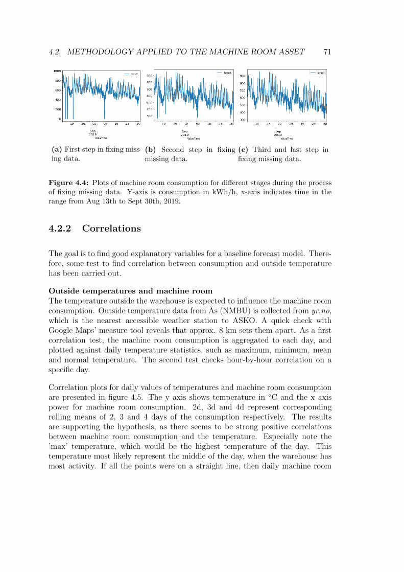
4.2. METHODOLOGY APPLIED TO THE MACHINE ROOM ASSET 71
(a) First step in fixing miss-ing data.
(b) Second step in fixingmissing data.
(c) Third and last step infixing missing data.
Figure 4.4: Plots of machine room consumption for different stages during the processof fixing missing data. Y-axis is consumption in kWh/h, x-axis indicates time in therange from Aug 13th to Sept 30th, 2019.
4.2.2 Correlations
The goal is to find good explanatory variables for a baseline forecast model. There-fore, some test to find correlation between consumption and outside temperaturehas been carried out.
Outside temperatures and machine roomThe temperature outside the warehouse is expected to influence the machine roomconsumption. Outside temperature data from As (NMBU) is collected from yr.no,which is the nearest accessible weather station to ASKO. A quick check withGoogle Maps’ measure tool reveals that approx. 8 km sets them apart. As a firstcorrelation test, the machine room consumption is aggregated to each day, andplotted against daily temperature statistics, such as maximum, minimum, meanand normal temperature. The second test checks hour-by-hour correlation on aspecific day.
Correlation plots for daily values of temperatures and machine room consumptionare presented in figure 4.5. The y axis shows temperature in ◦C and the x axispower for machine room consumption. 2d, 3d and 4d represent correspondingrolling means of 2, 3 and 4 days of the consumption respectively. The resultsare supporting the hypothesis, as there seems to be strong positive correlationsbetween machine room consumption and the temperature. Especially note the’max’ temperature, which would be the highest temperature of the day. Thistemperature most likely represent the middle of the day, when the warehouse hasmost activity. If all the points were on a straight line, then daily machine room
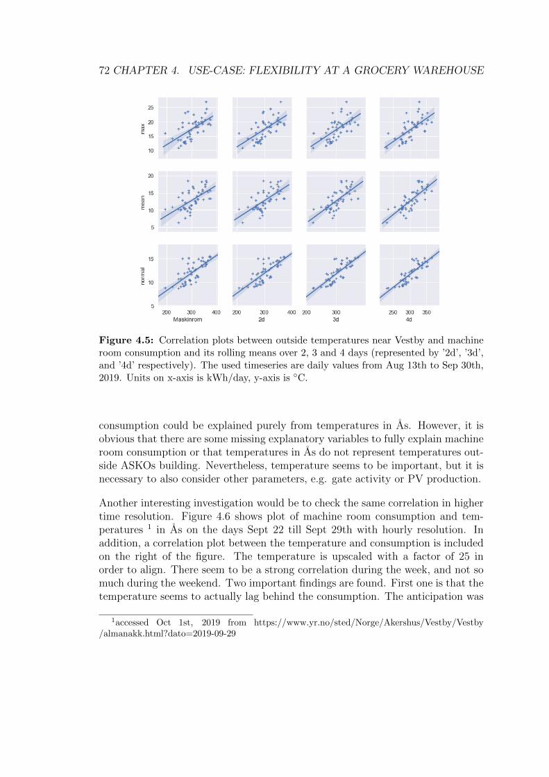
72 CHAPTER 4. USE-CASE: FLEXIBILITY AT A GROCERY WAREHOUSE
Figure 4.5: Correlation plots between outside temperatures near Vestby and machineroom consumption and its rolling means over 2, 3 and 4 days (represented by ’2d’, ’3d’,and ’4d’ respectively). The used timeseries are daily values from Aug 13th to Sep 30th,2019. Units on x-axis is kWh/day, y-axis is ◦C.
consumption could be explained purely from temperatures in As. However, it isobvious that there are some missing explanatory variables to fully explain machineroom consumption or that temperatures in As do not represent temperatures out-side ASKOs building. Nevertheless, temperature seems to be important, but it isnecessary to also consider other parameters, e.g. gate activity or PV production.
Another interesting investigation would be to check the same correlation in highertime resolution. Figure 4.6 shows plot of machine room consumption and tem-peratures 1 in As on the days Sept 22 till Sept 29th with hourly resolution. Inaddition, a correlation plot between the temperature and consumption is includedon the right of the figure. The temperature is upscaled with a factor of 25 inorder to align. There seem to be a strong correlation during the week, and not somuch during the weekend. Two important findings are found. First one is that thetemperature seems to actually lag behind the consumption. The anticipation was
1accessed Oct 1st, 2019 from https://www.yr.no/sted/Norge/Akershus/Vestby/Vestby/almanakk.html?dato=2019-09-29
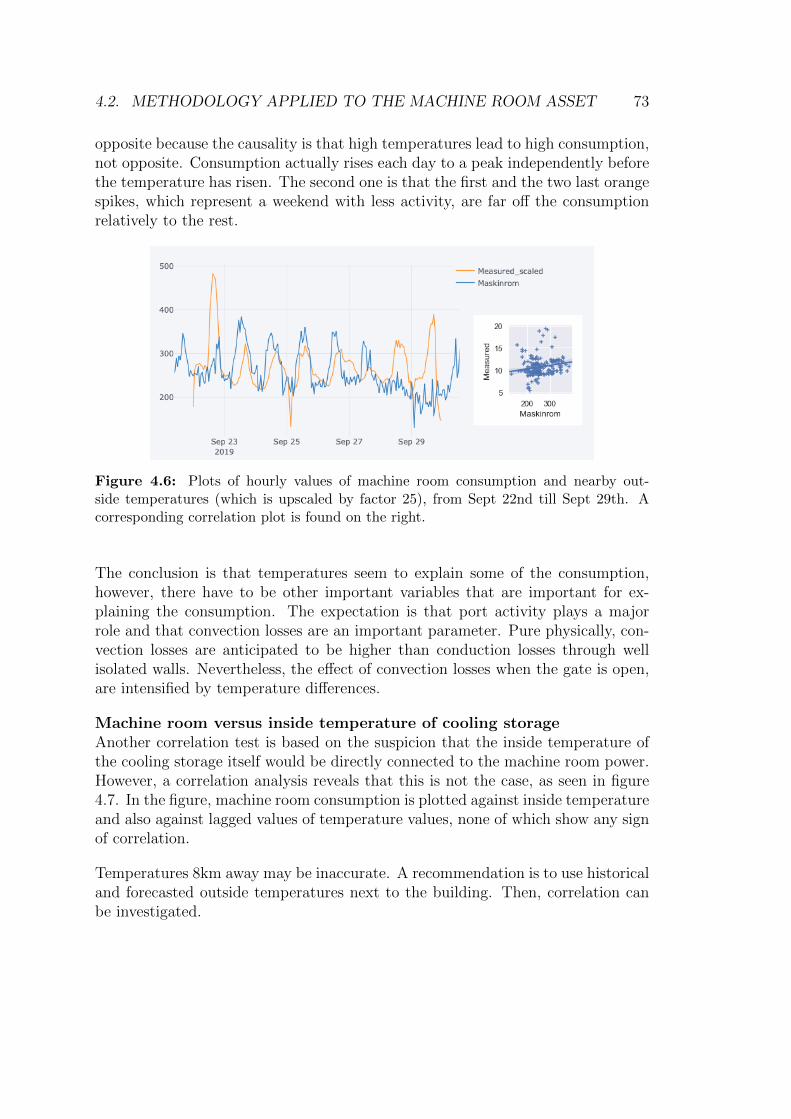
4.2. METHODOLOGY APPLIED TO THE MACHINE ROOM ASSET 73
opposite because the causality is that high temperatures lead to high consumption,not opposite. Consumption actually rises each day to a peak independently beforethe temperature has risen. The second one is that the first and the two last orangespikes, which represent a weekend with less activity, are far off the consumptionrelatively to the rest.
Figure 4.6: Plots of hourly values of machine room consumption and nearby out-side temperatures (which is upscaled by factor 25), from Sept 22nd till Sept 29th. Acorresponding correlation plot is found on the right.
The conclusion is that temperatures seem to explain some of the consumption,however, there have to be other important variables that are important for ex-plaining the consumption. The expectation is that port activity plays a majorrole and that convection losses are an important parameter. Pure physically, con-vection losses are anticipated to be higher than conduction losses through wellisolated walls. Nevertheless, the effect of convection losses when the gate is open,are intensified by temperature differences.
Machine room versus inside temperature of cooling storageAnother correlation test is based on the suspicion that the inside temperature ofthe cooling storage itself would be directly connected to the machine room power.However, a correlation analysis reveals that this is not the case, as seen in figure4.7. In the figure, machine room consumption is plotted against inside temperatureand also against lagged values of temperature values, none of which show any signof correlation.
Temperatures 8km away may be inaccurate. A recommendation is to use historicaland forecasted outside temperatures next to the building. Then, correlation canbe investigated.

74 CHAPTER 4. USE-CASE: FLEXIBILITY AT A GROCERY WAREHOUSE
Figure 4.7: Correlation plots between the machine room consumption and inside stor-age temperatures and its lagged values. The (+) and (-) indicate the forward leadrespectively backward lagged values of inside temperature.
Gate activityThe port activity is by hypothesis believed to play a major role to explain real-timemachine room consumption. Altering of gate activity data is currently not doneduring the work of this thesis.
4.2.3 One-step RNN forecasts
The RNN models in this work only use consumption data in addition to createdtime-features as a features set. They do not include any explanatory variables.A complete list of one-step RNN forecast models with corresponding predictionscores are found in Appendices A.1 and A.2, tables A.1 and A.2. Model parametersand architecture are included as well. Forecast plots for each model is also includedin the respective appendices, ref. figures A.1 to A.8. One of these models, the onewith name 10292019 1715 is showcased here.
RNN model with GRU, one-step forecast
The RNN forecast model has been trained to forecast machine room consumptionone hour ahead, using only lagged values of machine room consumption, timefeatures and lagged values of time series as well. The architecture consists of twolayers, first a GRU layer of 512 units, then a Dense layer with a sigmoid activationfunction to output a single value. It was trained with timeseries having temporalresolution of 1 hour, using batches with batch size of 256 and each sequence withlength of 168 (24*7). Extra features were generated, using lagged values of machineroom consumption with 1, 2, 3, 4, 5, 6, 24, 48 and 168 hour lag. Dummy binaryvariables of all categorical features were created, based on week of the year, day ofthe week and hour of the day. A train size of 90 % were used. A warmup period of12 timesteps is used to improve overall model performance, which means that the12 first timesteps of prediction will not count in MSE train validation, indicated
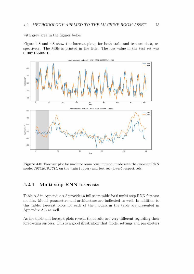
4.2. METHODOLOGY APPLIED TO THE MACHINE ROOM ASSET 75
with grey area in the figures below.
Figure 4.8 and 4.8 show the forecast plots, for both train and test set data, re-spectively. The MSE is printed in the title. The loss value in the test set was0.0071550351.
Figure 4.8: Forecast plot for machine room consumption, made with the one-step RNNmodel 10292019 1715, on the train (upper) and test set (lower) respectively.
4.2.4 Multi-step RNN forecasts
Table A.3 in Appendix A.3 provides a full score table for 6 multi-step RNN forecastmodels. Model parameters and architecture are indicated as well. In addition tothis table, forecast plots for each of the models in the table are presented inAppendix A.3 as well.
As the table and forecast plots reveal, the results are very different regarding theirforecasting success. This is a good illustration that model settings and parameters
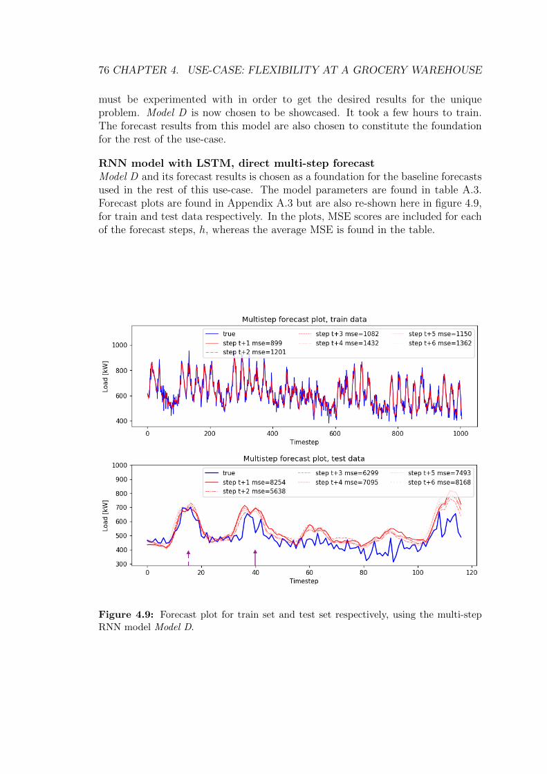
76 CHAPTER 4. USE-CASE: FLEXIBILITY AT A GROCERY WAREHOUSE
must be experimented with in order to get the desired results for the uniqueproblem. Model D is now chosen to be showcased. It took a few hours to train.The forecast results from this model are also chosen to constitute the foundationfor the rest of the use-case.
RNN model with LSTM, direct multi-step forecastModel D and its forecast results is chosen as a foundation for the baseline forecastsused in the rest of this use-case. The model parameters are found in table A.3.Forecast plots are found in Appendix A.3 but are also re-shown here in figure 4.9,for train and test data respectively. In the plots, MSE scores are included for eachof the forecast steps, h, whereas the average MSE is found in the table.
Figure 4.9: Forecast plot for train set and test set respectively, using the multi-stepRNN model Model D.

4.2. METHODOLOGY APPLIED TO THE MACHINE ROOM ASSET 77
Assumptions for the machine room assetIn lack of knowledge for the power and energy storage parameters for the ma-chine room asset, some assumptions must be done in order to succeed with thedemonstration. The assumptions are as following
• Temporal resolution is 1 hour, ∆t=1
• The baseline equals steady state consumption, b = Pcons,SS
• The estimated maximum power Pmax and minimum power Pmin used for cal-culating flexibility is +50 kW and -80 kW relative to the forecasted baselinerespectively. The estimated flexible power is therefore also +50 kW and -80kW from the forecasted baseline.
• The actual realized consumption is assumed to be the true baseline plusthe activated flexibility (and not the forecasted baseline plus the activatedflexibility).
• Initial SoC = 0.6
• ∆Erange is arbitrarily picked to be 600 kWh, so that the time frame seemsreasonable.
• Emax is arbitrarily set to be 8000 kWh.
4.2.5 Example demonstration of a bidding event line
A demonstration is created to follow exactly the design of the conceptual biddingevent line demonstration presented in the methodology chapter, figure 3.8. Torepeat, the goal is to demonstrate the a line of bidding events with both possiblebid outcomes. Referring to figure 3.1, the creation of a bid is made by followingstages 1-4 of the methodology and is followed by two possible outcomes - ignoredbid with pathway A or B or activated bid. The demonstration is designed so toshow both outcomes. The final figure of bid events is illustrated in figure 4.12.Each sub figure indicate successive events of bidding, where the red arrow indicatescurrent time.
The RNN forecast model that was recently showcased, model D, is used to provideforecasted baselines for each bid event. ’2019-09-26 07:00’ is chosen as the startingcurrent time of the demonstration, and for the first event (a) in figure 4.12. Thatcorresponds to timestep 9 in the test set. The corresponding bidding horizon isthen timestep 10 through 15. That represents the first peak seen in fig. ??.

78 CHAPTER 4. USE-CASE: FLEXIBILITY AT A GROCERY WAREHOUSE
The reason for choosing this starting point is two folded. Firstly, using predictionsclose to the train set in time is more realistic approach because the model mostlikely will be retrained regularly as new observations become available with time,e.g. each morning. Secondly, the predictions at the chosen current timestep seemsignificantly better than the rest of the test set, which is partly explained by thefirst reason. Test data that are less distant from the train set will probably relatemore with the train set, and therefore conform better with the trends learned bythe model. However, whether or not the forecasts in the beginning of a test areconsistently better is later investigated in the section Investigating online training.
Briefly about the bid event lineFigure 4.12(a) of illustrate the entered bid for event (a). It is for the biddingperiod 08:00-14:00 and is entered into the flexibility platform at 07:45. This bidis not bought and the bid is ignored. We proceed to the next timestep wherenew flexibility bids are made, as illustrated in figure 4.12(b). The bid is againignored. For event (c), the bid seen in figure 4.12(c) has been made by followingthe methodology. This time, a part of the bid is bought and must be activated.In event (d), the dispatch process goes on, the realized dispatch will be monitoredand the delivered flexible power will be measured as seen in figure 4.12(d). Priorto the end of activation, new bid estimates could be made, but for this asset, itseems appropriate to have a rebound period in order for the cooling storage torecover its SoC level.
4.2.6 Behind the curtains of the bid event line
A stepwise explanation is now to be given for the creation of each flexibility bidevent seen in figure 4.12, including the underlying processes. The figures 4.12,4.10 and 4.11 are going to referred to frequently. These figures contain real-timeforecast plots, flexplots and the flexibility bid for each event. The letters for eachsub-figure correspond to each other and to the events with same letter: event(a), (b), (c) and (d). In addition, table 4.1 contains the forecasted baseline forthe bidding horizon in each event, along with true values. The table and all thefigures are now shown, followed by the walkthrough.
In the table, each row represents the current timestep and contains the true loadon that current timestep and forecasted values for each of future timesteps h. Toclarify, the cells (step=10,h=2) and (step=11, h=1) are both a prediction for therealized true value at cell (step=12,h=0). The rows at timestep 9, 10, 11 and 15correspond with each respective event in the demonstration and to the forecast
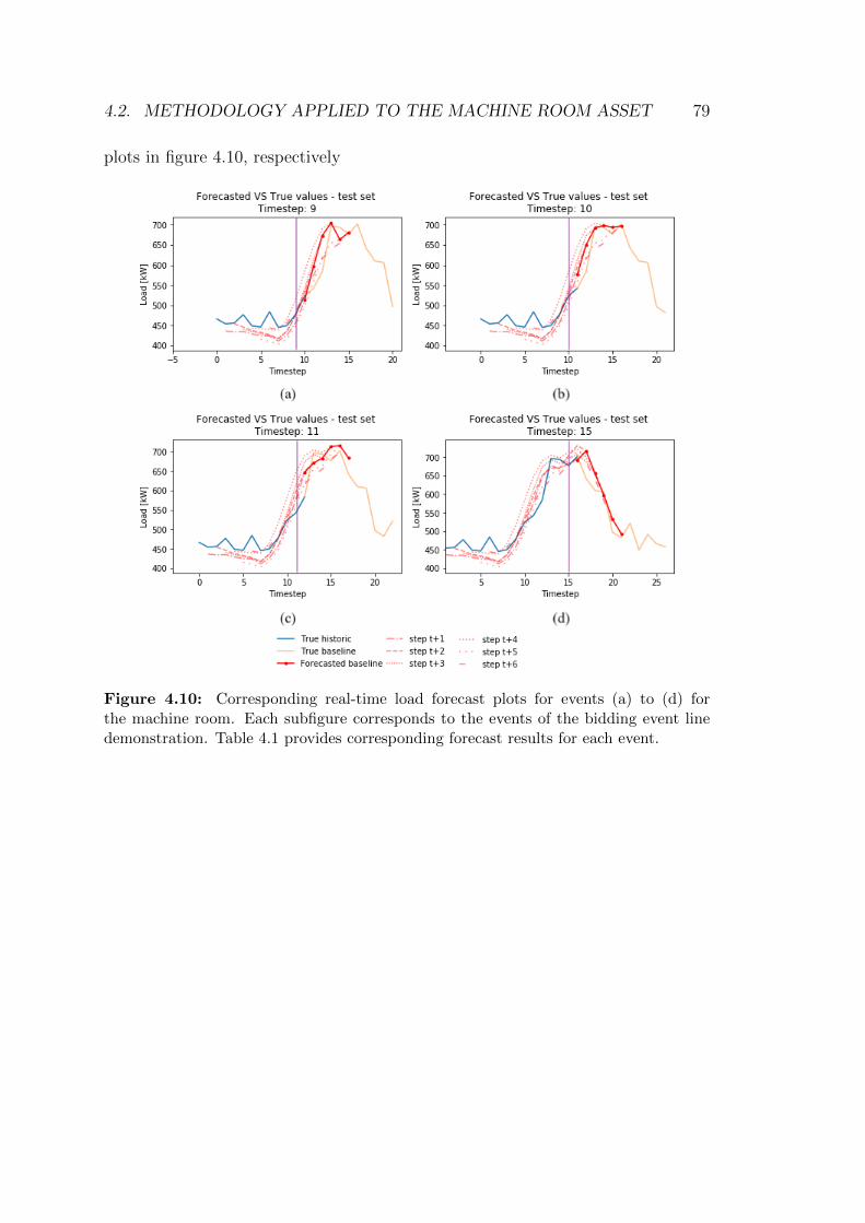
4.2. METHODOLOGY APPLIED TO THE MACHINE ROOM ASSET 79
plots in figure 4.10, respectively
Figure 4.10: Corresponding real-time load forecast plots for events (a) to (d) forthe machine room. Each subfigure corresponds to the events of the bidding event linedemonstration. Table 4.1 provides corresponding forecast results for each event.
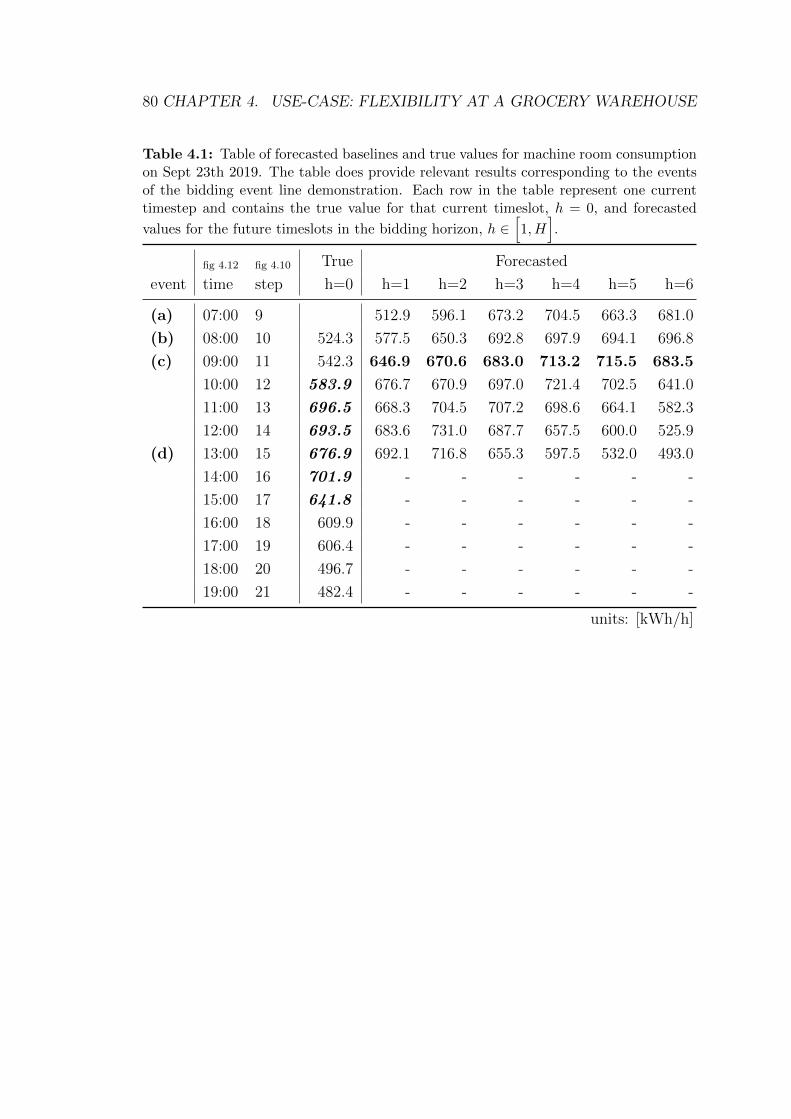
80 CHAPTER 4. USE-CASE: FLEXIBILITY AT A GROCERY WAREHOUSE
Table 4.1: Table of forecasted baselines and true values for machine room consumptionon Sept 23th 2019. The table does provide relevant results corresponding to the eventsof the bidding event line demonstration. Each row in the table represent one currenttimestep and contains the true value for that current timeslot, h = 0, and forecasted
values for the future timeslots in the bidding horizon, h ∈[1, H
].
fig 4.12 fig 4.10 True Forecasted
event time step h=0 h=1 h=2 h=3 h=4 h=5 h=6
(a) 07:00 9 512.9 596.1 673.2 704.5 663.3 681.0
(b) 08:00 10 524.3 577.5 650.3 692.8 697.9 694.1 696.8
(c) 09:00 11 542.3 646.9 670.6 683.0 713.2 715.5 683.5
10:00 12 583.9 676.7 670.9 697.0 721.4 702.5 641.0
11:00 13 696.5 668.3 704.5 707.2 698.6 664.1 582.3
12:00 14 693.5 683.6 731.0 687.7 657.5 600.0 525.9
(d) 13:00 15 676.9 692.1 716.8 655.3 597.5 532.0 493.0
14:00 16 701.9 - - - - - -
15:00 17 641.8 - - - - - -
16:00 18 609.9 - - - - - -
17:00 19 606.4 - - - - - -
18:00 20 496.7 - - - - - -
19:00 21 482.4 - - - - - -
units: [kWh/h]
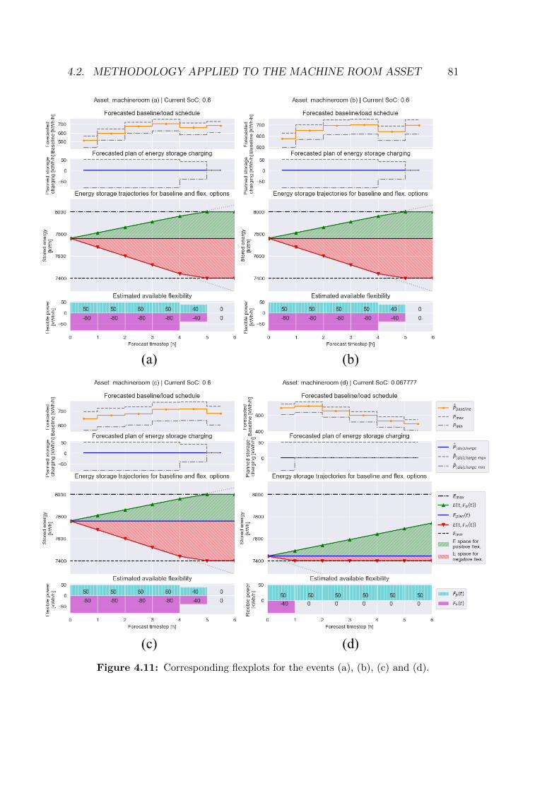
4.2. METHODOLOGY APPLIED TO THE MACHINE ROOM ASSET 81
Figure 4.11: Corresponding flexplots for the events (a), (b), (c) and (d).

82 CHAPTER 4. USE-CASE: FLEXIBILITY AT A GROCERY WAREHOUSE
Figure 4.12: Bidding event line plot. Example demonstration of a bid procedurefor the machine room asset, on Sept 26th, 2019. Real forecast baselines are used, butassumptions on asset parameters are made. The bid event in each subfigure representsuccessive bidding horizons where the current time equals (a) 07:00 (b) 08:00 (c) 09:00and (d) 10:00 → 13:00.

4.2. METHODOLOGY APPLIED TO THE MACHINE ROOM ASSET 83
Python implementationA complete script for creating and training the used RNN model, including theforecasts, is found in Appendix B.1. In the bottom of the same script, underAnimation, is code for creating the real-time forecast plots seen in figure 4.10. Theassumed asset parameters and the forecast results are entered into the Python assetmodelling framework, event by event. The asset class Asset presented in appendixB.2 is used for the purpose. The complete Python script used for simulating eachevent and for creating the flexplots in fig. 4.11 is found in appendix B.3 and usesthe baseline forecast results found table 4.1.
Event (a)The forecasted baseline (for timestep 10 through 15) is found in table 4.1 wherestep=9. The corresponding real-time forecast plot is shown in figure 4.10 (a) withred dots. The forecast is input as baseline to the asset model which together withall asset parameters estimate the available flexibility and energy storage trajector-ies. These estimations are visualized in its flexibility plot, figure 4.11 (a), revealingthat the energy storage cannot handle more than 4 hours of full flexible activation.The estimated positive and negative flexibility is formulated as a flexibility bid.The forecasted baseline and the flexibility bid are sent to the flexibility market, asseen in figure 4.12(a). The reader may notice that the +50kWh/h and -80kWh/his bidded for all slots, in contradiction to the constraints set by the energy storagelimits. This is done only to illustrate the freedom in bidding. Suppose that theflexibility buyer does not have to buy the first timeslot, but that they can choosefreely. Then, here, while the energy storage still impose constraints on flexibility,is reflected by a maximum and minimum activated energy quota as a part of thebid.
The bid is not activated by anyone at this point. According to the methodology bidignored, time increment as the methodology is reset for new flexibility estimates.
Event (b)Time has incremented and we are now at step 10, prior to the bidding period fortimesteps 11 through 16. The forecasted baseline is the row with step=10 in table4.1 and plotted in figure 4.10 (b). In a similar fashion to event (a), the flexibilityis estimated and a flexplot is made, found in figure 4.11(b). A bid is made andentered into NODES, shown in figure 4.12(b). The bid is ignored this time as well.Flexibility estimates for the next bidding period is prepared.
Event (c) - activationWe are now at timestep 11, and the methodology stages are done exactly as inprevious events. In table 4.1, the forecasted baseline is indicated by the numbers

84 CHAPTER 4. USE-CASE: FLEXIBILITY AT A GROCERY WAREHOUSE
in bold. The true baseline, which we only know because this is a hypotheticaldemonstration on historical data, is indicated by numbers in bold and italic. Real-time plot of the forecast is shown in figure 4.10(c). The forecast both overestimatesand underestimate slightly at different points, but this we do not actually ”know”yet in a real-life application. Based on the forecasted baseline, the flexibility isestimated and the energy storage level is simulated, shown in flexplot figure 4.11(c).A bid is created an presented in figure 4.12(c).
As opposed to previous events, the event (c) is subject to a bid activation froma flexibility buyer. They want to buy maximum negative flexibility for the firstfour timeslots. The corresponding summed energy is -320 kWh. This is all right,because it is below the energy limit of -340 kWh and will not exceed the energystorage limits. The building has now committed to deliver the bought amount offlexible power at each timeslot. It is measured relatively to the forecasted baseline,which is important to keep in mind.
According to the methodology, bid activation leads to a dispatch of the flexiblepower and we do now proceed to event (d) in figure 4.12.
Event (d) - dispatchingThe process of the dispatch is out of the scope of this thesis, and without furtherintel, the assumptions made regarding the dispatching ability must be followed.The assumption is a perfect dispatch from the real baseline, which is known in thishypothetical backtest. Because of that, the errors in of the flexibility estimates ofthis demonstration depend purely on the load forecast precision.
The building has now committed to deliver flexibility relative to the forecastedbaseline. The delivered flexible power is by assumption based on the true baseline,but the error of deliverance is measured from the forecasted baseline that wasentered to NODES. With some math, the resulting delivered flexibility relative tothe forecasted baseline, is shown in the event line, figure 4.12(d).
Using equation 3.19, the error of delivered flexible power is[− 63.0,−25.9,+10.5,−36.3
]kWh/h.
Summing up, the integrated delivered flexible power is -382.9 kWh, which is morethan what was anticipated and bought by the flexibility buyer. This is mostprobably not a problem, since the buyer most likely suffer most with too littlethan to much of what they desire. Hence, the delivered flexibility for timeslotsbetween 11:00 and 13:00 are most likely a more serious crime, because of too lowdeliverance. Accurate deliverance is nevertheless ideal.
What will be the new state after activation? Although the integrated delivered

4.2. METHODOLOGY APPLIED TO THE MACHINE ROOM ASSET 85
flexibility is above the limits, the discharge of the storage is still -80 kWh/h, as thiswas the main assumption. The total integrated discharged energy of the energystorage equals the bought energy of -320 kWh. This leads to a change in SoC of
∆SoC =−320kWh
600kWh= −0.533
leading to a new SoC of 0.600− 0.533 = 0.067. Before the activation period ends,the methodology will rerun to make new flexibility estimates. Considering the newSoC, the methodology will be repeated according to the methodology. The newsituation with updated flexibility estimates leads to the flexplot shown in figure4.11(d). The period after the activation period is however denoted as rest/reboundtime and is subject for discussion later in the thesis. There is no rest time for themachine room asset, but a rebound effect which results in extra high consumptionin order to recover the SoC level is expected.
Another example flexplot for machine roomNow, an example is presented to illustrate how the flexplot may look like with otherassumptions for Pmax and Pmin. Considerations that are made for the flexplotshown in figure 4.13 is as following:
• Pcons = Pcons,SS =[
696, 693 ↓ 676, 701, 641, 609, 606, 496, 482, 521]
kWh/h, where the arrow indicates current timestep.
• The maximum power Pmax and minimum power Pmin is +100 kW and -200kW relative to a rolling average (3h) of the baseline consumption.
• SoC is assumed to stay at 0.6, ∆E is arbitrarily picked to be 1000 kWh, sothat the time frame seems reasonable.
• Emax is arbitrarily set to be 9000 kWh.
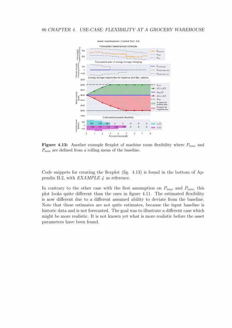
86 CHAPTER 4. USE-CASE: FLEXIBILITY AT A GROCERY WAREHOUSE
Figure 4.13: Another example flexplot of machine room flexibility where Pmax andPmin are defined from a rolling mean of the baseline.
Code snippets for creating the flexplot (fig. 4.13) is found in the bottom of Ap-pendix B.2, with EXAMPLE 4 as reference.
In contrary to the other case with the first assumption on Pmax and Pmin, thisplot looks quite different than the ones in figure 4.11. The estimated flexibilityis now different due to a different assumed ability to deviate from the baseline.Note that these estimates are not quite estimates, because the input baseline ishistoric data and is not forecasted. The goal was to illustrate a different case whichmight be more realistic. It is not known yet what is more realistic before the assetparameters have been found.

4.2. METHODOLOGY APPLIED TO THE MACHINE ROOM ASSET 87
Investigation of online trainingThe goal of this investigation can be comprehended as:
Does online retraining of a forecast model increase predictive performance of short-term forecasts, relative to the exact same model that is not retrained?
As aid for addressing this question, three identical forecast models are created.The models do have a slightly dataset foundation that differs in time. The modelsare trained on different time periods but all mak forecasts for the same givenpoint in time, in order to check if prediction for the given point is changed. Moreimportantly, do the forecasts become better as the training period moves closer tothe given time point?
The comparison is best understood by presenting the plot of the forecast results,presented in figure 4.14. Each subfigure presents each model, having a train-testsplit at slighly different occations. The respective solid and dashed arrows in allthe graphs, points at the same point of time and are used for the comparison. Donot get confused by the timestep axis, it can be ignored.
The dashed arrow actually refer to the same peak that was subject for the abovebidding event line demonstration. In figure 4.14 (a), the forecasted values do seemto have a clear positive bias, it overestimates. In addition, it seems to lag a bitbehind. The results in figure 4.14 (b) us achieved by moving a day ahead andusing the observations of that day in the training foundation for new forecasts.The results for the dashed arrow are considerably better. It seems to not have aclear bias and hits very well. The dashed arrow is not included in figure 4.14 (c).
Next comparison is the peak pointed at by the solid arrow. Starting at figure4.14 (a), the forecast seems to be consequently overestimating, also for the wholetest set. In figure 4.14 (b), it seems like the model has learned some importanttrends, as the forecasts for that peak look better. The interesting thing ti checkis whether the model will yield better results for that point with fresher trainingdata. As figure 4.14 (c) shows, there are no visible improvements, except for aslightly smoother forecast. It is hard to conclude anything instantly.
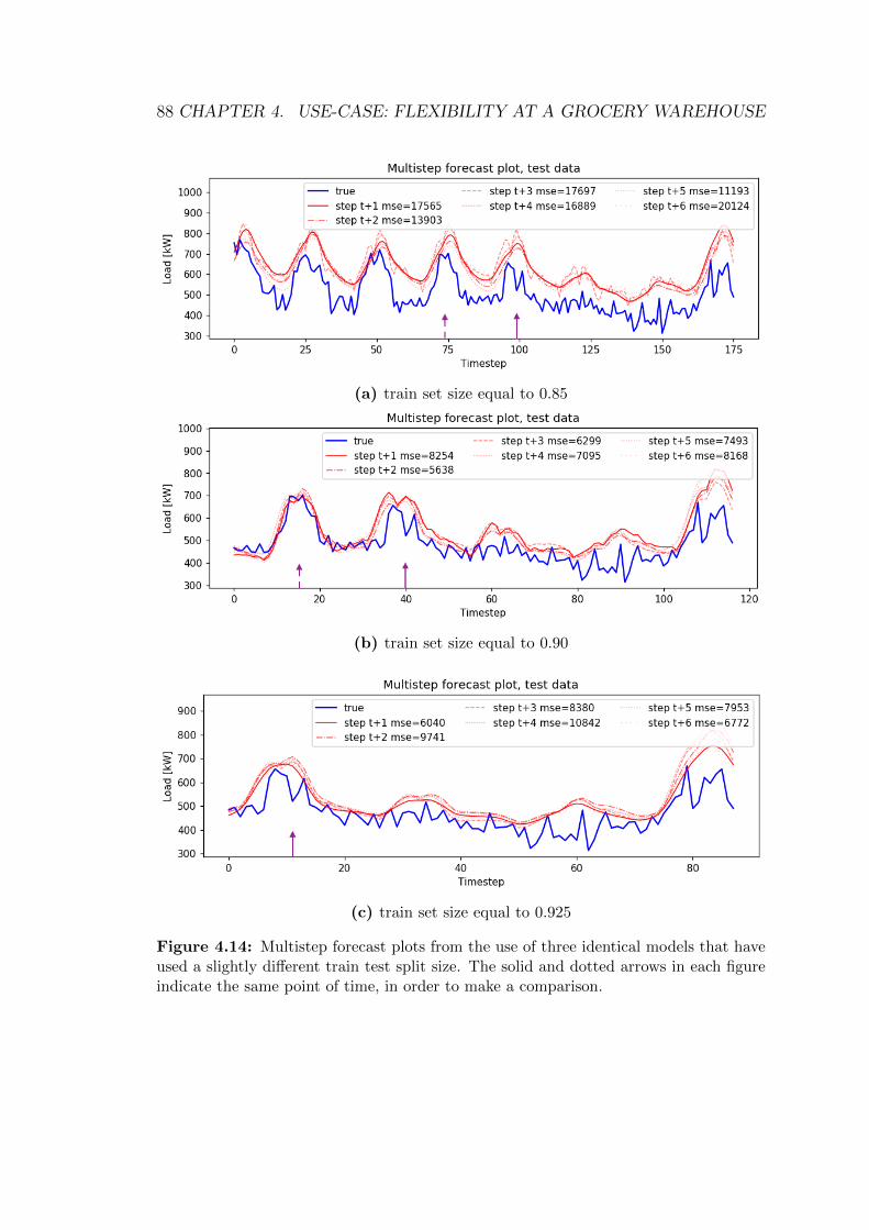
88 CHAPTER 4. USE-CASE: FLEXIBILITY AT A GROCERY WAREHOUSE
(a) train set size equal to 0.85
(b) train set size equal to 0.90
(c) train set size equal to 0.925
Figure 4.14: Multistep forecast plots from the use of three identical models that haveused a slightly different train test split size. The solid and dotted arrows in each figureindicate the same point of time, in order to make a comparison.

4.3. APPLICATION FOR OTHER ASSETS 89
4.3 Application for other assets
The following examples are not directly use-cases. The reason for this is they do notdirectly use data from the use-case, with one exception, and are merely hypothet-ical demonstrations. However, they are highly relevant, because the consideredassets belong to ASKO, although many asset parameters are picked arbitrarily.The data foundation for the water heater consumption is much inspired by dataprovided by ASKO.
4.3.1 Battery
Flexplot examples for both an active and a passive battery were presented in theMethodology chapter. The two following bid event line examples consider a passivebattery with the same parameters as the one in the flexplot figure 3.5.
Bidding event line example 1For this example it assumed that the flexibility buyer must activate all of eitherthe positive or negative flexibility if it wants to buy anything. The bid event lineexample is shown in figure 4.15. The flexibility bid is designed accordingly and isdirectly restricted by the energy capacity limits. When the negative flexibility bidis bought in (c), the battery will dispatch it during the two hours, followed by arebound period of two hours to recover the SoC level and bid again.
Bidding event line example 2Another bidding event line example is found in figure 4.16. The exact same situ-ation as above is assumed, except that the bid formulation now offers a free se-lection of bid slots. In addition, the flexibility buyer can choose anything in theoffered range of flexible power. As seen in (a) and (b), the flexibility bids arealways at maximum, not directly limited by any energy storage limits. The im-portant aspect in this case, is overall energy restrictions, here ±32.5 kWh. Aslong as total net activated flexible power does not exceed the energy restrictionsduring any point of the dispatch period, the bid shall be accepted. In (c), somearbitrarily flexibility bid slots are chosen to be activated by a flexibility buyer,and each flexibility slot is not fully activated. The first three bought slots are -10kWh/h out of the available -30 kWh/h. Thus, -30 kWh of the energy quota isused. The fourth and fifth slot contain +20 kWh/h of bought flexible power each.That sets our energy quota back and up to +10 kWh. The sixth and final slotis full negative activation. In end, the energy quota is -20 kWh. This is checked
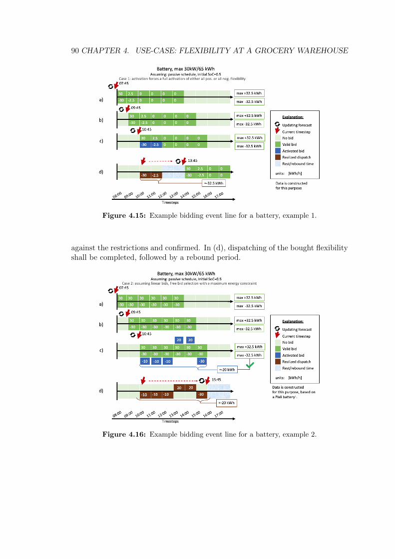
90 CHAPTER 4. USE-CASE: FLEXIBILITY AT A GROCERY WAREHOUSE
Figure 4.15: Example bidding event line for a battery, example 1.
against the restrictions and confirmed. In (d), dispatching of the bought flexibilityshall be completed, followed by a rebound period.
Figure 4.16: Example bidding event line for a battery, example 2.
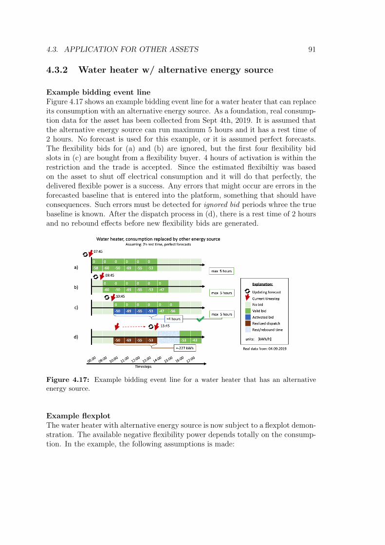
4.3. APPLICATION FOR OTHER ASSETS 91
4.3.2 Water heater w/ alternative energy source
Example bidding event lineFigure 4.17 shows an example bidding event line for a water heater that can replaceits consumption with an alternative energy source. As a foundation, real consump-tion data for the asset has been collected from Sept 4th, 2019. It is assumed thatthe alternative energy source can run maximum 5 hours and it has a rest time of2 hours. No forecast is used for this example, or it is assumed perfect forecasts.The flexibility bids for (a) and (b) are ignored, but the first four flexibility bidslots in (c) are bought from a flexibility buyer. 4 hours of activation is within therestriction and the trade is accepted. Since the estimated flexibiltiy was basedon the asset to shut off electrical consumption and it will do that perfectly, thedelivered flexible power is a success. Any errors that might occur are errors in theforecasted baseline that is entered into the platform, something that should haveconsequences. Such errors must be detected for ignored bid periods whree the truebaseline is known. After the dispatch process in (d), there is a rest time of 2 hoursand no rebound effects before new flexibility bids are generated.
Figure 4.17: Example bidding event line for a water heater that has an alternativeenergy source.
Example flexplotThe water heater with alternative energy source is now subject to a flexplot demon-stration. The available negative flexibility power depends totally on the consump-tion. In the example, the following assumptions is made:

92 CHAPTER 4. USE-CASE: FLEXIBILITY AT A GROCERY WAREHOUSE
• Alternative energy source has a max runtime of 4 hours.
• The load forecast of the water heater baseline is assumed to be perfectly
known, ~b =~b =
[↓ 300, 280, 270, 290, 340, 310
]kWh/h
• ∆t= 0.25
• Pmin = 0 kWh/h, Pmax = b
• Pcons,SS = 0 kWh/h
These assumptions yield the flexplot presented in figure 4.18. No energy storageis added, but the max runtime is implemented in the Python script. The negativeflexibility is clearly equal to the forecasted baseline. Suppose the bid is activatedand the consumption is set to zero. What the actual baseline would be if not forthe activation is impossible to know. The baseline forecast may have missed.
Figure 4.18: An example flexplot for a water heater with an alternative energy source.
Code snippet for creating the flexplot (fig. 4.18) is found in Appendix B.2, withEXAMPLE 3 as reference.

4.3. APPLICATION FOR OTHER ASSETS 93
4.3.3 Water heater w/ flexible heat storage
Example flexplotA flexplot is now demonstrated for a water heater with a heat storage. In theexample, the following assumptions are made:
• Tmax = 90 ◦C = 363 K
• Tmin = 60 ◦C = 333 K
• The load forecast of the water heater baseline is assumed to be the same asfor the water heater with alternative energy source,
~b =~b =
[↓ 300, 280, 270, 290, 340, 310
]kWh/h
• The heat capacity of medium is cp,water = 4.18 kJ/kgK = 0.00161 kWh/kgK
• The mass of the water content is m = 4000 kg
• Steady state consumption still equals the baseline.
• Initial SoC is 0.5
• ∆t= 0.25
• Pmin = 0 kWh/h, Pmax = 400 kWh/h
Inserting the temperature range, heat capacity and mass into equation 3.26, yields∆E = 193.2 kWh. Emin is set to 0. All in all, these assumptions yield the flexplotpresented in figure 4.19.
The negative flexibility is equal to the forecasted baseline, but gets quickly restric-ted by the energy storage. There are some positive flexibility as well. Increasingthe Tmax might lead to higher heat losses from the storage, but neglected here.To increase the flexibility, one can increase the mass or Pmax. Suppose the bid isactivated and the consumption is set to zero. What the actual baseline would beif not for the activation is impossible to know.
Code snippet for creating the flexplot (fig. 4.18) is found in Appendix B.2, withEXAMPLE 3 as reference.
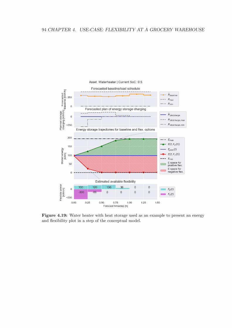
94 CHAPTER 4. USE-CASE: FLEXIBILITY AT A GROCERY WAREHOUSE
Figure 4.19: Water heater with heat storage used as an example to present an energyand flexibility plot in a step of the conceptual model.

Chapter 5
Discussion
The discussion section is divided into three sections: Discussion of the RNN results,the use-case and the methodology.
5.1 RNN results
Various RNN models have been experimented with in order to address problemstatement (S2). An extensive selection of RNN models with their results are foundin Appendix A. They will now be discussed.
In general, the models perform very differently regarding train scores, test scores,whether or not they generalize well and how precise they seem to be where itmatters. In other words, the choice of model architecture and parameters yieldcompletely different outcomes. What the desired outcome actually is, is also adiscussion. A general weakness of these results is that they do not tell us how themodels would perform on other train and test sets than the ones used. A modelperforming good on this chosen data set does not guarantee good performance onfuture sets (real life forecasting), but will nevertheless give indications of what agood model is.
Test set versus train set MSE scoresThe test score versus train score is much about whether or not the model haslearned the correct trends between the real explanatory variables and target. If ithas, then both test and train MSE could be low, with the test MSE being slightly
95

96 CHAPTER 5. DISCUSSION
worse. A very good train score and a terrible test score strongly indicate overfittingand is unsatisfying. If the test score is good and much better than the train score,there is a good chance there was a good portion of coincidental luck with the giventest set.
Consistency between test MSE score and visual precisionModel predictions could seem better in a prediction plot than what the MSE scoreindicate. An important topic to discuss is whether or not MSE scores provide ameaningful metric for determining if a model does what we want them to do. Firstof all, what we want the models to do can be different for different purposes. Forexample, one would perhaps want a model to rather hit the peaks than the restof the set. Another example is that one wants to predict the first 6 or 24 hours inthe test set accurately and the rest is uninteresting. Second of all, the scores donot tell anything about the volatility and stability of the forecasts. Such thingscan be seen in a forecast plot and perhaps with statistical tools. In some cases,it is desirable with smooth forecasts rather than very volatile ones. On the otherside, volatile forecasts could perhaps catch smaller trends, such as peaks, better,but are perhaps more sensitive to noise in the data. A solid and accurate featureset will give a good foundation for explaining every little trend in the target, buta good model will actually be able to learn them properly and ignore any noise.
In this use-case, it is important to have stable forecasts which catches the peaks.It is desirable to have good forecasts for the immideate future. Since Hafslundprobably is most interested in negative flexibility, it is better to overestimate theconsumption rather than underestimate it in order to not overestimate the avail-able negative flexibility.
Discussion around the results For the results in One-step forecasts 1, tableA.1, the trend is that all the train scores are better than the test scores. The trainscores seem consistently good, but the test scores are very different. The worst testscore is 11656 for model 10302019 2000. It happens to be that this model also hasthe best train score. That indicates it has overfitted on the training set and weren’table to generalize enough. It may have considered noise from the training set tobe important for explaining the test target, when it was actually not. However,when looking at the forecast plots, they reveal that there is not much noise inthe forecasts. The forecasts are actually pretty smooth and the predictions forthe train set hit very well. Even though the test score was horrible, they seemto have generalized well and catch the trends. It is consistently overestimating,something that could be considered valuable to the specific use-case if there is alack of accurate models. In addition, if it was not for the bad forecast on the lastpeak, the test MSE would have dropped considerably. This is a good example that

5.1. RNN RESULTS 97
the MSE is not representable for where we want good forecasts.
The two best models regarding test score are 10292019 1915 and 10302019 1110.They have test scores of around 4800. The first has the worst train score of themall, whereas the latter actually almost has the best train score of them all. For thefirst, the forecast plot reveals that many of the peaks were not reached in the trainset, but they were in the test set. The second model (10302019 1110 ) does notseem to have the same problem. It hits the peaks in the train set and performswell on the test set. It has a relatively simple structure of two LSTM layers with48 units each, as opposed to one single LSTM layer with 400 units. The modelswith a Masking layer seem not to work well and only worsen all the test scores.That could be explained by misuse and wrong implementation from my side. Tothis point, it seems like a small model architecture of two LSTM layers with asmall amount of units, performs the best. Larger networks with techniques toavoid overfitting are discussed for the multi-step forecasts.
For the results in One-step forecasts 2, table A.2, all models have much ofthe same architecture: two LSTM layers with 400 units each, except for the lastone which has 200 units each. Other parameters have been varied. The testscores are consistently worse than the train scores, except for one rare exception.Model 12112019 1327 has the best test MSE and it is better than its train MSE.This model has one distinct difference to the others, namely that it has a linearactivation function and not a sigmoid activation function. The reason of the goodtest score and why it is better than train score is probably because of what wesee in the forecast plots, fig A.6. None of the peaks and valleys in the train setare caught, as opposed to the test set. This fact tells more about the chosen testset than about the model. First, the model is very weak, from what is seen in thetrain set forecast plot. The test set seem to be a portion of the data where thepeaks and valleys are small. On this basis, it can be concluded that the choice ofthe test set highly influence the scores. If a model is overall good or not, cannot beconcluded before it has been tested on various test sets. We can however concludethat a premise for a good model is that the predictive performance for the trainset and the test set should be similar, and that the main trends both in the trainset and test set, such as peaks and valleys, are caught by the forecasts.
For the results in Multi-step forecasts, table A.3, the trend is good train scoresand bad test set scores. The MSE scores in the table is an average score ofthe separate MSE scores for each forecast step, found in the forecast plots. Ingeneral, the results look similar to the previous ones and the first two peaks inthe test set, a Thursday and Friday respectively, has considerably good forecasts.The last peak, a Monday, does not. Relatively big architectures with overfitting

98 CHAPTER 5. DISCUSSION
techniques, such as Dropout, do not seem to drastically improve results relative tothe previous and simpler ones in the one-step forecast section. On the other side,the forecasts for the train sets seem to be very precise and catch the peaks andvalleys well. That indicates that the trends of the target in the train set has beenlearned. Thus, there might be some benefits in large architectures with overfittingtechniques. The test set MSE scores are not good, but from what the plots show,they perform considerably well on the first two peaks. The predictions are howeverunstable because of bad performance on the last peak. As later discussed, the causeto this might be factors other than model architecture.
Model D was arbitrarily chosen from the fact that its forecasts were good for thetrain set and it performed well on the beginning of the test set, thus giving a goodfoundation for the use-case. For direct multi-step models, perhaps it could bebeneficial to optimize each model for each forecast step. Also, it is thought that arecursive-direct strategy would overcome some of the limits of a direct strategy.
For the many models having bad forecasts for the last peak of the test set, it shouldbe mentioned that this last peak is a Monday of a new week. This day has a newcategorical week feature, which has not been part of the training data. Theseforecasts therefore lack a part of its feature foundation for prediction. Skippingthe Monday during evaluation will provide more representable MSE scores. Itis also thought that replacing the categorical ’week of the year’ feature with analternative continuous and seasonal feature will provide more stable and betterforecasts.
Sources of errorThe real world contains uncertainties and can never be modelled perfectly. Never-theless, imperfect models can be important tools that are sufficient for the purpose.Some errors for RNN models can be identified and minimized. A source of erroris wrong measurements in the dataset. The monitoring equipment itself can havean error which means that it does not measure the values precisely. It could besystematic errors (bias) or random errors. Such errors cause noise for the forecastmodel.
In the use-case, it was found an error in the measured consumption of the machineroom components, which constituted the target. This was resolved by finding away to calculate the correct measurement based on the other assets which seemedto be correct. However, the other measurements can still contain errors, and ifthey do, there will be an error in the machine room consumption data as well.

5.1. RNN RESULTS 99
Weaknesses
What does the scores not tell us?It does not tell us how the models would perform on different test set at otherdata and periods. Therefore, as a further work, it is necessary to test a model onmany different train and test sets throughout time.
Length of input dataOne important topic regarding predictive performance is the length of the trainingdata. The RNN models in this use case were provided one and a half months ofdata. According to the literature, neural networks benefit from long and goodstructured datasets, which may not have been the case here. It is discussed that itcould affect predictive performance negatively, however it may not be purposefulto provide longer datasets.
Firstly, these models have been specialized in the trends of August and September.They have most probably not been able learn the various trends throughout theyear. When the winter comes, new trends will occur and unless the models areretrained with winter months, they will probably lose their predictive strength.An exception, of course, is if the RNN model has been provided all explanatoryparameters (features) that completely explain the target, both through seasonaland systematic changes.
As for the use-case, time features were made for ‘hour of the day’, ‘day of theweek’ and ‘week of the year’. The two first ones will repeat themselves frequentlythroughout the year and catch daily and weekly trends well. The training founda-tion for ‘hour of the day’ is good, there are around 50 observations for each category(01:00, 02:00 . . . 23:00). The ‘day of week’ has a weaker training foundation, butthere are at least 7 weeks of observations for each day (Monday, Tuesday,...). Thelatter, ‘week of the year’, has a lacking training foundation, because the trainingset needs to be of at least one year, so that each week is iterated through. Inthe use-case, the models were trained on a few weeks in the train set, but thislearning is not brought into the prediction of unseen weeks in the test set. Either,the model must be trained for a whole year of systematic and structured data, oranother approach for implementing seasonal structure must be used. One altern-ative, which does not demand a whole year of training to catch seasonal trends, isto create a continuous sinus-cosines feature, as proposed by Gabor [37]. Anotheralternative, as also concluded by the last paragraph, is to instead just have anexplanatory feature set which fully explains the target and all its seasonal trends,such as port activity/work schedules and temperatures.

100 CHAPTER 5. DISCUSSION
It might not be purposeful to make a complete model for the whole year, becausethe system can change.
Systematic changesAn RNN model based on historical data without explanatory variables performsgood when there is a clear structure in the data. What happens if there is astructural change in the data foundation, such as changing the work plans orchanging the properties of the asset, e.g. expanding the cooling storage? An RNNmodel without explanatory features would suffer from such systematic changes,because previous trends get broken. A model that is trained on previous trendsdoes not work on a new situation where the correlations between the historicaldata and the target have changed and a new model must be made.
On the other side, if the systematic change is caused by a change of the work plans,then a model that uses work plans as a feature will be able to handle that. Also,if the systematic change is caused by a change in storage size etc., again havinga model with such parameters as a part of the feature set will be able to handlethese changes. The same accounts for temperature trends.
Finding a good model is time consumingAnother setback for using RNN models, as with many other models, is that it istime consuming, demands knowledge on the field and finding the best predictivemodel is requiring. On the other side, this is a comprehensive work that is usuallyrequired once in the initial process. Finding the optimal model can be done bymeans of a grid search with cross-validation, which involve training and testing ofa vast amount of model parameter combinations and various test sets. It can berun once. It requires a lot of time, memory and computational resources. Gridsearch was however not done in this work, because optimizing model parameterswas not in the scope of this thesis, because it would be too time consuming anddemanding to perform with the available resources. A grid search will also revealwhich parameters have the most influence and also which parameter combinationsyield the best results.
Retraining of a model with new observations will also take some time. Retrain-ing is done because we think that longer training data might improve predictiveperformance and also that the model will learn new trends that are found in thenew observations. Computational time of retraining sets a restriction on how oftenmodels like this can be retrained. The computation complexity can be reducedby choosing a simpler model structure than those used. Simpler models may verywell perform as good or better. On the other side, it is perhaps not necessary toretrain a model that often. 1 week could work very well as each day. Retraining

5.1. RNN RESULTS 101
every month could even work, but then it is probably important to have manygood explanatory parameters in the feature set, as already mentioned many times.
Black boxAnother setback of using RNN model is that is hard to interpret the learnedtrends and rules behind its results, as opposed to other simpler ML methods andtraditional statistical methods.
Missing explanatory featuresThe RNN models in this thesis did not use the explanatory variables that werethought valuable for model performance. It is thought that including featuresfor port activity/work plan and outside temperatures will improve the stabilityand performance of the forecast model significantly. Then, the model is thoughtto also cope with structural and seasonal changes. This hypothesis has roots inthe physics of heat loss mechanisms, as presented in the theory and methodologychapters and it must be further investigated and tested.
Strengths
Retraining catch new trendsIt seems that the RNN models can catch trends and perform very well even onshort datasets without explanatory variables. Using RNNs as a load forecast mod-els seem promising, but further work is to use explanatory features and to findoptimized model parameters.
Making forecasts is quickAnother pro of RNN models is that they are really quick at making new fore-casts. Once the training process is finished, making real-time predictions withnew observations only take seconds.
Overcome input data errorsAn RNN model might overcome sources of error in input data, because it will stilllearn the trends between the dataset, although it contains errors, and the targetin order to explain the target. However, if the target contains errors, the modelwill learn to output a target with similar errors, which should be avoided.

102 CHAPTER 5. DISCUSSION
Investigation of online training
An investigation was done to check whether or not model D had consistently betterforecasts for a point in time when it got retrained with new observations.
Weaknesses with the experimentThere are some clear weaknesses with this experiment. First of all, the test is notvery extensive and the answers that are possibly found, are not general at all. Theanswers only tell us the case with this specific situation with these specific choicesof test sets.
Strengths with the experimentThere are however some strengths with the experiment. Figure 4.14 is now referredto. The results clearly indicate that some new trends have been learned from figure4.14 (a) to figure 4.14 (b) and the forecasts improve significantly for the wholetest set. How can this be explained? One explanation, that is slightly discussedabove, is the time feature ‘weak of the year’. Further investigation reveals thatthe arrows point to the peaks of a Thursday and a Friday. The test set in figure4.14 (a) starts with a Monday and indicates the beginning of a new week, whichis unseen for the model. Therefore, the model lacks some seasonal informationfor this week. Moving on to figure 4.14 (b), the forecasts suddenly improve. Thiscould be explained by that fact that the model now has been trained on Mondayand Tuesday of that week. The model thus contains trained weights for that week,which can be used for the forecasts in the rest of that week.
Although it seems like retraining with a new batch improves performance, it is hardto conclude that online retraining works, before the categorical feature ‘week of theyear’ is excluded as a probable cause. Using better explanatory features is alwaysthe best choice. Alternative ways to implement seasonal implementation shouldalso be considered. Further work for investigating the effect of online training is amore thorough analysis.
Implications for the methodology
RNN models do very well in some of the cases and good forecasts are essential forgood flexibility estimates. Bad forecasts will implicate high errors in the flexibilityestimates. The upcoming discussion is about the use-case results, followed by adiscussion on the methodology itself.

5.2. USE-CASE RESULTS 103
5.2 Use-case results
Weaknesses of the results
Many assumptionsOne of the main weaknesses for the use-case is that the results are merely basedon assumptions, especially made for asset parameters at stage 2. The assump-tions made for the parameters are crucial for the estimation of available flexibility.Therefore, the weakness of the use-case lays in the choice of the assumptions andwhether or not they represent a real case well. It is hard to know which assump-tions actually represent a real scenario in a good way, before practical tests aredone. Therefore, it is also hard to conclude what the results in real life would be.It was more difficult to find good assumptions for some assets than others. Themachine room asset was perhaps the most complex one. Therefore, two cases forthe machine room were presented. Based on different assumptions, they did showcompletely different results for the estimated flexibility and the delivered flexibilityas well. For the other assets, the task was simpler, and many of the assumptionswere logic.
The following discussion will be about the assumptions that were made for themachine room use-case. Questions that are tried to be answered, are:
Were the assumptions realistic? What were the consequences of the assumptions?Would different assumptions yield completely different results? Were the assump-tions crucial for the workflow of the methodology itself or just for the results? Doassumptions make up the pillars of the methodology?
The assumptions on steady state consumption for the thermal storages seemedto be reasonably realistic. There is of course not a steady state situation all thetime, at a continuous level, but it seems to be a reasonable assumption over theperiod of 15 minutes and especially 1 hour. The machine room use-case assumeda constant combined heat capacity (constant grocery volume). In real life, therewould be groceries that are transported in and out, having different temperatures,which will change the grocery volume and the energy of the storage. In real life,the total flexible energy storage range ∆Erange would actually vary with a variablegrocery volume, referring to m in equation 3.26. Estimations on a varying Emax
and Emin could be implemented in a further work. In addition, if incoming oroutgoing groceries for example have a lower temperature than the storage, it willadd to or subtract to Plosses respectively, however this aspect should be handledby a sufficiently good load forecast model. A perfect load forecast model will give

104 CHAPTER 5. DISCUSSION
perfect baseline forecasts, which in turn give perfect estimates on the steady stateconsumption, given a steady state situation.
The assumption on a steady state situation seems to be an important foundationfor the rest of the assumptions. If the steady state assumption does not hold inreal life, it would throw away the validity of the use-case. Then, another approachto find the steady state consumption must be found, e.g. an extensive physicalmodel.
For the results, assumptions made for the energy storage parameters are not asimportant as the assumption made for the power parameters. If the energy storageparameter would change, then this would only scale up or down the durability offlexibility.
The two other main assumptions are for Pmax and Pmin. The estimated flexibilitydepends directly on these parameters, in addition to the forecasted baseline whichalready has been discussed. Look at figure 4.11 (a) versus figure 4.13. The im-portant difference in the estimated flexibility between these flexplots, lays in theassumption for max and min power. As illustrated, the choice of max and minpower yielded very different results for estimated flexibility.
Determining Pmax and Pmin in practice could be done with step-responses. It ismerely about mapping how much power the asset can deviate under many differentcircumstances and potentially creating a function for Pmax and Pmin.
Look at figure 4.12 (d), showing the bid event line for the main machine room use-case. It was assumed that the dispatching ability was perfect. Delivered flexiblepower was assumed to be the true baseline in addition to the bought flexibility.That means that the only source of a failed delivered flexibility is due to errors inthe forecasted baseline. All of these assumptions are arbitrarily and is chosen justfor demonstration. In real life, the dispatch abilities are not perfect and neitherwill the true realized baseline be available. Whether or not the assumptions wererealistic or not is hard to conclude. The figure shows that the delivered flexibility isvery far from the committed, but this does not mean that the methodology is a flop.The result is completely dependent on the choice of correct the asset parameters.Another aspect of it all is that the dispatch system may have the intelligenceand ability to compensate and correct the dispatching according to match thecommitted flexibility. The wrong numbers in the results of delivered flexibility donot mean that the methodology is wrong, but merely that one needs better inputsto the stages and conduct practical experiments to get correct parameter.
The discussion shows that the methodology itself is not weak, but that the results

5.3. DISCUSSION OF THE METHODOLOGY 105
are very sensitive to the choices and assumptions for the asset parameters. Goodresults relies on reliable parameters. Many of the choices do have a significantimpact on the resulting flexibility estimates. The dispatch process itself dependson the control system. Good asset parameters will incorporate the abilities of thiscontrol system. It is time to move onto discussing the strengths of the use-case.
Strengths of the resultThe weaknesses reveal that that results are very fragile to the choices and assump-tions made in the various stages. Baseline forecast precision affect the ultimateresults as well. The good thing is that they do not disprove anything about theconcept. The methodology itself is very certain and stable where its stages is veryflexible and can be improved to improve the end results. For example, RNN mod-els could be replaced by other forecasting models in order to yield more preciseforecasts. The methodology does not really depend on any of the assumptionsand chosen parameters, although its success relies on them. Even if there is alot of uncertainty in the parameters, they do not affect the workflow. All of theassumptions and parameters can be adjusted and improved in order to yield thedesired flexibility estimate accuracy.
The results that are seen in fig 4.12d) are highly dependent on the assumptionsand choices made, and the failed delivered flexibility is specifically due to unpre-cise baseline forecast. The uncertainty lies in the choices of stage approaches,assumptions, parameters, the control system and etc. It can be concluded thatthe methodology itself has a minor uncertainty and do not depend on any assump-tions. That is a major advantage of the methodology. Another pro, in case theresults are not satisfactory, then the stages or parameters can be changed for thebetter.
5.3 Discussion of the methodology
In general, the weaknesses of the methodology are many of the ones discussed forthe use-case above. The methodology contains sources of errors for both flexibilityestimates and the dispatch process.
In general, the major sources that cause errors in the flexibility estimates havebeen identified as:
1. Unprecise baseline forecasts

106 CHAPTER 5. DISCUSSION
2. Wrong estimates on the ability for an asset to deviate, regarding power
3. Wrong storage parameters
The first error source to flexibility estimates is unprecise baseline forecasts. Preciseload forecast provide valuable information on how the asset is going to behave anddo directly affect the flexibility estimates. The RNN forecast models are alreadydiscussed above and will not be repeated.
The second error source is the power parameters of the asset. If the parametersPmin, Pmax and PSS does not represent the reality, the ultimate flexibility estimatewill neither. In general, if there are many external uncertainties, the parametersmay be impossible to determine perfectly. Practical experiments that can yieldsufficiently accurate estimates, will nevertheless be valuable for assessing the flex-ibility. It is more difficult to find these parameters for some assets, especially themachine room asset, than others.
For the machine room asset, the ability to dispatch flexible power must be meas-ured reliably in order to provide representable parameters. For all the other assets,the dispatch abilities, and thus the power parameters, seem to be easier to determ-ine.
The third source of error is wrong energy storage parameters. If they are wrong,we will have wrong information about the amount of flexible energy we can tweakaround with and for how long. Errors could lead to overestimating the durabilityof a flexibility bid. First counteraction is to remove the primary error sources andto actually yield good estimates of the energy storage level. For a thermal energystorage, precise temperature measurements and exact knowledge on the combinedheat capacity (incl. masses) are essential. Nonetheless, considering that thereare some errors in the energy storage parameters, the methodology can add somemechanisms to avoid overestimating the duration of flexibility. First is to reducethe energy range with some safety margin. Second is to subtract a safety marginfrom the estimated flexible power.
Another source of error to the methodology is uncertainties in the dispatch abilitiesitself, which depend on the control system, or dispatch system. Errors in unprecisedispatch systems are not errors of the methodology itself. They will howeverlead to errors in the delivered flexibility, thus making the flexibility estimates”wrong”. Uncertainties in the control system is an external uncertainty and is notan uncertainty of the methodology itself and is out of the scope of this thesis.
When that has been mentioned, the methodology for assessing flexibility and the

5.3. DISCUSSION OF THE METHODOLOGY 107
control system for dispatchment are two parallel systems that depend on eachother for the success of assessing available flexibility. They must interchangeablyexchange information in order to improve each other. This process is thought to beiterative. For example, a wrong flexibility estimate may have wrongly estimatedthe assets ability to deviate from the baseline, which ultimately leads to a faileddispatch of the committed flexible power. Learnings from this error must be fedback to the methodology by updating the parameters, which in turn yield a newflexibility estimate and a new dispatch. The ball is thrown back and forth and itmay take time before the process achieve a balance.
Strengths with the methodology
In general, the methodology has been showed to be stable and uncertain itself. Itis designed to work on many various types of assets and can be used to calculateboth positive and negative flexible power. The success of the methodology is onlyas good as each stage. The workflow of the methodology may provide accurateflexibility estimates, if the sources of error are being dealt with. With the dis-cussions provided here, it is hoped hope to provide sufficient insights on how theerrors can be dealt with.
Various discussion topics
Discussion on the bid formatNow, the bid formulation must be discussed. The available flexibility that isestimated using the methodology does not have to make up the bid. ASKO couldfor example hold back parts of the bid. They may do so for several reasons. Theymight for example believe that the flexibility bid has a higher value 3 hours later.More on that is discussed under “Where is the values of DFS?”. Another aspectabout the bid is the slots, and what slots the DSO can buy. Do they have tobuy the first slot and successive slots? Or can they choose to buy the secondand forth slot only? If they can only buy the first and any successive slot, andthey have to buy the maximum flexible power in each slot, that is what yieldsthe E(t, Fp/n(t)) pathways in the flex plots and is what impose restrictions on theflexibility estimate. However, if the DSO have the ability to freely choose timeslotsand also the ability to choose among a range of flexible power within each slot,this breaks down. In that case, none of the flexibility bid slot must be restrictedby potential energy limits. Instead, the bid should come with energy restrictionsthat puts limits for the maximum activated energy quota. However, it may not be

108 CHAPTER 5. DISCUSSION
advantageous for neither the flexibility provider nor buyer to allow free choice ofslots, because the estimates may actually become more precise the closer they areto operational time (which was the case here).
AggregationAggregation of flexibility has been left out of the scope of this thesis. Somethoughts on how to successfully aggregate bids, are that it is important to re-assure that the flexibility estimates are not consistently biased all in one direction.They should all even out. All estimates have errors, but it is important to makesure these errors zero out so that they do not add up to one major error in theaggregated estimate. The aggregated error can be calculated as a tool to identifyconsistent bias and prevent it.
Rebound effects/rest time implementationRebound effects and rest times have been briefly introduced, but not properlydiscussed. That is because there are many ways to solve it. One must rememberthe overarch goal of our quest, and that is to help with grid balance, relief thegrid and to solve local congestions. Therefore, it is important that activation ofone flexible source for solving a local congestion does not lead to another localcongestion. Rebound effects might lead to that, and this must be considered.Some suggestions are as following. To include estimates of the rebound effect asa part of the bid, so that this information is available for the DSO when theyactivate a bid. When they know the effects of a bid activation, they can eitherseek alternatives, activate it and later buy more flexibility to avoid it causingnew problems or activate it and just confirm that it does not cause new troubleelsewhere. Another solution is that the rebound effect is estimated and included asa part of the bought bid itself. Another aspect to mention is that NODES and someother flexibility platforms want to include an automatic rebalancing feature. Theidea is that a flexibility provider which is left out of balance with rebound effectsafter activation, could rebalance their portfolio by trading from other markets(ID/DA/reserve markets/other flexibility markets) that are connected to NODES.
Problems with weak forecastsDo weak baseline forecasts have any other negative effects than those alreadymentioned? On aspect to consider is that the forecasted baseline is input to theflexibility market platform and available for the DSO to see. It is very probablethat the DSO base their grid simulations on entered baseline forecasts. Shouldthere be any consequences on entered baseline forecasts that are very wrong?There probably should, because the DSO might perform actions on a false basis.Although uncertainties in RNN forecasts are left out of the scope of this thesis,it should be included in the further work. Then, if a forecast is known to have

5.3. DISCUSSION OF THE METHODOLOGY 109
a large amount of uncertainty, the uncertainty could be included as a part of theentered baseline for the DSO to know.
Problems with weak dispatch systemsWhat are the consequences of weak and unprecise dispatch systems? It wouldessentially lead to a failed deliverance of flexibility. However, a very good dispatchsystem could potentially compensate for errors in the flexibility estimates in orderto yield a successful delivered flexibility.
Transfer value to other casesThe methodology itself and the RNN forecast model does have transfer value toother scenarios and use-cases. It is thought that the methodology can have trans-fer value to other industry buildings and even neighbourhoods. The methodologyis flexible for other buildings and assets. as the developed methodology is generic.However, one must figure out how to implement it for new assets and find meth-ods to determine the asset parameters. The developed simplistic physical assetmodel is generic, but it could also be replaced with a more advanced one. Forneighbourhoods, aggregation techniques must be further looked into. Assessingshort-term flexibility, and especially a precise forecast model, is also thought to bebeneficial for load optimization models. The methodology is also thought to havetransfer value for other markets than NODES, such as GOPACS and other plat-forms that need a methodology to assess short-term demand-side flexible power.Short-term flexibility estimates are also valuable for market players who particip-ates in a DRM direct control program. Lastly, as briefly mentioned, precise loadforecast will probably add value to grid simulations, which will help to predictlocal congestion situations.
Expanded consequence thinkingNow comes some general high-level thoughts on what some broader consequencesof this methodology might be, for the building and for the DSO.
If the methodology is implemented in an unprecise manner, then both the buildingand the DSO might get trouble to succeed using flexibility markets to reach theoverarched goal on local congestion management. That is because they wronglyestimate available flexibility which may only worsen the congestion managementand not provide a reliable grid operation tool. However, if the methodology isprecise and provide accurate flexibility estimates coherent with the dispatch sys-tem, then it is an essential tool for entering flexibility markets. The building willget added value for their flexible resources. The DSO will get new grid operationmethods, with access to the building’s demand-side flexibility. However, it is giventhat the building chooses to allocate their flexibility into the market, when the

110 CHAPTER 5. DISCUSSION
DSO actually need it. The next challenge for the building and the aggregator is todecide a cost for their flexibility, and to find out where their flexibility is worth themost – by internal use or in flexibility markets? The DSO has to make sure thatthe building gets intel on when they desire their DFS, e.g. give signals on theirwillingness to pay, so that they actually have access to the building’s flexibilitywhen needed.
What happens if all the end-users in a distribution grid make use of their DFS witha methodology that is accurate, and enters the local flexibility market? Of course,that would be of the DSO’s greatest interest. They will then be able to choosethe cheapest and best alternative for grid operation and even have backups. Onthe other side, the flexibility providers will have higher competition, and overallcompetition lead to overall reduction in flexibility costs and revenue. That mightmake some flexibility providers to leave the game or to use their flexibility intern-ally. It is fine trade-off, but many buildings do possess easily accessible flexibilitythey did not utilize yet. In many cases, utilizing their flexibility only result inrevenues, so they might as well offer their flexibility if the cost for assessing it witha methodology and enter flexibility markets is low. Therefore, aggregators play animportant role in bringing DFS into the markets, and as they gain more experienceand knowledge, their services will become cheaper. All in all, the grid could bemore flexible at demand-side, however there us a right time for everything. Thegrid and participants must be mature for such an implementation and the gridmust perhaps firstly have a high share of VRES and high demand-side complexity.That is anticipated to happen many places. Importantly, it needs to be valuablefor everyone who is participating.
Where is DFS most valuable for ASKO and for the grid?The following discussion is on the problematic regarding where ASKOs flexiblepower is worth the most. Do they revenue the most for using it internally, e.g.exploit price variations and optimize against power tariffs, or when offering it atthe flexibility market? And to whom on the market is it worth the most? NODESsays that the value of flexibility could be different for different flexibility buyers,e.g. DSO versus TSO. They want flexibility to have a higher value where it ismore needed for grid congestion. Deciding when and where their flexibility is mostworth is something the building and aggregator must be able to foresee, in orderto maximize their revenues.
Take the following example of a building which optimize the use of their flexibilityin order to minimize their costs. The optimized load schedule could be set daybefore, or even again in the middle of the day. Even if the building has a loadschedule with active use of their own flexible assets, they can still estimate and

5.3. DISCUSSION OF THE METHODOLOGY 111
offer the remaining flexibility using the methodology in this master thesis. Butthat might lead to not being able to offer it on the market at a time when themarket is in need of it. Then the building will miss revenues, and the DSO will alsosuffer from the lack of available flexibility. Hence, this must be planned, so thatthe building maximizes their revenue, at the same time as the DSO have flexibilityavailable when they need it. NODES offer an availability contract, which force aflexibility provider to have flexibility at idle.
For a building, there are costs involved when deviating from a cost-optimized loadschedule, because that is how the optimized load schedule is defined [14]. Knowingthat deviating from an optimal schedule could lead to loss of profit, ASKO andeSmart must know that there is a higher pay-off when offering the flexibility on themarket instead. Therefore, they need to be able to predict what the remunerationmight be for their flexibility in the flexibility market at different times. If eSmartand ASKO believe that there is a higher pay-off in the market at a point, theywill plan ahead and for example make sure their assets are fully charged, or evenhold back on their flexibility bidding if they are afraid to miss out a greater pay-off shortly after. In the GOPACS platform in the Netherlands, the DSO sendsa message into the market platform with information on when and how muchflexibility they need. That gives all flexibility providers the ability to respondto this message and plan accordingly. Communication and collaboration betweenflexibility providers and the buyers are very important.

112 CHAPTER 5. DISCUSSION

Chapter 6
Conclusion and further work
6.1 Conclusion
To conclude, the main goal (M) has been addressed and has led to the developmentof the core result of this thesis: A methodology that assesses short-term flexibilityfor various assets for the making of flexibility bids into local markets. The flexibilityin a generic asset has been identified and involves the use of baseline forecasts andasset parameters to model and estimate the flexibility for multiple timesteps ahead.It takes into consideration the restrictions of a potential flexible energy storage.Making bid formulations could be relatively straightforward and the ultimate bidconsists of many timeslots, each containing a positive and negative flexibility bid.A demonstration of a bidding procedure has been developed and illustrates exactlythe methodology is used in real-time flexibility estimation.
Many RNN models has been developed to forecast the baseline consumption forthe machine room asset at ASKO and has proven to give a working foundation forthe methodology implementation. The models have used time-dependent featuresand historical consumption with a relative short train set length, and the resultsseem promising. It did learn the trends in the training data and to some degree inthe chosen test set. However, for these RNN models to become more accurate andreliable, they have to be optimized, tested on various test sets, include explanatoryvariables such as outside temperature and work schedules, and include alternativetime features. Accurate baseline forecasts will remove one source of error in theflexibility estimates.
113

114 CHAPTER 6. CONCLUSION AND FURTHER WORK
The asset model that has been used is simple, yet effective for the purpose. Itcan be applied for many different assets and constitutes an essential stage of themethodology. It does however require correct inputs which represent the correctproperties and constraints of the respective asset. If not, it will lay a false founda-tion regarding an assets ability to be flexible, and propagate errors to the flexibilityestimates. The task of determining correct parameters seem complex for a ma-chine room asset, but easier for the other assets. With correct model inputs, thesecond source of error to the flexibility estimates can be terminated.
In addition to a generic conceptual description of the methodology, its conceptualimplementation has also been thoroughly explained for five specific assets. Espe-cially complex is the machine room asset. The use-case have presented some resultsfor a practical application to a real machine room asset with a cooling storage.This use-case demonstration have successfully proved the methodology to work,although its flexibility estimates were hypothetical because of the assumptions thathad to be made for its asset parameters. Its results, being the flexibility estimates,were sensitive to different choices of assumed parameters, thus emphasizing theneed for the model to have accurate and representative inputs.
The methodology itself has proven its stability and certainty. It is flexible, withapplication to many assets either they are consuming or producing, or both. Itprovides estimates for both positive and negative power. Its results, namely theflexibility estimates, are only as good as the implementation of its constitutionalsteps. Therefore, provision of accurate load forecasts and asset parameters are cru-cial for the success of providing accurate flexibility estimates. Nevertheless, if someof its stages are not satisfying, they can be improved for the better, for examplechanging the forecast model or changing the asset parameters or assumptions. An-other crucial aspect is to have a proper dispatch system that have the ability todispatch the estimated flexible power accurately, preferably also compensate forflexibility estimate errors.
All in all, the methodology seems to work well on paper, and the flexibility es-timates are expected to be accurate if accurate forecasts and asset parameters areprovided. It is yet to be tested if it will bring success in a real life application,hence the word ”Preliminary...”.

6.2. FURTHER WORK, SUMMARIZED 115
6.2 Further work, summarized
The feasibility of the methodology was not shown the way it was thought concep-tually, mostly due to lack of practical experiments and the many assumptions thatwas needed to be done. Therefore, the first important work that must be done, isto fully map the correct parameters of the assets and to test out the methodologyin practice. During practical tests, one also needs to measure the accuracy of themethodology and address the sources of error, be it wrong asset parameters, thedispatch system or the RNN baseline forecasts. For the RNN forecast model forthe machine room, further work is to implement the features for port activity/-work schedule and outside temperatures as it was conceptually thought. That isthought to improve the model performance and its stability during the year andchanges ranging from daily to seasonal patterns. Additionally, the model must beoptimized, e.g. grid search, in order to find the optimal forecast model. It wouldbe beneficial having a way to implement uncertainties in the future methodology.That could be done either by having a compensating dispatch system or adjustingthe model parameters e.g. add safety margins.
Determining the price of a flexibility bid was left out of the scope of this thesis,but is of uttermost importance. The price setting must be done by the buildingor smart grid company (ASKO or eSmart). Further work is for them to determinea cost of their flexibility bids. They also need to develop methods to determinewhen they should offer the flexibility on the market, in order to maximize revenue.Hafslund needs to join the conversation and give indications on their willingnessto pay and join the discussion on temporal resolution, aggregation levels and etc.Investigating aggregation methods is also a further work. In the future, the ul-timate goal is to automatize the whole process of estimation, bidding, activationand dispatching.

116 CHAPTER 6. CONCLUSION AND FURTHER WORK

Bibliography
[1] Enerdata Yearbook. (2019). World energy primary production — energy pro-duction — enerdata, [Online]. Available: https://yearbook.enerdata.net/total-energy/world-energy-production.html (visited on 19/11/2019).
[2] BloombergNEF, ‘New energy outlook 2019’, 2019. [Online]. Available: https://about.newenergyfinance.com/new-energy-outlook/ (visited on 20/11/2019).
[3] European Comission, ‘Communication from the commission to the europeanparliament, the council, the european economic and social committee andthe committee of the regions energy roadmap 2050 (com/2011/0885 final)’,2014. [Online]. Available: https://eur-lex.europa.eu/legal-content/EN/ALL/?uri=CELEX:52011DC0885 (visited on 19/11/2019).
[4] R. Bacher, E. Peirano and M. de Nigris, ‘Vision 2050 integrating smartnetworks for the energy transition’, ETIP SNET, 2019. [Online]. Available:https : / / www . etip - snet . eu / etip - snet - vision - 2050/ (visited on23/11/2019).
[5] Statnett SF, ‘Fast frequency reserves 2018’, 2018. [Online]. Available: https://www.statnett.no/om-statnett/nyheter-og-pressemeldinger/Nyhetsarkiv-2018/fleksibelt-forbruk-bidrar-til-stabilitet-og-verdiskapning-i-det-nordiske-kraftsystemet/.
[6] Agora Energiwende, ‘A word on grids - how electricity grids can help in-tegrate variable renewable energy’, 2019. [Online]. Available: https://www.agora-energiewende.de/en/publications/a-word-on-grids/ (visited on20/11/2019).
[7] CINELDI, Centre for intelligent electricity distribution, ‘Annual report 2018’,2019. [Online]. Available: https://www.sintef.no/globalassets/sintef-energi/cineldi/annual- reports/cineldi annual report 2018 hr.pdf(visited on 19/11/2019).
[8] Z. Xu, ‘The electricity market design for decentralized flexibility sources’,OIES PAPER: EL 36, 2019. doi: https://doi.org/10.26889/9781784671433.
117

118 BIBLIOGRAPHY
[9] J. Radecke, J. Hefele and L. Hirth, ‘Markets for local flexibility in distributionnetworks’, eng, Kiel, Hamburg, Tech. Rep., 2019. [Online]. Available: http://hdl.handle.net/10419/204559 (visited on 15/12/2019).
[10] NODES market. (2019). Nodes web page, [Online]. Available: https : / /nodesmarket.com (visited on 13/11/2019).
[11] GOPACS. (). Gopacs web page, [Online]. Available: https://en.gopacs.eu(visited on 13/11/2019).
[12] NODES Market, ‘Nodes white paper - a fully integrated marketplace forflexibility’, 2018. [Online]. Available: https://nodesmarket.com/market-design/ (visited on 15/12/2019).
[13] J. Cochran, M. Miller, O. Zinaman, M. Milligan, D. Arent, B. Palmintier,M. O’Malley, S. Mueller, E. Lannoye, A. Tuohy, B. Kujala, M. Sommer, H.Holttinen, J. Kiviluoma and S. K. Soonee, ‘Flexibility in 21st century powersystems’, Thu May 01 00:00:00 EDT 2014. doi: 10.2172/1130630.
[14] R. De Coninck and L. Helsen, ‘Quantification of flexibility in buildings bycost curves–methodology and application’, Applied Energy, vol. 162, pp. 653–665, 2016. doi: https://doi.org/10.1016/j.apenergy.2015.10.114.
[15] L. Barth, N. Ludwig, E. Mengelkamp and P. Staudt, ‘A comprehensivemodelling framework for demand side flexibility in smart grids’, ComputerScience-Research and Development, vol. 33, no. 1-2, pp. 13–23, 2018.
[16] S. Ottesen, ‘Techno-economic models in smart grids, demand side flexibilityoptimization for bidding and scheduling problems’, 2017.
[17] Norges vassdrag- og energidirektorat. (2019). Smarte strømmalere (ams),[Online]. Available: https://www.nve.no/stromkunde/smarte-strommalere-ams/.
[18] Statnett SF. (2019). Fast frequency reserves 2018 - pilot for raske frekvens-reserver, [Online]. Available: https://www.statnett.no/contentassets/250c2da4dd564f269ac0679424fdfcfc/evaluering-av-raske-frekvensreserver.pdf.
[19] A. Ulbig and G. Andersson, ‘Analyzing operational flexibility of electricpower systems’, International Journal of Electrical Power & Energy Sys-tems, vol. 72, pp. 155–164, 2015. doi: https://doi.org/10.1016/j.ijepes.2015.02.028.
[20] (). Viking link, [Online]. Available: http://viking-link.com (visited on18/10/2019).
[21] (). Statnett sf, nord-link, [Online]. Available: https://www.statnett.no/en/our-projects/interconnectors/nordlink/ (visited on 18/10/2019).
BIBLIOGRAPHY 119
[22] M. K. Petersen, K. Edlund, L. H. Hansen, J. Bendtsen and J. Stoustrup, ‘Ataxonomy for modeling flexibility and a computationally efficient algorithmfor dispatch in smart grids’, in 2013 American Control Conference, 2013,pp. 1150–1156. doi: 10.1109/ACC.2013.6579991.
[23] R. Pinto, R. J. Bessa and M. A. Matos, ‘Multi-period flexibility forecastfor low voltage prosumers’, Energy, vol. 141, pp. 2251 –2263, 2017, issn:0360-5442. doi: https://doi.org/10.1016/j.energy.2017.11.142.[Online]. Available: http://www.sciencedirect.com/science/article/pii/S0360544217320005 (visited on 03/09/2019).
[24] Norges vassdrags- og energidirektorat. (2019). Markedssegmentene, [Online].Available: https://www.nve.no/reguleringsmyndigheten/engrosmarkedet/markedssegmentene/ (visited on 25/11/2019).
[25] Nord Pool AS. (2019). Price calculation, [Online]. Available: https://www.nordpoolgroup.com/trading/Day-ahead-trading/Price-calculation/(visited on 25/11/2019).
[26] Statnett SF. (2019). Primærreserver - fcr, [Online]. Available: https://www . statnett . no / for - aktorer - i - kraftbransjen / systemansvaret /kraftmarkedet/reservemarkeder/primarreserver/ (visited on 25/11/2019).
[27] D. Engelbrecht, A Schweer, R. Gehrcke, E. Lauen, B. Deuchert, J. Wilczek,H. Schuster and J. Buchner, ‘Demonstration of a market-based congestionmanagement using a flexibility market in distribution networks’, Interna-tionaler ETG-Kongress, pp. 306–311, 2019.
[28] H. Shi, M. Xu and R. Li, ‘Deep learning for household load forecasting—anovel pooling deep rnn’, IEEE Transactions on Smart Grid, vol. 9, no. 5,pp. 5271–5280, 2017.
[29] Python Machine Learning (Second Edition), eng. Packt Publishing, 2017.
[30] Deep Learning with Python, eng. Manning Publications, 2017, isbn: 9781617294433.
[31] S. Ruder, An overview of gradient descent optimization algorithms, 2016.arXiv: 1609.04747 [cs.LG]. [Online]. Available: https://arxiv.org/abs/1609.04747 (visited on 15/12/2019).
[32] G. Bontempi, S. Ben Taieb and Y.-A. Le Borgne, ‘Machine learning strategiesfor time series forecasting’, in Business Intelligence: Second European Sum-mer School, eBISS 2012, Brussels, Belgium, July 15-21, 2012, Tutorial Lec-tures, M.-A. Aufaure and E. Zimanyi, Eds. Berlin, Heidelberg: Springer Ber-lin Heidelberg, 2013, pp. 62–77, isbn: 978-3-642-36318-4. doi: 10.1007/978-3-642-36318-4 3.

120 BIBLIOGRAPHY
[33] N. Srivastava, H. Geofrrey, A. Krizhevsky, I. Sutskever and R. Salakhutdinov,‘Dropout: A simple way to prevent neural networks from overfitting’, Journalof Machine Learning Research 15, 2014. [Online]. Available: https://www.cs.toronto.edu/∼hinton/absps/JMLRdropout.pdf.
[34] Pixii. (). Powershaper 30 kw / 65 kwh, datasheet 11878, [Online]. Available:http://www.pixii.com/wp- content/uploads/2019/04/2019- 06- 27pixii-sheet.pdf. (visited on 18/10/2019).
[35] R. E. Sonntag and C. Borgnakke, Introduction to engineering thermodynam-ics, eng, Hoboken, N.J, 2007.
[36] Solar Energy: The Physics and Engineering of Photovoltaic Conversion,Technologies and Systems, eng. UIT Cambridge Ltd, 2016, isbn: 9781906860325.
[37] G. Petnehazi, ‘Recurrent neural networks for time series forecasting’, 2019.

Appendix A
An extensive selection of RNNmodel forecast results
This appendix contains a full overview of various tested RNN forecast models,both one-step and multi-step. Architecture, parameters and prediction scores aregiven in the tables. Corresponding forecast plots to each model are also attached.
121

122APPENDIX A. AN EXTENSIVE SELECTIONOF RNNMODEL FORECAST RESULTS
A.1 One-step forecasts 1
These one-step RNN forecast models were developed in the early phase of thework in this master thesis. Therefore, in addition to creating a lagged timestepsdimension dataset for Keras RNNs, the datasets used here also contain laggedvalues of the time features as extra added features.
A.1.1 Table of scores
Table A.1: Model architecture, parameters and forecast scores for various RNN one-step models, where lagged values of time features is created explicitly as new features.
NAME Model parameters. mse of train, test
10292019 1715 Layers: (GRU 512), lb=24*7, bs=256 2257, 6036
10292019 1851 Layers: (LSTM 100), lb=24*7, bs=256 1555, 8198
10292019 1915 Layers: (LSTM 400), lb=24*7, bs=256 2275, 4874
10302019 1110 Layers: (LSTM 48, LSTM 48), lb=24*8,bs=256
1471, 4884
10302019 2000 Layers: (Masking, LSTM 48, LSTM 48),lb=24*9, bs=256
1410, 11656
10312019 0900 Layers: (Masking, GRU 256, GRU 128),lb=24*10, bs=256
1629, 7724
10312019 1000 Layers: (Masking, LSTM 256, LSTM 256),lb=24*11, bs=256
1551, 7076
for all: Lagged values as features. act.fct.=sigmoid, loss-fct.=mse on train data,optimizer=RMSprop(lr=1e-3), train size=0.9, epochs=20, s/e=100, es pat=5
lb = N LOOKBACK, bs= batch size, s/e=steps per epoch, es pat = early stoppatience
A.1.2 Forecast plots
Forecast plots corresponding to the models in table A.1 follows on the next pages.
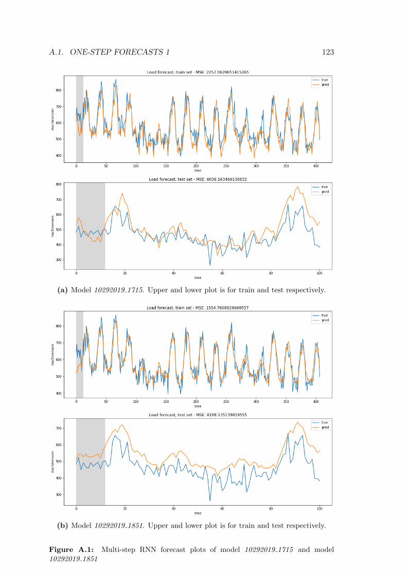
A.1. ONE-STEP FORECASTS 1 123
(a) Model 10292019 1715. Upper and lower plot is for train and test respectively.
(b) Model 10292019 1851. Upper and lower plot is for train and test respectively.
Figure A.1: Multi-step RNN forecast plots of model 10292019 1715 and model10292019 1851
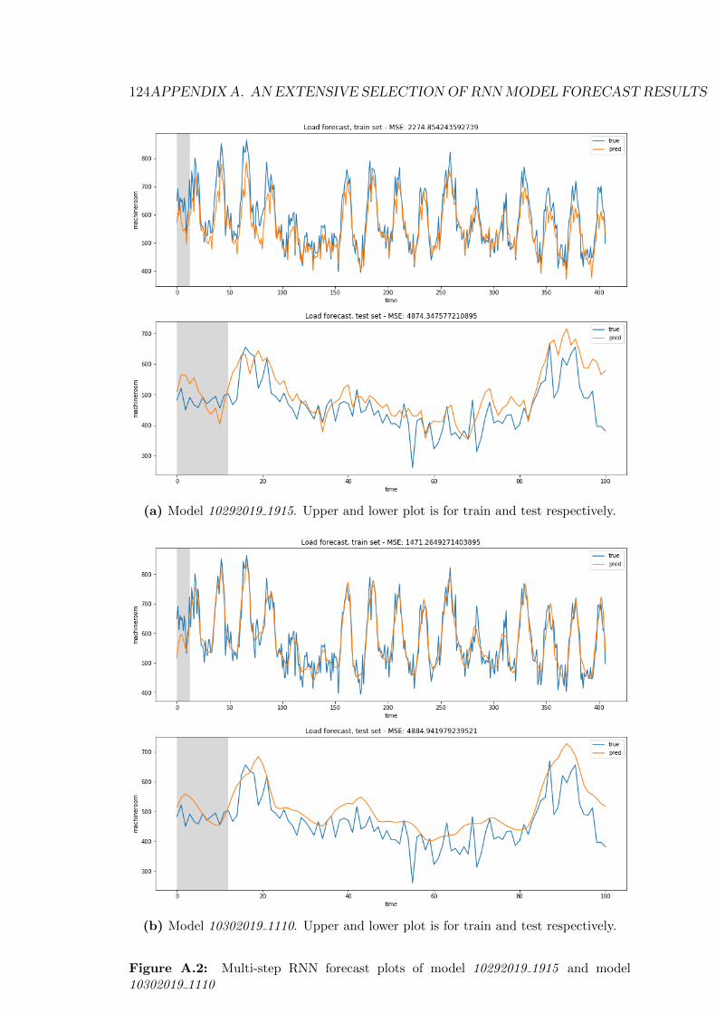
124APPENDIX A. AN EXTENSIVE SELECTIONOF RNNMODEL FORECAST RESULTS
(a) Model 10292019 1915. Upper and lower plot is for train and test respectively.
(b) Model 10302019 1110. Upper and lower plot is for train and test respectively.
Figure A.2: Multi-step RNN forecast plots of model 10292019 1915 and model10302019 1110
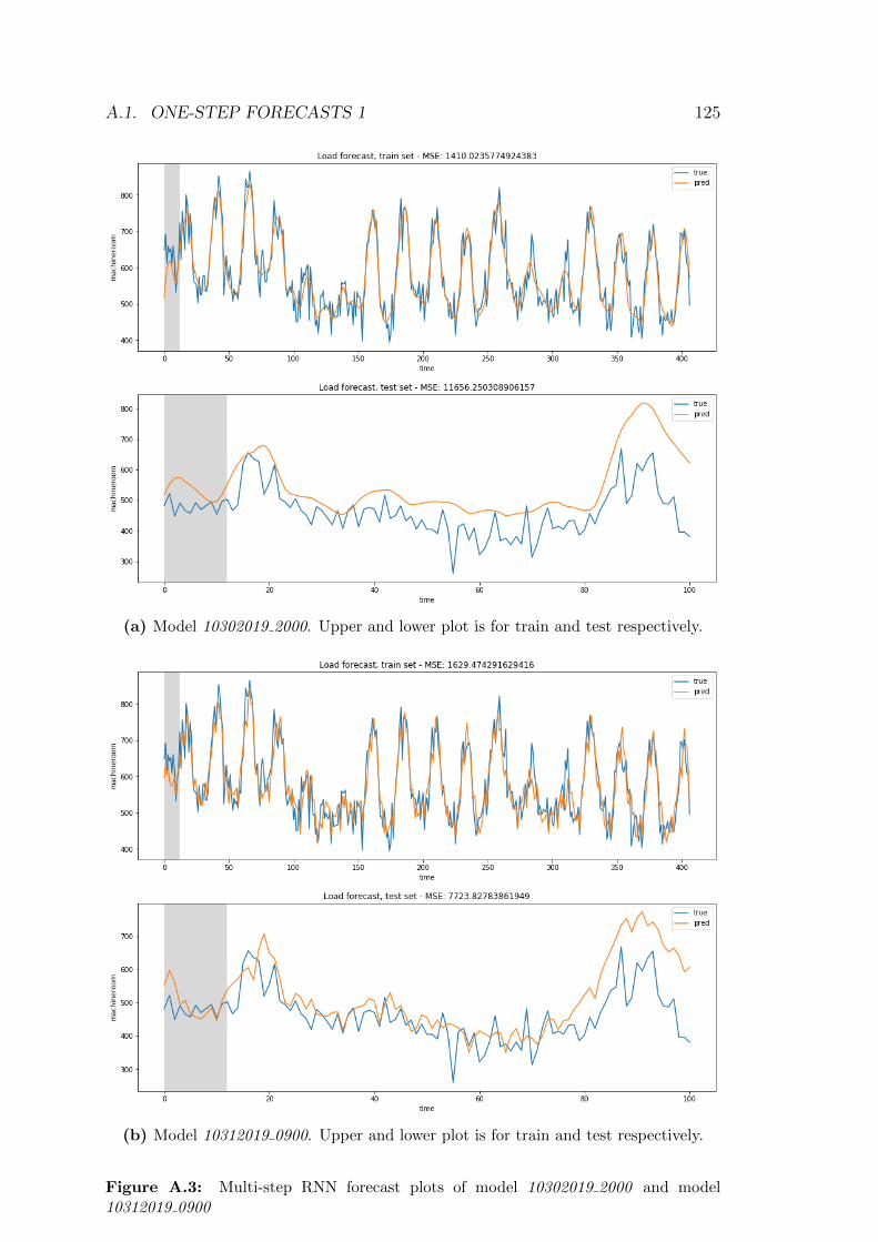
A.1. ONE-STEP FORECASTS 1 125
(a) Model 10302019 2000. Upper and lower plot is for train and test respectively.
(b) Model 10312019 0900. Upper and lower plot is for train and test respectively.
Figure A.3: Multi-step RNN forecast plots of model 10302019 2000 and model10312019 0900
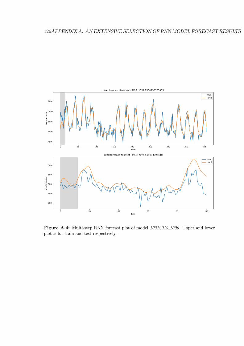
126APPENDIX A. AN EXTENSIVE SELECTIONOF RNNMODEL FORECAST RESULTS
Figure A.4: Multi-step RNN forecast plot of model 10312019 1000. Upper and lowerplot is for train and test respectively.

A.2. ONE-STEP FORECASTS 2 127
A.2 One-step forecasts 2
These one-step RNN forecast models were developed in the mid-phase of the workin this master thesis. For these models, the extra added lagged time features arenot present in the feature set as opposed to the previous models. However, atimestep dimension according to input shape of Keras RNNs is used to providetime memory to the models. The size of this memory of timesteps is determinedby N LOOKBACK.
A.2.1 Table of scores
Table A.2: Model architecture, parameters and forecast scores for various RNN one-step models, where no features is made from algged time features, but instead, the lagmemory is represented as the timestep dimension that Keras in Python want for RNNs.
NAME Model parameters. mse of train, test
No lagged features*, act.fct.=sigmoid, loss-fct.=mse on test data, optim-izer=adam, train size=0.9, steps per epoch=adapted to bs
11112019 1710 Layers: (LSTM 400, LSTM 400), lb=24*3,act.fct.=linear, missing data not fixed, bs=64, ep=50, no es, ts=0.9
1785, 7360
12112019 1327 Layers: (LSTM 400, LSTM 400), lb=24*3,act.fct.=linear, bs=64, ep=50, es pat=5,ts=0.9
5343, 4443
12112019 1344 Layers: (LSTM 400, LSTM 400), lb=24*3,act.fct.=sigmoid, bs=64, ep=50, es pat=8,ts=0.9
3007, 8119
12112019 1410 Layers: (LSTM 200, LSTM 200),lb=24*3, act.fct.=sigmoid, bs=128,ep=40, es pat=8, ts=0.9
2473, 8477
lb = N LOOKBACK, bs= batch size, s/e=steps per epoch
es ( pat)= early stop (patience)
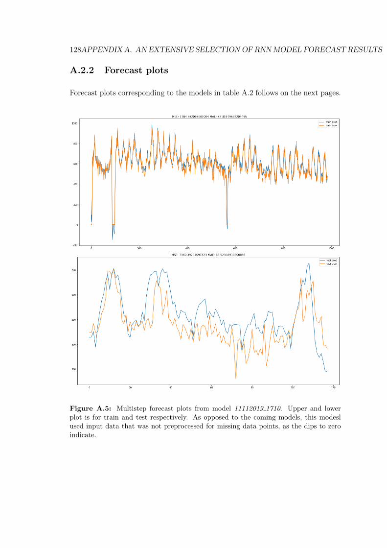
128APPENDIX A. AN EXTENSIVE SELECTIONOF RNNMODEL FORECAST RESULTS
A.2.2 Forecast plots
Forecast plots corresponding to the models in table A.2 follows on the next pages.
Figure A.5: Multistep forecast plots from model 11112019 1710. Upper and lowerplot is for train and test respectively. As opposed to the coming models, this modeslused input data that was not preprocessed for missing data points, as the dips to zeroindicate.
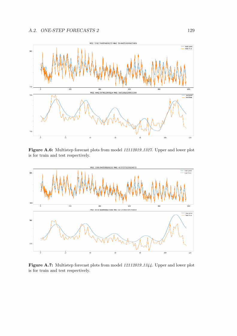
A.2. ONE-STEP FORECASTS 2 129
Figure A.6: Multistep forecast plots from model 12112019 1327. Upper and lower plotis for train and test respectively.
Figure A.7: Multistep forecast plots from model 12112019 1344. Upper and lower plotis for train and test respectively.
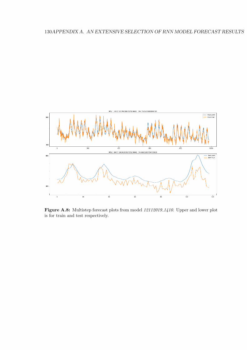
130APPENDIX A. AN EXTENSIVE SELECTIONOF RNNMODEL FORECAST RESULTS
Figure A.8: Multistep forecast plots from model 12112019 1410. Upper and lower plotis for train and test respectively.

A.3. MULTI-STEP FORECASTS 131
A.3 Multi-step forecasts
These models are direct multi-step models and was developed in the last phase ofthe work in this master thesis. Models experimented with in the mid-phase areextended into use in a direct strategy. In total, 6 models are presented, each withvarious model architecture and parameters.
A.3.1 Table of scores
Table A.3: Model architecture, parameters and forecast scores for various RNN multi-step models.
NAME Model parameters. mse of train, test
for all: s/e=100, act.fct.=sigmoid, loss fct.=mse on validation data
12112019 2252or A
Layers: (LSTM 400, LSTM 400), lb=24*3,bs=100, ep=50, es pat=8, ts=0.9
-, -
14112019 2020or B
Layers: (LSTM 200, LSTM 200), lb=24*2,bs=128, ep=50, es pat=8, ts=0.9
2015.8, 5936.67
C Layers: (LSTM 400, LSTM 400, Dropout0.1), lb=24*4, bs=32, ep=70, es pat=10,ts=0.9
2330.3, 7693
D Layers: (LSTM 100, LSTM 100, Dropout0.1), lb=24*2, bs=64, ep=70, es pat=20,ts=0.9
1187.67, 7157.8
E same as D, except for ts=0.925 1427.5, 8288
F same as D, except for ts=0.85 1531.3, 16228.5
lb = N LOOKBACK, bs= batch size, s/e=steps per epoch, ep=epochs,
es ( pat)= early stop (patience), ts=train size
A.3.2 Forecast plots
Forecast plots corresponding to the models in table A.3 follows on the next pages.
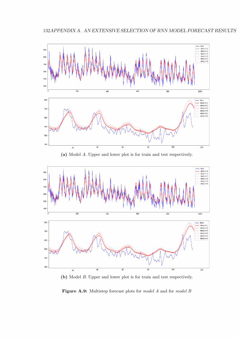
132APPENDIX A. AN EXTENSIVE SELECTIONOF RNNMODEL FORECAST RESULTS
(a) Model A. Upper and lower plot is for train and test respectively.
(b) Model B. Upper and lower plot is for train and test respectively.
Figure A.9: Multistep forecast plots for model A and for model B
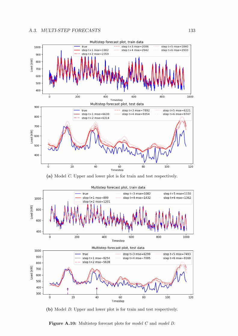
A.3. MULTI-STEP FORECASTS 133
(a) Model C. Upper and lower plot is for train and test respectively.
(b) Model D. Upper and lower plot is for train and test respectively.
Figure A.10: Multistep forecast plots for model C and model D.
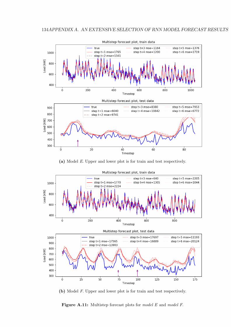
134APPENDIX A. AN EXTENSIVE SELECTIONOF RNNMODEL FORECAST RESULTS
(a) Model E. Upper and lower plot is for train and test respectively.
(b) Model F. Upper and lower plot is for train and test respectively.
Figure A.11: Multistep forecast plots for model E and model F.

Appendix B
Example Python Codes
B.1 RNN model with Keras - Example Code
The following code is the Python script used to make the direct multi-step forecastmodel D. The latter part of the script is used for the making of the forecast plotin ?? and the real-time forecast plots in figure 4.10.
1 #!/usr/bin/env python32 # -*- coding: utf-8 -*-3 MODEL_NAME = 'D' # name of model4
5 #%% IMPORTS6 import numpy as np7 import matplotlib.pyplot as plt8 import pandas as pd9
10 from sklearn.preprocessing import MinMaxScaler11 from sklearn.metrics import mean_squared_error , mean_absolute_error12
13 from tensorflow.python.keras.models import Sequential14 from tensorflow.python.keras.layers import Input , Dense , GRU , LSTM ,
Masking , Dropout15 from tensorflow.python.keras.optimizers import RMSprop , SGD , Adam16 from tensorflow.python.keras.callbacks import EarlyStopping ,
ModelCheckpoint , TensorBoard , ReduceLROnPlateau17 from tensorflow.python.keras.preprocessing.sequence import
TimeseriesGenerator18 np.random.seed (230) #random seed for reproducibility19
135
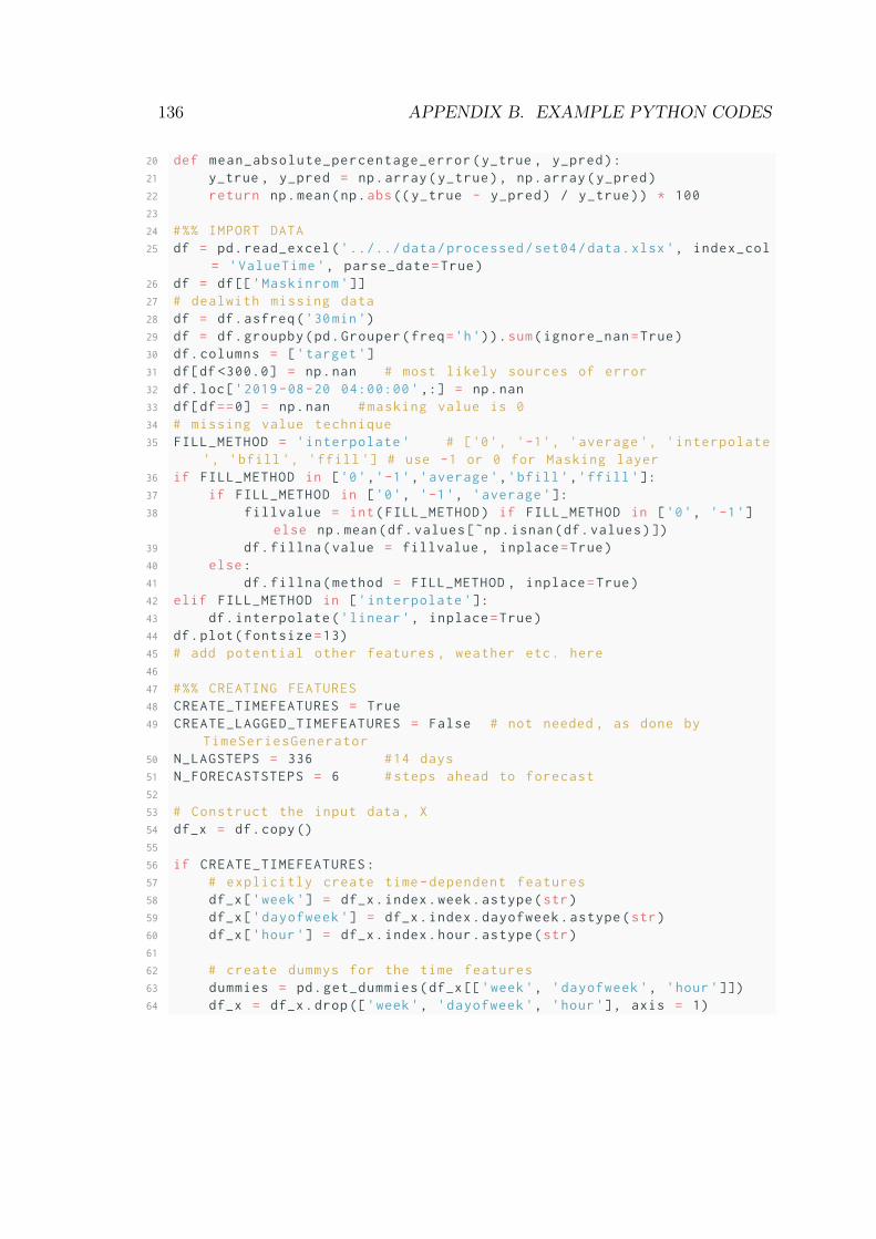
136 APPENDIX B. EXAMPLE PYTHON CODES
20 def mean_absolute_percentage_error(y_true , y_pred):21 y_true , y_pred = np.array(y_true), np.array(y_pred)22 return np.mean(np.abs(( y_true - y_pred) / y_true)) * 10023
24 #%% IMPORT DATA25 df = pd.read_excel('../../ data/processed/set04/data.xlsx', index_col
= 'ValueTime ', parse_date=True)26 df = df[['Maskinrom ']]27 # dealwith missing data28 df = df.asfreq('30min')29 df = df.groupby(pd.Grouper(freq='h')).sum(ignore_nan=True)30 df.columns = ['target ']31 df[df <300.0] = np.nan # most likely sources of error32 df.loc['2019-08-20 04:00:00 ' ,:] = np.nan33 df[df==0] = np.nan #masking value is 034 # missing value technique35 FILL_METHOD = 'interpolate ' # ['0', '-1', 'average ', 'interpolate
', 'bfill ', 'ffill '] # use -1 or 0 for Masking layer36 if FILL_METHOD in ['0','-1','average ','bfill ','ffill ']:37 if FILL_METHOD in ['0', '-1', 'average ']:38 fillvalue = int(FILL_METHOD) if FILL_METHOD in ['0', '-1']
else np.mean(df.values [˜np.isnan(df.values)])39 df.fillna(value = fillvalue , inplace=True)40 else:41 df.fillna(method = FILL_METHOD , inplace=True)42 elif FILL_METHOD in ['interpolate ']:43 df.interpolate('linear ', inplace=True)44 df.plot(fontsize=13)45 # add potential other features , weather etc. here46
47 #%% CREATING FEATURES48 CREATE_TIMEFEATURES = True49 CREATE_LAGGED_TIMEFEATURES = False # not needed , as done by
TimeSeriesGenerator50 N_LAGSTEPS = 336 #14 days51 N_FORECASTSTEPS = 6 #steps ahead to forecast52
53 # Construct the input data , X54 df_x = df.copy()55
56 if CREATE_TIMEFEATURES:57 # explicitly create time-dependent features58 df_x['week'] = df_x.index.week.astype(str)59 df_x['dayofweek '] = df_x.index.dayofweek.astype(str)60 df_x['hour'] = df_x.index.hour.astype(str)61
62 # create dummys for the time features63 dummies = pd.get_dummies(df_x[['week', 'dayofweek ', 'hour']])64 df_x = df_x.drop(['week', 'dayofweek ', 'hour'], axis = 1)
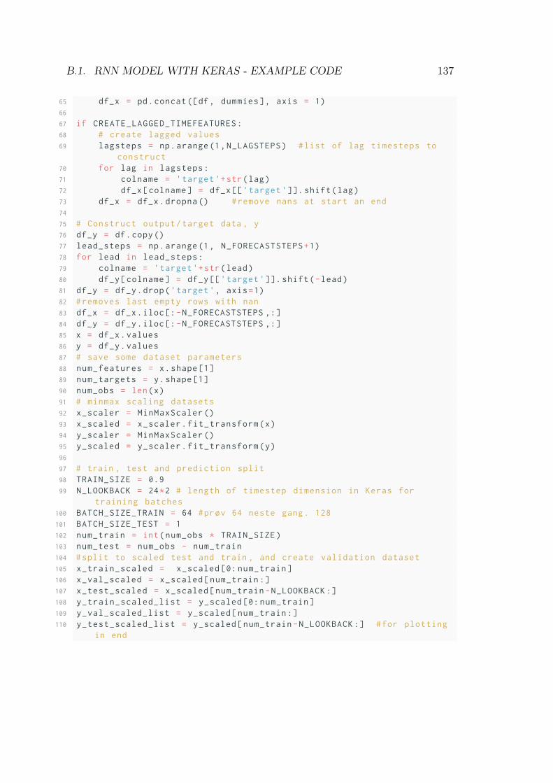
B.1. RNN MODEL WITH KERAS - EXAMPLE CODE 137
65 df_x = pd.concat ([df, dummies], axis = 1)66
67 if CREATE_LAGGED_TIMEFEATURES:68 # create lagged values69 lagsteps = np.arange(1, N_LAGSTEPS) #list of lag timesteps to
construct70 for lag in lagsteps:71 colname = 'target '+str(lag)72 df_x[colname] = df_x[['target ']]. shift(lag)73 df_x = df_x.dropna () #remove nans at start an end74
75 # Construct output/target data , y76 df_y = df.copy()77 lead_steps = np.arange(1, N_FORECASTSTEPS+1)78 for lead in lead_steps:79 colname = 'target '+str(lead)80 df_y[colname] = df_y[['target ']]. shift(-lead)81 df_y = df_y.drop('target ', axis=1)82 #removes last empty rows with nan83 df_x = df_x.iloc[:-N_FORECASTSTEPS ,:]84 df_y = df_y.iloc[:-N_FORECASTSTEPS ,:]85 x = df_x.values86 y = df_y.values87 # save some dataset parameters88 num_features = x.shape [1]89 num_targets = y.shape [1]90 num_obs = len(x)91 # minmax scaling datasets92 x_scaler = MinMaxScaler ()93 x_scaled = x_scaler.fit_transform(x)94 y_scaler = MinMaxScaler ()95 y_scaled = y_scaler.fit_transform(y)96
97 # train , test and prediction split98 TRAIN_SIZE = 0.999 N_LOOKBACK = 24*2 # length of timestep dimension in Keras for
training batches100 BATCH_SIZE_TRAIN = 64 #prøv 64 neste gang. 128101 BATCH_SIZE_TEST = 1102 num_train = int(num_obs * TRAIN_SIZE)103 num_test = num_obs - num_train104 #split to scaled test and train , and create validation dataset105 x_train_scaled = x_scaled [0: num_train]106 x_val_scaled = x_scaled[num_train :]107 x_test_scaled = x_scaled[num_train -N_LOOKBACK :]108 y_train_scaled_list = y_scaled [0: num_train]109 y_val_scaled_list = y_scaled[num_train :]110 y_test_scaled_list = y_scaled[num_train -N_LOOKBACK :] #for plotting
in end
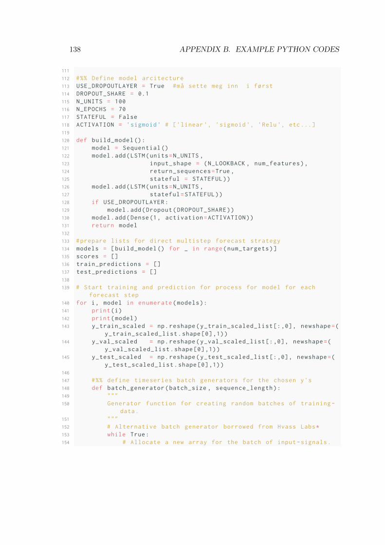
138 APPENDIX B. EXAMPLE PYTHON CODES
111
112 #%% Define model arcitecture113 USE_DROPOUTLAYER = True #ma sette meg inn i først114 DROPOUT_SHARE = 0.1115 N_UNITS = 100116 N_EPOCHS = 70117 STATEFUL = False118 ACTIVATION = 'sigmoid ' # ['linear ', 'sigmoid ', 'Relu ', etc ...]119
120 def build_model ():121 model = Sequential ()122 model.add(LSTM(units=N_UNITS ,123 input_shape = (N_LOOKBACK , num_features),124 return_sequences=True ,125 stateful = STATEFUL))126 model.add(LSTM(units=N_UNITS ,127 stateful=STATEFUL))128 if USE_DROPOUTLAYER:129 model.add(Dropout(DROPOUT_SHARE))130 model.add(Dense(1, activation=ACTIVATION))131 return model132
133 #prepare lists for direct multistep forecast strategy134 models = [build_model () for _ in range(num_targets)]135 scores = []136 train_predictions = []137 test_predictions = []138
139 # Start training and prediction for process for model for eachforecast step
140 for i, model in enumerate(models):141 print(i)142 print(model)143 y_train_scaled = np.reshape(y_train_scaled_list [:,0], newshape=(
y_train_scaled_list.shape [0],1))144 y_val_scaled = np.reshape(y_val_scaled_list [:,0], newshape=(
y_val_scaled_list.shape [0],1))145 y_test_scaled = np.reshape(y_test_scaled_list [:,0], newshape=(
y_test_scaled_list.shape [0],1))146
147 #%% define timeseries batch generators for the chosen y's148 def batch_generator(batch_size , sequence_length):149 """150 Generator function for creating random batches of training -
data.151 """152 # Alternative batch generator borrowed from Hvass Labs*153 while True:154 # Allocate a new array for the batch of input-signals.

B.1. RNN MODEL WITH KERAS - EXAMPLE CODE 139
155 x_shape = (batch_size , sequence_length , num_features)156 x_batch = np.zeros(shape=x_shape , dtype=np.float16)157 # Allocate a new array for the batch of output -signals.158 y_shape = (batch_size , sequence_length , 1)159 y_batch = np.zeros(shape=y_shape , dtype=np.float16)160 # Fill the batch with random sequences of data.161 for i in range(batch_size):162 # Get a random start-index.163 # This points somewhere into the training -data.164 idx = np.random.randint(num_train - sequence_length)165 # Copy the sequences of data starting at this index.166 x_batch[i] = x_train_scaled[idx:idx+sequence_length]167 y_batch[i] = y_train_scaled[idx:idx+sequence_length]168 yield (x_batch , y_batch)169
170 generator = batch_generator(batch_size=BATCH_SIZE_TRAIN ,sequence_length=N_LOOKBACK)
171
172 # Generators provided from Keras - TimeseriesGenerator173 train_data_gen_shuffle = TimeseriesGenerator(x_train_scaled ,
y_train_scaled ,174 length=N_LOOKBACK , sampling_rate=1,stride=1,175 batch_size=BATCH_SIZE_TRAIN , shuffle = True)176 train_data_gen = TimeseriesGenerator(x_train_scaled ,
y_train_scaled ,177 length=N_LOOKBACK , sampling_rate=1,stride=1,178 batch_size=BATCH_SIZE_TRAIN , shuffle = False)179 val_data_gen = TimeseriesGenerator(x_val_scaled , y_val_scaled ,180 length=N_LOOKBACK , sampling_rate=1,stride=1,181 batch_size=BATCH_SIZE_TEST , shuffle=True)182 test_data_gen = TimeseriesGenerator(x_test_scaled , y_test_scaled
,183 length=N_LOOKBACK , sampling_rate=1,stride=1,184 batch_size=BATCH_SIZE_TEST)185
186 #test the data generators187 if False:188 x_batch , y_batch = next(generator)189 print(x_batch.shape)190 print(y_batch.shape)191 x_batch , y_batch = train_data_gen [0]192 print(x_batch.shape)193 print(y_batch.shape)194 x_batch , y_batch = test_data_gen [0]195 print(x_batch.shape)196 print(y_batch.shape)197
198 #%% define all callbacks for model imoprovance199 USE_EARLYSTOPPING = True
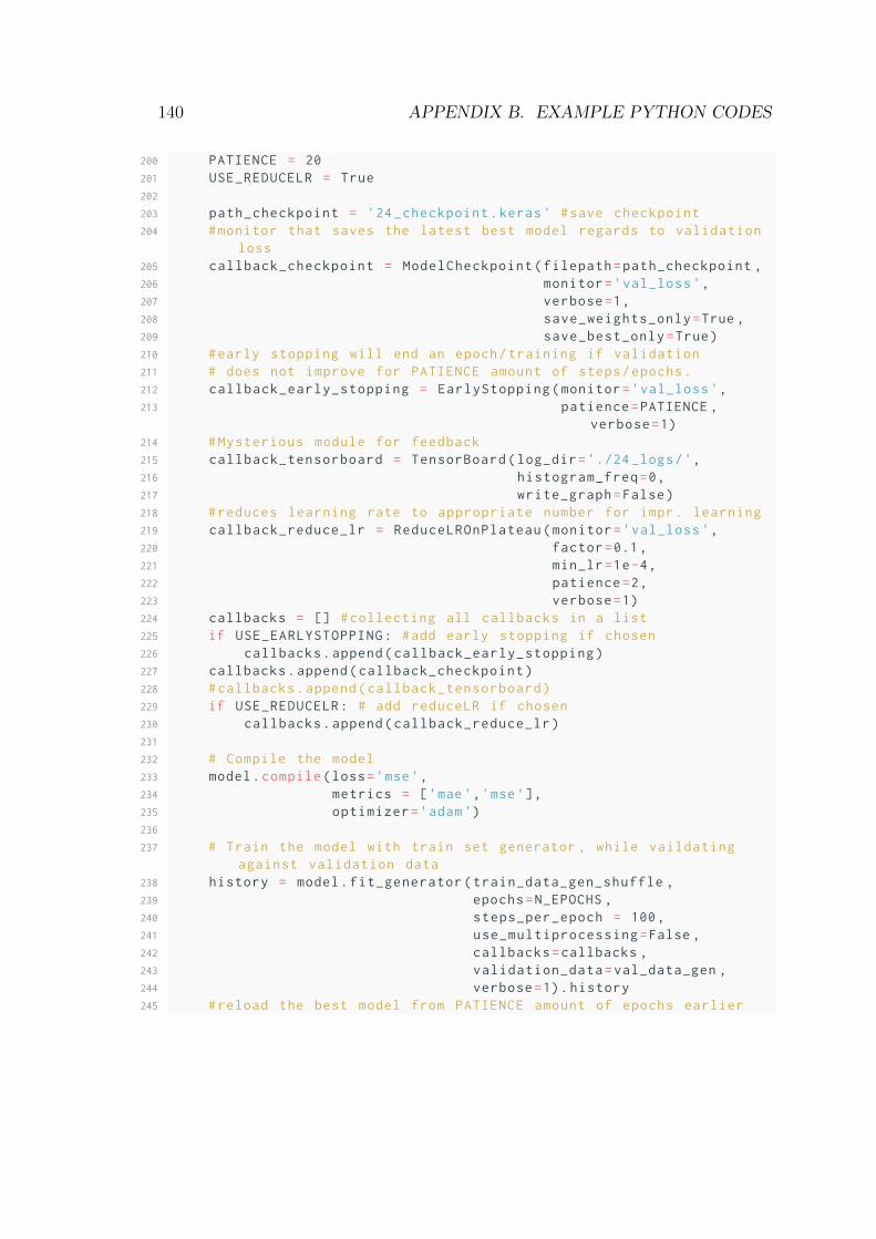
140 APPENDIX B. EXAMPLE PYTHON CODES
200 PATIENCE = 20201 USE_REDUCELR = True202
203 path_checkpoint = '24 _checkpoint.keras ' #save checkpoint204 #monitor that saves the latest best model regards to validation
loss205 callback_checkpoint = ModelCheckpoint(filepath=path_checkpoint ,206 monitor='val_loss ',207 verbose=1,208 save_weights_only=True ,209 save_best_only=True)210 #early stopping will end an epoch/training if validation211 # does not improve for PATIENCE amount of steps/epochs.212 callback_early_stopping = EarlyStopping(monitor='val_loss ',213 patience=PATIENCE ,
verbose=1)214 #Mysterious module for feedback215 callback_tensorboard = TensorBoard(log_dir='./24 _logs/',216 histogram_freq=0,217 write_graph=False)218 #reduces learning rate to appropriate number for impr. learning219 callback_reduce_lr = ReduceLROnPlateau(monitor='val_loss ',220 factor=0.1,221 min_lr=1e-4,222 patience=2,223 verbose=1)224 callbacks = [] #collecting all callbacks in a list225 if USE_EARLYSTOPPING: #add early stopping if chosen226 callbacks.append(callback_early_stopping)227 callbacks.append(callback_checkpoint)228 #callbacks.append(callback_tensorboard)229 if USE_REDUCELR: # add reduceLR if chosen230 callbacks.append(callback_reduce_lr)231
232 # Compile the model233 model.compile(loss='mse',234 metrics = ['mae','mse'],235 optimizer='adam')236
237 # Train the model with train set generator , while vaildatingagainst validation data
238 history = model.fit_generator(train_data_gen_shuffle ,239 epochs=N_EPOCHS ,240 steps_per_epoch = 100,241 use_multiprocessing=False ,242 callbacks=callbacks ,243 validation_data=val_data_gen ,244 verbose=1).history245 #reload the best model from PATIENCE amount of epochs earlier
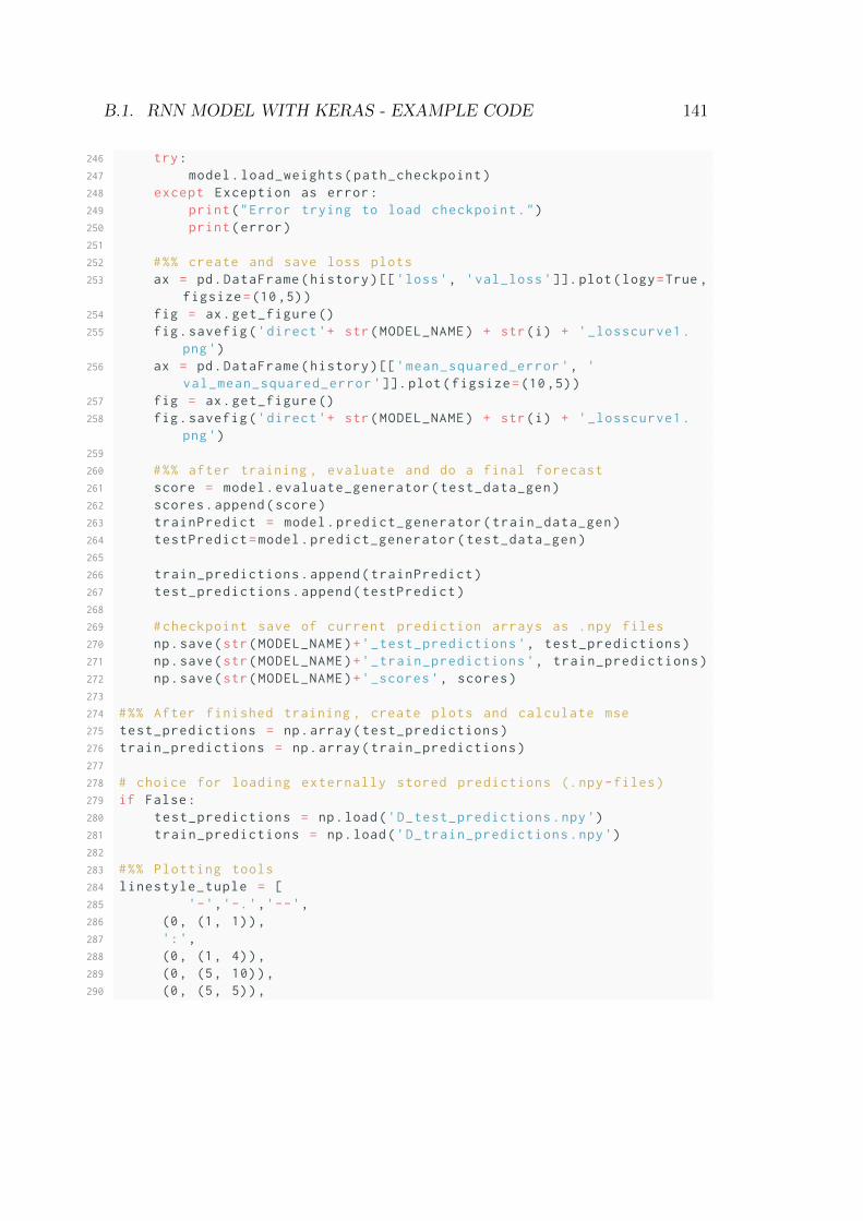
B.1. RNN MODEL WITH KERAS - EXAMPLE CODE 141
246 try:247 model.load_weights(path_checkpoint)248 except Exception as error:249 print("Error trying to load checkpoint.")250 print(error)251
252 #%% create and save loss plots253 ax = pd.DataFrame(history)[['loss', 'val_loss ']]. plot(logy=True ,
figsize=(10,5))254 fig = ax.get_figure ()255 fig.savefig('direct '+ str(MODEL_NAME) + str(i) + '_losscurve1.
png')256 ax = pd.DataFrame(history)[['mean_squared_error ', '
val_mean_squared_error ']]. plot(figsize=(10,5))257 fig = ax.get_figure ()258 fig.savefig('direct '+ str(MODEL_NAME) + str(i) + '_losscurve1.
png')259
260 #%% after training , evaluate and do a final forecast261 score = model.evaluate_generator(test_data_gen)262 scores.append(score)263 trainPredict = model.predict_generator(train_data_gen)264 testPredict=model.predict_generator(test_data_gen)265
266 train_predictions.append(trainPredict)267 test_predictions.append(testPredict)268
269 #checkpoint save of current prediction arrays as .npy files270 np.save(str(MODEL_NAME)+'_test_predictions ', test_predictions)271 np.save(str(MODEL_NAME)+'_train_predictions ', train_predictions)272 np.save(str(MODEL_NAME)+'_scores ', scores)273
274 #%% After finished training , create plots and calculate mse275 test_predictions = np.array(test_predictions)276 train_predictions = np.array(train_predictions)277
278 # choice for loading externally stored predictions (.npy-files)279 if False:280 test_predictions = np.load('D_test_predictions.npy')281 train_predictions = np.load('D_train_predictions.npy')282
283 #%% Plotting tools284 linestyle_tuple = [285 '-','-.','--',286 (0, (1, 1)),287 ':',288 (0, (1, 4)),289 (0, (5, 10)),290 (0, (5, 5)),

142 APPENDIX B. EXAMPLE PYTHON CODES
291 (0, (5, 1)),292 (0, (3, 10, 1, 10)),293 (0, (3, 5, 1, 5)),294 (0, (3, 1, 1, 1)),295 (0, (3, 5, 1, 5, 1, 5)),296 (0, (3, 10, 1, 10, 1, 10)),297 (0, (3, 1, 1, 1, 1, 1))]298 #inverse transform forecast results299 trainPred = y_scaler.inverse_transform(np.array(train_predictions).
squeeze ().T)300 testPred = y_scaler.inverse_transform(np.array(test_predictions).
squeeze ().T)301 # get the true values302 trainTrue = y[0: num_train ,0][-len(trainPred):]303 testTrue = y[num_train :,0][-len(trainPred):]304 # Changeable design parameters305 figsize = (10,3)306 dpi=110307
308 plt.figure(figsize=figsize , dpi=dpi)309 plt.plot(trainTrue , color = 'blue',label='true', linewidth=1)310 for i, vec in enumerate(trainPred.T):311 alph=1/((i/2)+1)312 plt.plot(np.arange(i, len(vec)+i), vec , label='step t+'+str(i+1)
+ ' mse=' + str(int(mean_squared_error(vec , trainTrue))),313 color='red', ls=linestyle_tuple[i], alpha = alph ,
linewidth=.7)314 plt.title('Multistep forecast plot , train data')315 plt.xlabel('Timestep ')316 plt.ylabel('Load [kW]')317 plt.ylim(None , max(trainTrue)+200)318 plt.legend(loc=1, ncol=3, fancybox=True)319 plt.show()320
321
322 plt.figure(figsize=figsize , dpi=dpi)323 plt.plot(testTrue , color = 'blue',label='true')324 for i, vec in enumerate(testPred.T):325 alph=1/((i/2)+1)326 plt.plot(np.arange(i, len(vec)+i), vec , label='step t+'+str(i+1)
+ ' mse=' + str(int(mean_squared_error(vec , testTrue))),327 color='red', ls=linestyle_tuple[i], alpha=alph ,
linewidth=1)328 plt.title('Multistep forecast plot , test data')329 plt.xlabel('Timestep ')330 plt.ylabel('Load [kW]')331 plt.ylim(None , max(testTrue)+300)332 plt.legend(loc=1, ncol=3, fancybox=True)333 plt.show()
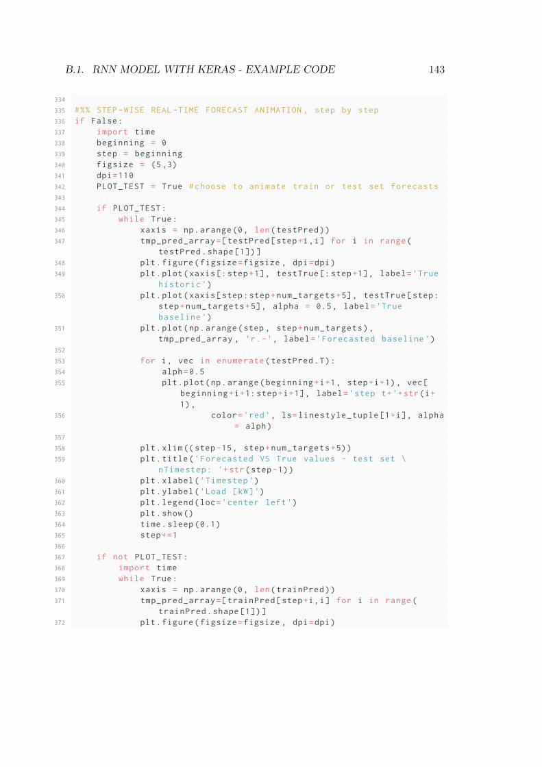
B.1. RNN MODEL WITH KERAS - EXAMPLE CODE 143
334
335 #%% STEP-WISE REAL-TIME FORECAST ANIMATION , step by step336 if False:337 import time338 beginning = 0339 step = beginning340 figsize = (5,3)341 dpi=110342 PLOT_TEST = True #choose to animate train or test set forecasts343
344 if PLOT_TEST:345 while True:346 xaxis = np.arange(0, len(testPred))347 tmp_pred_array=[testPred[step+i,i] for i in range(
testPred.shape [1])]348 plt.figure(figsize=figsize , dpi=dpi)349 plt.plot(xaxis[:step+1], testTrue [:step+1], label='True
historic ')350 plt.plot(xaxis[step:step+num_targets+5], testTrue[step:
step+num_targets+5], alpha = 0.5, label='Truebaseline ')
351 plt.plot(np.arange(step , step+num_targets),tmp_pred_array , 'r.-', label='Forecasted baseline ')
352
353 for i, vec in enumerate(testPred.T):354 alph=0.5355 plt.plot(np.arange(beginning+i+1, step+i+1), vec[
beginning+i+1:step+i+1], label='step t+'+str(i+1),
356 color='red', ls=linestyle_tuple [1+i], alpha= alph)
357
358 plt.xlim((step-15, step+num_targets+5))359 plt.title('Forecasted VS True values - test set \
nTimestep: '+str(step-1))360 plt.xlabel('Timestep ')361 plt.ylabel('Load [kW]')362 plt.legend(loc='center left')363 plt.show()364 time.sleep (0.1)365 step+=1366
367 if not PLOT_TEST:368 import time369 while True:370 xaxis = np.arange(0, len(trainPred))371 tmp_pred_array=[trainPred[step+i,i] for i in range(
trainPred.shape [1])]372 plt.figure(figsize=figsize , dpi=dpi)
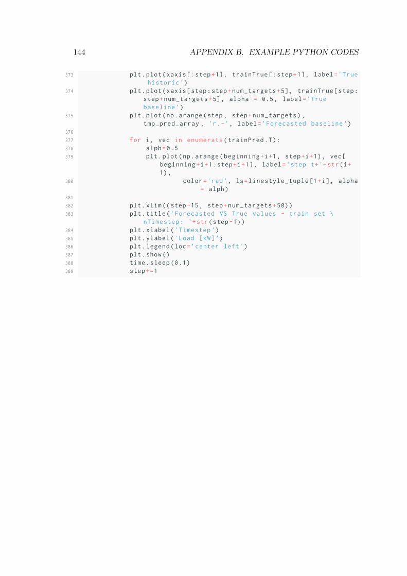
144 APPENDIX B. EXAMPLE PYTHON CODES
373 plt.plot(xaxis[:step+1], trainTrue [:step+1], label='Truehistoric ')
374 plt.plot(xaxis[step:step+num_targets+5], trainTrue[step:step+num_targets+5], alpha = 0.5, label='Truebaseline ')
375 plt.plot(np.arange(step , step+num_targets),tmp_pred_array , 'r.-', label='Forecasted baseline ')
376
377 for i, vec in enumerate(trainPred.T):378 alph=0.5379 plt.plot(np.arange(beginning+i+1, step+i+1), vec[
beginning+i+1:step+i+1], label='step t+'+str(i+1),
380 color='red', ls=linestyle_tuple [1+i], alpha= alph)
381
382 plt.xlim((step-15, step+num_targets+50))383 plt.title('Forecasted VS True values - train set \
nTimestep: '+str(step-1))384 plt.xlabel('Timestep ')385 plt.ylabel('Load [kW]')386 plt.legend(loc='center left')387 plt.show()388 time.sleep (0.1)389 step+=1
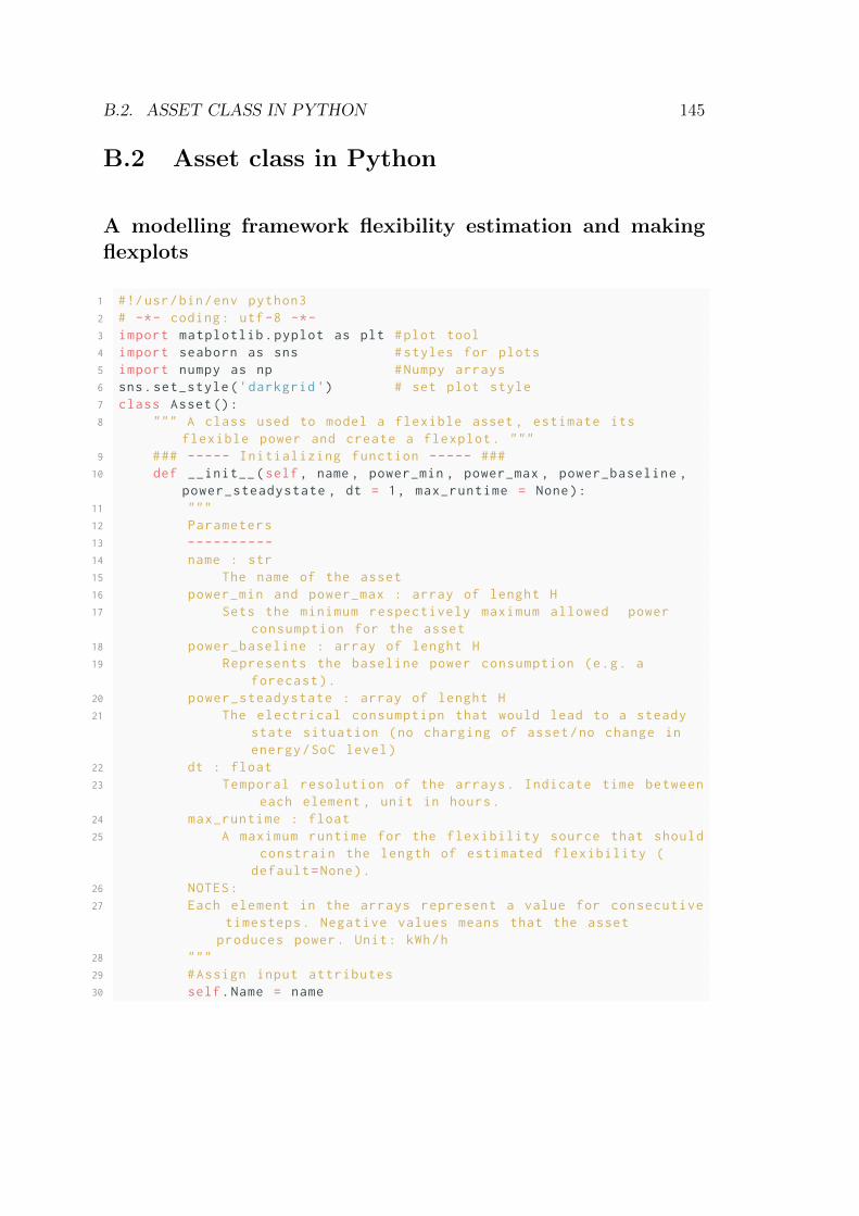
B.2. ASSET CLASS IN PYTHON 145
B.2 Asset class in Python
A modelling framework flexibility estimation and makingflexplots
1 #!/usr/bin/env python32 # -*- coding: utf-8 -*-3 import matplotlib.pyplot as plt #plot tool4 import seaborn as sns #styles for plots5 import numpy as np #Numpy arrays6 sns.set_style('darkgrid ') # set plot style7 class Asset():8 """ A class used to model a flexible asset , estimate its
flexible power and create a flexplot. """9 ### ----- Initializing function ----- ###10 def __init__(self, name , power_min , power_max , power_baseline ,
power_steadystate , dt = 1, max_runtime = None):11 """12 Parameters13 ----------14 name : str15 The name of the asset16 power_min and power_max : array of lenght H17 Sets the minimum respectively maximum allowed power
consumption for the asset18 power_baseline : array of lenght H19 Represents the baseline power consumption (e.g. a
forecast).20 power_steadystate : array of lenght H21 The electrical consumptipn that would lead to a steady
state situation (no charging of asset/no change inenergy/SoC level)
22 dt : float23 Temporal resolution of the arrays. Indicate time between
each element , unit in hours.24 max_runtime : float25 A maximum runtime for the flexibility source that should
constrain the length of estimated flexibility (default=None).
26 NOTES:27 Each element in the arrays represent a value for consecutive
timesteps. Negative values means that the assetproduces power. Unit: kWh/h
28 """29 #Assign input attributes30 self.Name = name
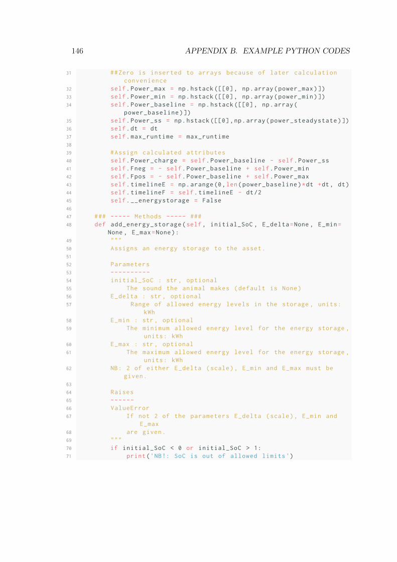
146 APPENDIX B. EXAMPLE PYTHON CODES
31 ##Zero is inserted to arrays because of later calculationconvenience
32 self.Power_max = np.hstack ([[0], np.array(power_max)])33 self.Power_min = np.hstack ([[0], np.array(power_min)])34 self.Power_baseline = np.hstack ([[0], np.array(
power_baseline)])35 self.Power_ss = np.hstack ([[0],np.array(power_steadystate)])36 self.dt = dt37 self.max_runtime = max_runtime38
39 #Assign calculated attributes40 self.Power_charge = self.Power_baseline - self.Power_ss41 self.Fneg = - self.Power_baseline + self.Power_min42 self.Fpos = - self.Power_baseline + self.Power_max43 self.timelineE = np.arange(0,len(power_baseline)*dt +dt, dt)44 self.timelineF = self.timelineE - dt/245 self.__energystorage = False46
47 ### ----- Methods ----- ###48 def add_energy_storage(self, initial_SoC , E_delta=None , E_min=
None , E_max=None):49 """50 Assigns an energy storage to the asset.51
52 Parameters53 ----------54 initial_SoC : str , optional55 The sound the animal makes (default is None)56 E_delta : str , optional57 Range of allowed energy levels in the storage , units:
kWh58 E_min : str , optional59 The minimum allowed energy level for the energy storage ,
units: kWh60 E_max : str , optional61 The maximum allowed energy level for the energy storage ,
units: kWh62 NB: 2 of either E_delta (scale), E_min and E_max must be
given.63
64 Raises65 ------66 ValueError67 If not 2 of the parameters E_delta (scale), E_min and
E_max68 are given.69 """70 if initial_SoC < 0 or initial_SoC > 1:71 print('NB!: SoC is out of allowed limits ')
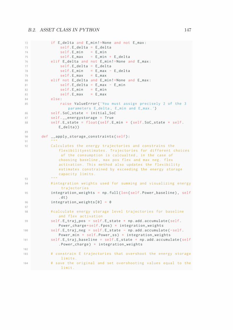
B.2. ASSET CLASS IN PYTHON 147
72 if E_delta and E_min!=None and not E_max:73 self.E_delta = E_delta74 self.E_min = E_min75 self.E_max = E_min + E_delta76 elif E_delta and not E_min!=None and E_max:77 self.E_delta = E_delta78 self.E_min = E_max - E_delta79 self.E_max = E_max80 elif not E_delta and E_min!=None and E_max:81 self.E_delta = E_max - E_min82 self.E_min = E_min83 self.E_max = E_max84 else:85 raise ValueError('You must assign precisely 2 of the 3
parameters E_delta , E_min and E_max.')86 self.SoC_state = initial_SoC87 self.__energystorage = True88 self.E_state = float(self.E_min + (self.SoC_state * self.
E_delta))89
90 def __apply_storage_constraints(self):91 """92 Calculates the energy trajectories and constrains the
flexibilityestimates. Trajectories for different choicesof the consumption is calcualted , in the case of
choosing baseline , max pos flex and max neg. flexactivation. This method also updates the flexibilityestimates constrained by exceeding the energy storagecapacity limits.
93 """94 #integration weights used for summing and visualizing energy
trajectories95 integration_weights = np.full(len(self.Power_baseline), self
.dt)96 integration_weights [0] = 097
98 #calculate energy storage level trajectories for baselineand flex activation
99 self.E_traj_pos = self.E_state + np.add.accumulate(self.Power_charge+self.Fpos) * integration_weights
100 self.E_traj_neg = self.E_state - np.add.accumulate(-self.Power_min + self.Power_ss) * integration_weights
101 self.E_traj_baseline = self.E_state + np.add.accumulate(self.Power_charge) * integration_weights
102
103 # constrain E trajectories that overshoot the energy storagelimits.
104 # save the original and set overshooting values equal to thelimit.

148 APPENDIX B. EXAMPLE PYTHON CODES
105 self.E_traj_pos_overshoot = self.E_traj_pos.copy()106 self.E_traj_neg_overshoot = self.E_traj_neg.copy()107
108 index_pos_overshooting = np.where(self.E_traj_pos > self.E_max)[0]
109 index_neg_overshooting = np.where(self.E_traj_neg < self.E_min)[0]
110 self.E_traj_pos[index_pos_overshooting] = self.E_max111 self.E_traj_neg[index_neg_overshooting] = self.E_min112
113 # Constrain parts of Fpos/Fneg that led to overshootingenergy storage limits
114 self.Fpos[index_pos_overshooting] = +(self.E_traj_pos[index_pos_overshooting] - self.E_traj_pos[index_pos_overshooting -1])/self.dt - self.Power_charge[index_pos_overshooting]
115 self.Fneg[index_neg_overshooting] = +(self.E_traj_neg[index_neg_overshooting] - self.E_traj_neg[index_neg_overshooting -1])/self.dt - self.Power_charge[index_neg_overshooting]
116 self.Fpos[self.Fpos <0] = 0117 self.Fneg[self.Fneg >0] = 0118
119 def __apply_time_constraints(self):120 self.Fpos[self.max_runtime+1:] = 0121 self.Fneg[self.max_runtime+1:] = 0122
123 def make_flexplot(self):124 """ Vizualization of flexibility estimate results ,
consistent of four subplots. """125 if self.max_runtime:126 self.__apply_time_constraints ()127 ### Create figure128 if self.__energystorage:129 fig , [ax2 ,ax3 ,ax,ax1] = plt.subplots(4, 1, figsize=(6*
0.95,8*0.95), dpi=100, sharex=True , gridspec_kw = {'height_ratios ':[1,1,3,1]})
130 ax2.set_title('Asset: ' + str(self.Name) + ' | CurrentSoC: ' + str(self.SoC_state) + '\n\n' + 'Forecastedbaseline/load schedule ')
131
132 #create the line arrays for the max and min energystorage capacity
133 self.__apply_storage_constraints ()134 E_max_curve = np.full(len(self.timelineE), self.E_max)135 E_min_curve = np.full(len(self.timelineE), self.E_min)136 elif not self.__energystorage:137 fig , [ax2 ,ax1] = plt.subplots(2, 1, figsize=(6*0.95,3*
0.95), dpi=100, sharex=True , gridspec_kw = {'
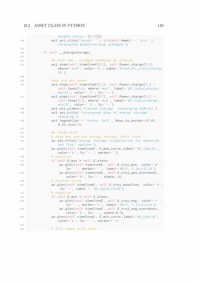
B.2. ASSET CLASS IN PYTHON 149
height_ratios ':[1 ,1]})138 ax2.set_title('Asset: ' + str(self.Name) + '\n\n' + '
Forecasted baseline/load schedule ')139
140 if self.__energystorage:141
142 ## PLOT TWO - PLANNED CHARGING OF STORAGE143 ax3.step(self.timelineF [1:], self.Power_charge [1:],
where='mid', color='b', label='$\hat{P}_{(dis)charge}$')
144
145 #max and min power146 ax3.step(self.timelineF [1:], self.Power_charge [1:] +
self.Fpos [1:], where='mid', label='$P_{(dis)charge ,max}$', color='.5', ls='--')
147 ax3.step(self.timelineF [1:], self.Power_charge [1:] +self.Fneg [1:], where='mid', label='$P_{(dis)charge ,min}$', color='.5', ls='-.')
148 ax3.set_ylabel('Planned storage \ncharging [kWh/h]')149 ax3.set_title('Forecasted plan of energy storage
charging ')150 ax3.legend(loc = 'center left', bbox_to_anchor=(1.01,
0.5),ncol=1)151
152 ## THIRD PLOT153 # draw max and min energy storage limit lines154 ax.set_title('Energy storage trajectories for baseline
and flex. options ')155 ax.plot(self.timelineE , E_max_curve ,label='$E_{max}$',
color='k', ls='-.', marker='')156 # positive157 if self.E_max > self.E_state:158 ax.plot(self.timelineE , self.E_traj_pos , color='g',
ls='-', marker='ˆ', label='$E(t, F_{p}(t))$')159 ax.plot(self.timelineE , self.E_traj_pos_overshoot ,
color='0', ls=':', alpha=.3)160 # planned route161 ax.plot(self.timelineE , self.E_traj_baseline , color='b',
ls='-', label = '$E_{plan}(t)$')162 # negative163 if self.E_min < self.E_state:164 ax.plot(self.timelineE , self.E_traj_neg , color='r',
ls='-', marker='v', label='$E(t, F_{n}(t))$')165 ax.plot(self.timelineE , self.E_traj_neg_overshoot ,
color='0', ls=':', alpha=0.3)166 ax.plot(self.timelineE , E_min_curve ,label='$E_{min}$',
color='k', ls='--', marker='')167
168 # fill space with color
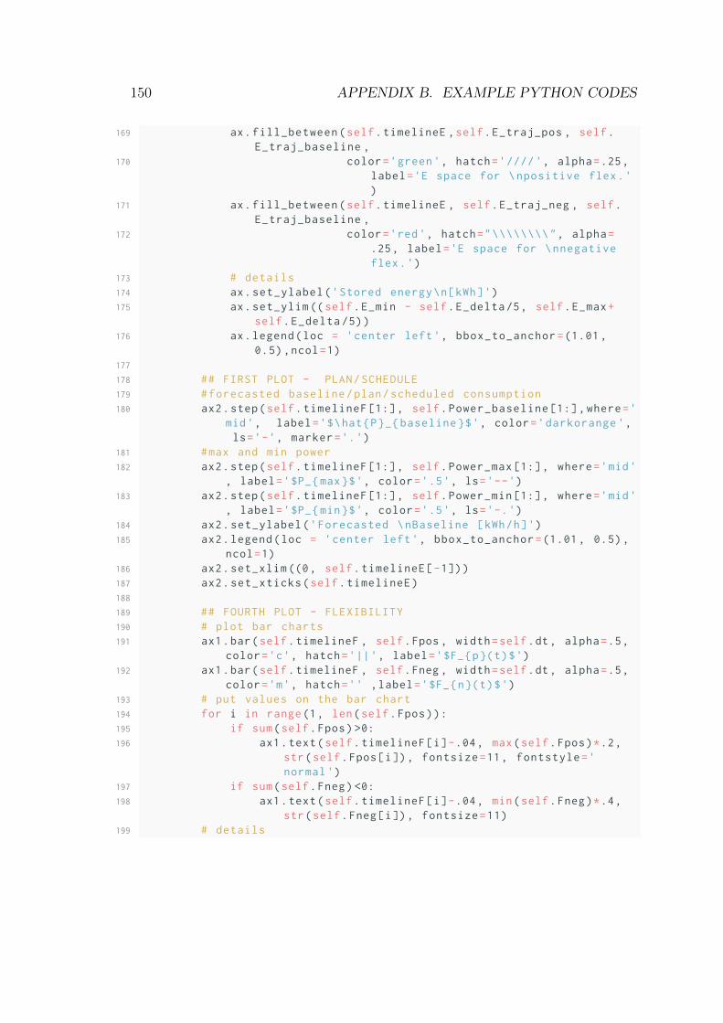
150 APPENDIX B. EXAMPLE PYTHON CODES
169 ax.fill_between(self.timelineE ,self.E_traj_pos , self.E_traj_baseline ,
170 color='green ', hatch='////', alpha=.25,label='E space for \npositive flex.')
171 ax.fill_between(self.timelineE , self.E_traj_neg , self.E_traj_baseline ,
172 color='red', hatch="\\\\\\\\", alpha=.25, label='E space for \nnegativeflex.')
173 # details174 ax.set_ylabel('Stored energy\n[kWh]')175 ax.set_ylim ((self.E_min - self.E_delta/5, self.E_max+
self.E_delta /5))176 ax.legend(loc = 'center left', bbox_to_anchor=(1.01,
0.5),ncol=1)177
178 ## FIRST PLOT - PLAN/SCHEDULE179 #forecasted baseline/plan/scheduled consumption180 ax2.step(self.timelineF [1:], self.Power_baseline [1:], where='
mid', label='$\hat{P}_{baseline}$', color='darkorange ',ls='-', marker='.')
181 #max and min power182 ax2.step(self.timelineF [1:], self.Power_max [1:], where='mid'
, label='$P_{max}$', color='.5', ls='--')183 ax2.step(self.timelineF [1:], self.Power_min [1:], where='mid'
, label='$P_{min}$', color='.5', ls='-.')184 ax2.set_ylabel('Forecasted \nBaseline [kWh/h]')185 ax2.legend(loc = 'center left', bbox_to_anchor=(1.01 , 0.5),
ncol=1)186 ax2.set_xlim ((0, self.timelineE[-1]))187 ax2.set_xticks(self.timelineE)188
189 ## FOURTH PLOT - FLEXIBILITY190 # plot bar charts191 ax1.bar(self.timelineF , self.Fpos , width=self.dt, alpha=.5,
color='c', hatch='||', label='$F_{p}(t)$')192 ax1.bar(self.timelineF , self.Fneg , width=self.dt, alpha=.5,
color='m', hatch='' ,label='$F_{n}(t)$')193 # put values on the bar chart194 for i in range(1, len(self.Fpos)):195 if sum(self.Fpos) >0:196 ax1.text(self.timelineF[i]-.04, max(self.Fpos)*.2,
str(self.Fpos[i]), fontsize=11, fontstyle='normal ')
197 if sum(self.Fneg) <0:198 ax1.text(self.timelineF[i]-.04, min(self.Fneg)*.4,
str(self.Fneg[i]), fontsize=11)199 # details

B.2. ASSET CLASS IN PYTHON 151
200 ax1.set_title('Estimated available flexibility ')201 ax1.legend(loc = 'center left', bbox_to_anchor=(1.01 , 0.5),
ncol=1)202 ax1.set_ylabel('Flexible power \n[kWh/h]')203 ax1.set_xlabel('Forecast timestep [h]')204
205 fig.show()206 #%%207 if __name__ == "__main__":208 # EXAMPLE 1209 ## Battery , passive schedule , constant planned SoC level210 battery1 = Asset('Battery , passive ',[-30]*6,[30]*6, [0]*6, [0]*
6, dt =0.25)211 battery1.add_energy_storage( 0.5, E_max = 65, E_min = 65*0.0)212 battery1.make_flexplot ()213
214 # EXAMPLE 2215 ## Battery , active schedile , charging then discharging216 battery2 = Asset('Battery , active ',[-30]*6,[30]*6, [30,30,30,-
30,-30,-30], [0]*6, dt =0.25)217 battery2.add_energy_storage (0.5, E_max = 65, E_min = 65*0.0)218 battery2.make_flexplot ()219
220 # EXAMPLE 3221 ## Water heater with alternative energy source222 max_runtime = 4223 wbaseline = np.array ([300, 280, 270, 290, 340, 310])224 waterheater1 = Asset('Waterheater ', [0]*len(wbaseline),
wbaseline , wbaseline , wbaseline , 1, max_runtime=max_runtime)225 waterheater1.make_flexplot ()226
227 # EXAMPLE 4228 ## Machine room229 machineroom1 = Asset('machineroom ',230 [538 ,540 ,523 ,501 ,469 ,420 ,378 ,350] ,231 [838 ,840 ,823 ,801 ,769 ,720 ,678 ,650] ,232 [676 ,701 ,641 ,609 ,606 ,496 ,482 ,521] ,233 [676 ,701 ,641 ,609 ,606 ,496 ,482 ,521] , dt =1)234 machineroom1.add_energy_storage( 0.6, E_max = 9000, E_delta =
1000)235 machineroom1.make_flexplot ()

152 APPENDIX B. EXAMPLE PYTHON CODES
B.3 Python Code for creating the flexplots in
machine room use-case
1 #!/usr/bin/env python32 # -*- coding: utf-8 -*-3 # CREATING THE FLEXPLOTS IN MACHINE ROOM USE-CASE4
5 import numpy as np6 from Asset import Asset # Import Asset class for usage7
8 # Constructing baseline matrixes for the forecasts and true realizedvalues*
9 # drom 'RNN multistep forecast result ' table presented in the masterthesis
10 bl_pred=np.array ([607, 638, 692, 678, 710, 730])11 bl_real=np.array ([574, 668, 737 ,673, 734, 768])12
13 bl_pred=np.array ([[513 , 596, 673, 704, 663, 681],14 [578, 650, 693, 698, 641, 697],15 [647, 671, 683, 713, 715, 684],16 [0,0,0,0,0,0],17 [0,0,0,0,0,0],18 [0,0,0,0,0,0],19 [692,718, 655, 598, 532, 493]])20
21 [524, 542, 584, 697, 694, 677, 702, 642, 610, 606, 497, 482]22
23 bl_real=np.array ([[524 , 542, 584, 697, 694, 677],24 [542, 584, 697, 694, 677, 702],25 [584, 697, 694, 677, 702, 642],26 [0,0,0,0,0,0],27 [0,0,0,0,0,0],28 [0,0,0,0,0,0],29 [702, 642, 610, 606, 497, 482]])30
31 # constants for the power the asset can deviate with from thebaseline.
32 plusmax = 50 #kWh/h33 minusmax = -80 #kWh/h34
35 #EVENT (a)36 start=037 machineroom_stepA = Asset('machineroom (a)', bl_pred[start]+minusmax
, bl_pred[start]+plusmax ,38 bl_pred[start], bl_pred[start], dt=1)39 machineroom_stepA.add_energy_storage( 0.6, E_max = 8000, E_delta =
600)
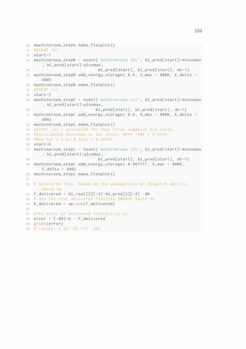
153
40 machineroom_stepA.make_flexplot ()41 #EVENT (b)42 start=143 machineroom_stepB = Asset('machineroom (b)', bl_pred[start]+minusmax
, bl_pred[start]+plusmax ,44 bl_pred[start], bl_pred[start], dt=1)45 machineroom_stepB.add_energy_storage( 0.6, E_max = 8000, E_delta =
600)46 machineroom_stepB.make_flexplot ()47 #EVENT (c)48 start=249 machineroom_stepC = Asset('machineroom (c)', bl_pred[start]+minusmax
, bl_pred[start]+plusmax ,50 bl_pred[start], bl_pred[start], dt=1)51 machineroom_stepC.add_energy_storage( 0.6, E_max = 8000, E_delta =
600)52 machineroom_stepC.make_flexplot ()53 #EVENT (d) - activateD the four first negative bid slots.54 #Anticipated decrease in SoC level: 80*4 /600 = 0.533355 #New SoC = 0.6- 0.5333 = 0.0666756 start=657 machineroom_stepC = Asset('machineroom (d)', bl_pred[start]+minusmax
, bl_pred[start]+plusmax ,58 bl_pred[start], bl_pred[start], dt=1)59 machineroom_stepC.add_energy_storage( 0.067777 , E_max = 8000,
E_delta = 600)60 machineroom_stepC.make_flexplot ()61
62 # Delivered flex , based on the assumptions on dispatch ability ,would be
63 F_delivered = bl_real [2][:4] -bl_pred [2][:4] -8064 # and the real delivered flexible ENERGY would be65 E_delivered = np.sum(F_delivered)66
67 #The error of delivered flexibility is68 error = [-80]*4 - F_delivered69 print(error)70 # result: [ 63 -26 -11 36]

154
Thank you.

Related Documents