Meshfree and Partition of Unity Methods for the Analysis of Composite Materials Ettore Barbieri Department of Mechanical Engineering University of Bath Thesis submitted as partial fulfilment for the degree of Doctor of Philosophy May 2010

Welcome message from author
This document is posted to help you gain knowledge. Please leave a comment to let me know what you think about it! Share it to your friends and learn new things together.
Transcript
Meshfree and Partition of Unity
Methods for the Analysis of
Composite Materials
Ettore Barbieri
Department of Mechanical Engineering
University of Bath
Thesis submitted as partial fulfilment for
the degree of Doctor of Philosophy
May 2010

COPYRIGHT
Attention is drawn to the fact that copyright of this thesis rests with
its author. A copy of this thesis has been supplied on condition that
anyone who consults it is understood to recognise that its copyright
rests with the author and they must not copy it or use material from
it except as permitted by law or with the consent of the author.

To my loving family

Acknowledgements
First and foremost, I am grateful to my supervisor, Dr Michele Meo,
for having believed in me and supported me during these three years
at the University of Bath. Throughout these years, he has been a
friend to me, rather than an academic.
He allowed me all the freedom I wanted, to follow my own steps. If
today I can claim to be an independent researcher, it is because of
him. His guidance was precious, especially in redirecting me on the
right path, yet without limiting my creativity. I will always remember
our interminable meetings, often over nice cups of Italian coffee.
Besides my supervisor, I would like to thank the academic and ad-
ministrative staff of the Department of Mechanical Engineering, par-
ticularly those in the Materials Research Centre such as Dr Martin
Ansell and Prof Darryl Almond.
My officemates and numerous friends played an important role in sup-
porting me with their friendship in the many difficulties of the PhD’s
journey: I would like to thank (not in order of importance) my of-
ficemates Francesco Amerini, Francesco Ciampa, Stefano Angioni, Si-
mon Pickering, Fulvio Pinto, Rocco Lupoi, Umberto Polimeno, Nando
Dolce, Giovanni De Angelis, Mikael Amura, Tiemen Postma, Amit
Visrolia and Panos Anestiou.

Abstract
The proposed research is essentially concerned on numerical simu-
lation of materials and structures commonly used in the aerospace
industry. The work is primarily focused on the study of the fracture
mechanics with emphasis to composite materials, which are widely
employed in the aerospace and automotive industry.
Since human lives are involved, it is highly important to know how
such structures react in case of failure and, possibly, how to prevent
them with an adequate design.
It has become of primary importance to simulate the material response
in composite, especially considering that even a crack, which could be
invisible from the outside, can propagate throughout the structure
with small external loads and lead to unrecoverable fracture of the
structure. In addition, structures made in composite often present a
complex behaviour, due to their unconventional elastic properties.
A numerical simulation is then a starting point of an innovative and
safe design.
Conventional techniques (finite elements for example) are not suffi-
cient or simply not efficient in providing a satisfactory description
of these phenomena. In fact, being based on the continuum assump-
tion, mesh-based techniques suffer of a native incapacity of simulating
discontinuities.
Novel numerical methods, known as Meshless Methods or Meshfree
Methods (MM) and, in a wider perspective, Partition of Unity Meth-
ods (PUM), promise to overcome all the disadvantages of the tradi-
tional finite element techniques.

The absence of a mesh makes MM very attractive for those problems
involving large deformations, moving boundaries and crack propaga-
tion.
However, MM still have significant limitations that prevent their ac-
ceptance among researchers and engineers. Because of the infancy of
these methods, more efforts should be made in order to improve their
performances, with particular attention to the computational time.
In summary, the proposed research will look at the attractive possi-
bilities offered by these methods for the study of failure in composite
materials and the subsequent propagation of cracks.

Contents
1 Statement of the problem 1
1.1 The Need for Meshless Methods . . . . . . . . . . . . . . . . . . . 1
1.2 Main differences between Finite Elements and Meshfree . . . . . . 8
1.3 Objectives . . . . . . . . . . . . . . . . . . . . . . . . . . . . . . . 14
1.4 Outline of the thesis . . . . . . . . . . . . . . . . . . . . . . . . . 16
2 Literature Review 17
2.1 Review Papers and Books on Meshfree Methods . . . . . . . . . . 17
2.2 Classification of Meshfree Methods . . . . . . . . . . . . . . . . . 18
2.3 Origins of Meshless Methods . . . . . . . . . . . . . . . . . . . . . 20
2.4 Reproducing Kernel Methods and Element Free Galerkin . . . . . 22
2.4.1 Reproducing Kernel Method . . . . . . . . . . . . . . . . . 22
2.4.2 Element Free Galerkin . . . . . . . . . . . . . . . . . . . . 24
2.5 Applications to Fracture Mechanics . . . . . . . . . . . . . . . . . 25
2.6 Applications to Nonlinear Mechanics . . . . . . . . . . . . . . . . 32
2.7 Other Meshfree Methods . . . . . . . . . . . . . . . . . . . . . . . 35
2.8 Shortcomings, Recent Improvements and Trends . . . . . . . . . . 35
3 Description of the Method 39
3.1 Definitions . . . . . . . . . . . . . . . . . . . . . . . . . . . . . . . 39
3.1.1 Kernel or Weight Function . . . . . . . . . . . . . . . . . . 40
3.1.2 Window function and its derivatives . . . . . . . . . . . . . 43
3.1.3 Partition of Unity and Consistency . . . . . . . . . . . . . 46
3.2 Smooth Particle Hydrodynamics (SPH) . . . . . . . . . . . . . . . 47
3.3 Reproducing Kernel Method (RKM) . . . . . . . . . . . . . . . . 47
vi

CONTENTS
3.4 Reproducing Kernel Particle Method (RKPM) . . . . . . . . . . . 49
3.5 Moving Least Squares (MLS) . . . . . . . . . . . . . . . . . . . . 50
3.6 Discontinuities in Approximations . . . . . . . . . . . . . . . . . . 52
3.7 Intrinsic Enrichments . . . . . . . . . . . . . . . . . . . . . . . . . 55
3.8 Extrinsic Enrichment . . . . . . . . . . . . . . . . . . . . . . . . . 56
3.8.1 Extrinsic Global Enrichment . . . . . . . . . . . . . . . . . 57
3.8.2 Extrinsic Local Enrichment . . . . . . . . . . . . . . . . . 58
3.9 Element-Free Galerkin (EFG) . . . . . . . . . . . . . . . . . . . . 62
4 Improvements to the Method 66
4.1 kd-Trees for Neighbour Search . . . . . . . . . . . . . . . . . . . . 68
4.1.1 Speed-up using a background mesh: a mixed kd-tree-elements
approach . . . . . . . . . . . . . . . . . . . . . . . . . . . . 75
4.1.2 The Matlab kd-tree . . . . . . . . . . . . . . . . . . . . . . 75
4.1.3 Results . . . . . . . . . . . . . . . . . . . . . . . . . . . . . 75
4.2 The Moment Matrix . . . . . . . . . . . . . . . . . . . . . . . . . 76
4.2.1 The window function handle . . . . . . . . . . . . . . . . . 78
4.2.2 Computation of scaled coordinates . . . . . . . . . . . . . 78
4.2.3 Computation of the polynomial basis . . . . . . . . . . . . 79
4.2.4 Computation of the sum of the polynomials . . . . . . . . 80
4.2.5 Derivatives of the moment matrix . . . . . . . . . . . . . . 82
4.2.6 Explicit Inverse of the Moments Matrix . . . . . . . . . . . 83
4.3 Inversion of the Moment Matrix through Partitioning . . . . . . . 84
4.3.1 Fast Inversion of the Moment Matrix and p-adaptivity . . 85
4.3.1.1 First Order Derivatives . . . . . . . . . . . . . . . 89
4.3.2 Fast Inversion of the Moment Matrix and h-adaptivity . . 91
4.4 The Kernel Corrective Term . . . . . . . . . . . . . . . . . . . . . 92
4.5 Assembly of the Stiffness Matrix . . . . . . . . . . . . . . . . . . . 94
4.6 Results . . . . . . . . . . . . . . . . . . . . . . . . . . . . . . . . . 99
5 Description of the Codes 108
5.1 The object-oriented programming . . . . . . . . . . . . . . . . . . 108
5.2 The class RKPM . . . . . . . . . . . . . . . . . . . . . . . . . . . . 109
5.2.1 The properties . . . . . . . . . . . . . . . . . . . . . . . . 109
vii
CONTENTS
5.2.2 The methods . . . . . . . . . . . . . . . . . . . . . . . . . 111
5.2.3 Inversion of the moments matrix through partitioning . . . 113
5.3 The class Mesh . . . . . . . . . . . . . . . . . . . . . . . . . . . . 117
5.3.1 The properties . . . . . . . . . . . . . . . . . . . . . . . . 117
5.3.2 The methods . . . . . . . . . . . . . . . . . . . . . . . . . 118
5.4 The class Load . . . . . . . . . . . . . . . . . . . . . . . . . . . . 119
5.4.1 The properties . . . . . . . . . . . . . . . . . . . . . . . . 120
5.4.2 The methods . . . . . . . . . . . . . . . . . . . . . . . . . 120
5.5 The class Constraint . . . . . . . . . . . . . . . . . . . . . . . . 121
5.5.1 The properties . . . . . . . . . . . . . . . . . . . . . . . . 121
5.5.2 The methods . . . . . . . . . . . . . . . . . . . . . . . . . 122
5.6 Other classes . . . . . . . . . . . . . . . . . . . . . . . . . . . . . 122
5.7 The class LinearElastic2D . . . . . . . . . . . . . . . . . . . . . 122
5.7.1 The properties . . . . . . . . . . . . . . . . . . . . . . . . 123
5.7.2 The methods . . . . . . . . . . . . . . . . . . . . . . . . . 123
5.8 The class LinearElastic3D . . . . . . . . . . . . . . . . . . . . . 125
6 Application to Composite Materials: Delamination 130
6.1 Review of simulation of delamination . . . . . . . . . . . . . . . . 133
6.2 Cohesive Zone Model . . . . . . . . . . . . . . . . . . . . . . . . . 137
6.3 The Cohesive Penalty approach . . . . . . . . . . . . . . . . . . . 142
6.3.1 The equations of equilibrium . . . . . . . . . . . . . . . . . 142
6.3.2 Discretization of equations of equilibrium . . . . . . . . . . 144
6.3.3 Tangent Stiffness Matrix . . . . . . . . . . . . . . . . . . . 147
6.3.4 Convergence Issues in the Numerical Continuation . . . . . 148
6.3.5 The class CohesiveContact . . . . . . . . . . . . . . . . . 150
6.3.5.1 The properties . . . . . . . . . . . . . . . . . . . 150
6.3.5.2 The methods . . . . . . . . . . . . . . . . . . . . 150
6.4 The Cohesive Segments method . . . . . . . . . . . . . . . . . . . 152
6.4.1 RKPM Enriched Approximation . . . . . . . . . . . . . . . 152
6.4.2 The equations of equilibrium . . . . . . . . . . . . . . . . . 155
6.4.3 Discretization of equations of equilibrium . . . . . . . . . . 158
6.4.4 Tangent Stiffness Matrix . . . . . . . . . . . . . . . . . . . 161
viii

CONTENTS
6.4.5 Selection of Enriched Nodes . . . . . . . . . . . . . . . . . 163
6.4.6 Numerical Examples . . . . . . . . . . . . . . . . . . . . . 166
6.4.6.1 Double Cantilevered Beam: T300/977-2 . . . . . 170
6.4.6.2 Double Cantilevered Beam: XAS-913C . . . . . . 172
6.4.6.3 Double Cantilevered Beam: AS4/PEEK . . . . . 173
6.4.6.4 Double Cantilevered Beam: Plane Stress or Plane
Strain? . . . . . . . . . . . . . . . . . . . . . . . 173
6.4.6.5 End Loaded Split (ELS) . . . . . . . . . . . . . . 175
6.4.6.6 Mode II End Notched Flexure: AS4/PEEK . . . 179
6.4.6.7 Mode II End Notched Flexure: T300/977-2 . . . 179
6.4.6.8 Central delamination with no pre-crack . . . . . . 182
6.4.6.9 Double Cantilevered Beam with multiple cavities 182
6.4.7 Comparison with the Penalty Approach . . . . . . . . . . . 192
6.4.8 Convergence issues . . . . . . . . . . . . . . . . . . . . . . 194
6.4.8.1 Effects of the inter-laminar strength τmax . . . . 194
6.4.8.2 Effects of the critical strain energy release rate Gc 196
6.4.8.3 Effects of a coarse mesh . . . . . . . . . . . . . . 197
6.4.9 The class Cohesive . . . . . . . . . . . . . . . . . . . . . . 198
6.4.9.1 The properties . . . . . . . . . . . . . . . . . . . 198
6.4.9.2 The methods . . . . . . . . . . . . . . . . . . . . 200
7 Conclusions and future works 201
7.1 Future works . . . . . . . . . . . . . . . . . . . . . . . . . . . . . 203
A Computation of the Integral Terms in Reproducing Kernel Meth-
ods 204
A.1 The Window Function w and its primitives Hn . . . . . . . . . . . 204
A.1.1 Non Compact Support Kernels . . . . . . . . . . . . . . . 206
A.1.2 Compact Support Kernels . . . . . . . . . . . . . . . . . . 208
A.2 Moments Matrix in One Dimension . . . . . . . . . . . . . . . . . 210
A.3 Two-Dimensional Domains . . . . . . . . . . . . . . . . . . . . . . 214
A.4 Three-Dimensional Domains . . . . . . . . . . . . . . . . . . . . . 217
A.5 Explicit Expression for Line Integrals . . . . . . . . . . . . . . . . 220
ix

CONTENTS
B Arc Length Numerical Continuation 225
B.1 Continuation of Equilibrium . . . . . . . . . . . . . . . . . . . . . 226
B.1.1 Predictor Phase . . . . . . . . . . . . . . . . . . . . . . . . 226
B.1.2 Corrector Phase . . . . . . . . . . . . . . . . . . . . . . . . 228
B.2 Line Search algorithm . . . . . . . . . . . . . . . . . . . . . . . . 231
References 255
x
List of Figures
1.1 Example of Mesh in Finite Element Analysis . . . . . . . . . . . . 2
1.2 Discretization: domain Ω is subdivided in elements ΩE . . . . . . 3
1.3 Examples of failure in laminated composite . . . . . . . . . . . . . 5
1.4 Example of Meshfree Method: nodes discretization of a femur . . 7
1.5 Discretization in Meshless Methods . . . . . . . . . . . . . . . . . 8
1.6 Mesh Distortion in FE . . . . . . . . . . . . . . . . . . . . . . . . 11
1.7 Difference between FE and meshless shape functions . . . . . . . 13
2.1 Visibility criterion . . . . . . . . . . . . . . . . . . . . . . . . . . . 25
2.2 Plate with circular hole under remote tension . . . . . . . . . . . 26
2.3 Typical Nodes Arrangement for edge crack problem . . . . . . . . 27
2.4 Diffraction criterion . . . . . . . . . . . . . . . . . . . . . . . . . . 28
2.5 h-adaptivity in FE (left) and meshfree (right) . . . . . . . . . . . 30
2.6 Example of Nonlinear Analysis: box-beam under impact . . . . . 33
2.7 Example of Large Deformation Analysis: hyperelastic material ten-
sile test . . . . . . . . . . . . . . . . . . . . . . . . . . . . . . . . 33
3.1 Examples of compact support . . . . . . . . . . . . . . . . . . . . 40
3.2 Window function of the 2k-th order spline . . . . . . . . . . . . . 43
3.3 Definition of the variables ξ and η . . . . . . . . . . . . . . . . . . 44
3.4 SPH shape functions . . . . . . . . . . . . . . . . . . . . . . . . . 48
3.5 Weight function for the visibility criterion . . . . . . . . . . . . . 53
3.6 Weight function for the transparency criterion . . . . . . . . . . . 54
3.7 Branch functions . . . . . . . . . . . . . . . . . . . . . . . . . . . 60
3.8 Near crack-tip polar coordinates . . . . . . . . . . . . . . . . . . . 60
xi

LIST OF FIGURES
3.9 Quadrature methods in MM . . . . . . . . . . . . . . . . . . . . . 64
3.10 Bounding box integration . . . . . . . . . . . . . . . . . . . . . . 65
4.1 Flowchart of the classic algorithm in meshfree methods . . . . . . 67
4.2 Sparsity pattern for meshfree shape functions on a segment . . . . 70
4.3 Neighbour Search: red crosses: evaluation points inside the sup-
port; blue crosses: evaluation points outside the support . . . . . 71
4.4 Neighbour Search: example of the mapping in equation (4.8) . . . 72
4.5 Example of kd-tree . . . . . . . . . . . . . . . . . . . . . . . . . . 74
4.6 Computational times for neighbour search: comparison between
brute force and kd-tree . . . . . . . . . . . . . . . . . . . . . . . . 76
4.7 Computational times for neighbour search using kd-tree . . . . . . 77
4.8 Flowchart of the proposed algorithm in meshfree methods . . . . . 86
4.9 Three dimensional case: geometry . . . . . . . . . . . . . . . . . . 100
4.10 Quadrature cells for the three-dimensional case . . . . . . . . . . 101
4.11 Computational run-times for the inversion of the moment matrix . 105
4.12 Computational run-times for the shape functions . . . . . . . . . 105
5.1 Three-dimensional code: vertical bending . . . . . . . . . . . . . . 127
5.2 Three-dimensional code: torsion . . . . . . . . . . . . . . . . . . . 128
5.3 Three-dimensional code: lateral bending . . . . . . . . . . . . . . 129
6.1 Failure modes for internal delamination . . . . . . . . . . . . . . . 133
6.2 Examples of equilibrium paths for non-linear equations . . . . . . 136
6.3 Failures in the load control and displacement control . . . . . . . 137
6.4 Reference frame for the interface . . . . . . . . . . . . . . . . . . . 138
6.5 Normal traction Tn - relative displacement un curve for α = 0
(equation (6.3) ) . . . . . . . . . . . . . . . . . . . . . . . . . . . 139
6.6 Bilinear softening model . . . . . . . . . . . . . . . . . . . . . . . 141
6.7 Description of the problem . . . . . . . . . . . . . . . . . . . . . . 143
6.8 Reference transformation from global coordinates to local coordinates144
6.9 Cohesive segments method . . . . . . . . . . . . . . . . . . . . . . 152
6.10 Decomposition of a continuous crack in discrete cracks . . . . . . 153
6.11 Cohesive segments: Gaussian points defined over the segment . . 165
xii
LIST OF FIGURES
6.12 Cohesive segments: Gaussian points defined over the segment (zoom)165
6.13 Cohesive segments: selection of enriched nodes . . . . . . . . . . . 166
6.14 Cohesive segments: selection of enriched nodes (zoom) . . . . . . 166
6.15 Double Cantilevered Beam: geometry and boundary conditions . . 168
6.16 End Loaded Split: geometry and boundary conditions . . . . . . . 168
6.17 End Notched Flexure: geometry and boundary conditions . . . . . 168
6.18 Simply Supported Double Cantilevered Beam: geometry and bound-
ary conditions . . . . . . . . . . . . . . . . . . . . . . . . . . . . . 169
6.19 Central Delamination: geometry and boundary conditions . . . . 169
6.20 Delamination Stages for DCB test T300/977-2: transverse stress
σy plot . . . . . . . . . . . . . . . . . . . . . . . . . . . . . . . . . 171
6.21 Force-Displacement curve for DCB test T300/977-2 . . . . . . . . 171
6.22 Force-Displacement curve for DCB test XAS-913C . . . . . . . . . 172
6.23 Delamination stress plot for DCB test XAS-913C . . . . . . . . . 173
6.24 Force-Displacement curve for DCB test AS4/PEEK . . . . . . . . 174
6.25 Force - Displacement curve for DCB test in Chen et al. (1999) . . 176
6.26 Force-Displacement curve for ELS test . . . . . . . . . . . . . . . 177
6.27 Delamination Stages for ELS test: longitudinal stress σx plot . . . 178
6.28 Delamination Stages for ELS test: longitudinal stress τxy plot . . 178
6.29 Force-Displacement curve for ENF test (AS4/PEEK) . . . . . . . 180
6.30 Delamination Stages for ENF test: longitudinal stress σx plot . . 180
6.31 Delamination Stages for ENF test: shear stress τxy plot . . . . . . 181
6.32 Force-Displacement curve for ENF test (T300/977-2) . . . . . . . 181
6.33 Delamination stages for the case of central delamination: longitu-
dinal stress σx plot . . . . . . . . . . . . . . . . . . . . . . . . . . 183
6.34 Delamination stages for the case of central delamination: longitu-
dinal stress σy plot . . . . . . . . . . . . . . . . . . . . . . . . . . 184
6.35 Delamination stages for the case of central delamination: longitu-
dinal stress τxy plot . . . . . . . . . . . . . . . . . . . . . . . . . . 185
6.36 Force-Displacement curve for central delamination . . . . . . . . . 186
6.37 Force-Displacement curve for central delamination (zoom on the
initial phase) . . . . . . . . . . . . . . . . . . . . . . . . . . . . . 186
xiii
LIST OF FIGURES
6.38 Force-Displacement curve for DCB test T300 with coarser mesh
5× 378 . . . . . . . . . . . . . . . . . . . . . . . . . . . . . . . . . 187
6.39 DCB with multiple cavities . . . . . . . . . . . . . . . . . . . . . . 189
6.40 DCB with one cavity close to the crack-tip . . . . . . . . . . . . . 189
6.41 DCB with one internal cavity . . . . . . . . . . . . . . . . . . . . 190
6.42 Force-Displacement curve for DCB with cavities . . . . . . . . . . 190
6.43 Shear Stress τxy plot for DCB with pre-crack and multiple failures 191
6.44 Force-Displacement curve for DCB with one cavity close to the
crack-tip . . . . . . . . . . . . . . . . . . . . . . . . . . . . . . . . 191
6.45 Force-Displacement curve for DCB with one cavity close to the
crack-tip . . . . . . . . . . . . . . . . . . . . . . . . . . . . . . . . 192
6.46 Comparison between cohesive segments and cohesive contact: DCB 193
6.47 Comparison between cohesive segments and cohesive contact: DCB
XAS-913C . . . . . . . . . . . . . . . . . . . . . . . . . . . . . . . 193
6.48 Comparison between cohesive segments and cohesive contact: ELS 194
6.49 Convergence issues: variable interlaminar strength . . . . . . . . . 195
6.50 Convergence issues for different Gc . . . . . . . . . . . . . . . . . 196
6.51 Bounce back of the continuation . . . . . . . . . . . . . . . . . . . 197
A.1 Non-Compact Support Kernel Functions: Gaussian Function . . . 207
A.2 Compact Support Kernel Functions: 2k − th order spline . . . . . 209
A.3 Moments Matrix in One Dimension . . . . . . . . . . . . . . . . . 211
A.4 Correction Factors in One Dimension for basis function pT (x) =
[1 x] . . . . . . . . . . . . . . . . . . . . . . . . . . . . . . . . . . 212
A.5 First Derivative of Moments Matrix in One Dimension . . . . . . 213
A.6 First Derivative of Correction Factors in One Dimension for basis
function pT (x) = [1 x] . . . . . . . . . . . . . . . . . . . . . . . . 214
A.7 Four Nodes Quadrilateral element . . . . . . . . . . . . . . . . . . 215
A.8 Examples of moment matrix entries in two dimensions . . . . . . 216
A.9 Three-dimensional polygonal subdivision . . . . . . . . . . . . . . 218
xiv

List of Tables
1.1 Main differences between FE and MM . . . . . . . . . . . . . . . 9
4.1 Elastic Properties for the benchmark case . . . . . . . . . . . . . 100
4.2 Geometry for the benchmark case . . . . . . . . . . . . . . . . . 100
4.3 Computational run-times for the connectivity . . . . . . . . . . . 102
4.4 Computational run-times for the correction term . . . . . . . . . . 102
4.5 Computational run-times for the assembly . . . . . . . . . . . . . 103
4.6 Computational run-times for the moment matrix . . . . . . . . . . 103
4.7 Computational run-times for the inversion of the moment matrix . 103
4.8 Computational Run-times for the Shape Functions . . . . . . . . . 104
4.9 Inversion of the moment matrix (classic method): goodness of
quadratic fit f(x) = p1x2 + p2x+ p3 . . . . . . . . . . . . . . . . . 106
4.10 Inversion of the moment matrix (new method) : goodness of linear
fit f(x) = p1x+ p2 . . . . . . . . . . . . . . . . . . . . . . . . . . 106
4.11 Shape functions (classic method) : goodness of quadratic fit f(x) =
p1x2 + p2x+ p3 . . . . . . . . . . . . . . . . . . . . . . . . . . . . 107
4.12 Shape functions (new method) : goodness of linear fit f(x) = p1x+p2107
6.1 Properties for T300/977-2 . . . . . . . . . . . . . . . . . . . . . . 170
6.2 Properties for DCB test XAS-913C . . . . . . . . . . . . . . . . . 172
6.3 Properties for AS4/PEEK . . . . . . . . . . . . . . . . . . . . . . 174
6.4 Properties for material in Chen et al. (1999) . . . . . . . . . . . . 177
6.5 Properties for DCB test with cavities . . . . . . . . . . . . . . . . 188
xv
Nomenclature
Acronyms
ALE Arbitrary Lagrangian Eulerian
CAD Computer Aided Design
CDM Continuum Damage Mechanics
CTM Cartesian Transformation Method
DCB Double Cantilevered Beam
EFG Element Free Galerkin
ELS End Loaded Split
ENF End Notched Flexure
FDM Finite Difference Method
FEM Finite Element Method
FPM Finite Point Method
FVM Finite Volume Method
LBIE Local Boundary Integral Equation
MFEM Meshless Finite Element Method
LS Line Search
xvi

LIST OF TABLES
MLPG Meshless Local Petrov-Galerkin
MLS Moving Least Squares
MLSSPH Moving Least Squares Smooth Particle Hydrodynamics
MLSRKM Moving Least Squares Reproducing Kernel Method
MM Meshfree Method
NEM Natural Element Method
NR Newton-Raphson scheme
OOP Object Oriented Programming
PDE Partial Differential Equation
PU Partition of Unity
RKM Reproducing Kernel Method
RKPM Reproducing Kernel Particle Method
SIF Stress Intensity Factor
SPH Smooth Particle Hydrodynamics
XFEM eXtended Finite Element Method
xvii
Chapter 1
Statement of the problem
1.1 The Need for Meshless Methods
Numerical methods are crucial for an accurate simulation of physical problems
as the underlying partial differential equations usually need to be approximated.
Approximation is necessary either for the complexity of the equations themselves
or for the complexity of the geometry where these equations need to be solved.
Among all the available numerical schemes, mesh-based methods have become
the most popular tool for engineering analysis over the last decades in academic
and industrial applications. Conventional mesh-based numerical methods are Fi-
nite Element Method (FEM) and Finite Volume Method (FVM) among the most
well-known members of the thoroughly developed methods. FEM for example
is nowadays widely used by engineers in all fields and several well-assessed com-
mercial codes are available. The applications of FEM range from structural me-
chanics, thermal analysis, acoustics, fluid dynamics, electromagnetism and even
multi-physics (i.e. coupling of physical phenomena) simulations.
A vast amount of scientific literature has been produced in the recent years
since their invention in 1960 Clough (1960). A large mathematical work has been
done by researchers to prove their convergence for both fluid and solid mechanics.
This testifies that FEM performs really well for a broad range of cases where a
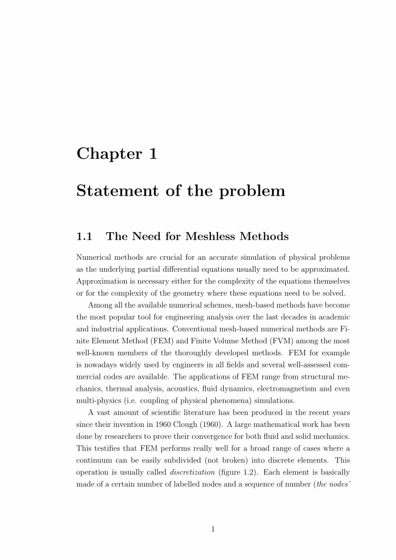
continuum can be easily subdivided (not broken) into discrete elements. This
operation is usually called discretization (figure 1.2). Each element is basically
made of a certain number of labelled nodes and a sequence of number (the nodes’
1

1.1 The Need for Meshless Methods
labels) that defines how these nodes are connected. This is the fundamental char-
acteristic of the mesh-based methods: a priori definition of the nodes connectivity,
commonly known as mesh. The mesh permits the compatibility of the interpola-
tion (figure 1.1), meaning that the resulting approximation is continuous.
Figure 1.1: Example of Mesh in Finite Element Analysis
FEM is robust and in particular for mechanics has been thoroughly and con-
tinuously developed since its creation. This includes static and dynamic, linear
or non-linear stress analysis of structures. The creation of a mesh, though, could
represent a challenging task. In fact, the analyst spends most of his work-time
in creating the mesh. It has become a major component of the total cost of a
simulation project because currently mere hardware is exponentially decreasing
its price. According to Liu (2003), who in 2003 wrote the first comprehensive
book on meshfree methods, the logical consequence is that the issue is now more
the manpower time, and less the computer time. Consequently, in an ideal world,
the meshing process would be fully performed by the computer without human in-
tervention. At the same time, with the increasing demand of high performance
products in the manufacturing industry, the problems in computational mechan-
ics grow more and more difficult and mechanicians need more and more sophisti-
cated numerical tools. These tools will eventually allow engineers to design even
more complex and high quality products. These tools are nowadays not purely
2
1.1 The Need for Meshless Methods
Figure 1.2: Discretization: domain Ω is subdivided in elements ΩE
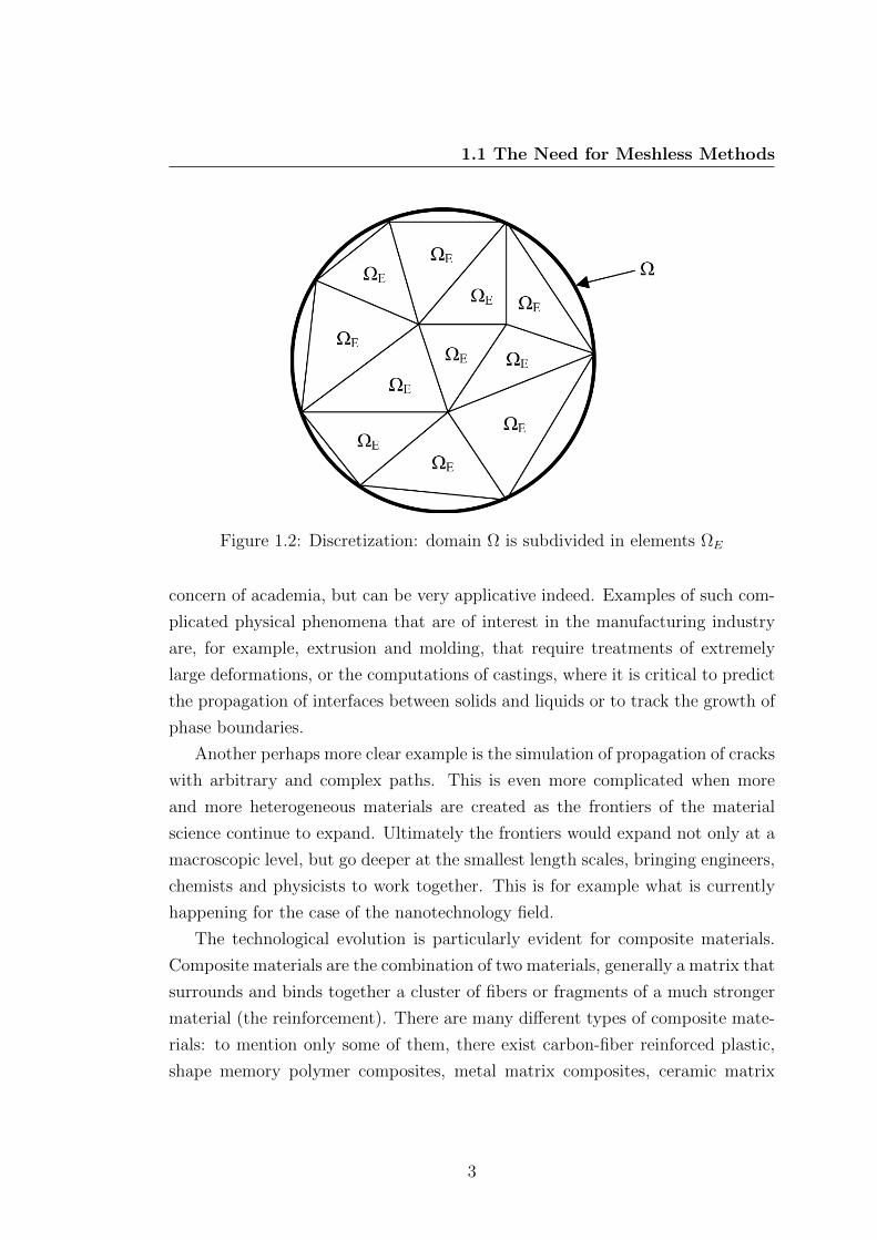
concern of academia, but can be very applicative indeed. Examples of such com-
plicated physical phenomena that are of interest in the manufacturing industry
are, for example, extrusion and molding, that require treatments of extremely
large deformations, or the computations of castings, where it is critical to predict
the propagation of interfaces between solids and liquids or to track the growth of
phase boundaries.
Another perhaps more clear example is the simulation of propagation of cracks
with arbitrary and complex paths. This is even more complicated when more
and more heterogeneous materials are created as the frontiers of the material
science continue to expand. Ultimately the frontiers would expand not only at a
macroscopic level, but go deeper at the smallest length scales, bringing engineers,
chemists and physicists to work together. This is for example what is currently
happening for the case of the nanotechnology field.
The technological evolution is particularly evident for composite materials.
Composite materials are the combination of two materials, generally a matrix that
surrounds and binds together a cluster of fibers or fragments of a much stronger
material (the reinforcement). There are many different types of composite mate-
rials: to mention only some of them, there exist carbon-fiber reinforced plastic,
shape memory polymer composites, metal matrix composites, ceramic matrix
3
1.1 The Need for Meshless Methods
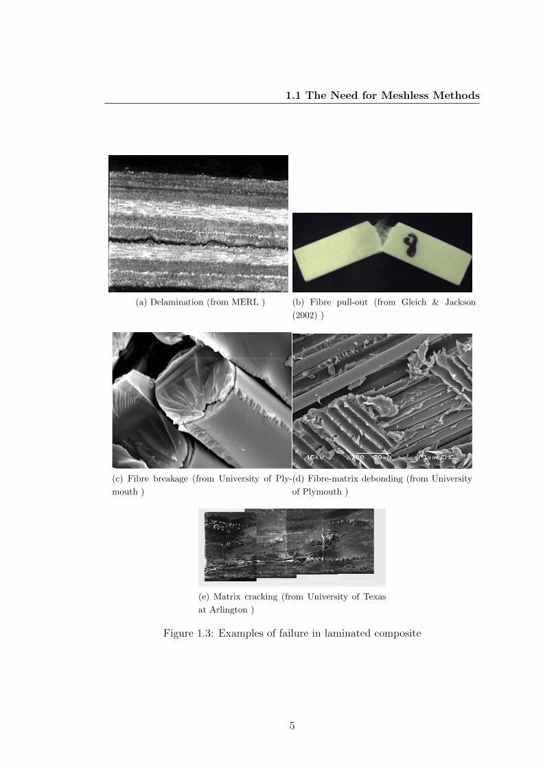
composites and sandwich composites. Being fairly complex materials, their fail-
ure cannot be easily treated with standard methods because failure modes for
composite materials are indeed quite different from the ones in metals. For ex-
ample, for laminated composite materials, where different plies are stacked up, a
very important failure mechanism is delamination (figure 1.3a), due to the lack
of reinforcement in the thickness. Delamination occurs for example in case of im-
pact events or for manufacturing defects. Moreover, since each ply is a mixture
of plastic matrix and fibers, fiber pull-out (figure 1.3b), fiber breakage (figure
1.3c), fiber-matrix debonding (figure 1.3d ) and matrix cracking ( figure 1.3e)
may initiate and propagate, compromising the integrity of the structure.
However, their unique characteristics of high strength and stiffness combined
to a much lower weight than aluminum and steel, make composite materials very
attractive to those manufacturing industries like automotive and aerospace, where
these requisites are more and more competitive values and influence the choice of
the customers. It suffices to think about the fuel that can be saved with lighter
vehicles without compromising the safety of the passengers. Less fuel would also
mean a positive impact on the environment. It is not a coincidence that the
two biggest aerospace industries like Boeing and Airbus have been trying (and
still are) to build either primary structural parts or entire airplanes in composite.
Another example is the automotive sector, one of the most competitive industrial
markets, where faster and more performing cars are proposed every year. This is
more stressed in competitive cutting edge sport sectors like Formula 1 when even
the smallest details can make the difference in a race.
Therefore the full understanding of these complex materials is at the same time
complicated but important, yet vital for a safe and competitive design. Their
importance, from an academic point of view, justifies the number of research
centers on composite materials and the number of researchers involved in the
many aspects of composite materials. The last international and most important
conference on composite materials 1 was attended by thousands of scholars from
all over the world.
We might then want to ask ourselves, what are the difficulties in the sim-
ulation of the mechanics of composite materials? Delaminations and fracture
1International Conference on Composite Materials 17 Edinburgh July, 2009
4
1.1 The Need for Meshless Methods
(a) Delamination (from MERL ) (b) Fibre pull-out (from Gleich & Jackson
(2002) )
(c) Fibre breakage (from University of Ply-
mouth )
(d) Fibre-matrix debonding (from University
of Plymouth )
(e) Matrix cracking (from University of Texas
at Arlington )
Figure 1.3: Examples of failure in laminated composite
5
1.1 The Need for Meshless Methods
breaking problems share a continuous change in the geometry of the domain un-
der study and their analysis with conventional methods could be a cumbersome
and expensive task as well as inaccurate. In fact, for crack propagation prob-
lems, FEM is not well suited to treat discontinuities that do not coincide with
the original mesh lines. Thus, the most viable strategy for dealing with moving
discontinuities in methods based on meshes would be to re-mesh in each step
of the evolution so that mesh lines remain coincident with the discontinuities
throughout the evolution of the problem.
Also, the analysis of large deformations problems by the FEM, may require
the continuous re-meshing of the domain to avoid the breakdown of the calcula-
tion due to excessive mesh distortion, which can either end the computation or
lead to drastic deterioration of accuracy. In addition, FEM often requires a very
fine mesh in problems with high gradients or with local character, which can be
again computationally expensive. Also, in order to compare successive stages of
the problem, all the meshes need to be stored, requiring more storage memory.
Furthermore, for fragmentation problems, like blasts or explosions, it seems nat-
ural to choose particle-based methods (or node-based) rather than mesh-based
methods.
In FEM it is very complicated to model the breakage into a large number of
fragments as FEM is intrinsically based on continuum mechanics, where elements
cannot be broken. The elements thus have to be either totally eroded or stay
as a whole piece, but this leads to a misrepresentation of the fracture path.
Serious errors can then occur because the nature of the problem is non-linear.
To overcome these problems related with the existence of a mesh, a numerical
scheme that relies only on nodes would be highly appreciated. These methods
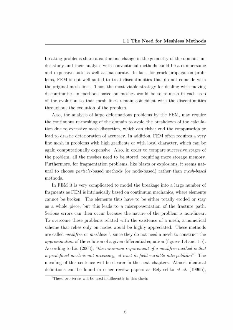
are called meshfree or meshless 1, since they do not need a mesh to construct the
approximation of the solution of a given differential equation (figures 1.4 and 1.5).
According to Liu (2003), “the minimum requirement of a meshfree method is that
a predefined mesh is not necessary, at least in field variable interpolation”. The
meaning of this sentence will be clearer in the next chapters. Almost identical
definitions can be found in other review papers as Belytschko et al. (1996b),
1These two terms will be used indifferently in this thesis
6
1.1 The Need for Meshless Methods
Figure 1.4: Example of Meshfree Method: nodes discretization of a femur (from
Doblare et al. (2005))
Duarte (1995), Fries & Matthies (2004), Gu (2005) Nguyen et al. (2008). More
details on classifications and definitions will be provided in section 2.2.
The ideal requirement would be, quoting Liu (2003), “that no mesh is nec-
essary at all throughout the process of solving the problem of given arbitrary ge-
ometry governed by partial differential system equations, subject to all kinds of
boundary conditions”.
Another interesting but different point of view can be found in Idelsohn &
Onate (2006). In this paper, even though the authors agree on considering as
meshfree a method where the shape functions depend only on the node positions,
this definition is not enough to justify the use of a meshless method. In fact, what
they consider as discriminating factor is the evaluation of the nodal connectivity.
According to them, a meshless method without a fast evaluation of the nodal
connectivity is useless. An additional requisite should be therefore added to
the definition of meshfree, i.e. that the computational complexity of the nodal
connectivity should be bounded in time and linear in number of operations with
the number of points in the domain. The problem of connectivity will be discussed
7

1.2 Main differences between Finite Elements and Meshfree
Figure 1.5: Discretization in Meshless Methods (from Doblare et al. (2005))
in a later chapter, although connectivity in this thesis will be intended not only
between the nodes, but also between nodes and Gaussian points. An algorithm
taken from the graph theory, known as kd-tree, will be used for this purpose, with
the aim of reducing the computational times related to connectivity and to derive
a fast method to assemble the matrices of the discretized problem.
1.2 Main differences between Finite Elements
and Meshfree
Before proceeding with the definition of the objectives of this thesis, it is necessary
to know the major differences (and/or similarities) between FE and MM, to
better individuate the weakness and the margin of improvements of the meshfree
techniques. Table 1.1, taken from Liu (2003), better resumes the major points.
Point 1 of table 1.1 illustrates the distinguishing difference between the two
methods, i.e. the absence of a mesh. This point it is still debatable, since some
meshfree methods do require a mesh, but only for integration purposes. However,
point 4 better clarifies point 1, since the construction of the approximation is
element based in FE and point based in MM. This makes a huge difference in terms
of the approximation to the differential equations and the (better) reproducibility
properties (and thus accuracy) that MM can achieve compared to FE. The term
reproducibility will be better explained in section 2.2.
8

1.2 Main differences between Finite Elements and Meshfree
FEM MM
1 Element mesh Yes No
2 Mesh creation and Difficult due to the Relatively easy
automation need for element and no connectivity
connectivity is required
3 Mesh automation and Difficult for 3D cases Can always be done
adaptive analysis
4 Shape function creation Element based Node Based
5 Shape function property Satisfy Kronecker May or may not satisfy
delta conditions Kronecker delta conditions
depending on the
method used
6 Discretized system Banded and Banded but symmetry
stiffness matrix symmetrical depends on the method
7 Imposition of essential Easy and standard Special methods
boundary condition may be required;
it depends on the method
8 Computation speed Fast 1.1 to 50 times slower
compared to the FEM
depending on the
method used
9 Retrieval of results Special technique Standard routine
required
10 Accuracy Accurate compared Can be more
with FDM accurate than FEM
11 Stage of development Very well developed Infancy, with many
challenging problems
12 Commercial software Many Very few and close to none
package availability
Table 1.1: Main differences between FE and MM; taken from Liu (2003)
9

1.2 Main differences between Finite Elements and Meshfree
The problem of the reproducing properties of FE is also contained partially
in point 2 of table 1.1. Having a higher order reproducibility capability usually
means that the approximation is more accurate. But, to achieve higher order
reproducibility properties, elements might be also of different shapes. A typical
example is the choice between triangular elements and quadrilateral elements.
Triangular elements with 3 nodes have linear reproducibility while quadrilateral
elements with 4 nodes can also reproduce the function xy. While a triangular
mesh is relatively easy to construct in an automatic manner, even for complicated
shapes, a quadrilateral mesh is usually more complicated to build automatically.
A software able to calculate a mesh is called meshers. A mesher able to
mesh arbitrary shapes with quadrilateral elements may not be as robust and may
not always work for complex surfaces (or volumes for hexagonal elements). The
algorithms behind the meshers are matter of a discipline called computational
geometry and there exists a vast literature for this topic Preparata & Shamos
(1985), De Berg et al. (2008). Nevertheless, even if a triangular mesh is easy
to build, not all the triangular meshes are equal. In fact it is defined a quality
factor for the meshes, that is an element-wise measure that depends on the ratio
between the area of the element and the sum of the squares of the length of the
edges of the element Bank (1990). Ideally, an optimal mesh is made only by
equilateral triangles. Of course this is not always possible; hence the quality of
a mesh must be checked on a case basis. Therefore, a mesh can really affect a
FE simulation, and not all the meshes are the same. Obtaining a good mesh can
then be difficult, since it is not a mere triangulation of points.
The meshfree methods that require a mesh do not need to submit to these
restrictions. In fact, meshes do not have any influence whatsoever on the ap-
proximation resulting from a MM. Mesh connectivity is a serious problem in
mesh-based calculations for cracks. For crack problems, with MM there is no
need of costly re-meshing. This also applies especially in problems with large
deformations or moving discontinuities. In fact, FE mesh distortions (figure 1.6)
in large deformation problems can compromise the solution, since most commer-
cial codes normally arrest the algorithm, unless special numerical expedients are
performed, like elements erosion or the Jacobian sign check. Conversely to FE,
MM do not need to define a priori connectivity, neither suffers of mesh alignment
10
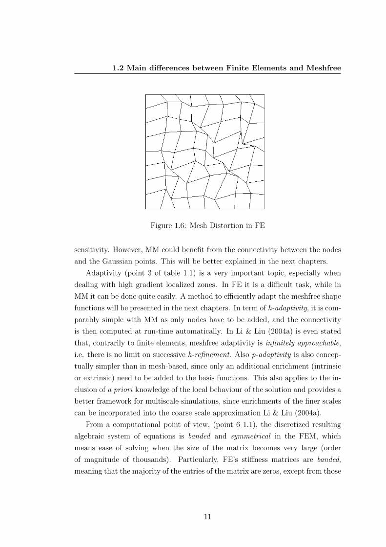
1.2 Main differences between Finite Elements and Meshfree
Figure 1.6: Mesh Distortion in FE
sensitivity. However, MM could benefit from the connectivity between the nodes
and the Gaussian points. This will be better explained in the next chapters.
Adaptivity (point 3 of table 1.1) is a very important topic, especially when
dealing with high gradient localized zones. In FE it is a difficult task, while in
MM it can be done quite easily. A method to efficiently adapt the meshfree shape
functions will be presented in the next chapters. In term of h-adaptivity, it is com-
parably simple with MM as only nodes have to be added, and the connectivity
is then computed at run-time automatically. In Li & Liu (2004a) is even stated
that, contrarily to finite elements, meshfree adaptivity is infinitely approachable,
i.e. there is no limit on successive h-refinement. Also p-adaptivity is also concep-
tually simpler than in mesh-based, since only an additional enrichment (intrinsic
or extrinsic) need to be added to the basis functions. This also applies to the in-
clusion of a priori knowledge of the local behaviour of the solution and provides a
better framework for multiscale simulations, since enrichments of the finer scales
can be incorporated into the coarse scale approximation Li & Liu (2004a).
From a computational point of view, (point 6 1.1), the discretized resulting
algebraic system of equations is banded and symmetrical in the FEM, which
means ease of solving when the size of the matrix becomes very large (order
of magnitude of thousands). Particularly, FE’s stiffness matrices are banded,
meaning that the majority of the entries of the matrix are zeros, except from those
11

1.2 Main differences between Finite Elements and Meshfree
close to the main diagonal. The number of non-zero entries in the same row close
to the diagonal is called bandwidth. If the bandwidth is small and constant for all
the rows, then these entries can be efficiently stored, since it is necessary to store
a fixed number of columns much smaller than the number of rows. Moreover,
if the matrix is symmetrical, the number of columns halves. From a numerical
point of view, solving linear system of equations with this particular structure
is relatively easy and more suitable for large system of equations. For MM, the
stiffness matrix could be banded, but the bandwidth could be slightly larger than
FE and not constant, although the stiffness matrix is symmetrical, depending on
the method used 1. Nonetheless, the structure is more generally sparse, which
means that the majority of the entries are non-zero. In this case, only the row
and column indexes along with the entry need to be stored. Moreover, there exist
methods able to efficiently solve sparse systems of equations Duff et al. (1989).
Another major disadvantage of the FEM is the post-processing (point 9 1.1).
Re-meshing is not just computationally expensive, but it also degrades the ac-
curacy of the solution. Even in the post-processing of re-meshed solids requires
considerable effort, since one need to keep track of all the meshes for example
during the time-histories. MM on the contrary have a post-processing nature,
because shape functions are natively smooth. Any order of continuity can also
be achieved adjusting the weight functions and adding more polynomials to the
basis, reaching the desired order according to the order of the differential equa-
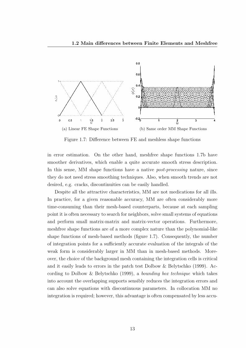
tions. For example, in figure 1.7 are compared MM shape functions and FE linear
shape functions. MM shape functions 1.7b are much smoother than the FE ones
1.7a for the same order of the basis. Let us suppose that linear FE shape func-
tions are used to carry out a stress analysis. In stress calculations, the stresses
obtained using FEM packages are discontinuous and less accurate, because the
simplest shape functions used in FEM are usually linear (figure 1.7a) or however
low-order polynomials. Thus, since displacements fields are of the same order of
the approximating functions, their derivatives (stress fields) are one order lower.
If linear functions are used for example, stress field will be piecewise constant,
which could be an unsatisfactory description of the stress distribution. In these
cases, stress smoothing techniques must be used, especially for stress recovery
1The methods used in this thesis generate symmetric stiffness matrices
12
1.2 Main differences between Finite Elements and Meshfree
(a) Linear FE Shape Functions (b) Same order MM Shape Functions
Figure 1.7: Difference between FE and meshless shape functions
in error estimation. On the other hand, meshfree shape functions 1.7b have
smoother derivatives, which enable a quite accurate smooth stress description.
In this sense, MM shape functions have a native post-processing nature, since
they do not need stress smoothing techniques. Also, when smooth trends are not
desired, e.g. cracks, discontinuities can be easily handled.
Despite all the attractive characteristics, MM are not medications for all ills.
In practice, for a given reasonable accuracy, MM are often considerably more
time-consuming than their mesh-based counterparts, because at each sampling
point it is often necessary to search for neighbors, solve small systems of equations
and perform small matrix-matrix and matrix-vector operations. Furthermore,
meshfree shape functions are of a more complex nature than the polynomial-like
shape functions of mesh-based methods (figure 1.7). Consequently, the number
of integration points for a sufficiently accurate evaluation of the integrals of the
weak form is considerably larger in MM than in mesh-based methods. More-
over, the choice of the background mesh containing the integration cells is critical
and it easily leads to errors in the patch test Dolbow & Belytschko (1999). Ac-
cording to Dolbow & Belytschko (1999), a bounding box technique which takes
into account the overlapping supports sensibly reduces the integration errors and
can also solve equations with discontinuous parameters. In collocation MM no
integration is required; however, this advantage is often compensated by less accu-
13

1.3 Objectives
racy and more stability problems. In addition, conversely to FE, meshfree shape
functions unfortunately do not satisfy (depends on the method used) the Kro-
necker condition (3.3), (point 5 1.1), thus essential boundary conditions cannot be
directly imposed. Essential boundary conditions in MM require opportune treat-
ments (point 7 1.1), like the use of penalty-methods Fernandez-Mendez & Huerta
(2004), Gavete et al. (2000) and Gunther & Liu (1998) or Lagrange multipliers
Belytschko et al. (1996b).
It is evident from the table 1.1, that beside the many advantages of the MM,
still their infancy (with the mentioned problems) and the lack of dedicated com-
mercial packages prevent their wide acceptance in the engineering community.
1.3 Objectives
The industrial sector has been relying on FE for decades. Well-developed com-
mercial codes, even for multi-physics simulations, integration with CAD software,
not to mention the well-established mathematical work made by researchers in
the past years.
It is understandable that industry is often reluctant to open to new method-
ologies, especially if these new methods cannot offer better performances of FE
in terms of reliability and speed. This is also the reason why a compromise that
put together the benefits of both methods seems to catch on. This compromise is
the Extended Finite Element Method (XFEM) Black & Belytschko (1999), Moes
et al. (1999). The invention of XFEM is subsequent to the invention of MM 1
and, in a philosophical perspective it could be thought as the synthesis between
thesis (FEM) and antithesis (meshfree).
The XFEM is essentially FEM with enrichments. The meaning of the word
enrichment will be well explained in the next sections and represents the core
of this thesis. For the purpose of this introduction, it suffices to say that these
enrichments are able to simulate discontinuities independently from a mesh, even
though the method is mesh-based.XFEM could be more acceptable for industry
because it is essentially a FE which overcomes the limitations due to the presence
1The first meshfree paper appeared in 1994 whereas the first paper on XFEM appeared
around 1999
14
1.3 Objectives
of a mesh concerning fracture mechanics problems. A wide literature exists for
this topic and review papers can be found in Abdelaziz & Hamouine (2008),
Karihaloo & Xiao (2003), Mohammadi (2008). However, XFEM are still mesh-
based therefore they inherit the other disadvantages of FE, like mesh-distortion,
piecewise stress representation for linear elements and so on.
An interesting thread of discussion about the future of meshless methods can
be found on the website imechanica.org.
The aim of this thesis is NOT to prove that MM are completely alternative
to FE, since for many applications FE represents an unbeatable standard, but
rather to study their possible applications to a more narrow class of problems, like
the failure of composite materials. Particularly it is studied the capability of MM
to simulate strong discontinuities as occurs for example in delaminations. More
complex failure mechanisms like matrix failure and fibers breakage, originate at
smaller length scales (micro-scale) is part of a broader research topic called multi-
scale methods and will not be covered in this thesis. More reliability and speed is
requested to MM or PUM methods to represent a remedy for the disadvantages
of FE. A welcome outcome would be the integration of MM in commercial codes
or the development of brand new commercial packages.
That brings to the objectives of this thesis. Broadly speaking they are:
1. The production of prototype codes for 2D and 3D simulations, to be further
developed for large scale simulations
2. The applications to the simulation of macroscopic failure in composite ma-
terials and analysis of advantages and disadvantages deriving from the ap-
plication of MM
3. The reduction of computational times of MM.
The main outcome of this research has been the production of object-oriented
codes developed in MATLAB. Even though Matlab is not suitable to large scale
simulations, it is still quite easy to use, to debug errors and to post-process the
results, therefore it is a useful tool to prototype a code since one does not have to
spend time in re-writing well-established numerical routines, like the solution of
linear systems of equation, matrix products and so on. Even if it is believed to be
15

1.4 Outline of the thesis
not as fast as traditional programming languages like Fortran, with appropriate
programming tricks and compilation of the codes, Matlab can be reasonably fast
for medium-size applications (with number of unknowns order of magnitude of
thousand and number of Gaussian point order of hundreds of thousands).
The codes served as basis for the simulation of delamination, proposed in the
final chapters. From a geometric point of view, delamination is modeled with
an enrichment that exploits the property of partition of unity of the meshfree
shape functions. The physics of the delamination process will be simulated with
a constitutive model called cohesive zone, derived from the damage mechanics.
The combination of the cohesive law with MM will result in the cohesive segments
method.
For the third point, the innovations that will be proposed are
1. the employment of a more efficient node searching method known as KD-
trees
2. a faster assembly procedure based on a connectivity map between nodes
and Gaussian points
3. a new matrix-inversion procedure that also facilitates hp-adaptivity
Finally, from a more theoretical point of view, the explicit integration in
Reproducing Kernel Methods has been published by the author. More details
can be found in appendix A.
1.4 Outline of the thesis
The outline of the thesis is the following: in chapter 2 the literature and the
chronological history on meshfree methods will be reviewed, with particular at-
tention to fracture mechanics and composite materials; in chapter 3 the main
meshfree methods will be described in detail; subsequently in chapter 4 some
improvements to the existing techniques will be proposed, along with results and
considerations; chapter 5 will provide a description of the codes developed, while
in chapter 6 MM will be applied to the simulation of delamination. Finally,
conclusions are presented in chapter 7.
16
Chapter 2
Literature Review
In this section meshfree methods will be firstly classified and a survey of the ex-
isting literature on the topic will be presented. Successively, the review will cover
particularly two methods, the Element Free Galerkin (EFG) and the Reproducing
Kernel Particle Method (RKPM) . It has been proven that these two approaches
lead to identical shape functions Liu et al. (1997b), Li & Liu (1996), Jin et al.
(2001), even if they start from different ideas.
This is a frequent problem in MM. Being a rapidly developing method, con-
fusion and disorder about different methods may arise. In fact in a recent paper
Orkisz & Krok (2008) it is reported that there exist about hundred different
names of the MM, mostly presenting very similar or even identical ideas. Some
of the methods differ only by the names of the authors or by the methods’ name,
and this certainly leads to confusion.
2.1 Review Papers and Books on Meshfree Meth-
ods
A good number of review papers and books on meshfree methods have been pub-
lished in the recent years. The first review appeared in Duarte (1995) almost
at the beginning of the MM era, shortly followed by the more general overview
Belytschko et al. (1996b). While Duarte (1995) is more focused on the mathe-
matical properties of these methods, Belytschko et al. (1996b) is more complete
17

2.2 Classification of Meshfree Methods
and more suitable for an engineering audience, since it contains many details on
the implementation of MM, especially for applications to crack problems.
The review Shaofan & Liu (2002) instead emphasizes the MM applications
for large deformation problems and reviews with particular attention multiscale
and particle methods. A subclass of particle methods is the molecular dynamics,
widely employed in computational chemistry. This paper is the background of
the book Li & Liu (2004b).
The first book on MM is instead Liu (2003) and it is in the author’s opinion
the most complete work on meshfree methods, since it contains many examples
(beams, shells, plates) and comparisons with different methods. A demonstrative
software has been also produced from the authors called MFREE2D, although
such software does not allow treatment of cracks or enrichments.
Updated reviews on meshfree methods can be found in Fries & Matthies (2004)
and Nguyen et al. (2008). Fries & Matthies (2004) reports also a classification
scheme to better discriminate the different MM, while Nguyen et al. (2008) con-
tains also a Matlab didactic code.
Special issues in international journals have been dedicated to MM Liu (1996),
Chen (2000) and Chen (2004).
2.2 Classification of Meshfree Methods
Several classifications have been proposed, but the debate is currently ongoing.
Liu (2003) proposed a classification based on the point of view that all the
meshless methods (MM) so far are not ideal and fail in one of the following
categories:
• methods that require background cells for the integration of system ma-
trices derived from the weak form over the problem domain. These meth-
ods are not truly mesh free. These methods are practical in many ways,
as the creation of a background mesh is generally feasible and can always
be automated using a triangular mesh for two-dimensional (2D) domains
and a tetrahedral mesh for three-dimensional (3D) domains. It needs to
be stressed out that this mesh is necessary only for integration purposes;
18
2.2 Classification of Meshfree Methods
this means that the driving criterion in the generation of such a mesh is
the minimization of the integration error rather than the accuracy of the
approximation.
• Methods that require background cells locally for the integration of
system matrices over the problem domain. These methods are said to be
truly mesh free because creating a local mesh is easier than creating a
mesh for the entire problem domain and it can be performed automatically
without any predefinition for the local mesh.
• Methods that do not require a mesh at all, but that are less stable and less
accurate. Collocation methods and finite difference methods fall into this
category. This type of method has a very significant advantage: it is very
easy to implement, because no integration is required.
• Particle methods that require a predefinition of particles for their volumes or
masses. The algorithm will then carry out the analysis even if the problem
domain undergoes extremely large deformation and separation.
Fries & Matthies (2004) instead proposed a classification based on three char-
acterizing features:
• the capability of realizing a Partition of Unity of order n with the intrinsic
basis
• the presence of enrichments or more generally extrinsic basis
• the use of the test function
The last one discriminate between collocation-based methods or Galerkin meth-
ods. According to Fries & Matthies (2004), a meshfree method can have one or
more of these three features. Moreover, it is also individuated a grey area contain-
ing hybrid methods. Therefore, the classification suggested in Fries & Matthies
(2004) is based on the capability to reproduce polynomials up to a chosen de-
gree with or without an intrinsic basis. Moreover, the classification can be also
conducted on the choice of test functions, leading to local, global weak forms or
collocation methods.
19

2.3 Origins of Meshless Methods
2.3 Origins of Meshless Methods
The very first meshless method is Smoothed Particle Hydrodynamics (SPH) and it
was introduced for the study of astrophysical phenomena without boundaries such
as exploding stars and dust clouds and it is due to Lucy (1977). Later Monaghan
in Monaghan (1982), Monaghan (1988) and Monaghan (1992) provided a more
mathematical basis through the means of kernel estimates. Particularly in the
paper Monaghan (1982) is demonstrated that the way a function is represented
in particle methods is a special case of interpolation using information from a set
of points. Moreover general equations for numerical work can be derived without
specifying the details of the interpolation method, showing similarities between
finite difference, spectral and particle methods.
Even though SPH was initially conceived for solving astrophysics problem, in
Libersky & Petschek (1990) SPH is applied for the first time in solid mechanics
and further to study dynamic material response under impact Libersky et al.
(1993). A recent review on the developments of SPH in impact problems can
be found in Vignjevic & Campbell (2009). However, the original SPH version
suffered from spurious instabilities, like tensile instability Swegle et al. (1995).
Nevertheless, such instabilities have been successful treated in Vignjevic et al.
(2000). Moreover, SPH lacks of consistency properties, especially at the bound-
aries, where SPH is not able to reproduce even the constant function. For these
reasons these methods worked well for unbounded problems like astrophysics,
where the domain can be certainly considered as infinite. This is not the case in
solid mechanics, where the domains under study are bounded; more importantly,
at the boundaries, forces, tractions, displacements are usually applied. Therefore
correction terms are needed in order to restore consistency.
Corrections to SPH and related treatment of boundary conditions have been
proposed in several papers by the Vignjevic and co-workers, for example in Camp-
bell et al. (2000) and Vignjevic et al. (2006).
In Rabczuk & Eibl (2003), Dilts (1999), Dilts (2000) and Cueto-Felgueroso
et al. (2004) SPH is used in a Galerkin weak form using MLS shape functions
(MLSSPH ).
20
2.3 Origins of Meshless Methods
It is important here to recall the concept of consistency because it is crucial
for the convergence properties of any numerical scheme. Liu (2003) distinguishes
between reproducibility and consistency. Reproducibility for MM is defined as the
ability of the shape functions to reproduce exactly all the functions in its basis,
whilst consistency is the property of reproducing polynomial functions.
This is due to the fact that if the unknown solution u(x) is expanded in
Taylor series around a generic point x, since the approximation reproduces for
example polynomials up to degree n, then the approximation is able to reproduce
the solution of a differential problem until the order n. It is easy to understand
therefore that consistency is a highly desired property for a numerical method.
If the basis contains only polynomials, then reproducibility and consistency are
equivalent. If the basis contains only functions different from polynomials, the
approximation has only reproducibility but it is not consistent, hence it may
not converge to the solution. If the basis contains both polynomials and other
functions, the basis is called enriched or enhanced and it is not only consistent
but also able to reproduce these other functions. If these other functions are for
example known solutions of the equations, this means that the approximation
is able to reproduce the exact solution of the problem. This concept is the
foundation of the enriched methods for crack propagation. In fact, for linear
elastic fracture mechanics Anderson (1991), the theoretical solution is singular at
the crack tip.
Classical finite elements fail to reproduce accurately the solution. Also, non-
enriched meshfree methods are not able to reproduce exactly the solution. Con-
versely to finite elements, though, meshfree approximation can easily handle the
discontinuity while finite elements need elements conforming to the crack. More-
over, using enrichments, it is possible to reproduce singular functions because
these singularities can be included in the basis. This is one of the most attractive
features of MM.
21

2.4 Reproducing Kernel Methods and Element Free Galerkin
2.4 Reproducing Kernel Methods and Element
Free Galerkin
While SPH and their corrected versions were based on a strong form, other meth-
ods were developed in the 1990s, based on a weak form. The first of them is based
on a global weak form and it was invented by Belytschko and his coworkers, who
exploited the Moving Least Squares (MLS) approximation Lancaster & Salkauskas
(1981). MLS have been already used to generalize finite elements in the work of
Nayroles et al. (1992), where diffuse elements were proposed. The MLS has its
origins in the computer graphics to smooth and interpolate scattered data, thus
it seems reasonable to apply this method when only scattered nodes are available
as a result of a discretization.
Belytschko et al. (1994b) refined and modified the work of Nayroles and called
their method Element Free Galerkin EFG, which is currently one of the most used
meshless methods. This class of methods is consistent, up to n-th degree depend-
ing on the polynomials used in the basis function, and quite stable although
substantially more expensive than SPH.
One year later Liu et al. (1995) developed the Reproducing Kernel Particle
Method (RKPM) which uses wavelets theory, contrarily to MLS. Surprisingly,
the imposition of the reproducibility for the polynomials led to shape functions
almost identical to MLS.
2.4.1 Reproducing Kernel Method
Reproducing Kernel Method (RKM) has its origins in wavelets theory Liu et al.
(1996) and its discrete counterpart has given birth to Reproducing Kernel Particle
Method (RKPM) which is one of the emerging classes of methods called meshless
methods. Moreover, RKPM shares similarities with moving least squares (MLS)
method and RKM is ultimately more a category within these methods can be
classified Liu et al. (1997b), even though MLS has its origins in data fitting.
Indeed, sometimes RKM is referred to as a corrected SPH.
In standard Smoothed Particle Hydrodynamics (SPH) method Gingold &
Monaghan (1977), Monaghan (1992), the function is simply approximated by an
22

2.4 Reproducing Kernel Methods and Element Free Galerkin
its convolution with a kernel function, which satisfies a set of properties. One of
them is that the kernel is a compact support function with dilatation parameter
ρ. The approximation is then filtered conferring a smoother behaviour to the
approximation. SPH scheme though, suffers of inconsistencies at the boundaries,
precisely at a distance equal to ρ Liu et al. (1997a). SPH is not able to reproduce
even the constant function, i.e. it does not realize a partition of unity Belytschko
et al. (1996b). This is also the reason SPH is more suitable for unbounded
domains.
In order to restore this condition, a corrected kernel must be used. It can
be demonstrated that using a modified kernel Liu et al. (1996) by the means of
a moments matrix, the reproducibility condition up to order n is restored. This
moments matrix has entries that are essentially the kernel estimates of polynomial
functions up to degree 2n. The resulting approximation is known as Reproducing
Kernel Method (RKM).
Although this theory is mathematically correct, its implementation might
pose problems since it is necessary to evaluate integrals. Thus in real computa-
tions a discretization is often necessary. This discretization is based on particles
associated with a measure of the domain and the integrals are replaced with
summations. However, an explicit computation of the integrals involved in RKM
without discrete summations has been proposed in Barbieri & Meo (2009b). A
description of this method will be proposed in the next chapters.
While in RKM the moments matrix depends only on the domain (actually,
only on the domain’s boundaries Barbieri & Meo (2009b)), in RKPM, because
of the discrete sums, it depends on the particles distribution. RKPM therefore
associates the advantage of being meshless with a higher accuracy, keeping the
multi-resolution property assured by the dilatation parameter of the kernel.
In Liu et al. (1996) and Liu et al. (1997a) the wavelets character of RKPM
allowed to generalize the method to multiple length scales. In Liu et al. (1996) is
proposed an approach to unify all the reproducing kernel methods under one large
family and an extension to include time and spatial shifting. In the latter Liu
et al. (1997a) the approach is particularized for its particle version RKPM. The
Fourier analysis is used to address error estimation and convergence properties.
23
2.4 Reproducing Kernel Methods and Element Free Galerkin
2.4.2 Element Free Galerkin
In parallel, Belytschko et al. (1994b) applied another meshless approximation
scheme called moving least squares (MLS) Lancaster & Salkauskas (1981) to
a Galerkin approach creating the Element Free Galerkin (EFG) method. In
MLS a function is approximated by a weighted least squares procedure where the
weighting function is moving in the sense that it depends on the evaluation point.
The weighting function plays the same role of the kernel function in RKM, since
it is a smooth compact support function where the size of the support is ρ. The
support is centered on the evaluation point, around which fall a certain number
of nodes. The result is that the function is not interpolated, but approximated at
the nodes (similarly to the particles).
Thus, the resulting minimization of the sum of the squares of the error leads
to solving a linear system of equations in each point of interest. The matrix of
this system is called moment matrix and in fact it is the same of the RKPM.
The similarities between the two methods became more evident in the Moving
least-square reproducing kernel methods (MLSRKM), where a general framework
is introduced Liu et al. (1997b), Li & Liu (1996). From MLSRKM , both RKPM
and MLS can be derived, where the sum of the square errors can be interpreted
in a continuous way if an inner product based on integrals is considered. These
integrals are the same introduced in the moment matrix.
Applications of both RKPM and EFG have been quite successful in the recent
years, especially in problems with discontinuities and singularities and a large
number of papers can be found which dealt with these questions. The leap in
these methods has been provided by the works of Melenk & Babuska (1996)
and Duarte & Oden (1996) where it is recognized that MLS approximation is a
particular partition of unity.
The essence of the partition of unity method relies on the fact that whatever
partition of unity can be multiplied with any independent basis to form a new
and better basis. Sometimes the choice of an independent basis can be based
on users’ prior knowledge and experience about the problem. This led to the
creation of the enrichments for MLS (or RKPM) shape functions, which have
been wisely and widely exploited for fracture mechanics problem.
24
2.5 Applications to Fracture Mechanics
2.5 Applications to Fracture Mechanics
There is a vast amount of literature about applications of MLS or RKPM in
fracture mechanics, most of them by the Northwestern University group of Be-
lytschko and W.K.Liu. Probably Belytschko et al. (1994a) is the first application
of EFG to crack problem contemporary to the publication of the classic paper
Belytschko et al. (1994b).
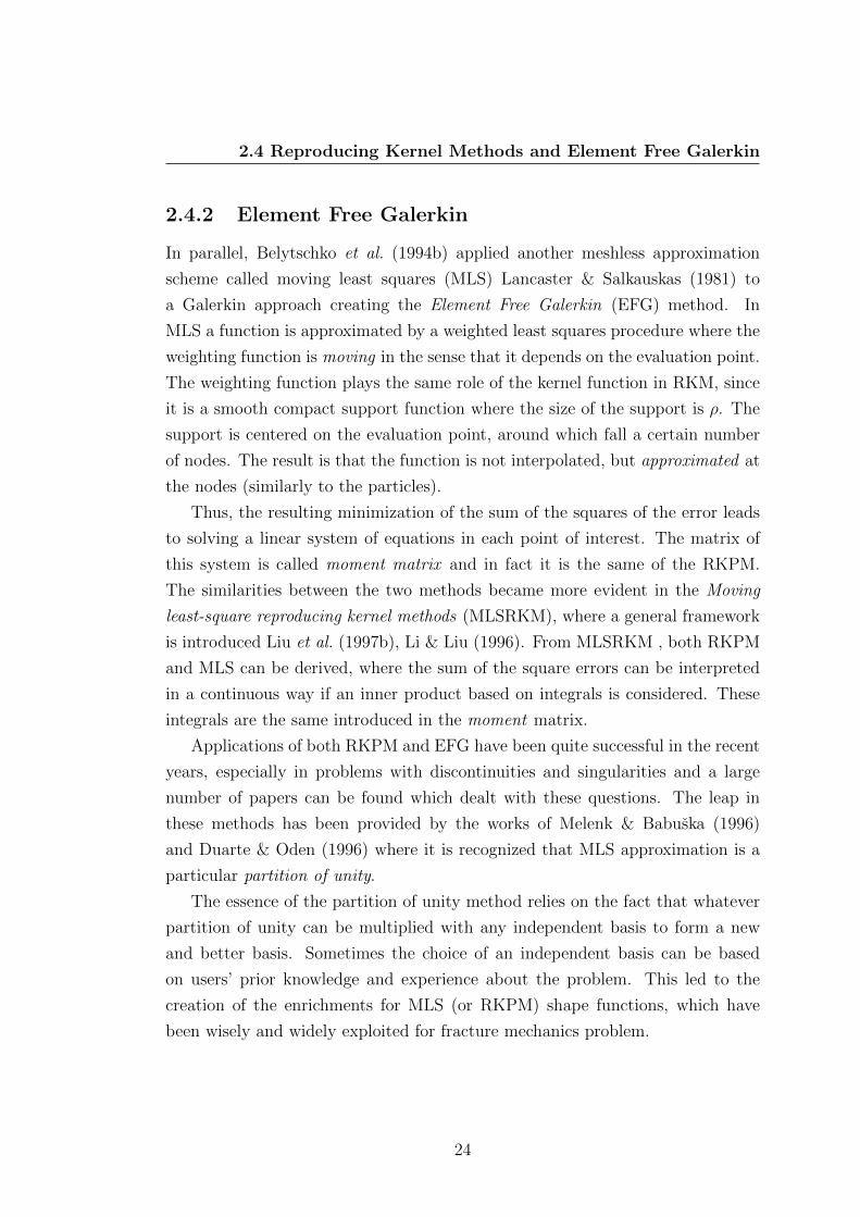
In Belytschko et al. (1994a) a visibility criterion is applied to model disconti-
nuities in the domain. This criterion is the very first one that has been applied
and it was subsequently modified to give more accurate representations of a crack
tip.
(a) (b) failure for non-convex domains
Figure 2.1: Visibility criterion (from Belytschko et al. (1994a))
Lagrange multipliers can be used to enforce essential boundary conditions,
even if penalty method is mentioned as well. A crack propagation criterion based
on the stress intensity factors (SIF) is used, and the SIFs are calculated according
to the famous J-integral Rice (1968) opportunely converted in a domain integrals.
All the integrals are evaluated in this paper with the mean of Gauss quadrature
with special mention to the problems that can arise. Also, the distribution of
nodes is a circular arrangement around the crack tip which can effectively capture
the stress singularity and the SIFs. Moreover it is possible to move a dense
25
2.5 Applications to Fracture Mechanics
arrangement of nodes around a crack tip without re-meshing, which is the greatest
advantage over FE methods.
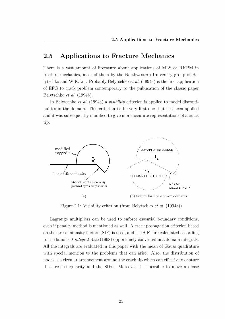
In Belytschko et al. (1995a) the classic problem of a plate with circular hole
under remote tension loading is presented. (figure 2.2)
Figure 2.2: Plate with circular hole under remote tension (from Belytschko et al.
(1995a))
On the outer boundaries the exact solution in terms of stresses is applied and
due to symmetry, only a quadrant of the problem is considered. Results show that
when concentrating the nodes distribution nearby the hole, the calculated stresses
are identical to the analytical ones. Regarding the edge crack problem, SIFs are
calculated for different ratio of width and length showing good comparison with
known solutions. Instead of visibility criterion, each node lying on the crack line
is split in two nodes, separated from a very small distance. It is shown that to
obtain greater accuracy, not only the number of nodes needs to be increased, but
also they need to be arranged along circular line around the crack tip (figure 2.3).
In fact, regular arrangement even with more nodes gives less accurate results than
the circular arrangement.
The two cases are then combined in a problem with cracks emanating from
a circular hole in order to study crack propagation. A criterion based on SIF
26

2.5 Applications to Fracture Mechanics
Figure 2.3: Typical Nodes Arrangement for edge crack problem (picture taken
from Belytschko et al. (1996a))
and angle θ for the direction of the crack growth is used to predict the propaga-
tion path, derived from the Paris-Erdogan law for fatigue crack growth Paris &
Erdogan (1963).
Same approach with identical procedures is proposed in Belytschko et al.
(1995b), with the addition of a simulation of cracks in a dynamic field, i.e. how
a crack propagates in a moving body. Integration in time is carried out with
a β-Newmark integrator and solutions for dynamic stress factors are in agree-
ment with the analytical solution by Freund (1990). Another important work in
dynamic fracture mechanics with similar results is Belytschko & Tabbara (1996).
In Belytschko et al. (1996a) a new procedure to treat discontinuities is firstly
introduced, which overcome the disadvantages in the visibility criterion Belytschko
et al. (1994a). In fact visibility criterion fails with non-convex boundaries (figure
2.1b). This new procedure is the diffraction criterion (figure 2.4) and it is based
on the relative distance among each sampling point x, the discretization nodes
xI and the crack tip xc. With this procedure, nodes hidden by a non-convex
boundary are considered, leading to new weight functions capable of handling
the presence of a line of discontinuity. Also, in the same paper, a procedure
to accelerate the computation of shape function is introduced for the first time.
27

2.5 Applications to Fracture Mechanics
Figure 2.4: Diffraction criterion; figure taken from Belytschko et al. (1996a)
Since shape functions are the results of small system of equations, LU factor-
ization can be used and the factorized matrices L and U stored for subsequent
usage in the derivatives calculation. This indeed permits to save computational
costs.
One of the most important steps forward in MM is surely the work of Duarte
& Oden (1996), where the Partition of Unity method (PUM) is introduced. Ba-
sically, PU functions are constructed starting from a set of N scattered nodes xI
in a domain Ω. Each nodes is the center of a sub-domain (or clouds) ΩI . On
each sub-domain, a function φI(x) is defined, which is non-zero outside ΩI (figure
1.5). Differently from FE, these sub-domains overlap, therefore the condition of
the partition of unity (i.e. the sum of all these function on Ω is equal to 1) is not
automatically guaranteed, but they have to be constructed accordingly.
Apart from classic FE functions, another class of functions that easily realize
PU is Shepard’s function where simply each function is normalized to the sum
of all φI(x). From the consistency point of view introduced in subsection 2.3,
this class lacks of accuracy, since they can only reproduce exactly constant func-
tions. Their advantage is the ease with these functions can be calculated, since
conversely to other MM, they do not need the resolution of a system of linear
equations. The importance of this work is that, even starting from Shepard’s func-
tion with low accuracy, more accurate shape functions can be constructed simply
by multiplying Shepard’s function with another basis function, which contains
enhanced or enriched functions. These functions could be either polynomials or
28
2.5 Applications to Fracture Mechanics
functions similar to the known solution of the differential equation, like in Melenk
& Babuska (1996) for the Helmholtz equation in one dimension.
This method is also called extrinsic enrichment since the augmented basis is
external to the basis used to construct φI(x). The greatest drawback of these
methods is that more unknowns are introduced. If N is the number of nodes and
k the number of enhanced functions, there are N × k more unknowns than the
usual N . Since usually in real computations N could be a very large number, this
method can sensibly increase the computational cost. Therefore, usually only few
nodes are enriched; for example in edge crack problems, the nodes close to the
crack tip are enhanced. The contribution of Duarte & Oden (1996) is that, since
MLS shape functions are specific instance of PU (they are actually PU of order
n ≥ 1), they can replace Shepard’s functions.
The advantage is that hp-adaptivity is much more facilitated. In general adap-
tivity is a method to assess the quality of the results (based on error estimation
theory) and modify the mesh during the solution aiming to achieve approximate
solution within some bounds from the exact solution of the continuum problem.
Precisely:
• h-adaptivity in FE is when elements are refined (or unrefined). In MM this
is done simply adding nodes (figure 2.5)
• p-adaptivity when the order of polynomial basis functions is changed
• hp-adaptivity is a combination of the above
Fleming et al. (1997) presented for the first time a different way of enrich basis
functions, called intrinsic enrichment. Because of the reproducibility property
of the MLS, enhanced function can be added to the basis. In Fleming et al.
(1997) the two methods of extrinsic and intrinsic enrichment are compared. The
augmented functions are the well known asymptotic solution of the crack tip
in linear elastic fracture mechanics, whose stresses are singular at the end of
the crack line. Therefore functions whose derivatives are singular need to be
considered, for example the square root of the distance between the crack tip and
a generic point. In contrast to the extrinsic method, the intrinsic one does not
require additional unknowns. However, since the size of the basis is increased,
29

2.5 Applications to Fracture Mechanics
Figure 2.5: h-adaptivity in FE (left) and meshfree (right)
more computational effort is needed to invert the moment matrix. Moreover, for
multiple cracks, additional terms are required for each crack. Enriched basis can
lead to a moment matrix which exhibits some ill-conditioning. LU factorization is
used to alleviate this ill-conditioning. In Fleming et al. (1997) is also introduced
a smoothing factor to the diffraction method and also a mapping for kinked crack
is proposed.
The benefit of the introduction of the enrichment is quite evident. Non-
enriched functions cannot reproduce the exact stress field, while enriched methods
show perfect agreement with the analytical solution. Also, oscillations are elimi-
nated without extra refining at the crack tip. Convergence considerations about
discontinuous approximations introduced by these enrichments are presented in
Krysl & Belytschko (1997). Krysl & Belytschko (1997) pointed out that much of
the mathematics for FE is applicable to EFG.
Therefore EFG method satisfies all the requirements under which conver-
gence estimates based on interpolation theory apply to conforming finite element
method. Consequently it can be expected that this FEM convergence theory will
apply also to the EFG method. It is shown that the enrichment greatly increases
the absolute accuracy. Accuracy means that the errors are small compared to the
exact solution and thus the code provides results close to the truth. When the
solution is unknown, the error is estimated.
In fact, for regular EFG (linear basis), the rate of convergence (which means
the increase in accuracy due to uniform nodal refinement) for problems with a
30

2.5 Applications to Fracture Mechanics
singularity is controlled by the order of the singularity for a polynomial basis of
any order. For linear basis, the theoretical rate of convergence is therefore 1/2
(because the exact solution goes with the square root of the distance from the
crack tip). For the enriched approximations the exact solution is contained in
the trial function and according to the theory of minimum potential energy there
should be no errors due to approximation. In this case, the errors arise because
of quadrature error and discretization of the essential boundary conditions.
The early works with EFG dealt with two-dimensional structures until 1997
when the first applications to three-dimensional domain started to appear. In
Sukumar et al. (1997) 3D EFG is generalized in a straightforward manner. The
ease stands in the fact that, since no elements are required, one simply needs to
add function to the basis functions like z or z2. Weight functions are tensor prod-
ucts of one-dimensional weight functions, whereas implicit enriched functions are
used to achieve higher accuracy for the crack representation. An extended diffrac-
tion criterion is used to create shape functions which reproduce the discontinuity
line introduced by the edge stationary crack. While computational technology
for stationary cracks is well established, for 3D domains the main issue is the
geometrical representation of arbitrary evolving cracks.
MM appears to be one the most promising method to handle even three
dimensional cracks. In Krysl & Belytschko (1999) FE are coupled to EFG in the
sub-domain where the crack exists. Representation of the crack surface is made
by a triangular mesh and segments are used for the crack front. Since kinks in
the crack might be present, a smooth representation is not preferred.
A quite complex algorithm called node inclusion is presented to create dis-
continuous shape functions. The crack propagation algorithm is based on SIFs.
The addition of triangular elements is made with advance vectors. Recalculation
of shape functions is made accordingly. The method is applied successfully to
simulation of mixed-mode growth of center-through crack in a finite plate, mode-
I surface-breaking penny-shaped crack in a cube, penny-shaped crack growing
under general mixed-mode conditions and torsion-tension rectangular bar with
center through crack. Comparisons are made with respect to classic methods like
FE, showing that complex re-meshing is avoided.
31

2.6 Applications to Nonlinear Mechanics
In the comprehensive paper Belytschko & Fleming (1999) the whole EFG
method is reviewed. Classic test cases are replicated such as infinite plate with
a hole, near-tip crack, plate with a hole and two cracks and compression-loaded
cracks. Beside the already known results, an innovation is introduced, precisely
the contact between two bodies or self-contact as in cracks problem. The contact
is implemented with the same penalty method used to impose essential boundary
conditions.
In Ventura et al. (2002) a new vector level set method for modeling propagat-
ing cracks in EFG is presented. With this approach only nodal data are used to
describe the crack and no geometrical entity is introduced for the crack trajectory.
The vector level set basically consists in a local extrinsic enrichment when one
of the enhanced functions is a sign function of the distance between the enriched
node and the crack line. Only the nodes whose support is cut by the crack line
have this type of enrichment. The nodes close to the crack tip have as enhanced
functions the linear elastic fracture mechanics solution for an infinite plate. The
update of the vector set is made through an advance vector of the crack tip.
2.6 Applications to Nonlinear Mechanics
As anticipated in section 1.1, MM are also employed in problems with large
deformations.
A large deformations in FE easily causes element distortion, resulting in a
lack of accuracy. In Chen et al. (1996) there is the first application of RKPM to
large deformation in hyper-elastic (figure 2.7) and elasto-plastic materials. The
advantage is that the compact support of a RKPM material shape function covers
the same set of particles during the deformation and hence there is no tension
instability. This is achieved with the introduction of a material (i.e. the initial
reference configuration) kernel function that deforms with the material, rather
than using a kernel with a fixed support. In fact fixed supports could lead to
instabilities under large deformations. The usage of material shape functions
avoids the re-adjustment of kernel function hence without creating an additional
burden.
32

2.6 Applications to Nonlinear Mechanics
Figure 2.6: Example of Nonlinear Analysis: box-beam under impact; picture
taken from Chen et al. (1996)
Figure 2.7: Example of Large Deformation Analysis: hyperelastic material tensile
test; picture taken from Chen et al. (1996)
33

2.6 Applications to Nonlinear Mechanics
The same approach is successfully used in Chen et al. (1997) to model the
behaviour of rubber in test cases like uni-axial tension-compression of a plane-
strain rubber unit, shear tests, inflation of an infinitely long rubber tube, disk
inflation and the analysis of a silent block rubber bushing assembly.
In Sukky Jun (1998) several issues regarding fast and exact algorithms for
large deformation problems have been addressed and it is suggested an algorithm
for the simulation of large deformation problems. The method is then applied to
a hyper-elastic material and also to a highly non-linear large deformation problem
and complex phenomenon as underwater bubble dynamics, to test the goodness
of the method.
In Liu & Jun (1998) the multi-resolution properties of RKPM Liu et al. (1996),
Liu et al. (1997a) are exploited to detect the different scales of the response of
a largely deformed material.In fact, due to this multi-resolution property, the re-
sponse of a complex mechanical system can be separated into different scales and
each scale is investigated separately. Therefore the non-linear Cauchy Green ten-
sor is decomposed in a high scale and a low scale component, where the high-scale
component of the solution is useful as a criterion for the procedure of adaptivity.
In Ponthot & Belytschko (1998) an Arbitrary Lagrangian Eulerian (ALE)
formulation is applied to EFG. ALE is particularly used in fluid-structure inter-
action problems and a combination of the two classic points of view in continuum
mechanics, i.e. Lagrangian and Eulerian description. The reason of using such a
combined formulation stays in the fact that neither the Lagrangian nor the Eule-
rian descriptions are well suited because of their well-known intrinsic limitations.
Essentially, the Eulerian description can deal with very large material distortions
but have limited spatial resolution to track a moving boundary. Conversely the
Lagrangian description can precisely track a moving boundary or interface but
is limited by mesh distortions. In fact, the Eulerian and Lagrangian formula-
tions viewpoints have rather complementary virtues. ALE has the possibility to
automatically retain an evolving high density of nodes where it is required and
in Ponthot & Belytschko (1998) this ability is joined with the ease of EFG in
treating discontinuities.
Other interesting applications of RKPM regard simulations of large deforma-
tion of thin shell structures Li et al. (2000b). These structures are simulated
34
2.7 Other Meshfree Methods
as 3D continuum, differently from shell elements in FE. Results are quite sur-
prising, showing that RKPM can easily simulate large deformation problems of
both elasto-plastic and hyper-elastic thin shell structures like cylindrical shells
and conic shells.
Other interesting non-linear applications include shear band formations Li
et al. (2000a), Liew et al. (2002a), plasticity due to impacts Eskandarian et al.
(2003), Chen et al. (2005) and Beissel et al. (2006), non-linear fracture mechanics
Rao & Rahman (2004) and non-linear analysis of plates and laminates Belinha
& Dinis (2007).
2.7 Other Meshfree Methods
As mentioned in section 2.2 there are many different MM, most of them presenting
very similar or even identical ideas.
A probably non-comprehensive list of MM is Finite Point Method Onate et al.
(1996) , the Meshless Local Petrov-Galerkin (MLPG) Atluri & Zhu (1998), Local
Boundary Integral Equation (LBIE) Zhu et al. (1998), Natural Element Method
(NEM) Sukumar et al. (1998), Meshless Finite Element Method (MFEM) Idel-
sohn et al. (2003), Finite sphere De & Bathe (2000) and hp-clouds Duarte &
Oden (1996).
2.8 Shortcomings, Recent Improvements and Trends
Despite their attractive features, MM still have some drawbacks. The most prob-
lematic is the solution of small systems of equation at each point of evaluation,
since it really slows down the computational run-time.
Recently efforts have been made in this sense, with the work from Fasshauer
(2002) Fasshauer & Zhang (2003). The final goal of these works would be an
explicit representation of shape functions, avoiding so the burden of the numer-
ical solution of a linear system of equations. In fact, beside the computational
costs, another issue to take into account when dealing with numerical solution
of equation is the conditioning of the matrix. As for Lagrangian interpolation,
35
2.8 Shortcomings, Recent Improvements and Trends
ill-conditioning of the moment matrix may appear whenever polynomials are in-
cluded in the basis function. One of the most effective remedies is an appropriate
scaling and translating of these polynomials.
An important work in this sense is made in Breitkopf et al. (2000) and Zhou
et al. (2005) where the moments matrix is evaluated symbolically, providing ex-
plicit representation of the shape functions. It is showed that computation of
shape functions in RKM is considerably speeded up. It has been verified by the
author that when the moment matrix exceeds the size 5×5, symbolic tools cannot
provide an explicit and stable expression for the entries of the inverse. This aspect
has been investigated by this thesis’ author and an alternative method, based on
the inversion of partitioned matrix, will be proposed in the next chapters.
Another issue is related with the quadrature, since meshfree shape functions
are usually not integrable explicitly. Therefore a background mesh is necessary
to compute the integrals involved in a weak formulation. This is the reason why
some MM are called not truly meshfree. Duflot & Nguyen-Dang (2002) proposed
a quadrature with MLS Shepard Functions which realize a PU. The integration is
made on overlapping supports, as also proposed in Dolbow & Belytschko (1999).
The difference stays that no background cells are required, making the method
truly meshfree. The method is both simple and smart because the integration
scheme is related to the set of nodes used for the approximation. So, the quadra-
ture points concentrate automatically where the node density is high. Also, it is
particularly useful in adaptive computations when an increase in the number of
nodes in a given area will involve an increase in the number of quadrature points
in this area.
In Khosravifard & Hematiyan (2009) a rather different approach named Carte-
sian Transformation Method (CTM) is proposed as an alternative to the back-
ground regular grid integration. CTM makes use of the Gauss’ theorem to trans-
form domain integrals in boundary integrals. The resulting scheme is basically an
integration method based on regular grid arrangement with the difference that
even complicated boundaries are calculated more accurately. According to the
definition proposed in section 2.2, Khosravifard & Hematiyan (2009) CTM is a
truly meshfree method. However, CTM employs Gaussian points, which can eas-
ily outnumber the nodes. This means that the construction of the shape functions
36

2.8 Shortcomings, Recent Improvements and Trends
requires evaluations for a large number of points. The ideal requirements would
be that the shape functions are evaluated only on the nodes, without resorting to
Gaussian integration.
This type of integration is called nodal integration Beissel & Belytschko (1996).
The advantage of fewer evaluation points is on the other hand paid with less
accuracy and instabilities, since usually derivatives of the shape functions are
integrated in weak forms, and derivatives in nodes are usually zero. Therefore
stabilizing terms must be introduced. Different techniques have been proposed
to avoid this inconvenience, for example stabilized conforming nodal integration
(SCNI) Chen et al. (2001) and stabilized nodal averaging Puso et al. (2008), where
the calculation of the derivatives is not necessary, with undoubted alleviation of
the computational burden. Nevertheless these techniques still do not provide
the same accuracy of the Gaussian element integration, but further efforts and
developments of nodal integration techniques could really lead to a breakthrough
in meshfree methods.
Recent improvements have also been achieved in the way the discontinuities
are approximated. Duflot & Nguyen-Dang (2004a) Duflot (2006) suggested en-
riched weight functions rather than basis enrichment and more recently Muravin
& Turkel (2006b) Muravin & Turkel (2006a) proposed the spiral weight criterion
alternatively to the diffraction criterion. Spiral weight appears to solve issues
related with the diffraction criterion, for example it does not properly capture
the stress singularity at the crack tip when a linear basis is used.
Recently two papers dealt with the future trend of MM. Idelsohn & Onate
(2006) discussed the choice between mesh method and a meshless method for the
solution of a partial differential equation by a numerical method. In this very
interesting paper the author poses some tricky questions as ”‘why are so many
people trying to use meshless methods?”’ or ”‘is better to solve a problem with or
without mesh?”’.
This paper discusses this issue to show that in most of the applications, it
is not the right question, whether using a mesh or not. In fact, for Idelsohn &
Onate (2006), if the problem needs a permanent update of the nodal connectiv-
ity, the most important requirement is to ask for an algorithm giving a linear
relation between the number of nodes and the number of operations to generate
37
2.8 Shortcomings, Recent Improvements and Trends
the connectivity. When the problem to be solved needs a permanently update of
the nodal connectivity, if the algorithm is based on a mesh or a meshless method
is, in general, irrelevant. Both mesh based methods or meshless methods may
give the correct answer provided the algorithm used for the evaluation of the
node connectivity is bounded in computing time and is linear with the number
of nodes. According to Idelsohn & Onate (2006), this is crucial to decide the
appropriate method to use.
In Nguyen et al. (2008) is contained the most updated review on MM. In this
paper, the problem is posed in terms of competitiveness of meshfree methods
against other emerging method such as Extended Finite Elements (XFEM). In
fact both methods seem to have advantages and disadvantages, for example the
computational costs in MM. XFEM are essentially enriched FEM in presence
of cracks, using the PU property expressed in Duarte & Oden (1996). XFEM,
as FEM cannot deal with distorted meshes, which would decrease its direct ap-
plicability to problems involving high mesh distortion. Moreover, another item
for future research concerns the mathematical theory of meshfree methods. A
unified theory of the approximation properties and stability of meshfree methods
has attracted recent interests, and still a potential unified theory appears to be
missing.
The influence of the shape and size of the domains of influence on accuracy
and stability in MM based on local/global weak forms or collocation methods
remains unclear.
38

Chapter 3
Description of the Method
In the previous chapter the chronological development of the main meshfree meth-
ods has been presented. In this chapter the methods will be illustrated more in
detail, with particular emphasis on Reproducing Kernel Particle Method. The
chapter starts with some definitions and proceeds with describing the approxi-
mations in SPH and Reproducing Kernels. Subsequently, different methods for
the treatment of discontinuities will be described. Finally, the weak form and the
equations of equilibrium are presented in the last section.
3.1 Definitions
In this section are briefly recalled some concepts which are the basis of the MM.
Throughout this thesis the function to be approximated will be indicated as u(x)
where x ∈ Ω where Ω is the domain under consideration. The approximation will
be indicated with a superscript h, as uh(x) and the following holds
uh(x) =N∑I=1
φI(x)UI (3.1)
where φI : Ω→ R are the shape functions and UI is the i-th nodal value located at
the position xI where I = 1, . . . , N where N is the total number of nodes. In MM
it must be pointed out that most of the methods do not interpolate prescribed
values UI at the nodes xI
uh(xI) 6= UI . (3.2)
39
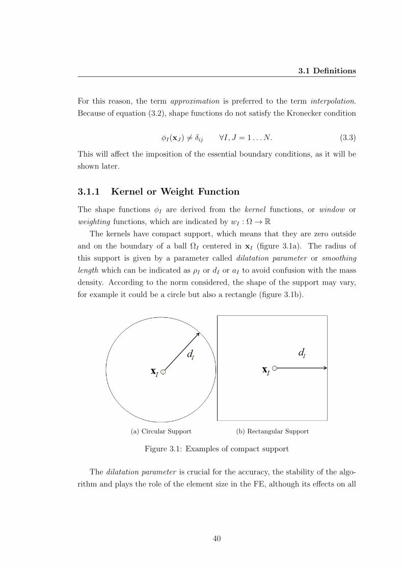
3.1 Definitions
For this reason, the term approximation is preferred to the term interpolation.
Because of equation (3.2), shape functions do not satisfy the Kronecker condition
φI(xJ) 6= δij ∀I, J = 1 . . . N. (3.3)
This will affect the imposition of the essential boundary conditions, as it will be
shown later.
3.1.1 Kernel or Weight Function
The shape functions φI are derived from the kernel functions, or window or
weighting functions, which are indicated by wI : Ω→ RThe kernels have compact support, which means that they are zero outside
and on the boundary of a ball ΩI centered in xI (figure 3.1a). The radius of
this support is given by a parameter called dilatation parameter or smoothing
length which can be indicated as ρI or dI or aI to avoid confusion with the mass
density. According to the norm considered, the shape of the support may vary,
for example it could be a circle but also a rectangle (figure 3.1b).
(a) Circular Support (b) Rectangular Support
Figure 3.1: Examples of compact support
The dilatation parameter is crucial for the accuracy, the stability of the algo-
rithm and plays the role of the element size in the FE, although its effects on all
40

3.1 Definitions
these aspects have not been rigorously demonstrated yet. Moreover, when vari-
able dilatation parameters are used, particular care must be taken in the choice
of these quantities. As a rule of thumb, with a background element mesh, it is
practical to choose
ρI = αmaxeleI (3.4)
where α1 is a scaling factor depending on the degree of the polynomial basis and
leI is the length of the eth edge of the all the elements having xI as a node.
When the nodes are distributed non-uniformly, according to (3.4) a variable
dilatation parameter is assigned to each particle. As a result, a non-uniform
distribution of ρI is obtained. Whenever a significant change in node density
exists, (e.g. to capture stress concentration, or in adaptivity), the distribution of
smoothing lengths over the domain will be therefore non-uniform (high ∇ρ). As
a drawback, the resulting approximation (regardless the differential equation) is
poor, since it is known that MLS approximants Rabczuk & Belytschko (2005) de-
grade in the presence of sudden change in the support size. A remedy is presented
in Rabczuk & Belytschko (2005), it could be, for example, based on averaging
the smoothing lengths. Nonetheless, the role of the dilatation parameters is still
not well understood and it represents an obscure area in MLS and RKPM, which
requires further mathematical work. A deeper look in the field of the approxima-
tion theory will hopefully clarify the role of the smoothing lengths and provide a
more rigorous rule for their choice.
The fact of being compact basically guarantees the sparsity and the bandness
of the stiffness matrix in a Galerkin formulation, which is particularly useful for
the computer algorithms of matrix inversion. The final characteristic of weight
functions is its functional form Fries & Matthies (2004).
Naming
s =‖x− xI‖
a(3.5)
1To avoid singularities of the moment matrix, α should be at least 2 − 2.2 for quadratic
basis in two dimensions, at least 2.4 for cubic polynomials and so on
41
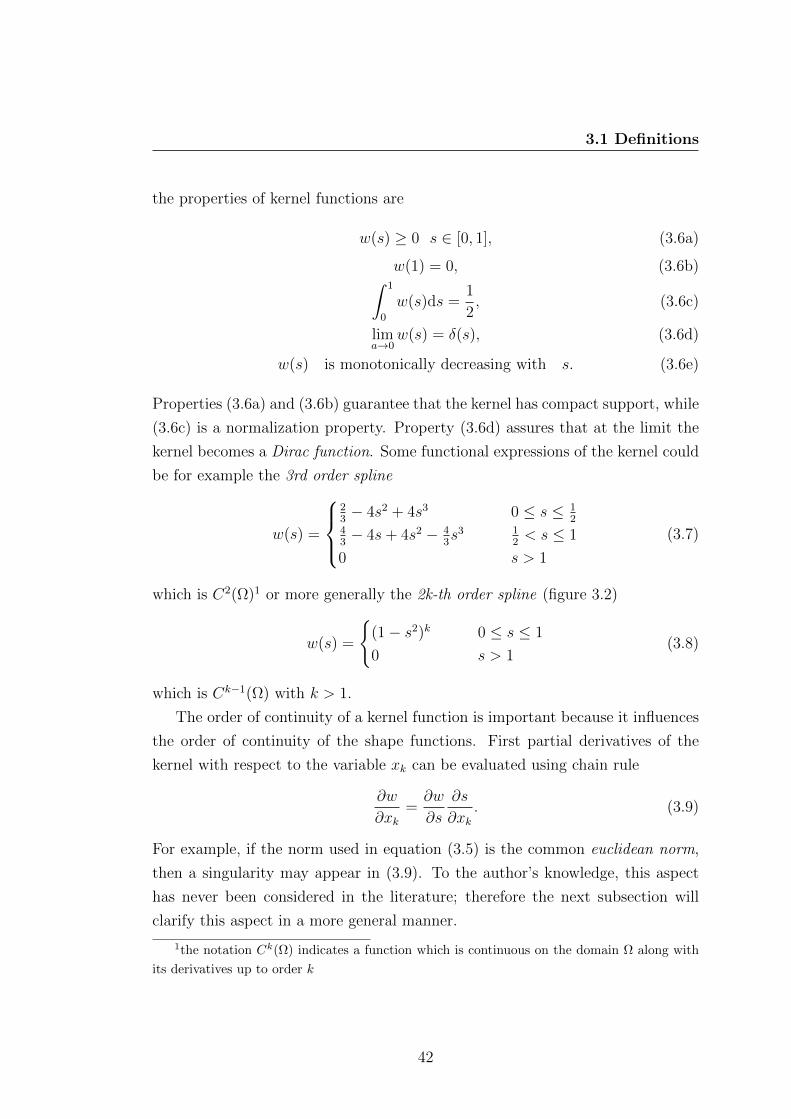
3.1 Definitions
the properties of kernel functions are
w(s) ≥ 0 s ∈ [0, 1], (3.6a)
w(1) = 0, (3.6b)∫ 1
0
w(s)ds =1
2, (3.6c)
lima→0
w(s) = δ(s), (3.6d)
w(s) is monotonically decreasing with s. (3.6e)
Properties (3.6a) and (3.6b) guarantee that the kernel has compact support, while
(3.6c) is a normalization property. Property (3.6d) assures that at the limit the
kernel becomes a Dirac function. Some functional expressions of the kernel could
be for example the 3rd order spline
w(s) =
23− 4s2 + 4s3 0 ≤ s ≤ 1
243− 4s+ 4s2 − 4
3s3 1
2< s ≤ 1
0 s > 1
(3.7)
which is C2(Ω)1 or more generally the 2k-th order spline (figure 3.2)
w(s) =
(1− s2)k 0 ≤ s ≤ 1
0 s > 1(3.8)
which is Ck−1(Ω) with k > 1.
The order of continuity of a kernel function is important because it influences
the order of continuity of the shape functions. First partial derivatives of the
kernel with respect to the variable xk can be evaluated using chain rule
∂w
∂xk=∂w
∂s
∂s
∂xk. (3.9)
For example, if the norm used in equation (3.5) is the common euclidean norm,
then a singularity may appear in (3.9). To the author’s knowledge, this aspect
has never been considered in the literature; therefore the next subsection will
clarify this aspect in a more general manner.
1the notation Ck(Ω) indicates a function which is continuous on the domain Ω along with
its derivatives up to order k
42

3.1 Definitions
Figure 3.2: Window function (3.8) for different values of k
3.1.2 Window function and its derivatives
Let us consider the weight function w and its first and second derivatives in two
dimensions. Defining the following coordinates as in figure 3.3
ξ =x− xIρI
η =y − yIρI
(3.10)
and
s =√ξ2 + η2 = s(ξ, η) (3.11)
then∂s
∂ξ=ξ
s
∂s
∂η=η
s(3.12)
and∂2s
∂ξ2=η2
s3,
∂2s
∂η2=ξ2
s3,
∂2s
∂ξ∂η= −ξη
s3. (3.13)
If the window functions is a spline
w(s) = 1− 6s2 + 8s3 − 3s4 =m∑k=0
aksk (3.14)
thendw
ds= −12s+ 24s2 − 12s3 =
m∑k=1
kaksk−1 (3.15)
andd2w
ds2= −12 + 48s− 36s2 =
m∑k=2
k(k − 1)aksk−2. (3.16)
43
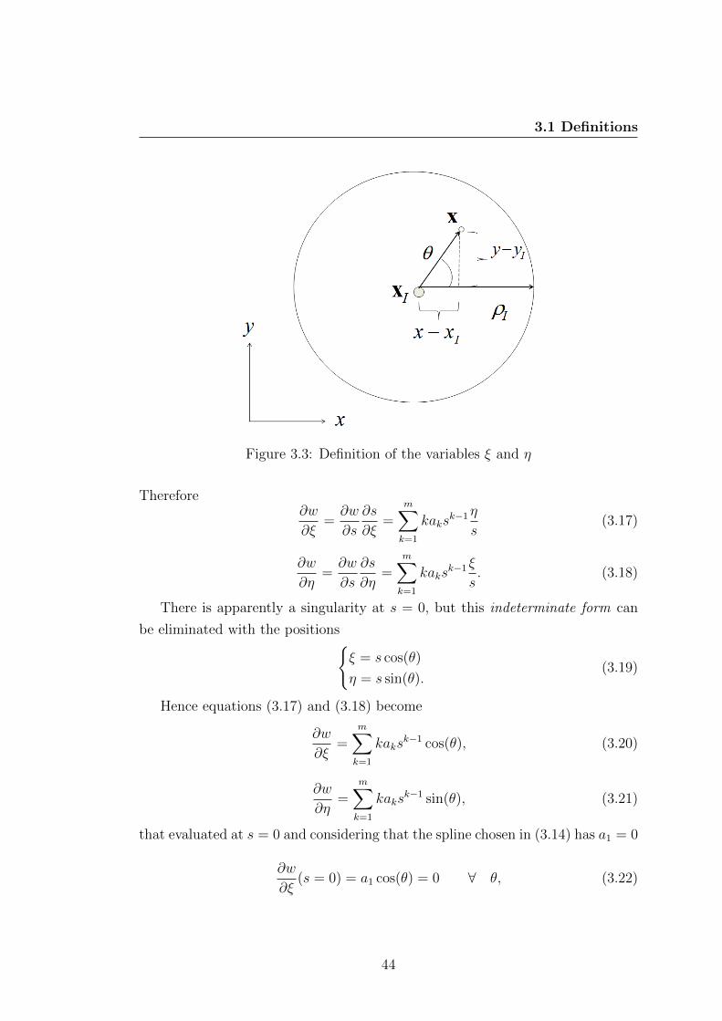
3.1 Definitions
Figure 3.3: Definition of the variables ξ and η
Therefore∂w
∂ξ=∂w
∂s
∂s
∂ξ=
m∑k=1
kaksk−1η
s(3.17)
∂w
∂η=∂w
∂s
∂s
∂η=
m∑k=1
kaksk−1 ξ
s. (3.18)
There is apparently a singularity at s = 0, but this indeterminate form can
be eliminated with the positionsξ = s cos(θ)
η = s sin(θ).(3.19)
Hence equations (3.17) and (3.18) become
∂w
∂ξ=
m∑k=1
kaksk−1 cos(θ), (3.20)
∂w
∂η=
m∑k=1
kaksk−1 sin(θ), (3.21)
that evaluated at s = 0 and considering that the spline chosen in (3.14) has a1 = 0
∂w
∂ξ(s = 0) = a1 cos(θ) = 0 ∀ θ, (3.22)
44

3.1 Definitions
∂w
∂η(s = 0) = a1 sin(θ) = 0 ∀ θ, (3.23)
∂2w
∂ξ2=d2w
ds2
(∂s
∂ξ
)2
+dw
ds
∂2s
∂ξ2=
m∑k=2
k(k − 1)aksk−2 ξ
2
s2+
m∑k=1
kaksk−1η
2
s3, (3.24)
∂2w
∂η2=d2w
ds2
(∂s
∂η
)2
+dw
ds
∂2s
∂η2=
m∑k=2
k(k − 1)aksk−2η
2
s2+
+m∑k=1
kaksk−1 ξ
2
s3, (3.25)
∂2w
∂ξ∂η=d2w
ds2
∂s
∂η
∂s
∂ξ+dw
ds
∂2s
∂ξ∂η=
m∑k=2
k(k − 1)aksk−2 ξη
s2+
−m∑k=1
kaksk−1 ξη
s3. (3.26)
With the same positions (3.19) equations (3.24), (3.25) and (3.25) become
∂2w
∂ξ2=d2w
ds2cos2(θ) +
dw
ds
sin2(θ)
s=
m∑k=2
k(k − 1)aksk−2 cos2(θ)+
+m∑k=1
kaksk−2 sin2(θ), (3.27)
which evaluated at s = 0 is
∂2w
∂ξ2(s = 0) = 2a2 cos2(θ) +
(lims→0
a1
s+ 2a2
)sin2(θ) = 2a2 ∀ θ (3.28)
because a1 = 0.
Analogously
∂2w
∂η2=d2w
ds2sin2(θ) +
dw
ds
cos2(θ)
s=
m∑k=2
k(k − 1)aksk−2 sin2(θ)+
+m∑k=1
kaksk−2 cos2(θ), (3.29)
45

3.1 Definitions
that is
∂2w
∂η2(s = 0) = 2a2 sin2(θ) +
(lims→0
a1
s+ 2a2
)cos2(θ) = 2a2 ∀ θ (3.30)
and
∂2w
∂ξ∂η=d2w
ds2cos(θ) sin(θ)− dw
ds
cos(θ) sin(θ)
s=
=m∑k=2
k(k − 1)aksk−2 cos(θ) sin(θ)−
m∑k=1
kaksk−2 cos(θ) sin(θ) (3.31)
and since a1 = 0
∂2w
∂ξ∂η(s = 0) = 2a2 cos(θ) sin(θ)−
(lims→0
a1
s+ 2a2
)cos(θ) sin(θ) = 0 ∀ θ.
(3.32)
3.1.3 Partition of Unity and Consistency
Shape functions realize a Partition of Unity (PU) if
N∑I=1
φI(x) = 1. (3.33)
More generally they realize a n− th order consistency if
N∑I=1
φI(x)x αI = xα (3.34)
where the multi-index notation is used
α =[α1 α2 . . . αd
], (3.35)
where d = dim(Ω) and∑d
i=1 αi ≤ n
xα = xα11 x
α22 . . . xαdd . (3.36)
Equations (3.35) and (3.36) simply define a complete basis according to the di-
mension of the domain, i.e. 1D, 2D or 3D. Therefore it follows that PU is a
zero− th order consistency. Consistency also means that the shape functions are
able to reproduce exactly all the polynomials of a complete basis in the dimension
d.
46
3.2 Smooth Particle Hydrodynamics (SPH)
3.2 Smooth Particle Hydrodynamics (SPH)
SPH is the forefather of the modern MM Monaghan (1982), Monaghan (1988)
and Monaghan (1992). It simply states that
uh(x) =
∫Ω
w(x− x′)u(x′)dΩ′ (3.37)
it is basically a convolution or a filtering of the function u through the kernel.
When discretized, equation (3.37) becomes
uh(x) =N∑I=1
w(x− xI)∆VIUI , (3.38)
where ∆VI = meas(ΩI) is a measure (i.e. length, area or volume ) of ΩI . There-
fore shape functions are given by
φI(x) = w(x− xI)∆VI . (3.39)
It can be shown Belytschko et al. (1996b) that, choosing a regular arrangement
of nodes, SPH shape functions do not realize a partition of unity, precisely at the
boundaries, therefore they cannot reproduce exactly even the constant function
(figure 3.4).
This is also the reason why these methods are used commonly in unbounded
domains. If the shape functions are normalized with respect to their sum, then
they realize a PU
φ 0I (x) =
φI(x)∑NI=1 φI(x)
. (3.40)
These functions are called Shepard’s functions and the superscript 0 means that
they have 0− th order consistency.
3.3 Reproducing Kernel Method (RKM)
RKM corrects SPH regarding consistency with a corrected kernel
uh(x) =
∫Ω
C(x,x− x′)w(x− x′)u(x′)dΩ′ (3.41)
47
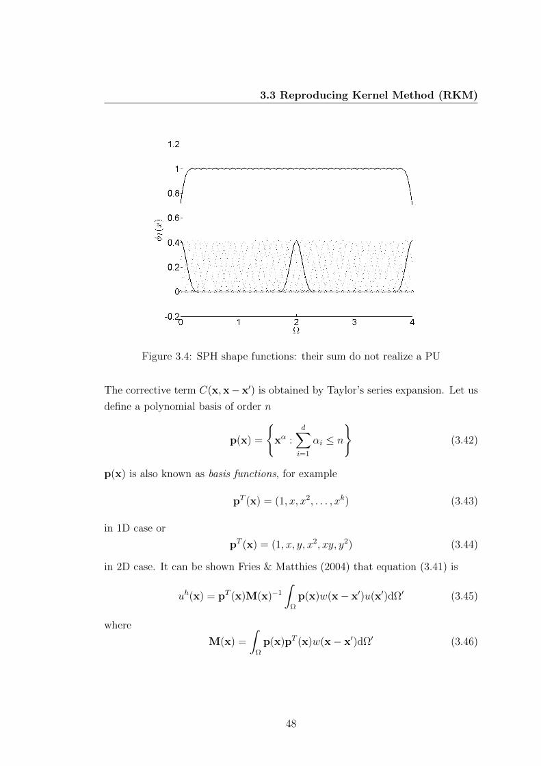
3.3 Reproducing Kernel Method (RKM)
Figure 3.4: SPH shape functions: their sum do not realize a PU
The corrective term C(x,x− x′) is obtained by Taylor’s series expansion. Let us
define a polynomial basis of order n
p(x) =
xα :
d∑i=1
αi ≤ n
(3.42)
p(x) is also known as basis functions, for example
pT (x) = (1, x, x2, . . . , xk) (3.43)
in 1D case or
pT (x) = (1, x, y, x2, xy, y2) (3.44)
in 2D case. It can be shown Fries & Matthies (2004) that equation (3.41) is
uh(x) = pT (x)M(x)−1
∫Ω
p(x)w(x− x′)u(x′)dΩ′ (3.45)
where
M(x) =
∫Ω
p(x)pT (x)w(x− x′)dΩ′ (3.46)
48
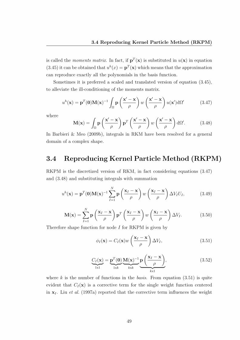
3.4 Reproducing Kernel Particle Method (RKPM)
is called the moments matrix. In fact, if pT (x) is substituted in u(x) in equation
(3.45) it can be obtained that uh(x) = pT (x) which means that the approximation
can reproduce exactly all the polynomials in the basis function.
Sometimes it is preferred a scaled and translated version of equation (3.45),
to alleviate the ill-conditioning of the moments matrix.
uh(x) = pT (0)M(x)−1
∫Ω
p
(x′ − x
ρ
)w
(x′ − x
ρ
)u(x′)dΩ′ (3.47)
where
M(x) =
∫Ω
p
(x′ − x
ρ
)pT(
x′ − x
ρ
)w
(x′ − x
ρ
)dΩ′. (3.48)
In Barbieri & Meo (2009b), integrals in RKM have been resolved for a general
domain of a complex shape.
3.4 Reproducing Kernel Particle Method (RKPM)
RKPM is the discretized version of RKM, in fact considering equations (3.47)
and (3.48) and substituting integrals with summation
uh(x) = pT (0)M(x)−1
N∑I=1
p
(xI − x
ρ
)w
(xI − x
ρ
)∆VIUI , (3.49)
M(x) =N∑I=1
p
(xI − x
ρ
)pT(
xI − x
ρ
)w
(xI − x
ρ
)∆VI . (3.50)
Therefore shape function for node I for RKPM is given by
φI(x) = CI(x)w
(xI − x
ρ
)∆VI , (3.51)
CI(x)︸ ︷︷ ︸1x1
= pT (0)︸ ︷︷ ︸1xk
M(x)−1︸ ︷︷ ︸kxk
p
(xI − x
ρ
)︸ ︷︷ ︸
kx1
, (3.52)
where k is the number of functions in the basis. From equation (3.51) is quite
evident that CI(x) is a corrective term for the single weight function centered
in xI . Liu et al. (1997a) reported that the corrective term influences the weight
49
3.5 Moving Least Squares (MLS)
functions only on a strip of length equal to the dilatation parameter around the
boundary.
Derivatives for the shape functions (3.51) are given by
∂φI∂x
=∂CI(x)
∂xw(x) + CI(x)
∂w(x)
∂x, (3.53)
where∂CI∂x
= pT (0)
[∂M(x)−1
∂xp + M(x)−1∂p
∂x
](3.54)
and∂M(x)−1
∂x= −M−1∂M
∂xM−1. (3.55)
In Belytschko et al. (1996a) it is explained how to speed up the computation of
the derivatives with the means of LU factorization.
In equations (3.49), it is clear as the computational burden of MM shape
functions is still a factor hindering the diffusion of the meshfree technology. In
the next chapter, a solution to this problem is proposed. In fact it is possible
to accelerate remarkably the inversion of the moments matrix and its derivatives
without using any numerical routines (such as Gauss elimination, LU factorization
etc...) and, most importantly, it is possible to avoid such routines at each point
of evaluation. This greatly facilitates the implementation and also the portability
of the codes on different platforms.
3.5 Moving Least Squares (MLS)
MLS is a least squares procedure where the weights are spatial functions that
span all over the domain Ω. As it will be shown later, this procedure leads to
the same equations of RKPM. The surprising fact is that, both MLS and RKPM
can be derived from the same framework even though they have been originated
from different contexts. Indeed, RKPM has its origins in wavelets theory while
MLS has its in the approximation theory Lancaster & Salkauskas (1981). More-
over in Liu et al. (1997b) and Li & Liu (1996) it is derived a continuous version
of MLS, precisely called Moving Least Squares Reproducing Kernel Method ML-
SRKM which is the definitive missing link between the two methods.
50
3.5 Moving Least Squares (MLS)
The approximation in MLS can be written as
uh(x) = pT (x)a(x). (3.56)
Given a set of nodes with coordinates xI at which the field variable UI is known,
a weighted L2 norm can be written
J =N∑I=1
w(x− xI)[pT (x)a(x)− UI
]2. (3.57)
The minimum of J with respect to the coefficients a(x) leads to a set of linear
equations
M(x)a(x) = C(x)U (3.58)
where
M(x) =N∑I=1
w(x− xI)p(xI)pT (xI), (3.59)
C(x) =[w(x− x1)p(x1) w(x− x2)p(x2) . . . w(x− xN)p(xN)
], (3.60)
U =[U1 U2 . . . UN
]T. (3.61)
Solving equation (3.58) and substituting in equation (3.56)
uh(x) =N∑I=1
pT (x)M−1(x)CI(x)UI =N∑I=1
φI(x)UI , (3.62)
where CI(x) is the I − th column of C. Thus the shape functions are
φI(x) = pT (x)M−1(x)p(xI)w(x− xI). (3.63)
As said previously, this version of shape functions could lead to ill-conditioning
of the moments matrix. Therefore a scaled and translated version is commonly
preferred, leading to the same equations of RKPM (3.51), (3.52) when ∆VI = 1.
It has been reported in Fries & Matthies (2004) that choosing ∆VI 6= 1 has no
effect on the evaluation of shape functions, thus it can be concluded that MLS
and RKPM are practically the same.
51

3.6 Discontinuities in Approximations
To reduce the number of computations in MLS or RKPM, derivatives can
be evaluated according to the procedure derived in Belytschko et al. (1996a). In
fact, if the linear system of equations (3.58) is solved by LU factor decomposition,
the matrices L and U can be stored for subsequent evaluation of the derivatives.
Re-writing equation (3.63) in the form
φI(x) = pT (x)M−1(x)p(xI)w(x− xI) = γ(x)p(xI)w(x− xI), (3.64)
the first derivatives are given by
∂φI(x)
∂x=γ(x)
∂xp(xI)w(x− xI) + γ(x)p(xI)
w(x− xI)
∂x. (3.65)
γ is obtained from the following
M(x)γ(x) = pT (x). (3.66)
Derivatives of γ can be obtained differentiating equation (3.66)
M(x)γ(x)
∂x=∂p
∂x− ∂M(x)
∂xγ(x), (3.67)
which can be solved using the same LU decomposition used to solve equation
(3.66) and therefore only back-substitutions are necessary to compute equation
(3.67).
3.6 Discontinuities in Approximations
In fracture mechanics the presence of a crack introduces a discontinuity in the
domain. In FE, elements need to be conforming to the crack line, i.e. no inter-
element cracks are allowed, therefore the crack is usually simulated with a very
small thickness or by duplicating or splitting the nodes located on the edges. As
a consequence, when dealing with propagating cracks, a re-meshing operation is
necessary, often requiring human interaction.
MMs overcome all these limitations, because discontinuities can be constructed
directly from the shape functions. The first method to introduce discontinuity
can be found in Belytschko et al. (1994a) and it is called visibility criterion. In
this method the boundaries of the body and any interior lines of discontinuity are
52
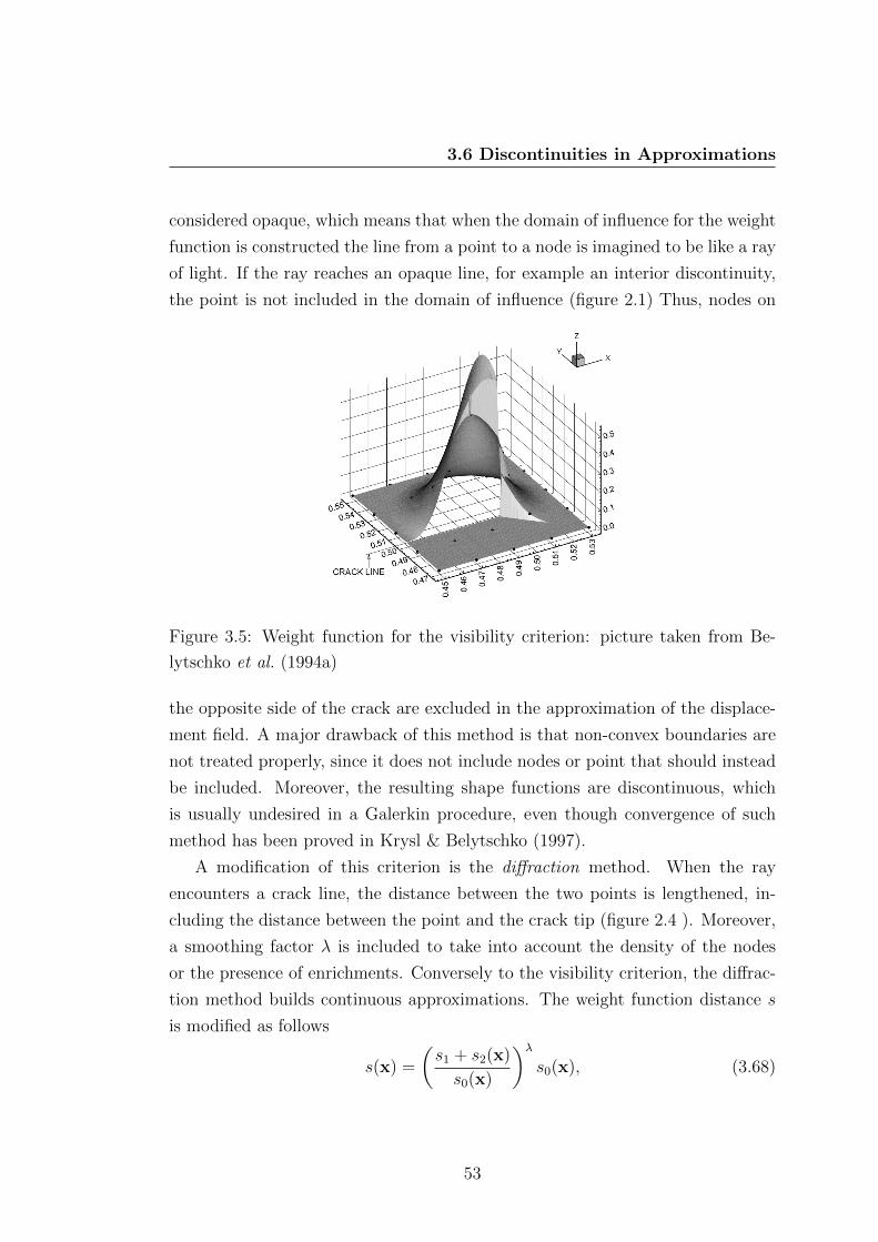
3.6 Discontinuities in Approximations
considered opaque, which means that when the domain of influence for the weight
function is constructed the line from a point to a node is imagined to be like a ray
of light. If the ray reaches an opaque line, for example an interior discontinuity,
the point is not included in the domain of influence (figure 2.1) Thus, nodes on
Figure 3.5: Weight function for the visibility criterion: picture taken from Be-
lytschko et al. (1994a)
the opposite side of the crack are excluded in the approximation of the displace-
ment field. A major drawback of this method is that non-convex boundaries are
not treated properly, since it does not include nodes or point that should instead
be included. Moreover, the resulting shape functions are discontinuous, which
is usually undesired in a Galerkin procedure, even though convergence of such
method has been proved in Krysl & Belytschko (1997).
A modification of this criterion is the diffraction method. When the ray
encounters a crack line, the distance between the two points is lengthened, in-
cluding the distance between the point and the crack tip (figure 2.4 ). Moreover,
a smoothing factor λ is included to take into account the density of the nodes
or the presence of enrichments. Conversely to the visibility criterion, the diffrac-
tion method builds continuous approximations. The weight function distance s
is modified as follows
s(x) =
(s1 + s2(x)
s0(x)
)λs0(x), (3.68)
53

3.6 Discontinuities in Approximations
where s1 = ‖xI − xc‖, s2(x) = ‖x− xc‖ and s0(x) = ‖x− xI‖ where xc is
the crack tip position and λ is a smoothing factor which for problems with a
normal nodal distribution and a linear basis, is chosen as 2. For problems with
enrichments, it could be either 1 or 2.
Figure 3.6: Weight function for the transparency criterion: figure taken from
Belytschko et al. (1996a)
Derivatives of weight function are evaluated accordingly
∂s
∂xi= λ
(s1 + s2(x)
s0(x)
)λ−1∂s2
∂xi+ (1− λ)
(s1 + s2(x)
s0(x)
)λ∂s0
∂xi, (3.69)
where∂s0
∂xi(x) =
xi − xIis0(x)
(3.70)
and∂s2
∂xi(x) =
xi − xcis0(x)
. (3.71)
Another technique for obtaining continuous approximations is the transparency
method (figure 3.6). The transparency is not uniform for the whole length but it
changes so that it is completely transparent at the tip and becomes completely
opaque a short distance from the tip. In this manner, the range of vision for each
node near the crack tip is not suddenly truncated when it reaches the crack tip,
54
3.7 Intrinsic Enrichments
but diminishes smoothly to zero at a short distance from the tip. The length
modifies as follows:
s(x) = s0(x) + ρI
(sc(x)
sc
), (3.72)
where sc(x) is the distance between the crack tip and the intersection point
between the ray and the crack line, ρI is the dilatation parameter for node I and
sc it is a parameter that regulates the transparency transition from the tip to the
point of complete opacity. One drawback of the transparency method is that it
does not work well when nodes are placed too close to the crack surface.
Other methods employed are the see-through method and most recently, the
spiral weight method Muravin & Turkel (2006b) takes into consideration the ad-
vantages and drawbacks of the diffraction method. It is claimed in this method
that the use of this weight function can accurately solve for the stresses even
when using a linear basis with no enrichments.
3.7 Intrinsic Enrichments
Intrinsic enrichment consists simply in adding functions to the basis that resem-
ble the known solution of a particular problem. For example, for linear elastic
fracture mechanics in two dimensions, one can include the asymptotic near-tip
displacement field
pT (x) =[1 x y
√r cos θ
2
√r sin θ
2
√r cos θ
2sin θ
√r sin θ
2sin θ
], (3.73)
where
r =√
(x− xc)2 + (y − yc)2 (3.74)
and
θ = atan2(y − yc, x− xc), (3.75)
where θ ∈ [−π/2, π/2] is the angle from the segment between the point x and the
crack tip xc and the tangent of the crack line (figure 3.8).
55
3.8 Extrinsic Enrichment
It can be proved that these augmented functions can reproduce exactly the
near-tip asymptotic displacement field
u(x) =k1
2µ
√r
2πcos
(θ
2
)[κ− 1 + 2 sin2
(θ
2
)], (3.76a)
v(x) =k1
2µ
√r
2πsin
(θ
2
)[κ− 1 + 2 cos2
(θ
2
)], (3.76b)
where κ is the Kolosov constant
κ =
3− 4ν plane strain(3−ν)1+ν
plane stress, (3.77)
µ is the shear modulus and k1 is the stress intensity factor for mode I.
Even though there are no extra unknowns, for multiple cracks, four additional
terms need to be added to the basis for each crack. This increase the size of
the moments matrix, which means more computational effort and more dense
distribution of nodes, because each support must contain at least a number of
nodes equal to the size of the basis Huerta & Fernandez-Mendez (2000).
There are also ill-conditioning issues when the basis contains non-polynomial
basis Belytschko & Fleming (1999). A method for coupling approximation with
enriched and polynomial basis is proposed in Belytschko & Fleming (1999) where
uh(x) = Ruenr(x) + (1−R)ulin(x), (3.78)
where uenr(x) is the enriched approximation, ulin(x) is the linear basis approxi-
mation and R is a ramp function which is equal to unity on the enriched boundary
of the coupling region and equal to zero on the linear boundary of the coupling
region. The same approach is used in Belytschko et al. (1996b) to couple FE and
MM.
3.8 Extrinsic Enrichment
Extrinsic enrichments are based on the broader concept of Partition of Unity
Duarte & Oden (1996) Melenk & Babuska (1996). There are two different types
of extrinsic enrichment, namely extrinsic global enrichment and extrinsic local
56

3.8 Extrinsic Enrichment
enrichment. The global enrichment consists in adding functions to the approx-
imation that are evaluated on all the Gaussian points of the domain, whereas
an extrinsic local enrichment limits these extra functions only in specific parts of
the domain. It will be shown in the next sections that the second approach is
achieved exploiting the PU property of the shape functions.
3.8.1 Extrinsic Global Enrichment
In the global enrichment the approximation uh(x) for each component of the
displacement is written as
uhi (x) = pT (x)ai(x) +nc∑j=1
αjQji (x) i = 1, . . . , nc, (3.79)
where nc is the number of the cracks, ai(x) coefficients of the polynomial ba-
sis, αj is an unknown associated with the j − th crack and Qji (x) are near-tip
displacement field for mode I
Q1(x) =1
2µ
√r
2πcos
(θ
2
)[κ− 1 + 2 sin2
(θ
2
)], (3.80a)
Q2(x) =1
2µ
√r
2πsin
(θ
2
)[κ− 1 + 2 cos2
(θ
2
)]. (3.80b)
Using MLS procedure, in terms of shape functions, equation (3.79) becomes
uhi (x) =N∑I=1
φI(x)UIi +nc∑j=1
αj
[Qji (x)−
N∑I=1
φI(x)Qji (xI)
], (3.81)
where φI(x) is the shape function defined in equation (3.63). It should be noted
that in this method there are only nc additional unknowns of the problem. This
means that if only 1 crack exists, there is just one more unknown per component
of displacements, which is quite advantageous. Moreover, for crack problems,
in Nguyen et al. (2008) is reported that extrinsic global enrichments for crack
problems are far superior in terms of accuracy on the stress intensity factors with
respect to the local enrichment and can be directly obtained without considering
the J-integral. However, the computational cost is higher since the enrichment
57
3.8 Extrinsic Enrichment
is applied in the entire domain. The extrinsic local enrichment based on the
PU is only slightly less accurate but computationally more efficient, since the
enrichment is applied locally and little modifications to existing codes are needed
to turn a standard meshfree code into an enriched one.
3.8.2 Extrinsic Local Enrichment
The extrinsic local enrichment or extrinsic PU enrichment instead makes use
of the Shepard’s function (3.40). This approach will be later used to simulate
delaminations in composite materials.
For the sake of the clarity, let us start with a simple example.
uh(x) =N∑I=1
φI(x)UI + Ψ(x) (3.82)
where Ψ(x) is a generic enrichment function, for example the near-tip crack en-
richment or a strong discontinuity like the Heaviside function.
It may seem that (3.82) is similar to the global extrinsic equation. Indeed, to
localize the enrichment, one simply has to consider (3.33) and multiply 1 to Ψ(x)
uh(x) =N∑I=1
φI(x)UI + Ψ(x) 1︸︷︷︸∑NeI=1 φ
0I(x)aI
=
=N∑I=1
φI(x)UI + Ψ(x)Ne∑J=1
φ0J(x)aJ =
N∑I=1
φI(x)UI +Ne∑J=1
φ0J(x)Ψ(x)aJ , (3.83)
where the superscript 0 means zero-th order consistency. The number Ne is the
number of enriched nodes and aJ are added unknowns to these nodes. If all the aJ
are equal to 1, then, for the PU, the (3.83) becomes (3.82) and therefore Ψ(x) is
reproduced exactly. The locality of the enrichment stays in the term φ0J(x)Ψ(x).
In fact, the enriched nodes are chosen as the nodes whose support contains the
enrichment. If it is a discontinuity, then the enriched nodes are the ones whose
support is cut by the discontinuity. If Ψ(x) is a near-tip crack enrichment, then
the enriched nodes are the ones whose support contains the crack tip. Since
the φ0J are compact support functions, the enrichment Ψ(x) does not have to be
58
3.8 Extrinsic Enrichment
evaluated to all the x ∈ Ω but only to all the (Gaussian) points x belonging to
the Ne supports of the φ0J .
Duarte & Oden (1996) pointed out that also standard MLS shape functions
(3.63) are PU; therefore in equation (3.82) Shepard’s functions could be replaced
by φnI (x) where the superscript n denotes any shape functions satisfying a PU of
order n.
Apart from the minor computational cost of this formulation, another advan-
tage is the facilitation of hp-adaptivity, since the enhanced functions may vary
from node to node. In fact, for crack problems, it is possible to use the following
enrichment Ventura et al. (2002)
uh(x) =N∑I
φI(x)UI +Nc∑J
φj(x)H(x)aj +
Nb∑k
φk(x)4∑
α=1
Bα(x)bαk, (3.84)
where aj and bαk are added unknowns, H(x) is the Heaviside function, Nc is the
number of nodes whose support is completely cut by the crack, Nb is the number
of nodes whose support contains the crack tip and Bα are the branch functions
(figure 3.7 )
BT =[√
(r) cos(θ2
) √(r) sin
(θ2
) √(r) sin
(θ2
)sin(θ)
√(r) cos
(θ2
)sin(θ)
](3.85)
where
r =√x2 + y2 (3.86)
θ =y√
x2 + y2 + x(3.87)
as shown in figure 3.8.
For completeness, here the derivatives of the branch functions are also reported
∂(r, θ)
∂(x, y)=
x/r y/r
−y/(2r2) x/(2r2)
(3.88)
59

3.8 Extrinsic Enrichment
(a) B1 (b) B2
(c) B3 (d) B4
Figure 3.7: Branch functions
Figure 3.8: Near crack-tip polar coordinates
60

3.8 Extrinsic Enrichment
∂B
∂(r, θ)=
12√r
cos(θ2
)−√r sin
(θ2
)1
2√r
sin(θ2
)−√r cos
(θ2
)1
2√r
sin2(θ2
)cos(θ2
) √r(3 cos2
(θ2
)− 1) (
sin(θ2
))1
2√r
cos2(θ2
)sin(θ2
) √r(3 cos2
(θ2
)− 2) (
cos(θ2
))
. (3.89)
Therefore∂B
∂(x, y)=
∂B
∂(r, θ)
∂(r, θ)
∂(x, y), (3.90)
∂B1
∂x=
1
2cos
(θ
2
)x
r3/2+
1
4sin
(θ
2
)y
r3/2, (3.91)
∂B1
∂y=
1
2cos
(θ
2
)y
r3/2− 1
4sin
(θ
2
)x
r3/2, (3.92)
∂B2
∂x=
1
2sin
(θ
2
)x
r3/2− 1
4cos
(θ
2
)y
r3/2, (3.93)
∂B2
∂y=
1
2sin
(θ
2
)y
r3/2+
1
4cos
(θ
2
)x
r3/2, (3.94)
∂B3
∂x= sin2
(θ
2
)cos
(θ
2
)x
r3/2− 1
2
(3 cos2
(θ
2
)− 1
)sin
(θ
2
)y
r3/2, (3.95)
∂B3
∂y= sin2
(θ
2
)cos
(θ
2
)y
r3/2+
1
2
(3 cos2
(θ
2
)− 1
)sin
(θ
2
)x
r3/2, (3.96)
∂B4
∂x= sin2
(θ
2
)cos
(θ
2
)x
r3/2− 1
2
(3 cos2
(θ
2
)− 1
)sin
(θ
2
)y
r3/2, (3.97)
∂B4
∂y= cos2
(θ
2
)sin
(θ
2
)y
r3/2+
1
2
(3 cos2
(θ
2
)− 2
)cos
(θ
2
)x
r3/2. (3.98)
61
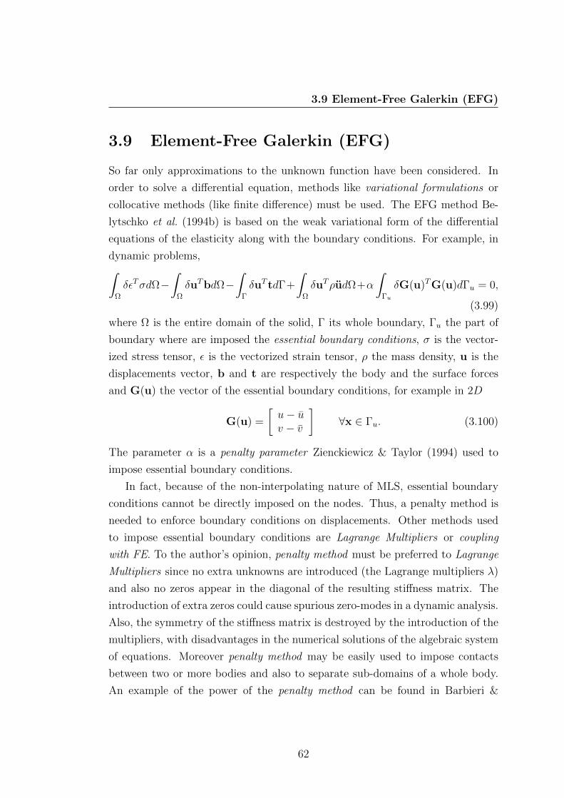
3.9 Element-Free Galerkin (EFG)
3.9 Element-Free Galerkin (EFG)
So far only approximations to the unknown function have been considered. In
order to solve a differential equation, methods like variational formulations or
collocative methods (like finite difference) must be used. The EFG method Be-
lytschko et al. (1994b) is based on the weak variational form of the differential
equations of the elasticity along with the boundary conditions. For example, in
dynamic problems,∫Ω
δεTσdΩ−∫
Ω
δuTbdΩ−∫
Γ
δuT tdΓ+
∫Ω
δuTρudΩ+α
∫Γu
δG(u)TG(u)dΓu = 0,
(3.99)
where Ω is the entire domain of the solid, Γ its whole boundary, Γu the part of
boundary where are imposed the essential boundary conditions, σ is the vector-
ized stress tensor, ε is the vectorized strain tensor, ρ the mass density, u is the
displacements vector, b and t are respectively the body and the surface forces
and G(u) the vector of the essential boundary conditions, for example in 2D
G(u) =
[u− uv − v
]∀x ∈ Γu. (3.100)
The parameter α is a penalty parameter Zienckiewicz & Taylor (1994) used to
impose essential boundary conditions.
In fact, because of the non-interpolating nature of MLS, essential boundary
conditions cannot be directly imposed on the nodes. Thus, a penalty method is
needed to enforce boundary conditions on displacements. Other methods used
to impose essential boundary conditions are Lagrange Multipliers or coupling
with FE. To the author’s opinion, penalty method must be preferred to Lagrange
Multipliers since no extra unknowns are introduced (the Lagrange multipliers λ)
and also no zeros appear in the diagonal of the resulting stiffness matrix. The
introduction of extra zeros could cause spurious zero-modes in a dynamic analysis.
Also, the symmetry of the stiffness matrix is destroyed by the introduction of the
multipliers, with disadvantages in the numerical solutions of the algebraic system
of equations. Moreover penalty method may be easily used to impose contacts
between two or more bodies and also to separate sub-domains of a whole body.
An example of the power of the penalty method can be found in Barbieri &
62
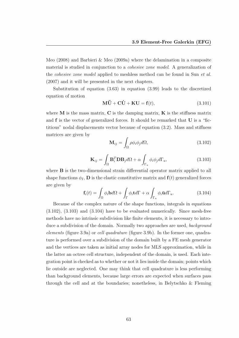
3.9 Element-Free Galerkin (EFG)
Meo (2008) and Barbieri & Meo (2009a) where the delamination in a composite
material is studied in conjunction to a cohesive zone model. A generalization of
the cohesive zone model applied to meshless method can be found in Sun et al.
(2007) and it will be presented in the next chapters.
Substitution of equation (3.63) in equation (3.99) leads to the discretized
equation of motion
MU + CU + KU = f(t), (3.101)
where M is the mass matrix, C is the damping matrix, K is the stiffness matrix
and f is the vector of generalized forces. It should be remarked that U is a “fic-
titious” nodal displacements vector because of equation (3.2). Mass and stiffness
matrices are given by
Mij =
∫Ω
ρφiφjdΩ, (3.102)
Kij =
∫Ω
BTi DBjdΩ + α
∫Γu
φiφjdΓu, (3.103)
where B is the two-dimensional strain differential operator matrix applied to all
shape functions φI , D is the elastic constitutive matrix and f(t) generalized forces
are given by
fi(t) =
∫Ω
φibdΩ +
∫Γ
φitdΓ + α
∫Γu
φiudΓu. (3.104)
Because of the complex nature of the shape functions, integrals in equations
(3.102), (3.103) and (3.104) have to be evaluated numerically. Since mesh-free
methods have no intrinsic subdivision like finite elements, it is necessary to intro-
duce a subdivision of the domain. Normally two approaches are used, background
elements (figure 3.9a) or cell quadrature (figure 3.9b). In the former one, quadra-
ture is performed over a subdivision of the domain built by a FE mesh generator
and the vertices are taken as initial array nodes for MLS approximation, while in
the latter an octree cell structure, independent of the domain, is used. Each inte-
gration point is checked as to whether or not it lies inside the domain; points which
lie outside are neglected. One may think that cell quadrature is less performing
than background elements, because large errors are expected when surfaces pass
through the cell and at the boundaries; nonetheless, in Belytschko & Fleming
63

3.9 Element-Free Galerkin (EFG)
(a) Background elements (b) Cell quadrature
Figure 3.9: Quadrature methods in MM; pictures taken from Belytschko et al.
(1996b)
(1999) it is reported that no significant difference can be found using the two
different types.
In Dolbow & Belytschko (1999) is proposed a bounding box technique which
takes into account the overlapping supports. This technique seems reasonable for
tensor-product kernels (figure 3.10a), where the product of 2 shape functions in
different nodes is different from zero only where the supports overlap each other.
The minimal regions of these overlapping determine the bounding box technique
in figure 3.10b. Therefore such integration method is expected to greatly reduce
the numerical errors due to numerical integration, whenever a tensor product
kernel is used. Moreover, it is usually recommended to use Gaussian integration
over these cells rather than trapezoidal integration, since Gaussian is more accu-
rate than the trapezoidal for the same number of integration points. In Dolbow
& Belytschko (1999) it is also mentioned that more smaller integration cells with
less integration points is a better choice than larger integration cells with higher
order accuracy, because shape functions usually vary quite rapidly over a small
portion of the domain. The use of cells or elements for the numerical integration
might sound incoherent, since MMs are expected not to use any sort of mesh.
This is indeed a quite controversial topic, that led some researchers to distinguish
between truly meshless methods and not truly MM Atluri & Zhu (1998).
In fact, to create truly MM, one needs to construct local weak formulations
64

3.9 Element-Free Galerkin (EFG)
(a) Tensor product kernels (b) Bounding box technique
Figure 3.10: Bounding box integration; pictures taken from Dolbow & Belytschko
(1999)
Atluri & Zhu (1998), while EFG is a global weak formulation.
In response to this paradox, Liu (2003) said:
”One may ask now, why do we not simply use the conventional finite
element method (FEM) with triangular elements, which has been fully
developed? The answer is simply the well-known fact that the FEM
results using triangular elements are very poor. This is due to the poor
quality of the linear shape functions constructed based on three-node
element confined interpolation schemes. In meshfree methods, how-
ever, the interpolation/ approximation is not cell/element confined.
Basically, it can ”freely,” ”automatically,” and ”dynamically” choose
surrounding nodes to construct the shape functions. This freedom
of node selection enabled by meshfree technology is truly powerful.
Based on this argument, the difference between FEM and meshfree
methods is essentially the difference in the interpolation scheme, and
this is also the reason the interpolation technique is the key to the
success of the meshfree methods.”
65
Chapter 4
Improvements to the Method
The major factors hindering the spreading of the meshfree methods are of practi-
cal nature. Indeed, for equation (3.49), it is necessary to invert a matrix M, called
the moment matrix, for each point of interest. If the number of points is large,
then this operation must be repeated several times, raising the computational
cost.
Another issue regards the search for points located within the support radius.
In fact, for equation (3.5), meshfree shape functions are compact support func-
tions, which means that they are zero outside a ball of radius ρI centered in the
I − th node. This means that, in equation (3.49), the summation can be limited
to the nodes that have x in their support. Hence, to evaluate the shape functions,
the following operations must be performed at every point x (figure 4.1) Krysl &
Belytschko (2001) and Fries & Matthies (2004):
• search for neighbors within the set of nodes
• calculate the moment matrix (see equation (3.50))
• invert the moment matrix
• apply the corrective term to the weight function (see equation (3.51))
Also derivatives are usually of interest in Galerkin formulations.
Since these operations are carried out within a loop over the Gaussian points,
and since the Gaussian points are always more than the nodes, it is easy to see
that the overall code is incredibly slowed down.
66

Figure 4.1: Flowchart of the classic algorithm in meshfree methods
67

4.1 kd-Trees for Neighbour Search
In this chapter some remedies to implementation issues in MM will be pre-
sented, while in the next chapter the complete code will be described.
As a general guideline, the double-looping over the nodes and the Gaussian
points should be avoided as much as possible. This is true for every programming
language but it is more evident for Matlab , where significant speeds-up can be
achieved with loop vectorization. Moreover, the Gaussian points are usually are
more numerous than the nodes, therefore instead of looping over the Gaussian
points and looking for the nodes, it is more convenient to focus on nodes and
search for the Gaussian points included in the support.
In the following sections the typewriter character A will be used to indicate
the computer variable, while A will indicate the mathematical entity (vector,
matrix, etc...).
4.1 kd-Trees for Neighbour Search
Meshfree shape functions are compact support functions, as stated in equation
(3.5) and properties (3.6a) and (3.6b).
The purpose of the compactness is to discretize the domain, as in FE, i.e. to
give a local character to the approximation. As a result, stiffness matrix is sparse,
i.e. with most entries equal to zero. The compactness of the shape functions can
be exploited to better store the matrix values and to efficiently evaluate the
integrals in Galerkin formulations. In fact, figure 4.2 shows the sparsity pattern
arising from a typical meshfree discretization over a line segment. If ng is the
number of evaluation points (rows) and ns the number of nodes, the meshfree
shape functions resulting from a discretization can be stored in a ng × ns matrix
PHI.
For example, for a fixed column 1 PHI contains the values of the j − th shape
function on all the points that belong to the support of the j − th node.
PHI(:, j) j = 1, . . . , ns. (4.1)
1it is used the Matlab notation where the colon : in a matrix means variation over that
dimension
68
4.1 kd-Trees for Neighbour Search
Since on the same evaluation point there should be enough nodes for the meshfree
approximation 1, analogously, for a fixed row PHI contains the values of the shape
functions of the nodes that have the i− th evaluation point within their support.
PHI(i, :) i = 1, . . . , ng. (4.2)
The sparsity diagram 4.2 is a representation of the non-zero values of PHI,
where a blue dot corresponds to a non-null entry. Firstly, it can be seen how the
number of evaluation points is usually much larger than the number of nodes.
These evaluation points usually are Gaussian points, if the variational weak form
is used. Secondly, it can be clearly seen that the vast majority of entry is zero
and concentrated on the main diagonal.
This reflects the fact that for each node, only the nearest Gaussian points
are considered. When two supports for two different nodes overlap, then there is
a non-zero entry for the stiffness matrix, otherwise the correspondent entry will
be null. Thus, it seems reasonable not to store the shape functions matrix as
a full matrix, but rather as sparse matrix. The only values stored are then the
row-index, the column-index and the non-zero entry. A full matrix would have
had all the values, even the zero ones, arranged in a table-like manner.
As an example of the amount of memory saved, a factor called density d is
normally calculated for sparse matrix. It is the ratio of the number of non-zero
values nnz and the total number of elements of the matrix, i.e. the product of the
total number of rows r for the total number of columns c. For meshfree shape
functions, this factor could be around 6%, depending of course on the dilatation
parameter.
d =nnzrc. (4.3)
In order to obtain this sparse matrix, it is crucial an algorithm capable of
searching the evaluation points within a certain radius (figure 4.3).
Given a set of ns approximation nodes (variable GRIDSET)
S1 = xJ : J = 1, . . . , ns ⊂ Rk k = 1, 2, 3 (4.4)
1to avoid ill-conditioning of the moment matrix Fries & Matthies (2004) and Nguyen et al.
(2008)
69
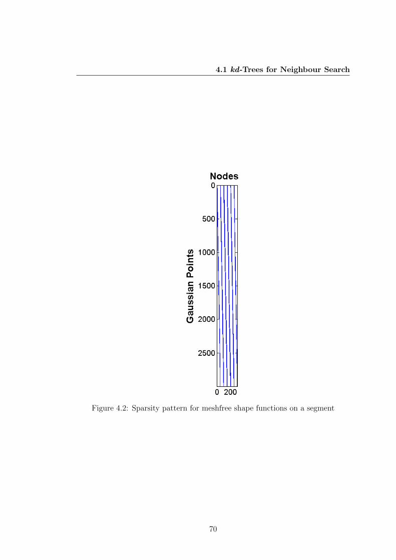
4.1 kd-Trees for Neighbour Search
Figure 4.2: Sparsity pattern for meshfree shape functions on a segment
70

4.1 kd-Trees for Neighbour Search
Figure 4.3: Neighbour Search: red crosses: evaluation points inside the support;
blue crosses: evaluation points outside the support
and a second set of ng evaluation points (variable GGRID1)
S2 = xI : I = 1, . . . , ng ⊂ Rk k = 1, 2, 3 (4.5)
the complete distance matrix S would be a matrix ng × ns where
SIJ =|xI − xJ |
ρJ, (4.6)
where ρJ is the dilatation parameter for the J-th node.
After S matrix is constructed, for equation (3.5) only the values less than or
equal to one must be considered. Let us call nnz the number of elements in S
satisfying
s = I ∈ 1, . . . ng, J ∈ 1, . . . ns : SIJ ≤ 1 (4.7)
then, the output of such procedure would eventually be 3 vectors of length nnz,
ig, js and s such that (figure 4.4)
Sigi,jsi= si i = 1, . . . , nnz. (4.8)
71

4.1 kd-Trees for Neighbour Search
Figure 4.4: Neighbour Search: example of the mapping in equation (4.8)
This is a well-known problem in the field of the computational geometry and
it is called neighbour search or range query.
A naive implementation would loop over the Gaussian points S2, loop again
over the nodes S1, compare the distance with the dilatation parameter and then
decide whether a point belongs to the node or not. This brute force algorithm
is said to have a computational cost O(N2), which means that the number of
operations goes with the square of the number N of the elements. If N is a
large number, then it is easy to understand that the computational cost becomes
prohibitive. Yet, this algorithm for its simplicity is widely used in the meshfree
community as affirmed in Idelsohn & Onate (2006) and reported in several papers
Belytschko et al. (1996b) , Dolbow & Belytschko (1998), Krysl & Belytschko
(2001) and Nguyen et al. (2008).
The brute force algorithm is nonetheless inefficient when the number of nodes
notably grows. It is then especially not recommended for large scale simulations.
The neighbour search is indeed recognized as one of the greatest bottle-neck
for the meshfree technology. For a more efficient code, improvements should be
1in principle different from GRIDSET, but not necessarily
72
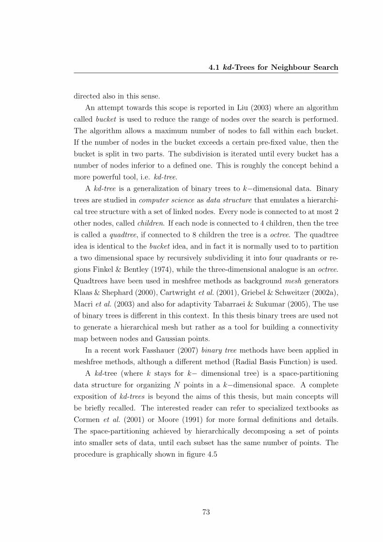
4.1 kd-Trees for Neighbour Search
directed also in this sense.
An attempt towards this scope is reported in Liu (2003) where an algorithm
called bucket is used to reduce the range of nodes over the search is performed.
The algorithm allows a maximum number of nodes to fall within each bucket.
If the number of nodes in the bucket exceeds a certain pre-fixed value, then the
bucket is split in two parts. The subdivision is iterated until every bucket has a
number of nodes inferior to a defined one. This is roughly the concept behind a
more powerful tool, i.e. kd-tree.
A kd-tree is a generalization of binary trees to k−dimensional data. Binary
trees are studied in computer science as data structure that emulates a hierarchi-
cal tree structure with a set of linked nodes. Every node is connected to at most 2
other nodes, called children. If each node is connected to 4 children, then the tree
is called a quadtree, if connected to 8 children the tree is a octree. The quadtree
idea is identical to the bucket idea, and in fact it is normally used to to partition
a two dimensional space by recursively subdividing it into four quadrants or re-
gions Finkel & Bentley (1974), while the three-dimensional analogue is an octree.
Quadtrees have been used in meshfree methods as background mesh generators
Klaas & Shephard (2000), Cartwright et al. (2001), Griebel & Schweitzer (2002a),
Macri et al. (2003) and also for adaptivity Tabarraei & Sukumar (2005), The use
of binary trees is different in this context. In this thesis binary trees are used not
to generate a hierarchical mesh but rather as a tool for building a connectivity
map between nodes and Gaussian points.
In a recent work Fasshauer (2007) binary tree methods have been applied in
meshfree methods, although a different method (Radial Basis Function) is used.
A kd-tree (where k stays for k− dimensional tree) is a space-partitioning
data structure for organizing N points in a k−dimensional space. A complete
exposition of kd-trees is beyond the aims of this thesis, but main concepts will
be briefly recalled. The interested reader can refer to specialized textbooks as
Cormen et al. (2001) or Moore (1991) for more formal definitions and details.
The space-partitioning achieved by hierarchically decomposing a set of points
into smaller sets of data, until each subset has the same number of points. The
procedure is graphically shown in figure 4.5
73
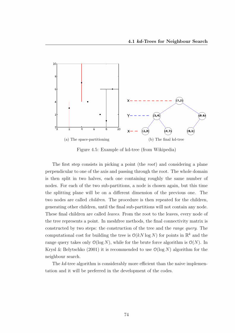
4.1 kd-Trees for Neighbour Search
(a) The space-partitioning (b) The final kd-tree
Figure 4.5: Example of kd-tree (from Wikipedia)
The first step consists in picking a point (the root) and considering a plane
perpendicular to one of the axis and passing through the root. The whole domain
is then split in two halves, each one containing roughly the same number of
nodes. For each of the two sub-partitions, a node is chosen again, but this time
the splitting plane will be on a different dimension of the previous one. The
two nodes are called children. The procedure is then repeated for the children,
generating other children, until the final sub-partitions will not contain any node.
These final children are called leaves. From the root to the leaves, every node of
the tree represents a point. In meshfree methods, the final connectivity matrix is
constructed by two steps: the construction of the tree and the range query. The
computational cost for building the tree is O(kN logN) for points in Rk and the
range query takes only O(logN), while for the brute force algorithm is O(N). In
Krysl & Belytschko (2001) it is recommended to use O(logN) algorithm for the
neighbour search.
The kd-tree algorithm is considerably more efficient than the naive implemen-
tation and it will be preferred in the development of the codes.
74

4.1 kd-Trees for Neighbour Search
4.1.1 Speed-up using a background mesh: a mixed kd-
tree-elements approach
A further speed-up in neighbour search can be achieved whenever a background
element mesh is used for integration purposes. In fact, for this type of integration,
Gaussian points do not need to be searched, since they are located within the
boundaries of each element. Knowing the inverse mapping between elements and
nodes, (i.e. which elements belong to each node), it is necessary to search inside
only one set of points, i.e. S1 (4.4). Since the number of nodes it is usually less
than the number of Gaussian points, this approach notably reduces the computa-
tional time. However, it can only be used in combination with elements. When a
different type of integration is implemented, for example regular background grid,
it is necessary to perform the full kd-tree neighbour search, which is nevertheless
O(logN).
4.1.2 The Matlab kd-tree
Matlab does not have a predefined kd-tree routine, but a free implementation can
be download from the internet at the Matlab Central File Exchange. The one
used in this thesis is by Dr. Guy Shechter and is covered by the BSD License.
4.1.3 Results
Numerical tests have been performed to assess the capabilities of the proposed
approach. The number of nodes of set S1 (4.4) has been fixed, while the number
of Gaussian points (set S2 (4.5) ) was varied.
As it can be seen in figure 4.6, for small data sets, the brute force algorithm
seems to perform better than kd-tree. However, this is simply due to overhead in
kd-tree (the construction of the tree). In fact, when the data set grows, the brute
force algorithm becomes incredibly slow, even using a highly vectorized version,
as in this case. This highly vectorized brute force version needs more storage
memory, since it requires the whole distance matrix. With the increase of the
Gaussian points then, the brute force becomes then prohibitive. In fact for the
75
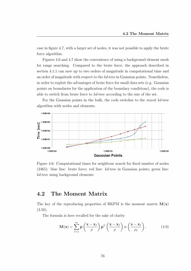
4.2 The Moment Matrix
case in figure 4.7, with a larger set of nodes, it was not possible to apply the brute
force algorithm.
Figures 4.6 and 4.7 show the convenience of using a background element mesh
for range searching. Compared to the brute force, the approach described in
section 4.1.1 can save up to two orders of magnitude in computational time and
an order of magnitude with respect to the kd-tree in Gaussian points. Nonetheless,
in order to exploit the advantages of brute force for small data sets (e.g. Gaussian
points on boundaries for the application of the boundary conditions), the code is
able to switch from brute force to kd-tree according to the size of the set.
For the Gaussian points in the bulk, the code switches to the mixed kd-tree
algorithm with nodes and elements.
Figure 4.6: Computational times for neighbour search for fixed number of nodes
(2465): blue line: brute force; red line: kd-tree in Gaussian points; green line:
kd-tree using background elements
4.2 The Moment Matrix
The key of the reproducing properties of RKPM is the moment matrix M(x)
(3.50).
The formula is here recalled for the sake of clarity
M(x) =ns∑I=1
p
(x− xIρ
)pT(
x− xIρ
)w
(x− xIρI
), (4.9)
76
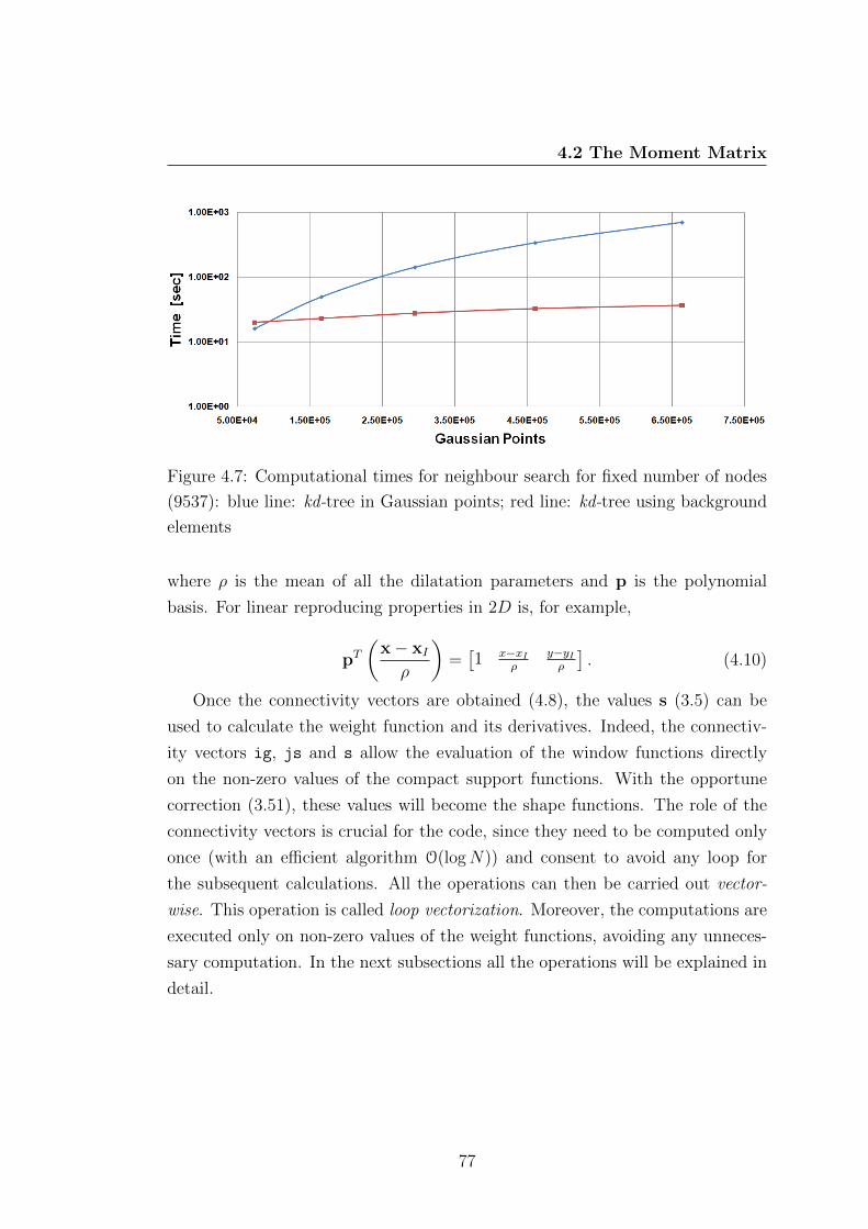
4.2 The Moment Matrix
Figure 4.7: Computational times for neighbour search for fixed number of nodes
(9537): blue line: kd-tree in Gaussian points; red line: kd-tree using background
elements
where ρ is the mean of all the dilatation parameters and p is the polynomial
basis. For linear reproducing properties in 2D is, for example,
pT(
x− xIρ
)=[1 x−xI
ρy−yIρ
]. (4.10)
Once the connectivity vectors are obtained (4.8), the values s (3.5) can be
used to calculate the weight function and its derivatives. Indeed, the connectiv-
ity vectors ig, js and s allow the evaluation of the window functions directly
on the non-zero values of the compact support functions. With the opportune
correction (3.51), these values will become the shape functions. The role of the
connectivity vectors is crucial for the code, since they need to be computed only
once (with an efficient algorithm O(logN)) and consent to avoid any loop for
the subsequent calculations. All the operations can then be carried out vector-
wise. This operation is called loop vectorization. Moreover, the computations are
executed only on non-zero values of the weight functions, avoiding any unneces-
sary computation. In the next subsections all the operations will be explained in
detail.
77

4.2 The Moment Matrix
4.2.1 The window function handle
In Matlab it is possible to define an object called function handle, which allows a
quick evaluation of a function. The function handle is defined using the following
command:
Kernel = @(s) 1− 6s2 + 8s3 − 3s4. (4.11)
In this case @(s) indicate an anonymous variable. Such mute variable can be
replaced with the actual variable s (4.7) and calculate the expression contained
in the object Kernel over all the values contained in s simply by executing the
command
PSI = Kernel(s), (4.12)
where the vector PSI1 contains the non-zero values of the weight functions for all
the nodes and for all the Gaussian points.
Once obtained the values PSI, the following operations are necessary to cal-
culate the entries of the moment matrix:
• the computation of the scaled coordinates ξI = x−xIρ
and ηIy−yIρ
,
• the computation of the polynomial basis (4.10),
• the computation of the sum of the polynomial basis (4.9).
4.2.2 Computation of scaled coordinates
Supposing GRIDSET is the coordinate list of the set S1 and GGRID the coordinate
list of the set S2 and CSI is the computer implementation of ξI ∀I = 1, . . . , ns
and ETA the computer variable for ηI ∀I = 1, . . . , ns , then the computation of ξI
and ηI is done in the following way:
CSI = (GGRID(ig, 1)− GRIDSET(js, 1))./mrho (4.13)
ETA = (GGRID(ig, 2)− GRIDSET(js, 2))./mrho (4.14)
where mrho is ρ the average of the dilatation parameters.
1PSI is used instead of W to avoid confusion with the Gaussian weights
78

4.2 The Moment Matrix
4.2.3 Computation of the polynomial basis
Similarly to the command (4.11), it is possible to define the polynomial basis as
function handle. For a more neat programming style, it is opportune to group
these functions in an array, or cell array.
A cell array is similar to a multidimensional array, but with the interesting
feature that data are allowed to be not necessarily of the same type.
PolyBasis.p1 = @(x,y) 1 (4.15)
PolyBasis.p2 = @(x,y) x (4.16)
PolyBasis.p3 = @(x,y) y (4.17)
PolyBasis.dpdx1 = @(x,y) 0 (4.18)
PolyBasis.dpdx2 = @(x,y) 1 (4.19)
PolyBasis.dpdx3 = @(x,y) 0 (4.20)
PolyBasis.dpdy1 = @(x,y) 0 (4.21)
PolyBasis.dpdy2 = @(x,y) 0 (4.22)
PolyBasis.dpdy3 = @(x,y) 1 (4.23)
Let us define a function handle of the type
P handle = @(P) P(CSI,ETA) (4.24)
where CSI is (4.13) and ETA is (4.14). In this way, by simply calling
P = cellfun(P handle,PolyBasis.p(1:3)).’ (4.25)
the values of the polynomial basis are readily calculated. Moreover, with the call
DPDX = cellfun(P handle,PolyBasis.dpdx(1:3)).’ (4.26)
79
4.2 The Moment Matrix
DPDY = cellfun(P handle,PolyBasis.dpdy(1:3)).’ (4.27)
the derivatives of the polynomial basis can also be automatically calculated, with-
out the need of defining dedicated function handles for the derivatives.
4.2.4 Computation of the sum of the polynomials
According to equation (4.9), in order to obtain the entries of the moment matrix,
the sum of the polynomials (4.25) must be performed over the nodes. After (4.25),
P is a 3 × 1 cell array. Every element of the cell contains nnz values, the same
number as the variables ig, js and s.
The sum is carried out in three steps:
1. the product
pi
(x− xIρI
)pj
(x− xIρI
)w
(x− xIρI
)i, j = 1, . . . , np, (4.28)
where np is the number of the polynomials included in the basis;
2. reshape of the matrix product (4.28);
3. sum over the columns (the second dimension) of the reshaped matrix.
The matrix product (4.28) originates n2p vectors of size nnz × 1. However,
since the moments matrix is symmetric, not all the products need to be stored,
but only np(np + 1)/2. Therefore in equation (4.28) the products to calculate are
only the ones i, j = 1, . . . , np with i ≤ j.
These indexes i, j for a symmetric matrix np×np can be grouped in two arrays
of length np(np + 1)/2. For example, if np = 3
i =[1 1 1 2 2 3
](4.29)
j =[1 2 3 2 3 3
](4.30)
Indexes in (4.29) and (4.30) allow the definition of a function handle for the
products in equation (4.28)
M handle=@(i,j) Pi.*Pj.*PSI (4.31)
80
4.2 The Moment Matrix
In fact, vectors Pi and PSI are the same size and thus can be multiplied in an
element-wise manner. The call
M = arrayfun(M handle,i,j) (4.32)
originates a cell array of size np(np + 1)/2, where each element contains the
product (4.28).
The next step is to reshape each element of the cell array M from a nnz vec-
tor to a matrix ng × ns. Luckily, the command sparse in Matlab allows this
transformation without filling with zeros, but keeping the indexes ig, js.
The command
S = sparse(i,j,s,m,n) (4.33)
uses vectors i, j, and s to generate an m× n sparse matrix such that
S(i(k), j(k)) = s(k) k = 1, . . . , nnz (4.34)
if vectors i, j, and s are all the same length.
Additionally, any elements of s that are zero are ignored, along with the
corresponding values of i and j. Any elements of s that have duplicate values of
i and j are added together.
Therefore, the following command can be defined
spar handle = @(C) sum(sparse(ig,js,C,ng,ns),2) (4.35)
where ng is ng and ns is ns.
Command (4.35) incorporates 2 commands, the first one is sparse, which
reshape the anonymous matrix C and the second one is the sum over the nodes,
where 2 stays for the second dimension of the matrix, i.e. the columns. It can
be seen that with the introduction of the connectivity vectors ig and js, it is
no longer necessary to search for nodes at each Gaussian point for the purpose
of the sum in the moment matrix. These operations can be indeed automatized
once the connectivity has been defined at the beginning of the calculation.
By calling
M = cellfun(spar handle,M) (4.36)
81

4.2 The Moment Matrix
the moment matrix M is finally calculated. The result of (4.36) is a cell
array of np(np + 1)/2 elements, each array containing ng elements, i.e. as many
as the number of the Gaussian points. By inverting M, it is possible to get the
corrective terms for the kernels (the weight functions) that restore the reproducing
properties.
4.2.5 Derivatives of the moment matrix
For completeness are here reported the commands necessary to calculate the
derivatives of the moment matrix. Firstly, it is necessary to calculate the deriva-
tives of the kernel, as in equation (3.9).
∂w
∂x=∂w
∂s
∂s
∂ξI
∂ξI∂x
=∂w
∂s
∂s
∂ξI
1
ρI(4.37)
∂w
∂y=∂w
∂s
∂s
∂ηI
∂ξI∂x
=∂w
∂s
∂s
∂ηI
1
ρI(4.38)
The first step is calculating∂w
∂sby defining the following function handle
dKernel = @(s) − 12s(s− 1)2 (4.39)
and then executing the command
dPSI = dKernel(S). (4.40)
The derivatives∂s
∂ξIand
∂s
∂ηIare calculated as follows
dDcsi= ((GGRID(ig,1)-GRIDSET(js,1))./rho(js))./S (4.41)
dDcsi(S==0) = 1 (4.42)
dDeta= ((GGRID(ig,2)-GRIDSET(js,2))./rho(js))./S (4.43)
dDeta(S==0) = 1 (4.44)
82
4.2 The Moment Matrix
where equations (4.42) and (4.44) eliminate the indeterminate form as described
in section (3.1.2). Derivatives of the kernel functions are
dPSIcsi = dPSI.*dDcsi (4.45)
dPSIeta = dPSI.*dDeta (4.46)
The handles for the derivatives of the moment matrix are
DMx handle = @(i,j) (DPDXi.*Pj + Pi.*DPDXj).*PSI
+ Pi.*Pj.*dPSIcsi
(4.47)
DMy handle = @(i,j) (DPDYi.*Pj + Pi.*DPDYj).*PSI
+ Pi.*Pj.*dPSIeta (4.48)
and the operations of product, reshape and sum are executed by calling these
commands
DMx = arrayfun(DMx handle,i,j) (4.49)
DMx = cellfun(spar handle,DMx) (4.50)
DMy = arrayfun(DMy handle,i,j) (4.51)
DMy = cellfun(spar handle,DMy) (4.52)
4.2.6 Explicit Inverse of the Moments Matrix
In section 4.2 the construction if the moment matrix for linear reproducing prop-
erty was illustrated.
If a linear reproducing property is desired, the moments matrix can be inverted
directly by symbolic manipulation, as in Breitkopf et al. (2000) and Zhou et al.
(2005) . This can still be done in 3D, when the moment matrix is size 4× 4.
However, if higher order reproducing properties are sought, this approach
cannot be used, since the symbolic inversion of a matrix of size larger than 5× 5
is unstable or even impossible to achieve practically. In section 4.3.1 an alternative
approach is proposed. It will be shown that the explicit inverse of the moments
83

4.3 Inversion of the Moment Matrix through Partitioning
matrix for linear reproducing property is indeed the starting point to calculate
the inverse of the moment matrix with higher reproducing capabilities.
The inversion of the moment matrix for linear reproducing properties can be
done following the Cramer’s rule
det(M) = (M2,2M3,3 −M22,3)M1,1 −M2
1,3M2,2 −M21,2M3,3+
+ 2M1,2M1,3M2,3 (4.53)
M−11,1 =
M2,2M3,3 −M22,3
det(M)(4.54)
M−11,2 = −M1,2M3,3 −M1,3M2,3
det(M)(4.55)
M−11,3 =
M1,2M2,3 −M1,3M2,2
det(M)(4.56)
M−12,2 =
M1,1M3,3 −M21,3
det(M)(4.57)
M−12,3 = −M1,1M2,3 −M1,2M1,3
det(M)(4.58)
M−13,3 =
M1,1M2,2 −M21,2
det(M)(4.59)
Derivatives of the inverse of the moments matrix can be calculated with equa-
tion (3.55).
4.3 Inversion of the Moment Matrix through
Partitioning
In the previous section, explicit inversion formulas for the moments matrix were
illustrated, for the case of linear reproducibility. This section is focused on the
following two questions:
1. how to calculate the shape functions if a higher order reproducibility is
sought?
2. how to calculate the shape functions if other points are inserted?
84

4.3 Inversion of the Moment Matrix through Partitioning
The first question is usually known as h-adaptivity, whilst the second is known
p-adaptivity. Together, they are known as hp-adaptivity. The hp-adaptivity con-
sists in a global/local refinement of the approximation through raising the order
of the polynomials in the approximating function and/or adding nodes to the
discretization, with the aim of reducing the local error or capturing high gradient
zones. Local h-refinement consists in adding nodes to limited zones of the domain,
usually detected when a measure of the error exceeds a predefined threshold, while
global h-refinement means refining the discretization in the whole domain. Lo-
cal p-refinement is done by enriching the approximation with the introduction of
extra-unknowns, as explained in section 3.8.2 and they not need to be necessarily
polynomials. Global p-refinement is instead obtained in meshfree methods by
adding extra-functions to the polynomial basis in equation (3.42). This section
will deal on global p-refinement, while enrichments will be treated in the next
chapters to simulate delamination.
With the aim of reducing the error, the error must be calculated. Of course,
if the error was known a priori, there would be no need of solving the equation
in the first place; therefore what it is usually done is estimating the error a
posteriori. Detailed informations on adaptivity in meshless methods can be found
in Liu & Tu (2002a) and Rabczuk & Belytschko (2005). Once these zones are
individuated, then nodes or polynomials must be practically inserted into the
approximation. In meshfree methods, this task is simpler than FE, as stated
in section 1.1. This section explains how practically insert extra polynomials or
nodes to the shape functions without carrying out expensive operations. Practical
computer implementations can be found in section 5.2.3. It will be shown that
the classic algorithm in figure 4.1 will be modified into the one in figure 4.8
4.3.1 Fast Inversion of the Moment Matrix and p-adaptivity
In this section is proposed a method to answer to the first of the questions in
4.3, i.e. to efficiently invert the moment matrix whenever the order of repro-
ducibility is greater than one. As a result, it can be proficiently used for global
p-adaptivity. A similar approach based on the imposing consistency constraints
can be found in Breitkopf et al. (2000). The reproducing properties are imposed
85

4.3 Inversion of the Moment Matrix through Partitioning
Figure 4.8: Flowchart of the proposed algorithm in meshfree methods
86
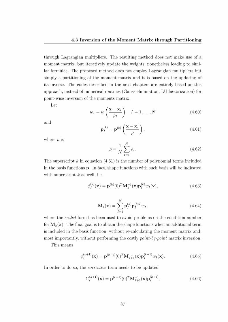
4.3 Inversion of the Moment Matrix through Partitioning
through Lagrangian multipliers. The resulting method does not make use of a
moment matrix, but iteratively update the weights, nonetheless leading to simi-
lar formulas. The proposed method does not employ Lagrangian multipliers but
simply a partitioning of the moment matrix and it is based on the updating of
its inverse. The codes described in the next chapters are entirely based on this
approach, instead of numerical routines (Gauss elimination, LU factorization) for
point-wise inversion of the moments matrix.
Let
wI = w
(x− xIρI
)I = 1, . . . , N (4.60)
and
p(k)I = p(k)
(x− xIρ
), (4.61)
where ρ is
ρ =1
N
N∑I=1
ρI . (4.62)
The superscript k in equation (4.61) is the number of polynomial terms included
in the basis functions p. In fact, shape functions with such basis will be indicated
with superscript k as well, i.e.
φ(k)I (x) = p(k)(0)TM−1
k (x)p(k)I wI(x), (4.63)
Mk(x) =N∑I=1
p(k)I p
(k)TI wI , (4.64)
where the scaled form has been used to avoid problems on the condition number
for Mk(x). The final goal is to obtain the shape functions when an additional term
is included in the basis function, without re-calculating the moment matrix and,
most importantly, without performing the costly point-by-point matrix inversion.
This means
φ(k+1)I (x) = p(k+1)(0)TM−1
k+1(x)p(k+1)I wI(x). (4.65)
In order to do so, the corrective term needs to be updated
C(k+1)I (x) = p(k+1)(0)TM−1
k+1(x)p(k+1)I , (4.66)
87
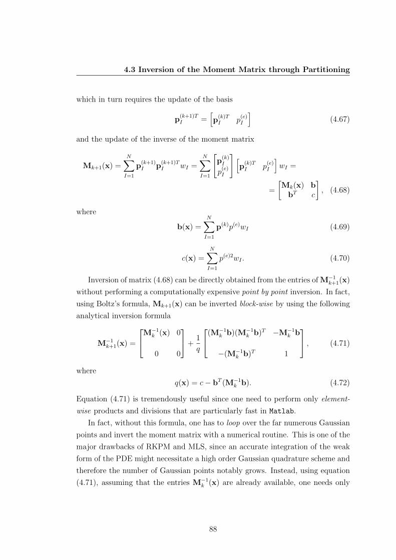
4.3 Inversion of the Moment Matrix through Partitioning
which in turn requires the update of the basis
p(k+1)TI =
[p
(k)TI p
(e)I
](4.67)
and the update of the inverse of the moment matrix
Mk+1(x) =N∑I=1
p(k+1)I p
(k+1)TI wI =
N∑I=1
[p
(k)I
p(e)I
] [p
(k)TI p
(e)I
]wI =
=
[Mk(x) b
bT c
], (4.68)
where
b(x) =N∑I=1
p(k)p(e)wI (4.69)
c(x) =N∑I=1
p(e)2wI . (4.70)
Inversion of matrix (4.68) can be directly obtained from the entries of M−1k+1(x)
without performing a computationally expensive point by point inversion. In fact,
using Boltz’s formula, Mk+1(x) can be inverted block-wise by using the following
analytical inversion formula
M−1k+1(x) =
M−1k (x) 0
0 0
+1
q
(M−1k b)(M−1
k b)T −M−1k b
−(M−1k b)T 1
, (4.71)
where
q(x) = c− bT (M−1k b). (4.72)
Equation (4.71) is tremendously useful since one need to perform only element-
wise products and divisions that are particularly fast in Matlab.
In fact, without this formula, one has to loop over the far numerous Gaussian
points and invert the moment matrix with a numerical routine. This is one of the
major drawbacks of RKPM and MLS, since an accurate integration of the weak
form of the PDE might necessitate a high order Gaussian quadrature scheme and
therefore the number of Gaussian points notably grows. Instead, using equation
(4.71), assuming that the entries M−1k (x) are already available, one needs only
88
4.3 Inversion of the Moment Matrix through Partitioning
to calculate the moments b and c and perform only element-wise operations to
update the moment matrix.
Boltz’ formula allows to vectorize the Matlab code and effectively speeds up
the calculation of the shape functions.
It must be pointed out though, that equation (4.71) shows how to update the
inverse of a matrix when an additional column (and a row) is introduced when
M−1k (x) is already known. Therefore to fully exploit the advantages of the block-
inversion, the entries of M−1k (x) must be obtained beforehand. Nevertheless, one
of the greatest advantage of equation (4.71) is that can be applied iteratively, in
the sense that can be applied several times until the desired order of reproduction
is achieved.
For example, a linear reproduction property is at least required for the con-
vergence of the weak form. Therefore shape functions at least must satisfy linear
reproduction conditions, which lead to a 3× 3 moment matrix in two dimensions
and a 4× 4 moment matrix in three-dimensions. These sizes of matrices are eas-
ily invertible analytically, for example with Cramer’s rule for the two-dimensional
case and with symbolic inversion for 4× 4, that again do not require any numer-
ical routine for matrix inversion and can be obtained with element-wise matrix
operations.
It must be remarked that symbolic inversion is unstable (and sometimes im-
possible for some symbolic softwares) for 5× 5 and impossible to obtain for ma-
trices of higher size. Nonetheless linear reproduction property can be the starting
point of the inversion of a bigger size matrix. In fact once M−13 (x) is calculated
for the two-dimensional case, with (4.71) it is possible to obtain M−14 (x). Once
obtained M−14 (x) one proceeds to M−1
5 (x) and so on until the sought order of
reproduction is achieved.
4.3.1.1 First Order Derivatives
In the assembly of the stiffness matrix of a weak form, at least first order deriva-
tives of the shape functions are required, hence a fast computation of the first
89
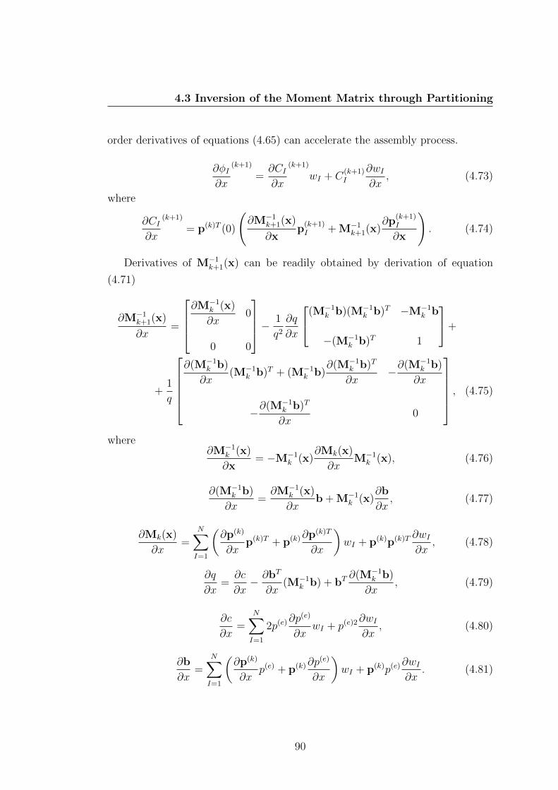
4.3 Inversion of the Moment Matrix through Partitioning
order derivatives of equations (4.65) can accelerate the assembly process.
∂φI∂x
(k+1)
=∂CI∂x
(k+1)
wI + C(k+1)I
∂wI∂x
, (4.73)
where
∂CI∂x
(k+1)
= p(k)T (0)
(∂M−1
k+1(x)
∂xp
(k+1)I + M−1
k+1(x)∂p
(k+1)I
∂x
). (4.74)
Derivatives of M−1k+1(x) can be readily obtained by derivation of equation
(4.71)
∂M−1k+1(x)
∂x=
∂M−1
k (x)
∂x0
0 0
− 1
q2
∂q
∂x
(M−1k b)(M−1
k b)T −M−1k b
−(M−1k b)T 1
+
+1
q
∂(M−1
k b)
∂x(M−1
k b)T + (M−1k b)
∂(M−1k b)T
∂x−∂(M−1
k b)
∂x
−∂(M−1k b)T
∂x0
, (4.75)
where∂M−1
k (x)
∂x= −M−1
k (x)∂Mk(x)
∂xM−1
k (x), (4.76)
∂(M−1k b)
∂x=∂M−1
k (x)
∂xb + M−1
k (x)∂b
∂x, (4.77)
∂Mk(x)
∂x=
N∑I=1
(∂p(k)
∂xp(k)T + p(k)∂p(k)T
∂x
)wI + p(k)p(k)T ∂wI
∂x, (4.78)
∂q
∂x=∂c
∂x− ∂bT
∂x(M−1
k b) + bT∂(M−1
k b)
∂x, (4.79)
∂c
∂x=
N∑I=1
2p(e)∂p(e)
∂xwI + p(e)2∂wI
∂x, (4.80)
∂b
∂x=
N∑I=1
(∂p(k)
∂xp(e) + p(k)∂p
(e)
∂x
)wI + p(k)p(e)∂wI
∂x. (4.81)
90

4.3 Inversion of the Moment Matrix through Partitioning
4.3.2 Fast Inversion of the Moment Matrix and h-adaptivity
In this section is proposed a method to answer to the second of the questions in
4.3.
Let us indicate with subscript N the moment matrix with N nodes
MN(x) =N∑I=1
pIpTI wI . (4.82)
If an additional node is introduced, the moment matrix inverse needs to be up-
dated.
MN+1(x) =N+1∑I=1
pIpTI wI =
N∑I=1
pIpTI wI + pN+1p
TN+1wN+1 = MN(x)+
+ pN+1pTN+1wN+1. (4.83)
Therefore it is simply a rank-1 update:
M−1N+1(x) = M−1
N (x)− (M−1N pN+1)(M−1
N pN+1)T
rwN+1, (4.84)
r = 1 + pTN+1(M−1N pN+1)wN+1, (4.85)
therefore
φI(x) = pT (0)M−1N+1(x)pIwI(x) I = 1, . . . , N + 1. (4.86)
Derivatives are given by
∂φI∂x
= pT (0)
[(∂M−1
N+1(x)
∂xpI + M−1
N+1(x)∂pI∂x
)wI(x)+
+M−1N+1(x)pI
∂wI∂x
], (4.87)
∂M−1N+1(x)
∂x=∂M−1
N (x)
∂x− 1
r2
[(∂(M−1
N pN+1)
∂x(M−1
N pN+1)T+
+(M−1N pN+1)
∂(M−1N pN+1)T
∂x
)r − (M−1
N pN+1)(M−1N pN+1)T
∂r
∂x
]wN+1−
+(M−1
N pN+1)(M−1N pN+1)T
r
∂wN+1
∂x, (4.88)
91

4.4 The Kernel Corrective Term
where∂(M−1
N pN+1)
∂x=∂M−1
N (x)
∂xpN+1 + M−1
N (x)∂pN+1
∂x, (4.89)
∂r
∂x=
[∂pTN+1
∂x(M−1
N pN+1) + pTN+1
∂(M−1N pN+1)
∂x
]wN+1+
+ pTN+1(M−1N pN+1)
∂wN+1
∂x. (4.90)
Finally, it should be remarked that the approach in formula (4.83) was firstly
noted in You et al. (2003), without explicitly suggesting the update of the inverse
of the moment matrix.
4.4 The Kernel Corrective Term
The term in equation (3.52) (here recalled for clarity) is called corrective be-
cause it allows to calculate the shape functions (4.91) from the kernel functions,
restoring the reproducing properties.
φI(x) = CI(x)w
(xI − x
ρ
), (4.91)
CI(x) = pT (0)M(x)−1pT(
xI − x
ρ
). (4.92)
The values of the weight functions are computed through the commands (4.12)
and stored in an array PSI of length nnz and so do the values of P, stored in a cell
array. The problem is the entries of the inverse of the moment matrix M−1, that
are stored in a cell array Minv and every element of the cell is an array of length
ng. Therefore, a naive approach would loop over the basis function, then double
loop over the nodes and over the evaluation points, calculating the correction
and then applying it to the weight functions. Instead, the corrective term can be
quickly calculated using the connectivity vector ig.
The code is the following:
C = 0;
if nargout>2
92

4.4 The Kernel Corrective Term
dCx = 0;
dCy = 0;
end
for i=1:np
for j=1:np
if P0i~=0
if i<=j
C = C + P0i.*Minvi,j(ig).*Pj;
if nargout>2
dCx = dCx + P0i.*DMinvxi,j(ig).*Pj +...
+ P0i.*Minvi,j(ig).*DPDXj;
dCy = dCy + P0i.*DMinvyi,j(ig).*Pj +...
P0i.*Minvi,j(ig).*DPDYj;
end
else
C = C + P0i.*Minvj,i(ig).*Pj;
if nargout>2
dCx = dCx + P0i.*DMinvxj,i(ig).*Pj +...
+ P0i.*Minvi,j(ig).*DPDXj;
dCy = dCy + P0i.*DMinvyj,i(ig).*Pj +...
+ P0i.*Minvj,i(ig).*DPDYj;
end
end
end
end
end
where ig act as a index in the command Minvi,j(ig). The variable nargout
is the number of output arguments. If more than two arguments are requested,
derivatives are calculated.
This index ig points to Minvi,j(:), in the same order PSI and P are stored,
allowing the generic entry of the moment matrix to become an array of length
nnz and multiply PSI and P in an element-wise manner. The same approach can
93
4.5 Assembly of the Stiffness Matrix
be applied also to the derivatives of the corrective term, i.e. dCx and dCy. Using
the same logic, the following handle can be defined
asb handle = @(f,g) f.*g(ig) (4.93)
that will be useful for the stiffness matrix assembly in the next section. Finally,
the shape functions are calculated as follows
PHI = C.*PSI;
if nargout>2
DPHIx = (dCx.*PSI + C.*dPSIcsi)/mrho;
DPHIy = (dCy.*PSI + C.*dPSIeta)/mrho;
end
At this stage, though, the values are stored in arrays of size nnz. To reshape the
arrays, the following handle can be defined
sp handle = @(f) sparse(ig,js,f,ng,ns). (4.94)
The object (4.94) transforms a sparse array f defined by indexes ig and js
into a sparse matrix ng× ns.
The inverse operation can be performed by the following command
desp handle = @(f) f(sub2ind(size(f),ig,js)). (4.95)
The final step for constructing the shape functions is
PHI = sp_handle(PHI);
if nargout>2
DPHIx = sp_handle(DPHIx);
DPHIy = sp_handle(DPHIy);
end
4.5 Assembly of the Stiffness Matrix
In this section the assembly of the stiffness matrix in equation (3.103) is explained
in detail for the two and three dimensional cases.
94
4.5 Assembly of the Stiffness Matrix
The infinitesimal strain is defined as
ε =
εxεyγxy
=
∂u
∂x
∂v
∂y
∂u
∂y+∂v
∂x
=
∂
∂x
∂
∂y
∂
∂y
∂
∂x
[uv
]= Lu, (4.96)
where L is the infinitesimal strain differential operator and u is the displacement
vector.
The linear elastic stress-strain relationship is defined through the Generalized
Hooke’s law (with the Voigt notation1)
σ = Cε =
C11 C12
C12 C22
C33
εxεy
2γxy
, (4.97)
where C is called the stiffness tensor and for two-dimensional orthotropic mate-
rials in plane stress tensional state is defined as
C =
C11 C12
C12 C22
C33
=
E11/(1− ν12ν21) ν12E22/((1− ν12ν21)
ν12E22/((1− ν12ν21) E22/(1− ν12ν21)
G12
,(4.98)
where Eii is the Young’s modulus along axis i, Gij is the shear modulus in di-
rection j on the plane whose normal is in direction i, νij is the Poisson’s ratio
that corresponds to a contraction in direction j when an extension is applied in
direction i.
If plane strain is desired, then the following changes are necessary
1The Voigt notation is the standard mapping for tensor indexes
95
4.5 Assembly of the Stiffness Matrix
E11 ←E11
1− ν212
, (4.99)
E22 ←E22
1− ν212
, (4.100)
G12 ←G12
1− ν212
, (4.101)
ν12 ←ν12
1− ν212
, (4.102)
ν21 ←ν21
1− ν212
. (4.103)
(4.104)
The displacement vector u is approximated with the meshfree shape functions
u(x) ≈ uh(x) =
ΦT (x)︸ ︷︷ ︸
1×ns
ΦT (x)︸ ︷︷ ︸1×ns
U︸︷︷︸ns×1
V︸︷︷︸ns×1
. (4.105)
It is opportune to distinguish between the mathematical vector Φ(x) which is
size ns × 1 and the computer array PHI in section 4.4, which is a sparse matrix
of size ng × ns.Applying (4.96) to (4.105), the strain resulting from the approximation is
εh(x) =
∂ΦT
∂x
∂ΦT
∂y
∂ΦT
∂y
∂ΦT
∂x
[UV
](4.106)
96

4.5 Assembly of the Stiffness Matrix
and applying (4.97) to (4.106)
σh =
C11 C12
C12 C22
C33
∂ΦT
∂x
∂ΦT
∂y
∂ΦT
∂y
∂ΦT
∂x
[UV
]=
C11∂ΦT
∂x+ C12
∂ΦT
∂y
C11∂ΦT
∂x+ C22
∂ΦT
∂y
C33∂ΦT
∂y+ C33
∂ΦT
∂x
[UV
].
(4.107)
In equation (3.99) the variational term for the stiffness matrix can be expressed
as follows
∫Ω
δεTσdΩ =[δUT δVT
] ∫Ω
∂Φ
∂x
∂Φ
∂y
∂Φ
∂y
∂Φ
∂x
C11∂ΦT
∂x+ C12
∂ΦT
∂y
C11∂ΦT
∂x+ C22
∂ΦT
∂y
C33∂ΦT
∂y+ C33
∂ΦT
∂x
dΩ
[UV
].
(4.108)
Therefore the stiffness matrix K can be written as
K =
K11 K12
KT12 K22
, (4.109)
where
K11 =
∫Ω
C11∂Φ
∂x
∂ΦT
∂x+ C33
∂Φ
∂y
∂ΦT
∂ydΩ, (4.110)
K22 =
∫Ω
C33∂Φ
∂x
∂ΦT
∂x+ C22
∂Φ
∂y
∂ΦT
∂ydΩ, (4.111)
K12 =
∫Ω
C12
(∂Φ
∂x
∂ΦT
∂y+
(∂Φ
∂x
∂ΦT
∂y
)T)dΩ. (4.112)
The stiffness matrix can be then computed whenever the following matrices
97

4.5 Assembly of the Stiffness Matrix
are calculated
Kxx =
∫Ω
∂Φ
∂x
∂ΦT
∂xdΩ, (4.113)
Kyy =
∫Ω
∂Φ
∂y
∂ΦT
∂ydΩ, (4.114)
Kxy =
∫Ω
∂Φ
∂x
∂ΦT
∂ydΩ. (4.115)
Integrals in (4.113), (4.114) and (4.115) are calculated using Gaussian quadra-
ture. Naming W as the vector of size ng × 1 containing the Gaussian weights
associated with the Gaussian points GGRID, then a brute force algorithm would
be
for i=1:ns
for j=1:ns
Kxx(i,j) = W.’*(DPHIx(:,i).*DPHIy(:,j))
end
end
Double loops however, really slow down the calculation. To avoid one loop, one
could then think to create an intermediate matrix
for i=1:nset
WX(i,:) = DPHIx(:,i)’.*W.’;
end
Kxx = WX*DPHIx;
To avoid loops, one could then think to calculating an intermediate matrix
WX = DPHIx.*repmat(W,1,ns)
and then
Kxx = WX.’*DPHIy
The command repmat creates ns replicas of the vector W along the columns.
Nevertheless, such an approach is costly in term of speed and memory storage,
since it creates a temporary array of size ng × ns.
98

4.6 Results
Instead, indexing can be used with the handle in equation (4.93). With the
command desp handle (4.95)
DPHIx = desp handle(DPHIx) (4.116)
the derivatives of the shape functions are reshaped into mono-dimensional arrays.
WX = asb handle(DPHIx,W) (4.117)
Then reshaping DPHIx and WX into bi-dimensional arrays with (4.94)
DPHIx = sp handle(DPHIx) (4.118)
WX = sp handle(WX) (4.119)
Ffinally equation (4.113) is computed
KXX = WX.’*DPHIx (4.120)
The same approach can be repeated for equations (4.115) and (4.114).
4.6 Results
In order to show the effectiveness of the improvements, in this section it will be
presented a comparison between the classical and the new methods based on the
computational run-times.
By classic it is intended the method based on a point-wise inversion of the
moment matrix (4.9), i.e. the moment matrix is calculated and then the inversion
is made by looping over the Gaussian points, create a temporary matrix, invert
it with a standard numerical routine (LU factorization or Gaussian elimination)
and then pass it back to the cell array Minv. Instead, the new method is the one
explained in section 4.3 whose computer implementation is explained in detail
in appendix 5.2.3. For both methods, the routines used for the connectivity,
the correction and the assembly are the same, i.e. the procedures explained
respectively in sections 4.1, 4.4 and 4.5.
99
4.6 Results
To assure a fair comparison, both methods have been executed on the same
computer, with a 3 GHz processor Intel R©Pentium R©with 1 GB of RAM. Nev-
ertheless, performances may vary and computational times reduce on different
computers. Hence, the computational times reported here should be intended as
a relative measure, not as an absolute measure of the code performances.
As a benchmark case, a three-dimensional model of a bar has been considered
as in figure 4.9, with elastic properties and geometry resumed in respectively in
tables 4.1 and 4.2.
Figure 4.9: Three dimensional case: geometry
E11 E22 = E33 G12 G23 ν12 = ν13 ν23
122.7 GPa 10.1 GPa 5.5 GPa 3.7 GPa 0.25 0.45
Table 4.1: Elastic Properties for the benchmark case
Lx Ly Lz
185 mm 25 mm 2.5 mm
Table 4.2: Geometry for the benchmark case
The quadrature cells considered are cubic as in figure 4.10
100
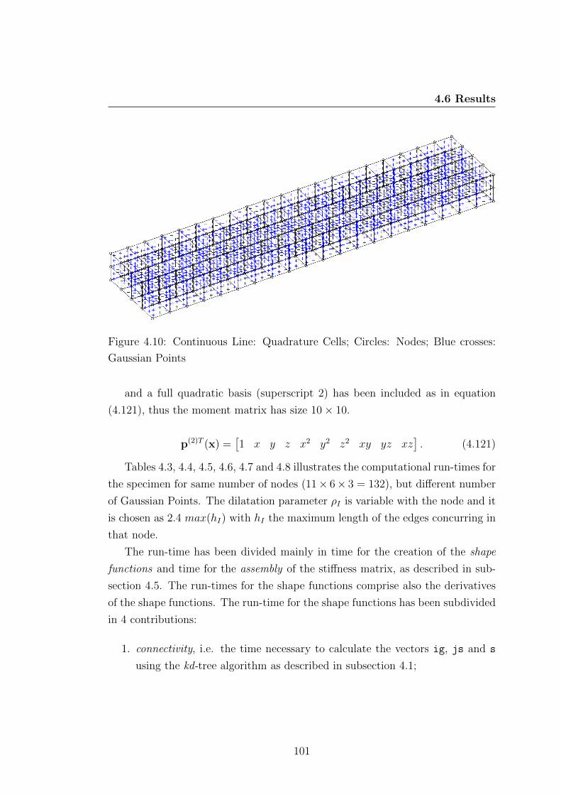
4.6 Results
Figure 4.10: Continuous Line: Quadrature Cells; Circles: Nodes; Blue crosses:
Gaussian Points
and a full quadratic basis (superscript 2) has been included as in equation
(4.121), thus the moment matrix has size 10× 10.
p(2)T (x) =[1 x y z x2 y2 z2 xy yz xz
]. (4.121)
Tables 4.3, 4.4, 4.5, 4.6, 4.7 and 4.8 illustrates the computational run-times for
the specimen for same number of nodes (11× 6× 3 = 132), but different number
of Gaussian Points. The dilatation parameter ρI is variable with the node and it
is chosen as 2.4 max(hI) with hI the maximum length of the edges concurring in
that node.
The run-time has been divided mainly in time for the creation of the shape
functions and time for the assembly of the stiffness matrix, as described in sub-
section 4.5. The run-times for the shape functions comprise also the derivatives
of the shape functions. The run-time for the shape functions has been subdivided
in 4 contributions:
1. connectivity, i.e. the time necessary to calculate the vectors ig, js and s
using the kd-tree algorithm as described in subsection 4.1;
101

4.6 Results
2. moment matrix, i.e. the time necessary to compute the cell array M as in
subsection 4.2;
3. inversion of the moment matrix, i.e. the time for inverting the moment
matrix;
4. correction term, i.e. the time for calculating the correction to the kernel as
in subsection 4.4.
Gaussian Points Classic (sec) New (sec)
800 0.1614 0.1269
2700 0.4329 0.4500
6400 0.8698 0.8728
12500 1.5980 1.5694
21600 3.0833 3.2427
34300 4.8564 4.2063
51200 7.4106 7.2022
Table 4.3: Computational run-times for the connectivity
Gaussian Points Classic (sec) New (sec)
800 0.2220 0.3374
2700 2.6361 2.5686
6400 4.7568 4.7648
12500 7.1372 7.7983
21600 12.5379 18.1758
34300 25.3300 24.7946
51200 34.6201 33.2414
Table 4.4: Computational run-times for the correction term
It can be observed that, as expected, the major differences are not in the
connectivity (table 4.3), in the correction term (table 4.4) and in the assembly
(table 4.5). In fact, for these purposes, the same routines have been used in
102

4.6 Results
Gaussian Points Classic (sec) New (sec)
800 0.3424 0.3908
2700 1.0952 1.0500
6400 2.9279 3.1260
12500 7.2566 5.9309
21600 14.7860 11.1589
34300 22.0235 21.5802
51200 29.3857 31.1248
Table 4.5: Computational run-times for the assembly
Gaussian Points Classic (sec) New (sec)
800 1.8273 0.5012
2700 11.4439 1.8473
6400 22.4772 3.9266
12500 49.4992 8.1483
21600 75.7696 14.1422
34300 135.0388 21.9535
51200 170.9730 35.3794
Table 4.6: Computational run-times for the moment matrix
Gaussian Points Classic (sec) New (sec)
800 1.5319 1.8981
2700 12.6961 9.5511
6400 58.8198 21.1465
12500 190.0229 39.9969
21600 555.5533 72.0766
34300 1344.9519 117.3779
51200 3002.2513 162.7680
Table 4.7: Computational run-times for the inversion of the moment matrix
103

4.6 Results
Gaussian Points Classic (sec) New (sec) New/Classic %
800 3.7471 2.8693 76.57 %
2700 27.2389 14.4471 53.04 %
6400 86.9840 30.7691 35.37 %
12500 248.3761 57.6299 23.20 %
21600 647.1185 107.8531 16.67 %
34300 1510.5029 168.6082 11.16 %
51200 3215.7002 239.0169 7.43 %
Table 4.8: Computational Run-times for the Shape Functions
both methods. Instead, there is a great difference for the computation times
related to the moment matrix (table 4.6), even though the same procedure of
subsection 4.2 has been used for both cases. The reason for such discrepancy
is that in the classic method, a symmetric 10 × 10 moment matrix need to be
constructed straight after the connectivity phase, whereas with the new method
(the partitioning inversion method) only a symmetric 4 × 4 moment matrix is
necessary. The symmetric 4 × 4 moment matrix for the partitioning method
can be inverted symbolically and represents the starting point of the iterative
procedure described in subsection 4.3. The remaining terms in the new method
are constructed at the same time of the inversion, allowing a huge saving in terms
of computational time, around 80% average for all the cases.
This saving is not only in terms of speed but also in terms of storage memory.
In fact, the number of entries of the moment matrix stored in the classic method
is 10×11/2 = 55, whereas in the partitioning method is 4×5/2 = 10. Therefore,
an estimation of the saving in terms of speed is (55− 10)/55× 100 = 81.18%.
Moreover, for the storage memory, there is another aspect to consider, which
is not evident from the computational times. After the inversion, the memory oc-
cupied by the moment matrix (4×4) can be cleared since it is no longer necessary.
The update is executed directly on the inverse of the moment matrix, through
previous calculation of the moments b (equation (4.69) and c (equation (4.70)).
After the update is executed, the moments b and c required for the update of the
inverse can be deleted as well. On the contrary, for the classic method, all the
104

4.6 Results
Figure 4.11: Computational run-times for the inversion of the moment matrix:
circles: classic method; squares: new method; dashed line: quadratic fit for the
classic method; continuous line: linear fit for the new method
Figure 4.12: Computational run-times for the shape functions: circles: classic
method; squares: new method; dashed line: quadratic fit for the classic method;
continuous line: linear fit for the new method
105

4.6 Results
Coefficients 95 % Coefficient Bounds
p1 = 389.7 (377.6, 401.8)
p2 = 789.8 (777.2, 802.4)
p3 = 403.9 (390.5, 417.3)
Coefficient of determination R2 0.999
Table 4.9: Inversion of the moment matrix (classic method): goodness of
quadratic fit f(x) = p1x2 + p2x+ p3
Coefficients 95 % Coefficient Bounds
p1 = 60.24 (56.9, 63.59)
p2 = 60.69 (57.59, 63.78)
Coefficient of determination R2 0.9977
Table 4.10: Inversion of the moment matrix (new method) : goodness of linear
fit f(x) = p1x+ p2
terms must be retained for the point-wise inversion, and deleted only after the
inversion is concluded. The inversion through partitioning of the moment matrix
is particularly advantageous, as shown in table 4.7. Moreover, figures 4.11 and
4.12 show another interesting side: the dataset of the computational times and
the number of Gaussian points can be fit by a quadratic curve for the classic
method and by a linear curve for the proposed method.
The classic method is fit by a quadratic polynomial with coefficients and
statistics resumed in table 4.9, while the ones for the proposed method are in
table 4.10. In both cases, the 95% coefficients bounds are pretty tight with a
coefficient of determination very close to 1.
The proposed method, either for the inversion of the moment matrix and
for the construction of the shape functions, has a computational cost O(n) with
respect to the number of Gaussian Points, compared to the O(n2) of the classic
one. The saving in computational time is tremendous: in fact, for the classic
method (table 4.8), for 51200 Gaussian points, almost an hour (54 minutes) is
needed to calculate the shape functions and their first derivatives, while with the
proposed method only 4 minutes.
106

4.6 Results
Coefficients 95 % Coefficient Bounds
p1 = 383.7 (380.5, 386.9)
p2 = 874 (870.7, 877.3)
p3 = 491 (487.5, 494.6)
Coefficient of determination R2 0.999
Table 4.11: Shape functions (classic method) : goodness of quadratic fit f(x) =
p1x2 + p2x+ p3
Coefficients 95 % Coefficient Bounds
p1 = 88.01 (83.85, 92.16)
p2 = 88.74 (84.9, 92.59)
Coefficient of determination R2 0.9983
Table 4.12: Shape functions (new method) : goodness of linear fit f(x) = p1x+p2
107
Chapter 5
Description of the Codes
In this chapter the prototype codes in Matlab will be presented. Firstly, the
purposes of the Object-Oriented Programming (OOP) will be briefly illustrated
in section 5.1, although a complete and rigorous description of the ideas can be
found in specialized textbooks. In this chapter the main ideas of the OOP will be
used to create the classes for the two-dimensional and three-dimensional codes.
5.1 The object-oriented programming
The most widely known programming technique is the procedural programming.
In the procedural coding, the data are variables or structures and the instructions
are executed in a sequential order, by calling functions that have these data as
inputs and/or outputs.
These functions perform one or more operations on the data. After these
operations are performed, the transformed data are passed back to the main
program which will continue to execute the list of the instructions.
The OOP is a rather different approach. In the OOP the main variables are
objects. An object is a specific instance of a class. A class is, from a programming
point of view, a complex structure which encapsulates both variables and func-
tions. The variables of the class are called properties and the functions defined on
these variables are called methods. The methods are not executed sequentially,
but only if a specific action is desired to be carried out on the class.
108
5.2 The class RKPM
When the input variables are given to the class, the class becomes an object.
The creation of an object, in this sense, is performed by a method called con-
structor which is compulsorily defined for every class. The constructor has the
same name of the class.
The class, in fact, describes the characteristics that all the (different) objects
have in common. Analogously to the procedural programming, the objects are the
variables, while the class is similar to the list of the instructions. The difference
is that the list of the instructions does not have to be executed obligatorily and
the variables are internal to the object. Object can then manage their own data
and different object can interact according to the actions (the methods) defined
on them.
Another interesting feature of the classes is that they can alert when any prop-
erty value is queried or changed. These notices are called events and objects can
broadcast the when for example a property value is changed. As a consequence,
other methods called listeners can be defined. Listeners execute other functions
in response to the notification of an event1.
5.2 The class RKPM
The class RKPM applies to both two-dimensional and three-dimensional linear elas-
tic objects. The purpose of this class is to provide the RKPM approximation
whenever evaluation points are inserted as input. This class is usually called to
compute the shape functions in the Gaussian points, either for the domain inte-
gral in the stiffness matrix and for the line integrals for the force vectors and for
the constraints.
5.2.1 The properties
The main properties defined for the class RKPM are
• nodes: vector ns×2 or ns×3; a list of the coordinates of the RKPM nodes
(4.4): initially it is set as the vertices of the integration mesh, but other
nodes can be added to the list if h-adaptivity is performed
1The classes presented in this chapter do not implement listeners and events at the moment
109

5.2 The class RKPM
• rho: dilatation parameters as in section 3.1.1
• PSI ,dPSIcsi, dPSIeta : the values of the kernel function and its derivatives
stored in a vector-wise manner, as defined in equations (4.12), (4.45) and
(4.46)
• ig, js: the connectivity vectors as defined in (4.8)
• PolyBasis: cell vector of function handles; contains the polynomial basis
functions as in equation (4.15).
• Kernel dKernel: function handles defining the functional form of the kernel
and its first derivative, as in equations (4.11) and (4.11)
• CSI and ETA: the scaled and translated coordinates as in equations (4.13)
and (4.14)
• P ,P0, DPDX, DPDY cell-arrays containing the values of the polynomial basis
as defined in equations (4.25), (4.26) and (4.27) stored in a vector-wise
manner
• Minv, DMinvx,DMinvy cell-arrays containing the values of the inverse of the
moment matrix and their derivatives, as it will be described in section 5.2.3
• sp handle : the function handle described in 4.94
• asb handle: the function handle described in 4.93
• desp handle : the function handle described in 4.95
• PHI, DPHIx, DPHIy the values of the shape functions and their derivatives
as described in 4.4, stored in a sparse manner
• pe, dpedx, dpedy cell arrays of function handles containing additional poly-
nomials to be added to the basis, as in p-adaptivity: in fact, as shown later,
the linear polynomial basis is inserted by default in PolyBasis
110
5.2 The class RKPM
5.2.2 The methods
The methods defined on the class RKPM are:
1. RKPM(varargin) : the constructor, named as the class itself, allows the
construction of the object. The input variables are the function handles
that define the kernel, its derivative and the optional enhanced polynomials.
function obj = RKPM(varargin)
obj.nodes = @(a)(a.fv.vertices);
obj.rho = @(a)(a.rho);
obj.Kernel = varargin1;
obj.dKernel = varargin2;
obj.PolyBasis.p1 = inline(’sparse(1:numel(x),1,1)’,’x’,’y’);
obj.PolyBasis.p2 = inline(’x’,’x’,’y’);
obj.PolyBasis.p3 = inline(’y’,’x’,’y’);
obj.PolyBasis.dpdx1 = inline(’sparse(numel(x),1)’,’x’,’y’);
obj.PolyBasis.dpdx2 = inline(’sparse(1:numel(x),1,1)’,’x’,’y’);
obj.PolyBasis.dpdx3 = inline(’sparse(numel(x),1)’,’x’,’y’);
obj.PolyBasis.dpdy1 = inline(’sparse(numel(x),1)’,’x’,’y’);
obj.PolyBasis.dpdy2 = inline(’sparse(numel(x),1)’,’x’,’y’);
obj.PolyBasis.dpdy3 = inline(’sparse(1:numel(x),1,1)’,’x’,’y’);
obj.nPB = 3;
obj.nPE = numel(varargin3);
obj.pe = varargin3;
obj.dpedx = varargin4;
obj.dpedy = varargin5;
end
2. ShapeAndDer: computes the shape functions and their derivatives in the
input points GGRID. This method firstly calls the function Conn that imple-
ments the kd-tree (section 4.1) and subsequently calls the kernel handles.
function obj = ShapeAndDer(obj,GGRID,obj2)
111
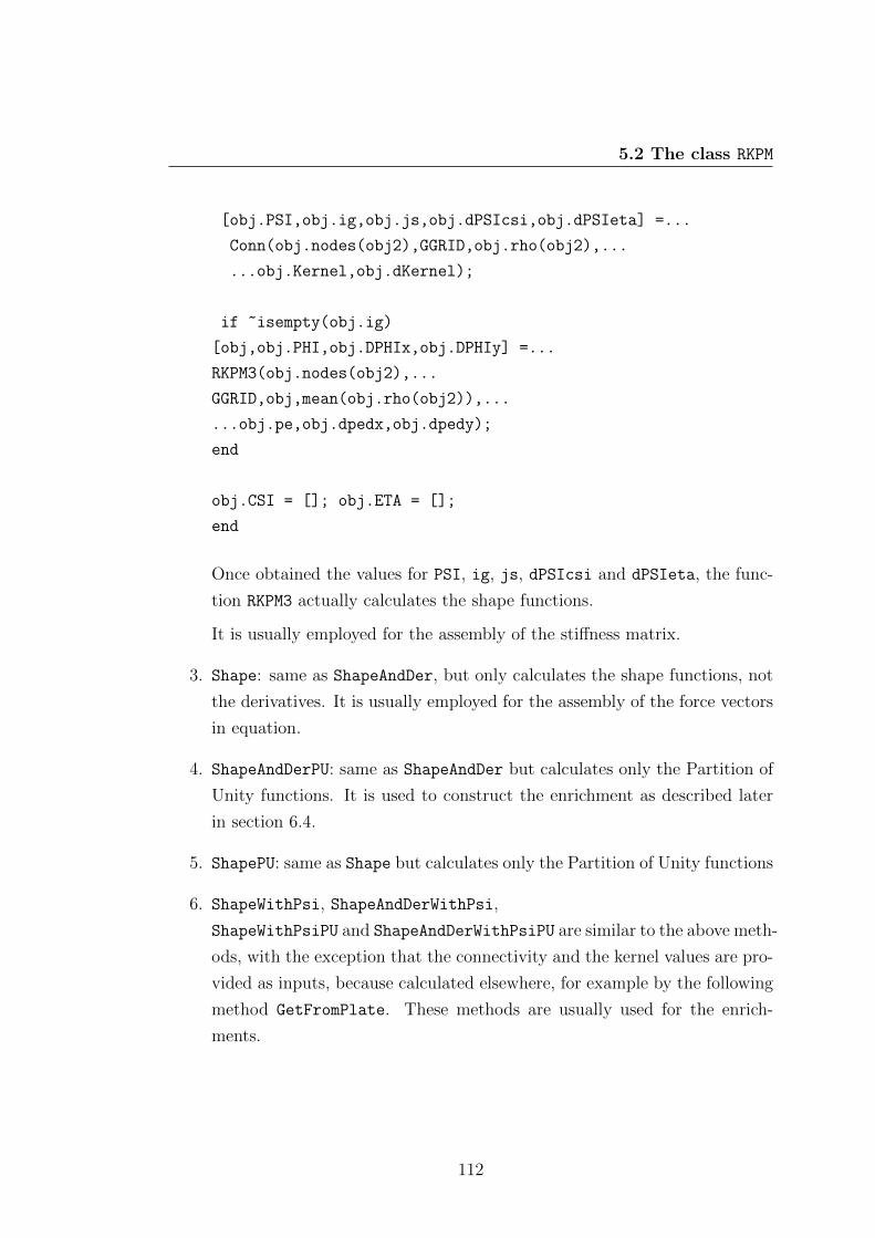
5.2 The class RKPM
[obj.PSI,obj.ig,obj.js,obj.dPSIcsi,obj.dPSIeta] =...
Conn(obj.nodes(obj2),GGRID,obj.rho(obj2),...
...obj.Kernel,obj.dKernel);
if ~isempty(obj.ig)
[obj,obj.PHI,obj.DPHIx,obj.DPHIy] =...
RKPM3(obj.nodes(obj2),...
GGRID,obj,mean(obj.rho(obj2)),...
...obj.pe,obj.dpedx,obj.dpedy);
end
obj.CSI = []; obj.ETA = [];
end
Once obtained the values for PSI, ig, js, dPSIcsi and dPSIeta, the func-
tion RKPM3 actually calculates the shape functions.
It is usually employed for the assembly of the stiffness matrix.
3. Shape: same as ShapeAndDer, but only calculates the shape functions, not
the derivatives. It is usually employed for the assembly of the force vectors
in equation.
4. ShapeAndDerPU: same as ShapeAndDer but calculates only the Partition of
Unity functions. It is used to construct the enrichment as described later
in section 6.4.
5. ShapePU: same as Shape but calculates only the Partition of Unity functions
6. ShapeWithPsi, ShapeAndDerWithPsi,
ShapeWithPsiPU and ShapeAndDerWithPsiPU are similar to the above meth-
ods, with the exception that the connectivity and the kernel values are pro-
vided as inputs, because calculated elsewhere, for example by the following
method GetFromPlate. These methods are usually used for the enrich-
ments.
112

5.2 The class RKPM
7. GetFromPlate a method that selects the ig, js PSI and optionally dPSIcsi
and dPSIeta from an existing set of nodes-Gaussian points.
function obj = GetFromPlate(obj,obj2,nodes)
[c,loc] = ismember(obj2.js,nodes);
obj.ig = obj2.ig(c);
obj.js = loc(c);
obj.PSI = obj2.PSI(c);
if ~isempty(obj2.dPSIcsi)
obj.dPSIcsi = obj2.dPSIcsi(c);
obj.dPSIeta = obj2.dPSIeta(c);
end
end
It should be noted that, even though Minv is defined as a property, there
is no property for the moment matrix. In fact, the moment matrix entries are
calculated internally in the function RKPM3.
5.2.3 Inversion of the moments matrix through partition-
ing
The function RKPM31 is defined internally in the class RKPM and its purpose is to
calculate the shape functions in the nodes and their derivatives.
The operations in RKPM3 have been already described in chapter 4, with the
exception of the details regarding the computer implementation of the inversion
of the moments matrix.
The inversion of the moments matrix is carried out by another function
RKPMp32, which is called (iteratively) after the symbolic inversion of the moments
matrix with linear reproduction properties, as described in subsection 4.2.6.
The inputs to RKPMp3 are the object obj, the properties pe, dpedx and dpedy
and the function handle spar handle (4.35), used for the computation of the
moments.
1the number 3 refers to the third version of the function2p stands for partitioning or p-adaptivity
113

5.2 The class RKPM
Firstly, using CSI and ETA, the properties P ,P0, DPDX and DPDY are augmented
by the i− th function in pe, dpedx and dpedy
np = numel(obj.PolyBasis.p);
obj.P0np+1,1 = pe(0,0);
obj.Pnp+1,1 = pe(obj.CSI,obj.ETA);
obj.PolyBasis.p1,np+1 = pe;
if nargin>4
obj.DPDXnp+1,1 = dpedx(obj.CSI,obj.ETA);
obj.DPDYnp+1,1 = dpedy(obj.CSI,obj.ETA);
obj.PolyBasis.dpdx1,np+1 = dpedx;
obj.PolyBasis.dpdy1,np+1 = dpedy;
end
The b vector in equation (4.69) (and its derivatives (4.81)) is calculated using
the spar handle
b_handle = @(i) obj.Pi.*obj.Pnp+1.*obj.PSI;
b = arrayfun(b_handle,1:np);
b = cellfun(spar_handle,b);
if nargin>3
dbdx_handle = @(i) obj.DPDXi.*obj.Pnp+1.*obj.PSI +
+ obj.Pi.*obj.DPDXnp+1.*obj.PSI +
+ obj.Pi.*obj.Pnp+1.*obj.dPSIcsi;
dbdx = arrayfun(dbdx_handle,(1:np).’);
dbdx = cellfun(spar_handle,dbdx);
dbdy_handle = @(i) obj.DPDYi.*obj.Pnp+1.*obj.PSI +
+ obj.Pi.*obj.DPDYnp+1.*obj.PSI +
+obj.Pi.*obj.Pnp+1.*obj.dPSIeta;
dbdy = arrayfun(dbdy_handle,(1:np).’);
dbdy = cellfun(spar_handle,dbdy);
end
Same process for c in equation (4.70) and its derivatives (4.80)
c = obj.Pnp+1.^2.*obj.PSI;
114
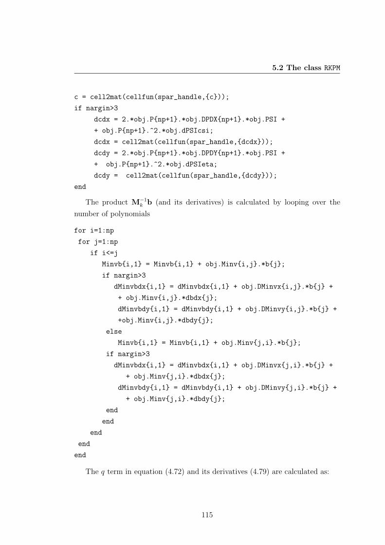
5.2 The class RKPM
c = cell2mat(cellfun(spar_handle,c));
if nargin>3
dcdx = 2.*obj.Pnp+1.*obj.DPDXnp+1.*obj.PSI +
+ obj.Pnp+1.^2.*obj.dPSIcsi;
dcdx = cell2mat(cellfun(spar_handle,dcdx));
dcdy = 2.*obj.Pnp+1.*obj.DPDYnp+1.*obj.PSI +
+ obj.Pnp+1.^2.*obj.dPSIeta;
dcdy = cell2mat(cellfun(spar_handle,dcdy));
end
The product M−1k b (and its derivatives) is calculated by looping over the
number of polynomials
for i=1:np
for j=1:np
if i<=j
Minvbi,1 = Minvbi,1 + obj.Minvi,j.*bj;
if nargin>3
dMinvbdxi,1 = dMinvbdxi,1 + obj.DMinvxi,j.*bj +
+ obj.Minvi,j.*dbdxj;
dMinvbdyi,1 = dMinvbdyi,1 + obj.DMinvyi,j.*bj +
+obj.Minvi,j.*dbdyj;
else
Minvbi,1 = Minvbi,1 + obj.Minvj,i.*bj;
if nargin>3
dMinvbdxi,1 = dMinvbdxi,1 + obj.DMinvxj,i.*bj +
+ obj.Minvj,i.*dbdxj;
dMinvbdyi,1 = dMinvbdyi,1 + obj.DMinvyj,i.*bj +
+ obj.Minvj,i.*dbdyj;
end
end
end
end
end
The q term in equation (4.72) and its derivatives (4.79) are calculated as:
115

5.2 The class RKPM
for i=1:np
bTMinvb = bTMinvb + bi.*Minvbi;
if nargin>4
dbTMinvbdx = dbTMinvbdx + dbdxi.*Minvbi +
+ bi.*dMinvbdxi;
dbTMinvbdy = dbTMinvbdy + dbdyi.*Minvbi +
+ bi.*dMinvbdyi;
end
end
q = c-bTMinvb;
if nargin>4
dqdx = dcdx - dbTMinvbdx;
dqdy = dcdy - dbTMinvbdy;
end
Finally, the update of the inverse of the moment matrix (4.71) (and its deriva-
tives 4.75) is done by
for i=1:np+1
for j=1:np+1
if i<=j
if i<=np && j<=np
obj.Minvi,j = obj.Minvi,j + Minvbi.*Minvbj./q;
if nargin>4
obj.DMinvxi,j = obj.DMinvxi,j +
- dqdx.*Minvbi.*Minvbj./(q.^2) +
+ dMinvbdxi.*Minvbj./q + Minvbi.*dMinvbdxj./q;
obj.DMinvyi,j = obj.DMinvyi,j +
- dqdy.*Minvbi.*Minvbj./(q.^2) +
+ dMinvbdyi.*Minvbj./q + Minvbi.*dMinvbdyj./q;
end
elseif i<=np && j==np+1
obj.Minvi,j = -Minvbi./q;
if nargin>4
obj.DMinvxi,j = dqdx.*Minvbi./q.^2 +
116
5.3 The class Mesh
-dMinvbdxi./q;
obj.DMinvyi,j = dqdy.*Minvbi./q.^2 +
-dMinvbdyi./q;
end
elseif i==np+1 && j==np+1
obj.Minvi,j = 1./q;
if nargin>4
obj.DMinvxi,j = -dqdx./q.^2;
obj.DMinvyi,j = -dqdy./q.^2;
end
end
end
end
end
5.3 The class Mesh
The class Mesh contains the background integration mesh, with the Gaussian
points and the weights for the domain Ω and the boundary ∂Ω.
5.3.1 The properties
The main properties defined on the class Mesh are
• fv a structure where fv.vertices is the list of the vertices of the back-
ground mesh and fv.faces is the connectivity matrix that defines the ele-
ments
• ne is the number of edges that composes the boundary ∂Ω
• bfv is an array of ne cells, where each cell is structure composed of vertices
and faces
• GP is the list of coordinates of the Gaussian points in Ω
• W is the list of the Gaussian weights
117

5.3 The class Mesh
• bGP is an array of ne cells, where each cell contains a structure composed
of Gaussian points and weights
• ng is the number of the Gaussian points in Ω
• rho is the array of the dilatation parameters, calculated as the
• RKPM is the RKPM object for the Gaussian points in Ω
5.3.2 The methods
The methods defined on the class Mesh are:
1. Mesh: the constructor of the class. The inputs to the constructor are the
name of the file containing the input data, the list of points, the vertices
and the edges of the background mesh. It also calls the function RhoHex
that calculates the dilatation parameter as ρs× the maximum length of the
edges of the elements that has the I−th node as vertex. ρs is a factor which
is usually 2 for quadratic basis or 2.4 for cubic basis. Moreover, the function
GaussQuad is called, that creates the Gaussian points and the weight on the
triangular mesh using the mapping
x = x1φ1(ξ, η) + x2φ2(ξ, η) + x3φ3(ξ, η), (5.1)
y = y1φ1(ξ, η) + y2φ2(ξ, η) + y3φ3(ξ, η), (5.2)
where (x1, y1), (x2, y2), (x3, y3) are the vertices of the element, ξ and η are
the local coordinates of the unit simplex and φ1, φ2 and φ3 are the finite
element shape functions deriving from Lagrangian interpolation.
φ1(ξ, η) = ξ, (5.3)
φ2(ξ, η) = η, (5.4)
φ3(ξ, η) = 1− ξ − η. (5.5)
The determinant of the Jacobian of equations (5.1) and(5.2) is∣∣∣∣∂(x, y)
∂(ξ, η)
∣∣∣∣ = (x1 − x3)(y2 − y3)− (x2 − x3)(y1 − y3) = 2A, (5.6)
where A is the area of the triangular element
118

5.4 The class Load
2. MeshB: behaves as Mesh but on a specified edge of the boundary, using the
mapping
x = x1φ1(ξ) + x2φ2(ξ), (5.7)
y = y1φ1(ξ) + y2φ2(ξ), (5.8)
where (x1, y1), (x2, y2) are the vertices of the element, ξ is the local coordi-
nates of the interval [−1, 1] and φ1, φ2 are the finite element shape functions
deriving from Lagrangian interpolation
φ1(ξ) =1− ξ
2, φ2(ξ) =
1 + ξ
2. (5.9)
The length of the tangent vector in equations (5.7) and (5.8) is∣∣∣∣∂(x, y)
∂ξ
∣∣∣∣ =
√(x2 − x1
2
)2
+
(y2 − y1
2
)2
. (5.10)
3. PlotBoundary and PlotMesh are methods that plot the mesh and the
boundary as patches. A patch is a graph object predefined in Matlab,
that uses the same vertices-faces structure defined in fv and bfv;
4. PlotGP and PlotOnGP(obj,fun) plot the Gaussian Points and a function
fun on the Gaussian points as scatter plots.
5. WDPHIx, WDPHIy, WPHI, IPHI, IPHIf, WbPHI, wbPHI are methods that calcu-
late the integrals using the asb handle as in command (4.93).
5.4 The class Load
The properties defined in class Load are the natural boundary conditions (loads
and displacements) applied to ∂Ω, while the methods calculate the force vectors
and plot the natural boundary conditions.
119

5.4 The class Load
5.4.1 The properties
The properties for the class Load are:
• DistributedTractions: a structure whose fields are the function handles
tx and ty, that contain the functional expressions for the applied dis-
tributed tractions;
• DistributedDisplacements: a structure whose fields are the function han-
dles dx and dy, that contain the functional expressions for the applied dis-
tributed displacements;
• PointForces: a structure whose fields are: P coordinates of the points
where concentrated forces are applied, tbar an array containing the com-
ponents of the forces;
• PointDisplacements: a structure whose fields are: P coordinates of the
points where concentrated displacements are applied, tbar an array con-
taining the components of the displacements;
• NBC: an array 2 × ne of logical, where 1 indicates an active component of
the distributed tractions on the j − th edge j = 1, . . . , ne and 0 otherwise;
• DBC: same as NBC for the applied distributed displacements.
5.4.2 The methods
The main methods defined on Load are:
1. ApplyDistrTrac(obj,obj2,ne,tx,ty): calculates the distributed tractions
tx and ty on the ne-th edge of ∂Ω, where obj2 is a Mesh object. The output
is the force vector∫
ΓφT tdΓ in equation (3.104). In order to calculate the
outputs, the MeshB method is called to create the Gaussian points and the
weights on the edge, then a RKPM object is constructed on these Gaussian
points and the method IPHI of the RKPM object is invoked for the integral.
120

5.5 The class Constraint
2. ApplyDistrDispl(obj,obj2,ne,dx,dy): same as ApplyDistrTrac but for
the distributed displacement. The output is the generalized force vector
in∫
ΓuφT udΓu in equation (3.104) and the matrix
∫ΓuφiφjdΓu in equation
(3.103). The method WbPHI is used to calculate the matrix.
3. ApplyPointForces same as ApplyDistrTrac but for concentrated forces;
4. ApplyPointDispl same as ApplyPointForces but for concentrated dis-
placements;
5. DeleteDistrTrac, DeleteDistrDispl, DeletePointForce and
DeletePointDispl are destructors, i.e. methods that allow to remove the
applied forces and displacements;
6. PlotLoads and PlotDisplacements are graphic methods that plot the ap-
plied loads and displacements on the boundary ∂Ω.
5.5 The class Constraint
The properties defined in class Load are the essential boundary conditions applied
to ∂Ω, while the methods calculate the matrix and plot the constraints.
5.5.1 The properties
The properties defined in the class Constraint are:
• Points structure similar to the one for the Load class (subsection 5.4.1). It
contains the informations related to essential boundary conditions applied
in points.
• EBC array similar to NBC in Load class (subsection 5.4.1): 1 indicates an
active constraint, otherwise the value is set to 0.
121

5.6 Other classes
5.5.2 The methods
The methods defined in the class Constraint are similar to the ones defined for
the class Load:
1. ApplyConstraints(obj,obj2,ne,c): applies essential boundary conditions
on the ne-th edge. The output is the matrix∫
ΓuφiφjdΓu in equation (3.103).
The method WbPHI is used to calculate the matrix;
2. ApplyPointConstraints: same as ApplyConstraints but on points rather
than segments.
5.6 Other classes
The remaining classes are auxiliary to the main one LinearElastic2D, described
later. The class ElasticProperties reads the elastic properties from the input
file and calculates the stiffness tensor for two-dimensional linear orthotropic ma-
terials as in section 4.5. The only method implemented is the computation of
equation (4.98).
The class PostProcessing extracts the solution of an elastic problem and
writes the files containing the displacements, the stress σ and strain ε tensors in
the Gaussian points. These data can be subsequently used for a deformation plot
or for a fringe plot of the stress or the strain.
If a Cohesive object 6.4.9 in given as additional input, a PostProcessing
class calculates the enriched approximation as in equations (6.73), (6.76), (6.77)
and (6.78)
5.7 The class LinearElastic2D
In this section it is finally described the class that comprehends the above de-
scribed classes. The instance created from this class is the object Plate.
The object behaves like an actual plate, where forces, displacements and con-
straints can be applied and the resulting deformed configuration (along with the
levels of stress or strain) can be displayed.
122
5.7 The class LinearElastic2D
5.7.1 The properties
The main properties defined on the class are:
• Elastic: the ElasticProperties object described in subsection 5.6;
• Omega: a Mesh object;
• Loads: a Load object;
• Constraints: a Constraint object;
• Results: a PostProcessing object;
• K: the stiffness matrix in equation (3.103);
• Vinc: the matrix output of the method ApplyConstraints;
• Vinc p : the matrix output of the method ApplyPointConstraints;
• Vincd p: the matrix output of the method ApplyPointDispl;
• Vincd : the matrix output of the method ApplyDistrDispl;
• F: the vector output of the method ApplyDistrTrac;
• Fd: the vector output of the method ApplyDistrDispl;
• F p: the vector output of the method ApplyPointForces;
• Fd p: the vector output of the method ApplyPointDispl.
5.7.2 The methods
The main methods of the class are
• LinearElastic2D: the constructor, which creates the objects Elastic, Omega,
Loads and Constraints by calling the correspondent classes;
123

5.7 The class LinearElastic2D
• ApplyDistrDispl, ApplyDistrTrac, ApplyPointForces, ApplyPointDispl,
ApplyConstraints and ApplyPointConstraints are overloaded methods
from the classes Load and Constraint for the application of forces and
constraints;
• DeleteDistrTrac, DeleteDistrDispl, DeletePointForces,
DeletePointDisplacements, DeleteConstraints and
DeletePointConstraints are overloaded methods from the classes Load
and Constraint for the deletion of forces and constraints;
• PlotLoads, PlotApplDisplacements PlotConstraints are overloaded meth-
ods from the classes Load and Constraint for the plot of forces and con-
straints;
• PlotMesh, PlotOnGP are overloaded methods from the class Mesh for the
plot of the mesh and the Gaussian points;
• Assembly: method that creates the stiffness matrix K as described in sec-
tion 4.5; It creates an object of the class RKPM for the shape functions in
the Gaussian points GP contained in the object Omega of the class Mesh;
• PostProcessing: overloaded constructor of the object Results;
• Solve is the method that solves the linear elastic problem once the stiffness
matrix and the force vectors are calculated:
R = (obj.K+obj.Options.Penalty*obj.Vinc+
+obj.Options.Penalty*obj.Vinc_p+
+obj.Options.Penalty*obj.Vincd_p +
+obj.Options.Penalty*obj.Vincd )\(obj.F +
+ obj.F_p + obj.Options.Penalty*obj.Fd +
+ obj.Options.Penalty*obj.Fd_p);
. The solution of the linear system of equations is performed by the built-in
operator \, that automatically chooses the most suitable algorithm accord-
ing to the structure of the matrix K. When the solution is completed, the
object Results is created
124
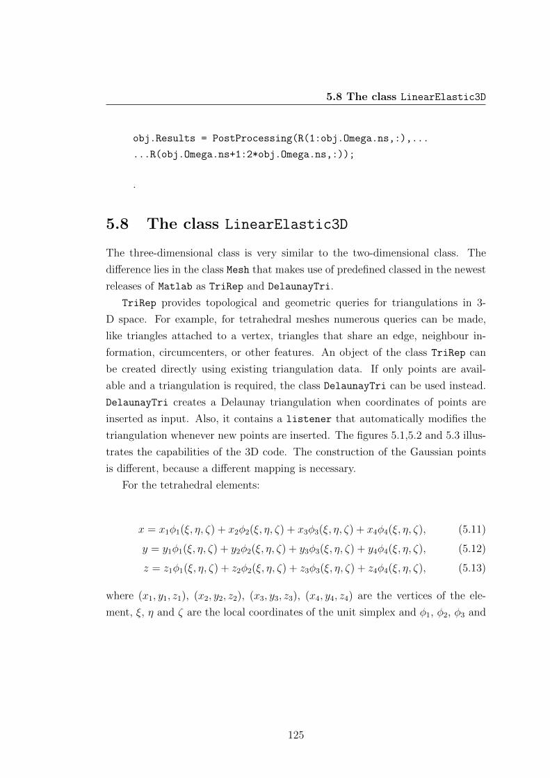
5.8 The class LinearElastic3D
obj.Results = PostProcessing(R(1:obj.Omega.ns,:),...
...R(obj.Omega.ns+1:2*obj.Omega.ns,:));
.
5.8 The class LinearElastic3D
The three-dimensional class is very similar to the two-dimensional class. The
difference lies in the class Mesh that makes use of predefined classed in the newest
releases of Matlab as TriRep and DelaunayTri.
TriRep provides topological and geometric queries for triangulations in 3-
D space. For example, for tetrahedral meshes numerous queries can be made,
like triangles attached to a vertex, triangles that share an edge, neighbour in-
formation, circumcenters, or other features. An object of the class TriRep can
be created directly using existing triangulation data. If only points are avail-
able and a triangulation is required, the class DelaunayTri can be used instead.
DelaunayTri creates a Delaunay triangulation when coordinates of points are
inserted as input. Also, it contains a listener that automatically modifies the
triangulation whenever new points are inserted. The figures 5.1,5.2 and 5.3 illus-
trates the capabilities of the 3D code. The construction of the Gaussian points
is different, because a different mapping is necessary.
For the tetrahedral elements:
x = x1φ1(ξ, η, ζ) + x2φ2(ξ, η, ζ) + x3φ3(ξ, η, ζ) + x4φ4(ξ, η, ζ), (5.11)
y = y1φ1(ξ, η, ζ) + y2φ2(ξ, η, ζ) + y3φ3(ξ, η, ζ) + y4φ4(ξ, η, ζ), (5.12)
z = z1φ1(ξ, η, ζ) + z2φ2(ξ, η, ζ) + z3φ3(ξ, η, ζ) + z4φ4(ξ, η, ζ), (5.13)
where (x1, y1, z1), (x2, y2, z2), (x3, y3, z3), (x4, y4, z4) are the vertices of the ele-
ment, ξ, η and ζ are the local coordinates of the unit simplex and φ1, φ2, φ3 and
125
5.8 The class LinearElastic3D
φ4 are the finite element shape functions deriving from Lagrangian interpolation.
φ1(ξ, η, ζ) = ξ, (5.14)
φ2(ξ, η, ζ) = η, (5.15)
φ3(ξ, η, ζ) = ζ, (5.16)
φ4(ξ, η, ζ) = 1− ξ − η − ζ. (5.17)
(5.18)
The determinant of the Jacobian of equations (5.11), (5.12) and (5.13)is∣∣∣∣∂(x, y, z)
∂(ξ, η, ζ)
∣∣∣∣ = 6V ; (5.19)
where V is the volume of the tetrahedral element.
For the triangular elements of the surfaces of the boundaries, the following
mapping is used
x = x1φ1(ξ, η) + x2φ2(ξ, η) + x3φ3(ξ, η), (5.20)
y = y1φ1(ξ, η) + y2φ2(ξ, η) + y3φ3(ξ, η), (5.21)
z = z1φ1(ξ, η) + z2φ2(ξ, η) + z3φ3(ξ, η), (5.22)
(5.23)
where (x1, y1), (x2, y2) and (x3, y3, z3) are the vertices of the element, ξ and η are
the local coordinates of the unit simplex and φ1, φ2 and φ3 are the finite element
shape functions deriving from Lagrangian interpolation. The Jacobian used in
the mapping is ∣∣∣∣∂(x, y, z)
∂ξ× ∂(x, y, z)
∂η
∣∣∣∣ = 2A, (5.24)
where A is the area of the triangle.
Finally, for the linear elements of the edges, the following mapping is used
x = x1φ1(ξ) + x2φ2(ξ), (5.25)
y = y1φ1(ξ) + y2φ2(ξ), (5.26)
z = z1φ1(ξ) + z2φ2(ξ), (5.27)
126

5.8 The class LinearElastic3D
where (x1, y1), (x2, y2) and (x3, y3) are the vertices of the element, ξ is the local
coordinates of the interval [−1, 1] and φ1, φ2 are the finite element shape functions
deriving from Lagrangian interpolation.
The length of the vector in equations (5.25) and (5.26) and (5.27) is∣∣∣∣∂(x, y, z)
∂ξ
∣∣∣∣ =
√(x2 − x1
2
)2
+
(y2 − y1
2
)2
+
(z2 − z1
2
)2
(5.28)
(a) Longitudinal stress (view 1) (b) Longitudinal stress(view 2)
Figure 5.1: Three-dimensional code: vertical bending
127

5.8 The class LinearElastic3D
(a) In-plane shear stress (b) In-plane shear stress
(c) Out-of-plane shear stress
Figure 5.2: Three-dimensional code: torsion
128
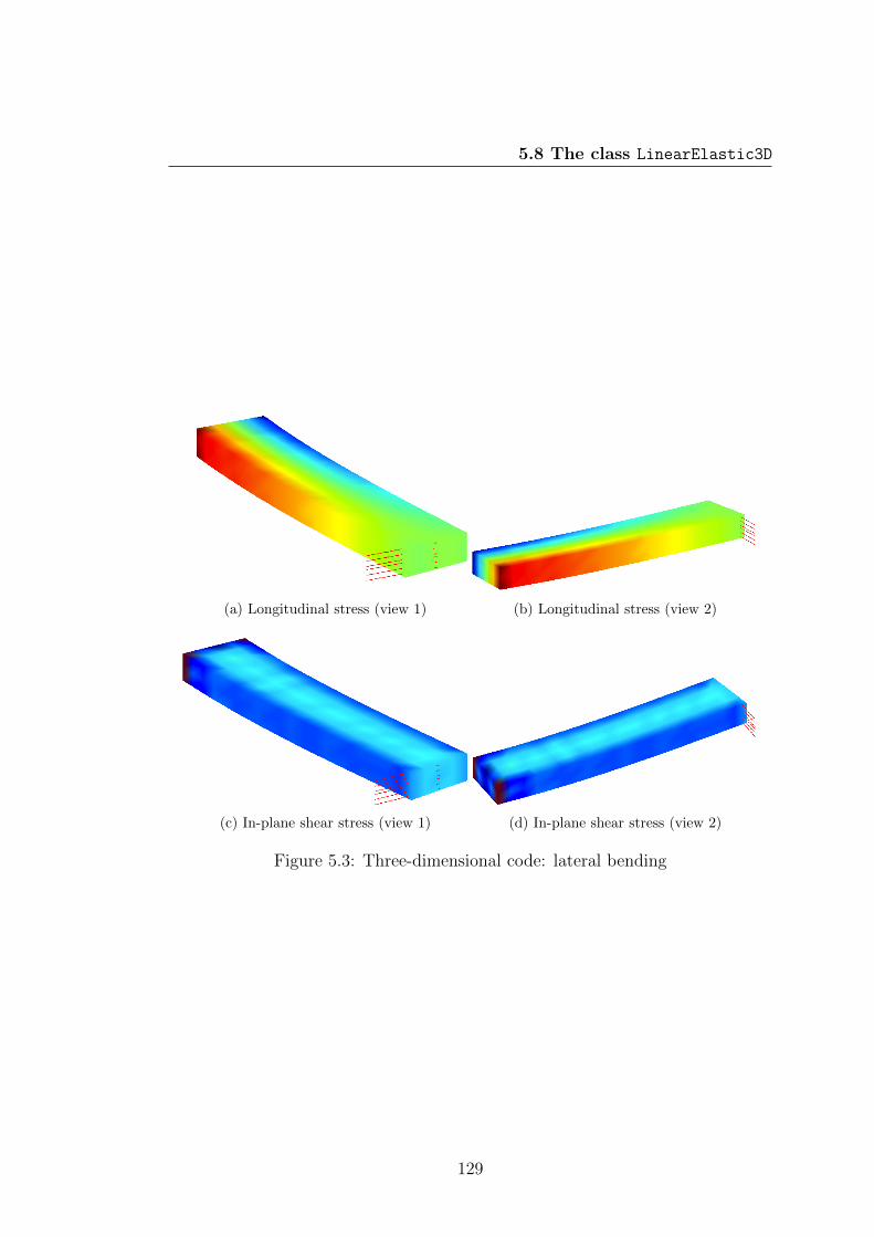
5.8 The class LinearElastic3D
(a) Longitudinal stress (view 1) (b) Longitudinal stress (view 2)
(c) In-plane shear stress (view 1) (d) In-plane shear stress (view 2)
Figure 5.3: Three-dimensional code: lateral bending
129
Chapter 6
Application to Composite
Materials: Delamination
In this chapter the meshfree techniques and the codes presented in the previous
chapters will be used to model failure in composite materials. With the term
failure is usually intended the event that occurs when the structure loses its
ability to withstand an external load. This load may be static or dynamics,
periodic or impulsive and the global/local response of the material might vary
according to its mechanical properties. Therefore by the word failure a broad
class of problems may be intended.
These problems may be classified by their dependency with time (static, quasi-
static, creep, fatigue, dynamic loading), or by the stress-strain constitutive rela-
tionship (classic elastic fracture mechanics, plastic fracture mechanics, ), or by
their ultimate behaviour (brittle or ductile materials). Moreover, materials can
have different behaviour if subjected to high-rate loads. For example metals are
ductile at quasi-static loads, but turn into brittle if subjected to shock loads.
Also, the opposite may occur. It is for example the case of concrete, which is
brittle for quasi static loads, but ductile at elevated rates.
Simulation of these phenomena may require quite complex computational
tools, not yet completely developed, since it can be done bridging different length
scales, as in the so called multi-scale methods. The advent of new technologies
with faster computers is fostering the application of these methodologies also to
large scale simulations.
130

Before proceeding further, it is then opportune to define and restrict the type
of failure that will be modeled with the presented method. Simulation of failure
will not be focused on multi-scale method, but rather on a more engineering level.
At a practical level, for the simulation of failure two approaches can be followed,
a damage mechanics based and a fracture mechanics based.
These two approaches are not mutually exclusive, but rather complementary
branches of the solid mechanics. Fracture mechanics utilizes balance laws (J-
integral Rice (1968)) or state variable derived criteria (Stress Intensity Factors) to
predict the failure, without modifying (introducing additional internal variables)
the underlying constitutive model(s) but rather works “on top” of them. Damage
mechanics 1, however, uses thermodynamics concepts. CDM introduces a new
state variable (the damage, be it scalar, vector, matrix, tensor) to the constitutive
model along with its evolution equation (and failure/initiation criteria etc.) and
coupling to other state variables. Damage mechanics is more suitable for the
prediction of the onset, while fracture mechanics is based on the pre-existence
of a crack. The method utilized in the proceeding of the chapter is a damage
mechanics based method combined to a fracture mechanics approach, able to
represent geometric discontinuities. Following damage mechanics, it is crucial
the choice of a correct constitutive model.
Nevertheless, in composite materials, the inhomogeneity introduces further
complexity and uncertainty to the derivation of constitutive models. Damage
initiation and propagation may be therefore completely different from the ones
in homogeneous materials. In fact matrix and fibers usually have independent
failure mechanisms and thresholds. On the top of that, bonding limits between
the individual components along their interfaces represent new modes of failure.
Generally, two categories of failure are predominant in laminated composite
materials, i.e. intra-laminar failures (for example matrix failure, fibers break-
ing, interface failure between matrix and fibers) and inter-laminar failure, i.e.
delamination. A complete review of the numerous failure theories available for
composite materials can be found in Orifici et al. (2008).
For fibers breaking there exist various criteria to predict the tensile failure,
for example Puck & Schurmann (2002). The breaking is due to accumulation of
1More often referred as Continuum Damage Mechanics CDM
131

each fibre within the ply and different criteria for the compressive failure, due to
microbuckling and formation of kink bands. Moreover, there are methods that do
not distinguish between the two types of failure, but use a global criterion that
comprises both tension and compression.
Matrix failure is due to coalescence of accumulated micro-cracks, typically
originated at defects or at fibre-matrix interface. Eventually this coalescence
leads to failure across a critical fracture plane. This plane can be predicted using
fracture mechanics tools. Examples of criteria can be found for example in Hashin
(1980) and Puck & Schurmann (2002).
The above mentioned mechanisms however will not be covered by the ap-
proaches developed in the the following sections. The main focus of this work
will be delamination, although the previous mentioned failure mechanism could
constitute the basis of future work, perhaps in a multiscale perspective.
Delamination is the debonding of the layers that may occur for example in case
of low velocity impact or from a manufacturing defect such shrinkage of the matrix
during curing. It is an important cause of failure in unidirectional fiber-reinforced
composites. Since there is no reinforcement in the direction perpendicular to
the layers, the plies are more exposed to failure in case of impact. The major
inconvenient resulting from delamination is a consistent reduction in the load
carrying capability of a structure.
There are mainly two types of delamination, as reported in Bolotin (1996)
and Bolotin (2001): near-surface delamination and internal delaminations. Near-
surface delaminations are localized on the surface of the laminate and their de-
formation is not much influenced by the rest of the laminate. The accurate
simulation of these delaminations prescribes the analysis of the local stability.
This chapter will be focused though on internal delaminations, with an exist-
ing pre-crack. As in fracture mechanics, three modes of failure exist for internal
delamination, as depicted in figure 6.1. Mode I is called opening mode, since
separation occurs perpendicularly to the loading force, while the other two are
shear modes. In the shear modes, the separation is parallel to the loading, but
while mode II is a sliding mode (in-plane shear stress), mode III is an out-of-plane
shear stress loading mode.
132

6.1 Review of simulation of delamination
Figure 6.1: Failure modes for internal delamination: (a) mode I , (b) mode II ,
(c) mode III
6.1 Review of simulation of delamination
The simulation of delamination in composites is usually divided into delamination
initiation and delamination propagation. The first one is usually based on the
strength of materials theory and employs stress criteria normally based on point
or average stress, while propagation is modeled with fracture mechanics tools
based on the evaluation of the energy release rate G.
In the past years finite elements (FE) have proved to be the most widely
used computer resource in the industrial and scientific community to model de-
lamination. Particularly, decohesion elements are the most popular choice and
they are nowadays implemented in many commercial FE packages. The main
advantage of the use of decohesion elements is the capability to predict both
onset and propagation of delamination. These elements could be of different
types, like continuous interface elements (zero-thickness or finite-thickness vol-
umetric elements) or point decohesion elements (non-linear springs connecting
nodes). Decohesion elements use the cohesive model as the constitutive relation-
ship between the relative displacements and the traction forces at the interfaces
Camanho et al. (2001), Camanho & Davila (2002), Camanho et al. (2003). Co-
hesive model will be described in detail in section 6.2. Finite elements methods,
like decohesion elements or interface elements, have the major disadvantage that
crack path is highly dependent on the mesh structure, since discontinuities must
133
6.1 Review of simulation of delamination
follow inter-element boundaries, therefore capturing of a propagating discontinu-
ity is achieved by constant re-meshing of the structure. This procedure is costly
not to mention the degradation of the accuracy of the solution.
These limitations are overcome with novel methods such as meshfree or other
Partition of Unity-based methods (PUM), where discontinuities are not restricted
to element boundaries or even no elements are necessary at all. An important
progress in this sense has been recently obtained with the introduction of par-
tition of unity-based methods (PUM) Babuska & Melenk (1997) like extended
finite element (XFEM) Moes et al. (1999), Black & Belytschko (1999), Dolbow
et al. (2000), Moes & Belytschko (2002) and meshless methods like Element-
Free Galerkin Belytschko et al. (1994b) or Reproducing Kernel Particle Method
(RKPM) Liu et al. (1995). In the papers of Wells & Sluys (2001) and Remmers
et al. (2003a), a new method called cohesive segments method is introduced. In
Wells & Sluys (2001) the PUM idea is applied in the context of cohesive cracks. A
full non-linear model is developed, with tractions acting on the cohesive surfaces.
These tractions are depending on the opening displacement (or discontinuous
displacement) and used to model crack propagation in three-points bending test
and single edge notched beam.
In Remmers et al. (2003a) these segments are introduced under a FE frame-
work, similarly to the Extended Finite Element Method (XFEM). Using a partic-
ular instance of a PUM , a continuous crack is approximated by a set of segments,
each one of them split the domain in two parts. At each of these interfaces, a
cohesive model is used in order to simulate the debonding of the parts. It can be
shown that by doing so, the total displacement is enriched by a sum of Heaviside
functions that can effectively represent the discontinuity. In this way, additional
unknowns are introduced to the final algebraic system of equations. These seg-
ments can be introduced at any time of the calculation, whenever a stress-based
failure criterion is satisfied, and the orientation of the onset cohesive segment is
given by the principal direction of the stress. In this way, no explicit represen-
tation of the crack surface is needed allowing arbitrary crack growth, which is
extremely useful when the crack propagation path is not known a priori. The
drawback of this method is that additional unknowns are introduced at each crack
segment. The unknowns are localized to the nodes of the elements cut by the
134
6.1 Review of simulation of delamination
discontinuity. In Remmers et al. (2008) the same approach is used to efficiently
simulate dynamic crack propagation.
The idea of combining cohesive segments with meshfree methods is a very
recent idea Sun et al. (2007), although delamination modeling with Element Free
Galerkin can be found in Guiamatsia et al. (2009), but combined with a Virtual
Crack Closure Method rather than cohesive laws.
When the crack path is known a priori, like in the case of single mode delami-
nation, the same approach can be used without adding additional unknowns, like
in Barbieri & Meo (2008) and Barbieri & Meo (2009a).
In this case, the domain can be decomposed in two parts connected by a
penalty parameter, as also suggested in Belytschko et al. (1996a). The variational
problem is formulated for each sub-domain and then a coupling term between
their displacements is introduced. The coupling term is nothing else than a
penalty factor defined on the whole contact segment. Penalty terms are well-
known in the meshfree community since, conversely to FE, the shape functions
do not possess the Kronecker condition Fries & Matthies (2004). This condition
allows in FE to directly impose essential boundary conditions on the nodes located
on the constrained boundaries. For simple constraints, though, a constant penalty
factor is sufficient throughout the whole boundary. The same approach can be
used to connect or disconnect two or more objects.
At this aim, a penalty-based finite element technology was introduced in Pan-
tano & Averill (2002) to assemble together independently modeled finite element
sub-domains. The same technology was subsequently used in Pantano & Aver-
ill (2004) to model mixed-mode delamination growth, using the concept that a
penalty factor that was previously used to bond together different parts can be
used as well for their separation. The simulation is almost mesh independent, but
additional unknowns are required for the interface, even for single delamination.
It will be shown in the next sections that using meshfree shape functions this
limitation can be removed.
The coupling term that derives from the application of the cohesive model at
the separation leads to a final nonlinear set of equations
Ψ(a, λ) = R(a)− λP = 0, (6.1)
135

6.1 Review of simulation of delamination
where a is a 2ns × 1 vector which is usually the displacement vector, P is the
unitary external force vector, λ is a scalar that quantifies the magnitude of the
applied force and R(a) is the internal force vector. Problem (6.1) is called para-
metric continuation.
In computational solid mechanics, equation (6.1) often refers to the search of
an equilibrium path (a, λ) and two approaches can be followed, as reported in
the classic book Crisfield (1991):
1. displacement control, where a displacement is applied and λ derives from a
posteriori computation of a reaction force (figure 6.2a)
2. force control where a force is applied and λ is treated as an additional
unknown (figure 6.2b)
(a) Displacement Control (b) Force Control
Figure 6.2: Examples of equilibrium paths for non-linear equations
Displacement control may be suitable when the equilibrium curve presents an
unstable point, where the tangent at the curve is horizontal to the displacement
axis (figure 6.3a). In fact, in this case for the same load level λ there exist two
different equilibrium states u1 and u2. Nevertheless, displacement control may
fail as well for the case illustrated in figure 6.3b, where the same equilibrium state
u1 is satisfied simultaneously by two different load levels λ1 and λ2.
Nonetheless, the equilibrium path could be more complicated and for example
in case in figure 6.3b both displacement and force control fail. A more general
136

6.2 Cohesive Zone Model
(a) Failure of the force control method (b) Failure of the displacement and force con-
trol method
Figure 6.3: Failures in the load control and displacement control
approach to trace the equilibrium path in figure 6.3b is therefore the force control
with an arc-length solver. To provide more robustness, the arc-length can be also
combined with a line-search approach. Following Crisfield (1991), a detailed
procedure is reported in appendix B. A Matlab in-house code has been written
to serve this scope.
The outline of the chapter is the following: firstly, in section 6.2, the cohesive
zone model will be reviewed, then in section 6.3 the penalty approach to model
delamination will be presented and numerical cases will be shown. Finally, in
section 6.4 a more general approach will be presented, known as the cohesive
segments method that exploits the PUM principle along with numerical cases.
6.2 Cohesive Zone Model
Cohesive models are based on the Dudgale - Barenblatt Barenblatt (1962) cohe-
sive zone approach, subsequently extended by Hillerborg Hillerborg et al. (1976)
and Needleman Needleman (1987).
The main purpose of cohesive zone models is to provide a more physical expla-
nation of the failure process, differently from classical linear fracture mechanics,
which lacks of a physics-based description Klein et al. (2001) and it is based on
the concentration of stress at notches. Conversely to classical fracture mechanics,
137

6.2 Cohesive Zone Model
the cohesive zone modeling approach does not involve crack tip stress singularities
and failure is regulated by relative displacements and stresses.
In the cohesive zone model instead, it is postulated the existence of a narrow
band of vanishing thickness ahead of a crack tip which represents the fracture
process zone. The bonding of the surfaces of the zone is obtained by cohesive
traction that derives from a potential. Specifically, in the work of Needleman
(1987) 1, it is introduced a potential φ(un, ut, ub) function of the normal com-
ponent un, the tangential component ut and the binormal component ub of the
displacement jump ∆ at the interface (figure 6.4).
Figure 6.4: Reference frame for the interface
φ(un, ut, ub) = −∫ u
0
Tndun + Ttdt + Tbdb =
=27
4σmax
(unδ
)2[1− 4
3
(unδ
)+
1
2
(unδ
)2]
+
+1
2α(utδ
)2[1− 2
(unδ
)+(unδ
)2]
+1
2α(ubδ
)2[1− 2
(unδ
)+(unδ
)2]
un ≤ δ,
(6.2)
where Tn, Tt and Tb are the tractions respectively on direction n, t and b and δ
is a characteristic length, σmax is the maximum traction carried at the interface
1the same notation will be used
138
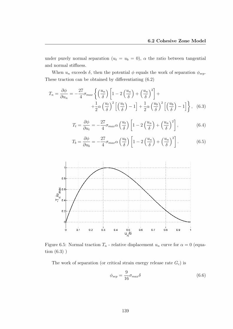
6.2 Cohesive Zone Model
under purely normal separation (ut = ub = 0), α the ratio between tangential
and normal stiffness.
When un exceeds δ, then the potential φ equals the work of separation φsep.
These traction can be obtained by differentiating (6.2)
Tn =∂φ
∂un= −27
4σmax
(unδ
)[1− 2
(unδ
)+(unδ
)2]
+
+1
2α(utδ
)2 [(utδ
)− 1]
+1
2α(ubδ
)2 [(ubδ
)− 1]
, (6.3)
Tt =∂φ
∂ut= −27
4σmaxα
(utδ
)[1− 2
(unδ
)+(unδ
)2], (6.4)
Tb =∂φ
∂ub= −27
4σmaxα
(ubδ
)[1− 2
(unδ
)+(unδ
)2]. (6.5)
Figure 6.5: Normal traction Tn - relative displacement un curve for α = 0 (equa-
tion (6.3) )
The work of separation (or critical strain energy release rate Gc) is
φsep =9
16σmaxδ (6.6)
139

6.2 Cohesive Zone Model
This model, though, describes only debonding by normal separation. In Tver-
gaard (1990) this model was generalized by introducing a damage variable D. In
addition, a cleavage unloading procedure can be added, in which the stiffness is
reduced when damage occurs but separation totally vanishes when the traction
is reduced to zero.
D = m
√(utδmax
)m+
(unδmax
)mD ∈ [0, 1], (6.7)
when m = 2, then the tractions are
Tn =27
4σmax
unδ
(1−D)2, (6.8)
Tt =27
4σmax
utδ
(1−D)2. (6.9)
Many different constitutive laws exist, for example the exponential or the bilinear
softening model Zou et al. (2003). These laws are typically regulated by both
strength of material parameters (like the tensile strength) and fracture mechanics
based parameters like the critical fracture energies for the considered fracture
mode. Crack growth occurs when a critical value is reached at which cohesive
traction disappears.
The cohesive model implemented in the following sections is a bilinear traction
- displacement relationship τ(∆), where τ is the traction at the interface and
∆(x) is the displacement jumps at the interface. The bilinear curve is divided
into three main parts (fig. 6.6) and the constitutive equations are the following:
• ∆ ≤ ∆0: elastic part : traction across the interface increases until it reaches
a maximum, and the stress is linked to the relative displacement via an
arbitrary interface stiffness K0 :
τ(∆) = K0∆; (6.10)
• ∆0 < ∆ ≤ vF : softening part : the traction across the interface decreases
until it becomes equal to zero: the two layers begin to separate. The damage
accumulated at the interface is represented by a variable D, which is equal
140

6.2 Cohesive Zone Model
to zero when there is no damage and reaches 1 when the material is fully
damaged:
τ(∆) = (1−D(∆))K0∆; (6.11)
• ∆ > ∆f : decohesion part : decohesion of the two layers is complete: there
is no more bond between the two layers, the traction across the interface is
null.
Figure 6.6: Bilinear softening model
The shaded area in figure 6.6 is the energy dissipated per unit area G for a
particular mode. Moreover, for mode II the diagram is symmetrical with respect
to the zero, since the sliding motion could occur in both senses (figure 6.1), while
to prevent inter-penetration of the crack surfaces, diagram for mode I is linear
for negative relative displacements ∆ and no damage is prescribed. In this way,
the stiffness parameter is restored in order to keep the interface closed.
When ∆ = ∆f the area of the whole triangle is the critical energy dissipated
per unit area Gc. It can be shown Rice (1968) that in this case cohesive zone
approaches can be related to Griffith’s theory of fracture. Moreover Alfano &
Crisfield (2001) showed that when ∆0 = ∆f (which means abrupt load fall to
zero) a perfectly brittle fracture can be simulated.
Two independent parameters are necessary to define a bilinear softening model,
i.e. the inter-facial maximum strength τm and the critical energy dissipated per
141
6.3 The Cohesive Penalty approach
unit area Gc, since the following relations hold
Gc =τm∆f
2(6.12)
τm = K0∆0 (6.13)
where K0 is an arbitrary initial penalty stiffness (dimensionally N/m3) which
is usually set as a large number. Then, once derived ∆0 and ∆f , the variable
damage D can be calculated as
D(∆) =
0 ∆ ≤ ∆0∆f (∆−∆0)
∆(∆f−∆0)if ∆0 < ∆ ≤ ∆F
1 ∆ > ∆F
(6.14)
6.3 The Cohesive Penalty approach
In the penalty approach, Barbieri & Meo (2009a), for single loading modes I
and II, the two layers are modelled as two independent beams, Ω1 and Ω2. The
key parameter of a bilinear cohesive model, i.e. the arbitrary penalty stiffness,
is defined over the contact surface Γc (figure 6.7) and weakened according to a
cohesive law.
6.3.1 The equations of equilibrium
Assuming that there are no body or inertia forces, the strong form of the equi-
librium equations along with the boundary conditions can be written as
∇ · σ = 0 x ∈ Ω, (6.15)
nt · σ = t x ∈ Γt, (6.16)
u = u x ∈ Γu, (6.17)
nc · σ = τ(∆) x ∈ Γc, (6.18)
where Ω is the entire domain, σ is the Cauchy stress tensor, nt is the normal unity
vector of the boundary Γt where the traction t is prescribed, nc is the normal
unity vector of the boundary Γc where the traction τ(∆) is prescribed and Γu is
the boundary where the displacement u is imposed.
142
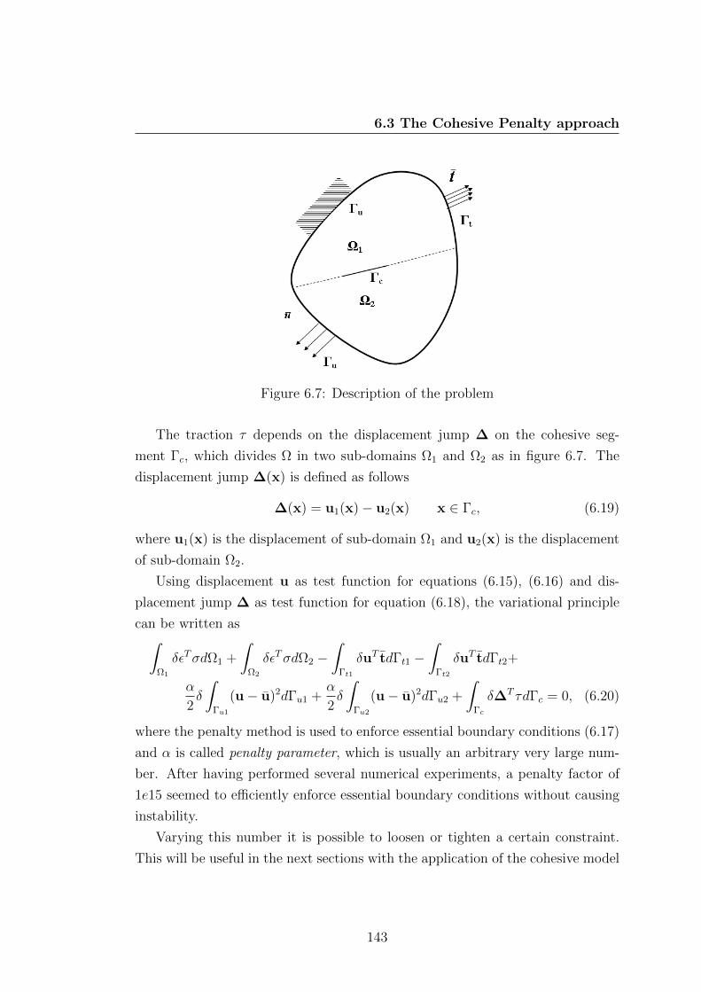
6.3 The Cohesive Penalty approach
Figure 6.7: Description of the problem
The traction τ depends on the displacement jump ∆ on the cohesive seg-
ment Γc, which divides Ω in two sub-domains Ω1 and Ω2 as in figure 6.7. The
displacement jump ∆(x) is defined as follows
∆(x) = u1(x)− u2(x) x ∈ Γc, (6.19)
where u1(x) is the displacement of sub-domain Ω1 and u2(x) is the displacement
of sub-domain Ω2.
Using displacement u as test function for equations (6.15), (6.16) and dis-
placement jump ∆ as test function for equation (6.18), the variational principle
can be written as∫Ω1
δεTσdΩ1 +
∫Ω2
δεTσdΩ2 −∫
Γt1
δuT tdΓt1 −∫
Γt2
δuT tdΓt2+
α
2δ
∫Γu1
(u− u)2dΓu1 +α
2δ
∫Γu2
(u− u)2dΓu2 +
∫Γc
δ∆T τdΓc = 0, (6.20)
where the penalty method is used to enforce essential boundary conditions (6.17)
and α is called penalty parameter, which is usually an arbitrary very large num-
ber. After having performed several numerical experiments, a penalty factor of
1e15 seemed to efficiently enforce essential boundary conditions without causing
instability.
Varying this number it is possible to loosen or tighten a certain constraint.
This will be useful in the next sections with the application of the cohesive model
143
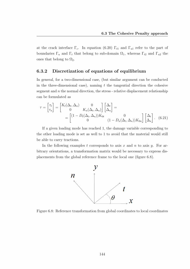
6.3 The Cohesive Penalty approach
at the crack interface Γc. In equation (6.20) Γt1 and Γu1 refer to the part of
boundaries Γu and Γt that belong to sub-domain Ω1, whereas Γt2 and Γu2 the
ones that belong to Ω2.
6.3.2 Discretization of equations of equilibrium
In general, for a two-dimensional case, (but similar argument can be conducted
in the three-dimensional case), naming t the tangential direction the cohesive
segment and n the normal direction, the stress - relative displacement relationship
can be formulated as
τ =
[τtτn
]=
[Kt(∆t,∆n) 0
0 Kn(∆t,∆n)
] [∆t
∆n
]=
=
[(1−Dt(∆t,∆n))K0t 0
0 (1−Dn(∆t,∆n))K0n
] [∆t
∆n
]. (6.21)
If a given loading mode has reached 1, the damage variable corresponding to
the other loading mode is set as well to 1 to avoid that the material would still
be able to carry tractions.
In the following examples t corresponds to axis x and n to axis y. For ar-
bitrary orientations, a transformation matrix would be necessary to express dis-
placements from the global reference frame to the local one (figure 6.8).
Figure 6.8: Reference transformation from global coordinates to local coordinates
144

6.3 The Cohesive Penalty approach
Displacement jump in equation (6.19) can be then expressed as
∆ =
[∆x
∆y
]=
[φT1cU1 − φT2cU2
φT1cV1 − φT2cV2
]=
[φT1c 0 −φT2c 00 φT1c 0 −φT2c
]U1
V1
U2
V2
= φTR,
(6.22)
where
φ1c = φ1(x) x ∈ Γc, (6.23)
where φ1(x) are the shape functions of sub-domain Ω1, whereas
φ2c = φ2(x) x ∈ Γc (6.24)
are the shape functions belonging to sub-domain Ω2,
φT =
[φT1c 0 −φT2c 00 φT1c 0 −φT2c
](6.25)
and RT1 =
[U T
1 V T1
]is the displacement vector for nodes located in Ω1 whereas
RT2 =
[U T
2 V T2
]is the displacement vector for nodes located in Ω2 and RT =[
R T1 R T
2
]is the total displacement vector. Substituting equations (3.1) and
(6.22) in the variational principle (6.20)
δRT1 K1R1 + δRT
2 K2R2 − δRT1 F1t − δRT
2 F2t + αδRT1 V1R1 − αδRT
1 F1u+
αδRT2 V2R2 − αδRT
2 F2u + δRT1 Fc
1 + δRT2 Fc
2 = 0, (6.26)
where
Ki =
∫Ωi
BDBTdΩi i = 1, 2, (6.27)
where D is the stress-strain relationship matrix, B is the differential strain oper-
ator matrix
Vi =
∫Γui
φφTdΓui i = 1, 2, (6.28)
Fiu =
∫Γui
φudΓui i = 1, 2, (6.29)
Fit =
∫Γti
φtdΓti i = 1, 2, (6.30)
145

6.3 The Cohesive Penalty approach
and
Fc1 =
[Fc
x1
Fcy1
], (6.31)
[Fc
x2
Fcy2
], (6.32)
Fcx1 =
∫Γc
φ1cτtdΓc, (6.33)
Fcy1 =
∫Γc
φ1cτndΓc, (6.34)
Fcx2 = −
∫Γc
φ2cτtdΓc, (6.35)
Fcy2 = −
∫Γc
φ2cτndΓc. (6.36)
Finally the following nonlinear set of equations can be obtained
[K + αV] R + Fc(R)− F− αFu = f(R) = 0 (6.37)
where
K =
[K1 00 K2
](6.38)
and
V =
[V1 00 V2
], (6.39)
F =
[F1t
F2t
], (6.40)
Fu =
[F1u
F2u
], (6.41)
Fc =
[Fc
1
Fc2
]. (6.42)
146
6.3 The Cohesive Penalty approach
6.3.3 Tangent Stiffness Matrix
Equation (6.37) must be solved iteratively. A commonly used scheme is the
Newton-Raphson method where the iteration n + 1 at a generic load step is
obtained from iteration n by the formula
R(n+1) = R(n) −(J(n)
)−1f(R(n)), (6.43)
where
J =∂f
∂R. (6.44)
In order to obtain the Jacobian matrix J, a linearization of equation (6.21) is
needed.
τ (n+1) = τ (n) +∂τ
∂∆
(∆(n+1) −∆(n)
)= τ (n) + T
(∆(n+1) −∆(n)
), (6.45)
where
T =∂τ
∂∆=
∂Kx
∂∆x
0
0∂Ky
∂∆y
=
−∂Dx
∂∆x
K0x 0
0 −∂Dy
∂∆y
K0y
. (6.46)
Deriving equation (6.14)
∂D
∂∆=
∆f∆0
∆2(∆f −∆0). (6.47)
Substituting (6.46) into (6.20), the expression of the Jacobian (6.44) can be ob-
tained as
J = K + αV + KT , (6.48)
where
KT =∂Fc
∂R=
∫Γc
φ1c
φ1c
−φ2c
−φ2c
∂τ
∂∆
∂∆
∂RdΓc. (6.49)
Considering equations (6.25) and (6.46)
KT =
∫Γc
φ1c
φ1c
−φ2c
−φ2c
T
[φT1c −φT2c
φT1c −φT2c
]dΓc, (6.50)
147
6.3 The Cohesive Penalty approach
KT =
[KT11 −KT12
−KTT12 KT22
], (6.51)
where
KT11 =
[KT11x 0
0 KT11y
], (6.52)
KT12 =
[KT12x 0
0 KT12y
], (6.53)
KT22 =
[KT22x 0
0 KT22y
], (6.54)
KT ijl =
∫Γc
φic
(Kl(∆l)−Kl0
∆f∆0
∆l(∆f −∆0)
)φjcdΓc i, j = 1, 2 l = x, y.
(6.55)
The equilibrium path for equation (6.37) will be traced with a single param-
eter arc-length continuation method, whose algorithm is explained in appendix
B. The continuation method is essentially based on the Newton-Rhapson algo-
rithm, with some modification in order to take into account the addition of the
parameter, which in this case is the magnitude of the applied force. Therefore
the method used is a force control method. A drawback of the Newton-Rhapson
algorithms is that their (quadratic) convergence is guaranteed only if the guess
solution is close enough to the real solution. In order to accelerate the Newton
process, a cubic polynomial line search (LS) algorithm has been used Press et al.
(1986). LS algorithms are instead globally convergent, since they may converge
independently from the tentative solution.
6.3.4 Convergence Issues in the Numerical Continuation
As reported in Camanho & Davila (2002) and Camanho et al. (2003), the soft-
ening nature of the bilinear cohesive zone model can pose numerical problems.
These problems are related to the convergence of the numerical scheme, that may
not be achieved in some cases. In fact, during the numerical simulations, it has
been experienced that the numerical continuation stops and does not proceed
further. The point of arrest is usually the first unstable point encountered in the
148
6.3 The Cohesive Penalty approach
path, which is when the delamination starts to propagate. In other words, this
point occurs when the relative displacement exceeds the critical value δf , which
means that the strain energy release rate is greater than the critical value Gc for
that particular mode, therefore, according to the Griffith’s theory, there is enough
energy to create new surfaces (the crack surfaces).
The choice of the penalty values is important since it could lead to large
unbalanced forces and shoot the iteration beyond its radius of convergence. Par-
ticularly, the value of inter-facial maximum strength τm exerts a major influence
on the fluency of the numerical scheme. It has been reported in Turon (2007), for
finite elements this effect is due to the length of the cohesive zone. The length of
the cohesive zone is defined as the distance from the crack tip (when the traction
is zero with the bilinear model) to the point where the maximum cohesive trac-
tion τm is attained. If the cohesive zone is discretized by too few elements, the
distribution of tractions ahead of the crack tip is misrepresented, analogously to
the under-sampling phenomenon of a digital signal.
Therefore a very fine mesh should be used if the cohesive length is too small.
The cohesive length is usually proportional to the fracture energy release rate Gc
and to 1τ2m
. The higher the inter-facial strength, the finer the mesh that should
be used. This suggests a way to use coarser mesh, i.e. to arbitrarily reduce the
inter-facial strength, as done in Chen et al. (1999) and Alfano & Crisfield (2001).
This reduction, though, does not compromise the resulting force-displacement
curve, if the reduction is reasonable, but can indeed ease the convergence. A
strong reduction, on the contrary, can lead to inaccurate results; therefore the
reduction of the τm should be used carefully.
Another problem related to the insufficient mesh size is the false instabilities.
Although the critical value can be accurately predicted, an oscillatory behaviour
can be observed in the force-displacement curve. In the finite element context,
these oscillations in the force-displacement curve are due to a sudden release of
the elastic strain energy caused by simultaneous failure of more than one element
per time. Unfortunately, reducing the step-length size in the arc-length proce-
dure does not solve this inconvenient, since it is inherently caused by insufficient
discretization of the interface, i.e. not enough elements.
149

6.3 The Cohesive Penalty approach
False instabilities will be observed in a later ad-hoc example when an artificial
void is introduced in the cohesive contact. This cavity is introduced simply
by setting the penalty parameter to zero in an internal zone of the interface.
One remedy to this issue is obviously to refine (globally or locally). Within
certain limits, though, refinement can be avoided by adding more nodes to the
enrichment, although this increases the number of extra-unknowns.
6.3.5 The class CohesiveContact
6.3.5.1 The properties
The properties of the CohesiveContact are
• d0t, dFt, d0n, dFn, GIc, GIIc, smax I, smax II are the parameters of the
cohesive zone model, as described in section 6.2;
• tx and ty: the tractions at the interface as defined in equation (6.21);
• vx and vy: the displacement jumps at the interface as in equation (6.21);
• ne1 and ne2: the ne1-th edge of Ω1 and the ne2-th edge of Ω2 where the
penalty contact is applied;
• RKPM1 RKPM2 are objects of the class RKPM that calculates φ1c and φ2c in
equation (6.23) and (6.24);
• hn, ht arrays defined on the Gaussian points of the shared edge, with values
0 if there is a pre-crack, 1 otherwise;
• KTt and KTn the derivatives of the penalty factors, as defined in equation
(6.55).
6.3.5.2 The methods
The methods defined for the class CohesiveContact are
• CohesiveContact the constructor, with inputs ne1, ne2 and the file con-
taining the CZM parameters;
150

6.3 The Cohesive Penalty approach
• ApplyContact creates the objects RKPM1 and RKPM2;
• InitSegm allows to insert a pre-crack by entering a logical expression like
x ≥ Lx − a0;
• DisplacementJump calculates equation (6.22)
function obj = DisplacementJump(obj,U1,V1,U2,V2)
obj.vx = obj.RKPM1.PHI*U1-obj.RKPM2.PHI*U2;
obj.vy = obj.RKPM1.PHI*V1-obj.RKPM2.PHI*V2;
end
• CohesiveTraction calculates (6.21) and KTt and KTn
function obj = CohesiveTraction(obj,U1,V1,U2,V2)
obj = DisplacementJump(obj,U1,V1,U2,V2);
[Dt,dDt] = dam(obj.vx,obj.d0t,obj.dFt);
obj.kt = (1-Dt).*obj.Kt0.*obj.ht;
obj.tx = obj.kt.*obj.vx;
obj.KTt = ((1-Dt) - obj.vx.*dDt).*obj.Kt0.*obj.ht;
[Dn,dDn] = dam(obj.vy,obj.d0n,obj.dFn);
obj.kn = (1-Dn).*obj.Kn0.*obj.hn;
obj.ty = obj.kn.*obj.vy;
obj.KTn = ((1-Dn) - obj.vy.*dDn).*obj.Kn0.*obj.hn;
clear Dt Dn dDn dDt
end
where dam is an internal function that calculates (6.14);
• AssembCoupl computes the generalized cohesive force vector (6.42) and the
tangent stiffness matrix (6.51) using the integration methods defined on the
RKPM objects.
151
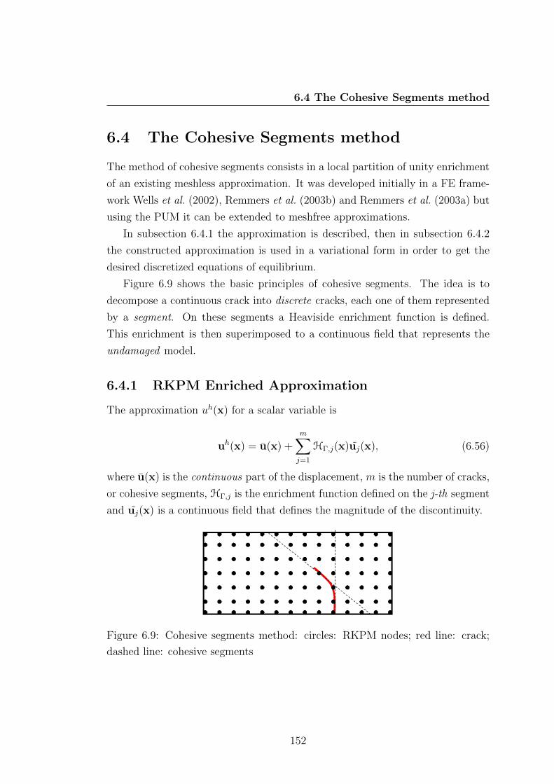
6.4 The Cohesive Segments method
6.4 The Cohesive Segments method
The method of cohesive segments consists in a local partition of unity enrichment
of an existing meshless approximation. It was developed initially in a FE frame-
work Wells et al. (2002), Remmers et al. (2003b) and Remmers et al. (2003a) but
using the PUM it can be extended to meshfree approximations.
In subsection 6.4.1 the approximation is described, then in subsection 6.4.2
the constructed approximation is used in a variational form in order to get the
desired discretized equations of equilibrium.
Figure 6.9 shows the basic principles of cohesive segments. The idea is to
decompose a continuous crack into discrete cracks, each one of them represented
by a segment. On these segments a Heaviside enrichment function is defined.
This enrichment is then superimposed to a continuous field that represents the
undamaged model.
6.4.1 RKPM Enriched Approximation
The approximation uh(x) for a scalar variable is
uh(x) = u(x) +m∑j=1
HΓ,j(x)uj(x), (6.56)
where u(x) is the continuous part of the displacement, m is the number of cracks,
or cohesive segments, HΓ,j is the enrichment function defined on the j-th segment
and uj(x) is a continuous field that defines the magnitude of the discontinuity.
Figure 6.9: Cohesive segments method: circles: RKPM nodes; red line: crack;
dashed line: cohesive segments
152
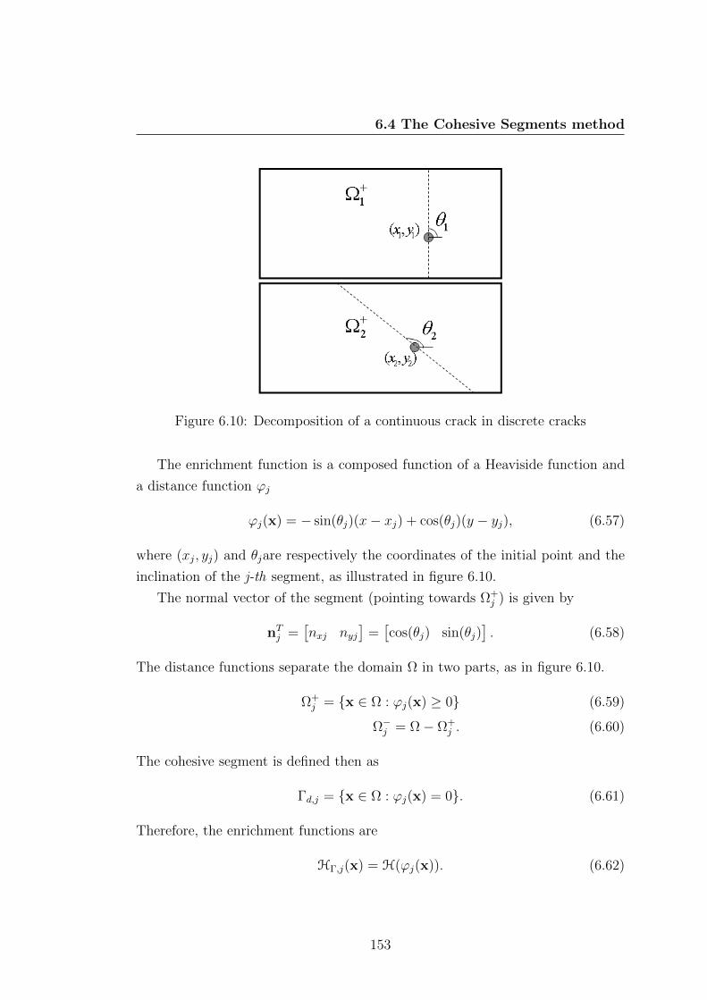
6.4 The Cohesive Segments method
Figure 6.10: Decomposition of a continuous crack in discrete cracks
The enrichment function is a composed function of a Heaviside function and
a distance function ϕj
ϕj(x) = − sin(θj)(x− xj) + cos(θj)(y − yj), (6.57)
where (xj, yj) and θjare respectively the coordinates of the initial point and the
inclination of the j-th segment, as illustrated in figure 6.10.
The normal vector of the segment (pointing towards Ω+j ) is given by
nTj =[nxj nyj
]=[cos(θj) sin(θj)
]. (6.58)
The distance functions separate the domain Ω in two parts, as in figure 6.10.
Ω+j = x ∈ Ω : ϕj(x) ≥ 0 (6.59)
Ω−j = Ω− Ω+j . (6.60)
The cohesive segment is defined then as
Γd,j = x ∈ Ω : ϕj(x) = 0. (6.61)
Therefore, the enrichment functions are
HΓ,j(x) = H(ϕj(x)). (6.62)
153

6.4 The Cohesive Segments method
The infinitesimal strain can be calculated as follows
εh = ∇su(x) +m∑j=1
H(ϕj(x))∇suj(x) + δ(ϕj(x)) (uj(x)⊗ nj) , (6.63)
where the superscript s means the symmetric part of the gradient ∇u(x) and the
δ1 is the Dirac function centered on the segment Γd,j2, i.e. when ϕj(x) = 0 . It
can be shown later that the Dirac term will originate the cohesive traction in the
cohesive segment. This is opposed to the classic linear elastic fracture mechanics
theory Rice (1968), where the fracture faces are considered traction-less, causing
the Dirac term to disappear.
Using the Voigt notation, equation (4.96) can be rearranged as
εh = Lu(x) +m∑j=1
H(ϕj(x))Luj(x) + δ(ϕj(x))Nuj(x), (6.64)
where
N =
nxj nyjnyj nxj.
(6.65)
The RKPM approximation is used for the continuous field u(x) and uj(x)
uh(x) =N∑I=1
φI(x)UI +m∑j=1
H(ϕj(x))
Nj∑i=1
φ(0)i (x)aij x ∈ Ω, (6.66)
where Ω is the domain of the elastic problem, N is the number of the standard
nodes (not enriched), φI is the RKPM shape function for the I − th node, UI is
the I − th (fictitious) displacement in node I , Nj is the number of the enriched
nodes for the j-th crack, φ(0)i (x) is the Shepard shape functions for the i − th
enriched node, aij is the i− th additional variable for the additional crack.
Similarly, for the v component of the displacement
vh(x) =N∑I=1
φI(x)VI +m∑j=1
H(ϕj(x))
Nj∑i=1
φ(0)i (x)bij x ∈ Ω. (6.67)
1not be confused with the variational δ2d means discontinuity
154
6.4 The Cohesive Segments method
If UI = VI = 0 ∀I and aij = bij = 1 ∀J , the functions (6.66) and (6.67) resort to
a sum of Heaviside functions that represent the discontinuities.
Finally, the displacement jump at the k-th segment is given by
∆k(x) =m∑j=1
H(ϕj(x))uj(x) =
=m∑j=1
H(ϕj(x))
[∑Nji=1 φ
(0)i (x)aij∑Nj
i=1 φ(0)i (x)bij
]x ∈ Γd,k. (6.68)
6.4.2 The equations of equilibrium
The equations of equilibrium in strong form are the same of section 6.3, i.e.
(6.15), (6.16), (6.17) with the exception of equation (6.18) that is modified to
allow multiple segments
nj · σ = τ(∆l,j) x ∈ Γd,j j = 1, . . . ,m, (6.69)
where nj is the normal unity vector of the segment Γd,j where the cohesive traction
τ(∆l) is prescribed, l is the local coordinate system.
The traction τ depends on the displacement jump ∆l (transformed in the
local reference t − n where t is the tangent to the segment and n is the normal
direction to the segment) on the cohesive segments Γd,j as described in section
6.2.
The displacement jump ∆(x)l in the local global reference for the j-th segment
instead is
∆l,j(x) = Rj(θ)∆j(x) x ∈ Γd,j (6.70)
where
Rj(θ) =
cos(θj) sin(θj)
− sin(θj) cos(θj)
. (6.71)
Using displacement u as test function for equations (6.15), (6.16) and the
(local) displacement jump ∆l as test function for equation (6.18), the variational
155
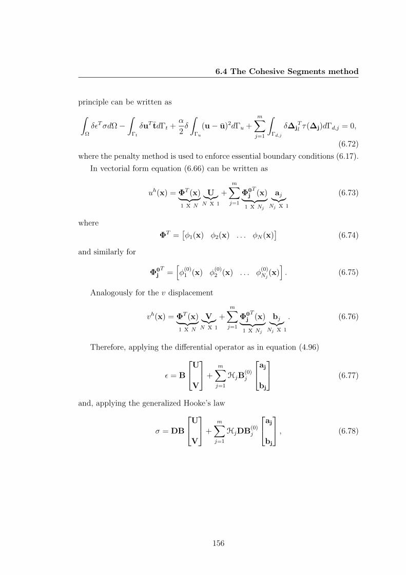
6.4 The Cohesive Segments method
principle can be written as∫Ω
δεTσdΩ−∫
Γt
δuT tdΓt +α
2δ
∫Γu
(u− u)2dΓu +m∑j=1
∫Γd,j
δ∆jTl τ(∆j)dΓd,j = 0,
(6.72)
where the penalty method is used to enforce essential boundary conditions (6.17).
In vectorial form equation (6.66) can be written as
uh(x) = ΦT (x)︸ ︷︷ ︸1 x N
U︸︷︷︸N x 1
+m∑j=1
Φ0jT
(x)︸ ︷︷ ︸1 x Nj
aj︸︷︷︸Nj x 1
(6.73)
where
ΦT =[φ1(x) φ2(x) . . . φN(x)
](6.74)
and similarly for
Φ0jT
=[φ
(0)1 (x) φ
(0)2 (x) . . . φ
(0)Nj
(x)]. (6.75)
Analogously for the v displacement
vh(x) = ΦT (x)︸ ︷︷ ︸1 x N
V︸︷︷︸N x 1
+m∑j=1
Φ0jT
(x)︸ ︷︷ ︸1 x Nj
bj︸︷︷︸Nj x 1
. (6.76)
Therefore, applying the differential operator as in equation (4.96)
ε = B
U
V
+m∑j=1
HjB(0)j
aj
bj
(6.77)
and, applying the generalized Hooke’s law
σ = DB
U
V
+m∑j=1
HjDB(0)j
aj
bj
, (6.78)
156

6.4 The Cohesive Segments method
the first term in (6.20) reads as
∫Ω
δεTσdΩ =
∫Ω
(δRTBT +
m∑j=1
δcTj HjB(0)Tj
)D
(BR +
m∑k=1
HkB(0)Tk ck
)dΩ =
= δRT
[∫Ω
BTDBdΩ
]R + δRT
m∑j=1
[∫Ω
BTDB(0)THjdΩ
]cj+
+m∑k=1
δcTk
[∫Ω
B(0)DBHkdΩ
]R +
m∑k=1
m∑j=1
δcTk
[∫Ω
B(0)TDB(0)HkHjdΩ
]cj
(6.79)
where RT =[UT , VT
]and cTj =
[aTj , bTj
]and Hj is the enrichment
function as in equation (6.62).
The variational term for the forces is as follow
∫Γt
δuT tdΓ = δRT
[∫Γt
ΦtxdΓ∫Γt
ΦtydΓ
]+
m∑j=1
δcTj Hj
[∫Γt
Φ(0)txdΓ∫Γt
Φ(0)tydΓ
]. (6.80)
The same term can be obtained for the cohesive forces, i.e. the term∫Γl,j
δ∆Tl,jτ(∆l,j)dΓd,j. (6.81)
In a non-linear perspective, the relative displacement ∆l,j must be calculated
first, in order to obtain the traction τ . Using the coordinate transformation
(6.70),
∆l,j = Rj(θ)∆j = Rj(θ)m∑k=1
Hk
[ΦT(0)
k ak
ΦT(0)k bk
]x ∈ Γd,j, (6.82)
∫Γd,j
δ∆l,jT τ(∆l,j)dΓd,j =
=m∑k=1
δcTkHk
[∫Γd,j
Φ(0)k [τt(∆l,j) cos(θj)− τn(∆l,j) sin(θj)] dΓd,j∫
Γd,jΦ(0)
k [τt(∆l,j) sin(θj) + τn(∆l,j) cos(θj)] dΓd,j
]. (6.83)
157
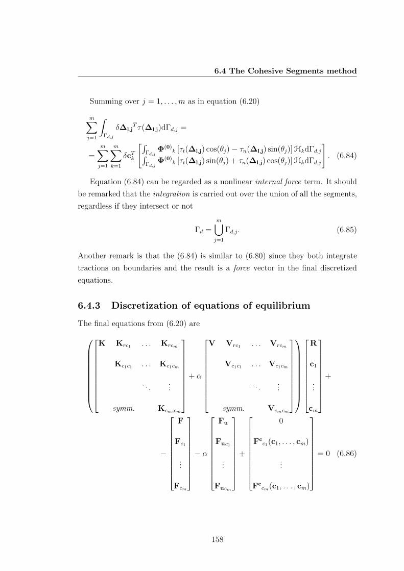
6.4 The Cohesive Segments method
Summing over j = 1, . . . ,m as in equation (6.20)
m∑j=1
∫Γd,j
δ∆l,jT τ(∆l,j)dΓd,j =
=m∑j=1
m∑k=1
δcTk
[∫Γd,j
Φ(0)k [τt(∆l,j) cos(θj)− τn(∆l,j) sin(θj)]HkdΓd,j∫
Γd,jΦ(0)
k [τt(∆l,j) sin(θj) + τn(∆l,j) cos(θj)]HkdΓd,j
]. (6.84)
Equation (6.84) can be regarded as a nonlinear internal force term. It should
be remarked that the integration is carried out over the union of all the segments,
regardless if they intersect or not
Γd =m⋃j=1
Γd,j. (6.85)
Another remark is that the (6.84) is similar to (6.80) since they both integrate
tractions on boundaries and the result is a force vector in the final discretized
equations.
6.4.3 Discretization of equations of equilibrium
The final equations from (6.20) are
K Krc1 . . . Krcm
Kc1c1 . . . Kc1cm
. . ....
symm. Kcm,cm
+ α
V Vrc1 . . . Vrcm
Vc1c1 . . . Vc1cm
. . ....
symm. Vcmcm
R
c1
...
cm
+
−
F
Fc1
...
Fcm
− α
Fu
Fuc1
...
Fucm
+
0
Fcc1(c1, . . . , cm)
...
Fccm(c1, . . . , cm)
= 0 (6.86)
158

6.4 The Cohesive Segments method
where
K =
∫Ω
BTDBdΩ, (6.87)
Krcj =
∫Ω+j
BTDB(0)j dΩ, (6.88)
Kcicj =
∫Ω+i ∩Ω+
j
B(0)Ti DB
(0)j dΩ, (6.89)
Vu = Vv =
∫Γu
ΦΦTdΓu, (6.90)
V =
Vu
Vv
, (6.91)
Vuaj = Vvbj =
∫Γu
ΦΦ(0)Tj HjdΓu, (6.92)
Vrcj =
Vuaj
Vvbj
, (6.93)
Vaiaj = Vbibj =
∫Γu
Φ(0)i Φ
(0)Tj HiHjdΓu, (6.94)
Vcicj =
Vaiaj
Vbibj
, (6.95)
Fx =
∫Γt
ΦtxdΓt, (6.96)
Fy =
∫Γt
ΦtydΓt, (6.97)
F =
Fx
Fy
, (6.98)
Fx,ci =
∫Γt
Φ(0)i txHidΓt, (6.99)
159
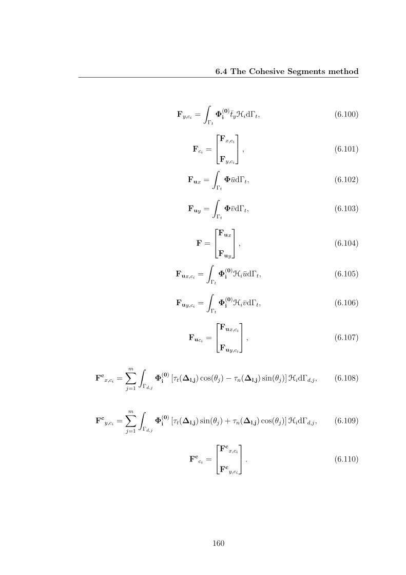
6.4 The Cohesive Segments method
Fy,ci =
∫Γt
Φ(0)i tyHidΓt, (6.100)
Fci =
Fx,ci
Fy,ci
, (6.101)
Fux =
∫Γt
ΦudΓt, (6.102)
Fuy =
∫Γt
ΦvdΓt, (6.103)
F =
Fux
Fuy
, (6.104)
Fux,ci =
∫Γt
Φ(0)i HiudΓt, (6.105)
Fuy,ci =
∫Γt
Φ(0)i HivdΓt, (6.106)
Fuci =
Fux,ci
Fuy,ci
, (6.107)
Fcx,ci =
m∑j=1
∫Γd,j
Φ(0)i [τt(∆l,j) cos(θj)− τn(∆l,j) sin(θj)]HidΓd,j, (6.108)
Fcy,ci =
m∑j=1
∫Γd,j
Φ(0)i [τt(∆l,j) sin(θj) + τn(∆l,j) cos(θj)]HidΓd,j, (6.109)
Fcci =
Fcx,ci
Fcy,ci
. (6.110)
160
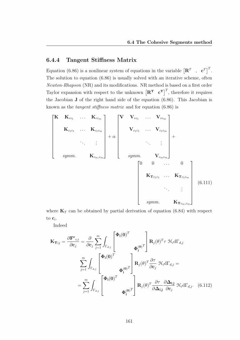
6.4 The Cohesive Segments method
6.4.4 Tangent Stiffness Matrix
Equation (6.86) is a nonlinear system of equations in the variable[RT , cT
]T.
The solution to equation (6.86) is usually solved with an iterative scheme, often
Newton-Rhapson (NR) and its modifications. NR method is based on a first order
Taylor expansion with respect to the unknown[RT cT
]T, therefore it requires
the Jacobian J of the right hand side of the equation (6.86). This Jacobian is
known as the tangent stiffness matrix and for equation (6.86) is
K Krc1 . . . Krcm
Kc1c1 . . . Kc1cm
. . ....
symm. Kcm,cm
+ α
V Vrc1 . . . Vrcm
Vc1c1 . . . Vc1cm
. . ....
symm. Vcmcm
+
0 0 . . . 0
KTc1c1 . . . KTc1cm
. . ....
symm. KTcm,cm
(6.111)
where KT can be obtained by partial derivation of equation (6.84) with respect
to ci.
Indeed
KTij =∂Fc
c,i
∂cj=
∂
∂cj
m∑j=1
∫Γd,j
Φi(0)T
Φ(0)i
T
Rj(θ)T τ HidΓd,j
m∑j=1
∫Γd,j
Φi(0)T
Φ(0)i
T
Rj(θ)T ∂τ
∂cjHidΓd,j =
=m∑j=1
∫Γd,j
Φi(0)T
Φ(0)i
T
Rj(θ)T ∂τ
∂∆l,j
∂∆l,j
∂cjHidΓd,j. (6.112)
161
6.4 The Cohesive Segments method
From equation (6.82)
∂∆l,j
∂cj= Rj(θ)Hj
Φ(0)j
T
Φ(0)j
T
. (6.113)
The Jacobian of the tractions with respect to the relative displacements is
equation (6.46). Therefore,
KTij =
∫Γd,j
HiHj
Φ(0)i
Φ(0)i
Rj(θ)TTRj(θ)
Φ(0)j
T
Φ(0)j
T
dΓd,j =
[KTij11 KTij12
KTij21 KTij22
](6.114)
where
KTij11 =
∫Γd,j
HiHjΦ(0)i Φ
(0)j
Tcos(θj)(T11 cos(θj)−T21 sin(θj))+
− sin(θj)(T12 cos(θj)−T22 sin(θj))dΓd,j, (6.115)
KTij12 =
∫Γd,j
HiHjΦ(0)i Φ
(0)j
Tcos(θj)(T12 cos(θj)−T22 sin(θj))+
+ sin(θj)(T11 cos(θj)−T21 sin(θj))dΓd,j, (6.116)
KTij21 =
∫Γd,j
HiHjΦ(0)i Φ
(0)j
Tcos(θj)(T21 cos(θj) + T11 sin(θj))+
− sin(θj)(T222 cos(θj) + T12 sin(θj))dΓd,j, (6.117)
KTij22 =
∫Γd,j
HiHjΦ(0)i Φ
(0)j
Tcos(θj)(T22 cos(θj) + T12 sin(θj))+
+ sin(θj)(T21 cos(θj) + T11 sin(θj))dΓd,j. (6.118)
162

6.4 The Cohesive Segments method
6.4.5 Selection of Enriched Nodes
Equations (6.66) and (6.67) allow the introduction of the enrichment. The choice
of the enriched nodes is therefore an important part of the algorithm, since it
allows to locally introducing the discontinuity. Equations (6.66) and (6.67) are
only valid if the PU is built on nodes whose support is cut (partially or entirely)
by the discontinuity.
The selection is then made upon comparison of the distances between the node
and the segment (figures 6.11 and 6.12). If the distance is less than the dilata-
tion parameter, then the node is selected for enrichment, otherwise is discarded.
Calling Senr,j the set of enriched nodes for the j − th crack
Senr,j = xI ∈ S1 : |xI − x| ≤ ρI x ∈ Γd,j (6.119)
where S1 is the set of RKPM nodes.
Naming h(xI ,x) = |xI − x| a distance function, equation (6.119) can be
formulated as
Senr,j = xI ∈ S1 : h(xI ,x) ≤ ρI x ∈ Γd,j . (6.120)
Hence, to correctly select the nodes, it is important to use an appropriate
distance function. In two dimensions, if Γd,j is a straight line, then it is easy to
construct h(x). If Γd,j is instead a segment P1P2
P1 ≡ (x1, y1) P2 ≡ (x2, y2) (6.121)
the distance function is slightly more elaborated. In fact, it should take into
account the endpoints of the segment, where the distance function is not the usual
distance from a straight line, but it is the distance from a point. An appropriate
distance function in this sense should blend these two distance function. In this
section a quite easy approach is proposed. The basic idea is to use Heaviside
functions on the parameter t that defines a segmentx(t) = x1 + t(x2 − x1)
y(t) = y1 + t(y2 − y1) t ∈ [0, 1]. (6.122)
163

6.4 The Cohesive Segments method
Defining
dT =[x2 − x1 , y2 − y1
], (6.123)
rT1 =[x− x1 , y − y1
], (6.124)
rT2 =[x− x2 , y − y2
], (6.125)
then the parameter t can be defined ∀ (x, y) ∈ R2
t = t(x, y) =dT r1
‖d‖2 =(x2 − x1)(x− x1) + (y2 − y1)(y − y1)
(x2 − x1)2 + (y2 − y1)2, (6.126)
then
a = (x− x1)2 + (y − y1)2, (6.127)
b = (x− x2)2 + (y − y2)2, (6.128)
c = [x− x1 − t(x2 − x1)]2 + [y − y1 − t(y2 − y1)]2. (6.129)
Then the (minimum) distance function (not signed) h(x, y) for a generic point
(x, y) from the segment P1P2 is
h(x, y) = a(x, y)H(−t(x, y)) + c(x, y) [H(t(x, y))−H(t(x, y)− 1)] +
+ b(x, y)H(t(x, y)− 1), (6.130)
where H is the Heaviside function.
The Matlab implementation can be easily done using function handles or
inline functions. For example
t = inline(’[(x2-x1).*(x-x1)+(y2-y1).*(y-y1)]./(((x2-x1).^2...
+(y2-y1).^2))’,’x’,’y’,’x1’,’x2’,’y1’,’y2’);
a = inline(’(x-x1).^2+(y-y1).^2’,’x’,’y’,’x1’,’y1’);
164

6.4 The Cohesive Segments method
b = inline(’(x-x2).^2+(y-y2).^2’,’x’,’y’,’x2’,’y2’);
c = inline(’(x-(x1+t(x,y,x1,x2,y1,y2)*(x2-x1))).^2+...
...+(y-(y1+t(x,y,x1,x2,y1,y2)*(y2-y1))).^2’...
...,’x’,’y’,’x1’,’x2’,’y1’,’y2’,’t’);
h = inline(’a(x,y,x1,y1).*heaviside(-t(x,y,x1,x2,y1,y2))+...
...+c(x,y,x1,x2,y1,y2,t).*[heaviside(t(x,y,x1,x2,y1,y2))+...
-heaviside(t(x,y,x1,x2,y1,y2)-1)]+...
...+b(x,y,x2,y2).*heaviside(t(x,y,x1,x2,y1,y2)-1)’,...
’x’,’y’,’x1’,’x2’,’y1’,’y2’,’a’,’b’,’c’,’t’)
Once known the vectors d and r1, function h can be directly evaluated on the
coordinates of the RKPM nodes and then compared to their respective dilatation
parameters.
Figures 6.13 and 6.14 show the selection of the nodes using the function h(x, y)
in equation (6.130) for a segment shown in figure 6.11.
Figure 6.11: Cohesive segments: Gaussian points defined over the segment; red
crosses: Gaussian points; black points: RKPM nodes
Figure 6.12: Cohesive segments: Gaussian points defined over the segment
(zoom); red crosses: Gaussian points; black points: RKPM nodes
165

6.4 The Cohesive Segments method
Figure 6.13: Cohesive segments: selection of enriched nodes; black: RKPM nodes;
pink: enriched nodes
Figure 6.14: Cohesive segments: selection of enriched nodes (zoom); black:
RKPM nodes; pink: enriched nodes
6.4.6 Numerical Examples
Numerical applications regarding single mode delamination are presented in this
section. The fracture modes studied are mode I with three Double Cantilevered
Beam (DCB) tests (figures 6.15 and 6.18) and mode II with an End Loaded
Split test (ELS) (figure 6.16) and two End Notched Flexure (ENF) tests (figure
6.17). These tests were performed assuming that an initial crack already existed.
In order to simulate an initial delamination (indicated with a0), penalty factors
were set to zero at the pre-crack.
An additional test (figure 6.19) with no initial crack was performed, with the
scope of simulating initiation of the fracture.
Furthermore, a DCB beam with multiple failures is simulated to better un-
derstand the phenomena of false instabilities in the equilibrium path.
In all cases a full quadratic polynomial basis and regular arrangement of nodes
have been used. By regular arrangement of nodes it is intended a distribution
of nodes disposed as the vertices of a rectangular grid, as in figure 6.9. In the
166

6.4 The Cohesive Segments method
following examples it will be indicated with ny × nx, where ny is the number of
nodes along the thickness and nx the number of nodes along the length.
The number nx is chosen according to the aspect ratio of the plate L/b
nx =L
bny (6.131)
approximated to the next integer number.
The numerical quadrature used to calculate the stiffness matrices and the
force vectors is Gaussian quadrature carried out over triangular elements, with a
3rd order quadrature.
The quadrature cells over the segments should be always constructed bearing
in mind the under-sampling problem due to the cohesive zone. In the following
examples the length is chosen to assure that the longest segment is discretized
with at least 200 quadrature cells.
Although quadrilateral elements may seem more suitable for a regular ar-
rangement of nodes. Nevertheless, triangular elements are preferred, since an
automatic triangular mesh can always be constructed with ease; therefore the
code gains in versatility and robustness. Moreover, since the kernel used is a
circular support one, the advantage of a background mesh aligned with the sup-
port, as in Dolbow & Belytschko (1999) would be lost anyway. Nonetheless,
accurate results can still be obtained, as shown in the next examples. The order
of quadrature chosen is the best compromise between number of Gaussian points
and quadrature. In fact, a higher order of quadrature could be more accurate,
but leads to a much greater number of points. Since a n − th order Gaussian
quadrature rule has accuracy O(2n− 1), for n = 3 the accuracy is guaranteed up
to the 5− th order.
A full quadratic basis was used for the standard RKPM approximation, while
the enrichments have been constructed with Shepard functions, that are very
easy to construct, as smooth as the kernel functions and have the same order
of continuity. Furthermore, the PSI, ig, js, dPSIcsi and dPSIeta used for the
RKPM can be stored and re-used to calculate the Shepard functions, allowing
savings in computational run-time.
167

6.4 The Cohesive Segments method
Figure 6.15: Double Cantilevered Beam: geometry and boundary conditions
Figure 6.16: End Loaded Split: geometry and boundary conditions
Figure 6.17: End Notched Flexure: geometry and boundary conditions
168
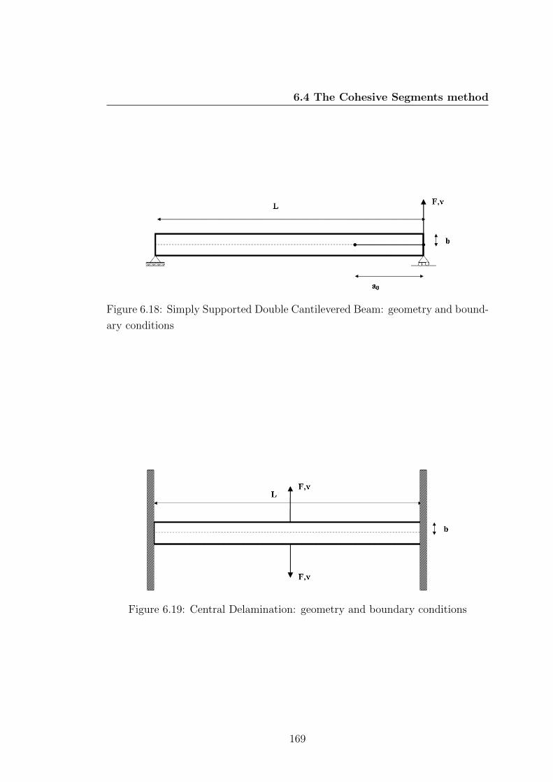
6.4 The Cohesive Segments method
Figure 6.18: Simply Supported Double Cantilevered Beam: geometry and bound-
ary conditions
Figure 6.19: Central Delamination: geometry and boundary conditions
169
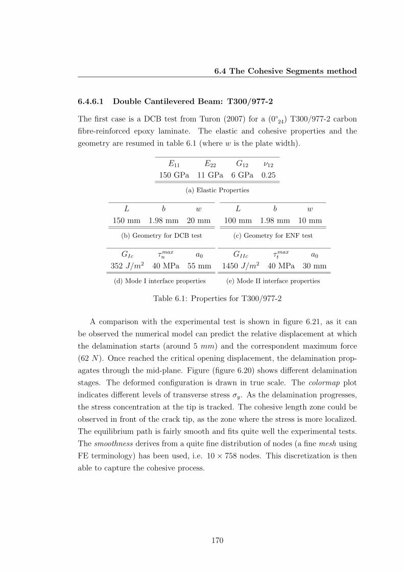
6.4 The Cohesive Segments method
6.4.6.1 Double Cantilevered Beam: T300/977-2
The first case is a DCB test from Turon (2007) for a (024) T300/977-2 carbon
fibre-reinforced epoxy laminate. The elastic and cohesive properties and the
geometry are resumed in table 6.1 (where w is the plate width).
E11 E22 G12 ν12
150 GPa 11 GPa 6 GPa 0.25
(a) Elastic Properties
L b w
150 mm 1.98 mm 20 mm
(b) Geometry for DCB test
L b w
100 mm 1.98 mm 10 mm
(c) Geometry for ENF test
GIc τmaxn a0
352 J/m2 40 MPa 55 mm
(d) Mode I interface properties
GIIc τmaxt a0
1450 J/m2 40 MPa 30 mm
(e) Mode II interface properties
Table 6.1: Properties for T300/977-2
A comparison with the experimental test is shown in figure 6.21, as it can
be observed the numerical model can predict the relative displacement at which
the delamination starts (around 5 mm) and the correspondent maximum force
(62 N). Once reached the critical opening displacement, the delamination prop-
agates through the mid-plane. Figure (figure 6.20) shows different delamination
stages. The deformed configuration is drawn in true scale. The colormap plot
indicates different levels of transverse stress σy. As the delamination progresses,
the stress concentration at the tip is tracked. The cohesive length zone could be
observed in front of the crack tip, as the zone where the stress is more localized.
The equilibrium path is fairly smooth and fits quite well the experimental tests.
The smoothness derives from a quite fine distribution of nodes (a fine mesh using
FE terminology) has been used, i.e. 10 × 758 nodes. This discretization is then
able to capture the cohesive process.
170

6.4 The Cohesive Segments method
Figure 6.20: Delamination Stages for DCB test T300/977-2: transverse stress σy
plot
Figure 6.21: Force-Displacement curve for DCB test T300/977-2 : continuous
line: numerical; squared line: experimental
171

6.4 The Cohesive Segments method
6.4.6.2 Double Cantilevered Beam: XAS-913C
The second DCB case is from Alfano & Crisfield (2001) for a XAS-913C carbon-
fiber epoxy composite. The distribution of nodes is 8× 533. The properties and
the initial conditions are reported in table 6.2. The plate has been modelled as
figure 6.15 and there is only a slight difference between the experimental test and
the numerical results regarding the reaction force (figure 6.22).
E11 E22 G12 ν12
126 GPa 7.5 GPa 4.981 GPa 0.281
(a) Elastic Properties
GIc τm a0
263 J/m2 57 MPa 30 mm
(b) Interface properties
L b w
100 mm 1.5mm 30 mm
(c) Geometry
Table 6.2: Properties for DCB test XAS-913C
Figure 6.22: Force-Displacement curve for DCB test XAS-913C : continuous line:
numerical; squared line: experimental
In figures 6.23 are depicted the stress color plot for the longitudinal stress
172

6.4 The Cohesive Segments method
σx (figure 6.23a) and the shear stress τxy (figure 6.23b). As expected, each de-
laminated arm behaves like a cantilevered beam in bending constrained at the
delamination tip. The same distribution can be identified in the next examples.
(a) σx
(b) τxy
Figure 6.23: Delamination stress plot for DCB test XAS-913C
6.4.6.3 Double Cantilevered Beam: AS4/PEEK
The third DCB case is taken from Camanho & Davila (2002) for a thermoplastic
laminate AS4/PEEK. The boundary conditions are in this case changed, as in
figure 6.18. The plate is simply supported at both ends, loaded with a vertical
force at the right end. Nevertheless, the plate is still loading in mode I. In fact,
the only reaction force is located at the right end, opposite the external force, as
in a DCB test. The elastic and interface properties are resumed in table 6.3 and
the distribution of nodes is 8× 523.
Even though local bumps in the equilibrium path appear to be more evi-
dent (figure 6.24), still there is a good fit between the numerical results and the
experimental tests.
6.4.6.4 Double Cantilevered Beam: Plane Stress or Plane Strain?
In the next example a comparison between two different tensional states is pre-
sented. For real structures, there are two cases where the stress (or the strain)
tensor can be simplified and some components neglected and therefore the anal-
ysis can be reduced from a three-dimensional stress analysis to a more simple
and less expensive two-dimensional analysis. Such two-dimensional structure can
173
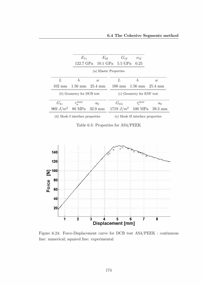
6.4 The Cohesive Segments method
E11 E22 G12 ν12
122.7 GPa 10.1 GPa 5.5 GPa 0.25
(a) Elastic Properties
L b w
102 mm 1.56 mm 25.4 mm
(b) Geometry for DCB test
L b w
100 mm 1.56 mm 25.4 mm
(c) Geometry for ENF test
GIc τmaxn a0
969 J/m2 80 MPa 32.9 mm
(d) Mode I interface properties
GIIc τmaxt a0
1719 J/m2 100 MPa 39.3 mm
(e) Mode II interface properties
Table 6.3: Properties for AS4/PEEK
Figure 6.24: Force-Displacement curve for DCB test AS4/PEEK : continuous
line: numerical; squared line: experimental
174

6.4 The Cohesive Segments method
be either in plane stress or plane strain. A plane stress state is usually found in
structures with one dimension much smaller than the other two, while for struc-
tures with one dimension much larger than the other two a plane strain state can
be more properly assumed.
The link between the two theories is equation (4.99) and one can pass from
one analysis to the other just changing the elastic properties. Nevertheless, the
stress states are rather different. Supposing z the third dimension, a plane stress
state assumes that σzz ≈ 0, but according to Hooke’s law, the consequence is
that εzz 6= 0, while for plane strain it is assumed that εzz ≈ 0 with a consequent
σzz 6= 0. Both these non-zero terms, though, can be temporarily removed from
the analysis and reducing the problem to a two dimensional one.
In the case of delamination, the length L is usually the largest dimension,
but also the dimension where the delamination propagates, so it cannot be ne-
glected. The dimension that can be neglected is the width w, since the relevant
mechanisms for delamination occur in the length and in the thickness 2b. In Al-
fano & Crisfield (2001) it is suggested that delamination can be treated as a two
dimensional analysis in plane strain, assuming the width as neglected dimension.
In order to verify this assumption, in this subsection it is simulated a DCB
in both plane stress and plane strain and the results compared. The elastic
properties and the geometry are reported in table 6.4 and the experimental results
taken from Chen et al. (1999). The distribution of nodes used is 8× 774. Figure
6.25 shows that the plane strain state predict the peak load more accurately
than the plane stress, while both can almost identically predict the post critical
opening phase.
6.4.6.5 End Loaded Split (ELS)
Delamination of mode II (sliding mode) has been modeled as in figure 6.16 with
a loading displacement applied at the free end of the bottom plate. For mode II
loading, the interfaces are here supposed frictionless. Properties and geometry
are summarized in table 6.4. Experimental results are taken from Chen et al.
(1999), while the distribution of nodes used is 8× 550.
175

6.4 The Cohesive Segments method
Figure 6.25: Force - Displacement curve for DCB test in Chen et al. (1999)
: continuous line: numerical plane strain; dashed line: numerical plane stress;
squared line: experimental
From figure 6.26 it can be observed that the model can capture the trend
with a minor difference from the experimental test. In figures 6.27 and 6.28 it
is pretty clear the presence of the damage and the stresses are distributed as
expected. In fact, in the longitudinal stress plot (figure 6.27) , two zones can
be readily identified: ahead the crack tip, the plate responds as an entire plate
and the distribution is typical for a plate in bending; behind the crack tip, where
there is separation, the longitudinal stress is representative of two distinct plates
in bending.
In figure 6.28 instead it can be observed the stress concentration due to the
presence of the delamination. The cohesive zone is shaped like a bubble and it
can usefully track the progression of the delamination.
The critical opening displacement is around 15 mm, after that the delamina-
tion advances quite rapidly (figures 6.27 and 6.28 ). The delamination is complete
(split) for a displacement of 21 mm, after that the two beams respond separately
to the loads.
176

6.4 The Cohesive Segments method
E11 E22 G12 ν12
130 GPa 8 GPa 5 GPa 0.27
(a) Elastic Properties
L b w
150 mm 1.55 mm 24 mm
(b) Geometry for DCB test
L b w
105 mm 1.525 mm 24 mm
(c) Geometry for ELS test
GIc τmaxn a0
257 J/m2 20 MPa 22 mm
(d) Mode I interface properties
GIIc τmaxt a0
856 J/m2 48 MPa 60 mm
(e) Mode II interface properties
Table 6.4: Properties for material in Chen et al. (1999)
Figure 6.26: Force-Displacement curve for ELS test : continuous line: numerical
; squared line: experimental
177

6.4 The Cohesive Segments method
Figure 6.27: Delamination Stages for ELS test: longitudinal stress σx plot
Figure 6.28: Delamination Stages for ELS test: longitudinal stress τxy plot
178

6.4 The Cohesive Segments method
6.4.6.6 Mode II End Notched Flexure: AS4/PEEK
Another example of Mode II loading is an ENF test where a vertical force is
applied in the middle of a simply supported beam with an initial delamination
length (three-point bending as in figure 6.17 ) Experimental results are taken from
Camanho & Davila (2002) and geometry and properties (AS4/PEEK) 6.3 are the
same of subsection 6.4.6.3. The distribution of nodes is 8 × 512. Once again a
good agreement can be observed between the experimental and the numerical
results. The critical opening displacement is perfectly predicted with a minor
difference in the value of the peak force. Delamination phases can be observed
from figures 6.30 and 6.31. From both pictures the effects of the delamination
are pretty clear. Wherever the bonding is full, the plate responds to the load
as a beam with a concentrated load in the middle, otherwise the disconnected
parts behave independently. The beam is, as expected, in tension for the bottom
and in compression for the top (6.30).This is true for both the areas ahead and
behind the crack tip. The crack tip can be easily individuated also from the
bubble-like shear stress concentration in figure 6.31. The last phase of picture
6.31 indicates full delamination and the shear stress is piecewise constant along
the beam length, with a discontinuity, as expected, in the middle where the load
is applied.
6.4.6.7 Mode II End Notched Flexure: T300/977-2
Final example for mode II is an ENF test for a graphite/epoxy material T300/977-
2 (same specimen of DCB test in subsection 6.4.6.1 but with different width) taken
from Davila et al. (2001) whose elastic and interface properties are resumed in
tables 6.1. The distribution of nodes used is 8 × 404. The figure 6.32 shows a
comparison with FE decohesion elements which has been the most widely FE-
based used technique for delamination modelling. As it can seen, results are very
similar. Moreover the curve is much smoother than the previous case. This is
mainly due to convergence issues as mentioned in the previous section 6.3.4.
179

6.4 The Cohesive Segments method
Figure 6.29: Force-Displacement curve for ENF test (AS4/PEEK) : continuous
line: numerical ; dashed line: experimental
Figure 6.30: Delamination Stages for ENF test: longitudinal stress σx plot
180

6.4 The Cohesive Segments method
Figure 6.31: Delamination Stages for ENF test: shear stress τxy plot
Figure 6.32: Force-Displacement curve for ENF test (T300/977-2) : continuous
thick line: RKPM ; continuous thin line: FE decohesion
181

6.4 The Cohesive Segments method
6.4.6.8 Central delamination with no pre-crack
The next case is a loading mode I delamination with no initial pre-crack. The
specimen is cantilevered at the ends and transversely loaded, as in figure 6.19.
The specimen is the same for Mode I in table 6.4 except that a0 = 0 . The cohesive
approach allows the initiation and subsequent propagation of the crack, as it can
be seen from the first phases of delamination in figures 6.33, 6.34 and 6.35. The
complete equilibrium path is shown in figure 6.36. The first part of the curve (in
figure 6.37 ) is an elastic phase with high stiffness and very small displacements
(from 0 to 500 N), since the material is supposed undamaged and a relatively
high force is necessary to overcome the cohesive tractions at the interface. After
500 N the response is plastic-like, until the delamination starts for a peak load of
almost 1500 N and an opening displacement of less than 0.05 mm. Subsequently
the delamination propagates symmetrically respect to the middle, with patterns
similar to the DCB tests examined previously, until complete delamination, when
the two beams split (around 2.25 mm).
6.4.6.9 Double Cantilevered Beam with multiple cavities
As anticipated in subsection 6.3.4, there are some numerical issued due to a char-
acteristic length related to the cohesive zone, namely the cohesive length. This
issue affects the nodes distribution, since it should be efficiently fine to capture the
concentration of the stress, otherwise the under-sampling can alter the equilib-
rium path. The consequences are normally two-fold: the arrest of the numerical
continuation and the appearance of spurious bumps in the equilibrium path. In
figure 6.38 is shown the path for the DCB case in 6.4.6.1 with a coarser mesh.
The false instabilities appear after the initiation of the delamination, although
the peak load is predicted very accurately. Therefore, if the main purpose of using
the code is to estimate the peak load and the critical opening length, a coarser
mesh, which is computationally inexpensive, would seem sufficient. Nevertheless,
the following examples will show that this approach fails due to the presence of
instabilities too close to the initial crack and the peak load might not be predicted
accurately.
182
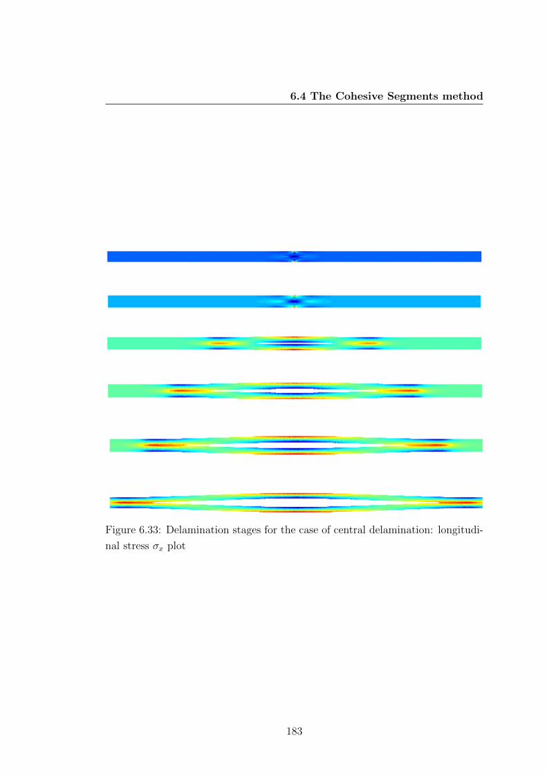
6.4 The Cohesive Segments method
Figure 6.33: Delamination stages for the case of central delamination: longitudi-
nal stress σx plot
183
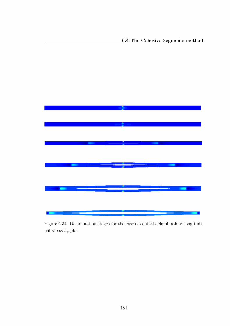
6.4 The Cohesive Segments method
Figure 6.34: Delamination stages for the case of central delamination: longitudi-
nal stress σy plot
184
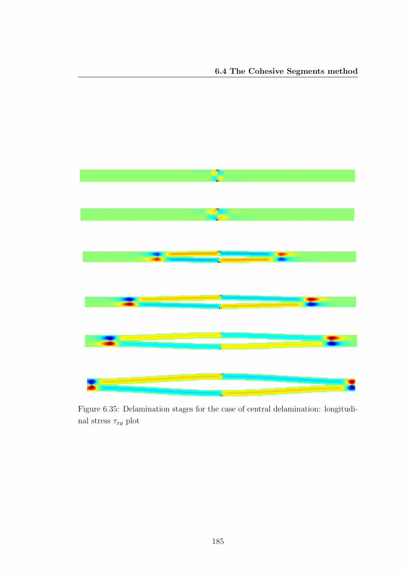
6.4 The Cohesive Segments method
Figure 6.35: Delamination stages for the case of central delamination: longitudi-
nal stress τxy plot
185

6.4 The Cohesive Segments method
Figure 6.36: Force-Displacement curve for central delamination
Figure 6.37: Force-Displacement curve for central delamination (zoom on the
initial phase)
186

6.4 The Cohesive Segments method
Figure 6.38: Force-Displacement curve for DCB test T300 with coarser mesh
5× 378
In Samimi et al. (2009) is reported that these local bumps are caused by
sudden release of strain energy. This release is due to simultaneous failure of
areas of the interface wider than the cohesive length. The areas are more precisely
elements, if too few it may happen more elements than necessary may improperly
satisfy the separation criterion and therefore cause de-bonding. To test this
statement, the false instabilities were simulated with failures in the contact, .i.e.
the penalty stiffnesses were set to zero locally (as in figure 6.39) and the position
and the number have been varied. The case tested is a DCB for an isotropic
material in plane stress. The elastic properties of the material and the geometry
are resumed in table 6.5 and the distribution of nodes is 11× 1100.
The first example is represented in figure 6.39 where a first pre-crack is present
and internal failures have been introduced periodically. The length of the failed
zone is the same of the pre-crack (1 mm) and their separation is equal to the
length of the pre-crack.
In figure 6.42 the presence of multiple failures is manifested by wide bumps in
the curve that occur when the delamination reaches a failed segment. Around a
187

6.4 The Cohesive Segments method
E ν
100 MPa 0.3
(a) Elastic Properties
GIc τm a0
100 J/m2 1 MPa 1 mm
(b) Interface properties
L b w
10 mm 1 mm 1 mm
(c) Geometry
Table 6.5: Properties for DCB test with cavities
displacement of 3 mm, the continuation interrupted as convergence of the model
was not further achieved. By interruption it is meant that the continuation code,
being a path following technique, tries to reduce the step-length on the equilib-
rium path. If convergence is not achieved, the step-length (a value of 10−5 m is
usually a good choice) is reduced further until a convergent state is found. Usu-
ally a very small length is set as an inferior bound (for example 10−15 m), below
which if convergence is not found, then it is convenient to interrupt the contin-
uation. In fact, it has been experienced by the author that setting the inferior
bound even lower, does not help in overcoming the obstacle.
Figure 6.43 shows the shear stress at the last convergent state. It can be seen
that the presence of the failures alters the stress distribution with respect to the
shear stress distribution showed in figure 6.23b. In fact, the next failed segment
introduces a sort of border effect that increases the stress concentration at its
ends. The more acute concentration of stress further reduces the cohesive length,
therefore more nodes (or element) are necessary to capture the concentrated field
and proceed with the numerical continuation.
The peak loads and the critical opening displacements are the same predicted
from the undamaged model. This is not the case for the following example (figure
6.41), when only one internal failure of reduced length 0.25 mm is introduced at
a distance 2 mm from the free end. In fact, even though the curve is the same,
the damaged model has a lower peak force (figure 6.44) and an earlier critical
opening displacement. This is due to the fact that the internal failure is close to
the pre-crack. In fact, if the cavity is inserted far from the crack-tip (figure 6.41,
188

6.4 The Cohesive Segments method
in the middle of the plate), the equilibrium path 6.45 is identical to the one with
no internal failures, except, of course, when the delamination reaches the failed
zone.
Figure 6.39: DCB with multiple cavities: continuous line: failed interface; dotted
line: undamaged interface
Figure 6.40: DCB with one cavity close to the crack-tip
In conclusion, to sum up:
• the presence of sudden localized failures, as in insufficient sampling of the
interface, can lead to local bumps in the equilibrium path;
• the continuation might stuck on these false instabilities due to excessive
stress concentration;
• if a pre-crack exists, if the failure is located close to the initial pre-crack,
the two cracks interact. In this case the peak load and the critical opening
displacement might not be predicted accurately: therefore the use of a
coarse mesh, even if less computationally expensive, could be inaccurate.
189

6.4 The Cohesive Segments method
Figure 6.41: DCB with one internal cavity
Figure 6.42: Force-Displacement curve for DCB with cavities: continuous line:
pre-crack and multiple failures ; dotted line: pre-crack and no failures
190

6.4 The Cohesive Segments method
Figure 6.43: Shear Stress τxy plot for DCB with pre-crack and multiple failures
Figure 6.44: Force-Displacement curve for DCB with one cavity as in fig. 6.40:
continuous line: pre-crack and one failure ; dotted line: pre-crack and no failures
191

6.4 The Cohesive Segments method
Figure 6.45: Force-Displacement curve for DCB with one cavity far from the
crack-tip as in fig. 6.41: continuous line: pre-crack and one failure ; dotted line:
pre-crack and no failures
6.4.7 Comparison with the Penalty Approach
In this subsection a comparison between the two approach is presented. It will
be shown that the cohesive segments method leads to almost identical results
to the penalty approach. The advantage of cohesive segments, though, is that
crack modelling is not restricted to the boundaries of sub-domains, i.e. when
the crack path is not known a priori. For the penalty approach, 8 nodes in the
thickness for each sub-plate were used. The number of nodes in the length is
chosen accordingly to equation (6.131). Numerical Gaussian quadrature of order
3 was performed over triangular elements and over the cohesive segments, where
ad-hoc quadrature cells are constructed in the class Cohesive (section 6.4.9).
Figures 6.46, 6.47 and 6.48 show a comparison between the penalty approach
and the cohesive segments method. As it can be seen, results are indistinguish-
able, apart from figure 6.47 where there is very little difference in the prediction
of the force in the post-critical phase. Nonetheless both methods agree quite well
with the experimental findings.
The penalty method is based on a sub-division of the domain, while the co-
hesive segments superimposed a discontinuity. The fact that both methods give
192

6.4 The Cohesive Segments method
Figure 6.46: Cohesive Segments DCB : Force - Displacement curve; continuous
line: cohesive segments; squares: experimental; crossed line: penalty approach
Figure 6.47: Cohesive Segments DCB XAS-913C: Force - Displacement curve;
continuous thin line: penalty approach; squares: experimental; continuous thick
line: cohesive segments
193
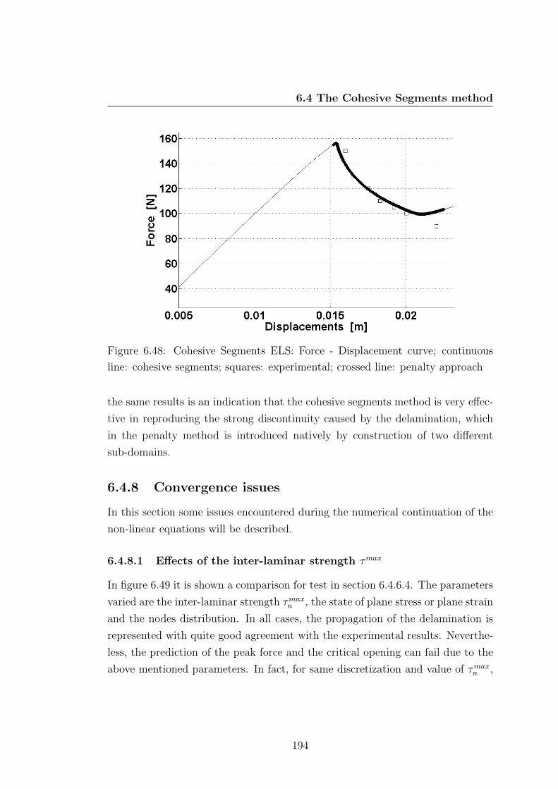
6.4 The Cohesive Segments method
Figure 6.48: Cohesive Segments ELS: Force - Displacement curve; continuous
line: cohesive segments; squares: experimental; crossed line: penalty approach
the same results is an indication that the cohesive segments method is very effec-
tive in reproducing the strong discontinuity caused by the delamination, which
in the penalty method is introduced natively by construction of two different
sub-domains.
6.4.8 Convergence issues
In this section some issues encountered during the numerical continuation of the
non-linear equations will be described.
6.4.8.1 Effects of the inter-laminar strength τmax
In figure 6.49 it is shown a comparison for test in section 6.4.6.4. The parameters
varied are the inter-laminar strength τmaxn , the state of plane stress or plane strain
and the nodes distribution. In all cases, the propagation of the delamination is
represented with quite good agreement with the experimental results. Neverthe-
less, the prediction of the peak force and the critical opening can fail due to the
above mentioned parameters. In fact, for same discretization and value of τmaxn ,
194

6.4 The Cohesive Segments method
better results are obtained if the plane strain is assumed, as shown also in section
6.4.6.4. From a cohesive-length point of view, the use of the plane strain length-
ens the cohesive length, since it is proportional to the elastic modulus. Indeed,
for equation (4.99), the elastic moduli are augmented when plane strain is used.
The reduction of τm is normally used to stretch the cohesive zone in coarse
mesh. Nonetheless, figure 6.49 shows that this trick might lead to inaccurate
prediction of the peak load. In fact, for same stress state and discretization, the
use of a higher inter-laminar strength improves the prediction to almost the ex-
perimental one. Finally, the thick line in figure 6.49 is the result slightly higher
inter-facial strength. A finer mesh better samples the cohesive process and ulti-
mately lead to an accurate prediction of the peak load.
Figure 6.49: Convergence issues: squares: experimental data; continuous line:
8×774 plane strain, τmaxn = 17 MPa; dash-dot line: 6×580 plane strain, τmaxn = 15
MPa; dotted line: 6 × 580 plane strain, τmaxn = 10 MPa; dashed line: 6 × 580
plane stress, τmaxn = 10 MPa
195
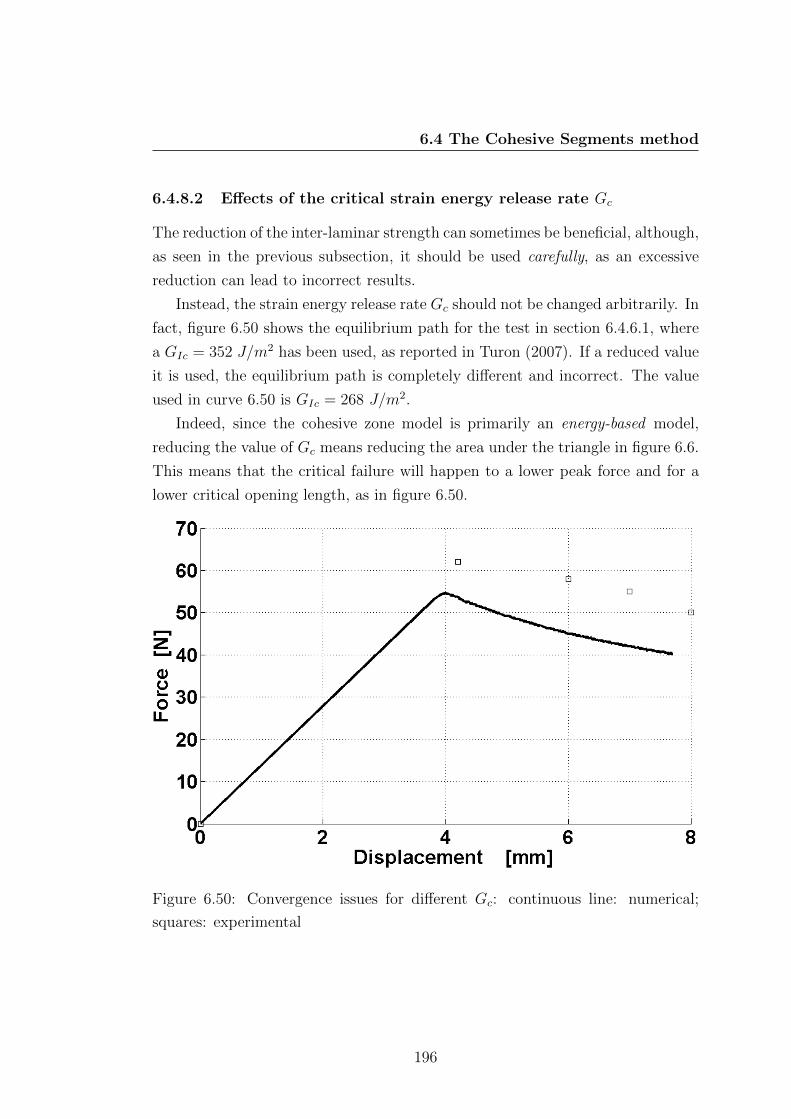
6.4 The Cohesive Segments method
6.4.8.2 Effects of the critical strain energy release rate Gc
The reduction of the inter-laminar strength can sometimes be beneficial, although,
as seen in the previous subsection, it should be used carefully, as an excessive
reduction can lead to incorrect results.
Instead, the strain energy release rate Gc should not be changed arbitrarily. In
fact, figure 6.50 shows the equilibrium path for the test in section 6.4.6.1, where
a GIc = 352 J/m2 has been used, as reported in Turon (2007). If a reduced value
it is used, the equilibrium path is completely different and incorrect. The value
used in curve 6.50 is GIc = 268 J/m2.
Indeed, since the cohesive zone model is primarily an energy-based model,
reducing the value of Gc means reducing the area under the triangle in figure 6.6.
This means that the critical failure will happen to a lower peak force and for a
lower critical opening length, as in figure 6.50.
Figure 6.50: Convergence issues for different Gc: continuous line: numerical;
squares: experimental
196

6.4 The Cohesive Segments method
6.4.8.3 Effects of a coarse mesh
The effects of a coarse mesh have been detailed in subsection 6.4.6.9, usually
accompanied by the arrest of the continuation. Another curious effect is the
bouncing back of the continuation, as in figure 6.51. The test in the example
is the ELS of subsection 6.4.6.5. When the critical force is reached (unstable
point), instead of starting the delamination, it can happen that the continuation
goes back to the previous convergent path. One possible explanation is that the
continuation code is used in combination with a line-search algorithm. The line
search looks for a reduction of the residual error. If this reduction cannot be
found after the critical point (i.e. for the difficulties due to a coarse mesh), the
only way to reduce the error and find the equilibrium is then to go back to the
previous convergent path, which is for sure an equilibrium path.
The result is then that no new equilibrium states are found but the continu-
ation rebounds on old equilibrium states.
Figure 6.51: Bounce back of the continuation
197

6.4 The Cohesive Segments method
6.4.9 The class Cohesive
6.4.9.1 The properties
Many properties are the same defined for the class CohesiveContact.
• d0t, dFt, d0n, dFn, GIc, GIIc, smax I, smax II are the parameters of the
cohesive zone model, as described in section 6.2;
• dist a structure that contains the functions in equation (6.126),(6.127),(6.128),
(6.129) and (6.130);
• H a function handle containing the enrichment function (6.62);
• nseg: the number of cohesive segments;
• Ind a cell array of size nseg, where each cell contains the indices of the
enriched nodes for each segment, selected according to equation (6.120);
• P0 an array size nseg× 2, containing the coordinates of the initial point of
the segment, as in figure 6.10;
• theta an array size nseg containing the inclination of each segment, as in
figure 6.10;
• L: an array size nseg containing the length of each segment, as in figure
6.10;
• tx and ty: cell array of size nseg, where each cell contains the tractions at
the interface as defined in equation (6.21);
• vx and vy: cell array of size nseg, where each cell contains the displacement
jumps at the interface as in equation (6.21);
• hn, ht cell array of size nseg, where each cell contains an array defined on
the Gaussian points of the segment, with values 0 if there is a pre-crack, 1
otherwise;
• KTt and KTn cell array of the derivatives of the penalty factors;
198

6.4 The Cohesive Segments method
• Krc cell array of size nseg× 1 containing the matrices in equation (6.88) ;
• Kcc cell array of size nseg×nseg containing the matrices in equation (6.89);
• Vrc cell array of size nseg× 1 containing the matrices in equation (6.93);
• Vcc cell array of size nseg×nseg containing the matrices in equation (6.95);
• KT cell array of size nseg×nseg containing the matrices in equation (6.114);
• Fc cell array of size nseg× 1 containing the vector in equation (6.110);
• Segments is a structure composed of five fields:
1. Omega: cell array of size nseg × 1, where each cell contains a RKPM
object, defined on the Gaussian points of Ω, with RKPM nodes defined
as the selected enriched nodes contained in Ind, as in equation (6.66)
and (6.67).
In this case, since the PSI, dPSIcsi, dPSIeta, ig and js vectors are
already available; they can be taken from the existing object Plate.
Therefore, the methods GetFromPlate and ShapeAndDerWithPsiPU
are used.
Subsequently, the enrichment function is imposed using the internal
function AddH that multiplies the shape functions and their derivatives
by the Heaviside function in equation (6.62).
These enriched shape functions are necessary to compute the matrices
Krc and Kcc;
2. Line: cell array of size nseg×nseg where the cell Linei,j contains
a RKPM object that calculates the shape functions on the Gaussian
points of the j-th segment but using the set of enriched nodes for the
i-th segment. In this case, the method ShapePU is used. If no Gaussian
points of the j-th segment are found within the supports of the nodes
for the i-th segment, the cell is left empty and no shape functions are
calculated;
199

6.4 The Cohesive Segments method
3. B: cell array of size equal to the number of edges, where each cell con-
tains a nested cell array of size nseg. Each nested cell contains a RKPM
object. For example, Bk.RKPMi computes the shape functions on
the i-th edge of ∂Ω, but using the set of enriched nodes for the i-th
segment. If no Gaussian points of the i-th edge are found within the
supports of the nodes for the i-th segment, the cell is left empty and
no shape functions are calculated;
This properties is used to calculate the force vectors in equations
(6.93), (6.95), (6.101)
4. PointForces and PointConstraints same as the previous field, but
for concentrated loads and point constraints.
6.4.9.2 The methods
The methods defined on the class are:
• Cohesive the constructor of the class. This method selects the node to
enrich as in section 6.4.5 and sets up the integration points for the segments
using the mapping in equations (5.7) and (5.8);
• DisplJump calculates the displacement jump as in equation (6.68) for each
segment;
• Assembly calculates the stiffness matrices Krc and Kcc, the constraint ma-
trices (6.93), (6.95) and the force vectors (6.101);
• PenaltyStiffness calculates the penalty factors according to the displace-
ment jumps, as in equation (6.21);
• AssemblyCohesive calculates the cohesive force vector (6.110) and the tan-
gent stiffness matrix (6.114);
• PlotSegments and PlotEnrichedNodes are graphic methods that plot the
Gaussian points of the cohesive segments and the enriched nodes, as in
figures 6.13 and 6.11.
200

Chapter 7
Conclusions and future works
The research has been focused mainly on exploring the possibilities offered by
the meshfree techniques. The topic of major interest has been the modelling of
failure characterized by strong discontinuities in composite materials.
Primarily, it has been shown that the meshfree methods can successfully sim-
ulate delaminations for different loading modes, without using finite elements
and/or re-meshing. Quite good agreement has been found with experimental
evidences taken from the literature. Most importantly, it has been shown that
discontinuities can be introduced in the model without the need of modelling
separate domains or the usage of interface elements, de-cohesion elements or
other finite element-based technique. Compared to these methods, it has been
demonstrated that delamination can be effectively modelled using meshfree with
enrichments, or extended meshfree method.
The success in this sense it is also due to the combination of the meshfree
capabilities with a constitutive relationship known as cohesive zone model. The
cohesive zone model establishes a traction-displacement relationship between the
cohesive traction at the interface of a crack with its opening displacement. The
main purpose of cohesive zone models is to give a more physical explanation of
the failure. This is different from classical linear fracture mechanics, which is not
suitable to composites, as it involves non-physical crack tip stress singularities.
Delamination is essentially a cohesive process and the possibility in the cohesive
models to introduce debonding is a key factor in modelling delamination. The
study of delamination was possible through the development of prototype meshfree
201
software.
The codes have been modified and improved from the very first naive one-
dimensional implementation, which was honestly quite slow. Since then, the
primary drive for continuous search of improvements has been the computational
run-time. The results of this search have been proposed in this work, showing that
with appropriate programming and mathematical manipulation, it is possible to
enhance the performance of the meshfree methods, notoriously known as good-
but-slow methods.
Another drive was the idea of designing a code that would have been similar
to a commercial one. Therefore the efforts were directed to build a more sophis-
ticated code. At the present time, the MM codes developed so far can handle
dynamic and static problems in 2D and 3D even with complex geometries. The
produced code is far from perfection, but hopefully would help the development
of even more sophisticated (maybe industry-oriented) codes.
Particularly helpful in this sense was the object-oriented programming, that
it is a flexible and intuitive philosophy of programming. The object-oriented
programming allows the creation of virtual models of the object under study, and
acting on it as it was a real object. Moreover, an object-oriented code facilitates
abstraction and opens to future improvements and modifications, by creating
new objects over existing ones, or brand new objects, and let them interact. For
example, the objects for the cohesive crack were created upon the existing linear
elastic object.
Fracture mechanics applications are so far limited to two-dimensions, due
also to the fact that it is still an open problem in the scientific community and
there is little knowledge on three-dimensional propagation paths. As a research
direction for the future, it would be great to extend the cohesive zone model to
three-dimensional structures. The introduction of large displacements would be
another step forward in the development of the code.
202

7.1 Future works
7.1 Future works
Future works will then consider mainly two aspects, one practical ( more powerful
programming language) and the other one more theoretical (the extension to
three-dimensional cracks).
The practical problem will therefore see the migration to a more powerful
language programming, more attention to storage problems and as a final goal,
the production of an effective simulation tool suitable for industry. The choice
to a different programming language should also take into account the inability
of normal desktop computers to carry out simulations with millions of degrees
of freedom. Proper programming is necessary if parallel capabilities need to be
exploited. It would be also highly desirable to further expand the capabilities of
the codes to include large deformations, aiming towards the simulation of impact
phenomena, in order to fully appreciate the ideas of the meshfree technology.
The present thesis has shown that it is possible to reduce the computational
costs of the construction of the shape functions. The burden of the neighbour
search has been alleviated through the use of the kd-tree algorithm. Nevertheless,
it has been shown that, for a fixed number of degrees of freedom, the computa-
tional cost goes linearly with the number of Gaussian points. Gaussian points
are needed to numerically evaluate the integrals in a weak form of the equations
of equilibrium. The experience of the author is that a good compromise between
accuracy and costs is given by a Gaussian quadrature of order 3, which means 9
Gaussian points per triangular element in two-dimensions and 27 Gaussian points
per tetrahedral element in three-dimensions.
This means that the bottle neck is represented by the number of Gaussian
points, even if with the proposed method they can be computed in a faster man-
ner with respect to the traditional point-wise LU factorization. In this sense,
a leap ahead would be then represented by further researching stabilization of
nodal integration techniques. Nodal integration is the Holy Grail of the meshless
methods. A truly-meshfree method that do not require a background mesh for
the purposes of the integration, will then eliminate the costs due to the necessity
of Gaussian points.
203

Appendix A
Computation of the Integral
Terms in Reproducing Kernel
Methods
In this appendix it is described a procedure to calculate the integrals in equation
(3.41), (3.47) and (3.48), as mentioned in section 3.3.
The full description can be found in Barbieri & Meo (2009b) and Barbieri &
Meo (submitted), here only the major points will be recalled. Particularly in this
appendix, only the calculation of the moments will be shown.
A.1 The Window Function w and its primitives
Hn
In this section are presented preliminary considerations about the window func-
tion w(ξ) and its primitives. Window functions in the case of RKM could have
compact support (for instance spline functions) or not, like Gaussian function.
In both cases though, it is possible to define their primitives. Their evaluation
204

A.1 The Window Function w and its primitives Hn
can be made once and for all for example through softwares capable of symbolic
computations. Moreover, since primitives are infinite in number, in order to de-
fine Hn functions uniquely, a further condition need to be imposed. Defining the
variable, with x′ being the integration variable
ξ =x′ − xρ
(A.1)
the functions Hn are n+ 1 antiderivatives, or primitives of the window
Hn(ξ) =
∫ ∫. . .
∫︸ ︷︷ ︸
n+1
w(ξ)dξ. (A.2)
Obviously, the following properties hold
dHn
dξ= Hn−1, (A.3a)
dn+1
dξn+1Hn = w(ξ), (A.3b)
∂Hn
∂x′=
1
ρxHn−1(ξ), (A.3c)
∂Hn
∂x= − 1
ρxHn−1(ξ), (A.3d)
∂(n+1)
∂x(n+1)Hn = − 1
ρn+1x
(−1)n+1w(ξ). (A.3e)
Moreover, it is possible to evaluate the moments Jk(ξ) of the window using these
functions. Indeed, applying the recursive integration by parts
Jk(ξ) =
∫ξkw(ξ)dξ =
k∑i=0
(−1)ik!
(k − i)!ξk−iHi(ξ), (A.4)
for example
J0(ξ) =
∫ξ0w(ξ)dξ = H0(ξ), (A.5a)
J1(ξ) =
∫ξ1w(ξ)dξ = ξH0(ξ)−H1(ξ), (A.5b)
J2(ξ) =
∫ξ2w(ξ)dξ = ξ2H0(ξ)− 2ξH1(ξ) + 2H2(ξ), (A.5c)
J3(ξ) =
∫ξ3w(ξ)dξ = ξ3H0(ξ)− 3ξ2H1(ξ) + 6ξH2(ξ)− 6H3(ξ). (A.5d)
205

A.1 The Window Function w and its primitives Hn
A.1.1 Non Compact Support Kernels
An example of kernels having non-compact support is the Gaussian function
w(ξ) = e−12ξ2 . (A.6)
The particular function in equation (A.6) it is 1 for ξ = 0 and it rapidly decays
to zero (even though is it not exactly zero) around ξ = ±3, as it can be seen from
figure A.1a. Moreover, since primitives are infinite in number, in order to define
Hn functions uniquely, a further condition need to be imposed. For non-compact
support, the following condition is chosen
limx→−∞
H0(ξ) = 0. (A.7)
In this case, Hn functions are
H0(ξ) =
√2π
2erf
(√2
2ξ
)+
√2π
2, (A.8)
H1(ξ) =√π
(√2
2ξ erf
(√2
2ξ
)+e−1/2 ξ2
√π
)+
√2π
2ξ, (A.9)
H2(ξ) =√π
(√2
2
(ξ2
2erf
(√2
2ξ
)− 2
(−√
2ξ
4eξ2
2
+
√π
4erf
(√2
2ξ
))1√π
)+
+
√2
2erf
(√2
2ξ
))+
√2π
4ξ2, (A.10)
where erf (x) is the error function defined as
erf (x) =2√π
∫ x
0
e−t2
dt. (A.11)
This functions are plotted in figures A.1. It can be observed that these functions
(figures A.1b, A.1c and A.1d ) outside ξ = 3 have respectively constant, linear
and quadratic behavior. This means that the boundary correction terms influence
only a small portion of the domain around the boundaries of measure ρ, as it is
also reported in Liu et al. (1997a). This is more evident for the moment matrix
entries depicted in figures A.3a, A.3b and A.3c.
206
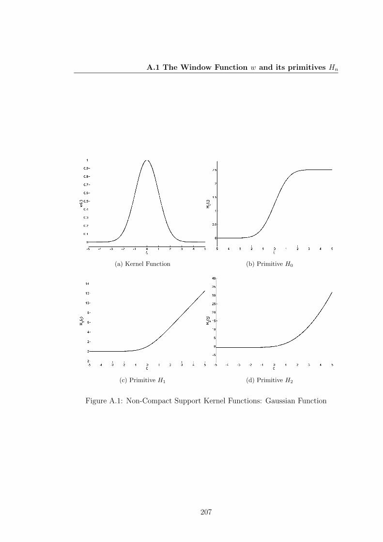
A.1 The Window Function w and its primitives Hn
(a) Kernel Function (b) Primitive H0
(c) Primitive H1 (d) Primitive H2
Figure A.1: Non-Compact Support Kernel Functions: Gaussian Function
207

A.1 The Window Function w and its primitives Hn
A.1.2 Compact Support Kernels
An example of compact support kernel is the 2kth order spline which can be
rewritten using the Heaviside function H as
w(ξ) = (1− ξ2)k [H(ξ + 1)−H(ξ − 1)] . (A.12)
For compact support functions, the condition on the primitive has been chosen
as
H0(ξ = −1) = 0. (A.13)
Thus, naming as 2F1(a, b; c; z) the classical standard hypergeometric series
H0(ξ) = ξ 2F1(1
2,−k;
3
2; ξ2) [H(ξ + 1)−H(ξ − 1)] +
+ 2F1(1
2,−k;
3
2; 1) [H(ξ + 1) + H(ξ − 1)] , (A.14)
H1(ξ) =
[2F1(
1
2,−k;
3
2; ξ2)(ξ − 1)− 1
2(k + 1)2F1(−1
2,−k − 1;
1
2; ξ2)
]H(ξ−1)+
+
[1
2(k + 1)2F1(−1
2,−k − 1;
1
2; ξ2) + 2F1(
1
2,−k;
3
2; 1)(ξ + 1)+
− 1
2(k + 1)2F1(−1
2,−k − 1;
1
2; 1)
]H(ξ + 1). (A.15)
This functions are drawn in figures A.2 for different degree k of spline. It can be
noted again the influence of the correction terms outside the support i.e. ξ = 1.
Moreover, it is useful to define the primitives Ik(ξ) of the moments Jk(ξ). These
functions are used in the computation of moments for three-dimensional domains.
Ik(ξ) =
∫Jk(ξ)dξ =
k∑i=0
(−1)i(i+ 1)k!
(k − i)!ξk−iHi+1(ξ) (A.16)
208

A.1 The Window Function w and its primitives Hn
(a) Kernel Function (b) Primitive H0
(c) Primitive H1 (d) Primitive H2
Figure A.2: Compact Support Kernel Functions: 2k − th order spline
209

A.2 Moments Matrix in One Dimension
for example
I0(ξ) =
∫J0(ξ)dξ = H1(ξ), (A.17a)
I1(ξ) =
∫J1(ξ)dξ = ξH1(ξ)− 2H2(ξ), (A.17b)
I2(ξ) =
∫J2(ξ)dξ = ξ2H1(ξ)− 4ξH2(ξ) + 6H3(ξ), (A.17c)
I3(ξ) =
∫J3(ξ)dξ = ξ3H1(ξ)− 6ξ2H2(ξ) + 18ξH3(ξ)− 24H4(ξ). (A.17d)
A.2 Moments Matrix in One Dimension
Using the Hn functions, it is immediate to evaluate the entries in the moments
matrix.
If Ω = [0, L], then the generic entry Mij of the moments matrix is
Mij(x) =
∫ L
0
ξi+jw(ξ)dx′ = ρx
∫ L−xρx
−xρx
ξi+jw(ξ)dξ. (A.18)
More generally: ∫ L−xρx
− xρx
ξkw(ξ)dξ = Jk
(L− xρx
)− Jk
(− x
ρx
). (A.19)
Therefore, from equation (A.4), it follows
Mij(x) = ρx
[i+j∑l=0
(−1)l(i+ j)!
(i+ j − l)!ξi+j−lHl(ξ)
]L−xρx
−xρx
. (A.20)
In figures A.4a and A.4b correction functions are plotted for basis functions
pT (x) = [1 x]. Indeed correction terms are given by pT (0)M(x)−1 that is
pT (0)M(x)−1 =[1 0
] [M−111 (x) M−1
12 (x)M−1
12 (x) M−122 (x)
]=[M−1
11 (x) M−112 (x)
](A.21)
where, using symbolic evaluation of the inverse of M(x)
M−111 (x) =
M22(x)
M11(x)M22(x)−M12(x)2, (A.22)
210
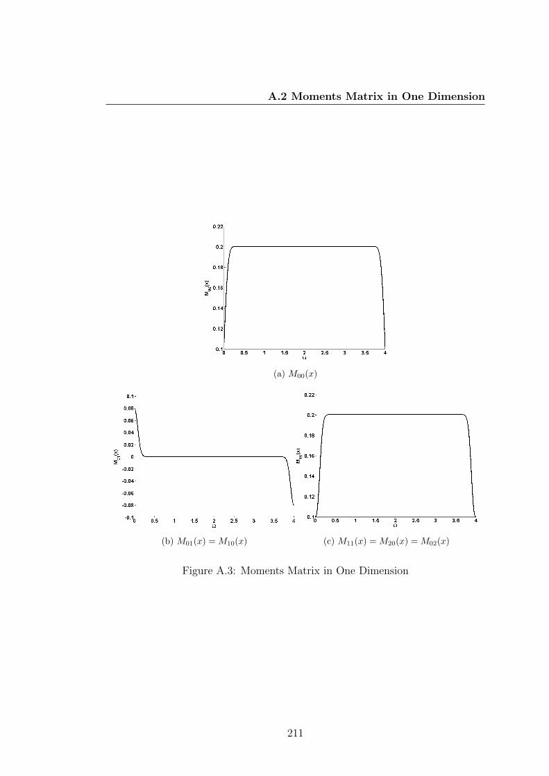
A.2 Moments Matrix in One Dimension
(a) M00(x)
(b) M01(x) = M10(x) (c) M11(x) = M20(x) = M02(x)
Figure A.3: Moments Matrix in One Dimension
211
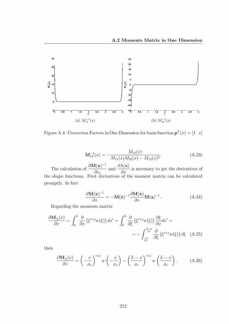
A.2 Moments Matrix in One Dimension
(a) M−111 (x) (b) M−1
12 (x)
Figure A.4: Correction Factors in One Dimension for basis function pT (x) = [1 x]
M−112 (x) = − M12(x)
M11(x)M22(x)−M12(x)2. (A.23)
The calculation of∂M(x)−1
∂xiand
∂Λ(x)
∂xis necessary to get the derivatives of
the shape functions. First derivatives of the moment matrix can be calculated
promptly. In fact
∂M(x)−1
∂x= −M(x)−1∂M(x)
∂xM(x)−1. (A.24)
Regarding the moments matrix
∂Mij(x)
∂x=
∫ L
0
∂
∂x
(ξi+jw(ξ)
)dx′ =
∫ L
0
∂
∂ξ
(ξi+jw(ξ)
) ∂ξ∂xdx′ =
= −∫ L−x
ρx
−xρx
∂
∂ξ
(ξi+jw(ξ)
)dξ (A.25)
then
∂Mij(x)
∂x=
(− x
ρx
)i+jw
(− x
ρx
)−(L− xρx
)i+jw
(L− xρx
). (A.26)
212

A.2 Moments Matrix in One Dimension
(a)∂M00
∂x(x) (b)
∂M01
∂x(x)
(c)∂M11(x)
∂x
Figure A.5: First Derivative of Moments Matrix in One Dimension
213
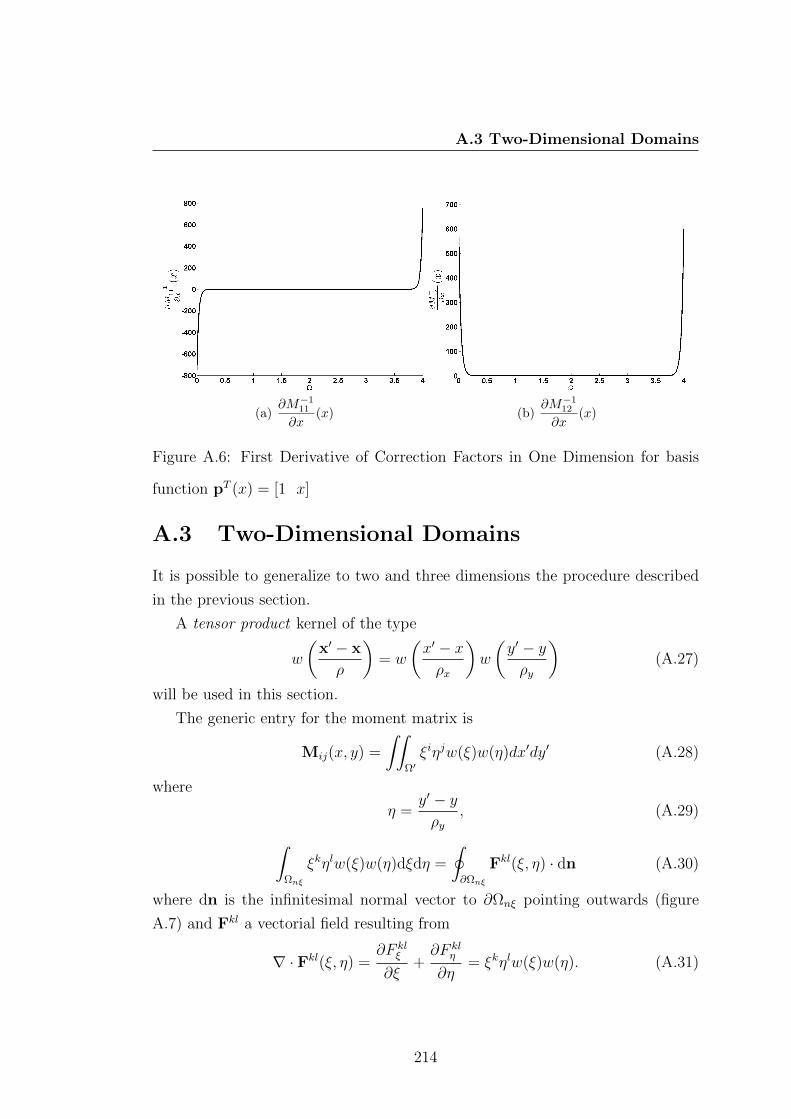
A.3 Two-Dimensional Domains
(a)∂M−1
11
∂x(x) (b)
∂M−112
∂x(x)
Figure A.6: First Derivative of Correction Factors in One Dimension for basis
function pT (x) = [1 x]
A.3 Two-Dimensional Domains
It is possible to generalize to two and three dimensions the procedure described
in the previous section.
A tensor product kernel of the type
w
(x′ − x
ρ
)= w
(x′ − xρx
)w
(y′ − yρy
)(A.27)
will be used in this section.
The generic entry for the moment matrix is
Mij(x, y) =
∫∫Ω′ξiηjw(ξ)w(η)dx′dy′ (A.28)
where
η =y′ − yρy
, (A.29)
∫Ωnξ
ξkηlw(ξ)w(η)dξdη =
∮∂Ωnξ
Fkl(ξ, η) · dn (A.30)
where dn is the infinitesimal normal vector to ∂Ωnξ pointing outwards (figure
A.7) and Fkl a vectorial field resulting from
∇ · Fkl(ξ, η) =∂F kl
ξ
∂ξ+∂F kl
η
∂η= ξkηlw(ξ)w(η). (A.31)
214
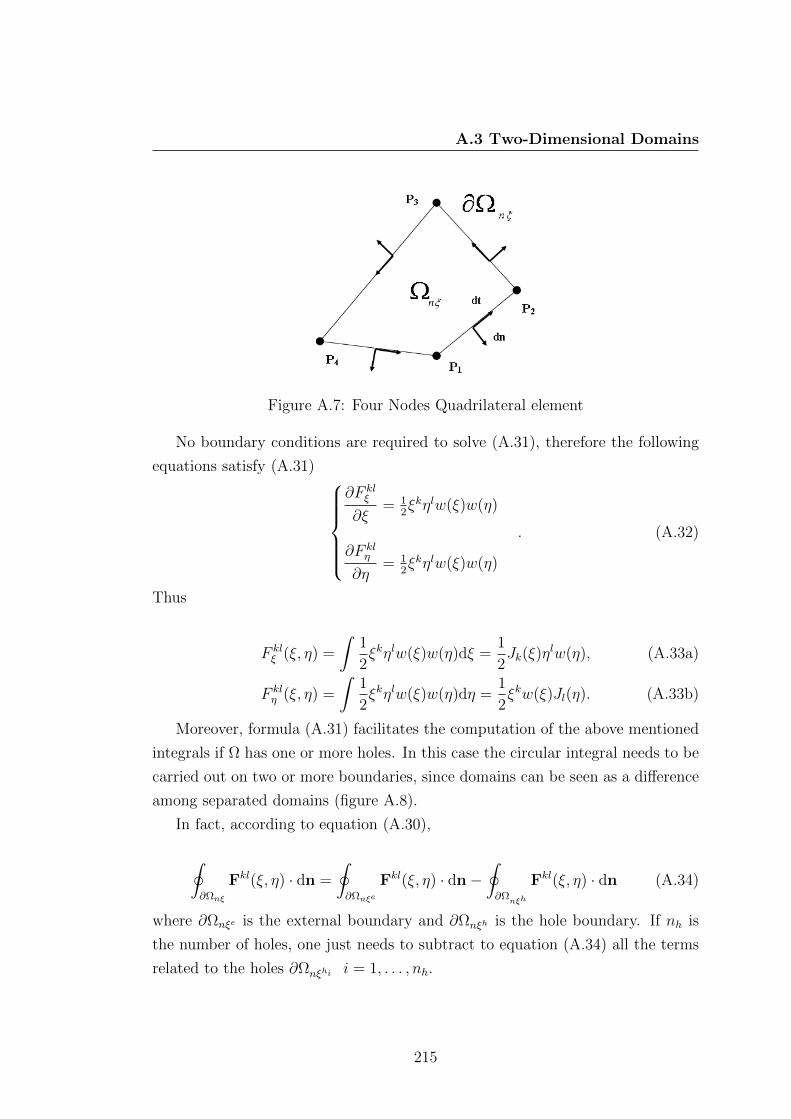
A.3 Two-Dimensional Domains
Figure A.7: Four Nodes Quadrilateral element
No boundary conditions are required to solve (A.31), therefore the following
equations satisfy (A.31) ∂F kl
ξ
∂ξ= 1
2ξkηlw(ξ)w(η)
∂F klη
∂η= 1
2ξkηlw(ξ)w(η)
. (A.32)
Thus
F klξ (ξ, η) =
∫1
2ξkηlw(ξ)w(η)dξ =
1
2Jk(ξ)η
lw(η), (A.33a)
F klη (ξ, η) =
∫1
2ξkηlw(ξ)w(η)dη =
1
2ξkw(ξ)Jl(η). (A.33b)
Moreover, formula (A.31) facilitates the computation of the above mentioned
integrals if Ω has one or more holes. In this case the circular integral needs to be
carried out on two or more boundaries, since domains can be seen as a difference
among separated domains (figure A.8).
In fact, according to equation (A.30),
∮∂Ωnξ
Fkl(ξ, η) · dn =
∮∂Ωnξe
Fkl(ξ, η) · dn−∮∂Ω
nξh
Fkl(ξ, η) · dn (A.34)
where ∂Ωnξe is the external boundary and ∂Ωnξh is the hole boundary. If nh is
the number of holes, one just needs to subtract to equation (A.34) all the terms
related to the holes ∂Ωnξhi i = 1, . . . , nh.
215

A.3 Two-Dimensional Domains
(a) (b)
(c) (d)
Figure A.8: Examples of moment matrix entries in two dimensions
216

A.4 Three-Dimensional Domains
A.4 Three-Dimensional Domains
The same approach applies to three-dimensional domains, where the generic in-
tegral in equation (A.30) is extended as∫Ωnξ
ξkηlζmw(ξ)w(η)w(ζ)dξdη =©∫∫
∂Ωnξ
Fklm(ξ, η, ζ) · dn (A.35)
where dn is the infinitesimal normal vector to ∂Ω pointing outwards and Fklm a
vectorial field resulting from
∇ · Fklm(ξ, η, ζ) =∂F klm
ξ
∂ξ+∂F klm
η
∂η+∂F klm
ζ
∂η= ξkηlζmw(ξ)w(η)w(ζ). (A.36)
Thus,
F klmξ (ξ, η, ζ) =
∫1
3ξkηlζmw(ξ)w(η)w(ζ)dξ =
1
3Jk(ξ)η
lw(η)ζmw(ζ), (A.37a)
F klmη (ξ, η, ζ) =
∫1
3ξkηlζmw(ξ)w(η)w(ζ)dη =
1
3ξkw(ξ)Jl(η)ζmw(ζ), (A.37b)
F klmζ (ξ, η, ζ) =
∫1
3ξkηlζmw(ξ)w(η)w(ζ)dζ =
1
3ξkw(ξ)ηlw(η)Jm(ζ). (A.37c)
A further reduction of integral (A.35) can be made if Ωnξ is part of a polygon
subdivision as defined in Li et al. (2004), here recalled
Polygon subdivision A partition Fn = Ω1, Ω2 . . .Ωn is a polygon subdivi-
sion if
1. Ωi i ∈ 1, . . . , n is a polygon;
2. Ωi ∩ Ωj = ∅ i 6= j;
3.⋃ni=1 Ωi = Ω;
4. if Ωi ∩ Ωj i 6= j consists of exactly one point, then it is the common vertex
of the two polygons;
5. if Ωi ∩ Ωj i 6= j consists of more than one point, then Ωi ∩ Ωj is either the
common surface or the common edge.
217
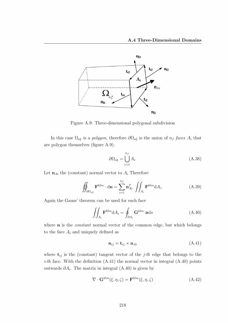
A.4 Three-Dimensional Domains
Figure A.9: Three-dimensional polygonal subdivision
In this case Ωnξ is a polygon, therefore ∂Ωnξ is the union of nf faces Ai that
are polygon themselves (figure A.9).
∂Ωnξ =
nf⋃i=1
Ai. (A.38)
Let nAi the (constant) normal vector to Ai Therefore
©∫∫
∂Ωnξ
Fklm · dn =
nf∑i=1
nTAi
∫∫Ai
FklmdAi. (A.39)
Again the Gauss’ theorem can be used for each face∫∫Ai
FklmdAi =
∮∂Ai
Gklm nds (A.40)
where n is the constant normal vector of the common edge, but which belongs
to the face Ai and uniquely defined as
nij = tij × nAi (A.41)
where tij is the (constant) tangent vector of the j-th edge that belongs to the
i-th face. With the definition (A.41) the normal vector in integral (A.40) points
outwards ∂Ai. The matrix in integral (A.40) is given by
∇ ·Gklm(ξ, η, ζ) = Fklm(ξ, η, ζ) (A.42)
218
A.4 Three-Dimensional Domains
that is
∂Gklmξξ
∂ξ+∂Gklm
ξη
∂η+∂Gklm
ξζ
∂ζ= F klm
ξ , (A.43a)
∂Gklmηξ
∂ξ+∂Gklm
ηη
∂η+∂Gklm
ηζ
∂ζ= F klm
η , (A.43b)
∂Gklmζξ
∂ξ+∂Gklm
ζη
∂η+∂Gklm
ζζ
∂ζ= F klm
ζ . (A.43c)
Equations (A.43) can be evaluated as usual
Gklmξξ (ξ, η, ζ) =
∫1
3F klmξ dξ =
1
9Ik(ξ)η
lw(η)ζmw(ζ), (A.44a)
Gklmξη (ξ, η, ζ) =
∫1
3F klmξ dη =
1
9Jk(ξ)Jl(η)ζmw(ζ), (A.44b)
Gklmξζ (ξ, η, ζ) =
∫1
3F klmξ dζ =
1
9Jk(ξ)η
lw(η)Jm(ζ), (A.44c)
Gklmηξ (ξ, η, ζ) =
∫1
3F klmη dξ =
1
9Jk(ξ)Jl(η)ζmw(ζ) = Gklm
ξη (ξ, η, ζ), (A.44d)
Gklmηη (ξ, η, ζ) =
∫1
3F klmη dη =
1
9ξkw(ξ)Il(η)ζmw(ζ), (A.44e)
Gklmηζ (ξ, η, ζ) =
∫1
3F klmη dζ =
1
9ξkw(ξ)Jl(η)Jm(ζ), (A.44f)
Gklmζξ (ξ, η, ζ) =
∫1
3F klmζ dξ =
1
9Jk(ξ)η
lw(η)Jm(ζ) = Gklmξζ (ξ, η, ζ), (A.44g)
Gklmζη (ξ, η, ζ) =
∫1
3F klmζ dη =
1
9ξkw(ξ)Jl(η)Jm(ζ) = Gklm
ηζ (ξ, η, ζ), (A.44h)
Gklmζζ (ξ, η, ζ) =
∫1
3F klmζ dζ =
1
9ξkw(ξ)ηlw(η)Im(ζ). (A.44i)
(A.44j)
Therefore if Ωnξ is a polygon, (for example like in FE discretization)∫Ωnξ
ξkηlζmw(ξ)w(η)w(ζ)dξdη =
nf∑i=1
nTAi
ns∑j=1
(∫eij
Gklmds
)nij (A.45)
where ns is the number of segments of the face and eij is the j-th edge that belongs
to the i-th face with normal vector nij. Thus it can be concluded that every
219
A.5 Explicit Expression for Line Integrals
integral for two and three-dimensional polygon subdivision is then reformulated
as a line integral for which an explicit expression can be provided.
A.5 Explicit Expression for Line Integrals
In order to calculate line integrals parametrization of the boundaries must be
provided.
For polygon subdivision, these lines are actually segments that are easy to
parametrize. If the orientated segment has starting point P1 = (x1, y1) and end
point P2 = (x2, y2), then ξ(t) = h(x) + αt ,
η(t) = q(y) + βt t ∈ [0, 1](A.46)
with h = x1−xρx
, q = y1−yρy
, α = x2−x1ρx
and β = y2−y1ρy
and normal vector nT =[β −α
].
These line integrals can be evaluated explicitly through symbolic manipula-
tion.
As an example∫ P2
P1
F 00ξ (ξ, η)dη − F 00
η (ξ, η)dξ =β
2
∫ 1
0
H0(h+ αt)w(q + βt) dt+
− α
2
∫ 1
0
w(h+ αt)H0(q + βt) dt. (A.47)
If either α = 0 (vertical segment) or β = 0 (horizontal segment), the integral
(A.47) is trivial since if α = 0
β
2
∫ 1
0
H0(h)w(q + βt) dt =H0(h)
2
∫ 1
0
w(q + βt) d(q + βt) =
=H0(h)
2[H0(q + β)−H0(q)] (A.48)
whereas if β = 0
220

A.5 Explicit Expression for Line Integrals
α
2
∫ 1
0
H0(q)w(h+ αt) dt =H0(q)
2
∫ 1
0
w(h+ αt) d(h+ αt) =
=H0(q)
2[H0(h+ α)−H0(h)] . (A.49)
If both α 6= 0 and β 6= 0 the expression becomes much more complicated, even
with simple spline window functions.
Defining the window function as
w(ξ) = f(ξ) [H(ξ + 1)−H(ξ − 1)] (A.50)
for example in (A.12)
f(ξ) = (1− ξ2)k (A.51)
and defining the primitive of f(ξ)
K0(ξ) =
∫ ξ
−1
f(ξ)dξ (A.52)
function H0(ξ) can be written as
H0(ξ) = K0(ξ) [H(ξ + 1)−H(ξ − 1)] +K0(1)H(ξ − 1). (A.53)
It has been experienced by the authors that symbolic softwares cannot provide
directly a closed form of the integral (A.47). This is mostly caused by the presence
of the Heaviside functions that can easily halt the calculation. If an explicit form
is desired, some preliminary manipulation is needed. Firstly, it can be noted from
equation (A.47) that the second term of the right hand side is exactly the same
of the first one provided that α and h are interchanged with β and q. Therefore,
it suffices to calculate only the first integral in (A.47). Such integral can be
expanded in the following form using equations (A.50), (A.52) and (A.53)
221
A.5 Explicit Expression for Line Integrals
∫ 1
0
H0(h+αt)w(q+βt) dt =
∫ 1
0
K0(h+at)f(q+bt) H(at+h+1)H(bt+q+1)dt+
−∫ 1
0
K0(h+ at)f(q + bt) H(at+ h− 1)H(bt+ q + 1)dt+
−∫ 1
0
K0(h+ at)f(q + bt) H(at+ h+ 1)H(bt+ q − 1)dt
+
∫ 1
0
K0(h+ at)f(q + bt) H(at+ h− 1)H(bt+ q − 1)dt+
+ K0(1)
∫ 1
0
f(q + bt) H(at+ h− 1)H(bt+ q + 1)dt+
−K0(1)
∫ 1
0
f(q + bt) H(at+ h− 1)H(bt+ q − 1)dt. (A.54)
Considering that generally for m = h+ 1, h− 1
H(at+m) = H(α)H(t+
m
α
)+ H(−α)H
(−(t+
m
α
))=
= (H(α)−H(−α))H(t+
m
α
)+ H(−α). (A.55)
and for p = q + 1, q − 1
H(αt+m)H(βt+ p) =
= (H(α)−H(−α)) (H(β)−H(−β))H(t+
m
α
)H
(t+
p
β
)+
H(−β)(H(α)−H(−α))H(t+
m
α
)+ H(−α)(H(β)−H(−β))H
(t+
p
β
)+
+ H(−α)H(−β) (A.56)
also considering that if spline window functions are used, the functions K0(h +
at)f(q + bt) and f(q + bt) can be re-grouped in polynomial form as
K0(h+ at)f(q + bt) = C(α, β, h(x), q(y))TT (A.57)
where T is a vector of monomial powers of t
T =[1 t t2 · · · tn
](A.58)
222

A.5 Explicit Expression for Line Integrals
and C(α, β, h(x), q(y))T is a vector of coefficients that does not depend on the
variable of integration t. Therefore the generic term that appears in integral
(A.54) can be re-written as∫ 1
0
K0(h+ αt)f(q + βt)H(αt+m)H(βt+ p) =
(H(α)−H(−α)) (H(β)−H(−β)) CT
∫ 1
0
TH(t+
m
α
)H
(t+
p
β
)dt+
+ H(−β)(H(α)−H(−α))CT
∫ 1
0
TH(t+
m
α
)dt+
+ CTH(−α)(H(β)−H(−β))
∫ 1
0
TH
(t+
p
β
)dt+
+ H(−α)H(−β)CT
∫ 1
0
Tdt. (A.59)
therefore one only needs to evaluate explicitly the integrals
I1n(α, β, n,m(x), p(y)) =
∫ 1
0
tnH(t+
m
α
)H
(t+
p
β
)dt =
1
αβ(n+ 1)
[H(mα
+ 1)((
bm(−mα
)n− αp
(− pβ
)n)H
(−mα
+p
β
)+
+α
(p
(− pβ
)n+ β
)H
(p
β+ 1
))−((
βm(−mα
)n− αp
(− pβ
)n)×
×H(−mα
+p
β
)+ αH
(p
β
)p
(− pβ
)n)H(mα
)], (A.60)
I2n(α, n,m(x)) =
∫ 1
0
tnH(t+
m
α
)dt =
1
α(n+ 1)
(H(
1 +m
α
)m(−mα
)n+
+H(
1 +m
α
)α−H
(mα
)m(−mα
)n), (A.61)
∫ 1
0
tndt =1
n+ 1(A.62)
with n ∈ N0 The same method can be used for the remaining terms in (A.54).
This approach can be repeated for all the vectorial fields Fklm and tensorial
Gklm and explicit integrals can be obtained with a software capable of symbolic
manipulations.
223

A.5 Explicit Expression for Line Integrals
Derivatives can be readily calculated as well since from equation (A.57)
∂C
∂x(α, β, h(x), q(y)) = − 1
ρx
∂C(α, β, h, q)
∂h, (A.63a)
∂C
∂y(α, β, h(x), q(y)) = − 1
ρy
∂C(α, β, h, q)
∂q. (A.63b)
The right hand side of equations (A.63a) is easy to evaluate since C is a vector
of polynomial functions in h(x) and q(y).
∂I1n
∂x= − 1
ρx
∂I1n
∂m= − 1
ρxα
[H(
1 +m
α
)−H
(mα
)]H
(αp− βm
αβ
)(−mα
)n,
(A.64)
∂I2n
∂x= − 1
ρx
∂I2n
∂m= − 1
ρxα
[H(
1 +m
α
)−H
(mα
)](−mα
)n, (A.65)
∂I1n
∂y= − 1
ρy
∂I1n
∂p= − 1
ρyβ
[H
(m+ α
α
)H
(−βm+ αp
αβ
)−
+H
(m+ α
α
)H
(p+ β
β
)+
−H(−βm+ αp
αβ
)H(mα
)+ H
(mα
)H
(p
β
)](− pβ
)n, (A.66)
∂I2n
∂y= − 1
ρy
∂I2n
∂p= − 1
ρyβ
[H
(1 +
p
β
)−H
(p
β
)](− pβ
)n. (A.67)
224

Appendix B
Arc Length Numerical
Continuation
Let us consider the following non-linear system of equation
Ψ(a, λ) = R(a)− λP = 0 (B.1)
where a is a n× 1 vector and λ is a scalar. An equilibrium state (a0, λ0) satisfies
a convergence criterion|Ψ(a0, λ0)||λ0P|
≤ β (B.2)
where β is a predefined tolerance, typically set to 0.001.
Let us define
Iterative change δ With the symbol δ it is indicated the change between two
successive iterations.
δak = ak+1 − ak. (B.3)
Incremental change ∆ With the symbol ∆ it is indicated the change between
an iteration ak and the previous convergent state a0
∆ak = ak − a0, (B.4a)
∆λk = λk − λ0. (B.4b)
225
B.1 Continuation of Equilibrium
Hence
∆ak+1 = ∆ak + δak, (B.5a)
∆λk+1 = ∆λk + δλk. (B.5b)
Equation (B.1) is a system of n equations in n+ 1 unknowns, therefore an addi-
tional equation (usually called constraint equation) is required.
Ψ(a, λ) = R(a)− λP = 0, (B.6a)
f(∆a,∆λ) = ∆aT∆a + α2∆λ2PTP− ds2 = 0. (B.6b)
Equation (B.6b) is the arc-length constraint.
B.1 Continuation of Equilibrium
Continuation is essentially the task of getting a new equilibrium state (a1, λ1)
starting from a previous convergent one (a0, λ0). Continuation is divided in two
phases: predictor and corrector.
B.1.1 Predictor Phase
In the predictor phase, one moves from the equilibrium state (a0, λ0) to the first
tentative state (a1, λ1). Expanding equation (B.1) in Taylor series around (a0, λ0)
Ψ(a1, λ1) = Ψ(a0, λ0) +∂Ψ
∂a(a0, λ0)δa0 +
∂Ψ
∂λ(a0, λ0)δλ0 + . . . (B.7)
since Ψ(a0, λ0) = 0 and supposing that Ψ(a1, λ1) ∼== 01 and neglecting higher
order terms, equation (B.7) becomes
KT (a0, λ0)δa0 −P(a0, λ0)δλ0 = 0 (B.8)
where∂Ψ
∂a(a0, λ0) = KT (a0, λ0) is the tangent stiffness matrix at state (a0, λ0)
and∂Ψ
∂λ(a0, λ0) = −P. Mathematically, equation (B.8) is an undetermined sys-
tem of equation, therefore there are infinite solutions[δaT0 δλ0
]∈ Null
([KT −P
]). (B.9)
1it is hoped that convergence is achieved in the next step
226
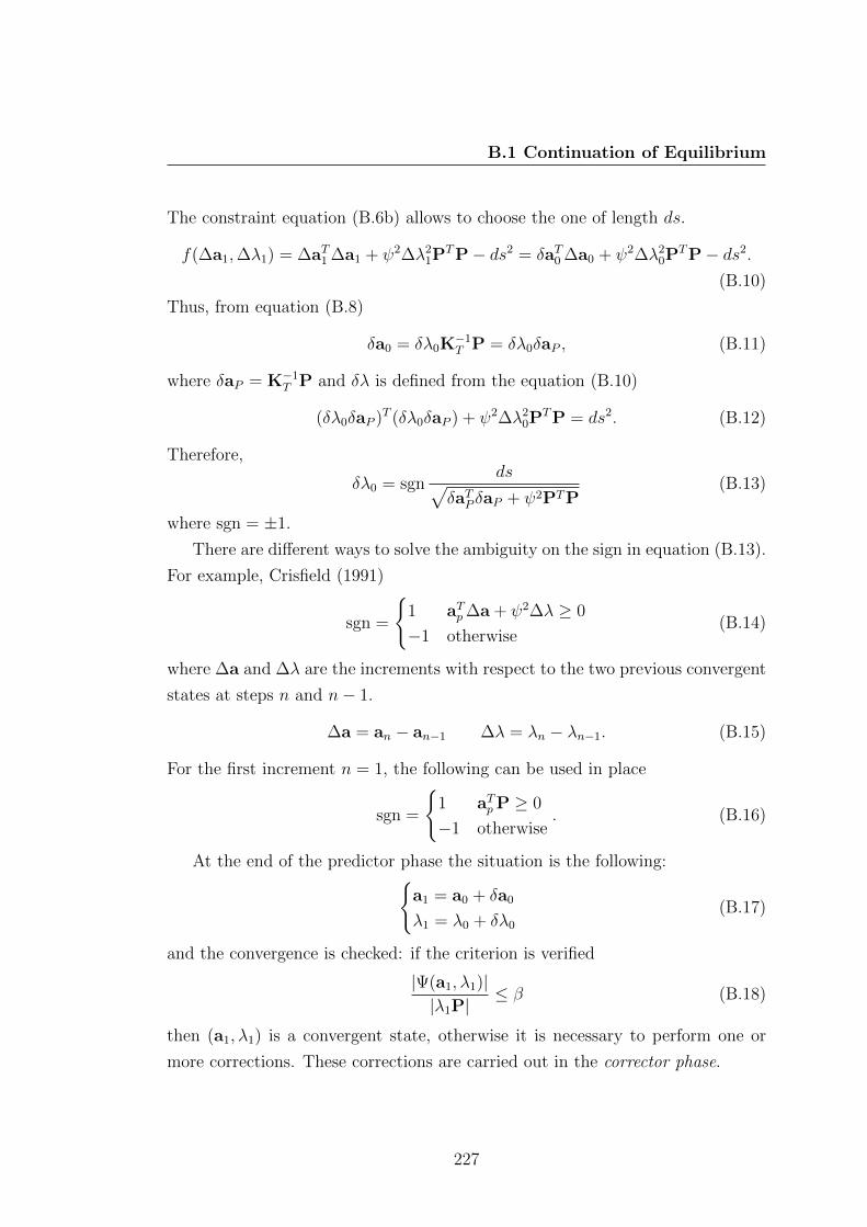
B.1 Continuation of Equilibrium
The constraint equation (B.6b) allows to choose the one of length ds.
f(∆a1,∆λ1) = ∆aT1 ∆a1 + ψ2∆λ21P
TP− ds2 = δaT0 ∆a0 + ψ2∆λ20P
TP− ds2.
(B.10)
Thus, from equation (B.8)
δa0 = δλ0K−1T P = δλ0δaP , (B.11)
where δaP = K−1T P and δλ is defined from the equation (B.10)
(δλ0δaP )T (δλ0δaP ) + ψ2∆λ20P
TP = ds2. (B.12)
Therefore,
δλ0 = sgnds√
δaTP δaP + ψ2PTP(B.13)
where sgn = ±1.
There are different ways to solve the ambiguity on the sign in equation (B.13).
For example, Crisfield (1991)
sgn =
1 aTp ∆a + ψ2∆λ ≥ 0
−1 otherwise(B.14)
where ∆a and ∆λ are the increments with respect to the two previous convergent
states at steps n and n− 1.
∆a = an − an−1 ∆λ = λn − λn−1. (B.15)
For the first increment n = 1, the following can be used in place
sgn =
1 aTp P ≥ 0
−1 otherwise. (B.16)
At the end of the predictor phase the situation is the following:a1 = a0 + δa0
λ1 = λ0 + δλ0
(B.17)
and the convergence is checked: if the criterion is verified
|Ψ(a1, λ1)||λ1P|
≤ β (B.18)
then (a1, λ1) is a convergent state, otherwise it is necessary to perform one or
more corrections. These corrections are carried out in the corrector phase.
227

B.1 Continuation of Equilibrium
B.1.2 Corrector Phase
The corrector phase includes all the corrections from a state (a1, λ1) that does
not satisfy equation (B.18) to a state (a1, λ1) that does satisfy (B.18). This
is normally achieved within few corrections unless some exceptions described in
subsection 6.3.4. Considering the generalized system of equation
Ψ(ak, λk) =
Ψ(ak, λk)
f(∆ak,∆λk)
. (B.19)
Expanding in Taylor series and neglecting terms of order higher than the first
Ψ(ak + δk, λk + δλk)︸ ︷︷ ︸≈0
= Ψ(ak, λk)︸ ︷︷ ︸6=0
+∂Ψ
∂a(ak, λk)δak +
∂Ψ
∂λ(ak, λk)δλk (B.20)
where
∂Ψ
∂a=
∂Ψ
∂a
∂f
∂a
=
KT
2∆aTk
, (B.21)
∂Ψ
∂λ=
∂Ψ
∂λ
∂f
∂λ
=
−P
2∆λkψ2PTP
. (B.22)
Thus, the expanded Newton-like problem to solve is KT
2∆aTk
δak +
−P
2∆λkψ2PTP
δλk + Ψ(ak, λk) = 0 (B.23)
or, in matrix form KT −P
2∆aTk 2∆λkψ2PTP
δakδλk
= −Ψ(ak, λk) (B.24)
which solved gives the iterationsδakδλk
= −
KT −P
2∆aTk 2∆λkψ2PTP
−1 Ψ(ak, λk)
f(ak, λk)
. (B.25)
228
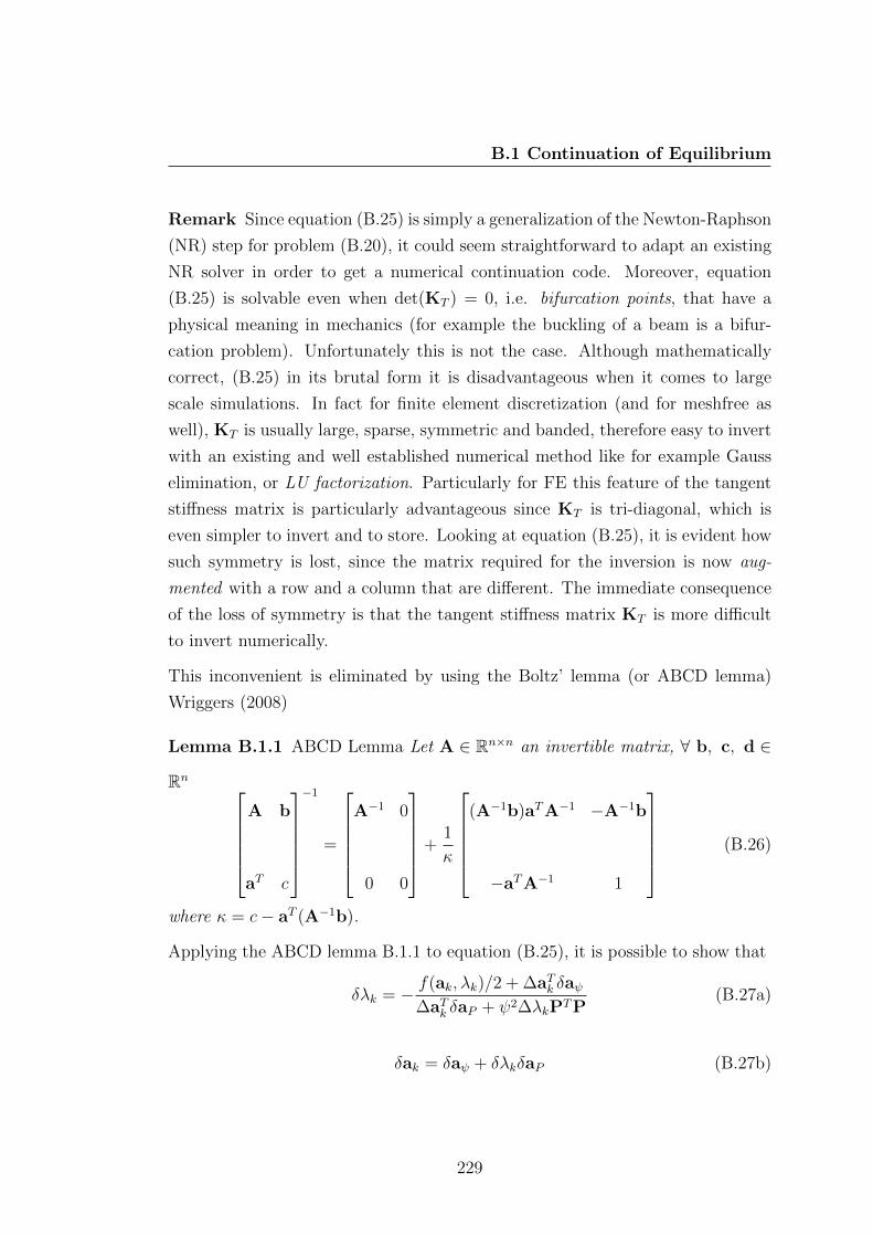
B.1 Continuation of Equilibrium
Remark Since equation (B.25) is simply a generalization of the Newton-Raphson
(NR) step for problem (B.20), it could seem straightforward to adapt an existing
NR solver in order to get a numerical continuation code. Moreover, equation
(B.25) is solvable even when det(KT ) = 0, i.e. bifurcation points, that have a
physical meaning in mechanics (for example the buckling of a beam is a bifur-
cation problem). Unfortunately this is not the case. Although mathematically
correct, (B.25) in its brutal form it is disadvantageous when it comes to large
scale simulations. In fact for finite element discretization (and for meshfree as
well), KT is usually large, sparse, symmetric and banded, therefore easy to invert
with an existing and well established numerical method like for example Gauss
elimination, or LU factorization. Particularly for FE this feature of the tangent
stiffness matrix is particularly advantageous since KT is tri-diagonal, which is
even simpler to invert and to store. Looking at equation (B.25), it is evident how
such symmetry is lost, since the matrix required for the inversion is now aug-
mented with a row and a column that are different. The immediate consequence
of the loss of symmetry is that the tangent stiffness matrix KT is more difficult
to invert numerically.
This inconvenient is eliminated by using the Boltz’ lemma (or ABCD lemma)
Wriggers (2008)
Lemma B.1.1 ABCD Lemma Let A ∈ Rn×n an invertible matrix, ∀ b, c, d ∈
Rn A b
aT c
−1
=
A−1 0
0 0
+1
κ
(A−1b)aTA−1 −A−1b
−aTA−1 1
(B.26)
where κ = c− aT (A−1b).
Applying the ABCD lemma B.1.1 to equation (B.25), it is possible to show that
δλk = − f(ak, λk)/2 + ∆aTk δaψ∆aTk δaP + ψ2∆λkPTP
(B.27a)
δak = δaψ + δλkδaP (B.27b)
229
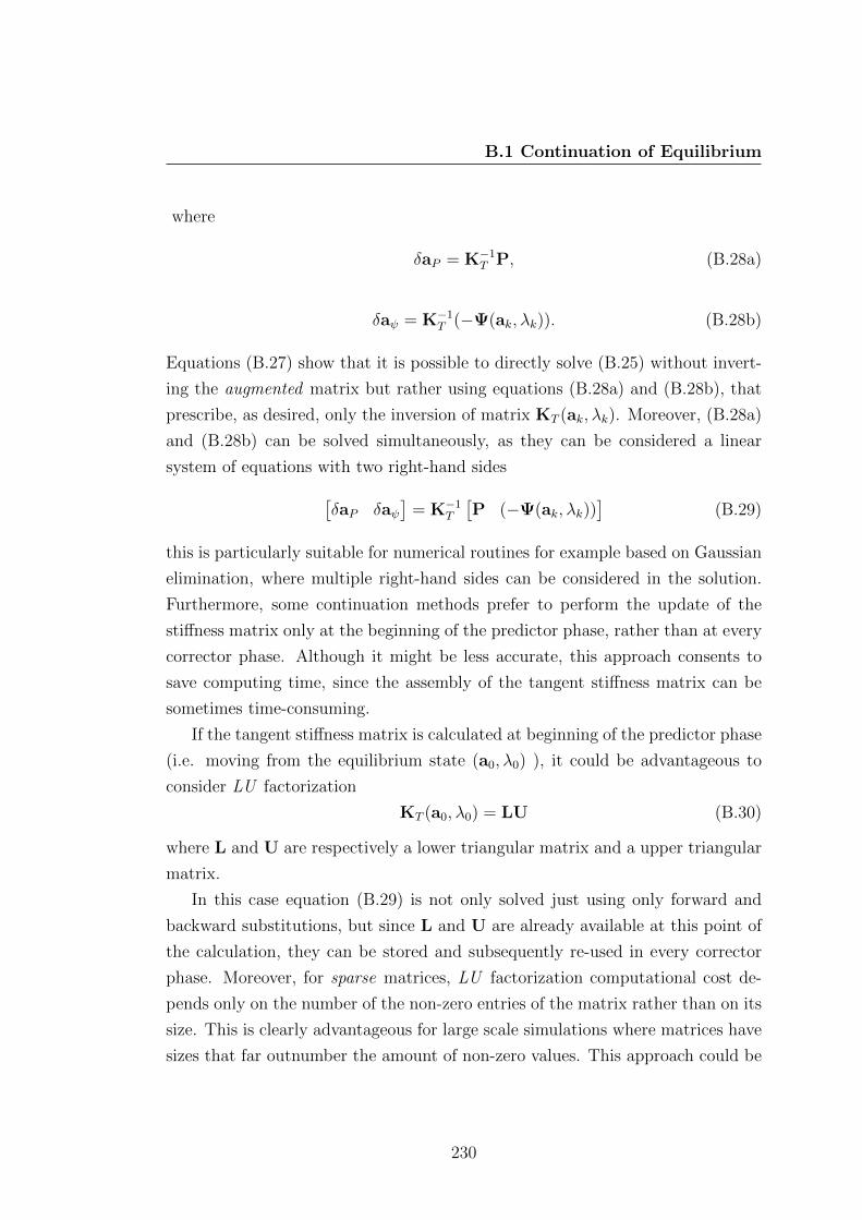
B.1 Continuation of Equilibrium
where
δaP = K−1T P, (B.28a)
δaψ = K−1T (−Ψ(ak, λk)). (B.28b)
Equations (B.27) show that it is possible to directly solve (B.25) without invert-
ing the augmented matrix but rather using equations (B.28a) and (B.28b), that
prescribe, as desired, only the inversion of matrix KT (ak, λk). Moreover, (B.28a)
and (B.28b) can be solved simultaneously, as they can be considered a linear
system of equations with two right-hand sides[δaP δaψ
]= K−1
T
[P (−Ψ(ak, λk))
](B.29)
this is particularly suitable for numerical routines for example based on Gaussian
elimination, where multiple right-hand sides can be considered in the solution.
Furthermore, some continuation methods prefer to perform the update of the
stiffness matrix only at the beginning of the predictor phase, rather than at every
corrector phase. Although it might be less accurate, this approach consents to
save computing time, since the assembly of the tangent stiffness matrix can be
sometimes time-consuming.
If the tangent stiffness matrix is calculated at beginning of the predictor phase
(i.e. moving from the equilibrium state (a0, λ0) ), it could be advantageous to
consider LU factorization
KT (a0, λ0) = LU (B.30)
where L and U are respectively a lower triangular matrix and a upper triangular
matrix.
In this case equation (B.29) is not only solved just using only forward and
backward substitutions, but since L and U are already available at this point of
the calculation, they can be stored and subsequently re-used in every corrector
phase. Moreover, for sparse matrices, LU factorization computational cost de-
pends only on the number of the non-zero entries of the matrix rather than on its
size. This is clearly advantageous for large scale simulations where matrices have
sizes that far outnumber the amount of non-zero values. This approach could be
230
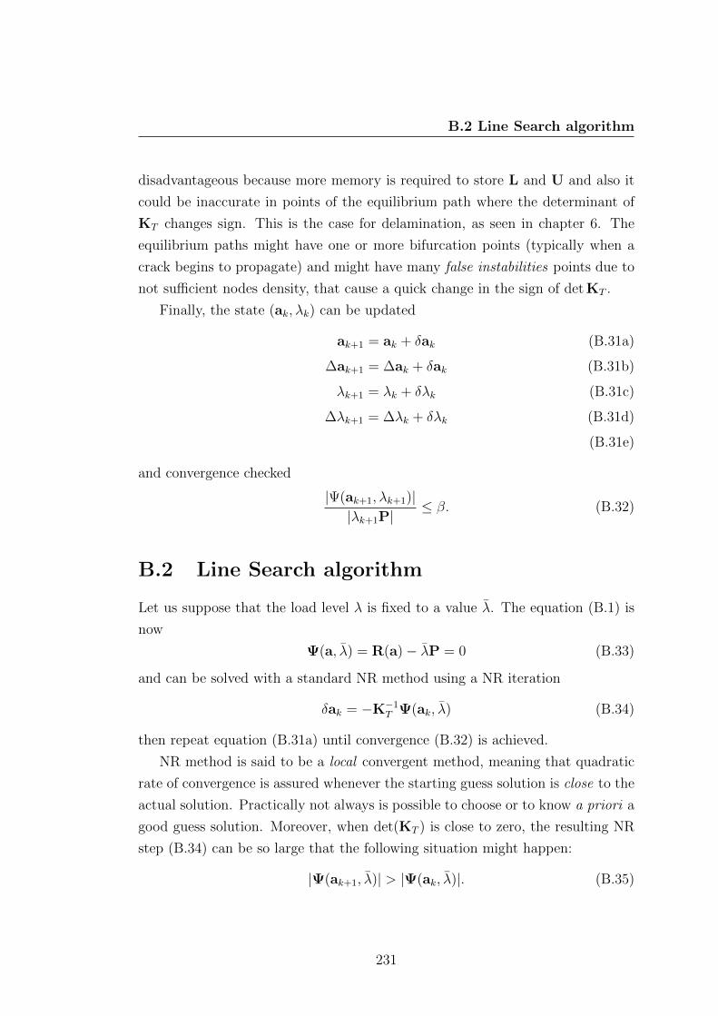
B.2 Line Search algorithm
disadvantageous because more memory is required to store L and U and also it
could be inaccurate in points of the equilibrium path where the determinant of
KT changes sign. This is the case for delamination, as seen in chapter 6. The
equilibrium paths might have one or more bifurcation points (typically when a
crack begins to propagate) and might have many false instabilities points due to
not sufficient nodes density, that cause a quick change in the sign of det KT .
Finally, the state (ak, λk) can be updated
ak+1 = ak + δak (B.31a)
∆ak+1 = ∆ak + δak (B.31b)
λk+1 = λk + δλk (B.31c)
∆λk+1 = ∆λk + δλk (B.31d)
(B.31e)
and convergence checked
|Ψ(ak+1, λk+1)||λk+1P|
≤ β. (B.32)
B.2 Line Search algorithm
Let us suppose that the load level λ is fixed to a value λ. The equation (B.1) is
now
Ψ(a, λ) = R(a)− λP = 0 (B.33)
and can be solved with a standard NR method using a NR iteration
δak = −K−1T Ψ(ak, λ) (B.34)
then repeat equation (B.31a) until convergence (B.32) is achieved.
NR method is said to be a local convergent method, meaning that quadratic
rate of convergence is assured whenever the starting guess solution is close to the
actual solution. Practically not always is possible to choose or to know a priori a
good guess solution. Moreover, when det(KT ) is close to zero, the resulting NR
step (B.34) can be so large that the following situation might happen:
|Ψ(ak+1, λ)| > |Ψ(ak, λ)|. (B.35)
231
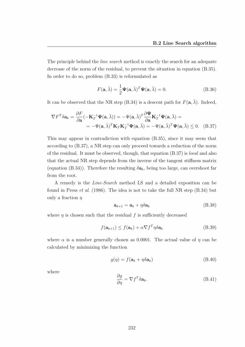
B.2 Line Search algorithm
The principle behind the line search method is exactly the search for an adequate
decrease of the norm of the residual, to prevent the situation in equation (B.35).
In order to do so, problem (B.33) is reformulated as
F (a, λ) =1
2Ψ(a, λ)TΨ(a, λ) = 0. (B.36)
It can be observed that the NR step (B.34) is a descent path for F (a, λ). Indeed,
∇F T δak =∂F
∂a(−K−1
T Ψ(a, λ)) = −Ψ(a, λ)T∂Ψ
∂aK−1T Ψ(a, λ) =
= −Ψ(a, λ)TKTK−1T Ψ(a, λ) = −Ψ(a, λ)TΨ(a, λ) ≤ 0. (B.37)
This may appear in contradiction with equation (B.35), since it may seem that
according to (B.37), a NR step can only proceed towards a reduction of the norm
of the residual. It must be observed, though, that equation (B.37) is local and also
that the actual NR step depends from the inverse of the tangent stiffness matrix
(equation (B.34)). Therefore the resulting δak, being too large, can overshoot far
from the root.
A remedy is the Line-Search method LS and a detailed exposition can be
found in Press et al. (1986). The idea is not to take the full NR step (B.34) but
only a fraction η
ak+1 = ak + ηδak (B.38)
where η is chosen such that the residual f is sufficiently decreased
f(ak+1) ≤ f(ak) + α∇fTηδak (B.39)
where α is a number generally chosen as 0.0001. The actual value of η can be
calculated by minimizing the function
g(η) = f(ak + ηδak) (B.40)
where∂g
∂η= ∇fT δak. (B.41)
232
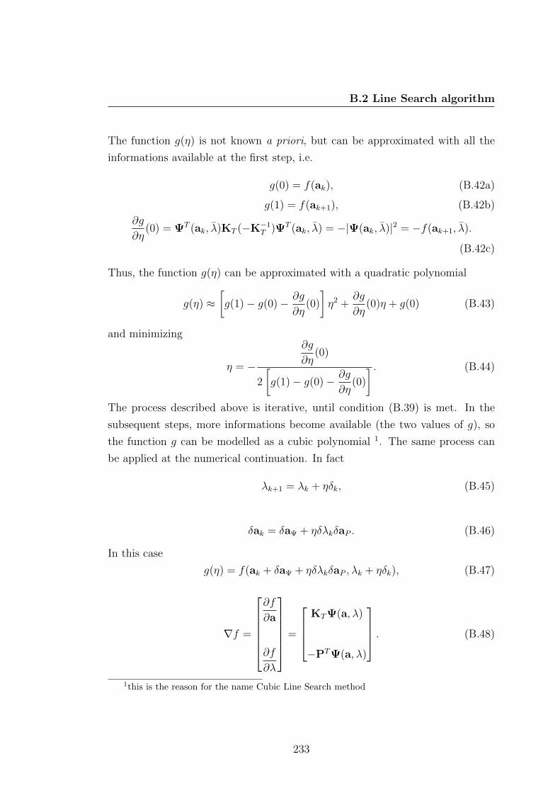
B.2 Line Search algorithm
The function g(η) is not known a priori, but can be approximated with all the
informations available at the first step, i.e.
g(0) = f(ak), (B.42a)
g(1) = f(ak+1), (B.42b)
∂g
∂η(0) = ΨT (ak, λ)KT (−K−1
T )ΨT (ak, λ) = −|Ψ(ak, λ)|2 = −f(ak+1, λ).
(B.42c)
Thus, the function g(η) can be approximated with a quadratic polynomial
g(η) ≈[g(1)− g(0)− ∂g
∂η(0)
]η2 +
∂g
∂η(0)η + g(0) (B.43)
and minimizing
η = −
∂g
∂η(0)
2
[g(1)− g(0)− ∂g
∂η(0)
] . (B.44)
The process described above is iterative, until condition (B.39) is met. In the
subsequent steps, more informations become available (the two values of g), so
the function g can be modelled as a cubic polynomial 1. The same process can
be applied at the numerical continuation. In fact
λk+1 = λk + ηδk, (B.45)
δak = δaΨ + ηδλkδaP . (B.46)
In this case
g(η) = f(ak + δaΨ + ηδλkδaP , λk + ηδk), (B.47)
∇f =
∂f
∂a
∂f
∂λ
=
KTΨ(a, λ)
−PTΨ(a, λ)
. (B.48)
1this is the reason for the name Cubic Line Search method
233
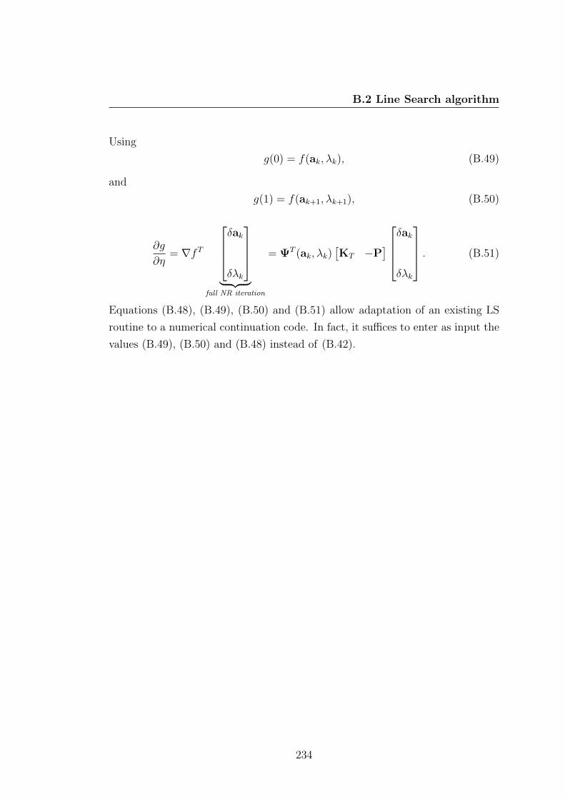
B.2 Line Search algorithm
Using
g(0) = f(ak, λk), (B.49)
and
g(1) = f(ak+1, λk+1), (B.50)
∂g
∂η= ∇fT
δak
δλk
︸ ︷︷ ︸
full NR iteration
= ΨT (ak, λk)[KT −P
] δak
δλk
. (B.51)
Equations (B.48), (B.49), (B.50) and (B.51) allow adaptation of an existing LS
routine to a numerical continuation code. In fact, it suffices to enter as input the
values (B.49), (B.50) and (B.48) instead of (B.42).
234

References
Abdelaziz, Y. & Hamouine, A. (2008). A survey of the extended finite ele-
ment. Computers and Structures , 86, 1141–1151. 15
Alfano, G. & Crisfield, M. (2001). Finite element interface models for the
delamination analysis of laminated composites: mechanical and computational
issues. Int. J. Numer. Meth. Engng , 50, 1701–1736. 141, 149, 172, 175
Anderson, T. (1991). Fracture mechanics . CRC Press. 21
Atluri, S. & Zhu, T. (1998). A new Meshless Local Petrov-Galerkin (MLPG)
approach in computational mechanics. Computational Mechanics , 22, 117–127.
35, 64, 65
Babuska, I. & Melenk, J. (1997). The partition of unity method. Interna-
tional Journal for Numerical Methods in Engineering , 40, 727–758. 134
Babuska, I., Banerjee, U. & Osborn, J. (2003). Survey of meshless and
generalized finite element methods: A unified approach. Acta Numerica, 12,
1–125.
Bank, R. (1990). PLTMG, a software package for solving elliptic partial differ-
ential equations: users’ guide 6.0 . Society for Industrial and Applied Mathe-
matics. 10
Barbieri, E. & Meo, M. (2008). Delamination modelling using an Element
Free Galerkin approach. In 13th European Conference on Composite Materials
ECCM-13, Stockholm, Sweden. 62, 135
235
REFERENCES
Barbieri, E. & Meo, M. (2009a). A meshfree penalty-based approach to de-
lamination in composites. Composites Science and Technology , 69, 2169–2177.
63, 135, 142
Barbieri, E. & Meo, M. (2009b). Evaluation of the integral terms in reproduc-
ing kernel methods. Computer Methods in Applied Mechanics and Engineering ,
198, 2485–2507. 23, 49, 204
Barbieri, E. & Meo, M. (submitted). Computation of the integral terms in
reproducing kernel element methods. Computer Methods in Applied Mechanics
and Engineering . 204
Barenblatt, G. (1962). Mathematical Theory of Equilibrium Cracks in Brittle
Failure. Advances in Applied Mechanics , 7. 137
Beissel, S. & Belytschko, T. (1996). Nodal integration of the element-free
Galerkin method. Computer Methods in Applied Mechanics and Engineering ,
139, 49–74. 37
Beissel, S., Gerlach, C. & Johnson, G. (2006). Hypervelocity impact com-
putations with finite elements and meshfree particles. International Journal of
Impact Engineering , 33, 80–90. 35
Belinha, J. & Dinis, L. (2006). Analysis of plates and laminates using the
element-free Galerkin method. Computers and Structures , 84, 1547–1559.
Belinha, J. & Dinis, L. (2007). Nonlinear analysis of plates and laminates
using the element free Galerkin method. Composite Structures , 78, 337–350.
35
Belytschko, T. & Fleming, M. (1999). Smoothing, enrichment and contact
in the element-free Galerkin method. Computers and Structures , 71, 173–195.
32, 56, 63
Belytschko, T. & Tabbara, M. (1996). Dynamic fracture using element-free
Galerkin methods. International Journal for Numerical Methods in Engineer-
ing , 39, 923–938. 27
236
REFERENCES
Belytschko, T., Gu, L. & Lu, Y. (1994a). Fracture and crack growth by
element-free Galerkin methods. Modelling Simul. Mater. Sci. Eng , 2, 519–534.
25, 27, 52, 53
Belytschko, T., Lu, Y. & Gu, L. (1994b). Element-free Galerkin methods.
International Journal for Numerical Methods in Engineering , 37, 229–256. 22,
24, 25, 62, 134
Belytschko, T., Lu, Y. & Gu, L. (1995a). Crack propagation by element-free
Galerkin methods. Engineering Fracture Mechanics , 51, 295–315. 26
Belytschko, T., Lu, Y., Gu, L. & Tabbara, M. (1995b). Element-free
Galerkin methods for static and dynamic fracture. International Journal of
Solids and Structures , 32, 2547–2570. 27
Belytschko, T., Krongauz, Y., Fleming, M., Organ, D. & Snm Liu,
W. (1996a). Smoothing and accelerated computations in the element free
Galerkin method. Journal of Computational and Applied Mathematics , 74,
111–126. 27, 28, 50, 52, 54, 135
Belytschko, T., Krongauz, Y., Organ, D., Fleming, M. & Krysl, P.
(1996b). Meshless methods: An overview and recent developments. Computer
Methods in Applied Mechanics and Engineering , 139, 3–47. 6, 14, 17, 23, 47,
56, 64, 72
Black, T. & Belytschko, T. (1999). Elastic crack growth in finite elements
with minimal remeshing. International Journal for Numerical Methods in En-
gineering , 45, 601–620. 14, 134
Bolotin, V. (1996). Delaminations in composite structures: its origin, buckling,
growth and stability. Composites. Part B, Engineering , 27, 129–145. 132
Bolotin, V. (2001). Mechanics of delaminations in laminate composite struc-
tures. Mechanics of Composite Materials , 37, 367–380. 132
237
REFERENCES
Bordas, S., Rabczuk, T. & Zi, G. (2008). Three-dimensional crack initi-
ation, propagation, branching and junction in non-linear materials by an ex-
tended meshfree method without asymptotic enrichment. Engineering Fracture
Mechanics , 75, 943–960.
Borg, R., Nilsson, L. & Simonsson, K. (2002). Modeling of delamination
using a discretized cohesive zone and damage formulation. Composites Science
and Technology , 62, 1299–1314.
Borg, R., Nilsson, L. & Simonsson, K. (2004). Simulating DCB, ENF and
MMB experiments using shell elements and a cohesive zone model. Composites
Science and Technology , 64, 269–278.
Borst, R., Remmers, J. & Needleman, A. (2006). Mesh-independent dis-
crete numerical representations of cohesive-zone models. Engineering Fracture
Mechanics , 73, 160–177.
Breitkopf, P., Rassineux, A., Touzot, G. & Villon, P. (2000). Explicit
form and efficient computation of MLS shape functions and their derivatives.
Int. J. Numer. Meth. Engng , 48, 466. 36, 83, 85
Brighenti, R. (2005). Application of the element-free Galerkin meshless method
to 3-D fracture mechanics problems. Engineering Fracture Mechanics , 72,
2808–2820.
Camanho, P. & Davila, C. (2002). Mixed-mode decohesion finite elements for
the simulation of delamination in composite materials. NASA-Technical Paper ,
211737. 133, 148, 173, 179
Camanho, P., Davila, C. & Ambur, D. (2001). Numerical Simulation of
Delamination Growth in Composite Materials. 133
Camanho, P., Davila, C. & de Moura, M. (2003). Numerical Simulation
of Mixed-Mode Progressive Delamination in Composite Materials. Journal of
Composite Materials , 37, 1415. 133, 148
238

REFERENCES
Campbell, J., Vignjevic, R. & Libersky, L. (2000). A contact algorithm
for smoothed particle hydrodynamics. Computer Methods in Applied Mechanics
and Engineering , 184, 49–65. 20
Carpinteri, A., Ferro, G. & Ventura, G. (2003). The partition of unity
quadrature in element-free crack modelling. Computers and Structures , 81,
1783–1794.
Cartwright, C., Oliveira, S. & Stewart, D. (2001). A parallel quadtree
algorithm for efficient assembly of stiffness matrices in meshfree galerkin meth-
ods. In Parallel and Distributed Processing Symposium., Proceedings 15th In-
ternational , 1194–1198. 73
Cartwright, C., Oliveira, S. & Stewart, D. (2007). Parallel support set
searches for meshfree methods. SIAM Journal on Scientific Computing , 28,
1318–1334.
Chen, J., Pan, C., Wu, C. & Liu, W. (1996). Reproducing Kernel Parti-
cle Methods for large deformation analysis of non-linear structures. Computer
Methods in Applied Mechanics and Engineering , 139, 195–227. 32, 33
Chen, J., Pan, C. & Wu, C. (1997). Large deformation analysis of rubber
based on a reproducing kernel particle method. Computational Mechanics , 19,
211–227. 34
Chen, J., Crisfield, M., Kinloch, A., Busso, E., Matthews, F. & Qiu,
Y. (1999). Predicting Progressive Delamination of Composite Material Speci-
mens via Interface Elements. Mechanics of Advanced Materials and Structures ,
6, 301–317. xiii, xv, 149, 175, 176, 177
Chen, J., Wu, C., Yoon, S. & You, Y. (2001). A stabilized conforming
nodal integration for Galerkin mesh-free methods. Int. J. Numer. Meth. Eng ,
50, 435–466. 37
Chen, L.W.e., J.S. (2000). Meshless particle methods (special issue). Compu-
tational Mechanics , 25, 99–317. 18
239

REFERENCES
Chen, L.W.e., J.S. (2004). Meshless methods: Recent advances and new ap-
plications (special issue). Computer Methods in Applied Mechanics and Engi-
neering , 193, 933–1321. 18
Chen, X., Liu, G. & Lim, S. (2003). An element free Galerkin method for the
free vibration analysis of composite laminates of complicated shape. Composite
Structures , 59, 279–289.
Chen, Y., Eskandarian, A., Oskard, M. & Lee, J. (2005). Meshless anal-
ysis of high-speed impact. Theoretical and Applied Fracture Mechanics , 44,
201–207. 35
Clough, R. (1960). The finite element method in plane stress analysis. In
Proceedings, 2nd ASCE Conference on Electronic Computations, Pittsburgh,
September 1960 , 960. 1
Cormen, T., Leiserson, C., Rivest, R. & Stein, C. (2001). Introduction
to algorithms . The MIT press. 73
Crisfield, M. (1991). Non-Linear Finite Element Analysis of Solids and Struc-
tures . John Wiley & Sons Inc. 136, 137, 227
Cueto-Felgueroso, L., Colominas, I., Mosqueira, G., Navarrina, F.
& Casteleiro, M. (2004). On the Galerkin formulation of the smoothed
particle hydrodynamics method. International journal for numerical methods
in engineering , 60, 1475–1512. 20
Davila, C., Camanho, P. & De Moura, M. (2001). Mixed-mode decohesion
elements for analyses of progressive delamination. In Proceedings of the 42nd
AIAA/ASME/ASCE/AHS/ASC Structures, Structural Dynamics and Materi-
als Conference, Seattle, WA. 179
De, S. & Bathe, K. (2000). The method of finite spheres. Computational Me-
chanics , 25, 329–345. 35
De Berg, M., Cheong, O., Van Kreveld, M. & Overmars, M. (2008).
Computational geometry: algorithms and applications . Springer-Verlag New
York Inc. 10
240
REFERENCES
de Borst, R. (2003). Numerical aspects of cohesive-zone models. Engineering
Fracture Mechanics , 70, 1743–1757.
de Borst, R. & Remmers, J. (2006). Computational modelling of delamina-
tion. Composites Science and Technology , 66, 713–722.
de Borst, R., Remmers, J. & Needleman, A. (2004). Computational as-
pects of cohesive zone models. Advanced Fracture Mechanics for Life and Safety
Assesments-Stockholm (Sweden).
Dilts, G. (1999). Moving-least-squares-particle hydrodynamics-I. Consistency
and stability. International Journal for Numerical Methods in Engineering ,
44, 1115–1155. 20
Dilts, G. (2000). Moving least-squares particle hydrodynamics II: conservation
and boundaries. International Journal for Numerical Methods in Engineering ,
48, 1503–1524. 20
Doblare, M., Cueto, E., Calvo, B., Martinez, M., Garcia, J. & Ce-
gonino, J. (2005). On the employ of meshless methods in biomechanics. Com-
puter Methods in Applied Mechanics and Engineering , 194, 801–821. 7, 8
Dolbow, J. & Belytschko, T. (1998). An introduction to programming the
meshless element free Galerkin method. Archives of Computational Methods in
Engineering , 5, 207–241. 72
Dolbow, J. & Belytschko, T. (1999). Numerical integration of the Galerkin
weak form in meshfree methods. Computational Mechanics , 23, 219–230. 13,
36, 64, 65, 167
Dolbow, J., Moes, N. & Belytschko, T. (2000). Discontinuous enrichment
in finite elements with a partition of unity method. Finite Elements in Analysis
& Design, 36, 235–260. 134
Duarte, C. (1995). A review of some meshless methods to solve partial differ-
ential equations. TICAM Report , 95–06. 7, 17
241
REFERENCES
Duarte, C. & Oden, J. (1996). Hp clouds–an hp meshless method. Numerical
Methods for Partial Differential Equations , 12, 673–705. 24, 28, 29, 35, 38, 56,
59
Duff, I., Erisman, A. & Reid, J. (1989). Direct methods for sparse matrices .
Oxford University Press, USA. 12
Duflot, M. (2006). A meshless method with enriched weight functions for three-
dimensional crack propagation. Int J Numer Methods Eng , 65, 1970–2006. 37
Duflot, M. & Nguyen-Dang, H. (2002). A truly Meshless Galerkin Method
based on a Moving Least Squares Quadrature [J]. Communications in Numer-
ical Methods in Engineering , 18, 1–9. 36
Duflot, M. & Nguyen-Dang, H. (2004a). A meshless method with enriched
weight functions for fatigue crack growth. Int. J. Numer. Meth. Engng , 59,
1945–1961. 37
Duflot, M. & Nguyen-Dang, H. (2004b). Fatigue crack growth analysis by
an enriched meshless method. Journal of Computational and Applied Mathe-
matics , 168, 155–164.
Eskandarian, A., Chen, Y., Oskard, M. & Lee, J. (2003). Meshless anal-
ysis of fracture. Plasticity and impact. Proceedings of IMECE , 3, 15–21. 35
Fasshauer, G. (2002). Matrix-free multilevel moving least-squares methods.
Approximation Theory, X St. Louis, MO , 271–278. 35
Fasshauer, G. (2005). Dual bases and discrete reproducing kernels: a uni-
fied framework for RBF and MLS approximation. Engineering Analysis with
Boundary Elements , 29, 313–325.
Fasshauer, G. (2007). Meshfree approximation methods with Matlab. World
Scientific Pub Co Inc. 73
Fasshauer, G. & Zhang, J. (2003). Recent results for moving least squares
approximation. Geometric Modeling and Computing , 163–176. 35
242

REFERENCES
Fernandez-Mendez, S. & Huerta, A. (2004). Imposing essential boundary
conditions in mesh-free methods. Computer Methods in Applied Mechanics and
Engineering , 193, 1257–1275. 14
Finkel, R. & Bentley, J. (1974). Quad trees a data structure for retrieval on
composite keys. Acta informatica, 4, 1–9. 73
Fleming, M., Chu, Y., Moran, B. & Belytschko, T. (1997). Enriched
element-free galerkin methods for crack tip fiels. International Journal for Nu-
merical Methods in Engineering , 40, 1483–1504. 29, 30
Freund, L. (1990). Dynamic Fracture Mechanics . Cambridge University Press.
27
Fries, T. & Matthies, H. (2004). Classification and overview of meshfree
methods, Informatikbericht Nr. 2003-3, Scientific Computing Univ. 7, 18, 19,
41, 48, 51, 66, 69, 135
Gavete, L., Benito, J., Falcon, S. & Ruiz, A. (2000). Implementation
of essential boundary conditions in a meshless method. Communications in
numerical methods in engineering , 16, 409–421. 14
Gingold, R. & Monaghan, J. (1977). Smoothed Particle Hydrodynamics:
theory and application. Monthly Notices of the Royal Astronomical Society ,
181, 375–389. 22
Gleich, K. & Jackson, T. (2002). Center for Composite Manufacturing Final
Report. 5
Griebel, M. & Schweitzer, M. (2002a). A Particle-Partition of Unity
Method–Part II: Efficient Cover Construction and Reliable Integration. SIAM
Journal on Scientific Computing , 23, 1655–1682. 73
Griebel, M. & Schweitzer, M. (2002b). A particle-partition of unity method,
Part II: Efficient cover construction and reliable integration. SIAM J. Sci. Com-
put , 23, 1655–1682.
243

REFERENCES
Gu, Y. (2005). Meshfree Methods and their comparisons. International Journal
of Computational Methods , 2, 477–515. 7
Guiamatsia, I., Falzon, B., Davies, G. & Iannucci, L. (2009). Element-
Free Galerkin modelling of composite damage. Composites Science and Tech-
nology . 135
Gunther, F. & Liu, W. (1998). Implementation of boundary conditions for
meshless methods. Computer Methods in Applied Mechanics and Engineering ,
163, 205–230. 14
Han, W. & Meng, X. (2001). Error analysis of the reproducing kernel particle
method. Computer Methods in Applied Mechanics and Engineering , 190, 6157–
6181.
Hashin, Z. (1980). Failure criteria for unidirectional fiber composites. Journal
of Applied Mechanics , 47, 329. 132
Hillerborg, A., Modeer, M., Petersson, P. et al. (1976). Analysis of
crack formation and crack growth in concrete by means of fracture mechanics
and finite elements. Cement and Concrete Research, 6, 773–782. 137
Huerta, A. & Fernandez-Mendez, S. (2000). Enrichment and coupling of
the finite element and meshless methods. Int. J. Numer. Meth. Engng , 48,
1615–1636. 56
Huerta, A., Belytscko, T., Fernandez-Mendez, S. & Rabczuk, T.
(2004). Chapter on Meshfree Methods .
Idelsohn, S. & Onate, E. (2006). To mesh or not to mesh. That is the ques-
tion. Computer Methods in Applied Mechanics and Engineering , 195, 4681–
4696. 7, 37, 38, 72
Idelsohn, S., Onate, E., Calvo, N. & Del Pin, F. (2003). The meshless
finite element method. International Journal for Numerical Methods in Engi-
neering , 58, 893–912. 35
244
REFERENCES
Jin, X., Li, G. & Aluru, N. (2001). On the equivalence between least-squares
and kernel approximations in meshless methods. Computer Modeling in Engi-
neering and Sciences , 2, 447–462. 17
Karihaloo, B. & Xiao, Q. (2003). Modelling of stationary and growing cracks
in FE framework without remeshing: a state-of-the-art review. Computers and
Structures , 81, 119–129. 15
Khosravifard, A. & Hematiyan, M. (2009). A new method for meshless
integration in 2D and 3D Galerkin meshfree methods. Engineering Analysis
with Boundary Elements , 34, 30–40. 36
Klaas, O. & Shephard, M. (2000). Automatic generation of octree-based
three-dimensional discretizations for partition of unity methods. Computational
Mechanics , 25, 296–304. 73
Klein, P., Foulk, J., Chen, E., Wimmer, S. & Gao, H. (2001). Physics-
based modeling of brittle fracture: cohesive formulations and the application
of meshfree methods. Theoretical and Applied Fracture Mechanics , 37, 99–166.
137
Krysl, P. & Belytschko, T. (1997). Element-free Galerkin method: Conver-
gence of the continuous and discontinuous shape functions. Computer Methods
in Applied Mechanics and Engineering , 148, 257–277. 30, 53
Krysl, P. & Belytschko, T. (1999). The Element Free Galerkin Method for
Dynamic Propagation of Arbitrary 3-D Cracks. Int. J. Numer. Meth. Engng ,
44, 767–780. 31
Krysl, P. & Belytschko, T. (2001). ESFLIB: A library to compute the
element free Galerkin shape functions. Computer Methods in Applied Mechanics
and Engineering , 190, 2181–2206. 66, 72, 74
Lancaster, P. & Salkauskas, K. (1981). Surfaces generated by moving least
squares methods. Mathematics of Computation, 37, 141–158. 22, 24, 50
245

REFERENCES
Leitao, V. (2001). A meshless method for Kirchhoff plate bending problems.
Int. J. Numer. Meth. Engng , 52, 1107–1130.
Li, S. & Liu, W. (1996). Moving least-square reproducing kernel method Part
II: Fourier analysis. Computer Methods in Applied Mechanics and Engineering ,
139, 159–193. 17, 24, 50
Li, S. & Liu, W. (1999a). Reproducing kernel hierarchical partition of unity
Part I: Formulation and theory. Int. J. Numer. Methods Eng , 45, 251–288.
Li, S. & Liu, W. (1999b). Reproducing kernel hierarchical partition of unity
Part II: Applications. Int. J. Numer. Methods Eng , 45, 289–317.
Li, S. & Liu, W. (2004a). Meshfree Particle Methods . Springer. 11
Li, S. & Liu, W. (2004b). Meshfree particle methods . Springer Verlag. 18
Li, S., Hao, W. & Liu, W. (2000a). Mesh-free simulations of shear banding in
large deformation. International Journal of Solids and Structures , 37, 7185–
7206. 35
Li, S., Hao, W., Liu, W., Center, A.H.P.C.R. & of Minnesota, U.
(2000b). Numerical simulations of large deformation of thin shell structures
using meshfree methods. Computational Mechanics , 25, 102–116. 34
Li, S., Lu, H., Han, W., Liu, W. & Simkins, D. (2004). Reproducing kernel
element method Part II: Globally conforming Im/Cn hierarchies. Computer
Methods in Applied Mechanics and Engineering , 193, 953–987. 217
Libersky, L. & Petschek, A. (1990). Smooth particle hydrodynamics with
strength of materials. Proceedings of the next Free-Lagrange Conference Jack-
son Lake Lodge, Moran, Wyoming, June. 20
Libersky, L., Petschek, A., Carney, T., Hipp, J. & Allahdadi, F.
(1993). High strain Lagrangian hydrodynamics: a three-dimensional SPH code
for dynamic material response. Journal of Computational Physics , 109, 67–75.
20
246

REFERENCES
Liew, K., Ng, T. & Wu, Y. (2002a). Meshfree method for large deformation
analysis–a reproducing kernel particle approach. Engineering Structures , 24,
543–551. 35
Liew, K., Wu, Y., Zou, G. & Ng, T. (2002b). Elasto-plasticity revisited:
numerical analysis via reproducing kernel particle method and parametric
quadratic programming. Int. J. Numer. Meth. Engng , 55, 669–683.
Liu, G. (2003). Mesh Free Methods: Moving Beyond the Finite Element Method .
CRC Press. 2, 6, 7, 8, 9, 18, 21, 65, 73
Liu, G. & Tu, Z. (2002a). An adaptive procedure based on background cells for
meshless methods. Computer Methods in Applied Mechanics and Engineering ,
191, 1923–1943. 85
Liu, G. & Tu, Z. (2002b). An adaptive procedure based on background cells for
meshless methods. Computer Methods in Applied Mechanics and Engineering ,
191, 1923–1943.
Liu, T.O.J.e., W.K.; Belytschko (1996). Meshless methods (special issue).
Computer Methods in Applied Mechanics and Engineering , 139, 1–400. 18
Liu, W. & Jun, S. (1998). Multiple-Scale Reproducing Kernel Particle Methods
for Large Deformation Problems. Int. J. Numer. Meth. Engng , 41, 1339–1362.
34
Liu, W., Jun, S. & Zhang, Y. (1995). Reproducing kernel particle methods.
International journal for numerical methods in fluids , 20, 1081–1106. 22, 134
Liu, W., Chen, Y., Uras, R. & Chang, C. (1996). Generalized multiple scale
reproducing kernel particle methods. Computer Methods in Applied Mechanics
and Engineering , 139, 91–157. 22, 23, 34
Liu, W., Hao, W., Chen, Y., Jun, S. & Gosz, J. (1997a). Multiresolution
reproducing kernel particle methods. Computational Mechanics , 20, 295–309.
23, 34, 49, 206
247
REFERENCES
Liu, W., Li, S. & Belytschko, T. (1997b). Moving least-square reproduc-
ing kernel methods (I) Methodology and convergence. Computer Methods in
Applied Mechanics and Engineering , 143, 113–154. 17, 22, 24, 50
Liu, W., Hao, S., Belytschko, T., Li, S. & Chang, C. (1999). Multiple
scale meshfree methods for damage fracture and localization. Computational
Materials Science, 16, 197–205.
Liu, W., Han, W., Lu, H., Li, S. & Cao, J. (2004). Reproducing kernel
element method. Part I: Theoretical formulation. Computer Methods in Applied
Mechanics and Engineering , 193, 933–951.
Lu, H., Li, S., Simkins, D., Kam Liu, W. & Cao, J. (2004). Reproduc-
ing kernel element method Part III: Generalized enrichment and applications.
Computer Methods in Applied Mechanics and Engineering , 193, 989–1011.
Lucy, L. (1977). A numerical approach to the testing of the fission hypothesis.
The Astronomical Journal , 82, 1013–1024. 20
Macri, M., De, S. & Shephard, M. (2003). Hierarchical tree-based discretiza-
tion for the method of finite spheres. Computers and Structures , 81, 789–803.
73
Melenk, J. & Babuska, I. (1996). The partition of unity finite element
method: Basic theory and applications. Computer Methods in Applied Me-
chanics and Engineering , 139, 289–314. 24, 29, 56
Meo, M. & Thieulot, E. (2005). Delamination modeling in a double cantilever
beam. Composite Structures , 71, 429–434.
Moes, N. & Belytschko, T. (2002). Extended finite element method for
cohesive crack growth. Engineering Fracture Mechanics , 69, 813–833. 134
Moes, N., Dolbow, J. & Belytschko, T. (1999). A finite element method for
crack growth without remeshing. International Journal for Numerical Methods
in Engineering , 46, 131–150. 14, 134
248

REFERENCES
Mohammadi, S. (2008). Extended finite element method . Oxford: Blackwell
Publishing. 15
Monaghan, J. (1982). Why Particle Methods Work. SIAM Journal on Scientific
and Statistical Computing , 3, 422. 20, 47
Monaghan, J. (1988). An introduction to SPH. Computer Physics Communi-
cations , 48, 89–96. 20, 47
Monaghan, J. (1992). Smoothed Particle Hydrodynamics. Annual Reviews in
Astronomy and Astrophysics , 30, 543–574. 20, 22, 47
Moore, A. (1991). A tutorial on kd-trees. Extract from PhD Thesis, available
from http://www.cs.cmu.edu/simawm/papers.html. 73
Muravin, B. & Turkel, E. (2006a). Multiple Crack Weight for Solution of
Multiple Interacting Cracks by Meshless Numerical Methods. Int. J. Numer.
Meth. Engng , 67, 1146–1159. 37
Muravin, B. & Turkel, E. (2006b). Spiral weight for modeling cracks in
meshless numerical methods. Computational Mechanics , 38, 101–111. 37, 55
Nayroles, B., Touzot, G. & Villon, P. (1992). Generalizing the finite
element method: Diffuse approximation and diffuse elements. Computational
Mechanics , 10, 307–318. 22
Needleman, A. (1987). A continuum model for void nucleation by inclusion
debonding. Journal of applied mechanics , 54, 525–531. 137, 138
Nguyen, V., Rabczuk, T., Bordas, S. & Duflot, M. (2008). Meshless
methods: A review and computer implementation aspects. Mathematics and
Computers in Simulation. 7, 18, 38, 57, 69, 72
Onate, E., Idelsohn, S., Zienkiewicz, O., Taylor, R. et al. (1996). A
finite point method in computational mechanics. Applications to convective
transport and fluid flow. International Journal for Numerical Methods in En-
gineering , 39, 3839–3866. 35
249

REFERENCES
Orifici, A., Herszberg, I. & Thomson, R. (2008). Review of methodologies
for composite material modelling incorporating failure. Composite Structures ,
86, 194–210. 131
Orkisz, J. & Krok, J. (2008). On classification of the meshless methods. In
8th. World Congress on Computational Mechanics (WCCM8). 17
Pantano, A. & Averill, R. (2002). A penalty-based finite element interface
technology. Computers and Structures , 80, 1725–1748. 135
Pantano, A. & Averill, R. (2004). A mesh-independent interface technology
for simulation of mixed-mode delamination growth. International Journal of
Solids and Structures , 41, 3809–3831. 135
Paris, P. & Erdogan, F. (1963). A Critical Analysis of Crack Propagation
Laws. J. Basic Eng. Trans. ASME Series D , 85, 528–534. 27
Ponthot, J. & Belytschko, T. (1998). Arbitrary Lagrangian-Eulerian for-
mulation for element-free Galerkin method. Computer Methods in Applied Me-
chanics and Engineering , 152, 19–46. 34
Preparata, F. & Shamos, M. (1985). Computational geometry: an introduc-
tion. Springer. 10
Press, W., Flannery, B., Teukolsky, S., Vetterling, W. et al. (1986).
Numerical recipes . Cambridge University Press New York. 148, 232
Puck, A. & Schurmann, H. (2002). Failure analysis of FRP laminates by
means of physically based phenomenological models. Composites Science and
Technology , 62, 1633–1662. 131, 132
Puso, M., Chen, J., Zywicz, E. & Elmer, W. (2008). Meshfree and fi-
nite element nodal integration methods. International Journal for Numerical
Methods in Engineering , 74, 416–446. 37
Quinlan, N., Basa, M. & Lastiwka, M. (2006). Truncation error in mesh-
free particle methods. Int. J. Numer. Meth. Engng , 66, 2064–2085.
250
REFERENCES
Rabczuk, T. & Belytschko, T. (2005). Adaptivity for structured meshfree
particle methods in 2D and 3D. Int J Numer Methods Eng , 63, 1559–1582. 41,
85
Rabczuk, T. & Eibl, J. (2003). Simulation of high velocity concrete frag-
mentation using SPH/MLSPH. Int. J. Numer. Meth. Engng , 56, 1421–1444.
20
Rabczuk, T., Belytschko, T. & Xiao, S. (2004). Stable particle methods
based on Lagrangian kernels. Computer Methods in Applied Mechanics and
Engineering , 193, 1035–1063.
Rao, B. & Rahman, S. (2004). An enriched meshless method for non-linear
fracture mechanics. Int. J. Numer. Meth. Engng , 59, 197–223. 35
Remmers, J., Wells, G. & De Borst, R. (2002). Analysis of delamina-
tion growth with discontinuous solid-like shell elements. In Proceedings of the
Fifth Congress on Computational Mechanics (WCCM V). Vienna University
of Technology, Vienna, Austria.
Remmers, J., Borst, R. & Needleman, A. (2003a). A cohesive segments
method for the simulation of crack growth. Computational Mechanics , 31, 69–
77. 134, 152
Remmers, J., Borst, R. & Needleman, A. (2003b). Simulation of fast crack
growth using cohesive segments. In VII International Conference on Compu-
tational Plasticity. COMPLAS . 152
Remmers, J., de Borst, R. & Needleman, A. (2008). The simulation of
dynamic crack propagation using the cohesive segments method. Journal of the
Mechanics and Physics of Solids , 56, 70–92. 135
Rice, J.R. (1968). A Path Independent Integral and the Approximate Analysis
of Strain Concentration by Notches and Cracks. Journal of Applied Mechanics ,
35, 379–386. 25, 131, 141, 154
251
REFERENCES
Samimi, M., van Dommelen, J. & Geers, M. (2009). An enriched cohesive
zone model for delamination in brittle interfaces. International Journal for
Numerical Methods in Engineering , 80. 187
Schembri, P., Crane, D. & Reddy, J. (2004). A three-dimensional com-
putational procedure for reproducing meshless methods and the finite element
method. Int. J. Numer. Meth. Engng , 61, 896–927.
Shaofan, L. & Liu, W. (2002). Meshfree and particle methods and their ap-
plications. Applied Mechanics Review , 55, 1–34. 18
Simkins, D., Li, S., Lu, H. & Kam Liu, W. (2004). Reproducing kernel
element method. Part IV: Globally compatible Cn (n ≥ 1) triangular hierarchy.
Computer Methods in Applied Mechanics and Engineering , 193, 1013–1034.
Sukky Jun, T.B., Wing Kam Liu (1998). Explicit Reproducing Kernel Parti-
cle Methods for large deformation problems. International Journal for Numer-
ical Methods in Engineering , 41, 137–166. 34
Sukumar, N. & Wright, R. (2007). Overview and construction of meshfree
basis functions: From moving least squares to entropy approximants. Int. J.
Numer. Meth. Engng , 70, 181–205.
Sukumar, N., Moran, B., Black, T. & Belytschko, T. (1997). An
element-free Galerkin method for three-dimensional fracture mechanics. Com-
putational Mechanics , 20, 170–175. 31
Sukumar, N., Moran, B. & Belytschko, T. (1998). The natural element
method in solid mechanics. Int. J. Numer. Meth. Eng , 43, 839–887. 35
Sun, C. & Zheng, S. (1996). Delamination characteristics of double-cantilever
beam and end-notched flexure composite specimens. Composites Science and
Technology , 56, 451–459.
Sun, Y., Hu, Y. & Liew, K. (2007). A mesh-free simulation of cracking and
failure using the cohesive segments method. International Journal of Engineer-
ing Science, 45, 541–553. 63, 135
252
REFERENCES
Swegle, J., Hicks, D. & Attaway, S. (1995). Smoothed Particle Hydrody-
namics Stability Analysis. Journal of Computational Physics , 116, 123–134.
20
Tabarraei, A. & Sukumar, N. (2005). Adaptive computations on conforming
quadtree meshes. Finite Elements in Analysis & Design, 41, 686–702. 73
Turon, A. (2007). Simulation of delamination in composites under quasi-static
and fatigue loading using cohesive zone models . Ph.D. thesis, Universitat de
Girona. 149, 170, 196
Turon, A., Camanho, P., Costa, J. & Davila, C. (2006). A damage model
for the simulation of delamination in advanced composites under variable-mode
loading. Mechanics of Materials , 38, 1072–1089.
Tvergaard, V. (1990). Material failure by void growth to coalescence. Advances
in Applied Mechanics , 27, 83–151. 140
Tvergaard, V. & Hutchinson, J. (1992). The Relation Between Crack
Growth Resistance and Fracture Process Parameters in Elastic–Plastic Solids.
Journal of the Mechanics and Physics of Solids , 40, 1377–1397.
Ventura, G., Xu, J. & Belytschko, T. (2002). A vector level set method
and new discontinuity approximations for crack growth by EFG. Int. J. Numer.
Methods Eng , 54, 923–944. 32, 59
Vignjevic, R. & Campbell, J. (2009). Review of development of the Smooth
Particle Hydrodynamics (SPH) method. Predictive Modeling of Dynamic Pro-
cesses , 367–396. 20
Vignjevic, R., Campbell, J. & Libersky, L. (2000). A treatment of zero-
energy modes in the smoothed particle hydrodynamics method. Computer
methods in Applied mechanics and Engineering , 184, 67–85. 20
Vignjevic, R., Reveles, J. & Campbell, J. (2006). SPH in a total La-
grangian formalism. Computer Modeling in Engineering & Sciences , 14, 181–
198. 20
253

REFERENCES
Wells, G. & Sluys, L. (2001). A new method for modelling cohesive cracks
using finite elements. International Journal for Numerical Methods in Engi-
neering , 50, 2667–2682. 134
Wells, G., de Borst, R. & Sluys, L. (2002). A consistent geometrically non-
linear approach for delamination. Int. J. Numer. Meth. Eng , 54, 1333–1355.
152
Wriggers, P. (2008). Nonlinear finite element methods . Springer Verlag. 229
Yang, Q. & Cox, B. (2005). Cohesive models for damage evolution in laminated
composites. International Journal of Fracture, 133, 107–137.
You, Y., Chen, J. & Lu, H. (2003). Filters, reproducing kernel, and adaptive
meshfree method. Computational Mechanics , 31, 316–326. 92
Zhang, Z., Zhou, J., Wang, X., Zhang, Y. & Zhang, L. (2004). Investi-
gations on reproducing kernel particle method enriched by partition of unity
and visibility criterion. Computational Mechanics , 34, 310–329.
Zhou, J., Wen, J., Zhang, H. & Zhang, L. (2003). A nodal integration
and post-processing technique based on Voronoi diagram for Galerkin mesh-
less methods. Computer Methods in Applied Mechanics and Engineering , 192,
3831–3843.
Zhou, J., Wang, X., Zhang, Z. & Zhang, L. (2005). Explicit 3-D RKPM
shape functions in terms of kernel function moments for accelerated compu-
tation. Computer Methods in Applied Mechanics and Engineering , 194, 1027–
1035. 36, 83
Zhu, T., Zhang, J. & Atluri, S. (1998). A local boundary integral equation
(LBIE) method in computational mechanics, and a meshless discretization ap-
proach. Computational Mechanics , 21, 223–235. 35
Zienckiewicz, O. & Taylor, R. (1994). The Finite Element Method. Mc
Graw Hill, London. 62
254
REFERENCES
Zou, Z., Reid, S. & Li, S. (2003). A continuum damage model for delamina-
tions in laminated composites. Journal of the Mechanics and Physics of Solids ,
51, 333–356. 140
255
Related Documents