Memory Partitioning and Scheduling Co-optimization in Behavioral Synthesis Peng Li, 1 Yuxin Wang, 1 Peng Zhang, 2 Guojie Luo, 1 Tao Wang, 1,3 Jason Cong 1,2,3 1 Center for Energy-Efficient Computing and Applications, School of EECS, Peking University, Beijing, 100871, China 2 Computer Science Department, University of California, Los Angeles, Los Angeles, CA 90095, USA 3 UCLA/PKU Joint Research Institute in Science and Engineering {peng.li, ayer.wang, gluo, wangtao}@pku.edu.cn, {cong, pengzh}@cs.ucla.edu Abstract—Achieving optimal throughput by extracting parallel- ism in behavioral synthesis often exaggerates memory bottleneck issues. Data partitioning is an important technique for increasing memory bandwidth by scheduling multiple simultaneous memory accesses to different memory banks. In this paper we present a vertical memory partitioning and scheduling algorithm that can generate a valid partition scheme for arbitrary affine memory inputs. It does this by arranging non-conflicting memory accesses across the border of loop iterations. A mixed memory partitioning and scheduling algorithm is also proposed to com- bine the advantages of the vertical and other state-of-art algo- rithms. A set of theorems is provided as criteria for selecting a valid partitioning scheme. This is followed by an optimal and scalable memory scheduling algorithm. By utilizing the property of constant strides between memory addresses in successive loop iterations, an address translation optimization technique for an arbitrary partition factor is proposed to improve performance, area and energy efficiency. Experimental results show that on a set of real-world medical image processing kernels, the proposed mixed algorithm with address translation optimization can gain speed-up, area reduction and power savings of 15.8%, 36% and 32.4% respectively, compared to the state-of-art memory parti- tioning algorithm. Keywords-Behavioral Synthesis; Memory Partitioning; Memory Scheduling I. INTRODUCTION With the exponentially increasing complexity in modern SoC designs, behavioral synthesis is gradually being accepted by the industry. For example, the AutoESL behavioral synthe- sis tool [1, 2] is now part of the Vivado Design Suit available to all Xilinx FPGA designs. By transforming untimed algo- rithmic descriptions into hardware implementations, behavior- al synthesis can significantly reduce time-to-market and de- sign cost with acceptable performance and power penalties. Typical applications for behavioral synthesis are data- intensive or computation-intensive kernels in signal pro- cessing and multimedia applications, where general-purpose processors often fail to meet the performance/power require- ments. Such computation kernels are usually loops that ma- nipulate multiple data elements simultaneously from arrays. Loop pipelining [3] is a common optimization technique that overlaps different loop iterations to increase performance by minimizing initiation interval (II). While more computation units can be added to exploit loop-level parallelism for arith- metic/logic operations, the support of multiple memory ac- cesses efficiently is a key problem to utilizing the potential performance gain made available by loop pipelining. It would be expensive and non-scalable in terms of both cost and power to simply increase the number of memory ports [4]. Moreover, for reconfigurable platforms such as FPGAs, the number of ports of on-chip block RAM is fixed. Duplicating the target array into multiple copies can support multiple simultaneous read operations with significant area and power overhead, but it doesn’t support simultaneous writes. A better approach is to divide the original data array into several disjoint memory banks using memory partitioning. At compile time, the behavioral synthesis tool can statically analyze the data access pattern of the target array and avoid the conflicts among memory accesses by partitioning the array into different memory banks. In parallel, memory partitioning for distributed computing has been studied for decades, where each processing unit ac- cesses its local memory [5-7]. The ideas of some memory par- titioning algorithms in distributed computing can be applied to memory partitioning in behavioral synthesis. For example, the algorithm in [8] that partitions memory into multiple banks to avoid communication between multiple tiles on a single chip is similar to the vertical partitioning algorithm proposed in this paper. However, there are also some fundamental differences between these two scenarios. The first difference is that memory partitioning in behavioral synthesis must meet cycle- level data access constraints to avoid simultaneous accesses on the same memory block. Therefore, memory partitioning and memory scheduling in behavioral synthesis should be an inte- grated process. The second difference is that in distributed computing, all the data elements accessed by a memory refer- ence have to be bound to the specific local memory bank (or processing unit) to which the reference is mapped. In behav- ioral synthesis multiple accesses of the same memory refer- ence can access different memory banks in different loop it- Permission to make digital or hard copies of all or part of this work for personal or classroom use is granted without fee provided that copies are not made or distributed for profit or commercial advantage and that copies bear this notice and the full citation on the first page. To copy otherwise, or republish, to post on servers or to redistribute to lists, requires prior specific permission and/or a fee. IEEE/ACM International Conference on Computer-Aided Design (ICCAD) 2012, November 5-8, 2012, San Jose, California, USA Copyright © 2012 ACM 978-1-4503-1573-9/12/11... $15.00 488

Welcome message from author
This document is posted to help you gain knowledge. Please leave a comment to let me know what you think about it! Share it to your friends and learn new things together.
Transcript

Memory Partitioning and Scheduling Co-optimization
in Behavioral Synthesis
Peng Li,1 Yuxin Wang,
1 Peng Zhang,
2 Guojie Luo,
1 Tao Wang,
1,3Jason Cong
1,2,3
1Center for Energy-Efficient Computing and Applications, School of EECS, Peking University, Beijing, 100871, China
2Computer Science Department, University of California, Los Angeles, Los Angeles, CA 90095, USA
3UCLA/PKU Joint Research Institute in Science and Engineering
{peng.li, ayer.wang, gluo, wangtao}@pku.edu.cn, {cong, pengzh}@cs.ucla.edu
Abstract—Achieving optimal throughput by extracting parallel-
ism in behavioral synthesis often exaggerates memory bottleneck
issues. Data partitioning is an important technique for increasing
memory bandwidth by scheduling multiple simultaneous
memory accesses to different memory banks. In this paper we
present a vertical memory partitioning and scheduling algorithm
that can generate a valid partition scheme for arbitrary affine
memory inputs. It does this by arranging non-conflicting memory
accesses across the border of loop iterations. A mixed memory
partitioning and scheduling algorithm is also proposed to com-
bine the advantages of the vertical and other state-of-art algo-
rithms. A set of theorems is provided as criteria for selecting a
valid partitioning scheme. This is followed by an optimal and
scalable memory scheduling algorithm. By utilizing the property
of constant strides between memory addresses in successive loop
iterations, an address translation optimization technique for an
arbitrary partition factor is proposed to improve performance,
area and energy efficiency. Experimental results show that on a
set of real-world medical image processing kernels, the proposed
mixed algorithm with address translation optimization can gain
speed-up, area reduction and power savings of 15.8%, 36% and
32.4% respectively, compared to the state-of-art memory parti-
tioning algorithm.
Keywords-Behavioral Synthesis; Memory Partitioning; Memory
Scheduling
I. INTRODUCTION
With the exponentially increasing complexity in modern
SoC designs, behavioral synthesis is gradually being accepted
by the industry. For example, the AutoESL behavioral synthe-
sis tool [1, 2] is now part of the Vivado Design Suit available
to all Xilinx FPGA designs. By transforming untimed algo-
rithmic descriptions into hardware implementations, behavior-
al synthesis can significantly reduce time-to-market and de-
sign cost with acceptable performance and power penalties.
Typical applications for behavioral synthesis are data-
intensive or computation-intensive kernels in signal pro-
cessing and multimedia applications, where general-purpose
processors often fail to meet the performance/power require-
ments. Such computation kernels are usually loops that ma-
nipulate multiple data elements simultaneously from arrays.
Loop pipelining [3] is a common optimization technique that
overlaps different loop iterations to increase performance by
minimizing initiation interval (II). While more computation
units can be added to exploit loop-level parallelism for arith-
metic/logic operations, the support of multiple memory ac-
cesses efficiently is a key problem to utilizing the potential
performance gain made available by loop pipelining.
It would be expensive and non-scalable in terms of both
cost and power to simply increase the number of memory
ports [4]. Moreover, for reconfigurable platforms such as
FPGAs, the number of ports of on-chip block RAM is fixed.
Duplicating the target array into multiple copies can support
multiple simultaneous read operations with significant area
and power overhead, but it doesn’t support simultaneous
writes. A better approach is to divide the original data array
into several disjoint memory banks using memory partitioning.
At compile time, the behavioral synthesis tool can statically
analyze the data access pattern of the target array and avoid
the conflicts among memory accesses by partitioning the array
into different memory banks.
In parallel, memory partitioning for distributed computing
has been studied for decades, where each processing unit ac-
cesses its local memory [5-7]. The ideas of some memory par-
titioning algorithms in distributed computing can be applied to
memory partitioning in behavioral synthesis. For example, the
algorithm in [8] that partitions memory into multiple banks to
avoid communication between multiple tiles on a single chip
is similar to the vertical partitioning algorithm proposed in this
paper. However, there are also some fundamental differences
between these two scenarios. The first difference is that
memory partitioning in behavioral synthesis must meet cycle-
level data access constraints to avoid simultaneous accesses on
the same memory block. Therefore, memory partitioning and
memory scheduling in behavioral synthesis should be an inte-
grated process. The second difference is that in distributed
computing, all the data elements accessed by a memory refer-
ence have to be bound to the specific local memory bank (or
processing unit) to which the reference is mapped. In behav-
ioral synthesis multiple accesses of the same memory refer-
ence can access different memory banks in different loop it-
Permission to make digital or hard copies of all or part of this work for
personal or classroom use is granted without fee provided that copies are not made or distributed for profit or commercial advantage and that
copies bear this notice and the full citation on the first page. To copy
otherwise, or republish, to post on servers or to redistribute to lists, requires prior specific permission and/or a fee.
IEEE/ACM International Conference on Computer-Aided Design
(ICCAD) 2012, November 5-8, 2012, San Jose, California, USA Copyright © 2012 ACM 978-1-4503-1573-9/12/11... $15.00
488

erations, which will greatly expand the solution space. A third
difference is that data arrays are typically partitioned into a
fixed number of banks determined by the hardware configura-
tion(proportional to the number of processors) in distributed
computing, while the number of partitioned banks, or partition
factor in behavioral synthesis can be an arbitrary number de-
termined by the data access pattern in a particular application.
The works that are most relevant to this paper are [9] and
[10]. Research in [9] attempts to partition and schedule multi-
ple memory references on a data array in the same loop itera-
tion to multiple cyclic banks to avoid confliction. Memory
padding was introduced before memory partitioning to handle
memory references with modulo operations [10]. While these
works take a first step towards efficient memory support for
loop pipelining in behavioral synthesis, the algorithms gener-
ate inefficient results for some inputs, as shown in the motiva-
tional examples in Section II.
In this paper a vertical memory partitioning and scheduling
algorithm, or a vertical MPS for short, is developed where
multiple accesses of the same memory reference in different
loop iterations are scheduled to different memory banks. In
contrast, approaches in [9-11] that schedule multiple memory
references in the same loop iteration to non-conflicting
memory banks are referred to as horizontal MPS in this paper.
We show that the vertical MPS can generate valid solutions
for arbitrary affine memory references1 within a loop for any
fixed memory port constraint. Furthermore, a mixed partition-
ing and scheduling algorithm, or a mixed MPS, that combines
the advantages of both the horizontal and vertical MPS is pro-
posed where different memory references in different itera-
tions on an array can be scheduled simultaneously and effi-
ciently to non-conflicting memory banks.
Traditionally, partition factors which are powers of 2 are
always preferred to other factors since modulo and divide op-
erations can be transformed into shift operations that are suita-
ble for hardware implementation. In this paper arbitrary parti-
tion factors are supported using a novel address translation
technique that considers the regularity of affine memory ac-
cesses between adjacent loop iterations, so that a larger design
space can be explored for better results.
Our contributions include the following: (i) A vertical and a
mixed memory partitioning and scheduling algorithm for effi-
ciently supporting arbitrary multiple affine memory references
in a loop in behavioral synthesis. (ii) An optimal and scalable
memory scheduling algorithm finding the maximum matching
with minimum cost on the bipartite memory scheduling graph.
(iii) An optimized address translation with arbitrary partition
factors which are not powers of 2.
Experimental results show that on a set of real-world medi-
cal image processing kernels, the proposed mixed MPS algo-
rithm with address translation optimization can gain speed-up,
area reduction, and power saving of 15.8%, 36% and 32.4%
respectively, compared to the horizontal MPS.
1 The address of an affine memory reference is a linear combination
of loop induction variables. Research in [12] shows that the majority
of array references in loop kernels are affine memory references.
The remainder of the paper is organized as follows. Section
II gives a motivational example for our memory partitioning
and scheduling problem. Section III formulates our problem of
memory partitioning and scheduling. Section IV presents pro-
posed memory partitioning and scheduling algorithms. Section
V reports experimental results and is followed by conclusions
in Section VI.
II. DEFINITIONS AND A MOTIVATIONAL EXAMPLE
In this paper, we focus on partitioning and scheduling mul-
tiple memory accesses to different memory banks to support
simultaneous memory accesses in loop pipelining. For sim-
plicity, loop stride is assumed to be 1 in this paper. Algorithms
and formulations are easily extended for any constant loop
stride. Assume that there are m affine memory references
R1:a1*i+b1, R2:a2*i+b2, …, Rm:am*i+bm on the same array in
the target loop without dependency constraints among them.
Rjk is used to represent the k-th loop iteration of Rj, whose ad-
dress is aj*k+bj. Common variables in this paper are shown in
Table 1.
DEFINITION 1 (MEMORY PARTITION). A Memory partition is
described as a function P which maps array access Rjk to parti-
tioned memory banks, i.e., P(Rjk) is the memory bank index
that Rjk belongs to after partitioning.
EXAMPLE 1. Cyclic partitioning (shown in Figure 1):
( )
In this paper, cyclic partitioning is used as the memory par-
titioning scheme where N is the partition factor.
DEFINITION 2 (MEMORY SCHEDULE). A Memory schedule is
described as a function T which maps array access Rjk to its
execution cycles, i.e., T(Rjk) is the cycle to which Rjk is sched-
uled.
0 1 2 …
0 N 2N …
1 N+1 2N+1 …
Bank 0
Bank 1
N-1 2N-1 3N-1 … Bank N-1
……
Figure 1. Cyclic partitioning
Table 1. Symbols Variables Meaning
i Loop induction variable
j,k,l,h,g Temporal variables
m Number of memory references in each loop iteration
Rj The j-th affine memory references in the target loop, can be expressed in the form of aj*i+bj
aj, bj Used to express Rj shown above
Rjk The k-th iteration of affine memory reference Rj. Can be
expressed in the form of aj*k+bj
N Cyclic partition factor
II Loop iteration interval
p Memory port number
VS Valid partition factor set
VSh, VSv,
VSm
Valid partition factor set for horizontal, vertical and mixed
MPS algorithms
489

DEFINITION 3 (HORIZONTAL SCHEDULE [9]). A Horizontal
schedule is a memory schedule with scheduling function T that
satisfies:
( ) .
EXAMPLE 2. Horizontal scheduling (II=1):
( ) , c is a constant.
If there are two affine memory references R1:a1*i+b1 and R2:
a2*i+b2 in a loop with initiation interval II=1 and port p=1,
research in [9] shows that the valid partition factor N using the
horizontal MPS must satisfy (1).
{
(1)
Equation (1) shows that horizontal MPS fails if , or generates large partition fac-
tors if is a large prime number, as shown in Table 2.
To address this problem, vertical schedule is proposed.
DEFINITION 4 (VERTICAL SCHEDULE). A Vertical schedule is
a memory schedule with scheduling function T that satisfies:
( )
where N is the partition factor.
EXAMPLE 3. Vertical scheduling (II=1):
( ) , c is a constant.
The difference between the horizontal and vertical MPS can
be illustrated using Figure 2. In Section IV, we will show that
the vertical MPS guarantees valid solutions for arbitrary affine
memory inputs, although it may generate worse results for
some inputs than the horizontal MPS (shown in Table 1).
A mixed memory partitioning and scheduling algorithm is
proposed to combine the advantages of both the horizontal and
vertical MPS algorithms. Using mixed MPS, different memory
references in different iterations on an array can be scheduled
simultaneously to non-conflicting memory banks.
We use a real-world application, denoise [13] as an example
to demonstrate the design trade-offs in the memory partition-
ing and scheduling problem. A simplified source code for de-
noise is shown in Figure 3(a). The value of an element is ac-
cumulated with all its neighbors in 8*8*8 three-dimensional
Table 2. Comparison between horizontal and vertical MPS Algorithms
Condition Example
Nhorizontal Nvertical R1 R2
Failed 4
Failed 4
Failed 3
is a large prime number
+1 N≥127 3
Case that horizontal MPS is better
+1 2 3
Tim
e
R11 R21
R12 R22
R10 R20
R10 R11
R20 R21
R12 R13
R22 R23
Horizontal MPS Vertical MPS
R13 R
23 … … … …
#define C (i+8*j+8*8*k)) #define R (C+1) #define L (C-1) #define D (C+8) #define U (C-8) #define O (C+8*8) #define I (C-8*8) for(k = 1; k < 7; k++) for(j = 1; j < 7; j++) for(i = 1; i < 7; i++)
v[C]=u[C]+u[R]+u[L]+u[D]+u[U]+u[O]+u[I];
(a) Sample code
u[C]i u[R]i u[L]
i u[D]
i u[U]
i u[O]
i u[I]
i
(b) Horizontal MPS (N=10)
u[D]i u[R]
i
N=7
u[C]i u[D]
i
N=8
u[D]i u[L]
i
N=9 (c) Conflict detection for horizontal MPS
Cycle 0
u[C]i u[C]
i+1 u[C]
i+2 u[C]
i+3 u[C]
i+4 u[C]
i+5 u[C]
i+6 Cycle 0
u[R]i u[R]
i+1 u[R]
i+2 u[R]
i+3 u[R]
i+4 u[R]
i+5 u[R]
i+6 Cycle 1
u[L]i u[L]
i+1 u[L]
i+2 u[L]
i+3 u[L]
i+4 u[L]
i+5 u[L]
i+6 Cycle 2
u[D]i u[D]
i+1 u[D]
i+2 u[D]
i+3 u[D]
i+4 u[D]
i+5 u[D]
i+6 Cycle 3
u[U]i u[U]
i+1 u[U]
i+2 u[U]
i+3 u[U]
i+4 u[U]
i+5 u[U]
i+6 Cycle 4
u[O]i u[O]
i+1 u[O]
i+2 u[O]
i+3 u[O]
i+4 u[O]
i+5 u[O]
i+6 Cycle 5
u[I]i u[I]
i+1 u[I]
i+2 u[I]
i+3 u[I]
i+4 u[I]
i+5 u[I]
i+6 Cycle 6
(d) Vertical MPS (N=7)
u[O]i Cycle 0
u[D]i u[O]
i+1 Cycle 1
u[C]i u[R]
i u[L]
i u[D]
i+1 u[O]
i+2 Cycle 2
u[C]i+1 u[R]
i+1 u[L]
i+1 u[D]
i+2 u[U]
i u[O]
i+3 Cycle 3
u[C]i+2 u[R]
i+2 u[L]
i+2 u[D]
i+3 u[U]
i+1 u[O]
i+4 u[I]
i Cycle 4
(e) Mixed MPS (N=7)
Figure 2. Comparison between horizontal and vertical MPS algorithms
Figure 3. A motivational example
490
space to filter out noises. In the innermost loop, there are 7
data accesses (C, R, L, D, U, O, I for center, right, left, down,
up, zout and zin) to the same array u. If the target loop is to be
fully pipelined using single-port memory banks, array u has to
be cyclic partitioned to multiple (at least 7) memory banks.
Using the horizontal MPS, seven data references on array u
in the same i-th iteration (u[C]i, u[R]i, u[L]i, u[D]i, u[U]i,
u[O]i and u[I]i) are scheduled simultaneously to non-
conflicting memory banks, as shown in Figure 3(b). Since the
difference between the address of u[D]i and u[R]i is always 7,
scheduling u[D]i and u[R]i in the same cycle will cause con-
flict if partition factor N=7. Likewise, 8 and 9 can not be used
as valid partition factors, as shown in Figure 3(c). Therefore,
array u needs to be partitioned into 10 memory banks.
Scheduling results using the vertical MPS is shown in Fig-
ure 3(d). In the first cycle, accesses to u[C] in 7 successive
loop iterations can be loaded simultaneously if the array is
partitioned into 7 cyclic banks. The loaded values are buffered
into temporal registers for future use. In the following cycles,
u[R], u[L], u[D], u[U], u[O] and u[I] in the 6 successive loop
iterations are also loaded into temporal registers. Accumula-
tion of data values will start at cycle 7 and u[C] in the next 7
loop iterations will be loaded in buffers. Compared to the hor-
izontal MPS, the vertical MPS can reduce the partition factor
from 10 to 7, but it adds 6 extra cycle latencies for the whole
loop with 42 registers overhead.
Scheduling results using the mixed MPS are shown in Fig-
ure 3(e). In the example, u[C]i+2, u[R]i+2, u[L]i+2, u[D]i+3,
u[U]i+1, u[O]i+4, u[I]i are scheduled to 7 cyclic banks. Com-
pared to the vertical MPS, a 2-cycle-latency and 25 registers
can be saved using the mixed MPS. Compared to the horizon-
tal MPS, 3 memory banks can be saved using the vertical and
mixed MPS algorithms.
III. PROBLEM FORMULATION
From the motivational example, we can see that vertical and
mixed schedules can potentially reduce the number of parti-
tioned memory banks and thus the cost of the overall memory
subsystem. These are the problems: how to find valid partition
factors, how to find the memory scheduling with minimum
cost for a given partition factor and how to find the best parti-
tion and schedule.
DEFINITION 5 (VALID MEMORY SCHEDULE). Given a loop-
based computation kernel with m affine memory references R1 ,
R2 , …, Rm on the same array, the target throughput requirement
II, the number of memory ports p, and partition factor N, a
valid memory schedule is one memory schedule that satisfies
both throughput and memory port requirements.
(2)
Btl={Rjk | = t and = l}
(3)
where Rjk is scheduled to T(Rjk) with loop prolog c. Equa-
tion (2) formulates memory throughput requirement. is the
set of all the memory accesses which access memory bank l in
cycle t, and (3) formulates the port number requirement.
DEFINITION 6 (VALID MEMORY SCHEDULE SET). A valid
memory schedule set SN is a set of valid memory schedules.
DEFINITION 7 (VALID PARTITION FACTOR SET). A valid par-
tition factor set VS is a set of partition factors with valid
memory schedules, i.e., VS={N | SN≠ }.
VSh, VSv and VSm are used to represent the valid partition
factor set solved by the horizontal, vertical and mixed algo-
rithms respectively.
The memory partitioning and scheduling problem can be
divided into the three problems formulated below.
PROBLEM 1 (MEMORY PARTITIONING). Given a loop-based
computation kernel with m affine memory references R1 , R2 , …,
Rm on the same array, target throughput requirement II, num-
ber of memory ports p, find the valid partition factor set VS.
PROBLEM 2 (MEMORY SCHEDULING). Given a loop-based
computation kernel with m affine memory references R1 , R2 , …,
Rm on the same array, target throughput requirement II, num-
ber of memory ports p, a platform-dependent cost function,
and a valid partition factor N∈VS, find the memory schedule
fN∈SN, s.t. for∀ SN , cost(fN) ≤cost(
).
PROBLEM 3 (MEMORY PARTITIONING AND SCHEDULING CO-
OPTIMIZATION). Given a loop-based computation kernel with
m affine memory references R1 , R2 , …, Rm on the same array,
target throughput requirement II, memory port limitation p,
and a platform-dependent cost function, find the memory
schedule f, s.t. for ∀N∈VS, ∀ ∈SN , cost(f) ≤cost(
).
IV. PARTITIONING AND SCHEDULING ALGORITHMS
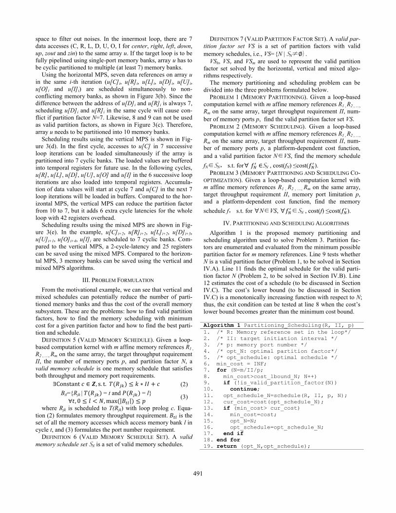
Algorithm 1 is the proposed memory partitioning and
scheduling algorithm used to solve Problem 3. Partition fac-
tors are enumerated and evaluated from the minimum possible
partition factor for m memory references. Line 9 tests whether
N is a valid partition factor (Problem 1, to be solved in Section
IV.A). Line 11 finds the optimal schedule for the valid parti-
tion factor N (Problem 2, to be solved in Section IV.B). Line
12 estimates the cost of a schedule (to be discussed in Section
IV.C). The cost’s lower bound (to be discussed in Section
IV.C) is a monotonically increasing function with respect to N;
thus, the exit condition can be tested at line 8 when the cost’s
lower bound becomes greater than the minimum cost bound.
Algorithm 1 Partitioning_Scheduling(R, II, p)
1. /* R: Memory reference set in the loop*/
2. /* II: target initiation interval */
3. /* p: memory port number */
4. /* opt_N: optimal partition factor*/
5. /* opt_schedule: optimal schedule */
6. min_cost = INF;
7. for (N=m/II/p;
8. min_cost>cost_lbound_N; N++)
9. if (!is_valid_partition_factor(N))
10. continue; 11. opt_schedule_N=schedule(R, II, p, N); 12. cur_cost=cost(opt_schedule_N); 13. if (min_cost> cur_cost) 14. min_cost=cost; 15. opt_N=N; 16. opt_schedule=opt_schedule_N; 17. end if 18. end for 19. return (opt_N,opt_schedule);
491
A. Memory Partitioning Algorithm
1) Vertical Partitioning Algorithm
Vertical MPS schedules memory accesses of the same
memory reference in successive loop iterations simultaneously
to different memory banks. The constraints for the vertical
partition for fully pipelining (II=1) and single-port memories
are:
LEMMA 1. If II=p=1,
{
(4)
PROOF.
( )
( )
( )
( )
{
THEOREM 1.
{
(5)
Proof omitted due to page limit.
Theorem 1 implies that for any memory reference
patterns, because we can always find a feasible N as for the conditions above. Alt-
hough other valid partition factors could be much smaller,
gives an upper bound of
valid solutions. This means that arbitrary affine memory refer-
ences in a loop can be fully pipelined by the vertical MPS.
Although it is easy to determine whether a given integer sat-
isfies (5), finding an explicit expression of the minimal cyclic
partition factor is not straightforward. Fortunately, in real-
world applications, in affine memory references are rela-
tively small, so the upper-bound is
also a moderate number. Enumeration from m to find the min-
imal cyclic partition factor N will not be a compute-intensive
work.
2) Mixed Partitioning Algorithm
As described in the motivational example, the mixed MPS
schedules memory accesses of the different memory refer-
ences in successive loop iterations to different memory banks
in different cycles.
Considering , only
memory accesses in the first N iterations are considered in
memory partitioning. Memory accesses in later iterations (k>N)
can be partitioned and scheduled using the same pattern based
on modulo scheduling.
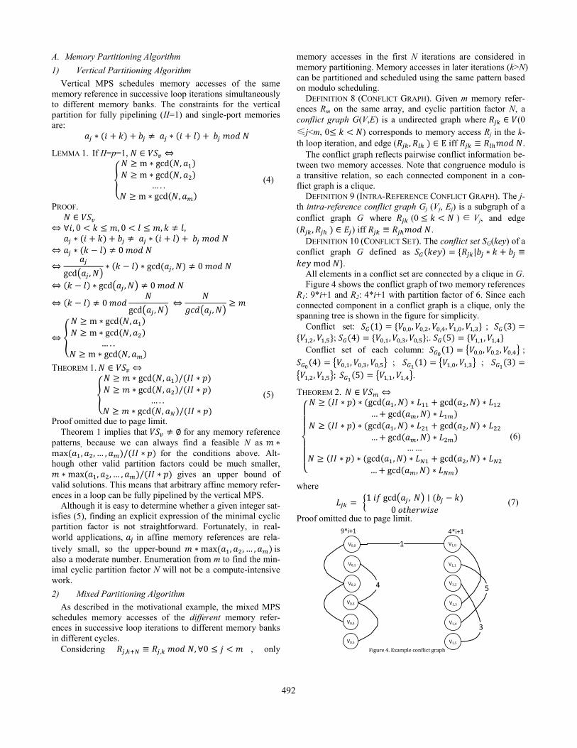
DEFINITION 8 (CONFLICT GRAPH). Given m memory refer-
ences Rm on the same array, and cyclic partition factor N, a
conflict graph G(V,E) is a undirected graph where (0
≤j<m, 0 ) corresponds to memory access Rj in the k-
th loop iteration, and edge ( iff .
The conflict graph reflects pairwise conflict information be-
tween two memory accesses. Note that congruence modulo is
a transitive relation, so each connected component in a con-
flict graph is a clique.
DEFINITION 9 (INTRA-REFERENCE CONFLICT GRAPH). The j-
th intra-reference conflict graph Gj (Vj, Ej) is a subgraph of a
conflict graph G where (0 ) ∈ Vj, and edge
( ) iff .
DEFINITION 10 (CONFLICT SET). The conflict set SG(key) of a
conflict graph G defined as
. All elements in a conflict set are connected by a clique in G.
Figure 4 shows the conflict graph of two memory references
R1: 9*i+1 and R2: 4*i+1 with partition factor of 6. Since each
connected component in a conflict graph is a clique, only the
spanning tree is shown in the figure for simplicity.
Conflict set: ;
; ;.
Conflict set of each column: { } ;
{ } ;
{ } ;
{ } { }.
THEOREM 2.
{
(6)
where
{ ( )
(7)
Proof omitted due to page limit.
V0,0
V0,1
V0,2
V0,3
V0,4
V0,5
4
V1,0
V1,1
V1,2
V1,3
V1,4
V1,5
3
5
1
9*i+1 4*i+1
Figure 4. Example conflict graph
492
The term in (6) represents whether | | , or
whether the j-th intra-reference conflict graph has a conflict
set with key k. Given input memory references, can be
calculated using (7). Therefore, (6) can be used to determine
whether a given integer N is a valid partition factor. As in the
vertical MPS, enumeration from m/(II*p) can be used to find
valid partition factors.
B. Memory Scheduling
As formulated in Problem 2, the memory scheduling prob-
lem is to find the valid schedule with minimum cost for a giv-
en valid partition factor . Considering
, only memory accesses in the first N
iterations are considered in memory scheduling. Memory ac-
cesses in later iterations can also be scheduled according to the
first N iterations.
A memory bank can be accessed by different array accesses
in different cycles. To model this, a memory bank can be
viewed as multiple virtual slots in different cycles.
DEFINITION 11 (VIRTUAL MEMORY SLOT). A virtual
memory slot is
the virtual instance of the g-th port of memory bank l at cycle
h.
EXAMPLE 4. Virtual memory slot:
Suppose II=1, p=2, N=2, the memory system has 8 virtual
memory slots: S000, S001, S010, S011, S100, S101, S110, S111.
With the concept of the virtual memory slot, in a valid
memory schedule at most one memory access is scheduled to
any virtual memory slot. The entire scheduling space can be
described using a memory-scheduling graph.
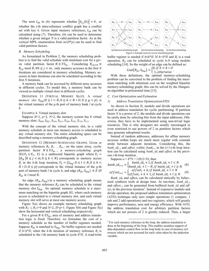
DEFINITION 12 (MEMORY-SCHEDULING GRAPH). Given m
memory references R0, R1, …, Rm-1 on the same array, cyclic
partition factor , a memory-scheduling graph
SG( , E) is a undirected bipartite graph where
{ | corresponds to memory access
Rj in the k-th loop iteration,
corresponds to the virtual instance of the g-th
port of memory bank l in cycle h, and edge ( iff
.
An edge ( in a memory scheduling graph means
that the memory reference Rjk can be scheduled to the virtual
memory slot . An optimal memory schedule is a maxi-
mum matching on the bipartite graph SG, where each memory
access is scheduled to a virtual memory slot, and each virtual
memory slot will serve at most one memory access.
Figure 5(a) shows an example memory scheduling graph
with R1: i, R2:i+9 and N=2, II=p=1. Figure 5(b) and Figure 5(c)
show the horizontal and vertical scheduling respectively.
For a given , area of memory and address transla-
tion logic is fixed. Therefore, we formulate the cost of a
memory schedule as the number of buffer registers needed.
Suppose is matched to . No buffer registers are needed
if h=k*II, when the k-th iteration of memory reference Rj is
scheduled to the l-th memory bank in cycle k*II. A read/write
buffer register is needed if h≠k*II. If h>k*II and Rj is a read
operation, Rjk can be scheduled to cycle h-N using modulo
scheduling [14]. So the weight of an edge can be defined as:
( ) {
.
With these definitions, the optimal memory-scheduling
problem can be converted to the problem of finding the maxi-
mum matching with minimum cost on the weighted bipartite
memory-scheduling graph; this can be solved by the Hungari-
an algorithm in polynomial time [15].
C. Cost Optimization and Estimation
1) Address Translation Optimization(ATO)
As shown in Section II, modulo and divide operations are
used in address translation for cyclic partitioning. If partition
factor N is a power of 2, the modulo and divide operations can
be easily done by selecting bits from the input addresses. Oth-
erwise, they have to be implemented using non-trivial logic
resources. This is why designers are usually encouraged or
even restricted to use powers of 2 as partition factors which
may generate suboptimal results.
Instead of random addresses, addresses for affine memory
accesses within loops are much more regular with constant
stride between adjacent iterations. Considering this, the
bank_idi+1 and offset_within_banki+1 in the (i+1)-th loop itera-
tion can be calculated using bank_idi and offseti in the previ-
ous i-th loop iteration.
Suppose a = k*N + l (0≤l<N), then
{
(8)
{
(9)
Bank_id0 and offset0 can be calculated statically by behav-
ioral synthesis tools at design time. At run-time, bank_idi+1
and offseti+1 can be generated from buffered bank_idi and off-
seti in the previous iteration2. Instead of expensive modulo and
divide operation, the proposed address translation optimization
(ATO) technique only uses simple operations (1 compare, 1
sub and 2 add operations) and two registers, which will greatly
improve performance, area and energy efficiency. With ATO,
the address translation cost for arbitrary partition factors
which are not powers of 2 is greatly reduced. Thus, a larger
2 For each memory reference in the loop, the address translation is
done at the beginning of the loop. This enables seamless support of
data-dependent control flow in the loop body in case of memory ref-
erences which are not accessed for each value taken by the induction
variable.
R00
R10
R01
R11
S000
S100
S010
S110
0
0
11
11
(a) Memory Scheduling Graph (b) Horizontal Scheduling (c) Vertical Scheduling
0
0
R00
R10
R01
R11
S000
S100
S010
S110
0
0
0
0
R00
R10
R01
R11
S000
S100
S010
S110
0
11
0
Figure 5. Example memory access scheduling graph
493

design space can be explored to obtain better results.
2) Overhead Estimization
Figure 6 shows the block diagram of a partitioned memory
system. It consists of memory banks, address translation unit,
control FSM, possible read/write buffer registers, N input
MUXs and m output MUXs.
The overhead of the partitioned memory system can be es-
timated using platform-specific cost functions, which can be
area- or power- oriented. Take the FPGA platform as an ex-
ample: the number of BRAMs is ⌈⌈
⌉
⌉. The cost of the control FSM unit is proportional
to N. With the proposed address translation optimization tech-
nique, the cost of an address translation unit is proportional to
the number of memory references m and independent of parti-
tion factor N. The number of buffer registers REG_N can be
calculated by finding minimum matching on the bipartite
memory-scheduling graph described in Section IV.B. The
number of inputs to the k-th input MUX is ∑ where
is defined in (7). CMUX(m) is the plat-form dependent cost of
m-input multiplexer. The number of inputs to the j-th output
MUX is N/gcd(aj, N). Therefore, the cost of optimal memory
scheduling with partition factor N is illustrated by (10) for
FPGAs where are platform-dependent parameters.
Costlbound in (11) is monotonically increasing with N, and thus
can be used in Algorithm 1 as the exit condition.
⌈⌈
⌉
⌉
∑ ∑
∑
( )
(10)
(11)
V. EXPERIMENTAL RESULTS
A. Experiment Setup
Horizontal, vertical and mixed MPS algorithms are imple-
mented as a source-to-source transformation pass. Loop ker-
nels in behavioral languages like C and design constrains in-
cluding memory port limitation and target II are taken as input.
The memory partitioning and scheduling results are dumped
into transformed source programs and accepted by the down-
stream behavioral synthesis tools.
Our test cases include a set of real-life medical imaging
processing kernels: denoise, registration, binarization, seg-
mentation and deconvolution [16]. All of these kernels have
abundant memory accesses to the same image data array and
are perfect examples for testing our MPS algorithms.
Although our algorithm is applicable to both ASIC and
FPGA designs, we chose FPGA as the target device in this
work because of the availability of downstream behavioral
synthesis and implementation tools. The Xilinx Virtex-6
FPGA, AutoESL 2011.4 and ISE 13.2 tools are used in our
experiments. Area utilization and critical path are reported by
ISE, and power data is reported by AutoESL.
B. Case Study: Denoise
The denoise program is used as a case study to compare
various approaches in memory partitioning and scheduling.
Loop II and memory port number p is set to 1 in the experi-
ment. The test results are shown in Table 3.
Horizontal, vertical and mixed memory algorithms are ap-
plied to the design. For each kind of algorithm, partition factor
can be an arbitrary number or restricted to power of 2. Ad-
dress translation optimization (ATO) can be applied to parti-
tion factors which are not powers of 2.
From the results, we can see that compared to the horizontal
MPS, the vertical MPS can reduce the number of block RAMs
at the cost of slices and DSPs due to the complex address
translation patterns. The mixed MPS is always better than both
the horizontal and vertical MPS algorithms in terms of area,
power and latency. The ATO techniques can be used to reduce
both area and power by reducing the number of DSPs signifi-
cantly. With ATO, the minimum partition factor is preferred to
the partition factor with power of 2. Among all approaches,
mixed-ATO shows the best performance, area-efficiency and
power-efficiency. Experimental results of all other test cases
are consistent with these observations.
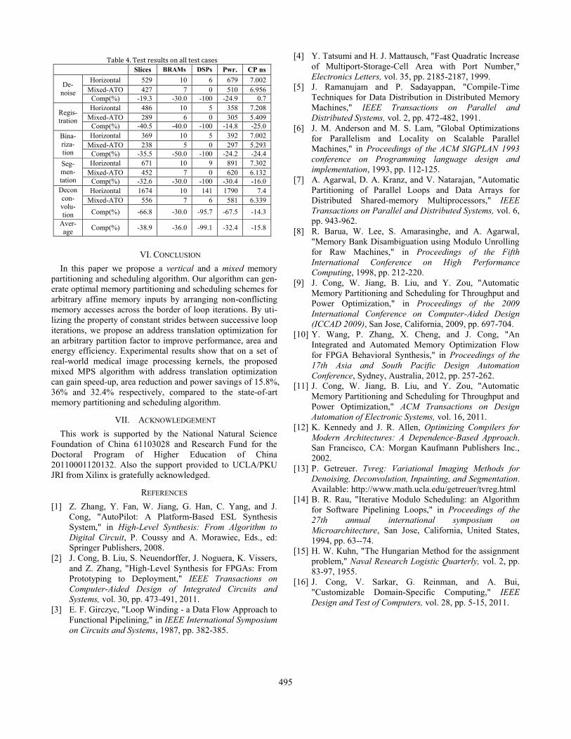
C. Test Results
Test results on all five test cases are listed in Table 4. The
horizontal MPS and mixed MPS with ATO are compared in
terms of power, critical path delay, the number of slices, block
RAMs and DSPs. On average, our proposed mixed MPS with
ATO can improve area efficiency by 38.9%, 36% and 99.1%
in terms of slices, block RAMs and DSPs compared to the
state-of-art horizontal MPS algorithm. A significant reduction
in DSPs is mainly achieved by using ATO techniques. The
mixed MPS with ATO can also improve power efficiency and
performance by 32.4% and 15.8%.
Table 3. Test results of Denoise
Slices RAMBs DSPs Power CP(ns)
horizontal 529 10 6 679 7.002
horizontal-ATO 459 10 0 537 7.287
horizontal-2^n 3254 256 0 5239 7.335
vertical 1007 7 72 1597 7.259
vertical-ATO 701 7 0 1403 6.505
vertical-2^n 1059 8 0 2477 7.105
mixed 511 7 6 573 6.33
mixed-ATO 427 7 0 510 6.956
mixed-2^n 555 8 0 549 7.046
Figure 6. Block diagram of a partitioned memory system
R
ead B
uffer
A
dd
ress Tran
slation
W
rite Bu
ffer
Control FSM
MUX
MUX
MUX
MUX
MUX
MUX
Memory System
… …
Mem Bank N-1
Mem Bank 1
Mem Bank 0
Resp m Req m
Resp 2
Req 2
Resp 1 Req 1
494
VI. CONCLUSION
In this paper we propose a vertical and a mixed memory
partitioning and scheduling algorithm. Our algorithm can gen-
erate optimal memory partitioning and scheduling schemes for
arbitrary affine memory inputs by arranging non-conflicting
memory accesses across the border of loop iterations. By uti-
lizing the property of constant strides between successive loop
iterations, we propose an address translation optimization for
an arbitrary partition factor to improve performance, area and
energy efficiency. Experimental results show that on a set of
real-world medical image processing kernels, the proposed
mixed MPS algorithm with address translation optimization
can gain speed-up, area reduction and power savings of 15.8%,
36% and 32.4% respectively, compared to the state-of-art
memory partitioning and scheduling algorithm.
VII. ACKNOWLEDGEMENT
This work is supported by the National Natural Science
Foundation of China 61103028 and Research Fund for the
Doctoral Program of Higher Education of China
20110001120132. Also the support provided to UCLA/PKU
JRI from Xilinx is gratefully acknowledged.
REFERENCES
[1] Z. Zhang, Y. Fan, W. Jiang, G. Han, C. Yang, and J.
Cong, "AutoPilot: A Platform-Based ESL Synthesis
System," in High-Level Synthesis: From Algorithm to
Digital Circuit, P. Coussy and A. Morawiec, Eds., ed:
Springer Publishers, 2008.
[2] J. Cong, B. Liu, S. Neuendorffer, J. Noguera, K. Vissers,
and Z. Zhang, "High-Level Synthesis for FPGAs: From
Prototyping to Deployment," IEEE Transactions on
Computer-Aided Design of Integrated Circuits and
Systems, vol. 30, pp. 473-491, 2011.
[3] E. F. Girczyc, "Loop Winding - a Data Flow Approach to
Functional Pipelining," in IEEE International Symposium
on Circuits and Systems, 1987, pp. 382-385.
[4] Y. Tatsumi and H. J. Mattausch, "Fast Quadratic Increase
of Multiport-Storage-Cell Area with Port Number,"
Electronics Letters, vol. 35, pp. 2185-2187, 1999.
[5] J. Ramanujam and P. Sadayappan, "Compile-Time
Techniques for Data Distribution in Distributed Memory
Machines," IEEE Transactions on Parallel and
Distributed Systems, vol. 2, pp. 472-482, 1991.
[6] J. M. Anderson and M. S. Lam, "Global Optimizations
for Parallelism and Locality on Scalable Parallel
Machines," in Proceedings of the ACM SIGPLAN 1993
conference on Programming language design and
implementation, 1993, pp. 112-125.
[7] A. Agarwal, D. A. Kranz, and V. Natarajan, "Automatic
Partitioning of Parallel Loops and Data Arrays for
Distributed Shared-memory Multiprocessors," IEEE
Transactions on Parallel and Distributed Systems, vol. 6,
pp. 943-962.
[8] R. Barua, W. Lee, S. Amarasinghe, and A. Agarwal,
"Memory Bank Disambiguation using Modulo Unrolling
for Raw Machines," in Proceedings of the Fifth
International Conference on High Performance
Computing, 1998, pp. 212-220.
[9] J. Cong, W. Jiang, B. Liu, and Y. Zou, "Automatic
Memory Partitioning and Scheduling for Throughput and
Power Optimization," in Proceedings of the 2009
International Conference on Computer-Aided Design
(ICCAD 2009), San Jose, California, 2009, pp. 697-704.
[10] Y. Wang, P. Zhang, X. Cheng, and J. Cong, "An
Integrated and Automated Memory Optimization Flow
for FPGA Behavioral Synthesis," in Proceedings of the
17th Asia and South Pacific Design Automation
Conference, Sydney, Australia, 2012, pp. 257-262.
[11] J. Cong, W. Jiang, B. Liu, and Y. Zou, "Automatic
Memory Partitioning and Scheduling for Throughput and
Power Optimization," ACM Transactions on Design
Automation of Electronic Systems, vol. 16, 2011.
[12] K. Kennedy and J. R. Allen, Optimizing Compilers for
Modern Architectures: A Dependence-Based Approach.
San Francisco, CA: Morgan Kaufmann Publishers Inc.,
2002.
[13] P. Getreuer. Tvreg: Variational Imaging Methods for
Denoising, Deconvolution, Inpainting, and Segmentation.
Available: http://www.math.ucla.edu/getreuer/tvreg.html
[14] B. R. Rau, "Iterative Modulo Scheduling: an Algorithm
for Software Pipelining Loops," in Proceedings of the
27th annual international symposium on
Microarchitecture, San Jose, California, United States,
1994, pp. 63--74.
[15] H. W. Kuhn, "The Hungarian Method for the assignment
problem," Naval Research Logistic Quarterly, vol. 2, pp.
83-97, 1955.
[16] J. Cong, V. Sarkar, G. Reinman, and A. Bui,
"Customizable Domain-Specific Computing," IEEE
Design and Test of Computers, vol. 28, pp. 5-15, 2011.
Table 4. Test results on all test cases
Slices BRAMs DSPs Pwr. CP ns
De-
noise
Horizontal 529 10 6 679 7.002
Mixed-ATO 427 7 0 510 6.956 Comp(%) -19.3 -30.0 -100 -24.9 0.7
Regis-tration
Horizontal 486 10 5 358 7.208
Mixed-ATO 289 6 0 305 5.409 Comp(%) -40.5 -40.0 -100 -14.8 -25.0
Bina-
riza-tion
Horizontal 369 10 5 392 7.002
Mixed-ATO 238 5 0 297 5.293 Comp(%) -35.5 -50.0 -100 -24.2 -24.4
Seg-men-
tation
Horizontal 671 10 9 891 7.302
Mixed-ATO 452 7 0 620 6.132 Comp(%) -32.6 -30.0 -100 -30.4 -16.0
Decon
con-volu-
tion
Horizontal 1674 10 141 1790 7.4
Mixed-ATO 556 7 6 581 6.339
Comp(%) -66.8 -30.0 -95.7 -67.5 -14.3
Aver-age
Comp(%) -38.9 -36.0 -99.1 -32.4 -15.8
495
Related Documents