Data Partitioning for Multiprocessors with Memory Heterogeneity and Memory Constraints

Data Partitioning for Multiprocessors with Memory Heterogeneity and Memory Constraints

Alexey Lastovetsky, Ravi Reddy

Department of Computer Science University College Dublin, Belfield Dublin 4, Ireland E-mail: [email protected], [email protected]

Abstract—The paper presents a performance model that can be used to optimally distribute computations over heterogeneous computers. This model is application-centric representing the speed of each computer by a function of the problem size. This way it takes into account the processor heterogeneity, the heterogeneity of memory structure, and the memory limitations at each level of memory hierarchy. A problem of optimal partitioning of an n-element set over p heterogeneous processors using this performance model is formulated, and its efficient solution of the complexity O(p3×log2n) is given. Index Terms—Heterogeneous (hybrid) systems, Scheduling and task partitioning, Load balancing and task assignment

1. Introduction

In this paper, we deal with the problem of optimal distribution of computations over heterogeneous computers taking into account the processor heterogeneity, the heterogeneity of memory structure, and the memory limitations at each level of memory hierarchy of a processor. We present a performance model that integrates these essential features having an impact on the execution time of parallel and distributed applications running on networks of heterogeneous computers.

In our previous research [1], we addressed the problem of optimal distribution or scheduling of computational tasks on networks of heterogeneous computers when one or more tasks do not fit into the main memory of the processors. We particularly addressed the problem of optimal data partitioning in heterogeneous environments when relative speeds of processors cannot be accurately approximated by constant functions of the problem size. We proposed a functional model that integrated all architectural differences in computers having an impact on the performance of computers depending on the size of the problem. These architectural differences are mainly the processor heterogeneity in terms of the speeds of the processors and memory heterogeneity in terms of the number of memory levels of the memory hierarchy and the size of each level of the memory hierarchy. Under this model, the speed of each processor is represented by a continuous and relatively smooth function of the problem size whereas standard models use a single number to represent the speed. This model is application-centric in the sense that generally speaking different applications will characterize the speed of the processor by different functions.

There are two main motivations behind the representation of the speed of the processor by a continuous and relatively smooth function of the problem size. First of all, we want the model to adequately reflect the behavior of common, not very carefully designed applications. Consider the experiments conducted by Lastovetsky and Twamley [2]

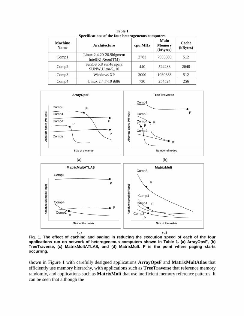
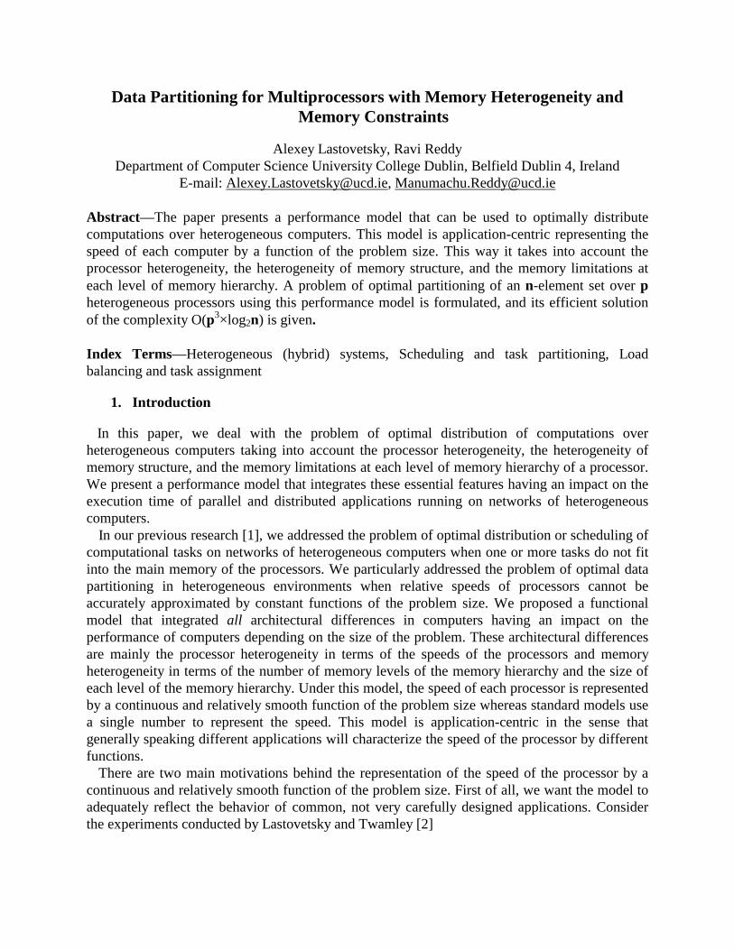
Table 1 Specifications of the four heterogeneous computers

Machine Name

Architecture cpu MHz Main

Memory (kBytes)

Cache (kBytes)

Comp1 Linux 2.4.20-20.9bigmem

Intel(R) Xeon(TM) 2783 7933500 512

Comp2 SunOS 5.8 sun4u sparc

SUNW,Ultra-5_10 440 524288 2048

Comp3 Windows XP 3000 1030388 512

Comp4 Linux 2.4.7-10 i686 730 254524 256

ArrayOpsF

Size of the array

Ab

solu

te s

peed

(MFl

ops)

Comp3

Comp4

Comp2

Comp1

P

P

PP

TreeTraverse

Number of nodes

Ab

solu

te s

peed

(MFl

ops) Comp3

Comp4

Comp2

Comp1

P

PP

P

(a) (b)

MatrixMultATLAS

Size of the matrix

Ab

solu

te s

peed

(MFl

ops)

Comp4

Comp2

Comp1

P

P

P

MatrixMult

Size of the matrix

Ab

solu

te s

peed

(MFl

ops)

Comp3

Comp2

Comp1

Comp4

P

P

P

(c) (d)

Fig. 1. The effect of caching and paging in reducing the execution speed of each of the four applications run on network of heterogeneous computers shown in Table 1. (a) ArrayOpsF, (b) TreeTraverse, (c) MatrixMultATLAS, and (d) MatrixMult. P is the point where paging starts occurring. shown in Figure 1 with carefully designed applications ArrayOpsF and MatrixMultAtlas that efficiently use memory hierarchy, with applications such as TreeTraverse that reference memory randomly, and applications such as MatrixMult that use inefficient memory reference patterns. It can be seen that although the

Size of the problem

Ab

solu

te S

pee

d

)(1 xs

)(2 xs

)(3 xs

experimentally obtained extrapolatedreal

11x

12x

13x 21x

22x

23x

Fig. 2. A small network of three processors whose speeds are shown against the size of the problem. The dotted lines passing through the origin represent solutions provided by the functional model. The bold curves represent the experimentally obtained speed functions. The dotted curves represent reasonable approximations of the speed functions in a continuous manner. The dashed curves represent the real behavior of the speed functions. The first dotted line giving the data distribution (x11,x12,x13) is a non-optimal solution. The second dotted line giving the data distribution (x21,x22,x23) is not a solution at all. applications ArrayOpsF, TreeTraverse, and MatrixMultAtlas demonstrate a sharp and distinctive performance curve of dependence of the absolute speed on the problem size, the application MatrixMult, which uses a naïve multiplication of two dense square matrices, displays a quite smooth dependence of speed on the problem size. Thus, to model execution of a common and not carefully designed application, we should realistically approximate the dependence of the speed of the processor by a continuous and relatively smooth function of the problem size.

The other main motivation is that we want to target general-purpose common heterogeneous networks. A computer in such a network is an integrated part of the network periodically performing some computations and communications just as such an integrated node of the network. It will experience fluctuations in the workload due to its integration into the network. This changing transient load will cause a fluctuation in the speed of computers on the network, in that the speed of the computer will vary when measured at different times while executing the same task. As a result, the fluctuations in speed must be modeled as a performance band. These performance bands representing the speeds of the processors are more realistically approximated by a continuous and relatively smooth function of the problem size even for carefully designed applications efficiently using the memory hierarchy. Figure 1 shows experiments on a set of computers whose specifications are shown in Table 1. These computers have varying specifications and varying levels of network integration and are representative of the range of computers typically used in networks of heterogeneous computers. The results reinforce the

representation of the speed of the processor by a continuous and relatively smooth function of the problem size.

In [1], we also formulated a problem of partitioning of an n-element set over p heterogeneous processors using the functional model and designed efficient algorithms to solve the problem. The optimal solution is the solution where the size of the problem assigned to each processor is proportional to the speed of the processor. The algorithms are based on the following observation: If a distribution of the elements of the set amongst the processors is obtained such that the number of elements is proportional to the speed of the processor, then the points, whose coordinates are number of elements and speed, lie on a straight line passing through the origin of the coordinate system and intersecting the graphs of the processors with speed versus the size of the problem in terms of the number of elements. The algorithms use the observation that the optimal solution obtained by these algorithms is a straight line passing through the origin of the coordinate system and intersecting the graphs of the processors with speed versus the size of the problem in terms of the number of elements. The algorithms take at most p2×log2n steps to find the optimal solution.

However this model fails to provide optimal solutions when the network consists of computers that are configured to avoid paging. Consider the experiments shown in Figure 1. The experiments show that Comp1 and Comp2 do not permit paging. This is typical of computers used as a main server. For applications designed to efficiently use cache memory, such computers show a constant speed function, up to a point where the process crashes, probably because it tries to invoke a paging procedure, not allowed due to its configuration. So if we have such computers, the real speed function of the size of the problem is not continuous any more but discontinuous at the point where paging happens, that is, there is a break in the continuity of the function at the point where paging happens.

Consider a small network of three processors, whose speeds as functions of problem size are shown in Figure 2. The processor represented by the speed function s1(x) is configured to permit paging. The processors represented by speed functions s2(x) and s3(x) are configured to avoid paging. The bold curves represent the experimentally obtained parts of the speed functions. Now assume that we want to obtain optimal distributions for problem sizes whose optimal solution lines lie beyond the bold curves. In this case we naturally extrapolate the curves in a continuous manner using some reasonable approximations. The extrapolations are shown by dotted curves. However it can be seen that sometimes the extrapolations are not accurate representations of the real shape of the speed functions as shown for the speed functions s1(x) and s2(x). The real speed functions are shown by dashed curves. Consider two data distributions obtained by the functional model and which are shown by dotted lines passing through the origin. Although the first data distribution (x11,x12,x13) is not the optimal solution just because the extrapolated speed functions s1(x) and s2(x) are not accurate representations of the real speed functions, it still give a reasonable sub-optimal solution of the problem. At the same time, the second data distribution (x21,x22,x23) is not a solution at all. This is because at the points x22 and x23 the paging starts occurring for computers with speed functions s2(x) and s3(x) and since these computers are configured to avoid paging, they crash. Therefore in order to obtain optimal and working solutions for such networks, we need to extend the functional model.

We naturally extend the functional model by including an additional parameter of maximum problem size. The maximum problem size represents the upper bound on the size of the problem that each processor can solve. For computers that are configured to avoid paging, it represents the

point where the computer crashes due to the occurrence of paging and where the speed function of the size of the problem becomes discontinuous.

The rest of the paper is organized as follows. In Section 2, we present the modified functional model. This is followed by a formulation of a general set-partitioning problem, which is the problem of partitioning of an n-element set over p heterogeneous processors using this modified functional model. Then we give its efficient solution of the complexity O(p3×log2n). This problem is a simple variant of the most advanced problem of partitioning a set with weighted elements [3]. We use the simple variant to explain how complex the problem of scheduling tasks amongst processors is when: (a) the processors have significantly different memory structure, and (b) there are memory limitations on the size of task that can be solved by each processor. We also use this variant to explain in simple terms how the modified functional model can be used to achieve better data partitioning on networks of heterogeneous computers before moving on to solve the most advanced problem.

To demonstrate the efficiency of the modified functional model, we perform experiments using naïve parallel algorithms for linear algebra kernel, namely, matrix multiplication and LU factorization using striped partitioning of matrices on a local network of heterogeneous computers. Our main aim is not to show how matrices can be efficiently multiplied or efficiently factorized but to explain in simple terms how the modified functional model can be used to optimally schedule tasks on networks of heterogeneous computers taking into account the processor and memory heterogeneity. We also view these algorithms as good representatives of a large class of data parallel computational problems and a good testing platform before experimenting more challenging computational problems.

2. The Performance Model The modified functional model of networks of heterogeneous computers has the following parameters:

• An upper bound on the size of the task that can be solved by each computer, and • The speed of the processor is represented by a continuous and smooth function of the

problem size until the upper bound. Beyond the upper bound, the speed of the processor is assumed to be zero.

The model retains the restrictions imposed by the functional model [1] on the shape of the graph representing the speed function. The shape of the graph should be such that there is only one intersection point of the graph with any straight line passing through the origin. That is the speeds of the processors must either be increasing or decreasing functions of problem size for the problem sizes for which the solutions are sought. These assumptions on the shapes of the graph are representative of the most general shape of graphs observed for applications experimentally as shown in Figure 1.

The upper bound could signify one of the following cases: • Allocation of a task whose size is beyond this bound could result in processor failure. • Allocation of the task whose size is beyond this bound could result in unacceptable

execution time to accomplish the task due to severe paging.

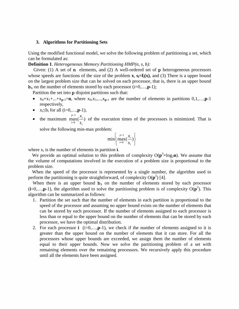
3. Algorithms for Partitioning Sets Using the modified functional model, we solve the following problem of partitioning a set, which can be formulated as: Definition 1. Heterogeneous Memory Partitioning HMP(n, s, b):

Given: (1) A set of n elements, and (2) A well-ordered set of p heterogeneous processors whose speeds are functions of the size of the problem x, si=fi(x), and (3) There is a upper bound on the largest problem size that can be solved on each processor, that is, there is an upper bound bi on the number of elements stored by each processor (i=0,…,p-1);

Partition the set into p disjoint partitions such that: • x0+x1+...+xp-1=n, where x0,x1,...,xp-1 are the number of elements in partitions 0,1,…,p-1

respectively, • xi≤bi for all (i=0,…,p-1),

• the maximum )(max1

0i

ip

i s

x−

= of the execution times of the processors is minimized. That is

solve the following min-max problem:

⎭⎬⎫

⎩⎨⎧ −

=)(maxmin

1

0i

ip

i s

x

where xi is the number of elements in partition i. We provide an optimal solution to this problem of complexity O(p3×log2n). We assume that

the volume of computations involved in the execution of a problem size is proportional to the problem size.

When the speed of the processor is represented by a single number, the algorithm used to perform the partitioning is quite straightforward, of complexity O(p2) [4].

When there is an upper bound bi on the number of elements stored by each processor (i=0,…,p-1), the algorithm used to solve the partitioning problem is of complexity O(p3). This algorithm can be summarized as follows:

1. Partition the set such that the number of elements in each partition is proportional to the speed of the processor and assuming no upper bound exists on the number of elements that can be stored by each processor. If the number of elements assigned to each processor is less than or equal to the upper bound on the number of elements that can be stored by each processor, we have the optimal distribution.

2. For each processor i (i=0,…,p-1), we check if the number of elements assigned to it is greater than the upper bound on the number of elements that it can store. For all the processors whose upper bounds are exceeded, we assign them the number of elements equal to their upper bounds. Now we solve the partitioning problem of a set with remaining elements over the remaining processors. We recursively apply this procedure until all the elements have been assigned.

Size of the problem

Ab

solu

te S

pee

d

)(1 xs

)(2 xs

)(3 xs

line 1

line 2

3x

Optimally sloped line

Bisections to obtain the optimal solution

1b

2b

3b

2x

3

3

2

2132 x

(x)s

x

(x)s , =−=+ bnxx

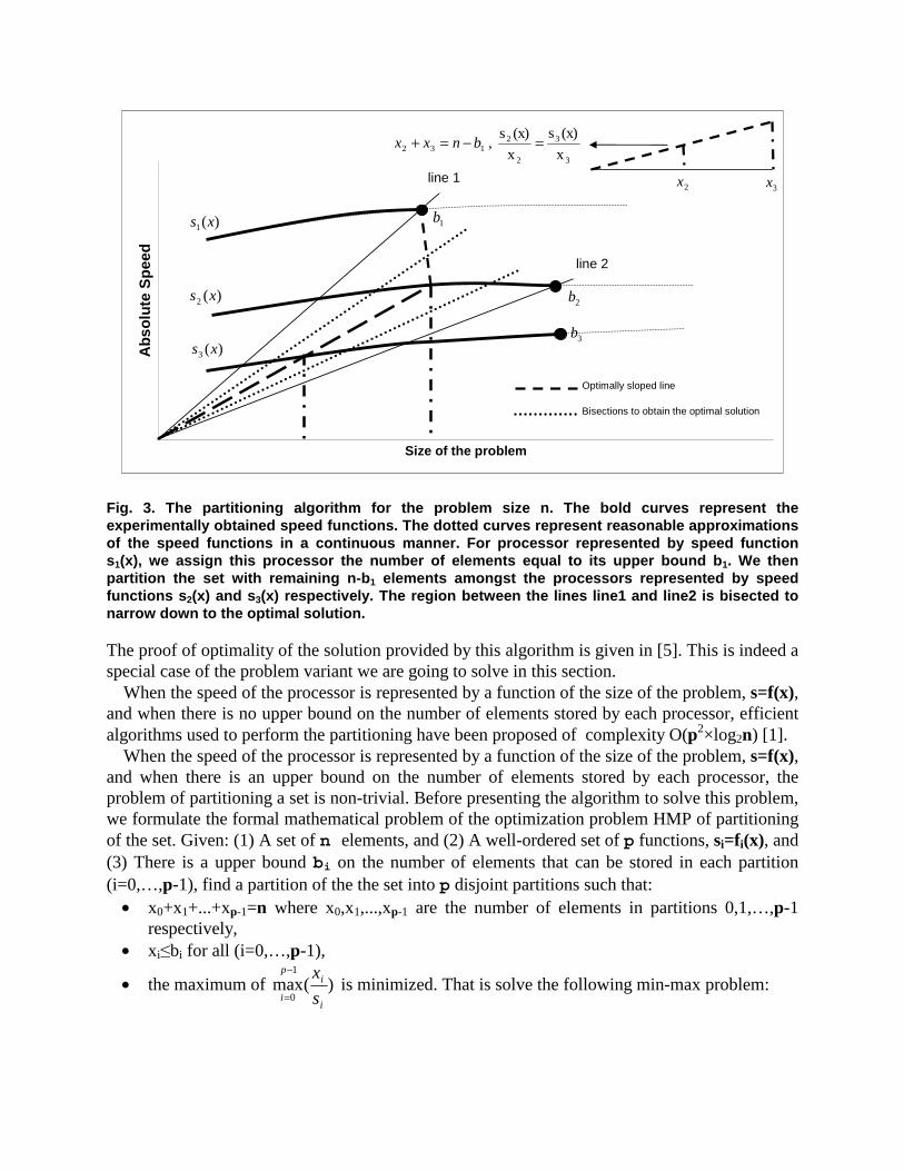
Fig. 3. The partitioning algorithm for the problem size n. The bold curves represent the experimentally obtained speed functions. The dotted curves represent reasonable approximations of the speed functions in a continuous manner. For processor represented by speed function s1(x), we assign this processor the number of elements equal to its upper bound b1. We then partition the set with remaining n-b1 elements amongst the processors represented by speed functions s2(x) and s3(x) respectively. The region between the lines line1 and line2 is bisected to narrow down to the optimal solution. The proof of optimality of the solution provided by this algorithm is given in [5]. This is indeed a special case of the problem variant we are going to solve in this section.

When the speed of the processor is represented by a function of the size of the problem, s=f(x), and when there is no upper bound on the number of elements stored by each processor, efficient algorithms used to perform the partitioning have been proposed of complexity O(p2×log2n) [1].

When the speed of the processor is represented by a function of the size of the problem, s=f(x), and when there is an upper bound on the number of elements stored by each processor, the problem of partitioning a set is non-trivial. Before presenting the algorithm to solve this problem, we formulate the formal mathematical problem of the optimization problem HMP of partitioning of the set. Given: (1) A set of n elements, and (2) A well-ordered set of p functions, si=fi(x), and (3) There is a upper bound bi on the number of elements that can be stored in each partition (i=0,…,p-1), find a partition of the the set into p disjoint partitions such that:

• x0+x1+...+xp-1=n where x0,x1,...,xp-1 are the number of elements in partitions 0,1,…,p-1 respectively,

• xi≤bi for all (i=0,…,p-1),

• the maximum of )(max1

0i

ip

i s

x−

= is minimized. That is solve the following min-max problem:

⎭⎬⎫

⎩⎨⎧ −

=)(maxmin

1

0i

ip

i s

x

where xi is the number of elements in partition i. Before we present the algorithm to solve the optimization problem HMP, we apply the

following assumptions: (1) The speed of each processor is represented by a continuous function of the size of the

problem up till its upper bound on the problem size. The speed of the processor is zero beyond the upper bound.

(2) The shape of the graph representing the speed function should be such that there is only one intersection point of the graph with any straight line passing through the origin. That is the speeds of the processors must either be increasing or decreasing functions of problem size for the problem sizes for which the solutions are sought and,

(3) For each processor, for all x ≥ y, where x and y are problem sizes, the execution times tx and ty to execute problems of sizes x and y respectively are related by tx ≥ ty. Algorithm Heterogeneous Memory Partitioning Algorithm HMPA(n, s, b). The algorithm we propose to solve this advanced partitioning problem is graphically illustrated in Figure 3 and has the following main points:

1. Partition the set such that the number of elements in each partition is proportional to the speed of the processor and assuming no upper bound exists on the number of elements that can be stored by the processor (we can use any continuous extension of the speed function beyond the maximal problem size, say, a constant equal to the speed for the maximal problem size). The partitioning algorithm used to perform this task is discussed in [1]. If the number of elements in each partition assigned to each processor is less than the upper bound on the number of elements that can be stored by the processor, we have an optimal distribution.

2. For each processor i (i=0,…,p-1), we check if the number of elements assigned to it is greater than the upper bound on the number of elements that it can store. For all the processors whose upper bounds are exceeded, we assign them the number of elements equal to their upper bounds. Now we solve the partitioning problem of a set with remaining elements over the remaining processors. We recursively apply this procedure until all the elements have been assigned.

Theorem 1. HMPA(n, s, b) gives the optimal solution to the optimization problem HMP(n, s, b). Proof. We prove the optimality of the solution using mathematical induction. We use the maximum time to solve the task assigned to each processor as the performance metric.

The cases for p=1 and p=2 are trivial. For p=3, let us assume the upper bounds of the processors 1, 2, and 3 on the number of elements that they can store are b1, b2, and b3 respectively. Suppose the optimal distribution assuming there are no upper bounds on the number of elements is (x1, x2, x3) such that x1+x2+x3=n where n is the size of the problem.

Consider the case where x1 > b1 and x2 > b2. Let us assign the number of elements equal to b1

for processor 1. The remaining distribution has to satisfy the equality 1'3

'2 bnxx −=+ where

'2x and '

3x are to be chosen such that the speed of the processor is proportional to the number of

elements assigned to it. If the speeds of the processors 2 and 3 are non-increasing functions of problem size, it can be proved that 2

'2 xx > and 3

'3 xx > . This gives us the inequality

22'2 bxx >> . Therefore we have to necessarily assign b2 number of elements to processor 2. If

the speeds of the processors 2 and 3 are non-decreasing functions of problem size, there are three possibilities, ( 2

'2 xx > , 3

'3 xx > ), ( 2

'2 xx < , 3

'3 xx > ) and ( 2

'2 xx > , 3

'3 xx < ). The first and the third

possibility give us the inequality 22'2 bxx >> . For the second possibility, any allocation ''

2x such

that ''2x < b2 would result in an allocation of ''

3x number of elements to processor 3 such that ''

3x > '3x thus resulting in a larger execution time. Therefore we have to necessarily assign b2

number of elements to processor 2. If the speed of the processor 2 is a non-decreasing function of problem size and speed of processor 3 is a non-increasing function of problem size, there are two possibilities, ( 2

'2 xx < , 3

'3 xx > ) and ( 2

'2 xx > , 3

'3 xx < ). In the first possibility, any allocation ''

2x

such that ''2x < b2 would result in an allocation of ''

3x number of elements to processor 3 such that ''

3x > '3x thus resulting in a larger execution time. The second possibility gives us the inequality

22'2 bxx >> . Therefore we have to necessarily assign b2 number of elements to processor 2. Consider the case of optimal distribution where x1 > b1 is true. For processor 1, we assign the

number of elements equal to b1. The remaining elements are allocated such that 1'3

'2 bnxx −=+

where '2x and '

3x are to be chosen such that the speed of the processor is proportional to the

number of elements assigned to it. Any other allocation ''1x such that ''

1x < b1 would result in an

allocation where one of the inequalities ( ''2x > '

2x ), ( ''3x > '

3x ) is satisfied thus resulting in a larger

execution time. It can be proved similarly for the case when x2 > b2. Assuming this to be true for p=k processors, we have to prove the optimality for p=k+1

processors. For a given problem size n, let us assume the distribution given by our algorithm to be kmm xxbbbx ,,,,,,, 1210 LL + such that nxbx k =+++ L10 , where without loss of generality

processors 1,…,m are allocated their upper bounds. It can be inferred that the execution times for the rest of the processors 0,m+1,…,k satisfy the equality km ttt === + L10 . It can also be

inferred that ikm tttt ≥+ ),,,( 10 L for all i=1,…,m. The execution time for the problem size is

equal to )(max0

i

k

imp tt

== = ),,,( 10 km ttt L+ . Consider an alternative solution with the distribution

''1

'0 ,,, kxxx L where nxxx k =+++ ''

1'0 L and mm bxbx ≤≤ '

1'1 ,,L . It can be easily seen that for

atleast one processor i (i=0,m+1,…,k), ii xx ≥' , thus giving an execution time 'it , which is greater

than the execution time given by our algorithm mpt .

Theorem 2. The complexity of the algorithm HMPA(n, s, b) is O(p3×log2n). Proof. There are p major steps in the algorithm. At each such major step i, we solve the problem of partitioning of a set amongst p-i processors such that the number of elements in each partition is proportional to the speed of the processor and assuming no upper bound exists on the number of elements that can be stored by the processor. The complexity of this step is O(p2×log2n) [1]. Since there are p such steps, the overall worst-case complexity is O(p3×log2n). Mathematically, the worst-case complexity is the summation of p terms:

( )( )

np

np

bbnbnnp

bbnbnnp

bbnpbnpnpC

p

23

22

10022

1020222

1022

022

22

log

)(log

))()((log

)(log)(loglog

1)(log)2( )(log)1(log

×≅

×≅

×−−×−××≅

+−−+−+×≅

++−−×−+−×−+×=

L

L

L

4. Applications of the Model

So far we have formulated a realistic performance model of a network of heterogeneous computers and designed efficient algorithms of data partitioning with this model. Now we present a list of practical applications of this model:

• Data partitioning on networks of heterogeneous computers, which only include computers that are configured to avoid paging. Such computers crash when problem sizes are allocated that requires paging. The largest problem size on such computers is the problem size where paging starts happening.

• Data partitioning on networks of heterogeneous computers, which only include computers that permit paging. However allocation of large problem sizes can cause severe paging on such computers as a result causing severe performance degradation and sometimes stalling of the entire application. The largest problem size on such computers is not the problem size where paging starts happening but the problem size which causes severe performance degradation of the application.

• Data partitioning on networks of heterogeneous computers, which include computers some of which permit paging and some of which are configured to avoid paging.

5. Experimental Results

The experimental results are divided into three sections. The first two sections are devoted to building the modified functional model. In the first section, we suggest ways to determine the upper bound on the size of the problem that each processor can solve. Then we present the parallel applications and the network of heterogeneous computers on which the applications are tested. For each application, we explain how to estimate the processor speed. This is followed by presentation of the procedure to build the speed functions of the processors. Finally we present the experimental results obtained by running these applications on the network of heterogeneous computers.

5.1 Determination of Largest Problem Size In this section, we highlight different approaches to determine the largest problem size of an application that can be solved efficiently on a given computer. We do not define the

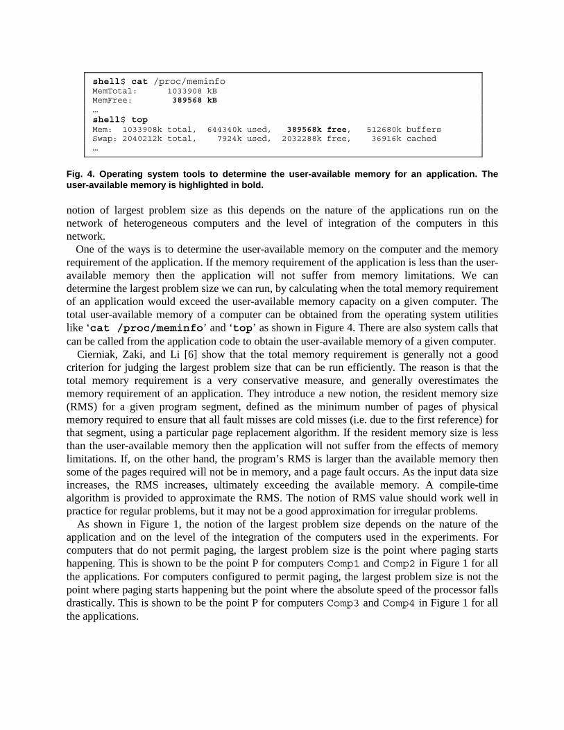
Fig. 4. Operating system tools to determine the user-available memory for an application. The user-available memory is highlighted in bold. notion of largest problem size as this depends on the nature of the applications run on the network of heterogeneous computers and the level of integration of the computers in this network.

One of the ways is to determine the user-available memory on the computer and the memory requirement of the application. If the memory requirement of the application is less than the user-available memory then the application will not suffer from memory limitations. We can determine the largest problem size we can run, by calculating when the total memory requirement of an application would exceed the user-available memory capacity on a given computer. The total user-available memory of a computer can be obtained from the operating system utilities like ‘cat /proc/meminfo’ and ‘top’ as shown in Figure 4. There are also system calls that can be called from the application code to obtain the user-available memory of a given computer.

Cierniak, Zaki, and Li [6] show that the total memory requirement is generally not a good criterion for judging the largest problem size that can be run efficiently. The reason is that the total memory requirement is a very conservative measure, and generally overestimates the memory requirement of an application. They introduce a new notion, the resident memory size (RMS) for a given program segment, defined as the minimum number of pages of physical memory required to ensure that all fault misses are cold misses (i.e. due to the first reference) for that segment, using a particular page replacement algorithm. If the resident memory size is less than the user-available memory then the application will not suffer from the effects of memory limitations. If, on the other hand, the program’s RMS is larger than the available memory then some of the pages required will not be in memory, and a page fault occurs. As the input data size increases, the RMS increases, ultimately exceeding the available memory. A compile-time algorithm is provided to approximate the RMS. The notion of RMS value should work well in practice for regular problems, but it may not be a good approximation for irregular problems.

As shown in Figure 1, the notion of the largest problem size depends on the nature of the application and on the level of the integration of the computers used in the experiments. For computers that do not permit paging, the largest problem size is the point where paging starts happening. This is shown to be the point P for computers Comp1 and Comp2 in Figure 1 for all the applications. For computers configured to permit paging, the largest problem size is not the point where paging starts happening but the point where the absolute speed of the processor falls drastically. This is shown to be the point P for computers Comp3 and Comp4 in Figure 1 for all the applications.

shell$ cat /proc/meminfo MemTotal: 1033908 kB MemFree: 389568 kB … shell$ top Mem: 1033908k total, 644340k used, 389568k free, 512680k buffers Swap: 2040212k total, 7924k used, 2032288k free, 36916k cached …

Table 2 Specifications of the Eleven Heterogeneous Computers

Machine Name

Architecture cpu MHz

Main Memory (kBytes)

Largest size of task

(Matrix-Matrix Multiplication)

Largest size of task (LU

factorization)

Cache (kBytes)

X1 Linux 2.4.20-20.9bigmem

Intel(R) Xeon(TM)

2783 7933500 116640000 262440000 512

X2 Linux 2.4.18-10smp Intel(R) XEON(TM)

1977 1030508 36000000 81000000 512

X3 Linux 2.4.18-10smp Intel(R) XEON(TM)

1977 1030508 36000000 81000000 512

X4 Linux 2.4.18-10smp Intel(R) XEON(TM)

1977 1030508 36000000 81000000 512

X5 Linux 2.4.18-10smp Intel(R) XEON(TM)

1977 1030508 36000000 81000000 512

X6 SunOS 5.8 sun4u sparc SUNW,Ultra-5_10

440 524288 31360000 64000000 2048

X7 SunOS 5.8 sun4u sparc SUNW,Ultra-5_10

440 524288 30250000 59290000 2048

X8 SunOS 5.8 sun4u sparc SUNW,Ultra-5_10

440 524288 30250000 64000000 2048

X9 SunOS 5.8 sun4u sparc SUNW,Ultra-5_10

440 524288 30250000 59290000 2048

X10 Linux 2.4.18-3 i686 Intel Pentium III

997 254576 24502500 30250000 256

X11 SunOS 5.5 Sun4m sparc

SUNW,SPARCstation-5

110 65536 6000000 6250000 512

The problem size at point P shown in Figure 1 is probably less than the largest problem size

but it is a good approximation. Speed functions built with large number of points with a wider range of problem sizes can give a better approximation of largest problem size that can be solved on a processor. However in this case it depends on a number of conditions such as how much time the application programmers are willing to spend to build the speed functions of the processors and their level of efficiency. This approach of determining the largest problem size should work well in practice for regular as well as irregular problems.

5.2 Applications A small heterogeneous local network of 11 different Solaris and Linux workstations shown in Table 2 is used in the experiments. The network is based on 100 Mbit Ethernet with a switch enabling parallel communications between the computers.

There are two applications used to demonstrate the efficiency of the modified functional model over the functional and the single number models. Matrix-matrix multiplication

,

C=AxBT

A B

(a)

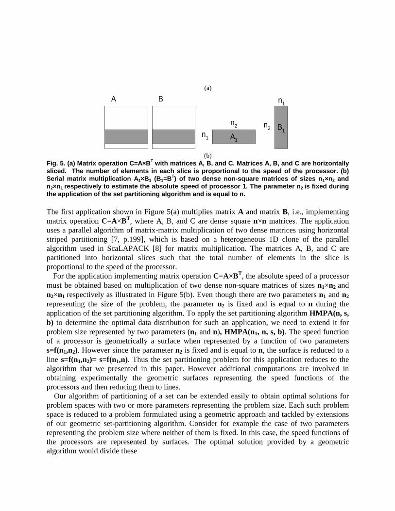
(b) Fig. 5. (a) Matrix operation C=A×BT with matrices A, B, and C. Matrices A, B, and C are horizontally sliced. The number of elements in each slice is proportional to the speed of the processor. (b) Serial matrix multiplication A1×B1 (B1=BT) of two dense non-square matrices of sizes n1×n2 and n2×n1 respectively to estimate the absolute speed of processor 1. The parameter n2 is fixed during the application of the set partitioning algorithm and is equal to n. The first application shown in Figure 5(a) multiplies matrix A and matrix B, i.e., implementing matrix operation C=A×BT, where A, B, and C are dense square n×n matrices. The application uses a parallel algorithm of matrix-matrix multiplication of two dense matrices using horizontal striped partitioning [7, p.199], which is based on a heterogeneous 1D clone of the parallel algorithm used in ScaLAPACK [8] for matrix multiplication. The matrices A, B, and C are partitioned into horizontal slices such that the total number of elements in the slice is proportional to the speed of the processor.

For the application implementing matrix operation C=A×BT, the absolute speed of a processor must be obtained based on multiplication of two dense non-square matrices of sizes n1×n2 and n2×n1 respectively as illustrated in Figure 5(b). Even though there are two parameters n1 and n2

representing the size of the problem, the parameter n2 is fixed and is equal to n during the application of the set partitioning algorithm. To apply the set partitioning algorithm HMPA(n, s, b) to determine the optimal data distribution for such an application, we need to extend it for problem size represented by two parameters (n1 and n), HMPA(n1, n, s, b). The speed function of a processor is geometrically a surface when represented by a function of two parameters s=f(n1,n2). However since the parameter n2 is fixed and is equal to n, the surface is reduced to a line s=f(n1,n2)= s=f(n1,n). Thus the set partitioning problem for this application reduces to the algorithm that we presented in this paper. However additional computations are involved in obtaining experimentally the geometric surfaces representing the speed functions of the processors and then reducing them to lines.

Our algorithm of partitioning of a set can be extended easily to obtain optimal solutions for problem spaces with two or more parameters representing the problem size. Each such problem space is reduced to a problem formulated using a geometric approach and tackled by extensions of our geometric set-partitioning algorithm. Consider for example the case of two parameters representing the problem size where neither of them is fixed. In this case, the speed functions of the processors are represented by surfaces. The optimal solution provided by a geometric algorithm would divide these

n2

n1

A

n2

n1B

A1

B1

Table 3 Results of serial matrix-matrix multiplication

Size of matrix

Absolute speed

(MFlops)

Size of matrix

Absolute speed

(MFlops)

Size of matrix

Absolute speed

(MFlops)

Size of matrix

Absolute speed

(MFlops) 256×256 67 1024×1024 67 2304×2304 67 4096×4096 59

128×512 68 512×2048 66 1152×4608 67 2048×8192 60 64×1024 67 256×4096 67 576×9216 69 1024×16384 59 32×2048 67 128×8192 67 288×18432 70 512×32768 60

Table 4 Results of serial LU factorization

Size of matrix

Absolute speed

(MFlops)

Size of matrix

Absolute speed

(MFlops)

Size of matrix

Absolute speed

(MFlops)

Size of matrix

Absolute speed(M

Flops) 1024×1024 115 2304×2304 129 4096×4096 131 6400×6400 132 512×2048 115 1152×4608 130 2048×8192 132 3200×12800 131 256×4096 116 576×9216 129 1024×16384 132 1600×25600 132 128×8192 117 288×18432 129 512×32768 131 800×51200 131

surfaces to produce a set of rectangular partitions equal in number to the number of processors such that the number of elements in each partition (the area of the partition) is proportional to the speed of the processor. We do not present the extensions of our algorithm here for such multi-dimensional representations of the size of the problem. We think it would complicate the presentation.

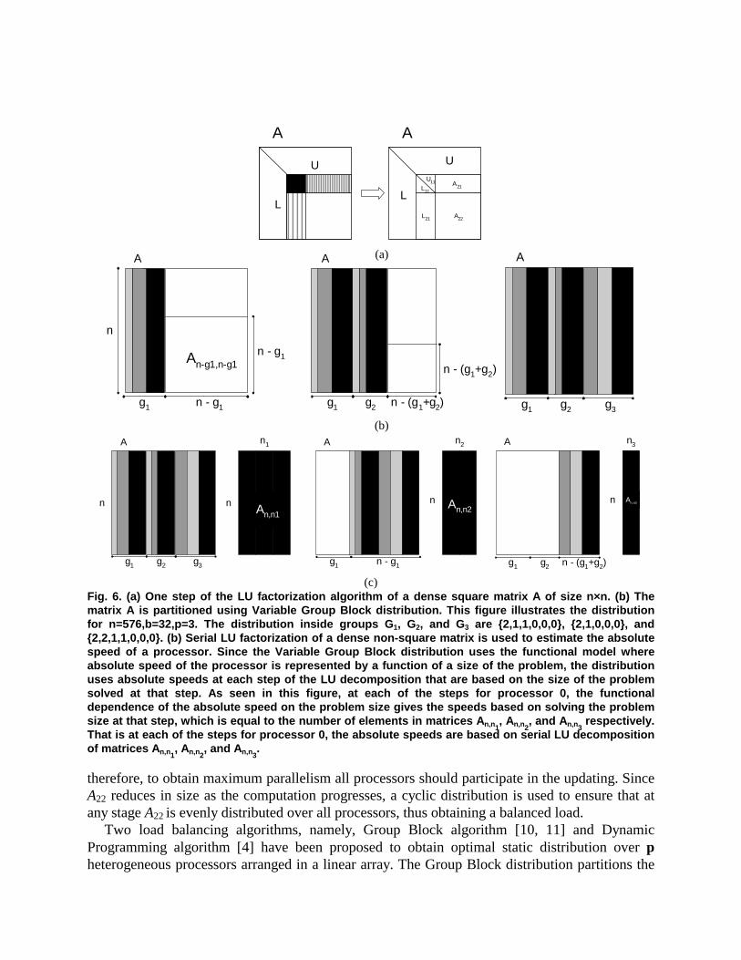
To calculate the absolute speed of the processor, we use a serial version of the parallel algorithm of matrix-matrix multiplication. The serial version performs matrix-matrix multiplication of two dense square matrices. Though the absolute speed must be obtained by multiplication of two dense non-square matrices, we observed that our serial version gives almost the same speeds for multiplication of two dense square matrices if the number of elements in a dense non-square matrix is the same as the number of elements in a dense square matrix. This is illustrated in Table 3 for one Linux computers X2-X5 whose specification is shown in Table 2. The behavior exhibited is the same for other computers. Thus speed functions of the processors built using dense square matrices will be the same as those built using dense non-square matrices. LU Factorization The second application is based on the parallel algorithm of LU factorization of a dense square n×n matrix A, one step of which is shown in Figure 6(a). On a homogeneous p-processor linear array, a CYCLIC(b) distribution of columns is used to distribute the matrix A where b is the block size [4, 9]. A cyclic distribution would assign block numbers 0,1,2,…,n-1 to processor 0,1,2,…,p-1,0,1,2…,p-1,0,…, respectively, for a p-processor linear array (n»p), until all n blocks are assigned. At each step of the algorithm, the processor that owns the pivot block factors it and broadcasts it to all the processors, which update their remaining blocks. At the next step, the next block of b columns becomes the pivot panel, and the computation progresses. Figure 6(a) shows how the column panel, L11 and L21, and the row panel, U11 and U12, are computed and how the trailing submatrix A22 is updated. Because the largest fraction of the work takes place in the update of A22,

(a)

(b)

(c) Fig. 6. (a) One step of the LU factorization algorithm of a dense square matrix A of size n×n. (b) The matrix A is partitioned using Variable Group Block distribution. This figure illustrates the distribution for n=576,b=32,p=3. The distribution inside groups G1, G2, and G3 are {2,1,1,0,0,0}, {2,1,0,0,0}, and {2,2,1,1,0,0,0}. (b) Serial LU factorization of a dense non-square matrix is used to estimate the absolute speed of a processor. Since the Variable Group Block distribution uses the functional model where absolute speed of the processor is represented by a function of a size of the problem, the distribution uses absolute speeds at each step of the LU decomposition that are based on the size of the problem solved at that step. As seen in this figure, at each of the steps for processor 0, the functional dependence of the absolute speed on the problem size gives the speeds based on solving the problem size at that step, which is equal to the number of elements in matrices An,n1

, An,n2, and An,n3

respectively. That is at each of the steps for processor 0, the absolute speeds are based on serial LU decomposition of matrices An,n1

, An,n2, and An,n3

. therefore, to obtain maximum parallelism all processors should participate in the updating. Since A22 reduces in size as the computation progresses, a cyclic distribution is used to ensure that at any stage A22 is evenly distributed over all processors, thus obtaining a balanced load.

Two load balancing algorithms, namely, Group Block algorithm [10, 11] and Dynamic Programming algorithm [4] have been proposed to obtain optimal static distribution over p heterogeneous processors arranged in a linear array. The Group Block distribution partitions the

U

L

A A

U

L

U11

L11

A21

L21 A22

A

g1 n - g1

n - g1An-g1,n-g1

n

A

g1 g2 n - (g1+g2)

n - (g1+g2)

A

g1 g2 g3

A n1

nn

g1 g2 g3

A

n

n2

g1 n - g1

A

n

n3

An,n3

g1 g2 n - (g1+g2)

An,n1An,n2

matrix into groups, all of which have the same number of blocks. The number of blocks per group (size of the group) and the distribution of the blocks in the group amongst the processors are fixed and are determined based on speeds of the processors, which are represented by a single constant number. Same is the case with Dynamic Programming distribution except that the distribution of the blocks in the group amongst the processors is determined based on dynamic programming algorithm.

We propose a Variable Group Block distribution, which is a modification of the Group Block algorithm. It uses the functional model where absolute speed of the processor is represented by a function of a size of the problem. Since the Variable Group Block distribution uses the functional model where absolute speed of the processor is represented by a function of a size of the problem, the distribution uses absolute speeds at each step of the LU decomposition that are based on the size of the problem solved at that step. That is at each step, the number of blocks per group and the distribution of the blocks in the group amongst the processors are determined based on absolute speeds of the processors given by the functional model, which are based on solving the problem size at that step. Thus it also takes into account the effects of paging.

Figures 6(b) and 6(c) illustrate the Variable Group Block algorithm of a dense square n×n matrix A over p heterogeneous processors. Given a dense n×n square matrix A and a block size of b, the Variable Group Block distribution is a static data distribution that vertically partitions the matrix into m groups of blocks whose column sizes are g1,g2,…,gm as shown in Figure 6(b). The groups are non-square matrices of sizes n×(g1×b),n×(g2×b),…,n×(gm×b) respectively. The steps involved in the distribution are:

1). To calculate the size g1 of the first group G1 of blocks, we adopt the following procedure: • Using the data partitioning algorithm, we obtain an optimal distribution of matrix A

such that the number of elements assigned to each processor is proportional to the speed of the processor. The optimal distribution derived is given by (xi, si) (0≤i≤p-1),

where xi is the size of the subproblem such that 21

0n=∑ −

=

p

i ix and si is the absolute

speed of the processor used to compute the subproblem xi for processor i. Calculate the

load index li = ∑ −

=

1

0

isp

k ks (0≤i≤p-1).

• The size of the group g1 is equal to ⎣ ⎦)min(/1 il (0≤i≤p-1). If g1/p<2,

then ⎣ ⎦)min(/2g1 il= . This condition is imposed to ensure there is sufficient number of

blocks in the group. • This group G1 is now partitioned such that the number of blocks g1,i is proportional to

the speeds of the processors si where 1

1-p

0i 1,i gg =∑ = (0≤i≤p-1).

2). To calculate the size g2 of the second group, we repeat step 1 for the number of elements equal to (n-g1)

2 in matrix A. This is represented by the sub-matrix An-g1,n-g1 shown in Figure 6(b). We recursively apply this procedure until we have fully vertically partitioned the matrix A.

3). For algorithms such as LU Factorization, only blocks below the pivot are updated. The global load balancing is guaranteed by the distribution in groups; however, for the group that holds the pivot it is not possible to balance the workload due to the lack of data. Therefore it is possible to reduce the processing time if the last blocks in each group are assigned to fastest processors, that is when there is not enough data to balance the workload then it should be the fastest processors doing the work. That

Matrix-Matrix Multiplication

80859095

100105110115120125130

0 2000 4000 6000 8000 10000 12000

Size of the matrix

Ab

solu

te s

pee

d (M

Flo

ps)

points=8 points=7points=6

points = Number of experimentally obtained points

Width of the band of accuracy is 5%

LU factorization

0

20

40

60

80

100

120

0 2000 4000 6000 8000 10000 12000

Size of the matrix

Ab

solu

te s

pee

d (

MF

lop

s)

points=8 points=7points=5

points = Number of experimentally obtained points

Width of the band of accuracy is 5%

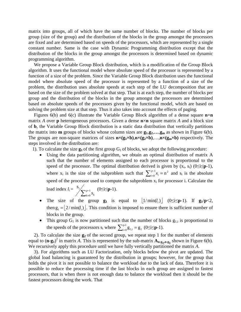
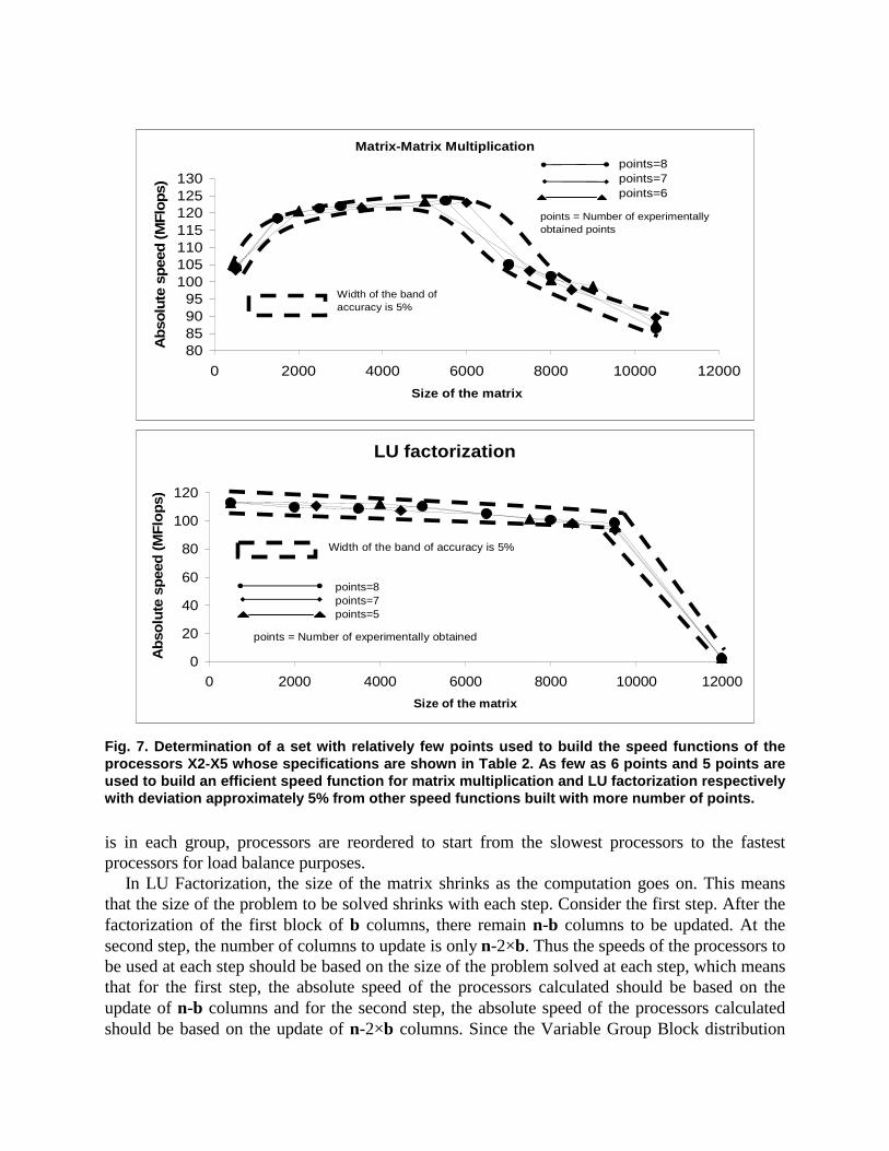
Fig. 7. Determination of a set with relatively few points used to build the speed functions of the processors X2-X5 whose specifications are shown in Table 2. As few as 6 points and 5 points are used to build an efficient speed function for matrix multiplication and LU factorization respectively with deviation approximately 5% from other speed functions built with more number of points.

is in each group, processors are reordered to start from the slowest processors to the fastest processors for load balance purposes.

In LU Factorization, the size of the matrix shrinks as the computation goes on. This means that the size of the problem to be solved shrinks with each step. Consider the first step. After the factorization of the first block of b columns, there remain n-b columns to be updated. At the second step, the number of columns to update is only n-2×b. Thus the speeds of the processors to be used at each step should be based on the size of the problem solved at each step, which means that for the first step, the absolute speed of the processors calculated should be based on the update of n-b columns and for the second step, the absolute speed of the processors calculated should be based on the update of n-2×b columns. Since the Variable Group Block distribution

uses the functional model where absolute speed of the processor is represented by a function of a size of the problem, the distribution uses absolute speeds at each step that are calculated based on the size of the problem solved at that step.

For the application implementing LU factorization, the absolute speed of a processor must be obtained based on LU factorization of a dense non-square matrix of size m1×m2 as shown in Figure 6(c). Even though there are two parameters m1 and m2 representing the size of the problem, the parameter m1 is fixed and is equal to n during the application of the set partitioning algorithm. To apply the set partitioning algorithm to determine the optimal data distribution for such an application, we need to extend it for problem size represented by two parameters, n and m2. The speed function of a processor is geometrically a surface when represented by a function of two parameters s=f(m1,m2). However since the parameter m1 is fixed and is equal to n, the surface is reduced to a line s=f(m1,m2)= s=f(n,m2). Thus the set partitioning problem for this application reduces to the algorithm that we have presented in this paper. However additional computations are involved in obtaining experimentally the geometric surfaces representing the speed functions of the processors and then reducing them to lines.

The set partitioning algorithm can also be extended here easily as explained for matrix multiplication. To calculate the absolute speed of the processor, we use a serial version of the parallel algorithm of LU factorization. The serial version performs LU factorization of a dense square matrix. Though the absolute speed must be obtained by using LU factorization of a dense non-square matrix, we observed that our serial version gives almost the same speeds for LU factorization of a dense square matrix if the number of elements in a dense non-square matrix is the same as the number of elements in a dense square matrix. This is illustrated in Table 4 for computers X2-X5 whose specification is shown in Table 2. The behavior exhibited is the same for other computers.

The absolute speed of the processor in number of floating point operations per second is calculated using the formula

executionoftime

nnnMF

executionoftime

nscomputatioofvolumespeedAbsolute

×××==

where n is the size of the matrix. MF is 2 for Matrix Multiplication and 2/3 for LU factorization. In the case of matrix-matrix multiplication, the size of the task is the number of elements in resultant matrix C=A×BT. In the case of LU factorization, the size of the task is the number of elements in the factorized matrix.

For these two applications, the network of heterogeneous computers shown in Table 2 contains some computers that permit paging and some computers that do not permit paging. For example, the computer X1 is a computer science departmental server running NFS and NIS, as well as web and database servers. It is configured to not permit paging. The largest problem size that can be solved on this computer is 116640000 and 262440000 for matrix-matrix multiplication and LU factorization respectively. Allocation of a task larger than this size will result in crash of this processor. The computers X2, X3, X4, and X5 permit paging. However allocation of a task to these computers, the size of which is greater than 36000000 and 81000000 for matrix-matrix multiplication and LU factorization respectively, will result in severe performance degradation of the parallel application. For each of these two applications, the largest problem size that can be solved on the network of heterogeneous networks shown in Table 2 is just the sum of the largest sizes of the tasks that can be solved on each computer.

There are three important issues in selecting a set of points to build a speed function of a processor:

1. The range of the set of points, that is, the minimal problem size and the maximal problem size experimentally used. The minimum problem size could be as low as a size of memory that fits into the top level of memory hierarchy of the computer and the maximum problem size is the upper bound on the largest problem size that the processor can solve,

2. The number of points in the set, and 3. The intervals between the points. The speed function for a processor is built using a set of few experimentally obtained points.

The more the number of points used in building the speed functions, the more accurate the speed functions are. However it is prohibitively expensive to use large number of points to build the speed functions of the processors. Hence for each processor, an optimal set of few points needs to be chosen to build an efficient speed function. Such a speed function built gives the speed of the processor for any problem size with certain deviation from the ideal speed function and speed functions built with sets with more number of points. This deviation must be within acceptable limits, ideally not exceeding the inherent deviation of the performance of computers typically observed in the network. In our experiments, we set the acceptable deviation to be %5± . This implies that the speed function should give the speed of the processor for a problem size within

%5± accuracy from the speed given by an ideal speed function or the speed functions built with sets with more number of points. Figure 7 show speed functions for matrix multiplication obtained using three sets of 6, 7, and 8 points and speed functions for LU factorization obtained using three sets of 5, 7, and 8 points for the computers X2-X5 whose specifications are shown in Table 2. It can be seen that 6 points and 5 points are enough to build an efficient speed function that fall within acceptable limits of deviation for matrix multiplication and LU factorization respectively.

A naïve approach to select a set of i points is: If (xmin, smin) is the point with minimal problem size experimentally obtained and (xmax, smax) is the point with maximal problem size experimentally obtained, the remaining i-2 points experimentally tested have problem sizes (xmin+(xmax-xmin)/(i-1)),…,(xmin+(i-2)*(xmax-xmin)/(i-1))) respectively.

In some cases, clever experimental methods can be adopted to determine the range that is used to choose a set of points to build the speed functions of the processors. Two examples are illustrated in Figure 8. Suppose the problem size is n and the number of processors involved in the execution of the problem size is p. For the first case shown in Figure 8(a), obtain the speeds of the processors with each processor executing a problem size of (n/p). We assume that the upper bounds of all the processors exceed (n/p). For the processor exhibiting the lowest speed (in this case the processor with speed function s1(x)), the set of points can be chosen from xmin to (n/p). For the processor that shows the maximum speed (in this case the processor with speed function s2(x)), the set of points can be chosen from (n/p) to xmax, where xmax represents the upper bound on the largest problem size that can be solved on each processor. For all the other processors, the set of points are chosen from xmin to xmax.

For the second case shown in Figure 8(b), the upper bound of at processor with speed function s4(x) is less than (n/p). For this processor, the set of points can be chosen from xmin to b4. Obtain the speeds of the processors with each processor executing a problem size of b4. For the processor with speed function s1(x) exhibiting the lowest speed, the set of points can be chosen from xmin to b4. For the processor with speed function s2(x) showing the maximum speed, the set

of points can be chosen from b4 to b2. For all the other processors, the set of points are chosen from xmin to xmax.

Size of the problem

Ab

solu

te s

pee

d

)(1 xs

)(2 xs

)(3 xs

Size of the problem = n

line 1 line 2

⎟⎟⎠

⎞⎜⎜⎝

⎛=

p

nx

1b

2b

3b

(a)

Size of the problem

Ab

solu

te s

pee

d

)(1 xs

)(2 xs

)(3 xs

Size of the problem = n⎟⎟⎠

⎞⎜⎜⎝

⎛=

p

nx

1b

2b

3b

)(4 xs

4b

4bx =

line1

line2

(b)

Fig. 8. Some advanced methods to determine the range that is used to choose a set of points to build the speed functions of the processors. In both the cases, the optimal solution line lies between line1 and line2.

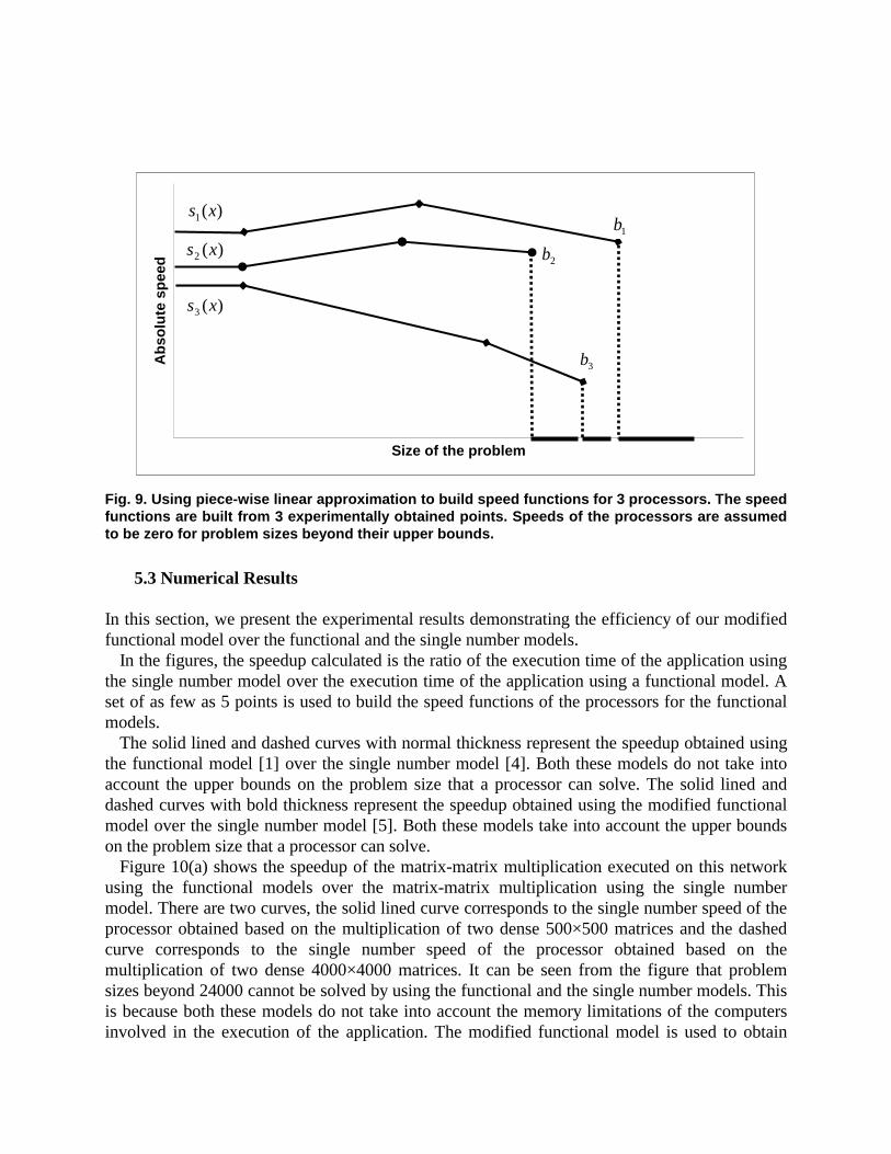
We use piece-wise linear function approximation illustrated in Figure 9 to build the speed function. Such approximation of the speed function is compliant with the requirements of the model, which are the shape requirements of the graph representing the speed function and that the speeds be continuous and smooth functions of problem size up till its upper bound on the problem size and zero beyond.

For the applications that we have chosen, the contribution of communication operations in the total execution time is negligibly small compared to that of computations. The inclusion of the cost of communications into the modified functional model is a subject of our current research.

Size of the problem

Ab

solu

te s

pee

d

)(1 xs

)(2 xs

)(3 xs

1b

2b

3b

Fig. 9. Using piece-wise linear approximation to build speed functions for 3 processors. The speed functions are built from 3 experimentally obtained points. Speeds of the processors are assumed to be zero for problem sizes beyond their upper bounds.

5.3 Numerical Results

In this section, we present the experimental results demonstrating the efficiency of our modified functional model over the functional and the single number models.

In the figures, the speedup calculated is the ratio of the execution time of the application using the single number model over the execution time of the application using a functional model. A set of as few as 5 points is used to build the speed functions of the processors for the functional models.

The solid lined and dashed curves with normal thickness represent the speedup obtained using the functional model [1] over the single number model [4]. Both these models do not take into account the upper bounds on the problem size that a processor can solve. The solid lined and dashed curves with bold thickness represent the speedup obtained using the modified functional model over the single number model [5]. Both these models take into account the upper bounds on the problem size that a processor can solve.

Figure 10(a) shows the speedup of the matrix-matrix multiplication executed on this network using the functional models over the matrix-matrix multiplication using the single number model. There are two curves, the solid lined curve corresponds to the single number speed of the processor obtained based on the multiplication of two dense 500×500 matrices and the dashed curve corresponds to the single number speed of the processor obtained based on the multiplication of two dense 4000×4000 matrices. It can be seen from the figure that problem sizes beyond 24000 cannot be solved by using the functional and the single number models. This is because both these models do not take into account the memory limitations of the computers involved in the execution of the application. The modified functional model is used to obtain

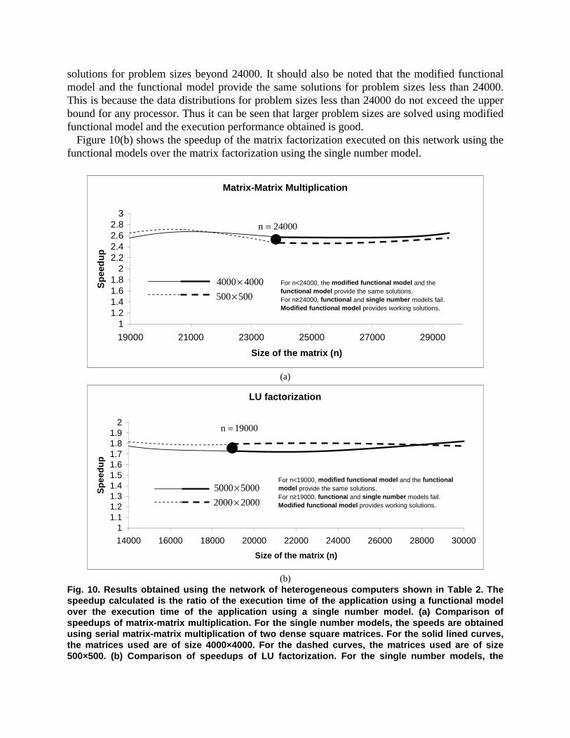
solutions for problem sizes beyond 24000. It should also be noted that the modified functional model and the functional model provide the same solutions for problem sizes less than 24000. This is because the data distributions for problem sizes less than 24000 do not exceed the upper bound for any processor. Thus it can be seen that larger problem sizes are solved using modified functional model and the execution performance obtained is good.

Figure 10(b) shows the speedup of the matrix factorization executed on this network using the functional models over the matrix factorization using the single number model.

Matrix-Matrix Multiplication

11.21.41.61.8

22.22.42.62.8

3

19000 21000 23000 25000 27000 29000

Size of the matrix (n)

Sp

eed

up

For n<24000, the modified functional model and the functional model provide the same solutions. For n≥24000, functional and single number models fail. Modified functional model provides working solutions.

24000n =

40004000×500500×

(a)

LU factorization

11.11.21.31.41.51.61.71.81.9

2

14000 16000 18000 20000 22000 24000 26000 28000 30000

Size of the matrix (n)

Sp

eed

up

For n<19000, modified functional model and the functional model provide the same solutions.For n≥19000, functional and single number models fail. Modified functional model provides working solutions.

19000n =

50005000×20002000×

(b)

Fig. 10. Results obtained using the network of heterogeneous computers shown in Table 2. The speedup calculated is the ratio of the execution time of the application using a functional model over the execution time of the application using a single number model. (a) Comparison of speedups of matrix-matrix multiplication. For the single number models, the speeds are obtained using serial matrix-matrix multiplication of two dense square matrices. For the solid lined curves, the matrices used are of size 4000×4000. For the dashed curves, the matrices used are of size 500×500. (b) Comparison of speedups of LU factorization. For the single number models, the

speeds are obtained using serial LU factorization of a dense square matrix. For the solid lined curves, the matrix used is of size 5000×5000. For the dashed curves, the matrix used is of size 2000×2000. There are two curves, the solid lined curve corresponds to the single number speed of the processor obtained based on the matrix factorization of a dense 2000×2000 matrix and the dashed curve corresponds to the single number speed of the processor obtained based on the matrix factorization of a dense 5000×5000 matrix. It can be seen from the figure that problem sizes beyond 19000 cannot be solved by using the functional model and single number models. This is because both these models do not take into account the memory limitations of the computers involved in the execution of the application. The modified functional model is used to obtain solutions for problem sizes beyond 19000. It should also be noted that the modified functional model and the functional model obtain the same solutions for problem sizes less than 19000. This is because the data distributions for problem sizes less than 19000 do not exceed the upper bound for any processor. Thus it can be seen that larger problem sizes are solved using the modified functional model and the execution performance obtained is good.

As can be seen from the figures, the modified functional model performs better than the currently existing models for a network of heterogeneous computers.

6. Related Work We survey related papers from the literature in this section. They fall into two categories: papers dealing with task partition and scheduling with memory constraints on dedicated environments and papers dealing with task scheduling with memory constraints on non-dedicated computing environments like the Heterogeneous Networks of Computers (HNOCs) and computing grids.

Li, Veeravalli, and Ko [12] investigate the problem of scheduling a divisible load onto a set of processors with finite-size buffers in heterogeneous single-level tree networks. They propose a fast algorithm called Incremental Balancing Strategy (IBS) to achieve the optimal processing time. In each increment, distribution of the load is found for processors with available memory according to the standard divisible load theory methods [13] without taking the memory constraints into account. Then, the distribution of the load is scaled proportionately such that at least one buffer is filled completely. The remaining available buffer capacities are memory sizes in the next increment. This process is continued until distributing the entire load. Drozdowski and Wolniewicz [14] propose a linear programming method of finding solutions with guaranteed optimality for the problem of scheduling divisible loads in networks of processors with limited memory and communication startup times. The complexity of the linear programming solutions that they use to solve their problem is O(p3.5×L), where p is the number of processors involved in the execution of the algorithm and L is the length of the string encoding all the parameters of linear program.

The works discussed take into account the processor heterogeneity in terms of speeds, memory heterogeneity in terms of memory limitation at each processor, and network heterogeneity in terms of the communication cost between a pair of processors. However, these works assume distributed systems with a flat memory model and are not applicable to systems with memory hierarchy. The dependence of the speed of the processor on the size of the problem is assumed to be linear as is usually observed on dedicated distributed multiprocessor computer systems. The largest problem size that can be solved at each processor is assumed to be the core memory at

that processor. This is a safe assumption on dedicated distributed multiprocessor computer systems. However on networks of heterogeneous computers, due to the nature of applications run and the level of integration of the computers involved in execution of these applications, the core memory at each processor is just an upper bound on the largest problem size that can be solved but is not a good approximation of the actual largest problem size that can be solved.

The modified functional model that we propose integrates the essential features underlying applications run on a network of heterogeneous computers, mainly, the processor heterogeneity, the heterogeneity of memory structure, and the memory limitations at each level of memory hierarchy. We also present efficient algorithms of data partitioning with this model with relatively low complexity of O(p3×log2n). However we do not consider the cost of communications in our modified functional model.

While resource management and task scheduling are identified challenges of Grid computing, current Grid scheduling systems mainly focus on CPU and network availability. Many heuristic scheduling algorithms [15, 16] have been proposed for traditional high performance computing. However these scheduling systems are for dedicated multiprocessor computer systems and also ignore the impact of memory resource availability on the scheduling decision-making.

Several studies have been reported on task allocation for load balance considering memory resource constraints. An opportunity cost approach proposed in [17] converts the usage of resources including CPU and memory to a single homogeneous cost. Based on the cost, task is assigned or reassigned to each node for load balance. Load sharing policies with the consideration of effective usage of global memory were studied in [18]. They consider two types of application workload, known memory demands and unknown memory demands. However their major concern is how to reduce the average slowdown of all individual jobs in the system, instead of how to schedule a parallel application to achieve its best performance. Xu and Sun [5] consider how to partition a Grid application and schedule it on a cluster of distributed heterogeneous resources to obtain a minimum application execution time with the consideration of both CPU resource availability and memory resource availability. Three task partition policies, namely, CPU-based, memory-based, and CPU-memory combined partition are studied. They show that the CPU-memory combined approach shows good performance gains over the other approaches. A heuristic CPU-memory algorithm for task scheduling of a meta-task is also proposed. The effect of local jobs on a grid application execution in the situation of resource sharing is evaluated using distribution functions. Currently our modified functional model and the algorithms using this model are not applicable for task scheduling of a meta-task.

The accurate modeling of the electronic structure of atoms and molecules involves computationally intensive tensor contractions involving large multidimensional arrays. The efficient computation of complex tensor contractions usually requires the generation of temporary intermediate arrays. These intermediates could be extremely large, but they can often be generated and used in batches through appropriate loop fusion transformations. To optimize the performance of such computations on parallel computers, Cociorva et al. [19] present a framework to address the optimization problem: given a set of computations expressed as a sequence of tensor contractions, an empirically derived measure of the communication cost for a given target computer, and a specified limit on the amount of available memory on each processor, re-structure the computation so as to minimize the total execution time while staying within the available memory. The framework considers only the heterogeneity in terms of the memory limitations of each computer and is not applicable for programming applications on

networks of heterogeneous computers, which exhibits processor heterogeneity in terms of speeds and memory heterogeneity in terms of memory hierarchy and memory limitations of each computer.

7. Conclusion In this paper, we address the problem of optimal distribution of computations over heterogeneous computers taking into account the processor heterogeneity, the heterogeneity of memory structure, and the memory limitations at each level of memory hierarchy of a processor. We have proposed a modified functional model of a network of heterogeneous computers and designed efficient algorithms of data partitioning with this model.

The modified functional model proposed can be used to design efficient algorithms of data partitioning for mathematical structures other than sets such as matrices, graphs, and trees. This model can be used to design efficient algorithms for the most general partitioning problem, which can be formulated as:

• Given: (1) An application of problem size n to be solved, and (2) A well-ordered set of p processors whose speeds are functions of the size of the problem, si=fi(x), and (3) There is a limit li on the largest problem size that can be solved on each processor,

• Partition the problem into p disjoint sub-problems xi (i=0,…,p-1) such that (1) There is a one-to-one mapping between the sub-problems and the processors, (2) The size of the sub-problem xi is proportional to the speed of the processor i owning the sub-problem xi, and (3) The size of the sub-problem xi is less than or equal to the limit li on the largest problem size that can be solved on each processor (xi ≤ li).

In the presented research we do not take account of communication cost. Although we well understand the importance of its incorporation in our model, this is just out of scope of this work. We also understand the importance of the problems of efficient building and maintaining of our model. These two problems are also out of scope of the paper and are subjects of our current research. REFERENCES [1] A. Lastovetsky and R. Reddy, “Data Partitioning with a Realistic Performance Model of Networks of Heterogeneous Computers,” In Proceedings of the 17th International Parallel and Distributed Processing Symposium (IPDPS 2004), 26-30 April 2004, New Mexico, France, CD-ROM/Abstracts Proceedings, IEEE Computer Society 2004. [2] A. Lastovetsky and J. Twamley, “Towards a Realistic Performance Model for Networks of Heterogeneous Computers,” In International Symposium on High Performance Computational Science and Engineering HPSCE’04, Toulouse, France, August 22-27, 2004. [3] A. Lastovetsky and R. Reddy, “Classification of Partitioning Problems for Networks of Heterogeneous Computers,” In Proceedings of the 5th International Conference on Parallel Processing and Applied Mathematics (PPAM 2003), Czestochowa, Poland, Lecture Notes in Computer Science, 3019, pp.921-929, September 2003. [4] O. Beaumont, V. Boudet, A. Petitet, F. Rastello, and Y. Robert, “A Proposal for a Heterogeneous Cluster ScaLAPACK (Dense Linear Solvers),” In IEEE Transactions on Computers, Volume 50, No. 10, pp.1052-1070, October 2001.

[5] M. Wu, and X.-H. Sun, “Memory Conscious Task Partition and Scheduling in Grid Environments,” In 5th IEEE/ACM International Workshop on Grid Computing (in conjunction with SuperComputing 2004), Pittsburgh, pp.138-145, November 2004. [6] M. Cierniak, W. Li, and M. J. Zaki, “Compile-time scheduling algorithms for heterogeneous network of workstations,” In Computer Journal, special issue on Automatic Loop Parallelization, Volume 40, No. 6, December 1997. [7] A. Lastovetsky. Parallel Computing on Heterogeneous Networks. John Wiley & Sons, 423 pages, 2003. [8] J. Choi, J. Demmel, I. Dhillon, J. Dongarra, S. Ostrouchov, A. Petitet, K. Stanley, D. Walker, and R.C. Whaley, “ScaLAPACK: A Portable Linear Algebra Library for Distributed Memory Computers - Design Issues and Performance,” In Computer Physics Communication, Volume 97, pp.1-15, 1996. [9] J. Choi, J. Dongarra, L. S. Ostrouchov, A. P. Petitet, D. W. Walker, and R. C. Whaley, “The Design and Implementation of the ScaLAPACK LU, QR, and Cholesky Factorization Routines,” In Scientific Programming, Volume 5, No. 3, pp.173–184, Fall 1996, ISSN 1058-9244. [10] J. Barbosa, J. Tavares, and A. J. Padilha, “Linear Algebra Algorithms in a Heterogeneous Cluster of Personal Computers,” In Proceedings of the 9th Heterogeneous Computing Workshop (HCW 2000), Cancun, Mexico, IEEE Computer Society Press, May 2000, pp.147-159. [11] J. Barbosa, C. N. Morais, and A. J. Padilha, “Simulation of Data Distribution Strategies for LU Factorization on Heterogeneous Machines,” In Proceedings of the 17th International Parallel and Distributed Processing Symposium (IPDPS 2004), 26-30 April 2004, New Mexico, France, CD-ROM/Abstracts Proceedings, IEEE Computer Society 2004. [12] X. Li, B. Veeravalli, and C.C. Ko, “Divisible Load Scheduling on Single-level Tree Networks with Finite-size Buffers,” In IEEE Transactions on Aerospace and Electronic Systems, Volume 36, No. 4, pp.1298-1308, October 2000. [13] B. Veeravalli, D. Ghose, V. Mani, and T. G. Robertazzi, “Scheduling Divisible Loads in Parallel and Distributed Systems,” In IEEE Computer Society Press and John Wiley & Sons, 312 pages, August 1996, ISBN: 0-8186-7521-7. [14] M.Drozdowski, and P.Wolniewicz, “Divisible load scheduling in systems with limited memory,” In special issue of Cluster Computing on Divisible Load Scheduling, Kluwer Academic Publishers, Volume 6, No. 1, pp.19-29, January 2003. [15] F. Berman, R. Wolski, H. Casanova, W. Cirne, H. Dail, M. Faerman, S. Figueira, J. Hayes, G. Obertelli, J. Schopf, G. Shao, S. Smallen, S. Spring, A. Su, and D. Zagorodnov, “Adaptive computing on the Grid using AppLeS,” In IEEE Transactions on Parallel and Distributed Systems (TPDS), Volume 14, No. 4, pp.369-382, April 2003. [16] X.-H. Sun, and M. Wu, “Grid Harvest Service: A System for Long-Term, Application-Level Task Scheduling,” In Proceedings of the 16th IEEE International Parallel and Distributed Processing Symposium (IPDPS 2003), Nice, France, April, 2003. [17] Y. Amir, B. Awerbuch, A. Barak, R. S. Borgstrom, and A. Keren, “An opportunity cost approach for job assignment in a scalable computing cluster,” In IEEE Transactions on Parallel and Distributed Systems, Volume 11, No. 7, pp.760-768, July 2000. [18] L. Xiao, S. Chen, and X. Zhang, “Dynamic Cluster Resource Allocations for Jobs with Known and Unknown Memory Demands,” In IEEE Transactions on Parallel and Distributed Systems, Volume 13, No. 3, pp.223-240, March 2002.

[19] D. Cociorva, G. Baumgartner, C. Lam, P. Sadayappan, and J. Ramanujam, “Memory-Constrained Communication Minimization for a Class of Array Computations,” In Proceedings of the 15th International Workshop on Languages and Compilers for Parallel Computing (LCPC '02), College Park, Maryland, July 2002. Alexey Lastovetsky received the PhD degree from the Moscow Aviation Institute in 1986, and the Doctor of Science degree from the Russian Academy of Sciences in 1997. He is currently a lecturer in the Computer Science Department at University College Dublin, National University of Ireland. His main research interests are parallel and distributed programming languages and systems for heterogeneous environments. Ravi Reddy is currently a PhD student in the Computer Science Department at University College Dublin, National University of Ireland. His main research interests are design of algorithms and tools for parallel and distributed computing systems.