Measurement of Productivity Improvements - CiteSeerX

IMeasurement of ProductivityImprovements: An Empirical Analysis

RAJIV D . BANKER*

SRIKANT M . DATAR*

MADHAV V. RAJ AN*

In this paper, we test for productivity gains resulting from theintroduction of a productivity-based incentive program in a largemanufacturing plant of a Fortune 500 corporation. We develop amethodology based on a stochastic nonparametric frontier esti-mation technique to evaluate productivity in the postincentive planperiod relative to the pre-incentive plan period. We also test forproductivity gains using stochastic parametric frontier approaches.The results of both the nonparametric and parametric stochasticfrontier analyses indicate that the incentive program has a positiveeffect on indirect labor, manufacturing services, and materials pro-ductivity and relatively little effect on direct labor productivity.

1. Introduction

Productivity improvement and cost control have become key objectivesof U.S. corporations in recent years. As a result, many corporations haveintroduced productivity improvement programs, especially productivity-based incentive payments to workers. The implementation and evaluationof the impact of such incentive programs have placed demands on man-agement accountants to develop reliable measures of productivity and man-ufacturing efficiency—an issue largely ignored in the managementaccounting literature.

The agency theory literature studies the motivational effects of providingincentives to woricers. The site at which a productivity-based scheme hasrecently b ^ n introduced serves as a natural experiment for testing the effectof an incentive contract intencted for improving labor productivity. Evalu-ation of its inqjact depends on tfje mettiod employed to measure productivity.

Univosity

319

I320 JOURNAL OF ACCOUNTING, AUDITING AND FINANCE

We use data from the site to compare conclusions drawn by altemativemethods of measuring productivity about the impact of the incentive planon productivity improvements.

In our model, productivity measures the efficiency with which each offour inputs (direct labor, materials, indirect labor, and manufacturing supportservices) is consumed in producing two outputs. Accounting systems inpractice are not geared to evaluating productivity. Simple input-output quan-tity ratios implicitly assume constant returns to scale (CRS) and the absenceof multiple inputs and outputs. The use of input prices further obfuscatesmeasures of productivity. Standard usage variances ignore indirect laborproductivity and additionally assume linear and separable technologies.

Advanced management accounting textbooks, such as Kaplan (1982),discuss ordinary least squares (OLS) approaches for estimating cost func-tions. This can be adapted for estimating production functions and improve-ments in productivity by regressing each input on the outputs produced andtesting for decreases in input consumption in the' 'event'' period—the periodafter the introduction of the gain-sharing program. The specification ofstochastic disturbance terms with zero means implies Ae estimation of anaverage production function. The theoretical definition of a production func-tion expresses the minimum amount of each input to produce given outputswith a fixed technology. An ordinary least squares analysis is thereforeinconsistent with a frontier production function that forms the core of mi-croeconomic theory.

This has led to the development and estimation of parametric frontiercost and production functions in the economics literature (see, for instance,Aigner and Chu [1%8] and Aigner, Lovell, and Schmidt [1977]). A weak-ness of such parametric fh)ntier estimation is its inability to theoreticallysubstantiate or statistically test the maintained hypottiesis about the para-n^tric form for the production function and the postulated distribution forthe disturbance term. Furthennore, the restrictions imposed on the produc-tion correspondence by these hypottieses are not immediately apparent. Weadopt an altemative nonparametric stochastic frontier estimation techniquecalled Stochastic Data Envelopment Analysis that only imposes conditionsof monotonicity and concavity on the production function, llie techniquewe employ is sufficiently general to allow for multiple inputs and ouûtsand for some of the inputs to be fixed.

We examine these altemative n^thods of evaluating productivity usingdata from a large manufacturing plant that has recently establisted a pro-ductivity-based incentive compensation plan for its workers. Tlie plant man-ufactures traditional engineering products. It has gained a leadership positionby providing quality products at low cost. Maintaining cost advantage

MEASUREMENT OF PRODUCTIVITY IMPROVEMENTS 321

through {M-oductivity improvements is critical in this mature, stable, com-petitive industry. The gain-sharing bonus scheme is an incentive to enhancelabor productivity by sharing the financial gains from improved productivitywith employees. Indirect plant labor and salaried staff are included in theplan to provide incentives for savings in the shop floor-related portion ofindirect labor, including time spent on repairs and maintenance, equipmenthandling, set-ups, and inspection of set-ups.

Strong links exist between methods discussed in this paper and thoseof traditional capital markets research. Although we specify a productioneconomics model, as opposed to a financial economics one, we perform avariation of residual analysis based on an estimated standard. Patel (1976),for instance, estimates a referent market model for the relationship betweenfirm and market returns and uses deviations from this as a measure ofabnormal returns and thus the infonnation content of eamings forecasts.Similarly, we estimate a referent production set for the input-output cor-respondence and compute deviations from it to measure improvements inmanufacturing productivity and thereby the impact of the incentive scheme.Further, we use the 0-1 variables technique as in Schipper and Thompson(1983) to identify productivity gains in different periods of interest relativeto a common referent correspondence. The objective of our analysis is todescribe a methodology to examine the productive impact of the gain-sharingscheme in the setting described; additional refinements to the methodologymay be warranted based on the specific situation encountered by a researcherand his or her observations on the production process being studied.

This paper has the following structure: In Section 2 we discuss theempirical setting of the problem and issues involved in obtaining and han-dling the data. Section 3 examines the merits and demerits of various eco-nomic models used to identify stochastic input consumption frontiers inorder to measure deviations of actual input consumption from the frontierin the event period. We consider both parametric and nonparametric esti-mation techniques and describe the structure imposed and the correspondingestimation procedure employed. Section 4 discusses the results and interpretsour findings.

2. Empirical Setting

Our site is a manufacturing plant within a highly diversified Fortune500 company. Productivity improvement is a key component of the divi-sion's comp^tive strategy. The division leads its industry in technologicaladvancement and market share. It has secured and retained its position byiwoviding better quality and more reliable products at a lower cost than its

322 JOURNAL OF ACCOUNTING, AUDITING AND FINANCE

competition in a mature, no-growth industry. Productivity improvementsare critical for long-run competitive advantage. Output prices are controlledby competitive maiket forces and reductions in input prices are generallyavailable to competitors as well.

Historically, the company has made great strides in productivity im-provements, by producing more outputs with the same or lesser quantity ofinputs, through technological innovation, and by efficient shop floor man-agement rather than by substituting labor for capital. This fact is stressedby its chairman, who notes in the company's annual report that the com-pany's strategy was to put "increased emphasis on new technology and newengineering capacity, training, product quality, productivity and cost re-duction." Among management's stated "high-priority" areas were "ap-plying technology to new and improved products and processes" and"improving quality, productivity and employee motivation." To continuethis trend and to maintain its cost leadership, the company has embarkedon a IKW campaign to improve productivity.

The behavioral setting of our investigation is cost minimization. Pro-duction requirements are determined by the marketing department and takenas given by the manufacturing plant.* The plant's focus is on minimizingresource consumption while producing the outputs required. Productivitygains are manifested via reduced quantities of inputs required to producespecified quantities of outputs.

Ilie particular plant we focus on is labor intensive with relatively stablecapital. As a direct consequence of this nonemphasis on capital, depreciationaccounts for only 3% of total costs and is a relatively minor item in theplant's monthly expense summary accounts. Direct labor, on the other hand,constitutes 20-25 percent of total expenses, and indirect labor and super-visory costs 25-30 percent. As part of its campaign to increase productivity,a gain-sharing program^ was instituted at the plant with benefits tied pre-dominantly to improvements in labor efficiency. Hie gain-sharing plan in-cludes indirect plant labor and salaried staff b(»:ause these elements are asignificant percentage of t ( ^ labor costs and offer consider£d)le potentialfor {Hoductivity improvement. Including indirect labor in the gain-sharingarrangement also facilitates union negotiations because the incentive ar-rangement encompasses all wOTkers in tiie plant.

We describe below the basic steps of the gain-sharing computation.Labor "pnxluctivity" in successive periods is computed relative to a base

1. If inpats and outputs are simultaneously determined, a simuhimeous equMions model must beestimated (see Zellaor. Kmetta, uid Droe {1966}).

2. The design <^ this gain-diaring program is discussed in detail in Baidta- and Datar (1987b).


period benchmaii^. The first step entails a computation of the standard directlabor hours in die base period (denoted by s^,) obtained by multiplying thestandard direct labor hours per unit for each product (based on industrialengineering estimates) by the quantity of each product produced in the baseperiod. The actual total labor hours (denoted by a^) including direct labor,indirect plant labor, and salaried staff hours are also computed for thebase period. The ratio of actual direct and indirect labor hours to standarddirect labor hours in the base period determines a base ratio (denoted byTb — Ot/st,). In each subsequent nranth t, the ratio r, of actual total laborhours a, to the standard direct labor hours Sf (based on the direct labor contentof products produced in period t) is computed. The gain-sharing fraction g,

for period t is calculated as -^ = ~^. Values of ^, greater than one indicater, a,l Sy

"productivity" gains; values of g, less than one signal "productivity"declines.

The gain-sharing agreement calls for woricers to be paid at base-periodwage rates if g, in a period is less than one. When g, is greater than one,half of the "productivity" gains are paid to workers. For example if g, =1.14, which signals a 14 percent increase in "productivity," each workerreceives a bonus of 7 percent over the base wage or salary.

Our objective is to identify increases in productivity in each of the fourinputs in the 15 months following the program's introduction relative to the33 months preceding it. Monthly data were available for a 48-month periodlabeled 1 through 48, with the gain-sharing program taking effect in month34. Monthly data on the physical quantities of the two products producedwere obtained firom plant production reports. The summary of manufacturingcosts provided details of the actual number of direct and indirect labor hoursemployed each period. Gains in labor productivity are measured via reduc-tions in hours worked. This provides a good measure of productivity becausethe mix of workers at various skill levels and pay levels has remainedconstant over the entire period of study. Productivity gains as reflected ina reduction of labor hours is achieved by employing fewer temporarylaborers.

Tht two [Hoducts manufacbired in the plant use a common metal whichaccounts for 90 percent of total raw material cost (which constitutes about15-20 percent of total cost). We deflate material cost of production by theincrease in material prices each period to obtain a constant-cost estimate ofmaterial consunqition. For miscellaneous manufacturing oveiiieads, wegroup several relatively minor costs such as power (about 3 pereent of t c ^cost), gas (1-2 percent), perish^le tools and jigs (4 percent), and janitorial


services (1-2 percent) that represent important support services for the op-eration of the plant, under the single category of manufacturing supportservices (25-30 percent of full cost). We deflate the cost each period byappropriate indices, based on plant records and suppliers' bills, to obtain aconstant-cost estimate of consumption of manufacturing services.

The financial reporting focus of the accounting system required signif-icant assumptions to be made in our analysis. The only information availablewith respect to material cost was the material cost of goods sold for eachproduct. The material cost of production for each product is calculated bymultiplying the (deflated) material cost of goods sold by the ratio of goodsproduced to goods shipped for each individual product. The total materialcost of production is derived by aggregating material costs over all products.The material consumption data are thus noisy and approximate and ourresults with respect to material costs must be interpreted cautiously.

There are four cost components: direct labor, materials, indirect labor,and manufacturing services. The stability and relative maturity of the man-ufacturing process limits the potential for improvement in materials anddirect labor productivity. The input-output relationships including the noiseand stochasticity in these relationships are well known, and managementcan control these costs on the basis of inputs consumed and outputs produced.Indirect labor and manufacturing services inputs, on the other hand, arediscretionary in nature with no identified direct relationship between inputsand outputs. Consequently, these costs cannot be controlled by monitoringoutputs and inputs. Instead, incentives need to be provided to influence thebehavior and effort of workers. The labor-based gain-sharing program is anexample of such an incentive. Consequently, we expect the gain-sharingprogram to result in improvements in indirect labor and possibly manufac-turing services. The impact on manufacturing services is likely to be smallerbecause the program does not directly provide incentives to improve man-ufacturing services productivity. Nevertheless, the general focus on im-proving labor productivity may positively influence manufacturing servicespnxluctivity as well.

3. Methodfrilogy for Testing the Impact of ProductivityImprovement Programs

In describing the methodology, we (tenote die' two out{Hits produced asyi and yz written in vector form as y = (yttyz)- The {^ysical inputs Xi, X2,X3, and X4 are denoted by the vector x = (jt,,X2,JC3,jC4) where JC, representsdirect laixx, x^ indirect hSofX, x-^ materials consumption, aiMi X4 consumptionof manufacturing wrvices. ITie [Htxluction technology at the pknt permits


little substitution among inputs. Because the plant is labor intensive, thecapital employed is small and relatively constant over the period of ouranalysis. Similarly, material consumption cannot be reduced by substitutingother inputs for materials.

Our analysis of the production process indicated that the consumptionof each input depends on only the quantity of outputs y, and )'2 producedand in particular is independent of the level of consumption of the otherinputs. That is,

Xi = fi(y,,y2) for all i = 1,2,3,4.

Our objective is to evaluate if, after controlling for the outputs produced,input consumption in the post-gain-sharing period is less than the inputconsumption in the pre-gain-sharing period.

The usual approach for testing for efficiency gains in the post-gain-sharing period relative to the pre-gain-sharing period is to use a least squaresregression by fitting prespecified functional forms for the correspondencebetween outputs and each input. Following the methodology of Schipperand Thompson (1983), dummy (0-1) variables representing the pre- andpost—gain-sharing periods could be introduced to capture shifts in the re-lationships across these periods. For instance, specifying a loglinear rela-tionship between each input and output y, and 2 yields the followingestimation model:

[A] log Xi, = aoi + a,i log yi, -t- a2i log y^, + b A + âV i = l , . . . 4 , t = l , . . . 4 8

where D, = 0 for t = 1, . . .33= 1 for t = 3 4 , . . . 48

The eleiments of Ci are assumed to be distributed i.i.d. N(O,CT^) anduncorrelated withji andy2- Significantly negative values ofbi indicate lowerinput costs Xi (and productivity gains with respect to input i) in the post-gain-sharing period.

Hiere are two important limitations in applying least squares techniquesto estimate the input consumption relationship between each input Xi andthe output prcKluced y = (y^ya). First, tiie regression-based approach es-timates ibe average amount of input consumed to produce given levels ofouQmts, whereas the theoretical definition of a production function expressesthe minimum amount of input for given levels of outputs. Moreover, froma managennnt ccmtrol perspo^ve, comparing future period input con-sunq)tion with the regressicm-based estimated consumption indicates whetherinput consumption in tiie post-gain-sharing period has been less tiian av-


erage, rather than whether input consumption is lower than the best diatwas achieved in die pre-gain-sharing period. Furthermore, least squaresregression estimates assume that the disturbance term arises from an i.i.d.stochastic process so that deviations of actual observations from the esti-mated function are a s sun^ to result fiom random deviations. In reality,these deviations result from extemal random factors as well as inefficienciesof plant workers. Indeed, the productivity-based incentive plan is aimed atmotivating workers to put in greater effort to reduce inefficiency and improveproductivity. Second, regression-based parametric methods assumed a par-ticular and often arbitrary functional form on die input-output correspond-ence. This problem is partly mitigated by assuming a flexible parametricrelationship between inputs and outputs such as a translog or loglinearfunctional form. In die next section we provide a methodology to test forproductivity gains assuming a loglinear stochastic production technology.

3.1. Parametric Stociiastic Frratier Estimatitm

Estimating a frontier production function involves the specification ofthe error term as being made up of two components, one normal and dieother from a one-sided distribution. That is, the error structure is given by:

e,, = Vi, -f- Uu V i= 1 , . . . 4 and t = 1 , . . . 48.

TTie error component Ui, represents a symmetric disturbance, where for eachI, {UjJ are assumed to be independendy and identically distributed asN(O,(ji.). The error component Vj, is assumed to be distributed independently

of «i, satisfying Vj, S: 0. In particular, {vJ are a s sun^ to be independently

and identically distributed from a half-normal distribution Ar^(0,o^) trun-

ca t e below at zero.The logic untterlying this specification is that die production process is

subject to two disturbances. Hie irannegative disturbance Vj, refl«;ts thecondition that for each input the input consumption level must lie above thefircmtier (a minimum omsumption level) over all time periods. These de-viations are attributable to factcvs umler the worker's control such as iiwf-ficiencies, wastage, die effort provicted by employees, and the extent ofreworked, ctefective, and dmnaged products. For each i, die random dis-turbance term Ujt reixeseirts die stochastic nature of die frontier itself overtime, v ^ much like dn random disdirbance term in a least square regres-sion model. Hie Uj, t^m is the result of favtHabie as well as unfavtnableraiuknn extemal events not controllable at ihe plant level, such as rand(»n

p^cnmance, iiKMtel specificioicm, and cm»s of ob%rvati<»i and

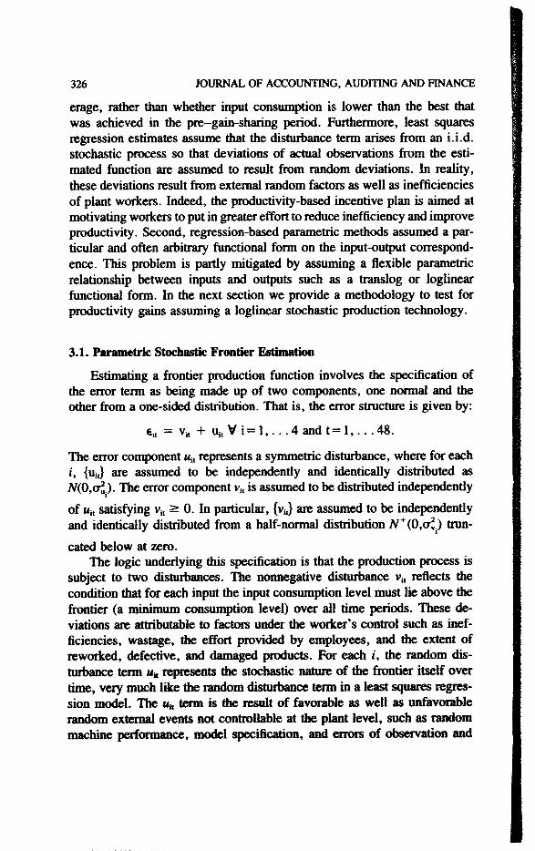
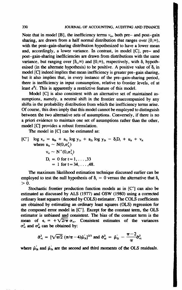
MEASUREMENT OF PRODUCnVlTY IMPROVEMENTS

INPUT

OUTPUT

Figure 1of Composed Error Specification

n:âsurement. Figure 1 distinguishes between average and frontier relation-ships and illustrates the notion of composed errors in the single-input andsingle-output case.

The point M represents an ouût level of OL and input consumptionof LM. Under ttie composed error model, the input consumption frontierlevel is estimated to be LN. The total deviation MN comprises the inefficiencycomponent NP and a random effect PM which exceeds the level ofinefficiency.

The stochastic input p(»sibility frontier expresses the Pareto efficientinput combinations necessary to {Hoduce specified vectors of outputs givendie existing technology. Input consumption in excess of frontier levels is areflectk»i of ii^fficiency in implementing production. Reducing the degreeof inefficiency in production is an inqxntant motivation for the introductionof a gain-sharing {nt^ram. It could alternatively be argued that incentives


{»x)vided by the gain-sharing agreement induce new ways of organizingproduction and result in shifts in the input possibility frontier. We take theposition that the input possibility frontier is not shifting (note that capitalinvestment in technology is also relatively stable over the period of ourfuialysis) and test whether the probability distribution generating the inef-ficiency terms decreases with the introduction of the gain-sharing program.

Our objective is to examine if productivity in the 15 months followingthe gain-sharing program increases relative to the 33 months preceding it.Production inefficiencies are measured by the nonnegative disturbance termVj, and represent deviations firom the frontier attributable to factors underthe workers' control. Note that since for each i, Vj, is assumed to be inde-pendently and identically distributed from a half-normal distributionN^{O,ail,) truncated below at zero, any increase in productivity will decreaseboth the mean and the variance of the distribution of Vu (because the meanand variance of a half-normal distribution are not independent). One wayto examine this is to test if v,, is distributed as half-normal A^ (O,CTVJ) forthe 33-nionth pre-gain-sharing period and as N^(O,(TI — 80 for the 15-month post-gain-sharing period.

Assuming a loglinear relationship (or, alternatively, a translog function),we could proceed by estimating the following model:

[B] log Xj, = aoi + au log y,, + azi log yz, + Cj,, i= 1 , . . . 4, t= 1 , . . . ,48where €(, = Ui, -I- Vj,and Ui, ~ N(O,a^.)

Vi, ~ N " ( 0 , a J . ) f o r t = l , . . . , 3 3

Vi, ~ N^(O,aJ. - 8i) for t = 3 4 , . . . ,48.

Henceforth, cFy. is used to denote (TI. for observations 1—33 and CTJ. ~ Si forobservations 34—48.

An approach to estimating the stochastic frontier production functionmodels as in [B] discussed by Aigner, Lovell, and Schmidt (ALS) (1977)and Olson, Schmidt, and Waldman (OSW) (1980) is a maximum likelihoodestimator (MLE). Following Weinstein (1964), the density function of €ifor each i = 1 , . . . 4 is given by:

wtere of = o . + o^., Xj = CTv/o^Bj and f*() and F*(-) are tfie standard

nonnal (tensity and distdbutiiHi functicms, reflectively.We tl^refore have:


that is.

Ln fied = Ln - ^ -I-TT

The relevant loglikelihood function for all 48 observations is given by:

Therefore,

L() = 48LnIT

48

+ Et = 34

33

V .

Ln[F*

2

CT

48

- 1 Ji - 8,

where €i, = ln Xjt — doi — «» In u ~ fl2i In )'2f The loglikelihood functioncan then be maximized with respect to the unknown parameters Ooi, au, 021,(TIJ (TI. and 8i using a nonlinear search algorithm (such as Fletcher-Powell).A test of the null hypothesis of 8; = 0 would then provide evidence onproductivity gains and reduction in inefficiency with respect to input i inthe post-gain-sharing period. The maximum likelihood estimator of 6i isconsistent and asymptotically efficient, but its finite sample distribution isnot known.

An alternative approach maintains somewhat different assumptions andit models the input-ou^t relationship as:

[C] log Xi, = aa + au log y,, + a2i log y2, + €;,wtere €i, = Uj, -I- Vj,and uu ~ N(0,cr2.)

fOT t= 1 , . . . ,33 wtere Vj, = vi -I- b,

for t = 3 4 , . . . ,48.


Note that in model [B], the inefficiency terms V;,, both pre- and post-gainsharing, are drawn from a half nonnal distribution that ranges over [0,<»),with the post-gain-sharing distribution hypothesized to have a lower meanand, accordingly, a lower variance. In contrast, in model [C], pre- andpost-gain-sharing inefficiencies are drawn from distributions with the samevariance, but ranging over [8i,oo) and [0,«>), respectively, with 8; hypoth-esised (in the altemate hypothesis) to be positive. A positive value of Sj inmodel [C] indeed implies tiiat mean inefficiency is greater pre-gain sharing,but it also implies that, in every instance of the pre-gain-sharing period,there is inefficiency in input consumption, relative to frontier levels, of atleast eî. This is apparently a restrictive feature of this model.

Model [C] is also consistent with an altemative set of maintained as-sumptions, namely, a neutral shift in the frontier unaccompanied by anyshifts in the probability distribution from which the inefficiency terms arise.Of cotirse, this does imply that this model cannot be employed to distinguishbetween the two altemative sets of assumptions. Conversely, if tiiere is noa priori evidence to maintain one set of assumptions rather than the other,model [C] provides a robust formulation.

The model in [C] can be estimated as:

[ C ] log X,, = aoj + a,i log y,, + a2i log y2, - B A + Uj, -I- \„where Uj, ~

V, ~ N"(O,aJ.)

D, = O f o r t = l , . . . , 3 3= 1 fort = 34, . . . , 48 .

Hie maximum likelihood estimation technique discussed earlier can beemployed to test the null hypothesis of Sj = 0 versus the altemative that 8> 0 .

Stochastic frontier production function models as in [C] can also beestimated as discussed by ALS (1977) and OSW (1980) using a correctedordinary least squares (denoted by CDLS) estimator. Hie COLS coefficientsare obtained by estimating an ordinary least squares (OLS) regression forthe composed error model in [C]. Except for the constant term, the OLSestimator is unbiased and consistent. Tlie bias of the constant term is themean of €i = + \/2hT (Tyj. Consistent estimates of the variances

l i can be obtained by:

4)il3i]^ and ^ = A- iIT

where |j4i and |i4i are the second and third monwnts of the OLS residuals.

MEASUREMENT OF reODUCnVITY IMPROVEMENTS 331

A consistent COLS estimate of the constant term is obtained by subtracting\/5/iir dvi ftom the OLS estimate of the constant term. This COLS estimate,however, is not asymjHotically efficient and its finite sample distribution isunknown.

In a Monte Carlo experiment designed to compare the COLS and MLEestimators mentioned above, OSW (1980) find diat die COLS estimator ismore n»an square error (MSE) efficient for sample sizes 200 and below.At sample sizes of 400 and 800, die MLE is MSE efficient for estimatingal., (TI., and a? but COLS is stUl superior for d,i and dj,. OSW (1980) couldnot reject the null hypothesis diat there is no difference in variance betweenMLE and COLS parameter estimates for any parameter for sample sizesgreater dian 25. OSW (1980) conclude diat COLS and MLE techniques areboth ai^licable in estimating parameters ofthe equation in [B] in moderatelysized samples.

The above discussion also suggests that the computationally simpleCOLS estimators are preferred to the MLE estimators in smaller samples.There is, however, one important problem widi the COLS estimator in diatthe estimator may not exist (in a meaningful form) in some samples. Thismay happen in one of two ways. A "Type I" failure occurs if dv. is negative.

The problem occurs when X; = a ./CTu is small. A "Type H" failure occurswhen d^ < 0 and corresponds to die situation when X is large. This problemdoes not' exist in the case of MLE estimators because the MLE proceduresimply maximizes the loglikelihood function widi respect to X and as reportedby OSW (1980) provides unbiased estimates of a^, au, and Oii- Indeed, asthe variance of o^. of the one-sided efficiency term increases, die MLEestimators dominate because die MLE mediodology takes die exact natureof the asymmetry of the distribution of the disturbance into account.

Because we encounter situations in which the COLS estimators do notexist, we report the results of both die COLS and MLE estimations of eachinput on the ouûts i»oduced.

3.2 N<Mq>anunrtric Stochietk Frontkr Estimation

Although die paranwtric stochastic estimation of production frontiersdescribed in Section 3.1 overcomes tte conceptual difficulties of estimatingan averse relationship between inputs and outputs inherent in the usualregression analysis, it does assume a particular functional form for theproduction cOTtespomience airi the error stmcture. TTw statistical distribu-titms of the i»rameters are based on ttese assumed functional forms. In-ferences based on die statistical tests are consequently conditional on die

specification of tbe nKxlel ctwiectly reflecting the un(teriying


production relation (see Hildenbrand [1981], Varian [1984], and Bankerand Maindiratta [1987]). But the choice of a particular functional form isdifficult to justify on a priori grounds. This problem can be partially mitigatedby using fiexible functional forms such as the translog that can be used toapproximate various production functions. Unfortunately, these forms re-quire the estimation of a large number of parameters relative to the 48available observations. Furthennore, the underlying regularity conditions ofmonotonicity and strict quasi-concavity are violated at many points of mostdata sets, thus biasing inference; for a theoretical analysis of regularityconditions see Caves and Christensen (1980) and Bamett and Lee (1985).

The problems inherent in parametric estimation can be overcome byestimating a nonparametric stochastic frontier using the approach of Sto-chastic Data Envelopment Analysis (SDEA) (see Banker [1986a]). Thistechnique is an extension of Data Envelopment Analysis (DEA), which wasintroduced by Chames, Cooper, and Rhodes (1978). DEA is a nonparametricmethod for evaluating productivity which assumes only the regularity con-ditions of monotonicity ofthe prodtiction function and convexity ofthe inputpossibility frontier; it imposes no additional stmcttire on the specified func-tional form. Banker, Chames, and Cooper (1984) show its flexibility inmodeling production operations in the presence of multiple outputs.

The DEA approach has been used in a variety of empirical settings.Examples include program evaluation (Chames, Cooper, and Rhodes[1981]), evaluation of school district efficiencies (Bessent et al. [1983]),productivity measurement for manufacturing operations (Banker [1985];Banker and Maindiratta [1986]), and tiie estimation of hospital productionfimctions (Banker, Conrad, and Strauss [1986]). Some other settings inwhich the DEA technique has been employed are steam-electric powergeneration (Banker [1984]), coal mines (Bymes, Fare, and Grosskopf[1984]), pharmacy stores (Banker and Morey [1986a]) and fast-food res-taurants (Banker and Morey [1986b]).

DEA's limitation lies in the fact that it does not allow for the possibilityof extemal random errors impacting the production process. Any differencebetween the actual input consumption and the estimated frontier level istherefore attributed to inefficiency. TTie SDEA model, on the otiier hand,allows for the possibility of random errors in model specification or mea-surement via a symmetric random error component, in addition to the one-sicted deviations attributable to inefficiency in the use of input resources.TMs formulfttion for the error term resembles tte composed error specifi-cations of the mo(tels of Aigner, Lovell, and Schmidt (1977) ar^ Meeusenand van det Broeck (1977) discussed in Secticm 3.1.

The nonlinear maximum likelilKxxl estimation models require an a pricm


(and often arbitrary) specification of the parametric distributions of the twoerror terms. On the other hand, the linear programming-based formulationof SDEA requires the relative weights for the two types of deviations (orerror terms) to be specified in the objective function. By varying the relativeweights, we examine the sensitivity ofthe estimation results to the postulatedimportance of deviations due to inefficiency or external random factors. Infact, for specific extreme values of these weights, the model includes thetraditional nonstochastic DEA model (in which all variations of actual valuesfrom the predicted frontier are attributed to inefficiency) and also the min-imum absolute deviations (MAD) regression model (in which all variationsof actual values from the predicted values are attributed to external randomfactors).

Since the consumption of each input is independent of the consumptionof other inputs, we employ the SDEA model to estimate a separate stochasticproduction frontier for each input i, that is, x, = f{y) relating the inputconsumed x, to the output vector y, with f:Y-^R where Y is the convexhull of y. We do not impose any parametric form on / and only assumethat/i is monotonic and convex.

We model the technological specification and the input possibility fron-tier for all inputs to be the same in the pre- and post-gain-sharing periods.Our objective is to examine if productivity of input consumption is greaterin the post-gain-sharing period than in the pre-gain-sharing period. To doso, we split the data comprising 33 observations in the pre-gain-sharingperiod and 15 observations in the post-gain-sharing period into two sets of24 observations each. The first set comprises all odd-numbered observationsand includes 17 observations from the pre-gain-sharing period and 7 ob-servations from the post-gain-sharing period. We refer to this sample as theestimation sample because this sample is used to actually estimate the sto-chastic nonparametric frontier for each input i.^ We then computed theefficiency scores for all observations in the second sample, referred to asthe test sample, by comparing the estimated minimum input consumptionwith the actual input consumption. These efficiency scores are used to testwhether productivity in the post-gain-sharing period is significantly greaterthan pnxiuctivity in the pre-gain-sharing period. The frontier values ii, =fi(yu, y^) are estimated by specifying the structure imposed on the deviationsof ;Ci, from 4 . As in Section 3.1, the deviation Xn - 4 is expressed as the

3. We also re-eaimated tf» fhwlier using a random sample of 17 observations from the 33 pre-gain-sharing observations and 7 (*servati<»is ftran the 15 pmt-gain-shahng observations. The resultswere sinilm' to Ibose repcxted in detail hoe.


sum of two components; Vj, represents the excess of input i consumed inperiod t due to inefficiency and u,, represents the effect of random factorsincluding specification and measurement errors. That is,

Xi, - X,, = Vi, -I- Ui,. ( 1 )

Because Vj, measures input inefficiency relative to the input consumptionfrontier, Vi, is nonnegative and the symmetric term u,, is unconstrained insign. Unlike the parametric stochastic frontier estimation of Section 3.1; noparticular parametric form is assume for Uj and Vi. As in goal programmingformulations, the symmetric error Un is expressed as:

u., = Uit - UiT widi Ui ; Ui7 > 0, (2)

andSr=,Ui: = 2r.,Ui7 (3)

Therefore,

Vi Xi, = Xi, = Vi, + Urt - Ui7 with Ui . Ui7 > 0 ,

The stochastic, nonparametric input consumption frontier values Hi, =fi(y,,,y2,) are estimated by minimizing a weighted sum of different com-ponents of deviations subject to die monotonicity and convexity constraints.The monotonicity and convexity conditions for ii, = ^(y,) can be representedby inequality (4) as follows:

For each t, i i, — ii, S: Wi,(ys — yj for all s= 1,—n (4)

where Wa is a nonnegative vector (see, for instance, Bazaraa and Shetty[1979] and Banker [1986a]). The intuition for (4) follows fitom die fact diatall points of a monotonic and convex function lie above die tangent hyper-plane at any point t. Substituting (1) and (2) into (4) yields:

x« - Xi, 2: Wi,(y, - yd + (Vis - Vj,) -I- (Ui ~ u^ - \i^ + u^)fora l l s= l , . . . ,n . (5)

For each input i, i= 1 , . . . ,4, the linear program to be solved is givenby:

[D] Minimize 2 ^ , (u^ -I- u^ -subject to


[ D . I ] for e a c h t = l , . . . , 2 4 .x« - Xi. > Wi,(y, - y.) + (vu - v,,)-I- (Uit - Ui7 - u.t + Ui7) for all s = 1 , . . . ,24, s 7 t

[D.2] 2 , ^ , (u,r - Ui7) = 0[D.3] Wi, > 0 , Vi,, Ui:,Ui, > 0 .

TTie weight Cj > 0 in the objective function is a prespecified constant.Varying the value of c, gives different estimates of the production frontiervalues. Small values of Ci corresponds to greater weight being placed on

the inefficiency term Vi, and for c, < - leads to the conventional DEAn

formulation in which all variation is attributable to inefficiency. IncreasingCi increases the amount of variation attributed to the random factors reflectedin the «i, terms and for Ci > 2 corresponds to MAD regression. By estimatingthe model for various values of c,, we are able to assess the sensitivity ofthe estimation to assumptions about the relative weights assigned to thedifferent sources of deviations of actual values from estimated frontiervalues.

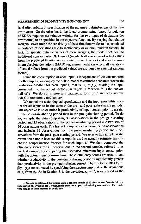
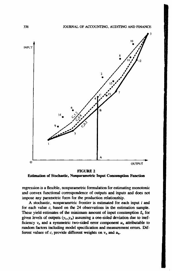
In Figure 2, we illustrate the estimation of the production frontier cor-responding to different values of c for the case of a single input and a singleoutput. Here, for small values of Cj (< 0.2) we obtain tiie DEA estimates,which assume no random specification or measurement errors and the linearprogram estimates the minimum amount of input consumption for a givenlevel of output assuming monotonicity and convexity. The frontier is com-puted based on available observations and without recourse to any a prioriassumptions about the specific underlying functional form ofthe input-outputcorrespondence. For each input, the input productivity measure in any periodt is the ratio of the minimum amount of input for the level of output producedas determined by tiie estimated fr ontier, and the actual input consumptionin that period. Thus, for period 4 the productivity equals ABIAC. This DEAmeasure of productivity is a relative measure because it evaluates the pro-ductivity of any period relative to available observations subject to tiieconditions of monotonicity, convexity, and minimum extrapolation.

For Ci = 0.8, the input consumption frontier is pulled upward becausesome of tte deviation of actual input consumption from estimated values isattributed to random stochastic factors rather than inefficiency alone. Theinefficiency scores for various observations is, in general, lower. For stilllarger values of c,(Ci = 1.2), variations of actual from estimated values areentirely ^tributed to random factc»s and yield the MAD regression equation.TMs has tte effect of fiirtter pushing up tiie estimated input consumptionfunction and reducing tite iirefficiency scores. Note, however, that the MAD

336

INPUT

JOURNAL OF ACCOUNTING, AUDITING AND FINANCE

OUTPUT

FIGURE 2Estimation <tf Sto<âstic, Ntrnpanunetrk Input Consumption Function

regression is a flexible, nonparametric formulation for estimating monotonicand convex functional correspondence of outputs and inputs and does notimpose any parametric form for the production relationship.

A stochastic, nonparan^tric frontier is eîmat^ for each input i andfor each value Cj basc^ on the 24 observations in die estimation sample.Tliese yield estimates of d^ minimum amount of input consunq^cm ij, forgiven levels of o u ^ t s {yu,y-hi assuming a one-sided (feviation due to inef-ficiency Vjt imd a symmetric two-sided emn* conqx)nent u^ attributable torandom factors including model specificaticm and nwasurement errors. E>if-ferent values of Cj provide different weights on Vjt and u^.

MEASUREMENT OF PRODUCnVITY IMPROVEMENTS 337

Productivity (efficiency) scores are then computed for each of the 24observations in the test sample for each input i and for all values c, as therado of the estimated consumption ii, and the actual consumption Xi,. TheMann-Whitney (1947), Welch (1937), and Kolmogorov-Smimoff (Conover[1980]) tests are used to examine if the average productivity of the 8 ob-servations in the post-gain-sharing period is significandy greater than theaverage productivity of the 16 observations in the pre-gain-sharing period.The tests are run for all inputs i, /= 1 , . . . ,4 and all values of Ci. Thisenables a determinadon of the sensitivity of our conclusions to changes inthe relative weights attributable to the random and inefficiency factors.Comparing the results ofthe nonparametric and parametric stochastic frontieranalysis provides some insight into the robustness of our conclusions aboutthe impact of the gain-sharing program at the particular site.

In addition to estimating productivity measures for each of the inputs,we compute an overall measure of productivity for each period using ageneralization ofthe Davis (1955) method. The overall productivity measureaggregates the individual input productivities in each period using the actualcost shares of the inputs in that period as weights."* The productivity of eachinput may be analyzed in terms of productivity variances analogous to directmaterial and direct labor usage variances in cost accounting.' The aggre-gation described above is equivalent to computing total variance for a periodas the weighted sum of the individual input variances. If inputs are notseparable, cost savings can be realized by subsdtuting one input for anotherin die event of changes in the relative prices of inputs. As in Banker (1985),we can compute two separate variances: an allocative variance that evaluatesdie ratio at which inputs are employed relative to their prices and a technicalvariance that examii^s the physical consumption of inputs reladve to theestimated firontier consumption for the given mix of inputs. The product ofthe two variances represents the aggregate variance. In the next section, wediscuss and interpret our findings based on both a nonparametric and aparametric analysis of stochastic input consumption functions.

4. Results and Interpretatioiis

Given the methodological advantages of nonparametric stochasdc fron-der estimadon, we start by discussing the results of Stochasdc Data En-

4. WeiiJiting each input productivity by the share of tfiat input in total cost emphasizes gains inthe most significimt ekments (tf total cost in the computation of total productivity.

5. Ualike vaHances, the n ^ measures described in this paper control for volume changes andlaoss periods.

I


velopment Analysis. Tables 1 through 5 contain the results of tests fordifferences in productivity scores in the pre- and post-gain-sharing periodsfor direct labor, indirect labor, materials, manufacturing services, and ag-gregate inputs. The one-sided Welch two-means test makes inferences onthe relative magnitude of means in the two periods. The one-sided Mann-Whitney test measures die presence of significant differences in the locationsof the underlying distributions in the pre- and post-gain-shMing periods.The Kolmogorov-Smimoff test evaluates a more general form of differencesamong productivity scores in the two periods. The alternative hypothesis isthat productivity scores in periods after gain sharing "tend to be higher"than those before its introduction.

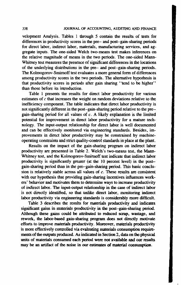
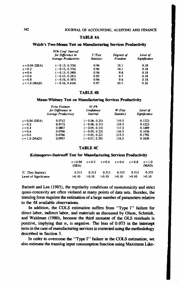
Table 1 presents the results for direct labor productivity for variousestimates of c that increases the weight on random deviations relative to theinefficiency component. The table indicates that direct labor productivity isnot significantly different in the post-gain-sharing period relative to tiie pre-gajn-sharing period for all values of c. A likely explanation is the limitedpotential for improvement in direct labor productivity for a mature tech-nology. The input-output relationship for direct labor is well documentedand can be effectively monitored via engineering standards. Besides, im-provements in direct labor productivity may be constrained by machine-operating constraints and strict quality-control standards in place at the plant.

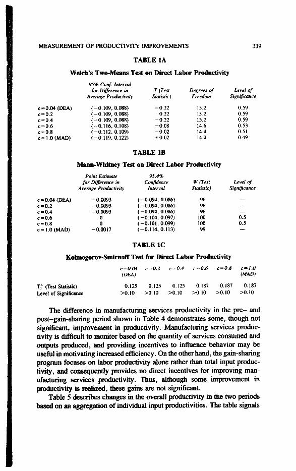
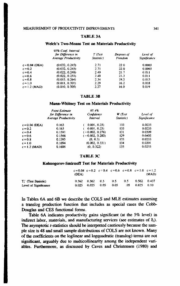
Results on the impact of the gain-sharing program on indirect laborproductivity are presented in Table 2. Welch's two-means test, the Mann-Whitney test, and the Kolmogorov-Smimoff test indicate tiiat indirect laborproductivity is significantly greater (at the 10 percent level) in the post-gain-sharing period than in the pre-gain-sharing period. This basic conclu-sion is relatively st^le across all values of c. These results are consistentwith our hypothesis that providing gain-sharing incentives influences work-ers' behavior and motivates tiiem to determine ways to increase productivityof indirect labor. The input-output relationship in Has. case of indirect laboris not directly identified, so that unlike direct labor, monitoring indirectlabor productivity via engineering standards is considerably more difficult.

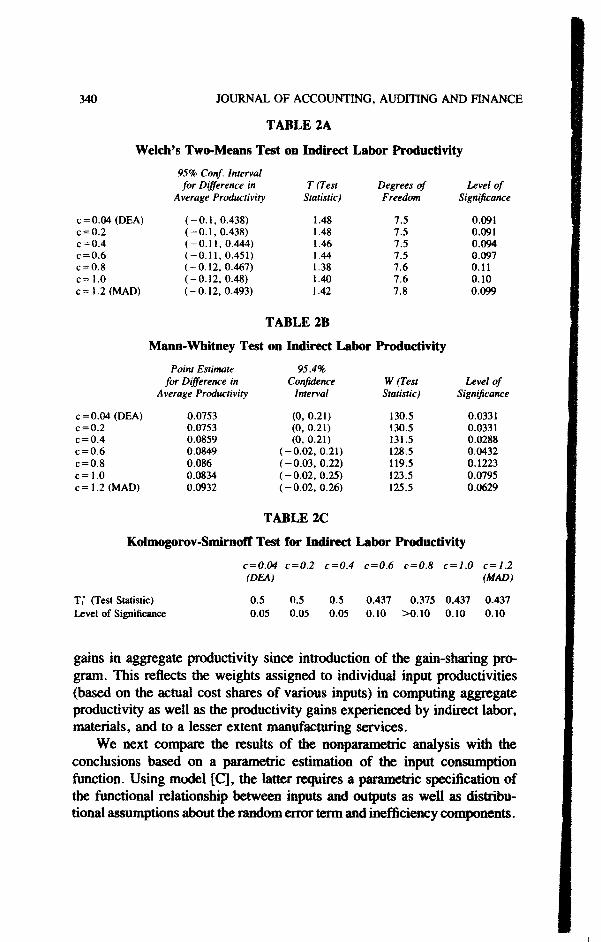
Table 3 describes tiie results for materials productivity and indicatessignificant gains in materials productivity in the post-gain-sharing period.Although these gains could be attributed to reduced scrap, wastage, andreworic, the labor-tosed gain-sharing program does not directly motivateefforts to improve materials productivity. Morraver, mataials {ooductivityis more effectively controlled via evaluating materials consunoption require-ments of the ouûts produc»l. As indicate in Section 2, data on ti^ {riiysicalunits of materials consumed each period were •aot available and our resultsmay be an artifact of the noise in our estimates (rf material


TABLE lA

Welch's Two-Means Test on Direct Labor Productivity

c=0.04 (DEA)0 = 0.2c = 0.40 = 0.60 = 0.80=1.0 (MAD)

c = 0.04 (DEA)0=0.20 = 0.40=0.60 = 0.80=1.0 (MAD)

95% Conf. Intervalfor Difference in

Average Productivity

(-0.109,0.088)(-0.109,0.088)(-0.109,0.088)(-0.116,0.108)(-0.112,0.109)(-0.119,0.122)

r (TestStatistic)

-0 .22-0.22-0.22-0.08-0 .02+ 0.02

TABLE IB

Degrees ofFreedom

15.215.215.214.614.414.0

Mann-Whitney Test on Direct Labor Productivity

Point Estimatefor Difference in

Average Prodttctivity

-0.0093-0.0093-0.0093

00

-0.0017

95.4%Corîdence

Interval

o

o

o

o

o

o

o

o

o

o

o

o1

1 1

1 1 1

W (TestStatistic)

9610010099

Level ofSignificance

0.590.590.590.530.510.49


0.50.5

TABLE IC

K<dmogorov-Snilm(^ Test tor Direct Labor Productivity

T,* (Test Statistic)Level of Significance

c = 0.04(DEA)

0.125>0.10

c=0.2

0.125>0.10

c = 0.4

0.125>0.10

c = 0.6

0.187>0.10

-0.8 c=I.O(MAD)

0.187>0.10

0.187>0.10

The difference in manufacturing services productivity in the pre- andpost-gain-sharing period shown in Table 4 demonstrates some, though notsignificant, improvement in productivity. Manufacturing services produc-tivity is di£ficult to monitor based on tiie quantity of services consumed andtHi Hits produced, and providing incentives to influence behavior may beuseful in motivating incieased efficiency. On tiie other hand, the gain-sharing{Hognun focuses on labor productivity aloiK rather than total input produc-tivity, and consequently provides no direct incentives for improving man-ufacturing services jwoductivity. Thus, although some improvement injHoductivity is realized, tiiese gains are not significant.

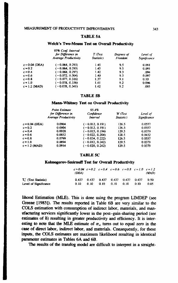
Tidde 5 describes changes in tiie overall jMtxiuctivity in the two periodsbased on an aggregation of individual input productivities. The table signals

I


TABLE 2A

Welch's Two-Means Test on Indirect Labor Productivity

c = 0.04 (DEA)c = 0.2c = 0.4c = 0.6c = 0.8c=I.Oc= 1.2 (MAD)

c = 0.04 (DEA)c = 0.2c = 0.4c = 0.6c = 0.8c=1.0c= 1.2 (MAD)



(-0.1,0.438)(-0.1,0.438)(-0.11,0.444)(-0.11, 0.451)(-0.12,0.467)(-0.12,0.48)(-0.12,0.493)

Mann-Whitney Test



0.07530.07530.08590.08490.0860.08340.0932

T (TestStatistic)

1.481.481.461.441.381.401.42

TABLE 2B

Degrees ofFreedom

7.57.57.57.57.67.67.8

on Indirect Labor Productivity

95.4%Confidence

Interval

(0, 0.21)(0, 0.21)(0, 0.21)

(-0.02,0.21)(-0.03,0.22)(-0.02,0.25)(-0.02,0.26)

W (TestStatistic)

130.5130.5131.5128.5119.5123.5125.5


0.0910.0910.0940.0970.110.100.099


0.03310.03310.02880.04320.12230.07950.0629

TABLE 2C

Kolmogorov-SmimofF Test for Indirect Labor Productivity

c = 0.04 c=0.2 c = 0.4 c = 0.6 c=0.8 c = 1.(DEA) (MAD)

Tl (Test Statistic)Level of Significance

0.50.05

0.50.05

0.50.05

0.4370.10

0.375>0.10

0.4370.10

0.4370.10

gains in aggregate productivity since introduction of the gain-sharing pro-gram. This reflects the weights assigned to individual input productivities(based on the actual cost shares of various inputs) in computing aggregateproductivity as well as the productivity gains experienced by indirect labor,materials, and to a lesser extent manufacturing services.

We next compare the results of the nonparametric analysis with theconclusions based on a parametric estitimticm of the input consumptionfunction. Using mo<tel [C], tl^ latter requires a jKinuneiric specification ofthe functional relationship between iapats and o u ^ t s as well as distiibu-tional assumptions about the random error term and inefficiency conqtoi^nts.


c = 0.04(DEA)c = 0.2c = 0.4c=0.6c = 0.8c=1.0c= 1.2 (MAD)

c = 0.04(DEA)c = 0.2c = 0.4c = 0.6c = 0.8c=1.0c= 1.2 (MAD)

TABLE 3A

Welch's Two-Means Test on Materials Productivity



(0.032, 0.245)(0.032. 0.245)(0.022. 0.248)(0.022.0.251)(0.015. 0.264)(0.011.0.301)(0.010. 0.305)

T (TestStatistic)

2.712.712.492.482.342.292.27

TABLE 3B

Mann-Whitney Test on Materials



0.1630.1630.15910.15660.13950.16940.1686

95.4%Confidence

Interval

( 0.001.0.25)( 0.001.0.25)(-0.002. 0.276)(-0.002,0.280)

(0. 0.3)(0.002. 0.331)(0. 0.322)

Degrees ofFreedom

22 022.021.721.319.516.216.0

Productivity

W (TestStatistic)

133133131129133134133


0.00650.00650.0110.0110.0150.0180.019


0.02330.02330.03090.04050.02330.02010.0233

TABLE 3C

Kolmogorov-SmirnofF Test for Materials Productivity

c = 0.04 c = 0.2(DEA)

= 0.4 c = 0.6 c = 0.8 c=1 .0 c=1 .2(MAD)

T,* (Test Statistic)Level of Significance

0.5620.025

0.5620.025

0.50.05

0.50.05

0.5.05

0.5620.025

0.4370.10

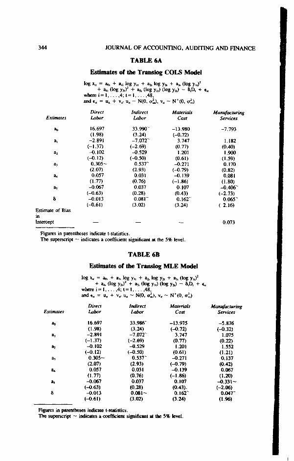
In Tables 6A and 6B we describe the COLS and MLE estimates assuminga translog production function that includes as special cases the Cobb-Douglas and CES functional forms.

Table 6A indicates productivity gains significant (at the 5% level) inindirect lahor, materials, and manufacturing services (see estimates of 5,).The asymptotic f-statistics should be interpreted cautiously because the sam-ple size is 48 and small sample distributions of COLS are not known. Manyof the coefficients on ttie loglinear and logquadratic (translog) terms are notsignificant, arguably due to multicollinearity among the independent vari-ables. Furttermore, as discussed by Caves and Christensen (1980) and


Wekh'!

0 = 0.04 (DEA)0 = 0.20 = 0.40 = 0.60 = 0.80=1.0 (MAD)

s Two-Means Test c



(-0.15,0.376)(-0.15,0.376)(-0.15,0.380)(-0.15,0.381)(-0.16,0.387)(-0.16,0.414)

Mann-Whitney Test on 1

0 = 0.04 (DEA)0 = 0.20 = 0.40 = 0.60 = 0.80=1.0 (MAD)



0.07120.01720.08070.07660.07660.0957

TABLE 4A

ta Maniifactoring

TfTest' Statistic)

0.%0.960.960.950.960.97

TABLE 4B

Services ProdiKtivity

Degrees ofFreedom

10.110.19.89.79.6

lO.l

Level cfSignificance

0.180180.180.180.180.18

Vf anufacturing Services Productivity

95.4%Corîdence

Interval

(-0.06,0.21)(-0.06,0.21)(-0.05,0.23)(-0.05,0.23)(-0.05,0.22)(-0.07,0.29)

W (TestStatistic)

119.5119.5117.5116.5115.5116.5


0.12230.12230.14890.16360.17920.1636

TABLE 4C

Kolmogorov-Smimoff Test for Manufacturing Services Productivity

T,* (Test Statistio)Level of Signifioanoe

0 = 0.04(DEA)

0.313>0.10

0 = 0.2 0 = 0.4 0=0.6 0 = 0.8

0.313>0.10

0.313>0.10

0.313>0.10

0.313>0.10

0=1.0(MAD)

0.375>0.10

Bamett and Lee (1985), the regularity conditions of monotonicity and strictquasi-concavity are often violated at many points of data sets. Etesides, thetranslog form requires the estimaticHi of a large number of parameters relativeto the 48 available observsrtions.

In addition, the COLS estimation suffers from "Type I" failure fordirect labor, indirect labor, and materials as discuêd by Olson, Schmidt,and Waidman (1980), because tl^ third mrniôt of the OLS residuals ispositive, implying tiiat a , is negative. Hie bias of 0.073 in die i n t e n dterm in the case of manufacturing %rvices is cfHiected using tiie n^tiKxloIogydescribed in Section 3.

In order to overconw tiie "Type I" failure in the COiJS estimatkm, wealso estimate the translog infmt consuroiHion function using Maximum Like-

NfEASUREMENT OF PRODUCnVlTY IMPROVEMENTS 343

c = 0.04 (DEA)c=0.2c=0.40=0.6c = 0.8c=1.0c= 1.2 (MAD)

c = 0.04 (DEA)c = 0.2c=0.4c = 0.6c=0.8c=1.0c= 1.2 (MAD)

TABLE SAWelch's Two-Means Test on OveraO Productivity



(-0.064,0.293)(-0.064,0.293)(-0.068,0.297)(-0.072,0.304)(-0.077,0.316)(-0.078,0.336)(-0.078,0.341)

T(TestStatistic)

.45

.45

.42

.40

.37

.41

.42

TABLE SB

Mann-Whitney Test on Overall



0.09040.09040.09280.08520.07990.08940.0914

95.4%Confidence

Interval

(-0.012,0.191)(-0.012, 0.191)(-0.015,0.194)(-0.022,0.204)(-0.024,0.222)(-0.012,0.242)(-0.020 0.242)

Degrees ofFreedom

9.59.59.39.39.19.29.2

Productivity

W (TestStatistic)

126.5126.5129.5128.5126.5129.5129.5


0.0910.091

.0940.0970.100.096

.095


0.05570.05570.03790.04320.05570.03790.0379

TABLE SC

for Overail Productivity

= 0.2 c = 0.4 c = 0.6 c = 0.8 c = I

T|* (Test Statistic)Level of Significance

(DEA)

0.4370.10

0.4370.10

0.4370.10

0.4370.10

0.4370.10

0.4370.10

(MAD)

0.500.05

lihood Estimation (MLE). This is done using the program LIMDEP (seeGreene [1985]). The results reported in Table 6B are very similar to theCOLS estimation with consumption of indirect labor, materials, and man-ufacturing services significantly lower in the post-gain-sharing period (seeestinuttes of 5) resulting in greater productivity and efficiency. It is inter-esting to note that the MLE estimate of <Ty, turns out to equal zero in thecase of direct labor, indirect l^x>r, and materials. Consequently, for theseinqputs, tte COLS estimates are maximum likelihood resulting in identicalpanaaster estimates in T^les 6A and 6B.

results of the translog model are difficult to interpret in a straight-


TABLE 6A

Estimates of the Translog COLS Model

log X, = ao, + a,i log y,, + a , log y,, + a,, (log y,,)'+ a* (log ya)' + %, (log y,,) (log y^) - 8,D, + e,

where i = l , . . . , 4 ; t = l 48,and €„ = !!„ + v«. u. ~ N(0, o i ) , v, ~ N*(0, aid

Estimates

ao

a,

a j

a3

a,

as

8

Estimate of BiasinIntercept

DirectLabor

16.697(1.98)-2.891

(-1.37)-0.102

(-0.12)0.305-(2.07)0.057

(1.77)-0.067

(-0.63)-0.013

(-0.61)

—

IndirectLabor

33.990~(3.24)-7.072~

(-2.69)-0.529

(-0.50)O.537~

(2.93)0.031

(0.76)0.037

(0.28)0.08r

(3.02)

—

MaterialsCost

-13.980(-0.72)

3.747(0.77)1.201

(0.61)-0.271

(-0.79)-0.139

(-1.86)0.107

(0.43)0.162~

(3.24)

—

ManitfacturingServices

-7.793

1.182(0.40)1.900

(1.59)0.170

(0.82)0.081

(1.80)-0.406~

(-2.73)0.065~

( 2.16)

0.073

Figures in parentheses indioate t-statistios.The superscript ~ indicates a ooeffioient signifioant at the 5% level.

TABLE 6B

Estimates of the Translog MLE Model

log X, = aa + a,, log y,, + aj. log y^ + a,, (log y,,)'+ a4, (log ya)' + a,, (log y,,) (log y j - 8,D, + e,,

where i = l , . . . , 4 ; t = l , . . . , 4 8 ,and €, = u,, + V,. u, ~ N(0, ai), v, ~ N*(0, al,)

EstimatesDirectLabor

16.697(1.98)-2.891

(-1.37)-0.102

(-0.12)0.305-(2.07)0.057

(1.77)-0.067

(-0.63)-0.013

(-0.61)

IndirectLabor

33.t«6~(3!24)-7.072~

(-2.69)-0.529

(-0.50)O.537~

(2.93)0.031

(0.76)0.037

(0.28)0 .081-(3.02)

MaterialsCost

-13.975(-O.72)

3.747(0.77)1.201

(0.61)-0.271

(-0.79)-0.139

(-1.86)O.tO7

(0.43).0.162"

(3.24)

MantrfacturingServices

-5.S76(-0.32)

1.075(0.22)1.552

(1.21)0.137

(0.42)0.067

(I.M)- 0 . 3 3 1 -(-2.06)

0.047~(1.96)

Figures in {HuentlKses indioate t-statistios.The superscript — indicates a ooefficwnt significant at the 5% tevel.


Estimates

Estimate of Biasin Intercept

TABLE 7A

Estimates of the LogUnear COLS Model

log X, = aa -I- a,, log y,, -I- aj, log y^ - 8 A + e,,where i = l , . . . ,4; t = l , . . . ,48,and e. = u, + v,. u, ~ N(0, a^), v« ~ N*(0, al,)

DirectLabor

3.638"(10.97)

0.725"(16.34)

0.213"(8.47)-0.008

(-0.36)

IndirectLtUmr

6.988"(16.76)

0.352"(6.32)0.135"

(4.28)0.093"

(3.35)

MaterialsCost

-0.449(-0.61)

0.842"(8.56)0.0514

(0.92)0.164~

(3.36)

ManufacturingServices

-0.024

0.641"(9.99)0.237"

(6.54)0.073"

(2.27)

Figures in parentheses indicate t-statisdcs.The superscript ~ indicates a coefficient significant at the 5% level.

TABLE 7B

Estimates of the LogUnear MLE Modei

log x, = ao, + a,, log y,, + a,, log y^ - 8 A + e,where i = l 4; t = l 48,and e. = u. -H V. u. ~ N(0, ai), v» ~ N*(0, aid

EstimatesDirectLabor

3.638"(10.97)

0.725"(16.34)

0.213~(8.47)

(-0.36)

0.105

IndirectLabor

6.988"(16.76)

0.352"(6.32)0.135"

(4.28)0.093"

(3.35)

MaterialsCost

-0.449(-0.61)

0.842"(8.56)0.051

(0.92)0.164"

(3.36)

ManitfacturingServices

0.412(0.75)0.644"

(10.27)0.201"

(5.32)0.062"

(2.12)

Figures in {xirentheses indicate t-statisdcs.The superscript ~ indicates a coefficient significant at the 5% level.

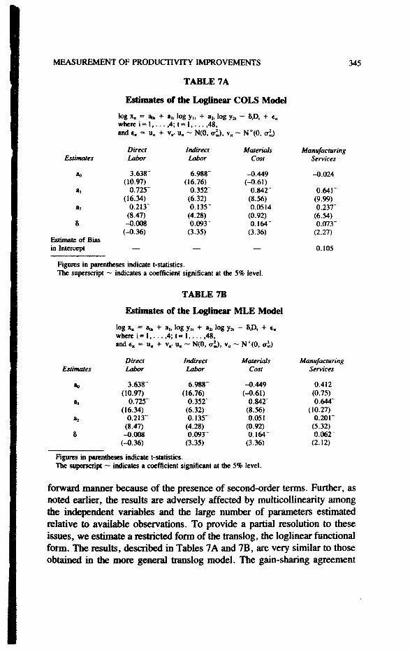
forward manner because of the presence of second-order terms. Further, asnoted earlier, the results are adversely affected by multicollinearity amongthe indepen^nt variables and the large number of parameters estimatedrelative to available oteervations. To provide a partial resolution to theseissues, we estimê a restiicted form of the translog, the logline^ functionalform. TTie results, described in Tables 7A and 7B, sue very similar to thoseobtaiiKd in tiw more general translog model. The gain-sharing agreement


has a positive impact on productivity of indirect labor, materials, and man-ufacturing services. Once again the COLS estimations presented in Table7A suffer from "Type I " failure due to negative estimates for av. Theloglinear form is re-estimated using MLE (see Table 7b) and yields estimatesvery similar to those obtained using COLS. In the cases of' 'Type I ' ' failures,MLE estimates av to equal zero.

The results of the nonparametric and parametric stochastic frontier anal-yses are remaricably similar. They suggest that the gain-sharing progr^nhas a positive effect on indirect labor, manufacturing services, and materialsproductivity and relatively little effect on direct labor. Our conclusionsappear to be robust to the assumed functional forms ofthe input consumptionfunctions although we are somewhat skeptical about the reliability of thematerials consumption data. Nevertheless, the consistency ofthe parametricanalysis with the stochastic nonparametric estimation increases the degreeof confidence in our analysis.

REFERENCES

1. Aigner. D. J.. C.A.K. Lovell, and P. J. Schmidt. "Formulation and Estimation of StochasticFrontier Production Models." Journal of Econometrics (19T7). pp. 21-37.

2. Aigner. D. J.. and S. F. Chu, "On Estimating the Industry Production Function," AmericanEconomic Review (1968). pp. 826-839.

3. Banker. R. D.. "Estimating Most Productive Scale Size Using Data Envelopment Analysis."European Journal of Operational Research (July 1984). pp. 35-44.

4. Banker. R. D.. "Productivity Measurement and Management Control," in The Management ofProductivity and Technology in Mamrfacturing. P. Kleindorfer (ed.) (New Yoric: Plenum, 1985).

5. Banker, R. D.. "Stochastic Data Envelc^ment Analysis," Camegie Mellon University, mimeo(1986a).

6. Banker. R. D.. "Maximum Likelihood. Consistency and Data Bivelopment Analysis." CarnegieMellon University, mimeo (1986b).

7. Banker. R. D., A. Chames, and W. W. Co<^r, "Models for the Estimation of Technical andScale Inefficiencies in Data Envelopment Analysis." Management Science (September 1984),pp. 1078-1092.

8. Banker. R. D., and A. Maindiratta. "Piecewise Loglinear Estimation of Efficient ProductionSurfaces." Management Science (January 1986), pp. 126-135.

9. Banker. R. D.. and A. Maindiratta. "Nonparametric Analysis of Technical and Allocative Ef-ficiencies in Production," Econometrica, in press (1987).

10. Banker. R. D., and R. C. Morey. "Efficiency Analysis for Exogenousiy Fixed Inputs andOutputs." Operations Research (1986a), pp. 513-521.

11. Banker, R. D., and R. C. Morey, "Data Enveic^Mnent Analysis with OtfegcHica] Inputs andOutputs." Management Science (December 1986b), i^. 1615-1627.

12. Banker. R. D., R. F. Conrad, and R. P Strauss, "A Cm^karative Af^licalion of DEA andTranslog Methods: An Illustrative Study of Hospital Production," Management Science (January1986), pp. 30-44.

13. Banker, R. D., and S. M. DaJar, ProductivityAccomtingfiirMimt^tmingOperations, researchmonograph commissioned by the American Accounting Association, in ptcss (1987a).

14. Banker, R. D., and S. M. Datar, "Accounting fm Ldx>r Productivity in Manufacturing Oper-almas: An Apfdicitfiai," in Field Studies in Management AcoomUing and ConOxA, W. Bransand R. Ka|4an (eds.), (Cambrid^, Mass.: Harvad Business School Press, forthcoming [1987b]).

15. Bamett, W. A., and Y. W. Lee, "The Global Prcqxsrties of the Minflex Laurent, GenoalizedLemtief and Traiisl<^ FlexiMe Functicnal Fffltns," Ectmometrica (1985), R I . 1421-1437.

MEASUREMENT OF HiODUCTIVITY IMPROVEMENTS 347

16. Bazaraa, M. S., and C. M. Shetty, Nonlinear Programming: Theory and Applications (NewYoric: Wiley, 1979).

17. Bessent, A., W. Bessent, J. Kennington, and B. Reagan, "An An>lication of MathematicalProgramming to Assess Productivity in the Houston Independent School District," ManagementScience (December 19S2), pp. 1355-1367.

18. Byrnes, P., R. Fare, and S. Grosski^f, "Measuring Productivity Efficiency: An Application toIllinois Strip Mines," Management Science (June 1984), pp. 671-681.

19. Caves, D. W., and L. R. Christensen, "Global Properties of Flexible Functional Forms," Amer-ican Economic Review (1980), K>. 422-432.

20. Chmnes, A., W. W. Cooper, and E. Rhodes, "Measuring the Efficiency of Decision-MakingUnits," European Journal of Operational Research (1978), pp. 429-444.

21. Chames, A., W. W. Cooper, and E. Rho(fes, "Evaluating Program and Managerial Efficiency,"Management Science (June 1981), pp. 668-697.

22. Conover, W. J., Practical Nonparametric Statistics (New Yoilc: Wiley, 1980).23. Davis, H. S., Productivity Accounting, The Wharton School of the University of Pennsylvania,

Industrial Research Unit (1955). (Reprint 1978.)24. Gieene, W. H., "LIMDEP" (New York, 1985).25. Hildenlwand, W.,"Short-run Production Functions Based on Micro-data," Econometrica (Sep-

tember 1981), pp. 1095-1125.26. K^lan, R. S., Advanced Management Accounting (Ea^viooACX\fk, N.J.: Prentice-Hall, 1982).27. Mann,M. B.,andD. R. Whitney, "On a Test of Whether One or Two Variables is Stochastically

Larger Than the Other," Annals of Mathematical Statistics (1947).28. Meeusoi, W., and J. van der Broeck, "Efficiency Estimation from Cobb-Douglas Production

FuncdcMis with Composed Error," Intemational Economic Review (1977), |^. 435-444.29. Olson, J. A., P. J. Schmidt, and D. M. Waldman, "A Monte Carlo Simuladon of Esdmators of

Stochastic Frontier Producdon Funcdons," Journal cf Econometrics (1980), pp. 67-82.30. Patell, J. M., "Corporate Fmecasts of Eamings per Share and Stock Price Behavior," Journal

of Accounting Research (1976), pp. 246-276.31. Richmond, J., "EstimatingtheEfiiciencyofProducdon,"/n/erna(iona/£cono/Ric/?evi>H'(l974),

K>. 515-521.32. Schii^jer, K., and R. Thompson,' 'The Impact of Merger-Related Reguladons on the Shareholders

of Acquiring Firms," Journal of Accounting Research (1983), pp. 184-221.33. Varian, H., "The Nonparametric Af^noach to Production Analysis," Econometrica (1984),

I^. 579-597.34. Weinsein, M. A., '"Vas Sum of Values fh>m a Normal and a Truncated Nonnal Distribution,"

Technometrics (1964), {^. 104-105.35. Welch, B. L., "Tte Significance of the Difference between Two Means When the Population

Variances Are Unequal," Biometrika (1937), pp. 350-62.36. Zellner, A., J. Kmento, and J. Dreze, "Specificadon and Esdmadon of Cobb-Douglas Production

FuDcdon Moifels," Econometrica (1966), pp. 784-795.

Measurement of Productivity Improvements - CiteSeerX

Documents