University of New Mexico UNM Digital Repository Physics & Astronomy ETDs Electronic eses and Dissertations Spring 5-12-2017 Measurement-Based Quantum Computation and Symmetry-Protected Topological Order Jacob E. Miller University of New Mexico - Main Campus Follow this and additional works at: hps://digitalrepository.unm.edu/phyc_etds Part of the Quantum Physics Commons is Dissertation is brought to you for free and open access by the Electronic eses and Dissertations at UNM Digital Repository. It has been accepted for inclusion in Physics & Astronomy ETDs by an authorized administrator of UNM Digital Repository. For more information, please contact [email protected]. Recommended Citation Miller, Jacob E.. "Measurement-Based Quantum Computation and Symmetry-Protected Topological Order." (2017). hps://digitalrepository.unm.edu/phyc_etds/149

Welcome message from author
This document is posted to help you gain knowledge. Please leave a comment to let me know what you think about it! Share it to your friends and learn new things together.
Transcript

University of New MexicoUNM Digital Repository
Physics & Astronomy ETDs Electronic Theses and Dissertations
Spring 5-12-2017
Measurement-Based Quantum Computation andSymmetry-Protected Topological OrderJacob E. MillerUniversity of New Mexico - Main Campus
Follow this and additional works at: https://digitalrepository.unm.edu/phyc_etds
Part of the Quantum Physics Commons
This Dissertation is brought to you for free and open access by the Electronic Theses and Dissertations at UNM Digital Repository. It has beenaccepted for inclusion in Physics & Astronomy ETDs by an authorized administrator of UNM Digital Repository. For more information, please [email protected].
Recommended CitationMiller, Jacob E.. "Measurement-Based Quantum Computation and Symmetry-Protected Topological Order." (2017).https://digitalrepository.unm.edu/phyc_etds/149

Candidate
Department This dissertation is approved, and it is acceptable in quality and form for publication: Approved by the Dissertation Committee: , Chairperson
Jacob Miller
Physics and Astronomy
Akimasa Miyake
Carlton Caves
Ivan Deutsch
Andrew Landahl

Measurement-Based QuantumComputation and Symmetry-Protected
Topological Order
by
Jacob Miller
B.S., Engineering with Physics, Olin College, 2011
M.S., Physics, University of New Mexico, 2015
DISSERTATION
Submitted in Partial Fulfillment of the
Requirements for the Degree of
Doctor of Philosophy
Physics
The University of New Mexico
Albuquerque, New Mexico
July, 2017

c©2017, Jacob Miller
iii

Acknowledgments
I’ve had so much help from so many amazing people at different points along myjourney towards finishing grad school. My greatest, loudest, and dearest thanks goesout to my parents, who have given me such tremendous support and guidance in mylife, and to my sister Hannah, who has been a constant inspiration to me over theyears. I’d also like to thank my close friends from Vermont, Olin, and Albuquerquewho have given me such incredible encouragement over the last six years, especiallyLynn Sipsey, Chen Wang, Satomi Sugaya, Adrian Chapman, Shannon Taylor, andAaron Peterson. You kept me going, and I’m eternally grateful for all of our longconversations about work, life, love, and whatever else came to mind.
I’d like to thank my advisor Akimasa Miyake, who started me on my path asa researcher and scientist, and who I’ve learned so much from during my time inCQuIC. Many thanks to the excellent professors, researchers, and post-docs I’ve hadthe pleasure of interacting with regularly here, notably Carl Caves, Ivan Deutsch,Elohim Becerra, Andrew Landahl, Robin Blume-Kohout, Josh Combes, Chris Ferrie,and Chris Jackson. It is hard to over-emphasize the wide range of disparate subjectssurrounding physics, mathematics, and computation which have been available to meand others here at CQuIC by virtue of the rich selection of visiting researchers bothregularly and at our annual SQuInT conference. My thanks go out to Akimasa, Ivan,Carl, Elohim, and especially to our wonderful program coordinator Gloria Cordovafor making all of that happen, I’ve learned so many wonderful and surprising thingsthrough it all. I’d also like to thank Akimasa, Carl, Ivan, and Andrew for takingtime out of their busy lives to read this thesis, constitute my dissertation committee,and provide helpful guidance on the next phase of my professional career.
I have lots of thanks for all of the amazing people I’ve met at Albuquerque,both in and outside UNM. I’ve shared a lot with long-term grad school friendsCharlie Baldwin, Lewis Chiang, Matt Curry, Ninnat Dangniam, Andy Ferdinand,Mark Gorski, Ken Obenberger, Xiaodong Qi, and Ezad Shojaee, who have beenhere since the beginning. My thanks go out to Albquerque friends Julian Antolin-Camerena, Karishma Bansal, Ben Q. Baragiola, Andrew Baxter, Mitchell Brickson,Anirban Chowdhury, Kathy DeBlasio, Matt DiMario, Tarraneh Eftekhari, Irene En-tila, Akram Etemadi, Hanieh Farsibaf, Farzin Farzam, Mohamadreza Fazel, AmyFoust, Jonathan Gross, Jim Hendrie, Anastasia Ierides, Jess Jungwirth, Joe Lan-ders, Linh Le, Megan Lewis, Sida Li, Nicki Maphis, Neil McFadden, Chelsea Mc-Fadden, Junwei Meng, Anupam Mitra, Gopi Muraleedharan, Leigh Norris, AdrianOrozco, Jaksa Osinski, Lee Ratzlaff, Zach Ratzlaff, Nate Ristoff, Keith Sanders,Xiaowen Si, Jaimie Stephens, Zahra Taghipour, Sarah Williams, Tzu-Cheng Wu,Laura Zschachner, and anyone else I somehow forgot to mention. It’s been reallygreat getting to know everyone here, and I hope we’ll see each other soon.
iv

Figure 0.1: For five years now, the TACLA coffee club at UNM has proudly stoodas a bulwark in the struggle for Progress, a proud friend and ally to over-caffeinatedgrad students, post-docs, and professors alike. Shown here is our flagship coffeemachine, the same one purchased by Carl Caves (thanks Carl!) and named in honorof Alexandre Tacla, a distinguished former grad student and post-doc of CQuIC-times past. Although it saddens me to step down from the distinguished role ofCoffee Commander (position established retroactively, effective immediately), I havegreat faith in future grad students to heed the call to adventure and grab hold ofthe lofty helm of TACLA. For there is no question that in the face of tough researchpuzzles, prickly conundrums, and flummoxes of every type, we can find solace in thewords of noted abolitionist Henry Ward Beecher that, “A cup of coffee—real coffee—home-browned, home ground, home made, that comes to you dark as a hazel-eye. . . neither lumpy nor frothing on the Java: such a cup of coffee is a match for twentyblue devils and will exorcise them all.”
v

Measurement-Based QuantumComputation and Symmetry-Protected
Topological Order
by
Jacob Miller
B.S., Engineering with Physics, Olin College, 2011
M.S., Physics, University of New Mexico, 2015
Ph.D., Physics, University of New Mexico, 2017
Abstract
While quantum computers can achieve dramatic speedups over the classical com-
puters familiar to us, identifying the origin of this quantum advantage in physical
systems remains a major goal of quantum information science. A useful tool here
is measurement-based quantum computation (MQC), a computational framework
utilizing the quantum entanglement found in many-body resource states. Not all
resource states are useful for quantum computation however, so an important ques-
tion is what properties of many-body entanglement characterize universal resource
states, which can implement any quantum computation.
Many-body states are also studied in condensed matter physics, where the collec-
tive behavior of quantum many-body systems sometimes define topological phases
of matter. These phases are defined by nonlocal many-body entanglement, making
topologically-ordered states natural candidates for MQC. We might wonder if these
vi

topological phases could be organized as phases of quantum computation, so that ev-
ery state within the phase is universal for MQC. While phases of symmetry-protected
topological order (SPTO) have arisen as natural candidates, previous attempts to
demonstrate an MQC-SPTO correspondence were mostly limited to nonuniversal 1D
spin chains, leaving the important 2D setting wide open.
In this dissertation, we explore the wide and varied connections between MQC
and SPTO, and obtain new results for 1D and 2D systems. After identifying a new
MQC-SPTO correspondence within 1D spin chains, we move up and explore the
operational use of 2D states with two complementary forms of SPTO. We create
a new Union Jack resource state, whose different form of SPTO than previous 2D
resource states permits a hierarchical notion of MQC universality. This state leads
us to consider an idealized model of 2D SPTO, where we show that an additional
symmetry condition makes these model states form universal resources for MQC only
when they have nontrivial SPTO. We finally study the intrinsic complexity of SPTO-
inspired states for classically intractable sampling, and identify inherent advantages
of MQC for this purpose. Our work highlights the rich complexity available in
states of entangled quantum matter, providing new evidence which sharpens our
understanding of the diverse connections between MQC and SPTO.
vii
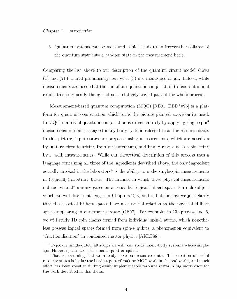
Contents
1 Introduction 1
2 Measurement-based Quantum Computation and Graph States 11
2.1 The 1D Cluster State . . . . . . . . . . . . . . . . . . . . . . . . . . . 12
2.2 Graph States . . . . . . . . . . . . . . . . . . . . . . . . . . . . . . . 18
2.3 Gottesman-Knill Theorem and the Clifford Hierarchy . . . . . . . . . 25
3 Matrix Product States and the 1D AKLT Spin Chain 30
3.1 Introduction to Matrix Product States . . . . . . . . . . . . . . . . . 31
3.2 Transfer Operators and the MPS Canonical Form . . . . . . . . . . . 35
3.3 The 1D AKLT State . . . . . . . . . . . . . . . . . . . . . . . . . . . 42
4 Symmetry-Protected Topological Order 49
4.1 Characteristic Features of SPTO . . . . . . . . . . . . . . . . . . . . 50
4.2 Suitability of Nontrivial SPTO for MQC . . . . . . . . . . . . . . . . 57
4.3 Mathematical Classification of SPTO . . . . . . . . . . . . . . . . . . 63
viii

Contents
4.4 The Cocycle State Model . . . . . . . . . . . . . . . . . . . . . . . . . 67
5 Universal Single-Qubit SPTO Phase in S4-symmetric Spin Chains 70
5.1 Matrix Product States and 1D SPTO . . . . . . . . . . . . . . . . . . 72
5.2 Main Results . . . . . . . . . . . . . . . . . . . . . . . . . . . . . . . 75
5.3 Illustration of Our Results . . . . . . . . . . . . . . . . . . . . . . . . 79
5.4 Conclusion . . . . . . . . . . . . . . . . . . . . . . . . . . . . . . . . . 80
5.5 Proofs and Discussion . . . . . . . . . . . . . . . . . . . . . . . . . . 82
5.5.1 Proof of Theorem 5.1 . . . . . . . . . . . . . . . . . . . . . . . 83
5.5.2 Proof of Theorem 5.2 . . . . . . . . . . . . . . . . . . . . . . . 88
5.5.3 The Renormalized Correlation Length . . . . . . . . . . . . . 92
6 A Universal Resource State with 2D SPTO 95
6.1 MQC and SPTO Background . . . . . . . . . . . . . . . . . . . . . . 97
6.2 Trivial 2D SPTO of the 2D Cluster State . . . . . . . . . . . . . . . . 100
6.3 The Resource State with Nontrivial 2D SPTO . . . . . . . . . . . . . 104
6.4 Discussion . . . . . . . . . . . . . . . . . . . . . . . . . . . . . . . . . 109
6.5 The Union Jack and Cluster States as SPTO Fixed Point States . . . 110
6.6 SPTO Signature of the 2D Cluster State . . . . . . . . . . . . . . . . 117
6.7 Proof of the Pauli Universality of the Union Jack State . . . . . . . . 122
7 Universal Resource Phases in 2D Model SPTO 133
ix

Contents
7.1 Background on MQC, SPTO, and the Cocycle State Model . . . . . . 135
7.2 Characterizing Cocycle States with Fractional Symmetry . . . . . . . 138
7.3 Outlook . . . . . . . . . . . . . . . . . . . . . . . . . . . . . . . . . . 144
7.4 Proofs of Theorem 7.1 (d = 3), Corollary 7.1, and Theorem 7.2 . . . 144
8 Quantum supremacy in constant-time measurement-based compu-
tation 152
8.1 Introduction . . . . . . . . . . . . . . . . . . . . . . . . . . . . . . . . 152
8.2 Background . . . . . . . . . . . . . . . . . . . . . . . . . . . . . . . . 156
8.2.1 IQP and Boolean Functions . . . . . . . . . . . . . . . . . . . 156
8.2.2 Classically Intractable Sampling and Verification . . . . . . . . 158
8.2.3 Measurement-Based Quantum Computation . . . . . . . . . . 160
8.3 MQC Protocol for Classically Intractable Sampling . . . . . . . . . . 163
8.4 Outlook . . . . . . . . . . . . . . . . . . . . . . . . . . . . . . . . . . 168
8.5 Comparison to Previous Work . . . . . . . . . . . . . . . . . . . . . . 169
8.6 Randomness of MQC Byproduct Polynomials . . . . . . . . . . . . . 171
8.7 Hardness of Approximate Sampling . . . . . . . . . . . . . . . . . . . 173
8.8 Verification of Classical Intractability . . . . . . . . . . . . . . . . . . 180
9 Outlook and Summary of Results 187
A Proof of Lemma 7.1 193
x

Contents
A.1 Symmetric 1-cochain states are generated by 1-cocycles . . . . . . . . 194
A.2 12-symmetric 2-cocycle states are generated by bilinear functions (Lemma 7.1,
d = 2) . . . . . . . . . . . . . . . . . . . . . . . . . . . . . . . . . . . 195
A.3 Symmetric 2-cochain states are generated by 2-cocycles . . . . . . . . 197
A.4 13-symmetric 3-cocycle states are generated by trilinear functions (Lemma 7.1,
d = 3) . . . . . . . . . . . . . . . . . . . . . . . . . . . . . . . . . . . 201
References 204
xi

Chapter 1
Introduction
This thesis is about quantum information science (a.k.a. quantum information, a.k.a.
quantum computation), the unexpected offspring of quantum physics and computer
science which studies the power of computational devices built from quantum hard-
ware. As anyone in quantum information knows, a major challenge in the subject
is finding explanations which accurately convey its big ideas to friends, family, and
curious strangers, the infamous “grandfather paradox” of our field1. It seems like any
reasonably honest explanation of what a quantum computer is or where the source
of its uniquely “quantum” power lies will inevitably fall back on some variant of,
Truism 1.1. A quantum computer is a computer whose operation and inner workings
are intrinsically governed by the laws of quantum mechanics.
This may seem like a cop-out, but the more direct answers we might reach for
just don’t do full justice to the subject. For starters, quantum computation isn’t
the provenance of any particular physical scale, so saying that quantum computers
are just “computers at the very small” neglects phenomena like Bose-Einstein con-
1That was a joke. The real grandfather paradox is about time travel, not the difficultyof explaining quantum computation to one’s grandparents.
1

Chapter 1. Introduction
densation [DGPS99] or cavity optomechanics [AKM14], where intrinsically quantum
behavior is observed in systems many orders of magnitude larger than the transistors
forming our classical (i.e. non-quantum) computers. Additionally, quantum behavior
transcends individual physical platforms [LJL+10], and the (small) quantum com-
puters currently available in laboratories have been realized in settings as varied
as trapped ions [SPM+10] and neutral atoms [BCJD99, JBC+99], superconducting
electrical circuits [MSS01] and quantum dots [LD98, ZDM+13], nitrogen-vacancy
centers in diamond [DCJ+07, CH13], and even within the internal states of light it-
self [KMN+07]. Not only can quantum states be encoded in all of these systems, they
can also be faithfully transferred between them with no ill effects [HSP10, DM10],
showing quantum information to be profoundly indifferent to its superficial physical
setting.
To best study these aspects of quantum computation, we should first look into
how they are dealt with in the more familiar setting of classical computation. In-
deed, many of the same issues emerge, with classical computation being realized in
many different ways and at many different scales, but in this setting we also find
well-established answers. At the core of classical computation lies the mythical bit,
an elemental building block which forms the theoretical bedrock for all digital com-
puters, regardless of the details of their physical implementation [FHA98]. A bit has
two possible values, 0 and 1, which encode its two mutually exclusive states of being.
Thought of this way, a classical computer is simply a collection of bits, together with
some allowed maps between configurations of those bits, which are referred to as its
available logic gates. The implementation of such computers in practice consequently
requires the ability to realize these complementary states in real-world systems, and
reliably act on them with the appropriate gates, a challenge which has been well-met
by modern semiconductor device fabrication technology [QS01].
The translation of this framework into the quantum setting, under the heading of
2

Chapter 1. Introduction
the quantum circuit model, has proven to be a tremendously useful tool in designing,
testing, and reasoning about quantum computers [NC00]. Here, bits get promoted
to quantum bits (qubits), which can be prepared not only in states |0〉 and |1〉,
but also in arbitrary quantum superpositions of these two states, typically described
as representing, “0 and 1 at the same time” (whatever that means). In this way
of thinking, a quantum computer is just a collection of qubits, together with some
allowed unitary maps between configurations of qubits, which are referred to as its
(quantum) logic gates. The implementation of quantum computers in the real world
is therefore typically described as requiring only2 the ability to realize these quantum
superpositions in real-world systems, and reliably act on them with the appropriate
gates [Ste98]. Seen this way, the power of our quantum computer lies in it being able
to implement nontrivial logic gates, and is said to possess a universal gate set when
these logic gates can generate all possible unitary operations.
While the quantum circuit model certainly draws a clear parallel between classical
and quantum computation, one might ask if there are other ways of framing the
operation of our quantum computer. After all, if quantum mechanics is really as
spooky and unintuitive as we always hear it made out to be, shouldn’t there be some
way of clearly seeing these uniquely quantum phenomena, without black-boxing them
into the action of quantum gates? A quick review of quantum mechanics a la standard
undergraduate texts [Sha94, Gri95] identifies the three following ingredients as being
fundamental in our interactions with any quantum system:
1. Quantum systems are associated with Hilbert spaces, which can be initialized
in definite quantum states formed from superpositions of basis states.
2. Quantum systems evolve under unitary operations U , which are reversible and
preserve superpositions of quantum states.
2“Only...” says the experimentalist, darkly.
3
Chapter 1. Introduction
3. Quantum systems can be measured, which leads to an irreversible collapse of
the quantum state into a random state in the measurement basis.
Comparing the list above to our description of the quantum circuit model shows
(1) and (2) featured prominently, but with (3) not mentioned at all. Indeed, while
measurements are needed at the end of our quantum computation to read out a final
result, this is typically thought of as a relatively trivial part of the whole process.
Measurement-based quantum computation (MQC) [RB01, BBD+09b] is a plat-
form for quantum computation which turns the picture painted above on its head.
In MQC, nontrivial quantum computation is driven entirely by applying single-spin3
measurements to an entangled many-body system, referred to as the resource state.
In this picture, input states are prepared using measurements, which are acted on
by unitary circuits arising from measurements, and finally read out as a bit string
by... well, measurements. While our theoretical description of this process uses a
language containing all three of the ingredients described above, the only ingredient
actually invoked in the laboratory4 is the ability to make single-spin measurements
in (typically) arbitrary bases. The manner in which these physical measurements
induce “virtual” unitary gates on an encoded logical Hilbert space is a rich subject
which we will discuss at length in Chapters 2, 3, and 4, but for now we just clarify
that these logical Hilbert spaces have no essential relation to the physical Hilbert
spaces appearing in our resource state [GE07]. For example, in Chapters 4 and 5,
we will study 1D spin chains formed from individual spin-1 atoms, which nonethe-
less possess logical spaces formed from spin-12
qubits, a phenomenon equivalent to
“fractionalization” in condensed matter physics [AKLT88].
3Typically single-qubit, although we will also study many-body systems whose single-spin Hilbert spaces are either multi-qubit or spin-1.
4That is, assuming that we already have our resource state. The creation of usefulresource states is by far the hardest part of making MQC work in the real world, and mucheffort has been spent in finding easily implementable resource states, a big motivation forthe work described in this thesis.
4
Chapter 1. Introduction
While computational power was determined in the quantum circuit model by a
collection of primitive logic gates, in MQC we make no use of entangling unitary
operations, and limit ourselves entirely to single-spin measurements. In this con-
strained environment, the only variable remaining is our many-body resource state
itself, whose physical properties must consequently determine the computations im-
plementable in MQC [GESPG07]. This viewpoint, a relatively unique feature of
MQC, holds the promise of enabling deep links between quantum information science
and many-body physics. For example, we could imagine the discovery of physical
observables which act as concrete witnesses to the usefulness of our state for quantum
computation, a finding which would drastically simplify the search for useful real-
world resource states. Or perhaps we might find that certain physically-motivated
quantities studied previously in many-body physics have surprising interpretations
in terms of the quantum circuits they can simulate within MQC. This would offer
new insights into how these quantities could be related and compared to each other,
and would act as a sturdy bridge for porting the problems of many-body physics into
a more flexible computational setting.
The MQC counterpart of a universal gate set is a universal resource state, a many-
body state which is capable of implementing any possible quantum computation
within its logical Hilbert space [dNDMB07, dNMDB06]. While there exist many
known universal resource states, the standard example being the 2D cluster state
[BR01], the discovery of new universal resource states is generally quite hard, and
typically relies on specific properties of the state in question. However, if universality
is really a physical property of many-body systems, it seems reasonable that it would
be characterized by general physical behavior which is detectable without detailed
knowledge of the many-body state. Such behavior would necessarily be related to
the presence of many-body entanglement in our resource state, which is necessary
for the state to be universal5 [dNDMB07].
5For a (pure) quantum state without entanglement, any single-spin measurement will
5

Chapter 1. Introduction
At this point, we turn to discuss the seemingly unrelated but very relevant topic
of topological order, a uniquely quantum phenomenon arising in certain many-body
systems [Wen90, SP97]. States with topological order can be divided into distinct
quantum phases of matter, which locally appear identical but globally are distin-
guished by different forms of persistent many-body entanglement [GW09, CGW10].
The most well-established flavor of topological order is intrinsic topological order,
which is characterized by nonlocal degrees of freedom whose multiplicity depends on
the global topology of the spatial arrangement of our state [WN90]. Intrinsic topolog-
ical order has many applications for quantum information processing, in particular
for defining the topological codes used in quantum error correction and for construct-
ing quantum memories [KL10]. The idea here is that the nonlocal degrees of freedom
in these systems cannot be altered by any local noise process, which makes them a
naturally robust platform for processing and storing encoded quantum information
[Kit03].
From its description, topological order seems like a good physical property for
characterizing universal resource states. After all, any interesting resource state
has to possess some entanglement, and states with topological order clearly have
that. Unfortunately though, the entanglement associated with intrinsic topological
order turns out to be a tad too strong for the purposes of MQC6. Intuitively, while
MQC uses local measurements to apply logical operations on encoded information,
the nonlocal degrees of freedom present in intrinsic topological order can only be
manipulated through global operations. For the concrete case of the 2D surface code,
a canonical many-body system exhibiting intrinsic topological order, the output of
either be pre-determined, or random and uncorrelated with other measurements. Theabsence of entanglement here means that our spins are unable to “pass along” logicalinformation to their neighbors, which makes interesting computations impossible.
6We should note that topological order can be used to enable the distinct computationalframework of measurement-only topological quantum computation [BFN08, BFN09], asubject we won’t discuss here.
6

Chapter 1. Introduction
any collection of single-qubit measurements is known to be easily simulatable using
a classical computer, making it a poor resource state for MQC [BR06]. Given this
negative outlook, what other kinds of topological order can we look at? Are there
any flavors which possess entanglement of a more local variety?
The concept we are looking for here is symmetry-protected topological order
(SPTO), a lightweight cousin of intrinsic topological order arising in the presence of
a defining symmetry group [HK10, CGLW12]. States with SPTO possess persistent
forms of entanglement and “edge mode” degrees of freedom, which are local in nature
and restricted to the spatial boundaries of the many-body system. Measuring the
spins living on these boundaries will result in a shift in the location of the boundary,
along with an overall transformation in the associated edge mode degrees of freedom.
If we use these edge modes to encode quantum information, then this process gives a
template for implementing MQC while also avoiding the nonlocal obstacles associated
with intrinsic topological order. Consequently, if we are looking for useful MQC
resource states, states with nontrivial SPTO seem to be a good place to begin our
search.
Given our goal of finding general indicators of computational universality, the
above proposal for using SPTO to define MQC resource states leads naturally to the
question of a general MQC-SPTO correspondence, where the computational univer-
sality of certain families of states for MQC is determined entirely by the SPTO phase
containing those states [ESBD12]. Such a correspondence would be practically useful,
revealing the existence of an infinite number of new MQC resource states, and would
also have deep conceptual implications regarding the interface of quantum informa-
tion and condensed matter physics. Proving a strong MQC-SPTO correspondence
would show that some SPTO phase is equivalently a phase of quantum computation,
so that (to name one example) order parameters describing the collective order of
different states would admit a dual computational interpretation as witnesses of the
7

Chapter 1. Introduction
capacity of those state for some nontrivial computational process [DB09].
The study of SPTO phases depends on the spatial dimension of the constituent
states, and is dramatically simpler in the setting of 1D spin chains. As a re-
sult, while previous investigations (relative to the work described in this thesis)
have studied the use of specific SPTO states for MQC [BM08, Miy10, CMDB10,
Miy11, WAR11, Wei13], and have found non-SPTO phases with useful resource states
[BEF+08, DB09, BBD+09a, SB09, DBB12, FM12, FNOM13, SAF+11, KKOS12,
OKBS13, FNOM13, WLK14], almost all general results bearing on the MQC-SPTO
correspondence have dealt with 1D phases [BBM+10, ESBD12, EBD12], without any
obvious generalization to 2D. Notable findings here are the results of [BBM+10] and
[ESBD12]. The first gives a numerical demonstration that spin chains in a nontrivial
SPTO phase with SO(3) rotational symmetry can be used to implement arbitrary
single-qubit logical operations, while the second proves that spin chains in a larger
nontrivial SPTO phase with discrete D2 ' (Z2)2 symmetry can be used to teleport
logical information. While these results are great motivating examples of an MQC-
SPTO correspondence, they both share the same practical limitation, that 1D spin
chains cannot form universal resource states. We see then that if we intend to iden-
tify computationally interesting examples of the MQC-SPTO correspondence, then
we will need to wade into the relatively uncharted territory of 2D states. Along the
way, we will encounter challenges, triumphs, and quite a few surprises.
In Chapter 2, we first give a general overview of MQC with a focus on the well-
known family of graph states, in particular the 1D and 2D cluster states. After
laying down the foundations of MQC in this simple setting, in Chapter 3 we describe
the matrix product state formalism, a remarkably useful set of tools which lets us
easily study the computational behavior of general 1D spin chains within MQC. In
Chapter 4 we then discuss the signature characteristics of nontrivial SPTO, with a
focus on 1D spin chains. This ends with some weighty higher mathematics, which
8

Chapter 1. Introduction
is necessary to understand the general classification of SPTO but can be skipped by
general readers.
Having laid down this background, in Chapter 5 we describe our investigation of
an SPTO phase of 1D spin chains defined by a symmetry group intermediate between
the SO(3) and D2 cases discussed above. We give an analytic proof showing that
almost all states in this phase can implement single-qubit logical operations in MQC,
and that the renormalization-inspired “buffering” procedure used to prove this fact
also causes certain logical and many-body quantities of interest to behave in identical
manners.
In Chapter 6, we describe our first encounter with 2D resource states possess-
ing SPTO, where we dust off a little-remarked result from [CGLW13] showing the
existence of two distinct forms of SPTO in 2D systems. Using specific examples,
we show that each type of SPTO can produce universal resource states for MQC.
We find that the majority of previously studied 2D resource states possess the same
type of SPTO, which leads us to define a model resource state utilizing the other
type. This state, which we dub the Union Jack state, is shown to possess the novel
capability of being “Pauli universal” for MQC, a form of universality which holds
even when our measurements are restricted to those of single-qubit Pauli operators.
This characterization of the Union Jack state is used in Chapter 7 to study a gen-
eral model of 2D SPTO first developed to represent the behavior of renormalization
fixed-point states. In this ideal setting, we show that a simple “fractional symmetry”
conditions for states on a 3-colorable lattice leads our resource states to be universal
if and only if they possess 2D SPTO. While we only show this manifestation of the
MQC-SPTO correspondence in a limited setting, the perfect correlation of compu-
tational power and SPTO phase here is strong evidence for the broad validity of this
correspondence within general 2D systems.
9

Chapter 1. Introduction
In Chapter 8 we describe the use of an SPTO-inspired MQC protocol for imple-
menting classically intractable sampling, a relatively recent form of quantum com-
plexity which holds the promise of being realized in the laboratory in the near-term.
We show that MQC allows us to perform this sampling in a constant time interval,
despite an inherent randomness which emerges as a byproduct.
Finally, in Chapter 9 we conclude with a summary of these various results, and
some discussion about potential future applications for each result.
This dissertation is based on the following collection of published articles and
preprints, with links to the chapter of the dissertation they appear in:
J. Miller and A. Miyake, Resource quality of a symmetry-protected topologically
ordered phase for quantum computation, Phys. Rev. Lett. 114, 120506 (2015),
arXiv:1409.6242. Described in Chapter 5.
J. Miller and A. Miyake, Hierarchy of universal entanglement in 2D measurement-
based quantum computation, npj Quantum Information 2, 16036 (2016),
arXiv:1508.02695. Described in Chapter 6.
J. Miller and A. Miyake, Latent computational complexity of symmetry-protected
topological order with fractional symmetry, arXiv:1612.08135, (2016).
Described in Chapter 7.
J. Miller, S.K. Sanders, and A. Miyake, Quantum supremacy in constant-time
measurement-based computation: A unified architecture for sampling and ver-
ification, arXiv:1703.11002, (2017). Described in Chapter 8.
10

Chapter 2
Measurement-based Quantum
Computation and Graph States
In this Chapter, we give an overview of the basic principles of MQC which highlights
the connections of the subject with many-body physics. In Section 2.1, we study the
1D cluster state, a prototypical multi-qubit resource state for MQC, and show how it
allows arbitrary single-qubit unitary gates to be induced through sequential single-
qubit measurements. The 1D cluster state is but one member of the large family
of graph states, whose appealing properties make them model resource states for
MQC. In Section 2.2, we describe graph states and prove that the 2D cluster state,
the most well-known MQC resource state, is universal. In Section 2.3, we shift our
focus to discuss the Gottesman-Knill theorem, which implies in our setting that the
evolution of any graph state under Pauli measurements can be efficiently simulated
using a classical computer, a result which we discuss alongside the Clifford hierarchy
of algebraic circuit complexity. Although our discussion here only describes the
operation of MQC using resource states of a restricted form, we will see in Chapter 3
how these ideas extend naturally to more general resource states.
11

Chapter 2. Measurement-based Quantum Computation and Graph States
2.1 The 1D Cluster State
We begin our investigation of MQC with the 1D cluster state |ψ1C〉 [BR01], a simple
spin chain formed by first initializing n qubits1 in the product state |+〉⊗n and then
entangling all neighboring spins using CZ gates, where |+〉 = 1√2(|0〉 + |1〉) denotes
the +1 eigenstate of X and CZ =∑1
α,β=0(−1)α·β|α, β〉〈α, β| the diagonal two-qubit
controlled-Z gate. We label our spins from 1 to n, with 1 indicating the rightmost
qubit and n the leftmost qubit. In the presence of periodic boundaries, qubits 1
and n are neighbors, so that the 1D cluster state with these boundary conditions is
|ψ1C〉 = U1D|+〉⊗n, where U1D is the formation circuit U1D =(∏n−1
i=1 CZi,i+1
)CZ1,n.
Another equivalent way of describing the 1D cluster state is in terms of the set
of n independent stabilizers Sini=1, where each Si = Zi−1XiZi+1 stabilizes |ψ1C〉
in the sense that Si|ψ1C〉 = (+1)|ψ1C〉 [RBB03]. For the choices i = 1 and n, the
choice of stabilizers may vary depending on the boundary conditions, with periodic
boundary conditions corresponding to the evaluation of i − 1 to n when i = 1 and
i + 1 to 1 when i = n. The fact that the Si do indeed stabilize |ψ1C〉 can be
derived using the logical Heisenberg picture, where states |ψ〉 and operators S co-
evolve under unitary operations U as |ψ〉 7→ U |ψ〉 and S 7→ USU †, which preserves
all eigenvalue relationships between states and operators [Got98]. Since |ψ1C〉 is
obtained from |+〉⊗n as |ψ1C〉 = U1D|+〉⊗n, and since |+〉⊗n can be described by the
n stabilizer conditions Xi|+〉⊗n = (+1)|+〉⊗n, this tells us that |ψ1C〉 is described by
the n stabilizer conditions(U1DXiU
†1D
)|ψ1C〉 = (+1)|ψ1C〉. Because U1DXiU
†1D =
Zi−1XiZi+1 = Si, this proves that every Si stabilizes |ψ1C〉.
MQC is carried out in the presence of open boundary conditions, where one edge
of |ψ1C〉, say the right edge, is used to encode a logical state. In this case, the logical
1As is the case with most many-body states, n should be thought of as a variable whichwe can make arbitrarily large. Many of the definitions appearing in MQC, such as theuniversality of resource states, are only meaningful when n is asymptotically large.
12

Chapter 2. Measurement-based Quantum Computation and Graph States
space is identical to the physical Hilbert space of qubit 1. The formation circuit for
the 1D cluster state on open boundary conditions is U ′1D =∏n−1
i=1 CZi,i+1, and we will
use |ψ1C(ϕ)〉 = U ′1D (|+〉⊗n−1|ϕ〉) to denote the variant of the 1D cluster state arising
when the rightmost qubit 1 is initialized in some arbitrary state |ϕ〉, rather than the
usual |+〉 (Figure 2.1a). In this case, we say that the Hilbert space containing |ϕ〉 is
an edge mode degree of freedom for the right boundary of the system, whose edge
mode state |ϕ〉 is the logical state of our MQC computation. In later Chapters we
will see more general examples of this idea of edge mode degrees of freedom, whose
“virtual” state only manifests physically in the reduced state of our spin chain near
its edge. One commonality of all of the MQC proposals discussed in this thesis is the
use of edge modes for encoding logical information, making this concept a broadly
useful one when studying MQC.
How do we characterize the logical action associated with a single-qubit mea-
surement on the right edge of |ψ1C(ϕ)〉? We can see that the physical effect of this
measurement will be to disentangle qubit 1 from the 1D cluster state, and to leave
an entangled n − 1 qubit state on qubits 2 through n. This new entangled state
is related to the original |ψ1C(ϕ)〉 as a partial inner product with the single-qubit
measurement outcome. If n is sufficiently large, we can neglect this change in overall
system size and say that the result is a new 1D cluster state |ψ1C(ϕ′)〉, identical to
our original |ψ1C(ϕ)〉 except for the right edge mode being in a different state |ϕ′〉.
Because this evolution of the spin chain is driven by the partial inner product, the
resulting transformation of the edge mode state from |ϕ〉 to |ϕ′〉 is linear, and gives
the logical evolution of our encoded data.
Let’s calculate these logical operations in detail for particular choices of measure-
ments on the 1D cluster state [RB01]. If we measure qubit 1 in the Pauli X basis
and obtain an outcome 〈sX | = 〈+|Zs, then our logical operation arises from the par-
tial inner product of 〈sX | with |ψ1C(ϕ)〉. As shown in Figure 2.1b, this contraction
13

Chapter 2. Measurement-based Quantum Computation and Graph States
(a)
(b)Measure X on Right Edge
...CZ
CZCZ...
Figure 2.1: (a) The 1D cluster state |ψ1C〉 is obtained by applying a formation circuitmade of CZ gates to the initial state |+〉⊗n. When a qubit on the right edge is ini-tialized in the state |ϕ〉, then we call |ϕ〉 the state of the right edge mode, and denotethe resultant global state by |ψ1C(ϕ)〉. (b) Teleportation using an X measurement onthe right edge, with outcome 〈sX | = 〈+|Zs (s = 0, 1). By contracting this outcomewith the CZ gate acting on our edge qubit, we obtain a linear operation which is(up to normalization) a unitary logical gate. The overall action of X measurementis consequently to teleport our logical edge state one site to the left, which results ina new cluster state of |ψ1C(ϕ′)〉, with |ϕ′〉 = XsH|ϕ〉.
of indices can be applied only to the entangling gate CZ1,2, which yields a linear
operation from qubit 1 to qubit 2 when we also contract the |+〉 initialized on qubit
14

Chapter 2. Measurement-based Quantum Computation and Graph States
2. This linear operation is then
〈sX1 |CZ1,2|+2〉 =1∑
α1,α2=0
(−1)α1α2〈sX |α1〉〈α2|+〉|α2〉〈α1|
=1
2
1∑α1,α2=0
(−1)α1α2(−1)α1s|α2〉〈α1|
=1√2HZs =
1√2XsH, (2.1)
where H = 1√2
∑1α1,α2=0(−1)α1α2|α2〉〈α1| is the single-qubit Hadamard operator2,
which satisfies HZ = XH and HX = ZH. We see from Eq. (2.1) that the action
of our measurement outcome 〈sX | on the right edge mode is to first apply the fixed
unitary H, followed by the outcome-dependent correction Xs. We consequently say
that our X measurement induces a logical H, with a byproduct operator of Xs.
On the other hand, how are we supposed to interpret the factor of 1√2
appearing in
Eq. (2.1)? This issue, rarely encountered in the quantum circuit model, occurs fre-
quently in MQC protocols, and is a reflection of the probabilistic nature of quantum
measurements. We will have more to say about this later, but for now just point out
that each possible outcome 〈sX | occurs with equal probability(
1√2
)2
= 12. Because
of this, we will typically neglect such scalar factors when expressing the action of
unitary gates arising from MQC, but with the understanding that all gates occur
probabilistically.
Given this characterization of single X measurements, we can determine the effect
of arbitrarily many X measurements. Given two successive X measurements with
outcomes s1 and s2, then the overall logical unitary applied to our edge mode state
is Xs2HXs1H = Xs2Zs1 , which is (up to global phase) just a random Pauli operator
2A casual glance at the left-hand side of Eq. (2.1) would suggest that the object weare calculating is a matrix element, rather than a single-qubit linear operator. This is anunfortunately consequence of bra-ket notation, which has no good means of writing partialinner products, an operation which is used frequently in the study of MQC. In these cases,we will try to use subscripts and/or diagrams as consistently as possible to indicate whichindices are contracted and which are not.
15

Chapter 2. Measurement-based Quantum Computation and Graph States
I, X, Y , or Z. Consequently, we say that two X measurements together induce a
logical identity, with a uniformly random Pauli byproduct operator. More generally,
any even number of X measurements on the 1D cluster state will produce a logical
identity and any odd number of X measurements will produce a logical Hadamard
operation, in both cases with a byproduct group consisting of uniformly random Pauli
operators. This behavior under X measurements leads to a natural interpretation of
the 1D cluster state as a “quantum wire” for MQC, which is capable of teleporting
information encoded in its edge modes [Joz05].
However, we can do more than just teleport information and apply logical Hadamard
using the 1D cluster state. Suppose we perform a measurement along the equator of
the Bloch sphere, with an outcome of 〈sθ| = 1√2(ei
θ2 〈0| + e−i
θ2 〈1|)Zs. What logical
operation does this implement? This is easily determined from our previous result
by recognizing that 〈sθ| is related to 〈sX | via a Z axis rotation RZ(θ) = exp(−i θZ2
)
as 〈sθ| = 〈sX |R†Z(θ). Because RZ(θ) is diagonal in the Z basis, it will commute with
CZ, leading to an overall logical action of
〈sθ1|CZ1,2|+2〉 = 〈sX1|CZ1,2|+2〉RZ(θ)
=1√2XsHRZ(θ). (2.2)
Thus, a single measurement along the Bloch equator induces the logical operation
HRZ(θ), and pre- or post-composing this by an X measurement will eliminate the
Hadamard and induce a rotation around the X or Z axis of the Bloch sphere, re-
spectively. Because any single-qubit unitary operation can be expressed in an Euler
decomposition as rotations around the X and Z axes of the Bloch sphere, this shows
that the 1D cluster state is capable of implementing arbitrary single-qubit logical
unitaries within MQC [RB01].
We’ve seen how measurements along the Bloch equator implement single-qubit
logical unitary gates, but what do we get from measuring edge qubit 1 in the Z
basis? We use the same trick as before, of using our Z basis outcome 〈s1|, along
16

Chapter 2. Measurement-based Quantum Computation and Graph States
with the |+〉 state initialized at qubit 2, to contract certain indices of the gate CZ1,2
appearing in the formation circuit for |ψ1C〉, which gives a logical gate of
〈s1|CZ1,2|+2〉 =1∑
α1,α2=0
(−1)α1α2〈s1|α1〉〈α2|+〉|α2〉〈α1|
=1√2
1∑α2=0
(−1)α2s1|α2〉〈s1|
= Zs1|+〉〈s1| = H|s1〉〈s1|. (2.3)
In other words, physical Z measurements on edge qubits induce logical Z measure-
ments on our encoded information, which serve to read out this information and
prepare a new edge state on the remaining qubits. Another way of seeing that these
measurements generate logical state readout rather than logical unitary evolution
is because Z commutes with the CZ appearing in Eq. (2.3), leading measurements
of Z on the physical space to translate into measurements of Z on the logical in-
formation. We also note that our calculation of Eq. (2.3) involved no additional
scalar factors, in contrast to the case of Eq. (2.1). This discrepancy comes from the
fact that measurements are already probabilistic operations, and different physical
measurement outcomes therefore occur with the probabilities of their corresponding
logical outcomes.
While the 1D cluster state is extremely useful as a quantum wire, and is a canon-
ical state for much of our work in Chapter 7, it is not a universal resource state
[Nie06]. The reason for this is that it can only encode one qubit in either one of its
edge modes, and therefore can’t be scaled up to perform general multi-qubit compu-
tations. This isn’t a particular failure of the 1D cluster state, but rather of all3 1D
resource states [dNDMB07]. This is an example of a common paradigm in MQC,
3Rather, all resource states which are “naturally” 1D, and which possess short-rangecorrelations. While higher-dimensional states can be arranged on a 1D lattice, the proper-ties of their many-body entanglement (in particular, their Schmidt rank across a connectedbipartition) will be noticeably different from genuinely 1D systems.
17

Chapter 2. Measurement-based Quantum Computation and Graph States
where a resource state uses one of its spatial dimensions to simulate the temporal
dimension appearing in a quantum circuit diagram, with the remaining spatial di-
mensions used to support the layout of different qubits. Because 1D resource states
have no additional spatial dimensions beyond this, our only achievable MQC com-
putations are those which use a constant number of qubits4. This line of reasoning
suggests the investigation of resource states in two or greater spatial dimensions.
2.2 Graph States
We now describe the family of graph states, a theoretically convenient generalization
of the 1D cluster state [H+06]. Each graph state is specified by an undirected graph
G, a collection of n vertices with edges between them, and with no self-edges. Given
G, we form our graph state |ψG〉 by interpreting every vertex of our graph as a qubit
in the |+〉 state, and every edge as a CZ gate, giving the state as |ψG〉 = UG|+〉⊗n.
The formation circuit for our graph state takes the form of UG =∏
e∈G CZe, where
CZe denotes a CZ gate applied between the qubits residing on the two endpoints
of an edge e. In this way, we see that the 1D cluster state formed by U1D is simply
U1D = UG1D |+〉⊗n, for G1D the regular 1D lattice with n vertices.
This representation of graph states in terms of graphs is quite convenient, as
it often lets us determine the effect of single-qubit measurements directly in terms
of transformations on the underlying graph [HEB04]. For example, suppose we
measure a vertex i of |ψG〉 in the Z basis and obtain an outcome si. What is the
post-measurement state of the remaining n− 1 qubits? As in the above, the partial
inner product is our tool of choice here, showing that the remaining state is given
4Classically, constant space computations are exactly those which can be implementedwith a finite automaton, while quantumly they are those which can be implemented witha complex weighted finite automaton, a computational setting which is equivalent to theformalism of matrix product states [CB08].
18

Chapter 2. Measurement-based Quantum Computation and Graph States
by5
〈si|UG|+i〉|+〉⊗(n−1) = 〈si|∏e∈G
CZe|+i〉|+〉⊗(n−1)
=1√2
(ZN(i)
)siUG−i|+〉⊗(n−1)
=1√2
(ZN(i)
)si |ψG−i〉. (2.4)
In the above, G− i is the graph formed of all vertices of G besides i and all edges of G
besides those which intersect i, while ZN(i) =⊗
j∈N(i) Zj is the product of Zj on all
vertices j which are neighbors of i. Eq. (2.4) tells us that up to outcome-dependent
Pauli byproduct operators, measuring one qubit of any graph state |ψG〉 in the Z basis
produces a new graph state |ψG−i〉 which has been “pruned” to remove the measured
vertex from the graph. Pauli byproduct operators typically won’t concern us when
dealing with graph states, or in MQC more generally, as they can be corrected for
in many cases by simply applying classical postprocessing to future measurement
outcomes [Joz05]. For example, if we had obtained a Z outcome of 〈si| on qubit
i followed by an X outcome of 〈±j| on qubit j ∈ N(i), then our second outcome
would be recorded as taking its opposite value 〈∓j| = 〈±j|Zj to account for the Zj
byproduct appearing in Eq. (2.4).
Let’s extend this graphical calculus further, by looking at Y measurements on
graph states6. If our Y measurement on qubit i of |ψG〉 gives the outcome 〈si,Y | =
5Note that our Z measurement is here associated with a scalar factor of 1√2, in contrast
to the Z measurements we implemented on 1D cluster state. The reason for this discrepancyis that our earlier use of Z measurements was in the presence of encoded logical qubits atthe edge of our system, whereas here we are studying the action of Z measurements in theinterior, which only act on underlying |+〉 states.
6Why not X measurements? These are fundamental to teleporting information in 1Dsystems, but are more difficult to characterize within the interior of our system. Whilegraph states admit a graph-theoretic rule for X measurements, it is rather messy andwon’t concern us here
19

Chapter 2. Measurement-based Quantum Computation and Graph States
(a)
(b)
12
3
4
1
2
3
4
Z
Y
Y
(c)
Figure 2.2: (a) Graph states are described in terms of (undirected) graphs, where nvertices correspond to n initial |+〉 states and edges correspond to CZ gates appliedbetween pairs of qubits. Here, our graph G contains n = 4 vertices and 4 edges,with the associated formation circuit UG to construct |ψG〉 shown. (b) The effect ofPauli measurements on graph states can be described as graph transformations onthe underlying graph, up to qubit-dependent local changes of basis. Measurement ofZ on a vertex removes the vertex and all edges incident to it, leaving a graph stateof the remaining induced subgraph on the unmeasured qubits. (c) Measurement ofY on a vertex removes the vertex and all edges incident to it, while also locallycomplementing the induced subgraph on its neighbors. This means that between theneighbors of that vertex, we replace edges by non-edges and vice-versa. In 1D MQCwires, Y measurements act as a wire splicing operation, which allows us to shortenthe effective length of our wire.
1√2(ei
π4 〈0|+ e−i
π4 〈1|)Xsi , then the remaining n− 1 qubit state is given by
〈si,Y |UG|+i〉|+〉⊗(n−1) =1
2(ZN(i))
si(eiπ4 I − e−i
π4ZN(i)
)UG−i|+〉⊗(n−1)
=1√2
(ZN(i))si√ZN(i)|ψG−i〉. (2.5)
We use√ZN(i) to indicate the operator square root of ZN(i), a diagonal unitary
operator which evaluates to 1 whenever ZN(i) = 1, and evaluates to i whenever
ZN(i) = −1. Because√ZN(i) is an entangling gate which isn’t a simple Pauli byprod-
uct operator, we still need to determine its action on |ψG−i〉 and see whether we
can express the final state as some choice of graph state. Some care is required
20

Chapter 2. Measurement-based Quantum Computation and Graph States
here, as√ZN(i) 6=
⊗j∈N(i)
√Zj, something which can be seen by the fact that for
Z1 = Z2 = −1,√Z1Z2 = 1 while
√Z1
√Z2 = −1. Some modular arithmetic on the
diagonal phases shows that the correct equality is√Z1Z2 =
√Z1
√Z2 CZ1,2, where
the final CZ1,2 accounts for complex phases which are able to wrap around the unit
circle inside√Z1Z2, but can’t do so in
√Z1
√Z2. An inductive argument then lets
us show that out final state is
〈si,Y |UG|+i〉|+〉⊗(n−1) =1√2
(ZN(i))si( ⊗j∈N(i)
√Zj)CZKN(i)
|ψG−i〉
=1√2
(ZN(i))si( ⊗j∈N(i)
√Zj)|ψG′〉, (2.6)
where KN(i) denotes the complete graph over the vertices neighboring i, and CZKN(i)
indicates the corresponding product of CZj,j′ ’s, one for every pair of qubits j and
j′ which form neighbors of i. The effect of these new CZ’s is to add edges between
neighbors of i which didn’t previously share an edge and to remove edges where they
did, a graph-theoretic operation called local complementation which is equivalent
to adding the edges in KN(i) to those in G − i modulo 2, yielding the graph G ′ =
KN(i) ⊕ (G − i). Eq. (2.6) therefore tells us that measuring a qubit of a graph state
in Y produces a new graph state in which the neighbors of the measured qubit have
been locally complemented, up to fixed√Zj’s and outcome-dependent byproduct
Z’s on the neighboring vertices [HEB04]. The Pauli byproducts can be dealt with as
above, while the fixed√Zj gates can be corrected for by adjusting the basis of later
measurements on the neighbors of i. For example, if we later wished to perform a Y
measurement on qubit j ∈ N(i), we would instead measure Xj =√Zj†Yj√Zj and
interpret our outcome as 〈∓Y,j| = 〈±j|√Zj.
We now introduce the 2D cluster state, a simple graph state which we will prove
is universal for MQC [BR01]. Just as the 1D cluster state was described by the
regular graph G1D, the 2D cluster state is described by the regular square lattice
G2D. The main technique for demonstrating the universality of the 2D cluster state
21

Chapter 2. Measurement-based Quantum Computation and Graph States
(a)
1
Z Z Z Z
Z Z Z Z
Z Z Z Z
2
1
2
Z ZY Y
1
2
1
2
1
2
X
ZZ
X
X X
X X
(b)
(c)
1
2
1
2
Figure 2.3: Graph state gadgets which can be prepared within the 2D cluster state.(a) Using connected rows of Z measurements, we can eliminate all entanglementbetween unmeasured rows, which reduces them to independent 1D quantum wires.Owing to the 2D geometry, there is no limit to the number of wires preparable thisway, which lets us teleport and perform single-qubit computation on arbitrarily manylogical qubits. (b) By leaving regions between 1D spin chains unmeasured by Z, wecan create entanglement between adjacent spin chains which implements entanglingtwo qubit unitary gates. Here, we measure the connecting site in Y , which (usinglocal complementation) applies a CZ to the adjacent sites. This then implementsa logical CZ when qubits are teleported through each wire. (c) We can implementspecial-purpose MQC gadgets to more efficiently perform particular logic gates. Herewe show a gadget for implementing SWAP , whose correctness can be proven usingthe logical stabilizer formalism [Got97].
is to use connected Z measurements to carve out m distinct 1D spin chains from
the surrounding 2D geometry (Figure 2.3a). These spin chains, locally identical to
the 1D cluster state, can be used in the same manner as in Section 2.1 to teleport
n encoded logical qubits, as well as apply arbitrary single-qubit logical unitaries.
Given these capabilities, the last ingredient needed for universal MQC is the ability
to apply entangling gates between neighboring logical qubits. This can be done by
leaving certain vertices connecting adjacent 1D quantum wires unmeasured during
our Z measurements, and instead measuring them in the Y basis (Figure 2.3b). This
22

Chapter 2. Measurement-based Quantum Computation and Graph States
has the effect of connecting the neighboring sites on each quantum wire with a CZ
edge, which implements a logical CZ when encoded qubits are teleported through
these sites. The addition of these CZ gates to our universal single-qubit unitaries
completes a universal gate set, which proves the 2D cluster state to be a universal
resource state for MQC7.
We have just shown how we can translate arbitrary quantum circuits into mea-
surement patterns on the 2D cluster state |ψG2D〉 which implement the desired se-
quence of gates as logical unitaries in MQC. In many cases, it is convenient to
supplement this picture with special-purpose MQC “gadgets,” regions of our system
which implement fixed logical unitaries directly, without building them up from a
universal gate set. For example, if we wished to translate a large circuit containing
many SWAP operations into some MQC measurement pattern on |ψG2D〉, then a
more efficient translation is achieved if we are able to apply SWAP directly, without
synthesizing it from CZ and H gates. This can be done with the SWAP gadget
shown in Figure 2.3c, which uses only six single-qubit X measurements and two
single-qubit Z measurements to simulate a nonplanar crossing of the corresponding
1D quantum wires. General MQC gadgets require a specification of input and out-
put qubits, the former which is initialized in our input logical state, and the latter
which receives the post-gadget output logical state. Gadgets can be composed by
choosing the output qubits of one gadget to be the input qubits of another gadget,
which gives a natural way of translating the time-ordered composition of quantum
circuits into the space-ordered composition of adjacent MQC measurement patterns
[RBB03]. We will make prominent use of special-purpose MQC gadgets when we
7If you stop and think about it, the fact that universal resource states exist at all isquite surprising. In the classical world, physical systems have deterministic states, andmeasurements can only reveal preexisting properties of these states. Even when faced withclassical randomness, we can always act as if our system has some definite state which wejust happen to be ignorant of. The central idea behind MQC, that the act of measurementalone can generate controlled computational processes of unbounded complexity, is a potentmanifestation of the famed weirdness of quantum systems.
23

Chapter 2. Measurement-based Quantum Computation and Graph States
prove the universality of our Union Jack resource state in Chapter 6.
The proof we just gave represents an “ab initio” approach for proving the uni-
versality of general MQC resource states, but more convenient methods exist for
showing a resource state is universal. A common technique here is the method of
state reduction [dNMDB06, dNDMB07, CDJZ10], where a many-body resource state
|Ψ〉 is shown to be universal by transforming it into some known universal resource
state using only single-spin measurements. For example, given a graph state |ψG〉
whose underlying graph G contains the regular 2D lattice G2D as a subgraph, we can
use Z measurements to eliminate all vertices besides those of G2D, leaving behind
only the 2D cluster state |ψG2D〉, up to unimportant Z byproducts. It is clear that
this method succeeds in proving that our original resource state |ψG〉 is universal,
since the combination of our state reduction measurements with subsequent circuit-
specific measurements on the resulting 2D cluster state |ψ2D〉 will lead to an overall
measurement pattern which is capable of implementing any quantum circuit8. Thus,
using only the idea of state reduction and our characterization of graph states under
Z measurements, we can immediately conclude that all graph states containing G2D
as a subgraph are universal for MQC.
A more interesting example of state reduction arises in [BEF+08], which investi-
gates the usefulness of random graph states where each possible edge of an infinite
2D lattice is only present with probability p. The authors there relate the usefulness
of these states to the subject of percolation theory, which studies the connectivity
properties of random ensembles of graphs. In particular, they show that the resulting
family of graph states can be efficiently reduced to the 2D cluster state using single-
8As a technical note, our state reduction should involve at most a polynomial overhead inthe number of qubits which need to be measured during state reduction in order to produceeach qubit of an output universal resource state. If this conversion process is exponentiallyinefficient, then our state reduction won’t preserve the ability to solve problems usingpolynomially bounded resources. This is rarely an issue in practice, but see [BEF+08] foran interesting setting where this problem naturally arises.
24

Chapter 2. Measurement-based Quantum Computation and Graph States
qubit Y and Z measurements only when p > pc, for a lattice-dependent threshold
probability pc. This condition is equivalent to our output graphs lying within the
supercritical phase of the underlying percolation problem, in which case the prob-
ability of finding connected edge paths spanning the whole system approaches 1 in
the large-system limit [SA94]. We will make use of this result in our characterization
of the Union Jack state given in Chapter 6.
2.3 Gottesman-Knill Theorem and the Clifford Hi-
erarchy
We now discuss the Gottesman-Knill theorem and the Clifford hierarchy of unitary
circuit complexity, tools which together give algebraic criteria for the possibility
or impossibility of universal quantum computation in particular settings [Got98,
GC99]. The central idea in both of these results is to study many-body states
whose associated stabilizers are all multi-qubit Pauli operators, and characterize
those evolutions which preserve the Pauli nature of these stabilizers. States whose
defining stabilizers are all contained within the Pauli group C1, consisting of all tensor
products of Pauli operators9, are called stabilizer states. Stabilizer states of n qubits
can be simply described in terms of their n multi-qubit Pauli stabilizers, which each
require 2n+2 bits to describe10. Specifying the n independent Pauli stabilizers which
characterize our n-qubit stabilizer state therefore requires only n(2n + 2) = O(n2)
bits, a huge improvement over the O(2n) bits required to describe general quantum
states.
9Additional phase factors of ±1,±i are required to make these Pauli operators forma closed group under multiplication, but we won’t need to consider these more detailedissues here.
10A single-qubit Pauli operator requires 2 bits to describe its X and Z components,leading an n-qubit Pauli operator to require 2n bits, plus 2 bits to specify an overall phaseof ±1,±i.
25

Chapter 2. Measurement-based Quantum Computation and Graph States
To characterize a stabilizer state’s evolution under some unitary gate, we can
always equivalently characterize the evolution of its Pauli stabilizers under conjuga-
tion by that gate, as described in Section 2.1. Because of the efficient description of
stabilizer states, the unitary gates which preserve the Pauli nature of its stabilizers
will be of interest to us. This collection of unitaries forms a closed group known as
the Clifford group, C2, which is characterized by the fact that Clifford unitaries sta-
bilize the Pauli group under conjugation, so that UPU † ∈ C1 whenever P ∈ C1 and
U ∈ C2. Because conjugation by unitaries respects operator multiplication, meaning
that (UAU †)(UBU †) = U(AB)U †, the conjugation action of U on any multi-qubit
Pauli stabilizer can be determined in terms of its action on the 2n single-qubit Pauli
operators Xi, Zini=1. Thus we see that any Clifford unitary can be fully described
using only 2n(2n+ 2) = O(n2) bits.
Given the ability to efficiently describe stabilizer states and their evolution under
Clifford unitaries, one last property we will make use of is the simple characteriza-
tion of outcome probabilities of any Pauli measurement made on a stabilizer state.
Suppose we measure some Pauli operator P on the stabilizer state |ψ〉, whose Pauli
stabilizers Sini=1 satisfy Si|ψ〉 = (+1)|ψ〉. The behavior of this measurement ad-
mits two possibilities, depending on whether P commutes with every stabilizer, or
whether it anticommutes with at least one stabilizer, say Si′ . In the former case, this
implies that P will be expressible as a product of stabilizers Si with an overall phase
of ±1, which means our measurement of P will always produce the corresponding
outcome of 1 or −1 with probability 1. In the latter case, the expectation value of
P must be zero on account of
〈ψ|P |ψ〉 = 〈ψ|Si′PSi′|ψ〉
= −〈ψ|P |ψ〉. (2.7)
The measurement of P will be uniformly random in this case, with 1 and −1 each
occurring with probability 12. Since we can efficiently determine whether P commutes
26

Chapter 2. Measurement-based Quantum Computation and Graph States
or anticommutes with any Pauli stabilizer set using Gaussian elimination in time
O(n3), this proves the efficient simulation of our arbitrary Pauli measurement on
any stabilizer state.
We have just seen that efficient classical descriptions of stabilizer states exist, and
can be efficiently evolved under unitary gates and used to simulate measurements of
arbitrary multi-qubit Pauli operators. This collection of convenient representations
underlies the Gottesman-Knill theorem:
Theorem 2.1 (Gottesman-Knill [Got98]). Suppose an initial stabilizer state |ψ〉 is
evolved under a unitary circuit of Clifford gates and measured in a sequence of Pauli
bases11. In this setting, we can use a classical computer to efficiently simulate the
evolution of our state and any resultant Pauli measurement statistics.
Originally described in [Got98] and revised to track the simulation of both sta-
bilizers and destabilizers in [AG04], Theorem 2.1 can be used in MQC to identify
necessary resources for achieving universal quantum computation. As one major ap-
plication, we note that the graph states of Section 2.2 are all stabilizer states, and any
Pauli measurements on graph states will therefore induce logical evolutions which are
classically simulatable. In fact, the logical evolutions induced by Pauli measurements
on graph states will always be Clifford operations, a nice consistency between the
complexity of the formation circuit and the complexity of the measurement-induced
logical evolutions. We will see how this pattern is generalized by the Union Jack
state in Chapter 6.
Since Clifford evolutions are a sub-universal gate set for quantum computation, we
would like to use some other resource which lets us circumvent the Gottesman-Knill
theorem. A common solution additional resource here is the use of measurements in
non-Pauli eigenbases, which will generally induce a non-Clifford logical evolution on
11The Gottesman-Knill theorem doesn’t depend on whether our choice of measurementbasis depends on the results of previous measurement outcomes [JN13].
27

Chapter 2. Measurement-based Quantum Computation and Graph States
our encoded information. For example, measuring the 1D cluster state in the eigen-
basis of the (Clifford) Hermitian observable√ZX = 1√
2(X+Y ) has the same logical
effect as first applying the non-Clifford unitary T =
1 0
0 eiπ4
to our logical data
and then teleporting it via an X measurement. Another alternative is to incorporate
non-Clifford gates in the formation unitary generating the initial resource state, es-
sentially freezing in a static pattern of computationally nontrivial entanglement. We
will introduce a resource states formed in this way, which allows it to achieve com-
putational universality using only single-qubit Pauli measurements. Resource states
with this more strict universality property are dubbed Pauli universal12, where the
measurement patterns which generate universal quantum computation can be chosen
entirely of single-qubit Pauli operators. We adopt this approach towards universal-
ity in Chapter 6, where we introduce our Pauli universal Union Jack resource state,
and in Chapter 7, where we study a more general class of states whose underlying
formation circuits naturally possess non-Clifford complexity.
The relationship between Pauli and Clifford operators can be generalized to the
full Clifford hierarchy of unitary gate complexity [GC99]. The Clifford hierarchy
consists of different levels, each of which contains a particular collection of unitary
gates, Ck. C1 is the Pauli group, C2 is the Clifford group, and each further Ck+1 is
defined inductively as Ck+1 = U | ∀P ∈C1, UPU† ⊆ Ck. In other words, a unitary
operator in Ck+1 is guaranteed to send any Pauli operator to a unitary operator in
Ck under conjugation. While C1 and C2 are groups, products of unitaries in higher
Ck generally occupy arbitrarily distant levels of the Clifford hierarchy, and therefore
don’t form closed groups13. One way of seeing this is with the well-known fact that C2
12One broad way of interpreting Theorem 2.1 is as a proof that graph states cannot bePauli universal resource states.
13The attentive reader might ask why we didn’t define Ck+1 = U | ∀V ∈ Ck, UV U † ⊆Ck, which mathematically would correspond to taking the normalizer of the gates at theprevious level. While this generalization is in many ways very natural, it also happensto be completely trivial! The Clifford group is its own normalizer, so that this alternate
28

Chapter 2. Measurement-based Quantum Computation and Graph States
can be extended with any non-Clifford gate to form a universal gate set for quantum
computation, which necessarily includes all gates in all Ck.
A convenient collection of representative gates at different levels of the Clifford
hierarchy is the family of multiply-controlled Z gates CkZk≥0, where each CkZ
is a unitary and Hermitian gate acting on k + 1 qubits. These gates are defined as
C0Z = Z, C1Z = CZ, and more generally CkZ acts in the computational basis as
CkZ|α1, . . . , αk+1〉 = (−1)α1α2···αk+1|α1, . . . , αk+1〉. It is easy to show that each CkZ
lies in the (k+ 1)’th level of the Clifford hierarchy, a pattern which we already know
holds true for Z ⊆ C1 and CZ ⊆ C2. For any k and any single-qubit Pauli operators P ,
the conjugated operator (CkZ)P (CkZ)† will either be P itself, or a disjoint product of
the form P (Ck−1Z) = (Ck−1Z)P . While graph states are generated from |+〉 states
by formation circuits composed of Z and CZ gates, resource states formed from
more general CkZ gates are known as hypergraph states [RHBM13, GCS+14]. We
will see in Chapters 6 and 7 that the increased gate complexity present in hypergraph
states has clear connections to SPTO, and in Chapter 8 that the non-universal circuit
family formed by CkZ2k=0 and X has interesting applications for quantum sampling
complexity.
hierarchy collapses to its second level, i.e. Ck = C2 for all k ≥ 2.
29

Chapter 3
Matrix Product States and the 1D
AKLT Spin Chain
While we saw in Chapter 2 how MQC can be implemented with graph states, if our
goal is to study general families of MQC resource states then we will have to expand
our vocabulary and introduce some new tools. In this Chapter, we introduce the
matrix product state (MPS) formalism, a means of describing general 1D spin chains
which is well-adapted to the needs of MQC [VC04a]. An MPS description on a state
|ψ〉 allows us not only to characterize many nontrivial many-body attributes of |ψ〉,
but also lets us determine the logical operations which can be induced within MQC
[GE07]. We will put the MPS formalism to work in introducing and studying the 1D
Affleck-Kennedy-Lieb-Tasaki (AKLT) state, a spin-1 system whose computational
behavior in MQC is largely similar to that of the 1D cluster state [BM08]. On the
other hand, the AKLT state has much closer ties to condensed matter physics than
graph states, and in particular is a prototypical example of 1D SPTO [PBTO12].
These issues are taken up and discussed in more detail in Chapters 4 and 5.
30

Chapter 3. Matrix Product States and the 1D AKLT Spin Chain
3.1 Introduction to Matrix Product States
A major difficulty in quantum many-body physics is the exponential explosion of
complexity inherent in describing general many-body states. For example, an n
qubit state will require in general O(2n) bits to describe uniquely. On the other
hand, unentangled product states only require O(n) bits to specify, a simplification
arising from their lack of entanglement1. But is this simplification in descriptive
complexity really reserved only for product states? What if we want to describe a
state which has just a little bit of entanglement?
The MPS formalism addresses these questions, and shows that systems in 1D
generally admit an efficient description whose complexity is determined solely by
their entanglement [Vid03]. Arising in several different sources, the MPS idea was
used in the description of the AKLT state [AKLT88], and was studied from a math-
ematical perspective under the name of finitely correlated states [FNW92]. The effi-
ciency of the MPS representation was the underlying source of the stunning successes
achieved by density matrix renormalization group (DMRG) simulations of 1D spin
chains [Whi92, Sch05], a fact which was connected to the MPS formalism only later
[VC06]. The MPS formalism gives a means of describing the states of short-range
correlated 1D spin chains, characterizing their many-body properties, and calculat-
ing measurement probabilities and expectation values with a complexity which only
grows linearly with the system size n, as O(n). This simplicity in some cases lets
us perform calculations directly at the thermodynamic limit, without having to ex-
trapolate from finite size estimates. Furthermore, MPS descriptions are convenient
ansatze for describing arbitrary spin chains, and let us efficiently obtain accurate
variational estimates of the ground state energy and gap of 1D Hamiltonians [SC10].
1This isn’t to say that unentangled systems are generally easy to study. Classicalmixed states also possess an exponentially large state space, but when our consideration isrestricted to pure quantum states, entanglement is the culprit of complexity.
31

Chapter 3. Matrix Product States and the 1D AKLT Spin Chain
For our purposes, the use of generic MPS descriptions will enable the derivation of
several nice analytical results connecting MQC and SPTO which apply not just to a
specific state, but to an entire phase of quantum matter.
The main object of study in the MPS formalism is the MPS tensor A, which has
three indices and can generally be written as A =∑d
α=1 Aα ⊗ |α〉, where each Aα
is an arbitrary D ×D matrix. The vectors |α〉dα=1 form an orthonormal basis for
the Hilbert space associated with each local spin of our spin chain, referred to as the
physical space, while the matrices Aα each act in a Hilbert space known as the virtual
space, whose dimension D is often called the “bond dimension”. When describing an
MPS tensor, it is common to omit the explicit tensor product and write A simply as
A =∑d
α=1Aα|α〉, notation which does not mean the (impossible) action of a virtual
Aα on a physical |α〉.
MPS tensors act as templates for constructing families of spin chains of variable
size [Oru14]. Given an MPS tensor A and a virtual boundary operator X, we can
construct an n spin state |ψX〉 as2
|ψX〉 =d∑
α1,α2,...,αn=1
Tr(XAαnAαn−1 · · ·A2A1)|αn, . . . , α1〉. (3.1)
We see that the dn different probability amplitudes of |ψX〉 are efficiently specified
in terms of the product of different matrices Aα, with the boundary operator X
ultimately used to specify a state of the virtual indices sitting on the edges. In the
degenerate case of bond dimension D = 1, each Aα is simply a complex number
ϕα which leads the resultant many-body state to be the product state |ϕ〉⊗n, where
|ϕ〉 =∑d
α=1 ϕα|α〉. For higher D, our spin chains will be entangled, but in a manner
2It is often necessary in more general settings to allow the matrices appearing in Eq. (3.1)to be associated with different MPS tensors for each of the n spins, a generalization whichis required to obtain arbitrary product states. We don’t use this site-dependent MPSformalism here, but mention that such a generalization shares the same qualitative featuresas the standard formalism discussed here.
32

Chapter 3. Matrix Product States and the 1D AKLT Spin Chain
(a)
= =
=......
...
...
...
Open boundary conditions
Closed boundary conditions
(b)
Figure 3.1: (a) An MPS tensor A has one physical index and two virtual indices,the former associated with a single-spin Hilbert space of dimension d, and the lattertwo with a virtual Hilbert space of dimension D. A is formed from d matrices Aα,each acting as a linear operator in the virtual space. Within MQC these matrices Aαact as logical operations induced by the measurement outcome 〈α|. (b) We obtain amany-body spin chain |ψX〉 formed from n spins by contracting n adjacent copies ofA on their virtual indices, using a boundary operator X which fixes the boundaryconditions of the state. Two common choices are X = |ϕR〉〈ϕL| for open boundaryconditions, and X = I for closed (i.e. periodic) boundary conditions. We typicallyassume open boundary conditions, and use one of the edge states |ϕR〉 to encodelogical information within MQC.
which is limited by the value of D. The collection of all many-body states expressible
using MPS tensors of increasing bond dimension form a hierarchy of 1D spin systems,
where higher D is associated with greater many-body entanglement [Eis13].
If MPS tensors are building blocks with which to build many-body states, then
what do the boundary operators X represent? One common interpretation comes
from the fact that any MPS system |ψ〉 can always be described as the ground state
of some translationally-invariant frustration-free parent Hamiltonian3 [PGVCW07].
3Frustration free Hamiltonians HFF are those for which a ground state of the globalHamiltonian is necessarily a ground state of each of the local Hamiltonian terms in HFF .
33

Chapter 3. Matrix Product States and the 1D AKLT Spin Chain
This ground state condition fully determines the state within the bulk, but generally
leaves some ambiguity near the system’s edges, associated with a degeneracy of local
Hamiltonian terms. Seen this way, the role of X is to uniquely specify the state
of these edge degrees of freedom, which are associated with a choice of boundary
conditions. Closed periodic boundary conditions correspond to X = I, while open
boundary conditions correspond to X = |ϕR〉〈ϕL|, a rank-1 operator. The states
|ϕR〉 and 〈ϕL| respectively specify the state of the left and right edge modes, which
play a significant role in both MQC and SPTO.
In the setting of MQC, edge mode degrees of freedom are used to encode logical
information and apply logical operations through measurements [GESPG07]. In
the following, we will ignore the left edge of the spin chain and work only with
the right edge, which we assume to be in the state |ϕ〉. Suppose we perform a
projective measurement on the rightmost spin which gives us some physical outcome
〈η| =∑d
α=1 ηα〈α|. How will this measurement act on the overall state of our system?
The act of measurement leads to an overall shortening of our spin chain, but with the
shortened spin chain now possessing a new right edge mode state which is linearly
related to the old state. This linearity is justified by the partial inner product of 〈η|
with our MPS spin chain, whose action on the rightmost spin of Eq. (3.1) shows the
new post-measurement edge state |ϕ′〉 to be
|ϕ′〉 = Aη|ϕ〉, where Aη =d∑
α=1
ηαAα. (3.2)
We should note that |ϕ′〉 will generally be sub-normalized, reflecting the probabilistic
nature of our measurement outcome 〈η|. While the proper normalization of our
new state can generally be somewhat involved to calculate4, when our MPS is in
4This issue revolves around the fact that the virtual space used in MPS representationsis generally only a complex vector space, and doesn’t have a “natural” inner product. Whilethis problem is largely resolved by converting our MPS representation into canonical form,there are still additional subtleties which affect the calculation of measurement probabilitieswhen the length of our spin chain is comparable to its correlation length.
34

Chapter 3. Matrix Product States and the 1D AKLT Spin Chain
the canonical form introduced in Section 3.2 we can treat |ϕ′〉 exactly as we would
any other quantum state vector. In particular, the probability of obtaining the
measurement outcome 〈η| is p(η) = 〈ϕ′|A†ηAη|ϕ′〉, while our post-measurement edge
mode is normalized as |ϕ′〉 7→ |ϕ′〉/√p(η).
In general, this shows us that the virtual space of our MPS representation acts
as the logical space on which MQC is performed, where the bond dimension D
measures the size of this logical Hilbert space. We have seen how the matrices Aα
appearing in the MPS tensorA determine the evolution of our logical edge state under
different measurements, with measurements in the basis |α〉dα=1 implementing the
logical operations Aα. In some cases, we can actually use this correspondence in
reverse, to determine an MPS tensor for a many-body state from a description of
its achievable MQC logical operations. For example, consider the 1D cluster state
and the measurement outcome contraction shown in Figure 2.1, which we used to
prove that X measurements with outcome 〈sX | induce the unitaries XsH. We can
incorporate this contraction into a resolution of the identity I =∑1
s=0 |sX〉〈sX |
to generate a three-index tensor A1C =∑1
s=01√2XsH|sX〉, where the factor of 1√
2
indicates the probabilistic nature of the corresponding measurement outcomes. This
three-index tensor is actually exactly the MPS tensor for the 1D cluster state, an
unusual case of MQC being used to study MPS.
3.2 Transfer Operators and the MPS Canonical
Form
Suppose we wish to determine the expectation value of a product of single-spin ob-
servables M = Mn ⊗Mn−1 ⊗ · · · ⊗M2 ⊗M1 on an MPS spin chain |ψX〉. One naive
way of setting up this calculation is to first generate a full description of |ψX〉 using n
35

Chapter 3. Matrix Product States and the 1D AKLT Spin Chain
copies of A, then use this state to calculate 〈M〉 = 〈ψX |M |ψX〉. While conceptually
straightforward, this method requires exponentially growing resources to represent
the global state of |ψX〉. The MPS formalism lets us drastically simplify this com-
putation, by calculating the expectation value “one site at a time” [PGVWC07].
With a little head scratching, we can see that the expectation value 〈M〉 is formed
by contracting the two physical indices of each Mk with the two single-spin indices
of each copy of |ψX〉 at site k, which are themselves formed from the contraction of
n copies of A along their virtual indices. Consequently, the expectation value can
be seen as one giant contraction of many local tensors along all of their free indices.
But the act of contracting these tensors satisfies a generalized notion of associativity,
which allows us to freely exchange the order in which we contract indices. This lets
us calculate 〈M〉 in a more efficient manner, by requiring that the Hilbert spaces
containing our tensors at intermediate stages of contraction are as small as possible
[Oru14].
A better way of calculating 〈M〉 is to start at the edge of our system and contract
all the indices associated with the edge spin, before continuing this contraction on
adjacent sites. This process is simplest in the presence of open boundary conditions,
where |ψX〉 is described by the boundary operator X = |ϕR〉〈ϕL|. Starting on the
right edge, which is described by the pure state ρR = |ϕR〉〈ϕR|, we first contract the
appropriate physical indices at site 1, associated with one copy of M1 and the two
tensors A and A† =∑d
α=1A†α〈α|, the latter of which gives an MPS representation of
the dual state 〈ψX |. If M1 =∑d
α,β=1(M1)α,β|α〉〈β|, then this contraction generates
the four-index tensor EM1 =∑d
α,β=1(M1)α,βA†α ⊗ Aβ, called the transfer operator
associated with M1. This operator acts on the edge mode state ρR by contraction
with the right indices of EM1 , which gives
EM1(ρR) =d∑
α,β=1
(M1)α,β AβρRA†α. (3.3)
36

Chapter 3. Matrix Product States and the 1D AKLT Spin Chain
We thus see that EM1 acts on edge mode states much like a quantum operation, the
primary difference being that EM1 isn’t generally a positive map. Nonetheless, when
M1 =∑d
α=1 pα|α〉〈α| is a positive operator, with pα ≥ 0 and |α〉 = u†|α〉 being the
eigenbasis of M1 obtained by a unitary change of basis u =∑d
α,β=1 uα,β|α〉〈β|, then
Eq. (3.3) acts as
EM1(ρR) =d∑
α=1
AαρRA†α, (3.4)
where Aα =√pα∑d
β=1 uα,βAβ. Represented this way, we see that the transfer op-
erator EM1 associated with a positive operator M1 is guaranteed to be a completely
positive map5, with Kraus operators given by Aαdα=1.
Returning to our original problem of calculating 〈M〉, we have so far contracted
all physical indices at the rightmost site 1, and then used this to evolve the density
operator ρR to a Hermitian operator ρ(1)R = EM1(ρR). We can now continue this
iterative process by forming a transfer operator EM2 for site 2, evolving our edge
mode to ρ(2)R = EM2(ρ
(1)R ), and continuing in this fashion until we reach the left edge
of |ψX〉, which is associated with the pure state ρL = |ϕL〉〈ϕL|. If each operator ρ(k)R
is defined similarly as ρ(k)R = EMk
(ρ(k−1)R ), then this prescription gives our expectation
value 〈M〉 as
〈M〉 = Tr(ρLρ
(n)R
)= Tr
(ρLEMn EMn−1 · · · EM2 EM1(ρR)
). (3.5)
Since each application of a channel EMkrequires time O(D4) to compute classically,
with D the dimension of the virtual Hilbert space, this shows that we can compute
the value of 〈M〉 relative to an entangled n-qubit spin chain in time O(nD4). One
immediate consequence of this scaling is that if D doesn’t grow with the size n of
our spin chain, then the asymptotic complexity of calculating any k-spin correlation
5We can perform a similar Kraus-type decomposition of EM1 for any Hermitian M1, butthe sum appearing in Eq. (3.4) will now be weighted with coefficients which are generallynegative.
37

Chapter 3. Matrix Product States and the 1D AKLT Spin Chain
function is O(n), the same as unentangled product states. The MPS formalism thus
shows us that for 1D systems, the resource which quantifies the difficulty of simulating
many-body behavior isn’t the number of spins in our many-body state, but rather the
size of the bond dimension D. When D grows polynomially with n, we can compute
most many-body quantities of interest in polynomial time, while exponential growth
of D signals the onset of classical intractability. Since D characterizes the amount
of entanglement in our spin chain, the MPS formalism consequently shows a clear
dependence of classical simulability on entanglement6.
A particularly important transfer operator is the transfer operator associated
with the identity, EI =∑d
α=1 AαA†α, where denotes a placeholder for the density
operator which EI ultimately acts on. To begin with, EI is used to determine the
normalization of our state |ψX〉 as
〈ψX |ψX〉 = Tr (ρLEnI (ρR)) , (3.6)
where EnI indicates the n-fold composition of EI with itself, and the edge states
ρL = |ϕL〉〈ϕL| and ρR = |ϕR〉〈ϕR| correspond to open boundary conditions. Eq. (3.6)
should evaluate to 1 if |ψX〉 is properly normalized, but how can we guarantee this?
Because the normalization of |ψX〉 is set by iterating EI many times, it is clear that
the eigenvalues of this operator7 cannot be greater than 1, as any λ with |λ| > 1
would cause an exponential blowup in Eq. (3.6). At the same time, there must be
6Although we only discussed the case of M being a tensor product of local operators,more general M can be dealt with using a matrix product operator (MPO) decomposition[VGRC04], which represents M as the contraction of local tensors along virtual indiceswhich reflect the amount of entanglement in the operator. We won’t discuss MPO’s in anydetail, and they are a subject with useful applications in 2D SPTO [CLW11].
7As a mathematical aside, although EI is completely positive, it isn’t typically a normaloperator, in the sense that EI E†I 6= E
†I EI in general. There consequently isn’t always
a spectral decomposition for EI , which leads the notion of eigenvalues and eigenvectors tobecome more subtle than is customary in quantum mechanics. This doesn’t lead to issuesin our setting, as the Jordan canonical form gives us a sufficiently well-behaved notionof eigenvalues, but we mention this as a cautionary note for anyone who might try todiagonalize general quantum channels.
38

Chapter 3. Matrix Product States and the 1D AKLT Spin Chain
some eigenvalue of EI with |λ| = 1, since otherwise our normalization would decay
exponentially to 0. We thus see that the simple condition of proper normalization
constrains the spectrum of EI , which must consequently have a largest eigenvalue of
unit magnitude [PGVWC07].
The spectrum of EI more generally determines key physical properties of |ψX〉,
a fact which is justified by the physical interpretation of EI as tracing out a spin in
|ψX〉. For example, to calculate a two-point correlation function between sites 1 and
k + 1, we can use Eq. (3.5) with Mj = I for all j except for j = 1 and j = k + 1.
This involves a composition of k EI ’s between our sites of interest, and with large k
the behavior of EkI is dominated by its largest eigenvalues. Letting (λ0, λ1, . . . , λr)
be the eigenvalues of EI arranged largest to smallest as |λ0| ≥ |λ1| ≥ . . . ≥ |λr|, the
limiting behavior of EkI will be to project onto eigenspaces associated with all λi with
unit norm, so that |λi| = |λ0| = 1. In the simple case where λ0 is the unique largest
eigenvalue, the associated eigenspace is always one-dimensional [NAJ09], which leads
Eq. (3.5) to factorize as the product of two independent terms associated with sites
1 and k. Consequently, the limit of our correlation function tends to 0, leading such
states to be called short-range correlated, or short-range entangled.
We will typically only deal with short-range correlated spin chains, which we just
saw exhibit an exponential decay of all two-point correlation functions with increasing
distance [Oru14]. The length scale of this decay, ξ = (− log(|λ1|))−1, is called the
correlation length of our spin chain, and is finite whenever |λ1| < 1. This exponential
decay leads to a useful observation, that by tracing out k ξ sites from the edge of
our spin chain, we always arrive at a unique limit state for each edge, which is a fixed
point of either EI for the right edge mode or a fixed point of E†I =∑d
α=1A†αAα for
the left edge. For either edge, the resulting limit state is completely independent of
the original edge state, in line with the vanishing of all long-range correlations. This
leads to a useful dichotomy between the behavior of our spin chain “in the bulk”,
39

Chapter 3. Matrix Product States and the 1D AKLT Spin Chain
where our focus is on regions far removed from the edge which are well-described by
limit edge states, and the behavior “on the boundary” where our focus is instead on
variable edge degrees of freedom. In Chapter 4, we will look more at how symmetry-
protected topological order in particular is characterized in short-range correlated
spin systems in terms of distinctive bulk and boundary behavior.
A convenient tool for studying 1D spin chains is the MPS canonical form of
[PGVWC07]. This canonical form involves a change of basis on the virtual Hilbert
space, so as to give a convenient form to the fixed-point states of EI and its adjoint
E†I =∑d
α=1A†α Aα. These physically corresponding to the limiting right and
left edge modes of |ψX〉, which set effective boundary conditions for calculations
performed within the bulk of |ψX〉. When written in canonical form, the operators
EI and E†I each have a unique fixed-point, given by
EI(Λ) =d∑
α=1
AαΛA†α = Λ (3.7)
E†I (I) =d∑
α=1
A†αAα = I, (3.8)
where Λ is a positive definite operator with Tr(Λ) = 1. Because E†I is unital in the
canonical form, EI is consequently trace preserving. The fact that these fixed points
are unique leads EkI in the limit of many iterations to approach the simple form of
limk→∞EkI = Tr() Λ. (3.9)
In other words, whatever our right edge mode had been, trace it out and replace it
by the fixed point Λ.
One nice property of the MPS canonical form is that the eigenvalues of Λ,
(p1, p2, . . . , pD), directly encode the square of the Schmidt coefficients of our spin
chain, relative to a Schmidt decomposition arising within the bulk of the system.
This convenient characterization of the entanglement spectrum comes from the use
40

Chapter 3. Matrix Product States and the 1D AKLT Spin Chain
of successive Schmidt decompositions of our state |ψX〉 when reducing to canonical
form [Vid03, PGVWC07]. Conversion to MPS canonical form also guarantees that
the bond dimension D is as small as possible for our given |ψX〉. These properties
will be used in Chapter 5 to study how an SPTO phase of 1D spin chains can be
used as resource states for MQC.
As a final note, we mention that the MPS formalism can be generalized to de-
scribe spin systems in spatial dimensions 2 or higher, under the name of projected
entangled pair states (PEPS) in the 2D setting [SMD98, VC04b], or tensor network
states (TNS) more generally [Bau11]. One interesting class of these TNS is given
by the multiscale entanglement renormalization ansatz (MERA), a representation in
terms of a tree-like network of tensors which is well-suited for describing self-similar
states exhibiting critical behavior [Vid08]. For more regular higher-dimensional ge-
ometries, we still work with a collection of operators Aαdα=1, but now the num-
ber of virtual indices associated with each Aα is greater than 2, meaning that our
Aα are themselves tensors which are contracted together according to some under-
lying higher-dimensional lattice. While these generalizations might appear rather
straightforward, working in this higher-dimensional setting leads to a wealth of new
behavior, which makes PEPS and TNS systems much harder to work with than 1D
MPS systems. As one example, the computational difficulty of contracting together
neighboring tensors within some spatial region in general scales exponentially with
the size of that region’s boundary. While the boundary of a connected 1D region
remains always of constant size, enabling the efficient contraction of neighboring
MPS tensors seen above, this boundary increases polynomially for larger regions in
higher dimensions, leading to an exponential blowup in computational complexity
[SWVC07]. This is closely tied to the concept of area laws, where the entanglement
entropy of local regions of a short-range entangled spin system scales linearly with
the size of that region’s boundary [ECP10]. While a wide range of techniques have
been developed to lessen the impact of this “curse of dimensionality” in PEPS and
41

Chapter 3. Matrix Product States and the 1D AKLT Spin Chain
TNS systems, we refer the reader to [WVHC08, JOV+08] for the details of such
constructions.
3.3 The 1D AKLT State
Having discussed the MPS formalism at length, let’s see how these tools are actu-
ally used in practice. We will analyze the 1D AKLT state [AKLT87, AKLT88], an
exactly solvable spin chain whose convenient MPS description lets us rapidly deter-
mine several interesting many-body properties of the state. Along the way, we will
see how the AKLT state and its surrounding Haldane phase [Hal83a, Hal83b] forms
a canonical model of 1D SPTO, and highlight the strong similarities between the 1D
AKLT state and the 1D cluster state. In this way, the AKLT state will be our point
of entry for explicit study of the MQC-SPTO correspondence, an approach in good
accord with the historical development of the subject [BM08]. These topics will be
considered further in Chapter 4.
The 1D AKLT state is a many-body spin chain composed of n spin-1 particles
which can be conveniently described in two ways, either in terms of a many-body
“parent” Hamiltonian or an MPS representation. In the former picture, the AKLT
state is described as the unique ground state of the Hamiltonian
HAKLT =n∑i=1
h(i)AKLT =
n∑i=1
~Si · ~Si+1 +1
3(~Si · ~Si+1)2, (3.10)
where each ~S = (Sx, Sy, Sz) is a vector of spin-1 angular momentum operators
which satisfy the familiar angular momentum commutation relations [Sx, Sy] = iSz,
[Sy, Sz] = iSx, and [Sz, Sx] = iSy. In this description we assume periodic boundary
conditions, so that i+ 1 = 1 when i = n.
The individual h(i)AKLT terms in HAKLT all commute with each other, which leads
the global ground state of HAKLT to also be a ground state of each local h(i)AKLT . The
42

Chapter 3. Matrix Product States and the 1D AKLT Spin Chain
commuting nature of HAKLT additionally makes it a gapped Hamiltonian, with the
gap between the ground state and first excited state energies of the global system
equal to the gap between the two lowest nondegerate eigenvalues of h(i)AKLT . The
AKLT state |ψAKLT 〉 is then the unique ground state of HAKLT , with an associated
ground state energy which we will see below is E0 = −23n.
We can alternately represent the 1D AKLT state as an MPS tensor AAKLT with
a spin-1 physical space and spin-12
virtual space, which is given by
AAKLT =∑
µ=x,y,z
Aµ|µ〉 =1√3
∑µ=x,y,z
σµ|µ〉. (3.11)
In the above, each σµ denotes the corresponding Pauli operator8 X, Y , or Z, while
the vectors |µ〉µ=x,y,z form an orthonormal basis which we call the spin-1 Cartesian
basis. These basis vectors are related to the standard Sz eigenbasis |mz〉mz=−1,0,1
as
|x〉 =1√2
−1
0
1
, |y〉 =i√2
1
0
1
, |z〉 =
0
1
0
. (3.12)
The labeling of these basis vectors comes from the fact that each is annihilated by its
corresponding angular momentum operator, as Sµ|µ〉 = 0. In this Cartesian basis,
the individual angular momentum operators are represented as the 3× 3 matrices
Sx = i
0 0 0
0 0 −1
0 1 0
, Sy = i
0 0 1
0 0 0
−1 0 0
, Sz = i
0 −1 0
1 0 0
0 0 0
. (3.13)
It is easy to see that in the Cartesian basis, the unitary rotations generated by
these spin-1 operators are identical to the standard orthogonal rotations in three-
8We will default to the notation I, X, Y , and Z for Pauli operators, but use σµ withµ = e, x, y, z when we need to explicitly use the mapping from classical labels to Paulioperators. This mapping forms a projective representation of the group D2 = Z2 × Z2 'e, x, y, z, which will become relevant in Chapter 4.
43

Chapter 3. Matrix Product States and the 1D AKLT Spin Chain
dimensional space studied in freshman mechanics courses, where |x〉, |y〉, and |z〉 act
exactly as the unit vectors ex, ey, and ez.
Returning to the MPS tensor AAKLT , we first determine the transfer opera-
tor E (AKLT )I associated with the AKLT state, which is defined as in Section 3.2 by
E (AKLT )I =
∑µ=x,y,z Aµ A†µ. By choosing the Pauli operator basis σµµ=e,x,y,z, we
can represent E (AKLT )I as a 4 × 4 matrix, whose matrix elements are obtained us-
ing the identity E (AKLT )I (σν) =
∑zµ=e
12Tr(σµE (AKLT )
I (σν))σµ. This leads the transfer
matrix to take the form
E (AKLT )I =
1 0 0 0
0 −1/3 0 0
0 0 −1/3 0
0 0 0 −1/3
. (3.14)
The real eigenvalues seen here are consistent with the fact that our transfer operator
is self-adjoint, since E (AKLT )I = 1
3
∑zµ=x σµ σµ = (E (AKLT )
I )†. The largest eigenvalue
is λe = 1, whose uniqueness implies that the AKLT state is short-range correlated.
The fixed-point eigenoperator associated with λe = 1 is I, which after comparison
with Eq. (3.7) shows our MPS representation AAKLT to be in canonical form as it
is. The right limit edge state of our MPS representation is the same as the left
limit edge state, namely ΛAKLT = 12I. Since the second largest eigenvalues are
all λµ = −13, this lets us calculate the correlation length of the AKLT state to be
ξAKLT = ln(3)−1 ≈ 0.91, a little less than one site.
Given these two complementary descriptions of the AKLT state, we should verify
that they actually do agree. We can use the transfer operator formalism described in
Section 3.2 to calculate the expectation value of the local Hamiltonian term h(i)AKLT ,
whose agreement with the minimum of −23
establishes that the MPS description and
Hamiltonian description of the AKLT state agree.
A straightforward calculation using the angular momentum operators of Eq. (3.13)
44

Chapter 3. Matrix Product States and the 1D AKLT Spin Chain
shows that the transfer operators associated with the two distinct terms in h(i)AKLT
are
E~Si·~Si+1= −4
3
1 0 0 0
0 1/3 0 0
0 0 1/3 0
0 0 0 1/3
, E(~Si·~Si+1)2 = 2
1 0 0 0
0 5/9 0 0
0 0 5/9 0
0 0 0 5/9
. (3.15)
This then lets us evaluate the expectation value of h(i)AKLT as
〈h(i)AKLT 〉 = Tr(E
h(i)AKLT
(Λ)) =1
2Tr
(E~Si·~Si+1
(I) +1
3E(~Si·~Si+1)2(I)
)(3.16)
= −2
3
(1 0 0 0
)
1 0 0 0
0 1/9 0 0
0 0 1/9 0
0 0 0 1/9
1
0
0
0
= −2
3. (3.17)
Since this coincides with the minimum energy of h(i)AKLT , we have just shown that
the AKLT state is indeed the ground state of HAKLT .
Having calculated several relevant many-body properties of the AKLT state, let’s
now show how it can be used as a resource state for single-qubit MQC [BM08].
We saw in Section 3.1 that given a single-spin measurement on a many-body spin
chain with outcome 〈η| =∑d
α=1 ηα〈α|, the effect on the right edge mode is to apply
the logical operation Aη =∑d
α=1 ηαAα to the encoded data. From the convenient
form of the MPS tensor for the AKLT state AAKLT =∑z
µ=xAµ|µ〉, this shows that
measurements in the Cartesian basis |µ〉zµ=x will apply one of X, Y , or Z to our
logical edge mode. We therefore see that up to Pauli byproducts, Cartesian basis
measurements induce teleportation of our encoded information, which in MQC is the
logical identity operation.
More generally, we can make measurements in the Z-rotated basis |µθ,Z〉zµ=x or
45

Chapter 3. Matrix Product States and the 1D AKLT Spin Chain
X-rotated basis |µθ,X〉zµ=x, defined as
|xθ,Z〉 = cos(θ/2)|x〉 − sin(θ/2)|y〉, |xθ,X〉 = |x〉, (3.18)
|yθ,Z〉 = sin(θ/2)|x〉+ cos(θ/2)|y〉, |yθ,X〉 = cos(θ/2)|y〉 − sin(θ/2)|z〉, (3.19)
|zθ,Z〉 = |z〉, |zθ,X〉 = sin(θ/2)|y〉+ cos(θ/2)|z〉. (3.20)
Up to an overall byproduct of Z or X, it is easy to verify that measurement outcomes
|xθ,Z〉 and |yθ,Z〉 each implement rotations about the Z axis of the Bloch sphere by
θ, while outcomes |yθ,X〉 and |zθ,X〉 implement rotations about the X axis of the
Bloch sphere by θ. The outcomes |zθ,Z〉 and |xθ,X〉 are each equivalent to the logical
identity, which means that measurements in the respectively rotated bases will only
apply Z or X rotations probabilistically, with a 23
chance at each step. This isn’t
an issue when we can adapt our measurement settings based on previous outcomes,
since we can adopt a trial until success strategy to efficiently implement arbitrary Z
or X rotations. Since X and Z rotations generate all single-qubit unitary gates using
an Euler angle decomposition, this proves that the AKLT state can implement any
single-qubit unitary in the MQC setting. A similar argument shows the ability to
perform single-qubit state preparation and readout operations, which shows that the
1D AKLT state is as useful for single-qubit MQC as the 1D cluster state, a property
called single-qubit universality9.
The similarity of the 1D cluster and AKLT states arises from the fact that both
states are almost identical after reblocking every two adjacent sites into one effective
site. In particular, any two adjacent qubits in the 1D cluster state collectively form
a four-level spin system, while any two adjacent spin-1 particles of the AKLT state
contain only spin-0 and spin-1 angular momentum representations, which together
form a four-level spin as well. This leads these two-site renormalized MPS tensors to
9Even when working exclusively with 1D spin chains, care should be taken to avoid usingthe unqualified phrase “universal”, which traditionally refers exclusively to universality ofmulti-qubit operations.
46

Chapter 3. Matrix Product States and the 1D AKLT Spin Chain
possess largely similar forms of A =∑z
µ=e
√pµ σµ|µ〉. The correspondence between
the four-level basis vectors |µ〉 and the physical two-spin basis vectors for the 1D
cluster state and 1D AKLT state is
|e1C〉 = |+〉|+〉, |eAKLT 〉 =1√3
(|x〉|x〉+ |y〉|y〉+ |z〉|z〉), (3.21)
|x1C〉 = |−〉|+〉, |xAKLT 〉 =i√2
(|y〉|z〉 − |z〉|y〉), (3.22)
|y1C〉 = −i|−〉|−〉, |yAKLT 〉 =i√2
(|z〉|x〉 − |x〉|z〉), (3.23)
|z1C〉 = |+〉|−〉, |zAKLT 〉 =i√2
(|x〉|y〉 − |x〉|y〉). (3.24)
The scalar weights appearing in the different MPS descriptions are pµ = 14
for the 1D
cluster state, and pe = 13, px = py = pz = 2
9for the AKLT state. These weights can
be interpreted as the four probabilities obtained in a measurement of the entangled
|µ〉zµ=e basis. After this reblocking of spins, we thus see that the 1D cluster and
AKLT states are only distinguished by the different weights of their measurement
outcomes, which has essentially no impact on their use as resource states for MQC.
On the other hand, these unequal weights lead to some small differences in many-
body behavior, such as the different correlation length of the AKLT state and the
1D cluster state.
We have seen how the MPS formalism simplified the calculation of many-body
properties of interest, and also allowed us to conveniently characterize the logical
action of different MQC measurements. In Chapter 4, we study additional proper-
ties of the AKLT state related to its SPTO, a subject which we will see has rich
connections to its logical behavior in MQC.
47

Chapter 3. Matrix Product States and the 1D AKLT Spin Chain
=...
...
12n-1n
i = ii+1 i+1
i==
(a)
(b)
Figure 3.2: (a) Given an MPS description with bond dimensionD, we can use transferoperator methods to evaluate the expectation value of any product of single-siteoperators M = Mn⊗Mn−1⊗· · ·⊗M2⊗M1 in time O(nD4). We convert each single-spin operator Mi into a transfer operator EMi
according to Eq. (3.3), a process whichgives a completely positive quantum channel whenever Mi is a positive operator.For open boundary conditions, we start at the right edge initialized in the pure stateρR = |ϕR〉〈ϕR|, and recursively apply each transfer operator EMi
in turn, and finallycontract with the left edge state. (b) For expectation values of operators in the bulk,the same method applies, but we now use limit edge mode density operators for ourboundary conditions. For an MPS representation in canonical form, these densityoperators are always I for the left edge and a strictly positive operator Λ for theright edge, where the eigenvalues of Λ specify the Schmidt coefficients of our statewithin the bulk.
48

Chapter 4
Symmetry-Protected Topological
Order
We have now seen in detail how MQC can be carried out with specific many-body
systems, including those 1D spin chains whose entanglement is described using the
MPS formalism. At this point, we wish to step back and discuss the other major
component of this thesis, symmetry-protected topological order (SPTO). In Sec-
tion 4.1, we begin by discussing the physical hallmarks of nontrivial SPTO, which
can be characterized in terms of physical observables, entanglement spectra, and
algebraic properties accessible via tensor network/MPS descriptions. Although our
ultimate focus is on quantum information applications, these condensed matter tools
are necessary for understanding how nontrivial SPTO emerges from many-body en-
tanglement, and in many cases end up having interesting connections to relevant
questions arising in MQC. In Section 4.2 we then give a more detailed discussion of
the usage of SPTO for defining MQC resource states, where a general operational
classification of SPTO is described which proves the presence of persistent entan-
glement in states with nontrivial SPTO. This discussion concludes with an elegant
result by Else, Schwarz, Bartlett, and Doherty [ESBD12], arbitrary 1D spin chains
49
Chapter 4. Symmetry-Protected Topological Order
with nontrivial SPTO protected by D2 ' Z2×Z2 symmetry are shown to be capable
of teleporting one qubit of encoded logical information. This has a particularly nice
description within the MPS formalism, which lays the groundwork for our results in
Chapter 5.
After this general overview, in Section 4.3 we dive into the mathematical classi-
fication of SPTO in general spatial dimensions. This subject, birthed in essentially
complete form within [CGLW13], is closely tied to the subject of group cohomol-
ogy theory, a somewhat abstract branch of mathematics developed in the 1940’s.
We give a practical overview of group cohomology theory as needed for classifying
SPTO, and then turn in Section 4.4 to the cocycle state model, a model family of
entangled many-body states argued to represent the general properties of “renor-
malization fixed-point” states possessing nontrivial SPTO. Owing to their difficulty
relative to earlier Sections, we view Sections 4.3 and 4.4 as primarily of interest to
experts in SPTO-related subjects, which can be largely skipped by casual readers.
The details of these subjects will be used extensively in our proof of Lemma 7.1
(Chapter 7), but otherwise makes no major appearances.
4.1 Characteristic Features of SPTO
We begin with a general discussion of some of the physical hallmarks of SPTO, which
manifest in both the bulk and the boundary behavior of many-body systems. We
should first emphasize that the concept of SPTO is only physically meaningful in
the presence of a defining symmetry G, so that every state in an SPTO phase is
necessarily symmetric under G [PBTO12]. We will restrict our consideration to the
case of on-site global symmetry groups, which are represented as a tensor product of
single-spin representations ugg∈G of a group G. This excludes the important cases
50

Chapter 4. Symmetry-Protected Topological Order
of time reversal and lattice point-group symmetries1, which aren’t needed for our
purposes. In addition, we will only consider lattice spin systems occupying the so-
called bosonic phases of SPTO, which simply means that tensor products of operators
at different lattice sites behave as we would expect in typical quantum information
settings, and don’t anticommute [CGLW13].
SPTO generally classifies the way in which a global symmetryG acting on a many-
body system can be restricted to the boundary of that system, typically yielding some
nontrivial edge representation of G in the process [EN14]. The origins of SPTO lie in
several sources, most notably the study of topological insulators2 [HK10] and the 1D
Haldane phase of SO(3)-invariant spin chains [Hal83a, Hal83b]. The Haldane phase
contains many ground states of the one-parameter family of bilinear-biquadratic
Hamiltonians, of the form
Hβ =n∑i=1
~Si · ~Si+1 − β(~Si · ~Si+1)2, (4.1)
where β is a real parameter and each ~S = (Sx, Sy, Sz) is the tuple of spin-1 angular
momentum operators described in Eq. (3.13). We have already run into one instance
of this Hamiltonian in Eq. (3.10), which represents the β = −13
AKLT point, and
the ground states associated with −1 < β < 1 behave in a largely similar qualitative
manner as the AKLT state. However, phase transitions are observable at β = 1,−1,
which nonetheless don’t correspond to any spontaneous symmetry-breaking between
the Haldane phase containing the AKLT state and the phases for which β > 1
or β < −1 [MK04]. The difference between these two can be explained using the
concept of topological order, wherein phases are distinguished not by any local order
1The classification of SPTO relative to these non-on-site symmetries is slightly differentthan its on-site classification, the details of which can be found in [CGW11, SPGC11].
2Topological insulators are typically three-dimensional, noninteracting, fermionic sys-tems with time reversal symmetry, and therefore embody almost every aspect of SPTO wewon’t be discussing here. Information on the classification of topological insulators is givenin [Kit09].
51

Chapter 4. Symmetry-Protected Topological Order
parameters, but rather by their overall pattern of nonlocal entanglement [GW09].
This connection to topological order will be a key guiding principle when studying
phases of SPTO in higher spatial dimensions.
Because of the inability of local order parameters to usefully characterize SPTO,
we must instead use quantities which detect certain forms of nontrivial entanglement
as indicators of nontrivial SPTO phases. One such indicator is the entanglement
spectrum of any symmetric state |ψ〉, which is guaranteed to possess a characteristic
two-fold degeneracy whenever |ψ〉 is contained within the Haldane phase [LH08,
PTBO10, CLLS12]. This two-fold degeneracy in turn characterizes the existence of
a two-level logical system embedded in the edge modes of any |ψ〉 within the Haldane
phase [ESBD12].
Another important means of detecting 1D SPTO is with string order parame-
ters, which resemble two-point correlation functions where the sites between each
local observable have been “filled in” with a string of on-site symmetry operators
[dNR89]. In particular, if a two-point correlation function is defined as T (ij) =
〈ψ|S(i)S(j)|ψ〉, where S(i) and S(j) are some phase-specific pair of operators sup-
ported on sites i and j, then the associated string order parameters are defined as
T(ij)g = 〈ψ|S(i)
(⊗j−1k=i+1 u
(k)g
)S(j)|ψ〉, for any g ∈ G. When the expectation val-
ues of S(i) and S(j) are each zero, the short-range correlated nature of SPTO spin
chains means that T (ij) = T(ij)e will be zero as well. Surprisingly though, states |ψ〉
with nontrivial 1D SPTO can have T(ij)g 6= 0 for g 6= e, a distinctively quantum
phenomenon arising from the nontrivial interaction of symmetry and entanglement
characteristic of SPTO.
Using the MPS techniques developed in Chapter 3, we can directly calculate the
value of a representative string order parameters T(ij)g for the 1D AKLT state, which
we show is non-zero despite the vanishing of all two-point correlation functions.
It isn’t obvious how the presence of unitary symmetry operators can lead to this
52

Chapter 4. Symmetry-Protected Topological Order
spontaneous emergence of correlations between the spin observables S(i) and S(j),
but we can indeed verify that it happens. We use the transfer operator formalism
developed in Section 3.2, which has already been used to determine other interesting
behavior of the AKLT state. We will calculate the string order parameter T(ij)z ,
associated with the π rotation about the z axis uz = eiπSz , and choose the endpoint
spin operators S(i) and S(j) to each be the spin-1 angular momentum operator Sz.
The operators uz and Sz each determine transfer operators, which in the basis of
Pauli operators are represented by the 4× 4 matrices
Euz =
−1/3 0 0 0
0 −1/3 0 0
0 0 −1/3 0
0 0 0 1
, ESz =2
3
0 0 0 1
0 0 0 0
0 0 0 0
−1 0 0 0
. (4.2)
Note that Euz is unitarily equivalent to our standard transfer channel EI , under the
permutation which swaps I with Z and X with Y . As a result, we see that the limit
of many iterations of (Euz)n, corresponding to the long-range limit |i − j| 1, will
yield a rank-1 projector onto the Pauli operator Z. This leads the long-range limit
of our string order parameter to be:
lim|i−j|1
T (i,j+1)z = lim
|i−j|1〈ψ|Sz ⊗ u⊗|i−j|z ⊗ Sz|ψ〉 (4.3)
= lim|i−j|1
Tr(ESz(Euz)|i−j|−1ESz(I)) (4.4)
=4
9
(1 0 0 0
)−1 0 0 0
0 0 0 0
0 0 0 0
0 0 0 0
1
0
0
0
= −4
9. (4.5)
The negative value of this string order parameter is the source of the “diluted” anti-
ferromagnetic order of the AKLT state, in which a string of adjacent measurements
in the Sz basis will always show the non-zero outcomes to alternate perfectly between
53

Chapter 4. Symmetry-Protected Topological Order
Sz = 1 and Sz = −1, independently of the number of Sz = 0 outcomes occurring
in between [AKLT88]. These correlations, along with analogous results arising from
the string order parameters T(ij)x = T
(ij)y = −4
9, demonstrate interesting many-body
behavior, but also act as witnesses of our ability to perform quantum teleportation
using the AKLT state. In particular, these correlations serve as proof of the non-zero
localizable entanglement [PVMDC05, VR05] of the AKLT state, a useful entangle-
ment measure which measures the distillability of long-range Bell pairs within MQC.
Although we have already shown that the AKLT state can perform teleportation,
the fact that we can prove this operational capability solely from the study of non-
local SPTO order parameters is surprising, and gives an interesting example of the
pervasive connections between SPTO and MQC.
Besides the entanglement spectrum and string order parameters, another impor-
tant means of characterizing and reasoning about nontrivial SPTO is studying the
transformation of the edge modes of a system under the on-site symmetry group.
In particular, while states within an SPTO phase are required to be invariant when
prepared with closed boundary conditions, in the presence of a nontrivial boundary
this on-site symmetry will generally act as a nontrivial transformation of the edge
mode degrees of freedom which live on the boundaries of our system. For 1D spin
chains, this on-site symmetry G will form a projective representation of G if and
only if our spin chain is in a nontrivial SPTO phase. More generally, this algebraic
characterization of SPTO is extremely useful for classifying the range of possible
SPTO phases with on-site symmetry G, which in 1D are precisely classified by the
inequivalent projective representations of G. The classification of SPTO phases in
higher spatial dimensions is given in terms of group cohomology, a topic covered in
Section 4.3.
To study the projective representations which characterize the Haldane phase,
we will relax our on-site symmetry group from full SO(3) rotational symmetry to
54

Chapter 4. Symmetry-Protected Topological Order
the discrete rotational subgroup D2 ' (Z2)2 ' e, x, y, z generated by π rotations
about the x, y, and z axes. The SO(3)-symmetric spin chains lying in the Haldane
phase are said to be in the D2 Haldane phase when considered with respect to this D2
subgroup, where the D2 Haldane phase contains many other states with nontrivial
SPTO but without full SO(3) symmetry. In Chapter 5, we will also investigate an
S4 Haldane phase defined similarly, where S4 is represented as the group of rotations
generated by π2
rotations about the x, y, and z axes. For each of these choices
of symmetry group, the corresponding Haldane phase is in fact the only nontrivial
SPTO phase possible [CGW11], which allows us to consider only the case of D2
symmetry.
When we are studying 1D systems with convenient MPS descriptions, there is
a simple means of directly determining the projective representations of G acting
on the left and right edge modes, which in turn uniquely identifies the SPTO phase
of our state. Given a state |ψ〉 represented by the MPS tensor A, the condition of
|ψ〉 being symmetric on closed boundaries under an on-site symmetry G turns out
to be exactly equivalent to A satisfying a certain algebraic condition. In particular,
whenever |ψ〉 is symmetric under a symmetry G with the on-site representation
ugg∈G, then the action of these symmetries on the physical index of A can always
be equivalently represented as a conjugation action on the constituent matrices Aα,
meaning that
d∑α=1
Aα ⊗ ug|α〉 =d∑
α=1
UgAαU†g ⊗ |α〉. (4.6)
The operators Ugg∈G act as symmetry operators on the virtual space of |ψ〉, and
are guaranteed to be unitary when A is in the MPS canonical form described in
Section 3.2. In the presence of open boundary conditions, these Ug will describe the
action of on-site G symmetry on the individual edge modes of the system, as can
be seen by applying Eq. (4.6) to all n spins in a 1D spin chain and cancelling the
operators Ug not acting on the edges of the system.
55

Chapter 4. Symmetry-Protected Topological Order
We have claimed that nontrivial 1D SPTO is characterized by the transforma-
tion of edge modes under projective representations, and since Ug characterizes this
transformation of edge modes, let’s verify in the specific case of the 1D AKLT
state that these Ug do indeed form a projective representation of D2. Determin-
ing the appropriate Ug isn’t difficult, since we know the MPS tensor here to be
AAKLT =∑z
µ=xAµ ⊗ |µ〉, and the on-site symmetry operators act in the |µ〉zµ=x
basis as
ux =
1 0 0
0 −1 0
0 0 −1
, uy =
−1 0 0
0 1 0
0 0 −1
, uz =
−1 0 0
0 −1 0
0 0 1
. (4.7)
When ug is applied to any physical basis vector |µ〉 appearing in AAKLT , we will
always acquire a simple phase of ±1 via ug|µ〉 = χµ(g)|µ〉, where each χµ(g) is a
unitary character acting as χµ(g) = 12Tr(σµσgσµσg) = ±1. Given this description of
χµ(g) in terms of different Pauli operators, a natural manner of representing these
phases in terms of conjugation on the virtual space of AAKLT is to choose Ug = σg,
for g ∈ e, x, y, z. And indeed, this gives the relationshipz∑
µ=x
σµ ⊗ ug|µ〉 =z∑
µ=x
χµ(g)σµ ⊗ |µ〉 =z∑
µ=x
σgσµσg ⊗ |µ〉. (4.8)
This relationship proves that the AKLT state is indeed invariant under on-site D2
symmetry when prepared on closed boundaries, but also that the edges transform
under the unitary operators Ug = σgzg=e when the AKLT state is prepared on
open boundaries. Furthermore, this choice of edge symmetry is clearly a projective
representation of D2, since any non-projective representation of the abelian group
D2 satisfies UgUh = Ugh = UhUg, while the Pauli operators satisfy UgUh = −UhUg.
In Section 4.3, we will discuss the classification of projective representations, and
revisit this example in more detail.
The above characterization of the SPTO of the AKLT state using the edge sym-
metry operators Ug required us to have an MPS tensor readily available, a conve-
56

Chapter 4. Symmetry-Protected Topological Order
nience which isn’t present for general states. Fortunately, there are other simple
methods available for diagnosing 1D SPTO. For starters, we had argued earlier that
the right limit edge mode Λ of a translationally-invariant state |ψ〉 has as its eigen-
values the (square of the) Schmidt coefficients of |ψ〉 for a bipartition occurring in
the bulk of the system. When |ψ〉 is invariant under on-site D2 symmetry, then Λ is
required to commute with the virtual symmetry operators Ug, which can always be
chosen to be of the form Ug ' σg⊗I for any |ψ〉 in the D2 Haldance phase [ESBD12].
This forces the Schmidt coefficients of |ψ〉 to have a two-fold degeneracy, which is
the origin of the entanglement spectrum degeneracy argued earlier to be a hallmark
of the Haldane phase. Although we arrived at this fact using MPS language, any
technique which is capable of giving information about the entanglement spectrum
can be used to detect this “smoking gun” signature of 1D SPTO [PTBO10].
As a final note, we mention that the 1D cluster state is also symmetric under a
representation of D2 generated by the application of Pauli X to every even site or to
every odd site. This symmetry doesn’t technically qualify as an on-site representation
of D2, owing to the even/odd application of symmetry operators, but is on-site after a
reblocking of every two neighboring sites into one effective site. The 1D cluster state
is also contained within the D2 Haldane phase, a fact which shouldn’t be surprising
given its close similarity with the 1D AKLT state.
4.2 Suitability of Nontrivial SPTO for MQC
We now give a general operational definition of SPTO which is applicable in arbitrary
spatial dimensions, and motivates the use of SPTO for defining resource states of
MQC. We begin by describing the closely-related concept of intrinsic topological
order, a form of strong many-body entanglement whose exact definition serves as
a useful template for defining phases of SPTO [GW09]. Intrinsic topological order
57

Chapter 4. Symmetry-Protected Topological Order
occurs when an entangled spin system possesses nonlocal degrees of freedom which
cannot be accessed or altered by any local operations. One prominent way in which
this nonlocal behavior manifests is in the degeneracy of these nonlocal degrees of
freedom, which depend on the topology of the spatial manifold defining the system
[WN90]. These robust nonlocal degrees of freedom naturally lead to the use of
topologically-ordered systems for fault-tolerant quantum computation and quantum
memories, since any environmental noise process wishing to change our nonlocally
encoded state must act on an extensive number of physical spins. A standard example
here is the 2D toric code, a many-body system defined on a torus which lies within the
ground subspace of a local commuting Hamiltonian [Kit03]. This Hamiltonian has
a fourfold degeneracy, equivalent to two encoded qubits, which is entirely nonlocal
and can only be altered by strings of Pauli operators forming closed loops around
the torus. One can also define other “topological codes”, such as the well-known 2D
color codes, which possess intrinsic topological order that can leveraged to achieve
robust error-correction capabilities [BMD06]. More generally, exotic “nonabelian”
phases of topological order can be used for topological quantum computation, a rich
subject which won’t be discussed here [NSS+08].
To prevent this talk of “nonlocal degrees of freedom” from devolving into hand-
waving, we give a concrete operational definition of topological order which is well-
suited for the needs of quantum information [GW09, CGW10]. We first say that
states |ψ〉 and |ψ′〉 in ds ≥ 1 spatial dimensions are locally related whenever |ψ′〉 can
be obtained by applying a quantum circuit Uψ→ψ′ to |ψ〉, where Uψ→ψ′ has a constant
circuit depth and is formed entirely of local gates, whose support is constant and
bounded3. This notion of local relation is symmetric, reflexive, and transitive, and
therefore defines an equivalence relation on the set of all many-body states in ds
3For this definition to be interesting, we must have |ψ〉 be not a particular state ofconstant size, but rather a family of states of increasing size. This is consistent with ourprevious approach of treating the number of spins n in our many-body systems as a variableparameter which can be made arbitrarily large.
58
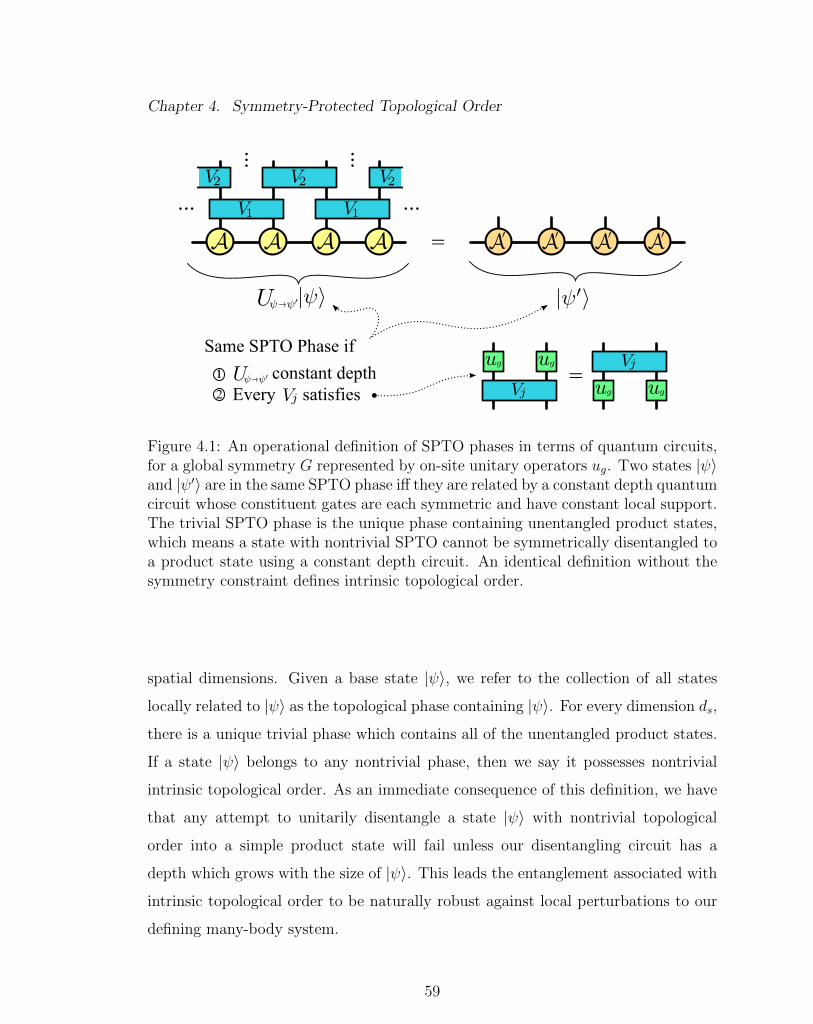
Chapter 4. Symmetry-Protected Topological Order
......
... ...
=
=Same SPTO Phase if
1 constant depth2 Every satisfies
Figure 4.1: An operational definition of SPTO phases in terms of quantum circuits,for a global symmetry G represented by on-site unitary operators ug. Two states |ψ〉and |ψ′〉 are in the same SPTO phase iff they are related by a constant depth quantumcircuit whose constituent gates are each symmetric and have constant local support.The trivial SPTO phase is the unique phase containing unentangled product states,which means a state with nontrivial SPTO cannot be symmetrically disentangled toa product state using a constant depth circuit. An identical definition without thesymmetry constraint defines intrinsic topological order.
spatial dimensions. Given a base state |ψ〉, we refer to the collection of all states
locally related to |ψ〉 as the topological phase containing |ψ〉. For every dimension ds,
there is a unique trivial phase which contains all of the unentangled product states.
If a state |ψ〉 belongs to any nontrivial phase, then we say it possesses nontrivial
intrinsic topological order. As an immediate consequence of this definition, we have
that any attempt to unitarily disentangle a state |ψ〉 with nontrivial topological
order into a simple product state will fail unless our disentangling circuit has a
depth which grows with the size of |ψ〉. This leads the entanglement associated with
intrinsic topological order to be naturally robust against local perturbations to our
defining many-body system.
59

Chapter 4. Symmetry-Protected Topological Order
The definition of SPTO phases proceeds in a largely similar manner as the oper-
ational definition of intrinsic topological order given above. We say that two states
|ψ〉 and |ψ′〉 in ds ≥ 1 spatial dimensions are in the same SPTO whenever |ψ′〉 they
can be locally related by the action of a local constant-depth quantum circuit Uψ→ψ′ ,
but we now require the gates forming this circuit to individually commute with our
on-site symmetry G. As was the case with intrinsic topological order, there is al-
ways a trivial phase of SPTO containing unentangled product states, and any other
SPTO phase is by extension said to be nontrivial. From its definition, we see that
phases of SPTO will represent more fine-grained partitions of many-body states than
phases of intrinsic topological order, and SPTO phases are in fact required by fiat
to only contain states whose intrinsic topological order is trivial4. This leads states
with nontrivial SPTO to possess a local form of entanglement which can always be
disentangled using some constant depth quantum circuit, but only by a circuit which
locally violates the on-site symmetry G. This is what the “symmetry-protected” in
SPTO refers to, since removing the symmetry-respecting condition on our disentan-
gling circuits would otherwise lead any SPTO phase to be considered trivial.
For the purposes of MQC, why should we prefer SPTO over intrinsic topological
order? We have already mentioned previously that the 2D toric code, a canonical
state of intrinsic topological order, is a non-universal resource state under single-
qubit measurements, which gives one specific example of a mismatch with MQC. For
the limited setting of 1D systems we have a much stronger argument though, namely
that nontrivial 1D intrinsic topological order doesn’t exist! More specifically, given
any short-range correlated 1D spin chain |ψ〉, it was argued in [CGW11] that |ψ〉
can always be disentangled into a trivial product state using a local quantum circuit
with constant depth. This no-go theorem shows that for 1D systems, SPTO is the
4This requirement isn’t fundamental, but rather promotes a separation of concernswhich makes the study of SPTO much easier. Systems which possess both intrinsic topo-logical order and a global symmetry group G are studied under the heading of symmetry-enriched topological order [MR13], a more difficult subject which won’t concern us here.
60

Chapter 4. Symmetry-Protected Topological Order
only show in town for defining phases of persistent many-body entanglement. More
generally, we have seen in Section 2.2 that proofs of universality for 2D resource
states typically rely on a reduction into independent 1D spin chains (see Figure 2.3)
which act as quantum wires for our logical qubits. One manner of ensuring that
these derived spin chains exhibit useful computational properties is to guarantee
their presence in a nontrivial phase of 1D SPTO, which will occur naturally when
our original 2D state possesses SPTO as well.
We now turn to describe a powerful result given in [ESBD12], which provides
a compelling demonstration of the MQC-SPTO correspondence in 1D. This result
proves that not only the AKLT state, but in fact any spin chain within the D2
Haldane phase can be used to teleport one qubit of encoded logical information.
While this applies to any on-site representation of D2, we will for simplicity only
discuss the case of spin-1 systems5. In this case, we see that generic spin chains in
the D2 Haldane phase share an important structural similarity with the AKLT state.
Theorem 4.1 (D2 Haldane Phase [ESBD12]). Given a short-range correlated 1D
spin chain of spin-1 particles in the D2 Haldane phase, the MPS tensor which de-
scribes this state can always be written as A =∑z
µ=xAµ|µ〉 =∑z
µ=x(σµ⊗aµ)|µ〉, such
that the matrices each factorize into a universal “protected” σµ and a non-universal
“junk” aµ.
Theorem 4.1 is proved using only general properties of SPTO and MPS represen-
tations which are true throughout the phase, and shows the virtual space of any spin
chain in the Haldane phase to be partitioned into a two-level protected space and an
arbitrary junk space6. The protected space gives us a guaranteed system in which
5The generalization to higher-dimensional spins isn’t hard to guess given Theorem 4.1,with the guiding principle that we replace the spin-1 Cartesian basis by a “wire basis”which simultaneously diagonalizes all symmetry operators ug. Because D2 is abelian, sucha basis will always exist.
6We should technically refer to these as subsystems of the virtual space, since theydecompose the virtual space via a tensor product rather than a direct sum.
61

Chapter 4. Symmetry-Protected Topological Order
we can store logical information, while the junk space captures the non-universal
behavior of the spin chain. By using the correspondence between measurements and
logical operators available in an MPS representation, this tells us that a measurement
in the Cartesian basis with outcome 〈µ| is guaranteed to apply σµ to our protected
space, which is simply teleportation of the encoded logical qubit. This proves the
operational characterization of the D2 Haldane phase as a phase uniformly capable
of single-qubit teleportation.
Can we implement more general logical operations than just teleportation? The
similarity of the form of our generic MPS tensor with that of the AKLT state sug-
gests that we might be able to apply unitary operations using measurements in
rotated bases, but we find a difficulty in the form of the junk space. For exam-
ple, if we measure in the Z-rotated basis of Eq. (3.18) and obtain the outcome
〈xθ,Z | = cos(θ/2)〈x|−sin(θ/2)〈y|, then the resultant logical operation (with a byprod-
uct operator correction) is
(X ⊗ I)Axθ,Z = cos(θ/2)I ⊗ ax − i sin(θ/2)Z ⊗ ay
6= [cos(θ/2)I − i sin(θ/2)Z]⊗ ax. (4.9)
Because ax 6= ay for arbitrary 1D spin chains, our rotated measurements will typically
generate entanglement between the protected and junk spaces, an undesirable effect
which leads to the leakage of logical information into non-universal degrees of freedom
within the edge modes.
This shows the uses and the limitations of the D2 Haldane phase, and perhaps
most importantly, gives a canonical example of the exact characterization of an
SPTO phase in terms of its uses for MQC. In Chapter 5, we will prove an exten-
sion of this result which reveals the S4 Haldane phase—a subset of the D2 Haldane
phase with higher on-site symmetry—to be capable not only of teleportation, but of
implementing any single-qubit unitary gate within the setting of MQC.
62

Chapter 4. Symmetry-Protected Topological Order
4.3 Mathematical Classification of SPTO
In this Section, we begin with a discussion of the classification of 1D SPTO phases
according to projective representations, which is used to motivate the more general
concepts of group cohomology theory needed for classifying higher-dimensional SPTO
phases. We then give a brief introduction to group cohomology, with a focus on those
elements which are needed for the relevant classification results. This material should
be of interest for researchers studying SPTO, but most of it can be safely skipped
by general readers. The topics discussed here will be used extensively in our proof
of Lemma 7.1, contained in Appendix A, but otherwise are largely unused.
We saw in Section 4.2 that phases of 1D SPTO are classified by the inequivalent
projective representations of the defining symmetry group G, but we didn’t justify
why projective representations were the right concept here, or what it means for two
projective representations to be inequivalent. To explain these issues, we revisit the
symmetry criterion of Eq. (4.6), which requires the MPS tensor of any symmetric
1D spin chain to be associated with unitary operators Ug which satisfy the equality∑dα=1Aα ⊗ ug|α〉 =
∑dα=1 UgAαU
†g ⊗ |α〉. This relation in itself says nothing about
SPTO, but we can ask what constraints it places on the different Ug. We assume
that the on-site symmetry operators ugg∈G form a representation of G, meaning
that ugh = uguh for all g, h ∈ G. Because we can express the on-site action of ug
within the virtual space, this requires the virtual conjugation action of Ug to also
form a representation of G. This doesn’t force Ug itself to form a representation of
G though, as the pairwise appearance of Ug and its adjoint leads any extraneous
complex phases appearing with Ug to cancel with those appearing with U †g . We
can therefore choose Ug to be a projective representation of G, meaning that the
composition of operators is given by UgUh = ω2(g, h)Ugh, with ω2(g, h) : G2 → C a
function outputting complex phases. This phase function ω2 is an algebraic object
called a 2-cocycle, which characterizes the projective representation formed by the
63

Chapter 4. Symmetry-Protected Topological Order
collection of Ug. For example, given the symmetry group D2 = e, x, y, z, the
projective representation formed by Pauli operators is defined by the 2-cocycle with
values ω2(g, g) = ω2(e, g) = ω2(g, e) = 1, ω2(x, y) = ω2(y, z) = ω2(z, x) = i, and
ω2(y, x) = ω2(z, y) = ω2(x, z) = −i.
While the presence of ω2 was allowed by our algebraic symmetry condition, ω2 is
subject to constraints arising from the matrix multiplication of different Ug being as-
sociative. The fact that (UgUh)Uf = Ug(UhUf ) implies that ω2(gh, f)ω2(g, h) =
ω2(g, hf)ω2(h, f) for all g, h, f ∈ G, a constraint which characterizes general 2-
cocycles. Also, since Ug only manifests physically in the presence of its adjoint
U †g , we are free to change the overall complex phase of each Ug without chang-
ing any physical behavior. If β1(g) defines a function of complex phases, called a
1-cochain, then changing the phase of Ug to be β1(g)Ug is the same as replacing the 2-
cocycle ω2(g, h) by ω′2(g, h) = ω2(g, h)β∗1(g)β1(gh)β∗1(h). We say in this case ω2(g, h)
and ω′2(g, h) define physically equivalent projective representations. This leads to
the natural question of how many physically inequivalent projective representations
there are, a classification problem whose general solution is known to be given by
the second cohomology group of G, H2(G,U(1)) [Sch04].
Group cohomology theory studies the cohomology groups Hd(G,U(1)) associated
to a group G, for arbitrary d ≥ 0. For our purposes, the elements of Hd(G,U(1))
classify the SPTO phases of short-range entangled many-body states with global
symmetry G in d−1 spatial dimensions7. The structure of the cohomology groups can
be calculated using d-cochains, which are arbitrary functions ξd mapping d-tuples of
elements of G, (g1, g2, . . . , gd) ∈ Gd, to individual complex phases ξd(g1, g2, . . . , gd) ∈
U(1). The set of all d-cochains is denoted by Cd(G,U(1)), and under pointwise
7It’s important to mention that this cohomology classification of SPTO is only completein spatial dimensions 1 or 2, with so-called “beyond cohomology” phases appearing in higherdimensions. These aren’t relevant for our present purposes, but information about theseexotic phases can be found in [VS13, WS13, BCFV14].
64

Chapter 4. Symmetry-Protected Topological Order
multiplication of function values forms an abelian group isomorphic to U(1)|G|d. The
identity element of Cd(G,U(1)) is the trivial d-cochain 1d, which outputs the constant
value 1. The (d’th) coboundary operator ∂d : Cd(G,U(1)) → Cd+1(G,U(1)) sends
every d-cochain ξd to a (d+ 1)-cochain ∂dξd, which acts as
∂dξd(g1, . . . , gd+1) = ξd(g2, . . . , gd+1)[ξn(g1, . . . , gd)](−1)d+1
×
d∏
k=1
[ξd(g1, . . . , gk−1, gkgk+1, gk+2, . . . , gd+1)](−1)k
. (4.10)
For example, when d = 2, ∂2ξ2(g1, g2, g3) = ξ2(g2, g3) ξ∗2(g1g2, g3) ξ2(g1, g2g3) ξ∗2(g1, g2).
The coboundary operator lets us define two important classes of cochains, the co-
cycles and coboundaries. A d-cocycle ωd is a d-cochain which lies in the kernel of
∂d, satisfying ∂dωd = 1d+1, while a d-coboundary ϕd is a d-cochain which lies in the
image of ∂d−1, satisfying ϕd = ∂d−1ξd−1 for some (d − 1)-cochain ξd−1. The collec-
tion of d-cochains and d-coboundaries are denoted by Zd(G,U(1)) and Bd(G,U(1))
respectively, both of which form subgroups of Cd(G,U(1)).
Eq. (4.10) can be used to show that ∂d+1∂dξd = 1d+2 for every d-cochain ξd,
which proves the inclusion Bd(G,U(1)) ⊂ Zd(G,U(1)). The d’th cohomology group
characterizes the extent to which the reverse inclusion fails to hold, viaHd(G,U(1)) =
Zd(G,U(1))/Bd(G,U(1)). The elements of Hd(G,U(1)), the cohomology classes,
are represented as equivalence classes of d-cocycles modulo d-coboundaries, [ωd]G ∈
Hd(G,U(1)), where [ω′d]G = [ωd]G if and only if ω′d ω−1d = ϕd ∈ Bd(G,U(1)).
While the above is in principle a complete discussion of the most basic defini-
tions and concepts of group cohomology theory, it is important to recognize that
this formalism can also be presented entirely in terms of “homogeneous” cochains,
which are simply reparameterized versions of the inhomogeneous cochains described
above. Given an inhomogeneous d-cochain ξd(g1 . . . , gd), we can uniquely define a
65

Chapter 4. Symmetry-Protected Topological Order
homogeneous d-cochain λd(a0, . . . , ad), which is related to ξd as
λd(a0, . . . , ad) = ξd(a−10 a1, a
−11 a2, . . . , a
−1d−1ad) (4.11)
ξd(g1 . . . , gd) = λd(e, g1, g1g2, . . . , g1g2g3 . . . gd). (4.12)
While homogeneous d-cochains are naively functions of d + 1 arguments, rather
than the d arguments appearing in ξd, this is compensated for by the symmetry
λd(a0, . . . , ad) = λd(e, a−10 a1, a
−10 a2, . . . , a
−10 ad), which holds for all a0 ∈ G. In the
setting of homogeneous cochains, the (d’th) coboundary operator acts as
∂dλd(a0, a1, . . . , ad+1) =d+1∏k=0
[λd(a1, . . . , ak−1, ak+1, . . . , ad+1)](−1)k . (4.13)
For example, when d = 2, ∂2λ2(a0, a1, a2, a3) = λ2(a1, a2, a3)λ∗2(a0, a2, a3)λ2(a0, a1, a3)
λ∗2(a0, a1, a2). Homogeneous d-cocycles (resp., d-coboundaries) are defined exactly
the same as in the inhomogeneous setting, as d-cochains lying in the kernel of ∂d
(resp., the image of ∂d−1). In what follows, we will denote general homogeneous
d-cocycles by νd.
While we would ideally avoid discussing both forms of d-cocycles within the same
setting, each form turns out to play a significant role in our work. Inhomogeneous
d-cocycles serve to capture the algebraic character of group cohomology, and have a
close relation to d-linear functions, whereas homogeneous d-cocycles serve to capture
the physical behavior of systems appearing in the d-cocycle model. This dual nature
is most apparent in Appendix A, during our proof of Lemma 7.1, where we start
with a homogeneous νd defining a d-cocycle state, and end with a proof that the
inhomogeneous counterpart of νd is a d-linear function. This issue is touched upon
in more detail in Section 4.4 and Appendix A.
66

Chapter 4. Symmetry-Protected Topological Order
4.4 The Cocycle State Model
In this Section, we discuss several important details of the cocycle state construction
[CGLW13], which we describe here in the more context-appropriate formalism of ho-
mogeneous d-cocycles. We also introduce the idea of “d-cochain states”, a relatively
uninteresting generalization of d-cocycle states which will be utilized in our proof of
Lemma 7.1.
While the correspondence between SPTO phases and cohomology classes has so
far been taken as a fact, the cohomology classification we have discussed was origi-
nally derived using the construction of SPTO fixed-point states within the cocycle
state model of [CGLW13]. This model concretely realizes an abstract d-cocycle ν as a
d-body unitary gate U(ν), which is then used to form a d−1 dimensional many-body
state |ψ(ν)〉. This state is invariant under the global symmetry group G associated
to ν, and belongs to the SPTO phase associated with [ν]G. We will focus here on
the 2D case (d = 3), but can extend this to any d ≥ 0 spatial dimensions.
To define our d-cocycle state, we need to choose a symmetry G, a d-cocycle
νd ∈ Zd(G,U(1)), and a lattice Λ. We use G to determine the Hilbert space of
a single qudit, HG, which is chosen to be the (left) regular representation of G.
This means that HG has dimension |G|, is spanned by an orthonormal “G basis”
|a〉a∈G, and is acted on by G as Xg|a〉 = |ga〉, for all g, a ∈ G. HG contains a
unique symmetric state |+G〉, given by |+G〉 =∑
a∈G |a〉 (up to normalization).
When G = Z2 ' 0, 1, HG corresponds to a single qubit, where the G basis is
the usual computational basis and X0 = I,X1 = X. For G = (Z2)m, our main case
of interest in the following Chapteres, we can use the isomorphism H(Z2)m ' (HZ2)⊗m
to identify each local spin with a collection of m qubits. This identification depends
on our choice of generating set for (Z2)m, relative to which an arbitrary G basis
vector splits as |a〉 '⊗m
i=1 |ai〉(i), with i indexing the m “virtual” qubits collectively
67

Chapter 4. Symmetry-Protected Topological Order
representing H(Z2)m . However, the identity |+(Z2)m〉 '⊗m
i=1 |+〉(i) remains true in
every generating set, where |+〉 := 1√2(|0〉+ |1〉).
Given HG, we can use our d-cocycle νd to construct a d-body “formation gate”
U(νd), which is used to generate |ψ(νd)〉. This gate is diagonal in the G basis, and
has the form of
U(νd) =∑a∈Gd
νd(e, a(1), a(2), . . . , a(d))|a〉〈a|. (4.14)
Here, a = (a(1), . . . , a(d)) is a tuple of d group elements a(c) ∈ G and |a〉 =⊗d
c=1 |a(c)〉(c)
is the corresponding d-qudit product state, with c indexing the d qudits which U(νd)
acts on.
To form our d-cocycle state |ψ(νd)〉, we place a symmetric qudit |+G〉 ∈ HG
at every vertex of our lattice Λ, then transversally apply U(νd) to the vertices sur-
rounding each d-simplex in Λ. We assume that Λ is a (d−1)-dimensional, d-colorable
simplicial complex with closed boundaries and n vertices. In this case, the d vertices
surrounding each d-simplex ∆d ∈ Λd are all different colors, which lets us pair the
final d indices of νd with the d colors of our lattice in a fixed manner. The transversal
application of U(νd) then defines a “formation circuit” UF , which forms |ψ(νd)〉 as
|ψ(νd)〉 = UF |+G〉⊗n. UF is given by
UF =∏
∆d∈Λd
U(νd)s(∆d), (4.15)
where U(νd) is applied to the d qudits surrounding each d-simplex ∆d, and s(∆d) =
±1 serves to alternately apply either U(νd) or its complex conjugate. s(∆d) is chosen
so that every pair of d-simplices ∆d,∆′d which overlap along a common (d−1)-simplex
satisfy s(∆d) = −s(∆′d). This alternation turns out to guarantee that |ψ(νd)〉 is
invariant under the global action of G to all n vertices in Λ, provided νd is a valid
d-cocycle. Further details on this construction can be found in [CGLW13].
68

Chapter 4. Symmetry-Protected Topological Order
It is also useful to define a slight generalization of the above construction, where
general d-cochains λd are used to form (d−1)-dimensional “d-cochain states” |ψ(λd)〉.
This construction is essentially identical to the d-cocycle construction just described,
but with λd taking the place of νd in Eq. (4.14). The biggest difference between
cocycle and cochain states is that the former always possess global G symmetry on
closed boundaries, while the latter generally do not. In determining whether a given
cochain state |ψ(λd)〉 is invariant under a symmetry operation Xg, we can always
instead determine whether the formation circuit UF commutes with Xg. This is mea-
sured by the group commutator, K(UF , Xg) := UFXgU†FX
†g . Clearly, K(UF , Xg) = I
implies Xg|ψ(λd)〉 = |ψ(λd)〉, but |ψ(λd)〉 being an even-magnitude superposition of
all G-basis states means that Xg|ψ(λd)〉 = |ψ(λd)〉 implies K(UF , Xg) = I as well.
69

Chapter 5
Universal Single-Qubit SPTO
Phase in S4-symmetric Spin Chains
Entanglement is ubiquitous in quantum many-body systems, and its complexity
has drawn attention from interdisciplinary research fields, such as condensed-matter
physics [LH08, PTBO10, CGW10, CLLS12], quantum information processing (QIP)
[RB01, RBB03, Vid03], and quantum simulation of quantum many-body systems
[CZ12, K+12, GAN14, EFG15, CR14]. A primary example is exotic ground states
of topologically ordered phases [Wen07, HK10, QZ11], which arise from underlying
nonlocal entanglement. It is widely known that braiding their excitations, known
as anyons, could be used for topological quantum computation [Kit03], and their
intrinsic insensitivity against local noise could be used for quantum error correction
[Kit03, KL10]. Many-body entanglement can be harnessed in a more direct way, and
certain many-body states like 2D cluster states [BR01] and certain tensor network
states [VC04a, GE07, GESPG07, CMDB10, Miy11, WAR11, L+11] are quantum re-
sources for measurement-based (or teleportation-based) quantum computation, in
that universal quantum computation can be implemented on these states using only
single-spin measurements.
70
Chapter 5. Universal Single-Qubit SPTO Phase in S4-symmetric Spin Chains
Having in hand a long list of many-body entanglement useful for QIP, however,
one may wonder “Is such computational usefulness robust in the same way that collec-
tive phenomena of quantum many-body systems do not depend on their microscopic
details?” Phrased differently, “Can we define quantum phases useful for certain QIP
tasks in the same way we define phase diagrams in condensed matter physics, which
are typically characterized by order parameters?” There have been several attempts
[BEF+08, DB09, BBD+09a, SB09, BBM+10, DBB12, EBD12, FM12, FNOM13] to
answer this affirmatively, but they unfortunately, with a few exceptions [BBM+10],
were largely based on a limited class of states, using rather artificial Hamiltonians
from a condensed matter physics perspective.
Here we tackle this challenge using the 1D counterpart of topologically ordered
phases as a key building block for measurement-based quantum computation, taking
advantage of recent characterizations of symmetry protected topologically ordered
(SPTO) phases [CGW11, GW09, SPGC11, PBTO12]. By inventing a physically-
feasible renormalization procedure which extracts the robust, macroscopic features
common among ground states within a phase, we prove that all the ground states
in the 1D SPTO phase corresponding to octahedral on-site symmetry can be used
to implement any one-qubit operations perfectly, as long as certain conditions on
characteristic length scales are met. The leverage of a discrete symmetry is somehow
reminiscent of magic states and their distillation [BK05] in the context of fault-
tolerant, universal quantum computation. Furthermore, we show that the gate fi-
delity, which is a typical measure of resource quality in QIP, can be interpreted as
an “operationally-motivated” order parameter of the phase, because it detects criti-
cal points of the phase in the same way as the conventional string order parameter
widely used in condensed matter physics. As a whole, our results constitute the first
solid evidence for quantum computationally useful phases of matter.
71

Chapter 5. Universal Single-Qubit SPTO Phase in S4-symmetric Spin Chains
5.1 Matrix Product States and 1D SPTO
We start by reviewing some relevant background material, which is covered in more
detail in Chapters 2, 3, and 4. The matrix product state (MPS) formalism [FNW92,
Vid03, PGVWC07] is an efficient means of describing the correlations in one-dimensional
spin chains. An MPS description is given by associating a matrix, Aα, to every vec-
tor |α〉 of a single-spin basis |α〉dα=1. The amplitude associated with a basis vector
|α1α2 . . . αn〉 is then given by
〈α1α2 . . . αn|ψ〉 = Tr (Aα1Aα2 · · ·Aαn) . (5.1)
The correlation length of our MPS is denoted by ξ, and our MPS is short-range
correlated if ξ is finite.
In the presence of an on-site symmetry group G, G-invariant MPS’s form distinct
symmetry protected topological ordered (SPTO) phases, a classification of which was
given in Refs. [CGW11, SPGC11]. Any transition between SPTO phases must be
accompanied by either the introduction of long-range correlations or the breaking of
on-site symmetry. This makes SPTO phase a robust property of many-body systems
in the presence of symmetry. The group of π rotations around the x, y, and z axes,
D2 ' Z2×Z2, defines two quantum phases, the trivial phase and the D2 SPTO phase.
The archetypical member of the D2 SPTO phase is the Affleck-Kennedy-Lieb-Tasaki
(AKLT) state [AKLT88], whose MPS matrices are Aµ = σµ. µ labels the vectors
in the spin-1 Cartesian basis |µ〉3µ=1, defined by S
(1)µ |µ〉 = 0, with S
(1)µ the spin-1
angular momentum operators. The σµ are the standard spin-12
Pauli operators.
Measurement-based quantum computation (MQC) [RB01, RBB03] is a conve-
nient setting for quantum computation where the quantum nature of computation
comes from the entanglement of an initial resource state. Through a sequence of
single-spin measurements, an MQC protocol harnesses this entanglement to imple-
ment a quantum algorithm. In this paper, we focus on one-dimensional resource
72

Chapter 5. Universal Single-Qubit SPTO Phase in S4-symmetric Spin Chains
states, which are an essential building block for constructing universal resource states
for quantum computation. As an illustration, we examine an MQC protocol utilizing
the AKLT state [BM08]. If we measure a spin in our AKLT chain and obtain an
outcome |ψk〉 =∑3
µ=1 ψk,µ|µ〉, then this results in an operator
A[ψk] =3∑
µ=1
ψ∗k,µAµ =3∑
µ=1
ψ∗k,µσµ. (5.2)
If we wish to implement a rotation by Θ around the z axis, UΘ = exp(−iΘ2σz), a
measurement outcome of |ψz,Θ〉 = cos(
Θ2
)|x〉 − sin
(Θ2
)|y〉 will suffice, since
A[ψz,Θ] = σx
[cos
(Θ
2
)I − i sin
(Θ
2
)σz
](5.3)
is indeed what we wanted, up to the σx term. This additional term is referred to as
a byproduct operator, and can be dealt with as long as we maintain a record of the
operator (See [RBB03] for details).
The above protocol characterizes one point within the D2 SPTO phase, namely
the AKLT state, as a resource state capable of generating arbitrary one-qubit op-
erations. As stated in the Introduction, to explore whether such a resource charac-
terization can be extended to the rest of the D2 SPTO phase, we wish to invent a
state-insensitive MQC protocol, in that an identical computation should be generated
despite microscopic differences of ground states. An initiative along this direction
was taken in [BBM+10], where all ground states of the 1D SO3-invariant Haldane
phase (or the so-called bilinear-biquadratic Hamiltonians) were studied using DMRG
calculations. The perfect resource quality of these states for arbitrary single-qubit op-
erations was demonstrated heuristically using a renormalization argument mapping
any ground state towards the AKLT state. Later, Else et. al. [ESBD12] developed an
algebraic characterization of the D2 SPTO phase, which includes the SO3-invariant
Haldane phase, showing that any state within this phase can be used to implement
a state-insensitive qubit teleportation operation. They obtain this result by show-
73

Chapter 5. Universal Single-Qubit SPTO Phase in S4-symmetric Spin Chains
ing that1 for any spin-1 MPS within the D2 SPTO phase, the component matrices
associated with that state’s MPS have the form
Aµ = σµ ⊗ aµ. (5.4)
The Hilbert spaces on the left and right side of the tensor product in Eq. (5.4) are
called the protected space and the junk space, respectively. While the details of the
junk operators, aµ, vary from state to state, the structure of the protected space
is common everywhere throughout the D2 SPTO phase. Thus, if we measure our
resource state in the Cartesian basis, we will always end up teleporting the state of
the protected space. In retrospect, this feature was first observed for certain ground
states of the D2 SPTO phase, like in the spin-1 XXZ Heisenberg model, as its so-
called localizable entanglement diverges, and can thus be used to implement the
identity channel [PVMDC05, VR05].
However, a simple argument given by Else et. al. [ESBD12] suggests that the
resource characterization of the D2 SPTO phase is limited to the identity channel
(namely teleportation). If we perform some non-Cartesian measurement, such as
that in Eq. (5.3), we end up applying the operation
A[ψz,π2] = cos
(Θ
2
)I ⊗ ax − i sin
(Θ
2
)σz ⊗ ay
6=[cos
(Θ
2
)I − i sin
(Θ
2
)σz
]⊗ ax. (5.5)
Because ax 6= ay for arbitrary states, this operation generally won’t have a well-
defined effect on the protected space, and thus doesn’t implement a state-insensitive
unitary rotation within the D2 SPTO phase.
1Their actual result is more general, but it is only the spin-1 D2 version of their resultthat is necessary for what follows.
74

Chapter 5. Universal Single-Qubit SPTO Phase in S4-symmetric Spin Chains
5.2 Main Results
Now we focus on MPS’s invariant under on-site octahedral symmetry. This group
can be generated by π2
rotations around the x and z axes of the octahedron, and is
actually isomorphic to the symmetric group of degree 4, S4. Since the π rotations in
S4 generate the group D2, any state with S4 symmetry also has D2 symmetry. It can
be shown that the classification of SPTO phases for on-site S4 symmetry is identical
to the case of D2, and consequently, any MPS in the S4 SPTO phase is automatically
in the D2 SPTO phase. This makes Eq. (5.4) applicable also to states in the S4 SPTO
phase, but the larger symmetry of S4 imposes finer constraints on MPS’s in the S4
SPTO phase. We emphasize that this abstract characterization of SPTO phases
is useful for making general statements, like the following two theorems, without
specifying a system Hamiltonian or other microscopic details (although one could
define a formal, local Hamiltonian for every MPS).
We study this S4 SPTO phase by means of an operational “renormalization” pro-
tocol called z-buffering, which extracts macroscopic features common among ground
states within the phase. This protocol, shown in Figure 5.1, consists of sequential
single-spin measurements, with postselection for a desired measurement outcome
which depends on the type of rotation we wish to implement. We first select a site,
the computational site, which will eventually be used to generate the desired unitary
rotation. Cartesian basis measurements are then performed on the m sites on each
side of this site. If we want to implement a z-axis rotation using the computational
site, we postselect for the all-|z〉 outcome on these 2m buffering sites, a process called
z-buffering. Similarly for x-axis rotations, x-buffering is utilized by postselecting the
all-|x〉 outcome. The ability to perform z and x-axis rotations is all we need, since
any single-qubit unitary gate can then be constructed using Euler angles.
If our desired outcome isn’t obtained, we just measure the computational site in
75

Chapter 5. Universal Single-Qubit SPTO Phase in S4-symmetric Spin Chains
the Cartesian basis and repeat this process on the next part of our spin chain, the
state of our protected space simply being teleported by this undesired measurement
outcome. Note that the probability of postselection is accounted for as overhead in
the chain length, but this does not qualitatively change the resource quality (and its
complexity), as long as it is finite. On the other hand, if our postselection succeeds,
then the remaining computational state is renormalized by an amount depending
on the ratio of m to a characteristic length scale, called the z-correlation length ζz,
which governs this RG flow for each state. When ζz is finite, this RG flow generally
terminates on a fixed point, which can be used to implement non-Pauli operations.
The exception to this rule is for certain pathological states, where the act of z-
buffering causes the state to become long-range correlated, in that the renormalized
correlation length ξ becomes infinite. This resource characterization is summarized
in the following Theorem:
Theorem 5.1. Consider any ground state of the 1D S4 symmetry-protected topolog-
ical ordered phase, which is characterized by a certain z-correlation length ζz and a
renormalized correlation length ξ. As long as ζz and ξ are both finite, the intrinsic
entanglement of this state enables us to efficiently implement all one-qubit unitary
operations under the setting of measurement-based quantum computation with arbi-
trarily high gate fidelity.
The fact that our protocol enables the behavior described in Theorem 5.1 is
proven in Section 5.5. The main idea behind our proof2 is that our MPS resource
state, by virtue of being in the D2 SPTO phase, will have SPTO degeneracy in
the protected space, but generally not in the junk space. When we postselect for a
repeated |z〉 outcome, we maintain this protected space degeneracy, but preferentially
amplify a one-dimensional subspace of the junk space. After enough buffering, the
2While the intuition is essentially the same, the case of non-normal az (i.e., [az, a†z] 6= 0)
needs some elaboration.
76

Chapter 5. Universal Single-Qubit SPTO Phase in S4-symmetric Spin Chains
(a)
(b)
(c)
? ?? ?
Figure 5.1: Schematic of renormalization procedure to manifest the quality of re-source states. (a) To perform z-buffering, we choose a computational site, and mea-sure m surrounding sites in the Cartesian basis. Here m = 2. (b) If our measure-ment fails to produce the all-|z〉 outcome, the computational site is measured in theCartesian basis, and we try again on another region. Since all of our measurementoutcomes simply induce Pauli operations, the state of the protected space is (up tobyproducts) unchanged. (c) If our measurement succeeds, the resource quality of ourcomputational site is improved, at least when ζz is finite (Theorem 5.1).
junk space is sufficiently restricted to this one-dimensional subspace, corresponding
to the largest eigenvalue λ1 of az, so that our renormalized system can be treated
effectively like the AKLT state. The length scale over which this happens, ζz, is set by
the ratio of the largest to the second largest eigenvalue. The expected measurement
overhead per gate required to achieve a gate fidelity 1− ε is
〈N〉 = O
(ζz
(1
ε
)4ζz log| 1λ1|
log
(1
ε
)). (5.6)
When the two largest eigenvalues of az become degenerate, corresponding to a diver-
gence in ζz, z-buffering cannot completely restrict the junk space, and our RG flow
stalls before reaching an AKLT-like state.
Theorem 5.1 says that the ground states of the S4 SPTO phase generally share a
common computational capability to implement perfect one-qubit gate operations.
77
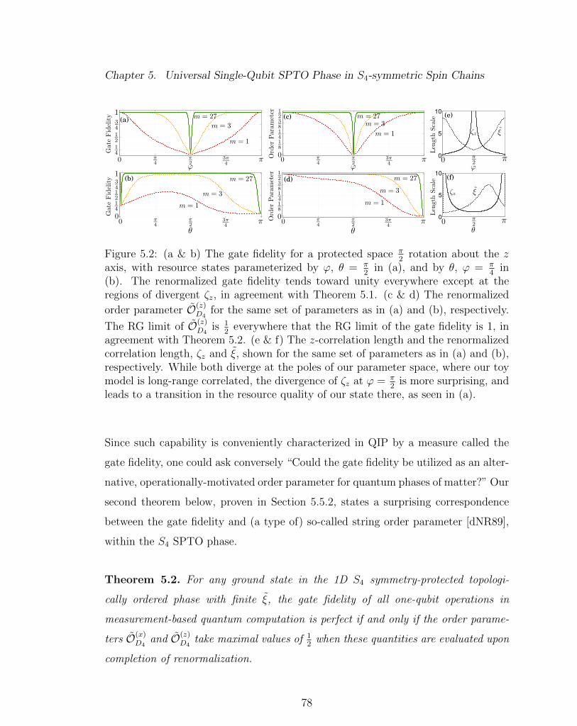
Chapter 5. Universal Single-Qubit SPTO Phase in S4-symmetric Spin Chains
0 0.7854 1.5708 2.3562 3.14160
0.125
0.25
0.375
0.5
Phi
Ord
er P
aram
eter
0 0.7854 1.5708 2.3562 3.1416
0.25
0.5
0.75
1
Phi
Gat
e Fi
delit
y (a)
0 0.7854 1.5708 2.3562 3.14160
0.25
0.5
0.75
1
Theta
Gat
e Fi
delit
y
0 0.7854 1.5708 2.3562 3.14160
0.125
0.25
0.375
0.5
Theta
Ord
er P
aram
eter
0
5
10 (f)
0
5
10(c)
(d)(b)
(e)
Figure 5.2: (a & b) The gate fidelity for a protected space π2
rotation about the zaxis, with resource states parameterized by ϕ, θ = π
2in (a), and by θ, ϕ = π
4in
(b). The renormalized gate fidelity tends toward unity everywhere except at theregions of divergent ζz, in agreement with Theorem 5.1. (c & d) The renormalized
order parameter O(z)D4
for the same set of parameters as in (a) and (b), respectively.
The RG limit of O(z)D4
is 12
everywhere that the RG limit of the gate fidelity is 1, inagreement with Theorem 5.2. (e & f) The z-correlation length and the renormalizedcorrelation length, ζz and ξ, shown for the same set of parameters as in (a) and (b),respectively. While both diverge at the poles of our parameter space, where our toymodel is long-range correlated, the divergence of ζz at ϕ = π
2is more surprising, and
leads to a transition in the resource quality of our state there, as seen in (a).
Since such capability is conveniently characterized in QIP by a measure called the
gate fidelity, one could ask conversely “Could the gate fidelity be utilized as an alter-
native, operationally-motivated order parameter for quantum phases of matter?” Our
second theorem below, proven in Section 5.5.2, states a surprising correspondence
between the gate fidelity and (a type of) so-called string order parameter [dNR89],
within the S4 SPTO phase.
Theorem 5.2. For any ground state in the 1D S4 symmetry-protected topologi-
cally ordered phase with finite ξ, the gate fidelity of all one-qubit operations in
measurement-based quantum computation is perfect if and only if the order parame-
ters O(x)D4
and O(z)D4
take maximal values of 12
when these quantities are evaluated upon
completion of renormalization.
78

Chapter 5. Universal Single-Qubit SPTO Phase in S4-symmetric Spin Chains
Note that our order parameters O(x)D4
and O(z)D4
are specializations of the string order
parameters R∞(u) from [PGWS+08] to the case of π2
rotations about the x and z
axes, urx and urz . In [PGWS+08], these string order parameters are argued to be
capable of detecting the presence of quantum phase transitions between different
SPTO phases. Our order parameters are given by:
O(µ)D4
= limn→∞〈ψµ|(urµ)⊗n|ψµ〉. (5.7)
The state |ψµ〉 is the state of our many-body MPS after it has been mapped to the
RG fixed point under µ-buffering, where µ is either x or z. While our bare spin
chain possesses full S4 symmetry, the process of renormalization breaks symmetry
by picking out a preferred direction (the x or z axis). Consequently, the symmetry
group of |ψµ〉 is reduced to D(µ)4 , which consists of the 8 rotations within S4 that
preserve this preferred axis.
5.3 Illustration of Our Results
To demonstrate Theorems 5.1 and 5.2, we study the behavior of MPS’s in the S4
SPTO phase with a two-dimensional junk space. We have developed a general for-
malism based on representation theory, and can show that spin-1 MPS’s of this
form make up a two-parameter family that is isomorphic to a sphere. Choosing
variables θ and ϕ, with 0 ≤ θ < π and 0 ≤ ϕ < 2π, gives a unique parame-
terization of this family of MPS’s. Because S4 symmetry includes D2 symmetry,
these MPS’s have well-defined protected and junk spaces, with component matrices
Aµ(θ, ϕ) = σµ ⊗ aµ(θ, ϕ), and
aµ(θ, ϕ) =1√3
cos
(θ
2
)I + eiϕ sin
(θ
2
)(~nµ ·~σ)
. (5.8)
The Pauli-type operators ~nµ ·~σ form a triad defined by
−1
2σx +
√3
2σy , −
1
2σx −
√3
2σy , σx , (5.9)
79

Chapter 5. Universal Single-Qubit SPTO Phase in S4-symmetric Spin Chains
for µ = x, y, z respectively. A numerical calculation of the gate fidelity, order param-
eter, and relevant length scales of states throughout the parameter space is shown
in Figure 5.2. We can see that the RG flow induced by z-buffering improves the
gate fidelity of a π2
rotation, an illustration by the “most non-Pauli” z-axis rotation,
almost everywhere in our toy model. The points at which the gate fidelity is not
improved are precisely those with divergent ζz, in agreement with Theorem 5.1. Fur-
thermore, we see remarkable similarity between the plots showing gate fidelity and
those showing O(z)D4
in Figure 5.2, both of which improve as the degree of z-buffering is
increased. After sufficient renormalization (i.e., at m =∞), the gate fidelity achieves
its maximum value precisely when O(z)D4
= O(x)D4
= 12, as stated in Theorem 5.2.
There are a few singular states in our parameter space with regard to their be-
havior under renormalization. As shown in Figure 5.2, the region with ϕ = ±π and
any θ, as well as the poles at θ = 0, π, have divergent ζz. This can be understood by
noticing that az is unitary at these points, so that z-buffering just acts as a change
of basis on the junk space. Interestingly, the original correlation length ξ, does not
diverge at ϕ = ±π, so that this is a new kind of singular state only detected by
our operationally motivated classification of quantum many-body states. In con-
trast, states at the poles (θ = 0, π) are not within the S4 SPTO phase, because the
original MPS’s are long-range correlated, having a divergent ξ. There is another
singular state at (θ, ϕ) = (2 arctan(2), 0), whose pathological behavior is discussed
in Section 5.5.3.
5.4 Conclusion
We proved two theorems to demonstrate the intrinsic, quantum computational use-
fulness of the 1D S4 SPTO phase as a “universal” quantum channel. We think that
our physically feasible renormalization procedure, called z-buffering, is interesting
80

Chapter 5. Universal Single-Qubit SPTO Phase in S4-symmetric Spin Chains
on its own, because our state-insensitive protocol indicates that it is possible to har-
ness such intrinsic capability of the phase without knowledge of microscopic details,
at least as long as the states are guaranteed to be in the phase. As an outlook,
since it is plausible that resource states for universal computation should generally
possess such universal-channel capability in two or higher dimensions, our work is
expected to serve as a stepping stone in the search for universal resource states in
naturally-occurring quantum many-body systems.
81
Chapter 5. Universal Single-Qubit SPTO Phase in S4-symmetric Spin Chains
5.5 Proofs and Discussion
In this Section, we give proofs to the two Theorems stated in the main text. For
completeness, we restate them here.
Theorem 5.1. Consider any ground state of the 1D S4 symmetry-protected topolog-
ical ordered phase, which is characterized by a certain z-correlation length ζz and a
renormalized correlation length ξ. As long as ζz and ξ are both finite, the intrinsic
entanglement of this state enables us to efficiently implement all one-qubit unitary
operations under the setting of measurement-based quantum computation with arbi-
trarily high gate fidelity.
Theorem 5.2. For any ground state in the 1D S4 symmetry-protected topologi-
cally ordered phase with finite ξ, the gate fidelity of all one-qubit operations in
measurement-based quantum computation is perfect if and only if the order parame-
ters O(x)D4
and O(z)D4
take maximal values of 12
when these quantities are evaluated upon
completion of renormalization.
Before giving the proofs of these two Theorems, we introduce some facts and
terminology useful for studying matrix product states. These are discussed in more
detail in Chapter 3.
While our original definition of MPS’s consisted of a single-spin basis |α〉dα=1
and a collection of matrices, Aα, one for each |α〉, we can treat these objects in a
unified manner by defining a three-index MPS tensor, A, as
A =d∑
α=1
Aα|α〉. (5.10)
The relevant Hilbert spaces here are the single-site space, referred to as the physical
space, and the abstract Hilbert space which the Aα act on, referred to as the virtual
space. We refer to the operators Aα as the component operators of A.
82

Chapter 5. Universal Single-Qubit SPTO Phase in S4-symmetric Spin Chains
Given a single-spin representation uG of a symmetry group G, the necessary and
sufficient condition for a MPS to be invariant under this symmetry group is if our
MPS tensor satisfies [PGWS+08, SWPGC09]
d∑β=1
(uG)α,β Aβ = UGAαU†G. (5.11)
UG is generally allowed to be a projective representation, with UgUh = eiθghUgh, and
the collection of eiθgh is actually what determines a MPS’s SPTO phase [CGW11].
Finally, any MPS tensor can be put in a special canonical form [PGVWC07], in
which its component matrices satisfy the following relations:
EI(Λ) :=d∑
α=1
AαΛA†α = Λ, (5.12)
E†I (I) :=d∑
α=1
A†αAα = I, (5.13)
where I is the identity operator, and Λ is a strictly positive operator satisfying
Tr(Λ) = 1. Viewing Eqns. (5.12) and (5.13) as setting the largest eigenvalue of
EI , the correlation length, ξ, of our state is determined by the magnitude of the
second largest eigenvalue. If Λ and I are the only operators with eigenvalues of unit
modulus, our MPS tensor is short-range correlated.
5.5.1 Proof of Theorem 5.1
In this section, we give a proof of Theorem 5.1. For clarity, we first give a mathe-
matical translation of each of the relevant terms in Theorem 5.1, for the case of z
rotations.
Finite ζz ζz is set by the eigenvalues of az. When az is a normal operator ([az, a†z] =
0), ζz is defined in terms of the ratio of the largest and second largest eigenvalues
83

Chapter 5. Universal Single-Qubit SPTO Phase in S4-symmetric Spin Chains
of az, λ1 and λ2 respectively, as ζz =(− log
∣∣∣λ2λ1 ∣∣∣)−1
. In the case of non-normal
az, the definition is the same, but λ1 and λ2 are required to be eigenvalues
associated with distinct Jordan blocks, when az is written in its Jordan normal
form. The condition of finite ζz requires |λ1| 6= |λ2|.
Finite ξ ξ is defined in terms of the ratio of the largest and second largest eigenvalues
of EI , where EI is the quantum channel in Eq. (5.12), but with the matrices Aα
replaced by their renormalized counterparts Ai. We specify the action of the
RG flow on the component matrices in Eq. (5.14), and show how this condition
is needed near the end of our proof.
Gate Fidelity We quantify the fidelity of a single-qubit unitary operation by F =
TrPTrJ [D(ρ)] U(P )Θ ρ(P )U
(P )†Θ , where ρ = ρ(P )⊗ρ(J), and where D is the actual
virtual space operation generated by measurement following renormalization.
The choice of ρ(P ) and ρ(J) isn’t particularly important for our proof, but we
will discuss their selection for Figures 5.2 and 5.3 at the end of Section 5.5.1.
Our proof involves modeling the MPS component operators under renormalization
and showing that, given finite ζz and ξ, the junk space components of the renor-
malized counterparts of Ax and Ay tend towards a common operator. In this case,
we can perform a z-axis rotation using the same single-site measurement as for the
AKLT state, and the gate fidelity of the resultant protected-space operation relative
to the desired rotation will converge exponentially fast to unity.
In z-buffering, we postselect for obtaining the all-|z〉 outcome for m sites on both
sides of our computational site. The effect of this is to modify the MPS component
operators of the computational site as follows:
Aµ 7→ A(m)µ = (Amz )Aµ(Amz ) = σµ ⊗ aµ (5.14)
Since Az = σz ⊗ az always has a trivial effect on the protected space, the interesting
part of our proof involves looking at the iterated term amz . If az is a normal operator,
84

Chapter 5. Universal Single-Qubit SPTO Phase in S4-symmetric Spin Chains
then it can be diagonalized by expressing it in its eigenbasis. If az is non-normal,
then we can block diagonalize it by writing it in its Jordan canonical form. In this
latter case,
az =
p⊕k=1
a(k)z , (5.15)
where a(k)z = λkIDk + QDk . Here, the index k parameterizes the p different Jordan
blocks in the decomposition, each of which has dimension Dk. IDk is the projector
onto the k’th Jordan block and QDk is the operator whose matrix form has 1’s
immediately above the diagonal and 0’s everywhere else. We assume that we have
ordered the Jordan blocks by eigenvalue size, such that |λ1| ≥ |λ2| ≥ . . . ≥ |λp|.
The form of Eq. (5.15) includes the normal az case as well (every Jordan block one-
dimensional), so we only need to prove the efficacy of z-buffering for non-normal
az.
Given this form, amz is
amz = (λ1)mp⊕
k=1
(λkλ1
)mPmk , (5.16)
where Pk = IDk + λ−1k QDk . If ζz is finite, then λ1 is the unique largest eigenvalue,
meaning that the weight attached to each Pmk with k > 1 decays exponentially with
m relative to that of Pm1 .
We now look at the element of S4 corresponding to a z-axis rotation by π2, whose
physical space representation is denoted urz . We know that urz|z〉 = |z〉, which in
turn implies via Eq. (5.11) that [Urz , Az] = 0 on the virtual space. Representation
theory can be used to show that the virtual symmetry operator Urz decomposes
along the protected-junk division as Urz = U(P )rz ⊗U
(J)rz , with U
(P )rz = e−i
π4σz and U
(J)rz
satisfying (U(J)rz )2 = I. This tells us that U
(J)rz has eigenvalues of ±1, and the fact
that Urz and Az commute tells us that each Jordan block of Eq. (5.15) can be labeled
85

Chapter 5. Universal Single-Qubit SPTO Phase in S4-symmetric Spin Chains
with one of these eigenvalues, denoted χk. Symbolically,
U (J)rz a
(k)z = χka
(k)z . (5.17)
When restricted to the junk space, the condition Eq. (5.11) becomes U(J)rz axU
(J)†rz =
ay, which also holds for the renormalized junk space components. If we define a± =
12(ax ± ay), this information, along with Eq. (5.16), gives us
a± =1
2(ax ± ay) =
1
2(ax ± U (J)
rz axU(J†)rz )
= λ2m1
∑j,k
χj=±χk
(λjλkλ2
1
)mPmj axP
mk , (5.18)
where the condition χj = ±χk limits the range of summed indices in each case. In
the large m limit, the term associated with λ21 dominates the sum in Eq. (5.18). Since
this term is contained within a+, and not a−, we see that ax and ay both converge
to a common operator a+ exponentially fast.
At any stage of renormalization, if we apply a projective measurement with mea-
surement outcome |ψz,Θ〉 = cos(
Θ2
)|x〉 − sin
(Θ2
)|y〉, the virtual operation imple-
mented is
A[ψz,Θ] = σx
[cos
(Θ
2
)I ⊗ ax − i sin
(Θ
2
)σz ⊗ ay
]= U
(P )+Θ ⊗ a+ + U
(P )−Θ ⊗ a−, (5.19)
where U(P )±Θ = σx
[cos(
Θ2
)I ∓ i sin
(Θ2
)σz]. The operation D used in our definition of
gate fidelity is defined in terms ofA[ψz,Θ] asD(ρ) = A[ψz,Θ] ρA[ψz,Θ]†/Tr(A[ψz,Θ] ρA[ψz,Θ]†).
Eq. (5.19) tells us that the operation induced by the measurement outcome is a coher-
ent combination of a rotation by Θ with another rotation by −Θ. The gate fidelity
of the reduced operation on the protected space is set by the relative size of the
junk space operators associated with the two rotations, and since a+ is exponentially
86

Chapter 5. Universal Single-Qubit SPTO Phase in S4-symmetric Spin Chains
larger in norm than a− in the large m limit, the gate fidelity between A[ψz,Θ] and
U(P )+Θ will converge to unity exponentially fast.
In this proof, we explicitly required S4 symmetry and finite ζz in order to give the
description of a± in Eq. (5.18) and show the exponential separation between a+ and
a−. Note, however, that our requirement of finite ξ was implicit in the assumption
that Pm1 axP
m1 6= 0. In Section 5.5.3, we examine carefully a point in our toy model
parameter space where this assumption is violated. Here we simply mention that
for such a state, the renormalized junk space operator az is exponentially larger in
norm than both ax and ay. For such a system, the renormalized identity-derived
operator tends exponentially fast towards EI = Az A†z, which has degeneracy in
the protected space portion of its eigenvalue spectrum. The correlation length of our
system consequently increases exponentially withm, and this violates our assumption
of finite ξ. Thus, given our assumptions, we are guaranteed Pm1 axP
m1 6= 0, and our
proof of Theorem 5.1 is complete.
We conclude with two remarks. First, in order to implement an arbitrary single
qubit unitary gate to accuracy ε, such that F ≥ 1 − ε, the expected overhead per
gate, 〈N〉, is
〈N〉 = O
(ζz
(1
ε
)4ζz log| 1λ1|
log
(1
ε
)). (5.20)
This comes from our postselection success probability and gate fidelity having asymp-
totic scaling of psucc ∼ |λ1|4m and F ∼ 1 − e−mζz . We note that for the case of non-
normal az, the convergence of the operator a+ to a definite limit form will generally
happen at a rate that is polynomial, rather than exponential, in m. However, since
we are only interested in applying U(P )Θ on the protected portion of our virtual space,
and that is not hindered by any dynamics within the junk space, our measure of
gate fidelity has been chosen to reflect only the reduced form of A[ψz,Θ] within the
protected space. From Eq. (5.19), we see that this reduced form of A[ψz,Θ] converges
87

Chapter 5. Universal Single-Qubit SPTO Phase in S4-symmetric Spin Chains
to U(P )Θ at a rate that is exponential in m, regardless of the much slower convergence
of a+.
Second, we mention that although a specific choice for ρ = ρ(P )⊗ρ(J) is relatively
unimportant for the scaling of our gate fidelity under renormalization, for the simu-
lations involving our toy model we chose to use ρ(P ) = |+〉〈+| and ρ(J) = 12I, where
|+〉 is the +1 eigenstate of σx. This choice of ρ(P ) is natural for probing the fidelity
of rotations about the z axis, while the choice of ρ(J) corresponds to the limit of our
junk space after sufficiently many unsuccessful postselection attempts. In particular,
while unsuccessful postselection simply acts as identity channels (teleportation) on
the protected space, at each stage we evolve the junk space by an unknown junk
space operator, leading to an unknown final state which we take to be maximally
mixed.
5.5.2 Proof of Theorem 5.2
To prove Theorem 5.2, we first have to give a definition of O(µ)D4
that is more amenable
to computation than that given in Eq. (5.7). To this end, we define the channel Eurµas the contraction of both indices of the physical symmetry urµ with MPS tensors.
Mathematically, Eurµ =3∑
ν,η=1
(urµ)ν,ηAη A†ν . Using Eq. (5.11), we find that Eurµ is
definable in terms of EI as
Eurµ = Urµ EI(U †rµ
). (5.21)
Now, using the standard method for calculating expectation values of tensor prod-
ucts of single-site operators on an MPS, we have that the string order parameters
evaluated on the bare state are given by
O(µ)D4
= limn→∞
Tr(Λ (Eurµ )n[I]
)= lim
n→∞Tr(
ΛUrµ(EI)n[U †rµ ]). (5.22)
88

Chapter 5. Universal Single-Qubit SPTO Phase in S4-symmetric Spin Chains
(EW )n here means the n-fold iterated operation of the quantum channel EW (W
representing either urµ or I), and Λ denotes the left limit edge mode of our MPS,
defined implicitly in Eq. (5.13). The value of O(µ)D4
, the renormalized string order
parameters, are given by the same expression as in Eq. (5.22), but with EI in place
of EI .
The action of z-buffering on the virtual space is described in Section 5.5.1. For
our purposes here, we only add that the rescaling in the normalization of our state
that is required by postselection can be compactly expressed as the requirement
that the spectral radius of EI is 1. The results of [PGVWC07], together with the
assumption that our renormalized MPS tensor is short-range correlated (finite ξ),
then tell us that we can pick a basis for our junk space which puts our renormalized
MPS tensor in canonical form. In this form, our channel EI satisfies the following
conditions:
EI(IP ⊗ Πz) =3∑
µ=1
Aµ(IP ⊗ Πz)A†µ = IP ⊗ Πz, (5.23)
E†I (IP ⊗ Λ) =3∑
µ=1
A†µ(IP ⊗ Λ)Aµ = IP ⊗ Λ, (5.24)
where Πz is a projector onto the section of our junk space with non-vanishing support
at the RG fixed point, and Λ is a strictly positive operator of unit trace, whose
support is exactly Πz.
Our proof of Theorem 5.2 consists of a case-by-case analysis of the renormalized
junk space operators ax and ay, depending on whether or not O(z)D4
= 12. We first show
that if O(z)D4
= 12, then ax = ay at the RG fixed point. In this case, a z-axis rotation
implemented using the z-buffered MPS will have perfect gate fidelity. We then show
that if O(z)D46= 1
2, then ax 6= ay. This causes the gate fidelity of our attempted z-axis
rotation to be less than unity at the RG limit. Proving both of these implications
under the assumption of finite ξ suffices to prove Theorem 5.2.
89

Chapter 5. Universal Single-Qubit SPTO Phase in S4-symmetric Spin Chains
For the first direction of the proof, we note that finite ξ means that IP ⊗Πz and
IP ⊗ Λ are the only fixed points of Eqns. (5.23) and (5.24). This, together with the
results of [NAJ09], tells us that (EI)n has the limit form
limn→∞
(EI)n =1
2Tr[(IP ⊗ Λ)] IP ⊗ Πz. (5.25)
We now insert the form of Eq. (5.25) into (the renormalized counterpart of) Eq. (5.22)
to get
O(z)D4
=1
4Tr[(IP ⊗ Λ)Urz ]Tr[(IP ⊗ Λ)U †rz ]
=1
4
∣∣∣Tr((IP ⊗ Λ)Urz)∣∣∣2 . (5.26)
As mentioned in Section 5.5.1, the virtual unitary Urz decomposes as Urz = U(P )rz ⊗
U(J)rz . Furthermore,
∣∣∣Tr(U
(P )rz
)∣∣∣2 = 2 for all states in the D2 SPTO phase, so the value
of O(z)D4
only depends on the behavior of the junk space.
To figure out this value, we first define Urz to be the restriction of U(J)rz to the
support of the junk space at the RG fixed point, Urz := ΠzU(J)rz Πz. The fact that
(U(J)rz )2 = IJ , along with [U
(J)rz , az] = 0, shows that (Urz)
2 = Πz. Consequently, U(J)rz
has eigenvalues of ±1, and we can write it as
U (J)rz = Π+
z − Π−z , (5.27)
for projectors Π+z and Π−z , which satisfy Π+
z Π−z = 0 and Π+z + Π−z = Πz.
Feeding this information into Eq. (5.26) gives
O(z)D4
=1
2
∣∣∣Tr(ΛU (J)rz )∣∣∣2 =
1
2
∣∣∣Tr[Λ(Π+z − Π−z )]
∣∣∣2 . (5.28)
Now, we come to the meat of our proof. Since Λ is a strictly positive operator with
unit trace, the only way to have O(z)D4
= 12
is to have either Π+z = 0 or Π−z = 0. In this
case, U(J)rz = ±Πz, which says our z-axis rotation acts trivially on the junk space of
90

Chapter 5. Universal Single-Qubit SPTO Phase in S4-symmetric Spin Chains
0
20
40
0 0.7854 1.5708 2.21432.3562 3.14160
0.25
0.5
0.75
1
Theta
Gat
e Fi
delit
y
0 0.7854 1.5708 2.21432.3562 3.14160
0.25
0.5
0.75
1
Theta
Ord
er P
aram
eter (b)(a) (c)
Figure 5.3: (a) The gate fidelity of a protected space π2
rotation about the z axis, forresource states along a North-to-South traversal of our parameter space (θ variable,ϕ = 0). While the renormalized gate fidelity tends toward unity most everywhere, itstays well below 1 at the South pole and at θc = 2 arctan(2), where ξ diverges. (b)
The renormalized order parameter O(z)D4
for the same set of parameters as in (a). The
value of O(z)D4
is 12
everywhere except at the South pole and, more surprisingly, at θc.
This unintuitive behavior can be explained by the divergence of ξ. (c) The lengthscales ζz and ξ for the same parameters. Both quantities diverge at the poles, butthe divergence of ξ at θc leads to the unexpected behavior seen in (a) and (b).
our renormalized MPS tensor. This last fact, which comes from assuming O(z)D4
= 12,
lets us prove the equality of ax and ay. This follows because
ax = U (J)rz ayU
(J)†rz = (±Πz)ay(±Πz) = ay. (5.29)
This gives the first direction of our proof.
For the other direction, assume that O(z)D46= 1
2. In this case, Eq. (5.28) tells us
that Π+z and Π−z are both non-zero. Thus, U
(J)rz is not simply ±Πz. What does this
say about ax and ay? We can answer this by looking at the commutator [U(J)rz , ax]. If
this is non-zero, then ax 6= ay. From Eq. (5.18), we see that the norms of a+ and a−
do not become exponentially separated in the RG limit, and thus our renormalized
state cannot be used to implement high-fidelity z-axis rotations on the protected
space.
On the other hand, if [U(J)rz , ax] = 0, then we can take linear combinations of this
91

Chapter 5. Universal Single-Qubit SPTO Phase in S4-symmetric Spin Chains
with the commutator [Πz, ax], which is always zero, to obtain
[Π+z , ax] = 0 (5.30)
[Π−z , ax] = 0, (5.31)
and the same for ay. Since additionally, [Π±z , az] = 0 always, these facts together
tell us that EI has two independent fixed points, IP ⊗ Π+z and IP ⊗ Π−z . But this
contradicts the assumption of finite ξ, and thus cannot be the case for our system.
Thus, we must have ax 6= ay, which completes the second desired implication, and
thus finishes our proof of Theorem 5.2.
5.5.3 The Renormalized Correlation Length
While the physical interpretation of ζz in our protocol is straightforward, simply being
the characteristic length scale of our RG flow, the interpretation of ξ is somewhat
less clear. In this section, we take a closer look at this quantity by means of our
toy model. Our toy model has three points for which ξ is divergent. Two of these
points, those on the poles of our parameter space, start out as long-range correlated
states before z-buffering, and thus aren’t particularly interesting. However, the last
point, lying at (θ, ϕ) = (θc, 0) (for θc := 2 arctan(2)), possesses a correlation length
that is only made divergent under z-buffering. We hope to clarify this behavior here
by exhibiting the somewhat pathological behavior of this point under z-buffering.
Since the component matrices of our toy model are normal, the proof of Sec-
tion 5.5.1 simplifies considerably, and can be phrased as follows:
• Z-buffering acts as Aµ 7→ A(m)µ = (Amz )Aµ(Amz ), which has a non-trivial effect
only on the junk space.
92

Chapter 5. Universal Single-Qubit SPTO Phase in S4-symmetric Spin Chains
• Since the eigenvector of az with largest eigenvalue is either |+〉 (when Re(eiϕ) >
0) or |−〉 (when Re(eiϕ) < 0), we have limm→∞
(az)m ∼ |±〉〈±|.
• Thus, for the portion of our parameter space with −π2< ϕ < π
2, our junk space
components at the m→∞ limit satisfy ax = ay = [cos(θ2
)− 1
2eiϕ sin
(θ2
)]|+〉〈+|,
and az = [cos(θ2
)+ eiϕ sin
(θ2
)]|+〉〈+|.
However, setting (θ, ϕ) to (θc, 0) shows that at this point, ax = ay = 0. In the
language of Section 5.5.1, this is equivalent to P1axP1 = 0, which is to say that
the leading order term in a+ vanishes. In this case, from Eq. (5.18) and from the
fact that U(J)rz = σx for our toy model, we see that the dominant terms in our junk
space components lie within a−. This conclusion, along with Eq. (5.19), tells us that
the RG limit of our effective protected space operation is U(P )−Θ , a rotation in the
opposite direction than we intended. While this can be accounted for by changing
the interpretation we attach to our measurement outcomes, this selective change
in interpretation would render our protocol no longer state-insensitive. Thus, for
consistency, we must rule this state out as a valid resource state for MQC under
z-buffering. The sharp dip in the gate fidelity seen at θc in Figure 5.3 is the natural
consequence of making such a consistent choice of gate fidelity.
Finally, we explain the strange behavior seen in the value of O(z)D4
at (θc, 0). While
this behavior appears quite surprising, it is explained by the fact that the channel
EI is Az A†z at this point. Thus, even though the junk space of our system is
restricted to a one-dimensional subspace here, the protected space portion of EIbecomes degenerate at the RG fixed point. Consequently, the limit form of O(z)
D4is
not given by Eq. (5.26), but rather by
O(z)D4
=1
2Tr(U (P )
rz U (P )†rz )Tr(ΛU (J)
rz )Tr(ΛU (J)†rz ) =
∣∣∣Tr(U (J)rz )∣∣∣2 = 1. (5.32)
This completes our examination of the behavior of the (θ, ϕ) = (θc, 0) point in our
parameter space. Our intent in this, besides simply giving a complete account of our
93

Chapter 5. Universal Single-Qubit SPTO Phase in S4-symmetric Spin Chains
toy model, is to demonstrate that states with divergent ξ have rather pathological
behavior that makes them unfit for use in our protocol. Thus, even without a concrete
physical interpretation for this quantity, the stipulation of finite ξ is clearly necessary
in both of our theorems.
94

Chapter 6
A Universal Resource State with
2D SPTO
The idea of measurement-based quantum computation (MQC), where computation
is carried out solely through single-qubit measurements on a fixed many-body re-
source state and classical feed-forward of measurement outcomes [RB01, RBB03,
Joz05], is quite surprising. This is because it highlights the origins of quantum ad-
vantage in terms of entanglement and non-commutative measurements, uniquely
quantum effects without counterparts in classical mechanics. In particular, so-
called universal resource states, the states that are capable of efficiently imple-
menting universal MQC, represent a class of maximal entanglement in the classi-
fication of many-body entanglement [dNMDB06], so that the structure and com-
plexity of their entanglement is of great interest for advancing the understand-
ing of quantum computation. Following the canonical example of the 2D clus-
ter state [BR01], many other universal resource states have been found, including
cluster states defined on various lattices [dNMDB06], some tensor network states
[VC04a, dNMDB06, GE07, GESPG07, CZG+09, CMDB10], and model ground states
in condensed matter physics such as 2D Affleck-Kennedy-Lieb-Tasaki (AKLT) states
95

Chapter 6. A Universal Resource State with 2D SPTO
[CMDB10, Miy11, WAR11, DBB12, Wei13, WR15].
Given the existence of these various known universal resource states, a natu-
ral question is whether we might be able to find any common key feature, so as
to explore more their variety in fundamental structures as well as practical ap-
plications. While the earliest resource states for MQC were found in short-range
correlated states described as somewhat artificial tensor network states [VC04a,
dNMDB06, GE07, GESPG07, CZG+09, CMDB10], a new insight has been that
a class of short-ranged entangled states structured by symmetry, endowed with
so-called symmetry-protected topological order (SPTO) [PTBO10, GW09, Kit09,
RSFL10, CGW11, SPGC11, PBTO12, CGLW12, CGLW13], make excellent candi-
date resource states systematically. Indeed, in the setting of 1D spin chains, the
ground states of several SPTO phases have already been shown to possess entan-
glement which can be leveraged to achieve various quantum computational tasks
[BM08, Miy10, BBM+10, ESBD12, EBD12, MM15, PW15].
Here, in adopting the concept of SPTO, we carry out such an investigation for
the first time in 2D MQC, and discover a completely new kind of MQC universal
resource state. Specifically, we first examine the 2D cluster state as well as a wide
range of other universal resource states, and show that their 2D SPTO is trivial,
of the same nature as unentangled product states. Looking more closely, we find
that these previously known resource states do possess some “weaker” SPTO, but
essentially of a type closer to that of 1D spin chains. Our discovery is made possible
owing to the recent progress of research into SPTO, which has revealed a hierarchy
of SPTO as representing different levels of nonlocality of quantum information (see
the next section for details). We then introduce our “Union Jack” state, which in
contrast possesses SPTO entirely of a 2D nature, and demonstrate that it is not
only a universal resource state but additionally is “Pauli universal,” in that it can
implement arbitrary quantum computation using only single-qubit measurements in
96

Chapter 6. A Universal Resource State with 2D SPTO
the Pauli bases. As elaborated later, this feature is forbidden in the 2D cluster state
on account of the Gottesman-Knill theorem [Got98], which proves the efficient clas-
sical simulability of certain quantum gates. We will conclude with the outlook that
our proof of principle result about Pauli universality may be true for more general
resource states with 2D SPTO, which we connect to a possible deep connection be-
tween a hierarchy of SPTO in condensed matter physics and the so-called Clifford
hierarchy of quantum computation.
6.1 MQC and SPTO Background
We first give a brief overview of some relevant topics regarding MQC, SPTO, and
the Clifford hierarchy, which will all be utilized here. A detailed discussion of these
topics can be found in Chapters 2, and 4.
Measurement-based quantum computation (MQC) is a means of utilizing an en-
tangled resource state to perform computation using (generally adaptive) single-qubit
measurements. Given a particular resource state, we specify our computational
process by choosing a specific pattern of single-qubit measurements. Due to the
probabilistic nature of measurement, different measurement outcomes will generally
implement different computations. However, rather than attempting to correct for
unintended measurement outcomes at every step, we can instead represent the effect
of such outcomes as the product of our intended operation with a so-called byproduct
operator. When these byproduct operators are sufficiently simple (e.g. Pauli oper-
ators), we can commute them through much of our computation, allowing disjoint
measurements to be performed in parallel without adaptation of our measurement
settings.
The canonical MQC resource state is the 2D cluster state [BR01], which is a uni-
versal resource state, in that arbitrary quantum circuits can be simulated efficiently
97

Chapter 6. A Universal Resource State with 2D SPTO
using an appropriate sequence of arbitrary single-spin measurements [Joz05, RBB03,
RB01]. The 2D cluster state is formed by preparing qubit states |+X〉 = 1√2(|0〉+|1〉)
on the vertices of a square lattice (with open boundary conditions), and apply-
ing entangling controlled-Z (CZ) operations, defined in the computational basis by
CZ|α, β〉 = (−1)αβ|α, β〉, between nearest-neighbor qubits. It is described by stabi-
lizer generators,
S(i)C = X(i)
⊗j∈neigh(i)
Z(j), (6.1)
where neigh(i) is the set of nearest neighbors of site i. An n-qubit cluster state |ψC〉
is the unique state satisfying S(i)C |ψC〉 = |ψC〉 for i = 1, 2, . . . , n.
The Clifford hierarchy is an ordered collection of unitary gates of increasing com-
putational generality [GC99]. The unitary gates in the d’th level of the Clifford
hierarchy Cd are defined inductively, with C1 consisting of tensor products of Pauli
operators, and Cd+1 = U | ∀P ∈C1, UPU† ⊆ Cd. Each level of the Clifford hierarchy
represents a greater degree of quantum-gate complexity in that, intuitively speaking,
higher levels contain gates which are more “quantum” than those in lower levels. The
gates in C2 form a group, known as the Clifford group, which preserves the group of
Pauli operators under conjugation. Exploiting this fact, the Gottesman-Knill theo-
rem [Got98] gives an efficient means of classically simulating any poly-sized circuit
composed of gates in C2, provided that initialization and measurement occur in the
single-qubit Pauli bases. By contrast, the gates in C3 form a universal gate set for
quantum computation.
In MQC, a stronger notion of universality for resource states is Pauli universality,
where the measurements used to carry out MQC are only of single-qubit Pauli opera-
tors X, Y , or Z. While the 2D cluster state is a universal resource state, it is formed
from CZ gates in C2 and therefore can be efficiently classically simulated when only
Pauli measurements are used, making the cluster state not Pauli universal.
98

Chapter 6. A Universal Resource State with 2D SPTO
Symmetry-protected topological order (SPTO) [PTBO10, GW09, Kit09, RSFL10,
CGW11, SPGC11, PBTO12, CGLW12, CGLW13] is a many-body phenomenon aris-
ing from many-body entanglement present in quantum states invariant under a sym-
metry group G. Given a state defined in d spatial dimensions with a finite correlation
length, we say that this state has nontrivial d-dimensional SPTO precisely when it
cannot be reduced to a product state using a finite-depth quantum circuit whose
gates are of constant size and commute with G. In this sense, nontrivial SPTO can
be thought of as an indicator of persistent entanglement, protected by G. More
generally, two d-dimensional states are said to be in different (d-dimensional) SPTO
phases when they cannot be transformed into each other using such a finite-depth,
symmetry-respecting quantum circuit.
Mathematically, d-dimensional SPTO phases are classified by elements ofHd+1(G,U(1)),
the (d+ 1)’th cohomology group of G, with the identity element of the group corre-
sponding to the trivial phase of G-invariant product states (see Chapter 4 and Sec-
tion 6.5 for more details of group cohomology theory). For example, when G = Z2
there is only one (trivial) 1D SPTO phase, but there are two 2D SPTO phases, one
trivial and one nontrivial. Nontrivial SPTO can be detected and characterized by
examining the manner in which G acts on edge degrees of freedom when a state is
prepared on a manifold with boundaries [CLW11, PT12, EN14, WBM+16]. Non-
trivial 1D SPTO manifests as a product of individual “fractionalized” degrees of
freedom on the edge, which transform under projective representations of G. On the
other hand, nontrivial 2D SPTO manifests in the form of long-range correlated edge
modes, which transform under non-separable matrix product unitary representations
of G [CLW11]. Concrete examples of this distinctive behavior of 1D and 2D SPTO
are shown in Figure 6.1.
An important—and often neglected—fact is that states in d spatial dimensions
can be classified not only by a label specifying its d-dimensional SPTO phase, but also
99

Chapter 6. A Universal Resource State with 2D SPTO
by other labels associated with k-dimensional SPTO, for 0 ≤ k < d [CGLW13]. We
call this collection of SPTO labels the SPTO signature of a state, denoted by Ωd in d
dimensions. For d = 2, Ω2 has the form Ω2 = 〈〈Θ2 ; Θ(x)1 ,Θ
(y)1 ; Θ0 〉〉, with Θk denot-
ing a k-dimensional SPTO label. For general d, Ωd contains(dk
)k-dimensional SPTO
labels, corresponding to the(dk
)independent k-dimensional surfaces in d-dimensional
space. When classifying phases, the Θk labels are chosen from Hk+1(G,U(1)), the
collection of k-dimensional SPTO phases for symmetry G. However, since we are
concerned here mainly with the existence of nontrivial SPTO, we will use an ab-
breviated notation where Θk = 0 or 1 indicates trivial or nontrivial k-dimensional
SPTO, respectively. Unlike d-dimensional labels, the lower-dimensional components
of a state’s SPTO signature can be altered by a local G-symmetric quantum cir-
cuit. However, these labels are unchanged by quantum circuits which respect both
on-site and lattice translational symmetries. See Section 6.5 for details about SPTO
signatures.
6.2 Trivial 2D SPTO of the 2D Cluster State
In this section, we determine the SPTO signature of the 2D cluster state, stated in
Theorem 6.1.
Theorem 6.1. The SPTO signature of the 2D cluster state with respect to on-site
(Z2)4 symmetry is Ω(C)2 = 〈〈 0 ; 1 , 1 ; 0 〉〉, corresponding to trivial 2D SPTO and
nontrivial 1D SPTO.
The on-site (Z2)4 symmetry of the cluster state comes from treating a 2× 2 unit
cell as a single site, as shown in Figure 6.2a. We refer to the four qubits within a unit
cell by the labels NW, NE, SE, and SW. From the form of the cluster state stabilizers,
we see that the global application of X to any of these four classes of qubits preserves
100

Chapter 6. A Universal Resource State with 2D SPTO
a)
X
X
Z
ZZZ b)
= CZZZ
Z
Z
XXX
X
X
X
X
XX
X X
ZZ
Z
Z
Z
Z
ZZ
ZZ
Z ZZ
ZZ ZYYY
YYYYYY
YYY
X X
X XX
XX X
X
X X X
X
X
X
X
X X X XX X
X
X
X
Figure 6.1: Manifestation of 1D and 2D SPTO in boundary symmetry operators,where X, Y , Z, and CZ represent the application of the corresponding unitaryoperation. The transversal application of X is only a symmetry when each state isprepared on closed boundaries. Near edges of the system, the symmetry operatormust be augmented with additional boundary terms, which reflect the distinct natureof 1D vs. 2D SPTO. a) The cluster state is invariant under the application of Xto all sites within a region with closed boundaries. When X is instead applied to aregion with open boundaries (boxed area), we must add additional Z (and hence Y ,whenever X and Z overlap) gates near the edges to obtain a genuine symmetry. b)The Union Jack state is invariant under the application of X to a region with closedboundaries. When X is instead applied to a region with open boundaries (boxedarea), we must add additional CZ gates near the edges to obtain a genuine symmetry.The higher-dimensional SPTO manifests here as a symmetry representation whichdoesn’t factorize into disjoint unitaries, and is built from gates at a higher level ofthe Clifford hierarchy.
these stabilizers everywhere, giving the system (Z2)4 on-site symmetry. This is the
largest on-site symmetry group of the cluster state, and its SPTO phase with respect
to this group sets its SPTO phase with respect to any on-site symmetry subgroup1.
We prove the 2D part of Theorem 6.1 by constructing a finite-depth quantum
circuit, shown in Figure 6.2b, whose gates each respect the on-site symmetry of the
cluster state, but which disentangles the state to a trivial product state. Because
1We don’t discuss SPTO of the 2D cluster state with respect to time reversal, inversion,or lattice rotations, as these symmetries wouldn’t alter Theorem 6.1.
101

Chapter 6. A Universal Resource State with 2D SPTO
1 2 3 4
5 6 7 8
9 10 11 12
13 14 15 16
NE
SESW
NWa) b)
Figure 6.2: a) Part of the 2D cluster state on a square lattice, with 2× 2 unit cellsshown. The four generators of the (Z2)4 on-site symmetry are labeled. b) Part ofthe circuit which disentangles the 2D cluster state. Solid lines indicate a CZ appliedbetween two sites. The gate VE is shown in center, which is the product of 6 CZoperations between sites (4, 8), (8, 12), (12, 14), (14, 10), (10, 6), and (6, 4). Alsoshown are portions of the VE gates directly above and below. Due to the “diagonal”CZ’s of adjacent VE’s canceling, a global tiling of these gates applies CZ between alladjacent NE and SE sites. This tiling is done in two layers, so that the gates in eachlayer don’t overlap. By applying displaced and rotated versions of these gates, wearrive at a symmetry-respecting circuit of depth 8, which disentangles the 2D clusterstate to a trivial product state.
the 2D component of a state’s SPTO signature is invariant under local symmetric
quantum circuits [CGLW13], this suffices to prove our claim. A more careful anal-
ysis of the 2D cluster state is needed in order to prove its nontrivial 1D SPTO.
In Section 6.6, we study a projected entangled pair state (PEPS) [VCM08] repre-
sentation of the cluster state, which lets us characterize the transformation of its
boundary under the (Z2)4 symmetry [WBM+16]. We find that individual sites along
both horizontal and vertical boundaries transform under a projective representation
of (Z2)4, giving us a “smoking gun” indication of nontrivial 1D SPTO. This fact,
demonstrated rigorously in Section 6.6, completes our proof of Theorem 6.1.
Importantly, a similar analysis of edge modes can be used to prove results anal-
102

Chapter 6. A Universal Resource State with 2D SPTO
1
a) b)a
a
b c
= CCZ
1
11
1
0
0 0
0
= CZFigure 6.3: a) The Union Jack lattice on which our resource state is defined. Everyvertex represents a qubit initialized in a | + X〉 state, and every triangular cellrepresents an applied 3-body unitary CCZ. A 2×2 unit cell is shown, with respectto which our system has (Z2)3 symmetry generated by X applied to sites a, b, or c.The Z2 symmetry of this state is a subgroup of (Z2)3 generated by applying X toall sites. b) Measuring the control sites (red) in the computational basis collapsesthe remaining system into a random graph state. The edges of the graph lie on the“domain walls” between different control site outcomes.
ogous to Theorem 6.1 for many other known universal resource states, including
cluster states defined on various lattices [dNMDB06] and certain 2D AKLT states
[CMDB10, Miy11, WAR11, DBB12, Wei13, WR15]. In this sense, the impact of
Theorem 6.1 is that not just the cluster state, but in fact the majority of commonly
studied universal resource states, are characterized by the absence of 2D SPTO, with
at most nontrivial 1D SPTO.
103

Chapter 6. A Universal Resource State with 2D SPTO
6.3 The Resource State with Nontrivial 2D SPTO
In this section we present a new MQC resource state that is both Pauli universal and
possesses nontrivial 2D SPTO, as summarized in Theorem 6.2. This is in contrast to
the 2D cluster state, which is universal but not Pauli universal, and only possesses
1D SPTO. Our “Union Jack” resource state is composed of qubits, each of which is
located at a vertex of the Union Jack lattice shown in Figure 6.3a. It is constructed
by preparing a | + X〉 state at every vertex, and then applying a 3-body doubly
controlled-Z unitary operation, CCZ, to every triangular cell in the lattice. CCZ is
diagonal in the qubits’ computational basis with non-zero matrix elements:
〈α1α2α3|CCZ|α1α2α3〉 =
−1, if (α1, α2, α3) = (1, 1, 1),
+1, otherwise,(6.2)
and belongs to the 3rd level of the Clifford hierarchy C3. The stabilizers generated
by these gates are
S(i)UJ = X(i)
⊗(j,k)∈tri(i)
CZ(j,k), (6.3)
where (j, k) ∈ tri(i) refers to all pairs of sites (j, k) which, together with i, form a
triangle in the lattice of Figure 6.3a. Our resource state |ψUJ〉 is the unique state
satisfying S(i)UJ |ψUJ〉 = |ψUJ〉 for i = 1, 2, . . . , n. Note, however, that it is not a
so-called stabilizer state because its stabilizer group is not contained in the n-qubit
Pauli group.
Our resource state is an example of a “renormalization group (RG) fixed point”
state used previously to study properties of Z2 SPTO [CGLW13], and consequently
has Z2 symmetry. However, if we redefine a single site of our system to be a particu-
lar 2×2 unit cell (shown in Figure 6.3a), then our system in fact has (Z2)3 symmetry.
With respect to this latter group, our resource state can be seen as an example of
104

Chapter 6. A Universal Resource State with 2D SPTO
a d = 2 decorated domain wall (DDW) state [CLV14], a method for creating sys-
tems with d-dimensional Z2×G SPTO in terms of systems with (d−1)-dimensional
G SPTO (here G = (Z2)2). We should however emphasize the importance of our
state being defined on the Union Jack lattice for proving Theorem 6.2, as the 2D
state in [CGLW13, CLV14] is essentially defined on a triangular lattice, so that it
disallows the intersection of domain walls under the procedure we use below for lo-
cally converting to a graph state [HEB04, H+06], and thus may not be a universal
resource state. On the other hand, our state is also an example of a generalization
of graph states, called hypergraph states in the quantum information community
[RHBM13, GCS+14], although their application for MQC has not been studied pre-
viously.
Theorem 6.2. The Union Jack state is a Pauli universal resource state for MQC,
meaning that arbitrary quantum circuits can be efficiently simulated using only mea-
surements of single-qubit Pauli operators and feed-forward of measurement outcomes.
Furthermore, its SPTO signature with respect to on-site (Z2)3 symmetry is Ω(UJ)2 =
〈〈 1 ; 0 , 0 ; 0 〉〉, corresponding to nontrivial 2D SPTO and trivial 1D SPTO.
Note that while we phrase Theorem 6.2 in terms of our state’s (Z2)3 SPTO,
the same statement holds if we replace (Z2)3 by Z2. Here we demonstrate the
Pauli universality of our state by efficiently simulating quantum circuits composed of
Hadamard (H) and Toffoli (TOFF ) gates — a universal set of unitary gates [Shi03]
— using only measurements of single-qubit Pauli operators.
Our means of simulating these circuits using the Union Jack state are divided
into two parts. We first show that portions of our state can be converted into
“cluster regions”, regions which are locally identical to the 2D cluster state. These
cluster regions are used to prepare and readout qubit states, teleport these states
over arbitrarily long distances, and apply Clifford gates (which include H gates) to
them, all with the use of only Pauli measurements. We then demonstrate that we
105

Chapter 6. A Universal Resource State with 2D SPTO
ClusterState
Union JackState
SPTO 1D 2DFormationCircuit
C2 C3
ByproductOperators
C1 C2
UniversalMeasurements
C2 C1
Table 6.1: A summary of the SPTO present in our representative resource states,the quantum circuit used to form each state, the logical byproduct operators ap-pearing during a computation, and the single-qubit operators whose eigenbasis weneed to measure to achieve universal MQC. Cd refers to gates chosen from the d’thlevel of the Clifford hierarchy. Higher-dimensional SPTO is associated with a highergate complexity in the formation circuit and logical byproduct operators, and con-sequently requires less complexity to be added in the form of measurements. Bycontrast, we must perform measurements in eigenbases of gates from C2 in order toachieve universal MQC with the cluster state.
can implement CCZ using certain “interaction gadgets”, which are prepared using
Pauli measurements. Since we can implement both H and CCZ gates, and because
TOFF and CCZ are related by TOFF (123) = H(3)CCZ(123)H(3), the combination
of cluster regions and interaction gadgets lets us implement H and TOFF gates,
and therefore arbitrary quantum circuits.
Our technique for creating cluster regions within the Union Jack state is to induce
a symmetry-breaking phase transition from 2D to 1D SPTO. This involves first
performing a computational basis measurement of all the Union Jack control qubits,
shown in Figure 6.3b. This symmetry-breaking measurement forces the remaining
part of our system, which lives on a regular square lattice, into a random graph state
whose edges (associated with nontrivial 1D SPTO) appear along the domain walls
in our measurement outcomes. In particular, we obtain an edge (CZ gate) in our
graph whenever two adjacent measurement outcomes differ, and no edge whenever
106

Chapter 6. A Universal Resource State with 2D SPTO
a)
=
c)b)
Z
X
XX
X
X
X
XX
XX
X
SWAP(12)
SWAP
SWAP
SWAP
SWAP=
Z 0 1
Y0 0
0 11
Z X
XX XX0
1
0
1
Z
Z 0 1Z ZX
Z
Figure 6.4: a) Our “interaction gadget”, which implements the non-Clifford operationUI , and is formed by measuring X and Z on seven logical sites, Y on one controlsite, and Z on the surrounding control sites. Postselection on 13 of the latter Zmeasurement outcomes is required in order for us to connect our gadget to thesurrounding cluster region, however this only introduces a constant overhead to thenumber of sites measured in our protocol, as shown in Section 6.7. b) A gadget forimplementing SWAP within a cluster region. This allows us to implement nonplanarwire crossings, which are necessary for simulating arbitrary circuits composed of Hand TOFF gates. c) A protocol for implementing a logical CCZ gate, where solidlines indicate teleportation of logical qubits. The majority of the sites involvedhave been converted to an extended cluster region, with the exception of the sitesused to construct interaction gadgets. Our diagram only reflects the topology ofthe relevant logical connections, whereas a realistic implementation would involve adetailed measurement pattern to perform teleportation throughout the cluster region,as well as a significantly greater distance between neighboring gadgets. More explicitdetails of our protocol can be found in Section 6.7.
they agree. We can then use the exact same protocol as in [BEF+08] to reduce this
random graph state to a state which is locally identical to the regular 2D cluster
state. This protocol succeeds with a probability that converges exponentially fast
to either 0 or 1 in the limit of large cluster regions, depending on whether our
random graph state percolates and has a macroscopic spanning cluster of connected
vertices. We perform numerical simulations of this percolation problem for different
107

Chapter 6. A Universal Resource State with 2D SPTO
system sizes, and conclude (see Figure 6.5) that our Union Jack system is in a
supercritical percolation phase and thus can be used to efficiently prepare connected
cluster regions.
Our technique for preparing interaction gadgets involves taking a small area of the
Union Jack state and applying an appropriate pattern of Pauli measurements to it
(see Figure 6.4a). When embedded within a cluster region, these gadgets implement a
three-body non-Clifford logical gate UI , defined by U(123)I = CCZ(123)
√CZ
(12)√CZ
(23),
where√CZ acts as
√CZ|α, β〉 = (i)αβ|α, β〉. Using UI , we can obtain CCZ by ap-
plying UI three times to the same triple of qubits, but with the qubits cyclically
permuted each time. This permutation involves crossing adjacent wires, something
which is forbidden in a strictly planar graph structure, but we can simulate a non-
planar wire crossing using a SWAP operation within our cluster regions (see Fig-
ure 6.4b). The identity U(123)I U
(231)I U
(312)I = CCZ(123)CZ(12)CZ(13)CZ(23) shows that
this gives the desired operation of CCZ, up to byproduct CZ gates. These byprod-
uct gates, as well as other byproduct Clifford gates which appear in our protocol,
are adaptively eliminated within cluster regions by applying the appropriate inverse
Clifford operations. This adaptive cancellation of byproduct operators is generally
necessary before the application of subsequent H or CCZ logical gates, since at-
tempting to commute them through these gates would lead to a byproduct group
which doesn’t close at any level of the Clifford hierarchy. Additional information
about our protocol for establishing Pauli universality of the Union Jack state is
given in Section 6.7.
Looking at the proof just given, we see that the disparity between the universality
of the cluster state and the Pauli universality of the Union Jack state arises from
the difference in gates implementable by each state under Pauli measurements, C2
for the former and C3 for the latter. Some insight can be gained by comparing this
computational difference to the fact that the cluster state and Union Jack state re-
108

Chapter 6. A Universal Resource State with 2D SPTO
Figure 6.5: A simulation of our percolation problem with increasing linear size, L.The exponential decay of the non-spanning probability is characteristic of the perco-lation supercritical phase, demonstrating that portions of our Union Jack state canbe locally reduced to a 2D cluster state with arbitrarily high probability. These clus-ter regions are used to perform Clifford operations upon our computational qubits,as well as to shuttle these qubits between spatially separated interaction gadgets,which can be connected together to produce logical CCZ gates.
spectively possess 1D and 2D SPTO, as summarized in Table 6.1. Generalizing from
these examples, we might expect this correspondence between SPTO and the Clifford
hierarchy to extend to a wider class of SPTO states, providing a general link between
types of SPTO and degrees of quantum gate complexity. Such a correspondence was
demonstrated in [Yos15b, Yos15a] for topological quantum error-correcting codes,
but proving this in the setting of MQC would give a means of directly associat-
ing computational characteristics to SPTO states, without the need for an auxiliary
higher-dimensional topologically ordered system.
6.4 Discussion
Although pertaining most immediately to MQC, our main results can be fruitfully
interpreted as general statements about the interplay of two intrinsically quantum
ingredients, entanglement and measurement, which play a leading role in quantum
109

Chapter 6. A Universal Resource State with 2D SPTO
information science. Our Theorem 6.1 demonstrates that previously studied re-
source states, despite differing in their microscopic details, possess identical forms
of macroscopic entanglement, namely 1D SPTO. While such entanglement is suffi-
cient for universal quantum computation using arbitrary single-qubit measurements,
our Theorem 6.2 demonstrates that the use of more complex forms of entanglement,
namely 2D SPTO, lets us achieve the same results using simpler Pauli measurements.
As argued in the previous section, we expect that this tradeoff between entanglement
and measurement is not only true of more general quantum systems, but in fact is
evidence of a deep connection between the hierarchies of SPTO and the Clifford
hierarchy of quantum computation. Such a connection between the computational
complexity of many-body systems and their emergent macroscopic behavior would
give a means of converting canonical condensed matter tools, such as order param-
eters, into interesting indicators of computational behavior, as was done with 1D
spin chains in [MM15]. The natural connection we demonstrate between the com-
putational complexity of many-body systems and emergent macroscopic order may
find applications for better understanding the emergence of classically intractable
complexity within quantum many-body simulation [CZ12, GAN14].
6.5 The Union Jack and Cluster States as SPTO
Fixed Point States
We now give a more complete discussion of the classification of SPTO in 2D systems,
including an overview of the relevant concepts from group cohomology theory. This
allows us to then demonstrate how the 2D cluster state and the Union Jack state are
examples of the SPTO fixed-point states originally introduced in [CGLW13].
Let us first review the topic of SPTO, with a focus on possible SPTO signatures
110

Chapter 6. A Universal Resource State with 2D SPTO
that are allowed for an arbitrary 2D state. We restrict our discussion to systems
with an on-site symmetry G, and ignore SPTO arising from global symmetries, such
as time reversal, spatial inversion, or lattice point group symmetries. However, we
do consider the effect of lattice translational symmetries, since this symmetry is
necessary for lower-dimensional portions of our SPTO signature to be well-defined.
After having given this general discussion of SPTO, we state the classification of
several SPTO phases in 2D and 1D which are relevant for our purposes.
The classification of SPTO phases is closely tied to group cohomology theory,
so we first give a brief introduction to some of the concepts from that field. Given
a symmetry group G, we can construct n-cochains ωn, which are functions from
the direct product of n copies of G to the group of complex phases, U(1) = α ∈
C |αα∗ = 1. The collection of n-cochains form an abelian group Cn(G,U(1)) under
pointwise multiplication, with the product of cochains ωn and ω′n given by a cochain
ωnω′n, where (ωnω
′n)(g1, . . . , gn) = ωn(g1, . . . , gn)ω′n(g1, . . . , gn). The identity element
in Cn(G,U(1)) is the trivial n-cochain, ω0n(g1, . . . , gn) = 1. We define an operation
called the coboundary operator, dn : Cn(G,U(1))→ Cn+1(G,U(1)), by
(dnωn)(g1, . . . , gn+1) =ωn(g2, . . . , gn+1)ω(−1)n+1
n (g1, . . . , gn)×n∏k=1
ω(−1)k
n (g1, . . . , gk−1, gkgk+1, gk+2, . . . , gn+1). (6.4)
A special role is played by the n-cocycles and n-coboundaries, which form subgroups
of Cn(G,U(1)) denoted by Zn(G,U(1)) and Bn(G,U(1)), respectively. An n-cochain
is an n-cocycle (resp. n-coboundary) if it lies in the kernel of dn (resp. the image
of dn−1). More explicitly, Zn(G,U(1)) = ωn | dnωn = ω0n+1 and Bn(G,U(1)) =
ωn | ∃ωn−1 s.t. dnωn−1 = ωn. One can show that the composite of coboundary
operators dn and dn+1 is trivial, in that it sends every n-cochain to the identity
(n + 2)-cochain. This implies that every n-coboundary is an n-cocycle, so that
Bn(G,U(1)) ⊆ Zn(G,U(1)).
111

Chapter 6. A Universal Resource State with 2D SPTO
We define the n’th cohomology group ofG,Hn(G,U(1)), to be the (abelian group)
quotient of Zn(G,U(1)) with respect to Bn(G,U(1)),Hn(G,U(1)) = Zn(G,U(1))/Bn(G,U(1)).
Equivalently, this is the group of equivalence classes of n-cocycles, Hn(G,U(1)) =
[ωn] |ωn ∈ Zn(G,U(1)), under the equivalence relation [ωn] = [ω′n]⇔ ωn = ω′nω′′n,
where ω′′n is an arbitrary n-coboundary. For ωn ∈ Zn(G,U(1)), we will call [ωn] ∈
Hn(G,U(1)) the cohomology class associated to ωn.
The relevance of this discussion for our purposes is that SPTO phases of G-
invariant many-body systems living in d-dimensional space are classified by elements
of the (d + 1)’th cohomology group. In particular, it was shown in [CGLW13] that
given any two distinct cohomology classes in H(d+1)(G,U(1)), we can construct d-
dimensional “fixed point” systems labeled by the cohomology classes which belong
to different SPTO phases. This construction will be discussed in more detail shortly.
An important point is that systems with both on-site G symmetry and transla-
tional symmetry admit a richer classification of SPTO phases [CGLW13]. In par-
ticular, while the SPTO phase of a system without translational symmetry can be
uniquely classified by a single cohomology class, with additional translational sym-
metry in place, the SPTO phase is classified by a full SPTO signature Ωd, which
consists of an ordered list of different cohomology classes. For systems in 2D, this
signature is of the form Ω2 = 〈〈 [ω3] ; [ω(x)2 ] , [ω
(y)2 ] ; [ω1] 〉〉, with [ω3] ∈ H3(G,U(1)),
[ω(x)2 ], [ω
(y)2 ] ∈ H2(G,U(1)), and [ω1] ∈ H1(G,U(1)). We refer to these respectively as
the 2D, 1D, and 0D portions of Ω2. For SPTO systems in d physical dimensions, there
will generally be(dk
)components to the k-dimensional sector of the SPTO signature,
corresponding to the number of independent k-dimensional surfaces in d-dimensional
space. Due to our present focus on only whether or not a system possesses SPTO,
we often use an abbreviated means of writing the components of an SPTO signature,
wherein a phase label is written as 0 if it corresponds to the trivial phase, and as 1
if it corresponds to any nontrivial phase.
112

Chapter 6. A Universal Resource State with 2D SPTO
We now introduce a few examples of concrete SPTO phases in 2D and 1D asso-
ciated with various symmetry groups. Since there is always a trivial phase for every
symmetry group and dimension, we will often neglect to mention these phases.
For G = Z2, we have no nontrivial phases in 1D, and one nontrivial phase in 2D.
Our Union Jack state lives in this nontrivial 2D Z2 phase when its symmetry group
is taken to be Z2.
For G = D2 ' (Z2)2, we have one nontrivial phase in 1D (known as the D2
Haldane phase), and 7 nontrivial phases in 2D. D2 is the smallest symmetry group
which is capable of manifesting SPTO in 1D.
For G = (Z2)3, we have 7 nontrivial phases in 1D and 127 nontrivial phases in 2D.
Using a known decomposition of 2D abelian SPTO phases (those with G abelian),
we can structure the 2D (Z2)3 phases as H3((Z2)3, U(1)) ' (Z2)3×(Z2)3×Z2 [Zal14].
The first (resp. second) (Z2)3 factor encodes the “type I” (resp. “type II”) phases,
those whose nontrivial SPTO arises from only one (resp., from pairs) of the Z2
components in (Z2)3. The last Z2 in the decomposition of H3((Z2)3, U(1)) is the
unique “type III” component of the phase, which is due to a nontrivial combination
of all three Z2 components in (Z2)3. Our Union Jack state with (Z2)3 symmetry
belongs to the phase (0, 0, 1), meaning the unique phase with trivial type I and II
SPTO, and nontrivial type III SPTO.
Having reviewed the necessary group cohomology theory, we now demonstrate
how both the Union Jack and 2D cluster states are examples of the construction
of [CGLW13] for building special RG fixed point states with nontrivial SPTO from
nontrivial cocycles of a symmetry group G. We show how our Union Jack state
belongs to this class of states both for G = Z2 and for G = (Z2)3, and how the 2D
cluster state belongs to this class of states.
The construction of [CGLW13] gives a means of taking d-dimensional SPTO sig-
113

Chapter 6. A Universal Resource State with 2D SPTO
natures, along with a representative (k+1)-cocycle for each k-dimensional component
of the signature, and constructing a d-dimensional state with that SPTO signature.
For our purposes, we will focus on d = 2, for which the 2D, 1D, and/or 0D labels are
allowed to be nontrivial. We will restrict first to the case of trivial lower-dimensional
SPTO (the case considered almost exclusively in [CGLW13]), and later explain how
these lower-dimensional labels can be made nontrivial.
To construct a 2D state from a chosen group G and 3-cocycle ω3, we first choose
a triangulated 2D lattice on which our state will live, and assign a Hilbert space HG
to every lattice vertex. HG has dimension |G|, the order of G, and is spanned by
an orthonormal basis labeled by the elements of G, |g〉g∈G. G acts on HG as the
regular representation uG, with ug|h〉 = |gh〉 for every g, h ∈ G. We first initialize
every HG in the unique invariant state |φG〉 = (1/√|G|)
∑g∈G |g〉, which gives a
symmetric global product state with trivial SPTO. We then apply to this system
a collection of 3-body unitary gates, each formed from our chosen 3-cocycle, which
generates the nontrivial 2D SPTO. The 3-body unitary ω3 generated from a 3-cocycle
ω3 is diagonal in the G-basis, and has non-zero matrix elements of
〈ghf |ω3|ghf〉 = ω3(g, g−1h, h−1f). (6.5)
Our desired state is obtained by applying ω3 or its inverse to the vertices around
every triangular cell in our chosen lattice. Whether we apply ω3 or ω†3 to a particular
triangular cell, as well as how we match up the 3 indices in Eq. (6.5) with the three
sites around that cell, depend on a certain ordering of lattice vertices. While the full
details are given in [CGLW13], if we restrict to 3-colorable lattices we can always
choose each of the three indices to be matched up with a different vertex color in a
fixed manner.
Choosing G = Z2 ' 0, 1, this construction outputs qubit states, with |φG〉 =
|+X〉. To produce our Union Jack state, we work with the Union Jack lattice, and
114

Chapter 6. A Universal Resource State with 2D SPTO
choose our 3-cocycle to be
ω3(g, h, f) =
−1, if (g, h, f) = (1, 1, 1)
+1, otherwise.(6.6)
Although this 3-cocycle produces a unitary ω3 which is distinct from CCZ, the
global state it produces is nonetheless the same. This can be seen from the relation
ω(123)3 = CCZ(123)CZ(13), which allows us to show that the transversal application
of ω3 to qubits in any 3-colorable lattice with closed (nonexistent) boundary yields
the same global unitary as the transversal application of CCZ. This proves that
the Union Jack state is a Z2 SPTO fixed point state, associated with the cocycle of
Eq. (6.6). Because this 3-cocycle belongs to the unique nontrivial cohomology class
in H3(Z2, U(1)), our Union Jack state consequently has nontrivial 2D SPTO.
Showing that our Union Jack state is isomorphic to a (Z2)3 SPTO fixed point
state is less obvious, since the lattice vertices of such states aren’t associated with
qubits, but rather with 8-dimensional qudits. We can get around this difficulty by
first treating each of the Z2 factors in (Z2)3 as a separate qubit system, and imagining
these three factors to be stacked vertically in three layers at each lattice site. Note
that this stacking is merely a convenient means of visualizing the separate qubit
factors in (Z2)3, while our lattice remains a genuine 2D lattice. In this case, the
state we initialize each site in is |φG〉 = |+X〉⊗3, a tensor product of one |+X〉 state
on each layer. If we write a generic element g ∈ (Z2)3 as g = (g1, g2, g3), where each
gi ∈ Z2 is associated with the i’th layer, then we can choose the following 3-cocycle
ω′3(g, h, f) =
−1, if (g1, h2, f3) = (1, 1, 1)
+1, otherwise,(6.7)
where addition is modulo 2. Using the relation Eq. (6.5), we can show that ω′3 equals
a CCZ gate on the qubits indexed by g1, h2, and f3, along with other terms which
cancel when ω′3 is applied globally. In other words, ω′3 ends up having a nontrivial
115

Chapter 6. A Universal Resource State with 2D SPTO
action only on the qubits on the first layer of the first site acted on, the second layer of
the second site, and the third layer of the third site. If we apply ω′3 transversally to all
triangular cells on a 3-colorable lattice, then at each site only one of the three layers
is acted on nontrivially, with the other two layers remaining unchanged. Thus, using
ω′3 to construct a (Z2)3 SPTO fixed point state defined on a Union Jack lattice with n
vertices yields a state which is a tensor product of our Union Jack state on n qubits,
with | + X〉 on the remaining 2n qubits. This proves that, up to addition/removal
of ancilla | + X〉 states, the Union Jack state is a (Z2)3 SPTO fixed point state,
associated with the cocycle of Eq. (6.7). This cocycle belongs to the nontrivial (Z2)3
cohomology class described at the end of Section 6.5, which consequently specifies
the nontrivial (Z2)3 SPTO phase our Union Jack state belongs to.
As the 2D cluster state only possesses lower-dimensional SPTO, we must use an
extended version of the previous construction to obtain the cluster state as an SPTO
fixed point state. In [CGLW13] it is shown that to generate 2D fixed point states
with 1D SPTO, we can use a construction almost identical to that given above, but
instead of starting with a 3-cocycle ω3 and converting it into a 3-body gate ω3, we
start with a 2-cocycle ω2 and convert it into a 2-body gate ω2, which has non-zero
matrix elements of
〈gh|ω2|gh〉 = ω2(g, g−1h). (6.8)
ω2 is then applied to all edges of a chosen 2D lattice, on which one copy of |φG〉 has
been prepared at every vertex. To generate the 2D cluster state in this manner, we
can choose G = (Z2)2 and use a similar decomposition of the local Hilbert space into
two qubits, stacked vertically in two layers. We then utilize the 2-cocycle
ω2(g, h) =
−1, if (g1, h2) = (1, 1)
+1, otherwise,(6.9)
where gi, hi ∈ Z2 is associated with the i’th component of g, h ∈ (Z2)2. This 2-
cocycle produces a 2-body unitary ω2 which upon global application is equivalent to
116

Chapter 6. A Universal Resource State with 2D SPTO
a CZ gate on the qubits indexed by g1 and h2, and an identity gate on the rest of the
qubits. In close analogy to how the Union Jack state was shown above to be a (Z2)3
SPTO fixed point state, we can work with the 2-colorable square lattice and show
that the transversal application of ω2 to all edges of the lattice yields a state which is
a tensor product of the 2D cluster state on n qubits, with |+X〉 on the remaining n
qubits. This proves that, up to addition/removal of ancilla |+X〉 states, the cluster
state is a (Z2)2 SPTO fixed point state.
Finally, we note that some care is required regarding the symmetry group of the
2D cluster state. The construction we just outlined outputs the cluster state as an
SPTO fixed point state with (Z2)2 symmetry, similar to how the 1D cluster state is
most naturally seen as possessing nontrivial SPTO associated with (Z2)2 symmetry.
However, as seen from Eq. (6.12), if we choose any particular (Z2)2 subgroup of
the full (Z2)4 on-site symmetry, we obtain a virtual representation of our symmetry
which is non-projective in at least one direction. This leads to an SPTO signature
which is either 〈〈 0 ; 0 , 1 ; 0 〉〉 or 〈〈 0 ; 1 , 0 ; 0 〉〉, rather than the SPTO signature of
〈〈 0 ; 1 , 1 ; 0 〉〉 which appears in Theorem 6.1. We interpret this fact as an indicator
that for states with lower-dimensional SPTO, we must take care in choosing the
symmetry group we use to arrive at an SPTO signature.
6.6 SPTO Signature of the 2D Cluster State
We present here a full demonstration that the SPTO signature of the 2D cluster
state is Ω(C)2 = 〈〈 0 ; 1 , 1 ; 0 〉〉, as stated in Theorem 6.1. To do this, we need to
determine the various cohomology classes corresponding to different components of
the cluster state’s signature. One known way [WBM+16] of doing this is by working
with a projected entangled pair state (PEPS) description of the cluster state, and
examining the behavior of the representation of its on-site symmetry group (Z2)4
117

Chapter 6. A Universal Resource State with 2D SPTO
along the boundary.
Restricting to states which live on a square lattice, a PEPS representation consists
of a rank-5 tensor, A ∈ Hp⊗(H∗v )⊗4, where Hp and Hv are referred to as the physical
and virtual Hilbert spaces, and where H∗ denotes the Hilbert space dual to H. A
can also be interpreted as a map A : H∗p → (H∗v )⊗4. We associate one copy of A to
each site of our lattice, with Hp corresponding to the Hilbert space of that site, and
the four H∗v ’s being used to represent correlations between our site and each of the
four nearest-neighbor sites. The dimension of Hv, Dv, is the bond dimension of our
PEPS representation, and can be thought of as a measure of entanglement in the
system. The condition for A to be a PEPS representation of a many-body state |ψ〉
is that the “tensor trace” of the A’s at every site, formed by contracting every pair
of adjacent H∗v ’s using maximally entangled states |φ0〉 =∑Dv
α=1 |α, α〉, yields |ψ〉.
This condition is depicted in Figure 6.6b.
Given a PEPS representation A of our many-body state |ψ〉, the condition for
|ψ〉 to be invariant under our on-site symmetry G, whose physical representation is
uG = ug | g ∈ G, is that there exists a virtual representation of G, UG, such that
AuG = eiθG UGA. (6.10)
In other words, when A is seen as a map from the physical to the virtual space, A
is required to be (possibly up to phase) an intertwiner between the representations
uG and UG. eiθG = eiθg | g ∈ G is a unitary character of G, and using the fact that
the collection of these characters is isomorphic to H1(G,U(1)), the particular choice
of eiθG ends up specifying the 0D component of our SPTO signature.
With the virtual representation UG : (H∗v )⊗4 → (H∗v )⊗4 in hand, we can calculate
the remaining portions of the SPTO signature of our state |ψ〉. The 2D portion of
this signature relates to whether or not we can decompose UG into a tensor product
of four unitaries on the four virtual subsystems in (H∗v )⊗4. If we cannot, such that
118

Chapter 6. A Universal Resource State with 2D SPTO
a) b)
c)
Figure 6.6: a) A single PEPS tensor for a square lattice. The dotted line representsour physical system, which corresponds to a single site of our lattice, and the foursolid edges represent the virtual space. b) After assigning a PEPS tensor to every siteof our lattice, we obtain a physical state by taking the “tensor trace” of all tensors.This involves contracting every pair of adjacent virtual indices using a maximally en-tangled state |φ0〉 =
∑Dvα=1 |α, α〉, with Dv the virtual space dimension. On a lattice
with no boundary, this will contract out all of the virtual spaces, leaving only ourphysical many-body state |ψ〉. c) An example of the physical/virtual symmetry cor-respondence given in Eq. (6.10) for the 2D cluster state. Our PEPS tensor is definedrelative to a 2×2 physical unit cell, with a four-qubit physical space and two-qubitvirtual spaces. Different generators of (Z2)4 will produce different combinations ofX and Z on the virtual space, whose noncommutativity demonstrates the nontrivial1D SPTO of the 2D cluster state.
UG is necessarily an entangled representation, then our state |ψ〉 has nontrivial 2D
SPTO. In such cases, there are several (somewhat involved) procedures for extracting
a 3-cohomology class to classify the 2D SPTO phase, but since our current interest
is in the case of trivial 2D SPTO, we won’t discuss these here. The interested reader
119

Chapter 6. A Universal Resource State with 2D SPTO
can consult [CLW11, LG12, Zal14] for examples of methods for obtaining information
about 2D SPTO.
Given trivial 2D SPTO, we can write UG as a tensor product of four terms, which
we will assume has the form UG = U(x)G ⊗ (U
(x)G )∗ ⊗ U (y)
G ⊗ (U(y)G )∗. These four terms
correspond to, in order, the left, right, top, and bottom portions of our virtual rep-
resentation, where (U(x)G )∗ (resp. (U
(y)G )∗) represent the complex-conjugated versions
of U(x)G (resp. U
(y)G ). We refer to U
(x)G and U
(y)G as the horizontal and vertical com-
ponents of our virtual representation, and these determine the 1D portion of our
SPTO signature. In particular, whether or not our system has nontrivial 1D SPTO
is equivalent to whether or not the horizontal/vertical components of our represen-
tation are nontrivial projective representations of G. More concretely, the product
of two elements of U(µ)G , U
(µ)g and U
(µ)h (µ standing for either x or y), will generally
only equal U(µ)gh up to a phase factor, such that U
(µ)g U
(µ)h = ω
(µ)2 (g, h)U
(µ)gh . Multiplica-
tion of elements of U(µ)G is associative, and this condition ends up forcing our phases
ω(µ)2 (g, h) to be 2-cocycles. The cohomology classes of these horizontal and vertical
cocycles, [ω(x)2 ] and [ω
(y)2 ], then form the 1D components of Ω2, the SPTO signature
of |ψ〉.
Let’s use these techniques to determine the SPTO signature of the 2D cluster
state. We can choose a PEPS representation for a single qubit site of the 2D cluster
state as A(1×1)C =
∑1α=0 |α〉 ⊗ Aα, with the Aα ∈ (H∗v )⊗4 given by
A0 = 〈+X, 0,+X, 0| , A0 = 〈−X, 1,−X, 1|. (6.11)
Hv is here a qubit space, and the ordering of our systems in Eq. (6.11) is as (H(left)v ⊗
H(right)v ⊗ H(top)
v ⊗ H(bottom)v )∗. We are interested in the SPTO signature of the 2D
cluster state with respect to a 2×2 unit cell, since the cluster state then has its
maximal on-site symmetry group of G = (Z2)4. To determine this, we contract
together four copies of the PEPS tensor of Eq. (6.11) to form a 2×2 PEPS tensor,
A(2×2)C , and then find the virtual symmetry representations U
(x)G and U
(y)G . These each
120

Chapter 6. A Universal Resource State with 2D SPTO
act on a two-qubit virtual space, which for U(x)G is decomposed as (H
(top)v ⊗H(bottom)
v )∗,
and for U(y)G is decomposed as (H
(left)v ⊗H(right)
v )∗.
As in the main text, we label the generators of (Z2)4 by their respective locations
in the 2×2 unit cell. One can then verify that the following choice of virtual symmetry
representation makes our PEPS tensor A(2×2)C an intertwiner with respect to the
physical representation uG (see Figure 6.6c):
U(x)NW = Z ⊗ I U
(y)NW = Z ⊗ I
U(x)NE = X ⊗ I U
(y)NE = I ⊗ Z
U(x)SE = I ⊗X U
(y)SE = I ⊗X
U(x)SW = I ⊗ Z U
(y)SW = X ⊗ I
(6.12)
The fact that we can choose a form for UG which factorizes into parts and satisfies
Eq. (6.10) with eiθG = 1 is confirmation of the trivial 2D and 0D SPTO of the 2D
cluster state. The only thing that remains is determining the two 1D components
of the SPTO signature. We can show that these are both nontrivial by considering
the commutation relation of elements of U(x)G and U
(y)G . While (Z2)4 is abelian, the
virtual representations in Eq. (6.12) aren’t, as shown by U(x)NWU
(x)NE(U
(x)NW )†(U
(x)NE)† =
U(y)NWU
(y)SW (U
(y)NW )†(U
(y)SW )† = −I⊗2. This means that the 2-cocycle ω
(µ)2 associated
with each of our virtual representations is different from the identity. Furthermore,
multiplying either of these 2-cocycles by an arbitrary 2-coboundary is equivalent to
modifying the phases associated to our individual U(µ)g as U
(µ)g 7→ ω1(g)U
(µ)g , with
ω1(g) ∈ C1(G,U(1)). This has no effect on the commutators of our symmetry group,
which proves that our 2-cocycles ω(x)2 and ω
(y)2 are in nontrivial 2-cohomology classes.
The SPTO signature of the 2D cluster state is therefore Ω(C)2 = 〈〈 0 ; 1 , 1 ; 0 〉〉,
meaning trivial 2D SPTO and nontrivial 1D SPTO, with the latter belonging to the
nontrivial D2 Haldane phase.
121

Chapter 6. A Universal Resource State with 2D SPTO
6.7 Proof of the Pauli Universality of the Union
Jack State
In this Section, we give a proof of the fact that our Union Jack resource state is Pauli
universal, meaning that it can carry out universal MQC using only measurements of
single-qubit Pauli operators. Achieving this universality requires several components,
namely:
• We can convert regions of our Union Jack to “cluster regions”, which are lo-
cally isomorphic to the 2D cluster state. This involves carrying out a pattern
of computational basis measurements which converts (a part of) our state to
a random graph state. The protocol of [BEF+08] (which uses only Pauli mea-
surements) is then used to concentrate this state into a 2D cluster state, which
in turn requires the percolation problem associated with our random graph
states to lie in a supercritical phase. We demonstrate the supercriticality of
this percolation problem, and thereby the ability to prepare cluster regions
within our state, in Section 6.7.
• We can teleport states and implement Clifford operations on them within the
cluster regions of our state, using only Pauli measurements. Due to these
cluster regions being identical to connected regions of the cluster state, we can
use the same measurement patterns described in [RBB03] to implement these
Clifford operations, which use only Pauli measurements.
• We can create “interaction gadgets”, which implement a three-qubit non-
Clifford operation, U(123)I = CCZ(123)
√CZ
(12)√CZ
(23), using only Pauli-basis
measurements. Furthermore, these gadgets can be connected to a surrounding
cluster region with a finite success probability, allowing us to use these gadgets
as logical gates which we can connect together to create a CCZ operation. We
122

Chapter 6. A Universal Resource State with 2D SPTO
Figure 6.7: A layout of our two-parameter percolation model. Cells labeled withpi (i = 1, 2) are independently sampled, such that the probability of obtaining anoutcome of 1 in that cell is pi. An edge of our random graph state is set when twoadjacent nodes differ in their values. This yields a deterministically empty latticeat (p1, p2) = (0, 0) or (1, 1), and a deterministically full lattice at (p1, p2) = (0, 1)or (1, 0). Additionally, setting p1 = 0 (resp. p2 = 0) gives a percolation problemwhich is isomorphic to a site percolation problem on a square lattice with a bondprobability of p2 (p1). Our problem of interest is located at (p1, p2) = (1
2, 1
2).
demonstrate these various facts in Section 6.7.
Taken together, these various facts successfully demonstrate the Pauli universality
of our Union Jack state.
Conversion to a 2D Cluster State
After giving a more complete description of the reduction of our Z2 resource state
to a random graph state, we describe the simulations we use to verify that the
associated percolation problem is indeed in the supercritical phase. These simulations
involve the construction of a two-parameter model which includes as a special case
123

Chapter 6. A Universal Resource State with 2D SPTO
Figure 6.8: The percolation phase diagram of our two-parameter model. Red (bottomleft and upper right) indicates a subcritical phase, while green (upper left to bottomright) indicates a supercritical phase. The yellow region contains the critical lineseparating the phases. This division is based on the spanning probability pspan whenm = 100, and in particular whether pspan ≤ 0.05, pspan ≥ 0.95, or 0.05 < pspan < 0.95.From the placement of our problem of interest at (p1, p2) = (1/2, 1/2), it is clear thatwe are within a supercritical phase, and can therefore use our 2D SPTO state as auniversal resource for MQC.
the percolation problem associated to our random graph state reduction protocol.
We show that our particular percolation problem lies within a supercritical phase,
thus demonstrating that the protocol of [BEF+08] can be used to efficiently convert
these random graph states to a 2D cluster state with arbitrarily high probability.
As described in the Methods, the method we use for reducing our 2D SPTO re-
source state to a random graph state consists simply of measuring all of the control
sites in the computational basis. Given n control sites initially, upon measurement
124

Chapter 6. A Universal Resource State with 2D SPTO
a)
b)
Figure 6.9: a) The percolation probability for lattices of increasing linear size L,as we vary a parameter ε from 0 to 1. The marginal bond probability varies aspB = ε(1 − 1
2ε), and the critical bond probability is seen to be pB = 0.484 ± 0.001.
b) Using the same tools as were used in (a) to study the canonical square latticebond percolation problem. The critical bond probability is known to be 1
2, and our
simulation reproduces this, locating it at pB = 0.500± 0.001.
we obtain a string of random outcomes c = (c1, c2, . . . , cn). What is the reduced
state of the logical portion of our system given a particular string of outcomes c?
To figure this out, we exploit the fact that the projector associated with our mea-
surement outcome commutes with all of the CCZ’s, since the latter are diagonal in
the computational basis. Thus, the state of our system after measurement is the
same as if we had initialized the control sites in their post-measurement states, and
afterwards applied CCZ everywhere in our lattice. The resulting (unnormalized)
125

Chapter 6. A Universal Resource State with 2D SPTO
state is then
|ψ(c)〉 =1√2n
∏`∈L2
(CZ`)c(`)+c′(`)|+X〉⊗n. (6.13)
Here, L2 is the collection of edges in our lattice, CZ` is a controlled-Z gate applied to
the endpoints of a logical edge `, while c(`) and c′(`) are the measurement outcomes
obtained on the two control sites adjacent to `. The factor of 1/√
2n emerges from
the inner product of our n measurement outcomes 〈0| or 〈1| with the |+X〉’s which
were used to initialize our state. What Eq. (6.13) tells us (ignoring normalization) is
that whenever the measurement outcomes on two adjacent control sites are not equal,
a CZ operation is performed on the logical edge in between them, while nothing is
done when the measurement outcomes are the same.
From this description, it is easy to see that every state |ψ(c)〉 is a graph state,
whose edges lie only along domain walls of the control site measurement outcomes.
The control site outcomes themselves are uncorrelated and uniformly distributed,
which follows from the equal magnitude of all of the unnormalized reduced states in
Eq. (6.13). More precisely, the probability of obtaining a particular outcome c, p(c),
is given by
p(c) = 〈ψ(c)|ψ(c)〉 =1
2n. (6.14)
Ignoring the quantum origin of the probabilities, this probabilistic reduction to a
graph state can be seen as defining a (classical) percolation problem, wherein edges of
a graph are filled based on the configuration of random control site variables. We wish
to conclusively determine whether this percolation problem, with site probabilities
given by Eq. (6.14), corresponds to subcritical or supercritical behavior in the large-
system limit. More explicitly, from the known behavior of percolation problems,
126
Chapter 6. A Universal Resource State with 2D SPTO
we expect that the probability of obtaining a connected graph component which
connects arbitrarily distant portions of our lattice goes to either 0 or 1 as we make
our system size larger, and we would like to know which of these possibilities holds.
To do this, we carry out numerical simulations of a two-parameter percolation
model identical to ours, but with tunable probabilities for different control site out-
comes. While Eq. (6.14) corresponds to a probability of 12
of obtaining 1 on any
arbitrary control site, our variable model has probabilities of p1 on one half of the
sites, and p2 on the other half of the sites. Figure 6.7 shows the checkerboard-style
layout of these sites. The percolation problem defined by our actual system then
corresponds to the point p1 = p2 = 1/2.
Figure 6.8 shows a phase diagram of this two-parameter model which demarcates
the approximate locations of the subcritical and supercritical percolation phases.
Although we haven’t attempted to determine the exact location of the line of crit-
icality which separates these two phases, it is clear that our system lies within the
supercritical percolation phase.
Figure 6.9a shows the spanning probability we obtain along a one-parameter
path through our configuration space. The path, parameterized by ε, travels along
p1 = p2 = 12ε for 0 ≤ ε ≤ 1. The marginal probability of obtaining a single bond
in our lattice is pB = p1 + p2 − 2p1p2 = ε(1 − 12ε) along our path. A percola-
tion phase transition is seen to occur at pB = 0.484 ± 0.001. For comparison, in
Figure 6.9b we show a simulation of the standard square lattice bond percolation
problem, wherein bonds appear independently of each other with probability pB.
Using identical methods, we identify a phase transition at pB = 0.500 ± 0.001, in
agreement with the known exact value of pB = 12.
These results, along with the percolation results in Figure 4, conclusively demon-
strate the supercritical behavior of the random graph states obtained in our state
127

Chapter 6. A Universal Resource State with 2D SPTO
Y=a) b)
Z 0 1
Y0 0
0 11
Z X
XX XX0
1
0
1
Z
Z 0 1Z ZX
Z
Figure 6.10: a) Our interaction gadget, which allows us to apply the gate UI tological information. Blue triangles here represent CCZ gates involved in forming theUnion Jack state which play nontrivial roles in preparing UI . We measure one controlsite in the Y-basis, six logical sites in the X-basis, and one logical site (along withmany surrounding control sites) in the Z-basis, then use postselection to fix 13 ofthe control site measurement outcomes. The postselection is necessary to guaranteewe can teleport information through the interaction gadget, the teleportation beingcarried out with the six X-basis measurements. b) The three-body operation whichproduces the diagonal unitary gate, UI . Qubit 4 is initialized in a |+X〉 state, thencontracted with a 〈+Y | outcome.
reduction protocol, thus proving our ability to prepare cluster regions within our
Union Jack state using only Pauli basis measurements.
Non-Clifford Gates using our Interaction Gadget
We first prove that our interaction gadget, associated with the measurement pattern
shown in Figure 6.10a, implements the unitary gate U(123)I = CCZ(123)
√CZ
(12)√CZ
(23),
and we give the Clifford byproduct operators associated with certain unintended
measurement outcomes. We then discuss how such gadgets can be embedded into a
surrounding cluster region, allowing them to act on arbitrary triples of qubits within
128

Chapter 6. A Universal Resource State with 2D SPTO
0 1
Y0 0
0 11
Z
1
0
a)
b)
0 1
0
1
0
00
1 1
1
1
0
1
0
0
0
0 0 0 0
110 0 1 1
0 1
Y0 0
0 11
Z
1
0
0 1
1
10 0
0 0 0
0
0
1
11
1
1
1
1 1
0
1
1
0 0
0 0
Figure 6.11: a) A pattern of control site outcomes which possesses the “correctwiring” for our interaction gadget (X-basis measurements not shown). The wirespercolate towards separate points on the boundary without intersecting each otherand without being acted on by stray CZ gates. b) An incorrect wiring pattern, whichwould require us to try again somewhere else in order to obtain a usable interactiongadget. Note that such regions can still be used as portions of cluster regions, withoutimpacting the overall efficiency of our protocol. In this case the control site markedY would instead be measured in the computational basis.
that region.
129

Chapter 6. A Universal Resource State with 2D SPTO
The core of our interaction gadget is the three-body operation given by multiply-
ing two overlapping copies of CCZ and contracting one of the overlapping sites with
an ancilla state | + X〉 and a Y-basis measurement outcome 〈±Y | = 1√2(〈0| ∓ i〈1|).
Choosing 〈+Y | to be the ideal outcome, this yields the operation
U(123)I = 〈+Y |(4)
(CCZ(124)CCZ(234)
)|+X〉(4), (6.15)
which is diagonal in the computational basis (shown in Figure 6.10b). Up to overall
normalization and phase, U(123)I gives a phase factor of i when acting on |110〉(123) or
|011〉(123), and a phase factor of 1 otherwise, proving that its operation is identical
to CCZ(123)√CZ
(12)√CZ
(23). Because 〈−Y | = (〈+Y |)∗, the operation given by the
outcome 〈−Y | is (U(123)I )∗, which is equal to U
(123)I up to Clifford byproduct operators
CZ(12)CZ(23).
The three-body operation discussed above assumes that a 〈0| outcome has been
obtained in the logical site Z measurement adjoining the control site Y measurement
(yellow Z in Figure 6.10a), and thus needs to be modified when a 〈1| outcome is
obtained. In this latter case, the overlapping CCZ(124)CCZ(234) in Eq. (6.15) is
replaced by CCZ(124)CCZ(234)CZ(14)CZ(34), and it can be shown that the resultant
gate is again equal to U(123)I up to Clifford byproduct operators S(1)S(3), where S is
the phase gate S = diag(1, i). Finally, the case of unintended Y and Z outcomes in
conjunction leads to Clifford byproduct operators (CZ(12)CZ(23)S(1)S(3))†.
In summary, we have shown that a combined Y and Z measurement is capable
of converting two non-Clifford CCZ gates into a three-body non-Clifford UI gate,
with variation in measurement outcomes being accounted for by Clifford byproduct
operators. Now how do we use this three-body unitary as a logical operation? One
method for doing this is by measuring the control sites surrounding our interaction
gadget in the computational basis, and then attempting to use the random graph
130

Chapter 6. A Universal Resource State with 2D SPTO
state we obtain to teleport qubits through the sites which UI acts on. In the process of
teleporting this information, UI is successfully applied to the three qubits of interest.
However, we aren’t guaranteed to obtain a graph state with the “correct wiring”, i.e.
one for which we can separately teleport each logical qubit to and from its respective
site adjoining the interaction gadget, as in Figure 6.11a. Because of the possibility
of obtaining graph states with incorrect wiring patterns, the successful embedding
of an interaction gadget into a surrounding cluster region only occurs with some
probability, which generically depends on the size of the surrounding cluster region.
We can show that the probability of obtaining a correct wiring pattern in the
large system limit is finite and non-zero, by exploiting the same supercritical perco-
lation properties which allowed us to prove the successful preparation cluster regions.
This constant success probability then guarantees that the stochastic nature of our
interaction gadget embedding only contributes a constant multiplicative factor to
the number of sites measured in our protocol. Consequently, our MQC protocol
gives a proof of principle demonstration that we can efficiently perform quantum
computation. Our proof involves first restricting ourselves to a region of finite size
surrounding a particular interaction gadget, then using postselection (with finite suc-
cess probability) to obtain a pattern of control qubit measurement outcomes which
prepares a graph state with the correct wiring. For example, choosing a 6 × 6 grid
of control qubits, we could postselect for the pattern shown in Figure 6.11a.
When our region is of sufficient size, our postselected pattern can always be chosen
so that distinct logical wires percolate without intersecting each other, and end at
sufficiently separated points on the boundary of this region. When the separation
between adjacent wire endpoints on the boundary of our finite region is much greater
than the characteristic percolation length scale (the length scale associated with the
exponential decay seen in Figure 4), the conditional probability of continuing our
postselected pattern to a macroscopic graph state with the correct wiring factorizes
131

Chapter 6. A Universal Resource State with 2D SPTO
into six uncorrelated probabilities. These probabilities, one for each wire, encode the
chance of each wire percolating to a point infinitely far from its starting point on the
finite region boundary. Because of the supercritical nature of this percolation, each
of these conditional success probabilities is finite, meaning that the total success
probability for embedding an interaction gadget in a large cluster region is finite.
Thus, our interaction gadgets can be embedded in cluster regions with a constant
multiplicative overhead, letting us efficiently use them as logical gates which, together
with the Clifford gates we get from our cluster regions, form a universal gate set.
132

Chapter 7
Universal Resource Phases in 2D
Model SPTO
Understanding the varied correspondence between quantum entanglement and quan-
tum computation is one of the leading goals of quantum information science. Measurement-
based quantum computation (MQC) [RB01, RBB03, Joz05], where computation is
driven by single-spin measurements on a many-body resource state, lets us study this
correspondence directly, in terms of the computations achievable with a fixed resource
state. Of particular interest are the universal resource states, whose many-body
entanglement lets us implement any quantum computation efficiently [dNMDB06,
dNDMB07, CDJZ10]. In trying to characterize the entanglement found in univer-
sal resource states, researchers have developed a long list of examples, from the 2D
cluster state [BR01, ZZXS03] and certain tensor network states [VC04a, dNMDB06,
dNDMB07, GE07, GESPG07, CZG+09, CMDB10], to condensed matter models such
as 2D Affleck-Kennedy-Lieb-Tasaki (AKLT) states [Miy11, WAR11, DBB12, Wei13,
WR15] and renormalization fixed-point states of interacting bosonic quantum matter
[MM16, NW15].
133

Chapter 7. Universal Resource Phases in 2D Model SPTO
An emergent insight from these examples has been the utility of symmetry-
protected topological order (SPTO), a form of quantum order arising from non-
trivial many-body entanglement protected by a symmetry [PTBO10, GW09, Kit09,
RSFL10, CGW11, SPGC11, PBTO12, CGLW12, CGLW13]. This insight has led
researchers to investigate the possibility of a general correspondence between SPTO
and MQC, with the ultimate aim of discovering a “universal computational phase” of
quantum matter. In such a phase, the constituent states’ SPTO and symmetry alone
are sufficient to organize them as universal resource states. While this approach has
uncovered increasingly general examples of single-qubit computational phases in 1D
spin chains [BM08, DB09, SB09, BBM+10, Miy10, ESBD12, EBD12, MM15, PW15,
RWP+16, SWP+16], much less is known in the computationally important setting of
2D spin systems outside of variously perturbed phases containing the cluster state
[SAF+11, KKOS12, OKBS13, FNOM13, WLK14]. This disparity comes not only
from the increased complexity present in 2D many-body systems, but also from the
existence of physically distinct forms of 2D SPTO with different operational capa-
bilities [MM16]. For these reasons, we have yet to develop even a base model for
realizing the idea of a universal computational phase within the framework of SPTO.
Here, we demonstrate the existence of a universal computational phase within the
simplified setting of “3-cocycle states” — 2D model states describing renormalization
fixed-point SPTO [CGLW13] — with global symmetry group G = (Z2)m. We first
characterize those states which satisfy an additional fractional symmetry condition,
where symmetry operators are applied to only a certain fraction of spins on a 3-
colorable lattice. We show that 3-cocycle states with fractional symmetry admit an
elementary description in terms of an algebraic component tensor, which constitutes a
powerful tool for analyzing such states. Using this description, we classify the families
of fractionally-symmetric states under local unitary equivalence, and show that every
such state is equal to a collection of multiple irreducible states. The Union Jack
state of [MM16] is seen to be the simplest nontrivial irreducible state, and its known
134

Chapter 7. Universal Resource Phases in 2D Model SPTO
universality for MQC lets us prove that every nontrivial G = (Z2)m 3-cocycle state
with fractional symmetry on a Union Jack lattice is a universal resource state. Our
findings, which include similar results in the setting of fractionally symmetric 1D spin
chains, constitute compelling evidence for the existence of a universal computational
phase among general fractionally symmetric SPTO states.
7.1 Background on MQC, SPTO, and the Cocycle
State Model
We begin by discussing some necessary background regarding MQC, SPTO, and the
cocycle state model of [CGLW13]. More details of these subjects can be found in
Chapters 2 and 4.
MQC is a means of using an entangled many-body resource state to perform
quantum computation via measurements which are local to single lattice sites. An
MQC protocol is adaptive if the choice of measurement basis depends on previous
measurement outcomes. A universal resource state is one which allows any unitary
quantum circuit to be efficiently implemented using single-site measurements.
While MQC has historically focused on the 2D cluster state [BR01], which has
a peculiar nature regarding SPTO (c.f. Theorem 1 of [MM16]), we will be more
interested here in its 1D spin chain cousin, as well as the Union Jack state of [MM16]
(see Figure 7.1). Within MQC, the 1D cluster state has the limited capability to
implement all single-qubit operations, while the Union Jack state has the special
property of being universal using only Pauli measurements, called Pauli universality.
Symmetry-protected topological order (SPTO) is a quantum phenomenon arising
in many-body systems with global symmetry G, which we will always assume to be
abelian. An SPTO phase is the collection of all many-body states connected to some
135

Chapter 7. Universal Resource Phases in 2D Model SPTO
(a) (b)
CZ
A
B
C
BA BA
B
A
B
B
A
A
C
C CCCZ
BA =
=
A
BA
C
Figure 7.1: The 1D cluster state |ψ1C〉 (a), and 2D Union Jack state |ψUJ〉 (b),canonical examples of the entangled many-body states we investigate here. (a) The1D cluster state is obtained by placing qubit |+〉 states (with |+〉 := 1√
2(|0〉 + |1〉))
in a 1D spin chain, then entangling all nearest-neighbors with the two-qubit unitaryCZ, acting as CZ|α, β〉 = (−1)α·β|α, β〉. (b) The Union Jack state is obtainedby placing |+〉 states on the vertices of a 2D Union Jack lattice, then entangling allnearest-neighbor triples with the three-qubit unitary CCZ, acting as CCZ|α, β, γ〉 =(−1)α·β·γ|α, β, γ〉. Both |ψ1C〉 and |ψUJ〉 possess a distinctive “fractional symmetry”,leaving them invariant when X is applied only to qubits on sites of a single color(A, B, or C). By replacing the (d− 1)-controlled Z gates by unitaries U(ωd) whichare parameterized by d-cocycles of a group G, we obtain the cocycle state model of[CGLW13].
fiducial short-range entangled state by the action of a constant depth quantum circuit
built from constant range, symmetry-respecting gates. The trivial SPTO phase is the
unique phase containing unentangled product states. In this sense, nontrivial SPTO
represents a form of persistent many-body entanglement, protected by a symmetry
group G.
SPTO phases can be mathematically classified using group cohomology theory
[CGLW13]. For 2D states, SPTO phases relative to G correspond to elements of the
third cohomology group of G, H3(G,U(1)). We can analyze H3(G,U(1)) using 3-
cocycles, complex-valued functions ω3(g1, g2, g3) : G3 → U(1) which satisfy the condi-
tion ∂3ω3(g0, g1, g2, g3) := ω3(g1, g2, g3)ω∗3(g0g1, g2, g3)ω3(g0, g1g2, g3)ω∗3(g0, g1, g2g3)
136

Chapter 7. Universal Resource Phases in 2D Model SPTO
ω3(g0, g1, g2) = 1, for all g0, g1, g2, g3 ∈ G. Each 3-cocycle ω3 belongs to a unique
“cohomology class”, [ω3]G ∈ H3(G,U(1)), with the cohomology class of the trivial
function ω3(g1, g2, g3) = 1 being the trivial SPTO phase. This extends to states in any
d ≥ 0 spatial dimensions, where SPTO phases can be classified using Hd+1(G,U(1)).
While the above correspondence between SPTO phases and cohomology classes
may appear obscure, it lets us construct useful SPTO fixed-point states within the co-
cycle state model of [CGLW13]. This model concretely realizes an abstract d-cocycle
ωd as a d-body unitary gate U(ωd), which is then used to form a d− 1 dimensional
many-body state |ψ(ωd)〉. This state is invariant under the global symmetry group
G associated to ωd, and belongs to the SPTO phase associated with [ωd]G. As above,
we will focus here on the 2D case (d = 3), but can extend this to any d ≥ 0 spatial
dimensions.
For a given symmetry group G, |ψ(ω3)〉 is formed from |G|-dimensional qudits
arranged on a 2D lattice with closed boundaries, Λ. Our on-site symmetry operators
Xg act in a generalized computational basis asXg|h〉 = |gh〉, for every g, h ∈ G. When
G = (Z2)m, choosing a generating set for G (explained below) lets us decompose our
qudit Hilbert space into m “virtual” qubits, on which Xg =⊗m
i=1(Xi)gi . We visualize
these qubits as being stacked in vertical layers, from i = 1 (top) to i = m (bottom).
The state |+G〉 = |+〉⊗m is the unique state which is invariant under all Xg.
ω3 sets the eigenvalues of our 3-body unitary U(ω3), as
U(ω3) =∑
g,h,f∈G
ω3(g, g−1h, h−1f)|g, h, f〉〈g, h, f |. (7.1)
We form |ψ(ω3)〉 by placing |+G〉 states at every vertex of a 3-colorable lattice, then
applying U(ω3) (or U(ω3)†) to all nearest-neighbor triples of qudits ∆3. The three
arguments g, h, f are paired with the three qudits in each ∆3 according to their
lattice colors. In this case, |ψ(ω3)〉 =(∏
∆3∈Λ U(ω)±1∆3
)|+G〉⊗n, where the alternation
of U(ω3) and its complex conjugate is described in [CGLW13].
137

Chapter 7. Universal Resource Phases in 2D Model SPTO
The 1D cluster state and Union Jack state are both examples of G = Z2 cocycle
states, with respective cocycles ω(1C)2 (g, h) = (−1)g·h and ω
(UJ)3 (g, h, f) = (−1)g·h·f
(c.f. Appendix B of [MM16]). However, the 1D cluster and Union Jack states
each possess additional “1d” fractional symmetry, leaving them invariant under the
application of Xg to all spins on a fixed vertex color of a d-colorable lattice. As we
show in Section 7.2, this symmetry arises from each cocycle being a d-linear function,
which we define explicitly for d = 3.
A function τ3(g, h, f) : G3 → U(1) is 3-linear (trilinear) when it satisfies τ3(gg′, h, f) =
τ3(g, h, f)τ3(g′, h, f), and similar conditions for its second and third arguments. Ev-
ery trilinear function is a 3-cocycle, but one which possesses additional algebraic
structure. This lets us efficiently describe the action of τ3 by choosing a generating
set for G = (Z2)m, defined to be a collection of m elements eimi=1 ⊆ G relative
to which any g ∈ G is g =∏m
i=1(ei)gi for a unique choice of binary coordinates gi.
Given a fixed generating set, we can express τ3(g, h, f) = (−1)∑mi,j,k=1 τ3(i,j,k)·gi·hj ·fk ,
where i, j, k index the generators of (Z2)m, and τ3(i, j, k) is a binary “component” of
τ3 which encodes the value of τ3(ei, ej, ek). These components form an m ×m ×m
binary tensor τ3, whose transformation under index-dependent changes of generating
set will be of interest to us below. We can similarly define 2-linear (bilinear) func-
tions τ2(g, h), which admit efficient descriptions in terms of m×m binary component
matrices τ2(i, j).
7.2 Characterizing Cocycle States with Fractional
Symmetry
Considering the presence of fractional symmetry in the 1D cluster state and Union
Jack state, it is natural to ask how this symmetry orders the entanglement of general
138

Chapter 7. Universal Resource Phases in 2D Model SPTO
many-body states. Our main results constitute a largely exhaustive answer to this
question for 1D 2-cocycle states and 2D 3-cocycle states. We first show that any
1d-symmetric cocycle state with d = 2 or d = 3 and G = (Z2)m is either a trivial
product state, or is reducible by local operations to one or more disjoint copies of the
1D cluster state or the Union Jack state, respectively. For d = 2, this characterization
is complete, in the sense that every nontrivial 12-symmetric cocycle state |ψ(ω2)〉 is
isomorphic to r copies of |ψ1C〉, for some ω2-dependent r ≥ 1. When d = 3 however,
we show that general 13-symmetric cocycle states with G = (Z2)m are isomorphic to r
disjoint “irreducible” 3-cocycle states, of which the Union Jack state is the simplest.
An operational procedure lets us finally prove that all nontrivial 3-cocycle states with
13-symmetry and G = (Z2)m are Pauli universal MQC resource states, identifying a
surprisingly robust correspondence between fractional symmetry and the utility of
algebraic resource states for quantum computation.
As a first step, we characterize the algebraic properties of cocycle states with 1d-
symmetry. We show that for d = 2, 3, d-cocycle state with 1d-symmetry are precisely
those generated by d-linear functions, as stated in Lemma 7.1.
Lemma 7.1. Let |ψ(ωd)〉 be a d-cocycle state defined on a d-colorable lattice with
closed boundaries, generated by a d-cocycle ωd with d = 2, 3. |ψ(ωd)〉 is 1d-symmetric,
i.e. is invariant under the application of G to all sites of any one of the d lattice
colors, if and only if it is generated by a unique d-linear function τd, so that |ψ(ωd)〉 =
|ψ(τd)〉.
Lemma 7.1 admits a natural generalization to arbitrary d, but due to our focus on
low-dimensional MQC resource states, we leave this general version as a conjecture.
Proving that d-linear cocycle states possess 1d-symmetry is trivial, so we focus on the
reverse implication. Our proof involves studying the action of fractional symmetry
operators on local regions of a d-cocycle state |ψ(ωd)〉, and iteratively building up
necessary conditions for |ψ(ωd)〉 to possess 1d-symmetry. We eventually find that ωd
139
Chapter 7. Universal Resource Phases in 2D Model SPTO
can be written as the product of a unique d-linear τd with additional terms which
only act on the boundaries of our system, proving our result. The detailed proof of
Lemma 7.1 can be found in Appendix A.
The specification of d-linear τd’s in terms of a d-index component tensor τd lets
us decompose U(τd) as a product of d-qubit component unitary gates, one for each
nonzero component of τd. When G = (Z2)m and d = 2 or 3, these component gates
are CZ or CCZ, respectively, which shows the states |ψ(τd)〉 to be examples of
so-called hypergraph states [RHBM13, GCS+14, SRMG16]. This decomposition of
U(τd) into CZ or CCZ gates relies on a choice of generating set for each vertex color
in our d-colorable lattice, on which color-dependent changes of generating set will act
as gauge freedoms in our description of |ψ(τd)〉. We can fix these spurious degrees
of freedom by determining the local unitary orbits of |ψ(τd)〉 under color-dependent
changes of basis, which in practice is equivalent to finding a normal form for our
component tensor τd.
For 1D and 2D states, this classification takes a particularly simple form in terms
of irreducible 1d-symmetric cocycle states |ψ(γi)〉 (defined below), as given in Theo-
rem 7.1.
Theorem 7.1. Let |ψ(τd)〉 be a nontrivial 1d-symmetric d-cocycle state on closed
boundaries, with global symmetry group G = (Z2)m and d = 2, 3. By an appropriate
color-dependent change of basis, there is a unique r with 1 ≤ r ≤ m such that
the nontrivial portion of |ψ(τd)〉 is isomorphic to r disjoint irreducible 1d-symmetric
cocycle states, i.e.⊗r
i=1 |ψ(γi)〉.
We use ζd(m) to denote the number of distinct irreducible d-cocycle states in
G = (Z2)m, which can be determined using the component tensors τd. When d = 2,
we reduce τ2 to normal form using color-dependent changes of generating set on
lattice colors A,B, which transform τ2 to χTAτ2χB with invertible binary matrices
140

Chapter 7. Universal Resource Phases in 2D Model SPTO
1A2A3A
1B2B3B
CZ
CZ
3C2C
1A2A3A
1B2B3B
1CCCZ
CCZCCZ
(a)
(b)
(c)
2C1A2A
1B2B
1C2C
2A 2B1A 1B
1C
2C1A2A
1B2B
1C2C
2A 2B1A 1B
1C=
3C2C
1A2A3A
1B2B3B
1CCCZCCZ
CCZ
A B
A B
C3 =
( (10
000
1111
1A2A3A
1B2B3B
CZ
CZCZ
CZ CZ
CCZ
( (10
000
10 00=
Figure 7.2: (a) By fixing a generating set for G = (Z2)m at sites A and B, we canrepresent the entangling gates U(τ2) which form our 1
2-symmetric 2-cocycle state in
terms of an m ×m binary component matrix, τ2. Each nonzero entry of τ2 gives aCZ gate between virtual qubits on different sites. Through color-dependent changesof generating set for G = (Z2)m (corresponding to color-dependent changes of basisfor the single-spin Hilbert spaces), we can use Gaussian elimination to reduce τ2 intoa diagonal normal form, in which our state is simply r = rank(τ2) disjoint 1D clusterstates. Here, m = 3 and r = 2. (b) In 2D, we again use color-dependent changes ofgenerating set to simplify our state, but now represent the 3-body entangling gatesU(τ3) in terms of a 3-index binary component tensor, τ3 (not shown). Each nonzeroentry of τ3 gives a CCZ gate between triples of virtual qubits. Our normal form inthis setting reduces our state to r disjoint irreducible 3-cocycle states, where hereagain m = 3 and r = 2. (c) Representatives of the ζ3(2) = 4 irreducible 3-cocyclestates which can exist in G = (Z2)2. Theorem 7.1 says that any 1
3-symmetric 3-
cocycle state with G = (Z2)m is either trivial, isomorphic to one of these states (upto permutation of lattice colors), or isomorphic to two disjoint copies of the UnionJack state (the only irreducible state in Z2). An exhaustive numerical search showsalso that of the 2m
3= 227 possible 1
3-symmetric cocycle states in G = (Z2)3, there
exist only ζ3(3) = 50 distinct irreducible states up to local changes of basis. However,a precise classification of irreducible cocycle states is unnecessary for our purposes,since every irreducible state is at least as operationally useful as the Union Jack state(Corollary 7.1).
χA, χB. By choosing χA and χB to implement elementary row and column operations,
we can transform τ2 into a simple diagonal normal form using Gaussian elimination.
This gives U(τ2) as a product of disjoint CZ gates forming r disjoint copies of |ψ1C〉,
where r is the rank of τ2 (see Figure 7.2a). This completes our proof of Theorem 7.1
for d = 2, and in the process shows also that ζ2(m) = 1 for all m. In other words,
the unique 1D irreducible cocycle state is the 1D cluster state.
141

Chapter 7. Universal Resource Phases in 2D Model SPTO
When d = 3, our formation unitaries U(τ3) correspond to 3-index component
tensors τ3, which are more difficult to characterize. In analogy to our proof for d = 2,
we use color-dependent changes of basis to rewrite τ3 as a collection of r irreducible
tensors, which form the r irreducible 13-symmetric cocycle states in Theorem 7.1.
More precisely, we say that a tensor τ3 is irreducible when it cannot be written as
the sum of two nonzero tensors with disjoint supports at every index. Unlike the
d = 2 case, in d = 3 there is no known analog of Gaussian elimination for efficiently
converting τ3 into this normal form. Despite this difficulty, we show in Section 7.4
that we still arrive at a normal form which allows us to prove Theorem 7.1 for d = 3.
In other words, the behavior of general 13-symmetric cocycle states can be determined
entirely through a classification of the irreducible cocycle states.
In the simplest case of m = 1, the only nontrivial trilinear function is ω(UJ)3
(defined in Section 7.1), which shows that ζ3(1) = 1. In contrast to the 1D setting
though, in 2D we find a wealth of distinct irreducible cocycle states, the simplest
of which are shown in Figure 7.2c. A numerical search shows that ζ3(2) = 4 and
ζ3(3) = 50, and we expect there to be an infinite number of irreducible states for
general (Z2)m. Despite this difficulty, it is nonetheless clear that every irreducible
13-symmetric cocycle state should contain at least as much usable entanglement as
the simple Union Jack state. This intuition allows us to prove a useful operational
corollary to Theorem 7.1 for d = 3.
Corollary 7.1. Let |ψ(τ3)〉 be a nontrivial 13-symmetric 3-cocycle state with global
symmetry group (Z2)m defined on a Union Jack lattice. By appropriate color-dependent
changes of basis and non-adaptive single-qubit Z measurements, |ψ(τ3)〉 can be re-
duced to r disjoint copies of the Union Jack state, for the same state-dependent
r ≥ 1 as in Theorem 7.1. Consequently, |ψ(τ3)〉 is a Pauli universal resource state
for MQC.
We prove Corollary 7.1 by showing that any irreducible |ψ(γi)〉 can be transformed
142

Chapter 7. Universal Resource Phases in 2D Model SPTO
by some color-dependent change of generating set into a single copy of the Union
Jack state, which is disjoint or “vertex entangled” with other virtual qubits. This
guarantees that measuring Z on all other virtual qubits will leave behind only the
Union Jack state, up to unimportant Pauli byproduct operators. Applying this
protocol to each irreducible |ψ(γi)〉 in Theorem 7.1 suffices to prove Corollary 7.1.
Further details can be found in Section 7.4.
Having discussed the general classification and computational power of low-dimensional
13-symmetric cocycle states |ψ(τ3)〉, we now move on to study their SPTO phases
relative to the fractional symmetry group G 13. This classification relative to G 1
3
is sufficient to determine the SPTO phase of |ψ(τ3)〉 relative to any subgroup of
G 13, including the usual global symmetry G. While G 1
3' G3 as groups, they dif-
fer operationally in the former arranging each copy of G on a distinct vertex color
(“horizontally”), and the latter arranging each copy on a distinct layer of a single
vertex (“vertically”). This leads to a simple characterization of the SPTO present
in these states, as given in Theorem 7.2.
Theorem 7.2. Let |ψ(τ3)〉, |ψ(τ ′3)〉 be two 13-symmetric 3-cocycle states with global
symmetry group G, where τ3 and τ ′3 are trilinear functions. If τ3 6= τ ′3, then |ψ(τ3)〉
and |ψ(τ ′3)〉 belong to different SPTO phases relative to G 13. In particular, if τ3 is
nontrivial, then |ψ(τ3)〉 possesses nontrivial SPTO relative to G 13.
We prove Theorem 7.2 by embedding each 3-cocycle state |ψ(τ3)〉 into a larger
Hilbert space associated with G3, where the original G 13
fractional symmetry of
|ψ(τ3)〉 is simulated using an operationally equivalent G3 global symmetry. This lets
us use a known classification of 2D SPTO phases relative to global G3 symmetry
to show that each component of τ3 is actually a unique label of the SPTO phase
of |ψ(τ3)〉, relative to G 13. As a result, two states |ψ(τ3)〉, |ψ(τ ′3)〉 are in the same
SPTO phase only when their associated tensors τ3, τ′3 are identical, which proves
Theorem 7.2. Further details of our proof can be found in Section 7.4.
143

Chapter 7. Universal Resource Phases in 2D Model SPTO
7.3 Outlook
We have shown that computationally universal entanglement is a ubiquitous prop-
erty of fixed-point states of SPTO with fractional symmetry. While we were able
to obtain “exact” universal resource states in our simplified setting of fixed-point
model states, more general states in each SPTO phase may require renormalization-
style techniques like those of [BBM+10, MM15, RWP+16, SWP+16] to extract their
usefulness for MQC. Overall, we expect fractional symmetry to be a powerful tool
for guaranteeing certain operational capabilities in more general quantum informa-
tion processing tasks, such as quantum simulation [CZ12, GAN14] and fault-tolerant
quantum computation [Yos15b, Yos15a, RYKB16].
7.4 Proofs of Theorem 7.1 (d = 3), Corollary 7.1,
and Theorem 7.2
In this Section, we will describe the proofs of Theorem 7.1 (for d = 3), Corollary 7.1,
and Theorem 7.2, all of which involve a study of the 3-index component tensors τ3
associated with general 13-symmetric 3-cocycle states. Theorem 7.1 is proved as a
straightforward consequence of our choice of disjoint normal form for trilinear func-
tions. Corollary 7.1 is proved by finding a simple change of basis which transforms
τ3 into an “edge disjoint” normal form, which is compatible with the normal form of
Theorem 7.1. Theorem 7.2 is proved using simple operational arguments, and some
known results about the structure of 2D SPTO phases relative to abelian G.
Before we begin these proofs, let’s briefly review the role of the 3-index binary
tensor τ3 in structuring our 3-cocycle state |ψ(τ3)〉. As we know from Lemma 7.1,
any 13-symmetric 3-cocycle state |ψ(ω3)〉 on closed boundaries is generated by a
144

Chapter 7. Universal Resource Phases in 2D Model SPTO
unique trilinear function τ3, so that |ψ(ω3)〉 = |ψ(τ3)〉. When G = (Z2)m, this
lets us drastically simplify our description of |ψ(ω3)〉, from the O(|G|2) = O(4m)
complex parameters needed to describe ω3 to the m3 binary components describing
τ3. By fixing a generating set, we can naturally arrange these components in an
m×m×m binary tensor τ3, whose algebraic properties encode details of the many-
body entanglement structure of |ψ(τ3)〉. For example, we showed in Section 7.2 that
for d = 2, the rank r of the component matrix τ2 is equal to the (logarithm of the)
Schmidt rank of our state |ψ(τ2)〉 across any bipartition, owing to |ψ(τ2)〉 ' |ψ1C〉⊗r.
When a fixed generating set is used, each tensor τ3 uniquely describes the many-
body state |ψ(τ3)〉; however, the lack of a canonical choice of generating set means
that two states with non-identical tensors τ3 and τ ′3 might nonetheless be related
by a local change of basis. To remedy this issue, we can analyze the “local unitary
orbits” of τ3 under index-dependent changes of basis, which act on each of τ3’s
indices as invertible matrices over GF (2), χA, χB, and χC . Using a decomposition
of χA, χB, χC into elementary matrices (those which implement elementary row and
column operations), it is easy to show that these changes of basis manifest physically
as a product of Clifford CNOT gates on the m virtual qubits at each site, and
consequently have no influence on the Pauli universality of our |ψ(τ3)〉.
Theorem 7.1 (d = 3)
Our proof of Theorem 7.1 for d = 3 involves a basic use of the normal form we
have chosen for our 3-index tensor τ3. We first define the support of τ3 at a specific
index, say C, which is a certain subgroup SC ⊆ (Z2)m associated to τ3. Our defini-
tion of the support is slightly unusual, as the collection of C-site unitary characters
ω(a0,b0)1 (c) obtained by fixing arbitrary A- and B-site arguments. Mathematically,
SC ' ω(a0,b0)1 (c) := τ3(a0, b0, c) | (a0, b0) ∈ G2. An obvious generalization of this
definition is used for the A- and B-site supports SA and SB of τ3.
145

Chapter 7. Universal Resource Phases in 2D Model SPTO
We choose our disjoint normal form to capture the maximal possible decompo-
sition of τ3 into tensors τ(i)3 with completely disjoint supports. Mathematically, this
means that if τ3 =∑r
i=1 τ(i)3 , and if S
(i)A , S
(i)B , and S
(i)C indicate the index-specific
supports of τ(i)3 , then S
(i)A ∩ S
(j)A = S
(i)B ∩ S
(j)B = S
(i)C ∩ S
(j)C = ∅ for all i 6= j. If
τ3 is nontrivial and there is no nontrivial decomposition of τ3 into multiple disjoint
tensors, then we say that τ3 is irreducible. When τ3 is the sum of r disjoint irre-
ducible tensors, |ψ(τ3)〉 is clearly the tensor product of r irreducible 3-cocycle states.
Consequently, proving that this normal form exists and is well-defined proves the
physical decomposition stated in Theorem 7.1.
The existence of our disjoint normal form for all tensors τ3 can be proved through
a simple argument. τ3 can be graphically represented as in Figure 7.2, as a collection
of triangles arranged between 3m vertices. If these triangles can be grouped into
two sets with no mutual intersections (triangles from one set don’t intersect those
from the other), then we immediately obtain a decomposition of τ3 into two disjoint
tensors. Conversely, when τ3 is irreducible, an exhaustive search of all possible index-
dependent changes of basis will find τ3 to never have a representation as two sets of
disjoint triangles. Performing this search will therefore end in either a decomposition
of τ3 into two disjoint tensors, or a proof that τ3 is irreducible. Continuing this
inductively will eventually obtain our desired disjoint normal form, which completes
our proof of Theorem 7.1 for d = 3.
Because of its use of exhaustive search, the runtime of our tensor normal form
algorithm is clearly exponential in m. This should be contrasted to the proof of
Theorem 7.1 when d = 2, where the normal form of τ2 was obtained efficiently using
Gaussian elimination. While a similarly efficient algorithm is obviously desirable
here, we emphasize that our above algorithm is still sufficient to prove that |ψ(τ3)〉 is
isomorphic to a product of r mutually unentangled irreducible 3-cocycle states, with
a unique r. Furthermore, we will see in Section 7.4 that any nontrivial |ψ(τ3)〉 can still
146

Chapter 7. Universal Resource Phases in 2D Model SPTO
be efficiently utilized as a Pauli-universal resource state, without any knowledge of its
decomposition into irreducible states. Consequently, the existence or nonexistence
of an efficient algorithm to compute this normal form has no impact on our ability
to utilize 13-symmetric cocycle states as Pauli-universal resource states.
Corollary 7.1
Here we give a proof of Corollary 7.1, which says that any nontrivial 13-symmetric
3-cocycle state with G = (Z2)m can be reduced to r disjoint copies of the Union
Jack state via single-site measurements, showing that every such state is a Pauli
universal resource state for MQC. We note that these single-site measurements are
single-qudit, but not generally single-qubit relative to the m virtual qubits at each
site. However, if our aim is only to prepare a single copy of the Union Jack state,
these measurements can always be chosen to be single-qubit.
Our proof is a simple index-dependent change of basis for the tensor τ3, which we
choose to eliminate any “edge incidences” between some arbitrary fiducial component
τ3(i0, j0, k0) and all other components. More concretely, if τ3(i, j, k) = τ3(i0, j0, k0) =
1 are two distinct nonzero components of τ3, we say these components are edge
incident when two of the equalities i = i0, j = j0, or k = k0 hold, vertex incident
when only one equality holds, and disjoint when none hold. By eliminating the edge
incident terms, we ensure that the measurement of all other virtual qubits in the Z
basis will leave a single copy of the Union Jack state on (color-specific) sites i0, j0,
and k0, up to Z byproduct operators at the intersecting vertices. These byproduct
operators can be accounted for with purely classical postprocessing, whereas edge-
incident terms would have led to CZ byproduct operators, which are nontrivial to
correct for. Exhibiting such a change of basis consequently proves that our nontrivial
13-symmetric cocycle state can be reduced to one copy of the Union Jack state, while
applying this procedure to each of the disjoint irreducible states in Theorem 7.1
147

Chapter 7. Universal Resource Phases in 2D Model SPTO
proves Corollary 7.1.
We determine our change of basis iteratively, by examining each nonzero compo-
nent which is edge incident with our fiducial component τ3(i0, j0, k0) = 1. If such a
component, say τ3(i0, j0, k1) = 1 (with k0 6= k1), is incident along the AB edge, we
can eliminate this component by applying a shear operation χC to the C index of
τ3. χC has nonzero matrix elements of χC(k, k) = 1 for all k with 1 ≥ k ≥ m, and
χC(k0, k1) = 1. These act on the components of τ3 as χC : τ3(i, j, k) 7→ τ3(i, j, k)
when k 6= k1, and χC : τ3(i, j, k1) 7→ τ3(i, j, k1) ⊕ τ3(i, j, k0) when k = k1, where ⊕
indicates addition mod 2. It is clear that this C-site change of basis will eliminate the
offending component τ3(i0, j0, k1), while also avoiding the introduction of any new
edge incident terms. We can utilize a similar technique to eliminate all components
which are edge incident along AC or BC edges, showing that a series of such changes
of basis will leave τ3 in our desired form, with τ3(i0, j0, k0) at most vertex incident
with all other components. This completes our proof of Corollary 7.1.
Theorem 7.2
Here we give a proof of Theorem 7.2, which states that every pair of non-identical
13-symmetric 3-cocycle states with G = (Z2)m belong to different SPTO phases rel-
ative to G 13. This in turn implies that every nontrivial 1
3-symmetric cocycle state
has nontrivial SPTO relative to G 13. Our proof requires first describing the classi-
fication of 2D SPTO phases relative to a global symmetry G = (Z2)m. We then
use an embedding argument to show that every component of the 3-index tensor τ3
itself constitutes a unique binary label of |ψ(τ3)〉’s SPTO phase relative to global
G3 symmetry. While this doesn’t necessarily give the state’s SPTO phase relative
to fractional symmetry G 13, an operational argument lets us show that these two
classifications coincide for the case of 13-symmetric cocycle states. Consequently, the
only way for two 13-symmetric states to have the same G 1
3SPTO phase is to have
148

Chapter 7. Universal Resource Phases in 2D Model SPTO
2C1A2A
1B2B
1C3C4C3A
4A
1A2A
5A6A
1B2B3B4B5B6B
1C2C
5C6C
Figure 7.3: An illustration of our embedding technique, where our 13-symmetric
cocycle state with global symmetry G = (Z2)2 state is mapped to a 3-cocycle statewith global symmetry G3 = (Z2)6. Each lattice color is sent to a different copy ofG in G3, so that the global application of each generator of G3 acts nontriviallyonly at a single color of our embedded state. For example, the application of Xto all qubits on the fifth layer of our embedded system is equivalent to the color-dependent application of X to the C1 qubits of our original system. This embeddingtechnique can be extended to achieve an embedding of constant-depth quantumcircuits, which lets us show that two states in the same SPTO phase relative tofractional G 1
3symmetry must be in the same SPTO phase relative to the global G3
symmetry of the embedded system. The reverse implication may fail in a sufficientlygeneral setting, owing to the lack of any obvious method for taking constant-depthquantum circuits defined on the embedded system and “unembedding” them intocircuits acting in the original setting of |G|-dimensional qudits.
the same component tensors, and consequently to be identical states. This suffices
to prove Theorem 7.2.
We can use known results from [dWP95] (see also [Zal14]) to determine the
structure of the cohomology group H3((Z2)m, U(1)), whose elements classify the
2D SPTO phases relative to G = (Z2)m. For simplicity, we will write H3((Z2)m)
for H3((Z2)m, U(1)). Using a Kunneth formula, H3((Z2)m) can be shown to be the
direct product of groupsH3I((Z2)m), H3
II((Z2)m), H3III((Z2)m), which are respectively
called type-I, type-II, and type-III factors. Each of these factors is isomorphic to a
product of multiple copies of Z2, as H3I((Z2)m) ' (Z2)m, H3
II((Z2)m) ' (Z2)(m2 ), and
149

Chapter 7. Universal Resource Phases in 2D Model SPTO
H3III((Z2)m) ' (Z2)(
m3 ), where each
(ml
)indicates a binomial coefficient. By fixing a
generating set for (Z2)m, the individual Z2 components of each of these factors can
be labeled by individual generators for H3I((Z2)m), by pairs of distinct generators
for H3II((Z2)m), and by triples of distinct generators for H3
III((Z2)m). Additionally,
[dWP95] shows how one can construct model 3-cocycles for each cohomology class,
which all happen to be trilinear functions.
We now show how this classification ends up giving the SPTO phases of our
13-symmetric cocycle states relative to G 1
3. While the G 1
3symmetry of |ψ(τ3)〉 isn’t
itself a global symmetry, we can make it into one by embedding each spin of |ψ(τ3)〉,
with local Hilbert space HG, into a larger Hilbert space HG3 . HG3 is isomorphic to
three copies of HG, and we choose to embed A-site spins in the first copy of HG,
B-site spins in the second copy, and C-site spins in the third (see Figure 7.3). The
virtual qubits at each site associated with the two unused copies of HG are initialized
in the |+〉 state, which ensures that the G 13
symmetry of our original state can be
faithfully reproduced using the G3 symmetry present in our embedded state. Recall
now that SPTO phases relative to G 13
are defined operationally as equivalence classes
of many-body states under the application of constant-depth, G 13-respecting local
quantum circuits. By embedding these circuits into our G3 setting, it is clear that
any G 13-respecting quantum circuit which connects two G 1
3-invariant states will yield
a G3-respecting quantum circuit connecting the associated embedded G3-invariant
states. This gives us the operational result that two 13-symmetric states in the same
SPTO phase relative to G 13
must be in the same SPTO phase relative to G3.
Since every embedded state is itself a 3-cocycle state of G3, we can use the above
classification to determine the SPTO phase of any 13-symmetric |ψ(τ3)〉 with respect
to global G3. In particular, each nontrivial component τ3(i, j, k) = 1 corresponds
in the embedded setting to a model 3-cocycle of type-III SPTO, associated with
the triple of distinct generators (i, j + m, k + 2m). This labeling arises from the
150

Chapter 7. Universal Resource Phases in 2D Model SPTO
site-dependent embedding of our original system into the larger Hilbert space HG3 ,
where a generator at layer i on sites A, B, or C will be sent to a generator at layer i,
layer i+m, or layer i+ 2m, respectively. Because each triple is an independent label
for the SPTO phase of |ψ(τ3)〉 relative to G3, this shows that any two 13-symmetric
states with non-identical tensors τ3, τ′3 belong to different SPTO phases relative to
G3. The contrapositive of our operational result described above then shows that our
non-identical states belong to different SPTO phases relative to G 13, which completes
our proof of Theorem 7.2.
151

Chapter 8
Quantum supremacy in
constant-time measurement-based
computation
8.1 Introduction
General-purpose quantum computers hold the promise of achieving quantum speed-
ups in many problems of practical importance, unmatched by any known classi-
cal methods [Sho97, Gro97, DJ92]. While the prospect of such speed-ups is excit-
ing, a growing realization is the extreme difficulty of achieving the levels of preci-
sion and control required for building truly scalable, fault-tolerant quantum hard-
ware. As an intermediate step towards this goal, several recent proposals have sug-
gested the development of special-purpose quantum devices which achieve so-called
“quantum supremacy” in certain tasks [TD04, BJS11, AA13, MFF14, BMS16b,
RKRC16, FH16, RBMD16, B+16, GWD17, Fuj16, BMS16a, LBR17, BVHS+17,
FFFG17, SLR17, DFFFG17, KD17]. Instead of solving general computational prob-
152

Chapter 8. Quantum supremacy in constant-time measurement-based computation
lems, these devices instead sample from probability distributions widely believed
to be impossible to simulate efficiently using classical means. The recent explo-
sion of proposals for such classically intractable sampling devices has begun to be
matched by actual demonstrations of sampling in the laboratory [S+13, TDH+13,
C+13, BFRK+13, W+16], although so far still at small enough scales to allow for
exact classical simulation.
An important question regarding such proposals is how far, and in what man-
ner, we can reduce the resources required to exhibit and certify a genuine quantum
advantage in sampling. The boson sampling protocol [AA13] shows that such quan-
tum advantage can be achieved using simple linear optical devices and single-photon
detectors. However, there are many challenges facing a realistic implementation of
boson sampling, including the parallel generation of many single photons, the pre-
cise timing constraints on these photons, and the robust and accurate arrangement
of the required beam splitters and phase shifters. An alternative proposal which
circumvents this bottleneck is the family of instantaneous quantum polynomial-time
(IQP) protocols [BJS11, BMS16b, BMS16a], where sampling distributions arise from
single-qubit measurements on the output of low-depth commuting quantum circuits.
If a quantum device can prepare sampling distributions associated with any unitary
within a circuit family, then that process would be classically intractable under rea-
sonable conjectures from complexity theory. Furthermore, the commuting nature of
these quantum circuits means that they can potentially be engineered to run in con-
stant time, maximally avoiding the threat of environmental noise and decoherence.
However, a practical issue which arises here is the extreme difficulty of engineering
the arbitrary long-range interactions needed for such a constant time implementa-
tion. While these long-range interactions can be simulated by bringing distant qubits
together using SWAP gates before applying local entangling operations, this pro-
cess would introduce a new bottleneck, the growing time required to shuttle qubits
between local interaction regions. In the absence of quantum error correction, the
153

Chapter 8. Quantum supremacy in constant-time measurement-based computation
growing influence of decoherence would quickly degrade the quality of our sampling
distributions, making this straightforward implementation likely untenable for prac-
tical demonstrations of quantum supremacy.
In this paper, we show how nonadaptive measurement-based quantum computa-
tion (MQC) [RB01, Joz05, BBD+09b] can be used to sample from the distributions
associated with IQP circuits, while at the same time verifying the classical intractabil-
ity of this sampling process. Our protocol uses a fixed resource state preparable by
a constant-depth local circuit, which is then nonadaptively measured at each site
in the Pauli X, Y , or Z bases. The setting of nonadaptive MQC allows us to re-
place the time complexity present in local IQP circuits (with SWAP gates) by a
spatial overhead in our resource state, which results in a protocol with constant
runtime and local interactions. The cost of this nonadaptivity is a fundamental ran-
domness in the distributions prepared by our protocol, arising from random MQC
byproduct operators. This leads each sample in our protocol to be obtained with
high probability from a different sampling distribution every time. Surprisingly, we
show that this inherent randomness has no impact on the hardness of our protocol,
which remains classically intractable under the same assumptions as in [BMS16b].
What’s more, we show that these random byproduct operators actually simplify our
implementation relative to a direct circuit-based counterpart, revealing an inherent
advantage of MQC for quantum sampling protocols. We further show that by simply
changing the single-qubit Pauli measurements used to obtain sampling statistics, we
can rigorously verify the classical intractability of our sampling. Our verification
scheme is inspired by the ground state certification protocol of [HKSE17], but uses
the special form of our IQP sampling distributions to replace the nonlocal operations
required for general Hamiltonian measurements with measurements of single-qubit
Pauli operators. This lets us switch between sampling and measurement by a simple
change in single-qubit measurement bases, allowing our procedure to achieve a ro-
bust demonstration of quantum supremacy capable of efficiently detecting any errors
154

Chapter 8. Quantum supremacy in constant-time measurement-based computation
which could potentially harm the correctness of our sampling distributions.
Our protocol is closely related to that of [BMS16b], as it constitutes a faith-
ful translation of their circuit-based IQP sampling into the context of MQC. How-
ever, we show that this translation itself contains several surprises, ultimately re-
volving around the nontrivial interface of MQC byproduct operators with classi-
cally intractable sampling. At first glance, our protocol has much in common with
[GWD17, BVHS+17], which also use nonadaptive MQC to perform classically in-
tractable sampling and verification. Upon further investigation however, the differ-
ent protocols are seen to utilize completely different mechanisms for demonstrating
quantum supremacy. While using a more involved resource state than the Ising-like
states of [GWD17, BVHS+17], the design of our protocol allows for a convenient du-
ality between sampling and verification, in which sampling and verification are both
implemented using only single-qubit measurements on our output sampling state.
In Section 8.2, we review the relevant theory behind IQP sampling, verification,
and MQC. In Section 8.3 we present our protocol for preparing, sampling from, and
verifying different classically intractable sampling distributions using Pauli measure-
ments on a model resource state |ΨPrep〉. In Section 8.4 we comment on the features
unique to our protocol, and outline future directions for our work. A brief compari-
son of our proposal to other proposals within the rapidly growing field of classically
intractable sampling can be found in Section 8.5, with detailed proofs of the classical
intractability and verification of our sampling protocol found in Sections 8.6, 8.7 and
8.8.
155

Chapter 8. Quantum supremacy in constant-time measurement-based computation
8.2 Background
8.2.1 IQP and Boolean Functions
In the IQP sampling protocols of [BJS11, BMS16b, BMS16a], a sampling state |ψf〉 =
Uf |+〉⊗n is first prepared using an n-qubit diagonal unitary circuit Uf , and is then
measured everywhere in the Pauli X basis to obtain a random outcome |sX〉 =
H⊗n|s〉. In the above, |+〉 = 1√2(|0〉 + |1〉) denotes the +1 eigenstate of X, H the
single-qubit Hadamard operator, s = (s1, s2, . . . , sn) a bit string of length n, and
|s〉 the corresponding Z basis product state. If Uf is chosen from an appropriate
family of diagonal unitaries, then [BJS11] shows that the act of sampling from the
distribution Df (s) = |〈sX |ψf〉|2 is impossible to perform in polynomial time using a
classical computer, assuming the widely conjectured non-collapse of the polynomial
hierarchy of complexity theory [MS72, Sto77]. More generally, we use the phrase
classically intractable sampling to mean any sampling protocol which shares this
property of being impossible to simulate classically (given the non-collapse of the
polynomial hierarchy), possibly in the presence of some allowable error and under
the assumed truth of additional mathematical conjectures.
We now choose the n-qubit unitary gates Uf above to be parameterized by n-bit
binary functions f : GF (2)n → GF (2), where GF (2) ' 0, 1 denotes the finite field
of binary numbers. The functions f set the eigenvalues of Uf as
Uf =∑
x∈GF (2)n
(−1)f(x)|x〉〈x|, (8.1)
where x = (x1, x2, . . . , xn). When applied to |+〉⊗n, this results in the sampling state
|ψf〉 = 2−n/2∑
x∈GF (2)n
(−1)f(x)|x〉. (8.2)
156

Chapter 8. Quantum supremacy in constant-time measurement-based computation
We can alternately describe |ψf〉 as the unique state satisfying the n (nonlocal)
stabilizer relations h(i)f |ψf〉 = (+1) |ψf〉 for 1 ≤ i ≤ n, where
h(i)f = UfXiU
†f
= Xi
∑x∈GF (2)n
(−1)∂if(x)|x〉〈x|, (8.3)
and the polynomial ∂if is equal to the difference
∂if(x) = f(x1, . . . , xi + 1, . . . , xn)− f(x1, . . . , xi, . . . , xn). (8.4)
Because addition in GF (2) is modulo 2, it is easy to verify that ∂if(x) is always
independent of the value of xi.
We now restrict our binary functions to be cubic polynomials, so that f(x) can
be written in the form
f(x) =∑
1≤i<j<k≤n
aijkxixjxk +∑
1≤i<j≤n
bijxixj +∑
1≤i≤n
cixi, (8.5)
for some binary coefficients aijk, bij, and ci. These are generated by linear, quadratic,
and cubic monomials, whose associated diagonal unitary gates are Uxi = Zi, Uxixj =
CZij (controlled-Z), and Uxixjxk = CCZijk (controlled-controlled-Z). In the follow-
ing, any references to polynomials will be understood to refer specifically to binary
polynomials. We will use a, b, and c to denote homogeneous polynomials, for which
the only nonzero coefficients are of the form aijk, bij, or ci, respectively. Similarly,
b+c and a+b will denote polynomials for which all aijk = 0 or all ci = 0, respectively.
It will be convenient in the following to interpret n-bit vectors s as linear poly-
nomials of n variables, which act as
s(x) =n∑i=1
sixi. (8.6)
This is useful in giving the probability of different sampling outcomes, as the prob-
ability of obtaining any given |sX〉 when |ψf〉 is measured in the X product basis
157

Chapter 8. Quantum supremacy in constant-time measurement-based computation
is
Df (s) =∣∣〈sX |ψf〉∣∣2
=
∣∣∣∣2−n ∑x∈GF (2)n
(−1)f(x)+s(x)
∣∣∣∣2= ngap2(f + s). (8.7)
ngap2(f) refers here to the square of ngap(f), the (signed) difference between the
fraction of inputs yielding f(x) = 0 and f(x) = 1. ngap(f) is known to be #P-
hard to compute for arbitrary cubic polynomials f [EK90], and we will see that this
hardness underlies the classical intractability of our sampling protocol.
8.2.2 Classically Intractable Sampling and Verification
It is shown in [BMS16b] that estimating the quantity ngap2(f) up to 14
multiplicative
error, so that |ngap2Est(f) − ngap2(f)| ≤ 1
4ngap2(f) for arbitrary cubic polynomials
f , is #P-hard, mirroring the difficulty of computing ngap(f). This hardness leads
to a similar finding as in [BJS11], that exactly sampling from the cubic polynomial
distributions Df defined in Eq. (8.7) is classically intractable. In particular, assuming
the existence of a classical randomized algorithm which can efficiently sample from
any of the distributions Df lets a technique called Stockmeyer approximate counting
[Sto85] be used to estimate the probabilities Df (s) up to 14
multiplicative error, and
thus to solve arbitrary #P problems. While Stockmeyer counting is an unphysical
process which cannot be implemented with realistic classical or quantum computers,
it can be carried out at a finite level of the polynomial hierarchy, and the hardness of
#P problems for this hierarchy then leads to its collapse. Details of this process can
be found in Section 8.7. On the other hand, we have seen that these distributions
appear naturally as the output distributions of the IQP sampling protocol described
above, which allows us to interpret a concrete implementation of this protocol as a
158

Chapter 8. Quantum supremacy in constant-time measurement-based computation
provable demonstration of “quantum supremacy”.
While straightforward and conceptually compelling, a major limitation of the
above result is the impossibility of verifying that any realistic quantum protocol is
sampling from exactly the ideal distribution Df1. In order to demonstrate quantum
supremacy in a more realistic setting, an alternate proof is given in [BMS16b] which
shows the classical intractability of sampling from any distribution Qf which is vari-
ationally close to Df . Variationally close means here that the statistical distance
between Qf and Df is bounded by a constant η0, so that
∣∣Qf −Df
∣∣1
=∑
s∈GF (2)n
|Qf (s)−Df (s)| ≤ η0, (8.8)
In [BMS16b] a value of η0 ≤ 1192
was shown to be sufficient for classically intractable
sampling, which in Section 8.7 we show can be relaxed to η0 ≤ 186
(although both
values rely on the particular value of ε0 appearing in Conjecture 8.1 below). This
result is appealing from a practical standpoint, as the quantity∣∣Qf − Df
∣∣1
can be
efficiently estimated in experiments involving quantum sampling distributions.
On the other hand, the above “average-case” sampling result relies upon one
additional complexity theoretic conjecture:
Conjecture 8.1 (Average-Case Hardness of ngap2(f)). Let f be an arbitrary cubic
polynomial of the form given in Eq. (8.5). Then it is #P-hard to efficiently calculate
an estimate ngap2Est(f) of ngap2(f) for which |ngap2
Est(f)− ngap2(f)| ≤ 14ngap2(f),
on at least 1− ε0 = 124
of polynomials f .
1The proof actually allows for the existence of some multiplicative error, in the form
of distributions Qf,Est which satisfy |Qf,Est(s) − Qf (s)| < Qf (s)poly(n) for all outcomes s, with
poly(n) a fixed polynomial. While sampling from such a distribution Qf,Est is still clas-sically intractable, this is unsatisfactory from a practical standpoint. For example, if anyoutcome s0 satisfies Qf (s0) = 0, then we must have the probability Qf,Est(s0) be exactly0 as well. This is clearly impossible to verify for any experimental distribution Qf,Est,leading exact classically intractable sampling results to have a more strained relationshipwith experimental realities than their average-case counterparts.
159

Chapter 8. Quantum supremacy in constant-time measurement-based computation
Intuitively, this conjecture states that even when our estimates ngap2Est(f) are allowed
to fail with some finite probability ε0, corresponding to realistic errors in our sampling
distributions Qf , the problem of estimating ngap2(f) on the remaining instances
is still #P-hard. While this reliance on an additional unproven conjecture isn’t
desirable, an analogous conjecture is required for every known average-case classically
intractable sampling result, and thus isn’t any special demerit of [BMS16b].
The techniques of [HKSE17] can be used to efficiently verify the condition∣∣Qf −
Df
∣∣1≤ η0 when Qf arises from measurements on experimentally prepared quantum
sampling states ρf , which approximate our intended |ψf〉. Given ρf , we can perform
measurements of the nonlocal Hermitian stabilizers h(i)f defined in Eq. (8.3), which
will always yield the outcome +1 in the ideal case where ρf = |ψf〉〈ψf |. In more
general cases, a sufficiently accurate empirical estimate of these n observables h(i)f can
be converted into a bound on the statistical distance between the distributionsQf and
Df . If the average⟨h
(i)f
⟩is sufficiently close to +1 so as to guarantee
∣∣Qf−Df
∣∣1≤ η0,
then we can confidently conclude that our quantum protocol is performing classically
intractable sampling. We will soon show that the nonlocal measurements of h(i)f can
actually be replaced with single-qubit X and Z measurements, which allows this
verification to be done entirely in the setting of MQC.
8.2.3 Measurement-Based Quantum Computation
MQC is a means of carrying out computation using only single-qubit measurements
on a fixed many-body resource state. In this framework, the choice of measurements
made on local regions of our resource state determines logical operations which are
applied to encoded logical qubits, while simultaneously teleporting these qubits to
adjacent unmeasured sites. The randomness of quantum measurement leads the out-
comes of these measurements to determine a so-called byproduct operator, which acts
160

Chapter 8. Quantum supremacy in constant-time measurement-based computation
as a random correction to the overall logical operation. For example, in Figure 8.1a
we show the standard protocol for teleporting one logical qubit within the MQC
quantum wire known as the 1D cluster state. Given two successive X measurements
with outcomes |t1,X〉 and |t2,X〉, the resultant logical operation is UX(t1, t2) = X t2Zt1 ,
showing the intended logical unitary to be the identity and the byproduct operator
to be a random Pauli X t2Zt1 . In Figure 8.1b we show a gadget for performing the
two-qubit SWAP operation on logical qubits, for which the byproduct operator is
a random two-qubit Pauli operator. In both of these examples, the collection of op-
erators appearing as byproducts for arbitrary measurement outcomes form a closed
group (up to global phase) of finite size, referred to as a byproduct group.
An MQC protocol is said to be adaptive if the choice of measurement in some re-
gion of our resource state depends on the outcome of measurements made in another
region. Adaptation can be seen as a means of ensuring that the byproduct group as-
sociated with a large computation remains finite (for example, contained within the
n-qubit Pauli group), whereas the use of nonadaptive MQC with arbitrary single-
qubit measurements will generally lead to a byproduct group of unbounded size.
On the other hand, nonadaptive MQC computations can always be implemented in
constant time by performing all measurements simultaneously, a serious advantage
in the absence of quantum error correction. Within the usual scheme for univer-
sal MQC using resource states built from CZ gates, nonadaptive single-qubit Pauli
measurements are associated with byproduct groups formed from Pauli operators,
and implement logical operations contained within the Clifford group. The Clifford
group is defined as those unitaries U which preserve the Pauli group under conjuga-
tion, so that UPU † is a product of Pauli operators whenever P is. The evolution of
Pauli eigenstates under the Clifford group is known to be efficiently simulable using
classical means [Got98], which means that non-Clifford operations are necessary for
demonstrating quantum supremacy.
161

Chapter 8. Quantum supremacy in constant-time measurement-based computation
(a) (b)
B C
At1 t2
t3
Measure Y
Measure Z
Measure X
(c)t5
t4t3
t6 B
At1 t2
Measure X
t1 t2 A
. .
=
= .
Figure 8.1: The MQC gadgets utilized in our protocol. We describe the formationcircuit and outcome-dependent logical operations for each when sites are measuredeverywhere in some single-qubit Pauli basis. Initial states on input sites (dotted)are teleported to output sites (green) and acted on by characteristic logical opera-tions and measurement-dependent random byproduct operators. These outputs areidentified with the inputs of future gadgets. The relationship between the formationcircuits shown and the logical operations implemented is given by contracting withthe appropriate measurement outcomes, which additionally contributes a scalar fac-tor of 1√
2per measurement (not shown). Mathematically, this leads our measurement
outcomes si to occur uniformly randomly. (a) 1D cluster state wire of length 2, wheresolid lines indicate CZ formation unitaries. Measuring X on two sites implementsthe identity, with a uniformly random Pauli byproduct group. (b) Planar MQC gad-get for implementing nonplanar wire crossings. Measuring X on 6 sites implementsSWAP , with a byproduct group of uniformly random two-qubit Pauli operators. (c)Non-Clifford gadget for conditional CCZ, where blue triangles indicate CCZ gatesused to form the gadget. Measuring Y on 3 non-logical control sites (red) gives CCZon sites A, B, and C, whereas measuring Z on these sites instead gives the identity.In both cases, the teleportation is trivial (output and input sites coincide), whilethe byproduct group is a product of uniformly random CZ’s between A and C, andbetween B and C.
162

Chapter 8. Quantum supremacy in constant-time measurement-based computation
In Figure 8.1c, we give an example of an MQC gadget which implements a non-
Clifford CCZ gate when nonadaptive Pauli measurements are applied. This gadget,
which will be utilized in our classically intractable sampling protocol below, is itself
formed from non-Clifford CCZ gates, and has a byproduct group containing non-
Pauli CZ gates. A similar gadget was shown in [MM16] to enable universal MQC
using only Pauli measurements, but with adaptation of measurement bases so as
to avoid a byproduct group of unbounded size. In our MQC sampling protocol
below, we will show that restricting our logical operations to those generating sub-
universal quantum computation will allow us to avoid this use of adapation, while
still maintaining a byproduct group of finite size. In fact, we will find that this
non-Pauli byproduct group actually leads to a simplification in our protocol relative
to circuit-based counterparts.
8.3 MQC Protocol for Classically Intractable Sam-
pling
Our MQC implementation of the classically intractable sampling protocol of [BMS16b]
uses nonadaptive Pauli measurements to prepare, sample from, and verify the n-qubit
sampling states |ψf〉 described above, for arbitrary cubic polynomials f . Our pro-
tocol uses a 2D resource state |ΨPrep〉 which is capable of preparing any sampling
state |ψf〉 using only single-qubit Pauli measurements. |ΨPrep〉 is constructed from
the teleportation, SWAP , and CCZ gadgets described in Section 8.2.3, which are
configured to implement any of the IQP circuits Ua associated with arbitrary homo-
geneous cubic polynomials a. The choice of a is determined by the choice of Pauli
measurement basis applied to each CCZ gadget in |ΨPrep〉. By virtue of the byprod-
ucts arising from our nonadaptive MQC implementation, our output sampling states
end up being random |ψf〉 where f = a + b + c is a sum of the intended a, along
163

Chapter 8. Quantum supremacy in constant-time measurement-based computation
with random quadratic and linear polynomials b and c. Owing to this randomness
in b + c, we are unable to deterministically prepare any fixed sampling state |ψf〉.
Despite this fundamental indeterminism, we will show how the act of sampling from
randomly prepared |ψf〉 with X measurements at the final stage of our protocol
remains classically intractable, even in the presence of realistic noise which leads
our output sampling distributions to be some imperfect Qf . We state the classical
intractability of our protocol, and the precise conditions which guarantee this, as
Theorem 8.1.
Theorem 8.1. Assume the validity of Conjecture 8.1 and the non-collapse of the
polynomial hierarchy. If the distributions Qf (s) arising from our MQC sampling
protocol are close on average to the distributions Df (s) defined in Eq. (8.7), meaning
that the average `1 norm over all f meets the experimental threshold⟨∣∣Qf−Df
∣∣1
⟩f≤
η0 = 186
, then our protocol is impossible to efficiently simulate using a classical com-
puter, i.e. is classically intractable.
Our protocol for classically intractable sampling is divided into two stages: prepa-
ration of the random sampling state |ψf〉 and sampling/verification measurements
on |ψf〉 (see Figure 8.2). In the preparation stage, we use m = O(n4) single-qubit
measurements of Pauli X, Y , and Z on |ΨPrep〉 with outcomes t = (t1, t2, . . . , tm) to
prepare the n-qubit state |ψf(t)〉 associated with a t-dependent polynomial f(t) =
a + b(t) + c(t). These measurements are chosen to implement the unitary Ua by
means of a depth O(n3) quantum circuit built from local CCZ and SWAP gates.
The CCZ gates in this ideal circuit are applied conditionally as (CCZ)aijk , depend-
ing on the coefficients of a, with teleportation and SWAP gates used before each
application to move qubits i, j, and k into the same region. The application of
these conditional CCZ’s is structured within three nested levels of iteration, which
together apply all(n3
)three-body terms in the lexicographic order of the triples
(i, j, k), where i < j < k. Loop I, the lowest level of iteration, involves fixing qubits
164

Chapter 8. Quantum supremacy in constant-time measurement-based computation
i and j in a designated interaction region, then successively cycling the remaining
qubits k > j through this region. (CCZ)aijk is applied in turn to each triple, until
all triples (i, j, k) with fixed i and j have been processed in this manner. Loop II,
the next level of iteration, involves successively replacing qubit j by qubit j+1, then
repeating Loop I for all qubits k > j+1 until all triples (i, j, k) with fixed i have been
processed. Finally, Loop III involves successively replacing qubit i by qubit i+ 1, in
the process shifting the location of the interaction region, and repeating Loop II for
all qubits j, k > i + 1 until (CCZ)aijk has been applied to all triples of qubits. The
resulting unitary operation is clearly Ua.
While the simple circuit described above is only capable of producing sampling
states |ψa〉 associated with homogeneous cubic a, our MQC implementation utilizes
random byproduct operators to implement the remaining quadratic and linear terms
required for the preparation of arbitrary |ψf〉. This reveals a simplification within
nonadaptive MQC compared to a direct circuit-based counterpart, which would re-
quire additional CZ and Z gates to implement Uf for arbitrary f . Each of the
conditional operations (CCZ)aijk is implemented using the CCZ gadget shown in
Figure 8.1c, which is measured in Y if aijk = 1 and Z otherwise. For either choice of
measurement, the non-Clifford nature of these gadgets leads the resultant byproduct
operators to consist of non-Pauli CZ gates, which generate random quadratic terms
in the output |ψf〉. Because our logic gates and byproduct operators are made up
of X and the diagonal Z, CZ, and CCZ gates, which together form a closed (non-
universal) gate set under multiplication, the byproduct group associated with our
computation will always remain finite.
The CCZ gadgets used in our protocol are embedded in regular intervals in
|ΨPrep〉, and are then connected together using 1D cluster wires and SWAP gad-
gets, which simulate the movement of qubits utilized in our ideal quantum circuit
described above. These cluster wires and SWAP gadgets are always measured in
165

Chapter 8. Quantum supremacy in constant-time measurement-based computation
X, which leads to a product of random Pauli X and Z byproduct operators. The
Z byproducts eventually end up generating random linear terms in the output state
|ψf〉, while the X byproducts can be commuted backwards in our circuit, to eventu-
ally be annihilated on the initial |+〉⊗n which our logical quantum circuit is applied
to. This commutation of X byproduct operators induces conditional (CZ)aijk and
(Z)aijk byproduct operators arising from prior CCZ gadgets, which results in addi-
tional randomness in the overall byproduct group. Despite this seeming complexity
in the distribution of byproduct operators, we prove in Section 8.6 that the random
outcomes t of preparation measurements on |ΨPrep〉 lead the random quadratic and
linear terms in the polynomial f = a + b + c associated with |ψf〉 to be uniformly
random, simplifying our analysis.
In the second stage of our protocol we apply a final series of n single-qubit Pauli
measurements to our output state which, while ideally equal to |ψf〉〈ψf |, will realisti-
cally be some mixed state ρf . The choice of single-qubit measurement bases depends
on whether we are implementing sampling or verification, which can be chosen ran-
domly with 12
probability. During sampling, we simply measure all qubits in the X
basis to generate a sample from the distribution Qf (s) = Tr(ρf |sX〉〈sX |), exactly as
described in Section 8.2.2. Although the randomness in the f associated with ρf
means that we will almost certainly obtain each sample from a different distribution
Qf , our MQC sampling protocol remains classically intractable nonetheless. To prove
this classical intractability, we can treat the overall process of preparing a random
ρf and then sampling an outcome s as itself a sampling process with probability
Pra(b+c, s). Given this description, and our knowledge of the complete randomness
of the byproduct contributions b + c, Stockmeyer approximate counting can then
be used to estimate Qf (s) as a conditional probability which is directly proportional
to Pra(b + c, s). This suffices to proves Theorem 8.1 using the same arguments as
in other classically intractable sampling proposals, the details of which are given in
Section 8.7.
166

Chapter 8. Quantum supremacy in constant-time measurement-based computation
If we choose to perform verification instead of sampling, then we measure all
qubits in the Z basis, except for a random qubit i which is measured in X. The
outcome of this measurement v = (v1, v2, . . . , vn) is then fed into a parity function
π(i)f (v) = ∂if(v) + vi, where ∂if(v) is defined in Eq. (8.4). This process results in
an output value of 0 or 1, which we show in Section 8.8 gives the same information
as a measurement of the nonlocal stabilizer h(i)f described in Eq. (8.3), with outcome
(−1)π(i)f (v). Because of our ability to characterize the closeness of ρf to |ψf〉〈ψf | using
measurements of h(i)f , this means that we can interpret π
(i)f (v) = 0 as a successful
verification measurement, and π(i)f (v) = 1 as a deviation of ρf from our intended
|ψf〉. By obtaining many samples of π(i)f (v) for random i, v, and ρf , the resultant
estimate of⟨π
(i)f
⟩lets us guarantee the classical intractability of our MQC sampling
protocol to any desired statistical significance using only O(n2) rounds of verification
measurements, as stated in Theorem 8.2.
Theorem 8.2. Suppose that the empirical average of our parity function after µn2
verification measurements satisfies⟨π
(i)f (v)
⟩v,i,f≤ η20
n, for the η0 appearing in The-
orem 8.1. Then we can conclude with probability p ≥ 1 − e−O(µ2) that our sampling
distributions Qf satisfy the assumptions of Theorem 8.1, and thus generate classically
intractable sampling.
We give a detailed proof of Theorem 8.2 in Section 8.8. We should mention that
another potential means of verifying the classical intractability of our sampling pro-
tocol would have been to directly measure the O(n4) local stabilizers of our resource
state |ΨPrep〉, analogous to the technique used in [GWD17, BVHS+17]. The idea be-
hind this verification scheme is that, if we guarantee our MQC resource state to be
the ideal |ΨPrep〉, then performing our prescribed Pauli measurements should always
generate the ideal sampling states |ψf〉. Unfortunately, this resource state verifi-
cation scheme doesn’t detect errors occurring during preparation measurements, so
that even when given an ideal MQC resource state, measurement imperfections dur-
167

Chapter 8. Quantum supremacy in constant-time measurement-based computation
ing state preparation will still lead to logical errors which harm our output sampling
state ρf . In order for this verification scheme to rigorously guarantee the classical
intractability of sampling in our setting, the single-qubit error rates for measurement
must be less than O(n−4), whereas our verification technique only needs errors rates
of O(n−1). Since this latter rate is the maximum allowed for any kind of sampling
to maintain a constant variational error, this shows our verification scheme to be
optimal with regards to its soundness under measurement imperfections.
8.4 Outlook
We have demonstrated the use of MQC to perform classically intractable sampling
and verification in a unified manner, with identical resource requirements for each
task. This shows that verifying the hardness of a quantum sampling protocol doesn’t
need to be any harder than the actual sampling, and in certain architectures comes
essentially for free. This contrasts sharply with many existing quantum supremacy
proposals[AA13, B+16, FFFG17, DFFFG17], for which verifying the non-classical
nature of sampling is significantly harder than the sampling itself, likely requiring
exponential computational resources to ensure correctness. By using nonadaptive
MQC to drive our protocol, we have furthermore allowed both sampling and verifi-
cation to be carried out in constant time, which minimizes the effect of environmental
decoherence, and potentially allows us to avoid the use of quantum error correction.
As an outlook, we expect that a hybrid MQC sampling platform combining the
simple physical implementation of [GWD17] or [BVHS+17] with the convenient theo-
retical analysis and flexibility available here would represent an extremely appealing
framework for implementing classically intractable sampling. In particular, a sam-
pling protocol using nonadaptive MQC with non-Clifford√CZ gadgets embedded
in a 2D brickwork-type lattice could potentially demonstrate quantum supremacy
168

Chapter 8. Quantum supremacy in constant-time measurement-based computation
in constant time using only O(n log(n)) qubits, and with entirely local interactions.
Such a protocol would implement the “sparse” IQP circuits appearing in [BMS16a],
which require only O(n log(n)) two-body interactions. While this can be imple-
mented in our framework using a 2D lattice of O(n2 log(n)) qubits which generalizes
our |ΨPrep〉, the possibility of reducing resource requirements further, potentially to
O(n log(n)) qubits, would require using local complementation operations on graph
states. As these operations can quickly generate long-range entanglement using only
local Y basis measurements, we consider such capabilities to represent a unique fea-
ture of MQC which are well-suited to reproducing the long-range, low-depth quantum
circuits often utilized for quantum sampling.
8.5 Comparison to Previous Work
We now discuss the relationship of our work to previous proposals for classically
intractable sampling with qubits, the class of boson sampling protocols having a
largely different flavor with regards to theoretical underpinnings and experimental
implementations. As mentioned before, our work is most closely related to that of
[BMS16b], as it implements their circuit-based IQP sampling in the context of MQC.
We have seen that this translation has several practical advantages, mainly that it
allows us to use constant depth quantum circuits generated by local interactions
to perform classically intractable sampling in constant time. This translation also
reveals the role of MQC byproduct operators in simplifying our protocol, with an
associated randomness which ends up having no impact on the classical intractability
of sampling. Furthermore, the convenient verification scheme utilized in our protocol
can be applied equally well in any classically intractable sampling implementation
using the IQP sampling states associated with Conjecture 8.1, revealing an inherent
practical advantage of sampling from this class of states. This advantage more gen-
169

Chapter 8. Quantum supremacy in constant-time measurement-based computation
erally applies to any protocol which samples from output distributions defined by
so-called hypergraph states[RHBM13, GCS+14].
Although our work doesn’t make use of the alternate Conjecture 2 of [BMS16b],
concerning the average-case hardness of estimating fully-connected Ising partition
functions, our techniques can be easily generalized to define a similar MQC sampling
protocol which relies upon Conjecture 2. In this alternate protocol, our CCZ gad-
get would be replaced by gadgets for the non-Clifford√CZ and T gates, and our
byproduct group would contain not only CZ, but also√Z gates. In terms of the
Clifford hierarchy of unitary operations [GC99], the pattern which emerges here is
that using gadgets which implement operations at the third level of the Clifford hi-
erarchy leads to a random byproduct group formed from Clifford gates at the second
level of the Clifford hierarchy. Just as with our protocol, this would eliminate the
need to apply any Clifford gates “by hand”, reducing the physical resources needed
for sampling.
Our work also has many similarities to the MQC sampling protocol of [GWD17],
which similarly runs in constant time using a fixed “brickwork” resource state prepara-
ble by a constant depth quantum circuit, and also allows for verification. In our
protocol, the average-case hardness of sampling relies on Conjecture 8.1, while the
average-case hardness in [GWD17] relies upon a conjecture regarding the estima-
tion of output probabilities of random quantum circuits, argued in [LBR17] to be
a stronger assumption. On the other hand, this latter conjecture is very similar to
that used in [B+16, AC16, BVHS+17].
On a different note, the simple byproduct group appearing in our protocol, which
is necessary for our preparation measurements to always implement IQP circuits,
allows us to carry out verification using only single-qubit measurements on our output
sampling states ρf . In contrast, the more general unitaries implemented in [AA13,
B+16] would likely preclude any simple verification schemes based on the ideas of
170

Chapter 8. Quantum supremacy in constant-time measurement-based computation
[HKSE17].
8.6 Randomness of MQC Byproduct Polynomials
Here we study the preparation stage of our MQC protocol, and show that the polyno-
mials f = a + b + c associated with our random output states ρf contains uniformly
random quadratic and linear coefficients, so that every bij and ci is an independent
binary random variable with equal 12
probability. We show this by first characterizing
the distribution of preparation outcomes Pa(t), where t = (t1, t2, . . . , tm), then using
this to characterize the distribution Pa(b + c) of “byproduct polynomials” arising in
our protocol. We show that Pa(b + c) is uniformly random, a fact which holds true
in the presence of arbitrary noise with spatial correlations of a bounded distance.
This result will be used in our proofs of sampling and verification in Sections 8.7 and
8.8.
We calculate Pa(t) using the Born rule, which in our ideal setting says that given
a-dependent preparation measurements on |ΨPrep〉, the probability of obtaining an
outcome |ta〉 (where a denotes the appropriate single-qubit eigenbases) is
Pa(t) = |〈ta|ΨPrep〉|2. (8.9)
The expression 〈ta|ΨPrep〉 here denotes not a scalar, but a partial inner product on
|ΨPrep〉, consisting of an n-qubit state which isn’t measured until the sampling and
verification stage of our protocol. Consequently, Eq. (8.9) says that Pa(t) is equal
to the squared norm of this state 〈ta|ΨPrep〉. Although we would expect this out-
put state to be the sampling state |ψf〉, a careful calculation of the inner products
arising in our protocol reveals an additional 1√2
scalar factor per preparation mea-
surement, as remarked in Figure 8.1. This shows that 〈ta|ΨPrep〉 = ( 1√2)m |ψf〉, where
f = a + b(t) + c(t), which then proves the preparation measurement outcomes to
171

Chapter 8. Quantum supremacy in constant-time measurement-based computation
be distributed as Pa(t) = 2−m. We note that this independence of measurement
outcomes is a generic feature of MQC state preparation protocols, as the implemen-
tation of norm-preserving unitary operations in every preparation measurement will
necessarily force Eq. (8.9) to take a constant value for all t, corresponding to every
preparation outcome ti being uncorrelated and uniformly random.
We now use the uniform randomness of preparation measurement outcomes t
to prove the uniform randomness of byproduct polynomials b + c, which depend
on t as b(t) + c(t). These global byproducts arise from the local byproduct op-
erators associated with random outcomes ti in each of the MQC gadgets shown in
Figure 8.1, which are then commuted through our computation to contribute linear
and quadratic terms to b(t) + c(t). Each quadratic and linear coefficient in b + c
can thus be expressed as a sum (mod 2) of many different measurement outcomes
ti, and it is clear that the complete randomness of each measurement outcome will
lead every byproduct coefficient in b + c which contains even a single random ti
to be itself completely random. It is clear that every quadratic coefficient contains
contributions from at least one random ti, with the one exception of b1n. Because
our CCZ gadgets only apply CCZ byproduct operators between nearest neighbor
logical qubits, and since qubits 1 and n are never adjacent to each other in the circuit
diagram of Figure 8.2, it remains possible that b1n will always be 0. A simple fix
for this is to simply vary the ordering among each triple of qubits entering a non-
Clifford gadget using SWAP gadgets, so that all qubits are adjacent to all other
qubits equally often. In this case, every quadratic coefficient bij(t) in b(t)+c(t) will
receive O(n) random contributions from outcomes ti arising in CCZ gadgets, and
every linear coefficient ci(t) will receive O(n3) contributions from outcomes arising
in 1D cluster wires and SWAP gadgets. This clearly proves that the distribution
of byproduct operators will be uniformly random as Pa(b + c) = 2−(nb+n), where
nb =(n2
).
172

Chapter 8. Quantum supremacy in constant-time measurement-based computation
The above analysis which counts the number of measurement outcomes contribut-
ing to each coefficient of b + c is unnecessary in an idealized setting, but is useful
in the presence of realistic noise and experimental imperfections. We can generally
characterize this behavior as a trace preserving quantum operation E which maps
our MQC resource state to some imperfect E(|ΨPrep〉〈ΨPrep|). Our measurement
statistics Pa(t) in this setting are again set by the Born rule, but now as
Pa(t) = Tr [E(|ΨPrep〉〈ΨPrep|)|ta〉〈ta|] (8.10)
= Tr[|ΨPrep〉〈ΨPrep|E†(|ta〉〈ta|)
], (8.11)
where E† represents the quantum operation which is adjoint to E . While E† may mod-
ify our measurement projectors |ta〉〈ta| so as to displace or correlate the probabilities
of local outcomes ti, we noted above that the coefficients of byproduct polynomials
are determined by at least O(n) different such measurement outcomes, any one of
which is capable of completely randomizing the probability of that coefficient. Con-
sequently, in order for noise to alter the distribution of byproduct operators, the
operator E† must induce correlations between at least O(n) different measurement
outcomes in our system. In the presence of any noise with a finite correlation length,
this is clearly impossible, which proves the uniform randomness of byproduct oper-
ators to be a robust property of our MQC protocol.
8.7 Hardness of Approximate Sampling
Here we give a detailed proof of the classical intractability of our MQC sampling
protocol under constant variational noise in the output sampling distributions Qf .
We first discuss the general idea behind average-case classically intractable sampling
protocols, so as to make clear what precisely needs to be demonstrated in our proof.
We then describe the use of classical post-processing on our measurement records to
implement “coarse-graining” in the description of our protocol. This coarse-graining
173

Chapter 8. Quantum supremacy in constant-time measurement-based computation
lets us simplify the analysis of failure probabilities required in our proof, and even-
tually lets us prove Theorem 8.1, with its associated variational error threshold of
η0 = 186
. We note a certain duality between the proof given here and the proof of
Theorem 8.2 given in Section 8.8, with the former using a guaranteed bound on η0
as a starting point and the latter deriving such a bound on η0 as an end result.
Any proof of classical intractability of quantum sampling requires adopting some-
what of a dual viewpoint. On the one hand, we recognize that our sampling procedure
is an intrinsically quantum task, but at the same time assume that the sampling
distributions arising from this quantum process can be exactly replicated using a
probabilistic classical algorithm. This assumption, analogous to the assumption of a
hidden variable model describing our quantum process, is made in order to derive a
(widely conjectured) contradiction, the collapse of the polynomial hierarchy of com-
plexity theory. Even though the probabilities of individual sampling outcomes Qf (s)
are exponentially small and would require exponential time to estimate empirically,
if they arise from a classical sampling process, then the technique of Stockmeyer ap-
proximate counting can be used to estimate these probabilities up to multiplicative
error. In particular, Stockmeyer counting can be used to output an estimate Qf,Est(s)
which is related to our probability of interest by |Qf,Est(s)−Qf (s)| ≤ Qf (s)
poly(n), for any
desired polynomial poly(n). The use of an average-case complexity conjecture, like
Conjecture 8.1 in our paper, is then required to connect the ability to estimate such
probabilities in the presence of noise to the ability to solve #P-hard problems, from
which a collapse of the polynomial hierarchy follows.
Stockmeyer counting is an unphysical process which cannot be carried out effi-
ciently using classical or quantum devices, but can be implemented with a hypo-
thetical “alternating Turing machine” capable of efficiently solving problems in the
third level of the polynomial hierarchy2. Furthermore, Stockmeyer counting involves
2For comparison, the familiar complexity classes P and NP are respectively contained inthe zero and first levels of the polynomial hierarchy (PH). While the randomized complexity
174

Chapter 8. Quantum supremacy in constant-time measurement-based computation
manipulations on a register of binary random variables underlying our random out-
comes, and consequently can only estimate probabilities arising as outcomes of clas-
sical randomized algorithms. Nonetheless, if we assume the existence of an efficient
classical algorithm for exactly sampling from the distribution Df (s) = ngap2(f + s),
Stockmeyer sampling would then permit a device existing in the third level of the
polynomial hierarchy to estimate any ngap2(f) up to multiplicative error, and thus
solve any problem in #P. Because solving arbitrary problems in #P is known by
Toda’s theorem [Tod91] to allow one to efficiently solve all problems in the hier-
archy, assuming the existence of this efficient classical algorithm for sampling from
distributions Df would necessarily collapse the polynomial hierarchy to its third
level, a contradiction. Hence, this proves the task of sampling from arbitrary Df to
be classically intractable.
A necessary ingredient in any average-case classically intractable sampling result
is a mathematical problem whose estimation remains #P-hard even when our es-
timates have some finite probability of failing to be multiplicatively close to their
actual value. In our setting, this problem is furnished by Conjecture 8.1, which
says that estimating ngap2(f) up to 14
multiplicative error is #P-hard, even when a
fraction ε ≤ ε0 = 2324
of our estimates fail to lie within this 14
multiplicative bound.
Evidence in support of Conjecture 8.1 is given in [BMS16b]. This failure probability
ε0 ends up determining the allowed deviation of our quantum sampling distributions
Qf from their ideal Df . If this deviation is sufficiently small, as measured by the
variational distance between Qf and Df , the assumed computational hardness of esti-
mating ngap2(f) then guarantees that our quantum sampling task will be classically
intractable. Consequently, our main goal in this proof is to analyze the deviations in
class BPP has only been proven to lie in the second level of the PH, a proof of the widelyconjectured P=BPP would place it in the zero (lowest) level as well. As a corollary, provingP=BPP would allow Stockmeyer counting to be implemented in the second level of thePH, causing the hypothetical collapse invoked in classically intractable sampling results tooccur at the second level of the PH, rather than the third.
175
Chapter 8. Quantum supremacy in constant-time measurement-based computation
our distributions Qf (s) = Tr(ρf |sX〉〈sX |) arising from deviations in our experimental
states ρf from their ideal |ψf〉〈ψf |, and to find sufficient conditions to guarantee that
the failure probability in estimating ngap2(f) using Stockmeyer sampling on Qf is
below our threshold ε0.
We now introduce the idea of coarse-grained sampling distributions, which indeed
we have already implicitly made use of in the description of our sampling protocol.
In Section 8.3, we described different preparation outcomes t = (t1, t2, . . . , tm) as
giving rise to different ideal sampling states |ψf(t)〉 via the correspondence f(t) =
a + b(t) + c(t). This means that whenever different preparation outcomes t 6= t′
generate the same byproduct polynomials b(t) + c(t) = b(t′) + c(t′), the resultant
sampling states will be identical. In reality though, it is entirely possible that these
preparation outcomes will generate different sampling states ρa,t 6= ρa,t′ , leading
our description of a single sampling state ρf(t) to represent a coarse-graining over
equivalent preparation outcomes t. In particular, if Pa(t) denotes the probability of
obtaining a preparation outcome t arising from our a-dependent Pauli measurements
on |ΨPrep〉, then we find ρf to be given by
ρf =1
Pa(b, c)
∑t|b(t)+c(t)=f+a
Pa(t)ρa,t . (8.12)
Pa(b, c) represents a normalization factor which gives the total probability on input
a of obtaining any outcome t associated with the byproduct polynomial b+c = f+a.
While the above coarse-graining might appear trivial, we will now show how this can
be used to effectively mix the inequivalent states ρf and ρf ′ when f and f ′ differ
only in their linear coefficients.
If we describe our overall sampling process at this stage as first preparing a
random state ρf with f = a + b + c, which is then sampled to obtain an X basis
outcome of s, then we would record this in an experiment as yielding the outcome
(b, c, s) ∈ Ωa in some outcome space Ωa. From the layout of our sampling protocol,
176

Chapter 8. Quantum supremacy in constant-time measurement-based computation
the probability of this outcome is clearly Pa(b, c, s) = Pa(b, c)Qf (s). Because of the
degeneracy Df+s(s) = ngap2(f) for all outcomes s, we say that any such outcome
samples from the polynomial f . These exponentially many outcomes are precisely the
ones which can be used to obtain an estimate of ngap2(f) via Stockmeyer counting,
and we will choose our coarse-graining to eliminate this degeneracy, so that each
ngap2(f) is determined by a unique sampling outcome from a unique output sampling
state. We note that this coarse-graining was used implicitly in [BMS16b], although
interpreted there as an “obfuscation” of output probabilities.
In Section 8.6 we showed that the distribution of byproduct polynomials is uni-
formly random as Pa(b, c) = 2−(nb+n), where nb =(n2
). Given this robust charac-
terization of Pa(b, c), we will use Qa+b(c) to indicate the conditional probability of
obtaining any outcome which samples from f = a + b + c, given that the quadratic
portion of our byproduct polynomial is b. This leads Qa+b(c) to be
Qa+b(c) = 2nb
∑s
Pa(b, c + s)Qf+s(s) (8.13)
=∑s
2−nTr (ρf+s|sX〉〈sX |) (8.14)
= Tr
(2−n
∑s
ρf+s|sX〉〈sX |
)(8.15)
= Tr (ρa+b|cX〉〈cX |) . (8.16)
We use |cX〉 to indicate the X basis outcome string corresponding to the linear terms
of f . In the above, we have also defined ρa+b to be the state
ρa+b = 2−n∑s
Zs (ρa+b+s)Zs, (8.17)
where Zs =⊗n
i=1(Zi)si indicates a product of Z operators. In the ideal setting where
each ρf = |ψf〉〈ψf |, the result of applying Zc to ρf is to simply remove the linear
components of f , leaving the state |ψa+b〉〈ψa+b|. In this idealized setting, the result
of averaging over all ρf and applying the correction Zc in each case is to leave the state
177

Chapter 8. Quantum supremacy in constant-time measurement-based computation
ρa+b = |ψa+b〉〈ψa+b|, which contains only cubic and quadratic terms. While we can’t
literally implement these unitary corrections Zc within the setting of MQC, we can
simulate their action through classical postprocessing on our measurement outcomes.
In particular, whenever we obtain an outcome of (b, c, s) ∈ Ωa in our sampling
experiment, we instead record this as a coarse-grained outcome (b, c + s) ∈ Ωa lying
in a simpler outcome space Ωa. This is equivalent to recording only the polynomial f
sampled by our experiment, and forgetting the relative contributions to f from MQC
byproduct operators and from sampling outcomes s. The equivalence of this coarse-
graining in our measurement records with the action of active unitary corrections
arises from the equality |sX〉〈sX | = Zc+s|cX〉〈cX |Zc+s used to derive Eq. (8.16).
Given this coarse-grained description of our experiment, we would like to bound
the failure probability ε of obtaining an estimate ngap2Est(f) which differs from the
true ngap2(f) by more than a multiplicative factor of 14. By requiring this prob-
ability to be less than the ε0 = 2324
appearing in Conjecture 8.1, we will arrive at
concrete conditions on our coarse-grained output states ρa+b in order for our MQC
protocol to implement classically intractable sampling. While the Stockmeyer count-
ing used to obtain ngap2Est(f) from our sampling probabilities Qa+b(c) technically
introduces its own multiplicative error in this estimate, because this error can be
reduced in our (hypothetical) Stockmeyer counting algorithm to any inverse polyno-
mial |ngap2Est(f)− Qa+b(c)| < Qa+b(c)
poly(n)while still retaining a polynomial runtime, we
will ignore this error in the following and simply set ngap2Est(f) = Qa+b(c).
We use Markov’s inequality to bound the probability of ngap2Est(f) failing to
lie within some constant distance of ngap2(f), Prf (|ngap2Est(f)− ngap2(f)| > 2−nδ),
over arbitrary polynomials f = a + b + c. We will later convert this into a failure
probability for obtaining an estimate of ngap2(f) outside of our allowed 14
multi-
plicative error. Since the approximate and exact values of ngap2(f) can both be
interpreted as probabilities in different distributions, ngap2Est(f) = Qa+b(c) and
178

Chapter 8. Quantum supremacy in constant-time measurement-based computation
ngap2(f) = Da+b(c), we find that the distance between these values, averaged over
c with fixed a + b, is proportional to the variational distance between these distri-
butions as⟨|ngap2
Est(f)−ngap2(f)|⟩c
= 2−n∑c
|Qa+b(c)−Da+b(c)| (8.18)
= 2−n∣∣Qa+b −Da+b
∣∣1
(8.19)
Defining ηa+b =∣∣Qa+b −Da+b
∣∣1
to be the variational distance between these distri-
butions, Markov’s inequality then tells us that for any δ > 0 and for f = a + b + c
with a fixed a + b,
Prc
(|ngap2
Est(f)− ngap2(f)| > 2−nδ)<ηa+b
δ, (8.20)
Having this bound in hand, we now give an anticoncentration bound on the
probability that 14ngap2(f) < 2−nδ, which lets us convert the above bound into a
statement about the failure probability ε. We utilize a particular form of Cantelli’s
inequality stating that for any non-negative random variable X and constant δ′ in
0 ≤ δ′ ≤ 1,
Pr(X ≤ δ′⟨X⟩) ≤
⟨X2⟩−⟨X⟩2⟨
X2⟩− δ′(2− δ′)
⟨X⟩2 . (8.21)
This agrees with the more well-known Paley-Zygmund inequality at δ′ = 0, 1, but
otherwise gives a more stringent upper bound. Setting X = ngap2(f), δ′ = 4δ, and
using the result⟨ngap4(a + b + c)
⟩b,c≤ 3 · 2−2n from [BMS16b], this lets us restrict
the probability of 14ngap2(f) being less than 2−nδ as
Prb,c
(1
4ngap2(a + b + c) ≤ 2−nδ
)≤ 2
2 + (1− 4δ)2. (8.22)
We now define η =⟨ηa+b
⟩a,b
to be the average variational distance between distri-
butions Qa+b and Da+b, averaged over all a + b. Combining Eq. (8.20) with the
179

Chapter 8. Quantum supremacy in constant-time measurement-based computation
average of Eq. (8.22) over all a, this results in a bound on the multiplicative failure
probability of
Prf
(|ngap2
Est(f)− ngap2(f)| > 1
4ngap2(f)
)<η
δ+
2
2 + (1− 4δ)2, (8.23)
which holds for every 0 ≤ δ ≤ 14.
We now require the failure probability to be at most 2324
, in line with Conjec-
ture 8.1, and numerically optimize over δ to find the largest allowed value of η0 for
which this can be achieved. This yields a maximum of η0 = 0.01169, which has a
rational lower bound of η0 ≈ 186
. This completes our proof of Theorem 8.1.
8.8 Verification of Classical Intractability
Here we prove that the verification scheme occurring in the last stage of our MQC
protocol does indeed guarantee the classically intractable of our sampling process.
We first show that the local X and Z measurements made on our sampling states ρf
during verification correspond to exact measurements of the nonlocal stabilizers h(i)f ,
via the parity functions π(i)f (v). This allows us to estimate the average
⟨h
(i)f
⟩i,f
with
respect to random ρf , which allows us to bound the average variational distance⟨∣∣Qf − Df
∣∣1
⟩f
using results from [HKSE17]. If our empirical estimate of⟨h
(i)f
⟩i,f
remains sufficiently low, an application of Hoffding’s inequality lets us show that
O(n2) verification measurements are sufficient to conclude that⟨∣∣Qf −Df
∣∣1
⟩f≤ 1
86
with any fixed statistical significance, proving Theorem 8.2.
We first briefly review our verification procedure. After preparation of a ran-
dom ρf , we choose with 50% probability to perform either sampling or verifica-
tion measurements on ρf . If verification is chosen, we further choose a random
180
Chapter 8. Quantum supremacy in constant-time measurement-based computation
qubit i of ρf which is measured in X, while all other n − 1 qubits are measured
in Z. We denote the measurement outcome string by v = (v1, v2, . . . , vn), ignor-
ing the fact that vi is associated with a different measurement basis. We then use
our knowledge of the polynomial f associated with ρf to compute a parity func-
tion of v, π(i)f (v) = ∂if(v) + vi, where ∂if is the polynomial difference ∂if(v) =
f(v1, . . . , vi + 1, . . . , vn) − f(v1, . . . , vi, . . . , vn). It is easy to show that ∂if(v) is
independent of the value of vi.
We show here that the process of measuring v using single-qubit Pauli measure-
ments and then computing π(i)f (v) is exactly equivalent to measuring the nonlocal
stabilizer h(i)f as h
(i)f (v) = (−1)π
(i)f (v), where h
(i)f (v) indicates the h
(i)f outcome cor-
responding to v. Both processes yield binary random variables as their output,
and in order to prove that their probability distributions are identical, we can prove
that both measurement schemes are associated with identical Hermitian observables.
While measurements of h(i)f are clearly associated with the Hermitian operator h
(i)f
itself, it isn’t immediately clear how we should interpret the measurements of v as
measuring any particular Hermitian operator. The answer comes by recognizing that
our relevant measurement statistics during verification consist only of the binary val-
ues π(i)f (v), and forgets the specific outcomes v which produced them. Translating
these π(i)f outcomes into equivalent h
(i)f outcomes shows the expectation value of h
(i)f
on ρf to be⟨(−1)π
(i)f (v)
⟩v
=∑
v∈GF (2)n
(−1)π(i)f (v) Pr(v|ρf ) (8.24)
=∑v
(−1)∂if(v)+viTr [ρf (Hi|v〉〈v|Hi)] (8.25)
= Tr
[ρf
(Xi
∑v
(−1)∂if(v)|v〉〈v|
)](8.26)
= Tr(ρfh
(i)f
). (8.27)
In the last equality, we have used the definition of h(i)f in Eq. (8.3), while in the
181

Chapter 8. Quantum supremacy in constant-time measurement-based computation
second to last equality we used Xi =∑
vi(−1)viHi|vi〉〈vi|Hi. This reveals that the
expectation value of (−1)π(i)f (v) is equal to that of h
(i)f on ρf , and since we made no
assumptions about ρf , this shows that our verification scheme is exactly equivalent
to measuring h(i)f
3.
As a concrete example, suppose we are working with the 3-qubit sampling state
|ψx1x2x3〉 = CCZ123|+〉⊗3 and wish to measure the stabilizer h(1)x1x2x3 = X1CZ23. In
this case, we would perform our verification by measuring X on qubit 1, Z on qubits
2 and 3, and then computing the polynomial π(i)f (v) = v1 +v2v3. This process, which
can be thought of as obtaining classical values and plugging them in to the stabilizer
itself, would indicate a success when v1 = 1 and v2 = v3 = 1, or when v1 = 0 and at
least one of v2 = 0 or v3 = 0 holds true.
Given the ability to measure arbitrary h(i)f using single-qubit X and Z measure-
ments, we now note that the average⟨h
(i)f
⟩i
= 1n
∑i
⟨h
(i)f
⟩over randomly chosen sites
i is equal to 1 on a given ρf only when ρf = |ψf〉〈ψf | is the ideal sampling state.
More generally, the techniques of [HKSE17] show that this average can be used to
bound the closeness of ρf to |ψf〉〈ψf |, as measured by the fidelity Ff =√〈ψf |ρf |ψf〉.
For our purposes, it will be more convenient to work with the square of this quantity,
F 2f . When
⟨h
(i)f
⟩i≥ 1− 2
n, ρf cannot be orthogonal to |ψf〉, and must have a fidelity
squared of at least F 2f ≥ 1− n
2(1−
⟨h
(i)f
⟩i). If we average both sides of this equality
over polynomials f = a + b + c with random b + c, then we find that the average
fidelity squared⟨F 2f
⟩f
of output states ρf relative to their intended |ψf〉 is bounded
3On the other hand, the effect of the measurements used in our verification scheme
on the measured state is different from that of direct measurements of h(i)f . For example,
performing a genuine quantum nondemolition measurement of h(i)f on the sampling state
|ψf 〉 would leave it unchanged, whereas our scheme always collapses it to a tensor productof single-qubit X and Z eigenstates. Since we only care about measurement statistics andnot the post-measurement state, this has no impact on our protocol.
182

Chapter 8. Quantum supremacy in constant-time measurement-based computation
by the average⟨h
(i)f
⟩i,f
as⟨F 2f
⟩f≥ 1− n
2(1−
⟨h
(i)f
⟩i,f
) (8.28)
With Eq. (8.28) in hand, we can now bound the average variational distance⟨∣∣Qf−Df
∣∣1
⟩f
between the sampling distributions arising from ρf and |ψf〉. We utilize
the fact that the quantum 1-norm distance∣∣∣∣ρf − |ψf〉〈ψf |∣∣∣∣1 ≥ ∣∣Qf −Df
∣∣1
gives an
upper bound on the variational distance of any output sampling distributions, where∣∣∣∣ρf − |ψf〉〈ψf |∣∣∣∣1 = Tr(∣∣ρf − |ψf〉〈ψf |∣∣) with |A| the operator absolute value. We
also use a well-known bound on the 1-norm distance,∣∣∣∣ρf − |ψf〉〈ψf |∣∣∣∣1 ≤√1− F 2
f ,
which together yield⟨∣∣Qf −Df
∣∣1
⟩f≤⟨∣∣∣∣ρf − |ψf〉〈ψf |∣∣∣∣1⟩f (8.29)
≤⟨√
1− F 2f
⟩f
(8.30)
≤√
1−⟨F 2f
⟩f
(8.31)
≤√n
2(1−
⟨h
(i)f
⟩i,f
). (8.32)
In the above, we used the two bounds mentioned, as well as Jensen’s inequality for the
concave function√
1−X in Eq. (8.31). Using the relationship between the average
of stabilizers and parity functions,⟨h
(i)f
⟩i,f
=⟨(−1)π
(i)f (v)
⟩v,i,f
= 1 − 2⟨π
(i)f (v)
⟩v,i,f
,
this finally lets us show that in order to verify that⟨∣∣Qf−Df
∣∣1
⟩f≤ η0, it is sufficient
for our parity function average to be below⟨π
(i)f (v)
⟩v,i,f≤ η2
0
n. (8.33)
This gives the bound appearing in Theorem 8.2.
Although any empirical estimate of⟨h
(i)f
⟩i,f
obtained from finitely many measure-
ments of π(i)f (v) isn’t guaranteed to accurately reflect its true value, we can bound
the closeness of this estimate with high probability using the uniformly random dis-
tribution of byproduct operators proved in Section 8.6. In particular, this tells us
183

Chapter 8. Quantum supremacy in constant-time measurement-based computation
that for any fixed a, the average⟨h
(i)f
⟩i,b,c
over output random byproducts is unbi-
ased towards any fixed ρf , and thus is an accurate indicator of the uniform closeness
of sampling states. This lets us treat⟨h
(i)f
⟩i,f
as a simple binary random variable,
and use Hoffding’s inequality to bound the probability of this estimate deviating too
far from the true value of⟨h
(i)f
⟩i,f
.
Hoffding’s inequality says that if we obtain an estimate X of a binary random
variable X using N independent samples, the probability of the true average⟨X⟩
lying above X by more than ζ is
Pr(⟨X⟩≥ X + ζ) ≤ exp(−2ζ2N) (8.34)
In our case, we choose X to be our random parity function, and ζ to be the difference
between our specified tolerance (1/86)2
n, and the more numerically precise tolerance
for classically intractable sampling derived in Section 8.7, (0.01169)2
n. Setting N = µn2,
this gives a failure probability of
pF ≤ exp(−(2.9138× 10⁻⁶)µ2) = exp(−O(µ2)). (8.35)
Converting this into a success probability p = 1 − pF then completes our proof of
Theorem 8.2.
A final remark is given to our means of measuring the highly nonlocal, non-Pauli
stabilizers h(i)f through single-qubit Pauli measurements. This technique can actually
be generalized to measure the stabilizers of any sampling state formed by starting
with |+〉⊗n and applying an IQP circuit composed of√Z, Z, CZ, CCZ, and any
higher multiply-controlled Z gates. As these states include all hypergraph states
as special instances, our verification scheme consequently extends that of [MTH17],
which requires the measured hypergraph stabilizers to be supported on a constant
number of qubits. Generalizing yet further, we see that the necessary and sufficient
condition for a local measurement scheme to exactly replicate measurements of a
nonlocal operator M in this manner is that M can be diagonalized in a basis which
184

Chapter 8. Quantum supremacy in constant-time measurement-based computation
is a tensor product of single-qubit eigenbases. While this allows us to measure many
different multi-qubit operators using only single-qubit measurements, a simple coun-
terexample is given by the Hermitian operator SWAP , which cannot be measured
in this manner owing to its unique −1 eigenstate being the entangled 1√2(|01〉−|10〉).
185

Chapter 8. Quantum supremacy in constant-time measurement-based computation
1
2
3
CC
Z)
)
123
4
5
.. .
1
2
nn 1
n 2
3
... ...
6 n 3
1
2
3
nn 1 4
4
5
6
7
n
SW
AP
'sn
2
CC
Z)
)
124
CC
Z)
)
125
CC
Z)
)
12n
CC
Z)
)
134
CC
Z)
)
135
.. .
.. .
.. .
CC
Z)
)234
...C
CZ
)
)
235
1
2
3
4
5
6
nn 1
.. .
.. .
Loop I
Loop II
SW
AP
'sn
2
CC
Z)
)
13n
1
2
nn 1
n 2
3
n 3
4
(a)
1
2
3
4
2
4
2
34
3
4
3
3
21
2
3
4
1 1
3 4
(b)
Figure 8.2: An overview of our constant-time MQC protocol for implementing theunitary Uf = Ub+cUa which prepares the sampling state |ψf〉. Our intended logicaloperation is Ua, while Ub+c is a byproduct contribution containing uniformly randomb and c. (a) Circuit diagram for Ua, which is formed from several repeating loops.In Loop I, qubits i0 and j0 remain fixed and all qubits k > i0, j0 are sequentiallycycled past i0 and j0 and acted on by a conditional three-body gate (CCZi0j0k)
ai0j0k
depending on the binary coefficient ai0j0k in f . The order of these qubits is reversedafter Loop I, which is undone by a sequence of SWAP ’s with circuit depth O(n).Loop II then involves replacing qubit j0 by j0 +1, and repeating Loop I for all triples(i0, j0 + 1, k), where k > i0, j0 + 1. Loop II continues cycling qubit j and applyingLoop I until all triples (i0, j, k) have been addressed. Loop III (not shown) theninvolves replacing qubit i0 by i0 +1, and repeating Loop II for all triples (i0 +1, j, k).At the completion of Loop III, we have addressed all triples of qubits within circuitdepth O(n3), producing the output state |ψa〉. (b) A concrete example of how theabove protocol is implemented in MQC using our resource state |ΨPrep〉, for n = 4.1D cluster state wires let us teleport information between non-Clifford gadgets, whichapply the logical gate (CCZ)aijk via an aijk-dependent choice of Y or Z measurementon control sites. While our state is drawn with nonplanar wire crossings, these aresimulated using the planar SWAP gadgets in Figure 8.1b. Measuring all preparationsites simultaneously prepares a random n-qubit state |ψf〉 on the output sites (green),where f = a + b + c contains a deterministic a set by the measurement bases and auniformly random b+c arising from random byproduct operators. The final n-qubitmeasurement is chosen to randomly implement sampling via all X measurements, orverification via a mixture of X and Z measurements.
186

Chapter 9
Outlook and Summary of Results
In the last 8 chapters, we have discussed some key concepts relating to MQC and
SPTO, and have gone over several important tools for their study. We have described
new results characterizing the complex interface between MQC and SPTO, which
collectively clarify the MQC-SPTO correspondence in the setting of both 1D and
2D systems. Throughout this, our work has focused on identifying the origin of
nontrivial computational capabilities in terms of the many-body entanglement of
resource states. We now give a final summary of our work, where each project is
described along with some general commentary and ideas for future research.
After our introductory Chapter 1 and background Chapters 2, 3, and 4, our Chap-
ter 5 outlined the operational characterization of the nontrivial 1D SPTO phase with
symmetry group G = S4 as being universal for single-qubit operations within MQC.
We obtained this result by using an MPS ansatz to describe generic states within the
phase, which was leveraged to prove the efficacy of a probabilistic Z-buffering pro-
tocol. This protocol implements a state-insensitive renormalization group evolution
on the states parameterized by the MPS tensors, which almost always terminates at
a fixed-point state close enough to the 1D AKLT state. This was sufficient to show
187

Chapter 9. Outlook and Summary of Results
that almost any state in the nontrivial S4 SPTO phase can implement arbitrary
unitary operations, giving the first analytic demonstration of a single-qubit SPTO
phase. We also showed that the behavior of both gate fidelity and a certain string
order parameter under this evolution are perfectly correlated, giving an example of
the dual computational and many-body nature of the concepts used to study the
MQC-SPTO correspondence. This duality is intrinsic to the entire phase, and opens
up the way toward a novel program to classify quantum many-body systems based
on their operational use for quantum information processing.
Not long after this result, [PW15] characterized the states in the nontrivial phase
of 1D SPTO with symmetry G = A4 (a subset of S4), and proved the existence of a
region in the phase whose constituent states are isomorphic to the AKLT state, and
therefore capable of implementing single-qubit operations in MQC. More recently,
[RWP+16, SWP+16] gave the surprising result that single-qubit universality is a
generic property of nontrivial 1D SPTO phases whose symmetry group contains D2
as a subgroup1. This result, proved using a buffering-induced renormalization flow
distinct from ours, demonstrates the MQC-SPTO correspondence for a large number
of different symmetry groups, and is close to a complete classification result for 1D
resource states. The renormalization flow given in [RWP+16] demonstrates a similar
failure behavior as ours on a measure-zero subset of states, which naturally leads to
the question of whether the failure sets in each protocol intersect (for S4 symmetry).
If this intersection is nontrivial, such that some states fail in both protocols, is it
possible these exceptional states could be fundamentally incapable of implementing
some single-qubit operations? If so, how would this unusual computational behavior
manifest in unusual many-body properties?
In Chapter 6, we gave a first survey of the MQC-SPTO correspondence in the 2D
setting, and made a small but important observation: There are two distinct kinds
1More precisely, the SPTO has to be nontrivial relative to the D2 subgroup of the fullsymmetry group.
188

Chapter 9. Outlook and Summary of Results
of SPTO in 2D, and we can find universal resource states containing either kind.
This involved both characterizing the SPTO of the 2D cluster state as having a 1D
nature, and defining a new universal resource state with stronger, intrinsically 2D
SPTO. Our Union Jack resource state was shown to be Pauli universal, a stricter
notion of universality which we argued is a manifestation of the state’s 2D SPTO. In
proving the universality of our Union Jack resource state, we utilized a protocol in
which regions of our state were condensed into randomly percolating domain walls
which form a 2D graph state. A numerical calculation then allowed us to show that
this percolation problem lies in a supercritical phase, proving the Pauli universality
of the Union Jack state. We believe this concrete connection between the latent
computational complexity of many-body systems and macroscopic quantum order
can be used for further applications in quantum many-body simulation, such as
benchmarking classically intractable complexity.
While the efficacy of our percolation protocol suggests wider applications of our
domain wall condensation technique in MQC, we should also make a general cau-
tionary note regarding its limitations. The Union Jack is just a specific example
of the family of 3-cocycle states, whose essential many-body properties and SPTO
are independent of any underlying lattice geometry. We would therefore expect any
concrete computational result arising from the SPTO of these states to be indepen-
dent of these lattice considerations as well. However, the proof of universality we
developed depends on the specific properties of the Union Jack lattice, and doesn’t
extend to other common lattices. For example, the same percolation technique fails
badly when applied to the triangular lattice counterpart of the Union Jack state,
where the percolating domain walls form closed 1D rings which never intersect each
other. Finding an alternate proof of universality which also applies to other lat-
tice geometries would therefore be a very welcome result, and would demonstrate a
clearer link between MQC and SPTO than our current Theorem 6.2.
189
Chapter 9. Outlook and Summary of Results
In Chapter 7, we used our results about the Union Jack state as a “beachhead” for
proving the universality of more general 3-cocycle states with nontrivial 2D SPTO.
Although these states form only a limited model of SPTO, they were designed to
possess a latent computational complexity which accurately captures the essential
behavior of short-range correlated states with 2D SPTO. This allowed us to interpret
a concrete assessment of the computational ability of these states as good evidence
for or against an MQC-SPTO correspondence in 2D systems. When even this more
modest task proved untenable, we turned to the surprisingly powerful additional
assumption of “fractional” symmetry, which requires the invariance of states under 3-
colorable symmetries of a lattice. We used the universality of the Union Jack and the
simple formation of fractionally-symmetric states from CCZ gates to show that any
3-cocycle state with nontrivial SPTO and fractional symmetry is a Pauli universal
resource state. This lends support to the idea that computational universality is a
ubiquitous property of 2D SPTO, and because these fractionally symmetric states
are already universal “out of the box”, it seems likely that more general cocycle
states can be dealt with by defining a renormalization protocol to map to states with
fractional symmetry.
Although we couldn’t find a good way of characterizing the usefulness of general
3-cocycle states for MQC, the biggest surprise in our investigation was the drastic
simplification achieved by assuming fractional symmetry, a simplification expressed
mathematically in Lemma 7.1. While we found that the study of general 3-cocycle
states required tedious and unintuitive calculations driven by arcane cocycle iden-
tities, 3-cocycle states with 13-symmetry require only linear algebra to study, a fact
which singlehandedly made possible our Theorems 7.1 and 7.2, as well as Corol-
lary 7.1. This leads us to strongly recommend researchers investigating general MQC
resource states to consider fractionally symmetric systems, whose mysterious powers
of simplification are currently not well understood.
190

Chapter 9. Outlook and Summary of Results
On this topic, we see two complementary generalizations of Lemma 7.1 as being
interesting topics for future research. First, we could generalize Lemma 7.1 to the
case of arbitrary spatial dimensions, occupied by d-cocycle states with d > 3. We
expect this might be straightforward for researchers with greater exposure to group
cohomology theory (i.e. mathematicians), who could likely identify a meaningful pat-
tern in our proof which can be inductively extended to arbitrary spatial dimensions.
More interestingly, we could try to generalize Lemma 7.1 to fractionally symmetric
2D systems more general than 3-cocycle states. Any symmetric 2D system can be
given a 3-cocycle reflecting its SPTO phase based on the transformation of its edge
modes under a defining symmetry [CLW11], and we might expect that the connection
between 13-symmetry and trilinearity of 3-cocycles seen in Lemma 7.1 would extend
to these 3-cocycles as well. How this might structure the PEPS tensor associated
with the fractionally symmetric system is another interesting open question. Addi-
tionally, the use of such states for fault-tolerant quantum computation would be of
obvious interest.
Finally, in Chapter 8 we switched up our routine a bit and considered the use
of an SPTO-inspired MQC resource state for sampling from classically intractable
probability distributions. We showed that this sampling process can be done using
only nonadaptive Pauli measurements, which allows our MQC protocol to run in
constant time. In the process, we found that the randomness of MQC byproduct
operators in our protocol, which we had ininitailly suspected would be an obstacle
to proving the hardness of drawing these samples, had no impact on the classical
intractability of our sampling. In fact, this randomness permits an overall simplifi-
cation of our protocol, in that all two-body and one-body unitary gates which would
need to be simulated in a circuit-based implementation are applied for free within
MQC as byproduct operators. We also uncovered a surprising benefit of the sampling
distributions associated with Conjecture 3 of [BMS16b] (our Conjecture 8.1), which
is that sampling and verification can both be done in almost identical manners, each
191

Chapter 9. Outlook and Summary of Results
requiring only single-qubit measurements on the output sampling states. This ca-
pability is inherent to any physical implementation of these sampling distributions,
but the requirement of single-qubit measurements is a particularly nice match with
the operational scenario assumed in MQC.
192
Appendix A
Proof of Lemma 7.1
This Appendix is intended to give the complete proof of Lemma 7.1 from Chapter 7,
which states that every 1d-symmetric d-cocycle state is generated by a unique d-
linear function τd, for d ≤ 3. While the d = 1 case is trivial (1-cochains are the
same as 1-linear functions), in Sections A.2 and A.4 we give proofs of Lemma 7.1
for d = 2 and d = 3, respectively. These proofs each rely upon certain technical
results, which guarantee that any (d− 1)-cochain state (see Section 4.4) with global
symmetry is generated by a (d − 1)-cocycle, up to boundary terms. These results
are given for d = 2 and d = 3 in Sections A.1 and A.3, respectively. While we
expect that this process can be inductively continued to give a proof of Lemma 7.1
for arbitrary d, we focus here on developing a physically motivated proof applicable
to our computationally relevant setting of 1D and 2D MQC resource states.
In the following, we refer in several places to “standard d-cocycle identities” (for
d = 2 or 3), which we typically mean to be rearrangements/reparameterizations of
one of the cocycle relations
ν2(e, a, b)ν∗2(e, g−1a, g−1b) = ν2(e, g, b)ν∗2(e, g, a) (A.1)
ν3(e, a, b, c)ν∗3(e, g−1a, g−1b, g−1c) = ν3(e, g, b, c)ν∗3(e, g, a, c)ν3(e, g, a, b). (A.2)
193

Appendix A. Proof of Lemma 7.1
We will frequently use parameterized cochains or cocycles, which will be writ-
ten with the variable parameter separated from the regular function arguments by a
semicolon. For example, a term of the form λ2(g; a, b) will indicate a g-parameterized
family of homogeneous 2-cochains with inputs a and b. When UF and Xg are unitary
operators, we will use K(UF , Xg) := UFXgU†FX
†g to indicate their group commutator
(as in Section 4.4), but we will also use this notation to indicate an appropriately
reparameterized product of cochains when the first argument is replaced by a d-
cochain λd. For example, the expression K(ν1(e, a), Xg) = ν1(e, a)Xgν†1(e, a)X†g is
simply ν1(a)ν†1(g−1a). Our indexing of physical sites in the following will generally
be limited to local regions whose sites are labeled as A, B, B’,. . ., and whose corre-
sponding group elements are labeled as a, b, b′, etc. Symmetry operators are labeled
analogously, and we will use X(A,B)g to indicate a symmetry operator acting on sites
A and B.
A.1 Symmetric 1-cochain states are generated by
1-cocycles
We first prove that any 1-cochain state |ψ(λ1)〉 defined on closed boundaries which
is invariant under global G symmetry is equivalently a 1-cocycle state, and that its
1-cochain λ1 is a 1-cocycle up to overall phase. This result will be used in Section A.2
to prove the d = 2 version of Lemma 7.1.
For our state to have “closed boundaries” in 0D, we can wlog choose our global
Hilbert space to consist of two separated spins, as shown in Figure A.1a. Our global
formation circuit is then UF = λ1(e, a)λ†1(e, a′), and the condition for global symme-
try (equivalently, 11-symmetry) is that K((X⊗2
g )†, UF ) = I. This means,
K((X⊗2g )†, UF ) = (λ1(e, ga)λ∗1(e, a)) (λ1(e, ga′)λ∗1(e, a′))
∗= 1. (A.3)
194

Appendix A. Proof of Lemma 7.1
It is helpful here to define ω1(g; a) := λ1(e, ga)λ∗1(e, a). In this case, Eq. (A.3) requires
ω1(g; a) = ω1(g; e), so that ω1(g; a) is independent of a. This lets us abbreviate
ω1(g) := ω1(g; e), in which case λ1(e, a) = ω1(a)λ1(e, e) = αω1(a), where α :=
λ1(e, e) contributes only a constant overall phase.
Using the above relations, we find that
ω1(gh) = λ1(e, gh)λ∗1(e, e) (A.4)
= (λ1(e, gh)λ∗1(e, h)) (λ1(e, h)λ∗1(e, e)) (A.5)
= ω1(g;h)ω1(h; e) (A.6)
= ω1(g)ω1(h). (A.7)
This is equivalent to ∂1ω1(g, h) = ω1(h)ω∗1(gh)ω1(g) = 1, which proves that ω1 is
a valid 1-cocycle. This shows that any symmetric 1-cochain state is generated by
a unique 1-cocycle ω1, and that the associated 1-cochain is proportional to that
1-cocycle as λ1(e, a) = αω1(a).
A.2 12-symmetric 2-cocycle states are generated by
bilinear functions (Lemma 7.1, d = 2)
We now move to the case of 1D 2-cocycle states with 12-symmetry, which we will
show are each generated by a unique bilinear function. Furthermore, we will show
that the associated 2-cocycle itself must be a bilinear function up to overall phase.
Although 12-symmetry is a global condition on our state |ψ(ν2)〉, it is simple to reduce
this to a local condition. In particular, if our global formation circuit is UF , then we
must have the commutator of UF with an A-site symmetry operator, K(UF , X(A)g ),
195

Appendix A. Proof of Lemma 7.1
be trivial at this A site. This commutator is given by
K(UF , X(A)g ) = (ν2(e, a, b)ν∗2(e, a, b′))
(ν2(e, g−1a, b)ν∗2(e, g−1a, b′)
)∗(A.8)
= ν2(g−1a, a, b)ν∗2(g−1a, a, b′) = λ1(g; a, b)λ∗1(g; a, b′), (A.9)
where λ1(g; a, b) := ν2(g−1a, a, b), and the second equality comes from a standard
2-cocycle identity. It is clear that λ1(g; a, b) is a 1-cocycle with respect to a and
b, and the above commutator being trivial on its associated A site is equivalent to
λ1(g; a, b) generating a symmetric 0D state on closed boundaries. From Section A.1,
we know that λ1(g) must have the form λ1(g; a, b) = α(g)ω1(g; a−1b), where each
ω1(g) is a 1-cocycle of G. Consequently, ν2(e, a, b) = α(a)ω1(a; a−1b).
We now wish to use the 2-cocycle nature of ν2 to constrain the manner in which
the phases α(a) and 1-cocycles ω1(a; a−1b) vary with a. If we take the commutator
of a single ν2(e, a, b) with the global symmetry operator X⊗ng , then we find
K(ν2(e, a, b), X⊗ng ) = ν2(e, a, b)ν∗2(e, g−1a, g−1b) (A.10)
= α(a)α∗(g−1a)ω1(a; a−1b)ω∗1(g−1a; a−1b) (A.11)
= ν∗2(e, g, a)ν2(e, g, b) (A.12)
= ω1(g; a−1b). (A.13)
In Eq. (A.11), we directly substitute α(a)ω1(a; a−1b) for each factor of ν2(e, a, b),
whereas in Eq. (A.13) we first use a standard 2-cocycle identity, then substitute for
each ν2 term. In order for these expressions to be equivalent, we must have the
following equality hold for all g, h, f ∈ G:
ω∗1(gh; f)ω1(g; f)ω1(h; f) = α(gh)α∗(h). (A.14)
Eq. (A.14) allows us to determine how α(g) and ω1(g; f) depend on their first ar-
guments. In particular, setting g = e in Eq. (A.14) shows that ω1(e; f) = 1 for all
196
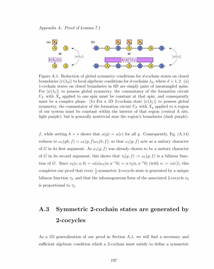
Appendix A. Proof of Lemma 7.1
Xg
A
(a) (b)Xg
A A B
Xg Xg
ABA B=
A A
=
2
B
AB ABA B B
Figure A.1: Reduction of global symmetry conditions for d-cochain states on closedboundaries |ψ(λd)〉 to local algebraic conditions for d-cochains λd, where d = 1, 2. (a)1-cochain states on closed boundaries in 0D are simply pairs of unentangled spins.For |ψ(λ1)〉 to possess global symmetry, the commutator of the formation circuitUF with Xg applied to one spin must be constant at that spin, and consequentlymust be a complex phase. (b) For a 1D 2-cochain state |ψ(λ1)〉 to possess globalsymmetry, the commutator of the formation circuit UF with Xg applied to a regionof our system must be constant within the interior of that region (central A site,light purple), but is generally nontrivial near the region’s boundaries (dark purple).
f , while setting h = e shows that α(g) = α(e) for all g. Consequently, Eq. (A.14)
reduces to ω1(gh; f) = ω1(g; f)ω1(h; f), so that ω1(g; f) acts as a unitary character
of G in its first argument. As ω1(g; f) was already chosen to be a unitary character
of G in its second argument, this shows that τ2(g, f) := ω1(g; f) is a bilinear func-
tion of G. Since ν2(e, a, b) = α(a)ω1(a; a−1b) = α τ2(a, a−1b) (with α := α(e)), this
completes our proof that every 12-symmetric 2-cocycle state is generated by a unique
bilinear function τ2, and that the inhomogeneous form of the associated 2-cocycle ν2
is proportional to τ2.
A.3 Symmetric 2-cochain states are generated by
2-cocycles
As a 1D generalization of our proof in Section A.1, we will find a necessary and
sufficient algebraic condition which a 2-cochain must satisfy to define a symmetric
197

Appendix A. Proof of Lemma 7.1
2-cochain state on closed boundaries. We will show that any such 2-cochain state is
generated by a unique 2-cocycle ν2, and that its associated 2-cochain can be factorized
as λ2(e, a, b) = ν2(e, a, b)λ(A)∗1 (e, a)λ
(B)1 (e, b). Here, λ
(A)1 and λ
(B)1 are homogeneous
1-cochains which end up only acting on the boundaries of our system. Consequently,
the state generated by λ2 on closed boundaries is exactly the same as that generated
by ν2, so that we can always associated a unique 2-cocycle to every globally symmetric
2-cochain state. This result will be used in Section A.4 to prove the d = 3 version of
Lemma 7.1.
The condition of being symmetric on closed boundaries in 1D is that the com-
mutator K(X⊗ng−1 , UF ) of our formation circuit with arbitrary global symmetry op-
erators is globally trivial. At a local level, this commutator can be expressed as a
product of two-body “defect gates” associated with the commutator η2(g; e, a, b) :=
K(X(A,B)†g , λ2(e, a, b)), and global symmetry requires the product of these defect
gates to be trivial in the interior of any region it is being transversally applied to
(see Figure A.1b). This implies that the A-interior product η2(g; e, a, b)η∗2(g; e, a, b′)
should be independent of a, and that the B-interior product η2(g; e, a, b)η∗2(g; e, a′, b)
should be independent of b. As we show below, these two algebraic conditions alone
are sufficient to show that the state generated by λ2 is a 2-cocycle state.
Before going further, we first derive an important consistency relation involving
η2. Since η2(g; e, a, b) = λ2(e, ga, gb)λ∗2(e, a, b), we have that
η2(gh; e, a, b) = λ2(e, gha, ghb)λ∗2(e, a, b) (A.15)
= (λ2(e, gha, ghb)λ∗2(e, ha, hb)) (λ2(e, ha, hb)λ∗2(e, a, b)) (A.16)
= η2(g; e, ha, hb)η2(h; e, a, b). (A.17)
We will make use of Eq. (A.17) shortly, but for now focus on expanding the algebraic
conditions mentioned above which arise from global symmetry. These conditions
require that certain overlapping products of η2(g; e, a, b) terms must be independent
198

Appendix A. Proof of Lemma 7.1
of the value taken within their region of overlap. This can be expressed as the
vanishing of double commutators
K(X(A)†h , η2(g; e, a, b)η∗2(g; e, a, b′)) =
η2(g; e, ha, b)η2(g; e, a, b′)
η2(g; e, a, b)η2(g; e, ha, b′)= 1 (A.18)
K(X(B)†h , η2(g; e, a, b)η∗2(g; e, a′, b)) =
η2(g; e, a, hb)η2(g; e, a′, b)
η2(g; e, a, b)η2(g; e, a′, hb)= 1 (A.19)
In order for Eqn.’s A.18 and A.18 to hold, we must have η2(g; e, ha, b)η∗2(g; e, a, b) be
independent of b, and η2(g; e, a, hb)η∗2(g; e, a, b) be independent of a, which lets us de-
fine ω(A)2 (g, h; e, a) := η2(g; e, ha, e)η∗2(g; e, a, e) and ω
(B)2 (g, h; e, b) := η2(g; e, e, hb)η∗2(g; e, b).
This allows us to express η2(g; e, a, b) as
η2(g; e, a, b) = ω(A)2 (g, a; e, e)η2(g; e, e, b) = α(g)ω
(A)2 (g, a)ω
(B)2 (g, b), (A.20)
where α(g) := η2(g; e, e, e), and we have chosen to abbreviate ω(A)2 (g, a) := ω
(A)2 (g, a; e, e)
and ω(B)2 (g, b) := ω
(B)2 (g, b; e, e). We can now insert this expression for η2 into
Eq. (A.17), which gives the following consistency relation between α, ω(A)2 , and ω
(B)2
∂1α(g, h) =α(g)α∗(gh)α(h)
=(ω
(A)2 (g, ha)ω
(A)∗2 (gh, a)ω
(A)2 (h, a)
)∗(ω
(B)2 (g, hb)ω
(B)∗2 (gh, b)ω
(B)2 (h, b)
)∗(A.21)
=ω(A)∗2 (g, h)ω
(B)2 (g, h),
where the last equality in Eq. (A.21) comes from setting a = b = e and using the
fact that ω(A)2 (h, e) = ω
(B)2 (h, e) = 1. This is allowed, since the second equality in
Eq. (A.21) reveals this quantity to be independent of a and b. Consequently, we have
that ω(A)2 (g, a) =
(ω
(B)2 (g, a) ∂1α(g, a)
)∗, which can be used to revise our expression
for η2(g; e, a, b) = α(ga)α∗(a)ω(B)∗2 (g, a)ω
(B)2 (g, b). We insert this back into Eq. (A.17)
to obtain(ω
(B)2 (g, ha)ω
(B)∗2 (gh, a)ω
(B)2 (h, a)
)(ω
(B)2 (g, hb)ω
(B)∗2 (gh, b)ω
(B)2 (h, b)
)∗= 1. (A.22)
199

Appendix A. Proof of Lemma 7.1
Because of the factorization of Eq. (A.22) into terms which depend only on a or only
on b, each term must be equal to some function of g and h alone, which we will
call φ(g, h) := ω(B)2 (g, hb)ω
(B)∗2 (gh, b)ω
(B)2 (h, b). Setting b = e in this expression for
φ(g, h) reveals that φ(g, h) = ω(B)2 (g, h), which is a key result. We can insert this
into our definition of φ(g, h) to show that ω(B)2 is a valid inhomogeneous 2-cocycle,
via
∂2ω(B)2 (g, h, b) = ω
(B)2 (h, b)ω
(B)∗2 (gh, b)ω
(B)2 (g, hb)ω
(B)∗
2 (g, h) = 1. (A.23)
With this 2-cocycle in hand, we can quickly express our original 2-cochain λ2 as
a homogeneous 2-cocycle with additional boundary terms. In particular, from our
original definition of η2(g; e, a, b), we see that λ2(e, a, b) = η2(a; e, e, a−1b)λ1(a, b),
where λ1(a, b) := λ2(e, e, a−1b) is a homogeneous 1-cochain. We can use this to
obtain
λ2(e, a, b) = α∗(e)ω(B)∗2 (a, e)α(a)λ1(a, b)ω
(B)2 (a, a−1b) (A.24)
=(∂1λ1(e, a, b)ω
(B)2 (a, a−1b)
)(α(a)λ∗1(e, a))λ1(e, b) (A.25)
= ν2(e, a, b)λ(A)∗1 (e, a)λ
(B)1 (e, b). (A.26)
In the second equality above, we have chosen to rewrite λ1(a, b) in terms of the ho-
mogeneous 2-coboundary ∂1λ1(e, a, b), whereas in the third equality, we have defined
λ(A)1 (e, a) := α∗(a)λ1(e, a), λ
(B)1 (e, b) := λ1(e, b), and ν2(e, a, b) := ∂1λ1(e, a, b)ω
(B)2 (a, a−1b).
From its definition, it is clear that ν2(e, a, b) is a valid homogeneous 2-cocycle, and
this consequently completes our proof that any symmetric 2-cochain state is gener-
ated by a unique 2-cocycle.
200

Appendix A. Proof of Lemma 7.1
A.4 13-symmetric 3-cocycle states are generated by
trilinear functions (Lemma 7.1, d = 3)
We now consider 2D 3-cocycle states with 13-symmetry, which we will show are each
generated by a unique trilinear function. Furthermore, we will show that the associ-
ated 3-cocycle must itself be a trilinear function, up to terms which only act on the
boundaries of our system. We take a similar approach as was done in Section A.2,
where we reduce the global 13-symmetry condition on the state |ψ(ν3)〉 to a local al-
gebraic condition on the 3-cocycle ν3. If our global formation circuit is UF , then we
must have the commutator of UF with an A-site symmetry operator, K(UF , X(A)g ),
be trivial at this A site. This commutator, which is only supported on the B and C
sites surrounding our A site, is given by
K(UF , X(A)g ) =
∏<i,j>
(ν3(e, a, bi, cj)ν
∗3(e, g−1a, bi, cj)
)(A.27)
=∏<i,j>
ν3(g−1a, a, bi, cj) =∏<i,j>
λ2(g; a, bi, cj), (A.28)
where λ2(g; a, bi, cj) := ν3(g−1a, a, bi, cj), and the second equality comes from using
a standard 3-cocycle identity. It is clear that λ2(g; a, b, c) is a 2-cocycle with re-
spect to a, b, and c, and the above commutator being trivial on its associated A
site is equivalent to λ2(g; a, b, c) generating a symmetric 1D state on closed bound-
aries. From Section A.3, we know that each λ2(g) must have the form λ2(g; a, b, c) =
ν2(g; a, b, c)λ(B)∗1 (g; a, b)λ
(C)1 (g; a, c), where each ν2(g) is a 2-cocycle, and all λ
(B)1 (g)’s,
λ(C)1 (g)’s are 1-cochains. While this condition on λ2(g) comes only from assuming
fractional symmetry with respect to A-site symmetries, full 13-symmetry requires
more, namely that each λ2(g) generates a 12-symmetric 1D state. From Section A.2,
we know that this forces each ν2(g) to be associated with a unique bilinear function
τ2(g). Consequently, we can make use of the ansatz ν3(e, a, b, c) = λ2(a; a, b, c) =
201
Appendix A. Proof of Lemma 7.1
τ2(a; a−1b, b−1c)λ∗1(a; a, b)λ1(a; a, c)β1(a; a, b), where λ1(g; a, c) := λ(C)1 (g; a, c) and
β1(g; a, b) := λ(B)∗1 (g; a, b)λ
(C)1 (g; a, b).
With this ansatz for ν3 in hand, we can now use the 3-cocycle nature of ν3 to
constrain the manner in which the 1-cochains λ1(g; a, c) and β1(g; a, b), as well as the
bilinear 2-cocycles τ2(g; a, b, c), vary with g. If we take the commutator of ν3(e, a, b, c)
with the global symmetry operator X⊗ng , we obtain
K(ν3(e, a, b, c), X⊗ng ) = ν3(e, a, b, c)ν∗3(e, g−1a, g−1b, g−1c) (A.29)
= τ2(a; a−1b, b−1c)τ ∗2 (g−1a; a−1b, b−1c)×(λ∗1(a; a, b)λ1(a; a, c)β1(a; a, b)
λ∗1(g−1a; a, b)λ1(g−1a; a, c)β1(g−1a; a, b)
)(A.30)
= ν3(e, g, a, b)ν∗3(e, g, a, c)ν3(e, g, b, c) (A.31)
= τ2(g; a−1b, b−1c)β1(g; g, b). (A.32)
In Eq. (A.30), we directly substitute our ansatz for each factor of ν3, whereas in
Eq. (A.32) we first use a standard 3-cocycle identity, then substitute for each ν3
factor. In order for these expressions to be equal, we must have the following hold
for all g, h, f ∈ G:
τ ∗2 (a; a−1b, b−1c)τ2(g; a−1b, b−1c)τ2(g−1a; a−1b, b−1c) = (A.33)
λ∗1(a; a, b)λ1(a; a, c)β1(a; a, b)β∗1(g; g, b)
λ∗1(g−1a; a, b)λ1(g−1a; a, c)β1(g−1a; a, b).
(A.34)
Eq. (A.34) can be used to generate general constraints on the λ1(g; a, c), β1(g; a, b),
and τ2(g; a, b, c) by considering particular values of g, a, b, and c. To begin with,
setting g = e gives the constraint τ2(e; a−1b, b−1c) = β∗1(e; e, b), which holds for all
values of a, b, and c. Choosing a = b = c shows that β1(e; e, a) = τ2(e; e, e) = 1,
where the last equality comes from the fact that τ2(g;h, f) = 1 whenever h = e or
f = e. Consequently, this shows that β1(e; a, b) = τ2(e; a−1b, b−1c) = 1.
202

Appendix A. Proof of Lemma 7.1
We can now set b = c to obtain β1(a; a, b)β∗1(g−1a; a, b)β∗1(g; g, b) = 1, which shows
that the factors of β1 appearing in Eq. (A.34) are collectively trivial. This lets us
update Eq. (A.34) to read
τ ∗2 (a; a−1b, b−1c)τ2(g; a−1b, b−1c)τ2(g−1a; a−1b, b−1c) =λ∗1(a; a, b)λ1(a; a, c)
λ∗1(g−1a; a, b)λ1(g−1a; a, c).
(A.35)
We can now set a = b in the above expression to obtain λ1(a; a, c)λ∗1(g−1a; a, c) =
δ(a)δ∗1(g−1a), where we have defined δ1(a) := λ1(a; e, e). This substitution allows us
to replace the entire right hand side of Eq. (A.35), obtaining
τ ∗2 (a; a−1b, b−1c)τ2(g; a−1b, b−1c)τ2(g−1a; a−1b, b−1c) = 1. (A.36)
Eq. (A.36) clearly shows that the three-index function τ3(g, h, f) := τ2(g;h, f) is
a unitary character of G with respect to its first argument, while the bilinear na-
ture of each τ2(g) guarantees that τ3 is a character in its other arguments as well.
Consequently, this proves that τ3 is a trilinear function of G, and that our original
3-cocycle is related to τ3 as ν3(e, a, b, c) = τ3(a, a−1b, b−1c)λ(B)∗1 (a; a, b)λ
(C)1 (a; a, c).
Since these last two parameterized 1-cochains act as 2-body terms between A and B
(or A and C) sites, they multiply away on closed boundaries, with the resulting state
identical to that generated by τ3, i.e. |ψ(ν3)〉 = |ψ(τ3)〉. This completes our proof of
Lemma 7.1 for d = 3.
203

References
A
[AA13] S. Aaronson and A. Arkhipov, The computational complexity of linearoptics, Theory of Computing 9, 143–252 (2013).
[AC16] S. Aaronson and L.-J. Chen, Complexity-theoretic foundations of quan-tum supremacy experiments, arXiv:1612.05903, (2016).
[AG04] S. Aaronson and D. Gottesman, Improved simulation of stabilizer cir-cuits, Phys. Rev. A 70, 052328 (2004).
[AKLT87] I. Affleck, T. Kennedy, E. H. Lieb, and H. Tasaki, Rigorous results onvalence-bond ground states in antiferromagnets, Phys. Rev. Lett. 59,799 (1987).
[AKLT88] I. Affleck, T. Kennedy, E. H. Lieb, and H. Tasaki, Valence bond groundstates in isotropic quantum antiferromagnets, Comm. Math. Phys.115, 477 (1988).
[AKM14] M. Aspelmeyer, T. J. Kippenberg, and F. Marquardt, Cavity optome-chanics, Rev. Mod. Phys. 86, 1391 (2014).
B
[B+16] S. Boixo et al., Characterizing quantum supremacy in near-term devices,arXiv:1608.00263 (2016).
[Bau11] R. B. Bauer, Tensor network states, PhD thesis, ETH Zurich (2011).
204

References
[BBD+09a] S. D. Barrett, S. D. Bartlett, A. C. Doherty, D. Jennings, andT. Rudolph, Transitions in the computational power of thermal statesfor measurement-based quantum computation, Phys. Rev. A 80, 062328(2009).
[BBD+09b] H. J. Briegel, D. E. Browne, W. Dur, R. Raussendorf, and M. V. denNest, Measurement-based quantum computation, Nature Physics 5,19–26 (2009).
[BBM+10] S. D. Bartlett, G. K. Brennen, A. Miyake, , and J. M. Renes, Quantumcomputational renormalization in the haldane phase, Phys. Rev. Lett.105, 110502 (2010).
[BCFV14] F. Burnell, X. Chen, L. Fidkowski, and A. Vishwanath, Exactly solu-ble model of a 3d symmetry protected topological phase of bosons withsurface topological order, Phys. Rev. B 90, 245122 (2014).
[BCJD99] G. K. Brennen, C. M. Caves, P. S. Jessen, and I. H. Deutsch, Quantumlogic gates in optical lattices, Phys. Rev. Lett. 82, 1060 (1999).
[BEF+08] D. E. Brown, M. B. Elliott, S. T. Flammia, S. T. Merkel, A. Miyake,and A. J. Short, Phase transition of computational power in the resourcestates for one-way quantum computation, New. J. Phys. 10, 023010(2008).
[BFN08] P. Bonderson, M. Freedman, and C. Nayak, Measurement-only topolog-ical quantum computation, Phys. Rev. Lett. 101, 010501 (2008).
[BFN09] P. Bonderson, M. Freedman, and C. Nayak, Measurement-only topo-logical quantum computation via anyonic interferometry, Annals ofPhysics 324, 787–826 (2009).
[BFRK+13] M. A. Broome, A. Fedrizzi, S. Rahimi-Keshari, J. Dove, S. Aaronson,T. Ralph, and A. G. White, Photonic boson sampling in a tunablecircuit, Science 339, 794–798 (2013).
[BJS11] M. J. Bremner, R. Jozsa, and D. J. Shepherd, Classical simulationof commuting quantum computations implies collapse of the polynomialhierarchy, Proc. R. Soc. A 467, 459–472 (2011).
[BK05] S. Bravyi and A. Kitaev, Universal quantum computation with idealclifford gates and noisy ancillas, Phys. Rev. A 71, 022316 (2005).
205

References
[BM08] G. K. Brennen and A. Miyake, Measurement-based quantum computerin the gapped ground state of a two-body hamiltonian, Phys. Rev. Lett.101, 010502 (2008).
[BMD06] H. Bombin and M. A. Martın-Delgado, Topological quantum distillation,Phys. Rev. Lett. 97, 180501 (2006).
[BMS16a] M. Bremner, A. Montanaro, and D. Shepherd, Achieving quantumsupremacy with sparse and noisy commuting quantum computations,arXiv:1610.01808 (2016).
[BMS16b] M. J. Bremner, A. Montanaro, and D. J. Shepherd, Average-case com-plexity versus approximate simulation of commuting quantum computa-tions, Phys. Rev. Lett. 117, 080501 (2016).
[BR01] H. J. Briegel and R. Raussendorf, Persistent entanglement in arrays ofinteracting particles, Phys. Rev. Lett. 86, 910 (2001).
[BR06] S. Bravyi and R. Raussendorf, On measurement-based quantum com-putation with the toric code states, arXiv:quant-ph/0610162 (2006).
[BVHS+17] J. Bermejo-Vega, D. Hangleiter, M. Schwarz, R. Raussendorf, andJ. Eisert, Architectures for quantum simulation showing quantumsupremacy, arXiv:1703.00466 (2017).
C
[C+13] A. Crespi et al., Integrated multimode interferometers with arbitrary de-signs for photonic boson sampling, Nature Photon. 7, 545–549 (2013).
[CB08] G. M. Crosswhite and D. Bacon, Finite automata for caching in matrixproduct algorithms, Phys. Rev. A 78, 012356 (2008).
[CDJZ10] X. Chen, R. Duan, Z. Ji, and B. Zeng, Quantum state reduction for uni-versal measurement based computation, Phys. Rev. Lett. 105, 020502(2010).
[CGLW12] X. Chen, Z.-C. Gu, Z.-X. Liu, and X.-G. Wen, Symmetry protectedtopological orders in interacting bosonic systems, Science 338, 1604(2012).
[CGLW13] X. Chen, Z.-C. Gu, Z.-X. Liu, and X.-G. Wen, Symmetry protectedtopological orders and the group cohomology of their symmetry group,Phys. Rev. B 87, 155114 (2013).
206

References
[CGW10] X. Chen, Z.-C. Gu, and X.-G. Wen, Local unitary transformation, long-range quantum entanglement, wave function renormalization, and topo-logical order, Phys. Rev. B 82, 155138 (2010).
[CGW11] X. Chen, Z. C. Gu, and X. G. Wen, Classification of gapped symmetricphases in one-dimensional spin systems, Phys. Rev. B 83, 035107(2011).
[CH13] L. Childress and R. Hanson, Diamond nv centers for quantum comput-ing and quantum networks, MRS bulletin 38, 134–138 (2013).
[CLLS12] G. D. Chiara, L. Lepori, M. Lewenstein, and A. Sanpera, Entangle-ment spectrum, critical exponents, and order parameters in quantumspin chains, Phys. Rev. Lett. 109, 237208 (2012).
[CLV14] X. Chen, Y.-M. Lu, and A. Vishwanath, Symmetry-protected topologicalphases from decorated domain walls, Nat. Commun. 5, 3507 (2014).
[CLW11] X. Chen, Z.-X. Liu, and X.-G. Wen, Two-dimensional symmetry-protected topological orders and their protected gapless edge excitations,Phys. Rev. B 84, 235141 (2011).
[CMDB10] J.-M. Cai, A. Miyake, W. D”ur, and H. J. Briegel, Universal quantumcomputer from a quantum magnet, Phys. Rev. A 82, 052309 (2010).
[CR14] I. Cohen and A. Retzker, Proposal for verification of the haldane phaseusing trapped ions, Phys. Rev. Lett. 112, 040503 (2014).
[CZ12] J. I. Cirac and P. Zoller, Goals and opportunities in quantum simulation,Nat. Phys. 8, 264 (2012).
[CZG+09] X. Chen, B. Zeng, Z.-C. Gu, B. Yoshida, and I. L. Chuang, Gappedtwo-body hamiltonian whose unique ground state is universal for one-way quantum computation, Phys. Rev. Lett. 102, 220501 (2009).
D
[DB09] A. C. Doherty and S. D. Bartlett, Identifying phases of quantum many-body systems that are universal for quantum computation, Phys. Rev.Lett. 103, 020506 (2009).
[DBB12] A. S. Darmawan, G. K. Brennen, and S. D. Bartlett, Measurement-basedquantum computation in a two-dimensional phase of matter, New J.Phys. 14, 013023 (2012).
207

References
[DCJ+07] M. G. Dutt, L. Childress, L. Jiang, E. Togan, J. Maze, F. Jelezko, A. Zi-brov, P. Hemmer, and M. Lukin, Quantum register based on individualelectronic and nuclear spin qubits in diamond, Science 316, 1312–1316(2007).
[DFFFG17] A. Deshpande, B. Fefferman, M. Foss-Feig, and A. V. Gorshkov, Com-plexity of sampling as an order parameter, arXiv:1703.05332 (2017).
[DGPS99] F. Dalfovo, S. Giorgini, L. P. Pitaevskii, and S. Stringari, Theory ofbose-einstein condensation in trapped gases, Rev. Mod. Phys. 71, 463(1999).
[DJ92] D. Deutsch and R. Jozsa, Rapid solution of problems by quantum com-putation, Proc. R. Soc. A 439, 553 (1992).
[DM10] L.-M. Duan and C. Monroe, Colloquium: Quantum networks withtrapped ions, Rev. Mod. Phys. 82, 1209 (2010).
[dNDMB07] M. V. den Nest, W. Dur, A. Miyake, and H. J. Briegel, Fundamentals ofuniversality in one-way quantum computation, New J. Phys. 9 (2007).
[dNMDB06] M. V. den Nest, A. Miyake, W. Dur, and H. J. Briegel, Universalresources for measurement-based quantum computation, Phys. Rev.Lett. 97, 150504 (2006).
[dNR89] M. den Nijs and K. Rommelse, Preroughning transitions in crystalsurfaces and valence-bond phases in quantum spin chains, Phys. Rev.B 40, 4709 (1989).
[dWP95] M. de Wild Propitius, Topological interactions in broken gauge theories,PhD thesis, University of Amsterdam (1995).
E
[EBD12] D. V. Else, S. D. Bartlett, and A. C. Doherty, Symmetry protectionof measurement-based quantum computation in ground states, New J.Phys. 14, 113016 (2012).
[ECP10] J. Eisert, M. Cramer, and M. B. Plenio, Colloquium: Area laws for theentanglement entropy, Rev. Mod. Phys. 82, 277 (2010).
[EFG15] J. Eisert, M. Friesdorf, and C. Gogolin, Quantum many-body systemsout of equilibrium, Nat. Phys. 11, 124 (2015).
208

References
[Eis13] J. Eisert, Entanglement and tensor network states, arXiv:1308.3318(2013).
[EK90] A. Ehrenfeucht and M. Karpinski, The computational complexity of(xor, and)-counting problems, Technical report, -CS (1990).
[EN14] D. V. Else and C. Nayak, Classifying symmetry-protected topologi-cal phases through the anomalous action of the symmetry on the edge,Phys. Rev. B 90, 235137 (2014).
[ESBD12] D. V. Else, I. Schwarz, S. D. Bartlett, and A. C. Doherty, Symmetry-protected phases for measurement-based quantum computation, Phys.Rev. Lett. 108, 240505 (2012).
F
[FFFG17] B. Fefferman, M. Foss-Feig, and A. V. Gorshkov, Exact sampling hard-ness of ising spin models, arXiv:1701.03167 (2017).
[FH16] E. Farhi and A. W. Harrow, Quantum supremacy through the quantumapproximate optimization algorithm, arXiv:1602.07674 (2016).
[FHA98] R. P. Feynman, J. Hey, and R. W. Allen, Feynman lectures on compu-tation, Addison-Wesley Longman Publishing Co., Inc. (1998).
[FM12] K. Fujii and T. Morimae, Topologically protected measurement-basedquantum computation on the thermal state of a nearest-neighbor two-body hamiltonian with spin-3/2 particles, Phys. Rev. A 85, 010304(R)(2012).
[FNOM13] K. Fujii, Y. Nakata, M. Ohzeki, and M. Murao, Measurement-basedquantum computation on symmetry breaking thermal states, Phys.Rev. Lett. 110, 120502 (2013).
[FNW92] M. Fannes, B. Nachtergaele, and R. F. Werner, Finitely correlated stateson quantum spin chains, Comm. Math. Phys., 144, 443 (1992).
[Fuj16] K. Fujii, Noise threshold of quantum supremacy, arXiv:1610.03632(2016).
209
References
G
[GAN14] I. M. Georgescu, S. Ashhab, and F. Nori, Quantum simulation, Rev.Mod. Phys. 86, 153 (2014).
[GC99] D. Gottesman and I. L. Chuang, Demonstrating the viability of universalquantum computation using teleportation and single-qubit operations,Nature 402, 390 (1999).
[GCS+14] O. Guhne, M. Cuquet, F. E. S. Steinhoff, T. Moroder, M. Rossi,D. Bruß, B. Kraus, and C. Macchiavello, Entanglement and nonclassicalproperties of hypergraph states, J. Phys. A 47, 335303 (2014).
[GE07] D. Gross and J. Eisert, Novel schemes for measurement-based quantumcomputation, Phys. Rev. Lett. 98, 220503 (2007).
[GESPG07] D. Gross, J. Eisert, N. Schuch, and D. Perez-Garcıa, Measurement-based quantum computation beyond the one-way model, Phys. Rev. A76, 052315 (2007).
[Got97] D. Gottesman, Stabilizer codes and quantum error correction, PhDthesis, Caltech (1997).
[Got98] D. Gottesman, The heisenberg representation of quantum computers, Intalk at International Conference on Group Theoretic Methods in Physics(1998).
[Gri95] D. J. Griffiths, Introduction to quantum mechanics, Prentice Hall(1995).
[Gro97] L. K. Grover, Quantum mechanics helps in searching for a needle in ahaystack, Phys. Rev. Lett. 79, 325 (1997).
[GW09] Z. C. Gu and X. G. Wen, Tensor-entanglement-filtering renormalizationapproach and symmetry-protected topological order, Phys. Rev. B 80,155131 (2009).
[GWD17] X. Gao, S.-T. Wang, and L.-M. Duan, Quantum supremacy for simu-lating a translation-invariant ising spin model, Phys. Rev. Lett. 118,040502 (2017).
210

References
H
[H+06] M. Hein et al., Entanglement in graph states and its applications, Tech-nical report, in Quantum Computers, Algorithms and Chaos Vol. 162,Int. School of Physics Enrico Fermi (eds Casati, G et al.), 115–218 (IOSPress) (2006).
[Hal83a] F. D. M. Haldane, Continuum dynamics of the 1-d heisenberg antifer-romagnet: identification with the o (3) nonlinear sigma model, PhysicsLetters A 93, 464–468 (1983).
[Hal83b] F. Haldane, Nonlinear field theory of large-spin heisenberg antiferromag-nets: semiclassically quantized solitons of the one-dimensional easy-axisneel state, Phys. Rev. Lett. 50, 1153 (1983).
[HEB04] M. Hein, J. Eisert, and H. J. Briegel, Multiparty entanglement in graphstates, Phys. Rev. A 69, 062311 (2004).
[HK10] M. Z. Hasan and C. L. Kane, Colloquium: Topological insulators, Rev.Mod. Phys. 82, 3045 (2010).
[HKSE17] D. Hangleiter, M. Kliesch, M. Schwarz, and J. Eisert, Direct certificationof a class of quantum simulations, Quantum Science and Technology2, 015004 (2017).
[HSP10] K. Hammerer, A. S. Sørensen, and E. S. Polzik, Quantum interfacebetween light and atomic ensembles, Rev. Mod. Phys. 82, 1041 (2010).
J
[JBC+99] D. Jaksch, H.-J. Briegel, J. Cirac, C. Gardiner, and P. Zoller, Entan-glement of atoms via cold controlled collisions, Phys. Rev. Lett. 82,1975 (1999).
[JN13] R. Jozsa and M. V. d. Nest, Classical simulation complexity of extendedclifford circuits, arXiv:1305.6190 (2013).
[JOV+08] J. Jordan, R. Orus, G. Vidal, F. Verstraete, and J. I. Cirac, Clas-sical simulation of infinite-size quantum lattice systems in two spatialdimensions, Phys. Rev. Lett. 101, 250602 (2008).
[Joz05] R. Jozsa, An introduction to measurement based quantum computation,arXiv:quant-ph/0508124 (2005).
211

References
K
[K+12] S. Korenblit et al., Quantum simulation of spin models on an arbitrarylattice with trapped ions, New J. Phys. 14, 095024 (2012).
[KD17] T. Kapourniotis and A. Datta, nNonadaptive fault-tolerant verificationof quantum supremacy with noise, arXiv:1703.09568 (2017).
[Kit03] A. Kitaev, Fault-tolerant quantum computation by anyons, Ann. Phys.303, 2 (2003).
[Kit09] A. Kitaev, Periodic table for topological insulators and superconductors,In AIP Conf. Proc. 1134, 22 (2009).
[KKOS12] H. Kalis, D. Klagges, R. Orus, and K. P. Schmidt, Fate of the clusterstate on the square lattice in a magnetic field, Phys. Rev. A 86, 022317(2012).
[KL10] A. Kitaev and C. Laumann, Topological phases and quantum computa-tion, Oxford University Press (2010).
[KMN+07] P. Kok, W. J. Munro, K. Nemoto, T. C. Ralph, J. P. Dowling, and G. J.Milburn, Linear optical quantum computing with photonic qubits, Rev.Mod. Phys. 79, 135 (2007).
L
[L+11] Y. Li et al., Thermal states as universal resources for quantum com-putation with always-on interactions, Phys. Rev. Lett. 107, 060501(2011).
[LBR17] A. P. Lund, M. J. Bremner, and T. C. Ralph, Quantum samplingproblems, bosonsampling and quantum supremacy, arXiv:1702.03061(2017).
[LD98] D. Loss and D. P. DiVincenzo, Quantum computation with quantumdots, Phys. Rev. A 57, 120 (1998).
[LG12] M. Levin and Z.-C. Gu, Braiding statistics approach to symmetry-protected topological phases, Phys. Rev. B 86, 115109 (2012).
212

References
[LH08] H. Li and F. D. M. Haldane, Entanglement spectrum as a general-ization of entanglement entropy: Identification of topological order innon-abelian fractional quantum hall effect states, Phys. Rev. Lett.101, 010504 (2008).
[LJL+10] T. D. Ladd, F. Jelezko, R. Laflamme, Y. Nakamura, C. Monroe, andJ. L. OBrien, Quantum computers, Nature 464, 45–53 (2010).
M
[MFF14] T. Morimae, K. Fujii, and J. F. Fitzsimons, On the hardness of clas-sically simulating the one clean qubit model, Phys. Rev. Lett. 112,130502 (2014).
[Miy10] A. Miyake, Quantum computation on the edge of a symmetry-protectedtopological order, Phys. Rev. Lett. 105, 040501 (2010).
[Miy11] A. Miyake, Quantum computational capability of a 2d valence bond solidphase, Ann. Phys. 326, 1656 (2011).
[MK04] H.-J. Mikeska and A. K. Kolezhuk, One-dimensional magnetism, InQuantum magnetism, pages 1–83, Springer (2004).
[MM15] J. Miller and A. Miyake, Resource quality of a symmetry-protectedtopologically ordered phase for quantum computation, Phys. Rev. Lett.114, 120506 (2015).
[MM16] J. Miller and A. Miyake, Hierarchy of universal entanglement in 2dmeasurement-based quantum computation, npj Quantum Information2, 16036 (2016).
[MR13] A. Mesaros and Y. Ran, Classification of symmetry enriched topologicalphases with exactly solvable models, Phys. Rev. B 87, 155115 (2013).
[MS72] A. R. Meyer and L. J. Stockmeyer, The equivalence problem for regularexpressions with squaring requires exponential space, In Proceedings ofthe 13th IEEE Symposium on Switching and Automata Theory, pages125–129 (1972).
[MSS01] Y. Makhlin, G. Schon, and A. Shnirman, Quantum-state engineeringwith josephson-junction devices, Rev. Mod. Phys. 73, 357 (2001).
[MTH17] T. Morimae, Y. Takeuchi, and M. Hayashi, Verified measurement-basedquantum computing with hypergraph states, arXiv:1701.05688 (2017).
213

References
N
[NAJ09] J. Novotny, G. Alber, and I. Jex, Random unitary dynamics of quantumnetworks, J. Phys. A 42, 282003 (2009).
[NC00] M. A. Nielsen and I. Chuang, Quantum computation and quantuminformation, Cambridge University Press (2000).
[Nie06] M. A. Nielsen, Cluster-state quantum computation, Reports on Math-ematical Physics 57, 147–161 (2006).
[NSS+08] C. Nayak, S. H. Simon, A. Stern, M. Freedman, and S. D. Sarma, Non-abelian anyons and topological quantum computation, Rev. Mod. Phys.80, 1083 (2008).
[NW15] H. P. Nautrup and T.-C. Wei, Symmetry-protected topologically orderedstates for universal quantum computation, Phys. Rev. A 92, 052309(2015).
O
[OKBS13] R. Orus, H. Kalis, M. Bornemann, and K. P. Schmidt, Bounds onuniversal quantum computation with perturbed two-dimensional clusterstates, Phys. Rev. A 87, 062312 (2013).
[Oru14] R. Orus, A practical introduction to tensor networks: Matrix productstates and projected entangled pair states, Annals of Physics 349, 117–158 (2014).
P
[PBTO12] F. Pollmann, E. Berg, A. M. Turner, and M. Oshikawa, Symmetry pro-tection of topological phases in one-dimensional quantum spin systems,Phys. Rev. B 85, 075125 (2012).
[PGVCW07] D. Perez-Garcia, F. Verstraete, J. I. Cirac, and M. M. Wolf, Peps asunique ground states of local hamiltonians, arXiv:0707.2260 (2007).
[PGVWC07] D. Perez-Garcıa, F. Verstraete, M. M. Wolf, and J. I. Cirac, Matrixproduct state representations, Quantum Inf. Comput. 7, 401 (2007).
214

References
[PGWS+08] D. Perez-Garcıa, M. M. Wolf, M. Sanz, F. Verstraete, and J. I. Cirac,String order and symmetries in quantum spin lattices, Phys. Rev. Lett.100, 167202 (2008).
[PT12] F. Pollmann and A. M. Turner, Detection of symmetry-protected topo-logical phases in one dimension, Phys. Rev. B 86, 125441 (2012).
[PTBO10] F. Pollmann, A. M. Turner, E. Berg, and M. Oshikawa, Entanglementspectrum of a topological phase in one dimension, Phys. Rev. B 81,064439 (2010).
[PVMDC05] M. Popp, F. Verstraete, M. A. Martın-Delgado, and J. I. Cirac, Local-izable entanglement, Phys. Rev. A 71, 042306 (2005).
[PW15] A. Prakash and T.-C. Wei, Ground states of one-dimensional symmetry-protected topological phases and their utility as resource states for quan-tum computation, Phys. Rev. A 92, 022310 (2015).
Q
[QS01] M. Quirk and J. Serda, Semiconductor manufacturing technology, vol-ume 1, Prentice Hall Upper Saddle River, NJ (2001).
[QZ11] X.-L. Qi and S.-C. Zhang, Topological insulators and superconductors,Rev. Mod. Phys. 83, 1057 (2011).
R
[RB01] R. Raussendorf and H. J. Briegel, A one-way quantum computer, Phys.Rev. Lett. 86, 5188 (2001).
[RBB03] R. Raussendorf, D. E. Browne, and H. J. Briegel, Measurement-basedquantum computation on cluster states, Phys. Rev. A 68, 022312(2003).
[RBMD16] P. P. Rohde, D. W. Berry, K. R. Motes, and J. P. Dowling, A quan-tum optics argument for the #p-hardness of a class of multidimensionalintegrals, arXiv:1607.04960 (2016).
[RHBM13] M. Rossi, M. Huber, D. Bruß, and C. Macchiavello, Quantum hyper-graph states, New J. Phys. 15, 113022 (2013).
215

References
[RKRC16] S. Rahimi-Keshari, T. C. Ralph, and C. M. Caves, Sufficient conditionsfor efficient classical simulation of quantum optics, Phys. Rev. X 6,021039 (2016).
[RSFL10] S. Ryu, A. P. Schnyder, A. Furusaki, and A. W. Ludwig, Topological in-sulators and superconductors: Ten-fold way and dimensional hierarchy,New J. Phys. 12, 065010 (2010).
[RWP+16] R. Raussendorf, D.-S. Wang, A. Prakash, T.-C. Wei, and D. T.Stephen, Symmetry-protected topological phases with uniform computa-tional power in one dimension, arXiv:1609.07549 (2016).
[RYKB16] S. Roberts, B. Yoshida, A. Kubica, and S. D. Bartlett, Symmetryprotected topological order at nonzero temperature, arXiv:1611.05450(2016).
S
[S+13] J. B. Spring et al., Boson sampling on a photonic chip, Science 339,798–801 (2013).
[SA94] D. Stauffer and A. Aharony, Introduction to percolation theory, CRCpress (1994).
[SAF+11] W. Son, L. Amico, R. Fazio, A. Hamma, S. Pascazio, and V. Vedral,Quantum phase transition between cluster and antiferromagnetic states,Europhys. Lett. 95, 50001 (2011).
[SB09] S. O. Skrøvseth and S. D. Bartlett, Phase transitions and localizableentanglement in cluster-state spin chains with ising couplings and localfields, Phys. Rev. A 80, 022316 (2009).
[SC10] N. Schuch and J. I. Cirac, Matrix product state and mean-field solutionsfor one-dimensional systems can be found efficiently, Phys. Rev. A 82,012314 (2010).
[Sch04] I. Schur, Uber die darstellung der endlichen gruppen durch gebrochenelineare substitutionen, J. Reine Angew. Math 127, 20–50 (1904).
[Sch05] U. Schollwock, The density-matrix renormalization group, Rev. Mod.Phys. 77, 259 (2005).
[Sha94] R. Shankar, Principles of quantum mechanics, Plenum Press (1994).
216

References
[Shi03] Y.-Y. Shi, Both toffoli and controlled-not need little help to do universalquantum computation, Quantum Inf. Comput. 3, 84 (2003).
[Sho97] P. W. Shor, Polynomial-time algorithms for prime factorization anddiscrete logarithms on a quantum computer, SIAM J. Sci. Statist.Comput. 26, 1484 (1997).
[SLR17] F. Shahandeh, A. P. Lund, and T. C. Ralph, Quantum correlations innonlocal bosonsampling, arXiv:1702.02156 (2017).
[SMD98] G. Sierra and M. Martın-Delgado, The density matrix renormaliza-tion group, quantum groups and conformal field theory, arXiv:cond-mat/9811170 (1998).
[SP97] S. D. Sarma and A. Pinczuk, Perspectives in quantum hall effects: Novelquantum liquids in low-dimensional semiconductor structures, John Wi-ley & Sons (1997).
[SPGC11] N. Schuch, D. Perez-Garcıa, and J. I. Cirac, Classifying quantum phasesusing matrix product states and projected entangled pair states, Phys.Rev. B 84, 165139 (2011).
[SPM+10] K. Singer, U. Poschinger, M. Murphy, P. Ivanov, F. Ziesel, T. Calarco,and F. Schmidt-Kaler, Colloquium: Trapped ions as quantum bits: Es-sential numerical tools, Rev. Mod. Phys. 82, 2609 (2010).
[SRMG16] F. E. S. Steinhoff, C. Ritz, N. Miklin, and O. Guhne, Qudit hypergraphstates, arXiv:1612.06418 (2016).
[Ste98] A. Steane, Quantum computing, Reports on Progress in Physics 61,117 (1998).
[Sto77] L. J. Stockmeyer, The polynomial-time hierarchy, Theor. Comp. Sci.3, 1–22 (1977).
[Sto85] L. J. Stockmeyer, On approximation algorithms for #p, SIAM J.Comput. 14, 849–861 (1985).
[SWP+16] D. T. Stephen, D.-S. Wang, A. Prakash, T.-C. Wei, and R. Raussendorf,Determining the computational power of symmetry protected topologicalphases, arXiv:1611.08053 (2016).
[SWPGC09] M. Sanz, M. M. Wolf, D. Perez-Garcıa, and J. I. Cirac, Matrix prod-uct states: Symmetries and two-body hamiltonians, Phys. Rev. A 79,042308 (2009).
217

References
[SWVC07] N. Schuch, M. M. Wolf, F. Verstraete, and J. I. Cirac, Computationalcomplexity of projected entangled pair states, Phys. Rev. Lett. 98,140506 (2007).
T
[TD04] B. M. Terhal and D. P. DiVincenzo, Adaptive quantum computation,constant depth quantum circuits and arthur-merlin games, Quant. Inf.Comput. 4, 134–145 (2004).
[TDH+13] M. Tillmann, B. Dakic, R. Heilmann, S. Nolte, A. Szameit, andP. Walther, Experimental boson sampling, Nature Photon. 7, 540–544 (2013).
[Tod91] S. Toda, Pp is as hard as the polynomial-time hierarchy, SIAM J.Comput. 20, 865–877 (1991).
V
[VC04a] F. Verstraete and J. I. Cirac, Valence-bond states for quantum compu-tation, Phys. Rev. A 70, 060302 (2004).
[VC04b] F. Verstraete and J. Cirac, Renormalization algorithms for quantum-many body systems in two and higher dimensions, arXiv:cond-mat/0407066 (2004).
[VC06] F. Verstraete and J. I. Cirac, Matrix product states represent groundstates faithfully, Phys. Rev. B 73, 094423 (2006).
[VCM08] F. Verstraete, J. I. Cirac, and V. Murg, Matrix product states, projectedentangled pair states, and variational renormalization group methodsfor quantum spin systems, Adv. Phys. 57, 143 (2008).
[VGRC04] F. Verstraete, J. J. Garcia-Ripoll, and J. I. Cirac, Matrix product den-sity operators: simulation of finite-temperature and dissipative systems,Phys. Rev. Lett. 93, 207204 (2004).
[Vid03] G. Vidal, Efficient classical simulation of slightly entangled quantumcomputations, Phys. Rev. Lett. 91, 147902 (2003).
[Vid08] G. Vidal, Class of quantum many-body states that can be efficientlysimulated, Phys. Rev. Lett. 101, 110501 (2008).
218

References
[VR05] L. C. Venuti and M. Roncaglia, Analytic relations between localizableentanglement and string correlations in spin systems, Phys. Rev. Lett.94, 207207 (2005).
[VS13] A. Vishwanath and T. Senthil, Physics of three dimensional bosonictopological insulators: Surface deconfined criticality and quantized mag-netoelectric effect, Phys. Rev. X 3, 011016 (2013).
W
[W+16] H. Wang et al., Multi-photon boson-sampling machines beating earlyclassical computers, arXiv:1612.06956 (2016).
[WAR11] T.-C. Wei, I. Affleck, and R. Raussendorf, Affleck-kennedy-lieb-tasakistate on a honeycomb lattice is a universal quantum computational re-source, Phys. Rev. Lett. 106, 070501 (2011).
[WBM+16] D. J. Williamson, N. Bultinck, M. Marien, M. B. Sahinoglu, J. Haege-man, and F. Verstraete, Matrix product operators for symmetry-protected topological phases: Gauging and edge theories, Phys. Rev.B 94, 205150 (2016).
[Wei13] T.-C. Wei, Quantum computational universality of affleck-kennedy-lieb-tasaki states beyond the honeycomb lattice, Phys. Rev. A 88, 062307(2013).
[Wen90] X.-G. Wen, Topological orders in rigid states, International Journal ofModern Physics B 4, 239–271 (1990).
[Wen07] X.-G. Wen, Quantum Field Theory of Many-body Systems, OxfordUniversity Press (2007).
[Whi92] S. R. White, Density matrix formulation for quantum renormalizationgroups, Phys. Rev. Lett. 69, 2863 (1992).
[WLK14] T.-C. Wei, Y. Li, and L. C. Kwek, Transitions in the quantum compu-tational power, Phys. Rev. A 89, 052315 (2014).
[WN90] X.-G. Wen and Q. Niu, Ground-state degeneracy of the fractional quan-tum hall states in the presence of a random potential and on high-genusriemann surfaces, Phys. Rev. B 41, 9377 (1990).
219

References
[WR15] T.-C. Wei and R. Raussendorf, Universal measurement-based quantumcomputation with spin-2 affleck-kennedy-lieb-tasaki states, Phys. Rev.A 92, 012310 (2015).
[WS13] C. Wang and T. Senthil, Boson topological insulators: a window intohighly entangled quantum phases, Phys. Rev. B 87, 235122 (2013).
[WVHC08] M. M. Wolf, F. Verstraete, M. B. Hastings, and J. I. Cirac, Area lawsin quantum systems: Mutual information and correlations, Phys. Rev.Lett. 100, 070502 (2008).
Y
[Yos15a] B. Yoshida, Gapped boundaries, group cohomology and fault-tolerantlogical gates, arXiv:1509.03626 (2015).
[Yos15b] B. Yoshida, Topological color code and symmetry-protected topologicalphases, Phys. Rev. B 91, 245131 (2015).
Z
[Zal14] M. P. Zaletel, Detecting two-dimensional symmetry-protected topologicalorder in a ground-state wave function, Phys. Rev. B 90, 235113 (2014).
[ZDM+13] F. A. Zwanenburg, A. S. Dzurak, A. Morello, M. Y. Simmons, L. C. Hol-lenberg, G. Klimeck, S. Rogge, S. N. Coppersmith, and M. A. Eriksson,Silicon quantum electronics, Rev. Mod. Phys. 85, 961 (2013).
[ZZXS03] D.-L. Zhou, B. Zeng, Z. Xu, and C.-P. Sun, Quantum computationbased on d-level cluster state, Phys. Rev. A 68, 062303 (2003).
220
Related Documents
![Title Fault-Tolerant Quantum Computation on Logical Cluster ......quantum computation under imperfect gate operations, namely fault-tolerant quantum computation [11, 12]. The main](https://static.cupdf.com/doc/110x72/60f3fd58ff2b1f2547000d7a/title-fault-tolerant-quantum-computation-on-logical-cluster-quantum-computation.jpg)