90 IEEE TRANSACTIONS ON SIGNAL PROCESSING, VOL. 52, NO. 1, JANUARY 2004 Mean-Square Performance of a Family of Affine Projection Algorithms Hyun-Chool Shin and Ali H. Sayed, Fellow, IEEE Abstract—Affine projection algorithms are useful adaptive fil- ters whose main purpose is to speed the convergence of LMS-type filters. Most analytical results on affine projection algorithms as- sume special regression models or Gaussian regression data. The available analysis also treat different affine projection filters sepa- rately. This paper provides a unified treatment of the mean-square error, tracking, and transient performances of a family of affine projection algorithms. The treatment relies on energy conservation arguments and does not restrict the regressors to specific models or to a Gaussian distribution. Simulation results illustrate the analysis and the derived performance expressions. Index Terms—Affine projection algorithm, energy-conservation, learning-curve, steady-state analysis, tracking analysis, transient analysis. I. INTRODUCTION T HE normalized least mean-squares (NLMS) algorithm is a widely used adaptive algorithm due to its computational simplicity and ease of implementation. However, colored input signals can deteriorate its convergence speed appreciably [1], [2]. To address this problem, Ozeki and Umeda [3] developed the basic form of an affine projection algorithm (APA) using affine subspace projections. APA is a useful family of adap- tive filters whose main purpose is to speed the convergence of LMS-type filters, especially for correlated data, at a computa- tional cost that is still comparable to that of LMS. This class of filters is particularly useful in echo cancellation applications, e.g., [4]. While NLMS updates the weights based only on the current input vector, APA updates the weights based on pre- vious input vectors. Since [3], many variants of APA have been devised independently from different perspectives such as the regularized APA (R-APA) [4], the partial rank algorithm (PRA) [5], the decorrelating algorithm (DA) [6], and NLMS with or- thogonal correction factors (NLMS-OCF) [7]. We will refer to all these algorithms as belonging to the APA family (see also [8] and [9]). Manuscript received October 23, 2002; revised April 11, 2003. This work was supported in part by the National Science Foundation under Grants ECS- 9820765 and CCR-0208573. This work was performed while H. Shin was a vis- iting graduate student at the UCLA Adaptive Systems Laboratory. His work was supported in part by the Brain Korea (BK) 21 Program funded by the Ministry of Education and in part by HY-SDR Reserch Center at Hanyang University under the ITRC Program of MIC, Korea. The associate editor coordinating the review of this paper and approving it for publication was Dr. Behrouz Farhang-Borou- jeny. H.-C. Shin is with Division of Electronics and Computer Engineering, Po- hang University of Science and Technology (POSTECH), Pohang, Korea. A. H. Sayed is with the Department of Electrical Engineering, University of California, Los Angeles, CA 90095 USA (e-mail: [email protected]). Digital Object Identifier 10.1109/TSP.2003.820077 The transient behavior of affine projection algorithms is not as widely studied as that of NLMS. The available results have progressed more for some variations than others, and most analyses assume particular models for the regression data. For example, in [10], convergence analyses in the mean and in the mean-square senses are presented for the binormalized data-reusing LMS (BNDR-LMS) algorithm. Although the results show good agreement with simulations, the arguments are based on a particular model for the input signal and are ap- plicable only to second-order APA. Likewise, the convergence results in [9] focus on NLMS-OCF and rely on a special model for the input signal vector. A convergence analysis of DA is given in [11], where the theoretical results of [6] are extended to the evaluation of learning curves assuming a Gaussian autoregressive input model. All these results provide useful design guidelines. However, each APA form is usually studied separately with specific techniques. Such distinct treatments tend to obscure commonalities that exist among algorithms. In this paper, we provide a unified treatment of the transient performance of the APA family. In particular, we derive expres- sions for the mean-square error and tracking performances, as well as conditions on the step-size for mean-square stability. Our derivation relies on energy conservation arguments [12]–[18], and it does not restrict the regression data to being Gaussian or white. Extensive simulations at the end of the paper illustrate the derived results. Throughout the paper, the following notations are adopted: Euclidean norm of a vector. Tr Trace of a matrix. diag Diagonal matrix of its entries . Hermitian conjugation (complex conjugation for scalars). Transpose of a vector or a matrix. Determinant of a matrix. Largest eigenvalue of a matrix. Set of positive real numbers. In addition, small boldface letters are used to denote vectors, and capital letters are used to denote matrices, e.g., and . The symbol denotes the identity matrix of appropriate dimensions. All vectors are column vectors except for the input data vector denoted by , which is taken to be a row vector for convenience of notation. The paper is organized as follows. In the next section, the data model and reviews of the APA family are provided. In Section III, by examining the mean-square performance of the APA family, expressions for the steady-state mean-square error (MSE) are derived. Section IV studies the tracking ability of the APA family. In Section V, the transient performance is analyzed, 1053-587X/04$20.00 © 2004 IEEE

Welcome message from author
This document is posted to help you gain knowledge. Please leave a comment to let me know what you think about it! Share it to your friends and learn new things together.
Transcript
90 IEEE TRANSACTIONS ON SIGNAL PROCESSING, VOL. 52, NO. 1, JANUARY 2004
Mean-Square Performance of a Family of AffineProjection Algorithms
Hyun-Chool Shin and Ali H. Sayed, Fellow, IEEE
Abstract—Affine projection algorithms are useful adaptive fil-ters whose main purpose is to speed the convergence of LMS-typefilters. Most analytical results on affine projection algorithms as-sume special regression models or Gaussian regression data. Theavailable analysis also treat different affine projection filters sepa-rately. This paper provides a unified treatment of the mean-squareerror, tracking, and transient performances of a family of affineprojection algorithms. The treatment relies on energy conservationarguments and does not restrict the regressors to specific models orto a Gaussian distribution. Simulation results illustrate the analysisand the derived performance expressions.
Index Terms—Affine projection algorithm, energy-conservation,learning-curve, steady-state analysis, tracking analysis, transientanalysis.
I. INTRODUCTION
THE normalized least mean-squares (NLMS) algorithm isa widely used adaptive algorithm due to its computational
simplicity and ease of implementation. However, colored inputsignals can deteriorate its convergence speed appreciably [1],[2]. To address this problem, Ozeki and Umeda [3] developedthe basic form of an affine projection algorithm (APA) usingaffine subspace projections. APA is a useful family of adap-tive filters whose main purpose is to speed the convergence ofLMS-type filters, especially for correlated data, at a computa-tional cost that is still comparable to that of LMS. This classof filters is particularly useful in echo cancellation applications,e.g., [4]. While NLMS updates the weights based only on thecurrent input vector, APA updates the weights based on pre-vious input vectors. Since [3], many variants of APA have beendevised independently from different perspectives such as theregularized APA (R-APA) [4], the partial rank algorithm (PRA)[5], the decorrelating algorithm (DA) [6], and NLMS with or-thogonal correction factors (NLMS-OCF) [7]. We will refer toall these algorithms as belonging to the APA family (see also[8] and [9]).
Manuscript received October 23, 2002; revised April 11, 2003. This workwas supported in part by the National Science Foundation under Grants ECS-9820765 and CCR-0208573. This work was performed while H. Shin was a vis-iting graduate student at the UCLA Adaptive Systems Laboratory. His work wassupported in part by the Brain Korea (BK) 21 Program funded by the Ministry ofEducation and in part by HY-SDR Reserch Center at Hanyang University underthe ITRC Program of MIC, Korea. The associate editor coordinating the reviewof this paper and approving it for publication was Dr. Behrouz Farhang-Borou-jeny.
H.-C. Shin is with Division of Electronics and Computer Engineering, Po-hang University of Science and Technology (POSTECH), Pohang, Korea.
A. H. Sayed is with the Department of Electrical Engineering, University ofCalifornia, Los Angeles, CA 90095 USA (e-mail: [email protected]).
Digital Object Identifier 10.1109/TSP.2003.820077
The transient behavior of affine projection algorithms is notas widely studied as that of NLMS. The available results haveprogressed more for some variations than others, and mostanalyses assume particular models for the regression data.For example, in [10], convergence analyses in the mean andin the mean-square senses are presented for the binormalizeddata-reusing LMS (BNDR-LMS) algorithm. Although theresults show good agreement with simulations, the argumentsare based on a particular model for the input signal and are ap-plicable only to second-order APA. Likewise, the convergenceresults in [9] focus on NLMS-OCF and rely on a special modelfor the input signal vector. A convergence analysis of DA isgiven in [11], where the theoretical results of [6] are extendedto the evaluation of learning curves assuming a Gaussianautoregressive input model. All these results provide usefuldesign guidelines. However, each APA form is usually studiedseparately with specific techniques. Such distinct treatmentstend to obscure commonalities that exist among algorithms.
In this paper, we provide a unified treatment of the transientperformance of the APA family. In particular, we derive expres-sions for the mean-square error and tracking performances, aswell as conditions on the step-size for mean-square stability. Ourderivation relies on energy conservation arguments [12]–[18],and it does not restrict the regression data to being Gaussian orwhite. Extensive simulations at the end of the paper illustratethe derived results.
Throughout the paper, the following notations are adopted:Euclidean norm of a vector.
Tr Trace of a matrix.diag Diagonal matrix of its entries .
Hermitian conjugation (complex conjugation forscalars).Transpose of a vector or a matrix.Determinant of a matrix.Largest eigenvalue of a matrix.Set of positive real numbers.
In addition, small boldface letters are used to denote vectors,and capital letters are used to denote matrices, e.g., and . Thesymbol denotes the identity matrix of appropriate dimensions.All vectors are column vectors except for the input data vectordenoted by , which is taken to be a row vector for convenienceof notation.
The paper is organized as follows. In the next section, thedata model and reviews of the APA family are provided. InSection III, by examining the mean-square performance of theAPA family, expressions for the steady-state mean-square error(MSE) are derived. Section IV studies the tracking ability of theAPA family. In Section V, the transient performance is analyzed,
1053-587X/04$20.00 © 2004 IEEE
SHIN AND SAYED: MEAN-SQUARE PERFORMANCE OF A FAMILY OF AFFINE PROJECTION ALGORITHMS 91
and then, the learning behavior is characterized. Section VI il-lustrates the theoretical results by giving several simulation re-sults.
II. DATA MODELS AND APA FAMILY
Consider reference data that arise from the linearmodel
(1)
where is an unknown column vector that we wish to es-timate, accounts for measurement noise, and denotes1 row input (regressor) vectors with a positive-definite co-variance matrix, . In this paper, we focus on ageneral class of affine projection algorithms for estimatingof the form
(2)
where , is an estimate for atiteration , is the step size, and
......
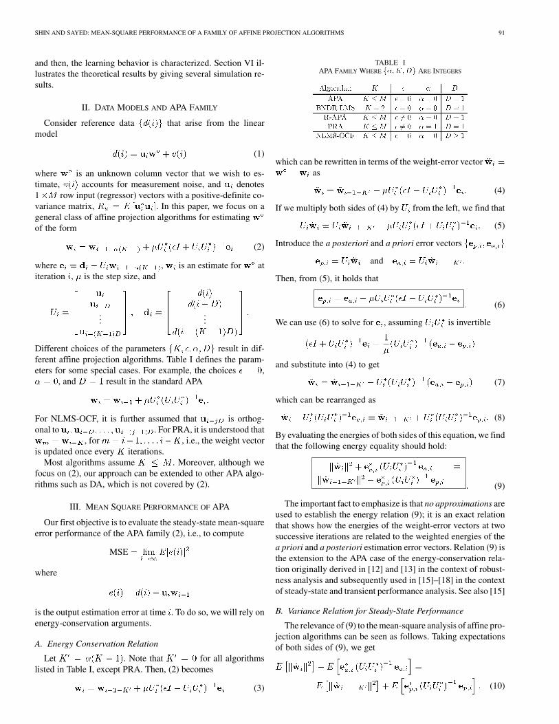
Different choices of the parameters result in dif-ferent affine projection algorithms. Table I defines the param-eters for some special cases. For example, the choices ,
, and result in the standard APA
For NLMS-OCF, it is further assumed that is orthog-onal to . For PRA, it is understood that
, for , i.e., the weight vectoris updated once every iterations.
Most algorithms assume . Moreover, although wefocus on (2), our approach can be extended to other APA algo-rithms such as DA, which is not covered by (2).
III. MEAN SQUARE PERFORMANCE OF APA
Our first objective is to evaluate the steady-state mean-squareerror performance of the APA family (2), i.e., to compute
MSE
where
is the output estimation error at time . To do so, we will rely onenergy-conservation arguments.
A. Energy Conservation Relation
Let . Note that for all algorithmslisted in Table I, except PRA. Then, (2) becomes
(3)
TABLE IAPA FAMILY WHERE f�;K;Dg ARE INTEGERS
which can be rewritten in terms of the weight-error vectoras
(4)
If we multiply both sides of (4) by from the left, we find that
(5)
Introduce the a posteriori and a priori error vectors
and
Then, from (5), it holds that
(6)
We can use (6) to solve for , assuming is invertible
and substitute into (4) to get
(7)
which can be rearranged as
(8)
By evaluating the energies of both sides of this equation, we findthat the following energy equality should hold:
(9)
The important fact to emphasize is that no approximations areused to establish the energy relation (9); it is an exact relationthat shows how the energies of the weight-error vectors at twosuccessive iterations are related to the weighted energies of thea priori and a posteriori estimation error vectors. Relation (9) isthe extension to the APA case of the energy-conservation rela-tion originally derived in [12] and [13] in the context of robust-ness analysis and subsequently used in [15]–[18] in the contextof steady-state and transient performance analysis. See also [15]
B. Variance Relation for Steady-State Performance
The relevance of (9) to the mean-square analysis of affine pro-jection algorithms can be seen as follows. Taking expectationsof both sides of (9), we get
(10)
92 IEEE TRANSACTIONS ON SIGNAL PROCESSING, VOL. 52, NO. 1, JANUARY 2004
Taking the limit as , and using the steady-state condition, we obtain
(11)
Substituting (6) into the right-hand side (RHS) of (11), we get
RHS of (11)
(12)
where we are defining
and
Using (12), equality (11) simplifies to
(13)
as . This equation can now be used to evaluate the mean-square performance of affine projection algorithms.
C. Mean-Square Performance
Introduce the noise vector
Then, (1) gives
and under the often realistic assumption that
A.1) the noise is i.i.d. and statistically independent ofthe regression matrix .
Neglecting the dependency of on past noises, we find thatthe variance relation (13) reduces to
(14)
as . This expression can be used to deduce an expressionfor the filter MSE or, equivalently, for the filter excess meansquare error (EMSE), which is defined by
EMSE
where . Now, from (1), we get
and therefore, the MSE and EMSE define each other via
MSE EMSE
In order to evaluate the EMSE, we need to deal with the expec-tations in (14). For this purpose, we shall rely on the followingassumption.
A.2) At steady-state, is statistically independent ofand moreover, where
for small and for large where
Note that since for all algorithms listed in Table I, exceptPRA, then, , and is the top entry of .For PRA, , and therefore, is alsoequal to the top entry of . The condition on ismotivated in Appendix A. Using (14) and A.2), the first term onthe left-hand side (LHS) of (14) becomes
Tr
Tr (15)
as . Similar manipulations can be applied to the re-maining terms in (14). Thus, we get
Tr (16)
and
Tr (17)
as .If we introduce the quantities (which are solely dependent on
the statistics of the regression data):
Tr and Tr (18)
then (14) becomes
Tr (19)
as , and the EMSE of the filter is therefore given by
EMSE Tr
(20)
and the steady-state MSE is
MSE Tr
(21)
Two simplifications can be made when the regularization pa-rameter is small.
• If is small enough so that its effect can be ignored, then, and the definitions of and will coincide.
In this case, (20) reduces to
EMSETr
Tr(22)
If we use , we obtain
EMSE
SHIN AND SAYED: MEAN-SQUARE PERFORMANCE OF A FAMILY OF AFFINE PROJECTION ALGORITHMS 93
and if we use , we get
EMSETr
• Another approximation assumes is small and is largeand uses
Tr and Tr
to get
EMSE Tr (23)
Note that this expression for the EMSE is proportional to . Incontrast, the expression given in [9] is
EMSE Tr
which does not take into account the effect of . Simulation re-sults in Section VI (see Figs. 7–12) show that (22) and (23) pro-vide good approximations for filter performance for relativelysmall step-size and order .
IV. TRACKING PERFORMANCE OF APA
A similar analysis can be used to evaluate the performanceof APA in nonstationary environments. Thus, assume that
, where the unknown system is nowtime-variant. It is assumed that the variation in is accordingto the random-walk model (see, e.g., [1], [2], [15], and [19])
(24)
where is an i.i.d. sequence with autocorrelation matrixand independent of the initial conditions
of the for all and of the for all . Let, , and . Then
and
(25)
If we multiply (25) by from the left, we obtain that (6) stillholds for the nonstationary case. Substituting (6) into (25), weget
(26)
Evaluating the energies of both sides of (26) and taking expec-tations, we find that
(27)
Using the random-walk model (24), we know thatfor , and therefore
Tr
(28)Substituting into (27), we obtain
Tr (29)
Comparing with (10), we see that the only difference in the non-stationary case is the appearance of the additional term
Tr . Note that the other terms are identical. Therefore,similar manipulations to those in Section III lead to
TrTr
(30)as , and the EMSE is then given by
EMSE Tr Tr
(31)
The two simplifications of Section III can be used to get
TrTr
(32)
or
TrTr (33)
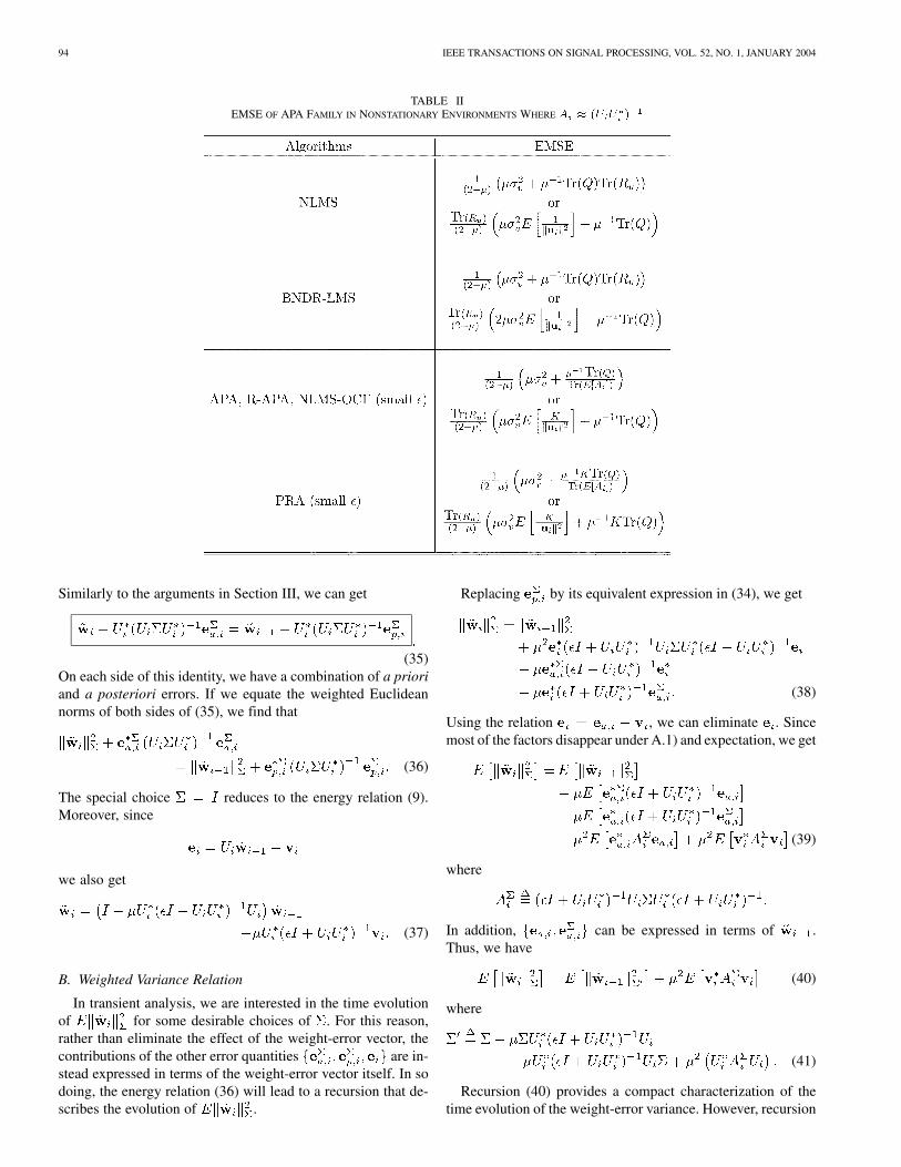
From (32) and (33), we see that for a given , there is anoptimal that minimizes the EMSE, and for a given , thereis an optimal that minimizes the EMSE. Comparisons ofthe tracking performance among the APA family are given inTable II.
V. TRANSIENT ANALYSIS OF APA
We now study the transient (i.e., convergence and stability)performance of the APA family. This task is more challengingthan mean-square performance. Nevertheless, the same energyconservation arguments of the previous section can still be usedif we incorporate weighting into the energy relation and into thedefinition of the error quantities [14], [17], as we now explain.We will assume, without loss of generality, that . Then,(2) becomes
In the following analysis, if we substitute by ,then the results for would be obtained.
A. Weighted Energy Relation
Let and . If we multiplyboth sides of the above recursion by from the left, for anyHermitian positive-definite matrix , we find that the a prioriand a posteriori estimation errors are related via
(34)
94 IEEE TRANSACTIONS ON SIGNAL PROCESSING, VOL. 52, NO. 1, JANUARY 2004
TABLE IIEMSE OF APA FAMILY IN NONSTATIONARY ENVIRONMENTS WHERE A � (U U )
Similarly to the arguments in Section III, we can get
(35)On each side of this identity, we have a combination of a prioriand a posteriori errors. If we equate the weighted Euclideannorms of both sides of (35), we find that
(36)
The special choice reduces to the energy relation (9).Moreover, since
we also get
(37)
B. Weighted Variance Relation
In transient analysis, we are interested in the time evolutionof for some desirable choices of . For this reason,rather than eliminate the effect of the weight-error vector, thecontributions of the other error quantities are in-stead expressed in terms of the weight-error vector itself. In sodoing, the energy relation (36) will lead to a recursion that de-scribes the evolution of .
Replacing by its equivalent expression in (34), we get
(38)
Using the relation , we can eliminate . Sincemost of the factors disappear under A.1) and expectation, we get
(39)
where
In addition, can be expressed in terms of .Thus, we have
(40)
where
(41)
Recursion (40) provides a compact characterization of thetime evolution of the weight-error variance. However, recursion
SHIN AND SAYED: MEAN-SQUARE PERFORMANCE OF A FAMILY OF AFFINE PROJECTION ALGORITHMS 95
(40) is still hard to propagate due to the presence of the expec-tation
This expectation is difficult to evaluate due to the dependence ofon and of on prior regressors. One way to overcome
this difficulty is to introduce an independence assumption on theregressor sequence , namely, to assume the following.
A.3) The matrix sequence is independent and identi-cally distributed.
This assumption guarantees that is independent of bothand . Clearly, A.3) is a strong assumption (it is actually
stronger than the usual independence assumption, which onlyrequires the to be i.i.d [1], [2]). Observe, however, from(41) for that it is sufficient for our purposes to require thefollowing:
A.3’) is independent of .This is generally a weaker assumption. In this way, recursion(40) reduces to
(42)
where now
(43)
with expectations appearing in (43). In addition, taking expec-tations of both sides of (37) and using assumption A.1), we ob-tain the following result for the evolution of the mean of theweight-error vector:
(44)
Relations (42) and (44) can be used to derive conditions formean-square stability, as well as expressions for the steady-stateMSE and mean-square deviation (MSD) of the APA family. Tosee this, we introduce some notation. The vec notation, e.g.,
vec , allows us to replace an arbitrary matrixby an 1 column vector whose entries are formed by
stacking the successive columns of the matrix on top of eachother. On the other hand, writing vec for an 1 columnvector results in an matrix whose entries are ob-tained from . Therefore, we also write vec . Thevec notation is convenient when working with Kroneckerproducts. The Kronecker product of two matrices and , sayof dimensions and , respectively, is denotedby [20]. For any matrices of compatible di-mensions, it holds that
vec vec (45)
Applying (45) to (40), we find that it leads to the vector relation
(46)
where the coefficient matrix is and defined by
(47)
with
We can rewrite the recursion for in (40) by using thevectors instead of the matrices , say, as
vec vec (48)
where, for the last term, we used the fact that
Tr
where vec . For compactnessof notation, we drop the vec notation from the subscripts andkeep the vectors so that the above is simply rewritten as
(49)
In addition, we obtain the following result for the evolution ofthe mean of the weight-error vector:
(50)
Recursion (49) shows that in order to evaluate , weneed to know , with a weighting matrix whoseentries are determined by . Now, the quantitycan be inferred from (49) by writing the recursion for , i.e.,
We again find that in order to evaluate , we needto know . The natural question is whether thisprocedure terminates. Fortunately, as in [14] and [17], this pro-cedure does terminate. This is because once we write (48) bysubstituting by , we get
where the weighting matrix on the RHS is . This term canbe deduced from the prior weighting factors. Indeed, letdenote the characteristic polynomial of ,
It is a polynomial of order in
with coefficients . Now, the Cayley–Hamilton theoremguarantees that so that
(51)
Theorem 1 [Transient Performance]: Under assumptionsA.1) and A.3’), the transient performance of the APA family(2) for is described by the state recursion
(52)
96 IEEE TRANSACTIONS ON SIGNAL PROCESSING, VOL. 52, NO. 1, JANUARY 2004
where
......
.... . .
...
... ...
vec , vec ,, and are coef-
ficients of the characteristic polynomial of .Observe that the eigenvalues of coincide with those of .
C. Learning Curves
The learning curve of an adaptive filter describes the timeevolution of the variance . Now, if the are assumedto be i.i.d., then
and the learning curve can be evaluated by computingfor each . This task can be accomplished recur-
sively from (48) by iterating it and setting vec .This yields
(53)That is
(54)
where the vector and the scalar satisfy the recursions
D. Mean-Square Stability
From (50), the convergence in the mean of the APA family isguaranteed for any satisfying
(55)
Moreover, recursion (49) is stable if, and only if, the matrixis stable. Thus, let and
so that . The following holds.Theorem 2 [Stability]: The convergence in the mean-square
sense of the APA family is guaranteed for any in the range
where , , and
.
The above condition on is in terms of the largest positiveeigenvalue of when it exists. The theorem is proved Ap-
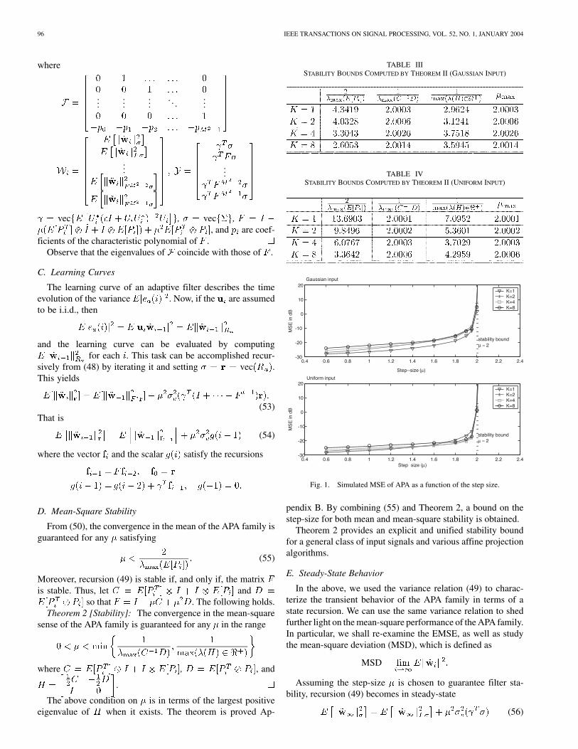
TABLE IIISTABILITY BOUNDS COMPUTED BY THEOREM II (GAUSSIAN INPUT)
TABLE IVSTABILITY BOUNDS COMPUTED BY THEOREM II (UNIFORM INPUT)
0.4 0.6 0.8 1 1.2 1.4 1.6 1.8 2 2.2 2.4-30
-20
-10
0
10
20
Step--size (µ)
MS
E in
dB
K=1K=2K=4K=8
0.4 0.6 0.8 1 1.2 1.4 1.6 1.8 2 2.2 2.4 -30
-20
-10
0
10
20
Step size (µ)
MS
E in
dB
K=1K=2K=4K=8
stability boundµ ≈ 2
stability boundµ ≈ 2
Gaussian input
Uniform input
Fig. 1. Simulated MSE of APA as a function of the step size.
pendix B. By combining (55) and Theorem 2, a bound on thestep-size for both mean and mean-square stability is obtained.
Theorem 2 provides an explicit and unified stability boundfor a general class of input signals and various affine projectionalgorithms.
E. Steady-State Behavior
In the above, we used the variance relation (49) to charac-terize the transient behavior of the APA family in terms of astate recursion. We can use the same variance relation to shedfurther light on the mean-square performance of the APA family.In particular, we shall re-examine the EMSE, as well as studythe mean-square deviation (MSD), which is defined as
MSD
Assuming the step-size is chosen to guarantee filter sta-bility, recursion (49) becomes in steady-state
(56)
SHIN AND SAYED: MEAN-SQUARE PERFORMANCE OF A FAMILY OF AFFINE PROJECTION ALGORITHMS 97
0 50 100 150 200 250 300 350 400 450 500-30
-25
-20
-15
-10
-5
0
Iteration number
MS
E in
dB
(a) K=1, D=8(b) K=2, D=8(c) K=4, D=8(d) K=8, D=8TheorySimulation
(a) K=1
(b) K=2
(c) K=4
(d) K=8
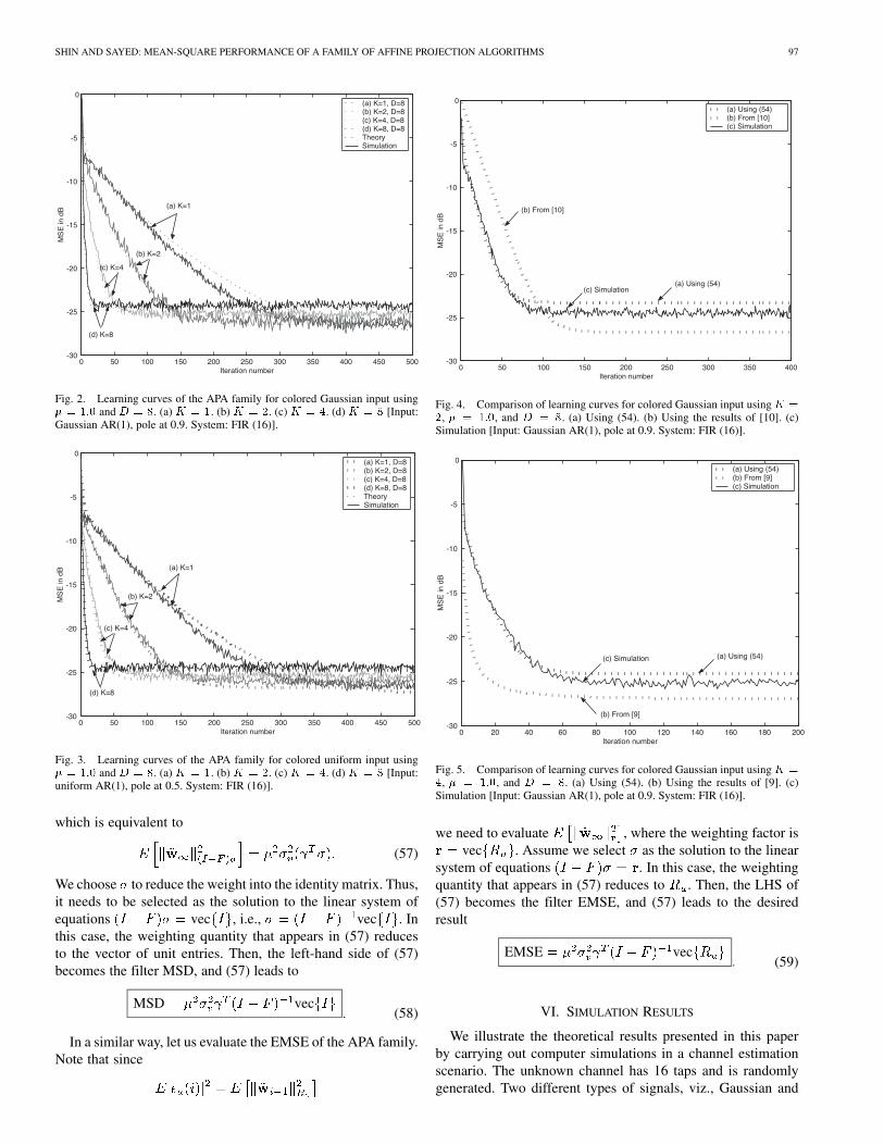
Fig. 2. Learning curves of the APA family for colored Gaussian input using� = 1:0 and D = 8. (a) K = 1. (b) K = 2. (c) K = 4. (d) K = 8 [Input:Gaussian AR(1), pole at 0.9. System: FIR (16)].
0 50 100 150 200 250 300 350 400 450 500-30
-25
-20
-15
-10
-5
0
Iteration number
MS
E in
dB
(a) K=1, D=8(b) K=2, D=8(c) K=4, D=8(d) K=8, D=8TheorySimulation
(a) K=1
(b) K=2
(c) K=4
(d) K=8
Fig. 3. Learning curves of the APA family for colored uniform input using� = 1:0 and D = 8. (a) K = 1. (b) K = 2. (c) K = 4. (d) K = 8 [Input:uniform AR(1), pole at 0.5. System: FIR (16)].
which is equivalent to
(57)
We choose to reduce the weight into the identity matrix. Thus,it needs to be selected as the solution to the linear system ofequations vec , i.e., vec . Inthis case, the weighting quantity that appears in (57) reducesto the vector of unit entries. Then, the left-hand side of (57)becomes the filter MSD, and (57) leads to
MSD vec(58)
In a similar way, let us evaluate the EMSE of the APA family.Note that since
0 50 100 150 200 250 300 350 400-30
-25
-20
-15
-10
-5
0
Iteration number
MS
E in
dB
(a) Using (54)(b) From [10](c) Simulation
(b) From [10]
(a) Using (54) (c) Simulation
Fig. 4. Comparison of learning curves for colored Gaussian input using K =
2, � = 1:0, and D = 8. (a) Using (54). (b) Using the results of [10]. (c)Simulation [Input: Gaussian AR(1), pole at 0.9. System: FIR (16)].
0 20 40 60 80 100 120 140 160 180 200-30
-25
-20
-15
-10
-5
0
Iteration number
MS
E in
dB
(a) Using (54)(b) From [9](c) Simulation
(a) Using (54) (c) Simulation
(b) From [9]
Fig. 5. Comparison of learning curves for colored Gaussian input using K =
4, � = 1:0, and D = 8. (a) Using (54). (b) Using the results of [9]. (c)Simulation [Input: Gaussian AR(1), pole at 0.9. System: FIR (16)].
we need to evaluate , where the weighting factor isvec . Assume we select as the solution to the linear
system of equations . In this case, the weightingquantity that appears in (57) reduces to . Then, the LHS of(57) becomes the filter EMSE, and (57) leads to the desiredresult
EMSE vec(59)
VI. SIMULATION RESULTS
We illustrate the theoretical results presented in this paperby carrying out computer simulations in a channel estimationscenario. The unknown channel has 16 taps and is randomlygenerated. Two different types of signals, viz., Gaussian and
98 IEEE TRANSACTIONS ON SIGNAL PROCESSING, VOL. 52, NO. 1, JANUARY 2004
0 20 40 60 80 100 120 140 160 180 200-30
-25
-20
-15
-10
-5
0
Iteration number
MS
E in
dB
(a) Using (54)(b) From [9](c) Simulation
(a) Using (54) (c) Simulation
(b) From [9]
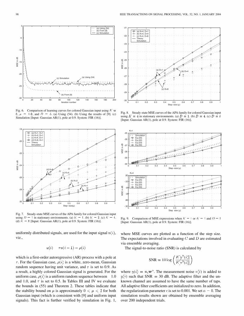
Fig. 6. Comparison of learning curves for colored Gaussian input using K =
8, � = 1:0, and D = 8. (a) Using (54). (b) Using the results of [9]. (c)Simulation [Input: Gaussian AR(1), pole at 0.9. System: FIR (16)].
0 0.1 0.2 0.3 0.4 0.5 0.6 0.7 0.8 0.9 1-30
-28
-26
-24
-22
-20
-18
Step--size(µ)
MS
E in
dB
(a) K=1, D=1(b) K=2, D=1(c) K=4, D=1(d) K=8, D=1TheorySimulation
(d) K=8
(c) K=4
(b) K=2
(a) K=1
Fig. 7. Steady-state MSE curves of the APA family for colored Gaussian inputusing D = 1 in stationary environments. (a) K = 1. (b) K = 2. (c) K = 4.(d) K = 8 [Input: Gaussian AR(1), pole at 0.9. System: FIR (16)].
uniformly distributed signals, are used for the input signal ,viz.,
which is a first-order autoregressive (AR) process with a pole at. For the Gaussian case, is a white, zero-mean, Gaussian
random sequence having unit variance, and is set to 0.9. Asa result, a highly colored Gaussian signal is generated. For theuniform case, is a uniform random sequence between 1.0and 1.0, and is set to 0.5. In Tables III and IV we evaluatethe bounds in (55) and Theorem 2. These tables indicate thatthe stability bound on is approximately for bothGaussian input (which is consistent with [9] and uniform inputsignals). This fact is further verified by simulation in Fig. 1,
0 0.1 0.2 0.3 0.4 0.5 0.6 0.7 0.8 0.9 1-30
-29
-28
-27
-26
-25
-24
-23
-22
-21
Step--size (µ)
MS
E in
dB
(a) K=4, D=1(b) K=4, D=4(c) K=4, D=8TheorySimulation
(a) D=1 (b) D=4
(c) D=8
Fig. 8. Steady-state MSE curves of the APA family for colored Gaussian inputusing K = 4 in stationary environments. (a) D = 1. (b) D = 4. (c) D = 8
[Input: Gaussian AR(1), pole at 0.9. System: FIR (16)].
0 0.1 0.2 0.3 0.4 0.5 0.6 0.7 0.8 0.9 1-30
-29
-28
-27
-26
-25
Step--size (µ)
MS
E in
dB
SimulationEq.(20)Eq.(22)Eq.(23)Eq.(59)
0 0.1 0.2 0.3 0.4 0.5 0.6 0.7 0.8 0.9 1- 30
-28
-26
-24
- 22
-20
Step size (µ)
MS
E in
dB
SimulationEq.(20)Eq.(22)Eq.(23)Eq.(59)
K=1
K=4
Fig. 9. Comparison of MSE expressions when K = 1 or K = 4 and D = 1
[Input: Gaussian AR(1), pole at 0.9. System: FIR (16)].
where MSE curves are plotted as a function of the step size.The expectations involved in evaluating and are estimatedvia ensemble averaging.
The signal-to-noise ratio (SNR) is calculated by
SNR
where . The measurement noise is added tosuch that SNR 30 dB. The adaptive filter and the un-
known channel are assumed to have the same number of taps.All adaptive filter coefficients are initialized to zero. In addition,the regularization parameter is set to 0.001. We set . Thesimulation results shown are obtained by ensemble averagingover 200 independent trials.
SHIN AND SAYED: MEAN-SQUARE PERFORMANCE OF A FAMILY OF AFFINE PROJECTION ALGORITHMS 99
0 0.1 0.2 0.3 0.4 0.5 0.6 0.7 0.8 0.9 1-30
-29
-28
-27
-26
-25
-24
-23
Step--size (µ)
MS
E in
dB
(a) Simulation(b) Eq.(20) (c) Eq.(22) (d) Eq.(23) (e) Eq.(59) (f) [8]
(f)
(b) or (c)
(a)
(d)
(e)
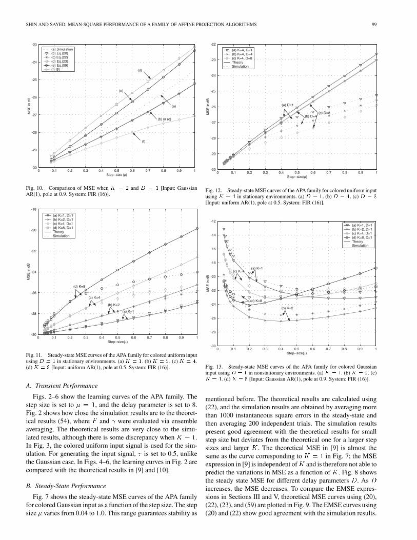
Fig. 10. Comparison of MSE when K = 2 and D = 1 [Input: GaussianAR(1), pole at 0.9. System: FIR (16)].
0 0.1 0.2 0.3 0.4 0.5 0.6 0.7 0.8 0.9 1-30
-28
-26
-24
-22
-20
-18
Step--size(µ)
MS
E in
dB
(a) K=1, D=1(b) K=2, D=1(c) K=4, D=1(d) K=8, D=1TheorySimulation
(d) K=8
(c) K=4
(b) K=2
(a) K=1
Fig. 11. Steady-state MSE curves of the APA family for colored uniform inputusing D = 1 in stationary environments. (a) K = 1. (b) K = 2. (c) K = 4.(d)K = 8 [Input: uniform AR(1), pole at 0.5. System: FIR (16)].
A. Transient Performance
Figs. 2–6 show the learning curves of the APA family. Thestep size is set to , and the delay parameter is set to 8.Fig. 2 shows how close the simulation results are to the theoret-ical results (54), where and were evaluated via ensembleaveraging. The theoretical results are very close to the simu-lated results, although there is some discrepancy when .In Fig. 3, the colored uniform input signal is used for the sim-ulation. For generating the input signal, is set to 0.5, unlikethe Gaussian case. In Figs. 4–6, the learning curves in Fig. 2 arecompared with the theoretical results in [9] and [10].
B. Steady-State Performance
Fig. 7 shows the steady-state MSE curves of the APA familyfor colored Gaussian input as a function of the step size. The stepsize varies from 0.04 to 1.0. This range guarantees stability as
0 0.1 0.2 0.3 0.4 0.5 0.6 0.7 0.8 0.9 1-30
-29
-28
-27
-26
-25
-24
-23
-22
Step--size(µ)
MS
E in
dB
(a) K=4, D=1(b) K=4, D=4(c) K=4, D=8TheorySimulation
(a) D=1
(b) D=4 (c) D=8
Fig. 12. Steady-state MSE curves of the APA family for colored uniform inputusing K = 4 in stationary environments. (a) D = 1. (b) D = 4. (c) D = 8
[Input: uniform AR(1), pole at 0.5. System: FIR (16)].
0 0.1 0.2 0.3 0.4 0.5 0.6 0.7 0.8 0.9 1-30
-28
-26
-24
-22
-20
-18
-16
-14
-12
Step--size(µ)
MS
E in
dB
(a) K=1, D=1(b) K=2, D=1(c) K=4, D=1(d) K=8, D=1TheorySimulation
(a) K=1
(b) K=2
(d) K=8
(c) K=4
Fig. 13. Steady-state MSE curves of the APA family for colored Gaussianinput using D = 1 in nonstationary environments. (a)K = 1. (b)K = 2. (c)K = 4. (d)K = 8 [Input: Gaussian AR(1), pole at 0.9. System: FIR (16)].
mentioned before. The theoretical results are calculated using(22), and the simulation results are obtained by averaging morethan 1000 instantaneous square errors in the steady-state andthen averaging 200 independent trials. The simulation resultspresent good agreement with the theoretical results for smallstep size but deviates from the theoretical one for a larger stepsizes and larger . The theoretical MSE in [9] is almost thesame as the curve corresponding to in Fig. 7; the MSEexpression in [9] is independent of and is therefore not able topredict the variations in MSE as a function of . Fig. 8 showsthe steady state MSE for different delay parameters . Asincreases, the MSE decreases. To compare the EMSE expres-sions in Sections III and V, theoretical MSE curves using (20),(22), (23), and (59) are plotted in Fig. 9. The EMSE curves using(20) and (22) show good agreement with the simulation results.
100 IEEE TRANSACTIONS ON SIGNAL PROCESSING, VOL. 52, NO. 1, JANUARY 2004
0 0.1 0.2 0.3 0.4 0.5 0.6 0.7 0.8 0.9 1-30
-28
-26
-24
-22
-20
-18
-16
Step--size(µ)
MS
E in
dB
(a) K=2, D=1(b) K=2, D=2(c) K=2, D=4TheorySimulation
(b) D=2 (c) D=4
(a) D=1
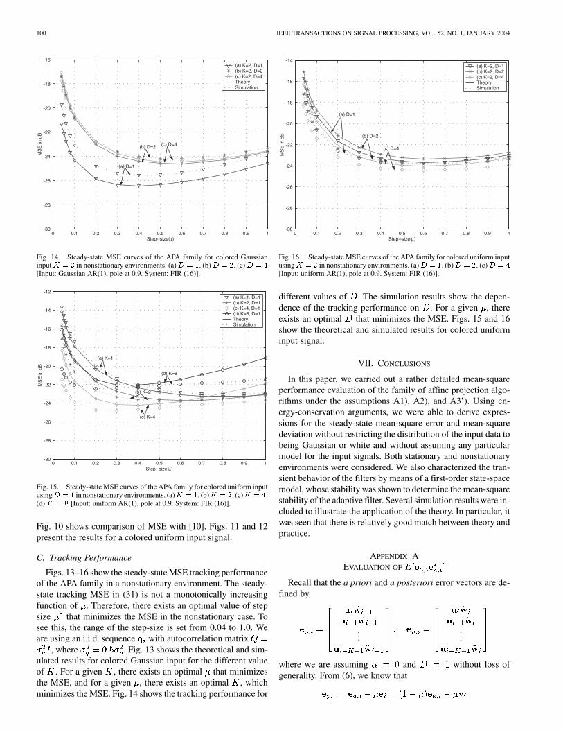
Fig. 14. Steady-state MSE curves of the APA family for colored GaussianinputK = 2 in nonstationary environments. (a)D = 1. (b)D = 2. (c)D = 4
[Input: Gaussian AR(1), pole at 0.9. System: FIR (16)].
0 0.1 0.2 0.3 0.4 0.5 0.6 0.7 0.8 0.9 1-30
-28
-26
-24
-22
-20
-18
-16
-14
-12
Step--size(µ)
MS
E in
dB
(a) K=1, D=1(b) K=2, D=1(c) K=4, D=1(d) K=8, D=1TheorySimulation
(a) K=1
(d) K=8
(c) K=4
(b) K=2
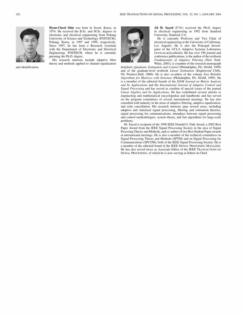
Fig. 15. Steady-state MSE curves of the APA family for colored uniform inputusingD = 1 in nonstationary environments. (a)K = 1. (b)K = 2. (c)K = 4.(d)K = 8 [Input: uniform AR(1), pole at 0.9. System: FIR (16)].
Fig. 10 shows comparison of MSE with [10]. Figs. 11 and 12present the results for a colored uniform input signal.
C. Tracking Performance
Figs. 13–16 show the steady-state MSE tracking performanceof the APA family in a nonstationary environment. The steady-state tracking MSE in (31) is not a monotonically increasingfunction of . Therefore, there exists an optimal value of stepsize that minimizes the MSE in the nonstationary case. Tosee this, the range of the step-size is set from 0.04 to 1.0. Weare using an i.i.d. sequence with autocorrelation matrix
, where . Fig. 13 shows the theoretical and sim-ulated results for colored Gaussian input for the different valueof . For a given , there exists an optimal that minimizesthe MSE, and for a given , there exists an optimal , whichminimizes the MSE. Fig. 14 shows the tracking performance for
0 0.1 0.2 0.3 0.4 0.5 0.6 0.7 0.8 0.9 1-30
-28
-26
-24
-22
-20
-18
-16
-14
Step--size(µ)
MS
E in
dB
(a) K=2, D=1(b) K=2, D=2(c) K=2, D=4TheorySimulation
(a) D=1
(b) D=2
(c) D=4
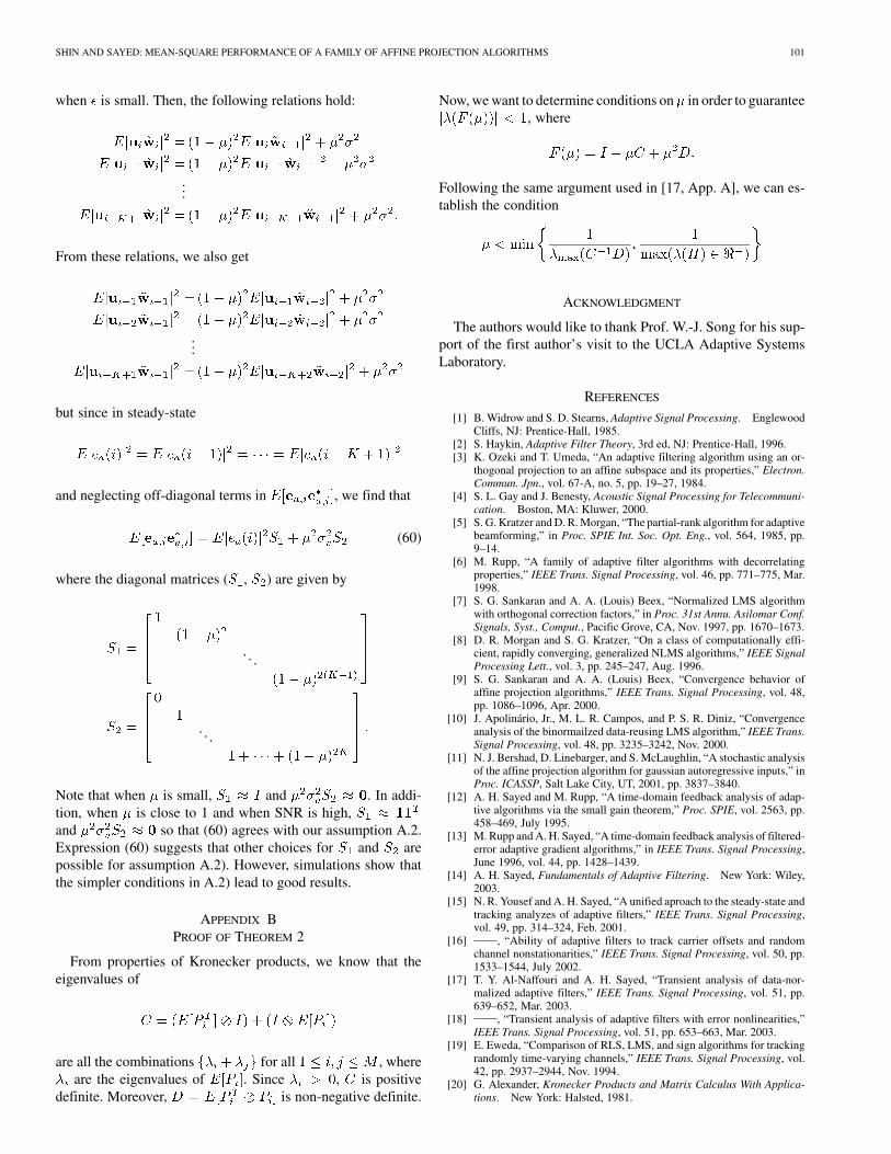
Fig. 16. Steady-state MSE curves of the APA family for colored uniform inputusingK = 2 in nonstationary environments. (a)D = 1. (b)D = 2. (c)D = 4
[Input: uniform AR(1), pole at 0.9. System: FIR (16)].
different values of . The simulation results show the depen-dence of the tracking performance on . For a given , thereexists an optimal that minimizes the MSE. Figs. 15 and 16show the theoretical and simulated results for colored uniforminput signal.
VII. CONCLUSIONS
In this paper, we carried out a rather detailed mean-squareperformance evaluation of the family of affine projection algo-rithms under the assumptions A1), A2), and A3’). Using en-ergy-conservation arguments, we were able to derive expres-sions for the steady-state mean-square error and mean-squaredeviation without restricting the distribution of the input data tobeing Gaussian or white and without assuming any particularmodel for the input signals. Both stationary and nonstationaryenvironments were considered. We also characterized the tran-sient behavior of the filters by means of a first-order state-spacemodel, whose stability was shown to determine the mean-squarestability of the adaptive filter. Several simulation results were in-cluded to illustrate the application of the theory. In particular, itwas seen that there is relatively good match between theory andpractice.
APPENDIX AEVALUATION OF
Recall that the a priori and a posteriori error vectors are de-fined by
......
where we are assuming and without loss ofgenerality. From (6), we know that
SHIN AND SAYED: MEAN-SQUARE PERFORMANCE OF A FAMILY OF AFFINE PROJECTION ALGORITHMS 101
when is small. Then, the following relations hold:
...
From these relations, we also get
...
but since in steady-state
and neglecting off-diagonal terms in , we find that
(60)
where the diagonal matrices ( , ) are given by
. . .
. . .
Note that when is small, and . In addi-tion, when is close to 1 and when SNR is high,and so that (60) agrees with our assumption A.2.Expression (60) suggests that other choices for and arepossible for assumption A.2). However, simulations show thatthe simpler conditions in A.2) lead to good results.
APPENDIX BPROOF OF THEOREM 2
From properties of Kronecker products, we know that theeigenvalues of
are all the combinations for all , whereare the eigenvalues of . Since , is positive
definite. Moreover, is non-negative definite.
Now, we want to determine conditions on in order to guarantee, where
Following the same argument used in [17, App. A], we can es-tablish the condition
ACKNOWLEDGMENT
The authors would like to thank Prof. W.-J. Song for his sup-port of the first author’s visit to the UCLA Adaptive SystemsLaboratory.
REFERENCES
[1] B. Widrow and S. D. Stearns, Adaptive Signal Processing. EnglewoodCliffs, NJ: Prentice-Hall, 1985.
[2] S. Haykin, Adaptive Filter Theory, 3rd ed, NJ: Prentice-Hall, 1996.[3] K. Ozeki and T. Umeda, “An adaptive filtering algorithm using an or-
thogonal projection to an affine subspace and its properties,” Electron.Commun. Jpn., vol. 67-A, no. 5, pp. 19–27, 1984.
[4] S. L. Gay and J. Benesty, Acoustic Signal Processing for Telecommuni-cation. Boston, MA: Kluwer, 2000.
[5] S. G. Kratzer and D. R. Morgan, “The partial-rank algorithm for adaptivebeamforming,” in Proc. SPIE Int. Soc. Opt. Eng., vol. 564, 1985, pp.9–14.
[6] M. Rupp, “A family of adaptive filter algorithms with decorrelatingproperties,” IEEE Trans. Signal Processing, vol. 46, pp. 771–775, Mar.1998.
[7] S. G. Sankaran and A. A. (Louis) Beex, “Normalized LMS algorithmwith orthogonal correction factors,” in Proc. 31st Annu. Asilomar Conf.Signals, Syst., Comput., Pacific Grove, CA, Nov. 1997, pp. 1670–1673.
[8] D. R. Morgan and S. G. Kratzer, “On a class of computationally effi-cient, rapidly converging, generalized NLMS algorithms,” IEEE SignalProcessing Lett., vol. 3, pp. 245–247, Aug. 1996.
[9] S. G. Sankaran and A. A. (Louis) Beex, “Convergence behavior ofaffine projection algorithms,” IEEE Trans. Signal Processing, vol. 48,pp. 1086–1096, Apr. 2000.
[10] J. Apolinário, Jr., M. L. R. Campos, and P. S. R. Diniz, “Convergenceanalysis of the binormailzed data-reusing LMS algorithm,” IEEE Trans.Signal Processing, vol. 48, pp. 3235–3242, Nov. 2000.
[11] N. J. Bershad, D. Linebarger, and S. McLaughlin, “A stochastic analysisof the affine projection algorithm for gaussian autoregressive inputs,” inProc. ICASSP, Salt Lake City, UT, 2001, pp. 3837–3840.
[12] A. H. Sayed and M. Rupp, “A time-domain feedback analysis of adap-tive algorithms via the small gain theorem,” Proc. SPIE, vol. 2563, pp.458–469, July 1995.
[13] M. Rupp and A. H. Sayed, “A time-domain feedback analysis of filtered-error adaptive gradient algorithms,” in IEEE Trans. Signal Processing,June 1996, vol. 44, pp. 1428–1439.
[14] A. H. Sayed, Fundamentals of Adaptive Filtering. New York: Wiley,2003.
[15] N. R. Yousef and A. H. Sayed, “A unified aproach to the steady-state andtracking analyzes of adaptive filters,” IEEE Trans. Signal Processing,vol. 49, pp. 314–324, Feb. 2001.
[16] , “Ability of adaptive filters to track carrier offsets and randomchannel nonstationarities,” IEEE Trans. Signal Processing, vol. 50, pp.1533–1544, July 2002.
[17] T. Y. Al-Naffouri and A. H. Sayed, “Transient analysis of data-nor-malized adaptive filters,” IEEE Trans. Signal Processing, vol. 51, pp.639–652, Mar. 2003.
[18] , “Transient analysis of adaptive filters with error nonlinearities,”IEEE Trans. Signal Processing, vol. 51, pp. 653–663, Mar. 2003.
[19] E. Eweda, “Comparison of RLS, LMS, and sign algorithms for trackingrandomly time-varying channels,” IEEE Trans. Signal Processing, vol.42, pp. 2937–2944, Nov. 1994.
[20] G. Alexander, Kronecker Products and Matrix Calculus With Applica-tions. New York: Halsted, 1981.
102 IEEE TRANSACTIONS ON SIGNAL PROCESSING, VOL. 52, NO. 1, JANUARY 2004
Hyun-Chool Shin was born in Seoul, Korea, in1974. He received the B.Sc. and M.Sc. degrees inelectronic and electrical engineering from PohangUniversity of Science and Technology (POSTECH),Pohang, Korea, in 1997 and 1999, respectively.Since 1997, he has been a Research Assistantwith the Department of Electronic and ElectricalEngineering, POSTECH, where he is currentlypursuing the Ph.D. degree.
His research interests include adaptive filtertheory and methods applied to channel equalization
and identification.
Ali H. Sayed (F’01) received the Ph.D. degreein electrical engineering in 1992 from StanfordUniversity, Stanford, CA.
He is currently Professor and Vice Chair ofelectrical engineering at the University of California,Los Angeles. He is also the Principal Investi-gator of the UCLA Adaptive Systems Laboratory(www.ee.ucla.edu/asl). He has over 190 journal andconference publications, is the author of the textbookFundamentals of Adaptive Filtering (New York:Wiley, 2003), is coauthor of the research monograph
Indefinite Quadratic Estimation and Control (Philadelphia, PA: SIAM, 1999)and of the graduate-level textbook Linear Estimation (Englewood Cliffs,NJ: Prentice-Hall, 2000). He is also co-editor of the volume Fast ReliableAlgorithms for Matrices with Structure (Philadelphia, PA: SIAM, 1999). Heis a member of the editorial boards of the SIAM Journal on Matrix Analysisand Its Applications and the International Journal of Adaptive Control andSignal Processing and has served as coeditor of special issues of the journalLinear Algebra and Its Applications. He has contributed several articles toengineering and mathematical encyclopedias and handbooks and has servedon the program committees of several international meetings. He has alsoconsulted with industry in the areas of adaptive filtering, adaptive equalization,and echo cancellation. His research interests span several areas, includingadaptive and statistical signal processing, filtering and estimation theories,signal processing for communications, interplays between signal processingand control methodologies, system theory, and fast algorithms for large-scaleproblems.
Dr. Sayed is recipient of the 1996 IEEE Donald G. Fink Award, a 2002 BestPaper Award from the IEEE Signal Processing Society in the area of SignalProcesing Theory and Methods, and co-author of two Best Student Paper awardsat international meetings. He is also a member of the technical committees onSignal Processing Theory and Methods (SPTM) and on Signal Processing forCommunications (SPCOM), both of the IEEE Signal Processing Society. He isa member of the editorial board of the IEEE SIGNAL PROCESSING MAGAZINE.He has also served twice as Associate Editor of the IEEE TRANSACTIONS ON
SIGNAL PROCESSING, of which he is now serving as Editor-in-Chief.
Related Documents