Mead Lake Watershed Sediment and Nutrient Export Modeling Adam Freihoefer and Paul McGinley A Report by the Center for Watershed Science and Education University of Wisconsin – Stevens Point August 2008 Photo: Mead Lake Reservoir

Welcome message from author
This document is posted to help you gain knowledge. Please leave a comment to let me know what you think about it! Share it to your friends and learn new things together.
Transcript

Mead Lake Watershed
Sediment and Nutrient Export Modeling
Adam Freihoefer and Paul McGinley
A Report by the Center for Watershed Science and Education University of Wisconsin – Stevens Point
August 2008
Photo: Mead Lake Reservoir

ii

iii
Executive Summary
The Mead Lake Reservoir (MLR) is exhibiting enrichment of nutrients,
particularly phosphorus. The 1.3 km2 impoundment was added to the Wisconsin’s 303d
impaired waterway list as a result of the sediment and nutrient loading. As a result of the
impaired designation, a sediment and phosphorus Total Maximum Daily Load (TMDL) is
being developed for the reservoir to meet water quality standards.
As a preliminary step in TMDL development for the MLR, the Soil and Water
Assessment Tool (SWAT) model approach was used to simulate the influence of land
management on sediment and phosphorus transfer throughout the Mead Lake Watershed
(MLW). The SWAT model approach relied on detailed management information and two
years of measured growing season discharge and water quality to calibrate the model.
The calibrated model allowed for various alternative management scenarios to be
implemented, evaluating the impact each scenario had on phosphorus contributions to the
MLR. The SWAT’s spatial discretization within each subwatershed of MLW required the
application of the field-scale Wisconsin-based SNAP model to evaluate individual fields.
The implementation of both models allowed greater flexibility in locating contributing
sources of nutrient loss at varying scales.
The SWAT model was calibrated to discharge and water quality measured during
the growing seasons (May to September) of 2002 and 2003. SWAT could be used
successfully to simulate the daily discharge (R2 = 0.63, N-S=0.62), monthly sediment (R2
= 0.54, N-S=0.49), and monthly phosphorus (R2 = 0.66, N-S=0.66). The majority of the
phosphorus export within the watershed came from two specific agricultural hydrologic
response units (HRUs) (113C and 114C).
The calibrated model was used to evaluate long term (1981-2004) alternative
management scenarios. Reductions in soil phosphorus and soil erosion would both lead
to a reduction in phosphorus transfer from the watershed. The modeling suggests that
watershed-wide reductions in soil phosphorus and sediment loss could lead to an almost
thirty percent reduction in phosphorus to Mead Lake.

iv
Acknowledgements
We wish to acknowledge those groups and individuals who contributed to the
successful completion of the project through funding, insight, and support.
This project would not have been possible had it not been for funding sources
including Eau Claire and Clark Counties, Lake Altoona and Lake Eau Claire
Associations, and the Wisconsin Department of Natural Resources.
The development of this project is a culmination of the efforts of many. Model
calibration would not have been possible without the previous research conducted by
William James and the Eau Galle Aquatic Ecology Laboratory of the U.S. Army Corp of
Engineers. UW-Stevens Point (UWSP) staff provided assistance during all stages of the
project. Digitizing and aerial photo analysis conducted by Alex Smith defined the spatial
extent of land management throughout the watershed. The assistance of Steven Weiss
during the data collection and model development periods allowed this project to finish in
a timely manner.
Clark County Conservationists Gregg Stangl and Matthew Zoschke, GIS Analyst
Bill Shockley, and the rest of the Clark County Conservation staff were integral in
providing land management identification, organizing field visits, and offering insight
into individual land management changes throughout the watershed. The Clark County
staffs ability to foster a positive experience was necessary for project completion.
The data collection of field-scale information would not have been possible
without individual landowner’s willingness to participate in a farm survey and grant UW-
Stevens Point staff access to their land.
Thanks to Buzz Sorge, Ken Schreiber, and Patrick Oldenburg of the Wisconsin
Department of Natural Resources for the active role they played during conceptual
development, model evaluation, and alternative scenario design.

v
Table of Contents
1.0 INTRODUCTION 1
1.1 PURPOSE 1 1.2 SITE DESCRIPTION 2
2.0 METHODS AND MATERIALS 3
2.1 SWAT MODEL DESCRIPTION AND APPROACH 5 2.2 COLLECTION OF DATA 7
2.2.1 Discharge 7 2.2.2 Water Quality 7
2.3 MODEL INPUTS 8 2.3.1 Topography 8 2.3.2 Soils 10 2.3.3 Hydrologic Network 10 2.3.4 Closed Depressions 11 2.3.5 Climate 16 2.3.6 Land Coverage 16 2.3.7 Land Management 20
2.4 CALIBRATION 25 2.5 STATISTICAL EVALUATION OF SWAT MODEL 26
3.0 MLW SWAT MODEL SIMULATION 26
3.1 WATERSHED MODEL APPROACH 26 3.2 DISCHARGE CALIBRATION 28 3.3 SEDIMENT CALIBRATION 32 3.4 TOTAL PHOSPHORUS CALIBRATION 36 3.5 CROP YIELD CALIBRATION 44
4.0 ALTERNATIVE MANAGEMENT SCENARIOS 45
4.1 BASELINE AND SCENARIO MODEL SIMULATIONS (1999-2004) 45 4.2 SCENARIO IMPLEMENTATION 46
4.2.1 Nutrient Management Scenarios (1, 3, 4, 8) 46 4.2.2 Land Management Scenarios (2, 5, 6, 7, 9) 46
4.3 BASELINE AND SCENARIO RESULTS 48
5.0 CONCLUSIONS AND RECOMMENDATIONS 49
6.0 REFERENCES 50
APPENDICES 53
APPENDIX A 54 APPENDIX B 57 APPENDIX C 62

vi
List of Tables
TABLE 1: MEAD LAKE WATERSHED CLIMATOLOGICAL COLLECTION STATIONS AND DURATIONS ................................................................................................................ 16
TABLE 2: MEAD LAKE WATERSHED LANDUSE COMPARISON BETWEEN 1992 AND 2001 ... 17 TABLE 3: PERCENTAGE OF MANAGEMENT PRACTICES PER SUBBASIN ............................... 22 TABLE 4: SUMMARY OF SWAT MODEL INPUT DATASET FOR SIMULATION ...................... 27 TABLE 5: SUMMARY OF AGRICULTURAL HRU ROTATION STAGGERING ........................... 27 TABLE 6: CALIBRATED PARAMETER VALUES FOR DISCHARGE IN THE MLW .................... 30 TABLE 7: CALIBRATED PARAMETER VALUES FOR SEDIMENT IN THE MLW ...................... 33 TABLE 8: CALIBRATED PARAMETER VALUES FOR PHOSPHORUS IN THE MLW .................. 38 TABLE 9: MEAD LAKE WATERSHED SIMULATED LAND AND NUTRIENT MANAGEMENT
SCENARIOS ................................................................................................................ 47 TABLE 10: SIMULATED AVERAGE PHOSPHORUS EXPORT FOR MEAD LAKE WATERSHED .. 48

vii
List of Figures
FIGURE 1: LOCATION OF MEAD LAKE WATERSHED WITHIN WISCONSIN 3 FIGURE 2: MEAD LAKE DEPTH CONTOUR MAP 4 FIGURE 3: DISCHARGE AND WATER QUALITY MONITORING AT CTY HWY MM IN THE
MLW 9 FIGURE 4: MEAD LAKE WATERSHED STREAM NETWORK AND MONITORING LOCATION 12 FIGURE 5: MLW SOIL CHARACTERISTICS (TEXTURE, ERODIBILITY, AND HYDROLOGIC
GROUP) 13 FIGURE 6: MLW BRAY-1 SOIL PHOSPHORUS CONCENTRATIONS (MG/KG) PER
SUBWATERSHED 14 FIGURE 7: MLW INTERNALLY DRAINED CLOSED DEPRESSIONS 15 FIGURE 8: MEAD LAKE WATERSHED LAND COVER CLASSIFICATION 18 FIGURE 9: MEAD LAKE LAND COVERAGE PERCENTAGES PER SUBWATERSHED 19 FIGURE 10: MANURE MANAGEMENT AND HERD SIZE PER SUBWATERSHED 23 FIGURE 11: AGRICULTURAL LAND MANAGEMENT WITHIN THE MEAD LAKE WATERSHED 24 FIGURE 12: MEASURED VERSUS SWAT SIMULATED DISCHARGE AT CTY HWY MM IN THE
MLW 31 FIGURE 13: MEASURED SEDIMENT LOAD VS. SWAT SIMULATED SEDIMENT LOAD 34 FIGURE 14: PERCENTAGE OF SEDIMENT LOAD CONTRIBUTION (1999-2004) PER
AGRICULTURAL MANAGEMENT PRACTICE 35 FIGURE 15: AVERAGE GROWING SEASON SEDIMENT YIELD (1999-2004) FOR DIFFERENT
HRU COMBINATIONS OF LAND MANAGEMENT AND SOIL HYDROLOGIC GROUP. 35 FIGURE 16: SOLUBLE REACTIVE P VERSUS SUSPENDED SOLIDS 39 FIGURE 17: ESTIMATED SEDIMENT P ENRICHMENT VERSUS SUSPENDED SOLIDS 40 FIGURE 18: MEASURED TP LOAD VS. SWAT SIMULATED TP LOAD 41 FIGURE 19: PERCENT TP EXPORT PER AGRICULTURAL PRACTICE BETWEEN 1999 - 2004 42

viii
LIST OF FIGURES (CONTINUED) FIGURE 20: AVERAGE GROWING SEASON PHOSPHORUS YIELD FOR DIFFERENT LAND
MANAGEMENT AND HYDROLOGIC SOIL GROUP COMBINATIONS (1999-2004). 43

ix
List of Acronyms ALPHA_BF Alpha Baseflow AMLE Adjusted Maximum Likelihood Estimation APM Peak Rate Adjustment Factor for Sediment Routing AVSWAT ArcView Soil and Water Assessment Tool AWC Available Water Capacity BE Biomass Energy Factor BMP Best Management Practice CMS Cubic Meter per Second CNOP Operational Crop Curve Number CREAMS Chemicals, Runoff, and Erosion from Agricultural Management Systems DEM Digital Elevation Model DRG Digital Raster Graphic EPIC Erosion-Productivity Impact Calculator ERORGP Organic Phosphorus Enrichment Ratio ESCO Evapotranspiration Coefficient FILTERW Filter Strip Trapping Efficiency GWSOLP Groundwater Soluble P Concentration GIS Geographical Information Systems GLEAMS Groundwater Loading Effects on Agricultural Management Systems HRU Hydrologic Response Unit ID Internal Drainage MLR Mead Lake Reservoir MLW Mead Lake Watershed N-S Nash Sutcliffe coefficient of efficiency NASS National Agriculture Statistical Service NCDC National Climatic Data Center ORL Other Resource Land P Phosphorus PEST Parameter Estimation PHOSKD Phosphorus Soil Portioning Coefficient PSP Phosphorus Availability Index RCN Natural Resources Conservation Service Curve Number SLSUBBSN Average Slope Length SOLBD Soil Bulk Density SOL_LABP Initial Soluble P Concentration in Soil Layer SOLK Soil Hydraulic Conductivity SWAT Soil and Water Assessment Tool SWRRB Simulator for Water Resources in Rural Basin TMDL Total Maximum Daily Load TP Total Phosphorus TSS Total Suspended Solids UBP Phosphorus Uptake Coefficient USACE United States Army Corp of Engineers USEPA United States Environmental Protection Agency USGS United States Geological Survey USLE_P USLE equation Support Practice Factor USDA-ARS United States Department of Agriculture – Agricultural Research Service UWSP University of Wisconsin at Stevens Point WIDNR Wisconsin Department of Natural Resources

1
1.0 Introduction
1.1 Purpose
The U.S. Environmental Protection Agency (USEPA) lists eutrophication as the
main cause of impaired waters in the United States (EPA 1996). Eutrophication is
nutrient enrichment and subsequent excessive biological productivity in lakes and
streams. While they grow, biota reduce water clarity and impair water use. When the
biota die and decompose, dissolved oxygen levels are reduced impairing aquatic
community composition within the lake. Although nitrogen also affects water quality,
phosphorus is usually the limiting nutrient for eutrophication of inland lakes (Correll
1998). The effects of eutrophication in Midwestern lakes are often observed when
concentrations of total phosphorus reach 0.02 mg/L (Shaw et al. 2000).
Phosphorus (P) concentrations in lakes are controlled by both internal and
external phosphorus loading. Internal phosphorus loading occurs when phosphorus
already in the lake system becomes available for use by biota. In eutrophic lakes, reduced
dissolved oxygen creates an anoxic environment favorable for the release of phosphorus
that was previously buried in lake sediment. External phosphorus loading is phosphorus
transported into the lakes from the watershed or the atmosphere. External loading can be
increased by land management that increases the movement or availability of phosphorus.
There is little argument that the phosphorus delivered externally to a reservoir system is a
principle cause of eutrophication. Slowing or reversing eutrophication requires that the
external and/or internal loads be reduced. Because internal loads are already in the lake, it
is critically important to understand and reduce, if possible, the external loading. To
efficiently address external loads, it is important to locate and manage the critical areas
within the watershed which are the largest phosphorus contributors.
Mead Lake is listed as a high priority on the Wisconsin Department of Natural
Resources (WIDNR) 303d impaired waterway list (WIDNR 2006). Impaired waters, as
defined by Section 303(d) of the federal Clean Water Act, are those waters that are not
meeting the state's water quality standards or use designations. The pollutants of concern
are phosphorus and sediment from non-point sources entering the lake by external
loading.

2
A two year study in 2002-2003 of Mead Lake’s water quality was conducted by
the Army Corps of Engineers (USACE) (James 2005). The study focused on external
loading (suspended sediments and nutrients from the South Fork of the Eau Claire River),
internal P fluxes from aquatic sediment, and in-lake water quality measurements. The
study found that on average 83% of the P load came from tributaries of Mead Lake. The
study concluded that “because Mead Lake impounds a large portion of the agriculturally-
dominated South Fork of the Eau Claire River watershed, it receives substantial P loads
that overwhelmingly contribute to poor water quality conditions.” The study went on to
recommend that “the management of internal P loading from the sediment should not be
attempted in Mead Lake until significant tributary P loading reduction has been achieved
through Best Management Practices (BMP) ” (James 2005). This project serves as a
preliminary step in identifying and managing P loading from the South Fork of the Eau
Claire River.
1.2 Site Description The Mead Lake Watershed (MLW), a subbasin of the Eau Claire River Watershed,
drains 248 km2 (61,282 acres) of West-Central Wisconsin (Figure 1). Approximately 99
percent of the watershed is within western Clark County, with the remaining one percent
in southwestern Taylor County. The northern section of the watershed is bisected by State
Highway 29. The watershed empties into Mead Lake, a 1.3 km2 impoundment west of
Greenwood, Wisconsin. Mead Lake has a volume of 1.9 hm3 and mean and maximum
depths of 1.5m and 5m, respectively (Figure 2) (James 2005). Mead Lake was created
when the South Fork of the Eau Claire River was dammed in the late 1940s. The South
Fork of the Eau Claire River (43.8 km channel length) is the primary tributary
contributing to Mead Lake.

3
Figure 1: Location of Mead Lake Watershed within Wisconsin
2.0 Methods and Materials
To understand sediment and phosphorus loading from nonpoint sources within the
watershed, a three phase project was developed. The first phase calibrated a watershed-
scale model to measured discharge and water quality. The second phase tested alternate
management practices with the calibrated watershed model to determine effective
measures of reducing sediment and nutrients to the reservoir. In the third phase, the
simulated discharge and water quality export from the watershed model was incorporated
with a reservoir routing model, simulating reservoir processes.

4
Figure 2: Mead Lake Depth Contour Map

5
2.1 SWAT Model Description and Approach
The SWAT model is a physically based, continuous daily time-step, geographic
information system (GIS) based model developed by the U.S. Department of Agriculture
- Agriculture Research Service (USDA-ARS) for the prediction and simulation of flow,
sediment, and nutrient yields from mixed landuse watersheds. The SWAT model
incorporates the effects of climate, surface runoff, evapotranspiration, crop growth,
groundwater flow, nutrient loading, and water routing for different land uses to predict
hydrologic response. A modified version of the SWAT2000 executable code was used in
all model simulations. The FORTRAN model modifications were made by Paul
Baumgart of the University of Wisconsin at Green Bay to improve simulation within a
watershed in northeast Wisconsin. Modifications to the SWAT program included a
correction to the wetland routine to correct P retention, a modification to correctly kill
alfalfa at the end of its growing season. Another modification included using root
biomass for the direct computation of the fraction of biomass transferred to the residue
fraction when a perennial crop goes dormant is computed using root biomass. For a
complete list of the FORTRAN code modifications completed by Paul Baumgart, refer to
Baumgart (2005).
The ArcView extension (AVSWAT) (version 1.0) of the SWAT model (Di Luzio
et al. 2002) was used in this project. The SWAT uses algorithms from a number of
previous models including the Simulator for Water Resources in Rural Basin (SWRRB)
model, the Chemicals, Runoff, and Erosion from Agricultural Management Systems
(CREAMS) model, the Groundwater Loading Effects on Agricultural Management
Systems (GLEAMS), and the Erosion-Productivity Impact Calculator (EPIC) (Neitsch
2002). The SWAT model incorporates the effects of weather, surface runoff,
evapotranspiration, crop growth, irrigation, groundwater flow, nutrient and pesticide
loading, and water routing for varying land uses (Kirsch et al. 2002; Neitsch et al. 2002).
SWAT was selected because it is being used to simulate P loading for watersheds
throughout Wisconsin (Kirsch et al. (2002), Baumgart (2005), FitzHugh and MacKay
(2000)).

6
Simulating P export from the landscape using SWAT begins at the subwatershed
scale. Subwatersheds are delineated using topography and user-defined sampling points
or stream junctions. Each subwatershed may contain multiple agricultural fields,
depending on the subbasin discretization. SWAT does not retain the spatial identity of
each field and its proximity to the stream reach becomes lost as the subwatershed is split
into the unique combinations of landuse and soil with a given slope called hydrologic
response units (HRUs). Landscape processes are simulated within each individual HRU
and each HRU is assumed to contribute directly to the stream reach.
Watershed water quality studies completed with SWAT frequently use a similar
calibration technique. The user compares the SWAT simulated values to data measured
in the field and then adjusts several HRU specific variables, such as the soil available
water capacity (AWC), evapotranspiration coefficient (ESCO), and NRCS runoff curve
numbers (RCN), to better fit the measured data set (SWAT Calibration Techniques 2005).
Typically, it is assumed values for these parameters are known based on previous
measurements or estimating tools (i.e. RCN). Many studies used a RCN value close to
that recommended by the NRCS, while others have used it as a calibration parameter.
The calibrated SWAT model can be used to evaluate the sensitivity of watershed
phosphorus export to changes in management practices. Different scenarios can be
simulated by making adjustments in the model reflecting the changes in management.
While the variability of P source and transport mechanisms in the watershed requires
understanding the impacts of changes made at the field-scale (Gburek and Sharpley 1998).
SWAT results provide a watershed-wide average response. The modeling results can be
combined with tools that provide a site-specific evaluation of management changes to
develop an implementation strategy.

7
2.2 Collection of Data
2.2.1 Discharge Seven of the ten subwatersheds (192 km2) contribute to the gauged discharge and
water quality at Hwy MM on the South Fork of the Eau Claire River. During the non-
melt periods of 2002 and 2003, a daily stage elevation (averaged from 15-minute interval
stage readings) was converted to average daily volumetric discharge using a rating curve.
Discharge readings were collected for 377 days between April 2002 and October 2003
and excluded the November through March time period (Table 1, Figure 3). The fraction
of flow from the MLW contributed by subsurface flow (groundwater contributed) was
estimated using a baseflow separation program developed by Arnold and Allen (1999).
Approximately 41% of the total discharge during the 377 observations days was baseflow.
2.2.2 Water Quality
Water quality samples (total suspended solids and total phosphorus) were
collected semimonthly (James 2005) at Hwy MM. The water quality sampling protocol
follows research indicating that systematic sampling of studies of 2 years or more
provided the least biased and most precise annual loads (Robertson and Roerish, 1999).
The samples collected captured both baseflow and events during the observed stream
discharge. The resulting 27 water quality samples were then converted into flow
weighted monthly mean load estimates (kg/d) of total phosphorus (TP) and total
suspended solids (TSS) with LOADEST, a Fortran-based program developed by the
United States Geological Survey (USGS) (Runkel et al 2004). Input files included
instantaneous daily measures of flow ranging from 0.21 to 30.91 cubic meter per second
(cms). Calibration files included 27 instantaneous measures of TP and TSS taken during a
7 and 6 month period in 2002 and 2003, respectively.
Eleven separate regression models were available through LOADEST. The
adjusted maximum likelihood estimation (AMLE) was used to calculate estimated
monthly loads. Regression model 2 (a0 + a1lnQ + a2 lnQ2) (where Q is the average daily
flow and a1 and a2 are fitted constants) was selected because the results were similar to
those presented in the Mead Lake water quality report (James 2005). For two monitored

8
years, the phosphorus loading estimated using LOADEST were 3% and 15% higher than
those presented in James (2005).
In addition to the South Fork of the Eau Claire River, water quality has also been
measured within Mead Lake. The 2005 James study collected in-lake TP and TSS from
Mead Lake 12 times in 2002 and 11 times in 2003. Secchi Disk depths, used to determine
water clarity and algal productivity, were monitored by citizens in correlation with the
self-help lake monitoring promoted by the WIDNR. Secchi measurements were collected
during the summer seasons of 1996 through 2006. The in-lake water quality
measurements were used with the reservoir modeling effort discussed in Section 4.0.
2.3 Model Inputs
2.3.1 Topography
The topographic relief of a watershed influences nutrient transport from
subwatersheds to the stream reaches through slope length/degree and contributing area.
Topography is represented within the SWAT model using digital elevation models
(DEM). DEM’s are terrain elevation points located at regularly spaced horizontal
intervals. The SWAT model uses topography to delineate the subwatershed boundaries
and define parameters such as average slope, slope length, and the accumulation of flow
for the definition of stream networks. The average slope and slope length are calculated
per HRU. The MLW was topographically subdivided into 10 subwatersheds based on the
stream network and sampling site location using the statewide 7.5 minute (or 1:24,000
scale) 30-meter grid based DEM obtained from the WIDNR. The 10-meter resolution
DEM is not currently available for this watershed.
The majority of the MLW had slopes of 0 to 5 percent. The northern section
(north of Country Highway N) of the watershed measured lower percent slopes than the
southern section of the watershed. The majority of the southern portion of the watershed
contained slopes between 3 and 10 percent.

9
Figure 3: Discharge and Water Quality Monitoring at Cty Hwy MM in the MLW

10
2.3.2 Soils
Soil characteristics, coupled with other landscape factors, are used to determine
soil moisture properties and erodibility potential within SWAT. Silt loam, located
predominantly in the upper half of the MLW, is the dominant soil texture. SWAT uses
the hydrologic soil group to determine the runoff potential of an area (A has the greatest
infiltration potential and D is the greatest runoff potential). The MLW is a mixture of the
B and C hydrologic soil group (Figure 2) with less permeable soils in the northern section.
The STATSGO soils database created by the USDA Soil Conservation Service
can be used to define soil attributes in SWAT. STATSGO provides a general
classification within the Mead Lake. Based on the STATSGO soils layer, the MLW
contained six soil groups, three of which contained similar hydraulic conductivity,
available water capacity, and bulk density and were therefore grouped together for
analysis. The STATSGO soil groups were identified as WI 15, 20, 26, 43, 56, and 58.
Soil nutrient levels are used as an input for simulating P export from
subwatersheds. The Clark Country Land Conservation Department collected soil test P
data during 2004 from 517 individual fields throughout the watershed. Soil test P is an
estimate of the plant available P in the soil and is often used as a measure of labile P in
SWAT (Chaubey et al. 2006). Soil test P levels (Bray 1 P) within the MLW ranged from
9 mg/kg to 210 mg/kg, with a watershed average of 34 mg/kg. The Clark County average
between 2000 and 2004 is 40 mg/kg (UW-Madison Soil and Plant Analysis Lab, 2007).
The average P value within each subwatershed field was used in the model simulation.
2.3.3 Hydrologic Network
The stream network is the primary means of surface water and sediment routing.
The SWAT model requires a user defined hydrology data set to determine preferred flow
paths within the watershed. Prior to being received by Mead Lake, two larger tributaries
flow into the South Fork of the Eau Claire (Norwegian Creek and Rocky Run) as well as
several unnamed creeks. The WIDNR 24K hydrography database was used as the
hydrology input layer for SWAT. The 24K Hydro layer was processed at double
11
precision to accuracy consistent with national map accuracy standards for 1:24000 scale
geographic data.
2.3.4 Closed Depressions Internally drained closed depressions (ID) are areas of land that do not contribute
overland flow and subsequent water quality to the stream network as a result of
topography. The water contributing to these areas only contributes to the lake’s water
budget in the form of groundwater recharge (baseflow). Frequently the ID areas terminate
in disconnected wetlands or small ponds. The ID areas within the MLW were determined
using the ArcGIS extension ArcHydro with a 30-meter DEM and 10-meter vertical
threshold to fill topographic sinks. Using a 10-meter threshold, areas that were internally
drained were excluded from the watershed delineation. The polygons created from the
GIS ID analysis went through a series of quality control steps prior to being accepted.
From the GIS derived ID shapefile, Digital Raster Graphics (DRGs) were used to verify
the presence of ponds or disconnected wetlands within internally drained areas. A 1000-
foot buffered shapefile was created around all streams and all internally drained areas
partially or fully within this buffer zone were removed. Approximately 80 percent of the
GIS defined internally drained areas were then field verified in April 2007. Field
examination was necessary as several ID areas were near the stream network and were
interconnected through man-made ditches. Areas in the northern section of the MLW
were relatively flat resulting in possible delineation error related to a 30-meter DEM.
Approximately 3.7% of the MLW is internally drained. Of the 3.7% of the land that is ID,
73% of ID is found in the northern subwatersheds (1-5). The ID areas were separated by
subwatershed to assist in model analysis.

12
Figure 4: Mead Lake Watershed Stream Network and Monitoring Location

13
Figure 5: MLW Soil Characteristics (Texture, Erodibility, and Hydrologic Group)

14
0
25
50
75
100
125
150
175
200
225
1 2 3 4 5 6 7 8 9
Subwatershed ID
Bra
y-1
Phos
phor
us C
once
ntra
tion
(mg/
kg)
Second Quartile
Third Quartile
Average
Figure 6: MLW Bray-1 Soil Phosphorus Concentrations (mg/kg) per Subwatershed

15
Figure 7: MLW Internally Drained Closed Depressions

16
2.3.5 Climate
SWAT can use observed weather data or simulate it using a database of weather
statistics from specific weather stations. The use of measured climatological data greatly
improves SWAT’s ability to reproduce stream hydrographs. Observed daily precipitation
and min/max temperature data were used from two weather stations within the Eau Claire
River Watershed (Table 2). Other weather parameters such as solar radiation and wind
speed were simulated from a SWAT weather generator database using statistical
information from the closest weather station within the SWAT model’s internal database
(Neillsville, WI).
Historic climate data for 2 monitoring stations was obtained from the National
Climatic Data Center (NCDC). Multiple stations are used for improved spatial
climatological definition. Each subwatershed uses the individual climatological station
closest to the subwatershed. The average measured annual precipitation from the two
stations in 2002 was 965 mm and 2003 recorded 508 mm. The average annual
precipitation in Wisconsin is 813 mm.
Table 1: Mead Lake Watershed Climatological Collection Stations and Durations
Station Identification Climatological Collection Time Period Stanley, Wisconsin 09/1903 to 11/2005 Owen, Wisconsin 07/1946 to 12/2005
2.3.6 Land Coverage
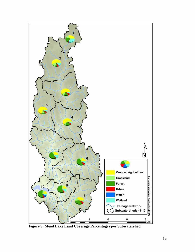
The MLW land cover is predominately cropped agricultural land (41%), with a
higher percentage (68%) of cropped land in the northern half (subwatersheds 1 through 5)
of the watershed (Table 3, Figures 4 & 5). A 2001 land coverage developed by Clark
County shows a decrease in agriculture and increase in forested land compared to the
1992 WISCLAND land coverage. This change may be a result of conversion of
agricultural to private / recreational land, or it may be due to the differences in coverage
production. The 1992 WISCLAND coverage used LANDSAT imagery and the 2001
Clark County coverage was hand digitized from a 1997 aerial photography and verified
17
during a 2001 windshield verification. Refer to Appendix A for land coverage
percentages per subwatershed.
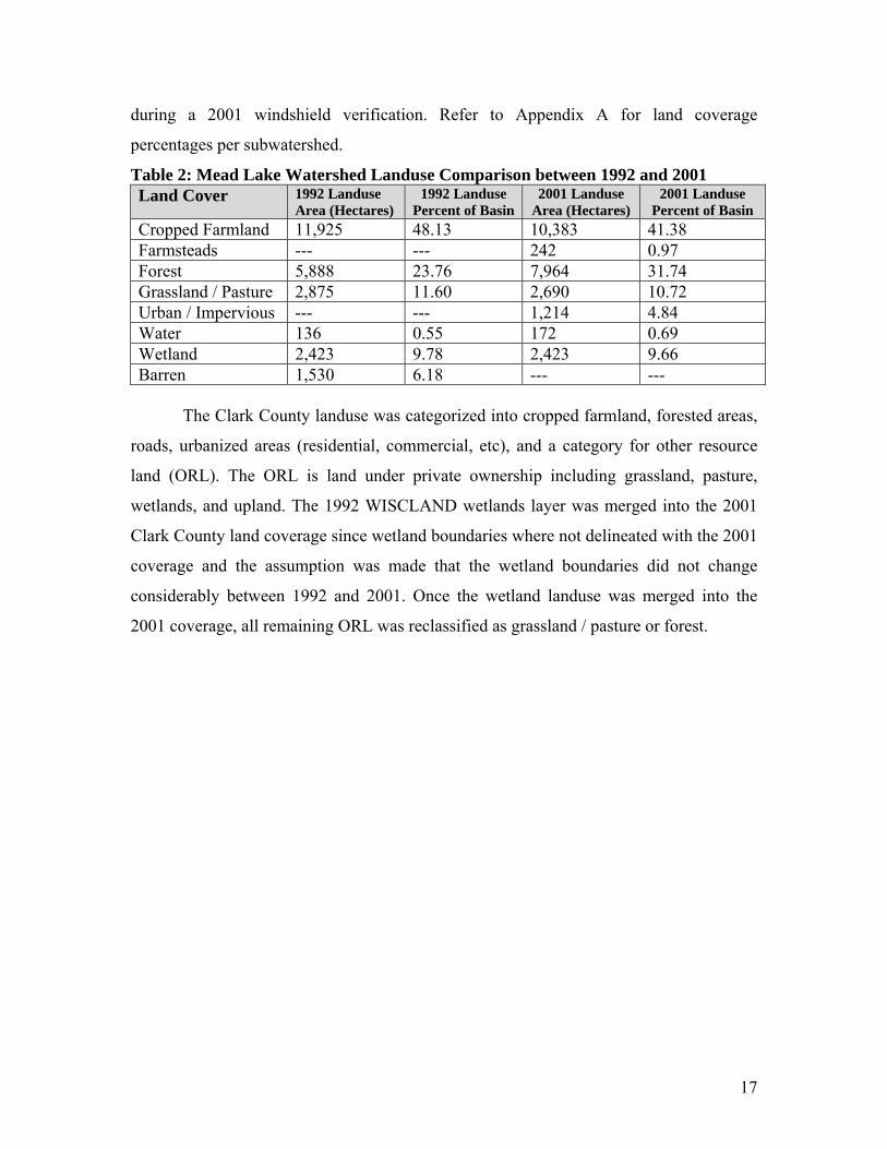
Table 2: Mead Lake Watershed Landuse Comparison between 1992 and 2001 Land Cover 1992 Landuse
Area (Hectares) 1992 Landuse
Percent of Basin 2001 Landuse
Area (Hectares) 2001 Landuse
Percent of Basin Cropped Farmland 11,925 48.13 10,383 41.38 Farmsteads --- --- 242 0.97 Forest 5,888 23.76 7,964 31.74 Grassland / Pasture 2,875 11.60 2,690 10.72 Urban / Impervious --- --- 1,214 4.84 Water 136 0.55 172 0.69 Wetland 2,423 9.78 2,423 9.66 Barren 1,530 6.18 --- ---
The Clark County landuse was categorized into cropped farmland, forested areas,
roads, urbanized areas (residential, commercial, etc), and a category for other resource
land (ORL). The ORL is land under private ownership including grassland, pasture,
wetlands, and upland. The 1992 WISCLAND wetlands layer was merged into the 2001
Clark County land coverage since wetland boundaries where not delineated with the 2001
coverage and the assumption was made that the wetland boundaries did not change
considerably between 1992 and 2001. Once the wetland landuse was merged into the
2001 coverage, all remaining ORL was reclassified as grassland / pasture or forest.

18
Figure 8: Mead Lake Watershed Land Cover Classification
19
Figure 9: Mead Lake Land Coverage Percentages per Subwatershed

20
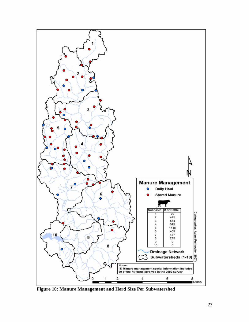
2.3.7 Land Management
The land management of the MLW was assessed using a 2002 farm survey, a land
evaluation completed by the Clark and Taylor County Land Conservation departments,
interviews with Clark County Land Conservation personnel, and a 1999 transect survey
conducted by the Clark County Land Conservation department.
The 2002 farm survey included 82 farms within the watershed, although some
farmers chose not to participate or did not have knowledge of the land practices due to
land rental. Of the 82 farmers, 74 gave information regarding herd size, manure
management, and crop rotation. The majority of the farmers had some type of dairy
rotation which usually consisted of two years of corn, one year of oats and alfalfa,
followed by three years of alfalfa. Some farms rotated corn for more then two years and
included soybeans, peas, or clover into the rotation. Farmers reported approximately
4,200 cattle within the watershed. At the time of the survey 68% of the watershed’s
farmers reported storing manure (Figure 6). The survey indicated several types of tillage
occurring throughout the growing season. Typically the soil was disked prior to planting
of corn, oats, and soybeans. During the growing season springtooth harrow, harrow tines,
or row cultivator tillage were used for corn. Fall tillage included moldboard and paraplow.
The Clark and Taylor County Land Conservation Departments were each given a
landuse map for their portion of the watershed. Dominant agricultural management
practices were indicated on the map and then entered into GIS for spatial analysis and
management practices were based on the 2001 Clark County land coverage attributes.
The 2001 Clark County land coverage defines all agricultural land as cropped farmland
(WISCLAND grid code 110); however, the land coverage was modified so that each
cropped farmland polygon has a related management rotation (Table 4) assigned to it.
The grid code, a numerical value assigned to a landuse in the WIDNR 1992 WISCLAND
layer, was modified so that each rotation had a unique grid code value. The dominant
rotations (dependent on being greater than 5% land area within the HRU threshold) of the
watershed was used for model simulations.
County conservationists indicated approximately 55% of the agricultural land
within the watershed was in a dairy rotation (one year corn, one year corn or soybean,

21
one year oats and alfalfa, three 3 years alfalfa) with stored manure (Appendix A). The
stored manure dairy rotation was the dominant management practice in five of the nine
subwatersheds (Figure 7, Table 4). Another approximately 4% of the watershed was in
cash grain with no storage and no manure.
A 1999 transect survey conducted by the Clark County Land Conservation
Department indicated the crops for 1998 and 1999. The transect route consisted of
approximately 18 sites within subwatershed six, eight, and ten. The transect survey points
correctly corresponded to the management practice GIS layer created from the Land
Conservation Departments.
The farm surveys, land evaluation, transect survey, and discussions with Clark
County Conservationist Matt Zoschke were used to summarize land and nutrient
management (Matt Zoschke, personal communication, June 2007). Six management
rotations were developed for MLW simulations. Clark County Conservationist Matt
Zoschke reviewed and confirmed the management rotations. Of the six rotations, two had
manure storage, one used no manure storage, and two consisted of no storage and no
manure. According to former Clark County Conservationist Gregg Stangl, the dairy
rotation with no manure and no storage was leased land rented by farmers (Gregg Stangl,
Personal Communication, November, 2006). That land is too far away from the main
operation to haul manure, so chemical fertilizers are used instead.
Each type of management applied different amounts and types of nutrients to the
landscape. The dairy management rotations assumed 56,043 kg/ha/year of wet manure
was applied to corn, with a greater amount typically applied in the spring. The Amish
rotation (Gridcode 115) incorporated 33,626 kg/ha/year of wet manure. The continuous
hay / pasture with grazing incorporated approximately 26,900 kg/ha/year of wet manure.
Fertilizers were applied to nearly all of the management rotations. In rotations were
manure was not applied, fertilizer was used as the sole nutrient application. Typically, a
starter fertilizer such as 09-23-30 or 05-14-42 was applied with planting of corn and
soybeans at a rate of 224 kg/ha. A nitrogen based fertilizer such as 46-00-00 was applied
in the spring.
22
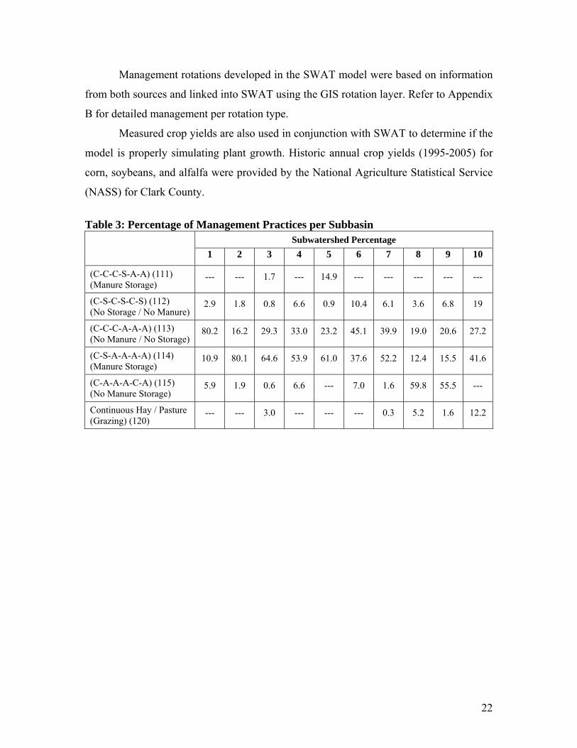
Management rotations developed in the SWAT model were based on information
from both sources and linked into SWAT using the GIS rotation layer. Refer to Appendix
B for detailed management per rotation type.
Measured crop yields are also used in conjunction with SWAT to determine if the
model is properly simulating plant growth. Historic annual crop yields (1995-2005) for
corn, soybeans, and alfalfa were provided by the National Agriculture Statistical Service
(NASS) for Clark County.
Table 3: Percentage of Management Practices per Subbasin Subwatershed Percentage
1 2 3 4 5 6 7 8 9 10
(C-C-C-S-A-A) (111) (Manure Storage)
--- --- 1.7 --- 14.9 --- --- --- --- ---
(C-S-C-S-C-S) (112) (No Storage / No Manure)
2.9 1.8 0.8 6.6 0.9 10.4 6.1 3.6 6.8 19
(C-C-C-A-A-A) (113) (No Manure / No Storage)
80.2 16.2 29.3 33.0 23.2 45.1 39.9 19.0 20.6 27.2
(C-S-A-A-A-A) (114) (Manure Storage)
10.9 80.1 64.6 53.9 61.0 37.6 52.2 12.4 15.5 41.6
(C-A-A-A-C-A) (115) (No Manure Storage)
5.9 1.9 0.6 6.6 --- 7.0 1.6 59.8 55.5 ---
Continuous Hay / Pasture (Grazing) (120)
--- --- 3.0 --- --- --- 0.3 5.2 1.6 12.2
23
Figure 10: Manure Management and Herd Size Per Subwatershed

24
Figure 11: Agricultural Land Management within the Mead Lake Watershed

25
2.4 Calibration
Calibration is the process of matching simulated model results to measured results.
Stream discharge, sediment, and nutrient yields are the primary calibration outputs with
the SWAT model. The SWAT model allows the user to modify hundreds of input
parameters to best simulate the study area. Manual trial and error calibration is the
standard approach in calibrating the SWAT model (Van Liew et al. 2003, Muleta and
Nicklow 2005). The large number of variables makes manual calibration a long, tedious,
and subjective process, especially for a complex watershed. A calibration guide created
by the SWAT developers directs users to the most sensitive input parameters for flow,
sediment, and nutrient simulation (Neitsch et al. 2002).
The SWAT model calibration of the MLW used a parameter estimation tool, the
Parameter ESTimation (PEST) software (Doherty 2004). PEST, a freeware tool, can be
used with any model by reading a model’s input and output files, finding optimum values
and sensitivity for each input parameter. PEST allows for a large number of parameters to
be fitted from nonlinear models like SWAT. PEST performs iterations using the Gauss-
Marquardt-Levenberg algorithm. PEST was used for both field and watershed-scale
simulation and calibration. In addition to the PEST Manual, Lin’s (2005) paper “Getting
Started with PEST” was used for instructional documentation to create the PEST batch
file, SWAT model input template files, SWAT model output reading instruction files, and
a PEST control file.
Calibration of the MLW used 377 streamflow measurements and monthly
sediment and phosphorus export during the growing season (May through September).
Water quality measurements were only collected during the growing season period. As a
result of a relatively short residence time (days rather than months), the Mead Lake
reservoir responds to seasonal inputs; therefore, the calibration did not include the non-
measured months of October – April. PEST input required the date, measured value, an
acceptable input variable range, and current values of the input variables. Previous
SWAT model studies were used to identify the parameters to adjust with PEST.

26
2.5 Statistical Evaluation of SWAT Model
Two statistical measures are typically used in the evaluation of the SWAT model;
the coefficient of determination (R2) and the Nash Sutcliffe coefficient of efficiency (N-S)
(Arabi and Govindaraju 2006). The R2 value is the square of the Pearson’s correlation
coefficient and ranges from 0 to 1, with a value of 1 representing a perfect correlation
between simulated and measured datasets. The N-S coefficient of efficiency has
historically been used to evaluate hydrologic models. The N-S values range from
negative ∞ to 1, with a value of 1 representing a perfect efficiency between the
simulation and measured datasets. The efficiency compares the actual fit to a perfect 1:1
line and measures the correspondence between the measured and simulated flows. Both
measures are particularly sensitive to any large differences between observed and
simulated values (Krause et al. 2005). The R2 values may be greater than N-S values as
individual event outliers tend to have a greater impact on the N-S value (Kirsch et al.
2002). Previous studies indicate that N-S values ranging from 0 – 0.33 are considered
poor model performance, 0.33 – 0.75 are acceptable values, and 0.75 – 1.0 are considered
good (Inamdar 2004; Motovilov et al. 1999).
3.0 MLW SWAT Model Simulation
3.1 Watershed Model Approach
For all watershed-scale simulations, the MLW was divided into ten subwatersheds
and 119 HRUs. The subwatersheds ranged from 1,011 to 3,773 ha in size. The HRUs
were developed using a 5% landuse composition threshold in AVSWAT. No threshold
was set for the soils layer (STATSGO). The cropped HRUs were a variation of dairy
forage or cash grain rotation. The calibration modeling used 12 year simulations (1993 –
2004) with the first 6 years acting as a warm-up period for the simulation. The primary
model run from 1993-2004 was the basis for all related scenarios discussed in this report.
All simulations used the Priestly-Taylor method of evapotranspiration. The watershed
was calibrated to daily output for discharge and monthly for water quality during the
growing season months of May through September. The stream water quality processes

27
and channel dimensions were deactivated within SWAT as a result of the inability to
quantify the fraction of load delivered versus channel derived. PEST was used for
calibration of input parameters and sensitivity analysis. Due to the relatively small dataset,
no validation period was used.
Simulating a heterogeneous landscape of agricultural management required
splitting each agricultural rotation (111, 113, 114, and 115) into 3 separate rotations to
simulate different years of the given rotation (Table 5). This resulted in 10 unique
rotations being applied to 40 different agricultural HRUs based on percent landuse within
the subwatersheds (Appendix C). Crop staggering shown in Table 5 was used to simulate
all phases of a crop rotation within a single model run.
Table 4: Summary of SWAT Model Input Dataset for Simulation Input Data Dataset
Topography 30-meter DEM (USGS) Hydrology 1:24,000 WIDNR Hydrology Precipitation and Temperature Stanley and Owen Weather Stations Land Use 2001 Hand Digitized Land Coverage Soils STATSGO Soils
Table 5: Summary of Agricultural HRU Rotation Staggering Land Coverage ID Rotation ID Rotation Stagger
Gridcode 111 (CRN) 111 (Orginal) CG-CG-CS-S-A-A111A CG-CG-CS-S-A-A
Gridcode 113 (CSIL) 113 (Orginal) CG-CG-CG-A-A-A113A CG-CG-CG-A-A-A113B A-A-CG-CG-C-A113C CG-A-A-A-CG-CG
Gridcode 114 (SOYB) 114 (Orginal) CG-S-A-A-A-A114A A-A-CG-S-A-A114B A-A-A-CG-S-A114C S-A-A-A-A-CG
Gridcode 115 (OATS) 115 (Orginal) CS-A-A-A-CS-A115A CS-A-CS-A-A-A115B A-A-CS-A-CS-A115C A-A-A-CS-A-CS

28
3.2 Discharge Calibration
As part of the USACE Mead Lake assessment (James 2005), average daily stream
discharge was simulated for 377 days between 2002 and 2003 at the County Highway
MM station. The measured discharge includes groundwater and surface water
contributions from the watershed.
To simulate landscape factors for the watershed, discharge was calibrated through
the manipulation of the model’s most sensitive hydrologic input parameters. Previous
studies and observed parameter sensitivity were used to determine the input parameters
for calibration. A combination of assigning parameter values based on default and
measured values with parameter estimation using the PEST program was used to
calibrate the model. The NRCS runoff curve numbers (RCN) were maintained at the
ratio similar to that in NRCS TR-55 (NRCS, 1985) and similar percentage adjustments
were made to all curve numbers in PEST to obtain the best agreement between the
observed and simulated daily flow. The model calibration did not use multiple RCN
changes within a simulation year because the current SWAT2000 program code does not
always recognize RCN changes after tillage changes. In addition to the RCN (SWAT
CNOP) other parameters used for surficial hydrologic model calibration were the soil
bulk density (SOLBD), soil available water capacity (AWC), soil hydraulic conductivity
(SOLK), and the evapotranspiration coefficient (ESCO). Some parameters were grouped
together for PEST analysis. The calibration of the CNOP used two separate values per
land use. The first group consisted of HRUs with soils in the hydrologic class C (Soil IDs
15, 26, and 58). The second group consisted of HRUs with soils in the hydrologic class B
(Soil IDs 20, 43, and 56). The PEST calibration used four soil groups, based on similar
soil properties, for calibration of SOLBD, SOLK, and AWC. The four groups were WI
20, WI 15, 26, and 58, WI 43, and WI 56. Prior to implementation of the PEST, the trial
and error calibrated simulation of the MLW overestimated discharge during events and
underestimated baseflow.
Parameter values were limited in how far they were allowed to deviate from
default values during calibration. The RCNs were allowed a +/- 10% deviation. The soil
properties (SOLBD, SOLK, and AWC) were allowed +/- 15 percent deviation from the

29
default values used for each soil grouping. In general, AWC retained a value similar to
the default range of 0.08 to 0.18 mm/mm. An increase in the AWC suggests greater
infiltration. The three of the four soil groups decreased the calibrated SOLK from the
default. This change reflects a larger retention of soil water. SOLBD increased from the
default to the calibrated value.
Groundwater parameters were also adjusted to allow for increased baseflow to the
Eau Claire River and its tributaries in the PEST calibration. The alpha baseflow
(ALPHA_BF), the direct index of groundwater flow response to changes in recharge, was
decreased from a default 0.048 days to 0.0095 days using PEST. The groundwater delay
was increased from a default 31 days to 255 days. The wetland HRUs were simulated as
having a larger evapotranspiration than other land uses.
Overall, SWAT was able to successfully simulate the daily discharge during the
377 non-melt days. The climatic conditions of the MLW in 2002 and 2003 created two
extremes in discharge creating challenging conditions for model calibration. Year 2002
was above and 2003 was below average annual rainfall. Simulation of the MLW daily
discharge had a R2 and N-S value of 0.63 and 0.62, respectively. Total simulated
discharge was less than one percent greater than the measured. The measured discharges
of 2002 and 2003 required PEST to calibrate to an average fit between the two year’s
observations points. Individual years yielded slightly different results than the statistical
evaluation of the entire measured period. In 2002, the R2 and N-S values for discharge
were 0.58 and 0.52, respectively with an overestimation in discharge of approximately
8%. In 2003, the R2 and N-S values for discharge were 0.75 and 0.71, respectively with
an underestimation in discharge of approximately 8%.

30
Table 6: Calibrated Parameter Values for Discharge in the MLW Constituent SWAT Variable Description Default
ValueCalibrated Value
Discharge CNOP (Corn) Curve Number - Corn 83, 77 83, 77CNOP (Soybean) Curve Number - Soybean 85, 78 85, 78CNOP (Alfalfa) Curve Number - Alfalfa 72, 59 71, 64CNOP (Tillage) Curve Number - Tillages --- 84, 69CNOP (Grassland) Curve Number - Grassland 72, 59 66, 54CNOP (Wetland) Curve Number - Wetland 79, 69 64, 52CNOP (Forest) Curve Number - Forest 72, 59 64, 52CNOP (Urban) Curve Number - Urban 80 66SOL_BD (20) Moist Soil Bulk Density (g/cm3) for soil WI 20 1.60 1.92SOL_BD (15,26,58) Moist Soil Bulk Density (g/cm3) for soil WI 15,26,58 1.50 1.80SOL_BD (56) Moist Soil Bulk Density (g/cm3) for soil WI 56 1.50 1.80SOL_BD (43) Moist Soil Bulk Density (g/cm3) for soil WI 43 1.45 1.74SOL_K (20) Soil Hydraulic Conductivity (mm/hr) for soil WI 20 160.00 60.00SOL_K (15,26,58) Soil Hydraulic Conductivity (mm/hr) for soil WI 15,26,58 14.00 11.32SOL_K (56) Soil Hydraulic Conductivity (mm/hr) for soil WI 56 950.00 60.00SOL_K (43) Soil Hydraulic Conductivity (mm/hr) for soil WI 43 51.00 61.20SOL_AWC (20) Soil Available Water Capacity (mm/mm) for soil WI 20 0.12 0.10SOL_AWC (15,26,58) Soil Available Water Capacity (mm/mm) for soil WI 15,26,58 0.16 0.18SOL_AWC (56) Soil Available Water Capacity (mm/mm) for soil WI 56 0.07 0.08SOL_AWC (43) Soil Available Water Capacity (mm/mm) for soil WI 43 0.12 0.14ESCO Evapotranspiration Coefficient 0.95 0.516GW_DELAY Groundwater Delay Time (days) 31.00 255ALPHA_BF Base Flow Alpha Factor (days) 0.0480 0.0095GW_REVAP (Wetland) Groundwater Revap Coefficient 0.02 0.20REVAPMN (Wetland) Threshold Deptth for Percolation (mm) 1.00 0.00GW_REVAP (Other HRUs) Groundwater Revap Coefficient 0.02 0.10REVAPMN (Other HRUs) Threshold Deptth for Percolation (mm) 1.00 0.08CANMX (Cropped HRUs) Maximum Canopy Storage (mm) 0.00 10.00CANMX (Other HRUs) Maximum Canopy Storage (mm) 0.00 20.00SURLAG Surface Runoff Lag Time (days) 4.00 1.00

31
Figure 12: Measured versus SWAT Simulated Discharge at Cty Hwy MM in the MLW

32
3.3 Sediment Calibration
Watershed sediment load was simulated on a monthly total rather than continuous
estimated daily load. Eleven months of measured sediment load was developed from 22
samples. Simulated sediment loss from the reach (metric tons) was totaled from the
SED_OUT field in the SWAT main channel output file (.rch). Sediment yield from the
HRUs represents a delivered sediment loss because we did not simulate downstream
deposition or channel erosion. Sediment load was calibrated using five SWAT input
parameters: USLE_P (USLE equation support practice factor), SLSUBBSN (average
slope length), Slope (average slope steepness), APM (peak rate adjustment factor for
sediment routing), and FILTERW (width of edge-of-field filter strip trapping efficiency).
Parameter estimation using PEST was used to identify values for the sediment
calibration. The USLE_P value (.mgt) was decreased for agricultural HRUs from a
default value of 1.00 to 0.50. Decreasing the USLE_P from the default decreases the
amount of sediment transported from the landscape. The USLE_P parameter was the
most sensitive of all sediment calibration parameters used with PEST, indicated by
relative sensitivity value in the PEST output. The APM (.bsn) parameter was decreased
from a default 1.00 to 0.64 to dampen the simulated flashy response from storm events in
the watershed. FILTERW was used to trap a portion of the sediment on the landscape and
served to simulate the loss of sediment during delivery between individual fields and the
stream reach.
The objective of the calibration was to find the best parameter combination for
simulating all the monthly sediment loads. We found that several months in particular
were difficult to calibrate. Because there is uncertainty in the monthly sediment loads
estimates from the USGS LOADEST estimating, we sought to minimize the overall
difference between sediment totals on an annual basis and visually sought to match the
monthly totals as closely as possible. The SWAT simulation of the eleven months of
measured sediment load resulted in R2 and N-S values of 0.54 and 0.49, respectively. The
calibration period yielded a five metric ton underestimation of sediment (0.6% error). The
greatest variability in calibrated values occurred during 2002 when above normal
precipitation occurred. The sediment delivered from the landscape into Mead Lake

33
originates primarily from agricultural lands; although due to spatial discretization of
fields with the same management and soils we could not unable to pinpoint the exact
location of the soil erosion.
Sediment export was analyzed during the six year calibration (1999-2004) per
landuse. The greatest percentage (95%) of sediment loading came from agricultural lands.
Of the 95% sediment load derived from agricultural lands, management types 114C and
113C contribute 89% of the sediment load to the stream reach. It is also important to
distinguish sediment load from yield. Examination of sediment yield finds 114C and
113C still yield a large amount of sediment per land area. 111C also yields a large
amount, but since it makes up a small percentage of land area, the sediment load is small.
Table 7: Calibrated Parameter Values for Sediment in the MLW
Constituent SWAT Variable Description Default Value
Calibrated Value
Sediment USLE_P (Cropped HRUs) USLE equation support practice factor for Crops 1.00 0.50SLSUBBSN (Cropped HRUs) Average Slope Length (m) 91.46 50.00SLOPE (Cropped HRUs) Average Slope Steepness (m/m) 0.03, 0.024 0.021, 0.017FILTERW (All HRUs) Filter Strip Width for Sediment Trapping Efficiency (m) 0.00 24.25APM Peak Adjustment for Sediment Routing 1.00 0.64

34
Figure 13: Measured Sediment Load vs. SWAT Simulated Sediment Load

35
2%54%
1%6%
2%35%
111C 113B 113C 114B 114C 115B Figure 14: Percentage of Sediment Load Contribution (1999-2004) Per Agricultural Management Practice
0
500
1000
1500
2000
2500
3000
3500
4000
4500
5000
111
C
113
B
113
C
114
B
114
C
115
B
Fore
st B
Fore
st C
Gra
ssln
d B
Gra
ssln
d C
Wet
lnd
B
Wet
lnd
C
Urb
an C
HRU / Soil Group
Ave
rage
Sed
imen
t Yie
ld B
etw
een
1999
- 20
04 (k
g / k
m2 /
May
- Se
pt)
Figure 15: Average growing season sediment yield (1999-2004) for different HRU combinations of land management and soil hydrologic group.

36
3.4 Total Phosphorus Calibration
The SWAT simulates P soil input as inorganic P fertilizer, organic P fertilizer,
and P tied up in plant residue. During storm events, the P can be transported to the stream
reach two ways: organic and mineral P attached to sediment or as soluble P. The
phosphorus calibration used the hydrology and sediment calibration with adjustments for
groundwater phosphorus concentration, phosphorus partitioning to soil solids, and
phosphorus enrichment in the eroded solids. The P related SWAT parameters included
modifying six input variables: initial soluble P concentration in soil layer (SOL_LABP),
the P soil portioning coefficient (PHOSKD), P availability index (PSP), the P uptake
distribution parameter (UBP), organic phosphorus enrichment ratio (ERORGP), and
groundwater soluble P concentration (GWSOLP). The value of SOL_LABP was
determined using the average P value within each subwatershed field was used in the
model simulation since multiple fields may represent a single HRU. A value of 20 m3/kg
was used for PHOSKD rather than the default of 175 m3/kg to reflect lower phosphorus
partitioning between solid and solution in the soil. This adjustment was necessary to
increase the soluble P quantity in the runoff. Because we used the filter option to trap
sediment in the watershed and that also removes soluble P, the change in the PHOSKD
was based on matching the relationship between MINP (which is largely the SWAT’s
soluble P) and the total P in the runoff. The simulation did not include stream processes,
so this represents the phosphorus delivered. We would anticipate that the fraction of the
P that is soluble would decrease as the TSS concentration increases. The PSP was
decreased from a default of 0.40 to 0.30. The PSP specifies the fraction of fertilizer P
which is in solution after an incubation period. The P uptake distribution parameter (UBP)
was decreased to allow for additional P to remain on the landscape.
The groundwater phosphorus was estimated based on observations of low-flow
phosphorus concentrations in the stream. Figure 16 shows that at very low suspended
solids concentration soluble reactive phosphorus concentrations range from 0.02 to more
than 0.1 mg/l. A groundwater P concentration of 0.08 mg/L was used to match the
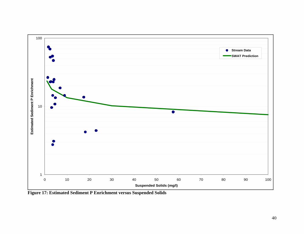
stream concentrations. The phosphorus enrichment of eroded solids (ERORGP) is
estimated in SWAT based on the suspended solids concentration in the runoff. SWAT

37
assumes that as the solids concentration is increased, the phosphorus content of the solids
decreases (the solid line in Figure 17). In Figure 17, the enrichment in the stream solids
estimated the phosphorus content by the difference between total P and soluble reactive P
and dividing by the suspended solids concentration. One of the difficulties with this
relationship in SWAT is that when relatively high solids concentrations are generated
during event days, the enrichment factor can be quite low. To better approximate the
observed enrichment, an enrichment factor of 10 was fixed. This does not allow higher
enrichment factors on low suspended solids events, but this increased the phosphorus
export consistent with the observed export.
Similar to the sediment calibration, the phosphorus calibration illustrated greater
variability in 2002 then 2003. The SWAT simulation of the eleven months of measured
sediment load resulted in R2 and N-S values of 0.66 and 0.66, respectively (Figure 18).
The calibration period yielded a 73 kg underestimation of total phosphorus (1.1% error).
Figure 19 compares the different sources of phosphorus by different management
rotations within the subwatersheds. The simulations show that between 1999 and 2004
over 75% of the phosphorus load originated from agriculturally managed lands.
Approximately 90% of that agricultural phosphorus was from lands managed within the
113C and 114C management classification. These are agricultural rotations on soils that
have higher runoff potential (hydrologic soil group C). .
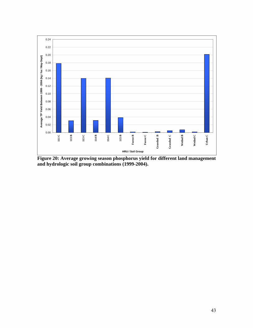
The SWAT modeling identifies management rotations and soil combinations that
are likely to have higher phosphorus export, but it does not identify specific parcels of
land. Within each subwatershed, the variations in slope, soil type, cropping and weather
timing, and proximity to ephemeral and perennial pathways will also need to be
considered in identifying sites that are likely to be most critical with respect to
phosphorus loss. Figure 20 shows the relative difference in average phosphorus loss that
was projected with the SWAT modeling. With this simulation, the hydrologic soil group
was a very strong indication of likely phosphorus loss and is consistent with water
movement from fields to streams as a dominant control over phosphorus export.

38
Table 8: Calibrated Parameter Values for Phosphorus in the MLW Constituent SWAT Variable Description Default
ValueCalibrated Value
Phosphorus SOL_LABP (Cropped HRUs) Initial Soluble Phosphorus Concentration in Soil (mg/kg) 0.00 21 - 44PHOSKD Phosphorus Partitioning Coefficient (m3/mg) 175.00 20.00UBP Phosphorus Uptake Distribution Parameter 20.00 5.00ERORGP Organic Phosphorus Enrichment Ratio 0.00 10.00GWSOLP Groundwater Soluble P Concentration (mg P/L) 0.00 0.08PSP Phosphorus Availability Index 0.400 0.300

39
0.00
0.02
0.04
0.06
0.08
0.10
0.12
0 1 2 3 4 5 6 7 8 9 10
Suspended Solids (mg/l)
Solu
ble
Rea
ctiv
e P
Figure 16: Soluble Reactive P versus Suspended Solids
40
1
10
100
0 10 20 30 40 50 60 70 80 90 100
Suspended Solids (mg/l)
Estim
ated
Sed
imen
t P E
nric
hmen
t
Stream Data
SWAT Prediction
Figure 17: Estimated Sediment P Enrichment versus Suspended Solids

41
Figure 18: Measured TP Load vs. SWAT Simulated TP Load

42
Figure 19: Percent TP Export per Agricultural Practice Between 1999 - 2004
43
0.00
0.02
0.04
0.06
0.08
0.10
0.12
0.14
0.16
0.18
0.20
0.22
0.24
111
C
113
B
113
C
114
B
114
C
115
B
Fore
st B
Fore
st C
Gra
ssln
d B
Gra
ssln
d C
Wet
lnd
B
Wet
lnd
C
Urb
an C
HRU / Soil Group
Ave
rage
TP
Yiel
d B
etw
een
1999
- 20
04 (k
g / h
a / M
ay-S
ept)
Figure 20: Average growing season phosphorus yield for different land management and hydrologic soil group combinations (1999-2004).

44
3.5 Crop Yield Calibration
Annual crop yield and daily biomass within SWAT is used to indicate the correct
simulation of plant growth. Simulated crop growth affects soil moisture,
evapotranspiration, and biomass. Simulation of additional biomass creates additional
post-harvest residue on the landscape, which in-turn lessens the erosive potential during a
runoff events (Baumgart 2005). Each annual crop yield was calibrated by modifying the
biomass energy factor (BE) in the crop database. The default value of corn’s BE (39) was
increased to a value of 49. Alfalfa and Soybeans’ BE were kept at the default values. The
simulated crop yields were within +/- 20 percent of the National Agriculture Statistics
Service (NASS) for Clark County.
Two additional adjustments within SWAT were used to more accurately simulate
crop yields. First, an additional 10 days was added to the original planting date because
SWAT assumes that the plant starts growing immediately instead of accounting for the
initial time the seed germinates (Baumgart 2005). The second adjustment was the use of
the auto-fertilization command for each management scenario. Initial simulations
indicated that the crop growth was affected by frequent nitrogen stress. This is likely due
to the model simulating excessive denitrification. It should be noted that this issue has
since been resolved in the latest version of the model (SWAT 2005). The auto
fertilization command added enough nitrogen to the system every year to displace the
excess being removed by excessive denitrification rates.

45
4.0 Alternative Management Scenarios Alternative management scenarios are modifications of the existing (baseline)
model simulation to explore the impact of changes on phosphorus export. The SWAT can
be used to explore different management and land use changes. These model simulations
are based on adjusting model parameters in ways that reflect these changes. Nine
alternative scenarios were developed from the original baseline model simulation. Each
scenario was run from 1975 through 2004 to incorporate climatological variability
required to develop a long-term average phosphorus contribution to Mead Lake. Besides
the changes made to implement the alternative scenarios, there were no other changes
made from the calibrated parameter set described in Section 3.0.
4.1 Baseline and Scenario Model Simulations (1999-2004) The baseline model simulation was created from the calibrated Mead Lake model.
The baseline model simulation used a 1999 through 2004 evaluation period following a
warm-up period. To account for some of the variability associated with year-to-year
cropping within the rotations, six different starting dates were used in the baseline and
scenario simulations. The starting dates were from 1988 to 1993. This allowed
simulation warm-up periods that ranged from six to eleven years prior to the 1999-2004
evaluation period. The results of the baseline and scenario model simulations are shown
as a range between the average and the maximum annual export for sediment and
phosphorus. The average is the mean of the thirty six different simulation years (six
evaluation years with six different simulations by varying starting years). The maximum
is the average of the highest export result for each year from the six different starting
dates.

46
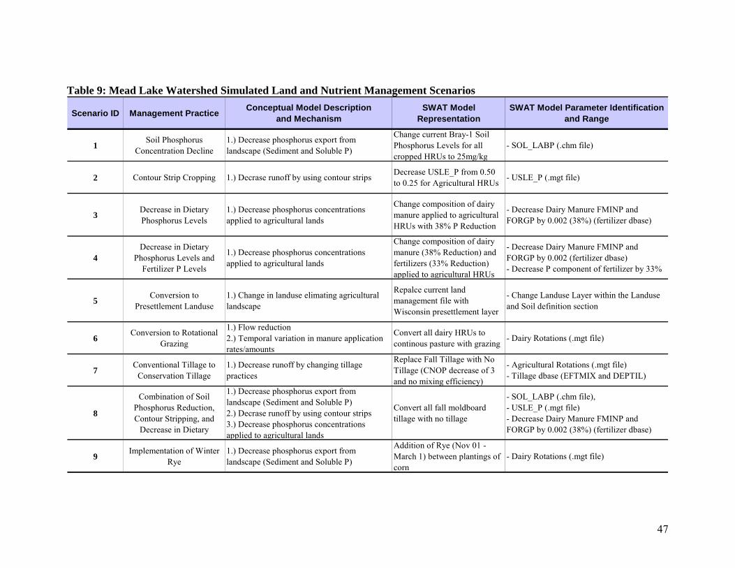
4.2 Scenario Implementation
Nine scenarios were implemented by deviating from the baseline calibration using
model parameters representative of different landuse impacts. The nine scenarios and
their associated techniques are outlined in Table 9. The nine scenarios were chosen as
ones most likely to be implemented in the MLW.
4.2.1 Nutrient Management Scenarios (1, 3, 4, 8)
Scenario 1 decreased the average measured soil phosphorus in each subbasin
agricultural HRUs to a standardized background concentration of 25 mg/kg. This
decrease reflects improvements in nutrient management across the entire watershed.
Scenario 3 changed the amount of phosphorus in cattle feed. This scenario had previously
shown large reductions in the nearby Coon Fork watershed in conjunction with SWAT
(Hung 2002). Scenario 4 decreased the amount of phosphorus in both the cattle feed and
the chemical fertilizers applied to the fields. The application of scenarios 3 and 4 would
likely not produce instantaneous results, but rather would result in a long-term decrease
in soil phosphorus concentrations on agricultural HRUs. Scenario 8 was a combination
scenario that combined the soil phosphorus reduction, the increased erosion control, and
the reduction in dietary phosphorus.
4.2.2 Land Management Scenarios (2, 5, 6, 7, 9) Scenario 2 implemented erosion control measures in the form of contour stripping
applied to all agricultural HRUs within the watershed. Scenario 5 simulated presettlement
conditions. During presettlement time the MLW was dominated by forested and wetland
regions. Scenario 6 changed the land management of agricultural HRUs to continuous
rotational grazing. With rotational grazing, manure is still applied to the land; however,
no tillage practices are implemented. Scenario 7 altered conventional fall tillage to
conservation tillage. This reduces the amount of runoff while the field is bare and
exposed to erosion. Scenario 9 also reduced fall runoff by planting winter rye to serve as
ground cover.
47
Table 9: Mead Lake Watershed Simulated Land and Nutrient Management Scenarios
Scenario ID Management Practice Conceptual Model Description and Mechanism
SWAT Model Representation
SWAT Model Parameter Identification and Range
1Soil Phosphorus
Concentration Decline1.) Decrease phosphorus export from landscape (Sediment and Soluble P)
Change current Bray-1 Soil Phosphorus Levels for all cropped HRUs to 25mg/kg
- SOL_LABP (.chm file)
2 Contour Strip Cropping 1.) Decrase runoff by using contour strips Decrease USLE_P from 0.50 to 0.25 for Agricultural HRUs - USLE_P (.mgt file)
3Decrease in Dietary Phosphorus Levels
1.) Decrease phosphorus concentrations applied to agricultural lands
Change composition of dairy manure applied to agricultural HRUs with 38% P Reduction
- Decrease Dairy Manure FMINP and FORGP by 0.002 (38%) (fertilizer dbase)
4Decrease in Dietary
Phosphorus Levels and Fertilizer P Levels
1.) Decrease phosphorus concentrations applied to agricultural lands
Change composition of dairy manure (38% Reduction) and fertilizers (33% Reduction) applied to agricultural HRUs
- Decrease Dairy Manure FMINP and FORGP by 0.002 (fertilizer dbase) - Decrease P component of fertilizer by 33%
5Conversion to
Presettlement Landuse1.) Change in landuse elimating agricultural landscape
Repalce current land management file with Wisconsin presettlement layer
- Change Landuse Layer within the Landuse and Soil definition section
6Conversion to Rotational
Grazing
1.) Flow reduction 2.) Temporal variation in manure application rates/amounts
Convert all dairy HRUs to continous pasture with grazing - Dairy Rotations (.mgt file)
7Conventional Tillage to
Conservation Tillage1.) Decrease runoff by changing tillage practices
Replace Fall Tillage with No Tillage (CNOP decrease of 3 and no mixing efficiency)
- Agricultural Rotations (.mgt file) - Tillage dbase (EFTMIX and DEPTIL)
8
Combination of Soil Phosphorus Reduction, Contour Stripping, and
Decrease in Dietary
1.) Decrease phosphorus export from landscape (Sediment and Soluble P) 2.) Decrase runoff by using contour strips 3.) Decrease phosphorus concentrations applied to agricultural lands
Convert all fall moldboard tillage with no tillage
- SOL_LABP (.chm file), - USLE_P (.mgt file) - Decrease Dairy Manure FMINP and FORGP by 0.002 (38%) (fertilizer dbase)
9Implementation of Winter
Rye1.) Decrease phosphorus export from landscape (Sediment and Soluble P)
Addition of Rye (Nov 01 - March 1) between plantings of corn
- Dairy Rotations (.mgt file)

48
4.3 Baseline and Scenario Results
Table 10, shown below, shows a summary of the management scenarios and their
impact on the annual average and growing season (May-September) phosphorus export
from the watershed. The results demonstrate that watershed-wide implementation of
reductions in soil phosphorus or sediment control could lead to a 10%-20% reduction in
phosphorus export to Mead Lake. By combining management actions (e.g., Scenario 8)
20%-30% reductions in soil phosphorus might be possible.
Table 10: Simulated Average Phosphorus Export for Mead Lake Watershed Average Annual
Phosphorus Export (Kg)
Average Growing Season Phosphorus
Export (Kg)
Annual Percent Reduction
Baseline 7200 – 9315 2221 - 3047 ---
Reduce Soil P (Scenario 1) 6072 - 7624 1893 - 2499 16%
Reduce Soil Erosion (Scenario 2) 5820 - 7086 1885 - 2388 19%
Dietary P Reduction (Scenario 3) 7035 - 8967 2159 - 2917 2%
Dietary & Fertilizer P Reduction (Scenario 4) 7034 - 8967 2159 - 2917 2%
Pre-settlement Land Use (Scenario 5) 2515 - 2656 857 - 934 65%
Rotational Grazing (Scenario 6) 5749 - 6084 1675 - 1856 20%
Conservation Tillage (Scenario 7) 5718 - 6882 2047 - 2616 21%
Combine Soil TP, Erosion and Dietary P Reduction (Scenario 8) 4931 - 5733 1596 - 1921 32%
Winter Rye (Scenario 9) 6657 - 8977 2208 - 3095 8%
Notes: Annual shown is January-December and growing season May-September. Results based on simulation from 1999-2004 using starting dates 1988-1993 (thirty six different year-simulations from six different years in the six simulations). Range developed from the average of the annual averages to the average of the annual maximums for the different simulations. Percent reduction based on average of annual averages.

49
5.0 Conclusions and Recommendations
• Through calibration, the SWAT model was able to simulate growing season hydrology, sediment and total phosphorus in the Mead Lake watershed.
• Using the results of the SWAT model, it was determined that a little more than
half of the phosphorus entering Mead Lake can be attributed to the row crop agricultural rotations in the Mead Lake watershed.
• SWAT was used to evaluate the magnitude of phosphorus export from the
different agricultural rotations and soils. Those soils with increased likelihood of surface runoff such as hydrologic group C soils, are expected to have the greatest unit-area phosphorus export.
• Average annual phosphorus export to Mead Lake is expected to range from 7200-9300 kilograms. Growing season phosphorus export is expected to range between 2200 and 3500 kilograms.
• Management practices can reduce the runoff volume, sediment loss and phosphorus export from the watershed. An evaluation of a group of management practices suggests that overall phosphorus reductions up to thirty percent are possible with wide-spread implementation of practices.
• As with any modeling study, the results should be interpreted carefully. While the modeling discussed here is a general tool for estimating phosphorus loading, it used only the principal agricultural rotation. Structural sources of phosphorus (e.g., barnyards & cattle crossings) and local variations in proximity to stream and drainage pathways are averaged into the results presented.

50
6.0 References Arabi, M., R. Govindaraju, M. Hantush, B. Engel (2006). Role of Watershed Subdivision
on Modeling the Effectiveness of Best Management Practices with SWAT. Journal of the American Water Resources Association 42(2), 513-528.
Arnold, J. G. and P. M. Allen, 1999. Validation of Automated Methods for Estimating Baseflow and Groundwater Recharge from Stream Flow Records. Journal of American Water Resources Association 35(2): 411-424. Baumgart, P. (2005). Source Allocation of Suspended Sediment and Phosphorus Loads
to Green Bay from the Lower Fox River Subbasins using the SWAT. Report to the Onidea Tribe, 9-127.
Chaubey, I., K.Migliaccio, C.Green, J. Arnold, R. Srinivasan. Phosphorus Modeling in
Soil and Water Assessment Tool (SWAT) Model. In Book Modeling Phosphorus in the Environment. Radcliff,D., M.Cabrera. CRC Press: Flordia, U.S., 2006, 163-187.
Correl, D. (1998). The Role of Phosphorus in the Eutrophication of Receiving Waters: A
Review. Journal of Environmental Quality 27, 261-265. Doherty, J. (2004) PEST: Model-Independent Parameter Estimation Users Manual. 5th
Edition. Di Luzio, M., R. Srinivasan, J.G. Arnold, and S. Neitsch. 2002. ARCVIEW interface for
SWAT 2000 user’s guide. Blackland Research Center. Texas Agricultural Experiment Station, Temple, Texas. Available at: http://www.brc.tamus.edu/swat/doc.html. Accessed July 2006.
FitzHugh,T. and D.Mackay (2000). Impacts of Input Parameter Spatial Aggregation on An Agricultural Nonpoint Source Pollution Model. Journal of Hydrology 236, 35-
53. Gburek,W. and A.Sharpley (1998).Hydrologic Controls on Phosphorus Loss from
Upland Agricultural Watersheds. Journal of Environmental Quality 27, 267-277. Inamdar, S (2004). Assessment of Modeling Tools and Data Needs for Developing the
Sediment Portion of the TMDL Plan for a Mixed Watershed. Final Report to the Great Lakes Basin Program. Buffalo, New York, 10-12.
Hung, B. (2002). Predicting Sediment and Phosphorus Loads to the Coon Fork Flowage
Using SWAT. Wisconsin Department of Natural Resources, 1-13.

51
James, W. (2005). Phosphorus Budget and Loading Reduction Analysis of Mead Lake, West-Central Wisconsin. Eau Galle Aquatic Ecology Laboratory of the Environmental Processes and Effects Division of the U.S. Army Corps of Engineers. Kirsch, K., A. Kirsch, J.Arnold (2002). Predicting Sediment and Phosphorus Loads in the
Rock River Basin Using SWAT. Transactions of the ASAE 45(6), 1757-1769. Krause, P., D. Boyle, K. Bäse (2005). Comparison of Different Efficiency Criteria for
Hydrological Model Assessment. Advances in Geosciences 5, 89-97. Lin, Z. (2005). Getting Started with PEST. Dept. of Crop and Soil Sciences. University of
Georgia. http://linzhulu.myweb.uga.edu/pdf/teaching/starting%20pest.pdf Muleta, M. and J.Nicklow (2005). Sensitivity and Uncertainty Analysis Coupled with
Automatic Calibration for a Distributed Watershed Model. Journal of Hydrology 306, 127-145.
Motovilov, Y., L.Gottschalk, K.Engeland, A.Rodhe (1999). Validation of a Distributed
Hydrological Model against Spatial Observations. Agricultural and Forest Meteorology 98-99, 257-277.
Neitsch, S., J. Arnold, J. Kiniry, J.Williams, K.King (2002). Soil and Water Assessment
Tool Theoretical Documentation – Version 2000. Texas Water Resources Institute, College Station, Texas. TWRI Report TR-191.
Runkel, R.L., Crawford, C.G., Cohn, T.A. (2004). Load Estimator (LOADEST): A
FORTRAN Program for Estimating Constituent Loads in Streams and Rivers. USGS Techniques and Methods Book 4, Chapter A5, p69.
Shaw, B., C.Mechenich, L. Klessing (2000). Understanding Lake Data. UW – Stevens
Point. University of Wisconsin Extension. Stangl, Gregg. Personal Communication. Clark County Land Conservation Department.
November 2006 SWAT Calibration Techniques (2005). USDA Agricultural Research Service. http://www.brc.tamus.edu/swat/publications/swat-calibration-techniques_slides.pdf U.S. Environmental Protection Agency (1996). Environmental Indicators of Water
Quality in the United States. EPA 841-R-96-002. UW-Madison Soil and Plant Analysis Lab, 2007. Wisconsin Soil Test Summary.
University of Wiscosnin – Madison. http://uwlab.soils.wisc.edu/madison/ Wisconsin Department of Natural Resources (2006). List of Impaired Waterways. http://dnr.wi.gov/org/water/wm/wqs/303d/303d.html

52
Van Liew, M., J.Arnold, J.Garbrecht (2003). Hydrologic Simulation on Agricultural
Watersheds: Choosing Between Two Models. Transactions of the ASAE 46(6), 1539-1551.
Zosehke, Matthew. Personal Communication. Clark County Land Conservation
Department. July 2007

53
APPENDICES

54
Appendix A
Landuse Characterization

55
Cropped Farmland (Hectares) Farmsteads (Hectares) Forest (Hectares) Grassland (Hectares) Impervious (Roads, Urban) (Hectares) Water (Hectares) Wetland (Hectares) Total (Hectares)Subbasin 1 360.41 4.8 235.19 132.41 19.78 11.77 323.99 1088Subbasin 2 1552.99 33.06 216.37 461.35 146.87 4.90 380.03 2796Subbasin 3 1713.10 39.67 485.45 277.94 173.10 4.20 179.87 2873Subbasin 4 1758.87 38.23 640.51 219.6 82.00 9.07 162.57 2911Subbasin 5 1666.63 33.73 115.46 273.62 95.29 0.84 138.22 2324Subbasin 6 810.08 29.05 1776.89 389.43 264.19 5.08 258.73 3533Subbasin 7 974.50 25.96 1910.10 292.92 88.71 4.01 537.00 3833Subbasin 8 1117.26 25.32 1023.76 391.98 231.76 4.91 152.72 2948Subbasin 9 239.32 7.36 772.83 86.06 47.65 8.55 178.78 1341Subbasin 10 189.43 5.15 787.73 164.23 65.05 119.15 111.52 1442Totals (Acres) 10383 242 7964 2690 1214 172 2423 25089Total % 41.38 0.97 31.74 10.72 4.84 0.69 9.66
Cropped Farmland (%) Farmsteads (%) Forest (%) Grassland (%) Impervious (Roads, Urban) (%) Water (%) Wetland (%)Subbasin 1 33.1 0.4 21.6 12.2 1.8 1.1 29.8Subbasin 2 55.6 1.2 7.7 16.5 5.3 0.2 13.6Subbasin 3 59.6 1.4 16.9 9.7 6.0 0.1 6.3Subbasin 4 60.4 1.3 22.0 7.5 2.8 0.3 5.6Subbasin 5 71.7 1.5 5.0 11.8 4.1 0.0 5.9Subbasin 6 22.9 0.8 50.3 11.0 7.5 0.1 7.3Subbasin 7 25.4 0.7 49.8 7.6 2.3 0.1 14.0Subbasin 8 37.9 0.9 34.7 13.3 7.9 0.2 5.2Subbasin 9 17.9 0.5 57.7 6.4 3.6 0.6 13.3Subbasin 10 13.1 0.4 54.6 11.4 4.5 8.3 7.7
MEAD LAKE WATERSHED LANDUSE CHARACTERIZATION

56
Dairy (CG-CG-CG-S-A-A) Code 111
(Manure Storage) (Ha)
Cash Grain (C-S-C-S-C-S) Code 112
(No Storage / Manure) (Ha)
Dairy (CG-CG-CG-A-A-A) Code 113
(No Storage / Manure) (Ha)
Dairy (CG-S-A-A-A-A) Code 114
(Manure Storage) (Ha)
Dairy / Amish (CS-A-A-A-CS-A) Code 115
(No Manure Storage) (Ha)
Hay / Pasture w/ Grazing Code 120
(Ha)Totals (Ha)
Subbasin 1 10.44 289.22 39.39 21.37 360Subbasin 2 28.27 251.51 1243.65 29.56 1553Subbasin 3 29.11 13.06 502.69 1107.36 9.38 51.49 1713Subbasin 4 115.85 580.10 947.13 115.8 1759Subbasin 5 248.74 14.94 386.86 1016.11 1667Subbasin 6 83.89 365.06 304.36 56.77 810Subbasin 7 59.14 388.90 508.35 15.59 2.51 974Subbasin 8 40.22 211.99 138.76 668.27 58.02 1117Subbasin 9 16.30 49.26 36.98 132.85 3.93 239Subbasin 10 36.05 51.44 78.80 23.13 189Totals (Acres) 277.85 418.16 3077.03 5420.89 1049.59 139.08 10383Total % 2.68 4.03 29.64 52.21 10.11 1.34
Dairy (CG-CG-CG-S-A-A) Code 111
(Manure Storage) (%)
Cash Grain (C-S-C-S-C-S) Code 112
(No Storage / No Manure) (Hectares)
Dairy (CG-CG-CG-A-A-A) Code 113
(No Manure / No Storage) (%)
Dairy (CG-S-A-A-A-A) Code 114
(Manure Storage) (%)
Dairy / Amish (CS-A-A-A-CS-A) Code 115
(No Manure Storage) (%)
Hay / Pasture w/ Grazing Code 120
(%)
Subbasin 1 0.00 2.90 80.25 10.93 5.93 0.00Subbasin 2 0.00 1.82 16.20 80.08 1.90 0.00Subbasin 3 1.70 0.76 29.34 64.64 0.55 3.01Subbasin 4 0.00 6.59 32.98 53.85 6.58 0.00Subbasin 5 14.92 0.90 23.21 60.97 0.00 0.00Subbasin 6 0.00 10.36 45.06 37.57 7.01 0.00Subbasin 7 0.00 6.07 39.91 52.17 1.60 0.26Subbasin 8 0.00 3.60 18.97 12.42 59.81 5.19Subbasin 9 0.00 6.81 20.58 15.45 55.51 1.64Subbasin 10 0.00 19.03 27.16 41.60 0.00 12.21
MEAD LAKE WATERSHED MANAGEMENT CHARACTERIZATION

57
Appendix B
Agricultural Management Rotations

58
Year Date Operation Crop / Type Rate Units2000 4/25 Manure Dairy 5,380 kg/ha2000 5/1 Tillage Disk Plow2000 5/5 Plant Corn Grain2000 5/5 Fertilizer 09-23-30 224 kg/ha2000 6/15 Herbicide Round-Up2000 10/15 Harvest/Kill Corn Grain2000 10/20 Manure Dairy 1,345 kg/ha2000 10/25 Tillage Moldboard Plow2001 4/25 Manure Dairy 5,380 kg/ha2001 5/1 Tillage Disk Plow2001 5/5 Plant Corn Grain2001 5/5 Fertilizer 09-23-30 224 kg/ha2001 6/15 Herbicide Round-Up2001 10/15 Harvest/Kill Corn Grain2001 10/20 Manure Dairy 1,345 kg/ha2001 10/25 Tillage Moldboard Plow2002 4/25 Manure Dairy 2,119 kg/ha2002 5/1 Tillage Disk Plow2002 5/5 Plant Corn Grain2002 5/5 Fertilizer 09-23-30 224 kg/ha2002 6/15 Herbicide Round-Up2002 10/15 Harvest/Kill Corn Grain2002 10/20 Manure Dairy 1,345 kg/ha2002 10/25 Tillage Moldboard Plow2003 4/25 Manure Dairy 1,345 kg/ha2003 5/10 Tillage Disk Plow2003 5/15 Plant Soybeans2003 10/1 Harvest/Kill Soybeans2003 10/25 Tillage Disk Plow2004 4/25 Plant Alfalfa2004 4/25 Fertilizer 05-14-42 224 kg/ha2004 9/5 Harvest Alfalfa2004 9/5 Fertilizer 00-00-60 224 kg/ha2005 6/10 Harvest Alfalfa2005 7/15 Harvest Alfalfa2005 9/1 Harvest Alfalfa2005 10/1 Kill Alfalfa Alfalfa2005 10/15 Manure Dairy 5,380 kg/ha2005 10/25 Tillage Moldboard Plow
Dairy (CG-CG-CS-S-A-A) (Manure Storage) (Gridcode 111)
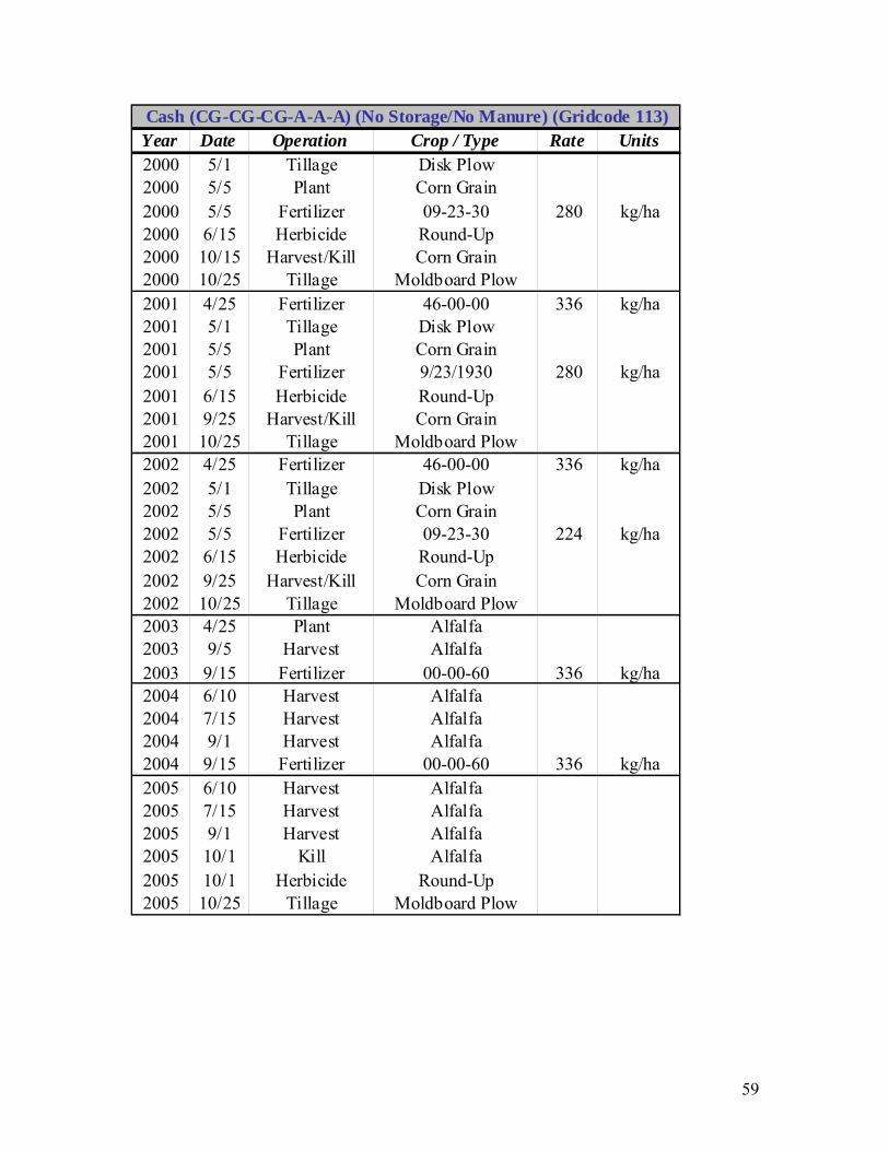
59
Year Date Operation Crop / Type Rate Units2000 5/1 Tillage Disk Plow2000 5/5 Plant Corn Grain2000 5/5 Fertilizer 09-23-30 280 kg/ha2000 6/15 Herbicide Round-Up2000 10/15 Harvest/Kill Corn Grain2000 10/25 Tillage Moldboard Plow2001 4/25 Fertilizer 46-00-00 336 kg/ha2001 5/1 Tillage Disk Plow2001 5/5 Plant Corn Grain2001 5/5 Fertilizer 9/23/1930 280 kg/ha2001 6/15 Herbicide Round-Up2001 9/25 Harvest/Kill Corn Grain2001 10/25 Tillage Moldboard Plow2002 4/25 Fertilizer 46-00-00 336 kg/ha2002 5/1 Tillage Disk Plow2002 5/5 Plant Corn Grain2002 5/5 Fertilizer 09-23-30 224 kg/ha2002 6/15 Herbicide Round-Up2002 9/25 Harvest/Kill Corn Grain2002 10/25 Tillage Moldboard Plow2003 4/25 Plant Alfalfa2003 9/5 Harvest Alfalfa2003 9/15 Fertilizer 00-00-60 336 kg/ha2004 6/10 Harvest Alfalfa2004 7/15 Harvest Alfalfa2004 9/1 Harvest Alfalfa2004 9/15 Fertilizer 00-00-60 336 kg/ha2005 6/10 Harvest Alfalfa2005 7/15 Harvest Alfalfa2005 9/1 Harvest Alfalfa2005 10/1 Kill Alfalfa2005 10/1 Herbicide Round-Up2005 10/25 Tillage Moldboard Plow
Cash (CG-CG-CG-A-A-A) (No Storage/No Manure) (Gridcode 113)

60
Year Date Operation Crop / Type Rate Units2000 4/25 Manure Dairy 5,380 kg/ha2000 5/1 Tillage Disk Plow2000 5/5 Plant Corn Grain2000 5/5 Fertilizer 09-23-30 224 kg/ha2000 6/15 Herbicide Round-Up2000 10/15 Harvest/Kill Corn Grain2000 10/20 Manure Dairy 5,380 kg/ha2000 10/25 Tillage Moldboard Plow2001 5/1 Tillage Disk Plow2001 5/15 Plant Soybeans2001 5/15 Fertilizer 05-14-42 224 kg/ha2001 6/25 Herbicide Round-Up2001 10/1 Harvest/Kill Soybeans2001 10/25 Tillage Disk Plow2002 4/10 Manure Dairy 1,345 kg/ha2002 4/15 Tillage Disk Plow2002 4/25 Plant Alfalfa2002 4/25 Fertilizer 05-14-42 224 kg/ha2002 9/1 Harvest Alfalfa2002 9/15 Fertilizer 00-00-60 224 kg/ha2003 6/10 Harvest Alfalfa2003 7/15 Harvest Alfalfa2003 9/1 Harvest Alfalfa2003 9/15 Fertilizer 00-00-60 224 kg/ha2004 6/10 Harvest Alfalfa2004 7/15 Harvest Alfalfa2004 9/1 Harvest Alfalfa2004 9/15 Fertilizer 00-00-60 224 kg/ha2005 6/10 Harvest Alfalfa2005 7/15 Harvest Alfalfa2005 9/1 Harvest Alfalfa2005 10/1 Kill Alfalfa2005 10/15 Manure Dairy 1,345 kg/ha2005 10/25 Tillage Moldboard Plow
Dairy (CG-S-A-A-A-A) (Manure Storage) (Gridcode 114)

61
Year Date Operation Crop / Type Rate Units2000 4/1 Manure Dairy 1,009 kg/ha2000 5/1 Tillage Disk Plow2000 5/1 Manure Dairy 1,009 kg/ha2000 5/20 Plant Corn Silage2000 5/20 Fertilizer 09-23-30 224 kg/ha2000 9/1 Manure Dairy 505 kg/ha2000 10/1 Harvest/Kill Corn Silage2000 10/1 Manure Dairy 505 kg/ha2000 10/25 Tillage Moldboard Plow2000 11/1 Manure Dairy 505 kg/ha2000 12/1 Manure Dairy 505 kg/ha2001 4/20 Tillage Disk Plow2001 4/25 Plant Alfalfa2001 9/5 Harvest Alfalfa2002 6/10 Harvest Alfalfa2002 7/15 Harvest Alfalfa2002 9/1 Harvest Alfalfa2003 6/10 Harvest Alfalfa2003 7/15 Harvest Alfalfa2003 9/1 Harvest Alfalfa2003 10/1 Kill Alfalfa2003 10/1 Manure Dairy 1,009 kg/ha2003 10/25 Tillage Moldboard Plow2004 4/1 Manure Dairy 1,009 kg/ha2004 5/1 Tillage Disk Plow2004 5/1 Manure Dairy 1,009 kg/ha2004 5/20 Plant Corn Silage2004 5/20 Fertilizer 09-23-30 224 kg/ha2004 9/1 Manure Dairy 505 kg/ha2004 10/1 Harvest/Kill Corn Silage2004 10/1 Manure Dairy 505 kg/ha2004 10/25 Tillage Moldboard Plow2004 11/1 Manure Dairy 505 kg/ha2005 4/20 Tillage Disk Plow2005 4/25 Plant Alfalfa2005 4/25 Plant Alfalfa2005 9/5 Harvest Alfalfa2005 10/1 Kill Alfalfa2005 10/1 Manure Dairy 1,009 kg/ha2005 10/25 Tillage Moldboard Plow
Dairy/Amish (CS-A-A-A-CS-A) (No Manure Storage) (Gridcode 115)

62
Appendix C
HRU Rotation Assignments

63
SUBBASIN # 1HRU # Acres % Subbasin Rotation ID10 Corn Silage-->CSIL/WI020 74 2.97 113A211 Corn Silage-->CSIL/WI015 311 12.43 113C112 Corn Silage-->CSIL/WI026 461 18.45 113B1
SUBBASIN # 2HRU # Acres % Subbasin Rotation ID13 Soybean-->SOYB/WI015 35.51 0.54 114A114 Soybean-->SOYB/WI026 2925.46 44.72 114B121 Corn Silage-->CSIL/WI015 66.01 1.01 113B122 Corn Silage-->CSIL/WI026 531.47 8.12 113C1
SUBBASIN # 3HRU # Acres % Subbasin Rotation ID25 Soybean-->SOYB/WI026 2714.38 38.97 114B126 Soybean-->SOYB/WI058 66.68 0.96 114A133 Corn Silage-->CSIL/WI026 1292.59 18.56 113A1
SUBBASIN # 4HRU # Acres % Subbasin Rotation ID36 Soybean-->SOYB/WI026 1528.32 21.74 114A137 Soybean-->SOYB/WI058 981.61 13.97 114B138 Soybean-->SOYB/WI056 34.71 0.49 114C248 Corn Silage-->CSIL/WI026 136.04 1.94 113C149 Corn Silage-->CSIL/WI058 1383.35 19.68 113A150 Corn Silage-->CSIL/WI056 116.90 1.66 113B2
SUBBASIN # 5HRU # Acres % Subbasin Rotation ID51 Soybean-->SOYB/WI026 1814.63 32.97 114B152 Soybean-->SOYB/WI058 790.84 14.37 114A153 Soybean-->SOYB/WI056 1.41 0.03 114C254 Corn-->CORN/WI026 656.20 11.92 111A161 Corn Silage-->CSIL/WI026 706.42 12.83 113C162 Corn Silage-->CSIL/WI058 209.38 3.80 113A1
SUBBASIN # 6HRU # Acres % Subbasin Rotation ID65 Soybean-->SOYB/WI058 131.05 1.61 114B166 Soybean-->SOYB/WI043 494.37 6.06 114A267 Soybean-->SOYB/WI056 175.05 2.14 114C277 Corn Silage-->CSIL/WI058 510.00 6.25 113A178 Corn Silage-->CSIL/WI056 446.04 5.46 113C2
SUBBASIN # 7HRU # Acres % Subbasin Rotation ID79 Soybean-->SOYB/WI058 903.28 9.69 114B180 Soybean-->SOYB/WI043 37.44 0.40 114C281 Soybean-->SOYB/WI056 356.63 3.82 114A291 Corn Silage-->CSIL/WI058 247.35 2.65 113C192 Corn Silage-->CSIL/WI043 219.27 2.35 113B293 Corn Silage-->CSIL/WI056 500.31 5.37 113A2
SUBBASIN # 8HRU # Acres % Subbasin Rotation ID94 Soybean-->SOYB/WI043 375.88 5.54 114B2100 Oats-->OATS/WI043 1715.80 25.57 115A2101 Corn Silage-->CSIL/WI043 536.79 7.91 113C2
SUBBASIN # 9HRU # Acres % Subbasin Rotation ID108 Oats-->OATS/WI043 323.10 9.83 115A2109 Oats-->OATS/WI056 45.18 1.37 115B2
SUBBASIN # 10HRU # Acres % Subbasin Rotation ID110 Soybean-->SOYB/WI043 216.28 6.35 114A2111 Soybean-->SOYB/WI056 4.06 0.12 114C2

64
Related Documents