Math 639: Lecture 20 - Hausdorff dimension - Stony Brook ...

Math 639: Lecture 20Hausdorff dimension

Bob Hough

April 25, 2017

Bob Hough Math 639: Lecture 20 April 25, 2017 1 / 64

Hausdorff dimension

This lecture follows Morters and Peres, Chapter 4.


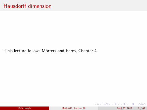
Minkowski dimension

Definition

Suppose E is a bounded metric space with metric ρ. A covering of E is afinite or countable collection of sets

E1,E2,E3, ... with E Ă8ď

i“1

Ei .

Define, for ε ą 0,

MpE , εq “ min!

k ě 1 :there exists finite covering E Ăkď

i“1

Ei

with maxi|Ei | ď ε

)

where |A| is the diameter of the set A.


Minkowski dimension

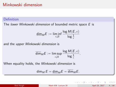
Definition

The lower Minkowski dimension of bounded metric space E is

dimME :“ lim infεÓ0

logMpE , εq

log 1ε

and the upper Minkowski dimension is

dimME :“ lim supεÓ0

logMpE , εq

log 1ε

.

When equality holds, the Minkowski dimension is

dimM E “ dimME “ dimME .


Minkowski dimension

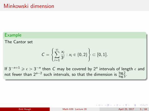
Example

The Cantor set

C “

#

8ÿ

i“1

xi3i

: xi P t0, 2u

+

Ă r0, 1s.

If 3ń`1 ě ε ą 3ń then C may be covered by 2n intervals of length ε andnot fewer than 2n´2 such intervals, so that the dimension is log 2

log 3 .


Minkowski dimension

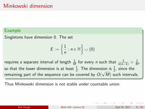
Example

Singletons have dimension 0. The set

E :“

"

1

n: n P N

*

Y t0u

requires a separate interval of length 1M for every n such that 1

npn´1q ą1M ,

so that the lower dimension is at least 12 . The dimension is 1

2 , since the

remaining part of the sequence can be covered by Op?Mq such intervals.

Thus Minkowski dimension is not stable under countable union.


Hausdorff dimension

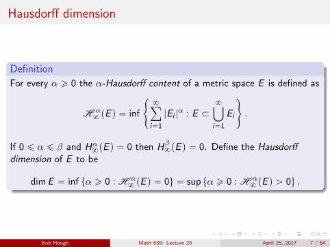
Definition

For every α ě 0 the α-Hausdorff content of a metric space E is defined as

H α8 pE q “ inf

#

8ÿ

i“1

|Ei |α : E Ă

8ď

i“1

Ei

+

.

If 0 ď α ď β and Hα8pE q “ 0 then Hβ

8pE q “ 0. Define the Hausdorffdimension of E to be

dimE “ inf tα ě 0 : H α8 pE q “ 0u “ sup tα ě 0 : H α

8 pE q ą 0u .


Hausdorff measure

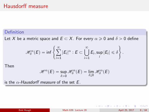
Definition

Let X be a metric space and E Ă X . For every α ě 0 and δ ą 0 define

H αδ pE q “ inf

#

8ÿ

i“1

|Ei |α : E Ă

8ď

i“1

Ei , supi|Ei | ď δ

+

.

ThenH αpE q “ sup

δą0H αδ pE q “ lim

δÓ0H αδ pE q

is the α-Hausdorff measure of the set E .


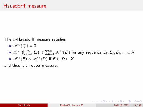
Hausdorff measure

The α-Hausdorff measure satisfies

H αpHq “ 0

H α`Ť8

i“1 Ei

˘

ďř8

i“1 H αpEi q for any sequence E1,E2,E3, ... Ă X

H αpE q ďH αpDq if E Ă D Ă X

and thus is an outer measure.


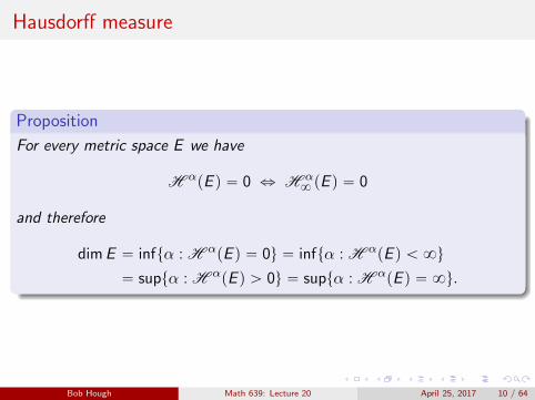
Hausdorff measure

Proposition

For every metric space E we have

H αpE q “ 0 ô H α8 pE q “ 0

and therefore

dimE “ inftα : H αpE q “ 0u “ inftα : H αpE q ă 8u

“ suptα : H αpE q ą 0u “ suptα : H αpE q “ 8u.


Hausdorff measure

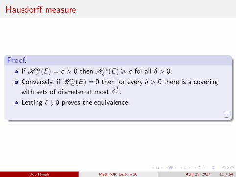
Proof.

If H α8 pE q “ c ą 0 then H α

δ pE q ě c for all δ ą 0.

Conversely, if H α8 pE q “ 0 then for every δ ą 0 there is a covering

with sets of diameter at most δ1α .

Letting δ Ó 0 proves the equivalence.


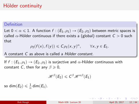
Holder continuity

Definition

Let 0 ă α ď 1. A function f : pE1, ρ1q Ñ pE2, ρ2q between metric spaces iscalled α-Holder continuous if there exists a (global) constant C ą 0 suchthat

ρ2pf pxq, f pyqq ď Cρ1px , yqα, @x , y P E1.

A constant C as above is called a Holder constant.

If f : pE1, ρ1q Ñ pE2, ρ2q is surjective and α-Holder continuous withconstant C , then for any β ě 0,

H βpE2q ď CβH αβpE1q

so dimpE2q ď1α dimpE1q.


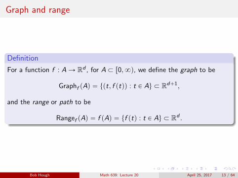
Graph and range

Definition

For a function f : AÑ Rd , for A Ă r0,8q, we define the graph to be

Graphf pAq “ tpt, f ptqq : t P Au Ă Rd`1,

and the range or path to be

Rangef pAq “ f pAq “ tf ptq : t P Au Ă Rd .


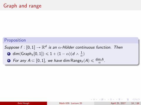
Graph and range

Proposition

Suppose f : r0, 1s Ñ Rd is an α-Holder continuous function. Then

1 dimpGraphf r0, 1sq ď 1` p1´ αqpd ^ 1αq

2 For any A Ă r0, 1s, we have dim Rangef pAq ďdimAα .


Graph and range

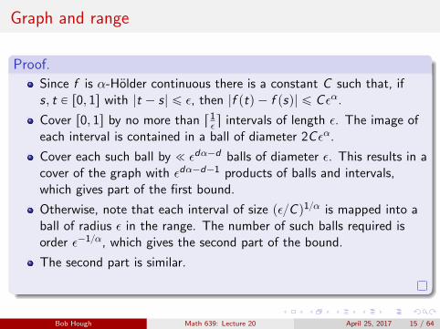
Proof.

Since f is α-Holder continuous there is a constant C such that, ifs, t P r0, 1s with |t ´ s| ď ε, then |f ptq ´ f psq| ď Cεα.

Cover r0, 1s by no more than r 1ε s intervals of length ε. The image of

each interval is contained in a ball of diameter 2Cεα.

Cover each such ball by ! εdα´d balls of diameter ε. This results in acover of the graph with εdα´d´1 products of balls and intervals,which gives part of the first bound.

Otherwise, note that each interval of size pε{C q1{α is mapped into aball of radius ε in the range. The number of such balls required isorder ε´1{α, which gives the second part of the bound.

The second part is similar.


Graph and range

Corollary

For any fixed set A Ă r0,8q the graph of a d-dimensional Brownianmotion satisfies, a.s.

dimpGraphpAqq ď

"

3{2 d “ 12 d ě 2

and its range satisfies, a.s.

dim RangepAq ď p2 dimAq ^ d .


Range of Brownian motion

Theorem

Let tBptq : t ě 0u be a Brownian motion in dimension d ě 2. Thenalmost surely, for any set A Ă r0,8q we have

H 2pRangepAqq “ 0.



Proof.

Let Cube “ r0, 1qd . It suffices to show thatH 2pRanger0,8q X Cubeq “ 0 for Brownian motion started atx R Cube. Also, we may assume that d ě 3, since 2 dimensionalBrownian motion is a projection, which does not increase theHausdorff measure.

Define the occupation measure µ by

µpAq “

ż 8

01ApBpsqqds, A Ă Rd , Borel.

Let Dk be the collection of all cubesśd

i“1rni2´k , pni ` 1q2´kq where

n1, ..., nd P t0, 1, ..., 2k ´ 1u.



Proof.

Fix a threshold m and let M ą m. We call D P Dk with k ě m a bigcube if

µpDq ě1

ε2´2k .

The collection C pMq consists of all maximal big cubes D P Dk ,m ď k ď M together with those cubes D P DM which are notcontained in a big cube but intersect Ranger0,8q.

The sets of C pMq are a cover of Ranger0,8q X Cube with sets ofdiameter at most

?d2´m.



Proof.

Given a cube D P DM let D “ DM Ă DM´1 Ă ... Ă Dm with Dk P Dk

the sequence of cubes containing D. Let D˚k be the cube with thesame center as Dk and 3

2 its side length.

Let τpDq be the first hitting time of cube D andτk “ inftt ą τpDq : Bptq R D˚k u the first exit time from D˚k .

Let Child “ r0, 12q

d and define the expanded sets Cube˚ and Child˚.

Define τ “ inftt ą 0 : Bptq R Cube˚u and

q :“ supyPChild˚

Proby

ˆż τ

01CubepBpsqqds ď

1

ε

˙

ă 1.



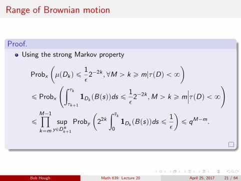
Proof.

Using the strong Markov property

Probx

ˆ

µpDkq ď1

ε2´2k ,@M ą k ě m|τpDq ă 8

˙

ď Probx

˜

ż τk

τk`1

1DkpBpsqqds ď

1

ε2´2k ,M ą k ě m

ˇ

ˇ

ˇτpDq ă 8

¸

ď

M´1ź

k“m

supyPD˚k`1

Proby

ˆ

22k

ż τk

01DkpBpsqqds ď

1

ε

˙

ď qM´m.



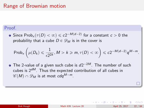
Proof.

Since ProbxpτpDq ă 8q ď c2´Mpd´2q for a constant c ą 0 theprobability that a cube D P DM is in the cover is

Probx

ˆ

µpDkq ď1

ε22k,M ą k ě m, τpDq ă 8

˙

ď c2´Mpd´2qqM´m.

The 2-value of a given such cube is d2´2M . The number of suchcubes is 2dM . Thus the expected contribution of all cubes inC pMq XDM is at most cdqM´m.



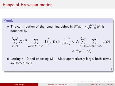
Proof.

The contribution of the remaining cubes in C pMq XŤM´1

k“m Dk isbounded by

M´1ÿ

k“m

d2´2kÿ

DPC pMqXDk

1

ˆ

µpDq ě1

ε22k

˙

ď dεM´1ÿ

k“m

ÿ

DPC pMqXDk

µpDq

ď dεµpCubeq.

Letting ε Ó 0 and choosing M “ Mpεq appropriately large, both termsare forced to 0.


The mass distribution principle

Definition

We call a measure µ on the Borel sets of a metric space E a massdistribution on E , if

0 ă µpE q ă 8.



Theorem

Suppose E is a metric space and α ě 0. If there is a mass distribution µon E and constants C ą 0 and δ ą 0 such that

µpV q ď C |V |α,

for all closed sets V with diameter |V | ď δ, then

H αpE q ěµpE q

Cą 0,

and hence dimE ě α.



Proof.

Suppose that U1,U2, ... is a cover of E by arbitrary sets with |Ui | ď δ. LetVi be the closure of Ui and note that |Ui | “ |Vi |. We have

0 ă µpE q ď µ

˜

8ď

i“1

Vi

¸

ď

8ÿ

i“1

µpVi q ď C8ÿ

i“1

|Ui |α.

Taking the inf and letting δ Ó 0 gives the claim.


Record time

Definition

Let tBptq : t ě 0u be a linear Brownian motion and tMptq : t ě 0u theassociated maximum process. A time t ě 0 is a record time for theBrownian motion if Mptq “ Bptq and the set of all record times for theBrownian motion is denoted by Rec.


Record time

Lemma

Almost surely, dimpRecXr0, 1sq ě 12 and hence dimpZerosXr0, 1sq ě 1

2 .


Record time

Proof.

t ÞÑ Mptq is continuous and increasing, hence is the distributionfunction of a positive measure µ, with µpa, bs “ Mpbq ´Mpaq.

The measure µ is supported on Rec.

For α ă 12 , Brownian motion is a.s. locally α-Holder continuous

Thus there exists a constant Cα such that, for all a, b P r0, 1s

Mpbq ´Mpaq ď max0ďhďbá

Bpa` hq ´ Bpaq ď Cαpb ´ aqα.

By the mass distribution principle, a.s.

dimpRecXr0, 1sq ě α.

The claim for Zeros follows because Y ptq “ Mptq ´ Bptq is reflectedBrownian motion.


Zeros

Lemma

There is an absolute constant C such that, for any a, ε ą 0,

Prob pthere exists t P pa, a` εq with Bptq “ 0q ď C

c

ε

a` ε.


Zeros

Proof.

Let A “ t|Bpa` εq| ď?εu. Thus

ProbpAq “ Prob

ˆ

|Bp1q| ď

c

ε

a` ε

˙

ď 2

c

ε

a` ε.

Let T be the stopping time T “ inftt ě a : Bptq “ 0u

ProbpAq ě Prob pAX t0 P Bra, a` εsuq

ě ProbpT ď a` εq minaďtďa`ε

Probp|Bpa` εq| ď?ε|Bptq “ 0q.

The minimum is achieved at t “ a where

Probp|Bpa` εq| ď?ε|Bpaq “ 0q “ Probp|Bp1q| ď 1q

which is a constant.


Zeros

Theorem

Let tBptq : 0 ď t ď 1u be a linear Brownian motion. Then with probability1 we have

dimpZerosXr0, 1sq “ dimpRecXr0, 1sq “1

2.


Zeros

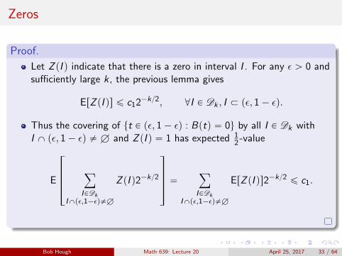
Proof.

Let Z pI q indicate that there is a zero in interval I . For any ε ą 0 andsufficiently large k , the previous lemma gives

ErZ pI qs ď c12´k{2, @I P Dk , I Ă pε, 1´ εq.

Thus the covering of tt P pε, 1´ εq : Bptq “ 0u by all I P Dk withI X pε, 1´ εq ‰ H and Z pI q “ 1 has expected 1

2 -value

E

»

—

—

–

ÿ

IPDkIXpε,1´εq‰H

Z pI q2´k{2

fi

ffi

ffi

fl

“ÿ


ErZ pI qs2´k{2 ď c1.


Zeros

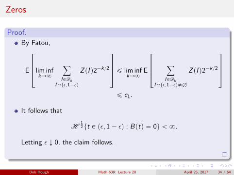
Proof.

By Fatou,

E

»

—

—

–

lim infkÑ8

ÿ

IPDkIXpε,1´εq

Z pI q2´k{2

fi

ffi

ffi

fl

ď lim infkÑ8

E

»

—

—

–

ÿ


Z pI q2´k{2

fi

ffi

ffi

fl

ď c1.

It follows that

H12 tt P pε, 1´ εq : Bptq “ 0u ă 8.

Letting ε Ó 0, the claim follows.


The energy method

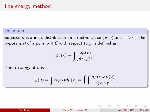
Definition

Suppose µ is a mass distribution on a metric space pE , ρq and α ě 0. Theα-potential of a point x P E with respect to µ is defined as

φαpxq “

ż

dµpyq

ρpx , yqα.

The α-energy of µ is

Iαpµq “

ż

φαpxqdµpxq “

ż ż

dµpxqdµpyq

ρpx , yqα.


The energy method

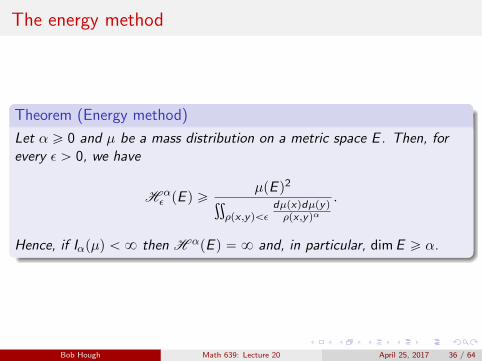
Theorem (Energy method)

Let α ě 0 and µ be a mass distribution on a metric space E . Then, forevery ε ą 0, we have

H αε pE q ě

µpE q2ť

ρpx ,yqăεdµpxqdµpyqρpx ,yqα

.

Hence, if Iαpµq ă 8 then H αpE q “ 8 and, in particular, dimE ě α.


The energy method

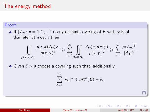
Proof.

If tAn : n “ 1, 2, ...u is any disjoint covering of E with sets ofdiameter at most ε then

ĳ

ρpx ,yqăε

dµpxqdµpyq

ρpx , yqαě

8ÿ

n“1

ĳ

AnÂn

dµpxqdµpyq

ρpx , yqαě

8ÿ

n“1

µpAnq2

|An|α,

Given δ ą 0 choose a covering such that, additionally,

8ÿ

n“1

|An|α ď H α

ε pE q ` δ.


The energy method

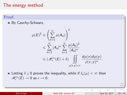
Proof.

By Cauchy-Schwarz,

µpE q2 ď

˜

8ÿ

n“1

µpAnq

¸2

ď

8ÿ

n“1

|An|α8ÿ

n“1

µpAnq2

|An|α

ď pH αε pE q ` δq

ĳ

ρpx ,yqăε

dµpxqdµpyq

ρpx , yqα.

Letting δ Ó 0 proves the inequality, while if Iαpµq ă 8 thenH αε pE q Ñ 0 as εÑ 0.


The dimension of Brownian motion

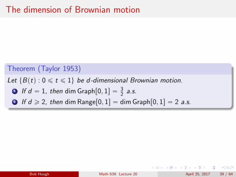
Theorem (Taylor 1953)

Let tBptq : 0 ď t ď 1u be d-dimensional Brownian motion.

1 If d “ 1, then dim Graphr0, 1s “ 32 a.s.

2 If d ě 2, then dim Ranger0, 1s “ dim Graphr0, 1s “ 2 a.s.



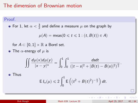
Proof.

For 1, let α ă 32 and define a measure µ on the graph by

µpAq “ measp0 ď t ď 1 : pt,Bptqq P Aq

for A Ă r0, 1s ˆ R a Borel set.

The α-energy of µ is

ĳ

dµpxqdµpyq

|x ´ y |α“

ż 1

0

ż 1

0

dsdt

p|t ´ s|2 ` |Bptq ´ Bpsq|2qα2

.

Thus

E Iαpµq ď 2

ż 1

0E´

pt2 ` Bptq2q´α2

¯

dt.



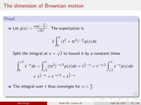
Proof.

Let ppzq “expp´ z2

2q

?2π

. The expectation is

2

ż 8

0pt2 ` tz2q´

α2 ppzqdz .

Split the integral at z “?t to bound it by a constant times

ż

?t

0t´αdz `

ż 8

?tptz2q´α{2ppzqdz “ t

12´α ` t´α{2

ż 8

?tz´αppzqdz

! t12´α ` t´α{2 ` t

12´α.

The integral over t thus converges for α ă 32 .



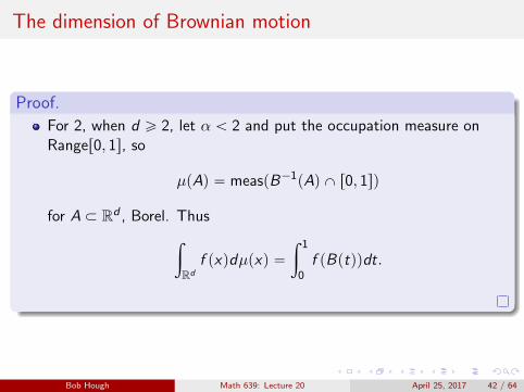
Proof.

For 2, when d ě 2, let α ă 2 and put the occupation measure onRanger0, 1s, so

µpAq “ measpB´1pAq X r0, 1sq

for A Ă Rd , Borel. Thus

ż

Rd

f pxqdµpxq “

ż 1

0f pBptqqdt.



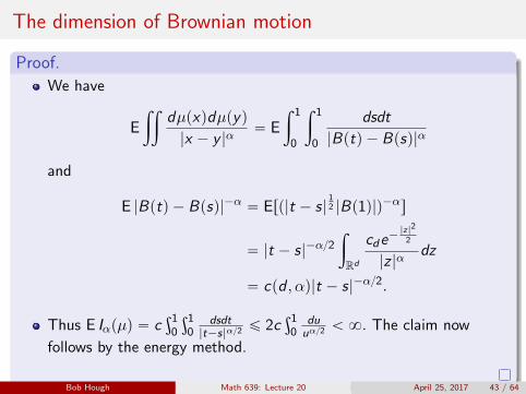
Proof.

We have

E

ĳ

dµpxqdµpyq

|x ´ y |α“ E

ż 1

0

ż 1

0

dsdt

|Bptq ´ Bpsq|α

and

E |Bptq ´ Bpsq|´α “ Erp|t ´ s|12 |Bp1q|q´αs

“ |t ´ s|´α{2ż

Rd

cde´|z|2

2

|z |αdz

“ cpd , αq|t ´ s|´α{2.

Thus E Iαpµq “ cş1

0

ş10

dsdt|t´s|α{2

ď 2cş1

0duuα{2

ă 8. The claim now

follows by the energy method.


Trees

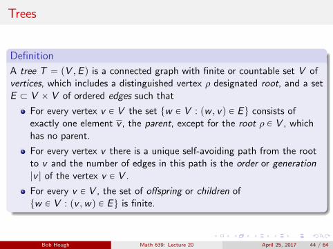
Definition

A tree T “ pV ,E q is a connected graph with finite or countable set V ofvertices, which includes a distinguished vertex ρ designated root, and a setE Ă V ˆ V of ordered edges such that

For every vertex v P V the set tw P V : pw , vq P Eu consists ofexactly one element v , the parent, except for the root ρ P V , whichhas no parent.

For every vertex v there is a unique self-avoiding path from the rootto v and the number of edges in this path is the order or generation|v | of the vertex v P V .

For every v P V , the set of offspring or children oftw P V : pv ,wq P Eu is finite.


Rays

Definition

For any v ,w P V we denote v ^w the furthest element from the rootcommon to the paths connecting pρ, vq and pρ,wq. Write v ď w if vis an ancestor of w , which is equivalent to v “ v ^ w .

Every infinite path started in the root is called a ray. The set of raysis denoted BT and is called the boundary of T . Given paths ξ and η,let ξ ^ η be the last vertex in common, and |ξ ^ η| the number ofedges in common. |ξ ´ η| :“ 2´|ξ^η|.

A set Π of edges is called a cutset if every ray includes an edge fromΠ.


Flows

Definition

A capacity is a function C : E Ñ r0,8q. A flow of strength c ą 0 througha tree with capacities C is a mapping θ : E Ñ r0, cs such that

For the root we haveř

w“ρ θpρ,wq “ c and for every vertex v ‰ ρ

θpv , vq “ÿ

w :w“v

θpv ,wq,

so that the flow into and out of each vertex other than the root isconserved.

θpeq ď C peq, i.e. the flow through the edge e is bounded by itscapacity.


Max-flow min-cut theorem

Theorem (Max-flow min-cut theorem)

Let T be a tree with capacity C . Then

max tstrengthpθq : θ a flow with capacities Cu

“ inf

#

ÿ

ePΠ

C peq : Π a cutset

+

.



Proof.

The LHS is a maximum by a diagonalization argument.

Every infinite cutset Π contains a finite cutset Π1 Ă Π. To see this,note that otherwise it would be possible to find an infinite sequenceof rays such that the jth ray has its first j elements not in Π. Aninfinite ray not meeting Π is found by taking a limit.

Let θ be a flow with capacities C and Π an arbitrary cutset. Let A bethe set of vertices which are connected to ρ by a path not meetingthe cutset. By the previous argument, this set is finite.



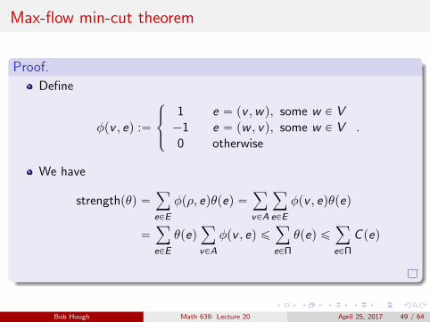
Proof.

Define

φpv , eq :“

$

&

%

1 e “ pv ,wq, some w P V´1 e “ pw , vq, some w P V0 otherwise

.

We have

strengthpθq “ÿ

ePE

φpρ, eqθpeq “ÿ

vPA

ÿ

ePE

φpv , eqθpeq

“ÿ

ePE

θpeqÿ

vPA

φpv , eq ďÿ

ePΠ

θpeq ďÿ

ePΠ

C peq



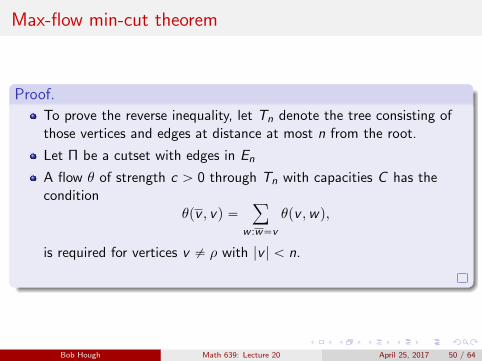
Proof.

To prove the reverse inequality, let Tn denote the tree consisting ofthose vertices and edges at distance at most n from the root.

Let Π be a cutset with edges in En

A flow θ of strength c ą 0 through Tn with capacities C has thecondition

θpv , vq “ÿ

w :w“v

θpv ,wq,

is required for vertices v ‰ ρ with |v | ă n.



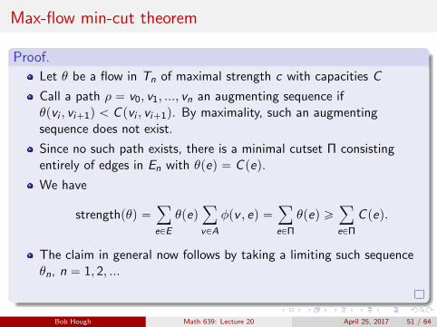
Proof.

Let θ be a flow in Tn of maximal strength c with capacities C

Call a path ρ “ v0, v1, ..., vn an augmenting sequence ifθpvi , vi`1q ă C pvi , vi`1q. By maximality, such an augmentingsequence does not exist.

Since no such path exists, there is a minimal cutset Π consistingentirely of edges in En with θpeq “ C peq.

We have

strengthpθq “ÿ

ePE

θpeqÿ

vPA

φpv , eq “ÿ

ePΠ

θpeq ěÿ

ePΠ

C peq.

The claim in general now follows by taking a limiting such sequenceθn, n “ 1, 2, ...


Frostman’s lemma

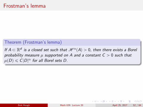
Theorem (Frostman’s lemma)

If A Ă Rd is a closed set such that H αpAq ą 0, then there exists a Borelprobability measure µ supported on A and a constant C ą 0 such thatµpDq ď C |D|α for all Borel sets D.


Frostman’s lemma

Proof.

Let A Ă r0, 1sd .

A compact cube of side length s in Rd may be split into 2d compactcubes of side length s{2.

Create a tree with the cube r0, 1sd at the root, and each vertex having2d edges emanating from it, leading to vertices at the 2d sub-cubes.

Erase edges ending in vertices associated with subcubes that do notintersect A

Rays in BT correspond to sequences of nested compact cubes


Frostman’s lemma

Proof.

There is a canonical map Φ : BT Ñ A which maps sequences ofnested cubes to their intersection.

If x P A then there is a unique element of BT specified bycontainment at each level of the tree. Thus Φ is a bijection.

Given edge e at level n define the capacity C peq “ pd12 2ńqα.


Frostman’s lemma

Proof.

Associate to cutset Π a covering of A consisting of those cubesassociated to the initial vertex of each edge in the cut-set. This indeedcovers A, since any ray which ends in a point a of A passes throughan edge of the cutset, so that a is contained in the associated cube.

Thus

inf

#

ÿ

ePΠ

C peq : Π a cutset

+

ě inf

#

ÿ

j

|Aj |α : A Ă

ď

j

Aj

+

.


Frostman’s lemma

Proof.

Now we define a measure on A – BT .

Given an edge e, let T peq denote the set of rays of BT which containe.

Define νpT peqq “ θpeq.

The collection C pBT q of all sets T peq, together with H is asemi-algebra on BT since if A,B P C pBT q then AX B P C pBT q, andif A P C pBT q then Ac is a finite disjoint union of sets from C pBT q.

Since the flow through any vertex is preserved, ν is countably additive.

It follows that ν may be extended to a measure ν on the σ-algebragenerated by C pBT q.


Frostman’s lemma

Proof.

Define Borel measure µ “ ν ˝ Φ´1 on A. Thus if C is the cubeassociated to the initial vertex of edge e then µpC q “ θpeq.

Let D be a Borel subset of Rd and n is the integer such that

2ń ă |D X r0, 1sd | ď 2´pn´1q.

Then D X r0, 1sd can be covered with at most 3d cubes from the

above construction of side length 2ń, or diameter d12 2ń. Thus

µpDq ď dα2 3d2ńα ď d

α2 3d |D|α

so that µ meets the requirements of the lemma.


Riesz capacity

Definition

Define the Riesz α-capacity of a metric space pE , ρq as

CapαpE q :“ sup

Iαpµq´1 : µ a mass distribution on E with µpE q “ 1

(

.

In the case of the Euclidean space E “ Rd with d ě 3 and α “ d ´ 2 theRiesz α-capacity is also known as the Newtonian capacity.


Riesz capacity

Theorem

For any closed set A Ă Rd ,

dimA “ suptα : CapαpAq ą 0u.


Riesz capacity

Proof.

The inequality dimA ě suptα : CapαpAq ą 0u follows from theenergy method, so it remains to prove the reverse inequality.

Suppose dimA ą α, so that for some β ą α we have H βpAq ą 0.

By Frostman’s lemma, there exists a nonzero Borel probabilitymeasure µ on A and a constant C such µpDq ď C |D|β

We may assume that the support of µ has diameter less than 1.


Riesz capacity

Proof.

Fix x P A and for k ě 1 let Skpxq “ ty : 2´k ă |x ´ y | ď 21´ku.

We have

ż

Rd

dµpyq

|x ´ y |α“

8ÿ

k“1

ż

Sk pxq

dµpyq

|x ´ y |αď

8ÿ

k“1

µpSkpxqq2kα

ď C8ÿ

k“1

|22´k |β2kα “ C 18ÿ

k“1

2kpα´βq.

Since β ą α,

Iαpµq ď C 18ÿ

k“1

2kpα´βq ă 8.


Dimension of Brownian motion

Theorem

Let A Ă r0,8q be a closed subset and tBptq : t ě 0u a d-dimensionalBrownian motion. Then, a.s.

dimBpAq “ p2 dimAq ^ d .



Proof.

The upper bound has already been proven.

For the lower bound let α ă dimpAq ^ pd{2q.

By the previous theorem there exists a Borel probability measure µ onA such that Iαpµq ă 8.



Proof.

Define, for D Ă Rd Borel, µpDq “ µptt ě 0 : Bptq P Duq. Thus

ErI2αpµqs “ E

„ĳ

d µpxqd µpyq

|x ´ y |2α

“ E

„ż 8

0

ż 8

0

dµptqdµpsq

|Bptq ´ Bpsq|2α

The denominator has the same distribution as |t ´ s|α|Z |2α.

Since 2α ă d , Er|Z |´2αs ă 8. Thus

ErI2αpµqs “

ż 8

0

ż 8

0Er|Z |´2αs

dµptqdµpsq

|t ´ s|αď Er|Z |´2αsIαpµq ă 8.

µ is supported on BpAq, so dimBpAq ě 2α.


Math 639: Lecture 20 - Hausdorff dimension - Stony Brook ...

Documents