Hausdorff Kernel for 3D Object Acquisition and Detection

Hausdorff Kernel for 3D Object Acquisition andDetection

Annalisa Barla, Francesca Odone, and Alessandro Verri

INFM - DISI, Universita di GenovaVia Dodecaneso 35, 16146 Genova, Italy{barla,odone,verri}@disi.unige.it

Abstract. Learning one class at a time can be seen as an effective so-lution to classification problems in which only the positive examples areeasily identifiable. A kernel method to accomplish this goal consists ofa representation stage - which computes the smallest sphere in featurespace enclosing the positive examples - and a classification stage - whichuses the obtained sphere as a decision surface to determine the positivityof new examples. In this paper we describe a kernel well suited to repre-sent, identify, and recognize 3D objects from unconstrained images. Thekernel we introduce, based on Hausdorff distance, is tailored to deal withgrey-level image matching. The effectiveness of the proposed method isdemonstrated on several data sets of faces and objects of artistic rele-vance, like statues.

1 Introduction

In the learning from examples paradigm the goal of many detection and clas-sification problems of computer vision – like object detection and recognition(see [9,10,11,12,13,20] for example) – is to distinguish between positive and neg-ative examples. While positive examples are usually defined as images or portionof images containing the object of interest, negative examples are comparativelymuch less expensive to collect but somewhat ill defined and difficult to char-acterize. Problems for which only positive examples are easily identifiable aresometimes referred to as novelty detection problems. In this paper we studya kernel method for learning one class at a time in a multiclass classificationproblem.

Kernel methods, which gained an increasing amount of attention in the lastyears after the influential work of Vapnik [17,18], reduce a learning problem ofclassification or regression to a multivariate function approximation problem inwhich the solution is found as a linear combination of certain positive definitefunctions named kernels, centered at the examples [3,4,19]. If the examples be-long to only one class, the idea is that of determining the spatial support of theavailable data by finding the smallest sphere in feature space enclosing the ex-amples [1]. The feature mapping, or the choice of the norm, plays here a crucialrole.

A. Heyden et al. (Eds.): ECCV 2002, LNCS 2353, pp. 20–33, 2002.c© Springer-Verlag Berlin Heidelberg 2002

Hausdorff Kernel for 3D Object Acquisition and Detection 21

In this paper, we introduce a kernel derived from an image matching tech-nique based on the notion of Hausdorff distance [7], well suited to capture imagesimilarities, while preserving meaningful image differences. The proposed kernelis tolerant to small amount of local deformations and scale changes, does notrequire accurate image registration or segmentation, and is well suited to dealwith occlusion issues.

We present experiments which show that this kernel outperforms the linearkernel (effectively corresponding to a standard template matching technique)and polynomial kernels in the representation and the identification of 3D objects.The efficacy of the method is assessed on databases of faces and 3D objects ofartistical interest. All the images used in the reported experiments are availablefor download at ftp://ftp.disi.unige.it/person/OdoneF/3Dobjects.

In summary, the major aim of this paper is to evaluate the appropriatenessof Hausdorff-like measures for engineering kernels well suited to deal with im-age related problems. A secondary objective is to assess the potential of kernelmethods in computer vision, in the case in which a relatively small number ofexamples of only one class is available. The paper is organized as follows. Thekernel method used in this paper, suggested by Vapnik [17] and developed in [1],is summarized in Section 2. Section 3 introduces and discusses the Hausdorffkernel for images. The experiments are reported in Section 4, Section 5 is left toconclusions.

2 Kernel-Based Approach to Learn One Class at a Time

In this section we review the method described in [1] which shares strong simi-larities with Support Vector Machines (SVMs) [17,18] for binary classification.The main idea behind this approach is to find the sphere in feature space of min-imum radius which contains most of the data of the training set. The possiblepresence of outliers is countered by using slack variables ξi which allow for datapoints outside the sphere. This approach was first suggested by Vapnik [17] andinterpreted and used as a novelty detector in [15] and [16]. If R is the sphereradius and x0 the sphere center, the primal minimization problem can be writtenas

minR,x0,ξi

R2 + C�∑

i=1

ξi (1)

subject to (xi − x0)2 ≤ R2 + ξi and ξi ≥ 0, i = 1, . . . , �.

with x1, ...,x� the input data, ξi ≥ 0 and C a regularization parameter. The dualformulation requires the solution of the QP problem

maxαi

−�∑

i=1

αixi · xi +�∑

i=1

�∑j=1

αiαjxi · xj (2)

subject to�∑

i=1

αi = 1, and 0 ≤ αi ≤ C.

22 A. Barla, F. Odone, and A. Verri

As in the case of SVMs for binary classification, the objective function isquadratic, the Hessian positive semi-definite, the inequality constraints are boxconstraints. The two main differences are the form of the linear term in the ob-jective function and the equality constraint (the Lagrange Multipliers sum to 1instead than 0). Like in the case of SVMs, the training points for which αi > 0are the support vectors for this learning problem.

The sphere center x0 is found as a weighted sum of the examples as x0 =∑αixi while the radius R can be determined from the Kuhn-Tucker condition

associated to any training point xi for which 0 < αi < C as

R2 = (xi − x0)2.

The distance between a point and the center can be computed with the followingequation

d2(x) = (x− x0)2 == x · x− 2x · x0 + x0 · x0 =

= x · x− 2�∑

i=1

αix · xi +�∑

i,j=1

αiαjxi · xj

In full analogy to the SVM case, one can introduce a kernel function K [18], andsolve the problem

maxαi

−�∑

i=1

αiK(xi,xi) +�∑

i=1

�∑j=1

αiαjK(xi,xj) (3)

subject to�∑

i=1

αi = 1 and 0 ≤ αi ≤ C, i = 1, . . . , �.

A kernel function K is a function satisfying certain mathematical constraints [2,18] and implicitly defining a mapping φ from the input space to the feature space– space in which the inner product between the feature points φ(xi) and φ(xj)is K(xi,xj). The constraints on αi define the feasible region of the QP problem.

In this case the sphere center in feature space cannot be computed explicitly,but the distance dK(x) between the sphere center and a point x can be writtenas

d2K(x) = K(x,x) − 2�∑

i=1

αiK(x,xi) +�∑

i,j=1

αiαjK(xi,xj).

As in the linear case, the radius RK can be determined from the Kuhn-Tuckerconditions associated to a support vector xi for which 0 < αi < C.

3 The Hausdorff Kernel

In this section we first describe a similarity measure for images inspired by thenotion of Hausdorff distance. Then, we determine the conditions under whichthis measure defines a legitimate kernel function.

Hausdorff Kernel for 3D Object Acquisition and Detection 23

3.1 Hausdorff Distances

Given two finite point sets A and B (both subsets of IRN ), the directed Hausdorffdistance h, can be written as

h(A,B) = maxa∈A

minb∈B

||a− b||.

Clearly the directed Hausdorff distance is not symmetric and thus not a “true”distance, but it is very useful to measure the degree of mismatch of one set withrespect to another. To obtain a distance in the mathematical sense, symmetrycan be restored by taking the maximum between h(A,B) and h(B,A). Thisbrings to the definition of Hausdorff distance, that is,

H(A,B) = max{h(A,B), h(B,A)}.A way to gain intuition on Hausdorff measures which is very important in relationto the similarity method we are about to define, is to think in terms of setinclusion. Let Bρ be the set obtained by replacing each point of B with a diskof radius ρ, and taking the union of all of these disks; effectively, Bρ is obtainedby dilating B by ρ. Then the following holds:Proposition The directed Hausdorff distance h(A,B) is not greater than ρ ifand only if A ⊆ Bρ.

This follows easily from the fact that, in order for every point of A to bewithin distance ρ from some points of B, A must be contained in Bρ.

3.2 Hausdorff-Based Measure of Similarity between Grey-LevelImages

Suppose to have two grey-level images, I1 and I2, of which we want to computethe degree of similarity; ideally, we would like to use this measure as a basis todecide whether the two images contain the same object, maybe represented intwo slightly different views, or under different illumination conditions. In order toallow for grey level changes within a fixed interval or small local transformations(for instance small scale variations or affine transformations), a possibility is toevaluate the following function [7]

k(I1, I2) =∑

p

θ(ε− minq∈Np

|I1[p] − I2[q]|) (4)

where θ is the unit step function. The function k counts the number of pixels p inI1 which are within a distance ε (on the grey levels) from at least one pixel q ofI2 in the neighborhood Np of p. Unless Np coincides with p, k is not symmetric,but symmetry can be restored by taking the max as for the Hausdorff Distance,or the average

K =12

[k(I1, I2) + k(I2, I1)] (5)

Equation (4), can be interpreted in terms of set dilation and inclusion, leadingto an efficient implementation [7] which can be summarized in three steps.

24 A. Barla, F. Odone, and A. Verri

1. Expand the two images I1 and I2 into 3D binary matrices I1 and I2, thethird dimension being the grey value:

I1(i, j, g) ={

1 if I1(i, j) = g;0 otherwise. (6)

2. Dilate both matrices by growing their nonzero entries by a fixed amount εin the grey value dimension, εr and εc (the size of the neighbourhood Np)in the space dimensions. Let D1 and D2 be the resulting 3D dilated binarymatrices. This dilation varies according to the degrees of similarity requiredand the transformations allowed.

3. Compute the size of the intersections between I1 and D2, and I2 and D1and take the average of the two values obtaining K(I1, I2).

3.3 Relationship with the Hausdorff Distance

The similarity measure k is closely related to the directed Hausdorff distance h:computing k is equivalent to fix a maximum distance ρmax (by choosing ε andNp) allowed between two sets, and see if the sets we are comparing, or subsetsof them, are within that distance. In particular, if the dilation is isotropic inan appropriate metric, and k(I1, I2) takes the maximum value s (which meansthat there is a total inclusion of one image in the dilation of the other), thenh(I1, I2) ≤ ρmax.

In general, if k(I1, I2) = m < s we say that the m-partial directed Hausdorffdistance [6] is not greater than ρmax, which means, loosely speaking, that asubset of I1, of cardinality m is within a distance ρmax from I2.

3.4 Is K a True Kernel?

A sufficient condition for a function K to be used as a kernel is the positivedefinitiveness: given a set X ⊆ IRn, a function K : X × X → IR is positivedefinite if for all integers n and all x1, . . . ,xn ∈ X, and α1, . . . , αn ∈ IR,

n∑i=1

n∑j=1

αiαjK(xi,xj) ≥ 0. (7)

In the case of interest the inequality (7) is always satisfied because, by definition,K(xi,xj) ≥ 0 for each xi and xj , and also in the feasible region of the optimiza-tion problem (3) all the αi are non-negative. In the case of binary classification,case in which the αi can also be negative, the proposed function is not a kernel,unless the dilation is appropriately redefined (see [8] for details).

4 Experiments

In this section we present results obtained on several image data sets, acquiredfrom multiple views: a group of data sets of faces for face recognition, and group

Hausdorff Kernel for 3D Object Acquisition and Detection 25

of data set of 3D objects of artistical interest acquired in San Lorenzo Cathedral.The two problems are closely related but distinct. As we will see in the case of thelatter, the notion of object is blurred with the notion of scene (the backgroundbeing as important as the foreground), while in face recognition this is not thecase.

In our approach we make a minimal use of preprocessing. In particular, wedo not compute accurate registration, since our similarity measure takes careof spatial misalignments. Also, since our mapping in feature space allows forsome degree of deformation both in the grey-levels and in space, the effects ofsmall illumination and pose changes are attenuated. Finally, we exploit full 3Dinformation on the object by acquiring a training set which includes frontal andlateral views.

In the remainder of this section we will first describe the recognition system,and then results of the applications on the two different families of data sets.All the images used have been resized to 72 × 57 pixels, therefore we work in aspace of more than 4000 dimensions. The results presented in this section havebeen obtained by applying a dilation of 1 on the spatial direction and a dilationof 3 on the grey-levels.

4.1 The Recognition System

Given a training set of images of the object of interest, we estimate the smallestsphere containing the training data in the feature space implicitly defined by thekernel K as described in Section 3. After training, a new image x is classified asa positive example if

K(x,x) − 2�∑

j=1

αjK(x,xj) +�∑

j,k=1

αjαkK(xj ,xk) = d2K(x) ≤ t. (8)

where t ≥ 0 is a threshold typically in the range of the square of radius RK . It isinteresting to remark that while in the case of the linear kernel and polynomialkernels all the terms in the l.h.s. of (8) need to be computed for each point, forthe Hausdorff kernel the only term which depends on point x is the second, theother two being constant. In this case the inequality d2K(x) ≤ t can be rewrittenas ∑

αiK(x,xi) ≥ τ, (9)

for some suitably defined threshold τ .

4.2 Application to Face Identification

First Data SetIn the first set of images, we acquired both training and test data in the samesession. We collected four sets of images (frontal and rotated views), one for eachof four subjects, for a total of 353 images, samples of which are shown in Figure1. To test the system we used 188 images of ten different subjects, including test

26 A. Barla, F. Odone, and A. Verri

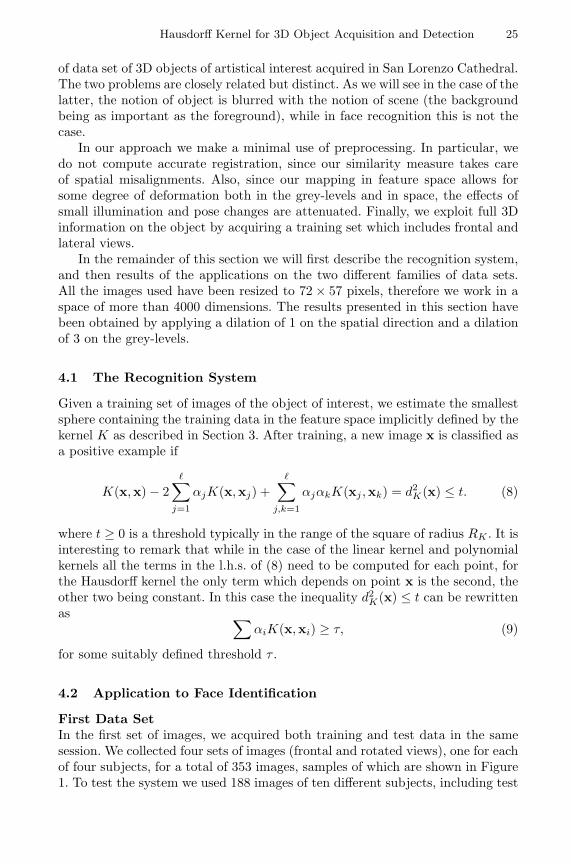
images of the four people used to acquire the training images (see the examplesin Figure 2).

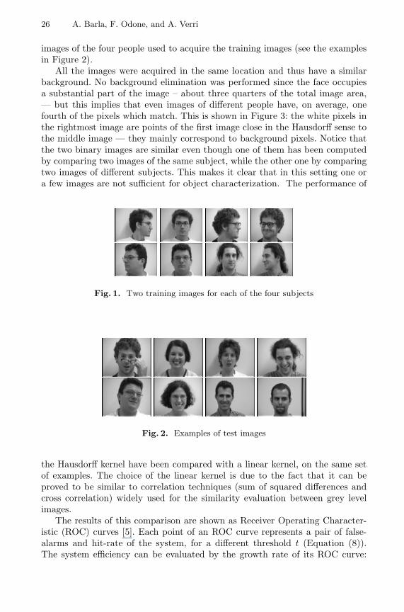
All the images were acquired in the same location and thus have a similarbackground. No background elimination was performed since the face occupiesa substantial part of the image – about three quarters of the total image area,— but this implies that even images of different people have, on average, onefourth of the pixels which match. This is shown in Figure 3: the white pixels inthe rightmost image are points of the first image close in the Hausdorff sense tothe middle image — they mainly correspond to background pixels. Notice thatthe two binary images are similar even though one of them has been computedby comparing two images of the same subject, while the other one by comparingtwo images of different subjects. This makes it clear that in this setting one ora few images are not sufficient for object characterization. The performance of

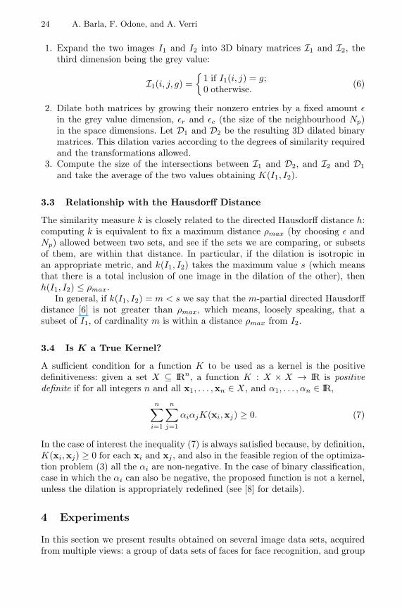
Fig. 1. Two training images for each of the four subjects

Fig. 2. Examples of test images

the Hausdorff kernel have been compared with a linear kernel, on the same setof examples. The choice of the linear kernel is due to the fact that it can beproved to be similar to correlation techniques (sum of squared differences andcross correlation) widely used for the similarity evaluation between grey levelimages.

The results of this comparison are shown as Receiver Operating Character-istic (ROC) curves [5]. Each point of an ROC curve represents a pair of false-alarms and hit-rate of the system, for a different threshold t (Equation (8)).The system efficiency can be evaluated by the growth rate of its ROC curve:

Hausdorff Kernel for 3D Object Acquisition and Detection 27

Fig. 3. Spatial support of the Hausdorff distance. Both rows: the white pixels inthe rightmost image show the locations of the leftmost image which are close, in theHausdorff sense, to the middle image.

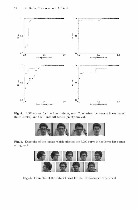
for a given false-alarm rate, the better system will be the one with the higherhit probability. The overall performance of a system can be measured by thearea under the curve. Figure 4 shows the ROC curves of a linear and Hausdorffkernels for all the four face recognition problems. The curve obtained with theHausdorff kernel is always above the one of the linear kernel, showing superiorperformance. The linear kernel does not appear to be suitable for the task: in allthe four cases, to obtain a hit rate of the 90% with the linear kernel one shouldaccept more than 50% false positives. The Hausdorff kernel ROC curve, instead,increases rapidly and shows good properties of sensitivity and specificity. Wetested the robustness of the recognition system by adding difficult positives toone of the test sets (see Figure 5). The corresponding ROC curve graph is theone in the lower left corner of Figure 4.

In a second series of experiments on the same training sets, we estimate thesystem performance in the leave-one-out mode. We trained the system on �− 1examples, and tested it on the one left out, for all possible choices of � − 1examples. Figure 6 shows samples from one of the training sets. Even if the setcontains a number of images which are difficult to classify, only 19% were foundto lie outside the sphere of minimum radius, but all of them within a distanceless than 3% of the estimated radius.

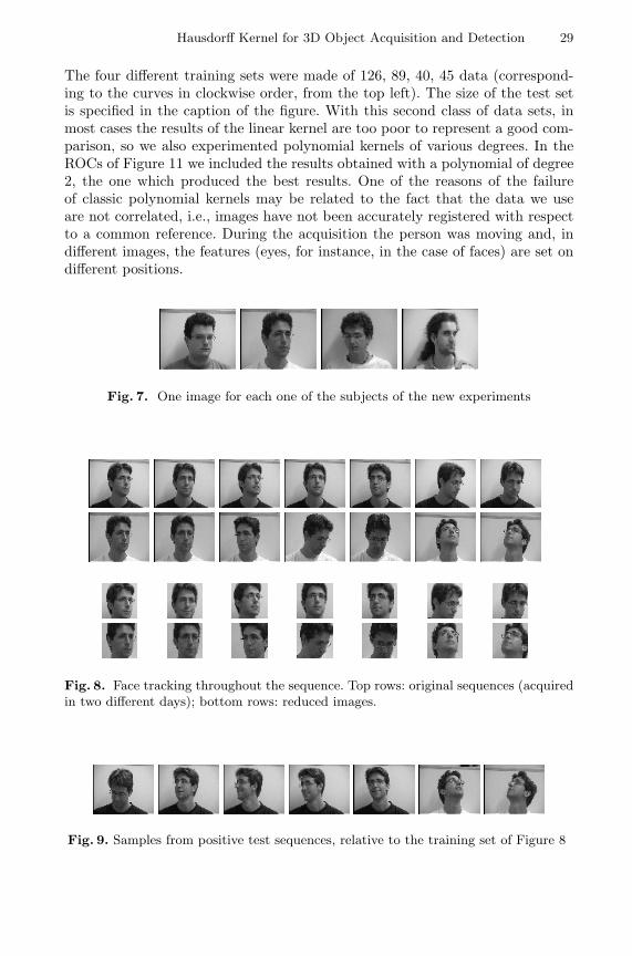
Second Data SetOther sets of face images were acquired on different days and under uncon-strained illumination (see examples in Figure 7). A change of scale is immediatelynoticeable comparing Figure 1 and Figure 7, which therefore necessitated back-ground elimination from the training data: to this purpose, we performed a semi-automatic preprocessing of the training data, exploiting the spatio-temporal con-tinuity between adjacent images of the training set. Indeed, we manually selecteda rectangular patch in the first image of each sequence, and then tracked it auto-matically through the rest of the sequence obtaining the reduced images shownin Figure 8. Figures 9 and 10 show positive and negative test images, respec-tively, used to test the machine trained with the images represented in Figure8. The result of the recognition is described by the ROC curve at the top rightof Figure 11. For space constraints we did not include examples of images fromall the four data sets, but Figure 11 shows the performance of the four systems.

28 A. Barla, F. Odone, and A. Verri

0.0 0.5 1.0false positive rate

0.0

0.5

1.0hi

t rat

e

0.0 0.5 1.0false positives rate

0.0

0.5

1.0

hit r

ate

0.0 0.5 1.0false positives rate

0.0

0.5

1.0

hit r

ate

0.0 0.5 1.0false positives rate

0.0

0.5

1.0

hit r

ate

Fig. 4. ROC curves for the four training sets. Comparison between a linear kernel(filled circles) and the Hausdorff kernel (empty circles).

Fig. 5. Examples of the images which affected the ROC curve in the lower left cornerof Figure 4

Fig. 6. Examples of the data set used for the leave-one-out experiment

Hausdorff Kernel for 3D Object Acquisition and Detection 29

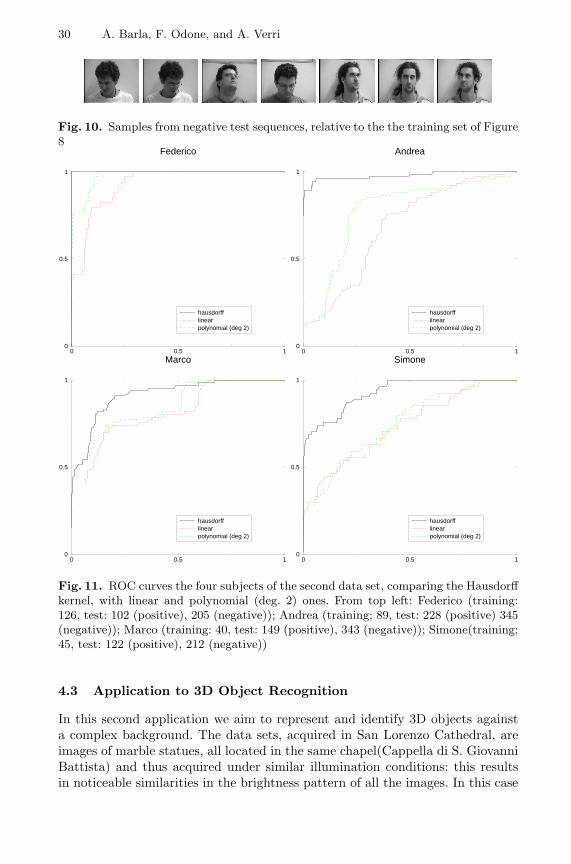
The four different training sets were made of 126, 89, 40, 45 data (correspond-ing to the curves in clockwise order, from the top left). The size of the test setis specified in the caption of the figure. With this second class of data sets, inmost cases the results of the linear kernel are too poor to represent a good com-parison, so we also experimented polynomial kernels of various degrees. In theROCs of Figure 11 we included the results obtained with a polynomial of degree2, the one which produced the best results. One of the reasons of the failureof classic polynomial kernels may be related to the fact that the data we useare not correlated, i.e., images have not been accurately registered with respectto a common reference. During the acquisition the person was moving and, indifferent images, the features (eyes, for instance, in the case of faces) are set ondifferent positions.

Fig. 7. One image for each one of the subjects of the new experiments

Fig. 8. Face tracking throughout the sequence. Top rows: original sequences (acquiredin two different days); bottom rows: reduced images.

Fig. 9. Samples from positive test sequences, relative to the training set of Figure 8

30 A. Barla, F. Odone, and A. Verri

Fig. 10. Samples from negative test sequences, relative to the the training set of Figure8

0 0.5 10

0.5

1

Federico

hausdorfflinearpolynomial (deg 2)

0 0.5 10

0.5

1

Andrea

hausdorfflinearpolynomial (deg 2)

0 0.5 10

0.5

1

Marco

hausdorfflinearpolynomial (deg 2)

0 0.5 10

0.5

1

Simone

hausdorfflinearpolynomial (deg 2)

Fig. 11. ROC curves the four subjects of the second data set, comparing the Hausdorffkernel, with linear and polynomial (deg. 2) ones. From top left: Federico (training:126, test: 102 (positive), 205 (negative)); Andrea (training; 89, test: 228 (positive) 345(negative)); Marco (training: 40, test: 149 (positive), 343 (negative)); Simone(training;45, test: 122 (positive), 212 (negative))

4.3 Application to 3D Object Recognition

In this second application we aim to represent and identify 3D objects againsta complex background. The data sets, acquired in San Lorenzo Cathedral, areimages of marble statues, all located in the same chapel(Cappella di S. GiovanniBattista) and thus acquired under similar illumination conditions: this resultsin noticeable similarities in the brightness pattern of all the images. In this case

Hausdorff Kernel for 3D Object Acquisition and Detection 31

no segmentation is advisable, since the background itself is representative of theobject. Here we can safely assume that the statues will not be moved from theirusual position.

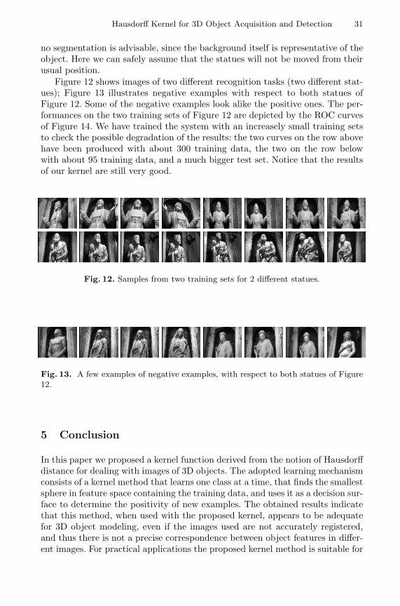
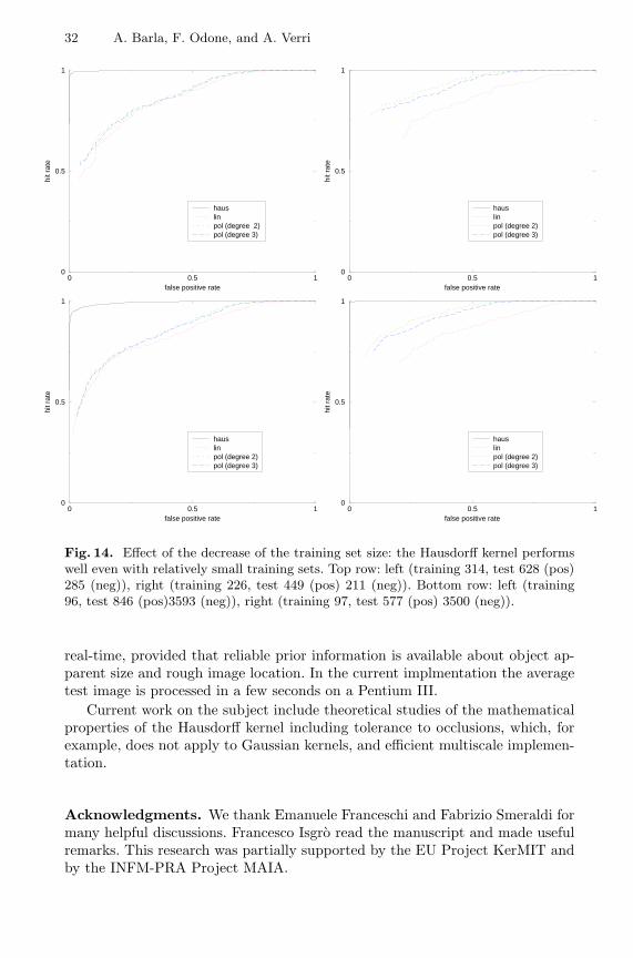
Figure 12 shows images of two different recognition tasks (two different stat-ues); Figure 13 illustrates negative examples with respect to both statues ofFigure 12. Some of the negative examples look alike the positive ones. The per-formances on the two training sets of Figure 12 are depicted by the ROC curvesof Figure 14. We have trained the system with an increasely small training setsto check the possible degradation of the results: the two curves on the row abovehave been produced with about 300 training data, the two on the row belowwith about 95 training data, and a much bigger test set. Notice that the resultsof our kernel are still very good.

Fig. 12. Samples from two training sets for 2 different statues.

Fig. 13. A few examples of negative examples, with respect to both statues of Figure12.

5 Conclusion

In this paper we proposed a kernel function derived from the notion of Hausdorffdistance for dealing with images of 3D objects. The adopted learning mechanismconsists of a kernel method that learns one class at a time, that finds the smallestsphere in feature space containing the training data, and uses it as a decision sur-face to determine the positivity of new examples. The obtained results indicatethat this method, when used with the proposed kernel, appears to be adequatefor 3D object modeling, even if the images used are not accurately registered,and thus there is not a precise correspondence between object features in differ-ent images. For practical applications the proposed kernel method is suitable for

32 A. Barla, F. Odone, and A. Verri

0 0.5 1false positive rate

0

0.5

1

hit r

ate

hauslinpol (degree 2)pol (degree 3)

0 0.5 1false positive rate

0

0.5

1

hit r

ate

hauslinpol (degree 2)pol (degree 3)

0 0.5 1false positive rate

0

0.5

1

hit r

ate

hauslinpol (degree 2)pol (degree 3)

0 0.5 1false positive rate

0

0.5

1

hit r

ate

hauslinpol (degree 2)pol (degree 3)

Fig. 14. Effect of the decrease of the training set size: the Hausdorff kernel performswell even with relatively small training sets. Top row: left (training 314, test 628 (pos)285 (neg)), right (training 226, test 449 (pos) 211 (neg)). Bottom row: left (training96, test 846 (pos)3593 (neg)), right (training 97, test 577 (pos) 3500 (neg)).

real-time, provided that reliable prior information is available about object ap-parent size and rough image location. In the current implmentation the averagetest image is processed in a few seconds on a Pentium III.

Current work on the subject include theoretical studies of the mathematicalproperties of the Hausdorff kernel including tolerance to occlusions, which, forexample, does not apply to Gaussian kernels, and efficient multiscale implemen-tation.

Acknowledgments. We thank Emanuele Franceschi and Fabrizio Smeraldi formany helpful discussions. Francesco Isgro read the manuscript and made usefulremarks. This research was partially supported by the EU Project KerMIT andby the INFM-PRA Project MAIA.

Hausdorff Kernel for 3D Object Acquisition and Detection 33

References

1. C. Campbell and K. P. Bennett. A linear programming approach to novelty de-tection. Advances in Neural Information Processing Systems, 13, 2001.

2. N. Cristianini and J. Shawe-Taylor An Introduction to Support Vector Machinesand other kernel-based learning methods Cambridge University Press, 2000.

3. T. Evgeniou, M. Pontil, and T. Poggio. Regularization Networks and SupportVector Machines. Advances in Computational Mathematics, 13:1–50, 2000.

4. F. Girosi, M. Jones, and T. Poggio. Regularization Theory and Neural NetworkArchitecture. Neural Computation, 7:219–269, 1995.

5. D. M. Green and J. A. Swets. Signal detection theory and psychophysics. Reprintedby Krieger, Huntingdon, New York, 1974.

6. D. P. Huttenlocher, G. A. Klanderman, and W. J. Rucklidge. Comparing imagesusing the Hausdorff distance. IEEE Trans. on Pattern Analysis and MachineIntelligence, 9(15):850–863, 1993.

7. F. Odone, E. Trucco, and A. Verri. General purpose matching of grey level arbitraryimages. In G. Sanniti di Baja C. Arcelli, L. P. Cordella, editor, 4th InternationalWorkshop on Visual Forms, Lecture Notes on Computer Science LNCS 2059, pages573–582. Springer, 2001.

8. F. Odone and A. Verri. Real Time Image Recognition, in Opto-MechatronicsSystems Handbook, H. Cho editor; CRC Press. To appear.

9. C. Papageorgiou and T. Poggio A trainable system for object detection. Interna-tional Journal of Computer Vision, 38:15–33, 2000.

10. M. Pontil and A. Verri Support Vector Machines for 3D object recognition IEEETrans. on Pattern Analysis and Machine Intelligence, 637–646, 1998.

11. T.D. Rikert, M.J. Jones, and P. Viola A cluster-based statistical model for objectdetection. in Proc. IEEE Conf. on Computer Vision and Pattern Recognition,1999.

12. H.A. Rowley, S. Baluja, and T. Kanade Neural Network-based face detection.IEEE Transactions on Pattern Analysis and Machine Intelligence, 20:23–38, 1998.

13. H. Schneiderman and T. Kanade A statistical method for 3-D object detectionapplied to faces and cars. in Proc. IEEE Conference on Computer Vision andPattern Recognition, 2000.

14. B. Scholkopf, J.C. Platt, J. Shawe-Taylor, A.J. Smola, and R. C. Williamson.Estimating the support of a high-dimensional distribution. Technical Report MSR-TR-99-87, Microsoft Research Corporation, 1999,2000.

15. D. Tax and R. Duin. Data domain description by support vectors. In M. Verleysen,editor, Proceedings of ESANN99, pages 251–256. D. Facto Press, 1999.

16. D. Tax, A. Ypma, and R. Duin. Support vector data description applied to machinevibration analysis. In Proc. of the 5th Annual Conference of the Advanced Schoolfor Computing and Imaging, 1999.

17. V. Vapnik. The nature of statistical learning theory. Springer Verlag, Berlin, 1995.18. V. Vapnik. Statistical learning theory. John Wiley and sons, New York, 1998.19. G. Wahba. Spline models for observational data. SIAM, 1990.20. L. Wiskott, J.-M. Fellous, N. Kruger, and C. von der Malsburg A statistical method

for 3-D object detection applied to faces and cars. in Proc. IEEE Int. Conf. onImage Processing, Wien, 1997.