Math 533 Extra Hour Material

Welcome message from author
This document is posted to help you gain knowledge. Please leave a comment to let me know what you think about it! Share it to your friends and learn new things together.
Transcript

Math 533
Extra Hour Material

A Justification for Regression

The Justification for Regression
It is well-known that if we want to predict a random quantity Yusing some quantity m according to a mean-squared error MSE,then the optimal predictor is the expected value of Y , µ;
E[(Y −m)2] = E[(Y − µ+ µ−m)2]
= E[(Y − µ)2] + E[(µ−m)2] + 2E[(Y − µ)(µ−m)]
= E[(Y − µ)2] + (µ−m)2 + 0
which is minimized when m = µ.
1

The Justification for Regression (cont.)
Now suppose we have a joint distribution between Y and X, andwish to predict the Y as a function of X, m(X) say. Using the sameMSE criterion, if we write
µ(x) = EY |X [Y |X = x]
to represent the conditional expectation of Y given X = x, we have
EX,Y [(Y −m(X))2] = EX,Y [(Y − µ(X) + µ(X)−m(X))2]
= EX,Y [(Y − µ(X))2] + EX,Y [(µ(X)−m(X))2]
+ 2EX,Y [(Y − µ(X))(µ(X)−m(X))]
= EX,Y [(Y − µ(X))2] + EX [(µ(X)−m(X))2] + 0
2
The Justification for Regression (cont.)
The cross term equates to zero by noting that by iteratedexpectation
EX,Y [(Y−µ(X))(µ(X)−m(X))] = EX [EY |X [(Y−µ(X))(µ(X)−m(X))]]
and for the internal expectation
EY |X [(Y−µ(X))(µ(X)−m(X))|X] = (µ(X)−m(X))EY |X [(Y−µ(X))|X] a.s.
andEY |X [(Y − µ(X))|X] = 0 a.s.
3
The Justification for Regression (cont.)
This the MSE is minimized over functions m(.) when
EX [(µ(X)−m(X))2]
is minimized, but this term can be made zero by setting
m(x) = µ(x) = EY |X [Y |X = x].
Thus the MSE-optimal prediction is made by using µ(x).
Note: Here X can be a single variable, or a vector; it can be randomor non-random – the result holds.
4

The Justification for Linear Modelling
Suppose that the true conditional mean function is represented byµ(x) where x is a single predictor. We have by Taylor expansionaround x = 0 that
µ(x) = µ(0) +
p−1∑j=1
µ(j)(0)
j!xj + O(xp)
where the remainder term O(xp) represents terms of xp inmagnitude or higher order terms, and
µ(j)(0) =djµ(x)dxj
∣∣∣∣∣x=0
5

The Justification for Linear Modelling (cont.)
The derivatives of µ(x) at x = 0 may be treated as unspecifiedconstants, in which case a reasonable approximating model takes theform
β0 +
p−1∑j=1
βjxj
where βj ≡ µ(j)(0) for j = 0, 1, . . . , p− 1.
Similar expansions hold if x is vector valued.
6

The Justification for Linear Modelling (cont.)
Finally, if Y and X are jointly normally distributed, then theconditional expectation of Y given X = x is linear in x.
• see Multivariate Normal Distribution handout.
7

The General Linear Model
The General Linear Model
The linear model formulation that assumes
EY|X[Y|X] = Xβ VarY|X[Y|X] = σ2In
is actually quite a general formulation as the rows xi of X can beformed by using general transforms of the originally recordedpredictors.
• multiple regression: xi = [1 xi1 xi2 · · · xik]• polynomial regression: xi = [1 xi1 x2
i1 · · · xki1]
8
The General Linear Model (cont.)• harmonic regression: consider single continuous predictor x
measured on a bounded interval.
Let ωj = j/n, j = 0, 1, . . . , n/2 = K, and then set
EYi|X [Yi|xi] = β0 +
J∑j=1
βj1 cos(2πωjxi) +
J∑j=1
βj2 sin(2πωjxi)
If J = K, we then essentially have an n× n matrix X specifyinga linear transform of y in terms of the derived predictors
(cos(2πωjxi), sin(2πωjxi)).
– the coefficients
(β0, β11, β12, . . . , βK)
form the discrete Fourier transform of y9

The General Linear Model (cont.)
In this case, the columns of X are orthogonal, and
X>X = diag(n, n/2, n/2, . . . , n/2, n)
that is, X>X is a diagonal matrix.
10
The General Linear Model (cont.)
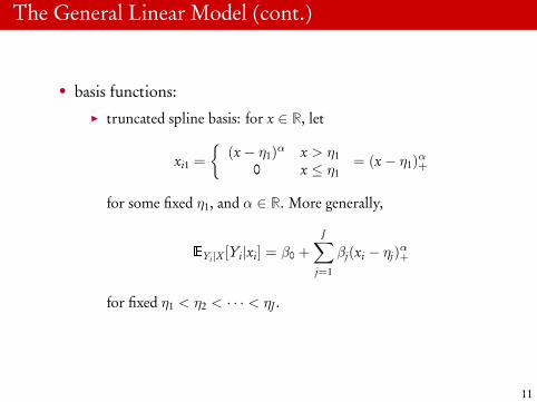
• basis functions:I truncated spline basis: for x ∈ R, let
xi1 =
{(x− η1)
α x > η10 x ≤ η1
= (x− η1)α+
for some fixed η1, and α ∈ R. More generally,
EYi|X [Yi|xi] = β0 +
J∑j=1
βj(xi − ηj)α+
for fixed η1 < η2 < · · · < ηJ .
11

The General Linear Model (cont.)I piecewise constant: : for x ∈ R, let
xi1 =
{1 x ∈ A10 x /∈ A1
= 1A1(x)
for some set A1. More generally,
EYi|X [Yi|xi] = β0 +
J∑j=1
βj1Aj(x)
for sets A1, . . . ,AJ . If we want to use a partition of R, we maywrite this
EYi|X [Yi|xi] =
J∑j=0
βj1Aj(x).
where
A0 =
J⋃j=1
Aj
′
12

The General Linear Model (cont.)
I piecewise linear: specify
EYi|X [Yi|xi] =
J∑j=0
1Aj(x)(βj0 + βj1xi)
I piecewise linear & continuous: specify
EYi|X [Yi|xi] = β0 + β1x +
J∑j=1
βj1(xi − ηj)+
for fixed η1 < η2 < · · · < ηJ .I higher order piecewise functions (quadratic, cubic etc.)I splines
13

Example: Motorcycle data
1 library(MASS)2 #Motorcycle data3 plot(mcycle,pch=19,main=’Motorcycle accident data’)45 x<-mcycle$times6 y<-mcycle$accel
14

Raw data
●●●●
● ●●● ●●●● ●●●
●●
●●●
●
●
●●●
●
●
●
●
●
●●
●
●●
●
●
●
●
●
●
●
●
●
●
●
●
●
●
●
●●
●
●
●
●
●
●
●●
●
●
●
●
● ●
●
●
●
●
●
●
●
●
●
●
●
●
●
●
●
●
●
●
●
●
●
●
●
●
●
●
●
●
● ●
●
●
●
●
●
●
●
●●
●
●
●
●
●
●
●
●
●
●
●
●
●
●
●●
● ●
●
● ●
●
●
●
●
●
●
●
10 20 30 40 50
−10
0−
500
50
Motorcycle accident data
times
acce
l
15

Example: Piecewise constant fit
1 #Knots2 K<-113 kappa<-as.numeric(quantile(x,probs=c(0:K)/K))45 X<-(outer(x,kappa,’-’)>0)^26 X<-X[,-12]78 fit.pwc<-lm(y∼ X)9 summary(fit.pwc)
10 newx<-seq(0,max(x),length=1001)1112 newX<-(outer(newx,kappa,’-’)>0)^213 newX<-cbind(rep(1,1001),newX[,-12])1415 yhatc<-newX %*% coef(fit.pwc)16 lines(newx,yhatc,col=’blue’,lwd=2)
16
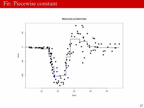
Fit: Piecewise constant
●●●●
● ●●● ●●●● ●●●
●●
●●●
●
●
●●●
●
●
●
●
●
●●
●
●●
●
●
●
●
●
●
●
●
●
●
●
●
●
●
●
●●
●
●
●
●
●
●
●●
●
●
●
●
● ●
●
●
●
●
●
●
●
●
●
●
●
●
●
●
●
●
●
●
●
●
●
●
●
●
●
●
●
●
● ●
●
●
●
●
●
●
●
●●
●
●
●
●
●
●
●
●
●
●
●
●
●
●
●●
● ●
●
● ●
●
●
●
●
●
●
●
10 20 30 40 50
−10
0−
500
50
Motorcycle accident data
times
acce
l
17

Example: Piecewise linear fit
17 X1<-(outer(x,kappa,’-’)>0)^218 X1<-X1[,-12]1920 X2<-(outer(x,kappa,’-’)>0)*outer(x,kappa,’-’)21 X2<-X2[,-12]2223 X<-cbind(X1,X2)2425 fit.pwl<-lm(y∼ X)26 summary(fit.pwl)27 newx<-seq(0,max(x),length=1001)2829 newX1<-(outer(newx,kappa,’-’)>0)^230 newX2<-(outer(newx,kappa,’-’)>0)*outer(newx,kappa,’-’)3132 newX<-cbind(rep(1,1001),newX1[,-12],newX2[,-12])3334 yhatl<-newX %*% coef(fit.pwl)35 lines(newx,yhatl,col=’red’,lwd=2)
18
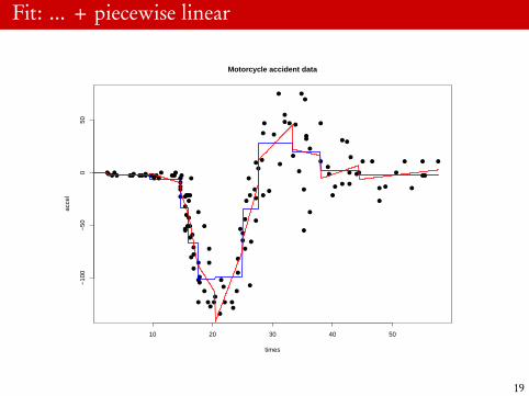
Fit: ... + piecewise linear
●●●●
● ●●● ●●●● ●●●
●●
●●●
●
●
●●●
●
●
●
●
●
●●
●
●●
●
●
●
●
●
●
●
●
●
●
●
●
●
●
●
●●
●
●
●
●
●
●
●●
●
●
●
●
● ●
●
●
●
●
●
●
●
●
●
●
●
●
●
●
●
●
●
●
●
●
●
●
●
●
●
●
●
●
● ●
●
●
●
●
●
●
●
●●
●
●
●
●
●
●
●
●
●
●
●
●
●
●
●●
● ●
●
● ●
●
●
●
●
●
●
●
10 20 30 40 50
−10
0−
500
50
Motorcycle accident data
times
acce
l
19

Example: Piecewise linear fit
36 X<-(outer(x,kappa,’-’)>0)*outer(x,kappa,’-’)37 X<-X[,-12]3839 fit.pwcl<-lm(y∼ X)40 summary(fit.pwcl)41 newx<-seq(0,max(x),length=1001)4243 newX<-(outer(newx,kappa,’-’)>0)*outer(newx,kappa,’-’)4445 newX<-cbind(rep(1,1001),newX[,-12])4647 yhatcl<-newX %*% coef(fit.pwcl)48 lines(newx,yhatcl,col=’green’,lwd=2)
20
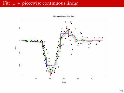
Fit: ... + piecewise continuous linear
●●●●
● ●●● ●●●● ●●●
●●
●●●
●
●
●●●
●
●
●
●
●
●●
●
●●
●
●
●
●
●
●
●
●
●
●
●
●
●
●
●
●●
●
●
●
●
●
●
●●
●
●
●
●
● ●
●
●
●
●
●
●
●
●
●
●
●
●
●
●
●
●
●
●
●
●
●
●
●
●
●
●
●
●
● ●
●
●
●
●
●
●
●
●●
●
●
●
●
●
●
●
●
●
●
●
●
●
●
●●
● ●
●
● ●
●
●
●
●
●
●
●
10 20 30 40 50
−10
0−
500
50
Motorcycle accident data
times
acce
l
21
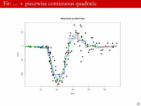
Fit: ... + piecewise continuous quadratic
●●●●
● ●●● ●●●● ●●●
●●
●●●
●
●
●●●
●
●
●
●
●
●●
●
●●
●
●
●
●
●
●
●
●
●
●
●
●
●
●
●
●●
●
●
●
●
●
●
●●
●
●
●
●
● ●
●
●
●
●
●
●
●
●
●
●
●
●
●
●
●
●
●
●
●
●
●
●
●
●
●
●
●
●
● ●
●
●
●
●
●
●
●
●●
●
●
●
●
●
●
●
●
●
●
●
●
●
●
●●
● ●
●
● ●
●
●
●
●
●
●
●
10 20 30 40 50
−10
0−
500
50
Motorcycle accident data
times
acce
l
22
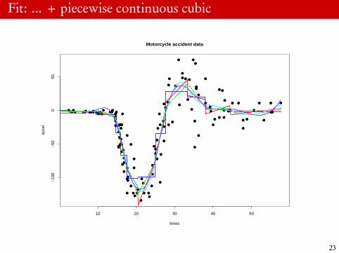
Fit: ... + piecewise continuous cubic
●●●●
● ●●● ●●●● ●●●
●●
●●●
●
●
●●●
●
●
●
●
●
●●
●
●●
●
●
●
●
●
●
●
●
●
●
●
●
●
●
●
●●
●
●
●
●
●
●
●●
●
●
●
●
● ●
●
●
●
●
●
●
●
●
●
●
●
●
●
●
●
●
●
●
●
●
●
●
●
●
●
●
●
●
● ●
●
●
●
●
●
●
●
●●
●
●
●
●
●
●
●
●
●
●
●
●
●
●
●●
● ●
●
● ●
●
●
●
●
●
●
●
10 20 30 40 50
−10
0−
500
50
Motorcycle accident data
times
acce
l
23
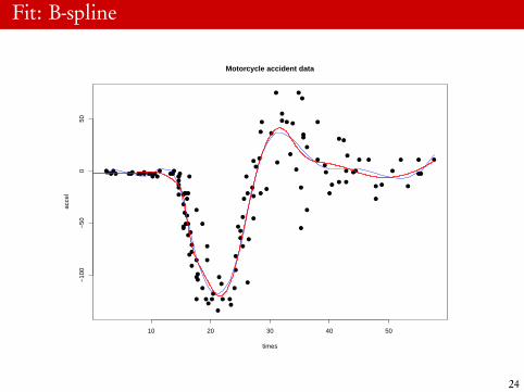
Fit: B-spline
●●●●
● ●●● ●●●● ●●●
●●
●●●
●
●
●●●
●
●
●
●
●
●●
●
●●
●
●
●
●
●
●
●
●
●
●
●
●
●
●
●
●●
●
●
●
●
●
●
●●
●
●
●
●
● ●
●
●
●
●
●
●
●
●
●
●
●
●
●
●
●
●
●
●
●
●
●
●
●
●
●
●
●
●
● ●
●
●
●
●
●
●
●
●●
●
●
●
●
●
●
●
●
●
●
●
●
●
●
●●
● ●
●
● ●
●
●
●
●
●
●
●
10 20 30 40 50
−10
0−
500
50
Motorcycle accident data
times
acce
l
24

Fit: Harmonic regression K = 2
●●●●
● ●●● ●●●● ●●●
●●
●●●
●
●
●●●
●
●
●
●
●
●●
●
●●
●
●
●
●
●
●
●
●
●
●
●
●
●
●
●
●●
●
●
●
●
●
●
●●
●
●
●
●
● ●
●
●
●
●
●
●
●
●
●
●
●
●
●
●
●
●
●
●
●
●
●
●
●
●
●
●
●
●
● ●
●
●
●
●
●
●
●
●●
●
●
●
●
●
●
●
●
●
●
●
●
●
●
●●
● ●
●
● ●
●
●
●
●
●
●
●
10 20 30 40 50
−10
0−
500
50
Motorcycle accident data
times
acce
l
25
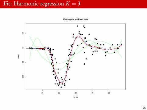
Fit: Harmonic regression K = 3
●●●●
● ●●● ●●●● ●●●
●●
●●●
●
●
●●●
●
●
●
●
●
●●
●
●●
●
●
●
●
●
●
●
●
●
●
●
●
●
●
●
●●
●
●
●
●
●
●
●●
●
●
●
●
● ●
●
●
●
●
●
●
●
●
●
●
●
●
●
●
●
●
●
●
●
●
●
●
●
●
●
●
●
●
● ●
●
●
●
●
●
●
●
●●
●
●
●
●
●
●
●
●
●
●
●
●
●
●
●●
● ●
●
● ●
●
●
●
●
●
●
●
10 20 30 40 50
−10
0−
500
50
Motorcycle accident data
times
acce
l
26

Fit: Harmonic regression K = 4
●●●●
● ●●● ●●●● ●●●
●●
●●●
●
●
●●●
●
●
●
●
●
●●
●
●●
●
●
●
●
●
●
●
●
●
●
●
●
●
●
●
●●
●
●
●
●
●
●
●●
●
●
●
●
● ●
●
●
●
●
●
●
●
●
●
●
●
●
●
●
●
●
●
●
●
●
●
●
●
●
●
●
●
●
● ●
●
●
●
●
●
●
●
●●
●
●
●
●
●
●
●
●
●
●
●
●
●
●
●●
● ●
●
● ●
●
●
●
●
●
●
●
10 20 30 40 50
−10
0−
500
50
Motorcycle accident data
times
acce
l
27
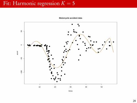
Fit: Harmonic regression K = 5
●●●●
● ●●● ●●●● ●●●
●●
●●●
●
●
●●●
●
●
●
●
●
●●
●
●●
●
●
●
●
●
●
●
●
●
●
●
●
●
●
●
●●
●
●
●
●
●
●
●●
●
●
●
●
● ●
●
●
●
●
●
●
●
●
●
●
●
●
●
●
●
●
●
●
●
●
●
●
●
●
●
●
●
●
● ●
●
●
●
●
●
●
●
●●
●
●
●
●
●
●
●
●
●
●
●
●
●
●
●●
● ●
●
● ●
●
●
●
●
●
●
●
10 20 30 40 50
−10
0−
500
50
Motorcycle accident data
times
acce
l
28

Reparameterization

Reparameterizing the model
For any modelEY|X[Y|X] = Xβ
we might consider a reparameterization of the model by writing
xnewi = xiA−1
for some p× p non-singular matrix A. Then
EYi|X [Yi|xi] = xiβ = (xnewi A)β = xnew
i β(new)
whereβ(new) = Aβ
29

Reparameterizing the model (cont.)
ThenXnew = XA−1 ⇐⇒ X = XnewA
and we may choose A such that
{Xnew}> {Xnew} = In
to give an orthogonal (actually, orthonormal) parameterization.
Recall that if the design matrix Xnew is orthonormal, we have forthe OLS estimate
β(new) = {Xnew}> y.
Note however that the “new” predictors and their coefficients maynot be readily interpretable, so it may be better to reparameterizeback to β by defining
β = A−1β(new)
30

Coordinate methods for inversion
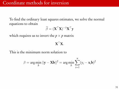
Coordinate methods for inversion
To find the ordinary least squares estimates, we solve the normalequations to obtain
β = (X>X)−1X>y
which requires us to invert the p× p matrix
X>X.
This is the minimum norm solution to
β = arg minb||y−Xb||2 = arg min
b
n∑i=1
(yi − xib)2
31
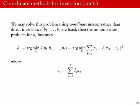
Coordinate methods for inversion (cont.)
We may solve this problem using coordinate descent rather thandirect inversion; if b2, . . . , bp are fixed, then the minimizationproblem for b1 becomes
b1 = arg minb1
S(b1|b2, . . . , bp) = arg minb1
n∑i=1
(yi − b1xi1 − ci1)2
where
ci1 =
p∑j=2
bjxij.
32
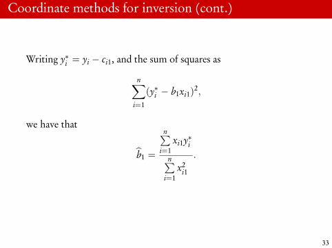
Coordinate methods for inversion (cont.)
Writing y∗i = yi − ci1, and the sum of squares as
n∑i=1
(y∗i − b1xi1)2,
we have that
b1 =
n∑i=1
xi1y∗in∑
i=1x2i1
.
33

Coordinate methods for inversion (cont.)
We may solve recursively in turn for each bj, that is, afterinitialization and at step t, update
b(t)j −→ b(t+1)j
by minimizing
minbj
S(bj|b(t+1)1 , b(t+1)
2 , . . . , b(t+1)j−1 , b(t)j+1 . . . , b
(t)p )
which does not require any matrix inversion.
34

Distributional Results
Some distributional results
Distributional results using the Normal distribution are key tomany inference procedures for the linear model. Suppose that
X1, . . . ,Xn ∼ Normal(µ, σ2)
are independent.1. Zi = (Xi − µ)/σ ∼ Normal(0, 1);2. Yi = Z2
i ∼ χ21;
3. U =∑n
i=1 Z2i ∼ χ
2n;
4. If U1 ∼ χ2n1
and U2 ∼ χ2n2
are independent, then
V =U1/n1
U2/n2∼ Fisher(n1, n2)
and1V∼ Fisher(n2, n1)
35
Some distributional results (cont.)
5. If Z ∼ Normal(0, 1) and U ∼ χ2ν , then
T =Z√U/ν
∼ Student(ν)
6. IfY = AX + b
whereI X = (X1, . . . ,Xn)> ∼ Normal(0, σ2In);I A is n× n;I b is n× 1;
thenY ∼ Normal(b, σ2AA>) ≡ Normal(µ,Σ)
say, and(Y− µ)>Σ−1(Y− µ) ∼ χ2
n.
36

Some distributional results (cont.)
7. Non-central Chi-squared distribution: If X ∼ Normal(µ, σ2), wefind the distribution of X2/σ2.
Y =Xσ∼ Normal(µ/σ, 1)
By standard transformation results, if Q = Y 2, then
fQ(y) =1√y
[φ(√y− µ/σ) + φ(−√y− µ/σ)]
This is the density of the non-central chi-squared distributionwith 1 degree of freedom and non-centrality parameterλ = (µ/σ)2, written
χ21(λ).
37

Some distributional results (cont.)
The non-central chi-squared distribution has many similarproperties to the standard (central) chi-squared distribution. Forexample if X1, . . . ,Xn are independent, with Xi ∼ χ2
1(λi), then
n∑i=1
Xi ∼ χ2n
( n∑i=1
λi
).
The non-central chi-squared distribution plays a role in testingfor the linear regression model as it characterizes the distributionof various sums of squares terms.
38
Some distributional results (cont.)8. Quadratic forms: If A is a square symmetric idempotent matrix,
and Z = (Z1, . . . ,Zn)> ∼ Normal(0, In), then
Z>AZ ∼ χ2ν
where ν = Trace(A).
To see this, use the singular value decomposition
A = UDU>
where U is an orthogonal matrix with U>U = In, and D is adiagonal matrix. Then
Z>AZ = Z>UDU>Z = (Z>U)D(U>Z) = {Z∗}>D{Z∗}
say. But
U>Z ∼ Normal(0,U>U) = Normal(0, In)
39

Some distributional results (cont.)
ThereforeZ>AZ = {Z∗}>D{Z∗}.
But A is idempotent, so
AA> = A
that is,UDU>UDU> = UDU>.
The left hand side simplifies, and we have
UD2U> = UDU>.
40
Some distributional results (cont.)
Thus, pre-multiplying by U>, and post-multiplying by U, wehave
D2 = D
and the diagonal elements of D must either be zero or one, so
Z>AZ = {Z∗}>D{Z∗} ∼ χ2ν
where ν = Trace(D) = Trace(A).
41

Some distributional results (cont.)9. If A1 and A2 are square, symmetric and orthogonal, and
A1A2 = 0
thenZ>A1Z and Z>A2Z
are independent. This result again uses the singular valuedecomposition; let
V1 = D1U>1 Z V2 = D2U>2 Z.
We have that
CovV1,V2 [V1,V2] = EV1,V2 [V2V>1 ]
= EZ[D2U>2 ZZ>U1D1]
= D2U>2 U>1 D1 = 0
as if A1 and A2 are orthogonal, then U>2 U>1 = 0.42
dsteph5
Highlight
dsteph5
Highlight

Bayesian Regression and Penalized
Least Squares

The Bayesian Linear Model
Under a Normality assumption
Y|X, β, σ2 ∼ Normal(Xβ, σ2In)
which defines the likelihood L(β, σ2; y,X), we may performBayesian inference by specifying a joint prior distribution
π0(β, σ2) = π0(β|σ2)π0(σ2)
and computing the posterior distribution
πn(β, σ2|y,X) ∝ L(β, σ2; y,X)π0(β, σ2)
43

The Bayesian Linear Model (cont.)
Prior specification:
• π0(σ2) ≡ InvGamma(α/2, γ/2), that is, by definition,1/σ2 ∼ Gamma(α/2, γ/2)
π0(σ2) =(γ/2)α/2)
Γ(α/2)
(1σ2
)α/2−1exp
{− γ
2σ2
}• π0(β|σ2) ≡ Normal(θ, σ2Ψ), that is, β is conditionally
Normally distributed in p dimensions,
where parametersα, γ, θ,Ψ
are fixed, known constants (’hyperparameters’)
44

The Bayesian Linear Model (cont.)
In the calculation of πn(β, σ2|y,X), we have after collecting terms
πn(β, σ2|y,X) ∝(
1σ2
)(n+α+p)/2−1
exp{− γ
2σ2
}exp
{−Q(β, y,X)
2σ2
}where
Q(β, y,X) = (y−Xβ)>(y−Xβ) + (β − θ)>Ψ−1(β − θ).
45
The Bayesian Linear Model (cont.)
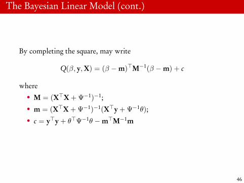
By completing the square, may write
Q(β, y,X) = (β −m)>M−1(β −m) + c
where• M = (X>X + Ψ−1)−1;• m = (X>X + Ψ−1)−1(X>y + Ψ−1θ);• c = y>y + θ>Ψ−1θ −m>M−1m
46

The Bayesian Linear Model (cont.)
From this we deduce that
πn(β, σ2|y,X) ∝(
1σ2
)(n+α+p)/2−1exp
{−(γ + c)
2σ2
}exp
{− 1
2σ2 (β −m)>M−1(β −m)
}that is
πn(β, σ2|y,X) ≡ πn(β|σ2, y,X)πn(σ2|y,X)
• πn(β|σ2, y,X) ≡ Normal(m, σ2M);• πn(σ2|y,X) ≡ InvGamma((n + α)/2, (c + γ)/2).
47

The Bayesian Linear Model (cont.)
The Bayesian posterior mean/modal estimator of β based on thismodel is
βB = m = (X>X + Ψ−1)−1(X>y + Ψ−1θ)
48
Ridge Regression
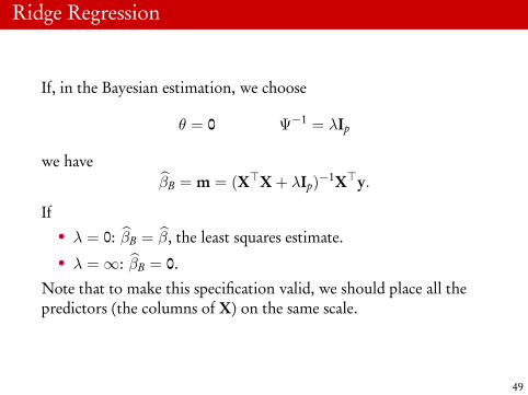
If, in the Bayesian estimation, we choose
θ = 0 Ψ−1 = λIp
we haveβB = m = (X>X + λIp)−1X>y.
If• λ = 0: βB = β, the least squares estimate.
• λ =∞: βB = 0.Note that to make this specification valid, we should place all thepredictors (the columns of X) on the same scale.
49
Ridge Regression (cont.)
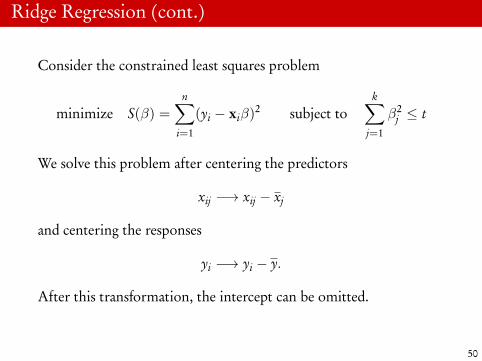
Consider the constrained least squares problem
minimize S(β) =
n∑i=1
(yi − xiβ)2 subject tok∑
j=1
β2j ≤ t
We solve this problem after centering the predictors
xij −→ xij − xj
and centering the responses
yi −→ yi − y.
After this transformation, the intercept can be omitted.
50

Ridge Regression (cont.)
Suppose that therefore there are precisely p β parameters in themodel.
We solve the constrained minimization using Lagrange multipliers:we minimize Sλ(β)
Sλ(β) = S(β) + λ
p∑j=1
β2j − t
We have that
∂Sλ(β)
∂β=∂S(β)
∂β+ 2λβ
– a p× 1 vector.
51
Ridge Regression (cont.)
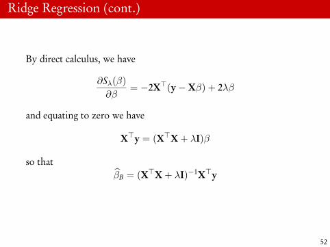
By direct calculus, we have
∂Sλ(β)
∂β= −2X>(y−Xβ) + 2λβ
and equating to zero we have
X>y = (X>X + λI)β
so thatβB = (X>X + λI)−1X>y
52
Ridge Regression (cont.)
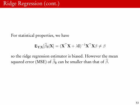
For statistical properties, we have
EY|X[βB|X] = (X>X + λI)−1X>Xβ 6= β
so the ridge regression estimator is biased. However the meansquared error (MSE) of βB can be smaller than that of β.
53

Ridge Regression (cont.)
If the columns of matrix X is orthogonal, so that
X>X = Ip
thenβBj =
11 + λ
βj < βj.
In general the ridge regression estimates are ‘shrunk’ towards zerocompared to the least squares estimates.
54

Ridge Regression (cont.)
Using the singular value decomposition, write
X = UDV>
where• U is n× p, columns of U are an orthonormal basis for the
column space of X, and
U>U = Ip.
• V is p× p, columns of V are an orthonormal basis for the rowspace of X;
V>V = Ip.
• D is diagonal with elements
d1 ≥ d2 ≥ · · · ≥ dp ≥ 0.
55
Ridge Regression (cont.)
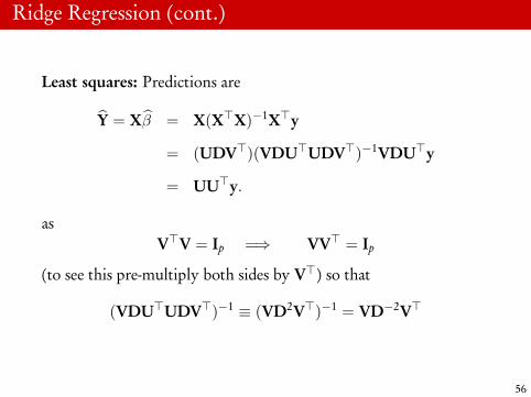
Least squares: Predictions are
Y = Xβ = X(X>X)−1X>y
= (UDV>)(VDU>UDV>)−1VDU>y
= UU>y.
asV>V = Ip =⇒ VV> = Ip
(to see this pre-multiply both sides by V>) so that
(VDU>UDV>)−1 ≡ (VD2V>)−1 = VD−2V>
56

Ridge Regression (cont.)
Ridge regression: Predictions are
Y = XβB = X(X>X + λIp)−1X>y
= UD(D2 + λIp)−1DU>y
=
p∑j=1
u˜j(
d2j
d2j + λ
)u˜>j y
where u˜j is the jth column of U.
57

Ridge Regression (cont.)
Ridge regression transforms the problem to one involving theorthogonal matrix U instead of X, and the shrinks the coefficientsby
d2j
d2j + λ
≤ 1.
For ridge regression, the hat matrix is
Hλ = X(X>X + λIp)−1X>
= UD(D2 + λIp)−1DU>
and the ‘degrees of freedom’ of the fit is
Trace(Hλ) =
p∑j=1
d2j
d2j + λ
58

Other Penalties
The LASSO penalty is
λ
p∑j=1
|βj|
and we solve the minimization
minβ
(y−Xβ)>(y−Xβ) + λ
p∑j=1
|βj|.
No analytical solution is available, but the minimization can beachieved using coordinate descent.
In this case, the minimization allows for the optimal value βj to beprecisely zero for some j.
59

Other Penalties (cont.)
A general version of this penalty is
λ
p∑j=1
|βj|q
and if q ≤ 1, there is a possibility of an estimate being shrunkexactly to zero.
For q ≥ 1, the problem is convex; for q < 1 the problem isnon-convex, and harder to solve.
However, if q ≤ 1, the shrinkage to zero allows for variableselection to be carried out automatically.
60

Model Selection using
Information Criteria

Selection using Information Criteria
Suppose we wish to choose one from a collection of modelsdescribed by densities f1, f2, . . . , fK with parameters θ1, θ2, . . . , θK .Let the true, data generating model be denoted f0.
We consider the KL divergence between f0 and fk:
KL(f0, fk) =
∫log(
f0(x)fk(x; θk)
)f0(x)dx
and aim to choose the model using the criterion
k = arg mink
KL(f0, fk)
61
Selection using Information Criteria (cont.)
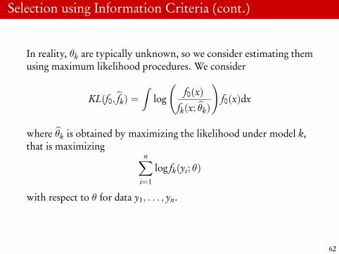
In reality, θk are typically unknown, so we consider estimating themusing maximum likelihood procedures. We consider
KL(f0, fk) =
∫log
(f0(x)
fk(x; θk)
)f0(x)dx
where θk is obtained by maximizing the likelihood under model k,that is maximizing
n∑i=1
log fk(yi; θ)
with respect to θ for data y1, . . . , yn.
62

Selection using Information Criteria (cont.)
We have that
KL(f0, fk) =
∫log f0(x)f0(x)dx−
∫log fk(x; θk)f0(x)dx
so we then may choose k by
k = arg maxk
∫log fk(x; θk)f0(x)dx
or if the parameters need to be estimated
k = arg maxk
∫log fk(x; θk(y))f0(x)dx.
63

Asymptotic results for estimation
under misspecification
Maximum likelihood as minimum KL
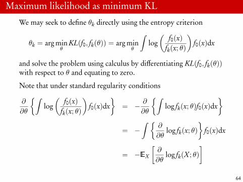
We may seek to define θk directly using the entropy criterion
θk = arg minθ
KL(f0, fk(θ)) = arg minθ
∫log(
f0(x)fk(x; θ)
)f0(x)dx
and solve the problem using calculus by differentiating KL(f0, fk(θ))with respect to θ and equating to zero.
Note that under standard regularity conditions
∂
∂θ
{∫log(
f0(x)fk(x; θ)
)f0(x)dx
}= − ∂
∂θ
{∫log fk(x; θ)f0(x)dx
}
= −∫ {
∂
∂θlog fk(x; θ)
}f0(x)dx
= −EX
[∂
∂θlog fk(X; θ)
]64
Maximum likelihood as minimum KL (cont.)
Therefore θk solves
EX
[∂
∂θlog fk(X; θ)|θ=θk
]= 0.
Under identifiability assumptions, we assume that is that there is asingle θk which solves this equation.
The sample-based equivalent calculation dictates that for theestimate θk
1n
n∑i=1
∂
∂θlog fk(xi; θ)|θ=θk = 0
which coincides with ML estimation.
65
Maximum likelihood as minimum KL (cont.)
Under identifiability assumptions, as
1n
n∑i=1
∂
∂θlog fk(Xi; θ)|θ=θk −→ 0,
by the strong law of large numbers we must have that
θk −→ θk
with probability 1 as n −→∞.
66

Maximum likelihood as minimum KL (cont.)Let
I(θk) = EX
[−∂
2 log fk(X; θ)
∂θ∂θ>
∣∣∣∣θ=θk
; θk
]be the Fisher information computed wrt fk(x; θk), and
I(θk) = EX
[−∂
2 log fk(X; θ)
∂θ∂θ>
∣∣∣∣θ=θk
]
be the same expectation quantity computed wrt f0(x). Thecorresponding n data versions, where log fk(X; θ) is replaced by
n∑i=1
log fk(Xi; θ)
areIn(θk) = nI(θk) In(θk) = nI(θk).
67
Maximum likelihood as minimum KL (cont.)
The quantity In(θk) is the sample based version
In(θk) = −
{ n∑i=1
∂2
∂θ∂θ>log fk(Xi; θ)
}θ=θk
This quantity is evaluated at θk = θk to yield In(θk); we have that
In(θk) −→ In(θk)
with probability 1 as n −→∞.
68

Maximum likelihood as minimum KL (cont.)
Another approach that is sometimes used is to uses the equivalencebetween expressions involving the first and second derivativeversions of I(θ); we have also that
I(θk) = EX
[∂ log fk(X; θ)
∂θ
∣∣∣∣⊗
2
θ=θk
; θk
]= J (θk)
with the expectation computed wrt fk(x; θk), where for vector U
U⊗
2 = UU>.
Let
J(θk) = EX
[∂ log fk(X; θ)
∂θ
∣∣∣∣⊗
2
θ=θk
]be the equivalent calculation with the expectation computed wrtf0(x).
69
Maximum likelihood as minimum KL (cont.)
Now by a second order Taylor expansion of the first derivative ofthe loglikelihood, if
˙k(θk) =∂ log fk(x; θ)
∂θ
∣∣∣∣θ=θk
¨k(θk) =∂2 log fk(x; θ)
∂θ∂θ>
∣∣∣∣θ=θk
at θ = θk, we have
˙k(θk) = ˙k(θk) + ¨k(θk)(θk − θk) +12
(θk − θk)>...` n(θ∗)(θk − θk)
= ¨k(θk)(θk − θk) + Rn(θ∗)
as ˙k(θk) = 0, ||θk − θ∗|| < ||θk − θk||, and where the remainderterm is being denoted Rn(θ∗).
70

Maximum likelihood as minimum KL (cont.)We have by definition that
−¨k(θk) = In(θk).
and in the limitRn(θ∗)
np−→ 0
that is, Rn(θ∗) = op(n), and
1nIn(θk)
a.s.−→ I(θk)
as n −→∞.
Rewriting the above approximation, we have
√n(θk − θk) =
{1nIn(θk)
}−1{ 1√n
˙k(θk)
}+
{1nIn(θk)
}−1{Rn(θ∗)
n
}71
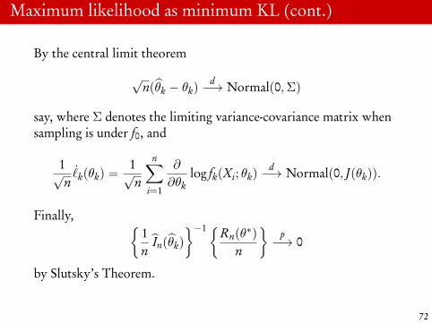
Maximum likelihood as minimum KL (cont.)
By the central limit theorem
√n(θk − θk)
d−→ Normal(0,Σ)
say, where Σ denotes the limiting variance-covariance matrix whensampling is under f0, and
1√n
˙k(θk) =1√n
n∑i=1
∂
∂θklog fk(Xi; θk)
d−→ Normal(0, J(θk)).
Finally, {1nIn(θk)
}−1{Rn(θ∗)
n
}p−→ 0
by Slutsky’s Theorem.
72

Maximum likelihood as minimum KL (cont.)
Therefore, by equating the asymptotic variances of the abovequantities, we must have
J(θk) = I(θk)ΣI(θk)
yielding thatΣ = {I(θk)}−1J(θk){I(θk)}−1
73

Model Selection using Minimum
KL
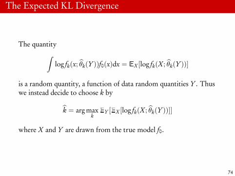
The Expected KL Divergence
The quantity∫log fk(x; θk(Y ))f0(x)dx = EX [log fk(X; θk(Y ))]
is a random quantity, a function of data random quantities Y . Thuswe instead decide to choose k by
k = arg maxkEY [EX [log fk(X; θk(Y ))]]
where X and Y are drawn from the true model f0.
74
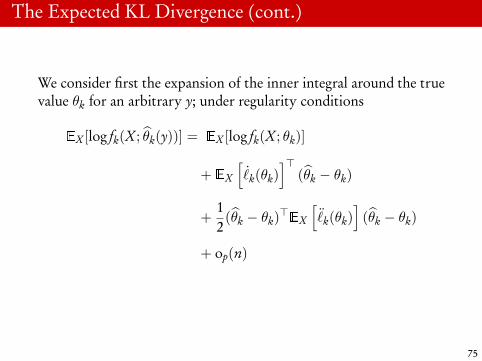
The Expected KL Divergence (cont.)
We consider first the expansion of the inner integral around the truevalue θk for an arbitrary y; under regularity conditions
EX [log fk(X; θk(y))] = EX [log fk(X; θk)]
+ EX
[˙k(θk)
]>(θk − θk)
+12
(θk − θk)>EX
[¨k(θk)
](θk − θk)
+ op(n)
75

The Expected KL Divergence (cont.)
By definition EX
[˙k(θk)
]= 0, and
EX
[¨k(θk)
]= −In(θk)
so therefore
EX [log fk(X; θk(y))] = EX [log fk(X; θk)]−12
(θk−θk)>In(θk)(θk−θk)+op(n)
We then must compute
EY [EX [log fk(X; θk(Y ))]]
The term EX [log fk(X; θk)] is a constant wrt this expectation.
76

The Expected KL Divergence (cont.)
The expectation of the quadratic term can be computed by standardresults for large n; under sampling Y from f0, we have as before that
(θk − θk)>In(θk)(θk − θk)
can be rewritten
{√n(θk − θk)}>
{1nIn(θk)
}{√n(θk − θk)}
where √n(θk − θk)
d−→ Normal(0,Σ)
and1nIn(θk)
a.s.−→ I(θk)
77
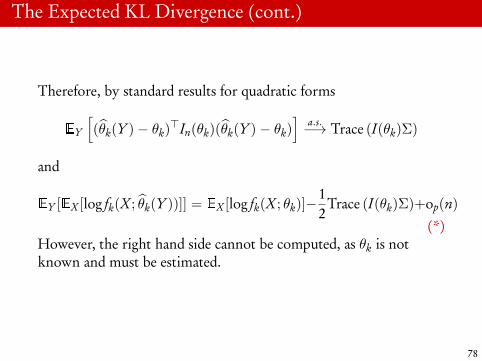
The Expected KL Divergence (cont.)
Therefore, by standard results for quadratic forms
EY
[(θk(Y )− θk)>In(θk)(θk(Y )− θk)
]a.s.−→ Trace (I(θk)Σ)
and
EY [EX [log fk(X; θk(Y ))]] = EX [log fk(X; θk)]−12
Trace (I(θk)Σ)+op(n)
(*)However, the right hand side cannot be computed, as θk is notknown and must be estimated.
78
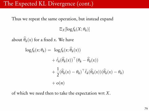
The Expected KL Divergence (cont.)
Thus we repeat the same operation, but instead expand
EX [log fk(X; θk)]
about θk(x) for a fixed x. We have
log fk(x; θk) = log fk(x; θk(x))
+ ˙k(θk(x))>(θk − θk(x))
+12
(θk(x)− θk)> ¨k(θk(x))(θk(x)− θk)
+ o(n)
of which we need then to take the expectation wrt X.
79
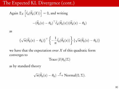
The Expected KL Divergence (cont.)
Again EX
[˙k(θk(X))
]= 0, and writing
−(θk(x)− θk)> ¨k(θk(x))(θk(x)− θk)
as
{√n(θk(x)− θk)}>
{− 1n
¨k(θk(x))}{√n(θk(x)− θk)}
we have that the expectation over X of this quadratic formconverges to
Trace (I(θk)Σ)
as by standard theory
√n(θk(x)− θk)
d−→ Normal(0,Σ).
80
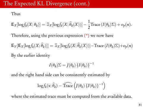
The Expected KL Divergence (cont.)
Thus
EX [log fk(X; θk)] = EX [log fk(X; θk(X))]− 12
Trace (I(θk)Σ) + op(n).
Therefore, using the previous expression (*) we now have
EY [EX [log fk(X; θk)]] = EX [log fk(X; θk(X))]−Trace (I(θk)Σ)+op(n)
By the earlier identity
I(θk)Σ = J(θk) {I(θk)}−1
and the right hand side can be consistently estimated by
log fk(x; θk)− Trace(J(θk) {I(θk)}−1
)where the estimated trace must be computed from the available data.
81

The Expected KL Divergence (cont.)
On obvious estimator of the trace is
Trace(J(θk(x))
{I(θk(x))
}−1)
although this might potentially be improved upon. In any case, ifthe approximating model fk is close in KL terms to the true modelf0, we would expect that
Trace(J(θk) {I(θk)}−1
)l dim(θk)
as we would have under regularity assumptions
J(θk) l I(θk)
82
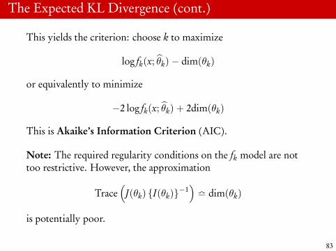
The Expected KL Divergence (cont.)
This yields the criterion: choose k to maximize
log fk(x; θk)− dim(θk)
or equivalently to minimize
−2 log fk(x; θk) + 2dim(θk)
This is Akaike’s Information Criterion (AIC).
Note: The required regularity conditions on the fk model are nottoo restrictive. However, the approximation
Trace(J(θk) {I(θk)}−1
)l dim(θk)
is potentially poor.
83
The Bayesian Information Criterion
The Bayesian Information Criterion (BIC) uses an approximation tothe marginal likelihood function to justify model selection. For datay = (y1, . . . , yn), we have the posterior distribution for model k as
πn(θk; y) =Lk(θk; y)π0(θk)∫Lk(t; y)π0(t) dt
.
where Lk(θ; y) is the likelihood function. The denominator is
fk(y) =
∫Lk(t; y)π0(t) dt
that is, the marginal likelihood.
84
The Bayesian Information Criterion (cont.)
Let
`k(θ; y) = logLk(θ; y) =
n∑i=1
log fk(yi; θ)
denote the log-likelihood for model k. By a Taylor expansion of`k(θ; y) around ML estimate θk, we have
`k(θ; y) = `k(θk; y) + (θ − θk)> ˙(θk; y)
+12
(θ − θk)> ¨(θk; y)(θ − θk) + o(1)
We have by definition that ˙(θk) = 0, and we may write
−¨(θk; y) ={Vn(θk)
}−1.
Vn(θk) is the Hessian matrix derived from n data points.
85
The Bayesian Information Criterion (cont.)
In ML theory, Vn(θk) estimates the variance of the ML estimatorderived from n data. We may denote that, for a random sample, that
Vn(θk) =1nV1(θk)
say, where
V1(θ) = n
{ n∑i=1
∂2
∂θ∂θ>log fk(yi; θ)
}−1
is a square symmetric matrix of dimension pk = dim(θk) recordingan estimate of the the variance of the ML estimator for a single datapoint n = 1.
86
The Bayesian Information Criterion (cont.)
Then, exponentiating, we have that
Lk(θ; y) l Lk(θk; y) exp{−1
2(θ − θk)>
{Vn(θk)
}−1(θ − θk)
}This is a standard quadratic approximation to the likelihood aroundthe ML estimate.
87
The Bayesian Information Criterion (cont.)
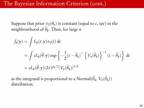
Suppose that prior π0(θk) is constant (equal to c, say) in theneighbourhood of θk. Then, for large n
fk(y) =
∫Lk(t; y)π0(t) dt
l∫
cLk(θ; y) exp{−1
2(t − θk)>
{Vn(θk)
}−1(t − θk)
}dt
= cLk(θ; y)(2π)pk/2|Vn(θk)|1/2
as the integrand is proportional to a Normal(θk,Vn(θk))distribution.
88
The Bayesian Information Criterion (cont.)
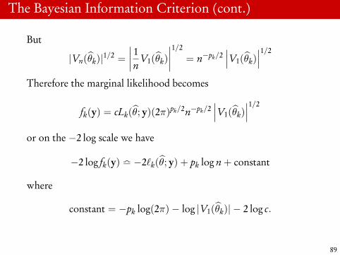
But
|Vn(θk)|1/2 =
∣∣∣∣ 1nV1(θk)
∣∣∣∣1/2= n−pk/2
∣∣∣V1(θk)∣∣∣1/2
Therefore the marginal likelihood becomes
fk(y) = cLk(θ; y)(2π)pk/2n−pk/2∣∣∣V1(θk)
∣∣∣1/2
or on the −2 log scale we have
−2 log fk(y) l −2`k(θ; y) + pk log n + constant
where
constant = −pk log(2π)− log |V1(θk)| − 2 log c.
89

The Bayesian Information Criterion (cont.)
The constant term is o(1) and is hence negligible, so the BIC isdefined as
BIC = −2`k(θ; y) + pk log n.
90
Related Documents