Math 2200 – Discrete Mathematics Summer 2015

Math 2200 – Discrete MathematicsSummer 2015

Instructor: Davar Khoshnevisan ([email protected])Department of Mathematics, University of Utah

Text: Discrete Mathematics by K.H. Rosen,McGraw Hill, NY, Seventh Edition, 2011

Contents1 Introduction 2

1.1 Some Questions . . . . . . . . . . . . . . . . . . . . . . . . . . . . . 21.2 Topics Covered . . . . . . . . . . . . . . . . . . . . . . . . . . . . . 3

2 Elementary Logic 32.1 Propositional Logic . . . . . . . . . . . . . . . . . . . . . . . . . . . 32.2 Equivalences and Tautologies . . . . . . . . . . . . . . . . . . . . . 62.3 Predicates and Quantifiers . . . . . . . . . . . . . . . . . . . . . . 8

3 Logic in Mathematics 103.1 Some Terminology . . . . . . . . . . . . . . . . . . . . . . . . . . . 103.2 Proofs . . . . . . . . . . . . . . . . . . . . . . . . . . . . . . . . . . . 11

3.2.1 Proof by Exhaustion . . . . . . . . . . . . . . . . . . . . . . 113.2.2 Proof by Contradiction . . . . . . . . . . . . . . . . . . . . 123.2.3 Proof by Induction . . . . . . . . . . . . . . . . . . . . . . . 13

4 Naive Set Theory 174.1 Some Terminology . . . . . . . . . . . . . . . . . . . . . . . . . . . 174.2 The Calculus of Set Theory . . . . . . . . . . . . . . . . . . . . . . 204.3 Set Identities . . . . . . . . . . . . . . . . . . . . . . . . . . . . . . . 24

5 Transformations 265.1 Functions . . . . . . . . . . . . . . . . . . . . . . . . . . . . . . . . . 265.2 The Graph of a Function . . . . . . . . . . . . . . . . . . . . . . . 285.3 One-to-One Functions . . . . . . . . . . . . . . . . . . . . . . . . . 295.4 Onto Functions . . . . . . . . . . . . . . . . . . . . . . . . . . . . . 325.5 Inverse Functions . . . . . . . . . . . . . . . . . . . . . . . . . . . . 325.6 Composition of Functions . . . . . . . . . . . . . . . . . . . . . . . 335.7 Back to Set Theory: Cardinality . . . . . . . . . . . . . . . . . . . 34

6 Patterns and Sequences 396.1 Recurrence Relations . . . . . . . . . . . . . . . . . . . . . . . . . 406.2 Infinite Series . . . . . . . . . . . . . . . . . . . . . . . . . . . . . . 426.3 Continued Fractions . . . . . . . . . . . . . . . . . . . . . . . . . . 43

7 Number Theory 457.1 Division . . . . . . . . . . . . . . . . . . . . . . . . . . . . . . . . . . 467.2 Modular Arithmetic . . . . . . . . . . . . . . . . . . . . . . . . . . . 48

1

1 IntroductionThere is a story about two friends, who were classmates in high

school, talking about their jobs. One of them became a statistician andwas working on population trends. He showed a reprint to his formerclassmate. The reprint started, as usual, with the Gaussian distributionand the statistician explained to his former classmate the meaning of thesymbols for the actual population, for the average population, and so on.His classmate was a bit incredulous and was not quite sure whetherthe statistician was pulling his leg. “How can you know that?” washis query. “And what is this symbol here?” “Oh,” said the statistician,“this is π.” “What is that?” “The ratio of the circumference of thecircle to its diameter.” “Well, now you are pushing your joke too far,“said the classmate, “surely the population has nothing to do with thecircumference of the circle.”

......

......

The preceding two stories illustrate the two main points which arethe subjects of the present discourse. The first point is that mathemat-ical concepts turn up in entirely unexpected connections. Moreover,they often permit an unexpectedly close and accurate description ofthe phenomena in these connections. Secondly, just because of thiscircumstance, and because we do not understand the reasons of theirusefulness, we cannot know whether a theory formulated in terms ofmathematical concepts in uniquely appropriate. We are in a positionsimilar to that of a man who was provided with a bunch of keys andwho, having to open several doors in succession, always hit on the rightkey on the first or second trial.

–Eugene Paul Wagner1

1.1 Some Questions- Is mathematics a natural science, or is it a human invention?

- Is mathematics the science of laboriously doing the same things overand over, albeit very carefully? If yes, then why is it that some peoplediscover truly-novel mathematical ideas whereas many others do not?Or, for that matter, why can’t we seem to write an algorithm that doesnew mathematics for us? If no, then is mathematics an art?

- Is mathematics a toolset for doing science? If so, then why is it thatthe same set of mathematical ideas arise in so many truly-differentscientific disciplines? Is mathematics a consequence of the humancondition, or is it intrinsic in the physical universe?

1“The unreasonable effectiveness of mathematics in the natural sciences,” Communicationsin Pure and Applied Mathematics (1960) vol. 13, no. 1.

2

- Why is it that many people are perfectly comfortable saying some-thing like, “I can’t do mathematics,” or “I can’t draw,” but very few arecomfortable saying, “I can’t read,” or “I can’t put on my socks in themorning”?

- Our goal, in this course, is to set forth elementary aspects of the lan-guage of mathematics. The language can be learned by most people,though perhaps with effort. Just as most people can learn to read orput on their socks in the morning. [What one does with this elaboratelanguage then has to do with one’s creativity, intellectual curiosity, andother less tangible things.]

1.2 Topics Covered- Propositional Logic, Modus Ponens, and Set Theory [Chapters 1-2]

- Algorithms [Chapter 3]

- Number Theory and Cryptography [Chapter 4]

- Induction and Recursion [Chapter 5]

- Enumerative Combinatorics and Probability [Chapters 6–8]

- Topics from logic, graph theory, and computability.

2 Elementary Logic2.1 Propositional LogicAccording to the Merriam-Webster online dictionary, “Logic” could meanany one of the following:

- A proper or reasonable way of thinking about or understanding some-thing;

- A particular way of thinking about something; and/or

- The science that studies the formal processes used in thinking andreasoning.

“Propositional logic” and its natural offspring, predicate logic, are early at-tempts to make explicit this process. Propositional logic was developed inthe mid-19th century by Augustus DeMorgan, George Boole, and others,and is sometimes also referred to as “naive logic,” or “informal logic.” Thefirst part of this course is concerned with the development of propositionallogic.

The building blocks of propositional logic are “propositions,” and “rulesof logic.” A proposition is a statement/declaration which is, by definition,

3

either true or false, but not both. If a proposition � is true, then its truthvalue is “true” or “T.” If � is false, then its truth value is “false” or “F.”

Example 2.1. Here are some simple examples of logical propositions:

1. “It is now 8:00 p.m.” is a proposition.

2. “You are a woman,” “He is a cat,” and “She is a man” are all propositions.

3. “�2 + �2 = �2” is not a proposition, but “the sum of the squares ofthe sides of a triangle is equal to the square of its hypotenuse” is aproposition. Notice that, in propositional logic, you do not have torepresent a proposition in symbols.

The rules of logic—essentially also known as Modus Ponens—are anagreed-upon set of rules that we allow ourselves to use in order to buildnew propositions from the old. Here are some basic rules of propositionallogic.

NOT. If � is a proposition, then so is the negation of �, denoted by ¬� [insome places, not here, also ∼ �]. The proposition ¬� declares that“proposition � is not valid.” By default, the truth value of ¬� is theopposite of the truth value of �.

Example 2.2. If � is the proposition, “I am taking at least 3 courses thissummer,” then ¬� is the proposition, “I am taking at most 2 coursesthis summer.”

Here is the “truth table” for negation.

� ¬�T FF T

AND. If � and � are propositions, then their conjunction is the proposition“� and � are both valid.” The conjunction of � and � is denoted by� ∧�. The truth value of � ∧� is true if � and � are both true; else, thetruth value of � ∧ � is false. Here is the “truth table” for conjunctivepropositions.

� � � ∧ �T T TT F FF T FF F F

OR. Similarly, the disjunction of two propositions � and � is the proposi-tion, “at least one of � and � is valid.” The disjunction of � and � isdenoted by � ∨ �.

4

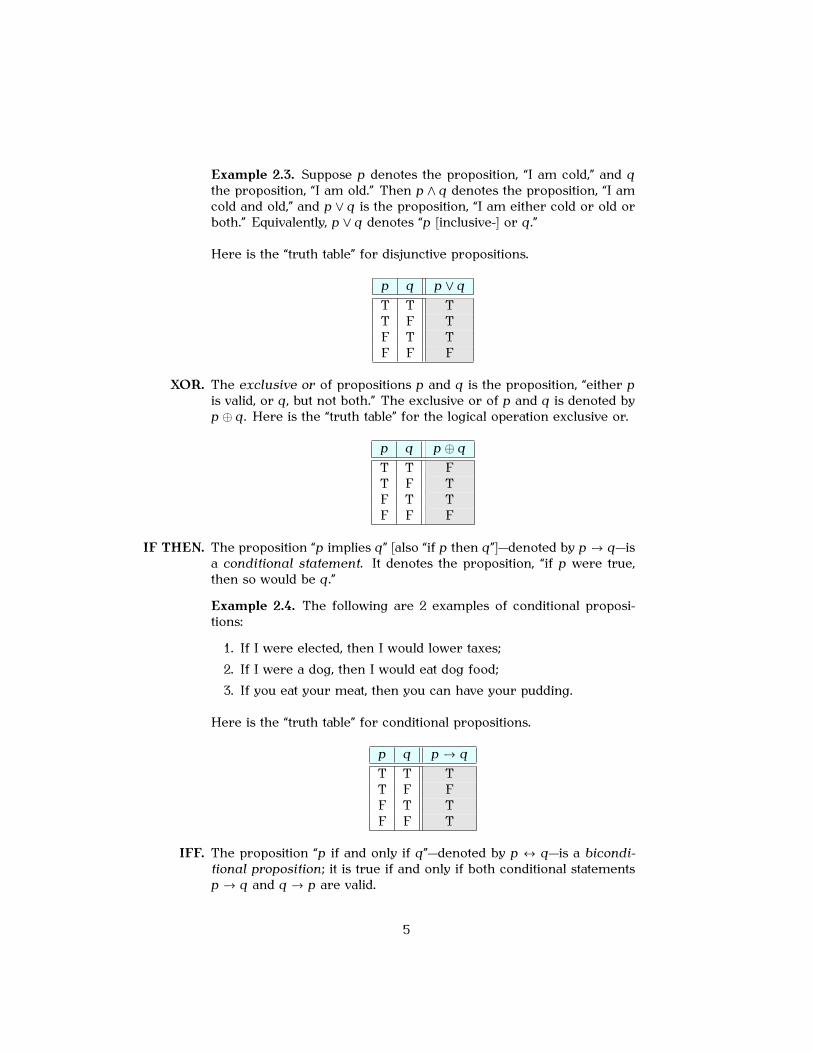
Example 2.3. Suppose � denotes the proposition, “I am cold,” and �the proposition, “I am old.” Then � ∧ � denotes the proposition, “I amcold and old,” and � ∨ � is the proposition, “I am either cold or old orboth.” Equivalently, � ∨ � denotes “� [inclusive-] or �.”

Here is the “truth table” for disjunctive propositions.

� � � ∨ �T T TT F TF T TF F F

XOR. The exclusive or of propositions � and � is the proposition, “either �is valid, or � , but not both.” The exclusive or of � and � is denoted by� ⊕ �. Here is the “truth table” for the logical operation exclusive or.

� � � ⊕ �T T FT F TF T TF F F

IF THEN. The proposition “� implies �” [also “if � then �”]—denoted by � → �—isa conditional statement. It denotes the proposition, “if � were true,then so would be �.”

Example 2.4. The following are 2 examples of conditional proposi-tions:

1. If I were elected, then I would lower taxes;2. If I were a dog, then I would eat dog food;3. If you eat your meat, then you can have your pudding.

Here is the “truth table” for conditional propositions.

� � � → �T T TT F FF T TF F T

IFF. The proposition “� if and only if �”—denoted by � ↔ �—is a bicondi-tional proposition; it is true if and only if both conditional statements� → � and � → � are valid.

5

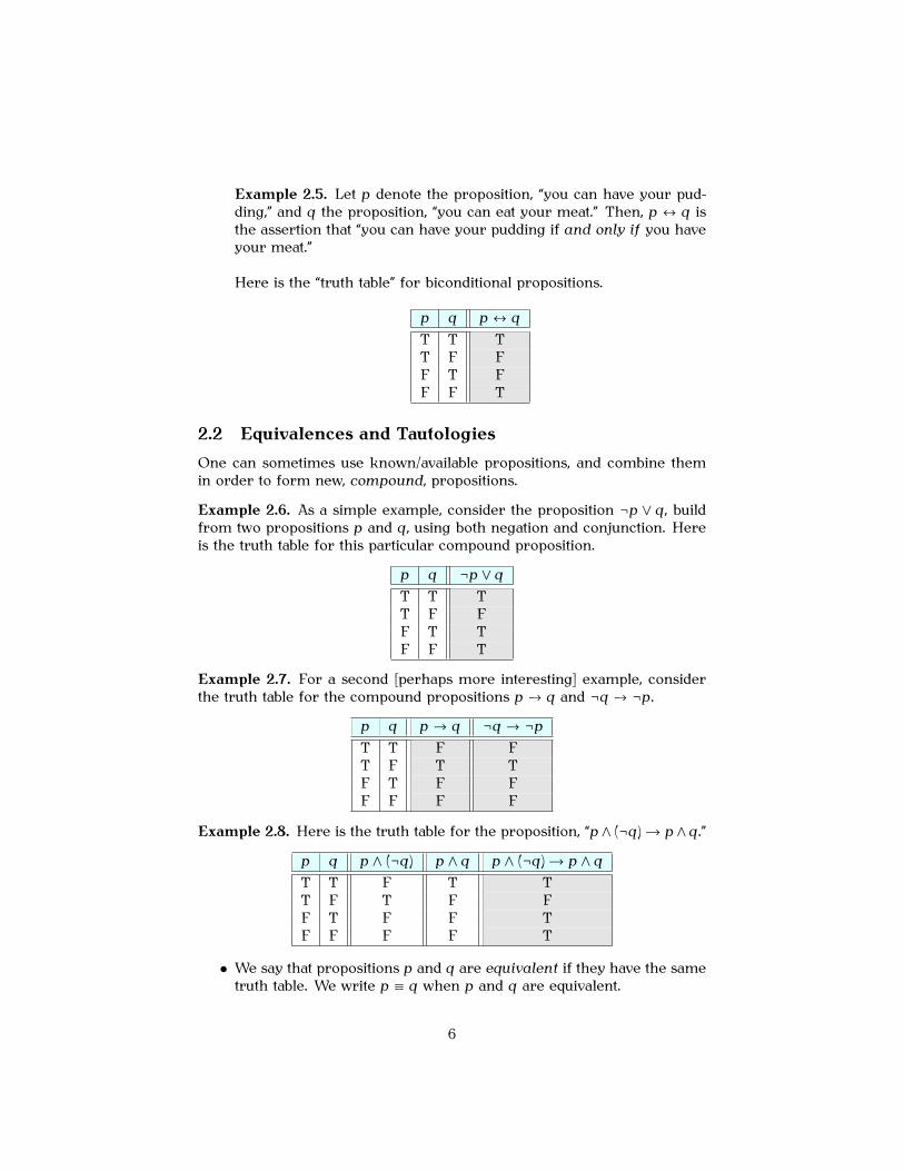
Example 2.5. Let � denote the proposition, “you can have your pud-ding,” and � the proposition, “you can eat your meat.” Then, � ↔ � isthe assertion that “you can have your pudding if and only if you haveyour meat.”

Here is the “truth table” for biconditional propositions.

� � � ↔ �T T TT F FF T FF F T

2.2 Equivalences and TautologiesOne can sometimes use known/available propositions, and combine themin order to form new, compound, propositions.

Example 2.6. As a simple example, consider the proposition ¬� ∨ � , buildfrom two propositions � and � , using both negation and conjunction. Hereis the truth table for this particular compound proposition.

� � ¬� ∨ �T T TT F FF T TF F T

Example 2.7. For a second [perhaps more interesting] example, considerthe truth table for the compound propositions � → � and ¬� → ¬�.

� � � → � ¬� → ¬�T T F FT F T TF T F FF F F F

Example 2.8. Here is the truth table for the proposition, “� ∧ (¬�) � � ∧ �.”

� � � ∧ (¬�) � ∧ � � ∧ (¬�) � � ∧ �T T F T TT F T F FF T F F TF F F F T

• We say that propositions � and � are equivalent if they have the sametruth table. We write � ≡ � when � and � are equivalent.

6

Example 2.9. Check the following from first principles:

– ¬(¬�) ≡ �. Another way to say this is that the compound propo-sition “−(¬�) ↔ �” is always true;

– (� ∧ �) ≡ (� ∧ �). Another way to say this is that the compoundproposition “(� ∧ �) ↔ (� ∧ �)” is always true;

– (� ∨ �) ≡ (� ∨ �). Another way to say this is that the compoundproposition “(� ∨ �) ↔ (� ∨ �)” is always true.

• A proposition is a tautology if it is always true, and a fallacy if it isalways false. Thus, � ≡ � is the same proposition as “� ↔ � is atautology.”

Example 2.10. If � is a proposition, then ¬� ∨ � is a tautology and¬� ∧ � is a fallacy. One checks these by computing truth tables:

� ¬� ¬� ∨ � ¬� ∧ �T F T FT F T FF T T FF T T F

In casual conversation, the word “tautology” is sometimes equated withother words such as “self-evident,” “obvious,” or even sometimes “triv-ial.” In propositional logic, tautologies are not always obvious. Alltheorems of mathematics and computer science qualify as logical tau-tologies, but many are far from obvious and the like. If “� ≡ � ,” thenwe may think of � and � as the same proposition.

• There are infinitely-many tautologies in logic; one cannot memorizethem. Rather, one learns the subject. Still, some tautologies arisemore often than others, and some have historical importance and havenames. So, educated folk will want to know and/or learn them. Hereare two examples of the latter type.

Example 2.11 (De Morgan’s Laws). The following two tautologies areknown as De Morgan’s Laws: If � and � are propositions, then:

¬(� ∧ �) ≡ ¬� ∨ ¬�;¬(� ∨ �) ≡ ¬� ∧ ¬��

You can prove them by doing the only possible thing: You write downand compare the truth tables. [Check!]

7

2.3 Predicates and QuantifiersIt was recognized very early, in the 19th century, that one needs a moreflexible, more complex, set of logical rules in order to proceed with moreinvolved logical tasks. For instance, we cannot use propositional logic toascertain whether or not “� = 2� + 1.” In order to do that, we also need toknow the numerical values of the “variables” � and �, not to mention someof the basic rules of addition and multiplication [i.e., tables]. “Predicate logic”partly overcomes this definiciency by: (i) including the rules of propositionallogic; and (ii) including “variables” and “[propositional] functions.”

• A propositional function P(�) is a proposition for every possible choiceof the variable �; P is referred to as a predicate.

Example 2.12. Let P(�) denote “� ≥ −1/8 for every real number �.Then, P(1) is a true proposition, whereas P(−1) is a false one.

Example 2.13. The variable of a proposition need not be a real num-ber. For instance, P(� � �) could denote the proposition, “� + � = 1.”In this case, the variable of P is a 2-vector (� � �) for every possiblereal number � and �. Here, for instance, P(1 � 1) is false, whereasP(5�1 � −4�1) is true. You can think of the predicate P, in English termsand informally, as the statement that the point (� � �) falls on a certainstraight line in the plane.

Predicate logic has a number of rules and operations that allow us tocreate propositions from predicates. Here are two notable operations:

FOR ALL. If P is a predicate, then ∀�P(�) designates the proposition, “P(�) forall �” within a set of possible choices for �. The “for all” operation∀ is a quantifier for P(�), and that set of possible choices of � is thedomain of the quantifier ∀ here. If the domain D is not universal [“forall real numbers �” and the like], then one includes the domain bysaying, more carefully, something like ∀�P(�)[� ≥ 0], or ∀�P(�)[(� ≥−2) ∨ (� ≤ 5)], etc.

Example 2.14. Suppose P(�) if the proposition that “� > 2,” for everyreal number �. Then ∀�P(�) is false; for example, that is because P(0)is false. But ∀�P(�)[� ≥ 8] is true.

FOR SOME. If P is a predicate, then ∃�P(�) designates the proposition, “P(�) forsome �” within a set of possible choices for �. The “there exits” oper-ation ∃ is a quantifier for P(�), and that set of possible choices of � isthe domain of the quantifier ∃ here.

Example 2.15. Suppose P(�) if the same proposition as before forevery real number �: That “� > 2�” Then ∃�P(�) is true; for example,that is because P(3) is true. But ∃�P(�)[� ≤ 0] is false.

8

• (De Morgan’s Laws for Quantifiers) We have the following tautologies:

¬∃�P(�) ≡ ∀�¬P(�);¬∀�P(�) ≡ ∃�¬P(�)�

One proves these De Morgan laws by simply being careful. For in-stance, let us verify the first one. Our ask is two fold:

1. We need to show that if ¬∃�P(�) is true then so is ∀�¬P(�); and2. We need to show that if ∀�¬P(�) is true then so is ¬∃�P(�).

We verify (1) as follows: If ¬∃�P(�) were true, then ∃�P(�) is false.Equivalently, P(�) is false for all � [in the domain of the quantifier] andhence ¬P(�) is true for all � [also in the domain of the quantifier]. Thisyields ∀�¬P(�) as true and completes the proof of (1). I will leave theproof of (2) up to you.

Example 2.16. The negation of “Everyone is smelly” is “someone isnot smelly.” In order to demonstrate this using predicate logic, let P(�)denote “� is smelly.” Then, “everyone is smelly” is codified as ∀�P(�);its negation is ∃�¬P(�), thanks to the De Morgan laws. I will leave itup to you to do the rest.

ex:smelly Example 2.17. The negation of “Someone will one day win the jack-pot” is “no one will ever win the jackpot.” In order to demonstratethis using predicate logic, let P(� � �) denote “� will win the jackpoton day �.” Then, “someone will win the jackpot one day” is codifiedas ∃(� � �)P(� � �), whose negation is—thanks to De Morgan’s laws—theproposition ∀(� � �)¬P(� � �). As an important afterthought, I ask, “Whatare the respective domains of these quantifiers?”

• Predicate logic allows us to define new predicates from old. For in-stance, suppose P(� � �) is a predicate with two variables � and �. Then,∀�P(� � �), ∃�P(� � �), . . . are themselves propositional functions [thefirst is a function of � and the second of �].

• Some times, if the expressions become too complicated, one separatesthe quantifiers from the predicates by a colon. For instance,

∀�∀�∀�∀α∃βP(� � � � � � α � β)

can also be written as

∀�∀�∀�∀α∃β : P(� � � � � � α � β)�

in order to ease our reading of the logical “formula.”

9

Example 2.18. See if you can prove [and understand the meaning of]the tautologies:

∀(� � �)P(� � �) ≡ ∀�∀�P(� � �) ≡ ∀�∀�P(� � �);∃(� � �)P(� � �) ≡ ∃�∃�P(� � �) ≡ ∃�∃�P(� � �);

¬�

∀�∃�P(� � �) ≡ ∃�∀�P(� � �)�

�

ex:sqrt:2 Example 2.19. A real number � is said to be rational if we can write� = �/� where � and � are integers. An important discovery of themathematics of antiquity—generally ascribed to a Pythagorean namedHippasus of Metapontum (5th Century B.C.)—is that

√2 is irrational;

that is, it is not rational. We can write this statement, using predicatelogic, as the following tautology:

¬∃�� � :√

2 = �� [�� � ∈ Z]�

where Z := {0 � ±1 � ±2 � · · · } denotes the collection of all integers, “:=”is shorthand for “is defined as,” and “∈” is shorthand for “is an elementof.”

ex:fermat:last:thm Example 2.20. Fermat’s last theorem, as conjectured by Pierre deFermat (1637) and later proved by Andrew Wiles (1994/1995), is thetautology,

¬�

∃�∃�∃�∃� P(� � � � � � �)�

[(�� �� � ∈ N) ∧ (� ∈ {3 � 4 � � � �})] �

where every P(� � � � � � �) denotes the proposition, “�� + �� = ��.”

ex:continuity Example 2.21. In calculus, one learns that a function � of a real vari-able � is continuous if, and only if, for every ε > 0 there exists δ > 0such that |� (�) − � (�)| ≤ ε whenever |� − �| ≤ δ. We can state thisdefinition, as a proposition in predicate logic as

∀ε∃δP(ε � δ) [ε > 0 ∧ δ > 0]�

where each P(ε � δ) denotes the following proposition:

∀�� �Q(� � � � ε) [−∞ < � < ∞ ∧ � − δ < � < � + δ]�

and every Q(� � � � ε) denotes the event that |� (�) − � (�)| ≤ ε.

3 Logic in Mathematics3.1 Some Terminology

• In mathematics [and related fields such as theoretical computer scienceand theoretical economics], a theorem is an assertion that:

10

1. Can be stated carefully in the language of logic [for instance, thelogical systems of this course, or more involved ones]; and

2. Is always true [i.e., a tautology, in the language of predicate logic].

• Note that, in the preceding, “true” is underlined to emphasize that itis meant in the sense of the logical system being used [explicitly], andtherefore can be demonstrated [in that same logical system] explicitly.

• Officially speaking, Propositions, lemmas, fact, etc. are also theorems.However, in the culture of mathematical writing, theorems are deemedas the “important” assertions, propositions as less “important,” and lem-mas as “technical” results en route establishing theorems. I have putquotations around “important” and “technical” because these are sub-jective annotations [usually decided upon by whoever is writing themathematics].

• Officially speaking, a Corollary is also a theorem. But we call a propo-sition a “corollary” when it is a “simple” or “direct” consequence ofanother fact.

• A conjecture is an assertion that is believed to be true, but does notyet have a logical proof.

• Frequently, one writes the domain of the variables of a mathematicalproposition together with the quantifiers, rather than at the end of theproposition. For instance, consider the tautology,

∀�� � : �� > 0 [� > 0 ∧ � > 0]�

Stated in English, the preceding merely says that if you divide two[strictly] positive numbers then you obtain a positive number. In math-ematics, we prefer to write instead of the preceding symbolism thefollowing:

∀�� � > 0 : �� > 0; or sometimes ∀� > 0� ∀� > 0 : �

� > 0�

3.2 ProofsThere is no known algorithm for proving things just as there is no knownalgorithm for living one’s life and/or for having favorite foods. Still, onecan identify some recurring themes in various proofs of well-understoodmathematical theorems.

3.2.1 Proof by Exhaustion

Perhaps the simplest technique of proof is proof by exhaustion. Insteadof writing a silly general definition, I invite you to consider the followingexample.

11

Proposition 3.1. There are 2 even integers between 3 and 7.

Proof. Proof by exhaustion does what it sounds like it should: In this case,you list, exhaustively, all even integers between 3 and 7. They are 4 and6.

Or you can try to prove the following on your own, using the method ofexhaustion.

Proposition 3.2. 2� < 2� for every integer � between 3 and 1000.

Enough said.

3.2.2 Proof by Contradiction

Recall that � → � is equivalent to ¬� → ¬�. The idea of proof by contradic-tion—also known as proof by contraposition—is that, sometimes, it is easierto prove ¬� → ¬� rather than � → �. I will cite a number of examples. Thefirst is a variation of the socalled pigeonhole principle to which we mightreturn later on.

Proposition 3.3. If �1 and �2 are two real numbers and �1 +�2 ≥ 10, thenat least one of �1 and �2 is ≥ 5. More generally, if �1 + · · · + �� ≥ �, allreal numbers, then �� ≥ �/� for some 1 ≤ � ≤ �.

Proof. The second statement reduces to the first when you specialize to� = 2. Therefore, it suffices to prove the second statement. We will proveits contrapositive statement. That is, we will prove that �1 + · · · + �� < �whenever �� < �/� for all 1 ≤ � ≤ �. Indeed, suppose �� < �/� for all1 ≤ � ≤ �. Then,

�1 + · · · + �� < �� + · · · + �

� = ��

This proves the contrapositive of the second assertion of the proposition.

Our next two examples are from elementary number theory.

Proposition 3.4. Suppose �2 − � + 1 is an even integer for some � ∈ N.Then, � is odd.

Proof. If � were even, then we would be able to write � = 2� for somepositive integer �. In particular,

�2 − � + 1 = 4�2 − 2� + 1 = 2�(2� − 1)� �� �an even integer

+1

would have to be an odd integer.

pr:xy:even Proposition 3.5. Suppose �� � are positive integers and �� is even. Then,at least one of � and � must be even.

12

Proof. If � and � were both odd, then we would be able to write � = 2� + 1and � = 2�+1 for two non-negative integers � and �. In that case, we wouldalso have to have

�� = (2� + 1)(2� + 1) = 4�� + 2� + 2� + 1 = 2(2�� + � + �)� �� �even integer

+1

be an odd number. Therefore, we have proved by contraposition that if ��is even then at least one of � or � must be even.

The preceding also has a converse. Namely,

pr:xy:odd Proposition 3.6. Suppose �� � are positive integers and �� is odd. Then,� and � must both be odd.

Proof. If � were even, then we would be able to write � = 2� for someinteger � ≥ 1, whence �� = 2�� is necessarily an even number. Similarly, if� were even, then we would be able to write � = 2� for some integer � ≥ 1,and hence �� = 2�� is even. This proves the result in its contrapositiveform.

We can combine Propositions 3.5 and 3.6 in order to deduce the follow-ing.

cor:xy:parity Corollary 3.7. Let � and � be two positive integers. Then, �� is odd ifand only if � and � are both odd.

3.2.3 Proof by Induction

Consider a propositional function P, whose variable � ≥ 1 is an integer, andsuppose that we wanted to prove that P(�) is valid for all � ≥ 1. “Mathemat-ical induction” is one method of proof that we could try. The method can beexplained quite quickly as follows: First prove, however you can, that P(1)is true. Then prove the following assertion:

∀� ≥ 1 : P(1) ∧ · · · ∧ P(�) → P(� + 1)� (1) eq:induction

It is easy to see why the method works when it does: P(1) is true by our adhoc reasoning. Since P(1) and (1) are true, we may appeal to (1) [specializedto � = 1] in order to see that P(2) is true. Now that we know that P(1) andP(2) are true, we apply (1) to deduce the truth of P(3), then P(4), etc. Wesee, in � steps, that P(�) is true for every � ≥ 1. This does the job.

The term “mathematical induction” is sometimes used in order to not mixthings up with “induction,” which is a rather different idea from logic [and,to a lesser extent, philosophy]. We will used both terms interchangeablysince we will not discuss the second notion of induction in this course.

The idea of using induction in mathematical proofs is quite old, datingback at least as far back as some of the writings of Plato (≈ 370 B.C.) do,and most likely much farther back still.

13

Here are some examples of induction in proofs. These are all examplesfrom antiquity.

pr:1+...+n Proposition 3.8. For every positive integer �,

1 + · · · + � = �(� + 1)2 � (2) eq:1+...+n

Definition 3.9 (Summation Notation). If �1� �2� � � � � �� are � real numbers,then we define,

��

�=1�� := �1 + · · · + ���

Note that “there is no �” anywhere on the right-hand side of the pre-ceding display. Therefore, the same is true of the quantity on the left. Inother words,

���=1 ��,

��θ=1 �θ ,

��ν=1 �ν ,

���=1 �� , etc. all designate the same

quantity, “�1 + · · · + ��.” However, “��

�=1 ��” is simply nonesense [why?].With these remarks in mind, we can rewrite Proposition 3.8 in the fol-

lowing equivalent form: For every positive integer �,��

�=1� = �(� + 1)

2 �

Proof. The assertion is clearly true when � = 1. Suppose (2) holds. We willprove that it holds also when � is replaced by � + 1. Since

�+1�

�=1� =

��

�=1� + (� + 1)�

our induction hypothesis, if (2) were valid for �, then

�+1�

�=1� = �(� + 1)

2 + � + 1 = (� + 1)��

2 + 1�

= (� + 1)(� + 2)2 �

This proves that (2) holds with � replaced by � + 1, and completes ourinduction proof.

pr:1+...+n:odd Proposition 3.10. For every positive integer �,��

�=1(2� − 1) = 1 + 3 + · · · (2� − 1)� �� �

the sum of all odd integers < 2�

= �2�

Proof. The assertion holds true for � = 1. To proceed with induction, wesuppose that

���=1(2� − 1) = �2, and use that induction hypothesis in order

14

to conclude that��+1

�=1 (2� − 1) = (� + 1)2 [sort this out!]. This will do the job.But the induction hypothesis shows that

�+1�

�=1(2� − 1) =

��

�=1(2� − 1) + (2� + 1) = �2 + (2� + 1)�

which is equal to (�+1)2. Therefore, the preceding concludes the proof.

We should pause to appreciate one of the many added benefits of havingintroduced good notation: Proposition 3.10 is a direct corollary of Proposi-tion 3.8 and elementary properties of addition, without need for an elaborateinduction proof. Simply note that

��

�=1(2� − 1) =

��

�=1(2�) −

��

�=11 = 2

��

�=1� − � = �(� + 1) − ��

where the last equality is deduced from Proposition 3.8. This does the jobbecause �(� + 1) − � = �2.Exercise. Find the numerical value of 1 + 2 + 4 + · · · + 2� [the sum of alleven integers between 1 and 2�, inclusive] for every positive integer �.

The following result is perhaps a little more interesting.Proposition 3.11. For every positive integer �,

��

�=1�2 = �(� + 1)(2� + 1)

6 � (3) eq:1^2+...+n^2

Proof. Let P(�) designate the proposition implied by (3). Since 1 = 1, P(1)is valid. Suppose P(�) is valid for some integer � ≥ 1; we aim to prove[conditionally] that P(� + 1) is valid. By the induction hypothesis,

�+1�

�=1�2 = �(� + 1)(2� + 1)

6 + (� + 1)2 = (� + 1)�

�(2� + 1)6 + � + 1

�

= (� + 1)�

2�2 + 7� + 66

�= (� + 1)

�(� + 2)(2� + 3)

6

��

Since (� + 2)(2� + 3) = ([� + 1] + 1)(2[� + 1] + 1), the preceding completes theinduction step [that is, the process of proving P(�) → P(� + 1)], and hencethe proof.

Let us use this opportunity to introduce one more piece of good notation.Definition 3.12 (Multiplication Notation). If �1� � � � � �� are real numbers,then we sometimes denote their product as

��

�=1�� := �1�2 · · · ���

15

Proposition 3.13. For every integer � ≥ 2,��

�=2

�1 − 1

�

�= 1

� �

Proof. The statement is clear for � = 2. Suppose the displayed formula ofthe proposition is valid for some integer �; we will use it conditionally toprove it is valid with � replaced by � + 1. Indeed, the induction hypothesisimplies that

�+1�

�=1

�1 − 1

�

�=

��

�=1

�1 − 1

�

�×

�1 − 1

� + 1

�= 1

� × �� + 1 �

which is manifestly equal to (� + 1)−1. This completes the induction step ofthe proof.

Interestingly enough, the preceding proposition shows that too muchreliance on notation [without relying on one’s own thought processes] canobfusciate the truth as well. Indeed, note that

��

�=2

�1 − 1

�

�= 1

2 × 23 × · · · × � − 2

� − 1 × � − 1� �

Therefore, we obtain the result by cancelling terms [in the only way thatis meaningful and possible here]. Still, a completely logical proof requiresinduction because � is arbitrary. [Sort this out!]

With the preceding remarks in mind, the following can be seen to be amore interesting example.

Proposition 3.14. For every integer � ≥ 2,��

�=2

�1 − 1

�2

�= � + 1

2� �

Proof. The statement is clear for � = 2. Suppose the displayed formula ofthe proposition is valid for some integer �; we will use it conditionally toprove it is valid with � replaced by �+1. Indeed, by the induction hypothesis,

�+1�

�=1

�1 − 1

�2

�=

��

�=1

�1 − 1

�2

�×

�1 − 1

(� + 1)2

�= � + 1

2� × �2 + 2�(� + 1)2 = � + 2

2(� + 1) �

This completes the induction step of the proof.

Let us finish this section with perhaps our most historically-interestingexample thus far. The proof is a blend of induction and proof by contradic-tion.

16

pr:Hippasus Proposition 3.15 (Ascribed to Hippasus, 5th Century B.C.).√

2 is irrational.

Proof. Suppose not. Then we would be able to find positive integers �0and �0 such that

√2 = �0/�0. Since �2

0 = 2�20 , it follows that �2

0 is even,whence also �0 is even by Proposition 3.5. Therefore we can find a positiveinteger �1 such that �0 = 2�1. Because 4�2

1 = (2�1)2 = �20 = 2�2

0� it followsthat �2

0 = 2�21 , whence �2

0 is even, whence also �0 is even. Therefore, wecan write �0 := 2�1 for some positive integer �1. Now we can observethat

√2 = �0/�0 = �1/�1. By induction [work out the details!], we can in fact

deduce the existence of a sequence of positive integers �0 = 2�1 = 4�2 = · · ·and �0 = 2�1 = 4�2 = · · · such that

√2 = ��/�� for all � ≥ 0. Now a second

round of induction [check!] shows that

�� = ��−12 = ��−2

4 = · · · = �02� for all � ≥ 0�

In particular, �� < 1 as soon as � is large enough to ensure that �0/2� < 1—that is, for all positive integers � > log2(�0). This shows that �� cannot bea positive integer when � > log2(�0), in contrary to what we had deduced,and yields the desired contradiction.

4 Naive Set Theory4.1 Some Terminology

• A set is a collection of objects. Those objects are referred to as theelements of the set. If A is a set, then we often write “� ∈ A” whenwe mean to say that “� is an element of A.” Sometimes we also saythat “� is in A” when we mean “� ∈ A.” If and when we can writeall of the elements of A, then we denote A by {�1 � �2 � � � � � ��}, where�1� � � � � �� are the elements of A. Note the use of curly brackets! Wewrite “� �∈ A,” when we mean to say that “� is not an element of A.”More precisely,

� �∈ A ↔ ¬(� ∈ A)�

Example 4.1. The collection of all vowels in English is a set. We canwrite that collection as {� � � � � � � � �}.

Example 4.2. {1 � 2} and {2 � 1} are the same set.

Example 4.3. {1 � 1 � 1}, {1 � 1}, and {1} are all the same set.

Example 4.4. We have already seen the set Z := {0 � ±1 � ±2 � � � �} of allintegers, and the set N := {1 � 2 � � � �} of all positive integers [also knownas numerals, or natural numbers]. We will sometimes also refer to Qas the set of all rational numbers, and R as the set of all real numbers.

17

Example 4.5. 1 is not a set, it is a number. However, {1} is a set, andhas one element; namely, 1. You should make sure that you understandclearly that {1} is not an element of {1}. This can be a subtle issue.Read on only after you have completely digested it.

Example 4.6. The ordered pair (1 � 2) is not a set; it is, just like it says,an ordered pair [or a vector, or a point in the plane, . . . ]. However,{(1 � 2)} is a set with one element. That element is the point (1 � 2).

Example 4.7. The collection of all straight lines in the plane is a set[sometimes denoted by the impressive-looking symbol, Gr(1 �R)]. Ev-ery element of that set is a straight line in the plane, and every suchstraight line is an element of that set.

Example 4.8. Very often, mathematicians and computer scientists buildsets with elements that are themselves sets. For instance, {{1}} is aset with one element; namely, {1}. Of {{1} � {1 � 2}} is a set with twoelements: {1} and {1 � 2}.

• By the empty set we mean the [unique] set that has no elements. Theempty set is often denoted by ?, sometimes also {}.

• Our definition of a set is naive in part because “collection” and “ob-ject” are ill-defined terms. Our definition has some undesirable con-sequences as well, as it allows some very nasty objects to be sets. Forexample, we could define, using the preceding, A to be the collection ofall sets. Since every set is an “object,” whatever that means, A would it-self have to be a set. In particular, A would have to have the extremelyunpleasant property that A is an element of itself! Bertrand Russel(1902) tried to correct this deficiency, and discovered that all of naiveset theory and naive logic is [somewhat] irrational; see Example 4.14.

• One can build a set by looking at all objects � that have a certain prop-erty Π. Such a set is written as {� : � has property Π}, or sometimes[as is done in your textbook, for example], {�| � has property Π}. Andby B := {� ∈ A : � has property Π} we mean the obvious thing: “B isdefined as the set of all elements of A that have property Π.”

Example 4.9. N = {� ∈ Z : � ≥ 1}.

Example 4.10. Q = {� ∈ R : � = �/� for some �� � ∈ Z}.

Example 4.11. Complex numbers are, by definition, elements of thefollowing set:

C := {�| � = � + �� for some �� � ∈ R}�

where � :=√

−1.

18

Example 4.12 (intervals). Suppose � and � are real numbers. If � ≤ �,then we may define

[� � �] := {� ∈ R : � ≤ � ≤ �} �

This is called the closed interval from � to �. If, in addition, � < �,then we may define

(� � �) := {� ∈ R : � < � < �} �(� � �] := {� ∈ R : � < � ≤ �} �[� � �) := {� ∈ R : � ≤ � < �} �

The first of these three is called the open interval from � to �; theother two are half-open, half-closed intervals.

• Two sets A and B are said to be equal if they have exactly the sameelements. In that case, we may write A = B. In other words,

(A = B) ↔ ∀��(� ∈ A) ↔ (� ∈ B)

��

The preceding is useful because frequently this is how one checks tosee whether or not A = B.Example 4.13. Suppose � is a strictly-increasing function of a realvariable. Let �−1 denote the inverse function to � . Then

{� : � (�) ≤ 1} = (−∞ � �−1(1)]�

Here is the proof: Let A denote the left-hand side and B the right-handside. If � ∈ A then � (�) ≤ 1; because �−1 is increasing, � = �−1(� (�)) ≤�−1(1) and hence � ∈ B. Conversely, if � ∈ B then � ≤ �−1(1). Since� is increasing, � (�) ≤ � (�−1(1)) = 1 and hence � ∈ A. We have shownthat � ∈ A if and only if � ∈ B; therefore, A = B.

ex:Russel Example 4.14 (Russel’s Paradox). Here is an example that was con-cocted by Bertrand Russel (1902) in order to show that naive set theory—and propositional and/or predicate logic, for that matter—are flawed.2Let � denote the collection of all sets � that are not elements of them-selves. That is,

� := {� : � �∈ �}�[Note that we really want “� �∈ �” and not “� �∈ {�},” the latter being atautology for any object �.] Russel’s set � is nonempty; for example,{1} ∈ �. At the same time, the definition of � immediately ensuresthe tautology,

(� ∈ �) ↔ (� �∈ �)�Thus, we must conclude that our definition of a “set” is flawed.

2The remedy is twentieth-century axiomatic set theory and axiomatic logic. There is goodnews and bad news for us. The bad news is that both axiomatic theories lie well beyond thescope of this course. The good news is that the naive set theory and logic of this course aregood enough for most elementary applications in other areas of mathematics.

19

4.2 The Calculus of Set Theory• Let A and B be two sets. We say that B is a subset of A, and denote it

by “B ⊆ A,” if every element of B is an element of A. In other words,

B ⊆ A ↔ ∀��� ∈ B → � ∈ A

��

• ? ⊆ A for every set A, since the following is a tautology:

� ∈ ? → � ∈ A�

• A ⊆ A for every set A, by default [� ∈ A � � ∈ A].

• A = B if and only if both of the following propositions are true: A ⊆ B;and B ⊆ A. In other words,

A = B ↔ [(A ⊆ B) ∧ (B ⊆ A)] �

• If A and B are two sets, then their intersection—denoted by A ∩ B—isthe set whose elements are all common elements of A and B. Moreprecisely,

A ∩ B := {� : (� ∈ A) ∧ (� ∈ B)}�

In other words, � ∈ A ∩ B if and only if � ∈ A and � ∈ B. For thisreason, some people refer to A∩B as A and B. The similarity betweenthe symbols “∩” and “∧” is by design and serves as a mnemonic.

• If A and B are two sets, then their union—denoted by A ∪ B—is the setwhose elements are all common elements of A and B. More precisely,

A ∪ B := {� : (� ∈ A) ∨ (� ∈ B)}�

In other words, � ∈ A ∪ B if and only if � ∈ A or � ∈ B. For thisreason, some people refer to A ∪ B as A or B. The similarity betweenthe symbols “∪” and “∨” is by design and serves as a mnemonic.

• If A and B are sets, then A \ B denotes the elements of A that are notelements of B; that is,

A \ B := {� ∈ A : � �∈ B}�

The set A \ B is called A set minus B; it is also sometimes called thecomplement of B in A.3

3Your textbook writes this as A − B. We will not do that in this course, because in most ofmathematics that notation is reserved for something else.

20

• In some contexts, we have a large [“universal”] set U and are inter-ested in subsets of U only. In such a context, we write A�—read as“A complement”—in place of U \ A. For instance, if we are studyingthe real numbers, then U := R, and [� � �]� denotes (−∞ � �) ∪ (� � ∞)whenever � ≤ � are two real numbers.4

• The collection of all subsets of a set A is a set; it is called the powerset of A and denoted by �(A). That is,

�(A) := {B : B ⊆ A}�

Example 4.15. The power set of {0 � 1} is

�({0 � 1}) =�? � {0} � {1} � {0 � 1}

��

Example 4.16. The set {? � 0 � 1 � {0 � 1}} is not the power set of anyset.

Example 4.17. The power set of {0 � 1 � 2} is

�({0 � 1 � 2}) =�? � {0} � {1} � {2} � {0 � 1} � {0 � 2} � {1 � 2} � {0 � 1 � 2}

��

• If A has many elements, then how can we be sure that we listed all ofits subsets correctly? The following gives us a quick and easy test.

pr:count:card Proposition 4.18. Choose and fix an integer � ≥ 0. If a set A has �distinct elements, then �(A) has 2� distinct elements.

I will prove this fact in due time.

• If A and B are two sets, then A × B is their Cartesian product, andis defined as the collection of all ordered pairs (� � �) such that � ∈ Aand � ∈ B; that is,5

A × B := {(� � �) : � ∈ A� � ∈ B}�

More generally, if A1� � � � � A� are � sets, then their Cartesian productis the collection of all ordered �-tuples (�1 � � � � � ��) such that �� ∈ A�for all 1 ≤ � ≤ �. That is,

A1 × · · · × A� := {(�1 � � � � � ��) : �� ∈ A� for all 1 ≤ � ≤ �} �

Example 4.19. Since [1 � 2] × [0 � 1] = {(� � �) : 1 ≤ � ≤ 2� 0 ≤ � ≤ 1},we can think of this set geometrically as a planar square with verticesat the points (1 � 0), (1 � 1), (2 � 0), and (2 � 1).

4Your textbook writes B instead of B� . We will not do that in this course because B meanssomething else in most of mathematics.

5More precisely still, A × B = {(� � �) : (� ∈ A) ∧ (� ∈ B)}.

21

• Let A be a set and � a positive integer. We frequently write A� in placeof the Cartesian-product set A × · · · × A [� times].

Example 4.20. Choose and fix positive integers � and �. Then, R�

denotes the collection of all �-tuples of real numbers, and N� denotesthe collection of all �-tuples of positive integers. For another exampleconsider the set,

A := {o �˛}�Then,

A2 =�

(o �o) � (˛ �˛) � (o �˛) � (˛ �o)�

�

The following is a sophisticated [and useful] way to restate “multiplica-tion tables” that we learn in second grade.

pr:|A x B| Proposition 4.21. If A has � distinct elements and B has � distinctelements, then A × B has �� distinct elements.

Remark 4.22. I am making some fuss about the word “distinct” becauseotherwise it is not clear what we mean when we say that “a set A has� elements.” For example, the set A := {˝ �˝} should really only haveone element because {˝ �˝} is the same set as {˝}, even though visualinspection might suggest that {˝ �˝} ought to have 2 elements.

We can draw a multiplication table in order to convince oneself of theverasity of Proposition 4.21. But is it really true? The answer is, “yes.”

Proof. We proceed by applying induction. First consider the case that� = 1, in which case we can write A = {�} for some �. If B is a set with� elements, say B = {�1 � � � � � ��}, then A × B is the collection of allpairs (� � ��) for � = 1� � � � � �. There are � such points. Therefore, A×B has �� = � elements in this case. In other words, the propositionis true when � = 1 [regardless of the numerical value of �].Choose and fix a positive integer �, and let P(�) denote the propositionthat “A×B has �� elements for all integers � ≥ 1 and all sets A and Bwith � and � elements respectively.” We just verified that P(1) is true.It suffice to suppose that P(1)� � � � � P(�) are true [this is our inductionhypothesis], and prove conditionally that P(� + 1) is true.If A has � + 1 elements, then we can write A = {�1� � � � � �� � ��+1}. IfB is any set of � elements, for any integer � ≥ 1, then we can alsowrite B := {�1 � � � � � ��}, in which case, A × B is the collection of allpairs (�� � �� ) for 1 ≤ � ≤ � + 1 and 1 ≤ � ≤ �. We can divide thiscollection of pairs into two disjoint parts: Those with index 1 ≤ � ≤ �and those with index � = � + 1. The induction hypothesis ensures thatthere are ��-many such pairs that are of the first type; and thereare � such pairs of the second type. Therefore, altogether there are�� + � = (� + 1)�-many such pairs. This completes the proof of theinduction step, whence also that of the proposition.

22

cor:multiply Corollary 4.23. Suppose A1� � � � � A� respectively have �1� � � � � �� dis-tinct elements. Then, A1 × · · ·×A� has �1 × · · ·×�� distinct elements.In particular, if A has � distinct elements then A� has �� distinctelements for every positive integer �.

Proof. We will prove the first assertion; the second follows from thefirst, after we specialize the latter to the case that A1 = · · · = A� = Aand �1 = · · · = �� = �.Let P(�) denote the assertion that “if A1� � � � � A� are sets that respec-tively have �1� � � � � ��-many distinct elements, then A1 × · · · × A� has�1 × · · · ��-many distinct elements.” Proposition 4.21 ensures that P(2)is true. Now suppose, as our induction hypothesis, that P(1)� � � � � P(�)are true for some integer � ≥ 1. We plan to prove that P(� + 1) istrue; this and the method of mathematical induction together implythat P(�) is true for all positive integers �. But

A1 × · · · × A�+1 = (A1 × · · · × A�)� �� �:=A

×A�+1�

By the induction hypothesis, A has N := �1 × · · ·×��-many distinct ele-ments. A second appeal to the induction hypothesis [using the validityof P(2)] shows us then that A×A�+1 has N��+1-many distinct elements.This completes the proof that P(�) is true for all � ≥ 1.

Let us close this section with the following.

Proof of Proposition 4.18. We first need to think of a good way to list allof the subsets of a finite set A := {1 � � � � � �} with � elements, say. List theelements of A, and then underneath your list assign a checkmark (X) or anxmark (7) to every element. Every time you see an 7 the element is ignored;elements that correspond to X are put into the subset. For example,

1 2 3 · · · � − 1 �7 7 X · · · X 7

is a way to code the subset {3 � � � � � � − 1},

1 2 3 · · · � − 1 �X 7 X · · · X X

is another way to write {1 � 3 � � � � � � − 1 � �}, and

1 2 3 · · · � − 1 �7 7 7 · · · 7 7

[all with xmarks] designates the empty subset ?. Every distinct 7/Xcode cre-ates a distinct subset of A. Conversely, every subset of A has an 7/Xassignment.

23

In summary, the total number of subsets of A is equal to the total numberof different ways we can create a list of � xmarks and checkmarks. The setof all lists of � xmarks and checkmarks is simply {7 �X}�. Corollary 4.23tells us that there are 2�-many such lists.

Example 4.24. This is a natural time to stop and re-examine the precedingproof by considering an example. Suppose A = {1 � 2 � 3} is a set with 3elements. There are 23 = 8 subsets of A which we can write, together withtheir 7/X code as follows:

Subset Code? {7� 7� 7}{1} {X� 7� 7}{2} {7�X� 7}{3} {7� 7�X}{1 � 2} {X�X� 7}{1 � 3} {X� 7�X}{2 � 3} {7�X�X}{1 � 2 � 3} {X�X�X}

4.3 Set IdentitiesThe calculus of sets implies countless relations between sets, just as thecalculus of functions does for functions. The latter topic fills a year offreshman “calculus.” Here are some examples of the former. Throughoutthis discussion, A, B, C, . . . denote a collection of sets. Whenever we writeU , then we imply that U is a universal set.

1. A ∩ B = B ∩ A.

Proof. The only way to prove this, and the following assertions, is tofollow the definition of equality for sets carefully. For this reason, Iwill prove this first assertion only. You should check a few more inorder to ensure that you understand this method.According to the definition of equality for sets, we need to prove twothing: (1) If � ∈ A∩B then � ∈ B∩A; and (2) If � ∈ B∩A then � ∈ A∩B.Now that we understand that we have to prove both (1) and (2), therest is pedantic: If � ∈ A ∩ B, then � is both in A and B. Equivalently,� is both in B and A. Hence, � ∈ B ∩ A. Conversely, if � ∈ B ∩ A, then� is both in A and B, whence � ∈ A ∩ B.

2. A ∪ ? = A.

3. A ∩ ? = ?.

4. A ∪ (B ∪ C) = (A ∪ B) ∪ C. Therefore, we may—and often will—omit theparentheses.

24

5. A ∩ (B ∩ C) = (A ∩ B) ∩ C. Therefore, we may—and often will—omit theparentheses.

6. A∩ (B∪C) = (A∩B)∪ (A∩C). Therefore, we may—and often will—omitthe parentheses.

7. A∪ (B∩C) = (A∪B)∩ (A∪C). Therefore, we may—and often will—omitthe parentheses.

8. A = (A�)� [when A is a subset of a universal set U].

9. A ∪ A� = U [when A is a subset of a universal set U].

10. A ∩ A� = ? [when A is a subset of a universal set U].

11. (A ∪ B)� = A� ∩ B� [when A and B are subsets of a universal set U].Therefore, we may not omit the parentheses.

12. (A ∩ B)� = A� ∪ B� [when A and B are subsets of a universal set U].Therefore, we may not omit the parentheses.

13. (A ∪ B ∪ C)� = A� ∩ B� ∩ B� [when A� B� C are subsets of a universal setU]. Therefore, we may not omit the parentheses.

14. (A ∩ B ∩ C)� = A� ∪ B� ∪ B� [when A� B� C are subsets of a universal setU]. Therefore, we may not omit the parentheses.

15. Etc.

Definition 4.25. We often write ∪��=1A� in place of A1 ∪ · · · ∪ A� , and ∩�

�=1A�in place of A1 ∩ · · · ∩ A� , whenever A1� � � � � A� are sets. More generally, ifA1� A2� � � � are sets, then ∪∞

�=1A� := A1 ∪ A2 ∪ · · · denotes the set of all pointsthat are in at least one of the A� ’s, and ∩�

�=1A� := A1 ∩ A2 ∩ · · · denotes theset of all points that are in every A�. More generally still, if A� is a set forall � in some index set I , then ∪�∈IA� denotes the set of all points that are inat least one A� and ∩�∈IA� denotes the set of all points that are in every A�.

Example 4.26. If � is a positive integer, then�−1�

�=1[� � � + 1] = [1 � �]�

��

�=1[� � �] = {�}� and

��

�=1[� � � + 1] = ?�

Example 4.27. R = ∪∞�=−∞[−� � −� + 1]. Moreover,

{1} =∞�

�=1

�1 � 1 + �−1�

and ? =∞�

�=1

�1 � 1 + �−1�

�

whereas

[1 � 2) =∞�

�=1

�1 � 1 + �−1�

and (1 � 2) =∞�

�=1

�1 � 1 + �−1�

�

25

Example 4.28. Here is a final example to work on:∞�

�=1

�1 � 1 + �−1�� = (−∞ � 1) ∪ [2 � ∞)�

5 Transformations5.1 Functions

• Let A and B denote two sets. A function � from A to B assigns to everyelement � ∈ A one element � (�) ∈ B. In this case, we sometimes saythat � maps A into B, or sometimes even � maps A to B.

• Functions are also known as mappings or transformations.

ex:cowdog Example 5.1. Sometimes it is more convenient to write “formulas,”as one does in school Calculus. For instance, � (�) := �2 for � ∈ R

describes a mapping that yields the value �2 upon input � ∈ R. Notethat “there is no �” in this formula; just the mapping � → �2. Butyou should not identify functions with such formulas because that canlead to non sense. Rather, you should think of a function � as analgorithm: “� accepts as input a point � ∈ A, and returns a point � (�) ∈B.” For example, the following describes a function � from the setA := {cow � dog} to the set B := {! �h �Í}:

� (cow) :=h� � (dog) :=!�

Question. Does it matter that the displayed description of � does notmake a reference to the computer-mouse symbol Í which is one ofthe elements of the set B?

Example 5.2. All assignments tables are in fact functions. And we donot always label functions as � , � , etc. For instance, consider the firsttruth table that we saw in this course:

� ¬�T FF T

This table in fact describes a function—which we denoted by “¬”—fromthe set of all possible truth assignments for � to the correspondingtruth assignments for ¬�. Namely, ¬(T) := F; and ¬(F) := T.

• The preceding remark motivates the notation “� : A → B” which isshort hand for “let � be a function from A to B.” We use this notationfrom now on.

26

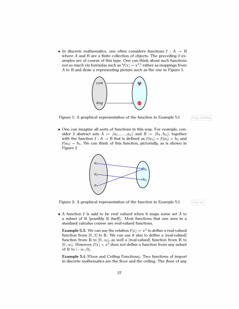
• In discrete mathematics, one often considers functions � : A → Bwhere A and B are a finite collection of objects. The preceding 2 ex-amples are of course of this type. One can think about such functionsnot so much via formulas such as “� (�) = �2,” rather as mappings fromA to B and draw a representing picture such as the one in Figure 1.

cow h

dog !

Figure 1: A graphical representation of the function in Example 5.1 fig:cowdog

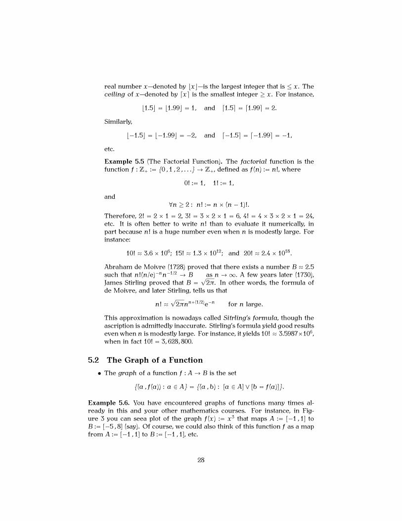
• One can imagine all sorts of functions in this way. For example, con-sider 2 abstract sets A := {�1 � � � � � �3} and B := {�1 � �2}, togetherwith the function � : A → B that is defined as � (�1) = � (�3) = �2 and� (�2) = �1� We can think of this function, pictorially, as is shown inFigure 2

�1

�1

�2

�2

�3

Figure 2: A graphical representation of the function in Example 5.1 fig:ab

• A function � is said to be real valued when it maps some set A toa subset of R [possibly R itself]. Most functions that one sees in astandard calculus course are real-valued functions.

Example 5.3. We can use the relation � (�) := �2 to define a real-valuedfunction from [0 � 1] to R. We can use it also to define a [real-valued]function from R to [0 � ∞), as well a [real-valued] function from N to[0 � ∞). However, � (�) = �2 does not define a function from any subsetof R to (−∞ � 0).

Example 5.4 (Floor and Ceiling Functions). Two functions of importin discrete mathematics are the floor and the ceiling. The floor of any

27

real number �—denoted by ���—is the largest integer that is ≤ �. Theceiling of �—denoted by ��� is the smallest integer ≥ �. For instance,

�1�5� = �1�99� = 1� and �1�5� = �1�99� = 2�

Similarly,

�−1�5� = �−1�99� = −2� and �−1�5� = �−1�99� = −1�

etc.

Example 5.5 (The Factorial Function). The factorial function is thefunction � : Z+ := {0 � 1 � 2 � � � �} → Z+, defined as � (�) := �!, where

0! := 1� 1! := 1�

and∀� ≥ 2 : �! := � × (� − 1)!�

Therefore, 2! = 2 × 1 = 2, 3! = 3 × 2 × 1 = 6, 4! = 4 × 3 × 2 × 1 = 24,etc. It is often better to write �! than to evaluate it numerically, inpart because �! is a huge number even when � is modestly large. Forinstance:

10! ≈ 3�6 × 106; 15! ≈ 1�3 × 1012; and 20! ≈ 2�4 × 1018�

Abraham de Moivre (1728) proved that there exists a number B ≈ 2�5such that �!(�/e)−��−1/2 → B as � → ∞� A few years later (1730),James Stirling proved that B =

√2π. In other words, the formula of

de Moivre, and later Stirling, tells us that

�! ≈√

2π��+(1/2)e−� for � large�

This approximation is nowadays called Sitrling’s formula, though theascription is admittedly inaccurate. Stirling’s formula yield good resultseven when � is modestly large. For instance, it yields 10! ≈ 3�5987×106,when in fact 10! = 3� 628� 800.

5.2 The Graph of a Function• The graph of a function � : A → B is the set

{(� � � (�)) : � ∈ A} = {(� � �) : [� ∈ A] ∨ [� = � (�)]}�

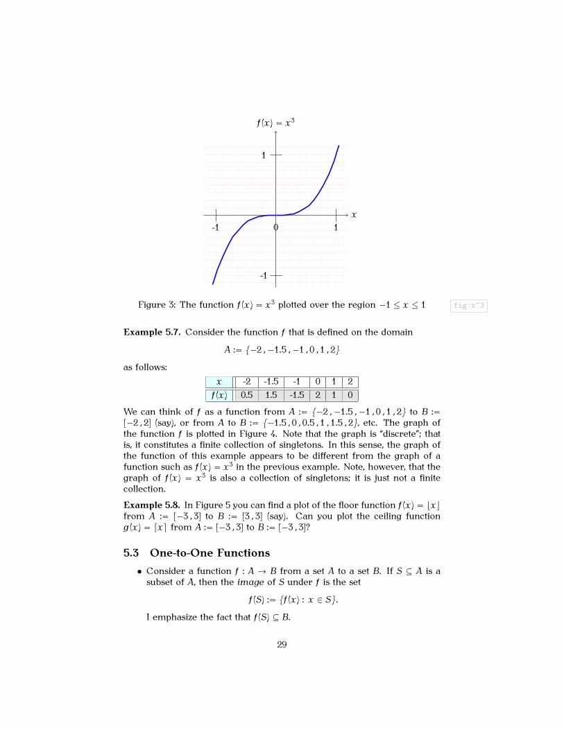
Example 5.6. You have encountered graphs of functions many times al-ready in this and your other mathematics courses. For instance, in Fig-ure 3 you can seea plot of the graph � (�) := �3 that maps A := [−1 � 1] toB := [−5 � 8] (say). Of course, we could also think of this function � as a mapfrom A := [−1 � 1] to B := [−1 � 1], etc.

28

�

� (�) = �3

1-1

-1

1

0

Figure 3: The function � (�) = �3 plotted over the region −1 ≤ � ≤ 1 fig:x^3

Example 5.7. Consider the function � that is defined on the domain

A := {−2 � −1�5 � −1 � 0 � 1 � 2}

as follows:� -2 -1.5 -1 0 1 2

� (�) 0.5 1.5 -1.5 2 1 0

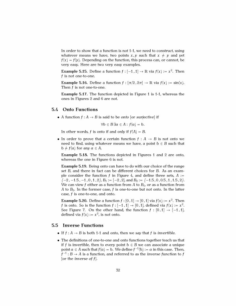
We can think of � as a function from A := {−2 � −1�5 � −1 � 0 � 1 � 2} to B :=[−2 � 2] (say), or from A to B := {−1�5 � 0 � 0�5 � 1 � 1�5 � 2}, etc. The graph ofthe function � is plotted in Figure 4. Note that the graph is “discrete”; thatis, it constitutes a finite collection of singletons. In this sense, the graph ofthe function of this example appears to be different from the graph of afunction such as � (�) = �3 in the previous example. Note, however, that thegraph of � (�) = �3 is also a collection of singletons; it is just not a finitecollection.Example 5.8. In Figure 5 you can find a plot of the floor function � (�) = ���from A := [−3 � 3] to B := [3 � 3] (say). Can you plot the ceiling function�(�) = ��� from A := [−3 � 3] to B := [−3 � 3]?

5.3 One-to-One Functions• Consider a function � : A → B from a set A to a set B. If S ⊆ A is a

subset of A, then the image of S under � is the set

� (S) := {� (�) : � ∈ S}�

I emphasize the fact that � (S) ⊆ B.

29

�

�

1 2-1-2

-1

-2

1

2

0

Figure 4: A discrete function fig:discrete:f

�

� (�) = ���

1 2 3-1-2-3

-1

-2

-3

1

2

3

0

Figure 5: The floor function fig:floor

Example 5.9. Consider the function � : {�1 � �2 � �3} → {�1 � �2 � �3},depicted in the following graphical representation:Then, � ({�2 � �3}) = {�2} and � ({�1}) = {�1}.

Example 5.10. Consider the function � : [0 � 2π] → R that is definedby � (�) := sin(�) for all � ∈ [0 � 1]. Then, � ([0 � π/2]) = � ([0 � π]) = [0 � 1],� ([π � 2π]) = [−π � 0], and � ([0 � 2π]) = [−1 � 1].

30

�1

�1

�2 �2

�3

�3

Figure 6: A function on three points. fig:ab:1

Example 5.11. If � is a real number, then there is a unique largestinteger that is to the left of �; that integer is usuall denoted by ���, andfunction � := �•� is usually called the floor, or the greatest integer,function. It is a good exercise to check that, if � denotes the floorfunction, then � [1/2 � 2] = {0 � 1 � 2}.

• Let � : A → B denote a function from a set A to a set B. We say that �is one-to-one [or 1-1, or injective] if

∀�� � ∈ A : [� (�) = � (�)] → [� = �]�

• Easy exercise: � : A → B is 1-1 if and only if

∀�� � ∈ A : [� (�) = � (�)] ↔ [� = �]�

Proposition 5.12. Consider a function � : A → B, where A ⊆ R andB ⊆ R, and suppose that � is strictly increasing; that is,

∀�� � ∈ A : [� < �] → [� (�) < � (�)]�

Then � is one-to-one.

Proof. It suffices to prove that

∀�� � ∈ A : [� �= �] → [� (�) �= � (�)]�

Suppose �� � ∈ A are not equal. Then either � < � or � < �. In thefirst case, � (�) < � (�) and in the second case, � (�) < � (�). In eithercase, we find that � (�) �= � (�).

Example 5.13. Define a function � : [0 � 1] → R via � (�) := �2. Then �is one-to-one.

Example 5.14. Define a function � : [π/2 � 3π/2] → R via � (�) := sin(�).Then � is one-to-one.

31

In order to show that a function is not 1-1, we need to construct, usingwhatever means we have, two points �� � such that � �= � and yet� (�) = � (�). Depending on the function, this process can, or cannot, bevery easy. Here are two very easy examples.Example 5.15. Define a function � : [−1 � 1] → R via � (�) := �2. Then� is not one-to-one.Example 5.16. Define a function � : [π/2 � 2π] → R via � (�) := sin(�).Then � is not one-to-one.Example 5.17. The function depicted in Figure 1 is 1-1, whereas theones in Figures 2 and 6 are not.

5.4 Onto Functions• A function � : A → B is said to be onto [or surjective] if

∀� ∈ B ∃� ∈ A : � (�) = ��

In other words, � is onto if and only if � (A) = B.

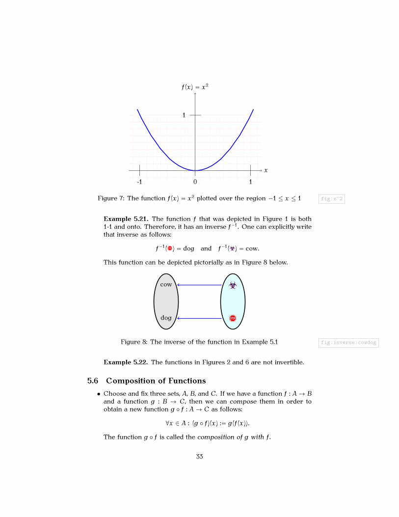
• In order to prove that a certain function � : A → B is not onto weneed to find, using whatever means we have, a point � ∈ B such that� �= � (�) for any � ∈ A.Example 5.18. The functions depicted in Figures 1 and 2 are onto,whereas the one in Figure 6 is not.Example 5.19. Being onto can have to do with our choice of the rangeset B, and there in fact can be different choices for B. As an exam-ple consider the function � in Figure 4, and define three sets, A :={−2 � −1�5 � −1 � 0 � 1 � 2}, B1 := [−2 � 2], and B2 := {−1�5 � 0 � 0�5 � 1 � 1�5 � 2}.We can view � either as a function from A to B1, or as a function fromA to B2. In the former case, � is one-to-one but not onto. In the lattercase, � is one-to-one, and onto.Example 5.20. Define a function � : [0 � 1] → [0 � 1] via � (�) := �2. Then� is onto. So is the function � : [−1 � 1] → [0 � 1], defined via � (�) := �2.See Figure 7. On the other hand, the function � : [0 � 1] → [−1 � 1],defined via � (�) := �2, is not onto.

5.5 Inverse Functions• If � : A → B is both 1-1 and onto, then we say that � is invertible.

• The definitions of one-to-one and onto functions together teach us thatif � is invertible, then to every point � ∈ B we can associate a uniquepoint � ∈ A such that � (�) = �. We define �−1(�) := � in this case. Then,�−1 : B → A is a function, and referred to as the inverse function to �[or the inverse of � ].

32

�

� (�) = �2

1-1

1

0

Figure 7: The function � (�) = �2 plotted over the region −1 ≤ � ≤ 1 fig:x^2

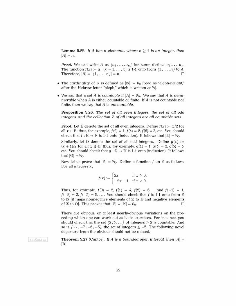
Example 5.21. The function � that was depicted in Figure 1 is both1-1 and onto. Therefore, it has an inverse �−1. One can explicitly writethat inverse as follows:

�−1(!) = dog and �−1(h) = cow�

This function can be depicted pictorially as in Figure 8 below.

cow h

dog !

Figure 8: The inverse of the function in Example 5.1 fig:inverse:cowdog

Example 5.22. The functions in Figures 2 and 6 are not invertible.

5.6 Composition of Functions• Choose and fix three sets, A, B, and C. If we have a function � : A → B

and a function � : B → C, then we can compose them in order toobtain a new function � ◦ � : A → C as follows:

∀� ∈ A : (� ◦ � )(�) := �(� (�))�

The function � ◦ � is called the composition of � with � .

33

A

�

�

B

�� = � (�)

C

� = �(�)

� ◦ �

Figure 9: The composition � ◦ � of � : B → C with � : A → B fig:compose

Figure 9 depicts graphically how the point � ∈ A gets mapped to � =� (�) ∈ B by the function � , and in turn to the point � = �(�) = �(� (�)) =(� ◦� )(�) ∈ C by the function � . We can think of the resulting mapping� ◦ � directly as a function that maps � ∈ A to � = (� ◦ � )(�) ∈ C.

Example 5.23. Suppose � (�) := �2 for every positive integer �, and�(�) := 1 + � for every positive integer �. Then, in this example,A = B = C = N, and (� ◦ � )(�) = 1 + �2 for every positive integer�. Because here we have A = B = C, we could also consider thecomposed function (� ◦ �)(�) = (1 + �)2 for every positive integer �.

• The following follows immediately from the definitions by merely re-versing the arrows in Figure 9. Can you turn this “arrow reversal”into a rigorous proof?.

Proposition 5.24. Suppose � : A → B and � : B → C are as above.Suppose, in addition, that � and � are invertible. Then, � ◦ � : A → Cis invertible and

∀� ∈ C : (� ◦ � )−1(�) = �−1 ��−1(�)

�=

��−1 ◦ �−1�

(�)�

5.7 Back to Set Theory: Cardinality• For every integer � ≥ 1, the cardinality of {1 � � � � � �} is defined as

|{1 � � � � � �}| := �.

• We say that A and B have the same cardinality if and only if thereexists a 1-1 onto function � : A → B. In this case, we write |A| = |B|.

34

Lemma 5.25. If A has � elements, where � ≥ 1 is an integer, then|A| = �.

Proof. We can write A as {�1 � � � � � ��} for some distinct �1� � � � � ��.The function � (�) := �� [� = 1� � � � � �] is 1-1 onto from {1 � � � � � �} to A.Therefore, |A| = |{1 � � � � � �}| = ��

• The cardinality of N is defined as |N| := ℵ0 [read as “aleph-naught,”after the Hebrew letter “aleph,” which is written as ℵ].

• We say that a set A is countable if |A| = ℵ0. We say that A is denu-merable when A is either countable or finite. If A is not countable norfinite, then we say that A is uncountable.

Proposition 5.26. The set of all even integers, the set of all oddintegers, and the collection Z of all integers are all countable sets.

Proof. Let E denote the set of all even integers. Define � (�) := �/2 forall � ∈ E; thus, for example, � (2) = 1, � (4) = 2, � (6) = 3, etc. You shouldcheck that � : E → N is 1-1 onto (induction). It follows that |E| = ℵ0.Similarly, let O denote the set of all odd integers. Define �(�) :=(� + 1)/2 for all � ∈ O; thus, for example, �(1) = 1, �(3) = 2, �(5) = 3,etc. You should check that � : O → N is 1-1 onto (induction). It followsthat |O| = ℵ0.Now let us prove that |Z| = ℵ0. Define a function � on Z as follows:For all integers �,

� (�) :=�

2� if � ≥ 0�−2� − 1 if � < 0�

Thus, for example, � (0) = 2, � (1) = 4, � (2) = 6� . . . and � (−1) = 1,� (−2) = 3, � (−3) = 5, . . . . You should check that � is 1-1 onto from Z

to N [it maps nonnegative elements of Z to E and negative elementsof Z to O]. This proves that |Z| = |N| = ℵ0.

There are obvious, or at least nearly-obvious, variations on the pre-ceding which one can work out as basic exercises. For instance, youshould check that the set {2 � 3 � � � �} of integers ≥ 2 is countable. Andso is {· · · � −7 � −6 � −5}, the set of integers ≤ −5. The following noveldeparture from the obvious should not be missed.

th:Cantor Theorem 5.27 (Cantor). If A is a bounded open interval, then |A| =|R|.

35

Proof. We can write A := (� � �), where � < � are real numbers. Define

� (�) := � − �� − � for � < � < ��

Because � : (� � �) → (0 � 1) is 1-1 onto, it follows that |(� � �)| = |(0 � 1)|.In particular, |(� � �)| does not depend on the numerical value of � < �;therefore, we may—and will—assume without loss of generality that� = −π/2 and � = π/2. Now consider the function

�(�) := tan(�) for −π2 < � < π

2 �

Because � : (−π/2 � π/2) → R is 1-1 onto, it follows that |(−π/2 � π/2)| =|R|, which concludes the proof.

• Suppose there exists a one-to-one function � : A → B. Then we say thatthe cardinality of B is greater than that of A, and write it as |A| ≤ |B|.The following might seem obvious, but is not when we pay close at-tention to the definitions [as we should!!].

th:SB Theorem 5.28 (Cantor, Schroder, and Bernstein). If |A| ≤ |B| and |B| ≤|A| then |A| = |B|.

The proof is elementary but a little involved. You can find all of thedetails on pp. 103–105 of the lovely book, Sets: Naıve, Axiomatic, andApplied by D. van Dalen, H. C. Doets, and H. de Swart [PergamonPress, Oxford, 1978], though this book refers to Theorem 5.28 as the“Cantor–Bernstein theorem,” as is also sometimes done. Instead ofproving Theorem 5.28, let us use it in a few examples.

Example 5.29. Let us prove that |(0 � 1)| = |(0 � 1]|. Because

(0 � 1) ⊆ (0 � 1] ⊆ R�

Theorem 5.27 shows that |(0 � 1)| ≤ |(0 � 1]| ≤ |R| = |(0 � 1)|� Now appealto Theorem 5.28 in order to conclude that |(0 � 1)| = |(0 � 1]|.

The following is another novel departure from the obvious.

th:Cantor:Q Theorem 5.30 (Cantor). Q is countable.

Proof. Because Z is countable, it suffices to find a 1-1 onto function � :Z → Q. In other words, we plan to list the elements of Q as a sequence· · · � �−3� �−2� �−1� �0� �1� �2� �3� � � � that is indexed by all integers.We start by writing all strictly-positive rationals as follows:Then we create a series of arrows as follows:

36

1/1 1/2 1/3 1/4 1/5 · · ·

2/1 2/2 2/3 2/4 2/5 · · ·

3/1 3/2 3/3 3/4 3/5 · · ·

4/1 4/2 4/3 4/4 4/5 · · ·

......

......

... . . .

Figure 10: A way to list all strictly-positive elements of Q

1/1 1/2 1/3 1/4

2/1 2/1 2/3 2/4

3/1 3/2 3/3 3/4

4/1 4/2 4/3 4/4

Figure 11: Navigation through strictly-positive elements of Q

Now we define a function � by “following the arrows,” except everytime we encounter a value that we have seen before, we suppress thevalue and proceed to the next arrow:

� (1) := 1/1 → � (2) := 1/2 → � (3) := 2/1 → � (4) := 3/1

→ � (5) := 3/2 → [3/3 suppressed] → � (6) := 2/3 → � (7) := 1/3

→ � (8) := 1/4 → [2/4 suppressed] → � (9) := 3/4 → [4/4 suppressed]→ � (10) := 4/3 → [4/2 suppressed] → � (11) := 4/1 → etc.

Also, define � (0) := 0 and � (�) := −� (−�) for all strictly-negative in-tegers �. Then � : Z → Q is 1-1 onto, whence |Z| = |Q|. Since Zis countable, the existence of such a function � proves that Q is alsocountable.

And here is an even more dramatic departure from the obvious:

th:Cantor:1 Theorem 5.31 (Cantor). R is uncountable.

37

Proof. Thanks to Theorem 5.27, Theorem 5.31 is equivalent to theassertion that (0 � 1)—or (eπ2 � π3) for that matter—is uncountable. I willprove that (0 � 1) is uncountable. Te proof hinges on a small preamblefrom classical number theory.Every number � ∈ (0 � 1) has a decimal representation,

� = 0��1�2 · · · = �110 + �2

100 + �31000 + · · · =

∞�

�=1

��10� �

where �1� �2� � � � ∈ {0 � � � � � 9} are the respective digits in the decimalexpansion of �. Note, for example, that we can write 1/2 either as 0�5 oras 0�49. That is, we can write, for � = 1/2, either �1 = 5, �2 = �3 = · · · =0, or �1 = 4, and �2 = �3 = · · · = 9. This example shows that the choiceof �1� �2� � � � is not always unique. From now on, we compute the �� ’ssuch that whenever we have a choice of an infinite decimal expansionthat ends in all 9’s from some point on or an expansion that terminatesin 0’s from some point on, then we opt for the 0’s case. In this way wecan see that the �� ’s are defined uniquely; that is, if �� � ∈ (0 � 1), then�� = �� for all � ≥ 1; and conversely, if �� = �� for all � ≥ 1 then � = �.The preceding shows that (0 � 1) is in 1-1, onto correspondence withthe collection � of all infinite sequences of the form (�1� �2� � � �) where�� ∈ {0 � · · · � 9} for all � ≥ 1� In particular, it suffices to prove that � isnot countable.Suppose, to the contrary, that � is countable. If this were so, thenwe could enumerate its elements as �1� �2� � � �; that is, � = {�1� �2� � � � },where the �� ’s are distinct and

�1 = (�1�1� �1�2� �1�3� � � �)��2 = (�2�1� �2�2� �2�3� � � �)��3 = (�3�1� �3�2� �3�3� � � �)� � � �

and ���� ∈ {0 � � � � � 9} for all �� � ≥ 1. In order to derive a contradictionwe will prove that there exists an infinite sequence � := (�1 � �2 � � � � )such that � �∈ �, and yet �� ∈ {0 � � � � � 9} for all � ≥ 1. This yieldsa contradiction since we know already that � is the collection of allsequences of the form �1� �2� � � � where �� ∈ {0 � � � � � 9}. In particular,it will follow that � cannot be enumerated.To construct the point �, we consider the “diagonal subsequence,”�1�1� �2�2� �3�3� � � � and define, for all � ≥ 1,

�� :=�

0 if ���� �= 0�1 if ���� = 0�

Then the sequence (�1 � �2 � � � �) is different from the sequence �� , forevery � ≥ 1, since �� and ���� are different. In particular, � �∈ �.

38

• The preceding argument is called “Cantor’s diagonalization argument.”

• One can learn a good deal from studying very carefully the proof ofTheorem 5.31. For instance, let us proceed as we did there, but expandevery � ∈ (0 � 1) in “base two,” rather than in “base ten.” In other words,we can associate to every � ∈ (0 � 1) a sequence �1� �2� � � � of digits in{0 � 1} such that

� = 0��1�2 · · · =∞�

�=1

��2� �

In order to make the choice of the �� ’s unique, we always opt for asequence that terminates in 0’s rather than 1’s, if that ever happens.[Think this through.] This expansion shows the existence of a 1-1 andonto function � : (0 � 1) → �, where � is the collection of all infinitesequences of 0’s and 1’s. In other words, |(0 � 1)| = |�|, and hence|�| = |R|, thanks to Theorem 5.27. Now let us consider the followingfunction � : � → �(Z+), where I recall �( · · · ) denotes the power setof whatever is in the parentheses: For every sequence (�1� �2� � � �) ∈ �of 0’s and 1’s, �(�1 � �2 � · · · ) := ∪{�}, where the union is taken over allnonnegative integers � such that �1 = 1. For instance,

�(0 � 0 � · · · ) = ?��(1 � 0 � 0 � · · · ) = {0}�

�(0 � 1 � 0 � 0 � � � � ) = {1}��(1 � 1 � 0 � 0 � 0 � � � � ) = {0 � 1}�

�(1 � 1 � 1 � · · · ) = Z+� · · · �

A little work implies that � : � → �(Z+) is 1-1 and onto, and hence|�| = |�(Z+)|, which we saw earlier is equal to |R|. We have shownmost of the proof of the following theorem [the rest can be patchedup with a little work].

Theorem 5.32. |R| = |�(Z+)|.

39