Math 141: College Calculus I

Math 141: College Calculus I

Mark Sullivan

June 29, 2018

1

Contents1 Tuesday, May 29 1

2 Wednesday, May 30 8

3 Thursday, May 31 15

4 Monday, June 3 22

5 Tuesday, June 5 24

6 Wednesday, June 6 25

7 Thursday, June 7 33

8 Monday, June 11 41











2

1 Tuesday, May 29

Calculus is the mathematical study of change.There are two fundamental questions that have driven the development of calculus.

1. The tangent line problem: Given a function f , how can one find the tangentline to f at a given x value?The field of mathematics that was developed to answer this question is called “dif-ferential calculus.”

2. The area problem: Given a function f , how can one find the area between thegraph of f and the x-axis from one given x value to another?The field of mathematics that was developed to answer this question is called “in-tegral calculus.”

In order to address these problems, we’ll need a concept known as a “limit.”

1

Chapter 2: Limits and DerivativesSection 2.2: The Limit of a Function

Definition 1.1 Let a be a real number, and suppose that f(x) is a function that is

defined near a.

(i) Given a real number L1, we say that L1 is the limit of f as x approaches a from

the left provided that the distance between f(x) and L1 can be made arbitrarily

small by selecting x-values that are close to a and less than a.

(ii) Given a real number L2, we say that L2 is the limit of f as x approaches a from

the right provided that the distance between f(x) and L2 can be made arbitrarily

small by selecting x-values that are close to a and greater than a.

Notation:(1) lim

x→a−f(x) = L1 means “L1 is the limit of f as x approaches a from the left.”

(2) limx→a+

f(x) = L2 means “L2 is the limit of f as x approaches a from the right.”

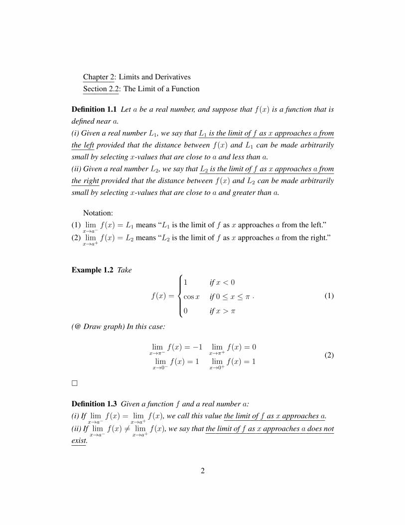
Example 1.2 Take

f(x) =

1 if x < 0

cosx if 0 ≤ x ≤ π

0 if x > π

. (1)

(@ Draw graph) In this case:

limx→π−

f(x) = −1 limx→π+

f(x) = 0

limx→0−

f(x) = 1 limx→0+

f(x) = 1(2)

�

Definition 1.3 Given a function f and a real number a:

(i) If limx→a−

f(x) = limx→a+

f(x), we call this value the limit of f as x approaches a.

(ii) If limx→a−

f(x) 6= limx→a+

f(x), we say that the limit of f as x approaches a does not

exist.

2

Notation: limx→a

f(x) = L means “L is the limit of f as x approaches a.”

In Example 1.2, limx→π

f(x) does not exist, but limx→0

f(x) = 1.

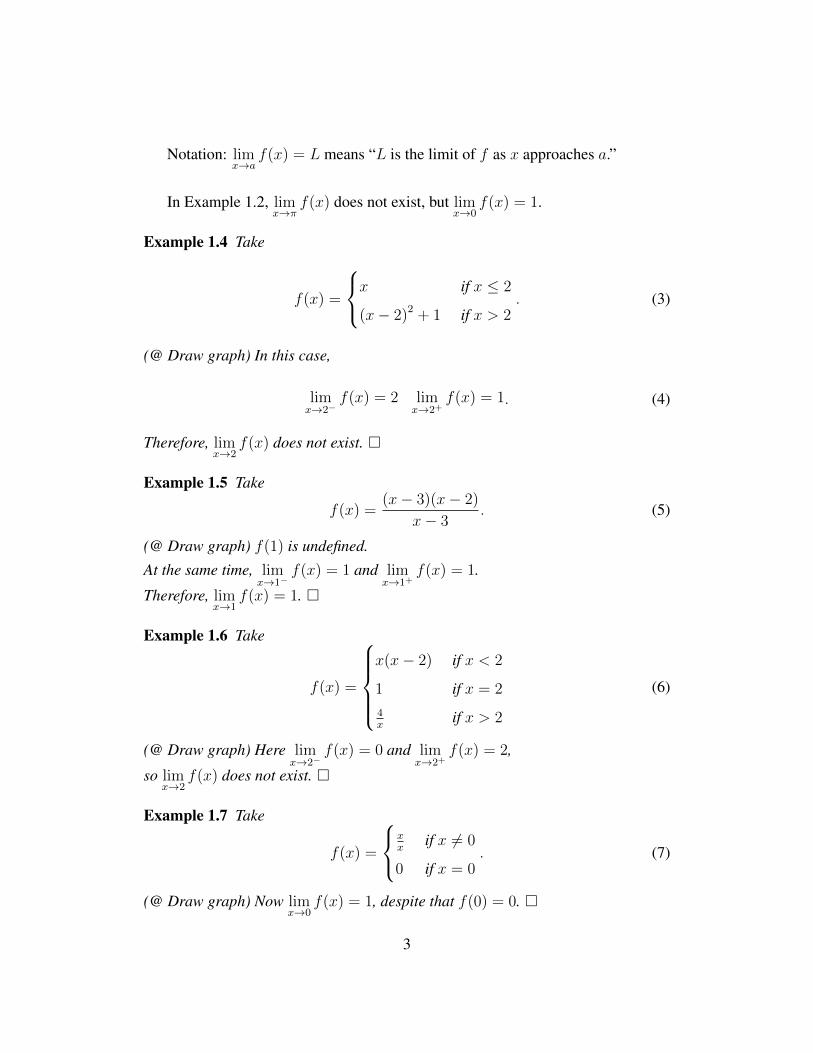
Example 1.4 Take

f(x) =

x if x ≤ 2

(x− 2)2 + 1 if x > 2. (3)

(@ Draw graph) In this case,

limx→2−

f(x) = 2 limx→2+

f(x) = 1. (4)

Therefore, limx→2

f(x) does not exist. �

Example 1.5 Take

f(x) =(x− 3)(x− 2)

x− 3. (5)

(@ Draw graph) f(1) is undefined.

At the same time, limx→1−

f(x) = 1 and limx→1+

f(x) = 1.

Therefore, limx→1

f(x) = 1. �

Example 1.6 Take

f(x) =

x(x− 2) if x < 2

1 if x = 2

4x

if x > 2

(6)

(@ Draw graph) Here limx→2−

f(x) = 0 and limx→2+

f(x) = 2,

so limx→2


Example 1.7 Take

f(x) =

xx

if x 6= 0

0 if x = 0. (7)

(@ Draw graph) Now limx→0

f(x) = 1, despite that f(0) = 0. �

3

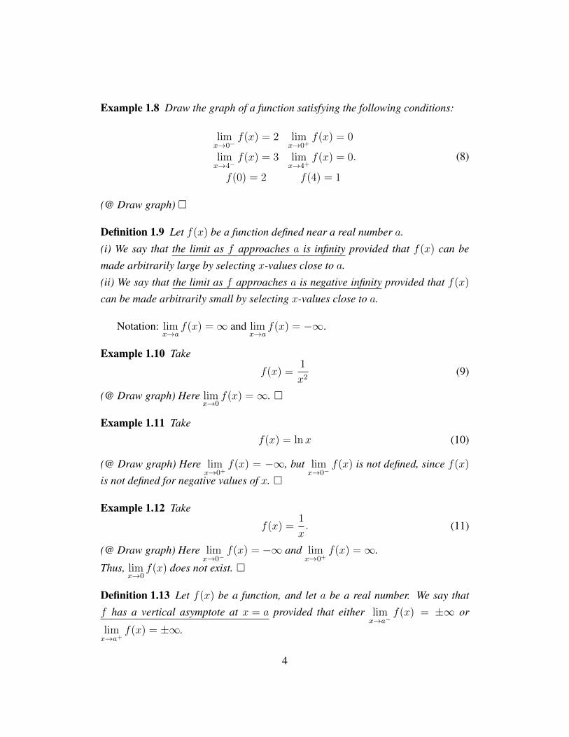
Example 1.8 Draw the graph of a function satisfying the following conditions:

limx→0−

f(x) = 2 limx→0+

f(x) = 0

limx→4−

f(x) = 3 limx→4+

f(x) = 0

f(0) = 2 f(4) = 1

. (8)

(@ Draw graph) �

Definition 1.9 Let f(x) be a function defined near a real number a.

(i) We say that the limit as f approaches a is infinity provided that f(x) can be

made arbitrarily large by selecting x-values close to a.

(ii) We say that the limit as f approaches a is negative infinity provided that f(x)

can be made arbitrarily small by selecting x-values close to a.

Notation: limx→a

f(x) =∞ and limx→a

f(x) = −∞.

Example 1.10 Take

f(x) =1

x2(9)

(@ Draw graph) Here limx→0

f(x) =∞. �

Example 1.11 Take

f(x) = lnx (10)

(@ Draw graph) Here limx→0+

f(x) = −∞, but limx→0−

f(x) is not defined, since f(x)

is not defined for negative values of x. �

Example 1.12 Take

f(x) =1

x. (11)

(@ Draw graph) Here limx→0−

f(x) = −∞ and limx→0+

f(x) =∞.

Thus, limx→0


Definition 1.13 Let f(x) be a function, and let a be a real number. We say that

f has a vertical asymptote at x = a provided that either limx→a−

f(x) = ±∞ or

limx→a+

f(x) = ±∞.

4

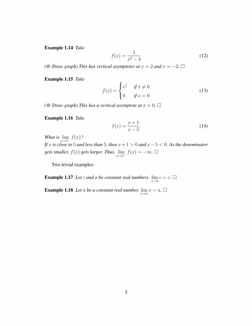
Example 1.14 Take

f(x) =1

x2 − 4(12)

(@ Draw graph) This has vertical asymptotes at x = 2 and x = −2. �

Example 1.15 Take

f(x) =

e1x if x 6= 0

0 if x = 0(13)

(@ Draw graph) This has a vertical asymptote at x = 0. �

Example 1.16 Take

f(x) =x+ 1

x− 5. (14)

What is limx→5−

f(x)?

If x is close to 5 and less than 5, then x+ 1 > 0 and x− 5 < 0. As the denominator

gets smaller, f(x) gets larger. Thus, limx→5−

f(x) = −∞. �

Two trivial examples:

Example 1.17 Let c and a be constant real numbers. limx→a

c = c. �

Example 1.18 Let a be a constant real number. limx→a

x = a. �

5

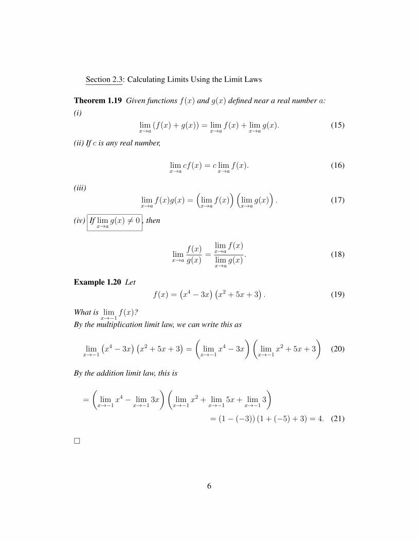
Section 2.3: Calculating Limits Using the Limit Laws

Theorem 1.19 Given functions f(x) and g(x) defined near a real number a:

(i)

limx→a

(f(x) + g(x)) = limx→a

f(x) + limx→a

g(x). (15)

(ii) If c is any real number,

limx→a

cf(x) = c limx→a

f(x). (16)

(iii)

limx→a

f(x)g(x) =(

limx→a

f(x))(

limx→a

g(x)). (17)

(iv) If limx→a

g(x) 6= 0 , then

limx→a

f(x)

g(x)=

limx→a

f(x)

limx→a

g(x). (18)

Example 1.20 Let

f(x) =(x4 − 3x

) (x2 + 5x+ 3

). (19)

What is limx→−1

f(x)?

By the multiplication limit law, we can write this as

limx→−1

(x4 − 3x

) (x2 + 5x+ 3

)=

(limx→−1

x4 − 3x

)(limx→−1

x2 + 5x+ 3

)(20)

By the addition limit law, this is

=

(limx→−1

x4 − limx→−1

3x

)(limx→−1

x2 + limx→−1

5x+ limx→−1

3

)= (1− (−3)) (1 + (−5) + 3) = 4. (21)

�

6

Example 1.21 Let

f(x) =x2 − x− 6

x− 2. (22)

What is limx→2

f(x)?

We can write this as

limx→2

(x− 2)(x+ 3)

x− 2= lim

x→2

(x− 2

x− 2(x+ 3)

)(23)

By the multiplication limit law,

=

(limx→2

x− 2

x− 2

)(limx→2

x+ 3)

= (1)(

limx→2

x+ limx→2

3)

= (1)(2 + 3) = 5. (24)

�

Example 1.22 Let

f(h) =(2 + h)3 − 8

h. (25)

What is limh→0

f(h)?

limh→0

f(h) = limh→0

(2 + h) (4 + 4h+ h2)− 8

h

= limh→0

8 + 8h+ 2h2 + 4h+ 4h2 + h3 − 8

h

= limh→0

12h+ 6h2 + h3

h

= limh→0

12 + 6h+ h2

= limh→0

12 + 6 limh→0

h+ limh→0

h2 = 12. (26)

�

7

2 Wednesday, May 30

What about f(x) = x cos(1x

)? How could one find lim

x→0f(x)?

Theorem 2.1 (Squeeze theorem) Let f(x), g(x) and h(x) be functions defined near

a real number a. Suppose that for every x-value, f(x) ≤ g(x) ≤ h(x). If L is a

real number such that limx→a

f(x) = L = limx→a

h(x), then limx→a

g(x) = L as well.

Example 2.2 Let

g(x) = x cos

(1

x

). (27)

What is limx→0

g(x)? We know that for all nonzero x-values, −1 ≤ cos(1x

)≤ 1.

Therefore,

−|x| ≤ x cos

(1

x

)≤ |x|. (28)

In other words, −|x| ≤ g(x) ≤ |x|. We know that

limx→0−|x| = 0 and lim

x→0|x| = 0. (29)

Thus, by the squeeze theorem, limx→0

g(x) = 0. �

Example 2.3 Let

g(x) = x2esin(πx ). (30)

What is limx→0

g(x)?

We know that for any nonzero x-value, −1 ≤ sin(πx

)≤ 1. Therefore,

e−1 ≤ esin(πx ) ≤ e1. (31)

Thus,

x2e−1 ≤ x2esin(πx ) ≤ x2e, (32)

or in other words, x2e−1 ≤ g(x) ≤ x2e. We know that

limx→0

x2e−1 = 0 and limx→0

x2e = 0. (33)

Thus, by the squeeze theorem, limx→0

g(x) = 0.

8

Section 2.5: Continuity

Example 2.4 Let

f(x) = x2 + x− 1. (34)

What is limx→1

f(x)? By the limit laws,

limx→1

f(x) = limx→1

x2 + x− 1 = limx→1

x2 + limx→1

x− limx→1

1 = 1 + 1− 1 = 1. (35)

�

Notice in Example 2.4 that limx→1

f(x) = f(1). In fact, for any real number a,limx→a

f(x) = f(a) for this function. This is not true in general, so functions thatsatisfy this property are given a special name.

Definition 2.5 Let f(x) be a function defined near a real number a. We say that f

is continuous at a provided that the following conditions are true:

(i) f(a) exists.

(ii) limx→a

f(x) exists.

(iii) f(a) = limx→a

f(x).

If f is not continuous at a, we say that f is discontinuous at a. If f is continuous at

every real number in its domain, then we say that f is a continuous function.

Example 2.6 Let

f(x) =

|x| if x < 1

0 if 1 ≤ x < 2

1 if x = 2

(x− 2)2 if 2 < x < 3

0 if x = 3

x− 4 if x > 3

. (36)

(@ Draw graph) f is discontinuous at 1, 2, and 3. f is continuous everywhere else.

�

Which functions are continuous?

9

Theorem 2.7 The following functions are continuous at each point in their domain.

(i) Every polynomial (functions like f(x) = cnxn+cn−1x

n−1+...+c2x2+c1x+c0).

(ii) Every rational function (functions like f(x) = p(x)q(x)

, where p and q are polyno-

mials).

(iii) Every root (functions like f(x) = n√x, where n is an integer).

(iv) Every trigonometric function (sin, cos, tan, sec, csc, cot).

(v) Every arc-trigonometric function (sin−1, cos−1, tan−1, etc.).

(vi) Every exponential function (functions like f(x) = ax for some a > 1).

(vii) Every logarithm (functions like f(x) = loga(x) for some a > 1).

Theorem 2.8 If f(x) and g(x) are continuous, then:

(i) f(x) + g(x) is continuous.

(ii) f(x)g(x) is continuous.

(iii) f(g(x)) is continuous on its domain.

(iv) f(x)g(x)

is continuous on its domain.

Example 2.9 All of the following functions are continuous on their domains:

f1(x) = lnx1x+x2 sinx

f2(x) = sin2x+ 3 sinx+ 2

f3(x) = sin−1x+ e1x

f4(x) =√x2 + sin (lnx)

. (37)

�

It’s easy to come up with continuous functions, but it’s also easy to come up withfunctions that are not continuous. Moreover, sometimes it’s hard to tell whether afunction is continuous or not.

Example 2.10 Let

f(x) =

sinx if x < π4

cosx if x ≥ π4

. (38)

Is f continuous?

First of all, if a > π4, then lim

x→af(x) = lim

x→asinx = sin a, since sinx is continuous.

10

Similarly, If a < π4, then lim

x→af(x) = lim

x→acosx = cos a, since cosx is continuous.

It remains to determine whether f is continuous at a = π4. We note that

limx→π

4−f(x) = lim

x→π4−

sinx = sin(π

4

)=

1√2. (39)

At the same time,

limx→π

4+f(x) = lim

x→π4+

cosx = cos(π

4

)=

1√2. (40)

Therefore, limx→π

4

f(x) = 1√2. Additionally,

f(π

4

)= cos

(π4

)=

1√2

= limx→π

4

f(x). (41)

Therefore, f is continuous at π4, and so f is a continuous function. 1�

In what ways can the concept of continuity help us? Limits can be “passedthrough” continuous functions:

Theorem 2.11 If f and g are continuous, then

limx→a

f (g (x)) = f(

limx→a

g(x)). (42)

Example 2.12 Let

f(x) = ln(√

1 + x2). (43)

What is limx→0

f(x)?

Since lnx is continuous on its domain,

limx→0

f(x) = limx→0

ln(√

1 + x2)

= ln(

limx→0

√1 + x2

). (44)

Since√x is continuous on its domain,

= ln

(√limx→0

(1 + x2)

)= ln

√1 = 0. (45)

11

�

Example 2.13 Let

f(θ) = sin (θ + sin θ) . (46)

What is limθ→π

f(θ)?

limθ→π

f (θ) = limθ→π

sin (θ + sin θ) . (47)

Since sinx is continuous,

= sin(

limθ→π

(θ + sin θ))

= sin(

limθ→π

θ + limθ→π

sin θ)

= sin (π + sin (π)) = sin (π + 0) = sinπ = 0. (48)

�

Example 2.14 Let

f(t) =

√t2 + 9− 3

t2. (49)

What is limt→0

f(t)?

We multiply the numerator and denominator by the “conjugate,”√t2 + 9 + 3:

limt→0

f(t) = limt→0

√t2 + 9− 3

t2

(√t2 + 9 + 3√t2 + 9 + 3

)

= limt→0

t2 + 9− 9

t2(√

t2 + 9 + 3) = lim

t→0

t2

t2(√

t2 + 9 + 3)

= limt→0

1√t2 + 9 + 3

=limt→0

1

limt→0

√t2 + 9 + lim

t→03

(50)

Now, since√x is continuous, lim

t→3

√t2 + 9 =

√limt→0

(t2 + 9), so

=1√

limt→0

(t2 + 9) + limt→0

3=

1√9 + 3

=1

6. (51)

�

12

Section 2.6: Limits at Infinity and Horizontal Asymptotes

Definition 2.15 Let f be a function defined on the real line.

(i) Given a real number L1, we say that L1 is the limit of f as x approaches infinity

provided that the distance between f(x) and L1 can be made arbitrarily small by

selecting x-values that are sufficiently large.

(ii) Given a real number L2, we say that L2 is the limit of f as x approaches nega-

tive infinity provided that the distance between f(x) and L2 can be made arbitrarily

small by selecting x-values that are sufficiently small.

Reminder: “very small” means “very negative.”

Notation: limx→∞

f(x) = L1, and limx→−∞

f(x) = L2.

Example 2.16 Let

f(x) = tan−1x (52)

(@ Draw graph) Here limx→∞

f(x) = π2

and limx→−∞

f(x) = −π2. �

Example 2.17 Let

f(x) = ex (53)

(@ Draw graph) Here limx→−∞

f(x) = 0. �

Example 2.18 Let

f(x) = e−x2

(54)

(@ Draw graph) Here limx→−∞

f(x) = 0 = limx→∞

f(x).

Definition 2.19 Let f be a function defined on the real line. Given a real number

L, we say that f has a horizontal asymptote at y = L provided that limx→∞

f(x) = L

or limx→−∞

f(x) = L.

Example 2.20 Suppose

f(x) =1

xr, (55)

13

where r > 0. What is limx→∞

f(x)?

Case 1: r is a positive integer. In that case,

f(x) =1

xr=

(1

x

)r=

(1

x

)(1

x

)...

(1

x

)︸︷︷︸

r factors

. (56)

Therefore, by the properties of limits,

limx→∞

f(x) = limx→∞

(

1

x

)(1

x

)...

(1

x

)︸︷︷︸

r factors

=

(limx→∞

1

x

)(limx→∞

1

x

)...

(limx→∞

1

x

)︸︷︷︸

r factors

= (0) (0) ... (0)︸︷︷︸r factors

= 0. (57)

What if r is not an integer?

Case 2: r may not be an integer, but r is rational.

Suppose r = mn

, where m and n are positive integers. In that case,

limx→∞

1

xr= lim

x→∞

1

xmn

= limx→∞

1n√xm

= limx→∞

n

√1

xm=

n

√limx→∞

1

xm=

n√

0 = 0. (58)

Case 3: r is irrational.

Select two rational numbers, p and q, such that 0 < p < r < q. For x > 1, this

implies that xp < xr < xq. Therefore,

1

xq<

1

xr<

1

xp. (59)

By Case 2, limx→∞

1xq

= 0 and limx→∞

1xq

= 0. Thus, we have that limx→∞

1xr

= 0, by the

squeeze theorem.

14

3 Thursday, May 31

The fact that limx→∞

1xr

= 0 for r > 0 will be greatly useful to us!

Example 3.1 Let

f(x) =4x3 + 6x2 − 2

2x3 − 4x+ 5. (60)

What are the horizontal asymptotes of f?

Divide the numerator and denominator by the highest power of x that appears in

the denominator:

f(x) =4 + 6

x− 2

x3

2− 4x2

+ 5x3

for x 6= 0. (61)

By the example, we know that limx→∞

1x

= limx→∞

1x2

= limx→∞

1x3

= 0. Therefore,

limx→∞

f(x) =4 + 0− 0

2− 0 + 0= 2. (62)

Similarly,

limx→−∞

f(x) =4 + 0− 0

2− 0 + 0= 2. (63)

Thus, f has a horizontal asymptote at y = 2, on both right and left. �

Example 3.2 Let

f(x) =

√1 + 4x6

2− x3. (64)


Divide by the highest power of x that appears in the denominator:

f(x) =

√1x6

+ 4

2x3− 1

for x 6= 0. (65)

We know that limx→∞

1x3

= limx→∞

= 0, so

limx→∞

f(x) =

√0 + 4

0− 1= −2. (66)

15

Similarly,

limx→−∞

f(x) =

√0 + 4

0− 1= −2. (67)

Thus, f has a horizontal asymptote at y = 2, on both right and left. �

Definition 3.3 Let f be a function defined on the real numbers.

(i) We say that the limit of f as x approaches infinity is infinity provided that f(x)

can be made arbitrarily large by selecting x-values that are sufficiently large.

(ii) We say that the limit of f as x approaches negative infinity is infinity provided

that f(x) can be made arbitrarily large by selecting x-values that are sufficiently

small.

Notation: limx→∞

f(x) =∞, limx→−∞

f(x) =∞.

Example 3.4 For any of the following functions, limx→∞

f(x) =∞.

f(x) = x

f(x) = x2 − 9

f(x) = 2x

f(x) =√x

f(x) = lnx

. (68)

�

CAUTION:∞ is not a real number. Therefore, it does not make sense to add,subtract, multiply or divide things with∞.

Example 3.5 Let

f(x) =√

4x2 + 3x+ 2x. (69)


First of all, by taking x sufficiently large, f(x) can be made arbitrarily large. Thus,

limx→∞

f(x) =∞, and so there is no asymptote on the right.

16

It remains to find limx→−∞

f(x). In order to do this, we’ll multiply this by the conjugate

divided by itself:

(√4x2 + 3x+ 2x

)(√4x2 + 3x− 2x√4x2 + 3x− 2x

)=

3x√4x2 + 3x− 2x

(70)

Now, as before, we’ll divide by the highest power of x appearing in the denominator.

We see x2, but since it is under a square root, x1 will suffice:

limx→−∞

3

−√

4 + 3x− 2

=3

−√

4 + 0− 2= −3

4. (71)

Difficult question: where did that negative sign in the denominator come from? There-

fore, f has a horizontal asymptote at y = −34

on the left. �

17

Section 2.7: Derivatives and Rates of Change, andSection 2.8: The Derivative as a Function

Now that we have a concept of limit we can solve the tangent line problem, atleast theoretically.

Definition 3.6 Let f be a function defined on the real line. A secant line of f is a

line that contains two distinct points on the graph of f .

Given a function f and any distinct real numbers a and b on the x-axis, we candraw the secant line to f that contains the points (a, f (a)) and (b, f (b)).(@ Draw graph)The slope of such a line would be

m =f(b)− f(a)

b− a. (72)

However, as a and b become close, the secant line begins to approximate a tangentline. Using limits, we can now find the slope of the tangent line.

Definition 3.7 Let f be a function defined around a real number a. The derivative

of f at a is the slope of the tangent line to f at a:

limx→a

f(x)− f(a)

x− a. (73)

Example 3.8 Let

f(x) = x2. (74)

What is derivative of f at x = 4?

Directly from the definition:

limx→4

f(x)− f(4)

x− 4= lim

x→4

x2 − 42

x− 4= lim

x→4

x2 − 16

x− 4= 8. (75)

�

Notation: f ′(a), Df(a), f(a) all mean “the derivative of f at a.”

18

Example 3.9 Let

f(x) =1

x. (76)

What is f ′(2)?

f ′(2) = limx→2

f(x)− f(2)

x− 2= lim

x→2

1x− 1

2

x− 2= lim

x→2

2−x2x

x− 2

= limx→2

2− x2x(x− 2)

= limx→2

−1

2x= −1

4. (77)

�

There is another way of evaluating the derivative. If we define h = x− a, thenthe definition becomes

f ′(a) = limx→a

f(x)− f(a)

x− a= lim

h→0

f(a+ h)− f(a)

h. (78)

Example 3.10 Let

f(x) = x3 − 3x+ 1. (79)

What is f ′(1)?

f ′(1) = limh→0

f(1 + h)− f(1)

h

= limh→0

((1 + h)3 − 3 (1 + h) + 1

)− (13 − 3 (1) + 1)

h

= limh→0

(1 + 3h+ 3h2 + h3 − 3− 3h+ 1)− (−1)

h

= limh→0

(h3 + 3h2 − 1) + 1

h= lim

h→0

h3 + 3h2

h

= limh→0

h (h2 + 3h)

h= lim

h→0h2 + 3h = 0. (80)

�

We can do even better than this. In each of the previous examples, we found thederivative f ′(a) at only one particular value of a. We can, in fact, find the derivative

19

at every value of a at once.

Example 3.11 Let

f(x) = x2 + 10. (81)

Find f ′(a) at every real value of a.

Directly from the definition,

f ′(a) = limx→a

f(x)− f(a)

x− a= lim

x→a

(x2 + 10)− (a2 + 10)

x− a

= limx→a

x2 − a2

x− a= lim

x→a

(x− a)(x+ a)

x− a= lim

x→ax+ a = a+ a = 2a. (82)

Now, whatever a is, we know that f ′(a) = 2a. �

Definition 3.12 Let f be a function defined around a real number a. The derivative

function of f is the function whose value at each x is the derivative of f at x. In

other words,

f ′(x) = limh→0

f(x+ h)− f(x)

h. (83)

Notation: f ′, f , ddxf , df

dxall mean “the derivative function of f .”

Example 3.13 Let

f(x) =√x+ 1. (84)

Find dfdx

.

20

df

dx= lim

h→0

f(x+ h)− f(x)

h= lim

h→0

√(x+ h) + 1−

√x+ 1

h

= limh→0

√x+ h+ 1−

√x+ 1

h

(√x+ h+ 1 +

√x+ 1√

x+ h+ 1 +√x+ 1

)= lim

h→0

x+ h+ 1− (x+ 1)

h(√

x+ h+ 1 +√x+ 1

)= lim

h→0

h

h(√

x+ h+ 1 +√x+ 1

)= lim

h→0

1√x+ h+ 1 +

√x+ 1

=1√

x+ 1 +√x+ 1

=1

2√x+ 1

. (85)

�

Is it possible for the derivative to fail to exist at a point?

Definition 3.14 Let f be a function defined around a real number a. We say that f

is differentiable at a provided that f ′(a) is a real number. If f is differentiable at

every x-value in its domain, then we say that f is a differentiable function.

21

4 Monday, June 3

Theorem 4.1 Let f be a function defined around a real number a. If f is differen-

tiable at a, then f must be continuous at a.

In other words, if f is not continuous at a, then f cannot be differentiable at a.Is there any other way a function could fail to be differentiable?

Example 4.2 Let

f(x) = |x|. (86)

Determine whether f is differentiable at x = 0.

We note that

f(x) =

−x if x < 0

x if x ≥ 0. (87)

Therefore,

limx→0+

f(x)− f(0)

x− 0= lim

x→0+

x− 0

x− 0= lim

x→0+1 = 1. (88)

However,

limx→0−

f(x)− f(0)

x− 0= lim

x→0−

−x− 0

x− 0= lim

x→0−−1 = −1. (89)

Thus, f ′(0) does not exist; f is not differentiable at x = 0. �

Reasons that a function f may fail to be differentiable at x = a:(i) f is not continuous at a. For example,

f(x) =

x2 if x < 0

1− x if x ≥ 0. (90)

(@ Draw graph)(ii) f has a corner at a. For example, f(x) = |x|. (@ Draw graph)(iii) f has a cusp at a. For example, f(x) = | cosx|. (@ Draw graph)(iv) f is not defined on both sides of a. For example, f(x) =

√1− x2 (@ Draw

graph)

22

(v) f has a vertical tangent line at a. For example, f(x) = 3√x. (@ Draw graph)

In general, when one says “find the derivative of f” without specifying a point,this means to find the derivative function of f at all of the points where it is defined.

Example 4.3 Let

f(x) = x32 . (91)

Find the derivative of f .

We note that f is not defined for x < 0, since f(x) =√x3.

f ′(x) = limh→0

f(x+ h)− f(x)

h= lim

h→0

(x+ h)32 − x 3

2

h

= limh→0

√(x+ h)3 −

√x3

h

√

(x+ h)3 +√x3√

(x+ h)3 +√x3

= lim

h→0

(x+ h)3 − x3

h

(√(x+ h)3 +

√x3) = lim

h→0

x3 + 3x2h+ 3xh2 + h3 − x3

h

(√(x+ h)3 +

√x3)

= limh→0

h (3x2 + 3xh+ h2)

h

(√(x+ h)3 +

√x3) = lim

h→0

3x2 + 3xh+ h2√(x+ h)3 +

√x3

=3x2 + 0 + 0√

(x+ 0)3 +√x3

=3x2

2x32

=3

2

√x for x 6= 0. (92)

Thus, f ′(x) is not defined at x = 0. �

23

5 Tuesday, June 5

(Test 1 was given on this day.)

24

6 Wednesday, June 6

Chapter 3: Differentiation RulesSection 3.1: Derivatives of Polynomials and Exponential Functions

The derivative is one of the most important theoretical accomplishments ofmathematics. However, computing the derivative has been difficult so far. In thischapter, we’ll work on some theorems that will assist us in finding the derivativesof a large variety of functions.

If f and g are two functions defined around a point a, then we can consider thederivative of f + g at a:

(f + g)′(a) = limx→a

(f(x) + g(x))− (f(a) + g(a))

x− a

= limx→a

(f(x)− f(a)) + (g(x)− g(a))

x− a= lim

x→a

(f(x)− f(a)

x− a+g(x)− g(a)

x− a

)= lim

x→a

f(x)− f(a)

x− a+ lim

x→a

g(x)− g(a)

x− a= f ′(a) + g′(a). (93)

Therefore, the derivative of a sum of functions is the sum of the derivatives:

Theorem 6.1 Given functions f and g defined on the real line,

d

dx(f + g) =

df

dx+

dg

dx. (94)

If f is defined around a point a, and c is a constant, then similarly, we canconsider the derivative of cf at a:

(cf)′(a) = limx→a

cf(x)− cf(a)

x− a= lim

x→a

c (f(x)− f(a))

x− a

= limx→a

cf(x)− f(a)

x− a= c lim

x→a

f(x)− f(a)

x− a= cf ′(a). (95)

Therefore, a constant can just be “pulled out” of a derivative:

25

Theorem 6.2 Given a function f defined on the real line and a constant c,

d

dx(cf) = c

df

dx. (96)

Now let’s look at some specific types of functions.

1. Constant functions : suppose f(x) = c for some real number c. In that case,

f ′(x) = limh→0

f(x+ h)− f(x)

h= lim

h→0

c− ch

= limh→0

0 = 0. (97)

Thus,

Theorem 6.3 Given any constant c,

d

dxc = 0. (98)

2. Powers of x

Theorem 6.4 (Power rule) Given any nonzero real number,

d

dxxr = rxr−1. (99)

Example 6.5 Let

f(x) = 3x53 − x3 + 1. (100)

Find f ′(x).

We need not resort to the definition of the derivative here. Due to the theorems

we’ve discussed,

f ′(x) =d

dx

(3x

53 − x3 + 1

)=

d

dx

(3x

53

)+

d

dx

(−x3

)+

d

dx(1)

= 3d

dx

(x

53

)− d

dx

(x3)

+d

dx(1)

= 3

(5

3x

23

)−(3x2)

+ 0

= 5x23 − 3x2. (101)

26

�

Example 6.6 Let

H(u) = (3u− 1) (u+ 2) . (102)

Find H ′(u).

H ′(u) =d

du

(3u2 + 5u− 2

)= 6u+ 5. (103)

�

Example 6.7 Let

G(t) =√

5t+

√7

t. (104)

Find G′(t).

G′(t) =d

dt

(√

5t+

√7

t

)=

d

dt

(√5t)

+d

dt

(√7

t

)=√

5d

dt

√t+√

7d

dt

1

t=√

5d

dtt12 +√

7d

dtt−1

=√

5

(1

2t−

12

)+√

7(−t−2

)=

1

2

√5

t−√

7

t2. (105)

�

Example 6.8 Let

y =

√x+ x

x2. (106)

Find dydx

.

dy

dx=

d

dx

(√x+ x

x2

)=

d

dx

(x

12 + x1

x2

)=

d

dx

(x−

32 + x−1

)= −3

2x−

52 − x−2 = − 3

2x52

− 1

x2. (107)

What is e?

27

Definition 6.9 Euler’s number is the real number e such that

limh→0

eh − 1

h= 1. (108)

3. The natural exponential function : suppose f(x) = ex. Let’s observe that

f ′(x) = limh→0

ex+h − ex

h= lim

h→0

ex(eh − 1

)h

= ex limh→0

eh − 1

h= ex(1) = ex. (109)

Therefore,

Theorem 6.10d

dxex = ex. (110)

This seemingly useless fact will become important soon.

28

Section 3.3: Derivatives of Trigonometric Functions, andSection 3.2: The Product and Quotient Rules

Theorem 6.11limx→0

sin θθ

= 1 and limx→0

cos θ−1θ

= 0. (111)

These are interesting by themselves, but more importantly:Suppose f(x) = sinx. In that case,

f ′(x) = limh→0

sin (x+ h)− sinx

h= lim

h→0

(sinx cosh+ cosx sinh)− sinx

h

= limh→0

sinx (cosh− 1) + cos x sinh

h

= limh→0

(sinx

cosh− 1

h+ cosx

sinh

h

)= sinx(0) + cos x(1) = cos x. (112)

Using similar methods, one can show that

d

dxcosx = − sinx. (113)

How could we find the derivatives of the other trigonometric functions?

tanx = sinxcosx

secx = 1cosx

cscx = 1sinx

cotx = cosxsinx

. (114)

In order to find these, we a rule for the derivative of a quotient of two functions.

Suppose that f and g are functions defined around x = a. Let’s look at the

29

derivative of fg at a:

(fg)′ (a) = limx→a

f(x)g(x)− f(a)g(a)

x− a

= limx→a

f(x)g(x)− f(x)g(a) + f(x)g(a)− f(a)g(a)

x− a

= limx→a

f(x) (g(x)− g(a)) + g(a) (f(x)− f(a))

x− a

= limx→a

(f(x) (g(x)− g(a))

x− a+g(a) (f(x)− f(a))

x− a

)= lim

x→af(x)

g(x)− g(a)

x− a+ lim

x→ag(a)

f(x)− f(a)

x− a

= f(a) limx→a

g(x)− g(a)

x− a+ g(a) lim

x→a

f(x)− f(a)

x− a= f(a)g′(a) + g(a)f ′(a). (115)

Therefore,

Theorem 6.12 (Product rule) If f and g are functions defined on the real line, then

d

dx(fg) = f

dg

dx+ g

df

dx= fg′ + gf ′. (116)

Example 6.13 Let

h(x) =(x+ 2

√x)ex. (117)

Find h′(x).

h′(x) =d

dx

(x+ 2x

12

)ex =

(x+ 2x

12

) d

dxex + ex

d

dx

(x+ 2x

12

)=(x+ 2x

12

)ex + ex

(1 + x−

12

)=(x+ 2x

12 + 1 + x−

12

)ex. (118)

�

Example 6.14 Let

f(x) = 3√x sinx. (119)

30

Find f ′(x).

f ′(x) =d

dx3√x sinx = x

13

d

dxsinx+ sinx

d

dxx

13

= x13 (cosx) + sin x

(1

3x−

23

). (120)

�

Next, what about fg?

Theorem 6.15 (Quotient rule) If f and g are functions defined on the real line and

g 6= 0, thend

dx

(f

g

)=g dfdx− f dg

dx

g2=gf ′ − fg′

g2. (121)

Example 6.16 Let

G(x) =x2 − 2

2x+ 1. (122)

Find G′(x).

G′(x) =d

dx

x2 − 2

2x+ 1=

(2x+ 1) ddx

(x2 − 2)− (x2 − 2) ddx

(2x+ 1)

(2x+ 1)2

=(2x+ 1) (2x)− (x2 − 2) (2)

(2x+ 1)2

=4x2 + 2x− 2x2 + 4

(2x+ 1)2=

2x2 + 2x+ 4

(2x+ 1)2. (123)

�

Example 6.17 Let

y =ex

1− ex. (124)

31

Find dydx

.

dy

dx=

d

dx

ex

1− ex=

(1− ex) ddxex − ex d

dx(1− ex)

(1− ex)2

=(1− ex) ex − ex (−ex)

(1− ex)2

=ex − e2x + e2x

(1− ex)2=

ex

(1− ex)2. (125)

�

4. Trigonometric functions :

d

dxtanx =

d

dx

sinx

cosx=

(cosx) ddx

sinx− (sinx) ddx

cosx

cos2x

=cos2x+ sin2x

cos2x=

1

cos2x= sec2x. (126)

Using similar methods, one can prove the other parts of the following theorem.

Theorem 6.18

ddx

sinx = cosx ddx

cosx = − sinxddx

tanx = sec2x ddx

cotx = −csc2xddx

secx = secx tanx ddx

cscx = − cscx cotx

. (127)

Example 6.19 Let

g (θ) = eθ (tan θ − θ) . (128)

Find g′ (θ).

g′ (θ) = eθd

dθ(tan θ − θ) + (tan θ − θ) d

dθeθ

= eθ(sec2θ − 1

)+ (tan θ − θ) eθ = eθtan2θ + eθ tan θ − eθθ

= eθ(tan2θ + tan θ − θ

). (129)

�

32

7 Thursday, June 7

Section 3.4: The Chain Rule

We already have theorems regarding functions being put together by addition,multiplication and division. There is one other important way to put functions to-gether.

Definition 7.1 Let f and g be functions defined on the real line. The composite

function f ◦ g is the function f (g (x)).

Example 7.2 (i) If f(x) = x2 and g(x) = x+ 1, then

f (g (x)) = (x+ 1)2

g (f (x)) = x2 + 1. (130)

(ii) If f(x) =√x and g(x) = 4x+ 1, then

f (g (x)) =√

4x+ 1

g (f (x)) = 4√x+ 1

. (131)

(iii) If f(x) = 11+x

and g(x) = tan−1x, then

f (g (x)) = 11+tan−1x

g (f (x)) = tan−1(

11+x

). (132)

�

Theorem 7.3 (Chain rule) Let f and g be functions defined on the real line. Define

h = f ◦ g. Given a real value x, if g is differentiable at x and f is differentiable at

g(x), then

h′(x) = f ′ (g (x)) g′ (x) . (133)

Example 7.4 Let

h(x) = sin√x. (134)

33

Find h′(x).

Let f(x) = sin x and g(x) =√x. We note that f ′(x) = cos x and g′(x) = 1

2√x.

Therefore, by the chain rule,

h′(x) = f ′ (g (x)) g′ (x) = cos(√

x) 1

2√x

=cos√x

2√x. (135)

�

Example 7.5 Let

h(x) =1

x3 + 2x2 + 3x+ 1. (136)

Find h′(x).

Let f(x) = 1x

and g(x) = x3 + 2x2 + 3x + 1. We know that f ′(x) = − 1x2

and

g′(x) = 3x2 + 4x+ 3. Therefore, by the chain rule,

h′(x) = f ′ (g (x)) g′ (x) =−1

(x3 + 2x2 + 3x+ 1)2(3x2 + 4x+ 3

)=

3x2 + 4x+ 3

(x3 + 2x2 + 3x+ 1)2(137)

�

Example 7.6 Let

f(x) = sin (cotx) . (138)

Find f ′(x).

By the chain rule,

f ′(x) = cos (cotx)(−csc2x

). (139)

�

Example 7.7 Let

y =√

2− ex. (140)

Find dydx

.

We note that

y = (2− ex)12 . (141)

34

Thus, by the chain rule,

dy

dx=

1

2(2− ex)−

12 (−ex) =

−ex

2√

2− ex. (142)

�

Example 7.8 Let

F (x) =(1 + x+ x2

)99. (143)

Find F ′(x).

F ′(x) = 99(1 + x+ x2

)98(1 + 2x) . (144)

�

Example 7.9 Let

g (θ) = cos2θ. (145)

Find g′ (θ).

We note that g (θ) = (cos θ)2, so

g′ (θ) = 2 (cos θ) (sin θ) = sin (2θ) . (146)

�

Example 7.10 Let

g(x) = ex2−x. (147)

Find g′(x).

g′(x) = ex2−x (2x− 1) . (148)

�

5. Exponential functions Let a > 0, and suppose that f(x) = ax. In that case,

f(x) =(eln a)x

= e(ln a)x. (149)

35

Therefore, by the chain rule,

f ′(x) = e(ln a)xd

dx((ln a)x) = e(ln a)x ln a = ax ln a. (150)

Theorem 7.11 If a > 0, then

d

dxax = ax ln a. (151)

Example 7.12 Let

f(t) = 2(t3). (152)

Find f ′(t).

f ′(t) =(

2(t3) ln 2) d

dtt3 = 2(t3) ln 2

(3t2)

= 3 (ln 2) 2(t3)t2. (153)

�

Example 7.13 Let

s(t) =

√1 + sin t

1 + cos t. (154)

Find s′(t).

We note that s(t) =(1+sin t1+cos t

) 12 , so

s′(t) =1

2

(1 + sin t

1 + cos t

)− 12 d

dt

(1 + sin t

1 + cos t

)=

1

2

(1 + sin t

1 + cos t

)− 12(

(1 + cos t) (cos t)− (1 + sin t) (− sin t)

(1 + cos t)2

)=

1

2

(1 + sin t

1 + cos t

)− 12

(cos t+ cos2t+ sin t+ sin2t

)(1 + cos t)2

=cos t+ sin t

2(1 + cos t)2

√1 + cos t

1 + sin t. (155)

�

36

Example 7.14 Let

y = xe−x2

. (156)

Find an equation of the tangent line to the curve at the point (0, 0).

We know that the tangent line will have the equation y = mx + b for some real

values m and b.

dy

dx=

d

dx

(xe−x

2)

= xd

dxe−x

2

+ e−x2 d

dxx

= x

(e−x

2 d

dx

(−x2

))+ e−x

2

(1) = xe−x2

(−2x) + e−x2

=(1− 2x2

)e−x

2

. (157)

Here m = y′(0) =(1− 2(0)2

)e−(0)

2

= 1. Therefore, the tangent line has the

equation y = x + b for some value of b. Since the tangent line contains the point

(0, 0), we have that 0 = 0+ b, and so b = 0. Thus, the tangent line has the equation

y = x. �

Example 7.15 At what point on the curve y =√

1 + 2x is the tangent line perpen-

dicular to the line 6x+ 2y = 1?

First, we find dydx

:

dy

dx=

d

dx(1 + 2x)

12 =

1

2(1 + 2x)−

12

d

dx(1 + 2x)

=1

2(1 + 2x)−

12 (2) =

1√1 + 2x

. (158)

Next, we note that the line in question is y = −3x + 12. Therefore, we must solve

the equation y′ = 13:

1√1 + 2x

=1

3, (159)

and so x = 4. This implies that y =√

1 + 2(4) = 3, and so the point we seek is

(4, 3). �

Example 7.16 Let

y =

√x+

√x+√x. (160)

37

Find dydx

.

First, we write

y =

(x+

(x+ x

12

) 12

) 12

. (161)

Using the chain rule,

dy

dx=

d

dx

(x+

(x+ x

12

) 12

) 12

=1

2

(x+

(x+ x

12

) 12

)− 12 d

dx

(x+

(x+ x

12

) 12

)=

1

2

(x+

(x+ x

12

) 12

)− 12(

1 +d

dx

(x+ x

12

) 12

)=

1

2

(x+

(x+ x

12

) 12

)− 12(

1 +1

2

(x+ x

12

)− 12 d

dx

(x+ x

12

))1

2

(x+

(x+ x

12

) 12

)− 12(

1 +1

2

(x+ x

12

)− 12

(1 +

1

2x−

12

))

=1 +

1+ 12√x

2√x+√x

2√x+

√x+√x. (162)

�

Example 7.17 Let

f(z) = ezz−1 . (163)

Find f ′(z).

f ′(z) =d

dze

zz−1 = e

zz−1

d

dz

z

z − 1= e

zz−1

(z − 1) ddz

(z)− (z) ddz

(z − 1)

(z − 1)2

= ezz−1

(z − 1) (1)− (z) (1)

(z − 1)2=−e

zz−1

(z − 1)2. (164)

�

38

Example 7.18 Let

y = esin 2x + sin(e2x). (165)

Find dydx

.

dy

dx=

d

dx

(esin 2x + sin

(e2x))

=d

dxesin 2x +

d

dxsin(e2x)

= esin 2x d

dxsin 2x+ cos

(e2x) d

dxe2x

= esin 2x cos (2x)d

dx(2x) + cos

(e2x)e2x

d

dx(2x)

= 2esin(2x) cos (2x) + 2e2x cos(e2x). (166)

�

Example 7.19 Let

y =1

(1 + tanx)2. (167)

Find dydx

.

We can write

y = (1 + tanx)−2. (168)

Thus,

dy

dx= −2(1 + tanx)−3

d

dx(1 + tan x)

= −2(1 + tan x)−3(sec2x

)=−2sec2x

(1 + tan x)3. (169)

�

Example 7.20 Let

y = 2

(3(4

x)). (170)

39

Find dydx

.

dy

dx=

d

dx2

(3(4

x))

= 2

(3(4

x))

(ln 2)

(d

dx3(4x)

)= 2

(3(4

x))

(ln 2)

(3(4x) (ln 3)

(d

dx4x))

= 2

(3(4

x))

(ln 2)(3(4x) (ln 3) (4x (ln 4))

)= (ln 2) (ln 3) (ln 4) 4x3(4x)2

(3(4

x)). (171)

�

Example 7.21 Let

F (t) =t2√t3 + 1

. (172)

Find F ′(t).

F ′(t) =d

dt

t2√t3 + 1

=(t3 + 1)

12 ddtt2 − t2 d

dt(t3 + 1)

12

t3 + 1

=(t3 + 1)

12 (2t)− t2

(12(t3 + 1)

− 12 ddt

(t3 + 1))

t3 + 1

=2t√t3 + 1− t2

(1

2√t3+1

(3t2))

t3 + 1=

2t√t3 + 1− 3t4√

t3+1

t3 + 1

=2t (t3 + 1)− 3t4

(t3 + 1)32

=t (2− t3)(t3 + 1)

32

. (173)

40

8 Monday, June 11

Section 3.5: Implicit DifferentiationSome curves are defined by equations that are not functions. In these cases, we

need to use a technique called “implicit differentiation:” taking the derivative ofboth sides of the equation.

Example 8.1 Find the slope of the tangent line to the circle x2 + y2 = 25 at the

point (4, 3).

We note that the slope of the tangent line to the curve is dydx

. We differentiate implic-

itly:ddx

(x2 + y2) = ddx

(25)ddxx2 + d

dxy2 = d

dx25

2x+ 2y dydx

= 0.

(174)

We now solve for dydx

:dy

dx= −x

y. (175)

Thus, the slope of the tangent line at (4, 3) is −43. �

Example 8.2 Find the slope of the tangent line to the ellipse defined by the equation

x2 + 2xy + 4y2 = 12, (176)

at the point (2, 1).

We seek dydx

. Differentiating implicitly,

ddx

(x2 + 2xy + 4y2) = ddx

(12)ddx

(x2) + ddx

(2xy) + ddx

(4y2) = 0

2x+ 2(x ddxy + y d

dxx)

+ 8y dydx

= 0

2x+ 2xdydx

+ 2y + 8y dydx

= 0.

(177)

41

Solving for dydx

:(2x+ 2y) + (2x+ 8y) dy

dx= 0

(2x+ 8y) dydx

= − (2x+ 2y)dydx

= −2x+2y2x+8y

= − x+yx+4y

.

(178)

Therefore, the slope of the tangent line to the ellipse at (2, 1) is

− (2) + (1)

(2) + 4(1)= −3

6= −1

2. (179)

�

Example 8.3 Given the curve

x3 − xy2 + y3 = 1, (180)

find dydx

.

Differentiating implicitly,

ddx

(x3 − xy2 + y3) = ddx

(1)ddx

(x3)− ddx

(xy2) + ddx

(y3) = 0

3x2 −(x ddxy2 + y2 d

dxx)

+ 3y2 dydx

= 0

3x2 − 2xy dydx

+ y2 + 3y2 dydx

= 0

(181)

We now solve for dydx

:

3x2 + y2 + (3y2 − 2xy) dydx

= 0dydx

= 3x2+y2

2xy−3y2 .(182)

�


xey = x− y, (183)

find dydx

.

42


ddx

(xey) = ddx

(x− y)

x ddxey + ey d

dxx = d

dxx− d

dxy

xey dydx

+ ey = 1− dydx

. (184)

Solving for dydx

:xey dy

dx+ dy

dx= 1− ey

(xey + 1) dydx

= 1− eydydx

= 1−eyxey+1

. (185)

�


cos (xy) = 1 + sin y, (186)

find dydx

.


ddx

(cos (xy)) = ddx

(1 + sin y)

− sin (xy) ddx

(xy) = ddx

1 + ddx

sin y

− sin (xy)(xdydx

+ y)

= cos y dydx

. (187)

Solving for dydx

:−x sin (xy) dy

dx− y sin (xy) = cos y dy

dx

−y sin (xy) = cos y dydx

+ x sin (xy) dydx

−y sin (xy) = (cos y + x sin (xy)) dydx

−y sin(xy)cos y+x sin(xy)

= dydx.

(188)

�

6. Arc trigonometric functionsSine and cosine take angles and give us a coordinate of a point on the unit circle.Arcsine and arccosine take a coordinate of a point on the unit circle and give us an

43

angle, within some particular range.

The following are always true:

sin(sin−1x

)= x cos

(cos−1x

)= x. (189)

However, the following are not always true:

sin−1 (sin θ) = θ cos−1 (cos θ) = θ. (190)

This is because the range of sin−1 is[−π

2, π2

], and the range of cos−1 is [0, π].

Example 8.6

sin−1(

sin

(3π

2

))= sin−1 (−1) = −π

26= 3π

2. (191)

cos−1(

cos

(3π

2

))= cos−1 (0) =

π

26= 3π

2. (192)

�

What happens if we differentiate x = sin(sin−1x

)implicitly?

ddx

(x) = ddx

(sin(sin−1x

))1 = cos

(sin−1x

)ddx

sin−1x. (193)

However, cos(sin−1x

)=√

1− x2. (?!) (@ Draw triangle)Therefore,

d

dxsin−1x =

1√1− x2

. (194)

Using similar methods, one can prove the rest of the following theorem.

Theorem 8.7ddx

sin−1x = 1√1−x2

ddx

cos−1x = −1√1−x2

ddx

sec−1x = 1x√x2−1

ddx

csc−1x = −1x√x2−1

ddx

tan−1x = 1x2+1

ddx

cot−1x = −1x2+1

. (195)

44

Example 8.8 Let

R(t) = sin−1(

1

t

). (196)

Find R′(t).

R′(t) =1√

1−(1t

)2 d

dt

1

t=

1√1−

(1t

)2 (−t−2) =−1

t2√

1− 1t2

. (197)

�

45

Section 3.6: Derivatives of Logarithmic Functions

7. The natural logarithm The function log |x| is an extension of the functionlog x, in the sense that it is defined for all real nonzero x.We know that eln |x| = |x|. What if we differentiate this implicitly?

ddxeln |x| = d

dx|x|

ddxeln |x| =

1 if x > 0

−1 if x < 0

eln |x| ddx

ln |x| =

1 if x > 0

−1 if x < 0

|x| ddx

ln |x| =

1 if x > 0

−1 if x < 0

ddx

ln |x| =

1|x| if x > 0

1−|x| if x < 0

ddx

ln |x| = 1x.

(198)

Theorem 8.9d

dxln |x| = 1

x. (199)

Example 8.10 Let

f(x) = ln(sin2x

). (200)

Find f ′(x).

f ′(x) =1

sin2x

d

dxsin2x =

1

sin2x2 sinx

d

dxsinx

=1

sin2x(2 sinx) (cosx) = 2 cotx. (201)

�

Logarithms have some useful properties for simplifying expressions.

46

Theorem 8.11 (i) Given positive real numbers a and b,

ln a+ ln b = ln (ab) . (202)

(ii) Given a positive real number a and a real number r,

ln (ar) = r ln a. (203)

From this theorem, you can also see that

ln a− ln b = ln a+ ln(b−1)

= ln a+ ln

(1

b

)= ln

(ab

). (204)

By taking the logarithm of both sides of an equation, one can make some deriva-tives easier.

Example 8.12 Let

y =e−xcos2x

x2 + x+ 1. (205)

Find dydx

.

We could use the quotient rule, but it would be annoying. What if we take the

logarithm of both sides first?

ln y = ln

(e−xcos2x

x2 + x+ 1

)= ln

(e−xcos2x

)− ln

(x2 + x+ 1

)= ln

(e−x)

+ ln(cos2x

)− ln

(x2 + x+ 1

)= −x+ 2 ln (cos x)− ln

(x2 + x+ 1

). (206)


1

y

dy

dx=

d

dx

(−x+ 2 ln (cos x)− ln

(x2 + x+ 1

))= −1 + 2

1

cosx(sinx)− 1

x2 + x+ 1(2x+ 1)

= −1 + 2 tanx− 2x+ 1

x2 + x+ 1. (207)

47

Therefore,

dy

dx= y

(−1 + 2 tanx− 2x+ 1

x2 + x+ 1

)=

e−xcos2x

x2 + x+ 1

(−1 + 2 tanx− 2x+ 1

x2 + x+ 1

). (208)

�

What about f(x) = xx?

8. Variable bases raised to variable powers : in order to take the derivative off(x)g(x), use logarithmic differentiation.

Example 8.13 Let

f(x) = xx. (209)

Find f ′(x).

Define y = f(x). We use logarithmic differentiation:

ln y = ln (xx) = x lnx. (210)

Now,

1

y

dy

dx= (x)

d

dx(lnx) + (ln x)

d

dx(x) = (x)

(1

x

)+ lnx = 1 + lnx. (211)

Thus,

f ′(x) =dy

dx= y (1 + ln x) = xx (1 + ln x) . (212)

�

Example 8.14 Let

y = (sinx)lnx. (213)

Find dydx

.

48

Using logarithmic differentiation:

ln y = ln(

(sinx)lnx)

= (lnx) (ln (sinx)) . (214)


1

y

dy

dx= (lnx)

d

dx(ln (sinx)) + (ln (sinx))

d

dx(lnx)

= (lnx)1

sinx

d

dx(sinx) + (ln (sinx))

1

x

= (lnx)1

sinx(cosx) +

ln (sinx)

x

= (lnx) cotx+ln (sinx)

x. (215)

Thus,

dy

dx= y

((lnx) cotx+

ln (sinx)

x

)= (sinx)lnx

((lnx) cotx+

ln (sinx)

x

). (216)

�


xy = yx, (217)

find dydx

.

We take the logarithm of both sides:

y lnx = x ln y. (218)


(y) ddx

(lnx) + (ln x) ddxy = (x) d

dx(ln y) + (ln y) d

dx(x)

y(1x

)+ (lnx) dy

dx= x 1

ydydx

+ ln yyx

+ (lnx) dydx

= xydydx

+ ln y

. (219)

49

Solving for dydx

:(lnx) dy

dx− x

ydydx

= ln y − yx(

lnx− xy

)dydx

= ln y − yx

dydx

=ln y− y

x

lnx−xy

= x ln y−yy lnx−x

. (220)

�


y =√xex

2−x(x+ 1)23 , (221)

find dydx

.

Taking the logarithm,

ln y = ln(√

xex2−x(x+ 1)

23

)= ln

√x+ ln

(ex

2−x)

+ ln(

(x+ 1)23

)=

1

2lnx+

(x2 − x

)+

2

3ln (x+ 1) . (222)

differentiating implicitly,

1

y

dy

dx=

1

2x+ 2x− 1 +

2

3 (x+ 1). (223)

Solving for dydx

:

dy

dx=√xex

2−x(x+ 1)23

(1

2x+ 2x− 1 +

2

3 (x+ 1)

). (224)

�

50

9 Tuesday, June 12

(The test review was given on this day)

51

10 Wednesday, June 13

(Test 2 was given on this day)

52

11 Thursday, June 14

Chapter 4: Applications of DerivativesSection 4.2: The Mean Value Theorem

Question: What sorts of functions have derivatives that are constantly zero?

Theorem 11.1 (Rolle’s theorem) Let f be a differentiable function. Given real

values a and b such that a < b, if f(a) = f(b), then there exists a real value c such

that a < c < b and f ′(c) = 0.

Example 11.2 Consider the function f(x) = −x2+x. (@ Draw graph.) We notice

that f(0) = f(1). Therefore, by Rolle’s theorem, there exists a real value c such

that 0 < c < 1 and f ′(c) = 0. �

Let f be a differentiable function. Suppose that a and b are real values such thata < b. Consider the new function

g(x) = f(x)− f(b)− f(a)

b− a(x− a) . (225)

We have thatg′(x) = f ′(x)− f(b)− f(a)

b− a. (226)

Notice thatg(a) = f(a)− f(b)−f(a)

b−a (0) = f(a)

g(b) = f(b)− f(b)−f(a)b−a (b− a) = f(a)

. (227)

Now g(a) = g(b), so Rolle’s theorem applies; there must exist some c such thata < c < b and g′(c) = 0. But this would mean that

f ′(c)− f(b)− f(a)

b− a= 0. (228)

Thus, we have the following theorem.

53

Theorem 11.3 Let f be a differentiable function. Given real values a and b such

that a < b, there exists a real value c such that a < c < b and

f ′(c) =f(b)− f(a)

b− a. (229)

Example 11.4 Suppose that f is a differentiable function and f ′(x) = 0 for all real

x-values. What sort of function is f?

Suppose a and b are two different real values. Suppose a < b. By the mean value

theorem, there must exist a real value c such that a < c < b and f ′(c) = f(b)−f(a)b−a .

However, f ′ is constantly zero, so f ′(c) = 0. This means that 0 = f(b)−f(a)b−a . Multi-

plying both sides by b− a, this gives us that 0 = f(b)− f(a), and so f(a) = f(b).

Thus, all the values of f are the same; f is a constant function. �

54

Section 3.7: Rates of Change in the Natural and Social Sciences

Question: given a function y = f(x), how sensitive is y to changes in x?Or: by how much does y depend on x?

A few interpretations:1. How quickly does the position of an object change as time goes on?2. By how much does a company’s profit change if the price of a unit changes?3. By how much does a substance’s melting point change as the pressure decreases?4. How quickly does the fish population of a body of water decline as the pollutionlevel of the water increases?5. By how much do a building’s maintenance costs change as the outside tempera-ture changes?

As we’ve shown, the mean value theorem implies that only constant functionscan have derivatives that are constantly zero. Thus, the derivative expresses the rate

of change of y as x varies.

Definition 11.5 (i) If y = f(t), where y is the position of a particle with respect to

a chosen reference point (measured in meters) and t is the time since a particular

moment (measured in seconds), then v(t) = dydt

is the velocity of the particle, mea-

sured in meters per second. The speed of the particle is the absolute value of the

velocity of the particle.

(ii) If M = f(t), where M is the concentration of a chemical (measured in atoms

per cubic centimeter) and t is the time since a chemical reaction began (measured

in seconds), then dMdt

is the rate of reaction of the chemical reaction, measured in

atoms per cubic centimeter per second.

(iii) If P = f(t), where P is the number of organisms born in a closed environment,

and t is the time since a particular moment (measured in days), then dPdt

is the birth

rate of the population, measured in individuals per day.

(iv) If C = f(x), where C is the cost of creating x units of a particular product

(measured in dollars), then dCdx

is the marginal cost of the product, measured in

dollars per unit.

55

Example 11.6 If a rock is thrown upward on a certain planet with a velocity of 10

m/s, then its height, t seconds after being thrown, can be described by the function

y(t) = 10t− 2t2. (230)

(a) Find the velocity of the rock after 1 second.

(b) When will the rock hit the surface?

(c) What will be the rock’s velocity as it hits the surface?

(a) We know that

v(t) =dy

dt= 10− 4t. (231)

Therefore, v(1) = 10− 4 = 6 m/s.

(b) We set y(t) = 0:

0 = 10t− 2t2 = t (10− 2t) . (232)

This has two solutions: t = 0 s and t = 5 s. Since the rock was thrown at t = 0, we

must have that the rock hits the surface at t = 5.

(c) We know that v(t) = 10 − 4t, and the rock will hit the surface at t = 5 s.

Therefore, the velocity of the rock as it hits the surface will be v(5) = −10 m/s. �

Question: How quickly is an object’s velocity changing?

Definition 11.7 Let f be a differentiable function defined on the real line.

(i) The first derivative of f is the derivative of f .

(ii) The second derivative of f is the derivative of the first derivative.

(iii) The nth derivative of f is the derivative of the (n− 1)th derivative of f .

Notation:(i) First derivative: f ′, or df

dx.

(ii) Second derivative: f ′′, or d2fdx2

.(iii) Third derivative: f ′′′, or d3f

dx3.

(iv) nth derivative: f (n), or dnfdxn

.

56

Definition 11.8 Let y = f(t) describe the position of an object (measured in me-

ters) as a function of time (measured in seconds). The acceleration of the object

is the second derivative a(t) = d2ydt2

= y′′(t) of the position function, measured in

(meters per second) per second.

57

12 Monday, June 18

Example 12.1 Suppose a particle moves along the x-axis with a position function

x(t) = t3 − 8t2 + 24, (233)

where t is measured in seconds and x is measured in feet. The particle’s motion

begins at t = 0.

(i) Find the velocity of the particle.

v(t) =dx

dt= 3t2 − 16t. (234)

(ii) Find the velocity of the particle after 1 second.

v(1) = 3(1)2 − 16(1) = −7 m/s (235)

(iii) When is the particle motionless?

We must solve equation v(t) = 0:

0 = v(t) = 3t2 − 16t = (3t− 16) t. (236)

The particle is motionless at t = 0 s and at t = 163

s.

(iv) When is the particle moving in the positive direction?

We must solve the inequality v(t) > 0:

v(t) = (3t− 16) t > 0 (237)

This occurs when: (3t − 16 > 0 and t > 0), and when (3t − 16 < 0 and t < 0).

We are not concerned with the latter situation, since the particle begins moving at

t = 0. Thus, the particle is moving in the positive direction when t > 163

s.

(v) Find the acceleration of the particle.

a(t) = x′′(t) = v′(t) = 6t− 16. (238)

58

(vi) Find the acceleration of the particle after 1 second.

a(1) = 6(1)− 16 = −10 m/s/s (239)

(vii) Graph the position, velocity and acceleration for 0 ≤ t ≤ 6.

(@ Draw graphs)

(iix) When is the particle speeding up?

The particle is speeding up in the positive direction when both v and a are

positive. We know that v(t) > 0 when t > 166

. Thus, we need to know when

a(t) > 0:

a(t) = 6t− 16 > 0. (240)

This occurs when t > 166

= 83

s. Therefore, the particle is speeding up in the positive

direction when both t > 163

s and t > 83

s, or in other words, when t > 163

s.

The particle is speeding up in the negative direction when both v and a are

negative. Therefore, we must solve the following system of inequalities:

v(t) = 3t2 − 16t < 0

a(t) = 6t− 16 < 0. (241)

The first inequality holds when t < 163

s. The second holds when t < 166

= 83

s.

Thus, the particle is speeding up in the negative direction when both t < 163

s and

t < 83

s, or in other words, when t < 83

s.

(ix) When is the particle slowing down?

This can only occur when the particle is not speeding up. Thus, this can only occur

when t ≥ 83

s and t ≤ 163

s. At t = 83

s, a(t) = 0, so the particle is neither speeding

nor slowing at t = 83

s. At t = 163

s, a(t) 6= 0, so the particle must be either speeding

up or slowing down. Since it is not speeding up at t = 163

s, it must be slowing down

at t = 163

s. Thus, the particle is slowing down in the time interval 83< t ≤ 16

3. �

Question: Does an object have to stop in order to change its direction of motion?

Theorem 12.2 (Intermediate value theorem) Let f be a continuous function defined

on the real line. Given real values a and b and a real value k, if f(a) ≤ k ≤ f(b)

59

or f(b) ≤ k ≤ f(a), then there exists a real value c between a and b such that

f(c) = k.

Applied mathematicians usually assume that every function they deal with iscontinuous and differentiable.

Example 12.3 A flying device is launched on earth. Its height as a function of time

is

y(t) = t5 + t2 − 3t (242)

Is there any time during its flight at which it is neither rising nor falling?

We want to know whether v(t) = 0 has any solutions. First, we note that

v(t) = y′(t) = 5t4 + 2t− 3. (243)

We notice that v(0) = −3 and v(1) = 4. Therefore, since v(0) ≤ 0 ≤ v(1), the

intermediate value theorem indicates that there exists a value t between 0 and 1

such that v(t) = 0. The answer, therefore, is yes.

60

Section 4.1: Maximum and Minimum Values

Definition 12.4 Let f be a function, and let c be a real value in the domain of f .

(i) We say that f(c) is an absolute or global maximum value of f provided that for

all x-values in the domain of f , f(x) ≤ f(c).

(ii) We say that f(c) is an absolute or global minimum value of f provided that for

all x-values in the domain of f , f(x) ≥ f(c).

Definition 12.5 Let f be a function, and let c be a real value in the domain of f .

(i) We say that f(c) is a relative or local maximum value of f provided that for

every x-value in an open interval containing c , f(x) ≤ f(c).

(ii) We say that f(c) is a relative or local minimum value of f provided that for

every x-value in an open interval containing c, f(x) ≥ f(c).

Example 12.6 (@ Draw a graph, label its interesting points, and ad lib which ones

are local and global extrema) �

Question: How can one find the local and absolute extreme values of a function?

Theorem 12.7 (Extreme value theorem) Let f be a continuous function defined on

the real line. On any closed interval [a, b], f has at least one absolute maximum

value and at least one absolute minimum value.

Example 12.8 Consider f(x) = x3. (@ Draw graph.) We know that there exists

no absolute maximum or minimum value of f over the entire real line. However,

the extreme value theorem indicates that there must be both an absolute maximum

and an absolute minimum of f over the closed interval [0, 1]. �

Example 12.9 Consider f(x) = 1− x. (@ Draw graph.) On the interval (0, 1], f

has an absolute minimum value of 0, but no absolute maximum value. (The extreme

value theorem does not apply, because (0, 1] is not a closed interval.) �

Theorem 12.10 (Fermat’s theorem on local extrema) Let f be a function defined

on the real line. Given a real value c, if f has a local maximum or local minimum

at c, then either f is not differentiable at c or f ′(c) = 0.

61

Is the converse to Fermat’s theorem true? No.

Example 12.11 Consider f(x) = x3. We know that f ′(x) = 3x2, and so f ′(0) = 0.

However, the point (0, 0) is neither a local maximum nor a local minimum of f . �

Definition 12.12 Let f be a function defined on the real line. Given a real value

c in the domain of f , we say that c is a critical number of f provided that either

f ′(c) = 0 or f ′(c) does not exist.

Theorem 12.13 Let f be a function defined on the real line. If c is a real value

such that f(c) is an absolute extreme value of f over a closed interval [a, b], then

either c is a critical number of f , or c = a or c = b.

Example 12.14 Let

f(x) = x3 − 6x2 + 5. (244)

Find the absolute maximum and absolute minimum values of f on the closed inter-

val [−3, 5].

We must find the critical numbers of f .

f ′(x) = 3x2 − 12x = 3x (x− 4) . (245)

This has critical numbers at x = 0 and x = 4. Now we know that the absolute

maximum must occur at x = −3, x = 0, x = 4 or x = 5. We inspect the y-values

at each of these:f (−3) = (−3)3 − 6(−3)2 + 5 = −74

f (0) = (0)3 − 6(0)2 + 5 = 5

f (4) = (4)3 − 6(4)2 + 5 = −27

f (5) = (5)3 − 6(5)2 + 5 = −20

. (246)

Thus, the absolute maximum value of f is 5 and the absolute minimum value of f

is −74. �

Example 12.15 Let

f(t) = t+ cot

(t

2

). (247)

62

Find the critical numbers of f on[π4, 7π

4

].

First, we must find the critical numbers of f .

f ′(t) = 1− 1

2csc2

(t

2

). (248)

We seek values of t for which f ′(t) is either zero or undefined.

In seeking values for t such that f ′(t) = 0:

0 = 1− 12csc2

(t2

)csc2

(t2

)= 2

1

sin( t2)= csc

(t2

)= ±√

2

sin(t2

)= ± 1√

2

. (249)

This has solutions when t2

= nπ4, where n is an odd integer. Thus, t = nπ

2. Since

we are only considering values for t such that π4≤ t ≤ 7π

4, this gives us critical

numbers at t = π2

and t = 3π2

.

In seeking values for t such that f ′(t) is undefined, we need to know when

csc(t2

)is undefined. This occurs when sin

(t2

)= 0, or in other words, t

2= mπ,

where m is any integer. Thus, we seek values t = 2mπ, where m is an integer, in

the interval[π4, 7π

4

]. No such values exist, so the only critical numbers are t = π

2

and t = 3π2

. �

63

Section 4.3: How Derivatives Affect the Shape of a Graph

If f ′(x) > 0 on some interval, then f is increasing on that interval. If f ′(x) < 0

on some interval, then f is decreasing on that interval.

At a local maximum, a function transitions from increasing to decreasing.At a local minimum, a function transitions from decreasing to increasing.

64

13 Tuesday, June 19

Example 13.1 Let

f(x) = 2x3 − 9x2 + 12x− 3. (250)

(i) Find the intervals on which f is increasing and decreasing.

We need to find where f ′(x) > 0. In order to do this, we’ll first find the critical

numbers of f .

f ′(x) = 6x2 − 18x+ 12 = 6(x2 − 3x+ 2

)= 6 (x− 1) (x− 2) . (251)

This yields the critical numbers x = 1 and x = 2. (@ Draw number line)

For x < 1, f ′(x) > 0.

For 1 < x < 2, f ′(x) < 0.

For x > 2, f ′(x) > 0.

Therefore, f is increasing on the intervals (−∞, 1) and (2,∞). Also, f is decreas-

ing on the interval (1, 2).

(ii) Find the local maximum points of f .

Local maxima occur at the critical numbers where f changes from increasing

to decreasing: the point (1, 2).

(iii) Find the local minimum points of f .

Local minima occur at the critical numbers where f changes from decreasing

to increasing: the point (2, 1).

Issue: there are multiple different ways in which a graph could increase. Thesign of the first derivative cannot distinguish them. (@ Draw graphs)

Definition 13.2 Let f be a function that is differentiable on an interval I .

(i) We say that f is concave up on I provided that the slope of the tangent line is

increasing on I .

(ii) We say that f is concave down provided that the slope of the tangent line is

decreasing on I .

A function is concave up if it curves upward. (@ Draw graph) This occurs whenthe second derivative is positive.

65

A function is concave down if it curves downward. (@ Draw graph) This occurswhen the second derivative is negative.

Definition 13.3 Let f be a function that is differentiable on an interval I . Given

a point (x, y) on the graph of f , we say that (x, y) is an inflection point of f pro-

vided that f is continuous at x and f changes from concave upward to concave

downward, or from concave downward to concave upward, at (x, y).

Example 13.4 Let

f(x) =x2 − 4

x2 + 4(252)

(i) Find the vertical and horizontal asymptotes.

(ii) Find the intervals on which f is increasing and decreasing.

(iii) find the local maxima and local minima.

(iv) Find the intervals of concavity, and inflection points.

(v) Sketch a graph of f .

(i) We note that x2+1 6= 0, so f has no vertical asymptotes. As for the horizontal

asymptotes:

limx→∞

f(x) = limx→∞

x2 − 4

x2 + 4= lim

x→∞

1− 4x2

1 + 4x2

=1− 0

1 + 0= 1. (253)

Thus, f has a horizontal asymptote at y = 1 on the right. As f is an even function,

the same is true on the left.

(ii) We first find the critical numbers of f .

f ′(x) =d

dx

x2 − 4

x2 + 4=

(x2 + 4) (2x)− (x2 − 4) (2x)

(x2 + 4)2

=2x3 + 8x− 2x3 + 8x

(x2 + 4)2=

16x

(x2 + 4)2. (254)

This is never undefined. However, f ′(x) = 0 at x = 0. Therefore, x = 0 is a critical

number.

(@ Draw number line.)

For x < 0, f ′(x) < 0, so f is decreasing on (−∞, 0).

66

For x > 0, f ′(x) > 0, so f is increasing on (0,∞).

(iii) f has a local minimum at x = 0, since it changes from decreasing to

increasing. Thus, (0,−1) is the only local minimum of f , and f has no local maxi-

mum.

(iv) We first need the second derivative of f :

f ′′(x) =d

dx

16x

(x2 + 4)2=

(x2 + 4)2

(16)− (16x) 2 (x2 + 4) (2x)

(x2 + 4)4

=(x2 + 4) (16)− (16x) (2) (2x)

(x2 + 4)3=

16x2 + 64− 64x2

(x2 + 4)3

=64− 48x2

(x2 + 4)3=

16 (4− 3x2)

(x2 + 4)3. (255)

This gives that f ′′(x) = 0 when x = ± 2√3.

(@ Draw number line.)

For x < − 2√3, f ′′(x) < 0, so f is concave down on the interval

(−∞,− 2√

3

).

For − 2√3< x < 2√

3, f ′′(x) > 0, so f is concave up on the interval

(− 2√

3, 2√

3

).

For x > 2√3, f ′′(x) < 0, so f is concave down on the interval

(2√3,∞)

.

We deduce that the points(− 2√

3,−1

2

)and

(2√3,−1

2

)are inflection points of f .

(v) We note that the graph of f has x-intercepts at (−2, 0) and (2, 0). (@ Draw

graph.) �

Example 13.5 Sketch the graph of a function that satisfies all of the given condi-

tions.

f ′(0) = 0 f ′(4) = 0

f ′(x) = 1 on (−∞,−1)

f ′(x) > 0 on (0, 2) f ′(x) < 0 on (−1, 0) ∪ (2, 4) ∪ (4,∞)

limx→2−

f ′(x) =∞ limx→2+

f ′(x) = −∞

f ′′(x) > 0 on (−1, 2) ∪ (2, 4) f ′′(x) < 0 on (4,∞)

(256)

(@ Draw graph) �

Wait a second: if f ′(x) = 0 and f ′′(x) > 0, then x must be a local minimum!

67

Similarly, if f ′(x) = 0 and f ′′(x) < 0, then x must be a local maximum!

Example 13.6 Let

f(x) =x2

x− 1. (257)

Find the local maximum and local minimum values of f .

f ′(x) =d

dx

x2

x− 1=

(x− 1) ddx

(x2)− (x2) ddx

(x− 1)

(x− 1)2

=(x− 1) (2x)− (x2) (1)

(x− 1)2=

2x2 − 2x− x2

(x− 1)2=x (x− 2)

(x− 1)2(258)

This gives us critical numbers x = 0, x = 1 and x = 2. If we find f ′′(x):

f ′′(x) =d

dx

x2 − 2x

x2 − 2x+ 1

=(x2 − 2x+ 1) (2x− 2)− (x2 − 2x) (2x− 2)

(x− 1)4

=2x− 2

(x− 1)4=

2

(x− 1)3. (259)

Since f ′′(0) < 0, f must have a local maximum at x = 0. Since f ′′(2) > 0, f must

have a local minimum at x = 2. However, f ′′(1) is undefined. (@ Draw graph) �

68

Section 4.4: Indeterminate forms and l’Hopital’s rule

Definition 13.7 Let f and g be functions defined on the real line such that g′ is not

constantly zero.

(i) Given an (extended) real value a, if limx→a

g(x) = 0 and limx→a

f(x) = 0, then we say

that the limit

limx→a

f(x)

g(x)(260)

is an indeterminate form of type 00.

(ii) Given an (extended) real value a, if limx→a

g(x) = ±∞ and limx→a

f(x) = ±∞, then

we say that the limit

limx→a

f(x)

g(x)(261)

is an indeterminate form of type ∞∞ .

Theorem 13.8 (l’Hopital’s rule) Let f and g be differentiable functions such that g′

is not constantly zero. Given an (extended) real value a, if limx→a

f(x)g(x)

is indeterminate

of type 00

or ∞∞ , then

limx→a

f(x)

g(x)= lim

x→a

f ′(x)

g′(x). (262)

Example 13.9 Find the limit

limx→−2

x3 + 8

x+ 2. (263)

We could factor x + 2 out of x3 + 8 and then cancel the factor of x + 2, but that

would be annoying. Since limx→−2

x + 2 = 0 and limx→−2

x3 + 8 = 0, l’Hopital’s rule

implies that

limx→−2

x3 + 8

x+ 2= lim

x→−2

3x2

1= 12. (264)

�

69



limt→0

8t − 5t

t. (265)

Since limt→0

8t − 5t = 0 and limt→0

t = 0, l’Hopital’s rule implies that

limt→0

8t − 5t

t= lim

t→0

8t ln 8− 5t ln 5

1= ln 8− ln 5 = ln

(8

5

). (266)

�


limx→0

x2

1− cosx. (267)

Since limx→0

x2 = 0 and limx→0

1− cosx = 0, l’Hopital’s rule implies that

limx→0

x2

1− cosx= lim

x→0

2x

sinx= lim

x→0

2

cosx= 2. (268)

�


limu→∞

u3

eu10

. (269)

Since limu→∞

eu10 =∞ and lim lim

u→∞u3 =∞, l’Hopital’s rule implies that

limu→∞

u3

eu10

= limu→∞

3u2

110eu10

= limu→∞

6u1

100eu10

= limu→∞

61

1000eu10

= 0. (270)

�


limθ→π

1 + cos θ

1− cos θ. (271)

70

CAUTION: limθ→π

1 − cos θ = 2, so l’Hopital’s rule does not apply. The following is

not correct:limθ→π

1 + cos θ

1− cos θ= lim

θ→π

− sin θ

sin θ= −1. (272)

In this case,

limθ→π

1 + cos θ

1− cos θ=

limθ→π

1 + cos θ

limθ→π

1− cos θ=

1 + (−1)

1− (−1)= 0. (273)

�


limx→∞

ln√x

x2. (274)


limx→∞

lnx

2x2. (275)

As limx→∞

lnx =∞ and limx→∞

2x2 =∞, l’Hopital’s rule implies that

limx→∞

lnx

2x2= lim

x→∞

1

4x2= 0. (276)

�


limx→∞

√xe−

x2 . (277)


limx→∞

√x

ex2

. (278)

Since limx→∞

√x =∞ and lim

x→∞ex2 =∞, l’Hopital’s rule can be applied:

limx→∞

√x

ex2

= limx→∞

12x−

12

12ex2

= limx→∞

1√xe

x2

= 0. (279)

�

71


limx→−∞

x ln

(1− 1

x

). (280)


limx→−∞

ln(1− 1

x

)x−1

. (281)

Since limx→−∞

ln(1− 1

x

)= 0 and lim

x→−∞1x

= 0, l’Hopital’s rule implies that

limx→−∞

ln(1− 1

x

)x−1

= limx→−∞

11− 1

x

ddx

(1− 1

x

)−x−2

= limx→−∞

11− 1

x

x−2

−x−2

= limx→−∞

−1

1− 1x

= limx→−∞

11x− 1

= −1. (282)

�


limx→0

(cscx− cotx) . (283)


limx→0

(1

sinx− cosx

sinx

)= lim

x→0

1− cosx

sinx. (284)

Since limx→0

1− cosx = 0 and limx→0

sinx = 0, l’Hopital’s rule implies that

limx→0

1− cosx

sinx= lim

x→0

sinx

cosx= 0. (285)

�


limx→0

(1

x− 1

tan−1x

). (286)

72


limx→0

(1

x− 1

tan−1x

)= lim

x→0

tan−1x− xxtan−1x

. (287)

Since limx→0

(tan−1x− x) = 0 and limx→0

xtan−1x = 0, l’Hopital’s rule implies that

limx→0

tan−1x− xxtan−1x

= limx→0

1x2+1− 1

x 1x2+1

+ tan−1x= lim

x→0

−x2

x+ (x2 + 1) tan−1x. (288)

Since limx→0−x2 = 0 and lim

x→0(x+ (x2 + 1) tan−1x) = 0, we can use l’Hopital’s rule

again:

limx→0

−x2

x+ (x2 + 1) tan−1x= lim

x→0

−2x

1 + (x2 + 1) 1x2+1

+ 2xtan−1x

= limx→0

−2x

1 + 1 + 2xtan−1x= lim

x→0

−x1 + xtan−1x

= 0. (289)

�

73

Section 4.7: Optimization problems

An optimization problem is a problem in which we want to make a certainparameter (called the “objective”) as small (or as large) as possible.

Example 14.10 What is the minimum vertical distance between the two parabolas

y = x2 + 1 and y = x− x2?(@ Draw picture)

The vertical distance between the curves at some point x would be given by

d(x) =∣∣ (x2 + 1

)−(x− x2

) ∣∣ = 2x2 − x+ 1. (290)

We say that d is our “objective:” we want to make d as small as possible. In order

to do this, we’ll look for local minima of d.

d′(x) = 4x− 1. (291)

This gives us a critical point at x = 14. One can show that this is a local minimum

of d. The vertical distance between the curves at this x-value is

d

(1

4

)= 2

(1

4

)2

−(

1

4

)+ 1 =

1

8− 1

4+ 1 =

1

8− 2

8+

8

8=

7

8. (292)

Thus, the minimum vertical distance between the curves is 78. �

Usually in optimization problems, we are given a condition that forces a certainequation (called the “constraint”) to hold.

Example 14.11 Find the dimensions of a rectangle whose area is 100 m2 and

whose perimeter is as small as possible.

(@ Draw picture)

We note that the area of a rectangle is A = xy. By assumption, A = 100, so

xy = 100. The perimeter is P = 2x+ 2y. Therefore, we have

P (x, y) = 2x+ 2y (objective)

xy = 100 (constraint). (293)

74

Since xy = 100, we have that x = 100y

. Therefore, we can rewrite the objective as

P (x) = x+100

x. (294)

In order to make the sum as small as possible, we must find a local minimum of P .

We first find the derivative of P :

P ′(x) = 1− 100

x2. (295)

This grants us the critical numbers x = 0 and x = ±10. We cannot have x = 0

or x = −10, so we are only concerned with x = 10. One can show that this

is a local minimum of P . Therefore, P is minimal when x = 10. Additionally,

y = 100x

= 10010

= 10. �

Example 14.12 The sum of the lengths of the legs of a right triangle is 16. What is

the smallest possible length of the hypotenuse?

(@ Draw picture)

By assumption, a + b = 16. Additionally, we know that c2 = a2 + b2, by the

Pythagorean theorem. Thus, we have the two equations

c2(a, b) = a2 + b2 (objective)

a+ b = 16 (constraint). (296)

We know that b = 16− a, so we can rewrite the objective as

c2 (a) = a2 + (16− a)2 = 2a2 − 32a+ 256 (297)

We can now take the derivative:

(c2)′

(a) = 4a− 32. (298)

This gives us a critical number at a = 8. One can show that this is a local minimum

75

of c2. Therefore, the smallest possible length of the hypotenuse is

c (8) =

√2(8)2 − 32 (8) + 256 =

√128 = 8

√2. (299)

�

Example 14.13 We have a square sheet of cardboard that is 3 ft wide. We want to

turn this into a box with an open top by cutting a square out from each of the four

corners and then bending up the sides. What is the largest possible volume of a box

constructed in this way?

(@ Draw picture)

We want to maximize the volume of the box, which would be V = w2h. We know

that the width of the cardboard sheet is 3 ft, so w + 2h = 3. Therefore, we have

V (w, h) = w2h (objective)

w + 2h = 3 (constraint). (300)

The constraint implies that w = 3− 2h, so we can rewrite the objective as

V (h) = (3− 2h)2h. (301)

We can now look for critical numbers of V .

V ′(h) = (3− 2h)2d

dhh+ h

d

dh(3− 2h)2

= (3− 2h)2 − 4h (3− 2h)

= (3− 2h) (3− 2h− 4h) = (3− 2h) (3− 6h) (302)

This gives the critical numbers h = 32

and h = 12. We cannot have h = 3

2(WHY?),

so we are only interested in h = 12. At this value of h,

V

(1

2

)=

(3− 2

(1

2

))2(1

2

)= 2 ft3. (303)

�

76

Example 14.14 A box with a square base and open top must have a volume of

32, 000 cm3. Find the dimensions of the box that minimize that amount of material

used to construct the box.

(@ Draw picture)

The amount of material used to construct the box is proportional to the surface area

of the box.S (x, z) = x2 + 4xz (objective)

x2z = 32000 (constraint). (304)

The constraint implies that

S(x) = x2 + 4x

(32000

x2

)= x2 +

128000

x. (305)

We seek the critical numbers of S.

S ′(x) = 2x− 128000

x2. (306)

If S ′(x) = 0, then0 = 2x− 128000

x2

x = 64000x2

x3 = 64000 = 43103

x = 40

. (307)

We also have a critical number at x = 0. One can show that a local minimum of S

occurs at x = 40. Additionally, z = 32000402

= 320001600

= 20. Therefore, the dimensions

of the box that uses the least amount of material are 40 cm× 40 cm× 20 cm. �

Example 14.15 A poster is to have an area of 180 in2 with 1 inch margins at the

bottom and sides and a 2 inch margin at the top. What dimensions will give the

largest interior area?

(@ Draw picture)

The interior area is A(x, y) = (x− 2) (y − 3). We know that xy = 180. Therefore,

A(x, y) = (x− 2) (y − 3) (objective)

xy = 180 (constraint). (308)

77

The constraint indicates that y = 180x

, so we can rewrite the objective as

A(x) = (x− 2)

(180

x− 3

). (309)

We now seek the critical numbers of A.

A′(x) = (x− 2)

(−180

x2

)+

(180

x− 3

)(1) =

360

x2− 3 = 3

(120

x2− 1

). (310)

This gives the critical numbers x = 0 and x = ±√

120 = ±2√

30. We cannot have

x = 0 or x = −2√

30, so x = 2√

30 is the width which maximizes the interior area.

When x = 2√

30, y = 1802√30

= 90√30

= 3√

30. �

Example 14.16 Find the point on the curve y =√x that is closest to the point

(3, 0).

(@ Draw picture)

d2(x, y) = (x− 3)2 + y2 (objective)

y =√x (constraint)

. (311)


d2(x) = (x− 3)2 + x. (312)

We seek the critical numbers of d2:

(d2)′

(x) = 2 (x− 3) + 1 = 2x− 5. (313)

This yields the critical number x = 52. One can show that a local minimum of d2

occurs at x = 52. At this point, y =

√52, so

(52,√

52

)is the point on y =

√x that is

closest to (3, 0). �

Example 14.17 Find the area of the largest trapezoid that can be inscribed in a

circle of radius 1 whose base is a diameter of the circle.

(@ Draw picture)

78

We note thatA(x, y) = (1 + x)y (objective)

x2 + y2 = 1 (constraint). (314)


y2 = 1− x2. (315)

We know that A will be maximal if A2 is maximal, so this allows us to write

A2(x) = (1 + x)2y2 = (1 + x)2(1− x2

)(316)

The derivative is

(A2)′

(x) = (1 + x)2 (−2x) +(1− x2

)2 (1 + x) (1)

= (1 + x)((1 + x) (−2x) + 2

(1− x2

))= (1 + x)

(−2x− 2x2 + 2− 2x2

)= (1 + x)

(−4x2 − 2x+ 2

)= −2 (1 + x)

(2x2 + x− 1

). (317)

This gives us critical points at x = −1 and

x =−1±

√1 + 4(2)(1)

2(2)=−1±

√9

4=−1± 3

4= −1,

1

2. (318)

We cannot have x = −1, so x = 12

is the only critical point in which we are

interested. One can show that a local maximum occurs here. Now,

A

(1

2

)=

√√√√(1 +1

2

)2(

1−(

1

2

)2)

=

√9

4

3

4=

3√

3

4. (319)

�

Example 14.18 A painting in an art gallery has height h and is hung on a wall so

that its lower edge is a distance d above the eye of an observer.

(@ Draw picture)

79

How far away from the wall should the observer stand to get the best view? (That

is, to maximize the angle θ subtended at the observer’s eye by the painting?)

Example 14.19 Let v1 be the velocity of light in air and v2 be the velocity of light

in water. A ray of light will travel from a point A in the air to a point B in the water

by a path ACB that minimizes the time taken.

(@ Diagram: label l as the horizontal distance between the two objects, a as the

vertical distance between A and the interface, b as the vertical distance between B

and the interface, and x as the horizontal distance between A and C.)

Prove Snell’s law:sin θ1sin θ2

=v1v2. (320)

80

15 Monday, June 25

(Test 3 was given on this day.)

81

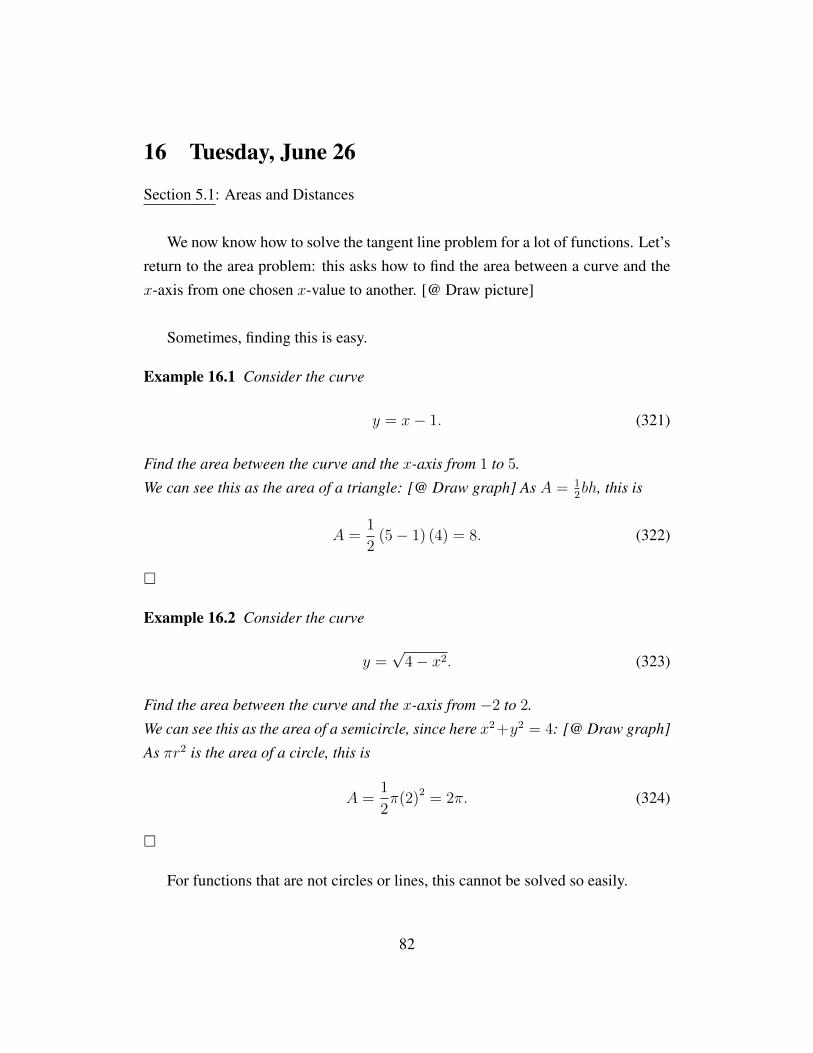
16 Tuesday, June 26

Section 5.1: Areas and Distances

We now know how to solve the tangent line problem for a lot of functions. Let’sreturn to the area problem: this asks how to find the area between a curve and thex-axis from one chosen x-value to another. [@ Draw picture]

Sometimes, finding this is easy.

Example 16.1 Consider the curve

y = x− 1. (321)

Find the area between the curve and the x-axis from 1 to 5.

We can see this as the area of a triangle: [@ Draw graph] As A = 12bh, this is

A =1

2(5− 1) (4) = 8. (322)

�

Example 16.2 Consider the curve

y =√

4− x2. (323)

Find the area between the curve and the x-axis from −2 to 2.

We can see this as the area of a semicircle, since here x2+y2 = 4: [@ Draw graph]

As πr2 is the area of a circle, this is

A =1

2π(2)2 = 2π. (324)

�

For functions that are not circles or lines, this cannot be solved so easily.

82

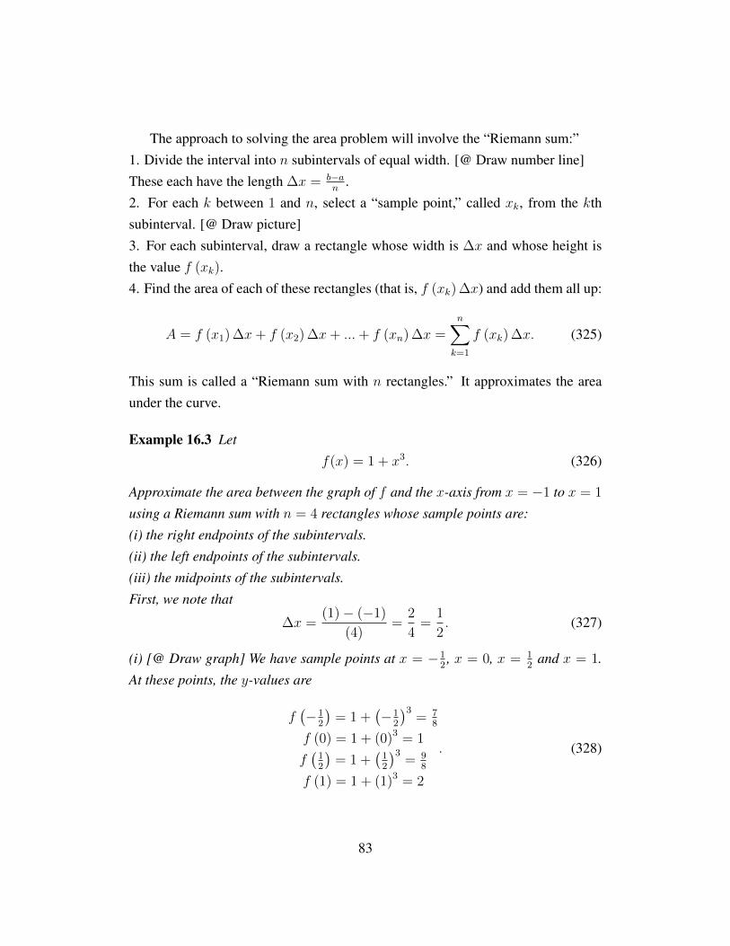
The approach to solving the area problem will involve the “Riemann sum:”1. Divide the interval into n subintervals of equal width. [@ Draw number line]These each have the length ∆x = b−a

n.

2. For each k between 1 and n, select a “sample point,” called xk, from the kthsubinterval. [@ Draw picture]3. For each subinterval, draw a rectangle whose width is ∆x and whose height isthe value f (xk).4. Find the area of each of these rectangles (that is, f (xk) ∆x) and add them all up:

A = f (x1) ∆x+ f (x2) ∆x+ ...+ f (xn) ∆x =n∑k=1

f (xk) ∆x. (325)

This sum is called a “Riemann sum with n rectangles.” It approximates the areaunder the curve.

Example 16.3 Let

f(x) = 1 + x3. (326)

Approximate the area between the graph of f and the x-axis from x = −1 to x = 1

using a Riemann sum with n = 4 rectangles whose sample points are:

(i) the right endpoints of the subintervals.

(ii) the left endpoints of the subintervals.

(iii) the midpoints of the subintervals.

First, we note that

∆x =(1)− (−1)

(4)=

2

4=

1

2. (327)

(i) [@ Draw graph] We have sample points at x = −12, x = 0, x = 1

2and x = 1.

At these points, the y-values are

f(−1

2

)= 1 +

(−1

2

)3= 7

8

f (0) = 1 + (0)3 = 1

f(12

)= 1 +

(12

)3= 9

8

f (1) = 1 + (1)3 = 2

. (328)

83

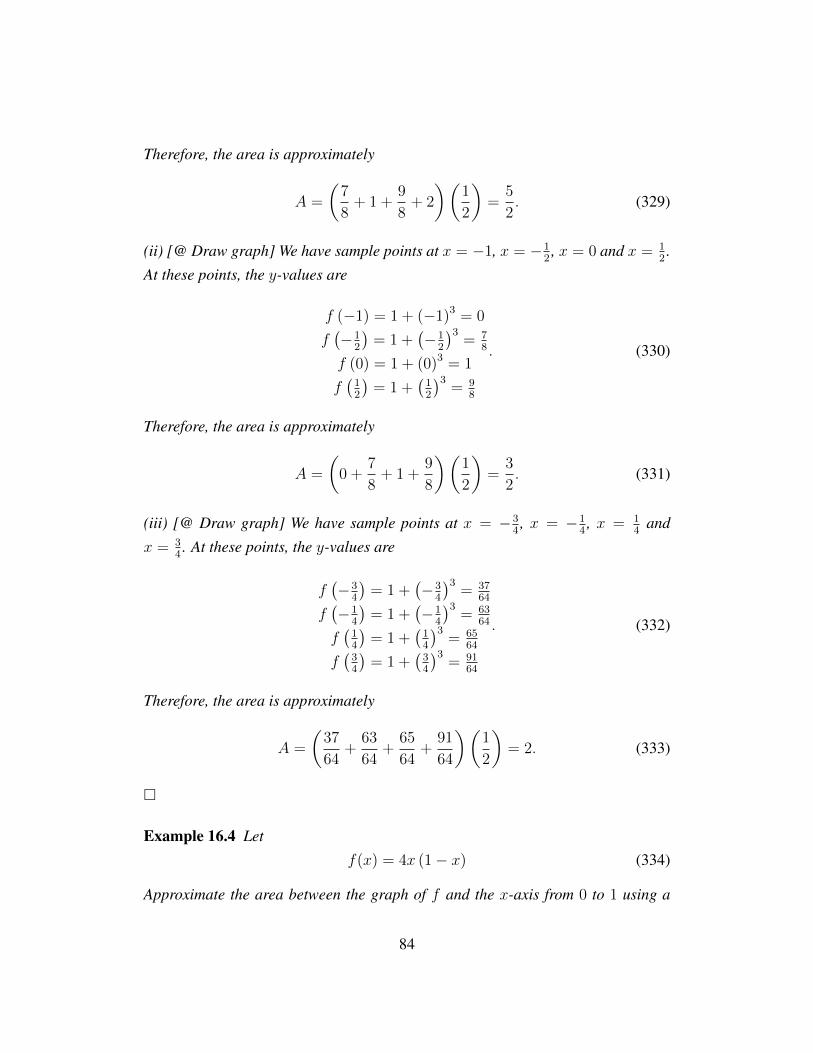
Therefore, the area is approximately

A =

(7

8+ 1 +

9

8+ 2

)(1

2

)=

5

2. (329)

(ii) [@ Draw graph] We have sample points at x = −1, x = −12, x = 0 and x = 1

2.

At these points, the y-values are

f (−1) = 1 + (−1)3 = 0

f(−1

2

)= 1 +

(−1

2

)3= 7

8

f (0) = 1 + (0)3 = 1

f(12

)= 1 +

(12

)3= 9

8

. (330)


A =

(0 +

7

8+ 1 +

9

8

)(1

2

)=

3

2. (331)

(iii) [@ Draw graph] We have sample points at x = −34, x = −1

4, x = 1

4and

x = 34. At these points, the y-values are

f(−3

4

)= 1 +

(−3

4

)3= 37

64

f(−1

4

)= 1 +

(−1

4

)3= 63

64

f(14

)= 1 +

(14

)3= 65

64

f(34

)= 1 +

(34

)3= 91

64

. (332)


A =

(37

64+

63

64+

65

64+

91

64

)(1

2

)= 2. (333)

�

Example 16.4 Let

f(x) = 4x (1− x) (334)

Approximate the area between the graph of f and the x-axis from 0 to 1 using a

84

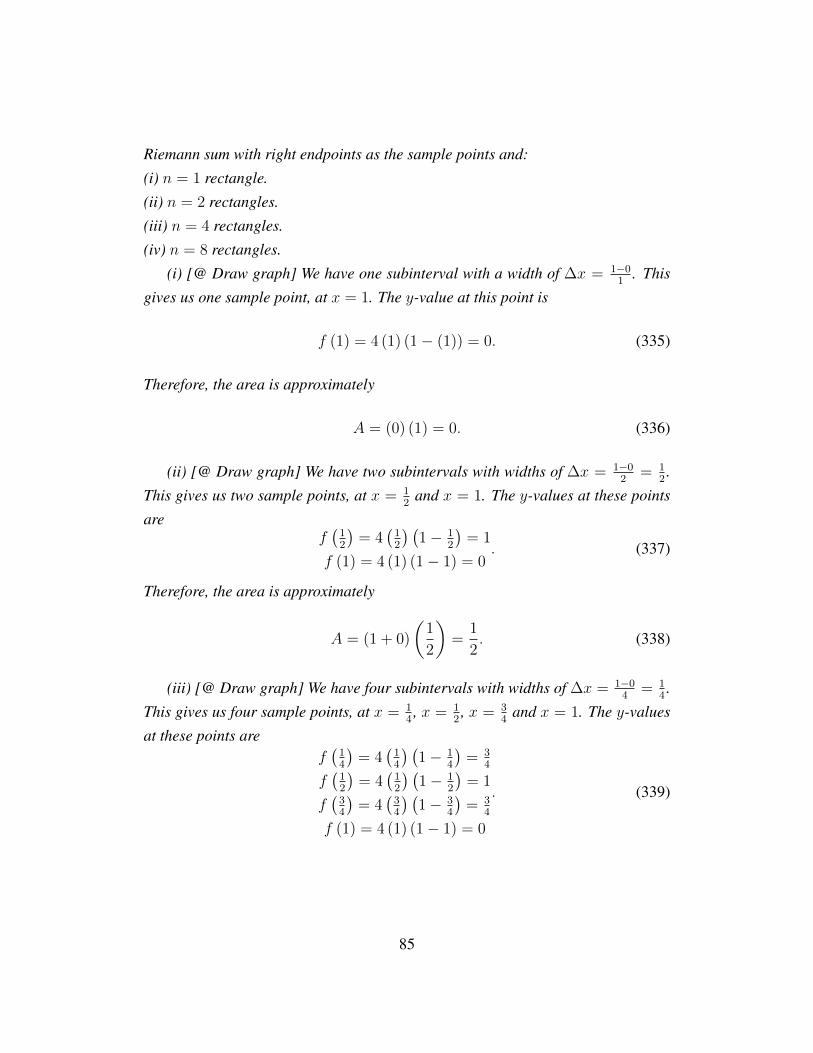
Riemann sum with right endpoints as the sample points and:

(i) n = 1 rectangle.

(ii) n = 2 rectangles.

(iii) n = 4 rectangles.

(iv) n = 8 rectangles.

(i) [@ Draw graph] We have one subinterval with a width of ∆x = 1−01

. This

gives us one sample point, at x = 1. The y-value at this point is

f (1) = 4 (1) (1− (1)) = 0. (335)


A = (0) (1) = 0. (336)

(ii) [@ Draw graph] We have two subintervals with widths of ∆x = 1−02

= 12.

This gives us two sample points, at x = 12

and x = 1. The y-values at these points

aref(12

)= 4

(12

) (1− 1

2

)= 1

f (1) = 4 (1) (1− 1) = 0. (337)


A = (1 + 0)

(1

2

)=

1

2. (338)

(iii) [@ Draw graph] We have four subintervals with widths of ∆x = 1−04

= 14.

This gives us four sample points, at x = 14, x = 1

2, x = 3

4and x = 1. The y-values

at these points aref(14

)= 4

(14

) (1− 1

4

)= 3

4

f(12

)= 4

(12

) (1− 1

2

)= 1

f(34

)= 4

(34

) (1− 3

4

)= 3

4

f (1) = 4 (1) (1− 1) = 0

. (339)

85


A =

(3

4+ 1 +

3

4+ 0

)(1

4

)=

10

16=

5

8. (340)

(iv) [@ Draw graph] We have eight subintervals with widths of ∆x = 1−08

= 18.

This gives us eight sample points, at x = 18, x = 1

4, x = 3

8, x = 1

2, x = 5

8, x = 3

4,

x = 78

and x = 1. The y-values at these points are

f(18

)= 4

(18

) (1− 1

8

)= 7

16

f(14

)= 3

4

f(38

)= 4

(38

) (1− 3

8

)= 15

16

f(12

)= 1

f(58

)= 4

(58

) (1− 5

8

)= 15

16

f(34

)= 3

4

f(78

)= 4

(78

) (1− 7

8

)= 7

16

f (1) = 0

(341)


A =

(7

16+

3

4+

15

16+ 1 +

15

16+

3

4+

7

16+ 0

)(1

8

)=

84

128=

21

32. (342)

�

86

1Section 5.2: The Definite Integral

Observe: more rectangles give more accurate approximations. In order to getthe true area, we’ll take the limit as the number of rectangles increases withoutbound.

Definition 16.5 Let f be a function defined on the real line. Given real values a

and b, the definite integral of f over the interval [a, b] is the limit

limn→∞

n∑k=1

f (xk) ∆x, (343)

where ∆x = b−an

, and for each k, xk is any real value satisfying the inequalities

a+ (k − 1)∆x ≤ xk ≤ a+ k∆x.

Notation:´ baf(x) dx means “the definite integral of f over the interval [a, b].

Notice: the definite integral could be negative. It gives a “signed area under thecurve.”

Theorem 16.6 Let f be a function defined on the real line, and let a and b be real

values. The following statements are true.

(i) ˆ b

a

f(x) dx = −ˆ a

b

f(x) dx. (344)

(ii) ˆ b

a

f(x) + g(x) dx =

ˆ b

a

f(x) dx+

ˆ b

a

g(x) dx. (345)

(iii) Given a real value c,

ˆ b

a

cf(x) dx = c

ˆ b

a

f(x) dx. (346)

87

(iv) Given a real value c,

ˆ c

a

f(x) dx =

ˆ b

a

f(x) dx+

ˆ c

b

f(x) dx. (347)

Example 16.7 Let

g(x) =

4− 2x if 0 ≤ x < 2

−√

4− x2 if 2 ≤ x < 6

x− 6 if 6 ≤ x < 7

. (348)

[@ Draw graph]

(i) Find ˆ 2

0

g(x) dx. (349)

This is ˆ 2

0

g(x) dx = A =1

2(2) (4) = 4. (350)

(ii) Find ˆ 6

2

g(x) dx. (351)

The area of the semicircle is

A =1

2π(2)2 = 2π. (352)

Since the graph is below the x-axis between 2 and 6, the integral is

ˆ 6

2

g(x) dx = −2π. (353)

(iii) Find ˆ 7

0

g(x) dx. (354)

88

We know that

ˆ 7

0

g(x) dx =

ˆ 2

0

g(x) dx+

ˆ 6

2

g(x) dx+

ˆ 7

6

g(x) dx

= 4− 2π +

ˆ 7

6

g(x) dx. (355)

Additionally, ˆ 7

6

g(x) dx =1

2(1) (1) =

1

2. (356)

Therefore, ˆ 7

0

g(x) dx = 4− 2π +1

2=

9

2− 2π. (357)

�

Finding the definite integral without any geometric reasoning can prove ratherdifficult.

Example 16.8 Evaluate the integral

ˆ 5

2

4− 2x dx. (358)

[@ Draw graph] By definition,

ˆ 5

2

4− 2x dx = limn→∞

n∑k=1

(4− 2xk) ∆x. (359)

If we choose the sample points to be the right endpoints of the intervals, then we

have xk = a+ k∆x. [@ Draw picture] Thus,

ˆ 5

2


n∑k=1

(4− 2 (2 + k∆x)) ∆x = limn→∞

n∑k=1

(−2k∆x) ∆x (360)

In our case, ∆x = 5−2n

= 3n

. Therefore, this becomes

ˆ 5

2


n∑k=1

(−2k

3

n

)3

n= lim

n→∞

(−18

n2

) n∑k=1

k. (361)

89

One can show that∑n

k=1 k = n(n+1)2

, so this is

ˆ 5

2


(−18

n2

)n(n+ 1)

2

= limn→∞

−9 (n+ 1)

n= lim

n→∞−9 +

1

n= −9. (362)

�

90


Section 5.3: The Fundamental Theorem of Calculus, andSection 4.9: Antiderivatives

The fundamental theorem of calculus explains a relationship between the deriva-tive and the definite integral.

In order to understand the statement, we will first examine functions of the form

g(x) =

ˆ x

a

f(t) dt, (363)

where a is a constant and f is a function defined on the real line.

Example 17.1 Let

f(t) = t+ 1. (364)

Define

g(x) =

ˆ x

0

f(t) dt. (365)

Let’s examine some values of the function g. [@ Draw graph]

g(0) =´ 00t+ 1 dt = 0

g(1) =´ 10t+ 1 dt = (1)(1) + 1

2(1)(1) = 3

2

g(2) =´ 20t+ 1 dt = (2)(1) + 1

2(2)(2) = 4

(366)

�

Theorem 17.2 (The fundamental theorem of calculus) If f is continuous on an

interval [a, b], thend

dx

ˆ x

a

f(t) dt = f(x). (367)

Example 17.3 Let

g(x) =

ˆ x

1

ln(1 + t2

)dt. (368)

91

Find g′(x).

By the fundamental theorem of calculus,

g′(x) =d

dt

ˆ x

1

ln(1 + t2

)dt = ln

(1 + x2

). (369)

�

Example 17.4 Let

R(y) =

ˆ 2

y

t3 sin t dt. (370)

Find R′(y).


R′(y) =d

dy

ˆ 2

y

t3 sin t dt = − d

dy

ˆ y

2

t3 sin t dt = −y3 sin y. (371)

�

Example 17.5 Let

h(x) =

ˆ √x1

z2

z4 + 1dz. (372)

Find h′(x).

We can understand h(x) = g (f (x)), where

f (x) =√x

g (x) =´ x1

z2

z4+1dz. (373)


g′(x) =d

dx

ˆ x

1

z2

z4 + 1dz =

x2

x4 + 1. (374)

Now, by the chain rule,

h′(x) = g′ (f (x)) f ′ (x) =(√x)

2

(√x)

4+ 1

(1

2x−

12

)=

x

2 (x2 + 1)√x. (375)

92

�

If we define g(x) =´ xaf(t) dt, then g′(x) = f(x). We say that g is an “an-

tiderivative” of f .

Definition 17.6 Let f and g be functions defined on the real line. We say that g is

an antiderivative of f provided that g′ = f .

Question: can a function have more than one antiderivative? In other words,can there exist two functions that have the same derivative?

If dgdx

= f and dhdx

= f , then

dgdx

= f = dhdx

dgdx− dh

dx= 0

ddx

(g − h) = 0

. (376)

Thus, g − h is a constant function. Therefore, if g and h are antiderivatives of f ,then they differ by a constant.

Example 17.7 Consider

f(x) = 2x. (377)

One can show that g(x) = x2 and h(x) = x2 + 4 are both antiderivatives of f . In

fact, for any fixed value C, k(x) = x2 + C is an antiderivative of f . �

If f is defined on the real line, and g(x) =´ xaf(t) dt for some real value a,

then g′(x) = f(x), by the fundamental theorem of calculus.If F is any antiderivative of f , then F and g differ by a constant; suppose that

F (x) = g(x) + C. Now, notice that

F (b)− F (a) = (g(b) + C)− (g(a) + C) = g(b)− g(a)

=

ˆ b

a

f(t) dt−ˆ a

a

f(t) dt =

ˆ b

a

f(t) dt. (378)

93

Corollary 17.8 If f is continuous on the interval [a, b], and F is any antiderivative

of f , then ˆ b

a

f(t) dt = F (b)− F (a). (379)

This makes evaluation of integrals much easier!


ˆ 5

2

4− 2x dx. (380)

First, we need an antiderivative of 4− 2x. How about F (x) = 4x− x2?

ˆ 5

2

4− 2x dx = F (5)− F (2) = 4x− x2∣∣∣∣52

=(4 (5)− (5)2

)−(4 (2)− (2)2

)= (−5)− (4) = −9. (381)

�

Function Antiderivativea ax

xr for r 6= −1 xr+1

r+11x

ln |x|ax for a > 1 ax

ln a

sinx − cosx

cosx sinx

sec2x tanx

secx tanx secx

−csc2x cotx

− cscx cotx cscx1√

1−x2 sin−1x1

x√x2−1 sec−1x1

x2+1tan−1x

(382)

94


ˆ 8

1

x−23 dx. (383)

ˆ 8

1

x−23 dx = 3x

13

∣∣∣∣81

= 3(8)13 − 3(1)

13 = 3(2)− 3(1) = 3. (384)

�


ˆ 1

0

1− 8v3 + 16v7 dv. (385)

ˆ 1

0

1− 8v3 + 16v7 dv = v − 2v4 + 2v8∣∣∣∣10

= 1− 2 + 2 = 1. (386)

�


ˆ 18

1

√3

zdz. (387)

ˆ 18

1

√3z−

12 dz = 2

√3z

12

∣∣∣∣181

= 2√

3(√

18−√

1)

= 2√

3(

3√

2− 1). (388)

�


ˆ π3

π4

csc2θ dθ (389)

ˆ π3

π4

csc2θ dθ = − cot θ

∣∣∣∣π3π4

= −

(cos(π3

)sin(π3

) − cos(π4

)sin(π4

)) =

1√21√2

−12√32

= 1− 1√3.

(390)�

95


ˆ 3

0

2 sinx− ex dx. (391)

2

ˆ 3

0

sinx dx−ˆ 3

0

ex dx = 2

(− cosx

∣∣∣∣30

)− ex

∣∣∣∣30

= 2 (1− cos 3)−(e3 − 1

)= 3− 2 cos 3− e3. (392)

�


ˆ 3

1

y3 − 2y2 − yy2

dy. (393)

ˆ 3

1

y − 2− 1

ydy =

1

2y2 − 2y − ln y

∣∣∣∣31

=

(1

2(3)3 − 2 (3)− ln (3)

)−(

1

2(1)3 − 2 (1)− ln (1)

)=

9

2− 6− ln 3− 1

2+ 2 = − ln 3 (394)

�

Example 17.16 Let

f(x) =

2 if − 2 ≤ x ≤ 0

4− x2 if 0 < x ≤ 2. (395)

Evaluate the integral ˆ 2

−2f(x) dx. (396)

96

ˆ 2

−2f(x) dx =

ˆ 0

−2f(x) dx+

ˆ 2

0

f(x) dx

=

ˆ 0

−22 dx+

ˆ 2

0

4− x2 dx = 2x

∣∣∣∣0−2

+

(4x− 1

3x3∣∣∣∣20

)

= (2 (0)− 2 (−2)) +

((4 (2)− 1

3(2)3

)−(

4 (0)− 1

3(0)3

))= 4 +

(8− 8

3

)− (0) = 12− 8

3=

28

3. (397)

�

97

Section 5.4: Indefinite integrals and the Net Change Theorem

Definition 17.17 Let f be a function defined on the real line. The indefinite integral

of f is the set of antiderivatives of f .

Example 17.18 Let

f(x) = ex − 2x2. (398)

Find the indefinite integral of f .

ˆf(x) dx =

êx − 2x2 dx = ex − 2

3x3 + C, (399)

where C is any real value. �

Notice: the definite integral is a real value. The indefinite integral is a family offunctions.

The corollary to the fundamental theorem of calculus says that if f is continuousand F is an antiderivative of f , then

ˆ b

a

f(t) dt = F (b)− F (a). (400)

If F is an antiderivative of f , then F ′ = f , so this can be written as

ˆ b

a

F ′(t) dt = F (b)− F (a). (401)

Thus, in applications, we can think of´ baf(t) dt as the “cumulative effect of a

varying rate of change.”

98

18 Thursday, June 28

Example 18.1 Water flows from the bottom of a tank at a rate of r(t) = 200 − 4t

liters per minute, where 0 ≤ t ≤ 50. Find the amount of water that flows from the

tank during the first 10 minutes.

ˆ 10

0

r(t) dt =

ˆ 10

0

200−4t dt = 200t−2t2∣∣∣∣100

= (2000− 200)−(0− 0) = 1800 L.

(402)�

Definition 18.2 If v(t) is the velocity of a particle with respect to a chosen reference

point (measured in meters per second) and t is the time since a particular moment

(measured in seconds), then given times t = a and t = b, the displacement of the

particle from t = a to t = b is the value´ bav(t) dt. The distance traveled by the

particle from t = a to t = b is the value´ ba|v(t)| dt.

Example 18.3 The velocity (in meters per second) for a particle moving along a

line is

v(t) = t2 − 2t− 3. (403)

(i) Find the displacement of the particle from t = 2 to t = 4.

ˆ 4

2

v(t) dt =

ˆ 4

2

t2 − 2t− 3 dt =1

3t3 − t2 − 3t

∣∣∣∣42

=

(1

3(4)3 − (4)2 − 3 (4)

)−(

1

3(2)3 − (2)2 − 3 (2)

)=

64

3− 16− 12− 8

3+ 4 + 6 =

56

3− 18 =

2

3m. (404)

(ii) Find the distance travelled by the particle from t = 2 to t = 4.

We need to know when v(t) is negative. We’ll first find out when v(t) is zero:

0 = v(t) = t2 − 2t− 3 = (t− 3) (t+ 1) . (405)

We have that v(t) = 0 at t = 3 and t = −1. (@ Draw number line.) This reveals

99

that v(t) < 0 for 2 ≤ t < 3 and v(t) > 0 for 3 < t. Therefore,

ˆ 4

2

|v(t)| dt =

ˆ 3

2

|v(t)| dt+

ˆ 4

3

|v(t)| dt =

ˆ 3

2

−v(t) dt+

ˆ 4

3

v(t) dt

=

ˆ 3

2

−(t2 − 2t− 3

)dt+

ˆ 4

3

t2 − 2t− 3 dt

=

(−t

3

3+ t2 + 3t

∣∣∣∣32

)+

(t3

3− t2 − 3t

∣∣∣∣43

)

=

(−27

3+ 9 + 9

)−(−8

3+ 4 + 6

)+

(64

3− 16− 12

)−(

27

3− 9− 9

)=

27

3− 22

3− 20

3+

27

3=

12

3= 4 m. (406)

�

Example 18.4 A bacteria population is 4000 at time t = 0 hours and its rate of

growth at t hours is r(t) = (1000) 2t bacteria per hour. What is the population

after 1 hour?

The change in the bacteria population is

ˆ 1

0

r(t) dt =

ˆ 1

0

(1000) 2t dt =1000

ln 22t∣∣∣∣10

=1000

ln 2

(21 − 20

)=

1000

ln 2≈ 1442.

(407)Since the original population is 4000, the new population is 5442 bacteria. �

Example 18.5 The acceleration (in meters per second per second) of a particle

moving along a straight line is

a(t) = t2 − 4t+ 6. (408)

The particle’s position at t = 0 is x(0) = 0 m and its velocity at t = 0 is v(0) = 1

m/s.

(i) Find the velocity of the particle.

We know that a(t) = v′(t), so

v(t) =

â(t) dt =

ˆt2 − 4t+ 6 dt =

1

3t3 − 2t2 + 6t+ C1. (409)

100

Since v(0) = 1,

1 =1

3− 2 + 6 + C1, (410)

so C1 = −103

. Therefore,

v(t) =1

3t3 − 2t2 + 6t− 10

3. (411)

(ii) Find the position of the particle.

We know that v(t) = x′(t), so

x(t) =

ˆv(t) dt =

ˆ1

3t3−2t2+6t−10

3dt =

1

12t4−2

3t3+3t2−10

3t+C2. (412)

We know that x(0) = 0, so

0 =1

12t4 − 2

3t3 + 3t2 − 10

3t+ C2, (413)

hence C2 = 0. Therefore,

x(t) =1

12t4 − 2

3t3 + 3t2 − 10

3t. (414)

�

Example 18.6 Suppose a particle moving along a straight line has a constant ac-

celeration a. In that case, its velocity is

v(t) =

â dt = at+ C1. (415)

Suppose v(0) = v0, the initial velocity. In that case,

v0 = v(0) = a(0) + C1 = C1, (416)

and so

v(t) = v0 + at. (417)

101

Additionally,

x(t) =

ˆv(t) dt =

ât+ v0 dt =

1

2at2 + v0t+ C2. (418)

Suppose x(0) = x0, the initial position. In that case,

x0 = x(0) =1

2a(0)2 + v0(0) + C2 = C2, (419)

and so

x(t) = x0 + v0t+1

2at2. (420)

�

102

Section 5.5: The substitution rule

Theorem 18.7 (u-substitution) Let f be a continuous function defined on the real

line. If u(x) is a differentiable function, then

ˆf (u (x))

du

dxdx =

ˆf (u) du (421)

Example 18.8 Evaluate ˆ−2xe−x

2

dx. (422)

We can understand e−x2

as eu, where u(x) = −x2. In that case, dudx

= −2x.

Therefore, this is êu

du

dxdx =

êu du = eu + C. (423)

Since u(x) = −x2, this is e−x2

+ C. �

Example 18.9 Evaluate ˆsin2θ cos θ dθ. (424)

If we say u(x) = sin θ, then dudx

= cos θ. Therefore, this becomes

û2

du

dxdx =

û2 du =

1

3u3 + C =

1

3sin3θ + C. (425)

�

Example 18.10 Evaluate ˆ √2t+ 1 dt. (426)

Define u = 2t+ 1. In that case, dudt

= 2. Notation:

u = 2t+ 1

du = 2 dt. (427)

103

Therefore, 12

du = dt, and so

ˆ √u

1

2du =

1

2

û

12 du =

1

2

2

3u

32 + C =

1

3(2t+ 1)

32 + C. (428)

�

Example 18.11 Evaluate ˆsec2 (2θ) dθ. (429)

We writeu = 2θ

du = 2 dθ. (430)

This becomesˆ

1

2sec2u du =

1

2tanu+ C =

1

2tan (2θ) + C. (431)

�

Example 18.12 Evaluate êcos t sin t dt. (432)

Selectu = cos t

du = − sin t dt. (433)

This becomes

−êu du = −eu + C = −ecos t + C. (434)

�

Example 18.13 Evaluate ˆcos (ln t)

tdt (435)

Selectu = ln t

du = 1t

dt. (436)

104

This becomes ˆcosu du = sinu+ C = sin (ln t) + C. (437)

�

Example 18.14 Evaluate ˆdt

cos2t√

1 + tan t. (438)

We can write this as ˆsec2t

1√1 + tan t

dt. (439)

If we selectu = 1 + tan t

du = sec2t dt. (440)

This becomesˆ

1√u

du =

û−

12 du = 2

√u+ C = 2

√1 + tan t+ C. (441)

�

Example 18.15 Evaluate ˆx

1 + x4dx. (442)

Selectu = x2

du = 2x dx. (443)

This becomes

1

2

ˆ1

1 + u2du =

1

2tan−1u+ C =

1

2tan−1

(x2)

+ C. (444)

�

For definite integrals, change the bounds when using u-substitution.

Example 18.16 Evaluate ˆ 1

0

(3t− 1)50 dt. (445)

105

Selectu = 3t− 1

du = 3 dt. (446)

When t = 0, u = −1, and when t = 1, u = 2. Therefore, this becomes

ˆ 2

−1u50 du =

1

51u51∣∣∣∣2−1

=1

51

((2)51 − (−1)51

)=

1

51

(251 + 1

). (447)

�


0

dx

5x+ 1. (448)

Selectu = 5x+ 1

du = 5 dx. (449)

When x = 0, u = 1 and when x = 3, u = 16. This becomes

1

5

ˆ 16

1

1

udu =

1

5ln |u|

∣∣∣∣161

=1

5ln (16) =

4

5ln 2. (450)

�


0

x√1 + 2x

dx. (451)

Selectu = 1 + 2x

du = 2 dx. (452)

When x = 0, u = 1 and when x = 4, u = 9. This becomes

1

2

ˆ 9

1

12

(u− 1)√u

du =1

4

ˆ 9

1

u− 1

u12

du =1

4

ˆ 9

1

u12 − u−

12 du

=1

4

(2

3u

32 − 2u

12

∣∣∣∣91

)=

1

4

(14− 2

3

)=

10

3. (453)

106

Math 141: College Calculus I

Documents