Differential Calculus: Mathematics 102 The University of British Columbia Notes by Leah Edelstein-Keshet 1 : All rights reserved September 1, 2014 1 This disclaimer is inserted in view of UBC Policy 81. Copyright Leah Edelstein-Keshet. Not to be copied, used, or revised without explicit written permission from the author.

Differential Calculus Math 102
Jan 11, 2016
Differential calculus course notes
Welcome message from author
This document is posted to help you gain knowledge. Please leave a comment to let me know what you think about it! Share it to your friends and learn new things together.
Transcript
Differential Calculus: Mathematics 102The University of British Columbia
Notes by Leah Edelstein-Keshet1: All rights reserved
September 1, 2014
1This disclaimer is inserted in view of UBC Policy 81. Copyright Leah Edelstein-Keshet. Not tobe copied, used, or revised without explicit written permission from the author.

ii Leah Edelstein-Keshet
Contents
Preface xi
1 Power functions as building blocks 11.1 Power functions . . . . . . . . . . . . . . . . . . . . . . . . . . . . . 11.2 How big can a cell be? A model for nutrient balance . . . . . . .. . . 3
1.2.1 Building the model . . . . . . . . . . . . . . . . . . . . . 41.2.2 Nutrient balance depends on cell size . . . . . . . . . . . 61.2.3 Even and odd power functions . . . . . . . . . . . . . . . 7
1.3 Sustainability and Energy balance on Planet Earth . . . . .. . . . . . 81.4 Combining power functions: first steps in graph sketching . . . . . . . 9
1.4.1 Sketching a simple (two-term) polynomial . . . . . . . . 91.4.2 Sketching a simple rational function . . . . . . . . . . . . 12
1.5 Rate of an enzyme-catalyzed reaction . . . . . . . . . . . . . . . .. . 121.5.1 Saturation and Michaelis-Menten kinetics . . . . . . . . .131.5.2 Hill functions . . . . . . . . . . . . . . . . . . . . . . . 15
1.6 Analysis versus computational tools: two sides of a coin. . . . . . . . 151.7 For further study: Michaelis-Menten transformed to a linear relationship 161.8 For further study: Spacing of fish in a school . . . . . . . . . . .. . . 17Exercises . . . . . . . . . . . . . . . . . . . . . . . . . . . . . . . . . . . . . 18
2 Average rates of change, average velocity and the secant line 252.1 Time-dependent data and rates of change . . . . . . . . . . . . . .. . 25
2.1.1 Milk temperature in a recipe for yoghurt . . . . . . . . . 262.1.2 Data for swimming Tuna . . . . . . . . . . . . . . . . . 272.1.3 Data for a falling object . . . . . . . . . . . . . . . . . . 28
2.2 The slope of a straight line is a rate of change . . . . . . . . . .. . . 292.3 The slope of a secant line is the average rate of change . . .. . . . . . 302.4 From average to instantaneous rate of change . . . . . . . . . .. . . . 34
2.4.1 Refined temperature data . . . . . . . . . . . . . . . . . 342.4.2 Refined data for the height of a falling object . . . . . . . 362.4.3 Instantaneous velocity . . . . . . . . . . . . . . . . . . . 37
2.5 Introduction to the derivative . . . . . . . . . . . . . . . . . . . . .. 37Exercises . . . . . . . . . . . . . . . . . . . . . . . . . . . . . . . . . . . . . 40
iii
iv Contents
3 Three faces of the derivative: geometric, analytic, and computational 453.1 The geometric view: Zooming into the graph of a function .. . . . . . 45
3.1.1 Locally, the graph of a function looks like a straight line . 453.1.2 At a cusp or a discontinuity, the derivative is not defined . 473.1.3 From the graph of a function, we can sketch its derivative 483.1.4 Constant and linear functions and their derivatives .. . . 493.1.5 Molecular motors . . . . . . . . . . . . . . . . . . . . . 51
3.2 Analytic view: calculating the derivative . . . . . . . . . . .. . . . . 523.2.1 Technical matters: continuous functions and limits .. . . 523.2.2 Computing the derivative . . . . . . . . . . . . . . . . . 56
3.3 Computational face of the derivative: software to the rescue! . . . . . 573.3.1 Concentration-dependent rate of chemical reaction .. . . 58
Exercises . . . . . . . . . . . . . . . . . . . . . . . . . . . . . . . . . . . . . 63
4 Differentiation rules, simple antiderivatives and applications 694.1 Rules of differentiation . . . . . . . . . . . . . . . . . . . . . . . . . 69
4.1.1 The derivative of power functions: the power rule . . . .704.1.2 The derivative is a linear operation . . . . . . . . . . . . 714.1.3 The derivative of a polynomial . . . . . . . . . . . . . . 714.1.4 Antiderivatives of power functions and polynomials .. . 724.1.5 Product and quotient rules for derivatives . . . . . . . . .744.1.6 The power rule for fractional powers . . . . . . . . . . . 76
4.2 Application: From acceleration to displacement . . . . . .. . . . . . 764.2.1 Position, velocity, and acceleration . . . . . . . . . . . . 77
4.3 Sketching first, second, and anti- derivatives . . . . . . . .. . . . . . 804.3.1 A biological speed machine . . . . . . . . . . . . . . . . 84
Exercises . . . . . . . . . . . . . . . . . . . . . . . . . . . . . . . . . . . . . 88
5 Tangent lines, linear approximation, and Newton’s method 935.1 The equation of a tangent line . . . . . . . . . . . . . . . . . . . . . . 93
5.1.1 Simple functions and their tangent lines . . . . . . . . . . 945.2 Generic tangent line equation and properties . . . . . . . . .. . . . . 97
5.2.1 Generic tangent line equation . . . . . . . . . . . . . . . 975.2.2 Where a tangent line intersects thex axis . . . . . . . . . 97
5.3 Close to a point, we can approximate a function by its tangent line . . 985.3.1 Accuracy of the linear approximation . . . . . . . . . . . 100
5.4 Tangent lines can help approximate the zeros of a function . . . . . . . 1025.4.1 Newton’s method . . . . . . . . . . . . . . . . . . . . . 103
5.5 Harder tangent line problems: Finding the point of tangency . . . . . . 106Exercises . . . . . . . . . . . . . . . . . . . . . . . . . . . . . . . . . . . . . 110
6 Sketching the graph of a function using calculus tools 1156.1 Overall shape of the graph of a function . . . . . . . . . . . . . . .. 115
6.1.1 Increasing and decreasing functions . . . . . . . . . . . . 1156.1.2 Concavity and points of inflection . . . . . . . . . . . . . 1166.1.3 Determining whetherf ′′(x) changes sign . . . . . . . . . 118
Contents v
6.2 Special points on the graph of a function . . . . . . . . . . . . . .. . 1186.2.1 Zeros of a function . . . . . . . . . . . . . . . . . . . . . 1196.2.2 Critical points . . . . . . . . . . . . . . . . . . . . . . . 1206.2.3 What happens close to a critical point . . . . . . . . . . . 120
6.3 Sketching the graph of a function . . . . . . . . . . . . . . . . . . . .1226.3.1 Global maxima and minima, endpoints of an interval . . .126
Exercises . . . . . . . . . . . . . . . . . . . . . . . . . . . . . . . . . . . . . 128
7 Optimization 1317.1 Simple biological optimization problems . . . . . . . . . . . .. . . . 131
7.1.1 Density dependent (logistic) growth in a population .. . 1317.1.2 Cell size for maximal nutrient accumulation rate . . . .. 133
7.2 Optimization with a constraint . . . . . . . . . . . . . . . . . . . . .. 1347.2.1 A cylindrical cell with minimal surface area . . . . . . . 1357.2.2 Wine for Kepler’s wedding . . . . . . . . . . . . . . . . 137
7.3 Checking endpoints . . . . . . . . . . . . . . . . . . . . . . . . . . . 1407.4 Optimal foraging . . . . . . . . . . . . . . . . . . . . . . . . . . . . . 142
7.4.1 For further study: Other patch functions . . . . . . . . . 1467.5 Additional Examples of geometric optimization . . . . . . .. . . . . 149
7.5.1 Rectangular box with largest surface area . . . . . . . . . 1497.5.2 A cylinder in a sphere . . . . . . . . . . . . . . . . . . . 150
Exercises . . . . . . . . . . . . . . . . . . . . . . . . . . . . . . . . . . . . . 152
8 Introducing the chain rule 1598.1 The chain rule . . . . . . . . . . . . . . . . . . . . . . . . . . . . . . 159
8.1.1 Function composition . . . . . . . . . . . . . . . . . . . 1598.1.2 The chain rule of differentiation . . . . . . . . . . . . . . 1608.1.3 Interpreting the chain rule . . . . . . . . . . . . . . . . . 161
8.2 Chain Rule applied to optimization problems . . . . . . . . . .. . . . 1648.2.1 Shortest path from food to nest . . . . . . . . . . . . . . 1658.2.2 Food choice and attention . . . . . . . . . . . . . . . . . 166
Exercises . . . . . . . . . . . . . . . . . . . . . . . . . . . . . . . . . . . . . 173
9 Chain rule applied to related rates and implicit differentiation 1759.1 Applications of the chain rule to “related rates” . . . . . .. . . . . . . 1759.2 Implicit differentiation . . . . . . . . . . . . . . . . . . . . . . . . .. 180
9.2.1 Implicit and explicit definition of a function . . . . . . .1809.2.2 Slope of a tangent line at the point on a curve . . . . . . . 181
9.3 The power rule for fractional powers . . . . . . . . . . . . . . . . .. 184Exercises . . . . . . . . . . . . . . . . . . . . . . . . . . . . . . . . . . . . . 189
10 Exponential functions 19510.1 Unlimited growth and doubling . . . . . . . . . . . . . . . . . . . . .195
10.1.1 The Andromeda Strain . . . . . . . . . . . . . . . . . . . 19510.1.2 The function2x and its “relatives” . . . . . . . . . . . . 197
10.2 Derivatives of exponential functions and the functionex . . . . . . . . 199
vi Contents
10.2.1 Calculating the derivative ofax . . . . . . . . . . . . . . 19910.2.2 The natural basee is convenient for calculus . . . . . . . 20110.2.3 Properties of the functionex . . . . . . . . . . . . . . . . 20210.2.4 The functionex satisfies a new kind of equation . . . . . 203
10.3 Inverse functions and logarithms . . . . . . . . . . . . . . . . . .. . 20410.3.1 The natural logarithm is an inverse function forex . . . . 20510.3.2 Derivative ofln(x) by implicit differentiation . . . . . . . 206
10.4 Applications of the logarithm . . . . . . . . . . . . . . . . . . . . .. 20610.4.1 Using the logarithm for base conversion . . . . . . . . . 20610.4.2 The logarithm helps to solve exponential equations .. . . 20710.4.3 Logarithms help plot data that varies on large scale .. . . 208
Exercises . . . . . . . . . . . . . . . . . . . . . . . . . . . . . . . . . . . . . 211
11 Differential equations for exponential growth and decay 21911.1 Introducing a new kind of equation . . . . . . . . . . . . . . . . . .. 219
11.1.1 Observations about the exponential function . . . . . .. 21911.1.2 The solution to a differential equation . . . . . . . . . . .22111.1.3 Where do differential equations come from? . . . . . . . 223
11.2 Differential equation for unlimited population growth . . . . . . . . . 22411.2.1 A simple model for human population growth . . . . . . 22511.2.2 A critique . . . . . . . . . . . . . . . . . . . . . . . . . 22811.2.3 Growth and doubling . . . . . . . . . . . . . . . . . . . 229
11.3 Radioactive decay . . . . . . . . . . . . . . . . . . . . . . . . . . . . 23011.3.1 Deriving the model . . . . . . . . . . . . . . . . . . . . 23111.3.2 Solution to the decay equation . . . . . . . . . . . . . . . 23311.3.3 The half life . . . . . . . . . . . . . . . . . . . . . . . . 233
11.4 Summary and Review . . . . . . . . . . . . . . . . . . . . . . . . . . 235Exercises . . . . . . . . . . . . . . . . . . . . . . . . . . . . . . . . . . . . . 237
12 Solving differential equations 24112.1 Introduction . . . . . . . . . . . . . . . . . . . . . . . . . . . . . . . 24112.2 Given a function, check that it is a solution . . . . . . . . . .. . . . . 24112.3 Equations of the formy′(t) = a− by . . . . . . . . . . . . . . . . . . 243
12.3.1 Reduction to a simpler differential equation . . . . . .. . 24412.3.2 Newton’s law of cooling . . . . . . . . . . . . . . . . . . 24612.3.3 Using Newton’s Law of Cooling to solve a mystery . . . 24812.3.4 Related applications and further examples . . . . . . . .249
12.4 Euler’s Method and numerical solutions . . . . . . . . . . . . .. . . 25012.4.1 Euler’s method applied to population growth . . . . . . .25212.4.2 Euler’s method applied to Newton’s law of cooling . . .. 254
Exercises . . . . . . . . . . . . . . . . . . . . . . . . . . . . . . . . . . . . . 257
13 Qualitative methods for differential equations 26313.1 Linear and nonlinear differential equations . . . . . . . .. . . . . . . 263
13.1.1 The logistic equation for population growth . . . . . . .. 26413.1.2 Linear versus nonlinear . . . . . . . . . . . . . . . . . . 264
Contents vii
13.1.3 Law of mass action . . . . . . . . . . . . . . . . . . . . 26513.1.4 Scaling the variable can simplify the ODE . . . . . . . . 266
13.2 The geometry of change . . . . . . . . . . . . . . . . . . . . . . . . . 26713.2.1 Slope fields . . . . . . . . . . . . . . . . . . . . . . . . . 26813.2.2 State-space diagrams . . . . . . . . . . . . . . . . . . . . 27213.2.3 Steady states and stability . . . . . . . . . . . . . . . . . 275
13.3 Applying qualitative analysis to biological models . .. . . . . . . . . 27513.3.1 Qualitative analysis for the logistic equation . . . .. . . 27613.3.2 A model for the spread of a disease . . . . . . . . . . . . 280
Exercises . . . . . . . . . . . . . . . . . . . . . . . . . . . . . . . . . . . . . 285
14 Trigonometric functions 29114.1 Basic trigonometry . . . . . . . . . . . . . . . . . . . . . . . . . . . . 291
14.1.1 Angles and circles . . . . . . . . . . . . . . . . . . . . . 29214.1.2 Defining the trigonometric functionssin(x) andcos(x) . 29314.1.3 Properties ofsin(x) andcos(x) . . . . . . . . . . . . . . 29414.1.4 Other trigonometric functions . . . . . . . . . . . . . . . 295
14.2 Periodic Functions . . . . . . . . . . . . . . . . . . . . . . . . . . . . 29514.2.1 Phase, amplitude, and frequency . . . . . . . . . . . . . 29714.2.2 Rhythmic processes . . . . . . . . . . . . . . . . . . . . 298
14.3 Inverse Trigonometric functions . . . . . . . . . . . . . . . . . .. . . 301Exercises . . . . . . . . . . . . . . . . . . . . . . . . . . . . . . . . . . . . . 308
15 Cycles, periods, and rates of change 31115.1 Derivatives of trigonometric functions . . . . . . . . . . . .. . . . . 311
15.1.1 Limits of trigonometric functions . . . . . . . . . . . . . 31115.1.2 Derivatives of sine, cosine, and other trigonometric functions31215.1.3 Derivatives of the inverse trigonometric functions. . . . 313
15.2 Changing angles and related rates . . . . . . . . . . . . . . . . . .. . 31415.3 The Zebra danio’s escape responses . . . . . . . . . . . . . . . . .. . 318
15.3.1 Visual angles . . . . . . . . . . . . . . . . . . . . . . . . 31815.3.2 The Zebra danio and a looming predator . . . . . . . . . 32015.3.3 Alternate approach involving inverse trig functions . . . . 323
15.4 For further study: Trigonometric functions and differential equations . 32415.5 Additional examples: Implicit differentiation . . . . .. . . . . . . . . 325Exercises . . . . . . . . . . . . . . . . . . . . . . . . . . . . . . . . . . . . . 328
16 Review Problems 335Exercises . . . . . . . . . . . . . . . . . . . . . . . . . . . . . . . . . . . . . 336
Appendices 349
A A review of Straight Lines 351A.A Geometric ideas: lines, slopes, equations . . . . . . . . . . .. . . . . 351Exercises . . . . . . . . . . . . . . . . . . . . . . . . . . . . . . . . . . . . . 354
B A precalculus review 357
viii Contents
B.A Manipulating exponents . . . . . . . . . . . . . . . . . . . . . . . . . 357B.B Manipulating logarithms . . . . . . . . . . . . . . . . . . . . . . . . . 357
C A Review of Simple Functions 359C.A What is a function . . . . . . . . . . . . . . . . . . . . . . . . . . . . 359C.B Geometric transformations . . . . . . . . . . . . . . . . . . . . . . . 360C.C Classifying . . . . . . . . . . . . . . . . . . . . . . . . . . . . . . . . 362C.D Power functions and symmetry . . . . . . . . . . . . . . . . . . . . . 362
C.D.1 Further properties of intersections . . . . . . . . . . . . . 363C.D.2 Optional: Combining even and odd functions . . . . . . . 365
C.E Inverse functions and fractional powers . . . . . . . . . . . . .. . . . 366C.E.1 Graphical property of inverse functions . . . . . . . . . . 366C.E.2 Restricting the domain . . . . . . . . . . . . . . . . . . . 367
C.F Polynomials . . . . . . . . . . . . . . . . . . . . . . . . . . . . . . . 368C.F.1 Features of polynomials . . . . . . . . . . . . . . . . . . 369
Exercises . . . . . . . . . . . . . . . . . . . . . . . . . . . . . . . . . . . . . 370
D Limits 373D.A Limits for continuous functions . . . . . . . . . . . . . . . . . . . .. 373D.B Properties of limits . . . . . . . . . . . . . . . . . . . . . . . . . . . . 374D.C Limits of rational functions . . . . . . . . . . . . . . . . . . . . . . .375
D.C.1 Case 1: Denominator nonzero . . . . . . . . . . . . . . . 375D.C.2 Case 2: zero in the denominator and “holes” in a graph . 376
D.D Right and left sided limits . . . . . . . . . . . . . . . . . . . . . . . . 378D.E Limits at infinity . . . . . . . . . . . . . . . . . . . . . . . . . . . . . 379D.F Summary of special limits . . . . . . . . . . . . . . . . . . . . . . . . 379
E Proof of the chain rule 381
F Trigonometry review 383F.A Summary of the inverse trigonometric functions . . . . . . .. . . . . 385
G Short Answers to Problems 387G..1 Answers to Chapter 1 Problems . . . . . . . . . . . . . . 388G..2 Answers to Chapter 2 Problems . . . . . . . . . . . . . . 390G..3 Answers to Chapter 3 Problems . . . . . . . . . . . . . . 392G..4 Answers to Chapter 4 Problems . . . . . . . . . . . . . . 394G..5 Answers to Chapter 5 Problems . . . . . . . . . . . . . . 396G..6 Answers to Chapter 6 Problems . . . . . . . . . . . . . . 397G..7 Answers to Chapter 7 Problems . . . . . . . . . . . . . . 399G..8 Answers to Chapter 8 Problems . . . . . . . . . . . . . . 401G..9 Answers to Chapter 9 Problems . . . . . . . . . . . . . . 402G..10 Answers to Chapter 10 Problems . . . . . . . . . . . . . 404G..11 Answers to Chapter 11 Problems . . . . . . . . . . . . . 406G..12 Answers to Chapter 12 Problems . . . . . . . . . . . . . 408G..13 Answers to Chapter 13 Problems . . . . . . . . . . . . . 410
Contents ix
G..14 Answers to Chapter 14 Problems . . . . . . . . . . . . . 412G..15 Answers to Chapter 15 Problems . . . . . . . . . . . . . 413G..16 Answers to Chapter 16 Problems . . . . . . . . . . . . . 415G..17 Answers to Appendix A Problems . . . . . . . . . . . . . 418G..18 Answers to Appendix B Problems . . . . . . . . . . . . . 419
Bibliography 421
Index 423

x Contents
Preface
This preface outlines the main philosophy of the course, andserves as a guide to theinstructor. It outlines reasons for the organization of thematerial and why this works for in-troducing first year students to the major concepts and many applications of the differentialcalculus.
Calculus arose as an important tool in solving practical scientific problems throughthe centuries. However, in many current courses, it is taught as a technical subject withrules and formulas (and occasionally theorems), devoid of its connection to applications.In this course, the applications form an important focal point, with a focus on life sci-ences.This places the techniques and concepts into practical context, as well as motivatingquantitative approaches to biology taught to undergraduates. While many of the exampleshave a biological flavour, the level of biology needed to understand those examples is keptat a minimum. The problems are motivated with enough detail to follow the assumptions,but are simplified for the purpose of pedagogy.
The mathematical philosophy is as follows: We start with elementary observationsabout functions and graphs, with an emphasis on power functions and polynomials. Thisintroduces the idea of sketching of a graph from elementary properties of the function,before calculus is discussed. It also leads to direct biological applications that illustrate theidea of which terms in an expression (polynomial or rationalfunction) dominate at whichrange(s) of the independent variable.
We introduce the derivative in three complementary ways: (1) As a rate of change,(2) as the slope we see when we zoom into the graph of a function, and (3) as a compu-tational quantity that can be approximated by a finite difference. We discuss (1) by firstdefining an average rate of change over a finite time interval.We use actual data to do so,but then by refining the time interval, we show how this average rate of change approachesthe instantaneous rate, i.e. the derivative. This helps to make the idea of the limit moreintuitive, and not simply a formal calculation. We illustrate (2) using a sequence of graphsor interactive graphs with increasing magnification. We illustrate (3) using simple compu-tation that can be carried out on a spreadsheet. The actual formal definition of the derivative(while presented and used) takes a back-seat to this discussion.
The next philosophical aspect of the course is that we develop all the ideas and appli-cations of calculus using simple functions (power and polynomials)first, before introducingthe more elaborate technical calculations. The aim is to show our students the usefulnessof derivatives for understanding functions (sketching andinterpreting their behaviour), andfor optimization problems, before having to grapple with the chain rule and more intricatecomputation of derivatives. This helps to illustrate what calculus can achieve, and decrease
xi
xii Preface
the focus on rote mechanical calculations.Once this entire “tour” of calculus is complete, we introduce the chain rule and its
applications, and then the transcendental functions (exponentials and trigonometric). Bothare used to illustrate biological phenomena (population growth and decay, then, later on,cyclic processes). Both allow a repeated exposure to the basic ideas of calculus - curvesketching, optimization, and applications to related rates. This means that the importantconcepts picked up earlier in the context of simpler functions can be reinforced again. Thestudent also learns to practice and apply the chain rule, andto compute more technicallyinvolved derivatives. But, even more than that, both these topics allow us to informallyintroduce a powerful new idea, that of a differential equation.
By making the link between the exponential function and the differential equationdy/dx = ky, we open the door to a host of applications in the slightly generalized form ofdy/dx = a − by. We demonstrate that understanding the first leads to understanding thesecond, merely by changing the variable of interest (fromy to z = y− (a/b). Applicationsinclude the temperature of a cooling object, the level of drug in the bloodstream, simplechemical reactions, and many more. Even though the student does not yet have the toolsto analyticallysolvea differential equation (tools developed only in a second semester),he/she can appreciate the link between the statement about rates of change and predictionsfor future behaviour of a system.
Ultimately, a first semester calculus course is all about theapplications of a deriva-tive. We use this fact to explore nonlinear differential equations of the first order, usingqualitative sketches of the direction field and the state space of the equation. These simpleyet powerful ideas allow us to get intuition to the behaviourof more realistic biologicalmodels, including density-dependent (logistic) growth and even spread of disease. Manyof the ideas here are geometric, and we return to interpreting the meaning of graphs andslopes yet again in this context.
The idea of a computational approach is reintroduced in several places, as appropri-ate. We use simple examples to motivate linear approximation and Newton’s method forfinding zeros of a function. Later, we use Euler’s method to solve a simple differential equa-tion computationally. All these methods are based on the derivative, and most introducethe idea of an iterated (repeated) process that is ideally handled by computer or calculator.The exposure to these computational methods, while novel and sometimes daunting, pro-vides an important set of examples of how properly understanding the math can lead us toeffective design of computational algorithms.
Chapter 1
Power functions asbuilding blocks
Some of the beautiful architectural marvels built by humansfrom ancient to modern timesthough very complicated as a whole, are made of simple component parts - bricks, beamsand joints. Similarly, some mathematical structures that seem complicated can be decom-posed into simpler subunits whose properties are straightforward. Understanding thesecomponent parts and how they fit together to form more interesting structures is an im-portant step in appreciating properties of more complex (mathematical) structures. Thiscentral idea forms the theme of the first chapter.
The components that we explore here are power functions. We first study these ontheir own, and compare their shapes. We examine an immediateapplication of our analysisto the biological problem of cell size. Then we expand our horizon to consider polynomialsand rational functions. Using the power functions as basic building blocks, we construct thefamily of polynomials, and investigate how their features are inherited from the underlyingbehaviour of power functions. Here, we begin to develop a fewimportant curve-sketchingskills that will be useful throughout this calculus course.
1.1 Power functions
Learning goals (LG)
1. Understand the shapes of power functions relative to one another (Figs. 1.1, 1.3).
2. Understand the idea that power functions with low powers dominate near the origin,and power functions with high powers dominate far away from the origin. (Figs. 1.1,1.3).
3. Be able to find points of intersection of two power functions (Example 1.1).
Let us consider the power functions, that is functions of theform
y = f(x) = xn
1
2 Chapter 1. Power functions as building blocks
wheren is a positive integer. Power functions are among the most elementary and “elegant”functions1. They are easy to calculate, very predictable and smooth, and, from the point ofview of calculus, very easy to handle.
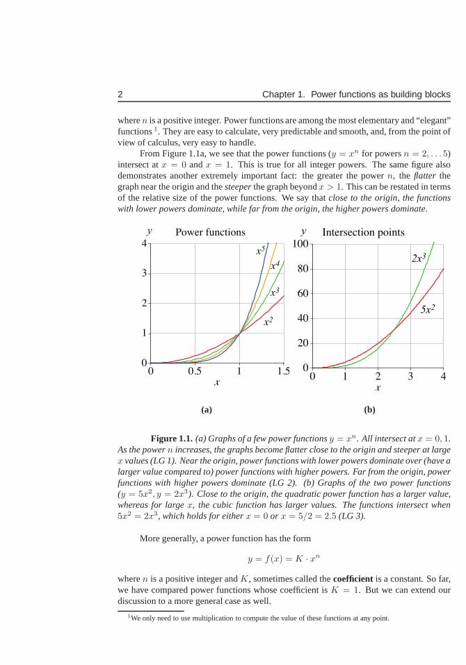
From Figure 1.1a, we see that the power functions (y = xn for powersn = 2, . . . 5)intersect atx = 0 andx = 1. This is true for all integer powers. The same figure alsodemonstrates another extremely important fact: the greater the powern, the flatter thegraph near the origin and thesteeperthe graph beyondx > 1. This can be restated in termsof the relative size of the power functions. We say thatclose to the origin, the functionswith lower powers dominate, while far from the origin, the higher powers dominate.
y
x2
x5
x3
x4
5x2
2x3
y
(a) (b)
Figure 1.1. (a) Graphs of a few power functionsy = xn. All intersect atx = 0, 1.As the powern increases, the graphs become flatter close to the origin and steeper at largex values (LG 1). Near the origin, power functions with lower powers dominate over (have alarger value compared to) power functions with higher powers. Far from the origin, powerfunctions with higher powers dominate (LG 2). (b) Graphs of the two power functions(y = 5x2, y = 2x3). Close to the origin, the quadratic power function has a larger value,whereas for largex, the cubic function has larger values. The functions intersect when5x2 = 2x3, which holds for eitherx = 0 or x = 5/2 = 2.5 (LG 3).
More generally, a power function has the form
y = f(x) = K · xn
wheren is a positive integer andK, sometimes called thecoefficient is a constant. So far,we have compared power functions whose coefficient isK = 1. But we can extend ourdiscussion to a more general case as well.
1We only need to use multiplication to compute the value of these functions at any point.
1.2. How big can a cell be? A model for nutrient balance 3
Example 1.1 Find points of intersection and compare the sizes of the two power functions
y1 = axn, and y2 = bxm.
wherea andb are constants. You may assume that botha andb are positive.
Solution: This comparison is a slight generalization of what we have seen above. First,we note that the coefficientsa andb merely scale the vertical behaviour (i.e. stretch thegraph along they axis. It is still true that the higher the power, the flatter the graph close tox = 0, and the steeper for large positive or negative values ofx. However, now the pointsof intersection of the graphs will occur atx = 0 and whenever
axn = bxm ⇒ xn−m = (b/a)
We can solve this further to obtain a solution in the first quadrant2,
x = (b/a)1/(n−m).
This is shown in Figure 1.1b for the specific example ofy1 = 5x2, y2 = 2x3. Here wepoint out that in general, ifb/a is a positive than this value is a real number. Since we haveassumed that botha andb are positive, this will be true.
Example 1.2 Determine points of intersection for the following pairs offunctions: (a)y1 = 3x4 andy2 = 27x2, (b) y1 = (4/3)πx3, y2 = 4πx2.
Solution: (a) Intersections occur atx = 0 and at±(27/3)1/(4−2) = ±√
9 = ±3. (b)These functions intersect only atx = 0, 3 but not for any negative values ofx.
In many cases, the points of intersection will be irrationalnumbers whose decimalapproximations can only be obtained by a scientific calculator or by some approximationmethod (such asNewton’s Method).
The observations we have made so far already allow us to examine a biological prob-lem related to the size of cells. We see that application of these ideas will provide insightinto why cells have a size limitation, as discussed in the next section.
1.2 How big can a cell be? A model for nutrientbalance
The shapes of living cells are designed to be uniquely suitedto their functions. Few cells arereally spherical. Many have long appendages, cylindrical parts, or branch-like structures.But here, we will neglect all these beautiful complexities and look at a simple sphericalcell. The question we want to explore is what physical or biological constraints determinethe size of a cell and why some size limitations exist. Why should animals be made ofmillions of tiny cells, instead of just a few hundred large ones?
2As we will shortly see, ifn, m are both even or both odd, there will also be an intersection in the thirdquadrant, atx = −(b/a)1/(n−m) .
4 Chapter 1. Power functions as building blocks
Learning goals
1. Follow and understand the derivation of a mathematical model for cell nutrient ab-sorption and consumption (Section 1.2.1).
2. Develop the skill of using parameters (k1, k2) rather than specific numbers in math-ematical expressions.
3. Understand the link between power functions in Section 1.1 and cell nutrient balancein the model (Eqs. 1.2).
4. Be able to verbally interpret the results of the model (Section 1.2.2).
r
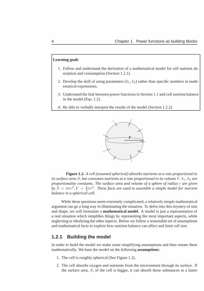
Figure 1.2.A cell (assumed spherical) absorbs nutrients at a rate proportional toits surface areaS, but consumes nutrients at a rate proportional to its volumeV. k1, k2 areproportionality constants. The surface area and volume of asphere of radiusr are givenby S = 4πr2, V = 4
3πr3. These facts are used to assemble a simple model for nutrientbalance in a spherical cell.
While these questions seem extremely complicated, a relatively simple mathematicalargument can go a long way in illuminating the situation. To delve into this mystery of sizeand shape, we will formulate amathematical model. A model is just a representation ofa real situation which simplifies things by representing themost important aspects, whileneglecting or idealizing the other aspects. Below we followa reasonable set of assumptionsand mathematical facts to explore how nutrient balance can affect and limit cell size.
1.2.1 Building the model
In order to build the model we make some simplifying assumptions and then restate themmathematically. We base the model on the followingassumptions:
1. The cell is roughly spherical (See Figure 1.2).
2. The cell absorbs oxygen and nutrients from the environment through its surface. Ifthe surface area,S, of the cell is bigger, it can absorb these substances at a faster
1.2. How big can a cell be? A model for nutrient balance 5
rate. We will assume that the rate at which nutrients (or oxygen) are absorbed isproportionalto the surface area of the cell.
3. The rate at which nutrients are consumed (i.e., used up) inmetabolism ispropor-tional to the volume,V , of the cell; This means that the rate of consumption is someconstant multiple of the volume, and it also implies that thebigger the volume, themore nutrients are needed to keep the cell alive. We will assume that the rate at whichnutrients (or oxygen) are consumed is proportional to the volume of the cell.
We define the following quantities for our model of a single cell:
A = net rate of absorption of nutrients per unit time,
C = net rate of consumption of nutrients per unit time,
V = cell volume,
S = cell surface area,
r = radius of the cell.
We now rephrase the assumptions mathematically. By assumption (2),A is propor-tional toS: This means that
A = k1S,
wherek1 is aconstant of proportionality . Since absorption and surface area are positivequantities, in this case only positive values of the proportionality constant make sense,sok1 must be positive. (The value of this constant would depend onthe permeability ofthe cell membrane, how many pores or channels it contains, and/or any active transportmechanisms that help transfer substances across the cell surface into its interior.)By usinga generic parameter to represent this proportionality constant, we keep the model generalenough to apply to many different cell types.(LG 2).
Further, by assumption (3), the rate of nutrient consumption,C is proportional toV ,so that
C = k2V,
wherek2 is a second proportionality constant (also positive3). The value ofk2 woulddepend on the rate of metabolism of the cell, i.e. how quicklyit consumes nutrients incarrying out its activities.
Since we have assumed that the cell is spherical, by assumption (1), the surface area,S, and volumeV of the cell are:
S = 4πr2, V =4
3πr3. (1.1)
Putting these facts together leads to the following relationships between nutrient absorption,consumption, and cell radius:
A = k1(4πr2) = (4πk1)r2, C = k2
(
4
3πr3
)
=
(
4
3πk2
)
r3.
3From now on, we will simply write “k2 > 0 is a constant” when we mean this constant to be positive.
6 Chapter 1. Power functions as building blocks
We note thatA, C are now quantities that depend on the radius of the cell.
A(r) = (4πk1)r2, and C(r) =
(
4
3πk2
)
r3. (1.2)
Indeed, since the terms in brackets on the right hand sides are just constant coeffi-cients,each of the above expressions is simply a power function(LG 3), with r the inde-pendent variable, that is
A(r) = ar2, C(r) = cr3 (wherea = 4πk1, c =4
3πk2 are constants).
Each of these expressions has the form of a power function,y = krn for some positiveconstant coefficientk. Most importantly, the powers aren = 3 for consumption andn = 2for absorption. We can now use the properties of power functions discussed perviously tounderstand how nutrient balance depends on cell size.
1.2.2 Nutrient balance depends on cell size
In our discussion of cell size, we found two power functions that depend on the cell ra-dius, namely the nutrient absorptionA(r) and consumptionC(r) rates given by Eqs. (1.2).Based on our discussion of power functions, we can characterize whether absorption orconsumption of nutrients dominates for small, medium, or large cells.
Example 1.3 Is the absorption rate or the consumption rate greater for small cells? Forlarge cells? For what cell size are the two rates equal?
Solution: For smallr, the power function with the lower power ofr (namelyA(r)) dom-inates, but for very large values ofr, the power function with the higher power (C(r))dominates. The switch takes place at the point of intersection of the two graphs
A(r) = C(r) ⇒(
4
3πk2
)
r3 = (4πk1)r2.
One trivial solution to this equation isr = 0. If r 6= 0, then we can cancel a factor ofr2
from both sides to obtain:
r = 3k1
k2.
For cells of this radius, absorption and consumption are equal, it follows that for smaller cellsizes the absorptionA ≈ r2 is the dominant process, while for large cells, the consumptionrateC ≈ r3 is higher than the absorption rate. We conclude that cells larger than the criticalsizer = 3k1/k2 will be unable to keep up with the nutrient demand, and will not survive.
Thus, using this simple geometric argument, we have deducedthat the size of the cellhas strong implications on its ability to absorb nutrients quickly enough to feed itself. Therestriction on oxygen absorption is even more critical thanthe replenishment of other sub-stances such as glucose. For these reasons, cells larger than some maximal size (roughly 1mm in diameter) rarely occur. Furthermore, organisms that are bigger than this size cannotrely on simple diffusion to carry oxygen to their parts—theymust develop a circulatorysystem to allow more rapid dispersal of such life-giving substances or else they will perish.
1.2. How big can a cell be? A model for nutrient balance 7
1.2.3 Even and odd power functions
So far, we have considered power functionsy = xn with x > 0. But in general, thereis no reason to restrict the independent variablex to positive values. Here we expandthe discussion to consider all real values ofx. This brings up some new ideas, includingsymmetry properties.
Even power functions
y=x2
-1.5 1.5
0.0
2.0
y=x6
y=x4
Odd power functions
-1.5 1.5
-2.0
2.0
y=x
y=x5
y=x3
(a) (b)
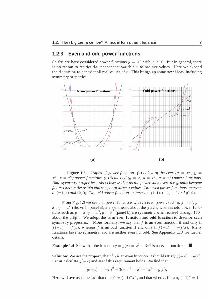
Figure 1.3. Graphs of power functions (a) A few of the even (y = x2, y =x4, y = x6) power functions (b) Some odd (y = x, y = x3, y = x5) power functions.Note symmetry properties. Also observe that as the power increases, the graphs becomeflatter close to the origin and steeper at largex values. Two even power functions intersectat (±1, 1) and(0, 0). Two odd power functions intersect at(1, 1), (−1,−1) and(0, 0).
From Fig. 1.3 we see that power functions with an even power, such asy = x2, y =x4, y = x6 (shown in panel a), are symmetric about they axis, whereas odd power func-tions such asy = x, y = x3, y = x5 (panel b) are symmetric when rotated through 180◦
about the origin. We adopt the termeven function and odd function to describe suchsymmetry properties. More formally, we say thatf is an even function if and only iff(−x) = f(x), whereasf is an odd function if and only iff(−x) = −f(x). Manyfunctions have no symmetry, and are neither even nor odd. SeeAppendix C.D for furtherdetails.
Example 1.4 Show that the functiony = g(x) = x2 − 3x4 is an even function
Solution: We use the property that ifg is an even function, it should satisfyg(−x) = g(x).Let us calculateg(−x) and see if this requirement holds. We find that
g(−x) = (−x)2 − 3(−x)4 = x2 − 3x4 = g(x).
Here we have used the fact that(−x)n = (−1)nxn, and that whenn is even,(−1)n = 1.
8 Chapter 1. Power functions as building blocks
All power functions are continuous andunbounded. Forx→∞ both even and oddpower functions satisfyy = xn → ∞. Forx → −∞, odd power functions tend to−∞.Odd power functions have the property that they areone-to-one. (That is, each value ofyis obtained from a unique value ofx and vice versa.) This is not the case for the even powerfunctions as we can see from Fig 1.3(a): for example,y = 1 is obtained by evaluating thefunctiony = x2 at eitherx = 1 or x = −1, and every other positive value ofy is similarlyobtained by evaluating a given power function at a positive or a negative value ofx. FromFig 1.3 we see that all power functions go through the point(0, 0). Even power functionshave alocal minimum at the origin whereas odd power functions do not.
Definition 1.5 (Local Minimum). A local minimum of a functionf(x) is a pointxmin
such that the value off is larger at all sufficiently close points. Formally,f(xmin ± ǫ) >f(xmin) for ǫ small enough.
1.3 Sustainability and Energy balance on PlanetEarth
The sustainability of life on Planet Earth depends on a fine balance between the temperatureof its oceans and land masses and the ability of life forms to tolerate climate change. As afollowup to our model for nutrient balance, we briefly introduce a simple energy balancemodel to track incoming and outgoing energy and to determinea rough estimate for theEarth’s temperature. We use the following basic facts:
1. Energy input from the sun to Earth given the Earth’s radiusr can be approximated as
Ein = (1− a)Sπr2, (1.3)
whereS is incoming radiation energy per unit area (also called thesolar constant)and0 ≤ a ≤ 1 is the fraction of that energy reflected.a is also called thealbedo,and depends on cloud cover, and other aspects of the planet (such as percent forest,snow, desert, and ocean).
2. Energy lost from Earth due to radiation into space dependson the current temperatureof the EarthT , and is approximated as
Eout = 4πr2ǫσT 4, (1.4)
whereǫ is theemissivityof the Earth’s atmosphere, which represents the Earth’s ten-dency to emit radiation energy. This constant depends on cloud cover, water vapor aswell as andgreenhouse gasconcentration in the atmosphere, such as carbon dioxide,and methane levels.σ is a physical constant (the Stephan-Bolzmann constant) whichis fixed for the purpose of our discussion.
Example 1.6 (Energy expressions are power functions)Explain in what sense the twoforms of energy above can be viewed as power functions, and what types of power functionsthey represent.
1.4. Combining power functions: first steps in graph sketching 9
Solution: BothEin andEout depend on Earth’s radius as the power∼ r2. however, sincethis radius is a constant, it will not be fruitful to considerit as an interesting variable forthis problem (unlike the cell size example we previously discussed). However, we note thatEout depends on temperature as∼ T 4. (We might also select the albedo as a variable andin that case, we note thatEin depends linearly on the albedoa4.)
Example 1.7 (Energy equilibrium for the Earth) Explain how the facts above can beused to determine the equilibrium temperature of the Earth,that is, the temperature atwhich the incoming and outgoing radiation energies are balanced.
Solution: The Earth will be at equilibrium when
Ein = Eout ⇒ (1− a)Sπr2 = 4πr2ǫσT 4.
We observe that the factorsπr2 cancel, and we obtain an equation that can be solved for thetemperatureT . (See Exercise 21) It is instructive to examine how this temperature dependson the constants in the problem, and how it is affected by cloud cover and greenhouse gaslevel. We discuss these issues in the same exercise.
1.4 Combining power functions: first steps in graphsketching
Properties of the power functions leads to important consequences in functions made upof such components. Here we discuss two important classes, simple polynomials (sumsof power functions) andrational functions (ratios of such functions). We show that theideas discussed in Section 1.1 lead directly and immediately to understanding the overallbehaviour of such functions. We also take some preliminary but fundamentally impor-tant steps in sketching the graphs of these functions, a skill that will prove of great valuethroughout this course.
Learning goals
1. Be able to easily sketch the graph of a simple polynomial ofthe formy = axn+bxm
(Fig. 1.4).
2. Be able to sketch a rational function such asy = Axn/(b + xm).
1.4.1 Sketching a simple (two-term) polynomial
Example 1.8 (Sketching a simple cubic polynomial)Sketch a graph of the polynomial
y = p(x) = x3 + ax. (1.5)
How would the sketch change if the constanta changes from positive to negative?
10 Chapter 1. Power functions as building blocks
x x x
y y y
a<0 a=0 a>0
x x x
x x x
y y y
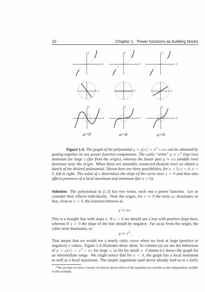
Figure 1.4.The graph of the polynomialy = p(x) = x3 + ax can be obtained byputting together its two power function components. The cubic “arms” y ≈ x3 (top row)dominate for largex (far from the origin), whereas the linear party ≈ ax (middle row)dominate near the origin. When these are smoothly connected(bottom row) we obtain asketch of the desired polynomial. Shown here are three possibilities, for a < 0, a = 0, a >0, left to right. The value ofa determines the slope of the curve nearx = 0 and thus alsoaffects presence of a local maximum and minimum (fora < 0).
Solution: The polynomial in (1.5) has two terms, each one a power function. Let usconsider their effects individually. Near the origin, forx ≈ 0 the termax dominates sothat, close tox = 0, the function behaves as
y ≈ ax.
This is a straight line with slopea. If a > 0 we should see a line with positive slope here,whereas ifa < 0 the slope of the line should be negative. Far away from the origin, thecubic term dominates, so
y ≈ x3.
That means that we would see a nearly cubic curve when we look at large (positive ornegative)x values. Figure 1.4 illustrates these ideas. In column (a) wesee the behaviourof y = p(x) = x3 + ax for largex, in (b) for smallx. Column (c) shows the graph foran intermediate range. We might notice that fora < 0, the graph has a local minimumas well as a local maximum. The simple arguments used above already lead us to a fairly
4We see that we have a variety of choices about which of the quantities to consider as the independent variablein this example.
1.4. Combining power functions: first steps in graph sketching 11
reasonable sketch of the function in (1.5). We can add further details by simple algebraicsteps as below.
Example 1.9 (Zeros)Find the places at which the polynomial (1.5) crosses thex axis, thatis, find thezerosof the functiony = x3 + ax.
Solution: The zeros of the polynomial can be found by setting
y = p(x) = 0 ⇒ x3 + ax = 0 ⇒ x3 = −ax.
The above equation always has a solutionx = 0, but if x 6= 0, we can cancel and obtain
x2 = −a.
This would have no solutions ifa is a positive number, so that in that case, the graph crossesthex axis only once, atx = 0, as shown in Figure 1.4. Ifa is negative, then the negativescancel, so the equation can be written in the form
x2 = |a|
and we would have two new zeros at
x = ±√
|a|.
For example, ifa = −1 then the functiony = x3 − x has zeros atx = 0, 1,−1.
Example 1.10 (A more general case)Explain how you would use the ideas of Exam-ple 1.8 to sketch the polynomialy = p(x) = axn + bxm. Without loss of generality,you may assume thatn > m ≥ 1 are integers.
Solution: As in Example 1.8, this polynomial has two terms that dominate at differentranges of the independent variable. Close to the origin,y ≈ bxm (sincem is the lowerpower) whereas for largex, y ≈ axn. The full behaviour is obtained by smoothly connect-ing these pieces of the graph. Finding zeros can refine the graph. Some examples of thistype are discussed in the Exercises (See Exercise 6).
The reasoning used here is a very important first step in sketching a polynomial. Laterin this course we will develop specialized methods to find zeros of more complicated cases(using an approximation calledNewton’s method). We will also use calculus to determinepoints at which the function attains local maxima or minima (calledcritical points ), andhow it behaves asymptotically, for large positive or negative values ofx. The elementarysteps described here will remain useful in later work as a quick approach for visualizingthe overall shape of a graph.
12 Chapter 1. Power functions as building blocks
1.4.2 Sketching a simple rational function
We use similar reasoning to consider the graphs of simple rational functions. Arationalfunction is a function that can be written as
y =p1(x)
p2(x), where p1(x) andp2(x) are polynomials.
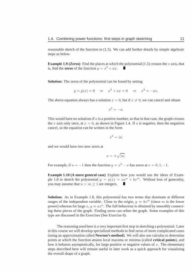
Example 1.11 (A rational function) Sketch the graph of the rational function
y =Axn
an + xn, x ≥ 0. (1.6)
What properties of your sketch depend on the powern? What would the graph look likefor n = 1, 2, 3?
Solution: We can break up the process of understanding this function into the followingsteps:
• The graph of the function (1.6) goes through the origin. (Atx = 0, we see thaty = 0.)
• For very smallx, (i.e.,x << a) we can approximate the denominator by the constantterman + xn ≈ an sincexn is negligible by comparison, so that
y =Axn
an + xn≈ Axn
an=
(
A
an
)
xn for smallx.
This means that near the origin, the graph looks like a power function,Cxn (whereC = A/an).
• For largex, i.e. x >> a, we havean + xn ≈ xn so that
y =Axn
an + xn≈ Axn
xn= A for largex.
This reveals that the graph has a horizontal asymptotey = A at large values ofx.
• Since the function behaves like a simple power function close to the origin, we con-clude directly that the higher the value ofn, the flatter is its graph near 0. Further,largen means sharper rise to the eventual asymptote.
The results are displayed in Fig. 1.5.
1.5 Rate of an enzyme-catalyzed reactionRational functions introduced in Example 1.11 often play a role in biochemistry. Here wediscuss two important examples and the contexts in which they appear. In both cases, weconsider the initial rise of the function as well as its eventual saturation.
1.5. Rate of an enzyme-catalyzed reaction 13
x
y
x
y
x
23
y
A
Small x Large x Smoothly connected
n=1
n=3
n=2n=1
Figure 1.5. The rational functions(1.6) with n = 1, 2, 3 are compared on thisgraph. Close to the origin, the function behaves like a powerfunction, whereas for largexthere is a horizontal asymptote aty = A. Asn increases, the graph becomes flatter closeto the origin, and steeper in its rise to the asymptote.
Learning goals
1. Understand the connection between Michaelis-Menten kinetics in biochemistry andrational functions described in Section 1.4.2.
2. Be able to interpret properties of a graph such as Fig. 1.7 in terms of properties of anenzyme-catalyzed reactions.
1.5.1 Saturation and Michaelis-Menten kinetics
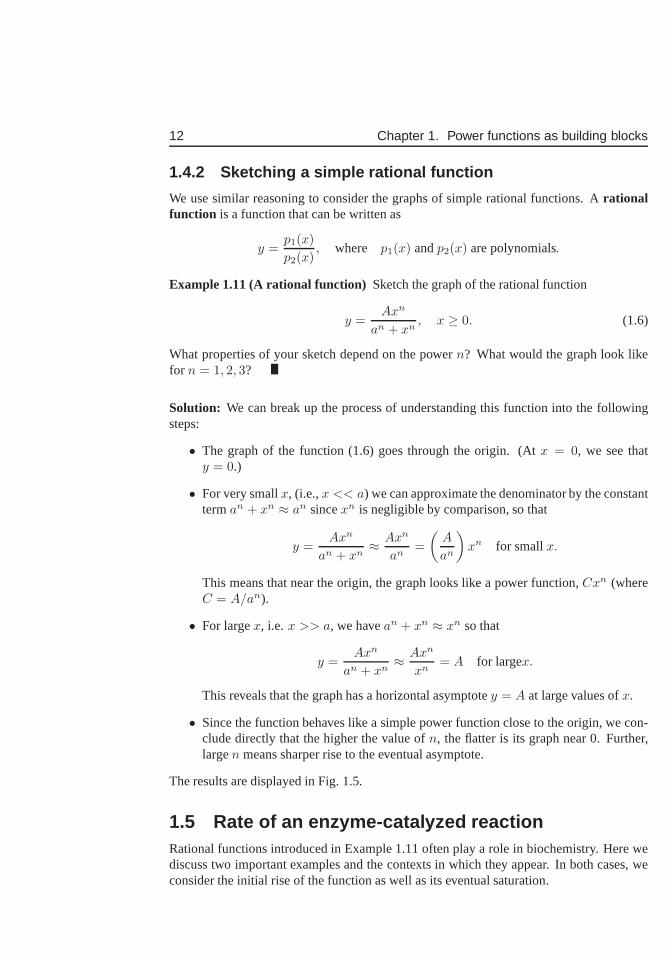
Biochemical reactions are often based on the action of proteins known asenzymesthatcatalyze many reactions in living cells. Shown in Fig. 1.6 isa typical scheme. The enzymeE binds to itssubstrateS to form acomplexC. The complex then breaks apart into aprod-uct, P, and an enzyme molecule that can repeat its action again. Generally, the substrate ismuch more plentiful than the enzyme.
E S C E P
k1
k-1
k2
Figure 1.6.An enzyme (catalytic protein) is shown binding to a substrate molecule(circular dot) and then processing it into a product (star shaped molecule).
In the context of this example,x represents the concentration of substrate in the re-action mixture. The speed of the reaction,v, (namely the rate at which product is formed)depends onx. But the relationship is not linear, as shown in Fig. 1.7. In fact, this relation-
14 Chapter 1. Power functions as building blocks
ships, known asMichaelis Mentenkinetics, has the form
v =Kx
kn + x, (1.7)
whereK, kn > 0 are positive constants that are specific to the enzyme and theexperimentalconditions.
n=3
0.0 10.0
0.0
3.0v
cinitial rise
saturation
0.0
1000.0
0.0
1.0
n=2
n=1K
K/2
kn
Michaelis Menten Kinetics Hill function Kinetics
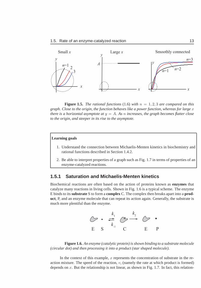
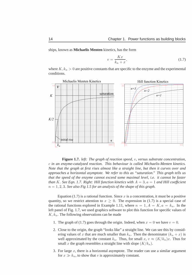
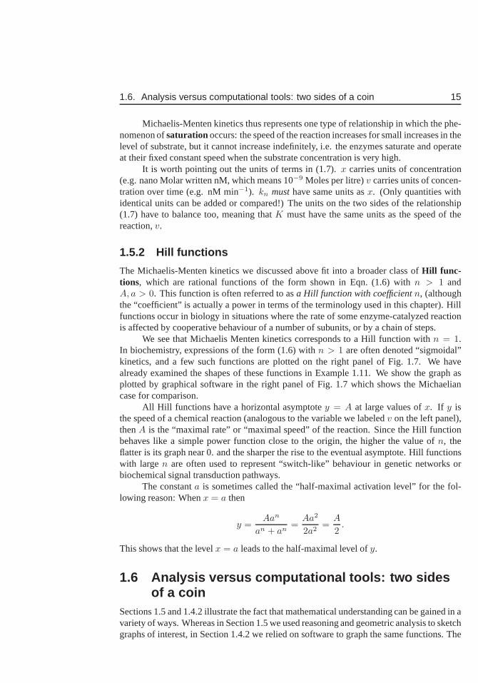
Figure 1.7. left: The graph of reaction speed,v, versus substrate concentration,c in an enzyme-catalyzed reaction. This behaviour is called Michaelis-Menten kinetics.Note that the graph at first rises almost like a straight line,but then it curves over andapproaches a horizontal asymptote. We refer to this as “saturation.” This graph tells usthat the speed of the enzyme cannot exceed some maximal level, i.e. it cannot be fasterthanK. See Eqn. 1.7. Right: Hill function kinetics withA = 3, a = 1 and Hill coefficientn = 1, 2, 3. See also Fig 1.5 for an analysis of the shape of this graph.
Equation (1.7) is a rational function. Sincex is a concentration, it must be a positivequantity, so we restrict attention tox ≥ 0. The expression in (1.7) is a special case ofthe rational functions explored in Example 1.11, wheren = 1, A = K, a = kn. In theleft panel of Fig. 1.7, we used graphics software to plot thisfunction for specific values ofK, kn. The following observations can be made
1. The graph of (1.7) goes through the origin. Indeed, whenx = 0 we havev = 0.
2. Close to the origin, the graph “looks like” a straight line. We can see this by consid-ering values ofx that are much smaller thankn. Then the denominator(kn + x) iswell approximated by the constantkn. Thus, for smallx, v ≈ (K/kn)x. Thus forsmallx the graph resembles a straight line with slope(K/kn).
3. For largex, there is a horizontal asymptote. The reader can use a similar argumentfor x≫ kn, to show thatv is approximately constant.
1.6. Analysis versus computational tools: two sides of a coin 15
Michaelis-Menten kinetics thus represents one type of relationship in which the phe-nomenon ofsaturation occurs: the speed of the reaction increases for small increases in thelevel of substrate, but it cannot increase indefinitely, i.e. the enzymes saturate and operateat their fixed constant speed when the substrate concentration is very high.
It is worth pointing out the units of terms in (1.7).x carries units of concentration(e.g. nano Molar written nM, which means 10−9 Moles per litre)v carries units of concen-tration over time (e.g. nM min−1). kn musthave same units asx. (Only quantities withidentical units can be added or compared!) The units on the two sides of the relationship(1.7) have to balance too, meaning thatK must have the same units as the speed of thereaction,v.
1.5.2 Hill functions
The Michaelis-Menten kinetics we discussed above fit into a broader class ofHill func-tions, which are rational functions of the form shown in Eqn. (1.6)with n > 1 andA, a > 0. This function is often referred to asa Hill function with coefficientn, (althoughthe “coefficient” is actually a power in terms of the terminology used in this chapter). Hillfunctions occur in biology in situations where the rate of some enzyme-catalyzed reactionis affected by cooperative behaviour of a number of subunits, or by a chain of steps.
We see that Michaelis Menten kinetics corresponds to a Hill function withn = 1.In biochemistry, expressions of the form (1.6) withn > 1 are often denoted “sigmoidal”kinetics, and a few such functions are plotted on the right panel of Fig. 1.7. We havealready examined the shapes of these functions in Example 1.11. We show the graph asplotted by graphical software in the right panel of Fig. 1.7 which shows the Michaeliancase for comparison.
All Hill functions have a horizontal asymptotey = A at large values ofx. If y isthe speed of a chemical reaction (analogous to the variable we labeledv on the left panel),thenA is the “maximal rate” or “maximal speed” of the reaction. Since the Hill functionbehaves like a simple power function close to the origin, thehigher the value ofn, theflatter is its graph near 0. and the sharper the rise to the eventual asymptote. Hill functionswith largen are often used to represent “switch-like” behaviour in genetic networks orbiochemical signal transduction pathways.
The constanta is sometimes called the “half-maximal activation level” for the fol-lowing reason: Whenx = a then
y =Aan
an + an=
Aa2
2a2=
A
2.
This shows that the levelx = a leads to the half-maximal level ofy.
1.6 Analysis versus computational tools: two sidesof a coin
Sections 1.5 and 1.4.2 illustrate the fact that mathematical understanding can be gained in avariety of ways. Whereas in Section 1.5 we used reasoning andgeometric analysis to sketchgraphs of interest, in Section 1.4.2 we relied on software tograph the same functions. The
16 Chapter 1. Power functions as building blocks
two approaches complement one another: one helps to anticipate the shape of the function,while the other provides greater accuracy provided we pick areasonable range of valuesfor the plot. This idea of using distinct but complementary approaches will be used often.Rough sketches will supplement the more precise graphing that we accomplish using thecalculus, while harnessing software to help finalize our results will also provide strongcomputational support for calculations that are otherwisetedious or repetitive.
1.7 For further study: Michaelis-Menten transformedto a linear relationship
Michaelis-Menten kinetics that we explored in (1.7) is a nonlinear saturating function inwhich the concentrationx is the independent variable on which the reaction velocity,vdepends. As discussed in Section 1.5.1, the constantsK andkn depend on the enzyme andare often quantified in a biochemical assay of enzyme action.In older times, a convenientway to estimate the values ofK andkn was to measurev for many different values of theinitial substrate concentration. Before nonlinear fittingsoftware was widely available, theexpression (1.7) was transformed (meaning that it was rewritten as a linear relationship.
We can do so with the following algebraic steps:
v =Kx
kn + x
so, taking reciprocals and expanding leads to
1
v=
kn + x
Kx,
=kn
Kx+
x
Kx
=
(
kn
K
)
1
x+
(
1
K
)
This suggests defining the two constants:
m =kn
K, b =
1
K.
In which case, the relationship between1/v and1/x becomes linear:
[
1
v
]
= m
[
1
x
]
+ b. (1.8)
Both the slope,m and interceptb of the straight line provide information about the param-eters. The relationship (1.8), which is a disguised variantof Michaelian kinetics is calledthe Linweaver-Burke relationship. Later, we will see how this can be used to estimate thevalues ofK andkn from biochemical data about an enzyme.
1.8. For further study: Spacing of fish in a school 17
1.8 For further study: Spacing of fish in a schoolMany animals live or function best when they are in a group. Social groups include herdsof wildebeest, flocks of birds, and schools of fish, as well as swarms of insects. Life in agroup can affect the way that individuals forage (search forfood), their success at detectingor avoiding being eaten by a predator, and other functions such as mating, protection ofthe young, etc. Biologists are interested in the ecologicalimplications of groups on theirown members or on other species with whom they interact, and how individual behaviour,combined with environmental factors and random effects affect the shape of the groups, thespacing, and the function.
In many social groups, the spacing between individuals is relatively constant fromone part of the formation to another, because animals that get too close start to move awayfrom one another, whereas those that get too far apart are attracted back. These spacingdistances can be observed in a variety of groups, and were described in many biologicalpublications. For example, Emlen [10] found that in flocks, gulls are spaced at about onebody length apart, whereas Conder [11] observed a 2-3 body lengths spacing distance intufted ducks. Miller [13] observed that sandhill cranes tryto keep about 5.8 ft apart in theflock he observed.
To try to explain why certain spacing is maintained in a groupof animals, it wasproposed that there are mutual attraction and repulsion interactions, (effectively acting likesimple forces) between individuals. Breder [3] followed a number of species of fish thatschool, and measured the individual spacing in units of the fish body length, showing thatindividuals are separated by 0.16-0.25 body length units. He suggested that the effectiveforces between individuals were similar to inverse power laws for repulsion and attraction.Breder considered a quantity he calledcohesiveness, defined as:
c =A
xm− R
xn, (1.9)
whereA, R are magnitudes of attraction and repulsion,x is the distance between individ-uals, andm, n are integer powers that govern how quickly the interactionsfall off withdistance. We could re-express the formula (1.9) as
c = Ax−m −Rx−n
Thus, the function shown in Breder’s cohesiveness formula is related to our power func-tions, but the powers are negative integers. A specific case considered by Breder wasm = 0, n = 2, i.e. constant attraction and inverse square law repulsion,
c = A− (R/x2)
Breder specifically considered the “point of neutrality”, wherec = 0. The distance atwhich this occurs is:
x = (R/A)1/2
where attraction and repulsion are balanced. This is the distance at which two fish wouldbe most comfortable: neither tending to move apart, nor get closer together.
Other ecologists studying a similar problem have used a variety of assumptions aboutforces that cause group members to attract or repel one another.
18 Chapter 1. Power functions as building blocks
Exercises1.1. Power functions: Consider the power function
y = axn, −∞ < x <∞
Explain verbally (or using a sketch) how the shape of the function changes whenthe coefficienta increases or decreases (for fixedn). How is this change in shapedifferent from the shape change that results from changing the powern?
1.2. Simple transformations: Consider the graphs of the simple functionsy = x, y =x2, andy = x3. What happens to each of these graphs when the functions aretransformedas follows:
(a) y = Ax, y = Ax2, andy = Ax3 whereA > 1 is some constant.
(b) y = x + a, y = x2 + a, andy = x3 + a wherea > 0 is some constant.
(c) y = (x− b)2, andy = (x− b)3 whereb > 0 is some constant.
1.3. Simple sketches:Sketch the graphs of the following functions:
(a) y = x2,
(b) y = (x + 4)2
(c) y = a(x− b)2 + c for the casea > 0, b > 0, c > 0.
(d) Comment on the effects of the constantsa, b, c on the properties of the graphof y = a(x− b)2 + c.
1.4. Sketching simple polynomials:Use arguments from Section 1.4 to sketch graphsof the following simple polynomials:
(a) y = 2x5 − 3x2,
(b) y = x3 − 4x5.
1.5. Finding points of intersection(I):
(a) Consider the two functionsf(x) = 3x2 andg(x) = 2x5. Find all points ofintersection of these functions.
(b) Repeat the calculation for the two functionsf(x) = x3 andg(x) = 4x5.
Observe that finding these points of intersection is equivalent to calculating thezerosof the functions in Problem 4.
1.6. Qualitative sketching skills:
(a) Sketch the graph of the functiony = ax− x5 for positive and negative valuesof the constanta. Comment on behaviour close to zero and far away fromzero.
(b) What are the zeros of this function and how does this depend ona ?
(c) For what values ofa would you expect that this function would have a localmaximum (“peak”) and a local minimum (“valley”)?
Exercises 19
1.7. Finding points of intersection(II): Consider the two functionsf(x) = Axn andg(x) = Bxm. Supposem > n > 1 are integers, andA, B > 0. Determine thevalues ofx at which the values of the functions are the same. Are there two placesof intersection or three? How does this depend on the integerm − n? (Remark:The point (0,0) is always an intersection point. Thus, we areasking when there isonly onemore and when there aretwo more intersection points. See Problem 5 fora simple example of both types.)
1.8. More intersection points: Find the intersection of each pair of functions.
(a) y =√
x, y = x2
(b) y = −√x, y = x2
(c) y = x2 − 1, x2
4 + y2 = 1
1.9. Crossing thex axis: Answer the following problem by solving forx in each case.Find all values ofx for which the following functions cross thex axis (also calledzerosof the function, orroots of the equationf(x) = 0.)
(a) f(x) = I − γx, whereI, γ are positive constants.
(b) f(x) = I − γx + ǫx2, whereI, γ, ǫ are positive constants. Are there caseswhere this function does not cross thex axis?
(c) In the case where the root(s) exist in part (b), are they positive, negative or ofmixed signs?
1.10. Crossing thex axis, continued:Answer Problem 9 by sketching a rough graph ofeach of the functions in parts (a-b) and using these sketchesto answer the questionof how many real roots there can be and where they are located (on the positive ornegativex axis). Note: This problem provides very important qualitative analysisskills that will become useful in later applications.
1.11. Power functions: Consider the functionsy = xn, y = x1/n, y = x−n, wheren isan integer (n = 1, 2..) Which of these functions increases most steeply for valuesofx greater than 1? Which decreases for large values ofx? Which functions are notdefined for negativex values? Compare the values of these functions for0 < x < 1.Which of these functions are not defined atx = 0?
1.12. Roots of a quadratic: Find the range ofm such that the equationx2− 2x−m = 0has two unequal roots.
1.13. Rational Functions: In support of Learning Goal 2 of Section 1.4, describe theshape of the graph of the functiony = Axn/(b + xm) in two cases: (a)n > m and(b) m > n.
1.14. Power functions with negative powers:Consider the function
f(x) =A
xa
whereA > 0, a > 1, with a an integer. This is the same as the functionf(x) =Ax−a, which is a power function with a negative power.
(a) Sketch a rough graph of this function forx > 0.
(b) How does the function change ifA is increased?
20 Chapter 1. Power functions as building blocks
(c) How does the function change ifa is increased?
1.15. Intersections of functions with negative powers:Consider two functions of theform
f(x) =A
xa, g(x) =
B
xb.
Suppose thatA, B > 0, a, b > 1 and thatA > B. Determine where these functionsintersect for positivex values.
1.16. Zeros of polynomials:Find all real zeros of the following polynomials:
(a) x3 − 2x2 − 3x
(b) x5 − 1
(c) 3x2 + 5x− 2.
(d) Find the points of intersection of the functionsy = x3 + x2 − 2x + 1 andy = x3.
1.17. Inverse functions: The functionsy = x3 andy = x1/3 areinverse functions.
(a) Sketch both functions on the same graph for−2 < x < 2 showing clearlywhere they intersect.
(b) The tangent line to the curvey = x3 at the point (1,1) has slopem = 3,whereas the tangent line toy = x1/3 at the point (1,1) has slopem = 1/3.Explain the relationship of the two slopes.
1.18. Properties of a cube:The volumeV and surface areaS of a cube whose sides havelengtha are given by the formulae
V = a3, S = 6a2.
Note that these relationships are expressed in terms of power functions. The inde-pendent variable isa, not x. We say that “V is a function ofa” (and also “S is afunction ofa”).
(a) SketchV as a function ofa andS as a function ofa on the same set of axes.Which one grows faster asa increases?
(b) What is the ratio of the volume to the surface area; that is, what is VS in terms
of a? Sketch a graph ofVS as a function ofa.
(c) The formulae above tell us the volume and the area of a cubeof a given sidelength. But suppose we are given either the volume or the surface area andasked to find the side. Find the length of the side as a functionof the volume(i.e. expressa in terms ofV ). Find the side as a function of the surface area.Use your results to find the side of a cubic tank whose volume is1 litre (1 litre= 103 cm3). Find the side of a cubic tank whose surface area is10 cm2.
1.19. Properties of a sphere:The volumeV and surface areaS of a sphere of radiusrare given by the formulae
V =4π
3r3, S = 4πr2.
Exercises 21
Note that these relationships are expressed in terms of power functions with constantmultiples such as4π. The independent variable isr, not x. We say that “V is afunction ofr” (and also “S is a function ofr”).
(a) SketchV as a function ofr andS as a function ofr on the same set of axes.Which one grows faster asr increases?
(b) What is the ratio of the volume to the surface area; that is, what is VS in terms
of r? Sketch a graph ofVS as a function ofr.
(c) The formulae above tell us the volume and the area of a sphere of a givenradius. But suppose we are given either the volume or the surface area andasked to find the radius. Find the radius as a function of the volume (i.e.expressr in terms ofV ). Find the radius as a function of the surface area. Useyour results to find the radius of a balloon whose volume is 1 litre. (1 litre =103 cm3). Find the radius of a balloon whose surface area is10 cm2
1.20. The size of cell: Consider a cell in the shape of a thin cylinder (lengthL and ra-dius r). Assume that the cell absorbs nutrient through its surfaceat ratek1S andconsumes nutrients at ratek2V whereS, V are the surface area and volume of thecylinder. Here we assume thatk1 = 12µM µm−2 per min andk2 = 2µM µm−3
per min. (Note:µM is 10−6 moles.µm is10−6meters.) Use the fact that a cylinder(without end-caps) has surface areaS = 2πrL and volumeV = πr2L to determinethe cell radius such that the rate of consumption exactly balances the rate of absorp-tion. What do you expect happens to cells with a bigger or smaller radius? Howdoes the length of the cylinder affect this nutrient balance?
1.21. Energy equilibrium for Earth: This problem focuses on Earth’s temperature, cli-mate change, and sustainability.
(a) Complete the calculation for Example 1.7 by solving for the temperatureT ofthe Earth at which incoming and outgoing radiation energiesbalance.
(b) Assume that greenhouse gasses decrease the emissivityǫ of the Earth’s atmo-sphere. Explain how this would affect the Earth’s temperature.
(c) Explain how the size of the Earth affects its energy balance according to themodel.
(d) Explain how the albedoa affects the Earth’s temperature.
1.22. Allometric relationship: Properties of animals are often related to their physicalsize or mass. For example, the metabolic rate of the animal (R), and its pulse rate(P ) may be related to its body massm by the approximate formulaeR = Amb andP = Cmd, whereA, C, b, d are positive constants. Such relationships are known asallometricrelationships.
(a) Use these formulae to derive a relationship between the metabolic rate and thepulse rate (Hint: eliminatem).
(b) A similar process can be used to relate the VolumeV = (4/3)πr3 and surfaceareaS = 4πr2 of a sphere to one another. Eliminater to find the correspond-ing relationship between volume and surface area for a sphere.
22 Chapter 1. Power functions as building blocks
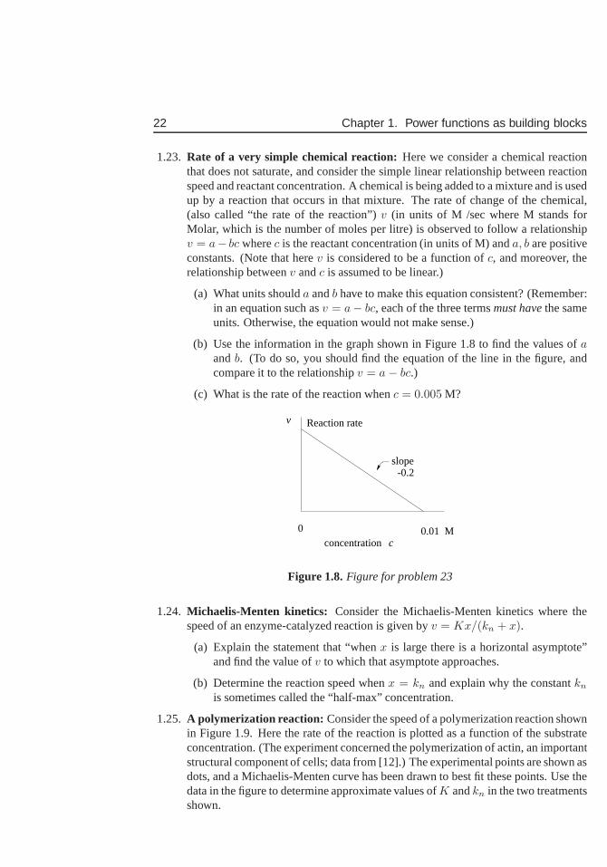
1.23. Rate of a very simple chemical reaction:Here we consider a chemical reactionthat does not saturate, and consider the simple linear relationship between reactionspeed and reactant concentration. A chemical is being addedto a mixture and is usedup by a reaction that occurs in that mixture. The rate of change of the chemical,(also called “the rate of the reaction”)v (in units of M /sec where M stands forMolar, which is the number of moles per litre) is observed to follow a relationshipv = a− bc wherec is the reactant concentration (in units of M) anda, b are positiveconstants. (Note that herev is considered to be a function ofc, and moreover, therelationship betweenv andc is assumed to be linear.)
(a) What units shoulda andb have to make this equation consistent? (Remember:in an equation such asv = a− bc, each of the three termsmust havethe sameunits. Otherwise, the equation would not make sense.)
(b) Use the information in the graph shown in Figure 1.8 to findthe values ofaandb. (To do so, you should find the equation of the line in the figure, andcompare it to the relationshipv = a− bc.)
(c) What is the rate of the reaction whenc = 0.005 M?
0 0.01 Mconcentration
v
c
slope
Reaction rate
-0.2
Figure 1.8.Figure for problem 23
1.24. Michaelis-Menten kinetics: Consider the Michaelis-Menten kinetics where thespeed of an enzyme-catalyzed reaction is given byv = Kx/(kn + x).
(a) Explain the statement that “whenx is large there is a horizontal asymptote”and find the value ofv to which that asymptote approaches.
(b) Determine the reaction speed whenx = kn and explain why the constantkn
is sometimes called the “half-max” concentration.
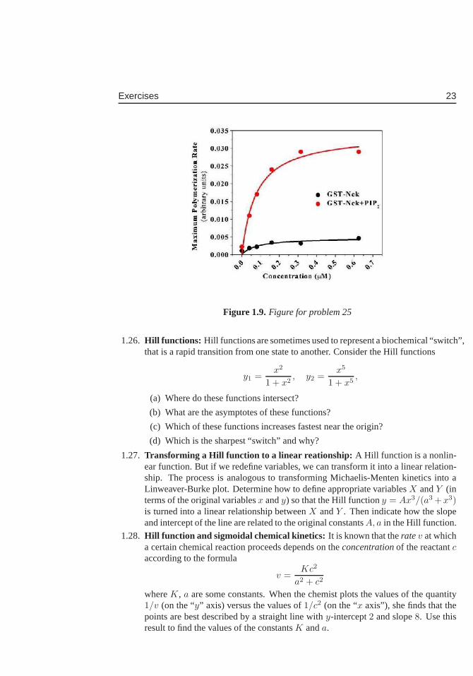
1.25. A polymerization reaction: Consider the speed of a polymerization reaction shownin Figure 1.9. Here the rate of the reaction is plotted as a function of the substrateconcentration. (The experiment concerned the polymerization of actin, an importantstructural component of cells; data from [12].) The experimental points are shown asdots, and a Michaelis-Menten curve has been drawn to best fit these points. Use thedata in the figure to determine approximate values ofK andkn in the two treatmentsshown.
Exercises 23
Figure 1.9.Figure for problem 25
1.26. Hill functions: Hill functions are sometimes used to represent a biochemical “switch”,that is a rapid transition from one state to another. Consider the Hill functions
y1 =x2
1 + x2, y2 =
x5
1 + x5,
(a) Where do these functions intersect?
(b) What are the asymptotes of these functions?
(c) Which of these functions increases fastest near the origin?
(d) Which is the sharpest “switch” and why?
1.27. Transforming a Hill function to a linear reationship: A Hill function is a nonlin-ear function. But if we redefine variables, we can transform it into a linear relation-ship. The process is analogous to transforming Michaelis-Menten kinetics into aLinweaver-Burke plot. Determine how to define appropriate variablesX andY (interms of the original variablesx andy) so that the Hill functiony = Ax3/(a3 +x3)is turned into a linear relationship betweenX andY . Then indicate how the slopeand intercept of the line are related to the original constantsA, a in the Hill function.
1.28. Hill function and sigmoidal chemical kinetics: It is known that theratev at whicha certain chemical reaction proceeds depends on theconcentrationof the reactantcaccording to the formula
v =Kc2
a2 + c2
whereK, a are some constants. When the chemist plots the values of the quantity1/v (on the “y” axis) versus the values of1/c2 (on the “x axis”), she finds that thepoints are best described by a straight line withy-intercept2 and slope8. Use thisresult to find the values of the constantsK anda.
24 Chapter 1. Power functions as building blocks
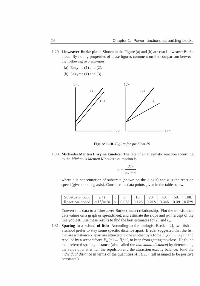
1.29. Linweaver-Burke plots: Shown in the Figure (a) and (b) are two Linweaver Burkeplots. By noting properties of these figures comment on the comparison betweenthe following two enzymes:
(a) Enzyme (1) and (2).
(b) Enzyme (1) and (3).
(1)
(2)
1/c
1/v
(1)
(3)
1/c
1/v
Figure 1.10.Figure for problem 29
1.30. Michaelis Menten Enzyme kinetics:The rate of an enzymatic reaction accordingto theMichaelis Menten Kineticsassumption is
v =Kc
kn + c,
wherec is concentration of substrate (shown on thex axis) andv is the reactionspeed (given on they axis). Consider the data points given in the table below:
Substrate conc nM c 5. 10. 20. 40. 50. 100.Reaction speed nM/min v 0.068 0.126 0.218 0.345 0.39 0.529
Convert this data to a Linweaver-Burke (linear) relationship. Plot the transformeddata values on a graph or spreadsheet, and estimate the slopeandy-intercept of theline you get. Use these results to find the best estimates forK andkn.
1.31. Spacing in a school of fish: According to the biologist Breder [2], two fish ina school prefer to stay some specific distance apart. Breder suggested that the fishthat are a distancex apart are attracted to one another by a forceFA(x) = A/xa andrepelled by a second forceFR(x) = R/xr, to keep from getting too close. He foundthe preferred spacing distance (also called theindividual distance) by determiningthe value ofx at which the repulsion and the attraction exactly balance. Find theindividual distancein terms of the quantitiesA, R, a, r (all assumed to be positiveconstants.)
Chapter 2
Average rates of change,average velocity and thesecant line
In this chapter, we introduce the idea of an average rate of change. To motivate ideas, weexamine data for two common processes, changes in temperature, and motion of a fallingobject. Simple experiments are described in each case, and some features of the data arediscussed. Based on each example, we define and calculate netchange over some timeinterval and so define theaverage rate of change. This concept generalizes to functions ofany variable (not only time). We interpret this idea geometrically, in terms of the slope ofa secant line.
In both cases, we then ask how to use the idea of the average rate of change (overa given interval) to find better and better approximations ofthe rate of change at a singleinstant, (i.e. at a point). We will see that one way to arrive at this abstract concept entailsrefining the dataset - collecting data at closer and closer time points. A second, moreabstract way, is to use the idea of a limit. Eventually, this procedure will allow us to arriveat the definition of thederivative, which is theinstantaneous rate of change.
2.1 Time-dependent data and rates of changeIn this section we consider two time dependent processes. Wemake several observationsabout actual data collected in studying those processes, and we arrive at the ideas of rates ofchange. We also use graphical software to represent the datafor the purpose of visualizationand for computing desired rates of change.
Section 2.1 Learning goals
1. Be able to use (your favorite) graphical software package(spreadsheet, graphics cal-culator, online tools, etc) to plot data points such as thosein Table 2.1.
2. Be able to describe verbally the trends seen in such data using words such as “in-creasing”, “decreasing”, “linear”, “nonlinear”, “shallow”, “steep” changes, etc.
25
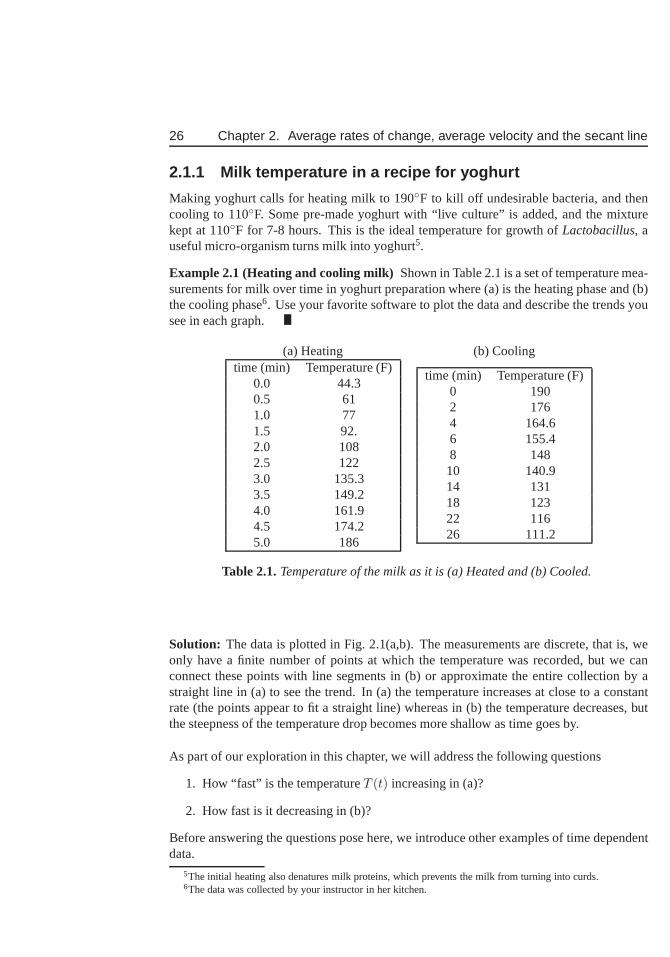
26 Chapter 2. Average rates of change, average velocity and the secant line
2.1.1 Milk temperature in a recipe for yoghurt
Making yoghurt calls for heating milk to 190◦F to kill off undesirable bacteria, and thencooling to 110◦F. Some pre-made yoghurt with “live culture” is added, and the mixturekept at 110◦F for 7-8 hours. This is the ideal temperature for growth ofLactobacillus, auseful micro-organism turns milk into yoghurt5.
Example 2.1 (Heating and cooling milk) Shown in Table 2.1 is a set of temperature mea-surements for milk over time in yoghurt preparation where (a) is the heating phase and (b)the cooling phase6. Use your favorite software to plot the data and describe thetrends yousee in each graph.
(a) Heating (b) Coolingtime (min) Temperature (F)
0.0 44.30.5 611.0 771.5 92.2.0 1082.5 1223.0 135.33.5 149.24.0 161.94.5 174.25.0 186
time (min) Temperature (F)0 1902 1764 164.66 155.48 14810 140.914 13118 12322 11626 111.2
Table 2.1.Temperature of the milk as it is (a) Heated and (b) Cooled.
Solution: The data is plotted in Fig. 2.1(a,b). The measurements are discrete, that is, weonly have a finite number of points at which the temperature was recorded, but we canconnect these points with line segments in (b) or approximate the entire collection by astraight line in (a) to see the trend. In (a) the temperature increases at close to a constantrate (the points appear to fit a straight line) whereas in (b) the temperature decreases, butthe steepness of the temperature drop becomes more shallow as time goes by.
As part of our exploration in this chapter, we will address the following questions
1. How “fast” is the temperatureT (t) increasing in (a)?
2. How fast is it decreasing in (b)?
Before answering the questions pose here, we introduce other examples of time dependentdata.
5The initial heating also denatures milk proteins, which prevents the milk from turning into curds.6The data was collected by your instructor in her kitchen.
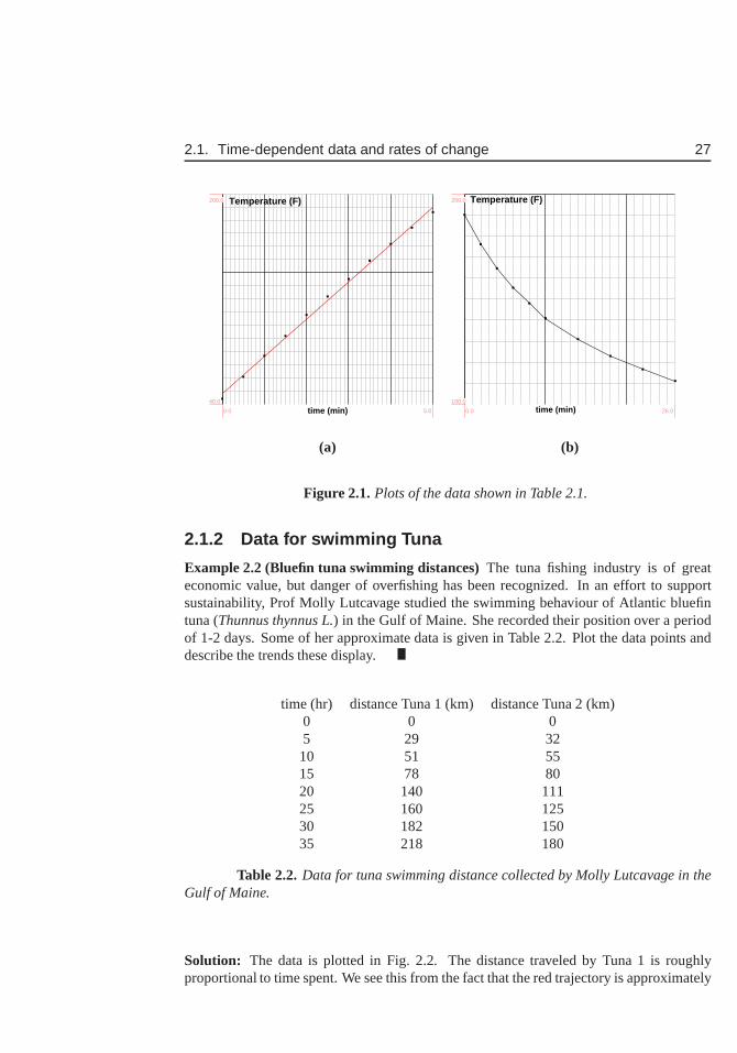
2.1. Time-dependent data and rates of change 27
Temperature (F)
time (min)0.0 5.0
40.0
200.0 Temperature (F)
time (min)0.0 26.0
100.0
200.0
(a) (b)
Figure 2.1.Plots of the data shown in Table 2.1.
2.1.2 Data for swimming Tuna
Example 2.2 (Bluefin tuna swimming distances)The tuna fishing industry is of greateconomic value, but danger of overfishing has been recognized. In an effort to supportsustainability, Prof Molly Lutcavage studied the swimmingbehaviour of Atlantic bluefintuna (Thunnus thynnus L.) in the Gulf of Maine. She recorded their position over a periodof 1-2 days. Some of her approximate data is given in Table 2.2. Plot the data points anddescribe the trends these display.
time (hr) distance Tuna 1 (km) distance Tuna 2 (km)0 0 05 29 3210 51 5515 78 8020 140 11125 160 12530 182 15035 218 180
Table 2.2.Data for tuna swimming distance collected by Molly Lutcavage in theGulf of Maine.
Solution: The data is plotted in Fig. 2.2. The distance traveled by Tuna1 is roughlyproportional to time spent. We see this from the fact that thered trajectory is approximately
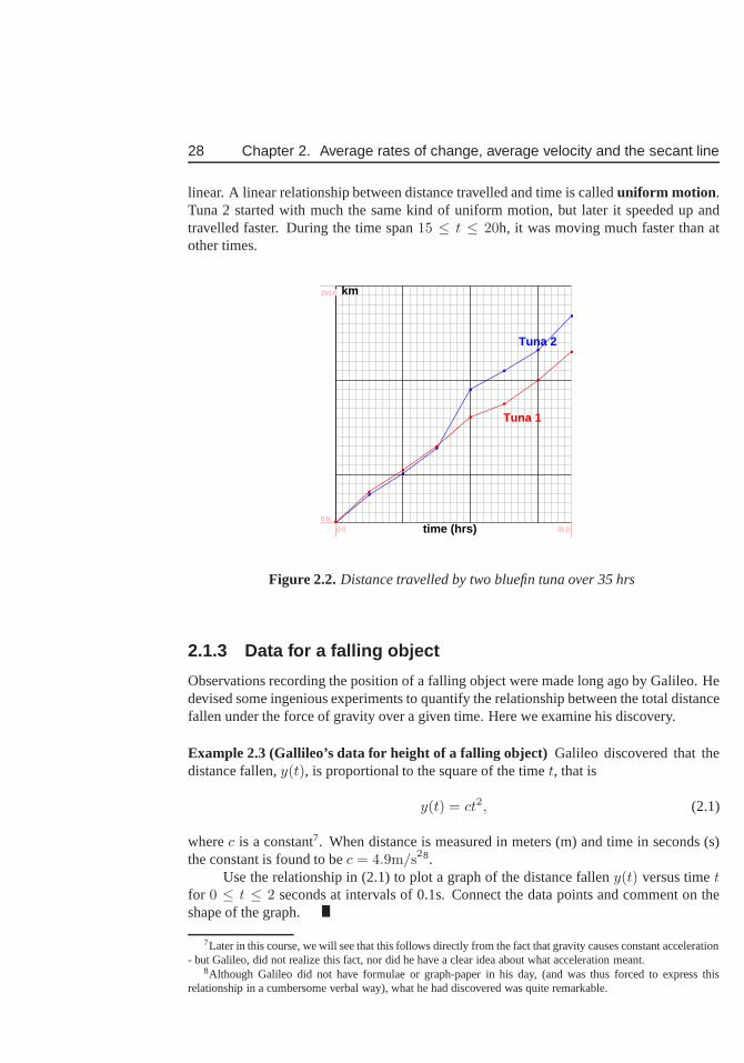
28 Chapter 2. Average rates of change, average velocity and the secant line
linear. A linear relationship between distance travelled and time is calleduniform motion .Tuna 2 started with much the same kind of uniform motion, but later it speeded up andtravelled faster. During the time span15 ≤ t ≤ 20h, it was moving much faster than atother times.
km
time (hrs)
Tuna 1
Tuna 2
0.0 35.0
0.0
250.0
Figure 2.2.Distance travelled by two bluefin tuna over 35 hrs
2.1.3 Data for a falling object
Observations recording the position of a falling object were made long ago by Galileo. Hedevised some ingenious experiments to quantify the relationship between the total distancefallen under the force of gravity over a given time. Here we examine his discovery.
Example 2.3 (Gallileo’s data for height of a falling object) Galileo discovered that thedistance fallen,y(t), is proportional to the square of the timet, that is
y(t) = ct2, (2.1)
wherec is a constant7. When distance is measured in meters (m) and time in seconds (s)the constant is found to bec = 4.9m/s
28.Use the relationship in (2.1) to plot a graph of the distance falleny(t) versus timet
for 0 ≤ t ≤ 2 seconds at intervals of 0.1s. Connect the data points and comment on theshape of the graph.
7Later in this course, we will see that this follows directly from the fact that gravity causes constant acceleration- but Galileo, did not realize this fact, nor did he have a clear idea about what acceleration meant.
8Although Galileo did not have formulae or graph-paper in hisday, (and was thus forced to express thisrelationship in a cumbersome verbal way), what he had discovered was quite remarkable.
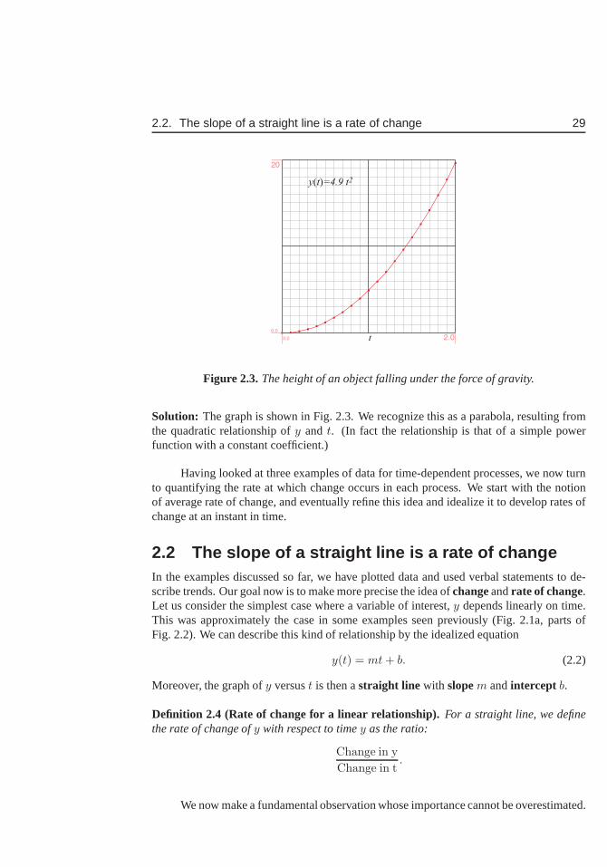
2.2. The slope of a straight line is a rate of change 29
y(t)=4.9 t2
0.0 2.0
0.0
20
t
Figure 2.3.The height of an object falling under the force of gravity.
Solution: The graph is shown in Fig. 2.3. We recognize this as a parabola, resulting fromthe quadratic relationship ofy and t. (In fact the relationship is that of a simple powerfunction with a constant coefficient.)
Having looked at three examples of data for time-dependent processes, we now turnto quantifying the rate at which change occurs in each process. We start with the notionof average rate of change, and eventually refine this idea andidealize it to develop rates ofchange at an instant in time.
2.2 The slope of a straight line is a rate of changeIn the examples discussed so far, we have plotted data and used verbal statements to de-scribe trends. Our goal now is to make more precise the idea ofchangeandrate of change.Let us consider the simplest case where a variable of interest, y depends linearly on time.This was approximately the case in some examples seen previously (Fig. 2.1a, parts ofFig. 2.2). We can describe this kind of relationship by the idealized equation
y(t) = mt + b. (2.2)
Moreover, the graph ofy versust is then astraight line with slopem andintercept b.
Definition 2.4 (Rate of change for a linear relationship).For a straight line, we definethe rate of change ofy with respect to timey as the ratio:
Change in y
Change in t.
We now make a fundamental observation whose importance cannot be overestimated.
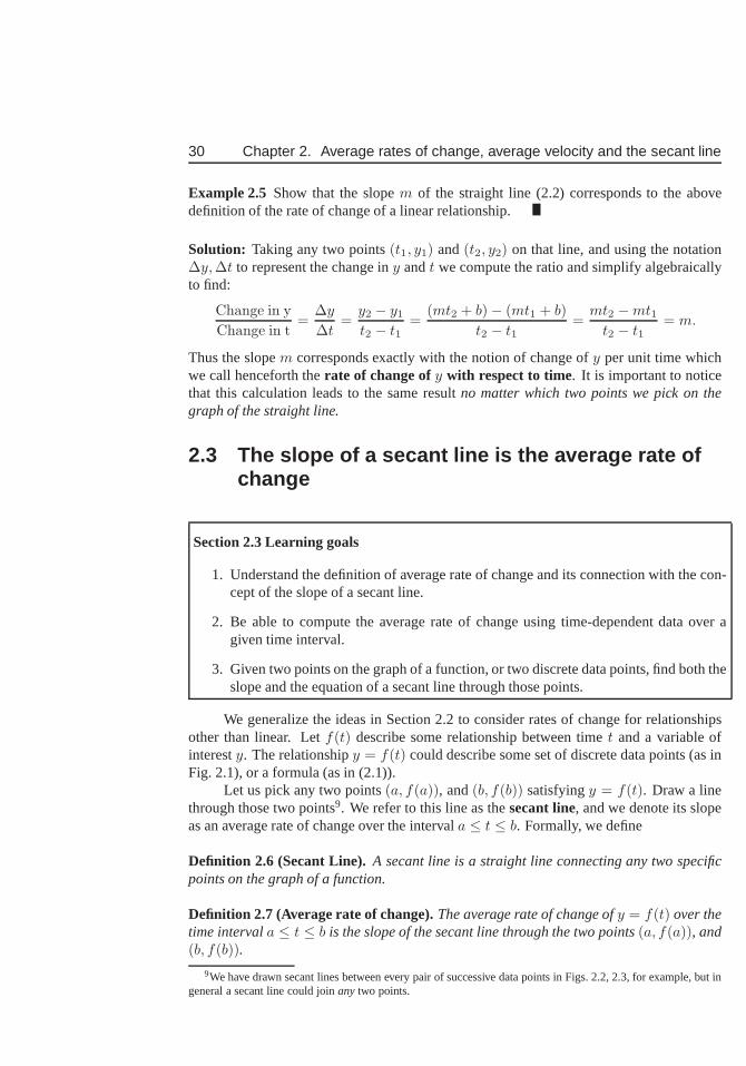
30 Chapter 2. Average rates of change, average velocity and the secant line
Example 2.5 Show that the slopem of the straight line (2.2) corresponds to the abovedefinition of the rate of change of a linear relationship.
Solution: Taking any two points(t1, y1) and(t2, y2) on that line, and using the notation∆y, ∆t to represent the change iny andt we compute the ratio and simplify algebraicallyto find:
Change in y
Change in t=
∆y
∆t=
y2 − y1
t2 − t1=
(mt2 + b)− (mt1 + b)
t2 − t1=
mt2 −mt1t2 − t1
= m.
Thus the slopem corresponds exactly with the notion of change ofy per unit time whichwe call henceforth therate of change ofy with respect to time. It is important to noticethat this calculation leads to the same resultno matter which two points we pick on thegraph of the straight line.
2.3 The slope of a secant line is the average rate ofchange
Section 2.3 Learning goals
1. Understand the definition of average rate of change and itsconnection with the con-cept of the slope of a secant line.
2. Be able to compute the average rate of change using time-dependent data over agiven time interval.
3. Given two points on the graph of a function, or two discretedata points, find both theslope and the equation of a secant line through those points.
We generalize the ideas in Section 2.2 to consider rates of change for relationshipsother than linear. Letf(t) describe some relationship between timet and a variable ofinteresty. The relationshipy = f(t) could describe some set of discrete data points (as inFig. 2.1), or a formula (as in (2.1)).
Let us pick any two points(a, f(a)), and(b, f(b)) satisfyingy = f(t). Draw a linethrough those two points9. We refer to this line as thesecant line, and we denote its slopeas an average rate of change over the intervala ≤ t ≤ b. Formally, we define
Definition 2.6 (Secant Line).A secant line is a straight line connecting any two specificpoints on the graph of a function.
Definition 2.7 (Average rate of change).The average rate of change ofy = f(t) over thetime intervala ≤ t ≤ b is the slope of the secant line through the two points(a, f(a)), and(b, f(b)).
9We have drawn secant lines between every pair of successive data points in Figs. 2.2, 2.3, for example, but ingeneral a secant line could joinanytwo points.
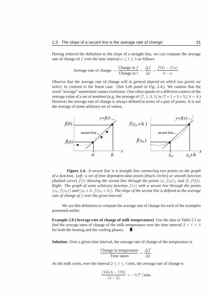
2.3. The slope of a secant line is the average rate of change 31
Having reduced the definition to the slope of a straight line,we can compute the averagerate of change off over the time intervala ≤ t ≤ b as follows
Average rate of change=Change infChange int
=∆f
∆t=
f(b)− f(a)
b− a.
Observe that the average rate of change will in generaldepend on which two points weselect, in contrast to the linear case. (See Left panel in Fig. 2.4.)We caution that theword “average” sometimes causes confusion. One often speaks in a different context of theaverage value of a set of numbers (e.g. the average of{7, 1, 3, 5} is (7+1+3+5)/4 = 4.)However the average rate of change is always defined in terms of a pair of points. It is notthe average of some arbitrary set of values.
of(x +h )
x +hx oo
f(x )o
y=f(x)
a
f(a)
y=f(t)
b
f(b)
t x
secant line secant line
Figure 2.4. A secant line is a straight line connecting two points on the graphof a function. Left: a set of time dependent data points (black circles) or smooth function(dashed curve)f(t) showing the secant line through the points(a, f(a)), and (b, f(b)).Right: The graph of some arbitrary functionf(x) with a secant line through the points(x0, f(x0)) and(x0 + h, f(x0 + h)). The slope of the secant line is defined as the averagerate of change off over the given interval.
We use this definition to compute the average rate of change for each of the examplespresented earlier.
Example 2.8 (Average rate of change of milk temperature)Use the data in Table 2.1 tofind the average rates of change of the milk temperature over the time interval2 < t < 4for both the heating and the cooling phases.
Solution: Over a given time interval, the average rate of change of the temperature is
Change in temperatureTime taken
=∆T
∆t.
As the milk cools, over the interval2 ≤ t ≤ 4 min, the average rate of change is
(164.6− 176)
(4− 2)= −5.7◦/min.
32 Chapter 2. Average rates of change, average velocity and the secant line
Over a similar time interval for the heating milk, the average rate of change of the temper-ature is
(161.9− 108)
(4− 2)= 26.95◦/min.
Were we to connect two points(2, T (2)) and(4, T (4)) on one of the graphs in Fig. 2.1,we would obtain a secant line whose slope matches the averagerate of change we havecomputed here.
Example 2.9 (Equation of a secant line)Write down theequation of the secant lineus-ing the fact that it goes through a known point(2, T (2)) and has a slope computed inExample 2.8.
Solution: The secant line goes through the point(t, T ) = (2, 108) and has slope 26.95.Therefore
(yT − 108)
t− 2= 26.95 ⇒ yT = 108 + 26.95(t− 2) ⇒ yT = 26.5t + 54.1,
where we have usedyT as the height of the secant line, to avoid confusion withT (t) whichis the actual temperature as a function of the time.
Definition 2.10 (Average velocity).For a moving body, the average velocity over a timeintervala ≤ t ≤ b is the average rate of change of distance over the given time interval.
Example 2.11 (Swimming velocity of Bluefin tuna)Use the tuna swimming data in Fig. 2.2to answer the following questions: (a) Determine the average velocity of each of these twofish over the 35h shown in the figure. (b) What is the fastest average velocity shown in thisfigure, and over what time interval and for which fish did it occur?
Solution: (a) We find that Tuna 1 swam 180 km over the course of 35 hr, whereas Tuna2 swam 218 km during the same time period. Thus the average velocity of Tuna 1 wasv = 180/35 ≈ 5.14 km/h, whereas a similar calculation for Tuna 2 yields 6.23 km/h.(b) The fastest average velocity would correspond to the segent of the graph that has thelargest slope. We see that the blue curve (Tuna 2) has the greatest slope during the timeinterval15 < t < 20. Indeed, we find that the tuna covered a distance from the distancecovered over that 5 hr interval was from 78 to 140 km over that time, a displacement of140-78=62km. Its average velocity over that time interval was thus62/5 = 12.4km/h.
Example 2.12 (Equation of secant line 2)Find the equation of the secant line connectingthe first and last data points for the swimming distances of Tuna 1 in Fig. 2.2.
Solution: Both Tuna 1 and 2 start at distance 0 at timet = 0, so that they intercept ofthe secant line is 0. We have already computed the slope of thesecant line (average rate ofchange) as5.14 km/h. Hence the equation of the secant line is
yS = 5.14t.
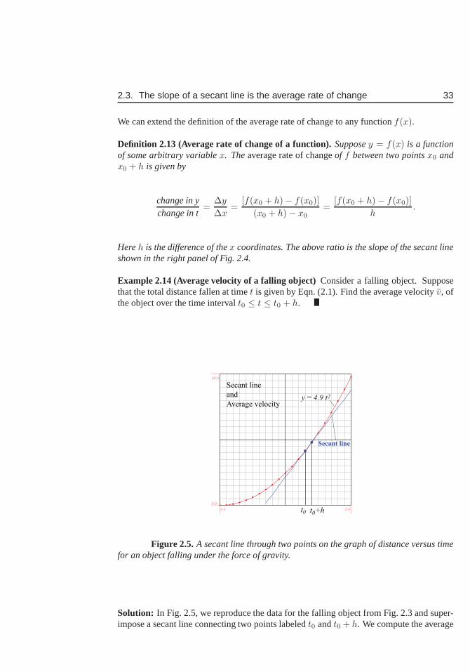
2.3. The slope of a secant line is the average rate of change 33
We can extend the definition of the average rate of change to any functionf(x).
Definition 2.13 (Average rate of change of a function).Supposey = f(x) is a functionof some arbitrary variablex. Theaverage rate of changeof f between two pointsx0 andx0 + h is given by
change in ychange in t
=∆y
∆x=
[f(x0 + h)− f(x0)]
(x0 + h)− x0=
[f(x0 + h)− f(x0)]
h.
Hereh is the difference of thex coordinates. The above ratio is the slope of the secant lineshown in the right panel of Fig. 2.4.
Example 2.14 (Average velocity of a falling object)Consider a falling object. Supposethat the total distance fallen at timet is given by Eqn. (2.1). Find the average velocityv, ofthe object over the time intervalt0 ≤ t ≤ t0 + h.
y = 4.9 t2
Secant line
0.0 2.0
0.0
20.0
Secant line
and
Average velocity
t0 t0+h
Figure 2.5.A secant line through two points on the graph of distance versus timefor an object falling under the force of gravity.
Solution: In Fig. 2.5, we reproduce the data for the falling object fromFig. 2.3 and super-impose a secant line connecting two points labeledt0 andt0 + h. We compute the average
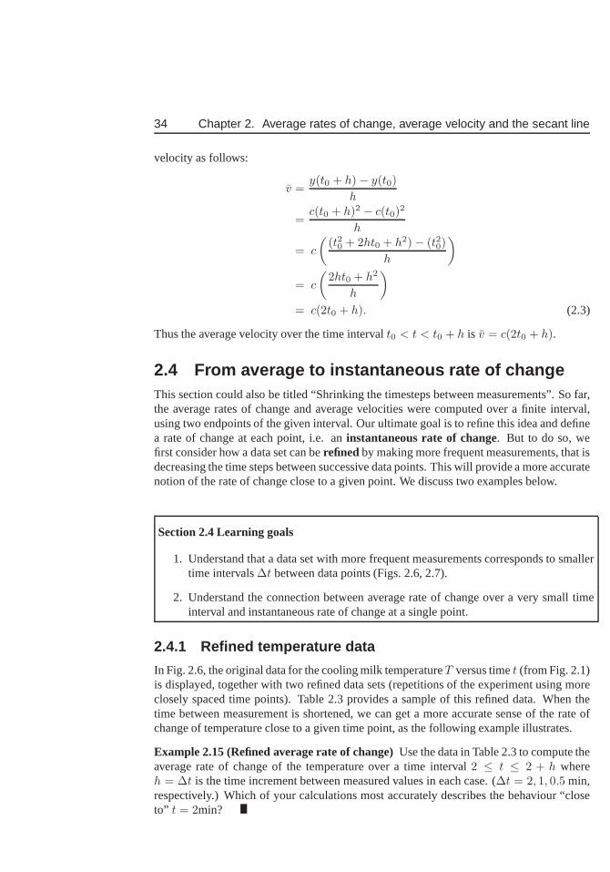
34 Chapter 2. Average rates of change, average velocity and the secant line
velocity as follows:
v =y(t0 + h)− y(t0)
h
=c(t0 + h)2 − c(t0)
2
h
= c
(
(t20 + 2ht0 + h2)− (t20)
h
)
= c
(
2ht0 + h2
h
)
= c(2t0 + h). (2.3)
Thus the average velocity over the time intervalt0 < t < t0 + h is v = c(2t0 + h).
2.4 From average to instantaneous rate of changeThis section could also be titled “Shrinking the timesteps between measurements”. So far,the average rates of change and average velocities were computed over a finite interval,using two endpoints of the given interval. Our ultimate goalis to refine this idea and definea rate of change at each point, i.e. aninstantaneous rate of change. But to do so, wefirst consider how a data set can berefined by making more frequent measurements, that isdecreasing the time steps between successive data points. This will provide a more accuratenotion of the rate of change close to a given point. We discusstwo examples below.
Section 2.4 Learning goals
1. Understand that a data set with more frequent measurements corresponds to smallertime intervals∆t between data points (Figs. 2.6, 2.7).
2. Understand the connection between average rate of changeover a very small timeinterval and instantaneous rate of change at a single point.
2.4.1 Refined temperature data
In Fig. 2.6, the original data for the cooling milk temperatureT versus timet (from Fig. 2.1)is displayed, together with two refined data sets (repetitions of the experiment using moreclosely spaced time points). Table 2.3 provides a sample of this refined data. When thetime between measurement is shortened, we can get a more accurate sense of the rate ofchange of temperature close to a given time point, as the following example illustrates.
Example 2.15 (Refined average rate of change)Use the data in Table 2.3 to compute theaverage rate of change of the temperature over a time interval 2 ≤ t ≤ 2 + h whereh = ∆t is the time increment between measured values in each case. (∆t = 2, 1, 0.5 min,respectively.) Which of your calculations most accuratelydescribes the behaviour “closeto” t = 2min?
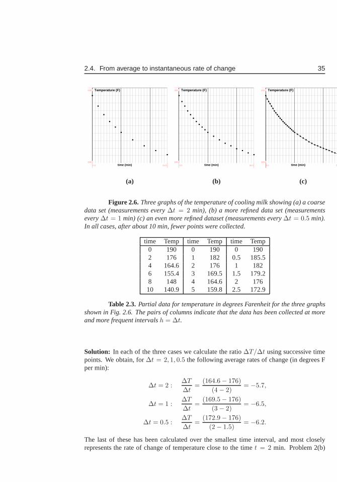
2.4. From average to instantaneous rate of change 35
Temperature (F)
time (min)0.0 26.0
100.0
200.0 Temperature (F)
time (min)0.0 26.0
100.0
200.0 Temperature (F)
time (min)0.0 26.0
100.0
200.0
(a) (b) (c)
Figure 2.6.Three graphs of the temperature of cooling milk showing (a) acoarsedata set (measurements every∆t = 2 min), (b) a more refined data set (measurementsevery∆t = 1 min) (c) an even more refined dataset (measurements every∆t = 0.5 min).In all cases, after about 10 min, fewer points were collected.
time Temp time Temp time Temp0 190 0 190 0 1902 176 1 182 0.5 185.54 164.6 2 176 1 1826 155.4 3 169.5 1.5 179.28 148 4 164.6 2 17610 140.9 5 159.8 2.5 172.9
Table 2.3.Partial data for temperature in degrees Farenheit for the three graphsshown in Fig. 2.6. The pairs of columns indicate that the datahas been collected at moreand more frequent intervalsh = ∆t.
Solution: In each of the three cases we calculate the ratio∆T/∆t using successive timepoints. We obtain, for∆t = 2, 1, 0.5 the following average rates of change (in degrees Fper min):
∆t = 2 :∆T
∆t=
(164.6− 176)
(4 − 2)= −5.7,
∆t = 1 :∆T
∆t=
(169.5− 176)
(3 − 2)= −6.5,
∆t = 0.5 :∆T
∆t=
(172.9− 176)
(2− 1.5)= −6.2.
The last of these has been calculated over the smallest time interval, and most closelyrepresents the rate of change of temperature close to the time t = 2 min. Problem 2(b)
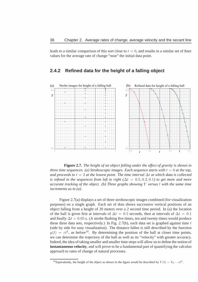
36 Chapter 2. Average rates of change, average velocity and the secant line
leads to a similar comparison of this sort close tot = 0, and results in a similar set of finervalues for the average rate of change “near” the initial datapoint.
2.4.2 Refined data for the height of a falling object
0.0 2.0
0.0
20.0
0.0 0.0
Refined data for height of a falling ball
t t t
Y
0.0
20.0
Y
Strobe images for height of a falling ball(a) (b)
Figure 2.7. The height of an object falling under the effect of gravity isshown inthree time sequences. (a) Stroboscopic images. Each sequence starts witht = 0 at the top,and proceeds tot = 2 at the lowest point. The time interval∆t at which data is collectedis refined in the sequences from left to right (∆t = 0.5, 0.2, 0.1) to get more and moreaccurate tracking of the object. (b) Three graphs showingY versust with the same timeincrements as in (a).
Figure 2.7(a) displays a set of three stroboscopic images combined (for visualizationpurposes) on a single graph. Each set of dots shows successive vertical positions of anobject falling from a height of 20 meters over a 2 second time period. In (a) the locationof the ball is given first at intervals of∆t = 0.5 seconds, then at intervals of∆t = 0.1and finally∆t = 0.05 s. (A strobe flashing five times, ten and twenty times would producethese three data sets, respectively.) In Fig. 2.7(b), each data set is graphed against timet(side by side for easy visualization). The distance fallen is still described by the functiony(t) = ct2, as before10. By determining the position of the ball at closer time points,we can determine the trajectory of the ball as well as its “velocity” with greater accuracy.Indeed, the idea of taking smaller and smaller time steps will allow us to define the notion ofinstantaneous velocity, and will prove to be a fundamental part of quantifying the calculusapproach to rates of change of natural processes.
10Equivalently, the height of the object as shown in the figure would be described byY (t) = Y0 − ct2.
2.5. Introduction to the derivative 37
2.4.3 Instantaneous velocity
To arrive at a notion of an instantaneous velocity at some time t0, we will consider definingaverage velocities over time intervalst0 ≤ t ≤ t0 + h, that get smaller and smaller: Forexample, we might make the strobe flash faster, so that the time between flashes,∆t =h decreases. (We use the notationh → 0 to denote the fact that we are interested inshrinking the time interval.) At each stage, we calculate anaverage velocity,v over thetime intervalt0 ≤ t ≤ t0 + h. As the interval between measurements gets smaller, i.e theprocess of refining our measurements continues, we arrive ata number that we will calltheinstantaneous velocity. This number represents “the velocity of the ball at the veryinstantt = t0”.
Definition 2.16 (Instantaneous velocity).The instantaneous velocity at timet0, denotedv(t0) is defined as
v(t0) = limh→0
v
wherev is the average velocity over the time intervalt0 < t < t0 + h. In other words,
v(t0) = limh→0
y(t0 + h)− y(t0)
h.
Example 2.17 (Computing an instantaneous velocity)Use Gallileo’s formula for the dis-tance fallen, (2.1) to compute the instantaneous velocity of a falling object at timet0.
Solution: We have already found the average velocity of the falling object over a timeintervalt0 < t < t0 + h in Example 2.14, obtaining (2.3),
v = c(2t0 + h).
Then, by Definition 2.16,
v(t0) = limh→0
v = limh→0
c(2t0 + h) = 2ct0.
This result holds for any timet0. More generally, we could write that at timet, the instan-taneous velocity isv(t) = 2ct. For example, using meters and seconds wherec = 4.9m/s2,we would find that the velocity of an object at time 1 s after initial release isv(1) = 4.9m/s.
2.5 Introduction to the derivativeWith the concepts introduced in this chapter, we are ready for the the definition of thederivative.
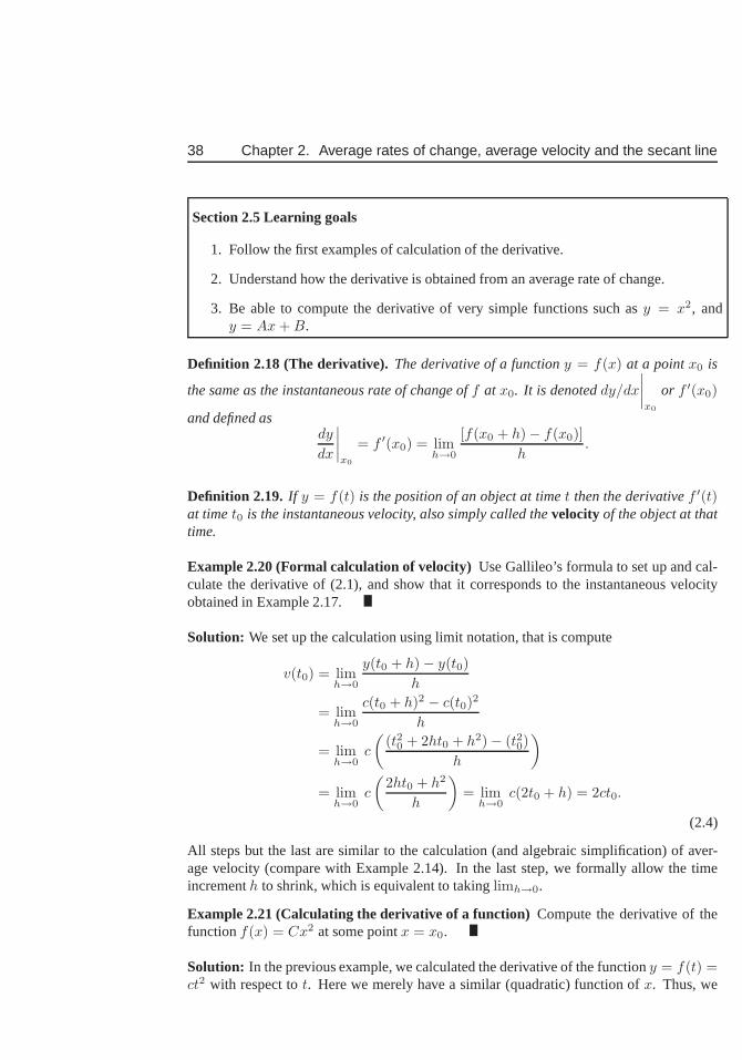
38 Chapter 2. Average rates of change, average velocity and the secant line
Section 2.5 Learning goals
1. Follow the first examples of calculation of the derivative.
2. Understand how the derivative is obtained from an averagerate of change.
3. Be able to compute the derivative of very simple functionssuch asy = x2, andy = Ax + B.
Definition 2.18 (The derivative). The derivative of a functiony = f(x) at a pointx0 is
the same as the instantaneous rate of change off at x0. It is denoteddy/dx
∣
∣
∣
∣
x0
or f ′(x0)
and defined asdy
dx
∣
∣
∣
∣
x0
= f ′(x0) = limh→0
[f(x0 + h)− f(x0)]
h.
Definition 2.19. If y = f(t) is the position of an object at timet then the derivativef ′(t)at timet0 is the instantaneous velocity, also simply called thevelocity of the object at thattime.
Example 2.20 (Formal calculation of velocity)Use Gallileo’s formula to set up and cal-culate the derivative of (2.1), and show that it correspondsto the instantaneous velocityobtained in Example 2.17.
Solution: We set up the calculation using limit notation, that is compute
v(t0) = limh→0
y(t0 + h)− y(t0)
h
= limh→0
c(t0 + h)2 − c(t0)2
h
= limh→0
c
(
(t20 + 2ht0 + h2)− (t20)
h
)
= limh→0
c
(
2ht0 + h2
h
)
= limh→0
c(2t0 + h) = 2ct0.
(2.4)
All steps but the last are similar to the calculation (and algebraic simplification) of aver-age velocity (compare with Example 2.14). In the last step, we formally allow the timeincrementh to shrink, which is equivalent to takinglimh→0.
Example 2.21 (Calculating the derivative of a function)Compute the derivative of thefunctionf(x) = Cx2 at some pointx = x0.
Solution: In the previous example, we calculated the derivative of thefunctiony = f(t) =ct2 with respect tot. Here we merely have a similar (quadratic) function ofx. Thus, we
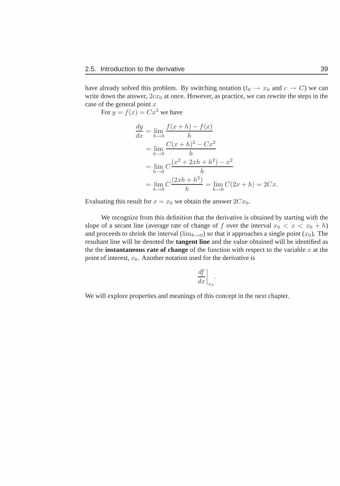
2.5. Introduction to the derivative 39
have already solved this problem. By switching notation (t0 → x0 andc → C) we canwrite down the answer,2cx0 at once. However, as practice, we can rewrite the steps in thecase of the general pointx
Fory = f(x) = Cx2 we have
dy
dx= lim
h→0
f(x + h)− f(x)
h
= limh→0
C(x + h)2 − Cx2
h
= limh→0
C(x2 + 2xh + h2)− x2
h
= limh→0
C(2xh + h2)
h= lim
h→0C(2x + h) = 2Cx.
Evaluating this result forx = x0 we obtain the answer2Cx0.
We recognize from this definition that the derivative is obtained by starting with theslope of a secant line (average rate of change off over the intervalx0 < x < x0 + h)and proceeds to shrink the interval (limh→0) so that it approaches a single point (x0). Theresultant line will be denoted thetangent line and the value obtained will be identified asthe theinstantaneous rate of changeof the function with respect to the variablex at thepoint of interest,x0. Another notation used for the derivative is
df
dx
∣
∣
∣
∣
x0
.
We will explore properties and meanings of this concept in the next chapter.
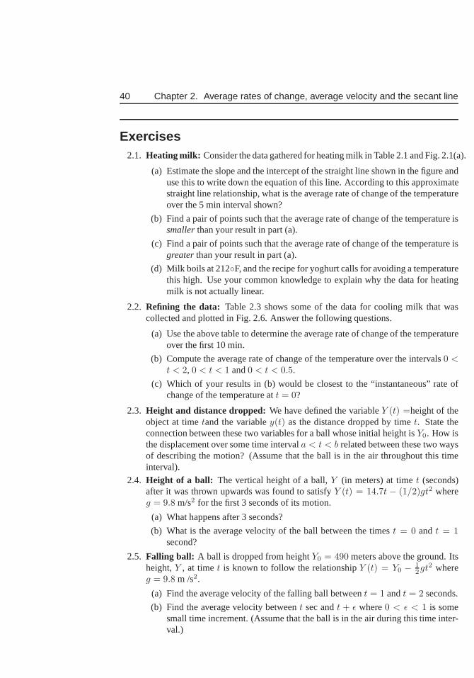
40 Chapter 2. Average rates of change, average velocity and the secant line
Exercises2.1. Heating milk: Consider the data gathered for heating milk in Table 2.1 and Fig. 2.1(a).
(a) Estimate the slope and the intercept of the straight lineshown in the figure anduse this to write down the equation of this line. According tothis approximatestraight line relationship, what is the average rate of change of the temperatureover the 5 min interval shown?
(b) Find a pair of points such that the average rate of change of the temperature issmallerthan your result in part (a).
(c) Find a pair of points such that the average rate of change of the temperature isgreaterthan your result in part (a).
(d) Milk boils at 212◦F, and the recipe for yoghurt calls for avoiding a temperaturethis high. Use your common knowledge to explain why the data for heatingmilk is not actually linear.
2.2. Refining the data: Table 2.3 shows some of the data for cooling milk that wascollected and plotted in Fig. 2.6. Answer the following questions.
(a) Use the above table to determine the average rate of change of the temperatureover the first 10 min.
(b) Compute the average rate of change of the temperature over the intervals0 <t < 2, 0 < t < 1 and0 < t < 0.5.
(c) Which of your results in (b) would be closest to the “instantaneous” rate ofchange of the temperature att = 0?
2.3. Height and distance dropped:We have defined the variableY (t) =height of theobject at timetand the variabley(t) as the distance dropped by timet. State theconnection between these two variables for a ball whose initial height isY0. How isthe displacement over some time intervala < t < b related between these two waysof describing the motion? (Assume that the ball is in the air throughout this timeinterval).
2.4. Height of a ball: The vertical height of a ball,Y (in meters) at timet (seconds)after it was thrown upwards was found to satisfyY (t) = 14.7t − (1/2)gt2 whereg = 9.8 m/s2 for the first 3 seconds of its motion.
(a) What happens after 3 seconds?
(b) What is the average velocity of the ball between the timest = 0 andt = 1second?
2.5. Falling ball: A ball is dropped from heightY0 = 490 meters above the ground. Itsheight,Y , at timet is known to follow the relationshipY (t) = Y0 − 1
2gt2 whereg = 9.8 m /s2.
(a) Find the average velocity of the falling ball betweent = 1 andt = 2 seconds.
(b) Find the average velocity betweent sec andt + ǫ where0 < ǫ < 1 is somesmall time increment. (Assume that the ball is in the air during this time inter-val.)
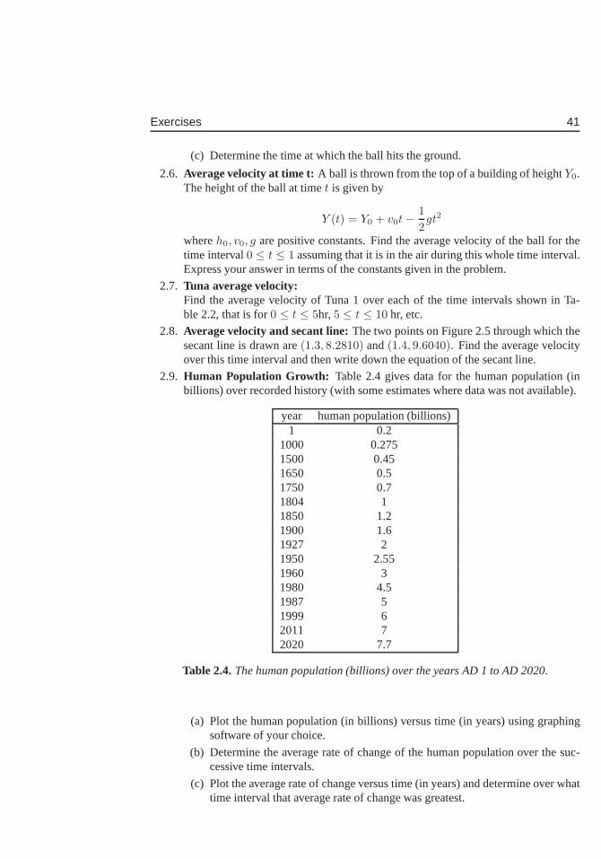
Exercises 41
(c) Determine the time at which the ball hits the ground.
2.6. Average velocity at time t: A ball is thrown from the top of a building of heightY0.The height of the ball at timet is given by
Y (t) = Y0 + v0t−1
2gt2
whereh0, v0, g are positive constants. Find the average velocity of the ball for thetime interval0 ≤ t ≤ 1 assuming that it is in the air during this whole time interval.Express your answer in terms of the constants given in the problem.
2.7. Tuna average velocity:Find the average velocity of Tuna 1 over each of the time intervals shown in Ta-ble 2.2, that is for0 ≤ t ≤ 5hr,5 ≤ t ≤ 10 hr, etc.
2.8. Average velocity and secant line:The two points on Figure 2.5 through which thesecant line is drawn are(1.3, 8.2810) and(1.4, 9.6040). Find the average velocityover this time interval and then write down the equation of the secant line.
2.9. Human Population Growth: Table 2.4 gives data for the human population (inbillions) over recorded history (with some estimates wheredata was not available).
year human population (billions)1 0.2
1000 0.2751500 0.451650 0.51750 0.71804 11850 1.21900 1.61927 21950 2.551960 31980 4.51987 51999 62011 72020 7.7
Table 2.4.The human population (billions) over the years AD 1 to AD 2020.
(a) Plot the human population (in billions) versus time (in years) using graphingsoftware of your choice.
(b) Determine the average rate of change of the human population over the suc-cessive time intervals.
(c) Plot the average rate of change versus time (in years) anddetermine over whattime interval that average rate of change was greatest.
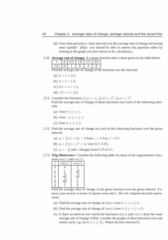
42 Chapter 2. Average rates of change, average velocity and the secant line
(d) Over what period (i.e. time interval) was this average rate of changeincreasingmost rapidly? (Hint: you should be able to answer this question either bylooking at the graph you have drawn or by calculation.)
2.10. Average rate of change:A certain function takes values given in the table below.t 0 0.5 1.0 1.5 2.0
f(t) 0 1 0 -1 0Find the average rate of change of the function over the intervals
(a) 0 < t < 0.5,
(b) 0 < t < 1.0,
(c) 0.5 < t < 1.5,
(d) 1.0 < t < 2.0.
2.11. Consider the functionsf1(x) = x, f2(x) = x2, f3(x) = x3.Find the average rate of change of these functions over each of the following inter-vals.
(a) Over0 ≤ x ≤ 1.
(b) Over−1 ≤ x ≤ 1.
(c) Over0 ≤ x ≤ 2.
2.12. Find the average rate of change for each of the following functions over the giveninterval.
(a) y = f(x) = 3x− 2 from x = 3.3 to x = 3.5.
(b) y = f(x) = x2 + 4x over[0.7, 0.85].
(c) y = − 4x andx changes from0.75 to 0.5.
2.13. Trig Minireview: Consider the following table of values of the trigonometricfunc-tionssin(x) andcos(x):
x sin(x) cos(x)0 0 1π6
12
√3
2π4
√2
2
√2
2π3
√3
212
π2 1 0
Find the average rates of change of the given function over the given interval. Ex-press your answer in terms of square roots andπ. Do not compute decimal expres-sions.
(a) Find the average rate of change ofsin(x) over0 ≤ x ≤ π/4.
(b) Find the average rate of change ofcos(x) overπ/4 ≤ x ≤ π/3.
(c) Is there an interval over which the functionssin(x) andcos(x) have the sameaverage rate of change? (Hint: consider the graphs of these functions over onewhole cycle, e.g. for0 ≤ x ≤ 2π. Where do they intersect?)
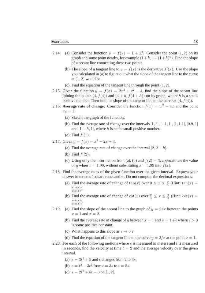
Exercises 43
2.14. (a) Consider the functiony = f(x) = 1 + x2. Consider the point(1, 2) on itsgraph and some point nearby, for example(1+h, 1+(1+h)2). Find the slopeof a secant line connecting these two points.
(b) The slope of a tangent line toy = f(x) is the derivativef ′(x). Use the slopeyou calculated in (a) to figure out what the slope of the tangent line to the curveat (1, 2) would be.
(c) Find the equation of the tangent line through the point(1, 2).
2.15. Given the functiony = f(x) = 2x3 + x2 − 4, find the slope of the secant linejoining the points(4, f(4)) and(4 + h, f(4 + h)) on its graph, whereh is a smallpositive number. Then find the slope of the tangent line to thecurve at(4, f(4)).
2.16. Average rate of change:Consider the functionf(x) = x2 − 4x and the pointx0 = 1.
(a) Sketch the graph of the function.
(b) Find the average rate of change over the intervals[1, 3], [−1, 1], [1, 1.1], [0.9, 1]and[1− h, 1], whereh is some small positive number.
(c) Findf ′(1).
2.17. Giveny = f(x) = x2 − 2x + 3.
(a) Find the average rate of change over the interval[2, 2 + h].
(b) Findf ′(2).
(c) Using only the information from (a), (b) andf(2) = 3, approximate the valueof y whenx = 1.99, without substitutingx = 1.99 into f(x).
2.18. Find the average rates of the given function over the given interval. Express youranswer in terms of square roots andπ. Do not compute the decimal expressions.
(a) Find the average rate of change oftan(x) over0 ≤ x ≤ π4 (Hint: tan(x) =
sin(x)cos(x) ).
(b) Find the average rate of change ofcot(x) over π4 ≤ x ≤ π
3 (Hint: cot(x) =cos(x)sin(x) ).
2.19. (a) Find the slope of the secant line to the graph ofy = 2/x between the pointsx = 1 andx = 2.
(b) Find the average rate of change ofy betweenx = 1 andx = 1+ǫ whereǫ > 0is some positive constant.
(c) What happens to this slope asǫ→ 0 ?
(d) Find the equation of the tangent line to the curvey = 2/x at the pointx = 1.
2.20. For each of the following motions wheres is measured in meters andt is measuredin seconds, find the velocity at timet = 2 and the average velocity over the giveninterval.
(a) s = 3t2 + 5 andt changes from2 to 3s.
(b) s = t3 − 3t2 from t = 3s to t = 5s.
(c) s = 2t2 + 5t− 3 on [1, 2].
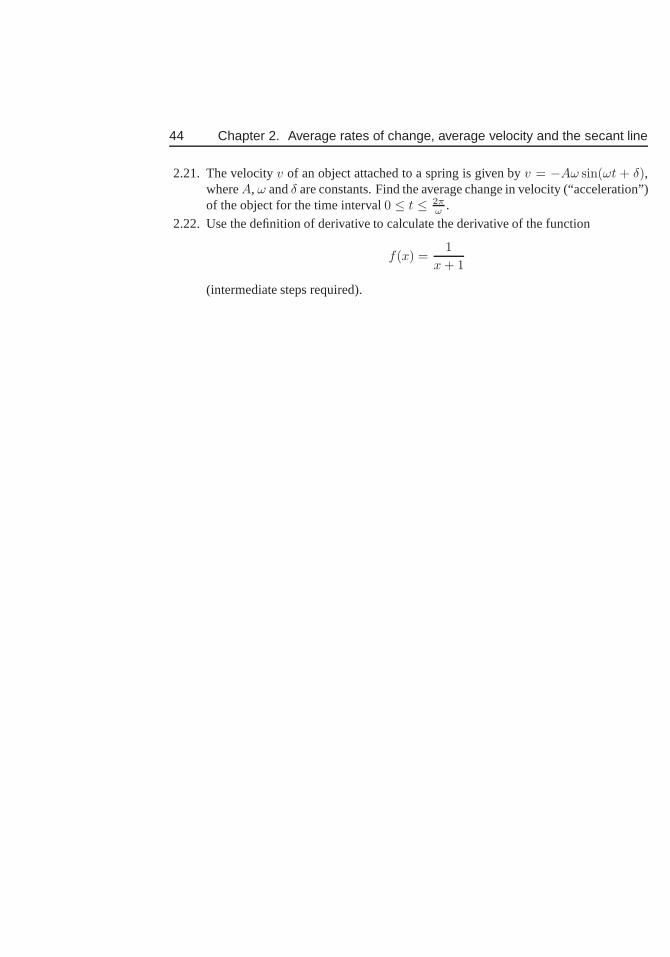
44 Chapter 2. Average rates of change, average velocity and the secant line
2.21. The velocityv of an object attached to a spring is given byv = −Aω sin(ωt + δ),whereA, ω andδ are constants. Find the average change in velocity (“acceleration”)of the object for the time interval0 ≤ t ≤ 2π
ω .
2.22. Use the definition of derivative to calculate the derivative of the function
f(x) =1
x + 1
(intermediate steps required).
Chapter 3
Three faces of thederivative: geometric,analytic, andcomputational
In Chapter 2 we used the concept of average rate of change (slope of secant line) to motivateand then define the notion of an instantaneous rate of change (the derivative). We arrivedat a “recipe” for calculating the derivative algebraically. We thereby introduced the idea oflimits, a concept that merits further discussion. We take upsome of the technical mattersrelated to limits to enable us to calculate the derivative algebraically.
Before doing so, we consider a distinct approach, which is geometric in flavour.Namely, we show that the local behaviour of a continuous function is described by a tangentline at a point on its graph, We arrive at that line by zooming into the graph of the function.This duality - the geometric (graphical) and analytic (algebraic calculation) views - willform important themes throughout the discussions to follow, and are two complementary,but closely related approaches to the calculus.
3.1 The geometric view: Zooming into the graph of afunction
Section 3.1 Learning goals
1. Understand the connection between the local behaviour ofa function (seen by zoom-ing into the graph) at a point and the tangent line to the graphof the function at thatpoint.
2. Given the graph of a function, be able to sketch its derivative.
3.1.1 Locally, the graph of a function looks like a straight l ine
In this section we consider well-behaved functions whose graphs are “smooth”, in contrastto the discrete data points of Chapter 2. We connect the derivative to the local shape ofthe graph of a given function. Bylocal behaviour we meet the behaviour seen when we
45
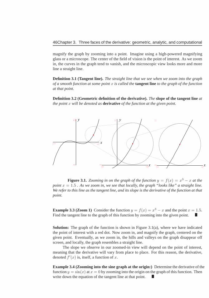
46Chapter 3. Three faces of the derivative: geometric, analytic, and computational
magnify the graph by zooming into a point. Imagine using a high-powered magnifyingglass or a microscope. The center of the field of vision is the point of interest. As we zoomin, the curves in the graph tend to vanish, and the microscopic view looks more and moreline a straight line.
Definition 3.1 (Tangent line). The straight line that we see when we zoom into the graphof a smooth function at some pointx is called thetangent line to the graph of the functionat that point.
Definition 3.2 (Geometric definition of the derivative).Theslope of the tangent lineatthe pointx will be denoted asderivative of the function at the given point.
-2.02.0
-6.0
6.0
0.5 2.0
0.0
4.0
1.4 1.6
1.6
2.2
x
x x
y y
Figure 3.1. Zooming in on the graph of the functiony = f(x) = x3 − x at thepointx = 1.5 . As we zoom in, we see that locally, the graph “looks like” a straight line.We refer to this line as the tangent line, and its slope is the derivative of the function at thatpoint.
Example 3.3 (Zoom 1)Consider the functiony = f(x) = x3 − x and the pointx = 1.5.Find the tangent line to the graph of this function by zoominginto the given point.
Solution: The graph of the function is shown in Figure 3.1(a), where we have indicatedthe point of interest with a red dot. Now zoom in, and magnify the graph, centered on thegiven point. Eventually, as we zoom in, the hills and valleyson the graph disappear offscreen, and locally, the graph resembles a straight line.
The slope we observe in our zoomed-in view will depend on the point of interest,meaning that the derivative will vary from place to place. For this reason, the derivative,denotedf ′(x) is, itself, a function ofx.
Example 3.4 (Zooming into the sine graph at the origin:)Determine the derivative of thefunctiony = sin(x) atx = 0 by zooming into the origin on the graph of this function. Thenwrite down the equation of the tangent line at that point.
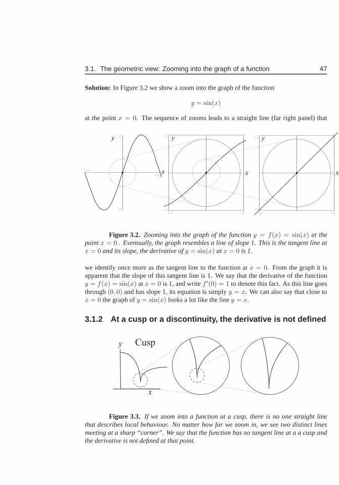
3.1. The geometric view: Zooming into the graph of a function 47
Solution: In Figure 3.2 we show a zoom into the graph of the function
y = sin(x)
at the pointx = 0. The sequence of zooms leads to a straight line (far right panel) that
-1.0 1.0
-1.0
1.0
-3.14
3.14
-1.0
1.0
-0.3 0.3
-0.3
0.3
xxx
y y y
Figure 3.2. Zooming into the graph of the functiony = f(x) = sin(x) at thepointx = 0 . Eventually, the graph resembles a line of slope 1. This is the tangent line atx = 0 and its slope, the derivative ofy = sin(x) at x = 0 is 1.
we identify once more as the tangent line to the function atx = 0. From the graph it isapparent that the slope of this tangent line is 1. We say that the derivative of the functiony = f(x) = sin(x) atx = 0 is 1, and writef ′(0) = 1 to denote this fact. As this line goesthrough(0, 0) and has slope 1, its equation is simplyy = x. We can also say that close tox = 0 the graph ofy = sin(x) looks a lot like the liney = x.
3.1.2 At a cusp or a discontinuity, the derivative is not defin ed
x
y Cusp
Figure 3.3. If we zoom into a function at a cusp, there is no one straight linethat describes local behaviour. No matter how far we zoom in,we see two distinct linesmeeting at a sharp “corner”. We say that the function has no tangent line at a a cusp andthe derivative is not defined at that point.
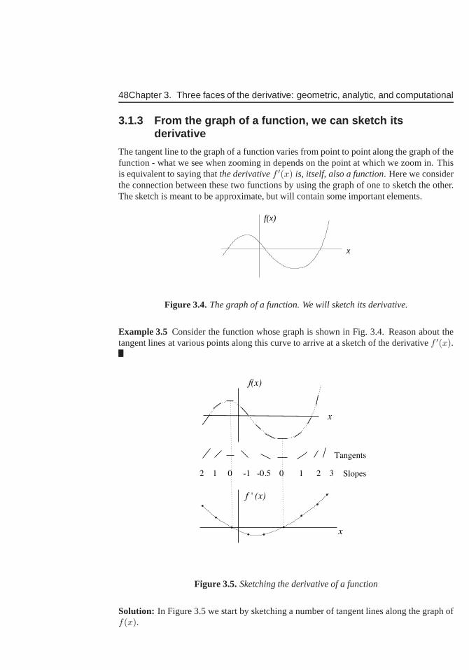
48Chapter 3. Three faces of the derivative: geometric, analytic, and computational
3.1.3 From the graph of a function, we can sketch itsderivative
The tangent line to the graph of a function varies from point to point along the graph of thefunction - what we see when zooming in depends on the point at which we zoom in. Thisis equivalent to saying thatthe derivativef ′(x) is, itself, also a function. Here we considerthe connection between these two functions by using the graph of one to sketch the other.The sketch is meant to be approximate, but will contain some important elements.
x
f(x)
Figure 3.4.The graph of a function. We will sketch its derivative.
Example 3.5 Consider the function whose graph is shown in Fig. 3.4. Reason about thetangent lines at various points along this curve to arrive ata sketch of the derivativef ′(x).
x
f(x)
Tangents
2 1 0 -1 -0.5 0 1 2 3 Slopes
x
f ' (x)
Figure 3.5.Sketching the derivative of a function
Solution: In Figure 3.5 we start by sketching a number of tangent lines along the graph off(x).
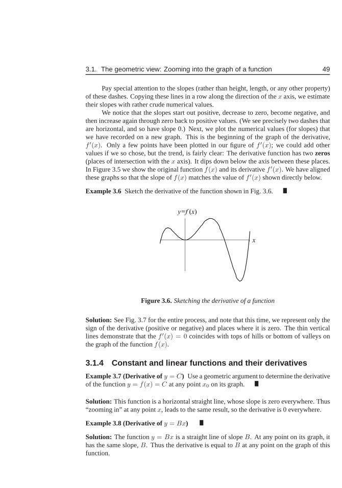
3.1. The geometric view: Zooming into the graph of a function 49
Pay special attention to the slopes (rather than height, length, or any other property)of these dashes. Copying these lines in a row along the direction of thex axis, we estimatetheir slopes with rather crude numerical values.
We notice that the slopes start out positive, decrease to zero, become negative, andthen increase again through zero back to positive values. (We see precisely two dashes thatare horizontal, and so have slope 0.) Next, we plot the numerical values (for slopes) thatwe have recorded on a new graph. This is the beginning of the graph of the derivative,f ′(x). Only a few points have been plotted in our figure off ′(x); we could add othervalues if we so chose, but the trend, is fairly clear: The derivative function has twozeros(places of intersection with thex axis). It dips down below the axis between these places.In Figure 3.5 we show the original functionf(x) and its derivativef ′(x). We have alignedthese graphs so that the slope off(x) matches the value off ′(x) shown directly below.
Example 3.6 Sketch the derivative of the function shown in Fig. 3.6.
x
y=f (x)
Figure 3.6.Sketching the derivative of a function
Solution: See Fig. 3.7 for the entire process, and note that this time, we represent only thesign of the derivative (positive or negative) and places where it is zero. The thin verticallines demonstrate that thef ′(x) = 0 coincides with tops of hills or bottom of valleys onthe graph of the functionf(x).
3.1.4 Constant and linear functions and their derivatives
Example 3.7 (Derivative ofy = C) Use a geometric argument to determine the derivativeof the functiony = f(x) = C at any pointx0 on its graph.
Solution: This function is a horizontal straight line, whose slope is zero everywhere. Thus“zooming in” at any pointx, leads to the same result, so the derivative is 0 everywhere.
Example 3.8 (Derivative ofy = Bx)
Solution: The functiony = Bx is a straight line of slopeB. At any point on its graph, ithas the same slope,B. Thus the derivative is equal toB at any point on the graph of thisfunction.
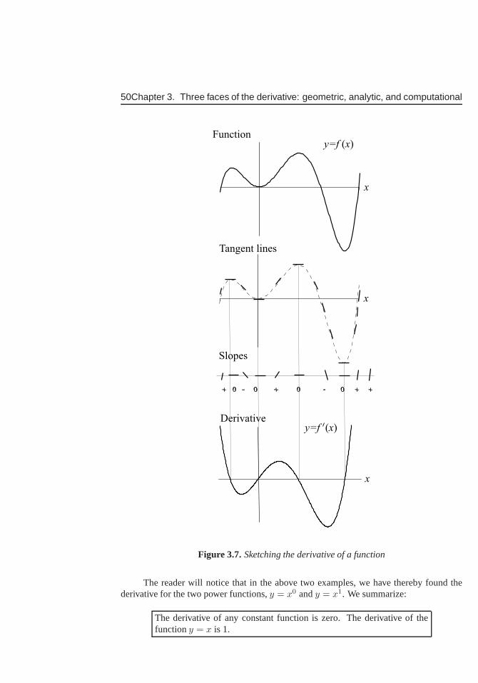
50Chapter 3. Three faces of the derivative: geometric, analytic, and computational
+ 0 - 0 + 0 - 0 + +
Slopes
x
x
x
y=f (x)
y=f (x)
Tangent lines
Function
Derivative
Figure 3.7.Sketching the derivative of a function
The reader will notice that in the above two examples, we havethereby found thederivative for the two power functions,y = x0 andy = x1. We summarize:
The derivative of any constant function is zero. The derivative of thefunctiony = x is 1.
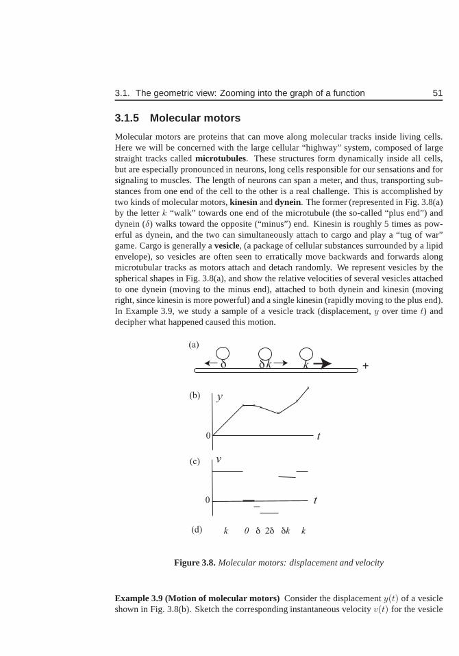
3.1. The geometric view: Zooming into the graph of a function 51
3.1.5 Molecular motors
Molecular motors are proteins that can move along moleculartracks inside living cells.Here we will be concerned with the large cellular “highway” system, composed of largestraight tracks calledmicrotubules. These structures form dynamically inside all cells,but are especially pronounced in neurons, long cells responsible for our sensations and forsignaling to muscles. The length of neurons can span a meter,and thus, transporting sub-stances from one end of the cell to the other is a real challenge. This is accomplished bytwo kinds of molecular motors,kinesin anddynein. The former (represented in Fig. 3.8(a)by the letterk “walk” towards one end of the microtubule (the so-called “plus end”) anddynein (δ) walks toward the opposite (“minus”) end. Kinesin is roughly 5 times as pow-erful as dynein, and the two can simultaneously attach to cargo and play a “tug of war”game. Cargo is generally avesicle, (a package of cellular substances surrounded by a lipidenvelope), so vesicles are often seen to erratically move backwards and forwards alongmicrotubular tracks as motors attach and detach randomly. We represent vesicles by thespherical shapes in Fig. 3.8(a), and show the relative velocities of several vesicles attachedto one dynein (moving to the minus end), attached to both dynein and kinesin (movingright, since kinesin is more powerful) and a single kinesin (rapidly moving to the plus end).In Example 3.9, we study a sample of a vesicle track (displacement,y over timet) anddecipher what happened caused this motion.
kkδδ +
v
t
t
y
k 0 δ 2δ δk k
0
0
x xx
x
x
x
(a)
(b)
(c)
(d)
Figure 3.8.Molecular motors: displacement and velocity
Example 3.9 (Motion of molecular motors) Consider the displacementy(t) of a vesicleshown in Fig. 3.8(b). Sketch the corresponding instantaneous velocityv(t) for the vesicle
52Chapter 3. Three faces of the derivative: geometric, analytic, and computational
and use your sketch to explain how many motors of each type could have been attachedover each of the time intervals in the plot.
Solution: The plot in Fig. 3.8(b) consists of straight line segments with sharp corners(cusps). Over each of these line segments, the slopedy/dt, which corresponds to theinstantaneous velocity,v(t), is constant. Segments with positive slope (the first, the lasttwo) correspond to times when the velocity was positive, when the vesicle was movingtoward the plus end. Over times where the slope is negative, the vesicle moved towardthe minus end of the microtubule. Where the slope is zero (flatgraph), the vesicle wasstationary. In Fig. 3.8(c), we sketch the rough graph of the instantaneous velocity,v(t).Observe thatv(t), which is the derivative ofy(t), is not defined at the points wherey(t)has “corners”. The larger the slope, the faster the velocity.
Based on Fig. 3.8(c), we can surmise which motors were attached. At first, the fastpositive velocity implies that the strong motor, kinesin, was at work. Once it got acciden-tally detached, the vesicle was stationary (0 motors). The motion in the opposite direction(negative velocity) suggests that 1-2 dyneins were then attached and working. After sometime, kinesin was bound, pulling more forcefully towards the plus end. Finally, only ki-nesin remained bound, and the velocity was positive and fast. We summarize this sequenceof event in Fig. 3.8(d).
3.2 Analytic view: calculating the derivative
Section 3.2 Learning goals
1. Be able to explain the definition of a continuous function,and function with varioustypes of discontinuities.
2. Understand how to evaluate simple limits of rational functions.
3. Be able to calculate the derivative of a simple function using the definition of thederivative, 2.18.
3.2.1 Technical matters: continuous functions and limits
We have studied two distinct types of functions so far. In Chapter 2, we found examples ofdiscrete data points, where a variable of interest (e.g. temperature) was defined only at afinite set of time points. We also encountered continuous functions, such as the height of afalling ball (2.1). Intuitively, we could describe a continuous function by saying that everypoint of its graph is connected to neighboring points. But using the concept of limits wecan be more accurate.
Definition 3.10 (Continuous function). We say thaty = f(x) is continuous at a pointx = a in its domain if
limx→a
f(x) = f(a).
3.2. Analytic view: calculating the derivative 53
By this we mean that the function is defined atx = a, that the above limit exists, and thatit matches with the value that the function takes at the givenpoint.
The function (2.1), for example, is continuous for all values of t, whereas a functionsuch asy =
√x is defined and continuous only forx ≥ 0. The functiony = 1/(x + 1) is
defined and continuous forx 6= −1.As discussed in Section 2.5, calculating a derivative requires the use of limits. The
two statements below emphasize this fact.
1. A secant line connects two points on the graph of a function(e.g. x andx + h). Inthe limit that those points get closer together (h→ 0), we obtain a tangent line.
2. The slope of a secant line is an average rate of change, but in the limit (h → 0), weobtain an instantaneous rate of change, which is the slope ofthe tangent line, namelythe derivative.
Tangent lines and derivatives are only defined at points where a function is continuousand smooth (has no cusps). Here we briefly discuss the idea of points of discontinuity andillustrate how limits are calculated, in preparation for understanding the way that derivativesare computed.
Function with a hole in its graph
Consider a function of the form
f(x) =(x− a)2
(x− a).
Then ifx 6= a, we can cancel a common factor, and obtain(x− a). If x = a, the functionis not defined (0/0). In short, we have
f(x) =(x− a)2
(x− a)=
{
x− a x 6= aundefined x = a.
Even though the function is not defined atx = a, we can evaluate the limit off asxapproachesa. We write
limx→a
f(x) = limx→a
(x− a)2
(x− a)= lim
x→ax− a = 0,
and say that “the limit asx approachesa” existsand is equal to 0. We also say that thefunction has aremovable discontinuity. If we add the point(a, 0) to the set of points atwhich the function is defined then we obtain a continuous function identical to the functionx− a. See also Appendix D.
Function with jump discontinuity
Consider the function
f(x) =
{
−1 x ≤ a,1 x > a.
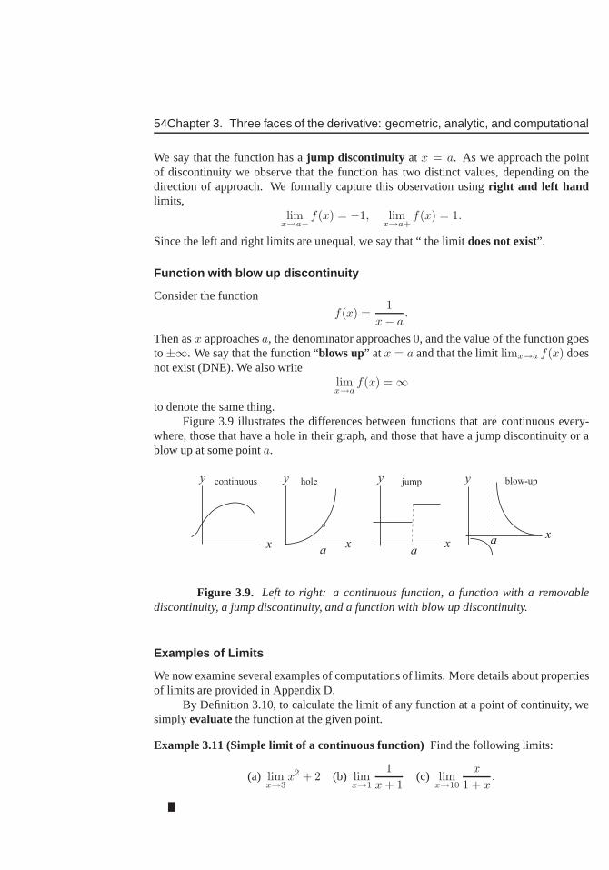
54Chapter 3. Three faces of the derivative: geometric, analytic, and computational
We say that the function has ajump discontinuity at x = a. As we approach the pointof discontinuity we observe that the function has two distinct values, depending on thedirection of approach. We formally capture this observation usingright and left handlimits,
limx→a−
f(x) = −1, limx→a+
f(x) = 1.
Since the left and right limits are unequal, we say that “ the limit does not exist”.
Function with blow up discontinuity
Consider the function
f(x) =1
x− a.
Then asx approachesa, the denominator approaches0, and the value of the function goesto±∞. We say that the function “blows up” at x = a and that the limitlimx→a f(x) doesnot exist (DNE). We also write
limx→a
f(x) =∞
to denote the same thing.Figure 3.9 illustrates the differences between functions that are continuous every-
where, those that have a hole in their graph, and those that have a jump discontinuity or ablow up at some pointa.
x x xx
a aa
y y y ycontinuous hole jump blow-up
Figure 3.9. Left to right: a continuous function, a function with a removablediscontinuity, a jump discontinuity, and a function with blow up discontinuity.
Examples of Limits
We now examine several examples of computations of limits. More details about propertiesof limits are provided in Appendix D.
By Definition 3.10, to calculate the limit of any function at apoint of continuity, wesimplyevaluatethe function at the given point.
Example 3.11 (Simple limit of a continuous function)Find the following limits:
(a) limx→3
x2 + 2 (b) limx→1
1
x + 1(c) lim
x→10
x
1 + x.
3.2. Analytic view: calculating the derivative 55
Solution: In each of the above, the function is continuous at the point of interest (atx =3, 1, 10, respectively). Thus, we simply “plug in” the values ofx in each case to obtain
(a) limx→3
x2 + 2 = 32 + 2 = 11 (b) limx→1
1
x + 1=
1
2(c) lim
x→10
x
1 + x=
10
11.
Example 3.12 (Hole in graph limits) Calculate the limits of the following functions. Notethat each has a removable discontinuity (“a hole in its graph”).
(a) limx→3
x2 − 6x + 9
x− 3(b) lim
x→−1
x2 + 3x + 2
x + 1.
Solution: We first simplify algebraically by factoring the numerator,and then evaluate thelimit. Note that the simplification is possible so long as we evaluate the limit, rather thanthe actual function, at the point of discontinuity.
(a) limx→3
x2 − 6x + 9
x− 3= lim
x→3
(x− 3)2
(x− 3)= lim
x→3(x− 3) = 0
(b) limx→−1
x2 + 3x + 2
x + 1= lim
x→−1
(x + 1)(x + 2)
(x + 1)= lim
x→−1(x + 2) = 1.
Example 3.13 (Limit involving sin(x)) Use the observation made in Example 3.4 to ar-rive at the value of the following limit:
limx→0
sin(x)
x
Solution: Example 3.4 illustrated the fact that close tox = 0 the functionsin(x) has thefollowing behaviour:
sin(x) ≈ x, orsin(x)
x≈ 1.
This is equivalent to the result
limx→0
sin(x)
x= 1. (3.1)
We read this “asx approaches zero, the limit ofsin(x)/x is 1.” We will find this limit usefulin later calculations involving derivatives of trigonometric functions.
56Chapter 3. Three faces of the derivative: geometric, analytic, and computational
3.2.2 Computing the derivative
We now apply the techniques so far to calculating a few derivatives based on the definitionof the derivative. We start with several simple examples, and work our way up to moreinteresting cases.
Example 3.14 (Derivative of a linear function) Using Definition 2.18 of the derivative,compute the derivative of the functiony = f(x) = Bx + C.
Solution: We have already used a geometric approach to find the derivative of relatedfunctions in Examples 3.7-3.8. Here we do the formal calculation as follows:
f ′(x) = limh→0
f(x + h)− f(x)
h(start with the definition)
= limh→0
[B(x + h) + C]− [Bx + C]
h(apply it to the function)
= limh→0
Bx + Bh + C −Bx− C
h(expand the numerator)
= limh→0
Bh
h(simplify)
= limh→0
B (cancel a factor ofh)
= B (evaluate the limit) (3.2)
Hence, we confirmed that the derivative off(x) = Bx+C is f ′(x) = B. This agrees withthe sum of the derivatives of the two parts,Bx andC found in Examples 3.7-3.8. Indeed,as we will establish shortly, the derivative of the sum of twofunctions is the same as thesum of their derivatives.
Example 3.15 (Derivative of the cubic power function)Compute the derivative of the func-tion y = f(x) = Kx3.
Solution: Fory = f(x) = Kx3 we have
dy
dx= lim
h→0
f(x + h)− f(x)
h
= limh→0
K(x + h)3 −Kx3
h
= limh→0
K(x3 + 3x2h + 3xh2 + h3)− x3
h
= limh→0
K(3x2h + 3xh2 + h3)
h
= limh→0
K(3x2 + 3xh + h2)
= K(3x2) = 3Kx2. (3.3)
Thus the derivative off(x) = Kx3 is f ′(x) = 3Kx2.
3.3. Computational face of the derivative: software to the rescue! 57
Example 3.16 Use the definition of the derivative to computef ′(x) for the functiony =f(x) = 1/x at the pointx = 1.
Solution: We write down the formula for this calculation at any pointx and then simplifyalgebraically, using common denominators to combine fractions, and then, in the final step,calculate the limit formally. Then we substitute the valuex = 1.
f ′(x) = limh→0
f(x + h)− f(x)
h(the definition)
= limh→0
1(x+h) − 1
x
h(applied to the function)
= limh→0
[x−(x+h)]x(x+h)
h(common denominator)
= limh→0
−h
hx(x + h)(algebraic simplification)
= limh→0
−1
x(x + h)(cancel factor ofh)
= − 1
x2(limit evaluated) (3.4)
(3.5)
Thus, the derivative off(x) = 1/x is f ′(x) = −1/x2 and at the pointx = 1 it takes thevaluef ′(1) = −1.
In Problem 10 we apply similar techniques to the derivative of the square-root func-tion to show that
y = f(x) =√
x ⇒ f ′(x) =1
2√
x. (3.6)
In the next chapter, we formalize some observations about derivatives of power funcitonsand rules of differentiation. This will allow us to avoid such tedious calculations in findingsimple derivatives.
3.3 Computational face of the derivative: software tothe rescue!
Mathematical computations and analysis benefit greatly from software methods that help tocomplement the algebraic and geometric approaches. Using avariety of software, we cangain insight, experiment, as well as design methods for accurate computations that would betoo tedious to carry out by hand. Here we show a third face of the derivative: its numericalimplementation using a simple spreadsheet. This easy introduction to a spreadsheet willlater help us devise techniques for solving a variety of problems where many repetitivecalculations are involved.
58Chapter 3. Three faces of the derivative: geometric, analytic, and computational
Section 3.3 Learning goals
1. Appreciate the fact that software can numerically compute an approximation to thederivative.
2. Understand that the approximation replaces a (true) tangent line with an (approxi-mating) secant line.
3. Be able to use a spreadsheet (or your favorite software aid) to graph a function andits derivative.
4. Be able to explain verbally how that the derivative shape is connected with the shapeof the original function.
5. Interpret the differences between two types of biochemical kinetics, Michaelis-Menten and Hill function.
Definition 3.17 (Numerical derivative).By a numerical derivative calculation we mean anumerical approximation to the value of the derivative, obtained by using a finite value,
f ′(x)numerical ≈∆f
∆xrather than the actual valuef ′(x)actual = lim
∆x→0
∆f
∆x.
The numerical derivative approximates the true derivativeprovided∆x is small rela-tive to the range over which the functionf changes dramatically. Since∆f is the differenceof two values off , (∆f = f(x+∆x)−f(x)) it follows that the numerical derivative is thesame as the slope of a secant line. This important realization, associated with LG 2, meansthata secant line is often used to approximate a tangent line, andthe slope of a secant lineis used to approximate a derivative in numerical computations. We will see this idea againin several contexts.
3.3.1 Concentration-dependent rate of chemical reaction
In Section 1.5, we studied two types of enzyme-catalyzed reactions, Michaelis-Mentenkinetics, (1.7) and Hill functions, (1.6). Usingc for the substrate concentration,vMM andvHill for the reaction rates, we repeat their expressions here:
vMM =Kc
a + c, (3.7)
vHill =Kcn
an + cn, (3.8)
In both cases, the reaction ratevi depends on the chemical concentrationc. In the left panelof Fig. 3.10 we plot both functions (3.7) and (3.8) on the samecoordinate system. (Seealso Fig. 1.5 for the same kind of plot.)
We ask “how does the reaction speed change when we vary the substrate concentra-tion?” or equivalently, “For each small increase inc, by how much doesv increase?”. This
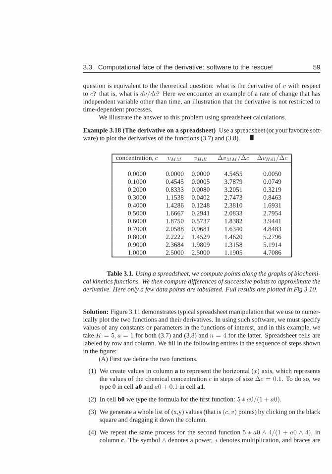
3.3. Computational face of the derivative: software to the rescue! 59
question is equivalent to the theoretical question: what isthe derivative ofv with respectto c? that is, what isdv/dc? Here we encounter an example of a rate of change that hasindependent variable other than time, an illustration thatthe derivative is not restricted totime-dependent processes.
We illustrate the answer to this problem using spreadsheet calculations.
Example 3.18 (The derivative on a spreadsheet)Use a spreadsheet (or your favorite soft-ware) to plot the derivatives of the functions (3.7) and (3.8).
concentration,c vMM vHill ∆vMM/∆c ∆vHill/∆c
0.0000 0.0000 0.0000 4.5455 0.00500.1000 0.4545 0.0005 3.7879 0.07490.2000 0.8333 0.0080 3.2051 0.32190.3000 1.1538 0.0402 2.7473 0.84630.4000 1.4286 0.1248 2.3810 1.69310.5000 1.6667 0.2941 2.0833 2.79540.6000 1.8750 0.5737 1.8382 3.94410.7000 2.0588 0.9681 1.6340 4.84830.8000 2.2222 1.4529 1.4620 5.27960.9000 2.3684 1.9809 1.3158 5.19141.0000 2.5000 2.5000 1.1905 4.7086
Table 3.1.Using a spreadsheet, we compute points along the graphs of biochemi-cal kinetics functions. We then compute differences of successive points to approximate thederivative. Here only a few data points are tabulated. Full results are plotted in Fig 3.10.
Solution: Figure 3.11 demonstrates typical spreadsheet manipulation that we use to numer-ically plot the two functions and their derivatives. In using such software, we must specifyvalues of any constants or parameters in the functions of interest, and in this example, wetakeK = 5, a = 1 for both (3.7) and (3.8) andn = 4 for the latter. Spreadsheet cells arelabeled by row and column. We fill in the following entires in the sequence of steps shownin the figure:
(A) First we define the two functions.
(1) We create values in columna to represent the horizontal (x) axis, which representsthe values of the chemical concentrationc in steps of size∆c = 0.1. To do so, wetype 0 in cella0anda0 + 0.1 in cell a1.
(2) In cellb0 we type the formula for the first function:5 ∗ a0/(1 + a0).
(3) We generate a whole list of (x,y) values (that is(c, v) points) by clicking on the blacksquare and dragging it down the column.
(4) We repeat the same process for the second function5 ∗ a0 ∧ 4/(1 + a0 ∧ 4), incolumnc. The symbol∧ denotes a power,∗ denotes multiplication, and braces are
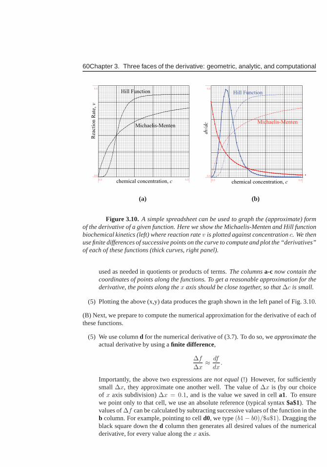
60Chapter 3. Three faces of the derivative: geometric, analytic, and computational
Michaelis-Menten
Hill Function
0.0 5.0
0.0
5.5
Rea
ctio
n R
ate,
v
chemical concentration, c 0.0 5.0
0.0
5.5
chemical concentration, c
Hill Function
Michaelis-Menten
dv/
dc
(a) (b)
Figure 3.10. A simple spreadsheet can be used to graph the (approximate) formof the derivative of a given function. Here we show the Michaelis-Menten and Hill functionbiochemical kinetics (left) where reaction ratev is plotted against concentrationc. We thenuse finite differences of successive points on the curve to compute and plot the “derivatives”of each of these functions (thick curves, right panel).
used as needed in quotients or products of terms.The columnsa-c now contain thecoordinates of points along the functions. To get a reasonable approximation for thederivative, the points along thex axis should be close together, so that∆c is small.
(5) Plotting the above (x,y) data produces the graph shown inthe left panel of Fig. 3.10.
(B) Next, we prepare to compute the numerical approximationfor the derivative of each ofthese functions.
(5) We use columnd for the numerical derivative of (3.7). To do so, weapproximatetheactual derivative by using afinite difference,
∆f
∆x≈ df
dx.
Importantly, the above two expressions arenot equal(!) However, for sufficientlysmall ∆x, they approximate one another well. The value of∆x is (by our choiceof x axis subdivision)∆x = 0.1, and is the value we saved in cella1. To ensurewe point only to that cell, we use an absolute reference (typical syntax$a$1). Thevalues of∆f can be calculated by subtracting successive values of the function in theb column. For example, pointing to celld0, we type(b1− b0)/$a$1). Dragging theblack square down thed column then generates all desired values of the numericalderivative, for every value along thex axis.
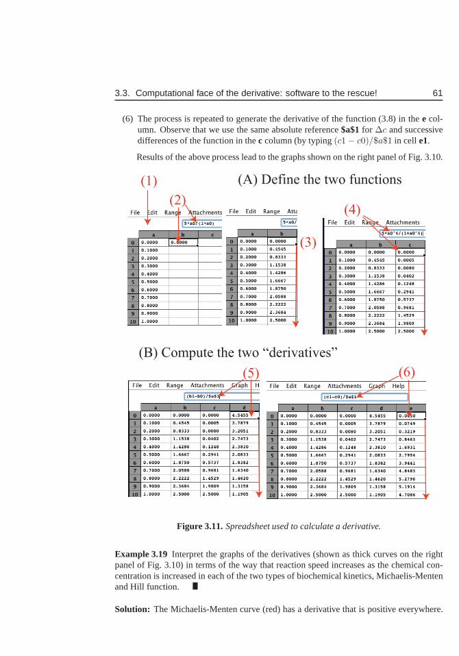
3.3. Computational face of the derivative: software to the rescue! 61
(6) The process is repeated to generate the derivative of thefunction (3.8) in thee col-umn. Observe that we use the same absolute reference$a$1for ∆c and successivedifferences of the function in thec column (by typing(c1− c0)/$a$1 in cell e1.
Results of the above process lead to the graphs shown on the right panel of Fig. 3.10.
(1)
(2)
(3)
(4)
(A) Define the two functions
(B) Compute the two “derivatives”
(5) (6)
Figure 3.11.Spreadsheet used to calculate a derivative.
Example 3.19 Interpret the graphs of the derivatives (shown as thick curves on the rightpanel of Fig. 3.10) in terms of the way that reaction speed increases as the chemical con-centration is increased in each of the two types of biochemical kinetics, Michaelis-Mentenand Hill function.
Solution: The Michaelis-Menten curve (red) has a derivative that is positive everywhere.
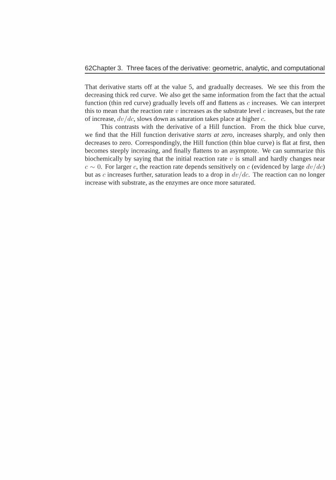
62Chapter 3. Three faces of the derivative: geometric, analytic, and computational
That derivative starts off at the value 5, and gradually decreases. We see this from thedecreasing thick red curve. We also get the same informationfrom the fact that the actualfunction (thin red curve) gradually levels off and flattens as c increases. We can interpretthis to mean that the reaction ratev increases as the substrate levelc increases, but the rateof increase,dv/dc, slows down as saturation takes place at higherc.
This contrasts with the derivative of a Hill function. From the thick blue curve,we find that the Hill function derivativestarts at zero, increases sharply, and only thendecreases to zero. Correspondingly, the Hill function (thin blue curve) is flat at first, thenbecomes steeply increasing, and finally flattens to an asymptote. We can summarize thisbiochemically by saying that the initial reaction ratev is small and hardly changes nearc ∼ 0. For largerc, the reaction rate depends sensitively onc (evidenced by largedv/dc)but asc increases further, saturation leads to a drop indv/dc. The reaction can no longerincrease with substrate, as the enzymes are once more saturated.
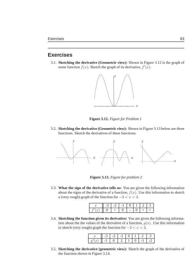
Exercises 63
Exercises3.1. Sketching the derivative (Geometric view):Shown in Figure 3.12 is the graph of
some functionf(x). Sketch the graph of its derivative,f ′(x).
x
y
Figure 3.12.Figure for Problem 1
3.2. Sketching the derivative (Geometric view):Shown in Figure 3.13 below are threefunctions. Sketch the derivatives of these functions.
x xx
yyy
Figure 3.13.Figure for problem 2
3.3. What the sign of the derivative tells us:You are given the following informationabout the signs of the derivative of a function,f(x). Use this information to sketcha (very rough) graph of the function for−3 < x < 3.
x -3 -2 -1 0 1 2 3f ′(x) 0 + 0 - 0 + +
3.4. Sketching the function given its derivative:You are given the following informa-tion about the the values of the derivative of a function,g(x). Use this informationto sketch (very rough) graph the function for−3 < x < 3.
x -3 -2 -1 0 1 2 3g′(x) -1 0 2 1 0 -1 -2
3.5. Sketching the derivative (geometric view):Sketch the graph of the derivative ofthe function shown in Figure 3.14.
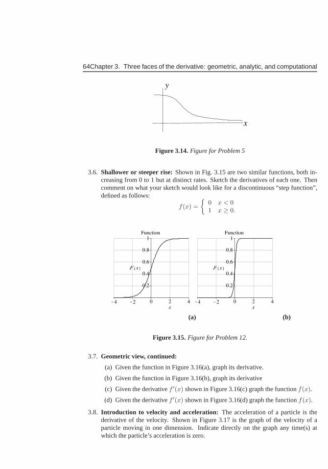
64Chapter 3. Three faces of the derivative: geometric, analytic, and computational
x
y
Figure 3.14.Figure for Problem 5
3.6. Shallower or steeper rise:Shown in Fig. 3.15 are two similar functions, both in-creasing from 0 to 1 but at distinct rates. Sketch the derivatives of each one. Thencomment on what your sketch would look like for a discontinuous “step function”,defined as follows:
f(x) =
{
0 x < 01 x ≥ 0.
(a) (b)
Figure 3.15.Figure for Problem 12.
3.7. Geometric view, continued:
(a) Given the function in Figure 3.16(a), graph its derivative.
(b) Given the function in Figure 3.16(b), graph its derivative
(c) Given the derivativef ′(x) shown in Figure 3.16(c) graph the functionf(x).
(d) Given the derivativef ′(x) shown in Figure 3.16(d) graph the functionf(x).
3.8. Introduction to velocity and acceleration: The acceleration of a particle is thederivative of the velocity. Shown in Figure 3.17 is the graphof the velocity of aparticle moving in one dimension. Indicate directly on the graph any time(s) atwhich the particle’s acceleration is zero.
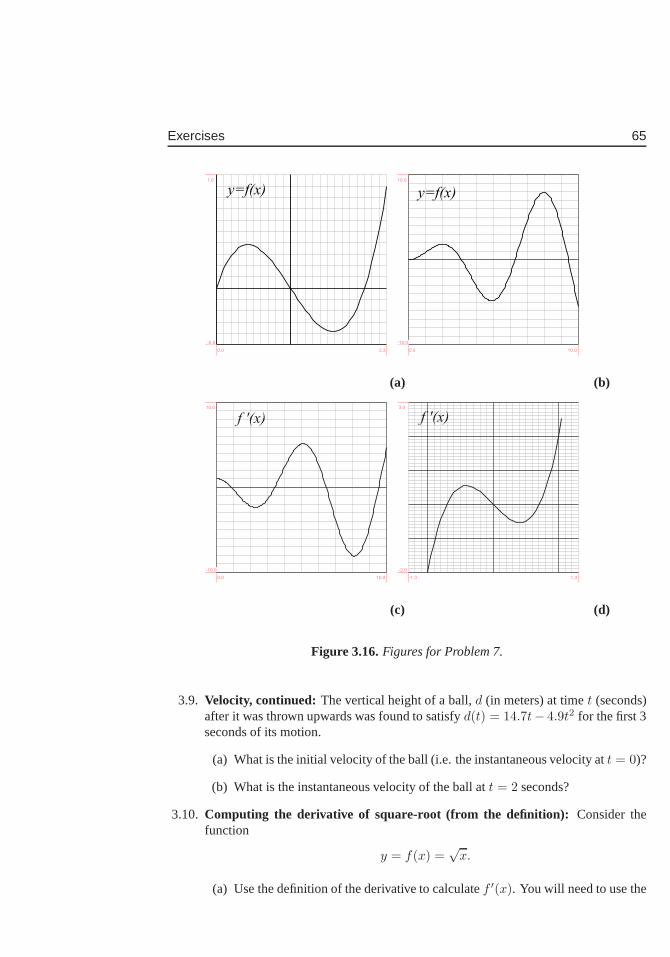
Exercises 65
y=f(x)
0.0 2.3
-0.5
1.0
0.0 10.0
-10.0
10.0
y=f(x)
(a) (b)
f '(x)
0.0 10.0
-10.0
10.0
-1.3 1.3
-2.0
3.0
f '(x)
(c) (d)
Figure 3.16.Figures for Problem 7.
3.9. Velocity, continued: The vertical height of a ball,d (in meters) at timet (seconds)after it was thrown upwards was found to satisfyd(t) = 14.7t− 4.9t2 for the first 3seconds of its motion.
(a) What is the initial velocity of the ball (i.e. the instantaneous velocity att = 0)?
(b) What is the instantaneous velocity of the ball att = 2 seconds?
3.10. Computing the derivative of square-root (from the definition): Consider thefunction
y = f(x) =√
x.
(a) Use the definition of the derivative to calculatef ′(x). You will need to use the
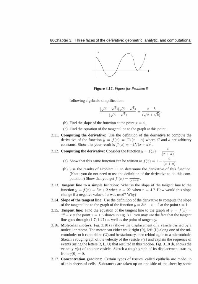
66Chapter 3. Three faces of the derivative: geometric, analytic, and computational
v
t
Figure 3.17.Figure for Problem 8
following algebraic simplification:
(√
a−√
b)(√
a +√
b)
(√
a +√
b)=
a− b
(√
a +√
b).
(b) Find the slope of the function at the pointx = 4.
(c) Find the equation of the tangent line to the graph at this point.
3.11. Computing the derivative: Use the definition of the derivative to compute thederivative of the functiony = f(x) = C/(x + a) whereC anda are arbitraryconstants. Show that your result isf ′(x) = −C/(x + a)2.
3.12. Computing the derivative: Consider the functiony = f(x) =x
(x + a).
(a) Show that this same function can be written asf(x) = 1− a
(x + a).
(b) Use the results of Problem 11 to determine the derivativeof this function.(Note: you do not need to use the definition of the derivative to do this com-putation.) Show that you getf ′(x) = a
(x+a)2 .
3.13. Tangent line to a simple function: What is the slope of the tangent line to thefunctiony = f(x) = 5x + 2 whenx = 2? whenx = 4 ? How would this slopechange if a negative value ofx was used? Why?
3.14. Slope of the tangent line:Use the definition of the derivative to compute the slopeof the tangent line to the graph of the functiony = 3t2 − t + 2 at the pointt = 1.
3.15. Tangent line: Find the equation of the tangent line to the graph ofy = f(x) =x3 − x at the pointx = 1.5 shown in Fig. 3.1. You may use the fact that the tangentline goes through(1.7, 1.47) as well as the point of tangency.
3.16. Molecular motors: Fig. 3.18 (a) shows the displacement of a vesicle carried by amolecular motor. The motor can either walk right (R), left (L) along one of the mi-crotubules or it can unbind (U) and be stationary, then rebind again to a microtubule.Sketch a rough graph of the velocity of the vesiclev(t) and explain the sequence ofevents (using the letters R, L, U) that resulted in this motion. Fig. 3.18 (b) shows thevelocity v(t) of another vesicle. Sketch a rough graph of its displacementstartingfrom y(0) = 0.
3.17. Concentration gradient: Certain types of tissues, called epithelia are made upof thin sheets of cells. Substances are taken up on one side ofthe sheet by some
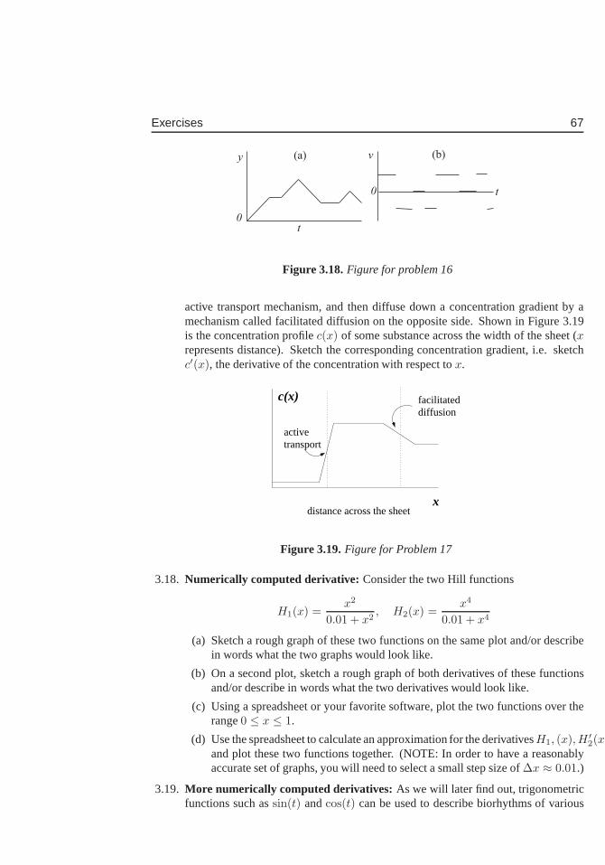
Exercises 67
t
y
0
0
v
t
(a) (b)
Figure 3.18.Figure for problem 16
active transport mechanism, and then diffuse down a concentration gradient by amechanism called facilitated diffusion on the opposite side. Shown in Figure 3.19is the concentration profilec(x) of some substance across the width of the sheet (xrepresents distance). Sketch the corresponding concentration gradient, i.e. sketchc′(x), the derivative of the concentration with respect tox.
x
c(x) facilitateddiffusion
activetransport
distance across the sheet
Figure 3.19.Figure for Problem 17
3.18. Numerically computed derivative: Consider the two Hill functions
H1(x) =x2
0.01 + x2, H2(x) =
x4
0.01 + x4
(a) Sketch a rough graph of these two functions on the same plot and/or describein words what the two graphs would look like.
(b) On a second plot, sketch a rough graph of both derivativesof these functionsand/or describe in words what the two derivatives would looklike.
(c) Using a spreadsheet or your favorite software, plot the two functions over therange0 ≤ x ≤ 1.
(d) Use the spreadsheet to calculate an approximation for the derivativesH1, (x), H ′2(x)
and plot these two functions together. (NOTE: In order to have a reasonablyaccurate set of graphs, you will need to select a small step size of∆x ≈ 0.01.)
3.19. More numerically computed derivatives: As we will later find out, trigonometricfunctions such assin(t) andcos(t) can be used to describe biorhythms of various
68Chapter 3. Three faces of the derivative: geometric, analytic, and computational
types. Here we numerically compute the first and second derivative ofy = sin(t)and show the relationships between the trigonometric functions and their derivatives.We will use only numerical methods (e.g. a spreadsheet), butlater, in Chapter 14,we will also study the analytical calculation of the same derivatives.
(a) Use a spreadsheet (or your favorite software) to plot, onthe same graph thetwo functions
y1 = sin(t), y2 = cos(t), 0 ≤ t ≤ 2π ≈ 6.28.
Note that you should use a fairly small step size, e.g.∆t = 0.01 to get areasonably accurate approximation of the derivatives.
(b) Use the same spreadsheet to (numerically) calculate (anapproximate) deriva-tive y′
1(t) and add it to your graph.
(c) Now calculatey′′1 (t), that is (an approximation to) the derivative of the deriva-
tive of the sine function and add this to your graph.
Chapter 4
Differentiation rules,simple antiderivativesand applications
In our investigation so far, we have defined the derivative ofa function,y = f(x) by
dy
dx= f ′(x) = lim
h→0
f(x + h)− f(x)
h.
We used this formula to calculate derivatives of a few power functions. Here, we will gatherresults so far, and observe a pattern, the power rule, for derivatives of power functions. Thepower law also allow us to find successive derivatives (e.g. second derivative etc.), todifferentiate polynomials, and even to find antiderivatives of such functions by applyingthe rule “in reverse” (find a function that has a given derivative). All these calculationsare useful to common applications of accelerated motion, investigated later in this chapter.We round out the technical material by stating several otheruseful rules of differentiation(product and quotient), allowing us to easily calculate derivatives of more complicated andinteresting functions.
4.1 Rules of differentiation
Learning goals (LG) for Section 4.1
1. Learn and understand the power rule (Table 4.1) and be prepared to apply it to bothderivatives and antiderivatives of power functions and polynomials.
2. Be able to explain what is meant by the statement that “the derivative is a linearoperation”.
3. Understand the concept of an antiderivative and why it is defined only up to someconstant.
4. Learn the product and quotient rules and be able to apply these to calculating deriva-tives of products and of rational functions.
69
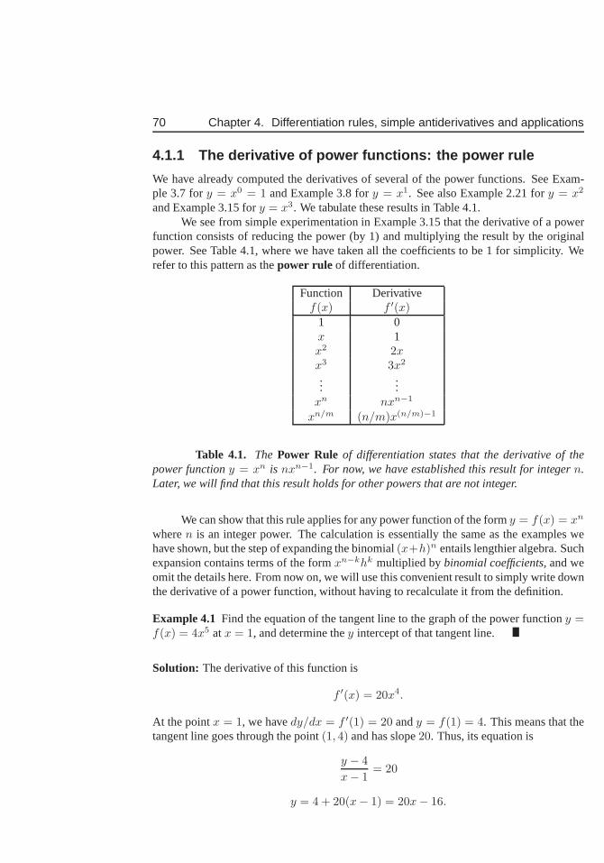
70 Chapter 4. Differentiation rules, simple antiderivatives and applications
4.1.1 The derivative of power functions: the power rule
We have already computed the derivatives of several of the power functions. See Exam-ple 3.7 fory = x0 = 1 and Example 3.8 fory = x1. See also Example 2.21 fory = x2
and Example 3.15 fory = x3. We tabulate these results in Table 4.1.We see from simple experimentation in Example 3.15 that the derivative of a power
function consists of reducing the power (by 1) and multiplying the result by the originalpower. See Table 4.1, where we have taken all the coefficientsto be 1 for simplicity. Werefer to this pattern as thepower rule of differentiation.
Function Derivativef(x) f ′(x)
1 0x 1x2 2xx3 3x2
......
xn nxn−1
xn/m (n/m)x(n/m)−1
Table 4.1. The Power Rule of differentiation states that the derivative of thepower functiony = xn is nxn−1. For now, we have established this result for integern.Later, we will find that this result holds for other powers that are not integer.
We can show that this rule applies for any power function of the formy = f(x) = xn
wheren is an integer power. The calculation is essentially the sameas the examples wehave shown, but the step of expanding the binomial(x+h)n entails lengthier algebra. Suchexpansion contains terms of the formxn−khk multiplied bybinomial coefficients, and weomit the details here. From now on, we will use this convenient result to simply write downthe derivative of a power function, without having to recalculate it from the definition.
Example 4.1 Find the equation of the tangent line to the graph of the powerfunctiony =f(x) = 4x5 atx = 1, and determine they intercept of that tangent line.
Solution: The derivative of this function is
f ′(x) = 20x4.
At the pointx = 1, we havedy/dx = f ′(1) = 20 andy = f(1) = 4. This means that thetangent line goes through the point(1, 4) and has slope20. Thus, its equation is
y − 4
x− 1= 20
y = 4 + 20(x− 1) = 20x− 16.
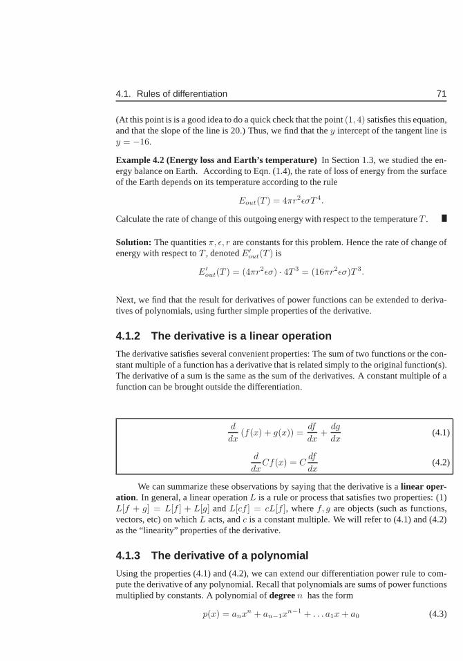
4.1. Rules of differentiation 71
(At this point is is a good idea to do a quick check that the point (1, 4) satisfies this equation,and that the slope of the line is 20.) Thus, we find that they intercept of the tangent line isy = −16.
Example 4.2 (Energy loss and Earth’s temperature)In Section 1.3, we studied the en-ergy balance on Earth. According to Eqn. (1.4), the rate of loss of energy from the surfaceof the Earth depends on its temperature according to the rule
Eout(T ) = 4πr2ǫσT 4.
Calculate the rate of change of this outgoing energy with respect to the temperatureT .
Solution: The quantitiesπ, ǫ, r are constants for this problem. Hence the rate of change ofenergy with respect toT , denotedE′
out(T ) is
E′out(T ) = (4πr2ǫσ) · 4T 3 = (16πr2ǫσ)T 3.
Next, we find that the result for derivatives of power functions can be extended to deriva-tives of polynomials, using further simple properties of the derivative.
4.1.2 The derivative is a linear operation
The derivative satisfies several convenient properties: The sum of two functions or the con-stant multiple of a function has a derivative that is relatedsimply to the original function(s).The derivative of a sum is the same as the sum of the derivatives. A constant multiple of afunction can be brought outside the differentiation.
d
dx(f(x) + g(x)) =
df
dx+
dg
dx(4.1)
d
dxCf(x) = C
df
dx(4.2)
We can summarize these observations by saying that the derivative is alinear oper-ation. In general, a linear operationL is a rule or process that satisfies two properties: (1)L[f + g] = L[f ] + L[g] andL[cf ] = cL[f ], wheref, g are objects (such as functions,vectors, etc) on whichL acts, andc is a constant multiple. We will refer to (4.1) and (4.2)as the “linearity” properties of the derivative.
4.1.3 The derivative of a polynomial
Using the properties (4.1) and (4.2), we can extend our differentiation power rule to com-pute the derivative of any polynomial. Recall that polynomials are sums of power functionsmultiplied by constants. A polynomial ofdegreen has the form
p(x) = anxn + an−1xn−1 + . . . a1x + a0 (4.3)
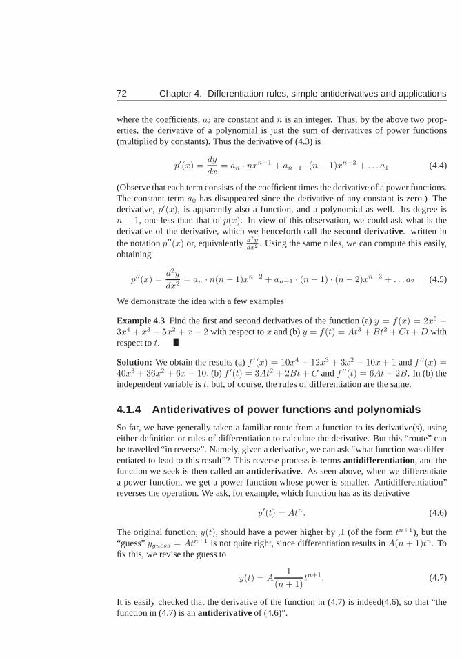
72 Chapter 4. Differentiation rules, simple antiderivatives and applications
where the coefficients,ai are constant andn is an integer. Thus, by the above two prop-erties, the derivative of a polynomial is just the sum of derivatives of power functions(multiplied by constants). Thus the derivative of (4.3) is
p′(x) =dy
dx= an · nxn−1 + an−1 · (n− 1)xn−2 + . . . a1 (4.4)
(Observe that each term consists of the coefficient times thederivative of a power functions.The constant terma0 has disappeared since the derivative of any constant is zero.) Thederivative,p′(x), is apparently also a function, and a polynomial as well. Itsdegree isn − 1, one less than that ofp(x). In view of this observation, we could ask what is thederivative of the derivative, which we henceforth call thesecond derivative. written inthe notationp′′(x) or, equivalentlyd2y
dx2 . Using the same rules, we can compute this easily,obtaining
p′′(x) =d2y
dx2= an · n(n− 1)xn−2 + an−1 · (n− 1) · (n− 2)xn−3 + . . . a2 (4.5)
We demonstrate the idea with a few examples
Example 4.3 Find the first and second derivatives of the function (a)y = f(x) = 2x5 +3x4 + x3 − 5x2 + x− 2 with respect tox and (b)y = f(t) = At3 + Bt2 + Ct + D withrespect tot.
Solution: We obtain the results (a)f ′(x) = 10x4 + 12x3 + 3x2 − 10x + 1 andf ′′(x) =40x3 + 36x2 + 6x− 10. (b) f ′(t) = 3At2 + 2Bt + C andf ′′(t) = 6At + 2B. In (b) theindependent variable ist, but, of course, the rules of differentiation are the same.
4.1.4 Antiderivatives of power functions and polynomials
So far, we have generally taken a familiar route from a function to its derivative(s), usingeither definition or rules of differentiation to calculate the derivative. But this “route” canbe travelled “in reverse”. Namely, given a derivative, we can ask “what function was differ-entiated to lead to this result”? This reverse process is termsantidifferentiation , and thefunction we seek is then called anantiderivative. As seen above, when we differentiatea power function, we get a power function whose power is smaller. Antidifferentiation”reverses the operation. We ask, for example, which functionhas as its derivative
y′(t) = Atn. (4.6)
The original function,y(t), should have a power higher by ,1 (of the formtn+1), but the“guess”yguess = Atn+1 is not quite right, since differentiation results inA(n + 1)tn. Tofix this, we revise the guess to
y(t) = A1
(n + 1)tn+1. (4.7)
It is easily checked that the derivative of the function in (4.7) is indeed(4.6), so that “thefunction in (4.7) is anantiderivative of (4.6)”.
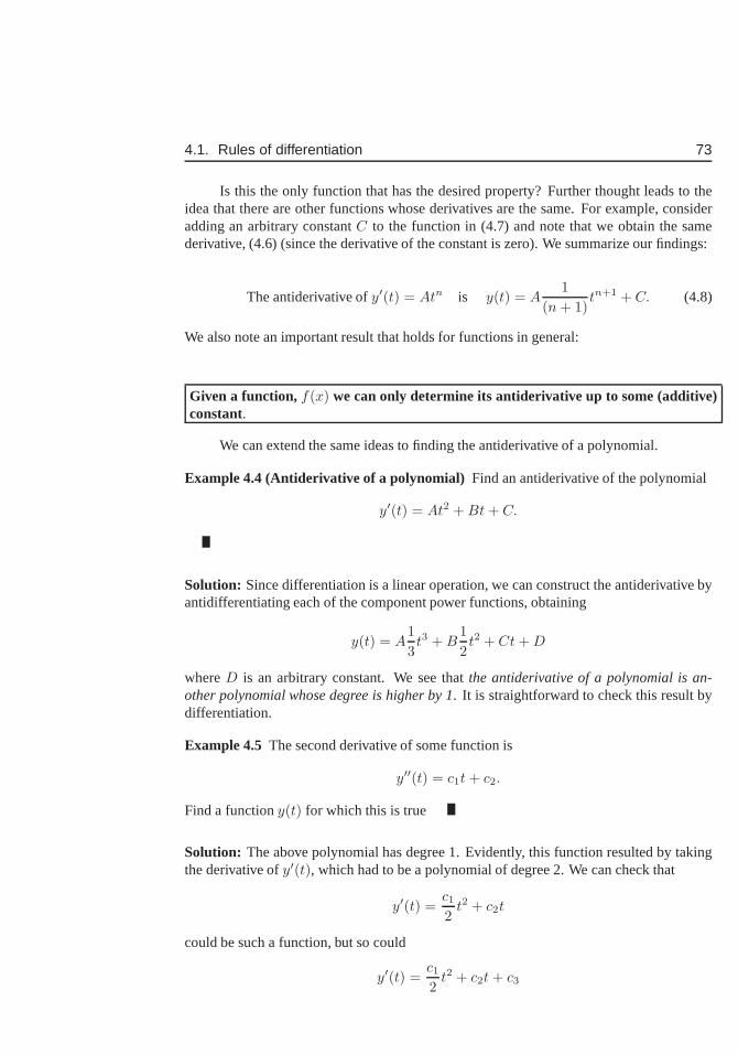
4.1. Rules of differentiation 73
Is this the only function that has the desired property? Further thought leads to theidea that there are other functions whose derivatives are the same. For example, consideradding an arbitrary constantC to the function in (4.7) and note that we obtain the samederivative, (4.6) (since the derivative of the constant is zero). We summarize our findings:
The antiderivative ofy′(t) = Atn is y(t) = A1
(n + 1)tn+1 + C. (4.8)
We also note an important result that holds for functions in general:
Given a function, f(x) we can only determine its antiderivative up to some (additive)constant.
We can extend the same ideas to finding the antiderivative of apolynomial.
Example 4.4 (Antiderivative of a polynomial) Find an antiderivative of the polynomial
y′(t) = At2 + Bt + C.
Solution: Since differentiation is a linear operation, we can construct the antiderivative byantidifferentiating each of the component power functions, obtaining
y(t) = A1
3t3 + B
1
2t2 + Ct + D
whereD is an arbitrary constant. We see thatthe antiderivative of a polynomial is an-other polynomial whose degree is higher by 1. It is straightforward to check this result bydifferentiation.
Example 4.5 The second derivative of some function is
y′′(t) = c1t + c2.
Find a functiony(t) for which this is true
Solution: The above polynomial has degree 1. Evidently, this functionresulted by takingthe derivative ofy′(t), which had to be a polynomial of degree 2. We can check that
y′(t) =c1
2t2 + c2t
could be such a function, but so could
y′(t) =c1
2t2 + c2t + c3
74 Chapter 4. Differentiation rules, simple antiderivatives and applications
for any constantc3. In turn, the functiony(t) had to be a polynomial of degree 3. We cansee that one such function is
y(t) =c1
6t3 +
c2
2t2 + c3t + c4
wherec4 is any constant. (This can be checked by differentiating.) The steps we have justillustrated are “antidifferentiation”. In short, the relationship is:
for differentiation y(t)→ y′(t)→ y′′(t)
whereas
for antidifferentiation y′′(t)→ y′(t)→ y(t).
(Arrows denote what is done to one function to arrive at the next.) These results will beuseful in an application to the acceleration, velocity, anddisplacement of a moving objectin Section 4.2.
4.1.5 Product and quotient rules for derivatives
So far, using a single “rule” for differentiation, the powerrule, together with properties ofthe derivative such as additivity and constant multiplication (described in Section 4.1.2),we were able to calculate derivatives of polynomials. here we state without proof, twoother rules of differentiation that will prove to be useful in due time.
The product rule: If f(x) andg(x) are two functions, each differentiable in the domainof interest, then
d[f(x)g(x)]
dx=
df(x)
dxg(x) +
dg(x)
dxf(x).
Another notation for this rule is
[f(x)g(x)]′ = f ′(x)g(x) + g′(x)f(x).
Example 4.6 Find the derivative of the product of the two functionsf(x) = x andg(x) =1 + x.
Solution: Using the product rule leads to
d[f(x)g(x)]
dx=
d[x(1 + x)]
dx=
d[x]
dx·(1+x)+
d[(1 + x)]
dx·x = 1 ·(1+x)+1 ·x = 2x+1.
(This can be easily checked by noting thatf(x)g(x) = x(1+x) = x+x2, whose derivativeagrees with the above.)
4.1. Rules of differentiation 75
The quotient rule: If f(x) andg(x) are two functions, each differentiable in the domainof interest, then
d
dx
[
f(x)
g(x)
]
=df(x)
dx g(x)− dg(x)dx f(x)
[g(x)]2.
We can also write this in the form[
f(x)
g(x)
]′=
f ′(x)g(x) − g′(x)f(x)
[g(x)]2.
Example 4.7 Find the derivative of the functiony = ax−n = a/xn wherea is a constantandn is a positive integer.
Solution: We can rewrite this as the quotient of the two functionsf(x) = a andg(x) = xn.Theny = f(x)/g(x) so, using the quotient rule leads to the derivative
dy
dx=
f ′(x)g(x) − g′(x)f(x)
[g(x)]2=
0 · xn − (nxn−1) · a(xn)2
=−anxn−1
x2n
After algebraic simplification, we obtaindy/dx = a(−n)xn−1−2n = a(−n)x−n−1. Thisis an interesting result:The power rule of differentiation holds for negative integerpowers.
Example 4.8 (Dynamics of actin in the cell)Actin is a structural protein that forms longfilaments and networks in living cells. The actin network is continually assembling fromsmall components (actin monomers) and disassembling back again. To study this process,scientists attach fluorescent markers to actin, and watch the fluorescence intensity changeover time. In a recent experiment, both red and green fluorescent labels were used. Thegreen label fluoresces only after it is activated by a pulse oflight, whereas the red fluores-cent protein is active continually.
It was noted that the red and green fluorescence intensities (R, G) satisfied the fol-lowing relationships11:
dR
dt= (a− b)R,
dG
dt= −bG
wherea, b are constants that characterize the rate of assembly and disassembly (“breakup”)of actin. Find the relationship satisfied by the ratio of the two fluorescent signalsR/G andthe derivative of that ratio (d(R/G)/dt).
Solution: This is an application of the quotient rule. We write
d(R/G)
dt=
dRdt G− dG
dt R
G2=
(a− b)RG− (−bGR)
G2=
aRG
G2= a(R/G)
Thus, the derivative of the ratio is proportional to that same ratio and the constant of pro-portionality is the parametera.
11These relationships between a function of time and its own derivative are examples ofdifferential equations,a topic we will revisit in later chapters.
76 Chapter 4. Differentiation rules, simple antiderivatives and applications
4.1.6 The power rule for fractional powers
Using the definition of the derivative, we have already shownthat the derivative of√
x isy′(x) = 1
2√
x(see Problem 10). We restate this result in terms of (one specific case) of a
fractional power. Recall that√
x = x1/2.
The derivative ofy =√
x is y′(x) = 12x−1/2.
This idea can be generalized to any fractional power. Indeed, we state here a useful result(to be demonstrated in Chapter 9).
Derivative of fractional-power function: The derivative of
y = f(x) = xm/n
isdy
dx=
m
nx( m
n −1).
Example 4.9 (Energy loss and Earth’s temperature, revisited) In Example 4.2, we cal-culated the rate of change of energy lost per unit change in the Earth’s temperature basedon Eqn. (1.4). Find the rate of change of Earth’s temperatureper unit energy loss based onthe same equation.
Solution: We are asked to finddT/dEout. We will first rewrite the relationship12 to expressT as a function ofEout. To do so, we solve forT in Eqn. (1.4), obtaining
T =
(
Eout
4πr2ǫσ
)1/4
=
(
1
4πr2ǫσ
)1/4
E1/4out = KE
1/4out .
Then, as we have indicated, the first term is a constant, and weuse the rule for a derivativeof a fractional power to compute that
dT
dEout=
(
1
4πr2ǫσ
)1/4
· 14E
(1/4)−1out =
(
1
16πr2ǫσ
)1/4
E−3/4out .
4.2 Application: From acceleration to displacementAs we have seen already, the derivative of a function is also,itself, a function. This leadsto the idea that we can apply the same process of differentiation over again to construct thederivative of that new function. We refer to the derivative of the derivative as thesecondderivative. As we discuss here, a natural example of a second derivativeis theaccelerationof an object: the rate of change of the velocity (which is, as we have seen, the rate of change
12In a later chapter we will show that this step is not essential. In fact, implicit differentiation will be intro-duced as a method of finding the desired derivative without solving for the variable of interest.
4.2. Application: From acceleration to displacement 77
of a displacement). We can also state the same relationshipsin terms of antiderivatives: thevelocity of an object is an antiderivative of the acceleration, and the displacement is anantiderivative of the velocity.
Section 4.2.1 Learning goals
1. Understand that velocity and acceleration are first and second derivatives of the po-sition with respect to time.
2. Understand that velocity and position are first and secondantiderivatives of acceler-ation.
3. Given that the acceleration of an object is constant in time, be able to find the velocityand displacement of that object.
4.2.1 Position, velocity, and acceleration
As an example of the relation between a function and its first and second derivative, wereturn to the discussion of displacement, velocity and acceleration of an object falling underthe force of gravity. Here we will use the notationy(t) to denote the position of the objectat timet. From now on, we will refer to the instantaneous velocity of aparticle or object attime t simply asthe velocity, v(t).
Definition 4.10 (The velocity).Given the position of some particle as a function of time,y(t), we define the velocity as the rate of change of the position, i.e. the derivative ofy(t):
v(t) =dy
dt= y′(t).
Here we have just used two equivalent notations for the derivative. In general,v maydepend on time, a fact we indicated by writingv(t).
Definition 4.11 (The acceleration).We will also define the acceleration as the (instanta-neous) rate of change of the velocity, i.e. as the derivativeof v(t).
a(t) =dv
dt= v′(t).
(Acceleration could also depend on time, hencea(t).)
Since the acceleration is the derivative of a derivative of the original function, wealso use the notation
a(t) =d
dt
(
dy
dt
)
=d2y
dt2= y′′(t)
Here we have used three equivalent ways of writing a second derivative. (This notationevolved for historical reasons, and is used interchangeably in science.) The acceleration ishence the second derivative of the position.
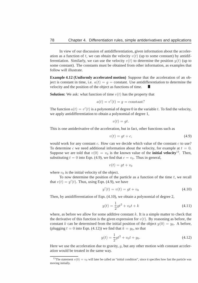
78 Chapter 4. Differentiation rules, simple antiderivatives and applications
In view of our discussion of antidifferentiation, given information about the acceler-ation as a function oft, we can obtain the velocityv(t) (up to some constant) by antidif-ferentiation. Similarly, we can use the velocityv(t) to determine the positiony(t) (up tosome constant). The constants must be obtained from other information, as examples thatfollow will illustrate.
Example 4.12 (Uniformly accelerated motion)Suppose that the acceleration of an ob-ject is constant in time, i.e.a(t) = g = constant. Use antidifferentiation to determine thevelocity and the position of the object as functions of time.
Solution: We ask: what function of timev(t) has the property that
a(t) = v′(t) = g = constant?
The functiona(t) = v′(t) is a polynomial of degree 0 in the variablet. To find the velocity,we apply antidifferentiation to obtain a polynomial of degree 1,
v(t) = gt.
This is one antiderivative of the acceleration, but in fact,other functions such as
v(t) = gt + c, (4.9)
would work for any constantc. How can we decide which value of the constantc to use?To determinec we need additional information about the velocity, for example att = 0.Suppose we are told thatv(0) = v0 is the known value of theinitial velocity 13. Then,substitutingt = 0 into Eqn. (4.9), we find thatc = v0. Thus in general,
v(t) = gt + v0
wherev0 is the initial velocity of the object.To now determine the position of the particle as a function ofthe timet, we recall
thatv(t) = y′(t). Thus, using Eqn. (4.9), we have
y′(t) = v(t) = gt + v0 (4.10)
Then, by antidifferentiation of Eqn. (4.10), we obtain a polynomial of degree 2,
y(t) =1
2gt2 + v0t + k (4.11)
where, as before we allow for some additive constantk. It is a simple matter to check thatthe derivative of this function is the given expression forv(t). By reasoning as before, theconstantk can be determined from the initial position of the objecty(0) = y0. A before,(pluggingt = 0 into Eqn. (4.12)) we find thatk = y0, so that
y(t) =1
2gt2 + v0t + y0. (4.12)
Here we use the acceleration due to gravity,g, but any other motion with constant acceler-ation would be treated in the same way.
13The statementv(0) = v0 will later be called an “initial condition”, since it specifies how fast the particle wasmoving initially.
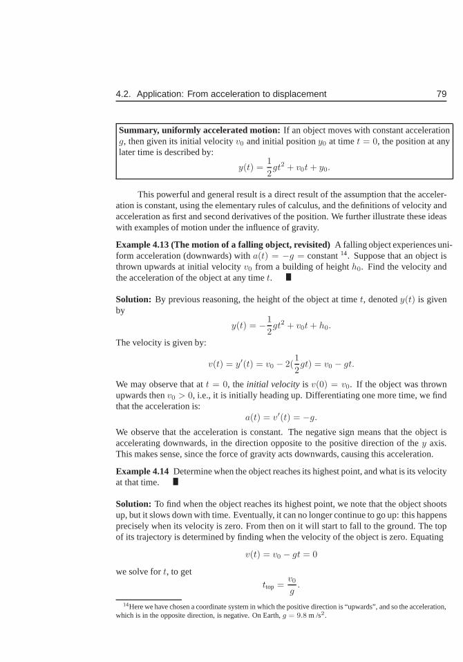
4.2. Application: From acceleration to displacement 79
Summary, uniformly accelerated motion: If an object moves with constant accelerationg, then given its initial velocityv0 and initial positiony0 at timet = 0, the position at anylater time is described by:
y(t) =1
2gt2 + v0t + y0.
This powerful and general result is a direct result of the assumption that the acceler-ation is constant, using the elementary rules of calculus, and the definitions of velocity andacceleration as first and second derivatives of the position. We further illustrate these ideaswith examples of motion under the influence of gravity.
Example 4.13 (The motion of a falling object, revisited)A falling object experiences uni-form acceleration (downwards) witha(t) = −g = constant14. Suppose that an object isthrown upwards at initial velocityv0 from a building of heighth0. Find the velocity andthe acceleration of the object at any timet.
Solution: By previous reasoning, the height of the object at timet, denotedy(t) is givenby
y(t) = −1
2gt2 + v0t + h0.
The velocity is given by:
v(t) = y′(t) = v0 − 2(1
2gt) = v0 − gt.
We may observe that att = 0, the initial velocity is v(0) = v0. If the object was thrownupwards thenv0 > 0, i.e., it is initially heading up. Differentiating one moretime, we findthat the acceleration is:
a(t) = v′(t) = −g.
We observe that the acceleration is constant. The negative sign means that the object isaccelerating downwards, in the direction opposite to the positive direction of they axis.This makes sense, since the force of gravity acts downwards,causing this acceleration.
Example 4.14 Determine when the object reaches its highest point, and what is its velocityat that time.
Solution: To find when the object reaches its highest point, we note thatthe object shootsup, but it slows down with time. Eventually, it can no longer continue to go up: this happensprecisely when its velocity is zero. From then on it will start to fall to the ground. The topof its trajectory is determined by finding when the velocity of the object is zero. Equating
v(t) = v0 − gt = 0
we solve fort, to get
ttop =v0
g.
14Here we have chosen a coordinate system in which the positivedirection is “upwards”, and so the acceleration,which is in the opposite direction, is negative. On Earth,g = 9.8 m /s2.
80 Chapter 4. Differentiation rules, simple antiderivatives and applications
Example 4.15 When does the object hit the ground? What is its velocity at that instant?
Solution: We will assume that the object hits the ground at levely = 0. Then we mustsolve fort in the equation:
y(t) = h0 + v0t−1
2gt2 = 0.
Here we must observe that the highest power of the independent variable is 2, so thaty is aquadratic function oft, and solving fort requires us to solve a quadratic equation. This isa quadratic equation, which could be written in the form
1
2gt2 − v0t− h0 = 0, ⇒ gt2 − 2v0t− 2h0 = 0.
Using the quadratic formula, we obtain
tground=2v0 ±
√
4v20 + 8gh0
2g⇒ tground =
v0
g±√
v20 + 2gh0
g.
We have found two roots. One is positive and the other is negative. Since we are interestedin t > 0, we will reject the negative root, so
tground =v0
g+
√
v20 + 2gh0
g.
To find the velocity of the object when it hits the ground. we need to use the time deter-mined in part (b). Substitutingtground into the expression for velocity, we obtain:
v(tground) = v0 − gtground = v0 − g
(
v0
g+
√
v20 + 2gh0
g
)
.
After some algebraic simplification, we obtain
v(tground) = −√
v20 + 2gh0.
We observe that this velocity is negative, indicating (as expected) that the object is fallingdown.
Figure 4.1 illustrates the relationship between the three functions.
4.3 Sketching first, second, and anti- derivatives
Section 4.3 Learning goals
1. Given a sketch of a function, be able to sketch both its firstand its second derivatives.
2. Given the sketch of a function, be able to sketch its first and second antiderivatives.
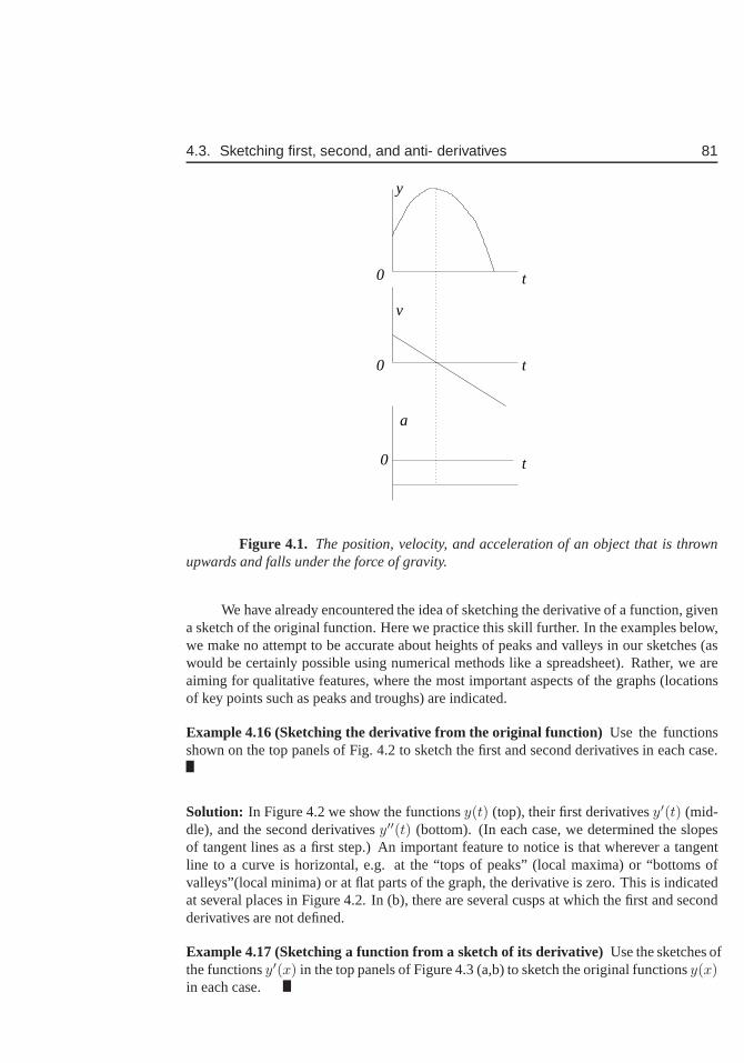
4.3. Sketching first, second, and anti- derivatives 81
t
t
t
y
v
a
0
0
0
Figure 4.1. The position, velocity, and acceleration of an object that is thrownupwards and falls under the force of gravity.
We have already encountered the idea of sketching the derivative of a function, givena sketch of the original function. Here we practice this skill further. In the examples below,we make no attempt to be accurate about heights of peaks and valleys in our sketches (aswould be certainly possible using numerical methods like a spreadsheet). Rather, we areaiming for qualitative features, where the most important aspects of the graphs (locationsof key points such as peaks and troughs) are indicated.
Example 4.16 (Sketching the derivative from the original function) Use the functionsshown on the top panels of Fig. 4.2 to sketch the first and second derivatives in each case.
Solution: In Figure 4.2 we show the functionsy(t) (top), their first derivativesy′(t) (mid-dle), and the second derivativesy′′(t) (bottom). (In each case, we determined the slopesof tangent lines as a first step.) An important feature to notice is that wherever a tangentline to a curve is horizontal, e.g. at the “tops of peaks” (local maxima) or “bottoms ofvalleys”(local minima) or at flat parts of the graph, the derivative is zero. This is indicatedat several places in Figure 4.2. In (b), there are several cusps at which the first and secondderivatives are not defined.
Example 4.17 (Sketching a function from a sketch of its derivative) Use the sketches ofthe functionsy′(x) in the top panels of Figure 4.3 (a,b) to sketch the original functionsy(x)in each case.
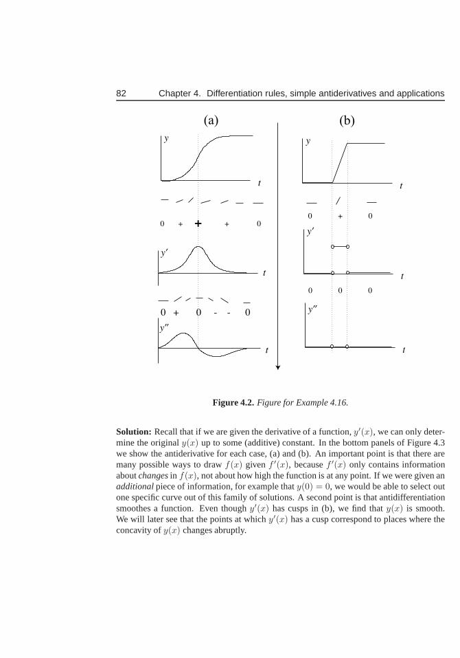
82 Chapter 4. Differentiation rules, simple antiderivatives and applications
0 + + 0+
0 + 0 - - 0
t
t
t
y
y’
y’’
t
y
t
y’
t
0 + 0
0 0 0
y’’
(a) (b)
Figure 4.2.Figure for Example 4.16.
Solution: Recall that if we are given the derivative of a function,y′(x), we can only deter-mine the originaly(x) up to some (additive) constant. In the bottom panels of Figure 4.3we show the antiderivative for each case, (a) and (b). An important point is that there aremany possible ways to drawf(x) given f ′(x), becausef ′(x) only contains informationaboutchangesin f(x), not about how high the function is at any point. If we were given anadditionalpiece of information, for example thaty(0) = 0, we would be able to select outone specific curve out of this family of solutions. A second point is that antidifferentiationsmoothes a function. Even thoughy′(x) has cusps in (b), we find thaty(x) is smooth.We will later see that the points at whichy′(x) has a cusp correspond to places where theconcavity ofy(x) changes abruptly.
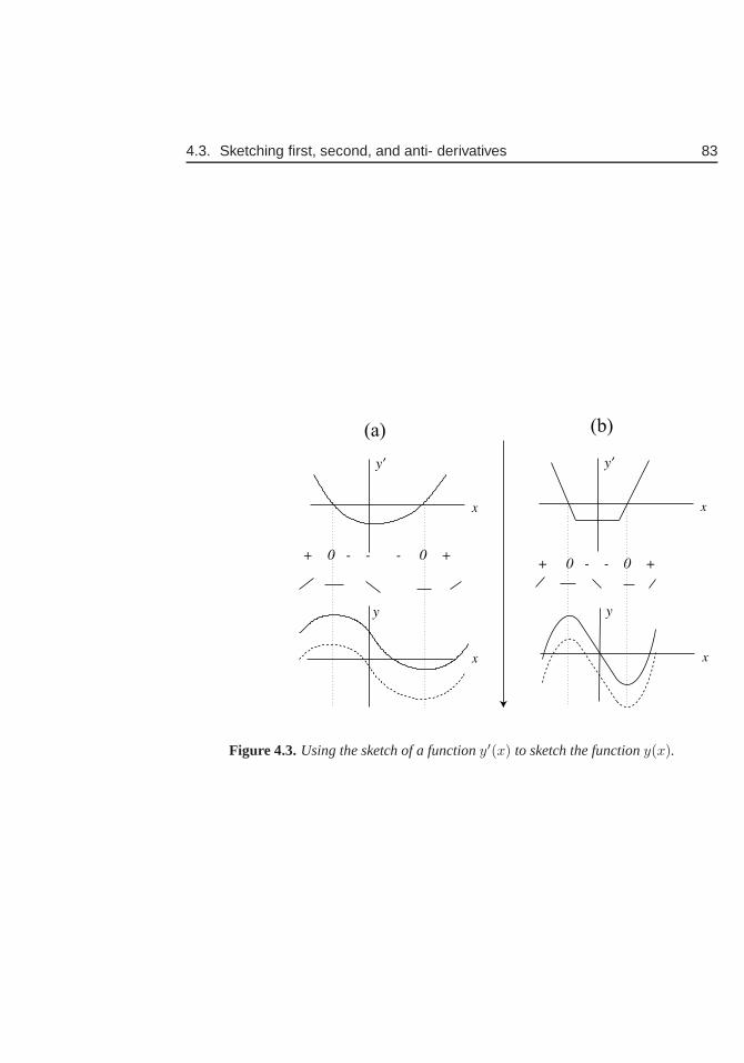
4.3. Sketching first, second, and anti- derivatives 83
+ 0 - - - 0 +
x
x
y’
y
x
y’
x
+ 0 - - 0 +
y
(a) (b)
Figure 4.3.Using the sketch of a functiony′(x) to sketch the functiony(x).
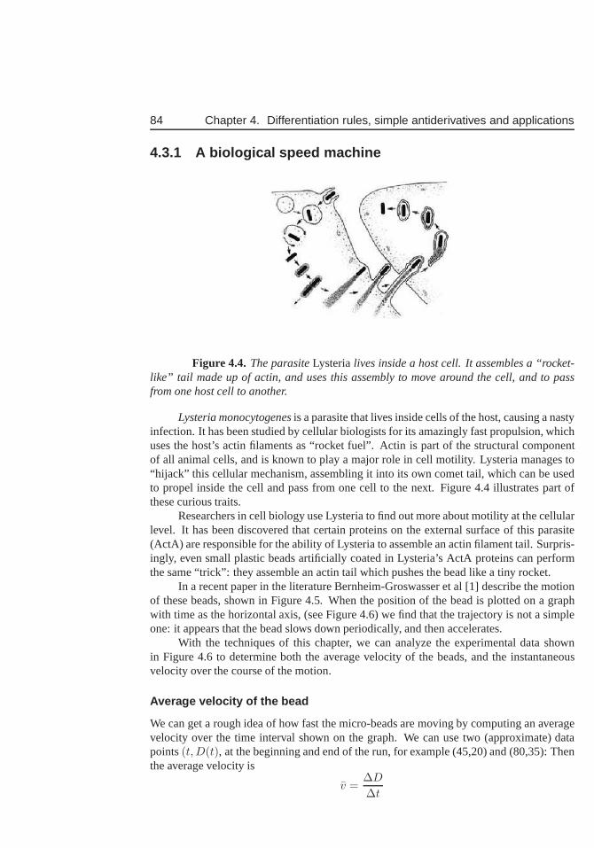
84 Chapter 4. Differentiation rules, simple antiderivatives and applications
4.3.1 A biological speed machine
Figure 4.4. The parasiteLysterialives inside a host cell. It assembles a “rocket-like” tail made up of actin, and uses this assembly to move around the cell, and to passfrom one host cell to another.
Lysteria monocytogenesis a parasite that lives inside cells of the host, causing a nastyinfection. It has been studied by cellular biologists for its amazingly fast propulsion, whichuses the host’s actin filaments as “rocket fuel”. Actin is part of the structural componentof all animal cells, and is known to play a major role in cell motility. Lysteria manages to“hijack” this cellular mechanism, assembling it into its own comet tail, which can be usedto propel inside the cell and pass from one cell to the next. Figure 4.4 illustrates part ofthese curious traits.
Researchers in cell biology use Lysteria to find out more about motility at the cellularlevel. It has been discovered that certain proteins on the external surface of this parasite(ActA) are responsible for the ability of Lysteria to assemble an actin filament tail. Surpris-ingly, even small plastic beads artificially coated in Lysteria’s ActA proteins can performthe same “trick”: they assemble an actin tail which pushes the bead like a tiny rocket.
In a recent paper in the literature Bernheim-Groswasser et al [1] describe the motionof these beads, shown in Figure 4.5. When the position of the bead is plotted on a graphwith time as the horizontal axis, (see Figure 4.6) we find thatthe trajectory is not a simpleone: it appears that the bead slows down periodically, and then accelerates.
With the techniques of this chapter, we can analyze the experimental data shownin Figure 4.6 to determine both the average velocity of the beads, and the instantaneousvelocity over the course of the motion.
Average velocity of the bead
We can get a rough idea of how fast the micro-beads are moving by computing an averagevelocity over the time interval shown on the graph. We can usetwo (approximate) datapoints(t, D(t), at the beginning and end of the run, for example (45,20) and (80,35): Thenthe average velocity is
v =∆D
∆t
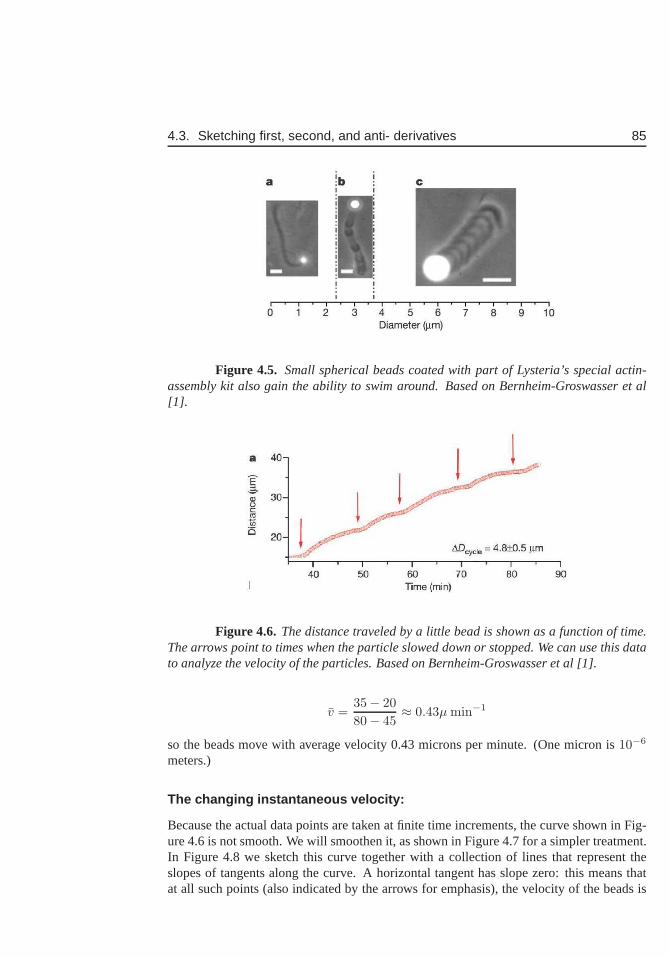
4.3. Sketching first, second, and anti- derivatives 85
Figure 4.5. Small spherical beads coated with part of Lysteria’s special actin-assembly kit also gain the ability to swim around. Based on Bernheim-Groswasser et al[1].
Figure 4.6. The distance traveled by a little bead is shown as a function of time.The arrows point to times when the particle slowed down or stopped. We can use this datato analyze the velocity of the particles. Based on Bernheim-Groswasser et al [1].
v =35− 20
80− 45≈ 0.43µ min−1
so the beads move with average velocity 0.43 microns per minute. (One micron is10−6
meters.)
The changing instantaneous velocity:
Because the actual data points are taken at finite time increments, the curve shown in Fig-ure 4.6 is not smooth. We will smoothen it, as shown in Figure 4.7 for a simpler treatment.In Figure 4.8 we sketch this curve together with a collectionof lines that represent theslopes of tangents along the curve. A horizontal tangent hasslope zero: this means thatat all such points (also indicated by the arrows for emphasis), the velocity of the beads is
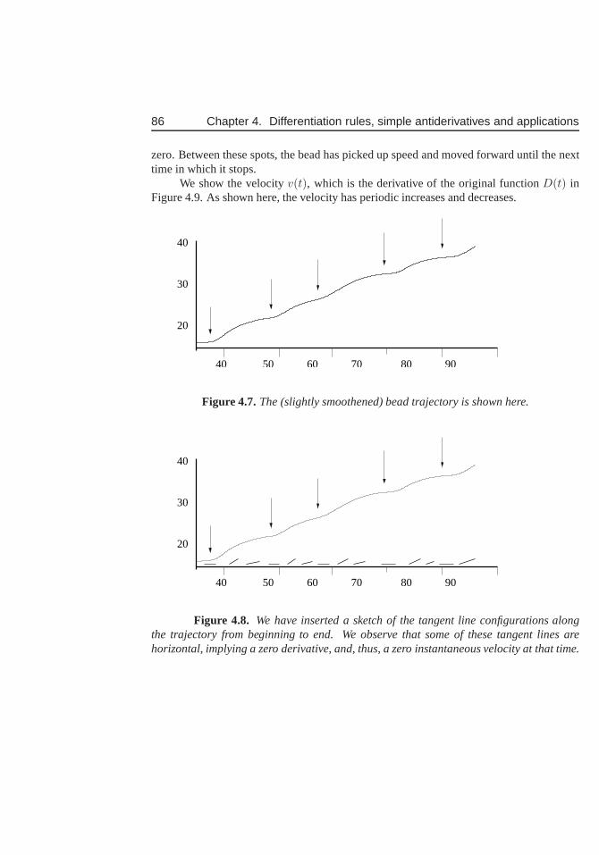
86 Chapter 4. Differentiation rules, simple antiderivatives and applications
zero. Between these spots, the bead has picked up speed and moved forward until the nexttime in which it stops.
We show the velocityv(t), which is the derivative of the original functionD(t) inFigure 4.9. As shown here, the velocity has periodic increases and decreases.
40 50 60 70 80 90
40
30
20
Figure 4.7.The (slightly smoothened) bead trajectory is shown here.
40 50 60 70 80 90
40
30
20
Figure 4.8. We have inserted a sketch of the tangent line configurations alongthe trajectory from beginning to end. We observe that some ofthese tangent lines arehorizontal, implying a zero derivative, and, thus, a zero instantaneous velocity at that time.
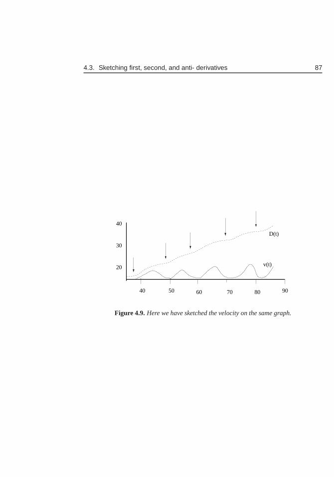
4.3. Sketching first, second, and anti- derivatives 87
40
30
20
D(t)
v(t)
40 50 60 70 9080
Figure 4.9.Here we have sketched the velocity on the same graph.
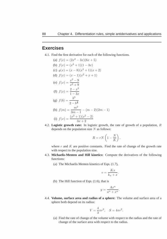
88 Chapter 4. Differentiation rules, simple antiderivatives and applications
Exercises4.1. Find the first derivative for each of the following functions.
(a) f(x) = (2x2 − 3x)(6x + 5)
(b) f(x) = (x3 + 1)(1 − 3x)
(c) g(x) = (x− 8)(x2 + 1)(x + 2)
(d) f(x) = (x− 1)(x2 + x + 1)
(e) f(x) =x2 − 9
x2 + 9
(f) f(x) =2− x3
1− 3x
(g) f(b) =b3
2− b23
(h) f(m) =m2
3m− 1− (m− 2)(2m− 1)
(i) f(x) =(x2 + 1)(x2 − 2)
3x + 24.2. Logistic growth rate: In logistic growth, the rate of growth of a population,R
depends on the population sizeN as follows:
R = rN
(
1− N
K
)
,
wherer andK are positive constants. Find the rate of change of the growthratewith respect to the population size.
4.3. Michaelis-Menten and Hill kinetics: Compute the derivatives of the followingfunctions:
(a) The Michaelis Menten kinetics of Eqn. (1.7),
v =Kx
kn + x.
(b) The Hill function of Eqn. (1.6), that is
y =Axn
an + xn.
4.4. Volume, surface area and radius of a sphere:The volume and surface area of asphere both depend on its radius:
V =4
3πr3, S = 4πr2.
(a) Find the rate of change of the volume with respect to the radius and the rate ofchange of the surface area with respect to the radius.
Exercises 89
(b) Find the rate of change of the surface area to volume ratioS/V with respectto the radius.
4.5. Derivative of Volume with respect to surface area: Consider the volume andsurface area of a sphere. (See Problem 4 for the formulae.)
(a) Eliminate the radius and expressV as a function ofS.
(b) Find the rate of change of the volume with respect to the surface area.
4.6. Surface area and volume of a cylinder:The volume of a cylinder and the surfacearea of a cylinder with two flat end-caps are
V = πr2L, S = 2πrL + 2πr2
whereL is the length andr the radius of the cylinder.
(a) Find the rate of change of the volume and surface area withrespect to theradius, assuming that the lengthL is held fixed.
(b) Find the rate of change of the surface area to volume ratioS/V with respectto the radius assuming that the lengthL is held fixed.
4.7. Growing circular colony: A bacterial colony has the shape of a circular disk withradiusr(t) = 2 + t/2 wheret is time in hours andr is in units of mm. Expressthe area of the colony as a function of time and then determinethe rate of change ofarea with respect to time att = 2hr.
4.8. Rate of change of energy during foraging:When a bee forages for nectar in apatch of flowers, it gains energy. Suppose that the amount of energy gained duringa foraging time spant is
f(t) =Et
k + t
whereE, k > 0 are constants.
(a) If the bee stays in the patch for a very long time, how much energy can it gain?
(b) Use the quotient rule to calculate the rate of energy gainwhile foraging in theflower patch.
4.9. Ratio of two species: In a certain lake it is found that the rate of change of thepopulation size of each of two species (N1(t), N2(t)) is proportional to the givenpopulation size. That is
dN1
dt= k1N1,
dN2
dt= k2N2
wherek1 andk2 are constants. Find the rate of change of the ratio of population
sizes(N1/N2) with respect to timed(N1/N2)
dt. Your answer will be in terms of
k1, k2 and the ratioN1/N2.
4.10. Invasive species and sustainability:An invasive species is one that can outcom-pete and grow faster than the native species, resulting in takeover and displacementof the local ecosystem, disrupting sustainability. Consider the two-lake system of
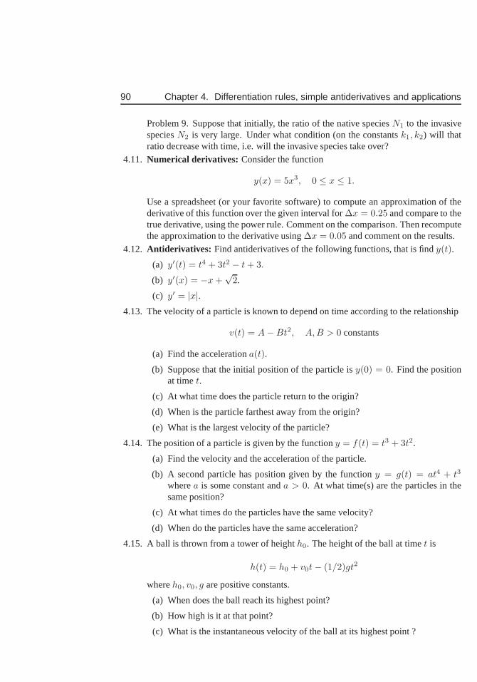
90 Chapter 4. Differentiation rules, simple antiderivatives and applications
Problem 9. Suppose that initially, the ratio of the native speciesN1 to the invasivespeciesN2 is very large. Under what condition (on the constantsk1, k2) will thatratio decrease with time, i.e. will the invasive species take over?
4.11. Numerical derivatives: Consider the function
y(x) = 5x3, 0 ≤ x ≤ 1.
Use a spreadsheet (or your favorite software) to compute an approximation of thederivative of this function over the given interval for∆x = 0.25 and compare to thetrue derivative, using the power rule. Comment on the comparison. Then recomputethe approximation to the derivative using∆x = 0.05 and comment on the results.
4.12. Antiderivatives: Find antiderivatives of the following functions, that is find y(t).
(a) y′(t) = t4 + 3t2 − t + 3.
(b) y′(x) = −x +√
2.
(c) y′ = |x|.4.13. The velocity of a particle is known to depend on time according to the relationship
v(t) = A−Bt2, A, B > 0 constants
(a) Find the accelerationa(t).
(b) Suppose that the initial position of the particle isy(0) = 0. Find the positionat timet.
(c) At what time does the particle return to the origin?
(d) When is the particle farthest away from the origin?
(e) What is the largest velocity of the particle?
4.14. The position of a particle is given by the functiony = f(t) = t3 + 3t2.
(a) Find the velocity and the acceleration of the particle.
(b) A second particle has position given by the functiony = g(t) = at4 + t3
wherea is some constant anda > 0. At what time(s) are the particles in thesame position?
(c) At what times do the particles have the same velocity?
(d) When do the particles have the same acceleration?
4.15. A ball is thrown from a tower of heighth0. The height of the ball at timet is
h(t) = h0 + v0t− (1/2)gt2
whereh0, v0, g are positive constants.
(a) When does the ball reach its highest point?
(b) How high is it at that point?
(c) What is the instantaneous velocity of the ball at its highest point ?
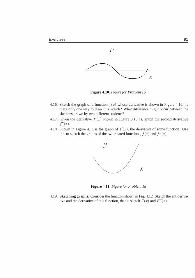
Exercises 91
x
f '
Figure 4.10.Figure for Problem 16
4.16. Sketch the graph of a functionf(x) whose derivative is shown in Figure 4.10. Isthere only one way to draw this sketch? What difference mightoccur between thesketches drawn by two different students?
4.17. Given the derivativef ′(x) shown in Figure 3.16(c), graph the second derivativef ′′(x).
4.18. Shown in Figure 4.11 is the graph off ′(x), the derivative of some function. Usethis to sketch the graphs of the two related functions,f(x) andf ′′(x)
x
y
Figure 4.11.Figure for Problem 18
4.19. Sketching graphs:Consider the function shown in Fig. 4.12. Sketch the antideriva-tive and the derivative of this function, that is sketchF (x) andF ′′(x).
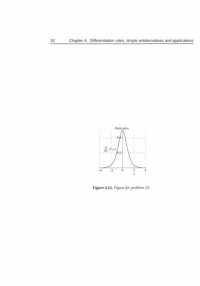
92 Chapter 4. Differentiation rules, simple antiderivatives and applications
Figure 4.12.Figure for problem 19.
Chapter 5
Tangent lines, linearapproximation, andNewton’s method
A straight line has the property that its slope is the same at every point on its graph. Thus,given a known point(x1, y1) on the line and the slopem, the equation of the line is foundfrom the statement that any other point(x, y) on the line should satisfy
riserun
=y − y1
x− x1= m. (5.1)
A review of properties of straight lines is provided in Appendix A. Here we use Eqn. (5.1)in many examples where we seek equations of tangent lines or properties of those lines.
Tangent lines approximate the local behaviour of a functionnear a point. This factwill lead us tolinear approximation , which is a way to estimate values of functions thatare not easy to calculate at a point of interest. A further application of the tangent line isto Newton’s methodfor approximating zeros of a function, that is values ofx for whichf(x) = 0.
5.1 The equation of a tangent lineWe first consider a number of simple examples of equations of atangent line that are easilyfound.
Section 5.1 Learning goals
1. Given a simple functiony = f(x) and a pointx, be able to find the equation of thetangent line to the graph at that point.
2. Be able to graph both the function and its tangent line using a spreadsheet or yourfavorite software.
93
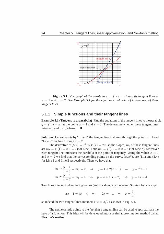
94 Chapter 5. Tangent lines, linear approximation, and Newton’s method
0.0 2.5
0.0
6.0
y=x2
Tangent line 1
Tangent line 2
intersection point
Figure 5.1. The graph of the parabolay = f(x) = x2 and its tangent lines atx = 1 andx = 2. See Example 5.1 for the equations and point of intersectionof thesetangent lines.
5.1.1 Simple functions and their tangent lines
Example 5.1 (Tangent to a parabola)Find the equations of the tangent lines to the parabolay = f(x) = x2 at the pointsx = 1 andx = 2. The determine whether these tangent linesintersect, and if so, where.
Solution: Let us denote by “Line 1” the tangent line that goes through the pointx = 1 and“Line 2” the line throughx = 2.
The derivative off(x) = x2 is f ′(x) = 2x, so the slopes,mi of these tangent linesarem1 = f ′(1) = 2·1 = 2 (for Line 1) andm2 = f ′(2) = 2·2 = 4 (for Line 2). Moreovereach tangent line intersects the parabola at the point of tangency. Using the valuesx = 1andx = 2 we find that the corresponding points on the curve,(x, x2), are (1,1) and (2,4)for Line 1 and Line 2 respectively. Then we have that
Line 1:y − 1
x− 1= m1 = 2, ⇒ y = 1 + 2(x− 1) ⇒ y = 2x− 1
Line 2:y − 4
x− 2= m2 = 4 ⇒ y = 4 + 4(x− 2) ⇒ y = 4x− 4
Two lines intersect when theiry values (andx values) are the same. Solving forx we get
2x− 1 = 4x− 4 ⇒ −2x = −3 ⇒ x =3
2.
so indeed the two tangent lines intersect atx = 3/2 as shown in Fig. 5.1.
The next example points to the fact that a tangent line can be used to approximate thezero of a function. This idea will be developed into a useful approximation method calledNewton’s method.
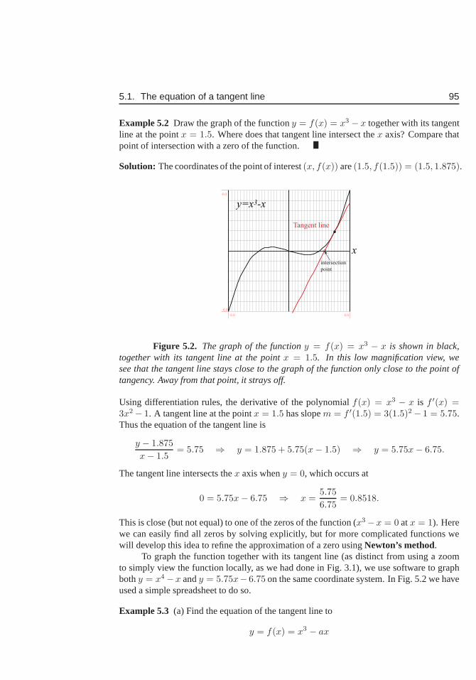
5.1. The equation of a tangent line 95
Example 5.2 Draw the graph of the functiony = f(x) = x3 − x together with its tangentline at the pointx = 1.5. Where does that tangent line intersect thex axis? Compare thatpoint of intersection with a zero of the function.
Solution: The coordinates of the point of interest(x, f(x)) are(1.5, f(1.5)) = (1.5, 1.875).
-2.0 2.0
-6.0
6.0
Tangent line
y=x3-x
xintersection
point
Figure 5.2. The graph of the functiony = f(x) = x3 − x is shown in black,together with its tangent line at the pointx = 1.5. In this low magnification view, wesee that the tangent line stays close to the graph of the function only close to the point oftangency. Away from that point, it strays off.
Using differentiation rules, the derivative of the polynomial f(x) = x3 − x is f ′(x) =3x2− 1. A tangent line at the pointx = 1.5 has slopem = f ′(1.5) = 3(1.5)2− 1 = 5.75.Thus the equation of the tangent line is
y − 1.875
x− 1.5= 5.75 ⇒ y = 1.875 + 5.75(x− 1.5) ⇒ y = 5.75x− 6.75.
The tangent line intersects thex axis wheny = 0, which occurs at
0 = 5.75x− 6.75 ⇒ x =5.75
6.75= 0.8518.
This is close (but not equal) to one of the zeros of the function (x3−x = 0 atx = 1). Herewe can easily find all zeros by solving explicitly, but for more complicated functions wewill develop this idea to refine the approximation of a zero using Newton’s method.
To graph the function together with its tangent line (as distinct from using a zoomto simply view the function locally, as we had done in Fig. 3.1), we use software to graphbothy = x4−x andy = 5.75x− 6.75 on the same coordinate system. In Fig. 5.2 we haveused a simple spreadsheet to do so.
Example 5.3 (a) Find the equation of the tangent line to
y = f(x) = x3 − ax
96 Chapter 5. Tangent lines, linear approximation, and Newton’s method
for a > 0 a constant, at the pointx = 1. (b) Find where that tangent line intersects thexaxis.
Solution: The function given in the example is a simple polynomial, so we easily calculateits derivative. The idea is very similar to that of the previous example, but the constantamakes this calculation a little less straightforward. (a)y = f(x) = x3−ax so the derivativeis
dy
dx= f ′(x) = 3x2 − a
and atx = 1 the slope (in terms of the constanta) is f ′(1) = 3 − a. The point of intereston the curve has coordinatesx = 1, y = 13 − a · 1 = 1− a.
We look for a line through(1, 1− a) with slopem = 3− a. That, is,
y − (1− a)
x− 1= 3− a.
Simplifying algebraically leads to
y = (3− a)(x − 1) + (1− a)
or simply
y = (3 − a)x− 2.
[Remark: at this point is is wise to check that the tangent line goes through the desiredpoint and has the slope we found. One way to do this is to pick a simple value fora, e.g.a = 1 and do a quick check that the answer matches what we have found.]
(b) To find the point of intersection, we set
y = (3− a)x− 2 = 0
and solve forx. We find that
x =2
3− a.
Example 5.4 Find the equation of the tangent line to the functiony = f(x) =√
x at thepointx = 4.
Solution: In Exercise 10 of Chapter 3, we verified that the derivative ofy = f(x) =√
xis f ′(x) = 1/(2
√x) (See (3.6)). Atx = 4 the slope of the function isf ′(4) = 1/(2
√4) =
1/4 and the point on the graph at which the tangent line is needed is (4, 2). Then theequation of the tangent line is
y − 2
x− 4= 0.25 ⇒ y = 2 + 0.25(x− 4).
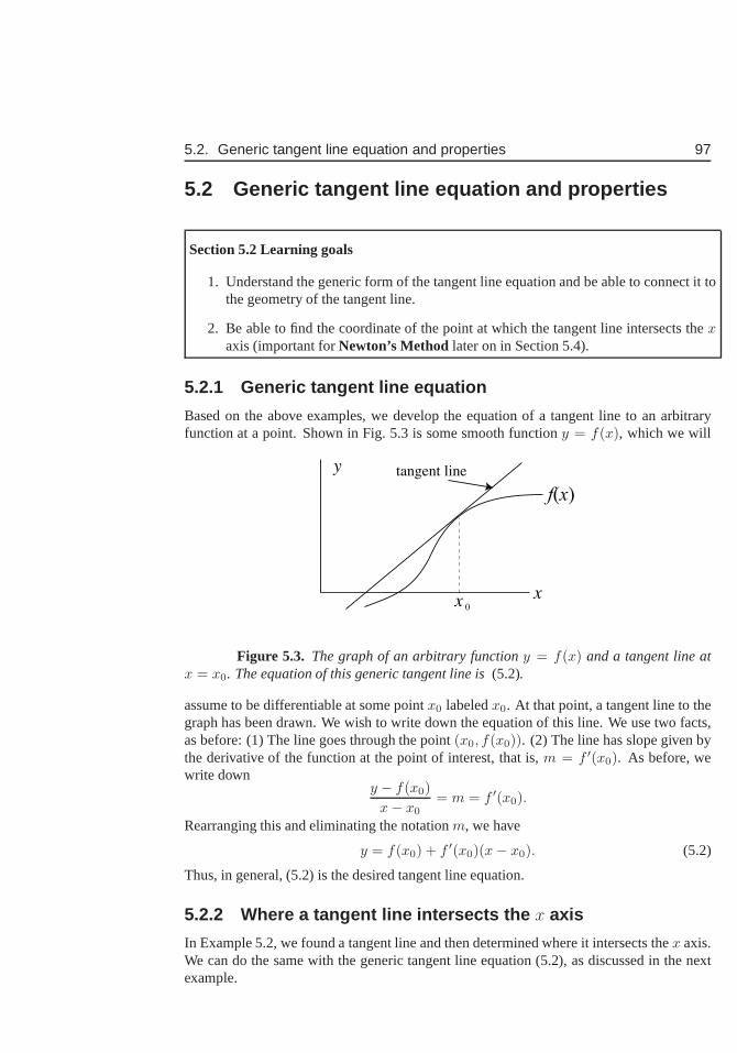
5.2. Generic tangent line equation and properties 97
5.2 Generic tangent line equation and properties
Section 5.2 Learning goals
1. Understand the generic form of the tangent line equation and be able to connect it tothe geometry of the tangent line.
2. Be able to find the coordinate of the point at which the tangent line intersects thexaxis (important forNewton’s Method later on in Section 5.4).
5.2.1 Generic tangent line equation
Based on the above examples, we develop the equation of a tangent line to an arbitraryfunction at a point. Shown in Fig. 5.3 is some smooth functiony = f(x), which we will
x
y
x
tangent line
0
f(x)
Figure 5.3. The graph of an arbitrary functiony = f(x) and a tangent line atx = x0. The equation of this generic tangent line is(5.2).
assume to be differentiable at some pointx0 labeledx0. At that point, a tangent line to thegraph has been drawn. We wish to write down the equation of this line. We use two facts,as before: (1) The line goes through the point(x0, f(x0)). (2) The line has slope given bythe derivative of the function at the point of interest, thatis, m = f ′(x0). As before, wewrite down
y − f(x0)
x− x0= m = f ′(x0).
Rearranging this and eliminating the notationm, we have
y = f(x0) + f ′(x0)(x− x0). (5.2)
Thus, in general, (5.2) is the desired tangent line equation.
5.2.2 Where a tangent line intersects the x axis
In Example 5.2, we found a tangent line and then determined where it intersects thex axis.We can do the same with the generic tangent line equation (5.2), as discussed in the nextexample.
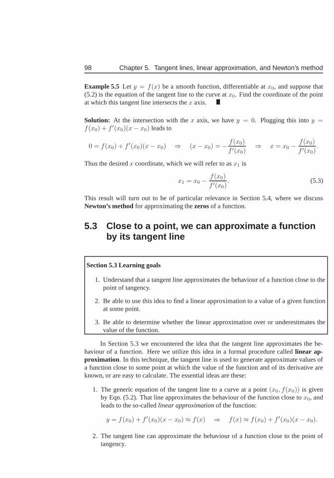
98 Chapter 5. Tangent lines, linear approximation, and Newton’s method
Example 5.5 Let y = f(x) be a smooth function, differentiable atx0, and suppose that(5.2) is the equation of the tangent line to the curve atx0. Find the coordinate of the pointat which this tangent line intersects thex axis.
Solution: At the intersection with thex axis, we havey = 0. Plugging this intoy =f(x0) + f ′(x0)(x− x0) leads to
0 = f(x0) + f ′(x0)(x− x0) ⇒ (x− x0) = − f(x0)
f ′(x0)⇒ x = x0 −
f(x0)
f ′(x0).
Thus the desiredx coordinate, which we will refer to asx1 is
x1 = x0 −f(x0)
f ′(x0). (5.3)
This result will turn out to be of particular relevance in Section 5.4, where we discussNewton’s methodfor approximating thezerosof a function.
5.3 Close to a point, we can approximate a functionby its tangent line
Section 5.3 Learning goals
1. Understand that a tangent line approximates the behaviour of a function close to thepoint of tangency.
2. Be able to use this idea to find a linear approximation to a value of a given functionat some point.
3. Be able to determine whether the linear approximation over or underestimates thevalue of the function.
In Section 5.3 we encountered the idea that the tangent line approximates the be-haviour of a function. Here we utilize this idea in a formal procedure calledlinear ap-proximation . In this technique, the tangent line is used to generate approximate values ofa function close to some point at which the value of the function and of its derivative areknown, or are easy to calculate. The essential ideas are these:
1. The generic equation of the tangent line to a curve at a point (x0, f(x0)) is givenby Eqn. (5.2). That line approximates the behaviour of the function close tox0, andleads to the so-calledlinear approximationof the function:
y = f(x0) + f ′(x0)(x− x0) ≈ f(x) ⇒ f(x) ≈ f(x0) + f ′(x0)(x − x0).
2. The tangent line can approximate the behaviour of a function close to the point oftangency.

5.3. Close to a point, we can approximate a function by its tangent line 99
3. The approximation is exact atx = x0, and holds well providedx is close tox0. (Theexpression on the right hand side is precisely the value ofy on the tangent line atx = x0).
For example, consider the function
y = f(x) =√
x.
The exact value of this function is well known at a number of judiciously chosen valuesof x, e.g.
√1 = 1,
√4 = 2,
√9 = 3, etc. Suppose we want to approximate the value
of the square root of 6. This is easily done with a scientific calculator, of course, but wecan also use a rough approximation which uses only simple “known” values of the squareroot function and some elementary manipulations. We know the value of the function atan adjoining point, i.e. atx = 4, sincef(4) =
√4 = 2. In Example 5.9 we use these
facts, together with the tangent line equation to estimate the decimal approximation of√
6.before doing so, we discuss other simple examples.
Example 5.6 Use the fact that the derivative of the functionf(x) = x2 is f ′(x) = 2x (asfound in Example 2.21) to find a linear approximation for the value(10.03)2.
Solution: We know that102 = 100, so that the point(10, 100) is on the graph of thefunctionf(x) = x2. Further, we know that the slope of the tangent line at that point isf ′(10) = 2(10) = 20. Thus the equation of the tangent line, and the linear approximationof the function are:
y − 100
x− 10= 20 ⇒ y = 100 + 20(x− 10), ⇒ f(x) ≈ 100 + 20(x− 10)
As before, we determine the value ofy corresponding tox = 10.03 as an approximation tothe value of the function. We obtain
f(10.03) ≈ 100 + 20(10.03− 10) = 100 + 20(0.03) = 100.6
This compares well with the true value of 100.6009 found using a calculator for the actualfunction.
Example 5.7 (Approximating the sine of a small angle)Use a linear approximation tofind a rough value forsin(0.1).
Solution: In Example 3.4, we found that when we are close tox = 0 the graph of thesine function looks very similar to the graph of its tangent line, y = x. This equation isthe linear approximation of the functiony = sin(x) nearx = 0. It implies that for smallenough values ofx, we can approximate the functiony = sin(x) by y ≈ x (providedx isin radians, (See Chapter 14). Thus, atx = 0.1 radians, we find thatsin(0.1) = 0.09983 ≈0.1.
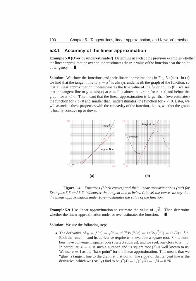
100 Chapter 5. Tangent lines, linear approximation, and Newton’s method
5.3.1 Accuracy of the linear approximation
Example 5.8 (Over or underestimate?)Determine in each of the previous examples whetherthe linear approximation over or underestimates the true value of the function near the pointof tangency.
Solution: We show the functions and their linear approximations in Fig. 5.4(a,b). In (a)we find that the tangent line toy = x2 is always underneath the graph of the function, sothat a linear approximation underestimates the true value of the function. In (b), we seethat the tangent line toy = sin(x) at x = 0 is above the graph forx > 0 and below thegraph forx < 0. This meant that the linear approximation is larger than (overestimates)the function forx > 0 and smaller than (underestimates) the function forx < 0. Later, wewill associate these properties with theconcavityof the function, that is, whether the graphis locally concave up or down.
0.0 20.0
0.0
400.0
y=x2
tangent line
-4.0 4.0
-2.0
2.0
tangent line
y=sin(x)
(a) (b)
Figure 5.4. Functions (black curves) and their linear approximations (red) forExamples 5.6 and 5.7. Whenever the tangent line is below (above) the curve, we say thatthe linear approximation under (over)-estimates the valueof the function.
Example 5.9 Use linear approximation to estimate the value of√
6. Then determinewhether the linear approximation under or over estimates the function.
Solution: We use the following steps:
• The derivative ofy = f(x) =√
x = x1/2 is f ′(x) = 1/(2√
(x)) = (1/2)x−1/2.Both the function and its derivative require us to evaluate asquare root. Some num-bers have convenient square roots (perfect squares), and weseek one close tox = 6.In particular,x = 4, is such a number, and its square root (2) is well known to us.We usex = 4 as the “base point” for the linear approximation. This meansthat we“glue” a tangent line to the graph at that point. The slope of that tangent line is thederivative, which we (easily) find to bef ′(4) = 1/(2
√4) = 1/4 = 0.25
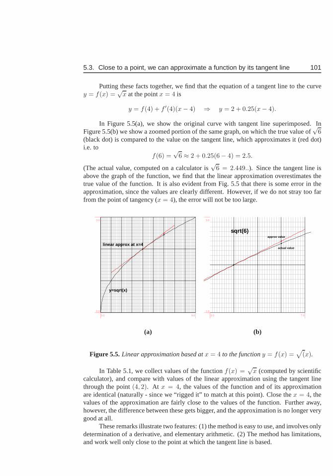
5.3. Close to a point, we can approximate a function by its tangent line 101
Putting these facts together, we find that the equation of a tangent line to the curvey = f(x) =
√x at the pointx = 4 is
y = f(4) + f ′(4)(x− 4) ⇒ y = 2 + 0.25(x− 4).
In Figure 5.5(a), we show the original curve with tangent line superimposed. InFigure 5.5(b) we show a zoomed portion of the same graph, on which the true value of
√6
(black dot) is compared to the value on the tangent line, which approximates it (red dot)i.e. to
f(6) =√
6 ≈ 2 + 0.25(6− 4) = 2.5.
(The actual value, computed on a calculator is√
6 = 2.449..). Since the tangent line isabove the graph of the function, we find that the linear approximation overestimates thetrue value of the function. It is also evident from Fig. 5.5 that there is some error in theapproximation, since the values are clearly different. However, if we do not stray too farfrom the point of tangency (x = 4), the error will not be too large.
y=sqrt(x)
linear approx at x=4
0.0 9.0
0.0
3.0
sqrt(6)
actual value
approx value
3.0 7.0
1.0
3.0
(a) (b)
Figure 5.5.Linear approximation based atx = 4 to the functiony = f(x) =√
(x).
In Table 5.1, we collect values of the functionf(x) =√
x (computed by scientificcalculator), and compare with values of the linear approximation using the tangent linethrough the point(4, 2). At x = 4, the values of the function and of its approximationare identical (naturally - since we “rigged it” to match at this point). Close thex = 4, thevalues of the approximation are fairly close to the values ofthe function. Further away,however, the difference between these gets bigger, and the approximation is no longer verygood at all.
These remarks illustrate two features: (1) the method is easy to use, and involves onlydetermination of a derivative, and elementary arithmetic.(2) The method has limitations,and work well only close to the point at which the tangent lineis based.
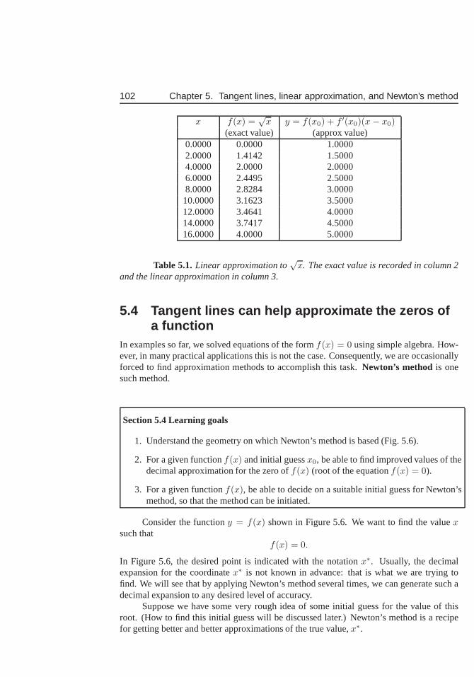
102 Chapter 5. Tangent lines, linear approximation, and Newton’s method
x f(x) =√
x y = f(x0) + f ′(x0)(x − x0)(exact value) (approx value)
0.0000 0.0000 1.00002.0000 1.4142 1.50004.0000 2.0000 2.00006.0000 2.4495 2.50008.0000 2.8284 3.000010.0000 3.1623 3.500012.0000 3.4641 4.000014.0000 3.7417 4.500016.0000 4.0000 5.0000
Table 5.1.Linear approximation to√
x. The exact value is recorded in column 2and the linear approximation in column 3.
5.4 Tangent lines can help approximate the zeros ofa function
In examples so far, we solved equations of the formf(x) = 0 using simple algebra. How-ever, in many practical applications this is not the case. Consequently, we are occasionallyforced to find approximation methods to accomplish this task. Newton’s method is onesuch method.
Section 5.4 Learning goals
1. Understand the geometry on which Newton’s method is based(Fig. 5.6).
2. For a given functionf(x) and initial guessx0, be able to find improved values of thedecimal approximation for the zero off(x) (root of the equationf(x) = 0).
3. For a given functionf(x), be able to decide on a suitable initial guess for Newton’smethod, so that the method can be initiated.
Consider the functiony = f(x) shown in Figure 5.6. We want to find the valuexsuch that
f(x) = 0.
In Figure 5.6, the desired point is indicated with the notation x∗. Usually, the decimalexpansion for the coordinatex∗ is not known in advance: that is what we are trying tofind. We will see that by applying Newton’s method several times, we can generate such adecimal expansion to any desired level of accuracy.
Suppose we have some very rough idea of some initial guess forthe value of thisroot. (How to find this initial guess will be discussed later.) Newton’s method is a recipefor getting better and better approximations of the true value,x∗.
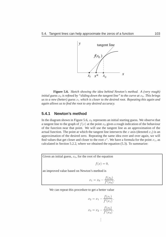
5.4. Tangent lines can help approximate the zeros of a function 103
x
y
x
f(x )
x x* 01
0
tangent line
Figure 5.6. Sketch showing the idea behind Newton’s method. A (very rough)initial guessx0 is refined by “sliding down the tangent line” to the curve atx0. This bringsus to a new (better) guessx1 which is closer to the desired root. Repeating this again andagain allows us to find the root to any desired accuracy.
5.4.1 Newton’s method
In the diagram shown in Figure 5.6,x0 represents an initial starting guess. We observe thata tangent line to the graph off(x) at the pointx0 gives a rough indication of the behaviourof the function near that point. We will use the tangent line as an approximation of theactual function. The point at which the tangent line intersects thex axis (denotedx1) is anapproximation of the desired zero. Repeating the same idea over and over again, we willfind values that get closer and closer to the rootx∗. We have a formula for the pointx1, ascalculated in Section 5.2.2, where we obtained the equation(5.3). To summarize:
Given an initial guess,x0, for the root of the equation
f(x) = 0,
an improved value based on Newton’s method is
x1 = x0 −f(x0)
f ′(x0).
We can repeat this procedure to get a better value
x2 = x1 −f(x1)
f ′(x1).
x3 = x2 −f(x2)
f ′(x2).
...
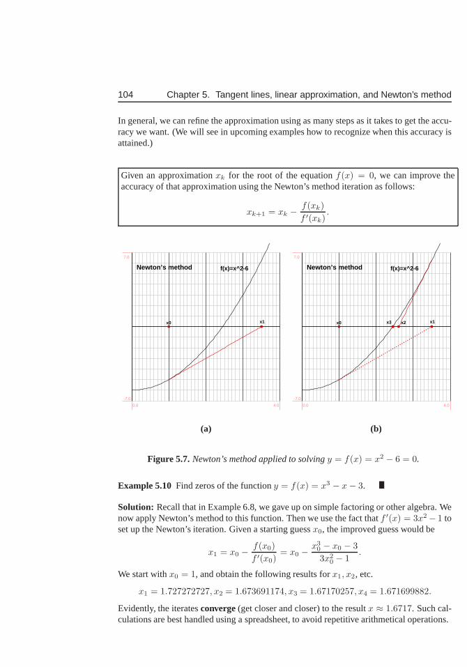
104 Chapter 5. Tangent lines, linear approximation, and Newton’s method
In general, we can refine the approximation using as many steps as it takes to get the accu-racy we want. (We will see in upcoming examples how to recognize when this accuracy isattained.)
Given an approximationxk for the root of the equationf(x) = 0, we can improve theaccuracy of that approximation using the Newton’s method iteration as follows:
xk+1 = xk −f(xk)
f ′(xk).
x0 x1
Newton’s method f(x)=x^2-6
0.0 4.0
-7.0
7.0
x0 x1
Newton’s method f(x)=x^2-6
x2x3
0.0 4.0
-7.0
7.0
(a) (b)
Figure 5.7.Newton’s method applied to solvingy = f(x) = x2 − 6 = 0.
Example 5.10 Find zeros of the functiony = f(x) = x3 − x− 3.
Solution: Recall that in Example 6.8, we gave up on simple factoring or other algebra. Wenow apply Newton’s method to this function. Then we use the fact thatf ′(x) = 3x2− 1 toset up the Newton’s iteration. Given a starting guessx0, the improved guess would be
x1 = x0 −f(x0)
f ′(x0)= x0 −
x30 − x0 − 3
3x20 − 1
.
We start withx0 = 1, and obtain the following results forx1, x2, etc.
x1 = 1.727272727, x2 = 1.673691174, x3 = 1.67170257, x4 = 1.671699882.
Evidently, the iteratesconverge(get closer and closer) to the resultx ≈ 1.6717. Such cal-culations are best handled using a spreadsheet, to avoid repetitive arithmetical operations.
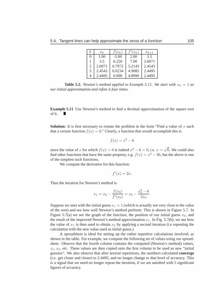
5.4. Tangent lines can help approximate the zeros of a function 105
k xk f(xk) f ′(xk) xk+1
0 1.00 -5.00 2.00 3.51 3.5 6.250 7.00 2.60712 2.6071 0.7972 5.2143 2.45433 2.4543 0.0234 4.9085 2.44954 2.4495 0.000 4.8990 2.4495
Table 5.2. Newton’s method applied to Example 5.11. We start withx0 = 1 asour initial approximation and refine it four times.
Example 5.11 Use Newton’s method to find a decimal approximation of the square rootof 6.
Solution: It is first necessary to restate the problem in the form “Find avalue ofx suchthat a certain functionf(x) = 0.” Clearly, a function that would accomplish this is
f(x) = x2 − 6
since the value ofx for whichf(x) = 0 is indeedx2 − 6 = 0, i.e. x =√
6. We could alsofind other functions that have the same property, e.g.f(x) = x4 − 36, but the above is oneof the simplest such functions.
We compute the derivative for this function:
f ′(x) = 2x.
Thus the iteration for Newton’s method is
x1 = x0 −f(x0)
f ′(x0)= x0 −
x20 − 6
2x0.
Suppose we start with the initial guessx1 = 1 (which is actually not very close to the valueof the root) and see how well Newton’s method perform: This isshown in Figure 5.7. InFigure 5.7(a) we see the graph of the function, the position of our initial guessx0, andthe result of the improved Newton’s method approximationx1. In Fig. 5.7(b), we see howthe value ofx1 is then used to obtainx2 by applying a second iteration (i.e repeating thecalculation with the new value used as initial guess.)
A spreadsheet is ideal for setting up the rather repetitive calculations involved, asshown in the table. For example, we compute the following setof values using our spread-sheet. Observe that the fourth column contains the computed(Newton’s method) values,x1, x2, etc. These values are then copied onto the first column to be used as new “initialguesses”. We also observe that after several repetitions, the numbers calculatedconverge(i.e. get closer and closer) to 2.4495, and no longer change to that level of accuracy. Thisis a signal that we need no longer repeat the iteration, if we are satisfied with 5 significantfigures of accuracy.
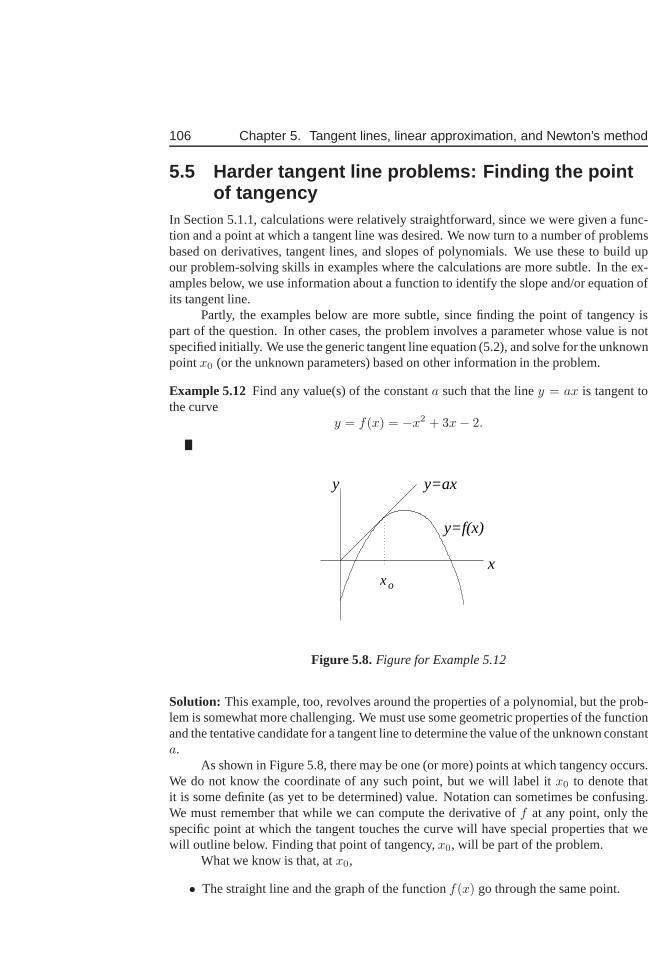
106 Chapter 5. Tangent lines, linear approximation, and Newton’s method
5.5 Harder tangent line problems: Finding the pointof tangency
In Section 5.1.1, calculations were relatively straightforward, since we were given a func-tion and a point at which a tangent line was desired. We now turn to a number of problemsbased on derivatives, tangent lines, and slopes of polynomials. We use these to build upour problem-solving skills in examples where the calculations are more subtle. In the ex-amples below, we use information about a function to identify the slope and/or equation ofits tangent line.
Partly, the examples below are more subtle, since finding thepoint of tangency ispart of the question. In other cases, the problem involves a parameter whose value is notspecified initially. We use the generic tangent line equation (5.2), and solve for the unknownpointx0 (or the unknown parameters) based on other information in the problem.
Example 5.12 Find any value(s) of the constanta such that the liney = ax is tangent tothe curve
y = f(x) = −x2 + 3x− 2.
xx
y
o
y=f(x)
y=ax
Figure 5.8.Figure for Example 5.12
Solution: This example, too, revolves around the properties of a polynomial, but the prob-lem is somewhat more challenging. We must use some geometricproperties of the functionand the tentative candidate for a tangent line to determine the value of the unknown constanta.
As shown in Figure 5.8, there may be one (or more) points at which tangency occurs.We do not know the coordinate of any such point, but we will label it x0 to denote thatit is some definite (as yet to be determined) value. Notation can sometimes be confusing.We must remember that while we can compute the derivative off at any point, only thespecific point at which the tangent touches the curve will have special properties that wewill outline below. Finding that point of tangency,x0, will be part of the problem.
What we know is that, atx0,
• The straight line and the graph of the functionf(x) go through the same point.
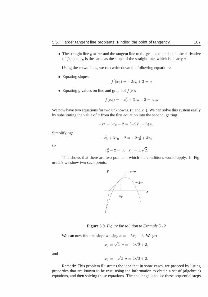
5.5. Harder tangent line problems: Finding the point of tangency 107
• The straight liney = ax and the tangent line to the graph coincide, i.e. the derivativeof f(x) atx0 is the same as the slope of the straight line, which is clearlya
Using these two facts, we can write down the following equations:
• Equating slopes:f ′(x0) = −2x0 + 3 = a
• Equatingy values on line and graph off(x):
f(x0) = −x20 + 3x0 − 2 = ax0
We now have two equations for two unknowns, (a andx0). We can solve this system easilyby substituting the value ofa from the first equation into the second, getting
−x20 + 3x0 − 2 = (−2x0 + 3)x0.
Simplifying:−x2
0 + 3x0 − 2 = −2x20 + 3x0
sox2
0 − 2 = 0, x0 = ±√
2.
This shows that there are two points at which the conditions would apply. In Fig-ure 5.9 we show two such points.
xx
y
o
y=f(x)
y=ax
Figure 5.9.Figure for solution to Example 5.12
We can now find the slopea usinga = −2x0 + 3. We get:
x0 =√
2 a = −2√
2 + 3,
andx0 = −
√2 a = 2
√2 + 3.
Remark: This problem illustrates the idea that in some cases, we proceed by listingproperties that are known to be true, using the information to obtain a set of (algebraic)equations, and then solving those equations. The challengeis to use these sequential steps
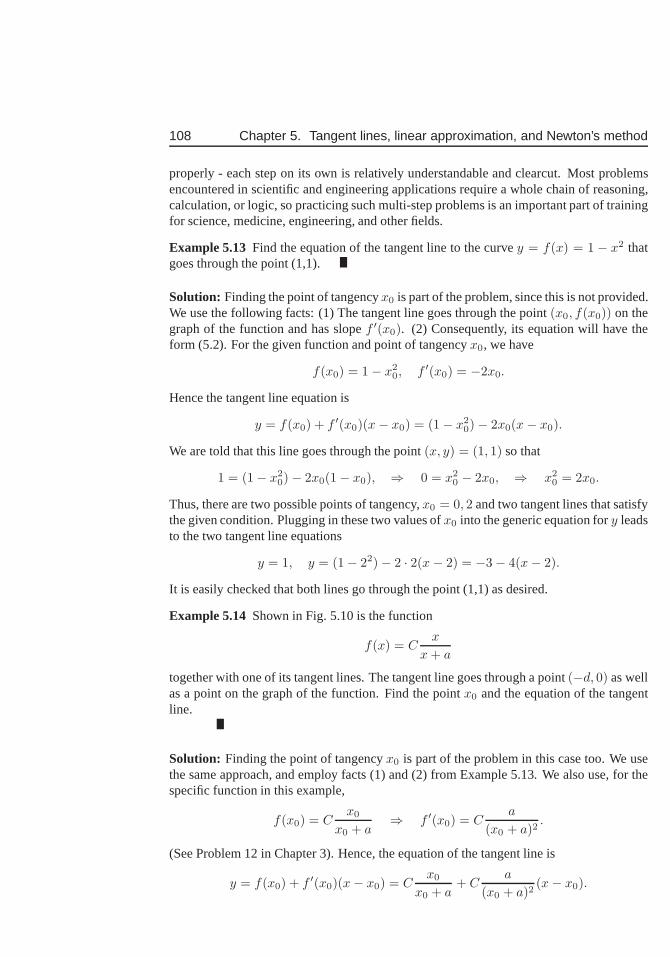
108 Chapter 5. Tangent lines, linear approximation, and Newton’s method
properly - each step on its own is relatively understandableand clearcut. Most problemsencountered in scientific and engineering applications require a whole chain of reasoning,calculation, or logic, so practicing such multi-step problems is an important part of trainingfor science, medicine, engineering, and other fields.
Example 5.13 Find the equation of the tangent line to the curvey = f(x) = 1 − x2 thatgoes through the point (1,1).
Solution: Finding the point of tangencyx0 is part of the problem, since this is not provided.We use the following facts: (1) The tangent line goes throughthe point(x0, f(x0)) on thegraph of the function and has slopef ′(x0). (2) Consequently, its equation will have theform (5.2). For the given function and point of tangencyx0, we have
f(x0) = 1− x20, f ′(x0) = −2x0.
Hence the tangent line equation is
y = f(x0) + f ′(x0)(x− x0) = (1− x20)− 2x0(x− x0).
We are told that this line goes through the point(x, y) = (1, 1) so that
1 = (1− x20)− 2x0(1− x0), ⇒ 0 = x2
0 − 2x0, ⇒ x20 = 2x0.
Thus, there are two possible points of tangency,x0 = 0, 2 and two tangent lines that satisfythe given condition. Plugging in these two values ofx0 into the generic equation fory leadsto the two tangent line equations
y = 1, y = (1− 22)− 2 · 2(x− 2) = −3− 4(x− 2).
It is easily checked that both lines go through the point (1,1) as desired.
Example 5.14 Shown in Fig. 5.10 is the function
f(x) = Cx
x + a
together with one of its tangent lines. The tangent line goesthrough a point(−d, 0) as wellas a point on the graph of the function. Find the pointx0 and the equation of the tangentline.
Solution: Finding the point of tangencyx0 is part of the problem in this case too. We usethe same approach, and employ facts (1) and (2) from Example 5.13. We also use, for thespecific function in this example,
f(x0) = Cx0
x0 + a⇒ f ′(x0) = C
a
(x0 + a)2.
(See Problem 12 in Chapter 3). Hence, the equation of the tangent line is
y = f(x0) + f ′(x0)(x− x0) = Cx0
x0 + a+ C
a
(x0 + a)2(x− x0).
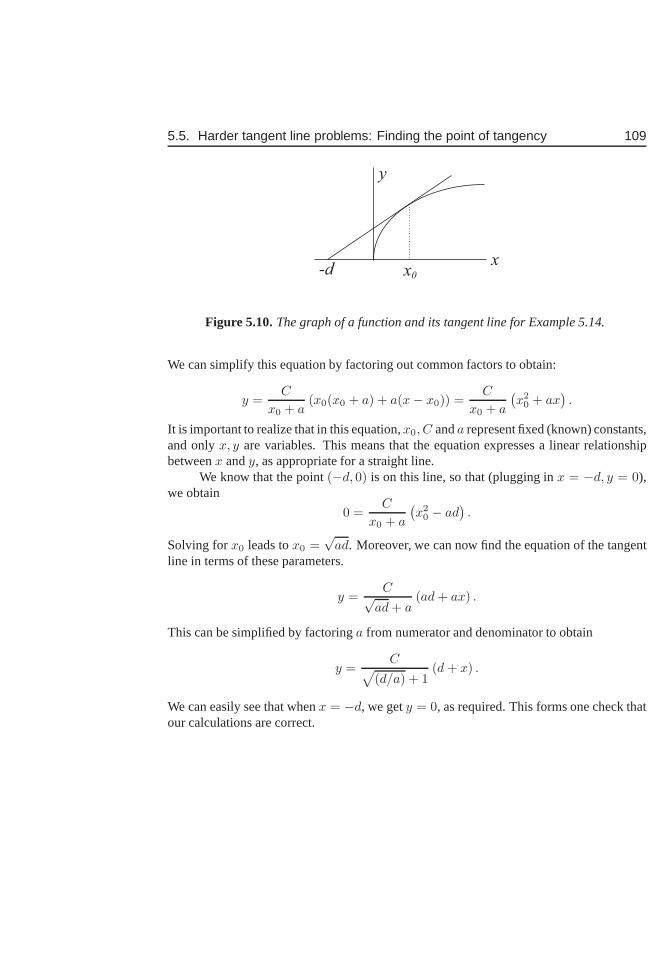
5.5. Harder tangent line problems: Finding the point of tangency 109
x-d x0
y
Figure 5.10.The graph of a function and its tangent line for Example 5.14.
We can simplify this equation by factoring out common factors to obtain:
y =C
x0 + a(x0(x0 + a) + a(x− x0)) =
C
x0 + a
(
x20 + ax
)
.
It is important to realize that in this equation,x0, C anda represent fixed (known) constants,and onlyx, y are variables. This means that the equation expresses a linear relationshipbetweenx andy, as appropriate for a straight line.
We know that the point(−d, 0) is on this line, so that (plugging inx = −d, y = 0),we obtain
0 =C
x0 + a
(
x20 − ad
)
.
Solving forx0 leads tox0 =√
ad. Moreover, we can now find the equation of the tangentline in terms of these parameters.
y =C√
ad + a(ad + ax) .
This can be simplified by factoringa from numerator and denominator to obtain
y =C
√
(d/a) + 1(d + x) .
We can easily see that whenx = −d, we gety = 0, as required. This forms one check thatour calculations are correct.
110 Chapter 5. Tangent lines, linear approximation, and Newton’s method
Exercises5.1. Find the equation of the tangent line to the functiony = f(x) = |x + 1| at:
(a) x = −1,
(b) x = −2,
(c) x = 0.
If there is a problem finding a tangent line at one of these points, indicate what theproblem is.
5.2. A functionf(x) satisfiesf(1) = −1 andf ′(1) = 2. What is the equation of thetangent line off(x) atx = 1?
5.3. Shown in Figure 5.11 is the graph ofy = x2 with one of its tangent lines.
(a) Show that the slope of the tangent to the curvey = x2 at the pointx = a is2a.
(b) Suppose that the tangent line intersects thex axis at the point (1,0). Find thecoordinate,a, of the point of tangency.
x
y
a1
Figure 5.11.Figure for Problem 3
5.4. Shown in Figure 5.12 is the functionf(x) = 1/x4 together with its tangent line atx = 1.
(a) Find the equation of the tangent line.
(b) Determine the points of intersection of the tangent linewith thex and theyaxes.
(c) Use the tangent line to obtain a linear approximation to the value off(1.1).Is this approximation larger or smaller than the actual value of the function atx = 1.1?
5.5. Tangent line, continued: Shown in Figure 5.13 is the functionf(x) = x3 with atangent line at the point(1, 1).
(a) Find the equation of the tangent line.
(b) Determine the point at which the tangent line intersectsthex axis.
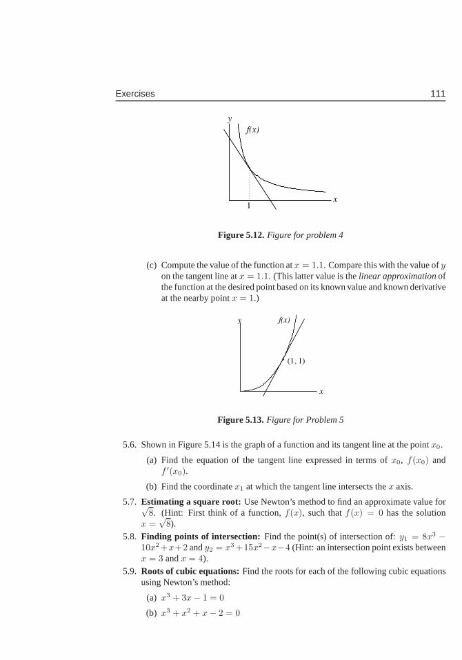
Exercises 111
x
y
f(x)
1
Figure 5.12.Figure for problem 4
(c) Compute the value of the function atx = 1.1. Compare this with the value ofyon the tangent line atx = 1.1. (This latter value is thelinear approximationofthe function at the desired point based on its known value andknown derivativeat the nearby pointx = 1.)
x
y
(1, 1)
f(x)
Figure 5.13.Figure for Problem 5
5.6. Shown in Figure 5.14 is the graph of a function and its tangent line at the pointx0.
(a) Find the equation of the tangent line expressed in terms of x0, f(x0) andf ′(x0).
(b) Find the coordinatex1 at which the tangent line intersects thex axis.
5.7. Estimating a square root: Use Newton’s method to find an approximate value for√8. (Hint: First think of a function,f(x), such thatf(x) = 0 has the solution
x =√
8).
5.8. Finding points of intersection: Find the point(s) of intersection of:y1 = 8x3 −10x2 +x+2 andy2 = x3 +15x2−x−4 (Hint: an intersection point exists betweenx = 3 andx = 4).
5.9. Roots of cubic equations:Find the roots for each of the following cubic equationsusing Newton’s method:
(a) x3 + 3x− 1 = 0
(b) x3 + x2 + x− 2 = 0
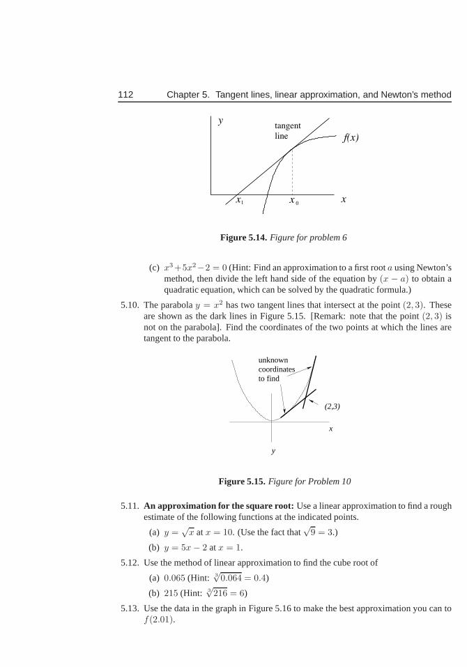
112 Chapter 5. Tangent lines, linear approximation, and Newton’s method
x
y
f(x)
xx
tangent
line
1 0
Figure 5.14.Figure for problem 6
(c) x3+5x2−2 = 0 (Hint: Find an approximation to a first roota using Newton’smethod, then divide the left hand side of the equation by(x − a) to obtain aquadratic equation, which can be solved by the quadratic formula.)
5.10. The parabolay = x2 has two tangent lines that intersect at the point(2, 3). Theseare shown as the dark lines in Figure 5.15. [Remark: note thatthe point(2, 3) isnot on the parabola]. Find the coordinates of the two points at which the lines aretangent to the parabola.
unknowncoordinatesto find
(2,3)
x
y
Figure 5.15.Figure for Problem 10
5.11. An approximation for the square root: Use a linear approximation to find a roughestimate of the following functions at the indicated points.
(a) y =√
x atx = 10. (Use the fact that√
9 = 3.)
(b) y = 5x− 2 atx = 1.
5.12. Use the method of linear approximation to find the cube root of
(a) 0.065 (Hint: 3√
0.064 = 0.4)
(b) 215 (Hint: 3√
216 = 6)
5.13. Use the data in the graph in Figure 5.16 to make the best approximation you can tof(2.01).
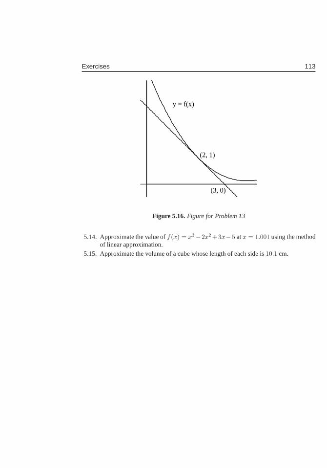
Exercises 113
(2, 1)
(3, 0)
y = f(x)
Figure 5.16.Figure for Problem 13
5.14. Approximate the value off(x) = x3−2x2 +3x−5 atx = 1.001 using the methodof linear approximation.
5.15. Approximate the volume of a cube whose length of each side is10.1 cm.
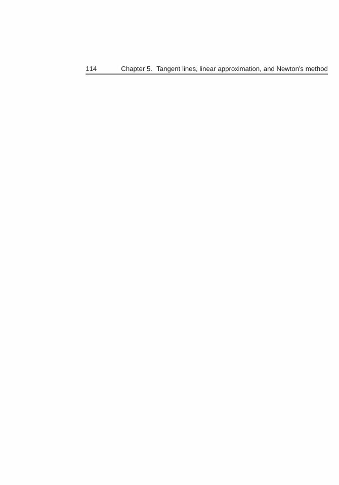
114 Chapter 5. Tangent lines, linear approximation, and Newton’s method
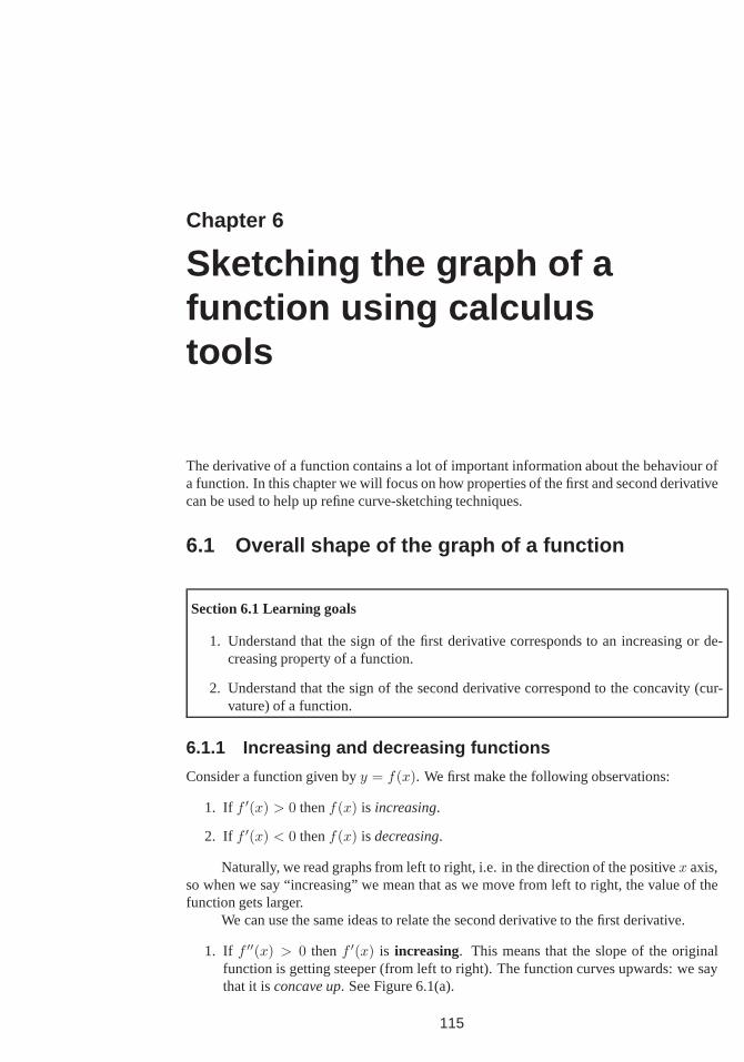
Chapter 6
Sketching the graph of afunction using calculustools
The derivative of a function contains a lot of important information about the behaviour ofa function. In this chapter we will focus on how properties ofthe first and second derivativecan be used to help up refine curve-sketching techniques.
6.1 Overall shape of the graph of a function
Section 6.1 Learning goals
1. Understand that the sign of the first derivative corresponds to an increasing or de-creasing property of a function.
2. Understand that the sign of the second derivative correspond to the concavity (cur-vature) of a function.
6.1.1 Increasing and decreasing functions
Consider a function given byy = f(x). We first make the following observations:
1. If f ′(x) > 0 thenf(x) is increasing.
2. If f ′(x) < 0 thenf(x) is decreasing.
Naturally, we read graphs from left to right, i.e. in the direction of the positivex axis,so when we say “increasing” we mean that as we move from left toright, the value of thefunction gets larger.
We can use the same ideas to relate the second derivative to the first derivative.
1. If f ′′(x) > 0 thenf ′(x) is increasing. This means that the slope of the originalfunction is getting steeper (from left to right). The function curves upwards: we saythat it isconcave up. See Figure 6.1(a).
115
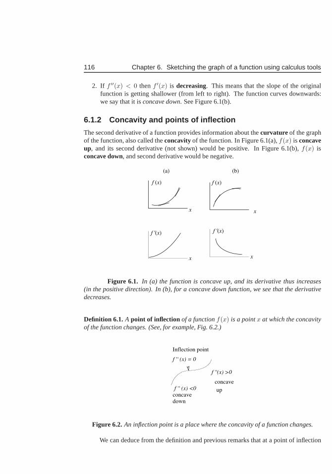
116 Chapter 6. Sketching the graph of a function using calculus tools
2. If f ′′(x) < 0 thenf ′(x) is decreasing. This means that the slope of the originalfunction is getting shallower (from left to right). The function curves downwards:we say that it isconcave down. See Figure 6.1(b).
6.1.2 Concavity and points of inflection
The second derivative of a function provides information about thecurvature of the graphof the function, also called theconcavityof the function. In Figure 6.1(a),f(x) is concaveup, and its second derivative (not shown) would be positive. InFigure 6.1(b),f(x) isconcave down, and second derivative would be negative.
x x
(a) (b)
x x
f (x) f (x)
f ’(x)f ’(x)
Figure 6.1. In (a) the function is concave up, and its derivative thus increases(in the positive direction). In (b), for a concave down function, we see that the derivativedecreases.
Definition 6.1. A point of inflection of a functionf(x) is a pointx at which the concavityof the function changes. (See, for example, Fig. 6.2.)
f ''(x) >0
f '' (x) <0
f '' (x) = 0
concave
upconcavedown
Inflection point
Figure 6.2.An inflection point is a place where the concavity of a function changes.
We can deduce from the definition and previous remarks that ata point of inflection
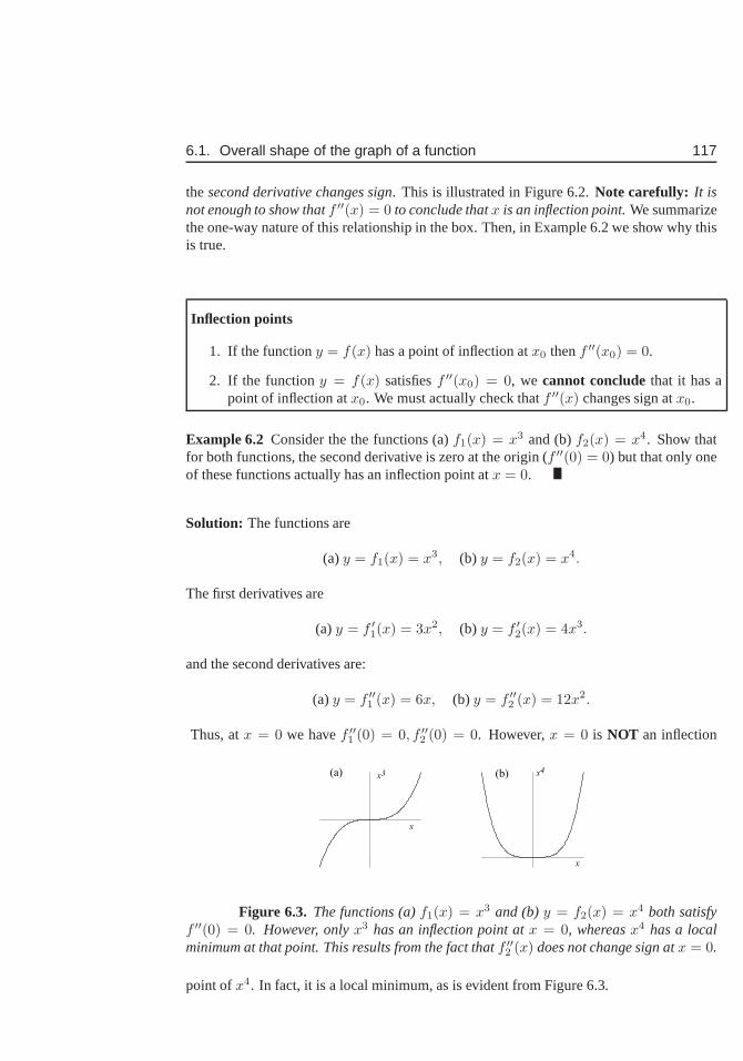
6.1. Overall shape of the graph of a function 117
thesecond derivative changes sign. This is illustrated in Figure 6.2.Note carefully: It isnot enough to show thatf ′′(x) = 0 to conclude thatx is an inflection point.We summarizethe one-way nature of this relationship in the box. Then, in Example 6.2 we show why thisis true.
Inflection points
1. If the functiony = f(x) has a point of inflection atx0 thenf ′′(x0) = 0.
2. If the functiony = f(x) satisfiesf ′′(x0) = 0, we cannot concludethat it has apoint of inflection atx0. We must actually check thatf ′′(x) changes sign atx0.
Example 6.2 Consider the the functions (a)f1(x) = x3 and (b)f2(x) = x4. Show thatfor both functions, the second derivative is zero at the origin (f ′′(0) = 0) but that only oneof these functions actually has an inflection point atx = 0.
Solution: The functions are
(a)y = f1(x) = x3, (b) y = f2(x) = x4.
The first derivatives are
(a)y = f ′1(x) = 3x2, (b) y = f ′
2(x) = 4x3.
and the second derivatives are:
(a)y = f ′′1 (x) = 6x, (b) y = f ′′
2 (x) = 12x2.
Thus, atx = 0 we havef ′′1 (0) = 0, f ′′
2 (0) = 0. However,x = 0 is NOT an inflection
x
x
x3 x4(a) (b)
Figure 6.3. The functions (a)f1(x) = x3 and (b)y = f2(x) = x4 both satisfyf ′′(0) = 0. However, onlyx3 has an inflection point atx = 0, whereasx4 has a localminimum at that point. This results from the fact thatf ′′
2 (x) does not change sign atx = 0.
point ofx4. In fact, it is a local minimum, as is evident from Figure 6.3.
118 Chapter 6. Sketching the graph of a function using calculus tools
6.1.3 Determining whether f ′′(x) changes sign
In the previous section, we defined an inflection point as a point on the graph of a functionat which the second derivative changes sign. But how do we detect if this sign changeoccurs at a given point? Here we address this question and provide a few helpful tools.
We first state the following important result
Sign change in a product of factors:If an expression is a product of factors, e.g.g(x) = (x− a1)
n1(x− a2)n2 . . . (x− am)nm ,
then
1. The expression can be zero only at the pointsx = a1, a2, . . . , am.
2. The expression changes sign only at pointsx = ai for which ni is an odd integerpower.
Example 6.3 Determine where the expressiong(x) = x2(x + 2)(x − 3)4 changes sign.
Solution: The zeros ofg(x) arex = 0,−2, 3. However,g(x) only changes sign atx = −2.Close to this point,g(x) ≈ g(−2) ≈ (−2)2(x + 2)(−5)4 = 2500(x + 2). Clearly forx < −2 this is negative and forx > −2, this is positive. Hence there is a sign change atx = −2. At x = 0 and atx = 3 there is no sign change as the termsx2 and(x − 3)4 arealways positive.
Example 6.4 Find all inflection points of the functionf(x) = (2/5)x6 − x4 + x.
Solution: We compute the derivatives of the function, and find these to be
f ′(x) = (12/5)x5−4x3+1, f ′′(x) = 12x4−14x2 = 12x2(x2−1) = 12x2(x+1)(x−1).
Here we have completely factorized the second derivative sothat it would be easy to iden-tify factors with even and odd powers, to find locations wherethe second derivative changessign. We see that there is NO sign change atx = 0, whereas at bothx = −1, 1 there is asign-changing factor. Thus the infection points are atx = −1, 1.
6.2 Special points on the graph of a functionIn this section we use tools of algebra and calculus to identify special points on the graphof a function. We first consider thezerosof a function, and then its critical points.
6.2. Special points on the graph of a function 119
Section 6.2 Learning goals
1. Understand the definition of a zero of a function and be ableto identify zeros forsimple functions (factorizable polynomials).
2. Understand that a functionf(x) can have various types of critical points (maxima,minima, and other types) at whichf ′(x) = 0.
3. Be able to find critical points for a given function.
4. Using first or second derivative tests, be able to classifya given critical point as amaximum, minimum (or neither).
6.2.1 Zeros of a function
Definition 6.5 (Zero). Given a functiony = f(x), we say thatx0 is azeroof f if f(x0) =0. In this case we also say that “x0 is a root of the equationf(x) = 0”.
Example 6.6 (Factoring) Find the zeros of the functiony = f(x) = x2 − 5x + 6.
Solution: This function is a polynomial that factors intof(x) = (x− 3)(x− 2). Thus welook for values ofx satisfying0 = (x− 3)(x− 2). We use the fact that when a product offactors is zero, at least one of the factors must be zero. Thismeans that either(x − 3) = 0or (x− 2) = 0, sox = 2, 3 are the two zeros of the function.
Example 6.7 Find zeros of the functiony = f(x) = x3 − 3x2 + x.
Solution: We can factor this function intof(x) = x(x2 − 3x + 1). From this we see thatx = 0 is one of the desired zeros off . To find the others, we use the quadratic formula onthe second factor, obtaining
x1,2 =1
2(3±
√
32 − 4) =1
2(3 ±
√5).
Thus, there is a total of three zeros in this case.
Example 6.8 Find zeros of the functiony = f(x) = x3 − x− 3.
Solution: This polynomial does not factor, nor is it easy to apply a cubic formula (analo-gous to the quadratic formula) for such cases. Rather than use such a formula, we will giveup the elementary algebraic techniques, and use an approximation method, to be discussedlater in Example 5.10.
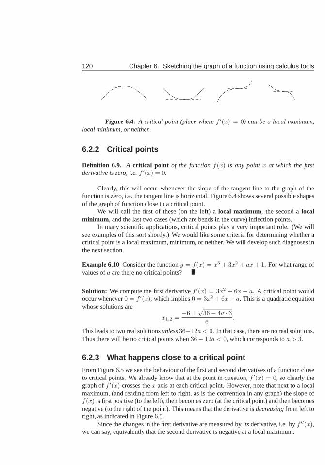
120 Chapter 6. Sketching the graph of a function using calculus tools
Figure 6.4. A critical point (place wheref ′(x) = 0) can be a local maximum,local minimum, or neither.
6.2.2 Critical points
Definition 6.9. A critical point of the functionf(x) is any pointx at which the firstderivative is zero, i.e.f ′(x) = 0.
Clearly, this will occur whenever the slope of the tangent line to the graph of thefunction is zero, i.e. the tangent line is horizontal. Figure 6.4 shows several possible shapesof the graph of function close to a critical point.
We will call the first of these (on the left) alocal maximum, the second alocalminimum , and the last two cases (which are bends in the curve) inflection points.
In many scientific applications, critical points play a veryimportant role. (We willsee examples of this sort shortly.) We would like some criteria for determining whether acritical point is a local maximum, minimum, or neither. We will develop such diagnoses inthe next section.
Example 6.10 Consider the functiony = f(x) = x3 + 3x2 + ax + 1. For what range ofvalues ofa are there no critical points?
Solution: We compute the first derivativef ′(x) = 3x2 + 6x + a. A critical point wouldoccur whenever0 = f ′(x), which implies0 = 3x2 + 6x + a. This is a quadratic equationwhose solutions are
x1,2 =−6±
√36− 4a · 36
.
This leads to two real solutionsunless36−12a < 0. In that case, there are no real solutions.Thus there will be no critical points when36− 12a < 0, which corresponds toa > 3.
6.2.3 What happens close to a critical point
From Figure 6.5 we see the behaviour of the first and second derivatives of a function closeto critical points. We already know that at the point in question, f ′(x) = 0, so clearly thegraph off ′(x) crosses thex axis at each critical point. However, note that next to a localmaximum, (and reading from left to right, as is the convention in any graph) the slope off(x) is first positive (to the left), then becomes zero (at the critical point) and then becomesnegative (to the right of the point). This means that the derivative isdecreasingfrom left toright, as indicated in Figure 6.5.
Since the changes in the first derivative are measured byits derivative, i.e. byf ′′(x),we can say, equivalently that the second derivative is negative at a local maximum.
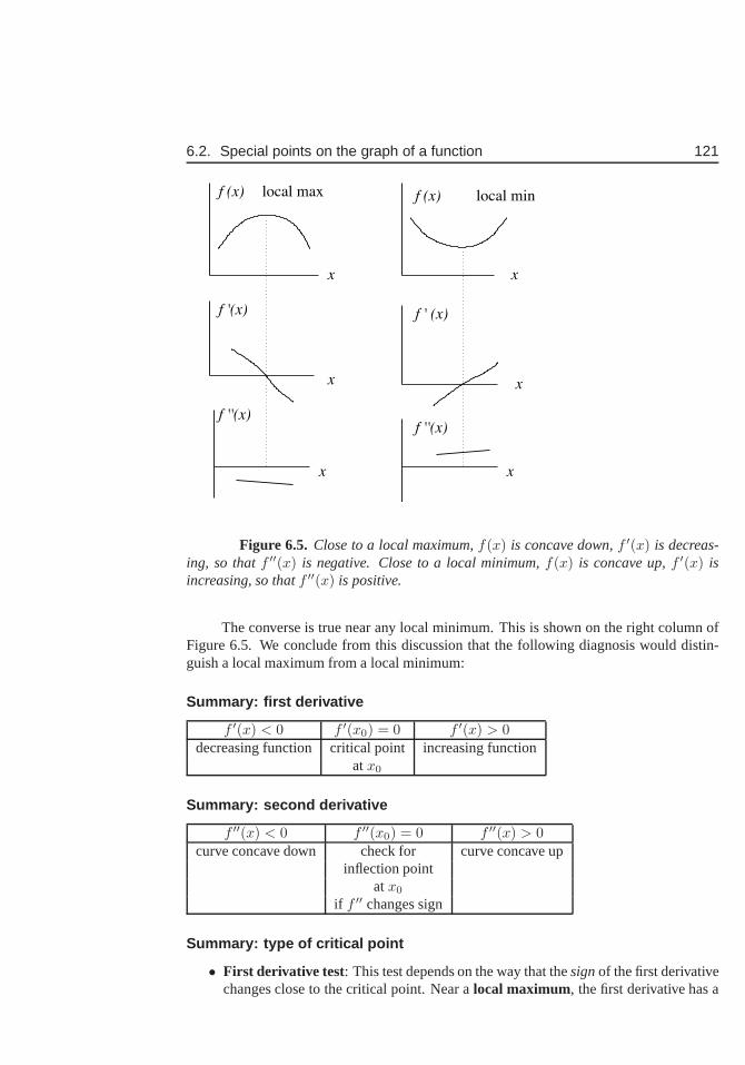
6.2. Special points on the graph of a function 121
x x
x x
f (x) f (x)
f '(x) f ' (x)
x x
f ''(x)f ''(x)
local max local min
Figure 6.5. Close to a local maximum,f(x) is concave down,f ′(x) is decreas-ing, so thatf ′′(x) is negative. Close to a local minimum,f(x) is concave up,f ′(x) isincreasing, so thatf ′′(x) is positive.
The converse is true near any local minimum. This is shown on the right column ofFigure 6.5. We conclude from this discussion that the following diagnosis would distin-guish a local maximum from a local minimum:
Summary: first derivative
f ′(x) < 0 f ′(x0) = 0 f ′(x) > 0decreasing function critical point increasing function
atx0
Summary: second derivative
f ′′(x) < 0 f ′′(x0) = 0 f ′′(x) > 0curve concave down check for curve concave up
inflection pointatx0
if f ′′ changes sign
Summary: type of critical point
• First derivative test: This test depends on the way that thesignof the first derivativechanges close to the critical point. Near alocal maximum, the first derivative has a
122 Chapter 6. Sketching the graph of a function using calculus tools
transition from positive to zero to negative values readingacross the graph from leftto right, as shown in the middle left panel of Fig. 6.5 and the table below:
x < x0 x = x0 x > x0
f ′(x) > 0 f ′(x0) = 0 f ′(x) < 0
Near alocal minimum, the first derivative goes from negative to zero to positivevalues as shown in the middle right panel of Fig. 6.5 and the table below:
x < x0 x = x0 x > x0
f ′(x) < 0 f ′(x0) = 0 f ′(x) > 0
• Second derivative test: At a local maximum, the second derivative is negative. At alocal minimum, the second derivative is positive.
Here we assume thatx0 is a critical point, i.e. a point at whichf ′(x0) = 0. Then thefollowing table summarizes what happens at that point
f ′′(x0) < 0 f ′′(x0) = 0 f ′′(x0) > 0
local maximum inconclusive local minimum
Inflection points:
We look for points at whichf ′′(x0) = 0 and check thatf ′′ changes sign atx0. When boththese conditions are satisfied, we conclude thatx0 is an inflection point.
6.3 Sketching the graph of a functionRecall that in Section 1.4, we used elementary reasoning about power functions to sketchthe graph of simple polynomials. Now that we have at our disposal more advanced calculustechniques, we will be able to hone such methods to produce more detailed and moreaccurate sketches of the graph of a function. We devote this section to illustrating thesenew methods and their application.
Section 6.3 Learning goals
1. Given a function (polynomial, rational function, etc) beable to find its zeros, criticalpoints, inflection points, and determine where it is increasing or decreasing, concaveup or down.
2. Using a combination of the above techniques, together with methods of Section 1.4,assemble a reasonably accurate sketch of the graph of the function.
3. Using these techniques, be able to identify all local as well as globalextrema (min-ima and maxima) of a functionf(x) on an intervala ≤ x ≤ b.
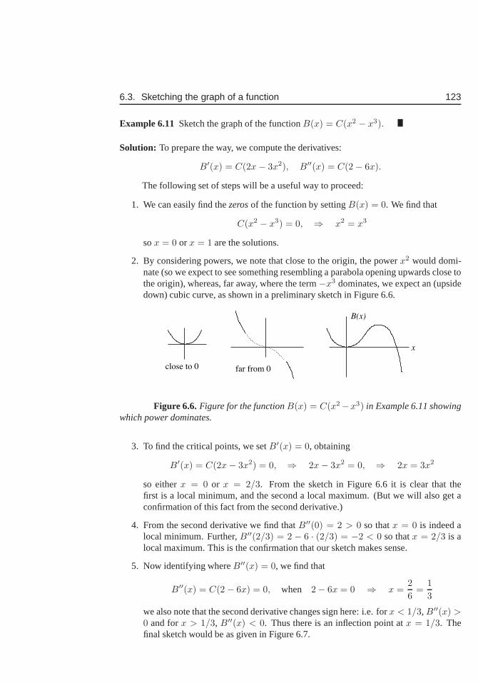
6.3. Sketching the graph of a function 123
Example 6.11 Sketch the graph of the functionB(x) = C(x2 − x3).
Solution: To prepare the way, we compute the derivatives:
B′(x) = C(2x− 3x2), B′′(x) = C(2 − 6x).
The following set of steps will be a useful way to proceed:
1. We can easily find thezerosof the function by settingB(x) = 0. We find that
C(x2 − x3) = 0, ⇒ x2 = x3
sox = 0 or x = 1 are the solutions.
2. By considering powers, we note that close to the origin, the powerx2 would domi-nate (so we expect to see something resembling a parabola opening upwards close tothe origin), whereas, far away, where the term−x3 dominates, we expect an (upsidedown) cubic curve, as shown in a preliminary sketch in Figure6.6.
x
B(x)
close to 0 far from 0
Figure 6.6.Figure for the functionB(x) = C(x2−x3) in Example 6.11 showingwhich power dominates.
3. To find the critical points, we setB′(x) = 0, obtaining
B′(x) = C(2x− 3x2) = 0, ⇒ 2x− 3x2 = 0, ⇒ 2x = 3x2
so eitherx = 0 or x = 2/3. From the sketch in Figure 6.6 it is clear that thefirst is a local minimum, and the second a local maximum. (But we will also get aconfirmation of this fact from the second derivative.)
4. From the second derivative we find thatB′′(0) = 2 > 0 so thatx = 0 is indeed alocal minimum. Further,B′′(2/3) = 2 − 6 · (2/3) = −2 < 0 so thatx = 2/3 is alocal maximum. This is the confirmation that our sketch makessense.
5. Now identifying whereB′′(x) = 0, we find that
B′′(x) = C(2 − 6x) = 0, when 2− 6x = 0 ⇒ x =2
6=
1
3
we also note that the second derivative changes sign here: i.e. forx < 1/3, B′′(x) >0 and forx > 1/3, B′′(x) < 0. Thus there is an inflection point atx = 1/3. Thefinal sketch would be as given in Figure 6.7.
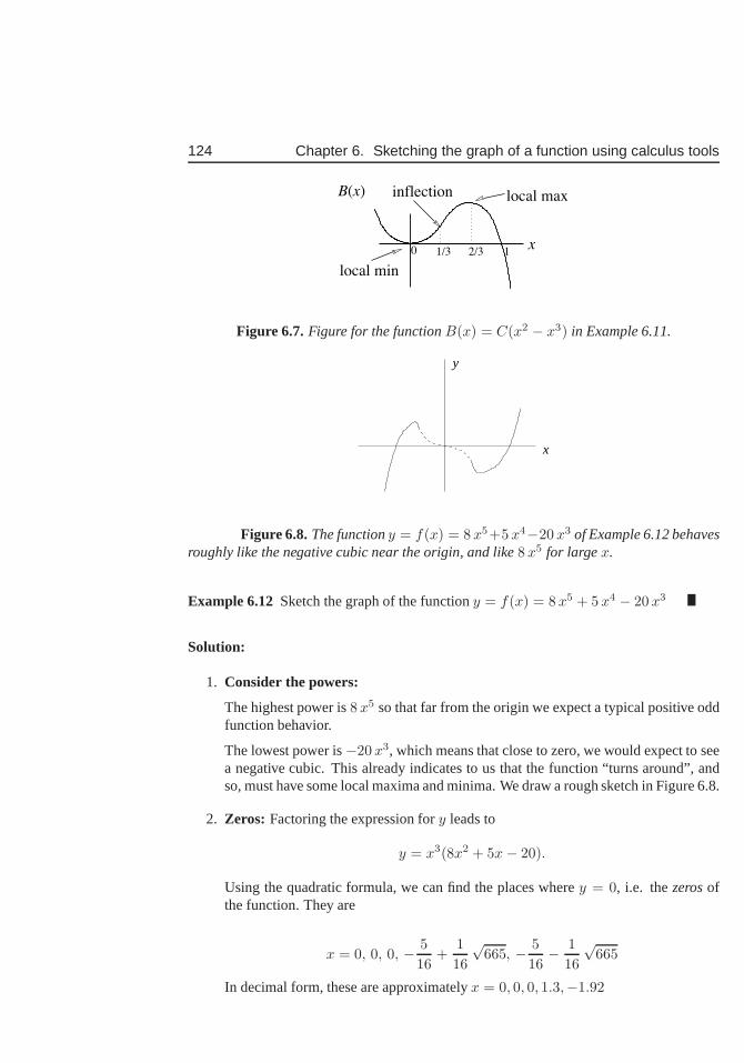
124 Chapter 6. Sketching the graph of a function using calculus tools
x0
local max
local min
B(x) inflection
1/3 2/3 1
Figure 6.7.Figure for the functionB(x) = C(x2 − x3) in Example 6.11.
x
y
Figure 6.8.The functiony = f(x) = 8 x5+5 x4−20 x3 of Example 6.12 behavesroughly like the negative cubic near the origin, and like8 x5 for largex.
Example 6.12 Sketch the graph of the functiony = f(x) = 8 x5 + 5 x4 − 20 x3
Solution:
1. Consider the powers:
The highest power is8 x5 so that far from the origin we expect a typical positive oddfunction behavior.
The lowest power is−20 x3, which means that close to zero, we would expect to seea negative cubic. This already indicates to us that the function “turns around”, andso, must have some local maxima and minima. We draw a rough sketch in Figure 6.8.
2. Zeros: Factoring the expression fory leads to
y = x3(8x2 + 5x− 20).
Using the quadratic formula, we can find the places wherey = 0, i.e. thezerosofthe function. They are
x = 0, 0, 0, − 5
16+
1
16
√665, − 5
16− 1
16
√665
In decimal form, these are approximatelyx = 0, 0, 0, 1.3,−1.92
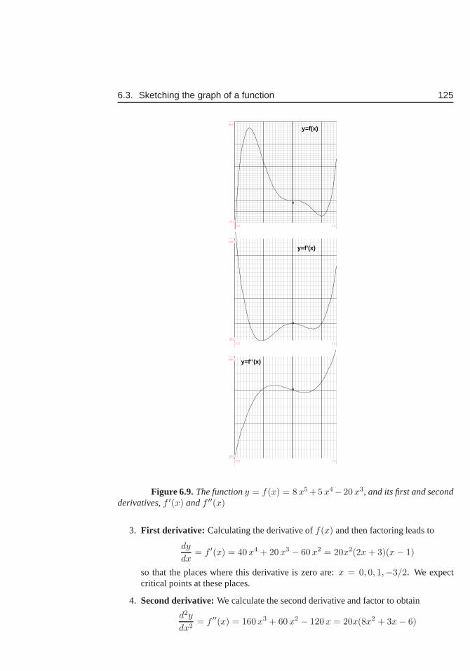
6.3. Sketching the graph of a function 125
0
y=f(x)
-2.0 1.5
-10.0
35.0
0
y=f’(x)
-2.0 1.5
-40.0
200.0
0
y=f’’(x)
-2.0 1.5
-800.0
400.0
Figure 6.9.The functiony = f(x) = 8 x5 +5 x4−20 x3, and its first and secondderivatives,f ′(x) andf ′′(x)
3. First derivative: Calculating the derivative off(x) and then factoring leads to
dy
dx= f ′(x) = 40 x4 + 20 x3 − 60 x2 = 20x2(2x + 3)(x− 1)
so that the places where this derivative is zero are:x = 0, 0, 1,−3/2. We expectcritical points at these places.
4. Second derivative:We calculate the second derivative and factor to obtain
d2y
dx2= f ′′(x) = 160 x3 + 60 x2 − 120 x = 20x(8x2 + 3x− 6)
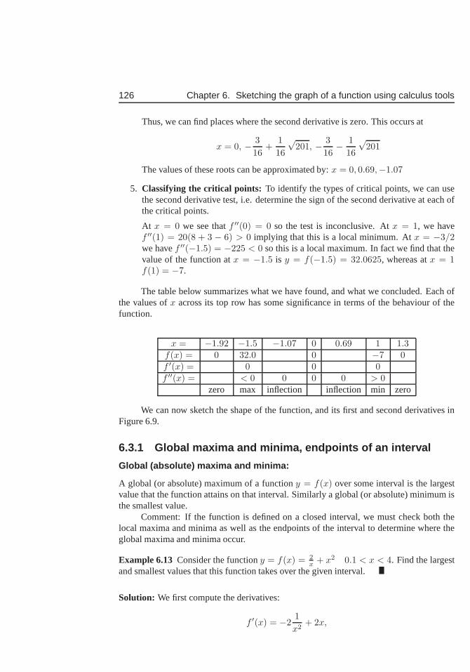
126 Chapter 6. Sketching the graph of a function using calculus tools
Thus, we can find places where the second derivative is zero. This occurs at
x = 0, − 3
16+
1
16
√201, − 3
16− 1
16
√201
The values of these roots can be approximated by:x = 0, 0.69,−1.07
5. Classifying the critical points: To identify the types of critical points, we can usethe second derivative test, i.e. determine the sign of the second derivative at each ofthe critical points.
At x = 0 we see thatf ′′(0) = 0 so the test is inconclusive. Atx = 1, we havef ′′(1) = 20(8 + 3 − 6) > 0 implying that this is a local minimum. Atx = −3/2we havef ′′(−1.5) = −225 < 0 so this is a local maximum. In fact we find that thevalue of the function atx = −1.5 is y = f(−1.5) = 32.0625, whereas atx = 1f(1) = −7.
The table below summarizes what we have found, and what we concluded. Each ofthe values ofx across its top row has some significance in terms of the behaviour of thefunction.
x = −1.92 −1.5 −1.07 0 0.69 1 1.3f(x) = 0 32.0 0 −7 0f ′(x) = 0 0 0f ′′(x) = < 0 0 0 0 > 0
zero max inflection inflection min zero
We can now sketch the shape of the function, and its first and second derivatives inFigure 6.9.
6.3.1 Global maxima and minima, endpoints of an interval
Global (absolute) maxima and minima:
A global (or absolute) maximum of a functiony = f(x) over some interval is the largestvalue that the function attains on that interval. Similarlya global (or absolute) minimum isthe smallest value.
Comment: If the function is defined on a closed interval, we must check both thelocal maxima and minima as well as the endpoints of the interval to determine where theglobal maxima and minima occur.
Example 6.13 Consider the functiony = f(x) = 2x + x2 0.1 < x < 4. Find the largest
and smallest values that this function takes over the given interval.
Solution: We first compute the derivatives:
f ′(x) = −21
x2+ 2x,
6.3. Sketching the graph of a function 127
f ′′(x) = 41
x3+ 2.
We now determine where critical pointsf ′(x) = 0 occur:
−21
x2+ 2x = 0.
Simplifying, we find−2 1x2 = 2x, sox3 = 1 and the critical point is atx = 1. Observe that
the second derivative at this point is
f ′′(1) = 41
13+ 2 = 6 > 0,
so thatx = 1 is a local minimum.We now calculate the value of the function at the endpointsx = 0.1 andx = 4
as well as at the critical pointx = 1 to determine where global and local minima and/ormaxima occur:
f(0.1) = 20.01 f(1) = 3 f(4) = 16.5global maximum global minimum
We see that the global minimum occurs atx = 1. There are no local maxima. Theglobal maximum occurs at the left endpoint.
128 Chapter 6. Sketching the graph of a function using calculus tools
Exercises6.1. A zero of a function is a place wheref(x) = 0.
(a) Find the zeros, local maxima, and minima of the polynomial y = f(x) =x3 − 3x
(b) Find the local minima and maxima of the polynomialy = f(x) = (2/3)x3 −3x2 + 4x.
(c) Determine whether each of the polynomials given in parts(a) and (b) have aninflection point.
6.2. Find critical points, zeros, and inflection points of the functiony = f(x) = x3−ax.Then classify the types of critical points that you have found.
6.3. For each of the following functions, sketch the graph for −1 < x < 1, findf ′(0), f ′(1), f ′(−1) and identify any local minima and maxima.
(a) y = x2,
(b) y = −x3,
(c) y = −x4
(d) Using your observations above, when can you conclude that a function whosederivative is zero at some point has a local maximum at that point?
6.4. Sketch a graph of the functiony = f(x) = x4 − 2x3, using both calculus andmethods of Chapter 1.
6.5. Find the global maxima and minima for the function in Problem 4 on the interval0 ≤ x ≤ 3.
6.6. Find the absolute maximum and minimum values on the given interval:
(a) y = 2x2 on−3 ≤ x ≤ 3
(b) y = (x− 5)2 on0 ≤ x ≤ 6
(c) y = x2 − x− 6 on1 ≤ x ≤ 3
(d) y =1
x+ x on−4 ≤ x ≤ −1
2.
6.7. A functionf(x) has as its derivativef ′(x) = 2x2 − 3x
(a) In what regions isf increasing or decreasing?
(b) Find any local maxima or minima.
(c) Is there an absolute maximum or minimum value for this function?
6.8. Sketch the graph ofx4 − x2 + 1 in the range−3 to 3. Find its minimum value.
6.9. Identify all the critical points of the following function.y = x3 − 27
6.10. Consider the functiong(x) = x4 − 2x3 + x2. Determine locations of critical pointsand inflection points.
6.11. Consider the polynomialy = x3 + 3x2 + ax + 1. Show that whena > 3 thispolynomial has no critical points.
Exercises 129
6.12. Find the values ofa, b, andc if the parabolay = ax2 + bx + c is tangent to the liney = −2x + 3 at (2,−1) and has a critical point whenx = 3.
6.13. Double Wells and Physics:In physics, a function such as
f(x) = x4 − 2x2
is often called adouble well potential. Physicists like to think of this as a “land-scape” with hills and valleys. They imagine a ball rolling along such a landscape:with friction, the ball eventually comes to rest at the bottom of one of the valleysin this potential. Sketch a picture of this landscape and useinformation about thederivative of this function to predict where the ball might be found, i.e. where thevalley bottoms are located.
6.14. (From Final Exam, Math 100 Dec 1996) Find the first and second derivatives of thefunction
y = f(x) =x3
1− x2.
Use information about the derivatives to determine any local maxima and minima,regions where the curve is concave up or down, and any inflection points.
6.15. Find all the critical points of the function
y = f(x) = 2x3 + 3ax2 − 12a2x + 1
and determine what kind of critical point each one is. Your answer should be givenin terms of the constanta, and you may assume thata > 0.
6.16. (From Final Exam Dec 1995) The functionf(x) is given by
y = f(x) = x5 − 10kx4 + 25k2x3
wherek is a positive constant.
(a) Find all the intervals on whichf is either increasing or decreasing. Determineall local maxima and minima.
(b) Determine intervals on which the graph is either concaveup or concave down.What are the inflection points off(x) ?
6.17. Muscle shortening: In 1938 Av Hill proposed a mathematical model for the rate ofshortening of a muscle,v, (in cm/sec) when it is working against a loadp (in gms).His so called force-velocity curve is given by the relationship
(p + a)v = b(p0 − p)
wherea, b, p0 are positive constants.
(a) Sketch the shortening velocity versus the load, i.e.,v as a function ofp. (Note:the best way to do this is to find the intercepts of the two axes,i.e. find thevalue ofv corresponding top = 0 and vice versa.)
(b) Find the rate of change of the shortening velocity with respect to the load, i.e.calculatedv/dp.
130 Chapter 6. Sketching the graph of a function using calculus tools
(c) What is the largest load for which the muscle will contract? (Hint: A contract-ing muscle has a positive shortening velocity, whereas a muscle with a veryheavy load will stretch, rather than contract, i.e. will have a negative value ofv.)
6.18. Reaction kinetics: Chemists often describe the rate of a saturating chemical reac-tion by using simplified expressions. Two examples of such expressions are:
Michaelis-Menten kinetics: Rm(c) =Kc
kn + c, Sigmoidal kinetics: Rs(c) =
K
k2n +
wherec is the concentration of the reactant,K > 0, kn > 0 are constants.R(c)is the speed of the reaction (Observe that the speed of the reaction depends on theconcentration of the reactant).
(a) Sketch the two curves. To do this, you should analyze the behaviour forc = 0,for smallc, and for very largec. You will find a horizontal asymptote in bothcases. We refer to that asymptote as the “maximal reaction speed”. What is the“maximal reaction speed” for each of the functionsRm, Rs ? (Note: expressyour answer in terms of the constantsK, kn.)
(b) Show that the valuec = kn leads to a half-maximal reaction speed.
For the questions below, you may assume thatK = 1 andkn = 1.
(c) Sketch the curvesRm(c), Rs(c).
(d) Show that sigmoidal kinetics, but not Michaelis Menten kinetics has an inflec-tion point.
(e) Explain how these curves would change ifK is increased; ifkn is increased.
6.19. Checking the endpoints !:Find the absolute maximum and minimum values of thefunction
f(x) = x2 +1
x2
on the interval[ 12 , 2]. Be sure to verify if any critical points are maxima or minimaand to check the endpoints of the interval.
Chapter 7
Optimization
In this chapter, we collect a variety of problems in which theideas developed in earliermaterial are put to use. In particular, we will use calculus to find local (and global) maxima,and minima so as to get the best (optimal) values of some desirable quantity. Setting upthese problems, from first verbal description, to clear cut mathematical formulation is themain challenge we will face. Often, we will use geometric ideas to express relationshipsbetween variables leading to our solution.
7.1 Simple biological optimization problemsWe start with relatively simple examples where the functionto optimize is specified. Thestudent merely has to take care with differentiation, and apply the diagnostic tests properly.An important skill to pick up at this point is distinguishingbetween variables and constantparameters in the differentiation step. A skill we reinforce is the elementary curve sketchingfrom earlier chapters.
Section 7.1 Learning goals
1. Given a function of some independent variable, be able to find the derivative of thatfunction and identify all critical points.
2. Using a combination of sketching and tests for critical points developed in Sec-tion 6.2.3, be able to determine whether that critical pointis a minimum, maximum(or neither).
7.1.1 Density dependent (logistic) growth in a population
Biologists often notice that the growth rate of a populationdepends not only on the size ofthe population, but also on how crowded it is. Constant growth is not sustainable. Whenindividuals have to compete for resources, nesting sites, mates, or food, they cannot invest
131
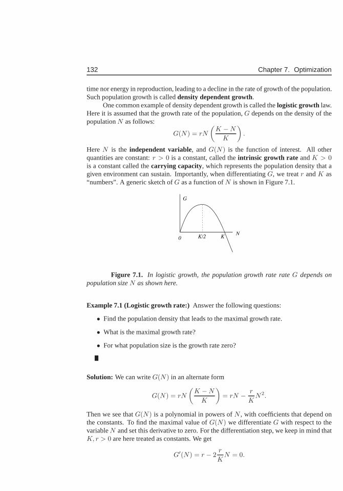
132 Chapter 7. Optimization
time nor energy in reproduction, leading to a decline in the rate of growth of the population.Such population growth is calleddensity dependent growth.
One common example of density dependent growth is called thelogistic growth law.Here it is assumed that the growth rate of the population,G depends on the density of thepopulationN as follows:
G(N) = rN
(
K −N
K
)
.
HereN is the independent variable, andG(N) is the function of interest. All otherquantities are constant:r > 0 is a constant, called theintrinsic growth rate andK > 0is a constant called thecarrying capacity, which represents the population density that agiven environment can sustain. Importantly, when differentiating G, we treatr andK as“numbers”. A generic sketch ofG as a function ofN is shown in Figure 7.1.
NK/2 K0
G
Figure 7.1. In logistic growth, the population growth rate rateG depends onpopulation sizeN as shown here.
Example 7.1 (Logistic growth rate:) Answer the following questions:
• Find the population density that leads to the maximal growthrate.
• What is the maximal growth rate?
• For what population size is the growth rate zero?
Solution: We can writeG(N) in an alternate form
G(N) = rN
(
K −N
K
)
= rN − r
KN2.
Then we see thatG(N) is a polynomial in powers ofN , with coefficients that depend onthe constants. To find the maximal value ofG(N) we differentiateG with respect to thevariableN and set this derivative to zero. For the differentiation step, we keep in mind thatK, r > 0 are here treated as constants. We get
G′(N) = r − 2r
KN = 0.
7.1. Simple biological optimization problems 133
Solving forN leads to
r = 2r
KN ⇒ N =
K
2.
We found a critical point, but we must still confirm that it is alocal maximum. We cando so either using the sketch in Fig. 7.1, or using one of the diagnosis tools developed inSection 6.2.3. Here we apply thesecond derivative test.. The second derivative is
G′′(N) = −2r
K
and is clearly is negative for all population sizes. This tells us that the functionG(N) isconcave down, and thatN = K/2 is a local maximum. Thus the density leading to largestgrowth rate is one half of the carrying capacity.
The growth rate at this density is
G(K
2) = r
(
K
2
)
(
K − K2
K
)
= rK
2
1
2=
rK
4.
To find the population size at which the growth rate is zero, wesetG = 0 and solve forN :
G(N) = rN
(
K −N
K
)
= 0.
The two solutions areN = 0 (which is not very interesting, since when there is no popula-tion there is no growth) andN = K.
We will have more to say about this type of density dependent growth a little later onin this course.
7.1.2 Cell size for maximal nutrient accumulation rate
We have seen in Section 1.2.2 that the absorption and consumption ratesA(r), C(r) for asimple spherical cell of radiusr are:
A(r) = k1S = 4k1πr2, C(r) = k2V =4
3πk2r
3,
wherek1, k2 > 0 are constants. We define thenet rate of increase of nutrientsas the rateof absorption minus the rate of consumption:
N(r) = A(r) − C(r) = 4k1πr2 − 4
3πk2r
3. (7.1)
As we can see, this quantity depends on the radiusr of the cell.
Example 7.2 Consider a spherical cell that is absorbing nutrients at a rate proportional toits surface area and consuming them at a rate proportional toits volume. Determine thesize of the cell for which the net rate of increase of nutrients is largest.
134 Chapter 7. Optimization
Solution: To find the size for greatest net nutrient increase rate, we find critical points ofN(r), keeping in mind that the coefficients8k1π and4k2π are constant for the purpose ofdifferentiation. Then the derivative of (7.1) is
N ′(r) = 8k1πr − 4k2πr2.
Critical points occur whenN ′(r) = 0, i.e.
N ′(r) = 8k1πr − 4k2πr2 = 0.
Simplifying leads to4πr(2k1 − k2r) = 0.
This is satisfied (trivially) whenr = 0, and also when
r = 2k1
k2.
To check that this is a local maximum, we find the second derivative
N ′′(r) = 8k1π − 8k2πr = 8π(k1 − k2r).
plugging inr = 2k1/k2 we get
N ′′ = 8π(k1 − k22k1
k2) = −8πk1 < 0.
Thus the second derivative is negative, and this verifies that we have a local maximum.
7.2 Optimization with a constraintWe continue to build experience with optimization problems. Here we encounter slightlymore challenging examples, where identifying the functionto optimize forms one of theaspects of the problem. We also consider cases where there are more than one independentvariables, but where there is an additional constraint thatcan be used to eliminate all butone. We include both biological and other practical examples in this analysis.
Section 7.2 Learning goals
1. Gain experience with setting up an optimization word problem involving formulaefor volume and surface area of geometric solids.
2. Understand the idea of a constraint in an optimization problem.
3. Be able to use the constraint to eliminate one of the independent variables, and finda desired critical point. (As before, this includes classifying that critical point as alocal minimum, maximum or neither.)

7.2. Optimization with a constraint 135
7.2.1 A cylindrical cell with minimal surface area
Not all cells are spherical. Some are skinny cylindrical filaments, or sausage shapes. Someeven grow as helical tubes, but we shall leave such complicated examples aside here. Wewill explore how minimization of surface area would determine the overall shape of acylindrical cell.
Consider a cell shaped like a cylinder with a circular cross-section. The volumeof the cell will be assumed to be fixed, because the cytoplasm in its interior cannot be“compressed”. However, suppose that the cell has a “rubbery” membrane that tends to takeon the smallest surface area possible. (In physical language, the elastic energy stored in themembrane tends to a minimum.) We want to find the proportions of the cylinder (e.g. theratio of length to radius) so that the cell hasminimal surface area.
Recall the following properties for a cylinder:
2 r
L
r
L
π
Figure 7.2.Properties of a cylinder
• the volume of a cylinder is the product of its base areaA and its height,h. That is,V = Ah. For a cylinder with circular cross-section:V = πr2L.
• A cylinder can be “cut and unrolled” into a rectangle. One side of the rectangle haslengthL and the other has length that made the perimeter of the circle, 2πr. Thesurface area of the unrolled rectangle is thenSside = 2πrL, as shown in Figure 7.2.
• If the “ends” of the cylinder are two flat circular caps, then the sum of the areas ofthese two ends isSends= 2πr2.
• The total surface area of the cylinder with flat ends is then
S = 2πrL + 2πr2.
We would expect that in a cell surrounded by a rubbery membrane, the end capswould not really be flat. However for simplicity, we will hereneglect this issue and assumethat the ends are flat and circular. Then, mathematically, our problem can be restated asfollows
Example 7.3 Minimize the surface areaS = 2πrL+2πr2 of the cell, given that its volumeV = πr2L = K is constant15.
15I would like to thank Prof Nima Geffen (Tel Aviv University) with providing the inspiration for this example.
136 Chapter 7. Optimization
Solution: The shape of the cell depends on both the lengthL, and the radiusr of thecylinder. However, these are not independent. They are related to one another because thevolume of the cell has to be constant. This is an example of an optimization problem withaconstraint, i.e. a condition that has to be satisfied. The constraint will allow us to eliminateone of the variables, as we show below.
The constraint is “the volume is fixed”, i.e.,
V = πr2L = K
whereK > 0 is a constant that represents the volume of the given cell. Wecan use this toexpress one variable in terms of the other. For example, we can solve forL.
L =K
πr2. (7.2)
The function to minimize isS = 2πrL + 2πr2.
We substitute the expression (7.2) forL as a function ofr to obtainS as a function ofralone:
S(r) = 2πrK
πr2+ 2πr2.
Simplification leads to
S(r) = 2K
r+ 2πr2.
observe thatS is now a function of only one independent variable,r, (K andπ are con-stants).
In order to find local minima, we will look for critical pointsof the functionS(r).We compute the relevant derivatives:
S′(r) = −2K
r2+ 4πr,
The second derivative will also be useful.
S′′(r) = 4K
r3+ 4π.
From the last calculation, we observe that the second derivative is always positive sinceK, r > 0, so the functionS(r) is concave up. Any critical point we find will thus be aminimum automatically. (In Exercise 7 we also consider the first derivative test as practice.)
To find a critical point, setS′(r) = 0:
S′(r) = −2K
r2+ 4πr = 0.
Solving forr, we obtain:
2K
r2= 4πr ⇒ r3 =
K
2π⇒ r =
(
K
2π
)1/3
.
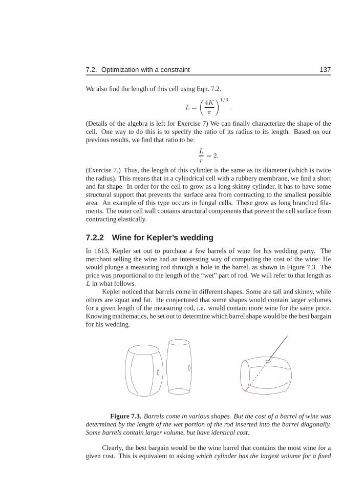
7.2. Optimization with a constraint 137
We also find the length of this cell using Eqn. 7.2.
L =
(
4K
π
)1/3
.
(Details of the algebra is left for Exercise 7) We can finally characterize the shape of thecell. One way to do this is to specify the ratio of its radius toits length. Based on ourprevious results, we find that ratio to be:
L
r= 2.
(Exercise 7.) Thus, the length of this cylinder is the same asits diameter (which is twicethe radius). This means that in a cylindrical cell with a rubbery membrane, we find a shortand fat shape. In order for the cell to grow as a long skinny cylinder, it has to have somestructural support that prevents the surface area from contracting to the smallest possiblearea. An example of this type occurs in fungal cells. These grow as long branched fila-ments. The outer cell wall contains structural components that prevent the cell surface fromcontracting elastically.
7.2.2 Wine for Kepler’s wedding
In 1613, Kepler set out to purchase a few barrels of wine for his wedding party. Themerchant selling the wine had an interesting way of computing the cost of the wine: Hewould plunge a measuring rod through a hole in the barrel, as shown in Figure 7.3. Theprice was proportional to the length of the “wet” part of rod.We will refer to that length asL in what follows.
Kepler noticed that barrels come in different shapes. Some are tall and skinny, whileothers are squat and fat. He conjectured that some shapes would contain larger volumesfor a given length of the measuring rod, i.e. would contain more wine for the same price.Knowing mathematics, he set out to determine which barrel shape would be the best bargainfor his wedding.
Figure 7.3. Barrels come in various shapes. But the cost of a barrel of wine wasdetermined by the length of the wet portion of the rod inserted into the barrel diagonally.Some barrels contain larger volume, but have identical cost.
Clearly, the best bargain would be the wine barrel that contains the most wine for agiven cost. This is equivalent to askingwhich cylinder has the largest volume for a fixed
138 Chapter 7. Optimization
(constant) lengthL. Below, we show how this optimization problem can be solved.Analternate approach is to seek the wine barrel that costs least for a given volume. We explorethis alternative in Exercise 14 and show that it leads to the same result.
Example 7.4 Find the proportions (height:radius) of the cylinder that contains the largestvolume for a fixed value of the lengthL of the wet rod in Fig. 7.3.
Solution: To simplify the problem, we will assume that the barrel is a simple cylinder, asshown in Figure 7.4. We also assume that the tap-hole (normally covered to avoid leaks) ishalf-way up the height of the barrel. We will definer as the radius andh as the height ofthe barrel. These two variables uniquely determine the shape as well as the volume of thebarrel. We’ll also assume that the barrel is full up to the topwith delicious wine, so that thevolume of the cylinder is the same as the volume of wine.
The volume of a cylinder is
V = base area× height.
The base is a circle of areaA = πr2, so that the volume of the barrel is:
V = πr2h. (7.3)
The rod used to “measure” the amount of wine (and hence determine the cost of the barrel)is shown as the diagonal of lengthL in Figure 7.4. Because the cylinder walls are perpen-dicular to its base, the lengthL is the hypotenuse of a right-angle triangle whose other sideshave lengths2r andh/2. (This follows from the assumption that the tap hole is half-wayup the side.) Thus, by the Pythagorean theorem,
L2 = (2r)2 +
(
h
2
)2
. (7.4)
The problem can be restated: maximizeV subject to a fixed value ofL. The fact thatL is fixed means that we have aconstraint as before. That constraint will be used to reducethe number of variables in the problem.
The function to be maximized is:
V = πr2h.
After expanding the squares, the constraint is:
L2 = 4r2 +h2
4.
We can use the constraint to eliminate one variable; in this case the simplest way is to doso is to solve Eqn. (7.4) forr2 and substitute the result intoV . We obtain
r2 =1
4
(
L2 − h2
4
)
.

7.2. Optimization with a constraint 139
L
h
h/2
2 r
Figure 7.4. Here we simplify and idealize the problem to consider a cylindricalbarrel with diameter2r and heighth. We assumed that the tap-hole is at heighth/2. ThelengthL denotes the “wet” portion of the merchant’s rod, used to determine the cost of thisbarrel of wine. We observe that the dotted lines form a Pythagorian triangle.
Then
V = πr2h =π
4
(
L2 − h2
4
)
h =π
4
(
L2h− 1
4h3
)
.
We now have a function of one variable, namely
V (h) =π
4
(
L2h− 1
4h3
)
.
For this function, the variableh could sensibly take on any value in the range0 ≤ h ≤ 2L.Outside this range, the volume is negative, and at the two endpoints the volume is zero.Thus, we anticipate that somewhere inside this range of values we should find the desiredoptimum.
To find any critical points of the functionV (h), we calculate the derivativeV ′(h)and set it to zero:
V ′(h) =π
4
(
L2 − 3
4h2
)
= 0
This implies thatL2 − 34h2 = 0, i.e.
3h2 = 4L2 ⇒ h2 = 4L2
3⇒ h = 2
L√3.
Now we must check whether this solution is a localmaximum(or a minimum).The second derivative is:
V ′′(h) =π
4
(
0− 2 · 34h
)
= −3
8πh < 0.
From this we see thatV ′′(h) < 0 for any positive value ofh. The the functionV (h) isconcave down whenh > 0. This verifies that the solution above is a local maximum.According to the discussion of the relevant range of values of h, this local maximum is also
140 Chapter 7. Optimization
the optimal solution we need. i.e. there are no larger valuesat endpoints of the interval0 ≤ h ≤ 2L.
To finish the problem, we can find the radius of the barrel having this height byplugging this result forh into the constraint equation, i.e. using
r2 =1
4
(
L2 − h2
4
)
=1
4
(
L2 − L2
3
)
=1
4
(
2
3L2
)
.
After simplifying and rewriting, we get
r =1√3√
2L.
The shape of the wine barrel with largest volume for the givenprice can now be specified.One way to do this is to specify the ratio of height to radius. (Tall skinny barrels have ahigh ratioh/r and squat fat ones have a low ratio.) By the above reasoning, the ratio ofh/r for the optimal barrel is
h
r=
2 L√3
1√3√
2L
= 2√
2. (7.5)
The height of the barrel should be2√
2 ≈ 3 times the radius in these most economical winebarrels.
7.3 Checking endpointsIn some cases, the optimal value of a function will not occur at any of its local maxima, butrather at one of the endpoints of an interval. Here we consider this situation.
Section 7.3 Learning goals
1. Understand the distinction between local and global extrema.
2. Be able to find the global minimum or maximum in a given word problem.
The following example illustrates this point:
Example 7.5 (maximal perimeter) The area of a rectangle having sides of lengthx andy is A = xy. Suppose that that the variablex is only allowed to take values in the range0.5 ≤ x ≤ 4 Find the dimensions of the rectangle having largest perimeter whose areaA = 1 is fixed. (The perimeter of a rectangle is the total length of its outer edge.)
Solution: The perimeter of a rectangle whose sides are lengthx, y is
P = x + y + x + y = 2x + 2y.
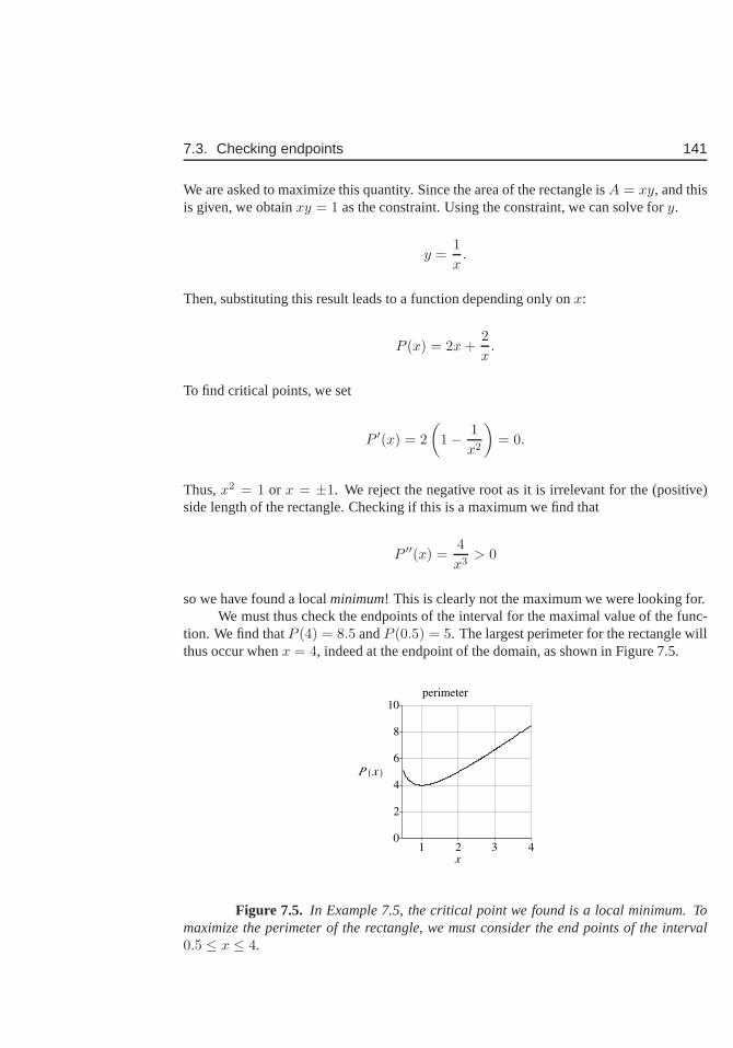
7.3. Checking endpoints 141
We are asked to maximize this quantity. Since the area of the rectangle isA = xy, and thisis given, we obtainxy = 1 as the constraint. Using the constraint, we can solve fory.
y =1
x.
Then, substituting this result leads to a function depending only onx:
P (x) = 2x +2
x.
To find critical points, we set
P ′(x) = 2
(
1− 1
x2
)
= 0.
Thus,x2 = 1 or x = ±1. We reject the negative root as it is irrelevant for the (positive)side length of the rectangle. Checking if this is a maximum wefind that
P ′′(x) =4
x3> 0
so we have found a localminimum! This is clearly not the maximum we were looking for.We must thus check the endpoints of the interval for the maximal value of the func-
tion. We find thatP (4) = 8.5 andP (0.5) = 5. The largest perimeter for the rectangle willthus occur whenx = 4, indeed at the endpoint of the domain, as shown in Figure 7.5.
Figure 7.5. In Example 7.5, the critical point we found is a local minimum. Tomaximize the perimeter of the rectangle, we must consider the end points of the interval0.5 ≤ x ≤ 4.
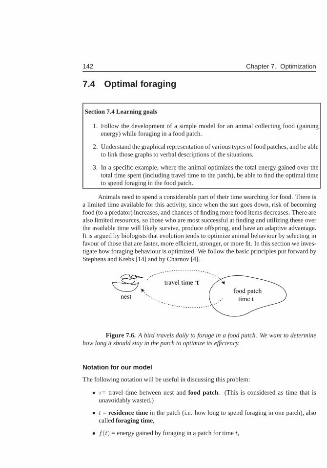
142 Chapter 7. Optimization
7.4 Optimal foraging
Section 7.4 Learning goals
1. Follow the development of a simple model for an animal collecting food (gainingenergy) while foraging in a food patch.
2. Understand the graphical representation of various types of food patches, and be ableto link those graphs to verbal descriptions of the situations.
3. In a specific example, where the animal optimizes the totalenergy gained over thetotal time spent (including travel time to the patch), be able to find the optimal timeto spend foraging in the food patch.
Animals need to spend a considerable part of their time searching for food. There isa limited time available for this activity, since when the sun goes down, risk of becomingfood (to a predator) increases, and chances of finding more food items decreases. There arealso limited resources, so those who are most successful at finding and utilizing these overthe available time will likely survive, produce offspring,and have an adaptive advantage.It is argued by biologists that evolution tends to optimize animal behaviour by selecting infavour of those that are faster, more efficient, stronger, ormore fit. In this section we inves-tigate how foraging behaviour is optimized. We follow the basic principles put forward byStephens and Krebs [14] and by Charnov [4].
travel time
food patch
time tnest
τ
Figure 7.6. A bird travels daily to forage in a food patch. We want to determinehow long it should stay in the patch to optimize its efficiency.
Notation for our model
The following notation will be useful in discussing this problem:
• τ= travel time between nest andfood patch. (This is considered as time that isunavoidably wasted.)
• t = residence timein the patch (i.e. how long to spend foraging in one patch), alsocalledforaging time,
• f(t) = energy gained by foraging in a patch for timet,
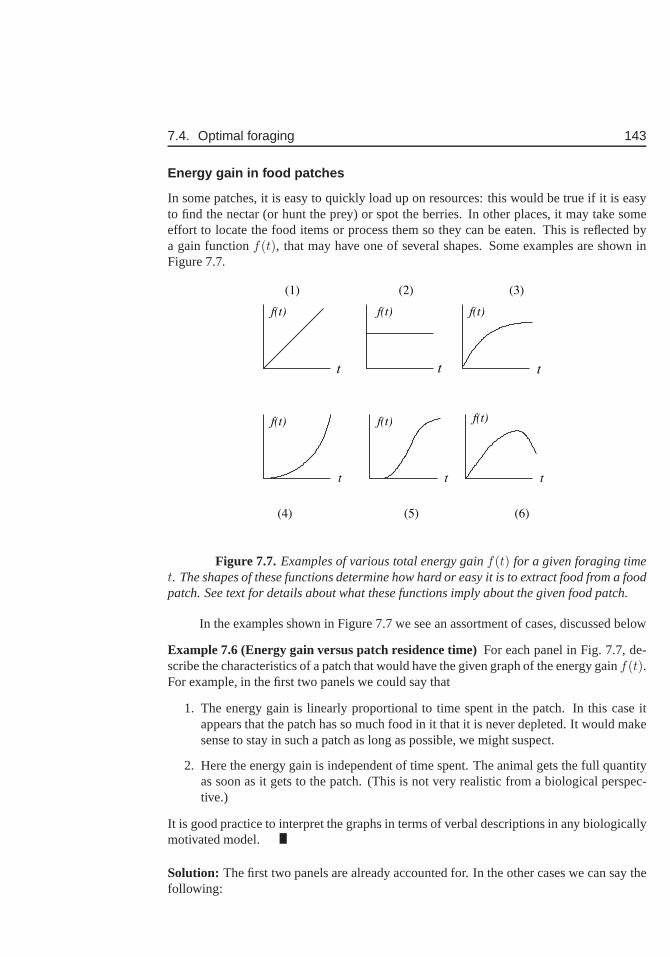
7.4. Optimal foraging 143
Energy gain in food patches
In some patches, it is easy to quickly load up on resources: this would be true if it is easyto find the nectar (or hunt the prey) or spot the berries. In other places, it may take someeffort to locate the food items or process them so they can be eaten. This is reflected bya gain functionf(t), that may have one of several shapes. Some examples are showninFigure 7.7.
t t t
f(t) f(t) f(t)
f(t) f(t) f(t)
(1) (2) (3)
(4) (5) (6)
t t t
Figure 7.7. Examples of various total energy gainf(t) for a given foraging timet. The shapes of these functions determine how hard or easy it is to extract food from a foodpatch. See text for details about what these functions implyabout the given food patch.
In the examples shown in Figure 7.7 we see an assortment of cases, discussed below
Example 7.6 (Energy gain versus patch residence time)For each panel in Fig. 7.7, de-scribe the characteristics of a patch that would have the given graph of the energy gainf(t).For example, in the first two panels we could say that
1. The energy gain is linearly proportional to time spent in the patch. In this case itappears that the patch has so much food in it that it is never depleted. It would makesense to stay in such a patch as long as possible, we might suspect.
2. Here the energy gain is independent of time spent. The animal gets the full quantityas soon as it gets to the patch. (This is not very realistic from a biological perspec-tive.)
It is good practice to interpret the graphs in terms of verbaldescriptions in any biologicallymotivated model.
Solution: The first two panels are already accounted for. In the other cases we can say thefollowing:
144 Chapter 7. Optimization
3. In this case, the food is gradually depleted in a given patch, (the total gain levels offto some constant level ast increases). There is diminishing return for staying longer.Here, we may expect to have some choice to make as to when to leave and look forfood elsewhere.
4. In this example, the rewards for staying longer actually multiply: the net energy gainhas an increasing slope (or, otherwise stated,f ′′(t) > 0). We will see that in thiscase, there is no optimal residence time: some other strategy, such as staying in justone patch would be optimal.
5. It takes some time to begin to gain energy but later on the gain increases rapidly.Eventually, the patch is depleted.
6. Here we have the case where staying too long in a patch is actually disadvantageousin that it leads to a net loss of energy. This might happen if the animal spends moreenergy looking for food that is already depleted. Here it is clear that leaving the patchearly enough is the best strategy.
For the purpose of a simple example, we will assume that the patch energy function is givenby
f(t) =Emaxt
k + twhere Emax, k > 0, are constants. (7.6)
Example 7.7 (Interpreting the assumed functionf(t)) Match the function we have as-sumed in Eqn. (7.6) with one of the panels in Fig. 7.7. Then interpret the meanings of theconstantsEmax, k.
Solution: We recognize Eqn. (7.6) as a function that is similar to the graph shown in theleft panel of Fig. 1.7 (Michaelis-Menten kinetics in biochemistry). Panel (3) in Fig. 7.7resembles this graph. Then, from our previous analysis in Chapter 1, we know thatEmax
is the horizontal asymptote, and corresponds to the greatest possible energy that can beextracted from the patch (if foraging continues indefinitely). The parameterk, which hasunits of time in Eqn. (7.6), controls the steepness of the rising phase of the function. Attime t = k, we find thatf = Emax/2 (Exercise 26(a)).
Currency to optimize
We will assume that animals try to maximize the average rate of energy gain over theforaging day. defined by the following ratio:
R(t) =Total energy gained
total time spent
i.e.,R, is theaverage energy gain per unit time. This quantity will depend on the amountof time t that is spent foraging during a day. The question we ask is whether there is anoptimal foraging time (i.e. a value of the time,t), that maximizesR(t). As we show below,whether or not an optimum exists depends greatly on how hard it is to extract food from afood patch. When an optimal foraging time exists, we will seethat it also depends on howmuch time is wasted in transit to such foraging sites.
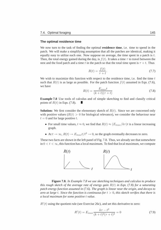
7.4. Optimal foraging 145
The optimal residence time
We now turn to the task of finding the optimalresidence time, i.e. time to spend in thepatch. We will make a simplifying assumption that all the patches are identical, making itequally easy to utilize each one. Now suppose on average, thetime spent in a patch ist.Then, the total energy gained during the day, isf(t). It takes a timeτ to travel between thenest and the food patch and a timet in the patch so that the total time spent isτ + t. Thus
R(t) =f(t)
τ + t. (7.7)
We wish to maximize this function with respect to the residence time, i.e. find the timetsuch thatR(t) is as large as possible. For the patch functionf(t) assumed in Eqn. (7.6),we have
R(t) =Emaxt
(k + t)(τ + t)(7.8)
Example 7.8 Use tools of calculus and of simple sketching to find and classify criticalpoints ofR(t) in Eqn. (7.8).
Solution: We first consider the elementary sketch ofR(t). Since we are concerned onlywith positive values (R(t) > 0 for biological relevance), we consider the behaviour neart = 0 and for large positivet.
• For small time values,t ≈ 0, we find thatR(t) ≈ (Emax/kτ)t is a linear increasinggraph.
• At t→∞, R(t)→ Emaxt/t2 → 0, so the graph eventually decreases to zero.
These two facts are shown in the left panel of Fig. 7.8. Thus, we already see that somewherein 0 < t <∞, this function has a local maximum. To find that local maximum, we compute
t
R(t)
t
R(t)
Figure 7.8. In Example 7.8 we use sketching techniques and calculus to producethis rough sketch of the average rate of energy gainR(t) in Eqn. (7.8) for a saturatingpatch energy function assumed in(7.6). The graph is linear near the origin, and decays tozero at larget. Since the function is continuous fort > 0, this sketch verifies that there isa local maximum for some positivet value.
R′(t) using the quotient rule (see Exercise 26c), and set this derivative to zero:
R′(t) = Emaxkτ − t2
(k + t)2(τ + t)2= 0 (7.9)
146 Chapter 7. Optimization
This can only be satisfied if the numerator is zero, that is
kτ − t2 = 0 ⇒ t1,2 = ±√
kτ .
We reject the negative root which is not relevant here, and deduce that the critical pointof the functionR(t) that we seek is attcrit =
√kτ . According to our sketch in Fig. 7.8,
this critical point is a local maximum. We can also confirm this using the techniques ofdiagnosis for critical points, as shown in the next example.(This example is for practice,as Fig. 7.8 is sufficient evidence.)
Example 7.9 Use one of the calculus tests for critical points to show thatt =√
kτ is alocal maximum for the functionR(t) in Eqn. (7.8).
Solution: SinceR(t) is a rational function, it is messy to calculate its second derivative,so we avoid using the second derivative test. Instead, we apply the first derivative test ofSection 6.2.3. We examine the sign of the first derivative to the left and to the right of thecritical point. Looking at Eqn. (7.9), we note that the denominator is positive so the sign ofR′(t) is determined by the numerator,kτ − t2. ThusR′(t) is positive (function increases)whenevert < tcrit, andR′(t) is negative (function decreases) whenevert > tcrit. So bythe first derivative test, the critical point is a local maximum. (We henceforth refer to it astmax.)
We have found that to optimize the average rate of energy gainR(t), the animal shouldstay in the patch for a time duration oft = tmax =
√kτ . We next ask what is the value of
the average rate of energy gain for this optimal patch residence time.
Example 7.10 Find the optimal average rate of energy gainR(t).
Solution: Here we are asked to computeR(t) for t = tmax =√
kτ . We find that
R(tmax) =Emaxtmax
(k + tmax)(τ + tmax)=
Emax
τ
1
(1 +√
k/τ)2(7.10)
The reader is asked to fill in the steps for this calculation inExercise 26(d).
7.4.1 For further study: Other patch functions
So far, we have carried out the calculations for a specific patch functionf(t) given byEqn. (7.6). However, we can gain insight and obtain an interesting result without makingthis assumption. Let us repeat our analysis with a more general example in mind.
Example 7.11 Carry out the calculations for the optimal value patch residence time for ageneral patch energy functionf(t), without using the formula (7.6).
Solution: We use the expression forR(t) given by (7.7). Differentiating, we find the firstderivative,
R′(t) =f ′(t)(τ + t)− f(t)
(τ + t)2=
G(t)
H(t)
7.4. Optimal foraging 147
whereG(t) = f ′(t)(τ + t)− f(t), H(t) = (τ + t)2.
(The calculation is easier with this notation.) To maximizeR(t) we set
R′(t) = 0
which can occur only when the numerator of the above equationis zero, i.e.
G(t) = 0.
This means thatf ′(t)(τ + t)− f(t) = 0
so that, after simplifying algebraically,
f ′(t) =f(t)
τ + t. (7.11)
A geometric argument
In practice, we would need to specify a function forf(t) in order to solve for the optimaltime t. However, we can also solve this problem using ageometric argument. The lastequation equates two quantities that can be interpreted as slopes. On the right is the slopeof a tangent line. On the left is the slope (rise over run) of some right triangle whoseheight isf(t) and whose base length isτ + t. In Figure 7.9, we show each slope on itsown: In the right panel,f ′(t) is the slope of the tangent line to the graph off(t). In thecentral panel, we have constructed some triangle with the property that its hypotenuse hasslopef(t)/[τ + t]. On the left panel we have superimposed both, selecting a value of t forwhich the slope of the triangle is the same as the slope of the tangent line. Notice that inorder to fit the triangle on the same diagram, we had to place its tip at the point−τ alongthe horizontal axis. When these slopes coincide, it means that we have satisfied equation(7.11), and we have found the desired timet for optimal foraging.
We can use this observation in general to come up with the following steps to solvean optimal foraging problem:
1. A biologist conducts some field experiments to determine the mean travel time fromfood to nest,τ , and the shape of the energy gain functionf(t). (This may requirecapturing the animal and examining the contents of its stomach. . . an unappetizingthought; we will leave this to task to our brave biological colleagues.)
2. We draw a sketch off(t) as shown in rightmost panel of Figure 7.9 and extend thet axis in the negative direction. At the point−τ we draw a line that just touches thecurvef(t) at some point (i.e. a tangent line). The slope of this line isf ′(t) for somevalue oft.
3. The value oft at the point of tangency is the optimal time to spend in the patch!
The diagram drawn in our geometric solution (right panel in Figure 7.9 is often called a“rooted tangent”).
We have shown that the point labeledt indeed satisfies the condition that we derivedabove forR′(t) = 0, and hence is a critical point.
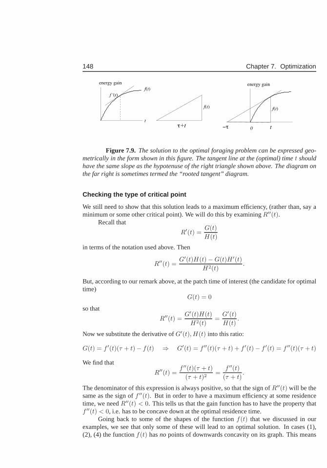
148 Chapter 7. Optimization
0 t
f(t)
f '(t)
t
energy gain energy gain
τ+t −τ
f(t) f(t)
Figure 7.9. The solution to the optimal foraging problem can be expressed geo-metrically in the form shown in this figure. The tangent line at the (optimal) timet shouldhave the same slope as the hypotenuse of the right triangle shown above. The diagram onthe far right is sometimes termed the “rooted tangent” diagram.
Checking the type of critical point
We still need to show that this solution leads to a maximum efficiency, (rather than, say aminimum or some other critical point). We will do this by examining R′′(t).
Recall that
R′(t) =G(t)
H(t)
in terms of the notation used above. Then
R′′(t) =G′(t)H(t)−G(t)H ′(t)
H2(t).
But, according to our remark above, at the patch time of interest (the candidate for optimaltime)
G(t) = 0
so that
R′′(t) =G′(t)H(t)
H2(t)=
G′(t)
H(t).
Now we substitute the derivative ofG′(t), H(t) into this ratio:
G(t) = f ′(t)(τ + t)− f(t) ⇒ G′(t) = f ′′(t)(τ + t) + f ′(t)− f ′(t) = f ′′(t)(τ + t)
We find that
R′′(t) =f ′′(t)(τ + t)
(τ + t)2=
f ′′(t)
(τ + t).
The denominator of this expression is always positive, so that the sign ofR′′(t) will be thesame as the sign off ′′(t). But in order to have a maximum efficiency at some residencetime, we needR′′(t) < 0. This tells us that the gain function has to have the propertythatf ′′(t) < 0, i.e. has to be concave down at the optimal residence time.
Going back to some of the shapes of the functionf(t) that we discussed in ourexamples, we see that only some of these will lead to an optimal solution. In cases (1),(2), (4) the functionf(t) hasno points of downwards concavity on its graph. This means
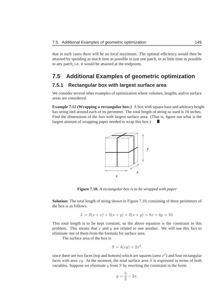
7.5. Additional Examples of geometric optimization 149
that in such cases there will be no local maximum. The optimalefficiency would then beattained by spending as much time as possible in just one patch, or as little time as possiblein any patch, i.e. it would be attained at the endpoints.
7.5 Additional Examples of geometric optimization7.5.1 Rectangular box with largest surface area
We consider several other examples of optimization where volumes, lengths, and/or surfaceareas are considered.
Example 7.12 (Wrapping a rectangular box:) A box with square base and arbitrary heighthas string tied around each of its perimeter. The total length of string so used is 10 inches.Find the dimensions of the box with largest surface area. (That is, figure out what is thelargest amount of wrapping paper needed to wrap this box.)
xx
y
Figure 7.10.A rectangular box is to be wrapped with paper
Solution: The total length of string shown in Figure 7.10, consisting of three perimeters ofthe box is as follows:
L = 2(x + x) + 2(x + y) + 2(x + y) = 8x + 4y = 10.
This total length is to be kept constant, so the above equation is the constraint in thisproblem. This means thatx andy are related to one another. We will use this fact toeliminate one of them from the formula for surface area.
The surface area of the box is
S = 4(xy) + 2x2.
since there are two faces (top and bottom) which are squares (areax2) and four rectangularfaces with areaxy. At the moment, the total surface areaS is expressed in terms of bothvariables. Suppose we eliminatey from S by rewriting the constraint in the form:
y =5
2− 2x.
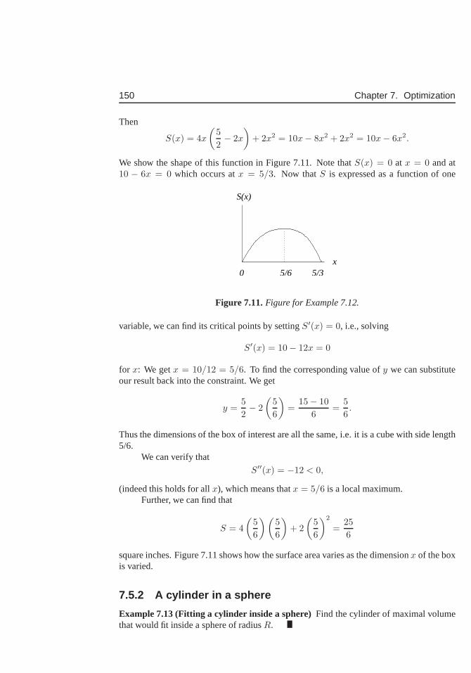
150 Chapter 7. Optimization
Then
S(x) = 4x
(
5
2− 2x
)
+ 2x2 = 10x− 8x2 + 2x2 = 10x− 6x2.
We show the shape of this function in Figure 7.11. Note thatS(x) = 0 at x = 0 and at10 − 6x = 0 which occurs atx = 5/3. Now thatS is expressed as a function of one
S(x)
x0 5/6 5/3
Figure 7.11.Figure for Example 7.12.
variable, we can find its critical points by settingS′(x) = 0, i.e., solving
S′(x) = 10− 12x = 0
for x: We getx = 10/12 = 5/6. To find the corresponding value ofy we can substituteour result back into the constraint. We get
y =5
2− 2
(
5
6
)
=15− 10
6=
5
6.
Thus the dimensions of the box of interest are all the same, i.e. it is a cube with side length5/6.
We can verify that
S′′(x) = −12 < 0,
(indeed this holds for allx), which means thatx = 5/6 is a local maximum.Further, we can find that
S = 4
(
5
6
)(
5
6
)
+ 2
(
5
6
)2
=25
6
square inches. Figure 7.11 shows how the surface area variesas the dimensionx of the boxis varied.
7.5.2 A cylinder in a sphere
Example 7.13 (Fitting a cylinder inside a sphere)Find the cylinder of maximal volumethat would fit inside a sphere of radiusR.
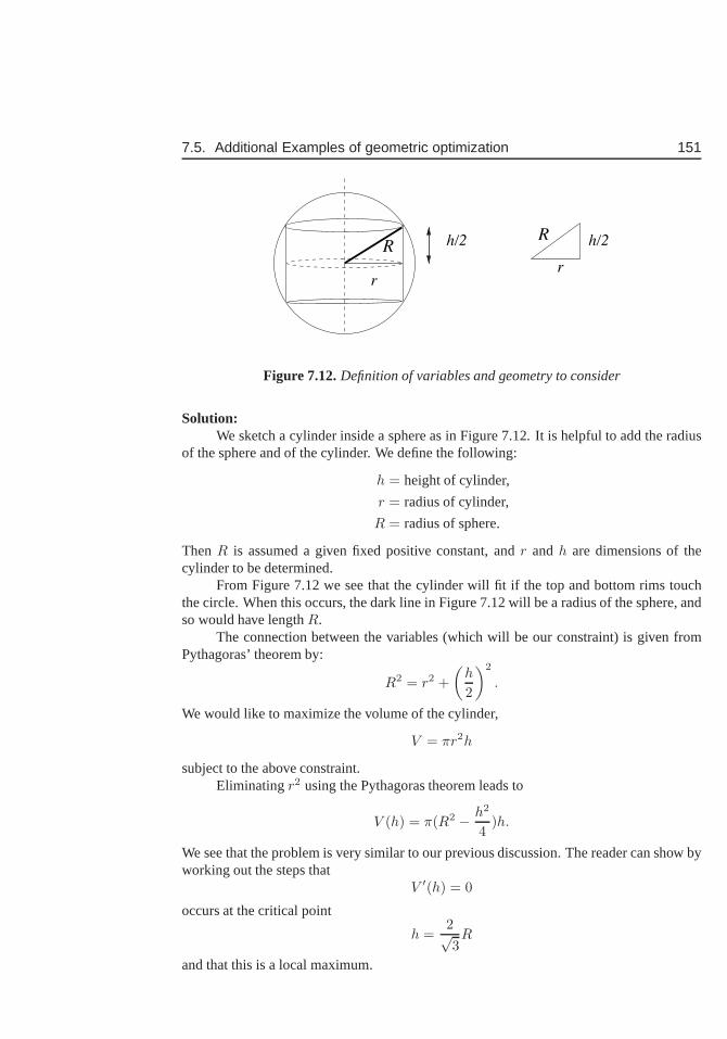
7.5. Additional Examples of geometric optimization 151
h/2
r
h/2
r
RR
Figure 7.12.Definition of variables and geometry to consider
Solution:We sketch a cylinder inside a sphere as in Figure 7.12. It is helpful to add the radius
of the sphere and of the cylinder. We define the following:
h = height of cylinder,
r = radius of cylinder,
R = radius of sphere.
ThenR is assumed a given fixed positive constant, andr and h are dimensions of thecylinder to be determined.
From Figure 7.12 we see that the cylinder will fit if the top andbottom rims touchthe circle. When this occurs, the dark line in Figure 7.12 will be a radius of the sphere, andso would have lengthR.
The connection between the variables (which will be our constraint) is given fromPythagoras’ theorem by:
R2 = r2 +
(
h
2
)2
.
We would like to maximize the volume of the cylinder,
V = πr2h
subject to the above constraint.Eliminatingr2 using the Pythagoras theorem leads to
V (h) = π(R2 − h2
4)h.
We see that the problem is very similar to our previous discussion. The reader can show byworking out the steps that
V ′(h) = 0
occurs at the critical point
h =2√3R
and that this is a local maximum.
152 Chapter 7. Optimization
Exercises7.1. The sum of two positive number is20. Find the numbers
(a) if their product is a maximum.
(b) if the sum of their squares is a minimum.
(c) if the product of the square of one and the cube of the otheris a maximum.
7.2. A tram ride at Disney World departs from its starting place att = 0 and travelsto the end of its route and back. Its distance from the terminal at time t can beapproximately described by the expression
S(t) = 4t3(10− t)
(wheret is in minutes,0 < t < 10, andS is distance in meters.)
(a) Find the velocity as a function of time.
(b) When is the tram moving at the fastest rate?
(c) At what time does it get to the furthest point away from itsstarting position?
(d) Sketch the acceleration, the velocity, and the positionof the tram on the sameset of axes.
7.3. At9A.M., carB is 25 km west of another carA. CarA then travels to the south at30 km/h and carB travels east at40 km/h. When will they be the closest to eachother and what is this distance?
7.4. A cannonball is shot vertically upwards from the groundwith initial velocity v0 =15m/sec. It is determined that the height of the ball,y (in meters), as a function ofthe time,t (in sec) is given by
y = v0t− 4.9t2
Determine the following:
(a) The time at which the cannonball reaches its highest point,
(b) The velocity and acceleration of the cannonball att = 0.5 s, andt = 1.5 s.
(c) The time at which the cannonball hits the ground.
7.5. Net nutrient increase rate: In Example 7.2, we considered the net rate of increaseof nutrients in a spherical cell of radiusr. Here we further explore this problem.
(a) Draw a sketch ofN(r) based on Eqn. (7.1). Use your sketch to verify that thisfunction has a local maximum.
(b) Use the first derivative test to show that the critical point r = 2k1/k2 is a localmaximum.
7.6. Nutrient increase in cylindrical cell: Consider a long skinny cell in the shape ofa cylinder with radiusr and a fixed lengthL. Then the volume and surface area ofsuch a cell (neglecting endcaps) areV = πr2L = K andS = 2πrL.

Exercises 153
(a) Adapt the formula for net rate of increase of nutrientsN(t) for a spherical cell(7.1) to the case of a cylindrical cell.
(b) Find the radius of the cylindrical cell that maximizesN(t). Be sure to verifythat you have found a local maximum.
7.7. Cylinder of minimal surface area: In this problem we continue to explore Exam-ple 7.3.
(a) Reason that the surface area of the cylinder,S(r) = 2Kr + 2πr2 is a function
that has a local minimum using curve-sketching skills.
(b) Use the first derivative test to show thatr =(
K2π
)1/3is a local minimum for
S(r).
(c) Show the algebra required to find the value ofL corresponding to thisr valueand show thatL/r = 2.
7.8. (From Final Exam, Math 100, Dec 1997) A closed 3-dimensional box is to be con-structed in such a way that its volume is 4500 cm3. It is also specified that the lengthof the base is 3 times the width of the base. Find the dimensions of the box whichsatisfy these conditions and have the minimum possible surface area. Justify youranswer.
7.9. A box with a square base is to be made so that its diagonal has length1. SeeFigure 7.13.
(a) What heighty would make the volume maximal?
(b) What is the maximal volume?
[Hint: A box having side lengthsℓ, w, h has diagonal lengthD whereD2 =ℓ2 + w2 + h2 and volumeV = ℓwh.]
x
x
Dy
Figure 7.13.Figure for Problem 9
7.10. Find the minimum distance from a point on the positivex-axis(a, 0) to the parabolay2 = 8x.
7.11. The largest garden: You are building a fence to completely enclose part of yourbackyard for a vegetable garden. You have already purchasedmaterial for a fenceof length 100 ft. What is the largest rectangular area that this fence can enclose?
7.12. “Good Fences make Good Neighbors”:A fence of length 100 ft is to be used toenclose two gardens. One garden is to have a circular shape, and the other to be
154 Chapter 7. Optimization
square. Find out how the fence should be cut so that the sum of the areas inside bothgardens is as large as possible.
7.13. A rectangular piece of cardboard with dimension12 cm by24 cm is to be made intoan open box (i.e., no lid) by cutting out squares from the corners and then turningup the sides. Find the size of the squares that should be cut out if the volume of thebox is to be a maximum.
7.14. Alternate solution to Kepler’s wine barrel: In this problem we follow an alter-nate approach to the most economical wine barrel problem posed by Kepler (Exam-ple 7.4).Out approach is to Find the proportions (height:radius) of the cylinder that mini-mizes the lengthL of the wet rod in Fig. 7.3 for a fixed volume.
(a) Explain why minimizingL is equivalent to minimizingL2 in Eqn. (7.4)
(b) Explain how Eqn. (7.3) can be used to specify a constraintfor this problem.(Hint: consider the volume,V to be fixed and show that you can solve forr2).
(c) Use your result in (c) to eliminater from the formula forL2. Now L2(h) willdepend only on the height of the cylindrical wine barrel.
(d) Use calculus to find any local minima forL2(h). Be sure to verify that yourresult is a minimum.
(e) Find the corresponding value ofr using your result in (b).
(f) Find the ratioh/r. You should obtain the same result as in (7.5).
7.15. Rectangle with largest area:Find the side lengths,x andy, of the rectangle withlargest area whose diameterL is given. (Hint: Eliminate one variable using theconstraint. Then, to simplify the derivative you can use thefact that critical points ofA would also be critical points ofA2, whereA = xy is the area of the rectangle. Orelse, if you have already learned the chain rule, you can use it in the differentiation.)
7.16. Find the shortest path that would take a milk-maid fromher house at(10, 10) tofetch water at the river located along thex axis and then to the thirsty cow at(3, 5).
7.17. Water and ice: Why does ice float on water? Because the density of ice is lower!In fact, water is the only common liquid whose maximal density occurs above itsfreezing temperature. (This phenomenon favors the survival of aquatic life by pre-venting ice from forming at the bottoms of lakes.) Accordingto theHandbook ofChemistry and Physics,a mass of water that occupies one liter at0◦C occupies avolume (in liters) of
V = −aT 3 + bT 2 − cT + 1
atT ◦C where0 ≤ T ≤ 30 and where the coefficients are
a = 6.79× 10⁻⁸, b = 8.51× 10⁻⁶, c = 6.42× 10⁻⁵.
Find the temperature between0◦C and30◦C at which the density of water is thegreatest. (Hint: maximizing the density is equivalent to minimizing the volume.Why is this?)
Exercises 155
7.18. Drug doses and sensitivity:TheReactionR(x) of a patient to a drug dose of sizex depends on the type of drug. For a certain drug, it was determined that a gooddescription of the relationship is:
R(x) = Ax2(B − x)
whereA andB are positive constants. TheSensitivityof the patient’s body to thedrug is defined to beR′(x).
(a) For what value ofx is the reaction a maximum, and what is that maximumreaction value?
(b) For what value ofx is the sensitivity a maximum? What is the maximumsensitivity?
7.19. Thermoregulation in a swarm of bees:In the winter, honeybees sometimes escapethe hive and form a tight swarm in a tree, where, by shivering,they can produce heatand keep the swarm temperature elevated. Heat energy is lostthrough the surface ofthe swarm at a rate proportional to the surface area (k1S wherek1 > 0 is a constant).Heat energy is produced inside the swarm at a rate proportional to the mass of theswarm (which you may take to be a constant times the volume). We will assumethat the heat production isk2V wherek2 > 0 is constant. Swarms that are not largeenough may lose more heat than they can produce, and then theywill die. The heatdepletion rate is the loss rate minus the production rate. Assume that the swarm isspherical. Find the size of the swarm for which the rate of depletion of heat energyis greatest.
7.20. A right circular cone is circumscribed about a sphere of radius5. Find the dimensionof this cone if its volume is to be a minimum. (Remark: this is arather challenginggeometric problem.)
7.21. Optimal Reproductive Strategy: Animals that can produce many healthy babiesthat survive to the next generation are at an evolutionary advantage over other, com-peting, species. However, too many young produce a heavy burden on the parents(who must feed and care for them). If this causes the parents to die, the advantage islost. Also, competition of the young with one another for food and parental attentionjeopardizes the survival of these babies. Suppose that the evolutionaryAdvantageA to the parents of having litter sizex is
A(x) = ax− bx2.
Suppose that theCostC to the parents of having litter sizex is
C(x) = mx + e.
TheNet Reproductive GainG is defined as
G = A− C.
(a) Explain the expressions forA, C andG.
(b) At what litter size is the advantage,A, greatest?
156 Chapter 7. Optimization
(c) At what litter size is there least cost to the parents?
(d) At what litter size is the Net Reproductive Gain greatest?.
7.22. Behavioural Ecology: Social animals that live in groups can spend less time scan-ning for predators than solitary individuals. However, they waste time fighting withthe other group members over the available food. There is some group size at whichthe net benefit is greatest because the animals spend least time on these unproductiveactivities, and thus can spend time on feeding, mating, etc.Assume that for a group of sizex, the fraction of time spent scanning for predatorsis
S(x) = A1
(x + 1)
and the fraction of time spent fighting with other animals over food is
F (x) = B(x + 1)2
whereA, B are constants. Find the size of the group for which the time wasted onscanning and fighting is smallest.
7.23. Logistic growth: Consider a fish population whose density (individuals per unitarea) isN , and suppose this fish population growslogistically, so that the rate ofgrowthR satisfies
R(N) = rN(1 −N/K)
wherer andK are positive constants.
(a) SketchR as a function ofN or explain Fig 7.1.
(b) Use a first derivative test to justify the claim thatN = K/2 is a local maximumfor the functionG(N).
7.24. Logistic growth with harvesting: Consider a fish population of densityN growinglogistically, i.e. with rate of growthR(N) = rN(1 − N/K) wherer andK arepositive constants. The rate of harvesting (i.e. removal) of the population is
h(N) = qEN
whereE, the effort of the fishermen, andq, the catchability of this type of fish, arepositive constants. At what density of fish does the growth rate exactly balance theharvesting rate ? (This density is called the maximal sustainable yield: MSY.)
7.25. Conservation of a harvested population:Conservationists insist that the densityof fish should never be allowed to go below a level at which growth rate of thefish exactly balances with the harvesting rate. (At this level, the harvesting is at itsmaximal sustainable yield. If more fish are taken, the population will keep droppingand the fish will eventually go extinct.) What level of fishingeffort should be used tolead to the greatest harvest at this maximal sustainable yield? [Remark: you shouldfirst do the previous problem.]
7.26. Optimal foraging: Consider Example 7.7 for the optimal foraging model.
(a) Show that the parameterk in (7.6) is the time at whichf(t) = Emax/2.
Exercises 157
(b) Consider panel (5) of Fig. 7.7. Show that a function such as a Hill functionwould have the shape shown in that sketch. Interpret any parameters in thatfunction.
(c) Use the quotient rule to calculate the derivative of the functionR(t) given byEqn. (7.8) and show that you get (7.9).
(d) Fill in the missing steps in the calculation in Eqn. (7.10) to find the optimalvalue ofR(t).
7.27. Rate of net energy gain while foraging and traveling:Animals spend energy intraveling and foraging. In some environments this energy loss is a significant portionof the energy budget. In such cases, it is customary to assumethat to survive, anindividual would optimize the rate ofnetenergy gain, defined as
Q(t) =Net energy gained
total time spent=
Energy gained− Energy losttotal time spent
(7.12)
Assume that the animal spendsp energy units per unit time in all activities (includingforaging and traveling). Assume that the energy gain in the patch (“patch energyfunction”) is given by (7.6). Find the optimal patch time, that is the time at whichQ(t) is maximized in this scenario.
7.28. Maximizing net energy gain: Suppose that the situation requires an animal to max-imize its net energy gainedE(t) defined as
E(t) = energy gained while foraging− energy spent while foraging and traveling.
(So, this means thatE(t) = f(t)− r(t+ τ).) wherer is the rate of energy spent perunit time andτ is the fixed travel time. Assume as before that the energy gained byforaging for a timet in the food patch isf(t) = Emaxt/(k + t). Find the amountof time t spent foraging that maximizesE(t). Then indicate a condition of the formk <?? that is required for existence of this critical point

158 Chapter 7. Optimization
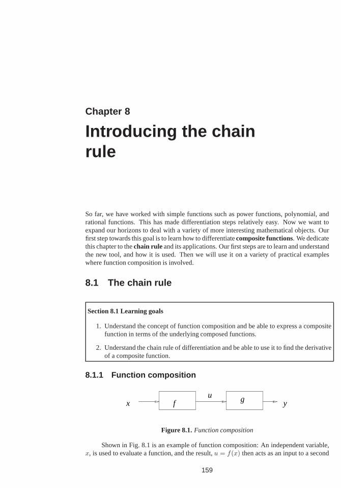
Chapter 8
Introducing the chainrule
So far, we have worked with simple functions such as power functions, polynomial, andrational functions. This has made differentiation steps relatively easy. Now we want toexpand our horizons to deal with a variety of more interesting mathematical objects. Ourfirst step towards this goal is to learn how to differentiatecomposite functions. We dedicatethis chapter to thechain rule and its applications. Our first steps are to learn and understandthe new tool, and how it is used. Then we will use it on a varietyof practical exampleswhere function composition is involved.
8.1 The chain rule
Section 8.1 Learning goals
1. Understand the concept of function composition and be able to express a compositefunction in terms of the underlying composed functions.
2. Understand the chain rule of differentiation and be able to use it to find the derivativeof a composite function.
8.1.1 Function composition
xu
yf g
Figure 8.1.Function composition
Shown in Fig. 8.1 is an example of function composition: An independent variable,x, is used to evaluate a function, and the result,u = f(x) then acts as an input to a second
159
160 Chapter 8. Introducing the chain rule
function,g. The final value isy = g(u) = g(f(x)). We refer to the two-step functionoperation asfunction composition.
Example 8.1 Consider the two functionsf(x) =√
x andg(x) = x2 + 1. Determine thetwo new functions obtained by composing these, namelyh1(x) = f(g(x)) andh2(x) =g(f(x)).
Solution: Forh1 we applyg first, followed byf , soh1(x) = (√
x)2 + 1 = x + 1. Forh2,the functions are applied in the reversed order so thath2(x) =
√x2 + 1. We note that the
domains of the two functions are slightly different.h1 is only defined forx ≥ 0 sincef(x)is not defined for negativex, whereash2 is defined for allx.
Example 8.2 Express the functionh(x) = 5(x3−x2)10 as the composition of two simplerfunctions. What are the domains of each of the functions?
Solution: We can write this in terms of the two functionsf(x) = x3−x2 andg(x) = 5x10.Thenh(x) = g(f(x)).
8.1.2 The chain rule of differentiation
Given a composite functiony = f(g(x)), such as the ones we have encountered in ourexamples, we are interested in understanding how changes inthe variablex affect changein y.
If y = g(u) and u = f(x) are both differentiable functions andy = g(f(x)) is thecomposite function, then thechain rule of differentiation states that
dy
dx=
dy
du
du
dx
Informally, the chain rule states that the change iny with respect tox is a product oftwo rates of change: (1) the rate of change ofy with respect to its immediate inputu, and(2) the rate of change ofu with respect to its input,x.
Why does it work this way? Although the derivative is not merely a quotient, we canrecall that it is arrived at from a quotient through a processof shrinking an interval. If wewrite
∆y
∆x=
∆y
∆u
∆u
∆x
then it is apparent that the “cancellation” of terms∆u in numerator and denominator lead tothe correct fraction on the left. The proof of the chain rule uses this essential idea, but careis taken to ensure that the quantity∆u is nonzero, to avoid the embarrassment of dealingwith the nonsensical ratio0/0.
Example 8.3 Apply the chain rule to differentiating the functionh(x) = 5(x3 − x2)10.
8.1. The chain rule 161
Solution: We express the function asy = h(x) = 5u10 whereu = (x3 − x2). Then
dy
dx=
dy
du
du
dx=
(
d(5u10)
du
)(
d(x3 − x2)
dx
)
= 5u9(3x2 − 2x).
Then, using the expression foru leads tody/dx = 5(x3 − x2)9(3x2 − 2x).
Example 8.4 Compute the derivative of the functiony = f(x) =√
x2 + a2, wherea issome positive real number.
Solution: This function can be considered as the composition ofg(u) =√
u andu(x) =x2+a2, That is, we can writef(x) = g(h(x)) We rewriteg in the form of a power functionand then use the chain rule to compute the derivative. We obtain
dy
dx=
1
2· (x2 + d2)−1/2 · 2x =
x
(x2 + d2)1/2=
x√x2 + d2
Example 8.5 Compute the derivative of the function
y = f(x) =x√
x2 + d2, whered is some positive real number
Solution: We use both the quotient rule and the chain rule for this calculation.
dy
dx=
[x]′ ·√
x2 + d2 − [√
x2 + d2]′ · x(√
x2 + d2)2
Here the′ denotes differentiation. Then
dy
dx=
1 ·√
x2 + d2 − [12 · 2x · (x2 + d2)−1/2] · x(x2 + d2)
We simplify algebraically by multiplying top and bottom by(x2 + d2)1/2 and cancelingfactors of 2 to obtain
dy
dx=
x2 + d2 − x2
(x2 + d2)1/2(x2 + d2)=
d2
(x2 + d2)3/2
8.1.3 Interpreting the chain rule
The following intuitive examples may help to motivate why the chain rule is based on aproduct of two rates of change.
Example 8.6 (Pollution level in a lake)A species of fish is sensitive to pollutants in itslake. As humans settle and populate the area adjoining the lake, one may see a decline inthe population of these fish due to increased levels of pollution. Quantify the rate at whichthe pollution level changes with time based on the pollutionproduced per human and therate of increase of the human population.
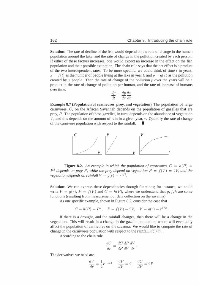
162 Chapter 8. Introducing the chain rule
Solution: The rate of decline of the fish would depend on the rate of change in the humanpopulation around the lake, and the rate of change in the pollution created by each person.If either of these factors increases, one would expect an increase in the effect on the fishpopulation and their possible extinction. The chain rule says that the net effect is a productof the two interdependent rates. To be more specific, we couldthink of time t in years,x = f(t) as the number of people living at the lake in yeart, andp = g(x) as the pollutioncreated byx people. Then the rate of change of the pollutionp over the years will be aproduct in the rate of change of pollution per human, and the rate of increase of humansover time:
dp
dt=
dp
dx
dx
dt
Example 8.7 (Population of carnivores, prey, and vegetation) The population of largecarnivores,C, on the African Savannah depends on the population of gazelles that areprey,P . The population of these gazelles, in turn, depends on the abundance of vegetationV , and this depends on the amount of rain in a given year,r. Quantify the rate of changeof the carnivore population with respect to the rainfall.
r
V
V
P
P
C
Figure 8.2. An example in which the population of carnivores,C = h(P ) =P 2 depends on preyP , while the prey depend on vegetationP = f(V ) = 2V, and thevegetation depends on rainfallV = g(r) = r1/2.
Solution: We can express these dependencies through functions; for instance, we couldwrite V = g(r), P = f(V ) andC = h(P ), where we understand thatg, f, h are somefunctions (resulting from measurement or data collection on the savanna).
As one specific example, shown in Figure 8.2, consider the case that
C = h(P ) = P 2, P = f(V ) = 2V, V = g(r) = r1/2.
If there is a drought, and the rainfall changes, then there will be a change in thevegetation. This will result in a change in the gazelle population, which will eventuallyaffect the population of carnivores on the savanna. We wouldlike to compute the rate ofchange in the carnivores population with respect to the rainfall, dC/dr.
According to the chain rule,
dC
dr=
dC
dP
dP
dV
dV
dr.
The derivatives we need are
dV
dr=
1
2r−1/2,
dP
dV= 2,
dC
dP= 2P.
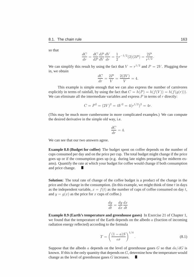
8.1. The chain rule 163
so thatdC
dr=
dC
dP
dP
dV
dV
dr=
1
2r−1/2(2)(2P ) =
2P
r1/2.
We can simplify this result by using the fact thatV = r1/2 andP = 2V . Plugging thesein, we obtain
dC
dr=
2P
V=
2(2V )
V= 4.
This example is simple enough that we can also express the number of carnivoresexplicitly in terms of rainfall, by using the fact thatC = h(P ) = h(f(V )) = h(f(g(r))).We can eliminate all the intermediate variables and expressP in terms ofr directly:
C = P 2 = (2V )2 = 4V 2 = 4(r1/2)2 = 4r.
(This may be much more cumbersome in more complicated examples.) We can computethe desired derivative in the simple old way, i.e.
dC
dr= 4.
We can see that our two answers agree.
Example 8.8 (Budget for coffee)The budget spent on coffee depends on the number ofcups consumed per day and on the price per cup. The total budget might change if the pricegoes up or if the consumption goes up (e.g. during late nightspreparing for midterm ex-ams). Quantify the rate at which your budget for coffee wouldchange if both consumptionand price change.
Solution: The total rate of change of the coffee budget is a product of the change in theprice and the change in the consumption. (In this example, wemight think of timet in daysas the independent variable,x = f(t) as the number of cups of coffee consumed on dayt,andy = g(x) as the price forx cups of coffee.)
dy
dt=
dy
dx
dx
dt
Example 8.9 (Earth’s temperature and greenhouse gases)In Exercise 21 of Chapter 1,we found that the temperature of the Earth depends on the albedoa (fraction of incomingradiation energy reflected) according to the formula
T =
(
(1− a)S
ǫσ
)1/4
. (8.1)
Suppose that the albedoa depends on the level of greenhouse gasesG so thatda/dG isknown. If this is the only quantity that depends onG, determine how the temperature wouldchange as the level of greenhouse gasesG increases.
164 Chapter 8. Introducing the chain rule
Solution: The information provided specifies thatT depends on the level of greenhousegases via the chain of dependenciesG→ a→ T . Let us write
T =
(
S
ǫσ
)1/4
(1− a)1/4
In this problem the quantitiesS, ǫ, σ are all constants, so it simplifies calculation to writethe function in the form shown above. According to the chain rule,
dT
dG=
dT
da
da
dG.
We are givenda/dG and we can computedT/da. Hence, we find that
dT
dG=
(
S
ǫσ
)1/4d
da
[
(1− a)1/4] da
dG=
(
S
ǫσ
)1/41
4(1− a)
(1/4)−1 · (−1)da
dG.
Rearranging leads to
dT
dG= −1
4
(
S
ǫσ
)1/4
(1− a)−3/4 da
dG.
In general, greenhouse gasses affect both the Earth’s albedo a and its emissivityǫ. Wegeneralize our results in Exercise 2.
8.2 Chain Rule applied to optimization problemsNow that the chain rule is available to us as a differentiation tool, we are able to extendthe repertoire of mathematical problems that are amenable to calculus solutions. Here weshow two examples where derivatives require the chain rule.In both cases, we consideroptimization problems based on a biological situation. Optimization will provide insightinto how animals organize to find their food.
Section 8.2 Learning goals
1. Read and follow the derivation of each optimization model.
2. Be able to carry out the calculations of derivatives appearing in the problems (usingthe chain rule)
3. Using optimization, find each critical point and verify its type.
4. Understand and be able to explain the interpretation of the mathematical results.
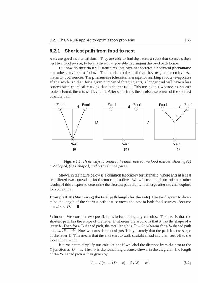
8.2. Chain Rule applied to optimization problems 165
8.2.1 Shortest path from food to nest
Ants are good mathematicians! They are able to find the shortest route that connects theirnest to a food source, to be as efficient as possible in bringing the food back home.
But how do they do it? It transpires that each ant secretes a chemicalpheromonethat other ants like to follow. This marks up the trail that they use, and recruits nest-mates to food sources. Thepheromone(chemical message for marking a route) evaporatesafter a while, so that, for a given number of foraging ants, a longer trail will have a lessconcentrated chemical marking than a shorter trail. This means that whenever a shorterroute is found, the ants will favour it. After some time, thisleads to selection of the shortestpossible trail.
Food
Nest
D
dFood Food
Nest
D
dFood Food
Nest
D
x
dFood
(a) (b) (c)
Figure 8.3.Three ways to connect the ants’ nest to two food sources, showing (a)a V-shaped, (b) T-shaped, and (c) Y-shaped paths.
Shown in the figure below is a common laboratory test scenario, where ants at a nestare offered two equivalent food sources to utilize. We will use the chain rule and otherresults of this chapter to determine the shortest path that will emerge after the ants explorefor some time.
Example 8.10 (Minimizing the total path length for the ants) Use the diagram to deter-mine the length of the shortest path that connects the nest toboth food sources. Assumethatd << D.
Solution: We consider two possibilities before doing any calculus. The first is that theshortest path has the shape of the letterT whereas the second is that it has the shape of aletterV. Then for a T-shaped path, the total length isD + 2d whereas for a V-shaped pathit is 2
√D2 + d2. Now we consider a third possibility, namely that the path has the shape
of the letterY. This means that the ants start to walk straight ahead and then veer off to thefood after a while.
It turns out to simplify our calculations if we label the distance from the nest to theY-junction asD − x. Thenx is the remaining distance shown in the diagram. The lengthof the Y-shaped path is then given by
L = L(x) = (D − x) + 2√
d2 + x2. (8.2)
166 Chapter 8. Introducing the chain rule
Now we observe that whenx = 0, thenLT = D + 2d, which corresponds exactly to theT-shaped path, whereas whenx = D thenLV = 2
√d2 + D2 which is the length of the
V-shaped path. Thus in this problem, we have0 < x < D as the appropriate domain, andwe have determined the values ofL at the two domain endpoints.
To find the minimal path length, we look for critical points ofthe functionL(x).Differentiating, we obtain (using results of Example 8.4)
L′(x) =dL
dx= −1 + 2
x√x2 + d2
.
Critical points occur atL′(x) = 0, which corresponds to
−1 + 2x√
x2 + d2= 0.
We simplify this algebraically to obtain
√
x2 + d2 = 2x ⇒ x2 + d2 = 4x2 ⇒ 3x2 = d2 ⇒ x =d√3.
To determine the kind of critical point, we find the second derivative (See Example 8.5).Then
L′′(x) = 2d2
(x2 + d2)−3/2> 0.
Thus the second derivative is positive and the critical point is a local maximum.To determine the actual length of the path, we substitutex = d/
√3 into the function
L(x) and obtain (after simplification, see Exercise 3)
L = L(x) = D +√
3d.
8.2.2 Food choice and attention
The example described in this section is taken from actual biological research. It has severalnoteworthy features: First, we put the chain rule to use. Second, we encounter a surprise insome of our elementary calculations. Third, we find that not every problem has an elegantor analytically simple solution, and arrive at an application of Newton’s method. Finally,we see that some very general observations can provide insight that we do not get as easilyfrom the specific cases. The problem is taken from the study ofanimal behaviour.
Paying attention
Behavioural ecologist Reuven Dukas (McMaster U) studies the choices that animals makewhen deciding which food to look for. His work has resulted inboth theoretical and ex-perimental conclusions about choices and strategies that animals follow. The example de-scribed below is based on his work with blue jays described inseveral publications [7, 8, 9].
Many types of food arecryptic , i.e. hidden in the environment, and require timeand attention to find. Some types of food are more easily detected, but other foods might
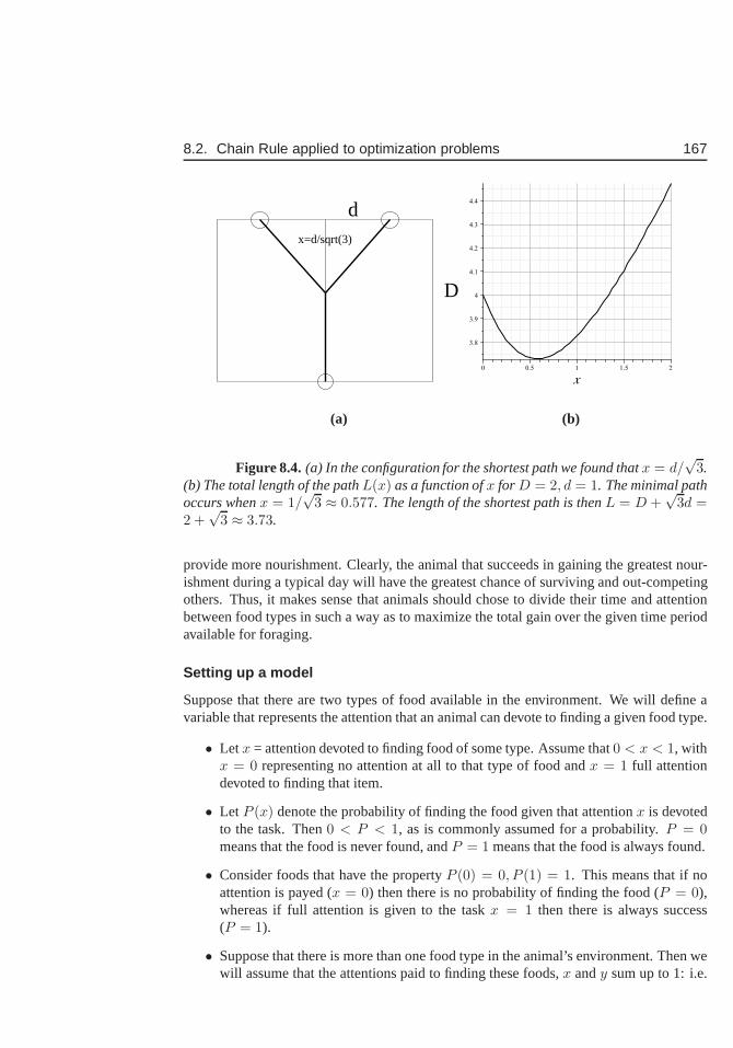
8.2. Chain Rule applied to optimization problems 167
x=d/sqrt(3)
D
d
(a) (b)
Figure 8.4. (a) In the configuration for the shortest path we found thatx = d/√
3.(b) The total length of the pathL(x) as a function ofx for D = 2, d = 1. The minimal pathoccurs whenx = 1/
√3 ≈ 0.577. The length of the shortest path is thenL = D +
√3d =
2 +√
3 ≈ 3.73.
provide more nourishment. Clearly, the animal that succeeds in gaining the greatest nour-ishment during a typical day will have the greatest chance ofsurviving and out-competingothers. Thus, it makes sense that animals should chose to divide their time and attentionbetween food types in such a way as to maximize the total gain over the given time periodavailable for foraging.
Setting up a model
Suppose that there are two types of food available in the environment. We will define avariable that represents the attention that an animal can devote to finding a given food type.
• Let x = attention devoted to finding food of some type. Assume that0 < x < 1, withx = 0 representing no attention at all to that type of food andx = 1 full attentiondevoted to finding that item.
• Let P (x) denote the probability of finding the food given that attentionx is devotedto the task. Then0 < P < 1, as is commonly assumed for a probability.P = 0means that the food is never found, andP = 1 means that the food is always found.
• Consider foods that have the propertyP (0) = 0, P (1) = 1. This means that if noattention is payed (x = 0) then there is no probability of finding the food (P = 0),whereas if full attention is given to the taskx = 1 then there is always success(P = 1).
• Suppose that there is more than one food type in the animal’s environment. Then wewill assume that the attentions paid to finding these foods,x andy sum up to 1: i.e.
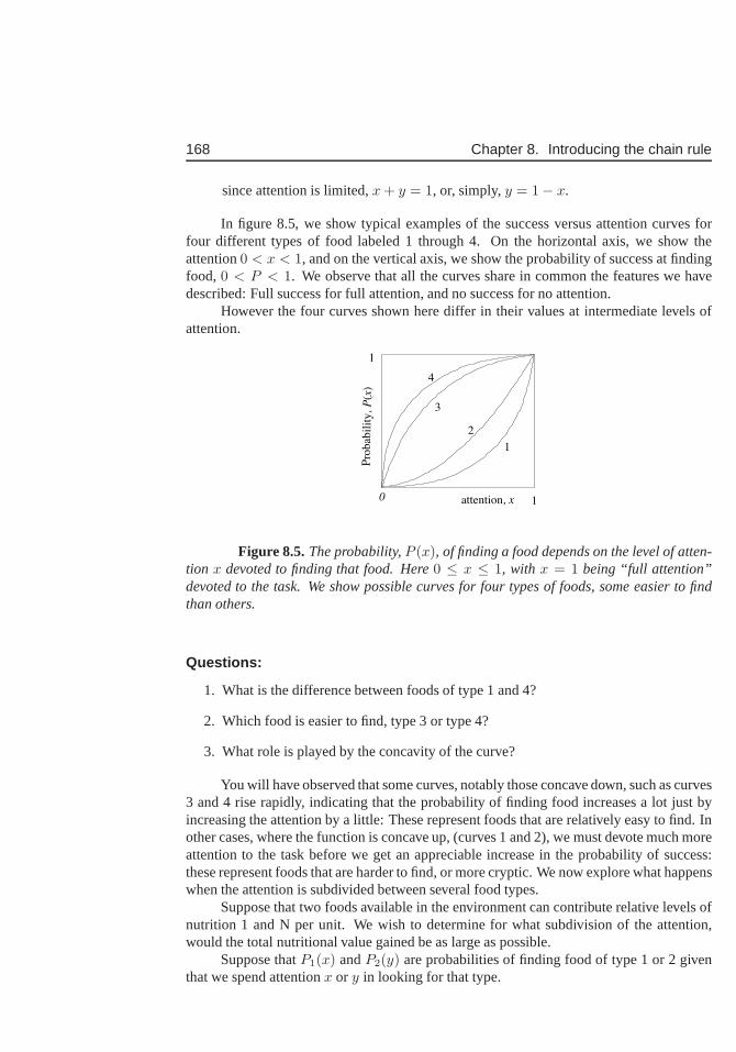
168 Chapter 8. Introducing the chain rule
since attention is limited,x + y = 1, or, simply,y = 1− x.
In figure 8.5, we show typical examples of the success versus attention curves forfour different types of food labeled 1 through 4. On the horizontal axis, we show theattention0 < x < 1, and on the vertical axis, we show the probability of successat findingfood, 0 < P < 1. We observe that all the curves share in common the features we havedescribed: Full success for full attention, and no success for no attention.
However the four curves shown here differ in their values at intermediate levels ofattention.
0 1
1
attention, x
1
2
3
4P
robab
ilit
y, P
(x)
Figure 8.5.The probability,P (x), of finding a food depends on the level of atten-tion x devoted to finding that food. Here0 ≤ x ≤ 1, with x = 1 being “full attention”devoted to the task. We show possible curves for four types offoods, some easier to findthan others.
Questions:
1. What is the difference between foods of type 1 and 4?
2. Which food is easier to find, type 3 or type 4?
3. What role is played by the concavity of the curve?
You will have observed that some curves, notably those concave down, such as curves3 and 4 rise rapidly, indicating that the probability of finding food increases a lot just byincreasing the attention by a little: These represent foodsthat are relatively easy to find. Inother cases, where the function is concave up, (curves 1 and 2), we must devote much moreattention to the task before we get an appreciable increase in the probability of success:these represent foods that are harder to find, or more cryptic. We now explore what happenswhen the attention is subdivided between several food types.
Suppose that two foods available in the environment can contribute relative levels ofnutrition 1 and N per unit. We wish to determine for what subdivision of the attention,would the total nutritional value gained be as large as possible.
Suppose thatP1(x) andP2(y) are probabilities of finding food of type 1 or 2 giventhat we spend attentionx or y in looking for that type.
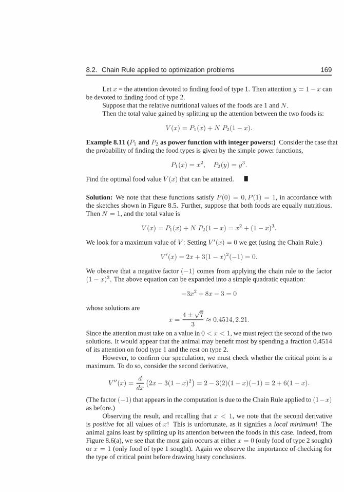
8.2. Chain Rule applied to optimization problems 169
Let x = the attention devoted to finding food of type 1. Then attentiony = 1− x canbe devoted to finding food of type 2.
Suppose that the relative nutritional values of the foods are 1 andN .Then the total value gained by splitting up the attention between the two foods is:
V (x) = P1(x) + N P2(1 − x).
Example 8.11 (P1 and P2 as power function with integer powers:) Consider the case thatthe probability of finding the food types is given by the simple power functions,
P1(x) = x2, P2(y) = y3.
Find the optimal food valueV (x) that can be attained.
Solution: We note that these functions satisfyP (0) = 0, P (1) = 1, in accordance withthe sketches shown in Figure 8.5. Further, suppose that bothfoods are equally nutritious.ThenN = 1, and the total value is
V (x) = P1(x) + N P2(1− x) = x2 + (1− x)3.
We look for a maximum value ofV : SettingV ′(x) = 0 we get (using the Chain Rule:)
V ′(x) = 2x + 3(1− x)2(−1) = 0.
We observe that a negative factor(−1) comes from applying the chain rule to the factor(1− x)3. The above equation can be expanded into a simple quadratic equation:
−3x2 + 8x− 3 = 0
whose solutions are
x =4±√
7
3≈ 0.4514, 2.21.
Since the attention must take on a value in0 < x < 1, we must reject the second of the twosolutions. It would appear that the animal may benefit most byspending a fraction 0.4514of its attention on food type 1 and the rest on type 2.
However, to confirm our speculation, we must check whether the critical point is amaximum. To do so, consider the second derivative,
V ′′(x) =d
dx
(
2x− 3(1− x)2)
= 2− 3(2)(1− x)(−1) = 2 + 6(1− x).
(The factor(−1) that appears in the computation is due to the Chain Rule applied to(1−x)as before.)
Observing the result, and recalling thatx < 1, we note that the second derivativeis positivefor all values ofx! This is unfortunate, as it signifies alocal minimum! Theanimal gains least by splitting up its attention between thefoods in this case. Indeed, fromFigure 8.6(a), we see that the most gain occurs at eitherx = 0 (only food of type 2 sought)or x = 1 (only food of type 1 sought). Again we observe the importanceof checking forthe type of critical point before drawing hasty conclusions.
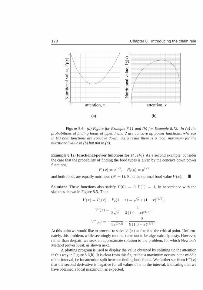
170 Chapter 8. Introducing the chain rule
0.0 1.0
0.0
1.0
attention, x
Nutr
itio
nal
val
ue,
V1(x
)
0.0 1.0
1.0
1.6
attention, x
Nutr
itio
nal
val
ue,
V2(x
)
(a) (b)
Figure 8.6. (a) Figure for Example 8.11 and (b) for Example 8.12. In (a) theprobabilities of finding foods of types 1 and 2 are concave up power functions, whereasin (b) both functions are concave down. As a result there is a local maximum for thenutritional value in (b) but not in (a).
Example 8.12 (Fractional-power functions forP1, P2:) As a second example, considerthe case that the probability of finding the food types is given by the concave down powerfunctions,
P1(x) = x1/2, P2(y) = y1/3
and both foods are equally nutritious (N = 1). Find the optimal food valueV (x).
Solution: These functions also satisfyP (0) = 0, P (1) = 1, in accordance with thesketches shown in Figure 8.5. Then
V (x) = P1(x) + P2(1− x) =√
x + (1 − x)(1/3),
V ′(x) =1
2√
x− 1
3 (1.0− x)(2/3),
V ′′(x) = − 1
4 x(3/2)− 2
9 (1.0− x)(5/3).
At this point we would like to proceed to solveV ′(x) = 0 to find the critical point. Unfortu-nately, this problem, while seemingly routine, turns out tobe algebraically nasty. However,rather than despair, we seek an approximate solution to the problem, for which Newton’sMethod proves ideal, as shown next.
A plotting program is used to display the value obtained by splitting up the attentionin this way in Figure 8.6(b). It is clear from this figure that amaximum occurs in the middleof the interval, i.e for attention split between finding bothfoods. We further see fromV ′′(x)that the second derivative is negative for all values ofx in the interval, indicating that wehave obtained a local maximum, as expected.

8.2. Chain Rule applied to optimization problems 171
Applying Newton’s method to finding the critical point
Example 8.13 Use Newton’s Method to find the critical point for the function V (x) inExample 8.12.
Solution: Let f(x) = V ′(x). Then finding the critical point ofV (x) reduces to finding thezero of the functionV ′(x), i.e. solvingf(x) = 0. This is the precise type of problem thatNewton’s Method addresses, as discussed in Section 5.4. SInce the interval of interest is0 ≤ x ≤ 1, we will start with an initial “guess” for the critical pointatx0 = 0.5. midwayalong this interval. Then, according to Newton’s method, the improved guess would be
x1 = x0 −f(x0)
f ′(x0).
and, repeating this, at thek’th stage,
xk+1 = xk −f(xk)
f ′(xk).
To use this method, we must carefully note that
f(x) = V ′(x) =1
2√
x− 1
3 (1.0− x)(2/3),
f ′(x) = V ′′(x) = − 1
4 x(3/2)− 2
9 (1.0− x)(5/3)
Thus, we might use a spreadsheet in which cells A1 stores our initial guess, whereas B1,C1, and D1 store the values off(x), f ′(x) andx0 − f(x0)/f ′(x0). In the typical syntaxof spreadsheets, this might read something like the following.
A1 0.5B1 =(1/(2 * SQRT(A1))-1/(3 * (1-A1)ˆ(2/3)))C1 =(-1/(4 * A1ˆ(3/2))-2/(9 * (1-A1)ˆ(5/2)))D1 =A1-B1/C1
Applying this idea, and repeating the calculation by dragging the values to successiverows would lead to iterated approximations as follows.
x0 = 0.50000, x1 = 0.59061, and thereafter, successive values 0.60816, 0.61473,0.61751, 0.61875, 0.61931, 0.61956, 0.61968, 0.61973, 0.61976, 0.61977, 0.61977, 0.61977. . .
Thus, we see that the values converge to the location of the critical point, x =0.61977 (andy = 1− x = 0.38022.) within the interval of interest.
Epilogue
While the conclusions drawn above were disappointing in onespecific case, it is not alwaystrue that concentrating all one’s attention on one type is optimal. We can examine theproblem in more generality to find when the opposite conclusion might be satisfied. In thegeneral case, the value gained is
172 Chapter 8. Introducing the chain rule
V (x) = P1(x) + N P2(1− x).
A critical point occurs when
V ′(x) =d
dx[P1(x) + N P2(1 − x)] = P ′
1(x) + NP ′2(1− x)(−1) = 0.
(By now you realize where the extra term(−1) comes from - yes, from the Chain Rule!)Suppose we have found a value ofx in 0 < x < 1 at which this is satisfied. We thenexamine the second derivative:
V ′′(x) =d
dx[V ′(x)] =
d
dx[P ′
1(x) −NP ′2(1− x)]
= P ′′1 (x)−NP ′′
2 (1 − x)(−1) = P ′′1 (x) + NP ′′
2 (1− x).
The concavity of the functionV is thus related to the concavity of the two functionsP1(x)andP2(1 − x). If these are concave down (e.g. as in food types 3 or 4 in Figure 8.5), thenV ′′(x) < 0 and a local maximum will occur at any critical point found by our differentia-tion.
Another way of stating this observation is: if both food types are relatively easy tofind, one can gain most benefit by splitting up the attention between the two. Otherwise, ifboth are hard to find, then it is best to look for only one at a time.
Exercises 173
Exercises8.1. Practicing the Chain Rule: Use the chain rule to calculate the following derivatives
(a) y = f(x) = (x + 5)5
(b) y = f(x) = 4(x2 + 5x− 1)8
(c) y = f(x) = (√
x + 2x)3
8.2. Earth’s temperature: In this problem, we expand and generalize the results ofExample 8.9. As before, letG denote the level of greenhouse gasses on Earth,and consider the relationship of temperature of the earth tothe albedoa and theemissivityǫ given by Eqn. (8.1).
(a) Suppose thata is constant, butǫ depends onG. Assume thatdǫ/dG is given.Determine the rate of change of temperature with respect to the level of green-house gasses in this case.
(b) Suppose that botha andǫ depend onG. Find dT/dG in this more generalcase. (Hint: the quotient rule as well as the chain rule will be needed in thiscase.)
8.3. Shortest path from nest to food sources:
(a) Use the first derivative test to verify that the valuex = d√3
is a local minimumof the functionL(x) given by Eqn (8.2)
(b) Show that the shortest path isL = D +√
3d.
(c) In Section 8.2.1 we assumed thatd << D, so that the food sources were closetogether relative to the distance from the nest. Now supposethatD = d/2.How would this change the solution to the problem?
8.4. Geometry of the shortest ants’ path:Use the results of Section 8.2.1 to show thatin the shortest path, the angles between the branches of the Y-shaped path are all120◦, You may find it helpful to recall thatsin(30) = 1/2, sin(60) =
√3/2.
8.5. More about the ant trail: Consider the lengths of the V and T-shaped paths in theant trail example of Section 8.2.1. We will refer to these asLV andLT , and bothdepend on the distancesd andD in Fig. 8.3.
(a) Write down the expressions for each of these functions.
(b) Suppose the distanceD is fixed. How do the two lengthsLV , LT depend onthe distanced? Use your sketching skills to draw a rough sketch ofLv(d), LT (d).
(c) Use you sketch to determine whether there is a value ofd for which the lengthsLV andLT are the same.
8.6. Divided attention:This problem is based on the material on food choice and attention described inSection 7.6. It is advisable to first read that section.A bird in its natural habitat feeds on two kinds of seeds, whose nutritional values are5 calories per seed of type 1 and 3 calories per seed of type 2. Both kinds of seedsare hidden among litter on the forest floor and have to be found. If the bird splits its
174 Chapter 8. Introducing the chain rule
attention into a fractionx1 searching for seed type 1 and a fractionx2 searching forseed type 2, then its probability of finding 100 seeds of the given type is
P1(x1) = (x1)3, P2(x2) = (x2)
5.
Assume that the bird pays full attention to searching for seeds so thatx1 + x2 = 1where0 ≤ x1 ≤ 1 and0 ≤ x2 ≤ 1.
(a) Write down an expression for the total nutritional valueV gained by the birdwhen it splits its attention. Use the constraint onx1, x2 to eliminate one ofthese two variables. (For example, letx = x1 and writex2 in terms ofx1.)
(b) Find critical points ofV (x) and classify those points.
(c) Find absolute minima and maxima ofV (x) and use your results to explainwhat is the bird’s optimal strategy to maximize the nutritional value of theseeds it can find.
Chapter 9
Chain rule applied torelated rates and implicitdifferentiation
9.1 Applications of the chain rule to “related rates”In many applications of the chain rule, we are interested in processes that take place overtime. We ask how the relationships between certain geometric (or physical) variables af-fects the rates at which they change over time. Many of these examples are given as wordproblems, and we are called on to assemble the required geometric or other relationshipsin solving the problem.
Section 9.1 Learning goals
1. Understand the application of the chain rule to problems in which a composite rela-tionship between variables is involved.
2. Given a geometric relationship and a rate of change of one of the variables, be ableto use the chain rule to find the rate of change of a related variable.
3. Understand how to use verbal information about rates of change to set up the requiredrelationships, and to solve a word problem involving an application of the chain rule(“related rates problem”).
A few relationships that we will find useful are concentratedin Table 9.1.
Example 9.1 (Tumor growth:) A tumor grows so that its radius expands at a constantrate,k. Determine the rate of growth of the volume of the tumor when the radius is onecentimeter. Assume that the tumor is approximately spherical.
Solution: The volume of a sphere depends on its radiusr, a fact we can express with thenotationV (r) = (4/3)πr3. In the situation under discussion,r changes with time, resultingin V changing with time. We indicate this chain of dependencies using the notationr(t)
175
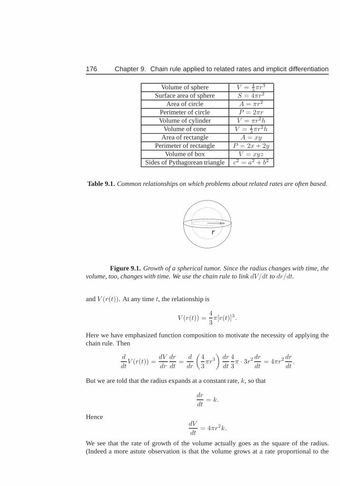
176 Chapter 9. Chain rule applied to related rates and implicit differentiation
Volume of sphere V = 43πr3
Surface area of sphere S = 4πr2
Area of circle A = πr2
Perimeter of circle P = 2πrVolume of cylinder V = πr2h
Volume of cone V = 13πr2h
Area of rectangle A = xyPerimeter of rectangle P = 2x + 2y
Volume of box V = xyzSides of Pythagorean trianglec2 = a2 + b2
Table 9.1.Common relationships on which problems about related ratesare often based.
r
Figure 9.1. Growth of a spherical tumor. Since the radius changes with time, thevolume, too, changes with time. We use the chain rule to linkdV/dt to dr/dt.
andV (r(t)). At any timet, the relationship is
V (r(t)) =4
3π[r(t)]3.
Here we have emphasized function composition to motivate the necessity of applying thechain rule. Then
d
dtV (r(t)) =
dV
dr
dr
dt=
d
dr
(
4
3πr3
)
dr
dt
4
3π · 3r2 dr
dt= 4πr2 dr
dt.
But we are told that the radius expands at a constant rate,k, so that
dr
dt= k.
HencedV
dt= 4πr2k.
We see that the rate of growth of the volume actually goes as the square of the radius.(Indeed a more astute observation is that the volume grows ata rate proportional to the
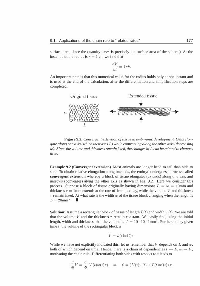
9.1. Applications of the chain rule to “related rates” 177
surface area, since the quantity4πr2 is precisely the surface area of the sphere.) At theinstant that the radius isr = 1 cm we find that
dV
dt= 4πk.
An important note is that this numerical value for the radiusholds only at one instant andis used at the end of the calculation, after the differentiation and simplification steps arecompleted.
Original tissue Extended tissue
L
w
Figure 9.2.Convergent extension of tissue in embryonic development. Cells elon-gate along one axis (which increasesL) while contracting along the other axis (decreasingw). SInce the volume and thickness remain fixed, the changes inL can be related to changesin w.
Example 9.2 (Convergent extension)Most animals are longer head to tail than side toside. To obtain relative elongation along one axis, the embryo undergoes a process calledconvergent extensionwhereby a block of tissue elongates (extends) along one axisandnarrows (converges) along the other axis as shown in Fig. 9.2. Here we consider thisprocess. Suppose a block of tissue originally having dimensions L = w = 10mm andthicknessτ = 1mm extends at the rate of 1mm per day, while the volumeV and thicknessτ remain fixed. At what rate is the widthw of the tissue block changing when the length isL = 20mm?
Solution: Assume a rectangular block of tissue of lengthL(t) and widthw(t). We are toldthat the volumeV and the thicknessτ remain constant. We easily find, using the initiallength, width and thickness, that the volume isV = 10 · 10 · 1mm3. Further, at any giventime t, the volume of the rectangular block is
V = L(t)w(t)τ.
While we have not explicitly indicated this, let us rememberthatV depends onL andw,both of which depend on time. Hence, there is a chain of dependenciest → L, w,→ V ,motivating the chain rule. Differentiating both sides withrespect tot leads to
d
dtV =
d
dt(L(t)w(t)τ) ⇒ 0 = (L′(t)w(t) + L(t)w′(t)) τ.
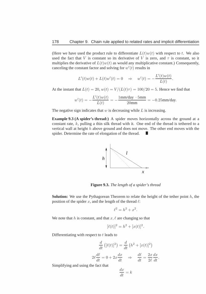
178 Chapter 9. Chain rule applied to related rates and implicit differentiation
(Here we have used the product rule to differentiateL(t)w(t) with respect tot. We alsoused the fact thatV is constant so its derivative ofV is zero, andτ is constant, so itmultiplies the derivative ofL(t)w(t) as would any multiplicative constant.) Consequently,canceling the constant factor and solving forw′(t) results in
L′(t)w(t) + L(t)w′(t) = 0 ⇒ w′(t) = −L′(t)w(t)
L(t).
At the instant thatL(t) = 20, w(t) = V/(L(t)τ) = 100/20 = 5. Hence we find that
w′(t) = −L′(t)w(t)
L(t)= −1mm/day · 5mm
20mm= −0.25mm/day.
The negative sign indicates thatw is decreasing whileL is increasing.
Example 9.3 (A spider’s thread:) A spider moves horizontally across the ground at aconstant rate,k, pulling a thin silk thread with it. One end of the thread is tethered to avertical wall at heighth above ground and does not move. The other end moves with thespider. Determine the rate of elongation of the thread.
h
x
l
Figure 9.3.The length of a spider’s thread
Solution: We use the Pythagorean Theorem to relate the height of the tether pointh, theposition of the spiderx, and the length of the threadℓ:
ℓ2 = h2 + x2.
We note thath is constant, and thatx, ℓ are changing so that
[ℓ(t)]2 = h2 + [x(t)]2.
Differentiating with respect tot leads to
d
dt
(
[ℓ(t)]2)
=d
dt
(
h2 + [x(t)]2)
2ℓdℓ
dt= 0 + 2x
dx
dt⇒ dℓ
dt=
2x
2ℓ
dx
dt.
Simplifying and using the fact thatdx
dt= k
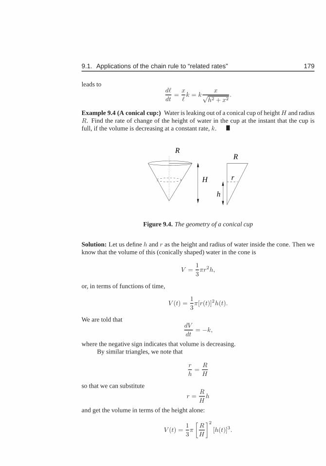
9.1. Applications of the chain rule to “related rates” 179
leads todℓ
dt=
x
ℓk = k
x√h2 + x2
.
Example 9.4 (A conical cup:) Water is leaking out of a conical cup of heightH and radiusR. Find the rate of change of the height of water in the cup at theinstant that the cup isfull, if the volume is decreasing at a constant rate,k.
H
RR
r
h
Figure 9.4.The geometry of a conical cup
Solution: Let us defineh andr as the height and radius of water inside the cone. Then weknow that the volume of this (conically shaped) water in the cone is
V =1
3πr2h,
or, in terms of functions of time,
V (t) =1
3π[r(t)]2h(t).
We are told thatdV
dt= −k,
where the negative sign indicates that volume is decreasing.By similar triangles, we note that
r
h=
R
H
so that we can substitute
r =R
Hh
and get the volume in terms of the height alone:
V (t) =1
3π
[
R
H
]2
[h(t)]3.
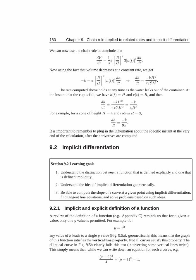
180 Chapter 9. Chain rule applied to related rates and implicit differentiation
We can now use the chain rule to conclude that
dV
dt=
1
3π
[
R
H
]2
3[h(t)]2dh
dt.
Now using the fact that volume decreases at a constant rate, we get
−k = π
[
R
H
]2
[h(t)]2dh
dt⇒ dh
dt=−kH2
πR2h2.
The rate computed above holds at any time as the water leaks out of the container. Atthe instant that the cup is full, we haveh(t) = H andr(t) = R, and then
dh
dt=−kH2
πR2H2=−k
πR2.
For example, for a cone of heightH = 4 and radiusR = 3,
dh
dt=−k
9π.
It is important to remember to plug in the information about the specific instant at the veryend of the calculation, after the derivatives are computed.
9.2 Implicit differentiation
Section 9.2 Learning goals
1. Understand the distinction between a function that is defined explicitly and one thatis defined implicitly.
2. Understand the idea of implicit differentiation geometrically.
3. Be able to compute the slope of a curve at a given point usingimplicit differentiation,find tangent line equations, and solve problems based on suchideas.
9.2.1 Implicit and explicit definition of a function
A review of the definition of a function (e.g. Appendix C) reminds us that for a givenxvalue, only oney value is permitted. For example, for
y = x2
any value ofx leads to a singley value (Fig. 9.5a). geometrically, this means that the graphof this function satisfies thevertical line property . Not all curves satisfy this property. Theelliptical curve in Fig. 9.5b clearly fails this test (intersecting some vertical lines twice).This simply means that, while we can write down an equation for such a curve, e.g.
(x− 1)2
4+ (y − 1)2 = 1,
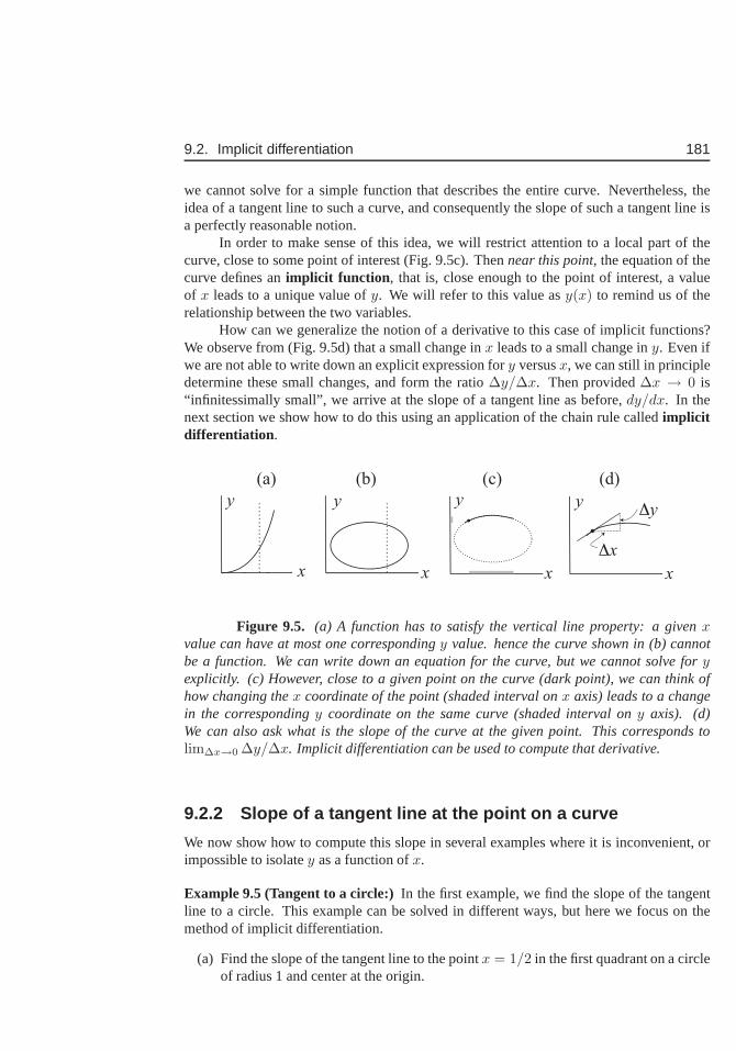
9.2. Implicit differentiation 181
we cannot solve for a simple function that describes the entire curve. Nevertheless, theidea of a tangent line to such a curve, and consequently the slope of such a tangent line isa perfectly reasonable notion.
In order to make sense of this idea, we will restrict attention to a local part of thecurve, close to some point of interest (Fig. 9.5c). Thennear this point, the equation of thecurve defines animplicit function , that is, close enough to the point of interest, a valueof x leads to a unique value ofy. We will refer to this value asy(x) to remind us of therelationship between the two variables.
How can we generalize the notion of a derivative to this case of implicit functions?We observe from (Fig. 9.5d) that a small change inx leads to a small change iny. Even ifwe are not able to write down an explicit expression fory versusx, we can still in principledetermine these small changes, and form the ratio∆y/∆x. Then provided∆x → 0 is“infinitessimally small”, we arrive at the slope of a tangentline as before,dy/dx. In thenext section we show how to do this using an application of thechain rule calledimplicitdifferentiation .
x x x x
y y yyΔy
Δx
(a) (b) (c) (d)
Figure 9.5. (a) A function has to satisfy the vertical line property: a givenxvalue can have at most one correspondingy value. hence the curve shown in (b) cannotbe a function. We can write down an equation for the curve, butwe cannot solve foryexplicitly. (c) However, close to a given point on the curve (dark point), we can think ofhow changing thex coordinate of the point (shaded interval onx axis) leads to a changein the correspondingy coordinate on the same curve (shaded interval ony axis). (d)We can also ask what is the slope of the curve at the given point. This corresponds tolim∆x→0 ∆y/∆x. Implicit differentiation can be used to compute that derivative.
9.2.2 Slope of a tangent line at the point on a curve
We now show how to compute this slope in several examples where it is inconvenient, orimpossible to isolatey as a function ofx.
Example 9.5 (Tangent to a circle:) In the first example, we find the slope of the tangentline to a circle. This example can be solved in different ways, but here we focus on themethod of implicit differentiation.
(a) Find the slope of the tangent line to the pointx = 1/2 in the first quadrant on a circleof radius 1 and center at the origin.
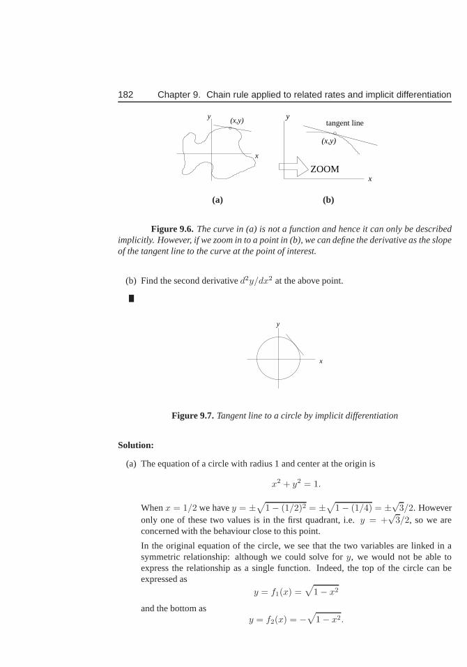
182 Chapter 9. Chain rule applied to related rates and implicit differentiation
(x,y)
x
y
x
y
(x,y)
tangent line
ZOOM
(a) (b)
Figure 9.6. The curve in (a) is not a function and hence it can only be describedimplicitly. However, if we zoom in to a point in (b), we can define the derivative as the slopeof the tangent line to the curve at the point of interest.
(b) Find the second derivatived2y/dx2 at the above point.
x
y
Figure 9.7.Tangent line to a circle by implicit differentiation
Solution:
(a) The equation of a circle with radius 1 and center at the origin is
x2 + y2 = 1.
Whenx = 1/2 we havey = ±√
1− (1/2)2 = ±√
1− (1/4) = ±√
3/2. Howeveronly one of these two values is in the first quadrant, i.e.y = +
√3/2, so we are
concerned with the behaviour close to this point.
In the original equation of the circle, we see that the two variables are linked in asymmetric relationship: although we could solve fory, we would not be able toexpress the relationship as a single function. Indeed, the top of the circle can beexpressed as
y = f1(x) =√
1− x2
and the bottom asy = f2(x) = −
√
1− x2.
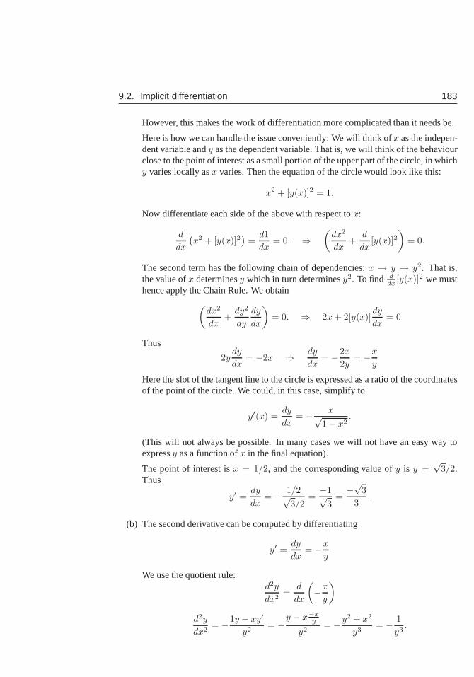
9.2. Implicit differentiation 183
However, this makes the work of differentiation more complicated than it needs be.
Here is how we can handle the issue conveniently: We will think of x as the indepen-dent variable andy as the dependent variable. That is, we will think of the behaviourclose to the point of interest as a small portion of the upper part of the circle, in whichy varies locally asx varies. Then the equation of the circle would look like this:
x2 + [y(x)]2 = 1.
Now differentiate each side of the above with respect tox:
d
dx
(
x2 + [y(x)]2)
=d1
dx= 0. ⇒
(
dx2
dx+
d
dx[y(x)]2
)
= 0.
The second term has the following chain of dependencies:x → y → y2. That is,the value ofx determinesy which in turn determinesy2. To find d
dx [y(x)]2 we musthence apply the Chain Rule. We obtain
(
dx2
dx+
dy2
dy
dy
dx
)
= 0. ⇒ 2x + 2[y(x)]dy
dx= 0
Thus
2ydy
dx= −2x ⇒ dy
dx= −2x
2y= −x
y
Here the slot of the tangent line to the circle is expressed asa ratio of the coordinatesof the point of the circle. We could, in this case, simplify to
y′(x) =dy
dx= − x√
1− x2.
(This will not always be possible. In many cases we will not have an easy way toexpressy as a function ofx in the final equation).
The point of interest isx = 1/2, and the corresponding value ofy is y =√
3/2.Thus
y′ =dy
dx= − 1/2√
3/2=−1√
3=−√
3
3.
(b) The second derivative can be computed by differentiating
y′ =dy
dx= −x
y
We use the quotient rule:d2y
dx2=
d
dx
(
−x
y
)
d2y
dx2= −1y − xy′
y2= −
y − x−xy
y2= −y2 + x2
y3= − 1
y3.
184 Chapter 9. Chain rule applied to related rates and implicit differentiation
Substitutingy =√
3/2 from part (a) yields
d2y
dx2= − 1
(√
3/2)3= − 8
3(3/2).
We have used the equation of the circle, and our previous result for the first deriva-tive in simplifying the above. We can see from this last expression that the secondderivative is negative fory > 0, i.e. for the top semi-circle, indicating that this part ofthe curve is concave down (as expected). Similarly, fory < 0, the second derivativeis positive, and this agrees with the concave up property of that portion of the circle.
As in the case of simple functions, the second derivative canthus help identify con-cavity of curves.
Example 9.6 (Energy loss and Earth’s temperature; implicitdifferentiation) Redo Ex-ample 4.9 using implicit differentiation, that is Find the rate of change of Earth’s tempera-ture unit energy loss based on Eqn. (1.4), but without solving for T as a function ofEout.
Solution: We write the equation in the form
Eout(T ) = (4πr2ǫσ)T 4
and observe that the term in braces is constant. Differentiate both sides with respect toEout. Then we find
dEout
dEout= (4πr2ǫσ)
dT 4
dT
dT
dEout
1 = (4πr2ǫσ) · 4T 3 dT
dEout.
The calculation is completed by rearranging this result,
dT
dEout=
1
16πr2ǫσ
1
T 3.
9.3 The power rule for fractional powersImplicit differentiation can help in determining the derivatives of a number of new func-tions. In this case, we use what we know about the integer powers to determine the deriva-tive for a fractional power such as1/2. A similar idea will recur several times later on inthis course, when we encounter a new type of function and its inverse function.
Example 9.7 (Derivative of√
x:) Consider the function
y =√
x
Use implicit differentiation to compute the derivative of this function.
9.3. The power rule for fractional powers 185
Solution: We can re-express this function in the form
y = x1/2.
In this example, we will show that the power rule applies in the same way to fractionalpowers: That is, we show that
y′(x) =1
2x−1/2
We rewrite the functiony =√
x in the form
y2 = x
but we will continue to think ofy as the dependent variable, i.e. when we differentiate, wewill remember that
[y(x)]2 = x
Taking derivatives of both sides leads to
d
dx
(
[y(x)]2)
=d
dx(x)
2[y(x)]dy
dx= 1
dy
dx=
1
2y.
We now use the original relationship to eliminatey, i.e. we substitutey =√
x. We findthat
dy
dx=
1
2√
x=
1
2x−1/2.
This verifies the power law for the above example.A similar procedure can be applied to a power function with fractional power. When
we apply similar steps, we find that
Derivative of fractional-power function: The derivative of
y = f(x) = xm/n
isdy
dx=
m
nx( m
n −1).
This is left as an exercise for the reader.
Example 9.8 (The astroid:) The curve
x2/3 + y2/3 = 22/3
has the shape of anastroid. It describes the shape generated by a ball of radius12 rolling
inside a ball of radius 2. Find the slope of the tangent line toa point on the astroid.

186 Chapter 9. Chain rule applied to related rates and implicit differentiation
Solution: We use implicit differentiation as follows:
d
dx
(
x2/3 + y2/3)
=d
dx22/3
2
3x−1/3 +
d
dy(y2/3)
dy
dx= 0
2
3x−1/3 +
2
3y−1/3 dy
dx= 0
x−1/3 + y−1/3 dy
dx= 0
We can rearrange into the form:
dy
dx= −x−1/3
y−1/3.
We can see from this form that the derivative fails to exist atbothx = 0 (wherex−1/3
would be undefined) and aty = 0 (wherey−1/3 would be undefined. This stems from thesharp points that the curve has at these places.
In the next example we put the second derivative to work in an implicit differentiationproblem. The goal is as follows:
Example 9.9 (Horizontal tangent and concavity on a rotated ellipse:) Find the highestpoint on the (rotated) ellipse
x2 + 3y2 − xy = 1
Solution: The highest point on the ellipse will have a horizontal tangent line, so we shouldlook for the point on this curve at whichdy/dx = 0. We proceed as follows:
1. Finding the slope of the tangent line:By implicit differentiation,
d
dx[x2 + 3y2 − xy] =
d
dx1
d(x2)
dx+
d(3y2)
dx− d(xy)
dx= 0.
We must use the product rule to compute the derivative of the last term on the LHS:
2x + 6ydy
dx− x
dy
dx− dx
dxy = 0
2x + 6ydy
dx− x
dy
dx− 1y = 0
Grouping terms, we have
(6y − x)dy
dx+ (2x− y) = 0
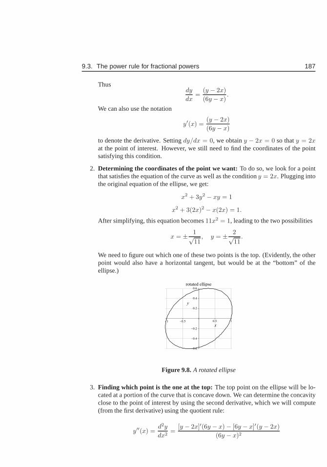
9.3. The power rule for fractional powers 187
Thusdy
dx=
(y − 2x)
(6y − x).
We can also use the notation
y′(x) =(y − 2x)
(6y − x)
to denote the derivative. Settingdy/dx = 0, we obtainy − 2x = 0 so thaty = 2xat the point of interest. However, we still need to find the coordinates of the pointsatisfying this condition.
2. Determining the coordinates of the point we want:To do so, we look for a pointthat satisfies the equation of the curve as well as the conditiony = 2x. Plugging intothe original equation of the ellipse, we get:
x2 + 3y2 − xy = 1
x2 + 3(2x)2 − x(2x) = 1.
After simplifying, this equation becomes11x2 = 1, leading to the two possibilities
x = ± 1√11
, y = ± 2√11
.
We need to figure out which one of these two points is the top. (Evidently, the otherpoint would also have a horizontal tangent, but would be at the “bottom” of theellipse.)
Figure 9.8.A rotated ellipse
3. Finding which point is the one at the top: The top point on the ellipse will be lo-cated at a portion of the curve that is concave down. We can determine the concavityclose to the point of interest by using the second derivative, which we will compute(from the first derivative) using the quotient rule:
y′′(x) =d2y
dx2=
[y − 2x]′(6y − x)− [6y − x]′(y − 2x)
(6y − x)2
188 Chapter 9. Chain rule applied to related rates and implicit differentiation
y′′(x) =[y′ − 2](6y − x)− [6y′ − 1](y − 2x)
(6y − x)2.
In the above, we have used the “prime” notation (’) to denote aderivative.
4. Plugging in information about the point: Now that we have set down the formof this derivative, we make some important observations about the specific point ofinterest: (Note that this is done as a final step, only after all derivatives have beencalculated!)
• We are only concerned with the sign of this derivative. The denominator is alwayspositive (since it is squared) and so will not affect the sign. (It is possible to workwith the sign of the numerator alone, though, in the interestof providing detailedsteps, we go through the entire calculation below.)
• At the point of interest (top of ellipse)y′ = 0, simplifying some of the terms above.
• At the point in question,y = 2x so the term(y − 2x) = 0.
We can thus simplify the above to obtain
y′′(x) =[−2](6y − x)− [−x](0)
(6y − x)2=
[−2](6y − x)
(6y − x)2=
−2
(6y − x).
Using again the fact thaty = 2x, we get the final form
y′′(x) =−2
(6(2x)− x)=−2
11x.
We see directly from this result that the second derivative is negative (implying concavedown curve) wheneverx is positive. This tells us that at the point with positivex value,x = 1/
√11, we are at the top of the ellipse. A graph of this curve is shownin Figure 9.8.
Exercises 189
Exercises9.1. Consider the growth of a cell, assumed spherical in shape. Suppose that the radius
of the cell increases at a constant rate per unit time. (Call the constantk, and assumethatk > 0.)
(a) At what rate would the volume,V , increase ?
(b) At what rate would the surface area,S, increase ?
(c) At what rate would the ratio of surface area to volumeS/V change? Wouldthis ratio increase or decrease as the cell grows? [Remark: note that the an-swers you give will be expressed in terms of the radius of the cell.]
9.2. Growth of a circular fungal colony: A fungal colony grows on a flat surface start-ing with a single spore. The shape of the colony edge is circular (with the initial siteof the spore at the center of the circle.) Suppose the radius of the colony increasesat a constant rate per unit time. (Call this constantC.)
(a) At what rate does the area covered by the colony change ?
(b) The biomass of the colony is proportional to the area it occupies (factor ofproportionalityα). At what rate does the biomass increase?
9.3. Limb development: During early development, the limb of a fetus increases in size,but has a constant proportion. Suppose that the limb is roughly a circular cylinderwith radiusr and lengthl in proportion
l/r = C
whereC is a positive constant. It is noted that during the initial phase of growth, theradius increases at an approximately constant rate, i.e. that
dr/dt = a.
At what rate does the mass of the limb change during this time?[Note: assume thatthe density of the limb is 1 gm/cm3 and recall that the volume of a cylinder is
V = Al
whereA is the base area (in this case of a circle) andl is length.]
9.4. A rectangular trough is2 meter long,0.5 meter across the top and1 meter deep. Atwhat rate must water be poured into the trough such that the depth of the water isincreasing at1 m/min when the depth of the water is0.7 m?
9.5. Gas is being pumped into a spherical balloon at the rate of 3 cm3/s.
(a) How fast is the radius increasing when the radius is15 cm?
(b) Without using the result from (a), find the rate at which the surface area of theballoon is increasing when the radius is15 cm.
9.6. A point moves along the parabolay =1
4x2 in such a way that atx = 2 the x-
coordinate is increasing at the rate of5 cm/s. Find the rate of change ofy at thisinstant.
190 Chapter 9. Chain rule applied to related rates and implicit differentiation
9.7. Boyle’s Law: In chemistry, Boyle’s law describes the behaviour of an ideal gas:This law relates the volume occupied by the gas to the temperature and the pressureas follows:
PV = nRT
wheren, R are positive constants.
(a) Suppose that the pressure is kept fixed, by allowing the gas to expand as thetemperature is increased. Relate the rate of change of volume to the rate ofchange of temperature.
(b) Suppose that the temperature is held fixed and the pressure is decreased gradu-ally. Relate the rate of change of the volume to the rate of change of pressure.
9.8. Spread of a population: In 1905 a Bohemian farmer accidentally allowed severalmuskrats to escape an enclosure. Their population grew and spread, occupyingincreasingly larger areas throughout Europe. In a classical paper in ecology, it wasshown by the scientist Skellam (1951) that the square root ofthe occupied areaincreased at a constant rate,k. Determine the rate of change of the distance (fromthe site of release) that the muskrats had spread. For simplicity, you may assumethat the expanding area of occupation is circular.
9.9. A spherical piece of ice melts so that its surface area decreases at a rate of 1 cm2/min.Find the rate that the diameter decreases when the diameter is 5 cm.
9.10. A Convex lens: A particular convex lens has a focal length off = 10 cm. Thedistancep between an object and the lens, the distanceq between its image and thelens and the focal lengthf are related by the equation:
1
f=
1
p+
1
q.
If an object is 30 cm away from the lens and moving away at 4 cm/sec, how fast isits image moving and in which direction?
9.11. A conical cup: Water is leaking out of a small hole at the tip of a conical paper cupat the rate of 1 cm3/min. The cup has height 8 cm and radius 6 cm, and is initiallyfull up to the top. Find the rate of change of the height of water in the cup when thecup just begins to leak. [Remark: the volume of a cone isV = (π/3)r2h.]
9.12. Conical tank: Water is leaking out of the bottom of an inverted conical tankat the
rate of1
10m3/min, and at the same time is being pumped in the top at a constant
rate ofk m3/min. The tank has height6 m and the radius at the top is2 m. De-
termine the constantk if the water level is rising at the rate of1
5m/min when the
height of the water is2 m. Recall that the volume of a cone of radiusr and heighthis
V =1
3πr2h.
9.13. The gravel pile: Gravel is being dumped from a conveyor belt at the rate of30 ft3/minin such a way that the gravel forms a conical pile whose base diameter and height
Exercises 191
are always equal. How fast is the height of the pile increasing when the height is
10 ft? (Hint: the volume of a cone of radiusr and heighth is V =1
3πr2h.)
9.14. The sand pile: Sand is piled onto a conical pile at the rate of10m3/min. Thesand keeps spilling to the base of the cone so that the shape always has the sameproportions: that is, the height of the cone is equal to the radius of the base. Findthe rate at which the height of the sandpile increases when the height is 5 m. Note:The volume of a cone with heighth and radiusr is
V =π
3r2h.
9.15. Water is flowing into a conical reservoir at a rate of4 m3/min. The reservoir is3 min radius and12 m deep.
(a) How fast is the radius of the water surface increasing when the depth of thewater is8 m?
(b) In (a), how fast is the surface rising?
9.16. A ladder10 meters long leans against a vertical wall. The foot of the ladder starts toslide away from the wall at a rate of3 m/s.
(a) Find the rate at which the top of the ladder is moving downward when its footis 8 meters away from the wall.
(b) In (a), find the rate of change of the slope of the ladder.
9.17. Sliding ladder: A ladder 5 m long rests against a vertical wall. If the bottom of theladder slides away from the wall at the rate of 0.5 meter/min how fast is the top ofthe ladder sliding down the wall when the base of the ladder is1 m away from thewall ?
9.18. Ecologists are often interested in the relationship between the area of a region (A)and the number of different speciesS that can inhabit that region. Hopkins (1955)suggested a relationship of the form
S = a ln(1 + bA)
wherea and b are positive constants. Find the rate of change of the numberofspecies with respect to the area. Does this function have a maximum?
9.19. The burning candle: A candle is placed a distancel1 from a thin block of wood ofheightH . The block is a distancel2 from a wall as shown in Figure 9.9. The candleburns down so that the height of the flame,h1 decreases at the rate of3 cm/hr. Findthe rate at which the length of the shadowy cast by the block on the wall increases.(Note: your answer will be in terms of the constantsl1 andl2. Remark: This is achallenging problem.)
9.20. Use implicit differentiation to show that the derivative of the function
y = x1/3
isy′ = (1/3)x−2/3.
First write the relationship in the formy3 = x, and then finddy/dx.
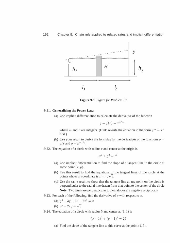
192 Chapter 9. Chain rule applied to related rates and implicit differentiation
l l
Hh h
1
1 1
y
2
Figure 9.9.Figure for Problem 19
9.21. Generalizing the Power Law:
(a) Use implicit differentiation to calculate the derivative of the function
y = f(x) = xn/m
wherem andn are integers. (Hint: rewrite the equation in the formym = xn
first.)
(b) Use your result to derive the formulas for the derivatives of the functionsy =√x andy = x−1/3.
9.22. The equation of a circle with radiusr and center at the origin is
x2 + y2 = r2
(a) Use implicit differentiation to find the slope of a tangent line to the circle atsome point(x, y).
(b) Use this result to find the equations of the tangent lines of the circle at thepoints whosex coordinate isx = r/
√3.
(c) Use the same result to show that the tangent line at any point on the circle isperpendicular to the radial line drawn from that point to thecenter of the circleNote: Two lines are perpendicular if their slopes are negative reciprocals.
9.23. For each of the following, find the derivative ofy with respect tox.
(a) y6 + 3y − 2x− 7x3 = 0
(b) ey + 2xy =√
3
9.24. The equation of a circle with radius5 and center at(1, 1) is
(x− 1)2 + (y − 1)2 = 25
(a) Find the slope of the tangent line to this curve at the point (4, 5).
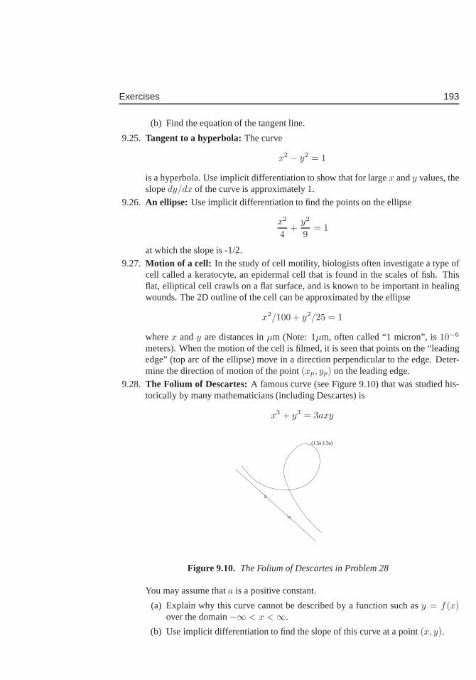
Exercises 193
(b) Find the equation of the tangent line.
9.25. Tangent to a hyperbola:The curve
x2 − y2 = 1
is a hyperbola. Use implicit differentiation to show that for largex andy values, theslopedy/dx of the curve is approximately1.
9.26. An ellipse: Use implicit differentiation to find the points on the ellipse
x2
4+
y2
9= 1
at which the slope is -1/2.
9.27. Motion of a cell: In the study of cell motility, biologists often investigatea type ofcell called a keratocyte, an epidermal cell that is found in the scales of fish. Thisflat, elliptical cell crawls on a flat surface, and is known to be important in healingwounds. The 2D outline of the cell can be approximated by the ellipse
x2/100 + y2/25 = 1
wherex andy are distances inµm (Note: 1µm, often called “1 micron”, is10−6
meters). When the motion of the cell is filmed, it is seen that points on the “leadingedge” (top arc of the ellipse) move in a direction perpendicular to the edge. Deter-mine the direction of motion of the point(xp, yp) on the leading edge.
9.28. The Folium of Descartes:A famous curve (see Figure 9.10) that was studied his-torically by many mathematicians (including Descartes) is
x3 + y3 = 3axy
a
-a
(1.5a,1.5a)
Figure 9.10. The Folium of Descartes in Problem 28
You may assume thata is a positive constant.
(a) Explain why this curve cannot be described by a function such asy = f(x)over the domain−∞ < x <∞.
(b) Use implicit differentiation to find the slope of this curve at a point(x, y).
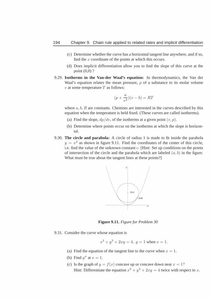
194 Chapter 9. Chain rule applied to related rates and implicit differentiation
(c) Determine whether the curve has a horizontal tangent line anywhere, and if so,find thex coordinate of the points at which this occurs.
(d) Does implicit differentiation allow you to find the slopeof this curve at thepoint (0,0) ?
9.29. Isotherms in the Van-der Waal’s equation: In thermodynamics, the Van derWaal’s equation relates the mean pressure,p of a substance to its molar volumev at some temperatureT as follows:
(p +a
v2)(v − b) = RT
wherea, b, R are constants. Chemists are interested in the curves described by thisequation when the temperature is held fixed. (These curves are called isotherms).
(a) Find the slope,dp/dv, of the isotherms at a given point(v, p).
(b) Determine where points occur on the isotherms at which the slope is horizon-tal.
9.30. The circle and parabola: A circle of radius 1 is made to fit inside the parabolay = x2 as shown in figure 9.11. Find the coordinates of the center of this circle,i.e. find the value of the unknown constantc. [Hint: Set up conditions on the pointsof intersection of the circle and the parabola which are labeled (a, b) in the figure.What must be true about the tangent lines at these points?]
x
y
(0,c)
(a,b)
Figure 9.11.Figure for Problem 30
9.31. Consider the curve whose equation is
x3 + y3 + 2xy = 4, y = 1 whenx = 1.
(a) Find the equation of the tangent line to the curve whenx = 1.
(b) Findy′′ atx = 1.
(c) Is the graph ofy = f(x) concave up or concave down nearx = 1?
Hint: Differentiate the equationx3 + y3 + 2xy = 4 twice with respect tox.
Chapter 10
Exponential functions
10.1 Unlimited growth and doublingIn this chapter, we introduce an important new class of functions, the exponential functions.We first describe the discrete process ofpopulation doubling and then show how thissimple idea leads to a continuous function that represents unlimited growth. An applicationof this idea will be investigated in the context of a bacterial colony that grows without limit.
We first consider the discrete integer powers of 2,2n, wheren is an integer . We willthen generalize this to a continuous function2x wherex is any real number. We investigatehow thebaseof the exponential functionax, wherea > 0 is arbitrary affects the pattern.Once a continuous function is defined, we can attach a meaningto the idea of its derivative.Computing the derivative of an exponential function, we encounter a specially convenientbase denotede, and then inestigate the exponential functionex.
Section 10.1 Learning goals
1. Follow and understand the example of doubling of a population and its link to integerpowers of base 2.
2. Given information about the doubling time of a populationand its initial size, be ableto determine the size of that population at some later generation.
3. Appreciate the connection between2n for integer values ofn and2x for a real num-berx.
10.1.1 The Andromeda Strain
”The mathematics of uncontrolled growth are frightening. Asingle cell of the bacterium E.coli would, under ideal circumstances, divide every twentyminutes. That is not particularlydisturbing until you think about it, but the fact is that bacteria multiply geometrically: onebecomes two, two become four, four become eight, and so on. Inthis way it can be shown
195
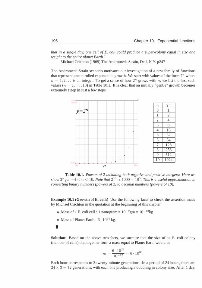
196 Chapter 10. Exponential functions
that in a single day, one cell of E. coli could produce a super-colony equal in size andweight to the entire planet Earth.”
Michael Crichton (1969) The Andromeda Strain, Dell, N.Y. p247
The Andromeda Strain scenario motivates our investigationof a new family of functionsthat represent uncontrolled exponential growth. We start with values of the form2n wheren = 1, 2 . . . is an integer. To get a sense of how2n grows withn, we list the first suchvalues (n = 1, . . . , 10) in Table 10.1. It is clear that an initially “gentle” growthbecomesextremely steep in just a few steps.
-4.0 10.0
0.0
1000.0
y=2n
n
n 2n
0 11 22 43 84 165 326 647 1288 2569 51210 1024
Table 10.1. Powers of 2 including both negative and positive integers: Here weshow2n for −4 < n < 10. Note that210 ≈ 1000 = 103. This is a useful approximation inconverting binary numbers (powers of 2) to decimal numbers (powers of 10).
Example 10.1 (Growth of E. coli:) Use the following facts to check the assertion madeby Michael Crichton in the quotation at the beginning of thischapter.
• Mass of 1 E. coli cell : 1 nanogram =10−9gm =10−12kg.
• Mass of Planet Earth :6 · 1024 kg.
Solution: Based on the above two facts, we surmise that the size of an E. coli colony(number of cells) that together form a mass equal to Planet Earth would be
m =6 · 1024
10−12= 6 · 1036.
Each hour corresponds to 3 twenty-minute generations. In a period of 24 hours, there are24× 3 = 72 generations, with each one producing a doubling in colony size. After 1 day,
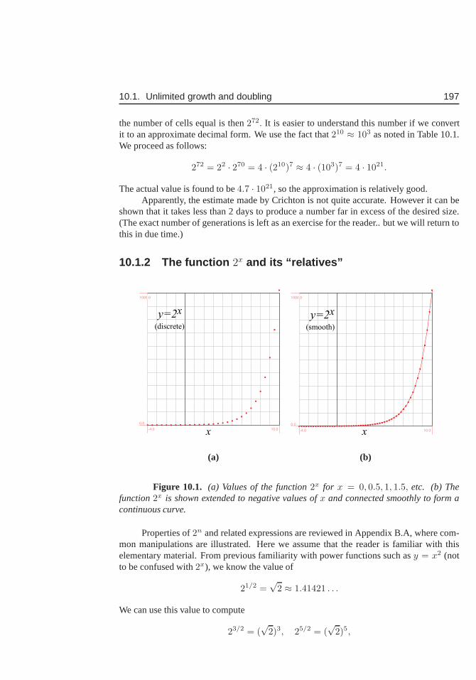
10.1. Unlimited growth and doubling 197
the number of cells equal is then272. It is easier to understand this number if we convertit to an approximate decimal form. We use the fact that210 ≈ 103 as noted in Table 10.1.We proceed as follows:
272 = 22 · 270 = 4 · (210)7 ≈ 4 · (103)7 = 4 · 1021.
The actual value is found to be4.7 · 1021, so the approximation is relatively good.Apparently, the estimate made by Crichton is not quite accurate. However it can be
shown that it takes less than 2 days to produce a number far in excess of the desired size.(The exact number of generations is left as an exercise for the reader.. but we will return tothis in due time.)
10.1.2 The function 2x and its “relatives”
-4.0 10.0
0.0
1000.0
y=2x
x
(discrete)
-4.0 10.0
0.0
1000.0
y=2x
x
(smooth)
(a) (b)
Figure 10.1. (a) Values of the function2x for x = 0, 0.5, 1, 1.5, etc. (b) Thefunction2x is shown extended to negative values ofx and connected smoothly to form acontinuous curve.
Properties of2n and related expressions are reviewed in Appendix B.A, wherecom-mon manipulations are illustrated. Here we assume that the reader is familiar with thiselementary material. From previous familiarity with powerfunctions such asy = x2 (notto be confused with2x), we know the value of
21/2 =√
2 ≈ 1.41421 . . .
We can use this value to compute
23/2 = (√
2)3, 25/2 = (√
2)5,
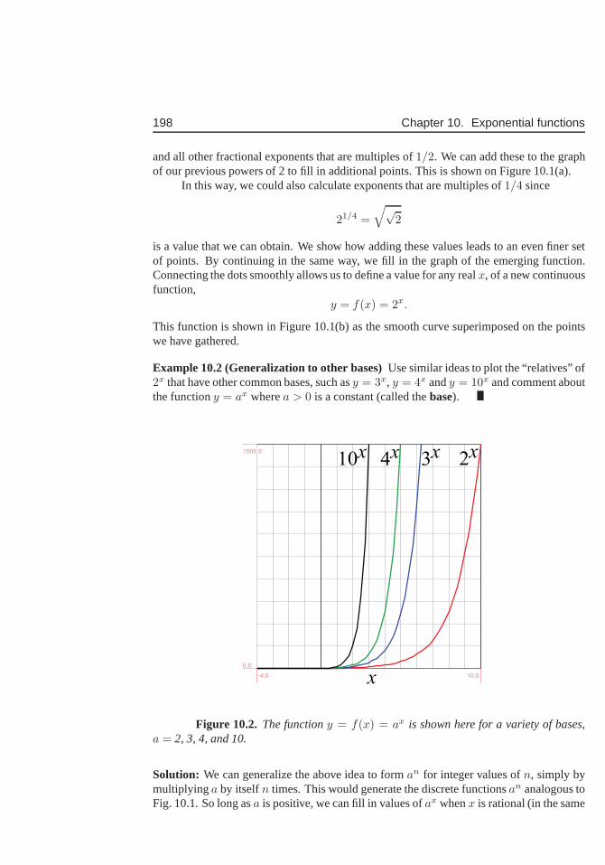
198 Chapter 10. Exponential functions
and all other fractional exponents that are multiples of1/2. We can add these to the graphof our previous powers of 2 to fill in additional points. This is shown on Figure 10.1(a).
In this way, we could also calculate exponents that are multiples of1/4 since
21/4 =
√√2
is a value that we can obtain. We show how adding these values leads to an even finer setof points. By continuing in the same way, we fill in the graph ofthe emerging function.Connecting the dots smoothly allows us to define a value for any realx, of a new continuousfunction,
y = f(x) = 2x.
This function is shown in Figure 10.1(b) as the smooth curve superimposed on the pointswe have gathered.
Example 10.2 (Generalization to other bases)Use similar ideas to plot the “relatives” of2x that have other common bases, such asy = 3x, y = 4x andy = 10x and comment aboutthe functiony = ax wherea > 0 is a constant (called thebase).
10x
-4.0 10.0
0.0
1000.0
4x 3x 2x
x
Figure 10.2. The functiony = f(x) = ax is shown here for a variety of bases,a = 2, 3, 4, and 10.
Solution: We can generalize the above idea to forman for integer values ofn, simply bymultiplyinga by itselfn times. This would generate the discrete functionsan analogous toFig. 10.1. So long asa is positive, we can fill in values ofax whenx is rational (in the same
10.2. Derivatives of exponential functions and the function ex 199
way as we did for2x, and we can smoothly connect the points to lead to the continuousfunctionax for any realx. Given some positive constanta, we will define the new functionf(x) = ax as the exponential function with basea. Shown in Figure 10.2 are the functionsy = 2x, y = 3x, y = 4x andy = 10x.
10.2 Derivatives of exponential functions and thefunction ex
Section 10.2 Learning goals
1. Be able to use the definition of the derivative to calculatethe derivative of the functiony = ax for an arbitrary basea > 0.
2. Understand the significance of the special basee.
3. Learn the properties of the functionex, its derivatives, and how to manipulate italgebraically.
4. Note the fact that the functiony = ekx has a derivative that is proportional to thesame function.
10.2.1 Calculating the derivative of ax
In this section we show how to compute the derivative of the new exponential function justdefined. We first consider an arbitrary positive constanta that will be used for the base ofthe function. Then fora > 0 let
y = f(x) = ax.
Then
dax
dx= lim
h→0
(
ax+h − ax)
h
= limh→0
(
axah − ax)
h
= limh→0
ax (ah − 1)
h
= ax
[
limh→0
ah − 1
h
]
.
Notice that the variablex appears only in the form ofax. Everything inside the squarebrackets does not depend onx at all! It is a constant that depends only on the base we used.To summarize, we have found that
The derivative of an exponential function ax is of the form Caax
whereCa is a constant that depends only on the basea.
200 Chapter 10. Exponential functions
We now examine this in more detail with the base 2 and the base 10.
Example 10.3 (Derivative of2x) Compute the derivative for the basea = 2 using theabove result.
Solution: For basea = 2, we have
d2x
dx= C22
x
where
C2(h) = limh→0
2h − 1
h≈ 2h − 1
hfor smallh.
Example 10.4 (The value ofC2) Find an approximation for the value of the constantC2
in Example 10.3 by using small values ofh, e.g.,h = 1, 0.1, 0.01, etc. Does this valueapproach a fixed real number?
Solution: We take these successively smaller values ofh so as to approximate the constantC2 with increasing levels of accuracy. Using a calculator, we find thath = 1 leads toC2 = 1.0, h = 0.1 leads toC2 = 0.7177, h = 0.001 leads toC2 = 0.6934, h = 0.00001to C2 = 0.6931. It is clear that this constant is approaching a fixed value. We representthis by writingC2 → 0.6931. Thus, the derivative of2x is
d2x
dx= C22
x = (0.6931) · 2x.
Example 10.5 (The base 10 and the derivative of10x) Determine the derivative ofy =f(x) = 10x.
Solution: If we had chosen base 10 for our exponential function, we would have
C10(h) ≈ 10h − 1
hfor smallh.
We find, by similar approximation, that
C10 = 2.3026,
so thatd10x
dx= C1010x = (2.3026) · 10x.
Thus, different bases come with different constant multipliers when derivatives are com-puted.
10.2. Derivatives of exponential functions and the function ex 201
10.2.2 The natural base e is convenient for calculus
In Examples 10.3-10.3, we found that when we differentiate an exponential function suchasax, we get the same function multiplied by some base-dependentconstant, i.e.Caax.These constants are somewhat inconvenient, but unavoidable if we use an arbitrary base.Here we ask whether there exists a more convenient base (to becalled “e”) for which theconstant is particularly simple, namely, such thatCe = 1. This indeed, is the property ofthenatural basethat we identify as follows.
Such a base would have to have the property that
Ce = limh→0
eh − 1
h= 1,
i.e. that, for smallheh − 1
h≈ 1.
This means that
eh − 1 ≈ h ⇒ eh ≈ h + 1 ⇒ e ≈ (1 + h)1/h.
More specifically,e = lim
h→0(1 + h)1/h.
We can find an approximate value for this interesting new baseby calculating the expressionshown above for some very small (but finite value) ofh, e.g.h = 0.00001. Using this value,we find that
e ≈ (1.00001)100000 ≈ 2.71826
To summarize, we have found that for this special base,e, we have the following property:
The derivative of the function ex is ex.
Remark: In the above computation, we came up with a little “recipe” for calculatingthe value of the basee. The recipe involves shrinking some valueh and computing a limit.We can restate this recipe in another way. Letn = 1/h. Then ash shrinks,n will be agrowing number, i.eh → 0 impliesn → ∞. Restated, we have found the following twoequivalent definitions for the basee:
The base of the natural exponential function is the number defined asfollows:
e = limh→0
(1 + h)1/h = limn→∞
(
1 +1
n
)n
Using the derivative ofex and the chain rule, we can now differentiate compositefunctions in which the exponential appears.
Example 10.6 Find the derivative ofy = ekx.
202 Chapter 10. Exponential functions
Solution: The simple chain rule withu = kx leads to
dy
dx=
dy
du
du
dx
butdu
dx= k so
dy
dx= euk = kekx.
This is a useful result, which we highlight for future use:
The derivative ofy = f(x) = ekx is f ′(x) = kekx
Example 10.7 (Chemical reactions)According to the collision theory of bimolecular gasreactions, a reaction between two molecules occurs when themolecules collide with energygreater than some activation energy,Ea, referred to as the Arrhenius activation energy.Ea > 0 is constant for the given substance. The fraction of bimolecular reactions in whichthis collision energy is achieved is
F = e−(Ea/RT )
whereT is temperature (in degrees Kelvin) andR > 0 is the gas constant. Suppose thatthe temperatureT increases at some constant rateC per unit time. Determine the rate ofchange of the fractionF of collisions that result in a successful reaction.
Solution: This is a related rates problem involving an exponential function that dependson the temperature, which itself depends on time. We are given
F = e−(Ea/RT ) anddT
dt= C.
Let u = −Ea/RT thenF = eu, We use the chain rule to calculate:
dF
dt=
dF
du
du
dT
dT
dt.
Further, we havedF
du= eu and
du
dT=
Ea
RT 2.
Assembling these parts, we have
dF
dt= eu Ea
RT 2C = C
Ea
RT−2e−(Ea/RT ).
10.2.3 Properties of the function ex
We list below some of the key features of this function: All ofthese stem from basicmanipulations of exponents as reviewed in Appendix B.A.
1. eaeb = ea+b as with all similar exponent manipulations.
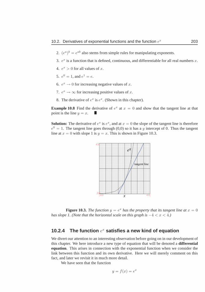
10.2. Derivatives of exponential functions and the function ex 203
2. (ea)b = eab also stems from simple rules for manipulating exponents.
3. ex is a function that is defined, continuous, and differentiable for all real numbersx.
4. ex > 0 for all values ofx.
5. e0 = 1, ande1 = e.
6. ex → 0 for increasing negative values ofx.
7. ex →∞ for increasing positive values ofx.
8. The derivative ofex is ex. (Shown in this chapter).
Example 10.8 Find the derivative ofex at x = 0 and show that the tangent line at thatpoint is the liney = x.
Solution: The derivative ofex is ex, and atx = 0 the slope of the tangent line is thereforee0 = 1. The tangent line goes through (0,0) so it has ay intercept of 0. Thus the tangentline atx = 0 with slope 1 isy = x. This is shown in Figure 10.3.
ex
tangent line
-4.0 4.0
0.0
4.0
x
Figure 10.3.The functiony = ex has the property that its tangent line atx = 0has slope 1. (Note that the horizontal scale on this graph is−4 < x < 4.)
10.2.4 The function ex satisfies a new kind of equation
We divert our attention to an interesting observation before going on in our development ofthis chapter. We here introduce a new type of equation that will be denoted adifferentialequation. This arises in connection with the exponential function when we consider thelink between this function and its own derivative. Here we will merely comment on thisfact, and later we revisit it in much more detail.
We have seen that the function
y = f(x) = ex
204 Chapter 10. Exponential functions
satisfies the relationshipdy
dx= f ′(x) = f(x) = y.
In other words, when differentiating, we get the same function back again.
The functiony = f(x) = ex is equal to its own derivative and hence, it satisfies theequation
dy
dx= y.
An equation linking a function and its derivative(s) is called adifferential equation.
This is a new type of equation, unlike ones seen before in thiscourse. We will seelater in this course that such equations have important applications.
10.3 Inverse functions and logarithmsSo far in this chapter, we have defined a new functionex and computed its derivative.Paired with this newcomer is an inverse function, the natural logarithm,ln(x). The readerwill find it helpful to review concepts of inverse functions in Appendix C. In particular, thefollowing key ideas are important:
Given a functiony = f(x), its inverse function, denotedf−1(x) satisfies
f(f−1(x)) = x, and f−1(f(x)) = x.
The range off(x) is the domain off1−(x) (and vice versa), which implies that in manycases, the relationship holds only on some subset of real numbers. An discussed in theappendix, the domain of a function (such asy = x2) has to be restricted (e.g. tox ≥ 0) sothat its inverse function (y = sqrtx) be defined. On that restricted domain, the graphs off andf−1 are mirror images of one another about the liney = x, which essentially stemsfrom the fact that the roles ofx andy are interchanged.
Section 10.3 Learning goals
1. Understand the concept of inverse function from both algebraic and geometric pointsof view: given a function, be able to determine whether (and for what restricted do-main) an inverse function can be defined and to sketch its inverse function. (ReviewAppendix C.E).
2. Understand the relationship between the domain and rangeof a function and therange and domain of its inverse function. (Review Appendix C.E).
3. Be able to apply these ideas to the logarithm, which is the inverse of an exponentialfunction.
4. Follow and be able to reproduce the calculation of the derivative of ln(x) using im-plicit differentiation.
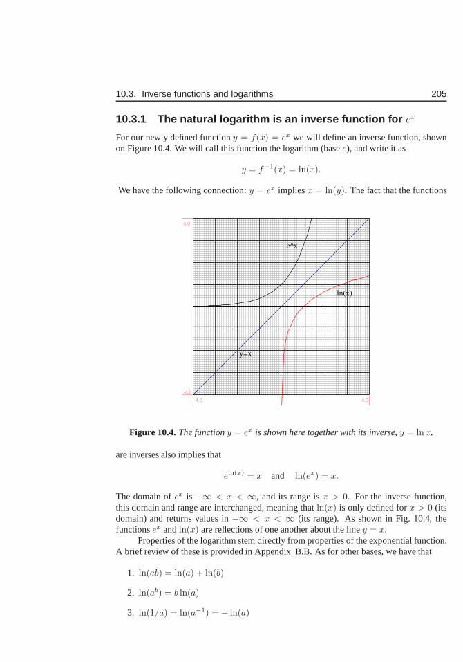
10.3. Inverse functions and logarithms 205
10.3.1 The natural logarithm is an inverse function for ex
For our newly defined functiony = f(x) = ex we will define an inverse function, shownon Figure 10.4. We will call this function the logarithm (basee), and write it as
y = f−1(x) = ln(x).
We have the following connection:y = ex impliesx = ln(y). The fact that the functions
e^x
ln(x)
y=x
-4.0 4.0
-4.0
4.0
Figure 10.4.The functiony = ex is shown here together with its inverse,y = lnx.
are inverses also implies that
eln(x) = x and ln(ex) = x.
The domain ofex is −∞ < x < ∞, and its range isx > 0. For the inverse function,this domain and range are interchanged, meaning thatln(x) is only defined forx > 0 (itsdomain) and returns values in−∞ < x < ∞ (its range). As shown in Fig. 10.4, thefunctionsex andln(x) are reflections of one another about the liney = x.
Properties of the logarithm stem directly from properties of the exponential function.A brief review of these is provided in Appendix B.B. As for other bases, we have that
1. ln(ab) = ln(a) + ln(b)
2. ln(ab) = b ln(a)
3. ln(1/a) = ln(a−1) = − ln(a)
206 Chapter 10. Exponential functions
10.3.2 Derivative of ln(x) by implicit differentiation
Implicit differentiation is helpful whenever an inverse function appears. Knowing thederivative of the original function allows us to easily compute the derivative of its inverseby using the special relationship. Here we use implicit differentiation to find the derivativeof the newly defined function,y = ln(x) as follows: First, restate the relationship in theinverse form, but considery as the dependent variable, that is think ofy(x) as a quantitythat depends onx:
y = ln(x) ⇒ ey = x ⇒ d
dxey(x) =
d
dxx
Here we apply the chain rule:
dey
dy
dy
dx= 1 ⇒ ey dy
dx= 1 ⇒ dy
dx=
1
ey=
1
x
We have thus shown the following:
The derivative ofln(x) is 1/x:
d ln(x)
dx=
1
x.
10.4 Applications of the logarithm
Section 10.4 Learning goals
1. Understand the relationships between propertied ofex and properties of its inverseln(x), and master manipulations of expressions involving both.
2. Be able to use logarithm for base conversions, and for solving equations involvingthe exponential function. (For instance, given an equationof the formA = ebt, solvefor t.)
3. Given a relationship such asy = axb, show thatln(y) is related linearly toln(x),and use data points for(x, y) to determine the values ofa andb.
10.4.1 Using the logarithm for base conversion
The logarithm is helpful in changing an exponential function from one base to another. Wegive some examples here.
Example 10.9 Rewritey = 2x in terms of basee.
Solution:y = 2x ⇒ ln(y) = ln(2x) = x ln(2)
10.4. Applications of the logarithm 207
eln(y) = ex ln(2) ⇒ y = ex ln(2)
We find (using a calculator) thatln(2) = 0.6931.. so we have
y = ekx where k = ln(2) = 0.6931..
Example 10.10Find the derivative ofy = 2x.
Solution: We have expressed this function in the alternate form
y = 2x = ekx with k = ln(2).
From Example 10.6 we have
dy
dx= kekx = ln(2)eln(2)x = ln(2)2x.
We have discovered that the constantC2 in the derivative of2x that we computed in Exam-ple 10.4 is actually related to the natural logarithm:C2 = ln(2).
10.4.2 The logarithm helps to solve exponential equations
Equations involving the exponential function can sometimes be simplified and solved usingthe logarithm. Here we provide a few examples of this kind.
Example 10.11Find zeros of the functiony = f(x) = e2x − e5x2
.
Solution: We are being asked to find values ofx for which f(x) = e2x − e5x2
= 0. Wewrite
e2x − e5x2
= 0 ⇒ e2x = e5x2 ⇒ e5x2
e2x= 1 ⇒ e5x2−2x = 1
Taking logarithm of both sides, and using the facts that
ln(e5x2−2x = 5x2 − 2x, ln(1) = 0
we obtain5x2 − 2x = 0 ⇒ x = 0, 5/2.
We see that the logarithm is useful in the last step of isolating x, after simplifying theexponential expressions appearing in the equation.
Earlier in this chapter we had posed a question: How long willit take for the Andromedastrain population to attain a size of6 · 1036 cells, i.e. to grow to an Earth-sized colony. Wecan now address this question and solve it fully.
Example 10.12 (The Andromeda strain)How long will it take for an E. coli colony toreach size of6 · 1036 cells by the unlimited doubling every 20 minutes??
208 Chapter 10. Exponential functions
Solution: We recall that the doubling time for the bacteria is20 min, so that one generation(or one doubling occurs for every multiple oft/20). However, it is not necessarily true thatall cells will split in a synchronized way. This means that after t minutes, we expect thatthe number,B(t) of bacteria would be roughly given by the smooth function:
B(t) = 2t/20.
(Note that this function agrees with our previous table and graph for powers of 2 at allinteger multiples of the generation time, i.e. fort = 20, 40, 60, 80.. minutes.)
We can compute this as follows:
6 · 1036 = 2t/20 ⇒ ln(6 · 1036) = ln(2t/20)
ln(6) + 36 ln(10) =t
20ln(2)
so
t = 20ln(6) + 36 ln(10)
ln(2)= 20
1.79 + 36(2.3)
0.693= 2441.27
This is the time in minutes. In hours, it would take 2441.27/60 = 40.68 hours for the colonyto grow to such a size.
Example 10.13 (Using basee:) Express the number of bacteria in terms of basee (forpractice with base conversions).
Solution: We would do this as follows:
B(t) = 2t/20 ⇒ ln(B) =t
20ln(2)
eln(B(t)) = et20
ln(2) ⇒ B(t) = ekt where k =ln(2)
20.
The constantk will be referred to as the growth rate of the bacteria. We observe that thisconstant can be written as:
k =ln(2)
doubling time.
We will see the usefulness of this approach very soon.
10.4.3 Logarithms help plot data that varies on large scale
Living organisms come in a variety of sizes, from the tiniestcells to the largest whales.Comparingattributes across species of vastly different sizes poses achallenge, as visualizing such dataon a simple graph obscures both extremes. This is particularly true in allometry, wherecomparisons are made of physiological properties across animals from mouse to elephant.An example of such data for metabolic rate versus mass of the animal is shown in Ta-ble 10.2. It would be hard to see all data points clearly on a regular graph. For this reason,it can be helpful to use logarithmic scaling for either or both variables. We show an exampleof this kind of log-log plot in Figure 10.5.
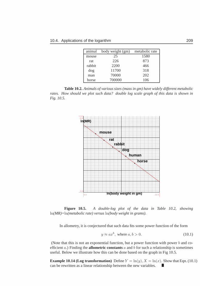
10.4. Applications of the logarithm 209
animal body weight (gm) metabolic ratemouse 25 1580
rat 226 873rabbit 2200 466dog 11700 318man 70000 202horse 700000 106
Table 10.2.Animals of various sizes (mass in gm) have widely different metabolicrates. How should we plot such data? double log scale graph ofthis data is shown inFig. 10.5.
ln(body weight in gm)
ln(MR)
mouse
ratrabbit
doghuman
horse
0.0 20.0
2.0
9.0
Figure 10.5. A double-log plot of the data in Table 10.2, showingln(MR)=ln(metabolic rate) versusln(body weight in grams).
In allometry, it is conjectured that such data fits some powerfunction of the form
y ≈ axb, wherea, b > 0. (10.1)
(Note that this is not an exponential function, but a power function with powerb and co-efficienta.) Finding theallometric constantsa andb for such a relationship is sometimesuseful. Below we illustrate how this can be done based on the graph in Fig 10.5.
Example 10.14 (Log transformation) DefineY = ln(y), X = ln(x). Show that Eqn. (10.1)can be rewritten as a linear relationship between the new variables.
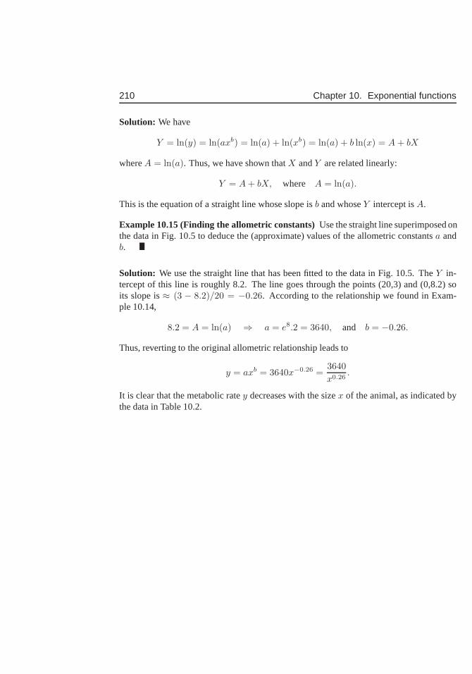
210 Chapter 10. Exponential functions
Solution: We have
Y = ln(y) = ln(axb) = ln(a) + ln(xb) = ln(a) + b ln(x) = A + bX
whereA = ln(a). Thus, we have shown thatX andY are related linearly:
Y = A + bX, where A = ln(a).
This is the equation of a straight line whose slope isb and whoseY intercept isA.
Example 10.15 (Finding the allometric constants)Use the straight line superimposed onthe data in Fig. 10.5 to deduce the (approximate) values of the allometric constantsa andb.
Solution: We use the straight line that has been fitted to the data in Fig.10.5. TheY in-tercept of this line is roughly 8.2. The line goes through thepoints (20,3) and (0,8.2) soits slope is≈ (3 − 8.2)/20 = −0.26. According to the relationship we found in Exam-ple 10.14,
8.2 = A = ln(a) ⇒ a = e8.2 = 3640, and b = −0.26.
Thus, reverting to the original allometric relationship leads to
y = axb = 3640x−0.26 =3640
x0.26.
It is clear that the metabolic ratey decreases with the sizex of the animal, as indicated bythe data in Table 10.2.
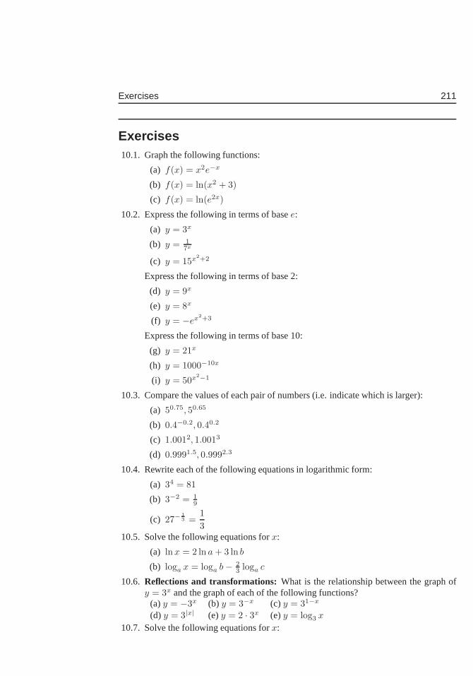
Exercises 211
Exercises10.1. Graph the following functions:
(a) f(x) = x2e−x
(b) f(x) = ln(x2 + 3)
(c) f(x) = ln(e2x)
10.2. Express the following in terms of basee:
(a) y = 3x
(b) y = 17x
(c) y = 15x2+2
Express the following in terms of base 2:
(d) y = 9x
(e) y = 8x
(f) y = −ex2+3
Express the following in terms of base 10:
(g) y = 21x
(h) y = 1000−10x
(i) y = 50x2−1
10.3. Compare the values of each pair of numbers (i.e. indicate which is larger):
(a) 50.75, 50.65
(b) 0.4−0.2, 0.40.2
(c) 1.0012, 1.0013
(d) 0.9991.5, 0.9992.3
10.4. Rewrite each of the following equations in logarithmic form:
(a) 34 = 81
(b) 3−2 = 19
(c) 27−13 =
1
310.5. Solve the following equations forx:
(a) lnx = 2 ln a + 3 ln b
(b) loga x = loga b− 23 loga c
10.6. Reflections and transformations: What is the relationship between the graph ofy = 3x and the graph of each of the following functions?
(a)y = −3x (b) y = 3−x (c) y = 31−x
(d) y = 3|x| (e)y = 2 · 3x (e)y = log3 x
10.7. Solve the following equations forx:
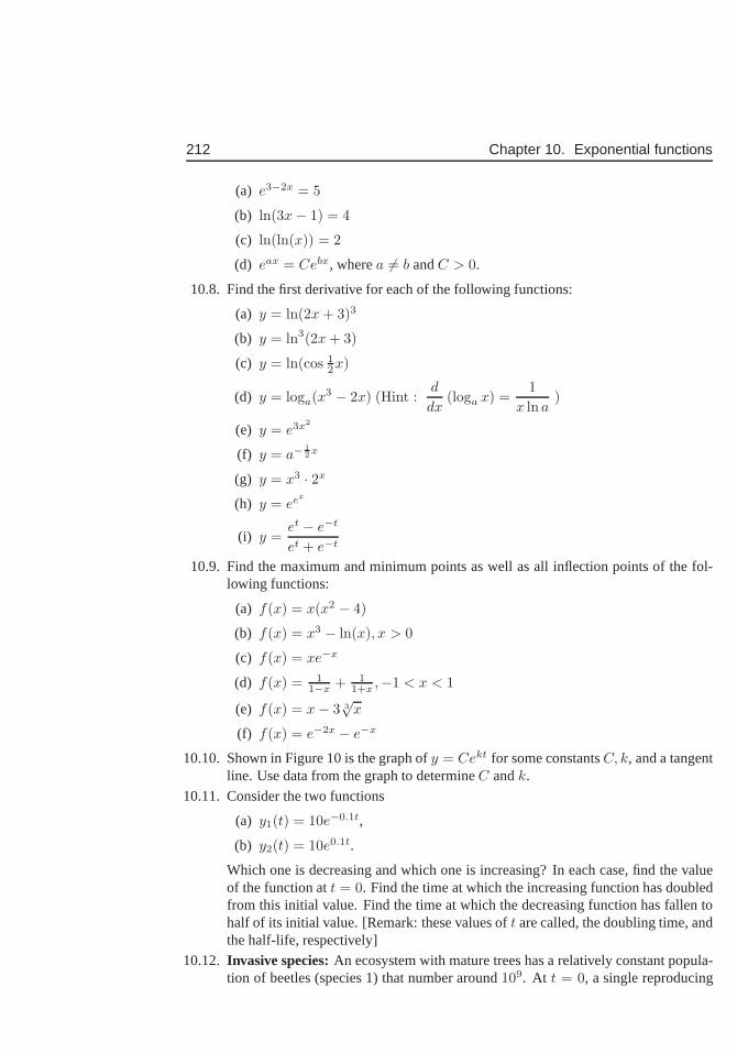
212 Chapter 10. Exponential functions
(a) e3−2x = 5
(b) ln(3x− 1) = 4
(c) ln(ln(x)) = 2
(d) eax = Cebx, wherea 6= b andC > 0.
10.8. Find the first derivative for each of the following functions:
(a) y = ln(2x + 3)3
(b) y = ln3(2x + 3)
(c) y = ln(cos 12x)
(d) y = loga(x3 − 2x) (Hint :d
dx(loga x) =
1
x ln a)
(e) y = e3x2
(f) y = a− 12x
(g) y = x3 · 2x
(h) y = eex
(i) y =et − e−t
et + e−t
10.9. Find the maximum and minimum points as well as all inflection points of the fol-lowing functions:
(a) f(x) = x(x2 − 4)
(b) f(x) = x3 − ln(x), x > 0
(c) f(x) = xe−x
(d) f(x) = 11−x + 1
1+x ,−1 < x < 1
(e) f(x) = x− 3 3√
x
(f) f(x) = e−2x − e−x
10.10. Shown in Figure 10 is the graph ofy = Cekt for some constantsC, k, and a tangentline. Use data from the graph to determineC andk.
10.11. Consider the two functions
(a) y1(t) = 10e−0.1t,
(b) y2(t) = 10e0.1t.
Which one is decreasing and which one is increasing? In each case, find the valueof the function att = 0. Find the time at which the increasing function has doubledfrom this initial value. Find the time at which the decreasing function has fallen tohalf of its initial value. [Remark: these values oft are called, the doubling time, andthe half-life, respectively]
10.12. Invasive species:An ecosystem with mature trees has a relatively constant popula-tion of beetles (species 1) that number around109. At t = 0, a single reproducing
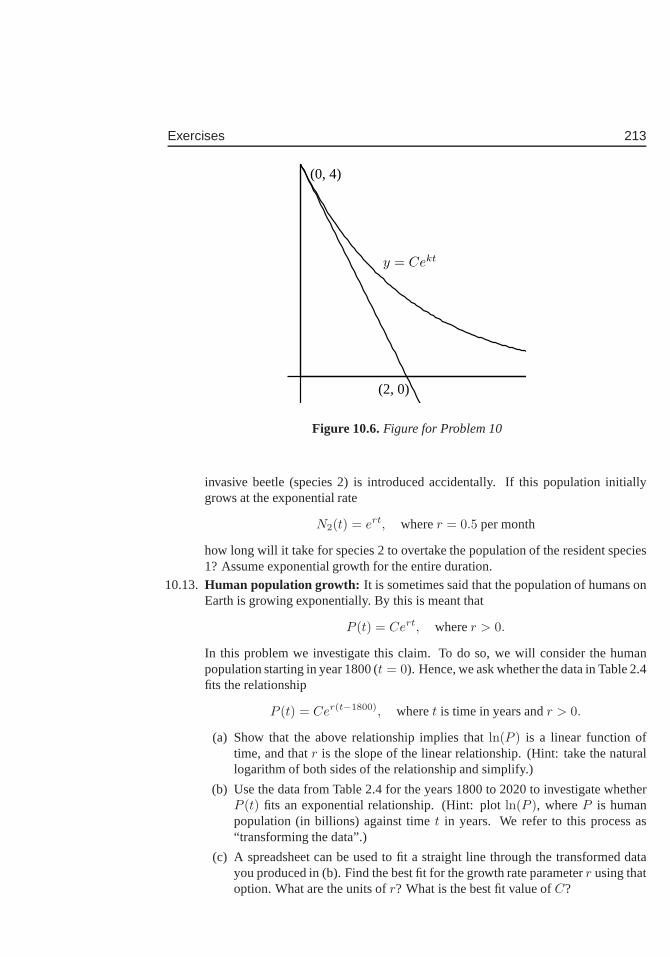
Exercises 213
(0, 4)
(2, 0)
y = Cekt
Figure 10.6.Figure for Problem 10
invasive beetle (species 2) is introduced accidentally. Ifthis population initiallygrows at the exponential rate
N2(t) = ert, wherer = 0.5 per month
how long will it take for species 2 to overtake the populationof the resident species1? Assume exponential growth for the entire duration.
10.13. Human population growth: It is sometimes said that the population of humans onEarth is growing exponentially. By this is meant that
P (t) = Cert, wherer > 0.
In this problem we investigate this claim. To do so, we will consider the humanpopulation starting in year 1800 (t = 0). Hence, we ask whether the data in Table 2.4fits the relationship
P (t) = Cer(t−1800), wheret is time in years andr > 0.
(a) Show that the above relationship implies thatln(P ) is a linear function oftime, and thatr is the slope of the linear relationship. (Hint: take the naturallogarithm of both sides of the relationship and simplify.)
(b) Use the data from Table 2.4 for the years 1800 to 2020 to investigate whetherP (t) fits an exponential relationship. (Hint: plotln(P ), whereP is humanpopulation (in billions) against timet in years. We refer to this process as“transforming the data”.)
(c) A spreadsheet can be used to fit a straight line through thetransformed datayou produced in (b). Find the best fit for the growth rate parameterr using thatoption. What are the units ofr? What is the best fit value ofC?
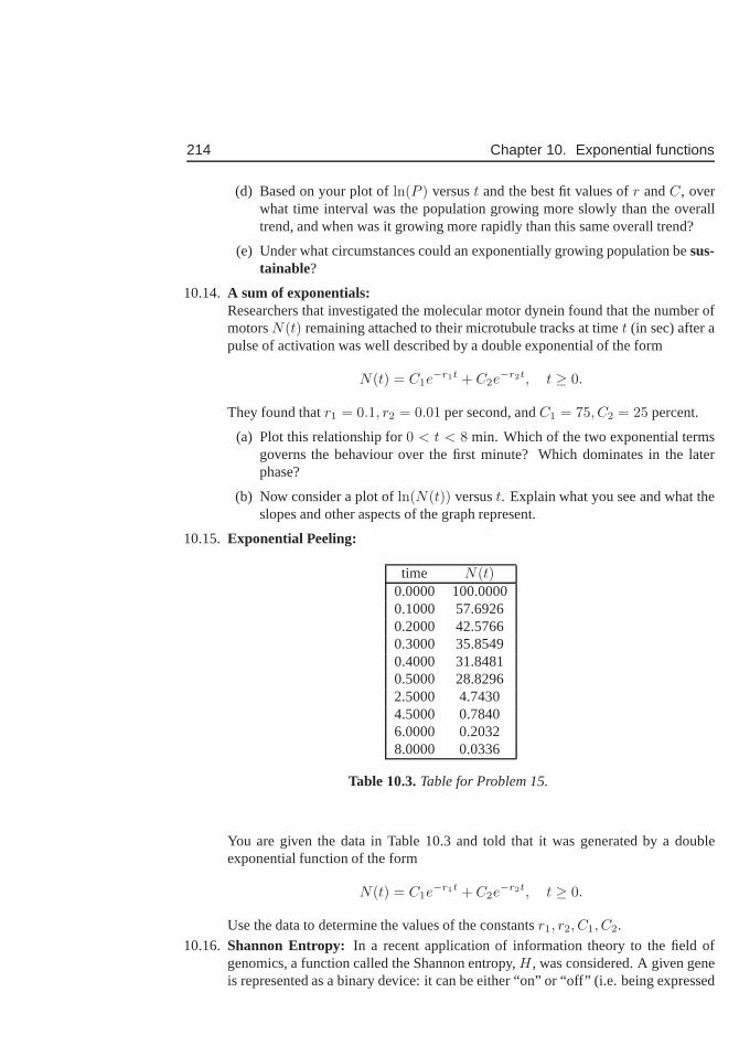
214 Chapter 10. Exponential functions
(d) Based on your plot ofln(P ) versust and the best fit values ofr andC, overwhat time interval was the population growing more slowly than the overalltrend, and when was it growing more rapidly than this same overall trend?
(e) Under what circumstances could an exponentially growing population besus-tainable?
10.14. A sum of exponentials:Researchers that investigated the molecular motor dynein found that the number ofmotorsN(t) remaining attached to their microtubule tracks at timet (in sec) after apulse of activation was well described by a double exponential of the form
N(t) = C1e−r1t + C2e
−r2t, t ≥ 0.
They found thatr1 = 0.1, r2 = 0.01 per second, andC1 = 75, C2 = 25 percent.
(a) Plot this relationship for0 < t < 8 min. Which of the two exponential termsgoverns the behaviour over the first minute? Which dominatesin the laterphase?
(b) Now consider a plot ofln(N(t)) versust. Explain what you see and what theslopes and other aspects of the graph represent.
10.15. Exponential Peeling:
time N(t)0.0000 100.00000.1000 57.69260.2000 42.57660.3000 35.85490.4000 31.84810.5000 28.82962.5000 4.74304.5000 0.78406.0000 0.20328.0000 0.0336
Table 10.3.Table for Problem 15.
You are given the data in Table 10.3 and told that it was generated by a doubleexponential function of the form
N(t) = C1e−r1t + C2e
−r2t, t ≥ 0.
Use the data to determine the values of the constantsr1, r2, C1, C2.
10.16. Shannon Entropy: In a recent application of information theory to the field ofgenomics, a function called the Shannon entropy,H , was considered. A given geneis represented as a binary device: it can be either “on” or “off” (i.e. being expressed
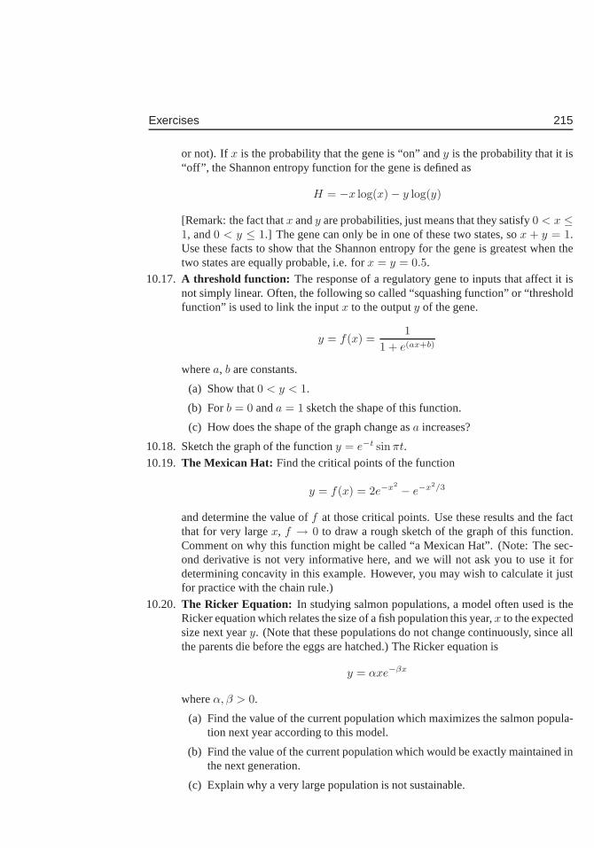
Exercises 215
or not). If x is the probability that the gene is “on” andy is the probability that it is“off”, the Shannon entropy function for the gene is defined as
H = −x log(x)− y log(y)
[Remark: the fact thatx andy are probabilities, just means that they satisfy0 < x ≤1, and0 < y ≤ 1.] The gene can only be in one of these two states, sox + y = 1.Use these facts to show that the Shannon entropy for the gene is greatest when thetwo states are equally probable, i.e. forx = y = 0.5.
10.17. A threshold function: The response of a regulatory gene to inputs that affect it isnot simply linear. Often, the following so called “squashing function” or “thresholdfunction” is used to link the inputx to the outputy of the gene.
y = f(x) =1
1 + e(ax+b)
wherea, b are constants.
(a) Show that0 < y < 1.
(b) Forb = 0 anda = 1 sketch the shape of this function.
(c) How does the shape of the graph change asa increases?
10.18. Sketch the graph of the functiony = e−t sin πt.
10.19. The Mexican Hat: Find the critical points of the function
y = f(x) = 2e−x2 − e−x2/3
and determine the value off at those critical points. Use these results and the factthat for very largex, f → 0 to draw a rough sketch of the graph of this function.Comment on why this function might be called “a Mexican Hat”.(Note: The sec-ond derivative is not very informative here, and we will not ask you to use it fordetermining concavity in this example. However, you may wish to calculate it justfor practice with the chain rule.)
10.20. The Ricker Equation: In studying salmon populations, a model often used is theRicker equation which relates the size of a fish population this year,x to the expectedsize next yeary. (Note that these populations do not change continuously, since allthe parents die before the eggs are hatched.) The Ricker equation is
y = αxe−βx
whereα, β > 0.
(a) Find the value of the current population which maximizesthe salmon popula-tion next year according to this model.
(b) Find the value of the current population which would be exactly maintained inthe next generation.
(c) Explain why a very large population is not sustainable.
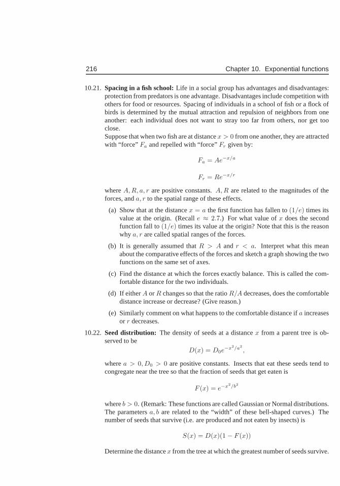
216 Chapter 10. Exponential functions
10.21. Spacing in a fish school:Life in a social group has advantages and disadvantages:protection from predators is one advantage. Disadvantagesinclude competition withothers for food or resources. Spacing of individuals in a school of fish or a flock ofbirds is determined by the mutual attraction and repulsion of neighbors from oneanother: each individual does not want to stray too far from others, nor get tooclose.Suppose that when two fish are at distancex > 0 from one another, they are attractedwith “force” Fa and repelled with “force”Fr given by:
Fa = Ae−x/a
Fr = Re−x/r
whereA, R, a, r are positive constants.A, R are related to the magnitudes of theforces, anda, r to the spatial range of these effects.
(a) Show that at the distancex = a the first function has fallen to(1/e) times itsvalue at the origin. (Recalle ≈ 2.7.) For what value ofx does the secondfunction fall to(1/e) times its value at the origin? Note that this is the reasonwhy a, r are called spatial ranges of the forces.
(b) It is generally assumed thatR > A and r < a. Interpret what this meanabout the comparative effects of the forces and sketch a graph showing the twofunctions on the same set of axes.
(c) Find the distance at which the forces exactly balance. This is called the com-fortable distance for the two individuals.
(d) If eitherA or R changes so that the ratioR/A decreases, does the comfortabledistance increase or decrease? (Give reason.)
(e) Similarly comment on what happens to the comfortable distance ifa increasesor r decreases.
10.22. Seed distribution: The density of seeds at a distancex from a parent tree is ob-served to be
D(x) = D0e−x2/a2
,
wherea > 0, D0 > 0 are positive constants. Insects that eat these seeds tend tocongregate near the tree so that the fraction of seeds that get eaten is
F (x) = e−x2/b2
whereb > 0. (Remark: These functions are called Gaussian or Normal distributions.The parametersa, b are related to the “width” of these bell-shaped curves.) Thenumber of seeds that survive (i.e. are produced and not eatenby insects) is
S(x) = D(x)(1 − F (x))
Determine the distancex from the tree at which the greatest number of seeds survive.
Exercises 217
10.23. Euler’s “ e”: In 1748, Euler wrote a classic book on calculus (“Introductio inAnalysin Infinitorum”) in which he showed that the functionex could be writtenin an expanded form similar to an (infinitely long) polynomial:
ex = 1 + x +x2
1 · 2 +x3
1 · 2 · 3 + ...
Use as many terms as necessary to find an approximate value forthe numbere andfor 1/e to 5 decimal places. Remark: we will see later that such expansions, calledpower series, are central to approximations of many functions.
218 Chapter 10. Exponential functions
Chapter 11
Differential equations forexponential growth anddecay
In this chapter we capitalize on an important observation made about exponential functionsto open the door to a new kind of mathematical equation in which functions and theirderivatives are related, that is differential equations. Here we merely acquaint the readerwith the special relationship betweenekx and one simple example of this class of equations.This relationship will lead us into a new and important link between scientific problems andmathematical descriptions.
11.1 Introducing a new kind of equation
Section 11.1 Learning goals
1. Understand that the exponential function and its derivative are proportional to oneanother, and thereby satisfy a relationship of the formdy/dx = ky.
2. Understand the definitions of a differential equation andof a solution to a differentialequation.
3. Understand thaty = ekt is a solution to the differential equationdy/dt = ky.
11.1.1 Observations about the exponential function
In a previous chapter we made an observation about a special property of the exponentialfunction
y = f(x) = ex
namely, that it satisfies the relationship
dy
dx= ex = y.
219
220 Chapter 11. Differential equations for exponential growth and decay
In this way, we encountered an important new class of equations,
dy
dx= y.
We call this adifferential equation because it connects (one or more) derivatives of afunction with the function itself.
Definition 11.1 (Differential equation). A differential equation is a mathematical equa-tion that relates one or more derivatives of some (possibly unknown) function to the func-tion itself. Solving the differential equation is the process of identifying the function(s) thatsatisfies the given relationship.
In this chapter we will study the implications of the above observation. Since mostof the applications that we examine will be time-dependent processes, we will here uset(for time) as the independent variable.
Then we can make the following observations:
1. Lety be the function of time:y = f(t) = et.
Thendy
dt= et = y.
With this slight change of notation, we see that the functiony = et satisfies thedifferential equation
dy
dt= y.
2. Now considery = ekt.
Then, using the chain rule, and settingu = kt, andy = eu we find that
dy
dt=
dy
du
du
dt= eu · k = kekt = ky.
So we see that the functiony = ekt satisfies the differential equation
dy
dt= ky.
3. If instead we had the functiony = e−kt,
we could similarly show that the differential equation it satisfies is
dy
dt= −ky.

11.1. Introducing a new kind of equation 221
4. Now suppose we had a constant in front, e.g. we were interested in the function
y = 5ekt.
Then, by simple differentiation and rearrangement we have
dy
dt= 5
d
dtekt = 5(kekt) = k(5ekt) = ky.
So we see that this function with the constant in frontalso satisfies the differentialequation
dy
dt= ky.
5. The conclusion we reached in the previous step did not depend at all on the constantout front. Indeed, if we had started with a function of the form
y = Cekt,
whereC is any constant, we would still have a function that satisfiesthe same differ-ential equation.
6. While we will not prove this here, it turns out that these are theonly functions thatsatisfy this equation.
The differential equationdy
dt= ky (11.1)
has as its solution, the function
y = Cekt. (11.2)
A few comments are worth making: First, unlikealgebraicequations, (whose solu-tions are numbers),differential equations have solutions that arefunctions. We have seenabove that depending on the constantk, we get either functions with a positive or witha negative exponent (assuming that timet > 0). This leads to the two distinct types ofbehaviour,exponential growthor exponential decayshown in Figures 11.1(a) and (b). Ineach of these figures we see afamily of curves, each of which represents a function thatsatisfies one of the differential equations we have discussed.
11.1.2 The solution to a differential equation
Definition 11.2 (Solution to a differential equation).By asolution to a differential equa-tion, we mean a function that satisfies that equation.
In the previous section we have seen a collection of solutions to each of the differen-tial equations we discussed. For example, each of the curvesshown in Figure 11.1(a) sharethe property that they satisfy the equation
dy
dt= ky.
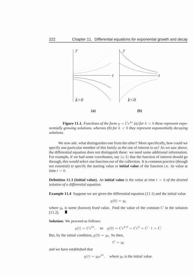
222 Chapter 11. Differential equations for exponential growth and decay
y
t
k>0
y
t
k<0
(a) (b)
Figure 11.1.Functions of the formy = Cekt (a) for k > 0 these represent expo-nentially growing solutions, whereas (b) fork < 0 they represent exponentially decayingsolutions.
We now ask: what distinguishes one from the other? More specifically, how could wespecify one particular member of this family as the one of interest to us? As we saw above,the differential equation does not distinguish these: we need some additional information.For example, if we had some coordinates, say(a, b) that the function of interest should gothrough, this would select one function out of the collection. It is common practice (thoughnot essential) to specify the starting value orinitial value of the function i.e. its value attime t = 0.
Definition 11.3 (Initial value). An initial value is the value at timet = 0 of the desiredsolution of a differential equation.
Example 11.4 Suppose we are given the differential equation (11.1) and the initial value
y(0) = y0
wherey0 is some (known) fixed value. Find the value of the constantC in the solution(11.2).
Solution: We proceed as follows:
y(t) = Cekt, so y(0) = Cek·0 = Ce0 = C · 1 = C.
But, by the initial condition,y(0) = y0. So then,
C = y0
and we have established that
y(t) = y0ekt, wherey0 is the initial value.
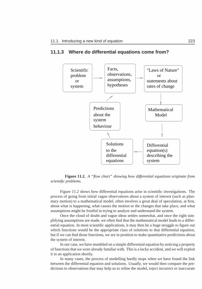
11.1. Introducing a new kind of equation 223
11.1.3 Where do differential equations come from?
Scientificproblem orsystem
Facts,observations,assumptions,hypotheses
"Laws of Nature" orstatements aboutrates of change
Mathematical
systemdescribing theequation(s)Differential
equationsdifferentialto theSolutions
Predictionsabout thesystem behaviour
Model
Figure 11.2. A “flow chart” showing how differential equations originatefromscientific problems.
Figure 11.2 shows how differential equations arise in scientific investigations. Theprocess of going from initial vague observations about a system of interest (such as plan-etary motion) to a mathematical model, often involves a great deal of speculation, at first,about what is happening, what causes the motion or the changes that take place, and whatassumptions might be fruitful in trying to analyze and understand the system.
Once the cloud of doubt and vague ideas settles somewhat, andonce the right sim-plifying assumptions are made, we often find that the mathematical model leads to a differ-ential equation. In most scientific applications, it may then be a huge struggle to figure outwhich functions would be the appropriate class of solutionsto that differential equation,but if we can find those functions, we are in position to make quantitative predictions aboutthe system of interest.
In our case, we have stumbled on a simple differential equation by noticing a propertyof functions that we were already familiar with. This is a lucky accident, and we will exploitit in an application shortly.
In many cases, the process of modelling hardly stops when we have found the linkbetween the differential equation and solutions. Usually,we would then compare the pre-dictions to observations that may help us to refine the model,reject incorrect or inaccurate
224 Chapter 11. Differential equations for exponential growth and decay
assumptions, or determine to what extent the model has limitations.A simple example of population growth modelling is given as motivation for some of
the ideas seen in this discussion.
11.2 Differential equation for unlimited populationgrowth
Section 11.2 Learning goals
1. Follow the derivation of the model for human population growth and understand thatit leads to a differential equation.
2. Appreciate that the solution to that equation is an exponential function.
3. Understand the definitions of per capita birth rates and rates of mortality, and followthe process of estimating their values from assumptions about a population.
4. Be able to compute the doubling time of the population fromits growth rate and viceversa.
In this section we will examine the way that a simple differential equation ariseswhen we study the phenomenon of uncontrolled population growth.
We will let N(t) be the number of individuals in a population at timet. The pop-ulation will change with time. Indeed the rate of change ofN will be due to births (thatincreaseN ) and deaths (that decrease it).
[
Change in Nper year
]
=
[
Number of birthsper year
]
−[
Number of deathsper year
]
We will assume that all individuals are identical in the population, and that the av-erageper capita birth rate , r, and averageper capita mortality rate , m are some fixedpositive constants. That is
r = per capita birth rate=number births per year
population size,
m = per capita mortality rate=number deaths per year
population size.
Consequently, we haveNumber of births per year= rN
Number of deaths per year= mN
We will refer to constants such asr, m asparameters. In general, for a given population,these would have specific numerical values that could be found from experiment, by col-lecting data, or by making simple assumptions. In Section 11.2.1, we will show how a setof assumptions about birth and mortality could lead to such values.
11.2. Differential equation for unlimited population growth 225
Then in yeart, the total number of births isrN , and the total number of deaths ismN . This means thatrN people per year enter the population whilemN people per yearleave it. The rate of change of the population as a whole is given by the derivativedN/dt.Thus we have arrived at:
dN
dt= rN −mN. (11.3)
This is a differential equation: it links the derivative ofN(t) to the functionN(t).By solving the equation (i.e. identifying its solution), wewill be able to make a projectionabout how fast the world population is growing.
We can first simplify the above by noting that
dN
dt= rN −mN = (r −m)N = kN.
where
k = (r −m).
This means that we have shown that the population satisfies a differential equation of theform
dN
dt= kN, for k = (r −m).
Herek is the so-callednet growth rate, i.e., birth rate minus mortality rate. This leads usto the following conclusions:
• The function that describes population over time is (by previous results) simply
N(t) = N0ekt = N0e
(r−m)t.
(The result is identical to what we saw previously, but withN rather thany as thetime-dependent function.)
• We are no longer interested in negative values ofN since it now represents a quantitythat has to be positive to have biological relevance, i.e. population size.
• The population will grow providedk > 0 which happens whenr−m > 0 i.e. whenbirth rate exceeds mortality rate.
• If k < 0, or equivalently,r < m then more people die on average than are born, sothat the population will shrink and (eventually) go extinct.
11.2.1 A simple model for human population growth
Let us apply the ideas developed in this chapter to the issue of human population expansion.Our goal in this section is to make some simplifying assumptions about births and mortalityof humans so as to estimate values for the ratesr andm that appear in Eqn. (11.3) (oralternately fork = r −m in Eqn. (11.2)). We list our assumptions and conclusions below.

226 Chapter 11. Differential equations for exponential growth and decay
Assumptions:
• The age distribution of the population is “flat”, i.e. there are as many 10 year-olds as70 year olds. (This is quite inaccurate, but will be a good place to start, as it will beeasy to estimate some of the quantities we need.) Figure 11.3shows such auniformage distribution.
age0 80
number of people
Figure 11.3. We assume a uniform age distribution to make it easy to determinethe fraction of people who are fertile (and can give birth) orwho are old (and likely to die).While slightly silly, this simplification will help estimate the desired parameters.
• The sex ratio is roughly 50%. This means that half of the population is female andhalf male.
• Women are fertile and can have babies only during part of their lives: We will assumethat the fertile years are between age 15 and age 55, as shown in Figure 11.4.
age0 80
number of people
15 55
fertile
Figure 11.4. We have assumed that only women between the ages of 15 and 55years old are fertile and can give birth. Then, according to our uniform age distributionassumption, half of all women are between these ages and hence fertile.
• A lifetime lasts 80 years. This means that for half of that time a given woman cancontribute to the birth rate, or that (55-15)/80=50% of women alive at any time areable to give birth.
• During a woman’s fertile years, we’ll assume that on average, she has one baby every10 years. (This is also a suspect assumption, since in the Western world, a womanhas on average 2-2.3 children over her lifetime, while in theDeveloping nations, thenumber of children per woman is much higher. )
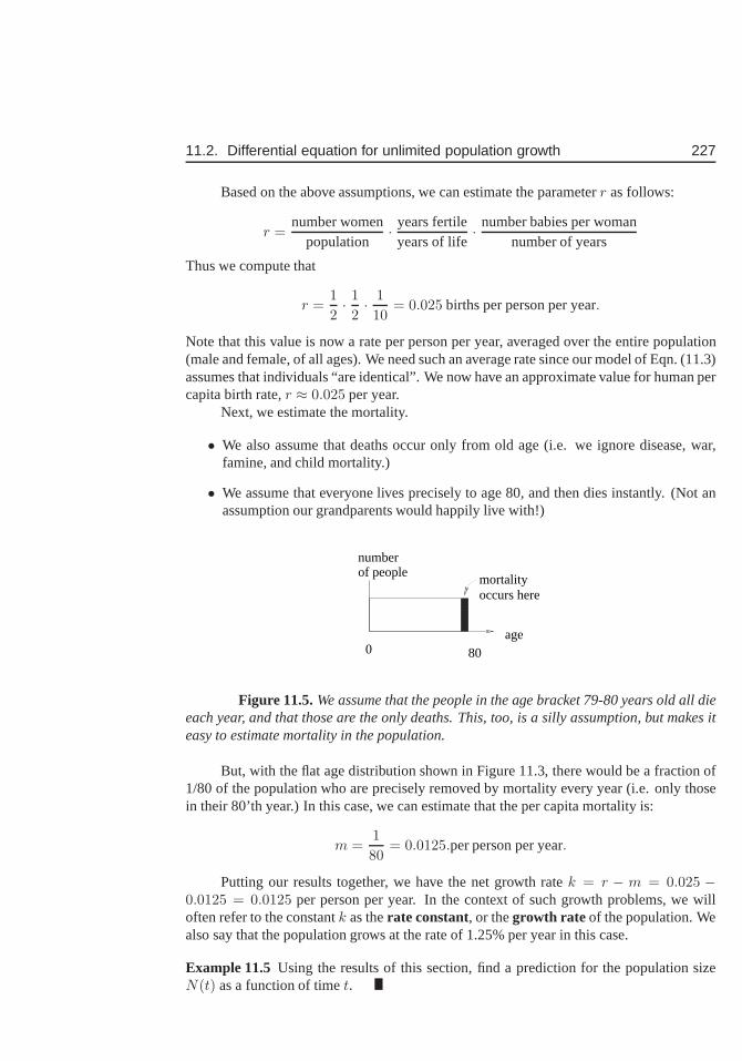
11.2. Differential equation for unlimited population growth 227
Based on the above assumptions, we can estimate the parameter r as follows:
r =number women
population· years fertile
years of life· number babies per woman
number of years
Thus we compute that
r =1
2· 12· 1
10= 0.025 births per person per year.
Note that this value is now a rate per person per year, averaged over the entire population(male and female, of all ages). We need such an average rate since our model of Eqn. (11.3)assumes that individuals “are identical”. We now have an approximate value for human percapita birth rate,r ≈ 0.025 per year.
Next, we estimate the mortality.
• We also assume that deaths occur only from old age (i.e. we ignore disease, war,famine, and child mortality.)
• We assume that everyone lives precisely to age 80, and then dies instantly. (Not anassumption our grandparents would happily live with!)
age0 80
number of people mortality
occurs here
Figure 11.5.We assume that the people in the age bracket 79-80 years old all dieeach year, and that those are the only deaths. This, too, is a silly assumption, but makes iteasy to estimate mortality in the population.
But, with the flat age distribution shown in Figure 11.3, there would be a fraction of1/80 of the population who are precisely removed by mortality every year (i.e. only thosein their 80’th year.) In this case, we can estimate that the per capita mortality is:
m =1
80= 0.0125.per person per year.
Putting our results together, we have the net growth ratek = r − m = 0.025 −0.0125 = 0.0125 per person per year. In the context of such growth problems, we willoften refer to the constantk as therate constant, or thegrowth rate of the population. Wealso say that the population grows at the rate of 1.25% per year in this case.
Example 11.5 Using the results of this section, find a prediction for the population sizeN(t) as a function of timet.
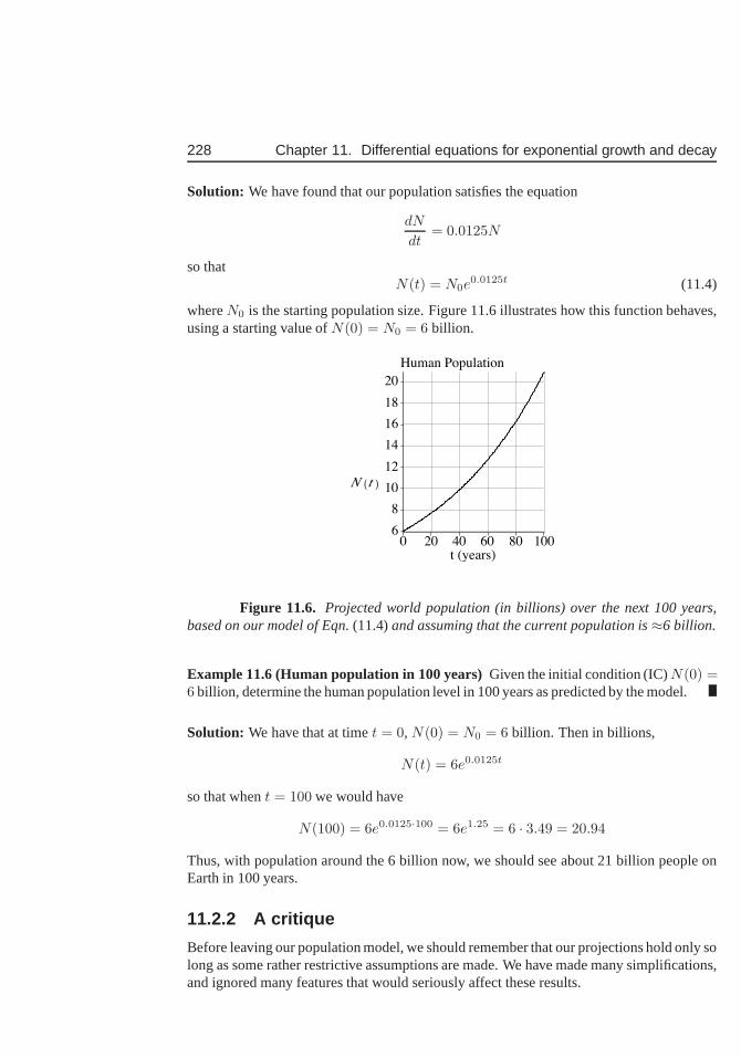
228 Chapter 11. Differential equations for exponential growth and decay
Solution: We have found that our population satisfies the equation
dN
dt= 0.0125N
so thatN(t) = N0e
0.0125t (11.4)
whereN0 is the starting population size. Figure 11.6 illustrates how this function behaves,using a starting value ofN(0) = N0 = 6 billion.
Figure 11.6. Projected world population (in billions) over the next 100 years,based on our model of Eqn.(11.4)and assuming that the current population is≈6 billion.
Example 11.6 (Human population in 100 years)Given the initial condition (IC)N(0) =6 billion, determine the human population level in 100 years as predicted by the model.
Solution: We have that at timet = 0, N(0) = N0 = 6 billion. Then in billions,
N(t) = 6e0.0125t
so that whent = 100 we would have
N(100) = 6e0.0125·100 = 6e1.25 = 6 · 3.49 = 20.94
Thus, with population around the 6 billion now, we should seeabout 21 billion people onEarth in 100 years.
11.2.2 A critique
Before leaving our population model, we should remember that our projections hold only solong as some rather restrictive assumptions are made. We have made many simplifications,and ignored many features that would seriously affect theseresults.
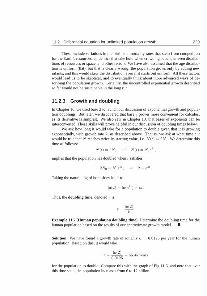
11.2. Differential equation for unlimited population growth 229
These include variations in the birth and mortality rates that stem from competitionfor the Earth’s resources, epidemics that take hold when crowding occurs, uneven distribu-tions of resources or space, and other factors. We have also assumed that the age distribu-tion is uniform (flat), but that is clearly wrong: the population grows only by adding newinfants, and this would skew the distribution even if it starts out uniform. All these factorswould lead us to be skeptical, and to eventually think about more advanced ways of de-scribing the population growth. Certainly, the uncontrolled exponential growth describedso far would not be sustainable in the long run.
11.2.3 Growth and doubling
In Chapter 10, we used base 2 to launch our discussion of exponential growth and popula-tion doublings. But later, we discovered that basee proves more convenient for calculus,as its derivative is simplest. We also saw in Chapter 10, thatbases of exponents can beinterconverted. These skills will prove helpful in our discussion of doubling times below.
We ask how long it would take for a population to double given that it is growingexponentially, with growth ratek, as described above. That is, we ask at what timet itwould be true thatN reaches twice its starting value, i.e.N(t) = 2N0. We determine thistime as follows:
N(t) = 2N0 and N(t) = N0ekt,
implies that the population has doubled whent satisfies
2N0 = N0ekt, ⇒ 2 = ekt.
Taking the natural log of both sides leads to
ln(2) = ln(ekt) = kt.
Thus, thedoubling time, denotedτ is:
τ =ln(2)
k.
Example 11.7 (Human population doubling time) Determine the doubling time for thehuman population based on the results of our approximate growth model.
Solution: We have found a growth rate of roughlyk = 0.0125 per year for the humanpopulation. Based on this, it would take
τ =ln(2)
0.0125= 55.45 years
for the population to double. Compare this with the graph of Fig 11.6, and note that overthis time span, the population increases from 6 to 12 billion.
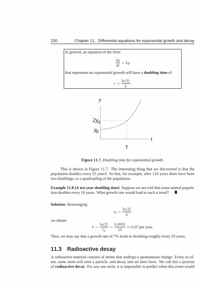
230 Chapter 11. Differential equations for exponential growth and decay
In general, an equation of the form
dy
dt= ky
that represents an exponential growth will have adoubling time of
τ =ln(2)
k.
t
y
y
2y
o
o
τ
Figure 11.7.Doubling time for exponential growth.
This is shown in Figure 11.7. The interesting thing that we discovered is that thepopulation doublesevery 55 years! So that, for example, after 110 years there have beentwo doublings, or a quadrupling of the population.
Example 11.8 (A ten year doubling time)Suppose we are told that some animal popula-tion doubles every 10 years. What growth rate would lead to such a trend?
Solution: Rearranging
t2 =ln(2)
k
we obtain
k =ln(2)
t2=
0.6931
10≈ 0.07 per year.
Thus, we may say that a growth rate of 7% leads to doubling roughly every 10 years.
11.3 Radioactive decayA radioactive material consists of atoms that undergo a spontaneous change. Every so of-ten, some atom will emit a particle, and decay into an inert form. We call this a processof radioactive decay. For any one atom, it is impossible to predict when this eventwould
11.3. Radioactive decay 231
occur exactly, but based on the behaviour of a large number ofatoms decaying sponta-neously, we can assign aprobability k of decay per unit time. In this section, we showhow simple book-keeping (Keeping track of the number of radioactive atoms remaining)leads naturally to a differential equation. Once we arrive at that equation, we use ideasdeveloped earlier to determine a likely candidate for its solution and to check its validity.We then use these results to make a long-term prediction about the amount of radioactivityremaining at any future time.
Section 11.3 Learning goals
1. Follow the model for the number of radioactive atoms and understand how this leadsto a differential equation.
2. Be able to determine the solution of the resulting differential equation.
3. Given the initial amount, be able to determine the amount of radioactivity remainingat a future time.
4. Understand the link between half-life of the radioactivematerial and its decay rate,and be able to find one when given the other.
11.3.1 Deriving the model
Let N(t) be the number of radioactive atoms at timet. Generally, we would knowN(0),the number present initially. Our goal is to make simple assumptions about the process ofdecay, and arrive at a mathematical model that will help us topredict values ofN(t) at anylater timet > 0.
Assumption 1a: The process is random, but on average, the probability of decay for agiven radioactive atom isk per unit time wherek > 0 is some constant.
Assumption 1b: During each (small) time interval of lengthh = ∆t, a radioactive atomhas probabilitykh of decaying. (This is merely a restatement of Assumption 1a.)
Suppose that at some timet0, there areN(t0) radioactive atoms. Then according to theabove assumptions, on averagekhN(t0) atoms would decay during the time periodt0 ≤t ≤ t0 + h. How many will there be at timet0 + h? We can write the following “word-equation”:
Amount leftat timet0 + h
=
Amount presentat time
t0
−
Amount decayedduring time interval
t0 ≤ t ≤ t0 + h
or, restated in symbols
N(t0 + h) = N(t0)− khN(t0). (11.5)
232 Chapter 11. Differential equations for exponential growth and decay
Here we have assumed thath is a small time period. Rearranging Eqn. (11.5) leads to
N(t0 + h)−N(t0)
h= −kN(t0).
Now leth get smaller and smaller (h→ 0) and recall that
limh→0
N(t0 + h)−N(t0)
h=
dN
dt
∣
∣
∣
∣
t0
= N ′(t0)
where we have used the notation for a derivative ofN with respect tot at the pointt = t0.We have thus shown that a description of the population of radioactive atoms reduces to
dN
dt
∣
∣
∣
∣
t0
= −kN(t0).
but this is true for any timet0, so we can replace this with the more general equation, whichholds at any timet,
dN
dt= −kN. (11.6)
We recognize this as a differential equation. As before, it provides a link between a functionof timeN(t) and its own rate of changedN/dt. Indeed, this equation specifies thatdN/dtis proportional toN , but with a negative constant of proportionality. We will shortly seethat this implies a process of decay.
ABove we formulated the entire model in terms of thenumber of radioactive atoms.However, as we shown in the next example, the same equation holds regardless of units wechose to measure the amount of radioactivity
Example 11.9 Define the number of moles of radioactive material byy(t) = N(t)/AwhereA is Avogadro’s number, which is the number of molecules in 1 mole). determinethe differential equation satisfied byy(t).
Solution: We writey(t) = N(t)/A in the formN(t) = Ay(t) and substitute this expres-sion forN(t) in Eqn. (11.6). We use the fact thatA is a constant to simplify the derivative.Then
dN
dt= −kN ⇒ Ady(t)
dt= −k(Ay(t)) ⇒ A
dy(t)
dt= A(−ky(t))
canceling the constantA from both sides of the equations leads to
dy(t)
dt= −ky(t), or simply
dy
dt= −ky. (11.7)
Thusy(t) satisfies the same kind of differential equation, with the same negative propor-tionality between the derivative and the original function. We will henceforth denote (11.7)as thedecay equation.
Next, we ask what kind of function has this property, i.e. we seek the solution of thisdifferential equation.
11.3. Radioactive decay 233
11.3.2 Solution to the decay equation
Here we explore the solution to Eqn. (11.7). Suppose that initially, there was an amounty0. Then, together, the differential equation and initial condition are
dy
dt= −ky, y(0) = y0. (11.8)
We often refer to this pairing between a differential equation and an initial condition asan initial value problem . Next, we show that an exponential function is an appropriatesolution to this problem
Example 11.10Show that the function
y(t) = y0e−kt. (11.9)
is a solution to the initial value problem (11.8).
Solution: As always, we can verify that a function is a solution to a differential equationby checking that it satisfies the equation. First we compute the derivative of the candidatefunction, obtaining
dy(t)
dt=
d
dt[y0e
−kt] = y0de−kt
dt= −ky0e
−kt = −ky(t).
We have used the fact thaty0 is a constant, and applied the chain rule to differentiatinge−kt. Then by the above algebra, we have verified that for the exponential function inquestion,dy
dt = −ky. We can also check that the initial condition is satisfied:
y(0) = y0e−k·0 = y0e
0 = y0 · 1 = y0.
Hence,y(0) = y0 and the initial condition is also satisfied. We can conclude that thefunction (11.9) is the solution to the initial value problemfor radioactive decay. Fork > 0a constant, this is a decreasing function of time that we refer to asexponential decay.
11.3.3 The half life
Given a process of exponential decay, we can ask how long it would take for half of theoriginal amount to remain. Let us recall that the “original amount” (at timet = 0) is y0.Then we are looking for the timet such thaty0/2 remains.
y(t) =y0
2.
We will refer to the value oft that satisfies this as thehalf life .
Example 11.11 (Half life) Determine the half life in the exponential decay described by(11.9).
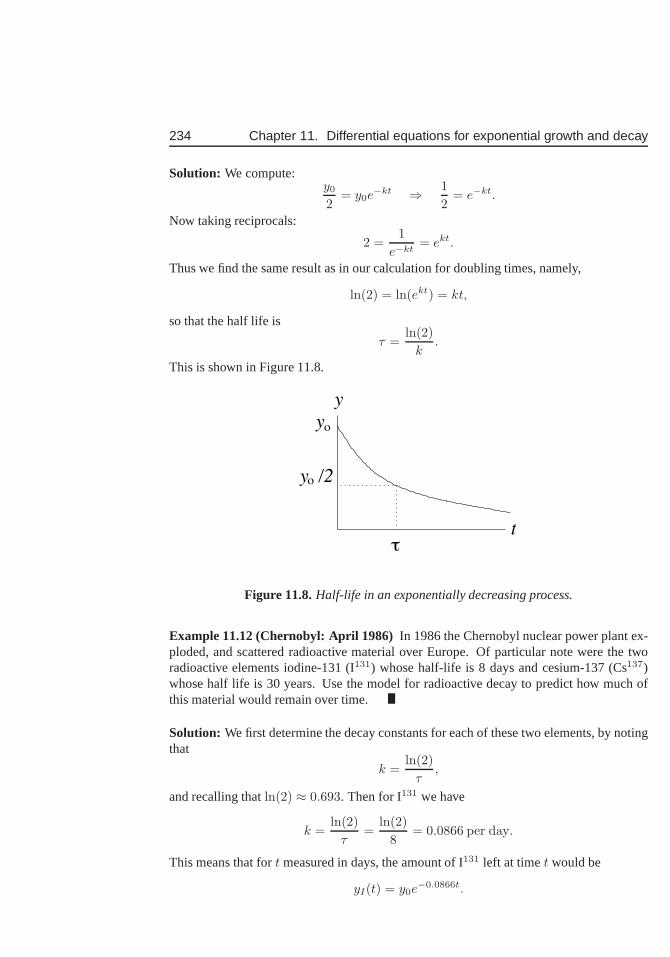
234 Chapter 11. Differential equations for exponential growth and decay
Solution: We compute:y0
2= y0e
−kt ⇒ 1
2= e−kt.
Now taking reciprocals:
2 =1
e−kt= ekt.
Thus we find the same result as in our calculation for doublingtimes, namely,
ln(2) = ln(ekt) = kt,
so that the half life is
τ =ln(2)
k.
This is shown in Figure 11.8.
t
y
τ
y
y /2ο
ο
Figure 11.8.Half-life in an exponentially decreasing process.
Example 11.12 (Chernobyl: April 1986) In 1986 the Chernobyl nuclear power plant ex-ploded, and scattered radioactive material over Europe. Ofparticular note were the tworadioactive elements iodine-131 (I131) whose half-life is 8 days and cesium-137 (Cs137)whose half life is 30 years. Use the model for radioactive decay to predict how much ofthis material would remain over time.
Solution: We first determine the decay constants for each of these two elements, by notingthat
k =ln(2)
τ,
and recalling thatln(2) ≈ 0.693. Then for I131 we have
k =ln(2)
τ=
ln(2)
8= 0.0866 per day.
This means that fort measured in days, the amount of I131 left at timet would be
yI(t) = y0e−0.0866t.
11.4. Summary and Review 235
For Cs137
k =ln(2)
30= 0.023 per year.
so that forT in years,yC(t) = y0e
−0.023T .
(We have usedT rather thant to emphasize that units are different in the two calculationsdone in this example.)
Example 11.13 (Decay to0.1% of the initial level) How long it would take for I131 to de-cay to 0.1 % of its initial level? (Assume that initial level was just after the explosion atChernobyl.)
Solution: We must calculate the timet such thatyI = 0.001y0:
0.001y0 = y0e−0.0866t ⇒ 0.001 = e−0.0866t ⇒ ln(0.001) = −0.0866t.
Therefore,
t =ln(0.001)
−0.0866=−6.9
−0.0866= 79.7 days.
Thus it would take about 80 days for the level of Iodine-131 todecay to 0.1% of its initiallevel.
11.4 Summary and ReviewHere is a brief review of what we have seen about differentialequations so far:
1. A differential equation is a statement linking the rate ofchange of some state variablewith current values of that variable. An example is the simplest population growthmodel: IfN(t) is population size at timet:
dN
dt= kN.
2. A solution to a differential equation is a function that satisfies the equation. Forinstance, the functionN(t) = Cekt (for any constantC) is a solution to the aboveunlimited growth model. (We checked this by the appropriatedifferentiation in aprevious chapter.) Graphs of such solutions (e.g. N versus t) are called solutioncurves.
3. To select a specific solution, more information is needed:Namely, some startingvalue (initial condition) is needed. Given this information, e.g.N(0) = N0, we canfully characterize the desired solution.
4. So far, we have seen simple differential equations with simple functions for theirsolutions. In general, it may be quite challenging to make the connection between thedifferential equation (stemming from some application or model) with the solution(which we want in order to understand and predict the behaviour of the system.)
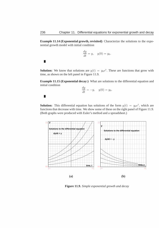
236 Chapter 11. Differential equations for exponential growth and decay
Example 11.14 (Exponential growth, revisited)Characterize the solutions to the expo-nential growth model with initial condition
dy
dt= y, y(0) = y0.
Solution: We know that solutions arey(t) = y0et. These are functions that grow with
time, as shown on the left panel in Figure 11.9.
Example 11.15 (Exponential decay:)What are solutions to the differential equation andinitial condition
dy
dt= −y, y(0) = y0.
Solution: This differential equation has solutions of the formy(t) = y0et, which are
functions that decrease with time. We show some of these on the right panel of Figure 11.9.(Both graphs were produced with Euler’s method and a spreadsheet.)
dy/dt = y
Solutions to the differential equation
y
time, t0.0 2.0
0.0
20.0
dy/dt = - y
Solutions to the differential equation
y
time, t
0.0 2.0
0.0
10.0
(a) (b)
Figure 11.9.Simple exponential growth and decay
Exercises 237
Exercises11.1. A differential equation is an equation in which some function is related to its own
derivative(s). For each of the following functions, calculate the appropriate deriva-tive, and show that the function satisfies the indicateddifferential equation
(a) f(x) = 2e−3x, f ′(x) = −3f(x)
(b) f(t) = Cekt, f ′(t) = kf(t)
(c) f(t) = 1− e−t, f ′(t) = 1− f(t)
11.2. Consider the functiony = f(t) = Cekt whereC andk are constants. For whatvalue(s) of these constants does this function satisfy the equation
(a) dydt = −5y,
(b) dydt = 3y.
[Remark: an equation which involves a function and its derivative is called a differ-ential equation.]
11.3. Find a function that satisfies each of the followingdifferential equations. [Remark:all your answers will be exponential functions, but they mayhave different depen-dent and independent variables.]
(a)dy
dt= −y,
(b)dc
dx= −0.1c andc(0) = 20,
(c)dz
dt= 3z andz(0) = 5.
11.4. If70% of a radioactive substance remains after one year, find its half-life.
11.5. Carbon 14: Carbon 14 has a half-life of 5730 years. This means that after5730years, a sample of Carbon 14, which is a radioactive isotope of carbon will have lostone half of its original radioactivity.
(a) Estimate how long it takes for the sample to fall to roughly 0.001 of its originallevel of radioactivity.
(b) Each gram of14C has an activity given here in units of 12 decays per minute.After some time, the amount of radioactivity decreases. Forexample, a sample5730 years old has only one half the original activity level,i.e. 6 decays perminute. If a 1 gm sample of material is found to have 45 decays per hour,approximately how old is it? (Note:14C is used in radiocarbon dating, aprocess by which the age of materials containing carbon can be estimated.W. Libby received the Nobel prize in chemistry in 1960 for developing thistechnique.)
11.6. Strontium-90: Strontium-90 is a radioactive isotope with a half-life of 29years.If you begin with a sample of 800 units, how long will it take for the amount ofradioactivity of the strontium sample to be reduced to
238 Chapter 11. Differential equations for exponential growth and decay
(a) 400 units
(b) 200 units
(c) 1 unit
11.7. More radioactivity: The half-life of a radioactive material is 1620 years.
(a) What percentage of the radioactivity will remain after 500 years?
(b) Cobalt 60 is a radioactive substance with half life 5.3 years. It is used inmedical application (radiology). How long does it take for 80% of a sample ofthis substance to decay?
11.8. Assume the atmospheric pressurey at a heightx meters above the sea level satisfies
the relationdy
dx= kx. If one day at a certain location the atmospheric pressures
are760 and675 torr (unit for pressure) at sea level and at1000 meters above sealevel, respectively, find the value of the atmospheric pressure at600 meters abovesea level.
11.9. Population growth and doubling: A population of animals has a per-capita birthrate ofb = 0.08 per year and a per-capita death rate ofm = 0.01 per year. Thepopulation density,P (t) is found to satisfy the differential equation
dP (t)
dt= bP (t)−mP (t)
(a) If the population is initiallyP (0) = 1000, find how big the population will bein 5 years.
(b) When will the population double?
11.10. Rodent population: The per capita birthrate of one species of rodent is 0.05 new-borns per day. (This means that, on average, each member of the population willresult in 5 newborn rodents every 100 days.) Suppose that over the period of 1000days there are no deaths, and that the initial population of rodents is 250. Write adifferential equation for the population sizeN(t) at timet (in days). Write down theinitial condition thatN satisfies. Find the solution, i.e. expressN as some functionof time t that satisfies your differential equation and initial condition. How manyrodents will there be after 1 year ?
11.11. Growth and extinction of microorganisms:
(a) The populationy(t) of a certain microorganism grows continuously and fol-lows an exponential behaviour over time. Its doubling time is found to be0.27 hours. What differential equation would you use to describe its growth? (Note: you will have to find the value of the rate constant,k, using thedoubling time.)
(b) With exposure to ultra-violet radiation, the population ceases to grow, and themicroorganisms continuously die off. It is found that the half-life is then 0.1hours. What differential equation would now describe the population?
11.12. A bacterial population: A bacterial population grows at a rate proportional to thepopulation size at timet. Let y(t) be the population size at timet. By experiment
Exercises 239
it is determined that the population att = 10min is 15, 000 and att = 30min it is20, 000.
(a) What was the initial population?
(b) What will the population be at timet = 60min?
11.13. Antibiotic treatment: A colony of bacteria is treated with a mild antibiotic agent sothat the bacteria start to die. It is observed that the density of bacteria as a function oftime follows the approximate relationshipb(t) = 85e−0.5t wheret is time in hours.Determine the time it takes for half of the bacteria to disappear. (This is called thehalf life.) Find how long it takes for 99% of the bacteria to die.
11.14. Chemical breakdown: In a chemical reaction, a substance S is broken down. Theconcentration of the substance is observed to change at a rate proportional to the cur-rent concentration. It was observed that 1 Mole/liter of S decreased to 0.5 Moles/literin 10 minutes. How long will it take until only 0.25 Moles per liter remain? Untilonly 1% of the original concentration remains?
11.15. Two populations: Two populations are studied. Population1 is found to obey thedifferential equation
dy1/dt = 0.2y1
and population2 obeysdy2/dt = −0.3y2
wheret is time in years.
(a) Which population is growing and which is declining?
(b) Find the doubling time (respectively half-life) associated with the given popu-lation.
(c) If the initial levels of the two populations werey1(0) = 100 andy2(0) =10, 000, how big would each population be at timet ?
(d) At what time would the two populations be exactly equal?
11.16. The human population: The human population on Earth doubles roughly every 50years. In October 2000 there were 6.1 billion humans on earth. Determine what thehuman population would be 500 years later under the uncontrolled growth scenario.How many people would have to inhabit each square kilometer of the planet for thispopulation to fit on earth? (Take the circumference of the earth to be 40,000 km forthe purpose of computing its surface area and assume that theoceans have dried up.)
11.17. First order chemical kinetics: When chemists say that a chemical reaction follows“first order kinetics”, they mean that the concentration of the reactant at timet, i.e.c(t), satisfies an equation of the formdc
dt = −rc wherer is a rate constant, hereassumed to be positive. Suppose the reaction mixture initially has concentration 1M(“1 molar”) and that after 1 hour there is half this amount.
(a) Find the “half life” of the reactant.
(b) Find the value of the rate constantr.
(c) Determine how much will be left after 2 hours.
(d) When will only 10% of the initial amount be left?
240 Chapter 11. Differential equations for exponential growth and decay
11.18. Fish in two lakes: Two lakes have populations of fish, but the conditions are quitedifferent in these lakes. In the first lake, the fish population is growing and satisfiesthe differential equation
dy
dt= 0.2y
wheret is time in years. At timet = 0 there were 500 fish in this lake. In the secondlake, the population is dying due to pollution. Its population satisfies the differentialequation
dy
dt= −0.1y,
and initially there were 4000 fish in this lake. At what time will the fish populationsin the two lakes be identical?
11.19. A barrel initially contains2 kg of salt dissolved in20 L of water. If water flows inthe rate of0.4 L per minute and the well-mixed salt water solution flows out atthesame rate. How much salt is present after8 minutes?
11.20. A savings account: You deposit a sumP (“the Principal”) in a savings accountwith an annualinterest rate, r and make no withdrawals over the first year. If theinterest iscompounded annually, after one year the amount in this account will be
A(1) = P + rP = P (1 + r).
If the interest is compounded semi-annually (once every 1/2year), then every 6months half of the interest is added to your account, i.e.
A
(
1
2
)
= P +r
2P = P
(
1 +r
2
)
A(1) = A
(
1
2
)
(
1 +r
2
)
= P(
1 +r
2
)(
1 +r
2
)
= P(
1 +r
2
)2
(a) Suppose that you invest $500 in an account with interest rate 4% compoundedsemi-annually. How much money would you have after 6 months?After 1year ? After 10 years ? Roughly how long does it take to double your moneyin this way? How would it differ if the interest was 8% ?
(b) Interest can also be compounded more frequently, for example monthly (i.e.12 times per year, each time with an increment ofr/12). Answer the questionsposed in part (a) in this case
(c) Is it better to save your money in a bank with 4% interest compoundedmonthly,or 5% interest compounded annually?
Chapter 12
Solving differentialequations
12.1 IntroductionIn the previous chapters, we were introduced to differential equations. We saw that the ver-bal descriptions of the rate of change of a process (for example, the growth of a populationor the decay of a radioactive substance) can be expressed in the format of a differentialequation, and that the functions associated with such equations allow us to predict the be-haviour of the process over time.
In this chapter, we will develop some of these ideas further.We will explore severaltechniques for finding and verifying that a given function isa solution to a differentialequation. We will then examine a simple class of differential equations that have manyapplications to processes of production and decay, and find their solutions. Finally we willshow how an approximation method provides for numerical solutions of such problems.
12.2 Given a function, check that it is a solutionIn this section we concentrate on analytic solutions to a differential equation. Byanalyticsolution, we mean a “formula” in the formy = f(x) that satisfies the given differentialequation. We have already seen in previous chapters that we can check whether a functionsatisfies a differential equation.
Suppose we encounter a new differential equation, and we aregiven a function that isbelieved to satisfy that equation. We can always check and verify that this claim is correct(or find it incorrect) by simple differentiation. Examples in this section show how this isdone.
241
242 Chapter 12. Solving differential equations
Section 12.2 Learning goals
1. Given a function, be able to check that whether that function does or does not satisfya given differential equation.
2. Be able to check whether a given function does or does not satisfy an initial condition.
Example 12.1 Show that the functiony(t) = (2t + 1)1/2 is a solution to the differentialequation and initial condition
dy
dt=
1
y, y(0) = 1.
Solution: First, we check the derivative, obtaining
dy(t)
dt=
d(2t + 1)1/2
dt=
1
2(2t + 1)−1/2 · 2 = (2t + 1)−1/2 =
1
(2t + 1)1/2=
1
y.
Next, we examine the initial condition, and find thaty(0) = (2 · 0 + 1)1/2 = 11/2 = 1.Hence the initial condition is also satisfied.
Example 12.2 Consider the differential equation and initial condition
dy
dt= 1− y, y(0) = y0.
Show that the functiony(t) = y0e−t is not a solution to this differential equation, but that
the functiony(t) = 1− (1− y0)e−t is a solution.
Solution: (a) To check whethery(t) = y0e−t is a solution, we differentiate this function,
obtainingdy
dt=
d[y0e−t]
dt= −y0e
−t = −y 6= 1− y.
Thus the function does not satisfy the differential equation.(b) We check if the second function satisfies the differential equation. We differenti-
ate the function, and get
dy
dt=
d
dt[1− (1− y0)e
−t] = −(1− y0)de−t
dt= −(1− y0)(−e−t) = (1− y0)e
−t
But the function isy(t) = 1 − (1 − y0)e−t so, rearranging this leads to1 − y(t) =
(1− y0)e−t. Hence, we see that
dy
dt= (1− y0)e
−t = 1− y(t) ⇒ dy
dt= 1− y.
Next, let us show that the initial condition is also satisfied. At time t = 0 we have that
y(0) = 1− (1− y0)e0 = 1− (1− y0) · 1 = 1− (1− y0) = y0.
Thus both the differential equation and the initial condition are satisfied.
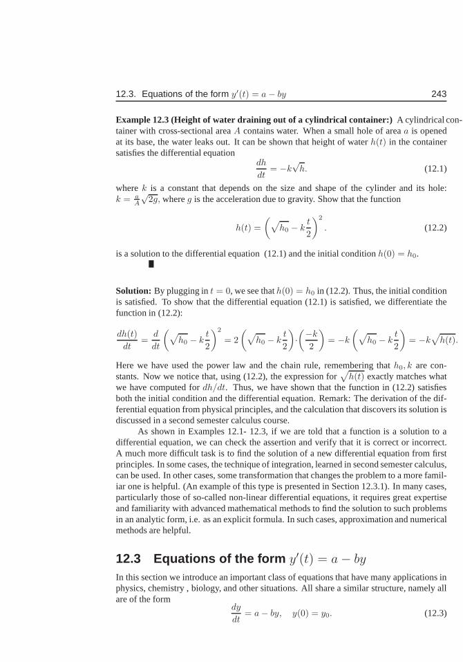
12.3. Equations of the form y′(t) = a− by 243
Example 12.3 (Height of water draining out of a cylindrical container:) A cylindrical con-tainer with cross-sectional areaA contains water. When a small hole of areaa is openedat its base, the water leaks out. It can be shown that height ofwaterh(t) in the containersatisfies the differential equation
dh
dt= −k
√h. (12.1)
wherek is a constant that depends on the size and shape of the cylinder and its hole:k = a
A
√2g, whereg is the acceleration due to gravity. Show that the function
h(t) =
(
√
h0 − kt
2
)2
. (12.2)
is a solution to the differential equation (12.1) and the initial conditionh(0) = h0.
Solution: By plugging int = 0, we see thath(0) = h0 in (12.2). Thus, the initial conditionis satisfied. To show that the differential equation (12.1) is satisfied, we differentiate thefunction in (12.2):
dh(t)
dt=
d
dt
(
√
h0 − kt
2
)2
= 2
(
√
h0 − kt
2
)
·(−k
2
)
= −k
(
√
h0 − kt
2
)
= −k√
h(t).
Here we have used the power law and the chain rule, remembering thath0, k are con-stants. Now we notice that, using (12.2), the expression for
√
h(t) exactly matches whatwe have computed fordh/dt. Thus, we have shown that the function in (12.2) satisfiesboth the initial condition and the differential equation. Remark: The derivation of the dif-ferential equation from physical principles, and the calculation that discovers its solution isdiscussed in a second semester calculus course.
As shown in Examples 12.1- 12.3, if we are told that a functionis a solution to adifferential equation, we can check the assertion and verify that it is correct or incorrect.A much more difficult task is to find the solution of a new differential equation from firstprinciples. In some cases, the technique of integration, learned in second semester calculus,can be used. In other cases, some transformation that changes the problem to a more famil-iar one is helpful. (An example of this type is presented in Section 12.3.1). In many cases,particularly those of so-called non-linear differential equations, it requires great expertiseand familiarity with advanced mathematical methods to find the solution to such problemsin an analytic form, i.e. as an explicit formula. In such cases, approximation and numericalmethods are helpful.
12.3 Equations of the form y′(t) = a− by
In this section we introduce an important class of equationsthat have many applications inphysics, chemistry , biology, and other situations. All share a similar structure, namely allare of the form
dy
dt= a− by, y(0) = y0. (12.3)
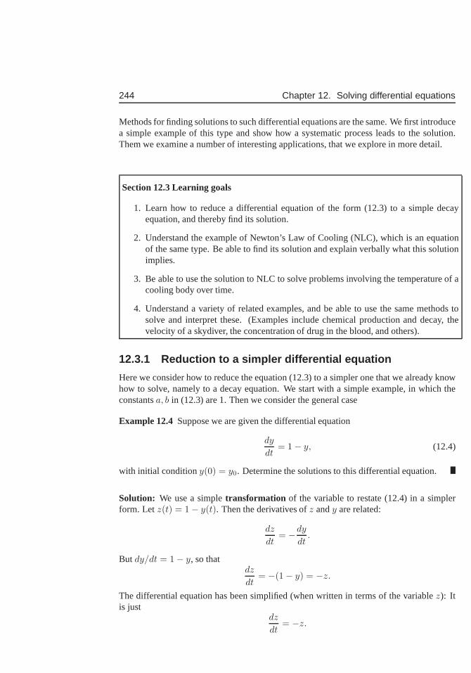
244 Chapter 12. Solving differential equations
Methods for finding solutions to such differential equations are the same. We first introducea simple example of this type and show how a systematic process leads to the solution.Them we examine a number of interesting applications, that we explore in more detail.
Section 12.3 Learning goals
1. Learn how to reduce a differential equation of the form (12.3) to a simple decayequation, and thereby find its solution.
2. Understand the example of Newton’s Law of Cooling (NLC), which is an equationof the same type. Be able to find its solution and explain verbally what this solutionimplies.
3. Be able to use the solution to NLC to solve problems involving the temperature of acooling body over time.
4. Understand a variety of related examples, and be able to use the same methods tosolve and interpret these. (Examples include chemical production and decay, thevelocity of a skydiver, the concentration of drug in the blood, and others).
12.3.1 Reduction to a simpler differential equation
Here we consider how to reduce the equation (12.3) to a simpler one that we already knowhow to solve, namely to a decay equation. We start with a simple example, in which theconstantsa, b in (12.3) are 1. Then we consider the general case
Example 12.4 Suppose we are given the differential equation
dy
dt= 1− y, (12.4)
with initial conditiony(0) = y0. Determine the solutions to this differential equation.
Solution: We use a simpletransformation of the variable to restate (12.4) in a simplerform. Letz(t) = 1− y(t). Then the derivatives ofz andy are related:
dz
dt= −dy
dt.
But dy/dt = 1− y, so thatdz
dt= −(1− y) = −z.
The differential equation has been simplified (when writtenin terms of the variablez): Itis just
dz
dt= −z.
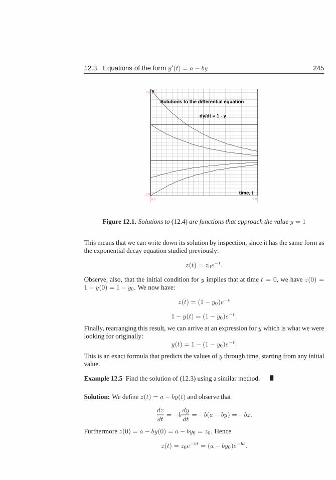
12.3. Equations of the form y′(t) = a− by 245
dy/dt = 1 - y
Solutions to the differential equation
time, t
y
0.0 2.0
0.0
3.0
Figure 12.1.Solutions to(12.4)are functions that approach the valuey = 1
This means that we can write down its solution by inspection,since it has the same form asthe exponential decay equation studied previously:
z(t) = z0e−t.
Observe, also, that the initial condition fory implies that at timet = 0, we havez(0) =1− y(0) = 1− y0. We now have:
z(t) = (1− y0)e−t
1− y(t) = (1− y0)e−t.
Finally, rearranging this result, we can arrive at an expression fory which is what we werelooking for originally:
y(t) = 1− (1− y0)e−t.
This is an exact formula that predicts the values ofy through time, starting from any initialvalue.
Example 12.5 Find the solution of (12.3) using a similar method.
Solution: We definez(t) = a− by(t) and observe that
dz
dt= −b
dy
dt= −b(a− by) = −bz.
Furthermorez(0) = a− by(0) = a− by0 = z0. Hence
z(t) = z0e−bt = (a− by0)e
−bt.
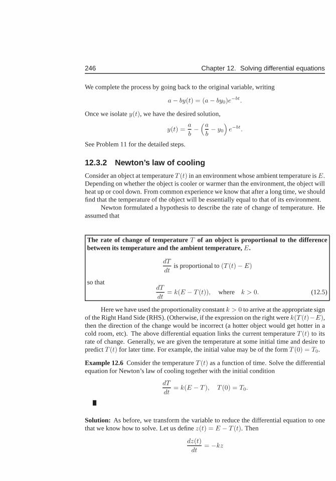
246 Chapter 12. Solving differential equations
We complete the process by going back to the original variable, writing
a− by(t) = (a− by0)e−bt.
Once we isolatey(t), we have the desired solution,
y(t) =a
b−(a
b− y0
)
e−bt.
See Problem 11 for the detailed steps.
12.3.2 Newton’s law of cooling
Consider an object at temperatureT (t) in an environment whose ambient temperature isE.Depending on whether the object is cooler or warmer than the environment, the object willheat up or cool down. From common experience we know that after a long time, we shouldfind that the temperature of the object will be essentially equal to that of its environment.
Newton formulated a hypothesis to describe the rate of change of temperature. Heassumed that
The rate of change of temperatureT of an object is proportional to the differencebetween its temperature and the ambient temperature,E.
dT
dtis proportional to(T (t)− E)
so thatdT
dt= k(E − T (t)), where k > 0. (12.5)
Here we have used the proportionality constantk > 0 to arrive at the appropriate signof the Right Hand Side (RHS). (Otherwise, if the expression on the right werek(T (t)−E),then the direction of the change would be incorrect (a hotterobject would get hotter in acold room, etc). The above differential equation links the current temperatureT (t) to itsrate of change. Generally, we are given the temperature at some initial time and desire topredictT (t) for later time. For example, the initial value may be of the form T (0) = T0.
Example 12.6 Consider the temperatureT (t) as a function of time. Solve the differentialequation for Newton’s law of cooling together with the initial condition
dT
dt= k(E − T ), T (0) = T0.
Solution: As before, we transform the variable to reduce the differential equation to onethat we know how to solve. Let us definez(t) = E − T (t). Then
dz(t)
dt= −kz
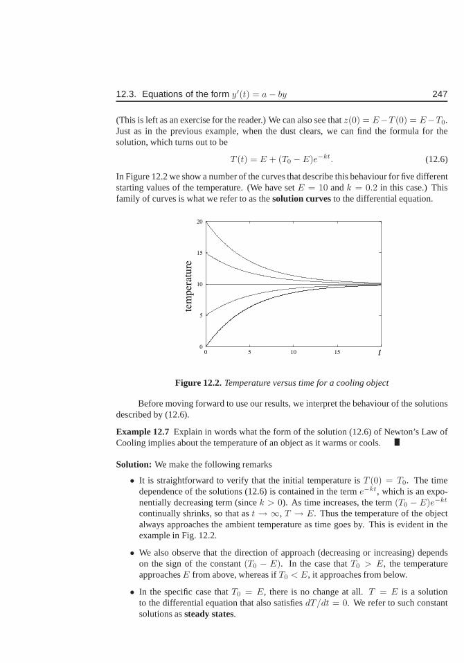
12.3. Equations of the form y′(t) = a− by 247
(This is left as an exercise for the reader.) We can also see thatz(0) = E−T (0) = E−T0.Just as in the previous example, when the dust clears, we can find the formula for thesolution, which turns out to be
T (t) = E + (T0 − E)e−kt. (12.6)
In Figure 12.2 we show a number of the curves that describe this behaviour for five differentstarting values of the temperature. (We have setE = 10 andk = 0.2 in this case.) Thisfamily of curves is what we refer to as thesolution curvesto the differential equation.
0
5
10
15
20
tem
per
atu
re
0 5 10 15 t
Figure 12.2.Temperature versus time for a cooling object
Before moving forward to use our results, we interpret the behaviour of the solutionsdescribed by (12.6).
Example 12.7 Explain in words what the form of the solution (12.6) of Newton’s Law ofCooling implies about the temperature of an object as it warms or cools.
Solution: We make the following remarks
• It is straightforward to verify that the initial temperature is T (0) = T0. The timedependence of the solutions (12.6) is contained in the terme−kt, which is an expo-nentially decreasing term (sincek > 0). As time increases, the term(T0 − E)e−kt
continually shrinks, so that ast → ∞, T → E. Thus the temperature of the objectalways approaches the ambient temperature as time goes by. This is evident in theexample in Fig. 12.2.
• We also observe that the direction of approach (decreasing or increasing) dependson the sign of the constant(T0 − E). In the case thatT0 > E, the temperatureapproachesE from above, whereas ifT0 < E, it approaches from below.
• In the specific case thatT0 = E, there is no change at all.T = E is a solutionto the differential equation that also satisfiesdT/dt = 0. We refer to such constantsolutions assteady states.
248 Chapter 12. Solving differential equations
12.3.3 Using Newton’s Law of Cooling to solve a mystery
Now that we have a detailed solution to the differential equation representing Newton’sLaw of Cooling, we can apply it to making exact determinations of temperatures over time,or of time at which a certain temperature was attained. The following example shows howthe solution can help us with an important determination oftime of death.
Example 12.8 (Murder mystery:) It is a dark clear night. The air temperature is10◦ C.A body is discovered at midnight. Its temperature is then27◦ C. One hour later, the bodyhas cooled to24◦ C. Use Newton’s law of cooling to determine the time of death.
Solution: We will assume that the temperature of the person just beforedeath is37◦ C, i.e.normal body temperature in humans. Letting the time of deathbet = 0, this would meanthatT (0) = T0 = 37. We want to find how much time elapsed until the body was found,i.e. the value oft at which the temperature of the body was27◦ C. We are told that theambient temperature isE = 10, and we will assume that this was constant over the timespan being considered. Newton’s law of cooling states that
dT
dt= k(10− T ).
The solution to this equation is
T (t) = 10 + (37− 10)e−kt = 27,
or27 = 10 + 27e−kt, i.e. 17 = 27e−kt.
We do not know the value of the constantk, but we have enough information to find it,since we know that att + 1 (one hour after discovery) the temperature was24◦ C, i.e.
T (t + 1) = 10 + (37− 10)e−k(t+1) = 24, ⇒ 24 = 10 + 27e−k(t+1).
Thus14 = 27e−k(t+1).
We have two separate equations for the two unknownst andk. We can find bothunknowns from these. Taking the ratio of the two equations weobtained we get
14
17=
27e−k(t+1)
27e−kt= e−k. ⇒ −k = ln
(
14
17
)
= −0.194
Thus we have found the constant that describes the rate of cooling of the body. Now to findthe time we can use
17 = 27e−kt ⇒ −kt = ln
(
17
27
)
= −0.4626
so
t =0.4626
k=
0.4626
0.194= 2.384.
Thus the time of discovery of the body was 2.384 hours (i.e. 2 hours and 23 minutes) afterdeath, i.e. at 9:37 pm.
12.3. Equations of the form y′(t) = a− by 249
12.3.4 Related applications and further examples
Let us return to the general example of the differential equation
dy
dt= a− by (12.7)
wherea, b > 0 are constants. The initial conditiony(0) = y0 then leads to solutions thatwe have already seen:
y(t) =a
b−(a
b− y0
)
e−bt. (12.8)
Newton’s Law of Cooling is a representative member of the class of differential equationsThis is easily seen by expanding the terms in (12.5):k(E−T ) = kE−kT and identifyingthe constants witha = kE, b = k in (12.7).
Hence, we can summarize the behaviour of solutions (12.8) byanalogy to our inter-pretation of the solutions to Newton’s Law of Cooling, namely
• The solutions should all satisfyy(0) = y0. The time dependence of the solutionsis contained in a terme−bt, which is an exponentially decreasing term (assumingb > 0). As time increases,t→∞, y → a/b.
• If y0 > a/b, theny approachesa/b from above, whereas ify0 < a/b, it approachesfrom below.
• In the specific case that initiallyy0 = a/b, there is no change at all. Thusy = a/b isasteady statesof (12.7).
In this section we describe a few other examples that share the same structure, andhence similar kind of dynamics .
Friction and terminal velocity
The velocity of a falling object changes due to the acceleration of gravity, but friction has aneffect of slowing down this acceleration. The differentialequation satisfied by the velocityv(t) of the falling object is
dv
dt= g − kv (12.9)
whereg > 0 is acceleration due to gravity andk > 0 is a constant that represents the effectof friction.
Example 12.9 Use our general results to write down the solution to the differential equa-tion (12.9) for the velocity of a skydiver given the initial conditionv(0) = v0. Interpretyour results in a simple verbal description of what happens over time.
Solution: Identifyingv → y, g → a, k → b, v0 → y0, we find the same kind of differentialequation and initial condition. Hence, without further calculation, we can conclude that thesolution of (12.9) together with the initial condition is:
v(t) =g
k−(g
k− v0
)
e−kt. (12.10)
250 Chapter 12. Solving differential equations
Then, as before, the velocity is initiallyv0, and eventually approachesg/k which is thesteady stateor terminal velocity for the object. The object will either slow down (ifv0 > g/k) or speed up (ifv0 < g/k) as it approaches this constant velocity.
Production and removal of a substance
An infusion containing a fixed concentration of substance isintroduced into a fixed vol-ume. Inside the volume, a chemical reaction results in decayof the substance at a rateproportional to its concentration. Lettingc(t) denote the time-dependent concentration ofthe substance, we obtain a differential equation of the form
dc
dt= Kin − γc (12.11)
whereKin > 0 represents the rate of input of substance andγ > 0 the decay rate.
Example 12.10Write down the solution to the differential equation (12.11) given the ini-tial conditionc(0) = c0. Determine the steady state concentration of the substance.
Solution: We can understand the behaviour of these systems by translating our notationfrom the general to the specific forms given above. For example,
c(t)→ y(t), Kin → a, γ → b.
As before, we can write down the solution:
c(t) =Kin
γ−(
Kin
γ− v0
)
e−γt. (12.12)
The steady state concentration isc = Kin/γ, and we expect that all initial chemical con-centrations will approach this level as time goes by.
As we have seen in this section, the behaviour found in the general case, can be in-terpreted in each of the specific situations of interest. This points to one of the powerfulaspects of mathematics, namely the ability to use results inabstract general cases to solve avariety of seemingly unrelated scientific problems that share the same mathematical struc-ture.
12.4 Euler’s Method and numerical solutionsSo far, we have explored ways of finding a solution to a differential equation in the form ofananalytic expression, namely a formula for the solution as a function of time. In manycases, this is difficult without extensive training, or impossible even for experts. Even ifwe can find such a solution, it may be inconvenient to determine its numerical values atarbitrary times, or to interpret its behaviour.
For that reason, we add a method for finding the desirednumerical solution using atechnique called Euler’s method, based on the fact that derivatives can be approximated byfinite differences.
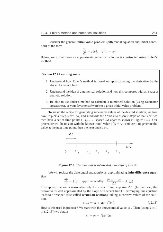
12.4. Euler’s Method and numerical solutions 251
Consider the generalinitial value problem (differential equation and initial condi-tion) of the form
dy
dt= f(y), y(0) = y0.
Below, we explain how an approximate numerical solution is constructed usingEuler’smethod.
Section 12.4 Learning goals
1. Understand how Euler’s method is based on approximating the derivative by theslope of a secant line.
2. Understand the idea of a numerical solution and how this compares with an exact oranalytic solution.
3. Be able to use Euler’s method to calculate a numerical solution (using calculator,spreadsheet, or your favorite software) to a given initial value problem.
To set up the recipe for generating successive values of the desired solution, we firsthave to pick a “step size”,∆t, and subdivide thet axis into discrete steps of that size: wethen have a set of time pointst1, t2, . . . , spaced∆t apart as shown in Figure 12.3. Ourprocedure will be to start with the known initial value ofy = y0, and use it to generate thevalue at the next time point, then the next and so on.
time
∆ t
t t t t t0 1 2 3 4 5
Figure 12.3.The time axis is subdivided into steps of size∆t.
We will replace the differential equation by an approximatingfinite difference equa-tion
dy
dt= f(y) approximated by
yk+1 − yk
∆t= f(yk).
This approximation is reasonable only for a small time step size ∆t. (In that case, thederivative is well approximated by the slope of a secant line.) Rearranging this equationleads to a “recipe” (also calledrecursion relation) linking successive values of the solu-tion.
yk+1 = yk + ∆t · f(yk). (12.13)
How is this used in practice? We start with the known initial value,y0. Then (usingk = 0in (12.13)) we obtain
y1 = y0 + f(y0)∆t.
252 Chapter 12. Solving differential equations
The quantities on the right are known, so we can compute the value ofy1, i.e. the value ofthe approximate “solution” at the time pointt1. We can then continue to generate the valueat the next time point in the same way, by approximating the derivative again as a secantslope. This leads to
y2 = y1 + f(y1)∆t.
The approximation so generated, leading to valuesy1, y2, . . . is calledEuler’s method.Applying this approximation repeatedly, leads to the recipe
y1 = y0 + f(y0)∆t,
y2 = y1 + f(y1)∆t,
...
yk+1 = yk + f(yk)∆t.
We get from this iterated technique the approximate values of the function for as many timesteps as desired starting fromt = 0 in increments of∆t up to some final timeT as desired.
It is customary to use the following notation to refer to the true ideal solution and theone that is actually produced by this approximation method:
• t0 = the initial time point, usually att = 0.
• h = ∆t = common notations for the step size, i.e. the distance between the pointsalong thet axis.
• tk = the k’th time point. Since the points are just at multiples ofthe step size thatwe have picked, it follows thattk = k∆t = kh.
• y(t) = the actual value of the solution to the differential equation at timet. This isusually not known, but in the examples discussed in this chapter, we can solve thedifferential equation exactly, so we have a formula for the functiony(t). In mosthard scientific problems, no such formula is known in advance.
• y(tk) = the actual value of the solution to the differential equation at one of thediscrete time points,tk. (Again, not usually known.)
• yk = the approximate value of the solution obtained by Euler’s method. We hopethat this approximate value is fairly close to the true value, i.e. thatyk ≈ y(tk),but there is always some error in the approximation. More advanced methods thatare specifically designed to reduce such errors are discussed in courses on numericalanalysis.
12.4.1 Euler’s method applied to population growth
Example 12.11Apply Euler’s method to approximating solutions for the simple exponen-tial growth model that was studied in Chapter 11,
dy
dt= ay,
12.4. Euler’s Method and numerical solutions 253
(wherea is a constant) with initial condition
y(0) = y0.
(See Eqn 11.1.)
Solution: Let us subdivide thet axis into steps of size∆t, starting witht0 = 0, andt1 = ∆t, t2 = 2∆t, . . . From the above discussion, we note that the first value ofy isknown to us exactly, namely,
y0 = y(0) = y0.
We replace the differential equation by the approximation
yk+1 − yk
∆t= ayk.
Thenyk+1 = yk + a∆tyk, k = 1, 2, . . .
In particular,y1 = y0 + a∆ty0 = y0(1 + a∆t),
y2 = y1(1 + a∆t),
y3 = y2(1 + a∆t),
and so on. At every stage, the quantity on the right hand side depends only on values ofyk
that are already known, so that this generates a recipe for moving from the initial value tosuccessive values of the approximation fory.
Example 12.12Consider the specific problem in which
dy
dt= −0.5y, y(0) = 100.
Use step size∆t = 0.1 and Euler’s method to approximate the solution for two time steps.
Solution: Euler’s method applied to this example would lead to
y0 =100.
y1 =y0(1 + a∆t) = 100(1 + (−0.5)(0.1)) = 95,
y2 =y1(1 + a∆t) = 95(1 + (−0.5)(0.1)) = 90.25,
and so on.Clearly, these kinds of repeated calculations are best handled on a spreadsheet or
similar computer software.
254 Chapter 12. Solving differential equations
12.4.2 Euler’s method applied to Newton’s law of cooling
We apply Euler’s method to Newton’s Law of Cooling. A motivation for doing so is thatwe can directly compare the approximate numerical solutiongenerated by Euler’s methodto the true (analytic) solution that we have worked out in this chapter.
Example 12.13 (Newton’s law of cooling:)Consider the temperature of an objectT (t)in an ambient temperature ofE = 10◦. Assume thatk = 0.2/min. Use the initial valueproblem
dT
dt= k(E − T ), T (0) = T0
to write down the the exact solution (12.6) in terms of the initial valueT0.
Solution: In this case, the differential equation has the form
dT
dt= 0.2(10− T ),
and its true solution (based on previous work) is
T (t) = 10 + (T0 − 10)e−0.2t.
Below, we investigate the solutions from several initial conditions,T (0) = 0, 5, 15, 20degrees.
Example 12.14 (Euler’s method applied to Newton’s law of cooling:) Write down the for-mula for Euler’s method to find an approximate solution for the problem outlined in Exam-ple 12.13.
Solution: Euler’s method leads to approximate the differential equation by
Tk+1 − Tk
∆t= 0.2(10− Tk).
or, in simplified form,Tk+1 ≈ Tk + 0.2(10− Tk)∆t.
Fig. 12.4 illustrates the “time-stepping” that this formula implies.
Example 12.15Use the formula from Example 12.14 and time steps of size∆t = 1.0 tofind the first few values of temperature versus time.
Solution: Note that∆t = 1.0 is not a “small step”, and we use it here only to illustrate theidea. Subdivide the horizontal (t) axis into steps of size∆t, and label the successive timevalues ast0, t1, t2, . . . tn where
t0 = 0, tk = k∆t.
This is shown in Figure 12.3. Then the initial condition willgive us the value ofT0 = T (0).We will find the temperatures at the successive times by
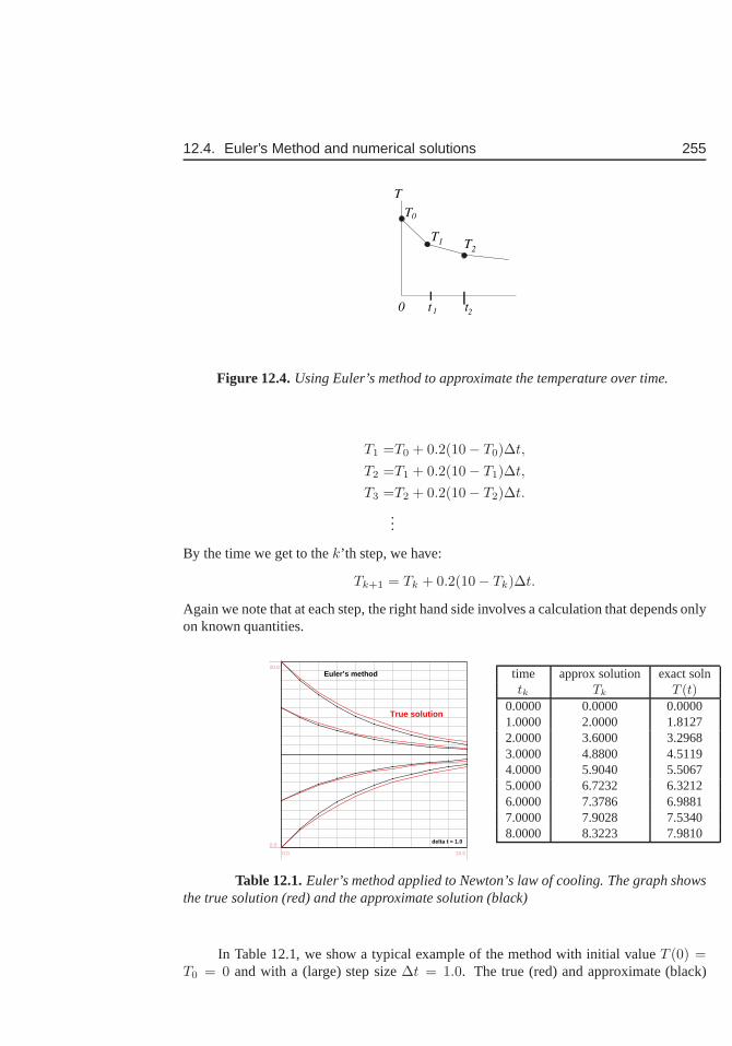
12.4. Euler’s Method and numerical solutions 255
T
T
TT
0 t t
12
0
1 2
Figure 12.4.Using Euler’s method to approximate the temperature over time.
T1 =T0 + 0.2(10− T0)∆t,
T2 =T1 + 0.2(10− T1)∆t,
T3 =T2 + 0.2(10− T2)∆t.
...
By the time we get to thek’th step, we have:
Tk+1 = Tk + 0.2(10− Tk)∆t.
Again we note that at each step, the right hand side involves acalculation that depends onlyon known quantities.
delta t = 1.0
Euler’s method
True solution
0.0 10.0
0.0
20.0
time approx solution exact solntk Tk T (t)
0.0000 0.0000 0.00001.0000 2.0000 1.81272.0000 3.6000 3.29683.0000 4.8800 4.51194.0000 5.9040 5.50675.0000 6.7232 6.32126.0000 7.3786 6.98817.0000 7.9028 7.53408.0000 8.3223 7.9810
Table 12.1.Euler’s method applied to Newton’s law of cooling. The graphshowsthe true solution (red) and the approximate solution (black)
In Table 12.1, we show a typical example of the method with initial valueT (0) =T0 = 0 and with a (large) step size∆t = 1.0. The true (red) and approximate (black)
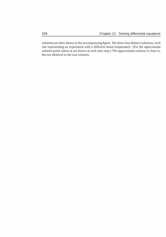
256 Chapter 12. Solving differential equations
solutions are then shown in the accompanying figure. We show four distinct solutions, eachone representing an experiment with a different initial temperature. (For the approximatesolution point values at are shown at each time step.) The approximate solution is close to,but not identical to the true solution.
Exercises 257
Exercises12.1. Consider the differential equation
dy
dt= a− by
wherea, b are constants.
(a) Show that the function
y(t) =a
b− Ce−bt
satisfies the above differential equation for any constantC.
(b) Show that by setting
C =a
b− y0
we also satisfy the initial condition
y(0) = y0.
Remark: You have now shown that the function
y(t) =(
y0 −a
b
)
e−bt +a
b
is a solution to theinitial value problem(i.e differential equation plus initialcondition)
dy
dt= a− by, y(0) = y0.
12.2. Steps in an example:Complete the algebraic steps in Example 12.5 to show thatthe solution to Eqn. (12.3) can be obtained by the substitutionz(t) = a− by(t).
12.3. Verifying a solution: Show that the function
y(t) =1
1− t
is a solution to the differential equation and initial condition
dy
dt= y2, y(0) = 1.
Comment on what happens to this solution ast approaches1.
12.4. For each of the following, show the given functiony is a solution to the given dif-ferential equation.
(a) t · dy
dt= 3y, y = 2t3.
(b)d2y
dt2+ y = 0, y = −2 sin t + 3 cos t.
258 Chapter 12. Solving differential equations
(c)d2y
dt2− 2
dy
dt+ y = 6et, y = 3t2et.
12.5. Show the function determined by the equation2x2 + xy − y2 = C, whereC is a
constant and2y 6= x, is a solution to the differential equation(x−2y)dy
dx= −4x−y.
12.6. Find the constantC that satisfies the given initial conditions.
(a) 2x2 − 3y2 = C, y|x=0 = 2.
(b) y = C1e5t + C2te
5t, y|t=0 = 1 and dydt |t=0 = 0.
(c) y = C1 cos(t− C2), y|t= π2
= 0 and dydt |t= π
2= 1.
12.7. Friction and terminal velocity: The velocity of a falling object changes due to theacceleration of gravity, but friction has an effect of slowing down this acceleration.The differential equation satisfied by the velocityv(t) of the falling object is
dv
dt= g − kv
whereg is acceleration due to gravity andk is a constant that represents the effectof friction. An object is dropped from rest from a plane.
(a) Find the functionv(t) that represents its velocity over time.
(b) What happens to the velocity after the object has been falling for a long time(but before it has hit the ground)?
12.8. Alcohol level: Alcohol enters the blood stream at a constant ratek gm per unit timeduring a drinking session. The liver gradually converts thealcohol to other, non-toxic byproducts. The rate of conversion per unit time is proportional to the currentblood alcohol level, so that the differential equation satisfied by the blood alcohollevel is
dc
dt= k − sc
wherek, s are positive constants. Suppose initially there is no alcohol in the blood.Find the blood alcohol levelc(t) as a function of time fromt = 0, when the drinkingstarted.
12.9. Newton’s Law of Cooling: Newton’s Law of Cooling states that the rate of changeof the temperature of an object is proportional to the difference between the temper-ature of the object,T , and the ambient (environmental) temperature,E. This leadsto thedifferential equation
dT
dt= k(E − T )
wherek > 0 is a constant that represents the material properties and,E is theambient temperature. (We will assume thatE is also constant.)
(a) Show that the function
T (t) = E + (T0 − E)e−kt
which represents the temperature at timet satisfies this equation.

Exercises 259
(b) The time of death of a murder victim can be estimated from the temperature ofthe body if it is discovered early enough after the crime has occurred. Supposethat in a room whose ambient temperature isE = 20◦ C, the temperatureof the body upon discovery isT = 30◦ C, and that a second measurement,one hour later isT = 25◦ C. Determine the approximate time of death. (Youshould use the fact that just prior to death, the temperatureof the victim was37◦C.)
12.10. A cup of coffee:The temperature of a cup of coffee is initially 100 degrees C.Fiveminutes later, (t = 5) it is 50 degrees C. If the ambient temperature isA = 20degrees C, determine how long it takes for the temperature ofthe coffee to reach30degrees C.
12.11. Newton’s Law of Cooling applied to data: The following data was gathered inproducing Fig. 2.1 for cooling milk during yoghurt production. According to New-ton’s Law of Cooling, this data can be described by the formula
T = E + (T (0)− E) e−kt.
whereT (t) is the temperature of the milk (in degrees Fahrenheit) at time t (in min),E is the ambient temperature, andk is some constant that we will determine in thisproblem.
time (min) Temp0.0 190.00.5 185.51.0 182.01.5 179.22.0 176.02.5 172.93.0 169.53.5 167.04.0 164.64.5 162.25.0 159.8
(a) Rewrite this relationship in terms of the quantityY (t) = ln(T (t) − E), andshow thatY (t) is related linearly to the timet.
(b) Explain how the constantk could be found from this converted form of therelationship.
(c) Use the data in the table and your favorite spreadsheet (or similar software) toshow that the data so transformed appears to be close to linear. Assume thatthe ambient temperature wasE = 20◦F.
(d) Use the same software to determine the constantk by fitting a line to the trans-formed data.
12.12. Lake Fishing: Fish Unlimited is a company that manages the fish population in aprivate lake. They restock the lake at constant rate (To restock means to add fish to
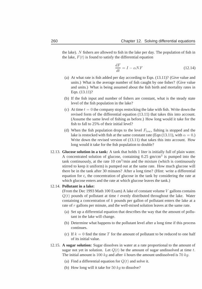
260 Chapter 12. Solving differential equations
the lake).N fishers are allowed to fish in the lake per day. The population of fish inthe lake,F (t) is found to satisfy the differential equation
dF
dt= I − αNF (12.14)
(a) At what rate is fish added per day according to Eqn. (13.11)? (Give value andunits.) What is the average number of fish caught by one fisher?(Give valueand units.) What is being assumed about the fish birth and mortality rates inEqn. (13.11)?
(b) If the fish input and number of fishers are constant, what isthe steady statelevel of the fish population in the lake?
(c) At timet = 0 the company stops restocking the lake with fish. Write down therevised form of the differential equation (13.11) that takes this into account.(Assume the same level of fishing as before.) How long would ittake for thefish to fall to 25% of their initial level?
(d) When the fish population drops to the levelFlow, fishing is stopped and thelake is restocked with fish at the same constant rate (Eqn (13.11), withα = 0.)Write down the revised version of (13.11) that takes this into account. Howlong would it take for the fish population to double?
12.13. Glucose solution in a tank:A tank that holds 1 liter is initially full of plain water.A concentrated solution of glucose, containing 0.25 gm/cm3 is pumped into thetank continuously, at the rate 10 cm3/min and the mixture (which is continuouslystirred to keep it uniform) is pumped out at the same rate. Howmuch glucose willthere be in the tank after 30 minutes? After a long time? (Hint: write a differentialequation for c, the concentration of glucose in the tank by considering the rate atwhich glucose enters and the rate at which glucose leaves thetank.)
12.14. Pollutant in a lake:(From the Dec 1993 Math 100 Exam) A lake of constant volumeV gallons containsQ(t) pounds of pollutant at timet evenly distributed throughout the lake. Watercontaining a concentration ofk pounds per gallon of pollutant enters the lake at arate ofr gallons per minute, and the well-mixed solution leaves at the same rate.
(a) Set up a differential equation that describes the way that the amount of pollu-tant in the lake will change.
(b) Determine what happens to the pollutant level after a long time if this processcontinues.
(c) If k = 0 find the timeT for the amount of pollutant to be reduced to one halfof its initial value.
12.15. A sugar solution: Sugar dissolves in water at a rate proportional to the amountofsugar not yet in solution. LetQ(t) be the amount of sugar undissolved at timet.The initial amount is100 kg and after4 hours the amount undissolved is70 kg.
(a) Find a differential equation forQ(t) and solve it.
(b) How long will it take for50 kg to dissolve?

Exercises 261
12.16. Leaking water tank: A cylindrical tank with cross-sectional areaA has a smallhole through which water drains. The height of the water in the tanky(t) at timetis given by:
y(t) = (√
y0 −kt
2A)2
wherek, y0 are constants.
(a) Show that the height of the water,y(t), satisfies the differential equation
dy
dt= − k
A
√y.
(b) What is the initial height of the water in the tank at timet = 0 ?
(c) At what time will the tank be empty ?
(d) At what rate is thevolumeof the water in the tank changing whent = 0?
12.17. Find those constantsa, b so thaty = ex andy = e−x are both solutions of thedifferential equation
y′′ + ay′ + by = 0.
12.18. Lety = f(t) = e−t sin t, −∞ < t <∞.
(a) Show thaty satisfies the differential equationy′′ + 2y′ + 2y = 0.
(b) Find all critical points off(t).

262 Chapter 12. Solving differential equations
Chapter 13
Qualitative methods fordifferential equations
Not all differential equations are easily solved analytically. Furthermore, even when wefind the analytic solution, it is not always easy to interpret, graph, or understand. Thismotivates a number of qualitative methods that lead us to an overall understanding of thebehaviour directly from information contained in the differential equation, without the chal-lenges of finding a full functional form of the solution. In this chapter we will expand ourfamiliarity with differential equations and assemble suchnew techniques for understandingthese. When these equations arenonlinear, i.e. when the functionf(y) in
dy
dt= f(y)
is not a simple linear function ofy, then it can be quite challenging to discover analyticsolutions. We will encounter both qualitative methods. Geometric techniques will form thecore of the concepts here discussed.
13.1 Linear and nonlinear differential equations
Section 13.1 Learning goals
1. Understand the distinction between unlimited and density dependent populationgrowth. Be able to explain terms in the logistic equation in its original (13.1) andrescaled (13.2) versions.
2. Be able to state the definition of a linear differential equation.
3. Understand the law of mass action, and be able to derive simple differential equationsfor interacting species based on this law.
263
264 Chapter 13. Qualitative methods for differential equations
In our previous model for population growth, in Chapter 11, we encountered thedifferential equation
dN
dt= kN,
whereN(t) is population size at timet andk is a constant per capita growth rate. Thisdifferential equation, as we have seen, has exponential solutions, which means that onlytwo possible behaviours are obtained: explosive growth ifk > 0 or extinction ifk < 0.But this is unrealistic. Most natural populations do not grow indefinitely in an explosive,exponential way. Due to limited resources or competition for territory, eventually the pop-ulation may attain some static level rather than expanding continually. This motivates arevision of our previous model to depictdensity dependent growth.
13.1.1 The logistic equation for population growth
Let N(t) represent the size of a population at timet, as before. Consider the differentialequation
dN
dt= rN
(K −N)
K. (13.1)
We call this differential equation thelogistic equation. Here the parameterr is theintrin-sic growth rate andK is thecarrying capacity. Both r, K are assumed to be positiveconstants for a given population in a given environment. Thelogistic equation has a longhistory in modelling population growth of microorganisms,animals, and human popula-tions.
In the form written above, we could interpret the logistic equation as
dN
dt=
[
r(K −N)
K
]
N.
then the termR(N) = [r(K − N)/K], which replaces the constant rate of growthk, isa so-calleddensity dependent growth rate. (It replaces the previously assumed constantgrowth rater, that leads to unlimited growth.)
We later show yet another interpretation that involves hostile interactions betweenindividuals in the population.
13.1.2 Linear versus nonlinear
The logistic equation introduces the first example of anonlinear differential equation.We explain the distinction and why it matters here.
Definition 13.1 (Linear differential equation). A first order differential equation is saidto be linear if it is a linear combination of terms of the form
dy
dt, y, 1
that is, it can be written in the form
αdy
dt+ βy + γ = 0
13.1. Linear and nonlinear differential equations 265
whereα, β, γ do not depend ony. (“First order” means that only up to the first derivativeoccurs in the equation.)
So far, we have seen several examples of this type with constant coefficientsα, β, γ.For exampleα = 1, γ = −a in Section 12.3, whereasα = 1, β = −k, γ = 0 in Eqn. 11.1.Any differential equation not of this simple form is said to be nonlinear.
Example 13.2 (Linear versus nonlinear differential equations) Which of the followingdifferential equations are linear and which are nonlinear?
(a)dy
dt= y2, (b)
dy
dt− y = 5, (c) y
dy
dt= −1.
Solution: Any term of the formy2,√
y, 1/y, etc is nonlinear iny. a producty dydt is also
nonlinear. Hence equations (a), (c) are nonlinear, while (b) is linear.The significance of the distinction between linear and nonlinear differential equations
is that nonlinearities make it much harder to systematically find a solution to the given dif-ferential equation by “analytic” methods. Most linear differential equations have solutionsthat are made of exponential functions or expressions involving such functions. This is nottrue for nonlinear equations. However, as we will see shortly, geometric methods becomevery helpful in understanding the behaviour of such nonlinear differential equations.
13.1.3 Law of mass action
Nonlinear terms in differential equations arise in variousways. One common source isinteraction between individuals or particles that affectstheir state. Here is a simple exampleof this type.
Consider a chemical reaction in which molecules of type A bind to those of type B toreact chemically and form some product P. Suppose we start out with a test-tube containinga mixture of A and B molecules at concentrationsa(t), b(t). These concentrations dependon time because the chemical reaction will use up both types in producing the product.
What can we say about the rate of the reaction? First, we note that the reaction onlyoccurs when A and B “collide” and interact. This happens randomly, but clearly the moreA is present, the more likely are such collisions, and similarly for B. Hence the rate ofreaction should be faster if the concentrationa(t) is higher, and/or if the concentrationb(t)is higher. The simplest assumption that captures both of these ideas is
rate of reaction∼ ab ⇒ rate of reaction= kab
wherek is some constant that represents the reactivity of the molecules.We can formally state this result, known as theLaw of Mass Action as follows:
The Law of Mass Action: The rate of a chemical reaction involving an interaction of twoor more chemical species is proportional to theproduct of the concentrationsof the givenspecies.
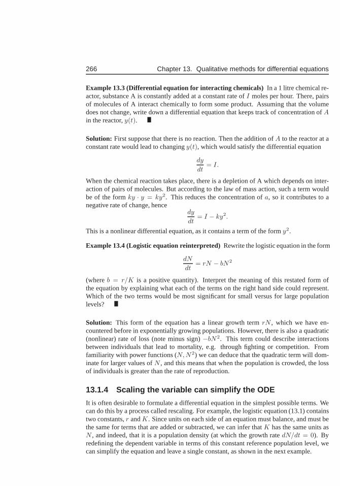
266 Chapter 13. Qualitative methods for differential equations
Example 13.3 (Differential equation for interacting chemicals) In a 1 litre chemical re-actor, substance A is constantly added at a constant rate ofI moles per hour. There, pairsof molecules of A interact chemically to form some product. Assuming that the volumedoes not change, write down a differential equation that keeps track of concentration ofAin the reactor,y(t).
Solution: First suppose that there is no reaction. Then the addition ofA to the reactor at aconstant rate would lead to changingy(t), which would satisfy the differential equation
dy
dt= I.
When the chemical reaction takes place, there is a depletionof A which depends on inter-action of pairs of molecules. But according to the law of massaction, such a term wouldbe of the formky · y = ky2. This reduces the concentration ofa, so it contributes to anegative rate of change, hence
dy
dt= I − ky2.
This is a nonlinear differential equation, as it contains a term of the formy2.
Example 13.4 (Logistic equation reinterpreted)Rewrite the logistic equation in the form
dN
dt= rN − bN2
(whereb = r/K is a positive quantity). Interpret the meaning of this restated form ofthe equation by explaining what each of the terms on the righthand side could represent.Which of the two terms would be most significant for small versus for large populationlevels?
Solution: This form of the equation has a linear growth termrN , which we have en-countered before in exponentially growing populations. However, there is also a quadratic(nonlinear) rate of loss (note minus sign)−bN2. This term could describe interactionsbetween individuals that lead to mortality, e.g. through fighting or competition. Fromfamiliarity with power functions (N, N2) we can deduce that the quadratic term will dom-inate for larger values ofN , and this means that when the population is crowded, the lossof individuals is greater than the rate of reproduction.
13.1.4 Scaling the variable can simplify the ODE
It is often desirable to formulate a differential equation in the simplest possible terms. Wecan do this by a process called rescaling. For example, the logistic equation (13.1) containstwo constants,r andK. Since units on each side of an equation must balance, and must bethe same for terms that are added or subtracted, we can infer thatK has the same units asN , and indeed, that it is a population density (at which the growth ratedN/dt = 0). Byredefining the dependent variable in terms of this constant reference population level, wecan simplify the equation and leave a single constant, as shown in the next example.
13.2. The geometry of change 267
Example 13.5 (Rescaling:)Define a new variable
y(t) =N(t)
K.
Interpret what this variable represents and show that the Logistic equation can be writtenin a simpler form in terms of this variable.
Solution: The rescaled variable,y(t), is a population density expressed in units of thecarrying capacity. (For example, if the environment can sustain 1000 individuals, and thecurrent population size isN = 950 then the value ofy is y = 0.950.) SinceK is assumedconstant,
dy
dt=
1
K
dN
dt
and we can simplify the equation:
dy
dt= ry(1 − y). (13.2)
We observe that indeed, this equation “looks simpler” and also has only one constant pa-rameter left in it. It is generally the case that rescaling reduces the number of parameters ina differential equation such as seen here.
13.2 The geometry of changeIn this section, we turn to some new methods for understanding differential equations,using graphical and geometric arguments that avoid the needfor “formulas”. We resort toconcepts learned much earlier in this course: the derivative as a slope of a tangent line, inorder to use the differential equation itself to assemble a sketch of its predicted behaviour.That is, rather than writing downy = F (t) as a solution to the differential equation (andthen graphing that function) we sketch the qualitative behaviour of such solution curvesdirectly from information contained in the differential equation.
268 Chapter 13. Qualitative methods for differential equations
Section 13.2 Learning goals
1. Understand the idea of aslope fieldof a differential equation. Given a differentialequation (linear or nonlinear), be able to construct such a diagram and use it to sketchsolution curves.
2. Understand the idea of astate-space diagram, and be able to construct such a dia-gram and use it to interpret the behaviour of solution curvesto a given differentialequation.
3. Understand the relationships between slope field, and state-space diagram, and fam-ilies of solution curves to a given differential equation.
4. Be able to identify steady states of a differential equation and determine whether theyare stable or unstable.
5. Given a differential equation and initial condition, be able to predict the behaviourof the solution fort > 0.
13.2.1 Slope fields
Here we discuss a geometric way of understanding what a differential equation is sayingusing aslope field, also denoteddirection field. We have already seen that solutions to adifferential equation of the form
dy
dt= f(y)
are curves in they, t plane that describe howy(t) changes over time. (Thus, these curvesare graphs of functions of time.) Each initial conditiony(0) = y0 is associated with oneof these curves, so that together, these curves form afamily of solutions. What do thesecurves have in common geometrically?
Simply stated, the slope of the tangent line (which is justdy/dt) at any point on anyof the curves has to be related to the value of they coordinate of that point, specified by thefunctionf(y). That is exactly what the differential equation is saying: at any point(t, y(t))on a solution curve, the tangent line must have slopef(y), which depends only on theyvalue, and not on the timet16. By sketching slopes at various values ofy, we obtain theslope field from which we can get a reasonable idea of the behaviour of the solutions to thedifferential equation.
Example 13.6 Consider the differential equation
dy
dt= 2y. (13.3)
Compute some of the slopes for variousy values and use this to sketch aslope fieldfor thedifferential equation (13.3).
16In more general cases, the expressionf(y) that appears in the differential equation might depend ont as wellasy. For the purpose of this course, we will not consider such examples in detail.
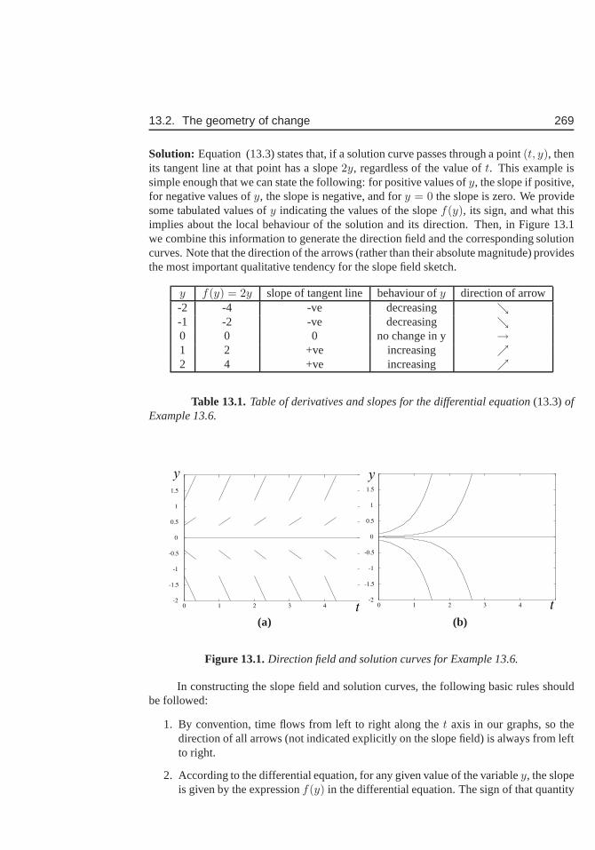
13.2. The geometry of change 269
Solution: Equation (13.3) states that, if a solution curve passes through a point(t, y), thenits tangent line at that point has a slope2y, regardless of the value oft. This example issimple enough that we can state the following: for positive values ofy, the slope if positive,for negative values ofy, the slope is negative, and fory = 0 the slope is zero. We providesome tabulated values ofy indicating the values of the slopef(y), its sign, and what thisimplies about the local behaviour of the solution and its direction. Then, in Figure 13.1we combine this information to generate the direction field and the corresponding solutioncurves. Note that the direction of the arrows (rather than their absolute magnitude) providesthe most important qualitative tendency for the slope field sketch.
y f(y) = 2y slope of tangent line behaviour ofy direction of arrow-2 -4 -ve decreasing ց-1 -2 -ve decreasing ց0 0 0 no change in y →1 2 +ve increasing ր2 4 +ve increasing ր
Table 13.1.Table of derivatives and slopes for the differential equation (13.3)ofExample 13.6.
-2
-1.5
-1
-0.5
0
0.5
1
1.5
0 1 2 3 4
y
t-2
-1.5
-1
-0.5
0
0.5
1
1.5
0 1 2 3 4
y
t
(a) (b)
Figure 13.1.Direction field and solution curves for Example 13.6.
In constructing the slope field and solution curves, the following basic rules shouldbe followed:
1. By convention, time flows from left to right along thet axis in our graphs, so thedirection of all arrows (not indicated explicitly on the slope field) is always from leftto right.
2. According to the differential equation, for any given value of the variabley, the slopeis given by the expressionf(y) in the differential equation. The sign of that quantity
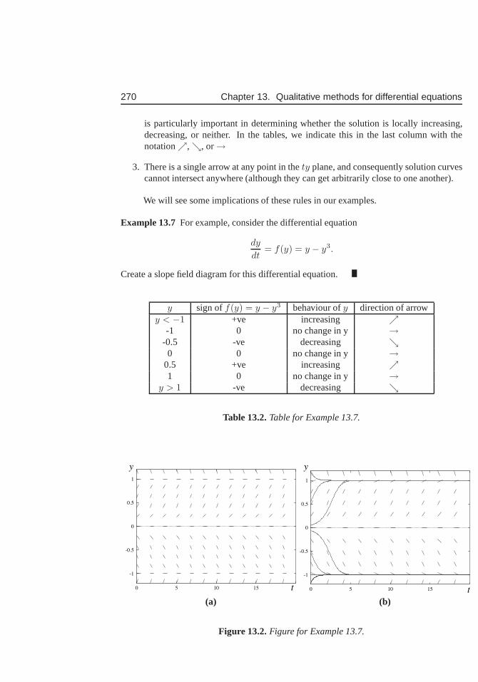
270 Chapter 13. Qualitative methods for differential equations
is particularly important in determining whether the solution is locally increasing,decreasing, or neither. In the tables, we indicate this in the last column with thenotationր,ց, or→
3. There is a single arrow at any point in thety plane, and consequently solution curvescannot intersect anywhere (although they can get arbitrarily close to one another).
We will see some implications of these rules in our examples.
Example 13.7 For example, consider the differential equation
dy
dt= f(y) = y − y3.
Create a slope field diagram for this differential equation.
y sign off(y) = y − y3 behaviour ofy direction of arrowy < −1 +ve increasing ր
-1 0 no change in y →-0.5 -ve decreasing ց0 0 no change in y →
0.5 +ve increasing ր1 0 no change in y →
y > 1 -ve decreasing ց
Table 13.2.Table for Example 13.7.
-1
-0.5
0
0.5
1
y
0 5 10 15 t
-1
-0.5
0
0.5
1
0 5 10 15 t
y
(a) (b)
Figure 13.2.Figure for Example 13.7.
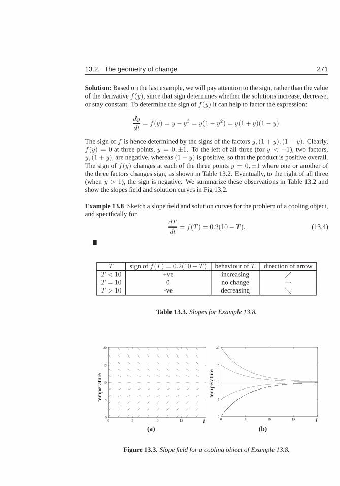
13.2. The geometry of change 271
Solution: Based on the last example, we will pay attention to the sign, rather than the valueof the derivativef(y), since that sign determines whether the solutions increase, decrease,or stay constant. To determine the sign off(y) it can help to factor the expression:
dy
dt= f(y) = y − y3 = y(1− y2) = y(1 + y)(1− y).
The sign off is hence determined by the signs of the factorsy, (1 + y), (1 − y). Clearly,f(y) = 0 at three points,y = 0,±1. To the left of all three (fory < −1), two factors,y, (1 + y), are negative, whereas(1− y) is positive, so that the product is positive overall.The sign off(y) changes at each of the three pointsy = 0,±1 where one or another ofthe three factors changes sign, as shown in Table 13.2. Eventually, to the right of all three(wheny > 1), the sign is negative. We summarize these observations in Table 13.2 andshow the slopes field and solution curves in Fig 13.2.
Example 13.8 Sketch a slope field and solution curves for the problem of a cooling object,and specifically for
dT
dt= f(T ) = 0.2(10− T ), (13.4)
T sign off(T ) = 0.2(10− T ) behaviour ofT direction of arrowT < 10 +ve increasing րT = 10 0 no change →T > 10 -ve decreasing ց
Table 13.3.Slopes for Example 13.8.
0
5
10
15
20
0 5 10 15
tem
per
ature
t0
5
10
15
20
tem
per
ature
0 5 10 15 t
(a) (b)
Figure 13.3.Slope field for a cooling object of Example 13.8.
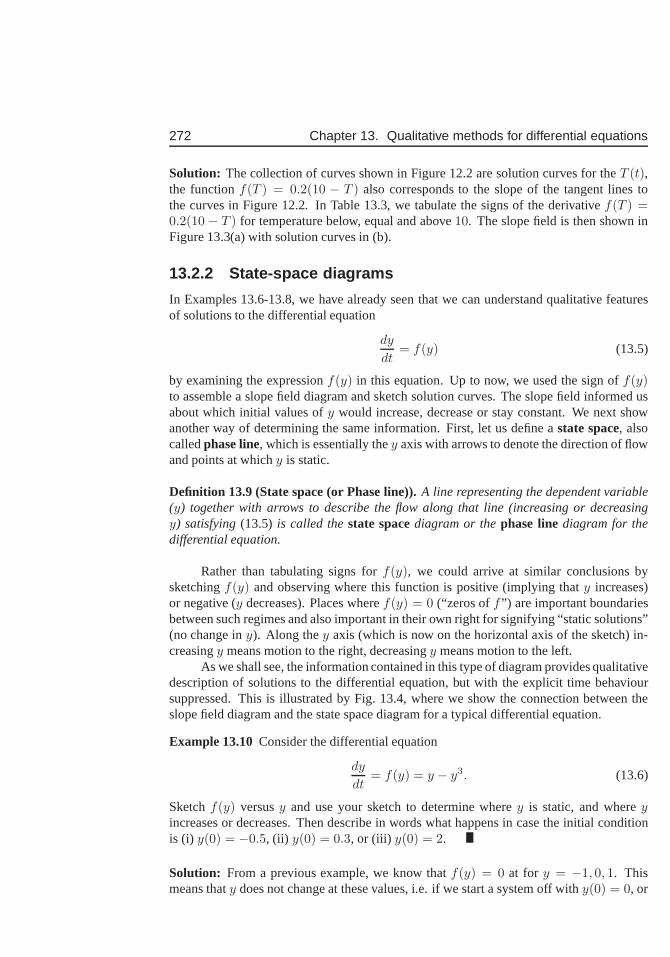
272 Chapter 13. Qualitative methods for differential equations
Solution: The collection of curves shown in Figure 12.2 are solution curves for theT (t),the functionf(T ) = 0.2(10 − T ) also corresponds to the slope of the tangent lines tothe curves in Figure 12.2. In Table 13.3, we tabulate the signs of the derivativef(T ) =0.2(10 − T ) for temperature below, equal and above10. The slope field is then shown inFigure 13.3(a) with solution curves in (b).
13.2.2 State-space diagrams
In Examples 13.6-13.8, we have already seen that we can understand qualitative featuresof solutions to the differential equation
dy
dt= f(y) (13.5)
by examining the expressionf(y) in this equation. Up to now, we used the sign off(y)to assemble a slope field diagram and sketch solution curves.The slope field informed usabout which initial values ofy would increase, decrease or stay constant. We next showanother way of determining the same information. First, letus define astate space, alsocalledphase line, which is essentially they axis with arrows to denote the direction of flowand points at whichy is static.
Definition 13.9 (State space (or Phase line)).A line representing the dependent variable(y) together with arrows to describe the flow along that line (increasing or decreasingy) satisfying(13.5) is called thestate spacediagram or thephase linediagram for thedifferential equation.
Rather than tabulating signs forf(y), we could arrive at similar conclusions bysketchingf(y) and observing where this function is positive (implying that y increases)or negative (y decreases). Places wheref(y) = 0 (“zeros off ”) are important boundariesbetween such regimes and also important in their own right for signifying “static solutions”(no change iny). Along they axis (which is now on the horizontal axis of the sketch) in-creasingy means motion to the right, decreasingy means motion to the left.
As we shall see, the information contained in this type of diagram provides qualitativedescription of solutions to the differential equation, butwith the explicit time behavioursuppressed. This is illustrated by Fig. 13.4, where we show the connection between theslope field diagram and the state space diagram for a typical differential equation.
Example 13.10Consider the differential equation
dy
dt= f(y) = y − y3. (13.6)
Sketchf(y) versusy and use your sketch to determine wherey is static, and whereyincreases or decreases. Then describe in words what happensin case the initial conditionis (i) y(0) = −0.5, (ii) y(0) = 0.3, or (iii) y(0) = 2.
Solution: From a previous example, we know thatf(y) = 0 at for y = −1, 0, 1. Thismeans thaty does not change at these values, i.e. if we start a system off with y(0) = 0, or
13.2. The geometry of change 273
y
t
y
y
f (y)
(a) (b) (c)
Figure 13.4. The relationship of the slope field and state space diagrams.(a) Atypical slope field. A few arrows have been added to indicate the direction of time flowalong the tangent vectors. Now consider “looking down the time axis” as shown by the“eye” in this diagram. Then thet axis points towards us, and we see only they axisas in (b). Arrows on they axis indicate the directions of flow for various values ofyas determined in (a). Now “rotate” they axis so it is horizontal, as shown in (c). Thedirection of the arrows exactly correspond to places wheref(y), in (c), is positive (whichimplies increasingy, →), or negative (which implies decreasingy, ←). The state spacediagram is they axis in (b) or (c).
y(0) = ±1, the value ofy will be static. The three places at which this happens are markedby heavy dots in Figure 13.5(a).
We also see thatf(y) < 0 for−1 < y < 0 and fory > 1. This means that the rate ofchange ofy is negative whenever−1 < y < 0 or y > 1, which, in turn, implies that if thevalue ofy(t) falls in either of these intervals at any timet, theny(t) must be a decreasingfunction of time. On the other hand, for0 < y < 1 or for y < −1, we havef(y) > 0, soy(t) is increasing. See arrows on Figure 13.5(b). We see from the directions marked thatthere is a tendency fory to move away from the valuey = 0 and to approach either of thevalues1 or −1 as time goes by. Starting from the initial values given above, we have (i)y(0) = −0.5 results iny → −1, (ii) y(0) = 0.3 leads toy → 1, and (iii) y(0) = 2 impliesy →∞.
Example 13.11 (A cooling object:)Sketch the same type of diagrams for the problem ofa cooling object and interpret its meaning.
Solution: Here, the differential equation is
dT
dt= f(T ) = 0.2(10− T ).
Here, the functionf(T ) = 0.2(10 − T ) is the rate of change associated with a giventemperatureT . A sketch of the rate of change,F (T ) versus the temperatureT is shown inFigure 13.6(a).
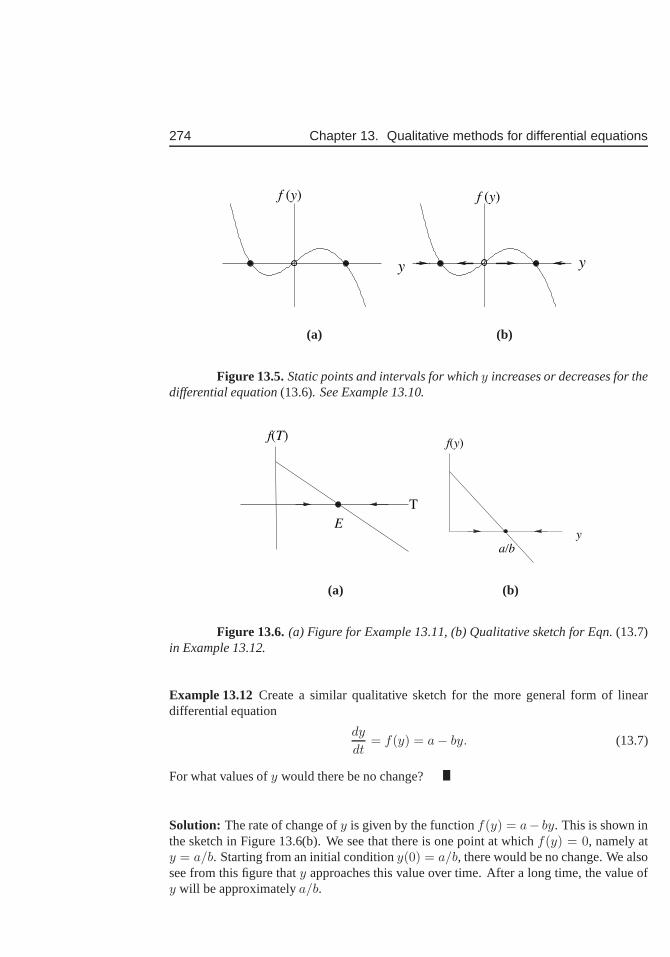
274 Chapter 13. Qualitative methods for differential equations
y
f (y)
y
f (y)
(a) (b)
Figure 13.5.Static points and intervals for whichy increases or decreases for thedifferential equation(13.6). See Example 13.10.
T
f(T)
E
f(y)
ya/b
(a) (b)
Figure 13.6.(a) Figure for Example 13.11, (b) Qualitative sketch for Eqn. (13.7)in Example 13.12.
Example 13.12Create a similar qualitative sketch for the more general form of lineardifferential equation
dy
dt= f(y) = a− by. (13.7)
For what values ofy would there be no change?
Solution: The rate of change ofy is given by the functionf(y) = a− by. This is shown inthe sketch in Figure 13.6(b). We see that there is one point atwhich f(y) = 0, namely aty = a/b. Starting from an initial conditiony(0) = a/b, there would be no change. We alsosee from this figure thaty approaches this value over time. After a long time, the valueofy will be approximatelya/b.
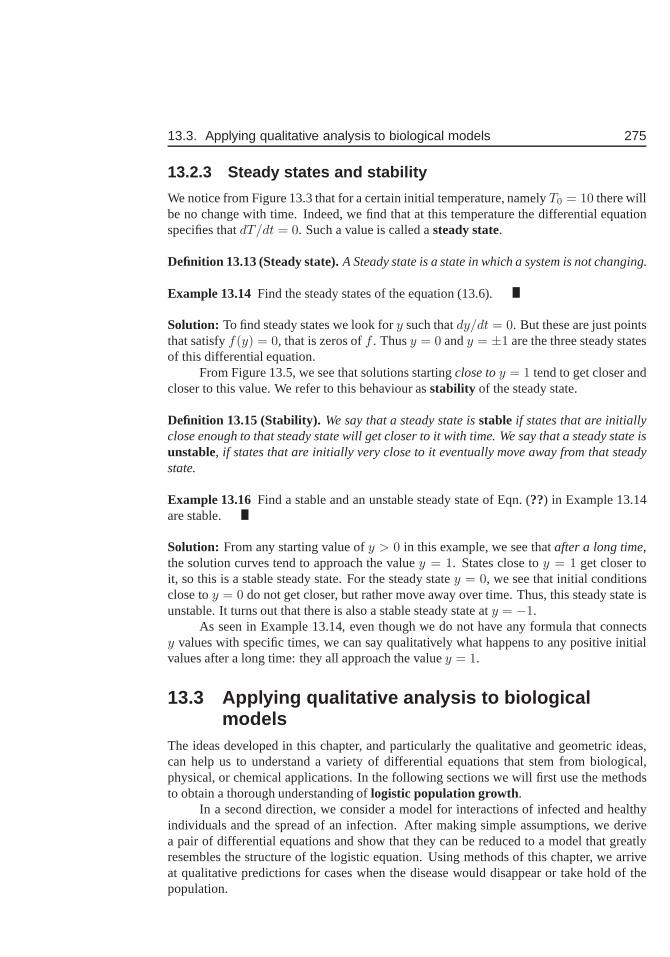
13.3. Applying qualitative analysis to biological models 275
13.2.3 Steady states and stability
We notice from Figure 13.3 that for a certain initial temperature, namelyT0 = 10 there willbe no change with time. Indeed, we find that at this temperature the differential equationspecifies thatdT/dt = 0. Such a value is called asteady state.
Definition 13.13 (Steady state).A Steady state is a state in which a system is not changing.
Example 13.14Find the steady states of the equation (13.6).
Solution: To find steady states we look fory such thatdy/dt = 0. But these are just pointsthat satisfyf(y) = 0, that is zeros off . Thusy = 0 andy = ±1 are the three steady statesof this differential equation.
From Figure 13.5, we see that solutions startingclose toy = 1 tend to get closer andcloser to this value. We refer to this behaviour asstability of the steady state.
Definition 13.15 (Stability). We say that a steady state isstable if states that are initiallyclose enough to that steady state will get closer to it with time. We say that a steady state isunstable, if states that are initially very close to it eventually move away from that steadystate.
Example 13.16Find a stable and an unstable steady state of Eqn. (??) in Example 13.14are stable.
Solution: From any starting value ofy > 0 in this example, we see thatafter a long time,the solution curves tend to approach the valuey = 1. States close toy = 1 get closer toit, so this is a stable steady state. For the steady statey = 0, we see that initial conditionsclose toy = 0 do not get closer, but rather move away over time. Thus, this steady state isunstable. It turns out that there is also a stable steady state aty = −1.
As seen in Example 13.14, even though we do not have any formula that connectsy values with specific times, we can say qualitatively what happens to any positive initialvalues after a long time: they all approach the valuey = 1.
13.3 Applying qualitative analysis to biologicalmodels
The ideas developed in this chapter, and particularly the qualitative and geometric ideas,can help us to understand a variety of differential equations that stem from biological,physical, or chemical applications. In the following sections we will first use the methodsto obtain a thorough understanding oflogistic population growth.
In a second direction, we consider a model for interactions of infected and healthyindividuals and the spread of an infection. After making simple assumptions, we derivea pair of differential equations and show that they can be reduced to a model that greatlyresembles the structure of the logistic equation. Using methods of this chapter, we arriveat qualitative predictions for cases when the disease woulddisappear or take hold of thepopulation.
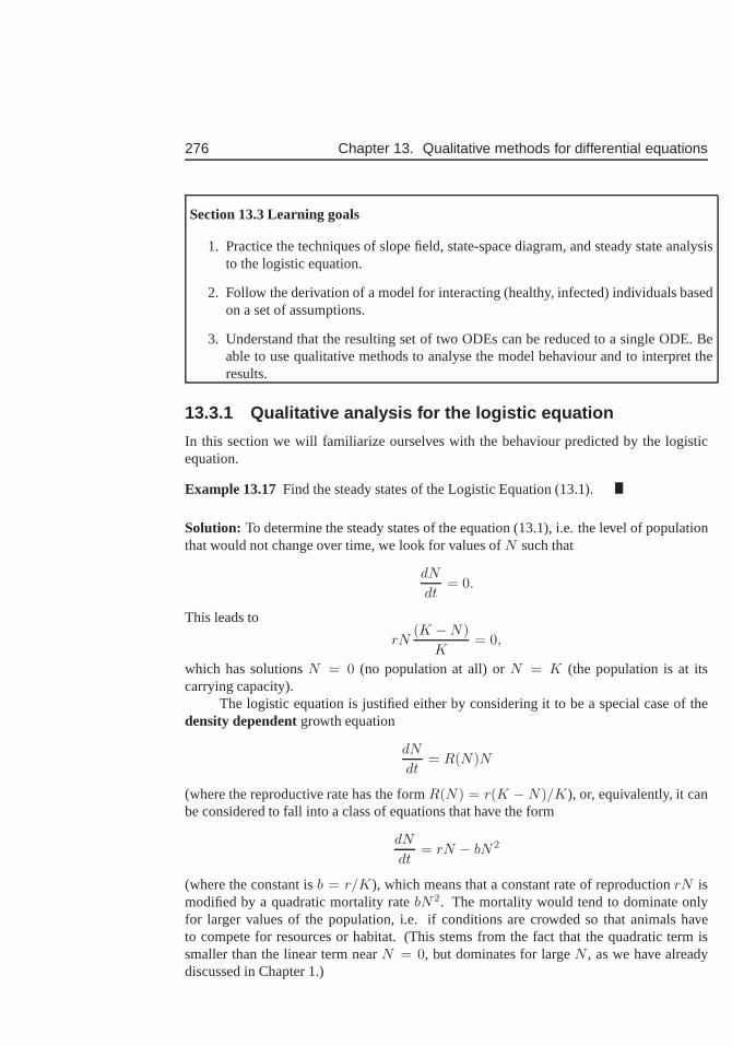
276 Chapter 13. Qualitative methods for differential equations
Section 13.3 Learning goals
1. Practice the techniques of slope field, state-space diagram, and steady state analysisto the logistic equation.
2. Follow the derivation of a model for interacting (healthy, infected) individuals basedon a set of assumptions.
3. Understand that the resulting set of two ODEs can be reduced to a single ODE. Beable to use qualitative methods to analyse the model behaviour and to interpret theresults.
13.3.1 Qualitative analysis for the logistic equation
In this section we will familiarize ourselves with the behaviour predicted by the logisticequation.
Example 13.17Find the steady states of the Logistic Equation (13.1).
Solution: To determine the steady states of the equation (13.1), i.e. the level of populationthat would not change over time, we look for values ofN such that
dN
dt= 0.
This leads to
rN(K −N)
K= 0,
which has solutionsN = 0 (no population at all) orN = K (the population is at itscarrying capacity).
The logistic equation is justified either by considering it to be a special case of thedensity dependentgrowth equation
dN
dt= R(N)N
(where the reproductive rate has the formR(N) = r(K −N)/K), or, equivalently, it canbe considered to fall into a class of equations that have the form
dN
dt= rN − bN2
(where the constant isb = r/K), which means that a constant rate of reproductionrN ismodified by a quadratic mortality ratebN2. The mortality would tend to dominate onlyfor larger values of the population, i.e. if conditions are crowded so that animals haveto compete for resources or habitat. (This stems from the fact that the quadratic term issmaller than the linear term nearN = 0, but dominates for largeN , as we have alreadydiscussed in Chapter 1.)
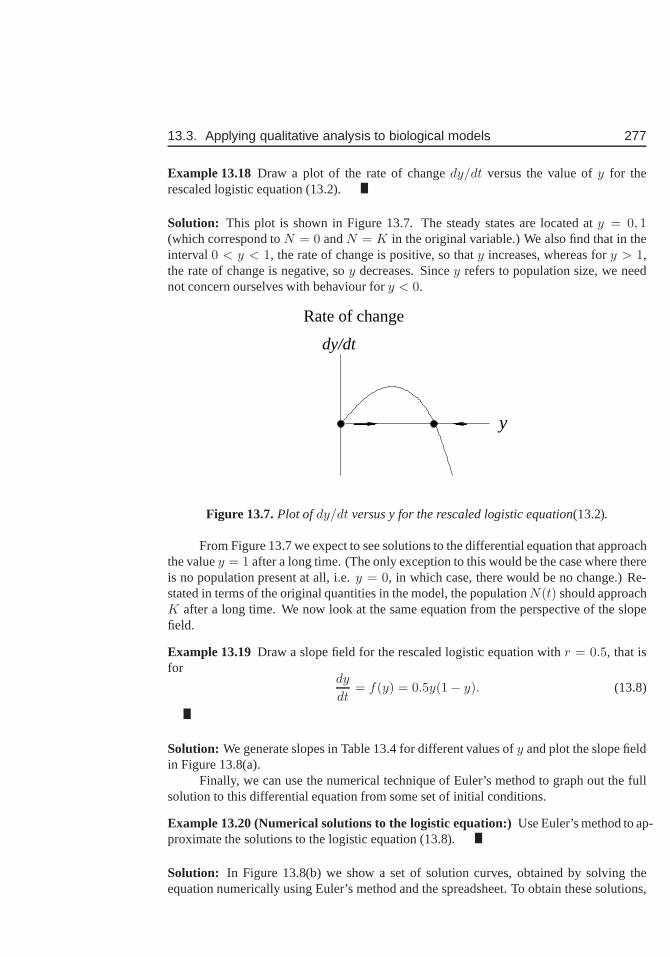
13.3. Applying qualitative analysis to biological models 277
Example 13.18Draw a plot of the rate of changedy/dt versus the value ofy for therescaled logistic equation (13.2).
Solution: This plot is shown in Figure 13.7. The steady states are located aty = 0, 1(which correspond toN = 0 andN = K in the original variable.) We also find that in theinterval0 < y < 1, the rate of change is positive, so thaty increases, whereas fory > 1,the rate of change is negative, soy decreases. Sincey refers to population size, we neednot concern ourselves with behaviour fory < 0.
Rate of change
dy/dt
y
Figure 13.7.Plot ofdy/dt versus y for the rescaled logistic equation(13.2).
From Figure 13.7 we expect to see solutions to the differential equation that approachthe valuey = 1 after a long time. (The only exception to this would be the case where thereis no population present at all, i.e.y = 0, in which case, there would be no change.) Re-stated in terms of the original quantities in the model, the populationN(t) should approachK after a long time. We now look at the same equation from the perspective of the slopefield.
Example 13.19Draw a slope field for the rescaled logistic equation withr = 0.5, that isfor
dy
dt= f(y) = 0.5y(1− y). (13.8)
Solution: We generate slopes in Table 13.4 for different values ofy and plot the slope fieldin Figure 13.8(a).
Finally, we can use the numerical technique of Euler’s method to graph out the fullsolution to this differential equation from some set of initial conditions.
Example 13.20 (Numerical solutions to the logistic equation:) Use Euler’s method to ap-proximate the solutions to the logistic equation (13.8).
Solution: In Figure 13.8(b) we show a set of solution curves, obtained by solving theequation numerically using Euler’s method and the spreadsheet. To obtain these solutions,
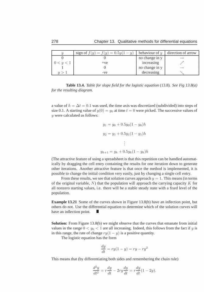
278 Chapter 13. Qualitative methods for differential equations
y sign off(y) = f(y) = 0.5y(1− y) behaviour ofy direction of arrow0 0 no change in y →
0 < y < 1 +ve increasing ր1 0 no change in y →
y > 1 -ve decreasing ց
Table 13.4.Table for slope field for the logistic equation(13.8). See Fig 13.8(a)for the resulting diagram.
a value ofh = ∆t = 0.1 was used, the time axis was discretized (subdivided) into steps ofsize 0.1. A starting value ofy(0) = y0 at timet = 0 were picked. The successive values ofy were calculated as follows:
y1 = y0 + 0.5y0(1− y0)h
y2 = y1 + 0.5y1(1− y1)h
...
yk+1 = yk + 0.5yk(1− yk)h
(The attractive feature of using a spreadsheet is that this repetition can be handled automat-ically by dragging the cell entry containing the results forone iteration down to generateother iterations. Another attractive feature is that once the method is implemented, it ispossible to change the initial condition very easily, just by changing a single cell entry.
From these results, we see that solution curves approachy = 1. This means (in termsof the original variable,N ) that the population will approach the carrying capacityK forall nonzero starting values, i.e. there will be a stable steady state with a fixed level of thepopulation.
Example 13.21Some of the curves shown in Figure 13.8(b) have an inflection point, butothers do not. Use the differential equation to determine which of the solution curves willhave an inflection point.
Solution: From Figure 13.8(b) we might observe that the curves that emanate from initialvalues in the range0 < y0 < 1 are all increasing. Indeed, this follows from the fact ify isin this range, the rate of changery(1− y) is a positive quantity.
The logistic equation has the form
dy
dt= ry(1 − y) = ry − ry2
This means that (by differentiating both sides and remembering the chain rule)
d2y
dt2= r
dy
dt− 2ry
dy
dt= r
dy
dt(1− 2y).
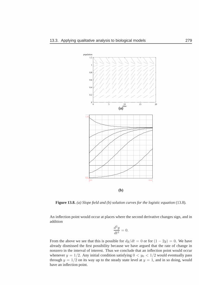
13.3. Applying qualitative analysis to biological models 279
0
0.2
0.4
0.6
0.8
1
1.2
population
0 5 10 15 20time
(a)
0.0 10.0
0.0
1.25
(b)
Figure 13.8.(a) Slope field and (b) solution curves for the logistic equation (13.8).
An inflection point would occur at places where the second derivative changes sign, and inaddition
d2y
dt2= 0.
From the above we see that this is possible fordy/dt = 0 or for (1 − 2y) = 0. We havealready dismissed the first possibility because we have argued that the rate of change innonzero in the interval of interest. Thus we conclude that aninflection point would occurwhenevery = 1/2. Any initial condition satisfying0 < y0 < 1/2 would eventually passthroughy = 1/2 on its way up to the steady state level aty = 1, and in so doing, wouldhave an inflection point.
280 Chapter 13. Qualitative methods for differential equations
13.3.2 A model for the spread of a disease
In the era of human immunodeficiency virus (HIV), Severe acute respiratory syndrome(SARS), Avian influenza (“bird flu”) and similar emerging infectious diseases, we are facedwith questions about how infection spreads, and how it can becontrolled or suppressed.Sustaining the health of the public at large requires an understanding of the dynamics ofdisease, motivating a simple example discussed here.
We consider a population with two types of individuals, those that are healthy andthose that are currently infected. We will assume that all healthy individuals are susceptibleto catching the infection, and those that are currently infected are also infectious, whichmeans that they can transmit the infection to others throughsocial interactions. We alsoassume that the infection is mild enough that individuals recover at some constant rate, andthat there is no disease-related mortality. Furthermore, we will consider this scenario inthe context of a fixed population (with no birth, death or migration during the timescaleof interest). Our goal in this section is to predict whether the infection would spread andtake hold in the population or whether it would run its courseand disappear. We will findthat this example illustrates the methods used so far and allows us to draw conclusions thatwere not intuitively obvious to begin with.
Let us use the following notation:
S(t) = size of population of susceptible (healthy) individuals
I(t) = size of population of infected individuals
N(t) = S(t) + I(t) = total population size
We make a few simplifying assumptions.
1. The population mixes very well, so each individual is equally likely to contact andinteract with any other individual. The contact is random.
2. Other than the state (S or I), individuals are “identical”. They recover at the same(constant) rate, and they have the same tendency to become infected.
3. On the timescale of interest, there is no birth, death or migration, only exchangebetweenS andI.
Example 13.22Suppose that the process can be represented by the scheme
S + I → I + I,
I → S
The first part, transmission of disease fromI to S involves interaction. The second partis recovery. Use the assumptions to track the two populations and to formulate a set ofdifferential equations forI(t) andS(t).
Solution: We first write down the following “word equations” to keep track of individuals
Rate ofchange of
I(t)
=
Rate of Gaindue to diseasetransmission
−
Rate of lossdue to
recovery
13.3. Applying qualitative analysis to biological models 281
According to our assumption, recovery takes place at a constant rate. We denote that rateby µ > 0 per unit time. By the law of mass action, the disease transmission rate should beproportional to the product of the populations,(S · I). Assigningβ > 0 to be the constantof proportionality leads to the following differential equations for the infected population(which simply restates the “word equation” in mathematicalnotation):
dI
dt= βSI − µI.
Similarly, we can write a word equation that tracks the population of susceptibles:
Rate ofchange of
S(t)
= −
Rate of Lossdue to diseasetransmission
+
Rate of gaindue to
recovery
Observe that loss from one group leads to (exactly balanced)gain in the other group. Bysimilar logic, the differential equation forS(t) is then
dS
dt= −βSI + µI.
We have arrived at two differential equations that describethe changes in each of thegroups,
dI
dt= βSI − µI, (13.9a)
dS
dt= −βSI + µI. (13.9b)
It is evident from Eqs. (13.9) that changes in one populationare linked to the levels of both,which means that the differential equations arecoupled(linked to one another). Hence, wecannot “solve one” independently of the other. We must treatthem as a pair. However, aswe will observe in the next examples, we can simplify thissystem of equationsusing thefact that the total population does not change.
Example 13.23Use equations (13.9) to show that the total population does not change.(Hint: show that the derivative ofS(t) + I(t) is zero.)
Solution: Add the equations to one another. Then we obtain
d
dt[I(t) + S(t)] =
dI
dt+
dS
dt= βSI − µI − βSI + µI = 0.
Henced
dt[I(t) + S(t)] =
dN
dt= 0,
which mean that the total population does not change, so thatN(t) = [I(t) + S(t)] =N=constant.
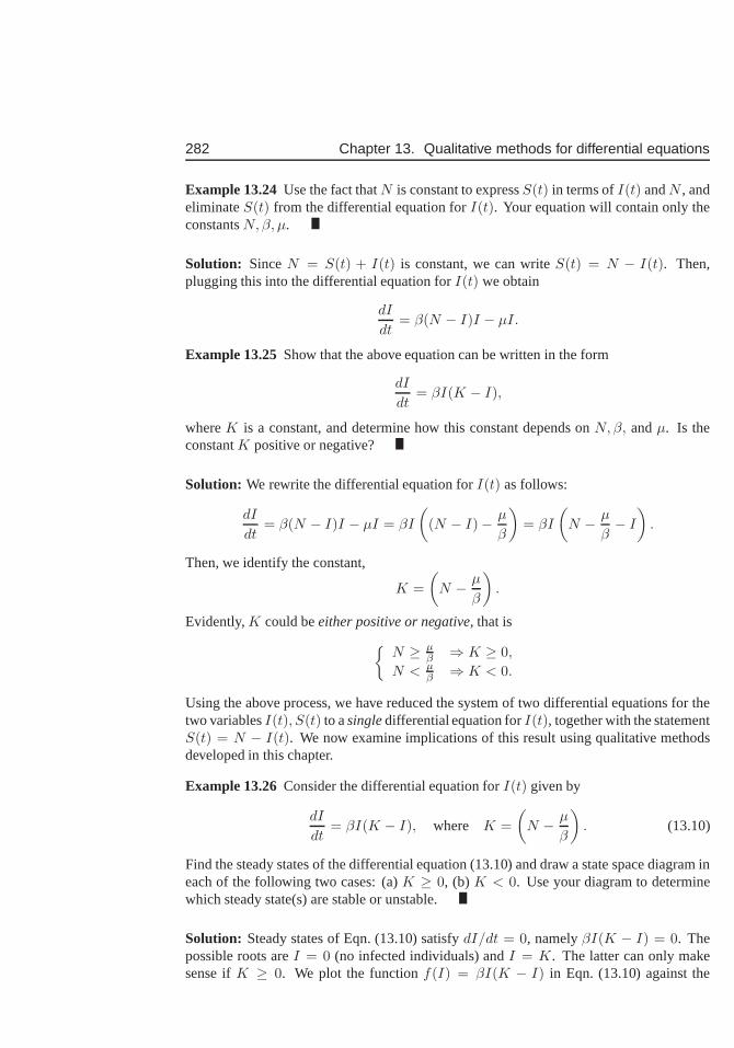
282 Chapter 13. Qualitative methods for differential equations
Example 13.24Use the fact thatN is constant to expressS(t) in terms ofI(t) andN , andeliminateS(t) from the differential equation forI(t). Your equation will contain only theconstantsN, β, µ.
Solution: SinceN = S(t) + I(t) is constant, we can writeS(t) = N − I(t). Then,plugging this into the differential equation forI(t) we obtain
dI
dt= β(N − I)I − µI.
Example 13.25Show that the above equation can be written in the form
dI
dt= βI(K − I),
whereK is a constant, and determine how this constant depends onN, β, andµ. Is theconstantK positive or negative?
Solution: We rewrite the differential equation forI(t) as follows:
dI
dt= β(N − I)I − µI = βI
(
(N − I)− µ
β
)
= βI
(
N − µ
β− I
)
.
Then, we identify the constant,
K =
(
N − µ
β
)
.
Evidently,K could beeither positive or negative, that is
{
N ≥ µβ ⇒ K ≥ 0,
N < µβ ⇒ K < 0.
Using the above process, we have reduced the system of two differential equations for thetwo variablesI(t), S(t) to asingledifferential equation forI(t), together with the statementS(t) = N − I(t). We now examine implications of this result using qualitative methodsdeveloped in this chapter.
Example 13.26Consider the differential equation forI(t) given by
dI
dt= βI(K − I), where K =
(
N − µ
β
)
. (13.10)
Find the steady states of the differential equation (13.10)and draw a state space diagram ineach of the following two cases: (a)K ≥ 0, (b) K < 0. Use your diagram to determinewhich steady state(s) are stable or unstable.
Solution: Steady states of Eqn. (13.10) satisfydI/dt = 0, namelyβI(K − I) = 0. Thepossible roots areI = 0 (no infected individuals) andI = K. The latter can only makesense ifK ≥ 0. We plot the functionf(I) = βI(K − I) in Eqn. (13.10) against the
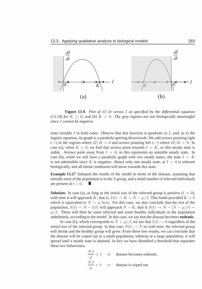
13.3. Applying qualitative analysis to biological models 283
K K
dI
dt
dI
dt
KK0 0I I
(a) (b)
Figure 13.9. Plot of dI/dt versusI as specified by the differential equation(13.10) for K ≥ 0, and (b)K < 0. The grey regions are not biologically meaningfulsinceI cannot be negative.
state variableI in both cases. Observe that this function is quadratic inI, and, as in thelogistic equation, its graph is a parabola opening downwards. We add arrows pointing right(→) in the regions wheredI/dt > 0 and arrows pointing left (←) wheredI/dt < 0. Incase (a), whenK ≥ 0, we find that arrows point towardsI = K, so this steady state isstable. Arrows point away fromI = 0, so this represents an unstable steady state. Incase (b), while we still have a parabolic graph with two steady states, the stateI = Kis not admissible sinceK is negative. Hence only one steady state, atI = 0 is relevantbiologically, and all initial conditions will move towardsthis state.
Example 13.27 Interpret the results of the model in terms of the disease, assuming thatinitially most of the population is in theS group, and a small number of infected individualsare present att = 0.
Solution: In case (a), as long as the initial size of the infected group is positive (I > 0),with time it will approachK, that is,I(t)→ K = N − µ/β. This holds providedK > 0which is equivalent toN > µ/beta. For this case, we also conclude that the rest of thepopulation,S(t) = N − I(t) will approachN − K, that isS(t) → N − (N − µ/β) =µ/β. There will then be some infected and some healthy individuals in the populationindefinitely, according to the model. In this case, we say that the disease becomesendemic.
In case (b), which corresponds toN < µ/β, we see thatI(t) → 0 regardless of theinitial size of the infected group. In that case,S(t) → N so with time, the infected groupwill shrink and the healthy group will grow. From these two results, we can conclude thatthe disease will be wiped out in a small population, whereas in a large population, it willspread until a steady state is attained. In fact we have identified a threshold that separatesthese two behaviours:
Nβ
µ> 1 ⇒ disease becomes endemic,
Nβ
µ< 1 ⇒ disease is wiped out.
284 Chapter 13. Qualitative methods for differential equations
The ratio of constants in these inequalities is called thereproductive number for the dis-ease. Many current and much more detailed models for diseasetransmission also havethreshold behaviour, and the ratio that determines whetherthe disease spreads or disappearsis denotedR0. This ratio represents the number of infections that arise when 1 infected in-dividual interacts with a population ofN susceptible individuals.

Exercises 285
Exercises13.1. Consider the differential equation
dy
dt= a− by
wherea, b are constants.
(a) Show that the function
y(t) =a
b− Ce−bt
satisfies the above differential equation for any constantC.
(b) Show that by setting
C =a
b− y0
we also satisfy the initial condition
y(0) = y0.
Remark: You have now shown that the function
y(t) =(
y0 −a
b
)
e−bt +a
b
is a solution to theinitial value problem(i.e differential equation plus initialcondition)
dy
dt= a− by, y(0) = y0.
13.2. Steps in an example:Complete the algebraic steps in Example 12.5 to show thatthe solution to Eqn. (12.3) can be obtained by the substitutionz(t) = a− by(t).
13.3. Verifying a solution: Show that the function
y(t) =1
1− t
is a solution to the differential equation and initial condition
dy
dt= y2, y(0) = 1.
Comment on what happens to this solution ast approaches1.
13.4. For each of the following, show the given functiony is a solution to the given dif-ferential equation.
(a) t · dy
dt= 3y, y = 2t3.
(b)d2y
dt2+ y = 0, y = −2 sin t + 3 cos t.
286 Chapter 13. Qualitative methods for differential equations
(c)d2y
dt2− 2
dy
dt+ y = 6et, y = 3t2et.
13.5. Show the function determined by the equation2x2 + xy − y2 = C, whereC is a
constant and2y 6= x, is a solution to the differential equation(x−2y)dy
dx= −4x−y.
13.6. Find the constantC that satisfies the given initial conditions.
(a) 2x2 − 3y2 = C, y|x=0 = 2.
(b) y = C1e5t + C2te
5t, y|t=0 = 1 and dydt |t=0 = 0.
(c) y = C1 cos(t− C2), y|t= π2
= 0 and dydt |t= π
2= 1.
13.7. Friction and terminal velocity: The velocity of a falling object changes due to theacceleration of gravity, but friction has an effect of slowing down this acceleration.The differential equation satisfied by the velocityv(t) of the falling object is
dv
dt= g − kv
whereg is acceleration due to gravity andk is a constant that represents the effectof friction. An object is dropped from rest from a plane.
(a) Find the functionv(t) that represents its velocity over time.
(b) What happens to the velocity after the object has been falling for a long time(but before it has hit the ground)?
13.8. Alcohol level: Alcohol enters the blood stream at a constant ratek gm per unit timeduring a drinking session. The liver gradually converts thealcohol to other, non-toxic byproducts. The rate of conversion per unit time is proportional to the currentblood alcohol level, so that the differential equation satisfied by the blood alcohollevel is
dc
dt= k − sc
wherek, s are positive constants. Suppose initially there is no alcohol in the blood.Find the blood alcohol levelc(t) as a function of time fromt = 0, when the drinkingstarted.
13.9. Newton’s Law of Cooling: Newton’s Law of Cooling states that the rate of changeof the temperature of an object is proportional to the difference between the temper-ature of the object,T , and the ambient (environmental) temperature,E. This leadsto thedifferential equation
dT
dt= k(E − T )
wherek > 0 is a constant that represents the material properties and,E is theambient temperature. (We will assume thatE is also constant.)
(a) Show that the function
T (t) = E + (T0 − E)e−kt
which represents the temperature at timet satisfies this equation.
Exercises 287
(b) The time of death of a murder victim can be estimated from the temperature ofthe body if it is discovered early enough after the crime has occurred. Supposethat in a room whose ambient temperature isE = 20◦ C, the temperatureof the body upon discovery isT = 30◦ C, and that a second measurement,one hour later isT = 25◦ C. Determine the approximate time of death. (Youshould use the fact that just prior to death, the temperatureof the victim was37◦C.)
13.10. A cup of coffee:The temperature of a cup of coffee is initially 100 degrees C.Fiveminutes later, (t = 5) it is 50 degrees C. If the ambient temperature isA = 20degrees C, determine how long it takes for the temperature ofthe coffee to reach30degrees C.
13.11. Newton’s Law of Cooling applied to data: The following data was gathered inproducing Fig. 2.1 for cooling milk during yoghurt production. According to New-ton’s Law of Cooling, this data can be described by the formula
T = E + (T (0)− E) e−kt.
whereT (t) is the temperature of the milk (in degrees Fahrenheit) at time t (in min),E is the ambient temperature, andk is some constant that we will determine in thisproblem.
time (min) Temp0.0 190.00.5 185.51.0 182.01.5 179.22.0 176.02.5 172.93.0 169.53.5 167.04.0 164.64.5 162.25.0 159.8
(a) Rewrite this relationship in terms of the quantityY (t) = ln(T (t) − E), andshow thatY (t) is related linearly to the timet.
(b) Explain how the constantk could be found from this converted form of therelationship.
(c) Use the data in the table and your favorite spreadsheet (or similar software) toshow that the data so transformed appears to be close to linear. Assume thatthe ambient temperature wasE = 20◦F.
(d) Use the same software to determine the constantk by fitting a line to the trans-formed data.
13.12. Lake Fishing: Fish Unlimited is a company that manages the fish population in aprivate lake. They restock the lake at constant rate (To restock means to add fish to
288 Chapter 13. Qualitative methods for differential equations
the lake).N fishers are allowed to fish in the lake per day. The population of fish inthe lake,F (t) is found to satisfy the differential equation
dF
dt= I − αNF (13.11)
(a) At what rate is fish added per day according to Eqn. (13.11)? (Give value andunits.) What is the average number of fish caught by one fisher?(Give valueand units.) What is being assumed about the fish birth and mortality rates inEqn. (13.11)?
(b) If the fish input and number of fishers are constant, what isthe steady statelevel of the fish population in the lake?
(c) At timet = 0 the company stops restocking the lake with fish. Write down therevised form of the differential equation (13.11) that takes this into account.(Assume the same level of fishing as before.) How long would ittake for thefish to fall to 25% of their initial level?
(d) When the fish population drops to the levelFlow, fishing is stopped and thelake is restocked with fish at the same constant rate (Eqn (13.11), withα = 0.)Write down the revised version of (13.11) that takes this into account. Howlong would it take for the fish population to double?
13.13. Glucose solution in a tank:A tank that holds 1 liter is initially full of plain water.A concentrated solution of glucose, containing 0.25 gm/cm3 is pumped into thetank continuously, at the rate 10 cm3/min and the mixture (which is continuouslystirred to keep it uniform) is pumped out at the same rate. Howmuch glucose willthere be in the tank after 30 minutes? After a long time? (Hint: write a differentialequation for c, the concentration of glucose in the tank by considering the rate atwhich glucose enters and the rate at which glucose leaves thetank.)
13.14. Pollutant in a lake:(From the Dec 1993 Math 100 Exam) A lake of constant volumeV gallons containsQ(t) pounds of pollutant at timet evenly distributed throughout the lake. Watercontaining a concentration ofk pounds per gallon of pollutant enters the lake at arate ofr gallons per minute, and the well-mixed solution leaves at the same rate.
(a) Set up a differential equation that describes the way that the amount of pollu-tant in the lake will change.
(b) Determine what happens to the pollutant level after a long time if this processcontinues.
(c) If k = 0 find the timeT for the amount of pollutant to be reduced to one halfof its initial value.
13.15. A sugar solution: Sugar dissolves in water at a rate proportional to the amountofsugar not yet in solution. LetQ(t) be the amount of sugar undissolved at timet.The initial amount is100 kg and after4 hours the amount undissolved is70 kg.
(a) Find a differential equation forQ(t) and solve it.
(b) How long will it take for50 kg to dissolve?
Exercises 289
13.16. Leaking water tank: A cylindrical tank with cross-sectional areaA has a smallhole through which water drains. The height of the water in the tanky(t) at timetis given by:
y(t) = (√
y0 −kt
2A)2
wherek, y0 are constants.
(a) Show that the height of the water,y(t), satisfies the differential equation
dy
dt= − k
A
√y.
(b) What is the initial height of the water in the tank at timet = 0 ?
(c) At what time will the tank be empty ?
(d) At what rate is thevolumeof the water in the tank changing whent = 0?
13.17. Find those constantsa, b so thaty = ex andy = e−x are both solutions of thedifferential equation
y′′ + ay′ + by = 0.
13.18. Lety = f(t) = e−t sin t, −∞ < t <∞.
(a) Show thaty satisfies the differential equationy′′ + 2y′ + 2y = 0.
(b) Find all critical points off(t).
290 Chapter 13. Qualitative methods for differential equations
Chapter 14
Trigonometric functions
In this chapter we will explore trigonometric functions andtheir properties. This importantnew class of functions will be introduced here; their basic properties and interconnectionswill be discussed. Belonging to a wider class of periodic functions, these illustrate the ideasof amplitude, frequency, period, and phase. We will find thatmany cyclic phenomena canbe described approximately by suitably adjusted basic functions such as sine and cosine. Asa second theme, we return to the idea of inverse functions andshow that important restric-tions must be applied to ensure the existence of an inverse, particularly for the trigonometricfunctions. Then, in the next chapter, we calculate the derivatives of trigonometric functionsand show applications to rates of change of periodic phenomena or changing angles.
14.1 Basic trigonometryTrigonometric functions are closely associated with angles and ratios of sides of a right-angle triangle. But they are also connected to motion of a point around a unit circle. Beforewe can understand these connections, we agree on a universalway of measuring angles,and then define the functions of interest.
Section 14.1 Learning goals
1. Understand the definition of theradian as a measure for angles.
2. Understand the correspondence between a point moving on aunit circle and the sineand cosine of the angle it forms at the origin.
3. Be able to make correspondence between ratios of sides of aPythagorean triangleand the trigonometric functions of one of its angles.
4. Review properties of the functionssin(x) andcos(x) and other trigonometric func-tions. Understand and be able to state and apply the connections between thesefunctions (“trigonometric identities”).
291
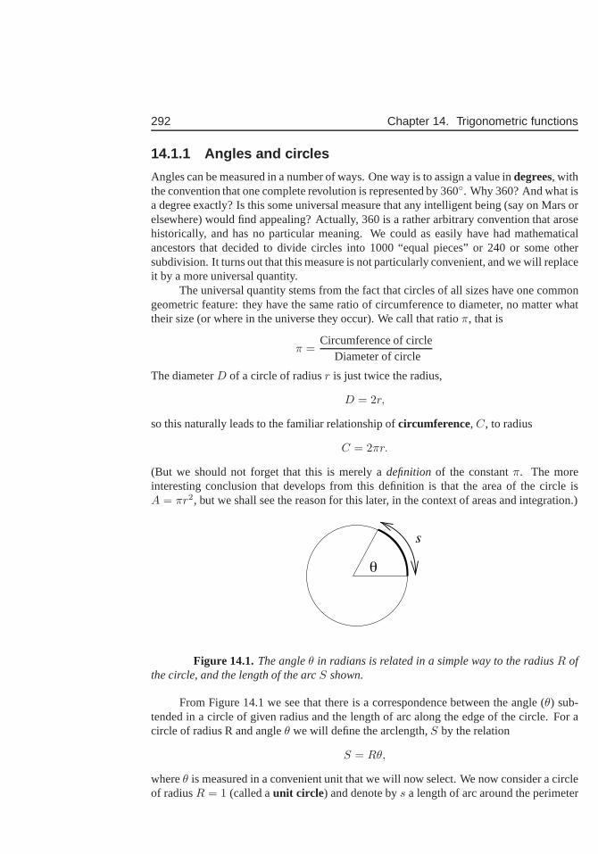
292 Chapter 14. Trigonometric functions
14.1.1 Angles and circles
Angles can be measured in a number of ways. One way is to assigna value indegrees, withthe convention that one complete revolution is representedby 360◦. Why 360? And what isa degree exactly? Is this some universal measure that any intelligent being (say on Mars orelsewhere) would find appealing? Actually, 360 is a rather arbitrary convention that arosehistorically, and has no particular meaning. We could as easily have had mathematicalancestors that decided to divide circles into 1000 “equal pieces” or 240 or some othersubdivision. It turns out that this measure is not particularly convenient, and we will replaceit by a more universal quantity.
The universal quantity stems from the fact that circles of all sizes have one commongeometric feature: they have the same ratio of circumference to diameter, no matter whattheir size (or where in the universe they occur). We call thatratioπ, that is
π =Circumference of circle
Diameter of circle
The diameterD of a circle of radiusr is just twice the radius,
D = 2r,
so this naturally leads to the familiar relationship ofcircumference, C, to radius
C = 2πr.
(But we should not forget that this is merely adefinitionof the constantπ. The moreinteresting conclusion that develops from this definition is that the area of the circle isA = πr2, but we shall see the reason for this later, in the context of areas and integration.)
θ
s
Figure 14.1.The angleθ in radians is related in a simple way to the radiusR ofthe circle, and the length of the arcS shown.
From Figure 14.1 we see that there is a correspondence between the angle (θ) sub-tended in a circle of given radius and the length of arc along the edge of the circle. For acircle of radius R and angleθ we will define the arclength,S by the relation
S = Rθ,
whereθ is measured in a convenient unit that we will now select. We now consider a circleof radiusR = 1 (called aunit circle ) and denote bys a length of arc around the perimeter
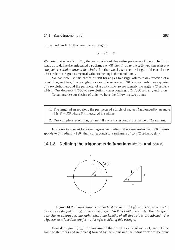
14.1. Basic trigonometry 293
of this unit circle. In this case, the arc length is
S = Rθ = θ.
We note that whenS = 2π, the arc consists of the entire perimeter of the circle. Thisleads us to define the unit called aradian: we will identify an angle of2π radians with onecomplete revolution around the circle. In other words, we use the length of the arc in theunit circle to assign a numerical value to the angle that it subtends.
We can now use this choice of unit for angles to assign values to any fraction of arevolution, and thus, to any angle. For example, an angle of90◦ corresponds to one quarterof a revolution around the perimeter of a unit circle, so we identify the angleπ/2 radianswith it. One degree is1/360 of a revolution, corresponding to2π/360 radians, and so on.
To summarize our choice of units we have the following two points:
1. The length of an arc along the perimeter of a circle of radiusR subtended by an angleθ is S = Rθ whereθ is measured in radians.
2. One complete revolution, or one full cycle corresponds toan angle of2π radians.
It is easy to convert between degrees and radians if we remember that360◦ corre-sponds to2π radians. (180◦ then corresponds toπ radians,90◦ to π/2 radians, etc.)
14.1.2 Defining the trigonometric functions sin(x) and cos(x)
t
t
y
x
(x,y)
1
Figure 14.2.Shown above is the circle of radius 1,x2+y2 = 1. The radius vectorthat ends at the point(x, y) subtends an anglet (radians) with thex axis. The triangle isalso shown enlarged to the right, where the lengths of all three sides are labeled. Thetrigonometric functions are just ratios of two sides of thistriangle.
Consider a point(x, y) moving around the rim of a circle of radius 1, and lett besome angle (measured in radians) formed by thex axis and the radius vector to the point
294 Chapter 14. Trigonometric functions
(x, y) as shown in Figure 14.2. We the functions sine and cosine, both dependent on theanglet (abbreviatedsin(t) andcos(t)) as follows:
sin(t) =y
1= y, cos(t) =
x
1= x
That is, the function sine tracks they coordinate of the point as it moves around the unitcircle, and the function cosine tracks itsx coordinate. (Remark: see also the review defini-tions of these trigonometric quantities as shown in Figure F.1 of Appendix F as the oppositeover hypotenuse and adjacent over hypotenuse in a right angle triangle. The hypotenuse inour diagram is simply the radius of the circle, which is 1 by assumption.)
14.1.3 Properties of sin(x) and cos(x)
We now explore the consequences of these definitions:
Values of sine and cosine
• The radius of the circle is 1. This means that thex coordinate cannot be largerthan 1 or smaller than -1. Same holds for they coordinate. Thus the functionssin(t) andcos(t) are always swinging between -1 and 1. (−1 ≤ sin(t) ≤ 1 and−1 ≤ cos(t) ≤ 1 for all t). The peak (maximum) value of each function is 1, theminimum is -1, and the average value is 0.
• When the radius vector points along thex axis, the angle ist = 0 and we havey = 0, x = 1. This means thatcos(0) = 1, sin(0) = 0.
• When the radius vector points up they axis, the angle isπ/2 (corresponding toone quarter of a complete revolution), and herex = 0, y = 1 so thatcos(π/2) =0, sin(π/2) = 1.
• Using simple geometry, we can also determine the lengths of all sides, and hence theratios of the sides in a few particularly simple triangles, namely equilateral triangles(in which all angles are60◦), and right triangles with two equal angles of45◦. Thesetypes of calculations (omitted here) lead to some easily determined values for thesine and cosine of such special angles. These values are shown in Table F.1 of theAppendix F.
Connection between sine and cosine
• The two functions, sine and cosine depict the same underlying motion, viewed fromtwo perspectives:cos(t) represents the projection of the circularly moving point ontothex axis, whilesin(t) is the projection of that point onto they axis. In this sense, thefunctions are a pair of twins, and we can expect many relationships to hold betweenthem.
• The cosine has its largest value at the beginning of the cycle, whent = 0 (sincecos(0) = 1), while the other the sine its peak value a little later, (sin(π/2) = 1).
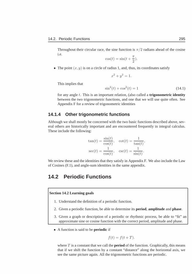
14.2. Periodic Functions 295
Throughout their circular race, the sine function isπ/2 radians ahead of the cosinei.e.
cos(t) = sin(t +π
2).
• The point(x, y) is on a circle of radius 1, and, thus, its coordinates satisfy
x2 + y2 = 1.
This implies thatsin2(t) + cos2(t) = 1 (14.1)
for any anglet. This is an important relation, (also called atrigonometric identitybetween the two trigonometric functions, and one that we will use quite often. SeeAppendix F for a review of trigonometric identities
14.1.4 Other trigonometric functions
Although we shall mostly be concerned with the two basic functions described above, sev-eral others are historically important and are encounteredfrequently in integral calculus.These include the following:
tan(t) =sin(t)
cos(t), cot(t) =
1
tan(t),
sec(t) =1
cos(t), csc(t) =
1
sin(t).
We review these and the identities that they satisfy in Appendix F. We also include the Lawof Cosines (F.1), and angle-sum identities in the same appendix.
14.2 Periodic Functions
Section 14.2 Learning goals
1. Understand the definition of a periodic function.
2. Given a periodic function, be able to determine itsperiod, amplitude andphase.
3. Given a graph or description of a periodic or rhythmic process, be able to “fit” anapproximate sine or cosine function with the correct period, amplitude and phase.
• A function is said to beperiodic if
f(t) = f(t + T ).
whereT is a constant that we call theperiod of the function. Graphically, this meansthat if we shift the function by a constant “distance” along the horizontal axis, wesee the same picture again. All the trigonometric functionsare periodic.
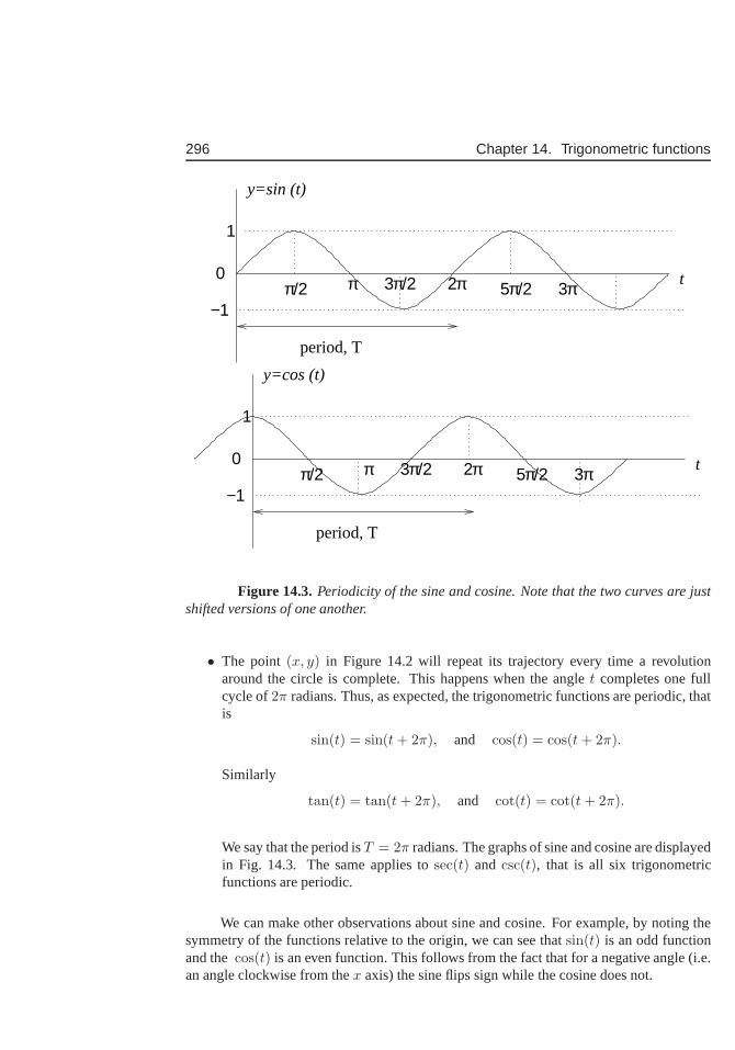
296 Chapter 14. Trigonometric functions
3π2πππ/2 3π/2 5π/2
1
−1
0
y=sin (t)
t
period, T
3π2πππ/2 3π/2 5π/2
1
−1
0 t
period, T
y=cos (t)
Figure 14.3.Periodicity of the sine and cosine. Note that the two curves are justshifted versions of one another.
• The point(x, y) in Figure 14.2 will repeat its trajectory every time a revolutionaround the circle is complete. This happens when the anglet completes one fullcycle of2π radians. Thus, as expected, the trigonometric functions are periodic, thatis
sin(t) = sin(t + 2π), and cos(t) = cos(t + 2π).
Similarly
tan(t) = tan(t + 2π), and cot(t) = cot(t + 2π).
We say that the period isT = 2π radians. The graphs of sine and cosine are displayedin Fig. 14.3. The same applies tosec(t) and csc(t), that is all six trigonometricfunctions are periodic.
We can make other observations about sine and cosine. For example, by noting thesymmetry of the functions relative to the origin, we can see thatsin(t) is an odd functionand thecos(t) is an even function. This follows from the fact that for a negative angle (i.e.an angle clockwise from thex axis) the sine flips sign while the cosine does not.
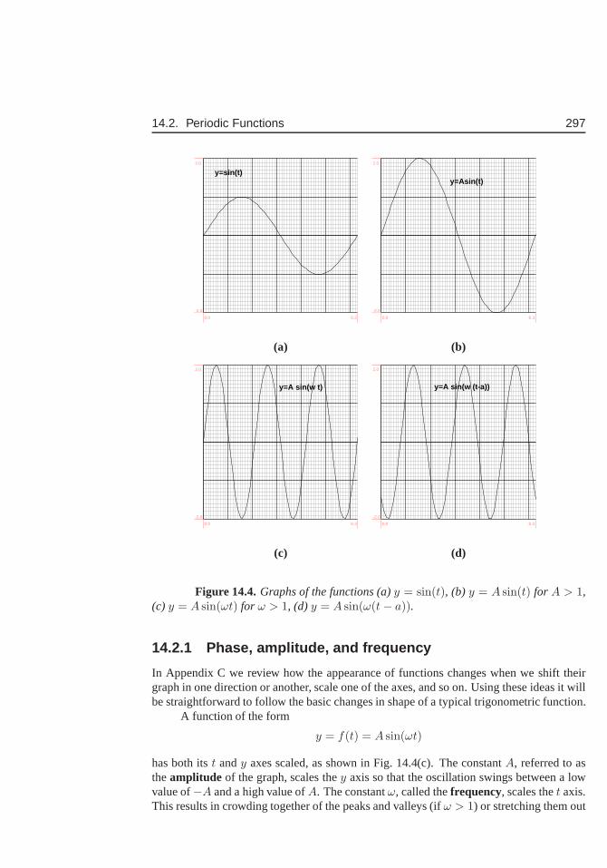
14.2. Periodic Functions 297
y=sin(t)
0.0 6.3
-2.0
2.0
y=Asin(t)
0.0 6.3
-2.0
2.0
(a) (b)
y=A sin(w t)
0.0 6.3
-2.0
2.0
y=A sin(w (t-a))
0.0 6.3
-2.0
2.0
(c) (d)
Figure 14.4.Graphs of the functions (a)y = sin(t), (b) y = A sin(t) for A > 1,(c) y = A sin(ωt) for ω > 1, (d) y = A sin(ω(t− a)).
14.2.1 Phase, amplitude, and frequency
In Appendix C we review how the appearance of functions changes when we shift theirgraph in one direction or another, scale one of the axes, and so on. Using these ideas it willbe straightforward to follow the basic changes in shape of a typical trigonometric function.
A function of the form
y = f(t) = A sin(ωt)
has both itst andy axes scaled, as shown in Fig. 14.4(c). The constantA, referred to astheamplitude of the graph, scales they axis so that the oscillation swings between a lowvalue of−A and a high value ofA. The constantω, called thefrequency, scales thet axis.This results in crowding together of the peaks and valleys (if ω > 1) or stretching them out
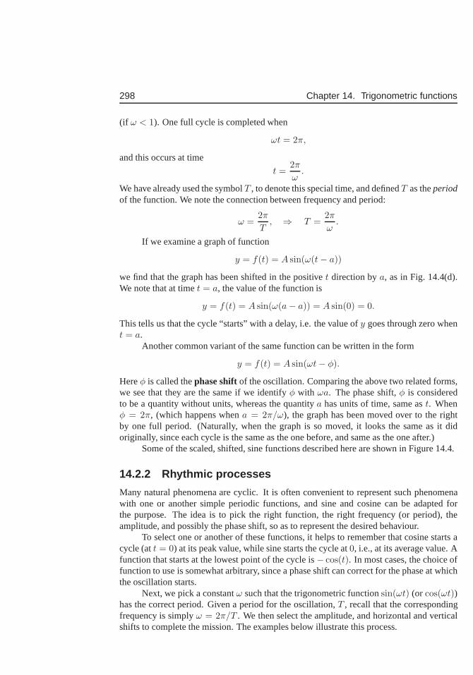
298 Chapter 14. Trigonometric functions
(if ω < 1). One full cycle is completed when
ωt = 2π,
and this occurs at time
t =2π
ω.
We have already used the symbolT , to denote this special time, and definedT as theperiodof the function. We note the connection between frequency and period:
ω =2π
T, ⇒ T =
2π
ω.
If we examine a graph of function
y = f(t) = A sin(ω(t− a))
we find that the graph has been shifted in the positivet direction bya, as in Fig. 14.4(d).We note that at timet = a, the value of the function is
y = f(t) = A sin(ω(a− a)) = A sin(0) = 0.
This tells us that the cycle “starts” with a delay, i.e. the value ofy goes through zero whent = a.
Another common variant of the same function can be written inthe form
y = f(t) = A sin(ωt− φ).
Hereφ is called thephase shiftof the oscillation. Comparing the above two related forms,we see that they are the same if we identifyφ with ωa. The phase shift,φ is consideredto be a quantity without units, whereas the quantitya has units of time, same ast. Whenφ = 2π, (which happens whena = 2π/ω), the graph has been moved over to the rightby one full period. (Naturally, when the graph is so moved, itlooks the same as it didoriginally, since each cycle is the same as the one before, and same as the one after.)
Some of the scaled, shifted, sine functions described here are shown in Figure 14.4.
14.2.2 Rhythmic processes
Many natural phenomena are cyclic. It is often convenient torepresent such phenomenawith one or another simple periodic functions, and sine and cosine can be adapted forthe purpose. The idea is to pick the right function, the rightfrequency (or period), theamplitude, and possibly the phase shift, so as to represent the desired behaviour.
To select one or another of these functions, it helps to remember that cosine starts acycle (att = 0) at its peak value, while sine starts the cycle at0, i.e., at its average value. Afunction that starts at the lowest point of the cycle is− cos(t). In most cases, the choice offunction to use is somewhat arbitrary, since a phase shift can correct for the phase at whichthe oscillation starts.
Next, we pick a constantω such that the trigonometric functionsin(ωt) (or cos(ωt))has the correct period. Given a period for the oscillation,T , recall that the correspondingfrequency is simplyω = 2π/T . We then select the amplitude, and horizontal and verticalshifts to complete the mission. The examples below illustrate this process.
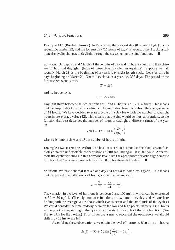
14.2. Periodic Functions 299
Example 14.1 (Daylight hours:) In Vancouver, the shortest day (8 hours of light) occursaround December 22, and the longest day (16 hours of light) isaround June 21. Approxi-mate the cyclic changes of daylight through the season usingthe sine function.
Solution: On Sept 21 and March 21 the lengths of day and night are equal, and then thereare 12 hours of daylight. (Each of these days is called anequinox). Suppose we callidentify March 21 as the beginning of a yearly day-night length cycle. Lett be time indays beginning on March 21. One full cycle takes a year, i.e. 365 days. The period of thefunction we want is thus
T = 365
and its frequency isω = 2π/365.
Daylight shifts between the two extremes of 8 and 16 hours: i.e. 12± 4 hours. This meansthat the amplitude of the cycle is 4 hours. The oscillation take place about the average valueof 12 hours. We have decided to start a cycle on a day for which the number of daylighthours is the average value (12). This means that the sine would be most appropriate, so thefunction that best describes the number of hours of daylightat different times of the yearis:
D(t) = 12 + 4 sin
(
2π
365t
)
wheret is time in days andD the number of hours of light.
Example 14.2 (Hormone levels:)The level of a certain hormone in the bloodstream fluc-tuates between undetectable concentration at 7:00 and 100 ng/ml at 19:00 hours. Approxi-mate the cyclic variations in this hormone level with the appropriate periodic trigonometricfunction. Lett represent time in hours from 0:00 hrs through the day.
Solution: We first note that it takes one day (24 hours) to complete a cycle. This meansthat the period of oscillation is 24 hours, so that the frequency is
ω =2π
T=
2π
24=
π
12.
The variation in the level of hormone is between 0 and 100 ng/ml, which can be expressedas 50± 50 ng/ml. (The trigonometric functions are symmetric cycles, and we are herefinding both the average value about which cycles occur and the amplitude of the cycles.)We could consider the time midway between the low and high points, namely 13:00 hoursas the point corresponding to the upswing at the start of a cycle of the sine function. (SeeFigure 14.5 for the sketch.) Thus, if we use a sine to represent the oscillation, we shouldshift it by 13 hrs to the left.
Assembling these observations, we obtain the level of hormone,H at timet in hours:
H(t) = 50 + 50 sin( π
12(t− 13)
)
.
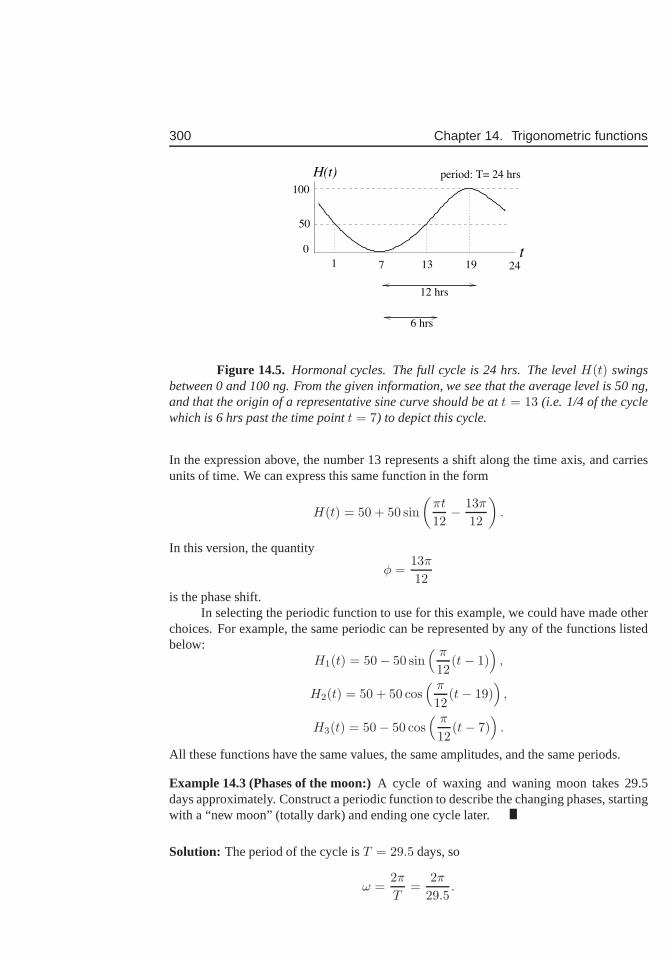
300 Chapter 14. Trigonometric functions
0
7 1913
50
100
t
12 hrs
H(t)
24
period: T= 24 hrs
6 hrs
1
Figure 14.5. Hormonal cycles. The full cycle is 24 hrs. The levelH(t) swingsbetween 0 and 100 ng. From the given information, we see that the average level is 50 ng,and that the origin of a representative sine curve should be at t = 13 (i.e. 1/4 of the cyclewhich is 6 hrs past the time pointt = 7) to depict this cycle.
In the expression above, the number 13 represents a shift along the time axis, and carriesunits of time. We can express this same function in the form
H(t) = 50 + 50 sin
(
πt
12− 13π
12
)
.
In this version, the quantity
φ =13π
12
is the phase shift.In selecting the periodic function to use for this example, we could have made other
choices. For example, the same periodic can be represented by any of the functions listedbelow:
H1(t) = 50− 50 sin( π
12(t− 1)
)
,
H2(t) = 50 + 50 cos( π
12(t− 19)
)
,
H3(t) = 50− 50 cos( π
12(t− 7)
)
.
All these functions have the same values, the same amplitudes, and the same periods.
Example 14.3 (Phases of the moon:)A cycle of waxing and waning moon takes 29.5days approximately. Construct a periodic function to describe the changing phases, startingwith a “new moon” (totally dark) and ending one cycle later.
Solution: The period of the cycle isT = 29.5 days, so
ω =2π
T=
2π
29.5.
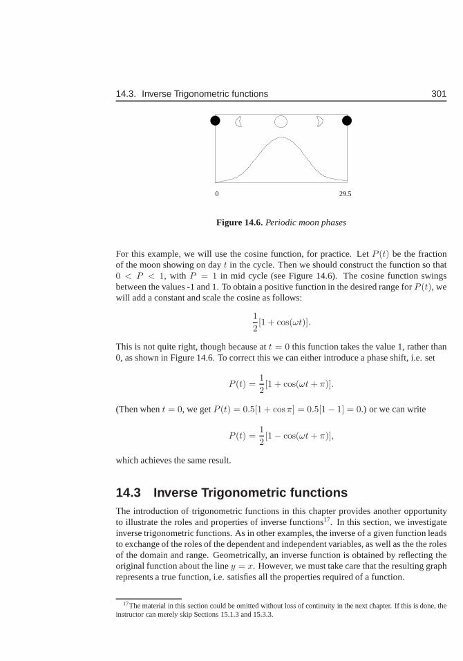
14.3. Inverse Trigonometric functions 301
0 29.5
Figure 14.6.Periodic moon phases
For this example, we will use the cosine function, for practice. LetP (t) be the fractionof the moon showing on dayt in the cycle. Then we should construct the function so that0 < P < 1, with P = 1 in mid cycle (see Figure 14.6). The cosine function swingsbetween the values -1 and 1. To obtain a positive function in the desired range forP (t), wewill add a constant and scale the cosine as follows:
1
2[1 + cos(ωt)].
This is not quite right, though because att = 0 this function takes the value 1, rather than0, as shown in Figure 14.6. To correct this we can either introduce a phase shift, i.e. set
P (t) =1
2[1 + cos(ωt + π)].
(Then whent = 0, we getP (t) = 0.5[1 + cosπ] = 0.5[1− 1] = 0.) or we can write
P (t) =1
2[1− cos(ωt + π)],
which achieves the same result.
14.3 Inverse Trigonometric functionsThe introduction of trigonometric functions in this chapter provides another opportunityto illustrate the roles and properties of inverse functions17. In this section, we investigateinverse trigonometric functions. As in other examples, theinverse of a given function leadsto exchange of the roles of the dependent and independent variables, as well as the the rolesof the domain and range. Geometrically, an inverse functionis obtained by reflecting theoriginal function about the liney = x. However, we must take care that the resulting graphrepresents a true function, i.e. satisfies all the properties required of a function.
17The material in this section could be omitted without loss ofcontinuity in the next chapter. If this is done, theinstructor can merely skip Sections 15.1.3 and 15.3.3.
302 Chapter 14. Trigonometric functions
Section 14.3 Learning goals
1. Review the concept of an inverse function, and be able to apply this idea to trigono-metric functions.
2. Understand the requirement of restricting the domain (ofthe original function) so asto be able to define its inverse. Given any of the trigonometric functions, be able toidentify a suitably restricted domain on which an inverse function can be defined.
3. Be able to simplify and/or interpret the meaning of expressions involving the trigono-metric and inverse trigonometric functions.
The domains ofsin(x) andcos(x) are both−∞ < x < ∞ while their ranges are−1 ≤ y ≤ 1. In the case of the functiontan(x), the domain excludes values±π/2 aswell as angles2nπ ± π/2 at which the function is undefined. The range oftan(x) is−∞ < y <∞.
There is one difficulty in defining inverses for trigonometric functions: the fact thatthese functions repeat their values in a cyclic pattern means that a giveny value is obtainedfrom many possible values ofx. For example, all of the valuesx = π/2, 5π/2, 7π/2, etcall have identical sine valuessin(x) = 1. We say that these functions are notone-to-one.Geometrically, this is just saying that the graphs of the trig functions intersect a horizontalline in numerous places. When these graphs are reflected about the liney = x, they wouldintersect avertical line in many places, and would fail to be functions: the function wouldhave multipley values corresponding to the same value ofx, which is not allowed. Thereader may recall that a similar difficulty was encountered in an earlier chapter with theinverse function fory = x2.
We can avoid this difficulty by restricting the domains of thetrigonometric functionsto a portion of their graphs that does not repeat. To do so, we select an interval overwhich the given trigonometric function is one-to -one, i.e.over which there is a uniquecorrespondence between values ofx and values ofy. (This just mean that we keep aportion of the graph of the function in which the y values are not repeated.) We then definethe corresponding inverse function, as described below.
Arcsine is the inverse of sine
The functiony = sin(x) is one-to-one on the interval−π/2 < x < π/2. We will definethe associated functiony = Sin(x) (shown in red on Figures 14.7(a) and (b) by restrictingthe domain of the sine function to−π/2 < x < π/2. On the given interval, we have−1 < Sin(x) < 1. We define the inverse function, called arcsine
y = arcsin(x) − 1 < x < 1
in the usual way, by reflection ofSin(x) through the liney = x as shown in Figure F.3(a).To interpret this function, we note thatarcsin(x) is “the angle whose sine isx”. In
Figure 14.8, we show a triangle in whichθ = arcsin(x). This follows from the observation
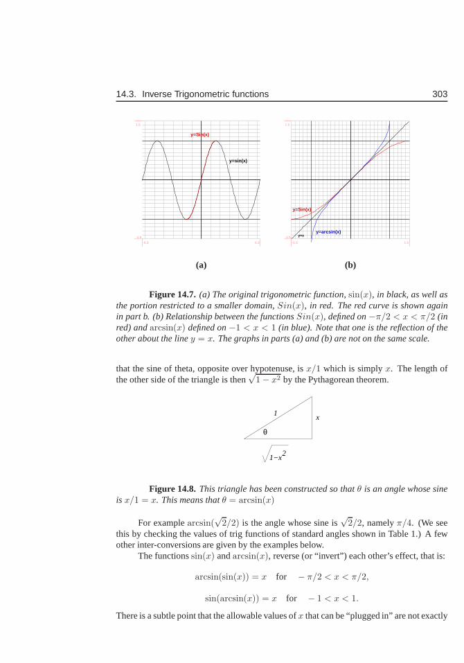
14.3. Inverse Trigonometric functions 303
y=sin(x)
y=Sin(x)
-6.3 6.3
-1.5
1.5
y=x
y=Sin(x)
y=arcsin(x)
-1.5 1.5
-1.5
1.5
(a) (b)
Figure 14.7. (a) The original trigonometric function,sin(x), in black, as well asthe portion restricted to a smaller domain,Sin(x), in red. The red curve is shown againin part b. (b) Relationship between the functionsSin(x), defined on−π/2 < x < π/2 (inred) andarcsin(x) defined on−1 < x < 1 (in blue). Note that one is the reflection of theother about the liney = x. The graphs in parts (a) and (b) are not on the same scale.
that the sine of theta, opposite over hypotenuse, isx/1 which is simplyx. The length ofthe other side of the triangle is then
√1− x2 by the Pythagorean theorem.
θ
1
1−x2
x
Figure 14.8.This triangle has been constructed so thatθ is an angle whose sineis x/1 = x. This means thatθ = arcsin(x)
For examplearcsin(√
2/2) is the angle whose sine is√
2/2, namelyπ/4. (We seethis by checking the values of trig functions of standard angles shown in Table 1.) A fewother inter-conversions are given by the examples below.
The functionssin(x) andarcsin(x), reverse (or “invert”) each other’s effect, that is:
arcsin(sin(x)) = x for − π/2 < x < π/2,
sin(arcsin(x)) = x for − 1 < x < 1.
There is a subtle point that the allowable values ofx that can be “plugged in” are not exactly
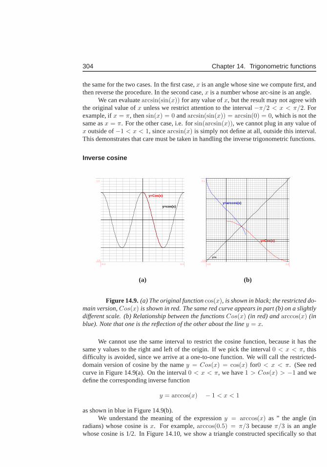
304 Chapter 14. Trigonometric functions
the same for the two cases. In the first case,x is an angle whose sine we compute first, andthen reverse the procedure. In the second case,x is a number whose arc-sine is an angle.
We can evaluatearcsin(sin(x)) for any value ofx, but the result may not agree withthe original value ofx unless we restrict attention to the interval−π/2 < x < π/2. Forexample, ifx = π, thensin(x) = 0 andarcsin(sin(x)) = arcsin(0) = 0, which is not thesame asx = π. For the other case, i.e. forsin(arcsin(x)), we cannot plug in any value ofx outside of−1 < x < 1, sincearcsin(x) is simply not define at all, outside this interval.This demonstrates that care must be taken in handling the inverse trigonometric functions.
Inverse cosine
y=cos(x)
y=Cos(x)
-6.3 6.3
-1.5
1.5
y=x
y=Cos(x)
y=arccos(x)
-1.0 3.1
-1.0
3.1
(a) (b)
Figure 14.9.(a) The original functioncos(x), is shown in black; the restricted do-main version,Cos(x) is shown in red. The same red curve appears in part (b) on a slightlydifferent scale. (b) Relationship between the functionsCos(x) (in red) andarccos(x) (inblue). Note that one is the reflection of the other about the liney = x.
We cannot use the same interval to restrict the cosine function, because it has thesame y values to the right and left of the origin. If we pick theinterval0 < x < π, thisdifficulty is avoided, since we arrive at a one-to-one function. We will call the restricted-domain version of cosine by the namey = Cos(x) = cos(x) for0 < x < π. (See redcurve in Figure 14.9(a). On the interval0 < x < π, we have1 > Cos(x) > −1 and wedefine the corresponding inverse function
y = arccos(x) − 1 < x < 1
as shown in blue in Figure 14.9(b).We understand the meaning of the expressiony = arccos(x) as ” the angle (in
radians) whose cosine isx. For example,arccos(0.5) = π/3 becauseπ/3 is an anglewhose cosine is 1/2. In Figure 14.10, we show a triangle constructed specifically so that
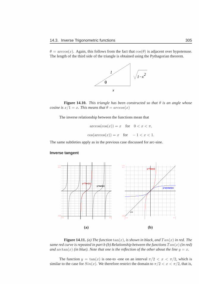
14.3. Inverse Trigonometric functions 305
θ = arccos(x). Again, this follows from the fact thatcos(θ) is adjacent over hypotenuse.The length of the third side of the triangle is obtained usingthe Pythagorian theorem.
θ
x
11−x
2
Figure 14.10. This triangle has been constructed so thatθ is an angle whosecosine isx/1 = x. This means thatθ = arccos(x)
The inverse relationship between the functions mean that
arccos(cos(x)) = x for 0 < x < π,
cos(arccos(x)) = x for − 1 < x < 1.
The same subtleties apply as in the previous case discussed for arc-sine.
Inverse tangent
y=tan(x)y=Tan(x)
-6.5 6.5
-10.0
10.0
y=x
y=Tan(x)
y=arctan(x)
-6.3 6.3
-6.3
6.3
(a) (b)
Figure 14.11.(a) The functiontan(x), is shown in black, andTan(x) in red. Thesame red curve is repeated in part b (b) Relationship betweenthe functionsTan(x) (in red)andarctan(x) (in blue). Note that one is the reflection of the other about the liney = x.
The functiony = tan(x) is one-to -one on an intervalπ/2 < x < π/2, which issimilar to the case forSin(x). We therefore restrict the domain toπ/2 < x < π/2, that is,
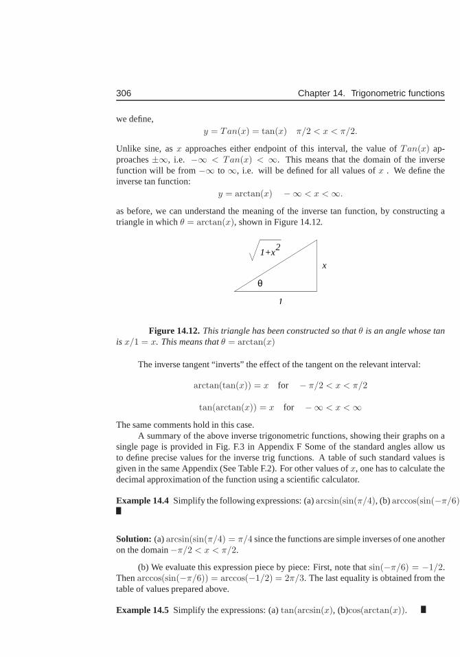
306 Chapter 14. Trigonometric functions
we define,y = Tan(x) = tan(x) π/2 < x < π/2.
Unlike sine, asx approaches either endpoint of this interval, the value ofTan(x) ap-proaches±∞, i.e. −∞ < Tan(x) < ∞. This means that the domain of the inversefunction will be from−∞ to∞, i.e. will be defined for all values ofx . We define theinverse tan function:
y = arctan(x) −∞ < x <∞.
as before, we can understand the meaning of the inverse tan function, by constructing atriangle in whichθ = arctan(x), shown in Figure 14.12.
θ
x
2
1
1+x
Figure 14.12.This triangle has been constructed so thatθ is an angle whose tanis x/1 = x. This means thatθ = arctan(x)
The inverse tangent “inverts” the effect of the tangent on the relevant interval:
arctan(tan(x)) = x for − π/2 < x < π/2
tan(arctan(x)) = x for −∞ < x <∞
The same comments hold in this case.A summary of the above inverse trigonometric functions, showing their graphs on a
single page is provided in Fig. F.3 in Appendix F Some of the standard angles allow usto define precise values for the inverse trig functions. A table of such standard values isgiven in the same Appendix (See Table F.2). For other values of x, one has to calculate thedecimal approximation of the function using a scientific calculator.
Example 14.4 Simplify the following expressions: (a)arcsin(sin(π/4), (b)arccos(sin(−π/6))
Solution: (a)arcsin(sin(π/4) = π/4 since the functions are simple inverses of one anotheron the domain−π/2 < x < π/2.
(b) We evaluate this expression piece by piece: First, note thatsin(−π/6) = −1/2.Thenarccos(sin(−π/6)) = arccos(−1/2) = 2π/3. The last equality is obtained from thetable of values prepared above.
Example 14.5 Simplify the expressions: (a)tan(arcsin(x), (b)cos(arctan(x)).
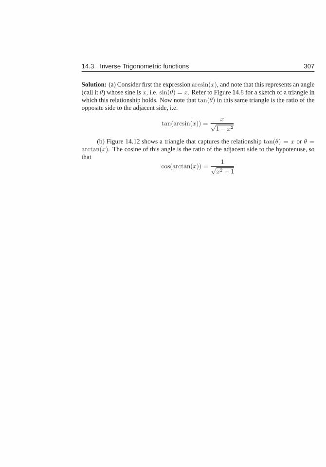
14.3. Inverse Trigonometric functions 307
Solution: (a) Consider first the expressionarcsin(x), and note that this represents an angle(call it θ) whose sine isx, i.e. sin(θ) = x. Refer to Figure 14.8 for a sketch of a triangle inwhich this relationship holds. Now note thattan(θ) in this same triangle is the ratio of theopposite side to the adjacent side, i.e.
tan(arcsin(x)) =x√
1− x2
(b) Figure 14.12 shows a triangle that captures the relationship tan(θ) = x or θ =arctan(x). The cosine of this angle is the ratio of the adjacent side to the hypotenuse, sothat
cos(arctan(x)) =1√
x2 + 1
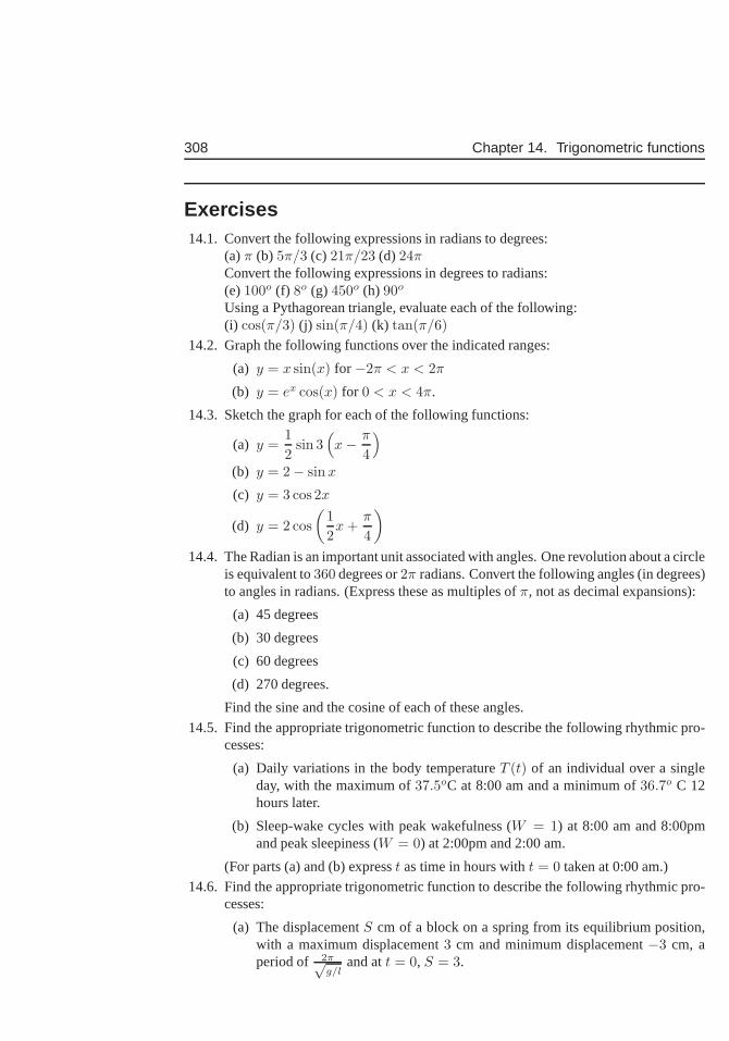
308 Chapter 14. Trigonometric functions
Exercises14.1. Convert the following expressions in radians to degrees:
(a)π (b) 5π/3 (c) 21π/23 (d) 24πConvert the following expressions in degrees to radians:(e)100o (f) 8o (g) 450o (h) 90o
Using a Pythagorean triangle, evaluate each of the following:(i) cos(π/3) (j) sin(π/4) (k) tan(π/6)
14.2. Graph the following functions over the indicated ranges:
(a) y = x sin(x) for −2π < x < 2π
(b) y = ex cos(x) for 0 < x < 4π.
14.3. Sketch the graph for each of the following functions:
(a) y =1
2sin 3
(
x− π
4
)
(b) y = 2− sin x
(c) y = 3 cos 2x
(d) y = 2 cos
(
1
2x +
π
4
)
14.4. The Radian is an important unit associated with angles. One revolution about a circleis equivalent to360 degrees or2π radians. Convert the following angles (in degrees)to angles in radians. (Express these as multiples ofπ, not as decimal expansions):
(a) 45 degrees
(b) 30 degrees
(c) 60 degrees
(d) 270 degrees.
Find the sine and the cosine of each of these angles.
14.5. Find the appropriate trigonometric function to describe the following rhythmic pro-cesses:
(a) Daily variations in the body temperatureT (t) of an individual over a singleday, with the maximum of37.5oC at 8:00 am and a minimum of36.7o C 12hours later.
(b) Sleep-wake cycles with peak wakefulness (W = 1) at 8:00 am and 8:00pmand peak sleepiness (W = 0) at 2:00pm and 2:00 am.
(For parts (a) and (b) expresst as time in hours witht = 0 taken at 0:00 am.)
14.6. Find the appropriate trigonometric function to describe the following rhythmic pro-cesses:
(a) The displacementS cm of a block on a spring from its equilibrium position,with a maximum displacement3 cm and minimum displacement−3 cm, aperiod of 2π√
g/land att = 0, S = 3.
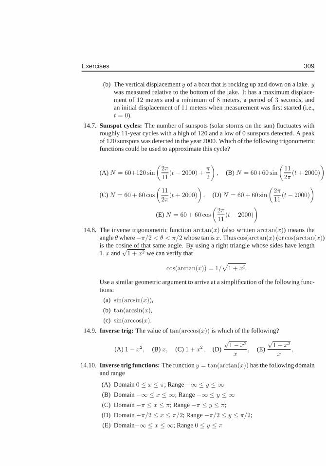
Exercises 309
(b) The vertical displacementy of a boat that is rocking up and down on a lake.ywas measured relative to the bottom of the lake. It has a maximum displace-ment of12 meters and a minimum of8 meters, a period of3 seconds, andan initial displacement of11 meters when measurement was first started (i.e.,t = 0).
14.7. Sunspot cycles:The number of sunspots (solar storms on the sun) fluctuates withroughly 11-year cycles with a high of 120 and a low of 0 sunspots detected. A peakof 120 sunspots was detected in the year 2000. Which of the following trigonometricfunctions could be used to approximate this cycle?
(A) N = 60+120 sin
(
2π
11(t− 2000) +
π
2
)
, (B) N = 60+60 sin
(
11
2π(t + 2000)
)
(C) N = 60 + 60 cos
(
11
2π(t + 2000)
)
, (D) N = 60 + 60 sin
(
2π
11(t− 2000)
)
(E) N = 60 + 60 cos
(
2π
11(t− 2000)
)
14.8. The inverse trigonometric functionarctan(x) (also writtenarctan(x)) means theangleθ where−π/2 < θ < π/2 whose tan isx. Thuscos(arctan(x) (orcos(arctan(x))is the cosine of that same angle. By using a right triangle whose sides have length1, x and
√1 + x2 we can verify that
cos(arctan(x)) = 1/√
1 + x2.
Use a similar geometric argument to arrive at a simplification of the following func-tions:
(a) sin(arcsin(x)),
(b) tan(arcsin(x),
(c) sin(arccos(x).
14.9. Inverse trig: The value oftan(arccos(x)) is which of the following?
(A) 1− x2, (B) x, (C) 1 + x2, (D)
√1− x2
x, (E)
√1 + x2
x,
14.10. Inverse trig functions: The functiony = tan(arctan(x)) has the following domainand range
(A) Domain0 ≤ x ≤ π; Range−∞ ≤ y ≤ ∞(B) Domain−∞ ≤ x ≤ ∞; Range−∞ ≤ y ≤ ∞(C) Domain−π ≤ x ≤ π; Range−π ≤ y ≤ π;
(D) Domain−π/2 ≤ x ≤ π/2; Range−π/2 ≤ y ≤ π/2;
(E) Domain−∞ ≤ x ≤ ∞; Range0 ≤ y ≤ π

310 Chapter 14. Trigonometric functions
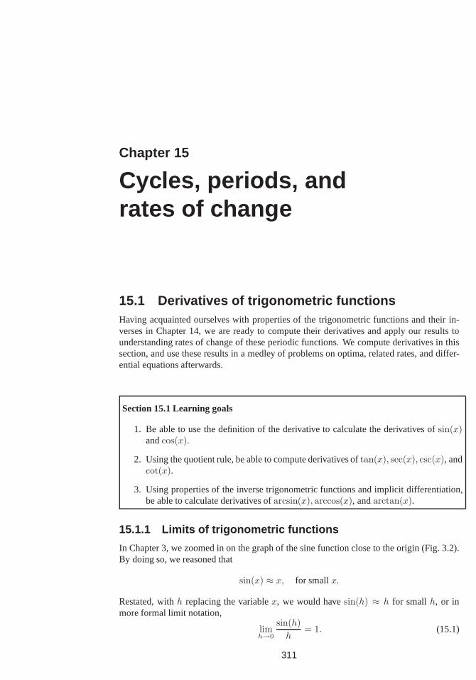
Chapter 15
Cycles, periods, andrates of change
15.1 Derivatives of trigonometric functionsHaving acquainted ourselves with properties of the trigonometric functions and their in-verses in Chapter 14, we are ready to compute their derivatives and apply our results tounderstanding rates of change of these periodic functions.We compute derivatives in thissection, and use these results in a medley of problems on optima, related rates, and differ-ential equations afterwards.
Section 15.1 Learning goals
1. Be able to use the definition of the derivative to calculatethe derivatives ofsin(x)andcos(x).
2. Using the quotient rule, be able to compute derivatives oftan(x), sec(x), csc(x), andcot(x).
3. Using properties of the inverse trigonometric functionsand implicit differentiation,be able to calculate derivatives ofarcsin(x), arccos(x), andarctan(x).
15.1.1 Limits of trigonometric functions
In Chapter 3, we zoomed in on the graph of the sine function close to the origin (Fig. 3.2).By doing so, we reasoned that
sin(x) ≈ x, for smallx.
Restated, withh replacing the variablex, we would havesin(h) ≈ h for small h, or inmore formal limit notation,
limh→0
sin(h)
h= 1. (15.1)
311
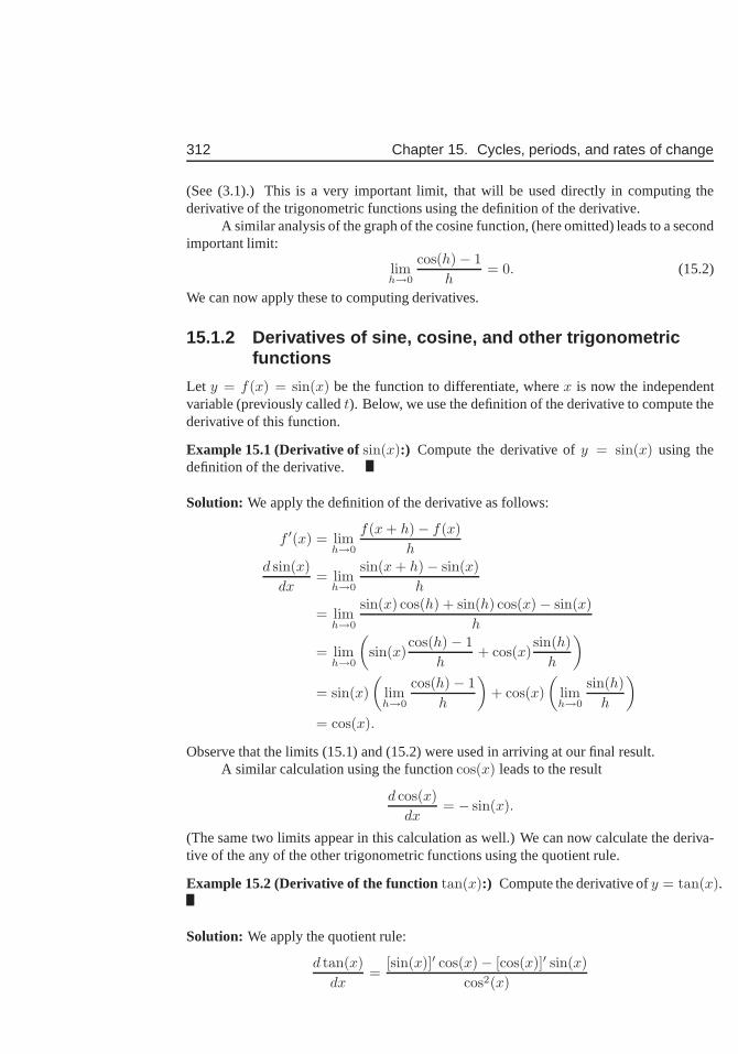
312 Chapter 15. Cycles, periods, and rates of change
(See (3.1).) This is a very important limit, that will be useddirectly in computing thederivative of the trigonometric functions using the definition of the derivative.
A similar analysis of the graph of the cosine function, (hereomitted) leads to a secondimportant limit:
limh→0
cos(h)− 1
h= 0. (15.2)
We can now apply these to computing derivatives.
15.1.2 Derivatives of sine, cosine, and other trigonometri cfunctions
Let y = f(x) = sin(x) be the function to differentiate, wherex is now the independentvariable (previously calledt). Below, we use the definition of the derivative to compute thederivative of this function.
Example 15.1 (Derivative ofsin(x):) Compute the derivative ofy = sin(x) using thedefinition of the derivative.
Solution: We apply the definition of the derivative as follows:
f ′(x) = limh→0
f(x + h)− f(x)
hd sin(x)
dx= lim
h→0
sin(x + h)− sin(x)
h
= limh→0
sin(x) cos(h) + sin(h) cos(x)− sin(x)
h
= limh→0
(
sin(x)cos(h)− 1
h+ cos(x)
sin(h)
h
)
= sin(x)
(
limh→0
cos(h)− 1
h
)
+ cos(x)
(
limh→0
sin(h)
h
)
= cos(x).
Observe that the limits (15.1) and (15.2) were used in arriving at our final result.A similar calculation using the functioncos(x) leads to the result
d cos(x)
dx= − sin(x).
(The same two limits appear in this calculation as well.) We can now calculate the deriva-tive of the any of the other trigonometric functions using the quotient rule.
Example 15.2 (Derivative of the functiontan(x):) Compute the derivative ofy = tan(x).
Solution: We apply the quotient rule:
d tan(x)
dx=
[sin(x)]′ cos(x)− [cos(x)]′ sin(x)
cos2(x)
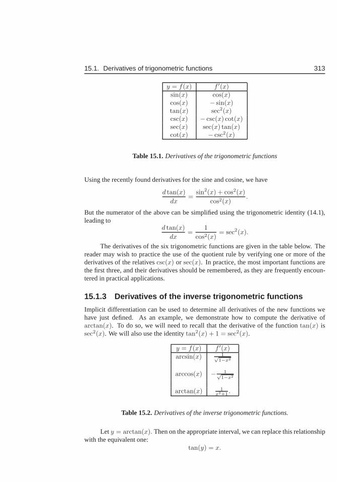
15.1. Derivatives of trigonometric functions 313
y = f(x) f ′(x)sin(x) cos(x)cos(x) − sin(x)tan(x) sec2(x)csc(x) − csc(x) cot(x)sec(x) sec(x) tan(x)cot(x) − csc2(x)
Table 15.1.Derivatives of the trigonometric functions
Using the recently found derivatives for the sine and cosine, we have
d tan(x)
dx=
sin2(x) + cos2(x)
cos2(x).
But the numerator of the above can be simplified using the trigonometric identity (14.1),leading to
d tan(x)
dx=
1
cos2(x)= sec2(x).
The derivatives of the six trigonometric functions are given in the table below. Thereader may wish to practice the use of the quotient rule by verifying one or more of thederivatives of the relativescsc(x) or sec(x). In practice, the most important functions arethe first three, and their derivatives should be remembered,as they are frequently encoun-tered in practical applications.
15.1.3 Derivatives of the inverse trigonometric functions
Implicit differentiation can be used to determine all derivatives of the new functions wehave just defined. As an example, we demonstrate how to compute the derivative ofarctan(x). To do so, we will need to recall that the derivative of the function tan(x) issec2(x). We will also use the identitytan2(x) + 1 = sec2(x).
y = f(x) f ′(x)
arcsin(x) 1√1−x2
arccos(x) − 1√1−x2
arctan(x) 1x2+1 .
Table 15.2.Derivatives of the inverse trigonometric functions.
Let y = arctan(x). Then on the appropriate interval, we can replace this relationshipwith the equivalent one:
tan(y) = x.
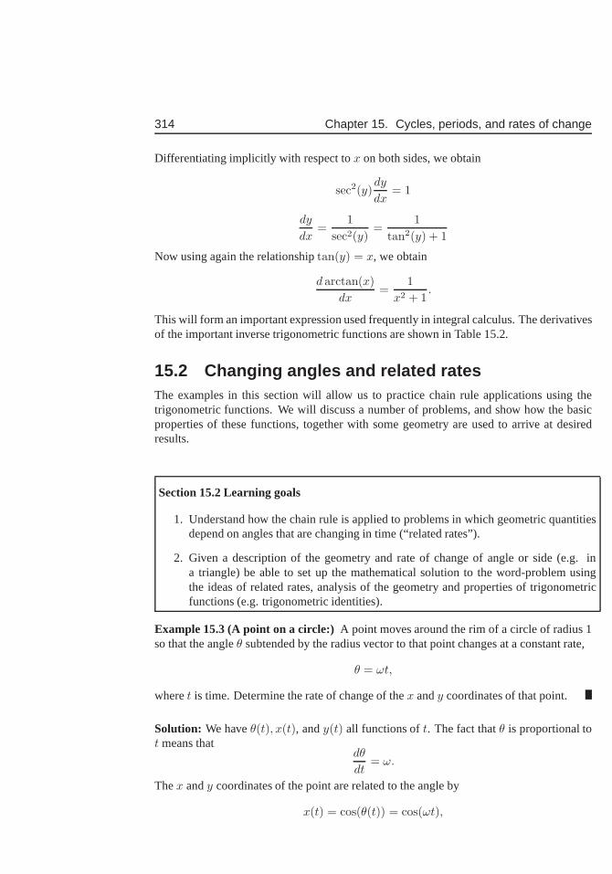
314 Chapter 15. Cycles, periods, and rates of change
Differentiating implicitly with respect tox on both sides, we obtain
sec2(y)dy
dx= 1
dy
dx=
1
sec2(y)=
1
tan2(y) + 1
Now using again the relationshiptan(y) = x, we obtain
d arctan(x)
dx=
1
x2 + 1.
This will form an important expression used frequently in integral calculus. The derivativesof the important inverse trigonometric functions are shownin Table 15.2.
15.2 Changing angles and related ratesThe examples in this section will allow us to practice chain rule applications using thetrigonometric functions. We will discuss a number of problems, and show how the basicproperties of these functions, together with some geometryare used to arrive at desiredresults.
Section 15.2 Learning goals
1. Understand how the chain rule is applied to problems in which geometric quantitiesdepend on angles that are changing in time (“related rates”).
2. Given a description of the geometry and rate of change of angle or side (e.g. ina triangle) be able to set up the mathematical solution to theword-problem usingthe ideas of related rates, analysis of the geometry and properties of trigonometricfunctions (e.g. trigonometric identities).
Example 15.3 (A point on a circle:) A point moves around the rim of a circle of radius 1so that the angleθ subtended by the radius vector to that point changes at a constant rate,
θ = ωt,
wheret is time. Determine the rate of change of thex andy coordinates of that point.
Solution: We haveθ(t), x(t), andy(t) all functions oft. The fact thatθ is proportional tot means that
dθ
dt= ω.
Thex andy coordinates of the point are related to the angle by
x(t) = cos(θ(t)) = cos(ωt),
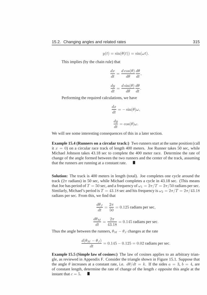
15.2. Changing angles and related rates 315
y(t) = sin(θ(t)) = sin(ωt).
This implies (by the chain rule) that
dx
dt=
d cos(θ)
dθ
dθ
dt,
dy
dt=
d sin(θ)
dθ
dθ
dt.
Performing the required calculations, we have
dx
dt= − sin(θ)ω,
dy
dt= cos(θ)ω.
We will see some interesting consequences of this in a later section.
Example 15.4 (Runners on a circular track:) Two runners start at the same position (callit x = 0) on a circular race track of length 400 meters. Joe Runner takes 50 sec, whileMichael Johnson takes 43.18 sec to complete the 400 meter race. Determine the rate ofchange of the angle formed between the two runners and the center of the track, assumingthat the runners are running at a constant rate.
Solution: The track is 400 meters in length (total). Joe completes one cycle around thetrack (2π radians) in 50 sec, while Michael completes a cycle in 43.18 sec. (This meansthat Joe has period ofT = 50 sec, and a frequency ofω1 = 2π/T = 2π/50 radians per sec.Similarly, Michael’s period isT = 43.18 sec and his frequency isω2 = 2π/T = 2π/43.18radians per sec. From this, we find that
dθJ
dt=
2π
50= 0.125 radians per sec,
dθM
dt=
2π
43.18= 0.145 radians per sec.
Thus the angle between the runners,θM − θJ changes at the rate
d(θM − θJ)
dt= 0.145− 0.125 = 0.02 radians per sec.
Example 15.5 (Simple law of cosines:)The law of cosines applies to an arbitrary trian-gle, as reviewed in Appendix F. Consider the triangle shown in Figure 15.1. Suppose thatthe angleθ increases at a constant rate, i.e.dθ/dt = k. If the sidesa = 3, b = 4, areof constant length, determine the rate of change of the length c opposite this angle at theinstant thatc = 5.
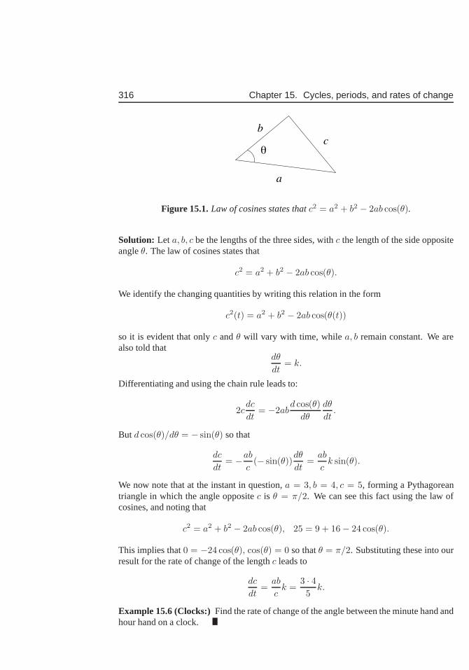
316 Chapter 15. Cycles, periods, and rates of change
a
bc
θ
Figure 15.1.Law of cosines states thatc2 = a2 + b2 − 2ab cos(θ).
Solution: Let a, b, c be the lengths of the three sides, withc the length of the side oppositeangleθ. The law of cosines states that
c2 = a2 + b2 − 2ab cos(θ).
We identify the changing quantities by writing this relation in the form
c2(t) = a2 + b2 − 2ab cos(θ(t))
so it is evident that onlyc andθ will vary with time, while a, b remain constant. We arealso told that
dθ
dt= k.
Differentiating and using the chain rule leads to:
2cdc
dt= −2ab
d cos(θ)
dθ
dθ
dt.
But d cos(θ)/dθ = − sin(θ) so that
dc
dt= −ab
c(− sin(θ))
dθ
dt=
ab
ck sin(θ).
We now note that at the instant in question,a = 3, b = 4, c = 5, forming a Pythagoreantriangle in which the angle oppositec is θ = π/2. We can see this fact using the law ofcosines, and noting that
c2 = a2 + b2 − 2ab cos(θ), 25 = 9 + 16− 24 cos(θ).
This implies that0 = −24 cos(θ), cos(θ) = 0 so thatθ = π/2. Substituting these into ourresult for the rate of change of the lengthc leads to
dc
dt=
ab
ck =
3 · 45
k.
Example 15.6 (Clocks:)Find the rate of change of the angle between the minute hand andhour hand on a clock.
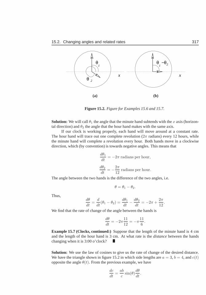
15.2. Changing angles and related rates 317
x
θ1
2 θx
θ1
−θ2
(a) (b)
Figure 15.2.Figure for Examples 15.6 and 15.7.
Solution: We will call θ1 the angle that the minute hand subtends with thex axis (horizon-tal direction) andθ2 the angle that the hour hand makes with the same axis.
If our clock is working properly, each hand will move around at a constant rate.The hour hand will trace out one complete revolution (2π radians) every 12 hours, whilethe minute hand will complete a revolution every hour. Both hands move in a clockwisedirection, which (by convention) is towards negative angles. This means that
dθ1
dt= −2π radians per hour,
dθ2
dt= −2π
12radians per hour.
The angle between the two hands is the difference of the two angles, i.e.
θ = θ1 − θ2.
Thus,dθ
dt=
d
dt(θ1 − θ2) =
dθ1
dt− dθ2
dt= −2π +
2π
12.
We find that the rate of change of the angle between the hands is
dθ
dt= −2π
11
12= −π
11
6.
Example 15.7 (Clocks, continued:)Suppose that the length of the minute hand is 4 cmand the length of the hour hand is 3 cm. At what rate is thedistancebetween the handschanging when it is 3:00 o’clock?
Solution: We use the law of cosines to give us the rate of change of the desired distance.We have the triangle shown in figure 15.2 in which side lengthsarea = 3, b = 4, andc(t)opposite the angleθ(t). From the previous example, we have
dc
dt=
ab
csin(θ)
dθ
dt.
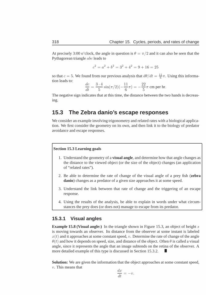
318 Chapter 15. Cycles, periods, and rates of change
At precisely 3:00 o’clock, the angle in question isθ = π/2 and it can also be seen that thePythagorean triangleabc leads to
c2 = a2 + b2 = 32 + 42 = 9 + 16 = 25
so thatc = 5. We found from our previous analysis thatdθ/dt = 116 π. Using this informa-
tion leads to:dc
dt=
3 · 45
sin(π/2)(−11
6π) = −22
5π cm per hr.
The negative sign indicates that at this time, the distance between the two hands is decreas-ing.
15.3 The Zebra danio’s escape responsesWe consider an example involving trigonometry and related rates with a biological applica-tion. We first consider the geometry on its own, and then link it to the biology of predatoravoidance and escape responses.
Section 15.3 Learning goals
1. Understand the geometry of avisual angle, and determine how that angle changes asthe distance to the viewed object (or the size of the object) changes (an applicationof “related rates”).
2. Be able to determine the rate of change of the visual angle of a prey fish (zebradanio) changes as a predator of a given size approaches it at some speed.
3. Understand the link between that rate of change and the triggering of an escaperesponse.
4. Using the results of the analysis, be able to explain in words under what circum-stances the prey does (or does not) manage to escape from its predator.
15.3.1 Visual angles
Example 15.8 (Visual angle:)In the triangle shown in Figure 15.3, an object of heightsis moving towards an observer. Its distance from the observer at some instant is labeledx(t) and it approaches at some constant speed,v. Determine the rate of change of the angleθ(t) and how it depends on speed, size, and distance of the object.Oftenθ is called a visualangle, since it represents the angle that an image subtends on the retina of the observer. Amore detailed example of this type is discussed in Section 15.3.2.
Solution: We are given the information that the object approaches at some constant speed,v. This means that
dx
dt= −v.

15.3. The Zebra danio’s escape responses 319
x
s
θ
Figure 15.3.A visual angleθ would change as the distancex decreases. The sizes is assumed constant. See Example 15.8.
(The minus sign means that the distancex is decreasing.) Using the trigonometric relations,we see that
tan(θ) =s
x.
If the size,s, of the object is constant, then the changes with time imply that
tan(θ(t)) =s
x(t).
We differentiate both sides of this equation with respect tot, and obtain
d tan(θ)
dθ
dθ
dt=
d
dt
(
s
x(t)
)
,
sec2(θ)dθ
dt= −s
1
x2
dx
dt,
so thatdθ
dt= −s
1
sec2(θ)
1
x2
dx
dt.
We can use the trigonometric identity
sec2(θ) = 1 + tan2(θ)
to express our answer in terms only of the size,s, the distance of the object,x and thespeed:
sec2(θ) = 1 +( s
x
)2
=x2 + s2
x2
sodθ
dt= −s
x2
x2 + s2
1
x2
dx
dt=
s
x2 + s2v.
(Two minus signs cancelled above.) Thus, the rate of change of the visual angle issv/(x2+s2).
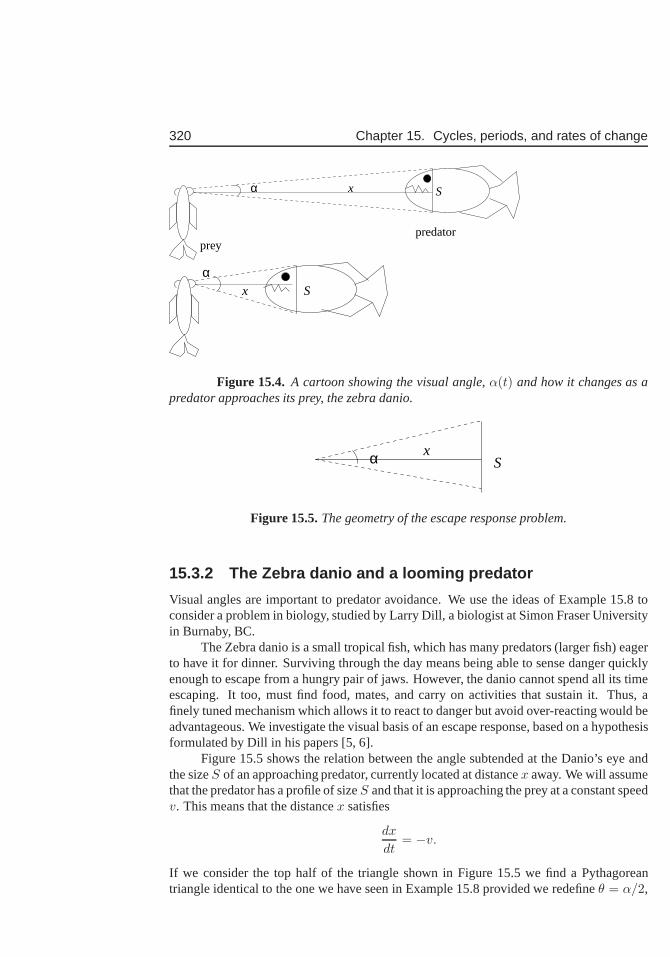
320 Chapter 15. Cycles, periods, and rates of change
α x S
preypredator
S
αx
Figure 15.4. A cartoon showing the visual angle,α(t) and how it changes as apredator approaches its prey, the zebra danio.
α xS
Figure 15.5.The geometry of the escape response problem.
15.3.2 The Zebra danio and a looming predator
Visual angles are important to predator avoidance. We use the ideas of Example 15.8 toconsider a problem in biology, studied by Larry Dill, a biologist at Simon Fraser Universityin Burnaby, BC.
The Zebra danio is a small tropical fish, which has many predators (larger fish) eagerto have it for dinner. Surviving through the day means being able to sense danger quicklyenough to escape from a hungry pair of jaws. However, the danio cannot spend all its timeescaping. It too, must find food, mates, and carry on activities that sustain it. Thus, afinely tuned mechanism which allows it to react to danger but avoid over-reacting would beadvantageous. We investigate the visual basis of an escape response, based on a hypothesisformulated by Dill in his papers [5, 6].
Figure 15.5 shows the relation between the angle subtended at the Danio’s eye andthe sizeS of an approaching predator, currently located at distancex away. We will assumethat the predator has a profile of sizeS and that it is approaching the prey at a constant speedv. This means that the distancex satisfies
dx
dt= −v.
If we consider the top half of the triangle shown in Figure 15.5 we find a Pythagoreantriangle identical to the one we have seen in Example 15.8 provided we redefineθ = α/2,
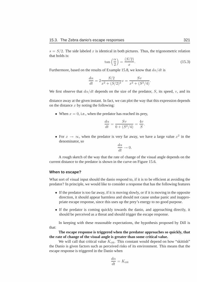
15.3. The Zebra danio’s escape responses 321
s = S/2. The side labeledx is identical in both pictures. Thus, the trigonometric relationthat holds is:
tan(α
2
)
=(S/2)
x. (15.3)
Furthermore, based on the results of Example 15.8, we know thatdα/dt is
dα
dt= 2
S/2
x2 + (S/2)2v =
Sv
x2 + (S2/4).
We first observe thatdα/dt depends on the size of the predator,S, its speed,v, and its
distance away at the given instant. In fact, we can plot the way that this expression dependson the distancex by noting the following:
• Whenx = 0, i.e., when the predator has reached its prey,
dα
dt=
Sv
0 + (S2/4)=
4v
S.
• For x → ∞, when the predator is very far away, we have a large valuex2 in thedenominator, so
dα
dt→ 0.
A rough sketch of the way that the rate of change of the visual angle depends on thecurrent distance to the predator is shown in the curve on Figure 15.6.
When to escape?
What sort of visual input should the danio respond to, if it isto be efficient at avoiding thepredator? In principle, we would like to consider a responsethat has the following features
• If the predator is too far away, if it is moving slowly, or if itis moving in the oppositedirection, it should appear harmless and should not cause undue panic and inappro-priate escape response, since this uses up the prey’s energyto no good purpose.
• If the predator is coming quickly towards the danio, and approaching directly, itshould be perceived as a threat and should trigger the escaperesponse.
In keeping with these reasonable expectations, the hypothesis proposed by Dill isthat:
The escape response is triggered when the predator approaches so quickly, thatthe rate of change of the visual angle is greater than some critical value.
We will call that critical valueKcrit. This constant would depend on how “skittish”the Danio is given factors such as perceived risks of its environment. This means that theescape response is triggered in the Danio when
dα
dt= Kcrit
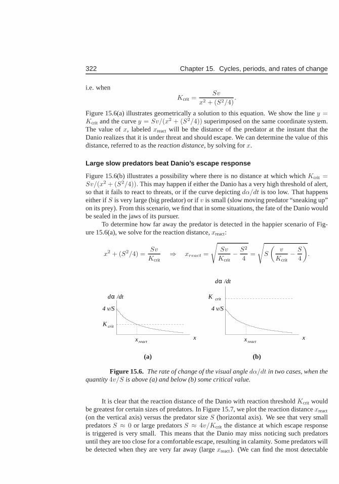
322 Chapter 15. Cycles, periods, and rates of change
i.e. when
Kcrit =Sv
x2 + (S2/4).
Figure 15.6(a) illustrates geometrically a solution to this equation. We show the liney =Kcrit and the curvey = Sv/(x2 + (S2/4)) superimposed on the same coordinate system.The value ofx, labeledxreact will be the distance of the predator at the instant that theDanio realizes that it is under threat and should escape. We can determine the value of thisdistance, referred to as thereaction distance, by solving forx.
Large slow predators beat Danio’s escape response
Figure 15.6(b) illustrates a possibility where there is no distance at which whichKcrit =Sv/(x2 + (S2/4)). This may happen if either the Danio has a very high threshold of alert,so that it fails to react to threats, or if the curve depictingdα/dt is too low. That happenseither ifS is very large (big predator) or ifv is small (slow moving predator “sneaking up”on its prey). From this scenario, we find that in some situations, the fate of the Danio wouldbe sealed in the jaws of its pursuer.
To determine how far away the predator is detected in the happier scenario of Fig-ure 15.6(a), we solve for the reaction distance,xreact:
x2 + (S2/4) =Sv
Kcrit⇒ xreact =
√
Sv
Kcrit− S2
4=
√
S
(
v
Kcrit− S
4
)
.
x
4 v/S
critK
α d /dt
xreactx
4 v/S
xreact
d /dt α
K crit
(a) (b)
Figure 15.6. The rate of change of the visual angledα/dt in two cases, when thequantity4v/S is above (a) and below (b) some critical value.
It is clear that the reaction distance of the Danio with reaction thresholdKcrit wouldbe greatest for certain sizes of predators. In Figure 15.7, we plot the reaction distancexreact
(on the vertical axis) versus the predator sizeS (horizontal axis). We see that very smallpredatorsS ≈ 0 or large predatorsS ≈ 4v/Kcrit the distance at which escape responseis triggered is very small. This means that the Danio may missnoticing such predatorsuntil they are too close for a comfortable escape, resultingin calamity. Some predators willbe detected when they are very far away (largexreact). (We can find the most detectable
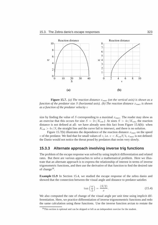
15.3. The Zebra danio’s escape responses 323
(a) (b)
Figure 15.7. (a) The reaction distancexreact (on the vertical axis) is shown as afunction of the predator sizeS (horizontal axis). (b) The reaction distancexreact is shownas a function of the predator velocityv
size by finding the value ofS corresponding to a maximalxreact. The reader may show asan exercise that this occurs for sizeS = 2v/Kcrit.) At sizesS > 4v/Kcrit, the reactiondistance is not defined at all: we have already seen this fact from Figure 15.6(b): whenKcrit > 4v/S, the straight line and the curve fail to intersect, and thereis no solution.
Figure 15.7(b) illustrates the dependence of the reaction distancexreact on the speedv of the predator. We find that for small values ofv, i.e. v < KcritS/4, xreact is not defined:the Danio would not notice the threat posed by predators thatswim very slowly.
15.3.3 Alternate approach involving inverse trig function s
The problem of the escape response was solved by using implicit differentiation and relatedrates. But there are various approaches to solve a mathematical problem. Here we illus-trate that an alternate approach is to express the relationship of interest in terms of inversetrigonometric functions, and then use the derivative of that function to find the desired rateof change18.
Example 15.9 In Section 15.4, we studied the escape response of the zebra danio andshowed that the connection between the visual angle and distance to predator satisfies
tan(α
2
)
=(S/2)
x. (15.4)
We also computed the rate of change of the visual angle per unit time using implicit dif-ferentiation. Here, we practice differentiation of inverse trigonomentric functions and redothe same calculation using these functions. Use the inversefunction arctan to restate the
18This section is optional and can be skipped or left as an independent exercise for the student.
324 Chapter 15. Cycles, periods, and rates of change
angleα in Eqn. 15.4 as a function ofx. Then differentiate that function using the chainrule to computedα/dt.
Solution: We can restate this relationship using the inverse trigonometric functionarctanas follows:
α
2= arctan
(
S
2x
)
.
Our experience with the derivative of this function will be useful below. Since both theangleα and the distance from the predatorx change with time, we indicate so by writing
α(t) = 2 arctan
(
S
2x(t)
)
.
We apply the chain rule to this expression to calculate the rate of change of the angleαwith respect to time. Letu = S/2x. Recall thatS is a constant. Then the derivative of theinverse trigonometric function,
d arctan(u)
du=
1
u2 + 1
and the chain rule leads to
dα(t)
dt=
d arctan(u)
du
du
dx
dx
dt=
1
u2 + 1
(
− S
2x2(t)
)
(−v).
By simplifying, we arrive at the same result, namely that
dα
dt=
Sv
x2 + (S2/4).
This is the rate of change of the visual angle, and agrees withExample 15.8.
15.4 For further study: Trigonometric functions anddifferential equations
As we have seen in this chapter, the functionssin(t) andcos(t) are related to one anothervia differentiation: one is the derivative of the other (with a multiple of the factor (-1).):
d sin(t)
dt= cos(t),
d cos(t)
dt= − sin(t).
The connection becomes even clearer when we examine the second derivatives of thesefunctions:
d2 sin(t)
dt2=
d cos(t)
dt= − sin(t),
d2 cos(t)
dt2= −d sin(t)
dt= − cos(t).
Thus, for each of the functionsy = sin(t), y = cos(t), we find that the function and itssecond derivative are related to one another by thedifferential equation (DE) d2y/dt2 =
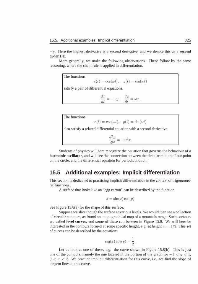
15.5. Additional examples: Implicit differentiation 325
−y. Here the highest derivative is a second derivative, and we denote this as asecondorder DE.
More generally, we make the following observations. These follow by the samereasoning, where the chain rule is applied in differentiation.
The functionsx(t) = cos(ωt), y(t) = sin(ωt)
satisfy a pair of differential equations,
dx
dt= −ωy,
dy
dt= ωx.
The functionsx(t) = cos(ωt), y(t) = sin(ωt)
also satisfy a related differential equation with a second derivative
d2x
dt2= −ω2x.
Students of physics will here recognize the equation that governs the behaviour of aharmonic oscillator, and will see the connection between the circular motion of our pointon the circle, and the differential equation for periodic motion.
15.5 Additional examples: Implicit differentiationThis section is dedicated to practicing implicit differentiation in the context of trigonomet-ric functions.
A surface that looks like an “egg carton” can be described by the function
z = sin(x) cos(y)
See Figure 15.8(a) for the shape of this surface.Suppose we slice though the surface at various levels. We would then see a collection
of circular contours, as found on a topographical map of a mountain range. Such contoursare calledlevel curves, and some of these can be seen in Figure 15.8. We will here beinterested in the contours formed at some specific height, e.g. at heightz = 1/2. Thissetof curves can be described by the equation:
sin(x) cos(y) =1
2.
Let us look at one of these, e.g. the curve shown in Figure 15.8(b). This is justone of the contours, namely the one located in the portion of the graph for−1 < y < 1,0 < x < 3. We practice implicit differentiation for this curve, i.e.we find the slope oftangent lines to this curve.
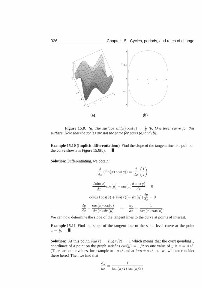
326 Chapter 15. Cycles, periods, and rates of change
–4
–2
0
2
4
x
–4
–2
0
2
4
y
–1
0
1
–1
–0.5
0
0.5
1
y
1 1.5 2 2.5
x
(a) (b)
Figure 15.8. (a) The surfacesin(x) cos(y) = 12 (b) One level curve for this
surface. Note that the scales are not the same for parts (a) and (b).
Example 15.10 (Implicit differentiation:) Find the slope of the tangent line to a point onthe curve shown in Figure 15.8(b).
Solution: Differentiating, we obtain:
d
dx(sin(x) cos(y)) =
d
dx
(
1
2
)
d sin(x)
dxcos(y) + sin(x)
d cos(y)
dx= 0
cos(x) cos(y) + sin(x)(− sin(y))dy
dx= 0
dy
dx=
cos(x) cos(y)
sin(x) sin(y)⇒ dy
dx=
1
tan(x) tan(y).
We can now determine the slope of the tangent lines to the curve at points of interest.
Example 15.11Find the slope of the tangent line to the same level curve at the pointx = π
2 .
Solution: At this point, sin(x) = sin(π/2) = 1 which means that the correspondingycoordinate of a point on the graph satisfiescos(y) = 1/2 so one value ofy is y = π/3.(There are other values, for example at−π/3 and at2πn ± π/3, but we will not considerthese here.) Then we find that
dy
dx=
1
tan(π/2) tan(π/3).
15.5. Additional examples: Implicit differentiation 327
But tan(π/2) = ∞ so that the ratio above leads todydx = 0. The tangent line is horizontal
as it goes though the point(π/2, π/3) on the graph.
Example 15.12Find the slope of the tangent line to the same level curve at the pointx = π
4 .
Solution: Here we havesin(x) = sin(π/4) =√
2/2, and we find that the y coordinatesatisfies √
2
2cos(y) =
1
2
This means thatcos(y) = 1√2
=√
22 so thaty = π/4. Thus
dy
dx=
1
tan(π/4) tan(π/4)=
1
1= 1
so that the tangent line at the point(π/4, π/4) has slope 1.
328 Chapter 15. Cycles, periods, and rates of change
Exercises15.1. Calculate the first derivative for the following functions.
(a) y = sin x2
(b) y = sin2 x
(c) y = cot2 3√
x
(d) y = sec(x− 3x2)
(e) y = 2x3 tan x
(f) y = xcos x
(g) y = x cosx
(h) y = e− sin2 1x
(i) y = (2 tan 3x + 3 cosx)2
(j) y = cos(sin x) + cosx sin x
15.2. Take the derivative of the following functions.
(a) f(x) = cos(ln(x4 + 5x2 + 3))
(b) f(x) = sin(√
cos2(x) + x3)
(c) f(x) = 2x3 + log3(x)
(d) f(x) = (x2ex + tan(3x))4
(e) f(x) = x2√
sin3(x) + cos3(x)
15.3. A point is moving on the perimeter of a circle of radius 1at the rate of 0.1 radiansper second. How fast is itsx coordinate changing whenx = 0.5? How fast is itsycoordinate changing at that time?
15.4. The derivatives of the two important trig functions are [sin(x)]′ = cos(x) and[cos(x)]′ = − sin(x). Use these derivatives to answer the following questions.Let f(x) = sin(x) + cos(x), 0 ≤ x ≤ 2π
(a) Find all intervals wheref(x) is increasing.
(b) Find all intervals wheref(x) is concave up.
(c) Locate all inflection points.
(d) Graphf(x).
15.5. Find all points on the graph ofy = tan(2x), − π
4< x <
π
4, where the slope of the
tangent line is4.
15.6. A “V” shaped formation of birds forms a symmetric structure in which the distancefrom the leader to the last birds in the V isr = 10m, the distance between thosetrailing birds isD = 6m and the angle formed by the V isθ, as shown in Figure 15.9below. Suppose that the shape is gradually changing: the trailing birds start to getcloser so that their distance apart shrinks at a constant rate dD/dt = −0.2m/min
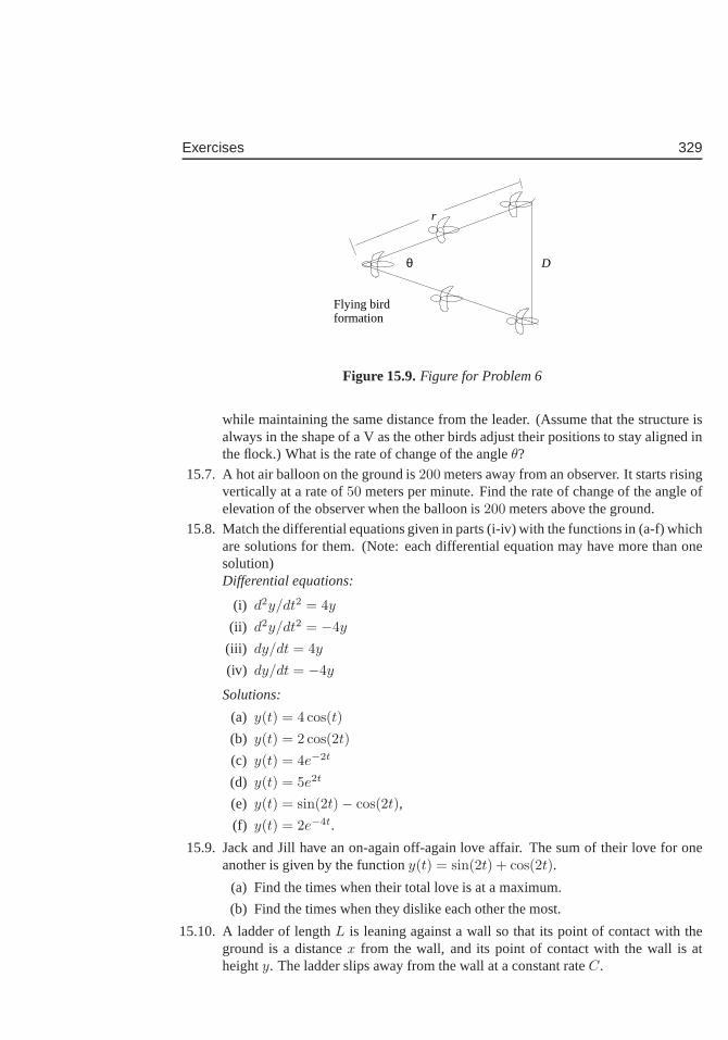
Exercises 329
θ
Flying birdformation
D
r
Figure 15.9.Figure for Problem 6
while maintaining the same distance from the leader. (Assume that the structure isalways in the shape of a V as the other birds adjust their positions to stay aligned inthe flock.) What is the rate of change of the angleθ?
15.7. A hot air balloon on the ground is200 meters away from an observer. It starts risingvertically at a rate of50 meters per minute. Find the rate of change of the angle ofelevation of the observer when the balloon is200 meters above the ground.
15.8. Match the differential equations given in parts (i-iv) with the functions in (a-f) whichare solutions for them. (Note: each differential equation may have more than onesolution)Differential equations:
(i) d2y/dt2 = 4y
(ii) d2y/dt2 = −4y
(iii) dy/dt = 4y
(iv) dy/dt = −4y
Solutions:
(a) y(t) = 4 cos(t)
(b) y(t) = 2 cos(2t)
(c) y(t) = 4e−2t
(d) y(t) = 5e2t
(e) y(t) = sin(2t)− cos(2t),
(f) y(t) = 2e−4t.
15.9. Jack and Jill have an on-again off-again love affair. The sum of their love for oneanother is given by the functiony(t) = sin(2t) + cos(2t).
(a) Find the times when their total love is at a maximum.
(b) Find the times when they dislike each other the most.
15.10. A ladder of lengthL is leaning against a wall so that its point of contact with theground is a distancex from the wall, and its point of contact with the wall is atheighty. The ladder slips away from the wall at a constant rateC.
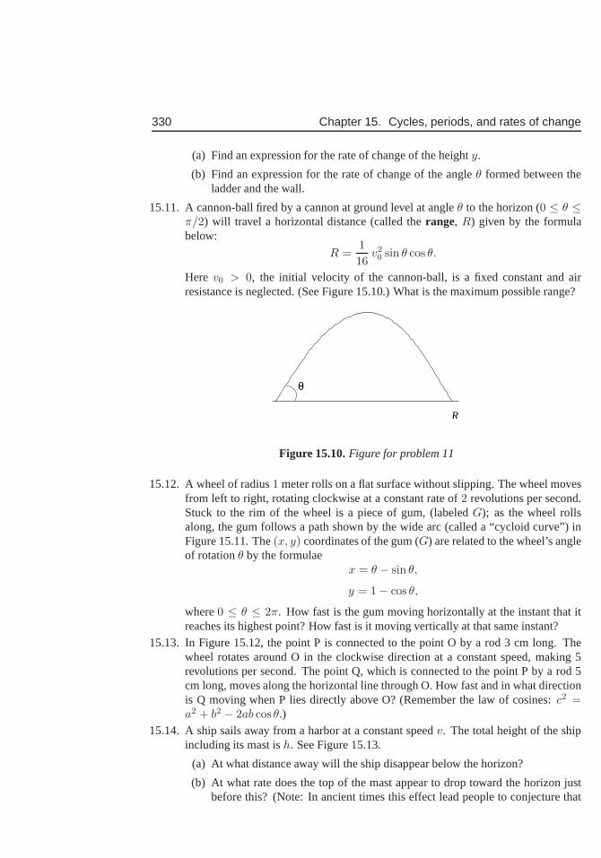
330 Chapter 15. Cycles, periods, and rates of change
(a) Find an expression for the rate of change of the heighty.
(b) Find an expression for the rate of change of the angleθ formed between theladder and the wall.
15.11. A cannon-ball fired by a cannon at ground level at angleθ to the horizon (0 ≤ θ ≤π/2) will travel a horizontal distance (called therange, R) given by the formulabelow:
R =1
16v20 sin θ cos θ.
Here v0 > 0, the initial velocity of the cannon-ball, is a fixed constantand airresistance is neglected. (See Figure 15.10.) What is the maximum possible range?
R
θ
Figure 15.10.Figure for problem 11
15.12. A wheel of radius1 meter rolls on a flat surface without slipping. The wheel movesfrom left to right, rotating clockwise at a constant rate of2 revolutions per second.Stuck to the rim of the wheel is a piece of gum, (labeledG); as the wheel rollsalong, the gum follows a path shown by the wide arc (called a “cycloid curve”) inFigure 15.11. The(x, y) coordinates of the gum (G) are related to the wheel’s angleof rotationθ by the formulae
x = θ − sin θ,
y = 1− cos θ,
where0 ≤ θ ≤ 2π. How fast is the gum moving horizontally at the instant that itreaches its highest point? How fast is it moving vertically at that same instant?
15.13. In Figure 15.12, the point P is connected to the point Oby a rod 3 cm long. Thewheel rotates around O in the clockwise direction at a constant speed, making 5revolutions per second. The point Q, which is connected to the point P by a rod 5cm long, moves along the horizontal line through O. How fast and in what directionis Q moving when P lies directly above O? (Remember the law of cosines:c2 =a2 + b2 − 2ab cos θ.)
15.14. A ship sails away from a harbor at a constant speedv. The total height of the shipincluding its mast ish. See Figure 15.13.
(a) At what distance away will the ship disappear below the horizon?
(b) At what rate does the top of the mast appear to drop toward the horizon justbefore this? (Note: In ancient times this effect lead peopleto conjecture that
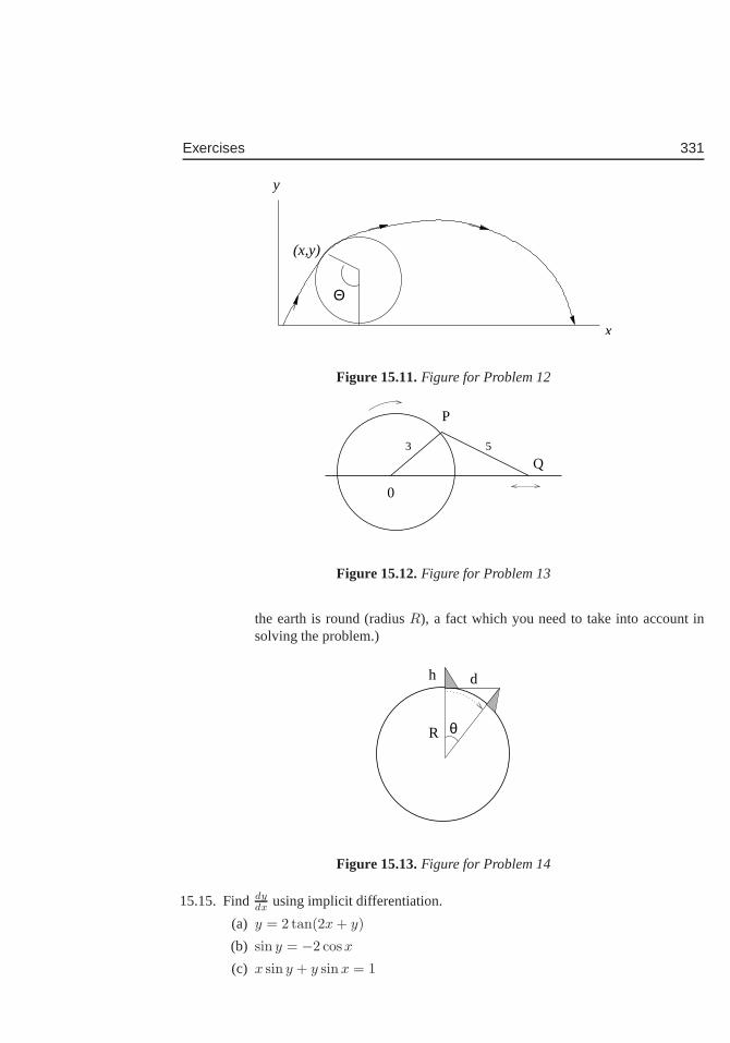
Exercises 331
Θ
y
x
(x,y)
Figure 15.11.Figure for Problem 12
0
P
Q3 5
Figure 15.12.Figure for Problem 13
the earth is round (radiusR), a fact which you need to take into account insolving the problem.)
R
h d
θ
Figure 15.13.Figure for Problem 14
15.15. Finddydx using implicit differentiation.
(a) y = 2 tan(2x + y)
(b) sin y = −2 cosx
(c) x sin y + y sin x = 1
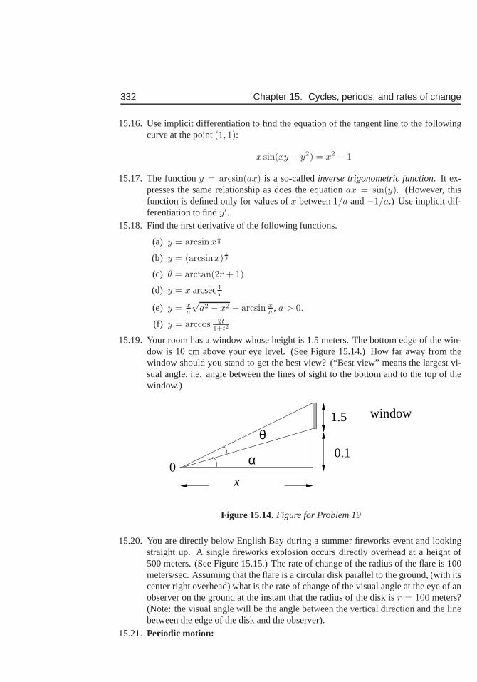
332 Chapter 15. Cycles, periods, and rates of change
15.16. Use implicit differentiation to find the equation of the tangent line to the followingcurve at the point(1, 1):
x sin(xy − y2) = x2 − 1
15.17. The functiony = arcsin(ax) is a so-calledinverse trigonometric function. It ex-presses the same relationship as does the equationax = sin(y). (However, thisfunction is defined only for values ofx between1/a and−1/a.) Use implicit dif-ferentiation to findy′.
15.18. Find the first derivative of the following functions.
(a) y = arcsinx13
(b) y = (arcsinx)13
(c) θ = arctan(2r + 1)
(d) y = x arcsec1x
(e) y = xa
√a2 − x2 − arcsin x
a , a > 0.
(f) y = arccos 2t1+t2
15.19. Your room has a window whose height is 1.5 meters. The bottom edge of the win-dow is 10 cm above your eye level. (See Figure 15.14.) How far away from thewindow should you stand to get the best view? (“Best view” means the largest vi-sual angle, i.e. angle between the lines of sight to the bottom and to the top of thewindow.)
0
θ
α
x
window1.5
0.1
Figure 15.14.Figure for Problem 19
15.20. You are directly below English Bay during a summer fireworks event and lookingstraight up. A single fireworks explosion occurs directly overhead at a height of500 meters. (See Figure 15.15.) The rate of change of the radius of the flare is 100meters/sec. Assuming that the flare is a circular disk parallel to the ground, (with itscenter right overhead) what is the rate of change of the visual angle at the eye of anobserver on the ground at the instant that the radius of the disk isr = 100 meters?(Note: the visual angle will be the angle between the vertical direction and the linebetween the edge of the disk and the observer).
15.21. Periodic motion:
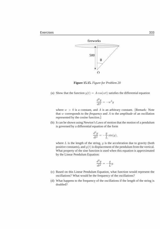
Exercises 333
fireworks
O
θ500
Figure 15.15.Figure for Problem 20
(a) Show that the functiony(t) = A cos(wt) satisfies the differential equation
d2y
dt2= −w2y
wherew > 0 is a constant, andA is an arbitrary constant. [Remark: Notethatw corresponds to thefrequencyandA to theamplitudeof an oscillationrepresented by the cosine function.]
(b) It can be shown using Newton’s Laws of motion that the motion of a pendulumis governed by a differential equation of the form
d2y
dt2= − g
Lsin(y),
whereL is the length of the string,g is the acceleration due to gravity (bothpositive constants), andy(t) is displacement of the pendulum from the vertical.What property of the sine function is used when this equationis approximatedby the Linear Pendulum Equation:
d2y
dt2= − g
Ly.
(c) Based on this Linear Pendulum Equation, what function would represent theoscillations? What would be the frequency of the oscillations?
(d) What happens to the frequency of the oscillations if the length of the string isdoubled?

334 Chapter 15. Cycles, periods, and rates of change
Chapter 16
Review Problems
335
336 Chapter 16. Review Problems
Exercises16.1. Multiple Choice:
(1) : The equation of the tangent line to the functiony = f(x) at the pointx0 is
(a)y = f ′(x0) + f(x0)(x − x0)
(b) y = x0 + f(x0)/f ′(x0)
(c) y = f(x)− f ′(x)(x − x0)
(d) y = f(x0) + f ′(x0)(x− x0)
(e)y = f(x0)− f ′(x0)(x − x0)
(2) : The functionsf(x) = x2 andg(x) = x3 are equal atx = 0 and atx = 1.Betweenx = 0 and atx = 1, for what value ofx are their graphs furthestapart?
(a)x = 1/2 (b) x = 2/3 (c) x = 1/3 (d) x = 1/4 (e)x = 3/4
(3) : Consider a point in the first quadrant on the hyperbolax2 − y2 = 1 withx = 2. The slope of the tangent line at that point is
(a)2/√
3 (b) 2/√
5 (c) 1/√
3 (d)√
5/2 (e)2/3
(4) : Fora, b > 0, solving the equationln(x) = 2 ln(a)− 3 ln(b) for x leads to
(a)x = e2a−3b (b) x = 2a− 3b (c) x = a2/b3 (d) x = a2b3 (e)x = (a/b)6
(5) : The functiony = f(x) = arctan(x) − (x/2) has local maXima (LX), localminima (LM) and inflection points(IP) as follows:
(a) LX: x = 1, LM: x = −1, IP: x = 0.
(b) LX: x = −1, LM: x = 1, IP: x = 0.
(c) LX: x = −1, LM: x = 1, IP: none
(d) LX: x =√
3, LM: x = −√
3, IP: x = 0.
(e) LX: x = −√
3, LM: x =√
3, IP: x = 0.
(6) Consider the functiony = f(x) = 3e−2x − 5e−4x
(a) The function has a local maximum atx = (1/2) ln(10/3)
(b) The function has a local minimum atx = (1/2) ln(10/3)
(c) The function has a local maximum atx = (−1/2) ln(3/5)
(d) The function has a local minimum atx = (1/2) ln(3/5)
(e) The function has a local maximum atx = (−1/2) ln(3/20)
(7) Let m1 be the slope of the functiony = 3x at the pointx = 0 and letm2 bethe slope of the functiony = log3 x atx = 1 Then
(a) m1 = ln(3)m2 (b) m1 = m2 (c) m1 = −m2 (d) m1 = 1/m2 (e)m1 = m2/ ln(3)
(8) Consider the curve whose equation isx4 + y4 + 3xy = 5. The slope of thetangent line,dy/dx, at the point(1, 1) is
(a) 1 (b) -1 (c) 0 (d) -4/7 (e) 1/7
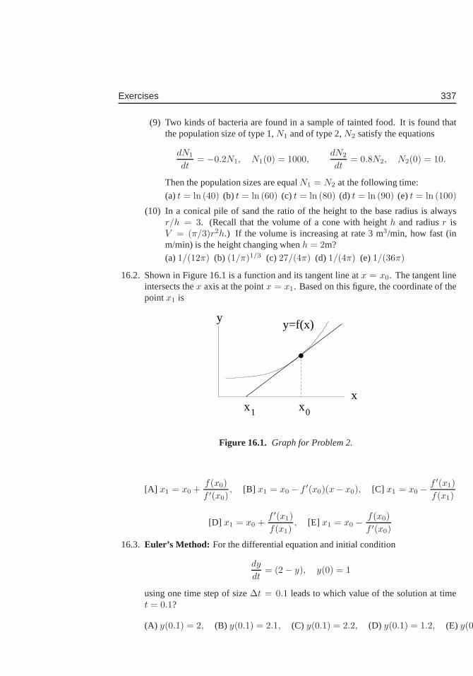
Exercises 337
(9) Two kinds of bacteria are found in a sample of tainted food. It is found thatthe population size of type 1,N1 and of type 2,N2 satisfy the equations
dN1
dt= −0.2N1, N1(0) = 1000,
dN2
dt= 0.8N2, N2(0) = 10.
Then the population sizes are equalN1 = N2 at the following time:
(a)t = ln (40) (b) t = ln (60) (c) t = ln (80) (d) t = ln (90) (e)t = ln (100)
(10) In a conical pile of sand the ratio of the height to the base radius is alwaysr/h = 3. (Recall that the volume of a cone with heighth and radiusr isV = (π/3)r2h.) If the volume is increasing at rate 3 m3/min, how fast (inm/min) is the height changing whenh = 2m?
(a)1/(12π) (b) (1/π)1/3 (c) 27/(4π) (d) 1/(4π) (e)1/(36π)
16.2. Shown in Figure 16.1 is a function and its tangent line at x = x0. The tangent lineintersects thex axis at the pointx = x1. Based on this figure, the coordinate of thepointx1 is
y
xx 01
y=f(x)
x
Figure 16.1. Graph for Problem 2.
[A] x1 = x0 +f(x0)
f ′(x0), [B] x1 = x0 − f ′(x0)(x− x0), [C] x1 = x0 −
f ′(x1)
f(x1)
[D] x1 = x0 +f ′(x1)
f(x1), [E] x1 = x0 −
f(x0)
f ′(x0)
16.3. Euler’s Method: For the differential equation and initial condition
dy
dt= (2 − y), y(0) = 1
using one time step of size∆t = 0.1 leads to which value of the solution at timet = 0.1?
(A) y(0.1) = 2, (B) y(0.1) = 2.1, (C) y(0.1) = 2.2, (D) y(0.1) = 1.2, (E) y(0.
338 Chapter 16. Review Problems
16.4. Linear approximation: Consider the functiony = cos(x) and its tangent line tothis function at the pointx = π/2. Using that tangent line as a linear approximationof the function would lead to
(A) Overestimating the value of the actual function for any nearbyx.
(B) Underestimating the value of the actual function for anynearbyx.
(C) Overestimating the function whenx > π/2 and underestimating the functionwhenx < π/2.
(D) Overestimating the function whenx < π/2 and underestimating the functionwhenx > π/2.
(E) Overestimating the function whenx < 0 and underestimating the functionwhenx > 0.
16.5. Related Rates: Two spherical balloons are connected so that one inflates as theother deflates, the sum of their volumes remaining constant.When the first balloonhas radius 10 cm and its radius is increasing at 3 cm/sec, the second balloon hasradius 20 cm. What is the rate of change of the radius of the second balloon? [Thevolume of a sphere of radiusr is V = (4/3)πr3].
16.6. Particle velocity: A particle is moving along thex axis so that its distance from theorigin at timet is given by
x(t) = (t + 2)3 + λt
whereλ is a constant
(a) Determine the velocityv(t) and the accelerationa(t).
(b) Determine the minimum velocity over all time.
16.7. Motion: A particle’s motion is described by y(t) = t3 − 6t2 + 9twherey(t) is thedisplacement(in metres)t is time (in seconds) and0 ≤ t ≤ 4seconds.
(a) During this time interval, when is the particle furthestfrom its initial position?
(b) During this time interval, what is the greatest speed of the particle?
(c) What is the totaldistance(including both forward and backward directions)that the particle has travelled during this time interval?
16.8. Falling object: Consider an object thrown upwards with initial velocityv0 > 0 andinitial heighth0 > 0. Then the height of the object at time t is given by
y = f(t) = −1
2gt2 + v0t + h0.
Find critical points off(t) and use both the second and first derivative tests to es-tablish that this is a local maximum.
16.9. Critical points:
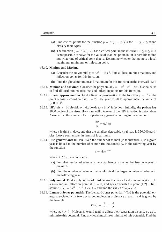
Exercises 339
(a) Find critical points for the functiony = ex(1 − ln(x)) for 0.1 ≤ x ≤ 2 andclassify their types.
(b) The functiony = ln(x)− ex has a critical point in the interval0.1 ≤ x ≤ 2. Itis not possible to solve for the value ofx at that point, but it is possible to findout what kind of critical point that is. Determine whether that point is a localmaximum, minimum, or inflection point.
16.10. Minima and Maxima:
(a) Consider the polynomialy = 4x5− 15x4. Find all local minima maxima, andinflection points for this function.
(b) Find the global minimum and maximum for this function on the interval [-1,1].
16.11. Minima and Maxima: Consider the polynomialy = −x5−x4+3x3. Use calculusto find all local minima maxima, and inflection points for thisfunction.
16.12. Linear approximation: Find a linear approximation to the functiony = x2 at thepoint whosex coordinate isx = 2. Use your result to approximate the value of(2.0001)2.
16.13. HIV virus: High-risk activity leads to a HIV infection. Initially, thepatient has1000 copies of the virus. How long will it take until the HIV infection is detectable?Assume that the number of virus particlesy grows according to the equation
dy
dt= 0.05y
wheret is time in days, and that the smallest detectable viral load is 350,000 parti-cles. Leave your answer in terms of logarithms.
16.14. Fish generations:In Fish River, the number of salmon (in thousands),x, in a givenyear is linked to the number of salmon (in thousands),y, in the following year bythe function
y = Axe−bx
whereA, b > 0 are constants.
(a) For what number of salmon is there no change in the number from one year tothe next?
(b) Find the number of salmon that would yield the largest number of salmon inthe following year.
16.15. Polynomial: Find a polynomial of third degree that has a local maximum atx = 1,a zero and an inflection point atx = 0, and goes through the point (1,2). Hint:assumep(x) = ax3 + bx2 + cx + d and find the values ofa, b, c, d.
16.16. Lennard-Jones potential: The Lennard-Jones potential,V (x) is the potential en-ergy associated with two uncharged molecules a distancex apart, and is given bythe formula
V (x) =a
x12− b
x6
wherea, b > 0. Molecules would tend to adjust their separation distance so as tominimize this potential. Find any local maxima or minima of this potential. Find the
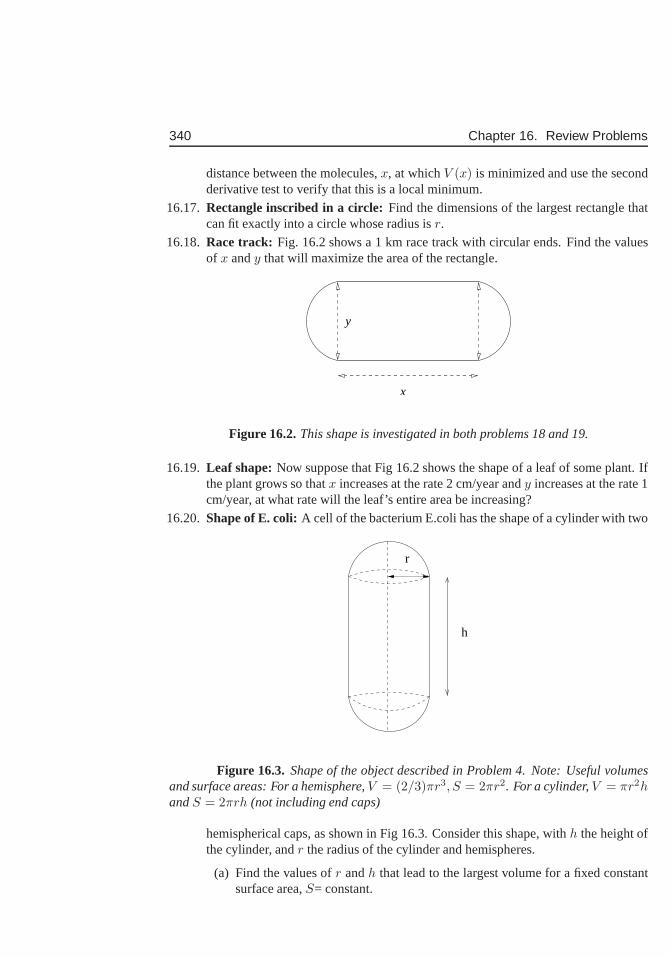
340 Chapter 16. Review Problems
distance between the molecules,x, at whichV (x) is minimized and use the secondderivative test to verify that this is a local minimum.
16.17. Rectangle inscribed in a circle:Find the dimensions of the largest rectangle thatcan fit exactly into a circle whose radius isr.
16.18. Race track: Fig. 16.2 shows a 1 km race track with circular ends. Find the valuesof x andy that will maximize the area of the rectangle.
x
y
Figure 16.2.This shape is investigated in both problems 18 and 19.
16.19. Leaf shape:Now suppose that Fig 16.2 shows the shape of a leaf of some plant. Ifthe plant grows so thatx increases at the rate 2 cm/year andy increases at the rate 1cm/year, at what rate will the leaf’s entire area be increasing?
16.20. Shape of E. coli:A cell of the bacterium E.coli has the shape of a cylinder withtwo
r
h
Figure 16.3. Shape of the object described in Problem 4. Note: Useful volumesand surface areas: For a hemisphere,V = (2/3)πr3, S = 2πr2. For a cylinder,V = πr2handS = 2πrh (not including end caps)
hemispherical caps, as shown in Fig 16.3. Consider this shape, withh the height ofthe cylinder, andr the radius of the cylinder and hemispheres.
(a) Find the values ofr andh that lead to the largest volume for a fixed constantsurface area,S= constant.
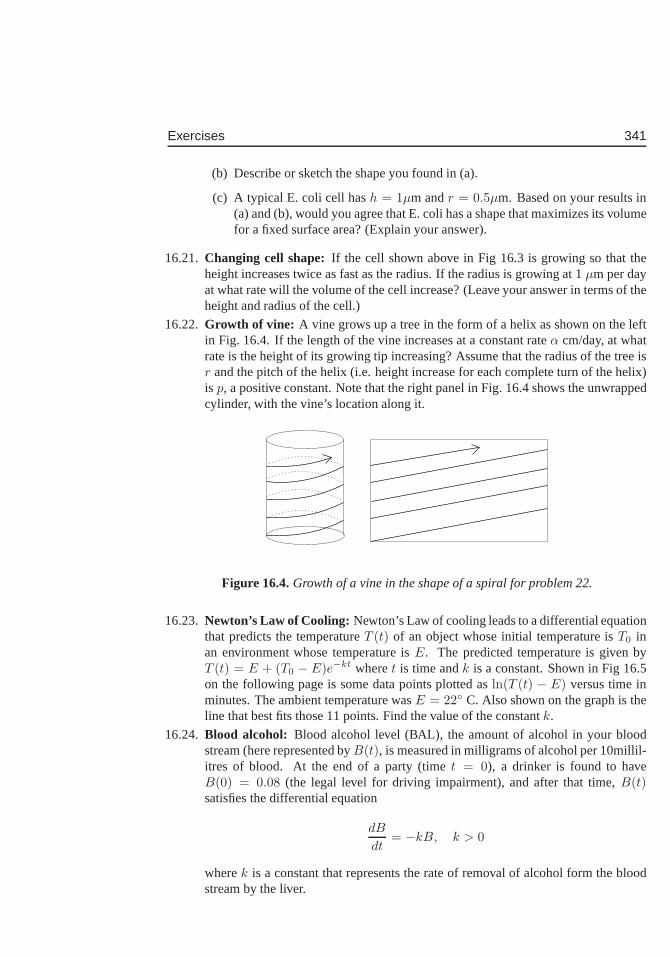
Exercises 341
(b) Describe or sketch the shape you found in (a).
(c) A typical E. coli cell hash = 1µm andr = 0.5µm. Based on your results in(a) and (b), would you agree that E. coli has a shape that maximizes its volumefor a fixed surface area? (Explain your answer).
16.21. Changing cell shape: If the cell shown above in Fig 16.3 is growing so that theheight increases twice as fast as the radius. If the radius isgrowing at 1µm per dayat what rate will the volume of the cell increase? (Leave youranswer in terms of theheight and radius of the cell.)
16.22. Growth of vine: A vine grows up a tree in the form of a helix as shown on the leftin Fig. 16.4. If the length of the vine increases at a constantrateα cm/day, at whatrate is the height of its growing tip increasing? Assume thatthe radius of the tree isr and the pitch of the helix (i.e. height increase for each complete turn of the helix)is p, a positive constant. Note that the right panel in Fig. 16.4 shows the unwrappedcylinder, with the vine’s location along it.
Figure 16.4.Growth of a vine in the shape of a spiral for problem 22.
16.23. Newton’s Law of Cooling: Newton’s Law of cooling leads to a differential equationthat predicts the temperatureT (t) of an object whose initial temperature isT0 inan environment whose temperature isE. The predicted temperature is given byT (t) = E + (T0 − E)e−kt wheret is time andk is a constant. Shown in Fig 16.5on the following page is some data points plotted asln(T (t) − E) versus time inminutes. The ambient temperature wasE = 22◦ C. Also shown on the graph is theline that best fits those 11 points. Find the value of the constantk.
16.24. Blood alcohol: Blood alcohol level (BAL), the amount of alcohol in your bloodstream (here represented byB(t), is measured in milligrams of alcohol per 10millil-itres of blood. At the end of a party (timet = 0), a drinker is found to haveB(0) = 0.08 (the legal level for driving impairment), and after that time, B(t)satisfies the differential equation
dB
dt= −kB, k > 0
wherek is a constant that represents the rate of removal of alcohol form the bloodstream by the liver.
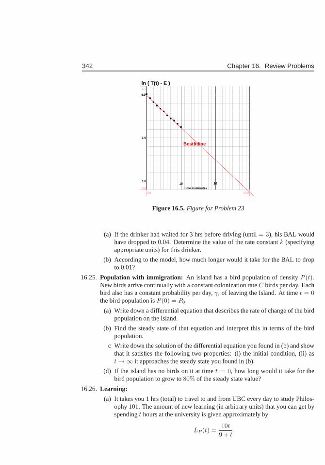
342 Chapter 16. Review Problems
ln ( T(t) - E )
Bestfitline
10 20
3.5
3.0
time in minutes
4.0
0.0 30.0
2.9
4.1
Figure 16.5.Figure for Problem 23
(a) If the drinker had waited for 3 hrs before driving (until= 3), his BAL wouldhave dropped to 0.04. Determine the value of the rate constant k (specifyingappropriate units) for this drinker.
(b) According to the model, how much longer would it take for the BAL to dropto 0.01?
16.25. Population with immigration: An island has a bird population of densityP (t).New birds arrive continually with a constant colonization rateC birds per day. Eachbird also has a constant probability per day,γ, of leaving the Island. At timet = 0the bird population isP (0) = P0
(a) Write down a differential equation that describes the rate of change of the birdpopulation on the island.
(b) Find the steady state of that equation and interpret thisin terms of the birdpopulation.
c Write down the solution of the differential equation you found in (b) and showthat it satisfies the following two properties: (i) the initial condition, (ii) ast→∞ it approaches the steady state you found in (b).
(d) If the island has no birds on it at timet = 0, how long would it take for thebird population to grow to80% of the steady state value?
16.26. Learning:
(a) It takes you 1 hrs (total) to travel to and from UBC every day to study Philos-ophy 101. The amount of new learning (in arbitrary units) that you can get byspendingt hours at the university is given approximately by
LP (t) =10t
9 + t.
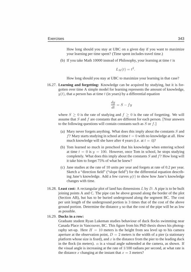
Exercises 343
How long should you stay at UBC on a given day if you want to maximizeyour learning per time spent? (Time spent includes travel time.)
(b) If you take Math 10000 instead of Philosophy, your learning at timet is
LM (t) = t2.
How long should you stay at UBC to maximize your learning in that case?
16.27. Learning and forgetting: Knowledge can be acquired by studying, but it is for-gotten over time A simple model for learning represents the amount of knowledge,y(t), that a person has at timet (in years) by a differential equation
dy
dt= S − fy
whereS ≥ 0 is the rate of studying andf ≥ 0 is the rate of forgetting. We willassume thatS andf are constants that are different for each person. [Your answersto the following questions will contain constants such asS or f .]
(a) Mary never forgets anything. What does this imply about the constantsS andf? Mary starts studying in school at timet = 0 with no knowledge at all. Howmuch knowledge will she have after 4 years (i.e. att = 4)?
(b) Tom learned so much in preschool that his knowledge when entering schoolat timet = 0 is y = 100. However, once Tom in school, he stops studyingcompletely. What does this imply about the constantsS andf? How long willit take him to forget 75% of what he knew?
(c) Jane studies at the rate of 10 units per year and forgets atrate of 0.2 per year.Sketch a “direction field” (“slope field”) for the differential equation describ-ing Jane’s knowledge. Add a few curvesy(t) to show how Jane’s knowledgechanges with time.
16.28. Least cost:A rectangular plot of land has dimensionsL by D. A pipe is to be builtjoining points A and C. The pipe can be above ground along the border of the plot(Section AB), but has to be buried underground along the segment BC. The costper unit length of the underground portion is 3 times that of the cost of the aboveground portion. Determine the distancey so that the cost of the pipe will be as lowas possible.
16.29. Ducks in a row:Graduate student Ryan Lukeman studies behaviour of duck flocks swimming nearCanada Place in Vancouver, BC. This figure from his PhD thesisshows his photog-raphy set-up. HereH = 10 meters is the height from sea level up to his cameraaperture at the observation point,D = 2 meters is the width of a pier (a stationaryplatform whose size is fixed), andx is the distance from the pier to the leading duckin the flock (in meters).α is a visual angle subtended at the camera, as shown. Ifthe visual angle is increasing at the rate of 1/100 radians per second, at what rate isthe distancex changing at the instant thatx = 3 meters?
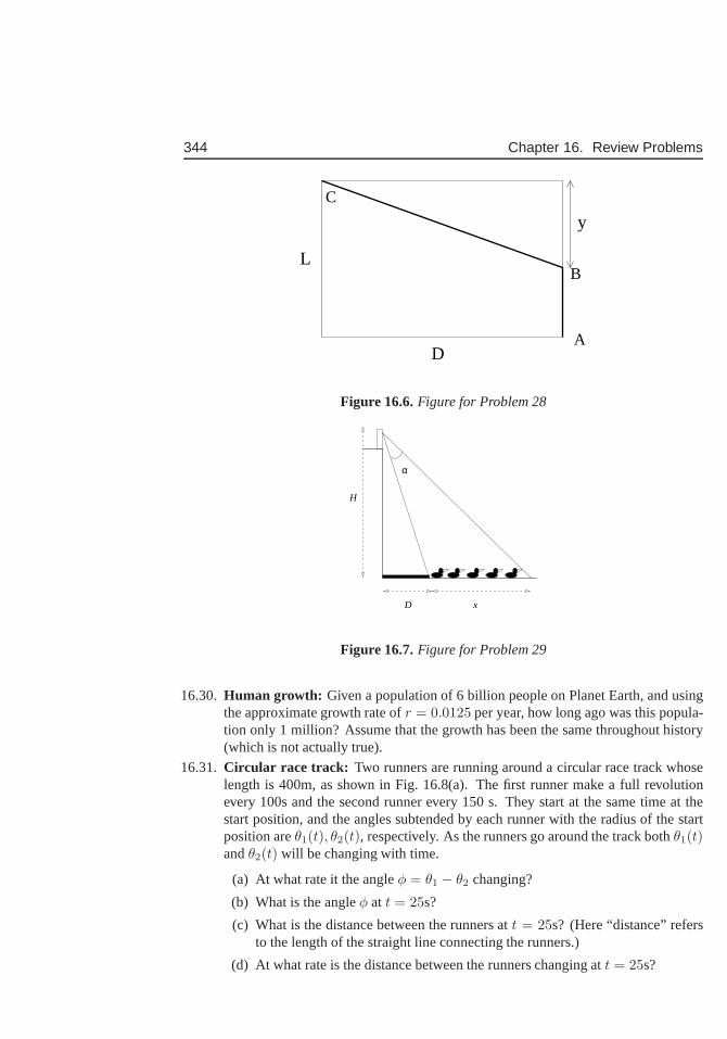
344 Chapter 16. Review Problems
C
D
L
A
B
y
Figure 16.6.Figure for Problem 28
D x
H
α
Figure 16.7.Figure for Problem 29
16.30. Human growth: Given a population of 6 billion people on Planet Earth, and usingthe approximate growth rate ofr = 0.0125 per year, how long ago was this popula-tion only 1 million? Assume that the growth has been the same throughout history(which is not actually true).
16.31. Circular race track: Two runners are running around a circular race track whoselength is 400m, as shown in Fig. 16.8(a). The first runner makea full revolutionevery 100s and the second runner every 150 s. They start at thesame time at thestart position, and the angles subtended by each runner withthe radius of the startposition areθ1(t), θ2(t), respectively. As the runners go around the track bothθ1(t)andθ2(t) will be changing with time.
(a) At what rate it the angleφ = θ1 − θ2 changing?
(b) What is the angleφ at t = 25s?
(c) What is the distance between the runners att = 25s? (Here “distance” refersto the length of the straight line connecting the runners.)
(d) At what rate is the distance between the runners changingat t = 25s?
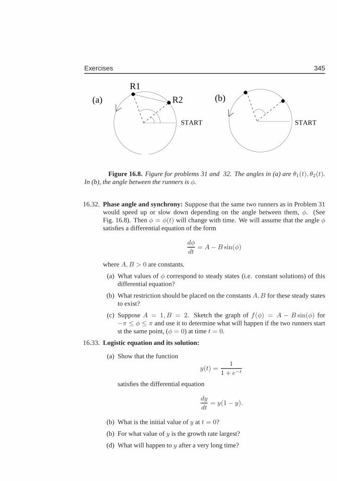
Exercises 345
(b)R1
R2
STARTSTART
(a)
Figure 16.8. Figure for problems 31 and 32. The angles in (a) areθ1(t), θ2(t).In (b), the angle between the runners isφ.
16.32. Phase angle and synchrony:Suppose that the same two runners as in Problem 31would speed up or slow down depending on the angle between them, φ. (SeeFig. 16.8). Thenφ = φ(t) will change with time. We will assume that the angleφsatisfies a differential equation of the form
dφ
dt= A−B sin(φ)
whereA, B > 0 are constants.
(a) What values ofφ correspond to steady states (i.e. constant solutions) of thisdifferential equation?
(b) What restriction should be placed on the constantsA, B for these steady statesto exist?
(c) SupposeA = 1, B = 2. Sketch the graph off(φ) = A − B sin(φ) for−π ≤ φ ≤ π and use it to determine what will happen if the two runners startst the same point, (φ = 0) at timet = 0.
16.33. Logistic equation and its solution:
(a) Show that the function
y(t) =1
1 + e−t
satisfies the differential equation
dy
dt= y(1− y).
(b) What is the initial value ofy at t = 0?
(b) For what value ofy is the growth rate largest?
(d) What will happen toy after a very long time?
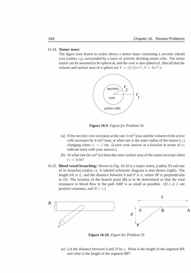
346 Chapter 16. Review Problems
16.34. Tumor mass:The figure (not drawn to scale) shows a tumor mass containing anecrotic (dead)core (radiusr2), surrounded by a layer of actively dividing tumor cells. The entiretumor can be assumed to be spherical, and the core is also spherical. (Recall that thevolume and surface area of a sphere areV = (4/3)πr3, S = 4πr2.)
1
r
r
active cells
necrotic
core
2
Figure 16.9.Figure for Problem 34
(a) If the necrotic core increases at the rate 3 cm3/year and the volume of the activecells increases by 4 cm3/year, at what rate is the outer radius of the tumor (r1)changing whenr1 = 1 cm. (Leave your answer as a fraction in terms ofπ;indicate units with your answer.)
(b) At what rate (in cm2/yr) does the outer surface area of the tumor increase whenr1 = 1cm?
16.35. Blood vessel branching:Shown in Fig. 16.10 is a major artery, (radiusR) and oneof its branches (radiusr). A labeled schematic diagram is also shown (right). Thelength 0A isL, and the distance between 0 and P isd, where 0P is perpendicularto 0A. The location of the branch point (B) is to be determinedso that the totalresistance to blood flow in the path ABP is as small as possible. (R, r, d, L arepositive constants, andR > r.)
0d
R
r P
L
B A
Figure 16.10.Figure for Problem 35
(a) Let the distance between 0 andB bex. What is the length of the segment BAand what is the length of the segment BP?
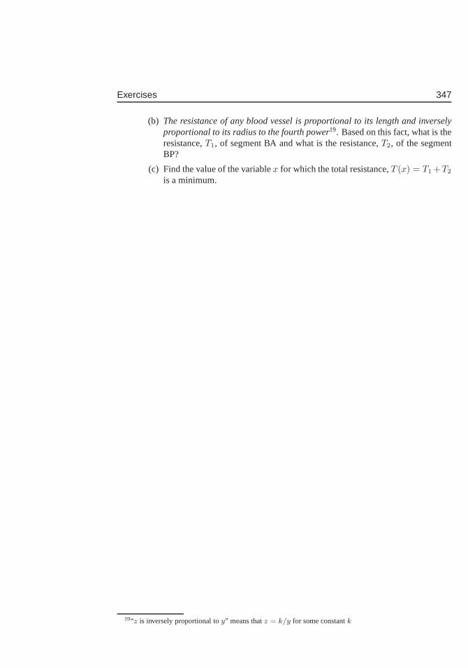
Exercises 347
(b) The resistance of any blood vessel is proportional to its length and inverselyproportional to its radius to the fourth power19. Based on this fact, what is theresistance,T1, of segment BA and what is the resistance,T2, of the segmentBP?
(c) Find the value of the variablex for which the total resistance,T (x) = T1 +T2
is a minimum.
19“z is inversely proportional toy” means thatz = k/y for some constantk

348 Chapter 16. Review Problems
Appendices
349

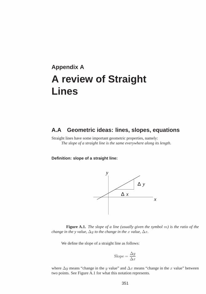
Appendix A
A review of StraightLines
A.A Geometric ideas: lines, slopes, equationsStraight lines have some important geometric properties, namely:
The slope of a straight line is the same everywhere along its length.
Definition: slope of a straight line:
∆ y
x
y
∆ x
Figure A.1. The slope of a line (usually given the symbolm) is the ratio of thechange in the y value,∆y to the change in thex value,∆x.
We define the slope of a straight line as follows:
Slope =∆y
∆x
where∆y means “change in they value” and∆x means “change in thex value” betweentwo points. See Figure A.1 for what this notation represents.
351
352 Appendix A. A review of Straight Lines
Equation of a straight line
Using this basic geometric property, we can find the equationof a straight line given any ofthe following information about the line:
• They intercept,b, and the slope,m:
y = mx + b.
• A point (x0, y0) on the line, and the slope,m, of the line:
y − y0
x− x0= m
• Two points on the line, say(x1, y1) and(x2, y2):
y − y1
x− x1=
y2 − y1
x2 − x1
Remark: any of these can be rearranged or simplified to produce the standard formy = mx + b, as discussed in the problem set.
The following examples will refresh your memory on how to findthe equation of theline that satisfies each of the given conditions.
Example A.1 In each case write down the equation of the straight line thatsatisfies thegiven statements. (Note: you should also be able to easily sketch the line in each case.)
(a) The line has slope 2 andy intercept 4.
(b) The line goes through the points (1,1) and (3,-2).
(c) The line hasy intercept -1 andx intercept 3.
(d) The line has slope -1 and goes through the point (-2,-5).
Solution:
(a) We can use the standard form of the equation of a straight line, y = mx + b wherem is the slope andb is they intercept to obtain the equation:y = 2x + 4
(b) The line goes through the points (1,1) and (3,-2). We use the fact that the slope is thesame all along the line. Thus,
(y − y0)
(x− x0)=
(y1 − y0)
(x1 − x0)= m.
Substituting in the values(x0, y0) = (1, 1) and(x1, y1) = (3,−2),
(y − 1)
(x− 1)=
(1 + 2)
(1− 3)= −3
2.
A.A. Geometric ideas: lines, slopes, equations 353
(Note that this tells us that the slope ism = −3/2.) We find that
y − 1 = −3
2(x− 1) = −3
2x +
3
2,
y = −3
2x +
5
2.
(c) The line hasy intercept -1 andx intercept 3, i.e. goes through the points (0,-1) and(3,0). We can use the method in (b) to get
y =1
3x− 1
Alternately, as a shortcut, we could find the slope,
m =∆y
∆x=
1
3.
(Note that∆ means “change in the value”, i.e.∆y = y1 − y0). Thusm = 1/3 andb = −1 (y intercept), leading to the same result.
(d) The line has slope -1 and goes through the point (-2,-5). Then,
(y + 5)
(x + 2)= −1,
so thaty + 5 = −1(x + 2) = −x− 2,
y = −x− 7.
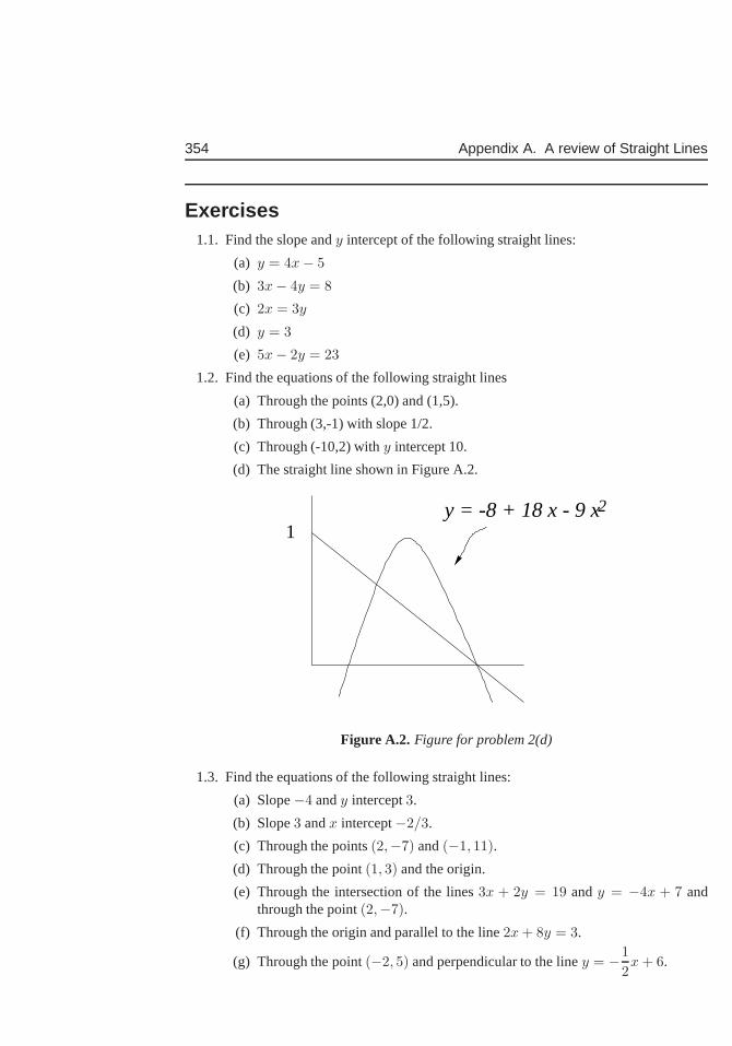
354 Appendix A. A review of Straight Lines
Exercises1.1. Find the slope andy intercept of the following straight lines:
(a) y = 4x− 5
(b) 3x− 4y = 8
(c) 2x = 3y
(d) y = 3
(e) 5x− 2y = 23
1.2. Find the equations of the following straight lines
(a) Through the points (2,0) and (1,5).
(b) Through (3,-1) with slope 1/2.
(c) Through (-10,2) withy intercept 10.
(d) The straight line shown in Figure A.2.
1y = -8 + 18 x - 9 x 2
Figure A.2. Figure for problem 2(d)
1.3. Find the equations of the following straight lines:
(a) Slope−4 andy intercept3.
(b) Slope3 andx intercept−2/3.
(c) Through the points(2,−7) and(−1, 11).
(d) Through the point(1, 3) and the origin.
(e) Through the intersection of the lines3x + 2y = 19 andy = −4x + 7 andthrough the point(2,−7).
(f) Through the origin and parallel to the line2x + 8y = 3.
(g) Through the point(−2, 5) and perpendicular to the liney = −1
2x + 6.
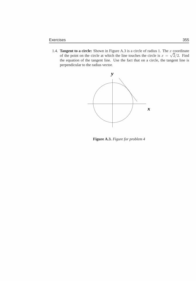
Exercises 355
1.4. Tangent to a circle: Shown in Figure A.3 is a circle of radius 1. Thex coordinateof the point on the circle at which the line touches the circleis x =
√2/2. Find
the equation of the tangent line. Use the fact that on a circle, the tangent line isperpendicular to the radius vector.
x
y
Figure A.3. Figure for problem 4

356 Appendix A. A review of Straight Lines
Appendix B
A precalculus review
B.A Manipulating exponentsRecall that2n = 2 · 2 . . . 2 (with n factors of 2).
This means that2n ·2m = (2 ·2 . . .2) ·(2 ·2 . . .2) = 2n+m, where we have expandedthe product inton and thenm factors of 2. Similarly, we can derive many properties ofmanipulations of exponents. A list of these appears below, and holes for any positive basea
1. 2a2b = 2a+b as with all similar exponent manipulations.
2. (2a)b = 2ab also stems from simple rules for manipulating exponents
3. 2x is a function that is defined, continuous, and differentiable for all real numbersx.
4. 2x > 0 for all values ofx.
5. We define20 = 1, and we also have that21 = 2.
6. 2x → 0 for increasing negative values ofx
7. 2x →∞ for increasing positive values ofx
B.B Manipulating logarithmsThe following properties hold for logarithms of any base. Since we have used the base 2 inour previous section, we keep the same base here as well Properties of the logarithm stemdirectly from properties of the exponential function, and include the following:
1. log2(ab) = log2(a) + log2(b)
2. log2(ab) = b log2(a)
3. log2(1/a) = log2(a−1) = − log2(a)
357

358 Appendix B. A precalculus review
Appendix C
A Review of SimpleFunctions
Herer we review a few basic concepts related to functions
C.A What is a functionA function is just a way of expressing a special relationshipbetween a value we consideras the input (“x”) value and an associated output (y) value. We write this relationship inthe form
y = f(x)
to indicate thaty depends onx. The only constraint on this relationship is that, for everyvalue ofx we can get at most one value ofy. This is equivalent to the“vertical lineproperty”: the graph of a function can intersect a vertical line at mostat one point. The setof all allowablex values is called thedomainof the function, and the set of all resultingvalues ofy are therange.
Naturally, we will not always use the symbolsx andy to represent independent anddependent variables. For example, the relationship
V =4
3πr3
expresses a functional connection between the radius,r, and the volume,V , of a sphere.We say in such a case that “V is a function ofr”.
All the sketches shown in Figure C.1 are valid functions. Thefirst is merely a collec-tion of points,x values and associatedy values, the second a histogram. The third sketchis here meant to represent the collection of smooth continuous functions, and these are thevariety of interest to us here in the study of calculus. On theother hand, the example shownin Figure C.2 is not the graph of a function. We see that a vertical line intersects this curveat more than one point. This is not permitted, since as we already said, a given value ofxshould have only one corresponding values ofy.
359
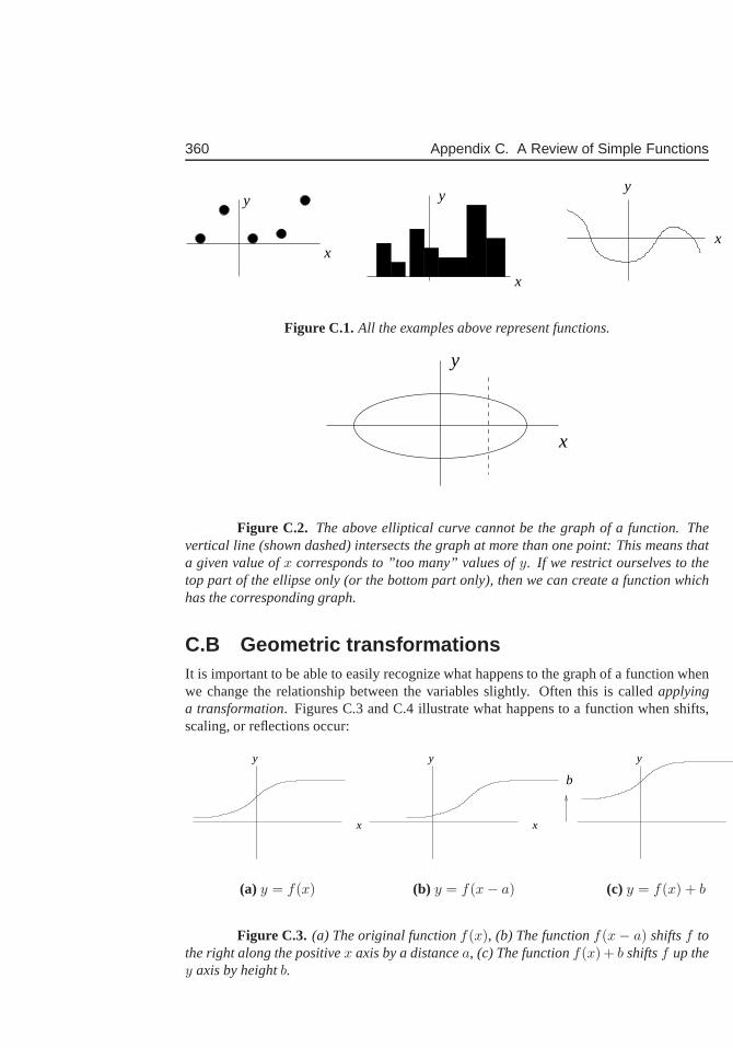
360 Appendix C. A Review of Simple Functions
x
x
x
yyy
Figure C.1. All the examples above represent functions.
x
y
Figure C.2. The above elliptical curve cannot be the graph of a function.Thevertical line (shown dashed) intersects the graph at more than one point: This means thata given value ofx corresponds to ”too many” values ofy. If we restrict ourselves to thetop part of the ellipse only (or the bottom part only), then wecan create a function whichhas the corresponding graph.
C.B Geometric transformationsIt is important to be able to easily recognize what happens tothe graph of a function whenwe change the relationship between the variables slightly.Often this is calledapplyinga transformation. Figures C.3 and C.4 illustrate what happens to a function when shifts,scaling, or reflections occur:
x
y
x
y y
b
(a) y = f(x) (b) y = f(x− a) (c) y = f(x) + b
Figure C.3. (a) The original functionf(x), (b) The functionf(x− a) shiftsf tothe right along the positivex axis by a distancea, (c) The functionf(x) + b shiftsf up they axis by heightb.
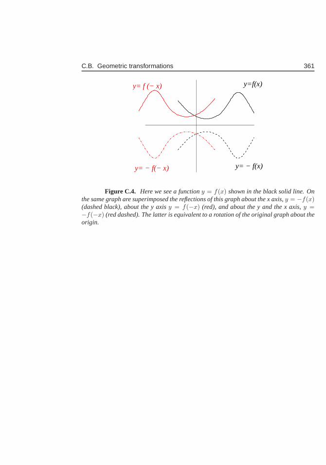
C.B. Geometric transformations 361
y= f (− x) y=f(x)
y= − f(x)y= − f(− x)
Figure C.4. Here we see a functiony = f(x) shown in the black solid line. Onthe same graph are superimposed the reflections of this graphabout the x axis,y = −f(x)(dashed black), about the y axisy = f(−x) (red), and about the y and the x axis,y =−f(−x) (red dashed). The latter is equivalent to a rotation of the original graph about theorigin.
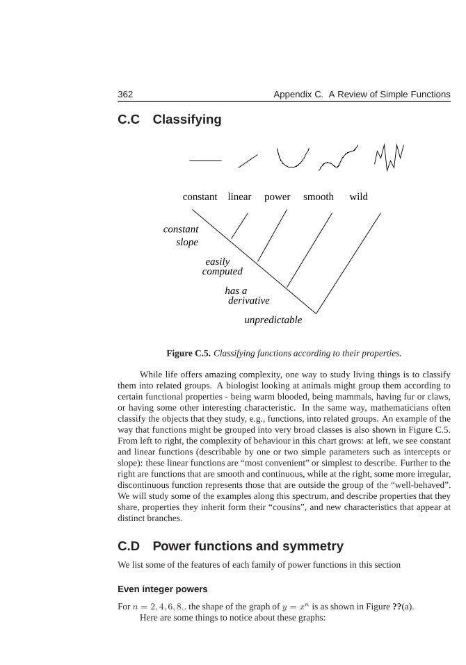
362 Appendix C. A Review of Simple Functions
C.C Classifying
constant linear power smooth wild
constantslope
easilycomputed
has aderivative
unpredictable
Figure C.5. Classifying functions according to their properties.
While life offers amazing complexity, one way to study living things is to classifythem into related groups. A biologist looking at animals might group them according tocertain functional properties - being warm blooded, being mammals, having fur or claws,or having some other interesting characteristic. In the same way, mathematicians oftenclassify the objects that they study, e.g., functions, intorelated groups. An example of theway that functions might be grouped into very broad classes is also shown in Figure C.5.From left to right, the complexity of behaviour in this chartgrows: at left, we see constantand linear functions (describable by one or two simple parameters such as intercepts orslope): these linear functions are “most convenient” or simplest to describe. Further to theright are functions that are smooth and continuous, while atthe right, some more irregular,discontinuous function represents those that are outside the group of the “well-behaved”.We will study some of the examples along this spectrum, and describe properties that theyshare, properties they inherit form their “cousins”, and new characteristics that appear atdistinct branches.
C.D Power functions and symmetryWe list some of the features of each family of power functionsin this section
Even integer powers
Forn = 2, 4, 6, 8.. the shape of the graph ofy = xn is as shown in Figure??(a).Here are some things to notice about these graphs:
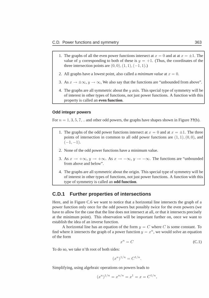
C.D. Power functions and symmetry 363
1. The graphs of all the even power functions intersect atx = 0 and at atx = ±1. Thevalue ofy corresponding to both of these isy = +1. (Thus, the coordinates of thethree intersection points are(0, 0), (1, 1), (−1, 1).)
2. All graphs have a lowest point, also called aminimum valueatx = 0.
3. Asx→ ±∞, y →∞, We also say that the functions are “unbounded from above”.
4. The graphs are all symmetric about they axis. This special type of symmetry will beof interest in other types of functions, not just power functions. A function with thisproperty is called aneven function.
Odd integer powers
Forn = 1, 3, 5, 7, .. and other odd powers, the graphs have shapes shown in Figure??(b).
1. The graphs of the odd power functions intersect atx = 0 and atx = ±1. The threepoints of intersection in common to all odd power functions are (1, 1), (0, 0), and(−1,−1).
2. None of the odd power functions have a minimum value.
3. Asx → +∞, y → +∞. As x → −∞, y → −∞. The functions are “unboundedfrom above and below”.
4. The graphs are all symmetric about the origin. This special type of symmetry will beof interest in other types of functions, not just power functions. A function with thistype of symmetry is called anodd function.
C.D.1 Further properties of intersections
Here, and in Figure C.6 we want to notice that a horizontal line intersects the graph of apower function only once for the odd powers but possibly twice for the even powers (wehave to allow for the case that the line does not intersect at all, or that it intersects preciselyat the minimum point). This observation will be important further on, once we want toestablish the idea of an inverse function.
A horizontal line has an equation of the formy = C whereC is some constant. Tofind where it intersects the graph of a power functiony = xn, we would solve an equationof the form
xn = C (C.1)
To do so, we take n’th root of both sides:
(xn)1/n = C1/n.
Simplifying, using algebraic operations on powers leads to
(xn)1/n = xn/n = x1 = x = C1/n,
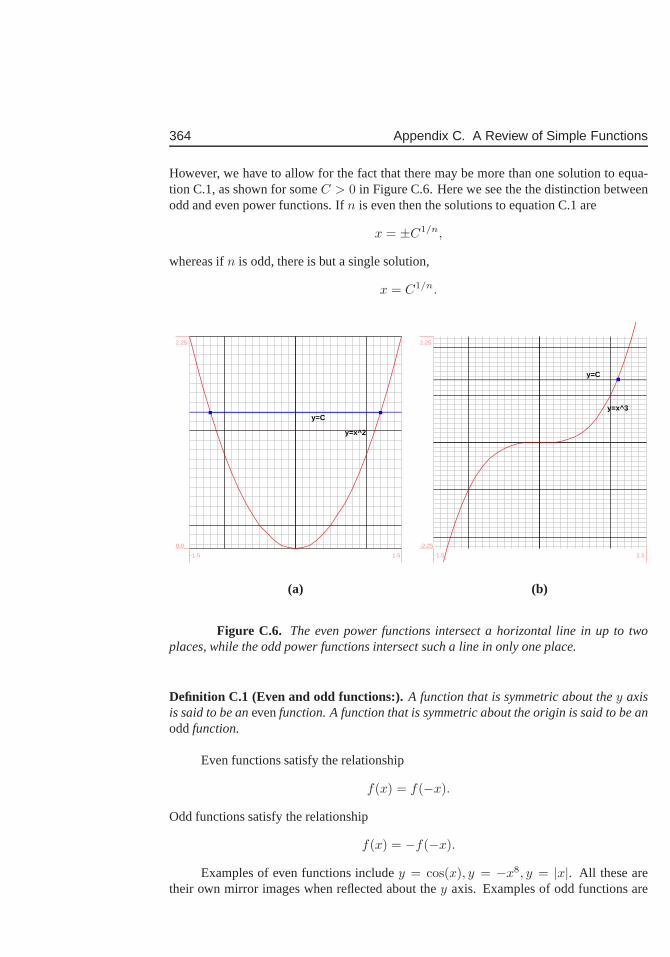
364 Appendix C. A Review of Simple Functions
However, we have to allow for the fact that there may be more than one solution to equa-tion C.1, as shown for someC > 0 in Figure C.6. Here we see the the distinction betweenodd and even power functions. Ifn is even then the solutions to equation C.1 are
x = ±C1/n,
whereas ifn is odd, there is but a single solution,
x = C1/n.
y=x^2
y=C
-1.5 1.5
0.0
2.25
y=x^3
y=C
-1.5 1.5
-2.25
2.25
(a) (b)
Figure C.6. The even power functions intersect a horizontal line in up totwoplaces, while the odd power functions intersect such a line in only one place.
Definition C.1 (Even and odd functions:).A function that is symmetric about they axisis said to be anevenfunction. A function that is symmetric about the origin is said to be anoddfunction.
Even functions satisfy the relationship
f(x) = f(−x).
Odd functions satisfy the relationship
f(x) = −f(−x).
Examples of even functions includey = cos(x), y = −x8, y = |x|. All these aretheir own mirror images when reflected about they axis. Examples of odd functions are
C.D. Power functions and symmetry 365
y = sin(x), y = −x3, y = x. Each of these functions is its own double-reflection (aboutyand then x axes).
In a later calculus course, when we compute integrals, taking these symmetries intoaccount can help to simplify (or even avoid) calculations.
C.D.2 Optional: Combining even and odd functions
Not every function is either odd or even. However, if we startwith symmetric functions,certain manipulations either preserve or reverse the symmetry.
Example C.2 Show that the product of an even and an odd function is an odd function.
Solution: Let f(x) be even. Then
f(x) = f(−x).
Let g(x) be an odd function. Theng(x) = −g(−x). We defineh(x) to be the product ofthese two functions,
h(x) = f(x)g(x).
Using the properties off andg,
f(x)g(x) = f(−x)[−g(−x)]
so, rearranging, we get
h(x) = f(x)g(x) = f(−x)[−g(−x)] = −[f(−x)g(−x)].
but this is just the same as−h(−x). We have established that
h(x) = −h(−x)
so that the new function is odd.A function is not always even or odd. Many functions are neither even nor odd.
However, by a little trick, we can show that given any function, y = f(x), we can write itas a sum of an even and an odd function.
Hint: Supposef(x) is not an even nor an odd function. Consider defining the two associ-ated functions:
fe(x) =1
2(f(x) + f(−x)),
and
f0(x) =1
2(f(x)− f(−x)).
(Can you draw a sketch of what these would look like for the function given in Fig-ure C.3(a)?) Show thatfe(x) is even and thatf0(x) is odd. Now show that
f(x) = fe(x) + f0(x).
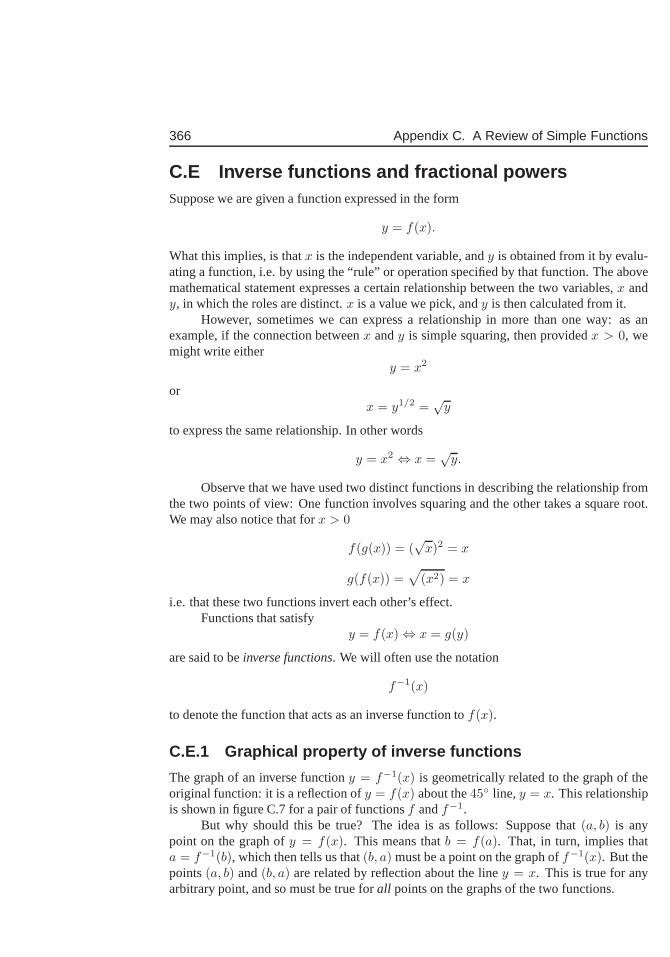
366 Appendix C. A Review of Simple Functions
C.E Inverse functions and fractional powersSuppose we are given a function expressed in the form
y = f(x).
What this implies, is thatx is the independent variable, andy is obtained from it by evalu-ating a function, i.e. by using the “rule” or operation specified by that function. The abovemathematical statement expresses a certain relationship between the two variables,x andy, in which the roles are distinct.x is a value we pick, andy is then calculated from it.
However, sometimes we can express a relationship in more than one way: as anexample, if the connection betweenx andy is simple squaring, then providedx > 0, wemight write either
y = x2
orx = y1/2 =
√y
to express the same relationship. In other words
y = x2 ⇔ x =√
y.
Observe that we have used two distinct functions in describing the relationship fromthe two points of view: One function involves squaring and the other takes a square root.We may also notice that forx > 0
f(g(x)) = (√
x)2 = x
g(f(x)) =√
(x2) = x
i.e. that these two functions invert each other’s effect.Functions that satisfy
y = f(x)⇔ x = g(y)
are said to beinverse functions. We will often use the notation
f−1(x)
to denote the function that acts as an inverse function tof(x).
C.E.1 Graphical property of inverse functions
The graph of an inverse functiony = f−1(x) is geometrically related to the graph of theoriginal function: it is a reflection ofy = f(x) about the45◦ line, y = x. This relationshipis shown in figure C.7 for a pair of functionsf andf−1.
But why should this be true? The idea is as follows: Suppose that (a, b) is anypoint on the graph ofy = f(x). This means thatb = f(a). That, in turn, implies thata = f−1(b), which then tells us that(b, a) must be a point on the graph off−1(x). But thepoints(a, b) and(b, a) are related by reflection about the liney = x. This is true for anyarbitrary point, and so must be true forall points on the graphs of the two functions.
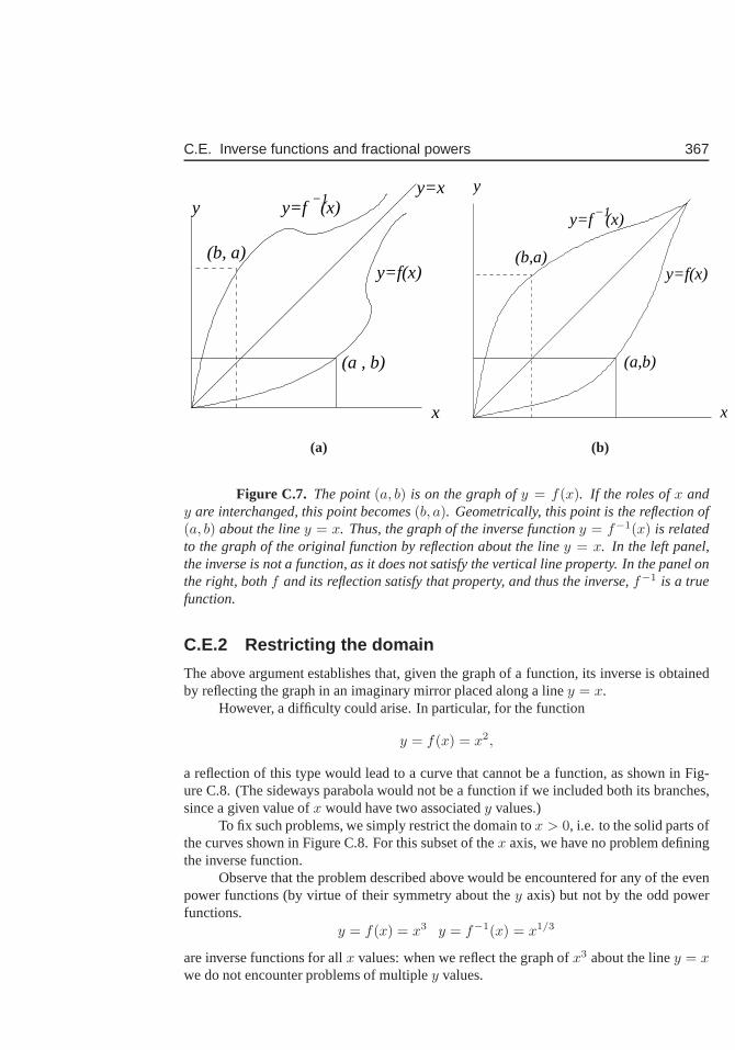
C.E. Inverse functions and fractional powers 367
x
yy=x
y=f(x)
y=f (x)−1
(a , b)
(b, a)
−1
y
x
(a,b)
(b,a)y=f(x)
y=f (x)
(a) (b)
Figure C.7. The point(a, b) is on the graph ofy = f(x). If the roles ofx andy are interchanged, this point becomes(b, a). Geometrically, this point is the reflection of(a, b) about the liney = x. Thus, the graph of the inverse functiony = f−1(x) is relatedto the graph of the original function by reflection about the line y = x. In the left panel,the inverse is not a function, as it does not satisfy the vertical line property. In the panel onthe right, bothf and its reflection satisfy that property, and thus the inverse,f−1 is a truefunction.
C.E.2 Restricting the domain
The above argument establishes that, given the graph of a function, its inverse is obtainedby reflecting the graph in an imaginary mirror placed along a liney = x.
However, a difficulty could arise. In particular, for the function
y = f(x) = x2,
a reflection of this type would lead to a curve that cannot be a function, as shown in Fig-ure C.8. (The sideways parabola would not be a function if we included both its branches,since a given value ofx would have two associatedy values.)
To fix such problems, we simply restrict the domain tox > 0, i.e. to the solid parts ofthe curves shown in Figure C.8. For this subset of thex axis, we have no problem definingthe inverse function.
Observe that the problem described above would be encountered for any of the evenpower functions (by virtue of their symmetry about they axis) but not by the odd powerfunctions.
y = f(x) = x3 y = f−1(x) = x1/3
are inverse functions for allx values: when we reflect the graph ofx3 about the liney = xwe do not encounter problems of multipley values.
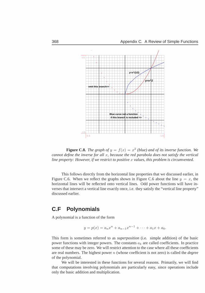
368 Appendix C. A Review of Simple Functions
y=x^2
y=x^(1/2)
omit this branch=>
Blue curve not a functionif this branch is included =>
-1.5 1.5
-1.5
1.5
Figure C.8. The graph ofy = f(x) = x2 (blue) and of its inverse function. Wecannot define the inverse for allx, because the red parabola does not satisfy the verticalline property: However, if we restrict to positivex values, this problem is circumvented.
This follows directly from the horizontal line properties that we discussed earlier, inFigure C.6. When we reflect the graphs shown in Figure C.6 about the liney = x, thehorizontal lines will be reflected onto vertical lines. Odd power functions will have in-verses that intersect a vertical line exactly once, i.e. they satisfy the “vertical line property”discussed earlier.
C.F PolynomialsA polynomial is a function of the form
y = p(x) = anxn + an−1xn−1 + · · ·+ a1x + a0.
This form is sometimes referred to assuperposition(i.e. simple addition) of the basicpower functions with integer powers. The constantsak are called coefficients. In practicesome of these may be zero. We will restrict attention to the case where all these coefficientsare real numbers. The highest powern (whose coefficient is not zero) is called thedegreeof the polynomial.
We will be interested in these functions for several reasons. Primarily, we will findthat computations involving polynomials are particularlyeasy, since operations includeonly the basic addition and multiplication.
C.F. Polynomials 369
C.F.1 Features of polynomials
• Zeros of a polynomialare values ofx such that
y = p(x) = 0.
If p(x) is quadratic (a polynomial of degree 2) then the quadratic formula gives asimple way of finding roots of this equation (also called “zeros” of the polynomial).Generally, for most polynomials of degree higher than 5, there is no analytical recipefor finding zeros. Geometrically, zeros are places where thegraph of the functiony = p(x) crosses thex axis. We will exploit this fact much later in the course toapproximate the values of the zeros usingNewton’s Method.
• Critical Points: Places on the graph where the value of the function is locallylargerthan those nearby (local maxima) or smaller than those nearby (local minima) will beof interest to us. Calculus will be one of the main tools for detecting and identifyingsuch places.
• Behaviour for very large x: All polynomials are unbounded asx → ∞ and asx→ −∞. In fact, for large enough values ofx, we have seen that the power functiony = f(x) = xn with the largest power,n, dominates over other power functions withsmaller powers.For
p(x) = anxn + an−1xn−1 + · · ·+ a1x + a0
the first (highest power) term willdominatefor largex. Thus for largex (whetherpositive or negative)
p(x) ≈ anxn for large x.
• Behaviour for small x: Close to the origin, we have seen that power functions withsmallest powers dominate. This means that forx ≈ 0 the polynomial is governed bythe behaviour of the smallest (non-zero coefficient) power,i.e,
p(x) ≈ a1x + a0 for small x.
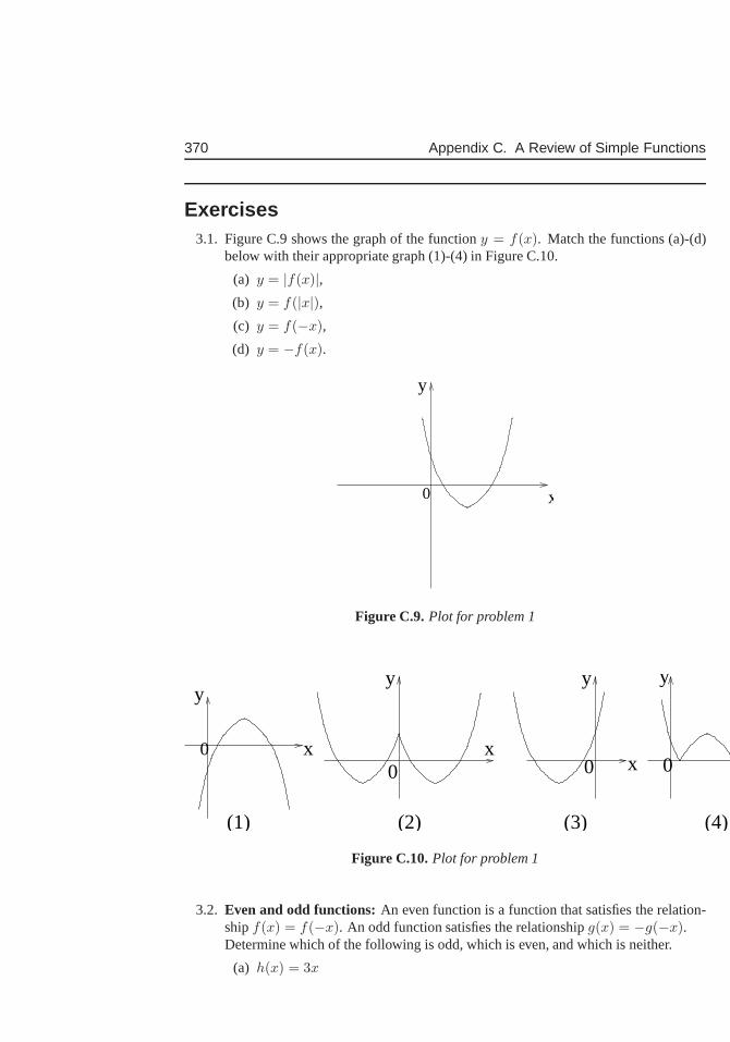
370 Appendix C. A Review of Simple Functions
Exercises3.1. Figure C.9 shows the graph of the functiony = f(x). Match the functions (a)-(d)
below with their appropriate graph (1)-(4) in Figure C.10.
(a) y = |f(x)|,(b) y = f(|x|),(c) y = f(−x),
(d) y = −f(x).
0
y
x
Figure C.9. Plot for problem 1
xx
y
x
y y
(1) (2) (3) (4)
y
0 000
Figure C.10.Plot for problem 1
3.2. Even and odd functions:An even function is a function that satisfies the relation-shipf(x) = f(−x). An odd function satisfies the relationshipg(x) = −g(−x).Determine which of the following is odd, which is even, and which is neither.
(a) h(x) = 3x
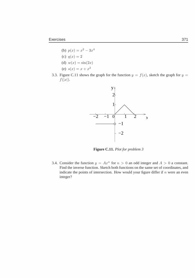
Exercises 371
(b) p(x) = x2 − 3x4
(c) q(x) = 2
(d) w(x) = sin(2x)
(e) s(x) = x + x2
3.3. Figure C.11 shows the graph for the functiony = f(x), sketch the graph fory =f(|x|).
0
2
−2 1 2−1
1
x
y
−1
−2
Figure C.11.Plot for problem 3
3.4. Consider the functiony = Axn for n > 0 an odd integer andA > 0 a constant.Find the inverse function. Sketch both functions on the sameset of coordinates, andindicate the points of intersection. How would your figure differ if n were an eveninteger?

372 Appendix C. A Review of Simple Functions
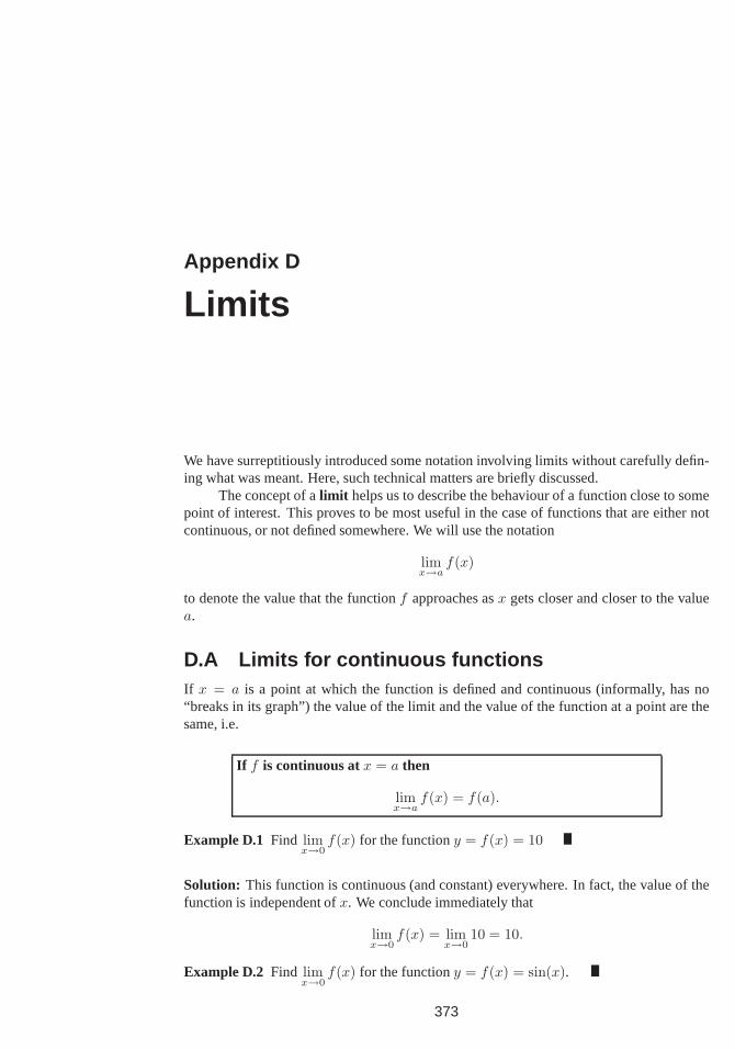
Appendix D
Limits
We have surreptitiously introduced some notation involving limits without carefully defin-ing what was meant. Here, such technical matters are briefly discussed.
The concept of alimit helps us to describe the behaviour of a function close to somepoint of interest. This proves to be most useful in the case offunctions that are either notcontinuous, or not defined somewhere. We will use the notation
limx→a
f(x)
to denote the value that the functionf approaches asx gets closer and closer to the valuea.
D.A Limits for continuous functionsIf x = a is a point at which the function is defined and continuous (informally, has no“breaks in its graph”) the value of the limit and the value of the function at a point are thesame, i.e.
If f is continuous atx = a then
limx→a
f(x) = f(a).
Example D.1 Find limx→0
f(x) for the functiony = f(x) = 10
Solution: This function is continuous (and constant) everywhere. In fact, the value of thefunction is independent ofx. We conclude immediately that
limx→0
f(x) = limx→0
10 = 10.
Example D.2 Find limx→0
f(x) for the functiony = f(x) = sin(x).
373
374 Appendix D. Limits
Solution: This function is a continuous trigonometric function, and has the valuesin(0) =0 at the origin. Thus
limx→0
f(x) = limx→0
sin(x) = 0
Power functions are continuous everywhere. This motivatesthe next example.
Example D.3 Compute the limitlimx→0
xn wheren is a positive integer.
Solution: The function in question,f(x) = xn is a simple power function that is continu-ous everywhere. Further,f(0) = 0. Hence the limit asx → 0 coincides with the value ofthe function oat that point, so
limx→0
xn = 0.
D.B Properties of limitsSuppose we are given two functions,f(x) andg(x). We will also assume that both func-tions have (finite) limits at the pointx = a. Then the following statements follow.
1.limx→a
(f(x) + g(x)) = limx→a
f(x) + limx→a
g(x)
2.limx→a
(cf(x)) = c limx→a
f(x)
3.limx→a
(f(x) · g(x)) =(
limx→a
f(x))
·(
limx→a
g(x))
4. Provided thatlimx→a
g(x) 6= 0, we also have that
limx→a
(
f(x)
g(x)
)
=
(
limx→a
f(x)
limx→a
g(x)
)
.
The first two statements are equivalent to linearity of the process of computing alimit.
Example D.4 Find limx→2
f(x) for the functiony = f(x) = 2x2 − x3.
Solution: Since this function is a polynomial, and so continuous everywhere, we can sim-ply plug in the relevant value ofx, i.e.
limx→2
(
2x2 − x3)
= 2 · 22 − 23 = 0.
Thus whenx gets closer to 2, the value of the function gets closer to 0. (In fact, the valueof the limit is the same as the value of the function at the given point.)
D.C. Limits of rational functions 375
D.C Limits of rational functions
D.C.1 Case 1: Denominator nonzero
We first consider functions that are the quotient of two polynomials,y = f(x)/g(x) atpoints wereg(x) 6= 0. This allows us to apply Property 4 of limits together with whatwe have learned about the properties of power functions and polynomials. Much of thisdiscussion is related to the properties of power functions and dominance of lower (higher)powers at small (large) values ofx, as discussed in Chapter 1. In the examples below, weconsider both limits at the origin (atx = 0) and at infinity (forx → ∞). The latter means“very largex”. See Section?? for examples of the informal version of the same reasoningused to reach the same conclusions.
Example D.5 Find the limit asx→ 0 and asx→∞ of the quotients
(a)Kx
kn + x, (b)
Axn
an + xn.
Solution: We recognize (a) as an example of the Michaelis Menten kinetics, found in (1.7)and (b) as a Hill function in (1.6) of Chapter 1. We now compute, first for x→ 0,
(a) limx→0
Kx
kn + x= 0, (b) lim
x→0
Axn
an + xn= 0.
This follows from the fact that, provideda, kn 6= 0, both functions are continuous atx = 0,so that their limits are the same as the actual values attained by the functions. Now forx→∞
(a) limx→∞
Kx
kn + x= lim
x→∞Kx
x= K, (b) lim
x→∞Axn
an + xn= lim
x→∞Axn
xn= A.
This follows from the fact that the constantskn, an are always “swamped out” by the valueof x asx→∞, allowing us to obtain the result. Other than the formal limit notation, thereis nothing new here that we have not already discussed in Sections 1.5.
Below we apply similar reasoning to other examples of rational functions.
Example D.6 Find the limit asx→ 0 and asx→∞ of the quotients
(a)3x2
9 + x2, (b)
1 + x
1 + x3.
Solution: For part (a) we note that asx → ∞, the quotient approaches3x2/x2 = 3. Asx → 0, both numerator and denominator are defined and the denominator is nonzero, sowe can use the 4th property of limits. We thus find that
(a) limx→∞
3x2
9 + x2= 3, lim
x→0
3x2
9 + x2= 0,
376 Appendix D. Limits
For part (b), we use the fact that asx → ∞, the limit approachesx/x3 = x−2 → 0. Asx→ 0 we can apply property 4 yet again to compute the (finite) limit, so that
(b) limx→∞
1 + x
1 + x3, lim
x→0
1 + x
1 + x3.
Example D.7 Find the limits of the following function at 0 and∞
y =x4 − 3x2 + x− 1
x5 + x.
Solution: for x→∞ powers with the largest power dominate, whereas forx→ 0, smallerpowers dominate. Hence, we find
limx→∞
x4 − 3x2 + x− 1
x5 + x= lim
x→∞x4
x5= lim
x→∞1
x= 0.
limx→0
x4 − 3x2 + x− 1
x5 + x= lim
x→0
−1
x= − lim
x→0
1
x=∞
So in the latter case, the limit does not exist.
D.C.2 Case 2: zero in the denominator and “holes” in a graph
In the previous examples, evaluating the limit, where it existed, was as simple as pluggingthe appropriate value ofx into the function itself. The next example shows that this isnotalways possible.
Example D.8 Compute the limit asx→ 4 of the functionf(x) = 1/(x− 4)
Solution: This function has a vertical asymptote atx = 4. Indeed, the value of the functionshoots off to+∞ if we approachx = 4 from above, and−∞ if we approach the same pointfrom below. We say that the limitdoes not existin this case.
Example D.9 Compute the limit asx→ −1 of the functionf(x) = x/(x2 − 1)
Solution: We compute
limx→−1
x
x2 − 1= lim
x→−1
x
(x − 1)(x + 1)
It is evident (even before factoring as we have done) that this function has a vertical asymp-tote atx = −1 where the denominator approaches zero. Hence, the limit does not exist.
Next, we describe an extremely important example where the function has a “hole” inits graph, but where a finite limit exists. This kind of limit plays a huge role in the definitionof a derivative.
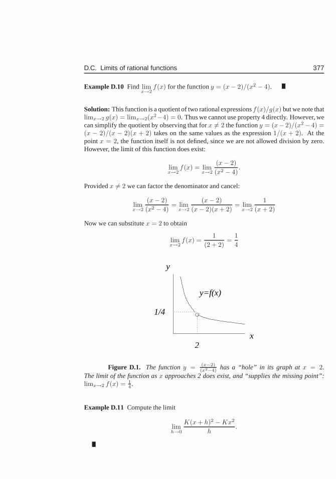
D.C. Limits of rational functions 377
Example D.10 Find limx→2
f(x) for the functiony = (x− 2)/(x2 − 4).
Solution: This function is a quotient of two rational expressionsf(x)/g(x) but we note thatlimx→2 g(x) = limx→2(x
2−4) = 0. Thus we cannot use property 4 directly. However, wecan simplify the quotient by observing that forx 6= 2 the functiony = (x− 2)/(x2− 4) =(x − 2)/(x − 2)(x + 2) takes on the same values as the expression1/(x + 2). At thepoint x = 2, the function itself is not defined, since we are not allowed division by zero.However, the limit of this function does exist:
limx→2
f(x) = limx→2
(x− 2)
(x2 − 4).
Providedx 6= 2 we can factor the denominator and cancel:
limx→2
(x− 2)
(x2 − 4)= lim
x→2
(x− 2)
(x− 2)(x + 2)= lim
x→2
1
(x + 2)
Now we can substitutex = 2 to obtain
limx→2
f(x) =1
(2 + 2)=
1
4
y
2
1/4
y=f(x)
x
Figure D.1. The functiony = (x−2)(x2−4) has a “hole” in its graph atx = 2.
The limit of the function asx approaches 2 does exist, and “supplies the missing point”:limx→2 f(x) = 1
4 .
Example D.11 Compute the limit
limh→0
K(x + h)2 −Kx2
h.
378 Appendix D. Limits
Solution: This is a calculation we would perform to compute the derivative of the functiony = Kx2 from the definition of the derivative. Details have already been displayed in Ex-ample 2.21. The essential idea is that we expand the numerator and simplify algebraicallyas follows:
limh→0
K(2xh + h2)
h= lim
h→0K(2x + h) = 2Kx.
Even though the quotient is not defined at the valueh = 0 (as the denominator is zerothere), the limit exists, and hence the derivative can be defined. See also Example 3.15 fora similar calculation for the functionKx3.
D.D Right and left sided limitsSome functions are discontinuous at a point, but we may stillbe able to define a limit thatthe function attains as we approach that point from the rightor from the left. (This isequivalent to gradually decreasing or gradually increasing x as we get closer to the pointof interest.
Consider the function
f(x) =
{
0 if x < 0;1 if x > 0.
This is a step function, whose values is 0 for negative real numbers, and 1 for positive realnumbers. The function is not even defined at the pointx = 0 and has a jump in its graph.However, we can still define a right and a left limit as follows:
limx→+0
f(x) = 0, limx→−0
f(x) = 1.
That is, the limit as we approach from the right is 0 whereas from the left it is 1. We alsostate the following result:
If f(x) has a right and a left limit at a point x = a and if those limitsare equal, then we say that the limit atx = a exists, and we write
limx→+a
f(x) = limx→−a
f(x) = limx→a
f(x)
Example D.12 Find limx→π/2
f(x) for the functiony = f(x) = tan(x).
Solution: The functiontan(x) = sin(x)/ cos(x) cannot be continuous atx = π/2 becausecos(x) in the denominator takes on the value of zero at the pointx = π/2. Moreover, thevalue of this function becomes unbounded (grows without a limit) asx→ π/2. We say inthis case that “the limit does not exist”. We sometimes use the notation
limx→π/2
tan(x) = ±∞.
(We can distinguish the fact that the function approaches+∞ asx approachesπ/2 frombelow, and−∞ asx approachesπ/2 from higher values.
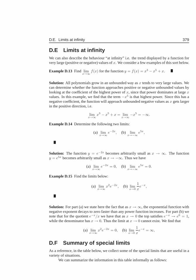
D.E. Limits at infinity 379
D.E Limits at infinityWe can also describe the behaviour “at infinity” i.e. the trend displayed by a function forvery large (positive or negative) values ofx. We consider a few examples of this sort below.
Example D.13 Find limx→∞
f(x) for the functiony = f(x) = x3 − x5 + x.
Solution: All polynomials grow in an unbounded way asx tends to very large values. Wecan determine whether the function approaches positive or negative unbounded values bylooking at the coefficient of the highest power ofx, since that power dominates at largexvalues. In this example, we find that the term−x5 is that highest power. Since this has anegative coefficient, the function will approach unboundednegative values asx gets largerin the positive direction, i.e.
limx→∞
x3 − x5 + x = limx→∞
−x5 = −∞.
Example D.14 Determine the following two limits:
(a) limx→∞
e−2x, (b) limx→−∞
e5x,
Solution: The functiony = e−2x becomes arbitrarily small asx → ∞. The functiony = e5x becomes arbitrarily small asx→ −∞. Thus we have
(a) limx→∞
e−2x = 0, (b) limx→−∞
e5x = 0.
Example D.15 Find the limits below:
(a) limx→∞
x2e−2x, (b) limx→0
1
xe−x,
Solution: For part (a) we state here the fact that asx→ ∞, the exponential function withnegative exponent decays to zero faster than any power function increases. For part (b) wenote that for the quotiente−x/x we have that asx → 0 the top satisfiese−x → e0 = 1,while the denominator hasx→ 0. Thus the limit atx→ 0 cannot exist. We find that
(a) limx→∞
x2e−2x = 0, (b) limx→0
1
xe−x =∞,
D.F Summary of special limitsAs a reference, in the table below, we collect some of the special limits that are useful in avariety of situations.
We can summarize the information in this table informally asfollows:
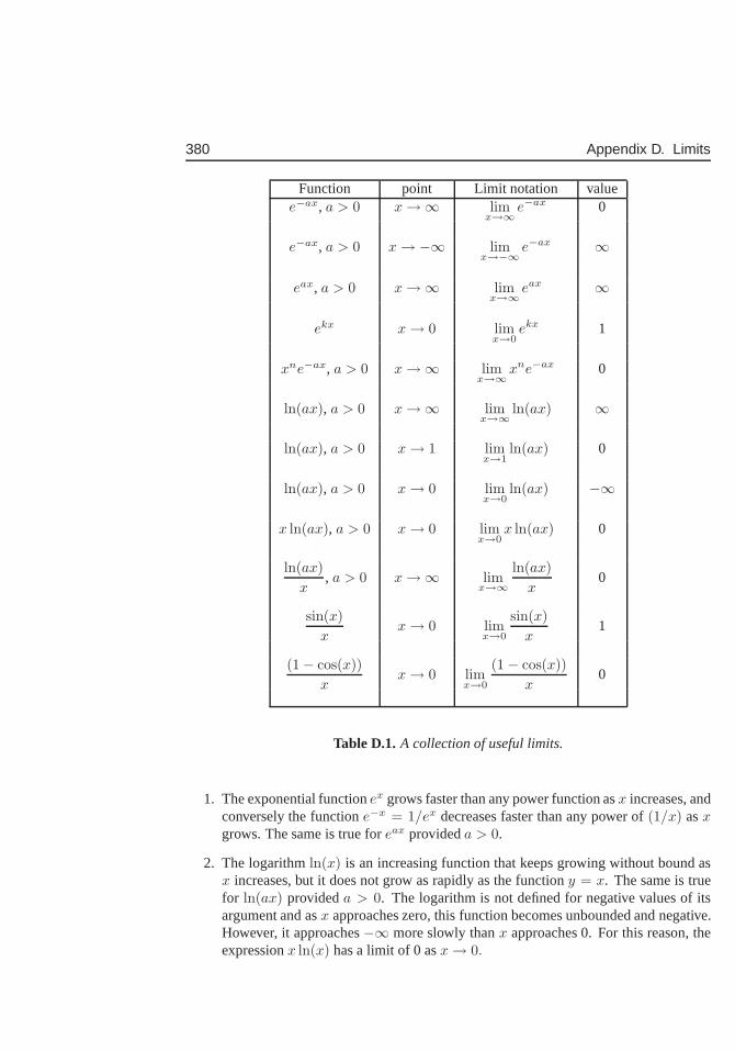
380 Appendix D. Limits
Function point Limit notation valuee−ax, a > 0 x→∞ lim
x→∞e−ax 0
e−ax, a > 0 x→ −∞ limx→−∞
e−ax ∞
eax, a > 0 x→∞ limx→∞
eax ∞
ekx x→ 0 limx→0
ekx 1
xne−ax, a > 0 x→∞ limx→∞
xne−ax 0
ln(ax), a > 0 x→∞ limx→∞
ln(ax) ∞
ln(ax), a > 0 x→ 1 limx→1
ln(ax) 0
ln(ax), a > 0 x→ 0 limx→0
ln(ax) −∞
x ln(ax), a > 0 x→ 0 limx→0
x ln(ax) 0
ln(ax)
x, a > 0 x→∞ lim
x→∞ln(ax)
x0
sin(x)
xx→ 0 lim
x→0
sin(x)
x1
(1− cos(x))
xx→ 0 lim
x→0
(1 − cos(x))
x0
Table D.1.A collection of useful limits.
1. The exponential functionex grows faster than any power function asx increases, andconversely the functione−x = 1/ex decreases faster than any power of(1/x) asxgrows. The same is true foreax provideda > 0.
2. The logarithmln(x) is an increasing function that keeps growing without bound asx increases, but it does not grow as rapidly as the functiony = x. The same is truefor ln(ax) provideda > 0. The logarithm is not defined for negative values of itsargument and asx approaches zero, this function becomes unbounded and negative.However, it approaches−∞ more slowly thanx approaches 0. For this reason, theexpressionx ln(x) has a limit of 0 asx→ 0.
Appendix E
Proof of the chain rule
Here we present a plausibility argument for the Chain Rule. First note that if a functionis differentiable, then it is also continuous. This means that whenx changes a very little,u can change only by a little. (There are no abrupt jumps). Then∆x → 0 means that∆u→ 0.
Now consider the definition of the derivativedy/du:
dy
du= lim
∆u→0
∆y
∆u
This means that for any (finite)∆u,
∆y
∆u=
dy
du+ ǫ
whereǫ→ 0 as∆u→ 0. Then
∆y =dy
du∆u + ǫ∆u
Now divide both sides by some (nonzero)∆x: Then
∆y
∆x=
dy
du
∆u
∆x+ ǫ
∆u
∆x
Taking∆x→ 0 we get∆u→ 0, (by continuity) and hence alsoǫ→ 0 so that as desired,
dy
dx=
dy
du
du
dx
381

382 Appendix E. Proof of the chain rule
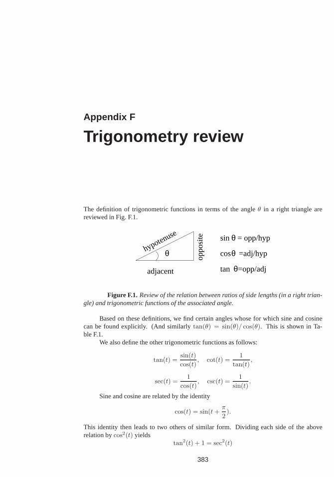
Appendix F
Trigonometry review
The definition of trigonometric functions in terms of the angle θ in a right triangle arereviewed in Fig. F.1.
adjacent
hypotenuse
θ oppo
site sin = opp/hyp
cos =adj/hyp
tan =opp/adj
θ
θ
θ
Figure F.1. Review of the relation between ratios of side lengths (in a right trian-gle) and trigonometric functions of the associated angle.
Based on these definitions, we find certain angles whose for which sine and cosinecan be found explicitly. (And similarlytan(θ) = sin(θ)/ cos(θ). This is shown in Ta-ble F.1.
We also define the other trigonometric functions as follows:
tan(t) =sin(t)
cos(t), cot(t) =
1
tan(t),
sec(t) =1
cos(t), csc(t) =
1
sin(t).
Sine and cosine are related by the identity
cos(t) = sin(t +π
2).
This identity then leads to two others of similar form. Dividing each side of the aboverelation bycos2(t) yields
tan2(t) + 1 = sec2(t)
383
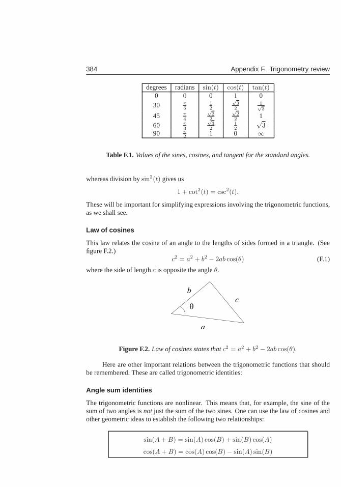
384 Appendix F. Trigonometry review
degrees radians sin(t) cos(t) tan(t)0 0 0 1 0
30 π6
12
√3
21√3
45 π4
√2
2
√2
2 1
60 π3
√3
212
√3
90 π2 1 0 ∞
Table F.1.Values of the sines, cosines, and tangent for the standard angles.
whereas division bysin2(t) gives us
1 + cot2(t) = csc2(t).
These will be important for simplifying expressions involving the trigonometric functions,as we shall see.
Law of cosines
This law relates the cosine of an angle to the lengths of sidesformed in a triangle. (Seefigure F.2.)
c2 = a2 + b2 − 2ab cos(θ) (F.1)
where the side of lengthc is opposite the angleθ.
a
bc
θ
Figure F.2. Law of cosines states thatc2 = a2 + b2 − 2ab cos(θ).
Here are other important relations between the trigonometric functions that shouldbe remembered. These are called trigonometric identities:
Angle sum identities
The trigonometric functions are nonlinear. This means that, for example, the sine of thesum of two angles isnot just the sum of the two sines. One can use the law of cosines andother geometric ideas to establish the following two relationships:
sin(A + B) = sin(A) cos(B) + sin(B) cos(A)
cos(A + B) = cos(A) cos(B)− sin(A) sin(B)
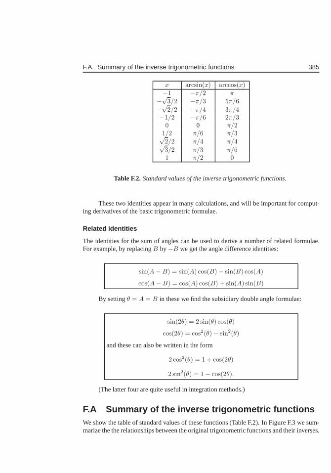
F.A. Summary of the inverse trigonometric functions 385
x arcsin(x) arccos(x)−1 −π/2 π
−√
3/2 −π/3 5π/6
−√
2/2 −π/4 3π/4−1/2 −π/6 2π/3
0 0 π/21/2 π/6 π/3√2/2 π/4 π/4√3/2 π/3 π/61 π/2 0
Table F.2.Standard values of the inverse trigonometric functions.
These two identities appear in many calculations, and will be important for comput-ing derivatives of the basic trigonometric formulae.
Related identities
The identities for the sum of angles can be used to derive a number of related formulae.For example, by replacingB by−B we get the angle difference identities:
sin(A−B) = sin(A) cos(B)− sin(B) cos(A)
cos(A−B) = cos(A) cos(B) + sin(A) sin(B)
By settingθ = A = B in these we find the subsidiary double angle formulae:
sin(2θ) = 2 sin(θ) cos(θ)
cos(2θ) = cos2(θ)− sin2(θ)
and these can also be written in the form
2 cos2(θ) = 1 + cos(2θ)
2 sin2(θ) = 1− cos(2θ).
(The latter four are quite useful in integration methods.)
F.A Summary of the inverse trigonometric functionsWe show the table of standard values of these functions (Table F.2). In Figure F.3 we sum-marize the the relationships between the original trigonometric functions and their inverses.
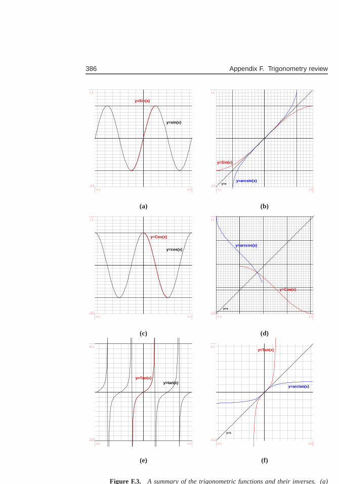
386 Appendix F. Trigonometry review
y=sin(x)
y=Sin(x)
-6.3 6.3
-1.5
1.5
y=x
y=Sin(x)
y=arcsin(x)
-1.5 1.5
-1.5
1.5
(a) (b)
y=cos(x)
y=Cos(x)
-6.3 6.3
-1.5
1.5
y=x
y=Cos(x)
y=arccos(x)
-1.0 3.1
-1.0
3.1
(c) (d)
y=tan(x)y=Tan(x)
-6.5 6.5
-10.0
10.0
y=x
y=Tan(x)
y=arctan(x)
-6.3 6.3
-6.3
6.3
(e) (f)
Figure F.3. A summary of the trigonometric functions and their inverses. (a)
Appendix G
Short Answers toProblems
387
388 Appendix G. Short Answers to Problems
G..1 Answers to Chapter 1 Problems
• Problem 1.1:
• Problem 1.2:
(a) Stretched iny direction by factorA; (b) Shifted up bya; (c) Shifted in positivexdirection byb.
• Problem 1.3:
Not Provided
• Problem 1.4:
• Problem 1.5:
(a)x = 0, (3/2)1/3; (b) x = 0, x = ±√
1/4.
• Problem 1.6:
(b) a < 0: x = 0; a ≥ 0: x = 0,±a1/4; (c) a > 0.
• Problem 1.7:
if m− n even:x = ±(
AB
)1/(m−n), x = 0; if m− n odd:x =
(
AB
)1/(m−n), x = 0
• Problem 1.8:
(a) (0, 0) and(1, 1); (b) (0, 0); (c) (√
72 , 3
4 ), (−√
72 , 3
4 ), and(0,−1).
• Problem 1.9:
(a)x = I/γ, (b)x =γ ±
√
γ2 − 4Iǫ
2ǫ.
• Problem 1.10:
• Problem 1.11:
y = xn; y = x−n; y = x1/n, n = 2, 4, 6, . . .; y = x−n, n = 1, 2, 3, . . .
• Problem 1.12:
m > −1
• Problem 1.13:
• Problem 1.14:
Not Provided
• Problem 1.15:
x =
(
B
A
)1
b−a
• Problem 1.16:
(a)x = 0,−1, 3; (b) x = 1; (c) x = −2, 1/3; (d) x = 1.
389
• Problem 1.17:
(a) Intersectionsx = −1, 0, 1.
• Problem 1.18:
(a)V ; (b)V
S=
1
6a, a > 0; (c) a = V
13 ; a = (1
6S)12 ; a = 10 cm; a =
√153 cm.
• Problem 1.19:
(a) V ; (b)r
3; (c) r =
(
34π
)1/3V 1/3; r =
(
14π
)1/2S1/2; r ≈ 6.2035 cm; r ≈
0.8921 cm.
• Problem 1.20:
r = 2k1/k2 = 12µm.
• Problem 1.21:
(a)T =
(
(1 − a)S
ǫσ
)1/4
.
• Problem 1.22:
(a)P = C(
RA
)d/b; (b) S = 4π
(
3V4π
)2/3.
• Problem 1.23:
(a)a: Ms−1, b: s−1; (b) b = 0.2, a = 0.002; (c) v = 0.001.
• Problem 1.24:
(a)v ≈ K, (b) v = K/2.
• Problem 1.25:
K ≈ 0.0048, kn ≈ 77 nM
• Problem 1.26:
(a)x = −1, 0, 1 (b) 1 (c)y1 (d) y2.
• Problem 1.27:
Line of slopea3/A and intercept1/A
• Problem 1.28:
K = 0.5, a = 2
• Problem 1.29:
Not Provided
• Problem 1.30:
m ≈ 67, b ≈ 1.2, K ≈ 0.8, kn ≈ 56
• Problem 1.31:
x =(
RA
)1
r−a .
390 Appendix G. Short Answers to Problems
G..2 Answers to Chapter 2 Problems
• Problem 2.1:
(a)m = 28◦/min, b = 50.
• Problem 2.2:
(a)−4.91◦F/min. (b) -7, -8, -9◦F/min. (c) -9◦F/min.
• Problem 2.3:
Displacements have same magnitude, opposite signs.
• Problem 2.4:
(b) 9.8 m/s.
• Problem 2.5:
(a)−14.7 m/s; (b)−gt− gǫ2 ; (c) t = 10 s.
• Problem 2.6:
v0 − g/2
• Problem 2.7:
5.8, 4.4, 5.4, 12.4, 4, 4.4, 7.2 (km/hr)
• Problem 2.8:
v = 13.23 m/s.; secant line isy = 13.23x− 2.226
• Problem 2.9:
• Problem 2.10:
(a)2; (b) 0; (c)−2; (d) 0.
• Problem 2.11:
(a)1; 1; 1; (b) 1; 0; 1; (c) 1; 2; 4.
• Problem 2.12:
(a)3; (b) 5.55; (c) 323 .
• Problem 2.13:
(a) 2√
2π ; (b) 6(1−
√2)
π ; (c) π/4 ≤ x ≤ 5π/4 (one solution).
• Problem 2.14:
(a)2 + h; (b) 2; (c) y = 2x.
• Problem 2.15:
2h2 + 25h + 104; slope =104
391
• Problem 2.16:
(b) 0,−4,−1.9,−2.1,−2− h; (c)−2.
• Problem 2.17:
(a)2 + h; (b) 2; (c) 2.98.
• Problem 2.18:
(a) 4π ; (b) 4
√3−12π .
• Problem 2.19:
(a)−1; (b) −21+ǫ ; (c) Slope approaches -2; (d)y = −2x + 4.
• Problem 2.20:
(a)v(2) = 12 m/s;v = 15 m/s; (b)v(2) = 0 m/s; v = 25 m/s; (c)v(2) = 13 m/s;v = 11 m/s.
• Problem 2.21:
0
• Problem 2.22:−1
(x+1)2
392 Appendix G. Short Answers to Problems
G..3 Answers to Chapter 3 Problems
• Problem 3.1:
Not Provided
• Problem 3.2:
Not Provided
• Problem 3.3:
Not Provided
• Problem 3.4:
Not Provided
• Problem 3.5:
Not Provided
• Problem 3.12:
• Problem 3.7:
Not Provided
• Problem 3.8:
Not Provided
• Problem 3.9:
(a)14.7 m/s; (b)−4.9 m/s.
• Problem 3.10:
(a)f ′(x) = 1/(2√
x), (b) 0.25 (c)y = 2 + 0.25(x− 4).
• Problem 3.11:
• Problem 3.12:
• Problem 3.13:
5; 5; no change; linear function
• Problem 3.14:
5.
• Problem 3.15:
y = 5.8x− 6.825.
• Problem 3.16:
• Problem 3.17:
Not Provided

393
• Problem 3.18:
• Problem 3.19:
394 Appendix G. Short Answers to Problems
G..4 Answers to Chapter 4 Problems
• Problem 4.1:
(a)36x2 − 16x− 15; (b)−12x3 + 3x2 − 3; (c) 4x3 − 18x2 − 30x− 6; (d) 3x2; (e)36x
(x2+9)2 ; (f) 6x3−3x2+6(1−3x)2 ; (g) 18b2−7b
83
3(2−b23 )2
; (h) −36m3+72m2−36m+5(3m−1)2 ; (i) 9x4+8x3−3x2−4x+6
(3x+2)2 .
• Problem 4.2:dR
dN= r − 2
r
KN .
• Problem 4.3:
(a)dv
dx= K
kn
(kn + x)2, (b)
dy
dx= A
nxn−1an
(an + xn)2.
• Problem 4.4:
• Problem 4.5:
(a)V = S3/2
6(π)1/2 , (b) dV/dS = 14(π)1/2 · S1/2.
• Problem 4.6:
(a)V ′(r) = 2πL + 4πr, S′(r) = 2πL + 4πr, (b) 2/r2.
• Problem 4.7:
A′(2) = 3πmm2/hr
• Problem 4.8:
(a)E
• Problem 4.9:d(N1/N2)
dt= (k1 − k2)
N1
N2
• Problem 4.10:
k2 > k1.
• Problem 4.11:
• Problem 4.12:
(a)y(t) = 15 t5 +t3− 1
2 t2 +3t+C, (b)y(x) = − 12x2 +
√2x+C, (c)y = | 12x2|+C.
• Problem 4.13:
(a) a(t) = −2Bt, (b) y(t) = At − (B/3)t3, (c) t =√
3A/B, (d) t =√
A/B, (e)v = A.
• Problem 4.14:
(a)v = 3t2 + 6t, a = 6t + 6; (b) t = 0,√
3/a; (c) t = 0,√
3/2a; (d) t = 1/√
2a.
395
• Problem 4.15:
(a) t = v0/g; (b) h0 +v20
2g ; (c) v = 0.
• Problem 4.16:
Not Provided
• Problem 4.17:
Not Provided
• Problem 4.18:
Not Provided
• Problem 4.19:
396 Appendix G. Short Answers to Problems
G..5 Answers to Chapter 5 Problems
• Problem 5.1:
(a) no tangent line; (b)y = −(x + 1); (c) y = (x + 1).
• Problem 5.2:
y = 2x− 3
• Problem 5.3:
(b) a = 2.
• Problem 5.4:
(a)y = −4x + 5; (b) x = 5/4, y = 5; (c) y = 0.6, smaller.
• Problem 5.5:
(a)y = 3x− 2; (b) x = 2/3; (c) 1.331; 1.3.
• Problem 5.6:
(a)y = f ′(x0)(x − x0) + f(x0); (b) x = x0 −f(x0)
f ′(x0).
• Problem 5.7:
2.83
• Problem 5.8:
(a) (3.41421, 207.237), (0.58580, 0.762), (−0.42858,−0.895);
• Problem 5.9:
(a)x = 0.32219; (b)x = 0.81054; (c)x = 0.59774, x = −0.68045,x = −4.91729.
• Problem 5.10:
(3, 9), (1, 1)
• Problem 5.11:
(a) 196 ; (b) 3.
• Problem 5.12:
(a)0.40208; (b) 5.99074.
• Problem 5.13:
0.99
• Problem 5.14:
−2.998
• Problem 5.15:
1030 cm3
397
G..6 Answers to Chapter 6 Problems
• Problem 6.1:
(a) zeros:x = 0, x = ±√
3; loc. max.:x = −1; loc. min.: x = 1; (b) loc. min.:x = 2; loc. max.:x = 1; (c) (a):x = 0; (b): x = 3/2.
• Problem 6.2:
Zeros at0,±√a; inflection point at0, local maximum at−√
a/3, local minimum at−sqrta/3.
• Problem 6.3:
(a) f ′(x) = 2x, f ′(0) = 0, f ′(1) = 2 > 0, f ′(−1) = −2 < 0. Local minimum atx = 0; (b) f ′(x) = −3x2, f ′(0) = 0, f ′(1) = −3 < 0, f ′(−1) = −3 < 0. No localmaxima nor minima; (c)f ′(x) = −4x3, f ′(0) = 0, f ′(1) = −4 < 0,f ′(−1) = 4 >0. Local maximum atx = 0.
• Problem 6.4:
Zeros at0, 2, Inflection point at0, local min at3/2.
• Problem 6.5:
Global maximum atx = 3, global minimum atx = 3/2.
• Problem 6.6:
(a) max.:18; min.: 0; (b) max.:25; min.: 0; (c) max.:0; min.: −6; (d) max.:−2;min.:−17/4.
• Problem 6.7:
(a) increasing:−∞ < x < 0, 1.5 < x < ∞; decreasing for0 < x < 1.5; (b) 0,local maximum;1.5, local minimum; (c) No.
• Problem 6.8:
min.: 3/4
• Problem 6.9:
x = 0
• Problem 6.10:
critical points:x = 0, 1, 1/2; inflection points:x =1
2±√
3
6
• Problem 6.11:
Not Provided
• Problem 6.12:
a = 1, b = −6, c = 7
398 Appendix G. Short Answers to Problems
• Problem 6.13:
Not Provided
• Problem 6.14:
min. atx = −√
3; max. atx =√
3; c.u.: x < −1, 0 < x < 1; c.d.:−1 < x <0,x > 1; infl.pt.: x = 0
• Problem 6.15:
loc. min.:x = a loc. max.:x = −2a
• Problem 6.16:
(a) increasing:x < 0, 0 < x < 3k, x > 5k; decreasing:3k < x < 5k; loc. max.:x = 3k; loc. min.:x = 5k; (b) c.u.: 0 < x < (3 −
√6
2 )k, x > (3 +√
62 )k; c.d.:
x < 0, (3 −√
62 )k < x < (3 +
√6
2 )k; infl.pts.:x = 0, (3±√
62 )k.
• Problem 6.17:
(b) dv/dp = −b (a+p0)(p+a)2 ; (c) p = p0.
• Problem 6.18:
Not Provided
• Problem 6.19:
abs. max. of4.25 at end points; abs. min. of2 atx = 1

399
G..7 Answers to Chapter 7 Problems
• Problem 7.1:
(a)10, 10; (b) 10, 10; (c) 12, 8.
• Problem 7.2:
(a)v(t) = 120t2 − 16t3; (b) t = 5; (c) t = 7.5.
• Problem 7.3:
9 : 24A.M., 15 km
• Problem 7.4:
(a)t ≈ 1.53 sec; (b)v(0.5) = 10.1 m/sec,v(1.5) = 0.3 m/sec,a(0.5) = −9.8 m/sec2,a(1.5) = −9.8 m/sec2; (c) t ≈ 3.06 sec.
• Problem 7.5:
See Example 7.2.
• Problem 7.6:
(a)N(r) = 2k1πrL − πk2r2L, (b) r = k1/k2.
• Problem 7.7:
• Problem 7.8:
30× 10× 15 cm
• Problem 7.9:
(a)y = (1/√
3); (b)√
3/9.
• Problem 7.10:
|a| if a < 4; 2√
2a− 4 if a ≥ 4
• Problem 7.11:
A = 625 ft2
• Problem 7.12:
All of the fencing used for a circular garden.
• Problem 7.13:
Squares of side6− 2√
3 cm.
• Problem 7.14:
• Problem 7.15:
A square withA = L2/2
400 Appendix G. Short Answers to Problems
• Problem 7.16:
Straight lines from(10, 10) to (163 , 0) then to(3, 5).
• Problem 7.17:
4 ◦C
• Problem 7.18:
(a)x = 2B/3, R = (4/27)AB3; (b) x = B/3, S = AB2/3.
• Problem 7.19:
r = 2k1/k2
• Problem 7.20:
h = 20, r = 5√
2
• Problem 7.21:
(b) x = a2b ; (c) x = 0; (d) x = a−m
2b .
• Problem 7.22:
x = (A/2B)1/3 − 1
• Problem 7.23:
• Problem 7.24:
NMSY = K(1− qE/r)
• Problem 7.25:
E = r/2q
• Problem 7.26:
• Problem 7.27:
topt =√
kτ .
• Problem 7.28:
401
G..8 Answers to Chapter 8 Problems
• Problem 8.1:
(a)y′(x) = 5(x + 5)4
• Problem 8.2:
(a)dT
dG= −1
4
(
(1 − a)S
σ
)1/4
ǫ−5/4 dǫ
dG.
• Problem 8.3:
(c) Global minimum occurs at an endpoint, rather than at a critical point.
• Problem 8.4:
Not Provided
• Problem 8.5:
(c) d = 3D/4.
• Problem 8.6:
(a)V (x) = 500x3+300(1−x)5, (b) Critical point atx1 = 3±√
52 is a local minimum.
(c) Best strategy isx1 = 1, x2 = 0.
402 Appendix G. Short Answers to Problems
G..9 Answers to Chapter 9 Problems
• Problem 9.1:
(a)4πr2k; (b) 8πrk; (c)− 3kr2 .
• Problem 9.2:
(a)dA/dt = 2πrC; (b) dM/dt = α2πrC.
• Problem 9.3:dMdt = Cπ(3r2)a
• Problem 9.4:dVdt = 1 m3/min
• Problem 9.5:
(a) 1300π cm/s; (b) 2
5 cm2/s.
• Problem 9.6:
5 cm/s
• Problem 9.7:
(a) dVdt = nR
PdTdt ; (b) dV
dt = −nRTP 2
dPdt .
• Problem 9.8:
π−1/2k.
• Problem 9.9:
− 110π cm/min
• Problem 9.10:
1 cm/sec toward lens
• Problem 9.11:dhdt = −1
36π cm/min
• Problem 9.12:
k = 110 + 4π
45
• Problem 9.13:dhdt = 6
5π ft/min
• Problem 9.14:
h′(5) = 25π m/min
• Problem 9.15:
(a) 14π m/min; (b) 1
π m/min.
403
• Problem 9.16:
(a)−4 m/s; (b)− 2532 per sec.
• Problem 9.17:−14√
6m/min
• Problem 9.18:dSdA = ab
1+bA ; no.
• Problem 9.19:dydt = 3 l2
l1cm/hr
• Problem 9.20:
Not Provided
• Problem 9.21:
Not Provided
• Problem 9.22:
(a) dydx = − 2x
2y = −xy ; (b) y = 1√
2(−x + r
√3); y = (1/
√2)(x − r
√3).
• Problem 9.23:
(a) dydx = 21x2+2
6y5+3 ; (b) dydx = − 2y
ey+2x ;
• Problem 9.24:
(a)−3/4; (b) y = −(3/4)x + 8.
• Problem 9.25:
Not Provided
• Problem 9.26:
( 2√10
, 9√10
) and(− 2√10
,− 9√10
)
• Problem 9.27:
m =4yp
xp
• Problem 9.28:
(b) dydx = (ay−x2)
(y2−ax) ; (c) x = 0, x = 21/3a; (d) No.
• Problem 9.29:
(a) dpdv = (2 a
v3 )− (p + av2 )/(v − b).
• Problem 9.30:
(0, 5/4)
• Problem 9.31:
(a)y − 1 = −1(x− 1); (b) y′′ = 45 ; (c) concave up.
404 Appendix G. Short Answers to Problems
G..10 Answers to Chapter 10 Problems
• Problem 10.1:
Not Provided
• Problem 10.2:
Not Provided
• Problem 10.3:
(a) 50.75 > 50.65; (b) 0.4−0.2 > 0.40.2; (c) 1.0012 < 1.0013; (d) 0.9991.5 >0.9992.3.
• Problem 10.4:
Not Provided
• Problem 10.5:
(a)x = a2b3; (b) x = b
c23
.
• Problem 10.6:
Not Provided
• Problem 10.7:
(a)x = 3−ln(5)2 ; (b) x = e4+1
3 ; (c) x = e(e2) = ee·e; (d) x = ln(C)a−b .
• Problem 10.8:
(a) dydx = 6
2x+3 ; (b) dydx = 6[ln(2x+3)]2
2x+3 ; (c) dydx = − 1
2 tan 12x; (d) dy
dx = 3x2−2(x3−2x) ln a ;
(e) dydx = 6xe3x2
; (f) dydx = − 1
2a− 12
x ln a; (g) dydx = x22x(3+x ln 2); (h) dy
dx = eex+x;(i) dy
dx = 4(et+e−t)2 .
• Problem 10.9:
(a) min.: x = 2√3; max.: x = − 2√
3; infl.pt.: x = 0; (b) min.: x = 1
3√
3; (c) max.:
x = 1; inf.pt.: x = 2; (d) min.: x = 0; (e) min.: x = 1; max.: x = −1; (f) min.:x = ln(2); infl. pt.: x = ln(4).
• Problem 10.10:
C = 4, k = −0.5
• Problem 10.11:
(a) decreasing; (b) increasing;y1(0) = y2(0) = 10; y1 half-life = 10 ln(2); y2
doubling-time= 10 ln(2)
• Problem 10.12:
41.45 months.
• Problem 10.13:
(c) r = 0.0101 per year,C = 0.7145 billions.
405
• Problem 10.14:
• Problem 10.15:
r1 ≈ −14.5, r2 ≈ −0.9 per unit time,C1 = 55, C2 = 45.
• Problem 10.16:
Not Provided
• Problem 10.17:
Not Provided
• Problem 10.18:
Not Provided
• Problem 10.19:
crit.pts.:x = 0, x ≈ ±1.64; f(0) = 1; f(±1.64) ≈ −0.272
• Problem 10.20:
(a)x = 1/β, (b) x = ln(α)/β.
• Problem 10.21:
(a)x = r; (c) x = ara−r ln
(
RA
)
; (d) decrease; (e) decrease.
• Problem 10.22:
x = b√
ln((a2 + b2)/b2)
• Problem 10.23:
Not Provided
406 Appendix G. Short Answers to Problems
G..11 Answers to Chapter 11 Problems
• Problem 11.1:
Not Provided
• Problem 11.2:
(a)C any value,k = −5; (b) C any value,k = 3.
• Problem 11.3:
(a)y(t) = Ce−t; (b) c(x) = 20e−0.1x; (c) z(t) = 5e3t.
• Problem 11.4:
t = − ln 2ln 7−ln 10
• Problem 11.5:
(a)57300 years; (b)22920 years
• Problem 11.6:
(a) 29 years; (b) 58 years; (c)279.7 years.
• Problem 11.7:
(a)80.7%; (b) 12.3 years.
• Problem 11.8:
y ≈ 707.8 torr
• Problem 11.9:
(a)P (5) ≈ 1419; (b) t ≈ 9.9years.
• Problem 11.10:dNdt = 0.05N ; N(0) = 250; N(t) = 250e0.05t; 2.1× 10¹⁰ rodents
• Problem 11.11:
(a)dy/dt = 2.57y; (b) dy/dt = −6.93y.
• Problem 11.12:
(a)12990; (b) 30792 bacteria.
• Problem 11.13:
1.39 hours;9.2 hours
• Problem 11.14:
20 min; 66.44 min
• Problem 11.15:
(a)y1 growing,y2 decreasing; (b)3.5, 2.3; (c)y1(t) = 100e0.2t, y2(t) = 10000e−0.3t;(d) t ≈ 9.2 years.
407
• Problem 11.16:
12265 people/km2
• Problem 11.17:
(a) 1 hour; (b)r = ln(2); (c) 0.25 M; (d)t = 3.322 hours.
• Problem 11.18:
6.93 years
• Problem 11.19:
1.7043 kg
• Problem 11.20:
(a) $510, $520.20, $742.97; 17.5 years; for 8% interest:$520, $540.80, $1095.56;(b) $510.08, $520.37, $745.42; (c) 5%.
408 Appendix G. Short Answers to Problems
G..12 Answers to Chapter 12 Problems
• Problem 12.1:
Not Provided
• Problem 12.11:
• Problem 12.3:
• Problem 12.4:
Not Provided
• Problem 12.5:
Not Provided
• Problem 12.6:
(a)C = −12; (b) C1 = 1, C2 = −5; (c) C1 = −1, C2 = 0.
• Problem 12.7:
(a)v(t) = − gk e−kt + g
k ; (b) v = gk .
• Problem 12.8:
c(t) = −ks e−st + k
s
• Problem 12.9:
(b) 46 minutes before discovery.
• Problem 12.10:
10.6 min
• Problem 12.11:
(a)Y = Y0 − kt, (d)k = 0.0333 per min.
• Problem 12.12:
(a) Input rateI, αF fish caught per day. Birth and mortality neglected. (b) Steadystate levelF = I/αN . (c) 2 ln(2)/αN days. (d)t = Flow/I days.
• Problem 12.13:
64.795 gm,250 gm
• Problem 12.14:
(a)Q′(t) = kr − QV r = − r
V [Q− kV ]; (b) Q = kV ; (c) T = V ln 2/r.
• Problem 12.15:
(a) dQdt = kQ; Q(t) = 100e(−8.9×10⁻²)t; (b) 7.77 hr.

409
• Problem 12.16:
(b) y0; (c) t =2A
√y0
k ; (d)−k√
y0.
• Problem 12.17:
a = 0, b = −1
• Problem 12.18:
(b) t = π/4 + nπ.

410 Appendix G. Short Answers to Problems
G..13 Answers to Chapter 13 Problems
• Problem 13.1:
Not Provided
• Problem 13.11:
• Problem 13.3:
• Problem 13.4:
Not Provided
• Problem 13.5:
Not Provided
• Problem 13.6:
(a)C = −12; (b) C1 = 1, C2 = −5; (c) C1 = −1, C2 = 0.
• Problem 13.7:
(a)v(t) = − gk e−kt + g
k ; (b) v = gk .
• Problem 13.8:
c(t) = −ks e−st + k
s
• Problem 13.9:
(b) 46 minutes before discovery.
• Problem 13.10:
10.6 min
• Problem 13.11:
(a)Y = Y0 − kt, (d)k = 0.0333 per min.
• Problem 13.12:
(a) Input rateI, αF fish caught per day. Birth and mortality neglected. (b) Steadystate levelF = I/αN . (c) 2 ln(2)/αN days. (d)t = Flow/I days.
• Problem 13.13:
64.795 gm,250 gm
• Problem 13.14:
(a)Q′(t) = kr − QV r = − r
V [Q− kV ]; (b) Q = kV ; (c) T = V ln 2/r.
• Problem 13.15:
(a) dQdt = kQ; Q(t) = 100e(−8.9×10⁻²)t; (b) 7.77 hr.
411
• Problem 13.16:
(b) y0; (c) t =2A
√y0
k ; (d)−k√
y0.
• Problem 13.17:
a = 0, b = −1
• Problem 13.18:
(b) t = π/4 + nπ.
412 Appendix G. Short Answers to Problems
G..14 Answers to Chapter 14 Problems
• Problem 14.1:
(a)180o (b) 300o (c) 164.35o (d) 4320o
(e)5π/9 (f) 2π/45 (g) 5π/2 (h) π/2
(i) 1/2 (j)√
2/2 (k)√
3/3
• Problem 14.2:
Not Provided
• Problem 14.3:
Not Provided
• Problem 14.4:
Not Provided
• Problem 14.5:
(a)T (t) = 37.1 + 0.4 cos[π(t− 8)/12]; (b) W (t) = 0.5 + 0.5 cos[π(t− 8)/6].
• Problem 14.6:
(a)S = 3 cos(√
gl t)
; (b) y = 2 sin(
2π3 t + π
6
)
+ 10.
• Problem 14.7:
(E)
• Problem 14.8:
(a)x; (b) x/√
1− x2; (c)√
1− x2.
• Problem 14.9:
(D)
• Problem 14.10:
(B)
413
G..15 Answers to Chapter 15 Problems
• Problem 15.1:
(a) dydx = 2x cosx2; (b) dy
dx = sin 2x; (c) dydx = − 2
3x− 23 (cot 3
√x)(csc2 3
√x); (d)
dydx = (1−6x) sec(x−3x2) tan(x−3x2); (e) dy
dx = 6x2 tan x+2x3 sec2 x; (f) dydx =
cos x+x sin xcos2 x ; (g) dy
dx = cosx − x sin x; (h) dydx =
sin 2x
x2esin2 1x
; (i) dydx = 6(2 tan 3x +
3 cosx)(2 sec2 3x− sin x); (j) dydx = − sin(sin x) · cosx + cos 2x.
• Problem 15.2:
(a)f ′(x) = −(4x3+10x) sin(ln(x4+5x2+3))(x4+5x2+3) ; (b)f ′(x) =
(3x2−2 cos(x) sin(x)) cos(√
cos2(x)+x3
(2√
cos2(x)+x3)
(c)f ′(x) = 6x2+ 1x ln(3) ; (d)f ′(x) = 4(x2ex+tan(3x))3(2xex+x2ex+3 sec2(3x));
(e)f ′(x) = 2x√
sin3(x) + cos3(x) + 3x2(sin2(x) cos(x)−cos2(x) sin(x))
2√
sin3(x)+cos3(x).
• Problem 15.3:
−√
3/20, 1/20
• Problem 15.4:
(a) [0, π/4], [5π/4, 2π]; (b) [3π/4, 7π/4]; (c) x = 3π/4, 7π/4.
• Problem 15.5:
±(π8 , 1)
• Problem 15.6:
−0.021 rad/min
• Problem 15.7:
0.125 radians per minute
• Problem 15.8:
Not Provided
• Problem 15.9:
(a)π/8; (b) 5π/8.
• Problem 15.10:
(a) dydt = − Cx√
L2−x2; (b) dθ
dt = Cy .
• Problem 15.11:
R = 132 v2
0
• Problem 15.12:
8π m/s;0 m/s
414 Appendix G. Short Answers to Problems
• Problem 15.13:
30π cm/s; to the right
• Problem 15.14:
(a)√
h2 + 2hR; (b)−v√
h2 + 2hR/R.
• Problem 15.15:
(a) dydx = 4 sec2(2x+y)
1−2 sec2(2x+y) ; (b) dydx = 2 sin x
cos y ; (c) dydx = − y cos x+sin y
x cos y+sin x .
• Problem 15.16:
y = −x + 2
• Problem 15.17:
y′ = a/√
1− a2x2
• Problem 15.18:
(a)dy
dx=
1
3x23
√
1− x23
; (b)dy
dx=
1
3(arcsinx)23
√1− x2
; (c)dθ
dr=
1
2r2 + 2r + 1;
(d)dy
dx= arcsec1x − x√
1−x2; (e)
dy
dx=−2x2 + a2 − a
a√
a2 − x2; (f)
dy
dt= −
∣
∣
∣
∣
1 + t2
1− t2
∣
∣
∣
∣
·2(1− t2)
(1 + t2)2.
• Problem 15.19:
0.4 m
• Problem 15.20:526 rad/s
• Problem 15.21:
(c) y(t) = A cos(√
g/Lt).
415
G..16 Answers to Chapter 16 Problems
• Problem 16.1:
1(d), 2(b), 3(a), 4(c) , 5(a), 6(a), 7(d), 8(b), 9(e), 10(a).
• Problem 16.2:
(E)
• Problem 16.3:
(E)
• Problem 16.4:
(D)
• Problem 16.5:
3/4 cm/sec.
• Problem 16.6:
(a)v(t) = 3(t + 2)2 + λ, a(t) = dv/dt = 6(t + 2). (b) λ.
• Problem 16.7:
(a) t = 1 andt = 4, (b) 9 m/s (c) 12 m.
• Problem 16.8:
Local max att = v0/g.
• Problem 16.9:
(a) Inflection point atx = 1. (b) Local maximum.
• Problem 16.10:
(a) Critical points atx = 0, 3, inflection atx = 9/4. (b) Global minx = −1, globalmaxx = 0.
• Problem 16.11:
Local minx = −9/5, inflection pointx = 0.
• Problem 16.12:
4.0004
• Problem 16.13:
t = ln(350)0.05 days.
• Problem 16.14:
(a)x = 0, ln(A)/b (b)x = 1/b.
• Problem 16.15:
p(x) = −x3 + 3x.
416 Appendix G. Short Answers to Problems
• Problem 16.16:
Local min atx = (2a/b)1/6.
• Problem 16.17:
Square of side lengthr/√
2.
• Problem 16.18:
x = 14P .
• Problem 16.19:dAleaf
dt = 2y(t) + x(t) + πy(t)2
• Problem 16.20:
(a)r = 12
√
Sπ andh = 0, (b) a sphere, (c) No.
• Problem 16.21:dVdt =
(
2π[r(t)h(t) + r(t)2] + 4πr(t)2)
.
• Problem 16.22:
• Problem 16.23:
k ≈ 1/27
• Problem 16.24:
(a)k = ln(2)/3 per hr (b) 6 more hrs.
• Problem 16.25:
(a)dP/dt = C − γP (b) P = C/γ (d) t = (ln(1/0.2)/γ.
• Problem 16.26:
(a) t = 3h (b) 23 h.
• Problem 16.27:
(a)y = 4S (b) T = 2τ1/2 = 2 ln(2)/f (c) y → 50
• Problem 16.28:
y = D/√
8
• Problem 16.29:
0.125m/s
• Problem 16.30:
696 ys.
• Problem 16.31:
(a)π/150 radians/s (b)π/6 radians (c)D = 200π (2−
√3)1/2 (d) dD
dt = 23(2−
√3)1/2
417
• Problem 16.32:
(a)φ = arcsin(A/B), (b)−1 < arcsin(A/B) < 1, (c) φ→ π/6
• Problem 16.33:
(b) y(0) = 0.5 (c) aty = 0.5 (d) y → 1.
• Problem 16.34:
(a)r′1(t) = 74π cm/year, (b)S′(t) = 14.
• Problem 16.35:
(a) BA lengthL− x, BP length√
x2 + d2. (b) Resistance of BA is(L− x)/R4, BP
is√
x2 + d2/r4. (c) r4d√R8−r8
.
418 Appendix G. Short Answers to Problems
G..17 Answers to Appendix A Problems
• Problem 1:
(a) slope4, y intercept−5; (b) slope34 , y intercept−2; (c) slope2
3 , y intercept0; (d)slope0, y intercept3; (e) slope5
2 , y intercept− 232 .
• Problem 2:
(a) y = −5(x − 2) = −5x + 10; (b) y = 12x − 5
2 ; (c) y = 45x + 10; (d) y =
−(3/4)x + 1.
• Problem 3:
(a)y = −4x + 3; (b) y = 3x + 2; (c) y = −6x + 5; (d) y = 3x; (e)y = −6x + 5;(f) y = −x/4; (g) y = 2x + 9.
• Problem 4:
y =√
2− x
419
G..18 Answers to Appendix B Problems
• Problem 1:
Not Provided
• Problem 2:
(a) Odd; (b) Even; (c) Even; (d) Odd; (e) Neither.
• Problem 3:
Not Provided
• Problem 4:
y = [(1/A)x]1/n; x = 0,±(1/A)1/(n−1)

420 Appendix G. Short Answers to Problems
Bibliography
[1] Anne Bernheim-Groswasser, Sebastian Wiesner, Roy M Golsteyn, Marie-France Car-lier, and Cecile Sykes. The dynamics of actin-based motility depend on surface pa-rameters.Nature, 417(6886):308–311, 2002.
[2] C.M. Breder. Structure of a fish school.Bull. Amer. Mus. Nat. Hist., 98:1–27, 1951.
[3] C.M. Breder. Equations descriptive of fish schools and other animal aggregations.Ecology, pages 361–370, 1954.
[4] Eric L Charnov. Optimal foraging, the marginal value theorem. Theoretical popula-tion biology, 9(2):129–136, 1976.
[5] Lawrence M Dill. The escape response of the zebra danio (Brachydanio rerio) I. Thestimulus for escape.Animal Behaviour, 22(3):711–722, 1974.
[6] Lawrence M Dill. The escape response of the zebra danio (Brachydanio rerio) II. Theeffect of experience.Animal Behaviour, 22(3):723–730, 1974.
[7] Reuven Dukas and Stephen Ellner. Information processing and prey detection.Ecol-ogy, 74(5):1337–1346, 1993.
[8] Reuven Dukas and Alan C Kamil. The cost of limited attention in blue jays.Behav-ioral Ecology, 11(5):502–506, 2000.
[9] Reuven Dukas and Alan C Kamil. Limited attention: the constraint underlying searchimage.Behavioral Ecology, 12(2):192–199, 2001.
[10] John T Emlen Jr. Flocking behavior in birds.The Auk, 1952.
[11] Conder P. J. Individual distance.Ibis, 91:649–655, 1949.
[12] Rajat Rohatgi, Peter Nollau, Hsin-Yi Henry Ho, Marc W Kirschner, and Bruce JMayer. Nck and phosphatidylinositol 4, 5-bisphosphate synergistically activate actinpolymerization through the N-WASP-Arp2/3 pathway.Journal of Biological Chem-istry, 276(28):26448–26452, 2001.
[13] Miller R.S. and Stephen W. J.D. Spatial relationships in flocks of sandhill cranes.Ecology, 47(2):323–327, 1966.
421
422 Bibliography
[14] D. W. Stephens and J. R. Krebs.Foraging theory. Princeton University Press, Prince-ton NJ, 1986.
Index
Arrhenius, 202differential equation, 221Lysteria
monocytogenes, 84
acceleration, 76, 77, 81uniform, 78
ActA, 84actin, 75, 84age distribution, 226
uniform, 226albedo, 8, 21, 163, 173allometric constants, 209allometry, 208ambient temperature, 246amplitude, 295, 297analytic solution, 241Andromeda strain, 196, 207angle
degrees, 292radians, 293
ant trails, 165antiderivative, 72, 77antidifferentiation, 72, 78approximation
linear, 98arc length, 292arccosine, 304arcsine, 302arctan, 306argument
geometric, 6astroid, 185attention, 166attraction, 17average
rate of change, 33
Avogadro’snumber, 232
base, 198of exponent, 195
biochemicalreaction, 13
bird flock, 17birth rate
human, 227box
rectangular, 149
carrying capacity, 132, 264cell
length, 137shape, 3size, 133spherical, 4
cesium-137, 234chain rule, 159, 160, 175Chernoby, 234circle
area of, 292circumference of, 292
circumferenceof circle, 292
clock hands, 316, 317coefficient
power function, 2coffee budget, 163comet tail, 84concave
down, 116up, 116
concavity, 100, 116cone, 179
423
424 Index
constraint, 136, 138converge, 104, 105convergent extension, 177cooling, 26cooling object, 273cosine, 384
derivative, 312cosines
law of, 315coupled
ODEs, 281Crichton
Michael, 196critical point, 120critical points, 11
classifying, 126cryptic food, 166cubic, 56curvature, 116cycle, 293
peridic, 298cylinder
surface area, 135volume, 135
datarefined, 34
daylight cycle, 299decay
equation, 232exponential, 233
decreasingfunction, 116
degreeof polynomial, 71
density dependentgrowth, 132growth rate, 264
derivative, 25, 38, 46definition, 37
differential equation, 75, 203, 204, 220,241, 325
DillLarry, 320
direction field, 268discontinuity
jump, 54removable, 53
disease, 280doubling, 195doubling time, 229, 230Dukas
Reuven, 166dynein, 51
E. coli, 196Earth
temperature of, 8, 21, 71, 76, 163,173, 184
ellipserotated, 186
emissivity, 8, 173endemic
disease, 283endpoints
maxima at, 140energy
balance, 21energy balance, 8, 71energy gain, 143enzyme, 13equinox, 299escape
response, 320Euler’s method, 236, 251, 252, 277even
function, 7, 296exponential decay, 236exponential function, 199, 219
base 10, 200base 2, 200base e, 201
exponential growth, 252extrema, 122
falling object, 77, 79, 249fertility, 226finite difference, 60finite difference equation, 251first derivative
test, 121fish school, 17
Index 425
fluorescence, 75food patch, 142food type, 167foraging
optimal, 142foraging time, 142frequency, 297function
composition, 159
Galileo, 28geometric argument, 6, 147geometric relationships, 175gravity, 28, 77greenhouse gas, 8, 21, 163, 173growth
density dependent, 264growth rate, 227
intrinsic, 132
half life, 233harmonic oscillator, 325heating, 26Hill
coefficient, 14function, 15
HIV, 280hormone cycle, 299
identitytrigonometric, 295
implicitdifferentiation, 181function, 181
implicit differentiation, 76, 325increasing
function, 115independent variable, 132inflection
point, 116influenza, 280infusion, 250initial
velocity, 78initial value, 222
problem, 233
initial value problem, 251instantaneous
rate of change, 39intercept, 29intrinsic growth rate, 264invasive species, 89, 213inverse function, 205, 301iodine-131, 234iteration, 104, 105
Kepler, 137wedding, 137
kinesin, 51
Lactobacillus, 26law of cosines, 315, 384Law of Mass Action, 265level curves, 325limit, 52
DNE, 54exists, 53right and left, 54
linearapproximation, 93operation, 71relationship, 29
linearityof derivative, 71of limits, 374
Linweaver-Burke, 16local
behaviour, 45maximum, 120minimum, 120
log-log plot, 208logarithm
natural, 205logistic
growth, 131logistic equation, 264, 276logistic growth, 88, 132
maximum, 131absolute, 126global, 126
Michaelis-Menten
426 Index
kinetics, 14, 88microtubules, 51minimum, 131
absolute, 126global, 126local, 8
modelmathematical, 4
molecular collision, 202moon phase, 300mortality, 227motion
uniform, 28motor
molecular, 51moving bead, 84murder mystery, 248
net growth rate, 225Newton’s
law of cooling, 246, 254method, 3
Newton’s method, 11, 93–95, 98, 102nM
nano Molar, 15nonlinear
differential equation, 263, 264nuclear power plant, 234numerical solution, 250nutrient
absorption, 5balance, 4consumption, 5
oddfunction, 7, 296
one-to-one, 8, 302optimal
foraging, 142oxygen, 6
parameter, 224per capita
birth rate, 224mortality rate, 224
percent
growth, 227perimeter
maximal, 140of circle, 293
period, 295periodic function, 295phase, 295phase line, 272phase shift, 298pheromone, 165Pi (π), 292pollution, 161polynomial, 9, 71
derivative of, 71population
density, 132growth, 224, 235
position, 81power
dominant, 2function, 2, 7
power rule, 75, 184powers
of 2, 196predator
size, 321Preface, xiprobability
of decay, 231proportional, 5proportionality
constant, 5Pythagoras theorem, 151, 303, 305Pythagorian
triangle, 291
race track, 315radian, 99, 291, 293radioactive decay, 230rate
constant, 227rate of change
average, 25, 29, 33instantaneous, 25, 34
rationalfunction, 9
Index 427
rational function, 12, 14reaction
speed, 13recursion relation, 251related rates, 175, 314, 318reproductive
number, 284repulsion, 17rescaling, 266, 267residence time, 142, 145restricting the domain, 302Ricker
equation, 215root, 19
of equation, 119
SARS, 280saturation, 15scientific problems, 223secant
line, 25, 30second derivative, 72, 76, 120
test, 122, 133second order
DE, 325shortest path, 165sine, 384
derivative, 312sketching
the derivative, 48, 81slope
of straight line, 29of tangent line, 46
slope field, 268solar constant, 8solution
to differential equation, 221solution curve, 235, 247spacing distance, 17spreadsheet, 105, 253stability, 275stable
steady state, 275state space, 268, 272steady state, 247, 249, 275step function, 64
step size, 251straight line, 29stroboscope, 36substrate, 13surface area
minimal, 135sustainability, 8, 21, 27, 41, 71, 76, 89,
131, 156, 163, 173, 196, 207,213, 215, 224, 229, 239, 259,260, 264, 276, 280, 287, 288
systemof equations, 281
tangent line, 39, 46, 95temperature
milk, 26terminal velocity, 249time of death, 248trigonometric
functions, 291identities, 291
trigonometric functions, 291, 301trigonometric identities, 384tug of war, 51tumor growth, 175
unbounded, 8unit circle, 292unstable, 275
velocity, 38, 77, 81instantaneous, 36, 37terminal, 250
vertical line property, 180vesicle, 51visual angle, 318, 324
wine barrel, 137
yoghurt, 26
zebra danio, 320zero, 19, 49, 118, 119zeros, 11
of a function, 124zoom, 46
Related Documents