mat_540_w2.ppt

Quantitative Methods

MAT 540

Decision Analysis

Objectives• When you complete this lesson, you will be able to:

• List the components of a decision-making situation.• Make decisions without probabilities using the maximax, maximin,

minimax regret, Hurwicz, and equal likelihood criteria. • Compute the expected value of a decision when probabilities are

known.• Compute the expected value of perfect information.• Construct decision trees to calculate the expected value of a

decision. • Construct decision trees to calculate the expected value of a

sequence of decisions.• Conduct a decision analysis with additional information.• Compute the expected value and efficiency of sample information.

Components of Decision Making

• The decision itself

• The states of nature

• Payoff table

Decision Making Without Probabilities

• Real estate example

The Maximax Criterion

• Maximum of the maximum payoffs

• Assumes the most favorable state of nature

The Maximin Criterion

• Maximum of the minimum payoffs

• Assumes least favorable state of nature

The Minimax Regret Criterion

• Minimizes the maximum regretGood Economic Conditions Poor Economic Conditions

$100,000 - 50,000 = $50,000 $30,000 - 30,000 = $0

$100,000 - 100,000 = $0 $30,000 – (- 40,000) = $70,000

$100,000 - 30,000 = $70,000 $30,000 - 10,000 = $20,000

The Hurwicz Criterion

• Compromise between maximax and maximin• Coefficient of optimism

• α = 0.4

• 1 – α = 0.6

Decision Values

Apartment building $50,000(.4) + 30,000(.6) = $38,000

Office building $100,000(.4) – 40,000(.6) = $16,000

Warehouse $30,000(.4) + 10,000(.6) = $18,000

The Equal Likelihood Criterion

• Weights each state of nature equally

Decision Values

Apartment building $50,000(.5) + 30,000(.5) = $40,000

Office building $100,000(.5) – 40,000(.5) = $30,000

Warehouse $30,000(.5) + 10,000(.5) = $20,000

Summary of Criteria Results

• Warehouse is dominated by apartment building

Criterion Decision (Purchase)

Maximax Office building

Maximin Apartment building

Minimax regret Apartment building

Hurwicz Apartment building

Equal likelihood Apartment building

Solution of Decision-Making Problems Without Probabilities with QM for Windows

Decision Making with Probabilities

• Expected value• Estimate the probability of occurrence of each

state of nature• Compute

n

iii xPxxE

1

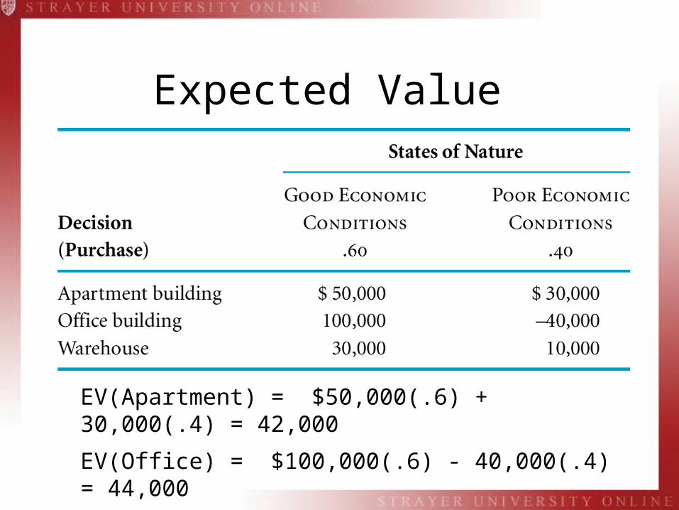
Expected Value

EV(Apartment) = $50,000(.6) + 30,000(.4) = 42,000

EV(Office) = $100,000(.6) - 40,000(.4) = 44,000

EV(Warehouse) = $30,000(.6) + 10,000(.4) = 22,000

Expected Opportunity Loss

EOL(Apartment) = $50,000(.6) + 0(.4) = 30,000

EOL(Office) = $0(.6) + 70,000(.4) = 28,000

EOL(Warehouse) = $70,000(.6) + 20,000(.4) = 50,000

Solution of Expected Value Problems with QM for Windows

Expected Value of Perfect Information

$100,000(.60) + 30,000(.40) = $72,000

EV(office) = $100,000(.60) - 40,000(.40) = $44,000

EVPI = $72,000 - 44,000 = $28,000

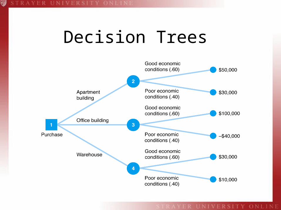
Decision Trees

Decision Trees, continued

• Compute expected values• EV(node 2) = .60($50,000) + .40(30,000) = $42,000

• EV(node 3) = .60($100,000) + .40(-40,000) = $44,000

• EV(node 4) = .60($30,000) + .40(10,000) = $22,000

Decision Trees with Excel and TreePlan

Sequential Decision Trees

Sequential Decision Trees, continued

• Apartment building: $1,290,000 – 800,000 = $490,000

• Land: $1,360,000 – 200,000 = $1,160,000

Decision Analysis with Additional Information

• Bayesian analysis

• EV(office building) = $44,000

Decision Analysis with Additional Information, continued

• Conditional probabilities:

g = good economic conditions, P(g) = .6

p = poor economic conditions, P(p) = .4

P = positive economic report

N = negative economic report

P(Pg) = .80 P(NG) = .20

P(Pp) = .10 P(Np) = .90

Decision Analysis with Additional Information, continued

• Posterior probabilities

• P(g|N) = .25• P(p|P) = 0.77• P(p|N)=.75

923.

4.1.6.8.

6.8.

ppPggP

ggPPg

PPPP

PPP

Decision Trees with Posterior Probabilities

Decision Trees with Posterior Probabilities, continued

• Probability of two dependent events• P(AB) = P(A|B)P(B)

• P(Pg) = P(P|g)P(g)

• P(Pp) = P(P|p)P(p)

Decision Trees with Posterior Probabilities, continued

• Mutually exclusive events• P(P) = P(Pg) + P(Pp) = P(P|g)P(g) + P(P|p)P(p) = (.8)(.6) + (.1)(.4) = .52

• P(N) = P(N|g)P(g) + P(N|p)P(p) = (.2)(.6) + (.9)(.4) = .48

Decision Trees with Posterior Probabilities, continued

• EV(apartment) = $50,000(.923) + 30,000(.077) = $48,460

The Expected Value of Sample Information

• EVSI = EVwith information – EVwithout information

= $63,194 – 44,000

= $19,194

• Efficiency = EVSI ÷ EVPI

= $19,194 / 28,000

= .68

Summary

• Components of decision making• Decision making without probabilities• Decision making with probabilities• Expected value of perfect information• Decision trees• Sequential decisions• Decision making with additional information• Expected value of sample information