www.sciencemag.org/cgi/content/full/326/5959/1541/DC1 Supporting Online Material for Mapping Human Genetic Diversity in Asia The HUGO Pan-Asian SNP Consortium† †To whom correspondence should be addressed. E-mail: [email protected] (L.J.); [email protected] (E.T.L.); [email protected] (M.S.); [email protected] (S.X.) Published 11 December 2009, Science 326, 1541 (2009) DOI: 10.1126/science.1177074 This PDF file includes: Materials and Methods SOM Text Figs. S1 to S38 Tables S1 to S4

Welcome message from author
This document is posted to help you gain knowledge. Please leave a comment to let me know what you think about it! Share it to your friends and learn new things together.
Transcript
www.sciencemag.org/cgi/content/full/326/5959/1541/DC1
Supporting Online Material for
Mapping Human Genetic Diversity in Asia
The HUGO Pan-Asian SNP Consortium†
†To whom correspondence should be addressed. E-mail: [email protected] (L.J.); [email protected] (E.T.L.); [email protected] (M.S.); [email protected] (S.X.)
Published 11 December 2009, Science 326, 1541 (2009)
DOI: 10.1126/science.1177074
This PDF file includes:
Materials and Methods
SOM Text
Figs. S1 to S38
Tables S1 to S4
1
Additional Acknowledgments China: The work of Shanghai group for PASNPI was supported by National Outstanding Youth Science Foundation of China (30625016, 30625019), National Science Foundation of China (30890034), Chinese High-Tech (863) Program (2006AA020706, 2006AA020704�2007AA02Z312), National Key Project for Basic Research (2002CB512900, 2004CB518605), Shanghai Leading Academic Discipline Project (B111), Science and Technology Commission of Shanghai Municipality (04DZ14003, 06XD14015, 09ZR1436400), Knowledge Innovation Program of Shanghai Institutes for Biological Sciences, Chinese Academy of Sciences (2008KIP311), and K.C.Wong Education Foundation, Hong Kong. India: IGIB would like to acknowledge the “Council for Scientific and Industrial Research” (CSIR), India for financial support (MLP001). It would also like to acknowledge the technical help from “The Centre for Genomic Applications” (TCGA) genotyping facility. Indonesia: This study was supported as part of the Eijkman Institute program on Indonesian Human Genome Diversity in Biotechnology (Principal Investigator - Herawati Sudoyo), with funding managed through the Indonesian Ministry for Research and Technology. We thank Dr. Yahwardiah Siregar and Prof. Gontar Siregar (University of North Sumatra, Medan), Prof. Dasril Daud and Prof. Irawan Yusuf (Hasanudin University, Makassar), Dr. Marten Caley and Dr. Matius Kitu (Heads of District Health Agencies, Sumba ), and Dr. Paul Sukarno Manoempil and Dr. Eduardus Kleruk (Head of District Health Agencies, Alor and Flores), and their respective field teams for their support and participation in the field work with the ethnic populations of Tanah Batak, South Sulawesi, Sumba, Alor and Flores, respectively. Japan: This work was in part supported by Grant-in-Aid for Scientific Research on Priority Areas "Comprehensive Genomics" and "Genome Medicine" from the Ministry of Education, Culture, Sports, Science and Technology of Japan. Korea: The work of KNIH group was supported by intramural grants from the Korea National Institute of Health(KNIH), Korea Center for Disease Control and Prevention, Republic of Korea (Project No.: 2910-213-207). The work of KOBIC group was supported by a grant from ''KRIBB Research Initiative Program", MIC(Ministry of Information and Communication), Korea, under the KADO (Korea Agency Digital Opportunity & Promotion) support program, and MOST international collaboration fund (K20724000003-07B0400-00310). We also thank Jung Sun Park, So Hyun Hwang, Daeui Park, Yongseok Lee, Seongwoo Hwang and Maryana Bhak. Much of the calculation for this work was carried out by computer clusters provided by KOBIC, KRIBB, Korea. Malaysia: Juli Edo for anthropological expertise and liaison with Jabatan Hal Ehwal Orang Asli (JHEOA). Ministry of Science, Technology and Innovation (MOSTI), Malaysia for IRPA grant # 36-02-03-6006 1) This study was supported by The Fundamental Research Grant Scheme (FRGS Top-Down), Ministry of Higher Education, Malaysia. Grant number: 203/PPSP/6170025. 2) We would like to acknowledge our appreciation for the contribution from colleagues from the School of Medical Sciences, School of Health Sciences and School of Dental Sciences, Universiti Sains Malaysia. . The Philippines: People:
xushua
高亮
xushua
高亮
xushua
高亮
xushua
高亮
2
the Aetas, Agtas, Atis, Mangyan-Irayas, Mamanwas, Manobos for providing us the samples; Miriam M. Dalet, DNA Analysis Laboratory, Natural Sciences Research Institute, University of the Philippines; Minerva S. Sagum, DNA Analysis Laboratory, Natural Sciences Research Institute, University of the Philippines; Dr. Saturnina C. Halos, DNA Analysis Laboratory, Natural Sciences Research Institute, University of the Philippines; Dr. Victor J. Paz, Archaeological Studies Program, University of the Philippines, Diliman and Dr. Sabino G. Padilla, Department of Behavioral Sciences, University of the Manila. Agencies: Agusan del Sur Provincial Government, Christ Faith Fellowship Church Mission, Surigao del Norte, Dao Bible Believing Church, Mangyan Tribal Church Association (MCTA), National Commission on Indigenous Peoples (NCIP), Office of the Mayor, Malay of the Province of Aklan, Philippine National Red Cross (PNRC), Subic Bay Metropolitan Authority (SBMA) Ecology Center, Surigao del Norte Provincial Government Singapore: This research was supported by the Agency for Science Technology and Research (ASTAR). The Genome Institute of Singapore also wishes to acknowledge the organizational assistance of Chaylan Long. Taiwan: This research project was supported by grants from the National Science and Technology Program for Genomic Medicine, National Science Council, Taiwan (National Clinical Core for Genomic Medicine NSC95-3112-B-001-010 and National Genotyping Center NSC95-3112-B-001-011), and the Academia Sinica Genomic Medicine Multicenter Study. Thailand: 1. The staff of the Tribal Research Institute, Chiang Mai, Thailand, for field work organization. 2. This research project was supported by the Thailand Research Fund, Grant Numbers PHD/0011/2544, BGJ/26/2544, PHD/0058/2545, BGJ4580022. 3. Sissades Tongsima and the team from biostatistics and bioinformatics laboratory acknowledge the Thailand Research Fund and the Thailand Research Fund and the National Center for Genetic Engineering and Biotechnology for supporting this work. USA: We would like to acknowledge Shoba Gopalan for technical support and Michele Cargill for helpful comments and suggestions.
- 2 -
CONTENTS
1. METHODS ............................................................................................................................. ‐ 8 ‐ 1.1. Populations, Samples & Genotyping .............................................................................. ‐ 8 ‐ 1.2. Data integration .................................................................................................................. ‐ 9 ‐ 1.3. Determination of Ancestral alleles ................................................................................... ‐ 9 ‐ 1.4. AMOVA analysis ................................................................................................................ ‐ 9 ‐ 1.5. Genetic distance for individuals ..................................................................................... ‐ 10 ‐ 1.6. Principal component analysis for individuals ............................................................... ‐ 10 ‐ 1.7. Genetic distance for populations ................................................................................... ‐ 10 ‐ 1.8. Tree reconstruction .......................................................................................................... ‐ 11 ‐ 1.9. Great circle distance ........................................................................................................ ‐ 11 ‐ 1.10. Partial and multiple Mantel tests ................................................................................. ‐ 11 ‐
1.10.1. Tests for pre-historical divergence and isolation by distance effects .............................. ‐ 11 ‐
1.10.2. Tests for the correlation of linguistic and genetic affinity ................................................... ‐ 13 ‐
1.11. Simulation of genotypic data under isolation by distance (IBD) .............................. ‐ 13 ‐ 1.12. Structure analysis .......................................................................................................... ‐ 13 ‐
1.12.1. Full data set for structure analysis ....................................................................................... ‐ 13 ‐
1.12.2. Random sampling of markers for STRUCTURE analysis ................................................ ‐ 14 ‐
1.12.3. STRUCTURE settings ........................................................................................................... ‐ 14 ‐
1.12.4. Analysis of STRUCTURE results: Similarity coefficients and Determination of primary
clusters .................................................................................................................................................. ‐ 15 ‐
1.12.5. Constructing a phylogenetic tree of STRUCTURE clusters ............................................. ‐ 17 ‐
1.13. frappe analysis ............................................................................................................... ‐ 18 ‐ 1.14. Forward time simulation ............................................................................................... ‐ 18 ‐
1.14.1. Modeling one-wave and two-wave hypothesis .................................................................. ‐ 18 ‐
1.14.2. Computer simulation exploring the possibility of an undetected two-wave signal ........ ‐ 19 ‐
1.15. Haplotype-based analyses .................................................................................... ‐ 20 ‐ 1.15.1. Haplotype estimation ........................................................................................................ ‐ 20 ‐
1.15.2. Haplotype diversity ........................................................................................................... ‐ 20 ‐
1.15.3. Haplotype sharing analyses ............................................................................................ ‐ 21 ‐
1.15.3.1. Haplotype sharing by type ......................................................................................... ‐ 21 ‐
1.15.3.2. Haplotype sharing by both type and frequency ...................................................... ‐ 21 ‐
1.15.3.3. Identification of population/group private haplotypes ............................................ ‐ 23 ‐
1.15.3.4. Reconstructing phylogenetic trees of populations/groups with population/group
private haplotypes ........................................................................................................................... ‐ 23 ‐
2. SUPPLEMENTARY DESCRIPTION AND DISCUSSIONS .............................................................. ‐ 24 ‐
2.1. Additional notes on genotyping and integration of data from multiple centers .. ‐ 24 ‐ 2.2. Additional notes on the population samples and related issues .......................... ‐ 25 ‐ 2.3. Additional notes on STRUCTURE analyses ........................................................... ‐ 25 ‐ 2.4. Additional notes on PCA results ............................................................................... ‐ 26 ‐ 2.5. Evaluation of the influence of ascertainment bias on inferences in this study ... ‐ 28 ‐
2.5.1. Evaluation of the influence of ascertainment bias ........................................................ ‐ 29 ‐
- 3 -
2.5.1.1. Evaluation of the influence on genetic distance estimation .................................... ‐ 29 ‐
2.5.1.2. Evaluation of the influence on tree topologies ......................................................... ‐ 30 ‐
2.6. Additional notes on language replacement ............................................................. ‐ 31 ‐ 2.7. Additional notes on Taiwan Aborigines .................................................................... ‐ 31 ‐ 2.8. Additional notes on Indian populations .................................................................... ‐ 32 ‐ 2.9. Addition notes on isolation by distance and pre-historical population divergence ... ‐ 33 ‐
2.9.1. Geographical distance versus genetic distance ........................................................... ‐ 33 ‐
2.9.2. IBD versus historical divergence .................................................................................... ‐ 34 ‐
2.10. Evidences of south origin of East Asian and South-to-North migration .......... ‐ 36 ‐ 2.10.1. Topology of maximum likelihood tree of populations ................................................... ‐ 37 ‐
2.10.2. Distance of STRUCTURE/frappe components ............................................................. ‐ 37 ‐
2.10.3. Topology of STRUCTURE/frappe component tree ...................................................... ‐ 37 ‐
2.10.4. Distribution of samples in PCA plots .............................................................................. ‐ 38 ‐
2.10.5. Geographical distribution of genetic diversities ............................................................ ‐ 38 ‐
2.10.6. Haplotype sharing proportions ........................................................................................ ‐ 38 ‐
2.10.7. Phylogeny of group private haplotypes .......................................................................... ‐ 40 ‐
2.11. Peopling of Asia: one-wave versus two-wave hypothesis ................................ ‐ 40 ‐ 2.11.1. Topology of population trees ........................................................................................... ‐ 41 ‐
2.11.2. Topology of STRUCTURE/frappe component tree ...................................................... ‐ 41 ‐
2.11.3. Phylogeny of group private haplotypes .......................................................................... ‐ 42 ‐
2.11.4. Simulation results .............................................................................................................. ‐ 42 ‐
2.11.5. Final comments ................................................................................................................. ‐ 44 ‐
3. REFERENCES ......................................................................................................................... ‐ 45 ‐
4. SUPPLEMENTARY TABLES ...................................................................................................... ‐ 46 ‐
Table S1. Analysis of molecular variance (AMOVA). ......................................................... ‐ 47 ‐ Table S2. Institutions that performed the genotyping. ........................................................ ‐ 48 ‐ Table S3. Data quality control for samples. ......................................................................... ‐ 49 ‐ Table S4. Details of SNP filtering. ......................................................................................... ‐ 51 ‐
5. SUPPLEMENTARY FIGURES .................................................................................................... ‐ 52 ‐
- 4 -
Supplementary Figures
Figure S1 Estimated population structure from the full data set (Full) and 10 subsets of the data (S1-S10) (K=2). ...................................................................................................... - 53 -
Figure S2 Estimated population structure from the full data set (Full) and 10 subsets of the data (S1-S10) (K=3). ...................................................................................................... - 54 -
Figure S3 Estimated population structure from the full data set (Full) and 10 subsets of the data (S1-S10) (K=4). ...................................................................................................... - 55 -
Figure S4 Estimated population structure from the full data set (Full) and 10 subsets of the data (S1-S10) (K=5). ...................................................................................................... - 56 -
Figure S5 Estimated population structure from the full data set (Full) and 10 subsets of the data (S1-S10) (K=6). ...................................................................................................... - 57 -
Figure S6 Estimated population structure from the full data set (Full) and 10 subsets of the data (S1-S10) (K=7). ...................................................................................................... - 58 -
Figure S7 Estimated population structure from the full data set (Full) and 10 subsets of the data (S1-S10) (K=8). ...................................................................................................... - 59 -
Figure S8 Estimated population structure from the full data set (Full) and 10 subsets of the data (S1-S10) (K=9). ...................................................................................................... - 60 -
Figure S9 Estimated population structure from the full data set (Full) and 10 subsets of the data (S1-S10) (K=10). .................................................................................................... - 61 -
Figure S10 Estimated population structure from the full data set (Full) and 10 subsets of the data (S1-S10) (K=11). .................................................................................................... - 62 -
Figure S11 Estimated population structure from the full data set (Full) and 10 subsets of the data (S1-S10) (K=12). .................................................................................................... - 63 -
Figure S12 Estimated population structure from the full data set (Full) and 10 subsets of the data (S1-S10) (K=13). .................................................................................................... - 64 -
Figure S13 Estimated population structure from the full data set (Full) and 10 subsets of the data (S1-S10) (K=14). .................................................................................................... - 65 -
Figure S14 Estimated population structure from the full data set (Full) and 2 subsets of the data (S1-S2) (K=2). ........................................................................................................ - 66 -
Figure S15 Estimated population structure from the full data set (Full) and 2 subsets of
- 5 -
the data (S1-S2) (K=3). ........................................................................................................ - 66 -
Figure S16 Estimated population structure from the full data set (Full) and 2 subsets of the data (S1-S2) (K=4). ........................................................................................................ - 67 -
Figure S17 Estimated population structure from the full data set (Full) and 2 subsets of the data (S1-S2) (K=5). ........................................................................................................ - 67 -
Figure S18 Estimated population structure from the full data set (Full) and 2 subsets of the data (S1-S2) (K=6). ........................................................................................................ - 68 -
Figure S19 Estimated population structure from the full data set (Full) and 2 subsets of the data (S1-S2) (K=7). ........................................................................................................ - 68 -
Figure S20 Estimated population structure from the full data set (Full) and 2 subsets of the data (S1-S2) (K=8). ........................................................................................................ - 69 -
Figure S21 Estimated population structure from the full data set (Full) and 2 subsets of the data (S1-S2) (K=9). ........................................................................................................ - 69 -
Figure S22 Estimated population structure from the full data set (Full) and 2 subsets of the data (S1-S2) (K=10). ...................................................................................................... - 70 -
Figure S23 Estimated population structure from the full data set (Full) and 2 subsets of the data (S1-S2) (K=11). ...................................................................................................... - 70 -
Figure S24 Estimated population structure from the full data set (Full) and 2 subsets of the data (S1-S2) (K=12). ...................................................................................................... - 71 -
Figure S25 Estimated population structure from the full data set (Full) and 2 subsets of the data (S1-S2) (K=13). ...................................................................................................... - 71 -
Figure S26 Estimated population structure from the full data set (Full) and 2 subsets of the data (S1-S2) (K=14). ...................................................................................................... - 72 -
Figure S27 Neighbor-Joining tree of individuals based on the Allele Sharing Distance. The colors represent individuals of different language families as indicated in the legend. ................................................................................................................................................. - 73 -
Figure S28 Maximum likelihood tree of 126 population samples. Bootstrap values based on 100 replicates are shown. Language families are indicated with colors as shown in the legend. All population IDs except the four HapMap samples (YRI, CEU, CHB and JPT) are denoted by four characters. The first two letters indicate the country where the samples were collected or (in the case of Affymetrix) genotyped according to the following convention: AX: Affymetrix; CN: China; ID: Indonesia; IN: India; JP: Japan; KR: Korea; MY: Malaysia; PI: the Philippines; SG: Singapore; TH: Thailand; TW: Taiwan. The
- 6 -
last two letters are unique ID’s for the population. The rest population IDs are adopted from HGDP sample names. ................................................................................................. - 74 -
Figure S29 Hypothetical models of the peopling of Asia. Model 1 and Model 2 represent the “two waves” hypothesis, and Model 3 represents the “one wave” hypothesis. AF: African; NG: Negrito; AS: Asian; EU: European. .............................................................. - 75 -
Figure S30 Simulated trees based on Model 1 and Model 2. M: gene flow proportion from AS to NG. Only those trees with either altered bootstrap values or topology are shown. ..................................................................................................................................... - 76 -
Figure S31 Geographical distribution of 71 PanAsia population samples and the 4 HapMap population samples. .............................................................................................. - 77 -
Figure S32 Distribution of sample sizes of different ethnic groupings or language families. The 75 populations represent 10 language families as shown in Figure 1. The Malaysian Negritos speak Austro-Asiatic languages and the Philippine Negritos speak Austronesian languages, but are shown separately. Sample sizes are shown in parentheses. .......................................................................................................................... - 78 -
Figure S33 Comparison of pairwise FST between populations in full data set and sub-datasets. A: sub-dataset were obtained based on expected MAF spectrum in YRI; B: sub-dataset were obtained based on expected MAF spectrum in CEU; C: sub-dataset were obtained based on expected MAF spectrum in CHB; D: sub-dataset were obtained based on ENCODE MAF spectrum in YRI; E: sub-dataset were obtained based on ENCODE MAF spectrum in CEU; F: sub-dataset were obtained based on ENCODE MAF spectrum in CHB. The overall correlation coefficient for each comparison is as follows: 0.993 (A), 0.998 (B), 0.998 (C), 0.981 (D), 0.989 (E) and 0.992 (F). ............................ - 79 -
Figure S34 Maximum likelihood tree of 75 populations reconstructed from sub-datasets. The annotations of populations are the same as that in Figure 1. Branches with bootstrap values less than 50% were condensed. A: 100 sub-datasets of which SNPs were selected based on their expected allele frequency distribution in YRI. B: 100 sub-datasets of which SNPs were selected based on their expected allele frequency distribution in CEU. C: 100 sub-datasets of which SNPs were selected based on their expected allele frequency distribution in CHB. ................................................................. - 80 -
Figure S35 Maximum likelihood tree of 75 populations reconstructed from sub-datasets. The annotations of populations are the same as that in Figure 1. Branches with bootstrap values less than 50% were condensed. A: 100 sub-datasets of which SNPs were selected based on YRI allele frequency distribution in ENCODE regions. B: 100 sub-datasets of which SNPs were selected based on CEU allele frequency distribution in ENCODE regions. C: 100 sub-datasets of which SNPs were selected based on CHB allele frequency distribution in ENCODE regions. ............................................................ - 81 -
- 7 -
Figure S36 Maximum likelihood tree of 75 populations reconstructed from sub-datasets. The annotations of populations are the same as that in Figure 1. Branches with bootstrap values less than 50% were condensed. A: 100 sub-datasets of which SNPs were selected based on their expected allele frequency distribution in Malay Negritos (MY-NG). B: 100 sub-datasets of which SNPs were selected based on their expected allele frequency distribution in Philippine Negritos (PI-NG). ..................................................... - 82 -
Figure S37 Haplotype diversity versus latitudes. Haplotypes were estimated from combined data and dieversity was measured by herterozygosity of haplotypes. ① Indonesian; ② Malay; ③ Philippine; ④ Thai; ⑤ South Chinese minorities; ⑥ Southern Han Chinese; ⑦ Japanese & Korean; ⑧ Northern Han Chinese; ⑨ Northern Chinese Minorities; ⑩ Yakut. ............................................................................ - 83 -
Figure S38 Group specific haplotype sharing analysis (PanAsia data). Haplotypes were estimated from PanAsia data. JP: Japanese; KR: Korean; HAN: Han Chinese; S-CM: Southern Chinese minorities; EA: East Asian. .................................................................. - 84 -
- 8 -
1. METHODS
1.1. Populations, Samples & Genotyping
DNA samples from 1,903 unrelated individuals representing 71 populations
from China, India, Indonesia, Japan, Malaysia, the Philippines, Singapore, South
Korea, Taiwan, and Thailand were collected and genotyped. Additionally, genotypes
for 60 unrelated European-Americans (CEU, Utah residents with ancestry from
northern and western Europe), 60 Yoruba (YRI, Yoruba from Ibadan, Nigeria), 45
Chinese (CHB, Han Chinese in Beijing), and 44 Japanese (JPT, Japanese in Tokyo)
were downloaded from the International HapMap Project Website (S1). All samples
were collected with informed consent and approved by local ethics and institutional
review boards (IRBs) in the respective countries. Copies of IRB approvals were
reviewed and deposited with the Policy Review Board (PRB) of the Pan Asia SNP
Consortium. Prior to genotyping and analysis, all samples were stripped of personal
identifiers (if any existed). The 75 populations represent 10 language families.
Detailed sample information is shown in Figure 1, Figure S31, and Figure S32.
Genotyping with the Affymetrix Genechip Human Mapping 50K Xba array was
performed at eight different genotyping centers (Table S2), according to the
manufacturer’s protocols (Affymetrix, GeneChip Mapping 100K Assay Manual rev. 3,
2004). .CEL files containing raw intensity data were centralized and analyzed at the
Genome Institute of Singapore. The files were analyzed first with the DM algorithm
using the Affymetrix Genechip Data Analysis Software (GDAS). Samples with a
call-rate below 90% (N=142) were excluded from further analyses. Files passing this
QC filter were next analyzed in three separate runs of the Affymetrix BRLMM algorithm.
Again, samples with a call-rate below 90% (N=20) were excluded from further analysis.
In addition, 22 sample duplicates were discovered, and the member of each pair with
the lower call-rate was dropped from downstream analyses. Of the 1,903 DNA
samples attempted, 1,719 (90%) provided data that passed our QC filters. Sample
- 9 -
call-rates ranged from 90.28-99.96% with a mean of 98.81% and median of 99.49%.
We also applied SNP filtering as described in Table S4. A total of 4,166 SNPs (7%)
were removed from downstream analyses, resulting in a final dataset containing
genotypes for 54,794 autosomal SNPs. The SNPs are fairly evenly spaced across all
of the autosomes, with 1,189 SNPs mapping to the X chromosome.
1.2. Data integration
We integrated three data sets [HapMap data (S2), PanAsia 50K data, and
HGDP-CEPH 650K data (S3)] according to SNP ID (rs number). This effort yielded
19,934 SNPs genotyped in all 126 population samples (S4). By comparing the
genotypes of five Melanesian samples (AX-ME) that had been typed in both the
PASNPI and HGDP-CEPH 650K data sets, only 80 genotypes were discordant in the
two datasets, resulting in genotyping concordance between Affymetrix and Illumina
technologies of greater than 99.9% (S4). The physical positions of SNPs and the
coding of alleles were synchronized to the forward strand on Homo sapiens Genome
Build 36. The average spacing between adjacent markers is 137.7 kb, with a minimum
of 17 bp and a maximum of 29.6 Mb, the median inter-marker distance (IMD) is 65.4
kb.
1.3. Determination of Ancestral alleles
The ancestral states of 42,793 SNPs were determined by genotyping 21
chimpanzees and 1 gorilla. All SNPs called homozygous in chimps and gorilla were
used to assign the ancestral state as previously described (S5, 6)
1.4. AMOVA analysis
The genetic structure of populations was investigated here by an analysis of
molecular variance (AMOVA) as implemented in Arlequin 3.0 (S7). We defined various
groupings of populations to be tested in this way (see Table S1 for results and details
- 10 -
of the design). A hierarchical analysis of variance partitions the total variance into
covariance components due to intra-individual differences, inter-individual differences,
and/or inter-population differences. The covariance components are used to compute
fixation indices, as originally defined by Wright (S8), in terms of inbreeding coefficients,
or, later, in terms of coalescent times by Slatkin (S9). AMOVA was performed by
Arleguin 3.0 with 100,000 permutations. The population groupings and results are
shown in Table S1 where the confidence intervals are based on 100,000 bootstrap
replicates across loci.
Consistent with previous results, the average proportion of genetic variation
among individuals from different populations only slightly exceeds that among
individuals from within a single population. The within-population component of
genetic variation was estimated at 95 - 96%, as shown in Table S1, when only 72
Asian populations were considered. When including the non-Asian populations, this
within-population component of genetic variation drops to 93 - 94%.
1.5. Genetic distance for individuals
We used an allele sharing distance (S10, 11) as a measure of genetic distance
between individuals and a 1928 × 1928 inter-individual genetic distance matrix was
generated from genotypes of 54,794 autosomal SNPs.
1.6. Principal component analysis for individuals
Principal components analysis (PCA) was performed at the individual level using
EIGENSOFT version 2.0 (S12).
1.7. Genetic distance for populations
Three genetic distance measurements, FST (S13), Nei’s standard distance (S14),
and Nei’s DA (S15) were used to estimate genetic divergence among populations.
- 11 -
1.8. Tree reconstruction
Distance based individual and population trees were reconstructed using the
Neighbor-Joining algorithm (S16) with the Molecular Evolutionary Genetics Analysis
software package (MEGA version 4.0) (S17). Maximum likelihood trees of populations
were reconstructed using maximum likelihood method (S18) with CONTML program in
PHYLIP package (S19).
1.9. Great circle distance
Great circle distance calculations followed the approach of Ramachandran et al.
(S20), Rosenberg et al. (S21) and Jakobsson et al. (S22). For world-wide populations,
Addis Ababa (9ºN, 38ºE) was used as starting point in East Africa. Waypoint routes
followed Ramachandran et al. (S20). Paths involving Africa (including the Mozabite
population) passed through Cairo, Egypt (30ºN, 31ºE); paths involving Europe
(excluding Adygei), the Middle East (excluding Mozabites), Asia and Oceania passed
through Istanbul, Turkey (41ºN, 28ºE); paths involving Oceania passed through
Phnom Penh, Cambodia (11ºN, 104ºE); paths involving the Americas all passed
through Anadyr, Russia (64ºN, 177ºE) and Prince Rupert, Cannda (54ºN, 130ºW).
For populations within Asia, no waypoint was used.
1.10. Partial and multiple Mantel tests
1.10.1. Tests for pre-historical divergence and isolation by distance effects
We used partial and multiple Mantel tests to simultaneously test pre-historical
divergence effects and isolation by distance (IBD) effects. The general idea is that the
IBD process occurs on a much smaller time-scale than long-term historical isolation or
deep-time coalescence (S23). Therefore, the obvious and simpler solution would be to
apply Mantel tests correlating genetic and geographic distances for each clade (or
cluster, or group) separately. There are three different matrices to be analyzed: 1)
genetic distances; 2) geographic distances, and 3) a model matrix expressing
- 12 -
pre-historical divergence (S23). Logarithm transformed FST (S13) values were used as
genetic distances and great circle distances (S20) were used as geographic distances.
If groups of local populations could be explicitly defined to diverge under long-term
historical processes, multiple Mantel tests could be used to partition the contemporary
(IBD) and historical effects. Pre-historical divergence can be inferred by “external”
information (biogeographical and ecological data) or can be derived from phylogenetic
analysis (S23) (see also Santos et al. (S24), for a recent example). The groups of
populations belonging to the same clade, or group, could be linked in a pairwise model
matrix (S25-28), in which the value 1.0 indicates that two populations are “linked”
(within the same group), and zero elsewhere (S23). In our case, populations were
grouped according to PCA results (Fig. 2) and STRUCTURE (Fig. 1, Fig. S1-S13) &
frappe results (Fig. S14-S26).
The other approach is to use Mantel tests under a multiple correlation and
regression design (S29-31) to simultaneously evaluate the effect of long-term
historical divergence and effect of more recent and local IBD. In this case, it would be
possible to establish which part of the total explained variance of genetic distances
could be attributed to these effects and to the overlap between them. These relative
values could be obtained simply by performing Mantel tests, using each effect
separately and combined into a single model, as described below.
Using the notation by Legendre and Legendre (S31) and following Telles et al.
(S23), the unexplained variation in genetic divergence (d) is given by 1 - R2T, where
R2T is the squared correlation coefficient of a Mantel test performed using a general
linear model that includes both matrices (geographic distances, to evaluate IBD, and
the binary model matrix representing long-term historical divergence), which
corresponds to the portion (a + b + c). The overlap between IBD and long-term
historical divergence (b) is equal to (a + b) + (b + c) - (a + b + c), where (a + b) is given
by the R2 of the Mantel test using geographic distances only (R2I), and (b + c) is given
by the R2 of the Mantel test using model matrix (R2H). We can then partition variation
explained by IBD only (a) and the long-term historical divergence only (c), simply by
(R2I - b) and (R2
H - b), respectively.
- 13 -
1.10.2. Tests for the correlation of linguistic and genetic affinity
The Mantel test designs were similar to that above. Pairwise FST values were used
as genetic distances between populations and great circle distances were used as
geographic distances. Linguistic affinities between populations were coded by a binary
model matrix, in which the value 1.0 indicates that two populations are belonging to
the same linguistic family, and zero elsewhere.
1.11. Simulation of genotypic data under isolation by distance (IBD)
To further investigate whether the genetic structure observed in this study reflects
pre-historical migration signals or resulted from isolation by distance effects, we
carried out a simulation study under isolation by distance using the computer program
IBDsim (S32) version 1.0. We employed a lattice model without edge effects so that
habitats of sub-populations have complete homogeneity in space, sub-populations
were assumed to split simultaneously without hierarchical structure and without
directional migrations. Dispersal was constant in time, and throughout the simulation,
migration rates were set as a function of geographical distance. 100 populations were
simulated, phylogenetic trees were reconstructed, and heterozygosity was calculated
for each population and group of populations from the simulated data.
We also performed forward time simulations of isolation by distance effects under
the same assumptions described above. The allele frequency spectrum of the MRCA
is derived from the autosomes of 60 unrelated YRI samples from the HapMap project.
Both one-dimensional and two-dimensional IBD were simulated.
1.12. Structure analysis
1.12.1. Full data set for structure analysis
The program STRUCTURE implements a model-based clustering method for
inferring population structure using genotype data (S33). We performed STRUCTURE
- 14 -
analysis for the full dataset consisting of 1,928 individuals and 54,794 autosomal
SNPs. We ran STRUCTURE for the full data set from K = 2 to K = 20, and repeated it
3 times for each single K. All structure runs performed 20,000 iterations after a burn-in
of 30,000, under the admixture model, and assumed that allele frequencies were
correlated (S33).
1.12.2. Random sampling of markers for STRUCTURE analysis
In Version 2.1, the STRUCTURE program implemented a model that allows for
“admixture linkage disequilibrium” in which correlations that arise among linked
markers are modeled as the result of admixture (S34). However, the program was not
designed to model the linkage disequilibrium (LD) that occurs within populations
between tightly linked markers (so called “background LD”) (S33, 34). In our data,
10% of the SNPs on the XBA array have inter-marker distances (IMD) <0.2 kb; 52% of
SNPs have IMD < 20kb; and 95.6% of SNPs have IMD <200 kb. Previous studies
have shown that in many non-African populations, the extent of linkage disequilibrium
can range up to 100 kb or sometimes more(S2, 35-38). Therefore, we chose subsets
of randomly sampled markers with IMD larger than 500 kb to avoid strong LD within
populations. Due to the computational intensity of STRUCTURE analyses, we used 10
sub-datasets (S1~S2) with IMD larger than 500 kb, each dataset containing
approximately 4,300 SNPs, distributed across the 22 autosomes.
1.12.3. STRUCTURE settings
All STRUCTURE runs used 20,000 iterations after a burn-in of length 30,000, with
the admixture model and assuming that allele frequencies were correlated (S33). To
evaluate whether this burn-in time was sufficient for convergence, we performed
longer runs for dataset S1, all with a burn-in period of 100,000, and we compared
results based on later iterations with those of the first 20,000 iterations after the burn-in.
For each of K=2 ~ K=20, three runs were performed using dataset S1 and the
correlated allele frequencies model. Estimates of membership coefficients were
- 15 -
separately obtained using the first 20,000 iterations after completion of the burn-in,
iterations 40,001~60,000 after burn-in, iterations 60,001~80,000, and iterations
80,001~100,000. Using a symmetric similarity coefficient (S39), each of these four
stages in each run was compared to each stage in the other two runs with the same
value of K, as well as to the other three stages from the same run. In all cases of K < 8,
similarity scores were 0.98 or greater. For larger Ks (> 7), the splitting order of the
clusters varied slightly across runs involving different sub-data sets, as we show in the
following section. However, the membership coefficient estimates were still highly
similar (> 0.85) for the four stages, indicating that membership coefficient estimates
were nearly identical both for different runs with the same K as well as for the four
stages of the same run (S21). In addition, we found there were no changes in the
splitting order of the clusters in the four stages of the same run. Therefore, the
estimates would not be substantially different if longer iterations were used.
We also checked the distribution of alpha, as suggested by the authors of the
structure program. After 20,000 iterations, where it became relatively constant
indicating convergence. To ensure that the burn-in length was adequate, we
performed all STRUCTURE runs with a burn-in length of 30,000. We ran
STRUCTURE from K = 2 to K = 20, and repeated it 10 times for each single K. Finally,
for each sub-dataset, we ran STRUCTURE from K = 2 to K = 20, and repeated it 10
times for each single K: we submitted a total of 10 × 10 × 19 = 1,900 jobs for
STRUCTURE analysis.
1.12.4. Analysis of STRUCTURE results: Similarity coefficients and
Determination of primary clusters
As recommended by the authors of STRUCTURE, one strategy for analyzing
highly structured data such as ours is to run multiple values of K (the number of
clusters) and to select the K that maximizes the posterior probability of the data (S33,
40).
- 16 -
However, for very complex datasets that include many groups, this criterion is
difficult to apply: the algorithm may converge to numerous distinct clustering schemes
for a given value of K, so that estimated probabilities differ across runs (S41). For the
full dataset, the maximum posterior probabilities of repeat runs were observed to
increase consistently while K was less than 16. For the ten data sets (S1-S10), the
maximal posterior probabilities of repeat runs were also seen to increase with
increasing K. We carefully compared the membership plots of (1) different Ks of the
same data set, (2) between different data sets, and (3) between subset of data and full
data set (see Figure S1 ~ S13). The symmetric similarity coefficient (SSC)(S39) was
computed as a measure of the similarity of the outcomes of the two population
structure estimates. For a given K, both SSC of each pair of runs within the same data
set and each pair of runs between data sets were calculated using the Greedy
algorithm of CLUMPP (S39). In all cases of K < 8, similarity scores were 0.98 or
greater; for larger Ks (K > 7), the splitting orders of clusters varied across different runs
and different data sets. However, for the same cluster mode, the membership
coefficient estimates were still high (> 0.85).
The primary clusters we identified from both the full data set and sub-datasets
show little variation among individuals of the same population, and correspond
overwhelmingly to language families or ethnic groups: (1) The Altaic cluster is
comprised mainly of Altaic and Sino-Tibetan speaking populations; (2) The
Tai-Kadai/Sino-Tibetan cluster includes mainly Tai-Kadai and Sino-Tibetan speaking
populations; (3) The Hmong-Mien cluster is seen exclusively in Hmong-Mien
speaking populations; (4) The Austro-Asiatic cluster delineates mainly Austro-Asiatic
speaking populations; (5) The Negrito-W cluster characterizes the two Malaysian
Negrito populations; (6) The Negrito-E cluster is found mainly among Philippine
Negrito populations; (7) The Papuan cluster characterizes mainly Papuan and East
Indonesian populations; (8) The Austronesian cluster is associated mainly with
Austronesian speaking populations; (9) The Dravidian cluster defines mainly
Indo-European and Dravidian speaking Indian populations; (10) The Indo-European
- 17 -
cluster defines mainly Indo-European speaking populations; the other four clusters
correspond to single populations, i.e. the Bidayuh population of Malaysia, the
proto-Malay Temuan population, the Mlabri) inhabiting Thailand, and the African
cluster confined mainly to the YRI.
We found that when K > 14 in sub-datasets or K > 15 in the full dataset, the newly
emerging clusters were generally confined to single populations, but that the splitting
order varied greatly for larger K’s across different runs and different data sets.
Considering the biological meaning of the clusters and the purpose of our study (we
focus on general, continent-wide patterns in this initial study), we used K ≤ 14 to
analyze population structure in the worldwide samples and in further analysis.
1.12.5. Constructing a phylogenetic tree of STRUCTURE clusters
Although the STRUCTURE analysis was designed to identify distinct and
putatively ancestral components without incorporating population-affiliations for each
individual, it does not reveal the relationships among such components. However, the
phylogenetic relationships of these clusters (referred to as the “component tree”),
given their statistical independence, should reveal an evolutionary history that is less
perturbed by recent gene flow and admixture than is a population phylogeny.
Therefore, we reconstructed a phylogenetic tree relating the clusters based on allele
frequencies in each cluster inferred from the STRUCTURE analysis (K=14). The
overall pattern of this component tree is similar to that of the population tree (Fig. 1)
with a few revealing exceptions. The component we associate with Austronesian
speakers now groups with the mainland East Asian components, consistent with the
idea that this language family expanded from mainland East Asia – possibly following
the development of rice agriculture, as has been previously hypothesized on
archeological and linguistic grounds (S42). The Negrito and Papuan groups are now
closer to the root of the East Asian and Southeast Asian clades, with the European
and Indian groups positioned outside the clade. This suggests that the divergence of
the Negrito groups and the other Asian populations occurred after the divergence of
- 18 -
Asian and European populations.
1.13. frappe analysis
The program frappe (S43) implements a maximum likelihood method to infer the
genetic ancestry of each individual. As in STRUCTURE analysis, this method
considers each person’s genome as having originated from K ancestral, but
unobserved, populations whose contributions are described by K coefficients that sum
to 1 for each individual (S3). We performed frappe analysis on the same set of 1,928
individuals and 54,794 SNPs, and two subsets of the full data (S1, S2). The program
was run for 10,000 iterations from K=2 to 14. The results are shown in Figure S14 ~
S26. The results from frappe analysis showed a general concordance with that of
STRUCTURE. The symmetric similarity coefficient (SSC)(S39) was computed as a
measure of the similarity of the outcomes of the two population structure estimates. In
all cases of K < 9, similarity scores between frappe results and STRUCTURE results
were 0.93 or greater; for larger Ks (K > 8), the splitting orders of clusters varied
between frappe and STRUCTURE. However, for the same cluster mode, the
membership coefficient estimates were still high (> 0.70). Notably, those main clusters
that we identified in STRUCTURE analysis were all identified by frappe as well.
1.14. Forward time simulation
1.14.1. Modeling one-wave and two-wave hypothesis
By considering various models for the peopling of Asia, we posited three potential
models, as illustrated in Figure S29. In Model 1, the ancestors of Asians (AS) and
Europeans (EU) separated from the ancestors of Africans (AF) and Negritos (NG) 100
thousand years (5,000 generations) ago, AF and NG separated from their MRCA
3,000 generations ago, and AS and EU separated from their MRCA 2,000 generations
ago. In Model 2, NG has an MRCA with AS and EU after separating from AF 5,000
generations ago, but NG separated from the MRCA of AS and EU 3,000 generations
- 19 -
ago, and then AS and EU separated 2,000 generations ago. In Model 3, NG has an
MRCA with AS and EU after separation from AF 5,000 generations ago, but EU
separated 3,000 generations ago before the separation of NG and AS 1,000
generations later. Models 1 and Model 2 are both consistent with a two-wave
hypothesis, while Model 3 suggests a “one-wave” hypothesis.
The effective population sizes of the four populations are assumed to be constant
following population subdivision at: 10,000, 1,000, 5,000, and 5,000 for Africans (AF),
Negritos (NG), Asians (AS), and Europeans (EU), respectively. For all three models, a
bottleneck size of 100 chromosomes is assumed for NG, a bottleneck size of 400
chromosomes is assumed for both AS and EU. Gene flow proportions from AS to NG
were set to different levels (M=0.005 ~ 0.95) to examine at which level the topology of
trees would change.
The allele frequency spectrum of the MRCA is derived from the autosomes of 60
unrelated YRI samples from the HapMap project. 10,000 SNPs were simulated, and
100 chromosomes were sampled for each population at the end of the simulations.
1.14.2. Computer simulation exploring the possibility of an undetected two-wave
signal
Although the observed genetic relationships of modern Asian populations did not
support a two-wave hypothesis, there is still a formal possibility that strong gene flow
from other Asian populations into the Negrito populations contributed to the observed
pattern of the trees. To test this hypothesis, and to examine how much gene flow from
other Asian populations (AS) would be required to alter the topology in a way that is
consistent with Models 1 or 2, we applied forward time simulations according to the
assumptions outlined above.
Results from these simulations are shown in Figure S30. For model 1, when the
gene flow proportion (M) is greater than 0.02, bootstrap values start to decrease,
- 20 -
however, the topology of the tree remains unchanged. The topology of the tree
changes when M ≥ 0.15, however, NG still remains outside the clade of AS and EU,
even at extremely high values of M = 0.95. For model 2, the topology of the tree is
unchanged until M ≥ 0.45, when NG and AS cluster together, however the bootstrap
value is very low (51%). As the gene flow proportion (M) increases, bootstrap values
increase, reaching 100% when M ≥ 0.80.
Our simulation results indicate that model 1 is not compatible with the empirical
data, and model 2 is only compatible if gene flow from other Asian populations to the
Negritos has been fairly extreme, with more than 50% of Negrito chromosomes
coming from other Asian populations, without dramatically affecting the Negrito
phenotype.
1.15. Haplotype-based analyses
1.15.1. Haplotype estimation
Haplotypes of 22 autosomes were estimated for each individual from its genotypes
with fastPHASE (S44) version 1.2. “Population labels” were applied during the model
fitting procedure to enhance accuracy. The number of haplotype clusters was set to 30,
the number of random starts of the EM algorithm (-T) was set to 20, and the number of
iterations of EM algorithm (-C) was set to 50. This analysis was used to generate a
“best guess” estimate of the true underlying patterns of haplotype structure (S44). We
ran fastPHASE for PanAsia data set (54,794 SNPs shared by 75 populations) and
combined PanAsia-HGDP data set (19,934 SNPs shared by 126 populations, see 1.1
and 1.2) separately. For both data sets, only unrelated individuals were included.
1.15.2. Haplotype diversity
Heterozygosity for single SNPs (HSe) was calculated based on SNP allele
frequencies. To calculate heterozygosity for haplotypes (HHe), the genome was
divided into 5 ~ 500 kb bins, with each distance bin having at least 2 SNPs per 5 kb
- 21 -
(bins not satisfy this criterion were not included in the following calculation),
frequencies of haplotypes were counted and HHe were calculated for each region
based on haplotype frequencies. Considering the substantial variation in
recombination rate across human genome (S2, 45), we adopted a sliding window
strategy and allowed the window to slide by half its length each time. For example,
two adjacent 100 kb windows could overlap by 50 kb. For each population, HHe was
averaged over all windows.
1.15.3. Haplotype sharing analyses
To investigate population or group relationships at the haplotype level, we
estimate haplotypes shared between populations or groups considering both (a) type
only and (b) type with frequency. In the analysis of (a), we compared the average
number of haplotypes across these sliding-window regions in each population or
group. In the analysis of (b), the frequency of haplotype was also considered. All the
analyses were also extended to the comparisons of three or more populations or
groups.
1.15.3.1. Haplotype sharing by type
In this analysis, we considered consecutive sets of markers within each bin as
defined above, and counted the total number of haplotypes observed across regions.
We asked how many haplotypes were, on average, shared by two populations /
groups. Since the results could be affected by varying sample size among populations,
we sampled 200 chromosomes without replacement in each population when counting
the number of haplotypes in each genomic interval. The sampling procedure was
repeated 100 times and the results were averaged for each genomic interval.
1.15.3.2. Haplotype sharing by both type and frequency
Haplotype sharing (HS) between populations or groups was estimated as the
proportion of sharing haplotypes in between populations or groups (S46). Suppose we
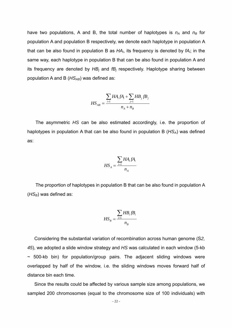
have two populations, A and B, the total number of haplotypes is nA and nB for
population A and population B respectively, we denote each haplotype in population A
that can be also found in population B as HAi, its frequency is denoted by fAi; in the
same way, each haplotype in population B that can be also found in population A and
its frequency are denoted by HBj and fBj respectively. Haplotype sharing between
population A and B (HSAB) was defined as:
BA
jjj
iii
AB nn
fBHBfAHAHS
+
+=
∑∑== 11
The asymmetric HS can be also estimated accordingly, i.e. the proportion of
haplotypes in population A that can be also found in population B (HSA) was defined
as:
A
iii
A n
fAHAHS
∑== 1
The proportion of haplotypes in population B that can be also found in population A
(HSB) was defined as:
B
iii
B n
fBHBHS
∑== 1
Considering the substantial variation of recombination across human genome (S2,
45), we adopted a slide window strategy and HS was calculated in each window (5-kb
~ 500-kb bin) for population/group pairs. The adjacent sliding windows were
overlapped by half of the window, i.e. the sliding windows moves forward half of
distance bin each time.
Since the results could be affected by various sample size among populations, we
sampled 200 chromosomes (equal to the chromosome size of 100 individuals) with - 22 -
- 23 -
replacement in each population/group when counting the number of haplotypes in
each genomic interval. The sampling procedure was repeated 100 times and the
results were averaged for each genomic interval.
1.15.3.3. Identification of population/group private haplotypes
Considering the possibility of gene flow among human populations, historical
inferences from haplotype sharing analyses could be affected by either ancient or
recent admixture. We identified population/group private haplotypes by comparing
multiple populations/groups which are interested in inferences. For example, in this
study, since we are interested in the pre-historical relationship among East-Asian (EA),
Southeast Asian (SE) and Central-South Asian (CSA) populations, we defined a
haplotype found only in EA sample but not observed in either SE or CSA samples as
an EA private haplotype, the same criterion was applied to identify private haplotypes
in SE and CSA samples as well. In subsequent comparisons, as in the above analyses,
type only or type with frequency were considered separately, the framework of
sampling was the same as described above.
1.15.3.4. Reconstructing phylogenetic trees of populations/groups with
population/group private haplotypes
Population/group private haplotypes were used to reconstruct phylogenetic
relationship of populations/groups. Pairwise distances between haplotypes were
calculated and summarized for all comparisons, a distance matrix was created among
populations/groups in each sliding window, and a neighbor-joining tree (S16) based on
these distance matrices was constructed.
- 24 -
2. Supplementary description and discussions
2.1. Additional notes on genotyping and integration of data from multiple
centers
As we mentioned in Methods, genotyping with the Affymetrix Genechip Human
Mapping 50K Xba array was performed at eight different genotyping centers (Table
S2). We were concerned about introducing a systematic bias in the data due to
differences amongst the genotyping centers, and therefore implemented several
measures to insure uniformity among the sites. First, all sites underwent training on
the Affymetrix 50K platform and this was conducted by the same technical support
manager for every site. Each site was required to pass the training with a set of control
samples. Secondly, a call rate cut-off of 90% was used for inclusion of samples into
the study. Samples falling below this cut-off were excluded from the study. A total of
162 samples were excluded based on this criterion. The resulting mean call rates for
each of the 7 sites was very high with surprisingly very little variation, ranging from
96.2% to 99.2% across sites. Furthermore, some of the genotyping centers served as
host sites for more than one country (and site of DNA collection), increasing our
confidence that geographic bias was not confounding the technical implementation of
the study. For example, the Genome Institute of Singapore (GIS) hosted the
genotyping of samples collected in Malaysia, the Philippines (including all Negrito
populations from both countries), Thailand and Indonesia, in addition to its own
collection of samples from Singapore. Lastly, some of the populations were composed
of samples collected and run by more than one genotyping center. For example,
samples of Han Chinese were run by three different centers; Malay and Japanese, as
well as two independently collected samples of the Miao population were each run at
two different genotyping centers. Based on the high call rates and the minimal
variation across sites, coupled with some of the sites running a variety of geographic
samples with little or no discernible variation, we feel confident that conclusions
formed from the data reported here represent geographic and population inferences
- 25 -
rather than technical effects. Finally, we observed very high concordance for 5 AX-ME
samples that were genotyping both in out study as well as the HGDP-CEPH 650K
dataset.
2.2. Additional notes on the population samples and related issues
We focused our attention on the initial peopling of East and Southeast Asia, and
the most population samples were collected from Southeast Asia, with less emphasis
on South and Central Asia, and few samples from elsewhere in Asia. A consensus has
developed that Southeast Asia was the site of initial entry of modern humans on the
basis of archeological and genetic data. Thus testing a comprehensive collection of
Southeast Asia populations is necessary to delineate the process in more detail. Since
Southeast Asia harbors the greatest linguistic and ethnic diversity in the continent, we
felt it important to “over” sample populations from Southeast Asia. While Central Asian
populations are represented only by the Uyghur, we included the CEPH-HGDP
samples in the combined dataset. In addition, our sampling from northern East Asia
(including multiple samples of Han Chinese from Beijing, Shanghai, Guangzhou, and
very recent immigrant communities in Taiwan and Singapore; Koreans; Japanese; and
Ryukyuans) is respectable, particularly since linguistic diversity is much less in north
Asia than Southeast Asia, and again, we included the CEPH-HGDP samples in the
combined dataset. The Ainu, which we were unable to sample, are often thought to
represent the descendants of an early migration to East Asia, but Y chromosome data
suggests that the Ryukyuans (who are included in our sampling) share substantial
connections with the Ainu (S47).
2.3. Additional notes on STRUCTURE analyses
We observed that the STRUCTURE results from the full dataset producesd
inferences that differ from those based on the subsets in larger Ks (Fig. S8 ~ S13). We
noticed that the difference between the full dataset and subsets is in the proportion of
admixture levels (or membership coefficients) of individuals, the other differences
- 26 -
were due to the different splitting order of clusters, but the cluster modes are
consistent. The background admixture present in the results of the full dataset could
result from the LD between closely linked markers, because the program
STRUCTURE assumes the loci are in linkage equilibrium within populations. The
program cannot handle markers that are extremely close together. Even in the latest
version, which implemented a “linkage model”, STRUCTURE can only deal with
weakly linked markers. Because, (1) in our data, there are 10% SNPs with between
marker distance (BMD) <0.2 kb, 52% of SNPs with BMD < 20 kb, 95.6% of SNPs with
BMD <200 kb; (2) although closely linked SNPs are not necessarily in strong LD, on
average, strong LD in Asian and European populations can extend to 100 kb or more
(S2, 35-38). Therefore, we did not think it is fully appropriate to perform STRUCTURE
analysis using the full dataset, so we also used reduced datasets to avoid LD (see
Methods for details). However, we found the STRUCTURE performed better than
expected under the situation of LD (as the case of full dataset). Because all the cluster
modes present in dataset S1 were observed frequently in the other datasets or in the
full dataset, and it reflects the full picture of the cluster modes in PanAsia data, it
seems reasonable that we selected it as a representative result. But we presented the
results of the subsets as well as that of the full dataset for all K’s, allowing the reader to
appreciate the subtle variation in outcomes at K’s >10.
2.4. Additional notes on PCA results
Phylogenetic analyses at the individual level generally show tight clustering within
populations, indicating that predefined population labels are usually informative about
the genetic relationships among individuals at the level of geographical sampling that
we have achieved (Fig. S27). This high degree of clustering is also apparent in
individual level analyses of the first two principal components (PC) (Fig. 2). In each
panel of Figure 2, population outliers have been identified, and then removed from the
successive plot. In these plots of the first two PCs it is apparent that individuals from
the same language family tend to cluster in close proximity to one another, and to their
- 27 -
geographic neighbors (with a few notable exceptions, which correspond very closely
with the linguistic outliers identified in Figure 1). Notably, in Fig. 2B, the first PC
generally orients individuals and populations according to their East-West coordinates
within Eurasia, while the second PC corresponds, with very few exceptions, to a South
to North axis. It is tempting to view the first PC, summarizing the greatest amount of
variation, as reflecting the predominant and oldest cline of genetic variation
established as modern humans first settled the Asian continent from Africa and the
Middle East, and then (as reflected by the 2nd PC in Fig. 2B) gradually populated more
northerly climes. However, it is likely that the detailed history of migrations is more
complex, with various agricultural expansions (especially from North to South within
Asia), and more recent movements in all directions affecting particularly the western
periphery of Asia (26). Nevertheless, we see little evidence that these more recent
events have greatly perturbed the geographic distribution of alleles that may have
been established very early in the initial settlement of Asia. To some extent, this may
be expected, since the demographic impact of each successive expansion would be
blunted by admixture with existing human populations at their periphery.
Under the one-wave theory, one expects that the most geographically distant
populations along the migration route will be the populations that are genetically most
diverged from the CEU group. However, in the PCA plot, the northern populations who
are most distant from Europe under a one-wave littoral theory (e.g. CHB, JPT) seem to
be even closer to CEU than are the southern populations (Fig. 2B). This seems
suggest that some degree of genetic contact with Europe and central or western Asia
along a northern route is likely, contrary to the our claims about a single littoral route.
However, we note that in the first PC, with or without the Yoruba, the CEU and the
CHB/JPT are actually maximally distant. This is true also of the second PC with the
Yoruba, but not when the Yoruba are removed. Given the intermediate position (both
geographically and in the PC plots) of the Uyghur and Spiti (IN-TB), two populations
with a known history of admixture among East Asian and Indo-European speaking
populations, we suspect that any similarity along the second PC is due to this
- 28 -
historical gene flow – and not necessarily a deep ancestral connection. For example,
the Uyghur (as also described in Li et al. 2008 Science 319:1100-1104) , like many
Central Asian populations, have received recent gene flow both from populations
tracing ancestry to East Asia but also to the Middle East/Europe. The position of the
Uyghur does not support an ancient shared ancestry between European and (north)
East Asian populations, as we observes previously (S4, 48). We also emphasize that
the second and higher PC’s explain very little of the total variance <= 1%, and that
results can be very sensitive to the populations which are included in the analyses. For
these reasons, we refrain from reaching strong conclusions on the basis of PC
analysis alone.
2.5. Evaluation of the influence of ascertainment bias on inferences in this study
Ascertainment bias is likely to happen when SNPs are chosen from public
database where the SNP discovery panels are often quite variable in size and
composition; the bias could be further enlarged by choosing only SNPs that had been
validated with high minor allele frequency (MAF) in population samples. In this section,
we first evaluate the ascertainment bias in the Affymetrix 50k genotyping chip by
comparing the observed allele frequency spectrum in 50k data and expected spectrum
assuming a simple coalescent model in particular populations. We also compared the
observed allele frequency spectrum of 50K SNP data with that of ENCODE region in
particular populations. We further evaluate whether and how much the ascertainment
bias affects the inferences in our study. The following analyses are all based on
autosomal data. Previous work has shown that haplotype-based methods are less
sensitive to the ascertainment protocols of individual SNPs (S49). We also found in
our data that haplotype diversity is highest in Africans and decreases as the distance
from Africa increases, which is consistent with a series of founder effects. In the
evaluation of ascertainment bias, we focus on the individual SNPs but not haplotype.
- 29 -
2.5.1. Evaluation of the influence of ascertainment bias
Most analyses we carried out in this study, which are based primarily on
tree-building algorithms rather than allele frequency distribution, thus in theory should
not have been much affected by ascertainment bias. However, considering the fact
that ascertainment bias exist in the data and its potential possibility of influence on
history inferences, we analyzed the sub-datasets generated above by repeating the
procedure that performed on original dataset. These analyses are to examine whether
and how much ascertainment bias affects the inferences if a set of SNPs are chosen
based on their frequencies in particular populations.
2.5.1.1. Evaluation of the influence on genetic distance estimation
We firstly investigated whether population genetic distances calculated from
sub-datasets are significantly different with that calculated from the original dataset.
FST matrix was estimated from 75 populations in subset1 data selected based on
expected spectrum in YRI under coalescence model; Figure S33 displayed a
correlation relationship between FST matrices calculated from subset and full dataset.
The overall correlation of FST between full dataset and sub-dataset is very high,
indicated by high correlation coefficient (r > 0.98) and significant p-value (p < 10-4),
nonetheless, we do observe different FST distribution between full data and
sub-datasets. For example, in sub-dataset of which SNPs were selected based on
expected MAF spectrum in YRI under coalescent model (Figure S33A), all FST
comparisons between African and nonAfrican deviate from the correlation line. FST
values calculated from sub-dataset selected in YRI are generally higher than FST
values calculated from full data for comparisons of YRI and non-African populations.
This result indicated the genetic difference between YRI and non-African populations
are larger. When SNPs were selected based on their MAF spectrum in CEU, the
deviated FST comparisons are between CEU and the other populations (Figure S33B),
with the genetic differences between CEU and Asian increased in sub-datasets.
However, when SNPs were selected based on their MAF spectrum in CHB, there is
- 30 -
not obvious deviation (Figure S33C), but the overall FST values are larger in
sub-dataset than that in full data. A similar pattern was observed in sub-datasets
selected based on their MAF spectrum in ENCODE regions (Figure S33E, F, G), but
the deviations are still stronger which, to a large extent, due to the MAF spectrum in
ENCODE regions including much more low frequency SNPs compared with than in full
Affymetrix 50K data.
2.5.1.2. Evaluation of the influence on tree topologies
The above analyses showed differences exist in distributions between full
Affymetrix 50K data and sub-datasets with biased SNPs selected based on allele
frequencies in single particular population, but it is not clear whether or how much the
tree topologies are affected. We further analyzed 100 sub-datasets selected above
based on expected spectrum in YRI under coalescence model and reconstructed a
maximum likelihood tree (Figure S34A), maximum likelihood trees based on 100
sub-datasets selected in CEU (Figure S34B) and CHB (Figure S34C) were also
reconstructed respectively. We also analyzed sub-datasets of which SNPs were
selected in particular population based on their MAF spectrum in ENCODE regions,
the maximum likelihood trees reconstructed from 100 sub-datasets selected in YRI,
CEU and CHB were shown in Figure S35A, B, C respectively. Using the same
procedure, maximum likelihood trees were also reconstructed from 100 sub-datasets
selected based on expected allele frequency distribution in Malay Negritos and
Philippine Negritos respectively, the results were shown in Figure S36A, B,
respectively. In all cases, we do not see significant change of tree topologies and
population grouping pattern compared with that reconstructed from the full dataset,
and notably, the topologies and population grouping pattern of three maximum
likelihood trees are also consistent. This result indicated that ascertainment bias does
not invalidate the inferences based on tree topologies.
- 31 -
2.6. Additional notes on language replacement
Populations from the same linguistic group tend to cluster together, showing the
expected correlation between genetic and linguistic distances, with the exception of
eight populations with known or suspected histories of admixture or language
replacement: the Uyghur (CN-UG), a Central Asian population in western China along
the route of the ancient Silk Road connecting Europe to Asia; the Ladakhi (Spiti)
(IN-TB), a Sino-Tibetan speaking population in India, south of the Himalayas; the Mon
of Thailand (TH-MO); the Malaysian Negritos (MY-JH and MY-KS), with a likely history
of language replacement that we discuss below; the Nasioi Melanesians (AX-ME),
grouping with several eastern Indonesian populations known to have mixed with
Papuan speaking populations to their east; and the Karen (TH-KA) and the Jinuo
(CN-JN), both of which speak Sino-Tibetan languages but inhabit Southeast Asia and
are surrounded primarily by the Austro-Asiatic, Tai-Kadai, and Hmong-Mien speaking
populations among whom they cluster in the tree.
2.7. Additional notes on Taiwan Aborigines
A recent classification of Austronesian languages showing maximal diversity in the
languages of Taiwan (21) has suggested this island as the ancestral “homeland” for
Austronesian speaking populations throughout the Indo-Pacific. We sampled two
populations (AX-AM/Ami and AX-AT/Atayal) representing two deeply differentiated
Austronesian sub-families (Paiwanic and Atayalic) in Taiwan. STRUCTURE/frappe
analysis (Fig. S1-S26) indicates that the two aboriginal populations of Taiwan share a
common component with most other Austronesian speaking populations. In addition,
the topology of the maximum-likelihood population tree (Fig. 1) seems to suggest that
Taiwan aborigines may be derived from, rather than ancestral to other Austronesian
populations, because they occupy central, rather than peripheral positions within the
cluster of Austronesian speaking populations. This observation seems to contradict a
- 32 -
commonly cited Taiwan “homeland” hypothesis of Austronesian populations. Given a
nearly total lack of prior autosomal data from Southeast Asian populations (9, 10), and
conflicting evidence based on mtDNA analyses, some of which questions the Taiwan
homeland story (22, 23), we believe our data should prompt a reexamination of
hypotheses for the origins of the Austronesian languages and their speakers.
2.8. Additional notes on Indian populations
In all of our analyses, Indian populations showed considerable evidence of
similarity to European populations (Fig. 1, Fig. 2, S1~S26, S27, S28), and in
STRUCTURE/frappe results, Indian populations have a substantial contribution of
'European' ancestry (Fig. S1~S26). This is highly consistent with what we know about
the introduction of Indo-European languages into both India and Europe. Our data
therefore differ markedly from the results of Rosenberg et al. (S50), which posited
India as a vast (yet entirely homogenous) reservoir of a unique component of human
diversity found nowhere else on earth. The reasons for our differing results are not
entirely obvious, but possibilities include: differing mutation rates or ascertainment
biases in the SNP vs. microsatellite markers; differing population samples (theirs were
from Indians resident in the U.S.A., ours were sampled in India); and our sample
includes only one Dravidian speaking population, theirs includes 4 (although they also
sample from 11 Indo-European speaking populations). Nearly all of our population
samples were donated by members of high castes, and there is compelling historical
and genetic data (Genome Res. 11:994-1004) that the Indo-European migrants both
established the caste system, and ensconced themselves in the highest castes.
Finally, though we have no direct evidence for it, it is possible that the genotypes for
the Indian samples in Rosenberg et al. (S50) were called differently than those of all
the other populations, and this would certainly tend to group the Indians separately
from all other populations. The Indian samples were genotyped as a group in 2004
(and possibly at another lab), while the other samples were genotyped in 2002. As
Rosenberg et al. discuss (and made some statistical, but indirect and thus imperfect,
efforts to correct), many changes in both the primer sequences and (crucially)
fragment sizing software had changed between the two genotyping episodes, and
- 33 -
thus inconsistent allele-calling is a real possibility.
The relatively recent introduction to India of Indo-European languages and the
genes of their speakers (which, as we now explicitly remark in the manuscript, is
evident in our data) is unanimously accepted by nearly every student of Indian
prehistory. Therefore, we discuss the pre-historical migration in Asia, we are not
discussing the arrival of Indo-European speaking populations in India, Instead, we
focus on the major entry to Southeast and East Asia. Our one- and two-wave models
concern the settling of Southeast and Northeast Asia. The genetic proximity of
Northeast Asian and European populations seen in earlier studies of classical markers
has led to the idea of a second wave of migration predominantly to Northeast Asia – a
wave that would also have contributed to or emanated from Europe. Our data do not
show this relative similarity between Northeast Asian and European populations,
leading us to question the evidence for a second major wave of migration into East
Asia.
2.9. Addition notes on isolation by distance and pre-historical population
divergence
2.9.1. Geographical distance versus genetic distance
Previous studies have hypothesized a serial founder effect originating in Africa by
showing a relationship between genetic and geographic distances (11, 24, 25). We
combined data for 19,934 common SNPs typed in 52 HGDP samples (11) and
calculated FST (26) and great circle geographic distances from East Africa for the 126
populations. Our results confirmed previous observations of a linear increase in
genetic distance with geographic distance. The PC analysis further emphasizes this
geographic patterning of the populations (Fig. 2). Notably, in Fig. 2B, the first PC
generally orients individuals and populations according to their East-West coordinates
within Eurasia, while the second PC corresponds, with very few exceptions, to a South
to North axis. This pattern is consistent with a serial founder effect during the initial
peopling of Asia. The same pattern is echoed in the branching order of groups on the
- 34 -
population tree (Fig. 1), which shows a South-North pattern – from the Austronesian
and Austro-Asiatic speaking populations in the extreme south, to the Tai-Kadai,
Hmong-Mien, Sino-Tibetan, and, finally, the northernmost Altaic speaking populations.
2.9.2. IBD versus historical divergence
Although the branching pattern of population tree (Fig. 1, Fig. S28) showed a
hierarchical splitting of ethnic or linguistic groups and indicated the possible
pre-historical divergence with South-North migration of Asian populations, the
alternative model of current divergence and equilibrium process such as isolation by
distance (IBD) can also explain such a pattern. The expression “isolation by distance”
was initially introduced by S. Wright (S51, 52), it indicates the tendency of populations
to exchange genes with nearest neighbors, resulting in a greater genetic affinity
between geographically closer groups and the likely occurrence of genetic differences
between groups that are far apart because of genetic drift (S53). The models
developed by Wright have been conceptually influential but have had little practical
application. More popular have been the models of IBD developed by Malécot (S54)
and by Kimura and Weiss (S55) in spaces of one or two dimensions, according to
whether the migrating populations are supposed to live on a linear habitat (e.g., a
group of islands placed along a line) or on a more common two-dimensional habitat.
The approaches by Malécot and by Kimura and Weiss differ, but the qualitative
predictions are alike. The one-dimensional models are consistent in showing an
exponential decrease of the genetic similarity between two demes with their
geographic distance (S53).
We used partial and multiple Mantel tests to simultaneously test pre-historical
divergence effects and IBD effects. Partial Mantel regression was used to partition the
effects of geographic structure and long-term divergence associated with possible
pre-historical population splits. The general idea is that the IBD process occurs on a
much smaller time-scale than long-term historical isolation or deep-time coalescence
(S23).
- 35 -
The simple matrix correlation of genetic and geographic distance was 0.332 (P <
0.0001 with 10,000 permutations), consequently, about 11% of the variation in genetic
distances can be attributed to geographic distances between pairs of populations;
while correlation of genetic and clustering indicator matrix was 0.462 (P < 0.0001 with
10,000 permutations), thus about 21.3% of the variation in genetic distances can be
attributed to pre-historical divergence of Asian populations. Partial correlation of
genetic and geographic distance was 0.228 (P < 0.0006 with 10,000 permutations),
after controlling for clustering indicator matrix; while partial correlation of genetic and
clustering indicator matrix was 0.403 (P < 0.0001 with 10,000 permutations) after
controlling for geography.
When the Mantel test was applied to the populations within each clade (cluster or
group), the correlation between genetic and geographic distance generally decreased.
For example, the correlation between genetic and geographic distance in Tai-Kadai
group was 0.293 (P = 0.208 with 10,000 permutations); the correlation between
genetic and geographic distance in Indian group was 0.135 (P = 0.263 with 10,000
permutations); in some groups, the correlation even reversed, for example, the
correlation between genetic and geographic distance in Hmong-Mien group was -0.99
(P = 0.168 with 10,000 permutations), which was unexpected by IBD model. Therefore,
the relationship between these populations and those on the other groups is not fully
additive and these groups are probably subject to different evolutionary processes
(S23).
Overall about 16.2% of the variation in the genetic distances (FST) could be
attributed to pre-historical divergence alone, whereas only 5.2% of the variation in
genetic distances could be attributed to IBD. In other words, spatial patterns in genetic
distances are much better explained by differences between groups of populations
than by similarity among adjacent local populations within these groups. However, as
expected, there is a large overlap between the two processes, the long-term
divergence binary matrix is also structured in geographic space (r = 0.301; P < 0.0001
with 10,000 permutations), in such a way that it is not possible to entirely partition
population divergence between historical and contemporary processes such as IBD
(S23).
- 36 -
We further carried out a simulation study under isolation by distance (IBD) to
explore whether IBD could alone generate the patterns that were observed. Our
simulation results showed two-dimensional model of IBD could not generate the
branching patterns of population trees observed in this study; one-dimensional model
(gene flow along south-north way) of IBD could generate similar tree branching
patterns observed in East Asian populations with a few exceptions, but was not
compatible with the distribution of herterozygosity pattern observed in East Asian
populations, i.e. herterozygosity decreasing from south to north. When admixture of
West Eurasian ancestry in Southeast Asia was simulated in one-dimensional IBD, the
observed diversity pattern could to some degree be mimicked, however, the
phylogeny of group private haplotypes could not be recovered, i.e. the East Asian
private haplotypes and West Eurasian private haplotypes cluster together firstly since
East Asian private haplotypes initially derived from West Euroasian in simulation under
“pincer model” (S56); while in real data East Asian private haplotypes and Southeast
Asian private haplotypes cluster firstly. Therefore, both two-dimensional and
one-dimensional IBD effects could not totally explain the observed pattern in current
data.
On balance, although we could not totally ignore the contribution of IBD, our data
show strong signal of the effect due to pre-historical population divergence.
2.10. Evidence of southern origins of East Asian populations and
South-to-North migration
Origin of East Asian populations has been debatable in human evolutionary
studies, here, after analyzing genome-wide data in adequate Asian samples, we
provide evidence that supports the south origin of East Asian and South-to-North
migration, i.e. East Asian initially most likely derived from Southeast Asian populations,
with contribution from north in later time.
- 37 -
2.10.1. Topology of maximum likelihood tree of populations
Using 42,793 SNPs whose ancestral allele states are known, we reconstructed a
maximum likelihood tree of 75 human populations with most recent common ancestor
of humans as an out group (Fig. 1). East Asian populations cluster together with
Southeast Asian populations and are the last split of branches, the topology and
branching pattern of the tree support the south origin of East Asian populations. A
maximum likelihood tree of 126 world-wide populations with CEPH-HGDP samples
included (Fig. S28) also supports this idea.
2.10.2. Distance of STRUCTURE/frappe components
At K=2 (Fig. S1, Fig. S14) and K=3 (Fig. S2, Fig. S15), all Southeast (SE) and
East Asian (EA) samples are united by predominant membership in a common cluster,
with the other cluster(s) corresponding largely to Indo-European (IE) and African (AF)
ancestries. At K = 4 (Fig. S3, Fig. S16), the new component accounts for shared
ancestry of all SE samples and dominated in both Negrito and Papuan samples, the
net nucleotide distance (S33, 34) between SE and EA (0.020) inferred from
STRCTURE components are much less than any other pair comparisons (0.062 for
SE-AF, 0.065 for EA-AF, 0.049 for IE-AF, and 0.032 for both SE-IE and EA-IE), which
suggest SE and EA shared the most recent common ancestral origins.
2.10.3. Topology of STRUCTURE/frappe component tree
We reconstructed a phylogenetic tree relating the clusters based on allele
frequencies in each cluster inferred from the STRUCTURE/frappe analysis.
Phylogenetic relationships of these clusters (referred to as the “component tree”),
given their statistical independence, should reveal an evolutionary history that is less
perturbed by recent gene flow and admixture than is a population phylogeny. With
African component as out group, the split of East Asian and Southeast Asian
components is the latest one, thus supports the idea of East Asian populations derived
- 38 -
from Southeast Asian populations, and again, the tree topology and branching pattern
support South-to-North migration history.
2.10.4. Distribution of samples in PCA plots
Distribution of Asian samples in PCA plot (Fig. 2D) consists the South-North
spatial pattern, strong correlation of PC1 and latitudes supports the South-North
migration.
2.10.5. Geographical distribution of genetic diversities
Generally speaking, later derived populations have less genetic diversity; the
decreasing trend of geographical distribution of genetic diversity indicates the
migration directions. Distribution of haplotype diversities of Southeast and East Asian
populations showed a South-to-North decreasing trend with strong correlation
between diversities and latitudes (Fig. 3A, Fig. S37), strongly suggesting the
South-to-North migration.
2.10.6. Haplotype sharing proportions
We conducted haplotype-based analysis to examine the contribution of other
source of haplotypes to East Asian (EA) gene pool. Due to the different marker
densities and population samples in PanAsia data and combined data (see Methods),
we considered the two data sets separately. Population/group private haplotypes were
identified using methods describes above.
For PanAsia data, we examined the contribution Southeast Asian (SE) and
Indians (IN) to East Asian (EA) gene pool. EA populations were grouped as Japanese
(JP, including JP-RK, JPT and JP-ML), Korean (KR, including KR-KR), Han Chinese
(HAN, including CHB, CN-SH, CN-GA, TW-HA, TW-HB and SG-CH), and Southern
Chinese minorities (S-CM, including CN-HM, CN-CC, CN-JI, CN-WA and CN-JN).
Haplotypes of each group were compared with that of SE and IN, and were classified
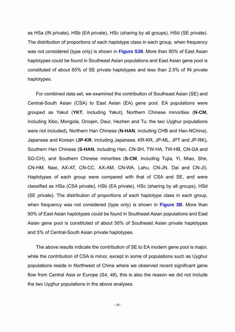
- 39 -
as HSa (IN private), HSb (EA private), HSc (sharing by all groups), HSd (SE private).
The distribution of proportions of each haplotype class in each group, when frequency
was not considered (type only) is shown in Figure S38. More than 90% of East Asian
haplotypes could be found in Southeast Asian populations and East Asian gene pool is
constituted of about 65% of SE private haplotypes and less than 2.5% of IN private
haplotypes.
For combined data set, we examined the contribution of Southeast Asian (SE) and
Central-South Asian (CSA) to East Asian (EA) gene pool. EA populations were
grouped as Yakut (YKT, including Yakut), Northern Chinese minorities (N-CM,
including Xibo, Mongola, Oroqen, Daur, Hezhen and Tu; the two Uyghur populations
were not included), Northern Han Chinese (N-HAN, including CHB and Han-NChina),
Japanese and Korean (JP-KR, including Japanese, KR-KR, JP-ML, JPT and JP-RK),
Southern Han Chinese (S-HAN, including Han, CN-SH, TW-HA, TW-HB, CN-GA and
SG-CH), and Southern Chinese minorities (S-CM, including Tujia, Yi, Miao, She,
CN-HM, Naxi, AX-AT, CN-CC, AX-AM, CN-WA, Lahu, CN-JN, Dai and CN-JI).
Haplotypes of each group were compared with that of CSA and SE, and were
classified as HSa (CSA private), HSb (EA private), HSc (sharing by all groups), HSd
(SE private). The distribution of proportions of each haplotype class in each group,
when frequency was not considered (type only) is shown in Figure 3B. More than
90% of East Asian haplotypes could be found in Southeast Asian populations and East
Asian gene pool is constituted of about 50% of Southeast Asian private haplotypes
and 5% of Central-South Asian private haplotypes.
The above results indicate the contribution of SE to EA modern gene pool is major,
while the contribution of CSA is minor, except in some of populations such as Uyghur
populations reside in Northwest of China where we observed recent significant gene
flow from Central Asia or Europe (S4, 48), this is also the reason we did not include
the two Uyghur populations in the above analyses.
- 40 -
2.10.7. Phylogeny of group private haplotypes
We further reconstructed phylogenetic relationship of group private haplotypes
(see Methods). Phylogeny of group private haplotypes showed EA has a closest
relationship with SE, thus supports the idea EA derived directly from SE, the
contribution from other sources (e.g. CSA) was minor and could have occurred in later
time.
2.11. Peopling of Asia: one-wave versus two-wave hypothesis
According to Cavalli-Sforza et al. (S57), anatomically modern humans (also called
Homo sapiens sapiens) spread into Asia through two routes. “The first was a southern
route, perhaps along the coast to south and Southeast Asia, from where it bifurcated
north and south. In the south, these modern humans reached Oceania between 60
and 40 kya, whereas the northern expansion later reached China, Japan and
eventually America (this might represent the second migration to America, associated
with the NaDene languages, postulated by Greenberg). The second was a central
route through the Middle East, Arabia or Persia to central Asia, from where migration
occurred in all directions reaching Europe, east and northeast Asia about 40 kya, after
which the first and principal migration to America suggested by Greenberg occurred
not later than 15 kya.” This hypothesis was based almost entirely on classical protein
and blood group data from a handful of markers which resulted in phylogentic tree
topologies appearing to show that populations in Northeast Asia are more similar to
European populations than they are to populations living in Southeast Asia.
Based on hypothesis of Cavalli-Sforza et al. and our observations on Asian
Negritos, we constructed three models which are testable, as illustrated in Figure S29
and described in Methods. Models 1 and Model 2 are both consistent with the
scenarios hypothesized by Cavalli-Sforza et al, which we call “two-wave” hypothesis,
while Model 3 suggests a “one-wave” hypothesis, i.e. the majority of the gene pool in
Asia (the part that gave rise to all modern East Asian and Southeast Asian populations)
- 41 -
was derived from a single initial entry of modern humans into the subcontinent.
In the following sub-sections, in addition to a phylogenetic tree topology which
contrasts sharply with Cavalli-Sforza’s older trees based on much less data, we list
some additional evidence in support of the one-wave hypothesis; or more precisely,
the idea that the majority of the gene pool in Asia (the part that gave rise to East Asian
and Southeast Asian populations) was derived from a single initial entry of modern
humans into the subcontinent.
2.11.1. Topology of population trees
As the topology of a maximum likelihood tree of 75 populations (Fig. 1) showed,
all Negrito populations cluster together with Southeast Asian populations and are the
last split of branches, the topology and branching pattern of the tree support the south
origin of East Asian populations. A maximum likelihood tree of 126 world-wide
populations with CEPH-HGDP samples included (Fig. S28) also supports this idea.
2.11.2. Topology of STRUCTURE/frappe component tree
We reconstructed a phylogenetic tree relating the clusters based on allele
frequencies in each cluster inferred from the STRUCTURE/frappe analysis.
Phylogenetic relationships of these clusters (referred to as the “component tree”),
given their statistical independence, should reveal an evolutionary history that is less
perturbed by recent gene flow and admixture than is a population phylogeny. With
African component as out group, the split of East Asian and Southeast Asian
components is the latest one, thus supports the idea of East Asian populations derived
from Southeast Asian populations.
The overall pattern of this component tree is similar to that of the population tree
(Fig. 1) with a few revealing exceptions. The component we associate with
Austronesian speakers now groups with the mainland East Asian components,
consistent with the idea that this language family expanded from mainland East Asia –
- 42 -
possibly following the development of rice agriculture, as has been previously
hypothesized on archeological and linguistic grounds (S42). The Negrito and Papuan
groups are now closer to the root of the East Asian and Southeast Asian clades, with
the European and Indian groups positioned outside the clade. This suggests that the
divergence of the Negrito groups and the other Asian populations occurred after the
divergence of Asian and European populations.
2.11.3. Phylogeny of group private haplotypes
Private haplotypes of Negrito (NG), Asian (AS) and European (EUR) were
identified and phylogenetic tree of group private haplotypes was reconstructed with
same method described in 2.11.6. Phylogeny of group private haplotypes indicated
NG and AS has the closest relationship, thus suggesting divergence of
non-Pygmy-Asian/Asian Pygmies was not earlier than that of Asian/European, this
result further implying the majority of the gene pool in Asia (the part that gave rise to
East Asian and Southeast Asian populations) was derived from a single initial entry of
modern humans into the subcontinent.
2.11.4. Simulation results
The topology of our population trees, both with or without the data from additional
European and Asian populations in (S3) provide little support for the two-wave model,
and appear more consistent with a single major peopling of Asia (Fig. 1, S28) – nor
does the population tree of ref (S3) based on all 642,690 SNPs. The rather
surprising tree topology that first led to the suggestion of a two-wave model, in which
populations in Northeast Asia were more similar to populations inhabiting Europe than
to populations in Southeast Asia is not seen with the much larger number of DNA
variants analyzed in recent studies. However, there is still a formal possibility that high
levels of gene flow from neighboring populations into the Negritos could have
contributed to the observed tree topology, which places the Negritos within the
monophyletic grouping of all other Asian populations within our sample. We therefore
- 43 -
performed simulations to estimate the level of gene flow from neighboring populations
that would have been required to change the tree topology. We examined three
relevant models (Fig. S29) based on the two-wave and one-wave hypotheses and
applied forward time simulations (see above descriptions). Results of the forward time
simulations (Fig. S30) indicate that the two-wave model is only compatible with the
empirical data if gene flow to Negrito populations has been extensive, i.e., if more than
half of the chromosomes in the Negrito populations resulted from recent admixture
with neighboring populations. Although such a high degree of gene flow (> 50%)
seems unlikely particularly in light of the phenotypic differences between Negritos and
other populations, we did observe such high degree of general Asian gene
contribution in some of Philippine Negrito populations, for example, and general Asian
components are summed together 61.0% for PI-AG and 58.7% for PI-IR. The average
proportion of general Asian components is 44.4% in Philippine Negritos, and 10.6% in
Malaysia Negritos. There could be some mechanism of natural or sexual selection
acting to preserve this phenotype in the presence of considerable admixture from later
migrants.
In addition, at K=2 in STRUCTURE/frappe results (Fig. S1, S14), East Indonesian
and Negrito populations show similarity to the YRI. This result seems potentially
suggests a second early migration, ancestral to Negritos and some Austronesians,
that has left detectable similarity to Africans despite admixture with descendants of
subsequent migrations. However, there is very little evidence that any non-African
populations (including SE Asian Negritos, termed “Orang Asli” in the paper of
Macaulay et al. Science (2005) 308:1034 – 1036) derive from other than a small
number of initial out-of-Africa events some 50,000 to 150,000 years ago. We would
speculate that this very tentative connection among Negrito and African populations
could be explained if the Negrito populations required fewer adaptive changes to life in
tropical latitudes similar to the ones their ancestors had inhabited in Africa. East Asian
populations inhabiting more northern climates, by contrast, are likely to have
experienced novel selection pressures as they moved into new latitudes and
- 44 -
environments. It would not be surprising if such adaptations significantly altered allele
frequencies throughout much of the genome, via linkage disequilibrium with selected
variants.
Furthermore, the placement of the AX-ME near the MY-JH and MY-KS in the PCA
plot (Fig. 2B) provides a similar result to the STRUCTURE analysis. We believe this
similarity of the AX-ME and the Malaysian Negritos (who also share some phenotypic
similarity) is consistent with, and in fact bolsters the one-wave hypothesis, in which
modern humans are thought to have first entered Southeast Asia along a mostly
coastal route and continued rapidly to modern day Australia, Papua, and neighboring
Melanesian Islands. These populations would be the most direct descendants of the
initial modern humans, with less need to adapt to changing climate and a non-tropical
environment. Descendants of these initial Southeast Asian populations appear then to
have moved, perhaps more gradually, to the north of the continent, with significant
adaptations occurring to the local climate and environment, which changes more
sharply with latitude than longitude.
2.11.5. Final comments
When the genetic data in this study are considered together with the geographical
distribution of the clusters and archeological and linguistic information, we propose the
following model of human migrations in Asia. The initial entry is likely to have followed
a southern route to Southeast Asia (S58). From there, populations gradually moved
north, adapting to climatic and local selective pressures. Subsequently, and
particularly with the development of agriculture as a stimulus, populations in northern
and central East Asia may have expanded southwards, altering the physical
characteristics of the original inhabitants.
- 45 -
3. References
S1. Nature 426, 789 (Dec 18, 2003). S2. K. A. Frazer et al., Nature 449, 851 (Oct 18, 2007). S3. J. Z. Li et al., Science 319, 1100 (Feb 22, 2008). S4. S. Xu, L. Jin, Am J Hum Genet 83, 322 (Sep 12, 2008). S5. G. C. Kennedy et al., Nat Biotechnol 21, 1233 (Oct, 2003). S6. C. Zhang et al., Bioinformatics 22, 2122 (Sep 1, 2006). S7. S. Schneider, D. Roessli, L. Excoffier, Genetics and Biometry Lab, Dept. of Anthropology, University of
Geneva., (2000). S8. S. Wright, Nature 166, 247 (Aug 12, 1950). S9. M. Slatkin, Genet Res 58, 167 (Oct, 1991). S10. B. Su et al., Am J Hum Genet 65, 1718 (Dec, 1999). S11. J. L. Mountain, L. L. Cavalli-Sforza, Am J Hum Genet 61, 705 (Sep, 1997). S12. A. L. Price et al., Nat Genet 38, 904 (Aug, 2006). S13. B. S. Weir, W. G. Hill, Annu Rev Genet 36, 721 (2002). S14. M. Nei, Am. Nat. 106, 283 (1972). S15. M. Nei, F. Tajima, Y. Tateno, J Mol Evol 19, 153 (1983). S16. N. Saitou, M. Nei, Mol Biol Evol 4, 406 (Jul, 1987). S17. S. Kumar, K. Tamura, M. Nei, Brief Bioinform 5, 150 (Jun, 2004). S18. J. Felsenstein, Am J Hum Genet 25, 471 (Sep, 1973). S19. J. Felsenstein, Cladistics 5, 164 (1989). S20. S. Ramachandran et al., Proc Natl Acad Sci U S A 102, 15942 (Nov 1, 2005). S21. N. A. Rosenberg et al., PLoS Genet 1, e70 (Dec, 2005). S22. M. Jakobsson et al., Nature 451, 998 (Feb 21, 2008). S23. M. P. Telles, J. A. Diniz-Filho, Genet Mol Res 4, 742 (2005). S24. S. Santos, H. Schneider, I. Sampaio, Genet. Mol. Biol. 26, 151 (2003). S25. B. F. J. Manly, The statistics of natural selection. (Chapman & Hall, London, UK., 1985). S26. B. F. J. Manly, Randomization, bootstrp and Monte Carlo methods in biology. (Chapman & Hall,
London, UK., 1997). S27. R. R. Sokal, N. L. Oden, J. Walker, D. M. Waddell, J. Hum. Evol. 32, 501 (1997). S28. F. M. Rodrigues, J. A. Diniz-Filho, L. A. M. Bataus, R. P. Bastos, Genet. Mol. Biol. 25, 435 (2002). S29. B. F. J. Manly, Res. Popul. Ecol. 28, 201 (1986). S30. B. A. Hawkins, E. E. Porter, J. A. F. Diniz-Filho, Ecology 84, 1608 (2003). S31. P. Legendre, L. Legendre, Numerical ecology., (Elsevier, Amsterdam, Holland, 1998). S32. R. Leblois, A. Estoup, F. Rousset, Mol Ecol Res, doi:10.1111/j.1755 (2008). S33. J. K. Pritchard, M. Stephens, P. Donnelly, Genetics 155, 945 (Jun, 2000). S34. D. Falush, M. Stephens, J. K. Pritchard, Genetics 164, 1567 (Aug, 2003). S35. H. M. Cann et al., Science 296, 261 (Apr 12, 2002). S36. G. A. Huttley, M. W. Smith, M. Carrington, S. J. O'Brien, Genetics 152, 1711 (Aug, 1999). S37. D. E. Reich et al., Nature 411, 199 (May 10, 2001). S38. M. Laan, S. Paabo, Nat Genet 17, 435 (Dec, 1997).
- 46 -
S39. M. Jakobsson, N. A. Rosenberg, Bioinformatics 23, 1801 (Jul 15, 2007). S40. N. A. Rosenberg et al., Science 298, 2381 (Dec 20, 2002). S41. N. A. Rosenberg et al., Genetics 159, 699 (Oct, 2001). S42. J. Diamond, P. Bellwood, Science 300, 597 (Apr 25, 2003). S43. H. Tang, J. Peng, P. Wang, N. J. Risch, Genet Epidemiol 28, 289 (May, 2005). S44. P. Scheet, M. Stephens, Am J Hum Genet 78, 629 (Apr, 2006). S45. S. Myers, L. Bottolo, C. Freeman, G. McVean, P. Donnelly, Science 310, 321 (Oct 14, 2005). S46. S. Xu, W. Jin, L. Jin, Mol Biol Evol (doi:10.1093/molbev/msp130), (Jun 29, 2009). S47. M. F. Hammer et al., J Hum Genet 51, 47 (2006). S48. S. Xu, W. Huang, J. Qian, L. Jin, Am J Hum Genet 82, 883 (Apr, 2008). S49. G. Hellenthal, A. Auton, D. Falush, PLoS Genet 4, e1000078 (May, 2008). S50. N. A. Rosenberg et al., PLoS Genet 2, e215 (Dec, 2006). S51. S. Wright, Genetics 28, 114 (Mar, 1943). S52. S. Wright, Genetics 31, 39 (Jan, 1946). S53. L. L. Cavalli Sforza, P. Menozzi, A. Piazza, The history and geography of human genes. (Princeton
University Press, Princeton, New Jersey, 1993), pp. 52. S54. G. Malécot, Les Mathematiques de L'Hérédité. (Masson, Paris, 1948). S55. M. Kimura, G. H. Weiss, Genetics 49, 561 (Apr, 1964). S56. Y. C. Ding et al., Proc Natl Acad Sci U S A 97, 14003 (Dec 5, 2000). S57. L. L. Cavalli-Sforza, M. W. Feldman, Nat Genet 33 Suppl, 266 (Mar, 2003). S58. P. Mellars, Science 313, 796 (Aug 11, 2006).
4. Supplementary Tables
Table S1. Analysis of molecular variance (AMOVA).
Table S2. Institutions that performed the genotyping.
Table S3. Data quality control for samples.
Table S4. Details of SNP filtering.
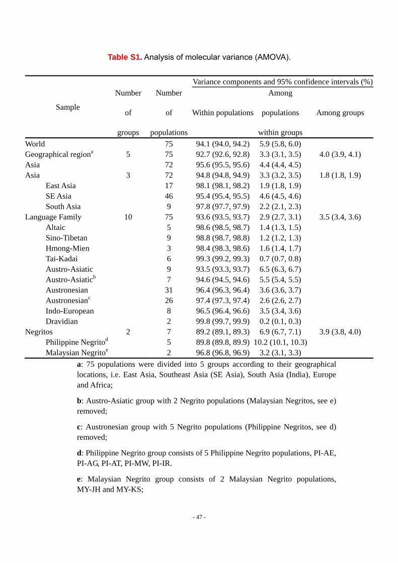
- 47 -
Table S1. Analysis of molecular variance (AMOVA).
Sample
Number
of
groups
Number
of
populations
Variance components and 95% confidence intervals (%)
Within populations
Among
populations
within groups
Among groups
World 75 94.1 (94.0, 94.2) 5.9 (5.8, 6.0)
Geographical regiona 5 75 92.7 (92.6, 92.8) 3.3 (3.1, 3.5) 4.0 (3.9, 4.1) Asia 72 95.6 (95.5, 95.6) 4.4 (4.4, 4.5)
Asia 3 72 94.8 (94.8, 94.9) 3.3 (3.2, 3.5) 1.8 (1.8, 1.9) East Asia 17 98.1 (98.1, 98.2) 1.9 (1.8, 1.9)
SE Asia 46 95.4 (95.4, 95.5) 4.6 (4.5, 4.6)
South Asia 9 97.8 (97.7, 97.9) 2.2 (2.1, 2.3)
Language Family 10 75 93.6 (93.5, 93.7) 2.9 (2.7, 3.1) 3.5 (3.4, 3.6) Altaic 5 98.6 (98.5, 98.7) 1.4 (1.3, 1.5)
Sino-Tibetan 9 98.8 (98.7, 98.8) 1.2 (1.2, 1.3)
Hmong-Mien 3 98.4 (98.3, 98.6) 1.6 (1.4, 1.7)
Tai-Kadai 6 99.3 (99.2, 99.3) 0.7 (0.7, 0.8)
Austro-Asiatic 9 93.5 (93.3, 93.7) 6.5 (6.3, 6.7)
Austro-Asiaticb 7 94.6 (94.5, 94.6) 5.5 (5.4, 5.5)
Austronesian 31 96.4 (96.3, 96.4) 3.6 (3.6, 3.7)
Austronesianc 26 97.4 (97.3, 97.4) 2.6 (2.6, 2.7)
Indo-European 8 96.5 (96.4, 96.6) 3.5 (3.4, 3.6)
Dravidian 2 99.8 (99.7, 99.9) 0.2 (0.1, 0.3)
Negritos 2 7 89.2 (89.1, 89.3) 6.9 (6.7, 7.1) 3.9 (3.8, 4.0) Philippine Negritod 5 89.8 (89.8, 89.9) 10.2 (10.1, 10.3)
Malaysian Negritoe 2 96.8 (96.8, 96.9) 3.2 (3.1, 3.3)
a: 75 populations were divided into 5 groups according to their geographical locations, i.e. East Asia, Southeast Asia (SE Asia), South Asia (India), Europe and Africa;
b: Austro-Asiatic group with 2 Negrito populations (Malaysian Negritos, see e) removed;
c: Austronesian group with 5 Negrito populations (Philippine Negritos, see d) removed;
d: Philippine Negrito group consists of 5 Philippine Negrito populations, PI-AE, PI-AG, PI-AT, PI-MW, PI-IR.
e: Malaysian Negrito group consists of 2 Malaysian Negrito populations, MY-JH and MY-KS;
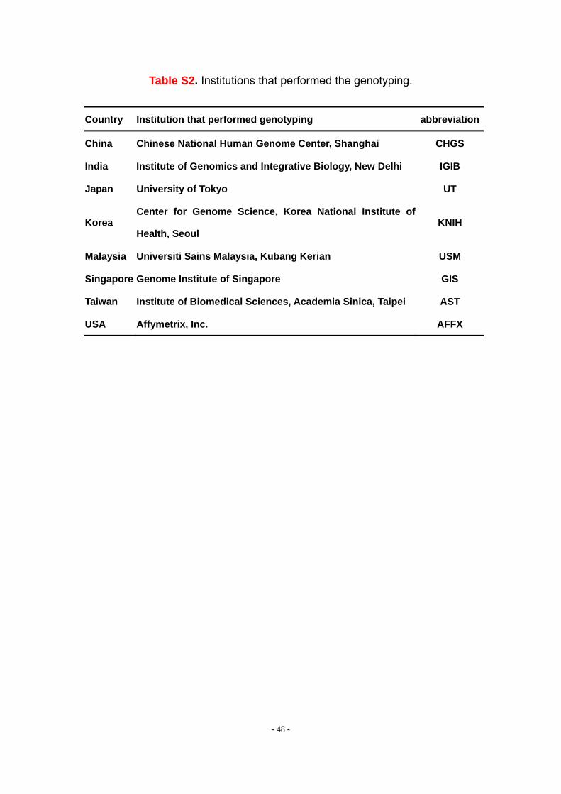
- 48 -
Table S2. Institutions that performed the genotyping.
Country Institution that performed genotyping abbreviation
China Chinese National Human Genome Center, Shanghai CHGS
India Institute of Genomics and Integrative Biology, New Delhi IGIB
Japan University of Tokyo UT
Korea Center for Genome Science, Korea National Institute of
Health, Seoul KNIH
Malaysia Universiti Sains Malaysia, Kubang Kerian USM
Singapore Genome Institute of Singapore GIS
Taiwan Institute of Biomedical Sciences, Academia Sinica, Taipei AST
USA Affymetrix, Inc. AFFX
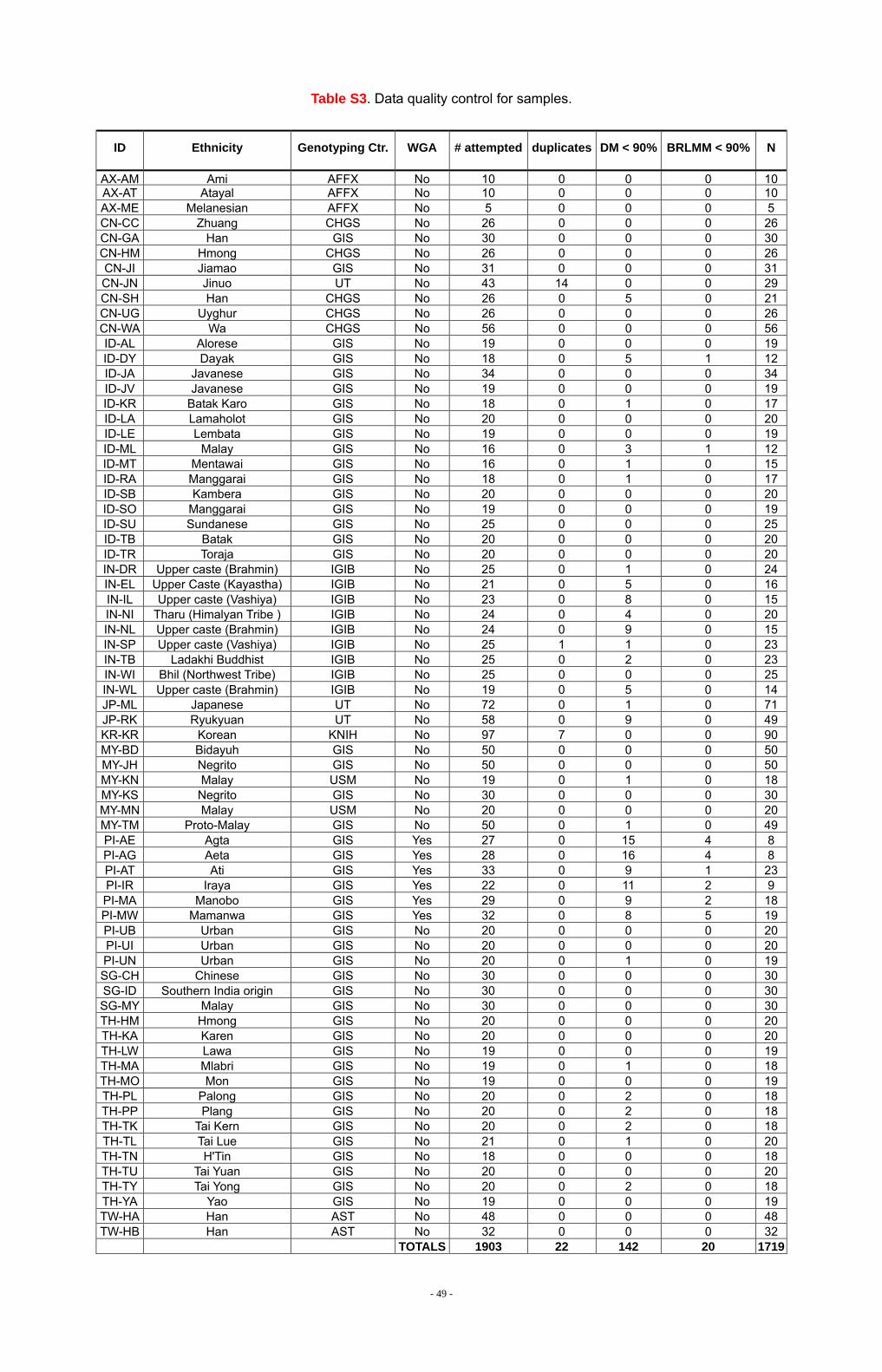
- 49 -
Table S3. Data quality control for samples.
ID Ethnicity Genotyping Ctr. WGA # attempted duplicates DM < 90% BRLMM < 90% N
AX-AM Ami AFFX No 10 0 0 0 10AX-AT Atayal AFFX No 10 0 0 0 10AX-ME Melanesian AFFX No 5 0 0 0 5 CN-CC Zhuang CHGS No 26 0 0 0 26CN-GA Han GIS No 30 0 0 0 30CN-HM Hmong CHGS No 26 0 0 0 26CN-JI Jiamao GIS No 31 0 0 0 31CN-JN Jinuo UT No 43 14 0 0 29CN-SH Han CHGS No 26 0 5 0 21CN-UG Uyghur CHGS No 26 0 0 0 26CN-WA Wa CHGS No 56 0 0 0 56ID-AL Alorese GIS No 19 0 0 0 19ID-DY Dayak GIS No 18 0 5 1 12ID-JA Javanese GIS No 34 0 0 0 34ID-JV Javanese GIS No 19 0 0 0 19ID-KR Batak Karo GIS No 18 0 1 0 17ID-LA Lamaholot GIS No 20 0 0 0 20ID-LE Lembata GIS No 19 0 0 0 19ID-ML Malay GIS No 16 0 3 1 12ID-MT Mentawai GIS No 16 0 1 0 15ID-RA Manggarai GIS No 18 0 1 0 17ID-SB Kambera GIS No 20 0 0 0 20ID-SO Manggarai GIS No 19 0 0 0 19ID-SU Sundanese GIS No 25 0 0 0 25ID-TB Batak GIS No 20 0 0 0 20ID-TR Toraja GIS No 20 0 0 0 20IN-DR Upper caste (Brahmin) IGIB No 25 0 1 0 24IN-EL Upper Caste (Kayastha) IGIB No 21 0 5 0 16IN-IL Upper caste (Vashiya) IGIB No 23 0 8 0 15IN-NI Tharu (Himalyan Tribe ) IGIB No 24 0 4 0 20IN-NL Upper caste (Brahmin) IGIB No 24 0 9 0 15IN-SP Upper caste (Vashiya) IGIB No 25 1 1 0 23IN-TB Ladakhi Buddhist IGIB No 25 0 2 0 23IN-WI Bhil (Northwest Tribe) IGIB No 25 0 0 0 25IN-WL Upper caste (Brahmin) IGIB No 19 0 5 0 14JP-ML Japanese UT No 72 0 1 0 71JP-RK Ryukyuan UT No 58 0 9 0 49KR-KR Korean KNIH No 97 7 0 0 90MY-BD Bidayuh GIS No 50 0 0 0 50MY-JH Negrito GIS No 50 0 0 0 50MY-KN Malay USM No 19 0 1 0 18MY-KS Negrito GIS No 30 0 0 0 30MY-MN Malay USM No 20 0 0 0 20MY-TM Proto-Malay GIS No 50 0 1 0 49PI-AE Agta GIS Yes 27 0 15 4 8 PI-AG Aeta GIS Yes 28 0 16 4 8 PI-AT Ati GIS Yes 33 0 9 1 23PI-IR Iraya GIS Yes 22 0 11 2 9 PI-MA Manobo GIS Yes 29 0 9 2 18PI-MW Mamanwa GIS Yes 32 0 8 5 19PI-UB Urban GIS No 20 0 0 0 20PI-UI Urban GIS No 20 0 0 0 20PI-UN Urban GIS No 20 0 1 0 19SG-CH Chinese GIS No 30 0 0 0 30SG-ID Southern India origin GIS No 30 0 0 0 30SG-MY Malay GIS No 30 0 0 0 30TH-HM Hmong GIS No 20 0 0 0 20TH-KA Karen GIS No 20 0 0 0 20TH-LW Lawa GIS No 19 0 0 0 19TH-MA Mlabri GIS No 19 0 1 0 18TH-MO Mon GIS No 19 0 0 0 19TH-PL Palong GIS No 20 0 2 0 18TH-PP Plang GIS No 20 0 2 0 18TH-TK Tai Kern GIS No 20 0 2 0 18TH-TL Tai Lue GIS No 21 0 1 0 20TH-TN H'Tin GIS No 18 0 0 0 18TH-TU Tai Yuan GIS No 20 0 0 0 20TH-TY Tai Yong GIS No 20 0 2 0 18TH-YA Yao GIS No 19 0 0 0 19TW-HA Han AST No 48 0 0 0 48TW-HB Han AST No 32 0 0 0 32
TOTALS 1903 22 142 20 1719
Table S3 Note:
QC data is shown for each population. The genotyping center at which the
typing was done is shown, as well as whether the template DNA had
undergone whole-genome amplification (WGA). The number of samples
attempted is shown, together with the number of samples that were removed
because they were duplicated, or because either their DM or BRLMM
call-rates were below 90%. The final sample size after all exclusions (N) is
also shown.
- 50 -
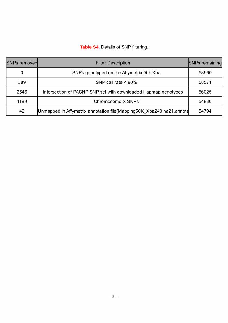
- 51 -
Table S4. Details of SNP filtering.
SNPs removed Filter Description SNPs remaining
0 SNPs genotyped on the Affymetrix 50k Xba 58960
389 SNP call rate < 90% 58571
2546 Intersection of PASNP SNP set with downloaded Hapmap genotypes 56025
1189 Chromosome X SNPs 54836
42 Unmapped in Affymetrix annotation file(Mapping50K_Xba240.na21.annot) 54794

- 52 -
5. Supplementary Figures
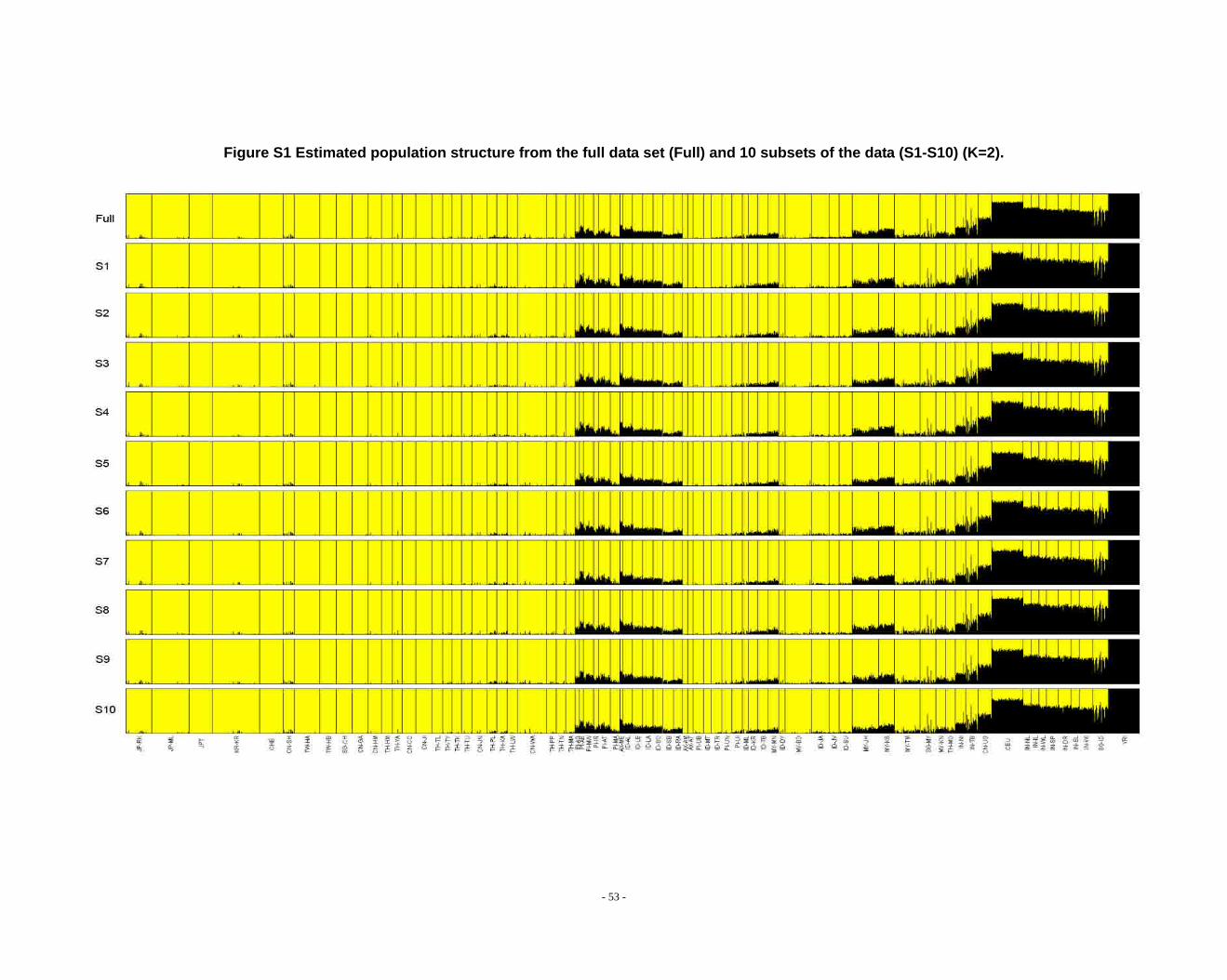
Figure S1 Estimated population structure from the full data set (Full) and 10 subsets of the data (S1-S10) (K=2).
- 53 -
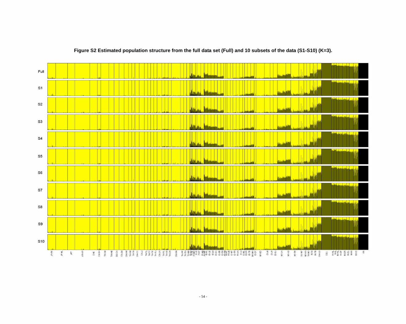
Figure S2 Estimated population structure from the full data set (Full) and 10 subsets of the data (S1-S10) (K=3).
- 54 -
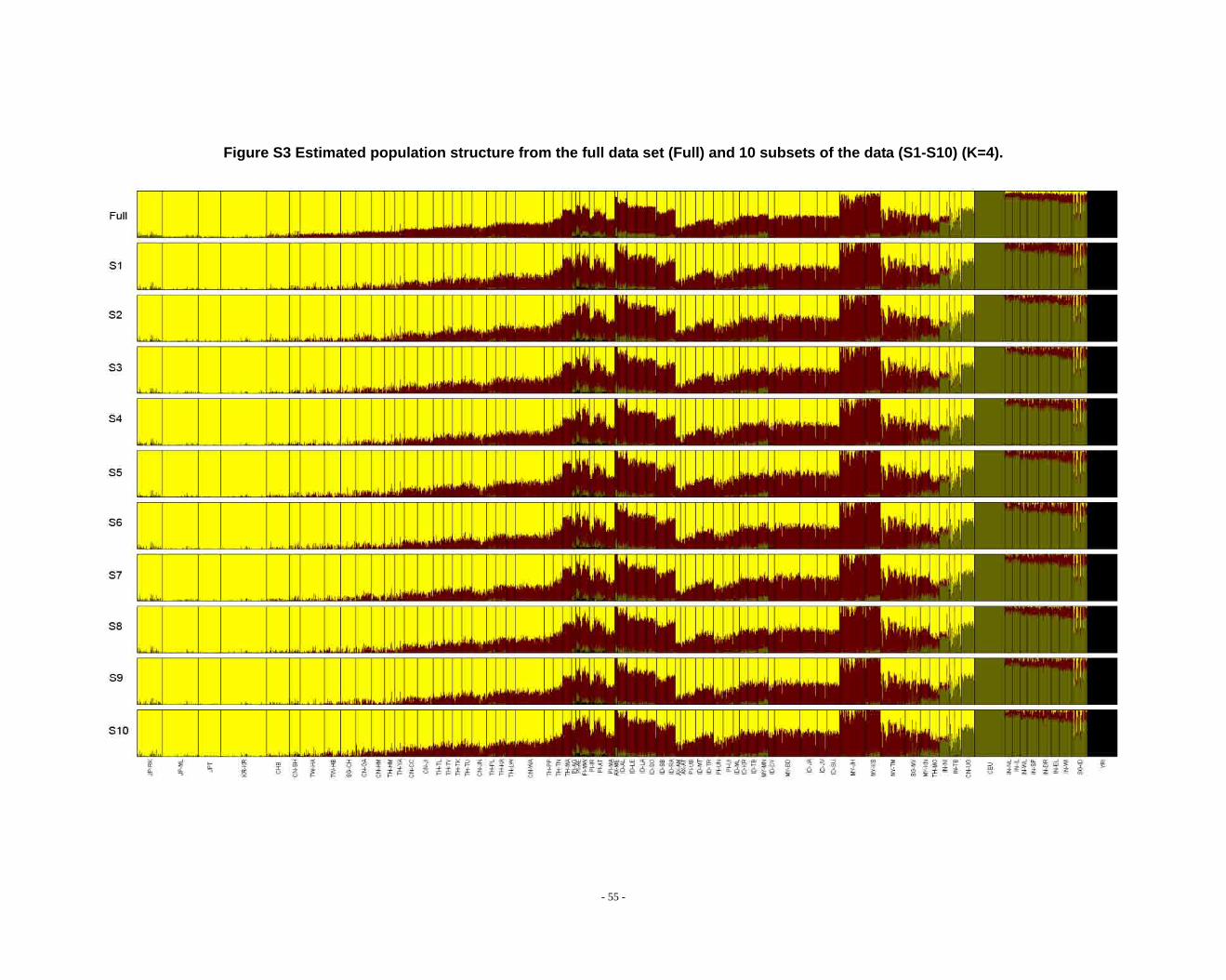
Figure S3 Estimated population structure from the full data set (Full) and 10 subsets of the data (S1-S10) (K=4).
- 55 -
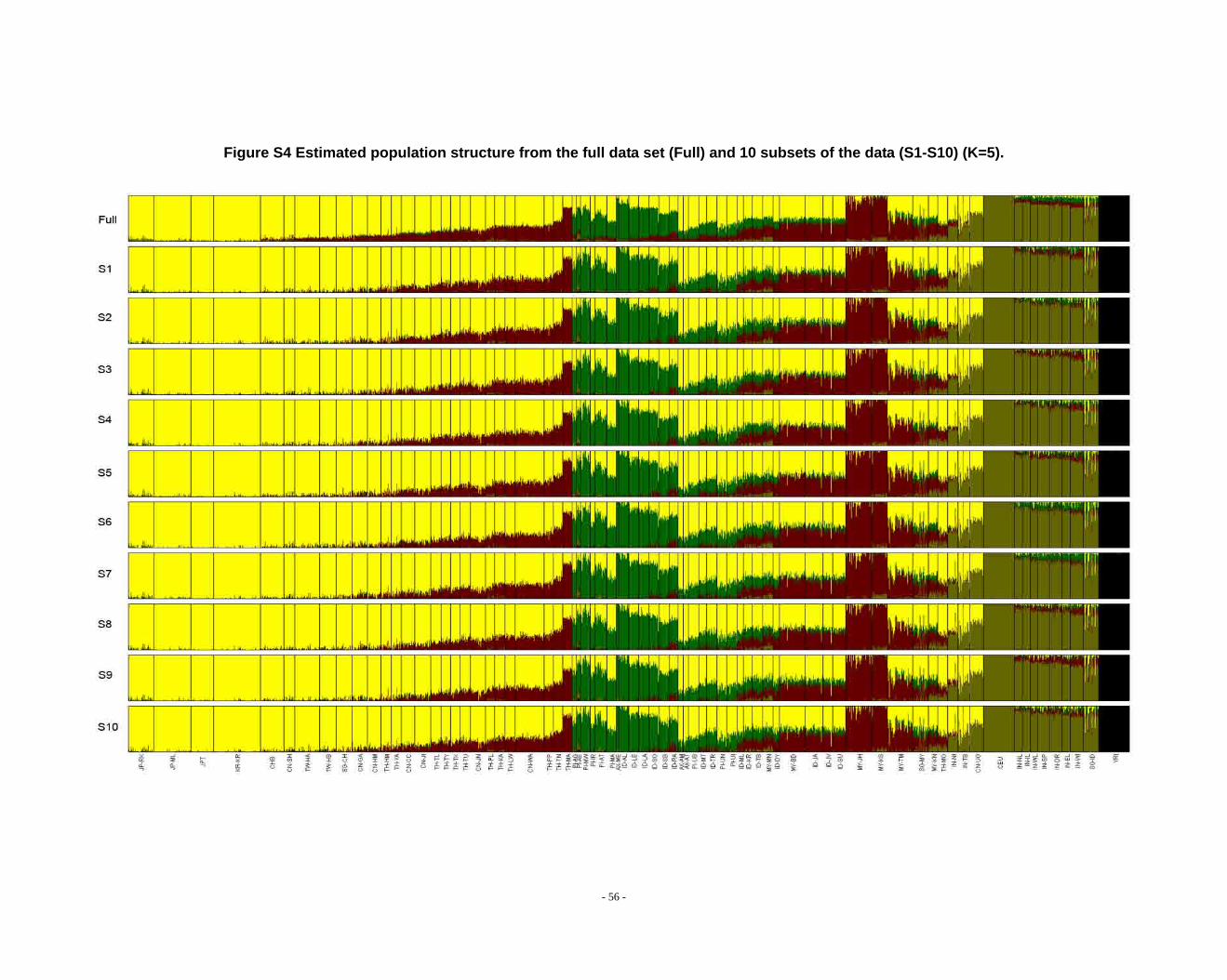
Figure S4 Estimated population structure from the full data set (Full) and 10 subsets of the data (S1-S10) (K=5).
- 56 -
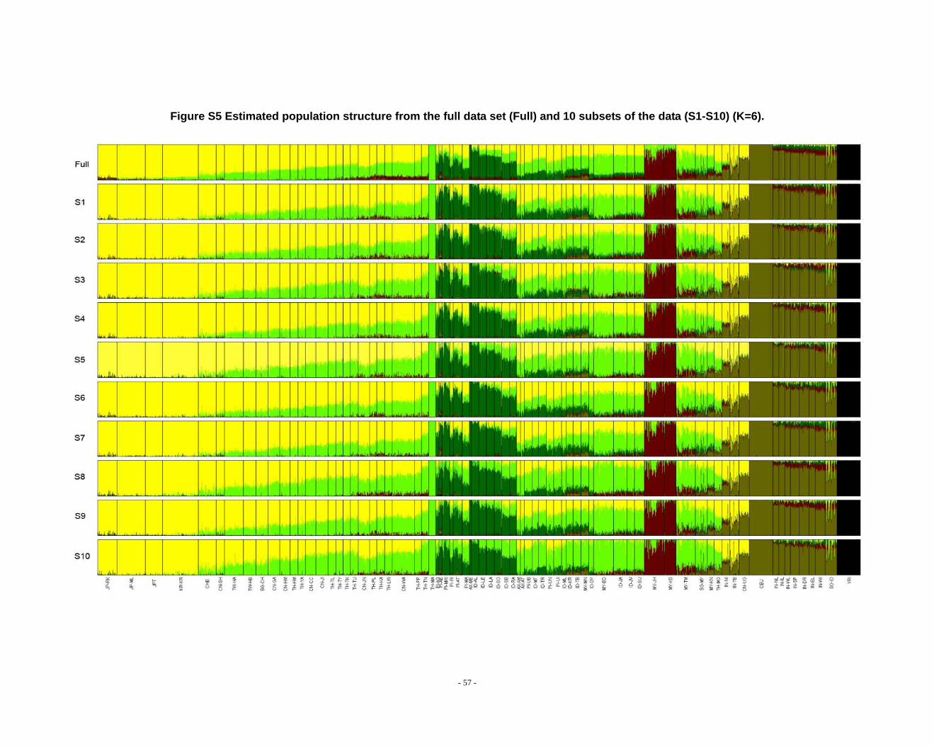
Figure S5 Estimated population structure from the full data set (Full) and 10 subsets of the data (S1-S10) (K=6).
- 57 -
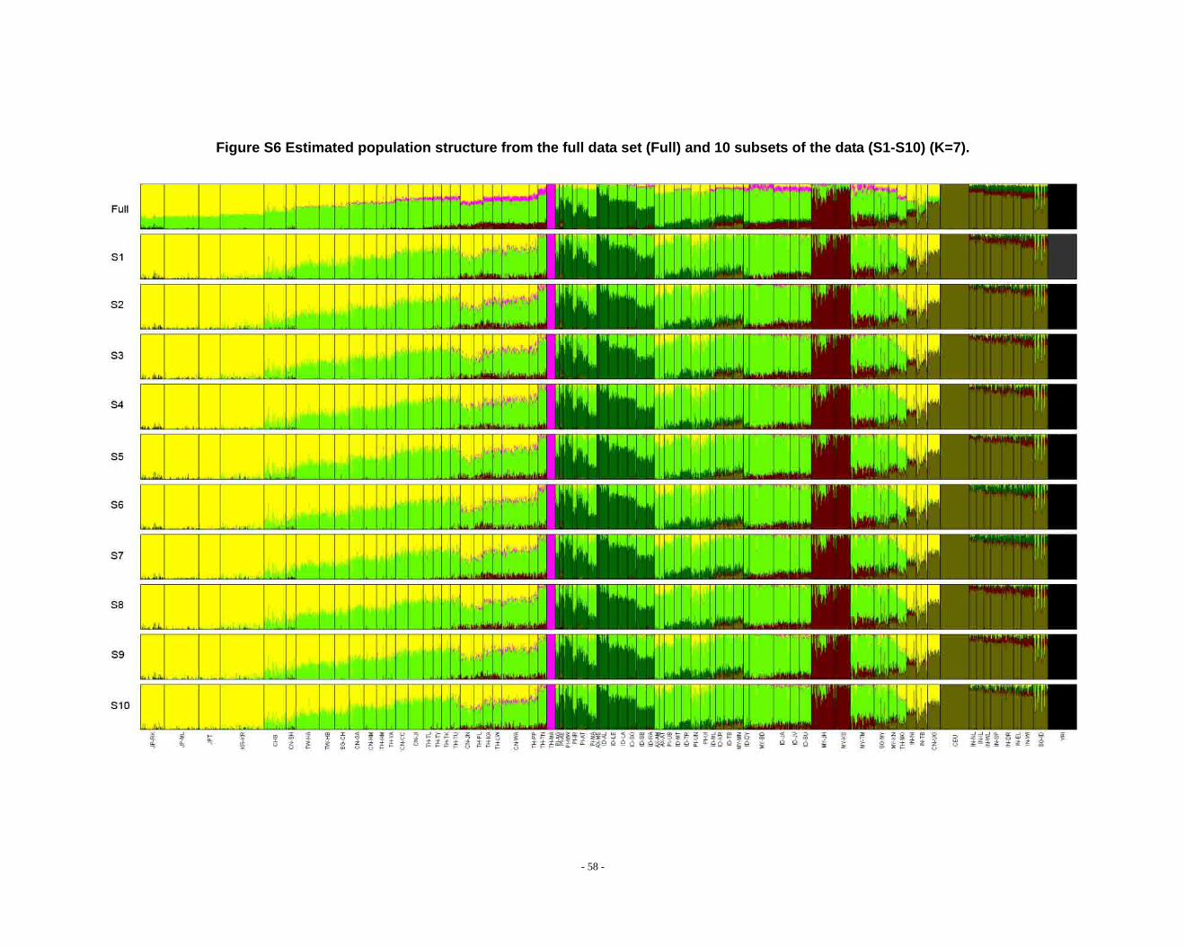
Figure S6 Estimated population structure from the full data set (Full) and 10 subsets of the data (S1-S10) (K=7).
- 58 -
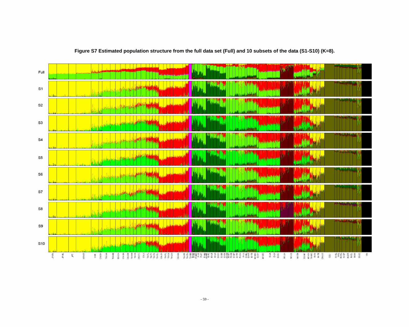
Figure S7 Estimated population structure from the full data set (Full) and 10 subsets of the data (S1-S10) (K=8).
- 59 -
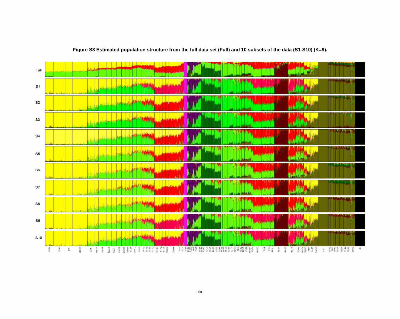
Figure S8 Estimated population structure from the full data set (Full) and 10 subsets of the data (S1-S10) (K=9).
- 60 -
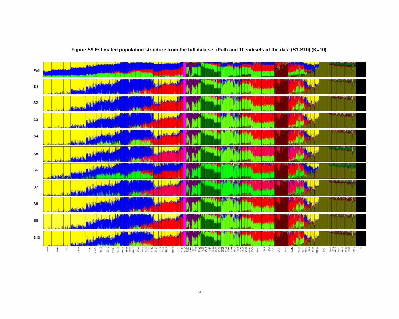
Figure S9 Estimated population structure from the full data set (Full) and 10 subsets of the data (S1-S10) (K=10).
- 61 -
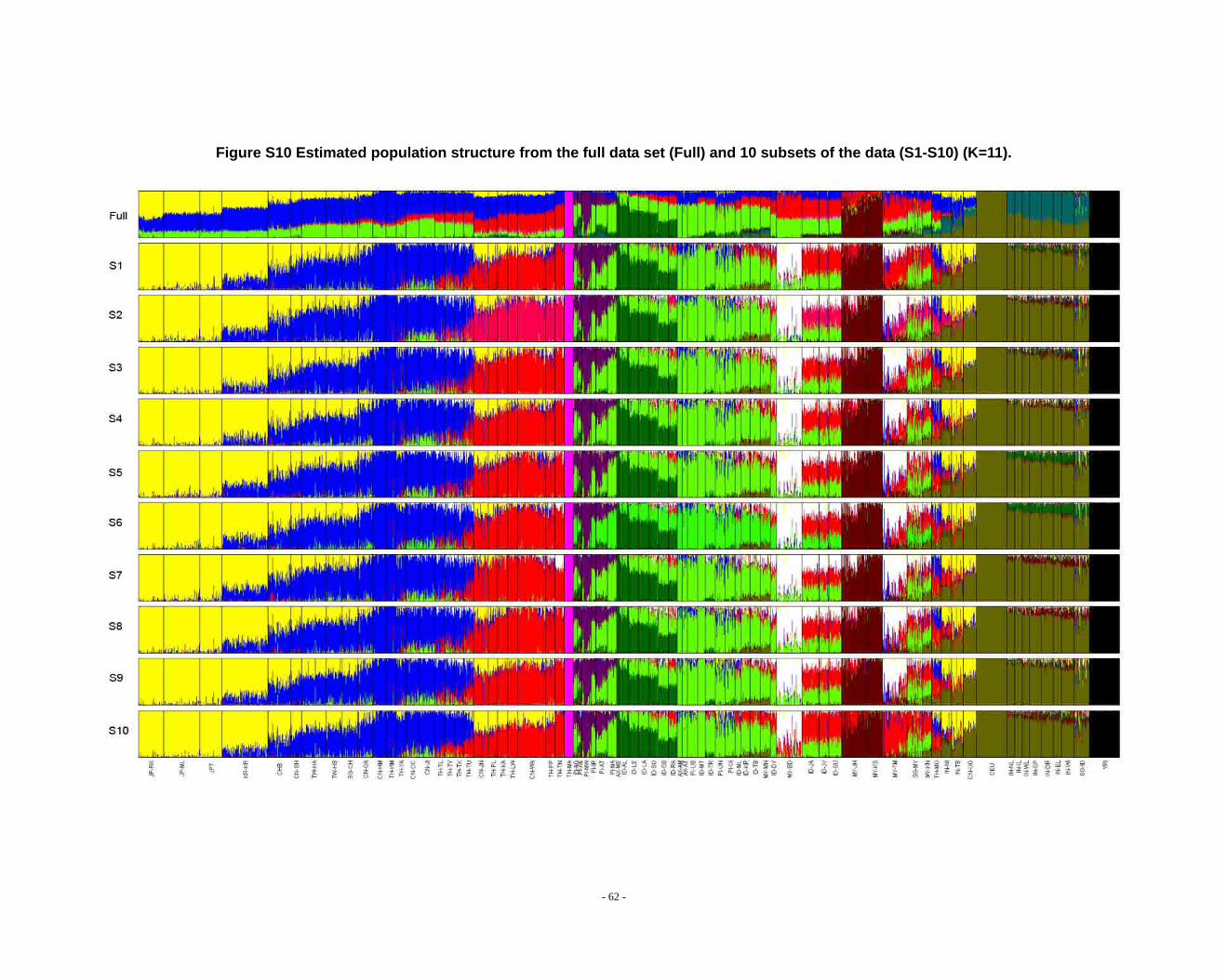
Figure S10 Estimated population structure from the full data set (Full) and 10 subsets of the data (S1-S10) (K=11).
- 62 -
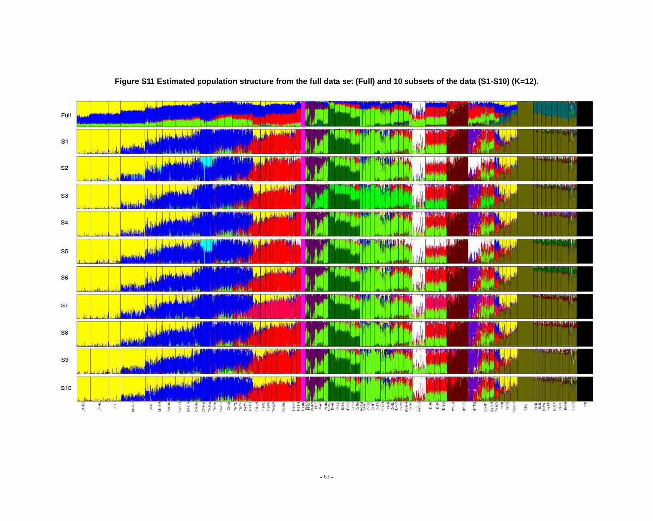
Figure S11 Estimated population structure from the full data set (Full) and 10 subsets of the data (S1-S10) (K=12).
- 63 -
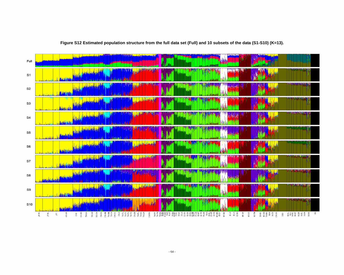
Figure S12 Estimated population structure from the full data set (Full) and 10 subsets of the data (S1-S10) (K=13).
- 64 -
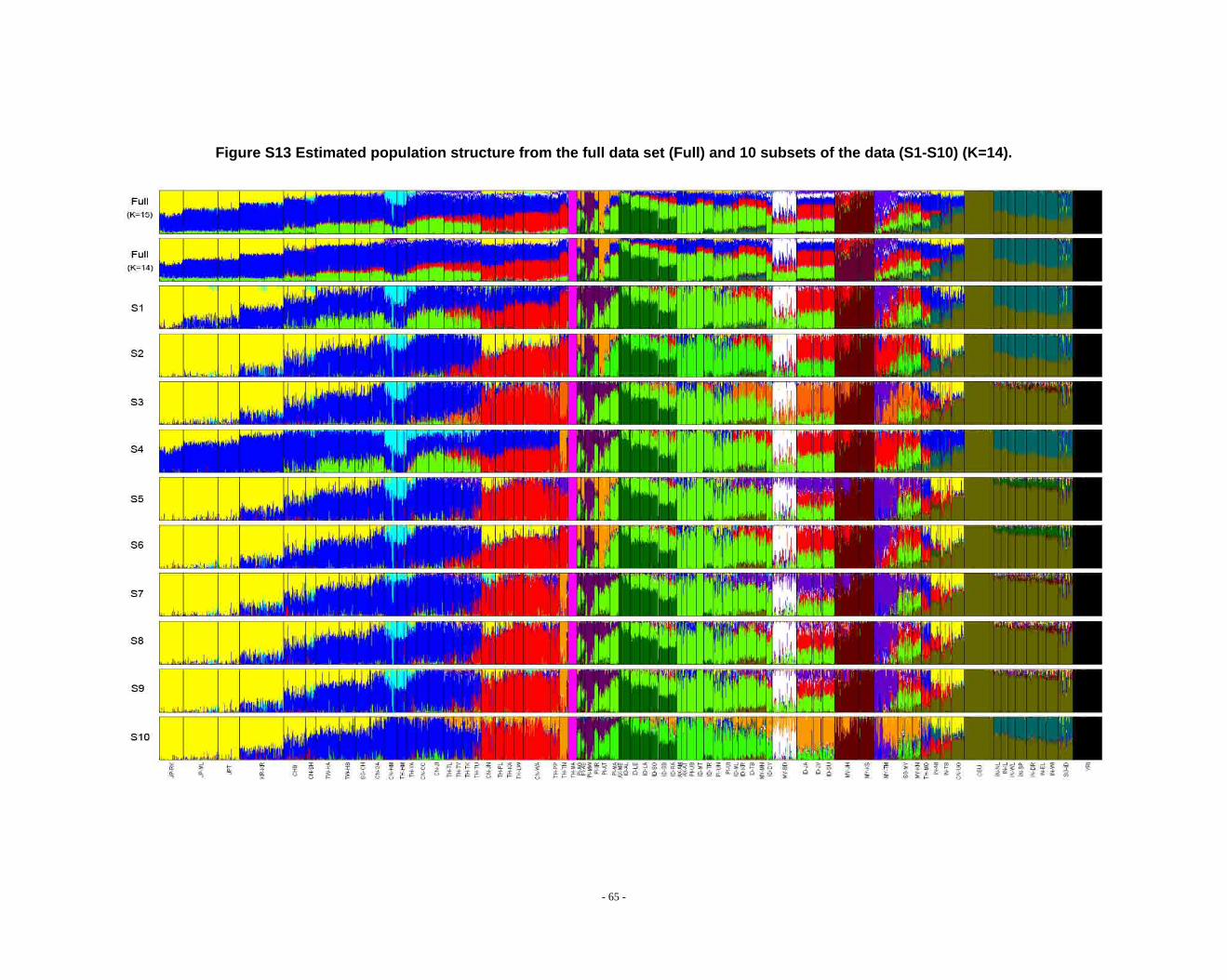
Figure S13 Estimated population structure from the full data set (Full) and 10 subsets of the data (S1-S10) (K=14).
- 65 -
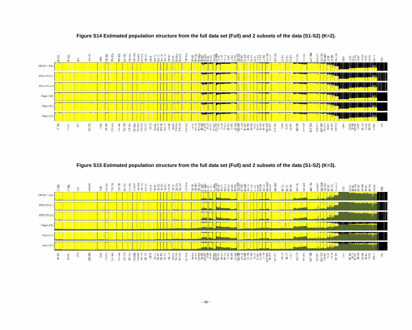
Figure S14 Estimated population structure from the full data set (Full) and 2 subsets of the data (S1-S2) (K=2).
Figure S15 Estimated population structure from the full data set (Full) and 2 subsets of the data (S1-S2) (K=3).
- 66 -
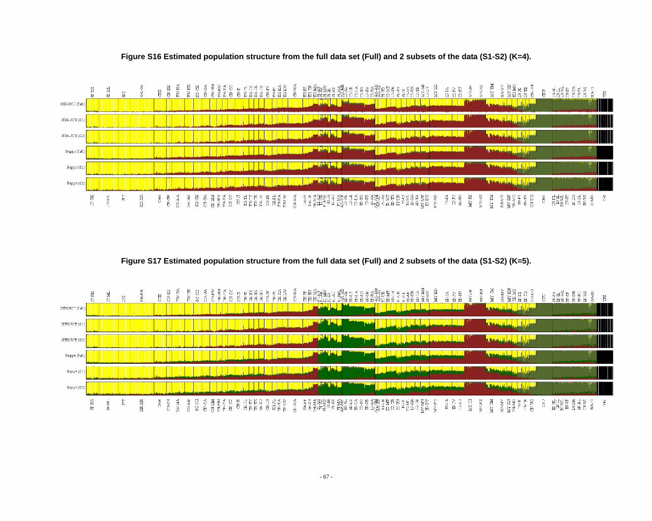
Figure S16 Estimated population structure from the full data set (Full) and 2 subsets of the data (S1-S2) (K=4).
Figure S17 Estimated population structure from the full data set (Full) and 2 subsets of the data (S1-S2) (K=5).
- 67 -
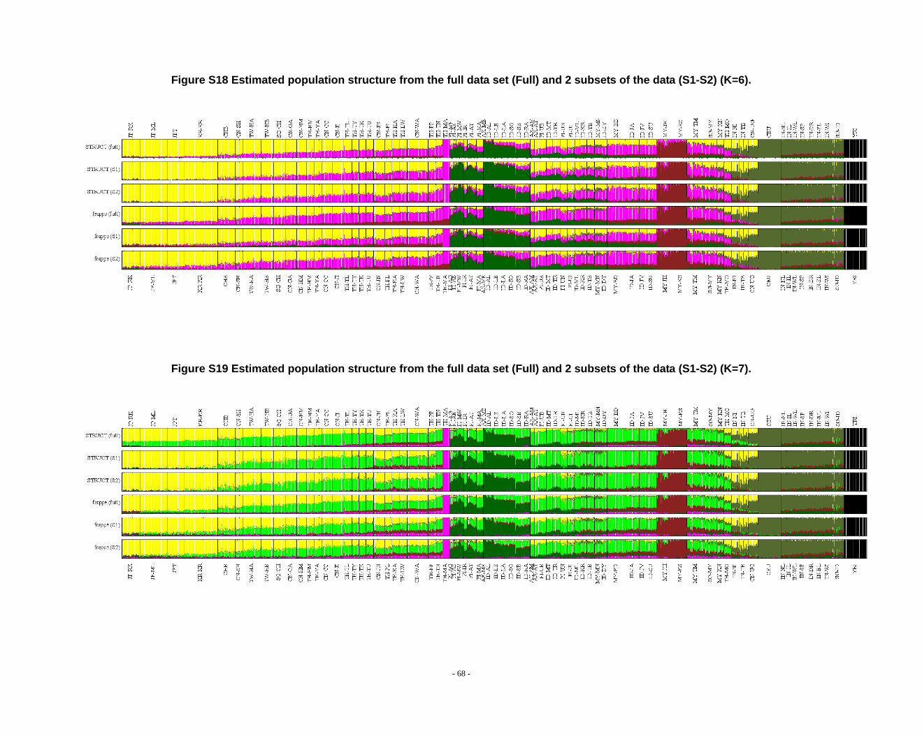
Figure S18 Estimated population structure from the full data set (Full) and 2 subsets of the data (S1-S2) (K=6).
Figure S19 Estimated population structure from the full data set (Full) and 2 subsets of the data (S1-S2) (K=7).
- 68 -
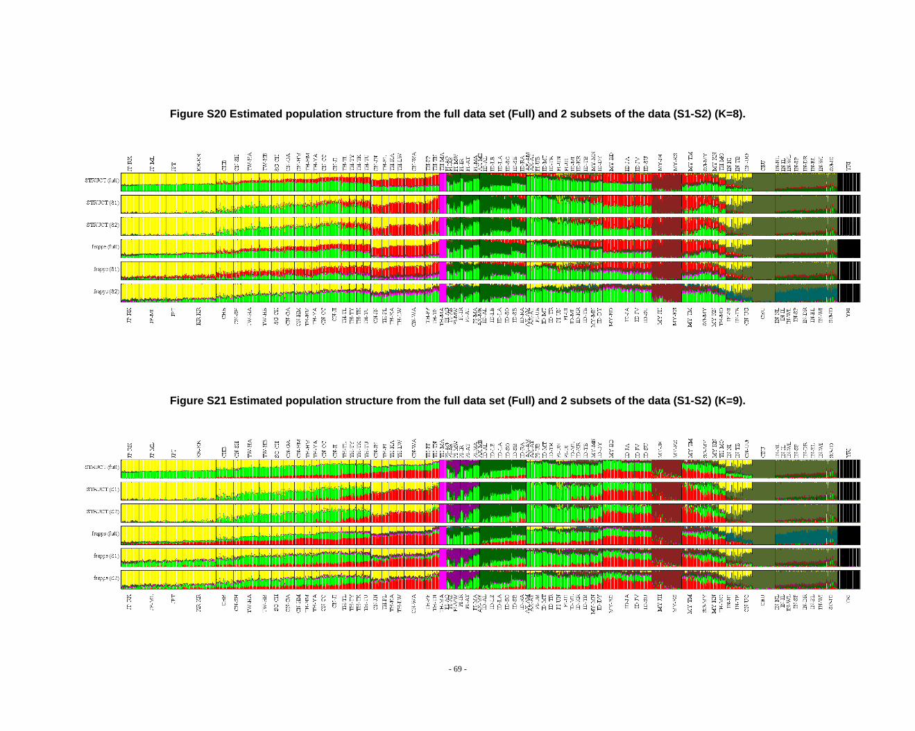
Figure S20 Estimated population structure from the full data set (Full) and 2 subsets of the data (S1-S2) (K=8).
Figure S21 Estimated population structure from the full data set (Full) and 2 subsets of the data (S1-S2) (K=9).
- 69 -
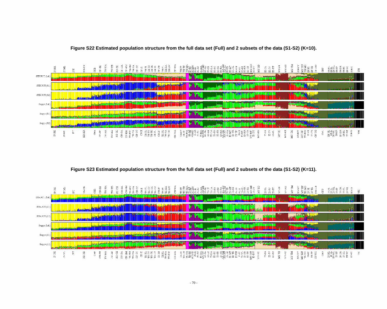
Figure S22 Estimated population structure from the full data set (Full) and 2 subsets of the data (S1-S2) (K=10).
Figure S23 Estimated population structure from the full data set (Full) and 2 subsets of the data (S1-S2) (K=11).
- 70 -
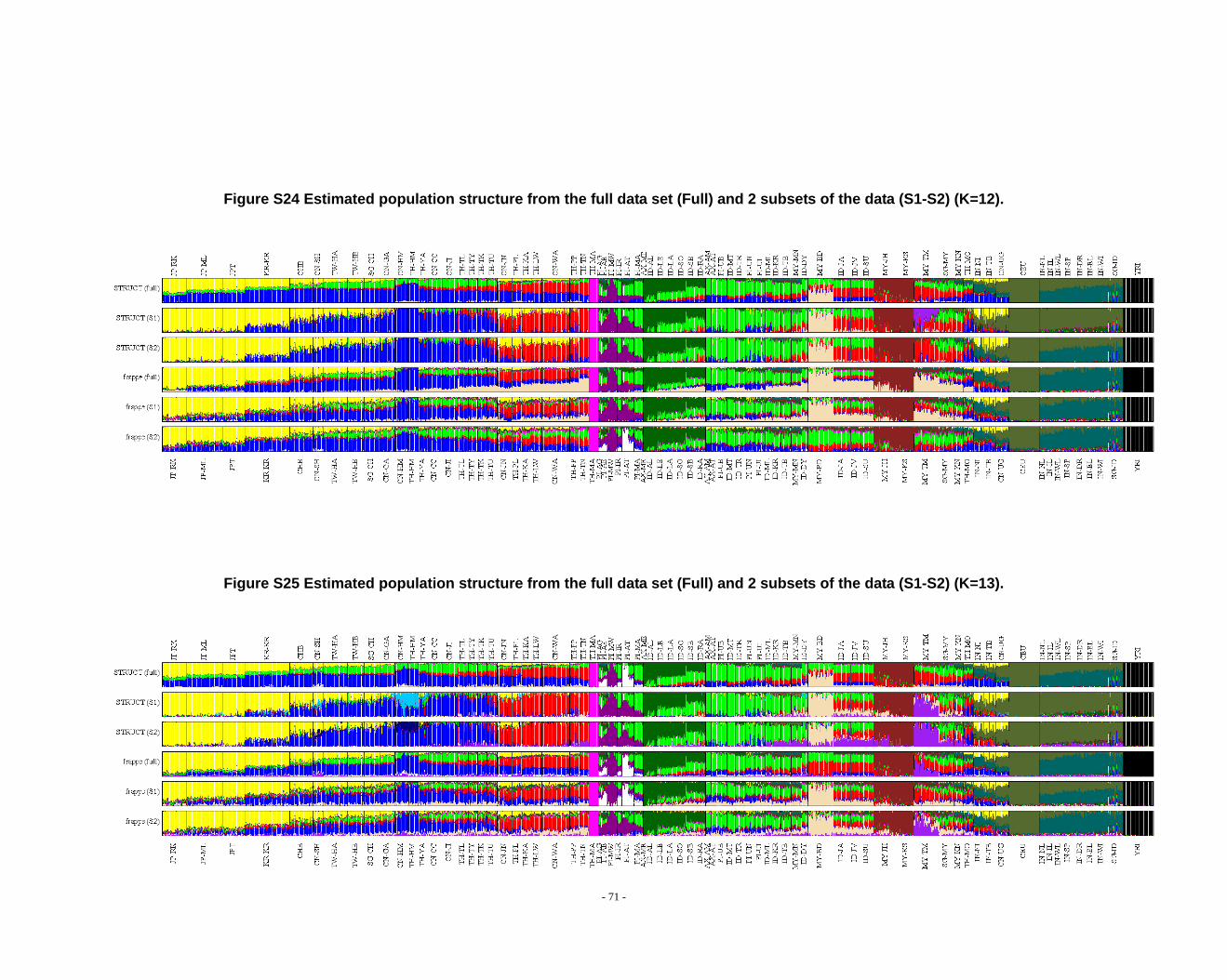
Figure S24 Estimated population structure from the full data set (Full) and 2 subsets of the data (S1-S2) (K=12).
Figure S25 Estimated population structure from the full data set (Full) and 2 subsets of the data (S1-S2) (K=13).
- 71 -
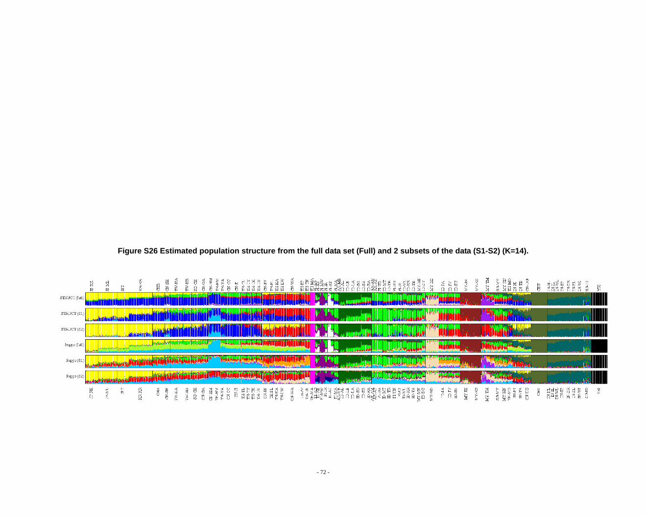
Figure S26 Estimated population structure from the full data set (Full) and 2 subsets of the data (S1-S2) (K=14).
- 72 -
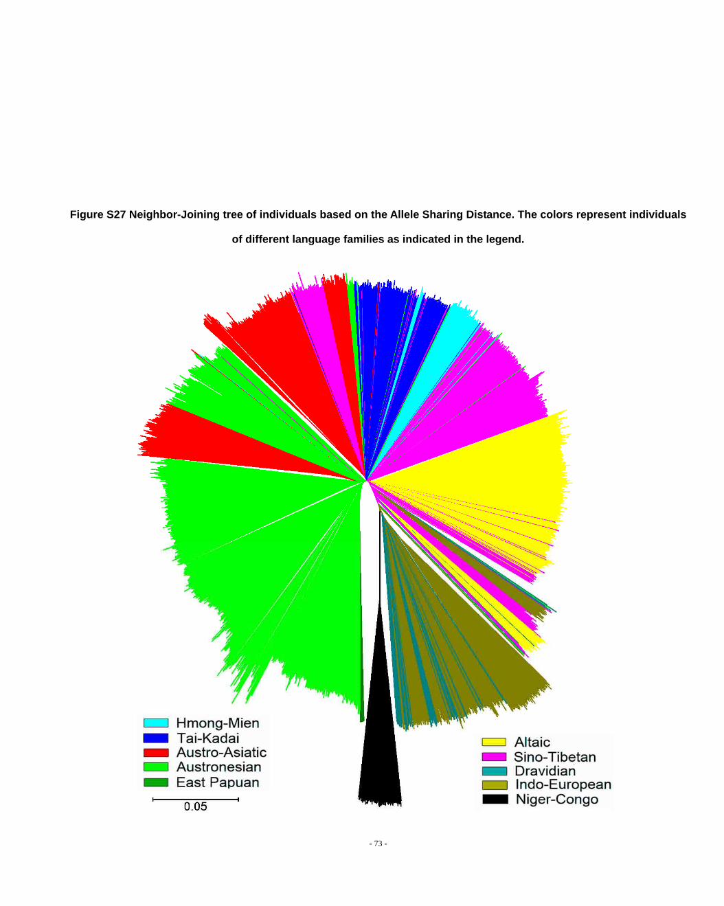
Figure S27 Neighbor-Joining tree of individuals based on the Allele Sharing Distance. The colors represent individuals
of different language families as indicated in the legend.
- 73 -
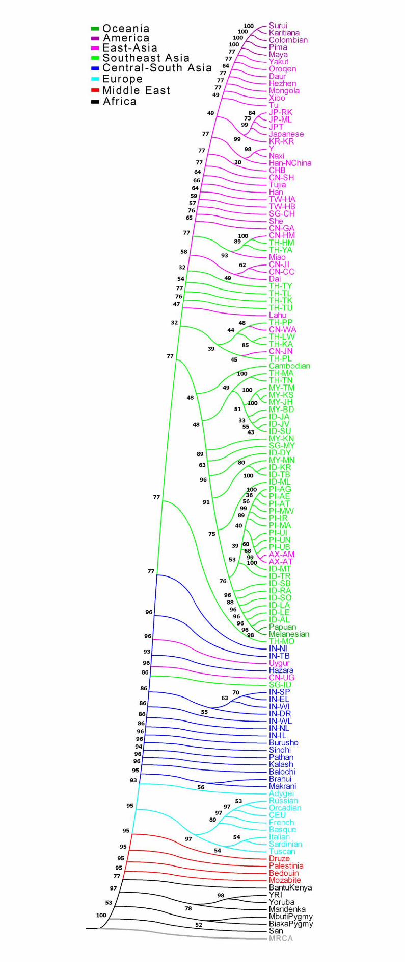
- 74 -
Figure S28 Maximum likelihood tree of 126 population samples. Bootstrap values based on 100 replicates are shown. Language families are indicated with colors as shown in the legend. All population IDs except the four HapMap samples (YRI, CEU, CHB and JPT) are denoted by four characters. The first two letters indicate the country where the samples were collected or (in the case of Affymetrix) genotyped according to the following convention: AX: Affymetrix; CN: China; ID: Indonesia; IN: India; JP: Japan; KR: Korea; MY: Malaysia; PI: the Philippines; SG: Singapore; TH: Thailand; TW: Taiwan. The last two letters are unique ID’s for the population. The rest population IDs are adopted from HGDP sample names.
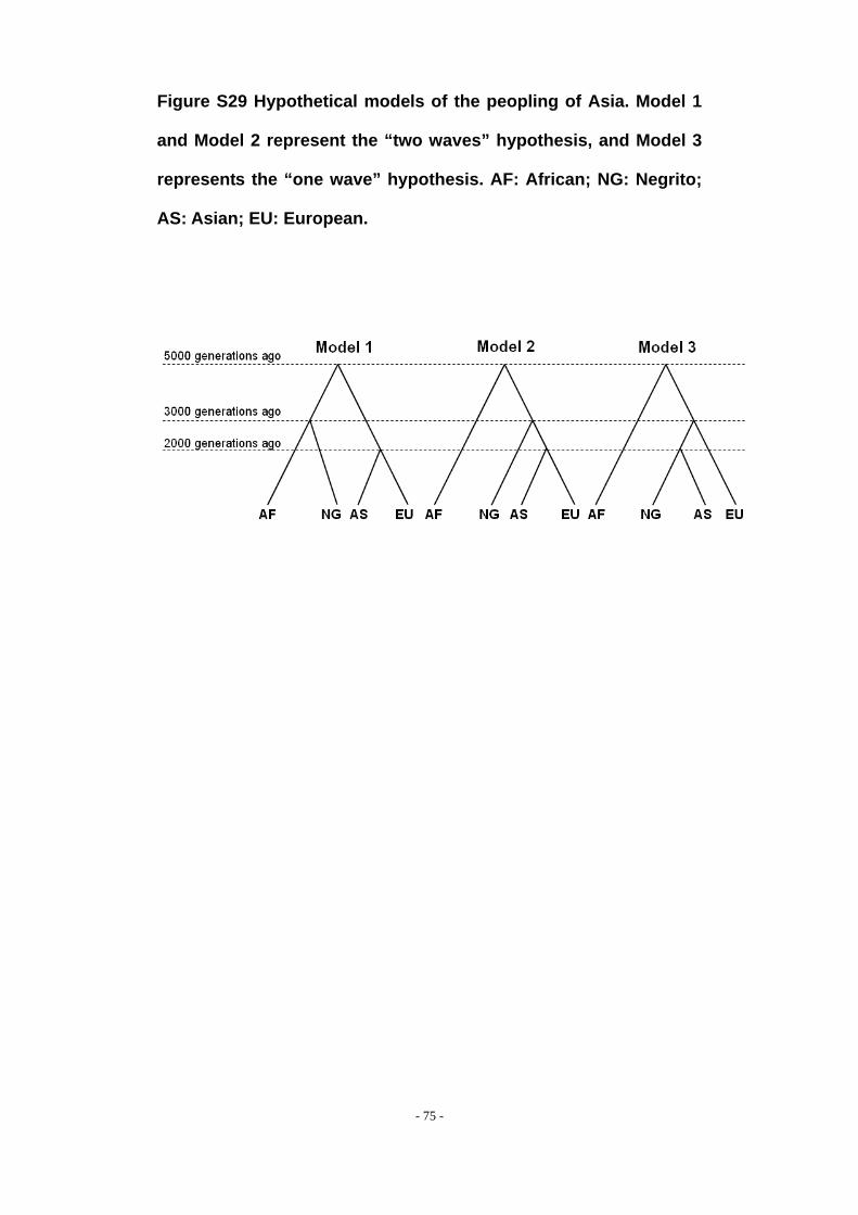
Figure S29 Hypothetical models of the peopling of Asia. Model 1
and Model 2 represent the “two waves” hypothesis, and Model 3
represents the “one wave” hypothesis. AF: African; NG: Negrito;
AS: Asian; EU: European.
- 75 -
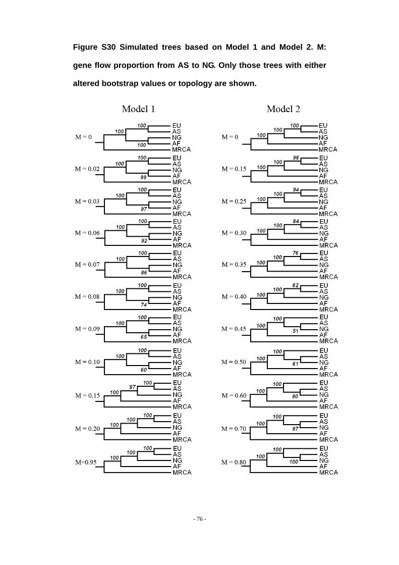
Figure S30 Simulated trees based on Model 1 and Model 2. M:
gene flow proportion from AS to NG. Only those trees with either
altered bootstrap values or topology are shown.
- 76 -
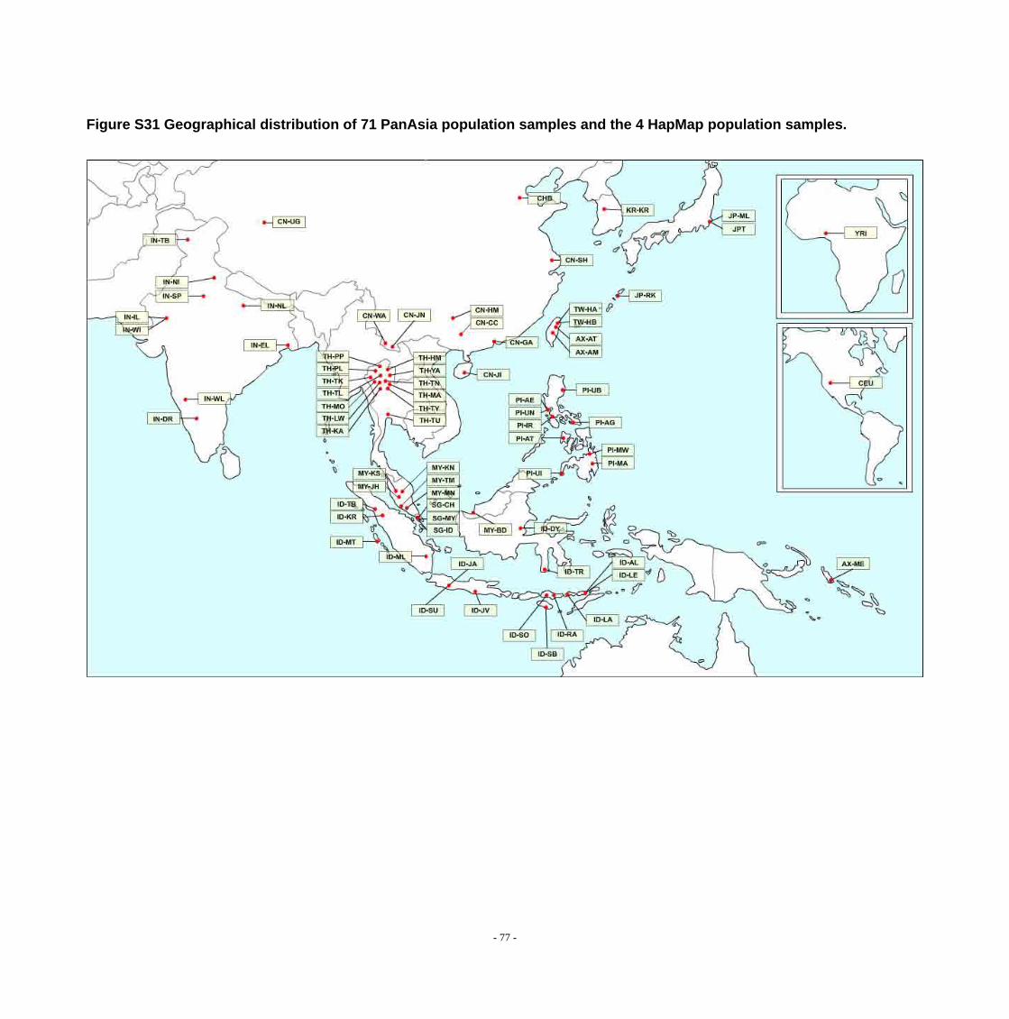
Figure S31 Geographical distribution of 71 PanAsia population samples and the 4 HapMap population samples.
- 77 -
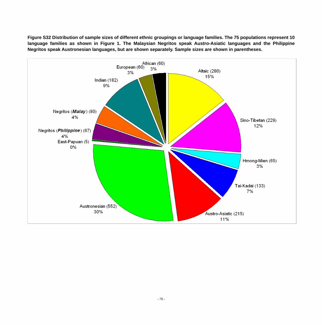
Figure S32 Distribution of sample sizes of different ethnic groupings or language families. The 75 populations represent 10 language families as shown in Figure 1. The Malaysian Negritos speak Austro-Asiatic languages and the Philippine Negritos speak Austronesian languages, but are shown separately. Sample sizes are shown in parentheses.
- 78 -
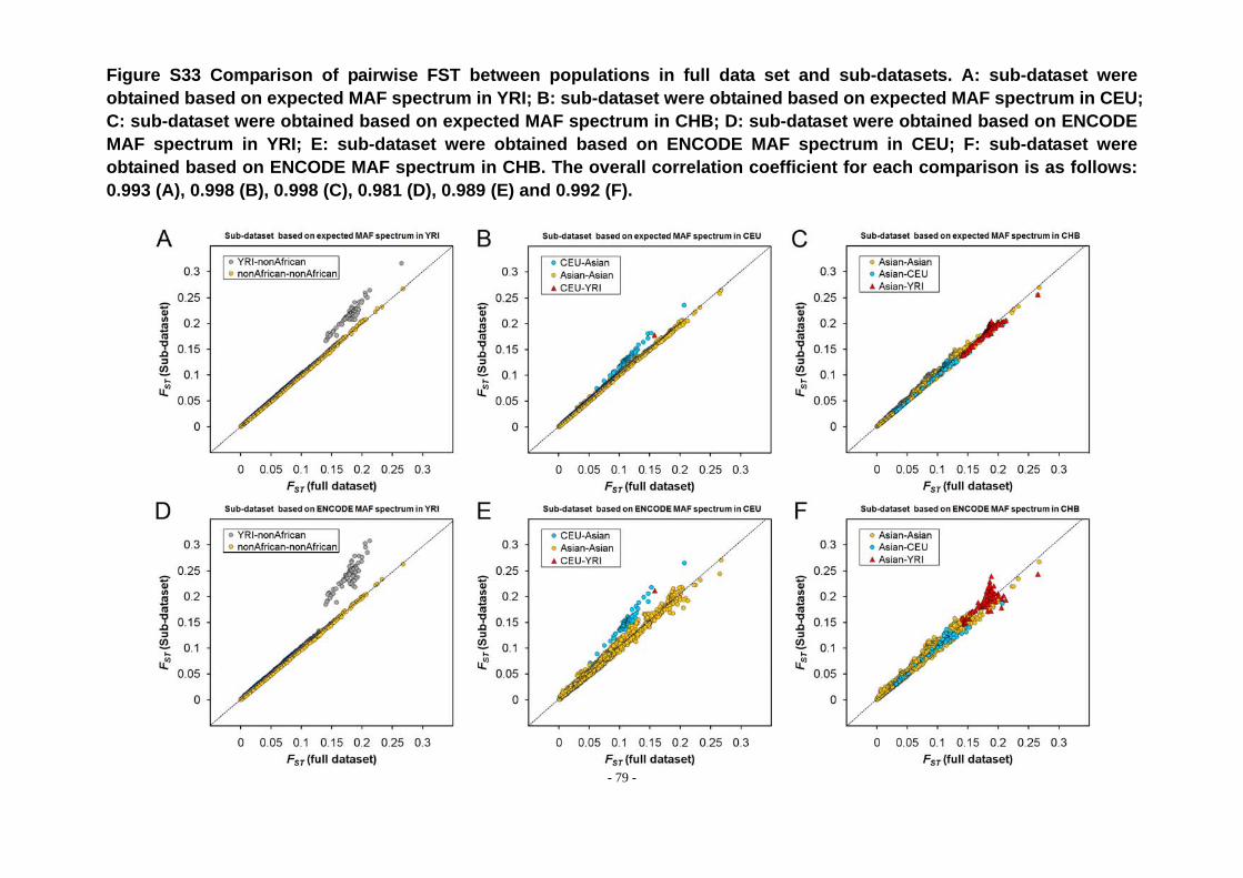
Figure S33 Comparison of pairwise FST between populations in full data set and sub-datasets. A: sub-dataset were obtained based on expected MAF spectrum in YRI; B: sub-dataset were obtained based on expected MAF spectrum in CEU; C: sub-dataset were obtained based on expected MAF spectrum in CHB; D: sub-dataset were obtained based on ENCODE MAF spectrum in YRI; E: sub-dataset were obtained based on ENCODE MAF spectrum in CEU; F: sub-dataset were obtained based on ENCODE MAF spectrum in CHB. The overall correlation coefficient for each comparison is as follows: 0.993 (A), 0.998 (B), 0.998 (C), 0.981 (D), 0.989 (E) and 0.992 (F).
- 79 -
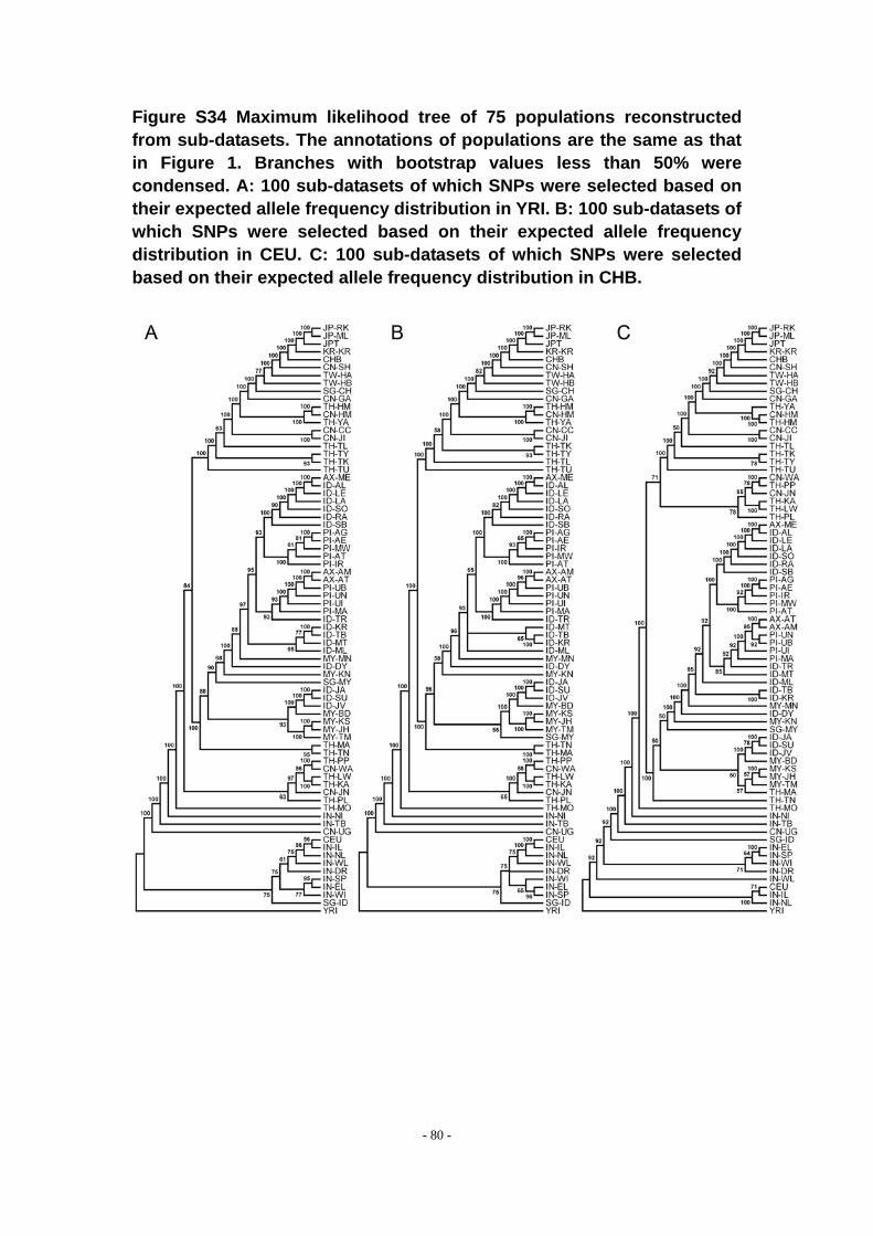
Figure S34 Maximum likelihood tree of 75 populations reconstructed from sub-datasets. The annotations of populations are the same as that in Figure 1. Branches with bootstrap values less than 50% were condensed. A: 100 sub-datasets of which SNPs were selected based on their expected allele frequency distribution in YRI. B: 100 sub-datasets of which SNPs were selected based on their expected allele frequency distribution in CEU. C: 100 sub-datasets of which SNPs were selected based on their expected allele frequency distribution in CHB.
- 80 -
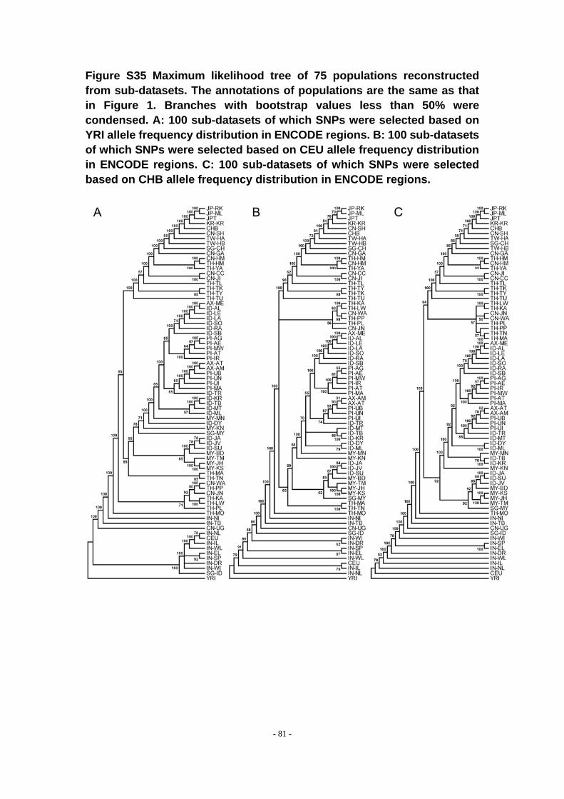
Figure S35 Maximum likelihood tree of 75 populations reconstructed from sub-datasets. The annotations of populations are the same as that in Figure 1. Branches with bootstrap values less than 50% were condensed. A: 100 sub-datasets of which SNPs were selected based on YRI allele frequency distribution in ENCODE regions. B: 100 sub-datasets of which SNPs were selected based on CEU allele frequency distribution in ENCODE regions. C: 100 sub-datasets of which SNPs were selected based on CHB allele frequency distribution in ENCODE regions.
- 81 -
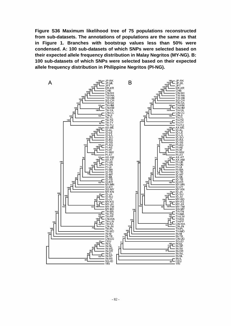
Figure S36 Maximum likelihood tree of 75 populations reconstructed from sub-datasets. The annotations of populations are the same as that in Figure 1. Branches with bootstrap values less than 50% were condensed. A: 100 sub-datasets of which SNPs were selected based on their expected allele frequency distribution in Malay Negritos (MY-NG). B: 100 sub-datasets of which SNPs were selected based on their expected allele frequency distribution in Philippine Negritos (PI-NG).
- 82 -
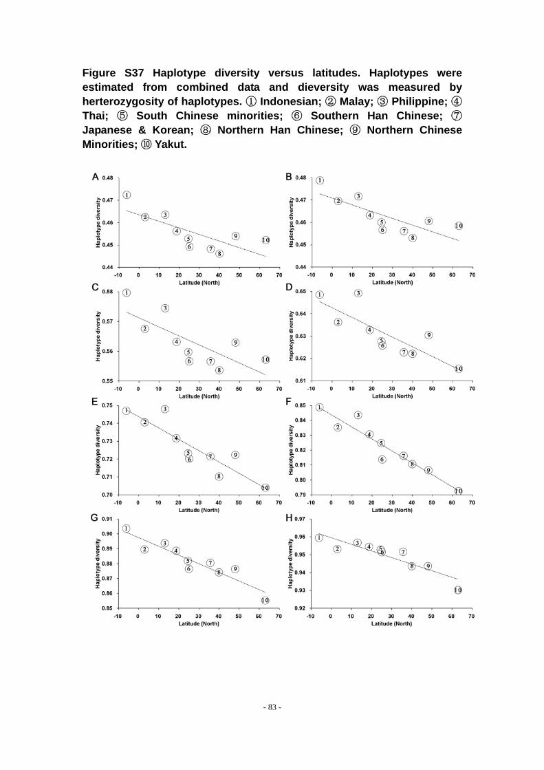
Figure S37 Haplotype diversity versus latitudes. Haplotypes were estimated from combined data and dieversity was measured by herterozygosity of haplotypes. ① Indonesian; ② Malay; ③ Philippine; ④ Thai; ⑤ South Chinese minorities; ⑥ Southern Han Chinese; ⑦ Japanese & Korean; ⑧ Northern Han Chinese; ⑨ Northern Chinese Minorities; ⑩ Yakut.
- 83 -
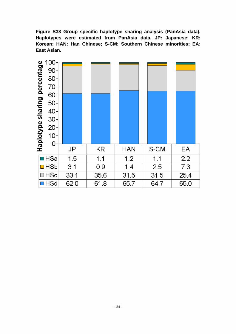
Figure S38 Group specific haplotype sharing analysis (PanAsia data). Haplotypes were estimated from PanAsia data. JP: Japanese; KR: Korean; HAN: Han Chinese; S-CM: Southern Chinese minorities; EA: East Asian.
- 84 -
Related Documents