Mapping forest plots: an efficient method combining ... · Mapping forest plots: an efficient method combining ... (tacheometry), which establishes the 3D vec-tors from the apparatus

457

www.metla.fi/silvafennica · ISSN 0037-5330The Finnish Society of Forest Science · The Finnish Forest Research Institute

Mapping Forest Plots: An Efficient Method Combining Photogrammetry and Field Triangulation

Ilkka Korpela, Tuukka Tuomola and Esko Välimäki

Korpela, I., Tuomola, T. & Välimäki, E. 2007. Mapping forest plots: an efficient method combining photogrammetry and field triangulation. Silva Fennica 41(3): 457–469.

Intra stand spatial information is often collected in ecological investigations, when functioning or interactions in the ecosystem are studied. Local relative accuracy is often given priority in such cases. Forest maps with accurate absolute positions in a global coordinate system are needed in remote-sensing applications for validation and calibration purposes. Establishing the absolute position is particularly difficult under a canopy as is creating undistorted coordinate systems for large plots in the forest. We present a method that can be used for the absolute mapping of point features under a canopy that is efficient for large forest plots. In this method, an undistorted network of control points is established in the forest using photogrammetric observations of treetops. These points are used for the positioning of other points, using redundant observations of interpoint distances and azimuths and a least squares adjustment. The method provides decimetre-level accuracy and only one person is required to conduct the work. An estimate of the positioning accuracy of each point is readily available in the field. We present the method, a simulation study that explores the potential of the method and results from an experiment in a mixed boreal stand in southern Finland.

Keywords least squares adjustment, intertree positioning, remote sensing, spatial resection, trilaterationAuthors’ address University of Helsinki, Department of Forest Resource Management, P.O. Box 27, FI-00014 University of Helsinki, Finland E-mail [email protected] 18 October 2006 Revised 8 February 2007 Accepted 6 July 2007Available at http://www.metla.fi/silvafennica/full/sf41/sf413457.pdf

Silva Fennica 41(3) research articles

458

Silva Fennica 41(3), 2007 research articles

1 IntroductionSpatial information within forest stands is needed in many ecological investigations and could also be used in the optimization of practical forest operations such as thinning or the treatment of seedling stands (Stendahl and Dahlin 2002). In many ecological studies the mapping of trees and other objects is needed when the interaction or functioning of ecosystem members is explained by the spatial structure. The phenomena under investigation affect the requirements of the scale of the mapping and its accuracy. In forest yield studies, for example, the typical plot size varies from 0.04 to 0.36 ha; the trees are positioned at the decimetre accuracy level, but the absolute position of the plot does not have to be accurately determined.

Absolute accuracy is important in applications of remote sensing. Inaccuracy in the field observa-tions is a source of noise, as is any geometric inac-curacy or misalignment of the remotely sensed signal. It is advantageous to minimize this noise because it simplifies the testing of the relation-ship between the target and signal. In single-tree remote sensing (STRS) particularly, where the aim is to identify, position and measure individual trees (e.g. Avery 1958, Talts 1977, Blasquez 1989, Persson et al. 2002, Korpela and Tokola 2006), it is required that trees mapped with STRS are one-to-one linkable with trees in the field. Tree-level field data are needed for the validation or cali-bration of the results, for training classification algorithms (Bortolot and Wynne 2005) or for the construction of estimation or correction models (Mäkinen et al. 2006). Effective methods for col-lecting forest data with high absolute positioning accuracy are therefore needed.

Here we present a new and efficient method for the mapping of objects within boreal forest stands directly into a global coordinate system. It is restricted to areas where recent large- or medium-scale aerial photography is available. It can be carried out by a single person with modest field equipment and provides decimetre-level accuracy. Options for mapping objects in the forest are discussed in Section 2 to provide background. The new method is described in Section 3. A simulation study that explores the potential of the method under varying assumptions of meas-

urement geometry, observation inaccuracy and observation intensity is presented in Section 4. The method was tested for the mapping of stems in a 0.5-ha mixed stand in southern Finland under conditions of rough topography and limited vis-ibility. The results of this test are in Section 5. Discussion of the results and concluding remarks complete the article.

2 Ways of Measuring Absolute Positions of Objects within Forest Stands

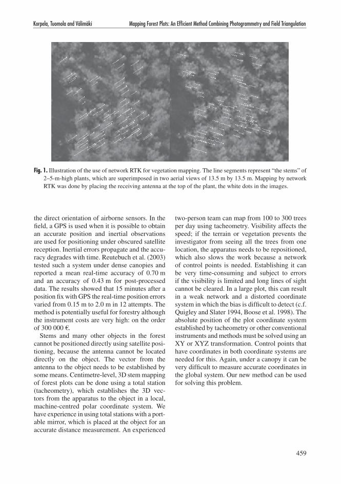
When the canopy height is less than 3–4 m, the most effective positioning method is perhaps satellite positioning using ordinary RTK (Real Time Kinematic) or network RTK (Wanninger 2005), which can provide real-time centimetre-level accuracy. We used VRS-GPS technique, which is an implementation of network RTK, for the 3D positioning of vegetation samples in seedling stands and in open mires to be used for remote-sensing reference (Fig. 1). In Finland, the VRS network covers the whole country and mapping can be carried out by only one person. The accuracy is high, 2–4 cm in X, Y and Z, when satellites are available (Häkli and Koivula 2004). Network RTK has high instrumentation costs, app. 20 000 €, and sometimes nearby high vegetation or terrain can pre-empt its use. Under a canopy it is almost always impossible to attain a state of centimetre-level accuracy and the inves-tigator is confined to an inferior level of accuracy, on the order of 1–2 m, depending on the avail-ability of satellites and the quality of the receiver and its algorithms (c.f. Næsset 1999). There might be more advanced satellites available with the future implementation of the European Galileo system. However, it is by no means certain that the probability of uninterrupted, real-time, cen-timetre-level network RTK positioning under a heavy canopy will increase notably.

The 1-m accuracy of network RTK under a canopy is insufficient for many applications. Quick and accurate positioning calls for other methods. One new solution is the combined use of accurate satellite positioning with inertial meas-urements. The technique is currently used for

459

Korpela, Tuomola and Välimäki Mapping Forest Plots: An Effi cient Method Combining Photogrammetry and Field Triangulation

the direct orientation of airborne sensors. In the fi eld, a GPS is used when it is possible to obtain an accurate position and inertial observations are used for positioning under obscured satellite reception. Inertial errors propagate and the accu-racy degrades with time. Reutebuch et al. (2003) tested such a system under dense canopies and reported a mean real-time accuracy of 0.70 m and an accuracy of 0.43 m for post-processed data. The results showed that 15 minutes after a position fi x with GPS the real-time position errors varied from 0.15 m to 2.0 m in 12 attempts. The method is potentially useful for forestry although the instrument costs are very high: on the order of 300 000 €.

Stems and many other objects in the forest cannot be positioned directly using satellite posi-tioning, because the antenna cannot be located directly on the object. The vector from the antenna to the object needs to be established by some means. Centimetre-level, 3D stem mapping of forest plots can be done using a total station (tacheometry), which establishes the 3D vec-tors from the apparatus to the object in a local, machine-centred polar coordinate system. We have experience in using total stations with a port-able mirror, which is placed at the object for an accurate distance measurement. An experienced

two-person team can map from 100 to 300 trees per day using tacheometry. Visibility affects the speed; if the terrain or vegetation prevents the investigator from seeing all the trees from one location, the apparatus needs to be repositioned, which also slows the work because a network of control points is needed. Establishing it can be very time-consuming and subject to errors if the visibility is limited and long lines of sight cannot be cleared. In a large plot, this can result in a weak network and a distorted coordinate system in which the bias is diffi cult to detect (c.f. Quigley and Slater 1994, Boose et al. 1998). The absolute position of the plot coordinate system established by tacheometry or other conventional instruments and methods must be solved using an XY or XYZ transformation. Control points that have coordinates in both coordinate systems are needed for this. Again, under a canopy it can be very diffi cult to measure accurate coordinates in the global system. Our new method can be used for solving this problem.

Fig. 1. Illustration of the use of network RTK for vegetation mapping. The line segments represent “the stems” of 2–5-m-high plants, which are superimposed in two aerial views of 13.5 m by 13.5 m. Mapping by network RTK was done by placing the receiving antenna at the top of the plant, the white dots in the images.

460


3 The New Mapping Method: Combined 2D Field Trilateration and Triangulation Using a Set of Known Points Derived by Photogrammetry

3.1 Principle

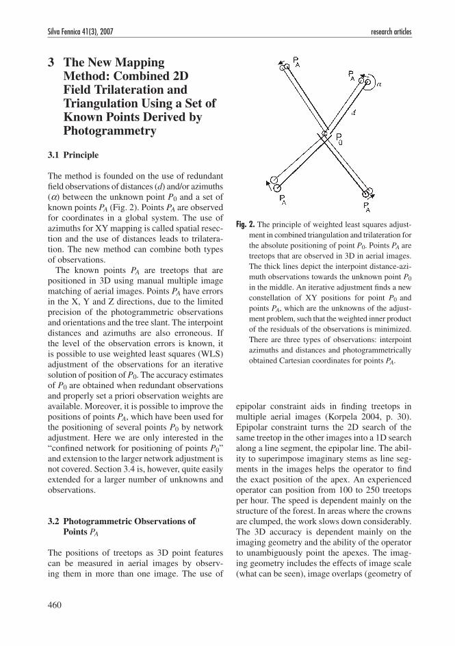
The method is founded on the use of redundant field observations of distances (d) and/or azimuths (α) between the unknown point P0 and a set of known points PA (Fig. 2). Points PA are observed for coordinates in a global system. The use of azimuths for XY mapping is called spatial resec-tion and the use of distances leads to trilatera-tion. The new method can combine both types of observations.

The known points PA are treetops that are positioned in 3D using manual multiple image matching of aerial images. Points PA have errors in the X, Y and Z directions, due to the limited precision of the photogrammetric observations and orientations and the tree slant. The interpoint distances and azimuths are also erroneous. If the level of the observation errors is known, it is possible to use weighted least squares (WLS) adjustment of the observations for an iterative solution of position of P0. The accuracy estimates of P0 are obtained when redundant observations and properly set a priori observation weights are available. Moreover, it is possible to improve the positions of points PA, which have been used for the positioning of several points P0 by network adjustment. Here we are only interested in the “confined network for positioning of points P0” and extension to the larger network adjustment is not covered. Section 3.4 is, however, quite easily extended for a larger number of unknowns and observations.

3.2 Photogrammetric Observations of Points PA

The positions of treetops as 3D point features can be measured in aerial images by observ-ing them in more than one image. The use of

epipolar constraint aids in finding treetops in multiple aerial images (Korpela 2004, p. 30). Epipolar constraint turns the 2D search of the same treetop in the other images into a 1D search along a line segment, the epipolar line. The abil-ity to superimpose imaginary stems as line seg-ments in the images helps the operator to find the exact position of the apex. An experienced operator can position from 100 to 250 treetops per hour. The speed is dependent mainly on the structure of the forest. In areas where the crowns are clumped, the work slows down considerably. The 3D accuracy is dependent mainly on the imaging geometry and the ability of the operator to unambiguously point the apexes. The imag-ing geometry includes the effects of image scale (what can be seen), image overlaps (geometry of

Fig. 2. The principle of weighted least squares adjust-ment in combined triangulation and trilateration for the absolute positioning of point P0. Points PA are treetops that are observed in 3D in aerial images. The thick lines depict the interpoint distance-azi-muth observations towards the unknown point P0 in the middle. An iterative adjustment finds a new constellation of XY positions for point P0 and points PA, which are the unknowns of the adjust-ment problem, such that the weighted inner product of the residuals of the observations is minimized. There are three types of observations: interpoint azimuths and distances and photogrammetrically obtained Cartesian coordinates for points PA.

461

Korpela, Tuomola and Välimäki Mapping Forest Plots: An Efficient Method Combining Photogrammetry and Field Triangulation

ray intersection) and the orientation accuracy of the images (accuracy of the intersecting rays). Previous studies have shown that it is possible to map trees in large-scale (1:6000−1:12 000) aerial images with an accuracy from 0.1 m to 0.5 m. The shape and optical properties of the crown affect the measurability in aerial images and the accuracy varies between species and age (Kor-pela 2004, p. 51). The 3D mapping of treetops gives estimates of tree heights, provided that an elevation model exists. Tree species classifica-tion can be done by visual photo-interpretation. This yields a map marked with points PA. In our experience 500–1000 measurements are needed to learn the technique of manual multiple image matching.

3.3 Fieldwork and Observations in Stem Mapping

The map of points PA can be processed into tree labels that have the tree number, intertree dis-tances and azimuths for the neighbouring trees as well as information on the height and species. Using the tree map, the labels and a compass the field worker identifies and labels the trees PA in the field. The speed of this work is greatly affected by the quality of the map. Commission errors, i.e. false trees, are especially disturbing. Our experi-ence has shown that this work phase also involves a learning curve. The speed of the labelling work has varied between 30 and 90 trees per hour.

The positioning of points P0 follows. In stem mapping, intertree azimuths (α) and/or distances (d) are observed. If a compass is used, the differ-ence between the magnetic north and the direc-tion of the photogrammetric (Cartesian) Y-axis must be solved for each compass and observer. We observed the difference for analogue Suunto precision compasses using an approximately 150-m long XY vector in a residential area. The correct α was determined with photogrammetric measurements of the end points. It is also possible to estimate the compass calibration by making it into an unknown in the WLS adjustment of Section 3.4. This is the standard case in geodetic triangulation, when angles are measured between known points and the orientation of the device is set as an unknown.

The intertree d should be measured horizon-tally and the direction must be recorded so that the correct half-stem diameter can be added to d value. The height of measurement should be as close as possible to the height of the diameter measurements to minimize imprecision. We used a low-cost handheld laser rangefinder.

3.4 WLS Adjustment of Distances, Azimuths and Photogrammetric Coordinates

The problem in finding the XY coordinates for point P0 with redundant d and/or α observa-tions to points PA by nonlinear adjustment is a standard procedure in surveying (e.g. Anderson and Mikhail 1998, Nielsen 2006). It calls for an iterative solution using linearized observation equations as well as an initial approximation.

One α and d observation towards a point PA can be used for solving the XY position of P0. The accuracy of P0 is determined by the inaccuracy of PA and the observation errors in d and α. Two α observations yield a point of intersection of two half-lines. Two d observations give two cir-cles that have from 0 to 2 intersections. Three d and/or α observations give the redundant case of WLS estimation. The redundancy is always N-2, where N is the sum of d and α observations. The photogrammetric coordinates of points PA, which are also unknowns, do not affect the redundancy, because each point PA adds two observations and two unknowns.

In the calculations, the intertree α values [0°, 360°] are transformed into [−π, +π] radians. A vector with α = 0 points to the east and a disconti-nuity at α = −π / +π in the west must be accounted for in the adjustment of the α residuals.

The unknown point P0 is first given an initial approximation. We used methods I−IV: I) one or several observation pairs of α and d, II) the line intersection points of half-lines given by α observations, III) the mean value of the surround-ing, observed control points PA or a grid of initial approximation points near this mean point and IV) intersections of circles when d observations only are available.

The observation equations that are linearized by a Taylor-series expansion are

462


Distance between P0 and PA:

( ) ( ) ( )( )X X Y Y dA A02

02 0 1− + − − =obs

Azimuth between P0 and PA:

arctan( )

( )( )( )

Y Y

X XA

A

0

00 2

−−

− =α obs

Coordinates of points PA:

X XA A− =( ) ( )obs 0 3

Y YA A− =( ) ( )obs 0 4

The partial derivatives of the observation equa-tions with respect to the unknown coordinates of points P0 and PA can be found in several text-books, e.g. Anderson and Mikhail (1998). The adjustment proceeds by calculating a vector of X and Y corrections, which are added to the initial approximation of P0 and to the photogrammetric coordinates of points PA. The corrections are the solution of equation (5) in vector x

x = (ATPA)–1ATPy (5)

where A is the design matrix that consists of the partial derivatives of the unknowns of the observa-tion equations (1–4) with respect to the unknowns. P is the diagonal weight matrix and y the vector of observation residuals. A has one row for each α and d observation and two rows for each point PA. There are two columns for each point P0 and PA. With four α and four d observations to four points PA, the dimension of A is 16 × 10 and the redundancy is 6. The adjustment continues until ||x|| vanishes. A and y are updated after each itera-tion. At the solution, usually after 2–4 iterations, the mean unit weight of the residuals (σ 0) is

σ 0 = y PyT

r( )6

where r is the redundancy. σ 0≈1, if the statisti-cal model is correct, assumptions on normality hold, and the weights in P are properly chosen to reflect the measurement inaccuracy and no gross blunders exist. Weights in P are set to a priori values of 1 / σ 2 for each type of observation d, α, XA and YA. At the solution the standard errors σXi

of the unknowns are computed from the diagonal elements i of the inverted normal equations

Q (A PA)

(Q )

xxT 1

xx

=

=

−

σ σXi 0

7diag

( )

The standard errors of X0 and Y0 define the minimal rectangle that contains the error ellipse of point P0. The orientation and extent of the error ellipse can be computed by eigenvalue decom-position of Qxx. The error ellipse is useful in the visualization of the inaccuracy and confidence intervals (Nielsen 2006, p. 25, see also Fig. 4).

The observations are subject to gross errors that can notably reduce the accuracy of point P0. It is possible to test for blunders by using their stand-ardized residuals wj, which are computed using the diagonal elements qj of the Qvv matrix:

Q P AQ Avv1

xxT= −

=

−

wy

qj

j

jσ 0

8( )

In all, each residual is affected by gross errors, any single gross error affects all residuals, and the influence of gross errors is affected by the geometry and correctness of the a priori weights in P and the underlying statistical model. Reli-able gross error detection requires high levels of redundancy. In practice, high values of σ 0 and σXi indicate the presence of a true observation error. It is advisable to check and repeat the field observations by starting from the point PA that is associated with the highest absolute value of the blunder statistics. The true observation error can reside in the azimuth, distance or in the photo-grammetrically obtained coordinates.

4 Simulations

4.1 Motivation

We feel that simulation is an effective tool for assessing the effects of the several underlying fac-tors that might affect the accuracy and efficiency of the mapping method. Visibility, terrain and stand density affect the intertree distances and

463


geometric layout of points PA. Measurement bias and imprecision will affect the accuracy of point P0. The number of observations affects gross error detection and the accuracy of P0. However, taking a large number of measurements is costly and the investigator should be able to optimize the actions in the field.

4.2 Simulator

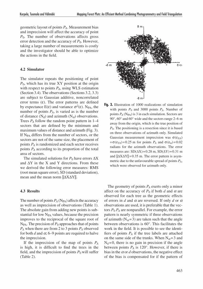
The simulator repeats the positioning of point P0, which has its true XY position at the origin with respect to points PA, using WLS estimation (Section 3.4). The observations (Sections 3.2, 3.3) are subject to Gaussian additive, noncorrelated error terms (ε). The error patterns are defined by expectance E(ε) and variance σ 2(ε). NPA, the number of points PA, is varied as is the number of distance (Nd) and azimuth (Nα) observations. Trees PA follow the random point pattern in 1–4 sectors that are defined by the minimum and maximum values of distance and azimuth (Fig. 3). If NPA differs from the number of sectors, or the sectors are not of the same size, the placement of points PA is randomized and each sector receives points PA according to its proportion of the total area of sectors.

The simulated solutions for P0 have errors ∆X and ∆Y in the X and Y directions. From these we derived the following error measures: RMS (root mean square error), SD (standard deviation), mean and the mean norm ||∆X∆Y||.

4.3 Results

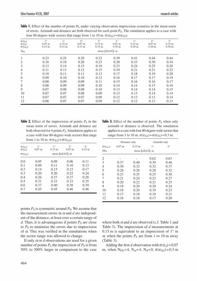
The number of points PA (NPA) affects the accuracy as well as imprecision of observations (Table 1). The absolute gain from adding new points is sub-stantial for low NPA values, because the precision improves to the reciprocal of the square root of NPA. The precision of P0 approaches that of points PA when there are from 2 to 3 points PA observed for both d and α; 6–9 points are required to halve the imprecision.

If the imprecision of the map of points PA is high, it is difficult to find the trees in the field, and the imprecision of points P0 will suffer (Table 2).

The geometry of points PA exerts only a minor affect on the accuracy of P0 if both d and α are observed for each tree as the geometric effects of errors in d and α are reversed. If only d or α observations are used, it is preferable that the vec-tors P0 PA are nonparallel. For example, the error pattern is nearly symmetric if three observations of azimuth (Nα = 3) are taken such that the angle between observations is 60°. This facilitates the work in the field. It is possible to see the identi-fiers of points PA if the tree labels are attached on the same side of the trunks. When Nα = 3 and Nd = 0, there is no gain in precision if the angle between points PA is 120°. However, if there is bias in the α or d observations, the negative effect of the bias is compensated for if the pattern of

Fig. 3. Illustration of 1000 realizations of simulation with points P0 and 3000 points PA. Number of points PA (NPA) is 3 in each simulation. Sectors are 90°, 60° and 60° wide and the sectors range 2–6 m away from the origin, which is the true position of P0. The positioning is a resection since it is based on three observations of azimuth only. Simulated Gaussian measurement imprecision was σ (εXA) = σ (εYA) = 0.25 m for points PA and σ (εα) = 0.02 radians for the azimuth observations. The error measures are: SD(∆X) = 0.28 m, SD(∆Y) = 0.31 m and ||∆X∆Y|| = 0.35 m. The error pattern is asym-metric due to the unfavourable spread of points PA, which were observed for azimuth only.

464


points PA is symmetric around P0. We assume that the measurement errors in α and d are independ-ent of the distance, at least over a certain range of d. Thus, it is advantageous if points PA are close to P0 to minimize the errors due to imprecision of α. This was verified in the simulations when the sector range was allowed to change.

If only α or d observations are used for a given number of points PA the imprecision of P0 is from 50% to 300% larger in comparison to the case

where both α and d are observed (c.f. Table 1 and Table 3). The imprecision of d measurements at 0.15 m is equivalent to an imprecision of 1° in α, when the points PA are from 1 to 10 m away (Table 3).

Adding the first d observation with σ (εd) = 0.07 m, when NPA = 4, Nα = 4, Nd = 0, σ (εXA) = 0.3 m

Table 1. Effect of the number of points PA under varying observation imprecision scenarios in the mean norm of errors. Azimuth and distance are both observed for each point PA. The simulation applies to a case with four 80-degree-wide sectors that range from 1 to 10 m. σ (εXA) = σ (εYA).

σ (εα)σ (εd)σ (εXA)

1°0.07 m0.15 m

1°0.15 m0.15 m

2°0.07 m0.15 m

2°0.15 m0.15 m

1°0.07 m0.30 m

1°0.15 m0.30 m

2°0.07 m0.30 m

2°0.15 m0.30 m

NPA mean ||∆X∆Y||, m

1 0.23 0.25 0.29 0.32 0.39 0.41 0.44 0.442 0.16 0.18 0.20 0.23 0.28 0.33 0.30 0.343 0.13 0.14 0.15 0.18 0.23 0.24 0.25 0.264 0.11 0.13 0.12 0.15 0.19 0.21 0.21 0.225 0.10 0.11 0.11 0.13 0.17 0.18 0.19 0.206 0.09 0.10 0.10 0.12 0.16 0.17 0.17 0.197 0.08 0.09 0.09 0.11 0.15 0.16 0.16 0.178 0.08 0.09 0.09 0.10 0.14 0.14 0.15 0.169 0.07 0.08 0.08 0.10 0.13 0.14 0.14 0.1510 0.07 0.07 0.08 0.09 0.13 0.13 0.14 0.1411 0.07 0.07 0.07 0.09 0.12 0.13 0.13 0.1412 0.06 0.07 0.07 0.09 0.12 0.12 0.12 0.13

Table 2. Effect of the imprecision of points PA in the mean norm of errors. Azimuth and distance are both observed for 4 points PA. Simulation applies to a case with four 80-degree-wide sectors that range from 1 to 10 m. σ (εXA) = σ (εYA).

σ (εα) 1° 1° 2° 2°σ (εd) 0.07 m 0.15 m 0.07 m 0.15 m

σ (εXA) mean ||∆X∆Y||, m

0.0 0.05 0.09 0.06 0.110.1 0.09 0.11 0.10 0.130.2 0.14 0.15 0.15 0.170.3 0.20 0.20 0.22 0.240.4 0.26 0.27 0.27 0.280.5 0.31 0.33 0.33 0.350.6 0.37 0.40 0.38 0.390.7 0.45 0.45 0.46 0.46

Table 3. Effect of the number of points PA when only azimuth or distance is observed. The simulation applies to a case with four 80-degree-wide sectors that range from 1 to 10 m. σ (εXA) = σ (εYA) = 0.3 m.

Distance only Azimuth only

σ (εobs) 0.07 m 0.15 m 1° 2°

NPA mean ||∆X∆Y||, m

2 - - 0.62 0.633 0.37 0.40 0.39 0.464 0.30 0.32 0.32 0.375 0.26 0.28 0.28 0.326 0.23 0.25 0.25 0.307 0.21 0.24 0.23 0.278 0.20 0.22 0.21 0.259 0.19 0.20 0.20 0.2410 0.18 0.20 0.19 0.2311 0.17 0.18 0.18 0.2112 0.16 0.18 0.17 0.20

465


and σ (εα) = 1° reduced the mean norm from 0.32 m to 0.27 m. Similarly, adding the first α observation when NPA = 4 and Nd = 4 reduced the mean norm from 0.30 m to 0.26 m. The simulator could be used for finding the optimal combination of observations, but it would require knowledge of the observation rates of d and α.

5 Field Test in the Pätsäinmäki Stand

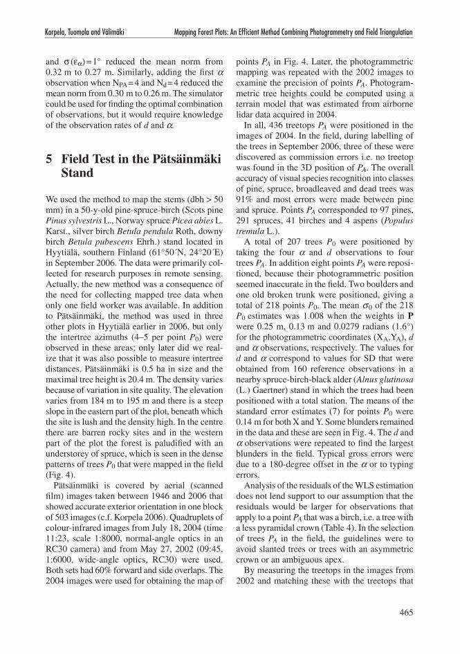
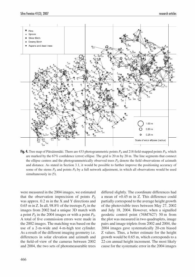
We used the method to map the stems (dbh > 50 mm) in a 50-y-old pine-spruce-birch (Scots pine Pinus sylvestris L., Norway spruce Picea abies L. Karst., silver birch Betula pendula Roth, downy birch Betula pubescens Ehrh.) stand located in Hyytiälä, southern Finland (61°50´N, 24°20´E) in September 2006. The data were primarily col-lected for research purposes in remote sensing. Actually, the new method was a consequence of the need for collecting mapped tree data when only one field worker was available. In addition to Pätsäinmäki, the method was used in three other plots in Hyytiälä earlier in 2006, but only the intertree azimuths (4–5 per point P0) were observed in these areas; only later did we real-ize that it was also possible to measure intertree distances. Pätsäinmäki is 0.5 ha in size and the maximal tree height is 20.4 m. The density varies because of variation in site quality. The elevation varies from 184 m to 195 m and there is a steep slope in the eastern part of the plot, beneath which the site is lush and the density high. In the centre there are barren rocky sites and in the western part of the plot the forest is paludified with an understorey of spruce, which is seen in the dense patterns of trees P0 that were mapped in the field (Fig. 4).

Pätsäinmäki is covered by aerial (scanned film) images taken between 1946 and 2006 that showed accurate exterior orientation in one block of 503 images (c.f. Korpela 2006). Quadruplets of colour-infrared images from July 18, 2004 (time 11:23, scale 1:8000, normal-angle optics in an RC30 camera) and from May 27, 2002 (09:45, 1:6000, wide-angle optics, RC30) were used. Both sets had 60% forward and side overlaps. The 2004 images were used for obtaining the map of

points PA in Fig. 4. Later, the photogrammetric mapping was repeated with the 2002 images to examine the precision of points PA. Photogram-metric tree heights could be computed using a terrain model that was estimated from airborne lidar data acquired in 2004.

In all, 436 treetops PA were positioned in the images of 2004. In the field, during labelling of the trees in September 2006, three of these were discovered as commission errors i.e. no treetop was found in the 3D position of PA. The overall accuracy of visual species recognition into classes of pine, spruce, broadleaved and dead trees was 91% and most errors were made between pine and spruce. Points PA corresponded to 97 pines, 291 spruces, 41 birches and 4 aspens (Populus tremula L.).

A total of 207 trees P0 were positioned by taking the four α and d observations to four trees PA. In addition eight points PA were reposi-tioned, because their photogrammetric position seemed inaccurate in the field. Two boulders and one old broken trunk were positioned, giving a total of 218 points P0. The mean σ 0 of the 218 P0 estimates was 1.008 when the weights in P were 0.25 m, 0.13 m and 0.0279 radians (1.6°) for the photogrammetric coordinates (XA,YA), d and α observations, respectively. The values for d and α correspond to values for SD that were obtained from 160 reference observations in a nearby spruce-birch-black alder (Alnus glutinosa (L.) Gaertner) stand in which the trees had been positioned with a total station. The means of the standard error estimates (7) for points P0 were 0.14 m for both X and Y. Some blunders remained in the data and these are seen in Fig. 4. The d and α observations were repeated to find the largest blunders in the field. Typical gross errors were due to a 180-degree offset in the α or to typing errors.

Analysis of the residuals of the WLS estimation does not lend support to our assumption that the residuals would be larger for observations that apply to a point PA that was a birch, i.e. a tree with a less pyramidal crown (Table 4). In the selection of trees PA in the field, the guidelines were to avoid slanted trees or trees with an asymmetric crown or an ambiguous apex.

By measuring the treetops in the images from 2002 and matching these with the treetops that

466


were measured in the 2004 images, we estimated that the observation imprecision of points PA was approx. 0.2 m in the X and Y directions and 0.65 m in Z. In all, 98.8% of the treetops PA in the images from 2002 had a unique 3D match with a point PA in the 2004 images or with a point P0. A total of five commission errors were made in the 2002 images. The matching was based on the use of a 2-m-wide and 4-m-high test cylinder. As a result of the different imaging geometry i.e. differences in solar elevation and azimuth and the field-of-view of the cameras between 2002 and 2004, the two sets of photomeasurable trees

differed slightly. The coordinate differences had a mean of +0.45 m in Z. This difference could partially correspond to the average height growth of the photovisible trees between May 27, 2002 and July 18, 2004. However, when a signalled geodetic control point (76M7627) 50 m from the plot was measured in two quadruplets, image pairs and image triplets from 2002 and 2004, the 2004 images gave systematically 20-cm biased Z values. Thus, a better estimate for the height growth would be 0.65 m, which corresponds to a 22-cm annual height increment. The most likely cause for the systematic error in the 2004 images

Fig. 4. Tree map of Pätsäinmäki. There are 433 photogrammetric points PA and 218 field-mapped points P0, which are marked by the 67% confidence (error) ellipse. The grid is 20 m by 20 m. The line segments that connect the ellipse centres and the photogrammetrically observed trees PA denote the field observations of azimuth and distance. As stated in Section 3.1, it would be possible to further improve the positioning accuracy of some of the stems PA and points P0 by a full network adjustment, in which all observations would be used simultaneously in (5).

467


is use of the wrong focal length of the camera, which was not compensated for in the orientation of the 2004 images, for which so-called direct georeferencing observations were available (Kor-pela 2006; see also Cramer et al. 2000).

We experienced that distance measurements with a laser instrument (Trimble HD150) are subject to gross errors resulting from obstruct-ing material between points P0 and PA. It was increasingly easy to verify the d measurement as free from gross errors as the distance became shorter. The instrument was operated in a “min-max mode”, and d was measured several times and recorded only after the same maximum d was obtained several times. Branches at the 1.3-m height make the measurement difficult, and if both P0 and PA have branches it may become laborious to get an accurate observation. In such cases we recommend that the d observations be compensated by additional observations of α.

6 Discussion

We present a method that can be used for the abso-lute positioning of objects under a canopy and that directly provides an absolute accuracy that ranges from 0.1 m to 0.3 m, assuming that the orientation of the imagery is correct. The accuracy achievable is dependent mainly on the accuracy of photo-grammetric treetop positioning and the number of field observations. Centimetre-level accuracy is possible, but requires tens of field observations. We assume that our method is applicable in areas where tree crowns are peaked and trunks are not slanted. These conditions are often encountered in the boreal forests. Mapping can be done by one person and the required equipment is of low cost.

For large plots (> 0.4 ha) the work rate compares with that of tacheometry and a two person field team, but in small plots other methods may well be more efficient. The size of the plot does not affect the accuracy and there is little danger of coordinate system distortions, which is not the case with traditional field methods. The use of a compass should be restricted to areas where local magnetic anomalies do not exist. It is pos-sible to replace the compass with an instrument that measures the angles and the orientation of the instrument is set as an unknown in the WLS estimation. However, this would require the use of indirect measurements, at least in stem map-ping, since it would be impossible to place the instrument at the stem.

Recent large-scale aerial photographs, which have been accurately oriented, are needed for the 3D measurement of treetop positions. In the tests we used image quadruplets on scales of 1:6000 and 1:8000, which had ground resolu-tions of 8.4 cm and 12 cm, respectively. Having multiple views is beneficial, because crowns that are impossible to discern in some views may be well seen in others. The solvability of the corre-spondence problem (the same treetop is pointed in the images used) is more reliable when several views and flight lines are available. We used our own digital photogrammetric workstation (DPW; software written in Basic and C/C++) for mono-scopic image measurements of image matching with epipolar constraints (Section 3.2). To the best of our knowledge, this type of functional-ity is a basic feature in commercial DPWs. We also used our own programs for printing the tree maps and tree labels. The WLS adjustment was implemented in a program that can be used in the forest for real-time calculations or in the office for postprocessing or simulations. In the field it is

Table 4. Means and standard deviations of the observation residuals of WLS positioning of points P0.

Species N Coordinates of PA Azimuth Distance XA, m YA, m α, radians d, m

Pine 234 −0.00 0.19 +0.04 0.20 +0.0025 0.0165 +0.009 0.063Spruce 534 −0.01 0.19 −0.01 0.19 +0.0029 0.0180 +0.012 0.065Birch 104 +0.04 0.22 −0.04 0.21 +0.0041 0.0128 +0.004 0.054All 872 +0.00 0.20 +0.00 0.20 +0.0029 0.0171 +0.010 0.063

468


advantageous if the positioning and calculation of error estimates can be done “on the fly” after each observation. There are commercial programs that can be used for network adjustment.

The method requires some basic knowledge in photogrammetry and surveying. Training is especially required for the photogrammetric work of 3D treetop positioning and species interpreta-tion. Our experience is that successful fieldwork requires care and undivided attention, although the measurements have built-in error measures that help the user.

One interesting extension of our mapping method would be its use for refining satellite positioning under a canopy. In such a case, the fieldwork would consist of making a local map in a polar coordinate system that would be matched with a tree map from a single-tree remote sens-ing application. If the maps have marks, e.g. stem diameters obtained with a Laser relascope (Kalliovirta et al. 2005) and heights from photo-grammetric or lidar-based application, we see it possible to obtain good matching automatically and thus obtain an accurate position without the need for identifying and labelling the trees.

Acknowledgements

We would like to thank Lic.Tech. Keijo Inkilä at Helsinki University of Technology, Mr. Jan Heik-kilä at Pieneering Company, Dr. Mark Breach at Nottingham Trent University and Dr. Juha Heik-kinen at the Finnish Forest Research Institute for their help with weighted least squares adjustment and spatial statistics. Funding by MATINE and Academy of Finland made this study possible.

References

Andersson, J.M. & Mikhail E.M. 1998. Surveying: theory and practice. 7th edition. McGraw-Hill Companies Inc. 1150 p.

Avery, G. 1958. Helicopter stereo-photography of forest plots. Photogrammetric Engineering 24(4): 617–624.

Blasquez, C.H. 1989. Computer-based image analy-

sis and tree counting with aerial color infrared photography. Journal of Imaging Technology 15: 163–168.

Boose, E.R., Boose, E.F. & Lezberg, A.L. 1998. A practical method for mapping trees using distance measurements. Ecology 79: 819–827.

Bortolot, Z.J. & Wynne, R.H. 2005. Estimating forest biomass using small footprint LiDAR data: an individual tree-based approach that incorporates training data. ISPRS Journal of Photogrammetry and Remote Sensing. 59(6): 342–360.

Cramer, M., Stallman, D. & Haala, N. 2000. Direct georeferencing using GPS/inertial exterior orien-tations for photogrammetric applications. Interna-tional Archives for Photogrammetry and Remote Sensing, Vol. XXXII/B Amsterdam, 2000. p. 198–205.

Häkli, P. & Koivula, H. 2004. Virtuaali-RTK (VRS) tutkimus. Geodeettinen laitos, Tiedote 27. 60 p. (In Finnish).

Kalliovirta, J., Laasasenaho, J. & Kangas, A. 2005. Evaluation of the Laser-relascope. Forest Ecology and Management 204(2–3): 181–194.

Korpela I. 2004. Individual tree measurements by means of digital aerial photogrammetry. Silva Fennica Monographs 3: 1–93.

— 2006. Geometrically accurate time series of archived aerial images and airborne lidar data in a forest environment. Silva Fennica 40(1): 109–126.

— & Tokola T. 2006. Potential of aerial image-based monoscopic and multiview single-tree forest inven-tory – a simulation approach. Forest Science 52(2): 136–147

Mäkinen, A., Korpela, I., Tokola, T., & Kangas, A. 2006. Effects of imaging conditions on crown diameter measurements from high resolution aerial images. Canadian Journal of Forest Research 36: 1206–1217.

Næsset, E. 1999. Point accuracy of combined pseu-dorange and carrier phase differential GPS under forest canopy. Canadian Journal of Forest Research 29: 547–553.

Nielsen, A. 2006. Least squares adjustment: linear and nonlinear weighted regression analysis. Technical University of Denmark. 47 p. Available at: http://www2.imm.dtu.dk/pubdb/p.php?2804. [Version dated January 2006].

Persson, A., Holmgren, J. & Soderman, U. 2002. Detecting and measuring individual trees using an

469


airborne laser scanner. Photogrammetric Engineer-ing and Remote Sensing 68(9): 925–932.

Quigley, M.F. & Slater, H.H. 1994. Mapping forest plots: a fast triangulation method for one person working alone. Southern Journal of Applied For-estry 18(3): 133–136.

Reutebuch, S.E., Carson, W.W. & Ahmed K.M. 2003. A test of the Applanix POS LS inertial positioning system for the collection of terrestrial coordinates under a heavy forest canopy. University of Wash-ington, Papers of the Precision Forest Cooperative. 11 p. Available at: http://www.cfr.washington.edu/research.pfc/publications/index.htm.

Stendahl, J. & Dahlin, B. 2002. Harvester-based forest inventory in thinnings. Scandinavian Journal of Forest Research 17: 548–555.

Talts, J. 1977. Mätning i storskaliga flygbilder för beståndsdatainsamling. Summary: Photogrammet-ric measurements for stand cruising. Royal College of Forestry, Department of Forest Mensuration And Management, Research Notes NR 6-1977. 102 p. (In Swedish).

Wanninger, L. 2005. Introduction to Network RTK. IAG Working Group 4.5.1: Network RTK. Avail-able at: http://www.network-rtk.info/intro/intro-duction.html. [Last modification Dec 3, 2005].

Total of 20 references

Mapping forest plots: an efficient method combining ... · Mapping forest plots: an efficient method combining ... (tacheometry), which establishes the 3D vec-tors from the apparatus

Documents