Management of agropastoral systems in a semiarid region

Management of agropastoral systems in a semiarid region E.D. Ungar

• • • • • • • • • • • •

HI ••B

1

Management of agropastora systems in a semiarid region

E.D. Ungar

Pudoc Wageningen 1990

Simulation Monographs 31

Simulation Monographs is a series on computer simulation in agriculture and its supporting sciences

CIP-data Koninklijke Bibliotheek, Den Haag

Ungar, E.D.

Management of agropastoral systems in a semiarid region / E.D. Ungar. Wageningen : Pudoc. - 111. - (Simulation monographs ; 31) With index. ISBN 90-220-0946-7 bound SISO 632.5 UDC 633.2.03:681.3 NUGI 835 Subject headings: agropastoral systems ; management.

ISSN 0924-8439

ISBN 90-220-0946-7 NUGI 835

Centre for Agricultural Publishing and Documentation (Pudoc), Wageningen, the Netherlands, 1990.

No part of this publication, apart from bibliographic data and brief quotations embodied in critical reviews, may be reported, re-recorded or published in any form including print, photocopy, microfilm, electronic or electromagnetic record without written permission from the publisher: Pudoc, P.O. Box 4, 6700 AA Wageningen, the Netherlands.

Printed in the Netherlands

Contents

Preface ix 1 Introduction 1

2 Theoretical framework 3 2.1 Classifying management decisions 3 2.2 Strategy and tactic in farm management 3 2.2.1 Case 1 3 2.2.2 Case 2 4 2.2.3 Case 3 4 2.3 Definition and application 5 2.4 Case 4: imperfect knowledge 5 2.5 Possible-outcome analysis 7

9 9

10 10 11 11 12 12 12 13

15 15 17 17 19 21 22 22

5 Tactical management decisions 23 5.1 Supplementary feeding of the ewe 23 5.1.1 Introduction 23 5.1.2 Target-oriented feeding 23 5.1.3 Programming considerations 24

3 3.1 3.2 3.3 3.4 3.4.1 3.4.2 3.4.3 3.4.4 3.4.5

4 4.1 4.2 4.3 4.4 4.5 4.6 4.7

Outline of the agropastoral model System The management decisions Structure of the model Programming considerations Time-step Initialization Meteorological data Output Programming conventions and COMMON blocks

Strategic management decisions Land allocation Stocking rate Breed Breeding Sowing density Fertilizer Standard values of parameters

5.2 Grazing schedule of the ewe 24 5.2.1 Approach 24 5.2.2 Programming considerations 27 5.3 Grazing deferment 27 5.3.1 Introduction 27 5.3.2 Objective function 27 5.3.3 Green-season dynamics 28 5.3.4 Dry-season dynamics 29 5.3.5 Behaviour of the model 29 5.3.6 Programming considerations 36 5.4 Early-season grazing of green wheat 36 5.4.1 Introduction 36 5.4.2 Objective function 37 5.4.3 Behaviour of the model 37 5.4.4 Programming considerations 39 5.5 Late-season grazing of green wheat 40 5.5.1 Introduction 40 5.5.2 Calculating the expected yield of grain 40 5.5.3 Choosing between grazing and grain 42 5.5.4 Programming considerations 43

Calculating the expected yield of grain 43 Choosing between grazing and grain 43

5.6 Lamb feeding 45 5.6.1 Introduction 45 5.6.2 Model formulation 45 5.6.3 Behaviour of the model 47 5.6.4 Programming considerations 51 5.7 Lamb rearing 51 5.7.1 Approach 51 5.7.2 Programming considerations 54 5.8 Baling of straw 58 5.8.1 Introduction 58 5.8.2 Algorithm for the decision 58 5.8.3 Programming considerations 59 5.9 Cutting of wheat for hay 61 5.9.1 Introduction 61 5.9.2 Algorithm for the decision 61 5.9.3 Programming considerations 63

6 Biological and financial framework of simulation 65 6.1 Primary production 65 6.1.1 Use of ARID CROP ' 65 6.1.2 Programming considerations 68 6.2 Animal nutrition and production 68

vi

6.2.1 Efficiency of utilization of metabolic energy 77 6.2.2 Energy requirements for maintenance 78

Fasting heat production 78 Energy allowance for grazing activity 78

6.2.3 Requirements for production and performance 79 Heat of combustion of gain in liveweight 79 Liveweight change 80 Pregnancy 80 Lactation 81 Total energy requirements of the ewe 85

6.2.4 Programming considerations 87 6.3 Intake 90 6.3.1 Approach 90 6.3.2 Programming considerations 94 6.4 Flock dynamics 97 6.5 Financial balance 97

7 Validation 99

8 Results of the agropastoral model 101 8.1 Standard run 101 8.2 Early-season grazing of green wheat 105 8.3 Late-season utilization of green wheat by grazing 106 8.4 Late-season utilization of green wheat for hay 107 8.5 Utilization of wheat aftermath by grazing and baling of straw 107 8.6 Lamb rearing 109 8.6.1 Main rearing patterns in the standard run 109 8.6.2 Effect of a fixed weaning age 113 8.6.3 Inclusion of sown legume for lamb grazing 114 8.7 Prices and price ratios 119 8.8 Stocking rate 119

9 Summary 125

Concluding remarks 127

10 References 129

11 Listing of model 133

12 Model directory 179 12.1 Local variables 179 12.2 Acronyms, definitions and units of measure 179 13 Index 211

vn

Preface

This study was conducted within the framework of a joint Dutch-Israeli research project "Actual and potential production from semiarid grasslands. Phase T\ It was partly funded by the Directorate-General for International Cooperation of the Dutch Ministry of Foreign Affairs.

It is based on a doctoral thesis with the same title submitted to the Senate of the Hebrew University of Jerusalem in 1984. The text and the model have been heavily revised.

Sincere gratitude is due to Professor I. Noy-Meir of the Botany Department of the Hebrew University for the privilege of his supervision. I am indebted to Professor N.G. Seligman of the Agricultural Research Organization of Israel for considerable assistance in both the funding and the content of this study.

E.D. Ungar

IX

1 Introduction

There are large regions in the world with a semiarid climate and deep arable soils (Aschmann, 1973; di Castri, 1981). The dry boundary of those regions lies at the edge of the area where production of rain-fed annual crops is not possible in most years, even though steps are taken to conserve and maximize available moisture. The moisture limit lies where droughts do not substantially limit the productivity of crops in most years (Bowden, 1979). The predominant food production systems in the semiarid regions are based on small-grain crops and ruminant grazing for meat and milk. Often those are combined into agropastoral (crop and grazing) systems of various forms (Walker, 1979).

In large parts of the semiarid regions, quite remarkable food production can be achieved by full and efficient exploitation of rainfall and soil resources. The actual agricultural production is much lower than the potential, being limited by the availability of the rainfall, by low soil fertility, and by extensive systems of land-use and management that attempt to adapt to those limitations rather than to overcome them. The pathway of agricultural development and intensification is strongly subject to socio-economic and cultural factors (Grigg, 1974). After a major research project in the Sahel Region (Penning de Vries & Djiteye, 1982), Breman & de Wit (1983) concluded that the introduction of'some major nutrients from the outside', such as phosphate and nitrogen, or 'the creation of other possibilities for gainful employment for the pastoral people' represent the only development options for that region. But as they indicate, such options are unlikely to be initiated internally but would require major intervention on the part of external agencies.

There are, however, semiarid regions where biological, socio-economic and cultural factors concur to make conventional pathways of intensification of the humid zone feasible, without major external aid. Notably, extensive agriculture is juxtaposed with an intensive agroindustrial infrastructure, inputs essential for intensification are available and developed markets are nearby.

The semiarid region of the Middle East and the Mediterranean Basin is a classic example of such an environment. Certain intensification processes occur sponta­neously by the actions of individual farmers. Others may be initiated or accelerat­ed by improving the technical knowledge and management skill of farmers, or by modest changes in government policy and support. In that situation, many new inputs and techniques become available, such as improved breeds, supplementary feeds and pasture fertilization.These can be combined into a diverse array of more intensive production systems, some of them complex. Though all increase food production, not necessarily all increase farmer income or its stability. A few of the options can be experimentally evaluated, but to examine many would be far too

1

time-consuming and expensive. The problem then is how to select system config­urations to implement in experimental or pilot projects, and how to use the information obtained in those projects for the biological and economic eval­uation of other configurations that have not yet been implemented.

The methodology of mathematical modelling, systems analysis and simulation has proved an effective tool to solve problems of that kind (Dent & Anderson, 1971; Anderson, 1974; Dalton, 1975; Arnold & de Wit, 1976; Christian et al., 1978). Such a methodology is adopted in this study with a strong emphasis on a problem-oriented approach (Spedding, 1975; 1979). In this approach, the system can be described as a series of problems or, in the present context, management decisions. For several of these, one can develop decision criteria or optimization algorithms with concise and autonomous formulations that include only directly relevant biological elements of the total system.

This study examines the management problems involved in operating intensive agropastoral systems in a semiarid environment (i.e. with unpredictable and highly variable rainfall), in a region where intensification is feasible. Emphasis is placed upon management options created by integration with wheat production. With the classification scheme of Noy-Meir (1975), the system studied here can be characterized as: lamb production from a flock of sheep, of constant number of animals from year to year, reproducing once a year at fixed dates. The flock is sedentary, grazing a rain-fed area (individually farmed) consisting of annual vegetation (all species of similar growth and palatability) in a semiarid, winter rainfall zone with mild to cool winters. The pasture is fertilized and the animals are supplemented to 'optimum' production. The economic environment is char­acterized by a high price ratio of meat to grain. There is no limitation to drinking water. Notably, the pastoral component is integrated with small-grain produc­tion (wheat). . The region used for the quantitative characterization of the system is the

northern Negev Region of Israel. The integration of wheat and sheep production has been examined over several years at the Migda Experimental Station in the northern Negev (Tadmor et al., 1974; Eyal et al., 1975; Benjamin et al., 1982). Research at Migda has aimed at determining the potential primary and secondary production in such an environment, and in designing farming systems that could be implemented widely in the region. Those systems would aim to provide a more stable income than the purely arable systems with wheat that currently predom­inate.

2 Theoretical framework

2.1 Classifying management decisions

It is useful to classify management decisions into two classes, strategic and tactical. Although there does not appear to be a widely accepted definition of those terms, strategy is generally taken to connote overall approach, direction and policy, whereas tactic has a more dynamic connotation, implying a response to some occurrence in a short-term context. For example, Dyckman et al. (1969) define a strategy as a decision criterion to select among actions. Riggs (1968) defines strategy as system objectives and tactics as operation objectives. A strategic decision selects the objective that makes the best use of resources in accordance with long-range goals. Tactics are the operational-level alternatives to achieve strategic plans.

Those definitions may be operationally useful in a business context, but seem less meaningful to farm management. The hierarchy of long-range goal, ob­jective, strategic plan, strategy and tactic implicit in the definition of Riggs is not adopted here. Rather, there is assumed to be a definable objective that can be formulated in monetary terms. The purpose of strategic and tactical decisions is to direct the system towards the achievement of the defined objective. However the way decisions are best reached may differ fundamentally between them. The following discussion serves to define and clarify the significance of those two decision classes.

2.2 Strategy and tactic in farm management

The dominant factor that gives rise to integrated agropastoral systems is the unpredictability of the amount and distribution of rainfall. Variability is suffi­ciently high to result in extremely poor pasture production and almost zero grain yield at one extreme, and primary production of over 10 t ha"1 at the other. To clarify how unpredictability of rainfall affects problems of farm management, three scenarios or 'cases' are considered.

2.2.1 Case 1

Case 1 is defined by three characteristics. A. All driving variables (i.e. variables across the system boundary that influence

system behaviour; these usually include climate, prices, pests and diseases) remain identical each seasonal cycle.

B. The behaviour of all driving variables is known.

C. There is perfect knowledge of the biology of the system, and the ability to predict accurately the impact of any management decision. Case 1 represents decision making under certainty. For such a system, one can,

in theory, optimize management. Concepts of strategy and tactic are irrelevant. The farmer has simply to implement the optimum management solution to maximize the selected objective function. In practice, a close approximation to the optimum can probably be achieved if the biological description of the system omits detail to which the solution is expected to be insensitive. In addition, management options that recur regularly can be thinned out to reduce the number of alternatives to more manageable proportions. The impact of such condensa­tion of the problem depends on the steepness of the response surface in the region of the global optimum.

2.2.2 Case 2

In Case 2, Characteristic A is relaxed and driving variables behave as they do in reality. Nevertheless, Characteristic B still holds and thus we are still dealing with certainty. It is still theoretically possible to optimize the management of such a system, but the magnitude of the problem is much larger than in Case 1, since seasons can no longer be taken in isolation.

Even if Case 1 or 2 existed, the package furnishing truly optimum solutions would probably not exist. Management decisions would be taken on the basis of the known outcome (there is still perfect knowledge) of various alternative options. Presumably, management would be improved by considering more options through time. A useful tool might predict the outcome of a large selection of management pathways from any given decision, and suggest the pathway most likely to contribute to the defined objectives. Even without uncertainty of driving variables (unpredictability), the manager has a formidable problem. We can now take the second step towards reality.

2.2.3 Case 3

Characteristic B is removed in proceeding to Case 3. Not only do driving variables behave as they do in reality, but they cannot be predicted either. Case 3 includes decision making under conditions of risk, where one recognizes the possible outcomes and the associated probabilities, and decision making with uncertainty, where one recognizes the possible outcomes but not the probabilities (Emory & Niland, 1968).

With risk or uncertainty, an optimum solution in the sense of a predefinable management pathway that maximizes the objective function is inapplicable. In Case 3, it is rational to base management decisions on the current state of the system and behaviour of driving variables; i.e. to create a feedback of system behaviour onto management. However one can study past behaviour of driving variables, assume that their future behaviour will show similar averages and

variabilities, and on that basis formulate a long-term 'optimum strategy': 'opti­mum' not in the sense that the objective function will be maximized, but that the objective function has the highest probability of being in an acceptably high range; 'strategy' for those management decisions that are best taken independ­ently of season. That is, they cannot be (or are only inconveniently or uneconom­ical^) changed from season to season and generally cannot be determined from the present state of the system or behaviour of driving variables. Management tactics will refer to those decisions that are dependent on season, meaning they are taken on the basis of the present state of the system and behaviour of driving variables.

In practice, the type of predictive tool that would be useful in Cases 1 and 2 is similar in purpose to the tool that would aid tactical decision making in Case 3. Uncertainty in predicting future driving variables, however, adds further com­plexity.

2.3 Definition and application

Uncertainty of driving variables gives rise to the distinction between strategic and tactical management decisions, the distinction between them hinging on the degree of season-dependence in their execution. A strategic decision is defined as a decision taken independently of the state of the system at the time of decision as well as independently of the expected performance of that system in the short to medium term.

A strategic decision is presumably formulated on the basis of long-term experience. An example of such a decision would be the allocation of available land area between alternative enterprises. In contrast, a tactical decision is defined as a decision that is taken in response to the immediate state and environment of the system or in consideration of the expected short-term to medium-term performance of the system. An example of a tactical decision would be whether to graze green wheat when faced witha high probability of crop failure.

2.4 Case 4: imperfect knowledge

Unfortunately, Case 3 (Section 2.2.3) is still outside the realms of reality. A further step is required and that is removal of Characteristic C, since knowledge of structure and functioning of the system is incomplete or even rudimentary. The model itself is often a means of testing complex hypotheses about the biology of the system. Discussion of methodological problems of how best to apply models in a management context may seem premature. However careful integration of knowledge can constitute a significant aid to the farmer and planner, despite imperfect understanding of the components.

The definition of 'optimum' now requires further qualification which will include the uncertainty of the model structure and parametrization itself, and not just of the environment where it operates. Sensitivity analysis to both structure

and parameter is the main technique used to measure the significance of that uncertainty. During the present study, a biological precision was required that cannot yet be achieved to release many management decisions from determina­tion a priori, and thereby make them accessible to even a crude form of optimiza­tion. Two alternatives are available in such circumstances. First, to construct a best-guess hypothesis and accept the risk that any 'optimum' management rec­ommendation grounded in that hypothesis may be highly sensitive to the struc­ture and parametrization used, and may thus be mathematically precise but biologically inaccurate. It may be no improvement over evaluation of the farmer or extension worker whose conceptual model of the system may be more accurate, even though it is not expressed in explicit mathematical terms. Certainly as a research tool and identifier of areas for further investigation, such an approach might be regarded as the essence of modelling.

The second and more pragmatic approach is to predetermine management rules for a subsystem that is problematic to model in a more mechanistic fashion. Input-output relationships are held firmly within the range encountered under good management practice. This closes off the option of optimization of that subsystem and hence of fixing a global optimum for the system as a whole. That, perhaps, is not really of concern if the response surface of objective functions of complex agricultural systems is fairly flat in the region of the global optimum. This second approach has been adopted here for supplementary feeding of ewes.

As yet, removal of Characteristic C has been discussed in terms of imperfect knowledge about the biology of the system; knowledge in the sense of under­standing. In a management context, imperfect knowledge about the state of the system can be just as significant, though here it is knowledge in the sense of information. It is inevitable that the more refined a management package be­comes, the more extensive and detailed will be the concomitant data base. Given the current state of the art, it is rarely possible to determine both optimum criteria for decisions and predict when these criteria will be met on a farm. A strong feedback of information from the field is essential both to regulate the model and to know when to implement recommendations.

That touches on a fundamental problem. In one direction of information flow, there is the gap from the manager's sharp intuitive sense, qualitatively monitoring and integrating over a broad base of indicators, to the exact reductionist model of low integrative facility. In the other direction, the model can sometimes provide precise thresholds for particular actions that cannot be used for lack of quantita­tive monitoring. A possible approach may therefore be the construction of rough-and-ready models, which require rough-and-ready information for guid­ance and implementation. Such an approach is exemplified by the fertilizer model DECIDE (Bennett & Ozanne, 1973). The challenge, then, is to construct such a model without its being trivial to the experienced farmer, extension worker or planner. Those considerations played a role in the development of the algorithms for tactical decisions (Chapter 5).

The approach to optimization of the two management decision classes is

fundamentally different. The formulation of criteria for tactical decisions can proceed independently, partly because the relevant biological subsystem can be isolated. The optimization of strategic decisions, on the other hand, involves a high degree of interrelation between strategic decisions and the algorithms to handle within-season tactical decisions. Ideally, optimization of strategic deci­sions should commence only when the tactical decisions have been handled. If a global optimum is to be found, the strategic decisions can only be optimized as a whole. Thus the approach taken in this study has been first to investigate tactical decisions and formulate algorithms for their solution for incorporation into the model. Only then are the strategic decisions treated, requiring multiseason runs of the model.

2.5 Possible-outcome analysis

Possible-outcome analysis is the evaluation of alternative pathways that a system can take from a given time or decision. There appear to be two types of possible-outcome analysis. In one, the possible outcomes derive directly from unpredictability of driving variables, and a major step in the analysis is the derivation of an outcome-probability function. Ultimately it is the farmer who must decide which course of action to take since that depends on his personal profile of risk avoidance. Here, the primary function of possible-outcome analysis is to provide an information base for rational decision making. However in a model that runs autonomously, some form of built-in decision criteria must be developed. That is done in the present study in evaluation of alternative uses of green wheat.

In the second type of analysis, the possible outcomes derive directly from management alternatives. The outcome of each alternative is associated with a low uncertainty and the task is to identify which alternative is preferable. The problem here lies in defining an 'outcome' (in the sense of how far into the future it is necessary to predict) and in formulating the* criterion by which to compare outcomes. That approach is applied to the problem of lamb rearing in an agropastoral system.

3 Outline of the agropastoral model

Many of the terms introduced here in defining the system, the management framework and the structure of the model will be explained in greater detail in subsequent chapters.

3.1 System

The model simulates an area of land of 1 ha that is divided between pasture, wheat and, optionally, special-purpose pasture to fatten lambs. The area of land does not include a holding paddock (which exists in all systems) nor a lamb-fattening unit (if used). Livestock consists of breeding ewes (including replacer hoggets) and lambs. Rams are not considered. Breeding stock is not bought into the system and stocking rate remains constant between years. Culling time and culling rate is season-independent and all replacers are drawn from locally produced lambs. Lambing is once-a-year only. The only sources of feed bought into the system are concentrates for ewes and lambs and poultry litter for ewes. Animal nutrition and production is based on energy balance. Supplementary feeding of ewes is target-oriented. Protein requirements are assumed not to be limiting. All prices are in dollars (US) and no inflationary effects are considered. Profit is defined as the gross margin divided by area and time.

The term 'locality' or 'nutritional locality' is used to distinguish between the physical areas of the system (pasture, wheat, special-purpose pasture, holding paddock, fattening unit) and also between different phases of use within those areas. Those distinctions are useful since management rules may differ through time for the same physical area, and they facilitate easy control over stock movements. Six possible localities are defined for the ewe: ~ green pasture ~ dry pasture - early-season green wheat (not as an alternative to grain) - late-season green wheat (as an alternative to grain) ~ wheat aftermath ~ holding paddock.

Eight possible nutritional localities are defined for the lamb: - holding paddock whilst sucking - holding paddock after weaning - pasture (green or dry) whilst sucking - pasture (green or dry) after weaning - wheat (green or dry) whilst sucking - wheat (green or dry) after weaning

- special-purpose pasture after weaning - fattening unit after weaning.

3.2 The management decisions

Chapter 2 introduced the distinction between strategic and tactical manage­ment decisions. The following strategic decisions are treated explicitly in the agropastoral model: - land allocation - stocking rate - breed - breeding - sowing density.

Each decision is represented by one or more parameters, which remain con­stant during a run. Those decisions are discussed in Chapter 4.

The tactical management decisions are as follows: - supplementary feeding of the ewe - the locality (grazing schedule) of the ewe - the locality (rearing pathway) of the lamb - baling of straw - cutting of wheat for hay.

Determining the locality of the ewe through time involves several more specific decisions: - for deferment of grazing on green pasture, what is the optimum time to

commence grazing? - for early-season grazing of green wheat, what is the optimum time to com­

mence grazing? - for late-season grazing of green wheat, is it better to graze and forfeit the

expected grain yield, or to leave the wheat for grain? Similarly, the rearing pathway of the lamb breaks down into more specific

decisions: - what is the optimum rate of supplementary feeding of the lamb at any given

nutritional locality? - which nutritional locality should the lamb be moved to?

The tactical management decisions are handled by a series of subroutines in the model. Those decisions are discussed in Chapter 5.

3.3 Structure of the model

The overall structure of the model is shown in Figure 1. The model comprises a main programme and a set of subroutines. The main programme is responsible for initialization, the issuing of calls to various biological subroutines to compute rates, the issuing of calls to various management subroutines, integration of all processes through time, output, and financial accounting.

10

MAIN PROGRAM

- Initialize function tables and parameters

- Initialize integrals

> - Set new year and initialize integrals

-> - Set new day and event switches

- Compute primary production for each location«

- Compute ewe herbage and supplements intake'

- Compute ewe performance

- Compute lamb herbage intake.

- Compute lamb performance—

- Output

If management decision time:

- Decide ewe location

- Decide lamb location-

- Hay cutting decision-

- Straw baling decis ion—

- Financial accounting

- Integration: plant processes

- Integration animal processes I I

SUBROUTINES

EWREQM

| SRATES

i EWPERF t w t s

INTAK lambs

LMPERF

EWMOVE

LAMOVE

—I—if CRITEw"

HAYCUT

STRABAL

m SUPOPT

GRYPRO

Figure 1. Overall structure of the agropastoral model. Arrows indicate connections and direction of calls between program units.

The model is coded in FORTRAN Version 5, which complies with ANSI FORTRAN 77 and has various extensions to it. The model is implemented on a Control Data CYBER Series Computer System under the NOS Version 1 oper­ating system. Chapter 11 gives a listing of the model and Chapter 12 the model directory. Details of the model relating more directly to the programming have been placed in sections entitled 'Programming considerations'. Those sections can be skipped without loss of continuity.

3.4 Programming considerations

3.4.1 Time-step

The biological and management sections of the model can be operated with different time-steps. A time-step of one day is used in the biological sections. The time-step taken for management decisions can be any value ^ 1 d. A 5-day time-step was used throughout this study.

11

3.4.2 Initialization

All values of parameters, function tables and initial conditions are read from file with the NAMELIST feature. This permits input of groups of variables and arrays with an identifying name. The file is set up similarly to a CSMP parameter file. Moisture conditions in soil are reinitialized to standard values at the begin­ning of each season. Values for other major state variables are carried over from one season to the next. Thus dead pasture or wheat biomass, ewe liveweight and body condition, and the hay and straw stacks are not reinitialized between seasons, and it is those variables that provide carry-over effects between seasons. So the results for a particular season can differ when simulated singly or as part of a multiseason run.

3.4.3 Meteorological data

The subroutine for primary production (SRATES) reads in daily meteorolog­ical data during the growing season from a set of disk files. The variables required are: rainfall, minimum and maximum temperature, daily total radiant exposure, daily wind run, and the dewpoint temperature at 08:00 and 14:00. Files for the period October to April of 1962 to 1982 are used.

The subroutine that computes the expected yield of wheat grain (GRYPRO) requires the historical rainfall data to be organized in 15-day totals for each season. Those data are provided in a separate file.

3.4.4 Output

Five types of output can be requested, and each is given on a separate output file: - CSMP-style tabular output. The variables to appear in the table are part of the

programme code and cannot be specified in the parameter file. Thus any change requires recompilation. The time interval between entries is defined in the parameter file.

- Summary table. At the end of each season, a set of summary statistics comprising three lines is added to that table. An overall summary is also given at the end of the run. The summary statistics include the total time spent and total feed consumed at each locality in the system. This is given separately for ewes and lambs. The amount of straw and hay put in the stack, and the gross margin for the season are also given.

- Debug output. All the subroutines in Figure 1, except SRATES, contain an output section that writes a selection of variable names and values to file each time the subroutine is called. An array of switch parameters, defined in the parameter file, controls which subroutines generate the detailed output and sometimes the number of variables listed.

12

- Event diary. Subroutine DIARY 1 generates a one-line entry to an output file recording various discrete events that occur during simulation. The following events are recorded: changes in ewe locality, changes in the 'existence' of a locality (e.g. green pasture is 'present' from germination to full maturity), changes in 'grazability' of a locality (e.g. green pasture is 'grazable' from the time the optimum biomass for deferment is reached), lambing, weaning, ewe culling, changes in lamb locality, sale of lambs, grain harvest, baling of straw, and hay cutting. A few summary statistics are also given at the end of each season.

- Lamb rearing trace. Since the behaviour of the lamb-rearing algorithm is of special interest, an output file can be requested that contains the key set of variables that deter­mine the rearing pathway.

3.4.5 Programming conventions and COMMON blocks

The following programming conventions were followed. The names of all local variables in any one subroutine (except SRATES), and only local variables, terminate with the same two alphanumeric characters. For example, all local variables in subroutine INTAK terminate with *L8', and in subroutine EW-MOVE with 'L7\ The same name is used for any variable that is accessed by more than one programme unit. With those conventions, one can build the COMMON blocks automatically with a series of simple FORTRAN programmes. The COMMON blocks are constructed such that only variables actually accessed by a programme unit appear in a COMMON block in that unit. This creates many COMMON blocks, but eliminates a potential source of errors that could be extremely hard to detect.

13

4 Strategic management decisions

4.1 Land allocation

Land allocation is defined broadly to include both the type of pasture and division of the area between pasture and wheat. Three pasture types are consid­ered here: natural (non-leguminous) pasture; sown leguminous pasture; sown non-leguminous pasture (small-grain species such as barley or wheat). Other options to allocate land are the incorporation of a fallow in the grain-producing component, and a rotation between the pastoral and grain-producing areas. So including wheat, there are five options for land-use. Several ways those can be combined are shown in Figure 2. The area fraction allocated to each component is variable.

The most obvious reason to replace natural with sown pasture is to eliminate undesirable species. A sown pasture species may also be faster-growing early in the season, may yield a higher initial biomass at emergence and may be more responsive to fertilizer. Those factors are of economic significance since they may strongly influence total herbage production and the deferment of grazing re­

s-component systems

1 W NP W <-» NP 4

7 WorF NP

2 5

8

W W <->

W o r F

SP SP

SP

3 6

9

W W *->

WorF

SL SL

SL

3-component systems — all components continuous

10 W SP NP 11 W SL SP 12 W NP SL

3-component systems — 1 component continuous

13 16 19 22 25

W SP<->NP WHF NP W«-»NP NP W<-»SP NP W<->SL NP

14 17 20 23 26

W SL<-»SP W«-»F SP W<-»NP SP W<->SP SP W«-»SL SP

15 18 21 24 27

W NP<-»SL W<->F SL W«-»NP SL W<->SP SL W«->SL SL

3-component systems — no component continuous

28 31

W«->SP<->NP W<-»F <-»NP

29 32

W<->SL<-»SP W<->F <->SP

30

33 W<-»NP<->SL W«->F <->SL

Figure 2. Some configurations for land allocation in an agropastoral system. W, wheat; F, fallow; NP, natural pasture; SP, sown non-leguminous pasture; SL, sown leguminous pasture; «->, rotation of any length. A holding paddock is required in all configurations.

15

quired at the start of the growing season. The economic value of sown pasture depends strongly on other management decisions. At low stocking rates, for example, grazing deferment may have little effect and rate of intake may be limited by availability of herbage for only short periods. At low stocking rates, the disadvantages of sown pasture may be decisive. The disadvantages are: - cost of establishment - a uniform decline in sward quality towards the end of the growing season - a possibly higher susceptibility to pests and diseases than natural pasture - poor adaptability to extreme fluctuations in seasonal conditions - an enforced off-pasture period between cultivation and sward establishment - the risk of not having sown before the first effective rains.

Sown legume pastures have been advocated largely to fatten lambs after weaning or as forward creep. Although growth early in the season tends to be somewhat slower than that of non-leguminous swards (though that claim is debatable), sown legume swards remain green later in the season and have a higher quality than sown or natural non-leguminous pastures. There is the obvious benefit of a leguminous component in a rotation with wheat, natural pasture or sown pasture, but costs of establishment are high and it can be difficult to maintain a sown legume sward for several years under semiarid conditions. As a special-purpose pasture to fatten lambs, sown legume may allow a higher weight at sale or replace expensive concentrates. For that purpose, a small area can be allocated to sown legume, which would be grazed by the lambs at a high stocking rate for a short period.

Systems incorporating a wheat-fallow rotation through time (i.e. on the same area; Figure 2, Configurations 7, 8 and 9) are unlikely to be managed as 2-component systems since that will result in years with no grain or straw produc­tion. The exact nature of the fallow may also be relevant. A truly bare fallow, maintained by occasional shallow cultivation, will conserve more moisture than a fallow on which naturally germinating vegetation is allowed to grow. In the latter case, however, that 'weed' vegetation can be grazed, and such use of the fallow is practised commercially. In general, the availability of cheap agricultural byprod­ucts in the region may be a decisive factor in considering the use of a fallow.

Total dependence on regrowth of natural pasture after one or more years of wheat (Figure 2, Configuration 4) may prove expensive in supplementary feed requirements until a normal seedling density at emergence is restored.

It is not feasible to evaluate such a large range of system configurations in the field. Our understanding of some of the features that distinguish between options for land allocation (such as the effect of climate and grazing on botanical composition) is too rudimentary for quantitative analysis. But is it reasonable to expect there to be large differences in meat and grain production between alternatives? If the answer to that question is no, then the logical choice is the configuration with the lowest costs. Thus natural pasture would be chosen over sown pasture if the primary productivity and quality of the two types of sward is similar. Local pest and disease conditions may determine whether a rotation or

16

fallow is essential for sustained grain yields. Since fallow is at the expense of grain yield, and rotation entails either sowing of pasture or suffering lower production from natural pasture, grain yields must be appreciably improved to justify such practices. For an initial quantitative analysis of agropastoral systems, the two configurations of wheat and natural pasture (Configuration 1), and wheat, natural pasture and sown legume to fatten lambs (Configuration 12) have been chosen. The sown legume is available to weaners only, and not as a forward creep.

4.2 Stocking rate

Stocking rate is defined here as the number of breeding ewes (including replacement hoggets) divided by area of system. Stocking rate is treated as a long-term management decision; purchase and sale of breeding stock in response to seasonal conditions is not considered, though such an option may be rational under certain conditions. The question of stocking rate in the context of maximi­zation of gross margin with reference to area is essentially related to the balance between nutrient requirement of the flock and nutrient supply from primary production, and the cost of covering nutrient deficits with purchased feeds. Other factors may play a large role in determining optimum stocking rates when the objective function includes goals at the whole farm or regional level.

4.3 Breed

Breed selection for ewe and ram is a fundamental management decision in that it determines the potential meat output, and strongly influences the labour requirement per ewe. Many factors are brought into consideration in determining breed, and these will generally include: - adaptation to local climatic and topographic conditions - prolificacy and seasonality of breeding - intensity of care required by ewes and lambs - sensitivity of productive performance of ewes (reproduction and lactation) to

adverse conditions and nutrition - performance characteristics of lambs - susceptibility to disease and metabolic disorders.

For economic analysis, the effect of prolificacy is the least problematic to quantify, though defining prolificacy as a function of breeding time is generally hampered by lack of information. Sufficient data are often available to character­ize the lactation curve of different breeds, but differences in persistence or responsiveness to improved nutrition are much harder to quantify. We have defined the milk curve according to Wood (1967):

17

Table 1. Parameters for strategic management decisions in the agropastoral model. The value is for the standard run of the model.

Parameter Value Acronym

- parameters for land allocation area fraction of system to pasture (1) area fraction of system to wheat (1) area fraction of system to special-purpose pasture (1) - parameter for stocking rate stocking rate of ewes 4- hoggets (ha-1) - breed-related parameters for the German Mutton Merino minimum body condition score (1) maximum body condition score (1) acceptable body condition score (1) liveweight of mature ewe (kg) difference quotient of liveweight change to body score change (kg) gestation period (d) birth weight of single lambs (kg) birth weight of twin lambs (kg) mortality of single lambs (1) mortality of twin lambs (1) lambing rate of hoggets', if tupped (1) lambing rate of mature ewes2 (1) litter size of hoggets, if tupped (1) litter size of mature ewes (1) mass fraction of solids in ewe's milk (1) content of metabolizable energy in ewe's whole milk (MJkg-1) - parameters in milk yield function (Equation 1) A/(l)3

*0) c(l) mass fraction of fat in ewe's milk (g kg"1) increase factor for milk yield with twins (1) body condition threshold for supplementation (l)4

maximum liveweight of lambs at sale (kg) - parameters in breeding regime switch for breeding system. 1 = conventional, 2 = early (1) culling rate of mature ewes (1) time of joining from 31 December (d) - agrotechnical aspects earliest time of wheat harvest from 31 December (d)

0.5 0.5 0

AREA(l) AREA(2) AREA(3)

5.0 NEWES

0 5.0 3.0 60.0 5.0

150 4.5 3.5 0.06 0.12 0.6 0.9 1.15 1.40 0.2 4.6

400.0 0.35 0.01 70.0 1.4 Figure 4 45.0

2 0.2 210

BCP1 BCP2 BCP3 BCP4 BCP5

GEST LBWS LBWT LMORTS LMORTT LPH LPM LSH LSM MDMC MEWM

MF1 MF2 MF3 MFC MIFT MNEBCT SLVWT

BSYS CULBS JOIND

150 EWHD

18

Table 1 (continued)

Parameter

time of applying fertilizer from 31 December (d) initial aerial biomass of pasture at full emergence (kg ha"1) initial aerial biomass of wheat at full emergence (kg ha"1) initial aerial biomass of special-purpose pasture at full emergence (kg ha"1) time of ploughing from 31 December (d) time of sowing from 31 December (d)

Value

295 50 50 40

290 300

Acronym

FERTD IBIOM(l) IBIOM(2) IBIOM(3)

PLOWD SOWD

1 Hoggets are defined as lambs retained for replacement of ewes at about 6 months of age at tupping and 11 months of age at lambing. 2 Ewes are defined as such from about 18 months of age. 3 Initial value at start of each season. This parameter varies somewhat with plane of nutrition; details are given in Section 6.2.3. If constant, yield of ewe's milk over 120 days, for a single lamb, would be about 100 kg. 4 Function table.

Y, = Mth exp (— ct) Equation 1

where Yt is rate of production of whole milk t is time post partum M,b, c are constants.

Throughout this study, the model is parametrized for the German Mutton Merino. The parameters used to characterize breed are given in Table 1 together with assumed long-term average values for the German Mutton Merino (breed­ing once a year). Since ewe nutrition is target-oriented, those performance parameters represent targets that must be matched by adequate nutrition.

4.4 Breeding

It is convenient to define alternative strategies for breeding schematically (Figure 3). For simplicity, we assume that events in the breeding schedule occur simultaneously for all animals involved. Each uniformly managed group of animals is represented by a separate pathway.

System 1 represents the essential features of what might be termed the 'conven­tional' breeding system. There is one breeding season per year; replacement hoggets are drawn from the lamb crop some time after weaning, and they are first put to the ram at about 18 months old. By that age, the hoggets can attain the necessary minimum weight with small inputs of supplementary feeds, and may be grouped separately until they join the breeding ewes before first mating.

19

0 30 60 90 120 150 180 210 240 270 300 330 360 time in days

lambs replacers

B pregnant

replacers

N^ non-pregnant 7\ 0 30 60 90 120 150 180 210 240 270 300 330 360

time in days S

B H

pregnant

L Tambs Y

X non-pregnant <

y \ 0 55" 180 270 360 450 540 630 720 810 900* 990 1080

time in days S L V / s U_/ IZ-/ tX-/

I i r—^ pr$q' ' ' ^ x T T ^ 7 p r e g ' ^ / p r e g

I L V ^ \ L V ^ JL V N ^ L V N^

— replacers non-pregnant

0 90 180 270 360 450 540 630 720 time in days s c

S > <• * L V y ^ L V l l

y s L v 7 ivy* B \ preg B \ preg B \ preg B preg

preg

1 B ^ JB'\ /d, X B A i ' • preg ^ ^ j • "•»""»

L v \ \ L v \ I L v \ s \ s ! s

: t

~ replacers non-pregnant

SYSTEM 1

18-MONTH BREEDING

SYSTEM 2

6-MONTH BREEDING

SYSTEM 3

4 BREEDING SEASONS IN

3 YEARS

culling flows not shown

SYSTEM 4

3 BREEDING SEASONS IN

2 YEARS

culling flows not shown

Figure 3. Schematic representation of various breeding systems. Time proceeds from left to right. Each line represents a relatively homogeneous group of animals distinguished by its physiological state or management. The breeding systems are referenced by number in the text. B, breeding; C, ewe culling; L, lambing; S, lamb sale; W, weaning.

In System 2, replacement hoggets are put to the ram at about 6 months old. The question of age at first mating seems most interesting if there is a possibility of gaining an extra lambing by advancing the first mating by one year. This would require a nutritional regime equivalent to fairly intensive fattening if hoggets are to reach the required weight in time for the tupping season. A simple calculation indicates that this extra cost can be justified with even a low proportion of hoggets lambing. However if early tupping reduces reproductive performance in sub­sequent years, it is questionable whether early mating is preferable.

20

Systems 1 and 2 represent the ewe lambing once a year. Even with hormones, high-quality feedstuff's and artificial rearers, there is a limit to the output that can be achieved in such systems. Further increases in output require accelerated breeding where each ewe has the opportunity to lamb more than once a year on average. There is no limit to the complexity that such systems can reach as concurrent staggered breeding cycles are added. Systems 3 and 4 are examples of accelerated breeding employing two concurrent cycles. Accelerated breeding is difficult to manage. Excellent records are essential to the success of such systems. Those systems can easily degenerate into virtual year-round breeding and lambing, with breeding seasons slipping, expanding and overlapping.

The reproductive performance of accelerated breeding systems, when poorly managed, might be little better than once-a-year breeding systems. Nevertheless, there is a clear discontinuity in management complexity and overall input (system 'intensity') between them. Furthermore, in the context of agropastoral systems in the semiarid region, we would expect the role of pasture in flock nutrition to be greatly diminished in accelerated breeding. Even without quantitative analysis, such systems are more sensitive to price ratios of meat to feed than the more extensive once-a-year breeding systems.

The standard run of the agropastoral model is based on lambing once a year with 6-month breeding of hoggets (System 2 in Figure 3). For simplicity in the programming, there is no time distribution of lambing in the flock.

The timing of breeding is treated as a strategic decision. Three primary factors influence the choice of breeding season: - the effect of time of mating on reproductive performance ~ the synchronization of ewe and lamb nutritional requirements with the quality

and amount of nutrient supply from pasture - the meat price curve.

No attempt is made to quantify the first of those factors since there is limited information about the breed and environment used in this study. Furthermore, a constant meat price is assumed. Thus the model can only investigate the supply and demand for nutrients in the decision about time of breeding.

Decisions about culling and replacement policy are essentially long term, though some flexibility can be introduced in response to flock performance in a particular season. The selection of individuals to cull is criteria-based, and the sophistication of those criteria depends on the quality of the flock records. In the absence of flock records, age is often the sole criterion for culling.

4.5 Sowing density

The agrotechnical aspects of wheat production and sown pasture management are not treated explicitly in this study. Such management questions can usually be answered on the basis of field experience or field trials. Interactions with other management decisions are extremely weak, if any. Sowing density, however, may

21

be one agrotechnical option that is related to other aspects of integration of wheat and sheep.

For wheat, work at Migda indicates that sowing rate can be doubled without detrimental effect on grain yield but with a large effect on accumulation of biomass early in the season (Yanuka et al., 1981). That is relevant if the green wheat might be grazed at some stage.

For pasture, initial biomass and early-season accumulation of biomass are major determinants of pasture dynamics and of the deferment of green grazing needed to ensure continued pasture productivity. Although systems with sown pasture are not analysed quantitatively in this study, the effect of initial biomass of natural pasture on system performance can be used to estimate the influence of sowing density.

4.6 Fertilizer

Nitrogen supply limits primary production in the semiarid region in all but drought years. Application of nitrogen to non-limiting rates can double or triple primary production. That might be a rational management strategy at medium to high stocking rates where additional primary production replaces purchased feedstuffs. Furthermore, research at Migda indicates that a high proportion of soil nitrogen not used one year through low rainfall remains available for the next season (Feigenbaum et al., 1983).That fact tends to strengthen the case for non-limiting application of N.

The agropastoral model uses a primary production module based on the simulation model ARID CROP (van Keulen, 1975). That model assumes N not to be limiting and so the model cannot be used to investigate other fertilizer strategies. The system is charged for N application according to the mean annual rate of application that would maintain soil N at a non-limiting level.

4.7 Standard values of parameters

The parameters related to the strategic decisions are given in Table 1 together with the values taken in the standard run of the model. All those parameters are defined in the parameter file, which is read by the program during initialization.

22

5 Tactical management decisions

5.1 Supplementary feeding of the ewe

5-1-1 Introduction

The problem of supplementary feeding of the ewe is to find the economically optimum rate of supplementary feeding through time. That is problematic given present limitations to understanding of animal nutrition and physiology. To explain that, it is useful to distinguish between the determination of feed input and the prediction of animal performance.

The feed input that supplies the nutrient requirements for a given performance is determined by a conservation approach and can be fairly accurate. That holds for any production mode, be it maintenance, pregnancy, lactation or liveweight change. However predicting the productive performance of an animal from knowledge of its feed inputs is only straightforward for the open dry animal, i.e. where there is only maintenance and liveweight change. Since maintenance requirements must be met, an energy balance approach can be applied to calcu­late liveweight change. Thus supplementary feeding of lambs can be treated in terms of output prediction, and that allows the development of optimum feeding for lambs. Once other productive modes are included, the accuracy of prediction is more restricted. For example, it is difficult to predict the effect of a reduction in energy intake during lactation. At the extremes, the animal may reduce milk production but maintain liveweight, or draw on body reserves (liveweight loss) in order to maintain milk yield. The problem is complicated by the dependence of the current physiological response of the animal on previous nutritional history. Significantly, however, the precision with which the relationship between nutri­tional history and reproductive performance can be defined is low relative to its importance. The derivation of output-prediction equations is hampered seriously in pasture-based systems for lamb production since variables such as intake of pasture by ewe and lamb, production of ewe's milk, and even liveweight are difficult to measure accurately.

5.1.2 Target-oriented feeding

The difficulty in predicting performance is one reason for adopting a 'target-oriented' management. Target-oriented feeding is based on input determination, since feeding is adjusted to ensure the achievement of specified production targets. These are generally set close to the animal's potential. Thus supple­mentation policy for ewes is based upon meeting performance targets during

23

pregnancy or lactation; that is, outputs for those productive functions are driving variables. Nevertheless, ewe bodyweight is allowed to fluctuate at times during the reproductive cycle when that is not expected to have a detrimental effect on productive performance.

In the agropastoral model, the minimum acceptable body condition over the physiological cycle of the ewe is defined. The function is adjusted according to the target reproductive performance of the ewe (Figure 4). The ewe is supplemented whenever body condition falls below the minimum acceptable value, and during lactation if herbage intake provides less than half the total energy requirements.

The adoption of a target-oriented approach to animal performance in a deterministic model necessitates care in interpreting the computed between-season variability of economic performance. In the field, the meat output per animal is unlikely to be constant from year to year even if a target-oriented approach could be strictly implemented. One would therefore expect the var­iability of economic performance in farming practice to be greater than the computed values.

5.7.3 Programming considerations

Supplementary feeding of the ewe is computed together with herbage intake in subroutine INTAK (Chapter 11, Lines 856-1182). That subroutine is described in Section 6.3, and computational details and values of parameters for supple­mentary feeding of ewes are given there.

5.2 Grazing schedule of the ewe

5.2.1 Approach

Six localities for ewes are defined in the agropastoral model: - green pasture - dry pasture - early-season green wheat (not as an alternative to grain) - late-season green wheat (as an alternative to grain) - wheat aftermath - holding paddock.

There are three stages in determining the locality of the ewe at any time of decision: - determine which localities are 'present' (only the holding paddock exists at all

times) - determine which of the 'present' localities are deemed 'grazable' - determine which 'grazable' locality to choose.

Determining which localities are 'present' is straightforward. The development stage (DVS) serves as the plant's phenological clock in simulating primary production, and is used to determine whether pasture and wheat are green (DVS<1) or dry (DVS^l). Early-season green wheat is distinguished from 24

c o 6 c o o

O JD O

33 o sz to

c o 5 c E Q. Q. 3 W

3.5

3.0

2.5

2.0

1.5

1.0 I— 0

JL

litter size of mature ewes

2.0

1.8

1.4

1.0

50 100 150 200 250 300 350

days from mating

Figure 4. Minimum body condition score below which the ewe is supplemented, as a function of physiological stage and target reproductive performance.

late-season green wheat by the parameter for the time limit of early-season wheat grazing.

Determining which localities are 'grazable' is more involved. Green pasture is grazable' from the moment biomass of pasture exceeds the optimum biomass for deferment. The problem of grazing deferment on pasture is dealt with in Section 5.3. Similarly, an optimum time for entry of stock can be defined for early-season green wheat (Section 5.4), which determines when that locality becomes 'graz­able'. Late-season green wheat is deemed 'grazable' only if it is economically preferable to graze the wheat rather than leave it for grain (Section 5.5). Dry pasture is 'grazable' if there is some minimum biomass in the field, and if the biomass exceeds that of the wheat aftermath. Similarly, wheat aftermath is grazable' if there is some minimum biomass in the field, which also exceeds that of the dry pasture.

The method used to choose between 'grazable' localities is to ascribe a priority ranking to all the localities, and always select the 'grazable' locality with the highest priority ranking. The relative ranking of localities that cannot coexist (e.g. any of the three wheat localities) is irrelevant.

The ranking of the holding paddock is a simple way of blocking certain localities altogether and so evaluating their contribution to the system. If the holding paddock is ranked lowest, the stock will only be moved there if no other locality is 'present' and 'grazable' (e.g. before germination, after the localities' dry pasture and wheat aftermath have been grazed out). If the holding paddock is ranked higher than some locality, that locality will never be selected since the holding paddock is always 'present' and 'grazable'. If the holding paddock is ranked higher than all three wheat grazing options, it would be possible to simulate a pastoral system in which straw is bought in. (The option of baling straw or cutting hay is not affected by the priority ranking.)

25

The ranking of green pasture with respect to early-season green wheat can also be significant. Consider a situation where the optimum time of entry to pasture is before the time limit for early-season wheat grazing. If the pasture is ranked higher than the wheat, the ewes would be transferred to the pasture as soon as the pasture is 'grazable'. If the wheat is ranked higher than the pasture, the ewes would remain on wheat until the time limit for early-season grazing, and only then be moved to the pasture.

The ranking of green pasture with respect to late-season green wheat is relevant. Late-season green wheat will only be deemed 'grazable' if it is econom­ically preferable to graze the wheat than continue supplementing the ewes at their current locality. That current locality could only be green pasture or the holding paddock. Both those localities would still be *grazable\ even if uneconomical, and therefore the ewes would not be moved to the wheat if the current locality is ranked higher than the wheat.

On the basis of those considerations, the priority ranking used in the standard run in this study is (highest to lowest): - late-season green wheat (as an alternative to grain) - green pasture - early-season green wheat (not as an alternative to grain) - wheat aftermath - dry pasture - holding paddock.

Table 2. Parameters and non-local variables used by subroutine EWMOVE of the agropas-toral model. The value is for the standard run of the model.

Name Value Acronym

area fraction of system to pasture (1) 0.5 stage of development of pasture locality (1) stage of development of wheat locality (1) ewe's current nutritional locality (1) time interval since emergence for wheat locality (d) user-defined priority ranking array for ewe locality. 5, 1,2, 3, 1 = green pasture, 2 = early-season green wheat, 3 = wheat 4, 6 aftermath, 4 = dry pasture, 5 = late-season green wheat, 6 = holding paddock (1) area fraction of system to wheat available for grazing (1) area fraction of system to green wheat allocated for late-season grazing of the ewe at current decision time (1) time limit of early-season grazing of green wheat from emergence (d) 42

AREA(l) DVS(l) DVS(2) EWELOC GRODY(2) PRIORT

WAAG WAGRE

WGTML

26

5.2.2 Programming considerations

The grazing schedule of the ewe is handled by subroutine EWMOVE (Chapter 11, Lines 1562-1668). Parameters and non-local variables used by the algorithm are given in Table 2. The non-local variables are of interest because they represent the information required for the decision. The algorithm determines which localities are 'present', calls subroutine CRITEW for each of those to determine whether the locality is 'grazable', and sets the ewe locality to the highest-ranking 'grazable' locality. The priority-ranking array (PRIORT) is set by the user in the parameter file.

5.3 Grazing deferment

5-3.1 Introduction

Grazing deferment has been defined as "discontinuance of grazing by livestock on an area for a specified period of time during the growing season to promote plant production, establishment of new plants, or restoration of vigour by old plants" (Huss, 1964). In the present context, the objectives of promoting plant reproduction and the establishment of new plants are relevant, though other considerations enter in determining the optimum deferment. Grazing deferment is one of the most important management controls over dynamics of grazing systems. At even the most abstract level of description, it is difficult to discuss appropriate or optimum stocking rates without considering grazing deferment. The influence of that management decision stems from the fact that: - the net rate of growth of a grazed sward is the balance between growth and

consumption processes - under a given set of environmental conditions, both those processes are

strongly related to the amount of herbage present - the balance between those two processes is negative or small over a wide range

of availability of herbage and stocking rates. Grazing deferment is essential if that balance is negative during the initial

growth phase. It may also be employed when the balance is positive but small to increase the rate at which availability increases.

5.3.2 Objective function

The optimum time to commence pasture grazing can be estimated with a simple low-resolution algorithm. It seems reasonable to assume that the time of entry to pasture that maximizes gross margin of the system will be similar, if not identical, to that which maximizes cumulative intake of herbage. Intake can be defined in terms of intake of green herbage (GC) and intake of dry herbage (DC), weighted according to their relative nutritive value. In the integrated agropastoral system, the lower requirement for herbage of dry pasture through intake of wheat

27

aftermath (WC) should be taken into account . The objective function to maxi­mize intake can thus be expressed as:

max {C + min [th -f fq, fdrcq] isHF} Equat ion 2

where C is cumulative green-season intake of herbage (kg h a " ) (h is grazing time provided by dry pasture per animal (d) tq is grazing time provided by wheat af termath per animal (d) /d is grazing t ime required during the dry season per animal (d) is is rate of intake per animal for satiation (kg d " ' ) H is s tocking rate ( h a - 1 ) F is relative nutri t ional value of d ry to green herbage (1)

5.3.3 Green-season dynamics

Cumulat ive green-season intake of herbage is calculated with a simple two-function model . G rowth dur ing the green season is described by the logistic function:

dVp/dt = // Vp(l - VJVX) Equation 3

where Vp is biomass of green pasture (kg ha"1) H is relative rate of growth at low biomass (d"1) Vx is peak undisturbed aerial biomass (kg ha"1)

A negative exponential function is used to define rate of intake as a function of biomass of pasture:

/h = / //s{l-exp[-(Kp-K r)/(Ks '-K r)]} V>Vr

/h = 0 V^ VT Equat ion 4

where /h is rate of intake of herbage with respect to area (kg h a " 1 d"1) Vx is ungrazable residual b iomass (kg ha" 1 ) Ks'is b iomass at which rate of intake is a factor about 0.63 of satiation (kg ha" 1 )

Since the deferment decision needs to be taken near the s tart of the green season, the growth function cannot be parametrized according to current season­al condit ions. The approach adopted is to take the long-term undisturbed growth curve. Fo r the Migda site, the undisturbed growth curve was simulated over 20 years with A R I D C R O P , and the logistic function was fitted to each curve. The following mean values of parameters were obtained: Vx — 4440 kg ha" 1 , n = 0.06 d _ 1 , for an average growing season of 120 d. Assumed values of parameters for the function of intake are: i% = 2.5 kg d"1 , Ks' = 400 kg ha" 1 , Vx = 50 kg ha" 1 .

28

5.3.4 Dry-season dynamics

The grazing-deferment algorithm computes C for all possible deferments from zero to 120 d. The biomass after 120 d is taken as the dry pasture available at the start of the dry season. The grazing time (d) at intake for satiation provided by that biomass is given by

'h = W i n [(K, + i%H/d)l(V% + i%H/d)] Equation 5

where V\ is biomass of dry pasture available at the start of the dry season (kg ha"1) K is biomass at which rate of intake for satiation is reached (kg ha"1) d is relative rate of'disappearance' of dry herbage during the dry season (d_1) Derivation of that function is given in Section 5.8.2.

The amount of wheat aftermath expected to be available for the dry season can be estimated from the peak undisturbed biomass, Kx, since total primary produc­tion for pasture and wheat are similar:

K = Vx(\-h)L Equation 6

where V* is biomass of wheat aftermath to be available for grazing during the dry season

(kg ha"1) h is harvest index or, more precisely, (1 — h) is fraction of peak wheat biomass

that remains available for grazing after harvest (1) L is area ratio of wheat to pasture (1)

The grazing time (d), at intake for satiation, provided by that biomass is given by

fq = 1/rfln [(Ka + /s H/d)l(Vt + /, H/d)] Equation 7

The total grazing time (d) required during the dry season, td req, is 245 d for an average green season of 120 d. Assumed values of parameters for F, h, V% (at dry herbage), and d are 0.5, 0.5, 1200 kg ha -1, and 0.003 d"1, respectively.

5.3.5 Behaviour of the model

Several biological feedback pathways constrain the cost of poor estimation of parameters in the decision to defer grazing. That can be understood intuitively by first considering maximization of total intake of green herbage only (Figure 5). For the parameter set used in the simple deferment algorithm, the response surface of GC is quite flat around the optimum time of entry (d) up to about //(ewes) = 9 ha -1. Over that range of stocking rates, little loss would be incurred by employing zero deferment management. In fact at low stocking rates, it is preferable to shorten the deferment than to extend it under uncertainty in estimation of parameters. Above a stocking rate of about 9 ha -1, the cost of poor decision making in terms of forfeited GC can be considerable. However at those

29

0 10 20 30 40 SO GO 70 80 90 100 110 12_n

10 20 100 30 40 SO 60 70 80 length of grazing deferment (d)

Figure 5. Response surface of pasture utilization to grazing deferment and to stocking rate, where utilization is defined as total consumption of green herbage (kg ha-1). Total consumption of green herbage is computed over 120 days. Growth rate of herbage is defined by a logistic function. Consumption rate of herbage is defined by a negative exponential function. A heavy line is drawn along the peak ridge of the surface and represents the deferment that maximizes total green herbage consumption for each stocking rate. Param­eter values are as given in Table 3.

stocking rates, it is preferable to extend the deferment, when faced with un­certainty, and so avoid the risk of a pasture 'crash'.

By adding utilization of dry herbage into the objective function, reductions in GC through deferment beyond the optimum are compensated by the additional dry biomass remaining at the end of the green season (Figure 6).

For comparison, cumulative intake can be normalized by dividing by the maximum (corresponding to the optimum time of entry (d)) and plotted against deferment. That is shown in Figure 7 for four stocking rates, representing different sectors of the response space. As an indication of robustness to decision making, the 'tolerance zone' for deferment that yields a cumulative intake within

30

SO GO 70 stocking rate (ha-1)

Figure 6. Response surface of pasture utilization to grazing deferment and to stocking rate, where utilization is defined as total consumption of green plus dry herbage (kg ha"'). Total consumption of green herbage is computed as described in Figure 5. To this is added the amount of dry herbage remaining at the end of the green season, or the total herbage requirement in the dry season, whichever is less. Consumption of dry herbage is weighted by a factor of 0.5 to reflect its low relative value. A heavy line is drawn along the peak ridge of the surface and represents the deferment that maximizes total consumption of green plus dry herbage for each stocking rate. Parameter values are as given in Table 3.

10% of the optimum is also shown. Stock entry before the optimum time of entry (d) results in a steeper decline in

relative intake when considering GC + DC than when considering GC only. In that region, there is no compensation since early stock entry reduces both cumulative green intake and Vv As indicated in Figure 7, adding utilization of dry herbage into the objective function results in a wider tolerance zone for de­ferment.

Adding availability of wheat aftermath into the objective function is qual­itatively different from proceeding from GC to GC -f DC. Here, there is no interaction between deferment and the amount of wheat aftermath that becomes available at the end of the green season. At low stocking rates (up to 2 ha"1), Vx is

31

not limiting for any deferment. Therefore the optimum deferment for maximum GC and maximum GC + DC are identical, and the availability of wheat aftermath has no effect on the optimum solution or the normalized curve for intake (Figure 7A). Over a higher range of stocking rates (2-3 ha"1), K, is limiting

o CM-

ZONE OF OC ADEQUACY

ZONE OF 0C*MC ADEQUACY

0.00 — i r 20.00

1 1 I 1 1 1 1 40.00 SO.00 80.00 100.00

DEFERMENT (DAYS) 120.od

O o

3 o c/> • / Z o o o • Q u-J o

<

cc O o

6C 10S ZONE

GC+DC 101 ZONE

GC+0C+KC 10S ZONE

ZONE OF 0OMC ADEQUACY

o 1 1 1 1 1 1 1 1 1 1 1 1 0.00 20.00 40.00 60.00 80.00 100.00 120.00

DEFERMENT (DAYS)

Figure 7. Relationship between normalized herbage consumption and grazing deferment.

32

2 on o

Q.

CO

2 O O Q N • -

o O H

<

O 2

o

o

o ru-

GC 101 ZONE

6C+DC 101 ZONE

6C*0C**C lOf ZONE

ZONE OF DC**C ADEQUACY

ZONE OF DC ADEQUACY

0.00 20.00 T 1

40.00 T 1

60.00 T 1

80.00 T 1 1 1

100.00 120.00 DEFERMENT (DAYS)

O o Q. •

D o co «• 2 o O O • Q u o

J o <

DC O o 2 CM-

0.00 1

20.00 T T

40.00 60.00 80.00 DEFERMENT (DAYS)

— i r 100.00

120.00

Figure 7. Relationship between normalized herbage consumption and grazing deferment for utilization of green, green plus dry, and green plus dry herbage plus wheat aftermath. The curves are normalized by dividing through by the maximum. Each curve is normalized independently. Horizontal lines indicate the range of deferment over which the remaining biomass of dry pasture, and biomass of dry pasture plus wheat aftermath, meets the total requirement in the dry season. Also indicated by horizontal bars is the range of deferment over which total utilization of herbage, for each definition, is within 10% of the maximum. Parameters are as given in Table 3. GC, consumption of green herbage; DC, consumption of dry herbage, WC, consumption of wheat aftermath. A. Stocking rate with ewes 1.5 ha~'. B. Stocking rate 2.5 ha"1. C. Stocking rate 4.5 ha"1. D. Stocking rate 8.0 ha-1.

33

(except for long deferments) and therefore the optimum deferment for maximum GC -f DC is different from that for maximum GC only. However there is sufficient wheat aftermath to make up the deficit in the dry season over the entire deferment range, and therefore the optimum deferment for maximum GC + DC -f WC equals that for maximum GC only. In addition, the 90% tolerance zone for intake is wider than that for GC only (Figure 7B).

Above a stocking rate of about 3 ha~ \ not only is K, always limiting, but there is insufficient wheat aftermath to make up the deficit in the dry season over a wide range of deferments. Thus the optimum deferment for maximum GC -f DC 4-WC differs from that for maximum GC only. However since there is no interac­tion between deferment and availability of wheat aftermath, the optimum time of entry (d) for maximum GC -f DC + WC is the same as that for maximum GC -f DC. Provision of wheat aftermath does, of course, alter the total absolute intake, and also broadens the tolerance zone for deferment relative to the other objective functions (Figures 1C and 7D).

This account explains the shape of the relationship between optimum de­ferment and stocking rate, shown in Figure 8. The lower bounding line represents stocking rates at which the total amount of dry herbage is not limiting (optimum equal to that for maximum GC only), and the upper bounding line represents stocking rates at which that amount is limiting (optimum equal to that for maximum GC + DC only). The position of the narrow transitional zone depends on the allocation of area between wheat and pasture.

^ pasture:wheat T area allocation 03

O)

m en as E o

!Q

c CD E o

*Q5

03

E Q. O

800

600

400

200

8 10

stocking rate at pasture (animals ha"1)

Figure 8. Optimum biomass at stock entry as a function of stocking rate and allocation of land between pasture and wheat. Herbage utilization is defined by Equation 2. Parameter values are as given in Table 3.

34

Table 3. Parameters and non-local variables in algorithm for deferment of grazing on pasture in agropastoral model. The symbol used in the text is given alongside the name and acronym, where applicable. The value is for the standard run of the model. Parameter VRES(l) is set to VRESG during the green season; where VRESG = 50 kg ha"1.

Name Value Acronym Symbol

area fraction of system to pasture (1) relative rate of disappearance of dead leaf in dry season (d_l) relative rate of disappearance of dead non-leaf in dry season (d-1) rate of intake per animal for satiation (kg d_l) switch indicating whether algorithm has been invoked (1) relative nutritional value of dry to green herbage (i) long-term average relative rate of growth at low biomass (d_l) harvest index (1) fraction of peak biomass of wheat available for grazing after harvest (1) average duration of green-pasture season (d) long-term average peak undisturbed aerial biomass (kg ha"1) multiplication factor for optimum biomass at entry of stock, used for error analysis (1) biomass at which rate of intake is a factor about 0.63 of satiation (kg ha-1) time interval since emergence for pasture locality (d) initial aerial biomass at full emergence for pasture locality (kg ha"1) stocking rate of ewes -f hoggets (ha"x) time limit for deferment of grazing from emergence (d) total aerial biomass for pasture locality (kg ha"') ungrazable residual biomass for pasture locality (kgha-1) dry biomass at which rate of intake for satiation is reached (kg ha-1) area fraction of system to wheat available for grazing (1)

0.5 0.004

0.002

2.5

0.5

0.06

0.5

121 4440

1

400

AREA(l) DCLV

DCNLV

GDCS GDDEC

GDF

GDG

GDI

GDTEND GDVM

GDVMF

GDVS

GRODY(l)

' .

F

/<

h \-h

K

K

50 IBIOM(l)

5.0 80

50

1200

NEWES PGDLIM

TADRW(l) VRES(l)

VSATD

K

K

WAAG

35

5.3.6 Programming considerations

The grazing-deferment algorithm is one section of subroutine CRITEW (Chapter 11, Lines 1729-1784). All parameters and non-local variables used by the algorithm are given in Table 3. Where applicable, corresponding symbols used in Chapter 5 and acronyms used in the model are given. The stocking rate on pasture (parameter H above) equals NEWES/AREA( 1). The relative 'disappear­ance' rate of dry herbage during the dry season (parameter d above) equals (DCLV -f DCNLV)/2. Optimum deferment is expressed as the biomass corre­sponding to the optimum time of entry (d), found by rearranging the logistic growth equation. Since optimum deferment is computed from long-term average pasture parameters, the algorithm is invoked once only at the start of the green season (when GDDEC = 0). On subsequent calls (when GDDEC = 1), the algorithm compares the computed optimum biomass at entry with current bio­mass of pasture (TADRW(l)). Grazing is also allowed to commence if the growing time (d) (GRODY(l)) has exceeded an arbitrary deferment limit (PGDLIM). If biomass of pasture has not reached the optimum by that time, it is probably a disastrous year and there is no point in deferring any longer. The algorithm returns a reply code of 1 if TADRW(l) exceeds the optimum biomass at entry or if GRODY(l)>PGDLIM, and 0 otherwise.

5.4 Early-season grazing of green wheat

5.4.1 Introduction

With deferred grazing, the flock is generally maintained in a holding paddock on supplementary feeds during grazing deferment. The cost of feeding can be considerable, since that period usually coincides with high pregnancy or early lactation in the ewe. Those feed costs can be reduced by grazing on green wheat during part of the pasture deferment. Trials at Migda indicate that there is a period of at least six weeks from emergence during which defoliation does not reduce yield of grain (Benjamin et al., 1976; Yanuka et al., 1981). Beyond that period, defoliation reduces yield of grain, the effect on yield increasing with lateness and severity of defoliation (Dann, 1968). Insufficient data are available to estimate the effect of extended grazing on yield of grain. In view of that un­certainty, it is assumed here that wheat grazed beyond six weeks after emergence is not harvested for grain. Such an option is discussed in Section 5.5.

The management decision about early-season grazing of green wheat is wheth­er to graze the wheat and at what time to commence grazing. Trials at Migda have shown that early-season defoliation reduces peak vegetative biomass by up to five times the biomass consumed. If the resultant reduction in availability of wheat aftermath needs to be replaced by purchased feeds, the benefit from early-season grazing may be cancelled. That question will be addressed with the system model.

36

5.4.2 Objective function

If the effect on availability of wheat aftermath is ignored, the optimum time to commence wheat grazing can be estimated with a simple low-resolution algo­rithm. It seems reasonable to assume that the time of entry to wheat (d) that maximizes gross margin of the system will be similar, if not identical, to that which maximizes cumulative intake of herbage during wheat grazing. Cumulative intake of herbage can be calculated with a simple two-function model.

Growth during the first six weeks after emergence can be assumed to be exponential:

dKw/d/=//Kw Equation 8

where J^is biomass of green wheat (kg ha"1) M is relative rate of growth at low biomass (d_1)

Rate of intake can be expressed as a ramp function of biomass of herbage:

Ih = H max {0, min [s(Vw— Kr), /J} Equation 9

where s rate of intake of herbage with respect to area (kg ha-1 d"1) s stocking rate (ha-1) s ungrazable residual biomass (kg ha"1) s rate of intake per animal for satiation (kg d"1) s 'grazing efficiency' or slope of the rising section of the ramp function of rate of intake per animal (ha d"1)

The optimum time of entry (d) is found by calculating the cumulative intake of herbage until 42 d after emergence for all possible times of entry (d) from the moment of decision. The biomass of wheat at the start of the grazing period is given by

V* = Vx exp (ji t) Equation 10

where V\ is biomass at the time of decision (kg ha"1) t is time interval from the moment of decision till the time of entry being

considered (d)

5.43 Behaviour of the model

Figure 9 shows the response surface of optimum time of entry (d) and mean daily intake during the grazing period to stocking rate and relative rate of growth of wheat. The long-term management decision about sowing density of wheat is relevant here, since it has a strong effect on the mean daily intake during the grazing period.

37

4 H K

s

I

o O)

o

(0

>

0 . 0 9

0 . 0 7

0 . 0 5 -

0 . 0 3 -

• 0 . 0 6

• 0 . 0 4

0 . 0 9

0 . 0 7

i

t; o.os o

o

k_

> 0.05

°'°2

stocking rate (ha"1) 10 i s 20 n , _

i i r i t ii i i i i 1 0 . 1 0

- 0 . 0 8

•2 .0 -

•1.S-

•o.s. •0.5-

0 . 0 6

0 . 0 4

B 1 I I I I I 1 I I I 1 I I 1 I I t I 1 I I Q Qp

S 10 IS

stocking rate (ha"1)

Figure 9. Results of the early-season green wheat grazing algorithm. A. Contour map of the optimum time of entry as a function of the relative growth rate of the wheat and stocking rate (contours, ha"1). B. Contour map of the mean rate of herbage intake per animal (kg d"1) as a function of the relative growth rate of the wheat and stocking rate (contours ha-1). Computed for the period from the stock entry day until 6 weeks after emergence. Growth rate of herbage is defined by an exponential function. Rate of consump­tion of herbage is defined by a ramp function. Parameter values are as given in Table 4.

38

5.4.4 Programming considerations

The early-season wheat-grazing algorithm is one section of subroutine CRI-TEW (Chapter 11, Lines 1786-1825). All parameters and non-local variables used by the algorithm are given in Table 4. The stocking rate on wheat (parameter //) equals NEWES/WAAG. Unlike the growth function in the grazing-deferment algorithm, parameters of the wheat-growth function are based on conditions at the time the algorithm is invoked. Parameter// in Equation 8 is computed from TADRW(2), GRODY(2) and IBIOM(2) by rearranging. A small computational saving is made by comparing only cumulative intake for grazing the wheat from the current decision time-step and from the next decision time-step.

Early-season wheat grazing is blocked if the expected average daily intake during the grazing period falls below some threshold (MNIEW). The algorithm returns a reply code of 1 if the cumulative intake from the current decision

Table 4. Parameters and non-local variables used by the algorithm for early-season grazing of wheat in the agropastoral model. The symbol used in the text is given alongside the name and acronym where applicable. The value is for the standard run of the model. Parameter VRES(2) is set to parameter VRESG during the green season; where VRESG = 50 kg ha"'.

Name Value Acronym Symbol

ewe's current nutritional locality (1) rate of intake per animal for satiation (kg d"1) time interval since emergence for wheat locality (d) initial aerial biomass at full emergence for wheat locality (kg ha"1) time-step between management decisions (d) minimum acceptable mean rate of intake (kgd"') stocking rate of ewes -f hoggets (ha ) 'grazing efficiency' or slope of the rising section of the ramp function of rate of intake per animal (had"1) total aerial biomass for wheat locality (kg ha"1) ungrazable residual biomass for wheat locality (kg ha"1) area fraction of system to wheat available for grazing (1) time limit of grazing from emergence (d)

2.5

50

EWELOC GDCS /s GRODY(2)

IBIOM(2)

5 0

5.0 0.005

50

MNGDEL MNIEW

NEWES S

TADRW(2) VRES(2)

s

K

42

WAAG

WGTML

39

time-step till WGTML is greater than that from the next decision time-step till WGTML, and if the mean expected average daily intake during the grazing period exceeds MNIEW. The reply code is otherwise 0. The algorithm is not invoked if the ewes have already started grazing the pasture area, and the decision is not re-evaluated once wheat grazing has commenced.

5.5 Late-season grazing of green wheat

J.J. 7 Introduction

Sheep-wheat integration provides the option of using green wheat for grazing as an alternative to grain. The period for that decision commences at the end of the early-season wheat-grazing period (about six weeks after emergence), and terminates when the wheat crop is ready for harvest. However in the early phase of the decision period green biomass is probably low, i.e. the benefits of grazing are limited, and uncertainty about expected yield of grain is high. In mid-season, biomass of herbage and quality are both high and the expected yield of grain can be estimated with less uncertainty. During that period, the decision becomes most relevant.

To choose between grazing and grain, it is necessary to estimate the expected yield of grain. In a first analysis, elements of risk are ignored and so it is only the mean expected yield of grain that needs to be estimated. As in other short-term management decisions, the problem of maximizing gross margin is reformulated in terms that allow the subsystem to be identified and treated with a simple algorithm for the decision.

J.J.2 Calculating the expected yield of grain

The expected yield of grain is calculated by possible-outcome analysis. The possible outcomes are the yields of grain resulting from possible future rainfall patterns. Thus the calculation involves generating possible rainfall patterns from the moment of decision to the end of the season, the estimation of yield of grain from each rainfall pattern generated and the computation of the mean expected yield of grain. The simplest way of generating possible rainfall patterns is to merge the actual rainfall pattern since the start of the season with historical data for the remainder of the season. For the Migda site, over 20 possible rainfall patterns can be constructed in that way. That series of rainfall patterns can be converted to a set of possible yield outcomes by the use of regression equations or dynamic models.

A regression equation of yield of grain on 30-day rainfall was used. The equation was based on rainfall data and wheat yields for the Migda site (Table 5):

40

Table 5. Total rainfall over 30-day periods, total seasonal rainfall, actual yield of grain and predicted yield of grain from Equation 11 for Migda, 1962/63 to 1982/83.

season rainfall (mm) grain yield (kg ha"1)

30-day period (from month-day/till month-day)

10-01/ 10-31/ 11-30/ 12-30/ 01-29 02-28/ 03-30/ 10-30 11-29 12-29 01-28 /02-27 03-29 04-28

whole actual pre­season die­

ted

62/63

63/64

64/65

65/66

66/67

67/68

68/69

69/70

70/71

71/72

72/73

73/74

74/75

75/76

76/77

77/78

78/79

79/80

80/81

81/82

82/83

mean

G =

where G

22

3

0

55

7

4

7

14

4

0

0

0

0

8

13

13

0

7

0

0

11

8

18.7/?,

8.7/\29 ]

0

8

73

13

0

53

26

60

7

41

71

66

40

22

0

3

19

27

10

45

120

33

0

151

39

4

104

32

62

0

80

154

55

11

47

64

0

75

38

97

174

0

28

58

0

96

198

22

32

79

62

45

66

26

95

119

28

21

102

22

56

110

41

42

107

65

10-30.10 " " "-6^31.10

1-27.2 + '-3^28.2-29.3

is expected yield of

is total rainfall over

grain I

• the D<

35

37

15

64

89

35

11

7

17

73

5

109

105

74

12

16

15

76

33

101

55

47

14

54

55

61

50

2

19

39

7

56

19

25

32

15

36

30

72

47

54

72

45

38

-29.11 + 12.5/?;

4- 4 . 4 K 3 0 3 _ 2 8 . 4

[kg ha"1)

*riod (mn a)

2 1 35

0

0

56

25

5

82

0

0

41

0

0

49

0

0

4

0

0

3

15

30.11 —29.12

- 1152

72

354

414

219

282

260

212

170

263

349

245

371

251

204

212

159

200

368

312

260

369

264

, +

0

2030

3000

950

2200

1600

900

550

1300

2500

1160

2170

1000

670

1120

920

960

3620

2500

1000

3200

1588

12.3/?301:

Equat

-332

2778

3141

1321

1800

1349

1103

604

1359

2505

1564

2388

1300

1016

927

679

848

2824

2299

1197

2685

1588

5-28.1 + ion 11

period

Any method of calculating yield of grain from rainfall data, including a complex simulation model, could be substituted here. That is not essential to the line of approach.

41

5.5.3 Choosing between grazing and grain

The choice between grazing and grain only arises if the combination of current pasture availability and current nutrit ional requirement of the ewe necessitates the provision of supplementary feed. (For lambs, the decision is based on different criteria to those outlined here. See Section 5.7.2.). T o retain the option of harvesting some grain if conditions improve later in the season, the grazing option is taken for an area of green wheat that would provide the ewe's requirement for one decision time-step. Thus the wheat is strip-grazed. The decision is re-evaluat­ed at each decision time-step. The model assumes that the option with the lowest net cost is consistent with overall gross margin maximization.

The net cost of choosing grain over grazing equals the supplementation cost on pasture:

Ch = icHpcn Equat ion 12

where Ch is cost of supplementary feeding on pasture (S h a - 1 ) ic is rate of intake of supplementary feed on pasture (kg d"1) H is stocking rate ( h a - 1 ) pc is price of supplementary feed ($ kg"1) n is time-step between management decisions (d)

The net cost of choosing grazing over grain is the forfeited grain income from an area of wheat that would provide the ewe's requirement over time n (d):

pftW = A(Gp„- Cw) Equat ion 13

A = [i%Hn(\ + 7)]/Kw Equat ion 14

where p(w is forfeited grain income ($ ha" 1 ) A is fraction of system area grazed as wheat (1) G is mean expected yield of grain (kg ha" 1 ) pw is price of wheat grain ($ kg"1) Cw is costs of harvesting wheat grain (S ha" 1 ) ;s is rate of intake per animal for satiation (kg d"1) T is strip-grazing wastage factor (1) Kw is biomass of vegetative wheat that would be grazed (kg ha" 1 )

A fraction, A , of the system area is grazed as wheat if Ch>/?f w:

icPcHn> {[isHn (1 + 7) ]/Vw} (G pw - Cw) Equat ion 15

OcPcWsO + T)] > (GPw - CJ/KW Equation 16

Equat ion 16 shows that the decision to graze o r harvest wheat depends upon the ratio of expected yield of grain to vegetative biomass and not on the expected yield of grain alone. In general, a lower expected yield of grain is associated with reduced vegetative

42

production, and so the area under wheat that is equivalent to a given nutritional requirement increases as the expected yield of grain declines. Hence, a low expected yield of grain is not a sufficient condition for grazing. Stocking rate does not appear in Equation 16. It can nevertheless influence the decision through its effect on availability of herbage, and so on ;c (Equation 16).

The essential element in that decision is the way the harvest index (or some related index) changes with aridity. Grazing is more likely when there has been good early-season vegetative growth followed by severe moisture stress at a phenological stage that is critical to the determination of yield of grain.

5.5.4 Programming considerations

Calculating the expected yield of grain Subroutine GRYPRO (Chapter 11, Lines 1897-1964) computes the expected yield of wheat grain. The current time (d) in the season and a vector of rainfall totals over 15-day periods from the start of the current season are passed to the algorithm. Historical rainfall data for one season is read from file. Those data are also given as totals over 15-day periods (Table 5). Actual rainfalls are substituted for historical values up to the end of the previous 15-day period in the season. Historical and current rainfall data for the current 15-day period are summed. The expected yield of grain is computed with Equation 11. That process is repeated for each record of historical data available on file. The mean expected yield of grain is computed and returned to the calling programme unit.

Choosing between grazing and grain The late-season wheat-grazing algorithm is one section of subroutine CRI-

TEW (Chapter 11, Lines 1843-1895). All parameters and non-local variables used by the algorithm are given in Table 6. There is some uncertainty about which plant fractions to include in Vw in Equation 14. To permit different definitions of P"w, an array WGCMPE is defined in the parameter file. Each element of that array corresponds to one plant fraction in the order live leaf, live non-leaf, grains, dead leaf, and dead non-leaf. An element is set to 1 if the corresponding plant fraction is assumed to be grazed. The algorithm sums the biomass of the selected plant fractions, and subtracts the ungrazable residual biomass, VRES(2), to obtain Kw. The algorithm returns a reply code of 0 without any further computa­tions if - the ewes are not currently being supplemented (ERSI = 0) - the ewes are on pasture and herbage rate of intake (ERPI) is more than 90%

(FRCS) of rate of intake for satiation (EWCS) - the ewes grazed the wheat during the last decision time-step (EWELOC = 5). If none of the conditions are met, the net cost of grazing and of not grazing the wheat are computed. If the net cost of grazing the wheat is less than the net cost of not grazing the wheat, the area under wheat to be allocated to the ewes is set (WAGRE), and the algorithm returns a reply code of 1.

As an indication of how sensitive the decision is to parametrization, the 43

o 3 c x> r* o

co * co

•ri e 4> C3

00

00 C

O ea

E cu 73 o 2 o oo C a | P -s o c x: 3

C " O . 3 . fc* * - S3 ea T3 4J C

•C ea * to"

<— 4> O . C

C © N **"

2 •-00 u

«-i ea o ** -C • P -

£* • cS M

& -Js J a •5 ca

o fc

C3 ^

3 • o

a co UJ > k*

o

6 C3 l- i

cd

a o w co co

6 c o k. CJ ea GO

3 - a oo c

3 « .2 E ' C ea ea C

— ° ea w

a o c

c ea oo

oo 00 c

"ca

c >

O 00

2 S a. « 1 ) —

H 3

00

erf > k. a> <—»

E 03 u cu

O N •

o & >-

crf a c <-» 3 O k*

X> 3 oo >»

JO

c o

•o GO oo ea a co _ • — I 3 ea V 00

3 -* ea O 5 II

g o o co « w

^ >

. 2 £>

i: t .2 ^

o X3

E CO

E c o O

<

^ 3 CO

>

'J ^ c 5: cj1^)

f N CM

X u. Lo U ca oi O < -J < U O D

T J ^ f l Q W N < OQ

CO

U O

CO J w

^ ^ ftj LU W LU W U .

UJ Q o z

CO UJ

vO

> z -

> a: >-A . CU Qu

UJ a: cu

CO

Cu <

on UJ Cu CO

UJ <

> ^

UJ UJ Cu

<N

a u < a o

CM

co' > -J

CO > -J z

co" Q CO

^ £ £

o o • • o «o «r>

<N rN O

00

o

v-> ( N O

© «r> — o

•a

o c o

o II «£ o

E E, c o C3 1> </) *-> C

3 U

.=«

I

•a 00

c o a i

^-s JC 00

I

C3

C3

E

00 ^

w O

73 ^ oo 5s?

CO P

C O

T3

~X

3

cr u

oo ' - ~ in £» C

E

z

' 3 , =» "O 00 <— w

O ca

3 ^ O 60

rt C/)

T3 O

— S3 <~ J= O < -i - O O GO «-< «-< O O

> o

c

ca

o.

ca

ca o

« ? b . CQ

c oo 3

o E 00 & ca - S

jO Cu

E 2 J

T3 o o

c o (J

o c

O <"

w 2 » ^ oo-o

• • I

00 ca C JJ

' N "J ea C w- o

^ 3

6 ca

ca oo

00 *N

O 00 C

' N ca

ob .9* *o C ' C cd

o </> «o o . 5 ca «f t - « 6 3 - " — 73 T3

>» 7

I ea

x: v

.£ * - T ca o

u . ca

t> — ca C

o O *^ ea

«—» ca

o a & ca

T3 T3 ea ca

T3 T3

O O (/) oo oo oo ea ca

E E o o

15 3

o o ^ Jid «»-ca ea O

.5 .S " IT" IT" ca

> o

c . -O X5 w ca

C

E 00 ea c ea

E

o 3 — ca ea co on

1> u

U oo ca E CO

h co c

s ^ s c UJ w

t o 3 c

O co

4>

X>

a «—> CO I

1 1

ea X ^ CO <->

00 00 o

JZ

+ CO <L> ^ o

u . O

ea Ui 00

c 'J2 o O CO

^ " • ^

1 00

JK CA

c "ea u. 00 *rf ea u

x: C M

o o o

00 J ^ ^ ^ c ea k. 00

"ea o

<— o

2 "7J '>% "O o <-> u 8.

C ea

E

>• k.

c2

c3 >> k. ca

c <u

E u "5. a 3 CO

C M

o ,2 ea

V o

I 00

J * «/»

CO

X )

E ea

•a -4>

ca

c

— .o ea

o -= s <-> ea

^ s -75 , «> ca w x : > & * * • g o * E ^ «

ca • «

O

4> CO

co ea

a a. 3 CO

£ E 2 o .2 E **> X3 g

E « J ci : ^3 c -c o co

co

ca i i

3 73 ^ i i c3 ^ S i> * - o

x : ca c ^ x : "

U M

^ 1» m

*> *> 3

E © ^ 3 w •• ^ c w w C u

o o Cw ^

1 ea

^-K x : 7 00 ca ^ , ^

JS -

^ ' ^ x :

? I i?

c o

o c o

co •*-'

C O c

o 2 E o -c g -c -c E

N k. ca *»-

o ea

b *>

o 13 ea ca 11 U h II 1 _ L_

^ 8 k- ^ 0 x l o ^

c2 u « t2 00 r" «^ ea co u ea —

^ 5J 00 *J= C CM N O ?3 co 00 ea

C. E •c O

ea * 2 ea >>

- c ca

C M t ) ea J S

u 1>

C u — 3 c a e a c a — c o X 3

X? co C M C M

o o co co co co ea ea

E E o o

'Jo 3

44

algorithm computes the price of supplementary feed, the price of wheat grain, and the expected yield of grain that would result in an equal net cost of grazing and of not grazing the wheat. The closer the computed and actual values, the greater the sensitivity to parametrization.

5.6 Lamb feeding

5.6.1 Introduction

The management decision on supplementary feeding and feeding of complete rations to the lamb consists of whether to provide feed and at what rate. The choice of feed is not considered here; a concentrate rich in energy and protein is available. Since only functions for maintenance and liveweight change are in­volved in the growing lamb, lamb feeding can be optimized. The approach to optimization will depend on whether the system is time-based or product-based.

In time-based systems, there is no inherent limitation to availability of re­sources or total output, as typified by many industrial situations and some agricultural systems such as yarding of cattle and systems for milk production. Annual profit is maximized by maximizing the rate of profit generation. That requires identifying the input at which marginal income equals marginal cost.

In product-based systems, an essential resource or the total output is limited. That limitation imposes a ceiling on income that cannot be exceeded. Systems for fat-lamb production that produce the lamb 'resource' locally from breeding stock within the system fall into that category. Income is defined as the product of the number of lambs sold, the average weight at sale, and the meat price. The number of lambs sold cannot exceed the number born, and the weight at sale also has an upper limit that the market will accept. So annual profit is maximized by maximizing profit with respect to output rather than as a rate, and the optimum rate of feeding is that which minimizes the cost of gain in liveweight (pA). The fact that time itself may represent a cost in terms of interest and risk does not alter the underlying approach. Such factors can be incorporated into the computation of pA. (In systems employing accelerated breeding, limitations such as the capacity of the fattening installation may necessitate some deviation from operating in strict accordance with minimization otpA. Nevertheless, that economic criterion remains the underlying target objective of all systems for fat-lamb production where lambs are produced locally.)

5.6.2 Model formulation

The functional form adopted is that given by GB-ARC (1980) relating scaled retention of energy to scaled intake of energy (scaling is in multiples of mainte­nance requirements):

£r,rct = B [1 - exp (-kETjn)] - 1 Equation 17

45

where £rrc t is scaled retention of energy (1) ErM is scaled intake o f energy (1) B, k are parameters, defined as functions of diet metabolizability.

Scaled retention of energy is converted to gain in liveweight as follows:

dm(lamb)/df = Erjet EnctJeA Equation 18

where w(lamb) is lamb liveweight (kg) £n e t m is rate of net energy required for maintenance (MJ d"1) eA is energy content o f gain (MJ kg" )

In the first analysis, only feed costs on a diet with a single feed are considered. In the agropastoral system, that would correspond to concentrate-based fattening in a fattening unit. Then pA is given by the ratio of the feed cost per unit time and the rate of gain in liveweight:

PA = PM,C ^r.in * W m /(^r.rct ^nc\,mleD

= PM, £r.in eJ{B[\ - exp ( -kE t J J ] -1} Equation 19

where pA is cost of gain in liveweight (S k g - 1 ) p M c is price of metabolizable energy in supplementary feed ($ M J - 1 )

To find £ r i n* that minimizes pA, we differentiate for £ r i n and set to zero. That rearranges to

1 - \/B = exp ( - * £ r j n ) (1 + * £r jn) Equation 20

Ex in* must be found numerically. That solution can be shown to be identical to maximum biological gross efficiency (Blaxter & Boyne, 1978).

When not in a concentrate-based fattening unit, the lamb grazes some form of pasture and may be sucking milk as well. Minimum pA is no longer synonymous with maximum biological efficiency, since different feeds with different prices are involved. The computation ofpA is more involved, since parameters B and /;, and the price of metabolizable energy, change with dietary composition (i.e. rate of supplementary feeding). A substitution effect, where intake of supplementary feed displaces intake of pasture to some extent, should also be considered. A maximum of 15 variables are required in the calculation otpA: the rate o f intake, price, content of metabolizable energy and metabolizability of each of milk, supplementary feeds and pasture (in the absence of supplementary feed), the pasture substitution ratio, maintenance requirements of lambs (£n e t m) , and the energy content of gain (ej. Here too, Er in* is found numerically with a simple algorithm.

Several time-based non-feed costs are incurred in the process o f lamb produc­tion and those should be included in the analysis. Those costs might include labour, interest, overheads and a risk factor. Those costs can be lumped together as the time-dependent rate of expenditure, which is converted to a cost of gain by

46

dividing by the rate of gain:

P{eJ(EncUmETJC{) = PveJ(Encum {B[\ - exp (-kEr,n)]- 1}) Equation 21

where Pt is rate of expenditure per lamb on time-dependent costs ($ d ) The cost of gain in liveweight is then

pA = (pMx £r,in eA + P{eJEncum)l{B[\ - exp (-*Erjn)] - 1} Equation 22

Differentiating/?^ for ZTrin and setting to zero yields:

1 - \/B = exp (-*£ r jB) {1 + A' [£rjB + ^ ^ 1 } Equation 23

If the term PJ(Enctm /?Mc) is much smaller than ZTrin, the inclusion of time-dependent rate of expenditure will have little effect on £rin*. The product Enctm pMc represents feed costs per day for maintenance, and so PJEnctm pMc

represents the ratio of non-feed rate of expenditure for 'maintenance' to rate of expenditure on feed for maintenance.

Note that the optimum rate of supplementary feeding is independent of the price of meat. If it is economical to continue lamb rearing at all (price of meat > pA), supplementation should be at the rate as defined by Equation 23.

5.6.3 Behaviour of the model

A set of relationships between pA and rate of supplementary feeding is shown in Figure 10. Each graph shows the relationship for three rates of intake of pasture in the absence of supplementation (/h_c = 0, 0.6, 1.0 kg d"1). For intake of pasture>0, the relationship is shown for three substitution ratios of concentrates for herbage intake (S = 0, 0.5, 1.0).

The curve for iht_c= 0.6 kg d"1, S = 1 is identical to the curve for /"ht_c= 0 beyond a rate of supplementary feeding of 0.6 kg d_I, because substitution is complete above that rate of supplementary feeding, and actual intake of pasture is zero. Similarly, the curve for ih _c = 0.6 kg d~ \ S = 0.5 is identical to the curve for /h _c= 0 beyond a rate of supplementary feeding of 1.2 kg d_1, and the curve for 'hf-c

= 1-0 kg d"1, S = 1 is identical to the curve for /hi_c= 0 beyond a rate of supplementary feeding of 1.0 kg d"1. That implicitly assumes that the grazing animal will consume all available supplementary feeds in preference to green pasture. Experience at Migda has not always confirmed that but, on the whole, it is a common situation.

Consider first the curves relating to a diet with only concentrates. As the rate of supplementary feeding increases beyond the rate for maintenance (at which pA tends to infinity),/? A rapidly declines, levelling off as it approaches the minimum, and increases only slowly for supplementary feeding above the optimum. The implication for management is that in situations where ad libitum feeding exceeds the optimum rate of supplementary feeding, it is safer to overfeed than underfeed

47

when uncertain. Suboptimum supplementary feeding can result in pA exceeding the price of meat.

The inclusion of time-dependent rate of expenditure shifts the cost curve upward and raises the optimum rate of supplementary feeding. For the value taken in those numerical examples, feeding would be ad libitum. The value Pt = 0.25 $ d~J is extreme. Interest on a lamb of value $150, for example, would reach about 0.08 $ d ~ * at an interest rate of 20% per year. Any other non-feed costs, per lamb, are likely to be low.

Curves with feeding for the two maintenance requirements (Figure 10) demar­cate the response envelope to that variable from a low estimate for a housed lamb to a high estimate for the grazing animal (of about 22 kg liveweight). The effect of Enct m is greatest at low rates of supplementary feeding (and rates of growth) where the maintenance component is large. In the absence of time-based costs, £rin* is independent of Enctm (Equation 20) and pA at £rin* remains constant with Enetm. Where Pt>0, the effect of £nct m on pA is more complex and is contrary to intuition. Er in* decreases with increasing £net m, though the optimum rate of supplementary feeding in absolute terms increases. pA at the optimum decreases slightly with increasing Enctm.

On pasture, if some minimum rate of growth can be supported in the absence of supplementary feeding and if the time-dependent rate of expenditure is low, no supplementary feeds should be provided. If intake of pasture in the absence of supplementation is insufficient to support growth or if the time-dependent rate of expenditure is high, the optimum rate of supplementary feeding tends to be ad libitum. Few of the cost curves shown in Figure 10 show an intermediate optimum rate of supplementary feeding.The response space of optimum rate of supple­mentary feeding to some parameters relevant to the calculation of pA shows large regions without supplementary feeding and with supplementary feeding ad lib­itum mediated by a fairly narrow zone of intermediate rates of supplementary feeding. It is reasonable to assume that, under field conditions, the system will traverse that boundary region fairly rapidly (e.g. increasing pasture availability, increasing time-dependent rate of expenditure, declining milk yield) and the problem of supplementary feeding of lambs reduces to a choice between two extreme, easily implemented actions.

As demonstrated earlier in other management decisions, there is a 'neutral' zone of low sensitivity in the parameter response space. The cost curves for Enclm

= 3.5 MJ d"1, Pt = 0.25 $ d"1, /hi_c= 1.0 kg d"1, at low pasture substitution ratios, show low sensitivity of pA to a wide range of rates of supplementary feeding. Intuitively, the effect of supplementation on the dietary cost is almost exactly offset by the effect on rate of growth. Since the optimum rate of supple­mentary feeding switches from zero to ad libitum over a narrow range of parameter space, the effect of a parameter change on the optimum will largely depend on how close one is to the switch-over zone to start with. Thus it is only relevant to estimate certain values of parameters accurately in the sensitive zone of the response space.

48

rate of supplementary feeding (kg d ) rate of supplementary feeding (kg d"1) 8- 8-,

8-

o i n -

8

1 0 5 10

000 — r -

0 20 0 40 T r-

0 60

T r— 0 80

-i r-1 oo

8J

o

8^ o-j 1 1 1 r 1 1 r

0 00 0 20 0 40 0 60 0 80

T 1 1 00

rate of supplementary feeding (kg d"1) rate of supplementary feeding (kg d"1)

Figure 10. Cost divided by liveweight gain of lamb as a function of rate of supplementary feeding.

49

rate of supplementary feeding (kg d"1)

o

8 o - | 1 1 1 1 1 1 1 1 1 T -

0 00 0 20 0 40 0 60 0 80 100

rate of supplementary feeding (kg d~1)

Figure 10 continued

50

o O"

o I f t -

a> 8-. ^ CO

60

D5 8 '

S J >

.=: M

c

O -•>« tn O O

o

8

1.0

000 0 20 0 40 0 60 0 80 1 00 - 1 rate of supplementary feeding (kg d"1)

8-, H

8 000 0 20 040 060 080 1 00

rate of supplementary feeding (kg d"1)

In the agropastoral model, all herbage consumed by the lamb is ascribed a zero price except when green wheat is being grazed as an alternative to grain. Compu­tation of the price of grazed herbage is given in Section 5.7.2. Intake of milk is also priced if the ewe is being supplemented at the time. Computation of the price of milk is given in Section 6.3.

5.6.4 Programming considerations

Supplementary feeding of lambs is optimized in subroutine SUPOPT (Chapter 11, Lines 2169- 2301). Parameters and non-local variables used by the algorithm are given in Table 7. Most of the equations in that subroutine concern the feeding system and are explained in Section 6.2.

5.7 Lamb rearing

5.7.1 Approach

The problem of management in lamb rearing is to select a rearing pathway that maximizes profit. The rearing pathway is a nutritional time course, where nutri­tion is determined by the physical locality of the lamb in the system, whether the lamb is sucking and supplementary feeding. In an agropastoral system, eight nutritional localities can be defined: - holding paddock whilst sucking - holding paddock after weaning - pasture (green or dry) whilst sucking - pasture (green or dry) after weaning - wheat (green or dry) whilst sucking - wheat (green or dry) after weaning - special-purpose pasture after weaning - fattening unit after weaning.

Figure 10. Cost of gain in liveweight gain of lamb as a function of rate of supplementary feeding. Number pairs are /h _c, rate of herbage intake in the absence of supplementation (kg d"1), and S, substitution rato of concentrates for herbage intake (1). A. Rate of net energy required for maintenance, £nctm = 3.5 MJ d"1, cost of grazed herbage, /?p = 0, rate of expenditive per lamb on time-dependent costs, Pt = O. B. Entim = 3.5 MJ d~\pp = 0.03 $ kg"1, Pt = 0.C.£neMn = 3.5 MJd"1,/?, = 0,Pt = 0.25$d-'.b. Jf^ = 3.5 MJd"1,^ = 0.03 5 kg-1, A = O ^ S d - ' . E . ^ = 6MJd-\/>/, = 0,Pt = O.F.ineMn = 6MJd-\/i, = 0.03 $ kg"1, Pt = 0. G. £ncun = MJ d-\p, = 0, Pt = 0.25 $ d"1. H. EneUm = MJ d~\pp = 0.03 5 kg-1, Pt = 0.25 Sd"1.

51

Table 7. Parameters and non-local variables used by subroutine SUPOPT of the agropasto-ral model. The value is for the standard run of the model. Parameters related to the nutritional system are explained in Section 6.2.

Name Value Acronym

allowance for activity in maintenance requirement. Equations 44,45(MJkg- ,d-') cost of gain in liveweight of lamb ($ kg-1) intercept in equation defining fraction of maximum allowance for grazing activity to add to requirements for maintenance. Equations 43, 44, 45 (1) slope in equation defining fraction of maximum allowance for grazing activity to add to requirements for maintenance. Equations 43, 44, 45 (1) maximum energy requirement for grazing activity relative to requirements for maintenance. Equations 43, 44, 45 (1) indicator of grazing by lamb. 0 = not grazing, 1 = grazing (1) age of Iamb (d) es function: lamb, solid diet, intercept. Equations 49, 53 (MJkg"1) eA function: lamb, solid diet, slope. Equations 49, 53 (MJ kg"2) eA function: lamb, milk diet, intercept. Equations 52, 53 (MJkg"1) eA function: lamb, milk diet, slope. Equations 52, 53 (MJ kg-2) content of metabolizable energy of herbage grazed by lambs (MJkg"1) function table giving rate of intake of concentrate ad libitum (kg d_1) in relation to liveweight of lamb (kg) substitution ratio of concentrates for herbage intake by lambs (1) metabolizability of herbage grazed by lambs (1) lamb's expected rate of intake of whole milk if moved to a sucking locality (kg d-1) lamb's expected rate of intake of herbage in absence of supplementary feeding (kg d_1) optimum rate of supplementary feeding of lamb (kg d-1) mass fraction of solids in ewe's milk (kg kg-1 = 1) content of metabolizable energy in supplementary feed (MJkg"1) content of metabolizable energy in ewe's whole milk (MJ kg-1) kf function: ewes and weaners, slope. Equations 33, 35 (1) kr function: ewes and weaners, intercept. Equations 33, 35 (1) kf function: lamb, milk diet. Equation 35 (1)

0.010 6 AAP

0.15

0.85

0.73

CPUG FGF1

FGF2

GF

2.3

0.4

3.73

0.419

Figure 17

0.2 12.55

4.6 0.78 0.006 0.7

GRAZL LAGE LEP1

LEP2

LEP3

LEP4 LMEPA

LPDMIT

LPSUBF LQMP LRMIX

LRPIX LRSIX MDMC MESU

MEWM PKF1 PKF2 PKF3

52

Table 7 continued

Name

km function: ewes and weaners, slope. Equations 30, 32 (1) km function: ewes and weaners, intercept. Equations 30, 32 (1) km function: lamb, milk diet. Equations 31, 32 (1) cost ascribed to ewe's whole milk in lamb's diet ($ kg-1) cost ascribed to lamb's intake of herbage ($ kg-1) price of supplementary feed for lambs ($ kg"1) time-dependent rate of expenditure for lamb rearing ($ d"1) metabolizability of ewe's milk (1) metabolizability of supplementary feed (1) tolerance limit o{pA in optimization ($ kg"1) weight exponent in equation for requirements for maintenance. Equations 40, 44, 45(1) liveweight of lamb (kg)

Value

0.35 0.503 0.85

0.25

0.7 0.622 0.000 1

0.75

Acronym

PKM1 PKM2 PKM3 PMILK PPAST PSUPPS PTIME QMM QMS TOL

WE WLAM

The fattening unit and holding paddock for weaners are nutritionally equivalent. In the development of the agropastoral model, we intended to avoid, as far as

possible, the definition a priori of rearing criteria. Instead, all possible options are defined, and the algorithm selects between them on the basis of a single economic criterion. The rearing options are contained in the lamb-movement matrix, which defines the possible flow links between each of the rearing localities. The standard configuration is shown in Figure 11.

from

holding paddock

pasture

wheat

medic

fattening unit

sucking

weaned

sucking

weaned

sucking

weaned

weaned

weaned

to holding paddock

sucking

1

0

1

0

1

0

0

0

weaned

1

1

0

0

0

0

0

0

pasture

sucking

1

0

1

0

1

0

0

0

weaned

1

1

1

1

1

1

0

1

wheat

sucking

1

0

1

0

1

0

0

0

weaned

0

medic

weanec

fattening unit

weaned

1 I 1

Figure 11. The matrix of lamb movement, which defines all possible transfers between nutritional localities of lambs in an agropastoral system. 0, transfer is not permitted; 1, transfer is, in principle, permitted. Lambs can be born into and sold from any locality.

53

Selection of the rearing pathway is based on a comparison of all possible management alternatives, as defined by the matrix. Thus the first step in the analysis is to predict lamb performance for each possible alternative, which should be calculated at the optimum rate of supplementary feeding for the locality with the algorithm described in Section 5.6. The second step in the analysis is to compare lamb performance at the various localities by a single economic crite­rion. Just as the optimum rate of supplementary feeding at a given nutritional locality is that which minimizes the cost of gain in liveweight (pA), here also the optimum locality is that which provides the lowest pA (for which rate of income accretion is positive). With that approach, it is not necessary to set criteria for weaning, supplementary feeding or sale of lambs.

That crude short-term optimization approach is inadequate if the response surface has local optima that represent a significantly lower total income than the global optimum. That would mean that there are circumstances where it might be more profitable to suffer poor economic performance in the short term in order to follow a pathway providing high income later. Such a possibility is not taken into account in the present approach. However the optimality of a rearing pathway can be checked by using the lamb-movement matrix to force alternative rearing pathways.

5.7.2 Programming considerations

The pathway of lamb rearing is determined in subroutine LAMOVE (Chapter 11, Lines 1965-2168). Parameters and non-local variables used by the algorithm are given in Table 8. In view of its central role in the model, the algorithm is described here in some detail. There are three stages to the algorithm.

1. The lamb-movement matrix (LMM) defines all transfers between localities that the user permits. The row of LMM that corresponds to the current locality for lambs (LAMLOC) is copied into an option vector. At that point, the vector contains the maximum set of options. Some of those may have to be excluded at the outset. If the lambs are not weaned and the ewe's body condition (EBC) is below some threshold (EBCLIM), all sucking localities in the option vector are set at zero. That will force weaning. If EBC>EBCLIM, the ewe's current locality (EWELOC) is the only option of a sucking locality retained for the lambs. The model is formulated such that the ewe's locality is determined independently of considerations of lamb rearing. Thus the lamb has to follow the ewe to continue sucking. The model does not accommodate separate localities for grazing ewes and lambs during the day with night-time access of the lambs to their dams. The lowest weaning age is 21 d. That limit should avoid the need to introduce the effect of early weaning on lamb survival. Estimating such an effect would be fairly arbitrary, yet even a small change in lamb survival rates could have a large impact on system profitability. These criteria of age limit and the ewe's body condition are the only explicit non-economic criteria of lamb rearing used in the algorithm.

54

Table 8. Parameters and non-local variables used by subroutine LAMOVE of the agropas-toral model. The symbol used in the text is given alongside the name and acronym, where applicable. The value is for the standard run of the model. Parameter PGYL5 is strictly a local variable but is passed on by subroutine GRYPRO. Parameter VRES(2) is set to parameter VRESG during the green season and to VRESD during the dry season; where VRESG = 50, VRESD = 300 kg ha"1.

Name Value Acronym Symbol

area fraction of system to pasture (1) area fraction of system to special-purpose pasture (1) vector of 15-day totals of daily rainfall for current season (mm) cost of gain in Hveweight of lamb at the selected locality ($ kg-1) costs of harvesting wheat grain (S ha"1) cost of gain in Hveweight of lamb ($ kg"') switch for culling ewes. 0 = no, 1 = yes (1) biomass of dead leaf for wheat locality (kg ha"1) biomass of dead non-leaf for wheat locality (kg ha"') stage of development of wheat locality (1) ewe's body condition score (1) threshold of ewe's body condition score below which weaning is forced (1) ewe's current nutritional locality (1) indicator of grazing by lamb. 0 = not grazing, 1 = grazing (1) time interval since emergence for wheat locality (d) age of lamb (d) code for present locality of lambs (1) matrix for lamb movement (1) substitution ratio of concentrates for herbage intake by lambs (1) lamb's actual rate of intake of whole milk (kgd"1) lamb's expected rate of intake of whole milk if moved to a sucking locality (kg d"1) lamb's expected rate of intake of herbage in absence of supplementary feeding (kg d"1) lamb's actual rate of intake of supplementary feed (kg d"1)

0.5 0

60

1

Figure 11

AREA(l) AREA(3)

ARF

CLLWG

COSTH CPUG CULL DLBIO(2) DNLBIO(2)

DVS(2) EBC EBCLIM

EWELOC GRAZL

GRODY(2)

LAGE LAMLOC LMM LPSUBF

LRMI

LRMIX

LRPIX

LRSI

cw pA

S

' h , -

55

Table 8 continued

Name Value Acronym Symbol

optimum rate of supplementary feeding of lamb (kgd-1) time-step between management decisions (d) stocking rate of lambs, including replacements (ha"1) price of wheat grain (S kg-1) mean expected yield of wheat grain (kg ha-1) cost ascribed to lamb's intake of herbage ($ kg"') price of Iamb's meat ($ kg-1) time in season from 30 September (d) switch for selling lambs. 0 = no, 1 = yes (1) maximum liveweight of lambs at sale (kg) ungrazable residual biomass for green and dry herbage for wheat locality (kg ha~l) area fraction of system to wheat available for grazing (1) area fraction of system to green wheat allocated for late-season grazing of lambs (1) switch for weaning lamb. 0 = no, 1 = yes (1) indicator of weaning status. 0 = not weaned, 1 = weaned (1) array of components of green wheat selected by lambs during strip-grazing. 0 = not selected, 1 = selected. Order: live leaf, live non-leaf, seeds, dead leaf, dead non-leaf (1) time limit of early-season grazing of green wheat from emergence (d) strip-grazing wastage factor (1) liveweight of lamb (kg) biomass of live leaf for wheat locality (kg ha'1) biomass of live non-leaf for wheat locality (kg ha"1) biomass of seed for wheat locality (kg ha"1)

LRSIX

5

0.22

2.5

45 50, 300

MNGDEL NLAMS

PGRN PGYL5 PPAST PRLAM SEADY SELL SLVWT VRES(2)

P» G

P?

K

WAAG

WAGRL

WEAN WEANED

11111 WGCMPL

42

0.1

WGTML

WGWF WLAM WLVS(2)

WNLVS(2)

WSDS(2)

(As yet, EBC has never reached EBCLIM, since feedbacks built into the sim­ulation of intake, supplementary feeding and performance are sufficiently strong to prevent EBC falling so low. Furthermore, performance of lambs weaned less than 21 d old is poor, and such an option would generally not be selected even if allowed in principle.)

56

2. For each option remaining in the option vector, the algorithm calls sub­routine INTAK to compute intake-related variables, and subroutine SUPOPT to optimize supplementary feeding and compute pA. Subroutine INTAK computes six variables required by either subroutine LAMOVE or subroutine SUPOPT: - metabolizability of herbage grazed by the lambs (LQMP) - content of metabolizable energy in herbage grazed by the lambs (LMEPA) - expected rate of herbage intake in the absence of supplementary feeding

(LRPIX) - current rate of intake of milk (LRMI), computed if the lamb has not been

weaned - cost ascribed to ewe's whole milk in lamb diet (PMILK), computed if the ewe is

receiving supplementation - substitution ratio of concentrates for herbage intake by lambs (LPSUBF). If the locality for lambs being tested is the current locality of the ewe, the expected rate of intake of milk (LRMIX) is set to LRMI. Otherwise, LRMIX = 0.

A complication arises when the locality for lambs being tested is late-season grazing of green wheat (i.e. as an alternative to grain). One approach might be to compare the value of wheat for grain with the value of wheat biomass converted to meat. However such an approach would only be valid if grain and meat production were mutually exclusive. That is not so in the agropastoral system. The correct approach is to incorporate the forfeited grain revenue from the grazed area into the feed cost of the animal and thereby into pA. The algorithm calls subroutine GRYPRO, which returns the mean expected yield of grain. The price of grazed wheat herbage is defined as

pp = (1 + T) (G/7W - CJ/VW Equation 24

where pp is price of grazed wheat herbage ($ kg"1) T is strip-grazing wastage factor (1) G is mean expected yield of grain (kg ha-1) pw is price of wheat grain (S kg"1) Cwis costs of harvesting wheat grain (S ha"1) Kwis biomass of vegetative wheat that would be grazed (kg ha"1)

There is some uncertainty about which plant fractions to include in Kw in Equation 24. To permit different definitions of Kw, an array WGCMPL is defined in the parameter file. Each element of that array corresponds to one plant fraction. An element is set to 1 if the corresponding plant fraction is assumed to be grazed. The algorithm sums the biomass of the selected plant fractions and subtracts the ungrazable residual biomass, VRES(2), to obtain Kw.

Subroutine SUPOPT is called. That computes the optimum rate of supple­mentary feeding (LRSIX) and the corresponding cost of gain in liveweight (CPUG). If CPUG is less than the price of lamb's meat (PRLAM), the values LRSIX and CPUG are stored.

57

3. If none of the localities in the options vector yielded CPUG<PRLAM or if the maximum weight at sale of the lamb has been reached, the lambs are sold. Localities for which CPUG<0 (through liveweight loss being predicted) are ruled out, as long as at least one locality yielded CPUG>0. (Liveweight loss can occur when predicting performance of young lambs at localities without milk. The maximum intake of dry matter from solid feed may be inadequate to meet maintenance requirements.) The locality with the lowest CPUG is found (or the locality with the maximum CPUG if all CPUG<0), and the rate of supplementary feeding of lambs and the new locality for lambs are set accordingly.

If the new locality for lambs is late-season green wheat, the area under wheat to be allocated to grazing is computed. An equation similar to Equation 14 for the ewes is used, except that /s is replaced by the expected rate of herbage intake by the lamb. That equals the herbage intake in the absence of supplementary feeding for the wheat locality (computed by subroutine INTAK) minus the product of the optimum rate of supplementary feeding (LRSI) and the substitution ratio of concentrates for herbage intake by lambs (LPSUBF).

Finally, if a change in locality for lambs happens to involve a move from a sucking to a weaned nutritional locality, the weaning and culling switches are set.

5.8 Baling of straw

5.8.1 Introduction

The decision on baling of straw determines the amount of wheat straw to bale rather than leave in the field. The amount baled should be the biomass that is surplus to grazing requirements during the dry season. Since straw is baled soon after harvesting grain, the decision needs to be based on expected daily require­ments during the dry season. The decision should consider the amount of wheat aftermath and dry pasture available and the rate of'disappearance' of biomass by processes other than grazing.

5.8.2 Algorithm for the decision

A simple algorithm for the decision calculates the amount of straw to bale. It assumes that the rate of disappearance of dry biomass is negligible in the absence of the grazing animal, but cannot be ignored when the dry biomass is grazed. The difference is largely due to the effect of trampling. Thus when grazed, the rate of change in availability of biomass (when availability does not limit intake, i.e. V^ Fs, where V% is the biomass at which rate of intake for satiation is reached) is given by

dV/dt = -dV - isH Equation 25

where V is biomass (kg ha"1)

58

d is relative rate of'disappearance' of dry herbage during the dry season (d_l) /s is rate of intake per animal for satiation (kg d"1) H is stocking rate (ha-1)

The biomass remaining after grazing for time t (assuming V^ Vs throughout the grazing period) equals

Vt = V{ exp (-dt) - is H/d[\ - exp (-dt)] Equation 26

where Vt is biomass remaining after grazing time t (kg ha -1) Vx is biomass at start of grazing (kg ha"1)

To find the grazing time (at satiation) provided by dry pasture, V{ in Equation 26 is set to the availability of dry pasture at the time of decision about baling of straw, Vt in Equation 26 is set to V%y and the equation rearranged:

/h = 1A/In [(V{ + i%H/d) /(Vt + isH/d)] Equation 27

where th is grazing time (at satiation) provided by dry pasture (d)

The grazing time required on wheat aftermath, /q rcq, is then:

/qrcq = max [0, /drcq - /h] Equation 28

where 'd.rcq is grazing time from the decision until ploughing (d)

To find the biomass of wheat aftermath required to provide intake for satiation for a period / , / in Equation 26 is set to /q req, Vx is set to Ks, and the equation rearranged:

Vq = (K, + /,///rf)/exp (-<//q,rcq) - /,///</ Equation 29

where Vq is biomass of wheat aftermath required (kg ha -1) The amount of straw baled is then the difference between the biomass of wheat aftermath and Vq. If the biomass that cannot be picked up by the baler exceeds K , that value is substituted for Vq in calculating the amount of straw baled. Straw is never baled if the cost of baling (S kg-1) exceeds the estimated value of straw (Skg"1).

5.8.3 Programming considerations

The decision is handled by subroutine STRABAL (Chapter 11, Lines 2703-2790). All parameters and non-local variables used by the algorithm are given in Table 9. The algorithm is invoked once immediately after harvest of grain. The baling option is not considered if there is too little biomass in the wheat field (TADRW (2)^STLEFT), or if the baling cost exceeds the value of straw (BA-LEC^PSTRW), or if the option switch prevents baling (STROP<0). If STROP >0 (and the biomass and price criteria are met), the maximum amount

59

Table 9. Parameters and non-local variables used by subroutine STRABAL of the agropas-toral model. The symbol used in the text is given alongside the name and acronym where applicable. The value is for the standard run of the model.

Name Value Acronym Symbol

approximate rate of intake of dry biomass per animal for satiation (kg d"1) area fraction of system to pasture (1) cost of baling wheat straw ($ kg"1) time in year from 31 December (d) relative rate of disappearance of dead leaf (d_1) relative rate of disappearance of dead non-leaf (d-1) stocking rate of ewes + hoggets (ha-1) time of ploughing from 31 December (d) price of straw ($ kg"1) array for priority ranking of all localities biomass of wheat straw baled with respect to system area (kg ha"1) biomass of straw left in field by baler (kg ha"1) switch for baling of straw: <0 = do not bale straw; 0 = bale according to normal criteria; >0 = bale maximum if value greater than costs of baling (1) total aerial biomass for pasture locality (kg ha"1) total aerial biomass for wheat locality (kg ha"1) dry biomass at which rate of intake for satiation is reached (kg ha"1) area fraction of system to wheat available for grazing (1)

1.5 APCS

0.5 0.018

0.004 0.002

5.0 290 0.06

1200 0

1200

AREA(l) BALEC DAY DCLV DCNLV

NEWES PLOWD PSTRW RATING STBL

STLEFT STROP

TADRW(l) TADRW(2) VSATD

WAAG

(TADRW(2) - STLEFT) is baled, irrespective of expected animal requirements. When the option switch is inoperative (STROP = 0), the amount baled is the biomass that is surplus to the requirements for grazing in the dry season.

The algorithm needs to consider any user-determined restrictions that may have been imposed on the ewe's grazing schedule. If the ewe has access to both the localities dry pasture and wheat aftermath (as in the standard run), fh, tq req, and Vq

are computed as before. If access by the ewe to the locality dry pasture is blocked (for whatever reason), /q rcqis set to /d req, and Vq is computed. If access by the ewe to the locality wheat aftermath is blocked, the maximum amount is baled.

60

5.9 Cutting of wheat for hay

5.9.1 Introduction

The option of grazing as late-season utilization of green wheat was discussed earlier. A second alternative to grain is to cut the wheat for hay. Here too, the period for that decision commences at the end of the early-season wheat-grazing period and terminates when the wheat crop is ready for harvest. The decision is based on a comparison of the current value of the standing biomass as hay and the value of the expected yield of grain.

Since the options of buying and selling hay have not been included in the model, one could argue that the value of the crop of hay should be defined in terms of supplementary feed saved, rather than some arbitrary monetary value. However the amount of purchased feed that will be replaced by a crop of hay depends on numerous future events and decisions, and is extremely difficult to estimate beforehand. So the market value has been taken as the value of the crop of hay. The value of the expected harvest of grain is computed by the algorithm as in Sections 5.5.2 and 5.5.4.

5.9.2 Algorithm for the decision > •

The simplest way of treating the decision is to assume that the expected yield of grain is a reliable estimate. If so, the entire area under wheat should be cut for hay if the profit from cutting hay exceeds the expected profit from grain. (That will, of course, be optimum in the long term and not necessarily in any particular year.) A more sophisticated approach would be to consider the likelihood of the expected yield of grain changing as the season progresses. The optimum strategy might then be only to harvest some portion of the area under wheat for hay at any single decision. Since it is not clear beforehand whether cutting for hay is ever a feasible alternative to grain, it was decided to adopt the simpler approach. The rule is to cut the entire area under wheat for hay if the following conditions are met: - the value of the current crop of hay exceeds the costs of harvesting hay - hay is more profitable than grain, assuming the expected yield of grain - conditions do not indicate that hay would be more profitable if cut at the time

of the next decision. The value of hay ($ kg"1) is defined as a function of crop development stage

(DVS), since that is closely correlated to quality. It remains at a maximum up to DVS = 0.4, declines linearly to 43% of the maximum at DVS = 0.74, and remains at that value afterwards. It always exceeds the costs of harvesting hay under the standard parameter set. The amount of hay cut is estimated to be the current biomass of wheat minus a constant amount that cannot be collected. The algorithm assumes that the value of the crop of hay with respect to area (S ha -1) increases up to DVS = 0.65, unless the crop is suffering severe water stress.

61

Table 10. Parameters and non-local variables used by subroutine HAYCUT of the agro-pastoral model. The symbol used in the text is given alongside the name and acronym where applicable. The value is for the standard run of the model.

Name Value Acronym Symbol

vector of 15-day totals of daily rainfall for current season (mm) costs of harvesting wheat grain (S ha"1) cumulative transpiration deficit for wheat locality (1) stage of development of wheat locality (1) forced price of hay (overrides calculated value if ^0)(Skg-1) expected yield of wheat hay (kg ha"') costs of cutting wheat for hay (S ha"1) cumulative transpiration deficit above which culling for hay, if feasible, is not delayed (1) stage of development above which cutting for hay, if feasible, is not delayed (1) costs of harvesting hay: intercept of cost function (S ha"1) costs of harvesting hay: slope of cost function (Skg-1) biomass of wheat left in field by baler (kg ha"1) option of cutting hay: <0 = do not cut hay; 0 = cut according to normal criteria; >0 = cut if value greater than costs of harvesting (1) ratio of top to bottom price of hay (1) parameter in function for price of hay: effect of stage of development (1) price of best-quality hay (S kg"1) price of wheat grain (S kg"1) mean expected yield of wheat grain (kg ha""1) time in season from 30 September (d) total aerial biomass for wheat locality (kg ha"1) area fraction of system to green wheat available for grazing (1) area fraction of system to green wheat to be cut for hay (1)

60.0

-1

1.0

0.65

0

0.017

1200 0

ARF

COSTH CTRDEF(2)

DVS(2) FORCPH

HAYLD HVCH HYCTR

HYDVS

HYHC1

HYHC2

HYLEFT HYOP

w

2.3 1.7

0.1 0.22

HYPF1 HYPF2

HYTOPP PGRN PGYHY SEADY TADRW(2) WAAG

Pw G

WACH

62

5.9.5 Programming considerations

The decision is handled by subroutine HAYCUT (Chapter 11, Lines 2639-2702). All parameters and non-local variables used by the algorithm are given in Table 10. The price of hay (S kg"1) is defined as HYPF2 * HYTOPP * (1 -DVS (2)), constrained between a lower limit of H YTOPP/H YPF1 and an upper limit of HYTOPP. The parameter FORCPH can be used to override that price function. Subroutine GRYPRO provides the expected yield of grain, which is required to calculate the expected profit from grain. Parameter HYOP can be used to override the decision criteria. If H YOP<0, hay is never cut. If H YOP>0, hay is cut if the value of the crop of hay covers harvesting costs, irrespective of the expected profit from grain.

63

6 Biological and financial framework of simulation

6.1 Primary production

6.1.1 Use of ARID CROP

Simulation of primary production is based on the model ARID CROP (van Keulen, 1975; van Keulen et al., 1981). ARID CROP simulates primary produc­tion under semiarid conditions where water is limiting but not nutrients (Figure 12). The model was based on data from fertilized natural pastures at Migda. No

e

J10 compartments

rate of transpiration «-t

root depth

leaf area index f-

•^ potential daily total gross assimilation «•

potential daily total growth rate <

water use efficiency '

actual rate of dry matter production

photosynthate * allocation functions

photosynthetic efficiency

conversion efficiency

maintenance respiration

total live biomass

temperature

leaf biomass

leaves death f -rate *•

seed biomass

rate

^ • , - , h

_v roots growth rate

root biomass

dead biomass

senescence water stress

O non-leaves growth rate

non-leaf biomass non-leaves f-

death rate *•

Figure 12. Simplified diagrammatic description of the simulation model ARID CROP. Boxes, state variables (integrals); bold flows, material flows; valves, rates of change; clouds, material source outside system boundary; narrow lines major causal pathways.

65

0.02 r

CD

C 0) E a o > CO

T3 a o

pasture

wheat

10 20 30 40 average daily ah temperature (°C)

Figure 13. Rate of development of crop (DVR) as a function of average daily air temper­ature (TMPA). Stage of development of crop (DVS) is the integral of rate development of the crop over time, and serves as the phenological clock of the plant in simulating primary production.

major adjustments were made in incorporating ARID CROP into the agropasto-ral model, except to distinguish between primary production of natural pasture, wheat and medic swards. The following functions and parameters change accord­ing to species.

The stage of development of the crop (DVS) is defined as the integral of the rate of development, which is a function of mean daily temperature. Many functional relations in ARID CROP and in the intake subroutine (the digestibility of plant fractions) are defined by DVS. For any temperature, the wheat and medic develop at 80% of the rate for natural pasture (Figure 13). Thus wheat and medic reach full maturity after natural pasture.

A feature distinguishing between pasture, wheat and medic is the allocation of photosynthetic products between plant sinks. Separate state variables are defined for roots, leaves, stems ('non-leaf) and seeds. DVS is used as the main determi­nant of allocation of photosynthetic products. Figure 14 shows the functions taken for allocation in the three species.

An efficiency of 0.75 for the conversion of primary photosynthetic products to structural plant material is assumed for both pasture and wheat. An efficiency of 0.66 is taken for medic to reflect the higher requirements for protein synthesis.

An initial aerial biomass at full emergence of 50 kg ha"' is taken for pasture and wheat, and 40 kg ha"1 for medic.

The model also assumes an effect of species on digestibility of herbage and hence on rate of intake of herbage. Those aspects are explained in Section 6.3.

66

•o

<5 o o "<5 c g

<0

•o ** «J u o

c o o (0

u o ~n c o u «0

1.0

0.8

0.6

0.4

0.2

n n

root

i

leaf

i i

\ stem

V ^ X seed

. i )

0.0 0.2 0.4 0.6 0.8

crop development stage

wheat

1.0

0.2 0.4 0.6 0.8

crop development stage

medic 1.0

0.8

0.6 -

0.4 -

0.2 -

0.0

_

- X

- root

•

leaf

i

stem

•

^ seed

1 T

0.0 1.0 0.2 0.4 0.6 0.8

crop development stage

Figure 14. Allocation of photosynthetic products between plant sinks as a function of crop development stage for pasture, wheat, and medic. The graphs were derived from the allocation function tables for photosynthetic products in ARID CROP. These are: CSRRT, CSRRTW, DISTFT, DISTFTM, DISTFTW, and GRAINT; all shown in Figure 15. The graphs are for unstressed growth.

67

6.1.2 Programming considerations

ARID CROP was originally coded in CSMP and translated to FORTRAN in the early stages of this study. Ungar & van Keulen (1982) give a description, listing and directory of the FORTRAN version. It is contained in subroutine SRATES of the agropastoral model (Chapter 11, Lines 1183-1561). Besides the adjustments listed in Section 6.1.1, dry-season processes were added to the model. When full maturity is reached (DVS = 1), values for green leaf and non-leaf material are transferred to the corresponding integral for dead biomass. Seed biomass is set at zero at the end of the green season because - no attempt is made to relate seed biomass at the end of the green season to the

initial biomass at emergence in the following season - research at Migda indicates that the availability to the grazing animal of seed

from natural pasture over the summer months is low, through efficient forag­ing for seeds by harvester ants and burial of seeds in the soil surface (Luria, 1984)

- yield of wheat grain is computed by a regression equation from rainfall (Section 5.5.2) and not by subroutine SRATES, since that was found to yield better predictions.

All parameters and non-local variables used by the subroutine are given in Table 11. Figure 15 shows the function tables used in ARID CROP. Initial values taken for dead leaf and dead non-leaf biomass at the start of any simulation are 400 and 600 kg ha-1, respectively. Those values are taken irrespective of the year in which simulation starts.

6.2 Animal nutrition and production

The agropastoral model calculates the performance of the ewe and lamb for any diet. Even though feeding of the ewe is target-oriented (Section 5.1), some deviation from the 'norm' in body weight and lactation curve is permitted in response to nutrition. The model also calculates the ewe's energy requirements for any current physiological state or performance. That is required because the rate of intake of the ewe is related to physiological state and energy requirements. Hence a fairly detailed set of equations is needed to describe nutrition.

The calculation of requirements and performance is based upon energy bal­ance. Almost all the equations are from GB-ARC (1980).

68

Table 11. Parameters used by subroutine SRATES of the agropastoral model. The value is for the standard run of the model. Parameters ADWW, IRTD, LBIB, TIMN and TIMX appear in the main program, not in subroutine SRATES.

Name Value Acronym

content of water in air-dry soil relative to content at wilting point (1) potential maximum rate of gross assimilation of C02

(single leaf) (kg ha"1 h"1) conversion efficiency of primary photosynthetic product (CH20) to structural plant material (dry matter) for pasture and wheat (kg kg"1 = 1) conversion efficiency of primary photosynthetic product (CH20) to structural plant material (dry matter) for medic (kg kg"' = 1) integration time-step (d) extension rate of the roots under optimum conditions (mm d~l) dryness factors of consecutive soil compartments at start of season relative to content of moisture at wilting point for all localities (1)

rate of development of crop as a function of average daily air temperature stage of development at which seed fill starts for pasture and medic (1) basic potential effectiveness of utilization of light at compensation point (kg ha"1 h"1 W"1 m2) field capacity (m3 m~3 = 1) mass fraction of water in dead plant material (1) psychrometer constant (mmHg °C_I) initial aerial biomass at full emergence for pasture (kg ha"1) initial aerial biomass at full emergence for wheat (kg ha~l) initial aerial biomass at full emergence for medic (kg ha"1) rooting depth at emergence for all localities (mm) latitude (Migda Farm) limiting biomass to be considered, as fraction of initial biomass (1) quotient of area to mass of leaf (m2 kg-1) enthalpy of vaporization of water (10 kcal kg"1)

0.333 40

0.75

ADWW AMAXB

CONFS

0.66

1 12

0.5, 0.75 0.9, 1.0, 1.0, 1.2, 1.2

, 0.8, 1.0, 1.2,

(Figure 13)

0.65

0.5

0.23 0.1 0.49 50

50

40

101 31 0.5

20 59

CONFSM

DELT DGRRT

DRF

DVRT

DVSSF

EFFEB

FLDCP FWDB GAMMA IBIOM(l)

IBIOM(2)

IBIOM(3)

IRTD LAT LBIB

LFARR LHVAP

69

Table 11 continued

Name Value Acronym

respiration factor for maintenance (kg kg-1 d"1 = d-1) maximum depth of rooting (mm) n constant (1) proportionality factor for division of evaporation of water from soil over various soil compartments (1) psychrometric constant (mbar °C~1 = 100 Pa K"1) cuticular resistance (d cm"1) reflectance of water (1) reference temperature for maintenance respiration (°C) volumic heat capacity of air (cal cm"3 °C-! = 4.2 MJ m"3 K"1) minimum stomatal resistance (d cm"') time constant for build-up of cumulative transpiration deficit (d) time constant for dying of leaf from water shortage (d) time constant for dying of non-leaf from water shortage (d) thickness of consecutive soil compartments from surface (cm)

time constant for decline in cumulative transpiration def­icit (d) initial minimum temperature of soil (°C) initial maximum temperature of soil (°C) temperature sum required for emergence (°C d) volume fraction of water in soil at wilting point (m3m"3 = 1)

0.02 1800 3.1416 15

0.67 0.000 37 0.05 25 0.000 286

0.000 018 5 10

5 5

2,3,5, 10, 10, 30, 30, 30, 30, 30 10

17.2 30.0 150 0.075

MRESF MXRTD PI PROP

PSCH RC REFCF REFT RHOCP

RS TCDPH

TCDRL TCDRNL

TCK

TCRPH

TIMN TIMX TSUMG WLTPT

70

<

0.

40 60 80 HRAD (cal cm 2 d "1)

LAI 3.5

5.0

10.0 12.0

100

1.0 r

•o- pasture & medic -o- wheat

Q

0.4 0.6 DVS

-Q- pasture -•• medic -A- wheat

Figure 15. Function tables in the simulation model ARID CROP.

71

10 r

Q. Q LU

1.01?-

0.8

GO

< Li .

06

0.4

0.2 -

0.0 0.0 0.2

_L X

0.4 0.6

RTFDEF

0.8 1.0

0.25 r

0.4 0.6 0.8

DVS

1.0

Figure 15 continued

72

6 9 12

SLCVR(m2ha"1 ) 15

{2 E

1.0

0.8

0.6

0.4

0.2

0.0 & 0.0 0.2

wheat

pasture & medic

Figure 15 continued

73

0.05

0.04

-2- 0.03 < DC Q & 0.02

0.01

0.00 b-0.0 0.2 0.4 0.6

C7RDEF

, „

•

Q DC Q DC

0.10

0.08

0.06

0.04

0.02

0.00-0.6

<£ 0.7 0.8

DVS 0.9 1.0

Figure 15 continued

74

1.0

0.9

O

0.8

M

0.7 10 20 30 40

TS (degree C) 50

§

1.01?

0.8

0.6

0.4

0.2 h

0.0 0.0 0.2 0.4

DVS

N

0.6 0.8

10 20 30 40

TS (degree C) 50

Figure 15 continued

75

0.4 0.6 AFGX

Figure 15. Function tables in the simulation model ARID CROP. A. ALPHAT. Proportionality factor for calculation of contribution of drying power of the

air to crop transpiration (ALPHA) as a function of average hourly radiation intensity during daylight hours (HRAD) and leaf area index (LAI).

B. CSRRT & CSRRTW. Fraction of total photosynthetic products allocated to shoot (CSRR) as a function of development stage of crop (DVS) for pasture, medic, and wheat.

C. DISTFT & DISTFTM & DISTFTW. Fraction of leaves in aerial vegetative growth (DISTF) as a function of development stage (DVS) for pasture, medic, and wheat.

D. EDPTFT. Activity coefficient of root (EDPTF) as a function of relative amount of available water in a soil compartment (AFGX).

E. FAMSTT. Reduction factor for photosynthetic products allocated to shoot (FAMST) as a function of relative transpiration deficit (RTRDEF).

F. FDMT. Fraction of dry matter in canopy (FDM) as a function of development stage (DVS).

G. FLTRT. Fraction of light transmitted through vegetation (FRLT) as a function of soil cover (SLCVR).

H. GRAINT. Fraction of total photosynthetic products allocated to seeds (FRTS) as a function of development stage (DVS). Development stage at which allocation to seeds commences in pasture and medic is given by parameter DVSSF.

I. RADTB. Daily total global radiation with clear sky (DGRCL) as a function of time from 1 October (DAY).

J. RDRAT. Relative rate of decrease of AMAX and EFFE parameters (RDRA) as a function of cumulative relative transpiration deficit (CTRDEF).

K. RDRT. Relative death rate (RDRD) as a function of development stage (DVS). L. REDFDT. Reduction factor for evaporation due to drying of soil (REDFD) as a

function of dimensionless water content of top soil compartment (WCPR). M. REDTTB. Multiplication factor for root growth (RFRGT) as a function of soil

temperature (TS). N. RFDVST. Reduction factor for transpiration (RFDVS) as a function of development

stage (DVS). O. TECT. Reduction factor for root conductivity (TEC) as a function of soil temperature

(TS). P. WREDT. Reduction factor for uptake of water by roots (WRED) as a function of

relative amount of available water in a soil compartment (AFGX).

76

6.2 J Efficiency of utilization of metabolic energy

The following equations define the efficiency of utilization of metabolic energy (ME) for maintenance, gain in liveweight, lactation and pregnancy.

km = 0.35 qm + 0.503 ewes and weaners Equation 30 (GB-ARC, 1980, p.80, Table 3.2, equation for 'all diets')

km = 0.85 milk-fed lambs Equation 31 (GB-ARC, 1980, p. 119)

km = (0.35 qm + 0.503) (1 - / ) + 0 . 8 5 / lambs on mixed diet Equation 32

k{ = 0.78 qm + 0.006 ewes and weaners Equation 33 (GB-ARC, 1980, p.84, Table 3.4, equation for 'all diets')

k{ = 0.95 /;, energy deposition in lactation Equation 34 (GB-ARC, 1980, p.91)

kr = (0.78 qm + 0.006) (1 -J) + 0 . 7 / lambs on mixed diet Equation 35

kp = 0.133 Equation 36 (GB-ARC, 1980, p.88)

kx = 0.35 qm + 0.420 dietary energy source Equation 37 (GB-ARC, 1980, p.81, Table 3.3; p.93)

A',' = 0.84 body energy source Equation 38 (GB-ARC, 1980, p.90)

9m = eM4/eG4 Equation 39 (GB-ARC, 1980, p.75) where km is efficiency of utilization of metabolic energy for maintenance (1) qm is metabolizability of the gross energy of feed at maintenance (1) / is mass fraction of milk in dry matter in diet (1) kr is efficiency of utilization of metabolic energy for gain in liveweight at a

rate of feeding of twice maintenance (1) kx is efficiency of utilization of metabolic energy for lactation from dietary

energy (1) k\ is efficiency of utilization of metabolic energy for lactation from body

energy (1) £p is efficiency of utilization of metabolic energy for pregnancy (1) eMd is content of metabolizable energy in the diet (MJ kg"1) eG,d is content of gross energy in the diet (MJ kg - 1)

77

1.0

0.8

0.6

0.4

0.2

n r\t

-

-

- /

y j

• • i

P

»

—•

I

0.0 0.2 0.4 0.6 0.8 1.0

AFGX

Figure 15. Function tables in the simulation model ARID CROP. A. ALPH AT. Proportionality factor for calculation of contribution of drying power of the

air to crop transpiration (ALPHA) as a function of average hourly radiation intensity during daylight hours (HRAD) and leaf area index (LAI).

B. CSRRT & CSRRTW. Fraction of total photosynthetic products allocated to shoot (CSRR) as a function of development stage of crop (DVS) for pasture, medic, and wheat.

C. DISTFT & DISTFTM & DISTFTW. Fraction of leaves in aerial vegetative growth (DISTF) as a function of development stage (DVS) for pasture, medic, and wheat.

D. EDPTFT. Activity coefficient of root (EDPTF) as a function of relative amount of available water in a soil compartment (AFGX).

E. FAMSTT. Reduction factor for photosynthetic products allocated to shoot (FAMST) as a function of relative transpiration deficit (RTRDEF).

F. FDMT. Fraction of dry matter in canopy (FDM) as a function of development stage (DVS).

G. FLTRT. Fraction of light transmitted through vegetation (FRLT) as a function of soil cover (SLCVR).

H. GRAINT. Fraction of total photosynthetic products allocated to seeds (FRTS) as a function of development stage (DVS). Development stage at which allocation to seeds commences in pasture and medic is given by parameter DVSSF.

I. RADTB. Daily total global radiation with clear sky (DGRCL) as a function of time from 1 October (DAY).

J. RDRAT. Relative rate of decrease of AMAX and EFFE parameters (RDRA) as a function of cumulative relative transpiration deficit (CTRDEF).

K. RDRT. Relative death rate (RDRD) as a function of development stage (DVS). L. REDFDT. Reduction factor for evaporation due to drying of soil (REDFD) as a

function of dimensionless water content of top soil compartment (WCPR). M. REDTTB. Multiplication factor for root growth (RFRGT) as a function of soil

temperature (TS). N. RFDVST. Reduction factor for transpiration (RFDVS) as a function of development

stage (DVS). O. TECT. Reduction factor for root conductivity (TEC) as a function of soil temperature

(TS). P. WREDT. Reduction factor for uptake of water by roots (WRED) as a function of

relative amount of available water in a soil compartment (AFGX).

76

6.2.1 Efficiency of utilization of metabolic energy

The following equations define the efficiency of utilization of metabolic energy (ME) for maintenance, gain in liveweight, lactation and pregnancy.

km = 0.35 qm + 0.503 ewes and weaners Equation 30 (GB-ARC, 1980, p.80, Table 3.2, equation for 'all diets')

km = 0.85 milk-fed lambs Equation 31 (GB-ARC, 1980, p. 119)

kn = (0.35 qm + 0.503) (1 - f) + 0 .85 / Iambs on mixed diet Equation 32

kf = 0.78 qm + 0.006 ewes and weaners Equation 33 (GB-ARC, 1980, p.84, Table 3.4, equation for 'all diets')

A'f = 0.95 kx energy deposition in lactation Equation 34 (GB-ARC, 1980, p.91)

k{ = (0.78 qm + 0.006) (1 - f) + 0 . 7 / lambs on mixed diet Equation 35

kp = 0.133 Equation 36 (GB-ARC, 1980, p.88)

kx = 0.35 qm + 0.420 dietary energy source Equation 37 (GB-ARC, 1980, p.81, Table 3.3; p.93)

A:,' = 0.84 body energy source Equation 38 (GB-ARC, 1980, p.90)

?m = eMJeGd Equation 39 (GB-ARC, 1980, p.75) where km is efficiency of utilization of metabolic energy for maintenance (1) qm is metabolizability of the gross energy of feed at maintenance (1) / is mass fraction of milk in dry matter in diet (1) kf is efficiency of utilization of metabolic energy for gain in liveweight at a

rate of feeding of twice maintenance (1) kx is efficiency of utilization of metabolic energy for lactation from dietary

energy (1) ky is efficiency of utilization of metabolic energy for lactation from body

energy (1) kp is efficiency of utilization of metabolic energy for pregnancy (1) eMd is content of metabolizable energy in the diet (MJ kg -1) eG,d is content of gross energy in the diet (MJ kg"1)

77

622 Energy requirements for maintenance

Fasting heat production

£nct.min = a ™ Equation 40 net.min

a = 0.215 mature ewes Equation 41

a = 0.245 — 0.02164 In / growing lambs Equation 42

where nct,min ' s minimum rate of net energy required (MJ d_I)

a is age-dependent coefficient (MJ kg"073 d~J) m is liveweight (kg) / is age of lamb (years) The function for growing Iambs yields the coefficients in GB-ARC, 1980, p. 100, Table 3.14. An activity allowance of 0.0106 m (MJ d"1) is added to £;ctmin (GB-ARC 1980, p.l 14, Table 3.31) and is assumed to be exclusive of any energy requirement for grazing activity.

Energy allowance for grazing activity

Values for sheep of 2.6 J kg -1 m - 1 for horizontal movement and 28 J kg^m" 1

for vertical movement are given by GB-ARC (p. 101). Assuming horizontal movement for 6 h d -1 at a mean walking speed of 10 cm s"1, the rate of expenditure of energy for grazing is 5.6m KJ d_l or about 7% of fasting metabo­lism. That estimate is low (Osuji, 1974, review of estimates). Benjamin et al. (1977) estimated maintenance requirements for caged and grazing sheep at Migda. The maintenance requirement of grazing sheep was found to be 73% higher than that of caged sheep. That figure was adopted here, though the reduction in intake of herbage (and presumably expenditure of energy for grazing) due to replacement by supplementary feeds is taken into account. The grazing activity increment is defined as

rj = 0.73 (0.15 + 0.85 /h//h,_c) Equation 43

where t] is grazing activity increment (1) /h is actual rate of intake of herbage (kg d "l) ih _c is rate of intake of herbage in the absence of supplementary feeding (kg

d-'> Derivation of /h and /h _c is given in Section 6.3.

Thus the net energy requirement for maintenance is defined as

£net,m = (0.215 m015 + 0.010 6 m) [1 + 0.73 (0.15 + 0.85 /h//h,_c)] <™ mature ewes Equation 44

£net,m = [(0.245 - 0.0216 4 In /) m015 + 0 . 0106w] [ l + 0.73(0.15 + 0 .85/h / /h _c)] lambs Equation 45

where £net is rate of net energy required for maintenance (MJ d ) net.m

The rate of metabolic energy required for maintenance is defined as 4t,m = EnctJkm Equation 46

(GB-ARC, 1980, p. 118) where £Mm is rate of metabolic energy required for maintenance (MJ d"1).

6.2.3 Requirements for production and performance

Heat of combustion of gain in liveweight

The heat of combustion of gain in liveweight (or 'energy content of gain') is defined as

e^ = 2.1 -f 0.45 m females Equation 47

eA = 2.5 -f 0.35 m males Equation 48 (GB-ARC 1980, p.106 and 118)

where eA is energy content of gain (MJ kg-1) m is liveweight (kg) for a diet such that at an empty body weight of 15 kg, gut fill with respect to empty body weight would be 300 g kg-1. Average values of parameters are taken for lambs, since the sexes are not differentiated:

eA = 2.3 + 0.4 m lambs Equation 49

A maximum eA of 28.4 MJ kg"' is set for mature ewes, on the basis of Blaxter et al. (1982, Table 7).

For milk-fed lambs,

eA = 3.67 + 0.472 m females Equation 50

eA = 3.79 + 0.365 m males Equation 51 (GB-ARC, 1980, p. 119)

for a diet such that at an empty body weight of 15 kg, gut fill with respect to empty body weight would be 60 g kg"1. The average values of parameters are taken in the model:

eA = 3.73 + 0.419 m milk-fed lambs Equation 52

On mixed diets, eA for lambs is computed as

eA = (2.3 + 0.4 m) (1 - f) + (3.73 + 0.419 m)f Equation 53

79

Liveweight change

Calculations are based on a negative exponential equation for scaled retention of energy:

£r,ret = B[\ - exp(-/:£ r in)] - 1 Equation 54

£r.in = ^M.in/ net,m Equation 55

B = kj(km — kf) Equation 56

k = km In (kjkf) Equation 57 (GB-ARC, 1980, p.103-104)

where £rrct is scaled retention of energy (1) £r in is scaled intake of energy (1) B, k are parameters, defined as functions of diet metabolizability (1) EM in is rate of intake of metabolic energy (M J d~') £nctm is rate of net energy required for maintenance (MJ d"1) km is efficiency of utilization of metabolic energy for maintenance (1) k( is efficiency of utilization of metabolic energy for gain in liveweight (1) km and k( are defined in terms of qm (Equations 30-35).

Where Erin}\/km (or EMin}EMm)y the animal is in positive energy balance and change in liveweight is calculated as

dm/dt = Errct EnetJeA Equation 58

where dm/dt is rate of change in liveweight (kg d"1)

If Er in< 1 /km, the animal is in negative energy balance. The energy deficit must be mobilized from body reserves. The model assumes that the energy content of mobilized reserves and the efficiency of mobilization are the same as those for tissue deposition. Thus

4i,d = 4i,m - 4un Equation 59

dm/dt = — EMdkm/eA Equation 60 (Kahn, 1982)

where £"Md is rate of metabolic energy deficit (MJ.d-1).

Pregnancy

Pregnancy requirements are always to be met. They are calculated from day 63 of pregnancy. The energy of the sheep foetus and gravid uterus for a lamb birth weight of 4 kg is given by

80

log10 Et = 3.322 - 4.979 exp (-0.006 43 /) Equation 61 (GB-ARC, 1980, p.8, Table 1.6)

where Et is energy in the sheep foetus and gravid uterus (MJ) / is time from conception (d) The rate of energy deposition (or net energy requirement) is given by

£nct P = £ t 0.073 72 exp ( - 0.00643 /) Equation 62 (GB-ARC, 1980, p. 119)

where £nctp is rate of net energy required for pregnancy (MJ d ). For other birth weights, retentions of energy are in proportion. A similar ad­justment is made for litter size.

The rate of metabolic energy required for pregnancy is defined as

4i,P = K«JK Equation 63

where £Mp is rate of metabolic energy required for pregnancy (MJ d_1) kp is efficiency of utilization of metabolic energy for pregnancy (1)

The animal is in positive energy balance if EMin)(EMm + EMp). Scaled intake of energy relative to maintenance is defined net of pregnancy requirements

£rjn = (4l.in ~ ^M.p)/ nct,m Equation 64

and dm/dt is calculated by Equation 58.

4i,d = £M.m + 4i,P - M,m Equation 65

and dm/dt is calculated by Equation 60.

Lactation

The lactation curve is described according to Wood (1967) by the expression

Yt = M tb exp (-ct) Equation 66

where Yt is rate of production of whole milk (kg d"1) t is time post partum (d) M, b, c are constants (1)

A potential lactation curve is taken yielding about 100 kg over 120 d, with values of parameters of 400, 0.35 and 0.01 for M, b and c, respectively. Those values are based on an analysis of data on intake of milk by lambs for Finn-

81

r = kx (EMin - EMm)/enca Equation 72

where T is rate of production of whole milk from surplus energy (kg d"1)

Equation 66 is rearranged for M to fit the yield trajectory to T:

AT = T/[tb exp(-ct)ft Equation 73

where A/' is theoretical milk curve parameter (1)

and the milk curve parameter is adjusted by a small fraction

Af,+I = A/,[l +/p(AT - A/,)] Equation 74

where Mt is current milk curve parameter (1) A/,+ 1 is milk curve parameter at next time-step (1) fp is fraction added to milk curve parameter (1) The fraction/p decreases linearly from 0.04 to 0.01 over the period 20 to 120 d of lactation.

If £Min<(£Mm -f £M1), the animal is in negative energy balance and body reserves are mobilized to compensate for the energy deficit. The following as­sumptions are made about mobilization of reserves and rate of production of milk. There is assumed to be a maximum rate at which reserves can be mobilized. A value equal to the net energy requirement for maintenance is taken. That is a minimum estimate based on the fact that a starving animal must be able to draw on mobilizable reserves at such a rate. Over a wide range of conditions, this is equivalent to a rate of liveweight loss of about 250 g d"1. Two multiplication factors are used to calculate the potential rate of mobilization. The first is related to stage of lactation and decreases linearly from 1 to 0 over the period 20 to 120 d of lactation. The second multiplication factor is related to body condition and increases linearly from 0 to 1 over the range 1 to 3 in body condition. The potential net energy rate for lactation made available by tissue mobilization is then defined as

4 c t / = £nct.m m i n lfvfb\ Equation 75

where EnctS* is potential rate of net energy mobilized for milk (MJ d ) £netm is rate of net energy required for maintenance (MJ d"1) fx is mobilization multiplication factor for stage of lactation (1) fb is mobilization multiplication factor for body condition (1)

If rate of intake of metabolic energy is sufficient to provide maintenance requirements, the actual rate of mobilization of net energy is defined as

Equation 76

83

Merino ewes at Migda (unpublished data). Milk yield is adjusted for litter size with an increase factor for twins:

f{ = Nlx + {Nl2fl2)jNx Equation 67

where fx is milk yield multiplication factor for litter size (1) iV,, is number o f lactating ewes with single lambs (1) Nl2 is number o f lactating ewes with twins (1) Nt is total number o f lactating ewes (1) f]2 is milk yield increase factor for twins (1) A value o f 1.4 is taken forfl2 (Benjamin, 1983).

The rate o f net energy secretion (or net energy requirement) as ewe's milk is given by

4cu = ^ n c u Equation 68

<?nctI = 0 .032 8 u + 0 .002 5 / + 2 .203 Equation 69 ( G B - A R C , 1980, p.46)

where £n c t l is rate o f net energy required for lactation (MJ d"1) Y is rate o f production o f whole milk (kg d - 1 ) ene0 is content o f net energy in whole milk (MJ kg"1) u is fat content o f whole milk (g k g - 1 ) / is t ime in lactation (d) A value o f 70 g kg"1 is taken for u.

The rate o f metabol ic energy required for lactation is defined as

A*.i = £ n e t A Equation 70

where EMl is rate o f metabolic energy required for lactation (MJ d"1) kx is efficiency o f utilization o f metabol ic energy for lactation from dietary

energy (1) If £ M i n > ( £ M m -f EM\), the animal is in positive energy balance.

Concomitant energy deposit ion in lactation is more efficient than energy deposi­tion in the dry animal and k( = 0.95 kx (Equation 34). Scaled intake o f energy relative to maintenance is defined net o f lactation requirements:

£r,in = (4i,in " ^M.l)/4et.m Equation 71

and dm/dt is calculated by Equation 58. Intake o f energy surplus to maintenance and lactation requirements is assumed

to raise the yield trajectory in proportion to the surplus, with a declining effect as lactation progresses. Actual yield is calculated by Equation 66, using current values o f parameters. The algorithm then calculates the yield that would result from all energy that is surplus to maintenance being used for milk production:

82

Total energy requirements of the ewe

When comput ing the energy requirement o f the ewe, an a l lowance is made for gain in l iveweight for ewes o f l ow body condi t ion when grazing feed o f reasonable quality. The max imum al lowance is set at 200 g d ~' with respect to body condi t ion score be low 2.5. That value is reduced linearly to zero over the range in qm o f 0.5 to 0.4. If the animal is lactating, the total rate o f metabol ic energy required by the animal is computed as

EMA = r ejkf Equat ion 84

/a = 1 + (£M.i + 4 I , A ) / ^M.m Equat ion 85

it = 1 + 0.018 (/a - 1) Equat ion 86

^M.I = 'f ( 4 u + 4 I , A + ^M.m) Equat ion 87

( G B - A R C , 1980, p.119)

where EM A is rate o f metabol ic energy required for gain (MJ d"') r is actual a l lowance for gain (kg d _ l ) eA is energy value o f gain (MJ k g - 1 ) k{ is efficiency o f util ization o f metabol ic energy for gain in l iveweight (1) /a is approximate level o f feeding (1) if is correction factor for level o f feeding (1) £ M t is total rate o f metabol ic energy required (MJ d )

For the dry animal, total rate o f metabol ic energy required is computed as

£r,ret = ' ^ n e t . m Equa t ion 88

£r, in = In [B/(B - Ew - \)]/k Equat ion 89

4 i , t = £net,m ^r.in + ^M.P Equation 90 (GB-ARC, 1980, p.104, 118)

where £rrcl is scaled retention of energy (1) £rin is scaled intake of energy (1) B, k are parameters (Equations 56 and 57) (1) £nclm is rate of net energy required for maintenance

(MJd-1) EM is rate of metabolic energy required for pregnancy (where relevant)

(MJd"1) Since pregnancy requirements are generally small compared to lactation re­

quirements, an adjustment for level of feeding is not made in allowing for pregnancy requirements. The retention of energy for pregnancy is not added to the retention of energy in gain in liveweight in calculating Er rct and thus ewe's l iveweight in the model does not include the products o f gestation.

85

Table 12. Parameters and non-local variables used by subroutine LMPERF of the agropas-toral model. The value is for the standard run of the model.

Name Value Acronym

allowance for activity in maintenance (MJ kg"1 d"1) intercept in equation defining fraction of maximum allowance for grazing activity to add to requirements for maintenance (1) slope in equation defining fraction of maximum allowance for grazing activity to add to requirements for maintenance (1) maximum energy requirement for grazing activity relative to requirements for maintenance (1) age of lamb (d)

cA function: Iamb, solid diet, intercept (MJ kg" ) es function: lamb, solid diet, slope (MJ kg-2) e^ function: lamb, milk diet, intercept (MJ kg-') eA function: lamb, milk diet, slope (MJ kg-2) lamb's rate of gain in liveweight (kg d~l) content of metabolizable energy of herbage grazed by lambs (MJkg"1) metabolizability of herbage grazed by lambs (1) lamb's actual rate of intake of whole milk (kg d"1) lamb's actual rate of intake of herbage (kgd-1) lamb's expected rate of intake of herbage in absence of supplementary feeding (kg d"1) lamb's actual rate of intake of supplementary feed (kg d"1) mass fraction of solids in ewe's milk (kg kg"' = 1) content of metabolizable energy in supplementary feed (MJkg"') content of metabolizable energy in ewe's whole milk (MJ kg"1) kf function: ewes and weaners, slope (1) k( function: ewes and weaners, intercept (1) k{ function: lamb, milk diet (1) km function: ewes and weaners, slope (1) km function: ewes and weaners, intercept (1) km function: lamb, milk diet (1) metabolizability of ewe's milk (1) metabolizability of supplementary feed (1) weight exponent in equation for requirements for maintenance (i) liveweight of lamb (kg)

0.010 6 0.15

0.85

0.73

2.3 0.4 3.73 0.419

0.2 12.55

4.6 0.78 0.006 0.7 0.35 0.503 0.85 0.7 0.622 0.75

AAP FGF1

FGF2

GF

LAGE LEP1 LEP2 LEP3 LEP4 LLWG LMEPA

LRMI LQMP LRPI LRPIX

LRSI MDMC MESU

MEWM PKF1 PKF2 PKF3 PKM1 PKM2 PKM3 QMM QMS WE

WLAM

86

62A Programming considerations

Sections of the nutritional system outlined above appear in four subroutines of the agropastoral model: - subroutine SUPOPT (Chapter 11, Lines 2169-2301) computes the optimum

rate of supplementary feeding of the lamb for any nutritional locality and so needs to calculate the rate of change in liveweight for any diet. That subroutine is called by the management section of the model. The only non-local variables changed by that subroutine are the optimum rate of supplementary feeding (LRSIX) and cost of gain in liveweight (CPUG). The parameters and non­local variables used by that subroutine were given in Table 7.

- subroutine LMPERF (Chapter 11, Lines 2302-2386) computes the actual change in liveweight of the lamb for any diet and is called by the biological section of the model. The only non-local variable changed by that subroutine is the rate of liveweight change of the lamb (LLWG). The parameters and non-local variables used by that subroutine are given in Table 12.

- subroutine EWREQM (Chapter 11, Lines 2524-2638) computes the total daily rate of metabolic energy required by the ewe for any physiological state and locality in the system. The only non-local variable changed by that subroutine is the rate of metabolic energy required by the ewe (MER). That subroutine is called by the intake subroutine.

- subroutine EWPERF (Chapter 11, Lines 2387-2523) computes the productive performance of the ewe for any diet and locality in the system. The only non-local variables changed by that subroutine are the daily change in live-weight of the ewe (ELWG), the rate of production of milk (EMY) and the change in parameter M of the milk curve function in response to level of nutrition (DMF1). That subroutine is called by the biological section of the model. Since the input requirements of subroutines EWREQM and EWPERF are similar, the parameters and non-local variables used by those subroutines are given together in Table 13.

Table 13. Parameters and non-local variables used by subroutines EWPERF and EWREQM of the agropastoral model. The value is for the standard run of the model. Parameter MXMF1 appears in the main program but not in subroutine EWPERF or EWREQM.

Name Value Acronym

allowance for activity in maintenance (MJ kg l d l) coefficient for energy requirement of fasting ewes (MJkg-^d' 1 ) maximum body condition score of ewe (1) change in parameter MF1 in equation for rate of production of milk with rate of feeding (d~l)

0.010 6 0.215

5.0

AAP ALFEW

BCP2 DMF1

87

where £net f is actual rate o f net energy mobilized for milk (MJ d"1) kx is efficiency of utilization o f metabolic energy for lactation from dietary

energy (1) Yield of milk is calculated as

y = K^Mjn - ^ M J * I + 4ct.f ^ilKct.1 Equation 77

where k{ is efficiency o f utilization o f metabolic energy for lactation from body

energy (1) ^ncll is content of net energy in whole milk (MJ kg"1) Change in liveweight is

dm(ewe)/df = — £"nctf/eA Equation 78

If rate of intake of metabolic energy is less than maintenance requirements,

4 * / = min [max [0, Enet/ - ( £ M m - EM]n)kml EncJk;] E^EMm

Equation 79

rate o f production o f milk is calculated as y= ^netA'AWi Equation 80

and change in liveweight is dm(ewe)/d/ = - [ £ n c t , f + (EMm - £ M in) kj/e^ Equation 81

The model assumes that the energy content o f mobilized reserves is the same as that for tissue deposit ion, hence eA in Equations 78 and 81. Undernutrition is assumed to depress the yield trajectory in proportion to the deficit, with an increasing effect as lactation progresses. The yield trajectory is fitted to the actual rate o f production o f milk

AT = Y/[tbexp(-ct)fl Equation 82

where M* is theoretical milk curve parameter (1) Y is actual rate o f production o f milk with £ M i n <(2sMfm + EMl) (kg d"1)

and the milk curve parameter is adjusted by a small fraction

A/ ,+ I = M,[\ +fp(AT - Mt)] Equation 83

where Mt is current milk curve parameter (1) M / + 1 is milk curve parameter at next time-step (1) fp is fraction added to milk curve parameter (1) though here Af(Mt and the fraction/p increases linearly from 0.01 to 0.04 over the period 20 to 120 d o f lactation.

The section o f the algorithm dealing with nutritional effects on lactation is speculative.

84

Table 13 continued

Name

minimum proportion of difference between actual and potential parameter in milk function that can be restored or reduced in one day (1) maximum proportion of difference between actual and potential parameter in milk function that can be restored or reduced in one day (1) content of metabolizable energy in wheat hay (MJ kg-1) content of metabolizable energy in poultry litter (MJ kg"1) rate of metabolic energy required by the ewe (MJ d"') content of metabolizable energy in wheat straw (MJ kg-1) content of metabolizable energy in supplementary feed (MJkg-1) calculated parameter in equation for rate of production of milk(l) parameter in equation for rate of production of milk (1) parameter in equation for rate of production of milk (1) mass fraction of fat in ewe's milk (g kg"1 = 10"3) parameter for mobilization of body reserves with stage of lactation (1) parameter for mobilization of body reserves with stage of lactation (1) parameter for mobilization of body reserves with body condition: rate of change (d_I) parameter for mobilization of body reserves with body condition: time of start of decline (d) maximum permissible value of parameter MF1 in milk function (1) time in ewe's lactation (d) time in ewe's pregnancy (d) stocking rate of ewes lambing (ha-1) stocking rate of lambs born (ha-1) &i function: slope (1) i function: intercept (1)

£f function: ewes and weaners, slope (1) fcr function: ewes and weaners, intercept (1) &f function: coefficient for energy deposition in lactation (1) &m function: ewes and weaners, slope (1) £m function: ewes and weaners, intercept (1) metabolizability of wheat hay (1) rnetabolizability of poultry litter (1)

Value

0.01

0.04

9.0 7.5

6.2 12.55

Acronym

MCRMN

MCRMX

MEHY MEPL MER MEST MESU

MF1

0.35 0.01 70 0.01

20

2

0.5

500

0.35 0.42 0.78 0.006 0.95 0.35 0.503 0.47 0.3

MF2 MF3 MFC MRP1

MRP2

MRP3

MRP4

MXMF1

NDLACT NDPREG NEWL NLB PKA1 PKA2 PKF1 PKF2 PKF4 PKM1 PKM2 QMHY QMPL

89

Table 13 continued

Name Value Acronym

metabolizability of supplementary feed (1) metabolizability of wheat straw (1) parameter in equation for content of net energy in the sheep foetus and gravid uterus (1) parameter in equation for content of net energy in the sheep foetus and gravid uterus (1) parameter in equation for content of net energy in the sheep foetus and gravid uterus (1) parameter in equation for requirement of net energy for preg­nancy (1) birth weight assumed in equation for content of net energy in the sheep foetus and gravid uterus (kg) stage of pregnancy from which pregnancy requirements are calculated (d) weight exponent in equation for requirements for maintenance 0.75 (1) liveweight of ewe (kg)

0.622 0.32 3.322

4.979

0.006 43

0.073 72

4

63

0.75

QMS QMST RP1

RP2

RP3

RP4

RP5

SPD

WE

WEWE

6.3 Intake

6.3.1 Approach

In view of the significance of rate of intake by the animal to both primary and secondary production, the algorithm to compute the rate of intake of herbage by ewe and lamb, and the rate of supplementary feeding of the ewe is described in detail. Rate of intake is defined in terms of three potentially limiting processes: ingestion, digestion and assimilation. The potential rates of those three processes are determined by availability of herbage, digestibility and total requirements of the animal, respectively. A ramp function defines the intake multiplication factor for availability as a function of the total biomass with reference to area of those plant fractions assumed to be selected by the grazing animal:

L = 0 L = (vg-vr)KK-K)

^

Equation 91

where /a is intake multiplication factor for availability (1)

g is biomass with reference to area of selected plant fractions (kg ha )

90

Table 13 continued

Name Value Acronym

parameter in equation for DMF1 (1) parameter in equation for DMF1 (1) ewe's body condition score (1) eA function: ewes, intercept (MJ kg ) es function: ewes, slope (MJ kg" ) eA function: ewes, maximum (MJ kg"1) parameter in equation for net energy content of milk (I) parameter in equation for net energy content of milk (1) parameter in equation for net energy content of milk (1) ewe's rate of change in liveweight (kg d~') content of metabolizable energy in herbage grazed by ewes (MJkg-1) ewe's actual rate of production of milk (kg d"1) factor for increase in yield of ewe's milk for average litter size 0) metabolizability of herbage grazed by ewes (1) ewe's rate of intake of (wheat) hay (kg d"1) ewe's rate of intake of herbage (kg d"1) expected rate of intake of herbage by ewe in absence of supplementary feed (kg d-1) ewe's rate of intake of poultry litter (kg d_l) ewe's rate of intake of supplementary feed (kg d"1) ewe's rate of intake of (wheat) straw (kg d"1) efficiency of utilization of body energy for lactation (1) ewe's current nutritional locality (1) multiplication factor for ewe's energy requirement for maintenance (1) intercept in equation defining fraction of maximum allowance for grazing activity to add to requirements for maintenance (1) slope in equation defining fraction of maximum allowance for grazing activity to add to requirements for maintenance (1) maximum allowance for ewe's gain in liveweight (kg d_l) maximum energy requirement for grazing activity relative to requirements for maintenance (1) efficiency of utilization of metabolic energy for pregnancy (1) mean birth weight of lambs (kg) correction parameter for relative rate of feeding (1)

100 20

2.1 0.45 28.4 0.032 8 0.002 5 2.203

0.84

1

0.15

0.85

0.2 0.73

0.133

0.018

DMP1 DMP2 EBC EEP1 EEP2 EEP3 ELP1 ELP2 ELP3 ELWG EM EPA

EMY EMYMF

EQMP ERHI ERPI ERPIX

ERPLI ERSI ERSTI EUBL EWELOC EWMTMF

FGF1

FGF2

GAP GF

KP LBW LFP

88

eM,d = Qm CGA

where

ewes Equation 92

Equation 93

Equation 94

/

?M,d

G,d D

is potential rate of intake per animal for satiation (kg d -1) is total rate of metabolic energy required (MJ d -1) is content of metabolizable energy in the selected herbage (MJ kg"1) is metabolizability of the selected herbage (1) is content of gross energy in the selected herbage (MJ kg"1) is digestibility of the selected herbage (1) is conversion factor for digestibility to metabolizability (1)

For ewes, £Ml is returned by subroutine EWREQM. Since metabolic energy requirements are a function of diet metabolizability, the value of qm for the grazed herbage is assumed. That is only an approximation if the ewes are to be supple­mented. The function of intake of concentrates ad libitum for lambs is shown in Figure 17. That function is based on some fattening trials with lambs at Migda (unpublished data).

A value of 0.81 is taken for/c(GB-ARC, 1965; Graham etal., 1976). A value of 18.4 MJ kg"1 is taken for the gross energy content of herbage dry matter (McKinney, 1972).

The rate of intake of herbage in the absence of supplementary feeding is then

'h,-c = min [faJd] zs

where

Equation 95

CD CO

<D

CO

T3 CD CD

O

•a 03

0.25 -

20 30 40

lamb liveweight (kg) 50 60

Figure 17. The rate of intake of supplementary feed by lambs ad libitum as a function of liveweight. Based upon four unpublished fattening trials with lambs at the Migda and Gilat experimental stations in the Northern Negev.

92

/h _c is rate of intake of herbage in the absence of supplementary feeding (kgd-1)

fd is intake multiplication factor for digestibility (1) /a is intake multiplication factor for availability (1)

Supplementary feeding of ewes is computed as follows. The ewe's body condi­tion deficit, dc, is the shortfall below the minimum acceptable body condition for the current physiological state of the ewe (Figure 4). If the ewe is grazing green herbage, the ewe is supplemented with 1 kg of concentrate for every unit of dc. Otherwise, the ewe is always allocated 0.5 kg d -1 poultry litter.

If the ewe is in the holding paddock or Jc>0 whilst grazing dry herbage, the ewe is supplemented with baled roughage, if available. Hay is given in preference to straw. In the holding paddock, the ration is 1.5 kg d"1. When grazing on dry herbage, the total intake of dry matter is made up to 1.5 kg d~ \ If rfc>0, the rate of metabolic energy required by the ewe is increased by 12.55 M J d~l per unit dc. Any remaining deficit in intake o f metabolic energy is made up with concentrates.

If the ewe is lactating and the total intake o f metabolic energy computed as yet provides less than half the total metabolic energy requirements, the metabolic energy deficit is made up with concentrates.

Supplementary feeding of lambs is determined in the management section of the model and is not altered by the intake subroutine. The actual rate o f intake o f herbage is computed from /h _c and the substitution ratio for herbage intake:

'h = 'h,-c — S ie Equation 96

S = K-c/('s/a)]2 Equation 97

where ih is actual rate of intake of herbage (kg d~ l ) /h _c is rate o f intake o f herbage in the absence o f supplementary feeding

( kgd" 1 ) S is substitution ratio o f concentrates for herbage intake (1) /c is rate o f intake o f supplementary feed on pasture (kg d _ 1 ) /s is rate o f intake o f herbage per animal for satiation (kg d _ 1 ) /a is intake multiplication factor for availability (1)

The rate o f intake o f the selected plant fractions is computed from /h in proportion to the biomass o f each fraction. Those rates are required in the updating o f the mass integrals o f herbage.

Finally, the rate o f intake o f milk and price o f milk are computed for lambs only. The rate o f intake o f milk equals the ewe's rate of production o f milk divided by the average number o f lambs sucking per lactating ewe. If the ewe is currently receiving concentrates, the price o f milk is estimated as the price o f supplementary feeds for ewes that would provide sufficient metabolic energy to produce 1 kg o f milk:

93

M,I

M,c

? B = A W ( V M J Equation 98

where pm is price of milk ($ kg~l) pc is price of supplementary feed for ewes ($ kg"1)

is content of metabolizable energy in whole milk (MJ kg"1) is efficiency of utilization of metabolic energy for lactation from dietary energy (Equation 37) (1) is content of metabolizable energy in supplementary feed for ewes (MJ kg"1)

Parameter^ is required by subroutine SUPOPT in computing the cost of gain in liveweight of the lamb.

6.3.2 Programming considerations

Herbage intake by ewe and lamb, and supplementary feeding of the ewe, is handled by subroutine INTAK (Chapter 11, Lines 856-1182). Parameters and non-local variables used by the subroutine are given in Table 14.

Table 14. Parameters used by subroutine INTAK of the agropastoral model. The value is for the standard run of the model. The parameter VRES is set to parameter VRESG during the green season and to VRESD during the dry season; where VRESG = 50, VRESD = 300kgha-'.

Name Value Acronym

area fraction of system to pasture (1) area fraction of system to wheat (1) area fraction of system to special-purpose pasture (1) conversion factor from digestibility to metabolizability (1) maximum digestibility of dry leaf (pasture or wheat) (1) maximum digestibility of dry non-leaf (pasture or wheat) (1) range in digestibility of dead leaf during dry season (1) range in digestibility of dead non-leaf during dry season (1) maximum digestibility of green leaf (pasture or wheat) (1) maximum digestibility of green non-leaf (pasture or wheat) (1) decrease in digestibility of green leaf over green season (1) decrease in digestibility of green non-leaf over green season (1) intercept of multiplication factor for digestibility: pasture and wheat (Figure 16) (1) intercept of multiplication factor for digestibility: legume (Figure 16) (1) time interval over which DDSL1 declines (d) time interval over which DDSL2 declines (d)

0.5 0.5 0 0.81 0.65 0.55 0.1 0.1 0.80 0.75 0.15 0.20 0.06

0.441

120 120

AREA(l) AREA(2) AREA(3) CFDM DDLP DDNLP DDSL1 DDSL2 DGLP DGNLP DGSL1 DGSL2 DINTG

DINTL

DND1 DND2

94

Table 14 continued

Name Value Acronym

slope of multiplication factor for digestibility: pasture and wheat (Figure 16) (1) slope of multiplication factor for digestibility: legume (Figure 16) (1) ewe's allowance of poultry litter at dry localities or holding paddock (kgd~l) array for matching ewe's nutritional locality to crop locality (1) gross energy content of herbage dry matter (MJ kg"1) array for matching locality for lambs to crop locality (1) rate of intake of concentrate ad libitum by lamb (kg d"1) in relation to lamb liveweight (kg) content of metabolizable energy in wheat hay (MJ kg"1) content of metabolizable energy in poultry litter (MJ kg-1) content of metabolizable energy in wheat straw (MJ kg"1) content of metabolizable energy in supplementary feed (MJkg"') content of metabolizable energy in ewe's whole milk (MJ kg-1) minimum store of hay or straw per ewe to permit feeding (kg) stocking rate of ewes + hoggets (ha-1) i function: slope (1)

kx function: intercept (1) price ratio of supplementary feed for ewe to lamb (1) price of supplementary feed for lambs ($ kg"1) metabolizability of poultry litter (1) metabolizability of supplementary feed (1) threshold fraction of metabolic energy required by ewe met by intake of herbage without supplementary feed below which ewe is supplemented on green or dry pasture during lactation (1) metabolizable energy rate of supplementary feed given to ewe per unit deficit of body condition score (MJ d"1) ungrazable residual biomass for green and dry herbage (kg ha"') dry biomass at which rate of intake per animal reaches satiation (kg ha"1) green biomass at which rate of intake per animal reaches satiation (kg ha"1) array of components of green wheat selected by ewes during strip-grazing. 0 = not selected, 1 = selected. Order: live leaf; live non-leaf; seeds; dead leaf; dead non-leaf (1)

1.35

0.86

0.5

18.4

Figure 17

9.0 7.5 6.2 12.55

4.6 2 5 0.35 0.42 0.8 0.25 0.3 0.622 0.5

DSLPG

DSLPL

EPLA

EWEMAT GEH LAM MAT LPDMIT

MEHY MEPL MEST MESU

MEWM MNSTR NEWES PKA1 PKA2 PRELF PSUPPS QMPL QMS SPFRC

12.55

50, 300

1200

500

1,1,1,1,1

SUPQ

VRES

VSATD

VSATG

WGCMPE

95

Table 14 continued

Name Value

array of components of green wheat selected by lambs during 1,1,1,1,1 strip-grazing. 0 = not selected, I = selected. Order: live leaf; live non-leaf; seeds; dead leaf; dead non-leaf (1) time limit of early-season grazing of green wheat from emer- 42 gence (d)

Acronym

WGCMPL

WGTML

Table 15. Economic parameters of the agropastoral model. The value is for the standard run of the model.

Name

cost of baling wheat straw (S kg-1) cost of land preparation for wheat ($ ha"1) cost of dressing wheat with fertilizer ($ ha"1) cost of harvesting wheat grain ($ ha"1) cost of sowing wheat ($ ha"1) fixed costs of pasture, including fertilizer ($ha_l year"1) cost function of harvesting hay: intercept (Sha"1) cost function of harvesting hay: slope (Skg"1) price of best-quality hay ($ kg"1) insurance costs per ewe ($ year"1) interest rate on overdraft (year-1) ewe's miscellaneous rate of expenditure as fraction of total variable costs of ewe (1) price of wheat grain ($ kg"1) price of dry matter of poultry litter ($ kg"1) price ratio of supplementary feed for ewe to lamb(l) price ratio of ewe's meat to lamb's meat (1) price of lamb's meat (S kg"1) price of straw ($ kg"') price of supplementary feed for lambs (Skg"1) veterinary costs per ewe ($ year"1)

When incurred Value Acronym

harvest 17 October 22 October harvest grain 27 October 22 October

0.018 60 60 60 50 50

BALEC CCULTW CFERTW COSTH CSOWW FXPC

hay harvest 0

hay harvest 0.017

HYHC1

HYHC2

29 July 15 September 29 July

as fed

.

as fed

0.1 4 0.08 0.1

0.22 0.034 0.8

0.6 2.5 0.06 0.25

HYTOPP INSUR LOANR MISC

PGRN PPL PRELF

PRELM PRLAM PSTRW PSUPPS

29 July VETC

96

6.4 Flock dynamics

The number of reproductive stock is comprised of'mature ewes' and 'hoggets'. In the early breeding system, both those groups produce lambs, whereas in the conventional 18-month breeding system only the mature ewes produce lambs. The number of mature ewes equals the total number of reproductive stock (the stocking rate parameter set by the user) divided by (1 -f culling rate). The number of hoggets is simply the difference between the total number of reproductive stock and the number of mature ewes.

Sheep are culled at weaning time and replacement stock are transferred at sale time. Since the flock is static, the number of mature ewes culled and the number of weaners retained for replacement are equal. That number is subtracted from the mature ewe class at weaning time and added to that class at the time lambs are sold. The size of the hogget class is constant, though strictly speaking an equal number of animals is added from the Iambs and transferred out to the mature ewe class at the time lambs are sold.

Rams are not considered; nor are mortality of mature ewes and of hoggets.

6.5 Financial balance

The accounting section of the model calculates the gross margin with respect to area for each year. The financial balance is initialized to zero at the start of each season. Direct costs are deducted from the balance as they are incurred. All costs and prices are given in Table 15. The total time-money integral (S d) for which the financial balance is in deficit is summed separately. The interest payment on that amount is deducted from the financial balance towards the end of the season.

Income derives from sale of lambs, culled ewes and wheat grain. Income from wool is assumed to be little more than the cost of shearing and so is ignored. Wheat hay and wheat straw are neither purchased nor sold.

97

Vs is biomass at which rate of intake for satiation is reached (kg ha -1) Vt is ungrazable residual biomass (kg ha -1)

The biomass at which intake reaches satiation, Ks, is set according to DVS. A value of 500 kg ha ~! is taken during the green season (DVS< 1) and a value of 1200 kg ha"1 is taken during the dry season (DVS^ 1). /a = 1 for late-season strip-grazing of green wheat.

The selected plant fractions are - green leaf and green non-leaf if DVS<1 and total green herbage exceeds Vs

- green leaf, green non-leaf and dead leaf if DVS^ 1 and total dead biomass exceeds Vs

- all plant fractions for late-season strip-grazing of green wheat as an alternative to grain

- all leaf and non-leaf plant fractions otherwise. On the basis of Thornton & Minson (1973), a ramp function defines the intake

multiplication factor for digestibility as a function of the weighted mean digest­ibility of those plant fractions assumed to be selected by the grazing animal (Figure 16). Digestibility (D) is calculated separately for leaf and non-leaf plant fractions: - of green leaf declines linearly from 0.8 (at DVS = 0) to 0.65 (at DVS = 1) - of green non-leaf declines linearly from 0.75 (at DVS = 0) to 0.55 (at DVS =

1) - of dead leaf declines linearly from 0.65 to 0.55 over the first 120 d of the dry

season and remains at 0.55 afterwards - of dead non-leaf declines linearly from 0.55 to 0.45 over the first 120 d of the

dry season and remains at 0.45 afterwards. The potential rate of intake for satiation in the ewe is a function of total rate of

metabolic energy required. In the lamb it is set equal to the rate of intake of high-quality feed ad libitum.

1.0 r

o o co c o

•%Z!Z

8 Q . *-« 3 E 0) .*: ra

0.9

0.8

0.7

0.6

•S 0.5

0.4 0.4 0.5 0.6 0.7 0.8 0.9 1.0

digestibility

Figure 16. Multiplication factor of intake for digestibility as a function of the weighted mean digestibility of selected fractions of plant.

91

7 Validation

Extensive checks of the coding of each subroutine were made by hand calcula­tion and a reasonable degree of confidence in the programme coding has been established.

The role of validation, where the measured and simulated performance of a system are compared, depends upon the main purpose of the model. Two modes or paradigms of scientific enquiry can be distinguished: hypothesis-testing and problem-solving. That distinction appears widely though terminology varies (e.g. Duhem, 1953, p.238). In hypothesis-testing, the model is the hypothesis and validation plays a central role. The emphasis is on testing how well a model can mimic reality. In problenvsolving, a solution is derived by rigorous argument on the basis of a set of assumptions. The emphasis is on proceeding from a set of assumptions to a solution. So there is concern to choose reasonable assumptions but that is not the focus of attention.

This study is primarily concerned with problem-solving in that it defines major problems of management in an agropastoral system and develops tools to solve them. If a management solution is derived by some deductive process, the correctness of that solution is not established by empirical validation. If the assumptions are correct and the deduction is logically consistent, the solution is by definition correct. Testing the solution in reality is a means of examining whether the assumptions are correct or whether there are additional factors that should be considered. That is valid and desirable but outside the scope of this study.

The task of validation in this study is to establish confidence in the assumptions of the model. These are largely contained in the adopted primary production model ARID CROP (van Keulen, 1975; van Keulen et al., 1981) and GB-ARCs (1980) system of animal nutrition. Both are the product of considerable long-term research and probably represent the state of the art.

Results of the model were found to compare well with the qualitative and semiquantitative behaviour of systems of that kind at Migda. The time course of the ewe's liveweight and body condition, herbage mass, rates of intake of herbage and supplementary feed by ewes and lambs, and the lamb's rate of growth were examined closely and found to be realistic.

A further major source of confidence in the model is the fact that the model was not tuned at all. All parameters remained at their originally estimated values. A single tuning parameter was used in the original version of the model (Ungar, 1984) but that was eliminated after correcting a coding error.

99

600

500

Tcd 400 x: | 300 'co

I 200 in

g 100 H co

• • • • "5— mean

•100 L

62 82 year

200

150 - Q

co CO

CD 100 c c rd CD

50

-O- mean

e •

62 82 year

CtJ

x:

700

600

03

iS 500 c o

is 400 c <p o c 8 300 h n E CO

200

a a

mean

62 82 year

Figure 18 continued A. Total rainfall (mm). B. Grain yield (kg ha"1 wheat). C. Gross margin ($ ha"1). D. Weaning age (d). E. Total intake of supplementary feed by lambs with respect to system area (kg ha-1).

102

800

600 x:

o 03

.E 400 cn

•c 200 h

E 03

_5j. ta- mean n •

oi- _n_

62 82 year

03

<D

03

+ O) 03

•e -c

3000

2500

2000

1500

1000

500

mean

D o

a 62 82

year

03 sz O)

o iS .c

03

C 0) o c o o o

i 1200

1000

800

600

400

200

n

1

D

a

•

H a

a o a

Q o a

B Q Q

a D B B

D

mean

62 82 year

Figure 18 Results of the standard run of the agropastoral model. F. Total intake of herbage by lambs with respect to system area (kg ha-1). G. Total intake of herbage and baled straw by ewes with respect to system area (kg ha-1). H. Total intake of supplementary feed by ewes with respect to system area (kg ha"1).

103

8 Results of the agropastoral model

8.1 Standard run

Results of the standard run will be presented in some detail, followed by a discussion of each management decision in terms of its effect on performance of the system.

Figure 18 shows the variability between seasons of some major performance indices for the standard run. Mean gross margin was 289.6 $ ha-1, with a standard deviation of 150.0 S ha''. Wheat hay was never cut. Straw was baled in 8 out of 21 seasons. An average with reference to system area of 1774 kg ha-1 (3548 kg ha"1

wheat) was baled in those 8 years. Over 70% of the straw baled was used. That

400

E E = 300 CO

c

g 200 o w

W

« 100

a a

-B- -B-Q Q - H — mean

n u m A D

62 82 year

03 .c O)

a o c 2 o

3000

2500

2000

1500

1000

500

n r

I-•

-

o

Q D

•

Q Q D O

a

•

n a •

• D

D •

•

B

•

mean

minimum yield to harvest

62 82 year

Figure 18. Results of the standard run of the agropastoral model.

101

Table 16 continued

Variable Value for Run Number

1 9 6 4 5 3 2 10

mean intake of herbage and straw by ewes in system (kg ha"1) 2041 2042 2051 1998 1838 1884 1634 1501 1330 mean intake of herbage by lambs in system (kg ha"1) 330 316 337 338 320 331 332 334 328

does not necessarily mean that the straw supply exceeded requirement, since utilization of straw depends strongly on the sequence of years of high and low rainfall. Average weaning age was 128 d.

Table 16 shows some summary key statistics. Average annual herbage intake by the ewe-lamb combination was 377 kg excluding utilization of baled straw and 474 kg including utilization of straw.

8.2 Early-season grazing of green wheat

In the standard run (R 1), the ewes grazed early-season green wheat for an average of 24 d per season. The average rate of intake of herbage by the ewe during those periods was about 0.5 kg d"1. Blocking the option of early-season grazing of green wheat (R9) increased mean gross margin by 2% (Table 16). Despite that negligible effect on profitability, there were some significant changes in the management pathway selected by the algorithms for the decisions. The immediate effect was to increase the average period spent by the ewe in the holding paddock by 20 d. That must have increased supplementary feeding to the ewe during that period. In three seasons, the additional time in the holding paddock triggered early weaning and major changes in the total intake of supplementary feed by ewes and lambs in those seasons. Blocking the option of early-season wheat grazing resulted in a small reduction in the late-season grazing of green wheat and so increased the amount of grain harvested. The amount of straw baled was also increased by not grazing the wheat early in the season. The additional available straw, together with a lower average weaning age, resulted in a reduction in total supplementary feeding of ewes. The average time spent by the lamb in either the holding paddock or fattening unit increased from 59 d per season in Run 1 to 79 days per season in Run 9. This resulted in an increase in supplementary feeding of lambs. Overall, the various effects on income and costs balanced out.

In farming practice, it is inconceivable that the complex set of interactions between the early-season grazing of green wheat and other aspects of system behaviour could be taken into account in a quantitatively meaningful way.

105

However the system exhibits 'compensatory' or 'buffering' properties that reduce sensitivity to that management option. Thus the simple algorithm for the decision about early-season wheat grazing would appear adequate. At Migda and at the stocking rate examined, the early-season grazing of green wheat is probably an unnecessary complication to management.

8.3 Late-season utilization of green wheat by grazing

An area of green wheat was grazed as an alternative to harvesting for grain in 8 out of 21 years in the standard run (R 1). The wheat-grazing period lasted for one, two and three management-decision time-steps (of 5 d) in 5, 2 and 1 season, respectively. The largest fraction of the area under wheat that was grazed in any one season was 17% (in 1977). Wheat grazing did not occur in all years that yielded insufficient grain to cover production plus harvesting costs, nor was wheat grazing confined exclusively to years with low yield of grain. The season with the highest yield of grain in which a fraction of the area under wheat was grazed was 1973. That season had the sixth highest yield of grain in 21 years, and the expected yield of grain during the grazing decision was only 6% below the actual yield. That highlights the dependence of the wheat-grazing decision on other factors besides expected yield of grain.

In some of the seasons in which the wheat was grazed in R 1, the decision to move the ewes to the wheat triggered weaning. In R6 (Table 16), the weaning option was blocked whenever the ewes were moved to the wheat and so the lambs were forced to follow the ewes to the wheat. That resulted in a delay in weaning of at least one month, and in four seasons increased the number of 5-day periods that the wheat was grazed. Changing the pathway of lamb rearing in that way generally had a negative effect on gross margin. Thus the effect of the wheat-grazing decision on the weaning decision in the standard run appears to have been correct management.

The simplest way to examine the optimality of the wheat-grazing decision for the ewe is to block the wheat-grazing option (R 4). The mean gross margin over 21 years was reduced by 3% (Table 16). This rather small effect on gross margin came about through major changes in management pathway in the 8 seasons that were directly affected. On the whole, blocking the wheat-grazing option resulted in a delay in weaning, with the lamb receiving a greater portion of its requirements from herbage and less from concentrates. However for the ewes, later weaning in those seasons increased intake of supplementary feed and reduced herbage utilization (presumably because of increased utilization of herbage by the lamb).

To examine whether the wheat should have been grazed more often than it was in R l , the wheat-grazing algorithm was adjusted to return a positive reply whenever the criteria that trigger the asking of the question were met (R 5). That resulted in a total of 42 5-day grazing periods over 21 years. Average gross margin was reduced by 22% to 227.1 $ ha"l (Table 16). In only one year was gross margin increased. At Migda and at a stocking rate of ewes with reference to system area of

106

5 ha ', the late-season utilization of green wheat by grazing is not a relevant option for management.

8.4 Late-season utilization of green wheat for hay

The area under wheat was never cut for hay in the standard run. However there were instances where the value of the crop of hay during decision was only slightly less than the expected grain profit. Thus the hay-cutting decision is probably sensitive to parametrization. The simplest way to trigger the cutting of hay is by adjusting the function for price of hay. Since hay is not sold out of the system, the function is purely an estimate of the internal value of the crop and does not directly contribute to income. A 25% increase in the function resulted in a 3% increase in mean gross margin. Hay was cut in 2 out of 21 years (Table 16, R 3). A 50% increase in the price of hay reduced mean gross margin by 1%, with hay being cut in 5 out of 21 years (Table 16, R 2). Further increases in price resulted in significant reductions in mean gross margin (Table 16, R 10 & R 7). Frequent cutting for hay does result in a large reduction in supplementary feeding of ewes with bought-in feedstufTs but that saving is insufficient to compensate for the loss in income from grain and the reduction in the amount of straw baled.

At Migda and for the price regime assumed in the standard run, the option of cutting green wheat for hay can be ignored. If hay is cut occasionally, the long-term profitability of the system may be affected only slightly. That long-term robustness is achieved by a large reduction in profit in the year hay is cut, followed by a small increase in profit over some seasons.

8.5 Utilization of wheat aftermath by grazing and baling of straw

In the standard run, straw was baled in 8 out of 21 years. A total of 14 190 kg ha"1 system was baled, of which 72% was used. On average, the ewes grazed the wheat aftermath for 107 d per season, with a utilization of 433 kg ha"1 system. The lambs spent an average of 11 d on wheat aftermath but that was in order to delay weaning and so maintain a low cost of gain, rather than for the nutritional value of the herbage.

The three options of management for early-season grazing of green wheat, grazing of wheat aftermath and baling of straw are closely related for obvious reasons. Those three management options can be combined in a variety of ways. The early-season grazing of green wheat can be blocked or allowed. Similarly, utilization of wheat aftermath by grazing can be allowed or blocked. Baling of straw can be blocked, allowed in accordance with the decision criteria outlined in Section 5.8 or forced whenever the value of straw exceeds the cost of baling. That yields a total of 12 permutations. These are shown in Table 17, ranked by mean gross margin. An additional run (R 12) was included where grazing of dry pasture was blocked as well as grazing of early-season wheat or wheat aftermath.

The results fall into two groups; those that permit baling of straw and those that

107

Table 16. Summary of results for the standard run, runs related to the early-season and late-season grazing of green wheat, and cutting for hay. Run Number

1 standard run. 2 increase of 50% in top price of hay (parameter HYTOPP). 3 increase of 25% in top price of hay (parameter HYTOPP). 4 no late-season grazing of green wheat by ewes. 5 force late-season grazing of green wheat by ewes when algorithm invoked. 6 lambs follow ewes to late-season grazing of green wheat. 7 increase of 200% in top price of hay (parameter HYTOPP). 9 no early-season grazing of green wheat. 10 increase of 100% in top price of hay (parameter HYTOPP).

Variable Value for Run Number

I 9 6 4 5 3 2 10 7

mean gross margin in system (Sha"1) 289.6 296.2 287.0 280.4 227.1 297.4 285.5 252.6 216.4 number of seasons hay cut (1) 0 total amount of hay cut in system (kg ha"1) 0 total amount of hay uti­lized in system (kg ha-1) 0 number of seasons straw baled (1) 8 total amount of straw baled in system (kg ha"1) 14190 16411 14190 14183 10499 11226 5340 810 0 total amount of straw uti­lized in system (kg ha"1) 10224 11454 10220 10268 6850 7261 2667 548 0 mean intake of concentrates by ewes in system (kg ha"1) 547 469 565 594 568 443 356 285 295 mean intake of concentrates by lambs in system (kg ha"1) 449 474 438 428 480 448 451 450 449 mean yield of grain har­vested in system (kg ha"1) 787 794 769 754 499 715 556 332 125 mean age at weaning (d) 128 117 140 143 115 129 128 129 130 mean time spent by ewes in holding paddock (d) 96 116 100 107 109 97 106 110 147

0

0

0

8

0

0

0

8

0

0

0

8

0

0

0

7

2

6373

6368

6

5 9 16

16316 28506 33410

13699 18033 22386

4 1 0

104

£ oo £ CD £ £

CD

0 0 , -N / - S

w O O >< z z f N OO

VO

NO O O O

(N ON 0 0 0 0 OO 0 0 Tf 0O ( N > 0 r- ^t r» —« ~-

fN oo

OO o o o z z z »o oo

fN 0 0

wo co vo O co vo © © o r-

( ^ ( N G\ -vO ON —« 0 0 ^r r*» —• —

N O 0 0

co

00 GO _ • OO m m O >n r f < N

—• > « > - « / i , n oo vo © © © r-ON 0O < 0 ^ t OO ( N >0 rj- r*- »-* ON

oo O N WO

CO

vO _ c/> _ l . wo O til O ° ° °N - * •^ t r ^ «0 ON fN O «£,/"• 4 , (N oo vo © © © t*»

CO rf vo NO t— ON *—» ~^ Tt t - ~* -m

vO «3- wo

© CO

CO GO O w w w >< > &>

VO O N O OO O fN ~

O *3* O ON fN

TJ- r t © ^r vO 0 0 — — WO

ON f ^ 0 O Tf O Tf 0 0 (N VO O c o ^t h « Os fN co

CO

CN

ON

a o o w Z Z PC

- en a z ><

NO ^ f fN ON O fN ~

fN vd fN ON O fN —

* * VO co oo co wo ^ wo ^ ON OO VO <o ^ r s r j

ON

fN vO 0 0

~ wo VO ~

5 t

ON vO

—• — Tf o ON ON rsi o • t r* -* co

-*r *t r» vo t ^ ON — ~ T f r » — —•

oo O N

rM

o fN

fN fN

NO

CO

CD

£ 03

co

03 c3

£ 3 £

c

>

ON

co

00 00 £ ^ m m < , r» NO

™ ™ S S 2 rjj O ^ LU 00 vo > Z 2 OS S 2

G O ^ J

O w < z > s

>< a °°. O 0 < w 22 2 Z Z *E D r* ^

fN

3 2

fN fN ON SO ~

VO Ov — O m ^

3 ^^ vO

ON «—x

V O fN ON ON

vO « 0 ON r -fN fN « 0 ON fN ^

o o r^ oo vO O N U~> O N

fN —

r - OO ^ r fN " t SO 0 0 —« fN fN

ON ON O O OO fN OO fN fN fN

r* fN t"- ON fN fN «A> 0O fN —

»o «—• r* o ON f N i O OO r o <n T t r t r - — ~

m vo >n >n in fN r^ ON »— m

fN 0 0 ON — OO

fN

fN

fN fN fN

vO m fN

OO

»n fN fN

t o ro

o m

fN

ro

00 00

O 5

t** ^

' ^ < .2 C3

>

C3

2J

E 2 a o C/i

^ s ^ ^ - Jif 1» > - D

O 00 c

1)

00

c T £ . 2

on . ^

OO 03

O

E

C G '5b 'ob 03 03

E E

E

'5 a*

I

I

w O 2 u. u o 0 0 0 0 w c c c C3 C3 C3 o OJ o

E E £

03

03

03 u W5

V) C

o 03 {/3

« E ^ 3

I 03

03

rf: oo 00 ^S

a -a N

03 Xi

03 o3

C/5 C/5

« * - U -O O

•» -» <—•

c c 3 3 O O

E E 03 03 C3 03

o o

£ o c ^

CO

CO

CD

to

• - 03 3 i5

£ • J CO

C/3

CO

E

CO

cu

c cu o c o o

u o o

^ 03 ^ ^ C

• ^ i ^

£ 03 <D

E

^^.^ «-> i 03

JS

00 - ^

c CD

o c o a

C M

O CD

^ 03 ^ ^ C

•^* £ 03 CD

E

I 03

00

CD CO

C/5

o T3

CO CD

C 2 T3

CD *—> co CD > 03

J 5

03 «

00 - o

•s > 03

.£•§ co cd CD w

03 u. 00

C M O

. ^ CD

oo 8 e E

00 6 D CD 03

03 CD

CD <—> *£ £ u-C, °

E -£ £

CD co >» CO

03 CD 0 0 03 £ £ £ 03 03 03 CD CD CD

E E E

CO

JD

E

jo

CD 0 0 03

. O t -CD

" *X 03 o

-C CD A 4 ^

r* V* »-"

£ i

£ ^

. . ^ 0 0

co £ • >_ •

5i 03 co tD

108

do not. Within each group, it is difficult to estimate how meaningful the differ­ences in mean gross margin are. It is surprising that certain runs yielded such similar results. Once again, the property of robustness under different manage­ment configurations emerges clearly. The variable that correlates most obviously with mean gross margin in Table 17 is the average annual amount of supple­mentary feed to the ewes. Two main determinants of supplementary feeding of ewes are the energy requirements of the ewe and the availability of herbage as grazing or straw. A critical parameter in determining the energy requirement of the ewe is the increment to activity due to grazing. That reaches a maximum of 73% of maintenance requirements when availability and quality of herbage do not limit intake, and grazing activity is at a maximum (Section 6.2.2, Equation 43). Thus the lowest energy requirements are achieved when the ewe spends the greatest time off pasture in the holding paddock. Moreover, the amount of straw baled is increased by not grazing the wheat early in the season or as aftermath. Thus combinations that maximized baling of straw and time spent in the holding paddock proved the most profitable. The considerable stabilizing effect of the increment to grazing activity is most evident in R 12, where only green pasture (plus a small amount of late-season green wheat) was grazed, and the ewes spent an average of 300 d per season in the holding paddock.

At Migda, the options of cutting green wheat for hay, early-season grazing of green wheat, and late-season grazing of green wheat were of marginal impor­tance. The main contribution of the wheat component in integrated systems is the availability of wheat aftermath. Utilization of wheat aftermath by baling and feeding in the holding paddock is preferable to grazing, because of the increase in energy requirements with grazing.

8.6 Lamb rearing

The algorithms for feeding and rearing lambs are based on the single economic principle of minimizing cost of gain in liveweight (pA). The model is not con­strained by other criteria in selecting a pathway for rearing lambs and any one of numerous permutations allowed by the lamb-movement matrix could, in princi­ple, be selected. A second feature of the algorithm is that it is based upon the/? J expected at any locality during decision. The pathway by which the lamb reached its current position and the future expected behaviour of the system are not considered at all in making decisions. Despite the simplicity of the decision criteria, the model generally selected conventional rearing pathways.

8.6.1 Main rearing patterns in the standard run

In the standard run, lambing is on 26 December. That is almost always after the first effective rains and germination. Usually the ewe is in the holding paddock at lambing, though in a few seasons the ewes are on early-season grazing of green wheat. Lambing was never on green pasture but was during the pasture de-

109

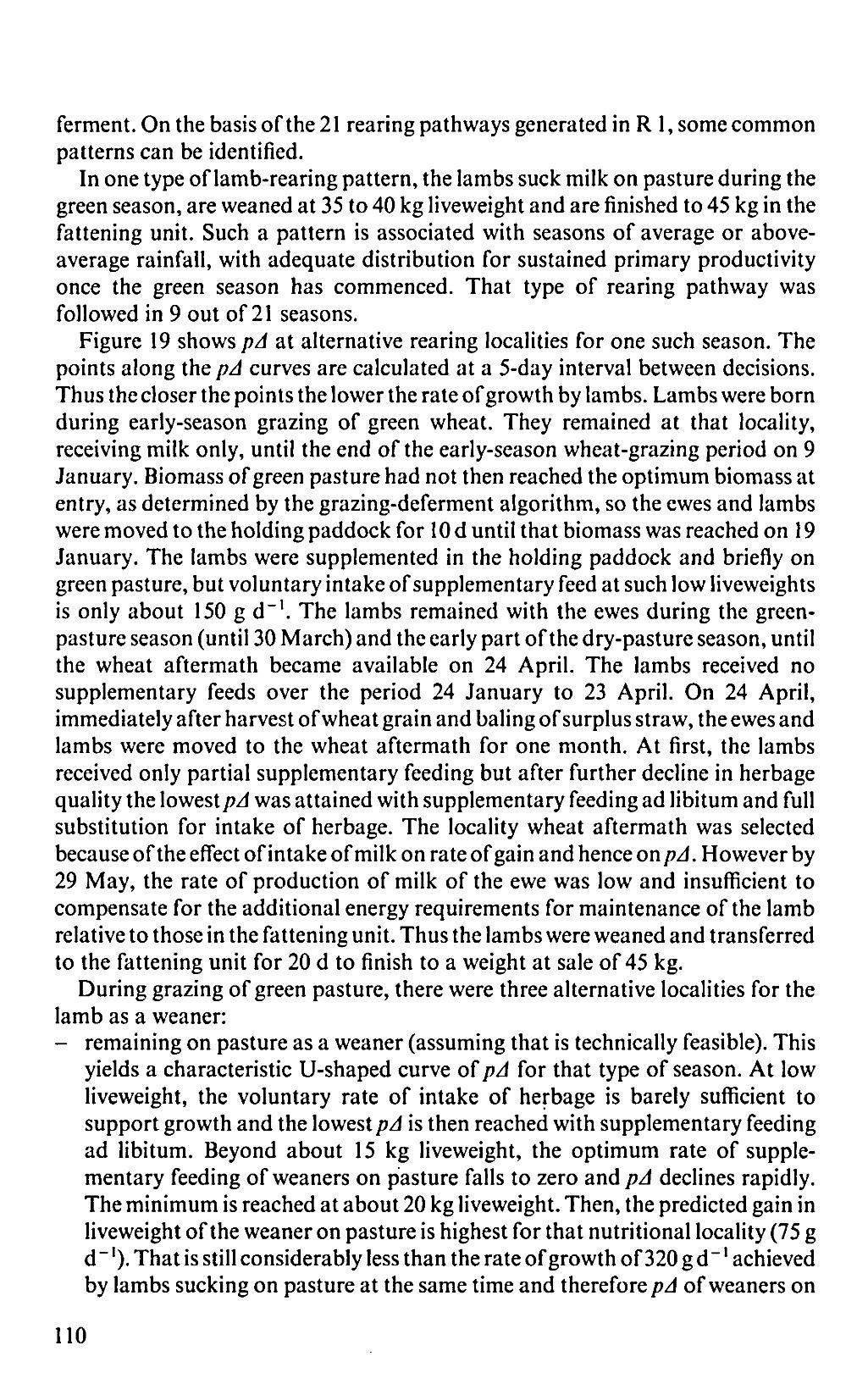
ferment. On the basis of the 21 rearing pathways generated in R 1, some common patterns can be identified.

In one type of lamb-rearing pattern, the lambs suck milk on pasture during the green season, are weaned at 35 to 40 kg liveweight and are finished to 45 kg in the fattening unit. Such a pattern is associated with seasons of average or above-average rainfall, with adequate distribution for sustained primary productivity once the green season has commenced. That type of rearing pathway was followed in 9 out of 21 seasons.

Figure 19 shows pA at alternative rearing localities for one such season. The points along the pA curves are calculated at a 5-day interval between decisions. Thus the closer the points the lower the rate of growth by lambs. Lambs were born during early-season grazing of green wheat. They remained at that locality, receiving milk only, until the end of the early-season wheat-grazing period on 9 January. Biomass of green pasture had not then reached the optimum biomass at entry, as determined by the grazing-deferment algorithm, so the ewes and Iambs were moved to the holding paddock for 10 d until that biomass was reached on 19 January. The lambs were supplemented in the holding paddock and briefly on green pasture, but voluntary intake of supplementary feed at such low liveweights is only about 150 g d"1. The lambs remained with the ewes during the green-pasture season (until 30 March) and the early part of the dry-pasture season, until the wheat aftermath became available on 24 April. The lambs received no supplementary feeds over the period 24 January to 23 April. On 24 April, immediately after harvest of wheat grain and baling of surplus straw, the ewes and lambs were moved to the wheat aftermath for one month. At first, the lambs received only partial supplementary feeding but after further decline in herbage quality the lowest pA was attained with supplementary feeding ad libitum and full substitution for intake of herbage. The locality wheat aftermath was selected because of the effect of intake of milk on rate of gain and hence on pA. However by 29 May, the rate of production of milk of the ewe was low and insufficient to compensate for the additional energy requirements for maintenance of the lamb relative to those in the fattening unit. Thus the lambs were weaned and transferred to the fattening unit for 20 d to finish to a weight at sale of 45 kg.

During grazing of green pasture, there were three alternative localities for the lamb as a weaner: - remaining on pasture as a weaner (assuming that is technically feasible). This

yields a characteristic U-shaped curve otpA for that type of season. At low liveweight, the voluntary rate of intake of herbage is barely sufficient to support growth and the lowest pA is then reached with supplementary feeding ad libitum. Beyond about 15 kg liveweight, the optimum rate of supple­mentary feeding of weaners on pasture falls to zero and/?A declines rapidly. The minimum is reached at about 20 kg liveweight. Then, the predicted gain in liveweight of the weaner on pasture is highest for that nutritional locality (75 g d "'). That is still considerably less than the rate of growth of 320 g d ~ * achieved by lambs sucking on pasture at the same time and therefore/?^ of weaners on

110

fattening unit

JAN 9 19 i—r

wheat

pasture

weaned

sucking ["""]

weaned

sucking

holding weaned paddock

sucking

"•!"» ••"" rrj\

*

Q

APR 24 T

P E

MAY 29 T

supplementation I I ad libitum ^ intermediate • zero

_ 1.6

^ 1.4 •1 — 1.2 = .E 1.0

§. ro0.8

o | 0.4 h

£ 0.2 h 0.0

A

X w T O

1 * *

?M^' oonn * M

x xx

* * * * *

a holding paddock * pasture, sucking x pasture, weaned o wheat, sucking A wheat, weaned + fattening unit

0 5 10 15 20 25 30 35 40 45

lamb liveweight (kg)

Figure 19. Time course of the cost per unit liveweight gain of the lamb, and the optimum supplementation level, at alternative rearing localities in one season (1964) of the standard run.

pasture does not reach the low values achieved by sucking lambs. Between 20 and 25 kg liveweight, the effect of declining herbage quality on rate of growth outweighs the effect of an increasing voluntary rate of intake and pA rises. Beyond 25 kg, herbage quality is too low to sustain growth and supplementary feeding switches (with small fluctuations) to ad libitum by the end of the green season. When supplementary feeding is ad libitum on pasture and availability of herbage is not limiting, there is virtually complete substitution of supple­mentary feed for herbage. Thus the only difference between the nutritional localities of weaners on pasture with supplementary feed ad libitum and the fattening unit is a lower requirement for maintenance of the housed animal.

I l l

That gives a small advantage in pA to the fattening unit. - The lambs could have been weaned during grazing on green pasture and

moved to the wheat for strip-grazing as an alternative to harvesting for grain. The expected grain yield resulted in a high value of grazed wheat herbage (Equation 24). Consequently, pA was lowest when supplementary feeds were provided ad libitum with complete substitution for wheat herbage. At the optimum rate of supplementary feeding, pA was slightly greater than that in the fattening unit through the small difference in energy requirements for maintenance at the two localities.

- Weaning the lambs and moving them to the fattening unit during the period of grazing green pasture would have resulted in a considerable increase in pA. The fattening unit cannot compete with a locality that provides both milk and quality herbage. A second type of pathway of lamb rearing occurs in years of extreme drought or

years with exceptionally poor rainfall distribution. The lambs are largely reared in the holding paddock, receiving milk and concentrates ad libitum. Since availabil­ity of herbage is low, the options for rearing lambs are the holding paddock on concentrates ad libitum plus milk or the fattening unit on the same diet of concentrates. The fact that part of the ewe's intake of supplementary feed in the holding paddock is used to produce milk is taken into account in computing pA. That will tend to counterbalance any reduction in pA arising from a higher rate of growth on a diet of milk plus concentrates than on a concentrate only diet. Nevertheless, in each of the four years characterized by that rearing pattern, the model consistently calculated a lower pA on a diet of milk plus concentrates in the holding paddock. Rates of growth by lambs were extremely high, averaging over 300 g d"1 for the four seasons and lactation continued till the lambs reached the weight at sale of 45 kg.

However the difference in pA between the holding paddock (supplementary feeds plus milk) and the fattening unit (supplementary feeds only) was often small and so the selected rearing pathway may be sensitive to inaccuracies. One possible inaccuracy is the assumption that milk does not replace concentrates or vice versa. If there is significant substitution, rates of growth by lambs would be slightly lower in the holding paddock than predicted, and pA in the holding paddock might exceed that in the fattening unit.

A third type of lamb-rearing pattern can be characterized as sucking on pasture until availability of green herbage limits intake, followed by weaning at 25 to 30 kg liveweight, and finishing in the fattening unit. Such a pattern is associated with seasons with rainfall below average. That rearing pathway was followed in 5 out of 21 seasons. In each case, availability of pasture became limiting during the green season and the ewes had to be supplemented on pasture. That resulted in an affirmative reply from the algorithm for late-season grazing of green wheat for the ewe. For the lambs, however, pA on wheat was higher than in the fattening unit and so the lambs were weaned and moved to the fattening unit.

When the option of grazing the green wheat late in the season was blocked to

112

the ewe (Table 16, R4) or when the lamb was forced to follow the ewe to late-season grazing of green wheat (Table 16, R6), weaning was considerably delayed in those five seasons and a different rearing pathway was followed. Such a marked change in rearing pathway was not forced in those two runs. The lambs could have been weaned within a few days of the weaning date in the standard run. Total supplementary feeding of lambs was reduced but that was offset by a greater increase in total supplementary feeding of ewes.

It is seasons of that third type that pose the most difficult decisions. In years with sufficient rainfall or in years of serious drought, the rational decision is either obvious or there are few alternative courses of action. In the intermediate seasons, different management pathways can be triggered by a single decision at a sensitive phase in the season. Here again, robustness of the system to alternative rational pathways of management tends to minimize the financial risk of uncertainty in making decisions.

8.6.2 Effect of a fixed weaning age

In view of the fact ihaipA is significantly lower when the Iamb is receiving milk, one might expect forced early weaning to have a negative effect on profitability. To examine that question, the lamb-rearing algorithm was adjusted to block all weaner localities before the lamb has reached a minimum age and to block all sucking localities after that age.

Forcing weaning at 34 d old reduced mean gross margin by only 7% to 269.3 $ ha - ' (Table 18, R 50). Forcing weaning at 64,94,123 or 147 d old (Table 18, R 51, R 52, R 72, R 73, respectively) had virtually no effect on mean gross margin. That remarkable robustness was obtained despite large effects on the management pathway of the ewe and lamb. As the age of forced weaning increased, the ewe increased its total intake of green pasture (through higher energy requirements), decreased its total intake of dry pasture (through a lower availability at the end of the green season) and increased its total intake of wheat aftermath (through lower availability of dry pasture). There was also an increase in time spent in the holding paddock and a reduction in baling of straw through increased utilization of herbage by both ewe and lamb. For the lamb, there was a trade-off between the time spent grazing and the time in the fattening unit. Earlier weaning increased the time spent in the fattening unit and hence total supplementary feeding of lambs, but the additional cost was balanced by a reduction in total supplementary feeding of ewes. The ewe required less purchased supplementary feed with earlier forced weaning because its body condition was higher at critical phases of the physiological cycle, more straw was baled and total energy requirements were slightly reduced.

Meat production is constant over the various management options being examined. That may be an unrealistic assumption, even under target-oriented management, if weaning age influences mortality of lambs or general state of health. One way of interpreting those results is to say that it is precisely manager-

113

Table 18. Summary of the results for the standard run and runs related to weaning according to age of lamb. Run Number 1: standard run, weaning by normal criteria.

Variable Value for Run Number

1 50 51 52 72 73

age at weaning (d) mean gross margin in system ($ ha-1) number of seasons straw baled (I) total amount of straw baled in system (kg ha"1) total amount of straw utilized in system (kg ha"') mean intake of concentrates by ewes in system (kg ha-1) mean intake of concentrates by lambs in system (kg ha-') mean yield of grain harvested in system (kg ha"1) mean age at weaning (d) mean time spent by ewes in holding paddock (d) mean intake of herbage and straw by ewes in system (kg ha-1) mean intake of herbage by lambs in system (kg ha-1) mean age of lambs at sale (d) mean time spent in fattening unit (d) mean total requirement of metabolic energy per ewe (MJ year-1)

30 60 90 120 150 289.6 269.3 282.1 288.3 288.2 286.7 8 9 9 9 8 8 14190 18436 17826 17037 15000 13645

10224 12175 11914 11523 10359 9568

547 359 425 485 553 589

449 693 579 495 437 417

787 805 805 792 772 765

93 34 64 94 96 88 91 94

123 147 100 101

2041 2007 2055 2086 2047 2032

330 187 197 229 307 342

171 184 160 153 162 165 58 71 56 43 30 16 6470 6197 6368 6453 6480 6490

related and site-specific factors (such as the effect of weaning age on total meat output) that should dictate the management option, in view of the considerable robustness to weaning age.

8.6.3 Inclusion of sown legume for lamb grazing

Although the inclusion of sown legume in the agropastoral system was defined earlier as a strategic decision, that management option is most appropriately discussed together with tactical decisions about lamb rearing. Viewed in isolation, sown legume swards do possess some advantages over non-leguminous swards (Section 4.1). However within the system, the fact that the area of at least one

114

other component must be reduced in order to include the legume is itself a disadvantage. If an area of wheat is displaced by the introduction of legume, there is a reduction in income from grain and availability of straw. If an area of pasture is displaced by the legume, grazing pressure by ewes on pasture is increased. That will effect the ewe's requirements for supplementary feed through the effect on total production of herbage and the deferment of pasture grazing. Those negative effects must be more than compensated by the saving in supplementary feeding of lambs achieved by the introduction of legume. In the agropastoral model, the costs of sowing and maintaining a legume sward are not included in the financial balance. However, assuming a sward life of 5 years, the mean annual production costs of a legume (medic) sward are about 100 S ha-1 (R. Benjamin, personal communication). Thus the mean gross margin would need to increase by at least 10 $ ha-1 to allocate an area of 0.1 ha to medic.

Results of the model did not generally favour use of a special-purpose pasture for the lambs. Relative to the standard run, allocation of an area fraction of 0.45, 0.45,0.1 to natural pasture, wheat and medic, respectively, decreased mean gross margin by about 1 % (Table 19, R 30). Increasing the area fraction of medic to 0.2 and 0.3 of the system, with the remainder divided equally between pasture and wheat, reduced mean gross margin by 3 and 9%, respectively (Table 19, R 31 & R 32). Not only did total supplementary feeding of ewes increase with increasing area under medic, as expected, but total amount of supplementary feed to lambs was also increased in the 3-component systems. That is a surprising result, especially since total utilization of herbage and total utilization of medic by lambs increased with increasing area under medic and the average time spent in the fattening unit decreased with increasing area under medic. However the increase in utilization of medic in R 30, R 31 and R 32 was much greater than the increase in utilization of herbage by the lambs. In other words, a significant portion of utilization of medic simply replaced utilization of herbage at other grazing localities. Furthermore, inclusion of medic resulted in earlier weaning and so a further portion of medic utilization can be regarded as replacing forfeited intake of milk. Whilst the average time spent by the lambs on concentrates ad libitum in the fattening unit was markedly reduced by the inclusion of an area under medic, the lambs did receive supplementary feed for a significant portion of the time spent on medic. That was due to low availability or quality of medic late in the season, supporting only low rates of growth by lambs and yielding a higher pA without supplementary feeds than with intermediate or supplementary feeding ad libitum.

In R 70 and R 71 (Table 19), the area fraction under wheat was maintained at 0.5 of system area and medic was introduced at the expense of natural pasture only. An allocation of an area fraction of 0.1 to medic increased mean gross margin by 1 % but increasing the medic allocation to 0.2 reduced mean gross margin by 3%. In R 70, the performance of lambs is similar to that in R 30. Once again, total amount of supplementary feed to lambs was increased relative to R 1. However there was a small increase in utilization of straw by the ewes and a small

115

Table 19. Summary of results for the standard run and runs related to the inclusion of medic area in the system. Run Number: 1 standard run; 78 with improved' medic; 79 with 'improved' medic, medic cannot trigger weaning.

Variable Value for Run Number

1 30 31 32 70 71 78 79

area fraction of system to pasture (1) 0.50 0.45 0.40 0.35 0.40 0.30 0.40 0.40 area fraction of system to wheat (1) 0.50 0.45 0.40 0.35 0.50 0.50 0.50 0.50 area fraction of system to medic (1) 0 0.10 0.20 0.30 0.10 0.20 0.10 0.10 mean gross margin in system (Sha"1) 289.6 286.1 280.2 263.8 292.8 280.2 304.6 297.3 number of seasons straw baled (1)8 8 8 6 8 8 8 8 total amount of straw baled in system (kg ha"') 14190 11598 9519 7355 13544 11131 14648 12730 total amount of straw utilized in system (kg ha"1) 10224 8986 8284 6197 10602 8194 10983 10353 mean intake of concentrates by ewes in system (kg ha"1) 547 560 573 610 530 595 512 549 mean intake of concentrates by lambs in system (kg ha"') 449 462 468 489 485 512 453 448 mean yield of grain harvested in system (kg ha"1) 787 719 635 554 798 800 800 784 mean age at weaning (d) 128 102 92 80 92 75 87 114 mean age of lambs at sale (d) 167 173 187 195 174 192 176 178 mean time spent on medic (d) 0 37 63 77 44 76 60 44 mean time spent in fattening unit (d) 58 30 24 27 30 25 22 14 mean intake of medic by lambs in system (kg ha"1) 0 145 259 335 168 301 265 202 mean rate of intake of medic per lamb (kg d'1) 0 0.74 0.78 0.82 0.72 0.75 0.84 0.87 mean intake of herbage by lambs in system (kg ha"1) 330 394 469 497 379 454 448 441 mean intake of herbage and straw by ewes in system (kg ha"1) 2041 1891 1782 1586 1930 1675 1943 1956

116

reduction in total supplementary feeding of ewes. That tended to cancel the increase in supplementary feeding of lambs and thus there was little overall effect on gross margin. The difference in total amount of supplementary feed to ewes or lambs between R 1 and R 70 shows a variable pattern (Figure 20). To account fully for the year-to-year differences in rate of supplementary feeding would require a detailed analysis beyond the scope of this study. Carry-over effects from season to season complicate the analysis. Such effects include the body condition

(a) ewes

CD , -

8.1 CD CD

05

100 r

CO

-c 50

0? M. _D_ -a-°.

«= § -50 f E

a-ioo C/5

-150

• o

1962 year

1982

JO

c .9

•^= CD

"o E _CD Q . Q .

CO

(b) lambs

250

200

150

100

50

0

-50 h

100

_Q- ~B- TTTJ M- O •• • ET

1962 1982 year

Figure 20. The effect of allocating 10% of system area to a medic sward on total supple­mentary feed intake over 21 years. Points indicate the difference in total supplementary feed intake each season between a system with 0.4, 0.5, 0.1 ha pasture, wheat, and medic, respectively (R70), and the standard run (R 1). A. Ewes. B. Lambs.

117

of the ewe and the amount of dry herbage remaining from the previous green season when the new season begins on 1 October. Not surprisingly though, the difference in total supplementary feeding of lambs correlates with the difference in lamb weight at which the final 'finishing' phase of supplementary feeding ad libitum begins.

The disappointing performance on medic may be due to poor parametrization of the model. To examine the sensitivity of the model to performance on medic, the digestibility of grazed herbage was increased by 30% or set equal to the calculated digestibility of green leaf, whichever was the lower. Those changes were implemented in R78 (Table 19), which was the same as R70 in all other respects. Relative to R 70, total utilization of medic was increased by 58% in R 78 but part of that increase replaced intake at other localities. Total amount of supplementary feed for lambs was lower in the 'improved medic' run but it was still higher than in R 1. Mean gross margin increased by 5% relative to R 1.

One possible problem with the selected pathway of lamb rearing in the systems including medic is that the lambs are weaned and moved to the medic sward too early. Besides forfeiting milk, early grazing of the medic may reduce availability at the end of the season of natural green pasture, just when the medic is most needed. To examine that possibility, the lamb-rearing algorithm was adjusted in R 79 to block the option of moving the lambs to the medic sward until after weaning, i.e. the medic sward itself could not trigger early weaning. In lamb performance, R 79 yielded promising results (Table 19). Total supplementary feeding of lambs was lower than in R 1, average weaning age was significantly later than in R78, average time in the fattening unit was reduced to two weeks and average daily intake on medic was the highest of all the runs with a medic component. But later weaning relative to R78 increased total utilization of non-medic herbage by the lamb. That ultimately caused total intake of supplementary feed by ewes to increase. The causal chain probably acted through reduced availability of pasture to the ewe, increased wheat aftermath requirement of the ewe, reduced baling of straw and so increased intake of supplementary feed. Mean gross margin in R 79 was slightly lower than in R78, indicating that the standard lamb-rearing crite­rion of minimum pA during decision, without any further complications, is a rational policy.

The inclusion of a medic sward in the agropastoral system seems not to improve profitability markedly. Unless there are factors that favour introduction of a medic sward that are not considered in the model, it can probably be regarded as a marginal option. One factor that has weighed in favour of inclusion of a medic sward at Migda has been the poor performance of lambs at natural pasture with a high fraction of Hordeum murinum. Late in the green season, the awns of Hordeum species can cause serious eye sores and impair performance. Since the model indicates that inclusion of medic in the absence of such problems has little effect on overall performance, one can assume that medic could make a significant contribution to overall performance when such problems exist.

118

8.7 Prices and price ratios

The prices of meat and purchased concentrates are critical parameters in the agropastoral system. Both the price ratio of meat to feed and the absolute prices have a strong influence on the economic performance of the integrated system. To illustrate this, a price ratio of meat to feed of 5 was taken, using different absolute prices. In R37, the price of meat was halved to 1.25 Skg"1. In R38, the prices of purchased concentrate and wheat grain were doubled to 0.50 and 0.44 $ kg-1, respectively. (A constant ratio between the prices of concentrate and grain was maintained in all runs.)

Mean gross margin in R37 and R38 was 5.6 and 245.9 $ ha-1, respectively, compared with 289.6 S ha-1 in the standard run. In both runs, the reduction in amount of meat sold was about 15%. That was because the lower price ratio of meat to grain caused/7 A to exceed the price of meat before the lambs reached the maximum weight at sale of 45 kg. On average, weaning was a week earlier and Iambs were sold about 25 d younger. The average time spent in the fattening unit was reduced from 25 d in R 1 to 6 d at the lower price ratio. The effect on gross margin was largely compensated in R 38 by the higher price received for grain in the wheat component of the system. There were no such compensatory features when the price of meat was changed in R37 and so mean gross margin was drastically reduced.

The absolute prices of feed and grain can affect lamb-rearing decisions, inde­pendently of the price of meat. The price of feed appears in the calculation of the price of milk when the ewes are being supplemented (Equation 98) and the price of grain appears in the calculation of the price of grazed wheat herbage when grazed late in the green season (Equation 24). Thus the ranking of alternative Iamb-rearing localities according top J and hence the rearing pathway could be altered by a change in prices of feed and grain. However one would expect only a small, perhaps negligible, impact on system performance.

8.8 Stocking rate

With target-oriented nutrition (i.e. the output per animal is based on potential production), the relation between gross margin and stocking rate has some predictable features. First, meat output and thus income increases linearly with stocking rate. We make the reasonable assumption that the price with respect to feed value of supplementary feed is greater than that of grazed herbage. Since the amount of nutrients that a grazed sward can provide is finite, the cost of income generated (the 'average cost') must increase over some range of stocking rate. Over this range, the function of total cost will therefore be convex (F'(.v)>0) and the gross margin function will be concave (f'(*)<0). Over a broader range of stocking rate, however, the function of gross margin may increase monotonically or be truly concave, depending on the price ratio of meat to feed (Figure 21). The

119

(a) meat:feed price ratio=10:1

C3 JZ &

e o o c

o o

1400

1200

1000

800 h

n total income • total costs A gross margin x grain income

/

2 4 6 8 stocking rate (ewes ha "1)

v fixed pasture costs, wheat fertilizer, cultivation, sowing, and grain harvesting costs

o^N veterinary, insurance, and miscellaneous animal costs

total ewe and lamb feed costs

03

o E o o c

o o

(b) meat:feed price ratio=5:1

D total income • total costs A gross margin x grain income

///. fixed pasture costs, wheat fertilizer, cultivation, sowing, and grain harvesting costs

\

^ s veterinary, insurance, and miscellaneous animal costs

total ewe and lamb feed costs

stocking rate (ewes ha"1)

Figure 21. Costs, income, and gross margin as a function of stocking rate, at two meat: feed price ratios. A. Meat: feed price ratio = 10:1. B. Meat: feed price ratio = 5:1.

lower price ratio came about by doubling the price of concentrates and of wheat grain.

The curve for total cost is divided into three components. - Fixed costs for pasture, wheat fertilizer, cultivation, sowing, and costs of

harvesting grain. Since the area fractions are pasture 0.5 and wheat 0.5 over all stocking rates, and the area of green wheat grazed as an alternative to harvesting for grain (and hence costs of harvesting grain) varied only slightly with stocking rate, the sum of those costs is almost constant with stocking rate. Neither is it affected by the price ratio of meat to feed.

- Veterinary, insurance and miscellaneous costs of animals. The veterinary and insurance costs are constant per animal. Miscellaneous costs are defined as 10% of the sum of costs of concentrates for the ewe, veterinary services and insurance. That is almost linear with stocking rate.

120

- Total costs of feed for ewes and lambs. That is defined as the sum of average annual intake of straw, poultry litter and concentrates by the ewe, plus the average annual intake of concentrates by the lamb multiplied by the respective prices. That function is not linear with stocking rate and indicates that the cost of feed per animal is not constant with stocking rate.

At both price ratios, the function for total cost appears to be comprised of two linear sections, with an inflection point at a stocking rate for ewes of 4 ha"1. That can be explained by examining the intake per ewe of grazed herbage, straw and concentrates (Table 20). Total intake of grazed herbage per ewe decreases monot-onically with stocking rate. However up to a stocking rate of 4 ha"1, there is sufficient surplus straw for grazing in the dry season to buffer the decline in intake of grazed herbage per ewe (i.e. total intake of grazed herbage plus baled herbage is almost constant up to 4 ha -1). Thus over that range of stocking rate, intake of concentrates per ewe is almost constant and represents some 'obligatory' mini­mum requirement of concentrates at even the lowest stocking rate. At a stocking rate above 4 ha"1, the intake of straw per ewe declines steeply with stocking rate and that is compensated by increasing feeding with concentrates at a ratio of about 0.5 kg concentrates per kg straw. So the functions for total cost at different prices of feed are not parallel. The effect of price of feed can be seen in Figure 22, which shows the average cost as a function of stocking rate. Average cost is almost constant up to 4 ha " l and afterwards increases at a slope that depends on the price of feed.

The total income curve in Figure 21 is divided into two components. - Income from grain. That is defined as the product of the average yield and

price of grain. Since the area of green wheat grazed as an alternative to harvesting for grain varied only slightly with stocking rate, the function for income from grain is almost constant with stocking rate for any price of grain.

- Meat income. That is defined as the sum of the income from lamb's meat and meat from culled ewes. The function of meat income is linear with stocking rate, though the slope of the function may vary with price ratio of meat to feed (Figure 21).

The function for gross margin in Figure 21 is essentially the difference between the total income and total cost, though the cost of baling straw that was not used was added, since that can represent a significant and unrealistic penalty at low stocking rates. (The other difference between the gross margin plotted in Figure 21 and that computed by the model is interest charges on periods of negative financial balance. Those charges are small and can be ignored for present purpos­es.)

At a price ratio of meat to feed of 10, the function for gross margin is concave in the region of a stocking rate for ewes of about 4 ha"1 but overall increases monotonically. The function does not have a maximum and a completely housed meat production system (without integration of any kind) returns a positive gross margin at that price ratio. At a price ratio of meat to feed of 5, the function for gross margin is overall concave and has a maximum at about 4 ha"1. In other

121

9 Summary

This study examines the management of intensive integrated agropastoral systems in a semiarid region where conventional pathways of agricultural in­tensification are technically and economically feasible.

Unpredictability and variability of rainfall creates the need to distinguish between tactical and strategic decisions. A strategic decision is taken independ­ently of the state of the system at the time of decision as well as independently of the expected short-term to medium-term performance of the system. A tactical decision is taken in response to the immediate state of the system or in consid­eration of the expected performance of the system in the short to medium term. Different approaches are appropriate for treating those two decision classes. Furthermore, imperfect knowledge of the biology of the system, both in terms of understanding (model formulation) and information (monitoring for imple­mentation), is a constraint that should impinge on the approach adopted.

The agropastoral model is comprised of separate management and biological sections. The subroutine for primary production is based upon an existing simulation model (van Keulen, 1975) and secondary production subroutines are based upon a widely adopted feeding system (GB-ARC, 1980). Strategic deci­sions are defined by a set of parameters that remain constant over each sim­ulation. Tactical decisions are treated individually by a series of optimization subroutines.

Supplementary feeding of ewes is target-oriented. Feeding is adjusted to ensure the achievement of production targets, which are set close to the animal's potential. The ewe's liveweight is allowed to fluctuate during the reproductive cycle when that is not expected to have a detrimental effect on productive performance.

The grazing schedule of the ewe is determined by a user-determined priority-ranking of all possible localities in the system and a series of optimization routines that determine when each locality should be grazed. The ewe is moved to the highest-ranking locality that is deemed grazable by the optimization routines.

Deferment of grazing on pasture can be critical to system dynamics. The optimum time to commence grazing is defined as that maximizing total intake of herbage. Intake of herbage is defined as total intake of green and dry herbage, allowing for utilization of wheat aftermath and the relative nutritive value of green and dry herbage. The solution is found numerically with a simple two-function model. Despite its compactness, the deferment model may well have provided the deepest insight into the general properties of a large class of grazing systems.

Early-season grazing of green wheat (not as an alternative to grain) can

125

10 References

Anderson, J.R., 1974. Simulation: methodology and application in agricultural economics. Review of Marketing and Agricultural Economics 42:3-55.

Arnold, G.W. & de Wit, C.T., 1976. Critical evaluation of systems analysis in ecosystem research and management. Pudoc, Wageningen. 114 pp.

Aschmann, H., 1973. Distribution and peculiarity of Mediterranean ecosystems. In: F. di Castri & H.A. Mooney (Eds): Mediterranean type ecosystems. Springer-Verlag, New York. p. 11-36.

Benjamin, R.W., Chen, M., Degen, A.A., Abdul-Aziz, N. & Al Hadad, M.J., 1977. Estimation of the dry- and organic-matter intake of young sheep grazing a dry mediter­ranean pasture, and their maintenance requirements. Journal of Agricultural Science, Cambridge 88:513-520.

Benjamin, R.W., Eyal, E., Noy-Meir, I. & Seligman, N.G., 1976. [The effect of sheep grazing on the grain yield and total dry matter production of wheat in an arid region.] Hassadeh 57:754-759 (Hebrew with English summary).

Benjamin, R.W., Eyal, E., Noy-Meir, I. & Seligman, N.G., 1982. [Intensive agro- pastoral systems at the Migda experimental farm in the Northern Negev.] Hassadeh 62:2022-2026 (Hebrew with English summary).

Benjamin, Y., 1983. A management model of a grassland sheep system under Israeli conditions. M.Phil, thesis, University of Reading, Reading. 162 pp.

Bennett, D. & Ozanne, P.G., 1973. Deciding how much superphosphate to use. Annual Report Division of Plant Industry 1972, CSIRO, Australia, p.45- 47.

Blaxter, K.L. & Boyne, A.W., 1978. The estimation of the nutritive value of feeds as energy sources for ruminants and the derivation of feeding systems. Journal of Agricultural Science, Cambridge 90:47-68.

Blaxter, K.L., Fowler, V.R. & Gill, J.C., 1982. A study of the growth of sheep to maturity. Journal of Agricultural Science, Cambridge 98:405-420.

Bowden, L., 1979. Development of present dryland farming systems. In: A.E. Hall, G.H. Cannell & H.W. Lawton (Eds): Agriculture in semi-arid environments. Springer-Verlag, Berlin, p.45-72.

Breman, H. & de Wit, C.T., 1983. Rangeland productivity and exploitation in the Sahel. Science, Washington 221:1341-1347.

Christian, K.R., Freer, M., Donnelly, J.R., Davidson, J.L. & Armstrong, J.S., 1978. Simulation of grazing systems. Simulation Monographs, Pudoc, Wageningen. 115pp.

Dalton, G.E., 1975. Study of agricultural systems. Proceedings of a symposium on the study of agricultural systems, University of Reading, Reading. Applied Science Publish­ers, London. 441pp.

Dann, P.R., 1968. Effect of clipping on yield of wheat. Australian Journal of Experimental Agriculture and Animal Husbandry 8:731-735.

129

Dent, J.B. & Anderson, J.R., 1971. Systems analysis in agricultural management. Wiley, Sydney. 394 pp.

di Castri, F., 1981. Mediterranean-type shrublands of the world. In: F. di Castri, D.W. Goodall, & R.L. Specht (Eds): Ecosystems of the world. 11. Mediterranean-type shru­blands. Elsevier, Amsterdam, p. 1-52.

Duhem, P., 1953. Physical theory and experiment. In: H. Feigl & M. Brodbeck (Eds): Readings in the philosophy of science. Appleton-Century-Crofts, New York, p.235-252.

Dyckman, T.R., Smidt, S. & McAdams, A.K., 1969. Management decision making under uncertainty. Macmillan, London. 662 pp.

Emory, C.W. & Niland, P., 1968. Making management decisions. Houghton Mifflin, New York. 306 pp.

Eyal, E., Benjamin, R.W. & Tadmor, N.H., 1975. Sheep production on seeded legumes, planted shrubs, and dryland grain in a semi-arid region of Israel. Journal of Range Management 28:100-107.

Feigenbaum, Sala, Seligman, N.G., Benjamin, R.W. & Feinerman, Dvorah, 1983. Recov­ery of tagged fertilizer nitrogen applied to rainfed spring wheat (Triticum aestivum L.) subjected to severe moisture stress. Plant and Soil 73:265-274.

GB-ARC, 1965. The nutrient requirements of farm livestock. No.2: Ruminants. HMSO, London.

GB-ARC, 1980. The nutrient requirements of ruminant livestock. Farnham Royal, Com­monwealth Agricultural Bureaux, Slough, England. 351 pp.

Graham, N. McC, Black, J.L., Faichney, G.J. & Arnold, G.W., 1976. Simulation of growth and production in sheep - model 1: A computer program to estimate energy and nitrogen utilisation, body composition and empty liveweight change, day by day for sheep of any age. Agricultural Systems 1:113-138.

Grigg, D.B., 1974. The agricultural systems of the world - an evolutionary approach. Cambridge University Press, London. 358 pp.

Huss, D.L., 1964. A glossary of terms used in range management. Range Term Glossary Committee (D.L. Huss, Chairman), American Society of Range Management, Portland, Oregon, 32 pp.

Kahn, H., 1982. The development of a simulation model and its use in the evaluation of cattle production systems. Ph.D. thesis, University of Reading, Reading. 266 pp.

Luria, M., 1984. Population dynamics of annual plants in fertilised grassland grazed by sheep. Ph.D. thesis, Hebrew University, Jerusalem.

McKinney, G.T., 1972. Simulation of winter grazing on temperate pasture. Proceedings of the Australian Society of Animal Production 9:31-37.

Noy-Meir, I., 1975. Primary and secondary production in'sedentary and nomadic grazing systems in the semi-arid region: analysis and modelling. Department of Botany, Hebrew University, Jerusalem. Research report to the Ford Foundation, Project 7/E-3.

Osuji, P.O., 1974. The physiology of eating and the energy expenditure of the ruminant at pasture. Journal of Range Management 27:437-443.

Penning de Vries, F.W.T. & Djiteye, M.A., 1982. La productivite des paturages Saheliens. Pudoc, Wageningen. 525 pp.

130

Riggs, J.L., 1968. Economic decision models. McGraw-Hill Book Company, New York. 401 pp.

Spedding, C.R.W., 1975. The biology of agricultural systems. Academic Press, London. 261 pp.

Spedding, C.R.W., 1979. Prospects and limitations of operations research application in agriculture-agrobiological systems. Paper presented at ORAGWA conference, Jerusa­lem, November 1979.

Tadmor, N.H., Eyal, E. & Benjamin, R.W., 1974. Plant and sheep production on semiarid annual grassland in Israel. Journal of Range Management 27:427-432.

Thornton, R.F. & Minson, D.J., 1973. The relationship between apparent retention time in the rumen, voluntary intake, and apparent digestibility of legume and grass diets in sheep. Australian Journal of Agricultural Research 24:889-898.

Ungar, E.D., 1984. Management of agro-pastoral systems in a semi-arid region. Ph.D. thesis, Hebrew University, Jerusalem. 169 pp.

Ungar, E.D. & van Keulen, H., 1982. FORTRAN version of the simulation model ARID CROP. CABO, Wageningen. 39 pp. Simulation report CABO-TT No 1.

van Keulen, H., 1975. Simulation of water use and herbage growth in arid regions. Simulation Monographs. Pudoc, Wageningen. 176 pp.

van Keulen, H., Seligman, N.G. & Benjamin, R.W., 1981. Simulation of water use and herbage growth in arid regions - a re-evaluation and further development of the model 'ARID CROP'. Agricultural Systems 6:159-193.

Walker, B.H., 1979. Management of semi-arid ecosystems. Elsevier, Amsterdam. 398 pp. Wood, P.D.P., 1967. Factors affecting the shape of the lactation curve in cattle. Animal

Production 11:307-316. Yanuka, M., Seligman, N.G. & Benjamin, R. W., 1981. The effect of defoliation early in the

growing season on the production of some improved barley and wheat cultivars in a semi-arid region of Israel. Internal report (mimeo). Department of Range Science, Agricultural Research Organization, Bet Dagan, Israel.

131

11 Listing of model

AGRO-PASTORAL SYSTEM MODEL

C C C C C C C C

ST IMPLICIT

INTEGER *

#

*

*

#

*

*

• *

PARAMETER CHARACTER*7

DIMENSION

TAPEIO -TAPE40 -TAPE50 -TAPE62-82 TAPE60 -TAPE90 -TAPE9S -TAPE99

REAL(A-Z)

BSYS, DELT,

GRAZL, ELS,

LAMB, MNGDEL,

NY, SEADY, MEAN,

STROP, (NR0=34) NAME(NRO)

PARAMETERS AND FUNCTION TABLES HISTORICAL RAINFALL RECORDS DIARY ENTRIES MET DATA FILES LAMB REARING SPECIAL TRACE DEBUG OUTPUT TABULAR OUTPUT SUMMARY TABLE

COL, EWELOC,

6R0DY, JJ,

LAMBD, Msy,

PLOW, SELL,

WEANED, DIDHRV,

CULL, EWEMAT,

HARV, JOIN,

LAMLOC, LLS,

PLOWD, SOW,

WST2BL, GDDEC,

II,12,13,Jl,DAY, FERT, FERTD,

HYOP, K,

LMM, NDPREG, PRIORT, STARDY,

YEAR,

IRN15, JOIND,

LAMMAT, NDLACT,

PRDEL, SOWD,

Y, NCAFG

DEB, GRAZE,

6EST, LA6E,

MATCH, NRO,

RATIN6, TIME,

YR,

*

«

*

*

*

*

*

ft

*

•

ft

ft

ft

ft

I ft

ft

DIMENSION

AREAC3) CRDLC3)

CRLVSC3) CSRRTW(2,15)

DEBC13) DISTFTW(2,12)

DRF(3,10) DVRT(2,5>

EFFEC3) EWEMAT<6>

FLTRT(2,10) GRNLVC3)

6RRTC3) IBI0MC3)

LAK3) LFK3)

LPDMIT(2,6>

MNEBCTC4,19> PRI0RTC6)

ALPHAT(7,25) ARFC16)

CRDNLC3) CRNLVSC3) CTRDEFC3)

DISTFTC2.5) DLBI0C3)

DRR(3,10) DVSC3)

EB(3,10> ENGRC3)

FAMSTT(2,5) 6RAINT<2,14)

GR0DYC3) 6RRWTC3)

IRWTC3) LAMMATC8) LMBI0MC3)

MAT(NRO,10)

MWATER(IO) PRVDVSC3)

AMAXC3) AVLARC3)

CRLFARC3) CSRRT(2,7)

DBI0MC3) DISTFTM(2,3)

DNLBI0C3) DVRC3) DVXC3)

EDPTFT(2,5) ER(3,10)

FDMT(2,3) GRLVSC3)

6RSDSC3) LAGRTRC3) LFAREAC3)

LMM(8,8/ MATCHC6)

PRVTV(3), PUSHDC3),

OOOl Q002 0003 0004 0005 0006 0007 0008 0009 0010 0011 0012 0013 0014 001S 0016 0017 0018 0019 0020 0021 0022 0023 0024 0025 0026 0027 0028 0029 0030 0031 0032 0033 0034 0035 0036 0037 0038 0039 0040 0041 0042 0043 0044 0045 0046 0047 0048 0049 0050 0051 0052 0053 0054 0055 0056 0057 0058

133

c c

*

#

•

*

*

*

#

*

*

*

*

*

*

*

*

*

•

(((

COMMON *

«

COMMON *

*

*

COMMON COMMON

#

•

«

COMMON *

•

*

*

#

COMMON COMMON COMMON

*

*

COMMON *

*

COMMON •

*

COMMON COMMON COMMON

*

*

*

COMMON COMMON COMMON COMMON COMMON COMMON COMMON

»

•

*

*

•

*

•

/

/

/

/

/

/

/

/

/

/

/

/

/

/

/

/

/

/

/

/

coMoa / APCS , STROP

C0M09 / FORCPH HYHC2 WACH

COMiO / COM11 /

OMF1 , MCRMX QMST

C0M12 / ALFEW , ELP3 MF2 PKF4 SPD ,

C0M13 / C0M14 / C0M15 /

LEP1 , Pnnw

C0M16 / AAP , PKM1 ,

C0M17 / CLLW6 , SLVWT ,

C0M18 / C0M19 / C0M20 /

DACS , 6DI , PGDLIM ,

C0M21 / C0N22 / C0M23 / COM2* / C0M25 / C0M26 / C0M27 /

ALPHAT , CSRRTW , DISTFTW, EB , EVAP , GAMMA , 6RS0S ,

PUSH6C3), RDAMAXC3),

RDLVSC3), RDRDTC2.6),

REDTTB<2,7), RITDFC3),

RTDC3), SLCVRC3),

TDBCIO), T0VSK3),

TMPSUM<3), m

rRAN(3). VRESC3),

WLVSK3), WREDT<2,7),

Y(21), W6CMPEC5),

, BALEC

, HAYLO , HYLEFT

BCP2

, OMP1 , MRP1

, EEP1 , EMYMF , MF3 , RP1 , WEWE

LLWG PTIME

, LEP2 , QMM

, FGF1 , PKM2

, CULL , WAGRL

6RAZL LAGE

, FRC8 , 60TEN0 p 3

DCLV TADRW MN6DEL ARF PRIORT WAGRE

, AMAX , DBIOM , DRR , EOPTFT

FAMSTT , GRAINT

INFR

, PLOWO

, HVCH , HYOP

, 6AP

, 0MP2 , MRP2

, EEP2 , EWMTMF , MFC , RP2

, TOL

, LEP3

, F6F2 , WE

, EBCLIM , WEAN

, 6DCS , GDVM

, OCNLV

, WGWF , COSTH

, AMAXB , DELT , DVR , EFFE , FDMT , GRLVS i K

1

1

t

9

1

1

%

I

f

•

»

f

1

t

I

f

1

1

f

•

I

f

»

t

»

1

1

RADTBC2, 14), RDEFFEC3), RDNLVSC3),

RATIN6C6), RDLFAC3),

RDRATC2.4), RDTDFC3), RE0FDTC2.10),

RFDVST<2,4), RRAMAXC3), RTW6HTC3),

TADRWC3), TDRAINC3), TECT(2,8), T0TRANC3), TRR(3,

W(3, ,10), 10),

WNLVSC3), WSDS(3),

T0TA<6, ,12), W6CMPLC5)

PSTRM

HYCTR HYPF1

LFP

ELWG MRP3

EEP3 KP NDPRE6 RP3

LEP4

GF

LAMLOC WEANED

GODEC 60VMF

RATING

P6RN •

CONFS OGRRT DVRT EFFEB FLDCP GRNLV LAGRTR

, 8TBL

, HYDVS , HYPF2

, EUBL , MRP*

, ELP1 , LBW , NEWL , RP4

, MDMC

, PKF1

, LMM

, GDF , 60V8

, CONFSM , 0ISTF1 , OVSSF , ENGR , FLTRT , GRRT , LAI

RREFFEC3), RWFB<3,10),

TCK(IO), TDRWT(3), TEVAP(3),

TPEVAPC3), TVEGMC3)

WLVSC3), WNLVSK3)

WT0TC3), T0TB(6,12)

, STLEFT ,

, HYHC1 , HYJOPP ,

, MCRMN , , QMMY

, ELP2 , , MF1 , NLB , RP5

, PKF3 ,

, PKF2

, SELL

, GD6 , MNIEW ,

, CSRRT , , DISTFTM , ovx . ER , FWOB , , 6RRWT , , LAT ,

, 0059 , 0060 , 0061 , 0062

0063 , 0064 , 0065 , 0066 , 0067 , 0068 , 0069 , 0070 , 0071 , 0072 , 0073 , 0074

0075 0076 0077 0076 0079

, 0080 0081 0082

, 0083 , 0084

0085 0066 0087

i 0088 , 0089

0090 0091

, 0092 , 0093 , 0094 , 0095

0096 0097 0098 0099

, 0100 Q101 0102

, 0103 0104 0105

, 0106 0107 0108 0109 0110

, 0111 , 0112

0113 0114 0115 0116 0117 0118 0119 0120

, 0121 , 0122 , 0123 , 0124 , 0125 , 0126 , 0127

134

c

c

*

*

*

*

*

*

*

*

*

*

COMMON COMMON COMMON COMMON COMMON

*

*

•

ft

*

*

ft

COMMON COMMON

#

*

COMMON COMMON COMMON COMMON COMMON COMMON COMMON COMMON COMMON COMMON COMMON COMMON COMMON COMMON COMMON COMMON COMMON COMMON COMMON COMMON COMMON COMMON COMMON COMMON

/

/

/

/

/

/

/

/

/

/

/

/

/

/

/

/

/

/

/

/

/

/

/

/

/

/

/

/

/

/

/

LFARR MXRTD PUSHD ROAMAX RDROT RFDVST , RTO TCK , TRAN , WCLIM ,

C0M28 / C0M29 / C0M30 / C0M31 / C0M32 /

CFDM , CRNLVL , DGNLP , DN02 , EWEMAT , MINEBC , 5UP0 ,

C0M33 / C0M34 /

EMEPA , MEPL ,

C0M35 / C0M36 / C0M37 / C0M38 / C0M39 / COM40 / C0M41 / C0M42 / C0M43 / C0M44 / COM45 / C0M46 / C0M47 / C0M48 / C0M49 / COM50 / COM51 / COM52 / C0MS3 / COM54 / COM55 / C0MS6 / COMS7 / C0M58 /

SAVE /C0MQ8/,/C0MG9/, * /C0M15/./C0M16/, * /C0M22/,/C0M23/, » /C0M29/,/C0M30/, * /C0M36/,/C0M37/, * /C0M43/,/C0M44/, * /C0M50/,/C0M51/, * /C0M57/./C0M58/

) ) )

FN

NAMELIST/ARIDFT/ *

«

•

*

WAMF1 Tfi :T>

, LHVAP ,

1 PI 1 , PUSHG , RDEFFE , , RDTDF , , RHOCP , , RWFB , , TCRPH , i TRR ,

WLTPT , CTRDEF IBIOM SEADY DAY

CRLFRE , DDLP , D6SL1 ,

, DSLP6 , 6EH , MNSTR | TDVS1 , MER

EMY , MEST , NDLACT , LRPI LPDMIT LMEPA , MESU , NLAMS , EBC LRMI , LRPIX , PRELF , NEWES , ERSI ERPI PSUPPS OLBIO , 6R0DY t

AREA WAAG EWELOC DEB AVLAR , WLVS , DVS T XME i

, LMBIOM , PROP , , RADTB , RDLFA , , REDFDT , , RITDF , , SLCVR ,

TDB , i TS ,

WREDT

CRLFRL , DDNLP , D6SL2 , DSLPL , HAY , NEWM , VSAT6

ERHI , QMPL PKA1 ,

MEWM QMS W6CMPL

LRSI WLAM WGCMPE VSATD

ONLBIO , WGTML

TVE6M WNLVS

YEAR

, MRESF , PRVDVS , ( RAIN , RDLVS , , REDTTB , , RRAMAX , , TCDPH ,

TDRMT , » TSO ,

CRLVE , DDSL1 , DINT6 , ECRDL , LAMMAT , NLR ,

ERPLI ,

PKA2

VRES ,

, MSW , PRVTV , RC , RDNLVS , , REFCF , RREFFE , , TCDRL ,

TECT , , TSUMG ,

CRLVL , DDSL2 , DINTL , ECRDNL , LCRDL , SPFRC ,

ERSTI ,

WSOS

, MWATER , , PSCH , , RCST , , RDRAT , i REFT , i RS t

, TCDRNL , TMPSUM ,

> « i

CRNLVE , D6LP , DND1 , EPLA , LCRDNL v

STRAW ,

MEHY ,

/COMIO/,/COM11/,/C0M12/,/C0M13/,/COM14/, /COM17/,/C0M18/,/C0N19/,/C0M20/,/COM21/, /C0M24/,/C0M25/,/C0M26/,/C0M27/,/C0M28/, /C0M31/,/C0M32/,/C0M33/,/C0M34/,/C0M35/, /C0M38/,/C0M39/,/COM40/,/C0M41/,/C0M42/, /C0M45/,/C0M46/,/COM47/,/C0M48/,/C0M49/, /C0M52/./C0M53/,/COM54/,/C0M55/,/C0MS6/,

CSRRT, CSRRTW, DISTFT,DISTFTM,DISTFTW EDPTFT, FAMSTT, FDMT, FLTRT, 6RAINT

RDRAT. RDRDT, REDFDT, REDTTB, RFDVST WREDT

ARTOAP/AI PHA T

, DVRT, , RADTB, , TECT,

0128 0129 0130 0131 0132 0133 0134 0135 0136 0137 0138 0139 0140 0141 0142 0143 0144 0145 0146 0147 0148 0149 0150 0151 0152 0153 0154 0155 0156 0157 0158 0159 0160 0161 0162 0163 0164 0165 0166 0167 0168 0169 0170 0171 0172 0173 0174 0175 0176 0177 0178 0179 0180 0181 0182 0183 0184 0185 0186 0187 0188 0189 0190 0191 0192 0193 0194 0195 0196

135

NAHELIST/ARIDSL/

NAHELIST/ * AAP * BCP2 * CONFS * OOLP * 06SL1 * ONOl * EEP3 * EWHTHF * FXPC * GDVH * HYOVS * INSUR * LEP1 * LHORTS * HCRHN

NAHELIST/ * MF2 * HNSTR * NEWES * PKF3 * PRELH « QHH * RP1 * SOWO * TCDRL * VRESO * WGWF

PARAH1/ ADWW BCP3

CONFSH DDNLP DGSL2

ON02 EFFEB FERTO 6AHHA 6DVHF HYHC1

IRTO LEP2

LHORTT HCRHX

PARAH2/ HF3,

HRESF, P6DLIH,

PKF4, PRIORT,

QHPL, RP2, SPO,

TCDRNL, VRESG, WLTPT

NAHELIST/OUTL/

NAHELIST/INCON1/ *

*

*

*

«

NAHELIST/SEASONS/

NAHELIST/INC0N2/

*

*

#

*

DRF,

ALFEW, BCP4,

COSTH, DDSL1, DI6ST, DSLPG, ELP1, FGF1,

6AP, GOVS,

HYHC2, JOIND,

LEP3, LOANR,

HDHC,

HFC, HRP1, P6RN, PKH1,

PRLAH, QMS, RP3,

SPFRC, TCRPH, VSATO,

TCK

AHAXB, BCP5,

CSOWW, DDSL2, DINTG, DSLPL, ELP2, FGF2, 6DCS,

6EH, HYLEFT,

KP, LEP4,

LPDHIT, HEHY,

HIFT, HRP2,

PI, PKH2, PROP%

QHST, RP4,

STAROY, TIHN,

VSATG,

NAHE, PRDEL,

CLLWG, OOLOAY,

HAY, LRPI,

NL8EL, SLW,

WLAH,

NY,

AHAX, COL,

6RAZE, PRVTV, TEHY,

TOTRAN,

TOTA,

CULINC, DV8,

IBIOH, LRPIX, NREP,

STRAW, WAGRE,

WLVS,

ARF, CTROEF, 6RAZL,

TEVAP, TPEVAP,

TSILF, DIOHRV

DATA HATCH/3,5,5,3,5,1/ DATA EWEHAT/1,2,2,1,2,999/ DATA LAHHAT/999,999,1,1,2,2,3,999/

APC8, BSY8,

CULBS, DELT,

DINTL, DVSSF, ELP3,

FLDCP, 6DF,

GEST, HYOP,

LAT, LFARR,

LPH, HEPL,

HI8C HRP3 PKA1 PKH3 PSCH

RC RP5

STLEFT TIMX

WE

DEB

CULL, EBC,

LA6E, LRSI,

NSUKL, TADRW, WA6RL, WNLVS,

AREA CCULTW

DACS DGLP DHP1

EBCLIH EPLA

FORCPH 6D6

GF HYPF1

LBIB LFP LPH

HEST

HNEBCT, HRP4, PKA2,

PLOWD, PSTRM, REFCF%

RS, STROP,

TOL, WGCMPE,

BALEC CFDH DCLV

DGNLP DHP2 EEP1 EUBL FRCS GDI

HORHC HYPF2

LBWS LHVAP

LSH HESU

HNGDEL, nXHF1,

PKF1, PPL,

PSUPPS, REFT,

S, SUPQ,

TSUH6, WGCHPL,

BCP1, CFERTM, DCNLV, DGRRT,

EEP2, EWHD, FWDB,

6DTEND, HYCTR,

HYTOPP, LBWT, LHH, LSH,

HEWH

HNIEW, HXRTD,

PKF2, PRELF, QHHY,

RHOCP, SLVWT, TCDPH, VETC,

WGTHL,

DBIOH, ELWG,

LAHLOC, NDLACT, NWNRS, TDRWT, WEAN, WSDS,

DLBIO, EWELOC,

LLWG, NDPREG, RTWGHT,

TDVS1, WEANED,

TOTB,

DNLBIO, GRODY, LRHI,

NLAHS, SELL,

TVE6H, WEWE,

DVX

AVLAR, BALANC, DOLDAY,

LAI, LFAREA, RTD, SLCVR,

TPIE, TPIL, PRVDVS,

EFFE, HF1,

8TBL, THPSUH,

TPLIE, WST2BL,

GDDEC, PGY,

TDRAIN, TOTINF,

TRAIN, WTOT,

C C READ IN PARAHETERS AND FUNCTION TABLES FROH TAPEIO

REWIND 10 READ(UNIT=10,FHT*ARIDFT> READ(UNIT=10,FHT=ARIDAP) READCUNIT=10,FHT»ARIDSL> READ(UNIT*10,FHT-PARAH1>

0197 0198 0199 0200 0201 0202 0203 0204 0205 0206 0207 0208 0209 0210 0211 0212 0213 0214 0215 0216 0217 0218 0219 0220 0221 0222 0223 0224 0225 0226 0227 0228 0229 0230 0231 0232 0233 0234 0235 0236 0237 0238 0239 0240 0241 0242 0243 0244 0245 0246 0247 0248 0249 0250 0251 0252 0253 0254 0255 0256 0257 0258 0259 0260 0261 0262 0263 0264 0265

136

READ(UNIT»10,FHT> READ(UNIT-10,FMT< READ(UNIT»10,FMT« READ<UNIT-10,FMT'

•PARAM2) •OUTL) •INCON1) REASONS)

C C

C C C

NCAF6-0 NCLIN TDB(l) MWATER(l) «

DO 20 11 TDBCI1) MWATER(Il) «

20 CONTINUE

00 40 11-1,6 00 30 Jl-1,6 IF(PRIORTCJl)

30 CONTINUE 40 CONTINUE

INITIALISATION OF VARIABLES - ONCE ONLY

WLTPT # ADWW TCKC1) FLDCP # TCK(l)

2, 10 TDB(Il-l) • TCK(Il) FLDCP * TCK(Il)

.EQ. I1)RATING(I1)-J1

AFG1 « AF6ENCDISTFT. 0.. S.'AFGl') DO 50 11 « 1, IRWT(Il) WLVSIU1) -WNLVSICI1) « LFICI1) LMBIOH(Il) «

50 CONTINUE

3 IBI0HCI1) IBIOH(Il) * AF61 IBIOH(Il) - WLVSHI1) WLVSIU1) # LFARR IBIOM(Il) « LBIB

LAKBD «H0D(J0IND*GEST,365) NBREW - NEWES/C1.+CULBS) NH06S - NEWES -NBREW NCULL - NBREW#CULBS

NEWL NLB NPEWS NPEMT SNGLB TWNLB SNGLR TWNLR NLR NEWH NMEWS NHEWT LBW EHYHF EHY

IFCLAMBD .ST. IFCSTARDY

ELSE IFCSTARDY , IFCSTARDY

ENDIF

WAAG»AREA<2)

• NBREW#LPM+NH0GS#LPH*(BSYS-1> • NSREW*LPH#LSN*NHOGS#LPH#LSH#(BSYS-1) « 2.«NEWL-NLB « NEWL-NPEWS s NPEWS « NPEWT*2. * SN6LB*(1.-LH0RTS> • TWNLB*(l.-LHORTT) « SNGLR+TWNLR « SN6LR+TWNLR/2. « SNGLR » NEWH-NMEWS * <SN6LR#LBWS+TWNLR*LBWT)/<NLR+N0T<NLR)> * <NHEWS+(NHEWT*HIFT>)/(NEWH+NOT<NEWH>> « 0.

JOIND)THEN ,LE. LAMBD)NDPRE6 » HAXO(0,STARDY-JOIND)

,6T. J0IND)NDPRE6 - STARDY-JOIND ,LT. LAMBD)NDPREG • 365+STARDY-JOIND

YEAR LOOP INITIALISATION OF INTEGRALS - EACH YEAR

DO 1000 YR»1,NY

0266 0267 0268 0269 0270 0271 0272 0273 0274 027S 0276 0277 0278 0279 0280 0281 0282 0283 0284 028S 0286 0287 0288 0289 0290 0291 0292 0293 0294 0295 0296 0297 0298 0299 0300 0301 0302 0303 0304 0305 0306 0307 0308 0309 0310 0311 0312 0313 0314 0315 0316 0317 0318 0319 0320 0321 0322 0323 0324 0325 0326 0327 0328 0329 0330 0331 0332 0333

137

YEAR -REMIND

Y(YR) YEAR

CALL DIARY11CYEAR,0.,0,0)

REWIND 10 READCUNIT-10,FMT»INC0N2>

DO 70 JJ DO 60 II

60 W(JJ,I1) 70 CONTINUE

TS10 - 5. * TS - TS10 TSO • TS10

DO 90 JJ 00 BO II

80 WTOT(JJ) 90 CONTINUE

1,3 1,10 DRF(JJ,I1) * WLTPT * TCKCI1)

CTIHN # 0.1

• TIMX)

1, 3 1, 10 WTOT(JJ) • W(JJ,I1)

DO 110 I1«1,NR0 DO 100 Jl -1,10

100 MATCH,J1>«0. 110 CONTINUE

C C TINE LOOP

00 SOO TIME - 0,364 SEADY - TIME • 1 DAY • MODCSTARDY

WEAN-CULL-SELL-JOIN IFCDAY .EQ. JOIND IFCDAY .EQ. LAMBD IFCDAY .EQ. SOWD IFCDAY .EQ. PLOWD IFCPLOW .EQ. 1) IFCDVXC2) .ST. 0.

# TIME .ST. EWHD IFCHARV .EQ. 1) IFCDAY .EQ. FERTD

• TIME, 365)

'LAMB-SOW-PLOW' .AND. NEWES .AND. NEWES .AND. AREAC2) .AND. AREAC2)

HARV' • ST. .ST. . 6 T . . ST •

<FERT< 0 . ) 0 . ) 0 . ) 0 . )

WACH-HVCM'

WAA6

STBL-0 JOIN LAMB SOU PLOW * AREAC2

.AND.

.AND.

.AND.

WAA6 .6T. 0.)

.6T. 0.)

C

C

AREAC2) EWSTS«INSWCDAY-J0IND*1.,365.-CJ0IND-DAY),1.»DAY-J0IND) MINEBC»TW0VARCMNEBCT,EWST6,LSM,9,4,'MNEBCT'> WEAN, SELL AND CULL DETERMINED IN SUBR LAMOVE

HARV WST2BL -DAY*

FERT

INPUT SWITCH ARID CROP MET MSW-1

DO 200 K»l,3

IFCAREACK) .ST. 0.)CALL SRATES

200 CONTINUE

SET CONSUMPTION RATES TO ZERO ECRDL -

#LCRDL « #CRDLC1)= *CRDLC2>= #CRDLC3>«

DO 10 K 10 VRESCK) «

ECRDNL LCRDNL CRDNLC1) CRDNLC2) CRDNLC3)

CRLVE CRLVL CRLVSC1) CRLVSC2) CRLVSC3)

CRNLVE CRNLVL CRNLVSC1) CRNLVSC2) CRNLVSC3)

CRLFRE CRLFRL CRLFARC1)-CRLFARC2)« CRLFARC3)»0.

1,3 INSWCDVSCK)-! VRES6, VRESD)

IFCNEUES .ST. 0.)THEN CALL INTAKC'EWES')

0334 033S 0336 0337 0336 0339 0340 0341 0342 0343 0344 0345 0346 0347 0348 0349 0350 0351 0352 0353 0354 0355 0356 0357 0358 0359 0360 0361 0362 0363 0364 0365 0366 0367 0368 0369 0370 0371 0372 0373 0374 0375 0376 0377 0378 0379 0380 0381 0382 0383 0384 0385 0386 0387 0388 0389 0390 0391 0392 0393 0394 0395 0396 0397 0398 0399 0400 0401 0402

138

GRAZE - 1 IF(EWEL0C .EQ. 6)6RAZE - 0 CALL EWPERF(GRAZE)

ENDIF

IF(LAHLOC .NE. 0)THEN CALL INTAK('LAMB'//CHAR(LAML0C+16)) GRAZL - 0 IF(2 .LT. LAHLOC .AND. LAHLOC .LT. 8)6RAZL CALL LMPERF(GRAZL)

ENDIF ELS - EWEMAT(EWELOC) IF(ELS ,NE. 999)THEN

CRDL (ELS) CRDNL (ELS) CRLVS (ELS) CRNLVS(ELS) CRLFAR(ELS)

ENDIF

CRDL (ELS) CRDNL (ELS) CRLVS (ELS) CRNLVS(ELS) CRLFAR(ELS)

ECRDL ECRDNL CRLVE CRNLVE CRLFRE

IF(LAMLOC .NE. 0)THEN LLS - LAMMAT(LAMLOC) IF(LLS .NE. 999)THEN

CRDL (LLS) CRDNL (LLS) CRLVS (LLS) CRNLVS(LLS) CRLFAR(LLS)

ENDIF ENDIF

»

•

•

•

m

CRDL (LLS) CRDNL (LLS) CRLVS (LLS) CRNLVS(LLS) CRLFAR(LLS)

• •

• • •

LCRDL LCRDNL CRLVL CRNLVL CRLFRL

IF(TINE-(TIME/PRDEL)*PRDEL .EQ. 0 .OR. TIME .EQ. 364)THEN

COL-COL+1

MAT(01,COL) MAT(02,C0L) MAT(03,C0L) MAT(04,C0L) MAT(05,COL) MAT(06,C0L) MAT(Q7,C0L) MAT(08,C0L) MAT(09,C0L) MAT(10,COL) HATdl.COL) MAT(12,C0L) MAT(13,C0L) MAT(14,COL) MAT(15fC0L) MAT(16,C0L) MAT(17,C0L) HAT(18,C0L) MAT(19,C0L) MAT(20,C0L) MAT(21,C0L) HAT(22,C0L) MAT(23,COL) MAT(24,C0L) MAT(25,C0L) MAT(26,C0L) MAT(27,C0L) MAT(28,C0L) MAT(29,C0L) MAT(30,COL) MAT(31fC0L) MAT(32,C0L)

TIME DAY DVS(l) TVE6M(1) DBIOM(l) WSDS(l) TADRW(l) DVS(2) TVEGM(2) DBI0M(2) WSDS(2) TADRWC2) TADRU(3) EWELOC WEWE ELW6 ESC MINEBC ERPI ERSI ERSTI ERHI ERPLI LAMLOC LAGE WLAM LLW6 LRMI LRPI LRSI WAAG HAY

0403 0404 0405 0406 0407 0408 0409 0410 0411 0412 0413 0414 0415 0416 0417 0418 0419 0420 0421 0422 0423 0424 0425 0426 0427 0428 0429 0430 0431 0432 0433 0434 0435 0436 0437 0438 0439 0440 0441 0442 0443 0444 0445 0446 0447 0448 0449 0450 0451 0452 0453 0454 0455 0456 0457 0458 0459 0460 0461 0462 0463 0464 0465 0466 0467 0468 0469 0470 0471

139

c 300

C

C 310

C 320

330 340

ST

FN

ST

FN

MATC33,C0L) » STRAW MATC34,C0L) - BALANC

ENDIF

IFCCOL .EQ. 10 .OR .HE

. CTIME .EQ.

. 0))THEN 364 .AND. COL

WRITE(95,300)NAHE(1),CMATC1,Jl),Jl-1,10), NAMECI)

F0RMATC'1',A.10CF8,

DO 320 11-2,NRO

.0,4X),1X,A,

WRITE(95,310)NAHECID, (MATCH, NAMECI1)

FORMATC /,A,10(1PS12.4),1X,A)

CONTINUE 00 340 11*1,NRO DO 330 Jl-1,10 HATCH,JD-O. CONTINUE COL-0

ENDIF

IFCNEWES .ST. 0.)TMEN

EN!

TPIE - TPIE • ERPI * NEWES TEMY « TEMY «• EHY TPIL - TPIL • LRPI » NLAMS TSILF - TSILF • LRSI * NLAMS * TPLIE - TPLIE • ERPLI * NEWES HAY - HAY - ERHI # NEWES STRAW - STRAW - ERSTI * NEWES

T0TA(1,12) - T0TA(1,12) + MER T0TA(1,EWEL0C) - TOTAd ,EWEL0C) • T0TA(2,EWEL0C) - T0TA(2,EWEL0C) • T0TA(3,EWEL0C) - T0TA(3,EWEL0C) • IF(ERSTI .6T. 0.)THEN

T0TA(1,9) - TOTAd,9) • 1.

INSWCLAMLOC

1. ERPI*NEWES ERPI*NEWES*I

T0TA(2,9) « T0TA(2,9) + ERSTI#NEWES T0TA(3,9) « T0TAC3,9) • ERSTI#NEWES#NEST

ENDIF IFCERHI .ST. 0.)THEN

TOTAd,10) - TOTAd,10) + 1. T0TA(2,10) « T0TA(2,10) • ERHI#NEWES T0TA(3,10) - T0TA(3,10) 4 ERHI*NEWES*MEHY

ENDIF IF(ERSI .GT. 0.)TH£N

T0TAC1,11) - TOTAd,11) • 1. T0TA(2,11) - T0TA(2,11) + ERSI#NEWES T0TA(3,11) - T0TA(3,11) • ERSI#NEWES#MESU

ENDIF )IF

IFCLAMLOC .NE. 0)THEN IFCLAMLOC .EQ. 1 .OR. LAMLOC .EQ.

LI-6 ELSEIFCLAMLOC .EQ. 3 .OR. LAMLOC ,

IFCDVSC1) .LT. D T H E N LI-1

ELSE LI-4

ENDIF ELSEIFCLAMLOC .EQ. 5 .OR. LAMLOC .

2)THEN

,EQ, 4)THEN .

EQ. 6)THEN

/ )

Jl),Jl-1,10),

-8.,0.,1.)

EMEPA

0472 0473 0474 0475 0476 0477 0478 0479 0480 0481 0482 0483 0484 0485 0486 0487 0488 0489 0490 0491 0492 0493 0494 0495 0496 0497 0498 0499

0501 0502 0503 0504 0505 0506 0507 0508 0509 0510 0511 0512 0513 0514 0515 0516 0517 0518 0519 0S20 0521 0522 0523 0524 0525 0526 0527 0528 0529 0530 0531 OS 32 0533 0534 0535 0536 0537 0538 0539 0540

140

IF (DVS(2) .LT . IF(GR0DY<2>

L I«2 ELSE

L I * 5 ENDIF

ELSE L I«3

ENDIF ELSEIFCLAHLOC .EQ. 7)THEN

L I»7 ELSEIF<LAHLOC

L I - 8 ELSE

PRINT * , ' ENDIF

l . )THEN .LE . WGTHDTHEN

.EQ. 8)THEN

LAMB ACCOUNTING ERROR

C C

C

C

T0TA(4,LI> -TOTA(5,LI> -T0TA(6 ,L I ) -IFCLRSI . 6 T . T O T A ( 5 , l l ) -T0TAC6,11) « IFCLRMI .ST. T0TA<5,12> «

ENDIF T0TA<5,8)«T0TA<5,8) • NLSEL»SLW#PRLAH * CULINC

T0TAC4,LI> • 1 . TOTA(5,LI> • LRPI*NLAHS T0TA(6,LI> • LRPI»NLAMS*LMEPA 0.>T0TA<4,11> - T0TA<4,11) • 1 T0TA(5,11) • LRSHNLAHS T0TA<6,11) •• LRSI#NLAHS#HESU 0 . )T0TA<4,12) - T0TA<4,12> • 1 T0TA<5,12) • LRHI

MANAGEMENT SECTION

IF(TIME-(TIME/MN6DEL)#MNGDEL .EQ. 0)THEN

B S S B B B S B B S B S B S S B S S S B S B B S B B B S B B B B B S B B B I

IF(NEWES .ST. 0.)CALL EWMOVE EWHOVE

LAMOVE PTIHE - WLAM * PRLAH * LOANR / 365 . IF<LAHLOC .NE. 0)CALL LAHOVE

B S B a s m B B « s s a s a s a K a s a a a B S K a a s s K B S B K * m B a i B K S K B Z X x B s s s B B S K s s a r H A Y C U T

IFCWAA6 . 6 T . 0 . .AND. 6R0DY(2) . 6 T . WSTHL .AND. DVSC2) .LT. 1.) THEN

CALL HAYCUT WACH » AMAXKO., WACH-WA6RE-WA6RL) IFCWACH . 6T . 0.)THEN

HAY » HAY • HAYLD * WACH T0TAC3,12) « T0TA<3,12>+HAYLD#WACH CALL DIARY13(INT(WACH#100.+0.5),HAYLD#WACH,TIME,DAY)

ENDIF ENDIF

IF(DAY .GE. MST2BL .AND. DIDHRV .EQ. WST2BL - 999 CALL STRABAL IFCSTBL .ST. 0.)THEN

STRAW-STRAW+STBL T0TA(2,12) - T0TA(2,12>+STBL CALL DIARY10(0,STBL,TIHE,DAY)

ENDIF ENDIF

WAAG-WAAG-WAGRE-WA6RL-WACH ENDIF

IFCHARV .EQ. DTHEN CALL 6RYPR0(PSY,SDY,AFY,SEADY,ARF) HARV - INSW(P6Y*P6RN-C0STH I0.11.)

1 .AND. WAAS :»»««« STRABAL . 6 T . 0.)THEN

t8BSS=BBBaB83B HARVEST

0541 0542 0543 0544 0545 0546 0547 0548 0549 0550 0551 0552 0553 0554 0555 0556 0557 0558 0559 0560 0561 0562

0564 0565 0566 0567 0568 0569 0570 0571 0572 0573 0574 0575 0576 0577 0578 0579 0580 0581 0582 0583 0584 0585 0586 0587 0588 0589 0590 0591 0592 0593 0594 0595 0596 0597 0598 0599 0600 0601 0602 0603 0604 0605 0606 0607 0608 0609

141

T0TA(2,6)«PGY 0610 T0TA<5,6)«PGY#WAAG*HARV 0611 DIDHRV « HARV 0612 CALL DIARY9(HARV,P6YlTIMEfDAY) 0613

ENOIF 0614 0615

c 0 & 1 &

C FINANCIAL ACC0UNTIN6 0617 0618

COSTS • FERT » AREA(l) # FXPC 0619 * • FERT * AREA(2) * CFERTM 0620 * • PLOW * AREA(2) * CCULTW 0621 * + SOW * AREA(2) * CSOWW 0622 « + HARV * WAAG * COSTH 0623 * • MACH # HVCH 0624 * + BALEC * STBL 0625 * • JOIN # NEWES # (VETC • INSUR) 0626 * • JOIN # NHOGS # HORMC # (BSYS-1) 0627 * • ERSI * NEWES * PSUPPS * PRELF 0628 * • ERPLI * NEWES # PPL 0629 * • LRSI • NLAHS * PSUPPS 0630 * + LOANR « 00LDAY/365. * FCNSWCTIHE-360.,0.,1.,0.) 0631 * • MISC * ( (VETC+INSUR) * NEWES 0632 * • T0TAC2.11) * PSUPPS * PRELF ) 0633 * * FCNSW(TIME-360.,0.,1.,0.) 0634

0635 INCON - NLSEL * SLW * PRLAH 0636

* • CULINC 0637 « • HARV * WAAG * PGRN • PGY 0638

0639 DOLDAY » DOLOAY + INSW(BALANC, -BALANC, 0.) 0640

0641 BALANC * BALANC + INCOH - COSTS 0642

0643 0644 c

C PLANT INTEGRATION 0645 00 450 KM ,3 0646 IF(AREACK) .EQ. 0.)60T0 450 0647

0648 PRVTV(K) • WLVS(K)+WNLVS(K) 0649 PRVDVS(K) « DVS(K) 0650 TPEVAP(K) - TPEVAP(K) • EVAP 0651 TMPSUH(K) - TMPSUHCK) • TS - ENGR(K) - TMPSUH(K)*PUSHD(K) 0652 TOTRAN(K) « TOTRAN(K) • TRAN(K) 0653 W(K,1) « W(K,1) • INFR - RWFB(K,1) - TRR(K,1) - ER(K,1) 0654 DO 400 Nl - 2, 10 0655

400 W(K,N1) - WCK,N1)+RWFB(K,N1-1)-RWFB(K,N1)-TRR(K,N1)-ER<K,N1) 0656 WTOT(K) « 0. 0657 00 410 II - 1,10 0658

410 WTOT(K) « WTOT(K) «• W(K,I1) 0659 TEVAP(K) - TEVAP(K) + EB(K,10) 0660 TORAIN(K) - TDRAIN(K) + DRR(K,10) 0661

0662 IFCPUSHG(K) • PLOW * FCNSWCK-2.,0.,1.,0.) .6T. Q.)THEN 0663

RT - -DLBIO(K) 0664 ELSEIFCPUSHDCK) • DVX(K) .GT. 0.)THEN 0665

RT - WLVS(K) 0666 ELSE 0667

RT - RDLVS(K) - DLBIO(K)#DCLV - CRDL(K) 0668 • - STBL/(WAAG^NOT(WAAG)) 0669 • * DLBIO<K)/(DBIOM(K)+NOT(DBIOHCK))) 0670 « * FCNSW(K-2.,0.,1.,0.) 0671 ENOIF 0672 OLBIO(K) " OLBIO(K) •• RT 0673 IF(PUSHGCK) • PLOW • FCNSWCK-2.,0.,1.,0.) .6T. 0.)THEN 0674

RT « -DNLBIO(K) 0675 ELSEIFCPUSHD(K) • DVX(K) .6T. 0.)THEN 0676

RT - WNLVS(K) 0677

142

ELSE RT

*

•

*

ENDIF DNLBIO(K) DBIOM(K) IFCPUSHGCK)

RT

RDNLVS(K) - DNLBIOCK)#DCNLV - CRDNL(K) - STBL/CWAA6+N0TCWAAG)) * DNLBIOCK)/CDBIOMCK)+NOTCDBIOMCK))) • FCNSWCK-2.,0.,1.,0.)

- DNLBIO(K) - DLBIO(K) .GT. 0.)THEN * WLVSKK)

• RT + DNLBIO(K)

ELSEIFCPUSHD(K) • DVX(K) .ST. 0.)THEN

ELSE RT « -MLVSCK)

RT « GRLVSCK) - RDLVS(K) - CRLVS(K)

- WLVS(K) • RT .6T. 0.)THEN - WNLVSKK)

ENDIF WLVSCK) 1F(PUSHG(K)

RT ELSEIFCPUSHDCK) • DVXCK) .6T. 0.)THEN

RT ELSE

ENDIF WNLVSCK) TVEGMCK) WSOSCK)

» -MNLVS(K)

RT « GRNLVCK) - RDNLVS(K) - CRNLVS(K)

*

I »

#

«

RTW6HTCK)

WNLVS(K) WLVS(K) WSOSCK)

RTW6HT(K)

TAORWCK) TDRWTCK) IFCPUSHG(K)

RT

« MLVSCK) * TADRWCK) •GT. 0.)THEN « LFI(K)

RT WNLVSCK) GRSOS(K) WSDSCK) MSDS(K) 6RRWTCK) IRWT(K) RTW6HTCK) RTMGHT(K) WNLVSCK) • RTMGHT(K)

« PUSHD(K) # DVX(K)

# PUSHolrW # PUSHD(K) # OVX(K) WSOSCK) +

ELSEIFCPUSHDCK).6T. 0.)THEN RT -LFAREACK)

ELSE

ENDIF LFAREACK) LAICK) AVLARCK) RTDCK)

RT « LA6RTRCK) - RDLFACK) - CRLFARCK)

« LFAREACK) • RT « LFAREACK) * l.E-4 - LFAREACK)/CWLVSCK)+NOTCWLVSCK)))

*

I

*

«

*

i

*

*

* <

#

EFFECK)

CTRDEFCK)

ANAXCK)

SLCVRCK)

IFCDVXCK) DVSCK)

#

6R0DYCK)

*50 CONTINUE

RTDCK)

EFFECK)

CTRDEFCK)

AMAXCK)

SLCVRCK)

.GT. 0.)TDVS1CK) « DVSCK)

6R0DYCK)

• GRRTCK) • IRTD - RTDCK) • EFFEB - EFFECK) - RDEFFECK) + RREFFECK) 4 RITDFCK) - RDTDFCK) - CTRDEFCK) + ANAXB - AHAXCK) - RDAHAXCK) • RRAHAXCK) • CLAGRTRCK) • LFICK) » - SLCVRCK) •

« 6R0DYCK) • DVRCK) • PUSHDCK) - DVSCK) • 1 - C6R0DYCK)

PUSHGCK) PUSHDCK) PUSHGCK) PUSHDCK)

PUSHDCK) PUSHGCK) PUSHDCK)

PUSH6CK) PUSHDCK)

DBIOHCK)

) # l.E-4

*

*

Cl.l-DVSCK)) PUSHGCK)

• 1) # PUSHGCK)

0676 0679 0680 0681 0682 0683 0684 0685 0686 0687 0688 0689 0690 0691 0692 0693 0694 0695 0696 0697 0698 0699 0700 0701 0702 0703 0704 0705 0706 0707 0708 0709 0710 0711 0712 0713 0714 0715 0716 0717 0718 0719 0720 0721 0722 0723 0724 0725 0726 0727 0728 0729 0730 0731 0732 0733 0734 0735 0736 0737 0738 0739 0740 0741 0742 0743 0744 0745 0746 143

0747 IFCRAIN .ST, 0.)THEN 0748 IRN15 - (SEAOY-D/15 + 1 0749 ARFCIRN15)- ARFCIRN1S>+RAIN 0750 ENOIF 0751 TRAIN - TRAIN+RAIN 0752 TOTINF « TOTINF+INFR 0753

C TS - 10 D RUNNING AVE OF AIR TEMP. 0754 TS • 0.1#CTS10+RCST> 0755 TS10 - TS10+RCST 0756

0757 c 0758

0759 C ANIMAL INTEGRATION 0760

0761 IF(CULL .EQ. DCALL 0IARY6CEWEL0C,AMIN1CNBREW,NCULL>,TIME,OAY) 0762 CULINC-CULL»AMIN1CNBREW,NCULL)#WEWE#PRELN#PRLAM 0763 WEWE»WEWE+ELWG -SELL*(BSYS-t)«NHOGS*(WEWE-WLAM)/(NBREW+NH06S) 0764 NREP «AMIN1CNCULL,NLAMS) 0765 NBREW -NBREW+CNH0GS*SELL)-AMIN1CNBREW,NCULL>*CULL 0766 NH06S -NHOGS+ CNREP*SELL>-CNHOGS»SELL) 0767 HEMES «NBREW*NHOGS 0768 NLSEL «SELL#CNLAMS-NREP> 0769 SLW »SELL#WLAM 0770 IF (SELL .EQ. DTHEN 0771

CALL DIARY8CLAML0C,NLSEL,TIME,DAY) 0772 LAMLOC-O 0773 LRSI«LRPI»LRPIX«LRMI»LLWG-CLLWG«0. 0774

ENOIF 0775 NWNRS «NUNRS-KNSUKL*WEAN)-(NUNRS*SELL)-(NSUKL*UEAN#SELL> 0776 NSUKL «NSUKL*LAHB»NLR-NSUKL#WEAN 0777 NLAMS -NSUKL+NWNRS 0778 WEANED »WEANED+WEAN-(SELL*WEANED)-WEAN*SELL 0779 IFCLAM8 .EQ. DTHEN 0780

LAMLOC-MATCHCEWELOC) 0781 CALL DIARY4CLAHL0C,NLAMS,TIME,DAY) 0782 GRAZL-0 0783 IF(2 .LT. LAMLOC .AND. LAHLOC .LT. 8)GRAZL-1 0784

ENOIF 0785 0786

NDPREG « 0 0787 IFCLAMBD .6T. J0IND)THEN 0788

IFCDAY .LE. LAMBD)NDPREG-MAXOCO,DAY-JOIND) 0789 ELSE 0790

IFCDAY .GT. J0IND)NDPREG - DAY-JOIND 0791 IFCDAY .LT. LAMBD)NDPRE6 - 365+DAY-J0IND 0792

ENDIF 0793 NDLACT -INSWC-NSUKL, NDLACT+1., 0.) 0794 LAGE -INSyC-NLAMS, LAGE+1., 0.) 0795 MF1 «AMIN1CMXMF1,MF1+DMF1) 0796 WLAM -WLAM+CLAMB*LBW)*LLWG#C1-SELL)-CSELL#WLAM) 0797 EBC «LIMITCBCP1,BCP2,BCP3+CWEWE-BCP4)/BCP5) 0798

0799 0800

500 CONTINUE 0801 0802

CALL DIARY14CINTCTPIE/NEUES+0.5), T0TAC2.11)/NEWES, 0803 * INTCTPIL/NLR+0.5), INTCT0TAC5,11)/NLR+0.5)) 0804

CALL DIARY12CINTCTRAIN+0.S),BALANC,0V0> 0805 0806

T0TAC6,12) - BALANC 0807 WRITEC99,600)YEAR,(CT0TACI1,J1),I1«1,2),J1« 1, 6), 0808

* CCT0TACI2,J2),I2«1,2),J2« 9,11), 0809 * CT0TACI3,12),I3»1,3> 0810

C ST 0811 600 F0RHATC1X,I2,' E',9CF5.0,F6.0),3F9.1) 0812

C FN 0813 0814

WRITE(99,610)YEAR,CCT0TACI1,J1),I1«4,5),J1« 1, 8), 0815

144

*

* ( ( T O T A ( 1 2 , J 2 ) , 1 2 - 4 , 5 ) , J 2 » 1 1 , 1 2 ) ,

TOTAC 6 , 12 ) C ST

610 F0RHAT(1X, I2 , ' L ' , 9 ( F 5 . 0 , F 6 . 0 ) , 3 F 9 . 1 ) C FN

DO 620 1 1 - 1 , 6 00 620 J l - 1 , 1 2

620 T0TB(I1,J1) - T0TBU1,J1>+T0TACX1,J1>

1000 CONTINUE

WRITE<99,640)((T0TB(I1,J1),I1«1,2),J1« 1, 6), * (<T0TB(I2,J2),I2«1,2),J2- 9,11), * (T0TB(I3,12),I3-1,3)

C ST 640 F0RMATC1X,'-- E' , 9<F5 .0,F6.0) ,3F9.1)

C FN

WRITE<99,650)((T0TBai,Jl),Il-4,5),Jl« 1, 8), * <<T0TBU2,J2),I2-4,5),J2«11,12), * TOTBC 6,12)

C 3T 650 FORMATUX,'-- L' ,9<F5.0,F6.0) ,3F9.1)

C FN

DO 630 11-1,6 DO 630 Jl-1,12

630 T0TB(I1,J1) « T0TB(I1,J1)/NY

WRITE<99,640)<<T0TB(I1,J1),I1-1,2),J1« 1, 6), * <<T0TB(I2,J2),I2«1,2),J2« 9,11), * <T0TBU3,12),I3«1,3)

WRlTE<99,650>((T0TBUl,Jl>fll«4,5),Jl- 1, 8), * <(T0TBU2,J2),I2«4,5),J2«11,12), * T0TB( 6,12)

PRINT #,'NUMBER OF AF6EN CALLS-',NCAF6 STOP END SUBROUTINE INTAK(ANIMAL)

# #

* ALTERS THE FOLLOWING VARIABLES IN COMMONJ ED LD # * EQMP LQMP * # EMEPA LMEPA # * ERPIX LRPIX # * ERPI LRPI # • CRLVE CRLVL • # CRNLVE CRNLVL * * ECRDL LCRDL * • ECRDNL LCRDNL « * CRLFRE CRLFRL * « HER LRMI * * ERSI PMILK # • ERHI LPSUBF * # ERSTI # « ERPLI # # *

######•#################################«**********»•********•**** ST IMPLICIT REAL(A-Z)

CHARACTER*(») ANIMAL

LOGICAL DAMW6L8

INTEGER TIME, GRODY, OEB, YEAR, EWELOC, NDLACT,

C C C C C C C C C C C C C C C C C C C C

0816 0817 0818 0819 0820 0821 0822 0823 0824 0825 0826 0827 0828 0829 0830 0831 0832 0833 0834 0835 0836 0837 0838 0839 0840 0841 0842 0843 0844 0845 0846 0847 0848 0849 0850 0851 0852 0853 0854 0855 0856 0857 0858 0859 0860 0861 0862 0863 0864 0865 0866 0867 U O O w

0869 0870 0871 0872 0873 0874 0875 0876 0877 0878 0879 0880 0881 0882 0883

145

SELLS, LCL8, IL8, LAMMAT, EWEMAT

DIMENSION

*

*

*

*

( < (

COMMON COMMON COMMON COMMON COMMON COMMON COMMON

/

/

/

/

/

/

/

• *

#

*

COMMON COMMON /

*

*

COMMON COMMON COMMON COMMON COMMON COMMON COMMON COMMON COMMON COMMON COMMON COMMON COMMON COMMON COMMON COMMON COMMON COMMON COMMON COMMON COMMON COMMON COMMON COMMON

/

/

/

/

/

SAVE

) ) )

FN

— « - INTA C0M02 / C0M03 / C0M04 / C0MQ5 / C0M06 / C0M07 / C0M32 /

CFDM CRNLVL DGNLP DND2 EWEMAT MINESC SUPQ

C0M33 / COM3* /

EMEPA , MEPL ,

/ C0M35 / / C0M36 / / COM37 / / C0M38 / / C0M39 / / C0M40 / / COM4! / / C0M42 / / C0M43 / / COM4* / / C0M45 / / C0M46 / / COM47 / / C0M48 / / C0M49 / / C0M50 / / COM51 / / C0M52 / / COM53 / / C0M54 / / C0N55 / / C0MS6 / / C0M57 / / C0M58 /

C0M02/./C0M03/, C0M33/,/C0M34/, COM40/,/COM41/, C0M47/./C0M48/, C0M54/,/C0M55/,

WNLVSC3), AVLARC3), DLBI0C3), GR0DYC3), TVE6MC3), WGCMPE<5>,

AREAC3), T0VS1C3), DEBC13),

DNLBI0C3), DVSC3), LPDMITC2.6),

VRES(3>, WLVSC3), WGCMPLC5), WSDSC3),

SELL8C5), EWEMATC6), LAMMATC8)

EQMP ERPIX PMILK LQMP LPSUBF EWC8

CRLFRE DDLP DGSL1

ben MNSTR T0VS1 MER

EMY MEST NOLACT LRPI LPDMIT LMEPA MESU NLAMS EBC LRMI LRPIX PRELF NEWES ERSI ERPI PSUPPS DLBIO 6R0DY AREA WAA6 EUELOC DEB AVLAR WLVS DVS TIME

/C0M04/, /C0M3S/, /C0M42/, /C0M49/, /C0M56/,

CRLFRL , CRLVE DDNLP , DDSL1 DGSL2 , DINTG DSLPL , ECRDL HAY , LAMMAT NEWM t NLR VSAT6

ERHI , ERPLI QMPL PKA1 , PKA2

McWM QMS W6CMPL

LRSI WLAM WGCMPE VSATO

, CRLVL , CRNLVE , DDSL2 , DGLP , OINTL , ONOl , ECRONL , EPLA , LCROL , LCRONL

, STRAW 8PFRC

ERSTI MEHY

ONLBIO WGTML

VRES WSOS

, TVE6M , WNLVS

, YEAR /COMOS/,/C0M06/,/C0M07/,/C0M32/, /C0M36/,/C0M37/,/C0N38/,/C0M39/, /C0M43/,/COM44/,/C0M45/,/COM46/, /COMSO/,/COM51/,/C0M52/,/C0M53/, /C0M57/,/C0M58/

f

i

i

i

i

t

• E W E S IFCANIMAL .EQ. 'EWES')THEN

DAMW6L8-.FALSE. VSATL8 -TSBL8

•R0FAL8 -EQMP •ERHI -ERSTI

-DGLL8 -DGNLLfi -DOLLS -DDNLL8 -ED -RDFDL8 -EMEPA -EWCS -ERPIX -MEINTL8-ERSI -MER -ERFDSL8-MEFRCL8-EPSBFL8-ERPI -SRL8 -CRLVE

0884 0885

0887 0888 ^j J J *j

0890 0891 0892 0893 0894 0895 0896 0897 0898 0899 0900 0901 0902 0903 0904 0905 0906 0907 0908 0909 0910 0911 0912 0913 0914 0915 0916 0917 0918 0919 0920 0921 0922 0923 0924 0925 0926 0927 0928 0929 0930 0931 0932 0933 0934 0935 0936 0937 0938 0939 0940 0941 0942 0943 0944 0945 0946 0947 0948 0949 0950 0951 0952

146

#CRNLVE «ECRDL «ECRDNL -CRLFRE -FSATL8 -ERPLI «0.

LCL8 * EWEHAT(EWELOC) IFCEUELOC .N£. 6>THEN

IF<TVE6HCLCL8>+DLBI0(LCL8)+DNLBI0(LCL8) IF(EWELOC .EQ. 5 .AND. DVSC2) .GE. 1.

.EQ. 0.)LCL8«999

.AND. WAAG .EQ. 0.)LCL8«999 ENOIF EBDEFL8 IFCLCL8

DO 1 IL8 SELL8CIL8) SELL8C3) VSATL8 IFCLCL8

i

IFC.NOT.

ELSE

ENOIF TSBLo

*

*

DGLL8 06NLL8

00LL8

DDNLL8

ED *

*

*

RDFDL8 RDFAL8 IF EQHP ENEPA

ENDIF IFCLCL8 .NE.

ELSE

ENDIF IF<(EWELOC

* AHAXKO.,MINEBC-EBC> .NE. 999)THEN - 1»5 » 1 = 0 - INSWCDVS<LCL8>,VSATGfVSATD> .EQ. 2 .AND. DVS(2) .LT. 1. .AND. GR0DY(2) .GT. WGTHL)DAHW6L8 • DAHWGL8)THEN IFCTVEGHCLCL8) .GT. VSATG)THEN

SELL8(4)«SELL8<5)«0 ELSEIFCDLBI0CLCL8) .GT. VSATD)THEN

SELL8(5)-0 ELSE ENDIF

00 2 IL8«1,5 SELLS<IL8)-WGCMPE<IL8>

•TRUE.

WLVSCLCL8) * WNLVSCLCL8) *

WS0SCLCL8) * DLBI0CLCL8) *

DNLBIO(LCLS) * D6LP - D6SL1 # DGNLP - DGSL2 # LIHIT(DDLP-DDSL1

SELL8C1) SELL8C2) SELL8C3) SELL8C4) SELL8(5) DVS(LCLS) DVS(LCLS) DDLP,

DDLP-<6RODY<LCL8>-TDVSl<LCL8>>*DDSLl/DN0t> LIHITCDDNLP-DDSL2, DDNLP, DDNLP-(6R0DY<LCL8)-TDVS1(LCL8)>*DDSL2/DND2> (

/

«

*

WLVSCLCL8) WNLVS(LCLS) USDS(LCLS)

DLBIO(LCLS) DNLBI0CLCL8)

»

*

SELL8C1) SELL8C2) SELL8C3) SELLS<4) SELL8C5)

1., DSLP6*ED+DINT6> ., (TSBL8-VRES(LCL8))/(VSATL8-VRES(LCL8))

D6LL8 DGNLL8 D6LL8 DDLL8

DDNLL8 TSBL8

LIHITCO., LIHITCO.,1 <DAHWGL8)RDFAL8 ED # CFDH EQNP * 6EH

999)THEN CALL EWREQH(1,EQHP> EWCS * NER/EHEPA ERPIX - EWCS * AHINKRDFDL8,RDFAL8) HEINTL8 - ERPIX # EHEPA

CALL EWREQH(0,<2.«QHS*QHPL>/3.)

.EQ. 1 .OR. EWELOC .EQ. 2 .OR. EWELOC .EQ. 5) .AND. LCL8 .NE. 999)THEN

ERSI * EBDEFL8#SUPQ/HE5U ELSE

ERPLI - EPLA IFCEBDEFL8 .GT. 0. .OR. LCL8 .EQ. 999)THEN

HER « HER+EBDEFL8*SUPQ IF(HAY .6T. NEWES*HNSTR)THEN

ERHI • AHAXK1.5-ERPIX,0.) ELSEIF(STRAW .GT. NEWES*HNSTR)THEN

ERSTI - AHAX1(1.5-ERPIX,0.)

0953 0954 0955 0956 0957 0958 0959 0960 0961 0962 0963 0964 0965 0966 0967 0968 0969 0970 0971 0972 0973 0974 0975 0976 0977 0978 0979 0980 0981 0982 0983 0984 0985 0986 0987 0988 0989 0990 0991 0992 0993 0994 0995 0996 0997 0998 0999 1000 1001 1002 1003 1004 1005 1006 1007 1008 1009 1010 1011 1012 1013 1014 1015 1016 1017 1018 1019 1020 1021

147

c

c

ELSE ENDIF HEINTL8 IF (HEINTL8 HEINTL8

ENDIF ENDIF IF(LCL8 .NE. 999>THEN

- MEINTL8+ERHI#MEHY+ERSTI#MEST+ERPLI*MEPL .LT. MER)ERSI«<MER-HEINTL8>/HESU

- MEINTL8+ERSI#MESU

MEFRCL8 IF ERSI IFCEWCS ,6T.

ERPI IF <LCL8

SRLfl -ELSEIFCLCL8

SRL8 cm* d c*

ENOIF IFC.NOT. OAMWGLfi)THEN

MEINTL8/MER (NDLACT .6T. 0 .AND. MEFRCL8 .LT. AHAXKERSI, <MER-MEINTL8>/MESU> 0.>FSATL8«ERPIX/(EWCS#RDFDL8>

FSATL8#FSATL8 AMAXi(ERPIX-EPSBFL8#ERSI,0.) .EQ. DTHEN NEWES/AREAM) .EQ. 2)THEN NEWES/MAA6

SPFRC)

CRLVE CRNLVE ECRDL ECRDNL CRLFRE ENDIF

ENDIF IF(DEB(2)

ERPI • 8RL8 * WLVS<LCL8> ERPI * SRL8 * WNLVSCLCL8) ERPI » 8RL8 * DLBI0CLCL8) ERPI * SRL8 * DNLBI0CLCL8) CRLVE#AVLAR(LCL8>

* SELL8C1) / TSBL8 * SELL8C2) / TSBL8 * SELL8C4) / TSBL8

.EQ. DTHEN

t •

WRITE<90,9)YEAR, TIME, ANIMAL, EWELOC, DSLL8, DDLL8, 06NLL8, D0NLL8, ED, RDFDL8, EMEPA, EQMP, MER, EMCS, R0FAL8, ERPI, CRLVE, CRNLVE, CRLFRE, EP8BFL8, ECRDL, ECRDNL, ERSI

ST 9 F0RMAT<5X,'CALL TO SUBROUTINE INTAK',/,

•'YEAR TINE ANIMAL EWELOC ED6L EDDL ED6NL EDDNL ED EREDFD EHEPA EQM #P MER//EWCS EREDFA ERPI CRLVE CRNLVE CRLFRE EPSBF ECRDL ECRDNL ERS •I', #/,I3,I4,lX,A,lX,Il,lX,9<lP612.4),/,10<lPG12.4>> FN ELSEIFCDEBC2) .EQ. 2 .OR. EUELOC .EQ. 5)THEN WRITE(90,4)YEAR, TIME,

*

*

ST 4 F0RMATC1X,

# • LC-# ' TSB1

# ' SR-FN ELSE ENDIF

DAMWGL8, TSBL8, EPSBFL8, ERPI,

t

--INT1

F5.0, F4.1,

YR«', MEI-' ED-', EPSBF

ANIMAL, ED, ERSI

12, F4.1, ' F3.2, ' F4.2, '

LCL8, EMCS,

T-', SEL-', EWCS-', ERPI/SI

MEINTL8, SELL8, ERPIX, SRL8,

13, 511, F3.1,

DAM-', ERPIX-'

A, LI,

.F4.2, 2F5.2)

L A M B S ELSE

DAMW6L8 - .FALSE. PMILK-VSATLS-TSBL8-DGLL8-DSNLL8-DDLL8-DDNLL8-LD-DSLPL8-DINTL8'

#RDFDL8«RDFAL8-LQMP"LNEPA«CSL8«LRPIX«NEINTL8»SRL8«LPSUBF«LRPI« *CRLVL»CRNLVL-LCRDL«LCRDNL»CRLFRL-FSATL8«0.

LCL8 IFCLCL8 LRMI IF(ERSI

•PMILK IFCLCL8

.EQ. 2

DO S IL8 SELL8UL8)

- LAHMAT<ICHAR<ANIMAL<5iS))-16> .AND. DVSC2) .6E. 1. .AND. WAA6 .EQ. 0.)LCL8-999

- EMY/CNLR/NEWM) .ST. 0.) - PSUPPS*PRELF*MEWM/<<PKA1*QMS+PKA2)«NESU> .HE. 999)THEN - 1,5

1022 1023 1024 1025 1026 1027 1028 1029 1030 1031 1032 1033 1034 1035 1036 1037 1038 1039 1040 1041 1042 1043 1044 1045 1046 1047 1048 1049 1050 1051 1052 1053 1054 1055 10S6 1057 1058 1059 1060 1061 1062 1063 1064 1065 1066 1067 1068 1069 1070 1071 1072 1073 1074 1075 1076 1077 1078 1079 1080 1081 1082 1083 1084 1085 1086 1087 1088 1089 1090

148

SELL8C3) VSATL8 IFCLCL8

IFC.NOT.

ELSE

ENDIF TSBL8

» INSW(DVSCLCL8),VSATG,VSATD> .EQ. 2 .AND. DVSC2) .LT. i. .AND. 6R0DYC2) .GT. W6TMDDAHW6L8 > DAMWGL8)THEN IFCTVE6M(LCL8> .6T. VSAT6)THEN

SELL8(4)»SELL8<5)-0 ELSEIFCDLBI0CLCL8) .GT. VSATD)THEN

SELL8<5)«0 ELSE ENDIF

DO 3 IL8«1,5 SELLS(IL8)-WGCMPL(IL8)

.TRUE.

#

#

#

#

DGLL8 0GNLL8 D0LL8

DDNLL8

LD

WLVS(LCLS) * • WNLVSCLCL8) # • WSDSCLCLS) • • DLBI0CLCL8) * • ONLBIO(LCLS) # m 06LP - D6SL1 # - D6NLP - D6SL2 # » LIMITCDDLP-DDSLl

SELL8C1) SELL8C2) SELL8C3) SELLS(4) SELL8C5) DVSCLCL8) DVSCLCL8) DDLP,

DDLP-(6R0DY<LCL8)-TDVS1CLCL8))*DDSL1/DND1> LIMITCDONLP-DDSL2, DDNLP, DDNLP-(6R0DY(LCL8)-TDVS1(LCL8))»DDSL2/DND2)

#

*

*

*

IFCLCL8

ELSE

ENDIF RDFDL8 RDFAL8 IF LQMP LMEPA

ENDIF ^^ Vm ^ ^%

IFCLCL8 LRPIX IF

- ( DGLL8 * • D6NLL8 # • DSLL8 # • DDLL8 # • DDNLL8 # / TSBL8

.EQ. 3)THEN DSLPL8 < DINTL8 <

DSLPL8 ' DINTL8 >

WLVS(LCLS) WNLVS(LCLS)

WSDSCLCL8) DLBI0CLCL8)

0NLBI0CLCL8)

DSLPL DINTL

» SELL8(1) * SELL8C2) • SELL8C3) # SELL8C4) * SELLS(5)

DSLPG DINTG

LIMITCO., 1 LIMITCO.,1. CDAMW6L8)RDFAL8«1 LD # CFDH LQMP # 6EH

DSLPL8*LD+ DINTL8) CTSBL8-VRESCLCL8>>/CVSATL8-VRESCLCL8>>

- AF6ENCLPDHIT,yLAH,6,'LPDMIT'> .NE. 999)THEN

« CSL8#ANIN1CRDFDL8,RDFALS> (LCL8 .EQ. DTHEN SRL8 - NLAMS/AREACD

ELSEIFCLCL8 .EQ. 2)THEN SRL8 - NLAHS/WAAG

ELSEIFCLCL8 .EQ. 3)THEN SRL8 - NLAMS/AREAC3)

ELSE ENDIF IFCCSLS .GT. 0.>FSATLS«LRPIX/CCSL8*RDFDLS> LPSUBF • FSATL8*FSATL8 LRPI - ANAX1CLRPIX-LRSI#LPSUBF,0.) IFC.NOT. DANW6L8)THEN CRLVL CRNLVL LCRDL LCRDNL CRLFRL ENOIF

ENDIF IF(DEB(3)

LRPI * SRL8 * WLVSCLCL8) LRPI « SRL8 * WNLVSCLCLS) LRPI » SRL8 * DLBI0(LCL8) LRPI * SRL8 * DNLBIO(LCLS) CRLVL*AVLAR(LCL8)

• EQ. DTHEN

* SELLS(1) * SELL8C2) * SELLSC4) * SELLS(5)

/

/

/

/

TSBL8

TooLB TSBL8

WRITEC90,40>YEAR, TINE, ANIMAL, PMILK, ERSI, D6LL8,

1091 1092 1093 1094 1095 1096 1097 1098 1099 1100 1101 1102 1103 1104 1105 1106 1107 1108 1109 1110 1111 1112 1113 1114 1115 1116 1117 1118 1119 1120 1121 1122 1123 1124 1125 1126 1127 1128 1129 1130 1131 1132 1133 1134 1135 1136 1137 1138 1139 1140 1141 1142 1143 1144 1145 1146 1147 1148 1149 1150 1151 1152 1153 1154 1155 1156 1157 1158 1159

149

c

c

c c

*

#

ST 40 F0RMATC5X,'

•'YEAR TIME #LREDFA LRPI »I3,I4,1X,A,

FN ELSEIF(0EB( WRITE<90,8>

*

*

ST 8 F0RNATC1X,'

# ' LC-', « ' TSB-', # ' SR-', FN ELSE ENDIF ENOIF RETURN END SUBROUTINE

D6NLL8, LD, R0FDL8, LMEPA, LQMP, CSL8, RDFAL8, LRPIX, CRLVL, CRNLVL, CRLFRL, LPSUBF, LRPI

CALL TO SUBROUTINE INTAK',/, ANIMAL PMILK ERSI LDGL LD6NL LD LREDFD LMEPA LQMP LCS// X CRLVL CRNLVL CRLFRL LPSUBF LRPI',/, lXf10<lPG12.4>f/f10<lPG12.4>)

3) .EQ. 2)THEN YEAR, TIME, DAMWGL8, TSBL8, LPSUBF, LRPI

--INTAK2- YR-', II, ' LRMI-', F5.0, ' LD-', F4.1, ' LPSUBF-

ANIMAL, LCL8, LD, CSL8,

LRMI, SELL8, LRPIX, SRL8,

12, F3.1, F3.2, F4.2,

T-', 8EL-', CS-', LRPI-',

13, 511, F3.1, F4.2)

SRATES

PRIMARY PRODUCTION

ST IMPLICIT REAL(A-Z)

INTEGER • *

DAY, DELT, FINI, MSN, N, SEADY,

EXTERNAL ANO

DIMENSION

«

ft

ft

«

ft

«

ft

ft

*

ft

*

*

ft

I •

ft

ft

«

«

ft

ft

ft

*

*

DIMENSION

ALPHAT(7,25) AWATER(IO)

CTRDEFC3) DISTFT<2,5)

DVRC3) EB(3,10) EFFEC3)

ERLB(IO) FDMT(2,3)

6RAINT<2,14> DVX(3),

GRRUTC3) LA6RTRC3)

MMATER(IO) PUSH6C3)

RDEFFEC3) RDNLVSC3)

RDTDFC3) RFDVST(2,4)

RREFFEC3) RWFB(3,10)

SWPB(IO) TDB(IO)

TMPSUMC3) TRR(3,10)

UNLVSC3)

AMAXC3) CSRRT(2,7)

DBI0MC3) DISTFTM(2,3)

DVRT(2,5) EDPTF(IO)

EN6RC3) F(10)

FINK3) GRLVSC3)

6R0WTRC3) 6RS0SC3)

LAK3) PRVTV(3)

RADTB(2,14) R0LFAC3)

RDRAT(2,4)

REDFDT(2,10) RITDFC3)

RTDC3) RWRB(IO)

PRVDVS(3) TDRUTC3)

TRANC3) TVE6MC3) N(3,10)

URED(IQ)

(<(

ANIM-', A, DAM-', LI, LRPIX-',F4.2,

J. TIME,

K, YEAR

AVLARC3) CSRRTU(2,15)

DRR(3,10), DISTFTMC2.12)

DVSC3) EDPTFT(2,5)

ER(3,10) FAMSTT(2,5) FLTRT(2,10)

GRNLVC3) 6RRTC3)

IBI0MC3) LMBI0M(3>

PUSHDC3) RDAMAXC3)

RDLVSC3) RDRDT(2,6)

REDTTB(2,7) RRAMAXC3)

RTL(IO) SLCVRC3) TCK(IO)

TECT(2,8) TRB(IO) VAR(IO) WLVS(3)

WREDT(2,7)

COMMON / C0M27 / SRAT

1160 1161 1162 1163 1164 1165 1166 1167 * 168 1169 1170 1171 1172 1173 1174 1175 1176 1177 1178 1179 1180 1181 1182 1183 1184 1185 1186 1187 1188 1189 1190 1191 1192 1193 1194 1195 1196 1197 1198 1199 1200 1201 1202 1203 1204 1205 1206 1207 1208 1209 1210 1211 1212 1213 1214 1215 1216 1217 1218 1219 1220 1221 1222 1223 1224 1225 1226 1227 1228

150

*

*

*

*

•

*

*

*

•

ft

ft

ft

ft

ft

ft

ft

ft

COMMON / COMMON / COMMON / COMMON / COMMON / COMMON / COMMON / COMMON /

ALPHAT , CSRRTW , DISTFTM, EB | EVAP , 6AMMA | 6RSDS , LFARR , MXRTD , PUSHO , RDAMAX , RDRDT , RFDVST , RTD , TCK , TRAN , WCLIM ,

C0M28 / C0M29 / C0M30 / C0M31 / COMS5 / C0MS6 / C0MS7 / C0MS8 /

SAVE /C0M27/./C0M28/ # /C0M57/./C0M58/

C ))) C FH

J-10

DVXCK) -IF(DVSCK)

ANOCl.-PRVOV • 6T • 1 • • Ar

FINI(K)-0

C

AMAX , , DBIOM , i DRR , , EOPTFT

FAMSTT , , GRAINT , , INFR , , LHVAP , i PI i , PUSHG ,

RDEFFE , , RDTDF , , RHOCP , , RWFB , , TCRPH , , TRR , , MLTPT ,

CTRDEF IBIOM SEAOY DAY AVLAR , WLVS , OVS TI ME

,/C0M29/,i

AMAXB f CONFS , , DELT , D6RRT , , DVR , DVRT , , EFFE , EFFEB , , FDMT , FLDCP , , GRLVS , GRNLV , , K , LA6RTR , , LMBIOM , MRESF , , PROP , PRVDVS , , RADTB , RAIN , , RDLFA , RDLVS , , REDFDT , REDTTB

RITDF , RRAMAX , , SLCVR , TCDPM , TDB , TDRWT , , TS , TSO , WREDT

, TVE6M , WNLVS

, YEAR

CONFSM , , DISTFT , , DVSSF , , ENGR , i FLJRT , , GRRT ,

LAI , i n b H

, PRVTV , » RC , , RDNLVS , , REFCF , , RREFFE , , TCDRL . TECT , , TSUMG

CSRRT , , DISTFTM i DVX i » ER ,

FWDB , , 6RRWT ,

LAT , , MWATER ,

PSCH , , RCST , , RDRAT , , REFT , i RS , , TCDRNL , , TMPSUM , i w

fC0M30/,/C0M31/,/C0M55/,/C0M56/,

/S(K),0VS(K)-1.) ID. TIME ,

GREEN SEASON

IFCMSW .EQ. D T H E N MSW-0

IFCSEADY .LE. 210)THEN

.GT. 180)G0T0 10

READ(YEAR,9)RAIN,MNT,MXTfDTR,HSR,DPT8.DPT2 C ST

9 F0RMAT(17X,F6.0,8) C FN

ELSE RAIN MNT MXT OTR WSR OPTS DPT2 ENDIF

OGRCL D6R0V FCL FOV LFOV TNPA OPT VPA SVPA INFR LWR

«

WSM

« 0. • 12. • 27. m 6 0 0 . - 160. * 9.0 - 7.0

(,F5.0,F6,

> 2.*AF6ENCRADTB * 0.2#D6RCL

,0,F7.0,F7.0,F6.0,F6.0)

,<DAY+Q.>,14,'RADTB'>

. <DTR-DGR0V)/CD6RCL-DGR0V+N0T(DGRCL-DGR0V>) » l.-FCl • LIMIT

m

(0.,1.,F0V> • <MNT*MXT)/2. « AMIN1((0PT8*0PT2)«0.5,TMPA) . 4.5S*EXP(17.4»DPT/<DPT+239.>> » 4.58#EXP<17.4»TMPA/<TMPA+239.)> « RAIN » 1.1781 E-7»(TMPA«

•<l.-0.9ftLF0V) i > USR/1 • 6

•273.)»ft4ft(0.58-0.( 39»SQRT(VPA>)

1229 , 1230 , 1231 , 1232

1233 , 1234

1235 , 1236

1237 , 1238 , 1239 , 1240

1241 , 1242 , 1243 , 1244

1245 1246 1247 1248 1249 1250 1251 1252 1253 1254 1255 1256 1257 1258 1259 1260 1261 1262 1263 1244 1265 1266 1267 1268 1269 1270 1271 1272 1273 1274 1275 1276 1277 1278 1279 1280 1281 1282 1283 1284 1 Z B 3

1286 1287 1288 1289 1290 1291 1292 1293 1294 1295 1296 1297

151

HZERO EA DELTA EVAP DTHPA DTHPA RCST DEC RAD SSIN CCOS TTE TT ASE AS DAYL EDAYL

RADO VPAH AVTD SVPAH USA RA ELWR

HNOT SLOPE SI CC HRAD

ENDIF

WCPR FRLT PEVAP REDFD AEVAP IF(LAKK) .GT

SLLAE X P P PS X P P D6CC D6CCE X P DGCO D6C0E IF(LAKK)

PDTGAS ELSE

FINT CI C2 01 02 IFCC1

CO CI C2

ENDIF D6CCAE

DTR#(1.-REFCF)-LWR 0.35*<SVPA-VPA)*<0.5+WSH/1Q0.)#LHVAP 17.4#SVPA#(1.-THPA/(THPA+239. ) ) / (THPA+239. ) <HZER0#DELTA/GAHHA+EA)/(1.+DELTA/GAHHA)#1./LHVAP DELAYTC10.THPA) INSW(TIHE-10.,0.1*TS0,DTHPA) (THPA-DTHPA)/DELT -23.4#C0S(PI#<DAYM0.173)/182.621) PI/180. SIN(RAD#LAT)#SIN<RAD#DEC) COS(RAD#LAT)#COS(RAD#DEC) <-SINC8.#RAD)+SSIN)/CC0S SSIN/CCOS ASIN(TTE) ASIN(TT) 12.«CPI+2.#AS)/PI 12.*CPI+2.*ASE)/PI

0.2*RADC 1»33*VPA HXT-0.25*<HXT-MNT) 6.11#EXP(17.4«AVTD/(AVTD*239.)) 1.333E5#WSR 3.O45E-3#S0RT(1./MSA)*63./WSA 1.17SE-7#<AVTD*273.)##4#(0.58-0.09#SQRT<VPA))# <1.Q-0.9#LF0V)#DAYL/24. Q »75*DTR~ELWR 17.4«SVPAH*(l.-AVTD/<AVTD*239.))/<AVT0+239.) (RA+RS)/RA 1./CSL0PE+S1*PSCH) DTR/DAYL

(y(K,l)/TCK(l)-MCLIH)/(FLDCP-yCLIM) AF6EN(FLTRTfSLCVR(K),10l'FLTRT') FRLT#EVAP AF€EN(REDFDT,WCPR,10,'REDFDT') PEVAP#REDFD 0.)THEN SIN<(90.+DEC-LAT)»RAD) O.45#EFFE(K)#RA0C/<SLLAE#AHAX<K)) AL0GC1.4X) P/CP+1.) SLLAE#P*EDAYL#AHAX(K) 0.55#EFFE<K)#RADC/(AHAX(K)#C5.-SLLAE)) AL0GC1.+X) P/CP+1.) PS+(5.-SLLAE)*AHAX<K)#EDAYL*P 0.95«D6CC+20.5 RADO#EFFE(K)/(AHAX(K)#5.) X/(X*1.) 5.*AHAX<K)#EDAYL*P 0.9935#D€C0+1.1

GE. 5.)THEN (LF0V»DGC0«Ml.-LF0V)#DSCC)»30./44. C 1 . - E X P C - 0 . 8 * L A I ( K ) ) ) FINT*D6CCE DAYL#LAKK)#AHAX(K) FINT#DGCOE C2

LE. C2)THEN CI C2 CO

C2#(1.-EXP(-C1/C2))

1291 1299 1300 1301 1302 1303 1304 1305 1306 1307 1308 1309 1310 1311 1312 1313 1314

1316 1317 1318 1319 1320 1321 1322 1323 1324 132S 1326 1327 1328 1329 1330 1331 1332 1333 1334 1335 1336 1337 1338 1339 1340 1341 1342 1343 1344 1345 1346 1347 1348 1349 1350 1351 1352 1353 1354 1355 1356 1357 1358 1359 1360 1361 1362 1363 1364 1365

152

IF(01 .LE. 02)THEN 00 -01 -02 -

ENDIF D6C0AE -PDTGAS •

ENDIF ELSE

01 02 00

02 (L 02#<l.-EXP<-01/02>> (LF0V*D6C0AE-Kl.-LF0V)#D6CCAE>*30./44.

1366 1367 1368 1369 1370 1371 1372 1373 1374

ENDIF

« * * * • * * • * • • * • * * * SOIL MATER DYNAHICS PART 1

VAR(l) «

sumo AWATERC1) AFGX EDPTF(l) RTL(l) ERLB(l) UCPR WREDC1) TEC R«FB(K,1) SUP SWPB(l) 0RR(K,1) DO 3 N-2.J

VAR(N) *

SUM10 AWATER(N) AF6X EDPTF(N) RTL(N) ERLB(N) WRED(N) RWFB(K,N) SUP

*

SWPB(N) DRR(K,N>

3 CONTINUE

* * * * * * * * *

ALPHA RFDVS PTRAN

*

APTRAN TRPMM MWRTD

* * * * * * * * * *

AMAX1<W(K,1)/TCK<1)-WCLIM,0.> #EXP(-PR0P#0.001#(0.5*TCK(1))) VAR(1)*TCK(1) AMAX1(0.,W(K,1>-TCK<1)#WLTPT> AWATER(1)/(HWATER(1)-TCK(1)#WLTPT) AF6EN<EDPTFT,AF6X,5,'EDPTFT') LIMIT CO.,TCK(1),RTD(K>> RTL(1)*EDPTF(1) (W(K,1)/TCK(1)-WCLIM)/(FLDCP-WCLIM) AF6EM(WREDT,AF6X,7,'WREDT') AF6EN<TECT,TS,8,'TECT') AHAXl(0.lINFR-(MWATER(l)-WCKfl))/DELT) FCNSW<AWATER<l)fO.,0.,AND<RTD(K>,TDB<l>-RTD<K>>> SUP RWFB<K,l)#AN0<MXRTD,TDB<l>-MXRT0*O.5)

AMAXKW(K,N>/TCK<N)-WCLIM,Q.> *EXP(-PR0P*0.001»(TDB<N-1>+0.S»TCK<N>>> SUM10+VAR(N)*TCK(N> AMAX1<0.,W(K,N>-TCK<N>#WLTPT> AWATER(N)/<MWATER(N)-TCK<N>#WLTPT) AF6EN(EDPTFT,AF6X,5,'EDPTFT'> LIMIT <0.,TCK(N>,RTD<K>-TDB(N-1>> ERLB(N-1)+RTL(N)*EDPTF(N> AF6ENCWREDT,AF6X,7,'WREDT') AMAXl(0.,RWFB(K,N-l)-(MWATER(N)-y(K1N))/DELT) FCNSW(AWATER(N),0.,0., AND(RTD(K)-TDB(N-1),TDB(N)-RTD(K))) SWPB(N-1)+SWP DRR(K,N-l)+RyFB(K,N)«ANO(MXRTD-TDB(N-l)1 TDB(N>-MXRTD+0.5)

CALCULATION OF POTENTIAL CROP TRANSPIRATION * * * * * * * *

- TyOVAR(ALPHAT,HRAD,LAI(K),12,7,'ALPHAT') • AF6EN(RFDVST,DVS(K),4I'RFDVST') « CC*((1.-EXP(-0.5*LAI(K)))#HN0T#SL0PE+ALPHA#LAI(K)#

RH0CP/RA*(SVPAM-VPAM)»DAYL/24.)/LHVAP » PTRAN*RFDVS « APTRAN/(ERLB(J)+NOT<ERLB(J>>> • RTD<K)»(FLDCP-WLTPT)+NOT<RTD(K>>

SOIL WATER DYNAMICS PART 2

F(l) ER(K,1) EB(K,1) TRR(K,1) TRB(l) RAWR RWRB(l)

« TCK(1)*VAR<1)/<SUM10+N0T<SUM10)> • AMIN1(W(K,1)-WCLIM#TCK(1),F(1)«AEVAP) « ER(K,1) . TRPMM*RTL(1)#EDPTF(1)#TEC*WRED(1) « TRR(K.l) « RTL(1)/TCK(1)#AWATER(1)/MWRTD » RAWR

REST OF WATER DYNAMICS OF OTHER COMPARTMENTS DO 2 N « 2,J

F(N) - TCK(N)*VAR(N)/(SUM10*N0T(SUM10))

1376 1377 1378 1379 1380 1381 1382 1383 1384 1385 1386 1387 1388 1389 1390 1391 1392 1393 1394 1395 1396 1397 1398 1399 1400 1401 1402 1403 1404 1405 1406 1407 1408 1409 1410 1411 1412 1413 1414 1415 1416 1417 1418 1419 1420 1421 1422 1423 1424 1425 1426 1427 1428 1429 1430 1431 1432 1433 1434

153

ER(KfN) EB(K,N) TRR(K,N) TRB(N) RAWR RWRB(N)

2 CONTINUE SW

• AMINl<W(KfN)-WCLIH#TCK<N),F(N)#AEVAP) - EB(K,N-1)+ER(K,N) « TRPHH«RTL(N)*EDPTF<N)#TEC»WRED(N) • TRB<N-1)+TRR<K,N) - RTL(N)/TCK<N)*AWATER<N)/HWRTD - RWRB(N-1)+RAWR

• y(K,l)4y(Kl2)+W(K,3)-WLTPT»TDB(3)

» • » * * * « « * » * » * *

TRAN(K) RTRDEF 81 CC1 PCTRAN TRANDF FDV

REST OF POT. CROP TRANSPIRATION

TRB(J) CPTRAN-TRAN(K))/<PTRAN+NOT<PTRAN)) (RA+RO/RA l . / (SL0PE+81»PSCH) PTRAN*CC1/CC (PCTRAN-TRAN(K))»DELT INSWCTRANDF,!.,-!.)

* * * « # * * * * * # # * * #

• # # # « # # # * # • # # * # * • GERMINATION * • • » * # • • • # • # • » • # • # • * • #

ENGR (K) « INSWCTSUMG-TMPSUM(K),0.,INSW(SWlTMPSUM(K)/0ELT$O.)) PUSHO(K) « AN0(PRVTV(K)-LHBI0H<K),LH6I0H<K)-(«LVS<K)*WNLVS<K))) PUSHGCK) « AN0(THPSU«(K)-TSUW€fO.5*IBIOH<K)-<MLVS(K)+HNLVS(K)>)

* »INSM(TIME-lftO.,l.fO.)*(l.-PUBH0(K))

# * » # » » # # * # # * # * * » * CROP PRODUCTION • » # # • * * • * # * # » » » » * » » » » #

OVR(K)

« • t

FOH RDLVSX

t

RDNLVX

RORD RDLVSA RDNLVA R0LVS2 RDNLV2 RDLVS1 RDNLV1 RDLVS(K) RONLVS(K) RDLFA(K) TEFR HAINT POTGR IF(K .EQ.

- AFGENtDVRT.THPA.S.'DVRT') #INSM((«LVS(K)+MNLVS(K))-LHBI0«(K),0.,1

#INSW< 0VS(K)-1 #INSW< <K-2)M AF6EN<FDHT,DVS(K),3,'FDHT') TRANDF#1.E4/((1.-FDM-FWDB)/FDH) * WLVS(K) / CTVEGM(K) • NOT(TVESH<K) TRANDFM .E4/<(1. -FDH-FWOB)/FDH) * WNLVS<K) / (TVESH(K) • NOTCTVEGMCK) AF6EN(R0R0T,DV8(K)V6,'RDR0T') RDLVSX/TCDRL RONLVX/TCDRNL RDRD#WLVS(K)#<1.-PUSHD<K)) RDRD*WNLVS(K)*(1.-PUSHD(K)) AMIN1(RDLVSA/DELT,WLVS(K)/DELT) AMINl(RDNLVA/DELTfWNLVS(K)/DELT) INSW(FDVIR0LVS1,RDLVS2)*(1.-PUSHD(K)) INSW(FDV,RDNLV1,RDNLV2)*<1.-PUSHD(K)) AVLAR(K)*RDLVS(K) 10.##<(TMPA-REFT)#AL0610C2.)/10.) (TDRWT(K)-DBIOM(K))#MRESF#TEFR <PDT6AS-HAINT)#C0NFS

3)PDTGR-CPDT€AS-HAINT)#C0NFSM

)#<1.-PUSHD(K)) 1., 0. ) 1., 0.8)

) )

) )

IFCPDT6R .ST. 0.)THEN WUSEFF - PDT6R/CPTRAN+N0TCPTRAN)) TGRWTH - TRAN(K)#WUSEFF FAMST « AF6EN(FAHSTT,RTRDEF,5,'FAHSTT') IF(K .EQ. 2)THEN C8RR - AF6EN(CSRRTW fDVS(K),15,'CSRRTy)*FAMST ELSE CSRR - AF6ENC CSRRT,OVS(K), 7, 'CSRRT')#FA«ST ENDIF SRRWT(K) - T6RMTH#(1.-CSRR)#(1.-PUSH0(K)) 6R0WTRCK) = TGRWTH#CSRR*(1.-PUSHD<K)> IF(K .EQ. 2)THEN FRTS « AFGEN(GRAINT,DVS<K),14,'6RAINT')

*INSW(GROWTR(K),0.,1.) ELSE FRTS *INSW(DVS < K)-DVSSF,0.,0.3)*INSW(6R0WTR <K),0.,1.> ENDIF

1435 1436 1437 1438 1439 1440 1441 1442 1443 1444 1445 1446 1447 1448 1449 1450 1451 1452 1453 1454 1455 1456 1457 1458 1459 1460 1461 1462 1463 1464 1465 1466 1467 1468 1469 1470 1471 1472 1473 1474 1475 1476 1477 1478 1479 1480 1481 1482 1483 1484 1485 1486 1487 1488 1489 1490 1491 1492 1493 1494 1495 1496 1497 1498 1499 1500 1501 1502 1503

154

GRSDS(K) - GROWTR(K)*FRTS IFCK .EQ. DTHEN OISTF « AFGEN< DISTFT, DVS(K), 5,'DISTFT' ) ELSEIFCK .EQ. 2)THEN OISTF ELSE DISTF ENDIF

- GROyTR(K)*(l.-FRTS) . 6R0WTV#DISTF - GR0WTV#<1.-DISTF) • 6RLVS(K)#LFARR

- AFGENCDISTFTW, OVS(K),12,'DISTFTW)

« AFGENCDISTFTM, DVS(K), 3,'DISTFTM')

6R0WTV 6RLVSCK) GRNLV(K) LAGRTR(K)

ELSE WUSEFF«T6RWTH«FAMST-CSRR»6RRWT(K)«GR0WTR<K)«FRTS«GRSDS(K)

# DISTF«GR0WTV«GRLVS(K)«6RNLV<K)«LAGRTR<K)«0. ENDIF

RFRGT GRRT(K)

AFGEN(REDTTB,TS,7f'REDTTB') SWPBCJ) * DGRRT « RFRGT *INSW((WLVS(K)+WNLVS(K))-IBIOM(K)?0.,1.) #INSM(RTDCK)-HXRTDI t.,0.) #INSMCOVS(K)-l., l.,0.) TVEGM(K)/(GRNLV<K)+6RLVS<K)+NOT<6RNLV<K)4GRLVSCK))) 0.4)THEN » 0. • (l.-CTRDEF(K)) * RTRDEF / TCDPH « AFGENCRDRA^CTRDEFCK)^,'RDRAT') » RDRA # EFFE(K) # (1.-PUSHD(K)) * RDRA # AMAX(K) • (1.-PUSHD(K)) « RDRA « RDEFFE(K) • ROAHAX(K) « 0. « CTRDEF(K) / TCRPH

GT. 0. .AND. CTRDEF(K) .LE. 0.5)THEN ) » (EFFEB-EFFE(K))/(TCREC*N0T(TCREO) ) « <AMAXB-AMAXCK))/(TCREC*NOT<TCREC))

) RRAHAX(K) 0.

C C C C C C C C

TCREC IF(RTRDEF .GT

RDTDF(K) RITDF(K) RDRA RDEFFE<K RDAMAXCK

ELSE RITDF(K) RDTDF(K)

ENDIF IF(TVEGH(K) .

RREFFECK RRAMAXCK

ELSE RREFFE(K

ENDIF RETURN

10 CONTINUE

DRY SEASON

IF(FINI(K).EQ. 1)RETURN

EB(Kf10)»DRR(Kf10)=PUSHD(K)=PUSHG(K)=GRLVS(K)«GRNLV(K)»6RSDS(K)» #DVR(K)«GRRMT(K)«GRRT(K)*RDEFFE(K)-RREFFECK)«RITDF(K)«RDTDF(K)• *INFR»RDAHAX(K)-RRAHAX(K)-RDLVS(K)«RDNLVS(K)«RDLFA(K)«INFR-TRAN(K)« #LA6RTR(K)-RCST«RAIN«EVAP*GR0WTR(K)«EN6R(K)«0.

DO 20 1-1,10 RWFB <K,I)-TRR(K,I)«ER(K,I)«0.

20 CONTINUE FINI(K)-1

RETURN END SUBROUTINE EWMOVE

EWE LOCATION ALGORITHM

* *

• ALTERS THE FOLLOWING VARIABLES IN COMMON: NA6RE * « EWELOC « « «

ft*****************************************************************

ST IMPLICIT REALCA-Z)

1504 1505 1506 1507 1508 1509 1510 1511 1512 1513 1514 1515 1516 1517 1518 1519 1520 1521 1522 1523 1524 1525 1526 1527 1528 1529 1530 1531 1532 1533 1534 1535 1536 1537 1538 1539 1540 1541 1542 1543 1544 1545 1546 1547 1548 1549 1550 1551 1552 1553 1554 1555 1556 1557 1558 1559 1560 1561 1562 1563 1564 1565 1566 1567 lbofi

1569 1570 1571 1572

155

INTEGER *

*

*

DIMENSION *

*

#

DAY, DEB, EWELOC, YEAR, GRODY, IL7, JL7, REPL7, 0LDEWL7,

P0SBL7, PRSNL7, PRIORT, PP0SL7, PPRSL7, TIME

DEBC13), AREAC3), DVSC3), 6R0DYO), P0SBL7C6),

PRSNL7(6>, PRI0RTC6), PP0SL7C6), PPRSL7C6)

C C

(((

EWMO COMMON COMMON COMMON COMMON COMMON COMMON COMMON COMMON COMMON COMMON SAVE

/

/

/

/

/

/

/

/

/

/

C0M25 C0M26 C0M31 C0M50 COM51 C0M52 C0MS3 C0M54 C0M57 C0M58

/

/

/

/

/

/

/

/

/

/

PRIORT WAGRE DAY GRODY AREA WAAG EUELOC DEB DVS TIME

WGTML

C C

) ) )

FH OATA DATA DATA DATA

, YEAR /C0M25/,/C0M26/,/C0M31/,/COM50/,/C0M51/,/C0M52/,/C0M53/, /C0M54/,/C0MS7/,/C0M58/

PRSNL7/0,0,0,0,0,1/ PPRSL7/0,0,0,0,0,1/ PP0SL7/0,0,0,0,0,1/ 0LDEWL7/6/

WAGRE-O.

SETTING OF VECTORS PRSNL7 AND P0SBL7 DO 10 IL7 - 1,6

10 PRSNL7UL7>«0 IF(AREACl) .6T. 0.)THEN

IF(DVSCl) .LT. l.)THEN PRSNL7(1)»1

ELSE PRSNL7(4)»1

ENDIF ENDIF IF(WAAG .GT. 0.)THEN

IF(DVS(2) .LT. l.)THEN IFCGR0DYC2) .LT. WGTMDTHEN

PRSNL7(2)-1 ELSE

PRSNL7(5)«1 ENDIF

ELSE PRSNL7(3)«1

ENDIF ENDIF PRSNL7(6)«P0SBL7(6)»1 DO 40 IL7-1.5

IF(PPRSL7(IL7) .HE. PRSNL7CIL7)) # CALL DIARY2<IL7,PRSNL7(IL7)#1.,TIME,DAY)

PPRSL7(IL7)»PRSNL7(IL7) 40 CONTINUE

DO 50 IL7«1,5 P0SBL7(IL7)»0 IF(PRSNL7(IL7) ,EQ. DTHEN CALL CRITEy<IL7,REPL7) P0SBL7(IL7)«REPL7 ENDIF

50 CONTINUE DO 60 IL7-1,5

IF(PP0SL7(IL7) .NE. P0SBL7UL7))

1573 1574 1575 1576 1577 1578 1579 1580 1581 1582 1583 1584 1585 1586 1587 1588 1589 1590 1591 1592 1593 1594 1595 1596 1597 1598 1599 1600 1601 1602 1603 1604 1605 1606 1607 1608 1609 1610 1611 1612 1613 1614 1615 1616 1617 1618 1619 1620 1621 1622 1623 1624 1625 1626 1627 1628 1629 1630 1631 1632 1633 1634 1635 1636 1637 1638 1639 1640 1641

156

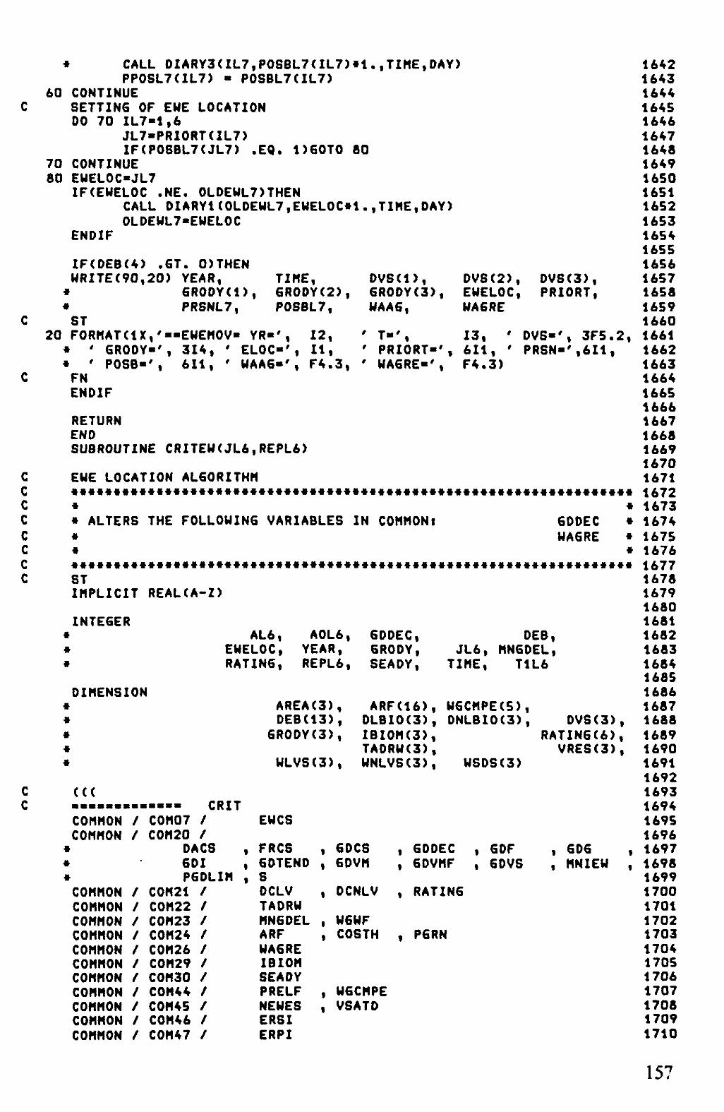
c c c c c c c c

c c

* CALL DIARY3UL7,P0SBL7<IL7)#1.,TIME,DAY) PP0SL7CIL7) « P0SBL7CIL7)

60 CONTINUE SETTIN6 OF EWE LOCATION DO 70 IL7-1.6

JL7-PRI0RTUL7) IFCP0SBL7UL7) .EQ. D60T0 80

70 CONTINUE 80 EUEL0C-JL7

IFCEWELOC .NE. 0LDEWL7)THEN CALL DIARYK0LDEWL7,EWEL0C*1.,TIME,DAY) 0LDEWL7-EWEL0C

ENDIF

IF(DEBC4) .ST. 0)THEN WRITEC90,20) YEAR,

*

ST

TIME, DVS(l), DVSC2), DVSC3), 6R0DYC1), GR0DYC2), 6R0DY<3), EWELOC, PRIORT, PRSNL7, P0SBL7, WAAG, WA6RE

13, ' DVS-', 3F5.2, 20 F0RMAT(1X,'--EWEM0V« YR«', 12, ' T«', * ' GRODY-', 314, ' ELOC-', It, ' PRIORT-', 611, ' PRSN«',6I1, * ' P08B-', 611, ' WAAG-', F4.3, ' MA6RE-', F4.3) FN ENDIF

RETURN END SUBROUTINE CRITEU(JL6,REPL6)

EWE LOCATION ALGORITHM

* #

* ALTERS THE FOLLOWING VARIABLES IN COMMON! GDDEC * « WA6RE • * #

ST IMPLICIT REAL(A-Z)

INTEGER

#

#

AL6, A0L6, 6DDEC, EWELOC, YEAR, 6R0DY, RATING, REPL6, SEADY,

DEB, JL6, MNGDEL,

TIME, T1L6

DIMENSION «

ft

ft

*

ft

(((

COMMON COMMON

COMMON COMMON COMMON COMMON COMMON COMMON COMMON COMMON COMMON COMMON COMMON

/

/

/

/

/

/

/

/

/

/

/

/

/

..... CRIT C0M07 / C0M20 /

DACS GDI PGDLIM

C0M21 / C0M22 / C0M23 / COM2* / C0M26 / COM2? / C0M30 / C0M44 / C0M45 / C0N46 / C0M47 /

AREAC3), DEBC13),

6R0DY(3),

WLVS(3>,

EWCS

FRCS 6DTEND S DCLV TADRW MNGDEL ARF WAGRE IBIOM SEADY PRELF NEWES ERSI ERPI

ARFC16), WGCMPEC5), DLBI0(3), DNLBI0C3), DVSC3), IBI0MC3), RATIN6C6), TADRUC3), VRES(3), WNLVSC3), WSDSC3)

, GDCS , 6DVM

, GDDEC , 6DVMF

, GDF , GDVS

, GDG , , MNIEU ,

DCNLV , RATIN6

W6WF COSTH PGRN

, UGCMPE , VSATD

1642 1643 1644 164S 1646 1647 1648 1649 1650 1651 1652 1653 1654 1655 1656 1657 1658 1659 1660 1661 1662 1663 1664 1665 1 ooo 1667 1668 1669 1670 1671 1672 1673 1674 1675 1676 1677 1678 1679 1680 1681 1682 1683 1684 1685 1686 1687 1688 1689 1690 1691 1692 1693 1694 1695 1696 1697 1698 1699 1700 1701 1702 1703 1704 1705 1706 1707 1708 1709 1710 157

COMMON COMMON COMMON COMHON COMMON COMMON COMMON COMMON COMMON COMMON SAVE

/

/

/

/

/

/

/

/

/

/

C0M48 C0M49 COM50 C0M51 C0M52 C0M53 C0M54 C0M56 C0M57 C0M58

/

/

/

/

/

/

/

/

/

/

PSUPPS DLBIO 6R0DY AREA WAA6 EWELOC DEB WLVS OVS TIME

, DNLBIO , WGTML

, WNLVS

, YEAR

VRES USDS

*

#

/C0M07/,/C0M2Q/,/C0M21/,/C0M22/,/C0M23/,/C0M24/,/C0M26/, /C0M29/,/C0M30/,/COM**/,/C0M45/,/C0M46/,/C0M47/,/C0M48/, /C0M49/,/COMSO/,/C0M51/,/C0M52/,/C0M53/,/COMS4/,/C0M56/, /C0M57/,/C0M58/

C C

) > )

FN GOTO(10,20,30,40,50),JL6

GREEN PASTURE 10 REPL6-1

IF(GOOEC .EQ. CMCXL6 G0HL6 DCL6 DRYQL6 D1PL6 D1WL6 IF(WAAG .GT.

D1WL6 0GWL6

#

ENDIF

0)THEN • 0. - NEWES/AREAC1) « <DCLV+DCNLV>/2. * <365.-6DTEND)*NEWES«6DCS m GDCS * G0HL6 / DCL6 m D6WL6 - 0. 0.)THEN « 6DCS * NEWES / CWAAG * DCL6) - AMAX1<0.,AL0G<(6DVH#<1.-6DI>+D1WL6>

/ (VSATD • Di«L6))/DCL6)

DO 11 TENTL6 CUMCL6 VL6

DO 12 TL6 6RL6 CL6

*

VL6 CUMCL6

12 CONTINUE DGPL6 CUMCL6

#

IFCCUMCL6 CMCXL6 0EDL6

ENDIF 11 CONTINUE

0EVL6 *

6DDEC

0.,GDTEND 0. 6DVM/<1.+(<(6DVM-IBI0M<1>>/IBI0M<1>> #EXP(-6D6#TENTL6)>) TENTL6,GDTEN0 6D6#VL6#<1.-VL6/6DVM> AMAXKO. ,GDHL6*GDCS * (1 . -EXPC-CVL6-VRESC1) ) / (6DVS-VRES( l> ) ) ) ) AMAXKO., VL6 • 6RL6 - CL6) CUMCL6+CL6

AMAXKO. , AL06(<VL6+D1PL6>/<VSATD+D1PL6>>/DCL6> CUMCL6*AREA(1) • AMIN1<<D€PL6+DGWL6>*NEWES*€DCS, DRYQL6) # 6DF

6T. CMCXL6)THEN CUMCL6 TENTL6

6DVM/<1.-K<<6DVM-IBI0M(1>>/IBI0M<1>> #EXP(-6D6»QEDL6))) 1

ST

*

*

FN

IF(0EB(5) .GT. 0)THEN WRITE(90,2)YEAR,TIME,CMCXL6,DCL6,D1PL6,D1WL6,DRYQL6,

DGPL6,D6WL6,0EDL6,0EVL6

FGRMAT(1X,'««CRITEU1» YR-',12,' T-',I3,' CMCX-',F8.1, ' DC«',F6.5,' D1P-',F8.1,' D1W-',F8.1,' DRYQ-',F6.0, ' D€P«',F4.0,' 06W-',F4.0,' OED-',F4.0,' 0EV«',F6.1>

ENDIF

ENDIF IF(TADRWd) .LT. 0EVL6*GDVMF .AND. 6R0DYC1) .ST. P6DLIM)

#WRITE(*,5)YEAR,TIME,6R0DY(1),PGDLIM,TADRW(1),0EVL6*6DVMF

1711 1712 1713 1714 171S 1716 1717 1718 1719 1720 1721 1722 1723 1724 172S 1726 1727 1728 1729 1730 1731 1732 1733 1734 1735 1736 1737 1738 1739 1740 1741 1742 1743 1744 1745 1746 1747 1748 1749 1750 1751 1752 1753 1754 1755 1756 1757 1758 1759 1760 1761 1762 1763 1764 1765 1766 1767 1768 1769 1770 1771 1772 1773 1774 1775 1776 1777 1778 1779

158

5 F0RMAT(1X,'### 6DEF ### YR,T,60DY,P6DLIM,TADRW,0EV#6DVMF', *3I5,3F12.4)

IF(TADRWCl) .GT. 0EVL6*6DVMF .OR. 6R0DYC1) .6T. PGDLIM)RETURN REPL6-0 RETURN

GREEN WHEAT NO DAMAGE GRAZING

20

22

21

REPL6-0 IFCEWELOC .EQ. IFCEWELOC .EQ.

REPL6-1 RETURN

ENOIF R6R2L6 A0L6 DO 21 AL6

VL6 CUMCL6 DO 22 T1L6

6RL6 CL6 VL6 CUMCL6

CONTINUE IFCCUMCL6

MAXCL6 A0L6

ENDIF CONTINUE CAVEL6 IFCA0L6 .EQ.

1 .OR. 2)THEN

GR0DYC2) .EQ. 0)RETURN

- AL06<TADRW(2>/IBI0M<2>)/GR0DY(2> « MAXCL6—1. - 0,MNGDEL,MN6DEL « TADRWC2>*EXP(RGR2L6*AL6) - 0. • AL6,W6TML-GR0DY(2> « RGR2L6»VL6 - AHAX1<NEWES/WAAG«AMIN1<S*(VL6-VRES<2>),GDCS),0.> - VL6+GRL6-CL6 - CUMCL6+CL6

.GT. MAXCL6)THEN - CUMCL6 - AL6

MAXCL6*WAA6/((WGTML-GRODY(2))*NEWES> .AND. CAVEL6 .6T. MNIEW>REPL6«1

IF(DEB(5) .GT. 0)THEN WRITE(90,3>YEAR, TINE, JL6, EWELOC, NEWES,

* RGR2L6, 6R0DYC2), WGTML, MAXCL6, A0L6, ST

3

WAA6, TADRWC2), CAVEL6, REPL6

F0RNAT<1X,'««< • ' J-', * ' WAA6-', * ' 6R0DY2-', # ' A0-', FN ENDIF

RETURN

CRITW2- YR-', 12, ' T«', 11, ' ELOC-', 11, ' NEWES-', F3.2, ' TADRW2-', F5.0, ' RGR2-', 13, ' WGTML-', F3.0, ' MAXC-', 12, ' CAVE-', F4.2, ' REP-',

13, F4.1,

F4.3, F6.1, ID

30

40

50

WHEAT AFTERMATH REPL6—1 IFCTADRWC2) .LT. VSATD/3.)REPL6-0 IFCRATINGC6) .LT. RATING(4>>RETURN IFCDVSCl) .GE. 1. .AND. TADRW(l) .GT.

• .AND. AREA(l) .6T. RETURN

DRY PASTURE REPL6-1 IF(TADRWd) .LT. VSATD/3.>REPL6«0 IFCRATIN6C6) .LT. RATIN6C3))RETURN IFCDVSC2) .GE. 1. .AND. TADRW(2) .GT.

* .AND. WAA6 .6T. RETURN

GREEN WHEAT DAMAGE GRAZING REPL6-0 WAGRE-O. IFCERSI .EQ. 0. .OR.

* ((EWELOC .EQ. 1 .OR. EWELOC .EQ. • .OR. EWELOC .EQ. 5 )RETURN

TA0RWC2) 0.) REPL6-0

TADRW(l) 0.) REPL6-0

4) .AND. ERPI .GT. FRCS*EWCS>

1780 1781 1782 1783 1784 1785 1786 1787 1788 1789 1790 1791 1792 1793 1794 1795 1796 1797 1798 1799 1800 1801 1802 1803 1804 1805 1806 1807 1808 1809 1810 1811 1812 1813 1814 1815 1816 1817 1818 1819 1820 1821 1822 1823 1824 1825 1826 1827 1828 1829 1830 1831 1832 1833 1834 1835 1836 1837 1838 1839 1840 1841 1842 1843 1844 1845 1846 1847 1848

159

C0PL6-ERSIftNEWESftPSUPPS»PRELF»MNGDEL

C

C

C C

C C

GWVEL6-0. IFCW6CMPECD .GT. IFCWGCMPEC2) .ST. IFCWGCMPEC3) .6T. IFCWGCMPEC5) .GT.

0.)GWVEL6« Q.)6WVEL6< 0.)GWVEL6« 0.)GWVEL6«

•6WVEL6+WLVSC2) 'GWVEL6+WNLVSC2) 'GWVEL6+WSDSC2) GWVEL6+DNLBI0C2)

6WVEL6-AMAX1(1.,6WVEL6-VRESC2))

UAXL6 « AMINlCWAAG,DACSftNEWES*MNGDEL*Cl.+WGWF)/GWVEL6) CALL 6RYPR0CP6YL6,SDYL6,AFYL6,SEADY,ARF) PGL6 « WAXL6»AMAX1C0.,PGYL6»P6RN-C0STH) CALCULATE THRESHOLD CONDITIONS BXL6 * DACS * CI. • WGWF) / PSPXL6 - BXL6 * CP6YL6 » P6RN PGNXL6 » CERSI * PSUPPS»PRELF PGYXL6 - CERSI • PSUPPSftPRELF

GWVEL6 - COSTH) / BXL6 • / BXL6 •

/ ERSI COSTH) / PGYL6 COSTH) / P6RN

IFCPGL6 .LT. REPL6 WAGRE

ENOIF

C0PL6)THEN « 1 - WAXL6

IFCOEBCS) .EQ. DTHEN WRITEC90,DYEAR, TIME, JL6, REPL6, ERPI, ERSI, EWCS, C0PL6,

» WAXL6, PGYL6, AFYL6, PGL6, WAAG, WAGRE, « PSPXL6, P6NXL6, P6YXL6, EWELOC, 6WVEL6, TADRWC2)

ST 1 FORMATC/,' CRITEW5 YEAR TIME JL6 REPL6 ERPI ERSI EWCS C0PL6 WAXL6

« PGYL6 AFYL6 PGL6 WAAG WAGRE PSPXL6 PGNXL6 PGYXL6 ELOC GWV TAD2', */,1X,I2,1X,I3,1X,2(I1 I 1X),3F5.2,1PG12.4, •0P,F6.3,2F7.1,lPG12.4,0P,2F6.3,3ClPG12.4),0P,l2,2F6.a) FN ELSEIFCDEBCS) .EQ. 2)THEN WRITEC90,4)YEAR, TIME, EWELOC, NEWES, WAAG,

ft WAXL6, C0PL6, PGL6, PGYL6, P6YXL6, ST

4 F0RMATC1X,'»»CRITW5- YR-', 12, ' T-', 13, » ' NEWES-', F4.1, ' WAA6-', F3.2, * ' COP-', F5.1, ' PG-', F5.1, ' PGY' ft ' WAGRE"', F4.3, ' REP-', ID

FN ELSE ENDIF

RETURN END

SUBROUTINE GRYPROCPGYGY, SDY6Y, AFYGY, SEADYGY, ARFGY)

GRAIN YIELD PREDICTION

ST IMPLICIT REALCA-Z)

6WVE-', F5.0, , FS.O,

6WVEL6, WAGRE,

ELOC-', WAX-', PGYX-',

REPL6

lit F4.3, FS.O,

DEB, I6Y, INDGY, JGY, NOYGY, SEADYGY, TIME, YEAR

ARFGYC16), DEBC13), 6YGYC25), 6YCGYC9), HRF6YC16)

INTEGER

DIMENSION

CCC ...«*«»»«»».» 6RYP COMMON / C0MS4 / DEB COMMON / C0M58 / TIME , YEAR SAVE /C0M54/,/C0M5S/ ))) FN DATA HRF6Y/16ftO./ DATA GYCGY/18.69,9.5S,12.47,12.31,8.68,7.29,4.36,0.,-1151.5/ DATA AF16Y,AF2GY/0.32,0.00003/

1849 1850 1851 1852 1853 1854 1 030

1857 1858 1859 I860 1861 1862 1863 1864 1865 1666 1867 1068 1869 1870 1871 1872 1873 1874 1875 1876 1877 1878 1879 1880 1881 1882 1883 1884 1885 1 Boo 1887 1S88 1 O U T

1890 1891 1892 1893 1894 1895 1896 1897 1898 1899 1900 1901 1902 1903 1904 1905 1906 1907 1908 1909 1910 1911 1912 1913 1914 1915 1916 1917 1918

160

c c c c c c c c c c c

REMIND 40 N0Y6Y-0 INOGY«INT((SEADYGY/15.)+0.5)-H IFCIND6Y .GT. 16)THEN

PRINT *,' GRYPRO WARNINGi YR,T,SEADY,IND-',YEAR,TIME,SEADYGY, « INOGY

INDGY-16 ENDIF

1 READ(40,*,END«5)(HRFGYCIGY),IGY-1,14) 00 3 IGY-1,INDGY-1

3 HRFGY(IGY) - ARFGY(IGY) HRF6Y<IN06Y) - HRF6Y<IND6Y)*ARF6Y<INDGY) NOYGY « NOYGY+1 6Y6Y(N0Y6Y) « 0. 00 4 IGY-1,8 J6Y - 2*I6Y GYGY(NOYGY) « 6YGY(N0Y6Y)+GYC6Y(IGY)*(HRF6Y(JGY-1)*HRF6Y<JGY))

4 CONTINUE GYGY(NOYGY) » GYGY(N0YGY)+GYCGY(9) 60T0 1

5 SYGY - 0 . SYSGY - 0 . 00 6 IGY-1,NOYGY SYGY - SY6Y+6YGYUGY) SYSGY - SYSGY*GYGY(IGY)#6YGY(IGY)

6 CONTINUE PGY6Y - SYGY/NOYGY SDY6Y - SQRT<A«AX1(SYSGY-SY6Y#SYGY/N0Y6Y,0.)/(N0Y6Y-1)) AFY6Y - PGYGY*C1./(AF1GY«VAF26Y»PGY6Y)-1.) CV6Y » SDYGY/P6Y6Y

IFCDEBC6) .EQ. 1)THEN WRITE(90,7)YEAR, TIME, NOYGY, INOGY, SYGY, SYSGY, PGY6Y, S0Y6Y,

* AFYGY, CVGY, HRFGY, ARFGY, (GYGY(IGY), IGY-1, 21) ST

7 F0RMATC1X,'--GRYPRO- YR«',I2, ' T«', 13, ' NOY-', 13, ' IND-', 13, *

*

*

*

' SYGY SYS6Y P6YGY SDY6Y AFYGY CV6Y', IX, F7.1, IX, F12.1, 3F8.1, F7.4,

/,IX,'HRFGY- ', 16F7.1, /,IX,'ARFGY- ', 16F7.1, /,1X,'6Y6Y- ', 21F6.0)

FN ENDIF

RETURN ENO SUBROUTINE LAMOVE

LAMB MOVEMENT ALGORITHM

* *

* ALTERS THE FOLLOWING VARIABLES IN COMMON! WEAN GRAZL * * CULL PPAST * « SELL LRMIX * * WAGRL LAMLOC * * LRSI CLLWG « * *

ST IMPLICIT REAL(A-Z)

CHARACTERS

INTEGER *

*

«

#

CHAST, CHAR1M

CULL, GRAZL,

LMM, MN6DEL, SEADY,

DAY, DEB, WEANED, EWELOC, 6R0DY, IL5, LAGE, LAMLOC,

0KL5,0LDLML5, 0PTVL5, YEAR, SELL, TIME, T0PTL5, WEAN

1919 1920 1921 1922 1923 1924 1925 1926 1927 1928 1929 1930 1931 1932 1933 1934 1935 1936 1937 1938 1939 1940 1941 1942 1943 1944 1945 1946 1947 1948 1949 1950 1951 1952 1953 1954 1955 1956 1957 1958 1959 1960 1961 1962 1963 1964 1965 1966 1967 1 TOO 1969 1970 1971 1972 1973 1974 1975 1976 1977 1978 1979 1980 1981 1982 1983 1984 1985 1986 1987

161

DIMENSION »

*

*

• *

*

C ((( Q s a x s s a i

COMMON COMMON COMMON

«

ft

COMMON COMMON COMMON COMMON COMMON COMMON COMMON COMMON COHHON COMMON COMMON COMMON COMMON COMMON COMMON COMMON COMMON COMMON COMMON

E J K S B S S S

/

/

/

/

/

/

/

/

/

/

/

/

/

/

/

/

/

/

/

/ /

/

C0M01 C0M06 C0M17

LAMO /

/

/

CLLW6 SLVWT

C0M18 C0M19 C0M23 COM2* C0M30 C0M31 C0M40 C0M41 C0M42 C0M43 C0M49 C0M50 C0M51 C0MS2 C0M53 C0MS4 C0M56 C0M57 C0M56

/

/

/

/

/

/

/

/

/

/

/

/

/

/

/

/

/

/

/

SAVE /C0M01/,/C0M06/ « /C0M30/,/C0M31/ # /COM50/./COM51/ * /C0M58/

C ))) C FN

DATA 0LDLML5/8/

I

CPUG LPSUBF

, CULL , WAGRL

6RAZL LAGE MN6DEL ARF SEADY DAY NLAMS EBC LRMI LRPIX OLBIO GROOY AREA WAAG EWELOC DEB WLVS DVS TIME

,/C0M17/ ,/C0M40/ ,/C0M52/

WEAN«CULL»SELL«TOPTL5»OKL5»0

WSDSC3), W6CMPLC5), DEBC13), DLBI0C3),

DVS<3>, GR0DYC3), LMM(8f8), AREAC3), SUPVL5C8). WLVSC3),

VRESC3)

, LRMIX , LRSIX ,

, EBCLIM , LAMLOC , , WEAN , WEANED

v W6WF , COSTH , PGRN

, WGCMPL

, LRSI , WLAM , DNLBIO , VRES , , WGTML

, WNLVS

, YEAR

ARFC16), DNLBI0C3)v

C0SVL5C8), 0PTVL5C8),

WNLVS(3),

PPAST

LMM

USDS

,/C0M18/,/C0M19/,/C0M23/, ,/C0M41/1/C0M42/l/C0N43/l

,/C0MS3/,/C0M54/,/C0MS6/,

POSL5-NESL5-LWIXL5-LPSWXL5-WA6RL-LRSI-0.

GWVLL5-•0. i

IF(W6CMPLC1> .ST. 0.

IFCWSCMPL(2> .GT. 0. IF(WGCMPL(3) .GT. 0. IFCWGCMPLC4) .6T. 0. IFCWGCMPLC5) .GT. 0. 6WVLL5- AMAXK1.

DO 1 IL5 8

1 0PTVL5CIL5) «

IFCAREAC1) .EQ. IF(WAA€ • EQ. IF(AREA(3) .EQ.

IFCWEANEC > .EQ.

)6WVLL5«< >6WVLL5-< >GWVLLS-< )GWVLL5«< )GWVLL5«<

SWVLL5+WLVSC2) EWVLL5*WNLVS<2> SWVLL5+WSDSC2) SMVLL5+DLBI0C2) SWVLLS+DNLBIO(2)

6WVLL5-VRESC2))

1.8 LMM(LAMLOC.ILS)

, 0.)0PTVLS<3)' 0.)0PTVL5<5>'

, 0.)0PTVL5(7)>

0)THEN IFCEBC .LT. EBCLIM)THEN

ELSE 0PTVL5C1)

IFCEWELOC

•0PTVL5<4>-0 •0PTVL5<6>«0 •0

« 0PTVL5C3) - 0PTVL5<5) « 0

.EQ. 1 J DR. EWELOC .EQ. 4>THEN 0PTVL5<1> » OPTVL5C5) - 0

ELSEIFCEWELOC .NE.

ELSE]

6)THEN 0PTVL5C1) - 0PTVL5C3) « 0

LFCEWE LOC .EQ. 6)THEN

, SELL ,

/C0M24/, /C0M49/, /C0M57/,

1988 1989 1990 1991 1992 1993 1994 1995 1996 1997 1998 1999 2000 2001 2002 2003 2004 2005 2006 2007 2008 2009 2010 2011 2012 2013 2014 2015 2016 2017 2018 2019 2020 2021 2022 2023 2024 2025 2026 2027 2028 2029 2030 2031 2032 2033 2034 2035 2036 2037 2038 2039 2040 2041 2042 2043 2044 2045 2046 2047 2048 2049 2050 2051 2052 2053 2054 2055 2056

162

0PTVL5C3) - 0PTVL5C5) • 0 2057 ELSE 2058

PRINT *,' LAHOVE ERROR 1' 205? ENDIF 2060

ENOIF 2061 IFCLAGE .LT. 2D0PTVL5C2) - 0PTVL5C4) - 0PTVL5C6) - 2062

# 0PTVL5C7) « 0PTVL5C8) « 0 2063 ENOIF 2064 DO 2 IL5 - 1,8 2065 C0SVL5UL5) « 20.E7 2066 SUPVL5CIL5) - 0. 2067 CHASTUL5iIL5>«' .' 2068

2 IF(0PTVL5(IL5) .EQ. 1>T0PTL5«T0PTL5+1 2069 IFCT0PTL5 .EQ. 0)PRINT *,' LAHOVE ERROR 2' 2070 DO 3 IL5 -1,8 2071

IFC0PTVL5CIL5) .EQ. DTHEN 2072 CALL INTAK('LAHB'//CHARUL5-H6)) 2073 GRAZL - 0 2074 IF(2 .LT. IL5 .AND. IL5 .LT. 8>6RAZL - 1 2075 LRHIX • PPAST « 0. 2076 IFCIL5 .EQ. 1 .OR. IL5 .EQ. 3 .OR. IL5 .EQ. 5>LRHIX«LRHI 2077

2078 IF((IL5 .EQ. 5 .OR. IL5 .EQ. 6) .AND. GR0DY(2) .6T. WGTHL 2079

# .AND. DVS(2) .LT . D T H E N 2080 CALL GRYPR0<PGYL5,SDYL5,AFYL5,SEADY,ARF> 2081 PPAST - <1.+W6«F>#AHAXK0.,(PGYL5#PGRN-C0STH>/6WVLL5) 2082 LWIXL5 - LRPIX 2083 LPSMXL5 « LPSUBF 2084

ENDIF 2085 2086

CALL SUP0PT(CHAR1,1L5) 2087 IFCCPU6 .LT. PRLAH)THEN 2088 C0SVL5CIL5) - CPUS 2089 SUPVL5CIL5) « LRSIX 2090 CHAST(IL5iIL5)-CHARl 2091 P0SL5 - P0SL5+INSM(CPU6,0.,1.) 2092 NE6L5 - NEGL5+INSU(CPU6,1.,0.) 2093 0KL5 » 1 2094 ENDIF 2095

ENDIF 2096 3 CONTINUE 2097

IFC0KL5 .EQ. 0 .OR. ULAN .GE. SLVMT)THEN 2098 IF(UEANED .EQ. 0)THEN 2099

WEAN * 1 2100 CALL DIARY5(LAHL0C,NLAHS,TIHE,DAY) 2101 CULL « 1 2102

ENDIF 2103 SELL - 1 2104

ELSE 2105 L0L5 - 111111. 2106 IF(P0SL5*NE6L5 .6T. 0.)THEN 2107

DO 6 IL5 "1,8 2108 6 IF(C0SVL5(IL5) .LT. 0.)C0SVL5(IL5) * L0L5 2109

ENDIF 2110 DO 4 IL5«1,8 2111

IF(ABS(C0SVL5(IL5)) .LT. L0L5)THEN 2112 L0L5 » C0SVL5(IL5) 2113 LAHLOC « IL5 2114 LRSI = SUPVL5CIL5) 2115 CLLWG » C0SVL5CIL5) 2116

ENDIF 2117 4 CONTINUE 2118

2119 IFCCLAHLOC .EQ. 5 .OR. LAHLOC .EQ. 6 ) .AND. 2120

# 6R0DYC2) . 6 T . W6THL .AND. DVSC2) . L T . D T H E N 2121 LWIXLS « AHAXK0.,LyiXL5-LRSI«LPSyXL5) 2122 WAGRL • AMIN1(WAA61LWIXL5#NLAMS*MN6DEL#(1.4WGWF)/6WVLL5) 2123

ENDIF 2124 2125

163

c

c

c

c

c c c c c c c

c c

ELSEIFCHXSIL4 - LRSIX .LT. O.OODTHEN CHAR1»'A'

ELSEIFCHXSIL4 .ST. LRSIX)THEN CHAR1«'I'

ELSE PRINT #,' #-#-# SUPLET #-* ',TIHE,HXSIL4,LRSIX

ENDIF

IF(OEB(8) .EQ. DTHEN WRITE(90,3)YEAR, TIHE, ULAN, 6RAZL, LA6E, LRPIX, LRPIL4,

• LRHIX, LRSIX, PTIHE, PLWGL4, NIL4, PFDHL4, CPUG, * PHILK, PPAST, ZL4, LEV6L4, HXSIL4, LHEPA, LQHP, » DHIL4, HEIL4, LFHDL4, DSUPL4, LPSUBF, QHL4, IL4, « LOCL4, CHAR1

ST 3 F0RHATC1X,'««SUP0PT- YR«', 12, ' T«', 13, ' W«' , F6.3,

* • GR-', 11, ' A6E-', 13, ' RPIX-',F5.3, ' RPI-', F5.3, * ' RHIX«',F5.3, ' RSIX«',F5.3, ' PT«', 1P612.4, OP, # ' PLUG-',F7.5, ' NI-', 13, /, ' PDH-', F5.3, • ' CPU6-',F9.6, ' PHILK-', F6.3,' PPAST-',F9.6,' 2-', F6.2, * ' LEVG-',F6.2, ' HXBI-',F6.3, • HEPA-',F6.2, ' QHP-', F6.3, # ' DHI-', F6.3, /, ' HEI-', F7.3, ' FHD-', F6.3, # ' DSUP«',F9.6, ' PSUB-',F6.3, ' QH-', F7.4, ' I-', F6.3, • ' LOO', 11, ' CHAR-',A)

FN ELSEIFCDEBC8) .EQ. 2)TMEN WRITE(90,4)YEAR, TIHE, WLAH, GRAZL, LAGE, LRPIX, LRPIL4,

» LRHIX, LRSIX, PTIHE, PLWGL4, NIL4, PFDHL4, CPUS ST

4 FORHAT(lX,'««SUPOPT« YR-', 12, ' T-', 13, * W-', F5.2, * ' GR-', 11, ' AGE"', 13, ' RPIX«',F4.2, ' RPI-', F4.2, # ' RHIX-',F4.2, ' RSIX«',F4.2, ' PT-', F5.2, ' PLWG»',F5.3, * ' NI-', 13, ' PDN-', F5.3, ' CPU6-',F6.3) FN ELSE ENDIF RETURN ENO SUBROUTINE LHPERFCGRAZL1)

LANS PERFORHANCE PREDICTION « • • • « # « • • • • * • « • • * # • # « • # • # # « * • • • # # • # * * • » # # * • * • # # » • # * # • # # * * * * * # • # • • •

• *

• ALTERS THE FOLLOWING VARIABLES IN COHHONt LLW6 # * *

• * • • • * • * # * • • * • • • • • # « * • • • « • • # • « * • * • • • • • • • • • * * • # « * * • • • • • # # • • # • # * • # # «

ST IHPLICIT REAL(A-Z)

INTEGER LAGE, DEB, TIHE, GRAZL1, YEAR

DIMENSION DEBC13)

(<(

COHHON / C0H05 / LQHP COHHON / C0H13 / LLWG COHHON / C0H15 /

# LEP1 , LEP2 , LEP3 , LEP4 , HDHC , PKF3 , • PKH3 , QnH

COHHON / C0H16 / # AAP , FGF1 , FGF2 , GF , PKF1 , PKF2 , # PKH1 , PKH2 , WE

COHHON / C0H19 / LAGE COHHON / C0H36 / LRPI COHHON / C0H3S / LHEPA , HEWH COHHON / C0H39 / HESU , QHS COHHON / C0H42 / LRHI , LRSI COHHON / C0H43 / LRPIX , WLAH

2264 2265 2266 2267 2268 2269 2270 2271 2272 2273 2274 2275 2276 2277 2278 2279 2280 2281 2282 2283 2284 2285 2286 2287 2288 2289 2290 2291 2292 2293 2294 2295 2296 2297 2298 2299 2300 2301 2302 2303 2304 2305 2306 2307 2308 2309 2310 2311 2312 2313 2314 2315 2316 2317 2318 2319 2320 2321 2322 2323 2324 2325 2326 2327 2328 2329 2330 2331 2332

166

COMMON / C0M54 / DEB 2333 COMMON / C0M58 / TIME , YEAR 2334 SAVE /C0M05 / , /C0M13 / , /C0M15 / , /CQM16 / , /C0M19 / , /C0M36 / , /C0M38 / , 2335

# /C0M39 / f /C0M42 / , /C0M43 / , /C0M54 / , /C0M58 / 2336 C ) ) ) 2337 C FN 2338

2339 KFL1«IL1«0. 2340

2341 HEIL1 - LRPI#LMEPA+LRSI#HESU+LRMI#MEWM 2342 0HIL1 « LRPI*LRSI+LRMI#MOMC 2343 LFH0L1 « LRMI*MDMC/(DMIL1+N0T(DMIL1>> 2344 ZL1 - <0.245-0.02164#AL06<LA6E/365.)>»WLAM»#WE+AAP#WLAM 2345 IFCGRAZL1 .EQ. DTHEN 2346

PCIAL1 • LRPI/<LRPIX • NOT(LRPIX)) 2347 PC6FL1 » F6F1 • F6F2#PCIAL1 2348 ZL1 » ZL1 * ( 1 . • PC6FL1#6F> 2349

ENDIF 235Q QML1 • (LRPI«LMEPA*LQMP*LRSI#MESU»QMS*LRMI#MEWM«QMM> 2351

# /<MEIL1+N0T<MEIL1>> 2352 KML1 • <PKM1#QMLH"PKM2>»<1.-LFMDL1>*CPKM3*LFMDL1> 2353 MEML1 - ZL1/KML1 2354 LEV6L1 - CLEPH-LEP2#WLAM)#C1.-LFMDL1>-KLEP3*LEP4#WLAM>#LFMDL1 2355 IFCMEIL1 .ST. MEMLDTHEN 2356

KFL1 - <PKF1#QML1*PKF2)#C1.-LFMDL1)«-<PKF3#LFMDL1> 2357 IL1 - NEIL1/ZL1 2358 LLWG « ARCKKML1,KFL1,IL1,ZL1,LEV6L1> 2359

ELSE 2360 LLW6 - -<MEML1-MEIL1)*KML1/LEV6L1 2361

ENDIF 2362 2363

IF(DEB(9) .EQ. DTHEN 2364 WRITE(90,1)YEAR, TIME, LAGE, WLAM, LRPI , LMEPA, LRSI , LRMI, LQMP, 2365

# MEIL1, LFMDL1, ZL1 , QHL1, KML1, MEML1, LEVGL1, KFL1, 2366 # LLW6 2367

W bI 2dbB 1 F0RMAT<5X,'CALL TO SUBROUTINE LMPERF' , / , 2369

# ' YEAR TIME LAGE WLAM LRPI LMEPA LRSI LRMI LQMP MEI LFMD Z QM//KM 2370 #MEM LEV6 KF LLWG', 2371 • / , I 3 , I 4 , I 4 , 1 X , 10<1PG12.4>, / , 10<1P612.4> ) 2372

C FN 2373 ELSEIF(DEB(9) .EQ. 2)THEN 2374 WRITE<90,2)YEAR, TIME, MLAM, GRAZL1, LAGE, LRPIX, LRPI , 2375

# LRMI, LRSI , LMEPA, MEIL1 , Z L 1 , MEML1, LLWG 2376 C ST 2377

2 F0RMAT(1X,'-«LMPERF« Y R » ' , I 2 , ' T « ' , I 3 , ' W « ' , F 5 . 2 , 2378 # ' G R « ' , I 1 , ' A 6 E « ' , I 3 , ' R P I X « ' , F 4 . 2 , ' R P I « ' , F 4 . 2 , 2379 # ' R M I « ' , F 4 . 2 , ' R S I « ' , F 4 . 2 , ' MEPA«' ,F5 .2 , * M E I « ' , F 5 . 2 , 2380 # ' Z « ' , F 5 . 2 , ' MEM«' ,F5 .2 , ' LW6- ' ,F5 .3> 2381

C FN 2382 ELSE 2383 ENDIF 2384 RETURN 2385 END 2386 SUBROUTINE EWPERFC6RAZL2) 2387

2388 C EWE PERFORMANCE PREDICTION 2389 C • « « • « # • • • • # « * « # • # # • # « * * « * « # # « • • * « • * * « # « * * • * • # « « « « * # • « « • « « • « • # * * « • • 2390 C # * 2391 C # ALTERS THE FOLLOWING VARIABLES IN COMMON: DMF1 # 2392 C # EMY # 2393 C # ELWG * 2394 C # * 2395 C ft***************************************************************** 2396 C ST 2397

IMPLICIT REAL(A-Z) 2398 2399

INTEGER NDPREG, TIME, DEB, YEAR, GRAZL2, NDLACT 2400 2401

167

c c

c c

DIMENSION

(((

COMMON / COMMON / COMMON /

*

*

*

COMMON / *

•

*

• »

COMMON / ft

ft

COMMON / »

*

COMMON / COMMON / COMMON / COMMON / COMMON / COMMON / COMMON /

C0M02 / EQMP C0M03 / ERPIX COM11 /

OMF1 , DMP1 MCRMX , MRP1 QMST

C0M12 / ALFEW , EEP1 ELP3 , EMYMF MF2 , MF3 PKF4 , RP1 8P0 , WEWE

C0M16 / AAP , FSF1 PKM1 , PKM2

C0M34 / EMEPA , EMY MEPL , MEST

C0M3S / NOLACT C0M39 f MESU C0M41 / EBC COM46 / ER8I C0M47 / ERPI C0MS4 / DEB C0M58 / TIME

SAVE /C0M02/,/C0MO3/,/C0Mll/, # / C 0 M 3 9 / , / C 0 M 4 1 / f / C 0 M 4 6 /

) ) )

FN

, 0MP2 , , MRP2 ,

, EEP2 , , EWMTMF , . HFC , RP2 ,

, F6F2 , i ME

, ERHI f , OMPL , PKA1 , y Q M S

, YEAR

ELWG MRP3

EEP3 KP NDPRE6 RP3

6F

ERPLI

PKA2

i

t

»

i

i

i

t

i

EUBL , MRP4 ,

ELPi , LBU , NEWL , RP4 ,

PKF1 ,

ERSTI ,

DEBC13)

MCRMN QMHY

ELP2 MF1 NLB RP5

PKF2

MEHY

,/C0M12/./C0M16/./C0M34/l/C0M35/f ,/C0M47/1/C0M54/,/C0M58/

EVPL2«NEPL2«MEPL2»KLL2«YPL2«NEML2«MELL2«KFL2-IL2«MRFSLL2« #MRFBCL2-MRFL2»MNEL2«MF1XL2-DMF1«EMY«PCIAL2«PC6FL2«0.

ZL2 ZL2 IFCGRAZL2

PCIAL2 PCGFL2 ZL2

ENDIF MEIL2 QML2

«

KML2 MEML2 IFCNDPREG

EVPL2= *

N E P L 2 -MEPL2«

ENOIF EEVGL2 -IFCNDLACT

KLL2 MYXL2 YPL2 NEML2 MELL2

ALFEM«WEWE#*WE+AAP#MEWE ZL2*EWMTMF .EQ. DTHEN - ERPI/CERPIX • NOT(ERPIX)) - F6F1 • F6F2#PCIAL2 - ZL2 # (1. • PC6FL2*6F>

ERPI#EMEPA*ERSI#MESU*ERSTI#MEST+ERHI*MEHY+ERPLI*MEPL <ERPI#EMEPA#EQMP + ERHI#MEHY #QMHY •

PKM1*QML2*PKM2 ZL2/KML2 .GE. SPD)THEN 10.*#<RP1-RP2#EXP(-

ERSI #MESU*QMS + ERSTI*MEST< iQMST + ERPLI#MEPL#QMPL)/CMEIL2*N0T(MEIL2>>

•RP3#NDPRE6>)* <LBW/RP5)*(NLB/NEML> EVPL2#RP4#EXP<-RP3#NDPRE6) NEPL2/KP

AMIN1<EEP3,EEP1+EEP2#WEME> .6T. 0.)THEN » PKAHQML2+PKA2 - NDLACT**MF2*EXP< >MF3*NDLACT) » MF1#MYXL2#EMYMF/1Q00. * ELP1#MFC*ELP2#N0LACT+ELP3 • YPL2*NEML2/KLL2

IF(MEIL2 .ST. MEML2*MELL2)THEN IL2 • (MEIL2-MELL2)/ZL2 KFL2 « PKF4#KLL2 ELMS » A R C 1 ( K M L 2 I K F L 2 I I L 2 , Z L 2 . E E V € L 2 ) EMY « YPL2 MYTHL2 - KLL2*(MEIL2-MEML2)/NEML2 MF1XL2 • 1000.#MYTHL2/(MYXL2#EMYMF) 0MF1 - (MF1XL2-MF1)#LIMIT(MCRMN,MCRMX 1

'

(MCRMX+UMCRMX

2402 2403 2404 2405 2406 2407 2408

, 2409 , 2410

2411 2412

, 2413 , 2414 , 2415 , 2416

2417 2418

f 2419 2420 2421

, 2422 2423 2424 2425 2426 2427 2428 2429 2430 2431 2432 2433 2434 2435 2436 2437 2438 2439 2440 2441 2442 2443 2444 2445 2446 2447 2448 2449 2450 2451 2452 2453 2454 2455 2456 2457 2458 2459 2460 2461 2462 2463 2464 2465 2466 2467 2468 2469 2470

168

# -MCRMN)/DMP1)*DMP2)-((MCRMX-MCRMN)/DMP1)#NDLACT) 2471 ELSE 2472

MRFSLL2 * LIMIT(0.,1.,1.-MRP1*(NDLACT-MRP2>> 2473 MRFBCL2 - LIMIT<0.,1.,EBC/MRP3-MRP4) 2474 MRFL2 * AMIN1(MRFSLL2,MRFBCL2) 2475 IFCMEIL2 .6T. MEML2)THEN 2476

HNEL2 » AMINK<MEML2*MELL2-MEIL2)*KLL2,ZL2#MRFL2) 2477 EMY » <<MEIL2-MEML2)*KLL2+<MNEL2*EUBL))/NEML2 2478 ELWG » -MNEL2/EEV6L2 2479

ELSE 2480 MNEL2 - AMINKAMAX1(0.,(ZL2*MRFL2)-<<MEML2-MEIL2) 2481

# #KML2>),YPL2*NEML2/EUBL) 2482 EHY « MNEL2#EUBL/NEML2 2483 ELWG » -<MNEL2+(<MEML2-MEIL2)*KML2))/EEVGL2 2484

ENDIF 2485 MF1XL2 » 1000.*EMY/(MYXL2#EMYMF) 2486 0RF1 « <MF1XL2-MF1)»LIMIT(MCRMN,MCRMX,(MCRMN-C<MCRMX 2487

# -MCRMN)/DMP1>»DMP2)+((MCRMX-MCRMN)/DMP1)*NDLACT) 2488 ENDIF 2489

ELSE 2490 IFCMEIL2 .6T. MEML2*MEPL2)THEN 2491

IL2 - (HEIL2-HEPL2)/ZL2 2492 KFL2 « PKF1#QML2+PKF2 2493 ELWG - ARC1(KHL2IKFL2IIL2,ZL2,EEVGL2) 2494

ELSE 2495 ELWG - -<MEML2*MEPL2-MEIL2)#KML2/EEVGL2 2496

ENDIF 2497 ENDIF 2498

2499 IF(DEBdO) .EQ. DTHEN 2500 WRITE(90,1)YEAR, TIME, 6RAZL2, NDPRE6, NDLACT, ZL2, MEIL2, QML2, 2501

# KML2, MEML2, EVPL2, NEPL2, MEPL2, EEVGL2, KLL2, YPL2, 2502 # NEML2, MELL2, MRFSLL2, MRFBCL2, MNEL2, EMY, MF1XL2, 2503 # DMF1, KFL2, ELWG 2504

C ST 2505 1 F0RMAT(5X,'CALL TO SUBROUTINE EWPERF',/, 2506 # ' YEAR TIME 6RAZ NDPRE6 NDLACT Z MEI QM KM MEM EVP NEP MEP 2507 # EEVG KL YP NEM MEL//MRFSL MRFBC MNE EMY MF1X DMF1 KF ELW6', 2508 # /,I3,I4,I2,2I4,13F9.4,/,14F9.4> 2509

C FN 2510 ELSEIF(DEBCIO) .EQ. 2)THEN 2511 WRITE(90,2)YEAR, TIME, WEWE, GRAZL2, QML2, NDPRE6, NDLACT, 2512

# ZL2, MEML2, MEIL2, EMY, MF1, DMF1, ELWG 2513 C ST 2514

2 F0RMAT(1X,'««EWPERF« YR«',12, ' T«',I3, ' WEWE«',F4.1, 2515 # ' GR»',I1, ' QM«',F4.3, ' NP«',I3, ' NL«',I3, 2516 # ' Z»',F5.2, ' MEM«',F5.2, ' MEI«',F5.2,' EMY«',F4.2, 2517 # ' MF1*',F5.1,' DMF1*',FS.l,' LWG=',FS.3> 2518

C FN 2519 ELSE 2520 ENDIF 2521 RETURN 2522 END 2523 SUBROUTINE EWREQM(GRAZL3,QML3> 2524

2525 C EWE REQUIREMENTS 2526 C #•#•*«•#•••••#•••##•»*••»##*#*••*••••••#••######«*##«#*»**####**«« 2527 C # * 2528 C # ALTERS THE FOLLOWING VARIABLES IN COMMGNt MER * 2529 C * * 2530 C ################################################################## 2531 C ST 2532

IMPLICIT REAL(A-Z) 2533 2534

INTEGER EWEL0C,NDPRE6, TIME, DEB, GRAZL3, NDLACT, YEAR 2535 2536

DIMENSION DEBC13) 2537 2538

C ((( 2539 169

# * # # *

# *

COMMON /

8 B 3 S X K B X X S B Z X EWRE

COMMON / C0M03 / COMMON / COMIO / COMMON / C0M12 /

ALFEW ELP3 MF2 PKF4 SPD

C0M16 / AAP , PKM1 ,

COMMON / C0M33 / COMMON / C0M35 / COMMON / COM41 / COMMON / C0M47 / COMMON / C0M53 / COMMON / COM54 / COMMON / C0M58 / SAVE /C0M03/,/C0Mia/,

* /C0M47/,/C0M53/, C ))) C FN

KLL3-YPL3-NEML3-MELL3 #IL3«BL3-PCIAL3-PC6FL3

ERPIX BCP2

EEP1 EMYMF MF3 RP1 WEWE

F6F1 PKM2 MER NDLACT EBC ERPI EWELOC OEB TIME

, GAP

, EEP2

LFP

EEP3 , EWMTMF , KP

MCr NO , RP3

ELP1 , KP , LBM

, MFC , NDPRE6 , NEWL RP2 BDI DPt RP4

FGF2 ME

PKA1

GF

PKA2

PKF1

ELP2 MF1 NLB RP5

PKF2

YEAR /COMt2/,/C0M16/,/C0M33/,/COM35/,/COM41/, /C0M54/,/C0M58/

•MEGL3-LL3«LFCFL3«EVPL3-NEPL3«MEPL3«RL3«KL3« -AELWL3-0.

ZL3 ZL3 IFC6RAZL3

PCIAL3 PCGFL3 ZL3

ENDIF KML3 MEML3 m

EEVGL3 -IF(EWELOC

*AELWL3 « IFCNDLACT

KLL3 YPL3 NEML3 MELL3 KFL3 MEGL3 LL3 LFCFL3 MER COMPUTE XLL3 XLFCFL3 XMERL3

ELSE IF(NOPRE6

EVPL3-*

NEPL3« MEPL3-

EN01F KFL3 BL3 KL3 RL3 IFCRL3

,10.#QML3-4.)

ALFEW#WEWE##WE+AAP#WEWE ZL3#EWMTMF .EQ. DTMEN « ERPI/CERPIX • NOTCERPIX)) « FGF1 • FGF2*PCIAL3 - ZL3 # (1. • PC6FL3#6F)

PKM1#QML3*PKM2 ZL3/KML3 AMIN1<EEP3,EEP1+EEP2#WEWE> .NE. 6) INSWCBCP2-EBC, 0., GAP)#LIMIT(Q.,1. .6T. 0)THEN

PKAHQML3+PKA2 MF1*NDLACT*»MF2*EXP(-MF3#NDLACT)/1000.*EMYMF ELP1#MFC+ELP2*NDLACT+ELP3 YPL3#NEML3/KLL3 PKF4#KLL3 AELWL3*EEVGL3/KFL3 1.•CMELL3+MEGL3)/MEML3 l.*LFP*(LL3-l.) LFCFL3#(MELL3+MEGL3+MEML3) MER WITHOUT ALLOWANCE FOR GAIN 1.+MELL3/MEML3 l.+LFP*(XLL3-l.) XLFCFL3#(MELL3+MEML3>

.GE. SPD)THEN 10.**(RP1-RP2*EXP(-RP3#NOPREG))*(LBW/RP5)

«(NLB/NEWL) EVPL3»RP4#EXP(-RP3*NDPREG> NEPL3/KP

* PKF1#QML3+PKF2 - KML3/CKML3-KFL3) • KML3#AL0G(KML3/KFL3) « AELWL3*EEV6L3/ZL3

.6T. BL3-DTHEN PRINT #lYEAR,TIMEtRL3,BL3 RL3-BL3-1.1 PRINT *,'RL3»',RL3

ENOIF IL3 - AL0G(BL3/(BL3-RL3-1.))/KL3

2540 2541 2542 2543 2544 2545 2546 2547 2548 2549 2550 2551 2552 2553 2554 2555 2556 2557 2558 2559 2560 2561 2562 2563 2564 2565 2566 2567 2b oo 2569 2570 2571 2572 2573 2574 2575 2576 2577 2578 2579 2580 2581 2582 2583 2584 2585 2586 2587 2588 2589 2590 2591 2592 2593 2594 2595 2596 2597 2598 2599 2600 2601 2602 2603 2604 2605 2606 2607 2608

170

c c c c c c c c

c c

c c

HER COMPUTE XIL3 XMtKL4

tNUih

ZL3*IL3*MEPL3 MER WITHOUT ALLOWANCE FOR GAIN AL06(BL3/(BL3-1.))/KL3 iLJ*XlL3*MtPL3

IF(DEB(11) ,EQ. 1)THEN WRITE(90,1)YEAR, TIME, 6RAZL3, NDPRE6, NDLACT, QML3, ZL3, KML3,

* MEML3, EEVGL3, AELWL3, KLL3, YPL3, NEML3, MELL3, * ME6L3, LL3, LFCFL3, EVPL3, NEPL3, MEPL3, RL3, KFL3, * BL3, KL3, IL3, MER.XMERL3 ST

1 F0RMAT(5X,'CALL TO SUBROUTINE EWREQM',/» »' YEAR TIME GRAZ NDPREG NDLACT QM Z KM MEM EEVG AELW KL YP NEM MEL * MEG L//LFCF EVP NEP MEP R KF B K I MER XMER', * /I3,I4,I2,2I4,12F9.4,/,14F9.4>

FN ELSEIFCDEB(ll) .EQ. 2)THEN WRITE(90,2)YEAR,TIME,WEWE,GRAZL3,QML3,NDPREG,NDLACT,ZL3,MEML3,

* AELWL3,MELL3,MEPL3,IL3,MER,XMERL3 ST

2 F0RMAT(1X,'««EWREQM« YR*',I2, ' T«',I3, ' WEWE«',F4.1, * ' GR»',Mi ' QM»',F4.3, ' NP«',I3, * ' Z«',F4.2, ' MEM*',F4.1,' AELW*',F4.3, * ' MEP-',F4.1,' I-'»F4.2, ' MER«',F5.2, FN ELSE ENDIF RETURN END SUBROUTINE HAYCUT #########*#####•*#################••###########**################# * «

* ALTERS THE FOLLOWING VARIABLES IN COMMONi HAYLD # # HVCH * # WACH * « *

ST

IMPLICIT REAL(A-Z)

INTEGER HYOP, SEADY, TIME, YEAR, DEB

DIMENSION ARF(16>, TADRW(3>, CTRDEFC3), DEB(13), DVSC3)

NL»',13, MEL«',F4.1, XM«',F5.2)

(((

COMMON /

COMMON COMMON COMMON COMMON COMMON COMMON COMMON COMMON SAVE /

* /

) ) )

FN WACH PRCHY IF HAYLD HVCH PRFHY

/

/

/

/

/

/

/

/

.«»«. HAYC C0M09 /

FORCPH HYHC2 WACH

C0M22 / CGM24 C0M28 C0M30 C0M52 C0M54 C0MS7 C0M58

/

/

/

/

/

/

/

HAYLD HYLEFT

TADRW ARF CTRDEF SEADY WAAG DEB DVS TIME

HVCH HYOP

COSTH

HYCTR HYPF1

PGRN

HYDVS HYPF2

HYHC1 , HYTOPP ,

YEAR C0M09/,/C0M22/,/C0M24/,/C0M28/,/C0M30/,/C0MS2/,/C0M54/, C0M57/,/C0M58/

0. LIMITCHYT0PP/HYPF1,HYTOPP,HYPF2*HYT0PP»(1.-DVSC2))) (FORCPH .GE. 0.)PRCHY - FORCPH AMAXKO., TADRW(2)-HYLEFT) HYHC1 • HYHC2 * HAYLD PRCHY * HAYLD - HVCH

2609 2610 2611 2612 2613 2614 2615 2616 2617 2618 2619 2620 2621 2622 2623 2624 2625 2626 2627 2628 2629 2630 2631 2632 2633 2634 2635 2636 2637 2638 2639 2640 2641 2642 2643 2644 2645 2646 2647 2648 2649 2650 2651 2652 2653 2654 2655 2656 2657 2658 2659 2660 2661 2662 2663 2664 2665 2666 2667 2668 2669 2670 2671 2672 2673 2674 2675 2676 2677

171

c c c c

CALL GPRFHY BEYGHY 6REQHY PRB1HY PRB2HY

c c c c c c

c c

c c

GRYPROCPGYHY,SDYHY,AFYHY,SEADY,ARF> - PGYHY * P6RN - COSTH = COSTH/PGRN * CPRFHY*C0STH)/P6RN « CUMPRCGREQHY,PGYHY,SDYHY) » CUMPR(BEY6HY,P6YHY,SDYHY)

IFCHYOP .LT. 0 .OR. PRFHY .LE. 0. )GOTO 1 IFCHYQP .6T. 0 .OR. PRFHY .6T. GPRFHY)WACH«WAA6 IF TOMORROW'S HAY IS LIKELY TO BE BETTER - WAIT IFCCTRDEFC2) .LT. HYCTR .AND. DVS(2) .LT. HYDVS)WACH»Q.

1 IF(0EB(12) .GT. 0)THEN WRITE(9012)YEAR,TIME,TADRWC2>,DVS<2>,WAAG,CTRDEF<2>,HY0P,

* PRCHY.HVCH,PRFHY,PGYHY,GPRFHY,WACH ST

2 F0RMAT(1X,'»«HAYCT* YR«', 12, ' T-', 13, * ' TAD-', F6.0, ' DVS-', F4.2, ' WAA-', F4.2, * ' DEF-', F4.2, ' OP*', 12, ' PRC-', F4.2, * ' HVC«', F4.0, ' PRF«', F5.0, ' PGY-', F5.0, * ' GPRF-', FS.O, ' WCH*', F4.2) FN ENDIF RETURN END SUBROUTINE STRABAL

* »

* ALTERS THE FOLLOWING VARIABLES IN CONHONf STBL * * # ft*****************************************************##«****#****

ST IMPLICIT REAL(A-Z)

INTEGER DAY, PLOWD, SECTSB, STROP, TIME, YEAR, DEB, RATING, « ISB, JSB, FRACSB

DIMENSION AREAC3), DEBC13), RATING(6), TADRMC3)

(((

.«».««««»«..» STRA COMMON / C0M08 /

* APCS , BALEC , PLOWD , PSTRW , STBL , STLEFT * STROP

COMMON / C0M21 / COMMON / C0M22 / COMMON / C0M31 / COMMON / COMAS / COMMON / C0MS1 / COMMON / C0M52 / COMMON / C0M54 / COMMON / C0MS8 / SAVE /C0M08/,/C0M21/,/C0M22/,/C0M31/,/C0M45/,/C0M51/,/C0MS2/,

* /C0M54/,/C0M58/ ) ) )

FN STMNSB«DCRSB«SECTSB-DVSB»ISB»JSB«

#FRACSB«STBL«VSURPSB«STMXSB-0. STMNSB » STLEFT IF(STROP .LT. 0 .OR. TADRW(2) .LE. STMNSB

* .OR. BALEC .GE. PSTRW )60T0 3 STMXSB • (TADRW(2)-STLEFT)*WAAG DCRSB - CDCLV*DCNLV>#0.5 IFCSTROP .GT. 0 .OR. NEWES .EQ. 0.)THEN

SECTSB • 1 STBL s STMXSB

ELS£IF(RATING(6) .6T. RATING(4) .AND. * RATINGC6) .GT. RATINGC3) .AND. AREA(l) .GT. Q.)THEN

BALEC

DCLV TADRW DAY NEWES AREA

WAAG DEB TIME

, PLOWD

, DCNLV

, VSATD

, YEAR

, PSTRW , STBL

, RATING

2678 2679 2680 2681 2682 2683 2684 2685 2686 2687 2688 2689 2690 2691 2692 2693 2694 2695 2696 2697 2698 2699 2700 2701 2702 2703 2704 2705 2706 2707 2708 2709 2710 2711 2712 2713 2714 2715 2716 2717 2718 2719 2720 2721 2722 2723 2724 2725 2726 2727 2728 2729 2730 2731 2732 2733 2734 2735 2736 2737 2738 2739 2740 2741 2742 2743 2744 2745 2746

172

c c

VSURPSB STBL

ELSEIF(RATING(4) .6T. * RATING(6) .GT.

AFTERMATH AND DRY PASTURE GRAZED D1PSB * APCS#NEWES/CAREA(1)*DCRSB) D6PSB » ALOG((VSATD + D1PSB)

/(TADRW(l)+DlPSB))/(-DCRSB) JSB « AMAX1(0.,PL0WD-DAY-DGPSB) D1WSB « APCS*NEWES/(WAAG*DCRSB) DVSB - (VSATD + D1WSB)

/EXP(-DCRSB#JSB) - D1WSB AMAX1(0.,TADRW(2)-AMAX1(DVSB,

* VSURPSB#WAAG RATINGC6) .AND. RATING(3))THEN

STLEFT))

SECTSB * AFTERMATH D1WSB « DVSB «

VSURPSB STBL

ELSEIF(RATIN6(6) .GT. * RATIN6C3) .GT.

3 ONLY GRAZED APCS*NEWES/(WAA6#DCRSB) (VSATD + D1WSB) /EXP(-DCRSB*(PLOWD-DAY))-DlWSB AMAX1(0.,TADRU(2)-AMAX1(DVSB, STLEFT))

» VSURPSB*WAA6 RATING(4) .AND. RATING(6) .AND. AREA(l) ,6T. 0.)THEN

SECTSB * 4 DRY PASTURE ONLY GRAZED STBL « STMXSB

ELSE

ENDIF FRACSB

SECTSB NEITHER STBL

- 5 GRAZED » STMXSB

100. * STBL/STMXSB

3 IF(DEB(13)

ST t

#

*

.GT. 0)THEN WRITE(90,4)YEAR, TIME, SECTSB, STMNSB, STMXSB, STROP, TADRW(l), TADRW(2), DGPSB, JSB, DVSB, FRACSB, STBL

FORMATdX, ' SECT-', ' STROP-', ' D6P«', ' FRAC-',

**STRABAL» YR'

Il» F4.0,

13,

STMN-', TADRW1-J«', STBL-',

12, F5.0, F5.0, 13, F5.0)

' T-'f STMX-', TADRy2*' DV-' .

13, F5.0, FS.O, F5.0,

FN ENDIF RETURN END FUNCTION CUMPR(YCM,AVEYCM,SDCM) IMPLICIT REAL(A-Z) CALCULATE CUMULATIVE PROBABILITY ON NORMAL DISTRIBUTION CURVE UPTO A POINT YCM FOR MEAN OF AVEYCM AND SD OF SDCM. XCM»AMAX1((YCM-AVEYCM)/(SDCM*N0T(SDCM)), -5.) CUMPR - O.S*ERFC(-XCM/SQRT(2.)) RETURN END FUNCTION ARC1(KMARC,KFARC,IARC,ZARC,EV6ARC) IMPLICIT REAL(A-Z)

KMARC/(KMARC-KFARC) KMARC*ALOG(KMARC/KFARC) BARC#(1.-EXP(-KARC*IARC))-1. RARC»ZARC/EVGARC LW6ARC

BARC KARC RARC LWGARC ARC1 RETURN END FUNCTION AFGEN(TAF,IVAF,NDAF,NMAF) REAL IVAF CHARACTER*(*) NMAF DIMENSION TAF(2,NDAF) COMMON / C0M59 / NCAFG SAVE C0M59 NCAFG-NCAFG+1

2747 2748 2749 2750 2751 2752 2753 2754 2755 2756 2757 2758 2759 2760 2761 2762 2763 2764 2765 2766 2767 2768 2769 2770 2771 2772 2773 2774 2775 2776 2777 2778 2779 2780 2781 2782 2783 2784 2785 2786 2787 2 /So 2789 2790 2791 2792 2793 2794 2795 2796 2797 2798 2799 2800 2801 2802 2803 2804 2805 2806 2807 2808 2809 2810 2811 2812 2813 2814

173

EVAF=IVAF 2815 IFCEVAF .LT. TAFC1,1))THEN 2816

AF6EN«TAFC2,1> 2817 URITE(»,1)NHAFIEVAF 2818

1 FORHATC ««AFGEN LOW IN ',A,'j X«'fF20.10> 2819 ELSEIFCEVAF .GT. TAFC1,NDAF>)THEN 2820

AFGEN»TAFC2,NDAF> 2821 WRITEC*,2)NMAF,EVAF 2822

2 FORHATC *«AFGEN HIGH IN ',A,'j X-',F20.10> 2823 ELSE 2824

NAF-1 2825 10 IFCEVAF .GT. TAFC1,NAF>>THEN 2826

NAF » NAF+1 2827 GOTO 10 2828

ENOIF 2829 IF(NAF .EQ. DTHEN 2830

AF6EN * TAF(2,1) 2831 ELSE 2832

X1AF « TAFC1.NAF-1) 2833 X2AF - TAF(2,NAF-1) 2834 SLPAF • (TAFC2fNAF>-X2AF)/CTAFCl,NAF>-XlAF> 2835 AFGEN » CEVAF-X1AF)»SLPAF+X2AF 2836

ENOIF 2837 ENOIF 2838 RETURN 2839 END 2840 FUNCTION DELAYTCNMDL,PRESDL> 2841 FUNCTION TO RETURN AVE AIR THPOL OF "NMDL" OAYS AGO 2842 DIMENSION TMPDL(20) 2843 OATA TMPDL/ 20#0./ 2S44 DELAYT«TMPDL<1> 2845 DO 1 NDL-l.NHOL-1 2846 TMPDLCNDL) -TMPDL CNOL-M) 2847

1 CONTINUE 2848 TMPDLCNMDL)«PRESDL 2849 RETURN 2850 END 2851 REAL FUNCTION LIMITCP1LM,P2LM,XLM) 2852

IFCP1LM .6E. P2LM)PRINT *,'LIMIT CHEC 2853 IFCXLM .LT. P1LM)THEN 2854

LIMIT-P1LM 2855 ELSEIFCXLM .GT. P2LM)THEN 2856

LIMIT-P2LM 2857 ELSE 2858

LIMIT-XLM 2859 ENDIF 2860

RETURN 2861 END 2862 REAL FUNCTION INSWCX1IN,X2IN,X3IN) 2863

IFCX1IN .LT. 0.)THEN 2864 INSW-X2IN 2865

ELSE 2866 INSW-X3IN 2867

ENOIF 2868 RETURN 2869 END 2870 FUNCTION FCNSW(X1FC,X2FCIX3FC,X4FC) 2871

IFCX1FC .LT. 0.)THEN 2872 FCNSW-X2FC 2873

ELSEIFCX1FC .EQ. 0.)THEN 2874 FCNSW«X3FC 2875

ELSE 2876 FCNSM-X4FC 2877

ENDIF 2878 RETURN 2879 END 2880 REAL FUNCTION NOT(XNT) 2881

IFCXNT .LE. Q.)THEN 2882 NOT-1. 2883

174

1Q

20

ELSE N0T«0.

ENDIF RETURN END FUNCTION AND(X1AD,X2AD>

IFCX1AD .GT. Q. .AND. X2AD .GT. 0.)THEN AND-1.

ELSE AND«0.

ENDIF RETURN END FUNCTION TW0VAR(MTV,IV1TV,IV2TVIMD1TVINP2TVINMTV) IHPLICIT REAL(A-Z) INTEGER ITVf LTV, HD1TV, NP2TV, NTV LOGICAL BADTV CHARACTER#(#) NMTV DIHENSION MTVCNP2TV.26) BADTV-.FALSE. EV1TV-IV1TV EV2TV-IV2TV IF(EV2TV .LT. MTVC1,1))THEN

TU0VAR«HTV<1,3> BADTV-.TRUE.

ELSEIF(EV2TV .6T. MTVCNP2TV.1))THEN TyOVAR-MTV(NP2TV,3) BADTV«.TRUE.

ELSE NTV«1 IF<EV2TV .GE. MTV<NTVfl))THEN

NTV-NTV+1 GOTO 10

ENDIF DO 1 ITV«NTV-1,NTV

LTV-2 IFCEV1TV .GE. MTVCITV.LTV) .AND. LTV .LT. 2#MD1TV)THEN

LTV»LTV+2 60T0 20

ENDIF IFCLTV .EQ. 2)THEN

TyOVAR«HTV(ITV,LTV) BADTV-.TRUE.

ELSEIFCLTV .EQ. 2#MD1TV .AND. NTVCITV.LTV) .LT. EV1TV)THEN TWOVAR«MTV(ITV,LTV) BADTV".TRUE.

ELSE HIL1TV=«TV(ITV,LTV-1) MIL2TV*MTV(ITV,LTV-2> SLPTV «(HTV(ITV,LTV+1)-MIL1TV)/(MTV(ITV,LTV)-HIL2TV) IFCITV .EQ. NTV-DTHEN

AP1TV«SLPTV#(EV1TV-MIL2TV)*MIL1TV ELSE

AP2TV«SLPTV#(EV1TV-MIL2TV)4MIL1TV ENDIF

ENDIF CONTINUE

ENDIF IF(BADTV)THEN

WRITE(*,4)NMTVIEV1TV1EV2TV FORMATC «»«TWOVAR PROB IN ',A,'j X«',F20.10t* Y-',F20.10>

ELSE TU0VAR*CC(AP2TV-AP1TV)/<MTV<NTVI1)-HTV<NTV-1,1>)>

# #(EV2TV-MTV(NTV-1,1)))+AP1TV ENDIF RETURN END SUBROUTINE DIARY1 CIDY, XDY.TIHEDY^AYDY) ST

2884 2885 2886 2887 2888 2889 2890 2891 2892 2893 289* 2895 2896 2897 2898 2899 2900 2901 2902 2903 2904 2905 2906 2907 2908 2909 2910 2911 2912 2913 2914 2915 2916 2917 2918 2919 2920 2921 2922 2923 2924 2925 2926 2927 2928 2929 2930 2931 2932 2933 2934 2935 2936 2937 2938 2939 2940 2941 2942 2943 2944 2945 2946 2947 2948 2949 2950 2951 2952

175

INTEGER IDY,JDY,TIMEDY,DAYDY 2953 CHARACTER*15 EDY(6) , LDY(8), C2DY, DATEM2, C1DY#12, C30Y#11 2954 FN 2955 DATA EDY/' GREEN PASTURE',' EARLY WHEAT','WHEAT AFTERMATH', 2956

* ' DRY PASTURE',' DAMA6E WHEAT','HOLDING PADDOCK'/ 2957 DATA LDY/'HOLDING PADDOCK','HOLDING PADDOCK',' 6R/DR PASTURE', 2958

* ' GR/OR PASTURE',' GR/DR WHEAT',' GR/DR WHEAT', 2959 2 'SPECIAL PASTURE',' FATTENING UNIT'/ 2960

2961 JDY-XDY 2962 C1DY-' EWE MOVE ' 2963 WR1TE(50,10)C1DY,EDYUDY),EDYCJDY),TIMEDY,OATE(DAYOY) 2964

10 F0RMAT(A,1X,A,' TO ',A,', TIME-',13,IX,A) 2965 RETURN 2966

2967 ENTRY DIARY2(IDY,XDY,TIMEDY,DAYDY) 2968 JDY-XDY 2969 CIDY-'NOT PRESENT ' 2970 IFCJDY .EQ. 1)CIDY-'PRESENT ' 2971 WRITE(50,20)EDY(IDY>,CIDY.TIMEDY,DATE(DAYDY) 2972

20 FORMATC LOCATION',4X,A,1X,A,7X,', TIME-',13,IX,A) 2973 RETURN 2974

2975 ENTRY 0IARY3(IDY,X0Y,TIMEDY,DAYDY) 2976 JDY-XDY 2977 CIDY-'NOT 6RAZABLE' 2978 IF(JDY .EQ. 1)C1DY-'6RAZABLE ' 2979 WRITE(50f20)EDY(lDY),ClDY,TIMEDY,DATE(DAYDY) 2980 RETURN 2981

2982 ENTRY 0IARY4(IDY,XDY,TIMEDY,DAYDY) 2983 C2DY-' LAMBS BORN IN ' 2984 C3DY-' LAMBING ' 2985 WRITE(50,30)C3DY,XDY,C2DY,LDY(IDY),TIMEDY,DATE(DAYDY) 2986

30 F0RMAT(A,F6.3,A,1X,A,', TIME-',13,IX,A) 2987 RETURN 2988

2989 ENTRY DIARY5(IDY,XDY,TIMEDY,DAYDY) 2990 C3DY-' WEANING ' 2991 C2DY-' LAMBS WEAN IN ' 2992 WRITE(50,30)C3DY,XDY,C2DY,LDY(IDY),TIMEDY,DATE(DAYDY) 2993 RETURN 2994

2995 ENTRY DIARY6(IDY,XDY,TIMEDY,DAYDY) 2996 C3DY-' CULLING ' 2997 C2DY-' EWES CULL IN ' 2998 WRITE(50,30)C3DY,XDY,C2DY,EDY(IDY),TIMEDY,DATE(DAYDY) 2999 RETURN 3000

3001 ENTRY DIARY7<IDY,XDY,TIMEDY,DAYDY) 3002 JDY-XDY 3003 C1DY-' LAMB MOVE ' 3004 WRITE(50,10)CIDY,LDY(IDY),LDY(JDY),TIMEDY,DATE(DAYDY) 3005 RETURN 3006

3007 ENTRY DIARY8(IDY,XDY,TIMEDY,DAYDY) 3008 C2DY-' LAMBS SOLD IN ' 3009 C3DY-' LAMB SALE ' 3010 WRITE(50,30)C3DY,XDY,C2DY,LDY(IDY),TIMEDY,DATE(DAYDY) 3011 RETURN 3012

3013 ENTRY DIARY9(IDY,XDY,TIMEDY,DAYDY) 3014 C1DY-' GRAIN HARV ' 3015 C2DY-' K6/HA ' 3016 C3DY - ' FORGET IT ' 3017 IFUDY .EQ. DC3DY-' HARVESTED ' 3018 WRITE(50,40)CIDY,XDY,C2DY,C3DY,TIMEDY,DATE(DAYDY) 3019

40 F0RMAT(A,4X,F6.0,A,A,', TIME-',13,1X,A) 3020 RETURN 3021

176

50

ENTRY DIARY10CIDY,XDY,TIMEDY,DAYDY) C1DY«' STRAW BALE ' C2DY-' KG/HA SYSTEM ' WRITEC50,50)C1DY,XDY,C2DY,TIMEDY,DATE(DAYDY> F0RMAT(A,4X,F6.0,A,11X,' , TIME-' ,13,IX,A) RETURN

ENTRY DIARY11(IDY,X0Y,TIME0Y,0AY0Y) C1DY«' NEW YEAR WRITE<50,60)C1DY,IDY

60 FORMAT(/,' *#*###**#*#*«*#*»**###»**##*######**«**«*###******##**# *****#•*««•##*»*',/,A,15X,I4,/)

RETURN

ENTRY DIARY12(IDY,XDY,TIMEDY,0AYDY) C30Y«' BALANCE C2DY-'RETURN TO LABOU' CIDY-'R & CAPITAL ' WRITE(SO,70)C3DY,XDY,C2DY,C1DY,IDY

70 F0RMAT<A,F7.1,'t/HA ',A,A,'<RAIN»',14,'MM)') RETURN

ENTRY 0IARY13(I0Y,X0Y,TIME0Y,0AY0Y) C1DY-' WHT HAY CUT' C2DY-' KG/HA SYSTEM ,' C3DY«'% OF SYSTEM' WRITE(50,80)C1DY,IDY,C3DY,XDY,C2DY,TIMEDY,DATE(DAYDY)

80 F0RMATCA,I4,A,F7.0,A,' TIME-',13,1X,A) RETURN

ENTRY DIARY14<IDY,XDY,TIME0Y,DAY0Y) IXDY-INTCXDY+0.5) WRITE(50,90)IDY,IXDY,TIMEDY,DAYDY

90 FORMATC INTAKE TP IE /E i ' , 13 , # ' TPIL/Lr ' , 13 ,

RETURN END FUNCTION DATE(DAYDT) IMPLICIT INTE6ERCA-Z) DIMENSION CMDTC13) CHARACTERM2 MDT(12),DATE DATA MDT /'JANUARY

*

DATA CMDT /O,31,59,90,120,151,181,212,243,273,304,334,365/ ACCEPTS DAY NUMBER (1-JAN 1) AND RETURNS THE DATE. DO 1 NDT«2,13

IFCDAYDT .LE. CMDT(NDT))THEN

TSIE/Ei TSIL/Li

13, 13)

' ,'FEBRUARY','MARCH 'MAY 'SEPTEMBER','OCTOBER

','JUNE ','APRIL ', ','AU6UST ',

','NOVEMBER','DECEMBER'/ 'JULY

N1DT DDT BDT ADT M D T ( N l D T ) d l i l l ) M D T ( N 1 D T ) ( 1 2 I 1 2 ) DATE RETURN

ENDIF 1 CONTINUE

END

NDT-1 DAYDT-CMDT(NIDT) DDT/10 DDT-BDT*10 CHARCBDT+16) CHAR(ADT+16) MDT(NIDT)

3022 3023 3024 3025 3026 3027 3028 3029 3030 3031 3032 3033 3034 3035 3036 3037 3038 3039 3040 3041 3042 3043 3044 3045 3046 3047 3048 3049 3050 3051 3052 3053 3054 3055 3056 3057 3058 3059 3060 3061 3062 3063 3064 3065 3066 3067 3068 3069 3070 3071 3072 3073 3074 3075 3076 3077 3078 3079 3080 3081

177

12 Model directory

12.1 Local variables

The following naming convention was adopted: variables ending with are local variables in subroutine ...

L8 INTAK L7 EWMOVE L6 CRITEW GY GRYPRO L5 LAMOVE L4 SUPOPT LI LMPERF L2 EWPERF L3 EWREQM HY HAYCUT SB STRABAL DY DIARY1

All other variables in these subroutines appear in COMMON. Codes after acronyms are

- P: parameters defined in the parameter file (TAPE 10), with the exception of AF1GY, AF2GY, EWEMAT, GYCGY, LAMMAT and MATCH, which are defined in DATA statements, and NRO that is defined in a PARAMETER statement, in the programme.

- F: function tables defined in the parameter file. - IR: variables that are initialized once only at the start of a run. Initialization is

always to zero, with the exception of DBIOM (3*1000), DLBIO (3*400), DNLBIO (3*600), DVS (3*1.1), EBC (3), EWELOC (6), GRODY (3*270), IBIOM (50,50,40), TADRW (3*1000), TDVS1 (3*140) and WEWE (60).

- IY: variables that are initialized at the start of each year. Initialization is always to zero, with the exception of MF1 (400), PRVDVS (l.l),andWST2BL(999). Local variables in subroutine SRATES are not listed below.

12.2 Acronyms, definitions and units of measure

AAP P allowance for activity in equation for mainte­nance requirement MJ kg-1 d_l

ADT auxiliary variable of DATE function 1

179

ADWW

AELWL3

AF1GY

AF2GY

AFG1

AFGEN

AFY AFYGY

AFYHY AFYL5 AFYL6 AL6

ALFEW

P content of water in air-dry soil relative to con­tent at wilting point allowance for ewe's gain in liveweight in calculation of ewe's energy requirements

P intercept of linear function relating harvest in­dex to yield of grain

P slope of linear function relating harvest index to yield of grain allocation of aerial biomass between leaves and stems at emergence linearly interpolated value returned by AFGEN function predicted yield of wheat aftermath dummy argument in GRYPRO subroutine: predicted yield of wheat aftermath predicted yield of wheat aftermath predicted yield of wheat aftermath predicted yield of wheat aftermath time of entry of stock in algorithm for early-season grazing of green wheat

P coefficient for energy requirement of fasting ewes

ALPHAT F proportionality factor for contribution of drying power of the air to crop transpiration (ALPHA) as a function of average hourly ir-radiance during daylight (HRAD) and of leaf area index (LAI)

IY current maximum rate of gross CO: assimila­tion (single leaf)

P potential maximum rate of gross C02

assimilation (single leaf) value (0 or 1) returned by AND function character string of dummy argument in subroutine INTAK ('EWES' or 'LAMB') optimum time of entry of stock in algorithm for early-season grazing of green wheat. 0 = today TWOVAR function variable. 1st estimate, based on lower bounding row TWOVAR function variable. 2nd estimate, based on upper bounding row

P approximate rate of intake of dry biomass for satiation

AMAX

AMAXB

AND ANIMAL

AOL6

AP1TV

AP2TV

APCS

1

kgd"1

1

ha kg-1

1

1 kg ha - i

kg ha-1

kg ha~' kg ha-1

kg ha-1

MJkg ,„-0.75 t - l

1

kg ha-1 h_l

kg ha-1 h~!

1

kgd - i

180

ARC1

AREA ARF

ARFGY

AVEYCM

AVLAR

BADTV

BALANC BALEC BARC

BCP1 BCP2 BCP3 BCP4

BCP5

BDT BL3 BSYS

BXL6 C1DY

C2DY

C3DY

CAVEL6

CCULTW CFDM

CFERTW P

rate of gain in liveweight returned by ARC1 function kgd - 1

P area fraction of system of the 3 localities 1 IY vector of 15-day totals of daily rainfall for the

current season mm dummy argument in GRYPRO subroutine: vector of 15-day totals of daily rainfall for the current season dummy argument in CUMPR function: mean predicted yield of wheat grain

IY quotient of area to mass of leaf at the 3 localities extrapolation warning indicator in TWOVAR function

IY annual financial balance P cost of baling wheat straw

ARC1 function parameter in equation for re­tention of energy

P body condition parameter; minimum score P body condition parameter; maximum score P body condition parameter; acceptable score P body condition parameter; liveweight corre­

sponding to BCP3 P body condition parameter; difference quotient

of liveweight change to body score change auxiliary variable in DATE function parameter in equation for retention of energy

P switch for breeding system. 1 = conventional 18-months, 2 = hoggets at 6 months auxiliary variable character string variable of DIARY subroutine character string variable of DIARY subroutine character string variable in DIARY subroutine mean rate of intake during early-season period of grazing green wheat

P cost of land preparation for wheat P conversion factor from digestibility to

metabolizability 1 cost of dressing wheat with fertilizer S ha

mm

kg ha-1

m2kg-!

1 S ha"1

Skg"1

1 1 1 1

kg

kg 1 1

1 had"1

1

1

1

kgd-» S ha-1

- i

181

CHAR1

CHAST

CL6

character returned by subroutine SUPOPT in­dicating optimum rate of supplementary feed­ing character string indicating optimum rate of supplementary feeding at each locality for lambs: used in output option for lamb-rearing trace rate of intake of herbage in algorithms for de­ferment of grazing of green pasture and early-season grazing of green wheat

IR cost of gain in liveweight of lamb at the se­lected locality maximum cumulative intake in algorithm for deferment of grazing of green pasture array for DATE function (cumulative time)

IY output matrix column P efficiency of conversion of primary photo-

synthetic product (CH20) to structural plant material (dry matter) for pasture and wheat

CONFSM P efficiency of conversion of primary photo-synthetic product (CH20) to structural plant material (dry matter) for medic cost of keeping flock on pasture and not graz­ing green wheat as an alternative to grain for 1 management time step

P costs of harvesting wheat grain with reference to area

CLLWG

CMCXL6

CMDT COL CONFS

COPL6

COSTH

COSTS COSVL5

CPUG CRDL

CRDNL

CRLFAR

CRLFRE CRLFRL CRLVE CRLVL CRLVS

CRNLVE

running costs vector of lamb's cost of gain for each nutri­tional locality of the lamb cost of gain in liveweight of lamb rate of intake of dead leaf by ewe plus lamb for the 3 localities rate of intake of dead non-leaf by ewe plus lamb for the 3 localities rate of intake of leaf area by ewe plus lamb for the 3 localities rate of intake of leaf area by ewe rate of intake of leaf area by lamb rate of intake of live leaf by ewe rate of intake of live leaf by lamb rate of intake of live leaf by ewe plus lamb for the 3 localities rate of intake of live non-leaf by ewe

4A\ T, 4Z'

'A\ T. 'Z\ V

kgha-'d"1

S kg"1

kg ha"1

d 1

1

1

S ha - i

S ha-' S ha-'d"1

Skg-1

Skg-1

kgha-'d-1

kgha-'d"1

n^ha-'d-1

m2 ha"1 d - ' n^ha-'d-1

kg ha"1 d"1

kgha-'d"1

kgha-'d"1

kgha-'d"'

182

CRNLVL CRNLVS

CSL8

kg ha d

csoww CSRRT

CTRDEF

CULBS CULINC CULL CUMCL6

CUMPR

CVGY

D1PL6 D1PSB D1WL6 D1WSB DACS

DAM-WGL8

DATE

DAY DAYDT

DAYDY

kg ha d

kgd"1

S ha-1

CSRRTW F

rate of intake of live non-leaf by lamb rate of intake of live non-leaf by ewe plus lamb for the 3 localities rate of intake of concentrate ad libitum by lamb, also taken as maximum rate of intake of herbage for satiation

P cost of sowing wheat F mass fraction of photosynthetic product allo­

cated to shoot (CSRR) as a function of stage of development of the crop (DVS) for pasture and medic 1 mass fraction of photosynthetic product allo­cated to shoot (CSRR) as a function of stage of development of the crop (DVS) for wheat

IY cumulative transpiration deficit for the 3 localities

P culling rate of mature ewes IR income from culled ewes S ha IR switch for culling ewes. 0 = no, I = yes

cumulative intake in algorithms for deferment of grazing of green pasture and early-season grazing of green wheat kg ha integral of normal curve returned by CUMPR function 1 coefficient of variation of predicted set of yields of wheat grain auxiliary variable in computing DGPL6 auxiliary variable in computing DGPSB auxiliary variable in computing DGWL6 auxiliary variable in computing DVSB

P approximate rate of intake for satiation with grazing green wheat as an alternative to grain kg d_I

- I , 4 - 1

- i A-\

1

1 1 S 1

indicator for grazing of green wheat as an al­ternative to grain. TRUE = being grazed, FALSE = not being grazed

date returned by DATE function

time in year from 31 December dummy argument of DATE function. Time in year from 31 December dummy argument of DIARY subroutine. Time in year from 31 December

character string character string d

183

DBIOM

DCL6

DCLV DCNLV DCRSB

DDLL8 DDLP

DDNLL8 DDNLP

DDSL1

DDSL2

DDT DEB DELAYT DELT DGLL8 DGLP

DGNLL8 DGNLP

DGPL6

DGPSB

DGRRT

DGSL1

DGSL2

DGWL6

DIDHRV

DINTG

kg ha

d-1

d-1

1

IR total mass of dead leaf and dead non-leaf for the 3 localities mean relative rate of disappearance of dead plant material

P relative rate of disappearance of dead leaf P relative rate of disappearance of dead non-leaf d_I

mean relative rate of disappearance of dead plant material digestibility of grazed dry leaf

P maximum digestibility of dry leaf (pasture or wheat) digestibility of grazed dry non-leaf

P maximum digestibility of dry non-leaf (pas­ture or wheat)

P range in digestibility of dead leaf during dry season

P range in digestibility of dead non-leaf during dry season auxiliary variable of DATE function

P array of switches for debug output value returned by DELAYT function

P integration time step digestibility of grazed green leaf

P maximum digestibility of green leaf (pasture or wheat) digestibility of grazed green non-leaf

P maximum digestibility of green non-leaf (pas­ture or wheat) time of grazing to satiation provided by dry pasture time of grazing to satiation provided by dry pasture

P rate of extension of roots under optimum con­ditions

P decrease in digestibility of green leaf between DVS = 0 and DVS = 1

P decrease in digestibility of green non-leaf be­tween DVS = 0 and DVS = 1 time of grazing to satiation provided by wheat aftermath

IY indicator for harvest of wheat grain. 0 = grain not yet harvested, 1 = grain harvested

P intercept of linear function relating ERDFDL8 to ED for ewes and LRDFDL8

- i « »

i

mm d_l

1

1

1

184

DINTL

DINTL8

DISTFT

DISTFTM F

DISTFTW F

DLBIO DMF1

DMIL1 DMIL4 DMP1 DMP2 DND1 DND2 DNLBIO DOLDAY DRF

DRR

DRYQL6

DSLPG

DSLPL

DSLPL8

DSUPL4

DVR

IR

to LD for lambs, on pasture and wheat intercept of linear function relating LRDFDL8 to LD for lambs, on legume intercept of function relating reduction factor of digestibility to digestibility, for lambs fraction of aerial vegetative growth to leaves (DISTF) as a function of stage of develop­ment of the crop (DVS) for pasture fraction of aerial vegetative growth to leaves (DISTF) as a function of stage of develop­ment of the crop (DVS) for medic fraction of aerial vegetative growth to leaves (DISTF) as a function of stage of develop­ment of the crop (DVS) for wheat biomass of dead leaf for the 3 localities change in parameter MF1 in equation for rate of production of milk with rate of feeding rate of intake of dry matter rate of intake of dry matter parameter in equation for DMF1 parameter in equation for DMF1 time interval over which DDSL1 declines time interval over which DDSL2 declines biomass of dead non-leaf for the 3 localities

IY cumulative negative financial balance P dryness factors of consecutive soil compart­

ments at start of season relative to content of moisture at wilting point, for the 3 localities cumulative deep drainage beyond potential rooting zone for the three localities total dry-season requirement of the flock with respect to system area

P slope of linear function relating ERDFDL8 to ED for ewes and LRDFDL8 to LD for lambs, on pasture and wheat

P slope of linear function relating LRDFDL8 to LD for lambs, at legume slope of function relating factor for reduction in digestibility to digestibility, for lambs increment in rate of supplementary feeding in algorithm for optimizing supplementary feed­ing of lambs rate of development of plant for the three localities

P P P P IR

1

1

1

1

1

n - l

i kg ha

d-1

kgd-' kgd-' 1 1 d d kg ha-1

d

1

mm d_1

kg ha - i

1

1

1

kgd"1

1

185

DVRT

DVS

DVSB

EDY

EEP1

EEP2

EEP3

EEVGL2 EEVGL3 EFFE

EFFEB

ELP1

ELP2

186

IR

IR

DVSSF

DVX

EB

EBC EBCLIM

EBDEFL8 ECRDL ECRDNL ED

EDPTFT F

rate of development of crop (DVR) as a func­tion of average daily air temperature (TMPA) stage of development of the crop at the 3 lo­calities biomass of wheat aftermath required to provide intake for satiation for a given period of time with respect to locality area stage of development at which seed fill starts for pasture and medic indicator for end of growing season for the 3 localities. 0 = DVS<1, 1 = DVS>1 cumulative evaporation over soil compartments for the three localities

IR ewe's body condition score P threshold of ewe's body condition score be­

low which weaning is forced deficit of ewe's body condition ewe's rate of intake of dead leaf ewe's rate of intake of dead non-leaf (ewe) digestibility of pasture or wheat herb­age root activity coefficient (EDPTF) as a function of relative amount of available water in a soil compartment (AFGX) array for ewe's locality in DIARY subroutine

P parameter in function for energy content of gain by ewes: intercept

P parameter in function for energy content of gain by ewes: slope

P parameter in function for energy content of gain by ewes: maximum energy content of gain by ewes energy content of gain by ewes

IY actual effectiveness of utilization of solar en­ergy for production of dry matter at light compensation point

P basic potential effectiveness of utilization of solar energy at the light compensation point

P parameter in equation for net energy content of milk

P parameter in equation for net energy content of milk

« v

1

kg ha '

1

1

mm d"1

1

1 1 kgha-'d-' kg ha_ ,d_ l

1

1 character string

MJkg - l

- l i , „ - i MJ kg"' kg

MJ kg"1

MJ kg"1

MJ kg"1

kgha-'h"1/ (Jm-2s-')

kgha-'h"1

W-'m2

1

ELP3

ELS

ELWG EMEPA

EMY EMYMF

ENGR

EPLA

EPSBFL8

EQMP

ER

ERFDSL8

ERHI ERPI ERPIX

ERPLI ERSI ERSTI EUBL

EV1TV

EV2TV

EVAF

EVAP EVGARC

EVPL2 EVPL3

P parameter in equation for net energy content of milk crop locality corresponding to ewe's current nutritional locality

IR ewe's rate of change in liveweight content of metabolizable energy in herbage grazed by ewes ewe's actual rate of production of milk factor for increase in yield of ewe's milk for average litter size rate of emptying of temperature sum when no seeds are germinating, for the three localities

P ewe's allowance of poultry litter at dry localities or holding paddock ratio of substitution of herbage for concentrates to ewe mctabolizability of herbage grazed by the ewes rate of evaporation from a soil compartment, for the three localities reduction factor for digestibility with intake of straw by ewe ewe's rate of intake of (wheat) hay ewe's rate of intake of herbage expected rate of intake of herbage by ewe in the absence of supplementary feed ewe's rate of intake of poultry litter ewe's rate of intake of supplementary feed ewe's rate of intake of (wheat) straw

P efficiency of utilization of body energy for lac­tation variable of TWOVAR function set equal to dummy argument IV1TV for computational efficiency variable of TWOVAR function set equal to dummy argument IV2TV for computational efficiency variable of AFGEN function set to dummy argument IVAF for computational efficiency potential evaporation of moisture from soil dummy argument of ARC 1 function: energy content of gain total energy content of products of gestation total energy content of products of gestation

1

1,2 or 3 kgd"'

MJkg"1

kgd-'

1

1

kgd-'

1

1

mm d - i

1 kgd-' kgd-«

kgd-1

kgd-' kgd-' kgd-'

1

1

1

1 mm d - '

MJkg-' MJ MJ

187

EWCS

EWELOC IR EWEMAT P

EWHD P

EWMTMF P

EWSTG FAMSTT F

FCNSW FDMT

FERT

FERTD FGF1

FGF2

FLDCP

FLTRT

FORCPH

FRACSB

FRCS

FSATL8

FWDB FXPC

P P

P P

ewe's mass rate of intake to meet energy requirements kgd" ewe's current nutritional locality 1 array for matching ewe's nutritional locality to crop locality 1 earliest time for wheat harvest from 31 December d multiplication factor for ewe's energy requirement for maintenance (set to 1 and therefore inoperative) 1 ewe's physiological stage from time of mating d reduction factor for allocation of photosynthetic products to shoot (FAMST) as a function of relative transpiration deficit (CTRDEF) 1 value returned by FCNSW function I mass fraction of dry matter in canopy (FDM) as a function of stage of development of the crop (DVS) 1 switch for application of fertilizer. 0 = no, 1 = yes 1 time of applying fertilizer from 31 December d intercept in equation defining fraction of maximum allowance for grazing activity (GF) to add to requirements for maintenance 1 slope in equation defining fraction of maximum allowance for grazing activity (GF) to add to requirements for maintenance 1 field capacity expressed as volume fraction of moisture 1 fraction of solar energy transmitted through vegetation (FRLT) as a function of soil cover (SLCVR) 1 forced price of hay (overrides calculated value if greater than or equal to zero) S kg mass fraction of STMXSB that is actually baled 1 fraction of EWCS above which the option of grazing green wheat as an alternative to grain is not considered 1 fraction of digestibility-limited intake achieved in absence of supplementary feed 1 mass fraction of water in dead plant material 1 fixed costs of pasture, including fertilizer $ ha year

188

GAMMA GAP

GDCS

GDDEC

GDF

GDG

GDHL6

GDI

GDTEND P

GDVM

GDVMF P

GDVS

GEH GEST GF

GPRFHY GRAINT

P psychrometer constant P maximum allowance for gain in liveweight by

ewe P rate of intake per animal for satiation in

algorithms for deferment of grazing of green pasture and early-season grazing of green wheat

IY switch indicating whether the algorithm for deferment of grazing on green pasture has been invoked. 0 = no, 1 = yes

P relative nutritional value of dry to green herbage for algorithm for deferment of grazing on green pasture

P long-term average relative rate of growth at low biomass in logistic growth function in algorithm for deferment of grazing on green pasture stocking rate at pasture for algorithm for deferment of grazing on green pasture

P harvest index in algorithm for deferment of grazing on green pasture: 1 — GDI = fraction of peak biomass that remains for grazing after harvest last possible time of entry of stock, i.e. average duration of green season, in algorithm for deferment of grazing on green pasture long-term average peak undisturbed aerial biomass in logistic growth function in algorithm for deferment of grazing on green pasture multiplication factor for optimum biomass at entry of stock, for error analysis in algorithm for deferment of grazing on green pasture biomass at 0.63 satiation intake in negative exponential function of intake in algorithm for deferment of grazing on green pasture gross energy content of herbage dry matter gestation period maximum energy requirement for grazing activity relative to requirements for maintenance expected mean profit from wheat grain fraction of photosynthetic product allocated

P P P

mrnHgT" 1

kgd"1

kgd - i

- i

ha - l

kg ha

kg ha l

MJkg"1

d

$ ha - i

189

GRAZE

GRAZL

GRAZL1

GRAZL2

GRAZL3

GRL6

GRLVS GRNLV GRODY

GRRT

GRRWT GRSDS GWVEL6

GWVLL5

GYCGY

GYGY HARV

HAY HAYLD

HORMC

HRFGY

190

to seeds (FRTS) as a function of stage of development of the crop (DVS). (DVS at which allocation to seeds commences in pasture and medic is given by parameter DVSSF)

IY indicator of grazing by ewe. 0 = ewe not grazing, 1 = ewe grazing

IY indicator of grazing by lamb. 0 = lamb not grazing, 1 = lamb grazing dummy argument of grazing by lamb to subroutine LMPERF dummy argument of grazing by ewe to subroutine EWPERF dummy argument of grazing by ewe to subroutine EWREQM rate of growth of green pasture in algorithms for deferment of grazing of green pasture and early-season grazing of green wheat rate of growth of leaf for the 3 localities rate of growth of non-leaf for the 3 localities

IR time interval since emergence for the 3 localities rate of vertical extension of the root system for the 3 localities rate of growth of the roots for the 3 localities rate of growth of the seeds for the 3 localities biomass of plant components grazed by ewe when grazing green wheat as an alternative to grain biomass of plant components grazed by lambs when grazing green wheat as an alternative to grain

P array of coefficients for multiple linear regression equation relating yield of wheat grain to 30-day rainfall vector of predicted yields of wheat grain switch for harvesting of wheat grain. 0 = no, 1 = yes

IR amount of hay in store expected yield of wheat hay with respect to wheat area

P cost of hormone per ewe in early-breeding system (BSYS = 2) historical rainfall vector from data file for 15-d periods

kgha-'d-1

kgha" ld-1

kgha-'d"1

mm d l

kgha-'d"1

kgha-'d"1

kg ha

kg ha

- i

- i

kg mm l

kg ha"1

kg ha '

kg ha-1

S

mm

HVCH HYCTR

HYDVS

HYHC1 HYHC2 HYLEFT HYOP

HYPF1 HYPF2

HYTOPP 11 12 13 IARC

P P P P

P P

P

IBIOM

IDY IGY IL1 IL2 IL3 IL4 IL5 IL7 IL8 INCOM INDGY

INFR INSUR INSW IRN15

IRTD IRWT

ITV

costs of cutting wheat for hay cumulative transpiration deficit above which cutting for hay, if feasible, is not delayed stage of development above which cutting for hay, if feasible, is not delayed cost function of harvesting hay: intercept cost function of harvesting hay: slope biomass of wheat left in field by baler option of cutting hay. <0, do not cut hay; = 0, cut according to normal criteria; >0, cut if value greater than costs of harvesting ratio of top to bottom price of hay parameter in function of price of hay: effect of stage of development top price of hay: price for best hay looping index looping index looping index dummy argument of function ARC1: scaled rate of intake of energy

IR initial aerial biomass at full emergence for the 3 localities dummy argument of DIARY subroutine index variable of GRYPRO subroutine scaled rate of intake of energy scaled rate of intake of energy scaled rate of intake of energy scaled rate of intake of energy index variable in subroutine LAMOVE index variable in subroutine EWMOVE index variable in subroutine INTAK rate of income from sale of products current decision time expressed in number of 15-day periods since start of season rate of infiltration of water into the soil

P insurance costs per ewe value returned by INSW function 15-day group number since the start of the season. 1-15 October = 1

P rooting depth at emergence for the 3 localities mass of roots with respect to area at emergence for the 3 localities variable of TWOVAR function: current bounding row

S ha

1

1 S ha Skg kg ha

- l

- l

I

1 1

1 Skg 1 1 1

1

kg ha"1

1 1 1 1 1 1 1 1 1 S ha-'d-1

1 mm d"1

Syear"1

1

1

mm

kg ha-1

1 191

IV1TV

IV2TV

IVAF

IXDY Jl J2 JDY JGY JJ JL6

JL7 JOIN JOIND JSB

K KARC

KFARC

KFL1

KFL2

KFL3

KFL4

KL3 KLL2

KLL3

KMARC

KML1

dummy argument of TWOVAR function: 1st independent variable dummy argument of TWOVAR function: 2nd independent variable dummy argument of AFGEN function: independent variable auxiliary variable of DIARY subroutine looping index looping index auxiliary variable of DIARY subroutine index variable of GRYPRO subroutine looping index dummy argument of CRITEW subroutine: ewe's locality index variable in subroutine EWMOVE joining (mating) switch. 0 = no, 1 = yes time of joining from 31 December grazing time needed on wheat aftermath after allowing for availability of dry pasture crop locality variable of ARC I function: parameter in equation for retention of energy dummy argument in ARC1 function: efficiency of utilization of metabolic energy for weight gain efficiency of utilization of metabolic energy for weight gain efficiency of utilization of metabolic energy for weight gain efficiency of utilization of metabolic energy for weight gain efficiency of utilization of metabolic energy for weight gain parameter in equation for retention of energy efficiency of utilization of metabolic energy for lactation efficiency of utilization of metabolic energy for lactation dummy argument in ARC1 function: efficiency of utilization of metabolic energy for maintenance efficiency of utilization of metabolic energy for maintenance

192

KML2

KML3

KML4

KP P

LAGE IR LAGRTR

LAI IY LAMB LAMBD LAMLOC IR LAMMAT P

LAT P

LBIB P

LBW LBWS LBWT LCL8

LCRDL LCRDNL LD LDY

LEP1

LEP2

LEP3

LEP4

LEVGL1 LEVGL4 LFAREA LFARR

P P

P

P

P

P

IY P

efficiency of utilization of metabolic energy for maintenance efficiency of utilization of metabolic energy for maintenance efficiency of utilization of metabolic energy for maintenance efficiency of utilization of metabolic energy for pregnancy age of lamb rate of growth of leaf in area for the 3 localities leaf area index for the 3 localities switch for lambing. 0 = no, 1 = yes time of lambing from 31 December code for present locality of lambs array for matching locality for lambs to crop locality latitude of locality (for Migda farm in northern Negev) limiting biomass to be considered, as fraction of initial biomass mean birth weight of lamb birth weight of single lambs birth weight of twin lambs locality in system corresponding to ewe's current locality or lamb's locality lamb's rate of intake of dead leaf lamb's rate of intake of dead non-leaf digestibility of grazed herbage by lamb array for locality of lambs in DIARY subroutine parameter in function for energy content of gain by lambs on solid diet: intercept parameter in function for energy content of gain by lambs on solid diet: slope parameter in function for energy content of gain by milk-fed lambs: intercept parameter in function for energy content of gain by milk-fed lambs: slope energy content of gain for lambs energy content of gain for lambs leaf area for the 3 localities quotient of area to mass of leaf

1 d

nrha-'d- 1

1 1 d 1

I

1 kg kg kg

1 kgha-'d-1

kgha-'d"1

1

1

MJkg'1

MJkg-'kg"1

MJkg"1

MJkg"1 kg"1

MJkg"1

MJkg"1

m2 ha-1

m2 kg"1

193

LFCFL3

LFI

LFMDL1

LFMDL4

LFP P

LHVAP P

LI LIMIT LL3

LLS

LLWG IR LMBIOM

LMEPA

LMM P LMORTS P LMORTT P LOANR P LOCL4

LOL5 LPDMIT F

LPH P LPM P LPSUBF

LPSWXL5

LQMP LRMI IR LRMIX

correction factor for relative rate of feeding in calculation of ewe's requirement area of leaf at emergence relative to land area for the 3 localities mass fraction of milk in dry matter of lamb's diet mass fraction of milk in dry matter of lamb's diet correction parameter for relative rate of feeding enthalpy of vaporization of water

TOTA matrix index value returned by LIMIT function approximate relative rate of feeding in calculation of ewe's requirement crop locality corresponding to current nutritional locality of lamb (1 to 8) lamb's rate of gain in liveweight limiting aerial biomass below which plant is considered dead for the 3 localities content of metabolic energy of herbage grazed by lambs matrix for lamb movement mortality of lambs at birth for singletons mortality of lambs at birth for twins interest rate on overdraft nutritional locality of lamb passed to subroutine SUPOPT by subroutine LAMOVE lowest value in COSVL5 array rate of intake of concentrate ad libitum by lamb in relation to lamb liveweight proportion of hoggets lambing (if tupped) proportion of mature ewes lambing substitution ratio of concentrates for herbage intake by lamb substitution ratio of concentrates for herbage intake by lamb if moved to green wheat as an alternative to grain metabolizability of herbage grazed by lambs lamb's actual rate of intake of whole milk lamb's expected rate of intake of whole milk if moved to a sucking locality

1

m2 ha - i

04calkg-' 4 200 J kg"1

,2 ,3 kgd"1

kg ha l

MJkg"' 1 1 1

Skg - i

kgd - 1

1 1

1

1 1 kgd"'

kgd-'

194

LRPI IR LRPIL4 LRPIX IR

LRSI IR

LRSIX

LSH LSM LTV

LWGARC

LWIXL5

MAT MATCH

MAXCL6

MCRMN

MCRMX

P P

P

P

P

MD1TV

MDMC P MDT

MEFRCL8

MEGL3

MEHY MEIL1 MEIL2 MEIL4 MEINTL8

kgd"1

1

1

lamb's actual rate of intake of herbage kg d lamb's rate of intake of herbage kg d lamb's expected rate of intake of herbage in absence of supplementary feeding kg d lamb's actual rate of intake of supplementary feed kgd optimum rate of supplementary feeding of lamb at a locality kg d litter size of hoggets (if tupped) 1 litter size of mature ewes 1 variable in TWOVAR function: upper bounding column 1 variable in ARC1 function: rate of gain in liveweight kg d lamb's rate of intake of herbage if moved to green wheat as an alternative to grain output matrix array for matching ewe's locality to locality for lambs maximum cumulative intake in algorithm for early-season grazing of green wheat kg ha minimum proportion of difference between MF1X and MF1 that can be restored or reduced in one day maximum proportion of difference between MF1X and MF1 that can be restored or reduced in one day dummy argument in TWOVAR function: maximum number of data pairs along a row of the data matrix mass fraction of solids in ewe's milk array for name of month in DATE function

fraction of ewe's requirement for metabolic energy met before considering stage of lactation ewe's requirement of metabolic energy for gain in liveweight content of metabolic energy in wheat hay rate of intake of metabolic energy rate of intake of metabolic energy rate of intake of metabolic energy rate of intake of metabolic energy by ewe (auxiliary variable) MJ d

- l

o - >

1 1 character string

1

MJd"1

MJkg"1

MJd"1

MJd"1

MJd"1

- i

195

MELL2

MELL3

MEML1

MEML2

MEML3

MEPL MEPL2

MEPL3

MER MEST MESU

MEWM

MF1

MF1XL2

P P

MF2

MF3

MFC MIFT

MIL1TV MIL2TV MINEBC

P

P

P P

MISC

rate of metabolic energy required for lactation for rate of production YPL2 rate of metabolic energy required for lactation for rate of production YPL3 rate of metabolic energy required for maintenance rate of metabolic energy required for maintenance rate of metabolic energy required for maintenance content of metabolic energy in poultry litter rate of metabolic energy required for pregnancy rate of metabolic energy required for pregnancy rate of metabolic energy required by the ewe content of metabolic energy in wheat straw content of metabolic energy in supplementary feed

P content of metabolic energy in ewe's whole milk

IY calculated parameter in equation for rate of production of milk parameter MF1 that would cause lactation trajectory to pass through yield resulting from all surplus energy being used for milk production parameter in equation for rate of production of milk parameter in equation for rate of production of milk mass fraction of fat in ewe's milk increase factor for ewe's milk yield with twins: ratio of rate of production of milk for twins to that for singletons auxiliary variable in TWOVAR function auxiliary variable in TWOVAR function ewe's minimum acceptable body condition for current stage in physiological cycle and litter size ewe's miscellaneous rate of expenditure as fraction of total variable costs of ewe

- i

MJd"

MJd"

MJd~

MJd"

MJd" MJkg

MJd"

MJd" MJd" MJkg-1

MJkg"1

MJkg"1

1

1

1

1 gkg" ' = 10 - 3

1

196

MNEBCT F

MNEL2

MNGDEL P MNIEW P

MNSTR P

MRESF P

MRFBCL2

MRFL2

MRFSLL2

MRPI P X

MRP2 P

MRP3 P

MRP4 P

MSW MTV

MWATER

MXMF1 P

MXRTD P MXSIL4

MYTHL2

MYXL2

Nl

(veterinary, insurance and supplementary feed) ewe's minimum acceptable body condition as function of physiological stage and litter size net rate of energy mobilization from body reserves for lactation time-step between management decisions minimum acceptable mean rate of intake during early-season grazing of green wheat minimum store of hay or straw per ewe to permit feeding respiration factor for maintenance: mass fraction rate of CH20 to plant mass reduction factor for ewe's mobilization of body reserves with respect to body condition reduction factor for ewe's actual mobilization of body reserves reduction factor for ewe's mobilization of body reserves with respect to stage of lactation parameter for mobilization of body reserves with stage of lactation: rate of change parameter for mobilization of body reserves with stage of lactation: time of start of decline parameter for mobilization of body reserves with body condition parameter for mobilization of body reserves with body condition switch for input of meteorological data dummy argument of TWOVAR function: data matrix maximum amount of water that can be held in a soil compartment maximum permissible value of parameter MF1 maximum rooting depth rate of intake of concentrate ad libitum by lamb theoretical rate of production of milk if all energy surplus to maintenance were used for milk production auxiliary variable in equation for rate of production of milk looping index

1

1

MJd"1

d

kgd"1

kg

d"1

1

1

1

d~l

d

1

1 1

1

mm

1 mm

kgd

kgd

1 1

- i

197

N1DT NAF

NAME NBREW

NCULL NDAF

NDL NDLACT NDPREG NDT NEGL5

NEML2 NEML3 NEPL2

NEPL3

NEWES

NEWL NEWM NHOGS

NIL4 NLAMS

NLB NLR NLSEL

NMAF

NMDL NMEWS

NMEWT

NMTV

198

auxiliary variable in DATE function variable in AFGEN function: upper bounding column

P variable names in output table stocking rate of mature breeding ewes for system area rate of culling of mature breeding ewes dummy argument in AFGEN function: number of data pairs variable in DELAYT function

IR time in ewe's lactation IR time in ewe's pregnancy

auxiliary variable in DATE function indicator of negative cost in liveweight. 0 = no net energy content of ewe's whole milk net energy content of ewe's whole milk rate of deposition of net energy in products of pregnancy rate of deposition of net energy in products of pregnancy

P stocking rate of reproductive stock (ewes + hoggets) with respect to system stocking rate of ewes lambing in system stocking rate of lactating ewes in system stocking rate of hoggets (breeding or not breeding) in system number of iterations

IR stocking rate of lambs, including replacements, in system stocking rate of lambs born in the system stocking rate of lambs reared in the system

IR stocking rate of lambs to be sold in the system dummy argument in AFGEN function: name of function table

dummy argument in DELAYT function stocking rate of lactating ewes with singletons in system stocking rate of lactating ewes with twins in system dummy argument in TWOVAR function: name of function table

1

1 1

ha"' ha"'year

1 1 d d 1

- i 1 MJkg MJ kg"'

MJd"1

MJd"1

ha"' ha"1

ha"1

ha"' 1

ha"1

ha"1

ha"'

ha - i

character string 1

ha"'

ha"1

character string

NOT NOYGY NP2TV

NPEWS NPEWT NREP

NRO NSUKL NTV

NWNRS NY OEDL6

IR

P IR

IR P

value returned by NOT function 0, 1 number of predictions of yield of grain 1 dummy argument in TWOVAR function: number of rows in data matrix 1 stocking rate of pregnant ewes with singletons ha-1

OEVL6

OKL5 OLDEWL7 OLDLML5

OPTVL5 P1LM P2LM PCGFL1

PCGFL2

PCGFL3

PCGFL4

PCIAL1

PCIAL2

stocking rate of pregnant ewes with twins stocking rate of lambs to be retained as replacers number of rows in output matrix stocking rate of sucking lambs variable in TWOVAR function: upper bounding row stocking rate of weaners (including replacers) duration of simulation run optimum time of stock entry in algorithm for deferment of grazing on green pasture optimum biomass at stock entry corresponding to OEDL6 in algorithm for deferment of grazing on green pasture indicator in subroutine LAMOVE ewe's locality at previous decision time-step locality of lambs at previous decision time-step vector of current options for lamb movement dummy argument in LIMIT function dummy argument in LIMIT function proportion of GF parameter to use for increment to requirement for maintenance due to grazing activity proportion of GF parameter to use for increment to requirement for maintenance due to grazing activity proportion of GF parameter to use for increment to requirement for maintenance due to grazing activity proportion of GF parameter to use for increment to requirement for maintenance due to grazing activity actual rate of intake of herbage as a proportion of rate of intake of herbage in the absence of supplementary feeding actual rate of intake of herbage as a proportion of rate of intake of herbage in the absence of supplementary feeding

ha - i

ha"1

1 ha"1

1 ha"1

year

kg ha l

1 1

1

199

PCIAL3

PCIAL4

PFDML4 PGDLIM

PGL6

PGNXL6

PGRN PGY PGYGY

PGYHY PGYL5 PGYL6 PGYXL6

PI PKA1

PKA2

PKF1

PKF2

PKF3

PKF4

P r

P P

P

P

P

P

P

PKM1

PKM2

actual rate of intake of herbage as a proportion of rate of intake of herbage in the absence of supplementary feeding actual rate of intake of herbage as a proportion of rate of intake of herbage in the absence of supplementary feeding price of dry matter in lamb's diet time limit for deferment of grazing from emergence in algorithm for deferment of grazing on green pasture cost of grazing green wheat as an alternative to grain instead of providing supplementary feed on pasture threshold price of wheat grain at which grazing of green wheat as an alternative to grain becomes feasible price of wheat grain

IY mean predicted yield of wheat grain dummy argument in GRYPRO subroutine: mean predicted yield of wheat grain mean predicted yield of wheat grain mean predicted yield of wheat grain mean predicted yield of wheat grain threshold yield of wheat grain at which grazing of green wheat as an alternative to grain becomes feasible pi constant parameter in equation for efficiency of utilization of metabolic energy for lactation parameter in equation for efficiency of utilization of metabolic energy for lactation parameter in equation for efficiency of utilization of metabolic energy for gain parameter in equation for efficiency of utilization of metabolic energy for gain efficiency of utilization of metabolic energy for gain of milk-fed lambs parameter in equation for efficiency of utilization of metabolic energy for gain during lactation parameter in equation for efficiency of utilization of metabolic energy for maintenance parameter in equation for efficiency of

$ kg - l

S ha

S kg"1

Skg"1

kg ha"'

kg ha"1

kg ha -1

kg ha -1

kg ha -1

kg ha - l

200

PKM3

PLOW PLOWD PLWGL4 PMILK POSBL7

POSL5

PPAST PPL PPOSL7

PPRSL7

PRCHY PRDEL PRELF

PRELM PRESDL

PRFHY PRIORT

PRLAM PROP

PRSNL7

PRVDVS

PRVTV

PSCH

PSPXL6

utilization of metabolic energy for maintenance

P efficiency of utilization of metabolic energy for maintenance for milk-fed lambs switch for cultivation. 0 = no, 1 = yes

P time of ploughing from 31 December predicted rate of gain in liveweight by lamb cost ascribed to ewe's whole milk in lamb diet array of possible localities for stock. 1 = could be stocked, 0 = could not be stocked indicator of positive cost of gain. 0 = none, >0 = yes cost ascribed to lamb's intake of herbage

P price of dry matter of poultry litter equal to array POSBL7 at previous decision time-step equal to array PRSNL7 at previous decision time-step price of hay

P time interval between entries in output table P price ratio of supplementary feed for ewe to

lamb P price ratio of ewe's meat to lamb's meat

dummy argument in DELAYT function: current temperature profit from cutting for hay

P user-defined priority ranking array for ewe locality: PRIORT(l) = highest ranked locality, etc.

P price of lamb's meat P proportionality factor for division of

evaporation of water from soil over various soil compartments array indicating presence of ewe's locality. 1 = present, 0 = not

IY stage of development at previous time-step for the three localities

IY total biomass of green leaf plus non-leaf at previous time-step for the three localities

P psychrometric constant

threshold price of supplementary feed at which grazing of green wheat as an alternative to grain becomes feasible

1

1 1 d kgd"1

Skg"1

1

1 Skg" ' Skg" 1

1

1 Skg"1

d

1 1

°C S ha"1

Skg - i

i

kg ha-1

mbar°C-' 100 Pa K.-1

Skg" 1

201

PSTRW PSUPPS

PTIME

P P

PUSHD PUSHG QMHY QML1 QML2 QML3

QML4 QMM QMPL QMS QMST RADTB

RAIN RARC

RATING

P

P P P P F

RC RCST RDAMAX

RDEFFE

RDFAL8

RDFDL8

- !

price of straw $ kg price of supplementary feed suitable for fattening of lambs S kg time-dependent rate of expenditure for lamb rearing S switch to kill vegetation for the 3 localities 1 switch for emergence at the 3 localities 1 metabolizability of wheat hay 1 metabolizability of diet 1 metabolizability of diet 1 estimated dummy parameter for metabolizability of diet from subroutine INTAK to subroutine EWREQM 1 metabolizability of diet 1 metabolizability of ewe's milk 1 metabolizability of poultry litter 1 metabolizability of supplementary feed 1 metabolizability of wheat straw 1 time integral of daily global irradiance with clear sky (DGRCL) as function of time from 1 October (DAY) rainfall rate variable in ARC1 function: scaled rate of retention of energy array for priority ranking of all localities: RATING(l) = priority ranking of Locality 1; higher value means lower priority; computed from user-defined PRIORT array 1 cuticular resistance d cm rate of change of temperature of soil °C d" rate of decline in light-saturated photosynthesis (areic mass of C02 fixed with respect to ground area and to fraction of day) for individual leaves in the 3 localities

- i

- !

Jm~2

mm d"1

1

kg ha l

d"»

- l

rate of decline in effectiveness of photosynthesis (areic mass rate of C02) for individual leaves at the 3 localities kg ha '

W"1

i

m h

2d"* reduction factor for intake of herbage with availability 1 reduction factor for intake of herbage with digestibility 1

202

RDLFA

RDLVS RDNLVS RDRAT F

RDRDT F

RDTDF

REDFDT F

REDTTB F

REFCF REFT

REPL6

REPL7

RGR2L6

RHOCP

RITDF

RL3 RP1

P

RFDVST F

rate of reduction in area of live leaf with death of leaf for the 3 localities rate of dying of leaf for the 3 localities rate of dying of non-leaf for the 3 localities relative rate of decline in parameters AM AX and EFFE (RDRA) as a function of cumulative relative deficit of transpiration (CTRDEF) relative death rate (RDRD) as a function of stage of development of the crop (DVS) rate of decrease in transpiration deficit for the 3 localities reduction factor for evaporation due to drying of soil (REDFD) as a function of dimensionless water content of top soil compartment (WCPR) multiplication factor for root growth (RFRGT) as a function of temperature of soil (TS) reflectance of water reference temperature for maintenance of respiration dummy argument in CRITEW subroutine: code returned to subroutine EWMOVE indicating possibility of stocking the locality with ewes code returned from subroutine CRITEW to subroutine EWMOVE indicating possibility of stocking the locality with ewes. 1 = could be stocked, 0 = could not be stocked reduction factor for transpiration (RFDVS) as a function of stage of development of the crop (DVS) relative growth from emergence to current time of decision in algorithm for early-season grazing of green wheat volumic heat capacity of air

rate of increase in transpiration deficit for the 3 localities scaled rate of retention of energy parameter in equation for content of net energy in the sheep foetus and gravid uterus

- i

- i m2ha-*d kg ha"1 d kgha- 'd" 1

1

1

mm d - l

1

°C

1

1

1

- 3 o, cal cm = 4.2 x m-'K'1

mm d !

1

1

106J

203

RP2

RP3

RP4

P

P

P

RP5

RRAMAX

RREFFE

RS P RT RTD IY RTWGHT IR RWFB

SDCM

SDY

SDYGY

SDYHY

SDYL5

SDYL6

SEADY SEADYGY

204

parameter in equation for content of net energy in the sheep foetus and gravid uterus parameter in equation for content of net energy in the sheep foetus and gravid uterus parameter in equation for requirement of net energy for pregnancy birth weight assumed in equation for content of net energy in the sheep foetus and gravid uterus rate of recovery of light-saturated photosynthesis (areic mass of C02 with respect to ground area and to fraction of day) for leaves in the 3 localities

rate of recovery in effectiveness of photo­synthesis (areic mass rate of C02) for individual leaves in the 3 localities

minimum stomatal resistance auxiliary variable in computation of rates rooting depth for the 3 localities root biomass for the 3 localities rate of flow of water from bottom of previous soil compartment in the 3 localities 'grazing efficiency' or slope of the rising section of the ramp function of intake per animal in algorithm for early-season grazing of green wheat dummy argument in CUMPR function: standard deviation of mean predicted yield of wheat grain standard deviation of mean predicted yield of wheat grain dummy argument in GRYPRO subroutine: standard deviation of mean predicted yield of wheat grain standard deviation of mean predicted yield of wheat grain standard deviation of mean predicted yield of wheat grain standard deviation of mean predicted yield of wheat grain time in season (from 30 September) dummy argument in GRYPRO subroutine: time in season (from 30 September)

kg

kgha-'h"1

d-'

kgha-'h"'

d cm"1

1 mm kg ha

mm d

o - i

- l

ha d - l

kg ha

kg ha

kg ha

kg ha

kg ha

kg ha d

SECTSB SELL SELL8

SLCVR

SLPAF

SLPTV

SPFRC

SRL8

SUPQ

SUPVL5

IR

SLVWT SLW SNGLB SNGLR SOW SOWD SPD

P IR

P P

STARDY STBL

STLEFT STMNSB

STMXSB

STRAW

STROP

P IY

P

IR

P

indicator of pathway in algorithm switch for selling lambs. 0 = no, 1 = yes array of components of plant for grazing: leaf; non-leaf; seed; dead leaf; dead non-leaf. 0 = not grazed, 1 = grazed

IY soil cover used in calculation of light transmission for the 3 localities variable for linear interpolation in AFGEN function variable for linear interpolation in TWOVAR function maximum liveweight of lambs at sale liveweight of lambs at sale stocking rate of single lambs at birth stocking rate of single lambs during rearing switch for sowing time of sowing from 31 December stage of pregnancy from which pregnancy requirements are calculated threshold value of MEFRCL8 below which supplementary feeds for lactating ewes are given on green or dry pasture stocking rate of ewe or lamb at current locality time of starting simulation from 31 December biomass of wheat straw baled with respect to system area at time of current decision biomass of straw left in field by baler biomass of aftermath that would exactly cover cost of baling straw with respect to locality area maximum baleable biomass of wheat straw for system total stock of baled straw with respect to system area switch for baling of straw; <0 = do not bale, 0 = bale according to normal criteria, >0 = bale maximum if value greater than costs of baling metabolizable energy rate of supplementary feed given to ewe per unit deficit of body condition score vector of optimum rate of supplementary feeding to lamb for each locality

2 un-\ m ha

1

1 kg kg ha"1

ha"1

1 d

1

ha"1

d

kg ha kg ha

kg ha

kg ha

kg ha

MJd - i

kgd - l

205

SYGY

SYSGY

T1L6

TADRW

TAF

TCDPH

TCDRL

TCDRNL

TCK TCRPH

TDB TDRAIN

TDRWT

TDVS1

TECT

TEMY

TENTL6

TEVAP

TIME TIMEDY

TIMN TIMX TL6

TMPDL

sum of predicted values of yield of wheat grain sum of squares of predicted values of yield of wheat grain time index in DO loop for integration of grazing dynamics in algorithm for early-season grazing of green wheat

IR total aerial (live + dead) biomass for the 3 localities dummy argument in AFGEN function: data matrix

P time constant for build-up of cumulative transpiration deficit

P time constant for dying of leaf through shortage of water

P time constant for dying of non-leaf through shortage of water

P thickness of consecutive soil compartments P time constant for decline in cumulative

transpiration deficit depth to bottom of soil compartment

IY cumulative loss of water by deep drainage below depth of 180 cm for the 3 localities

IR total aerial and subterranean biomass for the 3 localities

IR time from emergence at which DVS reached 1 for the 3 localities

F reduction factor for root conductivity (TEC) as a function of temperature of soil (TS)

IY ewe's cumulative production of milk from start of current lactation time of entry by stock in algorithm for deferment of grazing on green pasture

IY cumulative evaporative loss of water from soil for the 3 localities time from start of simulation dummy argument in DIARY subroutine: run time

P initial minimum temperature of soil P initial maximum temperature of soil

time index in DO loop for integration of grazing dynamics in algorithm for deferment of grazing on green pasture temperature array in DELAYT function

kg ha i

kg2 ha~2

d

kg ha"1

1

d

d

d mm

d mm

mm

kg ha"1

d

1

kg

mm d

d °C °C

d °C

206

TMPSUM IY

TOL P

TOPTL5 TOTA IY

TOTB

TPIE

TPIL

TS

TS10 TSBL8

TSILF

IR

TOTINF IY TOTRAN IY TPEVAP IY

IY

IY

TPLIE TRAIN TRAN TRR

IY IY

IY

TSO TSUMG TVEGM

TWNLB TWNLR TWOVAR

VETC VL6

VRES

VRESD

P IR

P

P

temperature sum from onset of germination for the 3 localities tolerance limit of CPUG for finding optimum rate of supplementary feeding for lambs number of feasible lamb movements annual summary matrix of performance of system between-year summary matrix of performance of system cumulative infiltration of water into the soil cumulative transpiration for the 3 localities cumulative potential evaporative loss from soil for the 3 localities cumulative intake of herbage (pasture or wheat) by ewes cumulative intake of herbage at all localities by lambs cumulative intake of poultry litter by ewes cumulative rainfall actual rate of transpiration for the 3 localities rate of uptake for transpiration from a single soil compartment for the 3 localities average temperature of soil: 10-day running average of air temperature auxiliary variable in computation of TS total availability of biomass selected at locality cumulative intake of concentrates by lambs at fattening auxiliary variable in computation of TS temperature sum required for emergence total biomass of green leaf and green non-leaf at the 3 localities stocking rate of twin lambs born stocking rate of twin lambs reared value returned by linear interpolation in TWOVAR function veterinary costs per ewe aerial biomass in algorithms for deferment of grazing on green pasture and early-season grazing on green wheat ungrazable residual biomass for the 3 localities ungrazable residual biomass for dry herbage

°Cd

Skg"1

1

1

1 mm mm

mm

kg ha - i

kg ha~l

kg ha"1

mm mm d_1

mm d

°C 1

kg ha

- i

- i

kg ha * 1 °Cd

kg ha"1

ha"1

ha"1

1 S year - i

kg ha - i

kg ha l

kg ha"1

207

VRESG P

VSATD P

VSATG P

VSATL8

VSURPSB

W

WAAG

WACH

WAGRE IR

WAGRL IR

WAXL6

WCLIM WE P

WEAN IR WEANED IR

WEWE IR WGCMPE P

WGCMPL P

208

ungrazable residual biomass for green herbage kg ha dry biomass at which rate of intake per animal reaches satiation for locality kg ha green biomass at which rate of intake per animal reaches satiation for locality kg ha biomass at which rate of intake per animal reaches satiation kg ha surplus baleable biomass of aftermath remaining after deducting expected requirements for grazing for locality kg ha amount of water in a soil compartment for the 3 localities mm area fraction of system to wheat available for grazing 1 area fraction of system to green wheat to be cut for hay 1 area fraction of system to green wheat allocated for grazing by ewe as an alternative to grain at current decision time in system 1 area fraction of system to green wheat allocated for grazing by lamb as an alternative to grain at current decision time in system 1 area fraction of system to green wheat that would be allocated for grazing as an alternative to grain volume fraction of water in air-dry soil exponent of liveweight in equation for requirement for maintenance 1 switch for weaning lamb. 0 = no, 1 = yes 1 indicator of weaning status. 0 = not weaned 1 = weaned 1 liveweight of ewe kg array of components of green wheat selected by ewes during strip-grazing as an alternative to grain. Order: live leaf; live non-leaf; seed; dead leaf; dead non-leaf. 0 = not grazed, 1 = grazed 1 array of components of green wheat selected by lambs during strip-grazing as an alternative to grain. Order: live leaf; live non-leaf; seed; dead leaf; dead non-leaf. 0 = not grazed, 1 = grazed 1

m3 m 3 = 1

WGTML P

WGWF

WLAM WLTPT

WLVS WLVSI WNLVS WNLVSI WREDT

IR P

IR

IR

F

WSDS WST2BL WTOT

XIAD X1AF X2AF X1FC X1IN X2AD X2FC X2IN X3FC X3IN X4FC XCM

IR IY IY

XDY XIL3 XLFCFL3

XLL3 XLM XMERL3

XNT Y YCM

time limit of early-season grazing of green wheat from emergence wastage factor in strip-grazing of green wheat as an alternative to grain liveweight of lamb volume fraction of water in soil at wilting point biomass of live leaf for the 3 localities initial biomass of leaf for the 3 localities biomass of live non-leaf for the 3 localities initial biomass of non-leaf for the 3 localities reduction factor for uptake of water by roots (WRED) as a function of relative amount of water available in a soil compartment (AFGX) biomass of seeds for the 3 localities switch for time of baling wheat straw total amount of water in the soil profile for the 3 localities

in AND function in AFGEN function in AFGEN function in FCNSW function in INSW function in AND function in FCNSW function in INSW function in FCNSW function in INSW function in FCNSW function

variable in CUMPR function: yield expressed as number of standard deviations from the mean dummy argument in DIARY subroutine same as IL3 but excluding allowance for gain same as LFCFL3 but excluding allowance for gain same as LL3 but excluding allowance for gain dummy argument in LIMIT function same as MER but excluding allowance for gain dummy argument in NOT function array of year numbers to be simulated dummy argument in CUMPR function: yield

dummy argument auxiliary variable auxiliary variable dummy argument dummy argument dummy argument dummy argument dummy argument dummy argument dummy argument dummy argument

kg

1 kg ha ' kg ha-1

kg ha"1

kg ha"1

kg ha

mm

year kg ha"1

209

YEAR YPL2

YPL3

YR Z1L4 Z2L4 ZARC

ZBASL4

ZL1

ZL2

ZL3

ZL4

current year number being simulated current potential rate of production of milk by ewe given adequate nutrition current potential rate of production of milk by ewe given adequate nutrition number of simulated year CPUG value 2 iterations ago CPUG value of previous iteration dummy argument in ARC1 function: net energy requirement for maintenance net energy requirement for maintenance (excluding activity) net energy requirement for maintenance (including grazing activity) net energy requirement for maintenance (including grazing activity) net energy requirement for maintenance (including grazing activity) net energy requirement for maintenance (including grazing activity)

year

kgd"'

kgd"' 1 Skg -1

Skg-'

MJd"

MJd"

MJd"

MJd"

MJd~

MJd~

210

13 Index

accelerated breeding 20, 21,45 accounting 10, 97 activity allowance (or increment) 78, 109 adjustment of energy retention for litter

size 81 adjustment of milk yield for litter size 82 aftermath. See under wheat age at first breeding 19 age of weaning. See weaning age agricultural byproduct 16 agricultural intensification 1-2 agropastoral system 1, 2, 3, 21 algorithm for cutting wheat for hay 61 algorithm for early-season grazing of

wheat 38, 39, 106 algorithm for grazing deferment 27-36 algorithm for intake of herbage 90 algorithm for lamb movement 54-58 algorithm for late-season grazing of wheat

112 algorithm for optimization 2, 6, 7 allocation of land 10, 15-17,34, 116-118 allocation of photosynthetic products 66,

67 allowance for activity 78, 109 allowance for liveweight gain 85 analysis. See under sensitivity, systems analysis of possible outcome 7, 39 analysis of systems 2 animal nutrition and production 9, 68-90 approximation of optimum 4 ARID CROP 22, 28, 65, 66, 68, 99 average cost 119, 123 avoidance of risk by farmer 7, 30

balance. See also financial balance balance of energy. See energy balance baling of straw 10, 58-59, 96, 101, 108-

110, 121

baling of straw, cost 59, 96, 121 between-season variability 24, 101, 106 biological gross efficiency 46 biological precision 6 biological subroutine 10 biological subsystem 7 biomass. See also herbage and under

initial, peak, ungrazable birth weight 18 birth weight, relation to requirement

during pregnancy 80 body condition. See condition and under

parameter body reserves. See reserves breed 10, 17, 19 breeding 10, 19-21, 97. See also lambing

and under accelerated buffering 106, 121 byproduct 16

carry-over of ewe's condition between seasons 12, 117

ceiling on income 45 certainty in making decisions 4 change in liveweight. See under liveweight choosing between grazable localities 24 choosing between grazing and grain 42-44 choosing between rearing options 51-54,

54-58 classification of agropastoral systems 2 classification of management decisions 3 COMMON block 13 compensation 30, 31, 106, 119, 121 complexity of management 21 concentrates. See supplementary feed conceptual model 6 condition of ewe. See also parameter

211

condition of ewe, carry-over between seasons 12, 117

condition of ewe, relation to allowance for gain 85

condition of ewe, relation to mobilization of reserves 83

condition of ewe, relation to rearing of lamb 54

condition of ewe, relation to supplementary feeding 23-24, 93

configuration of system 16-17 conservation approach 23 content of energy in liveweight gain 46,

78,85 content of energy in milk 82, 83 content of energy in mobilized reserves 84 content of fat in milk 82 content of gross energy in diet 77 content of gross energy in herbage 92 content of gross energy in herbage

selected 86, 92 content of metabolizable energy in diet 77 content of metabolizable energy in

herbage selected 57, 88, 92 content of metabolizable energy in milk

18,47,86,97 content of metabolizable energy in poultry

litter 89 content of metabolizable energy in

supplementary feed 47, 89, 97 content of metabolizable energy in wheat

hay 89 content of metabolizable energy in wheat

straw 89 content of net energy in milk 18, 83, 94 convention in programming 13 conventional breeding system 19 conversion factor from digestibility to

metabolizability 92 conversion of photosynthetic products,

efficiency 66 cost 97. See also interest, price and under

average, fixed, labour, marginal, minimum, overhead, time-based

cost, inflexion point 121 cost of baling straw 59, 96, 121 cost of gain in liveweight 45-51, 54, 57,

87,97,109 cost of grazed herbage 49-51 cost of grazing wheat 43 cost of harvesting grain 57, 96, 106 cost of medic pasture 116-118 cost of poor estimates of parameters 29 cost of shearing sheep 97 cost function 48, 96, 121 criterion. See also under economic criterion for culling 21 criterion for decision 2 CRITEW subroutine 11, 27, 36, 39,43 crop rotation 15-17 culling 9, 58, 97. See also replacement culling policy 21 culling criteria 21 curve. See function cutting of wheat for hay 10, 61-63, 101,

106

debugging 12 decision 2, 5, 11. See also under

classification, strategic, tactical decision criterion 2 decision making under certainty 4 decision making under risk 4 deferment of grazing 10, 16, 25, 27-36, 39,

109-110. See also under optimum deferment limit 36 deficit of energy 80, 93 defoliation. See also cutting, grazing defoliation, effect on grain yield 36, 105 density of sowing 10, 21-22, 37 density of stocking. See stocking rate deposition of tissue. See tissue deposition determining. See also estimation determining locality of ewe 24 deterministic model 24 development rate 65 development stage 24, 62, 65 diary of events 13

212

DIARY 1 subroutine 13 diet, content of gross energy 77 diet, content of metabolizable energy 77 diet, metabolizability 46, 80 digestibility 66, 91, 92 digestibility, conversion factor to

metabolizability 92 directory of model 179-210 disadvantage of sown pasture 16 disappearance of dry herbage 29, 36, 58 discontinuity in complexity of

management 21 distribution of lambing in time 21 driving variable 3, 4, 5, 24. See also under

unpredictability dry herbage, disappearance 29, 36, 58 dry pasture, ranking 26 dry-season dynamics 28-29 dynamics of dry season 28-29 dynamics of flock 97 dynamics of growing season 28

early-season green wheat 9, 10, 24-26, 36-38,39, 101, 105-106

economic criterion for rearing 54 efficiency. See also under biological,

grazing efficiency of conversion of photosynthetic

products 66 efficiency of deposition of tissue 80 efficiency of mobilization of reserves 80 efficiency of utilization of energy for

lactation 82 efficiency of utilization of metabolic

energy for gain 77, 80, 85 efficiency of utilization of metabolic

energy for lactation 77, 82, 84, 97 efficiency of utilization of metabolic

energy for maintenance 77, 80, 84 efficiency of utilization of metabolic

energy for pregnancy 77, 81, 88 empty body weight 79 energy. See also under gross, metabolic,

metabolizable, net

energy allowance for grazing activity 78, 109

energy balance 9 energy balance, approach 23 energy balance, negative 80, 83 energy balance, positive 80-82 energy content of liveweight gain 46, 78,

85 energy content of milk 82, 84 energy content of mobilized reserves 84 energy deficit 80, 93 energy in foetus 81 energy intake. See under scaled intake energy requirement 85, 91 energy requirement for gain 79-80 energy requirement for lactation 81-84 energy requirement for maintenance 46,

49-51,78-79,80,85,112 energy requirement for pregnancy 80-81,

85 energy requirement for production 79-85 energy retention, adjustment for litter size

80. See also under scaled energy, efficiency for lactation 82 energy, efficiency of deposition 82 equation. See function and under

regression estimation of parameters 29,48 event diary 13 ewe. See also culling, replacement and

under condition, grazing, supplementary feeding

ewe locality 9, 24-25 ewe performance 68, 85 EWMOVE subroutine 11, 13, 27 EWPERF subroutine 11, 87-90 EWREQM subroutine 11, 87-90 expected profit from grain 63 expected yield from grain 39, 41, 43-45,

57,62,63, 106, 112 exponential function 37, 38. See also

under negative

factor for conversion from digestibility to

213

metabolizability 92 factor for wastage in strip-grazing 41, 57 fallow 15-17 farming system, integration 2, 22, 39 fasting heat production 78 fasting metabolism 78 fat content in milk 82-84 fattening unit for lambs 9, 10, 46, 51 feed. See herbage and under

supplementary ^cd intake. See intake feed price 21, 119 feedback 4, 6, 29, 55 feeding level 85 feeding of lambs 45-51. See also under

optimum, supplementary feeding feeding on hay 93 feeding on straw 93, 103 feeding system 68-90 fertilizer 2, 22, 96 fertilizer for wheat 120 financial accounting 10 financial balance 97 fixed cost of pasture 96, 120 fixed age of weaning 113-114 flock dynamics 97 flock record 21 foetus, energy equivalent 81 FORTRAN 11, 13, 68 function. See also under cost, exponential,

logistic, negative, objective, ramp function for costs 48, 96, 119, 120, 121 function for gross margin 119, 121 function for meat income 121, 123 function for milk yield 17, 18, 68, 81-84 function for price of hay 106 function tables 12, 19,71-76

gain in liveweight. See under liveweight German Mutton Merino sheep 19 gestation. See also pregnancy gestation period 18 global optimum 4, 6, 7, 54 grain, choice against grazing 40-43

grain, cost of harvesting 57, 96, 106 grain, expected profit 63 grain, expected yield 39, 41-45, 57, 61-63,

106,112 grain, price 42, 57, 96, 119 grain income 121 grain yield 17, 68, 101-102, 106, 112 grain yield, effect of defoliation 36, 106 grazability of localities 24 grazable localities, choosing 24 grazed herbage. See herbage selected grazing. See also deferment, defoliation,

early-season green wheat, herbage, late-season green wheat, medic, pasture, strip-grazing, wheat aftermath

grazing, alternative to grain 40-43, 45 grazing activity, energy allowance 78, 109 grazing cost of green wheat 45 grazing efficiency 37 grazing schedule of ewe 10, 24-27 green pasture, ranking 25-26 green season. See growing season green wheat. See early-season green

wheat, late-season green wheat green wheat for hay. See wheat hay gross biological efficiency 46 gross energy, content in diet 77 gross energy, content in herbage 92 gross energy, content in herbage selected

86,92 gross energy, metabolizability 77 gross margin 9, 17, 27, 37, 97, 101, 102,

104, 106, 108, 109,113, 114, 115, 117, 122,123

growing season 28, 29. See also under dynamics

growth, relative rate 28, 35, 37, 38 GRYPRO subroutine 11, 12, 43, 53, 57 gut fill 79

harvest index 29, 43 harvesting cost of grain 57, 96, 106 hay 93. See also under cutting, feeding,

cost function, price function, wheat

214

HAYCUT subroutine 11, 62 heat of combustion of liveweight gain 78 heat production during fasting 78 herbage. See also under dry, substitution,

wheat herbage, content of gross energy 92 herbage, cost 49-51, 119 herbage, metabolizability 57, 88, 92 herbage, price 49-51, 119 herbage, relative rate of disappearance 29,

36,58 herbage intake 32-33, 90, 103 herbage selected, content of gross energy

86 herbage selected, content of metabolizable

energy 57, 88, 92 historical data on rainfall 39-40 hogget 9, 17, 19-20,97 hogget, age at first breeding 19 holding paddock 9, 24, 51-53, 93 holding paddock, ranking 25, 26 hormone 20 hypothesis testing 5, 99

identification of subsystem 39 income 97, 119. See also marginal income income ceiling 45 income from meat 120, 121, 123 income from wool 97 increment (or allowance) for activity 78,

109 index. See under harvest inflection point for total cost 121 initial biomass 15, 22, 66 initialization 10, 12, 22 input of feed 23 INTAK subroutine 11, 24, 57, 97, 94-96 intake 85-97. See also under scaled intake for satiation 28, 37, 42, 43, 59, 91,

93 intake in predicting performance 23 intake of herbage 32-33, 90, 103 intake of metabolic energy 80, 84, 93 intake of milk 57, 81,93

intake of supplementary feed. See supplementary feeding

integration of farming system 2, 22, 40 integration over time 10. See also time-

step intensification of agriculture 1-2 intensity of system 21 interest 45, 46, 48, 121 interest payment 97

knowledge. See under imperfect, perfect

abour cost 46 abour requirement 17 actation curve. See milk yield function actation, efficiency of metabolic energy

77, 82, 84, 97 actation, requirement of energy 81-83 actation, requirement of metabolic energy

82 actation, requirement of net energy 82-83 actation stage, relation to mobilization of

reserves 83 amb. See also fattening unit, medic,

rearing, weaning amb feeding 45-51. See also under

supplementary feeding amb locality 9-10, 51-54 amb performance 68 amb sale 54, 58, 97 amb survival 54 amb-movement algorithm 54-58 amb-movement matrix 53, 54, 109 ambing 9, 109. See also breeding ambing, time distribution 21 LAMOVE subroutine 11, 52, 54 and-use options 15 ate-season green wheat 9, 10, 24, 25, 26,

40-45,57,91, 106, 112 ate-season utilization of green wheat for

hay 61-63, 106 egume. See medic evel of feeding 85 imit of deferment 36

215

listing of model 133-177 litter. See also poultry litter litter size, adjustment of energy retention

80 litter size, adjustment of milk yield 82 liveweight change 80 liveweight gain 46, 85 liveweight gain, energy content 46, 78, 85 liveweight gain, cost 45-51, 54, 57, 87, 97,

109 liveweight gain, efficiency of metabolic

energy 77, 80, 85 liveweight gain, heat of combustion 79 liveweight gain, minimum cost 45 liveweight gain, requirement of energy

79-80 liveweight gain, requirement of metabolic

energy 85 liveweight gain of ewe, relation of

allowance to condition 85 LMPERF subroutine 11, 87 locality 9. See also under grazability,

grazable, grazing locality, presence 24 locality of ewes 9, 24-25 locality of lambs 9-10, 51-54 locality ranking 25-27 logistic function 28, 30, 36-38 lowest. See minimum

maintenance, efficiency of metabolic energy for maintenance, 77, 80, 84

maintenance, requirement of energy 46, 49-51,78,80,83,85,112

maintenance, requirement of metabolic energy 79

maintenance, requirement of net energy 46,49-51,78-79,80,83,85, 112

management. See also under optimization, optimum

management, rules for subsystem 6 management complexity 21 management decision. See decision management of grazing. See grazing

management strategy 5 management subroutines 11 management tactics 5 margin. See under gross marginal cost 45 marginal income 45 mass fraction. See content mathematical modelling 2 matrix for lamb movement 53, 54, 109 meat income 120, 121, 123 meat output 24, 119 meat price 21, 47, 96, 119 meat production 113 medic, cost 116-118 medic pasture for Iambs 16, 66, 67,

114-118. See also special-purpose pasture

metabolic energy, deficit 93 metabolic energy, efficiency (of utilization)

77 metabolic energy, efficiency for gain 77,

80,85 metabolic energy, efficiency for lactation

77, 82, 84, 97 metabolic energy, efficiency for

maintenance 77, 80, 84 metabolic energy, efficiency for pregnancy

77,81,88 metabolic energy, intake 80, 83, 93 metabolic energy, requirement for gain 85 metabolic energy, requirement for

lactation 82 metabolic energy, requirement for

maintenance 79 metabolic energy, requirement for

pregnancy 80-81, 85 metabolism during fasting 78 metabolizability, conversion factor from

digestibility 92 metabolizability of diet 46, 80 metabolizability of gross energy 77 metabolizability of herbage selected 57,

88,92 • v:

metabolizability of milk 46, 86

216

metabolizability of pasture 46 metabolizability of supplementary feed 46,

86,90 metabolizability of wheat hay 89 metabolizability of wheat straw 90 metabolizable energy, content in diet 77 metabolizable energy, content in herbage

selected 57, 88, 92 metabolizable energy, content in milk 18,

47, 86, 97 metabolizable energy, content in poultry

litter 89 metabolizable energy, content in

supplementary feed 47, 89, 97 metabolizable energy, content in wheat

hay 89 metabolizable energy, content in wheat

straw 89 metabolizable energy, price 46 meteorological data 12 milk: See also lactation milk, content of energy 82, 84 milk, content of fat 82, 84 milk, content of metabolizable energy 18,

47, 86, 97 milk, content of net energy 18, 84, 94 milk, intake 57, 81, 93 milk, metabolizability 46, 86 milk, price 51, 53, 57, 97, 119 milk curve. See milk yield function milk production 19, 81-84 milk yield, adjustment for litter size 82 milk yield function 17, 18, 68, 81-84 minimum cost of liveweight gain 45 minimum weaning age 54 mobilization of reserves 80, 83, 84. See

also under potential mobilization of reserves, efficiency 80 mobilization of reserves, relation to

condition 83 mobilization of reserves, relation to

lactation stage 83 mobilized reserves, energy content 84 model. See also under conceptual,

deterministic

model directory 179-210 model listing 133-177 model results 101-123 model structure 10-11 modelling, mathematical 2 moisture in soil 12, 69-70 mortality 97, 113 movement of lambs, algorithm 54-58 movement of lambs, matrix 53, 54, 109

NAMELIST feature 12 natural pasture 9, 15 negative energy balance 80, 83 negative exponential function 28, 30, 80 net energy, content in milk 18, 80, 94 net energy, potential mobilization 83 net energy, requirement for lactation

82-84 net energy, requirement for maintenance

46,49-51,78-79,80,83,85, 112 net energy, requirement for pregnancy

80-81,85 nitrogen application. See fertilizer nutrition. See also feeding and under ewe,

lamb nutritional history 23 nutritional locality. See locality

objective function 4-6, 10, 27-31 operating system 11 options for rearing, choice 51-54, 54-58 optimization algorithm 2, 6, 7 optimization of management 4-7 optimum. See also under global optimum, approximation 1 optimum deferment 32-36 optimum feeding 23 optimum management 4-6 optimum strategy 5 options for land-use 15 outcome probability (and possibility) 7, 39 outline of model 9-13 output 10, 12-13 output, prediction 23

217

output of meat 24, 119 overhead cost 46

paddock. See under holding parameter, standard value 18-19, 22 parameter estimation 29, 48 parameter initialization 10, 12, 22 parameter for tuning 99 parameter of body condition 18 parametrization 5, 6, 45, 106 pasture. See also deferment, herbage and

under dry, green, medic, natural, sown, special-purpose

pasture, dressing with fertilizer 2, 22, 96 pasture, fixed costs 96, 120 pasture, metabolizability 46 pasture, types 15 payment of interest 97 peak biomass 28 perfect knowledge 4 performance, prediction from intake 23 performance of ewe 68, 85 performance of lamb 68 performance target 23 period of gestation 18 photosynthetic products, allocation 66-67 photosynthetic products, efficiency of

conversion 66 policy on culling 21 positive energy balance 80-82 possible-outcome analysis 7, 39 potential mobilization of net energy 83 poultry litter 9, 93 poultry litter, price 96 precision. See also under biological predicted yield. See expected yield prediction of performance 23 pregnancy. See also gestation, breeding pregnancy, efficiency of metabolic energy

77,81,88 pregnancy, requirement of energy 80-81,

85 pregnancy, requirement of metabolic

energy 80-81, 85

pregnancy, requirement of net energy « 80-81,85

pregnancy requirement, relation to birth weight 80

presence of localities 24 priority. See ranking price 9, 97, 119 price function of hay 106 price of feed 21, 119 price of herbage selected 49-51, 119 priceofmeat21,47, 96, 119 price of mctubolizablc energy 46 priceofmiIk51,53, 57, 97, 119 price of poultry litter 96 price of straw 96 price of supplementary (ccd 42,

96,97, 119 price of wheat herbage 57, 119 price of grain 42, 57, 96, 119 price ratio 2, 21, 119, 121 primary production 65-68 priority ranking of localities 25-27 probability analysis of outcome 7, 39 problem-oriented approach 2 problem-solving 99 product. See also under photosynthetic product-based system 45 production. See also under primary production, requirement of energy 79-85 production of animals 9, 68-90 production of heat during fasting 78 production of meat 113 production of milk 19, 81-84. See also

lactation production target 23 profit 9. See also under expected programming considerations 11-13. See

also algorithm programming considerations in animal

nutrition 87 programming considerations in baling . straw 59

programming considerations in cutting wheat for hay 63

218

programming considerations in early-season grazing of wheat 38-39

programming considerations in grazing deferment 36

programming considerations in grazing schedule of ewe 26-27

programming considerations in intake 97 programming considerations in late-

season grazing of wheat 43, 45 programming considerations in primary

production 67-68 programming considerations in rearing

54-58 programming considerations in

supplementary feeding of ewe 23 programming considerations in

supplementary feeding of lamb 51 programming convention 13 programming language 11 protein requirement 9

rain-fed land 2 rainfall 39-40, 101-102 rainfall, unpredictability 2, 3 ram 9, 97 ramp function 37, 38, 90 ranking of localities 25-27 rate. See the respective processes rate of sowing. See sowing density rate of stocking. See stocking rate ratio. See also under substitution ratio of price 2, 21, 119, 121 rearing 10, 13, 51-58, 109-118 rearing, relation to condition of ewe 54 rearing options, choice 51-58 record of flock 21 references 129-131 regression equation 39, 68 relative rate of disappearance of herbage

29, 36, 58 relative rate of growth of herbage 28, 35,

37,38 replacement. See also culling

replacement hogget 9, 17, 19, 97 replacement policy 21 requirement during pregnancy, relation to

birth weight 80 requirement of energy for gain 79-80 requirement of energy for lactation 81-84 requirement of energy for maintenance 46,

49-51,78-79,80,83,85, 112 requirement of energy for pregnancy

80-81,85 requirement of energy for production

79-85 requirement of net energy for lactation

82-84 requirement of net energy for

maintenance 46, 49-51, 78-79, 80, 83, 85,112

requirement of net energy for pregnancy 80-81,85

requirement of protein 9 reserves mobilized 80, 83, 84 reserves mobilized, relation to condition

83 residual biomass. See under ungrazable response envelope 48-51 response space 30, 48 response surface 4, 6, 29-31, 37, 54 results of model 101-123 retention of energy. See under scaled risk avoidance 7, 30 risk in decision making 4, 6, 39, 45,46 robustness 30, 106, 109, 113, 114 rotation of crops 15-17 roughage. See hay, straw routine. See subroutine run. See under standard

sale of lambs 54, 58,97 satiation intake 28, 37, 42, 43, 59, 91, 93 schedule of grazing for ewe 10, 24-27 scaled intake of energy 46, 79, 85 scaled retention of energy 46, 79, 85 season. See also under dry, grazing,

growing

219

season-dependence of decisions 5 seasonal carry-over. See carry-over

between seasons section of model. See subroutine semiarid region 1,2, 16, 21, 22, 65 sensitivity analysis 5-6 shearing sheep, cost 97 simulation 2 size of litter, adjustment of energy

retention 80 size of litter, adjustment of milk yield 82 soil moisture 12, 69-70 solving problems 99 sown legume. See medic sown pasture 15, 16 sown pasture, disadvantages 16 space. See response space special-purpose pasture 9, 10, 16, 19, 51,

116-118. See also medic SRATES subroutine 11, 12, 13,68 stage of development 24, 62, 65 stage of lactation, relation to mobilization

of reserves 83 standard run of model 21, 101-105 standard value of parameter 18-19, 22 step. See time-step stocking rate (or density) 3, 10, 16, 17, 22,

28,37-39,42,43,59, 119-121 STRABAL 11, 59,60 strategic decision 3, 5, 7, 10, 15-22 strategy 3-5. See also management and

under optimum straw, content of metabolizable energy 89 straw, metabolizability 90 straw, price 96 straw as supplement 93, 103 straw baling 10, 58-59, 96, 101, 106-110 straw baling, cost 59, 96, 121 straw price 96 stress. See water stress strip-grazing of wheat 42, 57, 91, 105, 112 strip-grazing of wheat, factor for wastage

42,57 structure of model 10-11

subroutine. See also under biological t

subroutine CRITEW 11, 27, 36, 39, 43 subroutine DIARY1 13 subroutine EWMOVE 11, 13, 27 subroutine EWPERF 11, 87-90 subroutine EWREQM 11,87 subroutine GRYPRO 11, 12, 43, 53, 57 subroutine HAYCUT 11,62 subroutine INTAK 11, 24, 57, 97, 94-96 subroutine LAMOVE 11, 52-54 subroutine SRATES 11, 12, 13,68 subroutine STRABAL 11, 60 subroutine SUPOPT 11, 51, 57, 87, 97 subroutine management 11 substitution of supplementary feed for

herbage 47, 110 substitution ratio of supplementary feed

for herbage 46-48, 51, 57, 93 subsystem. See also under biological subsystem, identification 39 subsystem, management rules 6 summary 125-127 summary table of output 12 SUPOPT subroutine 11, 51, 57, 87, 97 supplementary feed, content of

metabolizable energy 47, 89, 97 supplementary feed, metabolizability 46,

86,90 supplementary feed, price 42, 96, 97, 119 supplementary feeding of ewe 6, 9, 10, 23,

42,93-97, 101, 103,109 supplementary feeding of ewe, relation to

condition 23-24, 93 supplementary feeding of lamb 9, 10, 23,

45-51,93-97, 102, 103, 105-110, 113 surface. See response surface survival of lambs 54 system 9-10. See also subsystem and

under agropastoral, conventional, operating, product-based, time-based

system analysis 2 system configuration 16-17 system intensity 21

220

tabular output 12 tactic 3-5 tactical decision 3, 5, 7, 10, 23-63 target for production 23 target for reproductive performance 24-25 target-oriented approach 24 target-oriented feeding 9, 19, 23-24, 119 target-oriented management 23, 113 testing hypotheses 5, 99 theoretical framework 3-7 time distribution of lambing 21 time-based cost 46-47 time-based optimization 45 time-based system 45 time-step 11,42 timing of breeding 21 tissue deposition, content of energy 80, 84 tissue deposition, efficiency 80 tissue deposition, efficiency of energy 82 tolerance zone 31, 34 trajectory. See function trampling 58 tuning parameter 99 types of pasture 15

uncertainty in estimating parameters 4, 5, 29,43. See also imperfect knowledge, unpredictability

ungrazable residual biomass 28, 37, 44, 91 unit. See fattening unit unpredictability of driving variables 4, 7 unpredictability of rainfall 2, 3 utilization. See also efficiency of

utilization utilization of wheat for hay 10, 61-63,

101, 106 utilization of wheat aftermath 106-109

validation 99 value. See under standard variability between seasons 24, 101, 106 variable. See also parameter, value and

under driving, unpredictability

wastage factor in strip-grazing 42, 57 water stress, relation to cutting of wheat

for hay 61 weaning 19, 51-58, 97, 106, 110-114, 118,

119 weaning age 102. See also under fixed,

minimum weight. See under birth, empty, live wheat. See also straw wheat, cutting for hay 10, 61-63, 101, 106 wheat, fertilizer 120 wheat aftermath 9, 24-25, 26, 27, 28, 29,

31,34,106-109 wheat grain. See grain wheat harvesting. See grain harvesting wheat hay, content of metabolizable

energy 89 wheat hay, metabolizability 89 wheat herbage. See also under early-

season, late-season wheat herbage, price 57, 119 wheat herbage, strip-grazing 40, 57, 91,

105,112 wheat straw. See straw wool income 97

yield. See also expected yield yield of grain 17,68, 101-102, 106, 112 yield of milk. See under milk

zone of tolerance 31, 34

221