Malaria Distribution in Kucha District of Gamo Gofa Zone ...

American Journal of Theoretical and Applied Statistics 2016; 5(2): 70-79 http://www.sciencepublishinggroup.com/j/ajtas doi: 10.11648/j.ajtas.20160502.15 ISSN: 2326-8999 (Print); ISSN: 2326-9006 (Online)

Malaria Distribution in Kucha District of Gamo Gofa Zone, Ethiopia: A Time Series Approach

Ashenafi Senbeta Bedane1, *

, Tejitu Kanko Tanto2, Tilahun Ferede Asena

3

1School of Mathematical and Statistical Sciences, Department of Statistics, Hawassa University, Hawassa, Ethiopia 2Department of Statistics, College of Natural and Computational Sciences, Dilla University, Dilla, Ethiopia 3Department of Statistics, College of Natural and Computational Sciences, Arba Minch University, Arba Minch, Ethiopia

Email address: [email protected] (A. S. Bedane) *Corresponding author

To cite this article: Ashenafi Senbeta Bedane, Tejitu Kanko Tanto, Tilahun Ferede Asena. Malaria Distribution in Kucha District of Gamo Gofa Zone, Ethiopia: A Time Series Approach. American Journal of Theoretical and Applied Statistics. Vol. 5, No. 2, 2016, pp. 70-79. doi: 10.11648/j.ajtas.20160502.15

Received: February 19, 2016; Accepted: February 29, 2016; Published: March 18, 2016

Abstract: Malaria is one of the major mortality and morbidity incidences in the country. The main aim of the study is to determine the malaria distribution along months of year 2003 to 2012 at Kucha district. The risks of morbidity and mortality associated with malaria are characterized by its distribution in a period of time through month of year. The time series analysis of malaria prevalence in the Kucha district was tested through test of randomness using turning point approach. A time series analysis trend analysis and box-Jenkins models were employed to the data obtained from health centers of Kucha districts. Autocorrelation Function and Partial Autocorrelation Function were adopted to identify the appropriate box-Jenkins models. Autoregressive Integrated Moving Average models were adopted for final data analysis with differencing to attain stationary data. The quadratic trend was found best fit for malaria data and it shows a decreasing trend along a period of month of year 2010 to 2012. Based on the results of model diagnostic checking ARIMA model was found to be significantly fit the data for malaria prevalence forecast. As a result malaria distribution shows seasonal variation in the district especially in the month September to January and July to August. The highest malaria prevalence was observed in December months of each year while, low rate of malaria prevalence was observed in July months of each year.A study recommends that health professionals should pay special attention on December months of each year by suggesting precaution action for those people living in the district.

Keywords: Arba Minch, Ethiopia, Gamo Gofa Zone, Kucha District, Malaria Distribution, Time Series Analysis

1. Backgrounds

Malaria is still endemic in more than 100 countries worldwide, living children and pregnant mothers being the most vulnerable groups for infections [1]. According to global estimates report 219 million malaria cases (range 154-289 million) with about 660 thousands deaths (range 610-971), most of these (90%) occurring in Africa. The impact of the malaria burden on the achievement of Millennium Development Goals is enormous, and its control is a potential contribution towards significant progress [1]. Malaria is transmitted by female Anopheles mosquitoes. The transmission intensity is therefore highly sensitive to

environmental variations that affect the densities of these vectors and their ability to transmit the infection. Variations in transmission intensity have been observed within very small localities due to geographical, biological or socio-economic factors [2, 3, 4, 5]. Understanding the heterogeneity in transmission and human exposure to malaria infection is critical for optimizing control programs and targeting interventions [6, 7, 8, 9].

Malaria disease burden and transmission can be assessed using incidence or prevalence in human hosts. Malaria is one of the leading causes of morbidity and mortality in the world, with an estimated 3.3 billion people at risk of malaria [10]. The incidence of malaria worldwide is estimated to be 216

American Journal of Theoretical and Applied Statistics 2016; 5(2): 70-79 71

million cases per year, with 81% of these cases occurring in sub-Saharan Africa. Malaria kills approximately 655,000 people per year; 91% of deaths occur in sub-Saharan Africa [10], mostly in children under five years of age. In Mali, West Africa, malaria represents 36.5% of consultation motives in health center; it is a leading cause of morbidity and mortality children of less than five years of age and the first reason of anemia in pregnant women [11]. In most of African countries malaria transmission is seasonal.

Malaria parasite transmission and clinical disease are characterized by important microgeographic variation, often between adjacent villages, households or families [6, 11]. This local heterogeneity is driven by a variety of factors including human genetics [7, 6], distance to potential breeding sites [9, 12], housing construction [13, 14, 15], presence of domestic animals near the household [16, 17], and socio-behavioral characteristics [18, 19]. WHO recommends the geographic stratification of malaria risk. An analysis of the local epidemiological situation is therefore essential, and such analyses formed one of the priorities of the 18th WHO report [20], reiterated in the 20th WHO report [21]. This involves an analysis of local variations, making it possible to define high-risk zones on a fine geographical scale, with the aim of increasing the efficacy of anti-malaria measures [23].

Since the suggestion in 1998 that global warming may trigger geographic spread of malaria transmission into previously malaria–free highland areas, multiple peer-reviewed publications, newspaper articles, editorials and blogs have been written without resolving the debate [25]. A time series of quality-controlled daily temperature and rainfall data from the Kenya Meteorological Department observing station at Kericho has helped to resolve this decade-long controversy. A significant upward temperature trend has occurred over the last three decades. These results support the view that climate should be included, along with factors such as land use change and drug resistance, when considering trends in malaria and the impacts of interventions for its control [25].

Malaria is the leading cause of morbidity and mortality in Ethiopia, accounting for over five million cases and thousands of deaths annually. The risks of morbidity and mortality associated with malaria are characterized by its distribution in a period of time through month of year.

Population living in Kucha district had been suffering with many diseases those could be communicable or non-communicable disease that often affected the people were malaria, typhoid, tuberculosis, diarrhea, HIV/AIDS, and other diseases. Each of these diseases had its own impact on economic and social wellbeing of the people living in the district.

In areas with unstable transmission, setting up systems for epidemic early warning has become essential. The quantification and use in early warning of the effect of epidemic-precipitating factors such as weather patterns has been difficult in epidemic-prone areas where slight changes might cause devastating epidemics. Currently there are

efforts to develop early warning systems that use weather monitoring and climate forecasts and other factors [8].

Specific forecasts of incidence would be helpful to local health services for appropriate preparedness and to take selective preventive measures in area that risk of epidemics. In this study, we explore whether it would be possible to forecast malaria incidence from the patterns of historical morbidity data alone (without external predictors) while making use of the correlation between successive observations, and compare different methods of doing so in terms of the level of accuracy obtained. Our aim was to find out what information can maximally be obtained from past morbidity trends and patterns which may be useful for prediction of future incidence levels, and to identify months or situations where additional information is needed most. We used monthly incidence data collected in areas with unstable transmission in Ethiopia [6].

2. Statement of the Problem

Malaria cases are depends on the environmental, seasonal, climatic and others different socioeconomic factors. Reducing malaria incidence at district level will needs identifications of seasonal variation of malaria incidence and it prevalence prediction for the future months of each year. So that, considering a seasonal variation of malaria transmission requires time series forecasting approaches. Hence, the study aimed to address seasonal variations and forecast malaria distribution at Kucha district.

3. Objectives

The main objective of the study is modelling of malaria distribution and forecasting its prevalence for months of each year at Kucha district. And also, the study aimed to identify seasonality pattern of malaria incidence at district level.

4. Methods

4.1. Description of the Study Area

The Kucha district was located 172 kilometers from Arba Minch town of Gamo Gofa Zone, Ethiopia. Kucha is one of the woredas in the Southern Nations, Nationalities, and Peoples' Region of Ethiopia. Part of the Gamo Gofa Zone, Kucha is bordered on the south by Dita and Deramalo, on the southwest by Zala, on the west by Demba Gofa, on the northwest by the Dawro Zone, on the north by the Wolayita Zone, on the east by Boreda, and on the southeast by Chencha. The capital town is Selamber. Based on the 2007 Census conducted by the CSA, this woreda has a total population of 149,287, of whom 74,207 are men and 75,080 women; 3.43% of its population are urban dwellers [23]. Kucha had 58 kilometers of all-weather roads and 8 kilometers of dry-weather roads, for an average road density of 48 kilometers per 1000 square kilometers [24].

72 Ashenafi Senbeta Bedane et al.: Malaria Distribution in Kucha District of GamoGofa Zone, Ethiopia: A Time Series Approach

4.2. Ethical Approval

This investigation was conducted according to the principles expressed in the Declaration of Kuch District Health centers. It was approved by the health worker at Kucha District Health centers and recorded based on malaria incidence at health centers.

4.3. The Data

The data were recorded based on monthly malaria incidence at Kucha District Health centers from year 2003 up to 2012. In this study all recorded monthly malaria incidence at the health centers from year 2003 up to 2012 were taken for data analysis.

4.4. Time Series Analysis

It deals with as a set of observation made sequentially the time. The special future of time series that data ordered with aspect to time and successive objection assume to be dependent, which facilitates to give reliable forecast. For our paper we use trend and seasonal component.

4.5. Trend Analysis

In order to measure trend the researcher would try to eliminate seasonal, cyclical, and irregular component from the time series data. Trend analysis fits general model to time series data and provides forecasts. Basically, there are Linear, Quadratic, Exponential and others trend estimation.

Trendanalysis were applies when the trend show a constant change by one direction. It also use for short period data.

t o 1 tY t= β + β + ε (1)

Where; oβ is the intercept

1β is the slope

tε is a random error Assumptions: Error term follow normal distribution i.e.

( )2t ~ N 0,ε δ

The error terms assumed to be have zero mean i.e. ( )tE 0ε = The variance of error terms assumed constant i.e.

( ) 2tVar ε = δ

The covariance of two successive values of error term is

zero, i. e. ( )i jCov , 0 i jε ε = ∀ ≠

Response variable is malaria incidence. So, for in the study paper the researcher would use linear estimation and nonlinear, such as quadratic and exponential although our data is not a long period. For attend time so drawn to be the best fit the average of all trend values must be the same as the average of all original values of the time series [25].

4.6. Measures of Accuracy of Time Series Trend

The fitness of trend line is determined by accuracy measures [26].

MAPE measures the accuracy of fitted time series values it express accuracy as a Percentage.

MAPE = ∑ [��Ŷ�] , Where Yt - is the actual value

Ŷ - is the forecasted/estimated value N - is the number of observation Mean squared deviation (MSD) MSD is very similar to mean square error commonly used

measure of accuracy of fitted time series values. Because MSD is always computed using the same denominator n, regardless of the model, you can compare MSD values across models. Because MSE’S are computed different degrees of freedom for different models, you cannot always compare MSE values across models.

MSD = ∑(��-Ŷ) � , Where Yt - is the actual value

Ŷ – is the forecasted/estimated value n - is the number of observation Mean absolute deviation (MAD) MAD is measures the accuracy of fitted time series values.

It expresses accuracy in the same units as the data, which helps conceptualize the amount of error.

MAD = ∑ [��Ŷ] , Where Yt – is the actual value

Ŷ – is the forecasted/estimated value n - is the number of observation Hypothesis test: This test will be use to check whether or

not the randomness of data. There are certain types of tests to check the randomness of data among these turning point test, rank test and phase length test from these let us explain only turning point test.

4.7. Turning Points Test of Randomness

It is a type of test based on counting the number of turning points. Meaning the number of times there is a local maximum or minimum in the series. A local maximum is defined to be any observation Yt such that Yt>Yt-1 and also Yt>Yt+1. A converse definition applies to local minimum. If the series really is random, one can work out the expected number of turning points and compare it with the observed value. Count the number of peaks or troughs in the time series plot. A peak is a value greater than its two neighbors. Similarly, a trough is a value less than its two neighbors. The two (peak and trough) together are known as Turning Points [26].

Now, define a counting variable C, where

Ci = �1, if Y� < Y�� > Y�� or Y� > Y�� < Y��0, !ℎ#$%&'#, (2)

Therefore, the number of turning points p in the series is given by p= ∑ C�(��)� and then the probability of finding a turning points in N consecutive values is

E(p) = E(Ci) = �(*��)+ .

4.8. Test Procedure

1. Ho: tY , t 1,2,3,.....,n= independent identically


distributed (test of random) H1: not Ho. Where, tY = observation at time t

2. The level of significance (α=0.05) 3. Let p is the number of turning point for the set of

observation

E (p) = 23

(n-2), where n is the number of observation

Var (p) = 16 n 29

90−

Where p ~ N (E (p), var (p))

4. Test of statistic, Z= p E(p)

var(p)

− ~N (0, 1)

5. Critical Value Zα⁄2 6. Decision Rule, reject Ho, If │Zcal│> Zα⁄2, that means

the time series is not independently identically distributed. If |Zcal|< Zα/2, accept Ho this indicates the time series independent identically distributed.

4.9. Stationary in Time Series

Stationary means there is no growth (decline in the data) to form forecasting most of the probability theory of time series is concerned and for these reason time series analyses often lagged one to turn a non-stationary series into stationary [26].

To say a time series data Yt is stationary, if mean and varaince of Yt is constant for all time period. And covariance between Yt and Yt+i is constant for time series and for fixed I where i=1, 2…k.

4.10. Examining Stationary of Time Series Data

4.10.1. Time Series Plot

If a time series is plotted and there is no evidence of a change in a mean over time then we say the series is stationary on the mean. If the plotted series shows no obvious change in the variance time then we say the series is in the variance (constant variance).

4.10.2. ACF (Autocorrelation Function)

The autocorrelation of stationary data drops to zero relatively quickly, while for non-stationary data they are significantly different from zero for several and PACF will have a large spike close to 1 at lag 1. A non-seasonal time series is stationary if the ACs is all zero (indicating a random error) or if they differ from zero only for the first few lags. However, for seasonal time series we are not only concerned with their behaviors at the early non-sectional lags (lags less than L, where L is the number of seasons in a year). We are also concerned with the seasonal lags (L, 2L, 3L…). Level of the ACF cuts off or dies down rapidly at the early lags (usually lag L or lag 2L).

4.10.3. Differencing

Differencing is the process of changing a non-stationary time series into a stationary time series. Regularly differencing is taking successive differences of the data. The method of taking first difference of the data is simply to subtract the values of two adjacent observations on time series. If the original data has n observations ( 1 2 nY , Y , ..., Y ),

the first differenced data would be n-1 observations that is

1 2 3 n(x , x , x ,... x )

Where, 2 2 1 3 3 2 n n n 1x x x , x x x , .... x x x .−= − = − = −

Generally, t t t t 1x Y Y Y −= ∆ = −

2t t t t 1 t t 1 t t 1 t 1 t 2Z Y (Y Y ) Y Y (Y Y ) (Y Y )− − − − −= ∆ = ∆ − = ∆ − ∆ = − − −

4.10.4. The Identification Procedure

To apply Box- Jenkins methodology on a time series data, before any analysis, the data should be checked for stationary. A stationary series is the one that does not contain trend i.e. it fluctuates around a constant mean. For non-seasonal data, taking first or second differences may result in a stationary time series while for seasonal data seasonal differencing is required.

4.10.5. Time Dependence

A characteristic feature of many economic time series is a clear dependence over time, and there are often non-zero correlations between observations at time t and t− k for some lag k. One way to characterize a stationary time series is by the autocorrelation function (ACF).

4.10.6. Studying of the ACF

The ACF measures the relationship or correlation a set of observation and a lagged set of observation in time series. It is defined as the correlation between t t ky and y − . Given a time series 1 2 3 nY Y Y ,.....,Y , the ACC between t t ky and y −

(denoted by kρ ) measures the correlation between the pairs

(Y1, Y1+k), (Y2, Y2+k), …, (Yn-k, Yn). The sample ACC ( kρ )

an estimated of kρ is obtained by the following formula.

( )( )t t k

t

Cov y , y, k ...., 2, 1,0,1,2,...k Var y

−ρ = = − −

The sample autocorrelations can be estimated by

(Y Y)(Y Y)t t kˆk 2(Y Y)t

− −∑ +ρ =−∑

(3)

Where Yt -is observed value of the time series Y - is mean of the time series Yt+k - is observed value of k periods apart A non-seasonal time series is stationary of the AC’s are all

zero (indicating random error) or if they differ from zero only for the first few lags. The non-seasonal level of the ACF cuts off or down rapidly at the early lags (usually lag L and 2L).

Note: - for monthly data L=12 and for quarterly data L=4. To test whether or not the ACC is statistically equal to

zero, we use the t-statistic. Ho: k 0ρ = (there is no autocorrelation)

HA: k 0ρ ≠ Test of statistic (Bartlett’s Approximation Formula)


kk

k

ˆt

ˆSρ

=ρ∑

, Where, k t

1ˆ ˆ~ N 0,n

ρ ρ

∑

For testing at 95% confidence interval, we use t-critical value 2 for non-seasonal lags and 1.25 for seasonal lags as a rule of thumb. Therefore, if | kt |>2 (for non-seasonal lags) or | kt |>1.25 (for seasonal lags), we reject the null hypothesis (Ho: k 0ρ = ) and concludes that the autocorrelation are statistically significant or ACs are significantly different from zero.

4.10.7. Studying Partial Autocorrelation Function

The Partial Autocorrelation Function (PACF) is similar to the ACF. It measures correlation between observations that are k time periods apart, after controlling for correlations at intermediate lags. A partial autocorrelation coefficient (PACC( kkρ )) is the measure of the relationship between two variables when the effect of the intervening variables has removed or held constant. The PACC ( kkρ ) is a measure of the relationship between the time series variables

t t kY and Y + when the effect of the intervening variables Yt+1, Yt+2…Yt+k-1 has been removed. This adjustment is made to see if the correlation between tY and t kY + is due to the intervening variables or if indeed there is something else causing the relationship.

4.11. Box-Jenkins Models

The pattern of partial autocorrelation coefficients enables to identify the orders for tentative Box-Jenkins models [26].

4.11.1. Autoregressive Processes

The autoregressive process of order p is denoted AR(p), and defined by

t 1 t 1 2 t 2 p t p tAR(p) : Y Y Y ... Y− − −= ϕ + ϕ + + ϕ + ε (4)

4.11.2. Moving Average Process

If the plot of autocorrelation coefficients has q-spikes, and the plot of partial autocorrelation coefficients decay exponentially and contain damped oscillations, our model is moving average of order q as shown below:

t 1 t 1 2 t 2 n t q tMA(q) : Y ..............− − −= µ − θ ε θ ε θ − − θ ε + ε (5)

4.11.3. Autoregressive Integrated Moving Average Process

If both autocorrelation coefficients and partial autocorrelation coefficients plots are decay exponentially and contain damped oscillations, our model becomes ARMA (p, q) (mixed model).

t 1 t 1 2 t 2 t 1 t 1 2 t 2 n t pARIMA (p,d,q) : Y Z Z ...... .........− − − − −= β + ϕ + ϕ + + ε − θ ε − θ ε − − θ ε (6)

Fig. 1. Malaria Prevalence and Distribution at Kucha District 2003-2012.

4.12. Test of Residual for Model Diagnostic Checking

It test through test of the significance of the next lag ((p+i) and (q+i)) of ARIMA (p,d,q) through the following hypothesis [26].

o o 1 k

1 i

H :P p .... p (the mod elis correct)

vsH : p 0for at least co min g lag i (mod el is incorrect)

= = =

≠

Test statistics (modified box-pierce statistics)

Q = n n . 2 0 r2n 1 k

3

4

Decision rule if ( )2calQ X lag p d p> − − − we reject Ho

that means model is not corrected.

5. Results and Discussions

Table 1. Descriptive Statistics of Malaria Distribution by Male and Female.

Variable N Mean SEMen StDev Median TrMean

Male 10 8366 587 1858 8362 8294 Female 10 9778 572 1810 9654 9784 Variable Minimum Q1 Q3 Maximum Male 6065 6357 10170 11240 Female 7200 7842 11634 12312

As shown in Table 1, the minimum number of males and females who had malaria incidence at Kucha district from the


beginning of 2003 to the end of 2012 is 6065 were 6065 and 7200 respectively. And also at the maximum there are 11240 males and 12312 females’ malaria incidence at Kucha district. The average or the mean number of males and females who had malaria incidence at Kucha district was 8366 and 9778 respectively. The value of mean and TrMean for both sex are almost similar; indicating that both male and female have proportional malaria incidence.

As displayed in Fig 1, the total monthly malaria prevalence at Kucha district show increasing movement along the period of some months in a year 2003 to 2012. It shows increasing movement along December 2003, February 2004, and November 2004. It also shows decreasing pattern in year October-January 2007, July 2001, September-December 2010. The down ward shows that, the number of patients decrease from year to year.

5.1. Test of Randomness

As shown in Fig 1, the month time series plot of malaria disease at Kucha district indicates the numbers of turning point for the series data are (p) =70. Hence, it used to test

the randomness of malaria disease along the months of year 2003 to 2012.

Thus, Number of observation (n) =120

( ) ( ) ( )2 n 2E p 2 120 2 78.673−= = − =

( ) ( ) ( )( )16*120 2916n 29Var p 21.01

90 90

−−= = =

Test statistics:

( )( )( )( )

( )cal 1/2

p E p 70 78.9Z 1.893

4.58Var p

− −= = =

Decision: since |Zcal|=1.893>Z0.025=1.96 Hence we have no evidence to reject H0 at α 0.05 level of

significance. Therefore, malaria data is found to be independent (random). As a result many techniques should be performing to attain the stationary of data.

12010896847260483624121

2000

1800

1600

1400

1200

1000

Time

ma

lari

a d

istr

ibu

tio

n

MAPE 13.0

MAD 184.9

MSD 48127.2

Accuracy Measures

Actual

Fits

Variable

Trend Analysis Plot for malaria distributionLinear Trend Model

Yt = 1762.3 - 4.10504*t

Fig. 2a. Linear Trend Plot for Malaria Distribution.

12010896847260483624121

2000

1800

1600

1400

1200

1000

time

ma

lari

a d

istr

ibu

tio

n

MAPE 12.7

MAD 182.3

MSD 46761.8

Accuracy Measures

Actual

Fits

Variable

Trend Analysis Plot for malaria distributionGrowth Curve Model

Yt = 1749.35 * (0.997363**t)

Fig. 2b. Growth Curve Plot for Malaria Distribution.


1 2 01 0 89 68 47 26 04 83 62 41 21

2 2 0 0

2 0 0 0

1 8 0 0

1 6 0 0

1 4 0 0

1 2 0 0

1 0 0 0

t im e

ma

lari

a d

istr

ibu

tio

nM A P E 9.3

M A D 134.8

M S D 24248.0

A c c u r a c y M e asu r e s

A c tu a l

F its

V a r ia b le

T r e n d A n a l y s i s P l o t f o r m a la r i a d i s t r i b u t i o nQ u a d r a tic T r e n d M o d e l

Y t = 2 1 1 6 .6 - 2 1 .5 3 * t + 0 .1 4 4 0 * t* * 2

Fig. 2c. Quadratic Trend Plot for Malaria Distribution 2003-2012.

Differencing is used to simplify the correlation structure used to help reveal any underlying pattern to fit an ARIMA model of malaria distribution but there is trend or seasonality present in our data. Differencing data is a common step in assessing likely estimate parameters of ARIMA models. As shown in Fig 3, the stationary data for malaria disease is observed after first differencing.

Fig. 3. First Differencing of Malaria Data 2003-2012.

Fig. 4. ACF and PACF for Malaria distribution.


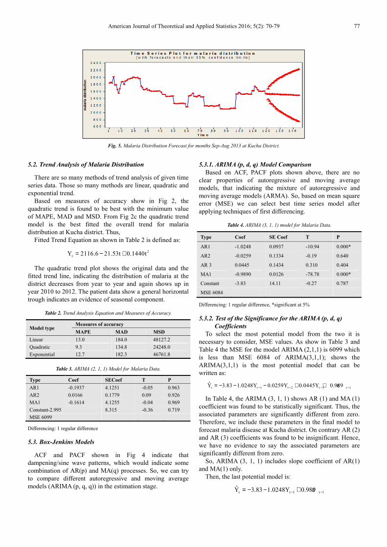
Fig. 5. Malaria Distribution Forecast for months Sep-Aug 2013 at Kucha District.

5.2. Trend Analysis of Malaria Distribution

There are so many methods of trend analysis of given time series data. Those so many methods are linear, quadratic and exponential trend.

Based on measures of accuracy show in Fig 2, the quadratic trend is found to be best with the minimum value of MAPE, MAD and MSD. From Fig 2c the quadratic trend model is the best fitted the overall trend for malaria distribution at Kucha district. Thus,

Fitted Trend Equation as shown in Table 2 is defined as:

2tY 2116.6 21.53t 0.1440t= − +

The quadratic trend plot shows the original data and the fitted trend line, indicating the distribution of malaria at the district decreases from year to year and again shows up in year 2010 to 2012. The patient data show a general horizontal trough indicates an evidence of seasonal component.

Table 2. Trend Analysis Equation and Measures of Accuracy.

Model type Measures of accuracy

MAPE MAD MSD

Linear 13.0 184.0 48127.2 Quadratic 9.3 134.8 24248.0 Exponential 12.7 182.3 46761.8

Table 3. ARIMA (2, 1, 1) Model for Malaria Data.

Type Coef SECoef T P

AR1 -0.1937 4.1251 -0.05 0.963 AR2 0.0166 0.1779 0.09 0.926 MA1 -0.1614 4.1255 -0.04 0.969 Constant-2.995 8.315 -0.36 0.719 MSE 6099

Differencing: 1 regular difference

5.3. Box-Jenkins Models

ACF and PACF shown in Fig 4 indicate that dampening/sine wave patterns, which would indicate some combination of AR(p) and MA(q) processes. So, we can try to compare different autoregressive and moving average models (ARIMA (p, q, q)) in the estimation stage.

5.3.1. ARIMA (p, d, q) Model Comparison

Based on ACF, PACF plots shown above, there are no clear properties of autoregressive and moving average models, that indicating the mixture of autoregressive and moving average models (ARMA). So, based on mean square error (MSE) we can select best time series model after applying techniques of first differencing.

Table 4. ARIMA (3, 1, 1) model for Malaria Data.

Type Coef SE Coef T P

AR1 -1.0248 0.0937 -10.94 0.000*

AR2 -0.0259 0.1334 -0.19 0.640

AR 3 0.0445 0.1434 0.310 0.404

MA1 -0.9890 0.0126 -78.78 0.000*

Constant -3.83 14.11 -0.27 0.787

MSE 6084

Differencing: 1 regular difference, *significant at 5%

5.3.2. Test of the Significance for the ARIMA (p, d, q)

Coefficients

To select the most potential model from the two it is necessary to consider, MSE values. As show in Table 3 and Table 4 the MSE for the model ARIMA (2,1,1) is 6099 which is less than MSE 6084 of ARIMA(3,1,1); shows the ARIMA(3,1,1) is the most potential model that can be written as:

t t 1 t 2 t 3 t 1Y 3.83 1.0248Y 0.0259Y 0.0445Y 0.989− − − −= − − − + + ε

In Table 4, the ARIMA (3, 1, 1) shows AR (1) and MA (1) coefficient was found to be statistically significant. Thus, the associated parameters are significantly different from zero. Therefore, we include these parameters in the final model to forecast malaria disease at Kucha district. On contrary AR (2) and AR (3) coefficients was found to be insignificant. Hence, we have no evidence to say the associated parameters are significantly different from zero.

So, ARIMA (3, 1, 1) includes slope coefficient of AR(1) and MA(1) only.

Then, the last potential model is:

t t 1 t 1Y 3.83 1.0248Y 0.989− −= − − + ε


5.3.3. Diagnostic Checking

In the Table 5, the box-pierce statistics gives no significant p-value (p value greater than significant level of α=0.05) indicating that the residual appeared too uncorrelated. Since the first regular differenced that we have done before shows the constant mean & variance the residuals are white noise. So the models are corrected or models are random.

Table 5. Box –pierce (L Jung –box ) Chi-square Statistic.

ARIMA(3, 1, 1)

Lag 12 24 36 48 Chi-Square 6.9 18.2 21.8 31.2 DF 7 19 31 43 P-Value 0.441 0.509 0.889 0.909

5.4. Forecasting of Malaria Distribution

Based on the fitted model the forecast is made for the coming 24 months. As it shown from Fig 5 the amount of malaria incidence forecast is gradually decrease for the year 2015 at Kucha district. The analysis of this series plot is measure the time long of horizontal axis and observes data on the vertical axis. It shows that in a given month it is increasing, on contrary in most months it shows decreasing patterns. For instance in 2013 the maximum expected number of patients is 1538 and 1533 which is in the 2nd & 4th October & December and minimum expected number of patient’s 1489 in the month July.

6. Conclusions

The objective of this study is to determine the malaria distribution along months of year 2003 to 2012 at Kucha district. Based on the result and discussion of the study, the following points were concluded on malaria distribution. As a result, malaria disease shows seasonal variation at district especially in the month September to January and July to August. The study found high malaria prevalence in December months of each year and on contrary, low rate of malaria prevalence is observed in July months of each year. The main reason to the distribution of malaria disease is mostly occurring on the variation of seasonal.

7. Recommendations

Based on the about conclusions we need to sound our recommendation to concerned bodies specifically, health center workers, malaria care units, governmental and non-governmental organizations. Mainly, health centers at district should consider December month of each year and take remedial precaution to malaria patients and others media to prevent people living in the district from malaria disease transmission. Likewise, health professionals should pay special attention on December months of each year to suggest precaution action for those people living in the area. And also, government and non-governmental organization should work on awareness creation before the season with highest malaria distribution is come at district. Finally, The

investigators would like to suggest the health professional working at the district health center have to record the patient detail information when they investigate for malaria.

List of Abbreviations

AIC Akaike’s Information Criterion

ARIMA Autoregressive Integrated Moving Average

Autocorrelation Coefficient ACC Autocorrelation Function ACF Mean Absolute Deviation MAD Mean Absolute Percentage Error MAPE

MA Moving Average Mean Squared Deviation MSD Mean Squared Error MSE Partial Autocorrelation Function PACF

SNNPR Southern Nations Nationalities and People Region

TS Time Series WHO World Health Organization

MDGs Millennium Development Goals

Authors’ Contribution

Author TKT wrote the research design and assists overall statistical analysis and interpretation. Author ASB edited the whole research design, reviewed relevant literatures and did overall statistical data analysis and result interpretations. Author TFA assists in compiling review of related literature and the references.

Acknowledgements

In the first place, we would like to thank Kucha district health center that provided us data were collected for the months of year 2003 to 2012 when the patients are examined and shows malaria incidence. Secondly, we appreciate Department of Statistics at Dilla University for material and reference books supports. In second place, we want to show our gratitude for author ASB for the great contribution he wrote the research design, overall statistical analysis and result interpretation. Finally, we need to acknowledge editor for full guidance and anonymous reviewers for their comments to improve the quality of manuscript presentation.

References

[1] WHO (2005).The World Malaria Report. Geneva.


[2] Ghebreyesus TA, Derressa Witten KH, Getachew A, Seboxa T. (2006). The epidemiology and ecology of health and disease in Ethiopia. In Malaria Edited, 556-576.

[3] Negash K, Kebede A, Medhin A, Argaw D, Babaniyi O, Guintran JO, Delacollette C. (2005). Malaria epidemics in the highlands of Ethiopia. East Afr Med J, 82:186-192.

[4] Gebremariam N (1988). The ecology of health and disease in Ethiopia. In Malaria. Edited by Kloos H, Zein AZ. Boulder Westview Press; 136-150.

[5] Tulu NA (1993). The ecology of health and disease in Ethiopia. In Malaria. Edited by Kloos H, Zein AZ. Boulder Westview Press; 341-352.

[6] Abeku A, van Oortmarssen GJ, Borsboom SJ, Habbema JDF (2003). Spatial and temporal variations of malaria epidemic risk in Ethiopia: factors involved and implications. Acta Tropica8:331-340.

[7] Abeku TA, de Vlas SJ, Borsboom GJJM, Tadege A, Gebreyesus Y, Gebreyohannes H, Alamirew D, Seifu A, Nagelkerke NJD, Habbema JDF (2004): Effects of meteorological factors on epidemic malaria in Ethiopia: a statistical modeling approach based on theoretical reasoning. Parasitology, 128:585-593.

[8] Teklehaimanot HD, Lipsitch M, Teklehaimanot A, Schwartz J (2004). Weather-based prediction of Plasmodium falciparum malaria in epidemic-prone regions of Ethiopia I. Patterns of lagged weather effects reflects biological mechanisms. Malar J, 3(1):41.

[9] Schaller KF, Kuls W: Äthiopien: Eine geographisch-medizinische Landeskunde (Ethiopia: A Geomedical Monograph). Heidelberg, Springer-Verlag, Berlin; 1972.

[10] Drissa C, Stanislas R, Mark T, Youssouf T, Matthew L, Abdoulaye K K, Karim T, Ando G, Issa D, Amadou N, Modibo D, Ahmadou D, Mody S, Bourema K, Nadine D, Jean G, Renaud P, Mahamadou A T, Christopher V P and Ogobara K D (2013).Spatio-temporal analysis of malaria within a transmission season in Bandiagara, Mali. Malaria Journal, 12:82.

[11] Worrall E, Rietveld A, Delacollette C (2004). The burden of malaria epidemics and cost-effectiveness of interventions in epidemic situations in Africa. Am J Trop Med Hyg 2004, 71(Suppl 2):136-40.

[12] Cox J, Craig M, le Sueur D, Sharp B. (1999). Mapping Malaria Risk in the Highlands of Africa. In Mapping Malaria Risk in Africa/Highland Malaria Project (MARA/HIMAL) Technical Report, MARA/Durban. London School of Hygiene and Tropical Medicine, London.

[13] Kiszewski AE, Tekelehaimanot A. (2002). A review of the clinical and epidemiologic burdens of epidemic malaria.

[14] Craig MH, Snow RW, le Sueur D (1999). A climate-based distribution model of malaria transmission in sub-Saharan Africa. Parasitol Today, 15:105.

[15] Gemperli A, Vounatsou P, Sogoba N, Smith T. (2006). Malaria mapping using transmission models: applications to survey data from Mali. Am J Epidemiol, 163:289-297.

[16] Kazembe LN, Kleinschmidt I, Holtz TH, Sharp BL (2006). Spatial analysis and mapping of malaria risk in Malawi using point-referenced prevalence of infection data.Int J Health Geogr, 5:41.

[17] Kiszewski AE (2004). A global index representing the stability of malaria transmission. Am J Trop Med Hyg, 70(5):486-498.

[18] Moffett A, Shackelford N, Sarkar S (2007): Malaria in Africa: Vector Species' Niche Models and Relative Risk Maps. PLoS ONE, 2(9):824.

[19] Carter R, Mendis KN, Roberts D (2000). Spatial targeting of interventions against malaria. WHO Bull, 78(12):1401-1411.

[20] Ghebreyesus TA, Haile M, Witten KH, Getachew A, Yohannes AM, Yohannes M, Teklehaimanot HD, Lindsay SW, Byass P (1999). Incidence of malaria among children living near dams in northern Ethiopia: community based incidence survey. BMJ, 319:663-666.

[21] Ghebreyesus TA, Haile M, Witten KH, Getachew A, Yohannes M, Lindsay SW, Byass P (2000). Household risk factors for malaria among children in the Ethiopian highlands. Trans R Soc Trop Med Hyg, 94(1):17-21.

[22] Thomas CJ, Lindsay SW (2000). Local-scale variation in malaria infection amongst rural Gambian children estimated by satellite remote sensing. Trans R Soc Trop Med Hyg, 94(2):159-63.

[23] CSA (2007). Census 2007 Tables: Southern Nations, Nationalities, and Peoples' Region.

[24] BFED (2009). Detailed statistics on roads, SNNPR Bureau of Finance and Economic Development website, Hawassa, Ethiopia.

[25] Samuel M. W, Judith A. O, Bradfield L, Madeleine C. T, Stephen J. C (2011). Revisiting the East African Malaria Debate, Bulletin WHO, 60(1).

[26] Tilahun Ferede Asena, Mohammed Shemsu and Ashenafi Senbeta Bedane. Statistical Analysis of Tourism Development, Management and Industry In Ethiopia. Journal of Pharmaceutical and Applied Sciences, Vol. 6(2):63-71, 2016.

Malaria Distribution in Kucha District of Gamo Gofa Zone ...

Documents